Controlling Quantum Information Devices - UWSpace
205
Controlling Quantum Information Devices by Felix Motzoi A thesis presented to the University of Waterloo in fulfillment of the thesis requirement for the degree of Doctor of Philosophy in Physics Waterloo, Ontario, Canada, 2012 c Felix Motzoi 2012
-
Upload
khangminh22 -
Category
Documents
-
view
3 -
download
0
Transcript of Controlling Quantum Information Devices - UWSpace

Controlling Quantum InformationDevices
by
Felix Motzoi
A thesispresented to the University of Waterloo
in fulfillment of thethesis requirement for the degree of
Doctor of Philosophyin
Physics
Waterloo, Ontario, Canada, 2012
c© Felix Motzoi 2012

I hereby declare that I am the sole author of this thesis. This is a true copy of thethesis, including any required final revisions, as accepted by my examiners.
I understand that my thesis may be made electronically available to the public.
ii
Abstract
Quantum information and quantum computation are linked by a common math-ematical and physical framework of quantum mechanics. The manipulation of thepredicted dynamics and its optimization is known as quantum control. Many tech-niques, originating in the study of nuclear magnetic resonance, have found commonusage in methods for processing quantum information and steering physical systemsinto desired states. This thesis expands on these techniques, with careful atten-tion to the regime where competing effects in the dynamics are present, and nosemi-classical picture exists where one effect dominates over the others. That is, thetransition between the diabatic and adiabatic error regimes is examined, with the useof such techniques as time-dependent diagonalization, interaction frames, average-Hamiltonian expansion, and numerical optimization with multiple time-dependences.The results are applied specifically to superconducting systems, but are general andimprove on existing methods with regard to selectivity and crosstalk problems, filter-ing of modulation of resonance between qubits, leakage to non-compuational states,multi-photon virtual transitions, and the strong driving limit.
iii

Acknowledgements
This research would not have been possible without the support and hard workof my collaborators and supervisors. I would like to thank my supervisor FrankWilhelm for his openness to taking a chance on me on as a graduate student. Hisleadership, methodology, and insight have all had a significant impact on my personaland academic development. My secondary supervisor, Jay Gambetta, has also beeninstrumental to the main lines of thought in this research and his vision and guidanceas well as his perseverence have opened many opportunities (and driven some homerun balls!). I would also like to thank Seth Merkel for his guidance and feedback. Ihave also been fortunate to help assist other graduate students in common research.Peter Groskowski, Botan Khani, Amira Eltony, Yuval Sanders, Likun Hu, VictorVetch, and Jerry Chow have all collaborated in quantum control projects that havegenerated many stimulating and valuable conversations. Finally, I would like tothank the fellow graduate students in 2117 for some freshness and brightness in aroom that had neither. This research was made possible by NSERC through thediscovery grants, QuantumWorks, and a PGS scholarship.
iv
Dedication
This thesis is dedicated to my three muses: my mother Ina who would havewritten it herself if she needed to, my sister Clairneige who tirelessly listened torants and ravings about the endless "wonders" of quantum physics growing up, andmy girlfriend Kanako who carried me through these arduous Ph.D. years.
v

Contents
List of Figures xi
1 Introduction 1
2 Universal Quantum Computation 102.1 Quantum gates . . . . . . . . . . . . . . . . . . . . . . . . . . . . . . 10
2.1.1 Superposition and measurement . . . . . . . . . . . . . . . . . 102.1.2 Unitary evolution . . . . . . . . . . . . . . . . . . . . . . . . . 112.1.3 Hamiltonians . . . . . . . . . . . . . . . . . . . . . . . . . . . 132.1.4 Non-unitary evolution . . . . . . . . . . . . . . . . . . . . . . 14
2.2 Quantum software . . . . . . . . . . . . . . . . . . . . . . . . . . . . 162.2.1 Assembly . . . . . . . . . . . . . . . . . . . . . . . . . . . . . 162.2.2 Outlook on algorithms . . . . . . . . . . . . . . . . . . . . . . 17
2.3 Quantum hardware . . . . . . . . . . . . . . . . . . . . . . . . . . . . 182.3.1 Candidate implementations . . . . . . . . . . . . . . . . . . . 19
2.3.1.1 Superconducting qubits . . . . . . . . . . . . . . . . 192.3.2 Controllability . . . . . . . . . . . . . . . . . . . . . . . . . . . 202.3.3 Coupling topologies . . . . . . . . . . . . . . . . . . . . . . . . 222.3.4 Coupling mechanisms . . . . . . . . . . . . . . . . . . . . . . . 22
2.4 Quantum errors . . . . . . . . . . . . . . . . . . . . . . . . . . . . . . 242.4.1 Worst-case error . . . . . . . . . . . . . . . . . . . . . . . . . . 242.4.2 Threshold theorem . . . . . . . . . . . . . . . . . . . . . . . . 252.4.3 Average error . . . . . . . . . . . . . . . . . . . . . . . . . . . 25
3 Elements of Quantum Control 273.1 Time-dependent fields . . . . . . . . . . . . . . . . . . . . . . . . . . 293.2 Selection error . . . . . . . . . . . . . . . . . . . . . . . . . . . . . . . 303.3 Off-resonant operator error . . . . . . . . . . . . . . . . . . . . . . . . 313.4 Resonant operator error . . . . . . . . . . . . . . . . . . . . . . . . . 33
vi

CONTENTS
3.5 Static non-deterministic error . . . . . . . . . . . . . . . . . . . . . . 333.6 Fast non-deterministic error . . . . . . . . . . . . . . . . . . . . . . . 34
4 Frame Transformations 354.1 General theory . . . . . . . . . . . . . . . . . . . . . . . . . . . . . . 35
4.1.1 Transformation formula . . . . . . . . . . . . . . . . . . . . . 364.1.2 Equivalent frames . . . . . . . . . . . . . . . . . . . . . . . . . 374.1.3 Interaction frames . . . . . . . . . . . . . . . . . . . . . . . . . 38
4.2 Phase transformations . . . . . . . . . . . . . . . . . . . . . . . . . . 384.2.1 Phase tracking . . . . . . . . . . . . . . . . . . . . . . . . . . 384.2.2 Rotating frames . . . . . . . . . . . . . . . . . . . . . . . . . . 394.2.3 Phase ramping . . . . . . . . . . . . . . . . . . . . . . . . . . 40
4.3 Diagonalization . . . . . . . . . . . . . . . . . . . . . . . . . . . . . . 414.3.1 Adiabatic expansion . . . . . . . . . . . . . . . . . . . . . . . 414.3.2 Interaction frame . . . . . . . . . . . . . . . . . . . . . . . . . 42
4.4 Magnus expansion . . . . . . . . . . . . . . . . . . . . . . . . . . . . 424.4.1 Interaction frame . . . . . . . . . . . . . . . . . . . . . . . . . 43
5 Numerical Simulation and Optimization 445.1 Time-slicing . . . . . . . . . . . . . . . . . . . . . . . . . . . . . . . . 445.2 Cost functions . . . . . . . . . . . . . . . . . . . . . . . . . . . . . . . 45
5.2.1 Overlap fidelity . . . . . . . . . . . . . . . . . . . . . . . . . . 455.2.2 Subspace fidelity . . . . . . . . . . . . . . . . . . . . . . . . . 465.2.3 Ensemble fidelity . . . . . . . . . . . . . . . . . . . . . . . . . 465.2.4 Penalties . . . . . . . . . . . . . . . . . . . . . . . . . . . . . . 47
5.3 Gradient Ascent . . . . . . . . . . . . . . . . . . . . . . . . . . . . . . 485.3.1 Non-unitary control . . . . . . . . . . . . . . . . . . . . . . . . 505.3.2 Robust control . . . . . . . . . . . . . . . . . . . . . . . . . . 51
5.4 Convergence improvements . . . . . . . . . . . . . . . . . . . . . . . . 51
6 Waveform Shaping 536.1 Introduction . . . . . . . . . . . . . . . . . . . . . . . . . . . . . . . . 536.2 Waveform generator example . . . . . . . . . . . . . . . . . . . . . . . 546.3 Numerical optimization with fast fields . . . . . . . . . . . . . . . . . 556.4 Response functions . . . . . . . . . . . . . . . . . . . . . . . . . . . . 56
6.4.1 Cubic spline interpolation . . . . . . . . . . . . . . . . . . . . 576.4.2 Filter function . . . . . . . . . . . . . . . . . . . . . . . . . . . 596.4.3 Fourier components . . . . . . . . . . . . . . . . . . . . . . . . 60
6.5 Filtered amplitude-modulated coupling . . . . . . . . . . . . . . . . . 61
vii
CONTENTS
6.6 Filtered frequency-modulated coupling . . . . . . . . . . . . . . . . . 646.7 Application to 2-qubit coupling . . . . . . . . . . . . . . . . . . . . . 66
6.7.1 Physical example: capacitively coupled phase qubits . . . . . . 676.7.2 Reduction to single qubit analytic treatment . . . . . . . . . . 696.7.3 Numerical optimization . . . . . . . . . . . . . . . . . . . . . 69
6.8 Summary . . . . . . . . . . . . . . . . . . . . . . . . . . . . . . . . . 70
7 Crosstalk 727.1 Frequency crosstalk . . . . . . . . . . . . . . . . . . . . . . . . . . . 73
7.1.1 Selectivity criteria . . . . . . . . . . . . . . . . . . . . . . . . . 747.1.2 Semiclassical spectrum analysis . . . . . . . . . . . . . . . . . 76
7.1.2.1 Doublet analysis . . . . . . . . . . . . . . . . . . . . 777.1.2.2 Multiplet analysis . . . . . . . . . . . . . . . . . . . 77
7.1.3 Quantum operator diagonalization . . . . . . . . . . . . . . . 807.1.3.1 Rotating frame . . . . . . . . . . . . . . . . . . . . . 807.1.3.2 Block diagonal frame . . . . . . . . . . . . . . . . . . 817.1.3.3 Solution basis of higher derivatives . . . . . . . . . . 837.1.3.4 Doublet analysis . . . . . . . . . . . . . . . . . . . . 847.1.3.5 Multiplet analysis . . . . . . . . . . . . . . . . . . . 87
7.2 Spatial crosstalk . . . . . . . . . . . . . . . . . . . . . . . . . . . . . . 897.2.1 Physical Model . . . . . . . . . . . . . . . . . . . . . . . . . . 907.2.2 Coupling landscape . . . . . . . . . . . . . . . . . . . . . . . . 927.2.3 Optimization of off-resonant coupling . . . . . . . . . . . . . . 947.2.4 Optimization of on-resonance coupling . . . . . . . . . . . . . 96
8 Leakage 988.1 Introduction . . . . . . . . . . . . . . . . . . . . . . . . . . . . . . . . 988.2 Mathieu equation . . . . . . . . . . . . . . . . . . . . . . . . . . . . . 1008.3 Qutrit approximation . . . . . . . . . . . . . . . . . . . . . . . . . . . 101
8.3.1 Coupling strength from dressing . . . . . . . . . . . . . . . . . 1028.4 Conventional control . . . . . . . . . . . . . . . . . . . . . . . . . . . 1058.5 Adiabatic diagonalization . . . . . . . . . . . . . . . . . . . . . . . . . 106
8.5.1 Exact solution to the qutrit . . . . . . . . . . . . . . . . . . . 1108.6 Generalized transformation . . . . . . . . . . . . . . . . . . . . . . . . 112
8.6.1 Zeroth order solutions . . . . . . . . . . . . . . . . . . . . . . 1138.6.2 First order solutions . . . . . . . . . . . . . . . . . . . . . . . 1138.6.3 Second order solutions . . . . . . . . . . . . . . . . . . . . . . 116
8.7 Numerical optimization . . . . . . . . . . . . . . . . . . . . . . . . . . 117
viii
CONTENTS
8.7.1 Prefactor optimization . . . . . . . . . . . . . . . . . . . . . . 1178.7.2 Full optimization . . . . . . . . . . . . . . . . . . . . . . . . . 119
8.8 Incoherent effects . . . . . . . . . . . . . . . . . . . . . . . . . . . . . 1208.8.1 Relaxation . . . . . . . . . . . . . . . . . . . . . . . . . . . . . 1208.8.2 Dispersion . . . . . . . . . . . . . . . . . . . . . . . . . . . . . 122
8.8.2.1 Optimization . . . . . . . . . . . . . . . . . . . . . . 1248.9 Implementation . . . . . . . . . . . . . . . . . . . . . . . . . . . . . . 127
9 Multi-Channel Leakage 1339.1 Duffing oscillator . . . . . . . . . . . . . . . . . . . . . . . . . . . . . 133
9.1.1 SNO approximation . . . . . . . . . . . . . . . . . . . . . . . . 1349.1.2 Numerical solutions . . . . . . . . . . . . . . . . . . . . . . . . 1369.1.3 Analytical solutions . . . . . . . . . . . . . . . . . . . . . . . . 139
9.2 Multiple leakages from one level . . . . . . . . . . . . . . . . . . . . . 1429.3 2-Qubit leakage . . . . . . . . . . . . . . . . . . . . . . . . . . . . . . 144
9.3.1 General Model . . . . . . . . . . . . . . . . . . . . . . . . . . 1449.3.2 Numerical solution . . . . . . . . . . . . . . . . . . . . . . . . 1469.3.3 Analytical solution . . . . . . . . . . . . . . . . . . . . . . . . 147
10 Virtual Transitions 15010.1 Raman transitions . . . . . . . . . . . . . . . . . . . . . . . . . . . . 15110.2 2-Qubit coupling . . . . . . . . . . . . . . . . . . . . . . . . . . . . . 154
10.2.1 Ansatz solution . . . . . . . . . . . . . . . . . . . . . . . . . . 15410.2.2 Optimization with two tones . . . . . . . . . . . . . . . . . . . 156
10.3 Driving through a cavity . . . . . . . . . . . . . . . . . . . . . . . . . 15710.4 Summary . . . . . . . . . . . . . . . . . . . . . . . . . . . . . . . . . 159
11 Strong Coupling 16111.1 Analytic solution . . . . . . . . . . . . . . . . . . . . . . . . . . . . . 16211.2 Numerical optimization . . . . . . . . . . . . . . . . . . . . . . . . . . 163
12 Summary and Conclusions 165
Appendix 170
A Matrix Exponentiation 171A.1 Taylor Expansion . . . . . . . . . . . . . . . . . . . . . . . . . . . . . 172A.2 Diagonalization . . . . . . . . . . . . . . . . . . . . . . . . . . . . . . 172A.3 Hamiltonian splitting . . . . . . . . . . . . . . . . . . . . . . . . . . . 173
ix

CONTENTS
A.4 Other methods . . . . . . . . . . . . . . . . . . . . . . . . . . . . . . 173
B Publications 174
Bibliography 175
x

List of Figures
2.1 (A) Nearest-neighbour topology (B) Phonon bus . . . . . . . . . . . . 21
3.1 Common pulse shapes . . . . . . . . . . . . . . . . . . . . . . . . . . 293.2 Energy level diagram of an anharmonic oscillator. . . . . . . . . . . . 32
6.1 Response function of a Tektronix AWG5014 at (A) 1 GSample/s and(B) 500 MSamples/s with spline and filter approximations. . . . . . 55
6.2 Gradient method including the sub-pixel dynamics. . . . . . . . . . . 586.3 Gate error as a function of the gate time for qutrit with filtering of
amplitude-modulation . . . . . . . . . . . . . . . . . . . . . . . . . . 626.4 Gate error as a function of the number of subpixels for qutrit with
filtering of amplitude-modulation . . . . . . . . . . . . . . . . . . . . 636.5 Energy level diagram for bringing a transition in and out of resonance 646.6 Analytic pulse sequences for modulation of energy levels for the filtered
frequency-modulation example . . . . . . . . . . . . . . . . . . . . . . 666.7 Gate error as a function of the initial splitting between energy levels
for the filtered frequency-modulation example . . . . . . . . . . . . . 676.8 Numerical pulse sequences for modulation of energy levels for the fil-
tered ISWAP example . . . . . . . . . . . . . . . . . . . . . . . . . . 70
7.1 Absolute Fourier transform of a Gaussian pulse, its derivative, andtheir sum . . . . . . . . . . . . . . . . . . . . . . . . . . . . . . . . . 78
7.2 Absolute Fourier transform of a Gaussian pulse and the sum of theGaussian with its 2nd derivative . . . . . . . . . . . . . . . . . . . . 79
7.3 Selection error for two uncoupled qubits . . . . . . . . . . . . . . . . 857.4 Selection error for three uncoupled qubits for use of different derivatives 877.5 Selection error for three uncoupled qubits using two derivatives . . . . 887.6 Selection error as a function of frequency offset when using the second
derivative. . . . . . . . . . . . . . . . . . . . . . . . . . . . . . . . . 89
xi

LIST OF FIGURES
7.7 Two different arrangements of flux qubits 1, 2, 3 and couplers A, B.(A) Straight-line shape (B) Capital “L” shape. . . . . . . . . . . . . . 91
7.8 (A) Interaction energies between qubits K12 , K23 , and K13 for anL-shape geometry. (B) Crosstalk K13, while keeping K12 = K23 ≈ 0. 93
7.9 A pulse sequence for a√iSWAP gate with three qubits off resonance 95
7.10 A pulse sequence for a CNOT gate with three qubits on resonance . . 96
8.1 Ratio of coupling strength of the |1〉 ↔ |2〉 transition to the |0〉 ↔ |1〉transition as a function of anharmonicity . . . . . . . . . . . . . . . . 103
8.2 Fourier transforms of the control fields and populations of the ground,first, and second excited for a Gaussian pulse of various lengths . . . 106
8.3 Gate error is plotted vs. leakage transition strength λ for solutions todifferent orders of the adiabatic expansion of a NOT gate operatingon a qutrit . . . . . . . . . . . . . . . . . . . . . . . . . . . . . . . . . 109
8.4 Gate error as a function of gate time for Gaussian and 2-tone exactsolution to the qutrit problem . . . . . . . . . . . . . . . . . . . . . . 111
8.5 Gate error for the implementation of a NOT gate in a d = 5 non-linearoscillator for first order solutions . . . . . . . . . . . . . . . . . . . . . 114
8.6 Gate error for the implementation of a NOT gate in a d = 5 non-linearoscillator for third order solutions . . . . . . . . . . . . . . . . . . . . 116
8.7 Gate error for the implementation of a NOT gate in a d = 5 usingnumerical prefactor optimization of ansatz solution . . . . . . . . . . 118
8.8 Pulse duration vs. pixel width for 1-control and 2-control optimiza-tions of the qutrit. The insert shows the two-control optimizationresultant pulse for tg = 1/4∆ . . . . . . . . . . . . . . . . . . . . . . 119
8.9 (A) Gate error vs. pulse duration for T1 = 40µs and (B) Minimumerror vs. T1 for Gaussian, Gaussian with DRAG, and GRAPE with1ns pixels solutions to qutrit leakage. . . . . . . . . . . . . . . . . . 121
8.10 The first four energy 1-D band structures are shown in the momentumbasis for four different potential depths r. . . . . . . . . . . . . . . . 124
8.11 Optimized controls for preparing a NOT-gate for the nonlinear oscil-lator when the optimization uses ten points in quasi momentum space 125
8.12 The maximum fidelity for an optimized pulse vs. gate time for thenonlinear oscillator when the optimization uses ten points in quasimomentum space. . . . . . . . . . . . . . . . . . . . . . . . . . . . . 126
8.13 Fidelity response vs. quasi-momentum for pulse of different lengthoptimized at k = 0.5 . . . . . . . . . . . . . . . . . . . . . . . . . . . 127
xii

LIST OF FIGURES
8.14 (A) Experimental realization of Gaussian and derivative pulse shapes(B) Measured 〈σz〉 for a test sequence consisting of pairs of π and π/2rotations . . . . . . . . . . . . . . . . . . . . . . . . . . . . . . . . . 128
8.15 Randomized benchmarking using (A) Gaussian pulses, and (B) addi-tional Gaussian derivative pulses on the quadrature channel. . . . . . 130
8.16 Experimental comparison of single-qubit gate errors vs. gate timewith and without DRAG . . . . . . . . . . . . . . . . . . . . . . . . . 131
8.17 Measured two-qubit Pauli sets for preparing the state |1, 1〉 with (a)Gaussian pulses and (b) DRAG pulses . . . . . . . . . . . . . . . . . 132
9.1 Energy level diagrams for multiple leakage channels. (A) connectedto both qubit levels (B) connected to a single level (C) for two qubits 134
9.2 Ratio of the eigen-energies of the RWA Hamiltonian and exact eigen-ergies of the anharmonic oscillator for the first nine energy levels,assuming nonlinearities δ = 0.01 and δ = 0.1. . . . . . . . . . . . . . . 135
9.3 The amplitudes of three pulse sequences optimized by GRAPE forpreparation of |1〉 , |2〉 , and |3〉 Fock states . . . . . . . . . . . . . . 136
9.4 (A)Fourier spectrum for preparing |2〉 state. (B) Populations of thedifferent states during the pulse taking |0〉 into |2〉 . . . . . . . . . . . 137
9.5 (A) Error vs. pulse time for creating the |1〉 state with exponential fit(B) Scaling of the minimal gate time with the nonlinearity parameterwith power-law fits . . . . . . . . . . . . . . . . . . . . . . . . . . . . 138
9.6 Gate error vs. gate time for the implementation of a NOT gate whenthere is leakage above and below the qubit subspace . . . . . . . . . . 141
9.7 Gate error vs. gate time for the implementation of a NOT gate whenthere are many leakage transitions for the excited state . . . . . . . . 142
9.8 (A) Control amplitude (inter-qubit coupling strength) J(t) as a func-tion of time an ISWAP (B) Fourier spectrum of the pulse . . . . . . . 146
9.9 (A) Optimal gate time T versus the intrinsic anharmonicity ∆ and(B) Optimal frequency offset ε versus anharmonicity ∆ for the ansatzsolution to coupling leaking qubits . . . . . . . . . . . . . . . . . . . . 147
10.1 Energy level diagram of a stimulated Raman transition for three levelsystem when (A) the temporary level is in the middle and (B) it is atthe top . . . . . . . . . . . . . . . . . . . . . . . . . . . . . . . . . . 151
10.2 Rotation error for Raman transition with two independent drives usingGaussian shaping and adding in a derivative . . . . . . . . . . . . . . 153
10.3 Energy level diagram for an anharmonic oscillator coupled to a cavity 154
xiii

LIST OF FIGURES
10.4 Gate error vs. gate time for sideband transition in J-C ladder withac-Stark shift and derivative corrections. . . . . . . . . . . . . . . . . 155
10.5 Gate error as a function of the number of subpixels for the multi-toneexample . . . . . . . . . . . . . . . . . . . . . . . . . . . . . . . . . . 157
10.6 Energy level diagram for an anharmonic oscillator coupled to a cavitywith no single qubit controls . . . . . . . . . . . . . . . . . . . . . . . 158
10.7 Pulse amplitude as a function of the time during gate for a qubit driventhrough a cavity for (A) a NOT gate and (B) an identity operation . 159
11.1 Error from counter-rotating terms in qubit frame for different analyticpulses . . . . . . . . . . . . . . . . . . . . . . . . . . . . . . . . . . . 163
11.2 Error from counter-rotating terms and leakage for a qutrit for differentnumerical pulses and different phases . . . . . . . . . . . . . . . . . . 164
xiv

Chapter 1
Introduction
The digital age has brought us the relentless digitization of information. At its veryheart, the framework given by the Universal Turing Machine (UTM) and the vonNeumann architecture tells us that any piece of information and any algorithm thatacts on it can be stored together as a single string of zeros and ones on one memorydevice [160]. This equivalence principle states that some piece of information "x"that we have cannot be distinguished in and of itself from some algorithm or function"f(x)" that acts on it. That the one represents the physical change in the other hasno repercussions in terms of its representation or storage.
Beyond this digital paradigm lie a plethora of characterizations and interpreta-tions of what is possible with a digital computer, but fundamentally they are allreducible to operation of a UTM. That is, different statistical measures of ‘efficiency’(such as the entropy, outcome probability, information dissipation, or the algorith-mic complexity) rely on the computation as a sequence of indivisible steps for whichboth the information x and the process acting on it f(x) are completely fixed. Andyet the statistical properties are not digital but real-valued and moreover actuallychanging during the atomic steps. Whether such ‘statistical properties’ of informa-tion are physically real was perhaps first questioned by the Greek philosopher Zenoin his arrow paradox [118], which asks whether something can be in one place andmoving at the same time. But, because physically observable quantities are effec-tively continuous (as formalized by calculus), one being the average of the other isnot discernible (they are independent variables [99]) and such speculation remainedphilosphical.
Nevertheless, classical laws of probability and logic are based on notions of dis-continuous events and objects (divisible into smaller and smaller particles) and theseconcepts made their way into our understanding of physics. Based on the motion of
1
individual particles, a statistical physical theory was developed behaving similarly to(but discovered independently from) modern statistical characterizations of digitalinformation, obeying a set of thermodynamic laws with similar concepts of entropy,heat dissipation, and other probabilistic effects. Yet, evidence of the continuousnessof physical phenomena remained a thorn in these developments, and in particular awave theory was concurrently developed that characterized analog oscillations andinteractions as propagations of contiguous waves.
Quantum mechanics [152] unified the notions of probabilistic properties of indi-vidual particles and continuous wave interactions between disconnected particles.In effect, both heat dissipation and wave propagation are dictated by the sameSchrödinger equation. Whether something behaves more like a particle (with fixedproperties) or more like a (delocalised) wave is primarily a question of context, thatis, of whether it is bound to a particular location or whether it is free to propagatein all directions. Moreover, just like a physical potential barrier keeps a particle ina specific location, a measurement event causes the measured property to localizeto a particular value. A lack of measurement or an escape from a binding potentialon the other hand lead to dissipation and propagation of energy and information.The properties of these objects that are measured can also be discontinous (quan-tum) or continuous, depending on whether they describe a bound state or a free one.In the quantum case it seems Zeno’s intuition was correct: both a given discreteproperty and a complementary property describing its change cannot simultaneoulsybe well defined. However, both properties are physically real, and context-specificlocalisation dictates which of them is well-defined.
A characterization of computers that somehow physically includes both the infor-mation (that we read off digitally) and also the change in the information, describedby the analog physical process that (infinitesimally) changes one piece of informationthat we observe into another, seems like it should be qualitatively richer1, much likequantum mechanics generalizes Newtonian dynamics. No less, such a formulation ofcomputations is necessarily equivalent and isomorphic to quantum mechanics [66].While the new paradigm does not alter the fundamental power of the UTM and thequestion of ‘tractability’ (the resolution of paradoxes such as the Halting Problemor “this statement is false” cannot be found on any computer), it turns out thatmeasures of efficiency such as informational entropy, probability, and dissipation areresources that are physically inherently present in the characterization, but perhapsmost interestingly, decreased algorithmic complexity is as well.
1At the very least, it should contain twice as much information. For example if the informationis encoded in terms of a position coordinate, velocity information would also be present. See also‘superdense coding’ [84].
2

For our purposes, we are interested in such complex algorithms. The most com-plex operations for a computer are computations about computations themselves.In the context of the first paragraph, for some information "x" and some functionacting on it "f(x)", a complex operation can roughly be understood as a function"g(f(x))" that computes some global property of the function f(x) for all possiblex. The "brute force" approach to computing this can be described as trying everysingle possible value of x, computing f(x), and from the total set of results comput-ing g(f(x)). When x can take on many different values such an approach is all butimpossible (it is exponential in the width of x). An insight in complexity arises fromidentifying the algorithm f(x) with the analog physical process underlying compu-tation. Then, global properties of the process f(x) can be measured directly, usingas input a wave spread over all possible values of x rather than feeding in the valuesindividually. For example, one can measure the frequency that the physical processrepeats itself with by appending another analog process (the Fourier transform) tothe input and simply reading off the answer [158].
As it turns out, the frequency is the key piece of information to breaking en-cryption functions used in RSA cryptosystems, used all over the planet for securityprotocols. Similarly, the characteristic energy of the process (its eigenvalue) is in-strumental to the simulation and characterization of physical systems [81], with suchpotential areas of applications as biochemistry and materials design. A crowningachievement but still an open problem would be if one could reliably obtain thecharacteristic input configuration (the eigenvector) for the lowest eigenvalue of aprocess (that one is trying to optimize), then this corresponds to a solution to agiven instance of the notoriously hard but ubiquitous NP-complete problems [44,77].
Of course, building such a computer is in many ways far more demanding thana digital computer because the analog process describing operations must not onlyavoid accidentally flipping a bit, but it must retain the coherence of the phase oscilla-tion (i.e. timing of the peaks and troughs of the wave). By the same token, a classicalanalog computer is limited, not only by a simple class of bit operations typically avail-able for the chosen encoding, but because heat dissipation limits the precision of suchoperations to a finite and relatively small number of bits. Using quantum mechanicscircumvents this problem with the important caveat that damping and dissipationmust be suppressed to remain quantum. The quantum framework not only providesa mathematical model for describing (continuous) computation, but from a hardwarepoint of view it provides numerous prospective physical implementations.
Candidate quantum implementations typically involve some small physical systemthat can be sufficiently isolated from the environment to allow its wave properties tobe manifested and retained. Additionally, the system must be sufficiently cooled to
3
prevent flipping of bits via energy decay processes. However, this isolation must becontrasted to the ability to introduce energy/phase shifts via control hardware whichmust couple to the quantum system. The most developed technologies in this regardhave benefited from research for many decades such as liquid state Nuclear MagneticResonance (NMR) and photonic systems. These systems have and continue to servewell as testbeds for advances in quantum information but are challenged by difficultiesin weak coupling between elements and scaling to larger system sizes. Other morecomplicated systems such as trapped atoms/ions and solid state implementations(e.g. semiconducting, superconducting) are more promising in this regard. Some ofthese implementation and design choices are discussed in Sec. 2.3.
The mathematical framework of quantum computing consists of defining a quan-tum bit (qubit) as some (stable) degree of freedom present in the physical systemwhich can be measured in one of two states, but for which the wave properties allowthat energy (and information) can be spread over multiple states simultaneously.Timed operations are controlled by the dynamics of the Schrödinger wave equationwhich allows coupling of qubits to control hardware or other qubits. An overview onquantum mechanics and operations is given in Sec, 2.1. The Schrödinger evolutionis typically controlled on a short time scale in order to define reusable high-qualityoperations (gates)2, and (remarkably) these operations can be subsequently chainedtogether as building blocks for more complicated operations and algorithms, justlike digital gates on a conventional computer. When the timing is performed cor-rectly, the coherence properties of the wave can spread over many qubits allowingfor operations (such as the Fourier transform) to now physically act simultaneouslyon arbitrarily many bits3.
The statement of this thesis is to describe the generation of quantum operations,acting on a small number of qubits, both in terms of the physics involved and themathematical features that expand on classical computation. The main reason wefocus on a small system size is that, by the very definition of the problem, engineeringmany-bit operations is not efficient using classical computers, which of course is allwe have access to without a quantum computer. In fact, most known multi-qubitoperations that are required for known algorithms can be decomposed into a series
2At this point, arbitrarily high-quality operations can be obtained using measurement of par-ticular “error syndrome” states [62]. This is another difference from classical analog computationin which measurement is only defined in the (final) steady-state of the system. Note that in somecases, such as typical implementations of adiabatic quantum computation, long operations are syn-thesized directly instead and error correction is therefore not used, in particular if the evolutioncan be shown to withstand the onset of decay and damping processes.
3As another example, using a single operation, one qubit can be simultaneously entangled witha large number of other qubits. Measuring one qubit measures all the others as well.
4

of smaller operations. Thus, for the purpose of well-defined operations, the error canbe made small by ensuring that the error in the short operations is proportionallysmaller. Thus, the main focus of the research is to engineer these short operations tohave low errors. Sec. 2.4 introduces some ways of quantifying the error of a quantumoperation.
The eventual goal, in most idealized terms, is to build a quantum computer. Inthis respect, the quantum computer is built up of three main components. The firstis the memory of the system, which can be digitally read out, and which is physicallyencoded in some quantum system. For example, this quantum information can be inthe spin (up or down) of a particle, in the energy level of an atom, or in a quantizedsuperconducting current. The second component is the “processor”, which is somecontrol hardware programmed to introduce radiation or other fields into the systemto change the configuration of the information stored in the physical device. Thedevice must effectively be able to perform the short operations with sufficiently lowerror, and so is central to this thesis. Thirdly, the software that runs on the computeris some algorithm, typically one that benefits in reduced complexity by running ona quantum computer. Some of the main developments in quantum software aredescribed in Sec. 2.2. All three of these components are very far from being afinished product, let alone fully understood. As much as all three components havegained tremendously from theoretical research and a variety of analytical insights,they are difficult to understand even for small number of bits.
In the context of a small number of qubits, all three components can often be de-scribed using a common physical model described by the Hamiltonian of the system.Both by experimentation and by numerical simulation and optimization, it is hopedthat new insights will be gained into the Hamiltonian dynamics that will help toscale the components to systems with more bits. In the case of numerics, solutionsto reducing error will often have symmetries from which an analytical expression ortechnique can be deduced. Finding control fields that contain identifiable featuressuch as specific frequency components or separation into a sequence of steps in timecan offer clues about how best to characterize problems and their solutions. Suchforms are also very useful because they can point out which physical resources aremost valuable in the physical implementation and design choices can be based onthese in the future. Finding that some imperfection is intrinsic or irreversible orinstead that it can be avoided or rendered irrelevant can avoid unnecessary dead-ends in terms of research and allow resources to go to more promising realizations.From a processing point of view, being able to solve simple problems involving fewbits analytically means that the solutions can be computed very efficiently and ifmultiple techniques can be combined then the solutions for larger numbers of bits
5

can often remain efficient. Specifically, solutions to different problems that involvedistinct controls or different basis elements for the same control, or even differentbases, can be applied effectively independently, at least to the highest order of anyapproximations that may be made in the solutions. In some cases, compound errorscoming from combing two different kinds of error still belong to the set of correctableerrors and can thus be removed to arbitrary accuracy by applying the analytic tech-niques in sequence. Moreover, the physics is all present in the interaction of veryfew components and adding in more components does not qualitatively alter thesituation, only adds in more combinations. Finally, from a software point of view,simulations and optimizations can offer insight into how an algorithm works andeven find faster ways of running the same algorithm, for example by speeding upthe individual gates with a proportional decrease in the time of the algorithm or bycombining several steps in the algorithm into a single step. Most notably, the sourcesof error in certain kinds of algorithms such as adiabatic computation impact directly(super-polynomially) on the algorithmic complexity of the solution [44, 77]. Theanalytical and numerical optimizations also have a direct effect on how and whichexperiments can be run. In some cases, the experiments even involve more bits thanthe simulations [21]. The same advantages that come from simulation can often befound in experimentation, as well as new benefits involved such as seeing exactlywhat can or cannot be realized. Optimizations allow more complex experiments andthe effects are compounded, taking us closer to large scale quantum computation.
A more immediate purpose to the study of quantum operations is to map outthe dynamics involved on a qualitative level. In a sense, such a study goes beyond ameasure of quantitative error but rather aims to find novel (and often less complex)ways in which particular problems (given by a particular Hamiltonian) can be solved.In effect, quantum computation (unitary evolution) is conceptually different from thebinary switching processes that take place in digital computation and understandingthe similarities and differences is of much theoretical interest. Not only is the amountof information present in the description of the computational system exponentiallylarger, but as mentioned the change in information is as much a resource as the in-formation itself. All this means that any path from one state to another can take onan infinite number of different trajectories through analog space. The basic study ofquantum control, the study of which quantum variables can be used to change or in-stead retain information in an efficient way, was pioneered in NMR systems since themiddle of last century [162]. This was the first experimental application of quantummechanics exploiting not simply the ensemble phenomena described by the theorybut manipulating and controlling individual pieces of quantum information as well.This progress has been steadily forthcoming as more precision and more complexity
6

has been incorporated into these operations. Initially it was found that irradiatingatomic transitions with resonant magnetic fields, one could drive oscillation betweena pair of energy states. This turned out to be useful for example in spectroscopyfor identifying the chemical structure of samples. Timing was improved so that aparticular state could reliably be obtained at a given time. This in turn allowedcomplex operations in time such that multiple (matrix) transitions could be sequen-tially traversed and multi-dimensional data could be obtained via spectroscopy suchas the strength of the couplings between atoms in molecules. The wave properties oflight-matter interaction was also fundamental to the progress. Pulse shaping beyondsquare monochromatic pulses improved reliability and spectral selectivity by for ex-ample using smoother shapes with a smaller more selective bandwidth [55]. Thetechnology developed further with complex sequences of control pulses being usedto manipulate information inside molecules and engineer specific chemical configu-rations. Thus, chemical analysis is where the basic ideas about quantum algorithmswere first laid out, with interference playing a prominent role between desired andundesired pathways for information.
The success of the pioneering efforts in quantum control was largely predicatedon a clear hierarchy of the importance of different operators in the system. Physi-cally, the atomic spin precession frequencies were much larger than the amplitudesof magnetic fields, which were much larger than the strengths of the inter-atomiccouplings in molecules, which were again much larger than damping and decay er-rors. In this limit, the effects could be separated and independently characterized.Thus, generating slow timescale evolutions could be understood as a pseudo-digitalsequence of operations which permit information to move inside or in between spins,decomposing the dynamics into a matrix algebra. This lead, for example, to power-ful techniques for using the faster single-spin dynamics to augment the inter-atomiccouplings, such as composite pulse sequences, which seek to obtain a new operationfrom a number of smaller operations. Most generally, the effect of the extra controlscan often be understood as changing (temporarily) the encoding (and for modelingpurposes, the representation) of information from energy to phase or something inbetween. On the other hand, in the limit of the fast dynamics, the representationis better understood as a continuous phenomenon for which the classical wave prop-erties such as bandwidth describe which information is affected. Yet such linearmeasures do not tell the whole story, in part because the solution to the Schrödingerequation (describing the spectroscopic response) is a trigonometric function ratherthan linear, and in part because the matrix mechanics allow information to be movedin a multi-dimensional manner.
In some sense, the combination of the analog and digital mechanics offers the most
7

interesting and difficult to predict dynamics but also the most promise in terms of di-rectly steering a set of arbitrary initial conditions to desired ones. One effect, knownas a Stark shift or a Bloch-Siegert shift, is to change the energies of all the levels inthe Hamiltonian matrix by essentially time-dependently rediagonalizing it. However,even this effect is best understood from the separation of time scales between thefrequency and amplitude of the pulse. The main difference with regard to this thesisis that we assume systems can now be built (many decades later than pioneeringNMR) that can have arbitrarily shaped (analog) and arbitrarily strong couplingsbetween the components, but, with no one term dominating in magnitude over oth-ers, very high precision control can in principle still be achieved. Thus the classicalinformation that can be extracted from the dynamics is neither well defined in fre-quency nor in time and the matrix mechanics must be described in continuous time.In this sense, the regime that will be studied is neither “ultra-strong” coupling norhighly adiabatic (low coupling), but at the cusp of where the adiabatic approximationbreaks down, which offers the interest both in terms of finding intuitive descriptionsfor the complex nature of simultaneous competing effects and practically in terms ofpushing the envelope of what can be done in experiment. The techniques that will beused are specializations and refinements of the study of quantum control. Ch. 3 listsall the different control problems that will be analysed in later chapters in terms ofwhich competing effects will be mathematically present and in terms of the physicalsystems considered. Analytic techniques used to describe and choose different per-tinent representations are discussed in Ch, 4. Meanwhile, advances in being able tosimulate and optimize quantum operations in an efficient way on classical computershave also blossomed with the field, and some relevant techniques are discussed inCh. 5.
The problems that are addressed in this thesis will in general be problems asso-ciated with this difficult regime, where multiple competing (non-commuting) effectsare roughly of the same magnitude, and in systems where this regime exists in partbecause fast dynamics within and between components can be largely engineered.The rest of the chapters deal with specific kinds of errors that can arise and so aregrouped by, in a sense, which operations they affect (thus mathematical or physicalcommonalities may be found across chapters). Ch. 6 analyses what happens whenthe variation in some control parameter due to the classical electronics is roughly asslow as the speed of the actual operation. In many physical applications, this is thelimiting factor that sets the gate time, but also if changes cannot occur approximatelyinstantaneously then the control terms can cause new errors by not commuting withthe rest of the Hamiltonian. Ch. 7 discusses the problem of having crosstalk er-ror, namely controls which unwittingly couple to more than one quantum element.
8

Sec. 7.1 discusses the case when the frequency difference between elements is roughlyon the order of the amplitude of the control while in Sec. 7.2 the amplitude of thecontrol varies from one element to the next (but not necessarily the frequency). Ch. 8looks at one specific quantum element, but now the element is allowed to containmultiple frequencies, only one of which should be resonant with the control. Onceagain, the energy difference is roughly of the same order as the amplitude of thecontrol. Ch. 9 continues with the same kind of error, but now compound errors areconsidered where multiple unwanted transitions are present in the element(s). Ch. 10also continues along the same tack, but now multiple transitions inside a system areused to define new transitions that do not intrinsically exist already. The cost is thatthe old transitions are still present but once again at a frequency difference, whichonce again can be as small or smaller than the amplitude of the control. The lastform of strong coupling that is considered is in Ch. 11, where now the amplitude of asingle control and its frequency are of the same order and shows that even in one ofthe simplest quantum systems the dynamics are far from trivial. Finally, in Ch. 12,the findings are summarized and conclusions drawn.
9

Chapter 2
Universal Quantum Computation
This chapter gives an overview of the main principles and notation used in quantumcomputation and applied throughout this thesis. For detailed surveys of quantumcomputation and quantum information see Refs. [129] and [84].
2.1 Quantum gates
2.1.1 Superposition and measurement
Quantum computation differs from conventional computation in that it is able tosatisfy two postulates of quantum mechanics simultaneously.
The first is that conventional digital (bit) readout signals 0 and 1 (representedas the
(10
)and
(01
)vector basis states, respectively) can be defined simultaneously
(as in the qubit(ab
)). Specifically, unlike conventional logical operations, the physical
processes that map one basis state to another should also be well defined at allintermediate times during the operation. In order for such a decomposition to bepossible, the operations must inherently be described using complex numbers, e.g.,(
0 11 0
)=
((1 + i)/2 (1− i)/2(1− i)/2 (1 + i)/2
)×(
(1 + i)/2 (1− i)/2(1− i)/2 (1 + i)/2
).
More abstractly, in the context of group theory where we take operations to be re-versible and of unit determinant, instead of being described as permutations (digitalcomputation) or stochastic matrices (probabilistic computation), quantum opera-tions are instead described by the unitary group [66]. Thus, we must have that aand b are complex numbers, which are analogous to amplitudes of a physical wave,and the vector
(ab
)is called the wave vector.
10

2.1. QUANTUM GATES
The second constraint is the basis states must be distinguishable. As entrenchedin our every day experience, where for example a car is or is not drivable or a womanmay or may not be pregnant, two physical states being distinguishable implies thatthey cannot simultaneously both be true. This distinguishibility in turn ensures thatany intermediary states have no interpretation as measurable elements of reality.This is same condition that is true for conventional digital computers (where signalsare either on or off) but differs from models of conventional analog computation(though, in practice, limited precision renders measurement digital as well). In thecontext of the reality of the basis states, this forces us to think of the complexnumbers a, b as somehow describing probabilities. The measure chosen by nature(and the only one conserved by unitaries [1]) is the distribution given by 2-norm(with |a|2 + |b|2 = 1). In effect, an (intended or otherwise) “instantaneous” act ofmeasurement of an intermediary state must impart an a posteriori reality to thedistinct computational vector states, either
(10
)with probability |a|2 or
(01
)with
probability |b|2. In between, both realities must somehow be possible.While these two postulates of quantum mechanics may seem at odds with one
another, with objects in effect enacting both waves and particles, they are both wellestablished and fundamental to quantum computation.
2.1.2 Unitary evolution
The advantage of this paradigm does not come from the speed or physical size of thesystem, nor solely from the parallelism of having probability amplitude distributionsover large numbers of possible states (since we can only measure one at the end),but rather from the otherwise unattainable instruction set made possible by (arbi-trarily precise) unitary state evolution 1. Detailing the dynamics of creating thesefundamental building blocks is central to this thesis.
For a single bit register (a qubit), the unitary operations can be thought of asrotations, of which the most prevalent are
UXθ ≡
(cos θ/2 i sin θ/2
i sin θ/2 cos θ/2
), UY
θ ≡(
cos θ/2 −i sin θ/2
i sin θ/2 cos θ/2
), UZ
θ ≡(
exp iθ/2 00 exp −iθ/2
)(2.1)
These generate the only non-trivial classical single bit operation, the negation (NOT)gate
1The measurement operation is also useful for such techniques as error-correction and telepor-tation which can in practice improve operational precision (see Sec. 2.4) as well as probabilisticalgorithms but strictly speaking is not fundamental to the computation.
11
2.1. QUANTUM GATES
−iUXπ = X ≡
(0 11 0
).
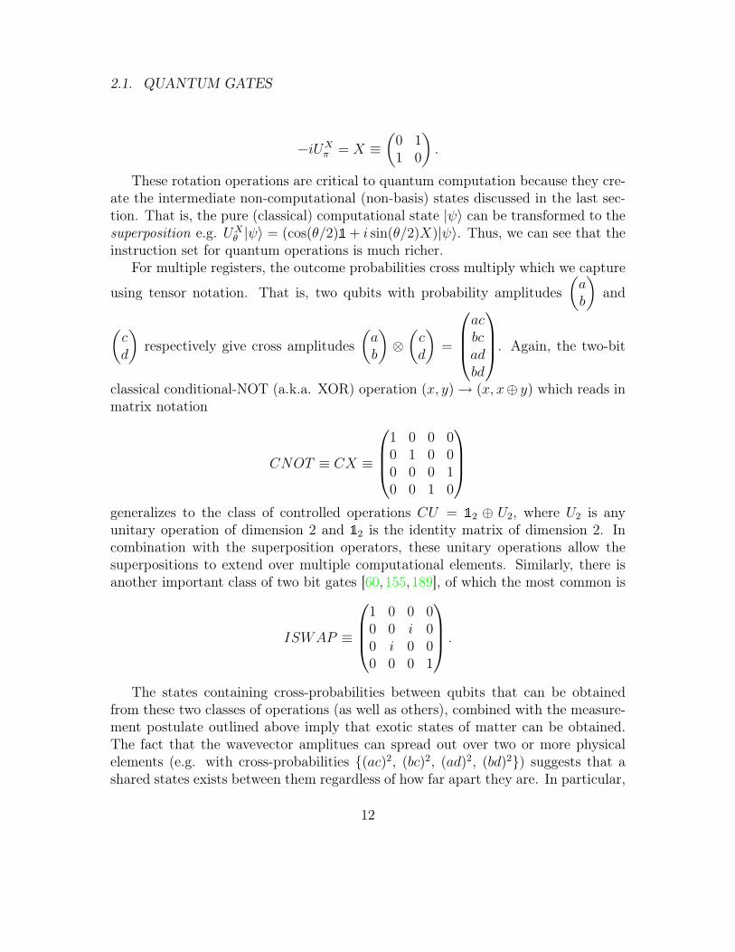
These rotation operations are critical to quantum computation because they cre-ate the intermediate non-computational (non-basis) states discussed in the last sec-tion. That is, the pure (classical) computational state |ψ〉 can be transformed to thesuperposition e.g. UX
θ |ψ〉 = (cos(θ/2)1+ i sin(θ/2)X)|ψ〉. Thus, we can see that theinstruction set for quantum operations is much richer.
For multiple registers, the outcome probabilities cross multiply which we capture
using tensor notation. That is, two qubits with probability amplitudes(ab
)and
(cd
)respectively give cross amplitudes
(ab
)⊗(cd
)=
acbcadbd
. Again, the two-bit
classical conditional-NOT (a.k.a. XOR) operation (x, y)→ (x, x⊕ y) which reads inmatrix notation
CNOT ≡ CX ≡
1 0 0 00 1 0 00 0 0 10 0 1 0
generalizes to the class of controlled operations CU = 12 ⊕ U2, where U2 is anyunitary operation of dimension 2 and 12 is the identity matrix of dimension 2. Incombination with the superposition operators, these unitary operations allow thesuperpositions to extend over multiple computational elements. Similarly, there isanother important class of two bit gates [60,155,189], of which the most common is
ISWAP ≡
1 0 0 00 0 i 00 i 0 00 0 0 1
.
The states containing cross-probabilities between qubits that can be obtainedfrom these two classes of operations (as well as others), combined with the measure-ment postulate outlined above imply that exotic states of matter can be obtained.The fact that the wavevector amplitues can spread out over two or more physicalelements (e.g. with cross-probabilities (ac)2, (bc)2, (ad)2, (bd)2) suggests that ashared states exists between them regardless of how far apart they are. In particular,
12

2.1. QUANTUM GATES
when only ac and bd are non-zero (or bc and ad), measurement correlations betweenthe two objects (where the random value of the first bit predicts the second) can beseen to be stronger than if one were to assume that the randomness in the sharedstate was pre-determined (regardless of spatial distance). Such entangled states havebeen experimentally verified.
Higher dimensional operations can also be defined, most notably N-qubit controlled-
U operations (CNU2 = 12N−2 ⊕ U2), Hadamard operations√
12N
(1 11 −1
)⊗N, and
the quantum Fourier transform transform (mapping basis elementsyk 7→ 1√
N
∑N−1j=0 e2πijk/Nxj) which generalizes the Hadamard operation.
2.1.3 Hamiltonians
To obtain the unitary evolution needed above we need to consider how to obtain itfrom the physical system in use. To this end, we should be able to gauge the differentphysical components that make up the system. In this mathematical treatment,a unitary matrix can more conveniently be defined as the exponential of an anti-Hermitian operator, or equivalently by U = exp(−iHt/~), where H is a Hermitianoperator known as the Hamiltonian and t parametrizes the evolution time. TheHamiltonian gives the intrinsic energies of the system, both for the basis states andfor the interactions that allow transfer of occupancy from one state to another. Inmatrix notation, the energy of the states is given along the diagonal (telling howfavourable a state is), while off-diagonal elements give the coupling energies betweenstates which tell how fast one state is replaced by another. As mentioned, thephysical time scale is irrelevant to any exponential speed-up, and as such we oftenuse dimensionless units as well as take ~ = 1. In general the unitary operationthat is performed will change over time and is described as the matrix productof a sequence of infinitesimal unitary operators. This is written by convention asU = T exp
(−i´H(t)dt
), where the infinite sequence of infinitesimal operators is
equivalent to the use of the time-ordering operator T , which can be used to expandthe integrand in an analytically tractable way. Alternatively, the Hamiltonian definesthe Schrödinger equation U = −iHU whose integration gives the evolution in time.Many different Hamiltonians will give the same evolution, a key point that will berevisited when complications arise.
In the absence of complications (that will arise), a constant H, or an H thatsatisfies the commutation relation [H(t), H(t′)] = 0, ∀t, t′, will simply give U =exp(−i
´H(t)dt) with which it is easy to predict and even engineer gate operations.
Such expressions (approximate or exact) are the reason it is more convenient to work
13
2.1. QUANTUM GATES
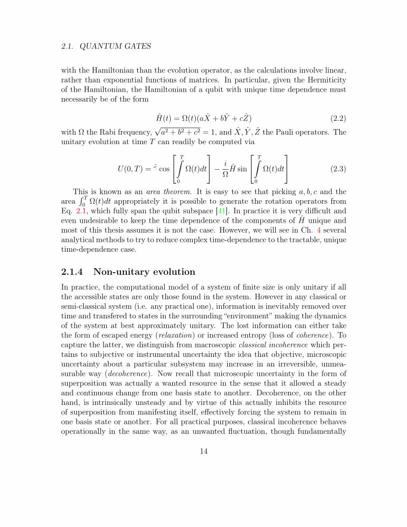
with the Hamiltonian than the evolution operator, as the calculations involve linear,rather than exponential functions of matrices. In particular, given the Hermiticityof the Hamiltonian, the Hamiltonian of a qubit with unique time dependence mustnecessarily be of the form
H(t) = Ω(t)(aX + bY + cZ) (2.2)
with Ω the Rabi frequency,√a2 + b2 + c2 = 1, and X, Y , Z the Pauli operators. The
unitary evolution at time T can readily be computed via
U(0, T ) = 1 cos
T
0
Ω(t)dt
− i
ΩH sin
T
0
Ω(t)dt
(2.3)
This is known as an area theorem. It is easy to see that picking a, b, c and thearea
´ T0
Ω(t)dt appropriately it is possible to generate the rotation operators fromEq. 2.1, which fully span the qubit subspace [41]. In practice it is very difficult andeven undesirable to keep the time dependence of the components of H unique andmost of this thesis assumes it is not the case. However, we will see in Ch. 4 severalanalytical methods to try to reduce complex time-dependence to the tractable, uniquetime-dependence case.
2.1.4 Non-unitary evolution
In practice, the computational model of a system of finite size is only unitary if allthe accessible states are only those found in the system. However in any classical orsemi-classical system (i.e. any practical one), information is inevitably removed overtime and transfered to states in the surrounding “environment” making the dynamicsof the system at best approximately unitary. The lost information can either takethe form of escaped energy (relaxation) or increased entropy (loss of coherence). Tocapture the latter, we distinguish from macroscopic classical incoherence which per-tains to subjective or instrumental uncertainty the idea that objective, microscopicuncertainty about a particular subsystem may increase in an irreversible, unmea-surable way (decoherence). Now recall that microscopic uncertainty in the form ofsuperposition was actually a wanted resource in the sense that it allowed a steadyand continuous change from one basis state to another. Decoherence, on the otherhand, is intrinsically unsteady and by virtue of this actually inhibits the resourceof superposition from manifesting itself, effectively forcing the system to remain inone basis state or another. For all practical purposes, classical incoherence behavesoperationally in the same way, as an unwanted fluctuation, though fundamentally
14

2.1. QUANTUM GATES
superpositions are not destroyed and information remains in the system, rather theinformation we have about the system becomes degraded [137]. On the other hand,information can also be removed from the system by an act of measurement, whichlike unitary evolution is a wanted form of fluctuation that steadily and continuouslytakes an arbitrary state to one of the measurement basis states. However the in-formation that is removed is done so in an apparently non-deterministic way, andas such again forces the system into a random measurement basis state. Whetherthe non-determinism reduces ultimately to classical incoherence or is it solely causedby objective decoherence (up until the moment of observation) is an open interpre-tational question though is somewhat moot due to the common phenomenologicalframework.
Now wanted an usable (i.e. deterministic) uncertainty had necessitated the useof vectors to capture the exponential number of combinations of the n pieces ofinformation as possible measurement outcomes. To model the nondeterministic un-certainty requires modeling only pairwise combinations of the deterministic uncer-tainties. That is, there are
(2n
2
)possible superpositions of two measurable basis
states, each with a coherence associated with it telling how much certainty remains.This construct is called the density matrix ρ and is captured for pure states via theouter product of the wave vector ψ with its conjugate transpose
ρ = |ψ〉〈ψ|
where we now use Dirac notation for the state vector. The diagonal entries ofthe density matrix give the effective probabilities of the respective basis states andare typically susceptible to relaxation. Uncertainty in the form of decoherence comesfrom considering a pure state with larger dimension and then removing environmen-tal degrees of freedom (entangled with the computational subsystem) via a partialtrace operation to give back a non-pure (a.k.a. mixed) state. To model classicalincoherence, on the other hand, we use an ensemble of wave vectors |ψi〉 withprobability distribution pi, giving
ρ =∑i
pi|ψi〉〈ψi|
In many cases, the degradation of the system is itself phenomenologically mo-tivated in that it is derived macroscopically and is found to fit the measurable ex-ponential decays of the diagonal and off-diagonal elements in our density matrix(corresponding to averaging many measurements). Assuming a common Hamilto-nian (and an initially unentangled, memoryless environment), it can be simulatedwith a Markovian master equation
15

2.2. QUANTUM SOFTWARE
ρ = −i[H, ρ] +M∑j=1
[1TjD[Aj]ρ
], (2.4)
where M decay processes are taking place each with characteristic decay timeTj and associated operator Aj, and D is the damping super-operator, defined asD[A]ρ = AρA†− 1
2A†Aρ− 1
2ρA†A. If there are no decay processes (a perfectly isolated
system where M = 0), then the evolution is equivalent to the Schrödinger unitaryevolution.
2.2 Quantum software
2.2.1 Assembly
As we have seen, being able to create (approximately) unitary operations is of utmostimportance for running quantum computations. Since there are an uncountably largenumber of unitaries even for a single qubit, a method is required to generate themwith finite resources. This construction is given by the Solovay-Kitaev theorem andis efficient [91]. Naturally, these operations need to scale with system size in a waythat is not prohibitive to design. However, generating such operations using high-dimensional Hamiltonians requires classical simulation and optimization, which iscontrary to our operating assumption that the quantum computer will scale betterthan its classical counterpart. Nonetheless, it has been shown that arbitrary singlequbit gates and a single entangling two qubit gate form a sufficient basis from whichto generate any unitary that could be desired in 2n dimensions [172], though theconstruction is not necessarily efficient. In practice, the resource allocation anddesign of high-dimensional gates follows from the needs of the algorithm and is oftenefficient for known algorithms.
We wish to have the gate set readily available for compilation of a quantum algo-rithm. Thus, one can consider the kinds of low dimensional gates that are requiredfor most known algorithms and build an entire instruction set of such possible oper-ations, which can be called upon to generate quantum circuits in the larger Hilbert(state) space [156]. The most generic model for operating quantum software is knownas the circuit model and utilizes such a construction. It is built up entirely of a se-quence of gates and one final measurement step at the end2, and thus it has themost stringent requirements in terms of suppression of errors in gate design. For
2Incidental techniques such as error-correction and teleportation will use additional measure-ments during the computation.
16

2.2. QUANTUM SOFTWARE
the purposes of optimal control as discussed this thesis, it is the most relevant andstands to gain the most from gate design.
On the other hand, high-fidelity gate operations are usually a resource that isdifficult to attain (given the chosen hardware) or not directly useful for the type ofcomputations required by the algorithm. In particular, decoherence and relaxationmay be prohibitive to achieving quality unitaries. In contrast to the gate model,the adiabatic model is an equivalent construction that relies on engineering quan-tum states rather than quantum unitary evolution. By changing the effective energystructure of the system (and its respective eigenstates) one can move from the knowneigenstate of a Hamiltonian to that of a different Hamiltonian, allowing one to effec-tively find the previously unknown ground or equilibrated state of the system. Thisis known as an adiabatic algorithm [44,77]. Many problems can easily be mapped tothis methodology though perhaps the most natural are simulation of physical mod-els. As before, changing the eigenstates requires manipulation of the Hamiltonian.In practice, this manipulation will involve the suppression of a variety of unwantederrors and the design can be optimized. In particular, remaining in the ground stateof the eigenbasis requires an adiabatic trajectory from initial state to final state,directly related to the spectral selectivity problem (Ch. 7.1).
Another way to avoid difficult to engineer gate operations is by moving to ameasurement-based model. Here, the entanglement in the system is generated bysome means at the beginning of operation (one option would be through unitaryoperations) and the remainder of the circuit is executed via measurement, single-qubit gates, and feed-forward of classical information. The measurement process(which typically involves single-qubit gates) can also be optimized though this fallsoutside the scope of this text. However, as in the other cases, the biggest challengeof this computing model involves designing and optimizing many-body operationsfor the purposes of entanglement. This model is not studied further in this thesis.
2.2.2 Outlook on algorithms
It is difficult to say what problem-solving applications will be most relevant to quan-tum information. At the present moment, there is no definitive proof of a substantialtechnological premium because while there are numerous positive results for efficientquantum algorithms there are no provably negative results with regard to solvingmost (NP) hard problems using classical techniques. Furthermore, many of theproven quantum algorithms may have classical workarounds or approximation tech-niques that are often sufficient to the task. What can be said however is that therewill be some applications and these will be more significant as the hardware improves.
17

2.3. QUANTUM HARDWARE
At the present time, some of the most rewarding techniques include crypto-graphically encoded communication by using the measurement properties quantumstates [9], and magnetic imaging techniques that use resonance protocols to measurequantum signatures in chemical samples [54, 45] (see Sec. 7.1.1). Quantum pro-tocols are also gaining importance in metrology applications and photon detectiondevices [19, 130].
In the medium term, much can be accomplished with small or imperfect devices.With a moderate number of qubits, by engineering larger but perhaps imperfectquantum structures, it will also be fairly straightforward to run simulations andcalculations with respect to physical theories, which can easily perform the unitaryevolutions required in the systems [81], as well as computations relating to field the-ories such as evaluating Jones polynomials [42]. These simulation type algorithmsmay be well suited in particular to adiabatic computation devices [44, 77]. With anincrease to a couple of hundred logical qubits, it is possible to run algorithms thatbreak present state-of-the-art encryption technology, the most famous of which isShor’s factoring algorithm [158]. It is based on a curious counting argument in num-ber theory: it relates prime number factoring to period finding of periodic functions,something that can be found directly (and therefore efficiently) from measuring thepeak of the Fourier transform of the function’s input. Similar algorithms which useunitaries corresponding to Fourier transforms over different algebraic groups havebeen formulated, generally referred to as the hidden subgroup problem.
Of course, in the long term, many more inventive, sophisticated, and large scaleapplications may be found. Whether this is solely for supercomputing tasks orwhether more mainstream, universal resources in quantum information can be iden-tified remains to be seen.
2.3 Quantum hardwareThere is a vast array of possibilities for implementations which is too extensive tocomprehensively analyse in detail here. Instead, we will outline some of the hardwarechoices that exist and focus on some fundamental design choices that any technologywill have to make. In particular, any engineered quantum computing technologywill face some tradeoffs early on between between isolation and controllability ofthe system, between separation of the qubits in frequency or in space and betweenmediated vs. direct coupling of the qubits.
18

2.3. QUANTUM HARDWARE
2.3.1 Candidate implementations
There are many candidate systems containing quantum degrees of freedom that canbe controlled. Natural qubit systems include NMR molecules with spin degrees offreedom [8, 61, 73] and photons’ polarization or mode [92]. One can also capturethese sorts of natural degrees of freedom using trapping potentials, in the form offor example trapped ions [65], optical lattices [169], NV centres, quantum dots [139],and electron spin resonance, which rely on controlling electronic energy states incomplex energy landscapes. Perhaps the most flexible from an engineering pointof view are human-made systems such as superconducting [29] and semiconductingmaterials [139], for which the energy landscape can largely be controlled and forwhich design choices are reflected directly in the control strategies to choose fromand their efficacy. Some of these implementations will be discussed in more detail asspecific applications to control problems that will be analysed (Ch. 6-11). Since themost general situation is also the most flexible one, where we have control over allthe energy and coupling parameters, engineered systems will often be preferentiallychosen to illustrate the control/design choices that can be made both within theseimplementations and between implementations where such parameters are fixed.
2.3.1.1 Superconducting qubits
For these purposes, a concise introduction to superconducting qubits is in order[30, 113, 153, 184]. The quantum degree of freedom involved is the mesoscopic su-perconducting current of Cooper pairs [79] which can be measured moving eitherclockwise or counter-clockwise in an electrical circuit. Alternatively, one can mea-sure other properties of the current, such as a relative number of Cooper pairs, aVoltage, or a phase shift imparted on other coupled quantum elements. Since low-frequency superconducting currents are dissipationless, the currents are resilient to(thermal) fluctuation and offer promise of retaining coherence [6,35]. However, whilesuperconductivity is maintained, the measurable degrees of freedom may still suf-fer population decay from one to another or otherwise lose coherence between eachother, an effect which is amplified by these large devices coupling very strongly totheir surrounding environment. Nonetheless, the large sizes and electrical nature area boon to prospective scaling in the number of qubits, thanks to industrial depositionand lithography techniques already being very advanced for the mass production ofconventional silicon based devices.
The physical realization of quantum information processing in superconduct-ing circuits has enjoyed remarkable progress over the last decade. While initiallydecoherence limited single qubits to only a few coherent oscillations [126], high
19

2.3. QUANTUM HARDWARE
precision, general quantum control is now possible over single- and few-qubit sys-tems. This is evident by the demonstration of high-fidelity nonclassical states oftwo-qubit [3, 26, 39, 164] and three-qubit [40, 127] systems, harmonic oscillators [71],and the demonstration of small quantum algorithms [39]. This success is partiallydue to our current understanding of sources of noise and the development of tech-niques and systems that are resilient to these noise sources. Examples include theoptimum working point [173] and the introduction of low-dispersion qubits like thetransmon [95,154] and the capacitively shunted flux qubit [165]. On the other hand,a promising route to success are qubits that contains only a minimal number ofelements, such as the phase qubit [117,116,164].
The fundamental electrical component used for superconducting qubits is theJosephson junction, which has a non-linear inductance and linear capacitance. Theelement ensures that the energy levels of the circuit are not harmonic which is re-quired for distinguishability of the states (see Ch. 8). By varying the relative strengthbetween the inductance and the capacitance one is able to change the dominatingdegrees of freedom in the Hamiltonian from the number of fluxoids (for large induc-tance) to the number of Cooper pairs (for large capacitance). Various Hamiltonians,design choices, and control strategies for superconducting systems will be consideredin the relevant chapters of the text.
2.3.2 Controllability
In generic terms, the controllability of a physical system refers to the ability to reachany particular state in the system given any input state, much akin to the universalitycondition for gate sets. We can consider a Hamiltonian
H = H0 +M∑k=1
Hk(t) (2.5)
where Hk are individual control Hamiltonians that can be tuned between on andoff, and determine whether the entire Hilbert space of the computational vectorscan be spanned. This can be straightforwardly be checked by seeing whether all thepermutations of the Hk generates the entire Lie algebra. Most commonly, the controlHamiltonians are parametrized as Hk(t) = ck(t)Hk which is a simplified case knownas bilinear control.
In practice, quantum systems usually not completely controllable. Because ofthe onset of damping and decay processes which are generally at least partially irre-versible, only the equilibrated states can be certifiably achieved. Instead, minimizing
20

2.3. QUANTUM HARDWARE
Figure 2.1: Two different coupling topologies: on the left is nearest neighbour cou-pling while on the right we see (trapped ion) qubits on a common (phonon) buswhich can all interchange energy (taken by R. Blatt’s group).
the total time for gate operations effectively minimizes the effect of structureless,Markovian decay processes. Here, we meet the first tradeoff between minimizing thetime that operations take and maximizing the efficiency of these operations. This isfirst of all a tradeoff between different physical implementations, as some systems canbe very well isolated from the environment (allowing for long operations) but thisisolation often only allows for weaker couplings to other elements or external controlwhich increases the amount of time needed for operations. In some cases, the isola-tion is so good that no direct coupling exists at all between states or between qubitsand indirect methods (which are often slower and less efficient) of coupling must befound. On the other hand, quantum elements that couple readily to (various) de-grees of freedom in their vicinity (and environment) will often be more controllablein terms of design and run-time parameters. This tradeoff is approximately redressedby speaking instead of the quality factor of quantum operations, namely the numberof such operations that can be executed in the characteristic time it takes for thedecay process to occur.
Note that although this benchmark is valuable it can sometimes be a simplisticor misleading. Most often, if the source of coupling to the environment can bedetermined then parameters can be found or strategies laid out that can counteractloss of coherence. These can often involve decreased decay processes at longer gatetimes and optimal values of multi-dimensional design parameters. Specific exampleswill be given in Sec. 8.8.2 and Sec. 10.3. In such cases, the decay processes must beincluded in the error analysis.
21

2.3. QUANTUM HARDWARE
2.3.3 Coupling topologies
Choosing an implementation and computational model for the system greatly reducesthe freedom in architectural design. Nonetheless, one can try to minimize interac-tions between elements by having tunable coupling, and moreover, one can decidewhich elements can even be coupled at all. In general, there is a tradeoff betweentwo particular paradigms, that of trying to couple all pairs of qubits irrespective ofphysical separation or that of only coupling neighbouring qubits (see Fig. 2.1) Arbi-trary couplings typically involve long range interactions (e.g. Rydberg blockade [169]or interactions inside a bus [15, 67]) and are in principle more efficient than nearestneighbour. They typically suffer from imperfect on-off times (e.g. from frequencymodulation, see Sec. (6.7)) and/or imperfect decoupling (e.g. from spatial selectiv-ity constraints). Nearest-neighbour type couplings can also be used but can sufferfrom a polynomial slowdown in computational speed resulting from having to moveinformation around to couple separated logical qubits. However, they may be lesssusceptible to errors as frequency and spatial selectivity is often not required. More-over, near-neighbour interaction involve fewer couplings which tends to increase gateefficiency, and also are a natural fit for certain topological qubit schemes (e.g. surfacecodes [52]). In these, many physical qubits correspond to a computational qubit andbenefit from topological protection against information loss due to conservation lawsgoverning certain quantities (such as the number of vortices inside a lattice).
2.3.4 Coupling mechanisms
In order to perform more complicated operations, and in particular to meet theminimum requirements for gate universality as outlined above, the different quantumcomponents in our system have to be able to interact so as to exchange information.There are two architectural choices, either direct coupling of qubits (by physicalproximity) or coupling via an intermediary component which can be used to carryinformation such as a bus (phonon, photon, etc) or auxiliary qubit. In general,two frequency separated qubits will only exchange energy if they are brought onresonance, e.g. for the Hamiltonian
H = αX1X2 + βY 1Y 2 + ω1Π1 + ω2Π2 (2.6)
with ω1 = ω2, the superscripts indexing the qubit, and the projector Πi = |1〉i〈1|i.This flip-flop interaction produces an evolution generating a gate in the class ofISWAP operations [155,189]. This is nice because qubits can be brought on resonancethis way (allowing beyond-nearest-neighbour interactions) but again suffers from
22

2.3. QUANTUM HARDWARE
frequency modulation issues (Sec. 6.7) and the fact that unwanted resonances maybe activated when a qubit frequency is changed. On the other hand, one can entanglequantum elements equally well by number-conserving interactions where the presenceof one qubit is felt by changing the energy landscape of the second and visa versa,for example with the Hamiltonian
H = γZ1Z2 + ω1Π1 + ω2Π2
known as a ZZ-interaction [189]. Here the interaction occurs irrespective of ω1
and ω2, avoiding having to change qubit frequencies (which is hard to do with naturalqubits), but an additional mechanism is required to turn the gate on or off. The gategenerated is a C-Z which again is equivalent via single qubit operations to ISWAP,CNOT, and other 2-qubit gates.
Natural interactions can arise in nature for two element that are coupled via someforce that bonds them together, as occurs between atoms in a molecule or elementsin a circuit. They usually give both flip-flop and ZZ interactions but with naturalqubits it is difficult to modify the effective qubit frequencies and so ZZ is often moreuseful. Natural couplings are by definition always on and so a major difficulty iseffectively turning them off for single qubit or identity operations. The technique fordoing this is known as dynamical decoupling and involves repeatedly “undoing” theinteraction (most famously the CPMG pulse sequence [76, 151]). Examples of newresults involving decoupling sequences will be given in Sec. 6.7 and Sec. 7.2.
On the other hand, external driving fields can be used to couple devices thatnormally would not exchange energy. For transitions that exist between the ele-ments but are off-resonance, the field can bring in energy that takes the system fromone energy level to another, effectively enabling energy conservation and allowingenergy-exchange to take place. Since the transition is effectively higher-order (vir-tual), this can greatly slow down the gate time but this need not be the case. Theenergy brought in can also be used to activate a single-qubit transition (to a non-computational state) which may then couple in an interesting way to other qubits,such as for Rydberg states. The main disadvantage here is that higher excitationstates are typically prone to more decoherence and relaxation.
Finally, mediated coupling corresponds to using an additional quantum elementas a bridge between qubits that (to at least first order) removes the coupling betweenthe elements. When the intermediary device is turned on, activated via a field, orotherwise brought into resonance, it can be used as a bus for information or otherwiseto directly (virtually) couple the connected qubits. Examples include using a cavity(Sec. 10.3), another qubit, collective phonon modes, and SQUIDS (Sec. 7.2). Onceagain, adding in additional elements can have adverse effects in terms of complicating
23

2.4. QUANTUM ERRORS
things by adding in unwanted terms, couplings to the environment, or just generallyslowing down operations.
In general, one has an additional operational freedom about the computationalbasis to work in. Effectively, for the various coupling strategies, this means thatone can choose between working in a bare basis corresponding to the “physical pic-ture” that one would have of different elements interacting with one another, or inthe dressed basis corresponding to diagonalizing all interactions and considering thewhole system as a single device with time-independent characteristic eigen-energies(only by turning on fields can off-diagonal transitions be activated). The bare frameimplies operationally that natural couplings always persist and must be removedvia dynamical decoupling, while in the dressed frame off-resonance effects permeateand can either be canceled/ignored or brought into resonance to activate a tran-sition [57]. Since non-computational transitions are typically also diagonalized inthe dressed frame, choosing one frame or the other also can have effects in terms ofchanging the coherence time for components with heterogeneous decay mechanisms.
2.4 Quantum errors
2.4.1 Worst-case error
We have seen that many imperfections can plague quantum operations. An erroroccurs when a gate generates an undesired output given some input state. Consideran algorithm which consists of M sequential operations. In order for the algorithmto succeed with non-negligible probability we need the error for each operation tobe less than 1/M where M is a large number. This ensures that the algorithmwill succeed some of the time, which we presumably can check by seeing whetherthe solution output solves the given problem. We can upper bound the worst caseby calculating how often the most pessimistically chosen initial state (with perfectpreparation) will evolve to the wrong final state (given perfect measurement) givenour implemented evolution Uget.
Emax = supψ
(1− 〈ψ|U †Uget|ψ〉), (2.7)
In essence, this figure of merit tells us how faithful our implemented unitary op-eration is to the one needed in the given quantum algorithm. This error correspondsto a theoretical prediction of what might happen in an experiment. Of course in anactual experiment, there is no way to know that that we have actually hit the bottom
24

2.4. QUANTUM ERRORS
in terms of the lowest error that we get. Theoretically though, given a particularimplementation, it is straightforward if not computationally expensive to obtain anestimate for this error. The objective of optimal control is to lower this error as muchas possible.
2.4.2 Threshold theorem
Once this error is low enough, the error can be further improved by the techniques oferror correction [22,163]. At the cost of adding in additional auxiliary quantum bits,the ingenuity of this technique comes from the fact that errors can be corrected whileavoiding finding out the state, using instead information redundancy. Ultimately,several rounds of error correction can be used to further minimize errors (at the costof even more quantum resources) but this is only possible if the error is low enough.The quantum threshold theorem states that for a given correction mechanism thereexists an error rate below which the error can be made arbitrarily small with the useof more and more quantum bits [93]. Thus it is always possible to get an error muchsmaller than 1/M provided we are willing to make the system large enough.
In practice what this means is that we only need to obtain single gate errors belowthe error-correction threshold rather than 1/M . This tacitly assumes that increasingthe system size does not further increase the individual gate errors. This may notalways be the case but is often justified by most coupling mechanisms decreasingexponentially with distance. Whether no error-correction, some error-correction, orfull error-correction is used is mostly dependent on which algorithm we want to runand how many steps it takes, which in turn for now is highly dependent on the error-rates themselves which we can implement and how many quantum bits can fit on ourset-up. Thus, any progress that can be made is highly in need of optimizing the lowesterror rates possible to benchmark proof of principles in algorithms, implementationsand topological design.
2.4.3 Average error
As mentioned, in practice, it is usually very difficult to calculate worst-case errorrates, especially for experiments. In simulations, it is possible but scales inefficientlyfor most systems. In fact, in virtually all cases calculating the average error suffices.This is defined as
EG =1−ˆdψ Tr
[Uideal|ψ〉〈ψ|U †idealE(|ψ〉〈ψ|)
], (2.8)
25

2.4. QUANTUM ERRORS
where E(ρ) is the actual process in the full Hilbert space. While certainly a verylarge worst-case error would be detrimental if every step of an algorithm were tohit this error, this seems unlikely. The reason is that by definition of the averageerror, the worst-case error is either close to the average error or else very unlikely tohappen. One could assume that for a particular input and choice of algorithm, theworst-case error would occur for every single gate. Even in this overly pessimisticscenario, one would still be able to run different inputs successfully, and one wouldstill be able to check whether the program was successful, thereby mitigating the riskof failure. Nonetheless, one can try to minimize norms other than the 2-norm, suchas the 3-norm or 4-norm which weigh the worst case errors more strongly [103].
In fact, one can bound the worst-case error from the average error. For lowdimension the two are within an order of magnitude of each other, and a very lowaverage error ensures the worst-case is also very low. In fact, virtually every knownalgorithm uses gates acting on few qubits, as there is no consistent way of generatinghigh-dimensional gates. Most importantly, error correction typically only uses singleand double qubit gates and can be used to diminish the errors further (assumingdistant qubits do not interact).
For single qubits, average errors can calculated via Ref. [17]
EG = 1−1
6
∑j=±x,±y,±z
Tr[UidealρjU
†idealE(ρj)
], (2.9)
where x, y, z represent the 6 axial states on the Bloch sphere. Clearly the worst-case for qubit error is less than 6 times the average error.
26

Chapter 3
Elements of Quantum Control
Having looked at quantum information from an operational level, we can look at whatis needed to physically control a quantum system. We have already stated that errorsper gate below a certain threshold are needed for applications to produce meaningfulresults. The focus here is therefore to look at quantum information from a controlpoint of view, with an eye towards common settings and their effect on the unitaryevolution of a system. Most importantly, we want to distinguish important classesof operators that can all be modeled in a similar way. Through careful analyticaland numerical examination, it is anticipated that efficient control strategies can bedevised to maximize faithfulness to the desired operations, and that these solutionswill scale and combine with each other with larger Hilbert space dimension.
Table 3.1 lists the main physical systems that will be studied in this thesis. Thecolumns identify usual, generic quantum control problems that can be associatedwith these and other quantum systems. Although, in fact, most of the problems arein fact quite ubiquitous, the models considered in this thesis will capture (only) afew problems at a time, in the interest of both focused and clear solutions.
As shown in table 3.1, it is instructive to separate the sources of imperfectioninto three broad classes: time independent, deterministically time-dependent, andnon-deterministic. As can be seen, these are respectively further subdivided into:on-resonant or off-resonant quantum operators; selective and/or smoothing (semi-classical) control functions; and either static or fast (irreversible) non-unitary evo-lution. Since the static, time-varying, and non-deterministic aspects of the controlare mostly independent these can be combined rather arbitrarily. For example, ir-reversible errors are the major cause of error in most systems; however, since manysystems cannot rectify these errors we choose to only include them when they arerelevant to the matter of control. In traditional quantum control (in NMR), where
27
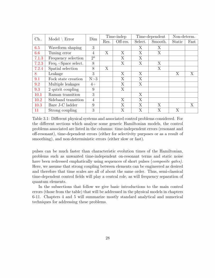
Ch.. Model \ Error Dim Time-indep Time-dependent Non-determ.Res. Off-res. Select. Smooth. Static Fast
6.5 Waveform shaping 3 X X6.6 Tuning error 4 X X X X7.1.3 Frequency selection 2n X X7.2.3 Freq.+Space select. 8 X X X7.2.4 Spatial selection 8 X X8 Leakage 3 X X X X9.1 Fock state creation N>3 X X9.2 Multiple leakages 4+ X X9.3 2 qutrit coupling 9 X10.1 Raman transition 3 X10.2 Sideband transition 4 X X10.3 Bare J-C ladder 9 X X X X11 Strong coupling 3 X X X X
Table 3.1: Different physical systems and associated control problems considered. Forthe different sections which analyse some generic Hamiltonian models, the controlproblems associated are listed in the columns: time-independent errors (resonant andoff-resonant), time-dependent errors (either for selectivity purposes or as a result ofsmoothing), and non-deterministic errors (either slow or fast).
pulses can be much faster than characteristic evolution times of the Hamiltonian,problems such as unwanted time-independent on-resonant terms and static noisehave been redressed emphatically using sequences of short pulses (composite gates).Here, we assume that strong coupling between elements can be engineered as desiredand therefore that time scales are all of about the same order. Thus, semi-classicaltime-dependent control fields will play a central role, as will frequency separation ofquantum elements.
In the subsections that follow we give basic introductions to the main controlerrors (those from the table) that will be addressed in the physical models in chapters6-11. Chapters 4 and 5 will summarize mostly standard analytical and numericaltechniques for addressing these problems.
28

3.1. TIME-DEPENDENT FIELDS
3.1 Time-dependent fieldsWe have seen with Eq. 2.2 that the fields that control the quantum evolution to gen-erate rotation operators can be time-dependent during the gate, and moreover thatthe condition [H(t), H(t′)] = 0, if satisfied, allows a simple method to calculate theunitary evolution. However, one might ask why introduce smooth time-dependenceto Ω(t) in the first place. There are two reasons: either the smoothness is due toexperimental imperfection or it is put in place to suppress another kind of error.
Figure 3.1: Common pulse shapes used in quantum control: a smoothed square(tangential) pulse ΩT (t) in red and a Gaussian pulse ΩG(t) in green.
In particular, there is a the finite turn-on time to most electronics. That is, it isnot strictly possible to specify a discontinuous jump of the field Ω(t) from one valueto another, and instead it typically follows an exponential path, e.g.
ΩT (t) =Ωmax
2
[tanh
(t
σ
)− tanh
(T − tσ
)], (3.1)
where σ is the rise-time and t ∈ [0, T ]. Such smoothed square (tangential) pulse(3.2) is plotted in Fig. 3.1 as the red line. More generally, for waveform responsefunctions f(t) that are memoryless (such as a filter), a control signal at input will bereplaced by a convolution at the qubit,
c(t) =
ˆ ∞−∞
f(t− t′)Ω(t′)dt′, (3.2)
where causality is taken into account by a suitable delay time (with Ω(t′) = 0, t′ > T ).Optimization using response functions will further be discussed in Ch. 6. Even
29
3.2. SELECTION ERROR
without the presence of filtering, choosing an Ω(t) that isn’t a constant functioncan be advantageous when the Hamiltonian is not a simple qubit. Many differentexamples will be given for control functions, but, due to its small bandwidth, by farthe most common is the Gaussian [7, 166]
ΩG(t) = A exp
[−(t− T/2)2
2σ2
](3.3)
where σ is the standard deviation and A is chosen such that the correct amount ofrotation is implemented (e.g. A = π/
√2πσ2erf[T/
√8σ] for a NOT, see Eq. 2.3). A
Gaussian pulse is plotted in Fig. 3.1 as the green line.
3.2 Selection errorThe most common reason to want to smooth the control field is to improve thefrequency selectivity of the pulse. As we have seen fields are often used to activatetransitions for single and two-qubit gates. This is usually accomplished by matchingthe frequency with that of the transition that is driven. Crosstalk typically ariseswhen the spatial (and frequency) extent of the field is larger than the separationbetween qubits. For a field that is on resonance with a particular transition but withcrosstalk to a second transition, a typical Hamiltonian will be of the form
H = Ω(t)X1 + λΩ(t)X2 + ∆ωΠ2
with ∆ω = ω1 − ω2 the energy separation between the two qubits/transitions.λ accounts for the difference in the Rabi frequency from one qubit to the next; inparticular if the spatial extent of the field is centered around the first qubit thenthe coupling will be smaller with the second. This problem will be discussed indetail in Ch. 7. Provided we are in the selective regime, namely λΩ ∆ω, theselectivity error can be indefinitely reduced provided we pick a large enough gatetime (resulting in a smaller Rabi frequency). On the other hand, increasing the timeintroduces further decoherence and relaxation, and so there is a limit to how manytransitions can be put in a given bandwidth. Spectral crowding occurs when thetransitions are too close to be individually selected.
The selectivity can be improved by choosing the appropriate waveform for theRabi frequency, where in general smoother functions will have a smaller bandwidth,and the most common is the Gaussian, Eq. 3.3. The most significant tool for esti-mating the error is the Fourier transform which is a classical scalar function. This
30

3.3. OFF-RESONANT OPERATOR ERROR
scalar can be generalized to the quantum case where it given instead by a nonlinearfunction of the envelope amplitude, as will be shown in Sec. 7.1.
Some common strategies for further reducing the spectral bandwidth beyond theGaussian envelope are spin pinging [55], Rapid Adiabatic Passage (RAP [10]), half-gaussians [55], and composite pulse Narrow Band schemes (NB1 and NB2 [181]).In this thesis another method is developed: Derivative Removal by Adiabatic Gate(DRAG).
It is noteworthy that selectivity is not limited to addressing qubits but otherquantum transitions as well for any given purpose. Examples that will be discussedthat include some selectivity criteria are crosstalk for two-qubit gates (in a 3 qubitmodel, Sec. 7.2), leakage transitions outside the qubit subspace in Ch. 8 and Ch. 9,higher-order virtual transitions (Ch. 10), and counter-rotating terms (Ch. 11).
3.3 Off-resonant operator errorThe effect of unwanted transitions is more subtle than unwanted lines in the spectralprofile of a pulse. The Hilbert space structure of quantum mechanics implies thatadding in additional operators that do not commute with the Hamiltonian will modifythe dynamics of the evolution in subtle ways. In particular, the matrices represent-ing the Hamiltonian will have modified eigenvalues (due to the extra terms). Thisin turn will result in an evolution where an unwanted phase difference will build upbetween the computational states (as well as other errors due to non-commutativity).These phase (and other) errors do not show up in the semi-classical shaping argu-ments that make certain pulse sequences more selective than others. However, theextra phase is still correctable, usually by changing the resonance frequency of theneeded transitions and/or by using extra gates. In the case of decoupled qubits orvirtual transitions (discussed in Ch. 10), these errors will act separately or even dis-appear altogether and can therefore easily be dealt with in isolation (e.g. with frametransformations, Sec. 4.2). The most significant effect is if and when the operatorerror cannot be separated from the selection error (they do not commute) wherebytechniques such as time-dependent diagonalization transformations (Sec. 4.3) andoperator expansions (Sec. 4.4) are required to find solutions.
This is most significant in the case where an unwanted “leakage” transition isconnected by a shared energy level to the driven transition. In fact, the conceptof a perfectly isolated two-level system is an idealization [182] and so this error ispresent to some extent in all quantum systems. An extra transition gives is a 3-levelHamiltonian
31

3.3. OFF-RESONANT OPERATOR ERROR
ω
∆2
|0⟩
Energy
|1⟩
|2⟩
|3⟩
Figure 3.2: Energy level diagram of an anharmonic oscillator. The qubit is formedby the |0〉 and |1〉 (green) levels and we aim to have complete control in this subspacewhen leakage to the |2〉 and then |3〉 etc. is possible (red arrows). The dotted blacklines indicate the positions the energy levels would be at if the system was a harmonicoscillator of frequency ω.
H = a(t)(X0,1 + λX1,2) + b(t)(Y 0,1 + λY 1,2) + c(t)(Π1 + 2Π2) + ∆2Π2 (3.4)
whereXj,,k = |j〉〈k|+|k〉〈j|, Y j,k = i|j〉〈k|−i|k〉〈j| are generalizations of the Paulimatrices in the j-k subspace and Πl is the projector onto the l-th energy level. Aparticularly significant case of leakage is found in the anharmonic oscillator (studiedin Ch. 8and Ch. 9), where each energy separation is different from the next by anamount ∆, the anharmonicity, which is typically quite small compared to otherleakage mechanisms.
Hqut = a(t)∑
λlXl−1,l + b(t)
∑λY l−1,l + c(t)
∑l
lΠl +∆
2
∑l
(l2 − l)Πl, (3.5)
Fig. 3.2 shows the first few levels of an anharmonic ladder, where the qutritapproximation (Eq. 3.4) is most often used. More complex leakage mechanismsinvolving multiple leakages will be dealt with in Ch. 9.
Note that there are also examples of situations where there is essentially noselection error but the off-resonant operator error still remains. This can occur forexample when the Fourier transform of the rectangular (unshaped) pulse happensto go to zero but leakage transitions (and their effect on the Hilbert space) are stillpresent. An example is given in Sec. 9.3.1.
32
3.4. RESONANT OPERATOR ERROR
3.4 Resonant operator errorWe have seen that certain kinds of unwanted terms are always present. These termsare usually not driven, and they are generally significant in that they are eitherdiagonal or off-diagonal and on-resonance so that there is no natural suppressionmechanism as was the case with selectivity error, where terms average out to zerofor longer gate times. This can also appear as another form of crosstalk for unwanteddriven couplings (Sec. 7.2). In all these cases, the unwanted terms cannot be compen-sated for using small parameter expansions as the operators can strongly influencethe state evolution. Instead the effect of these terms must somehow be undone,traditionally with temporal sequences of composite pulses that create trajectories inthe Hilbert space that undo the unwanted evolution. The preferred mathematicaltechnique for this purpose is average Hamiltonian theory (Sec. 4.4). For identityoperations, the canonical strategy involves reversing the unwanted evolution midwaythrough the clock cycle by flipping the qubit , known as a Hahn echo and moregenerally as dynamical decoupling [76, 151]. When a more complicated operationis desired, more complicated decoupling sequences can still be applied to remove avariety of error terms. For multiple couplings that need to be decoupled, multiplespin flips are required to antisymmetrize every pair of qubits. Near resonant tran-sitions that do not satisfy the selectivity criterion λΩ ∆ω can also be dealt withusing decoupling type pulses (Sec. (6.7)). Finally, quantum noise can often be dealtwith using decoupling sequences which often do not depend on the strength of theunwanted coupling, as will be seen next.
3.5 Static non-deterministic errorInstead of having constant or controllable terms, one can think of having an unknownterm in the Hamiltonian. The uncertainty can be constant, as in the case of collectivedegrees of freedom such as NMR molecules or atoms in an optical lattice. On theother hand, if the uncertainty is the result of noise, than we can distinguish betweenslow noise, which can be treated again as approximately constant (e.g. fabricationuncertainty), or fast noise which is essentially Markovian and irreversible (see thenext section). An interesting case occurs when the noise is roughly as fast as quantumgates, known as telegraph noise. This particular case is addressed using optimalcontrol methods in Ref. [121]. When the noise is very slow or constant, the dynamicaldecoupling sequences from the previous section often work as they are not dependenton the magnitude of the error term. On the other hand, if the noise is not constant itmay be advantageous to perform multiple time reversals to undo the evolution of the
33
3.6. FAST NON-DETERMINISTIC ERROR
unwanted terms on a fast time scale over which they are approximately constant. Themost renowned example of this is the CPMG sequence [76,151]. Once again, for noisethat interrupts a rotation, there are other composite sequences to correct this, suchas CORPSE [33, 168], for noise in the qubit frequency, and Broad Band compositepulses (BB1 [181]) for correcting noise in the Rabi frequency. In a sense, these can bethought of as the antithetic case of selectivity where narrowband behaviour is soughtafter. Of course the uncertainty can more generally occur for any parameter in theHamiltonian, and we will be considering two cases in particular using optimal control:Sec. 8.8.2 deals with structured energy and operator dispersion in an anharmonicoscillator (where coherence and anharmonicity form a tradeoff), and Sec. 11 dealswith uncertain phases in the driving field. For these purposes, classical uncertaintyis usually dealt with by modeling the system as a set of Hamiltonians Hφ obeyinga set of evolutions Uφ = T exp(−i
´Hφdt).
3.6 Fast non-deterministic errorNoise that is faster than the dynamics of the system is in general irreversible. Oneway to think of this noise is as an entanglement between the quantum system andanother Hilbert space. If the extra Hilbert space is small [150, 157], then we caninclude the extra dynamics and try to optimize over the larger Hilbert space (as wasdone for leakage, or can be done with auxiliary qubits, resonators , etc.). However ifthe extra space is macroscopic and/or fast then it is generally not possible to modelor even undo the dynamics and the best we can do is to avoid them. This can eitherbe done by finding a part of the computational space that is less affected by thenoise operators (e.g. Sec. 10.3 or Refs. [102, 131, 187]), or else to try to shorten theoperations as much as possible. The latter is generally the approach taken in thisthesis, where errors are often plotted against time with the implication that errordecreases with gate time while Markovian effects increase and so for any given rateof decay there will be an optimum point that minimizes both the error and the noise(see Sec. 8.8.1). Nonetheless, one can still model the full dynamics of the optimizedgate (as in Eq. 2.4) or include the decay in the optimization as in Sec. 8.8.2.
34

Chapter 4
Frame Transformations
In the limit of the Hamiltonian commuting with itself at different times and lowHilbert space dimension, there is often an analytic form for the evolution given bythe matrix exponential (e.g. Eq. 2.3). However, most quantum systems containmultiple qubit couplings and time-dependences and thus are difficult to evolve intime. While numerical techniques can usually work for larger Hilbert space dimen-sions, even these are limited by an exponential scaling with number of qubits. Thus,finding alternative, tractable representations for Hamiltonian structures with com-plicated time-dependence or in high dimension has the double advantage of allowinga conceptual understanding of its dynamics and a practical utility of being efficientto calculate (generally polynomial in the number of qubits). Combining analyticerror-removal strategies can also be accomplished, provided that the errors approxi-mately commute with each other (which is always true in the limit of small errors).For this purpose, in this chapter time-dependent transformations and expansions arediscussed that make such tractable representations possible. These will be used toanalyse specific kinds of errors as relating to various physical models. This chap-ter lays out the detailed theoretical ground work which will be used as required inchapters 6 through 11.
4.1 General theoryWe have seen that the physical design of our quantum system will have a largeimpact on its performance. There is also a mathematical freedom about what wechoose as the intrinsic energy basis (that defines our computational states) and whatthe Hamiltonian operator is that describes their evolution. The two extremes whereeither the basis states are completely static in time or the wavevectors (combinations
35

4.1. GENERAL THEORY
of the basis states) are completely static are known as the Heisenberg and Schrödingerpictures, respectively. A basis that does not contain implicit time-evolution of thebasis states is known as a bare basis while allowing such time-dependence givesrise to dressed basis states. However, if all of the evolution of the wavevector isimplicit as occurs in the Schrödinger picture, then this will not be useful for (vector)computation. Nonetheless, there is a whole range of possible descriptions in between,and a suitable choice will have important repercussions both in terms of operabilityof the implementation(see e.g. Sec. 2.3.4) and simplification of modeling of complexquantum problems.
The various descriptions have in common that they must satisfy the Schrödingerequation (~ = 1),
d
dt|ψ〉 = −iHψ|ψ〉 (4.1)
4.1.1 Transformation formula
We want to transform to some new dressed basis |φ〉 = V (t)|ψ〉. Then, using theSchrödinger equation again for the new picture we can derive a compound evolution
−iHφ|φ〉 =d
dt|φ〉
−iHφ|φ〉 =
(d
dtV
)|ψ〉+ V
(d
dt|ψ〉)
Hφ|φ〉 = (V Hψ + iV )|ψ〉Hφ|φ〉 = (V HψV
† + iV V †)|φ〉
Thus we obtain the general time-dependent transformation formulaHφ = V HψV†+
iV V †, where all terms have dependence on a common time, and which tells us thatthe total evolution of a system Hφ will be given by a combination of the explicit evo-lution of the wavevectors given by Hφ and the implicit evolution of its basis statesgiven by V.
In practice, we can also compute the effect of the transformation on an evolutionUφ(0, T ) from an initial wavevector state |φ(0)〉 to a final state |φ(T )〉 directly. To seethis we apply the time-ordering operator of the exponential map and then transformthe Hamiltonian as above:
36

4.1. GENERAL THEORY
Uφ(0, T ) = lim∆t→0
0∏l=dT/∆te
exp (−iHφ(l∆t)∆t)
= lim∆t→0
0∏l=dT/∆te
exp(V (l∆t)V †(l∆t)∆t
)exp
(−iV (l∆t)Hψ(l∆t)V †(l∆t)∆t
)= lim
∆t→0
0∏l=dT/∆te
V (∆t)V (l∆t) exp (−iHψ(l∆t)∆t)V †(l∆t)
= lim∆t→0
0∏l=dT/∆te
V ((l + 1)∆t)Uψ(l∆t, (l + 1)∆t)V †(l∆t)
= V (T )Uψ(0, T )V † (0)
which is the same result we expect given the direct transformation of the vectorstates,
〈φ(T )|Uφ(0, T )|φ(0)〉 = 〈φ(T )|V (T )Uψ(0, T )V †(0)|φ(0)〉 = 1
4.1.2 Equivalent frames
There is an important subclass of transformations which is those that do not modifythe computational states. As mentioned, these are important for finding alternativerepresentations of physical models that make analysis more tractable. Our require-ment is that the state of the quantum system be identical at the start and at the endof gate operations in both frames, but this leaves complete freedom both in the evo-lution and its representation of what happens in between. The constraint amountsto
V (0) = V (T ) = 1.
Clearly this also leaves the evolution U unchanged. This class of transformations isfundamental because it provides a way to move terms around in our Hamiltonian toobtain more tractable and intuitive forms without changing the other gates. Most ofthe explicit transformations that follow in this thesis are specializations of this classof transformations and serve this purpose.
37

4.2. PHASE TRANSFORMATIONS
4.1.3 Interaction frames
In between the Schrödinger frame and the Heisenberg frame lies the interaction frame,where some part of but not all of the terms in the Hamiltonian have been transformedaway. For a Hamiltonian of the form H = H0 + H1 where [H1(t), H1(t′)] = 0,then the interaction picture with respect to H1 is given by the transformation V =exp(i
´ t0H1dt). Then,
Heff = V (H0 +H1)V † + iV V †
Heff = V H0V† + V H1V
† −H1V V†
Heff = exp
(i
ˆ t
0
H1dt
)H0 exp
(−iˆ t
0
H1dt
)For constant time-dependence, V corresponds to undoing the Schrödinger evolu-
tion of the perturbation terms in the Hamiltonian, V = exp(iH1t). If H1 is cyclic,in the sense that it starts and ends at the same value (integrating to zero), then theinteraction frame evolution Ueff is equivalent to that of the original frame. Otherwise,the evolution is given by Ueff = V (T )U . In practice, one can often think of H1 as aperturbation to an otherwise known evolution and we will see in the next sectionssome expansions to gauge its impact on the effective evolution.
4.2 Phase transformationsIf we expand on our definition of frame equivalency to indistinguishability by mea-surement (we loosen the boundary condition to eiφ1V (0) = eiφ2V (T ) = 1), we includeall transformations which are diagonal. These transformations corresponds to a shift-ing of the clock reference of the processor, and thus can implement gate operationsthat shift the phase of a wavevector, essentially ’for free’ [43].
4.2.1 Phase tracking
The simplest scenario occurs when we simply want to perform a phase rotation UZθ
on a qubit. This can be as part of an algorithm or in order to undo an error thathas occurred of the opposite magnitude, UZ
−θ (we will see such errors occur in laterchapters, in particular for unwanted off-resonant operators, Sec. 3.3). The strategyis essentially to commute the phase gate operation with anything to its left so that inthe end only an unmeasurable phase is left over when the algorithm is complete. For
38

4.2. PHASE TRANSFORMATIONS
example, if we have the want to perform a UZθ followed (to the left) by the operation
U = e−iHt, then this is equivalent to demanding UUZθ = UZ
θ Ueff from which we seewe have to pick Ueff = UZ
θ UUZ−θ and giving the transformed Hamiltonian
Heff = UZθ HU
Z−θ = UZ
θ (a(t)X + b(t)Y )UZ−θ
= (cos(θ)a(t)− sin(θ)b(t))X + (cos(θ)b(t) + sin(θ)a(t))Y
which is nice because no Z operator need be physically implemented on the qubit(as this may be difficult or cumbersome). Of course, the phase accumulates to theleft as more operations are chained and therefore must be tracked over the lengthof the algorithm. In particular, if each operation U produces an error such that itgives in fact UUZ
θ then M such operations in a row can be corrected via M basistransformations, where theM -th basis transformation for theM -th call to U is givenby
Heff = (UZθ )MH(UZ
−θ)M = UZ
Mθ(a(t)X + b(t)Y )UZ−Mθ (4.2)
= (cos(Mθ)a(t)− sin(Mθ)b(t))X + (cos(Mθ)b(t) + sin(Mθ)a(t))Y (4.3)
4.2.2 Rotating frames
The analog equivalent to the sequential accumulation of phase UZMθ is a continuous
accumulation in the form of V = exp(i∑
h ωh|h〉〈h|t). Once again, this does not mod-ify the probabilities of measuring a given state |ψ〉 but only adds in a time-dependentphase |φ〉 = eiωψt|ψ〉. For unwanted phase operators that are continually present, thiscontinuous transformation is more suitable and corresponds to an interaction framewith respect to the unwanted diagonal operator.
As the most common example, suppose one wants to perform a X or Y rotationon a qubit where the energy splitting is much larger than the external control field.It is standard to move to an interaction frame with respect to the energy splittingand drive the rotations with sinusoidal fields1. We start off with the untransformedlab Hamiltonian
Hlab = (2a(t) cos(ωdt+ φ) + 2b(t) sin(ωdt+ φ))Xπ + (c(t) + ωq)Π1 (4.4)
1This is most easily accomplished in experiment by mixing the shaped waveform signal with acarrier pulse at the frequency of the desired transition
39

4.2. PHASE TRANSFORMATIONS
which differs from the conventional form Eq. 2.2. This form is not intuitive and lacksa simple method of exponentiation (due to lack of commutativity). However, usingthe transformation V = exp(iωΠ1t+ iφ) one can move to the effective Hamiltonian
Heff = eiωΠ1t(2a(t) cos(ωdt+ φ) + 2b(t) sin(ωdt+ φ))Xπ + c(t)Π1e−iωΠ1t
Heff = (c(t) + ∆ω)Π1 (4.5)+(a(t) cos(δωt) + b(t) sin(δωt))X (4.6)+(b(t) cos(δωt)− a(t) sin(δωt))Y
+(a(t) cos(ωΣt+ 2φ) + b(t) sin(ωΣt+ 2φ))X (4.7)+(−b(t) cos(ωΣt+ 2φ) + a(t) sin(ωΣt+ 2φ))Y
where δω = ωq−ω, ∆ω = ωd−ω, ωΣ = ωd+ω. The frame in which ∆ω = 0 is knownas the interaction frame (with respect to the energy eigenbasis). It is customary toignore the fast-oscillating last two lines (the counter-rotating terms) which will self-average to zero under the justification that ωΣ a, b, c, δω, known as the rotatingwave approximation (RWA). We will see this approximation is another example ofselectivity/off-resonant operator criteria. On the other hand, picking δω = 0 willbe referred to as the rotating frame and doesn’t contain any fast oscillations withinthe frame (beyond any ’slow’ time dependence in the envelopes a(t), b(t), c(t)) in theRWA limit. At resonance, δω = 0 and ∆ω = 0, the RWA Hamiltonian is now thesame as the simple qubit, Eq. 2.2.
If we have n independently driven qubits then the transformation generalizes toV = V1⊗V2 . . .⊗Vn with Vj = exp(iωjdΠ
jt+iφ), which is known as a multiply-rotatingframe. Once again we can go to an interaction or rotating frame for all the levels.Note that if there are more non-zero matrix elements than there are energy levelsor if any transition is driven by more than one drive then it is not possible to finda rotating frame that cancels all fast oscillations in the Hamiltonian. This notationwill be formalized further in Ch. 7 and strategies for quantifying and suppressingthe counter-rotating terms will be given in Ch.11.
4.2.3 Phase ramping
More generally, one will want to perform arbitrary phase operations c(t)Z on ourqubits via transformation methods. Going again to the interaction with respect tothe variable, we see we can simulate it with
40
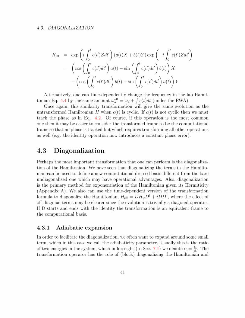
4.3. DIAGONALIZATION
Heff = exp
(i
ˆ t
0
c(t′)Zdt′)
(a(t)X + b(t)Y ) exp
(−iˆ t
0
c(t′)Zdt′)
=
(cos
(ˆ t
0
c(t′)dt′)a(t)− sin
(ˆ t
0
c(t′)dt′)b(t)
)X
+
(cos
(ˆ t
0
c(t′)dt′)b(t) + sin
(ˆ t
0
c(t′)dt′)a(t)
)Y
Alternatively, one can time-dependently change the frequency in the lab Hamil-tonian Eq. 4.4 by the same amount ωeff
d = ωd +´c(t)dt (under the RWA).
Once again, this similarity transformation will give the same evolution as theuntransformed Hamiltonian H when c(t) is cyclic. If c(t) is not cyclic then we musttrack the phase as in Eq. 4.2. Of course, if this operation is the most commonone then it may be easier to consider the transformed frame to be the computationalframe so that no phase is tracked but which requires transforming all other operationsas well (e.g. the identity operation now introduces a constant phase error).
4.3 DiagonalizationPerhaps the most important transformation that one can perform is the diagonaliza-tion of the Hamiltonian. We have seen that diagonalizing the terms in the Hamilto-nian can be used to define a new computational dressed basis different from the bareundiagonalized one which may have operational advantages. Also, diagonalizationis the primary method for exponentiation of the Hamiltonian given its Hermiticity(Appendix A). We also can use the time-dependent version of the transformationformula to diagonalize the Hamiltonian, Heff = DHψD
† + iDD†, where the effect ofoff-diagonal terms may be clearer since the evolution is trivially a diagonal operator.If D starts and ends with the identity the transformation is an equivalent frame tothe computational basis.
4.3.1 Adiabatic expansion
In order to facilitate the diagonalization, we often want to expand around some smallterm, which in this case we call the adiabaticity parameter. Usually this is the ratioof two energies in the system, which in foresight (to Sec. 7.1) we denote α = Ω
∆. The
transformation operator has the role of (block) diagonalizing the Hamiltonian and
41

4.4. MAGNUS EXPANSION
takes the form D = exp(iS). As before, the effective Hamiltonian corresponds to aTaylor expansion around the null transformation,
Hdiag = exp(iS)H exp(−iS) + DD†
=∑r
(iS)rH∑s
(−iS)s + S
= H + S + i[S,H]− 1
2[S, [S,H]] +O(α3)
4.3.2 Interaction frame
In addition to being a time-dependent diagonalization, the transformation can alsobe an interaction frame with respect to some parameter. Dividing the Hamiltonianinto H = Hbig +Hsmall, we can take the interaction frame with respect to Hsmall whichwe assume diagonalizes the rest of the Hamiltonian Hbig. giving after application ofV = exp(i
´Hsmall dt).
Hdiag = exp
(i
ˆHsmalldt
)Hbig exp
(−iˆHsmalldt
)= Hbig + i
[ˆHsmalldt,Hbig
]− 1
2
[ˆHsmalldt,
[ˆHsmalldt,Hbig
]]+ . . .
where in the second line we have assumed the integrand is small and can be expandedaround (as in the adiabatic expansion) though this may be superfluous when the di-agonalization can be done analytically (e.g. Sec. 7.1.3.4, Sec. 10.1). This expansionis most useful if one can find a small (cyclic) perturbation to add to the imperfectHamiltonian that diagonalizes unwanted parts. The net effect is then simply a shift-ing of the eigen-energies, which can readily be corrected for using the techniques ofSec. 4.2. Applications of using such an auxiliary control for the purposes of diagonal-ization will be seen: to deselect transitions (Sec. 7.1), to offset the effect of leakage(Ch. 8), to suppress the counter-rotating terms in the qubit lab Hamiltonian (Ch.11), or to enhance virtual transitions (Ch. 10).
4.4 Magnus expansionIn the limit of a small Hamiltonian, fast oscillation or a very small evolution time,the Magnus expansion [64, 110] is one of the most helpful tools in quantum controltheory. The expansion of a Hamiltonian is given in orders where the first three are
42

4.4. MAGNUS EXPANSION
H(1) = −iˆ T
0
H(t)dt
H(2) =1
2T
ˆ T
0
dt1
ˆ t1
0
dt2
[− iH(t1),−iH(t2)
]
H(3) =1
2T 2
ˆ t
0
dt1
ˆ t1
0
dt2
ˆ t2
0
dt3 ([−iH(t1), [−iH(t2),−iH(t3)]] + [−iH(t3), [−iH(t2),−iH(t1)]])
(4.8)
and the composite evolution is given by
U = e
(H(1) + H(2) + H(3) + H(4) + ···
)The convergence of the series is difficult to prove but a sufficient condition is that∣∣∣Tr´ T
0H(t)dt
∣∣∣ < π [23, 89]. For small enough T this can easily be satisfied. For Hthat obeys an area theorem or whose evolution can be broken into smaller segmentsall performing the same operation, the expansion can instead be shown to convergefor one such subsegment, which in turn is sufficient to show that the Hamiltonian isapplying the correct operation on concatenation.
4.4.1 Interaction frame
On the other hand, one often uses this expansion to gain insight into a Hamiltonianrather than to provide its final evolution. In this case, one tends to divide theHamiltonian according to a small useful part and an poorly understood large partto with respect to which will be applied the interaction frame V = exp
(i´Hbigdt
).
H = Hsmall +Hbig
Heff = exp
(i
ˆ t
0
Hbigdt′)Hsmall exp
(−iˆ t
0
Hbigdt′)
The Magnus expansion is then taken with respect to this interaction Hamiltonian.As a general rule, the larger Hbig the faster the effective Hamiltonian will rotate andthe convergence properties will be better. Note also that unlike for the adiabaticcase, the interaction frame is with respect to a large parameter rather than the smallone.
43

Chapter 5
Numerical Simulation andOptimization
The standard quantum control problem is to find a way to implement a desiredunitary operation Uideal, given discrete control vectors uk each of length N . It isstandard to assume that the underlying Hamiltonian is of the form H = H0 +∑
k ck(t)Hk where Hk is the control Hamiltonian and ck(t) is a continuous field whichis parameterized by the control uk. The goal is to choose controls uk such that atthe final time t = T , the dynamics of this system approximates the target unitaryoperator: Uideal. To find these controls one first needs to simulate the dynamicsof the system, given the Hamiltonian. In addition, a cost function C is needed todescribe how close a simulated operation is to Uideal. This allows us to evaluatethe performance of each uk and thus search the space of controls for an optimum.Further refinements to this method will be discussed in Ch. 6.1.
5.1 Time-slicingIn order to numerically integrate the Schrödinger equation it is necessary to discretizethe evolution, normally into piecewise constant intervals. The approach traditionallyused (e.g. in Ref. [85]) is to also use this discretization to map between the continuousfields and the control vector. That is
ck(t) =N−1∑j=0
uk,j uj (t,∆t), (5.1)
44

5.2. COST FUNCTIONS
with the rectangle function
uj (t,∆t) ≡ [Θ(t− j∆t)−Θ(t− (j + 1)∆t)] , (5.2)
where Θ is the Heaviside unit step function. Evaluating the Schrödinger evolutionusing these fields and the Hamiltonian in Eq. (2.5) yields
U(0, T ) =0∏
j=N−1
Uj, (5.3)
whereUj = exp
[−iH(j∆t)∆t
], (5.4)
the product running backwards is to enforce time-ordering, and N∆t = T .
5.2 Cost functionsIn Eq. (2.7) we saw that the maximum error given the most pessimistic input stateswas the required figure of merit for using the error threshold theorem. The averageerror Eq. (2.8) and for qubits Eq. (2.9) were given as appropriate alternativeswhenever certain basic conditions such as low Hilbert space dimension or variableinput states could be ascertained. Since the time-slicing equation Eq. (5.3) requiresthe multiplication and exponentiation of N d-dimensional matrices, which scales asO(Nd3), the criterion of low dimension for control theory can usually be met therebyallowing the use of average error as a cost function.
5.2.1 Overlap fidelity
For the purposes of evaluating quantum gates, it is standard to use another form ofthe average fidelity, namely the overlap fidelity
Φ4 =1
d2|Tr(U †U †get(T ))|2, (5.5)
where d is the dimension of the Hilbert subspace . It tells how close the two unitaryoperations are to one other where the squaring effectively removes a global phaseand gives the interpretations of a probability (for further discussion of Φ4 see [85]).This fidelity is equivalent to the average fidelity, Eq. (2.8), via [104]
Fg =1
dQ + 1(1 + dQΦ4),
45

5.2. COST FUNCTIONS
with dQ the dimension of the computational subspace. This overlap form is preferredbecause it does not make reference to the states of the quantum system and can becomputed more quickly using fast matrix multiplication.
5.2.2 Subspace fidelity
For larger dimensions where the qubits are embedded in a larger Hilbert space (e.g.,containing leakage channels, a cavity, or a non-Markovian environment) we can useinstead [148]
Φ5 =1
d2Q
|Tr(U †PQUget(T )PQ)|2, (5.6)
where PQ is a projector onto the computational subspace. This formulation reducesthe search space because it ignores correctly what happens to states mapped fromoutside of the computational subspace back onto outside of the computational sub-space. This effectively increases the number of possible optimal solutions and reducesthe expected search time.
We can also decompose the desired unitary evolution U †get(T ) =∏0
j=N−1 Uj =∏0j=N−1 Uj
∑ψi∈BH |ψi〉〈ψi| where BH is a basis for the entire Hilbert space into
rather a basis sum where we do not include basis elements outside those of thequbits’ subspace BHQ ; the whole Hilbert space dimension is however still used forthe simulation.
Φ6 =1
d2Q
|Tr(U †PQ
0∏j=N−1
Uj∑ψi∈BH
|ψi〉〈ψi|PQ)|2, (5.7)
=1
d2Q
|∑
ψi∈BHQ
〈ψi|U †0∏
j=N−1
Uj|ψi〉)|2 (5.8)
Computing the fidelity then requires multiplying into dQ vectors, where each mul-tiplication is O(d2). The total fidelity given N time steps then takes O(NdQd
2) whichcan often be smaller then O(Nd2.8) usually required for N matrix multiplications bystandard numerical software packages.
5.2.3 Ensemble fidelity
If one wants to include the incoherent dynamics (Sec. 2.1.4) by using numericalrather than analytic techniques (Sec. (3.5)), it is necessary to optimize over an
46

5.2. COST FUNCTIONS
ensemble of different descriptions of the system. To account for this, we define anaverage performance index
Φ7 =
ˆp
f(p)Φj(p)dp, (5.9)
where Φj(p) is one of the given fidelity functions evaluated using a value of theensemble parameter p , which is unknown for specific instantiations of the quantumcomputer but occurs according to the probability distribution f(p) (lacking specificknowledge we in this thesis set f(p) = 1). In practice, the integral is replaced bysummation, which we sample discretely as p, p2, . . . pM .
As a consequence of sampling, the optimization may find control sequences thatresult in discretely different trajectories in the Hilbert space from one value of theensemble parameter pi to the next (e.g. a different winding number around the Blochsphere). Then, values of the parameter in between may have an average trajectorythat differs significantly from either of the successful trajectories, thereby makingthe overall ensemble unsuccessful. While this situation can largely be alleviated byincreased sampling, in practice it can also be mitigated by ensuring that the globalphase of the operation from one ensemble member to the next remains the same,eliminating at least one common way in which different trajectories can happen.Thus, we move the squaring of the unitary product outside the sum of fidelities,which only disregards the common phase, giving
Φ8 =1
(dM)2
∣∣∣∣∣M∑l=1
Tr(U †U
(pl)get
)∣∣∣∣∣2
.
This fidelity is over-constrained but often gives better results in practice (seeSec. 8.8.2). Of course one can seek further refinements to the constrained solutionby optimizing further over Eq. (5.9) once a solution is found. As an additionalinsurance, one will want to sample non-uniformly over the ensemble parameter p.
5.2.4 Penalties
There are a number of additional constraints that one may want to impose on thecontrols from a practical point of view. For example one may want to limit theenergy of the pulses or avoid population of certain states during the gate. This isoften accomplished by adding additional cost elements to the cost function, wherethe prefactor tells the relative importance of the terms.
Φtot = Φj +∑k
λkPk,
47

5.3. GRADIENT ASCENT
where Φj is the chosen fidelity function and each penalty Pk has a multiplier λkassociated with it. In the ideal case, λk is a Lagrange multiplier, whose value isoptimized for the minimum point in the fidelity. However, in practice, choosing adifferent value may be more fruitful in terms of the trajectory used to get to theoptimum point by an optimization algorithm. That is, a large λk will enforce theconstraint more rigourously in the end, but it will give less freedom in terms of thesearch path towards an optimum, making it potentially harder to reach.
Unfortunately, any of the constraints that were tried in this thesis proved to betoo demanding for the available controls in the sense that the optimization was over-constrained, giving a tradeoff between the cost terms. This is particularly true in thelimit of short times where the controls are often already fully constrained. Thus if onewants to add in extra constraints it is usually necessary to increase the times of thepulses which may be more detrimental if irreversible forms of damping are significantin the error. In at least one case where the hard constraints are necessary to includeon our pulses, Sec. (6.1), we find that better describing the unitary evolution is amore accurate and elegant way than by manually setting the value of the multiplierto give a realistic pulse.
5.3 Gradient AscentThe mathematical statement of the optimization problem is to maximize Φ withrespect to the vector uk. It is not immediately apparent how one should performthis optimization. One of the simplest approaches is the steepest ascent (or gradientsearch) algorithm [20]. If we consider the multi-dimensional surface (control land-scape) formed by Φ(uk), steepest ascent is an iterative update procedure that locallyexamines the landscape at each iteration and provides a new uk by moving in thedirection that increases Φ the greatest. We take some initial guess for the controlsand iteratively update according to the rule uk → uk+ε∇ukΦ(uk), where ε is a unit-less step matrix. Given an arbitrary initial configuration for the control fields, thealgorithm follows a steepest ascent to a local optimum, at least in the case of small ε.For simplicity, in this work we take ε to be a scalar which is chosen adaptively. It isin no way clear that this procedure will produce anything other than local maxima,but remarkably, for the types of Φ’s we examine in quantum control, the landscapeis sufficiently under-constrained that gradient searches find global maxima with highprobability (to arbitrary precision), in particular for small dimensions and large gatetimes. This has implications for the topology of the control landscape [34,145].
The GRadient Ascent Pulse Engineering (GRAPE) algorithm [85] is an example
48

5.3. GRADIENT ASCENT
of a gradient search technique. A principle insight of GRAPE is that the gradient ofΦ can be computed more efficiently than that of an arbitrary function. Specifically,the derivative of Φ5 with respect to one of our control variables is
∂Φ5
∂uk,j=
2
d 2Q
Re[Tr
(U †idealPQ
∂U(T )
∂uk,jPQ
)× Tr
(UidealPQU(T )†PQ
) ],
(5.10)
where∂U(T )
∂uk,j=
(j+1∏
n=N−1
Un
)∂Uj∂uk,j
(0∏
n=j−1
Un
). (5.11)
The speedup over gradient searches based on a naïve approach where one queries thefidelity function for each variation in the control values comes from the observationthat the forward evolution U(t, 0) and the backwards evolution U(T, t) need only becalculated once for a given control configuration. This in turn allows each derivativeto be calculated with a constant number of matrix multiplications, as opposed to theN required for the full Schrödinger evolution, leading to an overall scaling of O(N)as opposed to O(N2).
The exact form of the derivative of the unitary time slice can be found in theoriginal GRAPE paper [85],
∂Uj∂uk,j
= −i∆tHk,jUj,
Hk,j =1
∆t
ˆ ∆t
0
e−iH(j∆t)τHkeiH(j∆t)τdτ.
(5.12)
For fine-grained control fields, i.e. ‖H∆t‖ 1, the derivative can be approximatedas
∂Uj∂uk,j
= −i∆tHkUj. (5.13)
This approximation can lead to difficulties in finding optimal solutions if the timestep ∆t is not sufficiently small, but this problem can be circumvented by evaluatingthe integral in Eq. (5.12) exactly [109]. Calculating this integral using the givenform of Uj is straightforward after obtaining the diagonalization of H(j∆t) (which isthe preferred method of exponentiating the Hamiltonian given its Hermiticity [120]).Thus, the form of the derivative of the time slice Uj with respect to the k-th control[as in Eq. (5.12)] in the diagonal basis of the full Hamiltonian is
49

5.3. GRADIENT ASCENT
〈mj|∂Uj∂ukj|nj〉 = 〈mj|Hk|nj〉
e−iλmj∆t − e−iλnj∆t
∆t(λmj − λnj)(5.14)
for nj 6= mj, or
〈mj|∂Uj∂uk,j
|mj〉 = −i∆t〈mj|Hk|mj〉e−iλmj∆t (5.15)
if nj = mj. Here, λmj and λnj are eigenvalues of the full Hamiltonian at time slicej, associated with eigenvectors |mj〉 and |nj〉 respectively. The actual derivative isthen calculated by reverting the matrix elements back to the original, non-diagonalframe.
The gradient formula, Eq. (5.10), explicitly assumes that the total Hamiltonian,control plus drift, is constant across each slice. For situations where the pulse shapingresolution limited by the pulse generator’s sampling rate is slower than the Hamilto-nian dynamics, it is important to consolidate the two time-scales. Several approacheshave been tried that avoid changing the existing framework. The first is to discretizethe dynamics into smaller slices and to penalize the differences between adjacent con-trol values. This would lead to a search which has a dimension that scales with thesmallest time-scale. Another approach would be to coarse-grain in a way that com-pletely discards the fast dynamics. For example, one can ignore the counter-rotatingterms in the rotating wave approximation (RWA). Sec. 6.1 develops a method thatredresses this tradeoff.
5.3.1 Non-unitary control
There are exceptions to the rule that shorter times lead to less decoherence forsystems with non-Markovian decoherence [150, 157] or approximately decoherence-free subspaces [102,131,187]. In particular, rather than looking at the Hilbert spaceevolution once can look at the evolution of the Liouvillian superoperator L obeyingthe master equation
L = −iHL,
which is equivalent to the evolution Eq. (2.4) and where the operator L gives theevolution of a vector whose entries are the elements of the density matrix ρ, thoughit is no longer unitary. The solution is given once again by the exponential
L = T exp(−iH∆t).
50

5.4. CONVERGENCE IMPROVEMENTS
This technique is not used in any of the optimizations in this thesis and ratherEq. (2.4) is used for evaluation of the optimized unitary pulses. Note also thatpenalty functions which avoid the O(d4) matrix elements in L for efficiency reasonshave been proposed [180] provided the decoherence is weak (which is usually the casefor quantum computation).
5.3.2 Robust control
For ensemble control, the fidelity is a linear combination of all the possible Φψ, andtherefore the gradient of Φ is found by
dΦ
duk,j=
ˆψ
dΦψ
duk,jdψ. (5.16)
For discrete sampling we must provide the derivative, ∂Φ/∂ukj, which we calcu-late by
∂Φ
∂ukj=
2
(dM)2Re
(Tr
[V †
M∑l=0
∂U (l)
∂ukj
]M∑l′=0
Tr[V †U (l′)
]∗). (5.17)
Essentially, we must calculate ∂U (l)/∂uk for M different evolutions leading to acomputational-scaling for evaluating this derivative that is only M times more thanstandard GRAPE on a d-dimensional system. However, this is significantly fasterthan optimizing a gate for a dM -dimensional Hilbert space since exponentiating andmultiplying d× d matrices scales as O(d3).
5.4 Convergence improvementsSpeed was not a central issue in this thesis as most applications were illustrative anddid not involve large Hilbert space dimension. Nonetheless, second order techniquessuch as Newton’s method and LBFGS [109] allow for much faster optimization. Theseapproaches are standard in quantum control as they decrease the number of iterationsnecessary by more accurately predicting the magnitude and direction of the step-sizeparameter ε. The fact that the optimization is multi-dimensional (i.e. over manycontrols) implies that this gradient/Hessian search is preferable to techniques thatoptimize over a single control at a time (such as Krotov’s method [109]) since thelandscape is climbed more efficiently.
Another improvement that will be necessary for further scaling of the numericswith dimension is to properly take into account the sparsity of most Hamiltonians.
51

5.4. CONVERGENCE IMPROVEMENTS
This would work well in conjunction with Eq. (5.7). One way to take advantage ofsparsity is by the so-called Hamiltonian-splitting method of exponentiation which isdiscussed in Appendix A.
Finally, given where modern computing is going, most search algorithms canbenefit from some form of parallelism. In particular, there are good libraries formatrix multiplications over GPUs or network clusters. This is another much neededimprovement for the optimization code developed for this thesis.
52

Chapter 6
Waveform Shaping
6.1 IntroductionAs the control of quantum systems becomes increasingly sophisticated, shorter andshorter pulses which are less prone to decoherence become in principle possible.Given the stringent requirements for quantum computation which require very lowerrors and very precise timings, it is inevitable to run into the limitations of the(classical) hardware which is used to activate these computations. This is no moretrue than in engineered solid-state quantum systems, such as superconducting qubits(Sec. 2.3.1.1), where quantum coherence is typically limited to times on the order ofmicroseconds [47], which necessitates very short pulses [27,106,183]. In these systems,the control technology is in the microwave frequency range where current state-of-the-art electronics restrict the variation in controls to a few nanoseconds [28, 107].However, ideal gates operate exactly in the few nanosecond regime in order to allowthousands of operations in the characteristic coherence time. Thus, the techniquesthat are otherwise well-developed in other contexts need to be tailored to theseconstraints. Properly quantifying the shape and controllability of fast pulses usingslow modulation is an important component of lowering effective error rates. Therehas been some progress in this direction with the development of smooth analyticoptimal control methods such as DRAG [122] and some preliminary numerics inRefs. [50, 147]. An added benefit is that faster gates linearly speed up computationin these systems.
Most numerical control methods assume that the sampling rate of the pulse shapethat can be optimized is identical to the sampling rate of the control field; in otherwords, either the control fields can be fully shaped in real time, or we shape theenvelope of a driving field represented by the Hamiltonian in an appropriate rotating
53
6.2. WAVEFORM GENERATOR EXAMPLE
frame where all remnants of time-dependence on the scale of the driving field disap-pear. In both cases, the time-evolution across a step of the shaped pulse, a pixel, canbe straightforwardly approximated using a time-independent Hamiltonian in eitherframe.
In this chapter, we are addressing a more general case in which the Hamiltonianacross the pixel is time-dependent. This can occur for a wealth of reasons. If thepulse-shaping hardware has an internal filter with a bandwidth that is much smallerthan the input control sample rate, then the control fields become smooth ratherthan a sequence of plateaux (see Sec. 6.2). Secondly, for many applications whereone requires a high-fidelity operation, performing a rotating wave approximation(dropping fast rotating terms from a Hamiltonian) becomes invalid when the controlpulses are extremely short. That is, the counterrotating terms should be taken intothe integration of the Schrödinger equation even though the input controls can onlybe changed on a time scale which is much slower than these terms. More generally,if multiple Fourier components of a driving field are applied in order to, e.g., induceAC Stark- and Zeeman-shifts, not all of these frequencies can be eliminated by asuitable transformation.
To account for this effect, we introduced an extra level of discretization. We sep-arate the discretization necessary for integrating the quantum evolution from that ofthe discretization of the control parameters. The method is derived in Sec. 6.3. Weshow with some examples that only a few extra subdivisions are needed to greatlyincrease the accuracy of the optimization (in Sec. 6.5 and see also Sec. 11.2). More-over, since the number of controls remains the same, the search space of possiblepulses does not change and the time-cost of the algorithm is only linearly affectedwith the number of subdivisions. These results are published in Ref. [123].
Another important application of filtering and finite rise-times is in using fre-quency selection to turn a transition on and off, where they are the main source oferror. This is generically discussed in Sec. 6.5 with an analytic solution found usingthe Magnus expansion of the evolution. The analysis is relevant in particular tofrequency coupling of qubits (see Sec. 2.3.4) . This is explored in Sec. 6.7. and thefull Hilbert space is also optimized using the numerical procedure.
6.2 Waveform generator exampleAs a motivating example, we have conducted a “theorist’s experiment" to show thetypical response function given by an arbitrary waveform generator (AWG) to a setof digital inputs. In Fig. 6.1, the dashed purple line was inputed into a TektronixAWG5014 (the AWG) and the response (solid green line) was measured on a LeCroy
54

6.3. NUMERICAL OPTIMIZATION WITH FAST FIELDS
a.Co
ntro
l am
plit
ude
(V)
T ime during pulse (ns)
b.
Cont
rol a
mplit
ude
(V)
T ime during pulse (ns)
10
12
14
1010
10 10
0 2 4 6 8 10 12 14
Figure 6.1: The purple dashed line represents the input controls uj,k for a arbitrarychosen 5 pixel pulse with (a) 1ns and (b) 2ns pixels, the green solid line is theoutput from the Tektronix AWG5014 running at 1 GSample/s (1ns pixels) and 500MSamples/s (2 ns pixels) respectively with 14 bit vertical resolution, the red dot-dashed line is the cubic spline interpolation, and the blue dotted line is the Gaussianfilter approximation (see text for details).
WavePro 725 Zi oscilloscope. This oscilloscope had a bandwidth of 2.5 GHz (-3dB)which was large enough to ensure that all smoothing of the pulse was from the AWGwith a 250 MHz bandwidth (-3dB). The pixels were set to 1ns and 2ns in Fig. 6.1 (a)and (b), respectively. Here it is abundantly clear that the piecewise constant inputcontrol field (dashed purple line) and the waveform produced by current state-of-the-art AWG (solid green line) are not the same, with significant smoothing takingplace. The remaining two lines (red dot-dashed and blue dotted line) representapproximations that will be discussed in Sec. 6.4.
6.3 Numerical optimization with fast fieldsOur method is to separate the control parameters from the integration steps. This,for example, occurs when a control field arising from an arbitrary waveform gener-ator (AWG) is mixed with a carrier field of frequency much larger than the allowedsample rate of the AWG, when the control field are a combination of multiple Fouriercomponents [161], or when the control parameters are smoothed by a filter. In gen-eral, the field ck(t) can depend on all input controls uk, though in many practicalsituations it only depends on local values of uk. Furthermore, our drift and controlHamiltonians can be time-dependent.
55

6.4. RESPONSE FUNCTIONS
To numerically integrate the Schrödinger equation, it is a necessity to discretizethe continuous fields ck(t) into sk,l, which is independent of our choice of uk. That is,time is digitized to t = lδt, where δt is the time scale chosen such that ‖dH
dt‖ δt‖H‖ 1
and Mδt = T .The evolution takes the form of Eq. (5.3) where now
U =0∏
l=M−1
Ul, (6.1)
with the propagator,
Ul = exp
[−i
(H0,l +
∑k
sk,lHk,l
)δt
]. (6.2)
Here, H0,l and Hk,l are time-sliced versions of H0(t) and Hk(t). The update rule foruk is computed the same as Eq. (5.3), but now the gradient of Φ is found through
∂Φ
∂uk,j=
M−1∑l=0
∂sk,l∂uk,j
∂Φ
∂sk,l, (6.3)
with∂Φ
∂sk,l=
2
d2Q
Re[Tr
(U †idealPQ
∂U(T )
∂sk,lPQ
)Tr (UidealPQU(T )dgPQ)
], (6.4)
where∂U(T )
∂sk,l=
(l+1∏
n=M−1
Un
)∂Ul∂sk,l
(0∏
n=l−1
Un
). (6.5)
Calculating the ∂Ul/∂sk,l proceeds exactly the same as in Sec. 5.3, either exactlyor through a linear approximation. While this method will only ever be a linearapproximation to the physical control fields, using the exact derivative as opposed tothe linear approximation may speed up the gradient search. The partial derivative∂sk,l/∂uk,j is provided by the response function sk,l(uk).
6.4 Response functionsThere are a wealth of response functions for taking the controls uk to the continuousfields ck(t). These response functions do not have to be linear but in many circum-stances a linear approximation is valid. For example, the filtering seen in Fig. 6.1can is well approximated by a linear response function.
56
6.4. RESPONSE FUNCTIONS
A linear response function can be represented by
sk,l =N−1∑j=0
Tk,l,juk,j, (6.6)
where the entirety of our response function is encapsulated in a transfer matrix, Tk,l,j.In this case, evaluating Eq. 6.3 is particularly straightforward since
∂sk,l∂uk,j
= Tk,l,j. (6.7)
In the case where the input controls uk are indexed by time, the response func-tion (such as an interpolating function, a filter, or a carrier function) will simplyreparametrize the weights of the individual control pixels. If the response functionprovides variations on a smaller time scale than the original input pixels then ad-ditional sub-pixels sk,l are required for the digitization of the continuous field to bevalid. This idea is illustrated in Fig. 6.2, where in particular we can think of thegradient of the (purple-dashed) control pixels as the weighted sum of the gradients(the black arrows) of the sub-pixels (orange bars) inside or near the control pixel butwhich we cannot directly control. Note that this visualization works only when thecontrol pixels are indexed in time. Otherwise, the input controls and response func-tions represent different dimensions (e.g. if the controls were Fourier components,the response would be in the time domain) though the same formalism still applies.
6.4.1 Cubic spline interpolation
If there is no detailed description of the transfer, smoothing can be approximatedby interpolating between a discrete set of points with a piecewise cubic spline in-terpolation. Like the piecewise approximation in Eq. 5.1, here we approximate thecontinuous fields as a piecewise function
ck(t) =N−1∑j=−1
Sk,j(t) uj+1/2 (t,∆t) (6.8)
but now instead of remaining constant over the ∆t interval the field is described bya cubic function,
Sk,j(t) = ak,jt3 + bk,jt
2 + ck,jt+ dk,j. (6.9)
57

6.4. RESPONSE FUNCTIONS
Cont
rol a
mpl
itud
e (V
)
T ime during pulse (ns)
Figure 6.2: The purple dashed line represents the input controls pixels uj,k, the solidblue line represents the continuous field ck(t), and the orange bars represent the sub-pixel approximation (sk,j,l) to the continuous field. The black arrows represent theupdate vector of the individual sub-pixels while the large purple arrows representthe update (weighted average) for the control pixels.
To ensure that the field and its first derivative are continuous across boundaries andto introduce the control parameters, we enforce
Sk,j((j + 1/2)∆t) =uk,j,
S ′k,j((j + 1/2)∆t) =uk,j+1 − uk,j−1
2∆t,
Sk,j((j + 3/2)∆t) =uk,j+1,
S ′k,j((j + 3/2)∆t) =uk,j+2 − uk,j
2∆t.
(6.10)
The box functions are offset by ∆t/2 so that the control parameters indicate thevalue at the center of the step and we additionally require that the function and itsderivatives are zero at the boundaries (which can be enforced by padding the controlvector with zeros).
We can now derive the transfer matrix Tk,l,j from the above conditions, and itis sparse. For each k, l pair there are only four non-zero transfer matrix elements.There exists a j′ such that (j′ + 1/2)∆t ≤ lδt < (j′ + 3/2)∆t. The non-zero matrix
58

6.4. RESPONSE FUNCTIONS
elements of Tk,l,j are then
Tk,l,j′−1 = − τ
2∆t(τ
∆t− 1)2
Tk,l,j′ = 1 +3τ 3
2∆t3− 5τ 2
2∆t2
Tk,l,j′+1 =τ
2∆t+
4τ 2
2∆t2− 3τ 3
2∆t3
Tk,l,j′+2 =τ 3
2∆t3− τ 2
2∆t2
(6.11)
where τ = lδt − (j′ + 1/2)∆t. Spline fits of this form are shown in Fig. 6.1 as thered dot-dashed line. In these figures, the spline is a better approximation to theAWG for the 2ns pulse(Fig. 6.1b) than for the 1ns pulse (Fig. 6.1a); this is primarilybecause for longer pixels there is less of an issue with the attenuation of the controls(which this model of the spline does not capture).
6.4.2 Filter function
Most electronic systems undergo some amount of filtering. It is important to modelthis to understand the shape the waveforms will take upon reaching our quantumsystems. To represent the effect of the filter the continuous field is
ck(t) =
ˆ ∞−∞
fk(t− t′)uk(t′)dt′
ck(t) =F−1[Fk(ω)F [uk(t)]],
(6.12)
where fk(t), and Fk(ω) are the response function and transfer function respectivelyof the filter for control k and F is the Fourier transform. As before, causality (theupper bound of the integral) is implicitly taken into account by a suitable delay timeof the response. To ensure that the pulse is zero at the boundaries we add a finitenumber of control parameters to the start and end of the pulse that are fixed atzero. The number of parameters necessary for such a padding, nr, depends on thebandwidth of the filter, ωB, according to nr = d2π/(ωB∆t)e.
In the frequency domain, the response function is
sk,l(t) =1
2π
ˆ ∞−∞
uk(t′)
ˆ ∞−∞
Fk(ω)eiω(lδt−t′)dωdt′ (6.13)
59
6.4. RESPONSE FUNCTIONS
Using this with the piecewise constant control fields in Eq. (5.1) and the assumptionthat the filter function in the frequency domain is even, the transfer matrix becomes
Tk,l,j =
ˆ ∞−∞
Fk(ω)cos[ω(lδt− (j + 1
2∆t)] sin[1
2ω∆t]
πωdω. (6.14)
It is easy to pre-compute Tk,l,j numerically, and for many filters it can be calculatedanalytically. Note also if |l δt
∆t−j| > nr we can assume that Tk,l,j ≈ 0. We demonstrate
a calculation of Tk,l,j using a Gaussian filter. In this case, the filter function is givenby
Fk(ω) = exp(−ω2/ω20k
) (6.15)
where ω0k is the reference frequency [178] for the k-th control. Performing the inte-gration we find
Tk,l,j =1
2
erf
[ω0k
(lδt− j∆t
2
)]− erf
[ω0k
(lδt− (j + 1)∆t
2
)]. (6.16)
Gaussian filters are often used to approximate the actual hardware filtering typ-ically found in experiments, which are usually parametrized by their bandwidthωB (frequency of 3dB attenuation). For a Gaussian the 3dB attenuation occurs atωB = 0.5887ω0. Thus for the AWG with a bandwidth of ωB/2π = 250 MHz wefind ω0/2π = 425.4 MHz. The Gaussian approximation to the Tektronix AWG5014is shown in Fig. 6.1 as the blue dotted line. Here, we see that it reasonably wellapproximates the experiment (much better then the spline) and for the remainder ofthe chapter, we used this as our benchmark.
6.4.3 Fourier components
In previous sections, we envision the control parameters as the magnitudes of piece-wise constant functions, i.e. square pulses, and the approximations as smoothedversions of these fields. In principle, we could instead look at the uk,j as more ar-bitrary parameters such as Fourier components (see e.g. Ref. [136]), where now wewrite
ck(t) =∑j
uk,j(t) sin(ωjt+ φj), (6.17)
and the transfer matrix is simply
Tk,l,j = sin(ωjlδt+ φj). (6.18)
60

6.5. FILTERED AMPLITUDE-MODULATED COUPLING
Often the the Fourier components uk,j are assumed to be a constant in time. Onthe other hand, perhaps the most common use of a Fourier component is to matchthat of the frequency of a qubit or other transition, as is the case of the lab frameHamiltonian, Eq. 4.4. The repercussions of the fast time-dependence of this systemis further analysed using this methodology in Ch. 11. It is also straightforward tocombine other response functions such as filters with frequency component mixing.Finally, one can also consider optimizing the value of the phase and frequency of theFourier components (e.g. Sec. 10.2.2) though this falls outside the domain of linearcontrol.
6.5 Filtered amplitude-modulated couplingFor the first example, we consider filtering at the Rabi frequency of a qubit system.To avoid the trivial area theorem solution to an on-resonant 2-level system (Sec. 3.1)which is not greatly affected by filtering, we consider the incremental complicationof a driven qutrit system. This system presents an important and widely applicablecontrol problem in its own right which will be studied in great detail in Ch. 8 buthere we are merely concerned with the (adverse) effect of filtering. We begin withthe following lab-frame Hamiltonian:
H = [Ex(t) cos(ω1t+ ψ) + Ey(t) sin(ω1t+ ψ)] (Γ + Γ†) +∑j=1,2
ωj|j〉〈j|, (6.19)
where ω1 is the 0− 1 transition frequency, ω2 is the 0− 2 transition frequency, ψ isthe unknown phase of the carrier signal at the start of the pulse, Γ is the effectivelowering operator Γ = |0〉〈1| +
√2|1〉〈2|, and Ex(t) and Ey(t) are the controls. With
this system we want to perform a π rotation in the subspace formed by the 0 and1 states without losing population to the third level. It is standard to define this πpulse in the frame rotating at the frequency ω1 (Sec. 4.2.2). Moving to this frameand making the rotating wave approximation (RWA), we can model this system bythe Hamiltonian
H = Ex(t)(Γ + Γ†)
2+ Ey(t)(iΓ− iΓ†)
2+ ∆|2〉〈2|, (6.20)
where ∆ = 2ω1 − ω2.Under the RWA with two controls (with infinite bandwidth and sampling rate)
it is always possible to find a solution that gives a perfect π pulse [122]. However,when we restrict the control parameters to 1ns pixels (a typical setting for current
61

6.5. FILTERED AMPLITUDE-MODULATED COUPLING
10-12
10-10
10-8
10-6
10-4
10-2
100
3 4 5 6 7 8
Gate
err
or(
1-Φ
)
Gate time (ns)
Figure 6.3: Gate error as a function of the gate time for the amplitude-modulationexample. The dotted purple line is the optimal grape solution without any filtering.The dashed green line is the predicted error when a the optimal grape solutions arefiltered by a Gaussian filter approximating a AWG with a 250 MHz bandwidth. Thedot-dashed cyan line is the predicted gate error after filtering with the Gaussian filterfor the spline optimization with 2 sub-pixels per control pixel. The solid red line andthe dotted blue line are the predicted gate errors after filtering with the Gaussianfilter for the Gaussian filter optimization with 2 and 20 sub-pixels per control pixel,respectively. The vertical dashed line indicates the gate time used in Fig. 6.4. Otherparameters are given in the text.
microwave AWGs), we find that we need a gate time of least 4ns (4 pixels) to reacherrors below 10−5. This is shown in Fig. 6.3 as the dotted purple line where we havetaken ∆/2π = −500MHz. Naively, one would then predict that these optimizedpulses could be perfectly implemented. However, due to the internal filtering imposedby the AWG this is not the case (see Fig. 6.1). To demonstrate this we take thenumerically optimized pulses and filter them with a Gaussian filter approximationto a AWG with an internal bandwidth of 250MHz (see Sec. 6.4.2), which for shortwe will call the ‘AWG filter’. The predicted error is then shown in Fig 6.3 as thedotted green line. Here we see that the effect of the filtering is drastic, and hencethe optimized pulses will not perform well for quantum operations with the AWGdue to shaping error.
Taking the filtering into account during the optimization allows for much betterpulses. We can do this either by finding smooth pulses with a cubic spline interpo-lation or by actually taking into account the filter. To demonstrate this we plot in
62
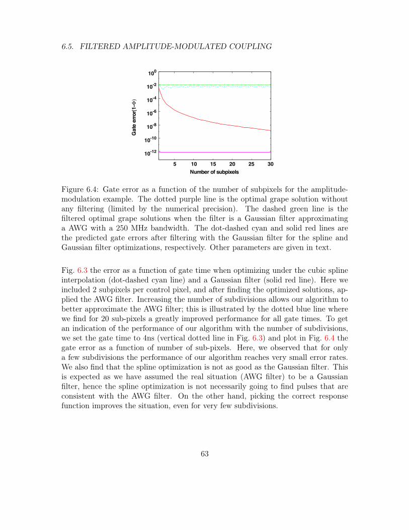
6.5. FILTERED AMPLITUDE-MODULATED COUPLING
Figure 6.4: Gate error as a function of the number of subpixels for the amplitude-modulation example. The dotted purple line is the optimal grape solution withoutany filtering (limited by the numerical precision). The dashed green line is thefiltered optimal grape solutions when the filter is a Gaussian filter approximatinga AWG with a 250 MHz bandwidth. The dot-dashed cyan and solid red lines arethe predicted gate errors after filtering with the Gaussian filter for the spline andGaussian filter optimizations, respectively. Other parameters are given in text.
Fig. 6.3 the error as a function of gate time when optimizing under the cubic splineinterpolation (dot-dashed cyan line) and a Gaussian filter (solid red line). Here weincluded 2 subpixels per control pixel, and after finding the optimized solutions, ap-plied the AWG filter. Increasing the number of subdivisions allows our algorithm tobetter approximate the AWG filter; this is illustrated by the dotted blue line wherewe find for 20 sub-pixels a greatly improved performance for all gate times. To getan indication of the performance of our algorithm with the number of subdivisions,we set the gate time to 4ns (vertical dotted line in Fig. 6.3) and plot in Fig. 6.4 thegate error as a function of number of sub-pixels. Here, we observed that for onlya few subdivisions the performance of our algorithm reaches very small error rates.We also find that the spline optimization is not as good as the Gaussian filter. Thisis expected as we have assumed the real situation (AWG filter) to be a Gaussianfilter, hence the spline optimization is not necessarily going to find pulses that areconsistent with the AWG filter. On the other hand, picking the correct responsefunction improves the situation, even for very few subdivisions.
63
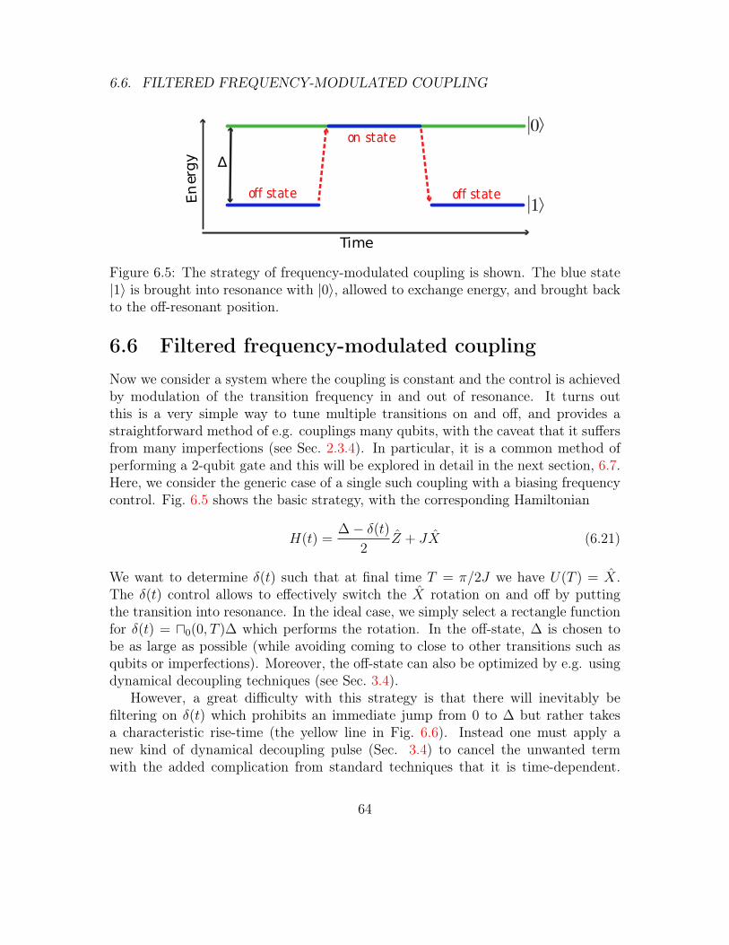
6.6. FILTERED FREQUENCY-MODULATED COUPLING
∆
Time
En
ergy
off state off state
on state
Figure 6.5: The strategy of frequency-modulated coupling is shown. The blue state|1〉 is brought into resonance with |0〉, allowed to exchange energy, and brought backto the off-resonant position.
6.6 Filtered frequency-modulated couplingNow we consider a system where the coupling is constant and the control is achievedby modulation of the transition frequency in and out of resonance. It turns outthis is a very simple way to tune multiple transitions on and off, and provides astraightforward method of e.g. couplings many qubits, with the caveat that it suffersfrom many imperfections (see Sec. 2.3.4). In particular, it is a common method ofperforming a 2-qubit gate and this will be explored in detail in the next section, 6.7.Here, we consider the generic case of a single such coupling with a biasing frequencycontrol. Fig. 6.5 shows the basic strategy, with the corresponding Hamiltonian
H(t) =∆− δ(t)
2Z + JX (6.21)
We want to determine δ(t) such that at final time T = π/2J we have U(T ) = X.The δ(t) control allows to effectively switch the X rotation on and off by puttingthe transition into resonance. In the ideal case, we simply select a rectangle functionfor δ(t) = u0(0, T )∆ which performs the rotation. In the off-state, ∆ is chosen tobe as large as possible (while avoiding coming to close to other transitions such asqubits or imperfections). Moreover, the off-state can also be optimized by e.g. usingdynamical decoupling techniques (see Sec. 3.4).
However, a great difficulty with this strategy is that there will inevitably befiltering on δ(t) which prohibits an immediate jump from 0 to ∆ but rather takesa characteristic rise-time (the yellow line in Fig. 6.6). Instead one must apply anew kind of dynamical decoupling pulse (Sec. 3.4) to cancel the unwanted termwith the added complication from standard techniques that it is time-dependent.
64
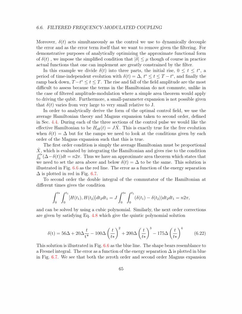
6.6. FILTERED FREQUENCY-MODULATED COUPLING
Moreover, δ(t) acts simultaneously as the control we use to dynamically decouplethe error and as the error term itself that we want to remove given the filtering. Fordemonstrative purposes of analytically optimizing the approximate functional formof δ(t) , we impose the simplified condition that |δ| ≤ µ though of course in practiceactual functions that one can implement are greatly constrained by the filter.
In this example we divide δ(t) into three parts, the initial rise, 0 ≤ t ≤ t∗, aperiod of time-independent evolution with δ(t) = ∆, t∗ ≤ t ≤ T − t∗, and finally theramp back down, T−t∗ ≤ t ≤ T . The rise and fall of the field amplitude are the mostdifficult to assess because the terms in the Hamiltonian do not commute, unlike inthe case of filtered amplitude-modulation where a simple area theorem would applyto driving the qubit. Furthermore, a small-parameter expansion is not possible giventhat δ(t) varies from very large to very small relative to J.
In order to analytically derive the form of the optimal control field, we use theaverage Hamiltonian theory and Magnus expansion taken to second order, definedin Sec. 4.4. During each of the three sections of the control pulse we would like theeffective Hamiltonian to be Heff(t) = JX. This is exactly true for the free evolutionwhen δ(t) = ∆ but for the ramps we need to look at the conditions given by eachorder of the Magnus expansion such that this is true.
The first order condition is simply the average Hamiltonian must be proportionalX, which is evaluated by integrating the Hamiltonian and gives rise to the condition´ t∗
0(∆−δ(t))dt = n2π. Thus we have an approximate area theorem which states that
we need to set the area above and below δ(t) = ∆ to be the same. This solution isillustrated in Fig. 6.6 as the red line. The error as a function of the energy separation∆ is plotted in red in Fig. 6.7.
To second order the double integral of the commutator of the Hamiltonian atdifferent times gives the condition
ˆ t∗
0
ˆ t1
0
[H(t1), H(t2)]dt2dt1 = J
ˆ t∗
0
ˆ t1
0
(δ(t1)− δ(t2))dt2dt1 = n2π,
and can be solved by using a cubic polynomial. Similarly, the next order correctionsare given by satisfying Eq. 4.8 which give the quintic polynomial solution
δ(t) = 56∆ + 20∆t
t*− 100∆
(t
t∗
)2
+ 200∆
(t
t∗
)3
− 175∆
(t
t∗
)4
(6.22)
This solution is illustrated in Fig. 6.6 as the blue line. The shape bears resemblance toa Fresnel integral. The error as a function of the energy separation ∆ is plotted in bluein Fig. 6.7. We see that both the zeroth order and second order Magnus expansion
65

6.7. APPLICATION TO 2-QUBIT COUPLING
0 2 4 6 8 100
10
20
30
40
Time during gate @nsDA
mpl
itude
Figure 6.6: Control amplitude as a function of the time during the gate operationfor the filtered ISWAP example. The yellow line is the unoptimized sequence withrise-time restriction. The red line represents the solution to the average Hamiltonianassuming the same rise-time of 1ns. The blue line represents the cubic polynomialsolution to the second order in the Magnus expansion given by Eq. 6.22 with t*=3ns.The short time of T=10ns is used for visual clarity.
corrections greatly reduce the rise-time error at small splittings but become worseas the initial detuning is increased. This related directly to the observation thatat the beginning of the pulse we have the detuning δ(t) J while near resonanceδ(t) J . The latter case is a clear application of average Hamiltonian theory wherethe expansion converges, while the former is not and requires a different treatment.In fact, it would be preferable to split the evolution into 5 parts, where the first andlast are defined as the region where δ(t) J , and their contribution to the erroris calculated differently. This type of error is known as off-resonant error and is anapplication of selectivity theory as will be studied beginning in Sec. 7.1.1 and againin later chapters.
6.7 Application to 2-qubit couplingThe implementation of quantum computing requires a universal set of gates [41].With single qubit rotations, the
√iSWAP or iSWAP [155] operations are universal
two-qubit gates and turn out to be a natural two-qubit gate for certain couplingHamiltonians [189]. In particular, they occur from an effective XX interaction be-tween two resonant qubits, written as Hint = −JX where X = σ+
1 σ−2 + σ−1 σ
+2 can be
understood as a Pauli matrix on the subspace spanned by |01〉, |10〉 and J is thecoupling strength. Time evolution for a time t under this interaction leads to theunitary U(θ) = exp(+iXθ) with θ = t/J . θ = π/4 gives the
√iSWAP and θ = π/2
66

6.7. APPLICATION TO 2-QUBIT COUPLING
0 1 2 3 410-6
10-5
10-4
0.0010.01
0.11
Splitting, D2Π @GHzDG
ate
Err
orFigure 6.7: Gate error as a function of the splitting between energy levels for thefiltered ISWAP example. The yellow line is the unoptimized sequence upon filtering.The red line represents the solution to the average Hamiltonian. The blue linerepresents the cubic polynomial solution to the second order in the Magnus expansiongiven by Eq. 6.22. Parameters are taken as J=30MHz and T = π/J .
gives the iSWAP. The XX interaction does not only occur naturally by the two-dimensional truncation of the exchange interaction. It occurs generically betweenweakly transversally coupled qubits [60]. This makes it ubiquitous in the interactionbetween resonantly tuned superconducting qubits [11, 30, 149, 185] as well as qubitsand resonators [15, 14, 71, 111, 116, 159]. Precisely timing the pulse to the right an-gle can be done by either having a tunable coupling strength J [12, 70, 140, 142] orby bringing initially far detuned in frequency qubits into resonance. The latter isthe more commonly used method. It is usually assumed that this tunneling is fullynon-adiabatic, i.e., the parameters of the Hamiltonian change without any changeof state. Realistically, it is slower than that, will exhibit a tendency to follow theadiabatic eigenbasis, and there will be a large error arising from the Landau-Zenertunneling. A similar situation occurs in the exchange-driven gates in the singlet-triplet qubit realized in semiconductor quantum dots [139]. Furthermore if the qubitis made from an anharmonic oscillator which is the case for many superconductingqubits there will be an additional source of error. This error is leakage from thetwo qubit subspace to the higher levels, controlled by the ratio between the couplingstrength between and the anharmonicity; it will be discussed in Ch. 9.
6.7.1 Physical example: capacitively coupled phase qubits
As a physical motivation for how this coupling can arise, consider two supercon-ducting phase qubits connected in parallel by a capacitor (see Sec. 2.3.1.1). UsingKirchoff’s laws, it is straightforward [60] to derive circuit equations and from these
67

6.7. APPLICATION TO 2-QUBIT COUPLING
to deduce the respective Lagrangian
L = IC1 cosφ1+C1 + C2
2
Φ0
2πφ2
1+Ib1Φ0
2πφ1+IC2 cosφ2+
C1 + C2
2
Φ0
2πφ2
2+Ib1Φ0
2πφ2+CG
Φ0
2πφ1φ2
where the subscripts b and c denote bias and critical current respectively, thenumerical subscript indexes the Josephson junction, and CG is a coupling capaci-tor. Using canonical quantization with ECiNi =
√Φ0
2πφi this gives the Hamiltonian
description
H =∑i
[EC1N1 − EJi cos φi − IbiΦ0
2πφi] + 4CGEC1EC2N1N2
with the introduction of the Josephson energy EJi. This Hamiltonian is wellapproximated by a polynomial given by the Taylor expansion of the cosine aroundφi = 0,
H w∑i
[EC1N1 + EJiφ2i − Ibi
Φ0
2πφi] + 4CGEC1EC2N1N2
This Hamiltonian in turn is a harmonic oscillator and is exactly solvable. Intro-ducing raising and lowering operators φi =
√ECi2EJi
(ai + a†i ) and Ni =√
ECi2EJi
i(ai− a†i )we can rewrite
H = ω1n1 + ω2n2 − 2CG
√E3C1E
3C2
EJ1EJ2
(a1 − a†1)(a2 − a†2)
with ωi =√
4ECiEJi and n the number of excitations in the qubit eigenbasis.Finally, we note that terms which do not conserve energy can be dropped (fast-rotating terms) and that the situation of variable qubit frequency can be realizedby tuning EC in situ by threading a flux through the Josephson junction loop.Truncating the Hilbert space by ignoring all states above ni = 1 gives the two-qubitflip-flop Hamiltonian
H2Q =ω1(t)
2Z1 +
ω2(t)
2Z2 − 2CG
√E3C1E
3C2
EJ1EJ2
(σ−1 σ+2 + σ−2 σ
+1 )
68

6.7. APPLICATION TO 2-QUBIT COUPLING
6.7.2 Reduction to single qubit analytic treatment
We consider two qubit gates realized by an exchange interaction,
H =∑i
ωi(t)
2Zi + J(σ−1 σ
+2 + σ−2 σ
+1 ) (6.23)
where ωi are the resonant frequencies of the two qubits which we assume can be variedand J is the coupling rate which we assume is fixed. This interaction is the naturalinteraction for two superconducting qubits coupled capacitively [116,133,132], induc-tively [11, 30, 185] or by virtually photons in the circuit QED architecture [15, 111].The variation in the frequencies can be achieved by changing the operation pointof the qubit with external flux lines. The above Hamiltonian can be dramaticallysimplified by defining a representation of the Pauli algebra given by,
I =σz1 + σz2
2,
X =σ−1 σ+2 + σ−2 σ
+1 ,
Y =− iσ−1 σ+2 + iσ−2 σ
+1 ,
Z =σz1 − σz2
2.
(6.24)
In this case Eq. 6.25 reduces to
H = Σ(t)I + ∆(t)Z + JX, (6.25)
where ∆(t) and Σ(t) are respectively the difference and sum of the two qubit frequen-cies. Effectively we can limit our controls to a single excitation algebra if we choose´
Σ(t)dt = 2nπ, and thus the task of designing a two-qubit gate is isomorphic to thatof generating a single qubit X-rotation using a Landau-Zener-type sweep [126]. Inparticular, the analysis of Sec. 6.6 is applicable. As a testament to the simplicity ofthis strategy, it is widely used for coupling superconducting qubits and the first-ordercontrol sequence forms the basis of present-day embodiments of the technology [57].
6.7.3 Numerical optimization
Once again we can apply the numerical optimization gradient ascent technique tooptimize the two-qubit gate in the presence of filtering. We optimize a single detuningfield δ(t) in the rotating frame Hamiltonian given by
69

6.8. SUMMARY
2 4 6 8 10 12 140
0.5
0.4
0.3
0.2
0.1
0
0.6
Time during gate (ns)
Contr
ol am
plitud
e (GH
z)
Figure 6.8: Optimized detuning δ(t) as a function of the gate time for the filtering2-qubit example. Parameters are given in the text.
H =∆− δ(t)
2Z1 + J(σ−1 σ
+2 + σ−2 σ
+1 ) (6.26)
For typical values of J (on the order of 50 MHz) and typical filtering (about250MHz bandwidth) it is always possible to fully remove the error. Interestingly, thepulses found are very similar to the polynomial found using the Magnus expansion,Eq. 6.22 and one such pulse is plotted in Fig. 6.8 for ∆ = 0.5GHz, and T=12ns, witha 2ns buffer. Using this technique, the error can be reduced arbitrarily given the useof the correct response function and coupling that is not faster than the smoothing.
6.8 SummaryWe have derived numerical and analytical techniques for dealing with fast-oscillationsin the Hamiltonian underlying slow variation of the control parameters. For gatesthat are very short to avoid the effect of decoherence, fast oscillations can be partic-ularly detrimental.
One kind of fast dynamics that has been studied in detail in this chapter isfiltering. In the case of filtering of amplitude modulated pulses, the effect can befairly subtle because the Hamiltonian approximately commutes with itself at differenttimes and therefore the filtering manifests itself as rather straightforward shapingerror. In the limit of simple time dependence, an area law or other suitable analyticapproximation (by e.g. taking the filter as a Gaussian function) allowed relativelylittle disturbance to the study of single qubit rotations.
70
6.8. SUMMARY
On the other hand, if the filtering affects an operator that does not commuteapproximately with the rest of the Hamiltonian then the effect of filtering is harderto understand. Analytically, a Magnus expansion of the evolution allowed to obtain apulse shape for the detuning of a coupling transition that permitted to effectively turnthe transition on and off as desired. Moreover, the shape can be easily understood asa polynomial satisfying a certain number of integral dynamical decoupling constraintsand matched closely to the optimum pulse shape found through optimization usingthe derived numerical techniques.
Other instances of fast dynamics in the presence of slow controls will be dis-cussed throughout the text. In particular, the presence of unwanted off-resonanttransitions can be thought of in this context for fast pulses. Specific applications forthe numerical technique will be discussed in Ch. 10 and Ch. 11 to optimize over mul-tiple driving fields at different frequencies, or one such field with multiple harmonicspresent, respectively.
71
Chapter 7
Crosstalk
In chapter 6, we saw that imperfections can change the intended shape of the fieldthat is sent to access a quantum coupling, hence causing errors if not accounted for.Now we consider imperfections not in the magnitude of the field but in its spatialextent. Both in real space and in frequency, it is desirable to separate qubits andother coupled energy levels from each other so that they are individually accessible.Crosstalk error occurs when manipulating one quantum element is not done inde-pendently of other elements. In order to minimize this effect, engineering qubits thatare sufficiently separated in space and in frequency while retaining sufficient couplingand scalability constraints is required (see Sec. 2.3.2). This chapter aims to examinethe techniques and tradeoffs of minimizing crosstalk terms while retaining couplingand scalability: section 7.1 deals with crosstalk for addressing individual qubits atdifferent frequencies while in 7.2 spatial crosstalk for two-qubit gates is discussed. Ingeneral, crosstalk is ubiquitous across quantum control strategies and physical imple-mentations of quantum information, namely it will reoccur in the context of leakagecouplings (Ch. 8 and 9), virtual couplings (Ch. 10), and strong coupling (Ch. 11).In this chapter, we elaborate on the idea that frequency crosstalk consists primarilyof semi-classical selectivity error (Sec. 3.2) and shifting of quantum eigen-energies(Sec. 3.3) which are primarily an exercise in pulse-shaping, while spatial crosstalkrequires performing trajectories in state space that are able in composite (Sec. 3.4)to act independently of and unwind unwanted operators.
Section 7.1 analyses the selectivity problem (Sec. 7.1.1) first from a semi-classicalperspective (Sec. 7.1.2) and with quantum corrections (Sec. 7.1.3). The writing ofthis section was aided by Frank Wilhelm. Next, Sec. 7.2 introduces the problem ofspatially separating (flux) qubits while simultaneously retaining (tunable) couplingbetween them (the coupling results are derived and analyzed by Peter Groszkowski;
72

7.1. FREQUENCY CROSSTALK
for the publication and the full derivation see Ref. [63]). The coupling landscape isused to demonstrate that sufficiently low error gates can be performed under real-istic constraints and minimal spatial separation, both with (Sec. 7.2.3) and without(Sec. 7.2.4) the additional use of frequency separation of the qubits.
7.1 Frequency crosstalkSpectroscopy is arguably the most commonly used experimental technique in physics[36, 101, 162]. It relies on the concept of resonance - the object of study is exposedto monochromatic radiation and responds if the radiation frequency matches a fre-quency of that system. In quantum systems, that frequency is the difference of twoof the systems’ energies. Complex systems usually contain a large wealth of thesefrequencies. The ability to selectively address these frequencies defines the spectralresolution. The limitation of spectral resolution can be twofold: On the one hand,the frequencies forming spectral lines are intrinsically broadened by decoherence and/ or relaxation. On the other hand, the idea of an ideally monochromatic externalexcitation is only a convenient fiction - in reality, the bandwidth of that externalsignal is limited by a on a scale of 1/T where T is the duration of the experimentalpulse.
In continuous wave spectroscopy, T is chosen to be so long that this restriction isnot a limiting factor. There are however situations in which this is not possible. Inmagnetic resonance, e.g., certain spectral lines can only be reached through complexpulse sequences that all need to be executed within the relaxation time of the system.Consequently, a wealth of techniques has been developed that reaches fine spectralselectivity with pulses of limited duration, including the case of 2D-spectroscopy[45,54,101] .
Quantum technologies such as quantum computing are often based on spectro-scopic ideas [24,125,46,129]. In fact, the already mentioned spin resonance is a pri-mary candidate for the implementation of quantum computing [8,61,73].This meansthat the quantum mechanical transitions corresponding to certain quantum logic op-erations are typically addressed through their transition frequency. This can occuron the level of single qubits, when the two states representing the qubit are takenout of a complex spectrum with low anharmonicity such as it is the case in supercon-ducting qubits [30, 38, 112, 153, 186] (see Ch. 8). It can occur when multiple qubitsare in close spatial proximity, much closer than the spatial resolution of the externalfield, as it is the case in spin resonance [54, 101, 129, 162]. It can also occur if singleelements are multifunctional, e.g., when a single qubit contains transitions pertinentto local rotations as well as to coupling different components [14,57,71,111,141,159]
73
7.1. FREQUENCY CROSSTALK
(see Ch. 10). Note that typical scalable quantum computing implementation can-didates typically do not rely on spectroscopic resolution alone and at least containsome element of local addressability. Still, clearly, a crowding of the frequency spec-trum will be detrimental to both spectroscopy and coherent quantum control. Inquantum information, it is a key requirement to perform a large number of highlyaccurate operations well below the coherence time of the system. Thus, the chal-lenge of reaching good enough spectral addressability in short times is in particularsignificant.
The above discussion holds essentially for all bit-flip type operations, where tran-sitions between energy eigenstates of a qubit system occur. On a single qubit level,these would e.g. include the NOT gate. Between qubits, these include the controlledNOT and the iSWAP gate [129].
Now a key difference between spectroscopy and quantum control in the pursuitof selective excitation is the following: spectroscopy is an analytic technique to findenergy levels through transition frequencies, hence we want to guarantee that beyonda narrow band around the desired transition, excitation profiles are suppressed. Inquantum control, the spectrum is well characterized and the positions of undesiredtransitions are known, hence, it is sufficient to suppress the excitation profile at thosefrequencies. This chapter aims primarily at the second approach.
7.1.1 Selectivity criteria
The controls that are used to manipulate quantum systems, typical external ACfields, can often neither spatially nor by selection rule distinguish between the quan-tum transition that is being controlled and other quantum transitions. This can bemitigated if all these transitions have distinct transition frequencies ωj,k = Ej − Ekwhere Ej is the energy eigenvalue of state j and here and henceforth we use naturalunits with ~ = 1. If we now drive the system control indexed by l with a drivefrequency ωdl that is much closer to a specific transition frequency labelled by j(l),k(l) than to any other, and/or if this control has an appreciable matrix element Γljkfor this transition, only it will be driven, and no other transition. We will quantifythis statement below and outline its limitations.
We start by assuming a Hamiltonian Htot = H0 + Hcontrol and work in the ba-sis of eigenstate of H0. We can formalize the statement about spectral selectivityby assuming that the drive Hamiltonian has some appreciable matrix elements for
74
7.1. FREQUENCY CROSSTALK
multiple quantum elements in the system, that is the control Hamiltonian
Hcontrol(t) =L−1∑l=0
Ωl(t)e−iφl
M−1∑m=0
Γlm + h.c. (7.1)
where there are M quantum elements in the system and L drives to controlthem. This can arise for example if we consider M qubits and a collective drivecomposed of L frequencies, each of which is meant to address a particular qubit buthas unintended crosstalk on the rest of the M qubits, as it e.g. occurs in NMR. Insuch a case, the lab Hamiltonian will read
Htot =∑l
Ωl(t)e−iφl cos
(ˆ t
0
ωdl dt
)(∑m
Xm
)+∑m
ωm0,1|1〉〈1|m (7.2)
Moving this to the interaction picture (Sec. 4.2.2), we can better appreciate theselectivity condition by introducing offsets ∆jkl = ωdl − ωj,k as
Γlm =∑
|j〉,|k〉∈Hm
λlj,ke−i∆jklt|j〉〈k|. (7.3)
where the total Hilbert space is Hsys =⊗M−1
m=0 Hm. In the qubits example, we have|j〉 = |0〉m, |k〉 = |1〉m. More generally, Hilbert spaces where selectivity criteria areused outside the scope of qubit crosstalk will be discussed in in Ch. 8, Ch. 10, andCh. 11.
Here, it is tacitly assumed that the envelope Ωl = ReΩl+iImΩl is complex-valued.For the implementation of simple drive pulses, the phase is typically assumed tobe constant which with appropriate choice of reference means ImΩ = 0, however,later we will explicitly use the ability to control both terms independently. Here,we assume that to each index l we match a transition j, k to which it is almostresonant, identified as j(l) and k(l). In this interaction frame representation, we canquantitatively formulate the selectivity condition: we observe that the terms on theright hand side of Eq. (7.3) are oscillating at frequency ∆jkl and have magnitudeλlj,kΩ. In order for the drive to be effective, it must not oscillate wildly on the timescale of the transition |λj,kΩ| −1 hence giving us the sufficient criterion that we havefrequency selectivity for all l if
∆jkl ∣∣λljkΩl
∣∣ ∀j, k 6= j(l), k(l) (7.4)
75
7.1. FREQUENCY CROSSTALK
On the other hand, in order to drive the desired transition efficiently, we demandto be on or close to resonance
∆j(l),k(l),l ∣∣λlj(l),k(l)Ωl
∣∣ (7.5)
As ωj,k are given by the quantum system under consideration, the choice of drivingfrequencies l can only maximize the left hand side of Eq. (7.4) to a certain limit whilealso obeying Eq. (7.5). Thus, obeying these conditions requires to keep the controlamplitudes Ωl low enough. On the other hand, this increases the duration of thecontrol pulse hence makes the transition vulnerable to decoherence and relaxation,thus we practically demand that λlj(l),k(l)Ωl γ where γ represents typical incoherentrates of the system. This constraint on addressability is a result of spectral crowd-ing and the loss of fidelity due to the need for long pulses degrades spectroscopictechniques as well as the implementation of coherent gates in a quantum computer.Thus, the spectrum sets a speed and fidelity limit on quantum control. Another wayto observe this is using the Fourier transform which we will use in the next section.
7.1.2 Semiclassical spectrum analysis
In this section, we develop a classical argument for our technique of excitation sup-pression and relate it to ideas of signal processing. It is well established [54,72,174,177] that for a system of qubits or spins 1/2 driven by a weak external field, i.e., forsmall T/∆, an excellent measure of off-resonant excitation is the Fourier transform
S(∆) =
ˆ T
0
(Ω(t)e−iφ)e−i∆tdt (7.6)
Note that this is a limited-interval Fourier transform that can be consolidatedwith the regular, infinite-time Fourier transform by assuming the pulse envelopeΩ(t) vanishes outside the integration interval.
Now as another caveat, when applying this measure to the design of gates, weneed to be aware that off-resonant levels can also induce phase errors (coming from,e.g., AC Stark shifts) [59]. It is suitable for population transfers, though. Often,phase errors in gates can be compensated for by inserting frame transformationsbetween pulsed operations (Eq. 4.2).
One established way to compensate spectral weight off -resonance while main-taining a pulse of limited length is to use Gaussian profiles for Ω(t), Eq. 3.3, becausethey are also well-confined Gaussians in frequency space. In this case, the Gaussfunction describing Ω(t) must be suitably chosen to start and end at zero amplitude.
76
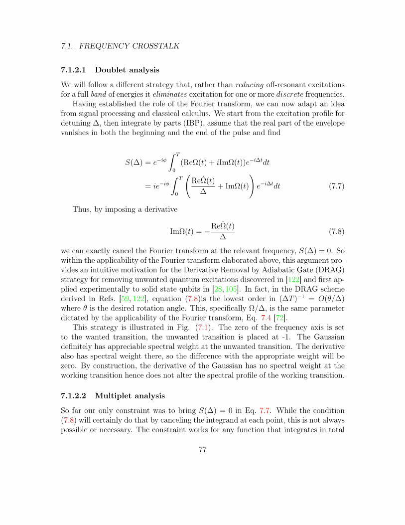
7.1. FREQUENCY CROSSTALK
7.1.2.1 Doublet analysis
We will follow a different strategy that, rather than reducing off-resonant excitationsfor a full band of energies it eliminates excitation for one or more discrete frequencies.
Having established the role of the Fourier transform, we can now adapt an ideafrom signal processing and classical calculus. We start from the excitation profile fordetuning ∆, then integrate by parts (IBP), assume that the real part of the envelopevanishes in both the beginning and the end of the pulse and find
S(∆) = e−iφˆ T
0
(ReΩ(t) + iImΩ(t))e−i∆tdt
= ie−iφˆ T
0
(ReΩ(t)
∆+ ImΩ(t)
)e−i∆tdt (7.7)
Thus, by imposing a derivative
ImΩ(t) = −ReΩ(t)
∆(7.8)
we can exactly cancel the Fourier transform at the relevant frequency, S(∆) = 0. Sowithin the applicability of the Fourier transform elaborated above, this argument pro-vides an intuitive motivation for the Derivative Removal by Adiabatic Gate (DRAG)strategy for removing unwanted quantum excitations discovered in [122] and first ap-plied experimentally to solid state qubits in [28, 105]. In fact, in the DRAG schemederived in Refs. [59, 122], equation (7.8)is the lowest order in (∆T )−1 = O(θ/∆)where θ is the desired rotation angle. This, specifically Ω/∆, is the same parameterdictated by the applicability of the Fourier transform, Eq. 7.4 [72].
This strategy is illustrated in Fig. (7.1). The zero of the frequency axis is setto the wanted transition, the unwanted transition is placed at -1. The Gaussiandefinitely has appreciable spectral weight at the unwanted transition. The derivativealso has spectral weight there, so the difference with the appropriate weight will bezero. By construction, the derivative of the Gaussian has no spectral weight at theworking transition hence does not alter the spectral profile of the working transition.
7.1.2.2 Multiplet analysis
So far our only constraint was to bring S(∆) = 0 in Eq. 7.7. While the condition(7.8) will certainly do that by canceling the integrand at each point, this is not alwayspossible or necessary. The constraint works for any function that integrates in total
77

7.1. FREQUENCY CROSSTALK
Figure 7.1: Abs Fourier transform of a Gaussian pulse(blue), its derivative(red), andtheir sum (yellow)
to the same area as the driving field. In particular, the off-resonant transition canbe simultaneously driven by additional fields Ωl at a different frequency difference∆jkl = ωdl − ωj,k which must together satisfy the condition
ˆ T
0
n∑l
Ωle−i∆jkltdt = 0 (7.9)
for excitation j − k to be suppressed. For multiple transitions jk ∈ S, the setof unwanted transitions, this sets up a system of equations to solve. For example,for one such unwanted transition, if we choose to put a second tone symmetricallyon the other side of the unwanted transition from the driving field (∆jk2 = −∆jk1),the relation works out to give
Re(Ω1(t))
∆jk1
= Ω2(t)e−i∆jk1T (7.10)
This will not work as well as Eq. 7.8 since it is only an average effect but may beuseful in conjunction with other tones to remove multiple transitions. Choosing Ω2
to be a derivative function rather than a function with area similar to Ω1 also has theadvantage of minimally disturbing the rest of the spectrum since Ω2 will typicallyrequire an energy smaller than Ω1 by a factor of about (∆jk2)2.
In general, the spectrum may be quite crowded with unwanted transitions oneither side of the working transition. Unfortunately, it is clear from Fig. 7.1 and fromthe anti-symmetry of Eq. 7.8 around ∆ = 0 that the derivative will only decrease theexcitation on one side of the working transition while increasing it on the other. On
78

7.1. FREQUENCY CROSSTALK
Figure 7.2: Absolute Fourier transform of a Gaussian(red) and the sum of theGaussian with its 2nd derivative (blue)
the other hand, the second derivative of of the envelope will be symmetric and effectboth sides in the same way. Applying IBP to Eq. 7.7 a second time (ignoring nowthe imaginary part) and setting now the boundary terms in the envelope functionand its first derivative to 0 gives the relation
ˆ T
0
ReΩ(t)e−i∆tdt =
ˆ T
0
− ReΩ(t)
∆2e−i∆tdt
Clearly, supplementing the driving function with another tone in-phase and atthe same frequency but proportional to the second derivative of the first will againsatisfy Eq. 7.9 for
Ω2(t) =Ω1(t)
∆2. (7.11)
The effect is demonstrated in Fig. 7.2. Off resonance, unwanted transitions arecancelled at the chosen ∆ = ±1. On resonance, setting the area to the desiredrotation angle θ via
´ T
0(Ω(t) + Ω(t))dt = θ allows the working transition (at ∆ = 0)
to remain unchanged. The cost of this technique is that the function and its firstderivative both need to begin and end at 0 for IBP to be valid, and the pulse shapemay be slightly harder to implement than a simple Gaussian or its first derivative.On the other hand, the strategy requires only one control to shape and synchronizeand it obeys an area theorem avoiding higher order effects such as phase shifts androtation errors on the working transition. An added benefit is that we can see theoverall bandwidth (above a given threshold – here 0.001) is decreased compared toa traditional Gaussian where some of the energy has been moved from the selective
79

7.1. FREQUENCY CROSSTALK
region to the tails where it instead falls below threshold. By placing the spectral holesappropriately at various frequency offsets one can engineer the bandwidth that fallsabove a desired selectivity threshold. This can be useful for narrowband behaviourwhere there are many transitions to be avoided such as used in resonance imaging andspectroscopy, with a decrease in bandwidth of about 25% compared to the optimalGaussian with the same threshold.
For multiple unwanted transitions it is straightforward to satisfy Eq. 7.9 to nullout a set S of unwanted spectral elements using multiple derivatives all at the samefrequency (∆jkl = ∆jk). Using the IBP formulae, the system of equations simplifiesto a set linear equations
1−|S|∑l=1
(∆jk)lal = 0, ∀jk ∈ S (7.12)
Ωl(t) = (i)laldl
dtlΩ(t)
which can easily be solved and which we will see can be generalized to the quan-tum case, at least for the first few orders of differentiation. As with simple Gaussianpulses, the IBP strategy ignores phase shifts (in this case both on and off resonance)but these are irrelevant for state transfer or easily compensated by frequency shiftingand/or inserting frame transformations (Sec. 4.2). In the next section we examinehow this mostly-classical argument can be generalized and derived for the quantumcase to account for these and other higher order errors.
7.1.3 Quantum operator diagonalization
7.1.3.1 Rotating frame
We now provide a quantum mechanical treatment starting from the interaction frameHamiltonian Eq. (7.1). In order to include the Hamiltonian dynamics it is preferableto have time-dependence coming only from the exponentiation of the matrix, and forthis purpose remove the explicit time-dependence from the Hamiltonian by movingto an (approximately) static frame. We choose to work in the rotating frame withthe frequency of a given drive (Sec. 4.2.2). To switch from one frame to the other andremove any oscillations in the Hamiltonian of frequency ∆j,k,l = ωdl −ωj,k (the detun-ing with respect to drive l) we apply a transformation Oj,k,l = exp(−i∆j,k,lt|k〉〈k|)which removes any exponential factors exp(−i∆j,k,lt) from the off-diagonal terms|j〉〈k|. For a set of such combinations of drive and non-zero, off-resonant matrix
80

7.1. FREQUENCY CROSSTALK
elements O = (j, k, l), the aggregate transformation O =∏
(j,k,l)∈O Ojkl has theeffect of removing all the sinusoidal oscillations in the Hamiltonian. Starting withthe interaction frame Hamiltonian now written as
Hint(t) =∑r,s,t
Hr,s,t(Ωt(t)e−i(φt+∆r,s,tt), 0) (7.13)
Hr,s,t(Ω,∆) = Ωλrst|s〉〈t|+ h.c.+ ∆|t〉〈t| (7.14)
and applying H(t) = OH int(t)O† + iOO† gives
H(t) =∑r,s,t
Hr,s,t
Ωt(t)e−i(φt+∆dif
r,s,tt),∑
(j,k,l)∈O
δj,rδk,sδl,t∆j,k,l(t)
(7.15)
∆difr,s,t = ∆r,s,t +
∑(j,k,l)∈O
(δk,s − δk,r)∆jkl (7.16)
where δa,b is the Kronecker delta. Unfortunately, if there are more non-zero matrixelements λj,k,l than there are levels and/or more than one drive per level, not alloscillation in the Hamiltonian can be removed in this way; however, we will typicallyonly be concerned with some or few of these elements. In these cases, the rotatingwave Hamiltonian simplifies greatly to
H(t) =∑r,s,t
Hr,s,t(Ωt(t)e−iφt ,∆r,s,t(t)) (7.17)
Note that we have chosen to make the detuning ∆r,s,t(t) time-dependent in thelast line though this was not done throughout the derivation for clarity. To seehow do derive the time-dependence in the simple qubit case see Sec. 4.2.2, whichconstrains several possible implementations.
7.1.3.2 Block diagonal frame
Now we use the intuition from the Fourier transform analysis to apply a procedurethat removes these off-resonant coupling terms. We want to see the effect an off-phase control can have and as such move to an interaction frame with respect to itStarting with the matrix transition element
81

7.1. FREQUENCY CROSSTALK
Hjkl(e−iφlΩl(t),∆jkl) = Hjkl(e
−iφlReΩl(t),∆jkl) +Hjkl(ie−iφlImΩl(t), 0)
we apply the interaction transformation
Djkl = exp
(ˆ t
0
Hjkl(e−iφlImΩl(t
′), 0)dt′)
(7.18)
Assuming we are under the conditions such that Eq. 7.17 applies (matrix elementsare not driven simultaneously at two frequencies), the effective Hamiltonian underthe transformation reads
Heffjkl(t) = DjklHjkl(e
−iφlΩl(t),∆jkl)D†jkl + iDjklD
†jkl
= DjklHjkl(e−iφlReΩl(t),∆jkl)D
†jkl +Hjkl(ie
−iφlImΩl(t), 0) + iDjklD†jkl
(7.19)
= DjklHjkl(e−iφlReΩl(t),∆jkl)D
†jkl
The goal is to achieve a perfect on-resonant excitation and block-diagonalizeHeff(t) as described, i.e.,
Heffj(l),k(l),l = Ωeff(t)e−iφλlj(l),k(l)|j(l)〉〈k(l)|+ h.c.
Heffj 6=j(l),k 6=k(l),l = ∆eff
j,k,l|k〉〈k|ˆ T
0
Ωeff(t)dt = θ
(7.20)
The driving field Ωeff(t) can be thought of as an adiabatic drive, in the sense thatthe energy input into the system via driving fields does not change the energy popu-lations of unwanted transitions but only temporarily shifts the level structures beforereverting to the original energy splitting (the net effect being only an accumulationof dynamical phase). In effect, we can think of these selectivity criteria as restoring’adiabaticity’ to the system.
In the case where the transitions are disconnected (the unwanted transitions arein separate quantum elements), the condition amounts to the removal of crosstalk.In this case the system of equations can be solved exactly in principle, as will bediscussed next. For an infinite ladder of connected transitions it is not possible tofind an exact solution and instead an iterative approach will be needed (see Sec. 8).
82

7.1. FREQUENCY CROSSTALK
7.1.3.3 Solution basis of higher derivatives
Now a single Ωl can cancel exactly one excitation. To completely suppress twotransitions using the method for a single constraint requires an additional control(for the additional constraint). Here, we again apply the IBP intuition and use asecond derivative component. To see the effect of the second derivative control for asingle constraint we move again to an interaction frame with respect to it
Ejkm = exp
(−iˆ t
0
Hjkm(ReΩm(t′), 0)dt′)
which gives an effective Hamiltonian according to
Heffjkl(Ω(t),∆jkl) =Ejkm (Hjkl(ReΩl(t) + ReΩm(t),∆jkl))E
†jkm + iEjkmE
†jkm
=EjkmHjkl(ReΩl(t),∆jkl)E†jkm
=Hjkl(ReΩl(t), 0) + ∆jklEjkm|k〉〈k|E†jkm
In this case the transformation does not directly diagonalize the unwanted cou-pling and instead to do this we should apply another (in this case non-interactionframe) transformation
Heffjkl(Ω(t),∆jkl) =DjklEjkmHjkl(ReΩl(t),∆jkl)E
†jkmD
†jkl + iDjklD
†jkl (7.21)
=DjklHjkl(ReΩl(t), 0)D†jkl + ∆jklDjklEjkm|k〉〈k|E†jkmD†jkl + iDjklD
†jkl
where the first term is diagonalized by cancelation with the real part of the secondterm, and the imaginary part of the second term cancels out with the third term.To first order Djkl is the same as the transformation defined in Eq. 7.19.
To combine the effect of multiple (derivative) controls, for a set jk ∈ Sl of un-wanted, off-resonant transitions connected to drive l, we have the compound formula
Heffjkl(Ωl(t),∆jkl) = DjklEjklHjkl(Ωl(t),∆jkl)E
†jklD
†jkl (7.22)
+ iDjklEjklHjkl(Ωl(t),∆jkl)E†jklD
†jkl + iDjklD
†jkl
where Djkl corresponds to the exponentiation of an imaginary operator and Ejklto the exponential of a real operator, as defined in the equations above. For more
83

7.1. FREQUENCY CROSSTALK
than two unwanted transitions, the control(s) is (are) a function of the higher orderderivatives of the original pulse shape (e.g. a Gaussian),
Ωl(t) =
|Sl|∑r=0
αrΩ(r)G + i
|Sl|∑r=1
βrΩ(r)G
where the superscripts denote the order of differentiation and which together withEq. 7.20 for each value of j, k give conditions for the coefficients αr, βr , which willbe a function of ΩG and ∆jkl. In order for the effective frame to be equivalent tothe original bare frame we must choose a pulse shape ΩG whose |Sl| derivatives arezero at the endpoints of the pulse (see Sec. 4.1.2). Note that although the solutionis approximately given simply by semi-classical Eq. 7.12, higher order quantummechanical corrections are needed to fully solve the system. Some of these will begiven in the next sections.
7.1.3.4 Doublet analysis
The simplest scenario are two disconnected transitions: two qubits. We put the driveon resonance with the first qubit (∆A = ωd0 −ωA0,1 ≈ 0) and letting ∆B = ωd0 −ωB0,1 =∆A + ∆ , Eq. 7.1 gives
Htot = Ω(t)e−iφ(λA01(σ+0,1)A ⊗ 1
B + λB011A ⊗ (σ+
0,1)Be−i∆t) + h.c. (7.23)
In the frame rotating at the drive frequency (O = (00, 01, 1), (10, 11, 1) ), thisgives
H(t) = H0,1,0(e−iφΩ(t), 0)⊗ 1B + 1
A ⊗H0,1,0(e−iφΩ(t),∆B)
Nulling the off-diagonal components for qubit B to give HeffB = ∆eff
B |1〉〈1| caneasily be satisfied through the diagonalizing transformation, by plugging Eq. 7.19,which for qubits simplifies to
D =
(cos(ˆ t
0
e−iφImΩl(t)λAjkdt
)1 + sin
(ˆ t
0
e−iφImΩl(t)λAjkdt)σ+
0,1 + h.c.
)
⊗
(cos(ˆ t
0
e−iφImΩl(t)λBjkdt
)1 + sin
(ˆ t
0
e−iφImΩl(t)λBjkdt)σ+
0,1 + h.c.
),
(7.24)
84
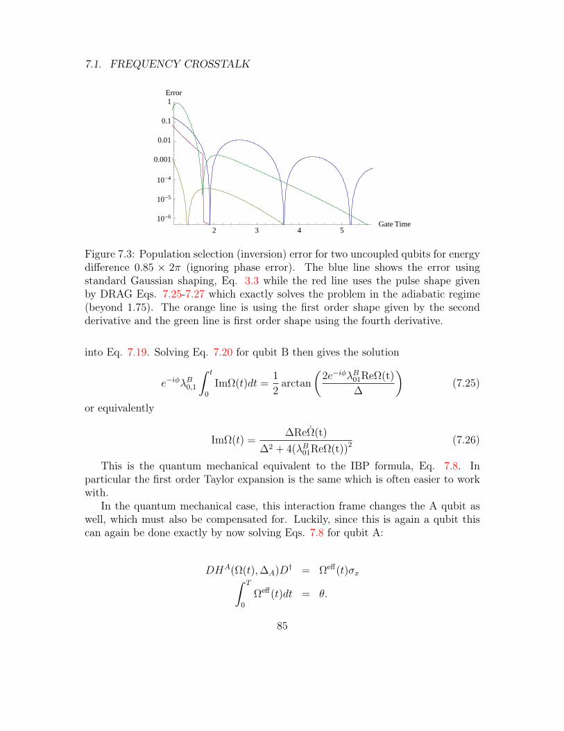
7.1. FREQUENCY CROSSTALK
2 3 4 5Gate Time
10-6
10-5
10-4
0.001
0.01
0.1
1Error
Figure 7.3: Population selection (inversion) error for two uncoupled qubits for energydifference 0.85 × 2π (ignoring phase error). The blue line shows the error usingstandard Gaussian shaping, Eq. 3.3 while the red line uses the pulse shape givenby DRAG Eqs. 7.25-7.27 which exactly solves the problem in the adiabatic regime(beyond 1.75). The orange line is using the first order shape given by the secondderivative and the green line is first order shape using the fourth derivative.
into Eq. 7.19. Solving Eq. 7.20 for qubit B then gives the solution
e−iφλB0,1
ˆ t
0
ImΩ(t)dt =1
2arctan
(2e−iφλB01ReΩ(t)
∆
)(7.25)
or equivalently
ImΩ(t) =∆ReΩ(t)
∆2 + 4(λB01ReΩ(t))2 (7.26)
This is the quantum mechanical equivalent to the IBP formula, Eq. 7.8. Inparticular the first order Taylor expansion is the same which is often easier to workwith.
In the quantum mechanical case, this interaction frame changes the A qubit aswell, which must also be compensated for. Luckily, since this is again a qubit thiscan again be done exactly by now solving Eqs. 7.8 for qubit A:
DHA(Ω(t),∆A)D† = Ωeff(t)σxˆ T
0
Ωeff(t)dt = θ.
85

7.1. FREQUENCY CROSSTALK
These equations can readily be satisfied by setting
∆A =1
2
(−∆ +
√−16(Ω(t))2 + ∆2
)(7.27)
ˆ T
0
Ω(t)∆
∆B
√1 + 4Ω(t)2
∆2B
= θ
Fig. 7.3 shows how this error can be fully removed in the adiabatic regime. ∆ ischosen to be 0.85× 2π and the selection error is plotted as a function of gate time.The error for a simple Gaussian of correct area is plotted in blue (ignoring againany net phase errors), while in red is the solution given by the technique we callDerivative Removal by Adiabatic Gate (DRAG), which generalizes the procedure wefound originally in Ref. [122]. Note that selection error is already suppressed for theGaussian whenever the Fourier transform at the frequency offset of the second qubit´ T
0Ω(t)e−i∆Btdt is nulled (this first happens at about T=2). This is essentially a first
order result. For DRAG, the error is always suppressed beyond about T = 2 whereboth qubit A is rotated and B is left intact. The result is exact provided the adia-baticity condition is met, 4Ω(t) < ∆B (otherwise the solution is undefined, thoughwe use in Fig. 7.3 the first order in 4Ω(t)
∆Bto show an improvement still exists here). In
the adiabatic regime, we see that the derivative (imaginary) control suppresses anycrosstalk to the second qubit (keeping things adiabatic) while the change of frameessentially shifts the energy levels temporarily during the gate such that the reso-nance condition needs to be adjusted according to Eq. 7.27. Practically speaking,the DRAG result is clearly more robust than using the single envelope solution as itis immune to changes in frequency or gate time. Note that both solutions containnet phase errors on qubit B that need to be corrected subsequently.
Using the second derivative result, an approximate solution (ignoring a term smallin Ω(t)
∆B) can similarly found from Eq. 7.21 with
ReΩ = ΩG +d
dt
ΩG
∆2 + 4ΩG2
which is plotted in orange in Fig. 7.3 clearly suppressing the Gaussian result and out-performing the first derivative result in the diabatic regime. Note that no change ofphase is induced because the main control and auxiliary control are in phase witheach other and therefore obey an area theorem (Sec. 2.3).
Using the third derivative result with Eq. 7.22, an approximate solution can befound as
86

7.1. FREQUENCY CROSSTALK
2 3 4 5 6 7Gate Time
10-6
10-4
0.01
1Error
Figure 7.4: Selection error for three uncoupled qubits for energy differences 0.85×2πand 1.445× 2π from the driven qubit. The blue line shows the error using standardGaussian shaping, Eq. 3.3 while the red line uses the pulse shape given by DRAGEqs. 7.25-7.27.
ImΩ =∆...ΩG
(∆2 + 4ΩG2)2
∆A = −2ΩG tan
(2
ˆ t
0
ImΩl(t)dt
)(7.28)
ˆ T
0
Ω(t) sec
(2
ˆ t
0
ImΩl(t)dt
)= θ
which is plotted in green in Fig. 7.3 still outperforming the Gaussian result in theadiabatic (long-time) limit.
7.1.3.5 Multiplet analysis
If more than 2 qubits are in the system, with a single amplitude control it becomesincreasingly difficult (at the cost of larger T) to find a gate time where crosstalk isavoided on all other qubits.
For instance, adding in an extra qubit C with ∆C = 1.7∆B such that the Hamil-tonian (Eq. 7.2) gives in the rotating frame
87

7.1. FREQUENCY CROSSTALK
2 4 6 8 10Gate Time
10-6
10-4
0.01
1Error
Figure 7.5: Selection error for three uncoupled qubits for energy differences 0.85×2πand 1.445× 2π from the driven qubit. The blue line shows the error using standardGaussian shaping, Eq. 3.3 while the red line uses the pulse shape given by DRAGsemi-classical Eq. 7.12.
H = Ω(t)e−iφ((σ+
0,1)A + (σ+0,1)B + (σ+
0,1)C + h.c.)
(7.29)+∆A|1〉〈1|A + ∆B|1〉〈1|B + ∆C |1〉〈1|C (7.30)
and applying the same pulse sequence Eq. 7.25 (which nulls crosstalk at B) is alsobeneficial to qubit C when it is on the same side of the spectrum from qubit A(∆C∆B > 0). In Fig. 7.4, we see that plotting again gate selection error for all threequbits vs. gate time, we get a distinct decrease in errors for all times when applyingthe DRAG correction. The situation is somewhat reversed from 2 qubits, wherenow the Gaussian error is somewhat constant but the Gaussian with DRAG has arecurrence of perfect addressability roughly once per unit time, when the Fouriertransform of the pulse at C is approximately zero.
Eq. 7.21 is in general difficult to solve exactly but to first order the analysis isthe same as using the semi-classical method. In particular, the solution for a singleunwanted transition is given still by the second derivative control, Eq. 7.11. For twounwanted transitions a↔ b and c↔ d it is necessary to solve the pair of conditionsgiven by Heff
abl(Ω(t),∆A) = ∆effA |b〉〈b| and Heff
cdl(Ω(t),∆C) = ∆effC |d〉〈d| . This simplifies
to the semiclassical scheme, Eq. 7.12, which for the two unwanted transitions gives
ReΩ = ΩG +ΩG
∆B∆C
and ImΩ =
(1
∆B
+1
∆C
)ΩG
88

7.2. SPATIAL CROSSTALK
-6 -4 -2 0 2 4 6
10-7
10-5
0.001
0.1
Figure 7.6: Selection error as a function of frequency offset when using the secondderivative.
The inversion error for this pulse sequence is plotted in Fig. 7.5 as comparedto the simple Gaussian. We see the error is completely suppressed beyond about 5time steps which is not as early as was the case for using a single derivative. This isbecause in order to enforce the first derivative starting and ending at zero a slightlyless selective basic shape must be used (with wider bandwidth) as a starting point andbecause we are using the semiclassical result which removes just the first order errorwhich is only dominant for larger times. The result can be improved by consideringhigher order quantum effects which is the direction of future research. Alternatively,two different derivatives can be also used (e.g. 2nd and 4th) which can remove thecommutativity error. Nonetheless, we see the suppression for the semi-classical resultis complete beyond the adiabatic limit and the robustness properties are returned.Similar results exist for four or more qubits.
Finally, we confirm the observation that using the second derivative can be usedfor its even symmetry around the driving transition to decrease the bandwidth ofselective pulses. As in the classical case, we see in Fig. 7.6 that appropriate weightingof the second derivative creates holes on either side of the working transition in theexcitation profile here (as opposed to the spectrum). Once again, we notice that theenergy has been moved from the selective region to the tails where it falls below thechosen selectivity threshold. We see a bandwidth improvement again of about 25%.
7.2 Spatial crosstalkAlternatively to being suppressed from energy conservation considerations, quantumelements that are spatially separated from the target will be attenuated as a result of
89

7.2. SPATIAL CROSSTALK
local addressing. An alternative or complementary scheme to avoid crosstalk there-fore is to design systems for control lines addressing one section to interact minimallywith others. In fact, the spectral crowding limitations developed above imply thatsome amount of spatial selectivity will be necessary to scale beyond the limitationsimposed by the coherence times of the quantum dynamics. Unfortunately, whilequbits themselves can be quite small in spatial extent and even engineered to bearbitrarily distanced from each other, the necessity for inter-qubit exchange of infor-mation provides a great challenge in terms of maximizing coupling between relevantdegrees of freedom while turning off unwanted coupling. In particular, this is exem-plified for superconducting qubits, for which both long-range and nearest-neighbourinteractions between circuit elements are possible. Moreover, both frequency selectivetransmission elements and spatially addressable control lines are feasible as buildingblocks in architectural designs. Thus, there are numerous proposals for designs ofsuperconducting coupling mechanisms [25,29,38,112,117,126,134,173,179,185].
In this section, we look at the motivating example of flux qubits inductively cou-pled using dc Superconducting QUantum Interference Devices (DC-SQUIDs) used fortunability. The DC-SQUIDs are treated as high excitation energy quantum objects(assumed to always stay in their ground states) where the circulating current medi-ates inductive coupling between pairs of qubits [5,75]. Because of the spatial extentof the couplers, there will result crosstalk to other qubits and couplers. This methodwas first theoretically described in [143], and subsequently demonstrated experimen-tally in [70]. Similar coupling approaches were presented in [18,69,132,138,170]. Thisexample is a case where the unwanted coupling between qubits can be very strong(in amplitude), and so here we investigate whether it is possible to achieve low errorusing dynamical decoupling control techniques, with or without the advantage ofenergy separation between components.
7.2.1 Physical Model
A flux qubit can be constructed from a superconducting loop interrupted by threeJosephson junctions [134]. A current flowing in one direction can represent a com-putational basis quantum state |0〉 and in the opposite direction, a state |1〉. Thestrength of the coupling between qubits is mediated by a circulating current in a DC-SQUID which is inductively coupled to each of the qubits. This circulating currentcan be controlled by the applied flux as well as the bias current, both of which canbe tuned experimentally. Furthermore, the DC-SQUIDs may also be used for qubitreadout [108,135,171].
The performance of any inductively coupled qubit architecture will strongly de-
90

7.2. SPATIAL CROSSTALK
Figure 7.7: Two different arrangements of flux qubits 1, 2, 3 and couplers A, B. “a”represents the arm length of the couplers, and “w” their width. We assume thatthe wires of couplers A and B overlap at most in two places around qubit 2. a)Straight-line shape. b) Capital “L” shape.
pend on the geometry of the qubit-coupler layout. The couplers themselves are basedon the long-distance design proposed in [53]. In this section we investigate two geome-tries, which can potentially serve as building blocks for topologically motivated ap-proaches to quantum computation [90,146] with high error thresholds [37,52,146,176].In these approaches the physical qubits are typically laid out in a (for example) 2Dsquare lattice. The geometries we study, which may be used to build such a lattice,are both shown in Fig. 7.7. In a), the coupling DC-SQUIDs form a straight line andin b), they enclose a 90˚ angle suggestive of a capital letter “L”. In both cases wehave two qubits at the end points (labeled “1” and “3”) and the third (labeled “2”)in the middle. The middle qubit is therefore surrounded by both of the couplers.We consider the qubits at the edge to be nearest-neighbours to the middle qubit.The qubits are placed inside the couplers, hence maximizing the qubit-coupler in-ductance. Even though the coupling DC-SQUIDs are the same in both geometries,we expect the coupling energies to differ as even for the same length couplers, thedistance between qubit 1 and 3 will be smaller in the ’L’ shaped scenario.
For concreteness, the following physical parameters are used. The edge lengthof the square qubits is taken to be 44µm, roughly the same as those used in [70].The distance between the qubit and the surrounding wire of the coupler is between 2and 4µm. The arm length a is varied between 25µm and 300µm and the arm widthbetween w = 48µm and w = 2µm (although in the latter case a 10× 10µm2 loop inthe center of the arm is used to deliver flux through the couplers).
91
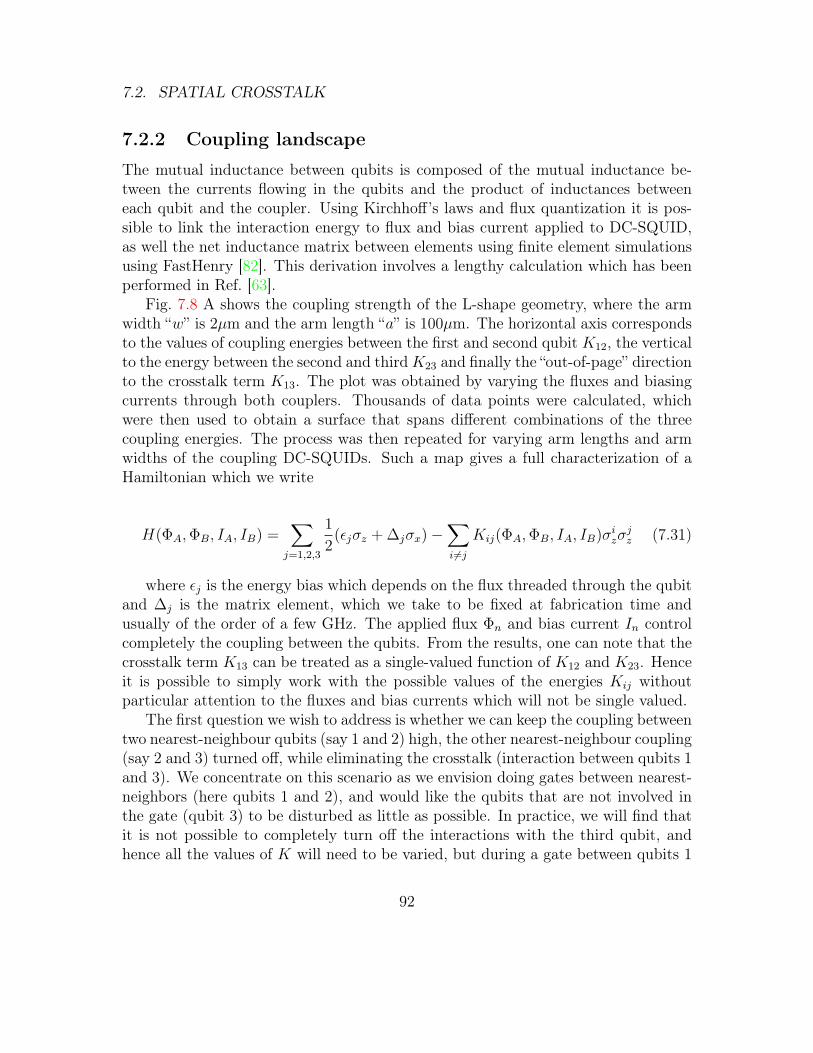
7.2. SPATIAL CROSSTALK
7.2.2 Coupling landscape
The mutual inductance between qubits is composed of the mutual inductance be-tween the currents flowing in the qubits and the product of inductances betweeneach qubit and the coupler. Using Kirchhoff’s laws and flux quantization it is pos-sible to link the interaction energy to flux and bias current applied to DC-SQUID,as well the net inductance matrix between elements using finite element simulationsusing FastHenry [82]. This derivation involves a lengthy calculation which has beenperformed in Ref. [63].
Fig. 7.8 A shows the coupling strength of the L-shape geometry, where the armwidth “w” is 2µm and the arm length “a” is 100µm. The horizontal axis correspondsto the values of coupling energies between the first and second qubit K12, the verticalto the energy between the second and thirdK23 and finally the “out-of-page” directionto the crosstalk term K13. The plot was obtained by varying the fluxes and biasingcurrents through both couplers. Thousands of data points were calculated, whichwere then used to obtain a surface that spans different combinations of the threecoupling energies. The process was then repeated for varying arm lengths and armwidths of the coupling DC-SQUIDs. Such a map gives a full characterization of aHamiltonian which we write
H(ΦA,ΦB, IA, IB) =∑j=1,2,3
1
2(εjσz + ∆jσx)−
∑i 6=j
Kij(ΦA,ΦB, IA, IB)σizσjz (7.31)
where εj is the energy bias which depends on the flux threaded through the qubitand ∆j is the matrix element, which we take to be fixed at fabrication time andusually of the order of a few GHz. The applied flux Φn and bias current In controlcompletely the coupling between the qubits. From the results, one can note that thecrosstalk term K13 can be treated as a single-valued function of K12 and K23. Henceit is possible to simply work with the possible values of the energies Kij withoutparticular attention to the fluxes and bias currents which will not be single valued.
The first question we wish to address is whether we can keep the coupling betweentwo nearest-neighbour qubits (say 1 and 2) high, the other nearest-neighbour coupling(say 2 and 3) turned off, while eliminating the crosstalk (interaction between qubits 1and 3). We concentrate on this scenario as we envision doing gates between nearest-neighbors (here qubits 1 and 2), and would like the qubits that are not involved inthe gate (qubit 3) to be disturbed as little as possible. In practice, we will find thatit is not possible to completely turn off the interactions with the third qubit, andhence all the values of K will need to be varied, but during a gate between qubits 1
92
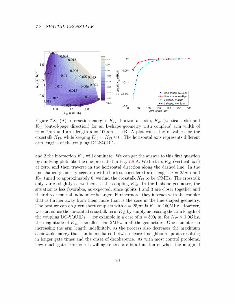
7.2. SPATIAL CROSSTALK
-0.027
0.027
-0.024
-0.024
-0.021
0.021
-0.019
-0.019
-0.015
-0.015
0.012
-0.012
-0.01
-0.006
-0.003
0
0.003
0.006
0.009
0.012
0.015
0.0 0.5 1.0
0.0
0.5
1.0
K12 HGHzhL
K23HG
HzhL
-0.027
-0.021
-0.015
-0.009
-0.003
0.003
0.009
0.015
GHzh
0 50 100 150 200 250 300−0.2
−0.15
−0.1
−0.05
0
Arm length (µm)
Cro
ssta
lk K
13 (
GH
z/h
)
Line shape, w=2µm
Line shape, w=48µm
L shape, w=2µm
L shape, w=48µm
Figure 7.8: (A) Interaction energies K12 (horizontal axis), K23 (vertical axis) andK13 (out-of-page direction) for an L-shape geometry with couplers’ arm width ofw = 2µm and arm length a = 100µm. . (B) A plot consisting of values for thecrosstalk K13, while keeping K12 = K23 ≈ 0. The horizontal axis represents differentarm lengths of the coupling DC-SQUIDs.
and 2 the interaction K12 will dominate. We can get the answer to this first questionby studying plots like the one presented in Fig. 7.8 A. We first fix K23 (vertical axis)at zero, and then traverse in the horizontal direction along the dashed line. In theline-shaped geometry scenario with shortest considered arm length a = 25µm andK23 tuned to approximately 0, we find the crosstalk K13 to be 47MHz. The crosstalkonly varies slightly as we increase the coupling K12. In the L-shape geometry, thesituation is less favorable, as expected, since qubits 1 and 3 are closer together andtheir direct mutual inductance is larger. Furthermore, they interact with the couplerthat is further away from them more than is the case in the line-shaped geometry.The best we can do given short couplers with a = 25µm is K13 ≈ 160MHz. However,we can reduce the unwanted crosstalk termK13 by simply increasing the arm length ofthe coupling DC-SQUIDs — for example in a case of a = 300µm, for K12 > 1.0GHz,the magnitude of K13 is smaller than 2MHz in all the geometries. One cannot keepincreasing the arm length indefinitely, as the process also decreases the maximumachievable energy that can be mediated between nearest-neighbours qubits resultingin longer gate times and the onset of decoherence. As with most control problems,how much gate error one is willing to tolerate is a function of when the marginal
93

7.2. SPATIAL CROSSTALK
decrease in error becomes smaller than the increase in incoherent decay of the states.In the next section, we examine how to remove this crosstalk error even when thequbits are closest.
The next question we wish to answer is whether the interaction between all pairsof qubits can be turned off completely. This may be useful when one wants toperform single gate operations on any (or all) of the qubits without affecting theothers. To determine this, we once again turn to Fig. 7.8 A (and its analogues forother geometries and values of arm lengths and widths — not explicitly shown).We can now look at the crossing of the two dashed lines, which corresponds toK12 = K23 = 0, and figure out the value of the crosstalk (K13). We plot the resultsin Fig. 7.8 B for both geometries and two different arm widths. From the data itis clear that there is no complete off-state. The straight-line geometry is much less(over 3 times in a case of shortest arm length we studied) susceptible to the unwantedcrosstalk K13. However the crosstalk energy dies off quickly, and in a case of armlength a > 200µm, its magnitude stays below 5MHz. The error can be very small(negligible when the qubits are off resonant) and is further correctable using standarddynamical decoupling sequences (Sec. 3.4).
7.2.3 Optimization of off-resonant coupling
We look at two gates, the first, the first is the√iSWAP, and the other a CNOT gate.
For demonstration purposes, we start with the simplest case, which is a√iSWAP
gate, which is a natural gate for the Hamiltonian. Moreover, we chose the qubitenergies to be ∆1/h = 5.0 GHz, ∆2/h = 5.4 GHz and ∆3/h = 5.8 GHz, whichprovides frequency selectivity.
We start with the system Hamiltonian shown in Eq. 7.31, and we switch basis,to the eigenbasis of σx, namely |+〉, |−〉 and furthermore go into a rotating framedefined by U = U1 ⊗ U2 ⊗ U3 with Uj = exp(−i∆j
2σjzt). We then assume that the
qubits can be driven at their respective resonances (meaning ∆j = ωj) and neglectthe fast oscillating terms (perform a RWA). All this leads to an effective Hamiltonianin the rotating frame and |+〉, |−〉 basis
He =−K12(t)e−i(∆1−∆2)t (|100〉〈010|+ |101〉〈011|) + h.c.
−K23(t)e−i(∆2−∆3)t (|001〉〈010|+ |110〉〈101|) + h.c.
−K13(t)e−i(∆1−∆3)t (|100〉〈001|+ |110〉〈011|) + h.c..
(7.32)
We explicitly make the Kij(t) terms time dependent to stress that they will vary. Weapply the GRAPE algorithm (Ch. 5.1) which we constrain by only allowing values
94

7.2. SPATIAL CROSSTALK
0 1 2 3 4 5 6 7−0.3
−0.2
−0.1
0
0.1
0.2
0.3
0.4
0.5
time (ns)
GH
z/h
K12
K13
Figure 7.9: A pulse sequence for a√iSWAP gate between qubits 1 and 2. Since
the system coupling is “natural” for this gate, no single-qubit rotations are needed.The pulses lead to the desired gate with 99.9% fidelity. In the calculations we take∆1/h = 5.0 GHz, ∆2/h = 5.4 GHz and ∆3/h = 5.8 GHz.
of Kij which can be achieved using physical controls (as described in section 7.2.2).We can think of this as staying on a surface spanned by the triplet (K12, K23, K13).From Section 7.2.2, we note that K13 can be treated as a single-valued function ofK12 and K23. This slightly simplifies our procedure of finding the gradient, since weare only dealing with two independent variables that account for all the interactionsin the problem. The gradient is not exact since the third variable depends implicitlyon the first two but this does not pose a problem in terms of convergence.
The resulting pulse for the√iSWAP is presented in Fig.. 7.9 which provides a
fidelity of 99.9% though this number can be increased with longer optimizations.Only the non-zero controls are explicitly shown. We study the case of the L-shapedgeometry with the arm length of 25µm where the unwanted crosstalk coupling K13
is the largest (and as can be seen from the plots, never zero). From the plot, it isclear that only coupling 1-2 has to be varied, and coupling 2-3 can be maintainedat 0. The shape found by the optimization is reminiscent of the strategy proposedby Ref. [11] which uses a coupling field oscillating at the frequency difference of thequbits to couple the flux qubits and overcome the energy difference between them.However in the analytic case there are many unaccounted errors and the techniqueis inexact while in the numerical case the pulse contains modulation on top of thecarrier which makes it arbitrarily precise. This is an example of a virtual couplingcontrol strategies, more of which will be discussed in Sec. 10.
95

7.2. SPATIAL CROSSTALK
The unwanted crosstalk couplingK13 is significant throughout the gate. However,since we have chosen the qubits to be off-resonance with each other, in the rotatingframe the terms K23 as well as the crosstalk K13 oscillate at frequencies (∆2 −∆3)and (∆1−∆3) respectively. The combination of small amplitude and high frequency(from the space and frequency separation of the qubits, respectively) effectively elim-inates the effect of these terms and it is visible that little correction is needed in thegenerated controls. Note that operating the qubits at different frequencies does notrisk running into spectral crowding limitations because there is only significant cou-pling between nearest-neighbour and next-to-nearest-neighbour qubits. Thus we seethat the combination of space and frequency separation is a powerful way to removecrosstalk and does not pose a problem in terms of scalability.
0 5 10 15
−1.5
−1
−0.5
0
0.5
1
1.5
time (ns)
GH
z/h
K12 K23 K13εx
1εx
2εx
3εy
3
Figure 7.10: A pulse sequence for a CNOT gate between qubits 1 and 2. Single-qubit rotations are applied to all three qubits. For timely convergence of the GRAPEalgorithm, we modulate both σx and σy quadratures on the third qubit. Furthermore,we allow all three interaction energies to vary. The pulses lead to the desired gatewith 99.9% fidelity. In the calculations we take ∆1/h = ∆2/h = ∆3/h = 5.0 GHz.
.
7.2.4 Optimization of on-resonance coupling
In the second example we introduce two additional complications. In this set-up,we study creating the CNOT gate, which is a “non-natural” gate in that it doesnot correspond to the evolution of the drift Hamiltonian. However, a CNOT gateis often used to describe the active error correction procedures in the topologicallymotivated schemes from e.g. Refs. [90, 146, 51] for which this qubit geometry is
96
7.2. SPATIAL CROSSTALK
a natural contender. Thus, it is useful to optimize this gate as it will be usedrepeatedly and overall algorithm performance can benefit from making this gate asshort as possible. As a second (though perhaps unjustified) complication, we take allqubits to be on resonance — meaning ∆1/h = ∆2/h = ∆3/h = 5.0 GHz, removingthe convenient energy penalty on the crosstalk terms. The added complexity canonly be mitigated by the use of extra controls, in particular single-qubit controls areneeded for performing dynamical decoupling. Note that each εj is time dependentand can be written as
εj(t) = 4εxj (t) cos(ωjt) + 4εyj (t) sin(ωjt). (7.33)
Switching basis to the eigenbasis of σx, going into the rotating frame, and performingthe RWA, we obtain
He =∑j
(εxj (t)σjx − ε
yj (t)σ
jy)−K12(t) (|100〉〈010|+ |101〉〈011|+ h.c.)
−K23(t) (|001〉〈010|+ |110〉〈101|)−K13(t) (|100〉〈001|+ |110〉〈011|) + h.c..
(7.34)
Fig. 7.10 shows a particular pulse found after optimization. In contrast to theoff-resonant case, to achieve high fidelities, qubit 3 must be repeatedly flipped androtated (via εx3 and εy3) to counteract the crosstalk term, corresponding to a sophis-ticated dynamical decoupling sequence (Sec. 3.4). Since qubits 1 and 2 are onresonance, the interaction naturally couples them. In turn, the single qubit controlson qubit 1 and 2 (εx1 and εx2) act to convert the flip-flop interaction (naturally driftinginto an ISWAP) into a CNOT transition [60, 189]. Of course, rather than applyingthe single qubit gates before and after the two-qubit operation as is the standardconversion [129], GRAPE is able to find much shorter pulses that are able to performthese rotations simultaneously. Once again, the pulses found perform with a fidelityof 99.9%, a number which can be improved with further optimization. The pulsesin general are not unique and can depend on the initial guesses which GRAPE thenmodifies. Finally, let us note that we have shown how one has to vary the energiesin the system to obtain the desired pulses. Alternatively one could concentrate onworking with values of physical parameters (currents, fluxes) which might be moreuseful when trying to devise an experimental demonstration of this system.
97

Chapter 8
Leakage
8.1 IntroductionUntil now we have assumed that quantum elements behave independently and errorscome from limitations of the control hardware. In reality the Hilbert space structureof quantum systems is far more complex and the next three chapters analyse theprinciple ways in which we want to / have to do away with the qubit assumption.The next logical approximation is a three-level system, the qutrit, which we considerin this chapter. We assume that the coupling to the third level is driven by afield, rather than being always-on, primarily because always-on couplings can bediagonalized to give back 2-level systems in a different eigenbasis (of course, in othercontexts always-on couplings can still be relevant, see Sec. 2.3.4). In fact, it has beenshown that no elementary particle can be a true qubit [182]. In many cases, thecoupling to a third level is weak or spectrally distinct from the qubit frequency andcontribute error only for very short gates. On the other hand, an important examplewhere the transitions are only slightly spectrally distinct is the weakly anharmonicoscillator.
It is known [49,74] that the time evolution operator of a linearly driven harmonicoscillator is a combination of a coherent displacement operator tracking the classicaltrajectory of the driven oscillator and a global phase factor. This evolution encom-passes all energy levels and cannot be reduced to a single-qubit rotation (betweentwo of these levels). Spectroscopically, this can be understood as follows: a singlequbit rotation is typically implemented by a pulse of radiation resonant with thequbit energy splitting. In a harmonic oscillator, all energy splittings are the same, sodriving one transition drives all others at the same time. A system starting initiallyin an energy eigenstate will quickly be driven into a superposition over many energy
98

8.1. INTRODUCTION
eigenstates. By this token, it is crucial that a qubit is nonlinear [30,86,113,153,173],that is that the transition frequency of the qubit levels is different by an amount ∆from the transition frequencies to the non-qubit levels (the anharmonicity). Spectro-scopically, we would expect that whenever the bandwidth of the pulse comes close to∆, i.e., when its duration becomes short on the scale of 1/∆, we expect significantleakage to higher states. Thus, it is a challenge to implement fast single-qubit gatesin weakly anharmonic systems. The implementation of faster gates is important asit allows more gates to be executed in a given coherence time, an important steptoward high-fidelity quantum logic.
While superconducting qubits are the most well known example of qubits madefrom weakly anharmonic oscillators, there are many other examples. Examples ofleakage states include higher vibrational states in optical lattices [114], polarized spinstates in the singlet-triplet qubits [139], and auxiliary states in ion traps [65] andRydberg atoms [56,68,169]. Within the framework of superconducting qubits, severalrelevant current realizations include low-dispersion qubits like the transmon [95,154]and the capacitively shunted flux qubit [165]. On the other hand, a promising route tosuccess are qubits that contains only a minimal number of elements, such as the phasequbit [117, 116, 164].What these systems have in common is a weakly anharmonicenergy level structure, i.e., the states that are outside of the qubit subspace spannedby |0〉 and |1〉 are only separated from each other and the qubit subspace by energiesonly slightly different than the qubit frequency.
In this chapter, we outline quantum control strategies to implement single-qubitquantum gates in qubits singled out from the spectrum of an anharmonic oscillator.The method of performing this approximation is summarized in Secs. 8.2 and 8.3.We develop an adiabatic expansion technique that leads to order-by-order constraintequations on a frame transformation and the control fields. This is done in aninteraction frame formalism in Sec. 8.5 (published in Ref. [122]) and again using ageneralized class of transformations in Sec. 8.6 (published in Ref. [59]). The latterderivations were aided by Seth Merkel and Jay Gambetta. Numerical optimizationis performed in Sec. 8.7 to further characterize the controllability of the system.Furthermore, we consider in Sec. 8.8 the influence of relaxation and dispersion in thecontrol of these systems. The model for dispersion permits a deeper analysis of thecontrol problem with further optimization via ensemble techniques which was carriedout by Botan Khani and published in Ref. [88,87]. Finally, the techniques developedin this chapter have gained traction in the experimental community, most notablywe were able to devise with Jerry Chow et al. at Yale (published in Ref. [28]) waysto benchmark the technique in their laboratory, with results reproduced in Sec. 8.9.
99

8.2. MATHIEU EQUATION
8.2 Mathieu equationGenerically, we can think of anharmonic systems as modeled by a particle in aperiodic potential. The Hamiltonian for such a system reads
H0 =p2
2m+ U0 sin2(kLx), (8.1)
where m is the mass of the atom, kL wave number of the lattice and U0 is the latticepotential depth. For a given value of p this is exactly solved by the special function,known as the Mathieu function. It is available in mathematical software packagessuch as Mathematica, but can also be solved using the Bloch theorem and centralmatrix theorem [4,87]. For a single well in the potential, the eigenstate correspondsinstead to a Wannier state and equals the weighted sum of several of the delocalizedBloch states [96]. For a finite lattice with fixed number of lattice sites and boundmomentum states, the eigenvalues are hybrids between the two descriptions.
This Hamiltonian precisely describes the vibrational energy of an alkali atom ina 1D optical lattice, where the periodic potential is given by the standing wave gen-erated by two counter-propagating laser fields, as described for instance in Refs [83,114,115].
Another example of a system well described by the lattice potential is the super-conducting Cooper pairs on a charge island, given by
H(ng) = 4EC(n− ng)2 − EJ cos φ (8.2)
where n is the number of Cooper pairs on the superconducting islands, φ is thephase difference to the island, EC and EJ are the charging and Josephson energy,respectively and ng is the effective gate charge. In addition, if one adds a (constantforce) term linear in the space coordinate, giving in dimensionless units
H0 = p2 + r cos 2x+ gx, (8.3)
then one obtains what is known as a tilted washboard potential, which describes boththe influence of gravity on a particle with mass, or a current source in a supercon-ducting circuit (a phase qubit). Note also that the physical quantities p, x, and r cancontain noise, which as we have seen can either be slow or fast, and originate frominhomogeneity of an ensemble, fluctuations, or uncertainties. We will examine pulsesand design choices that render uncertainties in these parameters less significant.
100

8.3. QUTRIT APPROXIMATION
8.3 Qutrit approximationWe consider a qutrit subspace formed by the three lowest levels of the anharmonicoscillator. These levels are separated in energy by ~ω, where ω is the transitionfrequency. The jth higher levels are different to ~jω by ~∆j, where ∆j is known asthe anharmonicity. That is, the Hamiltonian for the nonlinear oscillator of dimensiond is (~ = 1)
Hfr =d−1∑j=1
(jω + ∆j)Πj, (8.4)
where Πj = |j〉〈j| is the projection operator onto the jth energy level. Without lossof generality we set ∆1 = 0. This is illustrated in Fig. 3.2 with the qubit levelsbeing |0〉 and |1〉 (green). For many nonlinear oscillators the anharmonicity takesthe form ∆j = ∆2(j − 1)j/2, which we will call the standard nonlinear oscillator(SNO), essentially a Duffing oscillator within the rotating wave approximation [86].For the lowest few levels, superconducting qubits of the transmon [154], phase qubit[116], and capacitively shunted flux qubit [165] types are well approximated by aSNO. Furthermore, motional states in optical lattices [114], collective modes of iontraps [65] and nano-mechanical oscillators [97] are also described as SNOs.
We will assume that control in this system is due to some dipole-like interactionthat only allows single photon transitions. As for harmonic oscillators, this is a goodapproximation because parity forbids all other transitions. The control Hamiltonianis
Hct(t) = E(t)d−1∑j=1
λj−1σxj−1,j, (8.5)
where E(t) is the drive amplitude, σxj,k = |j〉〈k| + |k〉〈j| is one of the effective Paulispin operators for levels j and k, and λj is a dimensionless parameter that weighsthe relative strength of driving the |j〉 → |j + 1〉 transition versus the |0〉 → |1〉transition. In our model we take λ0 = 1 and leave the λjs as input parameters. For aharmonic oscillator controlled via a dipole interaction with an external field λj =
√j.
For the functional form of the drive E(t) we will assume that |E(t)| ω (weakdriving regime) and introduce envelope shaping of the driving field at carrier fre-quency ωd. This leads to
E(t) = Ωx(t) cos(ωdt+ φ0) + Ωy(t) sin(ωdt+ φ0). (8.6)
For quantum information processing it is well suited to define operations withrespect to the frame rotating at the driving frequency ωd (Sec. 4.2.2). In this frame
101

8.3. QUTRIT APPROXIMATION
we have three independent controls: δ(t) = ω(t)−ωd (the qubit detuning), Ωx(t) andΩy(t), which, projected to the qubit subspace, control application of the three Paulispin operators σz0,1, σx0,1, and σ
y0,1, respectively. For example, the identity operation
is achieved by setting δ(t) = Ωx(t) = Ωy(t) = 0. To move to the rotating frame wedefine the unitary
R(t) =d−1∑j=1
exp [−ijωdt] Πj, (8.7)
which determines the transformed Hamiltonian HR(t) = R†(t)H(t)R(t) + iR†(t)R(t)to be explicitly
HR(t) =d−1∑j=1
(jδ + ∆j)Πj +
[Ω(t)
2e−iωdt−iφ0 + c.c.
]×
d−1∑j=1
λj−1
[|j〉〈j − 1|eiωdt + h.c.
],
(8.8)
where c.c. stands for complex conjugate and Ω(t) = Ωx(t)+iΩy(t). Assuming that ωdis larger then any other rate or frequency in this frame we can perform the rotatingwave approximation (i.e. time average the fast rotating terms to zero). For the SNOcase this amounts to restricting the dimension d to be less then
√2ω/∆, specifically
d = 7. After this approximation we can write the Hamiltonian as
HR(t) =d−1∑j=1
(jδ(t) + ∆j)Πj +d−1∑j=1
λj−1
[Ωx(t)
2σxj−1,j +
Ωy(t)
2σyj−1,j
], (8.9)
where σyj,k = −i|j〉〈k|+i|k〉〈j| for k > j. Here we have included the φ0 into the energyeigenstates (|j〉 → eijφ0|j〉), and we see that within the rotating wave approximationthe relative phase between the envelope and the carrier at the start of the operationis irrelevant. We see that if we can restrict the system to the lowest two levels then allrotations in the single qubit space can be achieved by independent controls; however,in general, this is not true. In Sec. 8.4 we show that the higher level transitions leadto a combination of a rotating, phase and leakage error [2, 166, 122]. This has beenexperimentally measured in Refs. [27] and [106].
8.3.1 Coupling strength from dressing
To obtain explicitly the value of the couplings λj beyond the harmonic oscillator ap-proximation we should look at the coupling mechanism. In cases where the systemis a SNO and is driven directly, λj is well approximated by the harmonic oscillator
102

8.3. QUTRIT APPROXIMATION
matrix elements, namely λj ≈√j. This, for example, occurs for the phase qubit
when it is driven by a time-varying bias current [117] and the charge qubit when it isdriven by time-varying gate voltage [100]. Essentially, these systems are very nearlyharmonic oscillators and the controls are almost proportional to the quadrature op-erator. On the other hand, when the coupling is done via an intermediary quantumelement such as a cavity then one must look at the Hilbert space of the combinedsystem. This is the case for the cavity [68,119] or circuit [15,175] QED architecture.
In the cavity or circuit QED architecture, the anharmonic oscillator is coupledto a resonator and is controlled by driving the resonator far off-resonance. In thiscase, λj can take on essentially any value. To see this, we start by writing the fullHamiltonian for the multi-level anharmonic oscillator and resonator as
HJC =ωra†a+
d−1∑j=1
(jω + ∆j)Πj +d−1∑j=1
gj−1,j
(|j − 1〉〈j|a† + |j〉〈j − 1|a
), (8.10)
again ∆0 = ∆1 = 0. This is a generalized Jaynes-Cummings Hamiltonian [78] withωr being the resonator frequency, and gj,k being the vacuum Rabi coupling for thej to k levels. Again we have assumed that the anharmonic oscillator only allowsone-photon transitions.
−2
∆2/(ω−ωr)
λ1 0
2
4
−4
−2.0 −1.5 −1.0 0.0−0.5 1.00.5
Figure 8.1: Ratio of coupling strength of the |1〉 ↔ |2〉 transition to the |0〉 ↔ |1〉transition as a function of anharmonicity for control through a resonator (solid blue)and direct drive (dashed red).
If |ω′j−1,j−ωr| |gj−1,j| for all j where ω′j−1,j = ω+∆j−∆j−1 then diagonalizationof Eq. (8.10) can be performed to lowest order in gj−1,j/(ωj−1,j−ωr) by the canonicaltransformation HD
JC = D†HJCD where
D = exp
[d−1∑j=1
gj−1,j
ω′j−1,j − ωr(a†|j − 1〉〈j| − a|j〉〈j − 1|)
](8.11)
103

8.3. QUTRIT APPROXIMATION
to give
HDJC =(ωr − χ01)a†a+
d−1∑j=1
(jω + ∆j + χj−1,j) Πj +d−1∑j=1
(χ0,1 + χj−1,j − χj,j+1)a†aΠj.
(8.12)
Here χj−1,j = g2j−1,j/(ω
′j−1,j − ωr) is the Lamb shift induced on the anharmonic
oscillator by the resonator and the last term in Eq. (8.12) is the ac-Stark shift [58].Assuming that the dressed cavity is in vacuum then Eq. (8.12) is well approximatedby Eq. (8.4) with
ω → ω = ω + χ0,1 (8.13)∆j → ∆j = ∆j + χj−1,j − jχ0,1 (8.14)
and the tilde implies dressed values for the transition frequency and anharmonicityfrom the resonator.
As stated above, the control is usually through the resonator and is representedby the Hamiltonian
Hdr(t) = ε(t)(a+ a†) (8.15)
which under the transformation Eq. 8.11 becomes
HDdr(t) = ε(t)
(a+ a† +
d−1∑j=1
gj−1,j
ω′j−1,j − ωrσxj−1,j
). (8.16)
Assuming that ε(t) is a sinusoidal with a frequency close to the qubit then Eq. 8.16is well approximated by Eq. (8.5) with
E(t) =g0,1
ω′0,1 − ωrε(t) (8.17)
λj−1 =gj−1,j(ω
′0,1 − ωr)
g0,1(ω′j−1,j − ωr). (8.18)
To demonstrate the functional form of λ1, we will assume the anharmonic oscil-lator is in the SNO limit: ω′j−1,j = ω + (j − 1)∆2, and gj−1,j =
√jg0,1. In this case,
Eq. (8.18) becomes
λj−1 =
√j
1 + (j − 1)∆2/(ω − ωr), (8.19)
and is plotted in In Fig. 8.1 as a function of the bare anharmonicity in units of(ω − ωr). Here, it is clearly seen that λ1 is of not equal to
√2 and actually changes
104

8.4. CONVENTIONAL CONTROL
sign at the point (ω − ωr = −∆2). This point invalidates the diagonalization forthe second level and can not be treated under this model. Away from this point thevalues obtained from this model approximate the real situation. This was confirmedin Ref. [28] where the experimental value for λ1 for the operation point used wasfound to agree with Eq. 8.18. However, we propose that λj should be used as afitting parameter in any experiment as effects such as higher modes of the resonatorand higher order perturbation will result in additional corrections to this value [16].
8.4 Conventional controlOur goal is to implement gates contained within the qubit subspace. That is, wewant to shape Ωx(t), Ωy(t) and δ(t) in Eq. 8.9 so that according to the selectivityconditions 7.20 we have
Uideal = T exp
[−iˆ tg
0
HR(t)dt
]= eiφUqb ⊕ Urest, (8.20)
where tg is the gate time, T is the time ordering operator, Uqb is a unitary that actsonly in the qubit subspace, Urest acts only outside of the qubit space, and φ describesa relative phase. Therefore, Urest as well as the phase φ are completely irrelevant foroperations in the Hilbert space formed by the qubit.
To demonstrate the typical set of errors we choose Uqb = σx0,1, the NOT gate.For a leakage-free qubit this would be implemented by simply setting δ(t) = 0 andΩy(t) = 0, with the only requirement on Ωx that that
´ tg0
Ωx(t)dt = π. To reducethe leakage to the third level, the standard result prior to Ref. [122] was to useGaussian modulation of the envelope [7, 166], Eq. 3.3. The motivation for Gaussianshaping is that the small and strictly limited frequency bandwidth (1/σ) ensures littleexcitation at the leakage transition frequency. For short pulses however, there is stillsignificant spectral weight at the anharmonicity ∆2. This is shown in Fig. 8.2 (a, c,e) where the Fourier transforms of ΩG(t) are plotted for σ = 1/3, 2/3, 3/22π/∆2
and tg = 4σ respectively.To demonstrate the errors arising from Gaussian shaping we consider a d = 5 SNO
and numerically calculate the average gate error, Eq. 2.9, for σ = 1/3, 2/3, 3/22π/∆2
and tg = 4σ. We find gate errors of 0.198, 0.0160, and 0.0030 respectively.To understand these error values we plot the populations of the first three levels
in Fig. 8.2 (b, d, f). The ground state populations are given by the blue solid line;the red dotted line shows the first excited state; the green dashed line is the secondexcited state. We observe that for the shortest gate, σ = 2π/3∆2, the error after thepulse is mostly residual population of the third and higher level. This is what we refer
105

8.5. ADIABATIC DIAGONALIZATION
Figure 8.2: Fourier transforms of the control fields (a, c, e) and populations (b, d,f) of the ground (blue solid), first (red dotted), and second excited (green dash) in asimulation of a NOT gate with a Gaussian amplitude pulse for a d = 5 SNO. In (a,b) σ = 2π/3∆2, (c, d) σ = 4π/3∆2, and (e, f) σ = 3π/∆2 and the gate time is takento be 4σ.
to as the leakage error. For longer gates, e.g. σ = 4π/3∆2, the residual populationdoes not account for the calculated error. This error is mostly a combination ofphase and rotation error resulting from the finite population of the third level duringthe pulse. Even though the final state is restricted to the computational levels, theadmixture of the third level leads to a phase shift on the second level, resulting ina net phase error at the end of the pulse. At the longest time when the populationof the third level is nearly negligible there is still a large gate error. From theseresults we conclude that Gaussian shaping is of limited performance even if the pulsebandwidth is somewhat smaller than ∆2.
8.5 Adiabatic diagonalizationHaving established the importance of spectral considerations in studying the qutritproblem, we are ready to apply the DRAG methodology from Sec. 7.1 to this familyof systems. We have seen in Sec. 7.1.3 that the insight from the Fourier transformand the solution given by the integration by parts provides a motivation for usinga second control phase shifted from the first, and that the solution will resemble aderivative. In the case of crosstalk, the set of transitions driven by the field formed
106
8.5. ADIABATIC DIAGONALIZATION
a disjoint set, in the sense that no transitions were connected (i.e. qubits). Thisallowed a diagonalization transformation that did not introduce any new transitionsinto the operator space. In effect, this means that if there were M transitions whoseevolution needed to be fixed, then a basis of M functions would be sufficient. That isonly M functions were needed satisfy Eq. 7.20. In contrast, for the set of unwantedtransitions S, if these transitions are not simple qubits but the driven transitions areconnected to other transitions, then a transformation would remove the unwantedtransitions will also introduce new transitions that were previously undriven. In otherwords, a basis of M fields would not be enough. The possibility for an exact solutionis even more difficult for an infinite ladder where every time the transformation wereamended to remove the additional transition, yet a new transition would be addedin its place, the process continuing ad infinitum. In effect one would need an infinitenumber of basis fields (e.g. derivatives to the Gaussian) in order to exactly null outall the transitions.
Given the difficulty in defining such an exact transformation, it is wiser to cutone’s losses and define an iterative transformation instead. The transformation mustbe adiabatic in the sense that all values we work with are expanded in a smallparameter ε =
Ωl(t)λj,k,l∆j,k,l
. For a SNO this is a strong limitation in the sense thatfor every transition up the ladder, the energy splitting ∆k decreases and the matrixelements λk increase. Nonetheless, an expansion will be seen to be at least somewhatfruitful.
We define the transformation recursively via the iterator h such that
HD(h)(t) = Dh(t)HD(h−1)(t)D†h(t) + i
˙Dh(t)D
†h(t) (8.21)
with HD0 = HO and Hh
D(t) = O(εh). The condition for selectivity, Eq. 7.20, is
weakened to
HD(h)j(l),k(l),l = Ωeff(h)(t)e−iφΓj(l),k(l),l(0) + h.c.+O(εh)
HD(h)j 6=j(l),k 6=k(l),l = ∆
eff(h)j,k,l |k〉〈k|+O(εh)ˆ T
0
Ωeff(h)dt = θ
(8.22)
where effective operators are also expanded in the small parameter: Ωeff(h) =∑hg=0 Ωeff
g (t)εg and ∆eff(h)jkl =
∑hg=0(∆jkl)g(t)ε
g (with ∆eff(h)j(l),k(l),l = 0). Transformations
that perform this task are not fully constrained and a general solution is exploredin Sec. 8.6 for SNOs. For the case of a generalized Hilbert space the solution
107
8.5. ADIABATIC DIAGONALIZATION
space is even larger. Here, we look only at the transformations in the form of thetransformation operators that exactly solved Sec. 7.1.3 but now expanded in thesmall parameter. That is, we constrain the transformation operator to be in theform
Dh = exp
(−i∑jk
ˆ T
0
Hjkl(Ωhεh, 0)dt + h.c.
)Unlike in the case of the qubits, Sec. 7.1.3, we cannot ensure that the\is trans-
formation corresponds to an interaction frame with respect to one of our controls.That is, if the j − k transition corresponds to a control then we can cancel the+i
˙Dh(t)D
†h(t) term. However if this cancelation is not possible then the term must
be left in. Unfortunately, as made clear in Sec. 7.1.1 via the use of integration byparts, the derivative will have the same spectral weight as the original matrix elementand not much will be gained by moving to a higher order (only commutator errorswill be decreased). Both these situation will come up when studying the SNO.
Returning to the qutrit, we have derived
HR(t) =d−1∑j=1
(jδ(t) + ∆j)Πj +d−1∑j=1
λj−1
[Ωx(t)
2σxj−1,j +
Ωy(t)
2σyj−1,j
], (8.23)
with d set for simplicity to 3 Going to an interaction frame with respect to theout-of-phase control (here Ωy(t) = − Ωx(t)
∆) with the transformation
D1 = exp
(− i
(d−1∑j=1
λj−1
ˆ t
0
Ωy(t)
2dt
)σyj−1,j
)gives the interaction Hamiltonian
HD(1) =
(Ωx(t) +
(λ2 − 2)(Ωx(t))3
∆2
)σx0,1 +
λΩ2x(t)
2∆σx0,2 +
(∆ + 2δ(t) +
(λ2 + 2)Ω2x(t)
∆
)Π2
+
(δ(t)− (λ2 − 4)Ω2
x(t)
∆
)Π1 +O(ε3).
(8.24)
In this frame, it is easy to see there are three qubit errors associated withthe result. The selection error is corrected with the off-phase derivative control
108

8.5. ADIABATIC DIAGONALIZATION
Figure 8.3: For a 3-level system driven by a 7ns pi-pulse, gate error is plotted vs.leakage transition strength λ for solutions to the adiabatic expansion to differentorders HD(h) correcting for errors to order h. The top blue line is the simple Gaussianand each line below it (at λ=2) corrects errors to the next order in ε. That is the redline under it is correct to order ε2, the yellow under it to O(ε4), the green under thatto O(ε5), the blue under that to O(ε6), the red under that to O(ε7), and the yellowunder that to O(ε8).
Ωy(t) = − Ωx(t)∆
which again is exactly the semiclassical result. The phase er-ror can be corrected with δ(t) = (λ2−4)E2x
∆by either shifting the eigen-energies of
the system or by a combination of phase ramping and frame compensation (Sec.4.2). Finally the rotation error is significant and can be corrected by ensuringthe area law
(´ T0
(Ωx(t) + (λ2−2)(Ωx(t))3
∆2
)dt = θ. To avoid higher order commuta-
tor errors, it is even better to satisfy the condition at all times by constrainingΩx(t) = ΩG(t)− (λ2−2)(ΩG(t))3
∆2 .Now a control in the 0 − 2 transition is assumed not present in our system.
Therefore the next highest error λΩ2x(t)
2∆σx0,2 gives an error which according to our
arguments is largely uncorrectable with the present formulation. That is we have
D2 = exp
(iλΩ2
x(t)
2∆σy0,2/∆
)but the transformation leaves in the term +i
˙D2(t)D†2(t). To validate this hypothesis
we have calculated all orders of ˜HD(h) using this iterative technique up toh = 7.Fig. 8.3 shows the effect of correcting the phase, rotation, and leakage errors in thequbit by order as a function of the strength of the coupling element λ1. The topblue line is the zeroth order and corresponds to a Gaussian function. The red line
109

8.5. ADIABATIC DIAGONALIZATION
under it corrects the phase and selection error. The yellow line under that correctsthe second order rotation error. Each subsequent line corrects errors to the nextorder assuming a derivative of a function is of the same order as the function itself(rather than one greater). We see that beyond the second or third order, most of theerror is pushed into the derivatives which causes the expansion to exhibit asymptoticbehaviour. Next we look at some other transformations and expansions.
8.5.1 Exact solution to the qutrit
Of course, if we assume instead that a control in the 0 − 2 transition is possiblethen the expansion no longer behaves asymptotically. To see this, consider again ourrotating frame qutrit Hamiltonian with additional control Ωx
2(t),
HR(t) =2∑j=1
(jδ(t) + ∆j)Πj +2∑j=1
λj−1
[Ωx(t)
2σxj−1,j +
Ωy(t)
2σyj−1,j
]+
Ωx2(t)
2σx0,2,
(8.25)In practical terms the extra control is readily achievable given that SNOs are not
harmonic oscillators. This can be seen for example by taking the Jaynes-Cummingsdiagonalization in Sec. 8.3.1 to next highest order. Thus, non-adjacent levels willstill be coupled but the matrix element will simply be smaller. Note however that wecan just absorb the smaller λ0,2 into Ωx
2(t) by simply increasing the amplitude of thefield. Note also that Ωx
2(t) will be at a different carrier frequency than the adjacenttransitions as the energy level difference is approximately doubled.
We reuse the interaction frame transformation with respect to the off-phase con-trol but now we do not need to perform an adiabatic expansion
D = exp
(−i
d−1∑j=1
λj−1
ˆ t
0
Ωy(t)
2dt σyj−1,j
)
To simplify the resulting expression we assign A =√
3´ t
0
Ωy(t)
2dt and pick the most
common case λ1 =√
2. The transformed Hamiltonian HD = DHRD† is cumbersometo write but contains 4 conditions to satisfy, the rotation, phase, leakage in 1−2 andleakage in 0− 2 conditions (Eqs. 7.20), which are explicitly
110

8.5. ADIABATIC DIAGONALIZATION
Figure 8.4: Gate error for the implementation of a NOT gate in a d = 3 SNO asa function of gate time. The solid red line corresponds to a Gaussian pulse whilethe dotted green line corresponds to the exact solution given by Eqs. 8.27 and 8.30.Parameters chosen are λ1 =
√2 and ∆/2π = 400MHz.
2(
Ωx2(t) +
√2(2δ + ∆)
)cos [A] +
(4Ωx
2(t)−√
2(δ(t) + 2∆))
cos [2A]
+12Ωx2(t)− 3
√2δ(t) + 2
√6Ωx(t) sin [A]−
√6Ωx(t) sin [2A] = 0,
2(√
2Ωx2(t) + 4δ(t) + 2∆
)cos [A] +
(4√
2Ωx2(t)− 2δ(t)− 4∆
)cos [2A]
−6√
2Ωx2(t) + 3δ(t) + 4
√3Ωx(t) sin [A]− 2
√3Ωx(t) sin [2A] = 0,
12Ωx(t) cos [A]− 3Ωx(t) cos [2A]
−2√
3(√
2Ωx2(t) + 4δ(t) + 2∆ + (2
√2Ωx
2(t)− δ(t)− 2∆) cos [A])
sin [A] = 9Ωθ(t),
3√
2Ωx(t) cos [2A] + 2√
3(−Ωx2(t)−
√2(2δ + ∆)
+6√
2Ωx(t) cos [A] +(
4Ωx2(t)−
√2(δ(t) + 2∆)
)cos [A]) sin [A] = 0,
(8.26)
where´ T
0ΩΘ(t)dt = Θ. The first three equations can be solved in terms of A, as
111

8.6. GENERALIZED TRANSFORMATION
in,
δ(t) =4
9
(∆ +
6(−3∆ + 2∆cos [A] +
√3ΩΘ(t) (−2 sin [A] + sin [2A])
)8− 3cos [A] + cos [3A]
)
Ωx2(t) = −
4√
2 sin[A2
]2 (2∆cos [A] + ∆cos [2A] + 6
(∆ +
√3ΩΘ(t) sin [A]
))9 (8− 3cos [A] + cos [3A])
Ωx(t) =2(9ΩΘ(t)cos [A]− 2
√3∆ sin [A]3
)3 (8− 3cos [A] + cos [3A])
(8.27)
The last equation is a self-consistency equation for A,
− 3√
2ΩΘ(t) (2 + cos [3A])− 2√
6∆ (sin [A]− 2 sin [2A]) = 0 (8.28)
This can be solved by Taylor expansion followed by iterative solution,
A(0) =
√3ΩΘ(t)
2∆,
A(m) =m∑n=1
−1n
(2n)!(3A(m−1))2n32nΩθ(t) + 2∆A(m−1)(1− 22n+1)
6∆.
(8.29)
The second quadrature control is then easily recovered by taking the derivative of A
Ωy(t) =2√3
dA
dt(8.30)
We see in Fig. 8.4 that the error is exactly removed in the qutrit case when we arein the adiabatic limit (here T > 1.5ns) far surpassing what is possible with only theadjacent-level controls. Given the possibility of using a second control in experimentthis strategy is clearly preferable to the simple single frequency case. The sum istaken to 7th order before numerical precision becomes an issue.
8.6 Generalized transformationTo find a general scheme that satisfies Eq. 7.20 we write D(t) = exp[−iS(t)] whereS(t) is an arbitrary Hermitian operator that we decompose as
S(t) =∑j=1
sz,j(t)Πj +∑j<k
sx,j,k(t)σxj,k +
∑j<k
sy,j,k(t)σyj,k, (8.31)
112

8.6. GENERALIZED TRANSFORMATION
and by assuming a power series in the small parameter ε, we can write each elementas
sα,j,k(t) =h∑
n−1
s(n)α,j,kε
n,
where α = x, y, or z. Thus we can find solutions to different orders h.
8.6.1 Zeroth order solutions
To the zeroth order we have Eq. 8.22 which simplifies to
Ωeff(0)(t) = Ωeff0 (t)ε0, ∆eff(0)(t) = 0, (8.32)
giving control solutions
Ωeff0 (t) = ΩG(t), δ(t) = 0. (8.33)
These are the controls used in Sec. 8.4 and here we will use them as a benchmarkfor the higher order solutions. In Fig. 8.5, we plot the error, 1 − Fg with Fg givenby Eq. (5.5) (blue dashed line), between a NOT gate an a unitary from the controlfield given by Eq. (3.3) with A = π and tg = 4σ for a SNO with d = 5. In this figureit is clearly seen that the error associated with these controls is quite large; for fastgate times this error is unacceptable for quantum information processing, and longgate times will have additional error arising from decoherence.
8.6.2 First order solutions
To determine the first order solutions we need to determine the frame transformationconditions for S(1)(t) to remove leakage to first order. Direct substitution leads to
s(1)x,1,k(t) =0, s
(1)y,1,k(t) = −λ1tgΩG(t)δk,2/2 (8.34)
where all other parameters sα,j,k are free variables. To satisfy Eq. 8.22, the first ordercorrections to the control fields are
Ω(1)x (t) = 2s
(1)x,0,1(t), (8.35)
Ω(1)y (t) = 2s
(1)y,0,1(t)− s(1)
z,1(t)tgΩG(t), (8.36)
δ(1)(t) = s(1)z,1(t) + 2s
(1)y,0,1(t)tgΩG(t) +
λ21t
2gΩ
2G(t)
4. (8.37)
(8.38)
113

8.6. GENERALIZED TRANSFORMATION
pulse width σ [units 2π/∆2]E
rro
r 1
-Fg
0.5 1.0 1.5 2.0 2.510−7
10−6
10−5
10−4
10−3
10−2
10−1
Figure 8.5: Gate error for the implementation of a NOT gate in a d = 5 SNO as afunction of σ, with tg = 4σ, and a Gaussian shaped pulse. The blue dotted line isthe zeroth order solution. The black dash line is the first order Z-only correction.The red dash-dot-dot line is the first order Y -only correction. The green dash-dotline is the first order correction from the controls presented in Sec. (8.5). The purplesolid line is for the optimal first order correction.
Here we see that there is a continuous family of DRAG pulses as (8.35-8.37) is under-constrained; however, in this section we will consider four particular solutions. In allof these solutions we take s(1)
x,0,1(t) = 0 as it has no influence on our choice for Ω(1)y (t)
and δ(1)(t).The first solution we consider is one where the control field Ωy(t) = 0. This is
achieved by setting s(1)z,1(t) = 2s
(1)y,0,1(t)/tgΩG(t), resulting in
δ(1)(t) =2s
(1)y,0,1(t)
tgΩG(t)−
2s(1)y,0,1(t)ΩG(t)
tgΩ2G(t)
+ 2s(1)y,0,1(t)tgΩG(t) +
λ21t
2gΩ
2G(t)
4. (8.39)
The simplest solution that satisfies S(1)(0) = S(1)(tg) = 0 is s(1)y,0,1(t) = 0. In this case
the controls become
Ωx(t) =ΩG, Ωy(t) = 0, δ(t) =λ2
1Ω2G(t)
4∆2
. (8.40)
For the SNO considered in Fig. 8.5, the error for this control set is plotted as theblack dashed line. It clearly has a much lower error than the standard Gaussianamplitude modulation control, and we will refer to this as the Z-only correction.
The second control solution we consider is when the control field δ(t) = 0. Thisis achieved by setting s(1)
y,0,1(t) = −s(1)z,1(t)/2tgΩG(t)− λ2
1tgΩG(t)/8, which results in
Ω(1)y (t) =−
s(1)z,1(t)
tgΩG(t)+s
(1)z,1(t)ΩG(t)
tgΩ2G(t)
− λ21tgΩG(t)
4− s(1)
z,1(t)tgΩG(t). (8.41)
114

8.6. GENERALIZED TRANSFORMATION
Again, the simplest solution that satisfies S(1)(0) = S(1)(tg) = 0 is s(1)z,1(t) = 0. In
this case, the controls become
Ωx(t) =ΩG(t), Ωy(t) = −λ21ΩG(t)
4∆2
, δ(t) = 0, (8.42)
and, for the SNO considered in the numerical demonstration, the error for this controlset is plotted in Fig. 8.5 as the red dash-dot-dot line. Its error rate is lower thanboth the standard Gaussian controls and the Z-only correction. This is the controlprocedure used in Ref. [28] and Ref. [107], where it was referred to as simple DRAGand half derivative respectively. Here we will refer to this as the Y -only correction.
We also present the first order solution found in Sec. 8.5 [122]. This occurs whenwe choose s(1)
x,0,1(t) = s(1)z,1(t) = 0 and s(1)
y,0,1(t) = −ΩG(t)/2, resulting in
Ωx(t) =ΩG(t), Ωy(t) = −ΩG(t)
∆2
,
δ(t) =Ω2G(t)
4∆2
[λ21 − 4].
(8.43)
This solution corresponds to fully removing the selection error by avoiding leaving inany derivative term. In Fig. 8.5, the green dash-dot line shows how the error scaleswith this control set. We see that for the first order solution, the error is larger thanthe Y -only correction method. That is, the first order version of Ref. [122] is notoptimal. We will see below this can be traced to an increased rotation error.
The final solution we consider is what we refer to as the optimal first ordersolution. This is achieved by minimizing the elements in the effective Hamiltonianof O(ε2). The transformation that minimizes these is
s(2)y,0,2 = −1
2tgΩGλ1(tgΩG + s
(1)y,0,1), (8.44)
s(2)x,0,2 = −1
2tgΩGλ1s
(1)x,0,1, (8.45)
s(2)y,1,2 = −λ1s
(1)x,0,1, (8.46)
s(2)x,1,2 =
1
2λ1(2ΩG + 2s
(1)y,0,1 − 2tgΩGs
(1)z,1 + tgΩGs
(1)z,2).
Using these expressions and requiring that the matrix elements ofH(2)extra(t) are zero in
the qubit subspace (and elements coupling to the qubit subspace are zero) results ins
(1)x,0,1(t) = s
(1)z,1(t) = 0 and s(1)
y,0,1(t) = −tgΩG(t)λ1/4. Substituting these into Eq. 8.35
115

8.6. GENERALIZED TRANSFORMATION
gives the controls fields
Ωx(t) =ΩG(t), Ωy(t) = −ΩG(t)λ1
2∆2
,
δ(t) =Ω2G(t)
4∆2
[λ21 − 2λ1].
(8.47)
This optimal first order solution is plotted in Fig. 8.5 as the solid purple line. Itserror is substantially lower the the other first order correction methods.
8.6.3 Second order solutions
Err
or
1-F
g
pulse width σ [units 2π/∆2]0.5 1.0 1.5 2.0 2.5
10−12
10−10
10−8
10−6
10−4
10−2
Figure 8.6: Gate error for the implementation of a NOT gate in a d = 5 SNO as afunction of σ, with tg = 4σ, and a Gaussian shaped pulse. The blue dotted line isthe zeroth order solution. The black dash line is the second order Z-only correction.The red dash-dot-dot line is the second order Y -only correction. The green dash-dotline is the second order correction from the controls presented in Sec. 8.5. The purplesolid line is for the optimal first order correction.
The higher order solutions become impractical to solve in generality because thenumber of terms grows quickly with increasing order. However, we can easily findthe second and higher order corrections to the different first order solutions. Wefind that the corrections to the above four cases only change the Ωx(t) field. In theZ-only case, Ωx(t) becomes
Ωx(t) = ΩG(t) +λ2
1Ω3G
8∆22
, (8.48)
in the Y -only case, Ωx(t) becomes
Ωx(t) = ΩG(t)− λ21(λ2
1 − 4)Ω3G
32∆22
, (8.49)
116
8.7. NUMERICAL OPTIMIZATION
and the control set presented in Sec. 8.5 gives
Ωx(t) = ΩG(t) +(λ2
1 − 4)Ω3G
8∆22
. (8.50)
To demonstrate these corrections we plot in Fig. 8.6 the second order solutions. Theline marking and colours are the same as in Fig. 8.5 with the exception that theynow refer to second order solutions (all except the blue dotted line, which remainsthe zero order solution, and the purple solid line, which is the first order optimalsolution). We see that the second order only makes small improvements to the Y -only (red dash-dot-dot) and Z-only (black dashed) first order solutions. Remarkably,the original DRAG scheme from Ref. [122] (green dash-dot) is improved substantiallywhen corrected to second order. It is for this reason that we argue this is the bestsolution for implementing a DRAG correcting pulse.
We have not proven the DRAG solution to be optimal, and it seems likely thata better second order solution exists. Nonetheless it is clear that this is the onlysecond order solution that completely removes the derivative term thereby minimiz-ing selection error. Moreover, note that although these solutions are second order,the added complexity of implementing them in practice is minimal given that therotation error does not drastically change the shape of the Rabi envelope.
8.7 Numerical optimizationWe have explored the solution landscape to the leakage problem using the intuitionfrom the semiclassical argument and with particular consideration to practicalityand duration of the pulses. However, we have found that unlike in the case offrequency crosstalk, Sec. 7.1.1, an exact or optimal solution has been elusive, partlyfor algebraic complexity reasons (given the infinite Hilbert space) and partly becausethe transformations we have been able to derive appear to be asymptotic. Here we tryto answer these questions using numerical optimization techniques paying particularattention still to practicality and time-duration of the pulses.
8.7.1 Prefactor optimization
Given the ease of implementing the first order solutions, in this section we considerthe problem of numerically optimizing a value for the control fields with the following
117

8.7. NUMERICAL OPTIMIZATION
0.2 0.6 1.0 1.4
pulse width σ [units 2π/∆2]0.2 0.6 1.0 1.4
10−10
10−8
10−6
10−4
Err
or
1-F
g
10−2
10 0(a) (b)
Figure 8.7: Gate error for the implementation of a NOT gate in a d = 5 SNO as afunction of σ, with tg = 4σ, and a Gaussian shaped pulse. Panel (a) is for optimizedfirst order solutions. The blue is for optimized α with β = γ = δ0 = 0 (zerothorder solution). The black dashed is for optimized α and γ with β = δ0 = 0 (Z-only solution). Red dash-dot-dot is optimized α and β with γ = δ0 = 0 (Y -onlysolution). Purple solid line is for optimized α, β, and γ with δ0 = 0 (optimal firstorder solution). Panel (b) is the same as (a) but with δ0 being optimized.
ansatz
Ωx(t) =αΩG(t), Ωy(t) = −β ΩG(t)
∆2
,
δ(t) =γΩ2G(t)
∆2
+ δ0,
(8.51)
where α, β, γ and δ0 are fit parameters. We consider a SNO with ∆2 = −2π,λj−1 =
√j, d = 5, and a control field given by Eq. 3.3 with A = π and tg =
4σ (same as before). In Fig. 8.7 we plot the gate error as a function of σ fordifferent optimizations. The optimization procedure was done with Mathematicawith a working precision of 10. In Fig. 8.7 (a) we consider the case when δ0 = 0,and we find that optimizing the weighting of the control fields only improves thefirst order solutions slightly. This is expected as the second order solutions requiredifferent functional forms for the controls. However, when we allow δ0 to be non-zero,we find some interesting results. For the numerical parameters considered, we findthat implementing a time varying δ(t) (γ 6= 0) does not lead to any improvements.This is seen in Fig. 8.7 (b) where we show that the error arising from an optimizedGaussian with added constant detuning (blue dotted line) is approximately equalto the optimized Z-only correction with an added constant detuning (black dashedline). Furthermore, the optimized Y -only correction with an added constant detuning(red dash-dot-dot) is approximately equal to the optimal first order solution with an
118

8.7. NUMERICAL OPTIMIZATION
added constant detuning (solid purple). We also find that for the solutions withthe derivative for the Y -control (solid purple and red dash-dot-dot) the gate error ismuch lower then in the other cases (blue dotted and black dashed). This gate error isapproximately equal to those found with the second order corrections from Fig. 8.6(green dash-dot line). We see from these numerics that the optimal DRAG-likesolution can be obtained by applying a pulse to the x-axis (and its derivative to they-axis) with a frequency that is not equal to the transition frequency of qubit, Sec. 4.2.Once again, this corresponds to removing the selection error which effectively movesthe control problem back into a qubit problem where we know the right combinationof rotation angle and detuning can always find an optimal solution.
8.7.2 Full optimization
0 0.1 0.2 0.3 0.4 0.5 0.6 0.7 0.8 0.9 1 1.10
2
4
6
8
10
12
14
16
Pixel Width [ns]
Optim
al G
ate
Tim
e, t g
[n
s]
Pixel Width [1/"6"]0.25 0.5 0.75 1.0 1.25 1.5 1.75 2.0 2.25 2.5
5
10
15
20
25
30
35
40
Optim
al G
ate
Tim
e, tg [1
/"6"]
0 0.06 0.1ï
ï
ï
5
15
25
Time during pulse, t [ns]
Contr
ol A
mplit
ude [6
]
0.02 0.04 0.08
Figure 8.8: Pulse duration vs. pixel width for 1 control (blue solid) and 2 controls(red dashed). Pulse duration is calculated as the minimal time to bring the errordown to 10−5. The insert shows the two control GRAPE result for tg = 1/4∆ (bluesolid is Ωx, and green dashed is Ωy ).
We apply optimal control theory to our system by employing gradient ascent nu-merical optimization, Sec. 5.3. Restricting GRAPE to 1ns pixels (which is consistentwith current experimental limitations, Sec. 6.1) and setting the initial condition forthe Ωx quadrature to be the Gaussian pulse, Eq. (3.3), the algorithm quickly con-verges to the optimal solution. After optimization, the shape of the Gaussian in theEx quadrature is largely unchanged. However the Ωy quadrature changes from 0 toa shape that resembles the derivative of the Gaussian. GRAPE essentially takes theidea of DRAG to infinite order and discretizes the pulse. The shapes of the pulsesare smooth with no sudden rises or falls in the control amplitudes.
119

8.8. INCOHERENT EFFECTS
The two quadrature control GRAPE pulse outperforms its one quadrature controlversion [148]. Fig. 8.8 shows the minimal pulse duration to obtain gate errors smallerthan 10−5 vs the pixel width for both one (blue solid) and two (red dashed) controls.Here, we see that at small pixel widths (continuous limit) the one control saturatesat a time of 2π/∆ [148] (black dashed line), whereas the two controls allows forarbitrarily small pulse times, allowing operation to go well into the diabatic regime.This is because, in the one control case, phase cancelation of the leakage is donethrough phase accumulation by the natural precession of the third level, whereas, fortwo controls, it can be generated instantaneously. The insert of Fig. 8.8 shows sucha continuous two control pulse; this pulse clearly displays a combination of DRAGand composite features. The symmetry of the real control suggests that perhaps asecond derivative is being added to the pulse to remove selection error from the 0−2transition. At the larger pixels (more experimentally realizable), the two controlsoffer a substantial improvement over one control. For example, at 1ns pixels, thereis a factor of 3.5 improvement. The results are consistent with Sec. 8.6 where wesaw a drastic improvement when going from a single control to two controls and wenote the third (detuning) control can be generated from the other two controls usingphase transformations, Sec. 4.2, offering little if any additional improvement.
8.8 Incoherent effectsSuperconducting systems suffer greatly from loss of coherence. To properly bench-mark what control of these systems is possible requires taking these effects intoaccount [144]. We begin by considering the effect of decay on our control pulses.Secondly, we consider the effect of parameter uncertainty with regard to the energylandscape on the retention of coherence in the pulses. This has application to manyphysical systems, in particular optical lattices and other ensemble qubits where themeasurement of many particles lends itself vulnerable to inhomogeneity effects. Boththese effects are important and can be used to predict what kind of experimentalerrors to expect.
8.8.1 Relaxation
In realistic physical systems, decoherence cannot be neglected. Here, we include thiseffect by simulating the evolution by a master equation for each optimal pulse. The
120

8.8. INCOHERENT EFFECTS
master equation we use is
ρ = −i[HR, ρ] +∑j=1,2
[1
T j1D[σ−j ]ρ+ 1
T jφD[Πj]ρ
](8.52)
where ρ is the density matrix, T j1 and T jφ represent relaxation and pure dephasingtimes respectively, and D is the damping super-operator, defined as
D[A]ρ = AρA† − 1
2A†Aρ− 1
2ρA†A. (8.53)
0 10 20 30 40 50 60 70 80 900
2
4
6
8
Gate Time, tg [ns]
Ga
te E
rro
r, 1
-Fg [
x1
0-4
]
0.01 0.1 1 10 100 1,000
10ï
10ï
10ï
10ï
10ï
10ï
Ga
te E
rro
r, 1
-Fg
Relaxation time, T1 [+s]
Gate Time, tg [1/"6"]25 50 75 100 125 150 175 200
A
B
Figure 8.9: A. error vs. pulse duration for T1 = 40µs and B. minimum error vs. T1
for Gaussian (σ=tg/2) (blue solid), Gaussian (σ=tg/2) with DRAG (red dot-dashed),and GRAPE (purple dotted) with 1ns pixels.
For the simulation, we used parameters consistent with the low-dispersion Trans-mon qubit and as such take pure dephasing to be zero. The results are shown inFig. 8.9. Fig. 8.9A plots the gate error (1 − Fg) as a function of gate time forT1 = 40µs. Here, we see there is an optimal value for the gate time (when the errordue to decoherence is about the same as the error due to leakage) and for both theDRAG (green dashed) and the GRAPE (purple dotted) pulse, this is much less then
121

8.8. INCOHERENT EFFECTS
the standard Gaussian pulse (blue solid) with an optimal error of 5.3 × 10⁻⁵ and3.4× 10−5 respectively. Fig. 8.9B plots this minimum as a function of T1 where weobserve that at current experimental values T1 ≈ (1−4) µs [47] DRAG and GRAPEstill outperform the simple Gaussian by about an order of magnitude.
8.8.2 Dispersion
We wish to address uncertainty with respect to the quasi-momentum in our periodic-potential system (e.g. charge noise for a transmon/charge qubit) coming from dealingwith a statistical ensemble of systems either in time or in space (Sec. 3.5). To dothis we apply the numerical optimization theory developed in Sec. 5.3.2.
Bloch’s theorem states that a periodic Hamiltonian such as Eq. 8.3 has eigenstatesof the form, |ψ(k)
n 〉 or〈x||ψ(k)
n 〉 = ψ(k)n (x)eikx, (8.54)
where n indicates the energy band and k the quasi-momentum and ψ(k)n (mπx) =
ψ(k)n (x) for all integers m. These Bloch functions satisfy the Schrödinger equation
E(k)n ψ(k)
n = H(k)0 ψ(k)
n (8.55)
with the now k-dependent Hamiltonian
H(k)0 = (p− k)2 +
r
2(1− cos 2x), (8.56)
The resulting wavefunctions can be calculated using the central matrix method orthe Bloch method [4]. Of primary importance is that the quasi-momentum is pre-served. The single-particle energy eigenstates of the optical lattice thus, from acontrol perspective, form an inhomogeneous ensemble of discrete quantum systemswith different parameters in the Hamiltonian Eq. 8.56. We shall see later on that thecontrols at hand also conserve k thus this ensemble decomposition remains consistenteven with controls.
To control this system we introduce the parameters η(t) and φ(t) which representthe ratio of intensity with respect to r and the phase, respectively. These correspondto the vertical amplitude and horizontal displacement of the lattice potential, re-spectively. In particular, they correspond to the amplitude and phase of the controllaser in an optical lattice implementation [114], though a similar orthogonal set ofcontrols can be found in Josephson qubits. Rewriting (8.56) in terms of these new
122
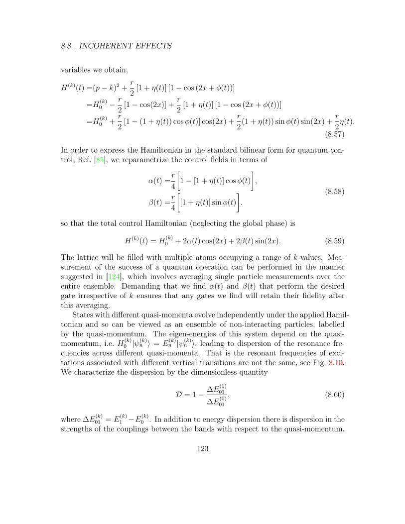
8.8. INCOHERENT EFFECTS
variables we obtain,
H(k)(t) =(p− k)2 +r
2[1 + η(t)] [1− cos (2x+ φ(t))]
=H(k)0 −
r
2[1− cos(2x)] +
r
2[1 + η(t)] [1− cos (2x+ φ(t))]
=H(k)0 +
r
2[1− (1 + η(t)) cosφ(t)] cos(2x) +
r
2(1 + η(t)) sinφ(t) sin(2x) +
r
2η(t).
(8.57)
In order to express the Hamiltonian in the standard bilinear form for quantum con-trol, Ref. [85], we reparametrize the control fields in terms of
α(t) =r
4
[1− [1 + η(t)] cosφ(t)
],
β(t) =r
4
[[1 + η(t)] sinφ(t)
].
(8.58)
so that the total control Hamiltonian (neglecting the global phase) is
H(k)(t) = H(k)0 + 2α(t) cos(2x) + 2β(t) sin(2x). (8.59)
The lattice will be filled with multiple atoms occupying a range of k-values. Mea-surement of the success of a quantum operation can be performed in the mannersuggested in [124], which involves averaging single particle measurements over theentire ensemble. Demanding that we find α(t) and β(t) that perform the desiredgate irrespective of k ensures that any gates we find will retain their fidelity afterthis averaging.
States with different quasi-momenta evolve independently under the applied Hamil-tonian and so can be viewed as an ensemble of non-interacting particles, labelledby the quasi-momentum. The eigen-energies of this system depend on the quasi-momentum, i.e. H(k)
0 |ψ(k)n 〉 = E
(k)n |ψ(k)
n 〉, leading to dispersion of the resonance fre-quencies across different quasi-momenta. That is the resonant frequencies of exci-tations associated with different vertical transitions are not the same, see Fig. 8.10.We characterize the dispersion by the dimensionless quantity
D = 1− ∆E(1)01
∆E(0)01
, (8.60)
where ∆E(k)01 = E
(k)1 −E
(k)0 . In addition to energy dispersion there is dispersion in the
strengths of the couplings between the bands with respect to the quasi-momentum.
123

8.8. INCOHERENT EFFECTS
The main consequence of the dispersion is that a single harmonic excitation cannotsimultaneously resonantly excite all transitions. This poses a formidable challenge forcontrolling an ensemble with high dispersion. For the lattice potential, the amountof energy dispersion decreases with an increase in the strength of potential, Fig.8.10. Unfortunately, the anharmonicity of the lattice, which is essential to resolvedifferent transition frequencies, also decreases with increasing potential depth. In thecase of the Transmon, the system is operated in the low dispersion regime (r>20)and dispersion is most often neglected. Here we aim to be more precise by quan-tifying the trade-off when choosing the depth of the lattice between dispersion andanharmonicity and the degree to which both can be simultaneously corrected.
Note that in superconducting qubits, the CORPSE pulse sequence [33] has beenapplied to mitigate fluctuations of the energy splittings [32], which has been investi-gated further numerically [121]. Here we look not only at dispersion in the energy butmore comprehensively at changes in the strength of all operators in the Hamiltonianas a function of quasi-momentum.
8.8.2.1 Optimization
Using the techniques outlined in Sec. 5.3.2, we optimized control parameters forthe lattice Hamiltonian in Eq. 8.3 for varying potential depths and pulse durations.
−1 0 10
10
20r=2
Energ
y [U
0/E
re]
−1 0 10
10
20
r=13
−1 0 10
10
20
30r=18
k [2π/(G m)]
Energ
y [U
0/E
re]
−1 0 10
20
40r=30
k [2π/(G m)]
Figure 8.10: The first four energy 1-D band structures are shown in the momentumbasis for four different potential depths r. The lower potential depth r = 2 (top left)shows the largest amount of energy dispersion with the closest energy crossings. Thedepth r = 30 (bottom right) shows a lesser amount of dispersion and larger energysplittings.
124

8.8. INCOHERENT EFFECTS
049
141822
0 1 2 3 4 5 6 7
Time (ωre-1s)
r[1+
η(t)
]-1.5-1.0-0.50.00.51.01.5
0 1 2 3 4 5 6 7
Time (ωre-1s)
φ(t)
Figure 8.11: Optimized controls for preparing a Xπ-gate when the optimization usesonly ten points in quasi momentum space. Pulses are well-behaved in the sense thatthey don’t translate the lattice by a full lattice site or possess very large excursionsfrom the initial value for r. (a) An optimized pulse for a potential depth r = 7 with32.7% dispersion and fidelity 98.7% which is calculated by sampling over 100 quasimomentum values. . The duration of the pulse was 5 free oscillations (at k=0).
Our target gate is a Xπ-gate on the first two energy bands. We considered both aRabi pulse assuming no dispersion and bounded random controls fields as the initialguesses for the control fields. The evolution is simulated using only the first sixenergy bands from our model and sampling over 10 values of the quasi-momentum.While we sampled over only a small number of values for the quasi-momenta in orderto have efficiently performed the numerical search, when we calculate the final fidelitywe sampled over a finer grid in quasi-momenta space.
Here are two examples of optimized controls for performing Xπ-gates on ourlattice model. One is a control for a lattice system with potential depth r = 7(which corresponds to a dispersion of 13.2%), as shown in Fig. 8.8.2.1. The durationof this control was 5 free oscillations (at k=0). The gate error across the ensemblewas less than 2% with the exception of particles with quasi-momentum near theedges of the Brillouin zone. Even with such high dispersions in the energies andcontrol Hamiltonians we are able to find gates with reasonable fidelities.
We observe the relationship between the maximum fidelity of the solutions andthe level of dispersion of the Hamiltonian. Ideally, our gradient search will haltwhen a local maximum in the fidelity is reached but this may take a considerableamount of computational resources. All our optimizations were halted after eitherthe algorithm converged to a solution or 105 updates in the control parameters were
125

8.8. INCOHERENT EFFECTS
0 5 1010
−5
10−4
10−3
10−2
10−1
100
Time (Free osc. at k=0)
Err
or
[1−
Φ]
r=0.25
r=0.5
r=1
r=1.5
r=2
r=7
r=12
r=17
r=22
r=30
r=50
r=70
r=90
r=110
0 20 40 60 8010
−6
10−5
10−4
10−3
10−2
10−1
100
Time (Free osc. at k=0)
Err
or
[1−
Φ]
r=0.25
r=0.5
r=1
r=1.5
r=2
r=7
r=12
r=17
r=22
r=30
r=50
r=70
r=90
r=110
Figure 8.12: The maximum fidelity for an optimized pulse over a range of times,from 1 to 10 free oscillations (at k=0), preparing a Xπ-gate as a series of differentpotential depths. The potential depth ranged from r = 0.25 to r = 110, giving adispersion ranging from 93.8% to 0.01%, respectively. Each point is an average ofoptimized pulses from 1 Rabi and 10 random initial pulse.
performed. Nevertheless, for short times (Fig. 8.12A) we find excellent control fields(F > 0.90) for the entire range of potential depths we considered, 0.25 ≤ r ≤ 110.
In general, for long gate times, the maximum fidelity solution forXπ-gates becamelower as the dispersion was increased, Fig. 8.12B. The optimization becomes lesstractable with higher dispersion since we are asking a single set of control fields tosolve wildly different problems depending on where the system is in quasi-momentumspace. As a result, broadband pulses must be tailored to accommodate a range ofpossible energies and couplings. We also find that for high dispersion the fidelitybecomes worse as the gate time becomes longer. This may seem counterintuitive,but it is due to the fact that as the gate time increases the fidelity can vary morequickly as a function of k. For very short gate times, the fidelity is fairly constantacross quasi-momentum space, but for long gates we find that the fidelity is onlyhigh for the specific points we optimized, and dips to almost zero in the intermediateregimes.
We can see the connection between gate duration and rate of change of fidelityvery easily through the simulation described in Fig. 8.13. Here we run GRAPE forexactly one value of the quasi-momentum and and then look at the performance ofthis control field across k. W find that as the duration of the gate increases thefidelity function become more and more tightly peaked about the single value weoptimized, consistent with the spectral bandwidth of the pulse.
126

8.9. IMPLEMENTATION
0.3 0.4 0.5 0.6 0.70
0.2
0.4
0.6
0.8
1
k
Fid
elit
y [
Φ]
5 free osc.
15 free osc.
70 free osc.
Figure 8.13: Pulses for performing Xπ-gate at r = 2 for three different times were op-timized specifically for k = 0.5 and the fidelity response over quasi-momenta shown.Shorter pulses have larger spectral bandwidth and thus affect a larger range of quasi-momenta.
8.9 ImplementationThe DRAG result was first implemented in superconducting qubits at Yale withtransmons in [28, 39] and shortly after with phase qubits at U.C. Santa Barbara[105]. The transmon qubit is a prime candidate for studying leakage because theanharmonicity ∆ is only ∼ 3− 5% of ω0,1. For reasons of practicality and simplicitythe Y-only solution from Sec. 8.6 is explored in this experiment for demonstrationpurposes though the full optimal solution would be achievable to implement, inparticular increased coherence times.
Although Gaussian control pulses (characterized by a width σ) are often theparadigm due to their localized frequency bandwidths given by B = 1/2πσ, leakageerrors can occur as gate times are reduced such that B is comparable to ∆. Thecorrection protocol to the leakage errors as prescribed above is to apply an additionalcontrol on the quadrature channel, Ey(t) = βEx(t) and a dynamical detuning of thedrive frequency δ(t) = Ex(t)2(−4β∆ + λ2)/4∆, where β is a scale parameter. For aqutrit driven without dynamical detuning, the optimal β = λ2/4∆.
The experiments are performed in a circuit QED sample consisting of two trans-mons coupled to a coplanar waveguide resonator. The sample fabrication and ex-perimental setup are described in Ref. [39]. The two transmons (designated L andR) are detuned from one another with ground to excited state (0 ↔ 1) transitionfrequencies of ωL,R
0,1 /2π = 8.210, 9.645GHz and the ground state cavity frequencyisωC/2π = 6.902 GHz. The anharmonicities of the transmons are found using two-
127

8.9. IMPLEMENTATION
tone spectroscopy measurements [154] to be ∆L,R = 330, 300 MHz and coherencetimes are measured to be T L,R
1 = 1.2, 0.9µs and T ∗L,R2 = 1.5, 1.1µs.
-1.0
-0.5
0.0
0.5
1.0
-1.0
-0.5
0.0
0.5
1.0
(a)
(b)
(c)
X XXX
XXX X X XXX
XX x xxx
x x xxxx
xxx x YYY Y
Y Y Y Y Y Y Y Y
Y Y yyy y
y y yyy y
yy y y
X = Rπx X = R−πx x = R
π/x x = R
−π/x Y = Rπ
y Y = R−πy y = Rπ/y y = R
−π/y
⟨σz⟩
Ex(t) = Ae−(t−σ)
/σ
Ey(t) = βdEx(t)/dt
Figure 8.14: (a) Gaussian and derivative pulse shapes applied to the in-phase andquadrature control channels, respectively, for implementing DRAG to first order. (b)Measured 〈σz〉 on qubit L (shaded red bars) with Gaussians with σ = 1ns for a testsequence consisting of pairs of π and π/2 rotations. The slash filled bars correspondto a master-equation simulation of a three-level system with parameters of the sampletested. The grey filled bars reflect ideal values. (c) Similarly measured 〈σz〉 on qubitL but using derivative pulses on the quadrature with a scale factor βL = 0.4 (shadedred bars), also overlaid on the ideal values (shaded dark grey bars).
To implement DRAG to first order and perform single-qubit gates on the trans-mons, we use an arbitrary-waveform generator to shape microwave-frequency pulseswith quadrature control, permitting rotations about either the x- or y-axis of eachqubit. We fix the drive frequency to ω0,1, and the pulse amplitudes and phases de-fine the rotation angle and axis orientation, respectively. When performing an xrotation, Ex(t) is a Gaussian pulse shape, Fig. (8.14)(a), while the derivative of theGaussian is applied simultaneously on the other quadrature, Ey(t) = βEx(t). All ofthe pulses are truncated to 2σ from the center with an added buffer time of 5ns toensure complete separation between concatenated pulses.
128

8.9. IMPLEMENTATION
A simple test sequence is used to tune up the scale parameter β as well as todemonstrate the effect of using first-order DRAG pulses versus standard single-quadrature Gaussians. The sequence consists of pairs of π and π/2 pulses aroundboth the x- andy-axes. An important feature of this sequence is that the final av-erage z-projection of the single qubit, 〈σz〉, will ideally take on values from the setS = +1, 0,−1, making any deviations easily visible.
Using Gaussian pulse shaping with σ = 1 ns and implementing the test sequencefor qubit L, we find significant deviations from S, as shown in the solid red bars ofFig. 8.14 B. The theoretical results for each pair of rotations are shown with solidgrey bars in the background. We observe that the largest errors occur when the tworotations are around different axes, which indicates the presence of significant phaseerror, or a residual z rotation after the first gate.
We repeat the same test sequence, but applying the derivative of the Gaussianto the quadrature channel. By varying β, it is possible to find an optimal value suchthat the measurements of 〈σz〉 agree very well with the theoretical predictions. Theshaded red bars of Fig. 8.14 C show measured 〈σz〉 for qubit L using β = 0.4. Here,deviations from the ideal grey bars decrease to < 2%. We have also applied theDRAG protocol for qubit R, finding the optimal value β = 0.25 (data not shown).From the experimental determination of β and α1, we can infer the second excitedstate coupling strengths λL,R = 1.82, 1.41. Using λL and the three-level model of Eq.(8.4), a master equation simulation for the Gaussian shaping gives the red hash-filledbars in Fig.8.14, which demonstrates good agreement with the experiment.
We find excellent agreement for λ with the calculation for the anticipated λ in acavity-transmon coupled system (Sec. 8.3.1). The cavity modifies the drive strengthsΩ0,1 and Ω1,2 due to its filtering effect. Specifically, for a transmon in a cavity, wehave
λ =gj−1,j(ω
′0,1 − ωC)
g0,1(ω′j−1,j − ωC). (8.61)
where j = 1, 2 for the transmon excitation level, γ = 1,−1 depending onwhether the qubit is located at the input or output side of the cavity, and gi,j is thematrix element coupling the i ↔ j transmon transition to the cavity [94]. Usingthe relevant parameters of the two transmons in the experiment and including onlythe fundamental mode of the cavity, we find λL,R) = 1.85, 1.57, within 12% of thosedetermined from the test sequence. There are corrections to the drive due to thehigher modes of the cavity, but it is difficult to use Eq. 8.61 to estimate as a resultof cutoff dependence.
We characterize the degree of improvement to single-qubit gates by using the
129

8.9. IMPLEMENTATION
exponential fit average fidelity final state fidelity
Fid
elit
y,
(a)
(b)
1.00
0.75
0.50
0.25
1.00
0.75
0.50
80604020Number of gates
Figure 8.15: Randomized benchmarking for qubit L with σ = 1 ns using (a) Gaussianpulses, and (b) additional Gaussian derivative pulses on the quadrature channel.The scattered grey points are extracted fidelities for 32 RB sequences, truncated atdifferent numbers of gates. A remarkable reduction in the extracted average errorper gate (black squares) of the benchmarking results is observed going from (a) to(b). The error bars indicate the variance of all the RB sequences and are smallerthan the squares in (b).
technique of randomized benchmarking (RB) [?]. RB allows us to determine theaverage error per gate through the application of long sequences of alternating Clif-ford gates (Rπ/2
x,y ) and Pauli gates, chosen from 1, Rπx , R
πy , R
πz [62]. We use the RB
pulse sequences originally given in Ref. [?] and adapted to superconducting qubitsin Ref. [27] for both the Gaussian and the derivative pulse shaping for transmon L.We truncate the randomized sequences at various lengths and compare the resultingmeasurement of 〈σz〉 to the ideal final state to obtain the fidelityF . There is anexponential decrease inF with an increasing number of gates in the randomized se-quences. This RB protocol is then repeated for various pulse widths, correspondingto different Gaussian standard deviations, σ ∈ 1, 2, 3, 4, 6 ns.
Using the Gaussian shaping, we find a large reduction in fidelity with the shortestpulses, σ = 1 ns, Fig. 8.15A. The scattered grey points give F for 32 differentrandomized sequences applied as a function of the number of gates in the sequences.When averaged together, we observe a simple decay of F as a function of the numberof gates (solid black squares). Fitting the data with an exponential decay (solid blackline), we extract an average error per gate, EPG = 1 − F of 0.13 ± 0.02. However,when employing the first-order DRAG, we find a dramatic improvement in the gateperformance at σ = 1 nsns, Fig. 8.15B. There is a significant reduction in the spread
130

8.9. IMPLEMENTATION
of the grey points corresponding to all the different randomized sequences, and a fit(solid black line) to the exponential decay of the average fidelity (solid black squares)gives EPG = 0.007± 0.005.
0.001
2
4
6
80.01
2
4
6
80.1
Erro
r per
gat
e, E
PG
25201510Total gate length (ns)
64321Pulse width σ (ns)
benchmarking with gaussian pulses three level simulation benchmarking with derivative pulses two level simulation
Figure 8.16: Comparison of single-qubit gate errors with and without DRAG. Errorper gate for the left qubit extracted from randomized benchmarking for different gatelengths using both Gaussian pulses (red squares) and first-order DRAG pulses (bluesquares). Excellent overlap with theory for gate error including qubit decoherence(black curve) suggests that the DRAG pulses successfully eliminate the errors dueto the presence of higher levels. Gate errors down to 0.007, which are otherwiseunattainable with Gaussian pulses, are reached using DRAG.
Figure 8.16 summarizes the improvement to EPG for different σ by using DRAG.The solid squares are the EPG found using Gaussians, revealing a minimum of0.02±0.007 at σ = 3 ns, before considerably increasing for shorter pulse lengths. Excellentagreement is found with a master equation simulation (dashed line) of the gate errorfor a qutrit system incorporating only decoherence times and coupling strengthsmeasured in independent experiments. Using first-order DRAG, we find the solidcircles in Fig. 8.16, which follow a monotonic decrease in EPG with decreasingσ. Here again we have included a master equation prediction (solid line) of justa single qubit with the same parameters, also giving excellent agreement with theexperimentally determined values and demonstrating that DRAG has reduced theresponse of the system to be like that of a single qubit.
Finally, implementing DRAG on both qubits simultaneously, we can also gen-erate and detect higher quality two-qubit states. Performing state tomography toobtain the two-qubit density matrix ρ via joint readout [26, 48] requires 15 linearlyindependent measurements, corresponding to the application of all combinations of
131

8.9. IMPLEMENTATION
-1
0
1
Elem
ent
valu
e
XI YI ZI IX IY IZ XY XZ YX YZ ZX ZY XX YY ZZPauli measurement
-1
0
1
(a)
(b)
Figure 8.17: Measured two-qubit Pauli sets for preparing the state |1, 1〉 with (a)Gaussian pulses and (b) DRAG pulses (βL = 0.4, βR = 0.25) applied to the quadra-ture channels of both transmon L and qubit R. The ideal Pauli set is shown in grey.
I, Rπx , R
π/2x , and Rπ/2
y on the two qubits prior to measurement. Thus, errors in theseanalysis rotations in addition to the state preparation pulses can result in incorrectdetermination of ρ. The two-qubit Pauli set ~P [26] can be used to visualize ρ forthe state |1〉L ⊗ |1〉R having used Gaussian (Fig. 8.17A) and DRAG (Fig. 8.17B)pulse shaping. ~P consists of ensemble averages of the 15 non-trivial combinationsof Pauli operators on both qubits. The ideal ~P of the state is characterized by unitmagnitude in〈ZI〉, 〈IZ〉, and 〈ZZ〉 and zero for all other elements. We can see thatwith the standard Gaussian pulse shaping, there are substantial (∼ 50 − 100% ofunity) deviations on ideally zero elements, whereas with the DRAG pulses, the Pauliset bars are very close to their ideal values.
By implementing a simple approximation to the optimal control pulses for amulti-transmon coupled-cavity system, we have reduced gate errors below the 10−2
level, limited by decoherence. The agreement of the various experiments with andwithout DRAG pulse shaping with a qutrit model reflects that gate errors due tothe coupling to a higher excited state can be minimized while continuing to shortengate time. Moving forward with optimal control, a tenfold decrease in gate timeto approach ∼ 1 ns through improved electronics or a tenfold increase in coherencetimes to∼ 10µs would place us right at the quoted 10−3 fault-tolerant threshold [122].Furthermore, DRAG is extendable to systems of more than two multi-level atoms forquantum information processing, and has already been employed to enhance single-qubit gates in a circuit QED device with four superconducting qubits [40].
132

Chapter 9
Multi-Channel Leakage
Complications in the Hilbert space nature of physical systems can be found beyondeven the qutrit approximation as a quantum system is scaled to include more elementsor when very low error rates are desired. Not only do simultaneous leakages have tobe taken into account, but introducing an external driving field may couple differentelements together (e.g. crosstalk in Sec. 7.2). In this section we consider three genericmulti-channel leakage problems. The first is encountered in Sec. 9.1 when trying totransition between higher energy levels in an anharmonic ladder such as a Duffingoscillator, where now leakages exist both below and above the driven transition (seeFig. 9.1A). This is first done numerically in Sec. 9.1.2 with our results publishedin Ref. [86] (pulses found by Botan Khani). Next the same problem is studiedanalytically in Sec. 9.1.3. Secondly, in Sec. 9.2, we find analytic forms for suppressingmultiple leakage channels coupled to the same energy level (see Fig. 9.1B). Theanalytic results of Secs. 9.1.3 and 9.2 are published in Ref. [59] with Seth Merkeland Jay Gambetta contributing to the derivations. Last, in Sec. 9.3, we consider twoqutrits and look at the simultaneous removal of both leakages when coupling them(see Fig. 9.1C). This is solved both numerically in Sec. 9.3.2 (solutions found byAmira Eltony) and analytically in Sec. 9.3.3.
9.1 Duffing oscillatorWe have seen that anharmonic systems such as those built from Josephson junctionscan be well described by the Duffing oscillator (Sec. 6.7.1), with Hamiltonian
H =p2
2m+mω2
0
2x2 + δ
m2ω20
3~x4 δ > 0 (9.1)
133

9.1. DUFFING OSCILLATOR
Figure 9.1: In (a) we consider the case when the qubit has leakage from both its |0〉and |1〉 level. In (b) we consider the case when the qubit has leakage from its |1〉level to more then one higher level. In (c) two anharmonic oscillators are coupledwith |11〉 leaking to both |02〉 and |20〉.
where x and p are coordinate and momentum, respectively, and ω0 is the resonancefrequency, in the limit δ → 0. Even though we focus on the hard case, δ > 0,we expect similar conclusions to hold for the soft case. This Hamiltonian can bemade dimensionless with raising and lowering operators analogous to the harmonicoscillator [31]. It then reads
H = ~ω0
(a†a+
1
2
)+
~δ12
(a+ a†)4. (9.2)
9.1.1 SNO approximation
By expanding the nonlinearity and ordering its terms, we can split the Hamiltonianas H = H0(n) + V into a term H0 that contains only the number operator n = a†athat will dominate perturbation theory for small δ/ω 1 and corresponds to therotating wave approximation, and a term V that goes beyond that approximation asit contains different powers of a and a†. We find
H0(n) = ~ω0
(n+
1
2
)+
~δ4
(2n2 + 2n+ 1). (9.3)
V =δ
12(a†4 + 6a†2 + 4a†(a2 + a†2)a+ 6a2 + a4). (9.4)
H0 can be re-parameterized to a simpler form using ω = ω0 + δ, while droppinga constant energy shift
H0 = ~[ωn+ 1
2δn(n− 1)
]. (9.5)
134
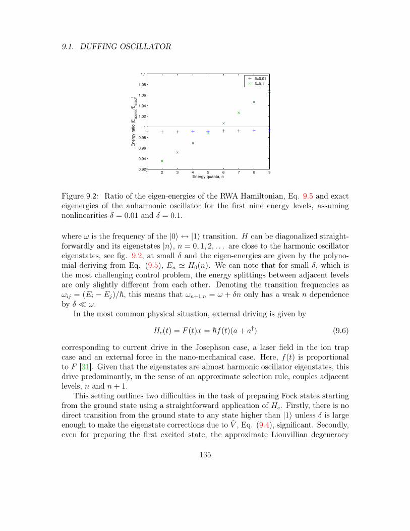
9.1. DUFFING OSCILLATOR
1 2 3 4 5 6 7 8 90.92
0.94
0.96
0.98
1
1.02
1.04
1.06
1.08
1.1
Energ
y r
atio (
Ea
pp
rox/E
exa
ct)
Energy quanta, n
δ=0.01
δ=0.1
Figure 9.2: Ratio of the eigen-energies of the RWA Hamiltonian, Eq. 9.5 and exacteigenergies of the anharmonic oscillator for the first nine energy levels, assumingnonlinearities δ = 0.01 and δ = 0.1.
where ω is the frequency of the |0〉 ↔ |1〉 transition. H can be diagonalized straight-forwardly and its eigenstates |n〉, n = 0, 1, 2, . . . are close to the harmonic oscillatoreigenstates, see fig. 9.2, at small δ and the eigen-energies are given by the polyno-mial deriving from Eq. (9.5), En ' H0(n). We can note that for small δ, which isthe most challenging control problem, the energy splittings between adjacent levelsare only slightly different from each other. Denoting the transition frequencies asωij = (Ei − Ej)/~, this means that ωn+1,n = ω + δn only has a weak n dependenceby δ ω.
In the most common physical situation, external driving is given by
Hc(t) = F (t)x = ~f(t)(a+ a†) (9.6)
corresponding to current drive in the Josephson case, a laser field in the ion trapcase and an external force in the nano-mechanical case. Here, f(t) is proportionalto F [31]. Given that the eigenstates are almost harmonic oscillator eigenstates, thisdrive predominantly, in the sense of an approximate selection rule, couples adjacentlevels, n and n+ 1.
This setting outlines two difficulties in the task of preparing Fock states startingfrom the ground state using a straightforward application of Hc. Firstly, there is nodirect transition from the ground state to any state higher than |1〉 unless δ is largeenough to make the eigenstate corrections due to V , Eq. (9.4), significant. Secondly,even for preparing the first excited state, the approximate Liouvillian degeneracy
135

9.1. DUFFING OSCILLATOR
Figure 9.3: The amplitudes of three pulse sequences optimized by GRAPE forpreparation of |1〉 (top), |2〉 (middle), and |3〉 (bottom) are shown. Each system hada Hilbert space consisting of 10 eigenstates, with δ = 0.12. Each optimized pulseleads to a fidelity of 0.9999.
(i.e., the weak n-dependence of ωn+1,n, prohibits short pulses: A short resonantπ-pulse of length Tr has, by the energy-time uncertainty principle of the Fouriertransform, a bandwidth of ωB ' π/Tr. If ωB becomes comparable to the smallparameter |ωn+1,n − ωn,n−1| = δ, a pulse applied to ωn,n−1 will have a significantFourier component at ωn+1,n. Hence, driving the transition from n − 1 to n willinevitably also drive n to n+ 1 inducing leakage to the next higher state n+ 1. Thiscould be overcome by a very long π-pulse that keeps ωB small, however, in a realisticsetting, this will compete with energy relaxation back to the ground state at a rateT1, effectively limiting ωB 1/T1.
9.1.2 Numerical solutions
We have analyzed this setting numerically in a number of cases using the methodologyof Ch. 5.1. In all cases, the initial state was chosen to be the ground state, |ψi〉 = |0〉and the first, second, and third excited state where chosen as final states, |ψf〉 =|n = 1, 2, 3〉. We have truncated the energy spectrum at n = 10 levels and verified,that changing the number of levels did not lead to a discernible change in the pulse.In Fig. 9.3 we show optimized pulses that display clear beating behavior.
This beating becomes more complex as we go to higher states. More clearly, thisstructure can be analyzed by its Fourier transform, as shown in fig. 9.4 A.
136
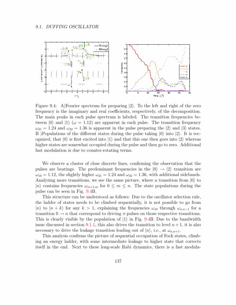
9.1. DUFFING OSCILLATOR
Figure 9.4: A)Fourier spectrum for preparing |2〉. To the left and right of the zerofrequency is the imaginary and real coefficients, respectively, of the decomposition.The main peaks in each pulse spectrum is labeled. The transition frequencies be-tween |0〉 and |1〉 (ω = 1.12) are apparent in each pulse. The transition frequencyω21 = 1.24 and ω32 = 1.36 is apparent in the pulse preparing the |2〉 and |3〉 states.B )Populations of the different states during the pulse taking |0〉 into |2〉. It is rec-ognized, that |0〉 is first excited into |1〉 and that this one then goes into |2〉 whereashigher states are somewhat occupied during the pulse and then go to zero. Additionalfast modulation is due to counter-rotating terms.
We observe a cluster of close discrete lines, confirming the observation that thepulses are beatings. The predominant frequencies in the |0〉 → |2〉 transition areω10 = 1.12, the slightly higher ω21 = 1.24 and ω32 = 1.36, with additional sidebands.Analyzing more transitions, we see the same picture, where a transition from |0〉 to|n〉 contains frequencies ωm+1,m for 0 ≤ m ≤ n. The state populations during thepulse can be seen in Fig. 9.4B.
This structure can be understood as follows: Due to the oscillator selection rule,the ladder of states needs to be climbed sequentially, it is not possible to go from|n〉 to |n + k〉 for any k > 1, explaining the frequencies ω10 through ωn,n−1 for atransition 0→ n that correspond to driving π-pulses on those respective transitions.This is clearly visible by the population of |1〉 in Fig. 9.4B. Due to the bandwidthissue discussed in section 9.1.1, this also drives the transition to level n+ 1, it is alsonecessary to drive the leakage transition leading out of |n〉, i.e., at ωn,n+1.
This analysis confirms the picture of sequential occupation of Fock states, climb-ing an energy ladder, with some intermediate leakage to higher state that correctsitself in the end. Next to these long-scale Rabi dynamics, there is a fast modula-
137

9.1. DUFFING OSCILLATOR
0.8 1.0 1.2 1.4 1.61.0×10-05
1.0×10-04
1.0×10-03
1.0×10-02
n=0 to n=1
T [ωo]
Error
0.1 11
10
n=0 to n=1
n=1 to n=2
δ
Minimum T [ωo]
Figure 9.5: (A) Error for a pulse aiming at creating the first excited state forδ = 0.12 along with an exponential fit (solid) and 95% confidence lines (dashed).(B) Scaling of the minimal gate time with the nonlinearity parameter with power-law fits. Exponents are −0.73 for |0〉 → |1〉 and −0.90 for |1〉 → |2〉.
tion on the scale of the average driving frequency typical for strong driving where thecounter-rotating component of the drive that is not part of standard Rabi physics [31]becomes important. In the end of the pulse, populations of |1〉 and |3〉 are broughtback to |2〉.
As mentioned in Sec. 8.1, nonlinearity is a resource for the creation of Fockstates. At very short pulse durations tg state transfer pulses must scale with aconstant area, i.e., their amplitudes will scale as 1/tg. Thus, if the pulse is tooshort the driving amplitude will be so high that the δ-term in the Hamiltonian canbe neglected and Fock state preparation will not be possible. We have numericallyinvestigated the gate fidelity as a function of pulse duration and found the error tobe roughly exponentially growing at short times, see Fig. 9.5A.
Next we investigate the minimal time to reach a fidelity of 0.99999% for pulses|0〉 → |1〉 and |1〉 → |2〉, Fig. 9.5B. We see that this minimal time is a power law of thenonlinearity parameter δ; tmin ∝ δα with α01 = −0.73±0.029 and α12 = −0.90±0.031
As a reference, we can construct the corresponding power law for non-optimized,single frequency Rabi pulses, starting from the |0〉 → |1〉 transfer. Transforming tothe frame rotating with the driving frequency, the effect of the pulse on the unwanted|1〉 → |2〉 transition is to switch a transition matrix element on and off. This matrixelement has to be compared to the detuning between the transition |ω21−ω10| ' δ. Inorder to create a Rabi pulse of fixed area π, the maximal amplitude of the transitionmatrix elements scales as 1/tg, and its rate of change thus scales as 1/t2g. In orderto not occupy the |2〉-state in the end of the pulse, the dynamics of the |1〉 ↔ |2〉-
138
9.1. DUFFING OSCILLATOR
transition must be fully adiabatic [122], i.e., following a standard result from Landau-Zener theory [98, 167, 188], we demand 1/t2g δ2 leading to a minimal gate time oftg ∝ 1/δ. We would not expect this scaling law to change for the 0 → 2 transition,which is ultimately a sequence of two transitions of length 1/tg, only a differentprefactor.
Thus, we can conclude that our optimal pulses qualitatively extend the limits ofFock state preparation by changing the minimal time to a softer power law, from1/δ to 1/δ0.73±0.029. One can conclude that this is due to quantum interference inthe higher levels. The difference is made possible by temporarily occupying higherstates and unpopulating them in the course of the pulse. It needs to be remarked,that our pulses qualitatively differ from quantum gate pulses, i.e., rotations of thefull basis instead of changing state [122, 148], where a 1/δ scaling of the minimaltime is found. This suggests that state preparation, which is less constrained, canuse quantum interference more efficiently. A related paper has been posted [80] thatlooks at preparation of |1〉 exclusively and finds different envelopes, probably due toadditional constraints.
9.1.3 Analytical solutions
We consider a qubit defined in the intermediate states of an anharmonic oscillator[Fig. 9.1 (a)]. This situation is important if the anharmonic oscillator is going to beused for qudit logic, as done in Ref. [128], or for state tomography of the qudit, asdone in Ref. [13]. The situation is also more constrained than Sec. 9.1.2 since weconsider logical gates rather than state preparation (though the logical gates can beused for state preparation). We rewrite the free Hamiltonian Eq. 9.5 and controlHamiltonian Eq. 9.6 as
Hfr =N∑
j=−N
(jω + ∆j)Πj, (9.7)
Hct(t) = E(t)N∑
j=−N+1
λj−1σxjs−1,j, (9.8)
where N = (d−1)/2 and again we take ∆0 = ∆1 = 0. Moving to a interaction framesimilar to Eq. (8.7) (the sum range is changed to be consistent with the above) we
139

9.1. DUFFING OSCILLATOR
find a dimensionless rotating frame Hamiltonian
H0 =N∑
j=−N, 6=0,1
∆j
∆2
Πj, (9.9)
Hz =N∑
j=−N
jΠj, (9.10)
Hx =N∑
j=−N+1
λj−1σxj−1,j, (9.11)
Hy =N∑
j=−N+1
λj−1σyj−1,j. (9.12)
To find the first order corrections, we follow a similar procedure to Sec. 8.6. Theframe constraints for Eq. 8.31 to remove leakage become
s(1)x,0,k(t) =0, s
(1)y,0,k(t) = −λ−1∆2tgΩG(t)δk,−1
2∆−1
,
s(1)x,1,k(t) =0, s
(1)y,1,k(t) = −λ1tgΩG(t)δk,2
2,
(9.13)
and the dimensionless first order control fields are
Ω(1)x (t) = 2s
(1)x,0,1(t), (9.14)
Ω(1)y (t) = 2s
(1)y,0,1(t)− s(1)
z,1(t)tgΩG(t), (9.15)
δ(1)(t) = s(1)z,1(t) + 2s
(1)y,0,1(t)tgΩG(t) (9.16)
+t2gΩ
2G(t)
4
(λ2
1 − ∆2
∆−1λ2−1
). (9.17)
From this we find the control fields for Z-only correction are
Ωx(t) =ΩG(t), Ωy(t) = 0,
δ(t) =Ω2G(t)
4
[λ21
∆2− λ2
−1
∆−1
],
(9.18)
the Y -only are
Ωx(t) =ΩG(t), Ωy(t) = −ΩG(t)
4
[λ21
∆2− λ2
−1
∆−1
],
δ(t) =0,
(9.19)
140

9.1. DUFFING OSCILLATOR
pulse width σ [units 2π/∆2]
Err
or
1-F
g0.5 1.0 1.5 2.0 2.5
10−6
10−5
10−4
10−3
10−2
10−1
Figure 9.6: Gate error for the implementation of a NOT gate when there is leakageabove and below the qubit subspace. The system considered is explained in the text.The blue dotted line is the zeroth order solution. The black dash line is the first orderZ-only correction. The red dash-dot-dot line is the first order Y -only correction. Thepurple solid line is for the optimal first order correction.
and the optimal first order control field corrections (after minimizing second orderterms) are
Ωx(t) = ΩG(t), (9.20)
Ωy(t) = −ΩG(t)
2∆2
√λ2
1 +∆2
2
∆2−1λ2−1, (9.21)
δ(t) =Ω2G(t)
4∆2
[λ2
1 −∆2
2
∆2−1λ−1
]. (9.22)
To demonstrate an improvement over the zeroth order solution we consider a SNO(of d = 6) where we want to control the 2 → 3 transition. In this case, we relabelj = 2 to 0 and so on, rescaling the coupling so that the new 0→ 1 transition is unity.This results in setting ∆3 = 3∆2, ∆−1 = ∆2, ∆−2 = 3∆2, and λ0 = 1, λ1 =
√4/3,
λ2 =√
5/3 λ−1 =√
2/3, λ−2 =√
1/3. In Fig. 9.6, the gate error for implementinga NOT gate is shown as a function of σ for the same Gaussian shaped pulse asconsidered in Sec. 8.4. Here we observe that the DRAG technique improves the gatefidelities substantially when compared to the zeroth order solution.
Finally, note that because of the Liouvillian degeneracy, ∆−1 = ∆2, this systemis a prime candidate for using a second derivative pulse (Sec. 7.1.3.5) which issymmetric around the driven transition. This may be addressed in future research.
141
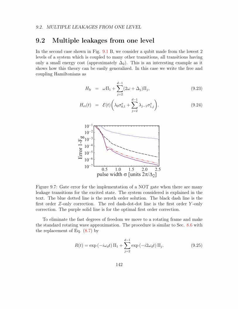
9.2. MULTIPLE LEAKAGES FROM ONE LEVEL
9.2 Multiple leakages from one levelIn the second case shown in Fig. 9.1 B, we consider a qubit made from the lowest 2levels of a system which is coupled to many other transitions, all transitions havingonly a small energy cost (approximately ∆2). This is an interesting example as itshows how this theory can be easily generalized. In this case we write the free andcoupling Hamiltonians as
Hfr = ωΠ1 +d−1∑j=2
(2ω + ∆j)Πj, (9.23)
Hct(t) = E(t)
(λ0σ
x0,1 +
d−1∑j=2
λj−1σx1,j
). (9.24)
pulse width σ [units 2π/∆2]0.5 1.0 1.5 2.0 2.5
10−7
10−6
10−5
10−4
Err
or
1-F
g
10−3
10−2
10−1
Figure 9.7: Gate error for the implementation of a NOT gate when there are manyleakage transitions for the excited state. The system considered is explained in thetext. The blue dotted line is the zeroth order solution. The black dash line is thefirst order Z-only correction. The red dash-dot-dot line is the first order Y -onlycorrection. The purple solid line is for the optimal first order correction.
To eliminate the fast degrees of freedom we move to a rotating frame and makethe standard rotating wave approximation. The procedure is similar to Sec. 8.6 withthe replacement of Eq. (8.7) by
R(t) = exp (−iωdt) Π1 +d−1∑j=2
exp (−i2ωdt) Πj. (9.25)
142
9.2. MULTIPLE LEAKAGES FROM ONE LEVEL
This results in a dimensionless rotating frame Hamiltonian equivalent to Eq. (9.24)with
H0 =d−1∑j=2
∆j
∆2
Πj, Hz = Π1 +d∑j=2
2Πj,
Hx = λ0σx0,1 +
d−1∑j=2
λj−1σx1,j, Hy = λ0σ
x0,1 +
d−1∑j=2
λj−1σy1,j.
Again, we find the zeroth order controls given by Eq. (3.3). To find the first ordercorrections, we find the first order frame transition to be
s(1)x,0,k(t) =0, s
(1)y,0,k(t) = 0,
s(1)x,1,k(t) =0, s
(1)y,1,k(t) = −λk−1tgΩG(t)∆2
2∆k
.(9.26)
This gives the dimensionless first order control fields
Ω(1)x (t) =2s
(1)x,0,1(t),
Ω(1)y (t) =2s
(1)y,0,1(t)− s(1)
z,1(t)tgΩG(t),
δ(1)(t) =s(1)z,1(t) + 2s
(1)y,0,1(t)tgΩG(t)
+t2gΩ
2G(t)∆2
4
(∑d−1k=2
λ2k−1
∆k
).
(9.27)
From this, we find the control fields for the Z-only correction are
Ωx(t) =ΩG(t), Ωy(t) = 0,
δ(t) =Ω2G(t)
4
∑d−1k=2
λ2k−1
∆k,
(9.28)
for the Y -only correction are
Ωx(t) =ΩG(t), Ωy(t) = −ΩG(t)
4
∑d−1k=2
λ2k−1
∆k,
δ(t) =0,
(9.29)
and the optimal first order control field corrections (after minimizing H(2)extra(t)) are
Ωx(t) =ΩG(t), Ωy(t) = −ΩG(t)
2∆2
√∑d−1k=2
∆22λ
2k−1
∆2k,
δ(t) =Ω2G(t)
4∆2
[∑d−1k=2
∆22λ
2k−1
∆2k− 2
√∑d−1k=2
∆22λ
2k−1
∆2k
].
(9.30)
143
9.3. 2-QUBIT LEAKAGE
We note that these solutions are identical to the previous solutions with a singleleakage channel where λ1 = λ,
λ ≡√∑d−1
k=2
∆22λ
2k−1
∆2k. (9.31)
To numerically demonstrate an improvement over the zeroth order solution, weconsider the implementation of a NOT gate for a d = 6 system with λj = 1 for all jand ∆3 = 2∆2, ∆4 = 3∆2, ∆5 = 4∆2 (note these are different parameters from theanharmonic oscillator considered in Sec. 9.1.1). The results are plotted in Fig. 9.7,where again, it is clearly seen that the DRAG technique improves the zeroth ordersolution.
9.3 2-Qubit leakage
9.3.1 General Model
The system that we consider consists of two coupled qubits. Each qubit is made upof the ground and first excited states of a slightly anharmonic oscillator (see Sec. 6.7).We examine the lowest three levels of the spectrum; the third level represents leakage.This results in a single qubit Hamiltonian given by
Hqubit = ~∑i=1,2
(ω1i Π
(1)i + ω2
i Π(2)i ) (9.32)
where we have projectors Π(i)j = |j〉〈j|i and transition energies ~ωj. The coupling
takes the form of voltage coupling, so that the qubit interaction term can be writtenas
Hint = J(t)(σx,10,1 + λ1σ
x,11,2
)(σx,20,1 + λ2σ
x,21,2
)(9.33)
where σx,ki,j = |i〉〈j|k+|j〉〈i|k and λk measures the relative strength of the 1-2 transitionto the 0-1 transition for the kth qubit. The parameter J(t) is the coupling strengthbetween the qubits. Control of the system is represented by this variable couplingterm. So, in the lab frame our Hamiltonian is
H = ~∑i=1,2
(ω1i Π
(1)i + ω2
i Π(2)i ) + J(t)
(σx,10,1 + λ1σ
x,11,2
)(σx,20,1 + λ2σ
x,21,2
)(9.34)
By making the rotating wave approximation (RWA), we can write the effective Hamil-tonian as
Heff = Hdrift + V (t) (9.35)
144

9.3. 2-QUBIT LEAKAGE
where V (t) is the effective coupling term and Hdrift is the effective single qubit Hamil-tonian. V (t) and Hdrift are given by
V (t) = J(t)[a1a
†2 + h.c.
]for ai = |0〉〈1|i + λ|1〉〈2|i (9.36)
Hdrift = ∆Π(1)2 + ∆Π
(2)2 (9.37)
where ∆ = ωi2 − 2ωi1 is the anharmonicity of the qubits, assumed to be the same forboth qubits i = 1, 2 which are brought on resonance, and we have set ~ = 1. Wehave also assumed that λ1 = λ2 = λ. The subspaces in H are coupled by V (t) in thefollowing way:
|01〉 to |10〉|12〉 to |21〉|11〉 to |02〉, |20〉 (coupling across subspaces)
So, we can write V(t) in terms of a degenerate subspace and another subspace thatrepresents leakage: V (t) = Vleak + Vdeg
where Vleak = J(t)[λ|02〉〈11|+ λ|11〉〈20|+ h.c.
](9.38)
Vdeg = J(t)[|01〉〈10|+ λ2|12〉〈21|+ h.c.
](9.39)
In the absence of the third (leakage) level, the coupling terms between the qubitsgenerate an ideal ISWAP gate. Namely, if
H = Vdeg = J[|01〉〈10|+ λ2|12〉〈21|+ h.c.
]with J =
π
2T(9.40)
a perfect ISWAP unitary propagator is formed U = T e−i´ T0 Hdt = e−iHT (where T
is the gate time). So, if ∆ is large, in which case the effect of the third level isessentially averaged out over the gate, very high fidelity can be obtained using aconstant coupling strength of π
2T. For example, for ∆ = 10 GRad/s (= 1.59 GHz)
and a gate time of 10 ns the fidelity of the ISWAP gate produced with this constantcoupling is F = 0.99814. For more practical anharmonicities in the vicinity of 300MHz, the fidelity drops significantly due to leakage. For example, for ∆ = 2.2GRad/s (= 350 MHz) and a gate time of 10 ns the fidelity is F = 0.947449; doublingthe gate time to 20 ns only increases the fidelity to F = 0.990626.
145
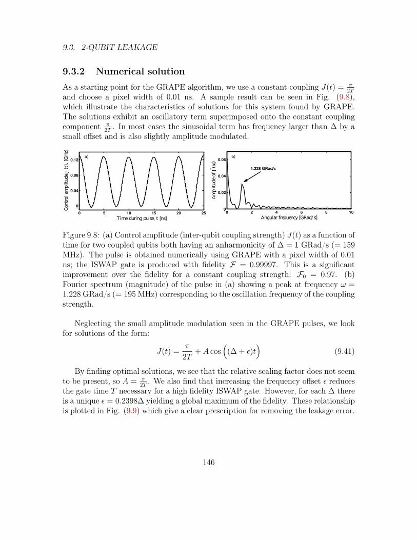
9.3. 2-QUBIT LEAKAGE
9.3.2 Numerical solution
As a starting point for the GRAPE algorithm, we use a constant coupling J(t) = π2T
and choose a pixel width of 0.01 ns. A sample result can be seen in Fig. (9.8),which illustrate the characteristics of solutions for this system found by GRAPE.The solutions exhibit an oscillatory term superimposed onto the constant couplingcomponent π
2T. In most cases the sinusoidal term has frequency larger than ∆ by a
small offset and is also slightly amplitude modulated.
AmplitudeofJ(ω)
Angular frequency [GRad/ s]
Timeduring pulse, t [ns]
ControlamplitudeJ(t),[GHz]
a) b)
Figure 9.8: (a) Control amplitude (inter-qubit coupling strength) J(t) as a function oftime for two coupled qubits both having an anharmonicity of ∆ = 1 GRad/s (= 159MHz). The pulse is obtained numerically using GRAPE with a pixel width of 0.01ns; the ISWAP gate is produced with fidelity F = 0.99997. This is a significantimprovement over the fidelity for a constant coupling strength: F0 = 0.97. (b)Fourier spectrum (magnitude) of the pulse in (a) showing a peak at frequency ω =1.228 GRad/s (= 195 MHz) corresponding to the oscillation frequency of the couplingstrength.
Neglecting the small amplitude modulation seen in the GRAPE pulses, we lookfor solutions of the form:
J(t) =π
2T+ A cos
((∆ + ε)t
)(9.41)
By finding optimal solutions, we see that the relative scaling factor does not seemto be present, so A = π
2T. We also find that increasing the frequency offset ε reduces
the gate time T necessary for a high fidelity ISWAP gate. However, for each ∆ thereis a unique ε = 0.2398∆ yielding a global maximum of the fidelity. These relationshipis plotted in Fig. (9.9) which give a clear prescription for removing the leakage error.
146
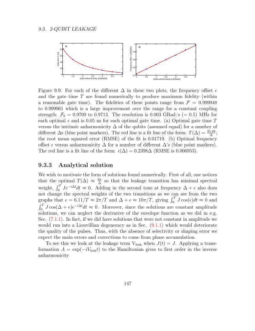
9.3. 2-QUBIT LEAKAGE
1 1.5 2 2.5 3 3.5 45
10
15
20
25
30
Qubit anharmonicity ∆ [GRad/s]
Gat
e tim
e T
[ns]
a)
1 1.5 2 2.5 3 3.5 40.2
0.4
0.6
0.8
1
Qubit anharmonicity ∆ [GRad/s]
Fre
quen
cy o
ffset
ε [G
Rad
/s]
b)
Figure 9.9: For each of the different ∆ in these two plots, the frequency offset εand the gate time T are found numerically to produce maximum fidelity (withina reasonable gate time). The fidelities of these points range from F = 0.999948to 0.999961 which is a large improvement over the range for a constant couplingstrength: F0 = 0.9709 to 0.9713. The resolution is 0.003 GRad/s (= 0.5) MHz foreach optimal ε and is 0.05 ns for each optimal gate time. (a) Optimal gate time Tversus the intrinsic anharmonicity ∆ of the qubits (assumed equal) for a number ofdifferent ∆s (blue point markers). The red line is a fit line of the form: T (∆) = 25.49
∆;
the root mean squared error (RMSE) of the fit is 0.01719. (b) Optimal frequencyoffset ε versus anharmonicity ∆ for a number of different ∆’s (blue point markers).The red line is a fit line of the form: ε(∆) = 0.2398∆ (RMSE is 0.006953).
9.3.3 Analytical solution
We wish to motivate the form of solutions found numerically. First of all, one noticesthat the optimal T (∆) ≈ 8π
∆so that the leakage transition has minimal spectral
weight,´ T
0Je−i∆tdt ≈ 0. Adding in the second tone at frequency ∆ + ε also does
not change the spectral weights of the two transitions as we can see from the twographs that ε = 6.11/T ≈ 2π/T and ∆ + ε ≈ 10π/T , giving
´ T0J cos(ε)dt ≈ 0 and´ T
0J cos(∆ + ε)e−i∆tdt ≈ 0. Moreover, since the solutions are constant amplitude
solutions, we can neglect the derivative of the envelope function as we did in e.g.Sec. (7.1.1). In fact, if we did have solutions that were not constant in amplitude wewould run into a Liouvillian degeneracy as in Sec. (9.1.1) which would deterioratethe quality of the pulses. Thus, with the absence of selectivity or shaping error weexpect the main errors and corrections to come from phase accumulation.
To see this we look at the leakage term Vleak when J(t) = J . Applying a trans-formation A = exp(−iVleakt) to the Hamiltonian gives to first order in the inverseanharmonicity
147
9.3. 2-QUBIT LEAKAGE
HA = Hdrift + Vdeg(t) +λ2J2
∆(2|11〉〈11|+ |02〉〈02|+ |20〉〈20|) +O(
1
∆2) (9.42)
We want to cancel the phase error (i.e. ac-Stark shift) in the qubit’s subspace
2λ2J2
∆|11〉〈11|
Note that the effect is entangling and cannot be canceled with single qubit gates.Instead we expect that adding the second tone J(t) = J cos(∆ + ε) has exactly thisneeded effect. To see this we can move to the frame rotating at frequency ∆ + ε viathe rotating frame R = exp(−i(∆ + ε)(Π
(1)1 + Π
(2)1 + 2Π
(1)2 + 2Π
(2)2 )t) which gives
HR = J(1 + cos[(∆ + ε)t])e−i(∆+ε)t(|01〉〈10|+ λ|02〉〈11|+ λ|11〉〈20|+ λ2|12〉〈21|) + h.c.
−(∆ + ε)Π(1)1 − (∆ + ε)Π
(2)1 − εΠ
(1)2 + εΠ
(2)2
Expanding the cosine into a sum of exponentials and dropping terms with fre-quency 2(∆ + ε) we can simplify this somewhat to
HR ∼= J(e−i(∆+ε)t +1
2)(|01〉〈10|+ λ|02〉〈11|+ λ|11〉〈20|+ λ2|12〉〈21|) + h.c.
−(∆ + ε)Π(1)1 − (∆ + ε)Π
(2)1 − εΠ
(1)2 + εΠ
(2)2
From this frame it is possible to deduce the effect of the extra term on the qubit’ssubspace, which can be seen via the transformation B = exp(i(− iJ
∆+ε|01〉〈10| −
iλJε|02〉〈11| − iλJ
ε|11〉〈20|+ h.c.)t) to give
HB = J(e−i(∆+ε)t)(|01〉〈10|+ λ|02〉〈11|+ λ|11〉〈20|+ λ2|12〉〈21|) + h.c.(9.43)
−(∆ + ε)Π(1)1 − (∆ + ε)Π
(2)1 − εΠ
(1)2 + εΠ
(2)2
−λ2J2
4ε(2|11〉〈11|+ |02〉〈02|+ |20〉〈20|)
− J2
4(∆ + ε)(|01〉〈01| − |10〉〈10|) +O(
1
∆2)
Comparing this equation with Eq. (9.42)we see that the necessary condition forcanceling the phase error on |11〉〈11| is
148

9.3. 2-QUBIT LEAKAGE
4ε = ∆.
This corresponds very closely to the relationship found in Fig. (9.9)B, with theslight deviation explainable by higher order corrections. Note that there is also ashift of the |01〉〈01| and |10〉〈10| levels but these are suppressed by a factor of ∆
8λ2(∆+ε)
which for typical values is about 20 times smaller than the original phase shift, witha similar decrease in the error. In fact, if we include this term in the |11〉〈11| shift,and choose 4.05ε = ∆ this comes even closer to the optimal value. This methodcan also easily be expanded to the case where the anharmonicities of the qubits aredifferent.
149
Chapter 10
Virtual Transitions
We have seen that errors in performing gate operations can arise from non-idealitiesin the driving fields and from complications in the Hilbert space of the qubits thatgo beyond a 2-level approximation. It turns out that complications in the Hilbertspace can also be beneficial. Frame transformations can be used to couple energylevels that do not ordinarily contain a matrix element in the physical lab frame (seee.g. Fig. 10). The advantage of such a situation is that if no matrix element is con-tained between the qubit levels then relaxation can in principle be greatly suppressed.In other cases, the virtual transition can be used where selectivity conditions wouldmake driving the individual transitions of which it is composed impossible. For vir-tual transitions, multiple photons are used, with the condition that their energies addup to the energy splitting of the driven transition for energy conservation to hold. Itis conventional wisdom to perform an adiabatic approximation for these transitionsthat any transition that does not conserve energy will be greatly suppressed. Thisapproximation will be quantified in an order expansion as it was in Ch. 8 and Ch. 9.On the other hand, it will be shown in this chapter that two photon (Raman) transi-tions can be obtained using an exact interaction frame representation where leakageis exactly suppressed and no adiabatic expansion is necessary. When the transitionsare driven with equal amplitude, it will be shown that these transitions can be drivenin arbitrarily small times. Finally, numerical optimization with response functions(Ch. 5.1) can be used when multiple tones at different frequencies are used to drivethe system. In particular, the numerical methodology is useful when not all of theoscillation can be removed from the Hamiltonian description.
The physical examples that will be considered are as follows. In Sec. 10.1, qutritswhere the qubit is formed from the first and last levels with driving via an interme-diary level will be considered. In Sec. 10.2, quantum elements are coupled using a
150

10.1. RAMAN TRANSITIONS
virtual sideband transition that couples |00〉 and |11〉 for an effective entangling gate.Finally, in Sec. 10.3, the situation where a qubit is isolated from the environment viaa cavity and all control is done through the cavity is considered, including virtuallydriving the qubit.
ωEnergy
(a) (b)
|0⟩
|1⟩
|2⟩
|0⟩|1⟩
|2⟩ω
1
2
ω1ω2
Figure 10.1: A stimulated Raman transition is shown where |0〉 and |1〉 qubit statesare not directly connected but indirectly via |2〉. In (a) the transition frequency isgiven by the sum of the single photon transitions while in (b) it is their difference.Driven transitions between levels exist where there are black arrows while the redarrows indicate the desired transitions.
10.1 Raman transitionsAn alternate strategy to assigning two adjacent levels of an energy spectrum to aqubit is to use two levels that are not connected by a matrix element in the Hamil-tonian, in order to avoid relaxation error between them. In this case, a temporarylevel with transitions to both qubit levels can be used to connect them. In practicethe auxiliary level will usually have greater decay so it is preferable to minimize in-termittent population to the level. To this end virtual multi-photon transitions canbe used that to a certain degree of approximation do not populate the intermediarylevels. The full dynamics can once again be obtained via a frame transformation.
Most simply, we have an interaction Hamiltonian with two independent drives ofthe form
H =(Ω1(t)e−iφ1Γ10,1(−δ) + Ω2(t)e−iφ2Γ2
1,2(δ)) + h.c. (10.1)
with Γla,b(δ) = λla,be−iδt|a〉〈b| as in Eq. 7.3. Without loss of optimality, we pick
Ω(t) = ReΩ1(t)λ10,1 = ReΩ2(t)λ2
1,2 and moving to frame rotating at the drivingfrequency we get
151

10.1. RAMAN TRANSITIONS
H(Ωe−iφ, δ) = (Ω(t)e−iφ(σ+0,2 + σ+
1,2) + h.c.) + δ|1〉〈1| (10.2)
Applying the interaction frame transformation for the off-phase control
D = exp(
ˆ t
0
H(ImΩ(t)dt, 0)dt)
we obtain a matrix equation for DH(ReΩ(t), 0)D† = Ωeff(t)σx0,1 which can easilybe solved for the imaginary control to be
ˆ t
0
ImΩ(t)dt =1
2√
2arctan
2√
2ReΩ(t)
δ(10.3)
This transformation leaves the Hamiltonian in the form
HD ≈
(1
4+
3
4
√1 +
8ReΩ2(t)
δ2
)δ|2〉〈2|
− 1
4
(−1 +
√1 +
8ReΩ2(t)
δ2
)δΓ0,1(0) + h.c.
(10.4)
Thus we have the simple condition for rotation that
ˆ T
0
1
4
(−1 +
√1 +
8ReΩ2(t)
δ2
)δdt =θ (10.5)
for an exact rotation, noting that there is no phase error because of the chosensymmetry of the solution between the two drives.
This is an exact solution and completely removes both leakage and rotation errorin the pulses. For all gate times and in the limit T → 0, the gate error is identically 0.The solution also tolerates small sampling/shaping error despite the large amplitudesrequired to drive a rotation at small times. In Fig. 10.2, we have chosen to leave inthe small sampling error to illustrate the dramatic decrease in error and gate timesfrom conventional to DRAG pulses. What is most striking about the solution is thatit works even for very large energies in the domain that is definitely not adiabatic.
152

10.1. RAMAN TRANSITIONS
0 2 4 6 8 10Gate Time10-6
10-5
10-4
0.001
0.01
0.1
1Error
Figure 10.2: Rotation error for Raman transition with two independent drives. Theblue line is the error from Gaussian shaping with the red line is the DRAG solutionunder finite sampling. For infinitesimal sampling this error is identically 0.
This is in contrast to conventional pulses (the blue line) which need to be slow inorder to minimize higher order terms in an adiabatic expansion.
For drives not of the same amplitude Ω1(t) 6= Ω2(t), such as is used in conventionalSTIRAP pulses [10], it is still exactly solvable but it is unclear whether there existsa closed expression. In this case there may be a similar expansion to Sec. 8.5.1 butgiven that the more constrained case already solves the problem exactly this has notbeen explored. Since STIRAP is also adiabatic, a dramatic improvement in unitarytransfer is also expected by using instead DRAG.
Note that if one uses a single drive (chosen at the halfway frequency of the twodriven transitions) one still gets the same Hamiltonian Eq. 10.2. However one cannotenforce both derivative conditions, Eq. 10.3 with a single first-derivative drive. Ineffect one runs into the same Liouvillian degeneracy issue as was the case in Sec.9.1.1and Sec. 9.3.1. As in the other two cases, this would be a good candidate to usethe second derivative as prescribed in Sec. 7.1.3.5 to simultaneously deselect bothtransitions.
In practice, it is better to drive the transitions separately. If there is no sepa-rate addressability to the transitions (as in Ch. 7) then we have the more generalHamiltonian
H =Ω1(t)e−iφ1(Γ10,1(∆ + δ) + Γ1
1,2(δ)) + h.c.
+ Ω2(t)e−iφ2(Γ20,1(−δ) + Γ2
1,2(∆− δ)) + h.c.(10.6)
Provided ∆ is large this does not significantly impact the solution presented,especially when the detunings are on the same side of each of the drive frequencies
153

10.2. 2-QUBIT COUPLING
(as would occur in Fig. 10A). For ∆ comparable to δ it may be possible to improvethe result by driving the virtual transition using all four transitions while suppressingall the single photon transitions, and this is a possible direction of future research.
10.2 2-Qubit coupling
Figure 10.3: We consider the case when the |00〉 to |11〉 transition contains no ex-plicit matrix element but by driving the single photon transitions at the correct sumfrequency this transition can be activated. Driven transitions between levels existwhere there are black arrows while the red arrows indicate the desired transitions.
10.2.1 Ansatz solution
We study the generalized Jaynes-Cummings system [78](also studied in Sec. (8.3.1))with the purposes of moving an excitation between the qubit and the cavity. As afurther complication, we allow the qubit to have leakage to a third level in keepingwith superconducting systems as our standard example (see Fig. 10.3). Then,
HJC =ωra†a+
d−1∑j=1
(jω + ∆j)Πj +d−1∑j=1
gj−1,j
(|j − 1〉〈j|a† + |j〉〈j − 1|a
), (10.7)
where all terms are defined in Sec. (8.3.1). The selected strategy is to drivea sideband transition between the |00〉 and |11〉 levels which is a virtual transi-tion [100]. Note that driving the transitions consecutively would not provide a re-versible/entangling gate because it involves only single qubit gates. However, itcannot even be used for state preparation (of e.g. a Bell state) because in practiceone cannot excite the cavity Fock states directly because it is a (infinite dimen-sional) harmonic system with no distinct transition energies. That is, photons thatare injected into the cavity are driven by a Hamiltonian of the form
154

10.2. 2-QUBIT COUPLING
Hdr(t) = ε(t)(a+ a†) (10.8)
Using this drive, three transitions can be combined into one virtual one via |00〉 ↔|01〉 ↔ |10〉 ↔ |11〉 where the first and last transition are driven and the middletransition is the natural coupling between the qubit and cavity at strength g0,1. Thesideband frequency that is used is exactly the halfway energy, ω+ωr
2. Rather than
calculating the matrix elements which are quite cumbersome and involve calculationsvery similar to Sec. (10.1) we use the ansatz that the primary errors will involvea derivative selection error on the off-resonant single photon transitions and an ac.Stark shift of the qubit transition. As in Sec. (8.7.1) we simply optimize the prefactorsA,B,C,D in front of these terms:
εx(t) = AΩT (t)
εy(t) = BΩT (t)
δω(t) = CΩ2T (t)
ω − ωr+D
with ΩT (t) defined in Eq. (3.1).
Figure 10.4: Gate error vs. gate time for sideband transition in J-C ladder withac-Stark shift and derivative corrections.
155

10.2. 2-QUBIT COUPLING
In Fig. (10.4) we compare gate error vs. gate time for 3 solutions. The red linerepresents the standard solution of constant driving with 1ns rise time (consistentwith electronics) and constant frequency whereby we optimize only A and D. Nextwe compute the “Z-only” solution (shown in dashed purple) which involves optimiz-ing A,C, and D and where for additional selectivity we use a larger rise-time of 5ns.Finally, the “optimal 1st order” solution is consider in which all prefactors are opti-mized and a rise-time of 5ns is used once again. We see an improvement of 2 ordersof magnitude compared to what is conventionally used.
10.2.2 Optimization with two tones
We now apply full numerical optimization to the problem of coupling two frequencyseparated qubits using a sideband transition. This example illustrates the needfor numerical optimization on a finer grain than the sampling of the controls (asintroduced in Sec. 6.1) in the common case that multiple frequency componentsare used in the control. This is an important problem as including more tones isstraightforward way to increase the fidelity of gate operations. We consider twooff-resonant qubits coupled by a XX + Y Y interaction and drive with two differentfrequencies, one resonant with one of the qubit’s transition frequency and the secondtuned to exactly the average of the qubits’ transition frequencies, in order to generatean√
ISWAP operation. Thus, we see the system has three frequencies, and there isno frame in which all fast dynamics can disappear. Specifically, we start with theHamiltonian of the form,
H =E (1)x (t)σ(1)
x cos(ω
(1)d t)
+ E (1)y (t)σ(1)
x sin(ω
(1)d t)
+ E (2)x (t)σ(2)
x cos(ω
(2)d t)
+ E (2)y (t)σ(2)
x sin(ω
(2)d t)
+ J(σ
(1)+ σ
(2)− + σ
(1)− σ
(2)+
)+ ω1σ
(1)z + ω2σ
(1)z ,
(10.9)
where the superscripts index the qubit, σ± are the raising and lowering operators,J is the strength of the coupling, ω1 and ω2 are the qubit frequencies, and ω(1)
d andω
(2)d are the drive frequencies.Choosing the frame rotating at the energies of the two qubits (which is conven-
tional, but not the only available frame) and setting the first drive to ω(1)d = ω1+ω2
2
156

10.3. DRIVING THROUGH A CAVITY
10-5
10-4
10-3
10-2
10-1
100
10 20 30 40 50 60 70 80 90 100
Gate
err
or(
1-Φ
)
Number of subpixels
Figure 10.5: Gate error as a function of the number of subpixels for the multi-toneexample. The solid red line is for ∆/2π = 1.0 GHz and the green dashed line is for∆/2π = 0.5 GHz. Other parameters are given in the text.
and the second drive to ω(2)d = ω2, we find
HR =E (1)x (t)
2(σ
(1)+ e−i∆t/2 + σ
(1)− ei∆t/2) +
E (2)x (t)
2σ(2)x
+E (1)y (t)
2(iσ
(1)+ e−i∆t/2 − iσ(1)
− ei∆t/2) +E (2)y (t)
2σ(2)y
+ J(σ(1)+ σ
(2)− ei∆t + σ
(1)− σ
(2)+ e−i∆t),
(10.10)
where ∆ = ω1 − ω2 is the energy difference between the qubits.We illustrate the scaling with number of subpixels for this example we choose a
gate time of tg = 20ns, J/2π = 94 MHz, and ∆/2π = 0.5 or 1.0, and in Fig. 10.5we plot the predicted error as a function of the number of sub-pixels for 1ns pixels.This error is calculated by integrating the Schrödinger equation for the optimizedcontrols on a much finer grid. As expected, we see that for the larger detuning muchmore subpixels are required to achieve the same low error control. Nonetheless, thismethod provides a valuable tool for quantum control when multiple fields are used,as is the case for but not limited to virtual transitions.
10.3 Driving through a cavityAs the final example of virtual coupling, one can consider a qubit inside a cavity wherethe two quantum elements are left distinct and the dispersive mode diagonalizationis not performed.
157

10.3. DRIVING THROUGH A CAVITY
Figure 10.6: We consider the case where a qubit is placed inside a cavity so the |00〉to |01〉 transition forms the qubit. No direct coupling exists between the qubit levelsand must be driven by the cavity. Driven transitions between levels exist where thereare black arrows while the red arrows indicate the desired transitions.
HJC =ωra†a+
d−1∑j=1
(jω + ∆j)Πj +d−1∑j=1
gj−1,j
(|j − 1〉〈j|a† + |j〉〈j − 1|a
)+ εx(t)(a+ a†) + iεy(t)(a− a†),
(10.11)
as above. As a design strategy there is no direct drive on the qubit (in orderto isolate it from sources of noise) and only the cavity is used to read and writeinformation to the qubit (with the expectation that will decouple most of the noisenear the qubit frequency). Here, we operate in the bare basis which means thatqubit rotations cannot be driven directly but virtually through the combination ofthe coupling and the cavity drive.
Optimization is performed using the response function methodology developedin Ch. 6, using pulses with 1ns pixels and a 250MHz filter, consistent limitations incurrent electronics (Sec. 6.2). An example of a pulse which generates a pi pulse fora 20ns pulse is given in Fig. 10.7 A with arbitrarily small error. Both the X andY quadratures are needed as was the case for the simple qutrit, with, as before foran X rotation, the εx being symmetric and εy being asymmetric. In Fig. 10.7 B, amemory operation is shown. Here the εy is more clearly approximately the derivativeof εx, with two rotations being indicative of a spin-echo sequence.
This setup has certain advantages compared to the dressed frame, namely thatleakage out of the cavity is smaller and can even be further suppressed using optimalcontrol techniques. Thus a major source of incoherent error can be avoided. Thisis again a selectivity problem where leakage does not come during gate operationbut instead during memory operations. Here we expect the main effect to be ana.c. Stark shift since the coupling is constant. Operating in this frame allows for
158

10.4. SUMMARY
-4
-2
0
2
4
2 4 6 8 10 12 14 16 18 20
Contr
ols
(G
Hz)
Time during Gate (ns)
-4
-2
0
2
4
2 4 6 8 10 12 14 16 18 20
Contr
ols
(G
Hz)
Time during Gate (ns)
Figure 10.7: Pulse amplitude as a function of the time during gate for a qubit driventhrough a cavity. The solid red line is the X quadrature control and the green dashedline is the Y . Parameters are given in the text. (A) is a NOT pulse, UX
π ; (B) is amemory operation, 1.
drastically better selectivity in this regard, enabling many qubits to be placed insidethe cavity. An additional benefit is that the cavity frequency is not shifted by thepresence of energy in the qubits, which means radiation coming into the cavity at acertain frequency will not be attenuated given the state of the qubits, resulting inrotation angle errors.
10.4 SummaryIn this chapter, we have seen that off-resonant terms and fast dynamics form an im-portant source of error in multi-photon transitions. We have explored three differentcases where virtual transitions form an integral part of the computation scheme witha clear benefit from a decrease in these forms of error. Methods such as STIRAPcan be used to exchange energy between two levels that do not normally share atransition. This can be extremely useful since relaxation cannot occur where thereis no transition and can be greatly suppressed where there are multi-photon tran-sitions. However, the conventional analysis is that these pulses must be adiabaticwhich can greatly slow down gate times making it prone to decoherence. In contrast,the two-photon DRAG solution derived is exact and works in the diabatic regime aswell, allowing for arbitrarily short pulses. Similarly, virtual transitions can be used toentangle a qubit (or anharmonic ladder) to a (harmonic) cavity where single photontransitions in the cavity could not be used for the same effect. Once again, in such asituation there is evidence that using a derivative shaped imaginary control greatlyreduces selection error. Finally, working with a non-linear oscillator and a cavity in
159

10.4. SUMMARY
the bare frame, it is shown numerically that all gate operations can be achieved usingvirtual transitions, where once again relaxation can be greatly decreased by avoidingputting population in the cavity where it can spontaneously decay. Such a schemecan have advantages also in terms of how many qubits can fit in the coupling cavity,since placing them at frequencies close to that of the cavity is less of a concern asmemory operations can be engineered to undo the effect of the Stark shift from thecavity.
160
Chapter 11
Strong Coupling
We have seen in Sec. 4.2.2 that transitions are typically driven with monochro-matic sinusoidal fields rather than constant or near-constant driving fields. We haveseen that in a rotating frame (Sec. 4.2.2) at the frequency of the monochromaticoscillation, a more intuitive representation is given by
Hrot = eiωΠ1t((2a(t) cos(ωdt+ φ) + 2b(t) sin(ωdt+ φ))Xπ + c(t)Π1)e−iωΠ1t
Hrot = (c(t) + ∆ω)Π1 (11.1)
+1
2(a(t) cos(δωt) + b(t) sin(δωt))X (11.2)
+1
2(b(t) cos(δωt)− a(t) sin(δωt))Y
+1
2(a(t) cos(ωΣt+ 2φ) + b(t) sin(ωΣt+ 2φ))X (11.3)
+1
2(−b(t) cos(ωΣt+ 2φ) + a(t) sin(ωΣt+ 2φ))Y
with the same notation as before and where we stress again that the last twolines (the counter-rotating terms) are usually dropped via energy considerations (theRWA). The statement can be made precise in the formulation of Sec. 7.1.1 withthe limiting condition that ωΣ a, b in order that selectivity hold true. Here, wewill retain the terms under the assumption of strong driving that the terms are allof roughly the same order ωΣ ' a, b. Following the prescription of Sec. 8.5, theselectivity in the presence of these counter-rotating terms can be improved by theadiabatic expansion technique, as will be done in Sec. 11.1. Next, in Sec. 11.2the adverse effect of the counter-rotating terms is suppressed using robust numericaloptimization techniques with the use of fine-graining.
161

11.1. ANALYTIC SOLUTION
11.1 Analytic solutionWe move to the rotating frame with respect to the off-resonant element with Rj,k,l =exp(i
∑j,l ωΣt|j〉〈j|)
H =1
2H0,1(Ω(t)eiφ,−ωΣ) +
1
2H0,1,0(Ω(t)eiφ, ωΣ) (11.4)
where we take Ω(t)eiφ = a(t)+ib(t) and as before H0,1,0
(Ω(t)φ,Σω) = Ω(t)e−iφσ++
h.c.+ Σω|1〉〈1| and H0,1(Ω(t)eiφ,−Σω) = Ω(t)e−iφ−iΣωtσ+ + h.c.+ ∆ω|1〉〈1|.Moving to the interaction frame with respect to the imaginary control ImΩ(t) =
ΣhΩh(t)εh and choosing for the counter-rotating terms the selectivity parameter ε =
Ω(t)2ωd
defines the transformation
D1 = exp(−i∑jk
ˆ t
0
Hjkl(iΩ1ε, 0)dt+ h.c.)
which gives upon expansion in the small parameter
D(1)H0,1,0(ReΩ(t)φ, 2ωd)D†(1) = −(ReΩ(t))2/16ωdσz + 2ωd|1〉〈1|B +O(ε3)
D(1)H0,1(ReΩ(t), φ,−2ωd)D†(1) =H0,1(ReΩ(t), φ,−2ωd)− (ReΩ(t))2/16ωσz
− (ReΩ(t))3/16ω2σ+ + h.c.+O(ε3)
This gives the second order solution to the selectivity criteria (Eqs. 7.20)
∆0,1(t) = (ReΩ(t))2/4ωd
Im(Ω(t)) = Re(Ω(t))/2ωdˆ T
0
(ReΩ(t))eff − (ReΩ(t))3/16ω2ddt = θ
(11.5)
Fig. 11.1 demonstrates the validity of this strategy. The red line shows gate errorvs. gate time when using a Gaussian pulse. The blue line shows the improvementwhen optimizing using only the derivative control. The yellow line shows the gateerror when both the derivative and detuning are applied, Eq. (11.5). In both caseswe see the RWA errors are completely suppressed.
162

11.2. NUMERICAL OPTIMIZATION
0.4 0.6 0.8 1.0 1.2 1.4Gate Time
10-5
10-4
0.001
0.01
0.1
1
Error
Figure 11.1: Error from counter-rotating terms in qubit frame. Gate error for Gaus-sian (red), Gaussian with derivative (blue), Gaussian with derivative and detuning(orange) are shown.
11.2 Numerical optimizationFinally, we numerically investigate the errors from making the RWA. We take thesame system as in Sec. 6.5, Eq. 6.20, but we optimize without making the RWA. Weare concerned with seeing the full extent that the errors arising from the counter-rotating terms can be suppressed. Moreover, the errors arising from the rotatingterms demonstrate a different use for carrier modulation optimization (Sec. 6.1). Inthis case, the Hamiltonian can be written as
H = + ∆|2〉〈2|+ Ex(t) [Γ(1 + e−2iω1t−2iψ) + h.c]
2+ Ey(t) [iΓ(1 + e−2iω1t−2iψ) + h.c]
2,
(11.6)
with terms defined as in Eq. 6.20. To demonstrate the error from using the over-simplified Hamiltonian, we first find optimal solutions for the π pulses assuming theRWA (optimization with Eq. 6.20) for ∆/2π = −500 MHz, ω1/2π = 2.0 GHz, andcontrol pixels of 0.125 ns. This optimal solution is shown in Fig. 11.2 as the solidpurple line as a function of the gate time. For each gate time the controls are thenused to evaluate what the fidelity of the operation would be if we did not make theRWA for various phases ψ (evolution under Eq. 11.6). These results are shown inFig. 11.2 as the dotted blue lines, where each line represents a randomly chosenphase. This figure clearly indicates that for short gate times, neglecting the rotatingterms leads to a large error.
To perform the optimization with the rotating terms we simply include themas a carrier function (Sec. 6.4.3). Since we would also like to find pulses which
163

11.2. NUMERICAL OPTIMIZATION
10-7
10-6
10-5
10-4
10-3
10-2
10-1
100
2 2.5 3 3.5 4 4.5 5 5.5 6G
ate
err
or
(1-
Φ)
Gate time (units of 2π/ω1)
Figure 11.2: Gate error as a function of gate time for the carrier example. Thehorizontal solid purple line is the (target and achieved) gate error for the optimalsolution when we make the RWA. The dotted blue lines are the predicted error whenwe do not make the RWA but find the optimal solution with the RWA. The lowerdashed green lines are the gate errors when we optimize without making the RWA.Each line represents one of the nine different values of the relative phase betweenthe envelope and the carrier: 2.46245, 2.13875, 1.57081, 0.304685, 0.043838, 1.65238,0.914728, 2.02047, 0.518253.
don’t depend on ψ, we also use the robust technique outlined in Sec. 5.3.2. Thisis essentially an optimization of average fidelity over all possible ψ. In Fig. 11.2we plot the gate error as a function of gate time (dashed green lines), seeing that itis possible to find pulses that robustly remove the rotation errors. Here we set thenumber of sub-pixels per control pixel to 100.
Together with the results from the previous subsection, this chapter demonstratesthat working in the rotating frame where dynamics are simplified there is a limitto how short pulses can be used. The adiabatic expansion and response functionformalism allow to push this limit to very short pulses. In comparison to conventionaltextbook techniques where many oscillations are assumed, pulses on the order ofone or two precessions of the qubit can still achieve the low errors required forcomputation. Moreover, it was shown numerically that errors from counter-rotatingterms and from leakage can both be removed simultaneously. While ideally a perfectsystem characterization is preferred, this chapter also shows that averaging effectsover the order of one or two precessions of the qubit are sufficient to make possiblerobustness against the effects of the unknown relative phase between the envelopeand carrier of shaped pulses.
164

Chapter 12
Summary and Conclusions
Quantum information promises to deepen our understanding of computation. Fun-damentally, existing and future progress in the endeavour relies on the wave-like(near-unitary) nature of the continuous time-evolution of quantum systems. Muchof the progress to be made rests in being able to manipulate the complicated in-teractions between many energy levels in a predictable way. Whether it is possibleto perform this task in the presence of non-commuting time-dependent operatorsand/or large Hilbert space dimension is an important question. Part of the answerlies in being able to effectuate specific transitions where a different transition is alsopossible and the spectral gap between them is relatively small. Whether a funda-mental time limit exists in such (generic) situations or whether quantum controlnear and into the the diabatic regime is possible may have important consequencesin quantum computation. Moreover, methods are desired for properly characteriz-ing and optimizing evolutions of such systems that involve many frequencies and/orsimultaneous drives across multiple matrix elements. Most of the research done forthis thesis involves control problems of this nature in various physical circumstances,with non-commuting effects competing on approximately the same time scales.
The first question that is addressed in Ch. 6 is whether it is possible to characterizeprecisely the control hardware of a quantum system. In particular, in the microwaverange that is used for solid state systems, technology is not readily available toarbitrarily shape control pulses, with filtering and other transfer functions playingan important limiting role in the electronics. Being able to accurately predict andoptimize the control shapes and their quantum effect is crucial across all technologiesfor the purposes of lowering error rates towards fault-tolerant thresholds. In thischapter, a new method is developed for optimization that separates the time-scalesbetween the digital shaping of the control field and the continuous dynamics that take
165

place at the quantum level. The method is versatile and usable with many differentkinds of controls and linear transfer functions, which includes splines, filters, andFourier components. The latter is used in later chapters when there are more than onefrequency per matrix element and standard numerics cannot be used. Quantifyingthe effect of filtering, on the other hand, has a drastic effect in terms of fidelity,and pulses that are as short as 3 or 4 digital control pixels become feasible in thepresence of non-commuting error (e.g. for qutrits). Rise-times are also studied, inparticular in the context of bringing off-resonant qubits into resonance in order toexchange energy. The non-commuting terms in the avoided crossing can be optimizedanalytically using a Magnus expansion, with a simple pulse with overshoot(s) beingfound that can straightforwardly be used in experiment, allowing high quality two-qubit gates. Quantifying the full effect of the filtering is also done numerically andconfirms the analytic result.
When multiple elements are controlled by a common global drive, being ableto control them individually is known as a spectral selectivity problem. The prob-lem is ubiquitous across implementations because while quantum elements can bemicroscopic, the control fields are often spread out and couple to multiple quantumelements. This is a severe impediment to the ability to scale the technologies as everyadditional qubit or control line adds crosstalk to the elements around it. An ana-lytic technique called DRAG is derived in Sec. 7.1 which addresses selecting qubitsat different operating frequencies. The technique improves greatly on semi-classicalapproaches based on bandwidth considerations by taking the full time-dependentquantum dynamics into account. For two qubits, the result involves using an aux-iliary control π/2 out of phase with the first and proportional to its derivative, andit is exact in the adiabatic limit. A full basis is produced using higher-order deriva-tives which allows suppressing multiple qubits, and a general result is derived to firstorder in the adiabaticity parameter. Even-order derivatives have the property of sup-pressing transitions both greater and smaller in frequency from the driven transition.This symmetry is useful in several contexts; in particular it can be used to reduce thequantum bandwidth of the pulse, with potential application in magnetic imaging.The more general case where there may not be frequency separation between thequbits is also considered in Sec. 7.2, in the context of crosstalk between inductivecouplers for flux qubits in a lattice topology. It is found that separation in the Rabifrequency can be successfully used instead, though in practice the separation in qubitfrequency is a valuable resource.
From an engineering point of view, it is desirable to find quantum implementationtechnologies that can be scaled to very large numbers of qubits. Superconductingtechnologies benefit from advanced lithographic techniques used in industry but are
166

impeded by electromagnetic circuit elements functioning as harmonic oscillators.Josephson junctions partially redress this problem but the regime in which they areuseful is typically weakly anharmonic. Whether these devices can be accurately con-trolled has remained an open question due to the absence of strong anharmonicity.However, the DRAG framework has shown conclusively both theoretically and ex-perimentally that fast pulses can be found, many orders shorter than the coherencetimes of these systems. In Ch. 8, these pulses are derived now using an iterativetechnique, due to the infinite number of states in the energy ladder. Using a secondfrequency at twice the frequency of the main driving field, which drives the two-photon transition, an exact analytical solution is found to the qutrit problem whichis strictly valid in the adiabatic regime, and still offers a significant improvement inthe infinite ladder situation. It is found that, contrary to the conventional belief thatan (a.c. Stark) phase shift is the primary effect of off-resonant coupling, at shorttimes the derivative (i.e. selection) error can dominate and removing it is crucial tooperation. This is also different from bandwidth arguments that rely on removingselection error on average by the end of the pulse. Since the derivative control com-mutes with the principle control to generate a phase shift, the derivative control canin fact be used both to remove selection error and phase error. A family of solutionsthus exists in the first order of the inverse anharmonicity which is able to partiallyremove both of these errors; it is useful in practice due to the fact that simpler func-tional form can be found that make it easier to calibrate. The full optimal solutionis also investigated numerically and it is found that the error decreases dramaticallywith pulse sampling rate, consistent with the result of adding in more higher deriva-tives. In particular, in the diabatic regime the decrease is exponential and arbitrarilyshort pulses can be engineered given high enough resolution. The problem of leakageto higher levels is also examined in the context of relaxation and decoherence. Whilelittle can be done about direct relaxation other than making the pulses faster, thereis a tradeoff between increasing the periodic potential which decreases energy disper-sion and decreasing it which increases the anharmonicity. Previous work motivatingthe transmon qubit has shown that dispersion can be decreased exponentially whilestill maintaining anharmonicity. The result in this chapter contends that dispersioncan also be increased somewhat because the energy dispersion is accompanied byoperator dispersion as well. The resultant uncertainty can thereafter be suppressedusing robust optimal control techniques while taking advantage of increased anhar-monicity such that shorter pulses are found in aggregate. To finish the chapter,the experimental realization is reviewed which verifies the two quadrature analyticalresult.
Operations involving multiple leakage channels have been even more difficult
167

to accurately control due to the larger number of constraints involved and as aresult two-qubit gates for superconducting qubits have lagged significantly behindsingle qubit gates. The DRAG framework is generalizable to situations with multipletransitions, as was the case with crosstalk to multiple qubits. In these situations, thederived analytic formulae can once again decrease the errors by orders of magnitudeand decrease gate times to the limits set by current pulse-shaping technology. Thereare essentially two ways in which the extra leakage can manifest itself and theseare explored in Ch. 9. The first is when there is a leakage channel connected toeither level of the driven transition, typically arising in higher level transitions in ananharmonic ladder. Driving population to higher levels has many potential usefulapplications including being used for qudit logic (encoding multiple qubits in onenon-linear oscillator), using higher level states for coupling qubits, and metrologywhere there can be a
√N factor in the signal strength. Driving these levels was
also investigated numerically with low error well into the diabatic regime (for fixedinput sampling rate of the control). On the other hand, multiple leakages can beconnected to the same level. This is typically the case when multiple ladder elementsare combined, such as an anharmonic qubit dressed by a cavity, or when couplingtwo anharmonic qubits. In the case where the leakage energies are both above andbelow the computational level (e.g. a Liouvillian degeneracy), an alternate scheme isfound that is particularly effective at low coupling strength, namely to use a secondtone to create a.c. Stark shifts near the leaking level to counteract the a.c. Starkshifts caused by the leakage transitions. Due to the larger coupling constant at higherlevels in (an)harmonic oscillators, and by placing the added tone very close to thephase-shifted level, the leaking level can be corrected with suppressed disturbanceto other computational states.
One of the most widely used techniques in quantum control is the use of vir-tual transitions. In particular, methods such as STIRAP can be used to exchangeenergy between two levels that do not normally share a transition. This can be ex-tremely useful since relaxation cannot occur where there is no transition and can begreatly suppressed where there are multi-photon transitions. However, the conven-tional analysis is that these pulses must be adiabatic which can greatly slow downgate times making it prone to decoherence. In contrast, in Ch. 10, the two-photonDRAG solution derived is exact and works in the diabatic regime as well, allowingfor arbitrarily short pulses. Other multi-photon schemes are also explored in thecontext of adding a derivative with decreases in the selectivity error as expected.Finally, working with a non-linear oscillator and a cavity in the bare frame, it isshown numerically that all gate operations can be achieved using virtual transitions,where once again relaxation can be greatly decreased by avoiding putting population
168

in the cavity where it can spontaneously decay. Such a scheme can have advantagesalso in terms of how many qubits can fit in the coupling cavity, since placing themat frequencies close to that of the cavity is less of a concern.
The last theme that is explored is the strong driving regime in the rotatingframe. The rotating wave approximation is ubiquitous in quantum control because itallows for very high quality control using the weak fields/couplings that are typicallyavailable or desired in complex quantum systems. The rotating frame is also veryintuitive and avoids the messy non-commutative algebra that is present at shortertimes. The DRAG formalism is also applicable to the error from this approximation,as is shown in Ch. 11, with simple and intuitive pulses that are ultra-short, less thantwo qubit precessions. The error is also examined numerically and can be removedin a way that is robust against the unknown phase between the envelope and carrierof the pulse.
Future research directions will consider control of larger Hilbert spaces and com-binations of a larger number of error terms and qubits. Numerically this may beachieved with a speed-up of the simulations and optimizations, with potential im-provements including parallelism, Hessian techniques, and sparse matrix algebra.From an analytical point of view, it should be possible to combine analytical solu-tions when multiple errors are present (such as shaping, off-resonant errors, robust-ness, etc.). In particular, situations with multiple linked transitions have not yetbeen investigated using a basis of orders of derivatives of Gaussians as was donefor crosstalk to several qubits. A particularly elegant solution may also exist wherethere is Liouvillian degeneracy, such as climbing up the anharmonic ladder or cou-pling qutrits, in which case the symmetry of the second derivative solution wouldmake it a prime candidate. Trying different pulse shapes other than Gaussians mayalso be beneficial, in particular finding shapes where the higher derivatives are zeroat the start and end of the pulse. Alternatively, finding different frames where itis not necessary to start and end at zero may be preferable since the bandwidthproperties of the base envelope shape would be persevered. Finally, there is strongnumerical evidence that higher pulse resolution / more frequency components cangreatly improve controllability into the diabatic regime. Investigating the use of ex-tra tones may be fruitful, using techniques derived earlier or new ideas such as usingan a.c. Stark shift in the middle of a transition to increase the gap size.
Other potential avenues of future research would include application of optimalcontrol ideas to areas other than optimizing gates. For example, measurement anderror correction both involve transfer of information between quantum elements andcan be optimized. Moreover, while most of the techniques applied are analog, manycircuits or measurement-based approaches involve digital sequences of gates which
169

could also be optimized together with or independently from the analog optimiza-tion of gates. That is, small algorithms that are digital or analog typically are notoptimized for specific physical dynamics but doing so would push the envelope ofwhat is presently possible and offer insight into the algorithms.
170

Appendix A
Matrix Exponentiation
Solving Schrödinger’s equation for larger Hilbert spaces can be difficult even whentime-dependence is trivial. We examine here some of the known methods of expo-nentiation.
The first step for any numerical techniques is to subdivide the time into timesteps of duration δt. We distinguish this time duration form the pixel size∆t (e.g.the inverse of the sampling rate in Ch. 5.1) given in other cases because it is not anintrinsic time scale in the system. Rather, it is an arbitrarily small enough time sothat the evolution looks approximately smooth on the coarse-grain. The conditionis roughly speaking |H|δt 1, though this is perhaps a bit strong. In practice, onecan see what time step will give convergence for the precision required. In any case,the evolution for a general Hamiltonian with multiple time-dependences of the formcan be approximated as
H(t) =M∑k=0
ck(t)Hk,
where c(t) are continuous time signals such as the convolutions, Eq. 3.2. Theevolution can then be calculated via
U =0∏
j=N−1
Uj =0∏
j=N−1
e−iH(jδt)δt
which bears resemblance to Eq. 5.1, with the important distinction that it is anapproximation.
171

A.1. TAYLOR EXPANSION
A.1 Taylor ExpansionIn the case where H is small, the simplest expansion is
U = exp(−iH∆t) = 1− iH∆t− H2∆t2
2+ . . .
This can be the case for a waveform generator with a large sampling rate (∆t 1,see Sec. 5.1) or when H is a perturbation such as an auxiliary control (see Sec. 7.1).It is also clearly valid in numerics with small time-slicing (Sec. 6.1, ∆t = δt).
If H is not small, it is still possible to use this expansion if desired using the so-called “scaling and squaring technique”. Using the special properties of exponentialfunctions, the above exponential can be written as
U = (U1/N)N = (exp(−iH∆t/N))N = (1− iH∆t
N− H2∆t2
2N2+ . . .)N .
In practice, the Nth power at the end can be accomplished by the repeatedsquaring technique where the matrix inside the parentheses is recursively multipliedwith itself lg2N times.
In general, this technique is most useful when H is sparse and matrix multiplica-tion is cost-effective.
A.2 DiagonalizationAnother useful analytic and numeric technique is eigenvector decomposition.
H = DHdiagD† (A.1)
which exponentiates trivially to
U = exp(−iH∆t) = D exp(−iHdiag∆t)D†.
The diagonal elements of Hdiag exponentiate like scalars. This spectral decompo-sition is justified by the Hermiticity of the Hamiltonian. The most time-consumingaspect is obtaining the diagonalization D as well as the matrix multiplication. Inwhat concerns the diagonalization, it can often be advantageous to pre-compute thedecomposition D when the form of the matrix to be exponentiated is known aheadof time. For H = a(t)H0 and H0 = DHdiagD
†,
172

A.3. HAMILTONIAN SPLITTING
U = exp(−iH∆t) = D exp(−ia(t)Hdiag∆t)D†, (A.2)
which again only involves scalar exponentiation and matrix multiplication.
A.3 Hamiltonian splittingIn the same vein, we have seen the Hamiltonian will most often be composed of atime-independent drift and several time-dependent controlled operators, as in Eq. 5.1.For short times the different components can be exponentiated separately with
Uj = exp(−iHjδt) ∼=N∏k=0
exp(−iuj,k(t)Hkδt).
To ensure this approximation is valid the scaling and squaring technique can beused here too. Less scaling can be required by using as many permutations of the theproducts as possible to ensure as many commutators in a BCH type expansion tendto 0. Calculating the individual exponentials can be done any number of ways thoughthe diagonalization is attractive since the eigen-decomposition need only be foundonce for each Hk if Eq. A.2 is then used. Once again, if matrix multiplication can bedone cheaply due to sparsity then this method may be preferable to diagonalization.
A.4 Other methodsThere are numerous other methods [120] which can be used to calculate the evolutionincluding the Padé expansion (used by Matlab for general matrices) and differentialequation solvers which may be useful for highly oscillatory functions.
173

Appendix B
Publications
• B. Khani, S. T. Merkel, F. Motzoi, J. M. Gambetta, and F. K. Wilhelm,"High-fidelity quantum gates in the presence of dispersion," Phys. Rev. A 85,022306 (2012). [arXiv:1111.1708 ]
• F. Motzoi, J. M. Gambetta, S. T. Merkel, and F. K. Wilhelm, "Optimalcontrol methods for fast time-varying Hamiltonians," Phys. Rev. A 84 (022307)(2011). [arXiv:1102.0584]
• P. Groszkowski, A. Fowler, F. Motzoi, and F. K. Wilhelm , "Tunable cou-pling between three qubits as a building block for a superconducting quantumcomputer," Phys. Rev. B 84, 144516 (2011). [arXiv:1102.0307]
• J. M. Gambetta , F. Motzoi, S. T. Merkel, and F. K. Wilhelm, "Analyticcontrol methods for high fidelity unitary operations in a weakly nonlinear os-cillator", Phys. Rev. A 83 ,012308 (2011). [arXiv:1011.1949]
• J. M. Chow, L. DiCarlo, J. M. Gambetta, F. Motzoi, L. Frunzio, S. M. Girvin,R. J. Schoelkopf, "Implementing optimal control pulse shaping for improvedsingle-qubit gates," Phys. Rev. A 82, 040305 (2010). [arXiv:1005.1279 ]
• B. Khani, J. M. Gambetta, F. Motzoi, and F. K. Wilhelm, "Optimal gener-ation of Fock states in a weakly nonlinear oscillator," Physica Scripta, T137,014021 (2009). [arXiv:0909.4788]
• F. Motzoi, J. M. Gambetta, P. Rebentrost, and F. K. Wilhelm, "Simple pulsesfor elimination of leakage in weakly nonlinear qubits", Phys. Rev. Lett. 103,110501 (2009). [arXiv:0901.0534]
174

Bibliography
[1] Scott Aaronson. Is quantum mechanics an island in theoryspace? quant-ph/0401062v2, 2004.
[2] Frederick W. Strauch Anne M. Forney, Steven R. Jackson. Multi-frequencycontrol pulses for multi-level superconducting quantum circuits. 2009.arXiv:0909.1577.
[3] Markus Ansmann, H. Wang, Radoslaw C. Bialczak, Max Hofheinz, ErikLucero, M. Neeley, A. D. O’Connell, D. Sank, M. Weides, J. Wenner, A. N.Cleland, and John M. Martinis. Violation of bell’s inequality in josephsonphase qubits. Nature, 461(7263):504–506, September 2009.
[4] N.W. Ashcroft and N.D. Mermin. Solid state physics. Holt-Saunders, 1976.
[5] S. Ashhab, AO Niskanen, K. Harrabi, Y. Nakamura, T. Picot, PC De Groot,C. Harmans, JE Mooij, and F. Nori. Interqubit coupling mediated by a high-excitation-energy quantum object. Phys. Rev. B, 77(1):14510, 2008.
[6] J. Bardeen, L. N. Cooper, and J. R. Schrieffer. Theory of superconductivity.Phys. Rev., 108(5):1175–1204, 1957.
[7] Christopher Bauer, Ray Freeman, Tom Frenkiel, James Keeler, and A. J.Shaka. Gaussian pulses. J. Magn. Reson., 58(3):442–457, 1984.
[8] J. Baugh, J. Chamilliard, C.M. Chandrasekhar, M. Ditty, A. Hubbard,R. Laflamme, M. Laforest, O. Moussa, C. Negrevergne, M. Silva, S. Simmonds,C.A. Ryan, D.G. Cory, J.S. Hodges, and C. Ramanathan. Quantum informa-tion processing using nuclear and electron magnetic resonance: Review andprospects. Phyiscs in Canada, 63(4):197, 2007.
[9] C. H. Bennett and G. Brassard. Quantum cryptography: Public key distri-bution and coin tossing. In Proceedings of IEEE International Conference on
175

BIBLIOGRAPHY
Computers, Systems, and Signal Processing, Bangalore, India, pages 175–179,New York, 1984. IEEE.
[10] K. Bergmann, H. Theuer, and B. W. Shore. Coherent population transferamong quantum states of atoms and molecules. Rev. Mod. Phys., 70:1003–1025, 1998.
[11] P. Bertet, C.J.P.M. Harmans, and J.E. Mooij. Parametric coupling for super-conducting qubits. Phys. Rev. B, 73:064512, 2006.
[12] R.C. Bialczak, M. Ansmann, M. Hofheinz, M. Lenander, E. Lucero, M. Neeley,A.D. O’Connell, D. Sank, H. Wang, M. Weides, J. Wenner, T. Yamamoto,A.N. Cleland, and J.M. Martinis. Fast tunable coupler for superconductingqubits. Phys. Rev. Lett., xx(accepted for publication), 2010.
[13] R. Bianchetti, S.Filipp, M. Baur, J. M. Fink, C. Lang, L. Steffen, M. Bois-sonneault, A. Blais, and A. Wallraff. Control and tomography of a three levelsuperconducting artificial atom. arXiv:1004.5504, 2010.
[14] A. Blais, J. Gambetta, A. Wallraff, D.I. Schuster, S.M. Girvin, M.H. Devoret,and R.J. Schoelkopf. Quantum-information processing with circuit quantumelectrodynamics. Phys. Rev. A, 75:032329, 2007.
[15] A. Blais, R-S. Huang, A. Wallraff, S.M. Girvin, and R.J. Schoelkopf. Cavityquantum electrodynamics for superconducting electrical circuits: An architec-ture for quantum computing. Phys. Rev. A, 69:062320, 2004.
[16] Maxime Boissonneault, Jay M. Gambetta, and Alexandre Blais. Dispersiveregime of circuit qed: Photon-dependent qubit dephasing and relaxation rates.Phys. Rev. A, 79(1):013819, 2009.
[17] M. D. Bowdrey, D. K. L. Oi, A. J. Short, K. Banaszek, and Jonathan A. Jones.Fidelity of single qubit maps. Phys. Lett. A, 294:258, 2002.
[18] A.M. Brink, AJ Berkley, and M. Yalowsky. Mediated tunable coupling of fluxqubits. New Journal of Physics, 7:230, 2005.
[19] M. Brune, S. Haroche, V. Lefevre, J. M. Raimond, and N. Zagury. Quantumnondemolition measurement of small photon numbers by rydberg-atom phase-sensitive detection. Phys. Rev. Lett., 65(8):976–979, 1990.
[20] A.E. Bryson and Y-C. Ho. Applied Optimal Control. Taylor and Francis, 1975.
176
BIBLIOGRAPHY
[21] C. A. Ryan M. Ditty F. Cyr-Racine W. Power N. Boulant T. Havel D.G. CoryR. Laflamme C. Negrevergne, T.S. Mahesh. Benchmarking quantum controlmethods on a 12-qubit system. Physical Review Letters, 96:170501, 2006.
[22] A. R. Calderbank and Peter W. Shor. Good quantum error-correcting codesexist. Phys. Rev. A, 54:1098–1105, 1996.
[23] Fernando Casas. Sufficient conditions for the convergence of the magnus ex-pansion. J. Phys. A: Math. Theor., 40:15001–15017, 2007.
[24] G. Chen, D.A. Church, B-G. Englert, C. Henkel, B. Rohwedder, M.O. Scully,and M.S. Zubairy. Quantum Computing Devices: Principles, Designs, andAnalysis. Chapman and Hall/CRC, Boca Raton, 2006.
[25] I. Chiorescu, Y. Nakamura, C.J.P.M. Harmans, and J.E. Mooij. Coherentquantum dynamics of a superconducting flux qubit. Science, 299:1869, 2003.
[26] J. M. Chow, L. DiCarlo, J. M. Gambetta, A. Nunnenkamp, Lev S. Bishop,L. Frunzio, M. H. Devoret, S. M. Girvin, and R. J. Schoelkopf. Detectinghighly entangled states with a joint qubit readout. Phys. Rev. A, 81(6):062325,Jun 2010.
[27] J. M. Chow, Jay M. Gambetta, L. Tornberg, Jens Koch, Lev S. Bishop, An-drew A. Houck, B. R. Johnson, L. Frunzio, Steven M. Girvin, and Robert J.Schoelkopf. Randomized benchmarking and process tomography for gate errorsin a solid-state qubit. Phys. Rev. Lett., 102(9):090502, 2009.
[28] J.M. Chow, L. DiCarlo, J.M. Gambetta, F. Motzoi, L. Frunzio, S.M. Girvin,and R.J. Schoelkopf. Implementing optimal control pulse shaping for improvedsingle-qubit gates. Phys. Rev. A, 82:040305(R), 2010.
[29] J. Clarke and F.K. Wilhelm. Superconducting qubits. Nature, 453:1031, 2008.
[30] J. Clarke and F.K. Wilhelm. Superconducting qubits. Nature, 453:1031, 2008.
[31] C. Cohen-Tannoudji, B. Diu, and F. Laloë. Quantum Mechanics. Wiley Inter-science, Weinheim, 1992.
[32] E. Collin, G. Ithier, A. Aassime, P. Joyez, D. Vion, and D. Esteve. Nmr-likecontrol of a quantum bit superconducting circuit. Phys. Rev. Lett., 93:157005,2004.
177
BIBLIOGRAPHY
[33] H.K. Cummins and J.A. Jones. Use of composite rotations to correct systematicerrors in nmr quantum computation. New J. Phys., 2:6, 2000.
[34] P. de Fouquieres and S. G. Schirmer. Quantum control landscapes: A closerlook. arxiv:1004.3492, 2010.
[35] P.G. de Gennes. Superconductivity of metals and alloys. Benjamin, N.Y., 1966.
[36] W. Demtröder. Laser Spectroscopy, volume 1. Springer, Berlin, 2008.
[37] E. Dennis, A. Kitaev, A. Landahl, and J. Preskill. Topological quantum mem-ory. Journal of Mathematical Physics, 43:4452, 2002.
[38] M.H. Devoret, A. Wallraff, and J.M. Martinis. Superconducting qubits: Ashort review. cond-mat/0411174.
[39] L. DiCarlo, J. M. Chow, J. M. Gambetta, Lev S Bishop, B. R. Johnson, D. I.Schuster, J. Majer, A. Blais, L. Frunzio, S. M. Girvin, and R. J. Schoelkopf.Demonstration of two-qubit algorithms with a superconducting quantum pro-cessor. Nature, 460(7252):240–244, Jul 2009.
[40] L. DiCarlo, M. D. Reed, L. Sun, B. R. Johnson, J. M. Chow, J. M. Gambetta,L. Frunzio, S. M. Girvin, M. H. Devoret, and R. J. Schoelkopf. Preparationand measurement of three-qubit entanglement in a superconducting circuit.arXiv:1004.4324, 2010.
[41] D.P. DiVincenzo. The physical implementation of quantum computation.Fortschr. Phys., 48:771, 2000.
[42] Zeph Landau Dorit Aharonov, Vaughan Jones. A polynomial quantum algo-rithm for approximating the jones polynomial. In Symposium on Theory ofComputing, arXiv:quant-ph/0511096v2, 2006.
[43] R. Martinez C.-H. Tseng E. Knill, R. Laflamme. A cat-state benchmark on aseven bit quantum computer. arXiv:quant-ph/9908051, 1999.
[44] Sam Gutmann Joshua Lapan Andrew Lundgren Daniel Preda Edward Farhi,Jeffrey Goldstone. A quantum adiabatic evolution algorithm applied to randominstances of an np-complete problem. Science, 292:472, 2001.
[45] R.R. Ernst and G. Bodenhausen and. A. Wokaun. Principles of Nuclear Mag-netic Resonance in One and Two Dimensions. International series of mono-graphs on chemistry. Oxford University Press, Oxford, 1990.
178

BIBLIOGRAPHY
[46] D. Esteve, J.-M. Raimond, and J. Dalibard, editors. Superconducting qubitsand the physics of Josephson junctions, volume LXXIX of Les Houches Session,Amsterdam, 2004. Universite Joseph Fourier, Elsevier.
[47] A. A. Houck et al. Phys. Rev. Lett., 101(080502), 2008.
[48] S. Filipp et al. Phys. Rev. Lett., 102(200402), 2009.
[49] R.P. Feynman and A.R. Hibbs. Quantum mechanics and path integrals.McGraw-Hill, 1965.
[50] R. Fisher, F. Helmer, S. J. Glaser, F. Marquardt, and T. Schulte-Herbrüggen.Optimal control of circuit quantum electrodynamics in one and two dimensions.Phys. Rev. B, 81(8):085328, Feb 2010.
[51] A.G. Fowler and K. Goyal. Topological cluster state quantum computing.Quantum Information and Computation, 9(9-10):0721–0738, 2009.
[52] Austin G. Fowler, Ashley M. Stephens, and Peter Groszkowski. High-threshold universal quantum computation on the surface code. Phys. Rev.A, 80(5):052312, 2009.
[53] Austin G. Fowler, William F. Thompson, Zhizhong Yan, Ashley M. Stephens,B. L. T. Plourde, and Frank K. Wilhelm. Long-range coupling and scalablearchitecture for superconducting flux qubits. Phys. Rev. B, 76,:174507, 2007.
[54] R. Freeman. Spin Choreography: Basic Steps in High Resolution NMR. OxfordUniversity Press, New York, 1998.
[55] Ray Freeman. Shaped radiofrequency pulses in high resolution nmr. Journalof Progress in Nuclear Magnetic Resonance Spectroscopy, 32:59–106, 1998.
[56] A. Gaëtan, Y. Mirosnychenko, T. Wilk, A. Chotia, M. Viteau, D. Comparat,P. Pillet, A. Browaeys, and P. Grangier. Observation of collective excitation oftwo individual atoms in the rydberg blockade regime. Nat. Phys., 5:115, 2009.
[57] A. Galiautdinov, A.N. Korotkov, and J.M. Martinis. Resonator/zero-qubitarchitecture for superconducting qubits. arXiv:1105.3997.
[58] Jay Gambetta, Alexandre Blais, David I. Schuster, Andreas Wallraff, L. Frun-zio, J. Majer, Michel H. Devoret, Steven M. Girvin, and Robert J. Schoelkopf.Qubit-photon interactions in a cavity: Measurement-induced dephasing andnumber splitting. Phys. Rev. A, 74(4):042318, 2006.
179

BIBLIOGRAPHY
[59] J.M. Gambetta, F. Motzoi, S.T. Merkel, and F.K. Wilhelm. Analytic controlmethods for high fidelity unitary operations in a weakly nonlinear oscillator.Phys. Rev. A, 83:012308, 2011.
[60] M.R. Geller, E.J. Pritchett, A. Galiautdinov, and J.M. Martinis. Quantumlogic with weakly coupled qubits. Phys. Rev. A, 81:012320, 2010.
[61] N.A. Gershenfeld and I.L. Chuang. Bulk spin-resonance quantum computing.Science, 275:350, 1997.
[62] Daniel Gottesman. Stabilizer Codes and Quantum Error Correction. PhDthesis, Caltech, 1997.
[63] Peter Groszkowski, Austin G. Fowler, Felix Motzoi, and Frank K. Wilhelm.Tunable coupling between three qubits as a building block for a superconduct-ing quantum computer, 2011.
[64] U. Haeberlen and J. S. Waugh. Coherent averaging effects in magnetic reso-nance. Phys. Rev., 175:453, 1968.
[65] H. Haeffner, C.F. Roos, and R. Blatt. Quantum computing with trapped ions.Phys. Rep., 469:155, 2008.
[66] Lucien Hardy. Quantum theory from five reasonable axioms. quant-ph/0101012, 2001.
[67] S. Haroche and D. Kleppner. Cavity quantum electrodynamics. Physics Today,page 24, 1989.
[68] Serge Haroche and Jean-Michel Raimond. Exploring the quantum: atoms,cavities and photons. Oxford University Press, Oxford, 2006.
[69] R. Harris, A. J. Berkley, M. W. Johnson, P. Bunyk, S. Govorkov, M. C.Thom, S. Uchaikin, A. B. Wilson, J. Chung, E. Holtham, J. D. Biamonte,A. Yu. Smirnov, M. H. S. Amin, and Alec Maassen van den Brink. Sign- andmagnitude-tunable coupler for superconducting flux qubits. Phys. Rev. Lett.,98(17):177001, Apr 2007.
[70] T. Hime, PA Reichardt, BLT Plourde, TL Robertson, C.E. Wu, AV Ustinov,and J. Clarke. Solid-state qubits with current-controlled coupling. Science,314(5804):1427–1429, 2006.
180
BIBLIOGRAPHY
[71] Max Hofheinz, H. Wang, Markus Ansmann, Radoslaw C. Bialczak, ErikLucero, Matthew Neeley, A. D. O’Connell, D. Sank, J. Wenner, John M. Mar-tinis, and A. N. Cleland. Synthesizing arbitrary quantum states in a supercon-ducting resonator. Nature (London), 459(7246):546–9, May 2009.
[72] D.I. Hoult. The solution of the bloch equations in the presence of a varying b1field — an approach to selective pulse analysis. J. Magn. Res., 35:69, 1979.
[73] R. Hughes, the ARDA Quantum Information Science, and Technology Panel.A quantum information science and technology roadmap. available athttp://qist.lanl.gov.
[74] K. Husimi. Miscellanea in elementary quantum mechanics, ii. Prog. Theor.Phys., 9:381, 1953.
[75] C. Hutter, A. Shnirman, Y. Makhlin, and G. Schön. Tunable coupling of qubits:Nonadiabatic corrections. Europhysics Letters, 74(6):1088–1094, 2006.
[76] Carr HY and Purcell EM. Effects of diffusion on free precession in nuclearmagnetic resonance experiments. Physical Review, 3:630–638, 1954.
[77] A. P. Young Itay Hen. Exponential complexity of the quantum adiabatic al-gorithm for certain satisfiability problems. Phys. Rev. E 84, 84:061152, 2011.
[78] E. T. Jaynes and Frederick W. Cummings. Comparison of quantum and semi-classical radiation theories with application to the beam maser. Proc. IEEE,51(1):89, 1963.
[79] K.B. Whaley J.I. Korsbakken, F.K. Wilhelm. The size of macroscopic super-position states in flux qubits. EPL (Europhysics Letters), 89(30003), 2010.
[80] H. Jirari, F.W.J. Hekking, and O. Buisson. Optimal control of superconductingn-level quantum systems. arXiv:0903.4028.
[81] K. G. Vollbrecht D. Poulin K. Temme, T. J. Osborne and F. Verstraete. Quan-tum metropolis sampling. Nature, 471:87–90, 2011.
[82] Mattan Kamon, Michael J. Tsuk, and Jacob White. Fasthenry: A multipole-accelerated 3-d inductance extraction program. In Design Automation Confer-ence, pages 678–683, 1993.
181

BIBLIOGRAPHY
[83] J F Kanem, S Maneshi, S H Myrskog, and A M Steinberg. Phase space to-mography of classical and nonclassical vibrational states of atoms in an opticallattice. Journal of Optics B: Quantum and Semiclassical Optics, 7(12):S705,2005.
[84] P. Kaye, R. Laflamme, and M. Mosca. An Introduction to Quantum Computing.Oxford University Press, Oxford, 2007.
[85] N. Khaneja, T. Reiss, C. Kehlet, T. Schulte-Herbrüggen, and S.J. Glaser. Op-timal control of coupled spin dynamics: Design of nmr pulse sequences bygradient ascent algorithms. J. Magn. Reson., 172:296, 2005.
[86] B Khani, J M Gambetta, F Motzoi, and Frank K. Wilhelm. Optimal generationof fock states in a weakly nonlinear oscillator. Physica Scripta, T137:014021(5pp), 2009.
[87] Botan Khani. Robust time-optimal control for the one-dimensional opticallattice for quantum computation. Master’s thesis, University of Waterloo, 2011.
[88] Botan Khani, Seth T. Merkel, Felix Motzoi, Jay M. Gambetta, and Frank K.Wilhelm. High-fidelity quantum gates in the presence of dispersion. PhysicalReview A, 85:022306, 2012.
[89] Kaveh Khodjasteh and Daniel A. Lidar. Rigorous bounds on the performanceof a hybrid dynamical decoupling-quantum computing scheme. Phys. Rev. A,78:012355, 2008.
[90] A.Y. Kitaev. Quantum measurements and the Abelian stabilizer problem.Arxiv preprint quant-ph/9511026, 1995.
[91] A.Y. Kitaev. Quantum computations: algorithms and error correction. RussianMathematical Surveys, 52(6):1191–1249, 1997.
[92] E. Knill, R. Laflamme, and G. J. Milburn. A scheme for efficient quantumcomputation with linear optics. Nature, 409(6816):46–52, 2001.
[93] E. Knill, R. Laflamme, and W. Zurek. Accuracy threshold for quantum com-putation. Science,, 279(5349):342–345, 1998.
[94] J. Koch, T.M. Yu, J. Gambetta, A. A. Houck, D. I. Schuster, J. Majer, A. Blais,M. H. Devoret, S. M. Girvin, and R. J. Schoelkopf. Charge-insensitive qubitdesign derived from the cooper pair box. Phys. Rev. A, 76(4):042319, 2007.
182
BIBLIOGRAPHY
[95] Jens Koch, Terri M. Yu, Jay Gambetta, Andrew A. Houck, David I. Schuster,J. Majer, Alexandre Blais, Michel H. Devoret, Steven M. Girvin, and Robert J.Schoelkopf. Charge-insensitive qubit design derived from the cooper pair box.Phys. Rev. A, 76(4):042319, 2007.
[96] W. Kohn. Analytic properties of bloch waves and wannier functions. PhysicalReview, 115:809–821, 1959.
[97] I. Kozinsky, H.W.Ch. Postma, O. Kogan, A. Husain, and M.L. Roukes. Basinsof attraction of a nonlinear nanomechanical resonator. Phys. Rev. Lett.,99:207201, 2007.
[98] L.D. Landau. A theory of energy transfer on collisions. Z. Phys. Sowjetunion,2:46, 1932.
[99] L.D. Landau and E.M. Lifshitz. Mechanics, volume 1 of Course of TheoreticalPhysics. Butterworth-Heinemann, Burlington, MA, 1982.
[100] P. J. Leek, S. Filipp, P. Maurer, M. Baur, R. Bianchetti, J. M. Fink, M. Göppl,L. Steffen, and A. Wallraff. Using sideband transitions for two-qubit operationsin superconducting circuits. Phys. Rev. B, 79(18):180511, May 2009.
[101] M. Levitt. Spin Dynamics. Basics of Nuclear Magnetic Resonance. Wiley,Chichester, 2nd edition, 2008.
[102] D. A. Lidar, I. L. Chuang, and K. B. Whaley. Decoherence-free subspaces forquantum computation. Phys. Rev. Lett., 81(12):2594–2597, Sep 1998.
[103] Frank Wilhelm Likun Hu. Higher norm fidelity functions with extra weightgiven to worse-case solutions. 2009.
[104] Klaus Mølmer Line Hjortshøj Pedersen, Niels Martin Møller. Fidelity of quan-tum operations. Physics Letters A, 367:47–51, 2007.
[105] E. Lucero, J. Kelly, R.C. Bialczak, M. Lenander, M. Mariantoni, M. Neeley,A.D. O’Connell, D. Sank, H. Wang, M. Weides, J. Wenner, T. Yamamoto, A.N.Cleland, and J.M. Martinis. Reduced phase error through optimized control ofa superconducting qubit. Phys. Rev. A, 82:042339, 2010.
[106] Erik Lucero, Max Hofheinz, Markus Ansmann, Radoslaw C. Bialczak, N. Katz,Matthew Neeley, A. D. O’Connell, H. Wang, A. N. Cleland, and John M.Martinis. High-fidelity gates in a single josephson qubit. Phys. Rev. Lett.,100(24):247001, 2008.
183

BIBLIOGRAPHY
[107] Erik Lucero, Julian Kelly, Radoslaw C. Bialczak, Mike Lenander, MatteoMariantoni, Matthew Neeley, A.D. O’Connell, Daniel Sank, H. Wang, MartinWeides, James Wenner, Tsuyoshi Yamamoto, A.N. Cleland, and John Mar-tinis. Reduced phase error through optimized control of a superconductingqubit. arXiv:1007.1690, 2010.
[108] A. Lupascu, E. F. C. Driessen, L. Roschier, C. J. P. M. Harmans, and J. E.Mooij. High-contrast dispersive readout of a superconducting flux qubit usinga nonlinear resonator. Phys. Rev. Lett., 96(12):127003, 2006.
[109] S. Machnes, U. Sander, S. J. Glaser, P. de Fouquieres, A. Gruslys,S. Schirmer, and T. Schulte-Herbrüggen. Comparing, optimising and bench-marking quantum control algorithms in a unifying programming framework.arXiv:1011.4874v2, 2010.
[110] W. Magnus. On the exponential solution of differential equations for a linearoperator. Comm. Pure and Appl. Math., VII (4):649–673, 1954.
[111] J. Majer, J.M. Chow, J.M. Gambetta, J. Koch, B.R. Johnson, J.A. Schreier,L. Frunzio, D.I. Schuster, A.A. Houck, A. Wallraff, A. Blais, M.H. Devoret,S.M. Girvin, and R.J. Schoelkopf. Coupling superconducting qubits via a cavitybus. Nature, 449:443, 2007.
[112] Yu. Makhlin, G. Schön, and A. Shnirman. Quantum-state engineering withJosephson-junction devices. Rev. Mod. Phys., 73:357, 2001.
[113] Yuriy Makhlin, Gerd Schön, and Alexander Shnirman. Quantum-state en-gineering with josephson-junction devices. Rev. Mod. Phys., 73(2):357–400,2001.
[114] S. Maneshi, J.F. Kanem, C. Zhuang, M. Partlow, and A.M. Steinberg. Efficientvibrational state coupling in an optical tilted-washboard potential via multiplespatial translations and application to pulse echo. Phys. Rev. A, 77:022303,2008.
[115] Samansa Maneshi, Chao Zhuang, Christopher R. Paul, Luciano S. Cruz, andAephraim M. Steinberg. Coherence freeze in an optical lattice investigated viapump-probe spectroscopy. Phys. Rev. Lett., 105:193001, Nov 2010.
[116] J.M. Martinis. Superconducting phase qubits. Quantum Information Process-ing, 8:81, 2009.
184

BIBLIOGRAPHY
[117] J.M. Martinis, S. Nam, J. Aumentado, and C. Urbina. Rabi oscillations in alarge Josephson-junction qubit. Phys. Rev. Lett., 89(11):117901, 2002.
[118] J. Mazur. Zeno’s Paradox: Unraveling the Ancient Mystery Behind the Scienceof Space and Time. Plume, 2007.
[119] R. Miller, T. E. Northup, K. M. Birnbaum, A. Boca, A. D. Boozer, and H. J.Kimble. Trapped atoms in cavity qed: coupling quantized light and matter. J.Phys. B, 38(9):–551, 2005.
[120] C. Moler and C. van Loan. Nineteen dubious ways to compute the exponentialof a matrix, twenty-five years later. SIAM Review, 45:3, 2003.
[121] Mikko Möttönen, Rogerio de Sousa, Jun Zhang, and K. Birgitta Whaley. High-fidelity one-qubit operations under random telegraph noise. Phys. Rev. A,73(2):022332, Feb 2006.
[122] F. Motzoi, J. M. Gambetta, P. Rebentrost, and Frank K. Wilhelm. Simplepulses for elimination of leakage in weakly nonlinear qubits. Phys. Rev. Lett.,103(11):110501, 2009.
[123] F. Motzoi, J.M. Gambetta, S.T. Merkel, and F.K. Wilhelm. Optimal controlmethods for fast time-varying hamiltonians. Physical Review A, 84(022307),2011.
[124] S. H. Myrskog, J. K. Fox, M. W. Mitchell, and A. M. Steinberg. Quantumprocess tomography on vibrational states of atoms in an optical lattice. Phys.Rev. A, 72(1):013615, Jul 2005.
[125] M. Nakahara, S. Kanemitsu, and M.M. Salomaa, editors. Physical Realiza-tions of Quantum Computing: Are the DiVincenzo Criteria Fulfilled in 2004?,Singapore, 2006. WorldScientific.
[126] Y. Nakamura, Y.A. Pashkin, and J.S. Tsai. Coherent control of macroscopicquantum states in a single-Cooper-pair box. Nature, 398:786, 1999.
[127] M. Neeley, R. C. Bialczak, M. Lenander, E. Lucero, M. Mariantoni, A. D.O’Connell, D. Sank, H. Wang, M. Weides, J. Wenner, Y. Yin, T. Yamamoto,A. N. Cleland, and J. M. Martinis. Generation of three-qubit entangled statesusing superconducting phase qubits. arXiv:1004.4246, 2010.
185

BIBLIOGRAPHY
[128] Matthew Neeley, Markus Ansmann, Radoslaw C. Bialczak, Max Hofheinz, ErikLucero, Aaron D. O’Connell, Daniel Sank, Haohua Wang, James Wenner, An-drew N. Cleland, Michael R. Geller, and John M. Martinis. Emulation of aquantum spin with a superconducting phase qudit. Science, 325(5941):722–725,2009.
[129] M.A. Nielsen and I.L. Chuang. Quantum Computation and Quantum Infor-mation. Cambridge University Press, Cambridge, UK, 2000.
[130] J. Niemeyer. Josephson arrays for DC and AC metrology. Supercond. Sci. andTechnology, 13:546, 2000.
[131] R. Nigmatullin and S.G. Schirmer. Implementation of fault-tolerant quantumlogic gates via optimal control. New. J. Phys, 11:105032, 2009.
[132] A.O. Niskanen, K. Harrabi, F. Yoshihara, Y. Nakamura, S. Lloyd, and J.S.Tsai. Quantum coherent tunable coupling of superconducting qubits. Science,316:5825, 2007.
[133] A.O. Niskanen, Y. Nakamura, and J.S. Tsai. Tunable coupling scheme for fluxqubits at the optimal point. Phys. Rev. B, 73:094506, 2006.
[134] T. P. Orlando, J. E. Mooij, L. Tian, C.H. van der Wal, L. S. Levitov, S. Lloyd,and J. J. Mazo. Superconducting persistent-current qubit. Phys. Rev. B,60:15398, 1999.
[135] T.P. Orlando, L. Tian, D.S. Crankshaw, S. Lloyd, C.H. van der Wal, J.E.Mooij, and F.K. Wilhelm. Engineering the quantum-measurement process forthe persistent current qubit. Phyisca C, 368:294, 2003.
[136] S. Montangero . P. Doria, T. Calarco. arxiv:1003.3750. 2010.
[137] Roger Penrose. Shadows of the Mind: A Search for the Missing Science ofConsciousness. Oxford University Press, 1989.
[138] B. Peropadre, P. Forn-Díaz, E. Solano, and J. J. García-Ripoll. Switchableultrastrong coupling in circuit qed. Phys. Rev. Lett., 105(2):023601, Jul 2010.
[139] H.R. Petta, A.C. Johnson, J.M. Taylor, E.A. Laird, A. Yacoby, M.D. Lukin,C.M. Marcus, M.P. Hanson, and A.C. Gossard. Coherent manipulation ofcoupled electron spins in semiconductor quantum dots. Science, 309:2180,2005.
186

BIBLIOGRAPHY
[140] R.A. Pinto, A.N. Korotkov, M.R. Geller, V.S. Shumeiko, and J.M. Martinis.Analysis of a tunable coupler for superconducting phase qubits. Phys. Rev. B,82, 2010.
[141] J. H. Plantenberg, P. C. de Groot, C. J. P. M. Harmans, and J. E. Mooij.Demonstration of controlled-not quantum gates on a pair of superconductingquantum bits. Nature, 447(7146):836–839, 2007.
[142] B.L.T. Plourde, J. Zhang, K.B. Whaley, F.K. Wilhelm, T.L. Robertson,T. Hime, S. Linzen, P.A. Reichardt, C.-E. Wu, and J. Clarke. Entanglingflux qubits with a bipolar dynamic inductance. Phys. Rev. B, 70:140501(R),2004.
[143] BLT Plourde, J. Zhang, KB Whaley, FK Wilhelm, TL Robertson, T. Hime,S. Linzen, PA Reichardt, C.E. Wu, and J. Clarke. Entangling flux qubits witha bipolar dynamic inductance. Phys. Rev. B, 70(14):140501, 2004.
[144] A. Poudel and M.G. Vavilov. Effect of ohmic environment on optimally con-trolled flux-biased phase qubit. arXiv:1008.2554.
[145] H. A. Rabitz, M. M. Hsieh, and C. M. Rosenthal. Quantum optimally con-trolled landscapes. Science, 303:1998–2001, March 2004.
[146] R. Raussendorf and J. Harrington. Fault-tolerant quantum computation withhigh threshold in two dimensions. Phys. Rev. Lett., 98(19):190504, 2007.
[147] P. Rebentrost, I. Serban, T. Schulte-Herbrüggen, and F. K. Wilhelm. Optimalcontrol of a qubit coupled to a non-markovian environment. Phys. Rev. Lett.,102(9):090401, Mar 2009.
[148] P. Rebentrost and F.K. Wilhelm. Optimal control of a leaking qubit. Phys.Rev. B, 79:060507(R), 2009.
[149] C. Rigetti, A. Blais, and M. Devoret. Protocol for universal gats in optimallybiased superconducting qubits. Phys. Rev. Lett., 94:240502, 2005.
[150] Walter Pötz Robert Roloff, Markus Wenin. Optimal control for open quantumsystems: Qubits and quantum gates. Journal reference: J. Comput. Theor.Nanosci., 6:1837, 2009.
[151] Meiboom S. and Gill D. Modified spin-echo method for measuring nuclearrelaxation times. The Review of Scientific Instruments, 29(8):688–691, 1958.
187
BIBLIOGRAPHY
[152] J.J. Sakurai. Advanced Quantum Mechanics. Addison-Wesley, New York, 1967.
[153] R.J. Schoelkopf and S.M. Girvin. Wiring up quantum systems. Nature, 451:664,2008.
[154] J. A. Schreier, Andrew A. Houck, Jens Koch, David I. Schuster, B. R. John-son, J. M. Chow, Jay M. Gambetta, J. Majer, L. Frunzio, Michel H. Devoret,Steven M. Girvin, and Robert J. Schoelkopf. Suppressing charge noise deco-herence in superconducting charge qubits. Phys. Rev. B, 77(18):180502, 2008.
[155] Norbert Schuch and Jens Siewert. Natural two-qubit gate for quantum com-putation using the xy interaction. Phys. Rev. A, 67(3):032301, 2003.
[156] T. Schulte-Herbrueggen, A. Spoerl, and S.J. Glaser. Quantum cisc compilationby optimal control and scalable assembly of complex instruction sets beyondtwo-qubit gates, 2007. arXiv:0712.3227.
[157] T. Schulte-Herbrueggen, A. Spoerl, N. Khaneja, and S. J. Glaser. Optimalcontrol for generating quantum gates in open dissipative systems. J. Phys. B:At. Mol. Opt. Phys., 44:154013, 2011.
[158] P. Shor. Algorithms for quantum computation: Discrete logarithms and factor-ing. Proceedings 35th Annual Symposium on Foundations of Computer Science,page 124, 1994.
[159] M.A. Sillanpää, J.I. Park, and R.W. Simmonds. Coherent quantum state stor-age and transfer between two phase qubits via a resonant cavity. Nature,449:438, 2007.
[160] Michael Sipser. Introduction to the Theory of Computation. Course Technology,2006.
[161] Thomas E. Skinner and Naum I. Gershenzon. Optimal control design of pulseshapes as analytic functions. Journal of Magnetic Resonance, 204(2):248 – 255,2010.
[162] C.P. Slichter. Principles of magnetic resonance. Number 1 in Series in SolidState Sciences. Springer, Berlin, 3. edition, 1996.
[163] Andrew Steane. Simple quantum error correcting codes. Phys. Rev. A, 54:4741–4751, 1996.
188
BIBLIOGRAPHY
[164] M. Steffen, M. Ansmann, Radoslaw C. Bialczak, N. Katz, Erik Lucero, R. Mc-Dermott, Matthew Neeley, E. M. Weig, A. N. Cleland, and J.M. Martinis.Measurement of the Entanglement of Two Superconducting Qubits via StateTomography. Science, 313(5792):1423–1425, 2006.
[165] Matthias Steffen, Shwetank Kumar, David P. DiVincenzo, J.R. Rozen,George A. Keefe, Mary Beth Rothwell, and Mark B. Ketchen. High coher-ence hybrid superconducting qubit. arXiv:1003.3054v1, 2010.
[166] Matthias Steffen, John M. Martinis, and Isacc L. Chuang. Accurate control ofjosephson phase qubits. Phys. Rev. B, 68(22):224518, 2003.
[167] E.C.G. Stückelberg. Theory of inelastic collisions between atoms. Helv. Phys.Acta, 5(369), 1932.
[168] R. Tycko. Broadband population inversion. Phys. Rev. Lett., 51(9):775777,1983.
[169] E. Urban, T.A. Johnson, T. Henage, L. Isenhower, D.D. Yavuz, T.G. Walker,and M. Saffman. Observation of rydberg blockade between two atoms. Nat.Phys., 5:110, 2009.
[170] S. H. W. van der Ploeg, A. Izmalkov, Alec Maassen van den Brink, U. Hueb-ner, M. Grajcar, E. Il’ichev, H. G. Meyer, and A. M. Zagoskin. Controllablecoupling of superconducting flux qubits. Phys. Rev. Lett., 98:057004, 2007.
[171] C.H. van der Wal, A.C.J. ter Haar, F.K. Wilhelm, R.N. Schouten,C.J.P.M.Harmans, T.P. Orlando, S. Lloyd, and J.E.Mooij. Quantum super-position of macroscopic persistent-current states. Science, 290:773, 2000.
[172] G. Vidal and C. M. Dawson. Universal quantum circuit for two-qubit trans-formations with three controlled-not gates. Phys. Rev. A, 69(1):010301, 2004.
[173] D. Vion, A. Aassime, A. Cottet, P. Joyez, H. Pothier, C. Urbina, D. Esteve,and Michel H. Devoret. Manipulating the quantum state of an electrical circuit.Science, 296:886, 2002.
[174] R.L. Vold, J.S. Waugh, M.P. Klein, and D.E. Phelps. J. Chem. Phys., 43:3831,1968.
189
BIBLIOGRAPHY
[175] Andreas Wallraff, David I. Schuster, Alexandre Blais, L. Frunzio, Ren-ShouHuang, J. Majer, S. Kumar, Steven M. Girvin, and Robert J. Schoelkopf.Strong coupling of a single photon to a superconducting qubit using circuitquantum electrodynamics. Nature (London), 431(7005):162–167, 2004.
[176] David S. Wang, Austin G. Fowler, and Lloyd C. L. Hollenberg. Surface codequantum computing with error rates over 1%. Phys. Rev. A, 83(2):020302, Feb2011.
[177] W.S. Warren. Effect of arbitrary laser or nmr pulse shapes on populationinversion and coherence. J. Chem. Phys., 81:5437, 1984.
[178] L. E. Weaver and D. C. Broughto. Gaussian filters for pulse shaping. Radioand Electronic Engineer, 41:457, 1971.
[179] G. Wendin and V.S. Shumeiko. Handbook of Theoretical and ComputationalNanotechnology, chapter Superconducting Quantum Circuits, Qubits and Com-puting. American Scientific Publishers, 2006.
[180] M. Wenin andW. Pötz. State-independent control theory for weakly dissipativequantum systems. Physical Review A, 78(012358), 2008.
[181] S. Wimperis. Broadband, passband, and narrowband pulses for use in advancednmr experiments. J. Magn. Reson., Ser. A, 109:221, 1994.
[182] L.-A. Wu and D.A. Lidar. Qubits as parafermions. J. Math. Phys., 43:4506,2002.
[183] F. Yoshihara, Y. Nakamura, and J. S. Tsai. Correlated flux noise and decoher-ence in two inductively coupled flux qubits. Phys. Rev. B, 81(13):132502, Apr2010.
[184] J. Q. You and Franco Nori. Quantum information processing with supercon-ducting qubits in a microwave field. Phys. Rev. B, 68(6):064509, 2003.
[185] J.Q. You, Y. Nakamura, and F. Nori. Fast two-bit operations in inductivelycoupled flux qubits. Phys. Rev. B, 71:0242532, 2005.
[186] J.Q. You and F. Nori. Superconducting circuits and quantum information.Phys. Today, 58:42, 2005.
[187] P. Zanardi and M. Rasetti. Noiseless quantum codes. Phys. Rev. Lett.,79(17):3306–3309, Oct 1997.
190

BIBLIOGRAPHY
[188] C. Zener. Non-adiabatic crossing of energy levels. Proc. R. Soc. Lond. A,137:696, 1932.
[189] J. Zhang, J. Vala, S. Sastry, and K.B. Whaley. Geometric theory of nonlocaltwo-qubit operations. Phys. Rev. A, 67:042313, 2003.
191