
Mining Topic Signals from Text - UWSpace - University of Waterloo
176
Mining Topic Signals from Text by Reem Khalil Al-Halimi A thesis presented to the University of Waterloo in fulfilment of the thesis requirement for the degree of Doctor of Philosophy in Computer Science Waterloo, Ontario, Canada, 2003 c Reem Khalil Al-Halimi 2003
-
Upload
khangminh22 -
Category
Documents
-
view
6 -
download
0
Transcript of Mining Topic Signals from Text - UWSpace - University of Waterloo

Mining Topic Signals from Text
by
Reem Khalil Al-Halimi
A thesis
presented to the University of Waterloo
in fulfilment of the
thesis requirement for the degree of
Doctor of Philosophy
in
Computer Science
Waterloo, Ontario, Canada, 2003
c©Reem Khalil Al-Halimi 2003

I hereby declare that I am the sole author of this thesis. This is a true copy of the
thesis, including any required final revisions, as accepted by my examiners.
I understand that my thesis may be made electronically available to the public.
ii

Abstract
This work aims at studying the effect of word position in text on understanding
and tracking the content of written text. In this thesis we present two uses of word
position in text: topic word selectors and topic flow signals. The topic word selectors
identify important words, called topic words, by their spread through a text. The
underlying assumption here is that words that repeat across the text are likely to
be more relevant to the main topic of the text than ones that are concentrated in
small segments. Our experiments show that manually selected keywords correspond
more closely to topic words extracted using these selectors than to words chosen
using more traditional indexing techniques. This correspondence indicates that
topic words identify the topical content of the documents more than words selected
using the traditional indexing measures that do not utilize word position in text.
The second approach to applying word position is through topic flow signals.
In this representation, words are replaced by the topics to which they refer. The
flow of any one topic can then be traced throughout the document and viewed as
a signal that rises when a word relevant to the topic is used and falls when an
irrelevant word occurs. To reflect the flow of the topic in larger segments of text
we use a simple smoothing technique. The resulting smoothed signals are shown
to be correlated to the ideal topic flow signals for the same document.
Finally, we characterize documents using the importance of their topic words
and the spread of these words in the document. When incorporated into a Support
Vector Machine classifier, this representation is shown to drastically reduce the
vocabulary size and improve the classifier’s performance compared to the traditional
word-based, vector space representation.
iii

Acknowledgements
This work has been made possible through the support of many individuals to whom
I am deeply grateful. Most notably, I am grateful for all the support, guidance and
patience of my supervisor Prof. Frank Tompa. I only hope one day I can become
to my students the mentor and teacher you have been to me.
My appreciation is also extended to my committee members Dr. Charles Clarke,
Dr. Robin Cohen, Dr. Chris Eliasmith, Dr. Marti Hearst, and Dr. Alexander
Penlidis for their valuable comments and suggestions.
Throughout my studies I was fortunate to meet and benefit from the experience
and knowledge of many individuals. My warmest thanks go to Dr. Rick Kazman,
Dr. Chrysanne DiMarco, Prof. Graeme Hirst, Dr. Mu Zhu and the people at
Open Text Corporation especially Saman Farazdaghi, Larry Fitzpatrick, Mei Dent,
Michael Dent, Jody Palmer, Raymond Tsui, and Gary Promhouse.
Alongside the academic knowledge is a strong net of support and encouragement
weaved by my family and friends. I am deeply indebted for the good advice and
support of my sisters, my brother, and my friends especially Dr. Soha Eid Moussa,
Dr. Nadia Massoud, and Ruba Skaik.
Finally, many thanks go out to the people at the Computing Research Reposi-
tory for making their collection available and for their promptness in responding to
our requests, and to Bell University Labs, Intel Corporation, The MITACS Cana-
dian Network of Centres of Excellence, The Natural Sciences and Engineering Re-
search Council of Canada (NSERC), and the University of Waterloo for providing
the financial support that made this work possible.
iv

To my beloved parents
Your unconditional love and encouragement were my guiding star. Nothing would
ever suffice to repay your endless sacrifices.
To my husband Waleed
Your patience and support sailed me through it all.
And to my kids Mostafa and Shereen
All you need to fulfill your dreams is within your souls. Do what is right and
never give up!
v

Contents
1 Introduction 1
2 Text as a Signal 5
2.1 Logical Views of Text . . . . . . . . . . . . . . . . . . . . . . . . . . 5
2.1.1 Text as a Bag of Words . . . . . . . . . . . . . . . . . . . . 6
2.1.2 Documents as Structured Units . . . . . . . . . . . . . . . . 7
2.1.3 Words in Context . . . . . . . . . . . . . . . . . . . . . . . . 9
2.1.4 Documents as Collections of Topics . . . . . . . . . . . . . . 11
2.2 Representing the Flow of Topics in Text . . . . . . . . . . . . . . . 13
3 Topic Relevance Measures 18
3.1 Topic Relevance . . . . . . . . . . . . . . . . . . . . . . . . . . . . . 18
3.2 Measuring Topic Relevance . . . . . . . . . . . . . . . . . . . . . . . 22
3.2.1 Measuring Topic Relevance using Document Frequency . . . 23
3.2.2 Measuring Topic Relevance using Modified Document Fre-
quency . . . . . . . . . . . . . . . . . . . . . . . . . . . . . . 24
vi

3.2.3 Measuring Topic Relevance using Term Frequency . . . . . . 26
3.2.4 Incorporating Relative Word Positions in Measuring Topic
Relevance . . . . . . . . . . . . . . . . . . . . . . . . . . . . 27
3.3 Evaluation . . . . . . . . . . . . . . . . . . . . . . . . . . . . . . . . 31
3.3.1 The CoRR Database . . . . . . . . . . . . . . . . . . . . . . 32
3.3.2 Preprocessing . . . . . . . . . . . . . . . . . . . . . . . . . . 34
3.3.3 Creating the Baseline . . . . . . . . . . . . . . . . . . . . . . 38
3.3.4 Evaluation Method . . . . . . . . . . . . . . . . . . . . . . . 45
3.3.5 Results . . . . . . . . . . . . . . . . . . . . . . . . . . . . . . 46
3.4 Conclusion . . . . . . . . . . . . . . . . . . . . . . . . . . . . . . . . 55
4 Putting it Together:
Building the Topic Flow Signal 60
4.1 Constructing the Initial Signal . . . . . . . . . . . . . . . . . . . . . 61
4.2 Zooming out: Representing the topic flow of larger segments . . . . 67
4.3 Evaluation . . . . . . . . . . . . . . . . . . . . . . . . . . . . . . . . 72
4.3.1 The Ideal Topic Flow Signal . . . . . . . . . . . . . . . . . . 77
4.3.2 Evaluation Abstract Sequences . . . . . . . . . . . . . . . . 79
4.3.3 Evaluation Method . . . . . . . . . . . . . . . . . . . . . . . 83
4.3.4 Results . . . . . . . . . . . . . . . . . . . . . . . . . . . . . . 90
4.4 Conclusions . . . . . . . . . . . . . . . . . . . . . . . . . . . . . . . 107
vii

5 An Application to Text Categorization 109
5.1 Text Categorization . . . . . . . . . . . . . . . . . . . . . . . . . . . 110
5.1.1 Definition and Applications . . . . . . . . . . . . . . . . . . 110
5.1.2 Preprocessing . . . . . . . . . . . . . . . . . . . . . . . . . . 110
5.1.3 Document Representation . . . . . . . . . . . . . . . . . . . 111
5.1.4 Document Classification . . . . . . . . . . . . . . . . . . . . 112
5.2 Text Categorization with Support Vector Machines . . . . . . . . . 115
5.2.1 Model Selection . . . . . . . . . . . . . . . . . . . . . . . . . 117
5.3 Using Topic Distribution in Documents with Support Vector Machines118
5.3.1 Previous Work . . . . . . . . . . . . . . . . . . . . . . . . . 118
5.3.2 Incorporating Topic Distribution into Document Features . . 120
5.4 Experiments . . . . . . . . . . . . . . . . . . . . . . . . . . . . . . . 122
5.4.1 Database . . . . . . . . . . . . . . . . . . . . . . . . . . . . 123
5.4.2 Experimental Setup . . . . . . . . . . . . . . . . . . . . . . . 123
5.4.3 Evaluation Measures . . . . . . . . . . . . . . . . . . . . . . 125
5.4.4 Results and Analysis . . . . . . . . . . . . . . . . . . . . . . 129
5.5 Conclusions . . . . . . . . . . . . . . . . . . . . . . . . . . . . . . . 137
6 Conclusions and Future Work 138
Bibliography 144
A Subject Areas of the CoRR Database 154
viii

List of Algorithms
1 Construct topic flow signal St for topic t in input document D . . . 63
2 Construct topic flow signal St for topic t in input document D at
segment size n . . . . . . . . . . . . . . . . . . . . . . . . . . . . . . 69
3 The averaging algorithm for the Haar Wavelet Transform . . . . . . 70
4 The Gradual Averaging algorithm . . . . . . . . . . . . . . . . . . . 73
ix
List of Tables
3.1 The CoRR database categories used in this evaluation . . . . . . . . 33
3.2 CoRR Category to CSA category mapping and the number of CSA
records under each mapped CoRR category . . . . . . . . . . . . . . 42
3.3 The number of CSA records collected to create the target list for
each of the nine CoRR categories, and the number of words in the
resulting target list. . . . . . . . . . . . . . . . . . . . . . . . . . . . 43
3.4 Ten most frequent word stems in the AI identifier list along with
example phrases containing these identifier words . . . . . . . . . . 44
3.5 Size of the CoRR database index used by each topic relevance mea-
sure in the SIMPLE and STOP indices. . . . . . . . . . . . . . . . . 48
4.1 The number TA and NA of abstracts belonging to each of our 12
CoRR topics in the T and N evaluation sequences, and the number
OTA and ONA of documents among the TA and NA documents that
have the topic as the only correct topic . . . . . . . . . . . . . . . . 82
4.2 Correlation between the concatenated ideal and test signals for the
T abstract sequences . . . . . . . . . . . . . . . . . . . . . . . . . . 91
x
4.2 The correlation coefficient of the concatented resolution levels 10–2
For the T abstract sequences. Each topic in the Topic column is the
name of an ideal topic flow signal. At each row, the Most Similar
column identifies the four topics whose test signals have the highest
correlation with the ideal signal, their correlation coefficient, t value
for the student’s ttest, and the statistical significance witha 95%
confidence interval . . . . . . . . . . . . . . . . . . . . . . . . . . . 94
4.3 Correlation between the concatenated ideal and test signals for the
N abstract sequences . . . . . . . . . . . . . . . . . . . . . . . . . . 95
4.3 The correlation coefficient of the concatented resolution levels 10–2
For the N abstract sequences. Each topic in the Topic column is the
name of an ideal topic flow signal . At each row, the Most Similar
column identifies the four topics whose test signals have the highest
correlation with the ideal signal and their correlation coefficient, t
value for the student’s ttest, and statistical significance within a 95%
confidence interval. . . . . . . . . . . . . . . . . . . . . . . . . . . . 98
4.4 The number of training documents belonging to each of our 12 top-
ics, and the most frequently co-occuring categories in the training
documents for each category. . . . . . . . . . . . . . . . . . . . . . . 100
4.5 The number TD of training documents belonging to each of our 12
CoRR topics, and the number OTD of documents among the TD
documents that identify no co-topic . . . . . . . . . . . . . . . . . . 101
4.6 Top Four Correlated Test Topics for each Ideal Signal at Resolution
Level 5 in the T Text . . . . . . . . . . . . . . . . . . . . . . . . . . 102
xi
4.6 The four most correlated test categories for each ideal signal in the T1
abstract sequence at resolution level 5 and the statistical significance
of these correlation coefficients at the 95% confidence interval. . . . 104
5.1 The number of test files for each category . . . . . . . . . . . . . . . 124
5.2 The values used to search for the best category model for each CoRR
category. −ve+ve
is the ratio of the number of negative category exam-
ples to the number of positive examples in the training database . . 126
5.3 The ratio of negative to positive examples used for the J parameter. 126
5.4 The cost factor C , the optimization parameter J , the γ factor for the
RBF kernel, and the degree d for the polynomial kernel for the top
ranking models for each CoRR cat for the TF*IDF approach. The
table also shows the VC-dimensions of the selected classifier and the
leave-one-out estimate of the precision, recall, and breakeven point. 130
5.5 The cost factor C , the optimization parameter J , the γ factor for the
RBF kernel, and the degree d for the polynomial kernel for the top
ranking models for each CoRR cat for the Bag-of-Ranks approach.
The table also shows the VC-dimensions of the selected classifier
and the leave-one-out estimate of the precision, recall, and breakeven
point. . . . . . . . . . . . . . . . . . . . . . . . . . . . . . . . . . . 131
5.6 The cost factor C , the optimization parameter J , the γ factor for the
RBF kernel, and the degree d for the polynomial kernel for the top
ranking models for each CoRR cat for the Topic-Spread approach.
The table also shows the VC-dimensions of the selected classifier
and the leave-one-out estimate of the precision, recall, and breakeven
point. . . . . . . . . . . . . . . . . . . . . . . . . . . . . . . . . . . 132
xii

5.7 The cpu time (in cpu seconds) taken by each of the three methods
to build the selected classification model and to classify each of the
12 CoRR categories. All experiments were run on an 8-cpu shared
Sun Sparc machine runing SunOS-5.8. . . . . . . . . . . . . . . . . 134
5.8 The micro and macroaveraged precision, recall, and breakeven points
for the approaches TF*IDF, Bag-of-Ranks, and Topic-Spread. The
maximum values among all three methods are bold faced. . . . . . . 135
xiii
List of Figures
2.1 Views of a document as a collection of topics . . . . . . . . . . . . . 11
2.2 Relevance of content word positions in sentence 2.2.1 to the topic
Artificial Intelligence. Positions containing non-content words such
as how, at, and her have been ignored. . . . . . . . . . . . . . . . . 15
2.3 Relevance signal for the topic Artificial Intelligence based on the
relevance values in Table 2.2. Each vertex in the signal is labeled by
the word that generated the vertex. . . . . . . . . . . . . . . . . . . 16
3.1 Concepts that are topically relevant to Artificial Intelligence . . . . 19
3.2 The steps involved in creating each of the indices used in the evalu-
ation experiments . . . . . . . . . . . . . . . . . . . . . . . . . . . . 37
3.3 A Sample Record From the CSA’s Computer and Information Sys-
tems Abstracts database . . . . . . . . . . . . . . . . . . . . . . . . 40
3.4 The average interpolated 11-point average precision-recall using a
100-word target list . . . . . . . . . . . . . . . . . . . . . . . . . . . 49
3.5 The average interpolated 11-point average precision-recall using a
200-word target list . . . . . . . . . . . . . . . . . . . . . . . . . . . 49
xiv

3.6 The average interpolated 11-point average precision-recall using a
300-word target list . . . . . . . . . . . . . . . . . . . . . . . . . . . 50
3.7 The average interpolated 11-point average precision-recall using a
400-word target list . . . . . . . . . . . . . . . . . . . . . . . . . . . 50
3.8 The average interpolated 11-point average precision-recall using a
500-word target list . . . . . . . . . . . . . . . . . . . . . . . . . . . 51
3.9 The average interpolated 11-point average precision-recall using a
1000-word target list . . . . . . . . . . . . . . . . . . . . . . . . . . 51
3.10 The average interpolated 11-point average precision-recall using a
2000-word target list . . . . . . . . . . . . . . . . . . . . . . . . . . 52
3.11 The average precision of the word lists generated by the MDF2 ,
MDF4 , MDF6 , and MDF8 measures using the SIMPLE, STOP, STEM,
and S&S indices. . . . . . . . . . . . . . . . . . . . . . . . . . . . . 53
3.12 The average precision of the word lists generated by the MDF10 ,
MDF12 , MDF14 , and MDF16 measure using the SIMPLE, STOP, STEM,
and S&S indices. . . . . . . . . . . . . . . . . . . . . . . . . . . . . 54
3.13 The average precision of the word lists generated by the MDF2 ,
MDF4 , MDF6 , MDF8 measures using the SIMPLE and STOP indices
versus the unstemmed ideal list. . . . . . . . . . . . . . . . . . . . . 56
3.14 The average precision of the word lists generated by the MDF10 ,
MDF12 , MDF14 , and MDF16 measures using the SIMPLE and STOP
indices versus the unstemmed ideal list. . . . . . . . . . . . . . . . . 57
3.15 The precision of the SIMPLE index words sorted by their frequencies
against the SMART stopword list. . . . . . . . . . . . . . . . . . . . 58
xv
4.1 Topic flow signal for the topic Artificial Intelligence based on the
relevance values in Table 2.2. Each vertex in the signal is labelled
by the word that generated the vertex. . . . . . . . . . . . . . . . . 65
4.2 Topic Flow signals for the topics Computation and Language and
Artificial Intelligence in Example 4.1.2. Each vertex in the signal
is labelled by the word that generated the vertex. Note the higher
ranks and the wider variation in these ranks within the Artificial
Intelligence signal. . . . . . . . . . . . . . . . . . . . . . . . . . . . 66
4.3 Segment sizes at different resolution levels for a 9-word text . . . . 76
4.4 The transform of the Computation and Language (triangles) and
Artificial Intelligence (asterisks) signals for the paper segment 4.1.2 76
4.5 A sample sequence of abstracts. The first and last abstracts belong to
Computation and Language, while the second abstract is on Networks
and the Internet. . . . . . . . . . . . . . . . . . . . . . . . . . . . . 78
4.6 The Computation and Language ideal topic flow signal at the word
level (level 7), and at increasingly larger segment sizes (levels 6 up to
0) for a sample document consisting of 3 abstracts the first and last
of which are Computation and Language abstracts and the second is
on Networks and the Internet . . . . . . . . . . . . . . . . . . . . . 80
4.7 An example of highly correlated ideal and test topic flow signals.
The signals represent the flow of Computation and Language in the
T1 abstract sequence at resolution level 7 . . . . . . . . . . . . . . . 85
xvi

4.8 An example of weakly correlated ideal and test topic flow signals.
The signals represent the flow of Computational Engineering, Fi-
nance, and Science in the N1 abstract sequence at resolution level
7 . . . . . . . . . . . . . . . . . . . . . . . . . . . . . . . . . . . . . 86
4.9 An example of moderately correlated ideal and test topic flow signals.
The signals represent the flow of Software Engineering in the N1
abstract sequence at resolution level 7 . . . . . . . . . . . . . . . . . 87
4.10 The Computation and Language ideal signal resulting from concate-
nating the signals at resolution levels 2–10 in the T1 abstract sequence 88
4.11 The Computation and Language test signal resulting from concate-
nating the signals at resolution levels 2–10 in the T1 abstract sequence 89
4.12 The Computation and Language scatter plot of resolution levels 10–2
for the ideal and test signals in the T1 abstract sequence. . . . . . . 106
5.1 A vector representing a sample document D which consists of the
terms bank and money with term weights a and b respectively. . . . 112
5.2 A general architecture for a text categorization system. The sys-
tem is categorizing document D under one or more of the categories
C1..Cn. The system is trained to recognize those categories using
training documents for each of the categories. . . . . . . . . . . . . 114
5.3 (a) An example of a linear data set with a linear hyperplane �H
separating the positive and negative examples with a margin δ. (b)
A nonlinear data set which cannot be separated by a linear hyperplane.117
5.4 Converting the Example 5.3.1 into the Bag-of-Ranks representation. 121
5.5 Converting the Example 5.3.1 into the Topic-Spread representation. 122
xvii

Chapter 1
Introduction
Text is an intensely rich medium where words, structure, and situational context
interact to weave the text’s meaning. Varying aspects of this fabric of meaning have
been used by researchers in text retrieval, text classification, text summarization,
and various natural language understanding tasks.
At the very basic level, the individual words in the document can provide a
crude picture of the text’s content. Many retrieval systems adopt this approach
in measuring the similarity of a document to other documents or to the users’
requests. SMART [Sal71] is one of the earliest examples of such systems. We are
interested in examining how to augment such a “bag-of-words” approach to obtain
characterization of text that is better suited for text retrieval, text classification,
and related text manipulation tasks.
Some systems improve on the basic model by utilizing the semantic interac-
tion between the words and recognizing those words that tend to co-occur in
similar contexts. Latent Semantic Indexing [DDL+90] and Linear Least Squares
Fit [YC93] achieve this through numerical analysis methods that measure the pos-
1
CHAPTER 1. INTRODUCTION 2
sibility of co-occurrence between any two words in the same context, while Morris
and Hirst [MH91] and Green [Gre97] [Gre98] utilize an online-thesaurus to create
semantic links between words in a process called lexical chaining.
Syntactic structure has also been used in understanding text. Clarke et al. [CCKL00],
for instance, parse users’ questions to identify the specific information requested in
the question.
Another useful aspect is the document’s logical structure. This structure helps
indicate the importance of words and sentences to the content, and it can thus be
useful in identifying and extracting important sentences for tasks such as summa-
rization (see for example [KPC95])
Other systems go even further by attempting to capture information about the
situation in which the text is produced. For example, in the Jabber project we
indexed video conferences by several aspects including the content of discussion,
the meeting agenda, and the forms of interaction between participants such as
arguments, discussions, brainstorming, and question-and-answer [KAHHM96].
Although these methods are useful in creating some idea about the text content,
they generally tend to group document words together regardless of their position
in the text, thus losing information about order. Therefore, such methods are dif-
ficult to use for tracking the change in topic and the degree of this change within a
document. Some researchers attempt to address this problem by dividing the doc-
ument into fixed segment sizes and studying the content in each of these segments
(e.g. [Hea94a] [SSBM96]), but this approach restricts our understanding of the text
content to these segment sizes. In some cases the approach also requires knowl-
edge of the whole text before its content can be analyzed (e.g [SSBM96] [MSB97])
making it unsuitable for tracking content of incoming streams of text. Bookstein
CHAPTER 1. INTRODUCTION 3
et al. [BKR98] exploit the influence of content on word usage in extracting index
words that are likely to be useful in satisfying user requests. They predict that such
words will tend to occur in close proximity to each other, or will have a pattern of
occurrence in the text that is quite different from the expected random pattern of
occurrence.
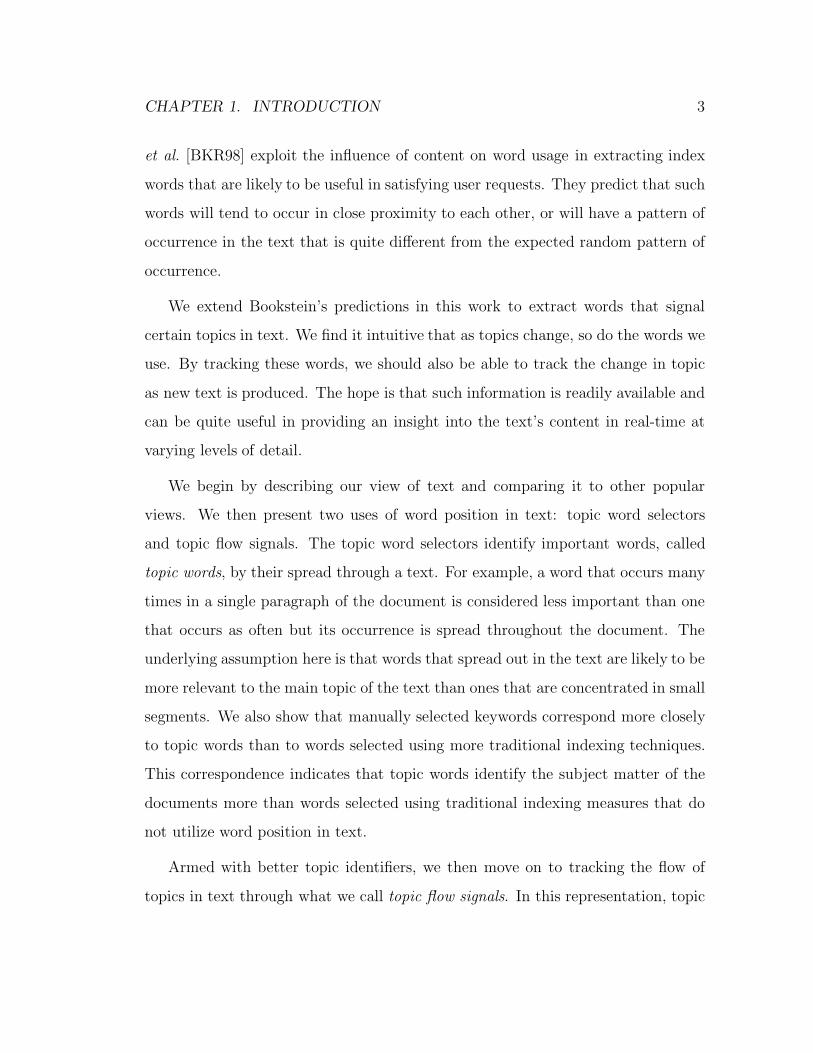
We extend Bookstein’s predictions in this work to extract words that signal
certain topics in text. We find it intuitive that as topics change, so do the words we
use. By tracking these words, we should also be able to track the change in topic
as new text is produced. The hope is that such information is readily available and
can be quite useful in providing an insight into the text’s content in real-time at
varying levels of detail.
We begin by describing our view of text and comparing it to other popular
views. We then present two uses of word position in text: topic word selectors
and topic flow signals. The topic word selectors identify important words, called
topic words, by their spread through a text. For example, a word that occurs many
times in a single paragraph of the document is considered less important than one
that occurs as often but its occurrence is spread throughout the document. The
underlying assumption here is that words that spread out in the text are likely to be
more relevant to the main topic of the text than ones that are concentrated in small
segments. We also show that manually selected keywords correspond more closely
to topic words than to words selected using more traditional indexing techniques.
This correspondence indicates that topic words identify the subject matter of the
documents more than words selected using traditional indexing measures that do
not utilize word position in text.
Armed with better topic identifiers, we then move on to tracking the flow of
topics in text through what we call topic flow signals. In this representation, topic

CHAPTER 1. INTRODUCTION 4
words are replaced by their relative relevance to the topic. The flow of any one
topic can then be traced throughout the document and viewed as a signal that
remains strong when words relevant to the topic are used and weakens when an
irrelevant word occurs. To reflect the flow of the topic in larger segments of text
we use a simple smoothing technique. The resulting smoothed signals are shown
to correlate to the ideal topic flow signals for the same document.
Finally, we represent documents by the relative importance of their topic words
and by the spread of these words in the document. This representation is then
incorporated into a Support Vector Machine for text classification and shown to
drastically reduce vocabulary size without loss in the classifier’s performance when
compared with the traditional TF*IDF representation.

Chapter 2
Text as a Signal
A solid comprehension of a retrieval approach is rooted in a clear vision of the
approach’s view of text and the criteria it attempts to preserve in a model. In this
chapter we discuss our view of text in addition to several text views that have been
used in the past. We then focus on how to represent text according to the view we
adopt in our work.
2.1 Logical Views of Text
Natural language text encodes large amounts of information at many levels, includ-
ing the syntactic, semantic, and structural levels. As far as we know, only some
of the information in text is needed for a retrieval task. The logical view of a text
defines criteria that capture the essential contents of a document for the task at
hand.
There are two dimensions for our view of text: the first is at the word level,
whereas the second is at the document level. The word level view defines the
5
CHAPTER 2. TEXT AS A SIGNAL 6
semantics of a word and the objects to which it refers, while the document level
view determines how the words in the text weave the meaning of the whole text.
At its simplest, a text is just an unordered collection of words. This is the bag of
words approach. More involved views take into account other information about
the text such as information regarding its structural content, the context in which a
word is used, or the position of the word in the text. The remainder of this section
focuses on several of these document level views along with some examples.
2.1.1 Text as a Bag of Words
The bag of words view assumes that the words used in a document are sufficient to
capture the main contents of the document. It also assumes that the probability
of using a word is independent of the other words in that document and of the
position of the word in the text. Under this view, a text is a flat entity with no
structural information.
This is one of the earliest text views and is very common in current information
retrieval research. Its main attraction is its simplicity. It may also be effective for
some simple retrieval tasks requiring exact word matching. In general, however,
many systems with this view attempt to enhance the system’s performance by
boosting their word semantics views through removing grammatical inflections, by
ignoring empty words through stopword removal, or other preprocessing tasks. An
early example of systems with the bag of words view is the earlier versions of
SMART [Sal71, SM83].
More recent systems augment the bag of words view with knowledge of word
co-occurrence in an attempt to boost their word semantics view, as is done in
the Least Linear Squares Fit approach [YC93], and the Latent Semantic Indexing

CHAPTER 2. TEXT AS A SIGNAL 7
(LSI) system [DDL+90]. In LSI, for example, a document is viewed as a bag of
words and is represented by the words it contains. The system then uses algebraic
methods to distinguish words that tend to co-occur in the database documents.
The assumption here is that words occurring in the same context are most likely
to share a common reference. If the system realizes that the words stocks and
shares, for instance, co-occur frequently in the database, a query containing the
word shares may retrieve a document on stocks even though the word shares is
not used in that document. A pure bag-of-words method retrieves only documents
containing the word shares.
The simplicity and effectiveness of this view are the main reasons behind its
popularity. But sometimes the bag of words view is too simple for the user’s
task. If a text is viewed as an unordered collection of words, then we lose all
information about the text’s structure. Systems using this view cannot retrieve
relevant segments of a document, nor can they identify key content indicators or
analyze the flow of discussion in the text. These capabilities are important for text
segmentation systems, document visualization systems, and paragraph retrieval
systems among others.
2.1.2 Documents as Structured Units
The bag of words method views documents as flat, unordered, sequences of words.
In reality, however, documents are sophisticated physical entities. Baeza-Yates
and Ribeoro-Neto [BYRN99] divide the physical structure of documents into three
types: flat fixed structures, hypertext, and hierarchical structures.
Flat structures separate the document into a list of independent units, each of
which is a bag of words. Emails, for example, consist of fields for the sender’s name,

CHAPTER 2. TEXT AS A SIGNAL 8
the recipient’s name, the date, the subject, and the message. Newspaper articles
and technical reports may be viewed as titles followed by lists of paragraphs. Flat
structures have the advantage that they retain the simplicity of the bag-of-words
view and yet are also capable of searching and retrieving relevant units only, rather
than retrieving the whole document. They may also provide additional information
about the contents of the text that can boost the effectiveness of a retrieval system.
More recent versions of SMART [SAB93] combined the bag of words view with
the view of a document as a list of paragraphs. Salton, Allan, and Buckley measured
an input query against both the full document in its flat bag of words form, and
against single paragraphs. If one or more paragraphs were found more relevant
to the query than the full text, then these paragraphs were returned, otherwise
the system returned the whole text if it were found relevant. This combined view
proved more effective than the simple bag of words view [SAB93].
Unlike flat structures, where a document is a linear list of structural units,
hypertext graph structures view a document as a set of interconnected units. HTML
web pages are one example of these structures. This view is usually extended
to the whole database, in which case each document acts as a node in a web of
interconnected documents.
The hypertext view is adopted by some of the World Wide Web search engines.
Only a few of these search engines, however, utilize the document-document connec-
tions in evaluating their retrieval results. Google’s PageRank [PBMW98] measures
the importance of a web page, and thus its expected usefulness to the user, by
the number of “good” web pages pointing to the page in question. Google is a
good example of how links between documents can provide a rich resource for the
system to understand the document contents, and the author’s view of how other
documents relate to it. However, graph structures are usually expensive to process,
CHAPTER 2. TEXT AS A SIGNAL 9
and the quality of the links is dependent on the context in which they appear, as
well as on the authors’ good judgment. Also, not all documents are prepared as
hypertext documents.
Hierarchical structures are a compromise between the richness of hypertext
and the simplicity of flat structured text. Examples of tree structured documents
are books containing chapters, which contain sections, which in turn may con-
tain subsections etc. Markup languages are usually used to reflect the relation
between units in the structure and allow search engines to exploit this struc-
ture [Tom89, Tom97]. PAT [ST94], MultiText [CCB94], and many web search
engines such as Google [PBMW98], for example, allow users to specify the partic-
ular substructure, called region, they are interested in searching.
Imposing structure on text usually conveys the author’s view of which consec-
utive portions of the text share a common attribute. It helps users search and
understand the document and the database as a whole. However, structure does
little to amend the drawbacks of the bag of words view if the latter is adopted
for segments within a structure. Although with structured text we can now search
and retrieve smaller segments of text, the contents of each of these segments is
still represented as an unordered set of words, and we are still missing information
regarding the local context within a segment and the topic flow in the text.
2.1.3 Words in Context
Rather than attempting to impose some structure on the whole text, some research
tasks require a more detailed view of the local context of the text. The local
context of a word is the words surrounding it in the document. This immediate
context usually assists the reader in restricting the possible meanings of the word,

CHAPTER 2. TEXT AS A SIGNAL 10
as well as the topics under discussion. For example, the word bank can carry many
different meanings, including a commercial bank and a river bank. But the phrase
river immediately adjacent to bank in the phrase river bank disambiguates it and
clarifies the local content of the text.
The idea of using surrounding words to disambiguate text has been investi-
gated for many different applications such as word sense disambiguation [CL85,
Les86, GCY93], query expansion [BYRN99], and character recognition [GCY93]
with varying degrees of success. The definition of “local context” or window also
varies: many systems define a local context as the words immediately preceding
a word as is done in the n-gram language model [MS99]. In this model a word is
assumed to be independent from all other words in the text except for the n − 1
words immediately preceding it.
Other researchers have defined a word’s context as the n words immediately
preceding and succeeding it. Gale et al. [GCY93], for instance, used local context
for sense disambiguation. They also studied a more relaxed definition of the local
context where the context of a word w begins some l words away from w. Interest-
ingly, they found that words as far away from w as 10, 000 words may be useful in
the disambiguation task. Recognizing the importance of local context, PAT [ST94]
and many web search engines such as AltaVista [SHMM98] and Google [PBMW98]
allow users to search for words within some proximity to each other. In MultiText
the relevance of a paragraph to a given set of terms is influenced by the proximity
of the matched terms in the paragraph [CCKL00].
This view of text retains partial information about the relative order of the
text words, and it is sufficient for applications where those local contexts are of
interest. However local context cannot provide a global view of the text and is thus
insufficient for representing the flow of topics in a document, nor is it appropriate

CHAPTER 2. TEXT AS A SIGNAL 11
Topic3
Paragraph 1
Paragraph 2
Paragraph 5
Paragraph 4
Paragraph 3
Topic2
Topic1
(a) Text as a connected set of top-
icsM
ain
topi
c
subtopic 1
subtopic 2
subtopic 3
(b) Text as main
topics that enclose
a sequence of
subtopics
subtopic 1
subtopic 2
Main topic
subtopic 1
(c) Text as a collec-
tion of main topics
that enclose paral-
lel subtopics
Figure 2.1: Views of a document as a collection of topics
for other tasks requiring a more unified view of the whole text.
2.1.4 Documents as Collections of Topics
Text words weave together the topics conveyed by the document. The words-in-
context view fragments the text and lacks an insight of the text as one unit within
which run many, possibly overlapping, topics. Figure 2.1 shows four text views that
focus on the document as a collection of topics.
The first view 2.1(a) is of the text as a connected set of topics. This view
makes no assumptions regarding the organization of the topics in the text. A
topic may be discussed in any set of text segments, and it may be discussed along
with any other. The main topic is defined as the one that is discussed in the
greatest number of segments. This view was adopted by Salton et al.in [SSBM96],

CHAPTER 2. TEXT AS A SIGNAL 12
where they represented a topic as a set of mutually similar segments. In this work
a document is segmented into paragraphs. The similarity of each paragraph is
measured against every other paragraph, and those paragraphs whose similarity is
higher than a preset threshold are assumed to discuss a common topic.
The attractiveness of this view is its flexibility allowing for topics to be inter-
rupted and re-introduced several times during the course of the text. However, the
view’s flexibility also entails the loss of the hierarchical relations between a main
topic and its subtopics.
The next text view, shown in 2.1(b), accounts for this relation between main
topics and their subtopics. In this view, a text is a set of one or more main
topics that run through the text in parallel with their subtopics. The subtopics are
expected to be linearly consecutive and mutually exclusive. Hearst adopted this
view in the automatic segmentation system TextTiles [Hea94c, Hea97]. Her goal
was to discover points of topic shift (thematic change) in any given document, and
use these boundaries as guides towards automatically segmenting text.
The first version of Hearst’s algorithm divides the document into several equal-
sized segments. It then measures the similarity between adjacent segments and
places topic boundaries where there is a sudden decrease in similarity relative to
adjacent segments. In this version of the algorithm a topic is a set of consecutive
segments of text bounded by two topic boundaries.
The second version of her algorithm is based on the lexical chains of Morris and
Hirst [MH91], who showed that coherent texts usually contain groups of semanti-
cally related words. Each of these groups is called a lexical chain. This version of
TextTiles represents a topic as a set of parallel lexical chains and places a topic
boundary when a set of chains ends and a new set begins.

CHAPTER 2. TEXT AS A SIGNAL 13
The view adopted in both versions of the algorithm assumes that subtopics are
consecutive and mutually exclusive. Although the linearity and mutual exclusion
expectations are justified in the automatic segmentation context, they are not gen-
erally accurate assumptions. Digressions, interruptions, and topic re-introduction
are to be expected in most types of text. At the same time, the ability to recognize
the main topics’ subtopics provides a deeper insight into the flow of topics in the
text. Therefore, our view of text is a combination of the two previous views. We
adopt Hearst’s view of the text as a set of main topics running throughout the text,
in parallel with their subtopics, as well as the view of Salton et al.that topics can
be modeled as independent entities which may be temporarily interrupted and then
revisited any number of times, and any paragraph may discuss any number of topics
simultaneously [SSBM96]. Figure 2.1(c) reflects this view. In this figure the main
topic is discussed across the text, and within the context of the main topic the first
subtopic subtopic1 is discussed in several segments of the document, and the second
subtopic subtopic2 is discussed only in the middle of the text where it temporarily
intersects with subtopic1. This model is less general than the model adopted by
Salton et al. [SSBM96] since it assumes at least one common theme throughout
a document. But when this assumption is true, as in news stories and technical
reports, it allows for a simpler representation. The model of Figure 2.1(c) is also
more flexible than the one adopted by Hearst [Hea94c, Hea97]. But the flexibility
and simplicity of a model is largely dependent on how we choose to represent it.
2.2 Representing the Flow of Topics in Text
An ideal representation of our topic flow model should preserve as much of the
model’s flexibility as possible and permit many simultaneous topics at any point
CHAPTER 2. TEXT AS A SIGNAL 14
in the text. This can best be achieved by representing each topic in the text
independently of all other topics. The text will then consist of parallel topic flow
representations, and the problem reduces to representing the flow of each individual
topic in a document.
Topic flow reflects the degree of relevance of the topic to various points in the
document. Assume we can measure the relevance level of a word w at point p in
the document to a topic t using a measure MD(p, t). To view the relevance of the
topic to every point containing a content word in the document, we can plot the
relevance levels given by this measure for each position in document D one after
the other. The resulting plot will reflect the flow of topic t in document D. Take
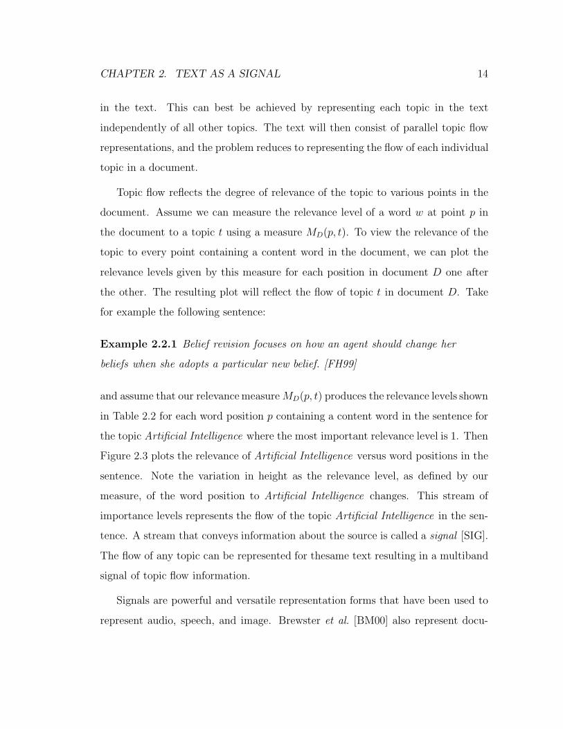
for example the following sentence:
Example 2.2.1 Belief revision focuses on how an agent should change her
beliefs when she adopts a particular new belief. [FH99]
and assume that our relevance measure MD(p, t) produces the relevance levels shown
in Table 2.2 for each word position p containing a content word in the sentence for
the topic Artificial Intelligence where the most important relevance level is 1. Then
Figure 2.3 plots the relevance of Artificial Intelligence versus word positions in the
sentence. Note the variation in height as the relevance level, as defined by our
measure, of the word position to Artificial Intelligence changes. This stream of
importance levels represents the flow of the topic Artificial Intelligence in the sen-
tence. A stream that conveys information about the source is called a signal [SIG].
The flow of any topic can be represented for thesame text resulting in a multiband
signal of topic flow information.
Signals are powerful and versatile representation forms that have been used to
represent audio, speech, and image. Brewster et al. [BM00] also represent docu-

CHAPTER 2. TEXT AS A SIGNAL 15
Word POSITION WORD RELEVANCE
0 belief 1
1 revision 1
2 agent 33
3 change 78
4 beliefs 1
5 belief 1
Figure 2.2: Relevance of content word positions in sentence 2.2.1 to the topic
Artificial Intelligence. Positions containing non-content words such as how, at, and
her have been ignored.
ments in terms of signals. They begin by identifying content-bearing words using
the method proposed by Bookstein et al. [BKR98]. The highest weighted content
words whose weights are higher than a preset threshold are called topics. Those with
weights below that threshold but higher than another, lower, threshold are called
cross-terms while all remaining content words with lower weights are discarded. In
their work each signal, or channel, reflects the association of each document term
to a topic. The collection of topic signals is used to build a single composite energy
signal that is meant to represent the document content and is the basis for their
document visualization and segmentation prototype [MWBF98]. No experimental
results have been reported on the accuracy of the channels and the collective en-
ergy signal in representing text content nor on their usefulness for the purposes of
visualization. Instead of forming a single compound signal, we represent documents
by multiple signals, each of which reflects a topic characterized by a user-defined
collection of documents.
Representing topics as signals allows us to preserve the flow of information and

CHAPTER 2. TEXT AS A SIGNAL 16
0 0.5 1 1.5 2 2.5 3 3.5 4 4.5 50
10
20
30
40
50
60
70
80
Word position in text
Top
ic w
ord
rank
Belief Example−AI
belief revision
agent
change
beliefs belief
Figure 2.3: Relevance signal for the topic Artificial Intelligence based on the rel-
evance values in Table 2.2. Each vertex in the signal is labeled by the word that
generated the vertex.

CHAPTER 2. TEXT AS A SIGNAL 17
retain the flexibility of our original flow model. It also provides multiple views of
the text simultaneously and efficiently. Even text streams produced in real-time
can be easily represented in terms of moving topic signals. These features can
prove useful in many areas of information retrieval including text segmentation,
text summarization, paragraph retrieval, and text filtering. It also opens up for
text processing a wide range of efficient and effective signal processing tools that
cannot be applied in conjunction with other representations of text.
Of course the quality of our signal is sensitive to the relevance measure MD(p, t)
used in constructing the signal. In the next chapter we discuss and compare several
candidate measures. Then, in the following chapter, we adopt these measures to
build topic flow signals. Finally, we study the effect of these relevance measures
and word position on text classification.

Chapter 3
Topic Relevance Measures
In the previous chapter we argued for representing topic flow in text in the form of
signals. We also showed some signal representation examples based on hypothetical
topic relevance values at each point in a sample text. In this chapter we define topic
relevance, then define and compare four different topic relevance measures M(w, t)
for a given word w and topic t. First let us attend to the basic question of topic
relevance.
3.1 Topic Relevance
A word w is strongly relevant to topic t if w reflects a concept that can be discussed
as a subtopic of t. For example, belief networks and agents are strongly relevant
to the topic Artificial Intelligence, and corpora and discourse analysis are strongly
relevant to the topic Computational Linguistics, but the and conductor are less
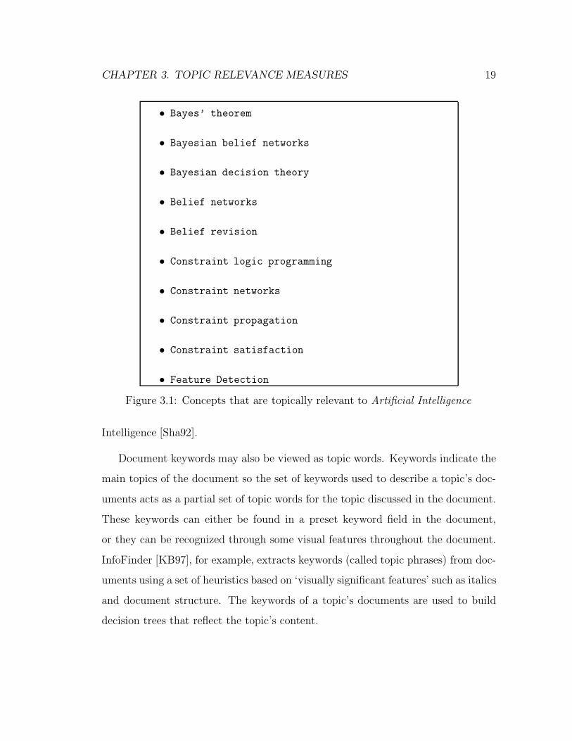
relevant to either topic. Figure 3.1 shows a list of concepts that are strongly relevant
to Artificial Intelligence, taken from the index of the Encyclopedia of Artificial
18
CHAPTER 3. TOPIC RELEVANCE MEASURES 19
• Bayes’ theorem
• Bayesian belief networks
• Bayesian decision theory
• Belief networks
• Belief revision
• Constraint logic programming
• Constraint networks
• Constraint propagation
• Constraint satisfaction
• Feature Detection
Figure 3.1: Concepts that are topically relevant to Artificial Intelligence
Intelligence [Sha92].
Document keywords may also be viewed as topic words. Keywords indicate the
main topics of the document so the set of keywords used to describe a topic’s doc-
uments acts as a partial set of topic words for the topic discussed in the document.
These keywords can either be found in a preset keyword field in the document,
or they can be recognized through some visual features throughout the document.
InfoFinder [KB97], for example, extracts keywords (called topic phrases) from doc-
uments using a set of heuristics based on ‘visually significant features’ such as italics
and document structure. The keywords of a topic’s documents are used to build
decision trees that reflect the topic’s content.
CHAPTER 3. TOPIC RELEVANCE MEASURES 20
Topically relevant words are Damerau’s domain-oriented vocabulary [Dam90].
Damerau defines such vocabulary as
a list of content words (not necessarily complete) that would character-
istically be used in talking about a particular subject, say education, as
opposed to the list of words used to talk about, say aviation. [Dam90]
Damerau tests two different approaches which extract domain-oriented vocab-
ulary from the body of plain text documents. In the first he sorts the list of all
words in the domain documents by their frequency, eliminates words bearing little
content such as the and it (called stopwords) from the list, and finally trims the
list size to a predetermined constant by removing the lowest frequency words. In
the second approach he creates two domain lists: for the first list he extracts from
a dictionary all words whose label is that of the domain, and for the second list he
indexes the words used in the domain documents. He then creates the final domain
list from words in common between these two lists. Given a previously unseen set
of documents for a domain, Damerau found that more of the domain’s list appeared
in the domain’s documents than words from most other domains’ lists. However,
this acceptance test does not guarantee that the words are domain-oriented. It
only shows that the selected words are used more often in the domain’s documents.
Therefore, words like she and her can easily be accepted as topic words by this test
if they happened to be used more often in one domain than in the other domains
tested. In this case she and her may be good discriminators of that domain, but
they are not topically relevant words.
This difference between topically relevant words and good discriminators also
applies to traditional information retrieval index terms. Unlike topically relevant
words (topic words), the importance of an index term in information retrieval is

CHAPTER 3. TOPIC RELEVANCE MEASURES 21
measured by how well it can discriminate a topic or document from all other topics
or documents, as well as how relevant it is to the content of the topic or docu-
ment [van79] [Sal75] [Dam90]. For example, the Earnings and Earnings Forecasts
category in the Reuter’s database [REU] contains the term < in place of the left
bracket at the end of company names. Therefore, < is a good discriminator of
that category against other categories in the database [MS99]. However, even if <
may be a good discriminator for the Earnings and Earnings Forecasts category, it
is not relevant to the meaning of the category. Therefore, although such discrim-
inators are appropriate as category markers, they lack essential content relevance
information and are not acceptable topic words.
With this definition of relevance, topic flow representation becomes a repre-
sentation of the distribution (in a non-statistical sense) of topic concepts in the
document. Furthermore, the variation in relevance values reflects the variation in
the strength of topic relevance to the various concepts across the text.
The ability to measure the relevance of a topic to a word implies some knowl-
edge of the word and the topic. In information retrieval this knowledge is usually
acquired by analyzing some sample documents and the topics to which they belong.
Assume we have access to a representative sample of plain text documents for each
topic t in the set of all possible topics T , and that each document is represented
by the words it contains in the order they occur in the document. In this chapter
we will call this set of sample documents the database of training documents, or
simply the database. Our task is to recognize strongly relevant words for each topic
from the representative sample. In the remainder of the chapter we will discuss and
compare several different measures of relevance.

CHAPTER 3. TOPIC RELEVANCE MEASURES 22
3.2 Measuring Topic Relevance
Topic words are clearly associated with their topics. Otherwise, it would be hard
to argue that they are “characteristically” used in discussing the topic. To measure
this association we use Pointwise Mutual Information (PMI). PMI is an extension
of the information theoretic measure Mutual Information [MS99]. It has been used
for many different retrieval tasks including feature extraction [YP97] and word
concordance discovery [CH90]. PMI measures the likelihood of observing two events
simultaneously as opposed to observing either event separately. This measure is
defined as follows:
I(x, y) = logp(x, y)
p(x)p(y)(3.1)
where:
• p(x, y) is the probability of observing x and y together in the database.
• p(x) (p(y)) is the probability of observing x (y) separately.
Within the context of topic relevance, x is the topic, y is the word whose rele-
vance to x is of interest, and I(x, y) reflects the relative likelihood of using a word
y when discussing topic x as compared to using either independently, or, since
I(x, y) = I(y, x), the relative likelihood that an observed instance of word y refers
to topic x as compared to using either independently.
In order to measure the PMI between a word and a topic, their probability of
co-occurrence p(w, t) should be estimated, as well as their probabilities of occur-
ring separately p(w) and p(t). The probability of occurrence of a word is usually
CHAPTER 3. TOPIC RELEVANCE MEASURES 23
estimated using some observable statistic of that word such as the number of doc-
uments in which it occurs (document frequency), or the word’s total number of
instances in the database (term frequency).
In what follows we will discuss how document frequency and term frequency
can be used to measure the relevance of a topic to a word, and we compare the
effectiveness of these two statistics to two other word statistics.
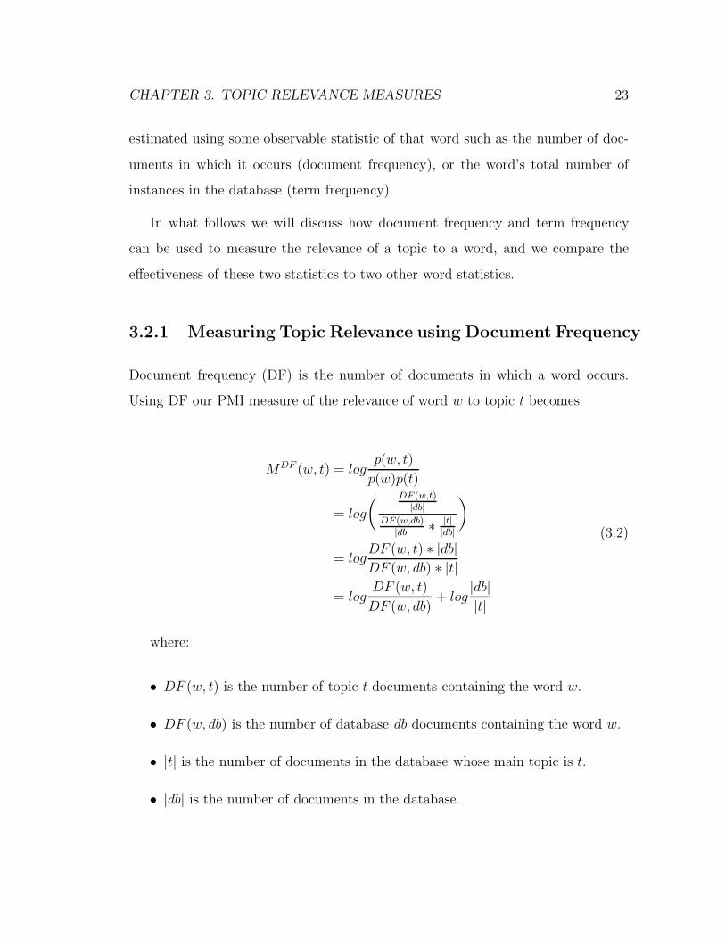
3.2.1 Measuring Topic Relevance using Document Frequency
Document frequency (DF) is the number of documents in which a word occurs.
Using DF our PMI measure of the relevance of word w to topic t becomes
MDF (w, t) = logp(w, t)
p(w)p(t)
= log
( DF (w,t)|db|
DF (w,db)|db| ∗ |t|
|db|
)
= logDF (w, t) ∗ |db|DF (w, db) ∗ |t|
= logDF (w, t)
DF (w, db)+ log
|db||t|
(3.2)
where:
• DF (w, t) is the number of topic t documents containing the word w.
• DF (w, db) is the number of database db documents containing the word w.
• |t| is the number of documents in the database whose main topic is t.
• |db| is the number of documents in the database.
CHAPTER 3. TOPIC RELEVANCE MEASURES 24
Since the term log |db||t| is independent of words for a fixed topic t and database
db, MDF (w, t) in Equation 3.2 compares words under t based on the ratio DF (w,t)DF (w,db)
.
Words that occur in significantly more documents of t than in the rest of the
database will be weighed more heavily than those occurring in relatively fewer
documents of t than the rest of the database.
Measuring topic relevance of a word by the number of documents in which it
occurs assumes that words that are not frequently used in a variety of documents
usually occur in a document if they are strongly relevant to a main topic of that
document, and that a word that is strongly relevant to a topic t will have a higher
proportion of the documents in which it appears falling under t. For example, a
word that only occurs in documents of t will have a higher weight than another
word where only some of its documents belong to t.
We find the basic assumption in this measure troublesome. In particular, the
measure will assign a high weight to singletons (words occurring only once in the
document) such as misspellings and other infrequent and irrelevant words. For
instance, mentioning the word treaty in this thesis does not mean the word is
strongly relevant to the topic of the thesis. Yet the above measure will count this
thesis as evidence of the relevance of the word to the main topic of the text.
One way to filter out some of these irrelevant words is to discard documents
where the word is a singleton, as we shall see next.
3.2.2 Measuring Topic Relevance using Modified Document
Frequency
As we mentioned in the previous section, the problem with using pure DF in mea-
suring topic relevance is that it exaggerates the importance of single occurrences in

CHAPTER 3. TOPIC RELEVANCE MEASURES 25
a document. To overcome this drawback we suggest discarding from the DF count
those documents where the word occurs only once. In this case our topic relevance
measure becomes:
M�DF (w, t) = log
DF (w, t) ∗ |db|DF (w, db) ∗ |t|
= logDF (w, t)
DF (w, db)+ log
|db||t|
(3.3)
where
• DF (w, t) is the number of topic t documents containing more than one oc-
currence of the word w.
• DF (w, db) is the number of database db documents containing more than one
occurrence of the word w.
• |t| and |db| are the number of documents in t and db respectively.
The new measure assumes that the probability of two occurrences of an irrele-
vant word is quite low, and that those words occurring at least twice anywhere in
the document may be strongly relevant to the main topic of the document. These
assumptions were made by Katz [Kat96], who argued that when a word is relevant
to the topic of the document it occurs in a burst of repetitions. Church also used
DF (w, db) in one of his adaptation measures [Chu00], where he shows that con-
tent words1 tend to occur at least twice in documents to which they are strongly
relevant.1Manning and Schutze define non-content words informally as “words that taken in isolation
.. do not give much information about the contents of the document” [MS99]. Note that although
a content word is usually relevant to the topic being discussed in the document, it does not need
to be.
CHAPTER 3. TOPIC RELEVANCE MEASURES 26
Based on the above assumptions, if the proportion of topic t documents con-
taining more than one occurrence of a word is high, then the measure assumes the
word is strongly relevant to t.
Replacing document frequency with DF alleviates the singleton-word problem.
But DF , as well as DF, assumes an independence of the number of times a word
is used within the document from the degree of relevance of the word to the docu-
ment’s topic. For both statistics a word repetition of 10 times in one document is
as good as repeating the same word twice only in that same document. Yet some
researchers assert that this is not valid. Katz for example states that
the total number of observed occurrences of the content word or phrase
in the document ought to be a function only of the degree of relatedness
of the concept named by the word to the document or, in other words,
of the intensity with which the concept is treated. [Kat96]
Luhn also hypothesized that the frequency of a word in a document is a strong
indicator of the word’s significance in the text [van79].
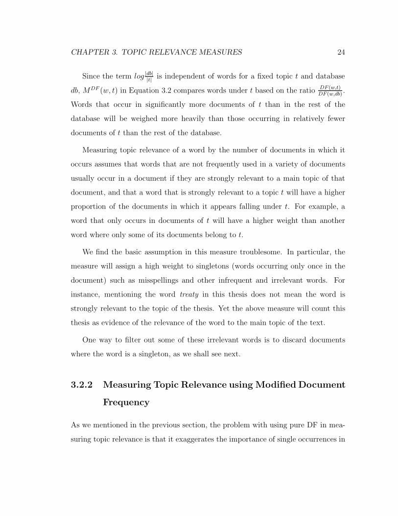
3.2.3 Measuring Topic Relevance using Term Frequency
Many researchers in the information retrieval community use term frequency TF as
an indicator of the importance of a word to a document. We can carry this concept
of frequency as an indicator of importance towards measuring topic relevance by
plugging TF into Equation 3.1 above:
MTF (w, t) = logTF (w, t) ∗ ||db||TF (w, db) ∗ ||t||
= logTF (w, t)
TF (w, db)+ log
||db||||t||
(3.4)

CHAPTER 3. TOPIC RELEVANCE MEASURES 27
where
• TF (w, t) is the number of occurrences of w in topic t documents.
• TF (w, db) is the number of occurrences of w in the database db.
• ||t|| and ||db|| are the number of terms in t and db respectively.
Equation 3.4 assumes that strongly relevant words are those that occur more
frequently in topic t than in the whole database. Damerau used essentially this
measure in determining domain-oriented vocabulary [Dam90] as discussed above,
and he uses a function similar to Equation 3.4 to extract 2-word domain phrases
for a set of pre-specified domains, based on the ratio of the frequency of the phrase
within the domain to its frequency in the whole database [Dam93]. The assumption
here is that good domain phrases will tend to occur more often on average in the
domain’s documents than in the whole database.
3.2.4 Incorporating Relative Word Positions in Measuring
Topic Relevance
Whether using term frequency or document frequency, the measures proposed so
far assume a bag of words document view, where the total number of occurrences in
the topic documents and in the database is sufficient to describe the contents of the
topic regardless of where the words occur. The bag of words view is incomplete for
our notion of text as an interweaved collection of topics. As we argued in Chapter 2,
the position of words in a document can be useful in understanding the document’s
content.

CHAPTER 3. TOPIC RELEVANCE MEASURES 28
In Chapter 2 we presented text as a collection of topics, with the main topic(s)
spanning the length of the text. Since words are the atomic units describing doc-
ument content, we expect topic words to span across the text as well. Some of
these topic words will occur in small segments of the text, while others will repeat
throughout the text. Bookstein et al. [BKR98] use this behavior of content-bearing
words to extract good index words that are likely to be useful in satisfying users’
requests. The authors apply goodness measures of such words that compare the
word’s occurrence behavior in the text to the expected random occurrence. They
define two occurrence behaviors: the word’s tendency to clump by repeating in
close proximity in a single textual unit such as a paragraph, and the word’s ten-
dency to occur at least once in several consecutive textual units in a document.
Their experiments show that such information on word occurrence improves the
quality of words selected for indexing when compared to pure inverse document
frequency. The experiments also indicate a link between content-bearing words
and these words’ tendency to clump.
Although their method identifies content words, the authors do not show how
to use the method to characterize the topic of a whole document or which words
are indicative of that topic.
Katz [Kat96] notes that although content words are likely to repeat in close
proximity to each other, those that are treated heavily and continuously in the text
will occur across the length of the text. We speculate that these intensely treated
content words are strongly related to the main topic of the document and are thus
good topic words. The challenge here is to identify words that repeat across the
text, and evaluate them based on their tendency to span the length of text in a
topic’s documents.
To identify words that repeat across the text we turn to a second measure
CHAPTER 3. TOPIC RELEVANCE MEASURES 29
introduced by Church [Chu00]. Church uses the notion of word spread to show
that content words adapt, i.e. their probability of occurrence changes based on the
lexical content of the document. Church divides each document into two halves:
the first half is called the history, and the second is called the test. He shows that
when a content word appears in the history, its probability of occurring in the test
segment rises significantly.
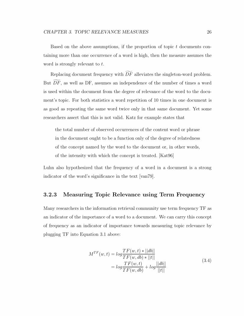
If a word spans the length of the text, then it will occur in both halves of the
document. Adopting Church’s idea of segmenting a document into two halves, our
topic relevance measure becomes
MDF2(w, t) = logp(w, t)
p(w)p(t)
= log
( DF2(w,t)|db|
DF2(w,db)|db| ∗ |t|
|db|
)
= logDF2(w, t) ∗ |db|DF2(w, db) ∗ |t|
= logDF2(w, t)
DF2(w, db)+ log
|db||t|
(3.5)
where:
• DF2(w, t) is the number of topic t documents containing the word w in both
halves of the document.
• DF2(w, db) is the number of database db documents containing the word w
in both halves of the document.
• |t| is the number of documents in the database whose main topic is t.
• |db| is the number of documents in the database.
CHAPTER 3. TOPIC RELEVANCE MEASURES 30
Under this measure, topically relevant words are those that occur in both halves
of the document in topic t significantly more often than in both halves of the
database documents.
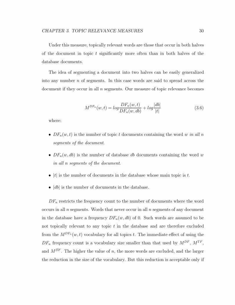
The idea of segmenting a document into two halves can be easily generalized
into any number n of segments. In this case words are said to spread across the
document if they occur in all n segments. Our measure of topic relevance becomes
MDFn(w, t) = logDFn(w, t)
DFn(w, db)+ log
|db||t| (3.6)
where:
• DFn(w, t) is the number of topic t documents containing the word w in all n
segments of the document.
• DFn(w, db) is the number of database db documents containing the word w
in all n segments of the document.
• |t| is the number of documents in the database whose main topic is t.
• |db| is the number of documents in the database.
DFn restricts the frequency count to the number of documents where the word
occurs in all n segments. Words that never occur in all n segments of any document
in the database have a frequency DFn(w, db) of 0. Such words are assumed to be
not topically relevant to any topic t in the database and are therefore excluded
from the MDFn(w, t) vocabulary for all topics t. The immediate effect of using the
DFn frequency count is a vocabulary size smaller than that used by MDF , MTF ,
and M DF . The higher the value of n, the more words are excluded, and the larger
the reduction in the size of the vocabulary. But this reduction is acceptable only if
CHAPTER 3. TOPIC RELEVANCE MEASURES 31
it does not harm the effectiveness of the MDFn measure in recognizing topic words.
In what follows we will look at the effectiveness of MDFn in extracting topic words
for several different values of n and compare that to the other three topic relevance
measures.
3.3 Evaluation
In Section 3.2 we proposed four different functions to measure the relevance of a
word to a topic. All measures use the PMI formula from Equation 3.1, with differ-
ent definitions of p(w, t), p(w), and p(t) for a given word w and topic t. Up until
now we have been deliberately ignoring the question of what constitutes a topic.
This is because the discussion has been general enough to apply to any topic one
may think of, be it politics or “today’s lunch.” However in order to compare the
topic relevance measures experimentally, we must simplify the concept of topic so
that it can be easily captured and quantified. For evaluation purposes we define
a topic as a predefined subject or category, such as the classes in Yahoo!’s classi-
fication hierarchy [Yah], the subject classes of the ACM Computing Classification
System [ACM], or the classification used in the Reuter’s database [REU].
For this evaluation we use the CoRR database [CORa] and the classification
system used by that database. For our purposes, CoRR has the advantage of longer
documents (all having several pages) which are not found in other, more widely used
databases such the Reuter’s database (most having one or two paragraphs only).
Documents longer than a few paragraphs are essential for testing the effectiveness
of the MDFn measure which is based on segmenting each document into many small
sections.
Given a predetermined set of categories, and a database of manually classified

CHAPTER 3. TOPIC RELEVANCE MEASURES 32
documents, we can now generate topic words and evaluate the four measures.
3.3.1 The CoRR Database
The CoRR database [CORa] is an online repository for research in computer science.
The database consists of theses, technical reports, conference papers, and journal
papers from the last decade. Documents range in length between 5 pages and
around 250 pages, but are on average about 13 pages long. They are mainly in
LaTeX format, with a few pdf, and some ps and html files.
Each document in the CoRR database has been classified by the paper’s authors
under one or more of the pre-determined 34 categories listed in the Appendix.
Our version of the database consists of documents submitted between January
1998 and June 2001 for a total of 1151 documents, mostly in LaTeX format. The
LaTeX documents were converted to text using a version of detex [DeT] that was
modified to ignore text preceding the \begin{document} command, as well as ig-
noring abstracts and footnotes. A few of the pdf files were converted using Adobe’s
pdf2txt. In total, 824 text files were converted successfully. Many of the 34 cate-
gories contain very few documents. Documents that belong exclusively to one or
more of these small categories were removed from the database leaving 736 docu-
ments. The remaining categories and their sizes in number of documents are shown
in Table 3.1. Some of these categories are still quite small, but they are useful in
understanding the effect of category size on the quality of the extracted vocabulary.

CHAPTER 3. TOPIC RELEVANCE MEASURES 33
Category Description size
CL Computation and Language 194 documents
LO Logic in Computer Science 130 documents
AI Artificial Intelligence 160 documents
CC Computational Complexity 100 documents
CG Computational Geometry 62 documents
DS Data Structures and Algorithms 90 documents
PL Programming Languages 76 documents
SE Software Engineering 38 documents
LG Learning 61 documents
DC Distributed, Parallel, and 41 documents
Cluster Computing
CE Computational Science, Engineering, 23 documents
and Finance
NI Networking and Internet Architecture 25 documents
Table 3.1: The CoRR database categories used in this evaluation

CHAPTER 3. TOPIC RELEVANCE MEASURES 34
3.3.2 Preprocessing
The details of preprocessing vary from one system to another but certain steps are
considered by all system designers. First we have to define the building blocks,
called tokens, of text. The input text is merely a sequence of characters prior to
preprocessing. It is the responsibility of the preprocessor to break the sequence into
semantic units in the tokenization step. These units can either be simple words such
as the words program and creation, or multi-word phrases such as The United States
(as opposed to United and States).
We define tokens as case-insensitive sequences of alphanumeric characters con-
sisting of at least one letter. Abbreviations containing a dot interleaved with the
alphanumerics are accepted, as well as words containing an underscore, as in the
sequence w t. The total vocabulary in our version of the CoRR database is 53, 877
unique words.
Two other pre-processing steps are widely used when indexing databases: stop-
word removal and word stemming. Stopword removal ignores words that are gen-
erally accepted as being content-free such as the and it, and stemming removes
morphological inflections from words.
Many researchers opt to remove stopwords using a preset stopword list for effi-
ciency and effectiveness [SM83] [YL99] [Joa98b]. Removing these words drastically
reduces the system’s vocabulary size thus improving its efficiency, and allows the
system to focus only on important content words thus improving its effectiveness.
The difficulty in this step is to remove stopwords only. If we remove too many
non-stopwords or leave in too many stopwords, we will increase the noise in the
database and reduce the system’s effectiveness. But this balance is hard to strike
because different databases have different stopwords, and what constitutes a stop-

CHAPTER 3. TOPIC RELEVANCE MEASURES 35
word in one database may be an important content word in another. Consider, for
example, the word computer : whereas computer may be a stopword in a computer
science database, it is most likely a content word in a general science database.
Alternatively, some systems resort to more general feature selection methods which
aim to weigh the uniqueness of each word and its value for the categorization task,
and keep only words deemed important for the task [YP97] [Lew92].
Stopword removal raises a concern when using the DFn frequency counts: re-
moving words from the body of a document will disrupt the position of the re-
maining words in the document thus disrupting the DFn frequency counts. The
approach we choose to deal with this change in DFn frequencies depends on our
view of the role of word position: if the importance of a word position is affected
by the word’s content then stopword positions are of little importance and can be
safely ignored. If, on the other hand, word position in a document is a rough reflec-
tion of the word’s sentence position then all word positions are important, including
those of stopwords, and words that occur in some segment of the document before
stopword removal should still occur in this same segment after stopword removal.
In this case, before removing stopwords their positions should be held by some null
word that can safely be discarded after all DFn frequencies are counted.
Stemming is another common preprocessing step. It reduces words with varying
morphological inflections to one common representation. Thus, runs and running
will both be represented by the stem run. This process has been reported to
help compress an index by up to 50% [Fra92]. Stemming has also been used to
increase the number of documents found by search systems although there is no
strong evidence of its effectiveness in discovering documents that satisfy the users’
request [Fra92].
There are many different approaches to stemming from simple table look-up and

CHAPTER 3. TOPIC RELEVANCE MEASURES 36
predefined stemming rules to methods that attempt to discover stems statistically
with no prior knowledge of any stemming rules. None of these approaches has been
shown to outperform the others in terms of precision or retrieval effectiveness, but
they differ in their compactness and simplicity. One of the most compact is the
Porter stemmer [Fra92] [BYRN99], which gradually reduces a word to its simplest
form by iteratively looking for the longest suffix it can remove based on a set of
predefined rules [Por80].
Thus we have four possibilities for representing documents’ words: with or with-
out stopwords and with or without stemming. To explore the effects of stopword
removal and stemming on the precision of our topic relevance measures, we created
four independent indices for the CoRR database. The first index (SIMPLE) is the
simplest one with no stopwords removed and no stemming performed. The sec-
ond index (STEM) does not remove stopwords, but replaces words by their stems
using the Porter stemmer prior to frequency count. The third index (STOP) re-
moves stopwords found on the SMART stopword list [STO], but does not stem
the remaining words. While the fourth version of the CoRR index (S&S) removes
stopwords as was done for the STOP index and stems the remaining words as was
done in the STEM index. We have opted to replace stopwords in the STOP and
S&S indices by a null word in order to preserve the words’ original positions in the
database.
Because the resulting topic word lists for two indices consist of stemmed words
while the STOP and SIMPLE indices may include several different morphological
variants of the same stem, we subsequently convert the unstemmed topic word lists
of STOP and SIMPLE into stemmed lists of topic words as follows: Each word in
the list is stemmed using the Porter stemmer and assigned the unstemmed word’s
weight. When several variants of the same stem occur in the list, only the first

CHAPTER 3. TOPIC RELEVANCE MEASURES 37
Raw wordstream
STOPtransform totopic list ofstems
experiment
Form topiclist ofwords
SIMPLE
stopwordsRemove
StemForm topiclist ofstems
STEM
S&S
Figure 3.2: The steps involved in creating each of the indices used in the evaluation
experiments
occurrence of the stem is preserved thus giving it the highest relevance weight of all
its variants. This removes from the unstemmed lists variations of the same word
and produces homogeneous topic word lists that can be cross-compared easily. The
creation process of the different indices is shown in Figure 3.2.
It is important to note that stemming after topic word list generation is different
from stemming prior to index creation. When words are stemmed before they are
indexed, their frequency counts will include the occurrence of all morphological
variants of the word in the database. But when stemming is done after the initial
topic word lists are created a stem will be assigned the highest topic relevance
weight of its variants each treated separately.
Now that we have our final topic word lists, we turn to the method used to
evaluate the relevance measures.

CHAPTER 3. TOPIC RELEVANCE MEASURES 38
3.3.3 Creating the Baseline
At the beginning of this chapter we define topic words for a category. The definition
highlights the criterion by which to judge our topic relevance measures: a word
that is identified by a relevance measure is acceptable as a topic word if the word
is used by humans in discussing that topic. According to this criterion we must
evaluate each topic relevance measure by comparing it against a manually selected
list of topic words for each category. The most obvious source for these words are
the keyword fields in the CoRR papers. These fields are usually assigned by the
authors to briefly describe the main contents of the paper. Thus, for a paper that is
classified under Artificial Intelligence for instance, its keywords will describe issues
discussed under Artificial Intelligence. The collection of all keywords used in all
the Artificial Intelligence papers could then form the list of manually selected topic
words for the Artificial Intelligence category. Unfortunately, very few papers in the
CoRR database contain the keyword field.
Luckily, since our goal is to compare the effectiveness of the topic relevance
measures in capturing what humans consider topic words, any database discussing
the category is a potential source for the manual topic word list. Furthermore,
seeking the target topic word list from a source other than our CoRR database has
the advantage that the words are more likely to be database independent. Thus
the success of a topic relevance measure in finding words from this ideal list is an
indication of the measure’s success in recognizing vital topic words independently
of the database. Also, since the ideal list is extracted from an external source, the
success of our topic relevance measures in finding some of these words shows that
topic words are universal for a topic and that given a sufficient amount of data about
a topic, the topic words found by these measures are in fact good representations

CHAPTER 3. TOPIC RELEVANCE MEASURES 39
of the topic.
One source of an ideal list is the index of the Encyclopedia of Artificial Intelli-
gence [Sha92] which provides a comprehensive list of artificial intelligence concepts.
Some online journal indices also provide topic words for many different categories.
These indices are easily searchable, and such large databases reduce the chances
of missing good topic words for any category in the index. The most accessible
index we found for the range of topics in the CoRR database was the Computer
and Information Systems Abstracts index from the Cambridge Scientific Abstracts
(CSA database) [CSA]. The online index is a database of 329,660 records from 850
serials. Each record contains several fields describing a serial’s article. The fields
include, among others, the title of the article, the author, the classification field
which contains the list of general classes under which the article falls, the descrip-
tors field which contains a list of closed vocabulary items describing the category
of the article, and the list of identifiers which are open vocabulary terms found by
human indexers to be strongly relevant to the contents of the article. Figure 3.3
shows a sample CSA record.
We assume that identifiers that are believed to be relevant to an article are also
relevant to the categories to which the article belongs. The identifiers are used
in discussing those categories and are therefore the equivalent to what we have
been calling topic words. Thus, given a large enough list of identifiers for each
category, we expect good topic words to appear on this list. To create such a list
for a category C we collect a large number of CSA records that are classified under
category C and extract the identifiers used to describe the papers indexed in these
records. We will call this the identifier list for C. The more of these identifiers a
topic relevance measure can discover, the better the measure.
But identifier lists contain phrases as well as individual words. Since we deal
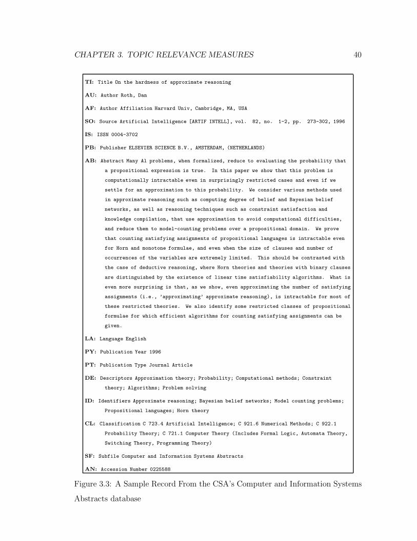
CHAPTER 3. TOPIC RELEVANCE MEASURES 40
TI: Title On the hardness of approximate reasoning
AU: Author Roth, Dan
AF: Author Affiliation Harvard Univ, Cambridge, MA, USA
SO: Source Artificial Intelligence [ARTIF INTELL], vol. 82, no. 1-2, pp. 273-302, 1996
IS: ISSN 0004-3702
PB: Publisher ELSEVIER SCIENCE B.V., AMSTERDAM, (NETHERLANDS)
AB: Abstract Many Al problems, when formalized, reduce to evaluating the probability that
a propositional expression is true. In this paper we show that this problem is
computationally intractable even in surprisingly restricted cases and even if we
settle for an approximation to this probability. We consider various methods used
in approximate reasoning such as computing degree of belief and Bayesian belief
networks, as well as reasoning techniques such as constraint satisfaction and
knowledge compilation, that use approximation to avoid computational difficulties,
and reduce them to model-counting problems over a propositional domain. We prove
that counting satisfying assignments of propositional languages is intractable even
for Horn and monotone formulae, and even when the size of clauses and number of
occurrences of the variables are extremely limited. This should be contrasted with
the case of deductive reasoning, where Horn theories and theories with binary clauses
are distinguished by the existence of linear time satisfiability algorithms. What is
even more surprising is that, as we show, even approximating the number of satisfying
assignments (i.e., ’approximating’ approximate reasoning), is intractable for most of
these restricted theories. We also identify some restricted classes of propositional
formulae for which efficient algorithms for counting satisfying assignments can be
given.
LA: Language English
PY: Publication Year 1996
PT: Publication Type Journal Article
DE: Descriptors Approximation theory; Probability; Computational methods; Constraint
theory; Algorithms; Problem solving
ID: Identifiers Approximate reasoning; Bayesian belief networks; Model counting problems;
Propositional languages; Horn theory
CL: Classification C 723.4 Artificial Intelligence; C 921.6 Numerical Methods; C 922.1
Probability Theory; C 721.1 Computer Theory (Includes Formal Logic, Automata Theory,
Switching Theory, Programming Theory)
SF: Subfile Computer and Information Systems Abstracts
AN: Accession Number 0225588
Figure 3.3: A Sample Record From the CSA’s Computer and Information Systems
Abstracts database

CHAPTER 3. TOPIC RELEVANCE MEASURES 41
with single words only, each identifier phrase is broken into its constituent words.
Stopwords are then removed from the resulting identifier list and the remaining
words are stemmed (using the Porter stemmer) and sorted by the total number of
CSA records in which the stem occurs.
In order to use the CSA database for evaluating our topic relevance measures,
we still have to attend to one more issue: the classification hierarchy defined by the
CSA database is quite different from the categories defined by the CoRR database,
but most of the twelve categories in the CoRR database can be mapped to ones
in the CSA database. One CoRR category cannot be mapped to an acceptable
equivalent, while two had too few documents for a reliable evaluation. The map-
pings for the remaining nine out of the twelve CoRR category areas are shown in
Table 3.2. Some of the CoRR categories are equivalent to CSA classes used in the
classification field, such as Artificial Intelligence which maps the C 723.4 Artificial
Intelligence class, and Programming Languages which maps the C 723.1.1 Com-
puter Programming Languages class; while other more specific classes can only be
mapped to descriptors: Computational Linguistics for example is mapped to the
descriptor Natural Language Processing. Two categories cover more than one class
or descriptor in the CSA database. For example Networking and Internet Archi-
tecture covers many different descriptors in the CSA database each pertaining to
some aspect of the category such as Wide Area Networks, Network Protocols, and
Computer Networks.
In summary, to create the ideal topic list for each of the nine CoRR categories
shown in Figure 3.2 we collected a total of 18, 700 CSA records, each satisfying the
CSA equivalent of at least one CoRR category. Table 3.3 shows the exact number
of records collected for each of the nine CoRR categories. We then extracted the
identifiers used in the identifier fields of all CSA records in each category. Identi-

CHAPTER 3. TOPIC RELEVANCE MEASURES 42
CoRR CSA CSA #CSA
Category Equivalent Field Records
AI Artificial Intelligence classifiers 21,910
PL Programming Languages classifiers 8,940
LO formal languages and grammars; classifiers 7,124
mathematical logic;
formal logic; formal languages; descriptors
theorem proving; computational logic;
lambda calculus;
set theory; temporal logic;
verification; correctness proofs; logic
programming;
CC Computational Complexity descriptors 9,016
CG Computational Geometry descriptors 2,257
SE Software Engineering descriptors 4,428
CL Natural Language Processing descriptors 810
DS Data Structures; Algorithms descriptors 45,053
NI Computer Networks; Communication descriptors 12,218
Networks; Network Protocols; Wide
Area Networks; Packet Networks
Table 3.2: CoRR Category to CSA category mapping and the number of CSA
records under each mapped CoRR category

CHAPTER 3. TOPIC RELEVANCE MEASURES 43
CoRR # CSA Target List
Category Records Size
AI 2, 357 2, 400
PL 2, 159 2, 081
LO 2, 000 2, 574
CC 2, 159 2, 463
CG 2, 210 2, 576
SE 2, 381 2, 301
CL 783 1, 153
DS 2, 500 2, 583
NI 2, 151 2, 106
Table 3.3: The number of CSA records collected to create the target list for each
of the nine CoRR categories, and the number of words in the resulting target list.
fier phrases were broken into single words, words found on the SMART stopword
list [STO] were removed, and the remaining words were stemmed using the Porter
stemmer [Por80]. The number of words in each category’s identifier list is shown
in Table 3.3.
Once the identifier lists were created, each list was sorted by the number of
occurrences of the identifier stem. This sorting de-emphasizes words that are rarely
used to discuss the category or which may have been used to discuss additional
categories to which the indexed paper belongs. Table 3.4 shows the ten most
frequent stems in AI ’s identifier list. The final identifier list is pruned down to the
top n words to form the target topic word list. We experimented with target lists
of size n = 100, 200, 300, 400, 500, 1000, and 2000 words.

CHAPTER 3. TOPIC RELEVANCE MEASURES 44
Identifier Word Stem Example Identifier Phrase
neural Neural Networks
network Neural Networks
learn Cooperative Learning Method
system Multi-agent Systems
model Recurrent Fuzzy Neural Model
algorithm Learning Algorithms
function Horn Function
base Knowledge Based Systems
method Cooperative Learning Method
fuzzi Fuzzy Rules
Table 3.4: Ten most frequent word stems in the AI identifier list along with example
phrases containing these identifier words

CHAPTER 3. TOPIC RELEVANCE MEASURES 45
3.3.4 Evaluation Method
The target lists provide us with the basis for comparing the effectiveness of each
of our topic relevance measures. Each of these lists contains a sample set from the
space of words used to discuss the list’s corresponding category. The measure that
consistently finds more of these stems, especially when more of the stems are found
near the start of the topic word list, is deemed to be more effective in extracting
topic words than the other measures. In the remainder of this section target list
refers to the list of identifiers (i.e. stems) presumed to represent a topic and topic
word list and word list refers to the list of words that has been extracted by a topic
relevance measure for a category. Each word list is sorted in decreasing order by
topic relevance value.
The aim in these experiments is to evaluate the relative effectiveness of our topic
relevance measures in extracting words humans view as topic words. We would also
like to see the effect of stemming and stopword removal on a measure’s word list.
To compare the effectiveness of the topic relevance measures we follow standard
procedure in information retrieval experimentation and use the average interpolated
11-point precision-recall curves [Har01]. Precision at any point in the sorted word
list is defined as the ratio of target words found until that point in the list to
the number of words seen so far, while recall at any word in the sorted list is the
ratio of the number of target words found up to this point in the sorted word list
to the total number of identifiers in the target list. The 11-point precision-recall
curves show the precision at 11 recall points from 0 to 1 with increments of 0.1.
Specifying the recall values allows us to compare the results for different topic word
list sizes. Since some of these recall points may not exist in our sorted list, we
use interpolated 11-point precision-recall curves (p-r curves). In the interpolated
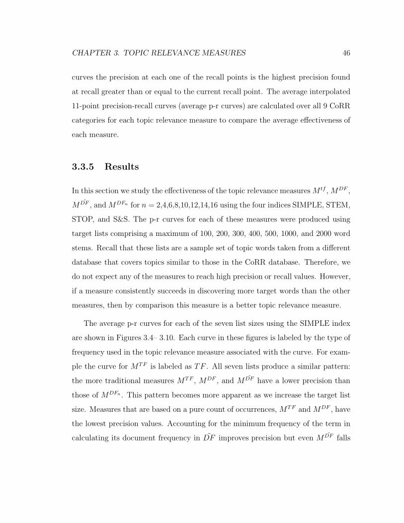
CHAPTER 3. TOPIC RELEVANCE MEASURES 46
curves the precision at each one of the recall points is the highest precision found
at recall greater than or equal to the current recall point. The average interpolated
11-point precision-recall curves (average p-r curves) are calculated over all 9 CoRR
categories for each topic relevance measure to compare the average effectiveness of
each measure.
3.3.5 Results
In this section we study the effectiveness of the topic relevance measures M tf , MDF ,
M DF , and MDFn for n = 2,4,6,8,10,12,14,16 using the four indices SIMPLE, STEM,
STOP, and S&S. The p-r curves for each of these measures were produced using
target lists comprising a maximum of 100, 200, 300, 400, 500, 1000, and 2000 word
stems. Recall that these lists are a sample set of topic words taken from a different
database that covers topics similar to those in the CoRR database. Therefore, we
do not expect any of the measures to reach high precision or recall values. However,
if a measure consistently succeeds in discovering more target words than the other
measures, then by comparison this measure is a better topic relevance measure.
The average p-r curves for each of the seven list sizes using the SIMPLE index
are shown in Figures 3.4– 3.10. Each curve in these figures is labeled by the type of
frequency used in the topic relevance measure associated with the curve. For exam-
ple the curve for MTF is labeled as TF . All seven lists produce a similar pattern:
the more traditional measures MTF , MDF , and M DF have a lower precision than
those of MDFn . This pattern becomes more apparent as we increase the target list
size. Measures that are based on a pure count of occurrences, MTF and MDF , have
the lowest precision values. Accounting for the minimum frequency of the term in
calculating its document frequency in DF improves precision but even M DF falls
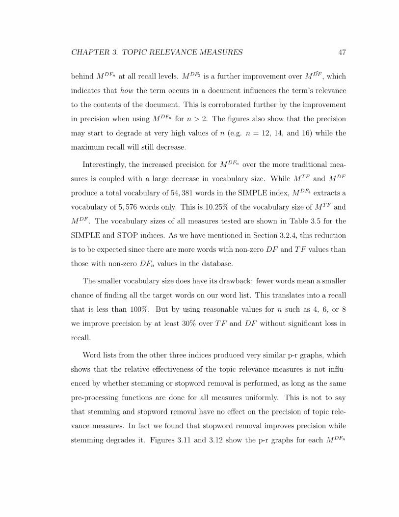
CHAPTER 3. TOPIC RELEVANCE MEASURES 47
behind MDFn at all recall levels. MDF2 is a further improvement over M DF , which
indicates that how the term occurs in a document influences the term’s relevance
to the contents of the document. This is corroborated further by the improvement
in precision when using MDFn for n > 2. The figures also show that the precision
may start to degrade at very high values of n (e.g. n = 12, 14, and 16) while the
maximum recall will still decrease.
Interestingly, the increased precision for MDFn over the more traditional mea-
sures is coupled with a large decrease in vocabulary size. While MTF and MDF
produce a total vocabulary of 54, 381 words in the SIMPLE index, MDF4 extracts a
vocabulary of 5, 576 words only. This is 10.25% of the vocabulary size of MTF and
MDF . The vocabulary sizes of all measures tested are shown in Table 3.5 for the
SIMPLE and STOP indices. As we have mentioned in Section 3.2.4, this reduction
is to be expected since there are more words with non-zero DF and TF values than
those with non-zero DFn values in the database.
The smaller vocabulary size does have its drawback: fewer words mean a smaller
chance of finding all the target words on our word list. This translates into a recall
that is less than 100%. But by using reasonable values for n such as 4, 6, or 8
we improve precision by at least 30% over TF and DF without significant loss in
recall.
Word lists from the other three indices produced very similar p-r graphs, which
shows that the relative effectiveness of the topic relevance measures is not influ-
enced by whether stemming or stopword removal is performed, as long as the same
pre-processing functions are done for all measures uniformly. This is not to say
that stemming and stopword removal have no effect on the precision of topic rele-
vance measures. In fact we found that stopword removal improves precision while
stemming degrades it. Figures 3.11 and 3.12 show the p-r graphs for each MDFn

CHAPTER 3. TOPIC RELEVANCE MEASURES 48
Measure SIMPLE Voc. STOP Voc.
M tf 54, 381 53, 877
MDF 54, 381 53, 877
M�DF 26, 964 26, 478
MDF2 15, 921 15, 447
MDF4 5, 576 5, 194
MDF6 3, 022 2, 715
MDF8 1, 842 1, 600
MDF10 1, 192 1, 002
MDF12 849 687
MDF14 616 471
MDF16 441 315
Table 3.5: Size of the CoRR database index used by each topic relevance measure
in the SIMPLE and STOP indices.

CHAPTER 3. TOPIC RELEVANCE MEASURES 49
0 10 20 30 40 50 60 70 80 90 1000
0.1
0.2
0.3
0.4
0.5
0.6
0.7
Inte
rpol
ated
Pre
cisi
on
% recall
Average Interp. Prec.−Stopwords Kept,CSA Id. Stemmed−100 CSA Ident.
tf df df~
df2 df4 df6 df8 df10df12df14df16
(a) The full p-r curve
0 5 10 15 20 25 30 35 40 45 500.05
0.1
0.15
0.2
0.25
0.3
0.35
0.4
0.45
0.5
0.55
Inte
rpol
ated
Pre
cisi
on
% recall
Average Interp. Prec.−Stopwords Kept,CSA Id. Stemmed−100 CSA Ident.
df8 df10df12df14df16
(b) The curves for MDF8 − MDF16
Figure 3.4: The average interpolated 11-point average precision-recall using a 100-
word target list
0 10 20 30 40 50 60 70 80 90 1000
0.1
0.2
0.3
0.4
0.5
0.6
0.7
Inte
rpol
ated
Pre
cisi
on
% recall
Average Interp. Prec.−Stopwords Kept,CSA Id. Stemmed−200 CSA Ident.
tf df df~
df2 df4 df6 df8 df10df12df14df16
(a) The full p-r curve
0 5 10 15 20 25 30 35 400.1
0.2
0.3
0.4
0.5
0.6
0.7
0.8
Inte
rpol
ated
Pre
cisi
on
% recall
Average Interp. Prec.−Stopwords Kept,CSA Id. Stemmed−200 CSA Ident.
df8 df10df12df14df16
(b) The curves for MDF8 − MDF16
Figure 3.5: The average interpolated 11-point average precision-recall using a 200-
word target list

CHAPTER 3. TOPIC RELEVANCE MEASURES 50
0 10 20 30 40 50 60 70 80 900
0.1
0.2
0.3
0.4
0.5
0.6
0.7
0.8
Inte
rpol
ated
Pre
cisi
on
% recall
Average Interp. Prec.−Stopwords Kept,CSA Id. Stemmed−300 CSA Ident.
tf df df~
df2 df4 df6 df8 df10df12df14df16
(a) The full p-r curve
0 5 10 15 20 25 30 35 400.2
0.3
0.4
0.5
0.6
0.7
0.8
0.9
Inte
rpol
ated
Pre
cisi
on
% recall
Average Interp. Prec.−Stopwords Kept,CSA Id. Stemmed−300 CSA Ident.
df8 df10df12df14df16
(b) The curves for MDF8 − MDF16
Figure 3.6: The average interpolated 11-point average precision-recall using a 300-
word target list
0 10 20 30 40 50 60 70 80 900
0.1
0.2
0.3
0.4
0.5
0.6
0.7
0.8
Inte
rpol
ated
Pre
cisi
on
% recall
Average Interp. Prec.−Stopwords Kept,CSA Id. Stemmed−400 CSA Ident.
tf df df~
df2 df4 df6 df8 df10df12df14df16
(a) The full p-r curve
0 5 10 15 20 25 300.2
0.3
0.4
0.5
0.6
0.7
0.8
0.9
Inte
rpol
ated
Pre
cisi
on
% recall
Average Interp. Prec.−Stopwords Kept,CSA Id. Stemmed−400 CSA Ident.
df8 df10df12df14df16
(b) The curves for MDF8 − MDF16
Figure 3.7: The average interpolated 11-point average precision-recall using a 400-
word target list

CHAPTER 3. TOPIC RELEVANCE MEASURES 51
0 10 20 30 40 50 60 70 80 900
0.1
0.2
0.3
0.4
0.5
0.6
0.7
0.8
Inte
rpol
ated
Pre
cisi
on
% recall
Average Interp. Prec.−Stopwords Kept,CSA Id. Stemmed−500 CSA Ident.
tf df df~
df2 df4 df6 df8 df10df12df14df16
(a) The full p-r curve
0 5 10 15 20 25 300.2
0.3
0.4
0.5
0.6
0.7
0.8
0.9
Inte
rpol
ated
Pre
cisi
on
% recall
Average Interp. Prec.−Stopwords Kept,CSA Id. Stemmed−500 CSA Ident.
df8 df10df12df14df16
(b) The curves for MDF8 − MDF16
Figure 3.8: The average interpolated 11-point average precision-recall using a 500-
word target list
0 10 20 30 40 50 60 70 800
0.1
0.2
0.3
0.4
0.5
0.6
0.7
0.8
0.9
Inte
rpol
ated
Pre
cisi
on
% recall
Average Interp. Prec.−Stopwords Kept,CSA Id. Stemmed−1000 CSA Ident.
tf df df~
df2 df4 df6 df8 df10df12df14df16
(a) The full p-r curve
0 5 10 15 20 25 300.3
0.4
0.5
0.6
0.7
0.8
0.9
1
Inte
rpol
ated
Pre
cisi
on
% recall
Average Interp. Prec.−Stopwords Kept,CSA Id. Stemmed−1000 CSA Ident.
df6 df8 df10df12df14df16
(b) The curves for MDF6 − MDF16
Figure 3.9: The average interpolated 11-point average precision-recall using a 1000-
word target list

CHAPTER 3. TOPIC RELEVANCE MEASURES 52
0 10 20 30 40 50 60 70 800
0.1
0.2
0.3
0.4
0.5
0.6
0.7
0.8
0.9
1
Inte
rpol
ated
Pre
cisi
on
% recall
Average Interp. Prec.−Stopwords Kept,CSA Id. Stemmed−2000 CSA Ident.
tf df df~
df2 df4 df6 df8 df10df12df14df16
(a) The full p-r curve
0 5 10 15 20 25 300.3
0.4
0.5
0.6
0.7
0.8
0.9
1
Inte
rpol
ated
Pre
cisi
on
% recall
Average Interp. Prec.−Stopwords Kept,CSA Id. Stemmed−2000 CSA Ident.
df6 df8 df10df12df14df16
(b) The curves for MDF6 − MDF16
Figure 3.10: The average interpolated 11-point average precision-recall using a
2000-word target list
for n = 2, 4, 6, 8, 10, 12, 14, 16 against the top 500 target words for topic words from
the SIMPLE, STOP, STEM, and S&S indices. These figures clearly show that
for n ≥ 2 stopword removal produces the highest precision while stemming always
generates the least precise word lists.
The negative effect of stemming might be due to several factors: first, it could
be that the genre of technical writing tends to repeat words in the same form.
Also, the stemmer used might be too aggressive. The Porter stemmer reduces
words to the smallest stem possible. This clusters together words that do not have
a common meaning (e.g. factory and factorial) thus over-emphasizing incorrect
words. A weaker stemmer that does limited stemming might have a more positive
effect on precision.
The effect of stopword removal on precision is rather surprising. Stopwords
are expected to behave in a similar manner across topics, thus getting a low topic

CHAPTER 3. TOPIC RELEVANCE MEASURES 53
0 10 20 30 40 50 60 70 800.08
0.1
0.12
0.14
0.16
0.18
0.2
0.22
0.24
Inte
rpol
ated
Pre
cisi
on
% recall
Effect of Word Stemming and Stopword Removal on the Average Interpolated Precision of Mdf2−500 Ident.
stopwords kept−no stemming stopwords removed−no stemming stopwords kept−words stemmed stopwords removed−words stemmed
(a) MDF2
0 10 20 30 40 50 600.15
0.2
0.25
0.3
0.35
0.4
0.45
0.5
0.55
0.6
0.65
Inte
rpol
ated
Pre
cisi
on
% recall
Effect of Word Stemming and Stopword Removal on the Average Interpolated Precision of Mdf4−500 Ident.
stopwords kept−no stemming stopwords removed−no stemming stopwords kept−words stemmed stopwords removed−words stemmed
(b) MDF4
0 5 10 15 20 25 30 35 40 45 500.2
0.25
0.3
0.35
0.4
0.45
0.5
0.55
0.6
0.65
0.7
Inte
rpol
ated
Pre
cisi
on
% recall
Effect of Word Stemming and Stopword Removal on the Average Interpolated Precision of Mdf6−500 Ident.
stopwords kept−no stemming stopwords removed−no stemming stopwords kept−words stemmed stopwords removed−words stemmed
(c) MDF6
0 5 10 15 20 25 300.2
0.3
0.4
0.5
0.6
0.7
0.8
0.9
Inte
rpol
ated
Pre
cisi
on
% recall
Effect of Word Stemming and Stopword Removal on the Average Interpolated Precision of Mdf8−500 Ident.
stopwords kept−no stemming stopwords removed−no stemming stopwords kept−words stemmed stopwords removed−words stemmed
(d) MDF8
Figure 3.11: The average precision of the word lists generated by the MDF2 , MDF4 ,
MDF6 , and MDF8 measures using the SIMPLE, STOP, STEM, and S&S indices.

CHAPTER 3. TOPIC RELEVANCE MEASURES 54
0 5 10 15 20 25 300.25
0.3
0.35
0.4
0.45
0.5
0.55
0.6
0.65
0.7
0.75
Inte
rpol
ated
Pre
cisi
on
% recall
Effect of Word Stemming and Stopword Removal on the Average Interpolated Precision of Mdf10−500 Ident.
stopwords kept−no stemming stopwords removed−no stemming stopwords kept−words stemmed stopwords removed−words stemmed
(a) MDF10
0 2 4 6 8 10 12 14 16 18 200.25
0.3
0.35
0.4
0.45
0.5
0.55
0.6
0.65
0.7
0.75
Inte
rpol
ated
Pre
cisi
on
% recall
Effect of Word Stemming and Stopword Removal on the Average Interpolated Precision of Mdf12−500 Ident.
stopwords kept−no stemming stopwords removed−no stemming stopwords kept−words stemmed stopwords removed−words stemmed
(b) MDF12
0 1 2 3 4 5 6 7 8 9 100.2
0.3
0.4
0.5
0.6
0.7
0.8
0.9
1
Inte
rpol
ated
Pre
cisi
on
% recall
Effect of Word Stemming and Stopword Removal on the Average Interpolated Precision of Mdf14−500 Ident.
stopwords kept−no stemming stopwords removed−no stemming stopwords kept−words stemmed stopwords removed−words stemmed
(c) MDF14
0 1 2 3 4 5 6 7 8 9 100.3
0.4
0.5
0.6
0.7
0.8
0.9
1
Inte
rpol
ated
Pre
cisi
on
% recall
Effect of Word Stemming and Stopword Removal on the Average Interpolated Precision of Mdf16−500 Ident.
stopwords kept−no stemming stopwords removed−no stemming stopwords kept−words stemmed stopwords removed−words stemmed
(d) MDF16
Figure 3.12: The average precision of the word lists generated by the MDF10 , MDF12 ,
MDF14 , and MDF16 measure using the SIMPLE, STOP, STEM, and S&S indices.

CHAPTER 3. TOPIC RELEVANCE MEASURES 55
relevance weight. This seems to be the case for the most frequent stopwords, such
as the and in, which are usually at the bottom of the sorted topic word list. But
there are also stopwords that are more common within some topics than others.
An example is behind which is near the top of MDF4 ’s word list for categories AI
and CL, but is not considered a topic word for any other category.
The positive effect of stopword removal is also evident in Figures 3.13 and 3.14.
In these figures we compare the unstemmed word lists obtained from the STOP and
STEM indices against the unstemmed target list which is created in the same man-
ner as the target list we have been using so far, except that we skip the stemming
step and sort CSA identifier words by their total frequency in their unstemmed
form.
3.4 Conclusion
In this chapter we define topic relevance and distinguish topically relevant words
from traditional information retrieval index terms. We then present four different
measures of topic relevance, each using a different word frequency statistic. The
first three of these measures are based on the document as a bag of words. These
measures use frequency statistics that are independent of word position in the text
to assess the word’s topic relevance. The other measure MDFn is based on our
view of text as a sequence of topic indicators. Under such a view the position of
the word in the document can be useful in understanding the document’s content.
This measure evaluates the topic relevance of a word by how it spreads out in the
document. We show that MDFn is more effective in selecting good topically relevant
words than the other three measures, and that medium values of n, namely n = 4, 6,
and 8, produce the best topic word lists. Moreover, these three measures generate
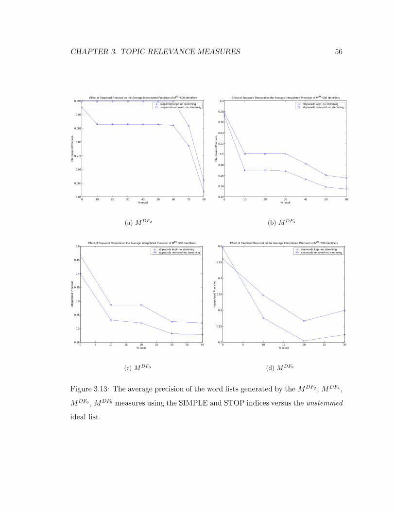
CHAPTER 3. TOPIC RELEVANCE MEASURES 56
0 10 20 30 40 50 60 70 800.06
0.065
0.07
0.075
0.08
0.085
0.09
0.095
Inte
rpol
ated
Pre
cisi
on
% recall
Effect of Stopword Removal on the Average Interpolated Precision of Mdf2−500 Identifiers
stopwords kept−no stemming stopwords removed−no stemming
(a) MDF2
0 10 20 30 40 50 600.12
0.14
0.16
0.18
0.2
0.22
0.24
0.26
0.28
0.3
Inte
rpol
ated
Pre
cisi
on
% recall
Effect of Stopword Removal on the Average Interpolated Precision of Mdf4−500 Identifiers
stopwords kept−no stemming stopwords removed−no stemming
(b) MDF4
0 5 10 15 20 25 30 35 400.15
0.2
0.25
0.3
0.35
0.4
0.45
0.5
Inte
rpol
ated
Pre
cisi
on
% recall
Effect of Stopword Removal on the Average Interpolated Precision of Mdf6−500 Identifiers
stopwords kept−no stemming stopwords removed−no stemming
(c) MDF6
0 5 10 15 20 25 300.2
0.25
0.3
0.35
0.4
0.45
0.5
Inte
rpol
ated
Pre
cisi
on
% recall
Effect of Stopword Removal on the Average Interpolated Precision of Mdf8−500 Identifiers
stopwords kept−no stemming stopwords removed−no stemming
(d) MDF8
Figure 3.13: The average precision of the word lists generated by the MDF2 , MDF4 ,
MDF6 , MDF8 measures using the SIMPLE and STOP indices versus the unstemmed
ideal list.
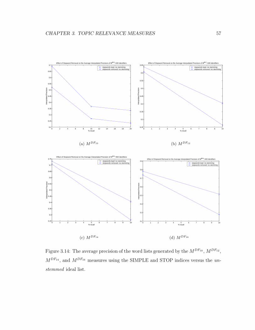
CHAPTER 3. TOPIC RELEVANCE MEASURES 57
0 2 4 6 8 10 12 14 16 18 200.2
0.25
0.3
0.35
0.4
0.45
0.5
0.55
0.6
0.65
0.7
Inte
rpol
ated
Pre
cisi
on
% recall
Effect of Stopword Removal on the Average Interpolated Precision of Mdf10−500 Identifiers
stopwords kept−no stemming stopwords removed−no stemming
(a) MDF10
0 1 2 3 4 5 6 7 8 9 100.25
0.3
0.35
0.4
0.45
0.5
0.55
0.6
0.65
Inte
rpol
ated
Pre
cisi
on
% recall
Effect of Stopword Removal on the Average Interpolated Precision of Mdf12−500 Identifiers
stopwords kept−no stemming stopwords removed−no stemming
(b) MDF12
0 1 2 3 4 5 6 7 8 9 100.25
0.3
0.35
0.4
0.45
0.5
0.55
0.6
0.65
0.7
0.75
Inte
rpol
ated
Pre
cisi
on
% recall
Effect of Stopword Removal on the Average Interpolated Precision of Mdf14−500 Identifiers
stopwords kept−no stemming stopwords removed−no stemming
(c) MDF14
0 1 2 3 4 5 6 7 8 9 100.2
0.3
0.4
0.5
0.6
0.7
0.8
0.9
Inte
rpol
ated
Pre
cisi
on
% recall
Effect of Stopword Removal on the Average Interpolated Precision of Mdf16−500 Identifiers
stopwords kept−no stemming stopwords removed−no stemming
(d) MDF16
Figure 3.14: The average precision of the word lists generated by the MDF10 , MDF12 ,
MDF14 , and MDF16 measures using the SIMPLE and STOP indices versus the un-
stemmed ideal list.
CHAPTER 3. TOPIC RELEVANCE MEASURES 58
0 10 20 30 40 50 60 70 800
0.1
0.2
0.3
0.4
0.5
0.6
0.7
0.8
0.9
1
% recall
Inte
rpol
ated
Pre
cisi
on
Average Interp. Prec. for the Database Index Sorted by Pure Freq against the SMART Stopword List
df tf df~ df
2
df4
df6
df8
df10
df12
df14
df16
0 5 10 15 20 25 300
0.1
0.2
0.3
0.4
0.5
0.6
0.7
0.8
0.9
1
% recall
Inte
rpol
ated
Pre
cisi
on
Partial Average Interp. Prec. for the Database Index Sorted by Pure Freq against the SMART Stopword List
df tf df~ df
2
df4
df6
df8
df10
df12
df14
df16
Figure 3.15: The precision of the SIMPLE index words sorted by their frequencies
against the SMART stopword list.
vocabulary sizes that are between 3% and 10% of the size used by the other more
traditional measures. The evaluations also indicate that stopword removal improves
the precision of the topic words extracted whereas stemming degrades it.
Although we use a preset stopword list for stopword removal in the evaluation,
it is preferable to be able to remove stopwords automatically with no reference
to a preset list. One possible approach is to sort index words by their pure DFn
database frequency and remove the top words from this sorted list. For example,
if we plan to use MDF4 to weigh topic words, we can start by sorting the SIMPLE
index words by DF4(w, db) and removing the top 10% of the words from the index.
Figure 3.15 compares the sorted pure frequency lists to SMART’s stopword list. The
plots in this figure are the traditional 11-point precision-recall plot with SMART’s
stopword list as the target vocabulary. These plots show that a high proportion
of the top words in any of the sorted lists are stopwords found on the SMART
stopword list. Therefore, removing these words will likely improve the precision

CHAPTER 3. TOPIC RELEVANCE MEASURES 59
of our MDF4 measure without losing too many non-stopwords from the list. This
approach is similar to the adhoc feature selection method mentioned by Yang and
Pedersen [YP97], where they report that removing words with the highest DF
values is one of the most effective feature selection methods for text categorization.
We leave further studies along these lines for future work.
In our evaluations we replaced stopwords by some null term to preserve their
positions in the text. For completeness, it would be interesting to further study the
effect of simply removing stopwords without preserving their position.
Another aspect we would like to investigate is the effect of a stemmer that is
less aggressive than the Porter stemmer used in our evaluations. A weaker stemmer
might reduce the number of words incorrectly represented by the same stem when
an aggressive stemmer is utilized, but at the same time recognize words with slightly
varying morphological formats, such as plurals, which would otherwise be treated
as different words when no stemming is performed.
It is also interesting to explore the effect of relaxing our spread measure to allow
for documents in which a word appears in m out of n segments for DFn, for some
preset value of m < n. This would recognize that the major topic of a paper could
be interrupted in one or two places for a tangential discourse.

Chapter 4
Putting it Together:
Building the Topic Flow Signal
Topic flow signals reflect the variation in the intensity of discussion related to the
topic across the text. Heavily discussed topics in a text tend to recur throughout
and remain relevant to most of the document. Therefore, such topics have a contin-
uous stream of strongly relevant topic words throughout the text. Topics that are
discussed less intensely, however, are either relevant to limited portions of the text,
or are interrupted often thus shifting the focus of discussion away from that topic.
Such topics have a more sparse distribution of relevant topic words indicating a
weaker presence in the text. So generating a topic flow signal for a given text is
simply a matter of representing the relevance of the topic to each segment of the
text.
We start by describing the signal construction algorithm, which generates the
most basic topic flow signals. The constructed signals are then used to view the
flow of the topic at varying levels of detail within the text. Finally, we show that
60

CHAPTER 4. BUILDING THE TOPIC FLOW SIGNAL 61
topic flow signals reflect the actual change in the intensity of discussion within the
document.
4.1 Constructing the Initial Signal
The most basic topic flow signal relies on our earlier observation that given a suf-
ficient list of topic words for a category we will find strongly relevant topic words
in text segments which discuss the category. By tracking the topic relevance of the
words across the text we can construct a word-based representation of the topic
flow within the text. The algorithm for representing the flow of a topic t in a given
document D is presented in Algorithm 1. The algorithm iterates through the doc-
ument, and at each word w’s position in the text the corresponding position in the
signal is assigned a value reflecting the word’s relevance to the topic. Our measure
of topic relevance is based on the sorted topic word lists of MDF4(w, t) which, as
we have seen in the previous chapter, produces one of the most accurate topic word
lists with little loss in vocabulary.
Given the topic word lists sorted by their MDF4 weights, at each word position
w in the text the algorithm assigns the corresponding signal position a value equal
to the rank of w in the sorted topic word list for topic t as described in the Rank
subroutine in Algorithm 1. If w is not on t’s topic word list but on some other
topic’s list, it is assigned one plus the maximum rank in topic t’s list, otherwise it
is discarded.
The resulting topic flow signal should remain low at points of strong relevance to
the topic and peak at points where there are shifts away from the topic. Therefore,
the signal should provide a good representation of the progression of the topic in

CHAPTER 4. BUILDING THE TOPIC FLOW SIGNAL 62
the document. We have already seen a sample signal in Chapter 2 for the text in
Example 4.1.1:
Example 4.1.1 Belief revision focuses on how an agent should change her
beliefs when she adopts a particular new belief. [FH99]
The signal in Figure 2.3 was constructed using MDF4 ’s topic word list for Artificial
Intelligence. The same signal is reproduced in Figure 4.1 with each vertex labelled
by the word that generated the vertex’s topic relevance value.
To take another example, Figure 4.2(a) shows the Computation and Language
signal for a segment from the paper entitled “Applying Natural Language Genera-
tion to Indicative Summarization” [KMK01]:
Example 4.1.2 We have presented a model for indicative multi-document sum-
marization based on natural language generation. In our model, summary content
is based on document features describing topic and structure instead of extracted
text. [KMK01]
As expected, the signal in Figure 4.2(a) has relatively low ranks for many terms
relevant to Computation and Language, such as model, language, content, and text.
The flow of any other topic in the text can be represented in a similar manner
through another signal. The assumption here is that any number of topics can
be discussed simultaneously in a document, and each of these topics can be repre-
sented by a separate topic flow signal. The topic flow of Artificial Intelligence for
Example 4.1.2 is shown in Figure 4.2(b). The variation among the vertex values
and the word ranks in this signal are higher than those in the Computation and
Language signal, indicating a relatively weaker presence of Artificial Intelligence’s
topic words in the segment, and thus a relatively weaker discussion of the topic.

CHAPTER 4. BUILDING THE TOPIC FLOW SIGNAL 63
Algorithm 1 Construct topic flow signal St for topic t in input document D
INPUT: Document D;
||D|| = The number of word positions in D;
Topic t;
T= Topic word list for t sorted by MDF4(w, t);
V oc=⋃
∀topics ti
topic word list for ti
OUTPUT: Topic flow signal St for topic t in document D;
sig position = 0;
for (text position = 0; text position < ||D||; text position++) do
w = word at text position in D;
if (w ∈ T ) then
St[sig position] = rank(w, T );
sig position++;
else if (w ∈ V oc) then
St[sig position] = 1 + maximum rank(T );
sig position++;
else
ignore w;
end if
end for
(continued)

CHAPTER 4. BUILDING THE TOPIC FLOW SIGNAL 64
SUB Rank
{Find the number of weights lower than word w’s in topic word list T}INPUT: word w; Sorted topic list T ;
OUTPUT: rank of weight of w in T ;
tmp rank = 0;
i = 0;
prev wt = T [i]{WEIGHT};while (NOT(Done) AND (i ≤ ||T ||)) do
if (T [i]{WEIGHT} �= prev wt) then
prev wt = T [i]{WEIGHTT};tmp rank + +;
end if
if (T [i]{WORD} == w) then
Done = TRUE;
end if
i + +;
end while
return(tmp rank);
Algorithm 1 (continued)

CHAPTER 4. BUILDING THE TOPIC FLOW SIGNAL 65
0 0.5 1 1.5 2 2.5 3 3.5 4 4.5 50
10
20
30
40
50
60
70
80
Word position in text
Top
ic w
ord
rank
Belief Example−AI
belief revision
agent
change
beliefs belief
Figure 4.1: Topic flow signal for the topic Artificial Intelligence based on the rel-
evance values in Table 2.2. Each vertex in the signal is labelled by the word that
generated the vertex.
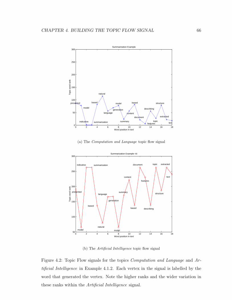
CHAPTER 4. BUILDING THE TOPIC FLOW SIGNAL 66
0 2 4 6 8 10 12 14 16 180
50
100
150
200
250
300
Word position in text
Top
ic w
ord
rank
Summarization Example
presented
model
indicative summarization
based
natural
language
generation
model
summary
content
based
document
features
describing
topic
structure
extracted
text
(a) The Computation and Language topic flow signal
0 2 4 6 8 10 12 14 16 1850
100
150
200
250
300
Word position in text
Top
ic w
ord
rank
Summarization Example−AI
presented
indicative summarization
based
natural
language
generation
model
summary
content
based
document
features
structure
topic
describing
extracted
text
model
(b) The Artificial Intelligence topic flow signal
Figure 4.2: Topic Flow signals for the topics Computation and Language and Ar-
tificial Intelligence in Example 4.1.2. Each vertex in the signal is labelled by the
word that generated the vertex. Note the higher ranks and the wider variation in
these ranks within the Artificial Intelligence signal.

CHAPTER 4. BUILDING THE TOPIC FLOW SIGNAL 67
4.2 Zooming out: Representing the topic flow of
larger segments
The topic flow signals constructed in the previous section represent the change in
topic relevance at individual word positions. Although words are the basic units for
expressing a topic, the overall topic of a sequence of words is a complex function
of many variables including the constituent words, the structure governing these
words, the order of the words, and the situational context within which the text
was produced. For simplicity we focus here on identifying the general topic of a
sequence of words from its constituent words and the context of each word. This
word sequence can be as long as the document itself. It can also be a segment of
the text in which case the topic relevance of the whole word sequence represents
the topic relevance of the document at that particular segment.
By dividing the whole text into consecutive word sequences we can represent the
topic flow within the text through these text segments rather than representing it
at individual word positions. The resulting segment-based topic flow signal should
provide a more general view of the text, and by varying the segment size we can
monitor the change in topic flow at different levels of detail.
We assume that the relevance of a single segment to a topic is a function of
the importance of the constituent words to that topic. Given the ranks of these
individual words in the sorted topic word list, the segment’s topic relevance is
represented by the average rank of the words in the segment:
M(SEG, t) =
∑∀w:((w∈SEG)∧(w a topic word for some topic τ∈T ))
RANK(w, t)
||SEG|| (4.1)

CHAPTER 4. BUILDING THE TOPIC FLOW SIGNAL 68
where:
• M(SEG, t) is the importance of topic t in segment SEG.
• RANK(w, t) is the rank of the topic relevance value for word w in the sorted
topic word list for t as defined in the RANK subroutine in Algorithm 1.
• ||SEG|| the number of words in segment SEG.
• T is the set of all possible topics.
This approach allows us to include all words within the segment when estimating
its topic relevance. Averaging the words’ ranks also smoothes out the effect of the
occasional noise word.
To view the topic flow in document D at the n-word segment size, we start
by dividing the document into equal segments, each consisting of approximately n
words. Next we calculate M(SEG, t) the importance of topic t for each of these seg-
ments as described in Equation 4.1 above. Algorithm 2, which is a slightly modified
version of the word-based signal construction algorithm described in Algorithm 1,
can then be used to construct the topic flow signal for this segment size.
With a few more operations we can also generate the topic flow at increasingly
larger segment sizes: Starting with the word-based signals, we can get the topic flow
at 2-word segment sizes by averaging every pair of consecutive words in the signal.
The signal for the 2-word segment size can then be used to generate the 4-word
segment signals. Similarly, for any segment size 2i we use the signal for segment
size 2i−1. This algorithm, shown in Algorithm 3, is extremely efficient requiring
only O(||D||) operations to construct the topic flow signals for all 2i segment sizes
from i = 1..log(||D||), where ||D|| is the number of words in the document D.

CHAPTER 4. BUILDING THE TOPIC FLOW SIGNAL 69
Algorithm 2 Construct topic flow signal St for topic t in input document D at
segment size n
INPUT: Document D divided into segments of size n each;
||S|| = The number of segments in D;
Topic t;
Topic relevance value M(SEG, t) for each segment SEG;
OUTPUT: Topic flow signal St for topic t in document D;
for (seg num = 0; seg num < ||S||; seg num++) do
SEG = segment seg num in D;
St[seg num] = M(SEG, t);
end for

CHAPTER 4. BUILDING THE TOPIC FLOW SIGNAL 70
Algorithm 3 The averaging algorithm for the Haar Wavelet Transform
{Construct topic flow signals Rt for larger segment sizes using the word-based
topic flow signal St}INPUT: Word-based topic flow signal St for topic t in document D;
||St|| = the number of points in signal St
OUTPUT: Set of topic flow signals Rt[0..(log(||St||))] where Rt[i] is the topic
flow signal representing text segments of size 2((log||St||)−i);
maxl = log||St||;for (i = 0; i < ||St|| ; i++) do
Rt[maxl][i] = St[i];
end for
for (l = maxl − 1; l >= 0 ; l−−) do
i = 0;
for (position = 0; position < ||Rt[l + 1]|| − 1; position = position + 2) do
Rt[l][i] = Rt[l+1][position]+Rt[l+1][position+1]2
;
i++;
end for
end for
CHAPTER 4. BUILDING THE TOPIC FLOW SIGNAL 71
Just as averaging pairs of consecutive points in a signal smoothes the signal,
taking the difference between these pairs emphasises the local changes in topic rel-
evance, usually due to noise. Adding the averaged signal and the difference signal
reproduces the original unsmoothed signal. Similarly, if we keep the signal repre-
senting topic flow for segments of size n, for some value of n, as well as the difference
between consecutive pairs at all the levels preceding that signal, we can reconstruct
our initial word-based signal. In this case, we will have transformed the initial word-
based signal into another equivalent representation that provides us with a different
view of the same text. This transformation is called the Haar Wavelet Transform,
the simplest type of wavelet transforms, which are used in many applications in-
cluding noise reduction, image processing, and signal compression [SN96] [JlCH01].
Since we are not interested in the noise within the signal, nor are we interested
in reconstructing the signal, we will not keep these differences. Instead, we are
interested in the various views of the text at different segment sizes, each of which
reflects the flow at a different level of detail. We will call these levels of detail levels
of resolution. Wavelet transformation is an efficient method to obtain these multi-
resolution signals. However they require a signal length that is a power of 2. When
this is not the case the signal is extended to the nearest power of 2 size by padding
it with some constant, by repeating a portion of the signal, or by some other signal
extension method [SN96] [JlCH01]. In the context of topic flow, concatenating the
signal with any artificial value disrupts the real topic flow representation. This
problem has posed serious concerns for us regarding the accuracy of the extended
signals in reflecting topic flow. The solution, however, turns out to be quite simple.
The power of 2 length requirement stems from the averaging approach where we
average every two consecutive words starting from the word-based topic flow signal.
Instead, we can start by recursively dividing the text into segments of equal sizes. At

CHAPTER 4. BUILDING THE TOPIC FLOW SIGNAL 72
each level of resolution, we are now certain that all segments are of roughly the same
size, thus representing equal portions of the text with no artificial values added.
The detailed algorithm is presented in Algorithm 4. For instance, a document
consisting of 9 words can be divided into 4 and 5 word segments, each of these two
segments can then be divided into 2 and 2, and 2 and 3 word segments respectively
for topic flow at the lower, more detailed, segment size. At the very bottom we
will find seven consecutive segments of size 1 word, and one segment of size 2. The
segment sizes for each level of resolution in this 9-word text is shown in Figure 4.3.
Now that we have segments of roughly equal size at each level of resolution, we
can proceed as before in finding the topic relevance for each segment at a certain
resolution level and constructing the topic flow signal for that resolution starting
from the most detailed level up to the more general levels with larger segments.
The main difference from the original averaging step in the wavelet transform is
that our segment sizes do not necessarily have power of 2 length, nor does our
text. We do, however, need to know apriori the total size of the text which may
not be available in some situations such as when streams of text are being received
and their signals constructed in real-time. Figure 4.4 shows the topic flow signals
for the topics Computation and Language and Artificial Intelligence at resolution
levels 0–5 for the sample text in Figure 4.1.2.
4.3 Evaluation
So far we have been concerned with building topic flow signals and viewing the flow
of topics at different levels of resolution. The assumption has been that words are
the “atomic units” used to describe the topics under discussion [Kat96], that by
following the relevance of these words to the topic we will manage to create a signal

CHAPTER 4. BUILDING THE TOPIC FLOW SIGNAL 73
Algorithm 4 The Gradual Averaging algorithm
{Construct topic flow signals Rt for larger segment sizes using the word-based
topic flow signal St}INPUT: Word-based topic flow signal St for topic t in document D;
||St|| = the number of points in signal St
OUTPUT: Set of topic flow signals Rt where:
Rt[i] is the topic flow signal at resolution level i, with the the most
general level at i = 0 which consists of one point representing the overall
average of relevance in the text.
{Get number of words in each segment at each level in the transform}get segment sizes( segment sizes, maxl );
for (i = 0; i < ||St|| ; i++) do
Rt[maxl + 1][i] = St[i];
end for
{Create the first level of the transform after Rt[maxl + 1]}get first sums( Rt, segment sizes, maxl );
for (l = max l − 1; l >= 0 ; l −−) do
i = 0;
for (position = 0; position < ||Rt[l + 1]|| − 1; position = position + 2) do
Rt[l][i] = Rt[l + 1][position] + Rt[l + 1][position + 1];
Rt[l + 1][position] = Rt[l + 1][position]/segment sizes[l + 1][position];
Rt[l+1][position+1] = Rt[l+1][position+1]/segment sizes[l+1][position+
1];
i++;
end for
end for
Rt[0][0] = Rt[0][0]/segment sizes[0][0];
(continued)

CHAPTER 4. BUILDING THE TOPIC FLOW SIGNAL 74
SUB get segment sizes
INPUT: ||St||;OUTPUT: segment sizes : an array containing number of words to include in
each segment at each level in the transform;
maxl the maximum level in segment sizes;
i = 0;
segment sizes[0][0] = ||St||;for ( l = 1; 2l ≤ ||St||; l++) do
p = 0;
maxl = l;
for ( i = 0; i < number of elements in segment sizes[l − 1]; i++) do
segment sizes[l][p] = �segment sizes[l−1][i]2
�;segment sizes[l][p + 1] = segment sizes[l − 1][i] − segment sizes[l][p];
p = p + 2;
end for
end for
Algorithm 4 (continued)
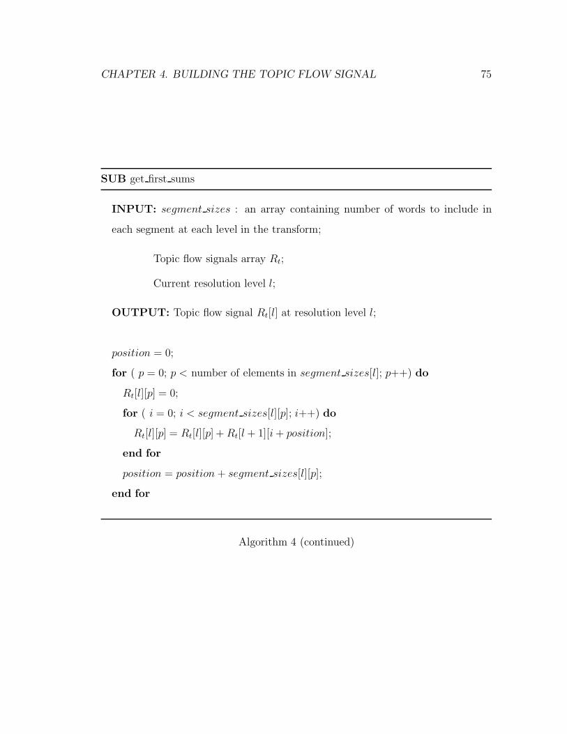
CHAPTER 4. BUILDING THE TOPIC FLOW SIGNAL 75
SUB get first sums
INPUT: segment sizes : an array containing number of words to include in
each segment at each level in the transform;
Topic flow signals array Rt;
Current resolution level l;
OUTPUT: Topic flow signal Rt[l] at resolution level l;
position = 0;
for ( p = 0; p < number of elements in segment sizes[l]; p++) do
Rt[l][p] = 0;
for ( i = 0; i < segment sizes[l][p]; i++) do
Rt[l][p] = Rt[l][p] + Rt[l + 1][i + position];
end for
position = position + segment sizes[l][p];
end for
Algorithm 4 (continued)

CHAPTER 4. BUILDING THE TOPIC FLOW SIGNAL 76
9
54
2 2 2 3
1 1 1 1 1 1 1 2
Resolution Level
0
1
2
3
Figure 4.3: Segment sizes at different resolution levels for a 9-word text
0 2 4 6 8 10 12 14 16 180
200
400
leve
l 5
Segment Position in Text
0 5 10 150
200
400
leve
l 4
0 1 2 3 4 5 6 70
200
400
leve
l 3
0 0.5 1 1.5 2 2.5 30
200
400
leve
l 2
0 0.1 0.2 0.3 0.4 0.5 0.6 0.7 0.8 0.9 10
200
400
leve
l 1
−1 −0.8 −0.6 −0.4 −0.2 0 0.2 0.4 0.6 0.8 10
100
200
leve
l 0
Topic Flow Signals AI and CL in Summarization Example at Different Levels of Resolution
Figure 4.4: The transform of the Computation and Language (triangles) and Arti-
ficial Intelligence (asterisks) signals for the paper segment 4.1.2

CHAPTER 4. BUILDING THE TOPIC FLOW SIGNAL 77
that can reflect topic flow in the text. By gradually smoothing this word-based
signal we get a more robust topic flow representation at larger text segments. This
section aims at evaluating the signals’ ability to represent topic flow.
4.3.1 The Ideal Topic Flow Signal
Evaluating the quality of our topic flow signals requires comparing these signals to
the ideal topic flow representation in the text. An ideal topic flow signal should
remain low when the corresponding text intensifies its discussion on the topic indi-
cating strong topic relevance, and peak when the corresponding text significantly
reduces its discussion of the topic indicating. But the knowledge of when the topic
discussion intensifies and when it abates necessitates usage of documents whose dif-
ferent segments have been manually categorized for any segment size. This manual
categorization would reflect the flow of topics at different segment sizes including
temporary digressions that take up small segments, as well as subtopics that may
span larger segments.
An alternative to manually categorizing document segments is to construct our
evaluation documents from smaller pre-categorized texts. Ideally, we would also like
these smaller texts to discuss the topics under which they have been categorized
throughout the text with no digressions to any other topic. These criteria are best
met in the abstracts of technical papers: abstracts are concise so the possibility of
digressions is minimal, and they aim to describe only the main topics of the paper
so they are more likely to discuss these topics throughout the abstract.
Given a sequence of abstracts each of which belongs to at least one category,
the ideal topic flow signal for a category t within this sequence is a reflection of the
distribution of the category’s abstracts. Such a signal would indicate the strongest

CHAPTER 4. BUILDING THE TOPIC FLOW SIGNAL 78
This paper compares the tasks of part-of-speech (POS) tagging and word-sense-tagging or
disambiguation (WSD), and argues that the tasks are not related by fineness of grain or
anything like that, but are quite different kinds of task, particularly becuase there is
nothing in POS corresponding to sense novelty. The paper also argues for the reintegration
of sub-tasks that are being separated for evaluation.
This paper describes the design of a control and management network (orderwire) for a mobile
wireless Asynchronous Transfer Mode (ATM) network. This mobile wireless ATM network is part
of the Rapidly Deployable Radio Network (RDRN). The orderwire system consists of a packet
radio network which overlays the mobile wireless ATM network, each network element in this
network uses Global Positioning System (GPS) information to control a beamforming antenna
subsystem which provides for spatial reuse. This paper also proposes a novel Virtual
Network Configuration (VNC) algorithm for predictive network configuration. A mobile ATM
Private Network-Network Interface (PNNI) based on VNC is also discussed. Finally, as a
prelude to the system implementation, results of a Maisie simulation of the orderwire system
are discussed.
We present a memory-based learning (MBL) approach to shallow parsing in which POS tagging,
chunking, and identification of syntactic relations are formulated as memory-based modules.
The experiments reported in this paper show competitive results, the F-value for the Wall
Street Journal (WSJ) treebank is: 93.8% for NP chunking, 94.7% for VP chunking, 77.1% for
subject detection and 79.0% for object detection.
Figure 4.5: A sample sequence of abstracts. The first and last abstracts belong
to Computation and Language, while the second abstract is on Networks and the
Internet.
topic relevance at points where the abstract belongs to category t, and peak to
its highest rank values indicating no topic relevance otherwise. Figure 4.5 shows a
sample sequence of abstracts.
The topic flow signals we have constructed in the previous sections are all word-
based. Our ideal signals should similarly be word-based. We will make the un-
realistic assumption that if an abstract is categorized under a topic, then every
vocabulary word in the abstract will be relevant to that topic. This is a restrictive
assumption that hypothesizes there is absolutely no noise in our abstracts, even
though it is possible to have vocabulary words within the abstract that are not rel-

CHAPTER 4. BUILDING THE TOPIC FLOW SIGNAL 79
evant to the abstract topic. Nevertheless, we believe that due to the concise nature
of abstracts, and the noise reduction effect of averaging, this assumption will not
have a huge impact on our evaluation.
Given a sequence of abstracts, we now proceed to build the ideal word-based
topic flow signals as follows: we start by removing from the abstracts all non-
vocabulary words. A vocabulary word is one that is known to be a topic word for
any of our 12 categories using the MDF4 topic word lists. We then create the ideal
topic flow signal for each of the 12 CoRR categories where for every topic t we
trace each word in the abstracts and mark its corresponding position in the signal
with a 1 if the abstract belongs to the topic t, or with a (max rank(t) + 1) if the
abstract does not belong to t, where max rank(t) is the maximum possible rank in
the topic word list for t. To get the ideal topic flow at larger segments, we simply
use the gradual averaging algorithm described earlier 4. Figure 4.6 shows the ideal
word-based topic flow signals as well as the topic flow at resolution levels 0− 7 for
the simple document in Figure 4.5 whose first and third abstracts are Computation
and Language abstracts, while its second abstract is a Networks and the Internet
abstract.
4.3.2 Evaluation Abstract Sequences
We created our evaluation abstract sequences using the abstracts of the technical
papers submitted to the CoRR website [CORa] between January 1998 and Dec 2001.
There are two evaluation sequences: The first, called the T sequence, consists of
736 abstracts summarizing the CoRR papers used by our system in creating its list
of topic words. The corresponding set of full papers is called the CoRR training
set. It is important to note, however, that before the training set was used to

CHAPTER 4. BUILDING THE TOPIC FLOW SIGNAL 80
0 20 40 60 80 100 120 1400
200
400
leve
l 7
Segment Position in Text
0 10 20 30 40 50 60 700
200
400
leve
l 6
0 5 10 15 20 25 30 350
200
400
leve
l 5
0 5 10 150
200
400
leve
l 4
0 1 2 3 4 5 6 70
200
400
leve
l 3
0 0.5 1 1.5 2 2.5 30
200
400
leve
l 2
0 0.1 0.2 0.3 0.4 0.5 0.6 0.7 0.8 0.9 1100
150
200
leve
l 1
−1 −0.8 −0.6 −0.4 −0.2 0 0.2 0.4 0.6 0.8 1148
150
152
leve
l 0
Sample Ideal Signal−CL
Figure 4.6: The Computation and Language ideal topic flow signal at the word level
(level 7), and at increasingly larger segment sizes (levels 6 up to 0) for a sample
document consisting of 3 abstracts the first and last of which are Computation and
Language abstracts and the second is on Networks and the Internet

CHAPTER 4. BUILDING THE TOPIC FLOW SIGNAL 81
extract topic words, the abstracts were stripped from the set’s papers. So although
the papers from which these abstracts come were in the training set, the abstracts
themselves were not. Nevertheless, the system will have been trained on most of
the topic words appearing in these abstracts. Therefore, the T abstract sequence
will assist us in evaluating our topic flow signals given that the system recognizes all
the important topic words, and that there is no inconsistency in the categorization
of the segments in the T abstract sequence versus the training set papers.
The second evaluation abstract sequence, called the N sequence, consists of 447
abstracts of papers that were submitted to the CoRR website between January
1998 and December 2001, but whose papers were not part of the training set. Since
the papers to which these abstracts belong were not used in training, the chances
of missing good topic words are much higher than in the T sequence. Therefore,
this document is useful in evaluating the robustness of our topic flow signals in the
presence of noise due to missing topic words, or due to inconsistencies in categorizing
the abstracts compared to the training set. Table 4.1 shows the number of abstracts
that fall under each of the 12 categories tested, as well as the number of abstracts
that belong solely to that category (“one-topic abstracts”) in the T and N abstract
sequences.
To ensure that there is no bias for the order in which abstracts are concatenated,
we created three different versions of each abstract sequence T and N where each
version contains a random ordering of the abstracts used in the sequence. We will
call the T sequence versions T1, T2, and T3, and those using the N sequence N1,
N2 and N3.
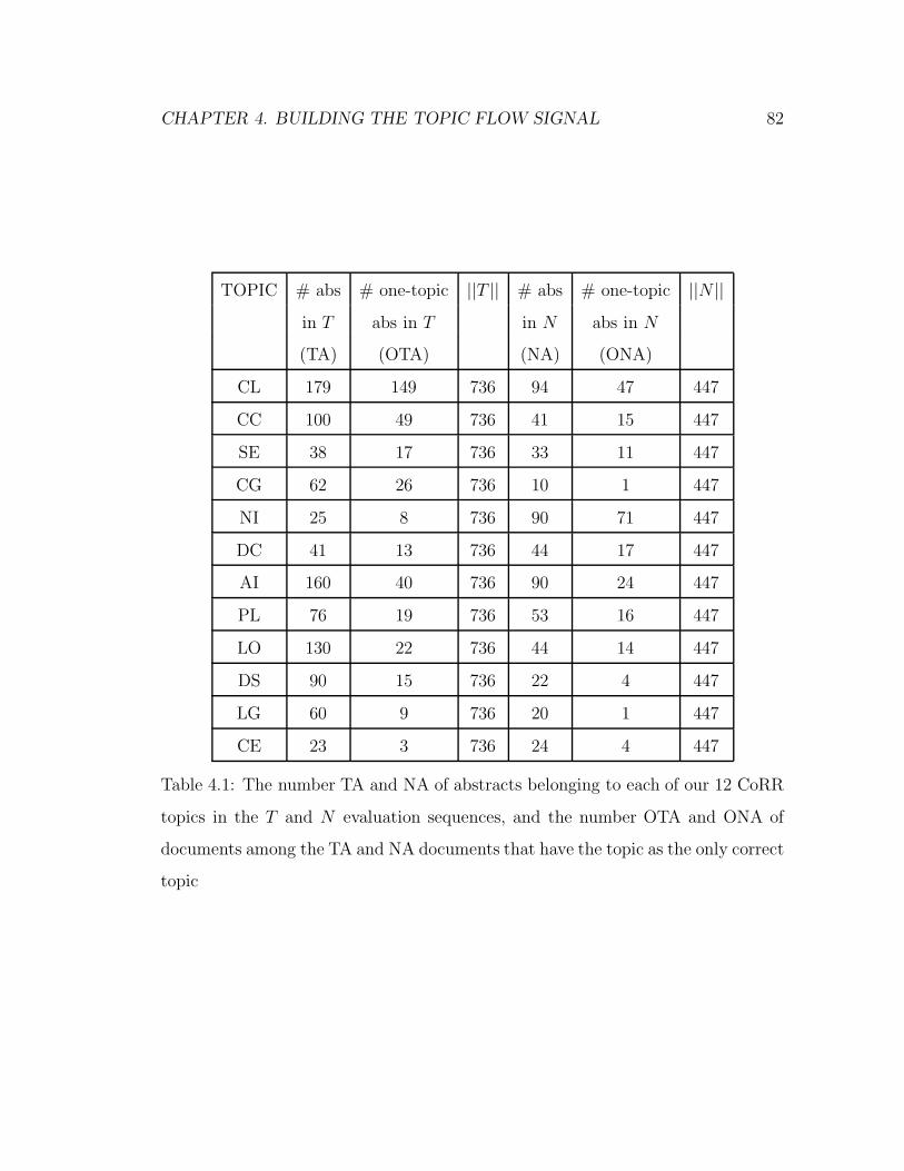
CHAPTER 4. BUILDING THE TOPIC FLOW SIGNAL 82
TOPIC # abs # one-topic ||T || # abs # one-topic ||N ||in T abs in T in N abs in N
(TA) (OTA) (NA) (ONA)
CL 179 149 736 94 47 447
CC 100 49 736 41 15 447
SE 38 17 736 33 11 447
CG 62 26 736 10 1 447
NI 25 8 736 90 71 447
DC 41 13 736 44 17 447
AI 160 40 736 90 24 447
PL 76 19 736 53 16 447
LO 130 22 736 44 14 447
DS 90 15 736 22 4 447
LG 60 9 736 20 1 447
CE 23 3 736 24 4 447
Table 4.1: The number TA and NA of abstracts belonging to each of our 12 CoRR
topics in the T and N evaluation sequences, and the number OTA and ONA of
documents among the TA and NA documents that have the topic as the only correct
topic

CHAPTER 4. BUILDING THE TOPIC FLOW SIGNAL 83
4.3.3 Evaluation Method
For each of our evaluation sequences T1–T3 and N1–N3 we first generate 12 ideal
topic flow signals each representing the flow of one of the 12 CoRR database topics.
These signals are then smoothed at resolution levels 0 through the maximum size
(the log of the size of the evaluation sequence).
Next, for each of the six sequences, we generate a topic flow signal as described
in Sections 4.1 and 4.2 above for each of the 12 CoRR categories. We will call these
the test signals.
For a given sequence, each one of the ideal signals is compared to each one
of the 12 test signals. Two signals match perfectly when they rise and fall at
exactly the same point. This match indicates that both signals reflect the same
flow. The most appropriate statistical measure for our purposes is the correlation
coefficient [Ost88]:
CORRCOEF (X, Y ) =(∑
∀x∈X and y∈Y (x − x)(y − y))
(∑
∀x∈X(x − x)2)(∑
∀y∈Y (y − y)2)(4.2)
where X and Y are the two signals to be matched composed of a sequence of
ranks, and x and y are the average ranks across X and Y respectively. The highest
correlation coefficient is +1 indicating a perfect match. A correlation coefficient of
0.65 or higher indicates strong correlation, a correlation coefficient between 0.3 and
0 indicates weak to no correlation between the shapes of the two signals, while a −1
indicates a reverse correlation between X and Y which means that when X is high,
Y is low, and vice versa. Figure 4.7 shows an example of highly correlated test and
ideal signals in the T1 evaluation sequence for the topic Computation and Language
at resolution level 6 (i.e. 27 segments). The correlation coefficient between the
two signals at this level is 0.9. Note how the two signals rise and decline at about

CHAPTER 4. BUILDING THE TOPIC FLOW SIGNAL 84
the same pace indicating similar changes in topic flow. Two non-correlated signals,
with correlation coefficient −0.05, are shown in Figure 4.8 for the Computational
Engineering, Finance, and Science ideal and test signals in the N1 sequence at
resolution level 7. In this case the test signal’s fluctuations are independent of those
of the ideal signal thus painting different pictures of topic flow in the document. In
between highly correlated signals and weakly correlated ones, some signals are said
to be moderately correlated. An example of moderately correlated signals is shown
in Figure 4.9. In this figure, the test and ideal signals represent the topic flow for
Software Engineering at resolution level 6 in the N1 evaluation sequence. The two
signals have a correlation coefficient value of 0.56. When the ideal signal indicates
a strong topic relevance through a low rank value, so does the test signal, but the
test signal also fluctuates at points where the ideal signal is constant.
The correlation between the test and ideal signals can be measured at any level
of resolution. At the most detailed levels we expect the effect of noise to be high
in the signals and, consequently, the correlation to be low. But as we proceed to
lower resolution levels, the noise should gradually diminish and correlation should
increase if the flow in both signals is similar. Ideally, we would like the noise to
have diminished completely at the resolution level where each point in the signal
corresponds to an average abstract size. At this segment size each abstract will
be represented by one low ranked point to reflect the fact that it discusses its
topic(s) throughout the abstract with minimal digressions. Thus, any noise will
have been mostly smoothed out at previous levels of resolution. In the T and N
sequences this segment size corresponds to the resolution levels log2(736) = 10
and log2(447) = 9, respectively. From this resolution level up to the most general
level 0, noise should be minimal, and correlation between the ideal and test signals
should be high. In order to evaluate the correlation between any test and ideal

CHAPTER 4. BUILDING THE TOPIC FLOW SIGNAL 85
0 20 40 60 80 100 120 1400
50
100
150
200
250
300CL TRAIN List Signals−Transform Level 7
Test signalIdeal signal
Figure 4.7: An example of highly correlated ideal and test topic flow signals. The
signals represent the flow of Computation and Language in the T1 abstract sequence
at resolution level 7

CHAPTER 4. BUILDING THE TOPIC FLOW SIGNAL 86
0 20 40 60 80 100 1200
50
100
150
200
250
300CE− Resolution Level 7
Segment position in text
Ran
k
Test signal Ideal signal
Figure 4.8: An example of weakly correlated ideal and test topic flow signals. The
signals represent the flow of Computational Engineering, Finance, and Science in
the N1 abstract sequence at resolution level 7
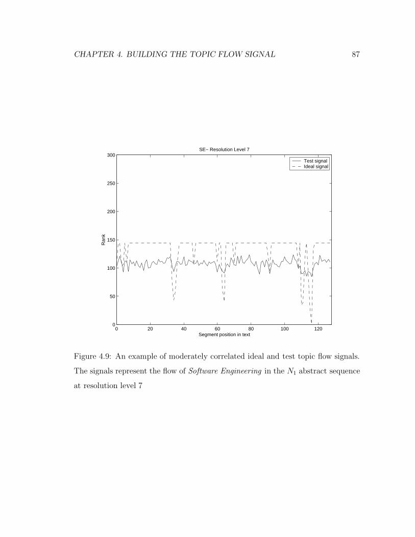
CHAPTER 4. BUILDING THE TOPIC FLOW SIGNAL 87
0 20 40 60 80 100 1200
50
100
150
200
250
300SE− Resolution Level 7
Segment position in text
Ran
k
Test signal Ideal signal
Figure 4.9: An example of moderately correlated ideal and test topic flow signals.
The signals represent the flow of Software Engineering in the N1 abstract sequence
at resolution level 7

CHAPTER 4. BUILDING THE TOPIC FLOW SIGNAL 88
0 200 400 600 800 1000 1200 1400 1600 1800 20000
50
100
150
200
250
300
Average Rank
Pos
ition
in C
onca
tena
ted
Sig
nal
Level 10 Level 9 Level 8 Level 7
Levels2−6
Figure 4.10: The Computation and Language ideal signal resulting from concate-
nating the signals at resolution levels 2–10 in the T1 abstract sequence
signal pairs at several levels of resolution we start by concatenating each topic’s
test signals at resolution levels 2–10 for each of the T abstract sequences, and
levels 2–9 for each of the N abstract sequences. The same concatenation process
is done for the ideal signals. Levels 1 and 0 are excluded because they contain
too few points for meaningful correlation coefficient values. Figures 4.10 and 4.11
show the concatenated signals for the Computation and Language category. By
concatenating the signals we can get a single pair of vectors for determining the
correlation between the test and ideal signals at multiple levels of resolution.

CHAPTER 4. BUILDING THE TOPIC FLOW SIGNAL 89
0 200 400 600 800 1000 1200 1400 1600 1800 20000
50
100
150
200
250
300
Position in Concatenated Signal
Ave
rage
Ran
k
Level 10Level 9 Level 8 Level 7 Levels2−6
Figure 4.11: The Computation and Language test signal resulting from concatenat-
ing the signals at resolution levels 2–10 in the T1 abstract sequence

CHAPTER 4. BUILDING THE TOPIC FLOW SIGNAL 90
4.3.4 Results
We measured the correlation between every concatenated ideal signal and each one
of the 12 concatenated test signals for each one of the abstract sequences. Tables 4.2
and 4.3 show the top four correlation coefficients for these signal pairs for each of
the T and N abstract sequences.
The table shows a consistently high correlation between the ideal signal and
its corresponding test signal for the same topic in the T abstract sequences all of
which are statistically significant within a 95% confidence interval. All of the ideal
signals in these sequences best resemble the corresponding test signal for the same
category. This shows that when sufficient topic words are provided, and when
categorization consistency can be guaranteed, then the topic flow representation
algorithms succeed in creating signals that accurately reflect the flow of the topic.
The table also shows the effect of extracting the topic word list from a training
set of multi-category documents. Since the CoRR training documents may belong
to more than one category, several resulting topic word lists may be influenced by
a single document. For example, the topic word chunker is a Computation and
Language word. However, because it occurs in a Computation and Language and
Learning training document, the word also occurs in the Learning topic word list as
well. Therefore, topic flow signals will tend to share more topic words than might
be expected. The higher the proportion of training documents a group of categories
share, the stronger the similarity between their signals. Table 4.4 shows the number
of training documents belonging to each category in the CoRR database and the
top three categories with which it shares documents. Looking back at Table 4.2
we note that the second most similar test signals to a topic’s ideal signal in the T
sequences are those of the top co-occurring categories.
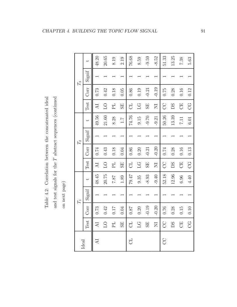
CHAPTER 4. BUILDING THE TOPIC FLOW SIGNAL 91
Tab
le4.
2:C
orre
lati
onbet
wee
nth
eco
nca
tenat
edid
eal
and
test
sign
als
for
the
Tab
stra
ctse
quen
ces
(con
tinued
onnex
tpag
e)
Idea
lT
1T
2T
3
Tes
tC
orr
Sig
nif
tTes
tC
orr
Sig
nif
tTes
tC
orr
Sig
nif
t
AI
AI
0.73
148
.45
AI
0.74
149
.56
AI
0.73
148
.20
LO
0.42
120
.75
LO
0.43
121
.60
LO
0.42
120
.65
PL
0.17
17.
87P
L0.
181
8.28
PL
0.18
18.
19
SE
0.04
11.
89SE
0.04
11.
7SE
0.05
12.
19
CL
CL
0.87
179
.47
CL
0.86
174
.76
CL
0.86
176
.68
LG
0.20
19.
35LG
0.20
19.
15LG
0.19
18.
59
SE
-0.1
91
-8.9
3SE
-0.2
11
-9.7
0SE
-0.2
11
-9.5
9
NI
-0.2
01
-9.4
0N
I-0
.20
1-9
.21
NI
-0.1
91
-8.5
2
CC
CC
0.76
152
.18
CC
0.74
150
.26
CC
0.75
151
.33
DS
0.28
112
.96
DS
0.28
113
.39
DS
0.28
113
.25
CE
0.15
16.
96C
E0.
161
7.11
CE
0.16
17.
38
CG
0.10
14.
40C
G0.
131
6.01
CG
0.12
15.
63

CHAPTER 4. BUILDING THE TOPIC FLOW SIGNAL 92
Tab
le4.
2:(c
onti
nued
)
Idea
lT
1T
2T
3
Tes
tC
orr
Sig
nif
tTes
tC
orr
Sig
nif
tTes
tC
orr
Sig
nif
t
CE
CE
0.60
134
.30
CE
0.58
132
.27
CE
0.60
133
.49
DS
0.23
110
.48
DS
0.19
18.
61D
S0.
221
10.1
0
NI
0.09
13.
91N
I0.
091
4.28
NI
0.09
14.
27
CG
0.07
13.
38C
G0.
051
2.18
CG
0.07
13.
14
CG
CG
0.72
147
.12
CG
0.73
147
.73
CG
0.72
146
.73
DS
0.17
17.
62D
S0.
171
7.77
DS
0.17
17.
75
CE
0.04
51
2.05
CE
0.05
12.
25C
E0.
071
3.04
CC
0.04
11.
75C
C0.
091
3.91
CC
0.08
13.
41
DS
DS
0.69
142
.88
DS
0.68
141
.80
DS
0.68
142
.22
CE
0.42
121
.16
CE
0.42
120
.66
CE
0.42
120
.74
CG
0.29
113
.78
CG
0.29
113
.68
CG
0.30
114
.15
CC
0.26
112
.26
CC
0.25
111
.87
CC
0.26
111
.99
DC
DC
0.71
145
.35
DC
0.69
143
.51
DC
0.68
141
.47
NI
0.39
119
.05
NI
0.34
116
.60
NI
0.36
117
.70
CE
0.12
15.
58C
E0.
081
3.78
CE
0.11
14.
98

CHAPTER 4. BUILDING THE TOPIC FLOW SIGNAL 93
Tab
le4.
2:(c
onti
nued
)
Idea
lT
1T
2T
3
Tes
tC
orr
Sig
nif
tTes
tC
orr
Sig
nif
tTes
tC
orr
Sig
nif
t
LG
0.12
15.
54LG
0.07
13.
29LG
0.10
14.
48
LG
LG
0.63
137
.02
LG
0.63
136
.46
LG
0.62
136
.05
CL
0.15
16.
84C
L0.
161
7.22
CL
0.17
18.
01
DC
0.09
14.
31D
C0.
071
3.29
DC
0.07
13.
26
NI
0.07
13.
29N
I0.
051
2.21
NI
0.07
13.
21
LO
LO
0.69
143
.52
LO
0.68
141
.56
LO
0.70
143
.75
AI
0.44
122
.30
AI
0.44
121
.92
AI
0.43
121
.76
PL
0.42
121
.13
PL
0.41
120
.61
PL
0.42
120
.70
SE
0.10
14.
40SE
0.12
15.
42SE
0.09
51
4.30
NI
NI
0.67
141
.26
NI
0.67
140
.49
NI
0.66
139
.89
DC
0.40
119
.82
DC
0.35
117
.01
DC
0.39
119
.23
CE
0.09
14.
19C
E0.
081
3.63
CE
0.09
14.
06
LG
0.09
14.
15LG
0.07
13.
36LG
0.11
14.
95
PL
PL
0.67
140
.74
PL
0.67
141
.10
PL
0.68
142
.08
SE
0.42
121
.09
SE
0.43
121
.32
SE
0.42
120
.91
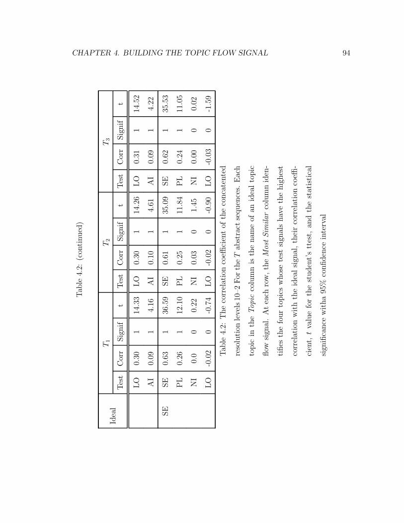
CHAPTER 4. BUILDING THE TOPIC FLOW SIGNAL 94
Tab
le4.
2:(c
onti
nued
)
Idea
lT
1T
2T
3
Tes
tC
orr
Sig
nif
tTes
tC
orr
Sig
nif
tTes
tC
orr
Sig
nif
t
LO
0.30
114
.33
LO
0.30
114
.26
LO
0.31
114
.52
AI
0.09
14.
16A
I0.
101
4.61
AI
0.09
14.
22
SE
SE
0.63
136
.59
SE
0.61
135
.09
SE
0.62
135
.53
PL
0.26
112
.10
PL
0.25
111
.84
PL
0.24
111
.05
NI
0.0
00.
22N
I0.
030
1.45
NI
0.00
00.
02
LO
-0.0
20
-0.7
4LO
-0.0
20
-0.9
0LO
-0.0
30
-1.5
9
Tab
le4.
2:T
he
corr
elat
ion
coeffi
cien
tof
the
conca
tente
d
reso
luti
onle
vel
s10
–2For
the
Tab
stra
ctse
quen
ces.
Eac
h
topic
inth
eTopic
colu
mn
isth
enam
eof
anid
ealto
pic
flow
sign
al.
At
each
row
,th
eM
ost
Sim
ilar
colu
mn
iden
-
tifies
the
four
topic
sw
hos
ete
stsi
gnal
shav
eth
ehig
hes
t
corr
elat
ion
wit
hth
eid
ealsi
gnal
,th
eir
corr
elat
ion
coeffi
-
cien
t,t
valu
efo
rth
est
uden
t’s
ttes
t,an
dth
est
atis
tica
l
sign
ifica
nce
wit
ha
95%
confiden
cein
terv
al

CHAPTER 4. BUILDING THE TOPIC FLOW SIGNAL 95
Tab
le4.
3:C
orre
lati
onbet
wee
nth
eco
nca
tenat
edid
eal
and
test
sign
als
for
the
Nab
stra
ctse
quen
ces
(con
tinued
onnex
tpag
e)
Idea
lN
1N
2N
3
Tes
tC
orr
Sig
nif
tTes
tC
orr
Sig
nif
tTes
tC
orr
Sig
nif
t
AI
AI
0.49
117
.76
AI
0.44
115
.44
AI
0.47
117
.06
LO
0.38
113
.23
LO
0.34
111
.69
LO
0.38
112
.95
PL
0.15
14.
95P
L0.
121
3.99
PL
0.15
15.
02
LG
0.05
61
1.78
CL
0.09
71
3.10
CL
0.08
12.
51
CL
CL
0.75
136
.45
CL
0.73
133
.88
CL
0.73
134
.17
LG
0.16
15.
12LG
0.15
14.
78LG
0.15
14.
77
AI
-0.0
61
-2.0
4A
I-0
.015
0-0
.47
AI
-0.0
20
-0.6
5
LO
-0.1
31
-4.1
2LO
-0.0
961
-3.0
9LO
-0.1
11
-3.4
7
CC
CC
0.60
123
.81
CC
0.61
124
.83
CC
0.62
125
.17
DS
0.34
111
.45
DS
0.35
111
.94
DS
0.34
111
.60
CG
0.29
19.
62C
G0.
301
9.92
CG
0.30
19.
85
LO
0.12
13.
94LO
0.1
13.
5LO
0.13
14.
23
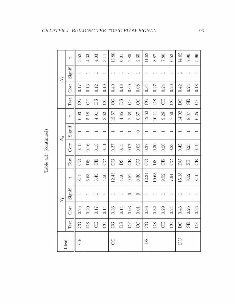
CHAPTER 4. BUILDING THE TOPIC FLOW SIGNAL 96
Tab
le4.
3:(c
onti
nued
)
Idea
lN
1N
2N
3
Tes
tC
orr
Sig
nif
tTes
tC
orr
Sig
nif
tTes
tC
orr
Sig
nif
t
CE
CG
0.25
18.
15C
G0.
191
6.03
CG
0.17
15.
52
DS
0.20
16.
63D
S0.
161
5.18
CE
0.13
14.
33
CE
0.17
15.
45C
E0.
151
4.91
DS
0.12
14.
03
CC
0.14
14.
50C
C0.
111
3.62
CC
0.10
13.
11
CG
CG
0.36
112
.43
CG
0.37
112
.57
CG
0.40
113
.80
DS
0.14
14.
50D
S0.
151
4.85
DS
0.18
16.
01
CE
0.03
00.
82C
E0.
071
2.38
CE
0.09
12.
85
CC
0.01
00.
30C
C0.
020
0.67
CC
0.08
12.
65
DS
CG
0.36
112
.34
CG
0.37
112
.62
CG
0.34
111
.63
DS
0.32
110
.63
DS
0.30
110
.11
DS
0.27
18.
87
CE
0.29
19.
52C
E0.
281
9.26
CE
0.24
17.
80
CC
0.24
17.
94C
C0.
231
7.50
CC
0.20
16.
52
DC
DC
0.43
115
.18
DC
0.42
114
.92
DC
0.42
114
.62
SE
0.26
18.
52SE
0.25
18.
37SE
0.24
17.
90
CE
0.25
18.
10C
E0.
191
6.25
CE
0.18
15.
96

CHAPTER 4. BUILDING THE TOPIC FLOW SIGNAL 97
Tab
le4.
3:(c
onti
nued
)
Idea
lN
1N
2N
3
Tes
tC
orr
Sig
nif
tTes
tC
orr
Sig
nif
tTes
tC
orr
Sig
nif
t
PL
0.09
51
3.06
PL
0.10
13.
24P
L0.
081
2.47
LG
LG
0.25
18.
22LG
0.28
19.
18LG
0.26
18.
57
CL
0.16
15.
33C
L0.
211
6.90
CL
0.19
16.
27
AI
0.05
11.
72A
I0.
071
2.26
AI
0.05
01.
60
DS
0.01
00.
32D
S-0
.01
0-0
.31
DS
0.00
00.
06
LO
LO
0.61
124
.55
LO
0.59
123
.08
LO
0.60
123
.83
AI
0.37
112
.76
AI
0.33
111
.15
AI
0.35
111
.79
PL
0.28
19.
42P
L0.
321
10.9
0P
L0.
331
11.1
5
CC
0.17
15.
45C
C0.
151
4.86
CC
0.13
14.
36
NI
NI
0.79
140
.58
NI
0.78
140
.28
NI
0.79
140
.52
DC
0.40
113
.74
DC
0.38
113
.06
DC
0.39
113
.48
CE
0.18
15.
94C
E0.
171
5.68
CE
0.19
16.
35
DS
-0.0
150
-0.4
7D
S-0
.01
0-0
.18
DS
0.01
00.
28
PL
PL
0.47
117
.01
PL
0.48
117
.29
PL
0.47
117
.19
SE
0.30
110
.15
SE
0.31
110
.50
SE
0.33
111
.11

CHAPTER 4. BUILDING THE TOPIC FLOW SIGNAL 98
Tab
le4.
3:(c
onti
nued
)
Idea
lN
1N
2N
3
Tes
tC
orr
Sig
nif
tTes
tC
orr
Sig
nif
tTes
tC
orr
Sig
nif
t
LO
0.17
15.
62LO
0.25
18.
15LO
0.19
16.
10
AI
0.14
14.
48A
I0.
171
5.65
AI
0.11
13.
66
SE
SE
0.49
117
.88
SE
0.47
117
.12
SE
0.49
118
.14
PL
0.38
113
.018
PL
0.37
112
.77
PL
0.38
113
.05
CL
0.02
00.
70LO
0.02
00.
58LO
0.00
0-0
.04
NI
-0.0
10
-0.2
9N
I-0
.01
0-0
.35
NI
0.00
00.
06
Tab
le4.
3:T
he
corr
elat
ion
coeffi
cien
tof
the
conca
tente
d
reso
luti
onle
vel
s10
–2For
theN
abst
ract
sequen
ces.
Eac
h
topic
inth
eTopic
colu
mn
isth
enam
eof
anid
ealto
pic
flow
sign
al.
Atea
chro
w,th
eM
ost
Sim
ilar
colu
mn
iden
-
tifies
the
four
topic
sw
hos
ete
stsi
gnal
shav
eth
ehig
hes
t
corr
elat
ion
wit
hth
eid
ealsi
gnal
and
thei
rco
rrel
atio
nco
-
effici
ent,
tva
lue
for
the
studen
t’s
ttes
t,an
dst
atis
tica
l
sign
ifica
nce
wit
hin
a95
%co
nfiden
cein
terv
al.

CHAPTER 4. BUILDING THE TOPIC FLOW SIGNAL 99
The effect of sharing training documents is also evident in the N sequence results
in Table 4.3 where the categories sharing the highest proportion of documents with
a category C are always among the top four signals most similar to C ’s ideal signal.
The N sequence results also reveal the effect of topic word lists with insufficiently
many words and categorization that is inconsistent with that of the training set.
The sequence has a generally lower correlation than the T sequences: only 10 out
of the 12 categories have a high or medium correlation with their corresponding
test signal, and 2 ideal signals (for CE and DS) were most similar to the test signal
of a different topic. We suspect this is due to a combination of factors, including
training set size, multi-topic training documents, and important keywords being
discarded from the N abstract sequences because they were not present in any
training documents.
One way to reduce the noise in the topic word lists and, consequently, in the
topic flow signals, is to extract the lists from a training set with a high proportion
of single-category documents. The number of single-category training documents in
the CoRR training set is shown in Table 4.5. The table also shows the proportion of
single-category documents to the total number of training documents for each CoRR
category. Nine of the ten categories containing the highest proportion of single-
category documents succeed in generating test topic flow signals that are highly
to moderately correlated with the corresponding ideal signal. The three categories
containing the lowest proportion of single-category documents all generate test
signals that are at best weakly correlated with the corresponding ideal signal.
The correlation values we have seen so far show that our approach for generating
topic flow signals succeeds in creating signals that reflect the flow of the topic in
the text. However, these correlations between the concatenated signals incorporate
noise from all resolution levels. Such noise causes the overall correlation to be lower

CHAPTER 4. BUILDING THE TOPIC FLOW SIGNAL 100
Mai
nTop
ic1st
co-t
opic
2nd
co-t
opic
3rd
co-t
opic
TO
PIC
trai
nin
gto
pic
docs
topic
docs
topic
docs
CL
194
AI
18LG
17SE
,PL,L
O,C
C,&
DS
1
CC
100
DS
19A
I9
LO
&LG
7
SE
38P
L13
AI
3LO
&D
S2
CG
62D
S5
AI
2SE
&N
I1
NI
25D
C6
CC
3D
S2
DC
41P
L&
DS
6LG
5A
I4
AI
160
LO
54LG
21C
L18
PL
76LO
29SE
13A
I10
LO
130
AI
54P
L29
CC
7
DS
90C
C19
CE
8A
I&LG
6
LG
61A
I21
CL
17C
C7
CE
23D
S8
CC
5A
I3
Tab
le4.
4:T
he
num
ber
oftr
ainin
gdocu
men
tsbel
ongi
ng
toea
chof
our
12to
pic
s,an
dth
em
ost
freq
uen
tly
co-o
ccuri
ng
cate
gori
esin
the
trai
nin
gdocu
men
tsfo
rea
chca
tego
ry.
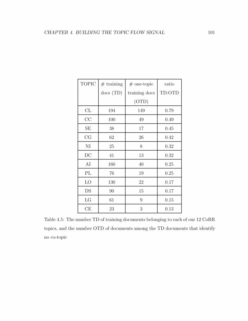
CHAPTER 4. BUILDING THE TOPIC FLOW SIGNAL 101
TOPIC # training # one-topic ratio
docs (TD) training docs TD:OTD
(OTD)
CL 194 149 0.79
CC 100 49 0.49
SE 38 17 0.45
CG 62 26 0.42
NI 25 8 0.32
DC 41 13 0.32
AI 160 40 0.25
PL 76 19 0.25
LO 130 22 0.17
DS 90 15 0.17
LG 61 9 0.15
CE 23 3 0.13
Table 4.5: The number TD of training documents belonging to each of our 12 CoRR
topics, and the number OTD of documents among the TD documents that identify
no co-topic

CHAPTER 4. BUILDING THE TOPIC FLOW SIGNAL 102
than the correlation between the test and ideal signals at individual resolution levels.
For example, the correlation between the test and ideal concatenated Learning
signals is 0.63 in the T1 text, yet the correlation between the individual levels 2–10
in this text are 0.76, 0.82, 0.75, 0.71, 0.69, 0.65, 0.61, 0.55, and 0.47, respectively.
This higher correlation can be observed for all topics in all 6 sequences. Table 4.6
for example shows the four most correlated test signals for each ideal signal at
resolution level 5.
Table 4.6: Top Four Correlated Test Topics for each Ideal
Signal at Resolution Level 5 in the T1 Text
Ideal Test Corr Signif t
AI AI 0.86 1 18.75
LO 0.60 1 8.51
PL 0.31 1 3.72
SE 0.08 0 0.91
CL CL 0.92 1 26.68
LG 0.28 1 3.25
CG -0.23 1 -2.71
NI -0.25 1 -2.86
CC CC 0.80 1 15.23
DS 0.31 1 3.67
CG 0.20 1 2.31
CE 0.13 0 1.52
SE SE 0.73 1 12.07
PL 0.24 1 2.81
NI 0.11 0 1.20

CHAPTER 4. BUILDING THE TOPIC FLOW SIGNAL 103
Table 4.6: (continued)
Ideal Test Corr Signif t
CE 0.03 0 0.35
CE CE 0.68 1 10.44
DS 0.42 1 5.14
CG 0.21 1 2.47
CC 0.16 1 1.79
CG CG 0.78 1 13.82
DS 0.25 1 2.95
CC 0.18 1 2.01
CE 0.10 0 1.15
DS DS 0.75 1 12.64
CE 0.62 1 8.83
CG 0.35 1 4.17
NI 0.28 1 3.23
DC DC 0.81 1 15.34
NI 0.49 1 6.30
CE 0.17 1 1.92
LG 0.16 1 1.86
LG LG 0.71 1 11.47
CL 0.24 1 2.80
NI 0.10 0 1.18
DC 0.06 0 0.64
LO LO 0.76 1 13.06
AI 0.56 1 7.53
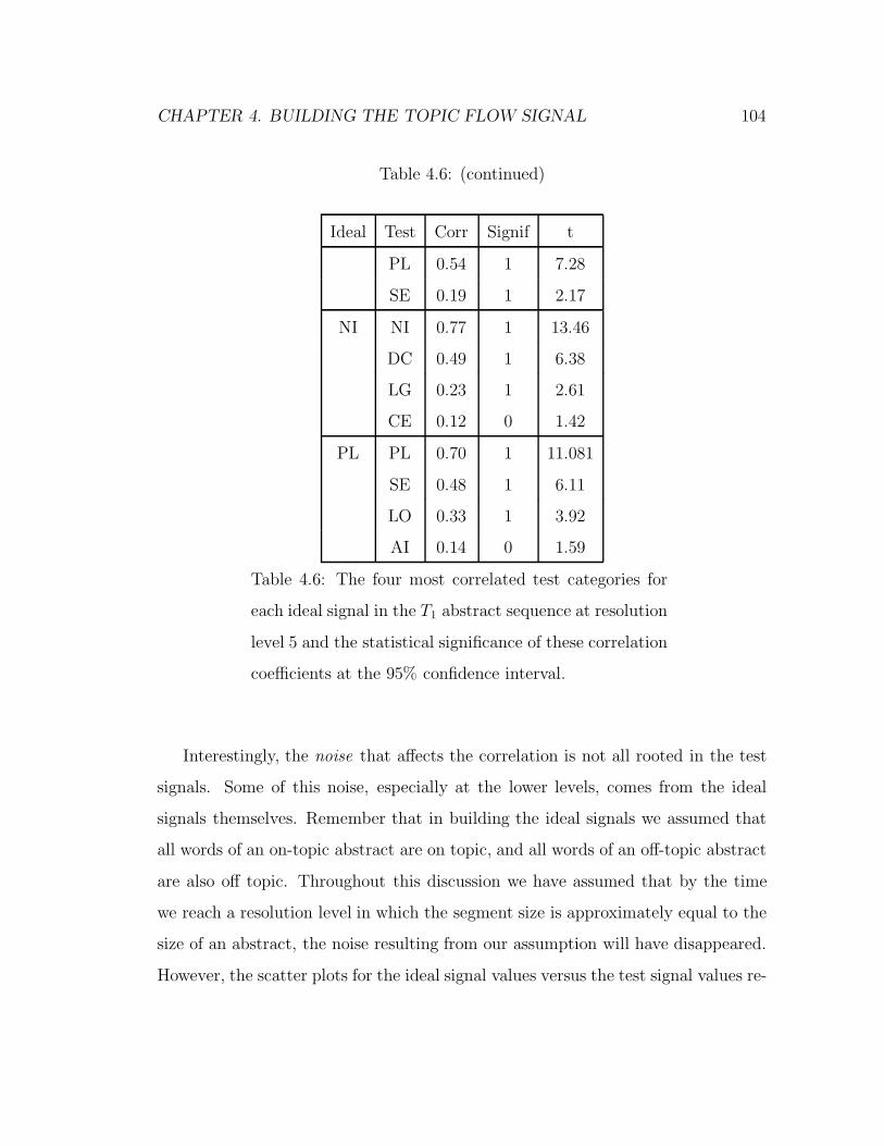
CHAPTER 4. BUILDING THE TOPIC FLOW SIGNAL 104
Table 4.6: (continued)
Ideal Test Corr Signif t
PL 0.54 1 7.28
SE 0.19 1 2.17
NI NI 0.77 1 13.46
DC 0.49 1 6.38
LG 0.23 1 2.61
CE 0.12 0 1.42
PL PL 0.70 1 11.081
SE 0.48 1 6.11
LO 0.33 1 3.92
AI 0.14 0 1.59
Table 4.6: The four most correlated test categories for
each ideal signal in the T1 abstract sequence at resolution
level 5 and the statistical significance of these correlation
coefficients at the 95% confidence interval.
Interestingly, the noise that affects the correlation is not all rooted in the test
signals. Some of this noise, especially at the lower levels, comes from the ideal
signals themselves. Remember that in building the ideal signals we assumed that
all words of an on-topic abstract are on topic, and all words of an off-topic abstract
are also off topic. Throughout this discussion we have assumed that by the time
we reach a resolution level in which the segment size is approximately equal to the
size of an abstract, the noise resulting from our assumption will have disappeared.
However, the scatter plots for the ideal signal values versus the test signal values re-

CHAPTER 4. BUILDING THE TOPIC FLOW SIGNAL 105
veal that this noise takes one or two more levels before it dissipates (see Figure 4.12.
These scatter plots show for each value in the ideal signal at a specific resolution
level all the values in the corresponding positions in the test signal at the same
level of resolution. For example, the ideal signal of Computation and Language at
resolution level 10 has the value 77.175 at two points in the signal: point number
3 and number 213. At these points the test signal has the values 127.0625 and
122.6375, respectively.
Figure 4.12 shows the scatter plot of the Computation and Language ideal signal
versus the test signal at resolution levels 2–10. The plot shows the linear relation-
ship between the ideal and test signals for this category. In general, when the ideal
signal is low, so is the test signal. The range of the test signal values that corre-
spond to a specific ideal signal value is also generally narrow except at the extremes
1 and 278. These extremes correspond to the lowest possible and the highest pos-
sible ranks for the Computation and Language category. A segment at resolution
level as high as 10 can only have such extreme values if all its words have the same
extreme values, and the only case where this occurs is in the ideal signal when the
segment is all on-topic or all off-topic. The test signal, on the other hand, cannot
have such a value in most cases since some of the words in an on-topic abstract
will undoubtedly be off-topic, and some of the words in an off-topic abstract may
appear to be on-topic. The ratio of on-topic words in the abstract affect its overall
average rank therefore creating a wide range of possible values, which plays a role in
lowering the correlation between the test and ideal signals at this resolution level.

CHAPTER 4. BUILDING THE TOPIC FLOW SIGNAL 106
0 50 100 150 200 250 30040
60
80
100
120
140
160
180
200
220
240Scatter Plot− Computation and Language
ideal values
test
val
ues
resolution lev 10resolution lev 9 resolution lev 8 resolution lev 7 resolution lev 6 resolution lev 5 resolution lev 4 resolution lev 3
Figure 4.12: The Computation and Language scatter plot of resolution levels 10–2
for the ideal and test signals in the T1 abstract sequence.
CHAPTER 4. BUILDING THE TOPIC FLOW SIGNAL 107
4.4 Conclusions
In this chapter we have shown how to construct signals that represent the flow of
topics in text. We started with a basic algorithm to construct word-based topic
flow signals. Next, we presented an averaging algorithm that allows us to use the
word-based topic flow signals in viewing the flow of topics in various sized segments
of text. Finally, we tested the quality of the topic flow signals and showed that
given a good topic word list, our algorithm is able to represent the flow of the topic
accurately. Our experiments also revealed that the quality of the topic flow signal
is dependent upon the quality of the topic word list, which in turn is dependent
upon the training set used to create the list. In the future we propose to study the
effect of varying the proportion of single-category documents in the training set on
the quality of the topic word lists and on the generated topic flow signals. We also
propose to experiment with the effect of different smoothing methods on the topic
flow signal. In particular, we would like to reduce the oscillation found in off-topic
segments thus reducing noise in these segments and clarifying the topic flow.
Topic flow signals provide a versatile representation of text content. An im-
portant distinction between our topic flow signals and other work in fields such as
text segmentation is that each individual point in the topic flow signal represents
the relevance of an individual segment in the text independent of the rest of the
text. This relevance is measured using our unique topic relevance measure MDFn
described in the previous chapter. This is quite different from the plots used in
segmentation by TextTiling [Hea97], for example, where each point in the plot rep-
resents the similarity between two consecutive segments. Our signals are meant to
represent the content of the text in such a way that they can be used for a variety
of applications including text segmentation, topic detection, topic tracking, and

CHAPTER 4. BUILDING THE TOPIC FLOW SIGNAL 108
document visualization.
In the next chapter we present one possible application for topic flow signals in
text categorization.
Chapter 5
An Application to Text
Categorization
The view of text as a sequence of topics can be beneficial for retrieval tasks that rely
on text content and on similar tasks such as text summarization, text segmentation,
document clustering, and text categorization. This chapter examines the benefits of
topic spread for text categorization. We first define text categorization and present a
general categorization model. Next, we describe Support Vector Machines, a state-
of-the-art categorization method, and show how we can improve its performance
through the use of topic words and topic distribution in text.
109

CHAPTER 5. AN APPLICATION TO TEXT CATEGORIZATION 110
5.1 Text Categorization
5.1.1 Definition and Applications
Text categorization systems group text data under a pre-specified set of labels or
categories. Applications of automatic text categorization are numerous [DPHS98],
the most obvious of which is automating manually categorized databases such as
Yahoo!’s and Infoseek’s. Automation provides a more consistent, less expensive,
and more efficient categorization. Another useful application is text filtering where
the system learns the user’s interests, then filters incoming documents or emails that
fall under categories deemed interesting to the user. In addition, automatic text
categorization can make large amounts of data more manageable, it may be used to
browse the data by topic, to search only data that belongs to certain categories, or to
view search results by category rather than viewing them as long lists of documents
(e.g. [CD00] [Hea94b]). But the applicability of text categorization is dependent
on its effectiveness and robustness against noisy real-life data. To this end, many
approaches have been proposed, each with its own advantages and disadvantages.
These systems share a common general model that we describe next.
5.1.2 Preprocessing
The input to a text categorization system is a set of categories and the document
to be categorized, and the output is the subset of categories most relevant to the in-
put text. But since text comes in many different formats and contains significantly
more information than the categorizer requires, the input document is usually pre-
processed before being passed through the classifier. The tokenization, stopword
removal, and stemming steps discussed in detail in Section 3.3.2 apply here.

CHAPTER 5. AN APPLICATION TO TEXT CATEGORIZATION 111
5.1.3 Document Representation
Once the input text is tokenized and stemmed and stopwords are removed, the text
must be converted to a representation that is acceptable to the categorizer. In the
most common representation, each document is represented by a vector in which
every dimension is associated with a unique feature and the value of the feature
represents its weight in the text. The method used to calculate the feature’s weight
varies, but in general the weight is meant to reflect the dominance of that feature in
the document. Many researchers (see for example [van79, BYRN99, SM83, MN98])
experimented with words as document features where each word is weighted by pure
term frequency, by the binary value of occurrence in the document, or by the tf*idf
function:
Wtf∗idf(wi) = TF (wi) ∗ log(|D|
DF (wi)) (5.1)
where:
• wi is a word in the document.
• TF (wi) is the term frequency of wi in the document.
• |D| is the number of documents in the training set.
• DF (wi) is the document frequency of the word wi.
Using term frequency has generally been found to perform better than binary
feature weights, but the extent of this improvement is influenced by the classification
method and the database used [MN98] [MS99] [Joa02].
To take a simple example, let us assume that our categorizer has the vocabu-
lary: bank, commerce, and money, and that our input text after tokenization and

CHAPTER 5. AN APPLICATION TO TEXT CATEGORIZATION 112
bank money commerce
a b 0
b
a
commerce
bank
money
D:
D
Figure 5.1: A vector representing a sample document D which consists of the terms
bank and money with term weights a and b respectively.
stemming consists of the words bank and money. Then the vector representation
of the document is shown in Figure 5.1 where a and b are the weights of bank and
money in the input text.
5.1.4 Document Classification
Now the input is ready to be forwarded to the categorizer. Before the system can
categorize documents, however, it needs to model each category in the category set.
One method to achieve this is supervised learning.
Supervised learning involves training the system using pre-labeled data. The
labels of the data reflect each document’s categories and are usually prepared by a
human and assumed to be correct. From this data, the system identifies criteria that
distinguish documents belonging to a category from those under other categories.

CHAPTER 5. AN APPLICATION TO TEXT CATEGORIZATION 113
Once the training phase is done, the categorizer is ready to accept and categorize
unlabeled input documents.
In binary text classification, supervised learning approaches are presented with
a set of training documents each labeled by humans as either positive or negative
examples of the category. The system creates from the given training data an
approximation function that represents the criteria distinguishing between positive
and negative training examples for that category. The learned model becomes
the classifier for the category and is used to label previously unseen documents
as either belonging to the category or not. For more than one category, several
binary classifiers are built, one for each category. If the documents can be multi-
labeled then each classifier makes its own independent decision of whether the
document belongs to its category. In some cases, however, each document is allowed
only a single label. One possible approach in this case is to attach a confidence
level with each category label for the document and allow only the label with
the highest confidence [Joa02]. Examples of these supervised learning systems are
the Rocchio algorithm [LSCP96], the Naive Bayes algorithm [Lew98], and Support
Vector Machines [Joa98b].
This general approach is shown in Figure 5.2. There are other variations of this
architecture. For instance, some categorizers skip the learning stage and represent a
category directly by its training documents. This is called lazy learning. In this type
of learning the system does minimal work, or none at all, during the training stage.
Instead, it compares incoming (unlabeled) input documents directly to the training
data. The most prominent example in this class is K-Nearest Neighbor [Mit97].
Of these categorization methods, Support Vector Machines (SVMs) have been
found to perform as well as or better than most other categorization systems
(e.g. [Joa02, YL99, Coo99]). In what follows we will discuss the basics of SVMs fol-
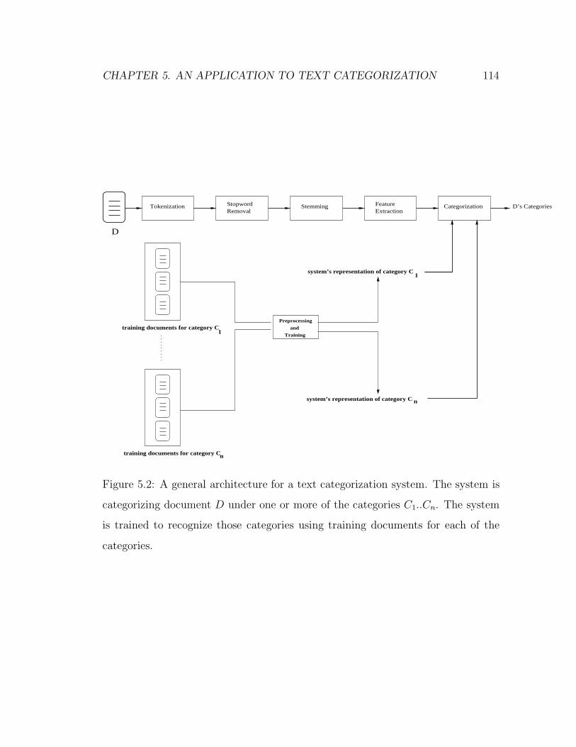
CHAPTER 5. AN APPLICATION TO TEXT CATEGORIZATION 114
and
Training
Preprocessing
nsystem’s representation of category C
training documents for category Cn
training documents for category C1
system’s representation of category C1
StemmingRemovalStopword
D
CategorizationFeatureExtraction
Tokenization D’s Categories
Figure 5.2: A general architecture for a text categorization system. The system is
categorizing document D under one or more of the categories C1..Cn. The system
is trained to recognize those categories using training documents for each of the
categories.

CHAPTER 5. AN APPLICATION TO TEXT CATEGORIZATION 115
lowing the description of Joachims [Joa02], then explore the effect of replacing the
traditional documents-as-bags-of-words vectors with representations which reflect
the distribution of topics in the document.
5.2 Text Categorization with Support Vector Ma-
chines
The simplest type of SVMs are Linear Support Vector Machines. Linear SVMs
create a hyperplane separating positive examples from negative ones. In placing
these hyperplanes, SVMs attempt to maximize the distance between the negative
and positive examples closest to the hyperplances which in turn minimizes the
error. The distance between the negative and positive examples closest to the
hyperplane is called the margin, while the closest training examples themselves are
called support vectors. The separating hyperplane that maximizes the margin δ
is described by a weight vector �w and the maximum margin δ. Given this plane,
the resulting classification function requires that a document �x is relevant to the
category if (�w�x + b) > 0. Figure 5.3(a) shows an example of a set of training
examples that can be separated by a hyperplane with margin δ.
An indication of the expressiveness of an SVM is its VC-dimension (VCdim).
When a VCdim of a model is too small the model is likely to overfit the data
creating too many false negatives, but a VCdim that is too large may indicate that
the model is too simple and the classifier may tend to over-generalize which means
the classifier tends to generate too many false positives. Joachims reports that
Vapnik [Joa02] showed that the hyperplane with the optimum VCdim is the one
with the largest distance from the closest training examples.

CHAPTER 5. AN APPLICATION TO TEXT CATEGORIZATION 116
SVMs that separate all positive examples from all negative ones are called Hard-
margin SVMs. In some cases it is not possible to find such a hyperplane. In this
case, it is possible to soften the condition of separation and allow some training
examples to be on the wrong side of the hyperplane for some cost C . These SVMs
are called Soft-margin SVMs. Sometimes there are many more positive examples
than negative ones or vice versa, in which case it may be desirable to assign two
different costs C and C ′ for each type of example to avoid putting more emphasis
on avoiding errors in assigning the more frequent type of examples.
Yet in other cases the training data may not be linearly separable. Figure 5.3(b)
shows one such example. SVMs solve this problem by using seed functions, called
Kernel functions, which succeed in mapping the data from the non-linear space into
a much simpler linear space for training. More specifically, the kernel functions map
the data from the original space into a high-dimensional space via implicit basis
expansion. Once the classifier is created, the same kernel function is used to map
test documents into the linear space before they can be classified. Examples of
popular kernels used in SVMs are polynomials (POLY) and radial basis functions
(RBF). For example, a document with two features x1 and x2 in the non-linear
space can be mapped onto a linear space using the polynomial kernel with degree d:
Kpoly( �x1, �x2) = (s. �x1. �x2 + r)d, or the RBF kernel Krbf ( �x1, �x2) = exp−γ( �x1 − �x2)2,
where the values r,s, d, and γ can be set by the user of the SVM learner. A
more detailed description of SVMs and their parameters can be found in Joachims’
dissertation [Joa02].

CHAPTER 5. AN APPLICATION TO TEXT CATEGORIZATION 117
δ
δ
δ
δ
H
+
+
+
+
-
--
-
-
+
+
+
(a)
y
x
++
++
++
+
+
++
+
+
+
+
-
--
-
-
+
+
+
(b)
Figure 5.3: (a) An example of a linear data set with a linear hyperplane �H sepa-
rating the positive and negative examples with a margin δ. (b) A nonlinear data
set which cannot be separated by a linear hyperplane.
5.2.1 Model Selection
Given a SVM and a training set, our mission is to generate a good classifier based on
this training data. It is possible that several different kernels and many variations
of parameter values can generate a classifier. Unfortunately, there is no automatic
way to select the one that will generate the best performance on unseen documents.
Rather, to choose between these classifiers we follow the algorithm described by
Joachims [Joa02], in which we first select the set of parameters and variables we
would like to consider. For each combination of these values, we calculate an
estimate of the expected performance using the training data and choose the model
with the best estimate.
Joachims [Joa02] tested the effectiveness of two different estimates in predict-
ing classifier performance, and determined that the Leave-One-Out Precision Recall
CHAPTER 5. AN APPLICATION TO TEXT CATEGORIZATION 118
Break Even Point(BEPloo) is most effective. In leave-one-out cross-validation esti-
mation, the system trains on n−1 training examples and then tests its performance
on the remaining document and records whether it succeeded in predicting the class
of the document. The same process is repeated n times until all the training doc-
uments have been used to test the classifier’s performance. Finally, the results are
used to calculate the classifier’s leave-one-out estimation of the precision and recall,
whose arithmatic mean is the BEPloo for this model.
5.3 Using Topic Distribution in Documents with
Support Vector Machines
5.3.1 Previous Work
SVM expects training documents to be represented as weighted vectors of features.
Many researchers experimented with SVMs using words as document features where
each word is weighted by pure term frequency, by the binary value of occurrence
in the document, or by the tf*idf function [Joa02, YL99]. But the definition of a
feature does not have to be a word; it can be any datum that helps distinguish
documents belonging to a category from all other documents. Among the other
interesting features studied are those suggested by Bekkerman et al. [BEYTW03],
where documents are represented by vectors of semantically similar word clusters
generated automatically using the Information Bottleneck approach (IB) [TPB99].
Initially, each word is labeled by the classes in which it occurs. The main idea
behind IB is to cluster words with minimal loss of the mutual information between
the words and the class labels, thus maximizing:

CHAPTER 5. AN APPLICATION TO TEXT CATEGORIZATION 119
I(CW , L) − βI(CW , W ) (5.2)
where:
• W is the set of labeled words.
• CW are the clusters created from W .
• L is the set of all labels.
• I(CW , L) (I(CW , W )) is the mutual information of CW and L (CW and W ).
• β is the factor controlling the allowed amount of reduction in mutual infor-
mation caused by clustering W into CW .
Bekkerman et al. compare this cluster-based SVM to the TF*IDF SVM which
uses tf*idf weights with and without feature selection. Their tests show a 0 − 3%
improvement in the microaveraged BEP over the tf*idf SVM using the ten most
frequent categories in the Reuters21578 database [REU].
Word clustering has also been used by Cristiani et al. to group words by their
co-occurrence statistics through what is called the Latent Semantic Kernels. The
features in this approach are still the document words, but the Latent Semantic
Kernels create a map between individual words and a cluster of semantically related
words. Unfortunately, tests using the Reuters21578 database did not result in an
improved performance over the linear TF*IDF SVM classifier.

CHAPTER 5. AN APPLICATION TO TEXT CATEGORIZATION 120
5.3.2 Incorporating Topic Distribution into Document Fea-
tures
Throughout this thesis we show the benefits of word spread in identifying important
topic words and in representing the relevance of topics within a document. Thus,
rather than using words as document features, one can represent documents by the
number of occurrences of the relevance rankings within the document, as defined
in Chapter 3. A document vector will thus contain a list of ranking levels each
weighted by the number of occurrences in the document. The more dominant
the category’s top ranking words are, the stronger the evidence of the document’s
relevance to the category.
To represent a document by the relevance ranking of its words to a category
we begin by replacing each word in the document by its relevance ranking. The
importance of each rank r in the document is then weighted by the number of times
the rank r occurs in that document. For example, in the previous chapter we saw
the signal for the Example 4.1.1:
Example 5.3.1 Belief revision focuses on how an agent should change her
beliefs when she adopts a particular new belief. [FH99]
In this example, four words belief, revision, beliefs, and belief have top rank 1
for category AI, while the remaining two vocabulary words agent and change have
lower ranks 33 and 78, respectively. Assuming that the maximum rank in the topic
word list for the category AI is 300, the vector representing this example with
respect to AI will have the features 1..300, with feature 1 having weight 4, features
33 and 78 having weight 1 each, and features 2..32, 34..77, and 79..300 having
weight 0 as shown in Figure 5.4. The same procedure is followed to represent the

CHAPTER 5. AN APPLICATION TO TEXT CATEGORIZATION 121
Relevance Rank
1 2 3 ... 33 ... ... 300
... ... ......
7834
4 0 0 1 0 1 0
Convert intoBag-of-Ranksrepresentation
beliefrevisionagentchangebeliefsbelief
words byReplace
ranks
1133
1178
Figure 5.4: Converting the Example 5.3.1 into the Bag-of-Ranks representation.
document with respect to another category using that category’s topic word ranks.
In this representation, relevance rankings replace words but, as with the bag-
of-words method, no position information is retained. Thus, we call this the Bag-
of-Ranks representation.
Our experiments in Chapter 3 show that word position information may be
useful in identifying better topic words. The idea behind the MDFn measure is
that when we discuss a topic, the topic’s words will spread across the length of
the text and occur in many segments of the document. The more important these
topic words and the more segments they occur in, the stronger the evidence that
the document is about the topic. Thus we can measure the spread of a rank
by the number of segments in which it occurs. Under this approach the vector
representing a document in a category T becomes a two dimensional matrix with
n rows reflecting the maximum number of segments, and R features in each row
where R is the maximum rank for category T . A feature weight for feature (i, r) is
the number of times relevance rank r occurs in at least i segments. For example if
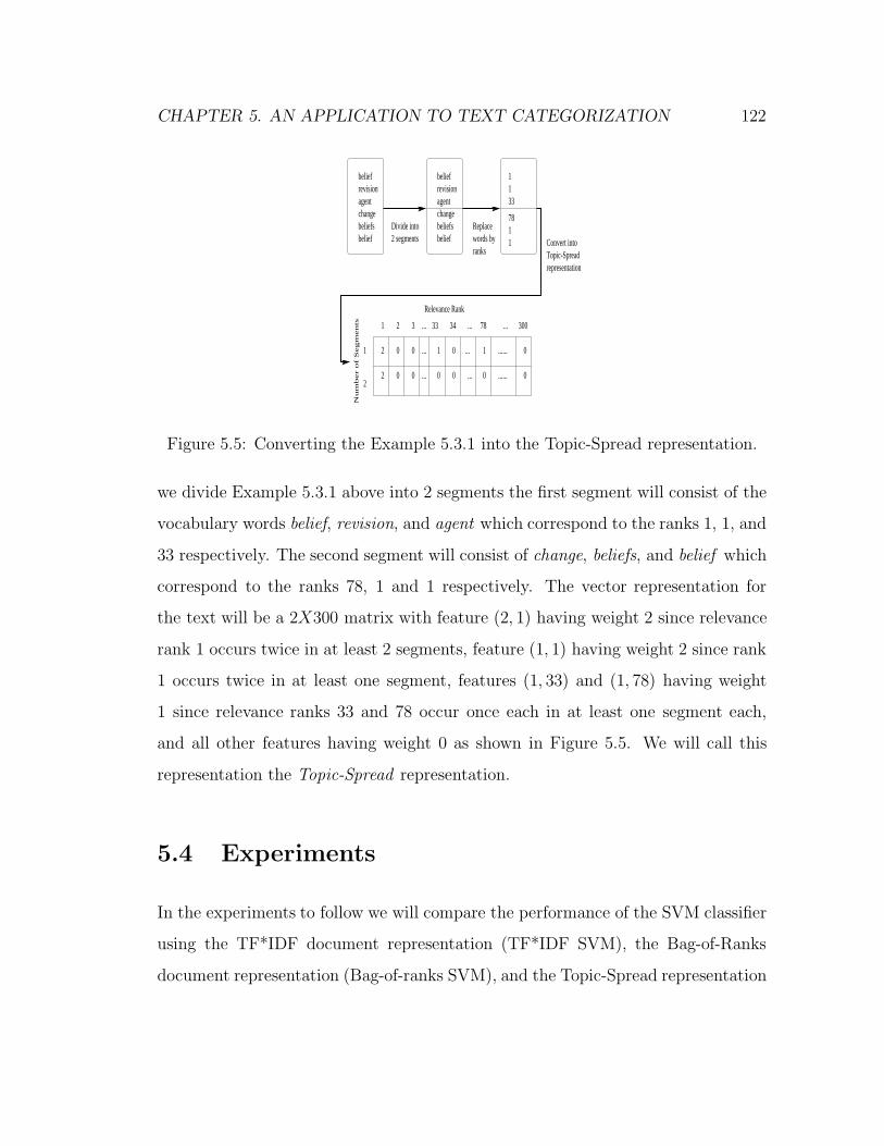
CHAPTER 5. AN APPLICATION TO TEXT CATEGORIZATION 122
0
0
0
2
2
34 78
......
......
...
...
...
...
300......33...3
0
Nu
mb
er
of
Seg
men
ts
Relevance Rank
2 segmentsDivide into
ranks
Replacewords by
0
0
0
1
0
0
0
1
2
1
2
agentrevisionbelief
beliefbeliefschangeagentrevisionbelief
1178
3311
change
1
representationTopic-SpreadConvert intobelief
beliefs
Figure 5.5: Converting the Example 5.3.1 into the Topic-Spread representation.
we divide Example 5.3.1 above into 2 segments the first segment will consist of the
vocabulary words belief, revision, and agent which correspond to the ranks 1, 1, and
33 respectively. The second segment will consist of change, beliefs, and belief which
correspond to the ranks 78, 1 and 1 respectively. The vector representation for
the text will be a 2X300 matrix with feature (2, 1) having weight 2 since relevance
rank 1 occurs twice in at least 2 segments, feature (1, 1) having weight 2 since rank
1 occurs twice in at least one segment, features (1, 33) and (1, 78) having weight
1 since relevance ranks 33 and 78 occur once each in at least one segment each,
and all other features having weight 0 as shown in Figure 5.5. We will call this
representation the Topic-Spread representation.
5.4 Experiments
In the experiments to follow we will compare the performance of the SVM classifier
using the TF*IDF document representation (TF*IDF SVM), the Bag-of-Ranks
document representation (Bag-of-ranks SVM), and the Topic-Spread representation

CHAPTER 5. AN APPLICATION TO TEXT CATEGORIZATION 123
(Topic-Spread SVM). We use Joachim’s SVM implementation SV M light [Joa98a] for
all three methods.
5.4.1 Database
We use the same training database and 12 categories as described in Section 3.3.1.
Our test documents consist of those submitted to the CoRR website between July
2001 and December 2001. These test documents were converted to text using the
same version of detex [DeT] that was used to convert the training documents. After
removing empty test documents and ones that do not belong to any of the categories
used in the training database, we are left with 142 test documents each categorized
under at least one category. Of these test documents 125 have one correct category
belonging to the 12 CoRR categories considered in our tests, 38 have two, only 2
test files have three correct categories each, and 20 do not to any of the 12 CoRR
categories considered. Table 5.1 shows the number of test files for each of the 12
categories.
5.4.2 Experimental Setup
There are 12 training sets, one for each category. For every category we begin by
preprocessing each training document as was done in Section 3.3.1. Each document
is then represented as a vector of features: For the TF*IDF SVM we use the
tf*idf function to weigh document words; while the Bag-of-Ranks SVM uses the
category’s topic word list sorted by MDF4 to replace document words by their
relevance ranking. Each ranking is then weighed by its frequency of occurrence
in the document. For the Topic-Spread method we linearize the two-dimensional
matrix into the one dimensional vector representation expected by SV M light using

CHAPTER 5. AN APPLICATION TO TEXT CATEGORIZATION 124
CATEGORY #test files
NI 2
LG 5
CE 5
SE 6
CG 7
DS 10
DC 12
LO 19
PL 21
AI 22
CC 24
CL 27
Table 5.1: The number of test files for each category

CHAPTER 5. AN APPLICATION TO TEXT CATEGORIZATION 125
row-major order, that is, by mapping each feature (n, r) in the two-dimensional
matrix to ((n ∗ 1000) + r) where: r is the rank, n is the number of segments, and
the maximum value for r is always less than 1000. Each document is then divided
into 4 segments, and rank occurrences within the document are counted using the
ranking in the sorted MDF4 topic word list for the category. Thereafter the weight
for feature (4, r) is the minimum number of occurrences of rank r in all 4 segments,
the weight for feature (3, r) is the minimum number of occurrences of rank r in at
least 3 segments, and so forth.
Once the document vectors are created for each of these methods, each vector
is normalized by its Eucledian length, and labeled in the training set as a positive
example if it belongs to the category, or as a negative example otherwise.
After the training set for each category is constructed, we move onto selecting
the best model for that category. We experimented with several different values for
the cost factor C , the factor J which adjusts the misclassification cost of positive
examples to (J∗C) while keeping the cost of negative examples to C , the polynomial
degree d, and the γ factor for the RBF kernel. For each combination of these values,
SV M light produces the leave-one-out estimate of the precision and recall. The model
that produces the highest PRAV Gloo for a category is the one we choose to classify
the test documents with respect to that category. Table 5.4.2 shows the values used
to search for the best classifier for each category. We will discuss our observations
regarding the resulting models in the results section below.
5.4.3 Evaluation Measures
Categorization systems are usually evaluated by comparing their category assign-
ments to those of humans. Two popular evaluation measures are Precision and

CHAPTER 5. AN APPLICATION TO TEXT CATEGORIZATION 126
General
Parameters
C 0, 0.05, 0.1, 0.5, 1, 5, 10, 1000
J 0.5, 1, 2, −ve+ve
Polynomial
kernel
b 1, 2, 3, 4, 5, 10
s 1
r 0
RBF kernel γ 0.01, 0.03, 0.1, 0.3, 1, 3
Table 5.2: The values used to search for the best category model for each CoRR
category. −ve+ve
is the ratio of the number of negative category examples to the
number of positive examples in the training database
category Ratio
AI 3.6
CC 6.4
CE 31
CG 10.8
CL 3.1
DC 17
DS 7.2
LG 11.3
LO 4.7
NI 28.4
PL 8.7
SE 18.4
Table 5.3: The ratio of negative to positive examples used for the J parameter.

CHAPTER 5. AN APPLICATION TO TEXT CATEGORIZATION 127
Recall. Precision is the proportion of correct categories assigned by the system
for test documents to the total number of categories the system assigns. Recall is
the proportion of correct categories assigned by the system to the total number of
categories assigned by humans.
When we are presented with several test documents we can calculate precision
by counting the number of correct categories assigned across all the test documents,
then dividing that by the total number of categories assigned by the system:
P =
∑∀d∈Test Corr S(d)∑
∀d Num(d)(5.3)
where:
• Test is the set of all test documents.
• Corr S(d) is the number of correct categories assigned by the system to test
document d.
• Num(d) is the number of categories, both correct and incorrect, assigned by
the system to test document d.
Recall can be calculated in a similar manner by dividing the number of correct
categories assigned by the system to the total number of correct categories assigned
by humans:
R =
∑∀d∈Test Corr S(d)∑
∀d Corr H(d)(5.4)
where:
• Test and Corr S(d) are as before.
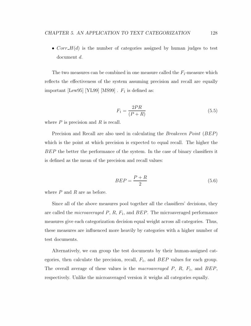
CHAPTER 5. AN APPLICATION TO TEXT CATEGORIZATION 128
• Corr H(d) is the number of categories assigned by human judges to test
document d.
The two measures can be combined in one measure called the F1-measure which
reflects the effectiveness of the system assuming precision and recall are equally
important [Lew95] [YL99] [MS99] . F1 is defined as:
F1 =2PR
(P + R)(5.5)
where P is precision and R is recall.
Precision and Recall are also used in calculating the Breakeven Point (BEP )
which is the point at which precision is expected to equal recall. The higher the
BEP the better the performance of the system. In the case of binary classifiers it
is defined as the mean of the precision and recall values:
BEP =P + R
2(5.6)
where P and R are as before.
Since all of the above measures pool together all the classifiers’ decisions, they
are called the microaveraged P , R, F1, and BEP . The microaveraged performance
measures give each categorization decision equal weight across all categories. Thus,
these measures are influenced more heavily by categories with a higher number of
test documents.
Alternatively, we can group the test documents by their human-assigned cat-
egories, then calculate the precision, recall, F1, and BEP values for each group.
The overall average of these values is the macroaveraged P , R, F1, and BEP ,
respectively. Unlike the microaveraged version it weighs all categories equally.

CHAPTER 5. AN APPLICATION TO TEXT CATEGORIZATION 129
In the experiments below we will be reporting both the microaveraged and the
macroaveraged BEP , F1, recall, and precision.
5.4.4 Results and Analysis
Model Selection
Starting with the parameter values shown in Table 5.4.2, we use SV M light [Joa98a]
to evaluate the leave-one-out BEP for each combination for each of the TF*IDF,
the Bag-of-Ranks, and the Topic-Spread methods. When two models have equal
BEP the model with the lower VC-dim is selected. The resulting models are ranked
by their BEP and the top model for every category for each method is selected.
The 12 selected models and their parameters are shown in Tables 5.4, 5.5, and 5.6.
The tables also show the kernel used in the model, the parameters that apply for
that kernel, the VC-dimension of each model as well as the leave-one-out estimate
of the precision, recall, and the BEP.
Although these models have the highest BEP values, there are several models
whose BEP is close to the top. This agrees with Joachims’ observation that there
is usually a range of classifiers that can produce similar performance [Joa02]. It is
interesting to note, however, that the TF*IDF method tends to select the linear
polynomial and the RBF kernels, whereas the Bag-of-Ranks and the Topic-Spread
methods tend to select the polynomial kernel but with varying degrees. Note also
the wide difference in the BEPloo values for the TF*IDF models which are mostly
around 70%, and those of the Bag-of-Ranks and Topic-Spread SVM’s which are
mostly around 90%. These estimates either indicate a tendency for overfitting the
data, or that the Topic-Spread and Bag-of-Ranks document representations succeed
in capturing useful information about the document content. Thus, in the presence
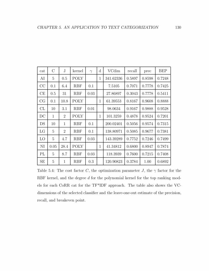
CHAPTER 5. AN APPLICATION TO TEXT CATEGORIZATION 130
cat C J kernel γ d VCdim recall prec BEP
AI 5 0.5 POLY 1 341.62336 0.5897 0.8598 0.7248
CC 0.1 6.4 RBF 0.1 7.5105 0.7071 0.7778 0.7425
CE 0.5 31 RBF 0.03 27.86897 0.3043 0.7778 0.5411
CG 0.1 10.8 POLY 1 61.39553 0.8167 0.9608 0.8888
CL 10 3.1 RBF 0.01 98.0634 0.9167 0.9888 0.9528
DC 1 2 POLY 1 101.3259 0.4878 0.9524 0.7201
DS 10 1 RBF 0.1 200.02401 0.5056 0.9574 0.7315
LG 5 2 RBF 0.1 138.80971 0.5085 0.9677 0.7381
LO 5 4.7 RBF 0.03 143.39289 0.7752 0.7246 0.7499
NI 0.05 28.4 POLY 1 41.34812 0.6800 0.8947 0.7874
PL 5 8.7 RBF 0.03 118.3939 0.7600 0.7215 0.7408
SE 5 1 RBF 0.3 120.90823 0.3784 1.00 0.6892
Table 5.4: The cost factor C , the optimization parameter J , the γ factor for the
RBF kernel, and the degree d for the polynomial kernel for the top ranking mod-
els for each CoRR cat for the TF*IDF approach. The table also shows the VC-
dimensions of the selected classifier and the leave-one-out estimate of the precision,
recall, and breakeven point.

CHAPTER 5. AN APPLICATION TO TEXT CATEGORIZATION 131
cat C J kernel γ d VCdim recall prec BEP
AI 1 3.6 POLY 5 119.80557 0.9038 0.9156 0.9097
CC 1 6.4 POLY 4 100.22017 0.9394 0.9029 0.9212
CE 0.1 31 RBF 1 57.65913 0.8261 1.00 0.9131
CG 1 2 POLY 10 25.80709 0.9000 1.00 0.9500
CL 5 1 POLY 2 74.60417 0.9896 0.9845 0.9871
DC 0.1 17 POLY 3 28.61864 0.9512 0.9070 0.9291
DS 5 2 POLY 1 240.319 0.8427 0.9615 0.9021
LG 0.5 2 POLY 3 40.23411 0.8475 0.9615 0.9045
LO 5 4.7 RBF 3 488.06805 0.8760 0.9040 0.8900
NI 1 2 RBF 3 39.90703 0.9600 1.00 0.9800
PL 5 8.7 POLY 1 379.84627 0.9733 0.7935 0.8834
SE 5 2 POLY 10 103.79613 0.9189 1.00 0.9595
Table 5.5: The cost factor C , the optimization parameter J , the γ factor for the
RBF kernel, and the degree d for the polynomial kernel for the top ranking models
for each CoRR cat for the Bag-of-Ranks approach. The table also shows the VC-
dimensions of the selected classifier and the leave-one-out estimate of the precision,
recall, and breakeven point.

CHAPTER 5. AN APPLICATION TO TEXT CATEGORIZATION 132
cat C J kernel γ d VCdim recall prec BEP
AI 1.0 2 POLY 4 101.05862 0.8974 0.9272 0.9123
CC 5 6.4 POLY 1 444.08250 0.9293 0.92 0.9246
CE 10 31 POLY 5 104.08289 0.9130 0.8750 0.894
CG 5 10.8 POLY 5 165.31334 0.9167 1.00 0.9583
CL 5 1 POLY 2 77.88067 0.9896 0.9845 0.9870
DC 5 2 POLY 5 84.34398 0.8780 1.00 0.939
DS 10 7.2 RBF 0.3 532.55819 0.8876 0.9186 0.9031
LG 0.5 2 POLY 4 39.91318 0.8475 0.9615 0.9045
LO 10 4.7 POLY 5 223.74791 0.8682 0.9032 0.8857
NI 0.5 2 POLY 5 17.32727 0.92 1.00 0.96
SE 1000 1 RBF 0.3 1094.67241 0.9189 0.9714 0.9451
PL 5 8.7 RBF 0.1 141.38082 1.00 0.75 0.875
Table 5.6: The cost factor C , the optimization parameter J , the γ factor for the
RBF kernel, and the degree d for the polynomial kernel for the top ranking models
for each CoRR cat for the Topic-Spread approach. The table also shows the VC-
dimensions of the selected classifier and the leave-one-out estimate of the precision,
recall, and breakeven point.

CHAPTER 5. AN APPLICATION TO TEXT CATEGORIZATION 133
of complete topic word lists, the two representations should produce more accurate
models than those found using the TF*IDF SVM. If, however, there is an overfitting
problem, then we expect the test results to show the recall falling behind that of
the TF*IDF method.
Table 5.7 shows the number of cpu seconds used by each method to create
the selected classification models on a shared Sun machine with 8 cpu’s and 16G
RAM running SunOS-5.8. The average time for the Topic-Spread method is 0.912
cpu-seconds which is 11% that of the TF*IDF method, while the average time for
the Bags-of-Ranks approach is 0.549 which is only 6.9% the average time for the
TF*IDF approach. Once the models are selected, they are used to classify each one
of the test documents.
Categorization Performance
The average classification time for each of the three approaches is shown in Ta-
ble 5.7. Again, the average time for the Topic-Spread and the Bag-of-Ranks ap-
proaches is much less than that for the TF*IDF method. The Topic-Spread method
has an average classification time of 1.66 cpu-seconds which is 7.4% the classification
time for the TF*IDF approach, while the Bag-of-Ranks approach has an average
classification time of 0.076 cpu-seconds which is only 3.4% the time for the TF*IDF
approach.
Table 5.8 shows the performance results on the test data. The micro and macro
averaged BEP and F1 for the Topic-Spread method are the highest among the
three methods indicating a positive effect of the DF4 frequency and the topic spread
information on classification performance. Note that this is coupled with the fact
that the Topic-Spread method and the Bag-of-Ranks method use a vocabulary

CHAPTER 5. AN APPLICATION TO TEXT CATEGORIZATION 134
cat
Cla
ssifi
cati
on
Buildin
gC
lass
ificati
on
Model
Topic
-Spre
ad
Bags-
of-ra
nks
TF*ID
FTopic
-Spre
ad
Bags-
of-R
anks
TF*ID
F
AI
0.32
0.14
2.45
1.66
0.85
8.72
CC
0.19
0.07
3.37
1.02
0.5
9.04
CE
0.08
0.12
3.18
0.57
1.55
8.98
CG
00.
011.
990.
390.
217.
73
CL
0.08
0.01
2.28
0.62
0.27
8.1
DC
0.08
0.15
1.39
0.47
0.76
6.38
DS
0.27
0.06
1.96
1.37
0.45
7.69
LG
0.18
0.09
1.72
10.
447.
17
LO
0.36
0.14
2.41
1.72
0.76
8.41
NI
0.05
0.02
2.24
0.36
0.13
8.16
PL
0.28
0.06
1.96
1.36
0.46
7.68
SE
0.1
0.04
1.94
0.41
0.21
7.69
AV
ER
AG
E0.1
66
0.0
76
2.2
41
0.9
12
0.5
49
7.9
79
Tab
le5.
7:T
he
cpu
tim
e(i
ncp
use
conds)
taken
by
each
ofth
eth
ree
met
hods
tobuild
the
sele
cted
clas
sifica
tion
model
and
tocl
assi
fyea
chof
the
12C
oRR
cate
gori
es.
All
exper
imen
tsw
ere
run
onan
8-cp
ush
ared
Sun
Spar
c
mac
hin
eru
nin
gSunO
S-5
.8.

CHAPTER 5. AN APPLICATION TO TEXT CATEGORIZATION 135
cat
TF*I
DF
Bag
sof
Ran
ks
Top
icSpre
ad
PR
BE
PF
1P
RB
EP
F1
PR
BE
PF
1
AI
0.68
70.
500.
594
0.57
90.
522
0.54
50.
534
0.53
30.
571
0.54
50.
559
0.55
8
CC
0.85
00.
708
0.77
90.
773
0.80
90.
708
0.75
90.
755
0.84
20.
667
0.75
40.
744
CE
1.0
0.20
0.60
0.33
31.
00.
200.
600.
333
0.66
70.
400.
533
0.50
CG
0.87
51.
00.
938
0.93
30.
778
1.0
0.88
90.
875
0.70
1.0
0.85
0.82
3
CL
0.92
30.
889
0.90
60.
906
0.89
30.
926
0.90
90.
909
0.92
60.
926
0.92
60.
926
DC
0.75
00.
250
0.50
0.37
50.
500.
500.
500.
500.
600.
250
0.42
50.
353
DS
0.0
0.0
0.0
0.0
0.25
00.
300.
275
0.27
30.
333
0.40
0.36
70.
364
LG
0.40
0.40
0.40
0.40
0.42
90.
600.
514
0.50
0.37
50.
600.
487
0.46
1
LO
0.66
70.
842
0.75
40.
744
0.72
20.
684
0.70
30.
703
0.70
60.
632
0.66
90.
667
NI
0.33
31.
00.
667
0.50
0.50
1.0
0.75
00.
667
0.50
1.0
0.75
00.
667
PL
0.75
00.
429
0.58
90.
545
0.68
40.
619
0.65
20.
650
0.65
00.
619
0.63
40.
634
SE1.
00.
167
0.58
30.
286
0.33
30.
167
0.25
00.
222
1.0
0.33
30.
667
0.50
mac
ro0.
686
0.53
20.
609
0.53
10.
618
0.60
40.
611
0.57
70.
656
0.61
40.
635
0.60
mic
ro0.
721
0.58
10.
651
0.64
40.
656
0.64
40.
650.
650.
682
0.63
10.
657
0.65
6
Tab
le5.
8:T
he
mic
roan
dm
acro
aver
aged
pre
cisi
on,re
call,an
dbre
akev
enpoi
nts
for
the
appro
aches
TF*I
DF,
Bag
-of-R
anks,
and
Top
ic-S
pre
ad.
The
max
imum
valu
esam
ong
allth
ree
met
hods
are
bol
dfa
ced.

CHAPTER 5. AN APPLICATION TO TEXT CATEGORIZATION 136
that is 10% the size of the vocabulary used by the TF*IDF method. The average
recall for both the Bag-of-Ranks and the Topic-Spread methods is higher than
that of TF*IDF which reflects the effect of the relevance ranking in identifying
relevant documents unrecognized by the tf*idf function. The method’s effect on
recall also makes it less likely that the high BEPloo values seen during training are
due to overfitting. Rather, it is more likely that the use of topic spread information
produces a more accurate category model than that produced using the TF*IDF
approach.
This improvement in recall is statistically significant at a 90% confidence interval
with 11 degrees of freedom. The improvement however comes at the cost of a slightly
lower precision which goes down from a macroaverage of 68.6% for TF*IDF to
61.6% for Bag-of-Ranks. Adding the topic word spread information in the Topic-
Spread method manages to compensate for most of that lost precision bringing the
macroaverage up to 65.6%. The effect on the microaveraged precision and recall is
similar. The overall BEP and F1 values are statistically insignificant at the 90%
confidence interval.
The TF*IDF method’s macroaveraged BEP of 0.609 is close to the estimated
BEPloo of 0.689 in Table 5.4. Unlike the TF*IDF method, however, the overall BEP
for the Topic-Spread and the Bag-of-Ranks methods are quite different from those
predicted from the training set falling from an estimated macroaveraged BEPloo of
0.924 and 0.919 seen in Tables 5.5 and 5.6, respectively, to a BEP macroaverage of
0.63 and 0.611. This difference is probably due to the coverage of the MDF4 topic
word list which was created from multi-labeled training documents thus introducing
noise within the lists and adversely affecting the quality of the vector representations
for the two methods. Nevertheless, the resulting classifiers still perform at least as
well as the TF*IDF method, while using only 10% the vocabulary size used by
CHAPTER 5. AN APPLICATION TO TEXT CATEGORIZATION 137
TF*IDF SVM.
5.5 Conclusions
This chapter presents text categorization as one possible application for the topic
spread and topic relevance methods discussed in the previous chapters. It proposes
document representations based on topic relevance rankings (Bag-of-Ranks) and
the distribution of these rankings within the document (Topic-Spread). Our tests
show that the two representations produce small improvements in performance over
the SVM which uses the traditional tf*idf vector representation even though they
use a vocabulary size that is only 10% the size of the vocabulary used by the tf*idf
vector representation. The proposed methods also reduce the model creation time
to as little as 6.9% the average time for the TF*IDF approach, and the classification
time to 3.4% the average classification time for the TF*IDF approach.
The experiments in this chapter explore the effect of using the MDF4 topic
word lists for the Bag-of-Ranks and the Topic-Spread representations. It would
be interesting to investigate the effect of using topic word lists produced by MDFn
for n > 4. Similarly, we would like to study the effect of increasing the maximum
number of segments n used in the Topic-Spread approach.
We suspect that the use of multi-labeled documents for creating the topic-word
lists has affected the quality of the results by introducing into the lists topic words
that are relevant to frequently co-occurring categories. It would be interesting to
look at the change in performance resulting from restricting training documents to
those with single labels only.

Chapter 6
Conclusions and Future Work
This work originated from our experience with the Jabber project [KAHHM96].
The project was aimed at indexing videoconferences by several aspects including
content of discussion, meeting agenda, and the forms of interaction between par-
ticipants. Our work in the project highlighted the importance of the temporal
positioning of words in tracking content. Word position information can be useful
for tasks requiring local content analysis such as topic flow identification, as well
as for passage retrieval, text summarization and segmentation.
In this thesis we presented two methods to utilize word position in text: topic
word selectors and topic flow signals. The topic word selectors identify important
words, called topic words, by their spread through a text. For example, a word
that occurs many times in a single paragraph of the document is considered less
important than one that occurs as often but its occurrence is spread throughout the
document. The underlying assumption here is that words that spread out in the
text are likely to be more relevant to the main topic of the text than ones that are
concentrated in small segments. In our experiments we divide each document into
138

CHAPTER 6. CONCLUSIONS AND FUTURE WORK 139
n equal-length segments, for a preset value of n. The spread of a topic word is then
defined by the number of documents in which the word occurs in all n segments
of the document DFn. Our experiments showed that manually selected keywords
correspond more closely to topic words selected using these selectors than to words
selected using more traditional indexing measures. This correspondence indicates
that topic words identify the topical content of documents more than words selected
using the traditional indexing measures which do not utilize word position in text.
The experiments also indicated that the topic word quality improves as the number
of segments n increases up to a certain value for n after which the quality of the
words starts to decrease. Word stemming using the Porter Stemmer [Por80] de-
grades the quality of the selected words but it remains to be seen if a less aggressive
stemmer has a different effect on topic word quality.
We would like to further study the effect of relaxing the condition on word spread
by allowing a topic word to occur in a subset of the document’s segments. It is also
interesting to explore the effect of document length on the quality of the generated
topic words. Another issue worth investigating is that of stopword removal. We
have used a predefined stopword list in this thesis for stopword removal but our
preliminary experiments indicate that using DFn for feature selection might be an
acceptable alternative.
Topic words can be useful in many applications. For instance, the short context
of topic words can form a helpful starting point for users trying to create a lexicon
for a particular topic by selecting from a set of short topic word contexts those
that reflect the topic. The idea of evaluating the quality of a word through its
spread within a document may also prove useful for feature selection which can
help improve the performance of the categorization and text retrieval systems.
The second approach to representing word position is through topic flow signals.
CHAPTER 6. CONCLUSIONS AND FUTURE WORK 140
In this representation, words are replaced by a measure of their relevance to the
topic. The flow of any one topic can then be traced throughout the document and
viewed as a signal that remains low when a word relevant to the topic is used, and
rises to indicate an irrelevant word occurrence. The intended flow of topics can
be represented by a multi-band signal. To reflect the flow of the topic in larger
segments of text we use a simple smoothing technique. The resulting smoothed
signals were shown to be correlated to the ideal topic flow signals for the same text
sequence. We would like to explore the effect of other smoothing techniques on the
quality of the signals. Incorporating the immediate short context of words may also
be useful in refining the signals although our preliminary experiments on using a
moving window for smoothing the signal did not show substantial improvements.
Our results have shown that the topic flow signals succeed in representing the flow
of a topic in the document when a sufficient list of topic words is used. However,
we suspect that the quality of the topic word lists, and, therefore, the quality
of the resulting topic flow signals, is influenced by the proportion of multi-labeled
training documents used. The relationship between the use of multi-labeled training
documents to extract topic-word lists and the quality of the topic flow signals using
these lists is left for further study.
Topic flow signals are versatile text representations emphasizing the relevance to
the topic at each individual point in the text. Thus, there are many applications for
topic flow signals. For example, topic flow signals may be used for topic tracking in
spoken discussions. Kazman et al. [KAHHM96] introduced an interesting interface
in the Jabber prototype JabPro. In that system users could view the progress of
a meeting in terms of parallel streams, each representing the speech content of a
meeting participant. Topic flow signals can be used to implement a similar interface
where users can track the change in intensity of discussion for any particular topic

CHAPTER 6. CONCLUSIONS AND FUTURE WORK 141
at any moment for each meeting participant. Our smoothing technique would
also allow users to view such change at different levels of detail in real time. A
similar application is possible through the visualization tool proposed by Miller et
al. [MWBF98]. They present a text visualization prototype that allows users to
view changes in the text content through a content signal and to navigate through
the text and its keywords using that signal at several levels of resolution. Our
topic flow signals would allow a richer view of the text since each signal reflects an
individual topic.
Topic flow signals can be useful for text segmentation by recognizing points in
the text where there is a sudden change in the topics being discussed, as was done
using different representations by Green [Gre97] and Hearst [Hea94c]. We may also
segment text by topic using individual topic flow signals. In this case different text
segments would reflect different degrees of relevance to the topic. These relevant
segments can then assist us in summarizing the document with respect to the topic.
It is important to note, however, that the topic flow signals discussed in this work
are quite different from those used in Hearst’s TextTiling [Hea94c]. While both
representations look like signals, the graphs generated by TextTiling reflect the
inter-similarity between consecutive text segments. There is no such inter-segment
similarity represented within our topic flow signals. Rather, each point in the signal
reflects the relevance of the corresponding point in the text to a specific topic. Once
a signal is smoothed, we get the average topic relevance of the text segment within
the smoothed portion not the cross similarity between the points in that segment.
Moreover, each text can be represented through any number of simultaneously
running topic flow signals. Methods which can be used to compare those bands of
signals effectively need further study.
Throughout this work we have defined topics as stationary entities represented

CHAPTER 6. CONCLUSIONS AND FUTURE WORK 142
by a fixed set of topic words. One may be able, however, to allow for dynamic topic
representations by continuously introducing new training documents discussing rel-
evant issues not seen before by the system. Such a dynamic representation is
essential in tasks where topic content changes continuously such as in the Topic
Tracking task of the Topic Detection and Tracking Conference (TDT) [TDT]. In
the TDT context, topics are defined as events through a set of newspaper sto-
ries [ACD+98] [Way98]. Any progress in that event is still viewed as part of the
same topic. For example, if the topic is The cow found in the U.S. infected with the
Mad Cow disease, all updates on this story which have yet to take place are part
of the topic. Given a dynamic topic representation, topic flow signals may then be
used in tracking the progress of a topic in an incoming stream of text.
Finally, Support Vector Machines were used to show the benefits of topic spread
for text categorization. In these experiments we showed that the way topic words
spread in a document is a good indication of the document’s main topics. To
reflect topic spread, we proposed two document representations, Topic-Spread and
Bags-of-Ranks, which define document features by the relevance of the document’s
words to each topic based on the MDF4 topic relevance selector, and by the spread of
these relevance values across the document. We then compared the categorization
effectiveness of these two representations to the SVM which used the traditional
words-as-features representation weighted by the tf*idf function (TF*IDF SVM).
Our document representations improved the recall levels over the TF*IDF SVM
classifier while reducing the average document vector length to 20% − 50% of the
length of the traditional tf*idf vector representation, and the vocabulary size to 10%
of the vocabulary size used by the TF*IDF representation. Our proposed methods
also reduced the SVM model creation time to as little as 6.9% of the average time
of the TF*IDF SVM, and the classification time to as little as 3.4% of the average

CHAPTER 6. CONCLUSIONS AND FUTURE WORK 143
classification time for the TF*IDF SVM. The effect of using other topic relevance
selectors MDFn on categorization performance is left for further study.
Written text has been the focus of this thesis. But we expect word position to
be even more beneficial in spoken discussions where important issues are discussed
for longer periods of time, and are more likely to be reintroduced repeatedly during
a meeting.
This work is a first step towards studying the effect of word position in text on
understanding and tracking the content of text. The results we have seen so far are
promising. We expect that with further refinement we can achieve an even more
accurate picture of written and spoken text content.

Bibliography
[ACD+98] J. Allan, J. Carbonell, G. Doddington, J. Yamron, and Y. Yang.
Topic detection and tracking pilot study: Final report. In Proceed-
ings of the DARPA Broadcast News Transcription and Understanding
Workshop, 1998.
[ACM] The 1998 ACM computing classification system.
http://www.acm.org/class/1998/ccs98.html.
[BEYTW03] Ron Bekkerman, Ran El-Yaniv, Naftali Tishby, and Yoad Winter.
Distributional word clusters vs. words for text categorization. Journal
of Machine Learning, 3:1183–1208, March 2003.
[BKR98] Abraham Bookstein, Shmuel T. Klein, and Timo Raita. Clumping
properties of content-bearing words. Journal of the American Society
of Information Science, 49(2):102–114, 1998.
[BM00] Mary E. Brewster and Nancy E. Miller. Information retrieval system
utilizing wavelet transform. United States Patent 6070133, 2000.
[BYRN99] Ricardo A. Baeza-Yates and Berthier A. Ribeiro-Neto. Modern In-
formation Retrieval. ACM Press / Addison-Wesley, 1999.
144

BIBLIOGRAPHY 145
[CCB94] Charlie L. A. Clarke, G. V. Cormack, and F. J. Burkowski. Schema-
independent retrieval from heterogeneous structured text. Technical
Report CS-94-39, University of Waterloo, 1994.
[CCKL00] C. L. A. Clarke, G. V. Cormack, D. I. E. Kisman, and T. R. Ly-
nam. Question answering by passage selection. In proceedings of
the Ninth Text REtrieval Conference (TREC-9), Gaithersburg, Mary-
land, November 2000.
[CD00] H. Chen and S. T. Dumais. Bringing order to the web: Automatically
categorizing search results. In Proceedings of CHI’00, Human Factors
in Computing Systems, 2000.
[CH90] K.W. Church and P. Hanks. Word association norms, mutual infor-
mation, and lexicography. Computational Linguistics, 16(1):22–29,
1990.
[Chu00] K. Church. Empirical estimates of adaptation: The chance of two
Noriega’s is closer to p/2 than p2. In Coling, pages 173–179, 2000.
[CL85] Y. Choueka and S. Lusignan. Disambiguation by short contexts. Com-
puters and the Humanities, 19(3):147–158, 1985.
[Coo99] R. Cooley. Classification of news stories using support vector ma-
chines. In IJCAI’99 Workshop on Text Mining, Stockholm, Sweden,
August 1999.
[CORa] Computing research repository (CoRR). http://arxiv.org/archive/cs.
[CORb] The subject classes used in the corr index.
http://arxiv.org/archive/cs/intro.html.
BIBLIOGRAPHY 146
[CSA] Computer and information systems abstracts.
http://www.csa3.com/csa/ids/databases-collections.shtml.
[Dam90] Fred J. Damerau. Evaluating computer-generated domain-oriented
vocabularies. Information Processing and Management, 26(6):791–
801, 1990.
[Dam93] Fred J. Damerau. Generating and evaluating domain-oriented multi-
word terms from texts. Information Processing and Management,
29(4):433–447, 1993.
[DDL+90] S. Deerwester, S. T. Dumais, T. K. Landauer, G. W. Furnas, and
R. A. Harshman. Indexing by latent semantic analysis. Journal of
the Society for Information Science, 41(6):391–407, 1990.
[DeT] DeTeX. http://www.cs.purdue.edu/homes/trinkle/detex/.
[DPHS98] S. T. Dumais, J. Platt, D. Heckerman, and M. Sahami. Inductive
learning algorithms and representations for text categorization. In
CIKM-98: Proceedings of the Seventh International Conference on
Information and Knowledge Management, 1998.
[FH99] Nir Friedman and Joseph Y. Halpern. Modeling belief in dy-
namic systems. The Computing Research Repository (CoRR), 1999.
www.arxiv.com/archive/cs.
[Fra92] William B. Frakes. Stemming algorithms. In William B. Frakes and
Richardo Baeza-Yates, editors, Information Retrieval: Data Struc-
tures and Algorithms, pages 131–160. Prentice Hall, Inc., Englewood
Cliffs, NJ, 1992.
BIBLIOGRAPHY 147
[GCY93] William A. Gale, Kenneth W. Church, and David Yarowsky. A
method for disambiguating word senses in a large corpus. Computers
and the Humanities, 26(5):415–439, 1993.
[Gre97] S. Green. Automatically generating hypertext by computing semantic
similarity. PhD thesis, Department of Computer Science, University
of Toronto, 1997.
[Gre98] Stephen J. Green. Automated link generation: Can we do better
than term repetition? Computer Networks and ISDN Systems, 30(1–
7):75–84, 1998.
[Har01] D. Harman, editor. Common Evaluation Measures, Gaithersburg,
Md, 2001. Department of Commerce, National Institute of Standards
and Technology.
[Hea94a] M. Hearst. Context and structure in automated full-text informa-
tion access. Ph.D. thesis UCB/CSD-94/836, UC Berkeley Computer
Science, April 1994.
[Hea94b] M. A. Hearst. Using categories to provide context for full-text re-
trieval results. In Proceedings of RIAO ’94; Intelligent Multimedia In-
formation Retrieval Systems and Management, pages 115–130, 1994.
[Hea94c] Marti Hearst. Multi-paragraph segmentation of expository text. In
32nd. Annual Meeting of the Association for Computational Linguis-
tics, pages 9–16, New Mexico State University, Las Cruces, New Mex-
ico, 1994.
[Hea97] M.A. Hearst. TextTiling: Segmenting text into multi-paragraph
subtopic passages. Computational Linguistics, 23:33–64, 1997.

BIBLIOGRAPHY 148
[JlCH01] Arne Jense and Anders la Cour-Harbo. Ripples in Mathematics: the
Discrete Wavelet Transform. Springer, 2001.
[Joa98a] T. Joachims. Making large-scale support vector machine learning
practical. In A. Smola B. Scholkopf, C. Burges, editor, Advances in
Kernel Methods: Support Vector Machines. MIT Press, Cambridge,
MA, 1998.
[Joa98b] Thorsten Joachims. Text categorization with support vector ma-
chines: learning with many relevant features. In Claire Nedellec
and Celine Rouveirol, editors, Proceedings of ECML-98, 10th Euro-
pean Conference on Machine Learning, number 1398, pages 137–142,
Chemnitz, DE, 1998. Springer Verlag, Heidelberg, DE.
[Joa02] T. Joachims. Learning to Classify Text Using Support Vector Ma-
chines: Methods, Theory, and Algorithms. Kluwer, 2002.
[KAHHM96] R. Kazman, R. Al-Halimi, W. Hunt, and M. Mantei. Four paradigms
for indexing video conferences. IEEE Multimedia, 3(1):63–73, 1996.
[Kat96] Slava M. Katz. Distribution of content words and phrases in text and
language modelling. Natural Language Engineering, 2(1):15–60, 1996.
[KB97] Bruce Krulwich and Chad Burkey. The infofinder agent: Learn-
ing user interests through heuristic phrase extraction. IEEE Expert,
12(5):22–27, 1997.
[KMK01] Min-Yen Kan, Kathleen R. McKeown, and Judith L. Klavans. Ap-
plying natural language generation to indicative summarization. In
Proceedings of the eighth European Workshop on Natural Language
Generation, 2001.

BIBLIOGRAPHY 149
[KPC95] Julian Kupiec, Jan O. Pedersen, and Francine Chen. A trainable
document summarizer. In Research and Development in Information
Retrieval, pages 68–73, 1995.
[Les86] M. Lesk. Automatic sense disambiguation: How to tell a pine cone
from an ice cream cone. In In Proceedings of the SIGDOC’86 Con-
ference, ACM, pages 24–26, 1986.
[Lew92] D. D. Lewis. Feature Selection and Feature Extraction for Text Cate-
gorization. In Proceedings of Speech and Natural Language Workshop,
pages 212–217, San Mateo, California, 1992. Morgan Kaufmann.
[Lew95] D. D. Lewis. Evaluating and Optimizing Autonomous Text Classi-
fication Systems. In E. A. Fox, P. Ingwersen, and R. Fidel, editors,
Proceedings of the 18th Annual International ACM SIGIR Confer-
ence on Research and Development in Information Retrieval, pages
246–254, Seattle, Washington, 1995. ACM Press.
[Lew98] David D. Lewis. Naive (Bayes) at forty: The independence assump-
tion in information retrieval. In Claire Nedellec and Celine Rou-
veirol, editors, Proceedings of ECML-98, 10th European Conference
on Machine Learning, number 1398, pages 4–15, Chemnitz, DE, 1998.
Springer Verlag, Heidelberg, DE.
[LSCP96] David D. Lewis, Robert E. Schapire, James P. Callan, and Ron Papka.
Training algorithms for linear text classifiers. In Hans-Peter Frei,
Donna Harman, Peter Schauble, and Ross Wilkinson, editors, Pro-
ceedings of SIGIR-96, 19th ACM International Conference on Re-

BIBLIOGRAPHY 150
search and Development in Information Retrieval, pages 298–306,
Zurich, CH, 1996. ACM Press, New York, US.
[MH91] Jane Morris and Graeme Hirst. Lexical cohesion computed by the-
saural relations as an indicator of the structure of text. Computational
Linguistics, 17(1):21–48, 1991.
[Mit97] Tom Mitchell. Machine Learning. McGraw-Hill Press, New York,
1997.
[MN98] A. McCallum and K. Nigam. A comparison of event models for naive
bayes text classification. In AAAI-98 Workshop on Learning for Text
Categorization, 1998.
[MS99] Christopher D. Manning and Hinrich Schutze. Foundations of Sta-
tistical Natural Language Processing. The MIT Press, Cambridge,
Massachusetts, 1999.
[MSB97] M. Mitra, A. Singhal, and C. Buckley. Automatic text summariza-
tion by paragraph extraction. In I. Mani and M. Maybury, editors,
Proceedings of the 14th National Conference on Artificial Intelligence
(AAAI-97), pages 31–36, 1997.
[MWBF98] Nancy E. Miller, Pak Chung Wong, Mary Brewster, and Harlan
Foote. TOPIC ISLANDS - A wavelet-based text visualization sys-
tem. In David Ebert, Hans Hagen, and Holly Rushmeier, editors,
IEEE Visualization ’98, pages 189–196, 1998.
[Ost88] Bernard Ostle. Statistics in research : basic concepts and techniques
for research workers. Iowa State University Press, Ames, 1988.

BIBLIOGRAPHY 151
[PBMW98] Lawrence Page, Sergey Brin, Rajeev Motwani, and Terry Winograd.
The PageRank citation ranking: Bringing order to the web. Technical
report, Stanford Digital Library Technologies Project, 1998.
[Por80] M.F. Porter. An algorithm for suffix stripping. Program, 14(3):130–
137, July 1980.
[REU] The Reuters-21578 text categorization test collection.
http://www.research.att.com/ lewis/reuters21578.html.
[SAB93] G. Salton, J. Allan, and C. Buckley. Approaches to passage retrieval
in information systems. In SIGIR 93, ACM, pages 49–58, New York,
1993.
[Sal71] G. Salton. The SMART Retrieval System - Experiments in Automatic
Document Processing. Prentice Hall, 1971.
[Sal75] G. Salton. Dynamic Information and Library Processing. Prentice-
Hall, Englewood Cliffs, New Jersey, 1975.
[Sha92] Stuart Shapiro, editor. Encyclopedia of Artificial Intelligence. John
Wiley, New York, NY, 1992.
[SHMM98] C. Silverstein, M. Henzinger, H. Marais, and M. Moricz. Analysis
of a very large altavista query log. Technical Report 1998-14, DEC
Systems Research Center, 1998.
[SIG] Introduction to digital signal processing.
http://www.dsptutor.freeuk.com/intro.htm.
[SM83] G. Salton and M. McGill. Introduction to Modern Information Re-
trieval. McGraw-Hill, 1983.

BIBLIOGRAPHY 152
[SN96] Gilbert Strang and Truong Nguyen. Wavelets and Filter Banks.
Wellesley-Cambridge Press, 1996.
[SSBM96] Gerard Salton, Amit Singhal, Chris Buckley, and Mandar Mitra. Au-
tomatic text decomposition using text segments and text themes. In
UK Conference on Hypertext, pages 53–65, 1996.
[ST94] A. Salminen and F. Tompa. Pat expressions: an algebra for text
search. Acta Linguistica Hungarica, pages 277–306, 1994.
[STO] The SMART stopword list. ftp://ftp.cs.cornell.edu/pub/smart/english.stop.
[TDT] Topic detection and tracking homepage.
http://www.nist.gov/speech/tests/tdt/.
[Tom89] F. W. Tompa. What is tagged text? In Proceedings of the 5th Annual
Conference of the UW Centre for the New Oxford English Dictionary,
pages 81–93, Oxford, England, 1989.
[Tom97] Frank W. Tompa. Views of text. In Digital Media Information Base
(DMIB ’97), 1997.
[TPB99] Naftali Tishby, Fernando C. Pereira, and William Bialek. The in-
formation bottleneck method. In Proc. of the 37-th Annual Allerton
Conference on Communication, Control and Computing, pages 368–
377, 1999.
[van79] C. J. van Rijsbergen. Information Retrieval. 2nd ed., Butterworths,
1979.

BIBLIOGRAPHY 153
[Way98] Charles L. Wayne. Topic detection and tracking (tdt) overview and
perspective. In Proceedings DARPA Broadcast News Transcription
and Understanding Workshop, Lansdowne, VA, 1998.
[Yah] Yahoo! http://www.yahoo.com.
[YC93] Y. Yang and C.G. Chute. An application of least squares fit mapping
to text information retrieval. In Proceedings of 16th Ann Int ACM
SIGIR Conference on Research and Development in Information Re-
trieval (SIGIR’93), pages 281–90, 1993.
[YL99] Yiming Yang and Xin Liu. A re-examination of text categorization
methods. In Proceedings of ACM SIGIR Conference on Research and
Development in Information Retrieval (SIGIR), pages 42–49, 1999.
[YP97] Yiming Yang and Jan O. Pedersen. A comparative study on feature
selection in text categorization. In Proc. 14th International Confer-
ence on Machine Learning, pages 412–420. Morgan Kaufmann, 1997.

Appendix A
Subject Areas of the CoRR
Database
(from [CORb])
AR - Architecture Covers systems organization and architecture. Roughly in-
cludes material in ACM Subject Classes C.0, C.1, and C.5.
AI - Artificial Intelligence Covers all areas of AI except Vision, Robotics, Ma-
chine Learning, Multiagent Systems, and Computation and Language (Nat-
ural Language Processing), which have separate subject areas. In particular,
includes Expert Systems, Theorem Proving (although this may overlap with
Logic in Computer Science), Knowledge Representation, Planning, and Un-
certainty in AI. Roughly includes material in ACM Subject Classes I.2.0, I.2.1,
I.2.3, I.2.4, I.2.8, and I.2.11.
CC - Computational Complexity Covers models of computation, complexity
classes, structural complexity, complexity tradeoffs, upper and lower bounds.
154

APPENDIX A. SUBJECT AREAS OF THE CORR DATABASE 155
Roughly includes material in ACM Subject Classes F.1, F.2.3, and F.4.3.
Some material in F.2.1 and F.2.2 may also be appropriate here, but is more
likely to have Data Structures and Algorithms as the primary subject area.
Some material in F.4.3 may have Logic in Computer Science as the primary
subject area.
CG - Computational Geometry Roughly includes material in ACM Subject
Classes I.3.5 and F.2.2.
CE - Computational Science, Engineering, and Finance Covers the use of
computational methods in all areas of Science (including Computational Bi-
ology and Computational Chemistry), Engineering, and Finance. Roughly
includes material in ACM Subject Classes J.2, J.3, and J.4.
CL - Computation and Language (subsumes cmp-lg) Covers natural language
processing. Roughly includes material in ACM Subject Class I.2.7.
CV - Computer Vision and Pattern Recognition Covers image processing,
computer vision, pattern recognition, and scene understanding. Roughly in-
cludes material in ACM Subject Classes I.2.10, I.4, and I.5.
CY - Computers and Society Covers impact of computers on society, com-
puter ethics, information technology and public policy, legal aspects of com-
puting, computers and education. Roughly includes material in ACM Subject
Classes K.0, K.2, K.3, K.4, K.5, and K.7.
CR - Cryptography and Security Covers all areas of cryptography and secu-
rity including authentication, public key cryptosytems, proof-carrying code,
etc. Roughly includes material in ACM Subject Classes D.4.6 and E.3.

APPENDIX A. SUBJECT AREAS OF THE CORR DATABASE 156
DB - Databases Covers database management, datamining, and data processing.
Roughly includes material in ACM Subject Classes E.2, E.5, H.0, H.2, and
J.1.
DS - Data Structures and Algorithms Covers data structures and analysis of
algorithms Roughly includes material in ACM Subject Classes E.1, E.2, F.2.1,
and F.2.2.
DL - Digital Libraries Covers all aspects of the digital library design and doc-
ument and text creation. Note that there will be some overlap with Informa-
tion Retrieval (which is a separate subject area). Roughly includes material
in ACM Subject Classes H.3.5, H.3.6, H.3.7, I.7.
DM - Discrete Mathematics Covers combinatorics, graph theory, applications
of probability. Roughly includes material in ACM Subject Classes G.2 and
G.3.
DC - Distributed, Parallel, and Cluster Computing Covers fault-tolerance,
distributed algorithms, stabilility, parallel computation, and cluster comput-
ing. Roughly includes material in ACM Subject Classes C.1.2, C.1.4, C.2.4,
D.1.3, D.4.5, D.4.7, E.1.
GL - General Literature Covers introductory material, survey material, predic-
tions of future trends, biographies, and miscellaneous computer-science re-
lated material. Roughly includes all of ACM Subject Class A, except it does
not include conference proceedings (which will be listed in the appropriate
subject area).
GR - Graphics Covers all aspects of computer graphics. Roughly includes ma-
terial in all of ACM Subject Class I.3, except that I.3.5 is is likely to have
APPENDIX A. SUBJECT AREAS OF THE CORR DATABASE 157
Computational Geometry as the primary subject area.
HC - Human-Computer Interaction Covers human factors, user interfaces, and
collaborative computing. Roughly includes material in ACM Subject Classes
H.1.2 and all of H.5, except for H.5.1, which is more likely to have Multimedia
as the primary subject area.
IR - Information Retrieval Covers indexing, dictionaries, retrieval, content and
analysis. Roughly includes material in ACM Subject Classes H.3.0, H.3.1,
H.3.2, H.3.3, and H.3.4.
LG - Learning Covers machine learning and computational (PAC) learning. Roughly
includes material in ACM Subject Class I.2.6.
LO - Logic in Computer Science Covers all aspects of logic in computer sci-
ence, including finite model theory, logics of programs, modal logic, and pro-
gram verification. Programming language semantics should have Program-
ming Languages as the primary subject area. Roughly includes material in
ACM Subject Classes D.2.4, F.3.1, F.4.0, F.4.1, and F.4.2.
MS - Mathematical Software Roughly includes material in ACM Subject Class
G.4.
MA - Multiagent Systems Covers multiagent systems, distributed artificial in-
telligence, intelligent agents, coordinated interactions. and practical applica-
tions. Roughly covers ACM Subject Class I.2.11.
MM - Multimedia Roughly includes material in ACM Subject Class H.5.1.
NI - Networking and Internet Architecture Covers all aspects of computer
communication networks, including network architecture and design, network

APPENDIX A. SUBJECT AREAS OF THE CORR DATABASE 158
protocols, and internetwork standards (like TCP/IP). Also includes topics,
such as web caching, that are directly relevant to Internet architecture and
performance. Roughly includes all of ACM Subject Class C.2 except C.2.4,
which is more likely to have Distributed, Parallel, and Cluster Computing as
the primary subject area.
NE - Neural and Evolutionary Computation Covers neural networks, con-
nectionism, genetic algorithms, artificial life, adaptive behavior. Roughly
includes some material in ACM Subject Class C.1.3, I.2.6, I.5.
NA - Numerical Analysis Roughly includes material in ACM Subject Class
G.1.
OS - Operating Systems Roughly includes material in ACM Subject Classes
D.4.1, D.4.2., D.4.3, D.4.4, D.4.5, D.4.7, and D.4.9.
OH - Other This is the classification to use for documents that do not fit any-
where else.
PF - Performance Covers performance measurement and evaluation, queueing,
and simulation. Roughly includes material in ACM Subject Classes D.4.8
and K.6.2.
PL - Programming Languages Covers programming language semantics, lan-
guage features, programming approaches (such as object-oriented program-
ming, functional programming, logic programming). Roughly includes mate-
rial in ACM Subject Classes D.1 and D.3.
RO - Robotics Roughly includes material in ACM Subject Class I.2.9.
APPENDIX A. SUBJECT AREAS OF THE CORR DATABASE 159
SE - Software Engineering Covers design tools, software metrics, testing and
debugging, programming environments, etc. Roughly includes material in all
of ACM Subject Classes D.2, except that D.2.4 (program verification) should
probably have Logics in Computer Science as the primary subject area.
SD - Sound Covers all aspects of computing with sound, and sound as an infor-
mation channel. Includes models of sound, analysis and synthesis, audio user
interfaces, sonification of data, computer music, and sound signal processing.
Includes ACM Subject Class H.5.5, and intersects with H.1.2, H.5.1, H.5.2,
I.2.7, I.5.4, I.6.3, J.5, K.4.2.
SC - Symbolic Computation Roughly includes material in ACM Subject Class
I.1.