A Hybrid of Stochastic Programming Approaches with Economic and Operational Risk Management for Petroleum Refinery Planning under Uncertainty

by

Cheng Seong Khor

A thesis presented to the University of Waterloo

in fulfilment of the thesis requirement for the degree of

Master of Applied Science in

Chemical Engineering

Waterloo, Ontario, Canada, 2006

© Cheng Seong Khor 2006

ii

I hereby declare that I am the sole author of this thesis. This is a true copy of the thesis,

including any required final revisions, as accepted by my examiners.

I understand that my thesis may be made electronically available to the public.

iii

Abstract

A Hybrid of Stochastic Programming Approaches with Economic and Operational Risk Management for Petroleum Refinery Planning under Uncertainty

The current situation of fluctuating high petroleum crude oil prices is a manifestation that

markets and industries everywhere are impacted by the uncertainty and volatility of the

petroleum industry. As the activity of petroleum refining is at the heart of the downstream

sector of the petroleum industry, it is increasingly important for refineries to operate at an

optimal level in the present turbulent, dynamic nature of the world economic

environment. Refineries must assess the potential impact of significant primary changes

that are posed by market demands for final products and their associated specifications;

costs of purchasing the raw material crude oils and prices of the commercially saleable

intermediates and products; and crude oil compositions and their relations to product

yields; in addition to even be capable of exploring and tapping immediate market

opportunities. Hence, this calls for a greater need in the strategic planning, tactical

planning, and operations control of refineries in order to execute operating decisions that

satisfy conflicting multiobjective goals of maximizing expected profit while

simultaneously minimizing risk, on top of sustaining long-term viability and

competitiveness. These decisions have to take into account uncertainties and constraints

in factors such as the source and availability of crude oils as the raw material; the

processing and blending options of the desired refined products that in turn depend on the

uncertainties of the components properties; and economic data such as prices of

feedstock, chemicals, and commodities; production costs; distribution costs; and future

market demand for finished products. Thus, acknowledging the shortcomings of

deterministic models, this work proposed a hybrid of stochastic programming

formulations for the optimal midterm production planning of a refinery that addresses

three major sources of uncertainties, namely prices of crude oil and saleable products,

product demands, and product yields. A systematic and explicit stochastic optimization

technique was employed by utilizing slack variables to account for violations of

constraints in order to increase model tractability. Four different approaches were

iv

considered to ensure model and solution robustness: (1) the Markowitzs meanvariance

(MV) model to handle randomness in the objective function coefficients of prices by

minimizing the variance of the expected value or mean of the random coefficients,

subject to a target profit constraint; (2): the two-stage stochastic programming with fixed

recourse via scenario analysis approach to model randomness in the right-hand side and

the left-hand side or technological coefficients by minimizing the expected recourse

penalty costs due to constraints violations; (3) incorporation of the Markowitzs mean

variance approach within the two-stage stochastic programming framework developed in

(2) to minimize both the expectation and the variance of the recourse penalty costs; and

(4) reformulation of the model developed in the third approach by utilizing the Mean

Absolute Deviation (MAD) as the measure of risk imposed by the recourse penalty costs.

In the two-stage modelling approach that provided the framework for the proposed

stochastic models, the deterministic first-stage planning variable(s) determined the

amount of resources for the refinery production operations, that is, the crude oil supply.

Subsequently, once the value of the planning variable had been decided and the random

events had been realized, the corrective action or the recourse were implemented by

selecting the random second-stage variables associated with operating decisions for

improvements. Therefore, the overall objective in the bilevel approach to decision-

making under uncertainty was to choose the planning variable of crude oil supply in such

a way that the first-stage planning costs and the expected value of the random second-

stage recourse costs were minimized. A representative numerical study was then

illustrated, with the solutions compared and contrasted by several metrics derived from

established relevant concepts, as follows. We found that the resulting outcome of the

stochastic models solutions consistently proposed higher expected profits than the

deterministic model and the fuzzy linear fractional programming approach of Ravi and

Reddy (1998) who worked on the same problem. Additionally, the stochastic models

demonstrated increased robustness and reliability (or certainty) as measured by the

coefficients of variation in comparison with the deterministic model.

v

Acknowledgements

First and foremost, I would like to thank my advisors/supervisors, Professor Dr. Peter L.

Douglas and in particular, Professor Dr. Ali Elkamel, and also Professor Kumaraswamy

Ponnu Ponnambalam (instructor for the course SYDE 760: Probabilistic Design, from

which the original idea of this line of work was conceived), for earnestly providing

mentorship to the best of their capability, even beyond the call of duty. They have been

exceptionally patient and understanding; at times, simply being friends by lending their

much-appreciated ears, in the course of my working on this thesis research. Working with

them has been a truly enriching experience, not solely in the academic sense but also in

contributing towards my personal development, possibly in more ways that they probably

realized.

I am also grateful, beyond mere formal working associations, to fellow researchers

and potentially life-long friends and collaborators of the petroleum refinery research

group; primarily Khalid Al-Qahtani, Ibrahim Alhajri, and Mohammad Ba-Shammakh, in

addition to Yusuf Ali Yusuf, Yousef Saif, and Aftab Khurram. I am also indebted to

Masoud Mahootchi in appreciation of the many fruitful and valuable discussions

especially at the initial stages of this work. All in all, thank you so very much for

educating me not just about research, mathematical programming, and the myriad of

refinery processes, but most importantly, about the meaning of a life well lived.

The encouragement and comradeship provided by the larger CO2 (carbon dioxide)

capture research group is equally instrumental, with due gratitude to Associate Professor

Dr. Eric Croiset; Flora Wai Yin Chui, without whom I would not have survived my first

term; officemates Mohammad Murad Chowdhuri and Guillermo Memo Ordorica; and

Colin Alie for providing the laughter and the intellectually-simulating conversations,

nonetheless.

I gratefully acknowledge financial support from Universiti Teknologi PETRONAS,

my generous employer, for sponsoring my graduate studies at the University of Waterloo,

Canada; more so, for granting me this opportunity and exposure so that I shall return with

vi

the knowledge and experience of educating and preparing successful future generations

of Malaysians.

Last but definitely not the least, I extend my most heartfelt gratitude to my parents

(beloved mother, Lee Swi Tin and father, Khor Geok Chuan) for sacrificing a great part

of their life through unconditional love for this child to ensure that he grows up to

become the person that he is today. I dearly hope that I am indeed that person who has

made all those sacrifices and love worthwhile.

I am sorry that I am not able to name each and everyone who have touched my life in

so many meaningful ways on these limited pages but I shall not forget your kind deeds,

even your mere presence, in my mind and my heart. Indeed, I salute you and thank you

all with the utmost sincerity and appreciation.

vii

To my beloved mother and father and brother;

and all my respected teachers, past and present

viii

Table of Contents

1 Introduction and Review of Current Modelling Practices and Related Literature 1

1.1 Approaches to Modelling and Decision Making under Uncertainty in

Operations−Production Planning and Scheduling Activities in Chemical Process

Systems Engineering (PSE) ......................... 5

1.2 Classifications under Uncertainty ........ 10

1.3 Management of Petroleum Refineries . 11

1.3.1 Introduction to Petroleum Refinery and Refining Processes ... 11

1.3.2 Production Planning and Scheduling ....................................... 19

1.3.3 The Need for Integration of Planning, Scheduling, and Operations

Functions in Petroleum Refineries ............................... 23

1.3.4 Planning, Scheduling, and Operations Practices in the Past ............ 26

1.3.5 Mathematical Programming and Optimization Approach for Integration

of Planning, Scheduling, and Operations Functions in Petroleum

Refineries ............................. 27

1.3.6 Current Persistent Issues in the Planning, Scheduling, and Operations

Functions of Petroleum Refineries ............................... 30

1.3.7 Petroleum Refinery Production and Operations Planning under

Uncertainty ................................... 31

1.3.8 Factors of Uncertainty in Petroleum Refinery Production and

Operations Planning ............................................. 34

1.3.9 Production Capacity Planning of Petroleum Refineries ........... 34

1.3.10 Other Applications of Stochastic Programming Models in the

Hydrocarbon Industry .............................................. 36

1.4 Stochastic Programming (SP) for Optimization under Uncertainty 37

1.4.1 Assessing the Need for Stochastic Programming Models: Advantages

and Disadvantages ................................................................ 39

1.4.2 General Formulation of Optimization Model for Operating Chemical Processes under Uncertainty 41

ix

1.4.3 Overview of the Concept and Philosophy of Two-Stage Stochastic

Programming with Recourse from the Perspective of Applications in

Chemical Engineering .. 42

1.4.4 The Classical Two-Stage Stochastic Linear Program with Fixed

Recourse ... 45

2 Research Objectives 47

2.1 Problem Description and Research Objectives ........................................ 47

2.2 Overview of the Thesis ............................................................................ 49

3 Methodology for Formulation of Mathematical Programming Models and

Methods for Problems under Uncertainty 52

3.1 Motivation for Implementation of Stochastic Optimization Models and Methods 52

3.2 An Overall Outlook on Formulation of Stochastic Optimization Models and

Methods for the Refinery Production Planning Problem under Uncertainty .. 53

3.3 Formulation of Stochastic Optimization Models . 55

3.3.1 The Deterministic Equivalent Model ... 56

3.4 Recourse Problems and Models ........... 59

3.5 Components of a Recourse Problem 59

3.6 Formulation of the Two-Stage Stochastic Linear Program (SLP) with Recourse

Problems .............................................. 60

3.7 Formulation of the Two-Stage Stochastic Linear Program (SLP) with Fixed

Recourse Problems .................................................................. 64

3.8 Formulation of the Deterministic Equivalent Program for the Two-Stage

Stochastic Linear Program (SLP) with Fixed Recourse and Discrete Random

Vectors ............................................................. 66

3.9 Nonanticipative Policies .. 68

3.10 Representations of the Stochastic Parameters . 70

3.10.1 Accurate Approach for Representation of the Stochastic Parameters via

Continuous Probability Distributions .. 73

3.11 Scenario Construction .. 74

x

4 General Formulation of the Deterministic Midterm Production Planning Model

for Petroleum Refineries 77

4.1 Establishment of Nomenclature and Notations for the Deterministic Approach 77

4.1.1 Indices .. 77

4.1.2 Sets ... 77

4.1.3 Parameters 77

4.1.4 Variables .. 78

4.1.5 Superscripts .. 79

4.2 Linear Programming (LP) Formulation of the Deterministic Model .. 79

4.2.1 Production Capacity Constraints .. 80

4.2.2 Demand Constraints . 81

4.2.3 Availability Constraints ... 81

4.2.4 Inventory Requirements ... 82

4.2.5 Material Balances (or Mass Balances) . 82

4.2.6 Objective Function ... 83

5 General Formulation of the Stochastic Midterm Production Planning Model under

Uncertainty for Petroleum Refineries 84

5.1 Stochastic Parameters .. 84

5.2 Approaches under Uncertainty .... 85

5.3 General Techniques for Modelling Uncertainty .. 87

5.4 Establishment of Nomenclature and Notations for the Stochastic Approach .. 87

5.4.1 Indices .. 87

5.4.2 Sets ... 88

5.4.3 Stochastic Parameters .. 88

5.4.3.1 Recourse Parameters ... 88

5.4.4 Stochastic Recourse Variables (Second-Stage Decision Variables) 88

5.5 Approach 1: Risk Model I based on the Markowitzs MeanVariance (EV or

MV) Approach to Handle Randomness in the Objective Function Coefficients of

Prices .... 89

5.5.1 Uncertainty in the Price of Crude Oil .. 89

xi

5.5.2 Uncertainty in the Prices of the Major Saleable Refining Products of

Gasoline, Naphtha, Jet Fuel, Heating Oil, and Fuel Oil .. 93

5.5.3 Reportage of Oil Prices 96

5.5.4 Stochastic Modelling of Randomness in the Objective Function

Coefficients of Prices for the General Deterministic Model ... 96

5.5.5 Sampling Methodology by Scenario Generation for the Recourse

Model under Price Uncertainty 98

5.5.6 Expectation of the Objective Function 99

5.5.7 Variance of the Objective Function . 101

5.5.8 Risk Model I 103

5.6 Approach 2: The Expectation Model as a Combination of the Markowitzs

MeanVariance Approach and the Two-Stage Stochastic Programming with

Fixed Recourse Framework . 106

5.6.1 Two-Stage Stochastic Programming with Fixed Recourse Framework

to Model Randomness in the Right-Hand-Side (RHS) Coefficients of

Product Demand Constraints ... 107

5.6.1.1 Rationale for Adopting the Two-Stage Stochastic

Programming Framework to Model Uncertainty in Product

Demand ... 108

5.6.1.2 Sampling Methodology by Scenario Generation for the

Recourse Model under Market Demand Uncertainty .. 109

5.6.1.3 Modelling Uncertainty in Product Demand by Slack

Variables in the Stochastic Constraints and Penalty Functions

in the Objective Function due to Production Shortfalls and

Surpluses .......................... 110

5.6.1.4 The surplus penalty ic+ and the shortfall penalty ic− .... 114

5.6.1.5 Limitations of Approach 2 ... 115

5.6.1.6 A Note on a More General Penalty Function for Production

Shortfalls .. 115

5.6.2 Two-Stage Stochastic Programming with Fixed Recourse Framework

to Model Randomness in the Left-Hand-Side (LHS) or

Technology/Technological Coefficients of Product Yield Constraints ... 116

xii

5.6.2.1 Uncertainty in Product Yields . 116

5.6.2.2 Product Yields for Petroleum Refining Processes ... 120

5.6.2.3 Product Yields from the Crude Distillation Unit (CDU) .... 120

5.6.2.4 Sampling Methodology by Scenario Generation for the

Recourse Model under Product Yields Uncertainty 123

5.6.2.5 Modelling Uncertainty in Product Yields by Slack Variables

and Penalty Functions for Shortages and Excesses in Yields 124

5.6.2.6 Expectation Model I 127

5.6.2.7 Expectation Model II ... 129

5.7 Approach 3: Risk Model II with Variance as the Measure of Risk of the Recourse

Penalty Costs ... 129

5.7.1 Two-Stage Stochastic Programming with Fixed Recourse to Model

Uncertainty in Prices, Demand, and Product Yields by Simultaneous

Minimization of the Expected Value and the Variance of the Recourse

Penalty Costs ................................................ 129

5.7.2 Limitations of Approach 3 ... 133

5.7.3 A Brief Review of Risk Modelling in Chemical Process Systems

Engineering (PSE) ............................................... 134

5.8 Approach 4: Risk Model III with Mean-Absolute Deviation (MAD) as the

Measure of Risk Imposed by the Recourse Penalty Costs .......... 134

5.8.1 The Mean-Absolute Deviation (MAD) 135

5.8.2 Two-Stage Stochastic Programming with Fixed Recourse to Model

Uncertainty in Prices, Demand, and Product Yields by Simultaneous

Minimization of the Expected Value and the Mean-Absolute Deviation

of the Recourse Penalty Costs .. 137

6 Model Implementation on the General Algebraic Modeling System (GAMS) 140

7 Analysis of Results from the Stochastic Models 143

7.1 Solution Robustness and Model Robustness ... 143

7.2 Coefficient of Variation ........................... 144

xiii

8 A Representative Numerical Example and Computational Results for Petroleum

Refinery Planning under UncertaintyI: The Base Case Deterministic Refinery

Midterm/Medium-Term Production Planning Model 147

8.1 Problem Description and Design Objective ................ 147

8.2 The Deterministic Refinery Midterm Production Planning Model . 148

8.2.1 Limitations on Plant Capacity .. 149

8.2.2 Mass Balances ...... 150

8.2.2.1 Fixed Yields ............ 150

8.2.2.2 Fixed Blends ............ 151

8.2.2.3 Unrestricted Balances .. 151

8.2.3 Raw Material Availabilities and Product Requirements .. 152

8.2.4 Objective Function ................... 152

8.3 Computational Results for Deterministic Model ................. 154

8.4 Sensitivity Analysis for the Solution of Deterministic Model ................ 154

8.5 Disadvantages of the Sensitivity Analysis of Linear Programming as Motivation

for Stochastic Programming ........................................................ 160

9 A Representative Numerical Example and Computational Results for Petroleum

Refinery Planning under UncertaintyII: The Stochastic Refinery

Midterm/Medium-Term Production Planning Model 162

9.1 Approach 1: Risk Model I based on the Markowitzs MeanVariance (EV)

Approach ................................................. 162

9.1.1 Computational Results for Risk Model I . 167

9.1.2 Analysis of Results for Risk Model I ... 170

9.2 Approach 2: The Expectation Models I and II .... 170

9.2.1 Two-Stage Stochastic Programming with Fixed Recourse Framework

to Model Uncertainty in Product Demand ....... 171

9.2.2 Two-Stage Stochastic Programming with Fixed Recourse Framework

to Model Uncertainty in Product Yields ...... 175

9.2.3 Computational Results for Expectation Model I . 184

9.2.4 Analysis of Results for Expectation Model I ... 186

xiv

9.2.5 Computational Results for Expectation Model II .... 188

9.2.6 Analysis of Results for Expectation Model II .. 190

9.3 Approach 3: Risk Model II .. 192

9.3.1 Two-Stage Stochastic Programming with Fixed Recourse of

Minimization of the Expected Value and the Variance of the Recourse

Penalty Costs .... 192

9.3.2 Computational Results for Risk Model II .... 193

9.3.3 Analysis of Results for Risk Model II . 200

9.3.4 Comparison of Performance between Expectation Model I and Risk

Model II ....... 203

9.4 Approach 4: Risk Model III .... 204

9.4.1 Two-Stage Stochastic Programming with Fixed Recourse for

Minimization of the Expected Value and the Mean-Absolute Deviation

(MAD) of the Variation in Recourse Penalty Costs 204

9.4.2 Comment on the Implementation of Risk Model III on GAMS .. 205

9.4.3 Computational Results for Risk Model III ... 205

9.4.4 Analysis of Results for Risk Model III .... 207

9.5 Summary of Results and Comparison against Results from the Fuzzy Linear

Fractional Goal Programming Approach .... 209

9.6 Additional Remarks ..... 211

10 Conclusions 212

10.1 Summary of Work ... 212

10.2 Major Contributions of this Research ..

11 Recommendations for Future Work and Way Forward 215

11.1 Summary of Recommendations for Future Work 215

11.2 Final Remarks .......................................... 220

References and Literature Cited 219

xv

Appendices 249

A A Review of the Markowitzs MeanVariance or Expected Returns−Variance of

Returns (E−V) Rule Approach . 249

B1 Daily crude oil price data for the period January 5, 2004December 30, 2005

(Energy Information Administration (EIA),

http://www.eia.doe.gov/pub/oil_gas/petroleum/analysis_publications/oil_market

_basics/Price_links.htm (accessed December 27, 2005),

http://www.eia.doe.gov/neic/historic/hpetroleum.htm (accessed December 28,

2005)) .. 251

B2 Weekly USA retail gasoline price (cents per gallon) for all grades and all

formulations for the period of January 5, 2004December 26, 2005 (Energy

Information Administration (EIA), Retail Gasoline Historical Prices,

http://www.eia.doe.gov/oil_gas/petroleum/data_publications/wrgp/mogas_histor

y.html, accessed on January 23, 2006) 255

B3 Daily USA Gulf Coast kerosene-type jet fuel spot price FOB (free-on-board) for

the period of January 5, 2004December 23, 2005 (Energy Information

Administration (EIA), Historical Petroleum Price DataOther Product Prices,

http://www.eia.doe.gov/neic/historic/hpetroleum2.htm#Other, accessed on

January 23, 2006) 256

B4 Weekly USA No. 2 heating oil residential price (cents per gallon excluding

taxes) for the period of January 5, 2004December 26, 2005 (Energy Information

Administration (EIA), Heating Oil and Propane Update at

http://tonto.eia.doe.gov/oog/info/hopu/hopu.asp, accessed on January 23, 2006) .. 259

B5 Monthly USA residual fuel oil retail sales by all sellers (cents per gallon) for the

period of January 5, 2004November 30, 2005 (Energy Information

Administration (EIA), Residual Fuel Oil Prices by Sales Type,

http://tonto.eia.doe.gov/dnav/pet/pet_pri_resid_dcu_nus_m.htm, accessed on

January 24, 2006) 260

C The Mean-Absolute Deviation (MAD) Model for Portfolio Optimization (Konno

and Yamazaki,1991; Konno and Wijayanayake, 2002) .. 261

D GAMS Program Codes for the Numerical Example

xvi

D1 The Deterministic Midterm Refinery Production Planning Model .............. 264

D2 Approach 1Risk Model I Based on the Markowitzs MeanVariance

(EV or MV) Approach to Handle Randomness in the Objective Function

Coefficients of Prices ............ 265

D3 Approach 2.1Expectation Model I as a Combination of the Markowitzs

MeanVariance Approach and the Two-Stage Stochastic Programming

with Fixed Recourse Framework .. 267

D4 Approach 2.2Expectation Model II as a Combination of the

Markowitzs MeanVariance Approach and the Two-Stage Stochastic

Programming with Fixed Recourse Framework ... 272

D5 Approach 3Risk Model II with Variance as the Measure of Risk of the

Recourse Penalty Costs . 277

D6 Approach 4Risk Model III with Mean-Absolute Deviation (MAD) as

the Measure of Risk Imposed by the Recourse Penalty Costs .. 282

xvii

List of Tables

1.1 Classification of Uncertainties (Li, 2004; Subrahmanyam et al., 1994; Rooney

and Biegler, 2003) ... 12

1.2 Summary of general processes of petroleum refining (OSHA Technical

Manual, http://www.osha.gov/dts/osta/otm/otm_iv/otm_iv_2.html, accessed

on September 30, 2005; Gary and Handwerk, 1994; Jechura,

http://jechura.com/ChEN409/, accessed on October 17, 2005; Speight, 1998) .. 14

1.3 Recent works (in chronological order of descending recency) on petroleum

industry supply chain planning and optimization under uncertainty with focus

on refinery production−operations planning ... 32

1.4 Possible factors of uncertainty in a petroleum refinery planning problem

(Maiti et al., 2001; Liu and Sahinidis, 1997) .. 35

5.1 Statistics of daily crude oil price data for the period of January 5, 2004

December 30, 2005 (Energy Information Administration (EIA), 2005) 92

5.2 Statistics of daily price data for the major saleable refining products of

gasoline, naphtha, jet fuel, heating oil, and fuel oil for the period of January 5,

2004December 30, 2005 (Energy Information Administration (EIA), 2005) .. 93

5.3 Attributes of the scenario construction for modelling price uncertainty for

product i .. 99

5.4 Representative scenarios of price uncertainty in the refinery planning under

uncertainty problem .... 99

5.5 Attributes of the scenario construction for modelling market demand

uncertainty for product i. . 109

5.6 Representative scenarios of market demand uncertainty in the refinery

planning under uncertainty problem ... 110

5.7 Factors influencing the yield pattern of processes in petroleum refining (Gary

and Handwerk, 1994) .. 121

xviii

5.8 Attributes of the scenario construction for modelling product yields

uncertainty from material i .. 124

5.9 Representative scenarios of product yields uncertainty in the refinery planning

under uncertainty problem .. 124

5.10 Complete scenario formulation for the refinery production planning under

uncertainty in commodity prices, market demands for products, and product

yields problem ..... 127

7.1 Coefficient of variation for the deterministic and stochastic models developed 146

8.1 Computational results for Deterministic Model from GAMS/CPLEX and

LINDO .... 155

8.2 Computational statistics for Deterministic Model .. 155

8.3 Sensitivity analysis for the objective function coefficients of Deterministic

Model ...................... 156

8.4 Sensitivity analysis for right-hand side of constraints of Deterministic Model .. 157

9.1 Attributes of the scenario construction example for modelling crude oil price

uncertainty ............................... 163

9.2 Representative scenarios of price uncertainty in the refinery planning under

uncertainty problem 163

9.3 Variance of the random objective function coefficients of commodity prices ... 166

9.4 Computational results for Risk Model I .. 168

9.5 Detailed computational results for Risk Model I for (i) target profit =

deterministic profit = $23 387.50 and (ii) target profit = $23 500 .. 169

9.6 Computational statistics for Risk Model I .. 169

9.7 Attributes of the scenario construction example for modelling market demand

uncertainty for gasoline ....................... 171

9.8 Representative scenarios of market demand uncertainty in the refinery

planning under uncertainty problem ... 172

9.9 Penalty costs incurred due to shortfalls and surpluses in production under

market demand uncertainty . 173

xix

9.10 Attributes of the scenario construction example for modelling uncertainty in

yield of naphtha from crude oil in the primary distillation unit .. 176

9.11 Representative scenarios of uncertainty in product yields from crude oil in the

primary distillation unit for the refinery planning under uncertainty problem ... 177

9.12 Penalty costs incurred due to uncertainty in product yields from crude oil 177

9.13 Complete scenario formulation for the refinery production planning under

uncertainty in commodity prices, market demands for products, and product

yields problem ..... 180

9.14 Computational results for Expectation Model I .. 185

9.15 Detailed computational results for Expectation Model I for θ1 = 0.000 03 186

9.16 Computational statistics for Expectation Model I ... 186

9.17 Computational results for Expectation Model II . 189

9.18 Detailed computational results for Expectation Model II for target profit =

deterministic profit = $23 387.50 .... 190

9.19 Computational statistics for Expectation Model II . 190

9.20 Computational results for Risk Model II for θ1 = 0.000 000 000 1 194

9.21 Detailed computational results for Risk Model II for θ1 = 0.000 000 000 1,

θ2 = 50 ..... 195

9.22 Computational results for Risk Model II for θ1 = 0.000 000 1 ... 196

9.23 Detailed computational results for Risk Model II for θ1 = 0.000 000 1, θ2 = 50 197

9.24 Computational results for Risk Model II for θ1 = 0.000 015 5 ... 198

9.25 Detailed computational results for Risk Model II for θ1 = 0.000 015 5,

θ2 = 0.001 ........................................ 199

9.26 Computational statistics for Risk Model II . 199

9.27 Computational results for Risk Model III for a selected representative range of

values of θ1 and θ3 ... 206

9.28 Detailed computational results for Risk Model III for θ1 = 0.000 8, θ3 = 0.01 .. 207

9.29 Computational statistics for Risk Model III .... 207

xx

9.30 Comparison of results obtained from the deterministic model, the stochastic

models, and the fuzzy linear fractional goal program by Ravi and Reddy

(1998) .. 210

B1 Daily crude oil price data for the period January 5, 2004December 30, 2005

(Energy Information Administration (EIA),

http://www.eia.doe.gov/pub/oil_gas/petroleum/analysis_publications/oil_mark

et_basics/Price_links.htm (accessed December 27, 2005),

http://www.eia.doe.gov/neic/historic/hpetroleum.htm (accessed December 28,

2005)) .. 251

B2 Weekly USA retail gasoline price (cents per gallon) for all grades and all

formulations for the period of January 5, 2004December 26, 2005 (Energy

Information Administration (EIA), Retail Gasoline Historical Prices,

http://www.eia.doe.gov/oil_gas/petroleum/data_publications/wrgp/mogas_hist

ory.html, accessed on January 23, 2006) 255

B3 Daily USA Gulf Coast kerosene-type jet fuel spot price FOB (free-on-board)

for the period of January 5, 2004December 23, 2005 (Energy Information

Administration (EIA), Historical Petroleum Price DataOther Product

Prices, http://www.eia.doe.gov/neic/historic/hpetroleum2.htm#Other,

accessed on January 23, 2006) 256

B4 Weekly USA No. 2 heating oil residential price (cents per gallon excluding

taxes) for the period of January 5, 2004December 26, 2005 (Energy

Information Administration (EIA), Heating Oil and Propane Update at

http://tonto.eia.doe.gov/oog/info/hopu/hopu.asp, accessed on January 23,

2006) ................................................... 259

B5 Monthly USA residual fuel oil retail sales by all sellers (cents per gallon) for

the period of January 5, 2004November 30, 2005 (Energy Information

Administration (EIA), Residual Fuel Oil Prices by Sales Type,

http://tonto.eia.doe.gov/dnav/pet/pet_pri_resid_dcu_nus_m.htm, accessed on

January 24, 2006) 260

xxi

List of Illustrations

1.1 A simplified process flow diagram for a typical petroleum refinery (OSHA Technical

Manual, http://www.osha.gov/dts/osta/otm/otm_iv/otm_iv_2.html, accessed on

September 30, 2005; Gary and Handwerk, 1994) 13

1.2 Typical functional hierarchies of corporate planning activities (McDonald, 1998) . 24

1.3 Structure of management activities in petroleum refineries (adapted from Li (2004)

and Bassett et al. (1996)) .. 24

1.4 Established optimization techniques under uncertainty (with emphasis on chemical

engineering applications as based on Sahinidis (2004)) ... 39

3.1 The scenario tree is a useful mechanism for depicting the manner in which events may

unfold. It can also be utilized to guide the formulation of a multistage stochastic

(linear) programming model (Sen and Higle, 1999). ... 69

3.2 Discrete representation of a continuous probability distribution .. 72

3.3 Scenario generation derived from discrete probability distributions (based on

Subrahmanyam et al., 1994) . 76

4.1 A network of processes and materials of a typical oil refinery operation (based on

Ierapetritou and Pistikopoulos, 1996) ... 80

5.1 Daily crude oil price data for the period January 5, 2004December 30, 2005 (Energy

Information Administration (EIA), 2005) ........ 92

5.2 Daily USA retail gasoline price (cents per gallon) for all grades and all formulations

for the period of January 5, 2004December 26, 2005 (Energy Information

Administration (EIA), Retail Gasoline Historical Prices,

http://www.eia.doe.gov/oil_gas/petroleum/data_publications/wrgp/mogas_history.html

accessed on January 23, 2006). . 94

xxii

5.3 Daily USA Gulf Coast kerosene-type jet fuel spot price FOB (free-on-board) for the

period of January 5, 2004December 26, 2005 (Energy Information Administration

(EIA), Historical Petroleum Price DataOther Product Prices,

http://www.eia.doe.gov/neic/historic/hpetroleum2.htm#Other, accessed on January 23,

2006). .... 94

5.4 Weekly USA No. 2 heating oil residential price (cents per gallon excluding taxes) for

the period of January 5, 2004December 26, 2005 (Energy Information Administration

(EIA), Heating Oil and Propane Update at

http://tonto.eia.doe.gov/oog/info/hopu/hopu.asp, accessed on January 23, 2006).

(Additional note: The No. 2 heating oil is a distillate fuel oil for use in atomizing type

burners for domestic heating or for use in medium capacity commercialindustrial

burner units.) ..... 95

5.5 Monthly USA residual fuel oil retail sales by all sellers (cents per gallon) for the

period of January 5, 2004December 26, 2005 (Energy Information Administration

(EIA), Residual Fuel Oil Prices by Sales Type,

http://tonto.eia.doe.gov/dnav/pet/pet_pri_resid_dcu_nus_m.htm, accessed on January

24, 2006). ...... 95

5.6 Graphical representation of the transformation of a deterministic models constraints

into a correspondingly formulated stochastic models constraints that capture its

possible scenarios ..... 114

5.7 Representation of the true boiling point (TBP) distillation curve for the crude

distillation unit (CDU) (taken from ENSPM−Formation Industrie, 1993) .. 122

5.8 Fractions from the distillation curve for the Arabian Light crude oil (taken from

Jechura, http://jechura.com/ChEN409/, accessed on October 17, 2005) . 123

5.9 Penalty functions for mean-absolute-deviation (MAD) and variance minimization

(based on Zenios and Kang (1993) and Samsatli et al. (1998))......... 136

6.1 Framework of the GAMS modelling system .... 141

8.1 Simplified representation of a petroleum refinery for formulation of the deterministic

linear program for midterm production planning . 148

xxiii

9.1 The efficient frontier plot of expected profit versus profit risk measured by standard

deviation for Risk Model I .... 169

9.2 The efficient frontier plot of expected profit versus profit risk measured by variance

for Expectation Model I .... 187

9.3 Plot of expected profit for different levels of risk as represented by the profit risk

factor θ1 with variance as the risk measure for Expectation Model I ... 188

9.4 The efficient frontier plot of expected profit versus profit risk measured by standard

deviation for Expectation Model II ... 191

9.5 The efficient frontier plot of expected profit versus risk imposed by variations in both

profit and the recourse penalty costs as measured by variance for Risk Model II. Note

that the plot for θ1 = 0.000 000 000 1 overlaps with the plot for θ1 = 0.000 000 1. . 201

9.6 Plot of expected profit for different levels of risk as represented by the profit risk

factor θ1 and the recourse penalty costs risk factor θ2 (with θ1 and θ2 in logarithmic

scales due to wide range of values) with variance as the risk measure for Risk Model

II. Note that the plot for θ1 = 0.000 000 000 1 overlaps with the plot for

θ1 = 0.000 000 1. ... 201

9.7 Investigating model robustness via the plot of expected total unmet demand (due to

production shortfall) versus the recourse penalty costs risk factor θ2... 202

9.8 Investigating model robustness via the plot of expected total excess production (due to

production surplus) versus the recourse penalty costs risk factor θ2 202

9.9 Investigating solution robustness via the plot of expected variation in the recourse

penalty costs versus the recourse penalty costs risk factor θ2. Note that the plot for θ1 =

0.000 000 000 1 overlaps with the plot for θ1 = 0.000 000 1. .. 203

9.10 The efficient frontier plot of expected profit versus risk imposed by variations in both

profit (measured by variance) and the recourse penalty costs (measured by mean-

absolute deviation) for Risk Model III ..... 208

xxiv

Nomenclature and Notations

Indices

i for the set of materials or products

j for the set of processes

t for the set of time periods

Sets

I set of materials or products

J set of processes

T set of time periods

Parameters

di,t demand for product i in time period t L,i td , U

,i td lower and upper bounds on the demand of product i during period t,

respectively Ltp , U

tp lower and upper bounds on the availability of crude oil during period t,

respectively fmin,i tI , fmax

,i tI minimum and maximum required amount of inventory for material i at the

end of each time period

bi,j stoichiometric coefficient for material i in process j

γi,t unit sales price of product type i in time period t

λ t unit purchase price of crude oil in time period t

,i tγ% value of the final inventory of material i in time period t

xxv

,i tλ% value of the starting inventory of material i in time period t (may be taken as

the material purchase price for a two-period model)

α j,t variable-size cost coefficient for the investment cost of capacity expansion of

process j in time period t

βj,t fixed-cost charge for the investment cost of capacity expansion of process j in

time period t

rt, ot cost per man-hour of regular and overtime labour in time period t

Variables

xj,t production capacity of process j (j = 1, 2, , M) during time period t

xj,t−1 production capacity of process j (j = 1, 2, , M) during time period t−1

yj,t vector of binary variables denoting capacity expansion alternatives of

process j in period t (1 if there is an expansion, 0 if otherwise)

CEj,t vector of capacity expansion of process j in time period t

Si,t amount of (commercial) product i (i = 1, 2, , N) sold in time period t

Li,t amount of lost demand for product i in time period t

Pt amount of crude oil purchased in time period t s,i tI , f

,i tI initial and final amount of inventory of material i in time period t

Hi,t amount of product type i to be subcontracted or outsourced in time period t

Rt, Ot regular and overtime working or production hours in time period t

Superscripts

( )L lower bound

( )U upper bound

xxvi

Nomenclature and Notations for the Numerical Example (as depicted in Figure 8.1)

PRIM

ARY

DIS

TIL

LAT

ION

UN

IT

Naphtha

x7

CR

AC

KER

Crude Oil

x15

x18

CrackerFeed

x9

x13

Gas Oil

x8

Jet Fuel

x14

FUEL OIL BLENDINGResiduum

x10

x20

x12

x17

x19

x11 x16Gasoline

x2

Naphthax3

Heating Oilx5

Jet Fuelx4

Fuel Oilx6

x1

Figure 8.1. Simplified representation of a petroleum refinery for formulation of the deterministic linear program for midterm production planning

x1 mass flow rate (in ton/day) of crude oil stream

x2 mass flow rate (in ton/day) of gasoline in combined streams of x11 and x16

x3 mass flow rate (in ton/day) of naphtha stream after a splitter

x4 mass flow rate (in ton/day) of jet fuel stream

x5 mass flow rate (in ton/day) of heating oil stream

x6 mass flow rate (in ton/day) of fuel oil stream

x7 mass flow rate (in ton/day) of naphtha stream exiting the primary

distillation unit (PDU)

x8 mass flow rate (in ton/day) of gas oil stream

x9 mass flow rate (in ton/day) of cracker feed stream

x10 mass flow rate (in ton/day) of residuum stream

x11 mass flow rate (in ton/day) of gasoline stream after splitting of naphtha

stream exiting the PDU

x12 mass flow rate (in ton/day) of gas oil stream after a splitter

xxvii

x13 mass flow rate (in ton/day) of gas oil stream entering the fuel oil blending

facility

x14 mass flow rate (in ton/day) of cracker feed stream after a splitter

x15 mass flow rate (in ton/day) of cracker feed stream entering the fuel oil

blending facility

x16 mass flow rate (in ton/day) of gasoline stream exiting the cracker unit

x17 mass flow rate (in ton/day) of stream exiting the cracker unit into a splitter

x18 mass flow rate (in ton/day) of heating oil stream after splitting of cracker

output

x19 mass flow rate (in ton/day) of cracker output stream

x19 mass flow rate (in ton/day) of heating oil stream exiting the cracker unit

1

CHAPTER 1

Introduction and Review of Current Modelling Practices and Related

Literature

Chemical process design, planning, and operations problems are usually treated as

deterministic problems with defined models and known constant parameters. In the real

world, however, the chemical process industry is typically ridden with uncertainties in a

multitude of factors spanning a wide range. These include market demands for products;

prices of raw materials and saleable products; lead times and availabilities in the supply

of raw materials as well as lead times or rates in the processing, production and

distribution of final products; product yields; product qualities; capital, technology,

competition, equipment, and facilities parameters such as reliability, availability, and

failures (Subrahmanyam et al., 1994; Applequist et al., 2000; Jung et al., 2004; Sahinidis

et al., 1989). Uncertainties might even arise in aspects as fundamental as

thermodynamics, kinetics, and other modelling parameters, as noted by Ahmed (1998).

These uncertainties could be present in the form of incomplete information, data

variability, randomness, and others (Shapiro and Homem-de-Mello, 1998). Thus,

uncertainties are inevitable and prevalent in mathematical models, parameters, and also in

enforcing the planning model itself to specifications. Consequently, this renders models

based on deterministic consideration to not always be optimal or even operable. In fact,

Ben-Tal and Nemirovski (2000) stress that optimal solution of deterministic linear

programming problems may become severely infeasible even if the nominal data is only

slightly perturbed. This is supported by Sen and Higle (1999) who affirmed that under

uncertainty, the deterministic formulation in which uncertain random variables are

mathematically and statistically replaced by their expected values may not provide a

solution that is feasible with respect to the random variables. Hence, the need to model

uncertainty in process design, planning, scheduling, and operations activities has long

been recognized as essential in the realm of chemical process systems engineering (PSE).

As a consequence of operating in such a rapidly changing dynamic and risky

environment, in making planning decisions, a firm must not only be restricted to

consideration of short-term economic criteria but ought to also identify and assess the

2

impact of vital uncertainties aforementioned to its business in order to be able to develop

coping strategies through implementation of contingency plans, to be effected as the

uncertainties unfold. Since the selection of current decisions depends on decisions taken

in previous time periods, it is essential to formulate planning decisions that not only

maximize the expected profit, but also ensure future feasibility. This can be achieved by

accounting for the minimization of economic risk involved in implementing a supposed

optimal plan besides sustaining long-term viability and competitiveness (Cheng et al.,

2003; Applequist, 2002; Applequist et al., 2000).

In fact, virtually all decision-making processes involve uncertain information,

particularly when future events are considered. Apart from production planning and the

related activity of process scheduling, other common engineering examples include

applications in optimal control, real-time optimization, and capacity planning with the

objective of expansion. Production planning applications are of particular interest due to

their inherently uncertain nature, high economic incentives, and strategic importance.

Furthermore, realistic production planning applications can be developed with well-

established linear programming models, which can be extended to include uncertainties

in parameters characterized by probability distribution functions, giving rise to the two-

stage stochastic linear program, which forms the underpinning framework in the models

proposed in this work.

In the chemical process systems engineering (PSE) literature, problems associated

with the design, planning, and operations of process systems under uncertainty have been

attracting considerable attention especially during the period of 1990s (Jung et al., 2004).

Over time, from early works in the chemical engineering field addressing issues of

uncertainties (for examples, see Grossmann and Sargent, 1978 and Malik and Hughes,

1979) to more recent works, numerous ideas have been proposed to formulate planning

(and design) problems dealing with uncertain model parameters. In general, the solution

approaches have proceeded along two main directions: (1) deterministic methods in

which the emphasis is on ensuring the feasibility of the solutions over a given domain of

the uncertain parameters, and (2) stochastic or probabilistic optimization techniques in

which the objective is to optimize solutions that anticipate uncertainty of parameters that

are described by probability distribution functions (Ierapetritou and Pistikopoulos, 1994b;

Tarhan & Grossmann, 2005).

3

In the deterministic approach, the description of uncertainty is provided either by

specific bounds on variables or by a finite number of fixed parameter values in terms of

scenarios or time periods, transforming the process model to a deterministic

approximation. These methods include:

(a) the wait-and-see approach, or sometimes referred to as scenario analysis or

what-if analysis. It is characterized by discretization over the uncertain parameter

space (for example, see Brauers and Weber, 1988);

(b) the use of multiperiod models, which is characterized by discretization over the

time horizon (for examples, see Grossmann and Sargent, 1979; Grossmann et al.,

1983; Sahinidis et al., 1989; Bok et al., 2000).

The model approximation can often be coupled with flexibility test or flexibility index

problems as employed by Pistikopoulos and Grossmann (1988, 1989a, 1989b).

On the other hand, the more sophisticated stochastic optimization techniques take into

account the detailed statistical properties of the parameter variations. These methods have

evolved around two traditional forms of approaches, namely:

(a) the here-and-now approach of two-stage stochastic programming with recourse

framework, originally proposed by Dantzig (1955) and Beale (1955) that is

extendable to multiple stages. It is based on the postulation of general probability

distribution functions describing process uncertainty with the objective of cost

minimization or profit maximization due to violation of constraint(s) (examples of

early work include Walkup and Wets, 1967; Wets, 1974; Grossmann and Sargent,

1978; Pai and Hughes, 1987, to mention only a few);

(b) the probabilistic modelling approach or also known as chance-constrained

programming, originally introduced by Charnes and Cooper (1959), which

includes in the constraints, the requirement that the probability of any constraint

to be satisfied must be greater than the desired level (Gupta et al., 2000; Aseeri

and Bagajewicz, 2004, again to mention only a few).

In addition, in a fairly more recent development, Ben-Tal and Nemirovski (2000)

propose a robust optimization methodology for linear programming problems with

uncertain data. In the realm of PSE, this approach has been adopted by Lin et al. (2004)

to mixed-integer linear program (MILP) scheduling problems under bounded uncertainty

in the coefficients of the objective function, the left-hand side parameters, and the right-

4

hand side parameters of the inequalities considered via the introduction of a small number

of auxiliary variables and constraints to determine the optimal schedule.

The two-stage stochastic programming approach has been proven to be most useful as

a source of reliable design and planning information (Johns et al., 1978; Wellons and

Reklaitis, 1989; Petkov and Maranas, 1998). As the name indicates, decisions are made in

two stages in this modelling framework by loosely dividing time into now and the

future. The decision maker makes the first stage decision(s)\ prior to the realization of

the uncertainty now and then makes the second stage recourse decision(s) contingent on

the revealed information upon resolution of the uncertainty in the future. The first-stage

decision variables are fixed while the second-stage operating variables are adjusted based

on the realization of the uncertain parameters. Note that the stages do not necessarily

correspond to periods in time. Each stage represents a decision epoch where decision

makers have an opportunity to revise decisions based on the additional available

information. For example, one can formulate a two-stage stochastic program for a

multiperiod problem in which the second stage represents a group of periods in the

remaining future (Cheng et al., 2005). Despite differences in individual details, most of

the representative works in production planning of processes (see, for example, Ahmed &

Sahinidis, 1998; Liu & Sahinidis, 1996; Petkov & Maranas, 1998; Ierapetritou &

Pistikopoulos, 1994c, 1996c), including recent works in refinery planning (see, for

example, Pongsakdi et al., in press; Neiro and Pinto, 2005; Aseeri and Bagajewicz, 2004),

have followed the general structure of the two-stage stochastic programming framework,

which provides an effective formulation for chemical process planning under uncertainty

problems as will be demonstrated in this work.

It might be of interest to point out the differences between formulations of stochastic

optimization problems that are derived from statistics and those that are motivated by

decision-making under uncertainty. The analysis of wait-and-see solutions is mostly of

interest in mathematical statistics in which information is collected and used during the

decision process. Decision-making under uncertainty through stochastic programming is

mostly concerned with problems that require a here-and-now decision, without making

further observations of the quantities modelled as random variables. The solution must be

found on the basis of the a priori information about these random quantities (Wets,

1989). Thus, the emphasis of stochastic programming lies in the methods of solution and

5

the analytical solution properties whereas statistical decision theory stresses on

procedures for constructing objectives and updating probabilities (Birge, 1997).

Additionally, two other notable approaches have also been proposed to deal with

uncertainties in model parameters:

1. fuzzy programming as originally conceived in the seminal paper by Bellmann and

Zadeh (1970) and popularized by Zimmermann (1991) with examples of application

in PSE by Liu and Sahinidis (1997) and Ravi and Reddy (1998); and

2. the flexibility index analysis and optimization approach in design and operational

planning problems. In the latter approach, flexibility is defined as the range of

uncertain parameters that can be dealt with by a specific design or operational plan

(Sahinidis, 2004). Flexibility thus refers to the ability of a system to readily adjust in

order to meet the requirements of changing conditions. Some examples include the

works of Pistikopoulos and Mazzuchi (1990); Straub and Grossmann (1993); and

Ierapetritou and Pistikopoulos (1994a). This is a very much active major research area

in PSE under the theme of integration of process design and control systems design

and will not be addressed within the scope of this work.

1.1 APPROACHES TO MODELLING AND DECISION MAKING UNDER

UNCERTAINTY IN OPERATIONS−PRODUCTION PLANNING AND

SCHEDULING ACTIVITIES IN CHEMICAL PROCESS SYSTEMS

ENGINEERING (PSE)

Operations and production planning activities in an industrial setting are crucial

components of a supply chain. In fact, in his excellent review on single-site and multisite

planning and scheduling, Shah (1998) considers medium-term or midterm planning as a

special case of supply chain planning. In general, planning involves making optimal

decisions about future events based on current information and available future

projections. In the context of the chemical processing industry (CPI), typical decisions

pertain to selection of new processes, expansion and/or shutdown policies of existing

processes and facilities, and optimal operating patterns for production chains. These

decisions have to be made in the face of the present inherently turbulent nature of

business economic environments due to increasing competition, stringent production

6

quality, fluctuating commodity prices and customer demands, and obsolescence in

technology. In addition, companies ought to constantly recognize the potential benefits of

new resources to be incorporated in conjunction with existing processes and facilities.

The interaction of these situations provide incentives for companies in CPI to be

concerned with the development of effective and efficient quantitative techniques and

solutions for planning, as these are necessary tools in hedging against future

contingencies for the eventual successful operation of even any modern-day enterprise,

for that matter (Ierapetritou and Pistikopoulos, 1996; Sahinidis et al., 1989).

It is a well-recognized problem that productionmanufacturing systems are subject to

uncertainties presented by random events such as raw material variation, demand

fluctuation, and equipment failures. The dynamic and random nature of product demands

alone results in their forecasting being very difficult or sometimes even impossible.

Despite the existence and availability of various planning models, managers often could

not find one that is suitable for their needs. As a result, production is planned following

an everyday practice without concern for achieving optimality. It is desirable to shift such

experience-based decision making to an information-based data-driven decision-making

model (Shapiro, 2004; 1999). This will require a systematic use of historical data and a

theoretically sound mathematical model that is applicable to the real situation, with

consideration for various possible operational and production uncertainties (Yin, K. K. et

al., 2004). The present work is intended to contribute in these directions via the utilization

of mathematical programming or optimization.

In the planning of chemical processes such as the vast array present in the operations

of a petroleum refinery, we often have to deal with parameters that can vary during the

operation and with parameters whose values are uncertain at the design stage. At this

juncture, as stressed earlier, determining the right modeling tools is one of the most

technologically challenging problems that operators and decision makers face today, as

corroborated by Escudero et a. (1999). Probabilistic or stochastic methods and analyses

have been demonstrated to be useful for screening the alternatives on the basis of the

expected value of the economic criteria, typically the maximum expected profit or the

minimum expected cost, and also the economic and financial risks involved. Several

approaches have been reported in the literature addressing the problem of production

7

planning under uncertainty. Extensive reviews addressing various issues in this area are

available, for example, by Applequist et al. (1997) and by Cheng et al. (2005).

According to Gupta and Maranas (1999, 2003) and Vidal and Goetschalckx (1997),

models of planning systems (with the term planning used here reflecting a general

broad sense) can be broadly categorized into three distinct temporal classifications based

on the addressed time frames or time horizons, namely strategic, tactical, and operational.

A discussion of their features and characteristics from a practical perspective is provided

by Shobrys and White (2000). The following aims to condense these views.

1. Long-range planning of capacity expansion and design models are termed as strategic

or planning models (contrary to the aforementioned, the term planning is used here

in a strict context to denote a long-term time horizon). They aim to identify the

optimal timing, location, and extent of additional investments in processing networks

over a relatively long time horizon ranging from the order of five to ten years. Thus,

the decisions executed may affect access to raw materials, product slates,

geographical markets, and obviously, production or distribution capacity. The

strategic level requires approximate and aggregated data. For examples, see Sahinidis

et al., (1989), Sahinidis and Grossmann (1991), and Norton and Grossmann (1994).

2. On the other extreme of the spectrum of planning models are short-term models

classified as scheduling or operational planning models. These models are

characterized by short time frames and therefore involve short-term decisions,

typically less than one hour or one day, but could also stretch to a few days to one-to-

two weeks to even two-to-three months. They address the exact full sequencing

(timing) and volumes of the multifarious manufacturing tasks while accounting for

the various resource and timing constraints, for instance, in the determination of the

qualities of commodities to be produced by an oil refinery. Specifically, key decision

variables involve the start time of an operation, and the duration and processing

volume of the associated operating unit, under consideration for product demand,

possible desire to keep major units operating continuously, and issues of containment.

This operational level requires transactional data. For examples, see Shah et al.

(1993), Xueya and Sargent (1996), and Karimi and McDonald (1997).

8

3. Medium-term or midterm or tactical planning models make up the third class of

planning models. They are intermediate in nature and characteristically address

planning horizons involving months, in a typical aggregation of two-to-six months,

and up to one-to-two years. They execute the company-wide function of setting

targets for operating performance, and coordinate activities across sales, materials

management, manufacturing, and distribution. They consolidate features from both

the strategic and operational models, including the amount and accuracy of data

required. For instance, they account for the carryover of inventory over time and

various key resource limitations, much like the short-term scheduling models; of

which, an example within a petroleum refinery would be in deciding the type of crude

oils to buy and the timing. On a contrasting note, similar to strategic planning models

and unlike the operational models, they account for the presence of multiple

production sites in the supply chain. In fact, refineries, with their typically large and

complex manufacturing facilities, may also have a tactical planning process for each

manufacturing site in order to coordinate activities across major units. The midterm

planning models derive their value from this overlap and integration of modelling

features. For examples, see McDonald and Karimi (1997) and Gupta and Maranas

(2000).

A number of key decisions must be made during each of these time frames of days,

months, and years in terms of the process operations. The crucial challenge is in

providing the necessary theoretical, algorithmic, and computational support to aid

optimal decision making accounting for future uncertainty primarily in product demands

and other parameter variability.

As highlighted earlier, problems of design and planning of chemical processes and

plants under uncertainty have been treated in the process systems engineering (PSE)

literature using the well known decision problem model of two-stage stochastic

programming with recourse. The two-stage programming strategy has been considered as

an effective approach to the solution of process engineering problems such as production

planning as it naturally differentiates between the following two sets (Acevedo and

Pistikopoulos, 1998; Ruszczynski, 1997; Grossmann et al., 1983):

9

(i) the first-stage deterministic planning variables of resources representing the plan,

that is, decisions that have to be made in advance and which remain fixed once

selected, and

(ii) the second-stage stochastic operating or production variables, which are flexible

and can be adjusted to represent operational decisions to achieve feasibility,

depending on the observed event.

Under this framework, we pose the decision problem as one of maximizing (or

minimizing, accordingly) an objective function consisting of two terms. The first

corresponds to a contribution by the global or planning variables whose values are chosen

independent of the uncertain parameters. The second term represents and quantifies the

expected value of the contribution due to local or production variables, whose values will

be adjusted in response to realization of specific values of the uncertain parameters.

Generally, the objective function is a net present value of the associated investment,

operating cost, and revenue streams. Thus, the objective in the two-stage modelling

approach to decision under uncertainty, as reflected and defined in the objective function,

is to choose the planning variables in such a way that the sum of the first-stage design

costs and the expected value of the random second-stage recourse costs is minimized.

Approaches differ primarily in how the expected value term is computed.

Moreover, the classification of the variables and constraints of a production planning

problem (such as that addressed in this work) into two distinct categories, resulting in a

two-stage hierarchical decision-making framework, can be effectively utilized for

incorporating uncertainty in the dominant random parameter of product demands as

dictated by market requirements, in addition to other parameters such as prices and

yields, on a simultaneous basis, as will be demonstrated in this work. In this bilevel

decision-making framework, the planning decisions are made here-and-now prior to the

resolution of uncertainty, while the production decisions are postponed to a wait-and-

see mode (Gupta and Maranas, 2000).

10

1.2 CLASSIFICATIONS OF UNCERTAINTY

According to Li (2004), uncertainty can be categorized based on different criteria. From

the time horizon point-of-view, uncertainty can be present in short term, mid term, and

long term. Short-term uncertainty typically involves day-to-day or week-to-week

processing variations, for example in flow rates and temperatures; cancelled or rushed

orders; and equipment failure; which requires the plant to respond within a short period

of time (Subrahmanyam et al., 1994). Midterm uncertainty addresses time horizons

spanning one to two years and incorporates features from both short-term and long-term

uncertainties (Gupta and Maranas, 2003). Long-term uncertainty includes raw material or

final product related issues of unit price fluctuations, seasonal demand variations, and

production rate changes, occurring over longer time frames ranging from five to ten years

(Sahinidis et al., 1989)

Li (2004) and Wendt et al. (2002) also classified uncertainties from the point-of-view

of process operations, into two categories: external uncertainties and internal

uncertainties. As indicated by its name, external uncertainties are exerted by outside

factors but impacts on the process. Examples include feedstock condition such as feed

composition and feed flowrate (for a petroleum refinery, this would be dictated by the

type of crude oil intake for processing from the upstream exploration and production

activities) and recycle flowrates as well as flows of utilities, the temperature and pressure

of coupled operating units, and market conditions. Internal uncertainties arise from

deficiency in the complete knowledge of the process. Some examples include yields of

reactions, especially in processes with multiple reactions such as in a petroleum refinery;

the kinetic parameters of reactions in units such as the fluidized-bed catalytic cracker

(FCC); and the transfer rate of units such as the crude distillation unit (CDU). According

to Goel and Grossmann (2004), Jonsbraten (1998) termed this class of uncertainty for

planning problems as project exogenous uncertainty and project endogenous uncertainty

to refer to external and internal uncertainties, respectively. As an aside, it is further noted

that the scenario tree employed in modeling project exogenous uncertainty is independent

of decisions made at preceding stages whereas the converse is true for its counterpart, that

is, the scenario tree is dependent on prior decisions in modeling project endogenous

uncertainty.

11

Uncertainties due to unknown input parameters are identified as (1) uncertain model

parameters and (2) variable process parameters from the observability point-of-view

(Rooney and Biegler, 2003). The exact values of uncertain model parameters are never

known exactly for the design or planning problem although the expected values and

confidence regions may be known. These include model parameters determined from

(offline) experimental studies such as kinetic parameters of reactions as well as

unmeasured and unobservable disturbances such as the influence of wind and sunshine.

On the other hand, variable process parameters, although unknown at the design or

planning stage, can be specified deterministically or measured accurately at later

operating stages. Examples of these are (i) internal unmeasured disturbances such as feed

flow rates, product demands, and process conditions and inputs (for example

temperatures and pressures) and (2) external unmeasured uncertainty such as ambient

conditions where an operation-of-interest takes place.

Table 1.1 summarizes the salient points on the three different categories to classify

uncertainties and some associated examples.

1.3 MANAGEMENT OF PETROLEUM REFINERIES

1.3.1 Introduction to Petroleum Refinery and Refining Processes

Petroleum refining is a central key component and crucial link in the oil supply chain. It

is where crude petroleum is transformed into products that can be used as transportation

and industrial fuels, and for the manufacture of plastics, fibres, synthetic rubbers and

many other useful commercial products. In general, a refinery is made up of several

distinct parts as outlined in the following (Favennec and Pigeyre, 2001):

• the various processing units that separate crude oil into different fractions or cuts,

upgrade and purify some of these cuts, and convert heavy fractions to light, more

useful, fractions;

• utilities that refer to the systems and processes providing the refinery with fuel,

flaring capability, electricity, steam, cooling water, effluent treatment, fire water,

sweet water, compressed air, nitrogen, etc., all of which are necessary for the

refinerys safe operation;

12

• the tankage area or tank farm where all crudes, finished products, and

intermediates are stored prior to usage or disposal; and

• facilities for receipt of crude oil and for blending and despatch of finished

products.

A simplified process flow diagram for a typical refinery is shown in Figure 1.1 while

Table 1.2 provides a summary of the general processes that make up crude oil refining

activities. Table 1.1. Classification of Uncertainties (Li, 2004; Subrahmanyam et al., 1994; Rooney and Biegler,

2003; Dantus and High (1999)) Time-Horizon Short Term • Process variations, e.g., flow rates and temperatures • Cancelled/Rushed orders • Equipment failure Mid Term (intermediate between short-term and long-term planning horizon) LongTerm • Unit price fluctuations • Seasonal demand variations • Production rate change • Capital cost fluctuation Process Operations External (Exogenous) • Sales uncertainty, e.g., unpredictable changes in prices and levels of demand of products • Raw material purchase uncertainty, e.g., unpredictable changes in prices and levels of availability of

raw materials (or feed stream), including raw material composition (i.e., feed composition) • Economic factors, e.g., capital costs, manufacturing costs, direct costs, liability costs, and other less

tangible costs • Equipment purchase uncertainty, e.g., difficulties in predicting the cost and availability of equipment

items • Discrete uncertainty involving equipment reliability, e.g., uncertainty associated with the availability of

an equipment item for normal operation, including other discrete random events • Environmental impact, e.g., release factors and hazardous levels/values • Regulatory uncertainty concerning laws, regulations, and standards, e.g., modification in emissions

standards and new environmentally-motivated regulations • Technology obsolescence • Time uncertainty, e.g., delays in investment (perhaps due to projection that a project might hold

promise of a better return/profit in the future in consideration of the current economic, political, and social situations)

Internal (Endogenous) Manufacturing uncertainty, i.e., variations in processing parameters, e.g., yields and processing times Observability (Rooney and Biegler, 2003) Uncertain (process) model parameters • From (offline) experimental studies, e.g., kinetic parameters (constants) of reactions, physical

properties, and transfer coefficients • Unmeasured and unobservable disturbances, e.g., influence of wind and sunshine Variable process parameters • Internal unmeasured disturbances, e.g., feed flow rates, stream quality, and process conditions and

inputs (e.g., variations in temperatures and pressures) • External unmeasured uncertainty, e.g., ambient conditions of operation

13

ATM

OSP

HER

ICD

ISTI

LLA

TIO

N

Alk

ylat

ion

Feed

But

ylen

eB

utan

e

POLY

MER

IZA

TIO

N

CA

TALY

TIC

ISO

MER

IZA

TIO

N

CA

TALY

TIC

REF

OR

MIN

GH

eavy

SR

Nap

htha

SR K

eros

ene

SR M

iddl

e D

istil

late

CA

TALY

TIC

HY

DR

OC

RA

CK

ING

HY

DR

OD

ESU

LFU

RIZ

ATI

ON/

HY

DR

OTR

EATI

NG

HY

DR

OD

ESU

LFU

RIZ

ATI

ON

/H

YD

RO

TREA

TIN

G

CA

TALY

TIC

CR

AC

KIN

G

SR G

as O

il

Ligh

t Vac

uum

Dis

tilla

teV

AC

UU

MD

ISTI

LLA

TIO

NH

eavy

Vac

uum

Dis

tilla

te

Vac

uum

Tow

erR

esid

ueSO

LVEN

TD

EASP

HA

LTIN

G

Asp

halt

CO

KIN

GV

ISB

REA

KIN

G

Ligh

t The

rmal

Cra

cked

Dis

tilla

te (G

as O

il)C

atal

ytic

Cra

cked

Cla

rifie

d O

ilR

ESID

UA

LTR

EATI

NG

&B

LEN

DIN

G

DIS

TILL

ATE

SWEE

TEN

ING

,TR

EATI

NG

&B

LEN

DIN

G

GA

SOLI

NE

(NA

PHTH

A)SW

EETE

NIN

G,

TREA

TIN

G,

&B

LEN

DIN

G

HY

DR

OTR

EATI

NG

SOLV

ENT

EXTR

AC

TIO

N

Raf

finat

eSO

LVEN

TD

EWA

XIN

G

Dew

axed

Oil

(Raf

finat

e)

Deo

iled

Wax

Hea

vy C

atal

ytic

Cra

cked

Dis

tilla

te

Ther

mal

ly C

rack

ed R

esid

ueV

acuu

m R

esid

ue

Hea

vy V

acuu

m D

istil

late

Ligh

t Cat

alyt

ic C

rack

ed D

istil

late

ALK

YLA

TIO

N

HD

S M

id D

istil

late

Ligh

t Stra

ight

Run

(SR

) Nap

htha

GA

SSE

PAR

ATI

ON

GA

S PL

AN

T

DES

ALT

ING

Ref

orm

ate

SR M

id D

istil

late

SR K

eros

ene

HD

S H

eavy

Nap

htha

Ligh

t Cat

alyt

ic

Cra

cked

Nap

htha

Ligh

t Hyd

rocr

acke

d N

apht

ha

HY

DR

O-TR

EATI

NG

&B

LEN

DIN

G

Lubr

ican

tsG

reas

esW

axes

Atm

osph

eric

Tow

er R

esid

ue

Ligh

t SR

Nap

htha

Iso-

Nap

htha

Ligh

t Cru

de O

ilD

istil

late

HY

DR

OD

ESU

LPH

UR

IZER

Gas

Poly

mer

izat

ion

Feed

Cru

de O

il

Des

alte

dC

rude

Oil

Atm

osph

eric

Tow

erR

esid

ue

Alk

ylat

e

Res

idua

lFu

el O

ils

Jet F

uels

Ker

osen

eSo

lven

ts

Dis

tilla

teFu

el O

ils

Die

sel

Fuel

Oils

n-B

utan

e

Poly

mer

izat

ion

Nap

htha

Liqu

efie

d Pe

trole

umG

as (L

PG)

Fuel

Gas

es

Avi

atio

nG

asol

ine

Solv

ents

Aut

omot

ive

Gas

olin

e

Figu

re 1

.1. A

sim

plifi

ed p

roce

ss fl

ow d

iagr

am fo

r a ty

pica

l pet

role

um re

finer

y (O

SHA

Tec

hnic

al M

anua

l, ht

tp://

ww

w.o

sha.

gov/

dts/

osta

/otm

/otm

_iv/

otm

_iv_

2.ht

ml,

acce

ssed

on

Sept

embe

r 30,

200

5; G

ary

and

Han

dwer

k, 1

994)

14

Tab

le 1

.2. S

umm

ary

of g

ener

al p

roce

sses

of p

etro

leum

ref

inin

g (O

SHA

Tec

hnic

al M

anua

l, ht

tp://

ww

w.o

sha.

gov/

dts/

osta

/otm

/otm

_iv/

otm

_iv_

2.ht

ml,

acce

ssed

on

Sept

embe

r 30

, 200

5; G

ary

and

Han

dwer

k, 1

994;

Jec

hura

, htt

p://j

echu

ra.c

om/C

hEN

409/

, acc

esse

d on

Oct

ober

17,

200

5; S

peig

ht, 1

998)

Proc

ess

Purp

ose

Func

tion/

A

ctio

n M

etho

d Fe

edst

ock

Cat

alys

t Pr

oces

s V

aria

ble

Prod

uct

Frac

tiona

tion

Proc

esse

s A

tmos

pher

ic

crud

e di

still

atio

n Se

para

te

crud

es

into

di

ffere

nt

boili

ng

rang

e fr

actio

ns i

n pr

epar

atio

n fo

r fur

ther

refin

ing

Sepa

ratio

n Th

erm

al

Cru

de o

il (n

one)

•

Cha

rge

rate

•

Tem

pera

ture

s •

Reflu

x ra

te

• Pr

oces

s ste

am

• Fu

el g

as

• Li

quef

ied

petro

leum

ga

s (L

PG)

• Li

ght n

apht

ha fr

om b

utan

e (C

4)

• H

eavy

nap

htha

•

Jet f

uel o

r ker

osen

e •

Ligh

t gas

oil

• H

eavy

gas

oil

• Re

sidu

al/R

esid

uum

V

acuu

m

crud

e di

still

atio

n Se

para

te

crud

es

into

fr

actio

ns

(sam

e as

at

mos

pher

ic d

istill

atio

n)

but w

ithou

t cra

ckin

g

Sepa

ratio

n Th

erm

al

Atm

osph

eric

tow

er

resi

dual

(n

one)

•

Cha

rge

rate

•

Tem

pera

ture

s •

Reflu

x ra

te

• Pr

oces

s ste

am

• G

as o

il •

Lube

feed

stoc

k •

Resi

duum

Con

vers

ion

Proc

esse

s of D

ecom

posi

tion

Cat

alyt

ic

crac

king

C

onve

rt he

avy

oils

int

o ga

solin

e an

d lig

hter

pr

oduc

ts

(i.e.

, up

grad

e ga

solin

e)

Alte

ratio

n C

atal

ytic

•

Gas

oil

• C

ycle

oil

• C

oke

dist

illat

e •

Resi

dual

fuel

oil

• Re

duce

d cr

ude

• A

cid-

treat

ed

natu

ral

alum

inos

ilica

tes

• A

mor

phou

s sy

nthe

tic

silic

aal

umin

a co

mbi

natio

ns

• C

ryst

allin

e sy

nthe

tic

silic

aal

umin

a,

i.e.,

zeol

ites/

mol

ecul

ar

siev

es

• C

rack

ing

tem

pera

ture

•

Cat

alys

t/Oil

ratio

•

Spac

e ve

loci

ty

• C

atal

yst

type

an

d ac

tivity

(fre

sh)

• C

rack

ing

zone

s

perc

enta

ge o

f ca

rbon

on

cata

lyst

•

Cat

alys

t poi

sons

•

Recy

cle

ratio

• Fo

r us

e as

gas

olin

e an

d pe

troch

emic

al fe

edst

ock:

− f

uel g

as,

− pro

pane

, − b

utan

e,

− nap

htha

, •

Ligh

t gas

oil

• H

eavy

gas

oil

• D

ecan

ted

oil

15

Hyd

rocr

acki

ng

Con

vert

heav

y oi

ls i

nto

gaso

line

and

light

er H

C

prod

ucts

Hyd

roge

natio

n C

atal

ytic

•

Gas

oil

• C

ycle

oil/

Crac

ked

oil

• C

oker

dist

illat

e •

Resi

dual

Cry

stal

line

mix

ture

of

si

lica

alum

ina

plus

tra

nsiti

on

met

als

• Re

acto

r te

mpe

ratu

re a

nd

pres

sure

•

Spac

e ve

loci

ty

• H

ydro

gen

(H2)

co

nsum

ptio

n •

Nitr

ogen

(N2)

cont

ent

• H

ydro

gen

sulp

hide

(H

2S) c

onte

nt

Ligh

ter,

high

er

qual

ity

prod

ucts

, e.g

.,:

• na

phth

a,

• fu

el g

as,

• lig

ht

disti

llate

s fr

om

prop

ane

(C3)

and

C4

Hyd

roge

n st

eam

re

form

ing

Prod

uce

hydr

ogen

D

ecom

posi

tion

Ther

mal

/ C

atal

ytic

•

Des

ulfu

rized

gas

•

Oxy

gen

• St

eam

Nic

kel-b

ased

on

an

α−a

lum

inao

r ca

lciu

m

alum

inat

e su

ppor

t med

ia

• Te

mpe

ratu

re

• Pr

essu

re

• Ex

cess

st

eam

(d

eter

min

es e

quili

briu

m)

• H

2 •

Car

bon

mon

oxid

e (C

O)

• C

arbo

n di

oxid

e (C

O2)

Stea

m c

rack

ing

Cra

ck la

rge

hydr

ocar

bon

mol

ecul

es

Dec

ompo

sitio

n (c

arbo

n re

ject

ion

to

redi

strib

uted

hy

drog

en

amon

g va

rious

co

mpo

nent

s)

Ther

mal

A

tmos

pher

ic t

ower

he

avy

fuel

/dis

tilla

te

(non

e)

• Te

mpe

ratu

re

of

supe

rhea

ted

stea

m

• Tu

rbul

ence

in

re

acto

r (p

reve

nts

coke

de

posi

tion)

• C

rack

ed n

apht

ha

• D

istil

late

•

Cok

e •

Resi

dual

Cok

ing

Con

vert

heav

y va

cuum

re

sidu

als

into

dis

tilla

tes

(nap

htha

and

gas

oils

) th

at m

ay b

e ca

taly

tical

ly

upgr

aded

(a

s fe

ed

to

cata

lytic

cra

cker

)

Poly

mer

izat

ion

Ther

mal

•

Gas

oil

• C

oke

dist

illat

e (n

one)

•

Pres

sure

•

Tem

pera

ture

•

Recy

cle

ratio

• G

asol

ine

• Pe

troch

emic

al fe

edst

ock

Vis

brea

king

Re

duce

vi

scos

ity

and

pour

poi

nts

(or

redu

ce

amou

nt o

f cu

tting

sto

ck

requ

ired

to

dilu

te

resi

dual

)

Dec

ompo

sitio

n Th

erm

al

Atm

osph

eric

tow

er

resi

dual

(n

one)

•

Tem

pera

ture

•

Pres

sure

•

Stan

dard

cu

tted

stoc

k am

ount

fo

r bl

endi

ng

visb

reak

er ta

r •

Fuel

con

sum

ptio

n •

Feed

stoc

ks

conv

ersi

on

and

char

acte

ristic

s •

Gas

oi

l de

nsity

an

d vi

scos

ity

• D

istil

late

•

Tar

16

Con

vers

ion

Proc

esse

s of U

nific

atio

n A

lkyl

atio

n U

nite

lig

ht

(i.e.

, lo

w

mol

ecul

ar

wei

ght)

olef

ins

(mai

nly

buty

lene

s)

with

is

opar

affin

s to

pro

duct

e hi

gh-o

ctan

e (i.

e.,

high

er

mol

ecul

ar

wei

ght)

gaso

line

Com

bina

tion

Cat

alyt

ic

• To

wer

is

obut

ane

+ is

obut

ylen

e or

+

isop

ropy

lene

•

Cra

cker

ole

fins

• H

ydro

fluor

ic a

cid

• Su

lphu

ric a

cid

• Re

actio

n te

mpe

ratu

re

• Ty

pe

of

olef

in

(pro

pyle

ne, b

utyl

enes

, or

pent

ene)

•

Isob

utan

e co

ncen

tratio

n •

Ole

fin

spac

e ve

loci

ty

(inje

ctio

n an

d m

ixin

g)

• C

atal

yst

(aci

d) t

ype

and

stre

ngth

• Is

o-oc

tane

(a

lkyl

ate)

ga

solin

e bl

endi

ng st

ock

• N

orm

al

prop

ane

and

buta

ne

incl

uded

in

th

e fe

ed

• Ta

r

Gre

ase

Com

poun

ding

C

ombi

ne/B

lend

met

allic

so

aps

(sal

ts

of

long

-ch

aine

d fa

tty a

cids

) an

d ad

ditiv

es in

to lu

bric

atin

g oi

l med

ium

Com

bina

tion

Ther

mal

•

Lube

oil

• Fa

tty a

cid

• A

lkyl

met

al

(non

e)

• M

etal

lic

elem

ent

(cal

cium

, so

dium

, al

umin

ium

, lith

ium

, etc

.) in

soap

s and

add

itive

s •

Vis

cosi

ty

Lubr

icat

ing

grea

se

Cat

alyt

ic

poly

mer

izat

ion

Con

vert

prop

ylen

e an

d bu

tyle

nes

to a

gas

olin

e bl

endi

ng st

ock

Poly

mer

izat

ion

•

Prop

ylen

e •

Buty

lene

Ph

osph

oric

aci

d on

cr

ushe

d qu

artz

or

ot

her

poro

us

solid

ca

rrie

r

• Te

mpe

ratu

re

• Pr

essu

re

• Fe

ed c

ompo

sitio

n •

Cat

alys

t act

ivity

•

Recy

cle

rate

• G

asol

ine

blen

ding

stoc

k •

C3

• C

4 •

Fuel

gas

Con

vers

ion

Proc

esse

s of A

ltera

tion

or R

earr

ange

men

t C

atal

ytic

Re

form

ing

• U

pgra

de

low

-oct

ane

naph

tha

to p

rodu

ce a

hi

gh

octa

ne

(C8)

gaso

line

blen

ding

st

ock,

•

H2

is p

rodu

ced

as a

n im

porta

nt b

y-pr

oduc

t

Alte

ratio

n/

Deh

ydra

tion

Cat

alyt

ic

• N

apht

ha

of

gaso

line

boili

ng

rang

e,

• So

met

imes

, ot

her

gaso

line

blen

ding

st

ocks

, e.

g.,

gaso

line

from

flu

id

cata

lytic

cr

acke

r (FC

C),

• C

oker

, •

Hyd

rocr

acke

r na

phth

a

• Pl

atin

um

on

a si

lica

or

silic

a−al

umin

a ba

se,

• Rh

eniu

m

or

anot

her

met

al

used

w

ith

plat

inum

• Te

mpe

ratu

re,

• Pr

essu

re,

• Pa

rtial

pre

ssur

e of

H2,

• Sp

ace

velo

city

, •

Cat

alys

t act

ivity

•

Cat

alys

t poi

sons

• H

igh

C8 g

asol

ine

blen

ding

st

ock

or re

form

ate

• H

2 fue

l gas

•

C3 a

nd C

4 •

Aro

mat

ics

17

Isom

eriz

atio

n Pr

oduc

t hi

gher

oc

tane

ga

solin

e bl

endi

ng s

tock

by

co

nver

ting

strai

ght

chai

n to

bra

nch

Rear

rang

emen

t C

atal

ytic

•

Buta

ne

• Pe

ntan

e (a

t 18

0°C

) •

Hex

ane

• Pl

atin

um

on

a si

lica

or

silic

a−al

umin

a ba

se

• M

olec

ular

siev

e

• Re

acto

r te

mpe

ratu

re a

nd

pres

sure

•

Spac

e ve

loci

ty

• Pa

rtial

pre

ssur

e of

H2

• C

atal

yst

activ

ity

(i.e.

, ca

taly

st ty

pe a

nd a

ge)

Hig

h pe

rcen

tage

iso

bute

ne,

isop

enta

ne,

and

isoh

exan

e fo

r gas

olin

e bl

endi

ng st

ock

Aro

mat

ics

Prod

uctio

n •

Sepa

rate

hi

gh

purit

y ar

omat

ics

from

so

lutio

ns

of

othe

r hy

droc

arbo

ns

• Pr

oduc

tion

of

low

ar

omat

ic r

affin

ate

for

jet

fuel

, hi

gh s

mok

e po

int

kero

sene

, an

d sp

ecia

lty p

rodu

cts

Cok

e ov

en s

ourc

es

or

petro

leum

(n

orm

ally

re

form

ate)

(non

e)

• Te

mpe

ratu

res

• D

ensi

ties

• Ef

ficie

ncy

of so

lven

t •

Reflu

x ra

tios

• C

ompo

sitio

n of

feed

• Be

nzen

e •

Tolu

ene

• X

ylen

e •

Ethy

lben

zene

•

Non

ane

(C9)

+ ar

omat

ics

• Je

t fue

l •

Hig

h sm

oke

poin

t ke

rose

ne

• Sp

ecia

lty p

rodu

cts

Tre

atm

ent P

roce

sses

D

esal

ting

Rem

ove

cont

amin

ants

(sal

t an

d su

spen

ded

solid

s) fr

om c

rude

oil

Deh

ydra

tion

Abs

orpt

ion

Cru

de o

il (n

one)

•

pH,

grav

ity,

and

visc

osity

of c

rude

oil

• V

olum

e of

was

h w

ater

pe

r vol

ume

of c

rude

s •

Tem

pera

ture

•

Wat

er/O

il ra

tio

Des

alte

d cr

ude

oil

Hyd

rotre

atin

g •

Cat

alyt

ical

ly

stab

ilize

pe

trole

um

strea

ms

and/

or

• Re

mov

e ob

ject

iona

ble

obje

cts

by

reac

ting

with

H2

Hyd

roge

natio

n C

atal

ytic

A

wid

e ra

nge

from

na

phth

a to

red

uced

cr

ude

of

crac

ked

hydr

ocar

bons

(H

Cs)

to re

sidu

als

Cob

alt

and

mol

ybde

num

oxi

des

on

alum

ina,

nic

kel

oxid

e,

nick

el

thio

mol

ybda

te,

tung

sten

, and

nic

kel

sulfi

des

• Te

mpe

ratu

re

• Pa

rtial

pre

ssur

e of

H2

• Sp

ace

velo

city

• St

abili

zed

pois

on-fr

ee

feed

stoc

k, e

.g.,

for c

rack

er

(FC

C) f

eed

• D

istil

late

•

Lube

Hyd

rode

sulp

huri

-zat

ion

Rem

ove

sulp

hur,

cont

amin

ants

Tr

eatm

ent

Cat

alyt

ic

Hig

h-su

lphu

r re

sidu

al/g

as o

il C

obal

t−

mol

ybde

num

•

Tem

pera

ture

•

Parti

al p

ress

ure

of H

2 •

Spac

e ve

loci

ty

Des

ulph

uriz

ed o

lefin

s

18

Furf

ural

ex

tract

ion

of

lube

oil

stoc

ks

Upg

rade

m

id

dist

illat

e an

d lu

bes

to

prod

uce

vario

us

grad

e of

lu

bric

atin

g oi

ls

Solv

ent

extra

ctio

n A

bsor

ptio

n •

Vac

uum

uni

t gas

•

Oils

an

d de

asph

alte

d va

cuum

un

it bo

ttom

s •

Dec

ante

d oi

l fr

om F

CC

•

Cyc

le o

ils

• Lu

be fe

edst

ocks

(non

e)

• Te

mpe

ratu

re g

radi

ent

• Re

cycl

e ra

te

• So

lven

t/Oil

ratio

•

Cha

rge

rate

s

• H

igh

qual

ity

purif

ied

dies

el a

nd l

ube

oil

stoc

k (r

affin

ate)

•

Lube

oi

l im

purit

ies

(ext

ract

)

Solv

ent

dew

axin

g of

lube

oi

ls

Rem

ove

wax

fro

m l

ube

oils

, th

us

impr

ovin

g th

eir p

our p

oint

s

Trea

tmen

t C

ool/

Filte

r Ra

ffina

te

from

fu

rfur

al

extra

ctio

n of

va

cuum

to

wer

lu

be o

ils

(non

e)

• Te

mpe

ratu

re

• So

lven

t effi

cien

cy

• So

lven

t/Oil

ratio

•

Solv

ent r

ecyc

le ra

te

• W

axes

•

Wax

-free

(de

wax

ed)

lube

oi

ls b

ases

tocl

Am

ine

treat

ing

Rem

ove

acid

ic

cont

amin

ants

Tr

eatm

ent

Abs

orpt

ion

• So

ur g

as

• H

ydro

carb

ons

with

C

O2

and

H2S

(non

e)

• Fl

ow ra

te

• C

ompo

sitio

n •

Tem

pera

ture

•

Pres

sure

•

Deg

ree

of re

cove

ry

Aci

d-fr

ee g

ases

and

liq

uid

HC

s

Dry

ing

and

swee

teni

ng

Rem

ove

wat

er

and

sulp

hur c

ompo

unds

Tr

eatm

ent

Abs

orpt

ion/

Th

erm

al

• Li

quid

HC

s •

LPG

•

Alk

yl fe

edst

ock

(non

e)

Solu

bilit

y D

ry a

nd sw

eet H

Cs

Phen

ol

extra

ctio

n Im

prov

e vi

scos

ity i

ndex

an

d co

lour

So

lven

t ex

tract

ion

Abs

orpt

ion/

Th

erm

al

Lube

oi

l ba

se

stoc

ks

(non

e)

Solu

bilit

y H

igh

qual

ity lu

be o

ils

Solv

ent

deas

phal

ting

Rem

ove

asph

alt

Trea

tmen

t A

bsor

ptio

n •

Vac

uum

to

wer

re

sidu

al

• Pr

opan

e

(non

e)

• Te

mpe

ratu

re

• Pr

essu

re

• C

once

ntra

tion

of

mix

ture

s •

Solu

bilit

y

• H

eavy

lube

oil

• A

spha

lt

Solv

ent

extra

ctio

n Se

para

te u

nsat

urat

ed o

ils

Solv

ent

extra

ctio

n A

bsor

ptio

n/

Prec

ipita

tion

• G

as o

il •

Refo

rmat

e •

Dis

tilla

te

(non

e)

• So

lubi

lity

• Po

rosi

ty

Hig

h-oc

tane

gas

olin

e

Swee

teni

ng

• Re

mov

e H

2S,

thio

phen

e,

and

mer

capt

an t

o im

prov

e co

lour

, od

our,

and

oxid

atio

n sta

bilit

y •

Con

vert

mer

capt

an

• Re

duce

C

O2

conc

entra

tion

Trea

tmen

t C

atal

ytic

U

ntre

ated

di

still

ate/

gaso

line

(non

e)

• N

atur

e of

frac

tion

• A

mou

nt

and

type

of

im

purit

ies

• En

d-pr

oduc

t sp

ecifi

catio

ns

Hig

h qu

ality

di

still

ate/

gaso

line

19

Petroleum refining is undoubtedly, one of the most complex chemical industries,

comprising many different and complicated processes with various possible

configurations and structures, as evidenced from Table 1.2. The critical objective of a

refinery operation, as in any other business-oriented ventures, is to generate maximum

profit by converting crude oils into valuable products such as gasoline, jet fuel, and

diesel. Expectedly, there are many decisions to be considered to achieve optimal

operation for a refinery. At the planning level, managers and executives need to decide

the types of crude oil(s) to process, the types of products to produce, the operating route

to use, the best operation mode for each process, the type of catalyst to select for each

process, and others. At the process level, engineers and operators have to determine

detailed operating conditions for each piece of equipment, namely temperatures,

pressures, detailed process flow, and other values of processing parameters. All these

decisions interact with one another; for example, temperature change in a reactor would

result in different product yields and distribution as well as different utility consumption,

hence different process performance would result. These are bound to implicate and

affect the decisions made at the planning level to select raw material feeds for the

processes involved and even possibly influence the overall operating scheme.

Consequently, integration of refinery planning, scheduling, and operations optimization,

or integrated (total) refinery optimization for short, is considered one of the most difficult

and challenging applications of large-scale optimization but the expected outcome would

be commensurable with the effort, time, and resources invested (Zhang and Zhu, 2000).

1.3.2 Production Planning and Scheduling

Production planning is the discipline related to the high level decision-making of macro-

level problems for allocation of production capacity (or production levels) and production

time (with less emphasis on the latter); raw materials, intermediate products, and final

products inventories; labour and energy resources; as well as investment in new facilities.

A coarse aggregation approach is typically employed, thus resulting in a loss of

manufacturing detail such as the sequence or the order in which specific manufacturing

20

steps are executed (Pekny and Reklaitis, 1998). If follows then that the primary objective

of planning is to determine a feasible operating plan consisting of production goals that

optimizes a suitable economic criterion, namely of maximizing total profit (or

equivalently, of minimizing total costs), over a specific extended period of time into the

future, typically in the order of a few months to a few years; given marketing forecasts

for prices, market demands for products, and considerations of equipment availability and

inventories (Reklaitis, 1982; Birewar and Grossmann, 1995; Grossmann et al., 2001;

Bitran and Hax, 1977). In essence, its fundamental function is to develop a good set of

operating goals for the future period. In the context of the hydrocarbon industry, planning

requirements have become increasingly difficult and demanding arising from the need to

produce more varied, higher-quality products while simultaneously meeting increasingly

tighter environmental legislations and policies (Fisher and Zellhart, 1995).

On the other hand, production scheduling, in the context of the chemical processing

industry, deals with lower level decision-making of micro-level problems embedded in

the production planning problem that involves deciding on the methodology that

determines the feasible sequence or order and timing in which various products are to be

produced in each piece of equipment, so as to meet the production goals that are laid out

by the planning model. Its major objective is to efficiently utilize the available equipment

among the multiple types of products to be manufactured, to an extent necessary to

satisfy the production goals by optimizing a suitable economic or systems performance

criterion; typically over a short-term time horizon ranging from several shifts to several

weeks. Scheduling functions specify the task(s) of each stage of production and this

includes defining and projecting the inputs to and outputs from each production

operation. It is particularly required whenever a processing system is used to produce

multiple products by allocating the available production time between products. A key

characteristic is the dynamic and extensive information required in scheduling activities

to describe the manufacturing operations, the resource requirements, and the product

demands. The sources of information are diverse and extend outside of the boundaries of

the manufacturing organization itself since the information spans the technical, financial,

and commercial domains. Furthermore, the data changes rapidly over time as customer

orders, resource availability, and the manufacturing processes themselves undergo

21

changes. Therefore, the resulting data complexity compels efficient management of

information resources a necessary prerequisite for effective scheduling (Reklaitis, 1982;

Birewar and Grossmann, 1995; Shobrys, 1995; Pekny and Reklaitis, 1998).

Hartmann (1998) and Grossmann et al. (2001) stresses the differences between a

planning model and a scheduling model. In general, process manufacturing planning

models consider economics of profit maximization of the operations by handling the

issues of what to do and how to do it within longer time horizons. Process manufacturing

scheduling models, on the other hand, consider feasibility of the operations for

accomplishing a given number of orders or on completing required tasks within the

shortest possible time, by addressing the question of when to do it. In particular, planning

models ignore changeovers and treat products grouped into aggregated families.

Conversely, scheduling models explicitly consider changeovers and consider products in

greater detail, including the shipment of specific orders for specific products to specific

customers.

Fisher and Zellhart (1995) also emphasizes that a planning model differs from a daily

scheduling model or an operational process controller. For example, they point out that

the product or process yields predicted or estimated in the planning model should not be

expected to be used exactly in executing operating conditions. This is because planning

models are almost always an average over time and not an accurate prediction of process

conditions at any particular instant. As opposed to planning models, operations are not

averaged over the scheduling period as time and operations move continuously from the

beginning of the particular period to the end. The schedule is revised as needed so that it

always starts from what is actually happening with revisions typically occur on each day

or on each shift.

Scheduling can be viewed as a reality check on the planning process. The objective of

scheduling is the implementation of the plan, subject to the variability that occurs in the

real world. This variability could be present in the form of feedstock supplies and quality,

the production process, customer requirements, or transportation. Schedulers assess how

production upsets and other changes will force deviations from the plan, and they

determine the actions to be taken in making corrections that would meet the plan

objectives

22

Thus, scheduling appears to be the most active juncture of business and manufacturing

systems. Schedulers are continually assessing how the capabilities of the production

process compare to the needs of the business. On a daily basis, a scheduler has to react to

process variability as well as business variability that can impact feedstock arrivals and

product movements. Scheduling involves dynamic interactions with the business

(marketing and customer service) as well as the manufacturing process and distribution.

Additionally, human factors add unpredictability to these interactions. On the other hand,

planning activities consider both business and manufacturing but the plans are updated

less frequently and consider less detail. In addition to planning and scheduling functions,

the third dimension in process plant management concerns operations control, in which

applications focus on the manufacturing process with the deployment of distributed

control systems (DCS) providing control capabilities for specific parts of the overall

process (Shobrys, 1995).

Nevertheless, despite the differences, it is obvious that production planning,

scheduling, and operations control are all closely-related activities. Decisions made at the

production planning level have a great impact at the scheduling level, while the

scheduling in itself determines the feasibility of executing the production plans with the

resulting decisions dictating operations control. Ideally, all three activities should be

analyzed and optimized simultaneously, thus calling for the need of the integration

between planning, scheduling, and operational activities, with the expectation that this

would greatly enhance the overall performance of not just the refinery or process plant

concerned, but the parent governing organization as well. However, this is in general a

difficult task given that for instance, even optimizing the scheduling problem in isolation

for fixed production demands is a nontrivial problem, as highlighted by Birewar and

Grossmann (1990) and emphasized in general by Bodington (19950. However, the recent

survey by Grossmann et al. (2001) pointed out that the distinction between planning and

scheduling functions is becoming increasingly blurred as evidenced by recent advances in

the capability of the simultaneous optimization of planning and scheduling decisions,

especially in the context of supply chain optimization problems. This has certainly

promises greater hope for addressing the issue of integrated planning, scheduling, and

operations, which provides the motivation for the following section.

23

1.3.3 The Need for Integration of Planning, Scheduling, and Operations Functions

in Petroleum Refineries

For the process industry in general, Bassett et al. (1996) define the term process

operations as tasks that must be addressed in managing a process plant so as to safely and

efficiently manufacture a desired slate of products. As mentioned earlier, these tasks are

principally composed of planning, scheduling, and operations, with the latter consisting

of supervisory control, fault diagnosis, monitoring, regulatory control, and data

acquisition and analysis. The tasks are conventionally viewed to be related in a

hierarchical fashion with long-term strategic planning decisions imposing goals, targets,

and constraints on midterm tactical decisions, which are in turn, implemented and

supported via a number of operational execution functions. All these decision-making

activities draw upon the enterprise information systems base, which forms the necessary

foundation upon which other levels are grounded, as depicted in Figure 1.2, which is

tailored for a petroleum refinery, but is in fact, sufficiently generic across all

manufacturing entities. In addition, it is desirable to extend the scope of this hierarchy to

include the highest level of strategic decision making, that is, the planning and design of

production capacities required for future operation. While these levels can be viewed to

constitute a hierarchy, the requirements of hierarchy dictate that these levels

communicate bidirectionally, that is, in a two-way interactive dynamics between the

different levels, with the lower levels communicating suitably aggregated performance

limits and capacities to the upper levels. This is essentially the challenge of integrating

the planning, scheduling, and operations functions of a process plant, primarily the flow

of information between the various levels, in which petroleum refineries stand out as a

prime example for the multifarious tasks involved that typically span several business and

operation departments, handling large amount of data (Julka et al., 2002) in dealing with

activities such as crude oil procurement, logistics of transportation, and scheduling of

processes (for example, storage tanks and distillation units).

24

Long Term220 years

StrategicCapacity Expansion

Joint VenturesCompetition

Strategic & OperationalDemand ManagementInventory ManagementCustomer Qualification

BusinessLeadership

Medium/Mid Term13 years

Short Term16 months

Real Time124 hours

Supply Chain

Manufacturing

Finance

SchedulingOrder Fulfillment

Plant MaintenanceUptime Excellence

OperationalRegulatory Control

Product QualityRate Changes

Marketing

Research

Figure 1.2. Typical functional hierarchies of corporate planning activities (McDonald, 1998)

Planning Office/Head OfficePlantwide Planning(capacity & design)

Operational Planning

Monitoring, Diagnosis,Control, & Online Optimization

Scheduling OfficeScheduling &

Supervisory Control

Unit Operations Office

Data Acquisition & Analysis

Real-Time Enterprise Database

Figure 1.3. Structure of management activities in an enterprise, typically for a petroleum refinery (adapted

from Li (2004) and Bassett et al. (1996))

25

Additionally, over the past decade or so, many companies have become aware that

improvement in the performance of the supply chain from customer order to product

delivery is essential to their continued success and sustainability, or even their mere

survival as a business entity. In the petroleum industry, traditionally known for its

sceptical view and slow response towards shifts in contemporary business practices

(partly attributable to the high risk associated with its capital-intensive nature), there

exists an increasingly widening organizational and operational gap in the supply chain

between the activities of planning for the business (corporate planning) on one end and

the scheduling and control of processes (operational planning) to meet commitments on

the other end (Bodington, 1995). Julka et al. (2002) highlight one of the primary reasons

as the incapability of currently available refinery decisions support systems (DSSs) in

effectively performing the following functions of: (i) integrating all the decision-making

activities within a refinery; (ii) interfacing with other co-existing DSSs; (iii)

incorporating dynamic-state data from various sources within and outside of the refinery

(for instance, from suppliers and vendors); and (iv) assisting functions of other

departments concurrently.

In the wake of the onslaught of political and economic (and even social) globalization,

coupled with the inherent complexities in the management of petroleum refineries as

stressed earlier, there is immensely increased emphasis on integrated refinery

optimization. This is typically declared in the overall objective of both corporate planning

and operations planning activities to align production activities with business objectives

in realizing a single ultimate goal of profit maximization. In simple terms, this basically

trickles down to operating process units in such a way so as to generate maximum profit.

On the one hand, rapid development of computing, information and communications

technology (ICT (or just IT)), and its decreasing cost of deployment have tremendously

aided and improved the manner in which refineries are operated. But on the other hand,

they have triggered intense competition among refineries located both within the local

geographic region and abroad, in executing the core activities of purchasing of crude oils

and marketing of refined saleable commercial products. Moreover, refining activities are

subjected to increasingly stringent environmental regulations such as allowable limits of

sulphur content in gasoline and diesel. These regulations inevitably impose significant

26

impacts on the profitability and the ensuing competitiveness of a refinery. These

challenges are prompting refineries to continuously seek, demand, and implement various

effective and efficient tools and technologies with the ultimate aim of total refinery

optimization through integrated planning, scheduling, and operations functions (Li, 2004;

Bodington, 1995). Of late, the current drive towards enterprise-wide optimization

(Grossmann, 2005; McDonald, 1998, with the latter apparently appearing to be

overlooked in related literature) offers an indication of renewed concerted effort towards

this end, aided especially with the explosive improvement (which is still revolving) in

scientific computing and information technology in recent years.

1.3.4 Planning, Scheduling, and Operations Practices in the Past

In the past, (strategic) planning in most non-integrated situations is performed by one

entity close to the marketing and supply functions, but not part of them. Planning

activities serve to consolidate feedstock purchases, commitments, and sales opportunities

by attempting to set achievable targets for the plant. Scheduling is undertaken by another

entity that stands between planning and operations. It attempts to produce a schedule that

is feasible, if not optimal, to meet commitments. Process operations are handled by yet

another entity, usually compartmentalized by processes, that operates the processes to the

best capability, given the information available from planning and scheduling activities.

The three entities have different objectives and possibly have different reward

motivations and reward structures, which lead to different philosophies of what

constitutes a job well done (Bodington, 1995)

On the whole, the petroleum industry has invested considerable effort in developing

sophisticated mathematical programming models to help planners provide overall

strategy and direction for refinery operations, crude oil evaluation, and other related

tasks. Likewise, there has been substantial and extensive development and

implementation of tools for scheduling. In addition, considerable efforts have been

assumed in advanced process control for process plants to enable plants to run close to

their optimal operating conditions. Unfortunately, a gap has existed between the three

27

activities, with inadequate attention and effort invested to providing tools that aid the

planner, the scheduler, and the operator in an integrated environment, as reported by

Fisher and Zellhart (1995).

Typically, the refinery scheduler attempts to use the monthly linear programming (LP)

model strategic plan to develop a detailed day-to-day schedule for refinery operations

based on scheduled crude and feedstock arrivals, product liftings, and process plant

availabilities and constraints. The schedule usually includes details of the operation of

each process units, the transfer of intermediates to and from the tank farm, and product

blending schedules. However, the scheduling is performed for each tank instead of for a

pool. Moreover, most refinery schedulers have few extensive computing tools to

accomplish this task. Many use spreadsheets that contain individual operating modes for

the primary processes and for the main feedstocks, based on the same data employed in

the LP model. The scheduler utilizes the spreadsheet to generate manufacturing plans on

a daily or weekly basis. It has been reported that some even use just plain paper, pencil,

and calculators as the their only aids in daily scheduling (Fisher and Zellhart, 1995).

Compounding the problem is the fact that deficiencies in planning or operations often

create problems that appear in the scheduling process. Operating deficiencies or inferior

data on the status of the production process could potentially lead to customer service

problems. These problems may also occur due to either a planning activity with an overly

optimistic estimate of available capacity or a poor understanding of the production

capabilities. Additionally, operations staff may not be effective or well-trained enough in

executing activities as scheduled (Shobrys, 1995).

1.3.5 Mathematical Programming and Optimization Approach for Integration of

Planning, Scheduling, and Operations Functions in Petroleum Refineries

The chemical process industry, as pointed out earlier, has been increasingly pursuing the

use of computing technology to gather, organize, disseminate, and exploit enterprise

information and to closely coordinate the decisions made at the various levels of the

process operational hierarchy so as to optimize overall corporate objectives. In refinery

28

management, computer software is commonly deployed nowadays to assist in terms of

planning, scheduling, and control functions by executing effective decisions chiefly

pertaining to crude oil selection, production planning, inventory control, and logistics of

transport and despatch management. Continuous research and development in these

aspects have gained important practical significance, as observed by Li (2004). In this

respect, we support the notion advanced by Li (2004), Zhang and Zhu (2000), Bassett et

al. (1996), and Bodington (1995), just to cite a few among many others, that the preferred

approach for achieving integration of planning, scheduling, and operations functions is

through the formulation and solution of suitably structured mathematical programming

models as they have been proven to offer the most effective tools. Indeed, it is the

governing theme of this work that mathematical optimization constructs offer the most

effective framework for integration at the strategic, tactical, and operational levels of

refineries. This shall provide the thrust for undertaking the current work in this thesis

research with the ultimate objective of developing better management tools for decision-

makers. In particular, we consider the mathematical programming approaches for

modelling under uncertainty in the problem parameters of the midterm planning of a

refinery.

As emphasized throughout the preceding discussion, the structure of the main

management activities of an integrated refinery consists of three layers: (1) planning at

the strategic level; (2) scheduling at the tactical level; and (3) unit operations at the

operational level, as illustrated previously in Figure 1.3. First, the planning office,

typically the head office, issues plans that are sent to the scheduling office as guidelines.

The scheduling office then decides on the detailed daily or weekly schedules for each unit

and subsequently sends these schedules to the unit operation office as operating

guidelines (Li, 2004).

The head office produces plantwide high-level strategic plans and tactical plans for the

refinery by considering plantwide factors in the form of market conditions, raw materials

availability, and operating capacities. These plans deal with business decisions such as

which units to run, which raw material(s) to process, and which products to produce. The

high-level strategic plans, in general, relate to a period of several years. On the other

hand, the tactical plans for local refinery management control are based on a refinerys

29

strategic business plan and are executed on a monthly, quarterly, and annual budget.

Further, according to Favennec (2001), the tactical plans include the use of management

monitoring processes and the regular calculation of the commercial results that are often

aligned with monthly accounting procedures.

On the whole, plantwide planning activities, with the underlying objective of seeking

optimal operating strategy than can maximize total profit, are obviously crucial to the

economics of a company (Li, 2004). In this work, several framework of midterm to long-

term strategic planning models are developed for a typical medium-sized refinery with

basic configuration.

The plantwide plans of the head office are then delivered to the scheduling office to

act as a guideline. The scheduling office then determines the detailed timing of actions

that are to be carried out in a plant within the specified ranges of the plantwide plans.

Generally, the scheduling time horizons stretch from one week to ten days. The objective

of scheduling is to seek feasible operating strategies that satisfy the planning

requirements while simultaneously minimize the operating cost. Li (2004) highlighted

that refinery scheduling pose one of the most challenging refinery management activities

simply because the currently available technology and knowledge-base is still immature

relative to the complexity that is demanded from it.

Refinery scheduling is further divided into three components as follows (Li, 2004):

• crude oil tankage area or tank farm scheduling that handles crude oil storing,

transporting, and charging activities;

• refining area scheduling that establishes the various unit operations operating

conditions and flow rates of stream flows; and

• blending area scheduling that decides blending recipe for intermediate streams to

produce products that meet quality specifications while maintaining appropriate

product inventory levels.

Subsequently, the detailed scheduling results are sent to the unit operations office

(which is typically housed in the plants main control room, often dubbed as the heart of

the plant) to enable the operators to run the units in such a way so as to realize the

outlined scheduling objective. Various tools and performance criteria of the operational

and logistical system for purposes of monitoring, diagnosis, control, and online

30

optimization (or also known as real time optimization, RTO) of systems and processes

are utilized to optimize the performance of the unit operations.

1.3.6 Current Persistent Issues in the Planning, Scheduling, and Operations

Functions of Petroleum Refineries

According to Fisher and Zellhart (1995), planning and scheduling for a refinery typically

encompass three areas: (1) crude oil management, (2) process unit optimization, and (3)

product scheduling and blending.

Crude management entails crude segregation and crude unit operation. Process unit

optimization deals with downstream (of the crude distillation unit (CDU)) process unit

operations that handle crude unit intermediates. Product scheduling and blending handles

the development of a product shipment schedule and an optimum blend recipe based on

information from process unit optimization and current operating data.

A major problem in refinery planning is prevalent even at the very foundation:

optimization of the CDU and its associated product yields. In addition to uncertainty

surrounding the future price of crude oils, the actual composition of crude oils (or crudes,

for short) is often only an educated guess. Crudes vary from shipment to shipment

because of the mixture of sources actually shipped. It is expected that the quality of

crudes does not significantly change over a short period of time, although this assumption

could also render a plan to be inaccurate or worse, infeasible. If the actual crude

composition does not closely agree with that modelled, then an error is committed that

often propagates through the rest of a refinery planning model.

A second, equally common source of error in optimizing the submodel for the CDU is

the assumption that the fractions from the distillation curve for the crude unit, or simply

referred to as the crude cuts or the swing cuts of distillates, are produced as modelled.

Frequently in practice, models are not even adjusted to show cut overlaps, all just because

of wishing to take the easy way out in developing crude cut yields and distillates. One of

the typical crude cutting procedures assigns distillation temperatures directly from the

true boiling point crude analysis, in which no adjustment is made for the actual refinery

31

degree of fractionation. This is a particular bad procedure for certain types of gasoline

that have tight 90 percent point limits. The fractionation efficiency of gasoline and

distillate components from all processes would have a significant effect in controlling

aromatics and other types of hydrocarbons. Therefore, planners and decision makers

ought to be more diligent by constantly reviewing the supposed optimized plans and

comparing to actual situations in an effort to improve the prediction accuracy of their

models.

The third component of the refinery planning and scheduling functions involve

product scheduling and blending where this is usually handled by preparing both a short-

range and a long-range plan, using the same model for the blending process. The long-

range plan, typically covering 30 days, provides aggregate pools of products for a

production schedule. The short-range plan, typically spanning seven days, fixes the blend

schedule and creates recipes for the blender. Desired output from the long-range model

includes (i) detailed product blend schedule; (ii) optimal blend recipes; (iii) predicted

properties of blend recipes; (iv) product and component inventories; (v) component

qualities, rundown rates, and costs; (vi) product prices; and (vii) equipment limits. For the

short-range model, the desired output are: (i) a detailed product blend schedule; (ii)

optimal blend recipes; (iii) predicted properties of blend recipes; and (iv) product and

component inventories as a function of time (Fisher and Zellhart, 1995).

1.3.7 Petroleum Refinery Production and Operations Planning under Uncertainty

In the discussion in preceding sections, we emphasize our conviction in mathematical

programming techniques under uncertainty, specifically stochastic programming

methods, towards improvement in tools and methodologies for integrating the planning,

scheduling, and operations functions of a refinery. This stems from the fact that it has

long been recognized that traditional deterministic refinery planning models are not

suitable for capturing the dynamic behaviour of the highly volatile oil and gas industry

due to the presence of data uncertainties, in which exact information that will be needed

in subsequent decision stages is not usually available to the decision maker when a

32

decision must be made. Although majority of the works on optimization of refinery

planning models are still based on deterministic programming, there has actually been

quite a substantial body of work that addresses the issue of uncertainty in market

conditions, mainly concerning product demands and prices (or costs) of crude oil and the

saleable refined products. Table 1 attempts to provide a brief survey of recent works in

the petroleum industry supply chain planning and optimization under uncertainty with

focus on works purely addressing refinery productionoperations planning.

Table 1.3. Recent works (in chronological order of descending recency) on petroleum industry supply

chain planning and optimization under uncertainty with focus on refinery production−operations planning

Author (Year) Application Uncertainty Factor Stochastic Modeling Approach

Pongsakdi et al. (in press)

Refinery production planning with emphasis on financial risk management

Product demands and prices

Two-stage SP with scenario analysisa full deterministic model is run for parameters of each scenario and the results are used to fix the first-stage variables; then, the same model is rerun for the rest of the scenarios to obtain second-stage values

Neiro & Pinto (2005)

Multiperiod refinery production planning for selection of different crude oil types under uncertainty and crude oil handling constraints

Prices and demands of crude oil and products

Two-stage SP with scenario analysis for MINLP model

Aseeri & Bagajewicz (2004)

Measures and procedures for financial risk management in the planning of natural gas commercialization (in the Asia region)

Demand and prices Two-stage SP with scenario analysis for MILP model (by varying transport process selection, expansion capacities, and production rates)

Aseeri et al. (2004)

Financial risk management of offshore oil (petroleum) infrastructure planning and scheduling to determine the sequence of oil platforms to build and the wells to drill as well as how to produce these wells over a period of time (with introduction of budgeting constraints that follow cash flow of the project, take care of the distribution of proceeds, and consider the possibility of taking loans against some built equity)

Oil prices and oil production (modelled via a productivity index)

Two-stage SP with sampling average algorithm (SAA) for MILP model

33

Table 1.3. Recent works (in chronological order of descending recency) on petroleum industry supply chain planning and optimization under uncertainty with focus on refinery production−operations

planning (continued)

Author (Year) Application Uncertainty Factor Stochastic Modeling Approach Goel & Grossmann (2004)

Optimal investment and operational planning of offshore gas field developments under uncertainty in gas reserves

Size and initial deliverability of gas fields

Multistage SP as a sequence of two-stage SP using conditional non-anticipativity constraints incorporating decision-dependence of the scenario tree via hybrid mixed-integer/disjunctive programming

Lababidi et al. (2004)

Supply chain of a petrochemical company

Market demand, market prices, raw material costs, and production yields

Two-stage SP with scenario analysis for MINLP model

Li et al. (2005); Li (2004), Li et al. (2004)

Planning, scheduling, and economic analysis of refinery management with the integration of production and energy systems

Raw material costs, product demands, and other changing market conditions

Two-stage SP with penalty functions replaced by decision makers service objectives of confidence level (probability of satisfying customer demands) and fill rate (proportion of demands met by plant) evaluated by loss functions

Jia & Ierapetritou (2003)

Mixed-integer linear programming model for gasoline blending and distribution scheduling

Hsieh & Chiang (2001)

Manufacturing-to-sale planning system for refinery fuel oil production

Demand and cost Fuzzy possibilities linear programming

Dempster et al. (2000)

Multiperiod supply, transformation, and distribution (STD) scheduling problem for strategic or tactical level planning of overall logistics operations in the petroleum industry

Product demands and spot supply costs/prices

Dynamic SP with scenario analysis

Escudero et al. (1999)

Multiperiod supply, transformation, and distribution (STD) scheduling problem

Product demand; product spot market supplying cost; product spot market selling price

Two-stage SP with scenario analysis based on partial recourse approach

Guldmann & Wong (1999)

Optimal selection of natural gas supply contracts by local gas distribution utilities

Weather variability Simulation and response surface estimation via regression analysis of a large MILP and a much smaller NLP approximation of the MILP

Bok et al. (1998)

Investment planning in the South Korean petrochemical industry

Product demand Two-stage SP for a multiperiod MINLP model

34

Table 1.3. Recent works (in chronological order of descending recency) on petroleum industry supply chain planning and optimization under uncertainty with focus on refinery production−operations

planning (continued)

Author (Year) Application Uncertainty Factor Stochastic Modeling Approach Liu & Sahinidis (1997)

Process planning with example for a petrochemical complex

Material availabilities, product demands, material costs, product prices, process yields

Fuzzy programming for MILP or MINLP (depending on type of uncertainty)

Liu & Sahinidis (1996)

Process planning Prices, demands, availabilities

Two-stage SP

Bopp et al. (1996)

Managing natural gas purchases Demands, frequent price change

Scenario analysis

Clay and Grossmann (1994)

Stochastic planning with example on refinery planning (based on Edgar et al., 2001)

Market demands Two-stage SP with fixed recourse

Nomenclature: SP: stochastic programming MILP: mixed-integer linear programming NLP: nonlinear programming MINLP: mixed-integer nonlinear programming

1.3.8 Factors of Uncertainty in Petroleum Refinery Production and Operations

Planning

In the spirit of the recent work by Goel and Grossmann (2004), we classify possible

factors of uncertainty in the planning of the production and operations of a petroleum

refinery into two classes, namely the exogenous or external factors and the endogenous or

internal factors, as shown in Table 1.4.

1.3.9 Production Capacity Planning of Petroleum Refineries

The planning and utilization of production capacity is one of the most important

managerial responsibilities for managers in the manufacturing industry, including

petroleum refineries. Such decisions have to be made in the face of uncertainty in several

35

Table 1.4. Possible factors of uncertainty in a petroleum refinery planning problem (Maiti et al., 2001; Liu and Sahinidis, 1997)

Exogenous (external) factors • Availabilities of sources of crude oil (raw material) supply • Economic data on feedstock, intermediates, finished products, utilities, and others ! Prices of crude oil and chemicals ! Production costs ! Distribution costs ! Market demands

• Production demands: final product volumes & specifications • Location • Budgets on capital investments for capacity expansion and new equipment purchases or replacements • Investment costs of processes (for example, licence fees to be paid to process licensors providing use of

a certain refining process technology such as UOP (Universal Oil Products) Endogenous (internal) factors • Properties of components • Product/process yields • Processing and blending options • Machine availabilities

important parameters, with the most important of these uncertainties being market

demand for the products being manufactured. Hence, manufacturing capacity planning

has long attracted the attention of economists as well as researchers in the practice of its

traditional domain, namely operations research and management science.

According to Escudero et al. (1993), there are two types of capacity planning

problems. The more commonly discussed problem of deciding how much capacity to

acquire and how to plan its utilization is a strategic problem that deserves careful

analysis. On the other hand, in the tactical time horizon, the second-type of capacity

problems are normally resolved through inventory buffers, additional workloads, or

through alternate sourcing. Although new capacity cannot be acquired in this time

horizon, it is often possible to develop alliances with other manufacturers or vendors to

manage the production of uneven or unanticipated production volumes.

Sahinidis and Grossmann (1989) state that a considerable number of works has been

reported, particularly in the operations research literature, concerning capacity expansion

problems in several areas of application. A classic review on this subject can be found in

Luss (1982). In the chemical engineering literature, a variety of methods has been applied

to expansions of chemical plants, for example, (i) dynamic programming by Roberts

(1964); (ii) branch-and-bound procedure combined with generalized reduced gradient of

constrained nonlinear programming (NLP) algorithm by Himmelblau and Bickel (1980);

36

(iii) multiperiod mixed-integer linear programming (MILP) formulation by Grossmann

and Santibanez (1980); (iv) goal programming by Shimizu and Takamatsu (1985) via a

procedure of stepwise and subjective judgement process by the decision-maker by

relaxation of flexible constraints and sensitivity analysis of linear programming, and (v)

recursive MILP by Jimenez and Rudd (1987) to achieve an optimum integration sequence

for a petrochemical industry. However, they are often ineffective for large-scale problems

and are thus limited in the size of problems that can be handled. In addition to that, of

particular interest is the problem of capacity expansion under uncertainty via the scenario

analysis approach, of which Eppen et al. (1989) is a frequently-cited work that treats a

real-world problem in the automobile industry by accounting for the expected downside

risk.

However, capacity expansion will not be considered in this work since the primary

objective is to focus on developing methodologies and tools for planning under

uncertainty. It will therefore be left to future work.

1.3.10 Other Applications of Stochastic Programming Models in the Hydrocarbon

Industry

Wallace and Fleten (2003) briefly discuss the applications of stochastic optimization

models in the oil and gas (and petrochemicals) industry, in addition to the problem of

refinery planning addressed in this work. They include the following:

• optimum oil field development to determine platform capacity for well drilling

and production operations; number of wells including their placement and timing;

and the production profile of wells, with stochasticity in random future oil prices

(Jonsbraten (1998) described using scenarios;

• scheduling arrivals of tankers at a refinery for loading of gasoline for export;

• scheduling of gas fields production to decide on the location and timing of fields

that should be developed and the ensuing pipelines that should be constructed;

• planning of gas storage facilities for contracted delivery, participation in

potentially profitable spot markets, and others;

• portfolio management of natural gas contracts.

37

1.4 STOCHASTIC PROGRAMMING (SP) FOR OPTIMIZATION UNDER

UNCERTAINTY

Stochastic programming (SP), as indicated by the section heading, is the subfield of

mathematical programming that considers optimization in the presence of uncertainty

(Dyer and Stougie, 2006). Within the context of modelling , it is the optimization branch

explicitly concerned with models with random parameters (Birge and Louveaux, 1997). It

is referred to as the study of practical procedures for decision making under the presence

of uncertainties and risks (Uryasev and Pardalos, 2001). Further, according to Roger J.-B

Wets (1996), arguably one of the most prominent theorists of the field, the motivation for

modelling decision problems as stochastic programs is derived mostly from the search for

a robust first-stage decision, that is, a decision that will put the decision maker in a

rather good position in whatever, or almost whatever, be the outcome of future events.

Even though 50 years have eclipsed since the pioneering seminal works of Dantzig

(1955) and Beale (1955), George B. Dantzig still considers planning under uncertainty as

the definitive open problem of utmost importance in the field of optimization (Horner,

1999). Thus, this augurs well for the consideration of uncertainty in the refinery

production planning problem addressed in this work.

Stochastic programming deals with optimization problems that are characterized by

two essential features: the uncertainty in the problem data and the sequence of decisions,

in which some of the model parameters are considered random variables that take values

from given or assumed discrete or continuous probability distributions. The decision must

be made before the actual values of these random parameters are realized. The need for

including uncertainty in complex decision models arose early in the history of

mathematical programming. The first forms of model, involving an action followed by

observation and reaction, that is, the two-stage stochastic programming with recourse,

appeared independently in Dantzig (1955) and Beale (1955) (as also referred to in the

preceding paragraph). (Dantzig uses the term linear programs under uncertainty while

Beale refers to it as linear programs with random coefficients. The identical year of

publication is a mere coincidence.) An alternative method, called chance- or

probabilistic-constrained programming, was also developed quite early, principally by

38

Charnes and Cooper (1959). Both forms have their origin in statistical decision theory,

but in contrast to decision theory, stochastic programming has emphasized methods of

solution and analytical solution properties over procedures for constructing objectives

and updating probabilities (Dupacova, 2002).

Stochastic programming with recourse is often used to model uncertainty, giving rise

to large-scale mathematical programs that require the use of decomposition methods and

approximation schemes for their solution. Surveys of developments and applications of

stochastic programming can be found in Ermoliev and Wets (1988), Wets (1989), Birge

and Wets (1991), Kall and Wallace (1994), and Ruszczynski and Shapiro (2003). There

has been tremendous progress in stochastic optimization problems from both theoretical

and practical perspectives, especially in stochastic linear programming, matching almost

in parallel, its deterministic counterpart (Wets, 1996). This is illustrated by the successful

use of stochastic programming approaches in a number of areas such as energy

(particularly electricity generation) and production planning, telecommunications, forest

and fishery harvest management, engineering, and transportation. Uryasev and Pardalos

(2001) mention also that it was recently realized that the practical experience gained in

stochastic programming can be expanded to a much larger spectrum of applications

including financial modeling, asset-liability management, bond portfolio management,

currency modelling, risk control, and probabilistic risk analysis.

Figure 1.3 depicts some of the more well-established optimization techniques under

uncertainty with emphasis on chemical engineering applications, based on the recent

review article by Sahinidis (2004). Interested readers are referred to Kall and Wallace

(1994), Birge and Louveaux (1997), and Prekopa (1995) as standard basic references for

the theory and application of multistage stochastic programs, in particular the two-stage

program with fixed recourse that is widely adopted in model developments pertaining to

this work.

39

FlexibleProgramming

PossibilisticProgramming

Stochastic LinearProgramming (SLP)

Stochastic Non-LinearProgramming (SNLP)

Stochastic IntegerProgramming (SIP)

Robust StochasticProgramming (RSP)

ProbabilisticProgramming

Programmingwith Recourse

FuzzyMathematical Programming

StochasticDynamic Programming

StochasticProgramming

OPTIMIZATIONUNDER UNCERTAINTY

Figure 1.4. Established optimization techniques under uncertainty (with emphasis on chemical engineering applications as based on Sahinidis (2004))

1.4.1 Assessing the Need for Stochastic Programming Models: Advantages and

Disadvantages

The starting point for many stochastic programming models is a deterministic linear

programming (LP) model (or simply, a linear program). If some of the parameters in an

LP are uncertain and the LP appears to be fairly sensitive to changes in the parameters,

then it may be appropriate to consider an SP model (Sen and Higle, 1999). For example,

consider a blending model for the production planning of a petroleum refinery that uses

LP to recommend recipes to produce a crude oil blend with specific characteristics in the

mixing tank preceding the crude distillation unit (CDU), by combining different types of

crudes. In some instances, the content of these mixtures of crude oil may, or are even

bound to, vary. If the optimal blend remains relatively unaffected within the range of

variation, then we can justify the certainty assumption of LP. On the other hand, if the

variations cause the optimal blend to vary substantially (which should be justifiably

anticipated), then it may be worth pursuing the comparatively more complex and more

computationally demanding stochastic programming model. In such a case, we can use

LP sensitivity analysis for diagnostic purposes and stochastic programming to obtain an

optimal blend. In a more general context, the distinction between deterministic models

and stochastic programming models lies in the sense that in considering possible

scenarios of a certain problem or a phenomenon, multiple scenarios with their associated

data are optimized one at a time in deterministic models, as if they will occur with

certainty. In contrast, a stochastic model considers the ensemble of all scenarios

40

simultaneously, each with an associated probability of occurrence, as a probabilistic

description of the future (Shapiro, 2004).

In many instances, we need stochastic programming models due to scant information

pertinent to executing decisions. Such a situation is likely to arise, for example, with the

introduction of new products or services. Consider the corporate planning or marketing

arm of an integrated oil and gas company that wishes to introduce a new lubricant

product from its refining activities. They may try to obtain information on the need for

this product in multiple ways. They may inspect usage data of an existing similar

product(s) in the market within their region and from a similar demographic region in a

different part of the country. They could also obtain surrogate data from a computer

simulation model. Finally, they could execute a market survey or perform a test within a

small segment of the region. All of these approaches provide estimates of market demand

for the new lubricant product, and these data estimates are likely to be different. With a

stochastic programming model, the company can include all these alternative forecasts

within one decision-making model to produce a more robust plan (Sen and Higle, 1999).

Moreover, stochastic programming has the additional benefit of allowing decision-

makers to impose constraints reflecting their judgement of the risks associated with the

firms performance under various possible business and even non-business (for example,

a socially-influenced event) scenarios. To illustrate this point, consider the set of

constraints that state that losses by a firm in year n cannot exceed US$M million under

any circumstance (or scenario). These constraints may alternatively be expressed as a

single probabilistic constraint requiring that the probability associated with losses

suffered by the firm surpassing US$M million in year n may not exceed a certain value p,

say 0.05 (for convenience sake). Decision-makers may of course view such targets as

being somewhat arbitrary, implying the need to apply methods of multiobjective

optimization to systematically explore the tradeoff of maximum expected net revenues

against risk targets. Therefore, by employing stochastic programming models, risk

management is translated into systematic procedures for identifying efficient frontiers

that describe the tradeoffs of expected return profit against explicit descriptions of risk

exposure faced by the firm and/or the decision-maker (Shapiro, 2004).

41

From a computational point-of-view, stochastic programming provides a general

framework to model path dependence of the stochastic process within an optimization

model. Furthermore, it permits uncountably many states and actions, together with

constraints, time-lags, and others. One of the important distinctions that should be

highlighted is that unlike dynamic programming, stochastic programming separates the

model formulation activity from the solution algorithm. One advantage of this separation

is that it is not necessary for stochastic optimization models to all obey the same

mathematical assumptions. This leads to a rich class of models for which a variety of

algorithms can be developed. However, on the downside of the ledger, stochastic

programming formulations can lead to large scale problems, thus methods based on

approximation and decomposition becomes paramount for as measures of circumvention

(Sen, 2001).

1.4.2 General Formulation of Optimization Model for Operating Chemical

Processes under Uncertainty

Pintaric and Kravanja (2000) present a general formulation of the mathematical model for

optimization of chemical processes under uncertainty, presented here in the following in

a slightly revised form for a production planning problem:

( )( )( )

maximize , ,

subject to , , 0

, , 0, ,

P x d

h x d

g x dx X d D TH

θ

θ =

θ ≤∈ ∈ θ ∈

(1.1)

where P is an objective function that usually represents the economic potential, for

example, profit; x represents the vector of operating variables (for example, flowrates,

compositions, temperatures, pressures); d is the vector of design or planning (size)

variables (for example, area, volume, diameter, height, power); θ is the vector of

uncertain parameters; and h and g are the vectors of process equality and inequality

42

constraints, respectively. X, D, and TH are continuous feasible regions of operating

variables, design variables, and uncertain parameters, respectively, defined by the lower

and upper bounds. The most common approach in addressing the optimization problem in

equation (1.1) is the two-stage stochastic programming formulation and this is addressed

and elaborated later.

( )( ) ( )( )( )

design or planning stage: max ,

subject to: operating stage: , max , ,

such that , , 0

, , 0, ,

d

x

EP E P d

P d P x d

h x d

g x dx X d D TH

θ= θ

θ = θ

θ =

θ ≤∈ ∈ θ ∈

(1.2)

where Eθ is the mathematical operator for the calculation of the expected value of the

objective function EP over θ. The objective of the design stage is to select an optimal

vector of design or planning variables, while the objective of the operating stage is to

determine an optimal vector of operating variables at fixed design or planning decisions.

1.4.3 Overview of the Concept and Philosophy of Two-Stage Stochastic

Programming with Recourse from the Perspective of Applications in Chemical

Engineering

Under the standard two-stage stochastic programming paradigm, the decision variables of

an optimization problem under uncertainty are partitioned into two sets according to

whether they are decided (or implemented) before or after an outcome of the random

variable(s) is observed. The first-stage variables are those that have to be decided before

the actual realization of the uncertain parameters. They can be regarded as proactive and

are often associated with planning issues such as capacity expansion decisions or in

aggregate production planning. Subsequently, once the random events have presented

themselves, further design, planning or operational policy improvements can be made by

selecting, at a certain cost, the values of the second-stage or recourse variables.

43

Traditionally, the second-stage variables are interpreted as corrective measures against

any infeasibility arising due to a particular realization of uncertainty, hence the term

recourse. They allow the decision-maker to model a response to the observed outcome

that constitutes his or her desired (and appropriate) recourse. The second-stage problem

may also be operational-level decisions following a first-stage plan and realization of the

uncertainty; hence they can be regarded as reactive. The corresponding second-stage cost

is a random variable due to uncertainty. Thus, the overall objective is to choose the first-

stage variables in a way that the sum of the first-stage costs and the expected value of the

random second-stage recourse costs is minimized. This concept of recourse has been

applied to linear, integer, and nonlinear programming problems (Sahinidis, 2004; Cheng

et al., 2005).

For the two-stage stochastic recourse models, the expected value of the cost resulting

from optimally adapting the plan according to the realizations of uncertain parameters is

referred to as the recourse function. A problem is said to have complete recourse if the

recourse cost for every possible uncertainty realization remains finite, independent of the

nature of the first-stage decisions. In turn, if this statement is true only for the set of

feasible first-stage decisions (that is, they satisfy the first-stage constraints, or in other

words, the first-stage constraints are not violated), then the problem is said to have the

slightly less restrictive property of relatively complete recourse. To ensure complete

recourse in any problem, penalty functions (of costs) for deviations from constraint

satisfaction of prescribed limits are used (Sen and Higle, 1999).

For example, in recourse planning, we model a response for each outcome of the

random elements that might be observed. In actuality, this response will also depend

upon the first-stage decisions. This type of planning in practice involves setting up

policies that will help the organization adapt to the revealed outcomes. Specific to

production and inventory systems, the first-stage decision might correspond to resource

quantities, and demand might be modelled using random variables. When demand

exceeds the amount available in stock, policy may dictate that customer demand be

backlogged at the expense of some shortage costs. This policy constitutes a recourse

response; to be precise, it is a simple recourse policy as according to the explanation in

the preceding paragraph. The exact level of this response (that is, the amount backlogged)

44

depends on the amounts produced and demanded. Under uncertainty, it is essential to

adopt initial policies that will accommodate alternative outcomes. Consequently, this

provides the conviction that modeling under uncertainty requires the incorporation of a

recourse policy model (Cheng et al., 2005).

Typically, a two-stage stochastic planning problem is derived from a deterministic

problem by identifying the decision variables that can be manipulated after the design,

planning, and construction stage, and deferring the decision with respect to those

variables until the operating stage. Since the manipulable variables or operating variables,

that is, the recourse variables can be controlled in a way such that the best outcomes are

obtained for the prevailing operating conditions established in the first-stage, a planning

problem reduces to one in which the remaining decision variables are to be determined

such that the expectation of an operationally-optimized economic objective is maximized

(Pai and Hughes, 1987).

According to Sen and Higle (1999), the presence of uncertainty affects both feasibility

and optimality of the optimization problem. In fact, formulating an appropriate objective

function itself raises interesting modelling and algorithmic questions. Furthermore, in

Section 1.1, we note that the many variants of the two-stage stochastic modelling

approach lies primarily in the distinct approaches taken to evaluate the expected value

term, which in principle (but not necessarily so) contains a multidimensional integral

involving (possibly) the joint probability distribution of the uncertain parameters.

However, this varies depending on the nature of the problem and information in the form

of historical data that is available to the decision maker (Applequist et al., 2000). Gupta

and Maranas (2003) rightly so pointed out that the main challenge in solving the two-

stage stochastic program lies in evaluating the second-stage expectation term. Various

techniques have been proposed in works addressing production planning under

uncertainty by employing the two-stage decision problem model. Ierapetritou and

Pistikopoulos (1994a, 1994b, 1996) proposed an algorithmic procedure using numerical

Gaussian quadrature integration to approximate the multiple integrals of the expected

profit with the corresponding quadrature points simultaneously obtained as a result of the

optimization procedure. Liu and Sahinidis (1996) use a Monte-Carlo sampling approach

to estimate the expectation of the objective function. Clay and Grossmann (1997) employ

45

a sensitivity-based successive disaggregation algorithm without consideration of capacity

expansion. Another approach in an earlier work is the technique employed by Friedman

and Reklaitis (1975) that incorporates flexibility in the system by allowing for possible

future additive corrections on the current decisions and optimize the system by applying

an appropriate cost-for-correction in the objective function, which is essentially similar to

the recourse model approach. It is deeply encouraging to note that recent applications of

two-stage stochastic programming for solvinuncertainties and control risks explicitly,

particularly the stochastic programming technique of two-stage stochastic linear

programming with fixed recourse or in general also known as the scenario analysis

technique. The underlying idea is to simultaneously consideg large-scale chemical

production and process planning problems, as chronicled in Table 1.3, marvellously

spans the entire full range of mathematical programming problems from linear programs

(which no longer pose any serious computational complication with current availabilities

of efficient algorithms and hardware computing prowess) and mixed-integer linear

programs (MILP) to nonlinear programs (NLP) and mixed-integer nonlinear programs

(MINLP).

1.4.4 The Classical Two-Stage Stochastic Linear Program with Fixed Recourse

Birge and Louveaux (1997) reiterated that stochastic programming is an attractive option

for planning problems because it allows the decision maker to analyze r multiple

scenarios of an uncertain future, each with an associated probability of occurrence. The

model simultaneously determines an optimal contingency plan, due to the incorporation

of recourse actions, for each scenario and an optimal plan that optimally hedges against

these contingency plans. Optimization entails maximization of expected net profits or

minimization of various expected costs, in which the term expected refers to

multiplying net profits or costs associated with each scenario by its probability of

occurrence (Lababidi et al., 2004).

On a more general note, a two-stage stochastic program with recourse is a special case

of multistage stochastic program. As observed by Romisch and Schultz (2001) and

Ahmed et al. (in press), much of the work in the area of multistage stochastic programs

46

has focused on stochastic linear programs, which do not handle integer requirements or

nonlinearities. This is mainly due to the highly desired property of convexity of the value

function of stochastic linear programs; however, breaks down in the case of stochastic

integer programs (Balasubramanian and Grossmann, 2004).

47

CHAPTER 2

Research Objectives

2.1 PROBLEM DESCRIPTION AND RESEARCH OBJECTIVES

The midterm production planning problem for petroleum refineries addressed in this

work can be stated as follows. It is assumed that the physical resources of the plant are

fixed and that the associated prices, costs, and market demand are externally imposed.

Thus, the following are all assumed to be known or given (Reklaitis, 1982):

• types and number of production units and inventory facilities;

• the product slate;

• the costs of materials, labour, and energy;

• the product prices; as well as

• the product demands.

With these assumed given information, the principal governing objective of this

research is to determine the optimal midterm (medium term) production planning of a

petroleum refinery by computing the amount of materials being processed at each time in

each unit and in each process stream, by explicitly and simultaneously accounting for the

three major factors of uncertainty, namely: (i) market demand or product demand; (ii)

prices of crude oil (the raw material) and the final saleable refining commercial products;

and (iii) product yields of crude oil from chemical reactions in the primary distillation

unit, or more commonly known nowadays as the crude distillation unit (CDU), of a

typical petroleum refinery. A hybrid of various stochastic optimization modelling

techniques within the framework of the classical two-stage stochastic programming with

recourse model structure are applied to reformulate a deterministic refinery production

planning problem into one that is both solution robust and model robust. This is

accomplished by adopting the Markowitzs meanvariance approach in handling risk

arising from variations in profit and penalty costs that are due to the recourse actions

incurred as a result of violations of constraints subjected to the factors of uncertainty

aforementioned.

48

A numerical study based on a representative example drawn from the literature is then

presented and solved to optimality to demonstrate the effectiveness of implementing the

stochastic models proposed. As indicated, we will achieve this through reformulating the

deterministic linear programming (LP) model developed by Allen (1971) for refinery

operations planning by introducing elements of uncertainty. Subsequently, the solutions

are provided by implementing four approaches or techniques for decision-making under

uncertainty, as elaborated in the following with a gradual increase of complexity:

• Approach 1: the Markowitzs meanvariance (EV or MV) model to handle

randomness in the objective function coefficients of prices by minimizing the

variance of the expected value (or mean) of the random coefficients, subject to a

target profit constraint;

• Approach 2: the two-stage stochastic programming with fixed recourse approach to

model randomness in the right-hand side and left-hand side (or technological)

coefficients by minimizing the expected recourse penalty costs due to violations of

constraints;

• Approach 3: incorporation of the Markowitzs MV model within the two-stage

stochastic programming framework developed in Approach 2 to minimize both the

expectation and the variance of the recourse penalty costs; and

• Approach 4: reformulation of the model developed in Approach 3 by utilizing the

Mean-Absolute Deviation (MAD) in place of variance as the measure of risk imposed

by the recourse penalty costs.

Finally, the results obtained will be analyzed, interpreted, and compared and

contrasted; the latter primarily with the work reported by Ravi and Reddy (1998), who

made use of the fuzzy linear fractional goal programming approach in their proposed

solution on the same deterministic model of Allen (1971).

Acknowledging the shortcomings of deterministic production planning models as

addressed in the earlier section on review of the existing literature in the field, the novelty

of the approaches in this work lies in striving to present an explicit method of stochastic

programming under uncertainty by utilizing existing concepts of straightforward yet

effective modelling techniques in formulating tractable stochastic models for application

in the large-scale optimization problem of petroleum refinery production planning. In

49

essence, the production plans are to be determined probabilistically within an

environment of incomplete information. As events materialize with the uncertainties

revealed, production rates of the refinery for the following planning period are to be

determined in conditional fashion, taking account of accumulating experience and future

possibilities, as denoted by the associated probabilities. The meaning and quantitative

consequences to be assigned to each such event is to be determined beforehand from the

scenario generation methodology that is applied, so that plans can be formulated and

evaluated in advance for each possible contingency. Finally, these efforts are undertaken

with the desirable intention of assessing potential future changes in the structure and

requirements of the decision-making activity of production planning within a petroleum

refinery (at least from a qualitative point-of-view, if not quantitatively through extending

the optimization models in future work).

As a final remark, Shapiro (1993) praised stochastic programming with recourse

models for offering rigorous formalism in evaluating the impact of uncertainty on

production planning and scheduling plans. However, it is rightly cautioned that a great

deal of artistry and problem specific analysis is required to effectively utilize the

formalism since it can easily lead to producing complex models demanding heavy

computational time. In line with this, justifications in using a specific modelling

technique will be provided and comparisons made with other forms and techniques.

2.2 OVERVIEW OF THE THESIS

A major part of the remainder of the thesis shall focus on the implementation of the four

approaches introduced in Section 2.1 for oil refinery planning under uncertainty and the

resulting proposed general models. This is followed by the application of the stochastic

models developed to a representative numerical example in order to test and demonstrate

their suitability, effectiveness, and robustness for decision-making activities.

In Chapter 3, we present an exposition on the methodology of problem formulation for

the planning of a large-scale process network under uncertainty, in view of application

for the production planning of petroleum refineries. Rigorous and detailed mathematical

50

treatment of the associated theories underpinning the concept of two-stage stochastic

programming with recourse model is thoroughly discussed.

In Chapter 4, we demonstrate the general formulation of the deterministic production

planning model for petroleum refineries. The framework and structure of the

deterministic planning model is based mainly on the production planning model proposed

by McDonald and Karimi (1997) and on the refinery planning model in the work by

Ierapetritou and Pistikopoulos (1996).

Subsequently, in Chapter 5, we reformulate the deterministic model developed in the

preceding chapter with the addition of stochastic dimensions to address uncertainties in

commodity prices, market demand, and product yields. As elaborated in the previous

section, four approaches are adopted, resulting in four stochastic models with gradual

complexity and capability, especially pertaining to risk management.

We dedicate Chapter 6 for a discussion on the implementation of the models on the

General Algebraic Modeling System (GAMS) platform. Here, we strive to succinctly

justify and advocate the use of a high-level modelling language like GAMS (and its

counterparts such as AMPL) for the ease of constructing and implementing a large-scale

optimization model.

Chapter 7 then discusses the two metrics that we deem most suitable in evaluating the

performance of the stochastic models and hence, the value of the venture of adopting

stochastic programming itself. The first metric pertains to the concepts of solution

robustness and model robustness as introduced in the seminal work by Mulvey et al.

(1995) while the second metric employs the use of coefficient of variation, traditionally

defined as the inverse ratio of data to the noise in the data. From this definition, it follows

that a small value of Cv is desirable as we strive to minimize the presence of noise. Thus,

Cv can be adopted as an indicator of the degree of uncertainty in a stochastic model.

Chapter 8 forms the heart of the thesis as it is essentially the test bed of the

performance of the proposed stochastic models. Without loss of generality, we consider

the deterministic midterm production planning model for a petroleum refinery by Allen

(1971) and Ravi and Reddy (1988) as the base case or core model of our numerical study.

First, the deterministic model is solved to optimality using GAMS with the results

validated by LINDO. Then, based on the detailed steps outlined in Chapter 5, the base

51

case model is reformulated according to the four approaches outlined to produce four

convex nonlinear quadratic stochastic models. We then proceed to compute the optimal

solution of the models and thereafter, a thorough analysis of the results obtained are

established in an effort to investigate the robustness of the solutions and the models, by

employing the aforementioned performance metrics.

Finally, we provide some concluding remarks with regards to the outlined research

objectives that we have managed to achieve, followed by recommendations of promising

future work to be undertaken, in Chapters 9 and 10, respectively. Miscellaneous

supporting information is collected under Appendix and the thesis is brought to a close by

a complete list of references detailing the multitude literature that has been cited in this

work, as a respectful acknowledgement of the vast contributions of previous and present

researchers to whom we owe our utmost gratitude.

52

CHAPTER 3

Methodology for Formulation of Mathematical Programming Models

and Methods for Problems under Uncertainty

3.1 MOTIVATION FOR IMPLEMENTATION OF STOCHASTIC

OPTIMIZATION MODELS AND METHODS

Westerberg (1996) advocates the view that optimization is a tool to aid decision-making

through the selection of better values in solving a problem. In real-world applications,

optimization problems in practice depend mostly on several model parameters, noise

factors, uncontrollable parameters, and others, whose quantities are not given or even

known, least of all fixed, at the planning stage. Typical examples from engineering,

economics, and operations research include material parameters (for example, elasticity

moduli, yield stresses, allowable stresses, moment capacities, specific gravity), external

loadings, friction coefficients, moments of inertia, length of links, mass of links, location

of the centre of gravity of links, manufacturing errors, tolerances, noise terms, product

demand parameters, technological coefficients in inputoutput functions, and cost factors

(and many others). Owing to the existence of several types of stochastic uncertainties,

namely physical uncertainty, economic uncertainty, statistical uncertainty, and model

uncertainty, these parameters must be modelled by random variables having a certain

probability distribution. In most cases, at least certain moments of this distribution are

known.

In order to cope with these uncertainties, a basic procedure in the

engineering/economic practice is to replace first, the unknown parameters by some

chosen nominal values, for example, statistically-computed expected or mean values,

estimates, or merely guesses, of the parameters. Then, the resulting and mostly increasing

deviation of the performance (output, behaviour) of the system or structure from the

prescribed performance, that is, the tracking error, is compensated by (online) input

corrections. However, the online correction of a system/structure is often time-consuming

and causes mostly increasing expenses, typically in terms of correction or recourse costs.

53

Very large recourse costs may arise in case of damages or failures of a manufacturing or

processing plant. This can be omitted to a large extent by taking into account upfront at

the planning stage, the possible consequences of the tracking errors and the known prior

and sample information about the random data of the problem. Hence, instead of relying

on ordinary deterministic parameter optimization methods based on some nominal

parameter values and then just applying some correction actions (conventionally via

sensitivity analysis or deterministic scenario analysis), stochastic optimization methods

should be applied. By incorporating the stochastic parameter variations into the

optimization process, expensive and increasing online correction expenses can be omitted

or at least reduced to a large extent (Marti, 2005).

3.2 AN OVERALL OUTLOOK ON FORMULATION OF STOCHASTIC

OPTIMIZATION MODELS AND METHODS FOR THE REFINERY

PRODUCTION PLANNING PROBLEM UNDER UNCERTAINTY

In principle, probabilistic or stochastic modelling is an iterative procedure that principally

comprises the following three steps, as outlined by Diwekar (2002, 2003):

1. specify the identified uncertainties or randomness in key input parameters in terms of

probability distributions;

2. perform sampling for the distribution of the specified random parameter in an iterative

fashion;

3. propagate the effects of uncertainties through the model and apply suitable statistical

techniques to analyze the results.

Planning under uncertainty requires the explicit representation of uncertain quantities

within an underlying decision model. When the underlying model is a linear program, the

representation of certain data elements as random variables results in a stochastic linear

program (SLP) (Higle 1998). This provides the underlying framework for the

deterministic refinery planning model problem considered in this work, subject to

uncertainties in commodity prices, market demand, and product yields from crude oil.

The fundamental idea behind SLP is the concept of recourse, that is, the ability to take

54

corrective action(s) after a random event has taken place. Recourse models use corrective

actions, usually in the form of penalty functions, to compensate for the violation of

constraints arising during the realization of uncertainty. In other words, it is the

opportunity to adapt a solution to the specific outcome observed. The two-stage model is

one of the main paradigms of recourse models. The two-stage model divides the decision

variables into two stages. The first-stage variables are those that have to be decided right

now (or here-and-now) before future actual realization of the uncertain parameters so

as to accommodate any future uncertain parameter realizations or perhaps those that fall

within some specified confidence limits. Hence, the two-stage formulation is also referred

to as the here-and-now model. Then, the second-stage variables are those used as

corrective measures, that is, recourse against any infeasibilities arising during the

realization of the uncertainty. In the context of the refinery production planning problem

under uncertainty, the raw material supply of crude oil(s) and the production rates are

determined in the first stage or planning stage. Then, the effects of the uncertain

parameters on system performance is established in the second stage or operating stage,

in which decisions are made concerning the amount of production required to meet the

actually realized product demand and product yields, or the amount of raw material

required from other suppliers to meet production requirements, or the opposite situation

of determining the inventory cost and space required to contain production surpluses.

It is apparent that the second stage is the most important part of the model since this is

the stage at which the flexibility of the planning is checked, possibly by including

consideration of variations of the operating variables to accommodate the uncertain

parameter realizations. This part of the model is also the most computationally

demanding, as remarks by Wellons and Reklaitis (1989).

55

3.3 FORMULATION OF STOCHASTIC OPTIMIZATION MODELS

Ponnambalam (2005) categorizes stochastic optimization problems into three classes of

parameter randomness (in a loosely restricted order of increasing complexity) as follows:

(1) randomness in the objective function coefficients; (2) randomness in the right-hand-

side coefficients of constraints; and (3) randomness in the left-hand-side coefficients (also

referred to as technological coefficients). He further discusses at least three conventional

and widely-adopted methods of problem formulation and their associated challenges or

difficulties when coefficients in a linear programming (LP) problem are random, as in the

following.

1. In the Markowitzs meanvariance formulation approach, the LP becomes a

quadratic programming (QP) problem that is somewhat harder to solve than an

LP.

2. In the two-stage stochastic linear programs with recourse method, two major

challenges are in (i) producing reasonable scenarios and their probabilities, and

(ii) in the exponentially increasing size of the problem with the number of

uncertain parameters. However, the results obtained are quite practical and mean

variance formulation can even be considered as a possible inclusion.

3. In the case of chance-constrained programming, the problem is quite easy to solve

in the case of right-hand side (RHS) coefficients randomness but becomes

nonlinear and increasingly difficult to solve in the case of left-hand side (LHS)

randomness. Moreover, if the constraints have to be satisfied with joint

probability, then the formulation becomes tedious and hard to solve. Furthermore,

the decision maker has to arbitrarily choose a probability value to satisfy.

In addition to these three conventional approaches of stochastic optimization, the

alternative method of robust optimization is also available in which an assumption on the

perturbations of the uncertain coefficients are made.

The general approach for the formulation of stochastic optimization models can be

found in any of the standard texts in the stochastic programming literature. The

discussion here is based on Kall and Wallace (1994). First, the general form of the

mathematical programming model is introduced as the following:

56

0minimize ( )

subject to ( ) 0, 1, 2, ,in

g xg x i m

x X

≤ =

∈ ⊂

L

(3.1)

Here, it is understood that the set X as well as the functions gi: n → , i = 0, , m,

with n denoting the set of real n-vectors, are given by the modelling process.

If there are random parameters in (3.1), they may lead to the problem

0"minimize" ( , )

subject to ( , ) 0, 1, 2, ,in

g x

g x i m

x X

ξ

ξ ≤ =

∈ ⊂

%

% L

(3.2)

where ξ% is a random vector varying over a set Ξ ⊂ k . More precisely, it is assumed

throughout that a family F of events, which are subsets of Ξ, and the probability

distribution P on F, are given. Hence, for every subset A ⊂ Ξ that is an event, as denoted

by A ∈ F, the probability P(A) is known. Furthermore, it is assumed that the functions

gi(x, ⋅ ): Ξ → ∀ x, i are random variables themselves, and that the probability

distribution P is independent of x.

However, problem (3.2) is not well defined since the meanings of minimize as well

as of the constraints are not clear at all, if we think of taking a decision on x before

knowing the realization of ξ% . Therefore, a revision of the modelling process is necessary,

leading to the so-called deterministic equivalent for (3.2) (Kall & Wallace, 1994).

3.3.1 The Deterministic Equivalent Model

If the following variable is defined:

( ) ( )( )

0 if , 0,,

, otherwisei

ii

g xg x

g x+ ξ ≤ξ =

ξ (3.3)

57

then, the ith constraint is violated if and only if ( ),ig x+ ξ > 0 for a given decision x and

realization ξ of ξ% . Hence, we could provide for each constraint, a recourse or second-

stage activity yi(ξ) that, after observing the realization ξ, is chosen so as to compensate

for the violation of a particular constraint, if there is one, by satisfying the condition

( ), ( ) 0i ig x yξ − ξ ≤ . This extra effort is assumed to cause an extra cost or penalty of qi

per unit, in which the additional costs termed as recourse function amount to:

( ) ( )1

, min ( ) ( ) , , 1, ,m

i i i iy iQ x q y y g x i m+

=

ξ = ξ ξ ≥ ξ = ∑ L (3.4)

Thus, this yields a total cost comprising first-stage and recourse cost of

( ) ( ) ( )0 0, , ,f x g x Q xξ = ξ + ξ (3.5)

Instead of (3.4), we might consider a more general linear recourse program with a

recourse vector ( ) ny Yξ ∈ ∈ (Y is some given polyhedral set, that is, a convex set with

linear inequalities, such as 0y y ≥ ), an arbitrary fixed m n× matrix W (the recourse

matrix), and a corresponding unit cost vector nq ∈ . This results in the following

recourse function for (3.5):

( ) ( ) , min , ,T

yQ x q y Wy g x y Y+ξ = ≥ ξ ∈ (3.6)

where ( ) ( ) ( )( )1, , , , ,T

mg x g x g x+ + +ξ = ξ ξL .

If we consider a situation of a factory producing m products, ( ),ig x ξ could be

understood as the difference between the demand and the output of a product i. Then,

( ),ig x+ ξ > 0 means that there is a shortage in product i, relative to the demand. If the

factory is assumed to be committed to cover the demands, problem (3.4) could, for

58

instance, be interpreted as buying the shortage of the products at the market. Problem

(3.6) instead could result from a second-stage or emergency production program, carried

through with the factor input y and a technology represented by the matrix W. Choosing

W = I, the m × m identity matrix, (3.4) turns out to be a special case of (3.6).

We could also consider a nonlinear recourse program to define the recourse function

for (3.5); for instance, ( ),Q x ξ could be chosen as:

( ) ( ) , min ( ) ( ) , , 1, , ; ni iQ x q y H y g x i m y Y+ξ = ≥ ξ = ∈ ⊂L (3.7)

where : nq → and : niH → are supposed to be given.

In any case, if it is meaningful and acceptable to the decision maker to minimize the

expected value of the total costs (that is, consisting of the first-stage and the recourse

costs) then instead of problem (3.2), we could consider its deterministic equivalent, the

two-stage stochastic program with recourse:

( ) ( ) ( ) 0 0min , min , ,x X x X

E f x E g x Q xξ ξ∈ ∈ξ = ξ + ξ% %% % % (3.8)

The above two-stage problem is immediately extendable to the multistage recourse

program as follows: instead of the two decisions x and y, to be taken at stages 1 and 2, we

are now faced with K + 1 sequential decisions ( )0 1, , , nKx x x x τ

τ ∈L , to be taken at the

subsequent stages τ = 0, 1,L , K. The term stages can, but need not necessarily or

strictly, be interpreted as time periods (depending on the context and nature of the

problem addressed). However, an extensive discussion on the multistage recourse

problems will not be presented here as this formulation is not considered in the present

work.

59

3.4 RECOURSE PROBLEMS AND MODELS

The term recourse refers to the opportunity to adapt a solution to the specific outcome

observed. Recourse models result when some of the decisions must be fixed before

information relevant to the uncertainties is available, while some of them can be delayed

until afterward to allow for the mentioned opportunity for recourse action to be taken. For

instance, in this problem of refinery planning under uncertainty, in addressing market

demand uncertainty, the resource quantities, that is, the crude oil supply, must be

determined fairly early, but the production quantities can be delayed until after the

demand is known. In this sense, the production quantities may be thought of as being

flexible or adaptive while the resource quantities of crude oil are not (Higle, 2005).

As elaborated earlier somewhat more mathematically, the general recourse model is to

choose some initial decision that minimizes current costs plus the expected value of

future recourse actions. With a finite number of second-stage realizations and all linear

functions, the full deterministic equivalent linear program or extensive form can always

be formed (Birge and Louveaux, 1997).

3.5 COMPONENTS OF A RECOURSE PROBLEM

Recourse problems are generally characterized by the following three properties: (1)

scenario tree, (2) scenario problems, and (3) nonanticipativity constraints. A scenario is

one specific, complete, realization of the stochastic elements that might appear during the

course of the problem, for instance, a possible sequence of demand over the duration of

the problem. The scenario tree is a structured distributional representation of the

stochastic elements and the manner in which they may evolve over the period of time

represented in the problem. A scenario problem is associated with a particular scenario

and may be looked upon as a deterministic optimization problem.

Nonanticipativity constraints are specific conditions that may be necessary to include

depending on the manner in which a problem is formulated so as to ensure that the

decision sequence honours the information structure associated with the scenario tree.

60

They are the only constraints linking the separate scenarios (or linking decisions across

scenarios in each period). Without them, a problem would decompose into a separate

problem for each scenario, maintaining the structure of that problem (Birge & Louveaux,

1997). They impose the condition that scenarios that share the same history of

information until a particular decision epoch, should also make the same decisions. In

reality, the nonanticipativity constraints ensure that the solutions obtained are

implementable, that is, actions that must be taken at a specific point in time depend only

on information that is available at that time. The future is uncertain; therefore, todays

decision cannot take advantage of knowledge of the future, thus, they are independent of

each other. Because of this, the terms nonanticipativity and implementability are

sometimes used interchangeably. These nonanticipativity constraints, which are derived

from the scenario tree, are a distinguishing characteristic of stochastic programs; solution

methods are typically designed to exploit their structure (Higle, 2005; http://www-

fp.mcs.anl.gov/otc/Guide/OptWeb/continuous/constrained/stochastic/index.html, accessed

November 2, 2005).

3.6 FORMULATION OF THE TWO-STAGE STOCHASTIC LINEAR

PROGRAM (SLP) WITH RECOURSE PROBLEMS

The classical two-stage stochastic linear program (SLP) with fixed recourse as originally

proposed in the seminal works of Dantzig (1955) and Beale (1955) has the following

general form:

( )minimize , ( )

subject to0

Tc x E Q x

Ax bx X

ξ + ξ ω =

∈ ≥ (3.9)

( )where , ( ) minimize ( ) ( )

subject to ( ) ( ) ( ) ( )( ) 0

TQ x q yW y h T xy

ξ ω = ω ωω ω = ω − ω

ω ≥ (3.10)

61

where nx ∈ is the vector of first-stage decision variables of size (n × 1);

c, A, and b are the first-stage data of sizes (n × 1); (m × n); and (m × 1)

respectively;

ω ∈ Ω represent random events;

q(ω), h(ω), and T(ω) are the second-stage data of sizes (k × 1); (l × 1); and (l × k)

respectively;

W(ω) is the random recourse coefficient matrix of size (l × k);

y(ω) is the vector of second-stage decision variables.

In this classical SLP model, the problem in (3.9) represents the first-stage model while

(3.10) corresponds to the second-stage model. x is also referred to as the here-and-now

decision. Note in particular that x does not respond to ω as it is effectively determined

before any information regarding the random or uncertain data is obtained, that is, before

the actual realization of the uncertain parameters. In other words, x is characterized as

being scenario-independent and its optimal value is not conditional on the realization of

the uncertain parameters. Thus, they are the design or planning variables (depending on

the context of the problem addressed). Variables in this set cannot be adjusted once a

specific realization of the uncertain data is observed. c is the column vector of cost

coefficient at the first stage. A is the first-stage coefficient matrix with b as the

corresponding right-hand side vectors.

In contrast, the second-stage variable y is determined only after observations regarding

ω have been obtained. For a given realization of ω, the second-stage problem data of q, h,

and T become known. Each component of q, h, and T is thus a possible random variable.

q is the vector of recourse cost coefficient vectors at the second stage. As stated, W is the

random second-stage recourse coefficient matrix with h as the corresponding right-hand

side vectors. T is the matrix that ties the two stages together while ω denotes scenarios in

the future. If ( )iT ω is the ith row of the matrix T(ω), then combining the stochastic

components of the second-stage data results in a vector of a particular realization of the

random data ( )1( ) ( ), ( ), ( ), , ( )T Tlq h T Tξ ω = ω ω ω ω L , which is also random with

potentially up to N = k + l + (l × n) components. In other words, a single random event or

state of the world ω influences several random variables that are all components of a

single random vector ξ. This is one of the most profound feature of a two-stage stochastic

62

program (Birge and Louveaux, 1997; Higle, 2005; Uryasev, 2005,

www.ise.ufl.edu/esi6912/FALL2005/DOCS/notes8.ppt, accessed November 11, 2005;

Lai et al., 2005; Mulvey et al., 1995).

In the literature, the problem in (3.10) is variously termed as the second-stage

problem, the subproblem, or the recourse subproblem. It allows some operational

recourse or corrective actions to take place to improve the objective and correct any

infeasibility. Essentially, the goal of a two-stage model is to identify a first-stage solution

that is well-hedged or simply well-positioned against all possible realizations of ω.

From an application point-of-view especially in the field of operations research and

management science, stochastic programs seek to minimize the cost of the first-stage

decision plus the expected cost of the second-stage recourse decision. (A contrasting

stand is usually taken in the financial engineering field in which the objective is typically

to maximize profit, hence leading to a stochastic maximization program.) The first linear

program minimizes the first-stage direct costs cTx plus the expected recourse cost

( ), ( )E Q xξ ξ ω over all possible scenarios while meeting the first-stage constraints, Ax

≥ b. The recourse cost Q depends on both x and ω. The second linear program describes

how to choose y in which a different decision is taken for each random scenario ω. It

minimizes the cost qTy subject to some recourse constraint Tx + Wy = h. As mentioned

earlier, this random constraint can be thought of as requiring some action to correct the

system after the random event occurs. It is the goal constraint in which violations of this

constraint are allowed, but the associated penalty cost as given by qTy will influence the

choice of x. Thus, qTy is the recourse penalty cost or the second-stage value function, or

just simply referred to as the recourse function, while ( ), ( )E Q xξ ξ ω denotes the

expected value of the recourse function.

In the case of refinery production planning under market demand uncertainty, x1, for

example, might correspond to the resource levels of crude oil to be acquired and h1

corresponds to a specific data scenario, notably the actual demands for the various

refining products. The decision y1 adapts to the specific combination of x1 and h1

obtained. In the event that the initial decision x1 is coupled with a bad outcome, the

variable y1 offers an opportunity to recover to the fullest extent possible. For example, the

random constraint would require the purchase of enough mass or volume of products as

the second-stage recourse measure to supplement the original amount that has been

63

produced in order to meet the demand, or it would require the expense cost of storage of

production surplus. Thus, recourse problems are always presented in the form of two or

more decision stages (Higle, 2005).

Additionally, Sen and Higle (1999) pointed out that this formulation emphasizes the

time-staged nature of the decision-making problem, that is, the selection of x is followed

by the selection of y, which is undertaken in response to the scenario that unfolds. Thus,

the first-stage decision x represents the immediate commitment made, while the second-

stage decision y is delayed until additional information is obtained. (For this reason, when

solving a recourse problem, one typically reports only the first-stage decision vector.)

Much of the difficulty associated with recourse models may be traced to difficulties

with evaluating and approximating the recourse function. In essence, the difficulty in

solving the recourse problem may be attributed to the evaluation of the expectation of the

random linear program value function ( ), ( )Q x ξ ω that involves multidimensional

integration. Notwithstanding the impracticality of the multidimensional integration of this

particular function, the recourse function possesses one of the most sought-after

properties in all of mathematical programming, namely convexity (Sen and Higle, 1999).

Higle (2005) made an interesting analytical remark that an optimal solution will tend

to have the property that x leaves the second-stage decision in a position to exploit

advantageous outcomes of ω without excessive vulnerability to disadvantageous

outcomes. She further noted that in such a case, careful attention to the specific outcomes

used to model the uncertainty is necessary. An overly coarse model may result in a failure

to adequately represent outcomes that should influence the first-stage decision, leaving

the second-stage in an un-modelled state of vulnerability. On the other hand, an

excessively fine and detailed model may typically result in increased computational

burden.

As presented without assuming any additional properties or structure on (3.10), this

formulation is referred to as the two-stage SLP with general recourse problem. Further,

there is specific structure in the recourse subproblem that can be exploited for

computational advantage. The following section describes the specific subproblem

structure type of fixed recourse, which extensively forms the underpinning structure of

most models proposed in this work.

64

3.7 FORMULATION OF THE TWO-STAGE STOCHASTIC LINEAR

PROGRAM (SLP) WITH FIXED RECOURSE PROBLEMS

A special case of the recourse model, known as the fixed recourse model, arises when the

constraint coefficients matrix W(ω) in the second-stage problem is not subject to

uncertainty, that is, it is fixed and hence is denoted simply as the matrix W. This is by far,

the most widely used form of the recourse models since most of the theory and

computational methods have been developed for this class of linear two-stage problems

(Ermoliev and Wets, 1988). For this, the recourse subproblem becomes:

( ), ( ) minimize ( ) ( )

subject to ( ) ( ) ( )( ) 0

TQ x q yWy h T xy

ξ ω = ω ωω = ω − ω

ω ≥ (3.11)

Reduction of the classical two-stage SLP with fixed recourse to the deterministic

equivalent program (DEP) yields

minimize ( )subject to ,

0

Tc x xAx bx

+=

≥

(3.12)

where

( )( ) , ( )x E Q xξ = ξ ω (3.13)

with the recourse function given by

( ) , ( ) min ( ) ( ) ( ) , 0T

yQ x q y Wy h T x yξ ω = ω = ω − ω ≥ (3.14)

65

and

( )1( ) ( ), ( ), ( ), , ( )T Tlq h T Tξ ω = ω ω ω ω L (3.15)

Since the expected value of the minimum recourse cost ( ), ( )Q x ξ ω modifies the

objective of the first-stage problem, the whole model has a certain internal dynamical

structure: in computing an optimal first-stage decision x, we have to take into account not

only the direct first stage profit cTx but also the expected value of the future recourse cost.

If there is no feasible solution to (3.11), we assume that ( ), ( )Q x ξ ω → +∞, and this

should also be considered in the first-stage decision (Ermoliev and Wets, 1988).

Further to that, Ermoliev and Wets (1988) also highlighted the widespread interest in

stochastic programming problems with recourse due to their vast application to modelling

decision problems that involve random data. If some constraints, for example, Tx = h in a

linear programming problem include random coefficients in T or h and a decision has to

be taken before knowing the realizations T(ω) and h(ω) of T and h, it is generally

impossible to require that the equality

T(ω)x = h(ω) (3.16)

be satisfied for each realization of the stochastic constraint parameters. The problem with

recourse is a way of overcoming these modelling difficulties; the recourse decision y may

be interpreted as a correction in (3.16), and the recourse cost ( ), ( )Q x ξ ω as a penalty for

discrepancy in (3.16).

66

3.8 FORMULATION OF THE DETERMINISTIC EQUIVALENT PROGRAM

FOR THE TWO-STAGE STOCHASTIC LINEAR PROGRAM (SLP) WITH

FIXED RECOURSE AND DISCRETE RANDOM VECTORS

In the following, the framework of the two-stage SLP with recourse model for random

vectors with discrete distributions is considered and examined in more detail for the case

of a discretely distributed random vector ξ% (or equivalently stated as discretely

distributed random elements), attaining values of:

( )1 1 1 1 1, , with probability 0,q h T pξ = >

( )2 2 2 2 2, , with probability 0,q h T pξ = >

L

( ), , with probability 0,L L L L Lq h T pξ = >

where 1

1L

ll

p=

=∑ (3.17)

In this case, the two-stage problem of (3.9) and (3.10) takes on the form

( )1

minimize ,

subject to0

LT

l ll

c x p Q x

Ax bx

=+ ξ

=≥

∑ (3.18)

where ( ), lQ x ξ is the minimum objective value in the recourse problem

minimize ( )subject to

0, 1, 2,3, ,

Tl

l l

q yWy h T xy l L

= −≥ = L

(3.19)

67

If we denote the solutions to problem (3.20) at a given x as ( )ly x for l = 1, 2,L, L, we

can express the first-stage objective as

1

( ) ( )L

T T ll l

lc x p q y x

=+∑ (3.20)

Although the solutions ( )ly x depend on x in a rather involved way, instead of

considering (3.19) and (3.20) as a bilevel problem, we can put together the first-stage

problem (3.19) and all realizations of the second-stage problem (3.20) into a large linear

programming model:

1 1 1 2 2 2

1 1 1

2 2 2

1 2

minimize ( ) ( ) ( )subject to

0 0 0 0

T T T TL L L

L L L

L

c x p q y p q y p q yAx bT x Wy hT x Wy h

T x Wy hx y y y

+ + + ++ =+ =+ =

+ =≥ ≥ ≥ ≥

L

M M O M M

(3.21)

Problems (3.19)(3.21) are equivalent in the sense that they have the same set of

solutions for the first-stage decision vector x in (3.18) and in which the optimal values of

y1, y2,L , yL in (3.21) are solutions to the realizations of the second-stage recourse

problem (3.20) at the optimal x. Hence, (3.21) is referred to as the deterministic

equivalent program of the two-stage SLP of (3.19)(3.20).

It is noted that the nonanticipativity constraint is met. There is only one first-stage

decision x whereas there are L second-stage decisions, one for each scenario. The first-

stage decision cannot anticipate one scenario over another and must be feasible for each

scenario, that is, the conditions imposed by Ax = b and l lWy h T x= − for l = 1, 2, 3,L , L.

Since all the decisions x and yi are solved simultaneously, x is thus chosen to be optimal,

in some sense, over all the anticipated scenarios.

68

Another feature of the deterministic equivalent problem worth noting is that since the

T and W matrices are repeated for every scenario in the model, the size of the problem

increases linearly with the number of scenarios. Since the structure of the matrices

remains the same and because the constraint matrix has a special shape, solution

algorithms can take advantage of these properties. Taking uncertainty into account leads

to more robust solutions but also requires more computational effort to obtain the

solution (http://www-fp.mcs.anl.gov/otc/Guide/OptWeb/continuous/constrained/

stochastic/index.html, accessed November 2, 2005). For further elaboration on the

properties of the deterministic equivalent program of stochastic programs with fixed

recourse, the interested reader is referred to the excellent extensive survey in the now

classical paper by Wets (1974).

3.9 NONANTICIPATIVE POLICIES

As emphasized earlier, one of the more important notions incorporated within a stochastic

programming formulation is that of implementability or nonanticipativity.

Nonanticipativity of the decision process is an inherent component of stochastic

optimization problems; this concept essentially and fundamentally distinguishes

stochastic from deterministic optimization problems (Wets,

http://www.math.ucdavis.edu/~rjbw/ARTICLES/ref2Circ.pdf, accessed on April 9,

2006). It reflects the requirement that under uncertainty, the design or planning decisions

x must be implemented before an outcome of the random variable is observed. That is,

the planning decision is made while the random variable is still unknown, and therefore,

it cannot be based on any particular outcome of the random variable. In the two-stage

SLP, this implies that the first-stage or first-period decision x is independent of which

second-stage or second-period scenario actually occurs. Thus, the wait-and-see approach,

which is anticipative, is not an appropriate decision-making framework for planning. On

the other hand, the adaptive here-and-now approach embodied in the two-stage SLP with

general recourse provides planning decisions x that are not dependent on any outcome of

the random variable and are hence nonanticipative (Sen and Higle, 1999).

69

The scenario tree portrayed in Figure 3.1 illustrates this concept of nonanticipativity or

implementability. Since information is revealed sequentially, two or more scenarios may

share a common sequence of outcomes for the first t periods, with t < T, where T denotes

the number of periods. For example, scenarios 1 and 2, which correspond to the paths a

→ b → d → h and a → b → d → i, share the same sequence of outcomes in the first two

periods, that is a → b, b → d and hence, these two scenarios are indistinguishable until

the third period. To maintain implementability, the decisions associated with these two

scenarios must be identical in the first two periods. In general, if two scenarios share the

same sequence of nodes during the first t periods, they ought to share the same

information base during these periods. Consequently, decisions associated with these

scenarios must be identical through period t. This is essentially the requirement of the

nonanticipativity condition as implicitly honoured in the formulation of the scenario tree

in Figure 3.1.

In simple words, nonanticipativity indicates that todays decisions cannot anticipate

specific occurrences of future random events. Therefore, careful consideration must be

given to the timing of all random events, hence rendering the stochastic structure as a

secondary characteristic that can only be defined after the temporal structure has been

determined (Gassmann, 1998).

h

ij

k

d

e

b

l

mn

o

f

g

c

a

Figure 3.1. The scenario tree is a useful mechanism for depicting the manner in which events may unfold. It can also be utilized to guide the formulation of a multistage stochastic (linear) programming model (Sen and Higle, 1999).

70

3.10 REPRESENTATIONS OF THE STOCHASTIC PARAMETERS

A key component in formulating stochastic optimization models for decision making

under uncertainty is the representation of the stochastic model parameters. According to

Escudero et al. (1999), three approaches are conventionally and widely employed to

represent and analyze uncertainty or randomness in this type of parameters or data: (1) by

its average or mean value, that is, its expected value, (2) in terms of the continuous

probability distribution that most aptly describe each item, or (3) based on a

representative collection of unplanned events, termed as scenarios, which in precise

probabilistic terms, corresponds to a discrete distribution given by a finite probability

space (Henrion et al., 2001).

The characterization of each of these parameters as a unique mean value appears to be

a vague exercise because it obviously could not be representative of the situation in all

cases. The alternative of considering the continuous probability distributions of the

parameters implicit in the model definition is a realistic and accurate approach (see for

example, Gupta and Maranas, 2003; Petkov and Maranas, 1998; Ierapetritou and

Pistikopouskos, 1996c; Wellons and Reklaitis, 1989). However, this approach usually

leads to a very complicated model because it typically requires the following information:

(a) statistical knowledge of a large number of historical data sets; (b) a given or known

continuous probability distribution assumption of estimation; (c) knowledge of certain

types of relationships or correlations among the variables; (d) methods of complicated

algorithms to solve the formulated model, essentially to evaluate the numerical

integration of the expectation terms; and (e) sound knowledge of statistical theory.

Therefore, the third alternative of scenario analysis is advocated as the most promising

and practical alternative (within the refinery planning under uncertainty literature, see for

example, Neiro & Pinto, 2005; Pongsakdi et al. (in press); Dempster et al., 2000; and

Escudero et al., 1999; for a representative work in the operations research literature, see

Eppen et al., 1989). The scenario-based technique attempts to represent a random

parameter by forecasting all of its possible and likely future outcomes, typically in a

scenario tree (or other methods) A representative scenario tree can be constructed, in

general, by adopting the following approaches (among many other variants that have

71

been proposed in the literature): (a) the decision-maker, who qualifies as an expert in

addressing the problem at hand, defines all the scenario items; (b) the decision-maker

defines the scenario set, and computer codes are written to select a representative subset;

(c) the decision-maker defines a typical basic scenario and the variability of the

parameters, and computer simulations, typically based on Monte Carlo methods, are

employed to create the scenario tree. This third option is also useful if a reduction of the

state space is desired (Bonfill et al., 2004).

The scenario analysis approach enables the user to define relationships among the

realizations of the parameters and between consecutive time periods (or groups of

periods), for instance, as joint distributions to account for correlations among parameters.

The likelihood of realization of each scenario depends on its assigned relative weight,

that is, in effect, its probability. A scenario is defined by a given realization of the

parameters along the time horizon. In the model developed in this work, a scenario is

given by values of the product demand, commodity prices, and product yields for three

possible representative outcomes generalized as the realistic event, the optimistic

event, and the pessimistic event, as well as its probability of happening, together with

the deterministic data (Escudero et al., 1999).

However, the infamous shortcoming of the scenario analysis or also known as the

progressive hedging approach (Birge and Wets, 1991) is that the number of scenarios

increases exponentially with the number of random parameters, resulting in an

exponential increase in the problem size. As a result, the computational strategy becomes

expensive because the computation time generally increases polynomially (quadratically

or even cubically) with the size of the optimization problem (Biegler, 1993). In this

aspect, continuous probability distributions for the uncertain parameters could be

considered to circumvent this difficulty, in which, a substantial reduction in the size of

the problem is usually accomplished at the expense of introducing nonlinearities into the

problem through multivariate integration over the continuous probability space. In

addition, the continuous distribution-based approach is used particularly in cases where a

natural set of discrete scenarios cannot be identified and only a continuous range of

potential futures can be predicted. By assigning a probability distribution to the

continuous range of potential outcomes, the need to forecast exact scenarios is obviated.

72

Typically, the distribution-based approach is adopted by modelling the uncertainty as

being normally distributed with a specified mean and standard deviation.

Nevertheless, Subrahmanyam et al. (1994) argued that since in many cases in the

industry, no sufficiently detailed forecast is available anyway to adequately construct a

continuous distribution, a discrete distribution for the uncertain parameters in the form of

scenarios still emerges as the most realistic and practical approach. Furthermore,

realizations of the random variables in a refinery planning problem generally correspond

to a finite number of representative scenarios that need to be taken into account in the

search for a hedging solution for the optimization under uncertainty problem. This is

particularly so when no statistical information is readily available about the uncertain

unknown parameters. From the solution perspective, this is an advantageous approach as

it eliminates the cumbersome handling of the nonlinear terms introduced by continuous

distributions, as stressed earlier. If a continuous distribution is indeed available, it can be

approximated by a set of scenarios too, as depicted in Figure 3.2. The continuous

distribution may be discretized into a number of parameter values with the associated

probabilities given by the corresponding area under the probability distribution function.

It is important to note that consideration in selecting the number of scenarios to represent

uncertainty or randomness in the parameters is a trade-off between model accuracy and

computational efficiency in which a larger number of scenarios would give higher

solution accuracy but is computationally expensive at the same time.

p2

p1p3

µ = 0

Continuous probability distribution

p2

p1

p3

µ = 0

⇓ in discrete representation

Figure 3.2. Discrete representation of a continuous probability distribution

73

3.10.1 Accurate Approach for Representation of the Stochastic Parameters via

Continuous Probability Distributions

As mentioned in earlier sections, Gupta and Maranas (2003) identified the evaluation of

the expectation of the inner recourse problem as the main challenge associated with

solving two-stage stochastic problems. For a scenario-based description of uncertainty,

this can be achieved by explicitly associating a second-stage variable with each scenario

and solving the resulting large-scale extensive formulation (Birge & Louveaux, 1997) by

efficient solution techniques such as Dantzig−Wolfe (1960) decomposition and Benders

(1962) decomposition. For continuous probability distributions, this challenge has been

primarily resolved through the actually similar methodology of explicit/implicit

discretization of the probability space in approximating the multivariate probability

integrals. The two most commonly used discretization techniques in the chemical process

systems engineering (PSE) literature are Monte Carlo sampling techniques (Liu &

Sahinidis, 1996; Diwekar & Kalagnanam 1997) (which is also used for discrete

distributions) and the Gaussian quadrature formula for approximation of integral

evaluation of the expectation terms (Acevedo and Pistikopoulos, 1998; Ierapetritou and

Pistikopoulos, 1994c, 1996c; Ierapetritou et al., 1996a; Straub & Grossmann, 1990). The

primary advantage of these methods lies in their relative insensitivity to the form of the

underlying probability distribution of the uncertain parameter. The Monte Carlo approach

lacks in terms of accuracy but avoids the high-dimensional numerical integration since

the expectations can be expressed as finite sums, with each constraint duplicated for each

scenario, in which a second-stage variable can be associated with each realization of the

random parameters (Bonfill et al., 2004).

However, the major downside to them, as also in the scenario-based approach, is the

exponential increase in the problem size with the increasing number of uncertain

parameters and the scenarios considered due to the nested structure of the two-stage

formulation (Shah, 1998). This directly translates to an intensive and excessively large

increase in computational requirements, rendering a limit to the practical commercial

applicability of these techniques. Petkov and Maranas (1998) propose a methodology to

narrow this computational gap, whose work is extended by Gupta and Maranas (2003,

74

2000). The approach explicitly solves the inner recourse problem analytically for the

second-stage variables in terms of the first-stage variables. This is followed by analytical

integration over all realizations of the random variables for the evaluation of the

expectation terms. By the explicit solution of the inner problem followed by analytical

integration over all product demand realizations, the need for discretization of the

probability space is obviated. The stochastic attributes of the problem are translated into a

resulting equivalent deterministic program at the expense of introducing nonlinearities

into the optimization problem. This obviated the need for discretization of the probability

space and hence, reduces the associated computational burden.

3.11 SCENARIO CONSTRUCTION

The issue of modelling the stochastic elements is perhaps the most crucial in stochastic

optimization. To accomplish this, scenario analysis offers an effective and easily

understood tool for addressing the stochastic elements in a multi-stage model. A scenario

can be defined as a single deterministic realization of all uncertainties over the planning

horizon. Ideally, the process constructs scenarios that represent the universe of possible

outcomes (Glynn and Iglehart, 1989; Dantzig and Infanger, 1993). This objective differs

from generation of a single scenario, for instance, as carried out in forecasting techniques

(or trading strategies in financial practices) (Mulvey et al., 1997).

Each scenario corresponds to a particular outcome of the random elements in a

random vector. It is largely a matter of notational convenience that we refer to these

vectors and matrices as being random. In most cases, only a small number of the elements

are actually random; the rest are constant (the latter are termed as degenerate random

variables). In defining the set of scenarios, it is necessary to identify all possible

outcomes of the random elements. This consists of identifying the values of those

elements that are fixed and the set of all possible outcomes of those random or uncertain

elements that vary. In undertaking the latter task, it is important to note the distinctions

between models of dependent and independent random variables, which are elaborated as

follows (Sen and Higle, 1999).

75

From a modelling perspective, dependence results when the random elements are

subject to a common influence and are most easily described using joint distributions. For

example, in a hydroelectric-power-planning model, all hydrological reserves are

influenced by the weather. In wet years, reservoirs will tend to be full; in dry years, they

will tend toward lower levels. In such a case, it would be convenient to model wet

periods and dry periods (or even multiple degrees of wet and dry periods) and to specify

the set of reservoir levels that correspond to each type of period. By specifying the

probability with which each type of period occurs, one obtains a joint distribution on the

reservoir levels (Sen and Higle, 1999).

Independent random variables result when there is no apparent link between the

various elements. In this case, one can most easily describe the random elements

individually using marginal distributions. For example, in the telecommunication network

planning example, the number of calls initiated between any pair of nodes is generally not

influenced by the calls between any other pair. Thus, one models the pairwise demand as

independent random variables using distributions appropriate to the application. (For

example, if it is reasonable to assume that arrival of calls follow a Poisson process, then a

Poisson distribution is appropriate.) In this case, a scenario identifies a value for each

realization. With independent random variables, the set of all possible outcomes is the

Cartesian product of the elemental outcomes for each random variable. The probability

associated with any given outcome is the product of the corresponding marginal

probabilities. For example, if there are two random variables with five outcomes each and

one random variable with four outcomes and the random variables are independent, there

are 5 × 5 × 4 = 100 possible scenarios being modeled. It is easy to see that with

independent random variables, the number of possible scenarios grows exponentially in

the number of random elements (Sen and Higle, 1999).

For the refinery planning problem under uncertainty, consider, for instance, the case of

demand uncertainty for two products, gasoline and jet fuel as shown in Figure 3.3. The

demand for each is described by three discrete points with point probability associated

with each of them. A unique combination of two such points, one from each distribution

of gasoline or jet fuel, constitutes a scenario. Assuming that demands for gasoline and jet

fuel are completely independent, the associated joint probability of occurrence of both

76

points are given by the product of the individual probabilities. Therefore, the number of

scenarios that can be generated is equal to the number of combinations that are possible

by considering every pair. Mathematically, this is given by the number of elements of

each scenario, that is, the number of possible states in each scenario, raised to the power

of the number of random parameters. In this example, a scenario incorporates the

possibility of the states of average (realistic), above average (the optimistic), and

below average (pessimistic) (number of states = 3) in demand uncertainty for products

gasoline and jet fuel (random parameters = 2). Therefore, the total number of scenarios is

given by 3 × 3 = 9 scenarios. Notice that the number of scenarios grows exponentially

with the number of random parameters and this presents a potential problem. A useful

technique is to generate scenarios by employing Monte-Carlo type sampling method for

the independent random parameters. A finite number of scenarios thus generated (which

will be small in number when compared to the total number of scenarios) is then included

in the planning analysis. The selection of scenarios is weighted by their probabilities in

which scenarios with higher probability are more likely to be realized. Additionally, the

scenario approach to uncertainty allows the designer to readily use intuitive forecasts in

the model where a realization of a scenario at any point of time may be easily

implemented, without having to cumbersomely deal with continuous distributions

(Subrahmanyam et al., 1994).

p1 = 0.35demand = 2835 t/d

Demand for gasoline

p2 = 0.45demand = 2700 t/d

p3 = 0.2demand = 2565 t/d

p1 = 0.35demand = 2415 t/d

Demand for jet fuel

p2 = 0.45demand = 2300 t/d

p3 = 0.2demand = 2185 t/d

Scenario Demand for gasoline (t/d) Demand for jet fuel (t/d) Probability

1 2835 2415 0.35 × 0.35 = 0.1225 2 2835 2300 0.35× 0.45 = 0.1575 3 2835 2185 0.35 × 0.2 = 0.07 4 2700 2415 0.45 × 0.35 = 0.1575 5 2700 2300 0.45 × 0.45 = 0.2025 6 2700 2185 0.45 × 0.2 = 0.09 7 2565 2415 0.2 × 0.35 = 0.07 8 2565 2300 0.2 × 0.45 = 0.09 9 2565 2185 0.2 × 0.2 = 0.04

Σ(Probability) = 1.000

Figure 3.3. Scenario generation derived from discrete probability distributions (based on Subrahmanyam et al., 1994)

77

CHAPTER 4

General Formulation of the Deterministic Midterm Production

Planning Model for Petroleum Refineries

4.1 ESTABLISHMENT OF NOMENCLATURE AND NOTATIONS FOR THE

DETERMINISTIC APPROACH

4.1.1 Indices

i for the set of materials or products

j for the set of processes

t for the set of time periods

4.1.2 Sets

I set of materials or products

J set of processes

T set of time periods

4.1.3 Parameters

di,t demand for product i in time period t L,i td , U

,i td lower and upper bounds on the demand of product i during period t,

respectively Ltp , U

tp lower and upper bounds on the availability of crude oil during period t,

respectively fmin,i tI , fmax

,i tI minimum and maximum required amount of inventory for material i at the

end of each time period

78

bi,j stoichiometric coefficient for material i in process j

γi,t unit sales price of product type i in time period t

λ t unit purchase price of crude oil in time period t

,i tγ% value of the final inventory of material i in time period t

,i tλ% value of the starting inventory of material i in time period t (may be taken as

the material purchase price for a two-period model)

α j,t variable-size cost coefficient for the investment cost of capacity expansion of

process j in time period t

βj,t fixed-cost charge for the investment cost of capacity expansion of process j in

time period t

rt, ot cost per man-hour of regular and overtime labour in time period t

4.1.4 Variables

xj,t production capacity of process j (j = 1, 2, , M) during time period t

xj,t−1 production capacity of process j (j = 1, 2, , M) during time period t−1

yj,t vector of binary variables denoting capacity expansion alternatives of

process j in period t (1 if there is an expansion, 0 if otherwise)

CEj,t vector of capacity expansion of process j in time period t

Si,t amount of (commercial) product i (i = 1, 2, , N) sold in time period t

Li,t amount of lost demand for product i in time period t

Pt amount of crude oil purchased in time period t s,i tI , f

,i tI initial and final amount of inventory of material i in time period t

Hi,t amount of product type i to be subcontracted or outsourced in time period t

Rt, Ot regular and overtime working or production hours in time period t

79

4.1.5 Superscripts

( )L lower bound

( )U upper bound

4.2 LINEAR PROGRAMMING (LP) FORMULATION OF THE

DETERMINISTIC MODEL

The basic framework for the deterministic linear production planning model for a

petroleum refinery will be mainly derived from models formulated by McDonald and

Karimi (1997) and Ierapetritou and Pistikopoulos (1994a), apart from the models specific

to refinery planning as proposed by Pongsakdi et al. (in press), Dempster et al. (2000),

and Escudero et al. (1999). In addition, we consider the remarks by Kallrath (2002) that a

refinery planning model should comprise the following constraints:

• flow of crude oil and components for blending operations (in the form of linear

material balances);

• proportional composition of flow streams (in the form of nonlinear equations);

• quality constraints and capacity limits of processing/production units and storage tanks

(in the form of inequalities denoting suitable lower and upper bounds); and

• assignment of processing/production units and storage tanks (in the form of equations

and inequalities involving binary variables).

Consider the production planning problem of a typical oil refinery operation with a

network of M continuous processes and N materials as shown in Figure 4.1. Let j ∈ J =

(1, 2,, M) index the set of continuous processes whereas i ∈ I = (1, 2,, N) index the

set of materials. These products are produced during n time periods indexed by t ∈ T =

(1, 2,, n) to meet a prespecified level of demand during each period. Given also are the

prices and availabilities of materials as well as investment and operating cost data over a

time period. The problem then consists of determining (i) the production profiles; (ii)

sales and purchases of chemical products; and (iii) capacity expansions for the existing

processes over each time period that will maximize profit over the time period by also

80

ensuring future feasibility. A typical aggregated linear planning model consists of the

following sets of constraints.

Raw Materials(Crude Oils/Crudes)

ProcessUnit

Intermediate Intermediate

Intermediate

ProcessUnits

ProcessUnit

Products

Figure 4.1. A network of processes and materials of a typical oil refinery operation (based on Ierapetritou

and Pistikopoulos, 1994a)

4.2.1 Production Capacity Constraints

, , 1 ,j t j t j tx x CE j J−= + ∀ ∈ (4.1)

L U, , , , , ,j t j t j t j t j ty CE CE y CE j J t T≤ ≤ ∀ ∈ ∀ ∈ (4.2)

where ,1 if there is an expansion0 otherwisej ty

=

(4.3)

where xj,t denotes the production capacity of process j during time period t; CEj,t

represents the (potential) capacity expansion of process j in t; yj,t are binary variables

deciding on expansion of process j in period t; and L,j tCE and U

,j tCE are the constant

81

lower and upper bounds of the capacity expansion variables CEj,t, respectively. If

capacity expansion is not considered, then equation (4.1) becomes

, , 1j t j tx x j J−≤ ∀ ∈ (4.4)

4.2.2 Demand Constraints

, , , P, ,i t i t i tS L d i I t T+ = ∀ ∈ ∀ ∈ (4.5)

L U, , , P, ,i t i t i td S d i I t T≤ ≤ ∀ ∈ ∀ ∈ (4.6)

where Si,t denotes the amount of product i sold in time period t; Li,t is the amount of lost

demand for product i in time period t; di,t is the demand for product i in time period t; and L,i td and U

,i td are the lower and upper bounds on the demand of product i during period t,

respectively.

4.2.3 Availability Constraints

L U 1, 2,..., ; 1, 2,...,t t tp P p i N t T≤ ≤ = = (4.7)

where Pt denotes the amount of crude oil purchased in time period t while Ltp and U

tp

are the lower and upper bounds of the availability of crude oil during period t,

respectively.

Note that an instance for which the bounds defined by (4.6) and (4.7) could arise is in

the case of long-term contracts in which fixed amounts of sales or

purchases/procurements are committed over several time periods (Iyer and Grossmann,

1998).

82

4.2.4 Inventory Requirements

In addition to the amount of materials purchased and/or produced, a certain level of

inventory must be maintained at both time periods to ensure material availability. If the

starting (initial) and final amount of inventory of material i in time period t is represented

with the variables s,i tI and f

,i tI , respectively, the following conditions hold:

f s, , 1 1,..., , 1,...,i t i tI I i N t T+= = = (4.8)

fmin f fmax, , , 1, 2,...,i t i t i tI I I i N≤ ≤ = (4.9)

where fmin,i tI and fmax

,i tI are the minimum and maximum required amount of inventory for

material i at the end of each time period. Equation (4.8) simply states that s, 1i tI + , the

starting inventory of material i in time period t+1 is the same as f,i tI , the inventory of

material i at the end of the preceding period t (if t = 1, then f f, ,1i t iI I= denotes the initial

inventory).

4.2.5 Material Balances (or Mass Balances)

s f, , , , , 0, ,t i t i j j t i t i t

j JP I b x S I i I t T

∈+ + − − = ∈ ∈∑ (4.10)

where bi,j is the stoichiometric coefficient for material i in process j. These balances can

be further classified into three categories, namely for (i) fixed production yields; (ii) for

fixed blends or splits; and (iii) for unrestricted balances, as accounted for explicitly by the

numerical example to be studied later.

83

4.2.6 Objective Function

A profit function over the time horizon is considered as the difference between the

revenue due to product sales and the overall cost, which consists of cost of raw materials,

operating cost, investment cost, and inventory cost:

( ) ( )

f s, , , , , , , , , , , ,

, , , ,

Profiti t i t i t i t i t i t i t i t j t j t i t i t

i I i I i I i I j J i I

t T j t j t j t j t t t t tj J

S I P I C x h H

CE y r R o O∈ ∈ ∈ ∈ ∈ ∈

∈∈

γ + γ − λ − λ − −

= − α + β − +

∑ ∑ ∑ ∑ ∑ ∑∑

∑

%%

(4.11)

where for the purpose of clearer presentation, the definition of each term is presented as

follows:

γi,t = unit sales price of product type i in time period t;

λ i,t = unit purchase price of product type i in time period t;

,i tγ% = value of the final inventory of material i in time period t;

,i tλ% = value of the starting inventory of material i in time period t (may be taken

as the material purchase price for a two-period model);

Cj,t = operating cost of process j in time period t;

hi,t = unit cost of subcontracting or outsourcing the production of product type i

in time period t;

Hi,t = amount of product type i to be subcontracted or outsourced in time period

t;

α j,t = variable-size cost coefficient for the investment cost of capacity

expansion of process j in time period t;

βj,t = fixed-cost charge for the investment cost of capacity expansion of process

j in time period t;

rt, ot = cost per man-hour of regular and overtime labour in time period t,

respectively;

Rt,

Ot

= regular and overtime working or production hours in time period t,

respectively.

84

CHAPTER 5

General Formulation of the Stochastic Midterm Production Planning

Model under Uncertainty for Petroleum Refineries

The refinery production planning problem under uncertainty differs from the

deterministic problem in that some (or even all) of the planning parameters or coefficients

are considered to be random variables. The production planning objective function must

now not only represent the net profit to be derived from the sales of refined products

(based on the amount of crude oil purchased); it must also reflect a measure of system

performance. The ultimate goal of the planning problem is then to determine the

maximum profit expected by implementing a production planning scheme that will

operate in a feasible manner while accounting for the expected revenue loss mainly due

to unmet demand and to a lesser degree, surplus of production (Wellons and Reklaitis,

1989).

5.1 STOCHASTIC PARAMETERS

The following are the uncertain or random parameters considered in this work:

• market demand or product demand (where similar meaning is implied in the

interchangeability of both terms);

• prices of crude oil (the raw material) and the final saleable products, referred to

collectively as the prices of commodities; and

• product yields of crude oil from chemical reactions in the primary distillation unit

of a typical petroleum refinery.

In spite of the resulting exponential increase in problem size, the scenario analysis

approach has been extensively applied and invoked in the open literature and has been

proven to provide reliable and practical results (Gupta and Maranas, 2003; 2000). Hence,

in this work, it is adopted for describing uncertainty in the stochastic parameters.

Representative scenarios are constructed to model uncertainty in

85

prices, product demand, and production yields. This is accomplished within one of the

most widely-used structures for decision making under uncertainty, that is, the two-stage

stochastic programming framework. To reemphasize, in this framework, the decision

variables of the problem are partitioned into two sets. The first-stage planning variables

correspond to decisions that need to be made prior to resolution of uncertainty (the here-

and-now decisions). Subsequently, based on these decisions and the realization of the

random events, the second-stage operating decisions are made subject to the restrictions

of the second-stage recourse problem (the wait-and-see decisions). The presence of

uncertainty is translated into the stochastic nature of the recourse penalty costs associated

with the second-stage decisions. Therefore, the objective function consists of the sum of

profits or costs determined by the first-stage decisions and the expected second-stage

recourse costs (Gupta and Maranas, 2000).

5.2 APPROACHES UNDER UNCERTAINTY

The stochastic model is developed with the objective of yielding a solution that is less

sensitive to the presence of uncertainties. The model attempts to minimize variation in

profits and costs that arise due to operation under unplanned events or scenarios. Two

methods to deal with uncertainty, discussed in light of the recent presentation by Nelissen

(http://www.gams.com/presentations/present_uncertainty.pdf, accessed December 17,

2005), are employed and combined in the proposed stochastic models in this work:

• the static model of Markowitzs meanvariance (EV or MV) approach to handle

randomness in the objective coefficients of prices by minimizing the expected

cost and the variance (for the given expected value or mean of the objective

function); and

• the dynamic approach of two-stage stochastic programming with fixed recourse to

handle randomness in the left-hand side (LHS) (or also known as technological

coefficients) and the right-hand side (RHS) coefficients by trading off between

maximizing profit and minimizing the impacts of the associated recourse penalty

costs through accounting for their expected values and deviations; deviations are

86

representation of the risks taken and in this work, they are quantified by two

measures, namely the variance and the mean-absolute deviation (MAD).

The following four approaches and approximation schemes are implemented in the

formulation of the stochastic models:

1. Approach 1: the Markowitzs meanvariance model to handle randomness in the

objective coefficients of prices by minimizing the variance of the expected value or

mean of the random coefficients subject to a target value constraint;

2. Approach 2: the two-stage stochastic programming with fixed recourse approach to

model randomness in the right-hand side and left-hand side (or technological)

coefficients by minimizing the expected recourse penalty cost due to violations of

constraints;

3. Approach 3: incorporation of the Markowitzs EV approach within the two-stage

stochastic programming framework developed in Approach 2 in order to minimize

both the expectation and the variance of the recourse penalty costs; this results in a

stochastic quadratic programming model with fixed recourse; and

4. Approach 4: reformulation of the model developed in Approach 3 by utilizing the

MeanAbsolute Deviation (MAD) as the measure of risk imposed by the recourse

penalty costs

As an overview, in the two-stage stochastic programming approach to a production

planning problem under uncertainty, the decision variables are classified into two sets.

The first-stage variables, which are often known as planning variables themselves, are

those that have to be decided before the actual realization of the uncertain parameters.

Planning variables depend only on the fixed and structural constraints that are

independent of uncertainty. These first-stage planning variables are typically the amount

of raw materials needed, the production rates required, and others. Subsequently, once the

values of the planning variables have been decided and the random events have presented

themselves, further operational policy improvements can be made by selecting, at a

certain cost, the values of the second-stage recourse variables, also known as the control

or operating variables for implementing corrective actions. Due to uncertainty, the

second-stage cost is a random variable. These second-stage recourse variables typically

determine the amount of products to be purchased from other producers (or to be

87

outsourced) to meet the market demand actually realized or the amount of raw material

required from other suppliers to achieve production requirements (Li et al., 2004).

5.3 GENERAL TECHNIQUES FOR MODELLING UNCERTAINTY

In general, uncertainties in commodity prices, future product demand, and process yields

can be modelled in either of these two ways: first, by considering a specified range T

defined as follows:

L U,T Tθ∈ = θ θ ≤ θ ≤ θ (5.1)

where θL = θN − ∆θ−,

θU = θN + ∆θ+,

θN = vector of the nominal values of the uncertain parameters,

∆θ−, ∆θ+ = expected positive and negative deviations, respectively;

or second, by providing probability distribution functions (Ierapetritou and

Pistikopouslos, 1994a; Ponnambalam, 2005). This work adopts the former technique

throughout.

5.4 ESTABLISHMENT OF NOMENCLATURE AND NOTATIONS FOR THE

STOCHASTIC APPROACH

5.4.1 Indices

s for the set of scenarios

k for the set of products with yield uncertainty

88

5.4.2 Sets

I set of materials or products

K set of products with yield uncertainty

5.4.3 Stochastic Parameters

ps probability of scenario s

γi,s,t unit sales price of product type i in time period t per realization of scenario s

λ t,s unit purchase price of crude oil in time period t per realization of scenario s

di,s,t demand for product i in time period t per realization of scenario s

5.4.3.1 Recourse Parameters

ic+ fixed unit penalty cost for shortfall in production (underproduction) of product type i

ic− fixed unit penalty cost for surplus in production (overproduction) of product type i

,i kq+ fixed unit penalty cost for shortage in yields from material i for product type k

,i kq− fixed unit penalty cost for excess in yields from material i for product type k

5.4.4 Stochastic Recourse Variables (Second-Stage Decision Variables)

,i sz+ amount of underproduction of product type i per realization of scenario s

,i sz− amount of overproduction of product type i per realization of scenario s

, ,i k sy+ amount of shortage in yields from material i for product type k per realization of

scenario s

, ,i k sy− amount of excess in yields from material i for product type k per realization of

scenario s

89

5.5 APPROACH 1: RISK MODEL I BASED ON THE MARKOWITZS MEAN

VARIANCE APPROACH TO HANDLE RANDOMNESS IN THE OBJECTIVE

FUNCTION COEFFICIENTS OF PRICES

5.5.1 Uncertainty in the Price of Crude Oil

The rapid rise in world petroleum crude oil prices in years 2004 to 2005, which triggered

off a similar trend in petroleum-based fuel prices, has cast much uncertainty in the

forecasting of future oil prices. This is a direct result of various events of global impact

including (but certainly not confined to) increased demand from the emerging economic

power of China; political conflicts and instability in major hydrocarbon resources and

petroleum supplier countries in the Middle East; high gasoline demand from North

America; an all-time thirty-year low of oil stocks in the Organization of Economic Co-

operation and Development (OECD) countries; supply uncertainty from Iraq, Nigeria,

Russia, and Venezuela; and the disparity between crude availability and refining capacity.

Coupled with the peaking in the world oil production and consumption (Hirsch et al.,

2006), it has indeed become highly pertinent to take into account the factor of crude oil

price uncertainty in refinery production planning, arguably the heart of the downstream

processing sector of the petroleum industry, as equally emphasized by Neiro and Pinto

(2005). All these factors compounds the intricacies of the crude oil price determination

process, this inevitably necessitates extending the price analysis beyond the markets for

petroleum. Didziulis (1990) reports that crude oil prices are determined in two closely-

related markets, namely the crude oil markets and the refined products markets. As the

raw material used in refineries in joint-products processes, for a given level of supply, the

value of petroleum or crude oil lies in the value of refined products derived from it.

Further elaboration on this issue is obviously beyond the scope of this work and the

interested reader is referred to the rich literature available on this subject.

As readily recognized, a competing issue facing decision-makers in oil refineries is

cost, which is directly related to price. To guarantee supplies of crude oil and availability

of transportation, decision-makers must effectively pay a premium. They can purchase

crude on a spot basis in each period at spot prices that could be lower than market

90

prices or firm prices. Spot prices, however, cannot be determined in advance. In addition,

crude availability at the spot price is by no means certain or guaranteed, nor can the

quantity of crude oil available be predicted. Similarly, transportation capacity can be

purchased in an interruptible basis in each period at a potentially lower cost than for

firm purchases, but again, availability and capacity are neither guaranteed nor predictable

in advance (Bopp et al., 1996).

The Petroleum Division of the Energy Information Administration (EIA) of the

Department of Energy (DOE), United States of America maintains an excellent website

providing recent and current information on price data of crude oil and its refined

products at http://www.eia.doe.gov/pub/oil_gas/petroleum/analysis_publications/

oil_market_basics/Price_links.htm (accessed December 27, 2005) while historical price

data are accessible at http://www.eia.doe.gov/neic/historic/hpetroleum.htm (accessed

December 28, 2005). Specific information on crude oil price in chronological order dated

since 1970 until the daily present time is available at http://www.eia.doe.gov/emeu/cabs/

chron.html (accessed December 27, 2005). To model the uncertainty in crude oil price in

this work, historical data on a daily basis for the Brent crude oil and the West Texas

Intermediate (WTI) at Cushing crude oil for the years 2004 and 2005 is analyzed and is

considered to be representative for midterm production planning activities (the

justification for this reasoning follows). Figure 5.1 depicts the daily price for both types

of crude oil for the considered period of January 5, 2004December 30, 2005. The

complete numerical data for this period and the associated computed analytical results are

provided in detail in Appendix B.

As stated earlier, the trend of oil price in this two-year period is considered to be

representative as it captured the four major events of spikes in oil price experienced since

the triggering of the rising oil price phenomenon, namely:

1. on October 22, 2004: the cumulative effects of the war on Iraq launched by the

government of the U.S.A. rapid increases in global demand for crude oil,

constrained capacity of the Organization of the Petroleum Exporting Countries

(OPEC), and low worldwide inventories resulted in an all-time high of $55.17 per

barrel for crude oil contract price as reported by the New York Mercantile

Exchange (NYMEX) for the WTI. The aftermath effects of Hurricane Ivan forced

91

the temporary termination of natural gas and crude oil production from the Gulf

Coast;

2. on April 4, 2005: Chevron-Texaco, the major oil company with ownership of the

fourth largest non-state-owned oil reserves in the world, agreed to buy Unocal, a

medium-size U.S.-based oil company. It was the largest mergeracquisition

exercise in the oil and gas industry since 2001;

3. on July 5, 2005: Tropical storm Cindy interrupted oil and natural gas production

in the U.S.s Gulf of Mexico region. The storm shut off oil and gas platforms,

forced the closure of the Louisiana Offshore Oil Port (the largest U.S. oil-import

terminal) and some refineries also ceased operations;

4. on August 28, 2005: Hurricane Katrina hit the U.S. Gulf of Mexico region near

New Orleans, resulting in a severe impact on the local oil and natural gas

production: shut down of key hydrocarbons infrastructure including the Louisiana

Offshore Oil Platform, the Capline crude oil pipeline, and the Colonial and

Plantation oil products pipelines; and disruption in operations of oil refineries.

The U.S. government announced that it would loan out crude oil from the

Strategic Petroleum Reserve to alleviate the situation and members of the

International Energy Agency (IEA) pledged offers of emergency reserves to the

U.S..

92

25.00

30.00

35.00

40.00

45.00

50.00

55.00

60.00

65.00

70.00

75.00

Jan-

04

Feb-

04

Mar

-04

Apr

-04

May

-04

Jun-

04

Jul-0

4

Aug

-04

Sep-

04

Oct

-04

Nov

-04

Dec

-04

Jan-

05

Feb-

05

Mar

-05

Apr

-05

May

-05

Jun-

05

Jul-0

5

Aug

-05

Sep-

05

Oct

-05

Nov

-05

Dec

-05

Day

Cru

de O

il Pr

ice

(USD

/bar

rel)

Brent Crude Oil WTI at Cushing Crude Oil Figure 5.1. Daily crude oil price data for the period January 5, 2004December 30, 2005 (Energy Information Administration (EIA), 2005)

From the data, the mean price of crude oil is determined. Three different statistics are

then employed to investigate and portray the degree of variations in the data that reflect

price uncertainty: (a) the standard error, that is, the percentage of difference from the

mean or average value; (b) the sample standard deviation, that is, the square root of

sample variance, which measures how widely values are dispersed from the mean (Ross,

2004); and (c) the maximum price. The statistical analysis computation is executed by

utilizing the Descriptive Statistics tool for Data Analysis in the Microsoft® Excel

spreadsheet software package (Microsoft Corporation, 2001). The results of the analysis

are summarized in Table 5.1.

Table 5.1. Statistics of daily crude oil price data for the period of January 5, 2004December 30, 2005

(Energy Information Administration (EIA), 2005)

Crude Oil Type

Mean Price (US$/barrel)

Standard Error

Standard Deviation

Maximum Price

Brent 47.04 0.4704 9.990 67.09 West Texas Intermediate (WTI) at Cushing 48.94 0.4325 9.671 69.82

93

5.5.2 Uncertainty in the Prices of the Major Saleable Refining Products of Gasoline,

Naphtha, Jet Fuel, Heating Oil, and Fuel Oil

Table 5.2 provides statistics of daily price data for the period January 5, 2004December

26, 2005 (Energy Information Administration (EIA), 2006) for the major saleable

refining products considered in the numerical study to be presented in the following

chapter. The products are gasoline, naphtha, jet fuel, heating oil, and fuel oil.

Table 5.2. Statistics of daily price data for the major saleable refining products of gasoline, naphtha,

jet fuel, heating oil, and fuel oil for the period of January 5, 2004December 30, 2005 (Energy Information Administration (EIA), 2005)

Product Mean Price

(cent/gallon) Standard

Error Standard Deviation

Maximum Price Remark

Gasoline 210.46

cent/gallon 3.139 32.01 311.7 Daily USA retail gasoline price

data for all grades and all formulations

(Source: Retail Gasoline Historical Prices, http://www.eia.doe.gov/oil_gas/petroleum/data_publications/wrgp/mogas_history.html, accessed on January 23, 2006) Naphtha $343/ton

MOPJ* (not available)

(Source: Naphtha Remained Firm at $340350, ChemLOCUS Chem Journal: Korea Chemical Market Information, http://www.chemlocus.com/news/daily_read.htm?menu=D1&Sequence=6538&cpage=14&sub=, accessed on January 24, 2006) Jet Fuel (Kerosene-type)

143.1909 cent/gallon

1.800 172 40.091 74 313.03 Daily USA Gulf Coast kerosene-type jet fuel spot price FOB (free-on-board)

(Source: Historical Petroleum Price DataOther Product Prices, http://www.eia.doe.gov/neic/historic/hpetroleum2.htm#Other, accessed on January 23, 2006) Heating Oil 204.4566

cent/gallon 4.902 018 33.962 18 269.159 Weekly USA No. 2 heating oil

residential price (excluding tax) (Source: Heating Oil and Propane Update, http://tonto.eia.doe.gov/oog/info/hopu/hopu.asp, accessed on January 23, 2006) Fuel Oil 86.813 04

cent/gallon 3.978 387 19.079 67 126.7 Monthly USA residual fuel oil

retail sales by all sellers(until November 30, 2005)

(Source: Residual Fuel Oil Prices by Sales Type, http://tonto.eia.doe.gov/dnav/pet/pet_pri_resid_dcu_nus_m.htm, accessed on January 24, 2006) *Note: MOPJ stands for Mean of Platts Japan, one of the industrys standards for reporting prices of petroleum products. For further information, the reader is referred to Platts Methodology and Specifications Guide for Asian Naphtha at http://www.platts.com/Content/Oil/Resources/ Methodology%20&%20Specifications/method_asian_naptha_2004.pdf (accessed on March 29, 2006).

94

0

50

100

150

200

250

300

350

Jan-

04

Feb-

04

Mar

-04

Apr

-04

May

-04

Jun-

04

Jul-0

4

Aug

-04

Sep-

04

Oct

-04

Nov

-04

Dec

-04

Jan-

05

Feb-

05

Mar

-05

Apr

-05

May

-05

Jun-

05

Jul-0

5

Aug

-05

Sep-

05

Oct

-05

Nov

-05

Dec

-05

Day

Pric

e of

Gas

olin

e (c

ent/g

allo

n)

Figure 5.2. Weekly USA retail gasoline price (cents per gallon) for all grades and all formulations for the period of January 5, 2004December 26, 2005 (Energy Information Administration (EIA), Retail Gasoline Historical Prices, http://www.eia.doe.gov/oil_gas/petroleum/data_publications/wrgp/mogas_history.html, accessed on January 23, 2006).

0

50

100

150

200

250

300

350

Jan-

04

Feb-

04

Mar

-04

Apr

-04

May

-04

Jun-

04

Jul-0

4

Aug

-04

Sep-

04

Oct

-04

Nov

-04

Dec

-04

Jan-

05

Feb-

05

Mar

-05

Apr

-05

May

-05

Jun-

05

Jul-0

5

Aug

-05

Sep-

05

Oct

-05

Nov

-05

Dec

-05

Day

Pric

e of

Jet

Fue

l (K

eros

ene-

Typ

e) (c

ent/g

allo

n)

Figure 5.3. Daily USA Gulf Coast kerosene-type jet fuel spot price FOB (free-on-board) for the period of January 5, 2004December 23, 2005 (Energy Information Administration (EIA), Historical Petroleum Price DataOther Product Prices, http://www.eia.doe.gov/neic/historic/hpetroleum2.htm#Other, accessed on January 23, 2006).

95

0

50

100

150

200

250

300

Jan-

04

Feb-

04

Mar

-04

Apr

-04

May

-04

Jun-

04

Jul-0

4

Aug

-04

Sep-

04

Oct

-04

Nov

-04

Dec

-04

Jan-

05

Feb-

05

Mar

-05

Apr

-05

May

-05

Jun-

05

Jul-0

5

Aug

-05

Sep-

05

Oct

-05

Nov

-05

Dec

-05

Week

Pric

e of

Hea

ting

Oil

(cen

t/gal

lon)

(exc

ludi

ng ta

xes)

Figure 5.4. Weekly USA No. 2 heating oil residential price (cents per gallon excluding taxes) for the period of January 5, 2004December 26, 2005 (Energy Information Administration (EIA), Heating Oil and Propane Update at http://tonto.eia.doe.gov/oog/info/hopu/hopu.asp, accessed on January 23, 2006). (Additional note: The No. 2 heating oil is a distillate fuel oil for use in atomizing type burners for domestic heating or for use in medium capacity commercialindustrial burner units.)

0

20

40

60

80

100

120

140

Jan-

2004

Feb-

2004

Mar

-200

4

Apr

-200

4

May

-200

4

Jun-

2004

Jul-2

004

Aug

-200

4

Sep-

2004

Oct

-200

4

Nov

-200

4

Dec

-200

4

Jan-

2005

Feb-

2005

Mar

-200

5

Apr

-200

5

May

-200

5

Jun-

2005

Jul-2

005

Aug

-200

5

Sep-

2005

Oct

-200

5

Nov

-200

5

Month

Pric

e of

Fue

l Oil

(cen

t/gal

lon)

Figure 5.5. Monthly USA residual fuel oil retail sales by all sellers (cents per gallon) for the period of January 5, 2004November 30, 2005 (Energy Information Administration (EIA), Residual Fuel Oil Prices by Sales Type, http://tonto.eia.doe.gov/dnav/pet/pet_pri_resid_dcu_nus_m.htm, accessed on January 24, 2006. Note that there is no data available for the following periods: (i) between March 16, 2004 and October 3, 2004 and (ii) between March 15, 2005 and October 2, 2005.

96

5.5.3 Reportage of Oil Prices

Agencies specializing in reporting prices of petroleum and petroleum products market

such as Platts Oilgram Journal (McGraw-Hill), Argus, and the London Oil Report obtain

price levels estimates from the trading houses. The resulting price estimates become the

market reference prices that are used to set prices for other transactions. Typically, prices

for more than 14 types of products are quoted daily. For certain products, there are three

forms of price quotations, depending on whether shipment is by cargo or by barge and

whether the price if on the basis of free-on-board (FOB) or cost, insurance, and freight

(CIF).

These published prices represent the estimated value at a particular time of a cargo of

a standard product of known characteristics; for instance, for gas oil, these properties

would be mass in tonnage, relative density, sulphur content, cetane index, and others.

Thus, the published quotations are far from being representative of the variety of products

that are actually traded.

The selling price for a cargo is agreed in terms of a differential from an agreed

quotation. This adjustment factor principally takes into account the tonnage, the method

of transportation, and the quality, plus all other aspects relevant to any commercial

transaction (Favennec, 2001)

5.5.4 Stochastic Modelling of Randomness in the Objective Function Coefficients of

Prices for the General Deterministic Model

The classical approach to model the tradeoffs between expectation and variability in a

stochastic optimization problem is to employ variance as the measure of variability or

dispersion. This gives rise to adopting the well-known meanvariance (E−V) portfolio

optimization model of Markowitz (1952, 1959), conveniently referred to as the MV or E

V approach. The goal of the Markowitz model consists of two criteria, namely to

maximize the first criterion of expected profit while appending a limiting constraint on

the magnitude of the second criterion of risk, which is measured by using variance

97

(Eppen et al., 1989). Malcolm and Zenios (1994) presented an application of this

approach by adopting the robust optimization framework proposed by Mulvey (1995) to

the problem of capacity expansion of power systems. The problem was formulated as a

large-scale nonlinear program with the variance of the scenario-dependent costs included

in the objective function. Another application using variance is presented by Bok et al.

(1998), also within a robust optimization model, for investment in the long-range

capacity expansion of chemical process networks under uncertain demand. A brief review

of the Markowitzs model is presented in Appendix A.

In his model, Markowitz (1952) introduced the concept of portfolio management

theory using a mathematical programming approach. An investor has a choice between

various financial instruments whose rate of return is uncertain. Theoretically, the investor

should maximize expected utility, but this utility function is not usually available.

Instead, the Markowitz approach is to draw the so-called efficient frontier, in which for

a given expected return, one solves a quadratic program that identifies the portfolio

minimizing variance. (Alternatively, the efficient frontier can be interpreted as the

solution that minimizes variance for an each expected return.) A plot of expectation

(typically, expected profit) versus variance is produced. The onus is then on the decision

maker to choose a point on this efficient frontier corresponding to the desired profit with

the associated bearable amount of risk (Wets, 1996).

It follows that the application of portfolio theory to the selection of production

planning programs will involve the determination of sets of programs that are efficient in

the returnrisk (or profitrisk) space. In this approach, portfolio variance is used as the

measure of risk. An efficient portfolio is defined as the minimum variance portfolio that

yields a specified level of expected return or profit under relevant constraints

characterizing the decision space. The efficient frontier is obtained by solving the

problem for a set of exogenously specified expected income or profit levels and joining

the optimum solutions in the expected profitvariance (EV) space. This framework,

which leads to a convex quadratic programming problem, is a widely used portfolio

management technique in the finance literature especially because of its desirable

theoretical properties (Cabrini et al., 2004).

98

As argued in the previous section, since prices are likely to be uncertain and to show

variability due to a multitude of possible reasons, it is desired to assume a distribution of

possible prices rather than a fixed price (typically the expected value or mean) for each

product. The goal of the stochastic model then is to determine production quantities (as

given by the variables xi, with i indicating the product type) that meet specified

requirements, as dictated by market demand, by simultaneously minimizing the various

expected production costs.

5.5.5 Sampling Methodology by Scenario Generation for the Recourse Model under

Price Uncertainty

A collection of scenarios that best captures and describes the trend of prices of the

different types of crude oil as raw material feeds and prices of the saleable refining

products for a reasonable period of time are generated based on available historical data

as presented in Section 5.6.1. The solution is bound to be more robust and representative

with more scenarios considered; however, as cautioned earlier, the major pitfall with the

recourse problem via scenario analysis is the explosive nature of exponential increase in

problem size with the number of uncertain parameters. Weights representing an a priori

probability measure can be assigned to all possible outcomes ω of the outcome space Ω.

As scenarios represent every possible environment ω that becomes an element of the

probability space, the associated probabilities of ps with index s = 1, 2, , NS denoting

the sth scenario are assigned to each scenario respectively to reflect the corresponding

likelihood of each scenario of state of the world being realized (Ermoliev and Wets,

1988), with 1ss S

p∈

=∑ . Table 5.3 summarizes attributes of the scenarios constructed for

modelling price uncertainty whereas Table 5.4 presents the scenario construction to

model price uncertainty for a refinery producing i = 1, 2, , N commercial products.

Note that the price of the raw material crude oil is expressed as a negative coefficient

because it is a cost term.

99

Table 5.3. Attributes of the scenario construction for modelling price uncertainty for product i

Price Uncertainty: Objective Function Coefficient of Prices ($/ton) Scenario 1

(s = 1) Scenario 2

(s = 2) L Scenario NS (s = NS)

Percentage of deviation from the expected value +χ1% −χ2% L +χNS%

Price of product i in scenario s ($/ton) ci,s

ci,1 ci,2 L ci,NS

Probability ps p1 p2 L pNS

Table 5.4. Representative scenarios of price uncertainty in the refinery planning under uncertainty problem

Price Uncertainty: Objective Function Coefficient of Prices ($/ton) Material/

Product Scenario 1 Scenario 2 L Scenario NS Product 1 (typically the raw material, crude oil)

c1,1 c1,2 L c1,NS

Product 2 c2,1 c2,2 L c2,NS Product 3 c3,1 c3,2 L c3,NS M M M L M Product N cN,1 cN,2 L cN,NS Probability ps p1 p2 L pNS

5.5.6 Expectation of the Objective Function

As mentioned earlier, the classical meanvariance approach devised by Markowitz (1952,

1959) is adopted in an attempt to maximize profit by minimizing the variance for the

given expected value (mean) of the objective function. To represent the different

scenarios accounting for uncertainty in prices, the price-related random objective

coefficients comprising (i) λ i,t for the raw materials costs of different types of crude oil

that can be handled by the crude distillation unit of a refinery and (ii) γi,t for the prices of

saleable refined products are added with the index s to denote the scenarios, taking into

account the probabilities of realization of each scenario. For ease of reference, both

groups of price (or cost) parameters are redefined as the parameter ci,s,t or ,i s tc ′ , in which

the only minor difference between the two is in the use of the index i′ and the

corresponding set of I′ to refer to products that are actually the raw materials crude oils

as distinguished from the index i used to indicate saleable products.

100

For any constants a and b, using the identity for expectations gives the following:

( ) [ ] [ ]E aX bY aE X bE Y± = ± (5.2)

Since the objective function given by equation (4.8) is linear, it is straightforward to show

that the expectation of the objective function with random price coefficients is given by

the following:

[ ] [ ]

( ) ( )

0

f s, , , , , , , , ,

, , , , , , , ,

, , ,

Profit

s i s t i t i t i t s i s t t i t i ti I s S i I i I s S i I

t T j t j t i t i t j t j t j t j t t t t tj J i I j J

s i s t i tt T i I s S

E z E

p c S I p c P IE

C x h H CE y r R o O

E p c S

′′ ′∈ ∈ ∈ ∈ ∈ ∈

∈∈ ∈ ∈

∈ ∈ ∈

=

+ γ − − λ

= − − − α + β − +

=

∑∑ ∑ ∑∑ ∑∑ ∑ ∑ ∑

∑∑∑

%%

( )

( )

f, , , ,

s, , , , , , , ,

, , , ,

i t i t s i s t tt T i I t T i I s S

i t i t i t i t j t j t j t j tt T i I t T i I t T j J

t t t tt T

s i s t i t it T i I s S

E I E p c P

E I E h H E CE y

E r R o O

p c S

′′ ′∈ ∈ ∈ ∈ ∈

∈ ∈ ∈ ∈ ∈ ∈

∈

∈ ∈ ∈

+ γ −

− λ − − α + β

− +

= + γ

∑∑ ∑∑∑

∑∑ ∑∑ ∑∑

∑

∑∑∑

%

%

%

( ) ( )

[ ]

f s, , , , ,

, , , , , ,

f s, , , , , , , , , ,

0

t i t s i s t t i t i tt T i I t T i I s S t T i I

i t i t j t j t j t j t t t t tt T i I t T j J t T

s i s t i t i t i t s i s t t i t i t i t ii I s S i I i I s S i I

I p c P I

h H CE y r R o O

p c S I p c P I h HE z

′′ ′∈ ∈ ∈ ∈ ∈ ∈ ∈

∈ ∈ ∈ ∈ ∈

′′ ′∈ ∈ ∈ ∈ ∈ ∈

− − λ

− − α + β − +

+ γ − − λ −=

∑∑ ∑∑∑ ∑∑

∑∑ ∑∑ ∑

∑∑ ∑ ∑∑ ∑

%

%%

( ),

, , , ,

ti I

t T j t j t j t j t t t t tj J

CE y r R o O∈

∈∈

− α + β + +

∑∑ ∑

(5.3)

It is pertinent to point out that consideration of the expected value of profit alone as

the objective function, which is characteristic of stochastic linear programs, is obviously

inappropriate for moderate and high-risk decisions under uncertainty since it is well

acknowledged that most decision makers are risk averse for important decisions. As

101

stressed by Mulvey et al. (1995), the expected value objective ignores both the risk

attribute of the decision maker and the distribution of the objective values. Hence,

variance of the objective function ought to be considered as a risk measure of the

objective function, which is the second major component of the Markowitzs mean

variance approach adopted in this Risk Model I.

5.5.7 Variance of the Objective Function

For any constants a and b, using the identity for variances gives the following:

( ) 2 2( ) ( )V aX bY a V x b V Y± = + (5.4)

Noting that it is the coefficients of the objective function that are random and not the

deterministic production mass variables xi for each product type i, thus variance for the

expected value of the objective function as shown in equation (5.3) is expressed as:

( ) ( ) ( )

f s, , , , , , , , , , , ,

0, , , , , ,

i s t i t i t i t i s t i t i t i t j t j ti I i I i I i I j J

t T i t i t j t j t j t j t t t t ti I j J

S I P I C x

V z Vh H CE y r R o O

∈ ∈ ∈ ∈ ∈

∈∈ ∈

γ + γ − λ − λ − =

− − α + β − +

∑ ∑ ∑ ∑ ∑∑

∑ ∑

%%

(5.5)

Similar to the derivation of the expectation of the objective function, the random price

coefficients are collectively redefined as ci,s,t to give the following relation for the

variance of profit:

( ) f0 , , , , ,i s t i t i t i t

t T i I t T i IV z V c S V I

∈ ∈ ∈ ∈

= + γ

∑∑ ∑∑ %

0

, , ,

s, ,

i s t i tt T i I

i t i tt T i I

V c P

V I

′ ′′ ′∈ ∈

∈ ∈

+

+ λ

∑∑

∑∑ %0

, ,j t j tj J

V C x∈

+

∑

0

, ,i t i tt T i I

V h H∈ ∈

+

∑∑

( )

0

, , , ,j t j t j t j tt T j J

V CE y∈ ∈

+ α + β

∑∑ ( )

0

t t t tt T

V r R o O∈

+ +

∑

( ) ( ) ( ) ( )( ) ( ) ( )

0

2 2, , , , , ,

2 20 , , , , , ,

i t i s t i t i s tt T i I t T i I

i t i s t i t i s tt T i I t T i I

S V c P V c

V z S V c P V c

′ ′′ ′∈ ∈ ∈ ∈

′ ′′ ′∈ ∈ ∈ ∈

= +

= +

∑∑ ∑∑

∑∑ ∑∑

(5.6)

102

Although the above derivation is mathematically and statistically sound, it does not

explicitly evaluate variances of the random price coefficients as given by ( ), ,i s tV c and

( ), ,i s tV c ′ . We therefore consider an alternative formulation using the following definition

for variance of X from Markowitz (1952) (but the definition should be easily available in

any standard text on statistics):

( ) ( ) ( ) ( )2 2 2 21 1 2 2 3 3 n nV p x E p x E p x E p x E= − + − + − + + −L (5.7)

If we consider NS number of different scenarios in set S, then variation in profit is given

by the probabilistically-weighted summation of the squared deviation of the objective

function of a scenario from the expected value of the objective function, as depicted

below:

( ) [ ]( )

( ) [ ]( ) [ ]( ) [ ]( )[ ]( )

1 1 2 2

20 0, 0

22 20 0 0 0

20NS NS

s ss S

s s s s s s

s s

V z p z E z

V z p z E z p z E z p z E z

p z E z

µ µ

∈= −

= − + − + + − +

+ −

∑

L L (5.6)

where sµ refers to the average scenario or the most likely scenario in which the

coefficients take on the expected values, thus resulting in the expression [ ]0sz E zµ

−

equals to zero and yielding:

( ) [ ]( )

( ) [ ]( ) [ ]( ) [ ]( )1 1 2 2

20 0, 0

2 2 20 0 0 0

s ss S

s s s s s s

V z p z E z

V z p z E z p z E z p z E zω ω

∈= −

= − + − + −

∑

L

(5.7)

103

5.5.8 Risk Model I

In the spirit of the Markowitzs meanvariance approach, the objective function for the

stochastic model can now be formulated as:

[ ]1 0 1 0maximize ( )s.t. constraints

z E z V z= − θ

−(4.1) (4.7) (5.8)

that is, the model is subject to the same set of constraints as the deterministic model, with

θ1 as the risk parameter or risk factor associated with risk reduction for the expected

profit (for convenience, θ1 will henceforth simply be referred to as the profit risk factor).

For the reason of obtaining a term that is dimensionally consistent with the expected

value term, the standard deviation of z0 may be considered instead of the variance as a

risk measure to reflect dispersions of the random objective function. In the case of

variance, the difference in dimensionality is taken care of by the risk factor θ1. This is

concurred by Markowitz (1952) where it is stated that even though variance is the more

well-known measure of dispersion about the expected, if instead of variance, an investor

was concerned with standard error or with the coefficient of dispersion σ/E (also known

as the coefficient of variation in more recent literature), the choice would still lie in the

set of efficient portfolios. (As an aside, a very recent paper by Kristoffersen (2005)

discusses a variety of risk measures in the two-stage stochastic linear programming

approach.)

Therefore, the objective function considering standard deviation, which would require

a different risk factor 1′θ , is expressed as:

[ ]1 0 1 0maximize ( )z E z V z′= − θ (5.9)

Note that the solution convergence is expected to be different for models (5.8) and (5.9)

due to the presence of the square root operation of variance in computing standard

104

deviation, which would be expected to increase the computation time. In this regard,

model (5.8) is preferred to model (5.9).

However, the primary difficulty in executing both models (5.8) and (5.9) is in

determining a suitable range of values for the profit risk factors θ1 and 1′θ , respectively

that will cater to decision makers who are either risk-prone or risk-averse. An approach to

overcome this is proposed, among others, by Terwiesch et al. (1994) and Ponnambalam

(2005), in which the variance or the standard deviation of the objective function is

minimized as follows:

1 0minimize ( )z V z= (5.10)

or

1 0minimize ( )z V z= (5.11)

while adding the inequality constraint for the mean of the objective function (as given by

equation (5.1)) that sets a certain target value for the desired profit to be achieved:

E[z0] ≥ Target objective function value (5.12)

The process of maximizing or minimizing one objective while specifying constraints on

another is a widespread practice in dealing with problems with two objectives (Eppen et

al., 1989) such as in this model, in which the two objectives considered are profit and the

risk associated with it.

In order to take advantage of the faster convergence rate in computing variance as

compared to standard deviation, the objective function given by equation (5.10) is

adopted in our model. Thus, in the model, the profit risk factor is now controlled by

specifying the desired profit that will give the target objective function value, with the

corresponding risk reflected by the variance expressed in the new objective function

(5.10). Mathematically, it is also noted that the target value constraint is needed;

105

otherwise, the optimization problem would simply compute the objective function value

to be zero as that obviously corresponds to the minimum value of variance. Note that an

equivalent representation of the objective functions (5.10) and (5.11) is given by the

negative of the corresponding maximization problem, which thus gives Risk Model I:

[ ]1 0

0

maximize Var( )s.t. Target objective function value

constraints

z zE z

= −≥

−(1) (7) (5.13)

while the equivalent expression for the inferiorly preferred objective function due to an

expected longer computation time is given by:

1 0maximize Var( )z z= − (5.14)

To determine the suitable range for the target objective function value (that is, the

desired profit), a test value is assumed and the corresponding solution is computed. Then,

the test value is increased or decreased, with the solution computed each time in order to

investigate and establish the range of target objective function values that ensures

solution feasibility. It is noted that the maximum target objective function value to

maintain solution feasibility should be fairly well approximated by the optimal objective

function value of the deterministic model.

As emphasized in the 1952 seminal paper by Markowitz, it is useful to keep in mind

that the decision with maximum expected return or profit is not necessarily the one with

minimum variance. There is a rate or trade-off at which an investor can gain expected

profit by taking on variance or risk, or reduce risk by giving up expected profit. In

essence, this trade-off will be demonstrated by the profit gained for different values of the

profit risk factor θ1 (or 1′θ ) specified.

As an additional note, the formulated model is alternatively known as a two-stage risk-

based programming approach. The model is now complete and is solved to optimality

106

based on a numerical example with the obtained results discussed, as to be found in the

subsequent part of the paper where a representative example is presented. In the

immediate following section on an alternative modelling approach, this Markowitzs

meanvariance model as developed here, is implemented within a two-stage stochastic

programming framework and is extended to become a recourse model.

5.6 APPROACH 2: THE EXPECTATION MODEL AS A COMBINATION OF

THE MARKOWITZS MEANVARIANCE APPROACH AND THE TWO-

STAGE STOCHASTIC PROGRAMMING WITH FIXED RECOURSE

FRAMEWORK

In this approach, the existing deterministic model is reformulated in an attempt to

minimize the expected value of the recourse penalty costs due to violations of constraints

by incorporating the Markowitzs meanvariance model within a two-stage stochastic

programming with fixed recourse framework. The model attempts to handle uncertainty

in the random objective coefficients of prices, the random left-hand side (LHS)

(technological) coefficients, and the random right-hand side (RHS) coefficients. One of

the primary motivations for adopting the recourse problem model of minimizing only the

expected penalty costs is to avoid the computationally more demanding nonlinear

quadratic programming problem that arises with the simultaneous minimization of both

the expected value and variance of the recourse penalty costs. (The latter, that is, the

approach of minimizing both the expected value and the variance of the penalty costs,

will be addressed in Approach 3 in the following section.) Additionally, as intended in

the model development of Approach 1 in the preceding section, the aim for the inclusion

of the Markowitzs meanvariance Model 1 is to account for randomness in the objective

coefficients due to uncertainty arising in prices of crude oil and the commodities (which

comprises) gasoline, naphtha, jet fuel, heating oil, fuel oil, and cracker feed.

107

5.6.1 Two-Stage Stochastic Programming with Fixed Recourse Framework to Model

Randomness in the Right-Hand-Side (RHS) Coefficients of Product Demand

Constraints

With the onslaught of an impending energy crisis due to rising crude oil prices, energy

over-consumption, and depletion of hydrocarbon resources worldwide, the oil and gas

industry has become increasingly competitive with market demand, essentially driven by

customers consumption needs, imposing a significant complexity in production

requirements. Jung et al. (2004) noted that among the many factors contributing to

uncertainties in a typical example of the chemical process industry (of which the

production planning of a petroleum refinery is a chief example), product demand

uncertainty, as dictated by market demand, may well hold the dominant impact on profits

and customer satisfaction. This is equally emphasized by a series of papers addressing

chemical production planning under uncertainty by Gupta and Maranas (2000, 2003) that

identified product demand as one of the key sources of uncertainties in the wider context

of any productiondistribution system. It is further noted that product demand

fluctuations over medium-term (12 years) to long-term (510 years) planning horizons

may be significant. Hence, deterministic planning and scheduling models may yield

unrealistic results by not capturing the effect of demand variability on the trade-off

between lost sales and inventory holding costs.

Demand uncertainty, leading to cause of failure in accounting for significant demand

fluctuations by incorporating a stochastic description of product demand, can result in

over- or under-production, with resultant excess inventories or unsatisfied customer

demand, respectively. The latter could also result in incurred cost due to outsourcing or

external purchasing for production make-up. Excess inventory incurs unnecessarily high

inventory holding charges, while the consequences of the inability to meet customer

needs eventually translates to both loss of profit and potentially, the long term loss of

market share. These are highly undesirable scenarios particularly in current market

settings where the profit margins are extremely tight. In terms of strategic corporate

planning, the former scenario results as a failure in effectively managing the downside

108

risk exposure of a company while the latter corresponds to a failure in recognizing an

opportunity to capture additional market share (Gupta and Maranas, 2000; 2003).

Even though it has been increasingly common for firms to subcontract or outsource

certain amount of production in order to meet increasing customer demand, in general,

they are still viewed as an additional cost to firms, as mentioned earlier. The expected

value of the ability to meet the product needs of customers is traditionally called the

customer satisfaction index. Under competitive market conditions, customer satisfaction

level, also known as service level, is recognized as an important index that must be

monitored and maintained at a high level. Thus, deterministic planning models, which do

not recognize the uncertainty in future demand forecasts, can be expected to result in

inferior planning decisions as compared to stochastic models that explicitly considers

uncertainty (Gupta et al., 2000).

5.6.1.1 Rationale for Adopting the Two-Stage Stochastic Programming Framework

to Model Uncertainty in Product demand

From the arguments presented in the previous section, it is highly evident that in

production systems, demand forecasts are often critical to the planning process. When

demand is assumed to be known with certainty, an optimal deterministic production plan

can easily be obtained, which in turn leads to an optimal capacity plan. But, as readily

acknowledged, in reality, demand is rarely known with absolute certainty. Consequently,

production planning decisions are usually postponed until better information is available.

However, capacity plans cannot be postponed, and hence cannot rely on the production

plan. Indeed, as demand varies from week to week, there may not be a unique production

plan. Thus, the two-stage nature of the production planning process is apparent, as

advocated by Higle and Sen (1996).

109

5.6.1.2 Sampling Methodology by Scenario Generation for the Recourse Model

under Market Demand Uncertainty

Uncertainty in market demand introduces randomness in constraints for production

demand, that is, the production requirements of intermediates and final saleable products

as given by equation (4.3). The sampling methodology employed for scenario generation

for the recourse model under demand uncertainty is similar to the case of price

uncertainty addressed in the previous section. Table 5.5 summarizes attributes of

scenarios constructed for modelling demand uncertainty.

Considering that there are numerous minor variations within the many complex

refining processes that cause random variations in the production of the major final

saleable commercial products, it is not unreasonable to assume by virtue of the Central

Limit Theorem that these cumulative minor random effects will be approximately

normally distributed. With demand di,s as the random variable where i denotes the

product type and s indicates the corresponding scenario considered, the following

relationship represents the random demand:

is d dd z= σ +µ (5.15)

where z is the variable for the standard normal distribution with mean 0 and variance 1

while µd and σd are the mean and variance for the distribution of demand. Similar to

Approach 1, a collection of representative events or scenarios of market demand

uncertainty for i = 1, 2, , NS products with associated probabilities to indicate their

comparative frequency of occurrence (Ermoliev and Wets, 1988) are depicted in Table

5.6.

Table 5.5. Attributes of the scenario construction for modelling market demand uncertainty for

product i

Demand Uncertainty: Right-Hand-Side Coefficient of Constraints for Product i Demand (ton/day) under Scenario s

Scenario 1 (s = 1)

Scenario 2 (s = 2) L Scenario NS

Percentage of deviation from the expected value +δ1% −δ2% L +δNS%

Demand for product i (ton/day) di,s

di,1 di,2 L di,NS

Probability ps p1 p2 L pNS

110

Table 5.6. Representative scenarios of market demand uncertainty in the refinery planning under uncertainty problem

Demand Uncertainty: Right-Hand-Side Coefficient of Constraints for Product i Demand

(ton/day) under Scenario s, di,s Product type i Scenario 1 Scenario 2 L Scenario NS Product 1 d1,1 d1,2 L d1,NS Product 2 d2,1 d2,2 L d2,NS Product 3 d3,1 d3,2 L d3,NS M M M L M Product N dN,1 dN,2 L dN,NS Probability ps p1 p2 L pNS

5.6.1.3 Modelling Uncertainty in Product Demand by Slack Variables in the

Stochastic Constraints and Penalty Functions in the Objective Function due to

Production Shortfalls and Surpluses

As emphasized earlier, one of the main consequences of uncertainty within the context of

decision-making is the possibility of infeasibility in the future. The two-stage recourse

models provide the liberty of addressing this issue by postponing some decisions into the

second stage; however, this comes at the expense of the use of corresponding penalties in

the objective function, as reiterated by Sen and Higle (1999). Decisions that can be

delayed until after information about the uncertain data is available almost definitely

offer an opportunity to adjust or adapt to the new information received. Although it is

acknowledged that it is typically beyond our control whether decisions can or cannot be

delayed, there is generally value associated with delaying a decision, when it is possible

to do so, until after additional information is obtained; this is advocated by Higle (2005).

In devising the appropriate penalty functions, we resort to the introduction of some

compensating slack variables in the probabilistic constraints to eliminate the possibility of

second-stage infeasibility. In addition to that, the recourse-based modelling philosophy

requires the decision maker to impute a price as a penalty to remedial activities that are

undertaken in response to the randomness. For some applications such as in production

planning and inventory models, these costs are standard. (However, in some situations, it

may be more appropriate to accept the possibility of infeasibility under some

111

circumstances, provided the probability of this event is restricted below a given

threshold) (Sen and Higle, 1999).

As pointed out by Clay and Grossmann (1997), compensating slack variables

accounting for shortfall and/or surplus in production are introduced in stochastic

constraints with the following results: (i) inequality constraints are replaced with equality

constraints; (ii) numerical feasibility of the stochastic constraints can be ensured for all

events; and (iii) penalties for feasibility violations can be added to the objective function.

Since a probability can be assigned to each realization of the stochastic parameter vector

(that is, to each scenario), the probability of feasible operation can be measured. Further

according to Clay and Grossmann (1997), assigning penalties to the feasibility slack

activities in the objective function is similar to the discrepancy cost approach suggested

by Dempster (1980). Using Dempsters approach, one assigns a cost to the violation of

any of the constraint conditions. In the production planning context, one example would

be to add a slack variable for producing less than the minimum demand for a product, and

then penalizing this slack based on the cost of purchasing this makeup product from the

outside market; likewise, for the condition of surplus production with respect to the

market demand, the slack variable is penalized based on the inventory cost for holding or

storing the excess of production.

In other words, the stochastic nature of a production requirement constraint is handled

accordingly by noting that there is an added cost associated with infeasibility of any

stochastic constraint, as equally noted, among others, by Evers (1967) and Wets (1983).

In addition, infeasibility requires appropriate action to be taken, hence, giving rise to the

notion of recourse and the subsequent construction of the desired recourse problems or

models. Thus, the principle that applies is that infeasibility due to violation(s) of the

constraints will be acceptable, but this is penalized through the introduction of slack

variables modelled as the expected shortfalls (or shortages) or surpluses in production.

The penalty for infeasibility is included in the objective function as a result of uncertainty

in market demand leading to randomness in production requirements. The penalty terms

in the objective function is handled by maximizing the expected profit while minimizing

the expected value or mean of the recourse penalty costs. (Later in Approach 3, the

112

variance of the expected recourse penalty costs is minimized as well to reflect the level of

risk undertaken by a decision maker).

The use of penalty functions in the objective function for stochastic models was

pioneered by Evers (1967) as a technique of accounting for losses due to infeasibility. In

our context of production planning of chemical plants (such as an oil refinery) under the

exogenous uncertainty of product demand, a penalty term in the objective function is

employed to quantify the effect of missed revenues and loss of customer confidence. It

typically assumes the following form:

( )1

max 0,N

i i ii

P Q=

−γ θ − ∑ (5.16)

where γ is the penalty coefficient whose value determines the relative weight attributed to

production shortfalls as a fraction of the profit margins (Wellons and Reklaitis, 1989;

Birewar and Grossmann, 1990; Ierapetritou and Pistikopoulos, 1996; Petkov and

Maranas, 1998).

Based on the concepts presented, the penalty coefficients in the stochastic refinery

planning model are supposed to be proportional to the respective shortfalls or surpluses in

products. These penalties are interpreted and assumed accordingly, per unit of

undeliverable or overproduced products, as follows:

ic+ : the fixed penalty cost paid per unit of demand di,s that cannot be delivered or

satisfied by production and thus, is considered as cost of lost demand, or if it is to be

obtained from other sources, then it is the cost of purchasing in the open market to

meet the shortfall in unsatisfied production requirement demand;

ic − : the fixed penalty cost paid per unit of the products produced in excess of di,s and

is typically the cost of inventory to store the production surplus that exceeds demand.

It is noted that inventory cost should always be lower than the cost of purchasing a

commodity in the open market as otherwise, it would be comparatively more economical

for the refinery to outsource their production, thus defeating the purpose of setting up an

inventory system.

As pointed out by Kall and Wallace (1994), the penalty costs incurred due to

violations in the constraints are actually determined after the observation of the random

113

data; hence, they are recourse costs that are imposed on the second-stage variables. Based

on statistical concepts, in a case involving repeated execution of the production as it is in

the operations of a refinery, it becomes appropriate to apply an expected value criterion.

More precisely, the objective of the model is to maximize the sum of the original first-

stage profit from sales terms while minimizing the expected recourse costs of the second-

stage variables. To accomplish this, Risk Model I developed in Approach 1 based on the

Markowitzs MV approach is reformulated to incorporate the penalty terms. Accordingly,

the following non-negative second-stage recourse slack variables are introduced and

defined as follows:

,i sz+ : the amount of unsatisfied demand of product i due to shortfall in supply or

underproduction (shortages in production) per realization of scenario s;

,i sz− : the amount of extra product i produced due to surplus in supply or

overproduction (excesses in production) per realization of scenario s;

where ,i sz+ ≡ max(0, z) is the positive part of z while ,i sz− ≡ max(0, −z) is the negative part

of z. Thus, the expected recourse penalty for the second-stage costs due to uncertainty in

product i demand for all considered scenarios generated is given by:

( ),demand , ,s s i i s i i si I s S

E p c z c z+ + − −

∈ ∈= +∑∑ (5.17)

To ensure that the original information structure associated with the decision process

sequence is honoured, for each of the products whose demand is uncertain, s new

constraints to model the s number of scenarios generated for each product are added to

the stochastic model in place of the original deterministic constraint. Herein lies a

demonstration of the fact that the size of a recourse model formulated to handle

uncertainty increases exponentially since the total number of scenarios grows

exponentially with the number of random parameters. This step ensures compliance with

the notion that while some decisions (as presented by the associated decision variables)

can respond to a specific scenario; other decisions represented by other constraints cannot

do so (Higle, 2005). In general, the new constraints are expressed as:

, , , , ,i i s i s i sx z z d i I s S+ −+ − = ∈ ∈ (5.18)

114

or in graphical representation:

Deterministic model constraint

Stochastic model constraints

Scenario 1

2 2 2i i i ix z z d+ −+ − =1 1 1i i i ix z z d+ −+ − =

, , ,i i s i s i sx z z d+ −+ − =

Scenario 2

Scenario sMM

i ix d≤

Figure 5.6. Graphical representation of the transformation of a deterministic models constraints into a correspondingly formulated stochastic models constraints that capture

its possible scenarios

5.6.1.4 The surplus penalty ic+ and the shortfall penalty ic−

In general, the ,i sz+ and ,i sz− recourse variables are used in stochastic linear programming

with simple recourse framework to obtain equality for all stochastic constraints. These

variables appear only once in the formulation and must be dealt with in a manner that

recognizes their economic consequences (Wets, 1983). As highlighted earlier, the role of

the recourse variables in the formulation is to obtain feasibility for the various possible

realizations of the stochastic demand constraints. Any deviation from the equality of the

stochastic constraints will raise a net cost. Therefore, the surplus stock ,i sz− that exists at

the end of a particular period is actually a liability since the cost of producing or

obtaining the surplus cannot be recovered. This excess production is dealt with by

assuming that the firm can realize a salvage value for it at the end of each period or is

simply sent to inventory. In the case of salvaging, the company will realize a cash inflow

from the sale of the surplus and the penalty will be negative since the total cost is reduced

(the cost of producing surplus has already been accounted for in the first-stage production

amount variables). The salvage value must be less than the cost of production or

subcontracting (or outsourcing) since otherwise, the refinery will always have an

incentive to overproduce, secure in the knowledge that the variable cost of production can

be later recaptured.

115

When the refinery underproduces, it must scramble to fill excess demand and incurs a

cost approximately equal to the cost of producing the required stock through

subcontracting/outsourcing or overtime labour or by purchasing the product from the

open market. If the refinery is operating at a level that is close to capacity (or if it is not

close to capacity but has to incur an additional setup cost), this will usually result in the

firm incurring costs that exceed normal production costs. The size of the penalty will then

depend on the cost of the least expensive and available alternative production route or

method (Kira et al., 1997).

5.6.1.5 Limitations of Approach 2

It is well-acknowledged that the scenario approach adopted in formulating recourse

models results in an exponential growth in the problem size as the number of scenarios

increases exponentially with the number of uncertain parameters to be modelled.

Additionally, employing penalty functions in modelling violations of constraints with

random parameters is also large restricted in that many new non-negative slack variables

,i sz+ and ,i sz− , accounting for the constraints violations, must be added.

5.6.1.6 A Note on a More General Penalty Function for Production Shortfalls

Birewar and Grossmann (1990) pointed out that the penalty function described simply as

the product of the cost of production shortfall and the shortfall quantity (penaltyi,t = cost

Ωit × shortfalli,t, i = 1, 2, , Np, t = 1, 2, , T) may not be able to adequately represent

loss of consumer satisfaction due to the shortfalls in orders booked. For example, it is

more realistic to assume that the degree of consumer dissatisfaction will increase as the

percentage shortfall increases. In other words, the constant of proportionality would rise

as the percentage shortfall increases. For example, if the shortfall SFit for product i in

interval t is less than 1,i tσ , then the penalty is proportional to the shortfall and the constant

116

of proportionality or the penalty constant is 1,i tΩ . For a shortfall between 1

,i tσ and 2,i tσ ,

the penalty constant is given by 2,i tΩ . For a shortfall greater than 2

,i tσ , the penalty

constant is given by 3,i tΩ .

The total penalty for each product i in interval t is defined by the following three

groups of constraints:

1, , , pPN SF , 1,2,..., , 1,2,...,i t i t i t i N t T≥ Ω = = (5.19)

( )1 1 1 2, , , , , pPN + SF , 1,2,..., , 1,2,...,i t i t i t i t it i t i N t T≥ σ Ω − σ Ω = = (5.20)

( )1 1 2 2 2 3, , , , , , , , pPN + + SF , 1,2,..., , 1,2,...,i t i t i t i t i t i t i t i t i N t T≥ σ Ω σ Ω − σ Ω = = (5.21)

provided

1 2 3, , , p, 1,2,..., , 1,2,...,i t i t i t i N t TΩ ≤ Ω ≤ Ω = = (5.22)

Similarly, any such group linear constraints can be used to replace the penalty constraints

in the model(s). This approach will be considered in future work.

5.6.2 Two-Stage Stochastic Programming with Fixed Recourse Framework to Model

Randomness in the Left-Hand-Side (LHS) or Technology/Technological Coefficients

of Product Yield Constraints

5.6.2.1 Uncertainty in Product Yields

The different types of petroleum crude oil and their associated values are defined,

identified, and distinguished according to their yields structure or pattern besides the

117

qualities of their refined useful products (OSHA Technical Manual,

http://www.osha.gov/dts/osta/otm/otm_iv/otm_iv_2.html, accessed on September 30,

2005). Thus, different types of crude oil would lead to varying degrees of product yields.

The yield pattern is dependent upon complex interaction of feed characteristics and

reactor conditions that determine severity of operation (Gary and Handwerk, 1994;

http://jechura.com/ChEN409/, accessed on October 17, 2005).

To determine the value of crude oil, comprehensive compilations of laboratory and

pilot plant data that define the properties of the specific crude oil are undertaken. These

data are termed as crude assays. A similar method is also used to establish the processing

parameters of a particular crude oil. At a minimum, the assay should contain a true

boiling point curve and a specific gravity curve for the crude oil. Most crude oil suppliers,

however, extend the scope of the assay to include sulphur contents, viscosity, pour points,

and many other properties (Jones, 1995; Gary and Handwerk, 1994; Speight, 1998).

In the literature, the term product yields (as used in Li (2004), for example) is also

variably referred to as production yields (Pongsakdi et al., in press; Lababidi et al., 2004),

processing yields (Fisher and Zellhart, 1995), or process yields (Bassett et al., 1997).

Estimating the yields of the desired fractions that might be obtained from a single crude is

a fairly simple task. However, the refiner is rarely processing a single crude but a mixture

of a number of crudes. Assays are usually available for single crudes, but only for very

few blends, and these are unlikely to be the ones of interest. Performing a complete assay

of a crude is therefore an expensive and time consuming procedure. The blend being

charged to the crude distillation unit, typically the first processing unit encountered in

refining processes, could change significantly before an assay could be completed. The

refiner, therefore, must have some other means of estimating the amounts of the various

streams that he should gain (that is, the product yields) from his current blend of crude

oils. Fortunately, computer programs are available that can take crude assay data and

derive from them, a complex of pseudo-hydrocarbon components that will satisfactorily

represent the actual crude. For a complete treatment of this subject, the reader is referred

to the text by Maples (1993).

Liou et al. (1989) reported that uncertainties in yield of reactors, or more precisely,

product yield of chemical reactions that take place in reactors, are mainly due to the

118

different impact of two factors, namely (1) nonideal flow and/or (2) catalytic pellet

transport limitations, on the performance of the laboratory or pilot plant reactors in the

scale-up procedure to commercial reactors. This problem is even more prominent and

demands increased attention when a large number of chemical reactions occur

simultaneously, as in the multiple unit operations that make up a petroleum refinery.

The factor of nonideal flow refers to deviation from ideal plug flow modelling used in

pilot plant studies during the scale-up procedure to industrial-standard reactors. The yield

in a relatively shorter laboratory reactor is affected by axial dispersion more than that of a

full-scale industrial reactor operating at the same residence time distribution. An a priori

estimate of the maximum deviation in the yield of a laboratory reactor from that of a full-

scale reactor is important in estimating the uncertainty involved in the scale-up practice.

This information is vital for predicting the minimum length of a laboratory reactor for

specified operating conditions so that the yield of a desired product will not deviate from

that of a commercial reactor by more than some specified value.

The second factor of transport limitations in catalytic pellets affects the yield of a

desired product when many isothermal reactions occur simultaneously. The yield in a

laboratory reactor is typically higher than that of an industrial unit as the catalytic pellets

used are usually smaller. Therefore, it is pertinent to model in order to predict the

maximum uncertainty that may be introduced by this difference. It is reported that

research has been carried out to determine the effect of diffusion on the local yield of a

desired product for a system with an arbitrary number of first-order isothermal reactions

in which the involved prediction requires knowledge of all rate constants.

As an example, the analysis and scale-up of a laboratory packed bed reactor is often

complicated by the presence of intraparticle diffusion resistance, which results in the

intrinsic kinetics becoming unclear. The difference in particle size and consequently, in

intraparticle diffusion, introduces an uncertainty in the scale-up procedure. Therefore, it

is crucial to be able to predict a priori, the maximum impact of both intraparticle

diffusion and axial dispersion on reactors with simultaneous multiple reactions (Liou et

al., 1989).

On the other hand, at the operational level, the phenomenon of catalyst deactivation

may affect the yield of reactions, thereby introducing significant uncertainties in

119

modelling product yields. By definition, any process, chemical or physical, which

decreases the intrinsic activity of a catalyst, can be classified as deactivation. In many

cases involving more complex catalysts or reactions, deactivation can be accompanied by

large changes in selectivity as well and hence, lead to uncertainty in related products

yields and conversion (Petersen and Bell, 1987). In general, catalyst deactivation can be

caused by coke formation; contamination of the active sites, agglomeration, and

poisoning of the catalyst. As an illustration, coke formation or coking, widely

experienced in the catalysis of hydrocarbon conversions, can deactivate both metallic and

acid catalytic active sites for hydrocarbon reactions. Accumulation of such carbonaceous

deposits affects selectivity in hydrocarbon conversions, thus resulting in uncertainty in

product yields (Sermon et al., 1996).

In addition, from the modelling point-of-view, Yang et al. (1996) remarked that

product yields for many reactions of organic species or compounds are known to be

relatively uncertain or random due to lack of data or to the lumping procedures used to

condense mechanisms of the reactions. For instance, feedstocks of fluidized catalytic

crackers, the major refinery unit operation for gasoline production, consist of thousands

of components, thus rendering the estimation of intrinsic kinetic constants to be very

difficult. Therefore, the lumping of components according to the boiling point range is

generally accepted, although as noted, this is bound to result in uncertainty of the product

yields (Alvarez-Ramirez, 2004).

Nevertheless, Fisher and Zellhart (1995) cautioned that planners and users of a

planning model must recognize that the developed planning model and the entailing plan

is a forecast for an uncertain future. Therefore, an excessive amount of time should not be

spent in trying to estimate product yields that are accurate to a very high degree.

Although product yields should always be as accurate as possible, it is not to the extent

that the curse of paralysis of analysis sets in due to concern that the yields are not

perfect. In general, it is acknowledged that yields within one percent of the actual

(correct) value are acceptable. Yields for each refinery process should be inspected for

mass balances, hydrogen balances, and balances for other significant materials such as

sulphur, where and when applicable.

120

There is relatively few works addressing uncertainty in product yields of chemical

reactions in the process systems engineering (PSE) literature pertaining to production

planning. The recent work of Pongsakdi et al. (in press) mentions accounting for this

factor of uncertainty; however, neither an explicit representation in the stochastic model

formulation nor a detailed discussion of yield uncertainty is presented. Uncertainty in

yield from a process, termed as productivities, appears to be an active work in the

Grossmann and coworkers research group at Carnegie Mellon University, with Goel

(2004) classifying yield in a process network problem under uncertainty as an

endogenous parameter, an under-treated issue in uncertainty modelling in which the

implication is that the structure of the scenario tree generated is dependent of when

decisions are made. This work has been extended by Tarhan and Grossmann (2005).

5.6.2.2 Product Yields for Petroleum Refining Processes

As product yields from a process feature as one of the primary sources of uncertainty in

the midterm planning of a refinery, it is deemed worthwhile to attempt to identify the

factors that influence the outcome of the yield pattern of a specific refining process, and

which directly (or possibly indirectly) contribute to uncertainty in product yields for the

particular process. This information is summarized in Table 5.7.

5.6.2.3 Product Yields from the Crude Distillation Unit (CDU)

The crude distillation unit (CDU) is the primary unit operation for the initial fractionation

of crude oil. A representation of the true boiling point (TBP) distillation curve for the

CDU is obtained by associating the temperature scale and the distilled percentages as

shown in Figure 5.7. In this diagram, each rectangular area represents the yield of the

different cuts from the crude. With this representation, it is possible to situate the types of

petroleum cuts and the corresponding temperature limits or cut points as that obtained in

refineries. An alternative representation of boiling temperature against cumulative

121

volume percentage, which is perhaps more commonly encountered, is shown in Figure

5.8 for the Arabian Light crude oil.

Table 5.7: Factors influencing the yield pattern of processes in petroleum refining (Gary and

Handwerk, 1994)

Refinery Process Factors influencing Yield Crude distillation • Crude oil type

• Feed characteristics • Reactor conditions/Operating severity, e.g., temperature and pressure

Coking • Temperature (high)

• Pressure (low) • Feed characteristics especially carbon residue

Catalytic cracking Catalyst type Catalytic hydrocracking • Crude oil type

• Previous processing operations • Catalyst type and activity • Operating conditions, e.g., temperature and pressure

Catalytic reforming • Reactor pressure

• Catalyst type and activity • Feed quality

Isomerization • Feed properties

• Operating severity Alkylation • Isobutane/Olefin ratio

• Temperature

In current industrial practice of refinery planning and optimization using linear

programming, the CDU is modelled based on the stream TBP cut point scheme using the

technique of swing cut modelling. (Sahdev et al., 2004,

www.cheresources.com/refinery_planning_optimization.shtml, accessed February 22,

2006). Swing cuts are increasingly used in linear programming assay tables to represent

the refinerys flexibility to alter cut-points for optimization of side-cut yields and

properties. (Tucker, Michael A, www.kbcat.com/pdfs/tech/tp_002.pdf, accessed February

22, 2006).

122

Fuel GasPropaneButane

Gasoline andNaphtha Cuts

light gasoline

heavy gasolineor

heavy naphtha

Kerosene Cut

0oC

0 C°

23

cuts

iC5

GasoilCuts

light gasoil

heavy gasoil13 cuts

Distillate Cuts/Vacuum Gas

Oil (VGO)

24 cuts

distillate 1

distillate 2

VacuumResidue

C1, C2

Finalboiling point145 C°

185 C°

220 Cto

240 C

°

°

360 Cto

380 C

°

°

550 Cto

600 C

°

°

Normal BoilingPoint (oC)

C3

C4

C5

C6

C7

to

C10, C11

• Final boiling point• Freezing point

Flash points

• Cloud point• Cold Filter Plugging Point

C9, C11

C13, C14

to

C13, C14

to

C20, C25

C20, C25

C50

C40C50+

• Colour• Metal contents

Figure 5.7. Representation of the true boiling point (TBP) distillation curve for the crude distillation unit (CDU) (taken from ENSPM Formation Industrie, 1993)

123

Figure 5.8. Fractions from the distillation curve for the Arabian Light crude oil (taken from Jechura, http://jechura.com/ChEN409/, accessed on October 17, 2005)

5.6.2.4 Sampling Methodology by Scenario Generation for the Recourse Model

under Product Yields Uncertainty

Uncertainty in product yields introduces randomness in the mass balances as given by

equation (4.7). The sampling methodology employed for scenario generation for the

recourse model under product yields uncertainty is similar to the case of demand

uncertainty addressed in the previous section. Table 5.8 summarizes attributes of

scenarios constructed for modelling product yields uncertainty whereas Table 5.9

presents the scenario construction to model yield uncertainty of products k = 1, 2, 3, ,

Nc from material i. Note that in order to ensure that the material balances are satisfied, the

summation of yields must equal to unity. Therefore, if there are Nc number of products

with randomness in yield, then the yield for the Ncth product considered is computed as

the difference of the summation of yields for the (Nc1) products subtracted from 1, that

is, , , , ,1

1c

c

N

i N s i k sk

y y=

= −∑ . In most situations pertaining to chemical processes planning,

doing so would not distort the physics of the problem as usually, there is provision to

account for yield losses. In the case of petroleum refining, the Ncth product usually refers

to a product at the bottom of the barrel of a certain processing unit, which possesses

relatively insignificant commercial value compared to the yields of the other products

produced by the same unit.

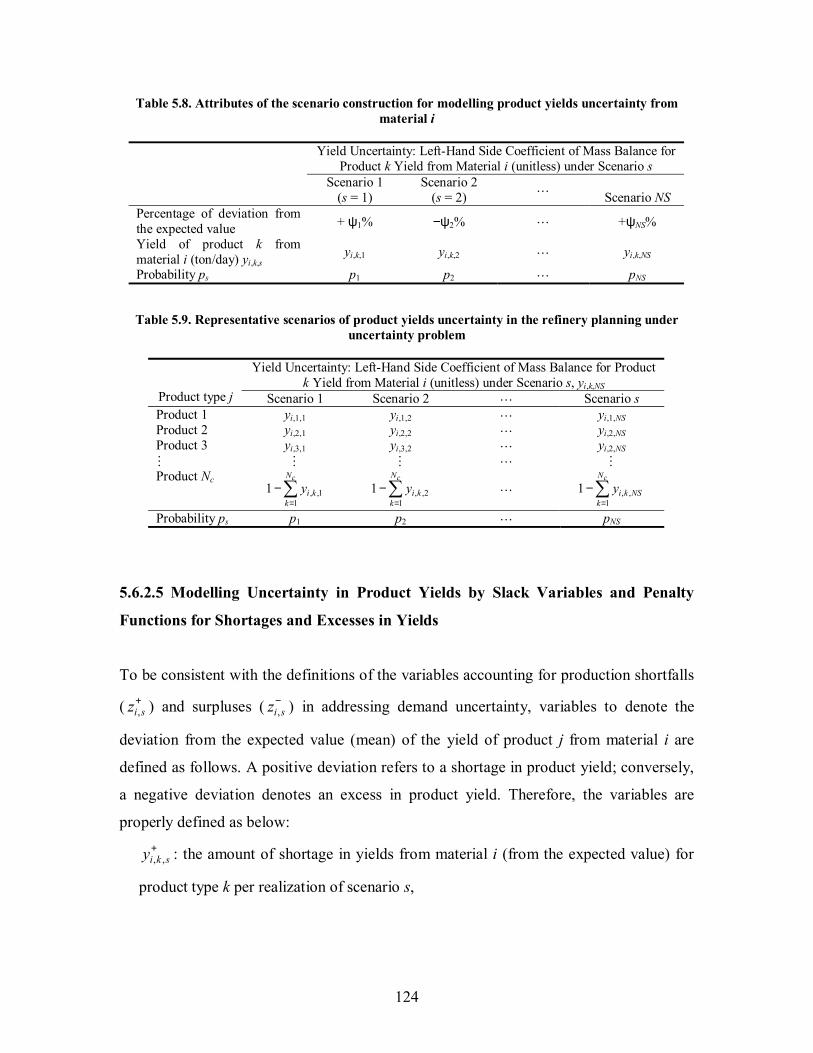
124

Table 5.8. Attributes of the scenario construction for modelling product yields uncertainty from material i

Yield Uncertainty: Left-Hand Side Coefficient of Mass Balance for

Product k Yield from Material i (unitless) under Scenario s Scenario 1

(s = 1) Scenario 2

(s = 2) L Scenario NS Percentage of deviation from the expected value + ψ1% −ψ2% L +ψNS%

Yield of product k from material i (ton/day) yi,k,s

yi,k,1 yi,k,2 L yi,k,NS

Probability ps p1 p2 L pNS

Table 5.9. Representative scenarios of product yields uncertainty in the refinery planning under uncertainty problem

Yield Uncertainty: Left-Hand Side Coefficient of Mass Balance for Product

k Yield from Material i (unitless) under Scenario s, yi,k,NS Product type j Scenario 1 Scenario 2 L Scenario s Product 1 yi,1,1 yi,1,2 L yi,1,NS Product 2 yi,2,1 yi,2,2 L yi,2,NS Product 3 yi,3,1 yi,3,2 L yi,2,NS M M M L M Product Nc

, ,11

1cN

i kk

y=

−∑ , ,21

1cN

i kk

y=

−∑ L , ,1

1cN

i k NSk

y=

−∑

Probability ps p1 p2 L pNS

5.6.2.5 Modelling Uncertainty in Product Yields by Slack Variables and Penalty

Functions for Shortages and Excesses in Yields

To be consistent with the definitions of the variables accounting for production shortfalls

( ,i sz+ ) and surpluses ( ,i sz− ) in addressing demand uncertainty, variables to denote the

deviation from the expected value (mean) of the yield of product j from material i are

defined as follows. A positive deviation refers to a shortage in product yield; conversely,

a negative deviation denotes an excess in product yield. Therefore, the variables are

properly defined as below:

, ,i k sy+ : the amount of shortage in yields from material i (from the expected value) for

product type k per realization of scenario s,

125

, ,i k sy− : the amount of excess in yields from material i (from the expected value) for

product type k per realization of scenario s,

The amount of shortage of yields from crude oil can be equivalently interpreted as the

amount of material to be added to compensate for the associated shortage in product k; in

contrary, the amount of excess of yields indicates the amount of material to be reduced to

account for the associated surplus in product k.

Based on the similar approach of adopting penalty functions for modelling demand

uncertainty, it is assumed that a fixed penalty cost of ,i kq+ is incurred per unit of , ,i k sy+

amount of shortage of yield from material i, and a fixed penalty cost of ,i kq− for per unit

of excess of yield from material i by the amount , ,i k sy− . Thus, the expected recourse

penalty for the second-stage costs due to uncertainty in yield of product k from material i

for all considered scenarios generated is given by:

( ),yield , , , , , ,s s i j i k s i j i k si I s S

E p q y q y+ + − −

∈ ∈= +∑∑ (5.23)

As in the case of product demand uncertainty, to ensure that the original information

structure associated with the decision process sequence is honoured, Ns new constraints

(in place of the original single deterministic fixed yield constraint) to account for the Ns

number of scenarios dealing with product yield uncertainty are introduced for each

product whose yield is uncertain (Higle, 2005). The general form of the new constraints

is:

1 , , , , 0, , ,i i i k s i k sT x x y y i I k K s S+ −+ + − = ∀ ∈ ∀ ∈ ∀ ∈ (5.24)

To obtain realistic values for the yield deviation terms, upper bounds of five (5)

percent of the crude oil mass flowrate are imposed as an estimate of the maximum value

that these terms could sensibly assume.

The combination of Tables 5.4, 5.6, and 5.9 as given by Table 5.10 completes the

scenario formulation in order to simultaneously model uncertainties in commodity prices,

126

product demand, and product yields as represented by randomness in the coefficients of

the objective function and the RHS and the LHS of the constraints, respectively. The

major assumption that prices, demand, and yields in each scenario are highly correlated

enables the combination of all the scenarios in a stochastic programming model with

discrete random variables. Otherwise, the computation would involve the construction of

joint probability distribution of random variables that are made up of scenarios depicting

all possible combinations of the three parameters of prices, demand, and yields. This will

be considered in future work.

The corresponding expected recourse penalty for the second-stage costs due to

uncertainties in both demand and yields is given by:

( ) ( )( ) ( )( ) ( )

,demand ,yield

, , , , , ,

, , , , , ,

, , , , , ,

s s s

s i i s i i s s i i k s i i k si I s S i I s S

s i i s i i s s i i k s i i k si I s S

s s i i s i i s i i k s i i k si I s S

s si s S

E E E

p c z c z p q y q y

p c z c z p q y q y

E p c z c z q y q y

p

+ + − − + + − −

∈ ∈ ∈ ∈

+ + − − + + − −

∈ ∈

+ + − − + + − −

∈ ∈

∈ ∈

= +

= + + +

= + + +

= + + +

= ξ

∑∑ ∑∑

∑∑

∑∑

∑ ( ) ( ), , , , , , ,

,

where i s i i s i i s i i k s i i k sI

s i si I s S

c z c z q y q y

E E

+ + − − + + − −

∈ ∈

ξ = + + +

=

∑

∑∑

(5.25)

The expression for sE ′ as given by equation (5.25) clearly formalizes and illustrates one

of the most profound concepts of the recourse model, that is, the sole random variable is

now redefined to be the scenarios and no longer the separate random variables of

coefficients denoting prices, demand, and yields as considered earlier. Mathematically,

single random vectors of the recourse variables ( ), , , , , ,, , ,i s i s i k s i k sz z y y+ − + −ξ =% are used in place

of the four single random variables ,i sz+ , ,i sz− , , ,i k sy+ , and , ,i k sy− , in which vectors ξ% are

random variables themselves (denoted here by the wavy line above the symbol). ξ% is

described by a finite discrete distribution of ( ) , , 1,2,3,..., 0s s sp s s p sξ = > ∀ as

depicted by the discrete probabilities in Table 5.10 (Kall and Wallace, 1994).

127

Table 5.10. Complete scenario formulation for the refinery production planning under uncertainty in commodity prices, market demand for products, and product yields problem

Material/Product Scenario 1 Scenario 2 L Scenario NS

Price Uncertainty: Objective Function Coefficient of Prices ($/ton) Product 1 c1,1 c1,2 L c1,NS Product 2 c2,1 c2,2 L c2,NS Product 3 c3,1 c3,2 L c3,NS M M M L M Product N cN,1 cN,2 L cN, NS

Demand Uncertainty: Right-Hand-Side Coefficient of Constraints for Product i Demand (ton/day) under Scenario s, di,s

Product 1 d1,1 d1,2 L d1,NS Product 2 d2,1 d2,2 L d2,NS Product 3 d3,1 d3,2 L d3,NS M M M L M Product N dN,1 dN,2 L dN,NS Yield Uncertainty: Left-Hand Side Coefficient of Mass Balance for Product j Yield

from Material i (unitless) under Scenario s, yi,k,s Product 1 yi,1,1 yi,1,2 L yi,1,NS Product 2 yi,2,1 yi,2,2 L yi,2,NS Product 3 yi,3,1 yi,3,2 L yi,2,NS M M M L M Product Nc

, ,11

1cN

i kk

y=

−∑ , ,21

1cN

i kk

y=

−∑ L , ,1

1cN

i k NSk

y=

−∑

Probability ps p1 p2 L pNS

5.6.2.6 Expectation Model I

A new reformulated objective function z2 is now proposed, consisting of the sum of the

following components: (1) maximization of the expected net profit from product sales

subtracting the raw material costs of purchasing crude oil and the operating costs; (2)

minimization of the sum of variance in profit; and (3) minimization of the sum of

expected recourse penalty costs due to shortfalls or surpluses in production and shortages

or excesses of product yields from certain materials. The mathematical expression for this

new objective function is presented as:

[ ]2 1 0 1 0maximize ( )s sz z E E z V z E′ ′= − = − θ − (5.26)

where

128

[ ] ( ) ( )

( ) ( ) ( )

f, , , , , , ,

0 s, , , , , , , ,

2 20 , , , , ,

s i s t i t i t i t s s t i ti I s S i I i I s S

t t t tt T t Ti t i t i t i t j t j t j t j t

i I i I j J

i t i s t i t s tt T i I t T i I

p S I p PE z r R o O

I h H CE y

V z S V P V

∈ ∈ ∈ ∈ ∈

∈ ∈∈ ∈ ∈

∈ ∈ ∈ ∈

γ + γ − λ

= − + − λ − − α + β

= γ − λ

∑∑ ∑ ∑∑∑ ∑∑ ∑ ∑

∑∑ ∑∑

%

%

subject to

deterministic constraints (first stage):

(4.1) and (4.2) for production capacity;

(4.7) for mass balances except for fixed production yields (which are random);

(4.4) for availability constraints;

(4.5) and (4.6) for inventory requirements;

stochastic constraints (second stage):

(5.18) for demand constraints

, , , , ,i i s i s i sx z z d i I s S+ −+ − = ∈ ∈ ;

(5.24) for mass balances for fixed production yields

1 , , , , 0, , ,i i i k s i k sT x x y y i I k K s S+ −+ + − = ∈ ∈ ∈ .

Solution of the first-stage variables provides decisions on the flowrate of production

streams. Historical data of actual commodity prices, market demand, and product yields

are considered, and depending on which scenario occurs, appropriate production will be

executed in order to satisfy the realized prices, demand, and yields. These are the second-

stage recourse decisions that are clearly constrained by what has been produced in the

first-stage (apart from being constrained or depended upon by the corresponding

scenario).

Theoretically, the solution is, in general, likely to be more representative or more

robust with more scenarios considered but at the expense of being computationally

expensive (that is, increase in computation time). Furthermore, with considerable number

of scenarios taken into account, typically in the hundreds (for example, Pongsakdi et al.

(in press) considered 600 scenarios), more noise is present in the data. A more practical

approach is perhaps to compute the expected values of the data obtained from the first

round of scenario generation, and then to subject these expected values to a second round

129

of scenario generation in order to obtain a more robust solution, although with a trade-off

in the increment of solution time. Another approach that can be considered is the use of

the concept of principal component analysis (PCA) in distilling the hundreds of scenarios

into a smaller number of representative scenarios, thus reducing both the amount of

computational time and the presence of noisy data.

5.6.2.7 Expectation Model II

As remarked in Approach 1, a potential complication with Expectation Model I lies in

computing a suitable range of values for the profit risk factor θ1. Therefore, the proposed

alternative modelling strategy of minimizing the variance, or in keeping to the

maximization problem, becomes maximizing the negative of the variance, while adding a

target value constraint for the mean of the original profit objective function; this is

employed as follows for Expectation Model II:

[ ]2 0

0

maximize ( )subject to Target objective function value

deterministic and stochastic constraints

sz V z EE z

′= − −≥

−(4.1) (4.7) (5.27)

5.7 APPROACH 3: RISK MODEL II WITH VARIANCE AS THE MEASURE OF

RISK OF THE RECOURSE PENALTY COSTS

5.7.1 Two-Stage Stochastic Programming with Fixed Recourse to Model Uncertainty

in Prices, Demand, and Product Yields by Simultaneous Minimization of the

Expected Value and the Variance of the Recourse Penalty Costs

As highlighted earlier, Mulvey et al. (1995) stress the inappropriateness of models with

the expected value objective since they ignore both the risk attitude of the decision-maker

and the distribution of the objective values sξ (as given by equation (5.25) for

130

Expectation Models I and II developed in the previous section). Higle (2005) equally

advocated this by noting that expected values are risk-neutral models; hence they do not

always provide a satisfactory model for decision-making under risk. This is especially so

in the settings of moderate and high-risk decision-making under uncertainty as most

decision-makers are risk-averse in making (relatively) important decisions.

Therefore, in this third approach, the expected value model developed in Approach 2

is extended to incorporate the measure of economic risk associated with an investment

alternative. This is accomplished by reformulating the recourse penalty terms, again in

the spirit of the Markowitzs meanvariance approach, as similar to the profit terms. The

resulting risk model obtained is one in which in maximizing expected profit by

minimizing its deviation (as computed by its variance), the expected value of the recourse

penalty costs is minimized as well as its deviation by computing a parameterized function

of the variance of the penalty costs. In general, this is the classical approach long

favoured among financial planners in the field of financial engineering to enable

decision-makers to investigate the tradeoffs between expectations and variances of costs

associated with their decisions (although by stating this, we do not intend in any way to

conceal the fact that there has also been published works doubting the practicality of the

MV approach, among others, by Michaud and Michaud (2006), Michaud (1998), and

Jobson and Korkie (1981)). According to Luenberger (1998), this approach enables the

tradeoffs between the means and the variances to be explicit while Mulvey et al. (1995)

perceives the incorporation of the variance term as an indicator of model robustness, as

will be analyzed through the numerical example on refinery midterm planning. Note that

we did not consider adopting the robust optimization model in the form originally

proposed by Mulvey et al. (1995) following the argument made by Sen and Higle (1999)

that the robust models are, in general, structurally unrelated to solutions obtained from

the recourse model based on Markowitzs meanvariance approach. Instead, they further

stressed that the robust optimization models are instead dominated by solutions derived

from the inferior least-cost model.

A brief review on the concept of variance for a random variable follows. If X is a

random variable (that is, a variable whose value is decided by chance) that can take on a

finite number of values x1, x2, x3, , xn, with the associated probability of such

131

occurrences given by p1, p2, p3, , pn, respectively, then the expected value or mean of X

is defined to be:

1 1 2 2 3 3 n nE p x p x p x p x= + + + +L (5.28)

From the definition of variance of X introduced earlier in equation (5.5) (Markowitz,

1952), the parameterized function of the variance for the various expected recourse

penalty for the second-stage costs Vs is thus derived as:

( )

( )( )

( )( )

2

2

2

, , , ,

, , , , , , , ,

s s s ss S

s s s ss S s S

i i s i i s i i s i i ss s s

s S i I i I s Si i k s i i k s i i k s i i k s

V p E

p p

c z c z c z c zV p p

q y q y q y q y

′∈

′ ′′ ′∈ ∈

+ + − − + + − −′ ′

′+ + − − + + − −′ ′∈ ∈ ∈ ∈ ′ ′

= ξ −

= ξ − ξ

+ + = − + + + +

∑

∑ ∑

∑ ∑ ∑∑

(5.29)

Note that the index s′ and the corresponding set S′ is merely used to denote scenarios for

the evaluation of the inner expectation term in order to distinguish from the original index

s used to represent the scenarios. The variance Vs is weighted by the risk tradeoff

parameter θ2 that is varied over the entire range of (0, ∞) to generate a set of feasible

decisions that have maximum return for a given level of risk. This feasible decisions set

is equivalent to the efficient frontier portfolios introduced by Markowitz (1952; 1959)

for financial investment applications. The parameter θ2 can be seen as reflecting the

decision makers attitude towards variability, that is, in more explicit terms, the risk

attitude of the decision maker. Hence, the following is the mathematical description of

Risk Model II, as a result of the recourse reformulation of Expectation Model I developed

in Approach 2, utilizing variance as the measure of risk by minimizing the variance in the

expected recourse penalty costs:

132

[ ]3 2 2 0 1 0 2maximize ( )subject to deterministic and stochastic constraints

s s sz z V E z V z E V′= − θ = − θ − − θ−(4.1) (4.7)

(5.30)

As denoted, Risk Model II is subject to the same set of constraints as for Expectation

Model I outlined in Approach 2.

It is desirable to demonstrate Risk Model II as possessing robustness both in terms of

its solution (solution robust) as well as the model itself (model robust). According to

Mulvey et al. (1995), a solution to a stochastic optimization model is defined as solution

robust if it remains close to optimality for all scenarios of the input data; and model

robust if it remains almost feasible for all data scenarios. In refinery planning, model

feasibility is as pertinent as solution optimality. In mitigating demand uncertainty, model

feasibility is measured by expected surpluses and shortfalls in production, in which each

denotes situation of excess production and unmet demand, respectively. Values of

expected unmet demand should be minimized in order to gain customer demand

satisfaction, while excess production should be simultaneously minimized to contribute to

better inventory management.

Risk Model II is characterized by solutions in the multiobjective space as defined by

the expected recourse penalty costs and the variance of the recourse costs. In the model, a

measure of solution robustness is obtained by varying the penalty parameter θ2 and

observing the corresponding changes in the expected value of recourse penalty costs and

expected feasibility. The model does not serve to present an absolute optimal solution

that corresponds to the best possible outcome (typically in terms of maximum profit and

minimum cost) desired by any decision-maker; it is merely a tool to facilitate a decision-

maker in determining the choice that constitutes the best decision. As pointed out by

Applequist et al. (2000), while the concept of using variance of the objective function

value as a measure of risk is sound, such an approach requires the specification of the

values of the one or more penalty of trade-off parameters (such as given by θ1 and θ2 in

this Risk Model II). It is therefore left entirely in the hands of the decision-maker to

effectively choose from a family of solutions corresponding to different values of these

trade-off parameters.

133

5.7.2 Limitations of Approach 3

This approach results in an even larger nonlinear programming (NLP) problem than

Approach 2, involving quadratic terms introduced by variance of the expected recourse

penalty costs, which adds to the computational burden in the solution. Therefore, in

general, it is undesirable to consider higher moments (beyond variance) in stochastic

modelling approach as even the consideration of variance already requires the solution of

a nonlinear program.

It should also be pointed out that incorporating the variance of the recourse function as

part of the objective function could potentially cause the problem to lose convexity. Thus,

without employing the techniques of global optimization, one is liable to get trapped in

local optima solutions. In some models, incorporating the variance of the recourse

function into the objective function leads to poor design or planning for cases in which

the variance is small, but the design is unnecessarily expensive (Sen, 2001). Furthermore,

Sen and Higle (1999) remarked that this approach that has its roots in the Markowitzs

model, which is based on assumptions such as normally distributed returns, that may not

necessarily hold in some applications.

In addition, since variance is a symmetric risk measure, profits both below and above

the target levels are penalized equally, when it is actually desirable to only penalize

profits of the former, that is, profits that are below the target (Barbaro and Bagajewicz,

2004). In other words, constraining or minimizing the variance of key performance

metrics to achieve robustness, which in this case are the profit and the recourse penalty

costs, may result in models that overcompensate for uncertainty, as reported by Samsatli

et al. (1998). They therefore propose a general approach to robustness that can be tailored

for various types of constraints to be imposed on the system and on specific suitable

performance metrics. Other potentially more representative risk measures should also be

considered with Kristofferson (2005) providing a recent review of a wide choice of risk

measures applicable within a two-stage stochastic optimization framework (as

highlighted earlier in Section 5.5.7).

134

5.7.3 A Brief Review of Risk Modelling in Chemical Process Systems Engineering

(PSE)

The subject of risk modelling, mainly incorporated through stochastic optimization

models, has been receiving increasing attention from the chemical process systems

engineering (PSE) community since the publication of one of the earliest papers (if not

the earliest) addressing this issue by Applequist et al. (2000) of the PSE research group at

Purdue University. Of late, the Miguel Bagajewicz research group at University of

Oklahoma, for instance, has produced a steady stream of publications addressing research

problems related to financial risk management in planning under uncertainty, mainly with

applications in the oil and gas industry. This can be found in the works of Pongsakdi et al.

(in press), Barbaro and Bagajewicz (2004a, 2004b), and Aseeri and Bagajewicz (2004).

Other works from Bagajewicz and co-workers that also incorporate the concept of

financial risk management include Guillen et al. (2005), Aseeri et al. (2005), Bonfill et al.

(2004),), and Romero et al. (2003).

5.8 APPROACH 4: RISK MODEL III WITH MEAN-ABSOLUTE DEVIATION

(MAD) AS THE MEASURE OF RISK IMPOSED BY THE RECOURSE

PENALTY COSTS

In this proposed fourth approach, we attempt to formulate a two-stage stochastic

programming with fixed recourse framework to model the same three factors of

uncertainties (namely commodity prices, market demand, and product yields) by

minimizing the mean-absolute deviation (MAD) of the various expected recourse penalty

for the second-stage costs. In essence, this model replaces the variance term in the

objective function of Risk Model II with the MAD term.

135

5.8.1 The Mean-Absolute Deviation (MAD)

The mean-absolute deviation (MAD) (often inaccurately called the mean deviation) is

defined as:

1

1MADN

i ii

f x xN =

= −∑ (5.31)

where N is the sample size, xi are the values of the samples, x is the mean, and fi is the

absolute frequency.

In their pioneering work, Konno and Yamazaki (1991) proposed a mean-absolute

deviation (MAD) portfolio model to formulate a large scale portfolio optimization

problem. This serves as an alternative measure of risk to the standard Markowitzs mean

variance portfolio selection model, which models risk by the variance of the rate of return

of a portfolio, thus leading to a nonlinear convex quadratic programming (QP) problem.

Although both measures are almost equivalent from a mathematical point-of-view, they

are substantially different from a computational point-of-view in the following ways.

First, the use of MAD, essentially as a proposed linearization method of the objective

function to produce an equivalent linear programming (LP) problem, serves to overcome

the computational difficulties of the QP portfolio model and therefore, enables large-scale

problems to be solved faster and more efficiently. This is a situation that held true at least

until the mid-1990s before greater advancements in computer technology increasingly

narrowed the gap in speed between the computational solution of an LP and a convex QP.

Second, since the model can be casted into a linear programming (LP) problem, it can be

solved much faster than a corresponding MV model. Third, the LP formulation has

computational advantages over the QP formulation when integer constraints and

nonconvex functions are considered. Thus, in the area of investment portfolios within the

financial engineering field, the LP formulation is more suitable in handling problems

associated with real transaction environments. Moreoever, it is further reported that the

minimization of MAD provides similar results as the Markowitz formulation if the return

is multivariate normally distributed (Konno and Wijayanayake,

136

2002; Konno and Koshizuka, 2005). Appendix C presents a theoretical treatment of

MAD based on Konno and Yamazaki (1991).

Three additional fundamental difficulties also exist with the MV model: (i) the

assumption that returns are normally distributed about the mean, which is not required in

the MAD model, (ii) the required storage and calculation of a usually dense variance

covariance matrix; which again is not required in the MAD model formulation and

consequently, its estimation is avoided; and (iii) the use of variance as a measure of risk

equally penalizes both upside and downside variation; when it should only be the latter

that is undesirable and thus penalized, as stressed earlier in Section 5.7.2 and

demonstrated graphically in Figure 5.9 (Konno and Yamazaki, 1991; Simaan, 1997;

Speranza, 1996; Murtagh, http://www.esc.auckland.ac.n/Organisations/

ORSNZ/conf37/Papers/Murtagh.pdf, accessed on November 12, 2005).

Penalty

Returnr

Penalty

ReturnrMean-Absolute Deviation (MAD) Variance

Figure 5.9. Penalty functions for mean-absolute-deviation (MAD) and variance minimization (based on

Zenios and Kang (1993) and Samsatli et al. (1998)). Ogryczak and Ruszczynski (1999) further demonstrated that MAD is an authentic

measure of risk in view of its compatibility with von Neumanns principle of

maximization of expected utility (MEU) under risk aversion; a result corroborated by

Speranza (1996). This substantiates the solid economic foundation of the theoretical

properties of MAD (Konno and Koshizuka, 2005).

137

5.8.2 Two-Stage Stochastic Programming with Fixed Recourse to Model Uncertainty

in Prices, Demand, and Product Yields by Simultaneous Minimization of the

Expected Value and the Mean-Absolute Deviation of the Recourse Penalty Costs

Konno and Yamazaki (1991) present the absolute deviation function, denoted as L1 risk,

as:

1 1

( )n n

j j j jj j

W E R x E R x= =

= − ∑ ∑x (5.32)

From equation (5.25) of Approach 2, the expected recourse penalty for the second-stage

costs due to the combined uncertainties in market demand and product yields from crude

oil is given by:

( ) ( ), , , , , ,s s i i s i i s i i k s i i k si I s S

E p c z c z q y q y+ + − − + + − −′ ′ ′ ′ ′ ′

′ ′∈ ∈

= + + + ∑ ∑ (5.25)

Thus, the corresponding mean-absolute deviation (MAD) of the expected penalty costs

due to violations of constraints for maximum product demand and product yields as a

result of randomness in both demand and yields is formulated as:

( )( )

( )( )

, , , ,

, , , , , ,

( )

( )

s s s ss S

s s s ss S s S

i i s i i s i i s i i ss s s

s S i I i I s Si i s i i s i i k s i i k s

W p p E

p p

c z c z c z c zW p p p

q y q y q y q y

′∈

′ ′′∈ ∈

+ + − − + + − −′ ′

′+ + − − + + − −′ ′∈ ∈ ∈ ∈ ′ ′

= ξ −

= ξ − ξ

+ + = − + + + +

∑

∑ ∑

∑ ∑ ∑∑

(5.33)

Since this function is not linear, it is linearized by adopting the transformation

procedure proposed by Konno and Yamazaki (1991) and revisited in Papahristodoulou

and Dotzauer (2004). The variables Yij ≥ 0 are defined, in which these Yij variables can be

138

interpreted as linear mappings of the nonlinear expression given by

( ) ( ) ( ) ( ), , , , , ,i is i is i is i is s i i s i i s i i k s i i k si I s S

c z c z q y q y p c z c z q y q y+ + − − + + − − + + − − + + − −′ ′ ′ ′ ′

′ ′∈ ∈

+ + + − + + + ∑ ∑ . Thus,

equation (5.33) is rewritten simply as

( )

( )( )

( ), , , ,

, , , , , ,

( )i i s i i s i i s i i s

ij s s ss S i I i I s Si i s i i s i i k s i i k s

c z c z c z c zY W p p p

q y q y q y q y

+ + − − + + − −′ ′

′+ + − − + + − −′ ′∈ ∈ ∈ ∈ ′ ′

+ + = = − + + + +

∑ ∑ ∑∑ (5.34)

subjected to the following three constraints:

( )

( )( )

( ), , , ,

, , , , , ,

i i s i i s i i s i i sij s s

s S i I i I s Si i s i i s i i k s i i k s

c z c z c z c zY p p

q y q y q y q y

+ + − − + + − −′ ′

′+ + − − + + − −′ ′∈ ∈ ∈ ∈ ′ ′

+ + ≥ − − + + + + ∑ ∑ ∑∑ (5.35)

( )

( )( )

( ), , , ,

, , , , , ,

i i s i i s i i s i i sij s s

s S i I i I s Si i s i i s i i k s i i k s

c z c z c z c zY p p

q y q y q y q y

+ + − − + + − −′ ′

′+ + − − + + − −′ ′∈ ∈ ∈ ∈ ′ ′

+ + ≥ − + + + + ∑ ∑ ∑∑ (5.36)

and the non-negativity constraints for Yij:

0ijY ≥ (5.37)

Similar to the formulation of Risk Model II in Approach 3 that utilizes variance as the

measure of risk for the recourse penalty costs, the adoption of MAD introduces the risk

parameter θ3, varied over the entire range of (0, ∞) to consider its trade-offs with the

expected profit term, the profit variability term, and the expected recourse term in the

objective function. Therefore, the reformulated mathematical program for Risk Model III,

which utilizes MAD as the measure of risk, is given by:

139

[ ][ ] ( ) ( )

( )( )

( )( )

3 2 3

0 1 0 3

3 0 1 0

3

maximize ( )Var( ) ( )

maximize Var( )

s

s s

s i is i is i is i isi I s S

i is i is i is i iss s

i is i is i is i is

z z W pE z z E W p

z E z z p c z c z q y q y

c z c z c z c zp p

q y q y q y q y

′

+ + − − + + − −

∈ ∈

+ + − − + + − −

+ + − − + + − −

= − θ= − θ − − θ

= − θ − + + +

+ + − θ − + + + +

∑∑

i I s S i I s S∈ ∈ ∈ ∈

∑∑ ∑∑

(5.38)

subject to the same set of constraints as for Expectation Model I and Risk Model II with

the addition of constraints (5.35)(5.37).

Note that the risk parameters θ1 and θ3, in their dual role as the scaling factors for the

variance term and the MAD term respectively, would mathematically necessitate that the

value of θ1 is (much) smaller than θ3 (θ1 < θ3) since θ1 is required to scale down the

squared operation involved in computing variance whereas the MAD term is in the same

dimension as the expectation terms.

140

CHAPTER 6

Model Implementation on the General Algebraic Modeling System

(GAMS)

In the past, users have to spend a substantial amount of time on computer coding to solve

mathematical programming problems. However, major progress has been achieved in

recent times in the development of mathematical optimization algorithms and computer

codes, thus reducing significant amount of time required to form and implement solution

procedures. This enables more time to be focussed on developing strong model

formulations rather than developing coding and solver development.

The formulation and solution of major types of mathematical programming problems

with increasingly larger scale can now be effectively performed with modelling systems

such as GAMS (General Algebraic Modeling System) (Brooke et al., 1998) and AMPL

(Fourer et al., 1992). While these require that the model be expressed explicitly in

algebraic form, they have the advantage of being automatically interfaced with codes of

solvers for solving the various types of problems that may be encountered. The modelling

platform GAMS, for instance, has a library of solvers with the capability of providing

global solutions for linear programs (LP), integer linear programs (ILP) and mixed

integer linear programs (MILP), as well as determining local optima of nonlinear

programs (NLP), integer nonlinear programs (INLP), and mixed integer nonlinear

programs (MINLP) that have nonlinearities in continuous variables (Rardin, 1999).

GAMS can also perform automatic differentiation and allow the use of indexed

equations, which greatly facilitates and enhances the generation of large scale models.

Furthermore, these modelling systems are now widely available on desktop personal

computers (PCs) (Grossmann et al., http://egon.cheme.cmu.edu/papers.html, accessed on

December 10, 2005).

In essence, GAMS allows the user to almost exclusively concentrate on modelling a

problem by making the setup simple: defining variables, equations, and data, and then

selecting an appropriate solver. In fact, GAMS possess the capability of providing a

default solver that is determined to be (most) suitable for the structure of the problem at

141

hand. The problem formulation can be altered with speed and ease, and the specification

of different solvers to be tested requires only minimal effort of a single line coding. All

solution algorithms can be deployed without requiring any change in existing models,

thus resulting in significant reduction of time dedicated to developing and executing

computational experiments.

As explained, GAMS is a modelling system for optimization that provides an interface

with a variety of different algorithms of solvers. Models are supplied by the user to

GAMS in an input file in the form of algebraic equations using a higher level language.

GAMS then compiles the model and interfaces automatically with a solver, which is an

optimization algorithm. The compiled model as well as the solution computed by the

solver is subsequently reported back to the user through an output file. The simple

diagram below, taken from Grossmann (1991, http://www.che.boun.edu.tr/che477/gms-

mod.html, accessed on September 30, 2005), illustrates this process.

Input FileMODEL

GAMSCompilation

of Model

Output FileRESULTS

OptimizationSolver

Figure 6.1. Framework of the GAMS modelling system

Note that in this work, the objective functions of the proposed stochastic models are

made up of convex functions as given by the expectation operation, the variance

operation, the recourse function, or the Mean-Absolute Deviation (MAD) expression, in

various forms of nonnegative-weighted combinations as stipulated in the formulation of

the respective models. We therefore conclude that all the models possess the highly

sought-after mathematical programming property of convexity based on the theorem that

states any f(x) formed as the nonnegative-weighted (αi ≥ 0) sum 1

( ) ( )k

i ii

f g=

α∑x x of

convex functions gi(x), i = 1,, k, is itself convex (Rardin, 1998). Since the local

142

optimal of a convex function is also the global optimal, a starting value to initialize the

solution in GAMS would not be required

Based on the established ease and advantages of using GAMS, numerical studies of

the deterministic model and the proposed stochastic models are coded and implemented

using GAMS Integrated Development Environment (IDE) version 2.0.19.0 (Module

GAMS Rev 130) for Windows platform. The models are then solved using CPLEX 9.0

(ILOG CPLEX Division, http://www.gams.com/dd/docs/solvers/cplex.pdf, accessed

February 12, 2006) for the linear deterministic case and CONOPT 3 (Drud, 1996,

http://www.gams.com/solvers/conopt.pdf, accessed on January 10, 2006) for the five

nonlinear stochastic cases on a Pentium IV, 1.40 GHz, 512 MB of RAM machine (a

notebook computer instead of a desktop, to be precise).

CPLEX is incidentally the default solver in GAMS for handling linear programs (LP),

whose algorithm is based on the interior point methods that were first introduced by

Karmarkar (1984). For nonlinear programming (NLP) problems, CONOPT 3 is also the

GAMS default solver, in which it is based on a feasible path generalized reduced gradient

method with restoration. The solutions generated for the deterministic equivalent

formulation of the stochastic problems consist of: (i) the first-stage decision variables of

production flowrates for all process streams and (ii) the second-stage recourse variables

of production deviations due to randomness in demands and yields. Due to the

nonlinearities of the stochastic models, starting values for the first-stage decision

variables have been initialized to the optimal solutions obtained from the deterministic

model in an effort to ensure solutions of global optimality. Although a global optimum

could not be guaranteed due to the general nonconvexities of the problems, multiple local

solutions have not been detected under tests of varied initial conditions. This also

indicates that CONOPT 3 is a robust solver for the nonlinear nonconvex stochastic

models.

In addition, it may be useful to note that nonlinear optimization algorithms often

search in the space defined by superbasic variables, which are variables that are not in the

basis but whose values are between the upper and lower bounds. If an infeasible solution

is found by the solver used in GAMS, it is most likely due to the non-existent of a

superbasic variable, in which the facility within GAMS would readily report.

143

CHAPTER 7

Analysis of Results from the Stochastic Models

In the context of production planning, robustness can be generally defined as a measure

of resilience of the planning model to respond in the face of parameter uncertainty and

unplanned disruptive events (Vin and Ierapetritou, 2001). For this, we propose the

adoption of two metrics that have previously been used in the optimization literature,

under similar and different contexts, to quantitatively measure and account for

characteristics of planning under simultaneous uncertainty in three different parameters

(namely commodities prices, market demands, and product yields). The two metrics are:

(1) the concepts of solution robustness and model robustness according to the pioneering

idea of robust optimization by Mulvey and co-workers (1995) and (2) the coefficient of

variation Cv.

7.1 SOLUTION ROBUSTNESS AND MODEL ROBUSTNESS

According to Mulvey et al. (1995), Bok et al. (1998) and Malcolm and Zenios (1994),

solution robustness of an optimization model with respect to optimality is indicated by

the optimal model solution that is almost optimal, or remains close to optimal, for any

realization of the uncertain scenarios. This implies solutions that are less sensitive to

changes in the data when different scenarios are considered. On the other hand, model

robustness refers to solution robustness with respect to feasibility, with the optimal model

solution that remains almost feasible for any realization of the scenarios. Thus, in

general, for production planning problems, model robustness or model feasibility is

represented by the optimal solution that has almost no shortfalls or surpluses in

production as reflected by the expected total unmet demand and total excess production,

respectively; both of which should be kept to a minimum. A trade-off exists between

solution optimality and model-and-solution robustness. In order to investigate these

144

trends, the following parameters are tabulated and analyzed from the raw computational

results of the refinery production rates for the stochastic models:

• the expected deviation in profit as measured by variance V(z0);

• the expected total unmet demand or production shortfall;

• the expected total excess production or production surplus; and

• the expected recourse penalty costs Es.

7.2 COEFFICIENT OF VARIATION

The concepts of the value of the stochastic solution VSS and the expected value of

perfect information EVPI (Birge, 1982; Birge, 2005; Birge and Louveaux, 1997; Gupta

and Maranas, 2000; Kall and Mayer, 2005; Uryasev, 2005) appear to be unsuitable in the

case of nonlinear quadratic programming problems such as in the present work.

Therefore, a different measure is sought to interpret the solutions obtained. One such

approach is to investigate the coefficient of variation Cv. Cv for a set of values is defined

as the ratio of the standard deviation to the expected value or mean, and is usually

expressed in percentage. It is calculated as:

vStandard Deviation 100% 100% 100%

MeanVCE

σ= × = × = ×µ

(7.1)

Statistically, Cv is a measure of reliability, or evaluated from the opposite but equivalent

perspective, it is also indicative of a measure of uncertainty. It is alternatively interpreted

as the inverse ratio of data to noise in the data in most conventional textbooks on

statistics. Therefore, it is apparent that a small value of Cv is desirable as it signifies a

small degree of noise or variability (in a data set, for instance) and hence, reflects low

uncertainty.

It follows then that in the realm of stochastic optimization, coefficient of variation can

be purposefully employed to investigate, denote, and compare and contrast the relative

uncertainty in models being studied. In a risk minimization model, as the expected value

145

of mean is reduced, the variability in the expected value (as typically measured by

variance or standard deviation) is reduced as well. The ratio of this change can be

captured and described by the coefficient of variation. Conversely, a comparison of the

relative merit of models in terms of their robustness can also be represented by their

respective values of coefficient of variation (that is, in the sense that a model with a lower

coefficient of variation is favoured since there is less uncertainty associated with it, thus

contributing to its reliability; this is in tandem with the original definition of Cv as a

measure of reliability).

In addition to these arguments, in the seminal paper of his Nobel Prize-winning work

(in the field of economics) of meanvariance model for optimization of investment

portfolio selection, Markowitz (1952) remarked that the use of coefficient of variation as

a measure of risk would equally ensure that the outcome of a decision-making process

still lies in the set of efficient portfolios.

In a data set of normally distributed demands, if the coefficient of variation Cv of

demand is given as a case problem parameter, the standard deviation is computed by the

multiplication of Cv with the deterministic demand (Jung et al., 2004) Increasing values

of Cv result in increasing fluctuations in the demand and this is again undesirable.

Computation of the coefficient of variation is based on the objective function of the

formulated model. Table 7.1 displays the expressions to compute the coefficient of

variation for the respective models developed in the preceding section. Note that the

coefficient of variation for the corresponding deterministic case of each model is

determined based on the expected (E) result of using the deterministic expected value

(EV) solution, or EEV for short. In more elaborate terms, EEV is the solution obtained

from solving the stochastic models using results from the deterministic expected value

problem (that is, the deterministic model with the random parameters replaced by their

expected values or means).

(Please turn the page over for Table 7.1.)

146

Table 7.1. Coefficient of variation for the deterministic and stochastic models developed

Approach Model Objective Function

Coefficient of Variation

vVCE

σ= =µ

Deterministic cTx [Given by the expected (E) result of using the deterministic expected value (EV) solution (EEV)]

1 Risk Model I 1 0max ( )z V z= −

[ ]1 0 1 0max ( )z E z V z= − θ

( )[ ]

0v

0

V zC

E z=

2 Expectation

Models I and II I: [ ]2 0 1 0max ( ) sz E z V z E= − θ − II: 2 0max ( ) sz V z E= − −

( )[ ]

0v

0 s

V zC

E z E=

−

3 Risk Model II [ ]3 0 1 0 2max ( ) s sz E z V z E V= − θ − − θ ( )

[ ]0

v0

s

s

V z VC

E z E+

=−

4 Risk Model III

(MAD) [ ]3 0 1 0 3max ( ) ( )s sz E z V z E W p= − θ − − θ ( )

[ ]0

v0

( )s

s

V z W pC

E z E+

=−

147

CHAPTER 8

A Representative Numerical Example and Computational Results for

Petroleum Refinery Planning under UncertaintyI: The Base Case

Deterministic Refinery Midterm/Medium-Term Production Planning

Model

As a representative numerical example for the purpose of computational experimentation

and testing, we consider the deterministic refinery production planning model proposed

by Allen (1971) as the base case or core model, without loss of generality. The model is

then reformulated with the addition of stochastic dimension according to the principles

and approaches that have been extensively outlined in the previous section on general

model development.

This model is also adopted in the work of Ravi and Reddy (1998), which employs the

fuzzy programming technique to account for uncertainty. This provides a further avenue

for us to analyze solutions from our work in light of the fuzzy approach solutions.

8.1 PROBLEM DESCRIPTION AND DESIGN OBJECTIVE

The base case models the planning of the operations of a petroleum refinery as an

ordinary single objective linear programming (LP) problem of total daily profit

maximization. Allen (1971) remarked that the LP approach is particularly useful in this

context it provides considerable flexibility in the way a plant could be operated.

148

8.2 THE DETERMINISTIC REFINERY MIDTERM PRODUCTION PLANNING

MODEL

PRIM

ARY

DIS

TIL

LAT

ION

UN

ITNaphtha

x7

CR

AC

KER

Crude Oil

x15

x18

CrackerFeed

x9

x13

Gas Oil

x8

Jet Fuel

x14

FUEL OIL BLENDINGResiduum

x10

x20

x12

x17

x19

x11 x16Gasoline

x2

Naphthax3

Heating Oilx5

Jet Fuelx4

Fuel Oilx6

x1

Figure 8.1. Simplified representation of a petroleum refinery for formulation of the deterministic linear program for midterm production planning

Figure 8.1 is a simplified representation of a refinery that is essentially made up of a

primary distillation unit (or more commonly known nowadays as the crude distillation

unit or CDU) and a middle distillates cracker (more widely known as the catalytic cracker

in modern settings). The refinery processes crude oil to produce gasoline, naphtha (for

gas making), jet fuel, heating oil, and fuel oil. The primary unit splits the crude into

naphtha (13 weight percent, or 13 wt% yield), jet fuel (15 wt%), gas oil (22%), cracker

feed (20%), and residue (30%). Gasoline is blended from naphtha and cracked blend

stock in equal proportions. Naphtha and jet fuel products are straight run. Heating oil is a

blend of 75% gas oil and 25% cracked oil. Fuel oil can be blended from primary residue,

cracked feed, gas oil, and cracked oil in any proportions. Yields for the cracker (weight

percent on feed) are flared gas (5%), gasoline blend stock (40%) and cracked oil (55%).

This information along with the flow diagram of Figure 8.1 describes the physical

system. All the variables that are in the same units of tonne/day, or denoted symbolically

as t/d, are first assigned to process streams to represent the flow rate in each. Since in

149

linear programming, decision variables cannot feasibly be negative, assigning a variable

to a stream also defines its direction of flow and prevents any possibility of flow reversal,

for instance, cracked blend stock going into naphtha product. In Figure 8.1, variables

have been assigned to all the streams.

The minimum number needed to define a system fully should be identified. In this

example, it is three since, for example, fixing x1 determines x7, x4, x8, x9, and x10; fixing x2

then determines x11, x16, x3, x14, x17, x20, and x15;and finally fixing x5 then determines x12,

x18, x13, x19, and x6. An LP model could be formulated using only these three structural

variables or any other suitable three variables. In this case, the solution would only give

values of the three variables and the remainder (if needed) would have to be calculated

from them afterwards. It is usually more convenient to include some additional variables

in the LP model over and above the minimum number. Each variable added needs an

additional mass balance constraint to define it. Instead of calculating a variable separately

from the solution, the means of finding its value is thus included in the model itself.

The next step is to construct linear constraints that describe the physical plant

relationships and define the amount of flexibility existing in plant operation. These

constraints are categorized as follows.

8.2.1 Limitations on Plant Capacity

In the example, the feed rates of crude oil to the primary unit and cracker, averaged over

a period of time, can be anything from zero to the maximum plant capacity. The

constraints are:

primary distillation unit: x1 ≤ 15 000 (8.1)

cracker: x14 ≤ 2500 (8.2)

150

8.2.2 Mass Balances

Mass balance constraints are in the form of equalities. There are three types of such

constraints: fixed plant yield, fixed blends or splits, and unrestricted balances. Except in

some special situations such as planned shutdown of the plant or storage movements, the

right hand-side of balance constraints is always zero. For the purpose of consistency, flow

into the plant or stream junction has negative coefficients and flows out have positive

coefficients. The constraints are as follows:

8.2.2.1 Fixed Yields

For the primary distillation unit:

1 70.13 0x x− + = (8.3)

1 40.15 0x x− + = (8.4)

1 80.22 0x x− + = (8.5)

1 90.20 0x x− + = (8.6)

1 100.30 0x x− + = (8.7)

For the cracker:

14 200.05 0x x− + = (8.8)

14 160.40 0x x− + = (8.9)

151

14 170.55 0x x− + = (8.10)

8.2.2.2 Fixed Blends

For gasoline blending:

2 110.5 0x x− = (8.11)

2 160.5 0x x− = (8.12)

For heating oil blending:

5 120.75 0x x− = (8.13)

5 180.25 0x x− = (8.14)

8.2.2.3 Unrestricted Balances

Naphtha: 7 3 11 0x x x− + + = (8.15)

Gas oil: −x8 + x12 + x13 = 0 (8.16)

Cracker feed: −x9 + x14 + x15 = 0 (8.17)

Cracked oil: −x17 + x18 + x19 = 0 (8.18)

Fuel oil: −x10 x13 x15 x19 + x6 = 0 (8.19)

152

8.2.3 Raw Material Availabilities and Product Requirements

The constraints considered so far are concerned with the physical plant. Constraints are

also needed relating to external factors such as the availability of raw materials and

product requirements over a time period. For this example, there are no restrictions on

crude oil availability or the minimum production required. The maximum production

requirement constraints (in t/d) are as follows:

Gasoline: x2 ≤ 2700 (8.20)

Naphtha: x3 ≤ 1100 (8.21)

Jet fuel: x4 ≤ 2300 (8.22)

Heating oil: x5 ≤ 1700 (8.23)

Fuel oil: x6 ≤ 9500 (8.24)

8.2.4 Objective Function

Although optimization can be stated in many different ways, the common optimization to

an industrial process is to maximize the profitability of the process, or to minimize the

overall costs, in which the former is adopted in this work. In this model, the whole

refinery is considered to be one process, where the process uses the given petroleum

crude oil to produce various petroleum products in order to achieve specific economic

objectives. Thus, the objective of the optimization at hand is to achieve maximum

profitability given the type of crude oil and the refinery facilities. No major hardware

change in the current facilities is considered in the optimization. The optimization tries to

find the optimal operation modes of units and stream flows that maximize the overall

profit of the whole refinery while observing all the possible process constraints.

153

Thus, the economic objective function considered is the net profit or net revenue to be

maximized, in units of $/day. The cost of acquiring the raw material crude oil and

transforming it to finished products are subtracted from the gross revenues accruing from

the sale of finished products. Note that there is no cost associated with blending as this

cost is netted out of the unit sales price of the finished products. The sign convention

denotes costs as negative and realization from sales as positive. Each element in it

consists of the product of coefficient of unit cost or unit sales price ($/ton) and a

production flowrate variable (ton/day or t/d). Thus, the objective function is as follows

(Shapiro, 1993):

1 1 14 2 3 4 5 6crude primary cracker gasoline jet fuelnaphtha heating oil fuel oil

oil unit

maximize 7.5 0.5 1.5 18.5 8.0 12.5 14.5 6.0z x x x x x x x x= − − − + + + + +

hence,

1 2 3 4 5 6 14maximize 8.0 18.5 8.0 12.5 14.5 6.0 1.5ix

z x x x x x x x= − + + + + + − (8.25)

Since linear programming variables cannot feasibly be negative, an additional constraint

to be specified is:

x1, x2, , x20 ≥ 0 or xi ≥ 0, i = 1, 2, 20 (8.26)

It is noted that the constraints of production requirements is directly impacted by the

market demand for the final refinery products. Therefore, in the stochastic version of the

model, the random decision variables will be introduced into these constraints. Since the

objective function is to maximize profit, the production requirements are expressed in

terms of inequalities with an upper bound (less than inequalities) in order to ensure that

the optimization problem is bounded (otherwise, the maximum profit can be solved to an

infinite value). Conversely, if the objective function is to minimize production cost, then

the production requirements would be expressed in the form of inequalities with a lower

bound. This can be deduced logically, as a less than inequality would include the

154

possibility of the solution of non-production (that is, the operations or production of the

refinery is halted or the entire plant is shut down) as cost is equals to zero in this

situation.

8.3 COMPUTATIONAL RESULTS FOR DETERMINISTIC MODEL

The deterministic LP model was set up on GAMS and solved using CPLEX version 9.0.2

(http://www.gams.com/dd/docs/solvers/cplex.pdf, accessed February 12, 2006). CPLEX

has been proven to be a very stable LP solver, and the default settings are almost always

sufficient to obtain an optimal solution within excellent solution times

(http://www.gams.com/solvers/solvers.htm#CPLEX, accessed February 12, 2006). The

solution computed was compared against the solution obtained using the computational

software package LINDO (Linear Interactive and Discrete Optimizer) (Schrage, 1990),

an easy-to-use engine for solving linear and integer optimization models. Both solutions

have been verified to be consistent with each other (with values generated accurate to

three decimal places for the computation with GAMS/CPLEX and to six decimal places

with LINDO) and is tabulated in Table 8.1.

In CPLEX, a normal run performs an iterative procedure analogous to the LP primal

simplex method until the optimal solution is reached. The optimal solution for this

deterministic model are obtained by CPLEX after three (3) iterations in a trivial CPU

time whereas nine (9) iterations are needed by using LINDO (also in within negligible

CPU time). Table 8.2 details the computational statistics for solving Deterministic Model.

8.4 SENSITIVITY ANALYSIS FOR THE SOLUTION OF DETERMINISTIC

MODEL

A sensitivity analysis for the objective function coefficients is performed using the

available facility in LINDO to determine lower and upper limits of each coefficient with

no change in the optimal solution. Table 8.3 displays the ensuing results of these limits in

155

Table 8.1. Computational results for Deterministic Model from GAMS/CPLEX and LINDO

Value (ton/day)

Decision Variable

Lower Limit Level

Upper Limit

Dual Price/ Marginal ($/ton)

Slack or Surplus Variable

Value (ton/day)

Dual Price/ Marginal ($/ton)

x1 0 12 500 +∞ 0 s1 2 500 0x2 0 2 000 +∞ 0 s2 0 3.575 x3 0 625 +∞ 0 s3 700 0x4 0 1 875 +∞ 0 s4 475 0x5 0 1 700 +∞ 0 s5 425 0x6 0 6 175 +∞ 0 s6 0 8.5 x7 0 1 625 +∞ 0 s7 3 325 0x8 0 2 750 +∞ 0 a8 0 8.0 x9 0 2 500 +∞ 0 a9 0 12.5 x10 0 3 750 +∞ 0 a10 0 6.0 x11 0 1 000 +∞ 0 a11 0 9.825 x12 0 1 275 +∞ 0 a12 0 6.0 x13 0 1 475 +∞ 0 a13 0 0x14 0 2 500 +∞ 0 a14 0 29.0 x15 0 0 +∞ −3.825 a15 0 6.0 x16 0 1 000 +∞ 0 a16 0 8.0 x17 0 1 375 +∞ 0 a17 0 29.0 x18 0 425 +∞ 0 a18 0 6.0 x19 0 950 +∞ 0 a19 0 6.0 x20 0 125 +∞ 0 a20 0 8.0

a21 0 6.0 a22 0 9.825 a23 0 6.0 a24 0 6.0

z ($/day) −∞ 23 387.50 +∞ (optimal objective function value = maximum profit)

Table 8.2. Computational statistics for Deterministic Model

Solver Single continuous

variables Constraints Resource usage/

CPU time (s) Iterations CPLEX 21 25 0.000 (trivial) 3

which the current solution or basis remains optimal. The allowable increase column

section indicates the amount by which an objective function coefficient can be increased

with the current basis remaining optimal, giving the lower limit value of the coefficient.

Conversely, the allowable decrease column section is the amount by which the objective

coefficient can be decreased with the current basis remaining optimal, thus determining

the upper limit.

We observe that nine out of the 20 decision variables have positive infinity as an upper

limit for their associated coefficients and this is deemed reasonable since all the decision

variables are positive; moreover, the objective is to maximize profit. For example, the

156

Table 8.3. Sensitivity analysis for the objective function coefficients of Deterministic Model

Objective function coefficient ranges ($/ton) Decision variable

Allowable decrease

Lower limit

Current value

Upper limit

Allowable increase

x1 0.715 000 −8.715 000 −8.000 000 −7.235 000 0.765 000 x2 4.468 750 14.031 25 18.500 000 +∞ +∞ x3 14.300 000 −6.300 000 8.000 000 13.884 615 5.884 615 x4 4.766 667 7.733 333 12.500 000 17.600 000 5.100 000 x5 8.500 000 6.000 000 14.500 000 +∞ +∞ x6 1.134 921 4.865079 6.000 000 7.062 500 1.062 500 x7 5.500 000 −5.500 000 0.000 000 5.884 615 5.884 615 x8 3.250 000 −3.250 000 0.000 000 3.477 273 3.477 273 x9 3.575 000 −3.575 000 0.000 000 3.825 000 3.825 000 x10 2.383 333 −2.383 333 0.000 000 2.550 000 2.550 000 x11 8.937 500 −8.937 500 0.000 000 +∞ +∞ x12 11.333 333 11.333 333 0.000 000 +∞ +∞ x13 3.250 000 3.250 000 0.000 000 3.477 273 3.477 273 x14 3.575 000 −5.075 000 −1.500 000 +∞ ∞ x15 +∞ −∞ 0.000 000 3.825 000 3.825 000 x16 8.937 500 −8.937 500 0.000 000 +∞ +∞ x17 6.500 000 −6.500 000 0.000 000 +∞ +∞ x18 34.000 000 −34.000 000 0.000 000 +∞ +∞ x19 6.500 000 −6.500 000 0.000 000 34.000 000 34.000 000 x20 71.500 000 −71.500 000 0.000 000 +∞ +∞

decision variable x2 denoting the production mass flow rate of gasoline (in ton/day) has

current objective function coefficient value of price of $18.50/ton for profit. The price of

gasoline can be as low as $4.47/ton without altering the optimum profit. Therefore, if a

customer wishes to enter into a purchasing agreement or contract for the commodities

produced by the refinery, the trader or marketer, acting with the knowledge of the

management, can negotiate the trading price down to as low as the extent of the lower

limits of prices listed in Table 8.2 without affecting or hurting the companys profit, so

to speak, as the optimal solution would not be changed. This boosts the refinerys

flexibility to negotiate prices so long as it is within the bounds of each coefficient as

determined in Table 8.2, especially in the volatile market of spot trading of crude oil and

the commodities (Zayed and Minkarah, 2004).

As before, the sensitivity analysis for the right-hand side of constraints is executed as

well by utilizing LINDO with the corresponding results displayed in Table 8.4. The upper

limits for some of the constraints are positive infinity while the lower limits vary. Lower

limits for most of the constraints are observed to be of negative value. Constraints whose

157

upper limits are allowed to go to positive infinity imply that they are not critical to the

production process. As an illustration, the right-hand side constraint for the production

requirement or demand of heating oil can be as low as none without inflicting a change in

the optimal solution. The other constraints can be analyzed in a similar manner (Zayed

and Minkarah, 2004).

The values of the slack or surplus variables and the dual prices in Table 8.1 provide

the most economical average operating plan for a 30-day period. For instance, it indicates

that the primary distillation unit is not at full capacity as the solution generates a

production mass of 12 500 tons/day against its maximum production capacity of 17 300

tons/day (as given by the summation of the right-hand-side values of constraints (8.20)

(8.24)). Another analytical observation reveals that the maximum production requirement

is only met for heating oil.

Table 8.4. Sensitivity analysis for right-hand side of constraints of Deterministic Model

Right-hand side of constraints ranges (ton/day)

Constraints Allowable decrease

Lower limit

Current value

Upper limit

Allowable increase

(8.1) 2 500.000 000 12 500.000 000 15 000.000 000 +∞ +∞ (8.2) 1340.909058 1 159.090 94 2 500.000 000 3 000.000 000 500.000 000 (8.3) 625.000 000 −625.000 000 0.000 000 475.000 000 475.000 000 (8.4) 1 875.000 000 −1 875.000 000 0.000 000 425.000 000 425.000 000 (8.5) 1 475.000 000 −1 475.000 000 0.000 000 3 325.000 000 3 325.000 000 (8.6) 500.000 000 −500.000 000 0.000 000 961.538 510 961.538 513 (8.7) 3 750.000 000 −3 750.000 000 0.000 000 3 325.000 000 3 325.000 000 (8.8) 125.000 000 −125.000 000 0.000 000 +∞ +∞ (8.9) 475.000 000 −475.000 000 0.000 000 350.000 000 350.000 000

(8.10) 950.000 000 −950.000 000 0.000 000 3 325.000 000 3 325.000 000 (8.11) 625.000 000 −625.000 000 0.000 000 475.000 000 475.000 000 (8.12) 475.000 000 −475.000 000 0.000 000 350.000 000 350.000 000 (8.13) 1 475.000 000 −1 475.000 000 0.000 000 1 275.000 000 1 275.000 000 (8.14) 950.000 000 −950.000 000 0.000 000 425.000 000 425.000 000 (8.15) 625.000 000 −625.000 000 0.000 000 475.000 000 475.000 000 (8.16) 1 475.000 000 −1 475.000 000 0.000 000 3 325.000 000 3 325.000 000 (8.17) 500.000 000 −500.000 000 0.000 000 961.538 510 961.538 513 (8.18) 950.000 000 −950.000 000 0.000 000 3 325.000 000 3 325.000 000 (8.19) 6 175.000 000 −6 175.000 000 0.000 000 3 325.000 000 3 325.000 000 (8.20) 700.000 000 2 000.000 000 2 700.000 000 +∞ +∞ (8.21) 475.000 000 625.000 000 1 100.000 000 +∞ +∞ (8.22) 425.000 000 1 875.000 000 2 300.000 000 +∞ +∞ (8.23) 1 700.000 000 0.000 000 1 700.000 000 3666.6666 1 966.666 626 (8.24) 3 325.000 000 6 175.000 000 9 500.000 000 +∞ +∞

158

By definition, the dual price or shadow price of a constraint of a linear programming

model is the amount (or rate) by which the optimal value of the objective function is

improved (increased in a maximization problem and decreased in a minimization

problem) if the right-hand-side of a constraint is increased by one unit, with the current

basis remaining optimal. A positive dual price means that increasing the right-hand side

in question will improve the objective function value. A negative dual price means that

increasing the right-hand side will have a reverse effect. Thus, the dual price of a slack

variable corresponds to the effect of a marginal change in the right-hand-side of the

appropriate constraint (Winston and Venkataramanan, 2003).

The dual prices of slacks on mass balance and product requirement rows can be

interpreted more specifically. Consider a mass balance constraint:

1 2 3 0x x x− − + = (8.27)

where x3 is the product stream. Introducing the artificial slack variable an and then

rearranging, we obtain:

1 2 3

1 2 3

0n

n

x x x ax x x a

− − + + =+ = +

(8.28)

The product stream is increased by an and the feed streams x1 and x2 must increase

correspondingly. The dual price of an indicates the effect of making marginally more

products without taking into account its realization (which is on x3), that is, it indicates

the cost added by producing one extra item of the product, or in other words, the marginal

cost of making the product. In addition to that, consider the product requirement

constraint:

3

3

3

11001100

1100m

m

xx sx s

≤⇒ + =⇒ = −

(8.29)

159

The dual price of the slack variable sm on this constraint indicates the effect of selling this

product at the margin, that is, it indicates the marginal profit on the product. If the

constraint is slack so that the slack variable is positive (basic), the profit at the margin

must obviously be zero and this is in line with the zero dual price of all basic variables.

Since cost + profit = realization for a product, the sum of the dual prices on its balance

and requirement constraints equal its coefficient in the original objective function.

In this problem, there are two balance constraints on heating oil as given by equations

(8.13) and (8.14), the dual prices of which are both $6.00/ton. This is the marginal cost of

diverting gas oil and cracked oil from fuel oil to heating oil. The dual price for the

constraint on heating oil production as given by inequality (8.23) is $8.50/ton and this is

the marginal profit on heating oil, in line with the realization of $14.50/ton in the

objective function as given by the coefficient of x5 (Allen, 1971).

From the economic interpretation viewpoint, the dual prices can be seen as prices for

the scarce resources that minimize the total accounting cost of these resources to the

refinery, and yet involve a scarce-factor cost of producing a unit of each commodity that

is no less than its unit profit yield. The dual prices indicate what proportion of its profits

that the refinery owes to each such scarce factor (Baumol, 1958).

As stated earlier, the solution for the deterministic model was verified with the

optimization software LINDO. Given that the numerical example presented as a case

study addresses only the three primary units of a typical oil refinery, it should be kept in

mind that while the example model is nonetheless representative, the results should be

viewed as a (preliminary) proof of concept rather than a well-tested planning model for

the operations of a refinery. The emphasis (and novelty) of this work lies chiefly in the

five stochastic models, to be presented in subsequent sections, for planning in the

downstream processing of the highly dynamic and uncertain hydrocarbon industry.

160

8.5 DISADVANTAGES OF THE SENSITIVITY ANALYSIS OF LINEAR

PROGRAMMING AS MOTIVATION FOR STOCHASTIC PROGRAMMING

Sensitivity analysis is used with a pretext of an attempt to study the robustness of the

solution to a linear programming (LP) model. If there is cause for concern regarding the

accuracy of the data used, sensitivity analysis is undertaken to determine the manner in

which the solution might change if the data were different. When the solution does not

change (or when the nature of the solution does not change, as in when the basis remains

optimal), it is believed that the proposed solution is appropriate. Unfortunately, such is

not true if the solution is sensitive to the data. A question arises as to how to proceed if

the solution, or the nature of the solution, varies when the data is changed. Therefore,

although sensitivity analysis offers some sense of security, it is important to recognize

that in many cases, this is really somewhat a false sense of security. If there is some

uncertainty about the values of some data elements, it ought to be included in the model.

This is precisely the situation for which the stochastic programming modelling approach

are intended, that is, when we know that some of the data elements are difficult to predict

or estimate (Higle, 2005).

Furthermore, in most cases, the output of SA is misleading when used to assess the

impact of uncertainty. SA is most appropriate when the basic structure of the model is not

altered by the presence of uncertaintyfor example, when all uncertainties will be

resolved before any decisions are made. When the decisions are to be made, a

deterministic model will be appropriate, but as long as the available data and information

remain uncertain, we will not know which deterministic model will be appropriate and

suitable. SA is merely able to help us appreciate the impact of uncertainty without

providing the measures to hedge against it. This is because sensitivity analysis based on

the output of a model constructed on the presumption of deterministic data as in an LP

will not reflect an ability to adopt to information that becomes available within a

sequential decision process, thus rendering it ineffectual for decision making under

uncertainty (Higle and Wallace, 2003).

This explains why Mulvey et al. (1995) argue that sensitivity analysis (SA) is a

reactive approach to controlling uncertainty in justifying the adoption of the stochastic

161

programming philosophy. As emphasized by Higle (2004), SA merely measures the

sensitivity of a solution to changes in the input data. It provides no mechanism by which

this sensitivity can be controlled. On the other hand, stochastic programming is a

constructive approach that is superior to SA. With stochastic linear programming (SLP)

models, the decision maker is afforded the flexibility of introducing recourse variables to

take corrective actions.

Nevertheless, the SLP model optimizes only the first moment of the distribution of the

objective value as it ignores higher moments of the distribution, in addition to the

decision makers preferences towards risk. These aspects are particularly important for

asymmetric distributions and for risk-averse decision makers. Therefore, in this work the

SLP formulation is extended by incorporating risk measures in the form of variance and

mean-absolute deviation (MAD), as will be demonstrated in the stochastic models

introduced in the following section.

In handling constraints, SLP models aim at finding the planning variable (x) such that

for each realized scenario, an operating variable setting (y) is possible in satisfying the

constraints. For systems with some redundancy, such a solution might always be possible.

The SLP literature even allows for the notion of complete recourse, whereby a feasible

solution y exists for all scenarios, and for any value of x that satisfies the recourse

constraints.

162

CHAPTER 9

A Representative Numerical Example and Computational Results for

Petroleum Refinery Planning under UncertaintyII: The Stochastic

Refinery Midterm/Medium-Term Production Planning Model

9.1 APPROACH 1: RISK MODEL I BASED ON THE MARKOWITZS MEAN

VARIANCE (EV) APPROACH

The deterministic objective function is given by:

1 2 3 4 5 6 148.0 18.5 8.0 12.5 14.5 6.0 1.5z x x x x x x x= − + + + + + − (8.25)

where in the following the coefficients, with the associated variables of amount of

production in mass flowrate indicated in parentheses, denote the price of crude oil (x1) as

the raw material and the sales prices of the products or commodities, namely gasoline

(x2), naphtha (x3), jet fuel (x4), heating oil (x5), fuel oil (x6), and the feed to the cracking

unit (x14) (henceforth, referred to simply as the cracker feed), respectively. Therefore, if c

is a row vector consisting of the price (or cost) coefficients as its elements and x is the

column vector of production flowrate, then the objective function can simply be generally

represented as:

Tz c x= (9.1)

For the prioritized purpose of method demonstration of the validity of the

mathematical programming tools proposed (that is, without claiming that the model

captures all detailed aspects of the problem), three possible coefficients of variation

(defined as the ratio of standard deviation to mean) depicting three different scenarios are

considered to be representative of the uncertainty in the objective function coefficients of

prices, based on the trends of the historical data presented in Sections 5.5.1 and 5.5.2. The

163

three representative scenarios are constructed as (i) the above average scenario

denoting a representative percentage of 10 percent positive deviation from the mean

value; (ii) the average scenario that takes on the expected value or mean; and (iii) the

below average scenario, correspondingly denoting a representative 10 percent negative

deviation from the mean value.

Table 9.1 summarizes attributes of modelling uncertainty in the price of crude oil.

Subsequently, Table 9.2 displays details of all three scenarios for all materials where

price uncertainty is considered.

Table 9.1. Attributes of the scenario construction example for modelling crude oil price uncertainty

Price Uncertainty: Objective Function Coefficient of Prices ($/ton)

Scenario 1 (s = 1) Scenario 2 (s = 2) Scenario 3 (s = 3) Above Average Price Average Price Below Average Price

Percentage of deviation from the expected value +10% 0

(i.e., the expected value) −10%

Price of crude oil ($/ton) Ps P1 = 8.8 P2 = 8.0 P3 = 7.2 Probability ps p1 = 0.35 p2 = 0.45 p3 = 0.20

Table 9.2. Representative scenarios of price uncertainty in the refinery planning under uncertainty problem

Price Uncertainty: Objective Function Coefficient of Prices ($/ton) Scenario 1 Scenario 2 Scenario 3

Material/Product (i)

Above Average Price (+10%)

Average Price (Expected Value/Mean)

Below Average Price (−10%)

Crude oil (1) −8.8 −8.0 −7.2 Gasoline (2) 20.35 18.5 16.65 Naphtha (3) 8.8 8.0 7.2 Jet fuel (4) 13.75 12.5 11.25 Heating oil (5) 15.95 14.5 13.05 Fuel oil (6) 6.6 6.0 5.4 Cracker feed (14) −1.65 −1.5 −1.35 Probability ps 0.35 0.45 0.2

As stressed in the general model development, since the objective function is linear,

the expectation of the objective function value is given by the original objective function

itself:

164

[ ] ( )( ) ( ) ( ) ( ) ( ) ( ) ( )

0 1 2 3 4 5 6 14

1 2 3 4 5 6 14

8.0 18.5 8.0 12.5 14.5 6.0 1.5

8.0 18.5 8.0 12.5 14.5 6.0 1.5

E z E x x x x x x x

E x E x E x E x E x E x E x

= − + + + + + −

= − + + + + + + −

[ ]0 1 2 3 4 5 6 148.0 18.5 8.0 12.5 14.5 6.0 1.5E z x x x x x x x= − + + + + + − (9.2)

To represent the three scenarios accounting for uncertainty in prices, the objective

coefficients of the expected value of price in equation (9.2) are rewritten as follows,

taking into account the probabilities of realization of each scenario:

[ ] ( ) ( ) ( ) ( ) ( )( ) ( ) ( ) ( ) ( ) ( ) ( ) ( ) ( ) ( )( ) ( )( ) ( ) ( ) ( )( ) ( )( ) ( ) ( ) ( )( ) ( )( ) ( ) ( ) ( ) ( ) ( )( )

0 1

2

3

4

5

0.35 8.8 0.45 8.0 0.2 7.2

0.35 20.35 0.45 18.5 0.2 16.65

0.35 8.8 0.45 8.0 0.2 7.2

0.35 13.75 0.45 12.5 0.2 11.25

0.35 15.95 0.45 14.5 0.2 13.05

0.35 6.6 0.45 6.0 0.2 5.4

E z E x

E x

E x

E x

E x

E x

= − + − + −

+ + +

+ + +

+ + +

+ + +

+ + + ( ) ( ) ( ) ( ) ( ) ( )

6

140.35 1.65 0.45 1.5 0.2 1.35E x + − + − + −

(9.3)

For a more explicit representation of the three scenarios considered, the terms in

equation (9.3) are rearranged and clustered into three expressions, with each denoting a

corresponding scenario:

[ ] ( ) ( )

( )( )( )( )

0 1 2 3 4 5 6 14

1 2 3 4 5 6 14

1 2 3 4 5 6 14

0.35 8.8 20.35 8.8 13.75 15.95 6.6 1.65

0.45 8.0 18.5 8.0 12.5 14.5 6.0 1.5

0.2 7.2 16.65 7.2 11.25 13.05 5.4 1.35

E z x x x x x x x

x x x x x x x

x x x x x x x

= − + + + + + −

+ − + + + + + −

+ − + + + + + −

(9.4)

or in a general compact representation as given below:

[ ] random0 price, 1, 2,3, 4,5, 6,14 , 1, 2,3s i i

i I s SE z p C x i I I s S

∈ ∈= = ∈ ⊆ = ∈∑∑ (9.5)

165

To formulate the variance for the given expected value of the objective function, note

that it is the coefficients of the objective function that are random (as also emphasized

earlier in the model development) and not the deterministic design variables x1, x2, x3, x4,

x5, x6, x14; thus, variance is expressed as:

( )( ) ( ) ( ) ( ) ( )

( ) ( )( ) ( ) ( ) ( ) ( )

( ) ( )

0 1 2 3 4 5 6 14

1 2 3 4 5

6 14

2 2 2 2 20 1 2 3 4 5

2 26 14

( ) 8.0 18.5 8.0 12.5 14.5 6.0 1.5

8.0 18.5 8.0 12.5 14.5

6.0 1.5

( ) 8.0 18.5 8.0 12.5 14.5

6.0 1.5

V z V x x x x x x x

V x V x V x V x V x

V x V x

V z x V x V x V x V x V

x V x V

= − + + + + + −

= − + + + +

+ +

= − + + + +

+ + −

(9.6)

or in a general compact representation:

2 random0 price( ) ( ), 1, 2,3, 4,5,6,14i i

i IV z x V C i I I

∈= = ∈ ⊆∑ (9.7)

To evaluate the variance of the price coefficients, we use the formulation presented in

equation (5.7) by substituting the objective functions for each of the three scenarios with

its general form as given by equation (9.1), as follows:

( ) ( ) ( ) ( )1 1 2 2 3 3

2 2 20

T T T T T Ts s s s s sV z p c x c x p c x c x p c x c x= − + − + − (9.8)

where i i

Ts sz c x= and 0[ ] TE z c x= .

Since Scenario 2 represents the average scenario, so 2

0T Tsc x c x− = and yields

( ) ( ) ( )( ) ( ) ( )

1 1 3 3

1 1 3 3

2 2

0

2 22 20

T T T Ts s s s

T T T Ts s s s

V z p c c x p c c x

V z p c c x p c c x

= − + −

= − + − (9.9)

166

Comparison between equations (9.6) and (9.9) reveals that the variances of the price

coefficients can be estimated as the variance for a sample consisting of the three

considered scenarios. As an example, variance for the price coefficient of crude oil is

given by:

( ) ( ) ( )( ) ( )

( ) ( ) ( ) ( ) ( ) ( )( )[ ] ( )[ ]( )( )

( )

1 1 3 3

1 1 2 3 3 2

2 2

2 2

2 2

2 2

8.0

0.35 8.8 8.0 0.2 7.2 8.0

0.35 0.8 0.2 0.8

0.35 0.2 0.64

8.0 0.352

T T T Ts s s s

T T T Ts s s s s s

V p c c p c c

p c c p c c

V

− = − + −

= − + −

= − − − + − − −

= − + −

= +

− =

(9.10)

Similar variance calculation procedure is carried out for the other variance terms to yield

the results tabulated in Table 9.3.

Table 9.3. Variance of the random objective function coefficients of commodity prices

Product Type (i) Variance of Price

Crude oil (1) 0.352 Gasoline (2) 1.882375 Naphtha (3) 0.352 Jet fuel (4) 0.859375 Heating oil (5) 1.156375 Fuel oil (6) 0.198 Cracker feed (14) 0.012375

Substituting the values of price variances calculated and tabulated in Table 9.3 into

equation (9.6) yields:

( ) ( ) ( ) ( )

( ) ( ) ( )

2 2 2 20 1 2 3 4

2 2 25 6 14

( ) 0.352 1.882 375 0.352 0.859 375

1.156 375 0.198 0.012 375

V z x x x x

x x x

= + + +

+ + + (9.11)

Therefore, Risk Model I is formulated as:

167

( ) ( ) ( ) ( )( ) ( ) ( )

1 0

2 2 2 21 2 3 4

2 2 25 6 14

maximize ( )

0.352 1.882 375 0.352 0.859 375

1.156 375 0.198 0.012 375

z V z

x x x x

x x x

= −

+ + += −

+ + +

s.t

[ ]( ) ( )

( ) ( )( ) ( )

1 2 3 4 5 6 14

0 1 2 3 4 5 6 14

1 2 3 4 5 6 14

Target0.35 8.8 20.35 8.8 13.75 15.95 6.6 1.65objective

0.45 8.0 18.5 8.0 12.5 14.5 6.0 1.5function

0.2 7.2 16.65 7.2 11.25 13.05 5.4 1.35 v

x x x x x x x

E z x x x x x x x

x x x x x x x

− + + + + + −

= + − + + + + + − ≥ + − + + + + + − alue

constraints (8.1)(8.24) and (8.26)

(9.12)

It is noted that the set of constraints for Risk Model I are the same as for the

Deterministic Model.

9.1.1 Computational Results for Risk Model I

Table 9.4 tabulates the computational results for the implementation of Risk Model I on

GAMS for a range of values of the target profit µ. Starting values of the first-stage

deterministic decision variables have been initialized to the optimal solutions of the

deterministic model presented earlier. From the raw computational results of Risk Model

I, the standard deviation σ of profit is determined by taking the square root of the

computed values of variance σ2 of profit as given by the objective values. The main

reason standard deviation is considered to be more representative for direct interpretation

is by virtue of it having the same dimension as the expected value term. Note that σ is

calculated by taking the square root of the absolute values of variance, that is, with the

negative sign of variance disregarded. (Recall that the negative sign is present essentially

because we are dealing with an optimization problem of profit maximization, in which it

is desirable to minimize the effect of variation in profit by subtracting it from the profit-

or cost-related terms.) Subsequently, Table 9.5 presents representative detailed results for

two values of target profit: one that is equals to the profit computed by the Deterministic

Model (that is, $23 387.50/day) and the other, for target profit = $23 500, with the

168

intention of investigating and thereafter, inferring observable general behaviours of Risk

Model I.

The problem size and the distribution of computational expense are noted in Table 9.6.

Figure 9.1 then shows the efficient frontier (of Markowitzs meanvariance model) plot

of expected maximum profit for different levels of risk as represented by the profit risk

parameter θ1 with standard deviation as the risk measure.

Table 9.4. Computational results for Risk Model I

vC σ=µ

Deterministic

Target profit

µ ($/day)

Optimal objective

value −V

Standard deviation

σ ( )V=

Crude oil, x1 (ton/day)

Stochastic σ µ Cv

15 000 −14 410 603.5083 3 796.130 07 4 606.231 0.253 0753 10 002.129 23 738.312 0.421 349 631 16 000 −16 396 064.4361 4 049.205 408 4 913.313 0.253 0753 10 002.129 23 738.312 0.421 349 631 17 000 −18 509 619.6173 4 302.280 746 5 220.395 0.253 0753 10 002.129 23 738.312 0.421 349 631 18 000 −20 751 269.0519 4 555.356 084 5 527.477 0.253 0753 10 002.129 23 738.312 0.421 349 631 19 000 −24 054 832.6088 4 904.572 622 5 970.926 0.258 1354 10 002.129 23 738.312 0.421 349 631 20 000 −35 268 148.8569 5 938.699 256 7 348.858 0.296 935 10 002.129 23 738.312 0.421 349 631 21 000 −49 062 075.3823 7 004.432 552 8 726.790 0.333 5444 10 002.129 23 738.312 0.421 349 631 22 000 −65 436 612.1851 8 089.289 968 10 104.723 0.367 695 10 002.129 23 738.312 0.421 349 631 23 000 −84 391 759.2651 9 186.498 749 11 482.655 0.399 413 10 002.129 23 738.312 0.421 349 631

23 387.50 −92 430 619.3808 9 614.084 428 12 016.604 0.411 077 9 10 002.129 23 738.312 0.421 349 631 23 400 −92 696 388.9748 9 627.896 394 12 033.828 0.411 448 6 10 002.129 23 738.312 0.421 349 631 23 500 −94 837 061.6591 9 738.432 197 12 171.621 0.414 401 4 10 002.129 23 738.312 0.421 349 631 23 600 −97 003 540.4462 9 849.037 539 12 309.415 0.417 332 1 10 002.129 23 738.312 0.421 349 631 23 700 −99 195 825.3361 9 959.710 103 12 447.208 0.420 240 9 10 002.129 23 738.312 0.421 349 631 23 730 −99 858 542.9931 9 992.924 647 12 488.546 0.421 109 3 10 002.129 23 738.312 0.421 349 631 23 735 −99 969 221.7394 9 998.460 969 12 495.436 0.421 253 9 10 002.129 23 738.312 0.421 349 631 23 736 −99 991 365.2304 9 999.568 252 12 496.814 0.421 282 8 10 002.129 23 738.312 0.421 349 631 23 737 −100 013 511.3021 10 000.675 54 12 498.191 0.421 311 7 10 002.129 23 738.312 0.421 349 631 23 738 −100 035 659.9544 10 001.782 84 12 499.569 0.421 340 6 10 002.129 23 738.312 0.421 349 631

23 738.50 (infeasible solution) (infeasible solution)

169

Table 9.5. Detailed computational results for Risk Model I for (i) target profit = deterministic profit = $23 387.50/day and (ii) target profit = $23 500/day

Stochastic Solution Target Profit ($/day)

First-Stage Variable 23 387.50 23 500.00 x1 12 016.604 12 171.621 x2 1 922.657 1 947.459 x3 600.830 608.581 x4 1 802.491 1 825.743 x5 1 700.000 1 700.000 x6 5 870.461 5 968.122 x7 1 562.159 1 582.311 x8 2 643.653 2 677.757 x9 2 403.321 2 434.324 x10 3 604.981 3 651.486 x11 961.328 973.730 x12 1 275.000 1 275.000 x13 1 368.653 1 402.757 x14 2 403.321 2 434.324 x15 0 0 x16 961.328 973.730 x17 1 321.826 1 338.878 x18 425.000 425.000 x19 896.826 913.878 x20 120.166 121.716

Table 9.6. Computational statistics for Risk Model I

Solver Single continuous

variables Constraints Resource usage/

CPU time (s) Iterations CONOPT 3 22 27 ≈ (0.01−0.02) 3

0

5000

10000

15000

20000

25000

3796.13007 4796.13007 5796.13007 6796.13007 7796.13007 8796.13007 9796.13007 10796.13007

Profit Risk (Standard Deviation)

Tar

get O

bjec

tive

Val

ue o

f Pro

fit ($

/day

)

Figure 9.1. The efficient frontier plot of expected profit versus profit risk measured by standard deviation for Risk Model I

170

9.1.2 Analysis of Results for Risk Model I

The riskreturn curve in Figure 8.2 provides a graphical representation of the relation

between the expected profit and its associated risk as computed by standard deviation. It

depicts the range of possible levels of solution robustness. The trend follows the shape of

the efficient frontier proposed by the Markowitzs meanvariance model. Thus, as

highlighted by Mulvey et al. (1995), the constructed efficient frontier provides an

opportunity for the decision-maker to achieve a robust recommendation, which is not

possible by means of traditional sensitivity analysis of the deterministic linear program

presented previously.

Note also that it is of interest to know the amount of crude oil to be purchased by a

refinery, as computed by the variable x1, in order to achieve the targeted expected profit.

Naturally, higher throughputs of crude oil commensurate with higher profits as this

translates to higher production volume, so long as the refining capacity is not exceeded.

With availability of information on the current price of crude oil, a decision-maker will

be in a good position to assess the trade-off between the raw material cost of purchasing

crude oil and the expected profit to be gained from sales of the production volume.

From Table 8.6, for a target profit equivalent to the deterministic profit, Risk Model I

computes a crude oil flow rate of 12 016.604 ton/day that is lower than the deterministic

model crude oil flow rate of 12 500 ton/day of crude oil. This exemplifies that for a lower

raw material purchasing cost for crude oil, the production plan proposed by the stochastic

Risk Model I is able to achieve the same amount of profit.

9.2 APPROACH 2: THE EXPECTATION MODELS I AND II

In this stochastic model, it is assumed that there is no alternative source of production and

hence, if there is a shortfall in production, the demand is actually lost. Thus, the

corresponding model considers the case where the in-house production of the refinery has

to be anticipated at the beginning of the planning horizon, that is, the production variables

x are fixed (which is essentially the underlying principle in adopting the two-stage

171

stochastic programming framework.), no vendor production is allowed, and all unmet

demand is lost.

9.2.1 Two-Stage Stochastic Programming with Fixed Recourse Framework to Model

Uncertainty in Product Demand

For the purpose of utilizing the techniques of introducing slack variables and penalty

functions in modelling randomness in the RHS coefficients of product demand

constraints, consider the constraint for the production requirement of gasoline, x2 as given

by inequality (8.20) to be uncertain:

x2 ≤ 2700 (8.20)

As in the case of price uncertainty, three possible realizations are also equivalently

considered for the RHS coefficient random variable of inequality (8.20), with each

representing the demand scenario corresponding to the possibility of average demand,

above average demand, and below average demand. Details of the scenarios

constructed to model uncertainty in market demand for gasoline is depicted in Table 8.8.

A five (5) percent standard deviation from the mean value of market demand for gasoline

is assumed to be reasonable based on preliminary investigation of available historical

data.

Table 9.7. Attributes of the scenario construction example for modelling market demand uncertainty

for gasoline

Demand Uncertainty: Right-Hand-Side Coefficient of Constraints for Gasoline Demand (ton/day)

Scenario 1 (s = 1) Scenario 2 (s = 2) Scenario 3 (s = 3)

Above Average Demand Average Demand Below Average Demand Percentage of deviation from the expected value +5% 0

(i.e., the expected value) −5%

Gasoline demand (ton/day) di,s

d2,1 = 2835 d2,2 = 2700 d2,3 = 2565

Probability ps p1 = 0.35 p2 = 0.45 p3 = 0.20

172

Again, for the purpose of illustrating the validity and capability of the mathematical

programming methods involved and improvised (with less emphasis on the actual

feasibility of the data to capture the detailed aspects of the problem), the similar three

possible scenarios assumed for price uncertainty are applied to describe uncertainty in the

demands of naphtha, jet fuel, heating oil, and fuel oil as given by the maximum

production requirements inequalities of (8.21) to (8.24), respectively. The resulting Table

8.9 displays the three scenarios constructed for demand uncertainty for the five products

considered, with their corresponding probabilities equivalent to the probabilities for the

three scenarios generated to model price uncertainty.

Assuming that it costs 2ic c+ += = $25 per unit of gasoline to purchase in the open

market to meet the production requirement demand if there is a shortfall, and that it costs

2ic c− −= = $20 per unit of gasoline to be stored in inventory if supply (production)

exceeds demand, thus the expected recourse penalty for the second-stage cost due to

uncertainty or randomness in gasoline demand is given by:

( ) ( ) ( )

( )( ) ( ) ( ) ( ) ( )

gasoline,demand 1 2 21 2 21 2 2 22 2 22 3 2 23 2 23

Scenario 1 Scenario 2 Scenario 3

21 21 22 22 23 230.35 25 20 0.45 25 20 0.2 25 20

sE p c z c z p c z c z p c z c z

z z z z z z

+ + − − + + − − + + − −

+ − + − + −

= + + + + +

= + + + + +

144424443 144424443 144424443 (9.13)

Table 9.8. Representative scenarios of market demand uncertainty in the refinery planning under

uncertainty problem

Demand Uncertainty: Right-Hand Side Coefficient of Constraints (ton/day) Scenario 1 Scenario 2 Scenario 3

Product (type i) Above Average Demand

(+5%) Average Demand

(Expected Value/Mean) Below Average Demand

(−5%) Gasoline (2) 2835 2700 2565 Naphtha (3) 1155 1100 1045 Jet fuel (4) 2415 2300 2185 Heating oil (5) 1785 1700 1615 Fuel oil (6) 9975 9500 9025 Probability ps 0.35 0.45 0.2

The penalty costs incurred due to shortfalls and surpluses in production for demand

uncertainty in the five products considered are listed in Table 8.10.

173

Table 9.9. Penalty costs incurred due to shortfalls and surpluses in production under market demand uncertainty

Penalty cost incurred per unit ($/ton)

Product Type (i) Shortfall in production ( isc+ ) Surplus in production ( isc− ) Gasoline (2) 25 20 Naphtha (3) 17 13 Jet fuel (4) 5 4 Heating oil (5) 6 5 Fuel oil (6) 10 8

Therefore, the overall expected recourse penalty for the second-stage costs due to

uncertainty in market demand as represented by randomness in the right-hand-side

coefficients of the related constraints is given by:

( ) ( ) ( )

( ) ( )

( )

2 21 2 21 3 31 3 31 4 41 4 41

gasoline naphtha jet fuel,demand 1

5 51 5 51 6 61 6 61

heating oil fuel oil

2 22 2 222

s

c z c z c z c z c z c z

E pc z c z c z c z

c z c zp

+ + − − + + − − + + − −

+ + − − + + − −

+ + − −

+ + + + + = + + + +

++

1442443 1442443 1442443

1442443 1442443

( ) ( )( ) ( )

( ) ( ) ( )( ) ( )

3 32 3 32 4 42 4 42

5 52 5 52 6 62 6 62

2 23 2 23 3 33 3 33 4 43 4 433

5 53 5 53 6 63 6 63

c z c z c z c z

c z c z c z c z

c z c z c z c z c z c zp

c z c z c z c z

+ + − − + + − −

+ + − − + + − −

+ + − − + − − − + + − −

+ + − − + + − −

+ + + + + + + + + + + + + + + + + +

(9.14)

Substituting the probabilities and the penalty cost terms with their actual values give:

( )( ) ( ) ( )

( ) ( )

( )( ) ( ) ( )

( ) ( )

( )( ) ( )

21 21 31 31 41 41,demand

51 51 61 61

22 22 32 32 42 42

52 52 62 62

23 23 33 33 43

25 20 17 13 5 40.35

6 5 10 8

25 20 17 13 5 40.45

6 5 10 8

25 20 17 13 50.2

s

z z z z z zE

z z z z

z z z z z z

z z z z

z z z z z

+ − + − + −

+ − + −

+ − + − + −

+ − + −

+ − − − +

+ + + + + = + + + + + + + + + + + + + +

+ + + ++

( )( ) ( )

43

53 53 63 63

4

6 5 10 8

z

z z z z

−

+ − + −

+ + + + +

(9.15)

174

The general compact representation for the above is given by:

( ) ( )

6 3

,demand2 1

randomdemand

,

2,3, 4,5, 6 , 1, 2,3

s s i is i is s i is i isi s i I s S

E p c z c z p c z c z

i I I s S

+ + − − + + − −

= = ∈ ∈= + = +

= ∈ ⊆ = ∈

∑∑ ∑∑ (9.16)

As highlighted in the general stochastic mode development, to ensure that the original

information structure associated with the decision process sequence is honoured, three

new constraints to model the three scenarios generated for each product with uncertain

demand are added to the stochastic model in place of the original deterministic constraint.

It is noted that out of the three new constraints, the one representing the average

scenario, is identical to the deterministic constraint as it models the mean-value

constraint. Altogether, this sums up to 3 × 5 = 15 new constraints in place of the five

constraints in the deterministic model for those five products. The general form of the

new constraints is given by:

randomdemand, 2,3, 4,5,6 , 1, 2,3i is is isx z z d i I I s S+ −+ − = = ∈ ⊆ = ∈ (9.17)

For the sake of completeness, the 15 constraints are listed below:

for the demand uncertainty of gasoline:

2 21 21 21x z z d+ −+ − = (9.18)

2 22 22 22x z z d+ −+ − = (9.19)

2 23 23 23x z z d+ −+ − = (9.20)

for the demand uncertainty of naphtha:

3 31 31 31x z z d+ −+ − = (9.21)

3 32 32 32x z z d+ −+ − = (9.22)

175

3 33 33 33x z z d+ −+ − = (9.23)

for the demand uncertainty of jet fuel:

4 41 41 41x z z d+ −+ − = (9.24)

4 42 42 42x z z d+ −+ − = (9.25)

4 43 43 43x z z d+ −+ − = (9.26)

for the demand uncertainty of heating oil:

5 51 51 51x z z d+ −+ − = (9.27)

5 52 52 52x z z d+ −+ − = (9.28)

5 53 53 53x z z d+ −+ − = (9.29)

for the demand uncertainty of fuel oil:

6 61 61 61x z z d+ −+ − = (9.30)

6 62 62 62x z z d+ −+ − = (9.31)

6 63 63 63x z z d+ −+ − = (9.32)

9.2.2 Two-Stage Stochastic Programming with Fixed Recourse Framework to Model

Uncertainty in Product Yields

For the purpose of utilizing the techniques of introducing slack variables and penalty

functions in modelling randomness in the LHS technological coefficients of product

yields, consider the mass balance given by equation (3) for the fixed yield of naphtha

from crude oil in the primary distillation unit (PDU):

176

1 70.13 0x x− + = (8.3)

To be consistent with the case of price and demand uncertainty, three possible scenarios

are also considered for the LHS coefficient random variable of x1 in equation (8.3), that

is, 0.13 (the minus sign is used to indicate inlet flow as pointed out in the presentation of

the deterministic model), with each scenario corresponding to the depiction of average

product yield, above average product yield, and below average product yield. The

three scenarios constructed to model uncertainty in yield of naphtha from crude oil in the

PDU are detailed in Table 9.10. A five (5) percent deviation from the mean value of

naphtha yield is assumed to be reasonable based on preliminary investigation of available

historical data. Then, by using a similar approach, all three scenarios accounting for

uncertainty in the other product yields from crude oil (besides naphtha), comprising

yields of naphtha, jet fuel, gas oil, and cracker feed in the PDU, are tabulated in Table

9.11. As stressed in the previous section general model development, in ensuring that the

material balances are satisfied, yields for residuum is determined by subtracting the

summation of yields for the other four products from unity. As emphasized also, this does

not mispresent the physical meaning of the problem as the yield of the residuum (or

residual) is relatively negligible anyway in a typical atmospheric distillation unit.

Table 9.10. Attributes of the scenario construction example for modelling uncertainty in yield of

naphtha from crude oil in the primary distillation unit

Yield Uncertainty: Left-Hand Side Coefficient of Mass Balance for Naphtha Yield from Crude Oil (unitless)

Scenario 1 (s = 1) Scenario 2 (s = 2) Scenario 3 (s = 3)

Above Average Yield Average Yield Below Average Yield

Percentage of deviation from the expected value +10%

0 (i.e., the expected value

or mean itself) −10%

Yield of naphtha from crude oil −0.143 −0.13 −0.117

Probability ps p1 = 0.35 p2 = 0.45 p3 = 0.20

177

Table 9.11. Representative scenarios of uncertainty in product yields from crude oil in the primary distillation unit for the refinery planning under uncertainty problem

Yield Uncertainty: Left-Hand Side Coefficient of Mass Balances for Fixed

Yields (unitless) Scenario 1 (s = 1) Scenario 2 (s = 2) Scenario 3 (s = 3)

Product Type (i) Above Average Yield

(+1%) Average Yield

(Expected Value/Mean) Below Average Yield

(−1%) Naphtha (x7) −0.1365 −0.13 −0.1235 Jet fuel (x4) −0.1575 −0.15 −0.1425 Gas oil (x8) −0.231 −0.22 −0.209 Cracker feed (x9) −0.21 −0.20 −0.19 Residuum (x10) −0.265 −0.30 −0.335 Probability ps 0.35 0.45 0.20

It is further assumed that a penalty cost of iq+ is incurred per unit of shortage of crude

oil yields ,i sy+ and a penalty cost of iq− for excess of crude oil yields ,i sy− . Thus, the

expected recourse penalty for the second-stage cost due to uncertainty or randomness in

crude oil yield to naphtha is given by:

( ) ( ) ( )naphtha,yield 1 2 21 2 21 2 2 22 2 22 3 2 23 2 23

Scenario 1 Scenario 2 Scenario 3

sE p q y q y p q y q y p q y q y+ + − − + + − − + + − −= + + + + +144424443 144424443 144424443

(9.33)

The associated penalty costs incurred due to deviations in product yields from crude

oil are assumed to be as depicted in Table 9.12.

Table 9.12. Penalty costs incurred due to uncertainty in product yields from crude oil

Cost incurred per unit deviation ($/unit)

Product Type (i) Yield decrement ( isq+ ) Yield increment ( isq− ) Naphtha (3) 5 3 Jet fuel (4) 5 4 Gas oil (x8) 5 3 Cracker feed (x9) 5 3 Residuum (x10) 5 3

Therefore, the expected recourse penalty for the second-stage costs due to uncertainty

in product yields from crude oil as represented by randomness in the left-hand-side

coefficients of the mass balances for fixed yields is given by:

178

( ) ( ) ( )

( ) ( )

3 31 3 31 4 41 4 41 8 81 8 81

naphtha jet fuel gas oil,yield 1

9 91 9 91 10 10,1 10 10,1

cracker feed residuum

3 322

s

q y q y q y q y q y q y

E pq y q y q y q y

q yp

+ + − − + + − − + + − −

+ + − − + + − −

+ +

+ + + + + = + + + +

++

1442443 1442443 1442443

1442443 144424443

( ) ( ) ( )( ) ( )

( ) ( ) ( )( ) ( )

3 32 4 42 4 42 8 82 8 82

9 92 9 92 10 10,2 10 10,2

3 33 3 33 4 43 4 43 8 83 8 833

9 93 9 93 10 10,3 10 10,3

q y q y q y q y q y

q y q y q y q y

q y q y q y q y q y q yp

q y q y q y q y

− − + + − − + + − −

+ + − − + + − −

+ + − − + + − − + + − −

+ + − − + + − −

+ + + + + + + + + + + + + + + + + +

(9.34)

Substituting the probabilities and the penalty cost terms with their actual values gives:

( )( ) ( ) ( )

( ) ( )

( )( ) ( ) ( )

( ) ( )

( )( ) ( ) ( )

21 21 31 31 41 41,yield

51 51 61 61

22 22 32 32 42 42

52 52 62 62

23 23 33 33 43 43

53 5

5 3 5 4 5 30.35

5 3 5 3

5 3 5 4 5 30.45

5 3 5 3

5 3 5 4 5 30.2

5 3

s

y y y y yE

y y y y

y y y y y y

y y y y

y y y y y y

y y

+ − + − + −

+ − + −

+ − + − + −

+ − + −

+ − − − + −

+

+ + + + + = + + + + + + + + + + + + + +

+ + + + ++

+ +( ) ( )3 63 635 3y y− + −

+ +

(9.35)

The general compact representation for the above is thus given by:

( ) ( )

10 3

,yield , , , ,3 1

randomyield

,

3, 4,8,9,10 , 1, 2,3

s s i i s i i s s i i s i i si s i I s S

E p q y q y p q y q y

i I I s S

+ + − − + + − −

= = ∈ ∈= + = +

= ∈ ⊆ = ∈

∑∑ ∑∑ (9.36)

To ensure that the original information structure associated with the decision process

sequence is honoured, three new constraints to account for the three scenarios dealing

with product yields uncertainty from crude oil are introduced for each affected product.

The general form of the constraints is:

179

random1 , yield0, 3, 4,8,9,10 , 1, 2,3i i i s isT x x y y i I I s S+ −+ + − = = ∈ ⊆ = ∈ (9.37)

For example, the three new constraints for the uncertainty in yield of naphtha from crude

oil is given by:

1 7 31 310.143 0x x y y+ −− + + − = (9.38)

1 7 32 320.13 0x x y y+ −− + + − = (9.39)

1 7 33 330.117 0x x y y+ −− + + − = (9.40)

Again, for the purpose of completeness, the entire set of three new constraints for every

product yield uncertainty from crude oil for the other products comprising jet fuel, gas

oil, cracker feed, and residuum is listed below:

for the randomness in jet fuel yield from crude oil:

1 4 41 410.165 0x x y y+ −− + + − = (9.41)

1 4 42 420.15 0x x y y+ −− + + − = (9.42)

1 4 43 430.135 0x x y y+ −− + + − = (9.43)

for the randomness in gas oil yield from crude oil:

1 8 81 810.242 0x x y y+ −− + + − = (9.44)

1 8 82 820.22 0x x y y+ −− + + − = (9.45)

1 8 83 830.198 0x x y y+ −− + + − = (9.46)

for the randomness in cracker feed yield from crude oil:

1 9 91 910.22 0x x y y+ −− + + − = (9.47)

1 9 92 920.20 0x x y y+ −− + + − = (9.48)

180

1 9 93 930.18 0x x y y+ −− + + − = (9.49)

for the randomness in residuum yield from crude oil:

1 10 10,1 10,10.33 0x x y y+ −− + + − = (9.50)

1 10 10,2 10,20.30 0x x y y+ −− + + − = (9.51)

1 10 10,3 10,30.27 0x x y y+ −− + + − = (9.52)

The complete scenario formulation to simultaneously handle uncertainties in

commodity prices, product demand, and product yields is given by the combination of

Tables 9.2, 9.8, and 9.11. As stressed in the general stochastic model development, the

major assumption that enables the combination of the sub-scenarios is that demands,

yields, and prices in each sub-scenario are highly-correlated. This means that for instance,

the possibility of the scenario where prices are average with demands being above

average and yields being below average (or any other combination of sub-scenarios) is

not considered. The combined tables are presented as Table 9.13.

Table 9.13. Complete scenario formulation for the refinery production planning under uncertainty in commodity prices, market demands for products, and product yields problem

Scenario 1 Scenario 2 Scenario 3

Product Type (i) Above

Average Average

(Expected Value/Mean) Below

Average Price Uncertainty: Objective Function Coefficient of Prices ($/day)

Crude oil (1) −8.8 −8.0 −7.2 Gasoline (2) 20.35 18.5 16.65 Naphtha (3) 8.8 8.0 7.2 Jet fuel (4) 13.75 12.5 11.25 Heating oil (5) 15.95 14.5 13.05 Fuel oil (6) 6.6 6.0 5.4 Cracker feed (14) −1.65 −1.5 −1.35

Demand Uncertainty: Right-Hand-Side Coefficient of Constraints for Production Requirement (ton/day)

Gasoline (2) 2835 2700 2565 Naphtha (3) 1155 1100 1045 Jet fuel (4) 2415 2300 2185 Heating oil (5) 1785 1700 1615 Fuel oil (6) 9975 9500 9025

Yield Uncertainty: Left-Hand Side Coefficient of Mass Balances for Fixed Yields (unitless)

Naphtha (7) −0.1365 −0.13 −0.1235 Jet fuel (4) −0.1575 −0.15 −0.1425 Gas oil (8) −0.231 −0.22 −0.209 Cracker feed (9) −0.21 −0.20 −0.19 Residuum (10) −0.265 −0.30 −0.335 Probability ps 0.35 0.45 0.20

181

The corresponding expected recourse penalty for the second-stage costs due to

uncertainties in both demands and yields is:

( )

( ) ( ) ( )( ) ( )( ) ( ) ( )

( ) ( )

,demand ,yield 1 1 2 2 3 3

21 21 31 31 41 41

51 51 61 61

31 31 41 41 81 81

91 91 10,1 10,1

25 20 17 13 5 4

6 5 10 80.35

5 3 5 4 5 3

5 3 5 3

s s s

s

E E E p p p

z z z z z z

z z z zE

y y y y y

y y y y

′

+ − + − + −

+ − + −

′+ − + − + −

+ − + −

= + = ξ + ξ + ξ

+ + + + + + + + + =

+ + + + + + + + + +

( )

( ) ( ) ( )( ) ( )( ) ( ) ( )

( ) ( )

( )

( )

22 22 32 32 42 42

52 52 62 62

32 32 42 42 82 82

92 92 10,2 10,2

23 23 33

25 20 17 13 5 4

6 5 10 80.45

5 3 5 4 5 3

5 3 5 3

25 20 17 13

0.2

z z z z z z

z z z z

y y y y y y

y y y y

z z z

+ − + − + −

+ − + −

+ − + − + −

+ − + −

+ − −

+ + + + + + + + + +

+ + + + + + + + + +

+ + +

+

( ) ( )( ) ( )( ) ( ) ( )

( ) ( )

33 43 43

53 53 63 63

33 33 43 43 83 83

93 93 10,3 10,3

5 4

6 5 10 8

5 3 5 4 5 3

5 3 5 3

z z z

z z z z

y y y y y y

y y y y

− + −

+ − + −

+ − − − + −

+ − + −

+ + + + + +

+ + + + + + + + + +

(9.53)

The general compact representation for the above is given by:

( ) ( ), , , ,s s i i s i i s i i s i i si I s S

E p c z c z q y q y+ + − − + + − −′

∈ ∈

= + + + ∑∑ (9.54)

Thus, Expectation Model I is represented as the following:

182

[ ]( ) ( )

( )( )( )

2 0 1 0

21 , , , ,

1 2 3 4 5 6 14

2 1 2 3

maximize ( )

( )

0.35 8.8 20.35 8.8 13.75 15.95 6.6 1.65

maximize 0.45 8.0 18.5 8.0 12.5

s

s i i i i s i i s i i s i i s i i si I s S i I i I s S

z E z V z E

p C x x V C p c z c z q y q y

x x x x x x x

z x x x

′

+ + − − + + − −

∈ ∈ ∈ ∈ ∈

= − θ −

= − θ − + + +

− + + + + + −

= + − + + +

∑∑ ∑ ∑∑

( )( ) ( )

( )

( )

( )

4 5 6 14

1 2 3 4 5 6 14

2 2 2 2 2 21 2 3 4 5 6

1214

14.5 6.0 1.5

0.2 7.2 16.65 7.2 11.25 13.05 5.4 1.35

32 1369 32 25 841 0.2475 600 75 24 600

0.015

25

0.35

x x x x

x x x x x x x

x x x x x x

x

+ + − + − + + + + + − + + + + + −θ +

−

( ) ( ) ( )( ) ( )( ) ( ) ( )

( ) ( )

( )

( ) ( )

21 21 31 31 41 41

51 51 61 61

31 31 41 41 81 81

91 91 10,1 10,1

22 22 32 32 42

20 17 13 5 4

6 5 10 8

5 3 5 4 5 3

5 3 5 3

25 20 17 13 5 4

0.45

z z z z z z

z z z z

y y y y y

y y y y

z z z z z z

+ − + − + −

+ − + −

+ − + − + −

+ − + −

+ − + − +

+ + + + + + + + +

+ + + + + + + + + +

+ + + + +

+

( )( ) ( )( ) ( ) ( )

( ) ( )

( )

( ) ( ) ( )( ) ( )

42

52 52 62 62

32 32 42 42 82 82

92 92 10,2 10,2

23 23 33 33 43 43

53 53 63 63

6 5 10 8

5 3 5 4 5 3

5 3 5 3

25 20 17 13 5 4

6 5 10 80.2

z z z z

y y y y y y

y y y y

z z z z z z

z z z z

−

+ − + −

+ − + − + −

+ − + −

+ − − − + −

+ − + −

+ + + +

+ + + + + + + + + +

+ + + + ++ + + + +

( ) ( ) ( )( ) ( )

33 33 43 43 83 83

93 93 10,3 10,3

5 3 5 4 5 3

5 3 5 3

y y y y y y

y y y y

+ − − − + −

+ − + −

+ + + + + + + + + +

(9.55)

s.t. deterministic constraints (first stage) (8.1), (8.2), (8.8)−(8.19), and (8.26),

stochastic constraints (second stage): (9.17)−(9.32) and (9.37)−(9.52).

The alternative Expectation Model II is given as follows:

183

( ) ( )

( )

( )

2 0

21 , , , ,

2 2 2 2 2 21 2 3 4 5 6

2214

maximize ( )

( )

32 1369 32 25 841 0.2475 600 75 24 600maximize0.015

s

i i s i i s i i s i i s i i si I i I s S

z V z E

x V C p c z c z q y q y

x x x x x xz

x

′

+ + − − + + − −

∈ ∈ ∈

= − −

= −θ − + + +

+ + + + + = − +

∑ ∑∑

( )

( ) ( ) ( )( ) ( )( ) ( ) ( )

( ) ( )

( )

( ) ( )

21 21 31 31 41 41

51 51 61 61

31 31 41 41 81 81

91 91 10,1 10,1

22 22 32 32

25 20 17 13 5 4

6 5 10 80.35

5 3 5 4 5 3

5 3 5 3

25 20 17 13

0.45

z z z z z z

z z z z

y y y y y

y y y y

z z z z

+ − + − + −

+ − + −

+ − + − + −

+ − + −

+ − + −

+ + + + + + + + +

+ + + + + + + + + +

+ + + +

− +

( )( ) ( )( ) ( ) ( )

( ) ( )

( )

( ) ( ) ( )( )

42 42

52 52 62 62

32 32 42 42 82 82

92 92 10,2 10,2

23 23 33 33 43 43

53 53 63 6

5 4

6 5 10 8

5 3 5 4 5 3

5 3 5 3

25 20 17 13 5 4

6 5 10 80.2

z z

z z z z

y y y y y y

y y y y

z z z z z z

z z z z

+ −

+ − + −

+ − + − + −

+ − + −

+ − − − + −

+ − +

+ + + + +

+ + + + + + + + + +

+ + + + +

+ + + ++

( )( ) ( ) ( )

( ) ( )

3

33 33 43 43 83 83

93 93 10,3 10,3

5 3 5 4 5 3

5 3 5 3

y y y y y y

y y y y

−

+ − − − + −

+ − + −

+ + + + + + + + + +

(9.56)

s.t

[ ]( ) ( )

( ) ( )( ) ( )

1 2 3 4 5 6 14

0 1 2 3 4 5 6 14

1 2 3 4 5 6 14

0.35 8.8 20.35 8.8 13.75 15.95 6.6 1.65 Target0.45 8.0 18.5 8.0 12.5 14.5 6.0 1.5 objective

function 0.2 7.2 16.65 7.2 11.25 13.05 5.4 1.35

x x x x x x x

E z x x x x x x x

x x x x x x x

− + + + + + −

= + − + + + + + − ≥ + − + + + + + − value

deterministic constraints (first stage) (8.1), (8.2), (8.8)−(8.19), and (8.26),

stochastic constraints (second stage): (9.17)−(9.32) and (9.37)−(9.52).

184

9.2.3 Computational Results for Expectation Model I

Table 9.14 tabulates the computational results and some analytical outputs for the

implementation of Expectation Model I on GAMS for a range of values of the profit risk

parameter θ1. Starting values of the first-stage deterministic decision variables have been

initialized to the optimal solutions of the deterministic model. A representative detailed

results for profit risk factor θ1 = 0.000 03 is presented Table 9.15. The problem size and

the distribution of computational expense are noted in the ensuing Table 9.16. Figure 9.2

then depicts the efficient frontier plot of expected profit versus profit risk as measured by

variance while an alternative representation of the computed results by plotting expected

profit against the profit risk factor θ1 (also with variance as the risk measure) is shown in

Figure 9.3.

Note that the actual true expected profit that is of interest in a stochastic model is still

the original equation or expression for the deterministic profit as given by equation (9.4).

This fact extends to all other stochastic models as well.

(Please turn the page over for Table 9.14.)

18

5

Tab

le 9

.14.

Com

puta

tiona

l res

ults

for

Exp

ecta

tion

Mod

el I

vC

σ=

µ

Prof

it ris

k fa

ctor

θ 1

Opt

imal

ob

ject

ive

valu

e

Expe

cted

de

viat

ion

in p

rofit

V(

z 0)

Expe

cted

to

tal

unm

et

dem

and/

pr

oduc

tion

shor

tfall

Expe

cted

to

tal e

xces

s pr

oduc

tion/

pr

oduc

tion

surp

lus

Expe

cted

re

cour

se

pena

lty

cost

s E s

0

()

Vz

σ=

Expe

cted

pr

ofit

E[z 0

]

µ

= |E

[z0]

E

s| St

ocha

stic

D

eter

min

istic

0

27 7

17.8

69

1.33

52E+

8 2

575.

000

26 8

15.0

00

54 0

56.8

75

11 5

55.2

47

81 7

74.7

44

27 7

17.8

69

0.41

6 88

8 0.

368

830

774

0.00

0 00

0 00

0 01

27

717

.867

1.

3352

E+8

2 57

5.00

0 26

815

.000

54

056

.875

11

555

.247

81

774

.744

27

717

.869

0.

416

888

0.36

8 83

0 77

4 0.

000

000

000

1 27

717

.855

1.

3352

E+8

2 57

5.00

0 26

815

.000

54

056

.875

11

555

.247

81

774

.744

27

717

.869

0.

416

888

0.36

8 83

0 77

4 0.

000

000

001

27 7

17.7

35

1.33

52E+

8 2

575.

000

26 8

15.0

00

54 0

56.8

75

11 5

55.2

47

81 7

74.7

44

27 7

17.8

69

0.41

6 88

8 0.

368

830

774

0.00

0 00

0 01

27

716

.534

1.

3352

E+8

2 57

5.00

0 26

815

.000

54

056

.875

11

555

.247

81

774

.744

27

717

.869

0.

416

888

0.36

8 83

0 77

4 0.

000

000

1 27

704

.516

1.

3352

E+8

2 57

5.00

0 26

815

.000

54

056

.875

11

555

.247

81

774

.744

27

717

.869

0.

416

888

0.36

8 83

0 77

4 0.

000

001

27 5

84.3

45

1.33

52E+

8 2

575.

000

26 8

15.0

00

54 0

56.8

75

11 5

55.2

47

81 7

74.7

44

27 7

17.8

69

0.41

6 88

8 0.

368

830

774

0.00

0 01

26

382

.631

1.

3352

E+8

2 57

5.00

0 26

815

.000

54

056

.875

11

555

.247

81

774

.744

27

717

.869

0.

416

888

0.36

8 83

0 77

4 0.

000

015

25 7

15.0

13

1.33

52E+

8 2

575.

000

26 8

15.0

00

54 0

56.8

75

11 5

55.2

47

81 7

74.7

44

27 7

17.8

69

0.41

6 88

8 0.

368

830

774

0.00

0 02

25

047

.394

1.

3352

E+8

2 57

5.00

0 26

815

.000

54

056

.875

11

555

.247

81

774

.744

27

717

.869

0.

416

888

0.36

8 83

0 77

4 0.

000

025

24 3

79.7

76

1.33

52E+

8 2

575.

000

26 8

15.0

00

54 0

56.8

75

11 5

55.2

47

81 7

74.7

44

27 7

17.8

69

0.41

6 88

8 0.

368

830

774

0.00

0 03

23

712

.157

1.

3352

E+8

2 57

5.00

0 26

815

.000

54

056

.875

11

555

.247

81

774

.744

27

717

.869

0.

416

888

0.36

8 83

0 77

4 0.

000

05

21 0

41.6

82

1.33

52E+

8 2

575.

000

26 8

15.0

00

54 0

56.8

75

11 5

55.2

47

81 7

74.7

44

27 7

17.8

69

0.41

6 88

8 0.

368

830

774

0.00

0 1

14 3

65.4

96

1.33

52E+

8 2

575.

000

26 8

15.0

00

54 0

56.8

75

11 5

55.2

47

81 7

74.7

44

27 7

17.8

69

0.41

6 88

8 0.

368

830

774

0.00

0 2

2 82

8.08

9 9.

6341

E+7

2 57

5.00

0 17

800

.529

40

232.

400

9 81

5.34

5 62

328

.689

22

096

.289

0.

444

207

8 0.

368

830

774

0.00

0 3

−6 8

06.0

11

9.63

41E+

7 2

575.

000

17 8

00.5

29

4023

2.40

0 9

815.

345

62 3

28.6

89

22 0

96.2

89

0.44

4 20

7 8

0.36

8 83

0 77

4 0.

000

5 −2

.527

E+4

8.83

71E+

7 3

610.

000

16 3

73.0

39

4219

8.20

8 9

400.

606

61 1

14.6

58

18 9

16.4

50

0.49

6 95

4 0.

368

830

774

0.00

1 −6

.172

E+4

5.55

05E+

7 11

880

.928

12

529

.639

64

716.

008

7 45

0.15

0 58

505

.228

6

210.

780

1.19

9 55

1 4

0.36

8 83

0 77

4 0.

002

−1.1

31E+

5 4.

4503

E+7

16 2

99.5

95

10 8

14.6

76

7847

6.37

1 6

671.

022

54 3

45.8

34

−2.

413E

+4

0.27

6 46

1 7

0.36

8 83

0 77

4 0.

003

−1.4

34E+

5 2.

0328

E+7

27 9

71.9

40

7 26

8.85

6 1.

2045

E+5

4 50

8.66

3 37

998

.995

8

.245

E+4

0.05

4 68

3 6

0.36

8 83

0 77

4 0.

004

−1.5

87E+

5 1.

1435

E+7

33 9

53.9

55

5 45

1.64

2 1.

4144

E+5

3 38

1.49

7 28

499

.246

−1

.129

E+5

0.02

9 95

1 3

0.36

8 83

0 77

4 0.

004

5 −1

.638

E+5

9.03

47E+

6 35

947

.960

4

845.

904

1.48

44E+

5 3

005.

775

25 3

32.6

63

−1.2

31E+

5 0.

024

417

3 0.

368

830

774

0.00

5 −1

.678

E+5

7.31

81E+

6 37

543

.164

4

361.

314

1.54

04E+

5 2

705.

198

22 7

99.3

97

−1.3

12E+

5 0.

020

618

9 0.

368

830

774

0.01

−1

.861

E+5

1.82

95E+

6 44

721

.582

2

180.

657

1.79

23E+

5 1

352.

599

11 3

99.6

98

1.67

8E+5

0.

008

060

8 0.

368

830

774

186

Table 9.15. Detailed computational results for Expectation Model I for θ1 = 0.000 03

Production Shortfall ijz+ or Surplus ijz− (t/d) Scenario 1 Scenario 2 Scenario 3

First- Stage

Variable Stochastic Solution Product (i) 1iz+ 1iz− 2iz+ 2iz− 3iz+ 3iz−

x1 15 000.000 Demands RHS Coefficients Randomness x2 2 000.000 Gasoline (2) 835.000 0 700.000 0 565.000 0x3 1 155.000 Naphtha (3) 0 0 0 55.000 0 110.000 x4 3 637.500 Jet Fuel (4) 0 1222.500 0 1337.500 0 1452.500 x5 3 835.000 Heating Oil (5) 0 2050.000 0.00 2135.000 0 2220.000 x6 9 500.000 Fuel Oil (6) 475.000 0 0 0 0 475.000 x7 2 155.000 x8 4 635.000 Production Yields LHS Coefficients Randomness x9 4 350.000 Naphtha (7) 0 107.500 0 205.000 0 302.500 x10 5 475.000 Jet Fuel (4) 0 1275.000 0 1387.500 0 1500.000 x11 1 000.000 Gas Oil (8) 0 1170.000 0 1335.000 0 1500.000 x12 2 876.250 Cracker Feed (9) 0 1200.000 0 1350.000 0 1500.000 x13 1 758.750 Residuum (10) 0 1500.000 0 975.000 0 450.000 x14 2 500.000 x15 1 850.000 E(Penalty Costs) 20 229.125 23 123.250 10 704.500 x16 1 000.000 Etotal 54 056.875 x17 1 375.000 x18 958.750 x19 416.250 x20 125.000

Expected Profit z0 ($/day)

81 774.744

Table 9.16. Computational statistics for Expectation Model I

Solver Single continuous

variables Constraints Resource usage/

CPU time (s) Iterations CONOPT 3 91 85 ≈ (0.03−0.11) 10

9.2.4 Analysis of Results for Expectation Model I

Note that since this is a profit maximization problem, larger values of the risk factor θ1

correspond to lower profits, in contrast with the general notion that higher profits are

associated with higher risks, which is typically the case in cost minimization problems. The

difference arise since a profit maximization problem is the negative of a cost minimization

problem, hence the observed reverse in the trend of the relationship between risk (as

computed by variance for this model) and expected profit.

187

It is observed that reducing values of θ1 translate to increment in the expected profit, since

this generally leads to a reduction in expected production shortfalls but with increasing

production surpluses, in which the fixed penalty cost for the former is higher than the latter.

Thus, this reflects high model feasibility although not in the absolute sense since there is

increase in excess production. Nonetheless, this shows that a suitable operating range of θ1

values ought to be selected in order to achieve optimality between expected profit and

expected production feasibility. However, this observation appears to be somewhat

contradictory to Mulvey et al. (1991) who reported that the more robustness desired, the

higher is the cost or the lower is the profit.

0

5000

10000

15000

20000

25000

30000

35000

40000

45000

50000

55000

60000

65000

70000

75000

80000

85000

0.00E+00 2.00E+07 4.00E+07 6.00E+07 8.00E+07 1.00E+08 1.20E+08 1.40E+08

Profit Risk (Variance)

Expe

cted

Pro

fit ($

/day

)

Expected profit under uncertainty in prices, demands, and yields

Deterministic profit = $23 387.50/day

Quadratic trendline for expected profit

Figure 9.2. The efficient frontier plot of expected profit versus profit risk measured by variance for Expectation Model I

188

0

10000

20000

30000

40000

50000

60000

70000

80000

90000

0 0.001 0.002 0.003 0.004 0.005 0.006 0.007 0.008 0.009 0.01

Profit Risk Factor θ1 (for Variance of Profit)

Exp

ecte

d Pr

ofit

($/d

ay)

Deterministic profit = $23 387.50/day

Expected profit under uncertainty in prices, demands, and yields

Quadratic trendline for expected profit

Figure 9.3. Plot of expected profit for different levels of risk as represented by the profit risk factor θ1 with variance as the risk measure for Expectation Model I

9.2.5 Computational Results for Expectation Model II

Table 9.17 tabulates the computational results for the implementation of Expectation Model

II on GAMS for a range of values of the target profit µ. Starting values of the first-stage

deterministic decision variables have been initialized to the optimal solutions of the

deterministic model. As in Risk Model I, a similar analytical procedure is adopted for

Expectation Model II, in which the standard deviation σ of profit is determined by computing

the square root of the absolute values of variance, obviating the negative sign.

Representative detailed results for the target profit equals to the deterministic profit of

$23 387.50/day is shown in Table 9.18 that immediately follows. Table 9.19 then displays

the associated problem size and the distribution of computational expense. Figure 9.4 is

plotted to show the efficient frontier plot of expected maximum profit for different levels of

risk as represented by the profit risk parameter θ1 with standard deviation as the risk measure.

18

9

Tab

le 9

.17.

Com

puta

tiona

l res

ults

for

Exp

ecta

tion

Mod

el II

vC

σ=

µ

Targ

et

prof

it E[

z 0]

($/d

ay)

Opt

imal

ob

ject

ive

valu

e −V

Stan

dard

de

viat

ion

σ (

)V

Cru

de

oil, x 1

(ton/

day)

Expe

cted

to

tal

unm

et

dem

and/

pr

oduc

tion

shor

tfall

Expe

cted

to

tal e

xces

s pr

oduc

tion/

pr

oduc

tion

surp

lus

Expe

cted

re

cour

se

pena

lty

cost

s E s

Expe

cted

pr

ofit

E[z 0

]a

µ =

|E[z

0]

Es|

Stoc

hast

ic

Det

erm

inis

tic

20 0

00

−5 4

78 2

39.9

155

2 34

0.56

4 01

7 2

388.

054

41 7

59.1

27

3 08

0.59

0 1.

7064

E+5

20 0

00.0

00

150

640

0.01

5 53

7 0.

2447

9023

5 21

000

−6

020

579

.754

9 2

453.

686

972

2 50

7.45

7 41

252

.084

3

234.

620

1.68

95E+

5 21

000

.000

14

7 95

0 0.

016

585

0.24

4790

235

22 0

00

−6.5

89E+

6 2

534.

205

000

2 62

6.86

0 40

745

.040

3

388.

649

1.67

26E+

5 22

000

.000

14

5 26

0 0.

017

672

0.24

4790

235

23 0

00

−7 1

84 8

73.4

139

2 68

0.46

1 41

8 2

746.

263

40 2

37.9

96

3 54

2.67

9 1.

6557

E+5

23 0

00.0

00

142

570

0.01

8 80

1 0.

2447

9023

5 23

387

.50

−7 4

22 7

31.2

055

2 69

4.03

3 00

0 2

792.

531

40 0

41.5

17

3 60

2.36

5 1.

6492

E+5

23 3

87.5

00

141

532.

5 0.

019

035

0.24

4790

235

24 0

00

−7 8

06 8

27.2

335

2 79

4.07

0 01

2 2

865.

665

39 7

30.9

53

3 69

6.70

8 1.

6389

E+5

24 0

00.0

00

139

890

0.01

9 97

3 (in

feas

ible

)25

000

−8

455

319

.046

6 2

907.

803

131

2 98

5.06

8 39

223

.909

3

850.

738

1.62

20E+

5 25

000

.000

13

7 20

0 0.

021

194

(infe

asib

le)

30 0

00

−12

095

848.

0135

3

477.

908

569

3 58

2.08

2 36

688

.691

4

620.

885

1.53

75E+

5 30

000

.000

12

3 75

0 0.

028

104

(infe

asib

le)

40 0

00

−21

370

060.

5296

4

622.

776

279

4 77

6.10

9 32

421

.525

6

964.

451

1.39

67E+

5 40

000

.000

99

670

0.

046

381

(infe

asib

le)

50 0

00

−33

300

678.

6457

5

770.

674

020

5 97

0.13

6 28

826

.906

9

980.

563

1.28

19E+

5 50

000

.000

78

190

0.

073

803

(infe

asib

le)

75 0

00

−75

956

886.

1800

8

715.

324

789

9 07

2.78

6 19

481

.863

17

833

.008

99

527

.049

75

000

.000

24

527

.05

0.35

5 33

5 (in

feas

ible

)10

0 00

0 −1

51 5

47 5

26.7

028

12 3

10.4

64 1

1 13

107

.107

12

269

.630

33

132

.289

1.

0328

E+5

1.00

00E+

5 3

280

3.75

3 19

(in

feas

ible

)10

3 00

0 −

167

799

266.

8795

12

953

.735

63

13 9

16.3

86

10 2

28.8

11

35 6

07.2

46

1.01

23E+

5 1.

0300

E+5

1 77

0 7.

318

495

(infe

asib

le)

104

000

−175

333

797

.229

5 13

241

.366

89

14 2

94.8

45

9 13

4.30

9 36

624

.542

99

572

.659

1.

0400

E+5

4 42

7.34

1 2.

990

817

(infe

asib

le)

105

000

−183

127

805

.403

3 13

532

.472

26

14 6

73.3

03

8 03

9.80

8 37

641

.838

97

913

.829

1.

0500

E+5

7 08

6.17

1 1.

909

702

(infe

asib

le)

105

500

−187

122

113

.674

1 13

679

.258

52

14 8

62.5

32

7 49

2.55

7 38

150

.486

97

084

.414

1.

0550

E+5

8 41

5.58

6 1.

625

467

(infe

asib

le)

105

800

−189

549

835

.975

4 13

767

.709

90

14 9

76.0

70

7 16

4.20

7 38

455

.675

96

586

.765

1.

0580

E+5

9 21

3.23

5 1.

494

34

(infe

asib

le)

105

900

(infe

asib

le so

lutio

n)

190

Table 9.18. Detailed computational results for Expectation Model II for target profit = deterministic profit = $23 387.50

Production Shortfall ijz+ or Surplus ijz− (t/d)

Scenario 1 Scenario 2 Scenario 3 First- Stage

Variable Stochastic Solution Product (i) 1iz+ 1iz− 2iz+ 2iz− 3iz+ 3iz−

x1 2792.531 Demands RHS Coefficients Randomness x2 647.867 Gasoline (2) 2187.133 0 2052.133 0 1917.133 0 x3 300.197 Naphtha (3) 854.803 0 799.803 0 744.803 0 x4 677.189 Jet Fuel (4)F 1737.811 0 1622.811 0 1507.811 0 x5 1150.523 Heating Oil (5) 634.477 0 549.477 0 464.477 0 x6 177.052 Fuel Oil (6) 8797.948 0 8322.948 0 7847.948 0 x7 624.131 x8 862.892 Production Yields LHS Coefficients Randomness x9 809.834 Naphtha (7) 0 242.950 0 261.102 0 279.253 x10 1019.274 Jet Fuel (4) 0 237.365 0 258.309 0 279.253 x11 323.934 Gas Oil (8) 0 217.817 0 248.535 0 279.253 x12 862.892 Cracker Feed (9) 0 223.402 0 251.328 0 279.253 x13 0 Residuum (10) 0 279.253 0 181.515 0 83.776 x14 809.834 x15 0 E(Penalty Costs) 60 733.785 73 530.470 30 655.398 x16 323.934 Etotal 1.6492E+5 x17 445.409 x18 287.631 x19 157.778 x20 40.492

Expected Profit Z ($/day)

23 387.50

Table 9.19. Computational statistics for Expectation Model II

Solver Single continuous

variables Constraints Resource usage/

CPU time (s) Iterations CONOPT 3 92 87 ≈ (0.07−0.081) 10−13

9.2.6 Analysis of Results for Expectation Model II

Table 9.17 shows that the maximum expected profit, with a corresponding (very) high

risk taken, is proposed to be approximately $105 800/day. For a target profit equivalent to

the deterministic profit of $23 387.5, the detailed computational results displayed in

Table 9.18 for Expectation Model II propose a marginally lower raw material flow rate of

2792.531 ton/day of crude oil compared to the flow rate of 12 500 ton/day proposed by

the deterministic model. This augurs well for the stochastic model since for a lower

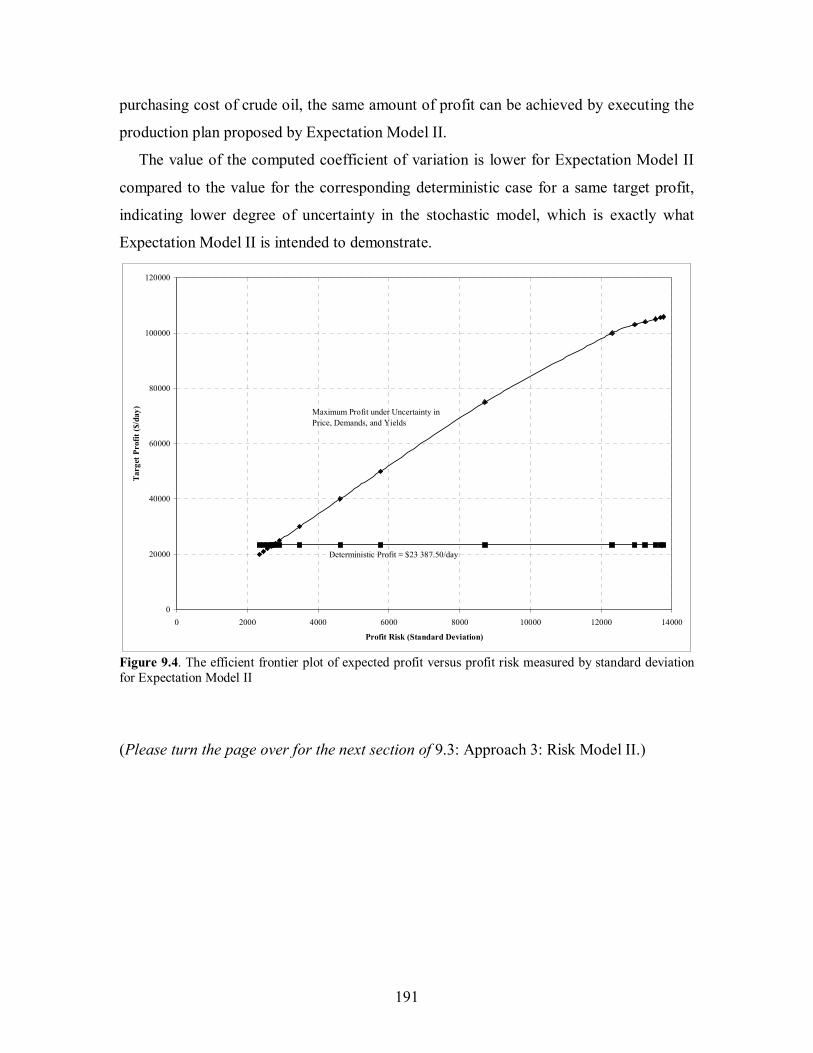
191

purchasing cost of crude oil, the same amount of profit can be achieved by executing the

production plan proposed by Expectation Model II.

The value of the computed coefficient of variation is lower for Expectation Model II

compared to the value for the corresponding deterministic case for a same target profit,

indicating lower degree of uncertainty in the stochastic model, which is exactly what

Expectation Model II is intended to demonstrate.

0

20000

40000

60000

80000

100000

120000

0 2000 4000 6000 8000 10000 12000 14000

Profit Risk (Standard Deviation)

Targ

et P

rofit

($/d

ay)

Deterministic Profit = $23 387.50/day

Maximum Profit under Uncertainty in Price, Demands, and Yields

Figure 9.4. The efficient frontier plot of expected profit versus profit risk measured by standard deviation for Expectation Model II

(Please turn the page over for the next section of 9.3: Approach 3: Risk Model II.)

192

9.3 APPROACH 3: RISK MODEL II

9.3.1 Two-Stage Stochastic Programming with Fixed Recourse of Minimization of

the Expected Value and the Variance of the Recourse Penalty Costs

Variance for the expected recourse penalty for the second-stage costs Vs is given by:

( ) ( ) ( )

( )( ) ( )( ) ( ) ( )

2 2 21 1 2 2 3 3

2 2 21 2 30.35 0.45 0.2

s s s s

s s s s

V p E p E p E

V E E E

′ ′ ′

′ ′ ′

= ξ − + ξ − + ξ −

= ξ − + ξ − + ξ − (9.57)

or in general representation:

( )

( )( )

( )

2

, , , ,

, , , ,

i i s i i s i i s i i ss s s

i I s S i I s Si i s i i s i i s i i s

c z c z c z c zV p p

q y q y q y q y

+ + − − + + − −

+ + − − + + − −∈ ∈ ∈ ∈

+ + = − + + + + ∑∑ ∑∑ (9.58)

where ξ1, ξ2, ξ3, and sE ′ is given by equation (9.53).

Therefore, Risk Model II is as follows:

[ ]( ) ( )

( )( )( )

3 2

0 1 0

21 , , , , 2

1 2 3 4 5 6 14

3 1

maximizeVar( )

( )

0.35 8.8 20.35 8.8 13.75 15.95 6.6 1.65

maximize 0.45 8.0 18

s

s s

s i i i i s i i s i i s i i s i i s si I s S i I i I s S

z z VE z z E V

p C x x V C p c z c z q y q y V

x x x x x x x

z x

+ + − − + + − −

∈ ∈ ∈ ∈ ∈

= −= − θ − −

= − θ − + + + − θ

− + + + + + −

= + − +

∑∑ ∑ ∑∑

( )( )( )

( ) ( ) ( ) ( ) ( )( ) ( )

2 3 4 5 6 14

1 2 3 4 5 6 14

2 2 2 2 21 2 3 4 5

1 2 26 14

.5 8.0 12.5 14.5 6.0 1.5

0.2 7.2 16.65 7.2 11.25 13.05 5.4 1.35

0.352 1.882 375 0.352 0.859 375 1.156 375

0.198 0.012 375

s s

x x x x x x

x x x x x x x

x x x x x

x x

E V

+ + + + − + − + + + + + −

+ + + +− θ

+ + − −

(9.59)

s.t. deterministic constraints (first stage) (8.1), (8.2), (8.8)−(8.19), and (8.26),

stochastic constraints (second stage): (9.17)−(9.32) and (9.37)−(9.52).

193

9.3.2 Computational Results for Risk Model II

Tables 9.20, 9.22, and 9.24 tabulate the computational results for the implementation of

Risk Model II on GAMS for a range of values of the recourse penalty costs risk

parameter θ2 for three distinct cases of the value of the profit risk parameter fixed at θ1 =

0.000 000 000 1, 0.000 000 1, and 0.000 015 5, respectively. Starting values of the first-

stage deterministic decision variables have been initialized to the optimal solutions of the

deterministic model. Representative detailed results are presented in Tables 9.21, 9.23,

and 9.25 that immediately follow each of the three cases for suitable (or particular

meaningful) values of θ2.A number of different parameters are of interest in observing the

trends and patterns that contribute to robustness in the model and robustness in the

computed solution, as extensively analyzed in the ensuing discussion.

(Please turn the page over for Table 9.20.)

19

4

Tab

le 9

.20.

Com

puta

tiona

l res

ults

for

Risk

Mod

el II

for

θ 1 =

0.0

00 0

00 0

00 1

vC

σ=

µ

Reco

urse

pe

nalty

co

sts

risk

fact

or

θ 2

Opt

imal

ob

ject

ive

valu

e

Expe

cted

va

riatio

n in

pr

ofit

V(z 0

)

Expe

cted

to

tal

unm

et

dem

and/

pr

oduc

tion

shor

tfall

Expe

cted

to

tal

exce

ss

prod

uctio

n/

prod

uctio

n su

rplu

s

Expe

cted

re

cour

se

pena

lty

cost

s Es

Expe

cted

va

riatio

n in

re

cour

se

pena

lty

cost

s Vs

σ =

0(

)s

Vz

V+

Expe

cted

pr

ofit

E[z 0

] µ

= E[

z 0]

E s

Stoc

hast

ic

Det

erm

inis

tic

0.00

0 00

1 27

709

.684

0 1.

7871

E+8

2 57

5.00

0 26

815

.000

54

056

.875

8.

1669

E+6

13 6

70.1

19

81 7

74.7

44

27 7

17.8

69

0.49

3 18

7 95

(in

feas

ible

) 0.

000

01

27 6

36.1

817

1.78

71E+

8 2

575.

000

26 8

15.0

00

54 0

56.8

75

8.16

69E+

6 13

670

.119

81

774

.744

27

717

.869

0.

493

187

95

(infe

asib

le)

0.00

0 1

26 9

01.1

589

1.78

71E+

8 2

575.

000

26 8

15.0

00

54 0

56.8

75

8.16

69E+

6 13

670

.119

81

774

.744

27

717

.869

0.

493

187

95

(infe

asib

le)

0.00

1 25

695

.421

5 1.

7818

E+8

2 46

6.60

5 26

706

.605

53

843

.639

2.

0473

E+5

13 3

56.2

32

79 7

43.8

05

25 9

00.1

66

0.51

5 68

1 32

8 (in

feas

ible

) 0.

01

25 5

11.1

674

1.78

18E+

8 2

539.

118

26 7

79.1

18

54 1

95.8

64

2047

.268

13

348

.516

79

727

.522

25

531

.658

0.

522

822

137

(infe

asib

le)

0.1

25 4

92.7

420

1.78

18E+

8 2

518.

476

26 7

58.4

76

54 2

31.0

86

20.4

73

13 3

48.4

28

79 7

25.8

93

25 4

94.8

07

0.52

3 57

4 38

9 (in

feas

ible

) 1

25 4

90.8

994

1.78

18E+

8 2

385.

328

26 6

25.3

28

54 2

34.6

09

0.20

5 13

348

.426

79

725

.731

25

491

.122

0.

523

649

999

(infe

asib

le)

2 25

490

.797

0 1.

7818

E+8

2 50

8.32

5 26

748

.325

54

234

.804

0.

051

13 3

48.4

26

79 7

25.7

22

25 4

90.9

17

0.52

3 65

4 21

(in

feas

ible

) 5

25 4

90.7

356

1.78

18E+

8 2

508.

330

26 7

48.3

30

54 2

34.9

22

0.00

8 13

348

.426

79

725

.716

25

490

.794

0.

523

656

737

(infe

asib

le)

10

25 4

90.7

152

1.78

18E+

8 2

565.

618

26 8

05.6

18

54 2

34.9

61

0.00

2 13

348

.426

79

725

.714

25

490

.753

0.

523

657

579

(infe

asib

le)

50

25 4

90.6

988

1.78

18E+

8 2

556.

034

26 7

96.0

34

54 2

34.9

92

8.18

91E−

5 13

348

.426

79

725

.713

25

490

.721

0.

523

658

236

(infe

asib

le)

100

25 4

90.6

967

1.78

18E+

8 2

518.

750

26 7

58.7

50

54 2

34.9

96

2.04

73E−

5 13

348

.426

79

725

.713

25

490

.717

0.

523

658

318

(infe

asib

le)

1 00

0 25

490

.694

9 1.

7818

E+8

2 51

8.75

0 26

758

.750

54

235

.000

0

13 3

48.4

26

79 7

25.7

13

25 4

90.7

13

0.52

3 65

8 40

1 (in

feas

ible

) 2

000

25 4

90.6

948

1.78

18E+

8 2

543.

023

26 7

83.0

23

54 2

35.0

00

0 13

348

.426

79

725

.713

25

490

.713

0.

523

658

401

(infe

asib

le)

3 00

0 25

490

.694

8 1.

7818

E+8

2 49

5.78

2 26

735

.782

54

235

.000

0

13 3

48.4

26

79 7

25.7

13

25 4

90.7

13

0.52

3 65

8 40

1 (in

feas

ible

) 4

000

25 4

90.6

947

1.78

18E+

8 2

518.

750

26 7

58.7

50

54 2

35.0

00

0 13

348

.426

79

725

.713

25

490

.713

0.

523

658

401

(infe

asib

le)

5 00

0 25

490

.694

7 1.

7818

E+8

2 38

5.00

0 26

625

.000

54

235

.000

0

13 3

48.4

26

79 7

25.7

13

25 4

90.7

13

0.52

3 65

8 40

1 (in

feas

ible

) 6

000

25 4

90.6

947

1.78

18E+

8 2

456.

349

26 6

96.3

49

54 2

35.0

00

0 13

348

.426

79

725

.713

25

490

.713

0.

523

658

401

(infe

asib

le)

7 00

0 25

490

.694

7 1.

7818

E+8

2 55

5.20

8 26

795

.208

54

235

.000

0

13 3

48.4

26

79 7

25.7

13

25 4

90.7

13

0.52

3 65

8 40

1 (in

feas

ible

) 8

000

25 4

90.6

947

1.78

18E+

8 2

518.

750

26 7

58.7

50

54 2

35.0

00

0 13

348

.426

79

725

.713

25

490

.713

0.

523

658

401

(infe

asib

le)

9 00

0 25

490

.694

7 1.

7818

E+8

2 50

8.33

3 26

748

.333

54

235

.000

0

13 3

48.4

26

79 7

25.7

13

25 4

90.7

13

0.52

3 65

8 40

1 (in

feas

ible

) 10

000

25

490

.694

7 1.

7818

E+8

2 54

2.31

2 26

782

.312

54

235

.000

0

13 3

48.4

26

79 7

25.7

13

25 4

90.7

13

0.52

3 65

8 40

1 (in

feas

ible

) 10

500

25

490

.694

7 1.

7818

E+8

2 40

8.75

0 26

648

.750

54

235

.000

0

13 3

48.4

26

79 7

25.7

13

25 4

90.7

13

0.52

3 65

8 40

1 (in

feas

ible

) 10

600

25

490

.694

7 1.

7818

E+8

2 59

1.66

7 26

831

.667

54

235

.000

0

13 3

48.4

26

79 7

25.7

13

25 4

90.7

13

0.52

3 65

8 40

1 (in

feas

ible

) 10

700

25

490

.694

7 1.

7818

E+8

2 58

9.65

8 26

829

.658

54

235

.000

0

13 3

48.4

26

79 7

25.7

13

25 4

90.7

13

0.52

3 65

8 40

1 (in

feas

ible

) 10

710

25

490

.694

7 1.

7818

E+8

2 59

1.66

7 26

831

.667

54

235

.000

0

13 3

48.4

26

79 7

25.7

13

25 4

90.7

13

0.52

3 65

8 40

1 (in

feas

ible

) 10

715

25

490

.694

7 1.

7818

E+8

2 54

3.94

4 26

783

.944

54

235

.000

0

13 3

48.4

26

79 7

25.7

13

25 4

90.7

13

0.52

3 65

8 40

1 (in

feas

ible

) 10

716

25

490

.694

7 1.

7818

E+8

2 50

8.33

3 26

748

.333

54

235

.000

0

13 3

48.4

26

79 7

25.7

13

25 4

90.7

13

0.52

3 65

8 40

1 (in

feas

ible

) 10

717

(G

AM

S ou

tput

: Infeasible solution. There are no superbasic variables.

) N

ote:

Tria

l sol

utio

ns fo

r θ1 <

0.0

00 0

01 a

re n

ot c

onsi

dere

d sin

ce im

prov

emen

t in

expe

cted

pro

fit is

not

ant

icip

ated

bas

ed o

n tre

nds i

n co

mpu

ted

valu

es.

19

5

Tab

le 9

.21.

Det

aile

d co

mpu

tatio

nal r

esul

ts fo

r R

isk M

odel

II fo

r θ 1

= 0

.000

000

000

1, θ

2 = 5

0

Prod

uctio

n Sh

ortfa

ll ijz+

or S

urpl

us

ijz− (t

/d)

Scen

ario

1

Scen

ario

2

Scen

ario

3

Firs

t- St

age

Var

iabl

e St

ocha

stic

So

lutio

n Pr

oduc

t (i)

1iz+

1iz−

2iz+

2iz−

3iz+

3iz−

x 1

15 0

00.0

00

Dem

ands

RH

S C

oeffi

cien

ts R

ando

mne

ss

x 2

2 00

0.00

0 G

asol

ine

(2)

835.

000

0 70

0.00

0 0

565.

000

0x 3

1

155.

000

Nap

htha

(3)

0 0

055

.000

0

110.

000

x 4

3 63

7.50

0 Je

t Fue

l (4)

0

1222

.500

0

1337

.500

0

1452

.500

x 5

3

597.

500

Hea

ting

Oil

(5)

0 18

12.5

00

0.00

18

97.5

0 0

1982

.500

x 6

9

737.

500

Fuel

Oil

(6)

237.

500

0 0

237.

500

0 71

2.50

0 x 7

2

155.

000

x 8

4

635.

000

Prod

uctio

n Y

ield

s LH

S C

oeffi

cien

ts R

ando

mne

ss

x 9

4 35

0.00

0 N

apht

ha (7

) 0

107.

500

020

5.00

0 0

302.

500

x 10

5 47

5.00

0 Je

t Fue

l (4)

0

1275

.000

0

1387

.500

0

1500

.000

x 1

1 1

000.

000

Gas

Oil

(8)

0 11

70.0

00

013

35.0

00

0 15

00.0

00

x 12

2 69

8.12

5 C

rack

er F

eed

(9)

0 12

00.0

00

013

50.0

00

0 15

00.0

00

x 13

1 93

6.87

5 Re

sidu

um (1

0)

0 15

00.0

00

097

5.00

0 0

450.

000

x 14

2 50

0.00

0

x 15

1 85

0.00

0 E(

Pena

lty C

osts

) 18

982

.250

24

405

.742

10

847

.000

x 1

6 1

000.

000

E tot

al

54 2

34.9

92

x 17

1 37

5.00

0

x 1

8 89

9.37

5

x 19

475.

625

x 2

0 12

5.00

0

Expe

cted

Pro

fit

z ($/

day)

79

725

.713

19

6

Tab

le 9

.22.

Com

puta

tiona

l res

ults

for

Risk

Mod

el II

for

θ 1 =

0.0

00 0

00 1

vC

σ=

µ

Reco

urse

pe

nalty

co

st

risk

fact

or

θ 2

Opt

imal

ob

ject

ive

valu

e

Expe

cted

va

riatio

n in

pr

ofit

V(z 0

)

Expe

cted

to

tal

unm

et

dem

and/

pr

oduc

tion

shor

tfall

Expe

cted

to

tal

exce

ss

prod

uctio

n/

prod

uctio

n su

rplu

s

Expe

cted

re

cour

se

pena

lty

cost

s E s

Expe

cted

va

riatio

n in

re

cour

se

pena

lty

cost

s Vs

σ =

0(

)s

Vz

V+

Expe

cted

pr

ofit

E[z 0

]

µ =

E[z 0

] E

s St

ocha

stic

D

eter

min

istic

0.

000

001

27 6

91.8

313

1.78

71E+

8 2

575.

000

26 8

15.0

00

54 0

56.8

75

8.16

69E+

6 13

670

.119

81

774

.744

27

717

.869

0.

493

187

95

(infe

asib

le)

0.00

0 01

27

618

.329

0 1.

7871

E+8

2 57

5.00

0 26

815

.000

54

056

.875

8.

1669

E+6

13 6

70.1

19

81 7

74.7

44

27 7

17.8

69

0.49

3 18

7 95

(in

feas

ible

) 0.

000

1 26

883

.306

2 1.

7871

E+8

2 57

5.00

0 26

815

.000

54

056

.875

8.

1669

E+6

13 6

70.1

19

81 7

74.7

44

27 7

17.8

69

0.49

3 18

7 95

(in

feas

ible

) 0.

001

25 6

77.6

209

1.78

18E+

8 2

467.

445

26 7

07.4

45

53 8

43.6

21

2.04

73E+

5 13

356

.232

79

743

.787

25

900

.166

0.

515

681

328

(infe

asib

le)

0.01

25

493

.367

1 1.

7818

E+8

2 56

4.89

0 26

804

.890

54

195

.862

20

47.2

64

13 3

48.5

16

79 7

27.5

20

25 5

31.6

58

0.52

2 82

2 13

7 (in

feas

ible

) 0.

1 25

474

.941

7 1.

7818

E+8

2 38

4.82

4 26

624

.824

54

231

.086

20

.473

13

348

.428

79

725

.893

25

494

.807

0.

523

574

389

(infe

asib

le)

1 25

473

.099

2 1.

7818

E+8

2 45

6.20

3 26

696

.203

54

234

.609

0.

205

13 3

48.4

26

79 7

25.7

31

25 4

91.1

22

0.52

3 64

9 99

9 (in

feas

ible

) 2

25 4

72.9

968

17.8

18E+

8 2

572.

688

26 8

12.6

88

54 2

34.8

04

0.05

1 13

348

.426

79

725

.722

25

490

.917

0.

523

654

21

(infe

asib

le)

3 25

472

.962

7 1.

7818

E+8

2 57

2.70

1 26

812

.701

54

234

.870

0.

023

13 3

48.4

26

79 7

25.7

19

25 4

90.8

49

0.52

3 65

5 60

7 (in

feas

ible

) 4

25 4

72.9

456

1.78

18E+

8 2

384.

996

26 6

24.9

96

54 2

34.9

02

0.01

3 13

348

.426

79

725

.717

25

490

.815

0.

523

656

305

(infe

asib

le)

5 25

472

.935

4 1.

7818

E+8

2 51

8.74

5 26

758

.745

54

234

.922

0.

008

13 3

48.4

26

79 7

25.7

16

25 4

90.7

94

0.52

3 65

6 73

7 (in

feas

ible

) 6

25 4

72.9

286

1.78

18E+

8 2

508.

330

26 7

48.3

30

54 2

34.9

35

0.00

6 13

348

.426

79

725

.716

25

490

.781

0.

523

657

004

(infe

asib

le)

7 25

472

.923

7 1.

7818

E+8

2 50

8.33

1 26

748

.331

54

234

.944

0.

004

13 3

48.4

26

79 7

25.7

15

25 4

90.7

71

0.52

3 65

7 20

9 (in

feas

ible

) 8

25 4

72.9

200

1.78

18E+

8 2

508.

331

26 7

48.3

31

54 2

34.9

51

0.00

3 13

348

.426

79

725

.715

25

490

.764

0.

523

657

353

(infe

asib

le)

9 25

472

.917

2 1.

7818

E+8

2 50

8.33

1 26

748

.331

54

234

.957

0.

003

13 3

48.4

26

79 7

25.7

15

25 4

90.7

58

0.52

3 65

7 47

6 (in

feas

ible

) 10

25

472

.914

9 17

.818

E+8

2 50

8.33

2 26

748

.332

54

234

.961

0.

002

13 3

48.4

26

79 7

25.7

14

25 4

90.7

53

0.52

3 65

7 57

9 (in

feas

ible

) 50

25

472

.898

5 17

.818

E+8

2 38

5.00

0 26

625

.000

54

234

.992

8.

1891

E−5

13 3

48.4

26

79 7

25.7

13

25 4

90.7

21

0.52

3 65

8 23

6 (in

feas

ible

) 10

0 25

472

.896

5 17

.818

E+8

2 38

5.00

0 26

625

.000

54

234

.996

2.

0473

E−5

13 3

48.4

26

79 7

25.7

13

25 4

90.7

17

0.52

3 65

8 31

8 (in

feas

ible

) 1

000

25 4

72.8

947

17.8

18E+

8 2

508.

333

26 7

48.3

33

54 2

35.0

00

0 13

348

.426

79

725

.713

25

490

.713

0.

523

658

401

(infe

asib

le)

2 00

0 25

472

.894

6 17

.818

E+8

2 55

6.00

3 26

796

.003

54

235

.000

0

13 3

48.4

26

79 7

25.7

13

25 4

90.7

13

0.52

3 65

8 40

1 (in

feas

ible

) 3

000

25 4

72.8

945

17.8

18E+

8 2

456.

250

26 6

96.2

50

54 2

35.0

00

0 13

348

.426

79

725

.713

25

490

.713

0.

523

658

401

(infe

asib

le)

4 00

0 25

472

.894

5 17

.818

E+8

2 55

6.96

0 26

796

.960

54

234

.000

0

13 3

48.4

26

79 7

25.7

13

25 4

90.7

13

0.52

3 65

8 40

1 (in

feas

ible

) 5

000

25 4

72.8

945

17.8

18E+

8 2

456.

250

26 6

96.2

50

54 2

35.0

00

0 13

348

.426

79

725

.713

25

490

.713

0.

523

658

401

(infe

asib

le)

6 00

0 25

472

.894

5 17

.818

E+8

2 45

6.25

0 26

696

.250

54

235

.000

0

13 3

48.4

26

79 7

25.7

13

25 4

90.7

13

0.52

3 65

8 40

1 (in

feas

ible

) 7

000

25 4

72.8

945

17.8

18E+

8 2

508.

333

26 7

48.3

33

54 2

35.0

00

0 13

348

.426

79

725

.713

25

490

.713

0.

523

658

401

(infe

asib

le)

8 00

0 25

472

.894

5 17

.818

E+8

2 51

8.75

0 26

758

.750

54

235

.000

0

13 3

48.4

26

79 7

25.7

13

25 4

90.7

13

0.52

3 65

8 40

1 (in

feas

ible

) 9

000

25 4

72.8

945

17.8

18E+

8 2

556.

150

26 7

96.1

50

54 2

35.0

00

0 13

348

.426

79

725

.713

25

490

.713

0.

523

658

401

(infe

asib

le)

10 0

00

25 4

72.8

945

17.8

18E+

8 2

475.

000

26 7

15.0

00

54 2

35.0

00

0 13

348

.426

79

725

.713

25

490

.713

0.

523

658

401

(infe

asib

le)

10 5

00

25 4

72.8

945

17.8

18E+

8 2

408.

750

26 6

48.7

50

54 2

35.0

00

0 13

348

.426

79

725

.713

25

490

.713

0.

523

658

401

(infe

asib

le)

10 6

00

25 4

72.8

945

17.8

18E+

8 2

589.

655

26 8

29.6

55

54 2

35.0

00

0 13

348

.426

79

725

.713

25

490

.713

0.

523

658

401

(infe

asib

le)

10 7

00

25 4

72.8

945

17.8

18E+

8 2

591.

146

26 8

31.7

50

54 2

35.0

00

0 13

348

.426

79

725

.713

25

490

.713

0.

523

658

401

(infe

asib

le)

10 7

10

25 4

72.8

945

17.8

18E+

8 2

518.

750

26 7

58.7

50

54 2

35.0

00

0 13

348

.426

79

725

.713

25

490

.713

0.

523

658

401

(infe

asib

le)

10 7

15

25 4

72.8

945

17.8

18E+

8 2

591.

667

26 8

31.6

67

54 2

35.0

00

0 13

348

.426

79

725

.713

25

490

.713

0.

523

658

401

(infe

asib

le)

10 7

16

25 4

72.8

945

17.8

18E+

8 2

584.

141

26 8

24.1

41

54 2

35.0

00

0 13

348

.426

79

725

.713

25

490

.713

0.

523

658

401

(infe

asib

le)

10 7

17

(GA

MS

outp

ut: Infeasible solution. There are no superbasic variables.

) N

ote:

Tria

l sol

utio

ns fo

r θ1 <

0.0

00 0

01 a

re n

ot c

onsi

dere

d sin

ce im

prov

emen

t in

expe

cted

pro

fit is

not

ant

icip

ated

bas

ed o

n tre

nds i

n co

mpu

ted

valu

es.

19

7

Tab

le 9

.23.

Det

aile

d co

mpu

tatio

nal r

esul

ts fo

r R

isk M

odel

II fo

r θ 1

= 0

.000

000

1, θ

2 = 5

0

Prod

uctio

n Sh

ortfa

ll ijz+

or S

urpl

us

ijz− (t

/d)

Scen

ario

1

Scen

ario

2

Scen

ario

3

Firs

t- St

age

Var

iabl

e St

ocha

stic

So

lutio

n Pr

oduc

t (i)

1iz+

1iz−

2iz+

2iz−

3iz+

3iz−

x 1

15 0

00.0

00

Dem

ands

RH

S C

oeffi

cien

ts R

ando

mne

ss

x 2

2 00

0.00

0 G

asol

ine

(2)

835.

000

0 70

0.00

0 0

565.

000

0x 3

1

155.

000

Nap

htha

(3)

0 0

055

.000

0

110.

000

x 4

3 63

7.50

0 Je

t Fue

l (4)

0

1222

.500

23

7.49

4 15

74.9

94

0 14

52.5

00

x 5

3 59

7.50

0 H

eatin

g O

il (5

) 0

1812

.500

0

1897

.500

0

1982

.500

x 6

9

737.

500

Fuel

Oil

(6)

237.

500

0 0

237.

500

0 71

2.50

0 x 7

2

155.

000

x 8

4

635.

000

Prod

uctio

n Y

ield

s LH

S C

oeffi

cien

ts R

ando

mne

ss

x 9

4 35

0.00

0 N

apht

ha (7

) 0

107.

500

020

5.00

0 0

302.

500

x 10

5 47

5.00

0 Je

t Fue

l (4)

0

1275

.000

0

1387

.500

0

1500

.000

x 1

1 1

000.

000

Gas

Oil

(8)

0 11

70.0

00

013

35.0

00

0 15

00.0

00

x 12

2 69

8.12

5 C

rack

er F

eed

(9)

0 12

00.0

00

013

50.0

00

0 15

00.0

00

x 13

1 93

6.87

5 Re

sidu

um (1

0)

0 15

00.0

00

097

5.00

0 0

450.

000

x 14

2 50

0.00

0

x 15

1 85

0.00

0 E(

Pena

lty C

osts

) 18

982

.250

24

405

.742

10

847

.000

x 1

6 1

000.

000

E tot

al

54 2

34.9

92

x 17

1 37

5.00

0

x 1

8 89

9.37

5

x 19

475.

625

x 2

0 12

5.00

0

Expe

cted

Pro

fit

E[z 0

] ($/

day)

79

725

.713

19

8

Tab

le 9

.24.

Com

puta

tiona

l res

ults

for

Risk

Mod

el II

for

θ 1 =

0.0

00 0

15 5

vC

σ=

µ

Reco

urse

pe

nalty

co

st

risk

fact

or

θ 2

Opt

imal

ob

ject

ive

valu

e

Expe

cted

va

riatio

n in

pr

ofit

V(z 0

)

Expe

cted

to

tal

unm

et

dem

and/

pr

oduc

tion

shor

tfall

Expe

cted

to

tal

exce

ss

prod

uctio

n/

prod

uctio

n su

rplu

s

Expe

cted

re

cour

se

pena

lty

cost

s Es

Expe

cted

va

riatio

n in

re

cour

se

pena

lty

cost

s Vs

σ =

0(

)s

Vz

V+

Expe

cted

pr

ofit

E[z 0

]

µ =

E[z 0

] E

s St

ocha

stic

D

eter

min

istic

0.

000

001

24 9

39.7

708

1.78

71E+

8 2

575.

000

26 8

15.0

00

54 0

56.8

75

8.16

69E+

6 13

670

.119

81

774

.744

27

717

.869

0.

493

187

95

(infe

asib

le)

0.00

0 01

24

866

.268

5 1.

7871

E+8

2 57

5.00

0 26

815

.000

54

056

.875

8.

1669

E+6

13 6

70.1

19

81 7

74.7

44

27 7

17.8

69

0.49

3 18

7 95

(in

feas

ible

) 0.

000

1 24

131

.245

7 1.

7871

E+8

2 57

5.00

0 26

815

.000

54

056

.875

8.

1669

E+6

13 6

70.1

19

81 7

74.7

44

27 7

17.8

69

0.49

3 18

7 95

(in

feas

ible

) 0.

000

2 23

604

.634

8 1.

7837

E+8

2 43

4.85

9 26

674

.859

53

594

.411

3.

0094

E+6

13 4

67.7

42

80 5

65.6

79

26 9

71.2

69

0.49

9 33

6 60

9 (in

feas

ible

) 0.

000

25

23 4

77.8

943

1.78

30E+

8 2

399.

000

26 6

39.0

00

53 4

76.0

76

2.15

50E+

6 13

433

.225

80

256

.306

26

780

.230

0.

501

609

77

(infe

asib

le)

0.00

0 26

23

456

.929

4 1.

7829

E+8

2 39

3.48

1 26

633

.481

53

457

.862

2.

0403

E+6

13 4

28.5

46

80 2

08.6

89

26 7

50.8

26

0.50

1 98

6 21

9 (in

feas

ible

) 0.

000

27

23 4

37.0

473

1.78

28E+

8 2

388.

370

26 6

28.3

70

53 4

40.9

96

1.93

81E+

6 13

424

.365

80

164

.594

26

723

.598

0.

502

341

227

(infe

asib

le)

0.00

0 28

23

418

.132

1 1.

7827

E+8

2 38

3.62

4 26

623

.624

53

425

.333

1.

8466

E+6

13 4

20.6

13

80 1

23.6

44

26 6

98.3

11

0.50

2 67

6 48

(in

feas

ible

) 0.

000

29

23 4

00.0

840

1.78

26E+

8 2

379.

204

26 6

19.2

04

53 4

10.7

49

1.76

44E+

6 13

417

.233

80

085

.515

26

674

.766

0.

502

993

466

(infe

asib

le)

0.00

0 3

23 3

82.8

164

1.78

25E+

8 2

375.

079

26 6

15.0

79

53 3

97.1

35

1.69

03E+

6 13

414

.175

80

049

.925

26

652

.789

0.

503

293

483

(infe

asib

le)

0.00

0 5

23 1

38.2

622

1.78

19E+

8 2

362.

668

26 6

02.6

68

53 4

46.5

96

8.18

69E+

5 13

379

.291

79

756

.099

26

309

.503

0.

508

534

54

(infe

asib

le)

0.00

1 22

933

.588

8 1.

7818

E+8

2 49

2.50

2 26

732

.502

53

840

.808

2.

0467

E+5

13 3

56.2

08

79 7

40.9

16

25 9

00.1

08

0.51

5 68

1 55

6 (in

feas

ible

) 0.

01

22 7

49.3

826

1.78

18E+

8 2

523.

914

26 7

63.9

14

54 1

95.5

82

2046

.737

13

348

.514

79

727

.234

25

531

.652

0.

522

822

182

(infe

asib

le)

0.1

22 7

30.9

619

1.78

18E+

8 2

531.

028

26 7

71.0

28

54 2

31.0

58

20.4

67

13 3

48.4

28

79 7

25.8

65

25 4

94.8

06

0.52

3 57

4 41

(in

feas

ible

) 1

22 7

29.1

199

1.78

18E+

8 2

578.

902

26 8

18.9

02

54 2

34.6

06

0.20

5 13

348

.426

79

725

.728

25

491

.122

0.

523

649

999

(infe

asib

le)

10

22 7

28.9

357

1.78

18E+

8 2

580.

388

26 8

20.3

88

54 2

34.9

61

0.00

2 13

348

.426

79

725

.714

25

490

.753

0.

523

657

579

(infe

asib

le)

50

22 7

28.9

193

1.78

18E+

8 2

408.

755

26 6

48.7

55

54 2

34.9

92

8.18

69E−

5 13

348

.426

79

725

.713

25

490

.721

0.

523

658

236

(infe

asib

le)

100

22 7

28.9

172

1.78

18E+

8 2

590.

624

26 8

30.6

24

54 2

34.9

96

2.04

67E−

5 13

348

.426

79

725

.713

25

490

.717

0.

523

658

318

(infe

asib

le)

500

22 7

28.9

156

1.78

18E+

8 2

550.

749

26 7

90.7

49

54 2

34.9

99

0 13

348

.426

79

725

.713

25

490

.713

0.

523

658

401

(infe

asib

le)

1 00

0 22

728

.915

4 1.

7818

E+8

2 53

1.81

8 26

771

.818

54

235

.000

0

13 3

48.4

26

79 7

25.7

13

25 4

90.7

13

0.52

3 65

8 40

1 (in

feas

ible

) 5

000

22 7

28.9

152

1.78

18E+

8 2

408.

750

26 6

48.7

50

54 2

35.0

00

0 13

348

.426

79

725

.713

25

490

.713

0.

523

658

401

(infe

asib

le)

10 0

00

22 7

28.9

152

1.78

18E+

8 2

560.

606

26 8

00.6

06

54 2

35.0

00

0 13

348

.426

79

725

.713

25

490

.713

0.

523

658

401

(infe

asib

le)

12 0

00

22 7

28.9

152

1.78

18E+

8 2

597.

388

26 8

37.3

88

54 2

35.0

00

0 13

348

.426

79

725

.713

25

490

.713

0.

523

658

401

(infe

asib

le)

12 5

00

(GA

MS

outp

ut: Infeasible solution. A free variable exceeds the allowable range.

) N

ote:

Tria

l sol

utio

ns fo

r θ1 <

0.0

00 0

01 a

re n

ot c

onsi

dere

d sin

ce im

prov

emen

t in

expe

cted

pro

fit is

not

ant

icip

ated

bas

ed o

n tre

nds i

n co

mpu

ted

valu

es.

199

Table 9.25. Detailed computational results for Risk Model II for θ1 = 0.000 015 5, θ2 = 0.001

Production Shortfall ijz+ or Surplus ijz− (t/d) Scenario 1 Scenario 2 Scenario 3

First- Stage

Variable Stochastic Solution Product (i) 1iz+ 1iz− 2iz+ 2iz− 3iz+ 3iz−

x1 15 000.000 Demands RHS Coefficients Randomness x2 2 000.000 Gasoline (2) 835.000 0 700.000 0 565.000 0 x3 1 155.000 Naphtha (3) 0 0 0 55.000 0 110.000 x4 3 637.500 Jet Fuel (4) 0 1222.500 0 1337.500 0 1452.500 x5 3 599.262 Heating Oil (5) 0 1814.262 0 1899.263 0 1984.262 x6 9735.738 Fuel Oil (6) 239.262 0 0 235.738 0 710.738 x7 2 155.000 x8 4 635.000 Production Yields LHS Coefficients Randomness x9 4 350.000 Naphtha (7) 0 107.500 0 205.000 0 302.500 x10 5 475.000 Jet Fuel (4) 0 1275.000 0 1387.500 0 1500.000 x11 1 000.000 Gas Oil (8) 0 1170.000 0 1335.000 0 1500.000 x12 2 699.447 Cracker Feed (9) 0 1200.000 0 1350.000 0 1500.000 x13 1 935.553 Residuum (10) 0 1500.000 0 975.000 0 450.000 x14 2 500.000 x15 1 850.000 E(Penalty Costs) 18 991.502 24 003.364 10 845.943 x16 1 000.000 Etotal 53 840.808 x17 1 375.000 x18 899.816 x19 475.184 x20 125.000

Expected Profit Z ($/day)

79 740.916

The problem size and the efficient distribution of computational expense are depicted

through the computational statistics shown in Table 8.30. Figure 8.6 then illustrates the

relationship between expected profit and the various levels of risk as dependent on the

tradeoff dictated by the profit risk factor θ1 and the recourse penalty costs risk factor θ2

with variance as the risk measure.

Table 9.26. Computational statistics for Risk Model II

Solver Single continuous

variables Constraints Resource usage/

CPU time (s) Iterations CONOPT 3 96 90 ≈ (0.07−0.081) 10−13

200

9.3.3 Analysis of Results for Risk Model II

The values of θ1 and θ2 denotes the importance of risk in the model as contributed by

variation in profit and variation in recourse penalty costs, respectively, in comparison

with the corresponding expected values of the models objective.

Similar to the expected value models, smaller values of θ1 correspond to higher

expected profit, as shown in Figure 9.5. With increasingly larger θ1, the reduction in

expected profit becomes almost constant as demonstrated for the cases of

θ1 = 0.000 000 1 and θ1 = 0.000 000 000 1; the converse is true as well, that is, with

increasingly smaller θ1, the increment in expected profit becomes roughly constant.

Although the pair of increasing θ2 with fixed value of θ1 corresponds to reduction

expected profit, it generally leads to a reduction of expected production shortfalls and

surpluses as well. Based on the conceptual definition of model robustness presented

earlier for Expectation Model I, this reflects high model feasibility. Therefore, a suitable

operating range of θ2 values ought to be selected in order to achieve optimality between

expected profit and expected production feasibility. Increasing θ2 also reduces the

expected variation or deviation in the recourse penalty costs under different realized

scenarios. This in turn translates to increased solution robustness. It thus depends on the

policy adopted by the decision maker, as characterized by the values of the factors θ1 and

θ2 chosen, in reflecting whether these tradeoffs are acceptable based on the desired

degree of model robustness and solution robustness, as reported by Bok et al. (1998).

In general, the coefficients of variation decrease with larger values of θ2. This is

definitely a desirable behaviour since for higher expected profits, there is diminising

uncertainty in the model, thus signifying model and solution robustness. It is also

observed that for larger values of θ2 until approximately greater than 100, the coefficient

of variation remain at a static value of 0.5237 (correct to four significant figures),

therefore indicating stability and minimal degree of uncertainty in the model.

201

79500

80000

80500

81000

81500

82000

13300 13350 13400 13450 13500 13550 13600 13650 13700

Profit and Recourse Penalty Costs Risk (Measured by Variance)

Exp

ecte

d Pr

ofit

($/d

ay)

0.000 000 000 10.000 000 10.000 015 5

θ1 = 0.000 015 5

Maximum Profit under Uncertainty in Price, Demands, and Yields

θ1 = 0.000 000 000 1

θ1 = 0.000 000 1

Figure 9.5. The efficient frontier plot of expected profit versus risk imposed by variations in both profit and the recourse penalty costs as measured by variance for Risk Model II. Note that the plot for θ1 = 0.000 000 000 1 overlaps with the plot for θ1 = 0.000 000 1.

79500

80000

80500

81000

81500

82000

0.000001 0.00001 0.0001 0.001 0.01 0.1 1 10 100 1000 10000 100000

Risk Parameter θ2 for Recourse Penalty Costs

Exp

ecte

d Pr

ofit

($/d

ay)

0.000 000 000 10.000 000 10.000 015 5

θ1 = 0.000 015 5

θ1 = 0.000 000 1

θ1 = 0.000 000 00 1

Maximum Profit under Uncertainty in Price, Demands, and Yields

Figure 9.6. Plot of expected profit for different levels of risk as represented by the profit risk factor θ1 and the recourse penalty costs risk factor θ2 (with θ1 and θ2 in logarithmic scales due to wide range of values) with variance as the risk measure for Risk Model II. Note that the plot for θ1 = 0.000 000 000 1 overlaps with the plot for θ1 = 0.000 000 1.

202

2300

2350

2400

2450

2500

2550

2600

2650

0.000001 0.00001 0.0001 0.001 0.01 0.1 1 10 100 1000 10000 100000

Risk Parameter θ2 for Recourse Penalty Costs

Expe

cted

Tot

al U

nmet

Dem

and

(Due

to P

rodu

ctio

n Sh

ortf

all)

(ton

/day

)

0.000 000 000 10.000 000 10.000 015 5

θ1 = 0.000 015 5

θ1 = 0.000 000 000 1θ1 = 0.000 000 1

Figure 9.7. Investigating model robustness via the plot of expected total unmet demand (due to production shortfall) versus the recourse penalty costs risk factor θ2

26550

26600

26650

26700

26750

26800

26850

26900

0.000001 0.00001 0.0001 0.001 0.01 0.1 1 10 100 1000 10000 100000

Risk Parameter θ2 for Recourse Penalty Costs

Expe

cted

Tot

al E

xces

s Pro

duct

ion

(Due

to P

rodu

ctio

n Su

rplu

s) (t

on/d

ay)

0.000 000 000 10.000 000 10.000 015 5

θ1 = 0.000 015 5

θ1 = 0.000 000 000 1

θ1 = 0.000 000 1

Figure 9.8. Investigating model robustness via the plot of expected total excess production (due to production surplus) versus the recourse penalty costs risk factor θ2

203

-1.00E+06

0.00E+00

1.00E+06

2.00E+06

3.00E+06

4.00E+06

5.00E+06

6.00E+06

7.00E+06

8.00E+06

9.00E+06

0.000001 0.00001 0.0001 0.001 0.01 0.1 1 10 100 1000 10000 100000

Risk Parameter θ2 for Recourse Penalty Costs

Expe

cted

Dev

iatio

n in

Rec

ours

e Pe

nalty

Cos

ts

0.000 000 000 10.000 000 10.000 015 5

θ1 = 0.000 015 5

θ1 = 0.000 000 000 1

θ1 = 0.000 000 1

Figure 9.9. Investigating solution robustness via the plot of expected variation in the recourse penalty costs versus the recourse penalty costs risk factor θ2. Note that the plot for θ1 = 0.000 000 000 1 overlaps with the plot for θ1 = 0.000 000 1.

9.3.4 Comparison of Performance between Expectation Model I and Risk Model II

As emphasized, the motivation for employing Risk Model II is to account for the

presence of risk in decision-making that is not considered by the risk-neutral Expectation

Model I. Although a robust mathematical (or statistical) approach for direct comparison

between the expected profit obtained by the proposed models of the two approach may

not be conventionally available, from the general trend computed, it is apparent that Risk

Model II consistently registers a higher expected profit, thus testifying to its superior

robustness in the face of multitude uncertainties. In fact, the average expected profit

registered by Risk Model II is a commendable $80 000/day for feasible pair of values of

(θ1, θ2) whereas for Expectation Model I, the expected profit even dipped below the

deterministic profit (of $23 387.50/day, for profit risk factor θ1 that are approximately

larger than 0.0045), as evidenced from Table 9.14.

204

9.4 APPROACH 4: RISK MODEL III

9.4.1 Two-Stage Stochastic Programming with Fixed Recourse for Minimization of

the Expected Value and the Mean-Absolute Deviation (MAD) of the Variation in

Recourse Penalty Costs

The mean-absolute deviation (MAD) for the expected variation in the recourse penalty

for the second-stage costs W(ps) is given by:

( )( ) ( ) ( ) ( )

1 1 2 2 3 3

1 2 30.35 0.45 0.2s s s s

s s s s

W p p E p E p E

W p E E E′ ′ ′

′ ′ ′

= ξ − + ξ − + ξ −

= ξ − + ξ − + ξ − (9.60)

where ξ1, ξ2, ξ3, and sE ′ is given by equation (9.53).

Therefore, Risk Model III is presented as follows:

( ) ( )

( ) ( ) ( )( )

4 2 3

0 1 0 3

0 1 0

3

maximize ( )( ) ( ) ( )

( ) ( )

s

s s

s i is i is i is i isi I s S

i is i iss i is i is i is i is s

i I s S i I s S i is i is

z z W pE z V z E W p

E z V z p c z c z q y q y

c z c zp c z c z q y q y p

q y q y

+ + − − + + − −

∈ ∈

+ + − −+ + − − + + − −

+ + − −∈ ∈ ∈ ∈

= − θ= − θ − − θ

= − θ − + + +

+ − θ + + + − + +

∑∑

∑∑ ∑∑

( )( )( ) ( )( ) ( )

( )

1 2 3 4 5 6 14

4 1 2 3 4 5 6 14

1 2 3 4 5 6 14

21

1

0.35 8.8 20.35 8.8 13.75 15.95 6.6 1.65

maximize 0.45 8.0 18.5 8.0 12.5 14.5 6.0 1.5

0.2 7.2 16.65 7.2 11.25 13.05 5.4 1.35

0.352 1.882 3

x x x x x x x

z x x x x x x x

x x x x x x x

x

− + + + + + −

= + − + + + + + − + − + + + + + −

+− θ

( ) ( ) ( )( ) ( ) ( )

( ) ( )

( ) ( ) ( )( )

2 2 22 3 4

2 2 25 6 14

3

75 0.352 0.859 375

1.156 375 0.198 0.012 375

s i is i is i is i isi I s S

i is i iss i is i is i is i is s

i I s S i is i is

x x x

x x x

p c z c z q y q y

c z c zp c z c z q y q y p

q y q y

+ + − − + + − −

∈ ∈

+ + − −+ + − − + + − −

+ + − −∈ ∈

+ + + + +

− + + +

+ − θ + + + − + +

∑∑

∑∑i I s S∈ ∈∑∑

(9.61)

205

s.t. deterministic constraints (first stage) (8.1), (8.2), (8.8)−(8.19), and (8.26),

stochastic constraints (second stage): (9.17)−(9.32) and (9.37)−(9.52).

where θ1 < θ3.

9.4.2 Comment on the Implementation of Risk Model III on GAMS

Since the absolute deviation is not differentiable at the singularity occurring at the

inflection point, this calls for the use of a solver within the GAMS environment that is

able to execute local optimization of a nonlinear program (NLP) with nonsmooth

functions (Rardin, accessed on September 30, 2005). The default solver stipulated in

GAMS for this class of problem is CONOPT 3 (Drud, 1996,

http://www.gams.com/solvers/conopt.pdf, accessed on January 10, 2006), which is also,

incidentally, the GAMS default solver for NLP. Hence, the default solve statement in

GAMS can be used without the need to specify the type of solver to be CONOPT 3.

9.4.3 Computational Results for Risk Model III

Table 9.27 records the computational results for the implementation of Risk Model III on

GAMS for a range of values for θ1, the tradeoff factor for variability in profit measured

by variance and for θ3, the tradeoff factor for variability in the recourse penalty costs

measured by the mean-absolute deviation (MAD). This is followed by a set of detailed

results for which the case of θ1 = 0.000 8 and θ3 = 0.01 is considered to be representative,

with a number of different parameters enumerated to investigate particular trends and

patterns that potentially contribute to robustness in the proposed model and solution. The

associated computational statistics describing the problem size and the efficient

distribution of computational expense is summarized in Table 9.28. Figure 9.6 then

depicts the Markowitzs efficient frontier plot of expected profit versus risk imposed by

deviations in both profit and the recourse penalty costs. Finally, the results are analyzed

and discussed.

20

6

Tab

le 9

.27.

Com

puta

tiona

l res

ults

for

Risk

Mod

el II

I for

a se

lect

ed r

epre

sent

ativ

e ra

nge

of v

alue

s of θ

1 and

θ3

vC

σ=

µ

Risk

fa

ctor

s θ 1

, θ3

(θ1 <

θ3)

Opt

imal

ob

ject

ive

valu

e

Expe

cted

de

viat

ion

betw

een

prof

it V(

z 0)

Expe

cted

to

tal

unm

et

dem

and/

pr

oduc

tion

shor

tfall

Expe

cted

to

tal

exce

ss

prod

uctio

n/

prod

uctio

n su

rplu

s

Expe

cted

re

cour

se

pena

lty

cost

s Es

Dev

iatio

n be

twee

n re

cour

se

pena

lty

cost

s W

(ps)

σ = 0

() (

) s

Vz W

p+

Ex

pect

ed

prof

it E[

z 0]a

µ

= |E

[z0]

E

s| St

ocha

stic

D

eter

min

istic

0,

0

27 7

17.8

688

1.33

52E+

8 25

75.0

00

26 8

15.0

00

54 0

56.8

75

2 61

8.43

7 11

555

.360

81

774

.744

27

717

.869

0.

416

892

078

(infe

asib

le)

0.00

0 00

1, 0

.000

1

27 5

84.0

832

1.33

52E+

8 25

75.0

00

26 8

15.0

00

54 0

56.8

75

2 61

8.43

7 11

555

.360

81

774

.744

27

717

.869

0.

416

892

078

(infe

asib

le)

0.00

0 01

, 0.0

01

26 3

80.0

130

1.33

52E+

8 25

75.0

00

26 8

15.0

00

54 0

56.8

75

2 61

8.43

7 11

555

.360

81

774

.744

27

717

.869

0.

416

892

078

(infe

asib

le)

0.00

0 01

, 0.0

0316

26

374

.357

2 1.

3352

E+8

2575

.000

26

815

.000

54

056

.875

2

618.

437

11 5

55.3

60

81 7

74.7

44

27 7

17.8

69

0.41

6 89

2 07

8 (in

feas

ible

) 0.

000

1, 0

.001

14

362

.877

6 1.

3352

E+8

2575

.000

26

815

.000

54

056

.875

2

618.

437

11 5

55.3

60

81 7

74.7

44

27 7

17.8

69

0.41

6 89

2 07

8 (in

feas

ible

) 0.

000

1, 0

.01

14 3

39.3

116

1.33

52E+

8 25

75.0

00

26 8

15.0

00

54 0

56.8

75

2 61

8.43

7 11

555

.360

81

774

.744

27

717

.869

0.

416

892

078

(infe

asib

le)

0.00

0 2,

0.0

1 2

801.

8097

9.

6341

E+7

2575

.000

17

800

.529

40

232

.400

2

627.

927

9 81

5.47

9 62

328

.689

22

096

.289

0.

444

213

913

(infe

asib

le)

0.00

0 3,

0.0

1 −6

832

.290

1 9.

6341

E+7

2575

.000

17

800

.529

40

232

.400

2

627.

927

9 81

5.47

9 62

328

.689

22

096

.289

0.

444

213

913

(infe

asib

le)

0.00

0 4,

0.0

1 −1

6 39

7.35

32

8.95

90E+

7 35

25.0

00

16 6

61.8

10

42 4

44.1

68

3 82

7.12

6 9

465.

385

61 9

20.9

58

19 4

76.7

90

0.48

5 98

2 80

3 (in

feas

ible

) 0.

000

5, 0

.01

−25

311.

7774

8.

8371

E+7

3610

.000

16

373

.039

42

198

.208

4

252.

945

9 40

0.83

2 61

114

.658

18

916

.450

0.

496

965

974

(infe

asib

le)

0.00

0 6,

0.0

1 −3

4 14

8.91

70

8.83

71E+

7 36

10.0

00

16 3

73.0

39

42 1

98.2

08

4 25

2.94

5 9

400.

832

61 1

14.6

58

18 9

16.4

50

0.49

6 96

5 97

4 (in

feas

ible

) 0.

000

7, 0

.01

−42

800.

1921

7.

9660

E+7

5555

.807

15

466

.745

47

553

.299

4

255.

947

8 92

5.50

3 60

557

.911

13

004

.612

0.

686

333

664

(infe

asib

le)

0.00

0 8,

0.0

01

−49

888.

4004

6.

3920

E+7

9424

.122

13

665

.010

58

199

.357

4

261.

916

7 99

5.25

4 59

451

.082

1

251.

725

6.38

7 38

8 60

4 (in

feas

ible

) 0.

000

8, 0

.01

−49

926.

7577

6.

3920

E+7

9423

.998

13

665

.067

58

199

.017

4

261.

916

7 99

5.28

4 59

451

.117

1

252.

101

6.38

5 49

4 46

1 (in

feas

ible

) 0.

000

9, 0

.01

−56

172.

9937

6.

2367

E+7

9836

.111

13

473

.118

59

333

.201

4

262.

552

7 89

7.55

3 59

333

.201

0

→ ∞

(in

feas

ible

) 0.

001,

0.0

1 −6

2 40

9.70

13

6.23

67E+

7 98

36.1

11

13 4

73.1

18

59 3

33.2

01

4 26

2.55

2 7

897.

553

59 3

33.2

01

0 →

∞

(infe

asib

le)

0.00

1, 0

.031

6 −6

2 50

1.77

24

6.23

67E+

7 98

36.1

11

13 4

73.1

18

59 3

33.2

01

4 26

2.55

2 7

897.

553

59 3

33.2

01

0 →

∞

(infe

asib

le)

0.01

, 0.1

−6

2 50

2.01

79

6.23

67E+

7 98

36.1

11

13 4

73.1

18

59 3

33.2

01

4 26

2.55

2 7

897.

553

59 3

33.2

01

0 →

∞

(infe

asib

le)

0.02

, 0.1

−1

247

767

.770

4 6.

2367

E+7

9836

.111

13

473

.118

59

333

.201

4

262.

552

7 89

7.55

3 59

333

.201

0

→ ∞

(in

feas

ible

) 0.

1, 0

.316

2 −6

238

055

.395

1 6.

2367

E+7

9836

.111

13

473

.118

59

333

.201

4

262.

552

7 89

7.55

3 59

333

.201

0

→ ∞

(in

feas

ible

) 0.

5, 0

.707

1 −3

1 18

6 55

1.93

17

6.23

67E+

7 98

36.1

11

13 4

73.1

18

59 3

33.2

01

4 26

2.55

2 7

897.

553

59 3

33.2

01

0 →

∞

(infe

asib

le)

1, 1

−6

2 37

1 33

8.31

45

6.23

67E+

7 98

36.1

11

13 4

73.1

18

59 3

33.2

01

4 26

2.55

2 7

897.

553

59 3

33.2

01

0 →

∞

(infe

asib

le)

40, 2

0 −2

494

768

281

.545

7 6.

2367

E+7

9836

.111

13

473

.118

59

333

.201

4

262.

552

7 89

7.55

3 59

333

.201

0

→ ∞

(in

feas

ible

) 10

0, 1

0 −6

236

750

201

.793

0 6.

2367

E+7

9836

.111

13

473

.118

59

333

.201

4

262.

552

7 89

7.55

3 59

333

.201

0

→ ∞

(in

feas

ible

) 10

00, 1

00

−62

367

502

017.

9260

6.

2367

E+7

9836

.111

13

473

.118

59

333

.201

4

262.

552

7 89

7.55

3 59

333

.201

0

→ ∞

(in

feas

ible

) 10

000

, 100

(G

AM

S ou

tput

: Infeasible solution. A free variable exceeds the allowable range.

) (in

feas

ible

)

207

Table 9.28. Detailed computational results for Risk Model III for θ1 = 0.000 8, θ3 = 0.01

Production Shortfall ijz+ or Surplus ijz− (t/d) Scenario 1 Scenario 2 Scenario 3

First- Stage

Variable Stochastic Solution Product (i) 1iz+ 1iz− 2iz+ 2iz− 3iz+ 3iz−

x1 10 282.158 Demands RHS Coefficients Randomness x2 2 000.000 Gasoline (2) 835.000 0 700.000 0 565.000 0 x3 1 155.000 Naphtha (3) 0 0 0 55.000 0 110.000 x4 2 493.423 Jet Fuel (4) 0 78.423 0 193.423 0 308.423 x5 1 700.000 Heating Oil (5) 85.000 0 0 0 0 85.000 x6 7 087.001 Fuel Oil (6) 2887.999 0 2412.999 0 1937.999 0 x7 2 155.000 x8 3 177.187 Production Yields LHS Coefficients Randomness x9 2 981.826 Naphtha (7) 0 751.485 0 818.319 0 885.153 x10 3 752.988 Jet Fuel (4) 0 873.983 0 951.100 0 1028.216 x11 1 000.000 Gas Oil (8) 0 802.008 0 915.112 0 1028.216 x12 1 275.000 Cracker Feed (9) 0 822.573 0 925.394 0 1028.216 x13 1 902.187 Residuum (10) 0 1028.216 0 668.340 0 308.465 x14 2 500.000 x15 481.826 E(Penalty Costs) 22 500.614 25 607.063 10 091.340 x16 1 000.000 Etotal 58 199.017 x17 1 375.000 x18 425.000 x19 950.000 x20 125.000

Expected Profit Z ($/day)

59 451.117

Table 9.29. Computational statistics for Risk Model III

Solver Single continuous

variables Constraints Resource usage/

CPU time (s) Iterations CONOPT 3 96 91 ≈ (0.049−0.100) 14

9.4.4 Analysis of Results for Risk Model III

As is the case with Risk Model II, the values of θ1 and θ3 denotes the importance of risk

in the model as contributed by variation in profit and variation in recourse penalty costs,

respectively, in comparison with the corresponding expected values of the models

objective.

From Table 8.31, similar trends with the expected value models are observed in which

reducing values of θ1 implicates higher expected profit. With increasingly smaller θ1, the

208

increment in expected profit becomes constant; the same constancy trend is also observed

in the initially declining expected profit for increasing values of θ1.

One of the reasons the pair of reducing values of θ1 with fixed value of θ3 leads to

increasing expected profit is attributable to the general decrement in production shortfalls

but increasing production surpluses, in which the fixed penalty cost for the latter is lower

than the former. Based on its conceptual definition (as mentioned earlier), it certainly

augurs well to select a higher operating value of θ1 to achieve both high model feasibility

as well as increased profit. Moreover, higher values of θ1 alto decreasing variation in the

recourse penalty costs, which implies solution robustness. This argument is further

strengthened by the decreasing values of the coefficient of variation, which indicates less

uncertainty in the model on a whole. This again demonstrates that a proper selection of

the operating range of θ1 and θ3 is crucial in varying the tradeoffs between the desired

degree of model robustness and solution robustness, to ultimately obtain optimality

between expected profit and expected production feasibility.

0

20000

40000

60000

80000

100000

7900 8100 8300 8500 8700 8900 9100 9300 9500 9700 9900 10100 10300 10500 10700 10900 11100 11300 11500 11700

Profit and Recourse Penalty Costs Risk

Expe

cted

Pro

fit ($

/day

)

Maximum Profit under Uncertainty in Price, Demands, and Yields

Deterministic Profit = $23 387.50/day

Figure 9.10. The efficient frontier plot of expected profit versus risk imposed by variations in both profit (measured by variance) and the recourse penalty costs (measured by mean-absolute deviation) for Risk Model III

209

9.5 SUMMARY OF RESULTS AND COMPARISON AGAINST RESULTS FROM

THE FUZZY LINEAR FRACTIONAL GOAL PROGRAMMING APPROACH

Ravi and Reddy (1998) adopted the fuzzy linear fractional goal programming approach to

the same deterministic linear program for refinery operations planning by Allen (1971)

that is used for the present numerical example. Based on their arguments that a decision

maker is very often more interested in the optimization of ratios, they identified the ratios

or the fractional goals to be treated as fuzzy goals for optimization as the following:

1 11 1

profitcapacity of the primary unit ( )

Zf fx x

= ⇒ =

(9.62)

2 114 14

profitcapacity of the cracker ( )

Zf fx x

= ⇒ =

(9.63)

for which the deterministic model of Allen (1971) is then reformulated accordingly.

Table 9.30 presents a summary of the results obtained from the base case deterministic

model and the five different approaches adopted in applying the methods of stochastic

optimization, to be compared against results from the fuzzy linear programming

approach.

Ravi and Reddy (1998) advocated that their results, although registering 1.3 percent

less profit than the linear programming approach of Allen (1971), yielded higher optimal

fractional goal values, thus translating to better ratio values of profit/capacity of primary

unit capacity f1 and profit/capacity of the cracker unit f2 simultaneously. Following the

same premise, we conclude that the stochastic models, in addition to proposing midterm

plans that consistently register higher expected profits than both the deterministic and the

fuzzy programming models, assure the decision maker of good ratios for both f1 and f2.

Maximization of these ratios lead to maximum or near maximum profit, with minimum

or near minimum capacities of the respective units simultaneously. As petroleum refiners

use the technology of fluidized bed catalytic crackers (FCC) to convert more crude oil to

blending stocks for producing gasoline, which is unarguably the most commercially

210

attractive end product of the refining activity, it certainly augurs well for the stochastic

models to have a good ratio of maximum profit with regards to a minimum capacity of

the highly capital-intensive FCC unit. Moreover, about 45 percent of worldwide gasoline

production is contributed by FCC processes and its ancillary unit. Thus, the overall

economic performance of a refinery considerably hinges on a prudent investment in FCC

due to its large throughput, high product-feed upgrade, and mercantile importance

(Alvarez-Ramirez et al., 2004).

Table 9.30. Comparison of results obtained from the deterministic model, the stochastic models, and

the fuzzy linear fractional goal program by Ravi and Reddy (1998)

First- Stage

Variable

Deterministic Linear

Program

Stochastic Risk

Model I

Stochastic Expectation

Model I (for

θ1 = 0.000 03)

Stochastic Expectation

Model II

Stochastic Risk

Model II (for

θ1 = 0.000 000 1, θ2 = 50)

Stochastic Risk

Model III (for

θ1 = 0.000 8, θ3 = 0.01)

Fuzzy Linear

Fractional Goal

Program* x1 12 500 12 171.621 15 000.000 2792.531 15 000.000 10 282.158 12 054.59 x2 2 000 1 947.459 2 000.000 647.867 2 000.000 2 000.000 1 928.74 x3 625 608.581 1 155.000 300.197 1 155.000 1 155.000 602.73 x4 1 875 1 825.743 3 637.500 677.189 3 637.500 2 493.423 1 808.19 x5 1 700 1 700.000 3 835.000 1150.523 3 597.500 1 700.000 1 700.00 x6 6 175 5 968.122 9 500.000 177.052 9737.500 7 087.001 5 894.39 x7 1 625 1 582.311 2 155.000 624.131 2 155.000 2 155.000 1 567.09 x8 2 750 2 677.757 4 635.000 862.892 4 635.000 3 177.187 2 652.01 x9 2 500 2 434.324 4 350.000 809.834 4 350.000 2 981.826 2 410.92 x10 3 750 3 651.486 5 475.000 1019.274 5 475.000 3 752.988 3 616.38 x11 1 000 973.730 1 000.000 323.934 1 000.000 1 000.000 964.37 x12 1 275 1 275.000 2 876.250 862.892 2 698.125 1 275.000 1 275.00 x13 1 475 1 402.757 1 758.750 0 1 936.875 1 902.187 1 377.01 x14 2 500 2 434.324 2 500.000 809.834 2 500.000 2 500.000 2 410.92 x15 0 0 1 850.000 0 1 850.000 481.826 0.0 x16 1 000 973.730 1 000.000 323.934 1 000.000 1 000.000 964.38 x17 1 375 1 338.878 1 375.000 445.409 1 375.000 1 375.000 1 326.01 x18 425 425.000 958.750 287.631 899.375 425.000 425.00 x19 950 913.878 416.250 157.778 475.625 950.000 901.01 x20 125 121.716 125.000 40.492 125.000 125.000 120.55

Profit ($/day) 23 387.50 23 500.000 81 774.744 23 387.50 79 725.713 59 451.117 23 069.06 f1 1.871 1.931 5.452 8.375 5.315 5.782 1.914 f2 9.355 9.654 32.710 28.879 31.890 23.780 9.569

* Taken from the work of Ravi and Reddy (1998)

211

9.6 ADDITIONAL REMARKS

In retrospect, we mildly caution the respected reader that this work primarily intends to

demonstrate the validity of the stochastic concepts reviewed along with the methods

developed and improvised by using a typical and realistic refinery planning problem

under uncertainty. However, it is certainly not our claim that the model captures all

detailed aspects of the problem but rather, it demonstrates the capabilities of the proposed

tools.

212

CHAPTER 10

Conclusions

10.1 SUMMARY OF WORK

This thesis research focuses on the methodology of developing effective yet

straightforward stochastic optimization models for the midterm production planning of a

petroleum refinery by accounting for three major factors of uncertainty simultaneously,

namely commodities prices, market demands, and product yields. In addition, we

consider the importance of risk in decision-making under uncertainty in the proposed

stochastic planning models by explicitly accounting for the tradeoffs between expected

profit and variation in both profit and the recourse penalty costs. These measures of risk

(in the form of variance for the price coefficients and variance or Mean-Absolute

Deviation (MAD) for the recourse penalty costs, adopted in different models) are

incorporated within the general framework of the proposed models with the aim of

achieving robustness in decision-making activities especially in view of the highly

volatile hydrocarbon industry in which the petroleum refineries operate. The following

four approaches are implemented, resulting correspondingly in four decision-making

models under uncertainty:

1. the Markowitzs meanvariance (MV) model to handle randomness in the

objective function coefficients of prices by minimizing the variance of the

expected value or mean of the random coefficients, subject to a target profit

constraint;

2. the two-stage stochastic programming with fixed recourse via scenario analysis

approach to model randomness in the right-hand side and the left-hand side

(technological) coefficients by minimizing the expected recourse penalty costs

due to constraints violations;

3. incorporation of the Markowitzs MV approach within the bilevel decision-

making framework developed in the preceding approach to minimize both the

expectation and the variance of the recourse penalty costs; and

213

4. reformulation of the model developed in the third approach by utilizing the Mean

Absolute Deviation (MAD) as the measure of risk imposed by the recourse

penalty costs.

An exposition for justifying the rationale for adopting each of the four stochastic

modelling methods is undertaken in this work by comprehensively surveying past

successes in employing such approaches in the open literature, but in the light of the

limitations of the approaches.

As emphasized throughout, the novelty of these approaches lies in the explicit

modelling and formulation of uncertainties considered for the large-scale optimization

problem of petroleum refinery production planning. This has been accomplished through

the utilization of slack variables to account for violations of the stochastic constraints of

possible scenarios of product demands and product yields, primarily within a bilevel

decision-making framework of two-stage stochastic programming that incorporates the

Markowitzs meanvariance model of portfolio selection optimization as a hedging tool

against the presence of risk that arises due to variation in profit and the penalty costs of

recourse actions.

10.2 MAJOR CONTRIBUTIONS OF THIS RESEARCH

The major contributions of this work are threefold. First, we formulate a slate of highly

tractable stochastic optimization models through an explicit modelling of the presence of

uncertainties for application in the production planning of petroleum refineries, primarily

within a two-stage stochastic programming framework. This is accomplished via the

systematic adoption of a hybrid of effective yet clear-cut stochastic optimization

techniques that obviates the use of the conventional brute force approach of Monte Carlo-

based methods.

Second, we consider the incorporation of the concept of Mean-Absolute Deviation

(MAD) as a measure of risk for the petroleum refining activities, instead of the traditional

measure using variance. The numerous benefits of doing so are elucidated in Section

5.8.1, with the most significant being the ability to linearize the MAD expression in the

214

objective function, thus producing an equivalent linear programming problem that can be

solved accurately and competently by harnessing the combination of efficient algorithms

with the power of todays modern computing technology.

Additionally, in an effort to establish the effectiveness of the proposed stochastic

models while simultaneously hedging against the various forms of uncertainties in

commodity prices, market demands, and product yields, we carry out a series of extensive

and rigorous computational experiments to investigate and interpret the behaviour and the

overall robustness of the multiobjective optimization models. This is executed in light of

similar methodologies that have been employed in previous works, notably the

applications of Mulvey et al. (1995)s robust optimization approach by Bok et al. (1998)

for the capacity expansion of a petrochemicals processing network and by Malcolm and

Zenios (1994) for the capacity expansion of power systems. Oftentimes, we also take into

account many of the useful suggestions and guidelines that are offered by the now

classical paper by Rardin and Lin (1982) on issues and techniques concerning test

problems for computational experiments. Two performance metrics are thus considered,

namely: (1) the concepts of solution robustness and model robustness as introduced by

Mulvey et al. (1995) and (2) the coefficient of variation Cv, in order to gauge the

performances of the four proposed stochastic models against each other, as well as

against the deterministic model and the fuzzy programming approach of Ravi and Reddy

(1998).

215

CHAPTER 11

Recommendations for Future Work and Way Forward

11.1 SUMMARY OF RECOMMENDATIONS FOR FUTURE WORK

In this chapter, we intend to bring together and consolidate under one roof, the numerous

recommendations scattered over the main content of the dissertation. We are also inclined

to offer some personal thoughts and opinions on a promising research agenda for future

undertakings in this exciting area of developing stochastic programming tools and

applications, for petroleum refinery operations management in specific and the wider

spectrum of business decision-making in general. To provide a compact discussion, the

essence of the recommendations and suggestions for future work are enumerated as

follows:

1. to implement extensions to the present general deterministic midterm production

planning model for petroleum refineries by considering the the following features:

• rigorous modelling of advanced petroleum refining process unit such as the

hydrotreating and hydrocracking units that are instrumental especially in the

current drive towards clean fuels production;

• capacity expansion through the installation of multiple number of processing

units; an example with apparent economic value would be the installation of an

additional piece of the fluidized bed catalytic cracker (FCCU) to increase the

production of gasoline that is arguably the most profitable of refining end

products;

• modelling nonlinearities in blending operations as constraints for production of

fuels in satisfying the following operating objectives, which are typically

prioritized in this order as advocated by Bodington (19950: (i) quality

specifications; (ii) shipment schedule; (iii) quality giveaway; (iv) blending cost;

and () inventory targets;

216

• multiferinery modelling of a network of refineries, with consideration for inter-

refinery transfer or transportation of intermediates and products under

subcontracting agreements, with the addition of production (supply) and

distribution modelling; interactions with potential spin-off industries particularly

petrochemicals processing will also be examined;

• incorporation of complex economic instruments such as royalties, taxes, and

tariffs in the objective function of net present value (van den Heever, 2001; van

den Heever et al., 2000; 2001);

2. improvements in methodology for dealing with uncertainty:

• implementation of multi-stage stochastic programming framework with the stages

corresponding to time periods, hence effectively formulating multiperiod models,

which is an established alternative strategy in dealing with uncertainty;

• incorporation of uncertainties in less-commonly considered but equally paramount

and planning-sensitive factors such as (i) process variations as indicated by

variable process parameters, for example, flow rates and temperatures; (ii)

cancelled/rushed orders; (iii) equipment failure; (iv) technology obsolescence; and

(v) sales uncertainty;

• improvement in effective procedures of scenario selection and generation, which

is a highly essential (if not the most essential) key component towards developing

stochastic programming models that are truly robust in the face of uncertainties; in

particular, we intend to pursue the incorporation of the scenario planning

paradigm (van der Heijden, 2005; Godet, 1987; Schoemaker and van der Heijden,

1992; Lindgren and Bandhold, 2003; Schwartz, 1991; Stokke et al., 1990; Huss

and Honton, 1987) that has been so successfully practised at Royal Dutch/Shell,

which is not only the leading oil-and-gas company worldwide but is even

arguably, one of the most successful corporations of modern times,

• improvement in the theory and procedure for specifying the weights for

multiobjective optimization to account for the tradeoffs between expected profit

and risk;

217

3. incorporation of advanced metrics for risk measurement and modelling since the

conventional metric of variance is a symmetric risk measure that desirably penalizes

profits below the target levels but also undesirably penalizes profits above the target

levels, other than the mean-absolute deviation (MAD) that is considered in this work

with much resulting promise; the alternative risk measures to be considered will

include the expected downside risk (Eppen et al., 1989), the Value-at-Risk (VaR)

(Barbaro and Bagajewicz, 2004a; Mulvey, 2001), and the Conditional Value-at-Risk

(CVaR) (Rockafellar and Uryasev, 2002).

11.2 FINAL REMARKS

We are convinced that there is still a plethora of research opportunities in this field with

directions of research problems themselves muddled with uncertainty (ironically) and

multitude of questions unanswered, as widely acknowledged by both academics and

practitioners of the field. In advancing this stand, we have the privilege of support from

none other than George (Bernard) Dantzig himself, fondly dubbed as the father of linear

programming (primarily for devising the simplex method) and one of the pioneers of

stochastic programming, with the following truly inspiring quote from Dantzig, which

has and will continue to serve to motivate researchers, both current and potential, in this

remarkably rich and fascinating field of stochastic optimization:

Planning under uncertainty. This, I feel, is the real field we should all be working

on. (http://www.e-optimization.com/directory/trailblazers/dantzig/

interview_planning.cfm, accessed on March 2, 2006; http://www2.informs.org/History/

dantzig/in_interview_irv10.htm, accessed on March 9, 2006).

Incidentally, to cap the wonderful journey of working on this thesis research, we take

this opportunity to pay our utmost respect and homage to Dantzig (November 8, 1914

May 13, 2005), whose recent demise last year would certainly carve a legacy that will

long survive him in continuing to spur the area of mathematical

programming/optimization/operations research towards attaining greater heights and

meaning. (As an aside, optimization is the term strongly preferred and even advocated

by George L. Nemhauser, truly one of the giants of the field and co-author with Laurence

A. Wolsey of the biblical encyclopaedia of the discrete sub-area of this field entitled

Integer and Combinatorial Optimization (Nemhauser, 1994).)

218

References and Literature Cited

To borrow a similar principle from perhaps one of the most highly readable advanced

level text in mathematics as Lectures on Polytopes (Springer-Verlag, 1995), beautifully

penned by Gunter M. Ziegler (which addresses a very useful theory for the strong

formulations of integer programming problems), I have attempted to compile a

bibliography on production planning focussing on problems under uncertainty with

emphasis on chemical process systems engineering (PSE)-related problems, with REAL

NAMES, to illustrate that behind all of these mathematics (some of it spectacularly

beautiful yet functional), there are actual REAL PEOPLE. In the few cases where I could not

find more than initials, perhaps just assume that that is all that they have (with this to be

taken in a light tone).

Acevedo, J. and Efstratios N. Pistikopoulos. Stochastic optimization based algorithms for

process synthesis under uncertainty. Computers & Chemical Engineering. 22 (1998):

647671.

Ahmed, Shabbir and Nikolaos Vasili Sahinidis. Robust process planning under

uncertainty. Industrial & Engineering Chemistry Research 37 (1998): 18831892.

Allen, D. H. Linear programming models for plant operations planning. British Chemical

Engineering.16 (1971): 685691.

Alvarez-Ramirez, Jose, Jesus Valencia, and Hector Puebla. Multivariable control

configurations for composition regulation in a fluid catalytic cracking unit. Chemical

Engineering Journal 99 (2004): 187201.

219

Applequist, George Einar. Economic risk management for chemical manufacturing

supply chain planning. PhD Thesis. West Lafayette, Indiana, USA: Purdue University,

2002.

Applequist, George Einar, Joseph F. Pekny, and Gintaras V. Reklaitis. Risk and

uncertainty in managing chemical manufacturing supply chains. Computers & Chemical

Engineering 24 (2000): 22112222.

Applequist, George Einar, O. Samikoglu, Joseph Pekny, and Gintaras V. Reklaitis. Issues

in the use, design, and evolution of process scheduling and planning systems. ISA

Transactions 36 (1997), 2: 81121.

Aseeri, Ahmed and Miguel J. Bagajewicz. New measures and procedures to manage

financial risk with applications to the planning of gas commercialization in Asia.

Computers & Chemical Engineering 28 (2004): 27912821.

Aseeri, Ahmed, Patrick Gorman, and Miguel J. Bagajewicz. Financial risk management

in offshore oil infrastructure planning and scheduling. Industrial & Engineering

Chemistry Research 43 (2004), 12: 30633072.

Balasubramanian, J. and Ignacio E. Grossmann. Approximation to multistage stochastic

optimization in multiperiod batch plant scheduling under demand uncertainty. Industrial

& Engineering Chemistry Research. 43 (2004): 36953713.

Barbaro, Andres and Miguel J. Bagajewicz. Managing financial risk in planning under

uncertainty. AIChE Journal 50 (May 2004a), 5: 963989.

Barbaro, Andres and Miguel J. Bagajewicz. Use of inventory and option contracts to

hedge financial risk in planning under uncertainty. AIChE Journal 50 (May 2004b), 5:

963989.

220

Bassett, M. H., P. Dave, Francis J. Doyle III, G. K. Kudva, Joseph F. Pekny. Gintaras V.

Reklaitis, S. Subrahmanyam, D. L. Miller, and M. G. Zentner. Perspectives on model

based integration of process operations. Computers & Chemical Engineering 20 (1996),

6/7: 821844.

Bassett, M. H., Joseph F. Pekny, and Gintaras V. Reklaitis. Using detailed scheduling to

obtain realistic operating policies for a batch processing facility. Industrial &

Engineering Chemistry Research 36 (1997): 17171726.

Baumol, William J. Activity analysis in one lesson. American Economic Review. 48

(1958), 5: 837 873.

Beale, E. On minimizing a convex function subject to linear inequalities. Journal of the

Royal Statistical Society, Series B (Methodological) 17 (1955), 2: 173184.

Bellman, R. and Lotfi Asker Zadeh. Decision-making in a fuzzy environment.

Management Science 17 (1970): 141161.

Benders, J. F. Partitioning procedures for solving mixed-variables programming

problems. Numerische, Mathematik 4 (1962): 238252.

Ben-Tal, Aharon. and Arkadi Nemirovski. Robust solutions of linear programming

problems contaminated with uncertain data. Mathematical Programming 88 (2000): 411

424.

Biegler, Lorenz T. From nonlinear programming theory to practical optimization

algorithms: a process engineering viewpoint. Computers & Chemical Engineering 17

(1993), Supplement 1: 6380.

221

Birewar, Deepak B. and Ignacio E. Grossmann. Simultaneous production planning and

scheduling in multiproduct plants. Industrial & Engineering Chemistry Research 29

(1990), 4: 570580.

Birge, John R. and Francois Louveaux. Introduction to Stochastic Programming. New

York: Springer-Verlag New York, Inc., 1997.

Birge, John R. and Roger J.-B. Wets. (editors). Preface for Proceedings of the 5th

International Conference on Stochastic Programming. Annals of Operations Research 30

& 31 (1991).

Birge, John R. The value of the stochastic solution in stochastic linear programs with

fixed recourse. Mathematical Programming 24 (1982): 314325.

Birge, John R. Stochastic programming computation and applications. INFORMS Journal

on Computing 9 (1997), 2: 111133.

Birge, John R. Personal Communication, 2005.

Bitran, Gabriel. R. and Hax, Arnaldo C. On the design of the hierarchical production

planning systems. Decision Sciences 8 (1977): 28 55.

Bodington, C. Edward. Management. In Planning, Scheduling, and Control Integration

in the Process Industries. Edited by C. Edward Bodington. New York: McGraw-Hill,

1995.

Bodington, C. Edward. Planning, Scheduling, and Control Integration in the Process

Industries. New York: McGraw-Hill, 1995.

222

Bok, Jin-Kwang, Heeman Lee, and Sunwon Park. Robust investment model for long-

range capacity expansion of chemical processing networks under uncertain demand

forecast scenarios. Computers & Chemical Engineering 22 (1998): 10371049.

Bok, Jin-Kwang., Ignacio E. Grossmann, and Sunwon Park. Supply chain optimization in

continuous flexible processes. Industrial & Engineering Chemistry Research 39 (2000):

12791290.

Bonfill, Anna, Miguel Bagajewicz, Antonio Espuna, and Luis Puigjaner. Risk

management in the scheduling of batch plants under uncertain market demand. Industrial

& Engineering Chemistry Research 43 (2004): 741750.

Bopp, A. E., V. R. Kannan, S. W. Palocsay, and S. P. Stevens. An optimization model for

planning natural gas purchases, transportation, storage, and deliverability. Omega:

International Journal of Management Science 24 (1996), 5: 511522.

Brauers, J. and M. Weber. A new method of scenario analysis for strategic planning.

Journal of Forecasting 7 (1988): 3147.

Brooke, A., D. Kendrick, A. Meeraus, and Ramesh Raman. GAMSA Users Guide:

Tutorial by Richard E. Rosenthal.

http://www.gams.com/docs/gams/GAMSUsersGuide.pdf (accessed December 9, 2005)

Washington DC, USA: GAMS Development Corporation, December 1998.

Cabrini, Silvina M., Brian G. Stark, Hayri Onal, Scott H. Irwin, Darrel L. Good, and Joao

Martines-Filho. Efficiency analysis of agricultural market advisory services: a nonlinear

mixed-integer programming approach. Manufacturing & Service Operations

Management 6 (Summer 2004), 3: 237252.

223

ChemLOCUS Chem Journal: Korea Chemical Market Information. Naphtha Remained

Firm at $340350. http://www.chemlocus.com/news/daily_read.htm?menu=

D1&Sequence=6538&cpage=14&sub= (accessed on January 24, 2006).

Cheng, Lifei, Eswaran Subrahmanian, and Arthur W. Westerberg. Multiobjective

decision processes under uncertainty: applications, problem formulations, and solution

strategies. Industrial & Engineering Chemistry Research 44 (2005): 24052415.

Cheng, L., Eswaran Subrahmanian, and Arthur W. Westerberg. Design and planning

under uncertainty: issues on problem formulation and solution. Computers & Chemical

Engineering 27 (2003): 781801.

Clay, R. L. and Ignacio E. Grossmann. Optimization of stochastic planning models.

Transaction of the Institution of Chemical Engineers (IChemE) 72 (May 1994), Part A:

415419.

Clay, R. L. and Ignacio E. Grossmann. A disaggregation algorithm for the optimization

of stochastic planning models. Computers & Chemical Engineering 21 (1997): 751774.

Charnes, Abraham. and William. W. Cooper. Chance-constrained programming.

Management Science 6 (October 1959), 1: 7379.

Dantus, Mauricio. M. and Karen A. High. Evaluation of waste minimization alternatives

under uncertainty: a multiobjective optimization approach. Computers & Chemical

Engineering 23 (1999): 14931508.

Dantzig George Bernard. Linear programming under uncertainty. Management Science 1

(1955), 3 & 4: 197206.

Dantzig George Bernard and Gerd Infanger. Multi-stage stochastic linear programs for

portfolio optimization. Annals of Operations Research 45 (1993): 5976.

224

Dantzig, George Bernard and P. Wolfe. The decomposition principle for linear programs.

Operations Research 8 (1960): 101111.

Dempster, Michael Alan Howarth. Introduction to stochastic programming. In Stochastic

Programming. Edited by M. A. H. Dempster. New York: Academic Press, 1980, pp. 3

59.

Dempster, Michael Alan Howarth, N. Hicks Pedron, E. A. Medova, J. E. Scott, and A.

Sembos. Planning logistics operations in the oil industry. Journal of the Operational

Research Society 51 (2000), 11: 12711288.

Didziulis, Vytis. Linkages between the markets for crude oil and the markets for refined

products. Ph.D Thesis (Advisor: Eugene Kroch). University of Pennsylvania, USA, 1990.

Dimitriadis, A. D., Nilay Shah, and C. C. Pantelides. RTN-based rolling horizon

algorithms for medium term scheduling of multipurpose plants. Computers & Chemical

Engineering S21 (1997): S1061S1066.

Diwekar, U. M. and Kalagnanam, J. R. Efficient sampling technique for optimization

under uncertainty. AIChE Journal 43 (February 1997), 2: 440447.

Diwekar, Urmilla M. Synthesis approach to the determination of optimal waste blends

under uncertainty.

Drud, Arne. CONOPT: A System for Large Scale Nonlinear Optimization, Reference

Manual for CONOPT Subroutine Library. Bagsvaerd, Denmark: ARKI Consulting and

Development A/S, 1996. http://www.gams.com/solvers/conopt.pdf (accessed on January

10, 2006).

Dupacova, Jitka. Applications of stochastic programming: achievements and questions.

European Journal of Operational Research 140 (2002): 281290.

225

Dutta, D., R. N. Tiwari, and J. R. Rao. Multiple objective linear fractional

programminga fuzzy set theoretic approach. Fuzzy Sets & Systems 52 (1992), 1: 3945.

Dyer, Martin and Leen Stougie. Computational complexity of stochastic programming

problems. Mathematical Programming, Series A 106 (2006): 423432.

Edgar, Thomas F., David Mautner Himmelblau, and Leon S. Lasdon. Optimization of

Chemical Processes. Second edition. New York, USA: McGraw-Hill, 2001.

Energy Information Administration, Department of Energy, United States of America.

World Oil Market and Oil Price Chronologies: 19702004.

http://www.eia.doe.gov/emeu/cabs/chron.html, accessed December 27, 2005.

ENSPM Formation Industrie. Training Course Notes on Refining Processes. France:

ENSPM Formation Industrie, IFP Training, 1993.

Eppen, Gary D., R. Kipp Martin, and Linus Schrage. A scenario approach to capacity

planning. Operations Research 37 (1989), 4: 517527.

Ermoliev, Yuri M. and Wets, Roger J. B.. Numerical Techniques for Stochastic

Optimization. Virginia, United States of America: Springer-verlag Berlin Heidelberg

New York, 1988.

Escudero, Laureano F., Pasumarti V. Kamesam, Alan J. King, and Roger J.-B. Wets.

Production planning via scenario modelling. Annals of Operations Research 43 (1993):

311335.

Escudero, Laureano F., F. J. Quintana, and J. Salmeron. CORO, a modeling and an

algorithmic framework for oil supply, transformation, and distribution optimization under

uncertainty. European Journal of Operational Research 114 (1999), 3, 638656.

226

Evers, W. H. A new model for stochastic linear programming. Management Science 13

(1967): 680.

Favennec, Jean-Pierre and Alain Pigeyre. Refining: a technical summary, investments,

margins, costs, probable future developments. In Refinery Operation and Management.

Volume 5 of Petroleum Refining Series. Edited by Jean-Pierre Favennec. Paris: Editions

Technip, 2001.

Favennec, Jean-Pierre (editor). Refinery Operation and Management. Volume 5 of

Petroleum Refining Series. Paris: Editions Technip, 2001.

Fisher, James N. and James W. Zellhart. Planning. In Planning, Scheduling, and Control

Integration in the Process Industries. Edited by C. Edward Bodington. New York:

McGraw-Hill, 1995.

Fourer, Robert. Linear Programming: Software Survey.

http://www.lionhrtpub.com/orms/orms-12-03/frlp.html (accessed on December 15, 2005).

Friedman, Y. and Gintaras V. Reklaitis. Flexible solutions to linear programs under

uncertainty: inequality constraints. AIChE Journal. 21 (1975): 7783.

G., A. Jimenez and Dale F. Rudd. Use of a recursive mixed-integer programming model

to detect an optimal integration sequence for the Mexican petrochemical industry.

Computers & Chemical Engineering 11 (1987), 3: 291301.

GAMS Corporation. Solver Descriptions for GAMS/CPLEX.

http://www.gams.com/solvers/solvers.htm#CPLEX, accessed February 12, 2006.

Gary, James H. and Glenn E. Handwerk. Petroleum Refining: Technology and

Economics. Third edition. New York: Marcel Dekker, Inc., 1994.

227

Gassmann, Horand I. Modelling support for stochastic programs. Annals of Operations

Research 82 (1998): 107137.

Geoffrion, A. M. Generalized Benders decomposition. Journal of Optimization Theory

and Applications 10 (1972): 237260.

Glynn, Peter W. and Donald L. Iglehart. Importance sampling for stochastic simulations.

Management Science 35 (1989): 13671391.

Godet, Michel. Scenarios and Strategic Management. London: Butterworth Scientific

Ltd, 1987.

Goel, Vikas and Grossmann, Ignacio E. A stochastic programming approach to planning

of offshore gas field developments under uncertainty in reserves. Computers & Chemical

Engineering 28 (2004): 14091429.

Grossmann, Ignacio E. Introduction to GAMS. Chemical Engineering Optimization

Models with GAMS, CACHE Design Case Studies Series, Case Study No. 6 (1991).

http://www.che.boun.edu.tr/che477/gms-mod.html (accessed on September 30, 2005).

Grossmann, Ignacio E. Enterprise-wide optimization: a new frontier in process systems

engineering. AIChE Journal 51 (2005), 7: 18461857.

Grossmann, Ignacio E. and R. W. H. Sargent. Optimum design of chemical plants with

uncertain parameters. AIChE Journal 24 (1978), 6: 10211028.

Grossmann, Ignacio E., and Roger W. H. Sargent. Optimum design of multipurpose

chemical plants. Industrial & Engineering Chemistry Process Design & Development 18

(1979): 343 348.

228

Grossmann, Ignacio E., K. P. Halemane, and Ross E. Swaney. Optimization strategies for

flexible chemical processes. Computers & Chemical Engineering. 7 (1983), 4: 439462.

Grossmann, Ignacio E. and Jorge Santibanez. Application of mixed-integer linear

programming in process synthesis. Computers & Chemical Engineering 4 (1980): 205

214.

Grossmann, Ignacio E., Susara A. van den Heever, and Iiro Harjunkoski. Discrete

optimization methods and their role in the integration of planning and scheduling.

Proceedings of Chemical Process Control Conference 6 at Tucson, 2001. Grossmann

Research Group at http://egon.cheme.cmu.edu/papers.html (accessed on December 10,

2005)

Guillen, G., Miguel Bagajewicz, S. E. Sequeira, A. Espuna, and Luis Puigjaner.

Management of pricing policies and financial risk as a key element for short term

scheduling optimization. Industrial & Engineering Chemistry Research 44 (2005), 3:

557575.

Guldmann, J. M. and F. Wang. Optimizing the natural gas supply mix of local

distribution utilities. European Journal of Operational Research 112 (1999): 598612.

Gupta, Anshuman and Costas D. Maranas. A hierarchical Lagrangean relaxation

procedure for solving midterm planning problems. Industrial & Engineering Chemistry

Research 38 (1999): 19371947.

Gupta, Anshuman and Costas D. Maranas. A two-stage modeling and solution framework

for multisite midterm planning under demand uncertainty. Industrial & Engineering

Chemistry Research 39 (2000): 37993813.

Gupta, Anshuman and Costas D. Maranas. Managing demand uncertainty in supply chain

planning. Computers & Chemical Engineering 27 (2003): 12191227.

229

Gupta, Anshuman, Costas D. Maranas, and Conor M. McDonald. Mid-term supply chain

planning under demand uncertainty: customer demand satisfaction and inventory

management. Computers & Chemical Engineering 24 (2000): 26132621.

Hartmann, J. C. M. Distinguish between scheduling and planning models. Hydrocarbon

Processing 77 (1998), 7: 59.

Heijden, Kees van der. Scenarios: The Art of Strategic Conversation. Second edition.

John Wiley & Sons, 2005.

Henrion, Rene, Pu Li, Andris Moller, Marc C. Steinbach, Moritz Wendt, and Gunter

Wozny. Stochastic optimization for operating chemical processes under uncertainty. In

Online Optimization of Large Scale Systems. Edited by Martin Grötschel, Sven O.

Krumke, Jörg Rambau. Berlin, New York: Springer, 2001.

Higle, Julia L. Variance reduction and objective function evaluation in stochastic linear

programs. INFORMS Journal on Computing 10 (Spring 1998), 2: 236 247.

Higle, Julia L. Stochastic programming: optimization when uncertainty matters. Chapter

1, The INFORMS Tutorials in Operations Research (OR) Series.

tucson.sie.arizona.edu/faculty/higle/images/pdf/

HigleInforms05.pdf (accessed on November 11, 2005). Presented at the Institute for

Operations Research and the Management Science (INFORMS) Annual Meeting at New

Orleans and San Francisco, November 1316, 2005.

Higle, Julia L. and Suvrajeet Sen. Stochastic Decomposition: A Statistical Method for

Large Scale Stochastic Linear Programming. Dordrecht, The Netherlands: Kluwer

Academic Publishers, 1996.

Higle, Julia L. and Stein W. Wallace. Sensitivity analysis and uncertainty in linear

programming. Interfaces 33 (2003), 4: 5360.

230

Himmelblau, David M. and T. C. Bickel. Optimal expansion of a hydrodesulfurization

process. Computers & Chemical Engineering 4 (1980): 101112.

Hirsch, Robert L., Roger Bezdek, and Robert Wendling. Peaking of world oil production

and its mitigation. AIChE Journal 52 (January 2006), 1: 28.

Horner, Peter. Planning under uncertainty: questions and answers with George Dantzig.

OR/MS Today. 26 (1999): 2630.

Hsieh, S. and C. C. Chiang. Manufacturing-to-sale planning model for fuel oil

production. International Journal of Advanced Manufacturing Technology 18 (2001):

303311.

Huss, William R. and Edward J. Honton. Scenario planningwhat style should you use?

Long Range Planning 20 (1987), 4: 2129.

Ierapetritou, M. G., J. Acevedo, and E. N. Pistikopoulos. An optimization approach for

process engineering problems under uncertainty. Computers & Chemical Engineering 20

(1996), 6/7: 703709.

Ierapetritou, Marianthi G, and Efstratios N. Pistikopoulos. Novel optimization approach

of stochastic planning models. Industrial & Engineering Chemistry Research 33 (1994a):

19301942.

Ierapetritou, Marianthi G. and Efstratios N. Pistikopoulos. Simultaneous incorporation of

flexibility and economic risk in operational planning under uncertainty. Computers &

Chemical Engineering 18 (1994b), 3: 163189.

Ierapetritou, Marianthi G, and Efstratios N. Pistikopoulos. Batch plant design and

operations under uncertainty. Industrial & Engineering Chemistry Research 35 (1996), 3:

772787.

231

Ierapetritou, Marianthi G., Efstratios N. Pistikopoulos, and Christodoulos A. Floudas.

Operational planning under uncertainty. Computers & Chemical Engineering 18 (1994),

Supplement: 163189.

Ierapetritou, Marianthi G., Efstratios N. Pistikopoulos, and Christodoulos A. Floudas.

Operational planning under uncertainty. Computers & Chemical Engineering 20 (1996),

12: 14991516.

ILOG CPLEX Division. CPLEX 9 Users Manual. Incline Village, NV: ILOG CPLEX

Division, 2000. http://www.gams.com/dd/docs/solvers/cplex.pdf (accessed February 12,

2006).

Infanger, G. Planning under Uncertainty: Solving Large Scale Stochastic Linear

Programs. Danvers, Massachusetts: Boyd and Fraser Publishing Co, 1994.

Iyer, R. R. and Ignacio E. Grossmann. A bilevel decomposition algorithm for long-range

planning of process networks. Industrial & Engineering Chemistry Research 37 (1998):

474481.

Janjira, Saran, Rathanawan Magaraphan, and Miguel J. Bagajewicz. Simultaneous

treatment of environmental and financial risk in process design. International Journal of

Environement and Pollution (in press).

Jechura, John. Course Notes for ChEN409: Refining Processes. Golden, Colorado, USA:

Colorado School of Mines. http://jechura.com/ChEN409/, accessed on October 17, 2005

Jia, Zhenya and Marianthi G. Ierapetritou. Mixed-integer linear programming model for

gasoline blending and distribution scheduling. Industrial & Engineering Chemistry

Research 42 (2003): 825835.

232

Jia, Zhenya and Marianthi G. Ierapetritou. Short-term scheduling under uncertainty using

MILP sensitivity analysis. Industrial & Engineering Chemistry Research 43 (2004), 14:

37823791.

Jia, Zhenya and Marianthi G. Ierapetritou. Efficient short-term scheduling of refinery

operations based on a continuous time formulation. Computers & Chemical Engineering

28 (2004), 67: 10011019.

Jobson, D. and B. Korkie. Putting Markowitz theory to work. Journal of Portfolio

Management 7 (1981), 4: 7074.

Johns W. R., G. Marketos, and D. W. T. Rippin. The optimal design of chemical plants to

meet time-varying demands in the presence of technical and commercial uncertainty.

Transactions of the Institution of Chemical Engineers 56 (1978): 249257.

Jones, D. S. J. Elements of Petroleum Processing. Chichester, West Sussex, England:

John Wiley & Sons. 1995.

Jonsbraten, T. W. Oil-field optimization under price uncertainty. Journal of the

Operational Research Society 49 (1998), 8: 811818.

Julka, Nirupam, Iftekhar Karimi, and Rajagopalan Srinivasan. Agent-based supply chain

management2: a refinery application. Computers & Chemical Engineering 26 (2002):

17711781.

Jung, June Young, Gary Blau, Joseph F. Pekny, Gintaras V. Reklaitis, and David

Eversdyk. A simulation-based optimization approach to supply chain management under

demand uncertainty. Computers & Chemical Engineering 28 (2004): 20872106.

Kall, Peter and Janos Mayer. Stochastic Linear Programming: Model, Theory, and

Computation. New York: Springer, 2005.

233

Kall, Peter and S. W. Wallace. Stochastic Programming. New York: John Wiley & Sons,

1994.

Karimi, Iftekhar A. and Conor M. McDonald. and. Planning and scheduling of parallel

semicontinuous processes. 2. Short term scheduling. Industrial & Engineering Chemistry

Research 36 (1997): 27012714.

Karmarkar, Narendra. A new polynomial-time algorithm for linear programming.

Combinatorica 4 (1984), 4: 373395.

Kira, D., M. Kusy, and I. Rakita. A stochastic linear programming approach to

hierarchical production planning. Journal of the Operational Research Society 48 (1997):

207 211.

Konno, Hiroshi and Tomoyuki Koshizuka. Mean-absolute deviation model. IIE

Transaction. 37 (2005): 893900.

Konno, Hiroshi and Annista Wijayanayake. Portfolio optimization under D.C. transaction

costs and minimal transaction unit constraints. Journal of Global Optimization 22 (2002):

137154.

Konno, Hiroshi and Hiroaki Yamazaki. Mean-absolute deviation portfolio optimization

model and its applications to Tokyo Stock Market. Management Science 37 (May 1991),

5: 519531.

Kristoffersen, Trine Krogh. Deviation measures in linear two-stage stochastic

programming. Mathematical Methods of Operations Research 62 (November 2005), 2:

255 274.

234

Lababidi, Haitham M. S., Mohamed A. Ahmed, Imad M. Alatiqi, and Adel F. Al-Enzi.

Optimizing the supply chain of a petrochemical company under uncertain operating and

economic conditions. Industrial & Engineering Chemistry Research 43 (2004): 6373.

Lai K, K, Stephen C. H. Leung, and Yue Wu. A two-stage recourse model for production

planning with stochastic demand. Lecture Notes in Computer Science, v 3483, n IV,

Computational Science and Its Applications − ICCSA 2005: International Conference,

Proceedings. 250260, 2005.

Lindgren, Mats and Hans Bandhold. Scenario Planning: The Link between Future and

Strategy. New York, USA: Palgrave Macmillan.

Lin, Xiaoxia, Stacy L. Janak, Christodoulos A. Floudas. A new robust optimization

approach for scheduling under uncertainty: I. Bounded uncertainty. Computers &

Chemical Engineering 28 (2004): 10691085.

Liou, Jiunn-Shyan, Vemuri Balakotaiah, Dan Luss. Dispersion and diffusion influences

on yield in complex reaction networks. AIChE Journal 35 (September 1989), 9: 1509

1520.

Liu, Ming Long and Nikolaos Vasili Sahinidis. Optimization in process planning under

uncertainty. Industrial & Engineering Chemistry Research 35 (1996): 4154xxxx.

Liu, Ming Long and Nikolaos Vasili Sahinidis. Process planning in a fuzzy environment.

European Journal of OperationalResearch 100 (1997), 1: 142169.

Li, Wenkai. Modeling Oil Refinery for Production Planning, Scheduling, and Economic

Analysis. Hong Kong University of Science and Technology: PhD Thesis, 2004.

235

Li, Wenkai, Chi-Wai Hui, and An-Xue Li. Integrating CDU, FCC, and product blending

models into refinery planning. Computers & Chemical Engineering 29 (2005): 2010

2028.

Li, Wenkai, Chi-Wai Hui, Pu Li, and An-Xue Li. Refinery planning under uncertainty.

Industrial & Engineering Chemistry Research 43 (2004): 67426755.

Luenberger, D. G. Investment Science. New York: Oxford University Press, 1998.

Luss, Hanan. Operations research and capacity expansion problems: a survey. Operations

Research 30 (1982), 5: 907947.

Lustig, Irvin J. Interview with George Dantzig by Irvin J. Lustig on planning under

uncertainty. George Dantzig Memorial Site

<http://www2.informs.org/History/dantzig/in_interview_irv10.htm>, accessed on March

9, 2006 and E −Optimization <http://www.e-

optimization.com/directory/trailblazers/dantzig/

interview_planning.cfm>, accessed on March 2, 2006.

Maiti, S. N., J, Eberhardt, S. Kundu, P. J. Cadenhouse-Beaty, and D. J. Adams. How to

efficiently plan a grassroots refinery. Hydrocarbon Processing. (2001)

Malcolm, Scott A. and Stavros A. Zenios. Robust optimization of power systems capacity

expansion under uncertainty. Journal of the Operational Research Society 45 (1994), 9:

10401049.

Manandhar, S., A. Tarim, and T. Walsh. Scenario-based stochastic constraint

programming. International Joint Conferences on Artificial Intelligence. Acapulco,

Mexico, August 915, paper 214.

236

Maples, Robert E. Petroleum Refinery Process Economics. Tulsa, Oklahoma, USA:

PennWell Publishing Company, 1993.

Markowitz, Harry Max. Portfolio selection. Journal of Finance 7 (1952), 1: 7791.

Markowitz, Harry M. Portfolio Selection: Efficient Diversification of Investments, Coyles

Foundation Monograph. New Haven and London: Yale University Press, 1959. This has

more recently been reprinted as: Markowitz, Harry M. Porfolio Selection. Oxford, United

Kingdom: Blackwell Publishers Inc., 1991.

Marti, Kurt. Stochastic Optimization Methods. Germany: Spring Berlin Heidelberg, 2005.

McDonald, Conor M. Synthesizing enterprise-wide optimization with global information

technologies: harmony or discord? AIChE Symposium Series: Proceedings of the Third

International Conference of the Foundations of Computer-Aided Process Operations,

Snowbird, Utah, USA, July 510, 1998, 94 (1998), 320: 6274.

McDonald, Conor M. and Iftekhar A. Karimi. Planning and scheduling of parallel

semicontinuous processes. 1. Production planning. Industrial & Engineering Chemistry

Research 36 (1997): 26912700.

Michaud, Robert. Efficient Asset Management. First published by Harvard Business

School Pres, 1998. New York: Oxford University Press, 2001.

Michaud, Richard and Robert Michaud. Issues in estimation error and portfolio

optimization. Presented at the Eighth Annual Financial Econometrics Conference,

Portfolio Selection, Estimation, and OptimizationNew Methods at the Centre for

Advanced Studies in Finance and the Institute for Quantitative Finance and Insurance,

University of Waterloo, March 3, 2006.

237

Mulvey, John M. Introduction to financial optimization: Mathematical Programming

Special Issue. Mathematical Programming Series B 89 (2001): 205216.

Mulvey, John M., Daniel. P. Rosenbaum, and Bala Shetty. Strategic financial risk

management and operations research. European Journal of Operations Research 97

(1997): 116.

Mulvey, John M., Robert J. Vanderbei, and Stavros A. Zenios. Robust optimization of

large-scale systems. Operations Research 43 (1995), 2: 264281.

Murtagh, Bruce A. Nonlinear programming and risk management. 37th Annual ORSNZ

Conference, November 2930, 2002, University of Auckland, New Zealand.

http://www.esc.auckland.ac.n/

Organisations/ORSNZ/conf37/Papers/Murtagh.pdf (accessed November 12, 2005).

Neiro, Sergio M. S. and Jose M. Pinto. Multiperiod optimization for production planning

of petroleum refineries. Chemical Engineering Communications 192 (2005): 6288.

Neiro, Sergio M. S. and Jose M. Pinto. A general modeling framework for the operational

planning of petroleum supply chains. Computers & Chemical Engineering. 28 (2004):

871896.

Nelissen, Franz. Optimization under uncertainty using GAMS: success stories and some

frustrations. Presented at the Gesellschaft fur Operations Research (GOR) Workshop

Optimization under Uncertainty at Bad Honnef, Germany on October 20 21, 2005.

http://www.gams.com/presentations/

present_uncertainty.pdf (accessed December 17, 2005).

Nemhauser, George L. The age of optimization: solving large-scale real-world problems.

Operations Research 42 (1994), 1: 513.

238

Nemhauser, George L. and Laurence A. Wolsey. Integer and Combinatorial

Optimization. New York, New York, USA: John Wiley & Sons, 1988.

Norton, Leon C. and Ignacio E. Grossmann. Strategic planning model for complete

process flexibility. Industrial & Engineering Chemistry Research 33 (1994): 6976.

Occupational Safety and Health Administration of the United States of America (USA)

Government. OSHA Technical Manual, Section IV, Chapter 2: Petroleum Refining

Processes (March 13, 2003). http://www.osha.gov/dts/osta/otm/otm_iv/otm_iv_2.html,

accessed on September 30, 2005.

Organization of Economic Co-operation and Development. http://www.oecd.org

(accessed January 3, 2006).

Pai, C. -C. David and R. R. Hughes. Strategies for formulating and solving two-stage

problems for process design under uncertainty. Computers & Chemical Engineering 12

(1987), 6: 695706.

Papahristodoulou, C. and E. Dotzauer. Optimal portfolios using linear programming

models. Journal of the Operational Research Society 55 (2004): 11691177.

Petersen, Eugene E. and Alexis T. Bell. Catalyst Deactivation. New York, United States

of America: Marcel Dekker, Inc.

Petkov, Spas B. and Costas D. Maranas. Design of single-product campaign batch plants

under demand uncertainty. AIChE Journal 44 (April 1998), 4: 896911.

Pflug, Georg Ch. Optimization of Stochastic Models: The Interface between Simulation

and Optimization. Bostob, Massachusetts: Kluwer Academic Publishers, 1996.

239

Pintaric, Zorka Novak and Zdravko Kravanja. The two-level strategy for MINLP

synthesis of process flowsheets under uncertainty. Computers & Chemical Engineering

24 (2000): 195201.

Pinto, J. M., M. Joly, and L. F. L. Moro. Planning and scheduling models for refinery

operations. Computers & Chemical Engineering. 24 (2000): 22592276.

Pinto, Jose. M. and L. F. L. Moro. A planning model for petroleum refineries. Brazilian

Journal of Chemical Engineering 14 (2000), 47, 575586.

Pistikopouslos, Efstratios N. and Grossmann, Ignacio E. Optimal retrofit design for

improving process flexibility in linear systems. Computers & Chemical Engineering 12

(1988), 7: 719731.

Pistikopouslos, Efstratios N. and Grossmann, Ignacio E. Optimal retrofit design for

improving process flexibility in nonlinear systems. I. Fixed degree of flexibility.

Computers & Chemical Engineering 13 (1989), 9: 10031016.

Pistikopouslos, Efstratios N. and Grossmann, Ignacio E. Optimal retrofit design for

improving process flexibility in nonlinear systems. II. Optimal level of flexibility.

Computers & Chemical Engineering 13 (1989), 10: 10871096.

Pistikopoulos, Efstratios N. and T. A. Mazzuchi. A novel flexibility analysis approach for

processes with stochastic parameters. Computers & Chemical Engineering 14 (1990):

9911000.

Pongsakdi, Arkadej, Pramoch Rangsunvigit, Kitipat Siemanond, and Miguel J.

Bagajewicz. Financial risk management in the planning of refinery operations.

International Journal of Production Economics 103 (2006): 6486.

240

Ponnambalam, K. Lecture Notes for Probabilistic Design Course.

http://epoch.uwaterloo.ca/~ponnu/syde511f05.html (accessed September 22, 2005).

Waterloo, Ontario, Canada: University of Waterloo, 2005.

Prekopa, Andras. Stochastic Programming. Dordrecht, The Netherlands: Kluwer

Academic Publishers, 1995.

Rardin, Ronald L. and Benjamin W. Lin. Test problems for computational experiments

issues and techniques. In Evaluating Mathematical Programming Techniques:

Proceedings of a Conference Held at the National Bureau of Standards at Boulder,

Colorado on January 5 6, 1981. Edited by John M. Mulvey. Berlin, Heidelberg, New

York: SpringerVerlag, 1982.

Rardin, Ronald L. Notes on GAMS for Optimization.

http://gilbreth.ecn.purdue.edu/~rardin/gams/

notes.html (May 21 1999) (accessed September 30, 2005).

Rardin, Ronald L. Optimization in Operations Research. Upper Saddle River, New

Jersey, USA: Prentice Hall, 1998.

Ravi, V. and P. J. Reddy. Fuzzy linear fractional goal programming applied to refinery

operations planning. Fuzzy Sets and Systems 96 (1998): 173182.

Reklaitis, Gintaras V. Review of scheduling of process operations. AIChE Symposium

Series: Selected Topics on Computer-Aided Process Design and Analysis 78 (1982), 214:

119133.

Roberts, S. M. Dynamic Programming in Chemical Engineering and Process Control.

New York, USA: Academic Press, 1964.

241

Rockafellar, R. Tyrrell and Stanislav Uryasev. Conditional Value-at-Risk for general loss

distributions. Journal of Banking and Finance 26 (2002), 7: 14431471.

Romero, J., M. Badell, Miguel Bagajewicz, and L. Puigjaner. Integrating budgeting

models into scheduling and planning models for the chemical batch industry. Industrial &

Engineering Chemistry Research 42 (2003), 24: 61256134.

Rooney, W. C. and Lorenz T. Biegler. Optimal process design with model parameter

uncertainty and process variability. AIChE Journal 49 (2003): 438449.

Ross, Sheldon M. Introduction to Probability and Statistics for Engineers and Scientists.

Burlington, Massachusetts, United States of America: Elsevier Academic Press, 2004.

Ruszczynski, Andrzej. Decomposition methods in stochastic programming. Mathematical

Programming 79 (1997), 13, 333353.

Ruszczynski, Andrzej and Alexander Shapiro. Stochastic Programming, Handbooks in

Operations Research and Management Science, Volume 10. Amsterdam, The

Netherlands: Elsevier Science, B.V., 2003.

Rudolf, M., H. J. Wolter, and H. Zimmermann. A linear model for tracking error

minimization. Journal of Banking & Finance 23 (1999): 85103.

Sabri, Ehap H. and Benita M. Beamon. A multi-objective approach to simultaneous

strategic and operational planning in supply chain design. Omega: International Journal

of Management Science 28 (2000): 581598.

Sahdev, M. K., K. K. Jain, and Pankaj Srivastava. Petroleum refinery planning and

optimization using linear programming, 2004.

www.cheresources.com/refinery_planning_optimization.shtml, accessed February 22,

2006.

242

Sahinidis, Nikolaos Vasili. Optimization under uncertainty: state-of-the-art and

opportunities. Computers & Chemical Engineering 28 (2004), 9: 971983.

Sahinidis, Nikolaos Vasili, Ignacio E. Grossmann, R. E. Fornari, and M. Chathrathi.

Optimization model for long range planning in chemical industry. Computers &

Chemical Engineering 13 (1989), 9: 10491063.

Sahinidis, Nikolaos Vasili and Ignacio E. Grossmann. Reformulation of multiperiod

MILP models for planning and scheduling of chemical processes. Computers & Chemical

Engineering 15 (1991), 4: 255272.

Samsatli, Nouri J., Lazaros G. Papageorgiou, and Nilay Shah. Robustness metrics for

dynamic optimization models under parameter uncertainty. AIChE Journal 44 (1998), 9:

19932006.

Schoemaker, P. and van der Heijden, Kees. Integrating scenarios into strategic planning

at Royal Dutch/Shell. Planning Review 20 (MayJune 1992), 3: 4146.

Schrage, Linus. Users Manual for LINDO. Palo Alto, California: Scientific Press, 1990.

Schwartz, P. The Art of the Long View. New York: Doubleday Currency, 1991.

Schwartz, P. Composing a plot for your scenario. Planning Review 20 (1992), 3: 49.

Sen, Suvrajeet. Stochastic programming: computational issues and challenges. In

Encyclopedia of Operations Research and Management Science. Edited by Saul I. Gass

and Carl M. Harris. Dordrecht, The Netherlands: Kluwer Academic Publishers, 2001, pp.

784789.

Sen, Suvrajeet and Julia L. Higle. An introductory tutorial on stochastic linear

programming models. Interfaces 29 (1999): 3361.

243

Sermon, P. A., M. S. W. Vong, and M. Matheson. Catalyst coking, activation, and

deactivation. In Deactivation and Testing of Hydrocarbon Processing Catalysts. Edited

by Paul O Connor, Toru Takatsuka, and Geoffrey L. Woolery. Developed from a

symposium sponsored by the Division of Petroleum Chemistry, Inc. at the 210th National

Meeting of the American Chemical Society, Chicago, Illinois, August 2025, 1995.

Washington DC, United States of America: American Chemical Society, 1996.

Shah, Nilay. Single- and multisite planning and scheduling: current status and future

challenges. AIChE Symposium Series: Proceedings of the Third International Conference

of the Foundations of Computer-Aided Process Operations, Snowbird, Utah, USA, July

510, 1998, 94 (1998), 320: 7590.

Shah, Nilay, Costas C. Pantelides, and Roger W. H. Sargent. A general algorithm for

short-term scheduling of batch operationsII. Computational issues. Computers &

Chemical Engineering 17 (1993), 2: 229244.

Shapiro, A. and T. A. Homem-de-Mello. A simulation-based approach to two-stage

stochastic programming with recourse. Mathematical Programming 81 (1998): 301325.

Shapiro, Jeremy F. Mathematical programming models and methods for production

planning and scheduling. In Handbooks in Operations Research and Management

Science, Volume 4: Logistics of Production and Inventory. Edited by Stephen C. Graves

Alexander H. G. Rinnooy Kan, and P. H. Zipkin. Amsterdam: Elsevier Science

Publishers B. V., 1993, pp. 371443.

Shapiro, Jeremy F. On the connections among activity-based costing, mathematical

programming models for analyzing strategic decisions, and the resource-based view of

the firm. European Journal of Operational Research 118 (1999): 295314.

Shapiro, Jeremy F. Challenges of strategic supply chain planning and modeling.

Computers & Chemical Engineering 28 (2004): 855861.

244

Shimizu, Y. and T. Takamatsu. Application of mixed-integer linear programming in

multiterm expansion planning under multiobjectives. Computers & Chemical

Engineering 9 (1985), 4: 367377.

Shobrys, Donald E. and Douglas C. White. Planning, scheduling and control systems:

why can they not work together. Computers & Chemical Engineering 24 (2000): 163

173.

Shobrys, Donald E. Scheduling. In Planning, Scheduling, and Control Integration in the

Process Industries. Edited by C. Edward Bodington. New York: McGraw-Hill, 1995, p.

123156.

Simaan, Yusif. Estimation of risk in portfolio selection: the mean-variance model and the

mean-absolute deviation. Management Science 43 (1997): 14371446.

Speranza, M. Grazia. A heuristic algorithm for a portfolio optimization model applied to

the Milan stock market. Computers & Operations Research 23 (1996), 5: 433441.

Subrahmanyam, Sriram, Joseph F, Pekny, and Gintaras V. Reklaitis. Design of batch

chemical plants under market uncertainty. Industrial & Engineering Chemistry Research

33 (1994): 26882701.

Speight, James G. Petroleum Chemistry and Refining. Washington, D. C., USA: Taylor

& Francis, 1998.

Straub, David Anthony and Ignacio E. Grossmann. Design optimization of stochastic

flexibility. Computers & Chemical Engineering 17 (1993): 339354.

Stokke, P. R., W. K. Ralston, T. A. Boyce, and I. H. Wilson. Scenario planning for

Norwegian oil and gas. Long Range Planning 23 (1990), 2: 1726.

245

Tarhan, Bora and Ignacio E. Grossmann. A Multistage Stochastic Programming

Approach with Strategies for Uncertainty Reduction in the Planning of Process Networks

with Uncertain Yields. http://egon.cheme.cmu.edu/Papers/Escape2006Bora.pdf, accessed

December 10, 2005.

Terwiesch, P., Mukul Agarwal, and David W. T. Rippin. Batch unit optimization with

imperfect modelling: a survey. Journal of Process Control 4 (1994), 238257.

Tucker, Michael A. LP modelingpast, present, and future.

www.kbcat.com/pdfs/tech/tp_002.pdf, accessed February 22, 2006.

Uryasev, Stanislav. Course Notes for ESI 6912: Introduction to Stochastic Optimization.

Industrial and Systems Engineering Department, University of Florida.

http://www.ise.ufl.edu/esi6912/FALL2005/

index.htm (accessed on November 11, 2005).

Uryasev, Stanislav and Panos M. Pardalos. Stochastic Optimization: Algorithms and

Applications. Dordrecht, The Netherlands: Kluwer Academic Publishers, 2001.

van den Heever, Susara A., Ignacio E. Grossmann, Sriram Vasantharajan, and Krisanne

Edwards. Integrating complex economic objectives with the design and planning of

offshore oilfield infrastructures. Computers & Chemical Engineering 24 (2000), 1049

1055.

van den Heever, Susara A., Ignacio E. Grossmann, Sriram Vasantharajan, and Krisanne

Edwards. A Lagrangean decomposition heuristic for the design and planning of offshore

hydrocarbon field infrastructures with complex economic objectives. Industrial &

Engineering Chemistry Research 40 (2001), 13: 28572875.

246

van den Heever, Susara A.. Multiperiod mixed-integer nonlinear programming (MINLP)

models and methods for the optimal design and planning of process and supply networks.

PhD Thesis.

Vidal, Carlos J. and Marc Goetschalckx. Strategic productiondistribution models: a

critical review with emphasis on global supply chain models. European Journal of

Operational Research 98 (1997): 118.

Vin, Jeetmanyu P. and Marianthi G. Ierapetritou. Robust short-term scheduling of

multiproduct batch plants under demand uncertainty. Industral & Engineering Chemistry

Research 40 (2001): 45434554.

von Neumann, John and Oskar Morgenstern. Theory of Games and Economic Behavior.

Princeton, New Jersey, USA: Princeton University Press, 1953.

Walkup, David W. and Roger J.-B. Wets. Stochastic programs with recourse. SIAM

Journal of Applied Mathematics 15 (1967), 6: 12991314.

Wellons, H. S. and Gintaras, V. Reklaitis. The design of multiproduct batch plants under

uncertainty with staged expansion. Computers & Chemical Engineering 13 (1989), 1/2:

115126.

Wendt, Moritz, Pu Li, and Gunter Wozny. Nonlinear chance-constrained process

optimization under uncertainty. Industral & Engineering Chemistry Research 41 (2002),

15: 36213629.

Westerberg, Arthur W. Optimization. In Batch Processing Systems Engineering:

Fundamentals and Applications for Chemical Engineering. Edited by Gintaras V.

Reklaitis, Aydin K. Sunol, David W. T. Rippin, and Oner Hortacsu, Berlin, Germany:

SpringerVerlag, 1996.

247

Wets, Roger J-B. Stochastic programs with fixed recourse: the equivalent deterministic

program. SIAM Review 16 (July 1974), 3: 309339.

Wets, Roger J.-B. Solving stochastic programs with simple recourse. Stochastics 10

(1983), 34, 219242.

Wets, Roger J.-B. Stochastic programming. Chapter VIII in Handbooks in Operations

Research & Management Science, Volume I: Optimization. Edited by G. L. Nemhauser,

Alexander H. G. Rinnooy Kan and M. J. Todd. Amsterdam, The Netherlands: Elsevier

Science Publsihers B. V., 1989.

Wets, Roger J.-B. Challenges in stochastic programming. Mathematical Programming 75

(1996): 115135.

Wets, Roger J.-B. Annotated Bibliography for my Banff IRS Lecture, May 2005, on

Equilibrium in a Stochastic Environment: A Constructive Approach.

http://www.math.ucdavis.edu/~rjbw/ARTICLES/ref2Circ.pdf, accessed on April 9, 2006

Winston, Wayne L. and Munirpallam Venkataramanan. Introduction to Mathematical

Programming. California, USA: Brooks/ColeThomson Learning, 2003.

Xueya, Zhang and R. W. H. Sargent. The optimal operation of mixed production

facilitiesextensions and improvements. Computers & Chemical Engineering 22 (1998),

9: 12871295.

Yang, Yueh Jiun, William R. Stockwell, and Jana B. Milford. Effect of chemical product

yield uncertainties on reactivities of VOCs and emissions from reformulated gasolines

and methanol fuels. Environmental Science & Technology 30 (April 1996), 4: 1392

1397.

248

Yin, Karen K., G. George Yin, and Hu Liu. Stochastic modeling for inventory and

production planning in the paper industry. AIChE Journal 50 (2004), 11: 28772890.

Zayed, Tarek M. and Issam Minkarah. Resource allocation for concrete batch plant

operation: case study. Journal of Construction Engineering and Management 130 (2004),

4: 560569.

Zenios, Stavros A. and Pan Kang. Mean-absolute deviation portfolio optimization for

mortgage-backed securities. Annals of Operations Research 45 (1993), 433450.

Zhang, N. and X. X. Zhu. A novel modelling and decomposition strategy for overall

refinery optimisation. Computers & Chemical Engineering 24 (2000): 15431548.

Zimmermann, H.-J. Fuzzy set theory and its applications. 2nd ed. Boston, Massachusetts,

United States of America: Kluwer Academic Publishers.

249

Appendices

APPENDIX A

A Review of the Markowitzs MeanVariance or Expected Returns−Variance of

Returns (E−V) Rule Approach

The following is a review of the widely-used Markowitzs meanvariance model as

found in Konno and Yamazaki (1991). Let Rj be a random variable representing the rate

of return (per period) of the asset Sj,

j = 1, , n. Also let xj be the amount of money to be invested in Sj out of the total fund

M0.

The expected return (per period) of this investment is given by

( )11 1

,...,n n

n j j j jj j

r x x E R x E R x= =

= =

∑ ∑ (A.1)

where E[⋅] represents the expected value of the random variable in the bracket. An

investor prefers to have ( )1,..., nr x x as large as possible. At the same time, he wants to

make the risk as small as possible.

Markowitz, in his seminal work (1959), employed the standard deviation of the (per

period) return:

( )11 1

,...,n n

n j j j jj j

x x E R x E R x= =

σ = − ∑ ∑ (A.2)

as the measure of risk and formulated the portfolio optimization problem as a parametric

quadratic programming problem, as presented in the following:

250

1 1

01

01

minimize

subject to ,

0 , 1,...,

n n

ij i ji j

n

j jj

n

jj

j j

x x

r x M

x M

x u j n

= =

=

=

σ

≥ ρ

=

≤ ≤ =

∑∑

∑

∑

(A.3)

where rj = E[Rj] and ( )( )ij i i j jE R r R r σ = − − and ρ is a parameter representing the

minimal rate of return required by an investor. Also, uj is the maximum amount of money

that can be invested into Sj. This model is known to be valid if (i) Rjs are multivariate

normally distributed and/or (ii) an investor is risk averse in the sense that he prefers less

standard deviation of the portfolio to more.

25

1

APP

EN

DIX

B1,

Par

t I

Dai

ly c

rude

oil

pric

e da

ta fo

r th

e pe

riod

Jan

uary

5, 2

004

Dec

embe

r 30

, 200

5 (E

nerg

y In

form

atio

n A

dmin

istr

atio

n (E

IA),

http

://w

ww

.eia

.doe

.gov

/pub

/oil_

gas/

petr

oleu

m/a

naly

sis_

publ

icat

ions

/oil_

mar

ket_

basi

cs/P

rice

_lin

ks.h

tm

(acc

esse

d D

ecem

ber

27, 2

005)

,

http

://w

ww

.eia

.doe

.gov

/nei

c/hi

stor

ic/h

petr

oleu

m.h

tm (a

cces

sed

Dec

embe

r 28

, 200

5)) (

Not

e: n

.a. =

not

ava

ilabl

e)

Pr

ice

(USD

/bar

rel)

Pr

ice

(USD

/bar

rel)

Pr

ice

(USD

/bar

rel)

Pr

ice

(USD

/bar

rel)

Pr

ice

(USD

/bar

rel)

Dat

e Br

ent

WTI

at

Cus

hing

D

ate

Bren

t W

TI a

t C

ushi

ng

Dat

e Br

ent

WTI

at

Cus

hing

D

ate

Bren

t W

TI a

t C

ushi

ng

Dat

e Br

ent

WTI

at

Cus

hing

01/0

1/04

n.

a.

n.a.

11

/02/

04

30.3

7 34

.08

23/0

3/04

n.

a.

37.7

0 03

/05/

04

n.a.

38

.23

11/0

6/04

35

.64

38.4

502

/01/

04

n.a.

n.

a.

12/0

2/04

30

.15

33.9

3 24

/03/

04

34.3

6 37

.58

04/0

5/04

n.

a.

38.9

8 14

/06/

04

35.6

5 37

.58

05/0

1/04

31

.02

33.7

8 13

/02/

04

30.1

8 33

.93

25/0

3/04

n.

a.

35.5

3 05

/05/

04

37.0

9 39

.58

15/0

6/04

34

.55

37.1

806

/01/

04

31.1

6 33

.73

16/0

2/04

31

.04

34.4

4 26

/03/

04

32.8

2 35

.73

06/0

5/04

37

.31

39.3

8 16

/06/

04

34.5

0 37

.33

07/0

1/04

n.

a.

33.6

3 17

/02/

04

30.9

6 35

.18

29/0

3/04

32

.38

35.4

5 07

/05/

04

n.a.

39

.93

17/0

6/04

35

.14

38.4

808

/01/

04

31.1

5 33

.98

18/0

2/04

31

.61

35.4

5 30

/03/

04

33.1

7 36

.25

10/0

5/04

37

.04

38.9

3 18

/06/

04

35.7

2 38

.75

09/0

1/04

31

.92

34.3

2 19

/02/

04

31.4

3 36

.03

31/0

3/04

32

.41

35.7

8 11

/05/

04

37.3

4 40

.08

21/0

6/04

34

.99

37.6

312

/01/

04

31.9

5 34

.73

20/0

2/04

31

.57

35.6

3 01

/04/

04

32.1

9 34

.28

12/0

5/04

38

.52

40.7

8 22

/06/

04

34.6

2 38

.13

13/0

1/04

32

.45

34.4

5 23

/02/

04

31.4

2 35

.78

02/0

4/04

30

.84

34.3

8 13

/05/

04

38.3

0 41

.08

23/0

6/04

34

.60

37.6

814

/01/

04

31.5

5 34

.53

24/0

2/04

n.

a.

36.0

8 05

/04/

04

31.1

6 34

.38

14/0

5/04

39

.07

41.3

8 24

/06/

04

34.8

5 37

.75

15/0

1/04

31

.94

33.6

5 25

/02/

04

32.4

0 37

.18

06/0

4/04

31

.43

34.9

8 17

/05/

04

38.9

0 41

.53

25/0

6/04

34

.40

37.1

516

/01/

04

31.2

3 35

.08

26/0

2/04

32

.20

35.5

3 07

/04/

04

33.0

8 36

.15

18/0

5/04

38

.15

40.5

3 28

/06/

04

33.2

5 36

.34

19/0

1/04

31

.61

35.0

8 27

/02/

04

32.5

3 36

.18

08/0

4/04

33

.31

37.1

3 19

/05/

04

38.6

9 41

.50

29/0

6/04

32

.73

35.6

820

/01/

04

32.1

8 36

.23

01/0

3/04

33

.63

36.3

3 09

/04/

04

n.a.

n.

a.

20/0

5/04

38

.90

40.9

3 30

/06/

04

33.0

4 37

.05

21/0

1/04

31

.41

34.9

8 02

/03/

04

34.2

7 36

.68

12/0

4/04

n.

a.

37.8

3 21

/05/

04

37.4

0 39

.98

01/0

7/04

33

.64

38.7

322

/01/

04

31.5

1 34

.43

03/0

3/04

n.

a.

35.8

3 13

/04/

04

33.7

1 37

.23

24/0

5/04

38

.85

41.8

8 02

/07/

04

35.1

2 38

.38

23/0

1/04

n.

a.

35.0

3 04

/03/

04

n.a.

36

.63

14/0

4/04

33

.00

36.7

3 25

/05/

04

38.2

7 41

.13

05/0

7/04

n.

a.

n.a.

26/0

1/04

n.

a.

34.4

8 05

/03/

04

n.a.

37

.28

15/0

4/04

33

.65

37.0

5 26

/05/

04

38.0

5 40

.70

06/0

7/04

36

.53

39.6

527

/01/

04

30.6

7 34

.43

08/0

3/04

33

.69

37.0

8 16

/04/

04

33.8

9 37

.73

27/0

5/04

36

.96

39.4

0 07

/07/

04

36.0

7 39

.08

28/0

1/04

n.

a.

33.7

5 09

/03/

04

n.a.

36

.28

19/0

4/04

33

.63

37.4

3 28

/05/

04

37.0

4 39

.90

08/0

7/04

36

.93

40.3

329

/01/

04

29.4

8 32

.68

10/0

3/04

n.

a.

36.1

3 20

/04/

04

33.1

5 37

.60

31/0

5/04

n.

a.

n.a.

09

/07/

04

37.6

4 39

.98

30/0

1/04

29

.52

33.1

5 11

/03/

04

n.a.

36

.78

21/0

4/04

32

.75

36.5

3 01

/06/

04

39.0

0 42

.35

12/0

7/04

37

.85

39.5

002

/02/

04

29.4

2 34

.98

12/0

3/04

n.

a.

36.1

8 22

/04/

04

32.8

7 37

.43

02/0

6/04

38

.42

39.9

5 13

/07/

04

36.5

3 39

.43

03/0

2/04

30

.05

34.1

3 15

/03/

04

n.a.

36

.93

23/0

4/04

33

.28

37.1

3 03

/06/

04

36.6

5 39

.30

14/0

7/04

37

.38

40.9

804

/02/

04

n.a.

33

.13

16/0

3/04

n.

a.

37.4

8 26

/04/

04

33.0

0 36

.98

04/0

6/04

35

.86

38.6

0 15

/07/

04

38.0

2 40

.78

05/0

2/04

29

.39

33.0

8 17

/03/

04

n.a.

38

.18

27/0

4/04

34

.33

37.5

3 07

/06/

04

35.3

0 38

.65

16/0

7/04

38

.81

41.0

306

/02/

04

n.a.

32

.48

18/0

3/04

34

.44

37.9

3 28

/04/

04

34.6

9 37

.48

08/0

6/04

35

.72

37.2

8 19

/07/

04

39.0

8 41

.45

09/0

2/04

29

.07

32.8

3 19

/03/

04

n.a.

38

.08

29/0

4/04

33

.98

37.3

3 09

/06/

04

34.7

4 37

.55

20/0

7/04

38

.94

40.8

610

/02/

04

n.a.

33

.88

22/0

3/04

n.

a.

37.1

3 30

/04/

04

35.0

2 37

.38

10/0

6/04

35

.80

38.4

5 21

/07/

04

38.6

3 40

.83

25

2

APP

EN

DIX

B1,

Par

t II (

cont

inue

d) (N

ote:

n.a

. = n

ot a

vaila

ble)

Pr

ice

(USD

/bar

rel)

Pr

ice

(USD

/bar

rel)

Pr

ice

(USD

/bar

rel)

Pr

ice

(USD

/bar

rel)

Pr

ice

(USD

/bar

rel)

Dat

e Br

ent

WTI

at

Cus

hing

D

ate

Bren

t W

TI a

t C

ushi

ng

Dat

e Br

ent

WTI

at

Cus

hing

D

ate

Bren

t W

TI a

t C

ushi

ng

Dat

e Br

ent

WTI

at

Cus

hing

22/0

7/04

39

.33

41.4

6 01

/09/

04

41.1

2 44

.01

12/1

0/04

51

.47

52.5

2 22

/11/

04

42.6

7 48

.50

31/1

2/04

23

/07/

04

39.4

8 41

.53

02/0

9/04

42

.10

44.0

7 13

/10/

04

49.8

2 53

.65

23/1

1/04

43

.05

48.7

5 03

/01/

05

42

.13

26/0

7/04

39

.32

41.4

4 03

/09/

04

41.3

3 44

.00

14/1

0/04

54.7

7 24

/11/

04

42.4

2 49

.27

04/0

1/05

40

.08

43.9

227

/07/

04

40.0

8 41

.84

06/0

9/04

15

/10/

04

51.1

5 54

.94

25/1

1/04

05

/01/

05

41.0

3 43

.40

28/0

7/04

41

.16

42.9

0 07

/09/

04

40.5

3 43

.35

18/1

0/04

49

.39

53.6

7 26

/11/

04

42.9

9

06/0

1/05

43

.07

45.5

729

/07/

04

40.8

8 42

.75

08/0

9/04

40

.94

42.7

8 19

/10/

04

48.8

4 53

.29

29/1

1/04

43

.57

49.7

7 07

/01/

05

43.5

4 45

.44

30/0

7/04

41

.61

43.8

0 09

/09/

04

41.7

6 44

.62

20/1

0/04

49

.43

54.9

2 30

/11/

04

44.0

4 49

.14

10/0

1/05

44

.63

45.5

402

/08/

04

41.6

8 43

.83

10/0

9/04

42

.48

42.8

2 21

/10/

04

50.7

3 54

.47

01/1

2/04

41

.47

47.5

0 11

/01/

05

43.1

6 45

.69

03/0

8/04

42

.51

44.1

5 13

/09/

04

43

.88

22/1

0/04

52

.09

55.1

7 02

/12/

04

38.2

5 43

.26

12/0

1/05

42

.76

46.3

804

/08/

04

41.9

4 42

.83

14/0

9/04

41

.68

44.4

0 25

/10/

04

52.1

3 55

.23

03/1

2/04

42.5

5 13

/01/

05

45.1

2 48

.05

05/0

8/04

43

.50

44.4

0 15

/09/

04

42.1

5 43

.59

26/1

0/04

51

.43

55.1

8 06

/12/

04

38.6

1 42

.99

14/0

1/05

45

.66

48.3

906

/08/

04

43.0

0 43

.95

16/0

9/04

41

.16

43.9

0 27

/10/

04

51.9

7 52

.47

07/1

2/04

37

.41

41.4

7 17

/01/

05

09/0

8/04

44

.00

44.8

5 17

/09/

04

42.6

8 45

.60

28/1

0/04

49

.79

50.9

3 08

/12/

04

37.5

2 41

.95

18/0

1/05

44

.86

48.3

910

/08/

04

43.3

2 44

.55

20/0

9/04

43

.49

46.3

6 29

/10/

04

48.0

2 51

.77

09/1

2/04

38

.36

42.5

4 19

/01/

05

45.0

5 47

.56

11/0

8/04

43

.30

44.8

0 21

/09/

04

44.3

6 47

.10

01/1

1/04

46

.54

50.1

4 10

/12/

04

38.0

7 40

.72

20/0

1/05

44

.10

46.9

212

/08/

04

44.0

4 45

.50

22/0

9/04

45

.93

48.5

6 02

/11/

04

45.9

2 49

.63

13/1

2/04

36

.86

41.0

2 21

/01/

05

45.7

5 48

.29

13/0

8/04

44

.96

46.5

8 23

/09/

04

48

.37

03/1

1/04

45

.17

50.8

9 14

/12/

04

37.2

5 41

.83

24/0

1/05

45

.65

48.6

216

/08/

04

45.1

3 46

.05

24/0

9/04

48.8

1 04

/11/

04

45.5

9 48

.83

15/1

2/04

44.2

0 25

/01/

05

46.0

8 49

.45

17/0

8/04

44

.60

46.7

5 27

/09/

04

47.0

0 49

.65

05/1

1/04

44

.54

49.6

2 16

/12/

04

40.6

7 44

.19

26/0

1/05

46

.23

48.7

918

/08/

04

44.2

6 47

.28

28/0

9/04

47

.09

49.9

1 08

/11/

04

44.2

7 49

.09

17/1

2/04

46.2

9 27

/01/

05

46.7

5 48

.85

19/0

8/04

44

.80

48.7

0 29

/09/

04

46.8

1 49

.51

09/1

1/04

42

.46

47.3

8 20

/12/

04

43.0

2 45

.65

28/0

1/05

44

.98

47.1

920

/08/

04

44.7

7 47

.86

30/0

9/04

47

.26

49.6

5 10

/11/

04

42.1

6 48

.87

21/1

2/04

42

.70

45.5

6 31

/01/

05

48

.21

23/0

8/04

44

.04

46.7

0 01

/10/

04

47.2

9 50

.13

11/1

1/04

43

.47

47.7

3 22

/12/

04

42.8

1 44

.05

01/0

2/05

45

.05

47.1

324

/08/

04

43.0

9 45

.61

04/1

0/04

47

.00

49.9

1 12

/11/

04

41.5

8 47

.33

23/1

2/04

41

.14

43.9

9 02

/02/

05

44.0

9 46

.70

25/0

8/04

42

.37

43.5

5 05

/10/

04

47.1

6 51

.10

15/1

1/04

46.8

8 24

/12/

04

03/0

2/05

43

.01

46.4

626

/08/

04

40.7

3 43

.10

06/1

0/04

47

.42

52.0

3 16

/11/

04

40.6

9 46

.12

27/1

2/04

41.3

3 04

/02/

05

43.6

2 46

.49

27/0

8/04

40

.63

43.1

8 07

/10/

04

48.4

4 52

.68

17/1

1/04

39

.83

46.8

5 28

/12/

04

41

.78

07/0

2/05

42

.68

45.2

930

/08/

04

42

.28

08/1

0/04

48

.99

53.3

2 18

/11/

04

40.0

3 46

.23

29/1

2/04

38

.96

43.6

5 08

/02/

05

45

.41

31/0

8/04

39

.75

42.1

2 11

/10/

04

50.7

6 53

.65

19/1

1/04

42

.45

48.4

5 30

/12/

04

39.9

0 43

.46

09/0

2/05

43

.37

45.4

7

25

3

APP

EN

DIX

B1,

Par

t III

(con

tinue

d) (N

ote:

n.a

. = n

ot a

vaila

ble)

Pr

ice

(USD

/bar

rel)

Pr

ice

(USD

/bar

rel)

Pr

ice

(USD

/bar

rel)

Pr

ice

(USD

/bar

rel)

Pr

ice

(USD

/bar

rel)

Dat

e Br

ent

WTI

at

Cus

hing

D

ate

Bren

t W

TI a

t C

ushi

ng

Dat

e Br

ent

WTI

at

Cus

hing

D

ate

Bren

t W

TI a

t C

ushi

ng

Dat

e Br

ent

WTI

at

Cus

hing

10/0

2/05

43

.90

47.1

1 23

/03/

05

50

.36

03/0

5/05

49

.83

49.5

1 14

/06/

05

53.2

9 55

.01

25/0

7/05

57

.44

56.0

111

/02/

05

44.3

4 47

.17

24/0

3/05

52

.36

51.1

0 04

/05/

05

50.0

7 50

.14

15/0

6/05

53

.50

55.5

7 26

/07/

05

58.5

2 59

.21

14/0

2/05

44

.00

47.4

5 25

/03/

05

05/0

5/05

48

.79

50.8

4 16

/06/

05

54.7

4 56

.58

27/0

7/05

58

.34

59.1

215

/02/

05

44.6

7 47

.27

28/0

3/05

54.0

6 06

/05/

05

50.2

1 50

.97

17/0

6/05

56

.15

58.4

8 28

/07/

05

58.4

4 59

.95

16/0

2/05

44

.83

48.3

4 29

/03/

05

51.2

8 54

.24

09/0

5/05

49

.45

52.0

4 20

/06/

05

57.1

7 59

.37

29/0

7/05

59

.79

60.5

717

/02/

05

45.9

9 47

.55

30/0

3/05

50

.54

54.0

0 10

/05/

05

50.2

6 52

.08

21/0

6/05

57

.32

58.9

1 01

/08/

05

61.0

1 61

.58

18/0

2/05

45

.74

48.3

6 31

/03/

05

52.9

0 55

.41

11/0

5/05

48

.94

50.4

6 22

/06/

05

55.9

2 57

.85

02/0

8/05

60

.39

61.9

021

/02/

05

01/0

4/05

53

.89

57.2

8 12

/05/

05

46.6

3 48

.55

23/0

6/05

57

.10

59.2

3 03

/08/

05

60.2

1 60

.87

22/0

2/05

47

.27

51.1

6 04

/04/

05

55.5

4 57

.01

13/0

5/05

46

.32

48.6

7 24

/06/

05

57.0

3 59

.65

04/0

8/05

61

.03

61.3

923

/02/

05

47.7

6 50

.63

05/0

4/05

54

.44

56.0

5 16

/05/

05

46.3

5 48

.62

27/0

6/05

58

.49

60.5

4 05

/08/

05

63.0

4 62

.32

24/0

2/05

49

.01

50.7

5 06

/04/

05

54.1

8 55

.86

17/0

5/05

47

.29

48.9

8 28

/06/

05

57.6

8 58

.20

08/0

8/05

62

.68

63.9

525

/02/

05

49.3

3 50

.95

07/0

4/05

54

.08

54.1

2 18

/05/

05

48.1

9 47

.26

29/0

6/05

55

.48

57.2

6 09

/08/

05

62.5

7 63

.08

28/0

2/05

51.7

6 08

/04/

05

51.7

6 53

.33

19/0

5/05

48

.09

46.9

3 30

/06/

05

55.3

5 56

.50

10/0

8/05

62

.74

64.9

001

/03/

05

49.9

2 51

.69

11/0

4/05

52

.11

53.7

2 20

/05/

05

48.2

2 46

.81

01/0

7/05

57

.29

58.7

6 11

/08/

05

65.6

4 65

.81

02/0

3/05

50

.63

53.0

6 12

/04/

05

52.6

1 51

.87

23/0

5/05

46

.63

48.6

2 04

/07/

05

12/0

8/05

67

.09

66.8

703

/03/

05

53.0

8 53

.58

13/0

4/05

50

.93

50.2

3 24

/05/

05

46.9

8 49

.38

05/0

7/05

57

.69

59.6

0 15

/08/

05

66.7

0 66

.28

04/0

3/05

52

.23

53.7

9 14

/04/

05

49.7

9 51

.14

25/0

5/05

48

.95

50.8

0 06

/07/

05

58.5

0 61

.29

16/0

8/05

66

.06

66.0

907

/03/

05

52.4

6 53

.90

15/0

4/05

50.5

0 26

/05/

05

48.9

9 51

.02

07/0

7/05

57

.43

60.7

4 17

/08/

05

63.7

1 63

.26

08/0

3/05

53

.03

54.6

0 18

/04/

05

49.4

8 50

.38

27/0

5/05

49

.71

51.8

5 08

/07/

05

58.9

5 59

.64

18/0

8/05

61

.71

63.2

809

/03/

05

53.8

5 54

.77

19/0

4/05

50

.20

52.3

0 31

/05/

05

50.5

2 51

.98

11/0

7/05

56

.04

58.9

3 19

/08/

05

63.9

3 65

.36

10/0

3/05

53.5

5 20

/04/

05

51.2

0 52

.45

01/0

6/05

51

.82

54.6

1 12

/07/

05

58.1

5 60

.63

22/0

8/05

65

.64

65.4

611

/03/

05

52.6

3 54

.43

21/0

4/05

51

.64

52.2

1 02

/06/

05

52.8

0 53

.64

13/0

7/05

58

.22

60.0

2 23

/08/

05

64.9

7 65

.37

14/0

3/05

53

.24

54.9

5 22

/04/

05

53.2

8 54

.40

03/0

6/05

53

.41

55.0

4 14

/07/

05

56.7

8 57

.81

24/0

8/05

66

.59

67.0

815

/03/

05

53.4

9 55

.05

25/0

4/05

53

.11

53.5

8 06

/06/

05

53.7

1 54

.50

15/0

7/05

57

.41

58.1

0 25

/08/

05

66.0

2 67

.30

16/0

3/05

54

.90

56.4

7 26

/04/

05

51.7

3 54

.21

07/0

6/05

53

.18

53.7

7 18

/07/

05

56.9

3 57

.33

26/0

8/05

66

.47

66.1

417

/03/

05

55.4

8 56

.40

27/0

4/05

51

.05

51.6

2 08

/06/

05

53.2

5 52

.55

19/0

7/05

56

.63

57.4

7 29

/08/

05

67

.21

18/0

3/05

55

.68

56.7

3 28

/04/

05

50.2

4 51

.78

09/0

6/05

52

.75

54.2

9 20

/07/

05

56.2

8 56

.73

30/0

8/05

66

.04

69.8

221

/03/

05

55.4

9 56

.62

29/0

4/05

50

.74

49.7

3 10

/06/

05

53.2

5 53

.55

21/0

7/05

55

.54

55.4

9 31

/08/

05

66.8

1 68

.95

22/0

3/05

55

.70

54.0

4 02

/05/

05

50

.93

13/0

6/05

53

.07

55.6

3 22

/07/

05

56.9

5 56

.66

01/0

9/05

66

.99

69.4

8

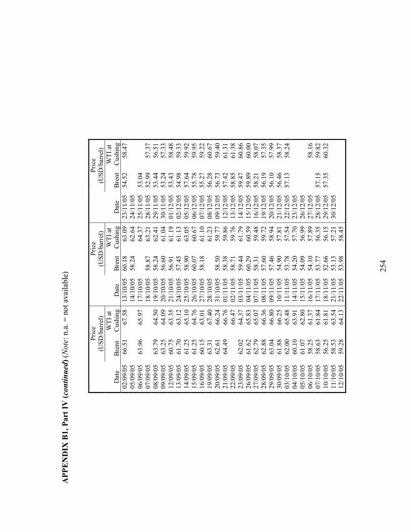
25

4

APP

EN

DIX

B1,

Par

t IV

(con

tinue

d) (N

ote:

n.a

. = n

ot a

vaila

ble)

Pr

ice

(USD

/bar

rel)

Pr

ice

(USD

/bar

rel)

Pr

ice

(USD

/bar

rel)

Dat

e Br

ent

WTI

at

Cus

hing

D

ate

Bren

t W

TI a

t C

ushi

ng

Dat

e Br

ent

WTI

at

Cus

hing

02/0

9/05

66

.51

67.5

8 13

/10/

05

60.1

8 63

.09

23/1

1/05

54

.52

58.4

705

/09/

05

14/1

0/05

58

.24

62.6

4 24

/11/

05

06/0

9/05

63

.96

65.9

7 17

/10/

05

64

.37

25/1

1/05

53

.04

07

/09/

05

18/1

0/05

58

.87

63.2

1 28

/11/

05

52.9

9 57

.37

08/0

9/05

63

.79

64.5

0 19

/10/

05

58.2

4 62

.41

29/1

1/05

53

.44

56.5

109

/09/

05

63.2

5 64

.09

20/1

0/05

56

.60

61.0

4 30

/11/

05

53.2

4 57

.33

12/0

9/05

60

.75

63.3

5 21

/10/

05

56.9

1 61

.19

01/1

2/05

53

.43

58.4

813

/09/

05

61.7

0 63

.12

24/1

0/05

57

.45

61.1

3 02

/12/

05

54.9

8 59

.33

14/0

9/05

61

.25

65.1

0 25

/10/

05

58.9

0 63

.05

05/1

2/05

57

.64

59.9

215

/09/

05

61.2

5 64

.76

26/1

0/05

60

.07

60.6

7 06

/12/

05

55.7

8 59

.95

16/0

9/05

60

.15

63.0

1 27

/10/

05

58.1

8 61

.10

07/1

2/05

55

.27

59.2

219

/09/

05

63.3

1 67

.40

28/1

0/05

61.2

3 08

/12/

05

56.2

8 60

.67

20/0

9/05

62

.61

66.2

4 31

/10/

05

58.5

0 59

.77

09/1

2/05

56

.73

59.4

021

/09/

05

64.4

9 66

.76

01/1

1/05

58

.38

59.8

6 12

/12/

05

57.4

2 61

.31

22/0

9/05

66.4

7 02

/11/

05

58.7

1 59

.76

13/1

2/05

58

.85

61.3

823

/09/

05

62.0

2 64

.37

03/1

1/05

59

.44

61.7

9 14

/12/

05

59.4

7 60

.86

26/0

9/05

61

.62

65.8

3 04

/11/

05

60.2

9 60

.59

15/1

2/05

59

.89

60.0

027

/09/

05

62.7

9 65

.07

07/1

1/05

58

.31

59.4

8 16

/12/

05

58.2

1 58

.07

28/0

9/05

62

.88

66.3

6 08

/11/

05

57.6

0 59

.72

19/1

2/05

56

.19

57.3

529

/09/

05

63.0

4 66

.80

09/1

1/05

57

.46

58.9

4 20

/12/

05

56.1

0 57

.99

30/0

9/05

61

.88

66.2

5 10

/11/

05

54.9

0 57

.81

21/1

2/05

56

.46

58.3

703

/10/

05

62.0

0 65

.48

11/1

1/05

53

.78

57.5

4 22

/12/

05

57.1

3 58

.24

04/1

0/05

60

.10

63.9

1 14

/11/

05

54.2

0 57

.70

23/1

2/05

05

/10/

05

61.0

7 62

.80

15/1

1/05

54

.09

56.9

9 26

/12/

05

06/1

0/05

58

.25

61.3

7 16

/11/

05

54.1

0 57

.89

27/1

2/05

58.1

607

/10/

05

58.6

3 61

.84

17/1

1/05

53

.77

56.3

5 28

/12/

05

57.1

5 59

.82

10/1

0/05

56

.25

61.8

1 18

/11/

05

52.6

6 56

.15

29/1

2/05

57

.35

60.3

211

/10/

05

58.5

3 63

.54

21/1

1/05

53

.13

57.2

1 30

/12/

05

12/1

0/05

59

.28

64.1

3 22

/11/

05

53.9

8 58

.45

255

APPENDIX B2

Weekly USA retail gasoline price (cents per gallon) for all grades and all

formulations for the period of January 5, 2004December 26, 2005 (Energy

Information Administration (EIA), Retail Gasoline Historical Prices,

http://www.eia.doe.gov/oil_gas/petroleum/data_publications/wrgp/

mogas_history.html, accessed on January 23, 2006) (Note: n.a. = not available)

Date Gasoline price (cent/gallon) Date

Gasoline price (cent/gallon) Date

Gasoline price (cent/gallon)

05/01/04 155.2 06/09/04 189.3 09/05/05 223.1 12/01/04 160.3 13/09/04 188.9 16/05/05 220.6 19/01/04 163.7 20/09/04 190.8 23/05/05 216.9 26/01/04 166.4 27/09/04 195.9 30/05/05 214.1 02/02/04 166 04/10/04 198 06/06/05 215.9 09/02/04 168.1 11/10/04 203.5 13/06/05 217.3 16/02/04 169 18/10/04 207.7 20/06/05 220.4 23/02/04 173 25/10/04 207.4 27/06/05 225.7 01/03/04 175.8 01/11/04 207.6 04/07/05 226.8 08/03/04 178 08/11/04 204.5 11/07/05 236.9 15/03/04 176.7 15/11/04 201.4 18/07/05 236 22/03/04 178.5 22/11/04 199.2 25/07/05 233.3 29/03/04 180 29/11/04 198.9 01/08/05 233.5 05/04/04 182.2 06/12/04 195.6 08/08/05 241 12/04/04 182.7 13/12/04 189.3 15/08/05 259.2 19/04/04 185.3 20/12/04 186.1 22/08/05 265.4 26/04/04 185.3 27/12/04 183.8 29/08/05 265.3 03/05/04 188.4 03/01/05 182.4 05/09/05 311.7 10/05/04 197.9 10/01/05 183.7 12/09/05 300.2 17/05/04 205.5 17/01/05 186.3 19/09/05 283.5 24/05/04 210.4 24/01/05 189.6 26/09/05 285.1 31/05/04 209.2 31/01/05 195.3 03/10/05 297.5 07/06/04 207.5 07/02/05 195.2 10/10/05 289.6 14/06/04 202.9 14/02/05 194.1 17/10/05 277.5 21/06/04 198.1 21/02/05 194.8 24/10/05 265.2 28/06/04 196.5 28/02/05 196.9 31/10/05 252.8 05/07/04 193.9 07/03/05 204 07/11/05 242.4 12/07/04 195.9 14/03/05 209.8 14/11/05 234.2 19/07/04 197.1 21/03/05 214.9 21/11/05 224.7 26/07/04 194.8 28/03/05 219.4 28/11/05 220 02/08/04 193 04/04/05 225.8 05/12/05 219.1 09/08/04 192 11/04/05 232.1 12/12/05 222.8 16/08/04 191.7 18/04/05 228 19/12/05 225.5 23/08/04 192.6 25/04/05 227.9 26/12/05 224.1 30/08/04 190.9 02/05/05 227.7

25

6

APP

EN

DIX

B3,

Par

t I

Dai

ly U

SA G

ulf C

oast

ker

osen

e-ty

pe je

t fue

l spo

t pri

ce F

OB

(fre

e-on

-boa

rd) f

or th

e pe

riod

of J

anua

ry 5

, 200

4D

ecem

ber

23,

2005

(E

nerg

y In

form

atio

n A

dmin

istr

atio

n (E

IA),

His

tori

cal

Petr

oleu

m

Pric

e D

ata

Oth

er

Prod

uct

Pric

es,

http

://w

ww

.eia

.doe

.gov

/nei

c/hi

stor

ic/h

petr

oleu

m2.

htm

#Oth

er, a

cces

sed

on J

anua

ry 2

3, 2

006)

(Not

e: n

.a. =

not

ava

ilabl

e)

Dat

e Je

t fue

l pric

e (c

ent/g

allo

n)

Dat

e Je

t fue

l pric

e (c

ent/g

allo

n)

Dat

e Je

t fue

l pric

e (c

ent/g

allo

n)

Dat

e Je

t fue

l pric

e (c

ent/g

allo

n)

Dat

e Je

t fue

l pric

e (c

ent/g

allo

n)

Dat

e Je

t fue

l pric

e (c

ent/g

allo

n)

05/0

1/04

96

.1

16/0

2/04

29/0

3/04

91

.79

11/0

5/04

11

4.6

23/0

6/04

10

4.28

04

/08/

04

118.

7 06

/01/

04

98.2

17

/02/

04

98.1

5 30

/03/

04

93.8

6 12

/05/

04

114.

9 24

/06/

04

106.

61

05/0

8/04

12

2.18

07

/01/

04

96.9

5 18

/02/

04

99

31/0

3/04

93

.63

13/0

5/04

11

6.88

25

/06/

04

106.

28

06/0

8/04

12

0.68

08

/01/

04

99.1

2 19

/02/

04

94.7

01

/04/

04

88.1

3 14

/05/

04

118.

5 28

/06/

04

104.

3 09

/08/

04

122.

38

09/0

1/04

10

1.83

20

/02/

04

90.5

02

/04/

04

88.3

8 17

/05/

04

115.

55

29/0

6/04

10

2.75

10

/08/

04

119.

78

12/0

1/04

10

2.66

23

/02/

04

90.8

5 05

/04/

04

88.1

5 18

/05/

04

111.

21

30/0

6/04

10

6.3

11/0

8/04

11

8.88

13

/01/

04

102.

66

24/0

2/04

91

.4

06/0

4/04

90

.8

19/0

5/04

11

0.63

01

/07/

04

112

12/0

8/04

12

2.37

14

/01/

04

98.1

8 25

/02/

04

96.3

1 07

/04/

04

93.6

20

/05/

04

108.

02

02/0

7/04

11

2.7

13/0

8/04

12

5.43

15

/01/

04

94.2

3 26

/02/

04

99.7

5 08

/04/

04

96.2

5 21

/05/

04

105.

43

05/0

7/04

16/0

8/04

12

3.85

16

/01/

04

98.8

3 27

/02/

04

98.2

5 12

/04/

04

99.5

24

/05/

04

109.

39

06/0

7/04

11

3.89

17

/08/

04

125.

23

19/0

1/04

01/0

3/04

10

0.45

13

/04/

04

97.8

8 25

/05/

04

105.

98

07/0

7/04

11

2.43

18

/08/

04

125.

9 20

/01/

04

103.

49

02/0

3/04

98

.85

14/0

4/04

99

.08

26/0

5/04

10

2.03

08

/07/

04

114.

21

19/0

8/04

13

0.9

21/0

1/04

10

6.25

03

/03/

04

94.3

5 15

/04/

04

102.

51

27/0

5/04

98

.94

09/0

7/04

11

2.1

20/0

8/04

12

7.1

22/0

1/04

10

6.63

04

/03/

04

97

16/0

4/04

10

1.65

28

/05/

04

101.

3 12

/07/

04

108.

8 23

/08/

04

124.

95

23/0

1/04

10

3.15

05

/03/

04

96

19/0

4/04

99

.28

01/0

6/04

10

7.05

13

/07/

04

109.

75

24/0

8/04

12

5.21

26

/01/

04

103.

15

08/0

3/04

85

.6

20/0

4/04

97

.88

02/0

6/04

10

1.85

14

/07/

04

112.

6 25

/08/

04

120.

9 27

/01/

04

99.4

8 09

/03/

04

92.6

21

/04/

04

97.5

3 03

/06/

04

102.

25

15/0

7/04

11

2.78

26

/08/

04

120

28/0

1/04

97

.35

10/0

3/04

91

.34

22/0

4/04

99

.4

04/0

6/04

10

0.75

16

/07/

04

113.

2 27

/08/

04

121.

98

29/0

1/04

95

11

/03/

04

92.1

23

/04/

04

98.4

4 07

/06/

04

102.

38

19/0

7/04

11

4.18

30

/08/

04

119.

96

30/0

1/04

93

.45

12/0

3/04

91

.38

26/0

4/04

10

0.8

08/0

6/04

99

.15

20/0

7/04

11

1.48

31

/08/

04

119.

53

02/0

2/04

93

.65

15/0

3/04

94

.55

27/0

4/04

99

.35

09/0

6/04

10

0.71

21

/07/

04

112.

55

01/0

9/04

12

5.18

03

/02/

04

95.0

3 16

/03/

04

94.3

2 28

/04/

04

99.9

3 10

/06/

04

102.

53

22/0

7/04

11

6.99

02

/09/

04

126.

48

04/0

2/04

90

.8

17/0

3/04

98

.5

29/0

4/04

10

1.93

11

/06/

04

23

/07/

04

118.

7 03

/09/

04

125.

68

05/0

2/04

89

.93

18/0

3/04

97

.65

30/0

4/04

10

2.35

14

/06/

04

100.

7 26

/07/

04

117.

35

06/0

9/04

06/0

2/04

87

.93

19/0

3/04

97

.2

03/0

5/04

10

4.98

15

/06/

04

101.

35

27/0

7/04

11

7.93

07

/09/

04

125.

48

09/0

2/04

88

.58

22/0

3/04

96

.2

04/0

5/04

10

5.8

16/0

6/04

10

1.23

28

/07/

04

119.

39

08/0

9/04

12

5.25

10

/02/

04

90.2

5 23

/03/

04

97.4

8 05

/05/

04

108.

83

17/0

6/04

10

5.57

29

/07/

04

119.

03

09/0

9/04

13

0.1

11/0

2/04

91

.63

24/0

3/04

94

.97

06/0

5/04

10

8.05

18

/06/

04

104.

7 30

/07/

04

121.

78

10/0

9/04

12

3.25

12

/02/

04

91.6

3 25

/03/

04

93.6

1 07

/05/

04

112.

05

21/0

6/04

10

1.79

02

/08/

04

120.

8 13

/09/

04

128.

23

13/0

2/04

95

.25

26/0

3/04

93

.83

10/0

5/04

11

0.55

22

/06/

04

104.

4 03

/08/

04

122.

53

14/0

9/04

13

3.4

25

7

APP

EN

DIX

B3,

Par

t II (

cont

inue

d) (N

ote:

n.a

. = n

ot a

vaila

ble)

Dat

e Je

t fue

l pric

e (c

ent/g

allo

n)

Dat

e Je

t fue

l pric

e (c

ent/g

allo

n)

Dat

e Je

t fue

l pric

e (c

ent/g

allo

n)

Dat

e Je

t fue

l pric

e (c

ent/g

allo

n)

Dat

e Je

t fue

l pric

e (c

ent/g

allo

n)

Dat

e Je

t fue

l pric

e (c

ent/g

allo

n)

15/0

9/04

13

4.25

29

/10/

04

141.

95

14/1

2/04

12

6.34

27

/01/

05

139.

38

14/0

3/05

15

4.8

28/0

4/05

15

3.8

16/0

9/04

13

5.26

01

/11/

04

135.

72

15/1

2/04

13

6 28

/01/

05

132.

95

15/0

3/05

15

6.2

29/0

4/05

14

6.9

17/0

9/04

13

8.55

02

/11/

04

133.

75

16/1

2/04

13

1.68

31

/01/

05

134.

5 16

/03/

05

161.

92

02/0

5/05

15

1.5

20/0

9/04

13

7.05

03

/11/

04

137.

9 17

/12/

04

134.

63

01/0

2/05

13

0.5

17/0

3/05

15

9.84

03

/05/

05

150.

75

21/0

9/04

13

9.46

04

/11/

04

131.

91

20/1

2/04

12

9.45

02

/02/

05

128.

33

18/0

3/05

16

1.68

04

/05/

05

153.

16

22/0

9/04

14

3.11

05

/11/

04

132.

95

21/1

2/04

13

0.19

03

/02/

05

124.

63

21/0

3/05

16

2.58

05

/05/

05

151.

75

23/0

9/04

14

4.3

08/1

1/04

13

2.05

22

/12/

04

127.

16

04/0

2/05

12

5.4

22/0

3/05

15

9.38

06

/05/

05

150.

38

24/0

9/04

14

5.55

09

/11/

04

130.

93

23/1

2/04

12

8.29

07

/02/

05

120.

53

23/0

3/05

16

0.75

09

/05/

05

150.

13

27/0

9/04

14

9.39

10

/11/

04

138.

46

24/1

2/04

08/0

2/05

12

3.17

24

/03/

05

159.

25

10/0

5/05

15

3.1

28/0

9/04

15

0.4

11/1

1/04

13

1.71

27

/12/

04

114.

91

09/0

2/05

12

6.88

28

/03/

05

158.

43

11/0

5/05

14

8.44

29

/09/

04

151

12/1

1/04

13

2.15

28

/12/

04

116.

1 10

/02/

05

130.

75

29/0

3/05

15

5.05

12

/05/

05

144.

96

30/0

9/04

14

9.05

15

/11/

04

129.

7 29

/12/

04

122.

75

11/0

2/05

13

0.25

30

/03/

05

160.

3 13

/05/

05

143.

4 01

/10/

04

151.

3 16

/11/

04

128.

05

30/1

2/04

12

0.95

14

/02/

05

129.

05

31/0

3/05

16

6.9

16/0

5/05

14

1.05

04

/10/

04

149.

24

17/1

1/04

13

5.58

31

/12/

04

15

/02/

05

129.

38

01/0

4/05

17

3.85

17

/05/

05

142.

65

05/1

0/04

14

8.98

18

/11/

04

137.

24

03/0

1/05

11

4.99

16

/02/

05

136.

73

04/0

4/05

16

9.63

18

/05/

05

141.

2 06

/10/

04

148.

83

19/1

1/04

14

2.68

04

/01/

05

119.

75

17/0

2/05

13

3.38

05

/04/

05

167.

88

19/0

5/05

14

3.8

07/1

0/04

14

7.28

22

/11/

04

138

05/0

1/05

12

1.1

18/0

2/05

13

6 06

/04/

05

164.

1 20

/05/

05

141.

4 08

/10/

04

149.

58

23/1

1/04

13

6.35

06

/01/

05

129

21/0

2/05

07/0

4/05

15

8.33

23

/05/

05

140.

78

11/1

0/04

15

0.7

24/1

1/04

13

9.35

07

/01/

05

129.

18

22/0

2/05

14

3.63

08

/04/

05

156.

18

24/0

5/05

14

3.35

12

/10/

04

148.

39

25/1

1/04

10/0

1/05

12

9.88

23

/02/

05

146.

68

11/0

4/05

15

4.91

25

/05/

05

147.

1 13

/10/

04

155.

83

26/1

1/04

11/0

1/05

13

1.73

24

/02/

05

145.

73

12/0

4/05

15

1.66

26

/05/

05

149.

33

14/1

0/04

16

0.3

29/1

1/04

13

8.45

12

/01/

05

132.

7 25

/02/

05

146.

25

13/0

4/05

15

1.96

27

/05/

05

149.

98

15/1

0/04

16

0.55

30

/11/

04

131.

95

13/0

1/05

13

5.9

28/0

2/05

14

7.73

14

/04/

05

155.

18

30/0

5/05

18/1

0/04

15

4.99

01

/12/

04

122.

63

14/0

1/05

13

6.95

01

/03/

05

148.

79

15/0

4/05

15

3.6

31/0

5/05

15

1.69

19

/10/

04

152.

08

02/1

2/04

11

9.23

17

/01/

05

02

/03/

05

151.

85

18/0

4/05

15

0.51

01

/06/

05

160.

2 20

/10/

04

156.

63

03/1

2/04

11

4.85

18

/01/

05

136.

5 03

/03/

05

148.

7 19

/04/

05

153.

75

02/0

6/05

16

1.4

21/1

0/04

15

8.53

06

/12/

04

113.

4 19

/01/

05

135.

95

04/0

3/05

14

8.4

20/0

4/05

15

5.73

03

/06/

05

167.

6 22

/10/

04

159.

18

07/1

2/04

11

1.29

20

/01/

05

136.

38

07/0

3/05

14

8.83

21

/04/

05

159.

2 06

/06/

05

165.

66

25/1

0/04

15

5.13

08

/12/

04

114.

79

21/0

1/05

14

1.2

08/0

3/05

15

3.24

22

/04/

05

160.

75

07/0

6/05

16

4.44

26

/10/

04

156.

03

09/1

2/04

12

0.18

24

/01/

05

142.

9 09

/03/

05

151.

93

25/0

4/05

15

7.18

08

/06/

05

159.

25

27/1

0/04

14

6.28

10

/12/

04

113.

35

25/0

1/05

14

4.3

10/0

3/05

15

1.88

26

/04/

05

156.

2 09

/06/

05

166.

46

28/1

0/04

14

0.9

13/1

2/04

12

0.3

26/0

1/05

14

2.9

11/0

3/05

15

5.88

27

/04/

05

151.

5 10

/06/

05

165.

15

25

8

APP

EN

DIX

B3,

Par

t III

(con

tinue

d) (N

ote:

n.a

. = n

ot a

vaila

ble)

Dat

e Je

t fue

l pric

e (c

ent/g

allo

n)

Dat

e Je

t fue

l pric

e (c

ent/g

allo

n)

Dat

e Je

t fue

l pric

e (c

ent/g

allo

n)

Dat

e Je

t fue

l pric

e (c

ent/g

allo

n)

Dat

e Je

t fue

l pric

e (c

ent/g

allo

n)

13/0

6/05

17

0.65

27

/07/

05

163.

65

09/0

9/05

19

4.88

25

/10/

05

195.

57

08/1

2/05

17

8.1

14/0

6/05

16

6.59

28

/07/

05

165.

8 12

/09/

05

184.

5 26

/10/

05

192.

74

09/1

2/05

17

2.18

15

/06/

05

164.

83

29/0

7/05

16

6.45

13

/09/

05

188.

26

27/1

0/05

19

3.75

12

/12/

05

174.

15

16/0

6/05

16

5.89

01

/08/

05

170.

43

14/0

9/05

20

0.44

28

/10/

05

196.

4 13

/12/

05

180.

55

17/0

6/05

16

9.1

02/0

8/05

17

0.05

15

/09/

05

196.

5 31

/10/

05

189.

38

14/1

2/05

18

0.7

20/0

6/05

16

9.35

03

/08/

05

166.

4 16

/09/

05

190.

5 01

/11/

05

182.

4 15

/12/

05

176

21/0

6/05

16

5.4

04/0

8/05

17

0 19

/09/

05

216.

5 02

/11/

05

178

16/1

2/05

17

1.98

22

/06/

05

164.

28

05/0

8/05

17

2.3

20/0

9/05

21

5.29

03

/11/

05

182.

75

19/1

2/05

16

9.38

23

/06/

05

169.

39

08/0

8/05

17

9.55

21

/09/

05

219.

79

04/1

1/05

17

6.55

20

/12/

05

165.

7 24

/06/

05

167.

55

09/0

8/05

17

7.55

22

/09/

05

225.

3 07

/11/

05

175.

95

21/1

2/05

16

9.5

27/0

6/05

16

8.63

10

/08/

05

185.

6 23

/09/

05

217.

5 08

/11/

05

174.

55

22/1

2/05

17

1.85

28

/06/

05

162.

78

11/0

8/05

19

2.83

26

/09/

05

239.

48

09/1

1/05

17

7.88

23

/12/

05

170.

5 29

/06/

05

161.

63

12/0

8/05

19

4.5

27/0

9/05

25

2.2

10/1

1/05

17

1.5

30/0

6/05

16

1.93

15

/08/

05

190.

59

28/0

9/05

29

5 11

/11/

05

169

01/0

7/05

17

0.6

16/0

8/05

18

9.6

29/0

9/05

30

2.5

14/1

1/05

16

9.53

04

/07/

05

17

/08/

05

179.

55

30/0

9/05

26

4.5

15/1

1/05

16

3.09

05

/07/

05

172.

57

18/0

8/05

18

2.88

03

/10/

05

290

16/1

1/05

16

7.65

06

/07/

05

179.

49

19/0

8/05

18

6.75

04

/10/

05

309.

97

17/1

1/05

16

4.45

07

/07/

05

174.

88

22/0

8/05

18

4.2

05/1

0/05

31

3.03

18

/11/

05

164.

7 08

/07/

05

170.

05

23/0

8/05

18

7.2

06/1

0/05

27

4.5

21/1

1/05

16

4.95

11

/07/

05

166.

3 24

/08/

05

194.

21

07/1

0/05

28

4 22

/11/

05

168.

42

12/0

7/05

17

1.9

25/0

8/05

19

2.1

10/1

0/05

27

8.2

23/1

1/05

16

9.25

13

/07/

05

167.

83

26/0

8/05

18

9.25

11

/10/

05

277.

7 24

/11/

05

14

/07/

05

163.

35

29/0

8/05

19

7.23

12

/10/

05

280

25/1

1/05

15/0

7/05

16

4.5

30/0

8/05

22

9.5

13/1

0/05

23

7.85

28

/11/

05

158.

53

18/0

7/05

16

0.75

31

/08/

05

228.

84

14/1

0/05

23

0.5

29/1

1/05

15

6.4

19/0

7/05

16

2.37

01

/09/

05

242.

25

17/1

0/05

25

6.8

30/1

1/05

16

0.65

20

/07/

05

159.

8 02

/09/

05

220.

5 18

/10/

05

252.

72

01/1

2/05

16

5.2

21/0

7/05

15

7.15

05

/09/

05

19

/10/

05

213.

75

02/1

2/05

16

8 22

/07/

05

163.

5 06

/09/

05

215.

25

20/1

0/05

19

2.15

05

/12/

05

172.

25

25/0

7/05

16

4.08

07

/09/

05

208.

85

21/1

0/05

19

3.25

06

/12/

05

174.

65

26/0

7/05

16

4.35

08

/09/

05

197.

78

24/1

0/05

18

3.77

07

/12/

05

170.

5

259

APPENDIX B4

Weekly USA No. 2 heating oil residential price (cents per gallon excluding taxes) for

the period of January 5, 2004December 26, 2005 (Energy Information

Administration (EIA), Heating Oil and Propane Update at

http://tonto.eia.doe.gov/oog/info/hopu/hopu.asp, accessed on January 23, 2006)

[Note: n.a. = not available. Also, there is no data available for the following periods: (i)

between March 16, 2004 and October 3, 2004 and (ii) between March 15, 2005 and

October 2, 2005.]

Date Heating oil price

(cent/gallon) Date Heating oil price

(cent/gallon) 05/01/04 149.797 03/01/05 195.116 12/01/04 156.176 10/01/05 194.56 19/01/04 158.444 17/01/05 196.386 26/01/04 162.162 24/01/05 198.994 02/02/04 162.521 31/01/05 201.789 09/02/04 161.531 07/02/05 199.034 16/02/04 161.116 14/02/05 198.119 23/02/04 160.947 21/02/05 198.377 01/03/04 160.256 28/02/05 204.27 08/03/04 160.13 07/03/05 208.85 15/03/04 159.122 14/03/05 211.85 04/10/04 182.787 03/10/05 269.159 11/10/04 190.849 10/10/05 264.83 18/10/04 199.156 17/10/05 265.007 25/10/04 206.028 24/10/05 262.298 01/11/04 205.961 31/10/05 257.725 08/11/04 202.824 07/11/05 250.824 15/11/04 201.673 14/11/05 246.556 22/11/04 202.522 21/11/05 243.124 29/11/04 202.964 28/11/05 241.72 06/12/04 197.013 05/12/05 241.035 13/12/04 194.709 12/12/05 241.403 20/12/04 199.344 19/12/05 243.803 27/12/04 197.757 26/12/05 243.3

260

APPENDIX B5

Monthly USA residual fuel oil retail sales by all sellers (cents per gallon) for the

period of January 5, 2004November 30, 2005 (Energy Information Administration

(EIA), Residual Fuel Oil Prices by Sales Type,

http://tonto.eia.doe.gov/dnav/pet/pet_pri_resid_dcu_nus_m.htm, accessed on

January 24, 2006) (Note: n.a. = not available)

Date Fuel oil price (cent/gallon)

Jan-2004 70.6 Feb-2004 69.1 Mar-2004 65.8 Apr-2004 67.6 May-2004 72.6 Jun-2004 73.4 Jul-2004 70.2

Aug-2004 72 Sep-2004 74.1 Oct-2004 81.3

Nov-2004 80.3 Dec-2004 74.4 Jan-2005 77.3 Feb-2005 81.4 Mar-2005 88.1 Apr-2005 96.5 May-2005 99.6 Jun-2005 99.5 Jul-2005 103.2

Aug-2005 109.6 Sep-2005 122.9 Oct-2005 126.7

Nov-2005 120.5

261

APPENDIX C

The Mean-Absolute Deviation (MAD) Model for Portfolio Optimization (Konno and

Yamazaki,1991; Konno and Wijayanayake, 2002)

Let Rj be the rate of return of jth asset (j = 1, , n) and let x = (x1, , xn) be a portfolio, a

vector of proportion of investments into each asset. Let X be an investable set, i.e., a set

of feasible portfolios. For simplicity, it is assumed that X is a set defined below:

X = x ( )11

, , 1, 0 , 1, ,n

n j j jj

x x x x j n=

= = ≤ ≤α =∑L L (C.1)

The rate of return R(x) of the portfolio x is given by

R(x) = 1

n

j jj

R x=∑ (C.2)

Let rj be the expected value of the rate of return Rj of the jth asset. The absolute

deviation W(x) of the rate of return R(x) of the portfolio x is given by

W(x) = E[|R(x) E[R(x)]|] (C.3)

It is assumed that R = (R1, , Rn) is distributed over a finite set of points (r1t,L , rnt),

t = 1,L ,T and that the probability of occurrence of (r1t,L , xnt) is given by pt, t = 1,

L ,T. Then:

1

T

j t jtt

r p r=

=∑ (C.4)

and

262

W(x) = ( )1 1

T n

t jt j jt j

p r r x= =

−∑ ∑ (C.5)

The mean-absolute deviation (MAD) portfolio optimization model is defined as

follows:

( )1 1

1

minimize ( )

subject to ,

,

T n

t jt j jt j

n

j jj

W x p r r x

r x

x X

= =

=

≡ −

= ρ

∈

∑ ∑

∑ (C.6)

where ρ is a given constant representing the expected rate of return of the portfolio. The

MAD model can be formulated in an alternative way:

( )1

1 1

maximize

subject to

n

j jj

T n

t jt j jt j

r x

p r r x w

x X

=

= =− ≤

∈

∑

∑ ∑ (C.7)

where w is a given constant representing the tolerable level of risk. Both (C.6) and (C.7)

can be used interchangeably to generate an efficient frontier.

By standard results in linear programming, the problem (C.7) can be converted to a

linear system of inequalities as follows:

263

( )

1

1

1

1

maximize

subject to2

, 0, 1, , ,

1, , 1, , .

n

j jj

T

tt

n

t t jt j j tj

n

j j jj

r x

wy

y p r r x y t T

x x U j n

=

=

=

=

≤

≥ − ≥ =

= ∈ =

∑

∑

∑

∑

L

L

(C.8)

264

APPENDIX D

GAMS Program Codes for the Numerical Example

Appendix D1: The Deterministic Midterm Refinery Production Planning Model

$TITLE Deterministic Model Variables Z; Positive Variables x1, x2, x3, x4, x5, x6, x7, x8, x9, x10, x11, x12, x13, x14, x15, x16, x17, x18, x19, x20; Equations OBJ, CON1, CON2, EQN3, EQN4, EQN5, EQN6, EQN7, EQN8, EQN9, EQN10, EQN11, EQN12, EQN13, EQN14, EQN15, EQN16, EQN17, EQN18, EQN19, CON20, CON21, CON22, CON23, CON24; OBJ.. Z =E= -8.0*x1 + 18.5*x2 + 8.0*x3 + 12.5*x4 + 14.5*x5 + 6.0*x6 - 1.5*x14; CON1.. x1 =L= 15000; CON2.. x14 =L= 2500; EQN3.. -0.13*x1 + x7 =E= 0; EQN4.. -0.15*x1 + x4 =E= 0; EQN5.. -0.22*x1 + x8 =E= 0; EQN6.. -0.20*x1 + x9 =E= 0; EQN7.. -0.30*x1 + x10 =E= 0; EQN8.. -0.05*x14 + x20 =E= 0; EQN9.. -0.40*x14 + x16 =E= 0; EQN10.. -0.55*x14 + x17 =E= 0; EQN11.. 0.5*x2 - x11 =E= 0; EQN12.. 0.5*x2 - x16 =E= 0; EQN13.. 0.75*x5 - x12 =E= 0; EQN14.. 0.25*x5 - x18 =E= 0; EQN15.. -x7 + x3 +x11 =E= 0; EQN16.. -x8 + x12 +x13 =E= 0; EQN17.. -x9 + x14 +x15 =E= 0; EQN18.. -x17 + x18 +x19 =E= 0; EQN19.. -x10 - x13 - x15 - x19 + x6 =E= 0; CON20.. x2 =L= 2700; CON21.. x3 =L= 1100; CON22.. x4 =L= 2300; CON23.. x5 =L= 1700; CON24.. x6 =L= 9500; Model Refinery / all /; Solve Refinery using LP maximizing Z;

265

Appendix D2: Approach 1Risk Model I Based on the Markowitzs Mean

Variance (EV or MV) Approach to Handle Randomness in the Objective Function

Coefficients of Prices

$TITLE Approach 1: Risk Model I Based on the Markowitz's Mean-Variance Approach to Handle Randomness in the Objective Function Coefficients of Prices Sets i product type /1*21/ s scenarios /1*3/ Table pc(i,s) price of product type i per realization s 1 2 3 1 8.8 8.0 7.2 2 20.35 18.5 16.65 3 8.8 8.0 7.2 4 13.75 12.5 11.25 5 15.95 14.5 13.05 6 6.6 6 5.4 14 1.65 1.5 1.35; Variables Z1; Positive Variables x1, x2, x3, x4, x5, x6, x7, x8, x9, x10, x11, x12, x13, x14, x15, x16, x17, x18, x19, x20, Ep; Scalars p1 "probability for scenario 1" /0.35/ p2 "probability for scenario 2" /0.45/ p3 "probability for scenario 3" /0.2/ v1 variance of price of crude oil /0.352/ v2 variance of price of gasoline /1.882375/ v3 variance of price of naphtha /0.352/ v4 variance of price of jet fuel /0.859375/ v5 variance of price of heating oil /1.156375/ v6 variance of price of crude oil /0.198/ v14 variance of price of cracker feed /0.012375/ Equations OBJ, CON0, CON1, CON2, EQN3, EQN4, EQN5, EQN6, EQN7, EQN8, EQN9, EQN10, EQN11, EQN12, EQN13, EQN14, EQN15, EQN16, EQN17, EQN18, EQN19, CON20, CON21, CON22, CON23, CON24, Eprofit; OBJ.. Z1 =E= -((v1*SQR(x1)) + (v2*SQR(x2)) + (v3*SQR(x3)) + (v4*SQR(x4)) + (v5*SQR(x5)) + (v6*SQR(x6)) + (v14*SQR(x14))); CON0.. [p1*(-pc('1','1')*x1 + pc('2','1')*x2 + pc('3','1')*x3 + pc('4','1')*x4 + pc('5','1')*x5 + pc('6','1')*x6 - pc('14','1')*x14)] + [p2*(-pc('1','2')*x1 + pc('2','2')*x2 + pc('3','2')*x3 + pc('4','2')*x4 + pc('5','2')*x5 + pc('6','2')*x6 - pc('14','2')*x14)]

266

+ [p3*(-pc('1','3')*x1 + pc('2','3')*x2 + pc('3','3')*x3 + pc('4','3')*x4 + pc('5','3')*x5 + pc('6','3')*x6 - pc('14','3')*x14)] =G= 23500; CON1.. x1 =L= 15000; CON2.. x14 =L= 2500; EQN3.. -0.13*x1 + x7 =E= 0; EQN4.. -0.15*x1 + x4 =E= 0; EQN5.. -0.22*x1 + x8 =E= 0; EQN6.. -0.20*x1 + x9 =E= 0; EQN7.. -0.30*x1 + x10 =E= 0; EQN8.. -0.05*x14 + x20 =E= 0; EQN9.. -0.40*x14 + x16 =E= 0; EQN10.. -0.55*x14 + x17 =E= 0; EQN11.. 0.5*x2 - x11 =E= 0; EQN12.. 0.5*x2 - x16 =E= 0; EQN13.. 0.75*x5 - x12 =E= 0; EQN14.. 0.25*x5 - x18 =E= 0; EQN15.. -x7 + x3 +x11 =E= 0; EQN16.. -x8 + x12 +x13 =E= 0; EQN17.. -x9 + x14 +x15 =E= 0; EQN18.. -x17 + x18 +x19 =E= 0; EQN19.. -x10 - x13 - x15 - x19 + x6 =E= 0; CON20.. x2 =L= 2700; CON21.. x3 =L= 1100; CON22.. x4 =L= 2300; CON23.. x5 =L= 1700; CON24.. x6 =L= 9500; Eprofit.. Ep =E= [p1*(-pc('1','1')*x1 + pc('2','1')*x2 + pc('3','1')*x3 + pc('4','1')*x4 + pc('5','1')*x5 + pc('6','1')*x6 - pc('14','1')*x14)] + [p2*(-pc('1','2')*x1 + pc('2','2')*x2 + pc('3','2')*x3 + pc('4','2')*x4 + pc('5','2')*x5 + pc('6','2')*x6 - pc('14','2')*x14)] + [p3*(-pc('1','3')*x1 + pc('2','3')*x2 + pc('3','3')*x3 + pc('4','3')*x4 + pc('5','3')*x5 + pc('6','3')*x6 - pc('14','3')*x14)]; Model Refinery / all /; Solve Refinery Using NLP Maximizing Z1;

267

Appendix D3: Approach 2.1Expectation Model I as a Combination of the

Markowitzs MeanVariance Approach and the Two-Stage Stochastic

Programming with Fixed Recourse Framework

$TITLE Approach 2: Expectation Model I as a Combination of the Markowitz's Mean-Variance Approach and the Two-Stage Stochastic Programming with Fixed Recourse Framework Sets i product type /1*21/ s scenarios /1*3/ k production shortfall and surplus or yield decrement or increment /1, 2/ Table pc(i,s) price of product type i per realization j 1 2 3 1 8.8 8.0 7.2 2 20.35 18.5 16.65 3 8.8 8.0 7.2 4 13.75 12.5 11.25 5 15.95 14.5 13.05 6 6.6 6 5.4 14 1.65 1.5 1.35; Table d(i,s) demand of product type i per realization j 1 2 3 2 2835 2700 2565 3 1155 1100 1045 4 2415 2300 2185 5 1785 1700 1615 6 9975 9500 9025; Table y(i,s) yield of product type i per realization j 1 2 3 3 -0.1365 -0.13 -0.1235 4 -0.1575 -0.15 -0.1425 8 -0.231 -0.22 -0.209 9 -0.21 -0.20 -0.19 10 -0.265 -0.30 -0.335; Table c(i,k) penalty cost for product type i due to production shortfall or surplus 1 2 1 55 50 2 25 20 3 17 13 4 5 4 5 6 5 6 10 8; Table q(i,k) penalty cost for product type i due to yield decrement or increment 1 2 3 5 3 4 5 4 8 5 3 9 5 3 10 5 3 Positive Variables x1, x2, x3, x4, x5, x6, x7, x8, x9, x10, x11, x12, x13, x14, x15, x16, x17, x18, x19, x20, z211, z212, z221, z222, z231, z232,

268

z311, z312, z321, z322, z331, z332, z411, z412, z421, z422, z431, z432, z511, z512, z521, z522, z531, z532, z611, z612, z621, z622, z631, z632, y311, y312, y321, y322, y331, y332, y411, y412, y421, y422, y431, y432, y811, y812, y821, y822, y831, y832, y911, y912, y921, y922, y931, y932, y1011, y1012, y1021, y1022, y1031, y1032 ; Variables Es1, Es2, Es3, Z2, Vp, Tshortfall, Tsurplus, Es, Vpsq, Ep, Ecv ; Scalars v1 "variance of price of crude oil" /0.352/ v2 "variance of price of gasoline" /1.882375/ v3 "variance of price of naphtha" /0.352/ v4 "variance of price of jet fuel" /0.859375/ v5 "variance of price of heating oil" /1.156375/ v6 "variance of price of crude oil" /0.198/ v14 "variance of price of cracker feed" /0.012375/ p1 "probability for scenario 1" /0.35/ p2 "probability for scenario 2" /0.45/ p3 "probability for scenario 3" /0.2/ Equations OBJ "maximize profit", CON1, CON2, EQN8, EQN9, EQN10, EQN11, EQN12, EQN13, EQN14, EQN15, EQN16, EQN17, EQN18, EQN19, Escenario, Escenario1, Escenario2, Escenario3, CONgas1, CONgas2, CONgas3, CONnap1, CONnap2, CONnap3, CONjf1, CONjf2, CONjf3, CONho1, CONho2, CONho3, CONfo1, CONfo2, CONfo3, CONlhsnap1, CONlhsnap11, CONlhsnap12, CONlhsnap2, CONlhsnap21, CONlhsnap22, CONlhsnap3, CONlhsnap31, CONlhsnap32, CONlhsjf1, CONlhsjf11, CONlhsjf12, CONlhsjf2, CONlhsjf21, CONlhsjf22, CONlhsjf3, CONlhsjf31, CONlhsjf32, CONlhsgo1, CONlhsgo11, CONlhsgo12, CONlhsgo2, CONlhsgo21, CONlhsgo22, CONlhsgo3, CONlhsgo31, CONlhsgo32, CONlhscf1, CONlhscf11, CONlhscf12, CONlhscf2, CONlhscf21, CONlhscf22, CONlhscf3, CONlhscf31, CONlhscf32, CONlhsr1, CONlhsr11, CONlhsr12, CONlhsr2, CONlhsr21, CONlhsr22, CONlhsr3, CONlhsr31, CONlhsr32, Eprofit, Vprofit, Totalshortfall, Totalsurplus, Vpsqrt, Ecvar; OBJ.. Z2 =E= [p1*(-pc('1','1')*x1 + pc('2','1')*x2 + pc('3','1')*x3 + pc('4','1')*x4 + pc('5','1')*x5 + pc('6','1')*x6 - pc('14','1')*x14)] + [p2*(-pc('1','2')*x1 + pc('2','2')*x2 + pc('3','2')*x3 + pc('4','2')*x4 + pc('5','2')*x5 + pc('6','2')*x6 - pc('14','2')*x14)] + [p3*(-pc('1','3')*x1 + pc('2','3')*x2 + pc('3','3')*x3 + pc('4','3')*x4 + pc('5','3')*x5 + pc('6','3')*x6 - pc('14','3')*x14)]

269

- 0.0000000001*Vp - Es; Vprofit.. Vp =E= (v1*SQR(x1)) + (v2*SQR(x2)) + (v3*SQR(x3)) + (v4*SQR(x4)) + (v5*SQR(x5)) + (v6*SQR(x6)) + (v14*SQR(x14)); CON1.. x1 =L= 15000; CON2.. x14 =L= 2500; *EQN3.. -0.13*x1 + x7 =E= 0; *EQN4.. -0.15*x1 + x4 =E= 0; *EQN5.. -0.22*x1 + x8 =E= 0; *EQN6.. -0.20*x1 + x9 =E= 0; *EQN7.. -0.30*x1 + x10 =E= 0; EQN8.. -0.05*x14 + x20 =E= 0; EQN9.. -0.40*x14 + x16 =E= 0; EQN10.. -0.55*x14 + x17 =E= 0; EQN11.. 0.5*x2 - x11 =E= 0; EQN12.. 0.5*x2 - x16 =E= 0; EQN13.. 0.75*x5 - x12 =E= 0; EQN14.. 0.25*x5 - x18 =E= 0; EQN15.. -x7 + x3 +x11 =E= 0; EQN16.. -x8 + x12 +x13 =E= 0; EQN17.. -x9 + x14 +x15 =E= 0; EQN18.. -x17 + x18 +x19 =E= 0; EQN19.. -x10 - x13 - x15 - x19 + x6 =E= 0; *CON20.. x2 =L= 2700; *CON21.. x3 =L= 1100; *CON22.. x4 =L= 2300; *CON23.. x5 =L= 1700; *CON24.. x6 =L= 9500; Escenario1.. Es1 =E= p1*(((c('2','1')*z211 + c('2','2')*z212) + (c('3','1')*z311 + c('3','2')*z312) + (c('4','1')*z411 + c('4','2')*z412) + (c('5','1')*z511 + c('5','2')*z512) + (c('6','1')*z611 + c('6','2')*z612)) + ((q('3','1')*y311 + q('3','2')*y312) + (q('4','1')*y411 + q('4','2')*y412) + (q('8','1')*y811 + q('8','2')*y812) + (q('9','1')*y911 + q('9','2')*y912) + (q('10','1')*y1011 + q('10','2')*y1012))); CONgas1.. x2 + z211 - z212 =E= d('2','1'); CONnap1.. x3 + z311 - z312 =E= d('3','1'); CONjf1.. x4 + z411 - z412 =E= d('4','1'); CONho1.. x5 + z511 - z512 =E= d('5','1'); CONfo1.. x6 + z611 - z612 =E= d('6','1'); CONlhsnap1.. y('3','1')*x1 + x7 + y311 - y312 =E= 0; CONlhsnap11.. y311 =L= 0.1*x1; CONlhsnap12.. y312 =L= 0.1*x1; CONlhsjf1.. y('4','1')*x1 + x4 + y411 - y412 =E= 0; CONlhsjf11.. y411 =L= 0.1*x1; CONlhsjf12.. y412 =L= 0.1*x1; CONlhsgo1.. y('8','1')*x1 + x8 + y811 - y812 =E= 0; CONlhsgo11.. y811 =L= 0.1*x1; CONlhsgo12.. y812 =L= 0.1*x1; CONlhscf1.. y('9','1')*x1 + x9 + y911 - y912 =E= 0; CONlhscf11.. y911 =L= 0.1*x1; CONlhscf12.. y912 =L= 0.1*x1; CONlhsr1.. y('10','1')*x1 + x10 + y1011 - y1012 =E= 0; CONlhsr11.. y1011 =L= 0.1*x1; CONlhsr12.. y1012 =L= 0.1*x1; Escenario2.. Es2 =E= p2*(((c('2','1')*z221 + c('2','2')*z222) + (c('3','1')*z321 + c('3','2')*z322) + (c('4','1')*z421 + c('4','2')*z422) + (c('5','1')*z521 + c('5','2')*z522) + (c('6','1')*z621 + c('6','2')*z622)) + ((q('3','1')*y321 + q('3','2')*y322) + (q('4','1')*y421 + q('4','2')*y422) + (q('8','1')*y821 + q('8','2')*y822) + (q('9','1')*y921 + q('9','2')*y922) + (q('10','1')*y1021 + q('10','2')*y1022))); CONgas2.. x2 + z221 - z222 =E= d('2','2'); CONnap2.. x3 + z321 - z322 =E= d('3','2'); CONjf2.. x4 + z421 - z422 =E= d('4','2'); CONho2.. x5 + z521 - z522 =E= d('5','2'); CONfo2.. x6 + z621 - z622 =E= d('6','2'); CONlhsnap2.. y('3','2')*x1 + x7 + y321 - y322 =E= 0;

270

CONlhsnap21..y321 =L= 0.1*x1; CONlhsnap22.. y322 =L= 0.1*x1; CONlhsjf2.. y('4','2')*x1 + x4 + y421 - y422 =E= 0; CONlhsjf21.. y421 =L= 0.1*x1; CONlhsjf22.. y422 =L= 0.1*x1; CONlhsgo2.. y('8','2')*x1 + x8 + y821 - y822 =E= 0; CONlhsgo21.. y821 =L= 0.1*x1; CONlhsgo22.. y822 =L= 0.1*x1; CONlhscf2.. y('9','2')*x1 + x9 + y921 - y922 =E= 0; CONlhscf21.. y921 =L= 0.1*x1; CONlhscf22.. y922 =L= 0.1*x1; CONlhsr2.. y('10','2')*x1 + x10 + y1021 - y1022 =E= 0; CONlhsr21.. y1011 =L= 0.1*x1; CONlhsr22.. y1012 =L= 0.1*x1; Escenario3.. Es3 =E= p3*(((c('2','1')*z231 + c('2','2')*z232) + (c('3','1')*z331 + c('3','2')*z332) + (c('4','1')*z431 + c('4','2')*z432) + (c('5','1')*z531 + c('5','2')*z532) + (c('6','1')*z631 + c('6','2')*z632)) + ((q('3','1')*y331 + q('3','2')*y332) + (q('4','1')*y431 + q('4','2')*y432) + (q('8','1')*y831 + q('8','2')*y832) + (q('9','1')*y931 + q('9','2')*y932) + (q('10','1')*y1031 + q('10','2')*y1032))); CONgas3.. x2 + z231 - z232 =E= d('2','3'); CONnap3.. x3 + z331 - z332 =E= d('3','3'); CONjf3.. x4 + z431 - z432 =E= d('4','3'); CONho3.. x5 + z531 - z532 =E= d('5','3'); CONfo3.. x6 + z631 - z632 =E= d('6','3'); CONlhsnap3.. y('3','3')*x1 + x7 + y331 - y332 =E= 0; CONlhsnap31..y331 =L= 0.1*x1; CONlhsnap32.. y332 =L= 0.1*x1; CONlhsjf3.. y('4','3')*x1 + x4 + y431 - y432 =E= 0; CONlhsjf31.. y431 =L= 0.1*x1; CONlhsjf32.. y432 =L= 0.1*x1; CONlhsgo3.. y('8','3')*x1 + x8 + y831 - y832 =E= 0; CONlhsgo31.. y831 =L= 0.1*x1; CONlhsgo32.. y832 =L= 0.1*x1; CONlhscf3.. y('9','3')*x1 + x9 + y931 - y932 =E= 0; CONlhscf31.. y931 =L= 0.1*x1; CONlhscf32.. y932 =L= 0.1*x1; CONlhsr3.. y('10','3')*x1 + x10 + y1031 - y1032 =E= 0; CONlhsr31.. y1031 =L= 0.1*x1; CONlhsr32.. y1032 =L= 0.1*x1; Escenario.. Es =E= Es1 + Es2 + Es3; Eprofit.. Ep =E= [p1*(-pc('1','1')*x1 + pc('2','1')*x2 + pc('3','1')*x3 + pc('4','1')*x4 + pc('5','1')*x5 + pc('6','1')*x6 - pc('14','1')*x14)] + [p2*(-pc('1','2')*x1 + pc('2','2')*x2 + pc('3','2')*x3 + pc('4','2')*x4 + pc('5','2')*x5 + pc('6','2')*x6 - pc('14','2')*x14)] + [p3*(-pc('1','3')*x1 + pc('2','3')*x2 + pc('3','3')*x3 + pc('4','3')*x4 + pc('5','3')*x5 + pc('6','3')*x6 - pc('14','3')*x14)]; Totalshortfall.. Tshortfall =E= z211 + z221 + z231 + z311 + z321 + z331 + z411 + z421 + z431 + z511 + z521 + z531 + z611 + z621 + z631 + y311 + y321 + y331 + y411 + y421 + y431 + y811 + y821 + y831 + y911 + y921 + y931 + y1011 + y1021 + y1031; Totalsurplus.. Tsurplus =E= z212 + z222 + z232 + z312 + z322 + z332 + z412 + z422 + z432 + z512 + z522 + z532 + z612 + z622 + z632 + y312 + y322 + y332 + y412 + y422 + y432 + y812 + y822 + y832 + y912 + y922 + y932 + y1012 + y1022 + y1032; *Vprofit2.. Vp2 =E= (v1*SQR(x1)) + (v2*SQR(x2)) + (v3*SQR(x3)) + (v4*SQR(x4)) + (v5*SQR(x5)) + (v6*SQR(x6)) + (v14*SQR(x14)); Vpsqrt.. Vpsq =E= SQRT((v1*SQR(x1)) + (v2*SQR(x2)) + (v3*SQR(x3)) + (v4*SQR(x4)) + (v5*SQR(x5)) + (v6*SQR(x6)) + (v14*SQR(x14))); Ecvar.. Ecv =E= Ep - Es;

271

*Covar.. Cv =E= Vpsq/(Ep - Es); Model REFINERY / ALL /; * Starting values x1.l = 12500; x2.l = 2000; x3.l = 625; x4.l = 1875; x5.l = 1700; x6.l = 6175; x7.l = 1625; x8.l = 2750; x9.l = 2500; x10.l = 3750; x11.l = 1000; x12.l = 1275; x13.l = 1475; x14.l = 2500; x15.l = 0; x16.l = 1000; x17.l = 1375; x18.l = 425; x19.l = 950; x20.l = 125; Option NLP = conopt3; Solve Refinery Using NLP Maximizing Z2;

272

Appendix D4: Approach 2.2Expectation Model II as a Combination of the

Markowitzs MeanVariance Approach and the Two-Stage Stochastic

Programming with Fixed Recourse Framework

$TITLE Approach 3: Expectation Model II as a Combination of the Markowitz's Mean-Variance Approach and the Two-Stage Stochastic Programming with Fixed Recourse Framework Sets i product type /1*21/ s scenarios /1*3/ k production shortfall and surplus or yield decrement or increment /1, 2/ Table pc(i,s) price of product type i per realization s 1 2 3 1 8.8 8.0 7.2 2 20.35 18.5 16.65 3 8.8 8.0 7.2 4 13.75 12.5 11.25 5 15.95 14.5 13.05 6 6.6 6 5.4 14 1.65 1.5 1.35; Table d(i,s) demand of product type i per realization s 1 2 3 2 2835 2700 2565 3 1155 1100 1045 4 2415 2300 2185 5 1785 1700 1615 6 9975 9500 9025; Table y(i,s) yield of product type i per realization s 1 2 3 3 -0.1365 -0.13 -0.1235 4 -0.1575 -0.15 -0.1425 8 -0.231 -0.22 -0.209 9 -0.21 -0.20 -0.19 10 -0.265 -0.30 -0.335; Table c(i,k) penalty cost for product type i due to production shortfall or surplus 1 2 1 55 50 2 25 20 3 17 13 4 5 4 5 6 5 6 10 8; Table q(i,k) penalty cost for product type i due to yield decrement or increment 1 2 3 5 3 4 5 4 8 5 3 9 5 3 10 5 3 Variables Z2,

273

x2, x3, x4, x5, x6, x7, x8, x9, x10, x11, x12, x13, x14, x15, x16, x17, x18, x19, x20, z211, z212, z221, z222, z231, z232, z311, z312, z321, z322, z331, z332, z411, z412, z421, z422, z431, z432, z511, z512, z521, z522, z531, z532, z611, z612, z621, z622, z631, z632, y311, y312, y321, y322, y331, y332, y411, y412, y421, y422, y431, y432, y811, y812, y821, y822, y831, y832, y911, y912, y921, y922, y931, y932, y1011, y1012, y1021, y1022, y1031, y1032, Es1, Es11, Es2, Es21, Es3, Es31, Vpsq, x1, Tshortfall, Tsurplus, Es, Ep, Ecv; Positive Variables x2, x3, x4, x5, x6, x7, x8, x9, x10, x11, x12, x13, x14, x15, x16, x17, x18, x19, x20, z211, z212, z221, z222, z231, z232, z311, z312, z321, z322, z331, z332, z411, z412, z421, z422, z431, z432, z511, z512, z521, z522, z531, z532, z611, z612, z621, z622, z631, z632, y311, y312, y321, y322, y331, y332, y411, y412, y421, y422, y431, y432, y811, y812, y821, y822, y831, y832, y911, y912, y921, y922, y931, y932, y1011, y1012, y1021, y1022, y1031, y1032, Es1, Es11, Es2, Es21, Es3, Es31, Vpsq, x1, Tshortfall, Tsurplus, Es, Ep; Scalars v1 variance of price of crude oil /0.352/ v2 variance of price of gasoline /1.882375/ v3 variance of price of naphtha" /0.352/ v4 variance of price of jet fuel" /0.859375/ v5 variance of price of heating oil" /1.156375/ v6 variance of price of crude oil" /0.198/ v14 variance of price of cracker feed" /0.012375/ p1 probability for scenario 1 /0.35/ p2 probability for scenario 2 /0.45/ p3 probability for scenario 3 /0.2/ Equations OBJ "maximize profit", CON0, CON1, CON2, EQN8, EQN9, EQN10, EQN11, EQN12, EQN13, EQN14, EQN15, EQN16, EQN17, EQN18, EQN19, Escenario, Escenario1, Escenario11, Escenario2, Escenario21, Escenario3, Escenario31, CONgas1, CONgas2, CONgas3, CONnap1, CONnap2, CONnap3, CONjf1, CONjf2, CONjf3, CONho1, CONho2, CONho3, CONfo1, CONfo2, CONfo3, CONlhsnap1, CONlhsnap11, CONlhsnap12, CONlhsnap2, CONlhsnap21, CONlhsnap22, CONlhsnap3, CONlhsnap31, CONlhsnap32, CONlhsjf1, CONlhsjf11, CONlhsjf12, CONlhsjf2, CONlhsjf21, CONlhsjf22, CONlhsjf3, CONlhsjf31, CONlhsjf32, CONlhsgo1, CONlhsgo11, CONlhsgo12, CONlhsgo2, CONlhsgo21, CONlhsgo22, CONlhsgo3, CONlhsgo31, CONlhsgo32, CONlhscf1, CONlhscf11, CONlhscf12, CONlhscf2, CONlhscf21, CONlhscf22,

274

CONlhscf3, CONlhscf31, CONlhscf32, CONlhsr1, CONlhsr11, CONlhsr12, CONlhsr2, CONlhsr21, CONlhsr22, CONlhsr3, CONlhsr31, CONlhsr32, Totalshortfall, Totalsurplus, Eprofit, Vpsqrt, Ecvar; *Ecvar; OBJ.. Z2 =E= -((v1*SQR(x1)) + (v2*SQR(x2)) + (v3*SQR(x3)) + (v4*SQR(x4)) + (v5*SQR(x5)) + (v6*SQR(x6)) + (v14*SQR(x14))) - Es; Vpsqrt.. Vpsq =e= SQRT((v1*SQR(x1)) + (v2*SQR(x2)) + (v3*SQR(x3)) + (v4*SQR(x4)) + (v5*SQR(x5)) + (v6*SQR(x6)) + (v14*SQR(x14))); CON0.. [p1*(-pc('1','1')*x1 + pc('2','1')*x2 + pc('3','1')*x3 + pc('4','1')*x4 + pc('5','1')*x5 + pc('6','1')*x6 - pc('14','1')*x14)] + [p2*(-pc('1','2')*x1 + pc('2','2')*x2 + pc('3','2')*x3 + pc('4','2')*x4 + pc('5','2')*x5 + pc('6','2')*x6 - pc('14','2')*x14)] + [p3*(-pc('1','3')*x1 + pc('2','3')*x2 + pc('3','3')*x3 + pc('4','3')*x4 + pc('5','3')*x5 + pc('6','3')*x6 - pc('14','3')*x14)] =G= 23387.50; *Ecvar.. Ecv =E= Ep - Es; CON1.. x1 =L= 15000; CON2.. x14 =L= 2500; *EQN3.. -0.13*x1 + x7 =E= 0; *EQN4.. -0.15*x1 + x4 =E= 0; *EQN5.. -0.22*x1 + x8 =E= 0; *EQN6.. -0.20*x1 + x9 =E= 0; *EQN7.. -0.30*x1 + x10 =E= 0; EQN8.. -0.05*x14 + x20 =E= 0; EQN9.. -0.40*x14 + x16 =E= 0; EQN10.. -0.55*x14 + x17 =E= 0; EQN11.. 0.5*x2 - x11 =E= 0; EQN12.. 0.5*x2 - x16 =E= 0; EQN13.. 0.75*x5 - x12 =E= 0; EQN14.. 0.25*x5 - x18 =E= 0; EQN15.. -x7 + x3 +x11 =E= 0; EQN16.. -x8 + x12 +x13 =E= 0; EQN17.. -x9 + x14 +x15 =E= 0; EQN18.. -x17 + x18 +x19 =E= 0; EQN19.. -x10 - x13 - x15 - x19 + x6 =E= 0; *CON20.. x2 =L= 2700; *CON21.. x3 =L= 1100; *CON22.. x4 =L= 2300; *CON23.. x5 =L= 1700; *CON24.. x6 =L= 9500; Escenario1.. Es1 =E= p1*Es11; Escenario11.. Es11 =E= (((c('2','1')*z211 + c('2','2')*z212) + (c('3','1')*z311 + c('3','2')*z312) + (c('4','1')*z411 + c('4','2')*z412) + (c('5','1')*z511 + c('5','2')*z512) + (c('6','1')*z611 + c('6','2')*z612)) + ((q('3','1')*y311 + q('3','2')*y312) + (q('4','1')*y411 + q('4','2')*y412) + (q('8','1')*y811 + q('8','2')*y812) + (q('9','1')*y911 + q('9','2')*y912) + (q('10','1')*y1011 + q('10','2')*y1012))); CONgas1.. x2 + z211 - z212 =E= d('2','1'); CONnap1.. x3 + z311 - z312 =E= d('3','1'); CONjf1.. x4 + z411 - z412 =E= d('4','1'); CONho1.. x5 + z511 - z512 =E= d('5','1'); CONfo1.. x6 + z611 - z612 =E= d('6','1'); CONlhsnap1.. y('3','1')*x1 + x7 + y311 - y312 =E= 0; CONlhsnap11.. y311 =L= 0.1*x1; CONlhsnap12.. y312 =L= 0.1*x1; CONlhsjf1.. y('4','1')*x1 + x4 + y411 - y412 =E= 0; CONlhsjf11.. y411 =L= 0.1*x1; CONlhsjf12.. y412 =L= 0.1*x1; CONlhsgo1.. y('8','1')*x1 + x8 + y811 - y812 =E= 0; CONlhsgo11.. y811 =L= 0.1*x1; CONlhsgo12.. y812 =L= 0.1*x1;

275

CONlhscf1.. y('9','1')*x1 + x9 + y911 - y912 =E= 0; CONlhscf11.. y911 =L= 0.1*x1; CONlhscf12.. y912 =L= 0.1*x1; CONlhsr1.. y('10','1')*x1 + x10 + y1011 - y1012 =E= 0; CONlhsr11.. y1011 =L= 0.1*x1; CONlhsr12.. y1012 =L= 0.1*x1; Escenario2.. Es2 =E= p2*Es21; Escenario21.. Es21 =E= (((c('2','1')*z221 + c('2','2')*z222) + (c('3','1')*z321 + c('3','2')*z322) + (c('4','1')*z421 + c('4','2')*z422) + (c('5','1')*z521 + c('5','2')*z522) + (c('6','1')*z621 + c('6','2')*z622)) + ((q('3','1')*y321 + q('3','2')*y322) + (q('4','1')*y421 + q('4','2')*y422) + (q('8','1')*y821 + q('8','2')*y822) + (q('9','1')*y921 + q('9','2')*y922) + (q('10','1')*y1021 + q('10','2')*y1022))); CONgas2.. x2 + z221 - z222 =E= d('2','2'); CONnap2.. x3 + z321 - z322 =E= d('3','2'); CONjf2.. x4 + z421 - z422 =E= d('4','2'); CONho2.. x5 + z521 - z522 =E= d('5','2'); CONfo2.. x6 + z621 - z622 =E= d('6','2'); CONlhsnap2.. y('3','2')*x1 + x7 + y321 - y322 =E= 0; CONlhsnap21..y321 =L= 0.1*x1; CONlhsnap22.. y322 =L= 0.1*x1; CONlhsjf2.. y('4','2')*x1 + x4 + y421 - y422 =E= 0; CONlhsjf21.. y421 =L= 0.1*x1; CONlhsjf22.. y422 =L= 0.1*x1; CONlhsgo2.. y('8','2')*x1 + x8 + y821 - y822 =E= 0; CONlhsgo21.. y821 =L= 0.1*x1; CONlhsgo22.. y822 =L= 0.1*x1; CONlhscf2.. y('9','2')*x1 + x9 + y921 - y922 =E= 0; CONlhscf21.. y921 =L= 0.1*x1; CONlhscf22.. y922 =L= 0.1*x1; CONlhsr2.. y('10','2')*x1 + x10 + y1021 - y1022 =E= 0; CONlhsr21.. y1011 =L= 0.1*x1; CONlhsr22.. y1012 =L= 0.1*x1; Escenario3.. Es3 =E= p3*Es31; Escenario31.. Es31 =E= (((c('2','1')*z231 + c('2','2')*z232) + (c('3','1')*z331 + c('3','2')*z332) + (c('4','1')*z431 + c('4','2')*z432) + (c('5','1')*z531 + c('5','2')*z532) + (c('6','1')*z631 + c('6','2')*z632)) + ((q('3','1')*y331 + q('3','2')*y332) + (q('4','1')*y431 + q('4','2')*y432) + (q('8','1')*y831 + q('8','2')*y832) + (q('9','1')*y931 + q('9','2')*y932) + (q('10','1')*y1031 + q('10','2')*y1032))); CONgas3.. x2 + z231 - z232 =E= d('2','3'); CONnap3.. x3 + z331 - z332 =E= d('3','3'); CONjf3.. x4 + z431 - z432 =E= d('4','3'); CONho3.. x5 + z531 - z532 =E= d('5','3'); CONfo3.. x6 + z631 - z632 =E= d('6','3'); CONlhsnap3.. y('3','3')*x1 + x7 + y331 - y332 =E= 0; CONlhsnap31..y331 =L= 0.1*x1; CONlhsnap32.. y332 =L= 0.1*x1; CONlhsjf3.. y('4','3')*x1 + x4 + y431 - y432 =E= 0; CONlhsjf31.. y431 =L= 0.1*x1; CONlhsjf32.. y432 =L= 0.1*x1; CONlhsgo3.. y('8','3')*x1 + x8 + y831 - y832 =E= 0; CONlhsgo31.. y831 =L= 0.1*x1; CONlhsgo32.. y832 =L= 0.1*x1; CONlhscf3.. y('9','3')*x1 + x9 + y931 - y932 =E= 0; CONlhscf31.. y931 =L= 0.1*x1; CONlhscf32.. y932 =L= 0.1*x1; CONlhsr3.. y('10','3')*x1 + x10 + y1031 - y1032 =E= 0; CONlhsr31.. y1031 =L= 0.1*x1; CONlhsr32.. y1032 =L= 0.1*x1; Escenario.. Es =E= Es1 + Es2 + Es3; Eprofit.. Ep =E= [p1*(-pc('1','1')*x1 + pc('2','1')*x2 + pc('3','1')*x3 + pc('4','1')*x4 + pc('5','1')*x5 + pc('6','1')*x6 - pc('14','1')*x14)] + [p2*(-pc('1','2')*x1 + pc('2','2')*x2 + pc('3','2')*x3 + pc('4','2')*x4 + pc('5','2')*x5 + pc('6','2')*x6 - pc('14','2')*x14)] + [p3*(-pc('1','3')*x1 + pc('2','3')*x2 + pc('3','3')*x3 + pc('4','3')*x4 + pc('5','3')*x5

276

+ pc('6','3')*x6 - pc('14','3')*x14)]; Totalshortfall.. Tshortfall =E= z211 + z221 + z231 + z311 + z321 + z331 + z411 + z421 + z431 + z511 + z521 + z531 + z611 + z621 + z631 + y311 + y321 + y331 + y411 + y421 + y431 + y811 + y821 + y831 + y911 + y921 + y931 + y1011 + y1021 + y1031; Totalsurplus.. Tsurplus =E= z212 + z222 + z232 + z312 + z322 + z332 + z412 + z422 + z432 + z512 + z522 + z532 + z612 + z622 + z632 + y312 + y322 + y332 + y412 + y422 + y432 + y812 + y822 + y832 + y912 + y922 + y932 + y1012 + y1022 + y1032; Ecvar.. Ecv =E= Ep - Es; *display Eprofit; *display Escenario; *display x1.l; Model Refinery / all /; Option NLP = conopt3; Solve Refinery Using NLP Maximizing Z2;

277

Appendix D5: Approach 3Risk Model II with Variance as the Measure of Risk of

the Recourse Penalty Costs

$TITLE Approach 3, Risk Model II for Two-Stage Stochastic Programming with Fixed Recourse of Minimization of the Expected Value and the Variance of the Recourse Penalty Costs Sets i "product type" /1*21/ s "scenarios" /1*3/ k "production shortfall and surplus or yield decrement or increment" /1, 2/ Table pc(i,s) "price of product type i per realization s" 1 2 3 1 8.8 8.0 7.2 2 20.35 18.5 16.65 3 8.8 8.0 7.2 4 13.75 12.5 11.25 5 15.95 14.5 13.05 6 6.6 6 5.4 14 1.65 1.5 1.35; Table d(i,s) "demand of product type i per realization s" 1 2 3 2 2835 2700 2565 3 1155 1100 1045 4 2415 2300 2185 5 1785 1700 1615 6 9975 9500 9025; Table y(i,s) "yield of product type i per realization s" 1 2 3 3 -0.1365 -0.13 -0.1235 4 -0.1575 -0.15 -0.1425 8 -0.231 -0.22 -0.209 9 -0.21 -0.20 -0.19 10 -0.265 -0.30 -0.335; Table c(i,k) "penalty cost for product type i due to production requirement shortfall or surplus compared against market demand" 1 2 1 55 50 2 25 20 3 17 13 4 5 4 5 6 5 6 10 8; Table q(i,k) "penalty cost for product type i due to yield decrement or increment" 1 2 3 5 3 4 5 4 8 5 3 9 5 3 10 5 3 Variables Z2, Ecv; Positive Variables

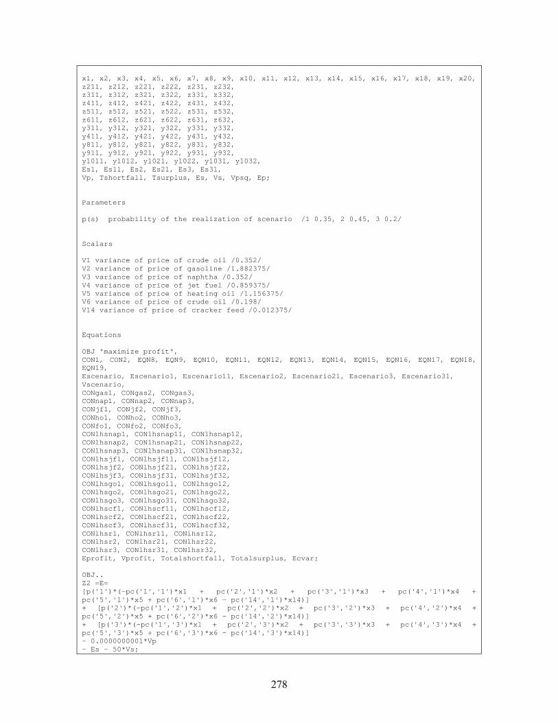
278

x1, x2, x3, x4, x5, x6, x7, x8, x9, x10, x11, x12, x13, x14, x15, x16, x17, x18, x19, x20, z211, z212, z221, z222, z231, z232, z311, z312, z321, z322, z331, z332, z411, z412, z421, z422, z431, z432, z511, z512, z521, z522, z531, z532, z611, z612, z621, z622, z631, z632, y311, y312, y321, y322, y331, y332, y411, y412, y421, y422, y431, y432, y811, y812, y821, y822, y831, y832, y911, y912, y921, y922, y931, y932, y1011, y1012, y1021, y1022, y1031, y1032, Es1, Es11, Es2, Es21, Es3, Es31, Vp, Tshortfall, Tsurplus, Es, Vs, Vpsq, Ep; Parameters p(s) probability of the realization of scenario /1 0.35, 2 0.45, 3 0.2/ Scalars V1 variance of price of crude oil /0.352/ V2 variance of price of gasoline /1.882375/ V3 variance of price of naphtha /0.352/ V4 variance of price of jet fuel /0.859375/ V5 variance of price of heating oil /1.156375/ V6 variance of price of crude oil /0.198/ V14 variance of price of cracker feed /0.012375/ Equations OBJ "maximize profit", CON1, CON2, EQN8, EQN9, EQN10, EQN11, EQN12, EQN13, EQN14, EQN15, EQN16, EQN17, EQN18, EQN19, Escenario, Escenario1, Escenario11, Escenario2, Escenario21, Escenario3, Escenario31, Vscenario, CONgas1, CONgas2, CONgas3, CONnap1, CONnap2, CONnap3, CONjf1, CONjf2, CONjf3, CONho1, CONho2, CONho3, CONfo1, CONfo2, CONfo3, CONlhsnap1, CONlhsnap11, CONlhsnap12, CONlhsnap2, CONlhsnap21, CONlhsnap22, CONlhsnap3, CONlhsnap31, CONlhsnap32, CONlhsjf1, CONlhsjf11, CONlhsjf12, CONlhsjf2, CONlhsjf21, CONlhsjf22, CONlhsjf3, CONlhsjf31, CONlhsjf32, CONlhsgo1, CONlhsgo11, CONlhsgo12, CONlhsgo2, CONlhsgo21, CONlhsgo22, CONlhsgo3, CONlhsgo31, CONlhsgo32, CONlhscf1, CONlhscf11, CONlhscf12, CONlhscf2, CONlhscf21, CONlhscf22, CONlhscf3, CONlhscf31, CONlhscf32, CONlhsr1, CONlhsr11, CONlhsr12, CONlhsr2, CONlhsr21, CONlhsr22, CONlhsr3, CONlhsr31, CONlhsr32, Eprofit, Vprofit, Totalshortfall, Totalsurplus, Ecvar; OBJ.. Z2 =E= [p('1')*(-pc('1','1')*x1 + pc('2','1')*x2 + pc('3','1')*x3 + pc('4','1')*x4 + pc('5','1')*x5 + pc('6','1')*x6 - pc('14','1')*x14)] + [p('2')*(-pc('1','2')*x1 + pc('2','2')*x2 + pc('3','2')*x3 + pc('4','2')*x4 + pc('5','2')*x5 + pc('6','2')*x6 - pc('14','2')*x14)] + [p('3')*(-pc('1','3')*x1 + pc('2','3')*x2 + pc('3','3')*x3 + pc('4','3')*x4 + pc('5','3')*x5 + pc('6','3')*x6 - pc('14','3')*x14)] - 0.0000000001*Vp - Es - 50*Vs;

279

Vprofit.. Vp =E= ((V1*SQR(x1)) + (V2*SQR(x2)) + (V3*SQR(x3)) + (V4*SQR(x4)) + (V5*SQR(x5)) + (V6*SQR(x6)) + (V14*SQR(x14))); Vscenario.. Vs =E= ((p('1')*SQR(Es11 - Es)) + (p('2')*SQR(Es21 - Es)) + (p('3')*SQR(Es31 - Es))); CON1.. x1 =L= 15000; CON2.. x14 =L= 2500; *EQN3.. -0.13*x1 + x7 =E= 0; *EQN4.. -0.15*x1 + x4 =E= 0; *EQN5.. -0.22*x1 + x8 =E= 0; *EQN6.. -0.20*x1 + x9 =E= 0; *EQN7.. -0.30*x1 + x10 =E= 0; EQN8.. -0.05*x14 + x20 =E= 0; EQN9.. -0.40*x14 + x16 =E= 0; EQN10.. -0.55*x14 + x17 =E= 0; EQN11.. 0.5*x2 - x11 =E= 0; EQN12.. 0.5*x2 - x16 =E= 0; EQN13.. 0.75*x5 - x12 =E= 0; EQN14.. 0.25*x5 - x18 =E= 0; EQN15.. -x7 + x3 +x11 =E= 0; EQN16.. -x8 + x12 +x13 =E= 0; EQN17.. -x9 + x14 +x15 =E= 0; EQN18.. -x17 + x18 +x19 =E= 0; EQN19.. -x10 - x13 - x15 - x19 + x6 =E= 0; *CON20.. x2 =L= 2700; *CON21.. x3 =L= 1100; *CON22.. x4 =L= 2300; *CON23.. x5 =L= 1700; *CON24.. x6 =L= 9500; *Scenario 1: High demand Escenario1.. Es1 =E= p('1')*Es11;; Escenario11.. Es11 =E= (((c('2','1')*z211 + c('2','2')*z212) + (c('3','1')*z311 + c('3','2')*z312) + (c('4','1')*z411 + c('4','2')*z412) + (c('5','1')*z511 + c('5','2')*z512) + (c('6','1')*z611 + c('6','2')*z612)) + ((q('3','1')*y311 + q('3','2')*y312) + (q('4','1')*y411 + q('4','2')*y412) + (q('8','1')*y811 + q('8','2')*y812) + (q('9','1')*y911 + q('9','2')*y912) + (q('10','1')*y1011 + q('10','2')*y1012))); CONgas1.. x2 + z211 - z212 =E= d('2','1'); CONnap1.. x3 + z311 - z312 =E= d('3','1'); CONjf1.. x4 + z411 - z412 =E= d('4','1'); CONho1.. x5 + z511 - z512 =E= d('5','1'); CONfo1.. x6 + z611 - z612 =E= d('6','1'); CONlhsnap1.. y('3','1')*x1 + x7 + y311 - y312 =E= 0; CONlhsnap11.. y311 =L= 0.1*x1; CONlhsnap12.. y312 =L= 0.1*x1; CONlhsjf1.. y('4','1')*x1 + x4 + y411 - y412 =E= 0; CONlhsjf11.. y411 =L= 0.1*x1; CONlhsjf12.. y412 =L= 0.1*x1; CONlhsgo1.. y('8','1')*x1 + x8 + y811 - y812 =E= 0; CONlhsgo11.. y811 =L= 0.1*x1; CONlhsgo12.. y812 =L= 0.1*x1; CONlhscf1.. y('9','1')*x1 + x9 + y911 - y912 =E= 0; CONlhscf11.. y911 =L= 0.1*x1; CONlhscf12.. y912 =L= 0.1*x1; CONlhsr1.. y('10','1')*x1 + x10 + y1011 - y1012 =E= 0; CONlhsr11.. y1011 =L= 0.1*x1; CONlhsr12.. y1012 =L= 0.1*x1; *Scenario 2: Medium demand Escenario2.. Es2 =E= p('2')*Es21; Escenario21.. Es21 =E= (((c('2','1')*z221 + c('2','2')*z222) + (c('3','1')*z321 + c('3','2')*z322) + (c('4','1')*z421 + c('4','2')*z422) + (c('5','1')*z521 + c('5','2')*z522) + (c('6','1')*z621 + c('6','2')*z622)) + ((q('3','1')*y321 + q('3','2')*y322) + (q('4','1')*y421 + q('4','2')*y422) + (q('8','1')*y821 + q('8','2')*y822) + (q('9','1')*y921 + q('9','2')*y922) + (q('10','1')*y1021 + q('10','2')*y1022))); CONgas2.. x2 + z221 - z222 =E= d('2','2');

280

CONnap2.. x3 + z321 - z322 =E= d('3','2'); CONjf2.. x4 + z421 - z422 =E= d('4','2'); CONho2.. x5 + z521 - z522 =E= d('5','2'); CONfo2.. x6 + z621 - z622 =E= d('6','2'); CONlhsnap2.. y('3','2')*x1 + x7 + y321 - y322 =E= 0; CONlhsnap21..y321 =L= 0.1*x1; CONlhsnap22.. y322 =L= 0.1*x1; CONlhsjf2.. y('4','2')*x1 + x4 + y421 - y422 =E= 0; CONlhsjf21.. y421 =L= 0.1*x1; CONlhsjf22.. y422 =L= 0.1*x1; CONlhsgo2.. y('8','2')*x1 + x8 + y821 - y822 =E= 0; CONlhsgo21.. y821 =L= 0.1*x1; CONlhsgo22.. y822 =L= 0.1*x1; CONlhscf2.. y('9','2')*x1 + x9 + y921 - y922 =E= 0; CONlhscf21.. y921 =L= 0.1*x1; CONlhscf22.. y922 =L= 0.1*x1; CONlhsr2.. y('10','2')*x1 + x10 + y1021 - y1022 =E= 0; CONlhsr21.. y1011 =L= 0.1*x1; CONlhsr22.. y1012 =L= 0.1*x1; *Scenario 3: Low demand Escenario3.. Es3 =E= p('3')*Es31; Escenario31.. Es31 =E= (((c('2','1')*z231 + c('2','2')*z232) + (c('3','1')*z331 + c('3','2')*z332) + (c('4','1')*z431 + c('4','2')*z432) + (c('5','1')*z531 + c('5','2')*z532) + (c('6','1')*z631 + c('6','2')*z632)) + ((q('3','1')*y331 + q('3','2')*y332) + (q('4','1')*y431 + q('4','2')*y432) + (q('8','1')*y831 + q('8','2')*y832) + (q('9','1')*y931 + q('9','2')*y932) + (q('10','1')*y1031 + q('10','2')*y1032))); CONgas3.. x2 + z231 - z232 =E= d('2','3'); CONnap3.. x3 + z331 - z332 =E= d('3','3'); CONjf3.. x4 + z431 - z432 =E= d('4','3'); CONho3.. x5 + z531 - z532 =E= d('5','3'); CONfo3.. x6 + z631 - z632 =E= d('6','3'); CONlhsnap3.. y('3','3')*x1 + x7 + y331 - y332 =E= 0; CONlhsnap31..y331 =L= 0.1*x1; CONlhsnap32.. y332 =L= 0.1*x1; CONlhsjf3.. y('4','3')*x1 + x4 + y431 - y432 =E= 0; CONlhsjf31.. y431 =L= 0.1*x1; CONlhsjf32.. y432 =L= 0.1*x1; CONlhsgo3.. y('8','3')*x1 + x8 + y831 - y832 =E= 0; CONlhsgo31.. y831 =L= 0.1*x1; CONlhsgo32.. y832 =L= 0.1*x1; CONlhscf3.. y('9','3')*x1 + x9 + y931 - y932 =E= 0; CONlhscf31.. y931 =L= 0.1*x1; CONlhscf32.. y932 =L= 0.1*x1; CONlhsr3.. y('10','3')*x1 + x10 + y1031 - y1032 =E= 0; CONlhsr31.. y1031 =L= 0.1*x1; CONlhsr32.. y1032 =L= 0.1*x1; Escenario.. Es =E= Es1 + Es2 + Es3; Eprofit.. Ep =E= [p('1')*(-pc('1','1')*x1 + pc('2','1')*x2 + pc('3','1')*x3 + pc('4','1')*x4 + pc('5','1')*x5 + pc('6','1')*x6 - pc('14','1')*x14)] + [p('2')*(-pc('1','2')*x1 + pc('2','2')*x2 + pc('3','2')*x3 + pc('4','2')*x4 + pc('5','2')*x5 + pc('6','2')*x6 - pc('14','2')*x14)] + [p('3')*(-pc('1','3')*x1 + pc('2','3')*x2 + pc('3','3')*x3 + pc('4','3')*x4 + pc('5','3')*x5 + pc('6','3')*x6 - pc('14','3')*x14)]; Totalshortfall.. Tshortfall =E= z211 + z221 + z231 + z311 + z321 + z331 + z411 + z421 + z431 + z511 + z521 + z531 + z611 + z621 + z631 + y311 + y321 + y331 + y411 + y421 + y431 + y811 + y821 + y831 + y911 + y921 + y931 + y1011 + y1021 + y1031; Totalsurplus.. Tsurplus =E= z212 + z222 + z232 + z312 + z322 + z332 + z412 + z422 + z432 + z512 + z522 + z532 + z612 + z622 + z632 + y312 + y322 + y332 + y412 + y422 + y432 + y812 + y822 + y832 + y912 + y922 + y932 + y1012 + y1022 + y1032; *Vprofit2.. Vp2 =E= (v1*SQR(x1)) + (v2*SQR(x2)) + (v3*SQR(x3)) + (v4*SQR(x4)) +

281

(v5*SQR(x5)) + (v6*SQR(x6)) + (v14*SQR(x14)); *Vpsqrt.. Vpsq =E= SQRT(Vp + Vs); Ecvar.. Ecv =E= Ep - Es; *Covar.. Cv =E= Vpsq/(Ep - Es); Model Refinery / all /; * Starting values x1.up = 15000; x1.l = 12500; x2.up = 2700; x2.l = 2000; x3.up = 1100; x3.l = 625; x4.up = 2300; x4.l = 1875; x5.up = 1700; x5.l = 1700; x6.up = 9500; x6.l = 6175; x7.up = 1950; x7.l = 1625; x8.up = 3300; x8.l = 2750; x9.up = 3000; x9.l = 2500; x10.up = 3000; x10.l = 3750; x11.up = 1350; x11.l = 1000; x12.up = 1275; x12.l = 1275; x13.up = 3300; x13.l = 1475; x14.up = 3000; x14.l = 2500; x15.up = 3000; x15.l = 0; x16.up = 1200; x16.l = 1000; x17.up = 1650; x17.l = 1375; x18.up = 425; x18.l = 425; x19.up = 1650; x19.l = 950; x20.up = 150; x20.l = 125; Options nlp = conopt3; Solve REFINERY USING NLP MAXIMIZING Z2;

282

Appendix D6: Approach 4Risk Model III with Mean-Absolute Deviation (MAD)

as the Measure of Risk Imposed by the Recourse Penalty Costs

$TITLE Approach 4: Risk Model III of Two-Stage Stochastic Programming with Fixed Recourse for Minimization of the Expected Value and the Mean-Absolute Deviation (MAD) of the Variation in Recourse Penalty Costs Sets i "product type" /1*21/ s "scenarios" /1*3/ k "production shortfall and surplus or yield decrement or increment" /1, 2/ Table pc(i,s) "price of product type i per realization j" 1 2 3 1 8.8 8.0 7.2 2 20.35 18.5 16.65 3 8.8 8.0 7.2 4 13.75 12.5 11.25 5 15.95 14.5 13.05 6 6.6 6 5.4 14 1.65 1.5 1.35; Table d(i,s) "demand of product type i per realization j" 1 2 3 2 2835 2700 2565 3 1155 1100 1045 4 2415 2300 2185 5 1785 1700 1615 6 9975 9500 9025; Table y(i,s) "yield of product type i per realization j" 1 2 3 3 -0.1365 -0.13 -0.1235 4 -0.1575 -0.15 -0.1425 8 -0.231 -0.22 -0.209 9 -0.21 -0.20 -0.19 10 -0.265 -0.30 -0.335; Table c(i,k) "penalty cost for product type i due to production shortfall or surplus" 1 2 1 55 50 2 25 20 3 17 13 4 5 4 5 6 5 6 10 8; Table q(i,k) "penalty cost for product type i due to yield decrement or increment" 1 2 3 5 3 4 5 4 8 5 3 9 5 3 10 5 3 Variables Z2, Ecv;

283

Positive variables x1, x2, x3, x4, x5, x6, x7, x8, x9, x10, x11, x12, x13, x14, x15, x16, x17, x18, x19, x20, z211, z212, z221, z222, z231, z232, z311, z312, z321, z322, z331, z332, z411, z412, z421, z422, z431, z432, z511, z512, z521, z522, z531, z532, z611, z612, z621, z622, z631, z632, y311, y312, y321, y322, y331, y332, y411, y412, y421, y422, y431, y432, y811, y812, y821, y822, y831, y832, y911, y912, y921, y922, y931, y932, y1011, y1012, y1021, y1022, y1031, y1032, Es1, Es11, Es2, Es21, Es3, Es31, MADs, MADs1, Vp, Tshortfall, Tsurplus, Es, Ep; Parameters p(s) probability of the realization of scenario /1 0.35, 2 0.45, 3 0.2/ Scalars V1 variance of price of crude oil /0.352/ V2 variance of price of gasoline /1.882375/ V3 variance of price of naphtha /0.352/ V4 variance of price of jet fuel /0.859375/ V5 variance of price of heating oil /1.156375/ V6 variance of price of crude oil /0.198/ V14 variance of price of cracker feed /0.012375/ Equations OBJ "maximize profit", CON1, CON2, EQN8, EQN9, EQN10, EQN11, EQN12, EQN13, EQN14, EQN15, EQN16, EQN17, EQN18, EQN19, Escenario, Escenario1, Escenario11, Escenario2, Escenario21, Escenario3, Escenario31, CONgas1, CONgas2, CONgas3, CONnap1, CONnap2, CONnap3, CONjf1, CONjf2, CONjf3, CONho1, CONho2, CONho3, CONfo1, CONfo2, CONfo3, CONlhsnap1, CONlhsnap11, CONlhsnap12, CONlhsnap2, CONlhsnap21, CONlhsnap22, CONlhsnap3, CONlhsnap31, CONlhsnap32, CONlhsjf1, CONlhsjf11, CONlhsjf12, CONlhsjf2, CONlhsjf21, CONlhsjf22, CONlhsjf3, CONlhsjf31, CONlhsjf32, CONlhsgo1, CONlhsgo11, CONlhsgo12, CONlhsgo2, CONlhsgo21, CONlhsgo22, CONlhsgo3, CONlhsgo31, CONlhsgo32, CONlhscf1, CONlhscf11, CONlhscf12, CONlhscf2, CONlhscf21, CONlhscf22, CONlhscf3, CONlhscf31, CONlhscf32, CONlhsr1, CONlhsr11, CONlhsr12, CONlhsr2, CONlhsr21, CONlhsr22, CONlhsr3, CONlhsr31, CONlhsr32, MADscenario, MADcon1, MADcon2, MADcon3, Eprofit, Vprofit, Totalshortfall, Totalsurplus, Ecvar; OBJ.. Z2 =e= [p('1')*(-pc('1','1')*x1 + pc('2','1')*x2 + pc('3','1')*x3 + pc('4','1')*x4 + pc('5','1')*x5 + pc('6','1')*x6 - pc('14','1')*x14)] + [p('2')*(-pc('1','2')*x1 + pc('2','2')*x2 + pc('3','2')*x3 + pc('4','2')*x4 +

284

pc('5','2')*x5 + pc('6','2')*x6 - pc('14','2')*x14)] + [p('3')*(-pc('1','3')*x1 + pc('2','3')*x2 + pc('3','3')*x3 + pc('4','3')*x4 + pc('5','3')*x5 + pc('6','3')*x6 - pc('14','3')*x14)] - 0.0008*Vp - Es - 0.01*MADs; Vprofit.. Vp =E= ((V1*SQR(x1)) + (V2*SQR(x2)) + (V3*SQR(x3)) + (V4*SQR(x4)) + (V5*SQR(x5)) + (V6*SQR(x6)) + (V14*SQR(x14))); CON1.. x1 =L= 15000; CON2.. x14 =L= 2500; *EQN3.. -0.13*x1 + x7 =E= 0; *EQN4.. -0.15*x1 + x4 =E= 0; *EQN5.. -0.22*x1 + x8 =E= 0; *EQN6.. -0.20*x1 + x9 =E= 0; *EQN7.. -0.30*x1 + x10 =E= 0; EQN8.. -0.05*x14 + x20 =E= 0; EQN9.. -0.40*x14 + x16 =E= 0; EQN10.. -0.55*x14 + x17 =E= 0; EQN11.. 0.5*x2 - x11 =E= 0; EQN12.. 0.5*x2 - x16 =E= 0; EQN13.. 0.75*x5 - x12 =E= 0; EQN14.. 0.25*x5 - x18 =E= 0; EQN15.. -x7 + x3 +x11 =E= 0; EQN16.. -x8 + x12 +x13 =E= 0; EQN17.. -x9 + x14 +x15 =E= 0; EQN18.. -x17 + x18 +x19 =E= 0; EQN19.. -x10 - x13 - x15 - x19 + x6 =E= 0; *CON20.. x2 =L= 2700; *CON21.. x3 =L= 1100; *CON22.. x4 =L= 2300; *CON23.. x5 =L= 1700; *CON24.. x6 =L= 9500; *Scenario 1: High demand Escenario1.. Es1 =E= p('1')*Es11; Escenario11.. Es11 =E= (((c('2','1')*z211 + c('2','2')*z212) + (c('3','1')*z311 + c('3','2')*z312) + (c('4','1')*z411 + c('4','2')*z412) + (c('5','1')*z511 + c('5','2')*z512) + (c('6','1')*z611 + c('6','2')*z612)) + ((q('3','1')*y311 + q('3','2')*y312) + (q('4','1')*y411 + q('4','2')*y412) + (q('8','1')*y811 + q('8','2')*y812) + (q('9','1')*y911 + q('9','2')*y912) + (q('10','1')*y1011 + q('10','2')*y1012))); CONgas1.. x2 + z211 - z212 =E= d('2','1'); CONnap1.. x3 + z311 - z312 =E= d('3','1'); CONjf1.. x4 + z411 - z412 =E= d('4','1'); CONho1.. x5 + z511 - z512 =E= d('5','1'); CONfo1.. x6 + z611 - z612 =E= d('6','1'); CONlhsnap1.. y('3','1')*x1 + x7 + y311 - y312 =E= 0; CONlhsnap11.. y311 =L= 0.1*x1; CONlhsnap12.. y312 =L= 0.1*x1; CONlhsjf1.. y('4','1')*x1 + x4 + y411 - y412 =E= 0; CONlhsjf11.. y411 =L= 0.1*x1; CONlhsjf12.. y412 =L= 0.1*x1; CONlhsgo1.. y('8','1')*x1 + x8 + y811 - y812 =E= 0; CONlhsgo11.. y811 =L= 0.1*x1; CONlhsgo12.. y812 =L= 0.1*x1; CONlhscf1.. y('9','1')*x1 + x9 + y911 - y912 =E= 0; CONlhscf11.. y911 =L= 0.1*x1; CONlhscf12.. y912 =L= 0.1*x1; CONlhsr1.. y('10','1')*x1 + x10 + y1011 - y1012 =E= 0; CONlhsr11.. y1011 =L= 0.1*x1; CONlhsr12.. y1012 =L= 0.1*x1; *Scenario 2: Medium demand Escenario2.. Es2 =E= p('2')*Es21; Escenario21.. Es21 =E= (((c('2','1')*z221 + c('2','2')*z222) + (c('3','1')*z321 + c('3','2')*z322) + (c('4','1')*z421 + c('4','2')*z422) + (c('5','1')*z521 + c('5','2')*z522) + (c('6','1')*z621 + c('6','2')*z622)) + ((q('3','1')*y321 + q('3','2')*y322) + (q('4','1')*y421 + q('4','2')*y422) + (q('8','1')*y821 + q('8','2')*y822) + (q('9','1')*y921 + q('9','2')*y922) +

285

(q('10','1')*y1021 + q('10','2')*y1022))); CONgas2.. x2 + z221 - z222 =E= d('2','2'); CONnap2.. x3 + z321 - z322 =E= d('3','2'); CONjf2.. x4 + z421 - z422 =E= d('4','2'); CONho2.. x5 + z521 - z522 =E= d('5','2'); CONfo2.. x6 + z621 - z622 =E= d('6','2'); CONlhsnap2.. y('3','2')*x1 + x7 + y321 - y322 =E= 0; CONlhsnap21..y321 =L= 0.1*x1; CONlhsnap22.. y322 =L= 0.1*x1; CONlhsjf2.. y('4','2')*x1 + x4 + y421 - y422 =E= 0; CONlhsjf21.. y421 =L= 0.1*x1; CONlhsjf22.. y422 =L= 0.1*x1; CONlhsgo2.. y('8','2')*x1 + x8 + y821 - y822 =E= 0; CONlhsgo21.. y821 =L= 0.1*x1; CONlhsgo22.. y822 =L= 0.1*x1; CONlhscf2.. y('9','2')*x1 + x9 + y921 - y922 =E= 0; CONlhscf21.. y921 =L= 0.1*x1; CONlhscf22.. y922 =L= 0.1*x1; CONlhsr2.. y('10','2')*x1 + x10 + y1021 - y1022 =E= 0; CONlhsr21.. y1011 =L= 0.1*x1; CONlhsr22.. y1012 =L= 0.1*x1; *Scenario 3: Low demand Escenario3.. Es3 =E= p('3')*Es31; Escenario31.. Es31 =E= (((c('2','1')*z231 + c('2','2')*z232) + (c('3','1')*z331 + c('3','2')*z332) + (c('4','1')*z431 + c('4','2')*z432) + (c('5','1')*z531 + c('5','2')*z532) + (c('6','1')*z631 + c('6','2')*z632)) + ((q('3','1')*y331 + q('3','2')*y332) + (q('4','1')*y431 + q('4','2')*y432) + (q('8','1')*y831 + q('8','2')*y832) + (q('9','1')*y931 + q('9','2')*y932) + (q('10','1')*y1031 + q('10','2')*y1032))); CONgas3.. x2 + z231 - z232 =E= d('2','3'); CONnap3.. x3 + z331 - z332 =E= d('3','3'); CONjf3.. x4 + z431 - z432 =E= d('4','3'); CONho3.. x5 + z531 - z532 =E= d('5','3'); CONfo3.. x6 + z631 - z632 =E= d('6','3'); CONlhsnap3.. y('3','3')*x1 + x7 + y331 - y332 =E= 0; CONlhsnap31..y331 =L= 0.1*x1; CONlhsnap32.. y332 =L= 0.1*x1; CONlhsjf3.. y('4','3')*x1 + x4 + y431 - y432 =E= 0; CONlhsjf31.. y431 =L= 0.1*x1; CONlhsjf32.. y432 =L= 0.1*x1; CONlhsgo3.. y('8','3')*x1 + x8 + y831 - y832 =E= 0; CONlhsgo31.. y831 =L= 0.1*x1; CONlhsgo32.. y832 =L= 0.1*x1; CONlhscf3.. y('9','3')*x1 + x9 + y931 - y932 =E= 0; CONlhscf31.. y931 =L= 0.1*x1; CONlhscf32.. y932 =L= 0.1*x1; CONlhsr3.. y('10','3')*x1 + x10 + y1031 - y1032 =E= 0; CONlhsr31.. y1031 =L= 0.1*x1; CONlhsr32.. y1032 =L= 0.1*x1; Escenario.. Es =E= Es1 + Es2 + Es3; MADscenario.. MADs =E= (p('1')*abs(Es11 - Es)) + (p('2')*abs(Es21 - Es)) + (p('3')*abs(Es31 - Es)); MADcon1.. MADs1 =G= -MADs; MADcon2.. MADs1 =G= MADs; MADcon3.. MADs1 =G= 0; *Vscenario.. Vs =E= (p1*SQR(Es11 - Es)) + (p2*SQR(Es21 - Es)) + (p3*SQR(Es31 - Es)); Eprofit.. Ep =E= [p('1')*(-pc('1','1')*x1 + pc('2','1')*x2 + pc('3','1')*x3 + pc('4','1')*x4 + pc('5','1')*x5 + pc('6','1')*x6 - pc('14','1')*x14)] + [p('2')*(-pc('1','2')*x1 + pc('2','2')*x2 + pc('3','2')*x3 + pc('4','2')*x4 + pc('5','2')*x5 + pc('6','2')*x6 - pc('14','2')*x14)] + [p('3')*(-pc('1','3')*x1 + pc('2','3')*x2 + pc('3','3')*x3 + pc('4','3')*x4 + pc('5','3')*x5 + pc('6','3')*x6 - pc('14','3')*x14)]; Totalshortfall.. Tshortfall =E= z211 + z221 + z231 + z311 + z321 + z331 + z411 + z421 + z431 + z511 + z521 + z531 + z611 + z621 + z631 + y311 + y321 + y331 + y411 + y421 + y431 + y811 + y821 + y831 + y911 + y921 + y931 +

286

y1011 + y1021 + y1031; Totalsurplus.. Tsurplus =E= z212 + z222 + z232 + z312 + z322 + z332 + z412 + z422 + z432 + z512 + z522 + z532 + z612 + z622 + z632 + y312 + y322 + y332 + y412 + y422 + y432 + y812 + y822 + y832 + y912 + y922 + y932 + y1012 + y1022 + y1032; *Vpsqrt.. Vpsq =E= SQRT(Vp + MADs); Ecvar.. Ecv =E= Ep - Es; Model Refinery / all /; * Starting values x1.up = 15000; x1.l = 12500; x2.up = 2700; x2.l = 2000; x3.up = 1100; x3.l = 625; x4.up = 2300; x4.l = 1875; x5.up = 1700; x5.l = 1700; x6.up = 9500; x6.l = 6175; x7.up = 1950; x7.l = 1625; x8.up = 3300; x8.l = 2750; x9.up = 3000; x9.l = 2500; x10.up = 3000; x10.l = 3750; x11.up = 1350; x11.l = 1000; x12.up = 1275; x12.l = 1275; x13.up = 3300; x13.l = 1475; x14.up = 3000; x14.l = 2500; x15.up = 3000; x15.l = 0; x16.up = 1200; x16.l = 1000; x17.up = 1650; x17.l = 1375; x18.up = 425; x18.l = 425; x19.up = 1650; x19.l = 950; x20.up = 150; x20.l = 125; Option dnlp = conopt3; Solve REFINERY USING DNLP MAXIMIZING Z2;

287

Final Remarks

Manuscript on parts of this dissertation have been submitted for publication as indicated

in the following:

Khor, C. S., A. Elkamel, and P. L. Douglas. Stochastic Refinery Planning with

Risk Management. To appear in Petroleum Science and Technology (accepted

October 21, 2006), 16 pages.

Khor, C. S., A. Elkamel, K. Ponnambalam, and P. L. Douglas. Two-stage

stochastic programming with fixed recourse via scenario planning with financial

and operational risk management for petroleum refinery planning under

uncertainty. Chemical Engineering and Processing (submitted for publication and

under review), 63 pages.

Brief Biographical Notes on the Author

Cheng Seong Khor is currently on study leave from a teaching position in the

PETRONAS University of Technology, the academic institution set up by PETRONAS,

the Malaysian state-owned national oil corporation, to pursue his graduate studies in the

Department of Chemical Engineering at the University of Waterloo, Ontario, Canada. His

general research interests concern the theory and application of the optimization approach

to chemical process systems engineering (PSE) problems, particularly in the hydrocarbon

industry. He holds a Bachelor in Chemical Engineering (Honours) degree from the

National University of Malaysia (Universiti Kebangsaan Malaysia).