Online Monitoring Framework for

Pressure Transient Detection in

Water Distribution Networks

by

Nina Feng

A thesis

presented to the University of Waterloo

in fulfillment of the

thesis requirement for the degree of

Master of Applied Science

in

Civil Engineering

Waterloo, Ontario, Canada, 2019

c© Nina Feng 2019

Author’s Declaration

I hereby declare that I am the sole author of this thesis. This is a true copy of the thesis,

including any required final revisions, as accepted by my examiners.

I understand that my thesis may be made electronically available to the public.

ii

Abstract

Access to potable drinking water is a necessity and basic human right. Most North

Americans obtain treated water through water distribution networks, an essential part of

municipal infrastructure that is subject to decay and degradation. Amongst the factors

influencing pipe failure are events that trigger abrupt pressure changes, or transients, which

can cause pipe breakages in the short term, and general fatigue in the long term. The ability

to quantify these transients as they occur is important for effective asset management,

and for preventing and mitigating the occurrence of failure. Current practices take a

largely reactive approach to event detection, and few systems capable of real-time transient

detection have ever been implemented.

This research addresses the need for an online monitoring framework aimed towards

understanding pressure transient effects and behaviour. The proposed system uses an

Internet of Things approach, combining pressure sensors with Raspberry Pi computers, as

well as open-source tools that transmit and display the data. The data analysis combines

computationally inexpensive methods in order to achieve an accurate decision-making tool

for both transient detection and abnormal transient risk identification. The techniques used

include different filtering and detrending methods, feature extraction for dimensionality

reduction, three-sigma statistical process control, and classification using voting methods.

The process also includes a second process, based on statistical process control and trained

using transient data identified in the original process, in order to assign a risk for a transient

to cause damage, as well as identify transients that are particularly severe.

Data was collected from a unique laboratory water distribution network as well as a

field installation in Guelph, Ontario. The results showed that the framework achieves real-

time transient identification with reasonable detection and error rates. Further analysis

illustrated the effect of factors such as transient source location, active flow in the pipes, and

transient type, on transient propagation and detection. The performance of the framework

proves the concept of IoT-based systems for pressure monitoring and event detection in

municipal water infrastructure.

iii

Acknowledgements

I’d like to express my appreciation first and foremost to my supervisor, Dr. Sriram

Narasimhan. I am immensely grateful for having been given the opportunity to move out

of my comfort zone, and for the guidance and encouragement that helped me succeed along

the way. Thank you so much for taking a chance on an Enviro who knew nothing about

structural dynamics, and still doesn’t really.

Without quality data and a reliable platform from which data could be collected, noth-

ing useful could have been accomplished in this thesis, or any other for that matter. I owe

much of the success of this research to Dirk, whose reliability, work ethic, and knack for

solving any and all problems has saved my life on many occasions. Another shout-out goes

to Terry, who somehow always came through with whatever part or tool we needed, and

never hesitated to teach us how to do things ourselves.

The project also could not have been completed without collaborating with our many

industry partners. Thank you to Jim and John with Optys, whom I’ll always remember,

for gracing us with their patience, knowledge, and personalities. Much of the development

of the many different technologies needed for research success can be attributed to Rick

and Don with HNSI, Ilia AKA Mr. Robot, as well as Eramosa and Terepac. Much of my

appreciation also goes to the City of Guelph, Precision Hydrant Services, and C3 Water

for their cooperation with field tests.

My graduate experience wouldn’t have been the same without my supportive research

group, especially Stan and Roya for their research help, and Dylan for always being moti-

vational.

On a personal note, I’d like to thank my family for always being there: my formidable

parents, my wonderful siblings, and my ever-supportive grandparents. I also need my

friends, the ones who spark joy in my life, to know that they’re very much appreciated

for having dealt with me, listened to me, and helped me pass the time as pleasantly as

possible.

iv

Dedication

To anyone who ever took a risk, and then struggled.

v

Table of Contents

List of Tables ix

List of Figures x

Abbreviations xii

1 Introduction 1

1.1 Motivation . . . . . . . . . . . . . . . . . . . . . . . . . . . . . . . . . . . . 1

1.2 Objective Statement . . . . . . . . . . . . . . . . . . . . . . . . . . . . . . 3

1.3 Research Scope . . . . . . . . . . . . . . . . . . . . . . . . . . . . . . . . . 3

2 Background and Literature Review 4

2.1 Pressure transients in WDNs . . . . . . . . . . . . . . . . . . . . . . . . . . 4

2.1.1 Transient behaviour and influencing factors . . . . . . . . . . . . . . 4

2.2 Transient detection techniques . . . . . . . . . . . . . . . . . . . . . . . . . 7

2.2.1 Offline techniques . . . . . . . . . . . . . . . . . . . . . . . . . . . . 7

2.2.2 Online transient detection techniques . . . . . . . . . . . . . . . . . 9

2.3 Condition monitoring in WDNs . . . . . . . . . . . . . . . . . . . . . . . . 11

2.3.1 Common current strategies . . . . . . . . . . . . . . . . . . . . . . . 11

2.3.2 Smart infrastructure and Internet of Things . . . . . . . . . . . . . 11

2.4 Summary of limitations and knowledge gaps . . . . . . . . . . . . . . . . . 12

2.4.1 Transient identification . . . . . . . . . . . . . . . . . . . . . . . . . 12

2.4.2 Condition monitoring . . . . . . . . . . . . . . . . . . . . . . . . . . 13

vi

3 Methodology 15

3.1 System architecture . . . . . . . . . . . . . . . . . . . . . . . . . . . . . . . 15

3.1.1 General overview . . . . . . . . . . . . . . . . . . . . . . . . . . . . 16

3.1.2 Sensing . . . . . . . . . . . . . . . . . . . . . . . . . . . . . . . . . 17

3.1.3 Data analysis . . . . . . . . . . . . . . . . . . . . . . . . . . . . . . 18

3.1.3.1 Raw data and pre-processing . . . . . . . . . . . . . . . . 19

3.1.3.2 Feature extraction and selection . . . . . . . . . . . . . . . 20

3.1.3.3 Anomaly detection and classification . . . . . . . . . . . . 21

3.1.3.4 Anomaly detection and classification for abnormal tran-

sient detection . . . . . . . . . . . . . . . . . . . . . . . . 22

3.1.4 Communication and Internet of Things . . . . . . . . . . . . . . . . 24

3.2 Experimental procedures . . . . . . . . . . . . . . . . . . . . . . . . . . . . 26

3.2.1 Laboratory experiments . . . . . . . . . . . . . . . . . . . . . . . . 26

3.2.1.1 Laboratory set-up . . . . . . . . . . . . . . . . . . . . . . 26

3.2.1.2 Laboratory test plan . . . . . . . . . . . . . . . . . . . . . 28

3.2.2 Field experiments . . . . . . . . . . . . . . . . . . . . . . . . . . . . 30

3.2.2.1 Field set-up . . . . . . . . . . . . . . . . . . . . . . . . . . 30

3.2.2.2 Field test plan . . . . . . . . . . . . . . . . . . . . . . . . 31

4 Results 33

4.1 Laboratory results . . . . . . . . . . . . . . . . . . . . . . . . . . . . . . . 33

4.1.1 Validation - original laboratory configuration . . . . . . . . . . . . . 33

4.1.1.1 Raw and pre-processed data . . . . . . . . . . . . . . . . . 33

4.1.1.2 Performance of anomaly detection algorithm . . . . . . . . 35

4.1.2 Sensitivity analysis - expanded laboratory configuration . . . . . . . 37

4.1.2.1 Transient induction method . . . . . . . . . . . . . . . . . 38

4.1.2.2 Flow conditions . . . . . . . . . . . . . . . . . . . . . . . . 40

4.1.2.3 Transient source location . . . . . . . . . . . . . . . . . . 41

vii

4.1.2.4 Summary of the sensitivity analysis . . . . . . . . . . . . . 43

4.1.3 Additional analysis for abnormal transient detection . . . . . . . . . 45

4.2 Field results . . . . . . . . . . . . . . . . . . . . . . . . . . . . . . . . . . . 48

4.2.1 Validation - Gosling Gardens . . . . . . . . . . . . . . . . . . . . . 48

4.2.2 Detailed analysis - Clairfields . . . . . . . . . . . . . . . . . . . . . 50

4.2.2.1 Location 1 - 38 Keys . . . . . . . . . . . . . . . . . . . . . 51

4.2.2.2 Location 2 - 70 Clairfields . . . . . . . . . . . . . . . . . . 52

4.2.2.3 Location 3 - 10 Murphy . . . . . . . . . . . . . . . . . . . 53

4.2.2.4 Location 4 - 30 Paulstown . . . . . . . . . . . . . . . . . . 54

4.2.3 Field application of abnormal transient detection algorithm . . . . . 55

4.3 Summary . . . . . . . . . . . . . . . . . . . . . . . . . . . . . . . . . . . . 58

5 Conclusions and Recommendations 60

5.1 Conclusions . . . . . . . . . . . . . . . . . . . . . . . . . . . . . . . . . . . 60

5.2 Recommendations for future work . . . . . . . . . . . . . . . . . . . . . . . 62

References 63

APPENDICES 67

A Hardware Datasheets 68

B List of Features 95

viii

List of Tables

3.1 Main device hardware components . . . . . . . . . . . . . . . . . . . . . . 17

3.2 Transient detection feature set . . . . . . . . . . . . . . . . . . . . . . . . . 21

3.3 SPC-based classification of transient behaviour and severity . . . . . . . . 24

3.4 Laboratory test matrix . . . . . . . . . . . . . . . . . . . . . . . . . . . . . 30

3.5 Field test matrix . . . . . . . . . . . . . . . . . . . . . . . . . . . . . . . . 32

4.1 Abnormal transient detection feature set for the laboratory . . . . . . . . . 47

4.2 Abnormal transient detection feature set for the field locations . . . . . . . 57

ix

List of Figures

2.1 Diagram of pressure transient development . . . . . . . . . . . . . . . . . . 5

2.2 Overview of relevant transient detection techniques in literature. . . . . . . 7

3.1 Diagram of node hardware architecture. . . . . . . . . . . . . . . . . . . . . 16

3.2 Diagram of three-sigma thresholds. . . . . . . . . . . . . . . . . . . . . . . 22

3.3 Diagram of Internet of Things architecture. . . . . . . . . . . . . . . . . . . 24

3.4 Examples of Internet of Things user interface. . . . . . . . . . . . . . . . . 25

3.5 Perspective view of initial laboratory configuration. . . . . . . . . . . . . . 27

3.6 Perspective view of expanded laboratory configuration. . . . . . . . . . . . 27

3.7 Cross-sectional view of sensor pressure chamber. . . . . . . . . . . . . . . . 28

3.8 Diagram of the solenoid valve state when inducing different transients. . . 29

3.9 Map of field test locations. . . . . . . . . . . . . . . . . . . . . . . . . . . . 31

4.1 Example time series with transient - original laboratory configuration. . . . 34

4.2 Example time series with transient, varying induction method - original

laboratory configuration. . . . . . . . . . . . . . . . . . . . . . . . . . . . . 35

4.3 Detection and error rates by feature vote threshold, varying transient induc-

tion method - original laboratory configuration. . . . . . . . . . . . . . . . 36

4.4 Example time series with transients and their feature votes - expanded lab-

oratory configuration. . . . . . . . . . . . . . . . . . . . . . . . . . . . . . . 37

4.5 Example time series with transient, varying induction method - expanded

laboratory configuration. . . . . . . . . . . . . . . . . . . . . . . . . . . . . 38

x

4.6 Detection and error rates by feature vote threshold, varying transient induc-

tion method - expanded laboratory configuration. . . . . . . . . . . . . . . 39

4.7 Example time series with transient, varying flow condition - expanded lab-

oratory configuration. . . . . . . . . . . . . . . . . . . . . . . . . . . . . . . 40

4.8 Detection and error rates by feature vote threshold, varying flow condition

- expanded laboratory configuration. . . . . . . . . . . . . . . . . . . . . . 41

4.9 Example time series with transient, varying transient source location - ex-

panded laboratory configuration. . . . . . . . . . . . . . . . . . . . . . . . 42

4.10 Detection and error rates by feature vote threshold, varying transient source

location - expanded laboratory configuration. . . . . . . . . . . . . . . . . . 43

4.11 Overall detection and error rates by feature vote threshold. . . . . . . . . . 44

4.12 Detection rate at each individual feature vote. . . . . . . . . . . . . . . . . 45

4.13 Error rate at each individual feature vote. . . . . . . . . . . . . . . . . . . 45

4.14 Probability distribution of laboratory transient Zero-Crossings Count data. 46

4.15 Probability distribution of laboratory transient Maximum data. . . . . . . 46

4.16 Probability distribution of transformed laboratory transient Maximum data. 47

4.17 Map of Gosling Gardens test location. . . . . . . . . . . . . . . . . . . . . 48

4.18 Sensor placement within a fire hydrant. . . . . . . . . . . . . . . . . . . . . 49

4.19 Water flowing from a hydrant port valve during field tests. . . . . . . . . . 49

4.20 Example time series with transients - Gosling Gardens field location. . . . 50

4.21 Map of Clairfields test location. . . . . . . . . . . . . . . . . . . . . . . . . 51

4.22 Frequency of transients classified - 38 Keys. . . . . . . . . . . . . . . . . . 52

4.23 Frequency of transients classified - 70 Clairfields. . . . . . . . . . . . . . . . 53

4.24 Frequency of transients classified - 10 Murphy. . . . . . . . . . . . . . . . . 53

4.25 Frequency of transients classified - 30 Paulstown. . . . . . . . . . . . . . . 54

4.26 Probability distributions of field transient Maximum data. . . . . . . . . . 56

4.27 Probability distributions of transformed field transient RMS data. . . . . . 57

4.28 Probability distributions of field transient Skewness data. . . . . . . . . . . 58

xi

Abbreviations

CUSUM cumulative sum

DMA district-metered area

IoT Internet of Things

RMS root-mean-square

SPC statistical process control

WDN water distribution network

xii

Chapter 1

Introduction

1.1 Motivation

Water is one of the most important natural resources for the support of life on Earth.

However, the availability of the supply is limited. Canada possesses 20% of the world’s fresh

water supply but even then, only 7% of that is renewable (Canada, 2017). The responsible

use of water is therefore imperative for sustainable human development, and care should

be taken to minimize of the loss and waste of an already depleting resource. The vast

majority of citizens residing in North America obtain their water through municipal water

distribution network (WDN), complex systems of mostly underground pipes that deliver

potable water from a treatment plant to the point of consumption residential homes. The

maintenance of a healthy pipe network is therefore an essential factor in providing the

public with a reasonable quality of life.

Water pipes may suffer damage from a number of different phenomena during their life-

time in a distribution network. The damage eventually leads to pipe failure and can occur

over a prolonged period of time, or as a result of catastrophic events. Failure mechanisms

resulting mostly from continuous stress include corrosion and pipe fatigue, while others can

develop much more suddenly and include circumferential and longitudinal cracking (Folk-

man, 2012). A study by Folkman in 2018 showed that break rates have been increasing

in North America, and have now reached 14 breaks/100 miles/year. Leaks and breakages

pose dangers both physical and health-related, disrupt water delivery, result in significant

water loss, and are expensive and inconvenient to rectify.

One of the primary contributors to damage-causing stress on water pipes is the occur-

1

rence of abrupt pressure changes, known as pressure transients. Transients are constantly

occurring in WDNs at different levels of severity, and their effect on pipes can be further

exacerbated by pipe age, pipe material, and temperature fluctuations. Quantifying the

frequency in which they occur, as well as identifying when the magnitude of the pressure

change carries a high risk of damage, is important for both preventing and responding to

failures exacerbated by pressure.

A monitoring system capable of continuously analyzing pressure data would therefore

be very beneficial for WDN maintenance. Very few solutions along these lines have been

developed thus far, and current practices consist of mostly routine inspection methods and

do not allow for the immediate detection of an event. While municipalities do have proac-

tive asset management plans in place for WDNs, many factors that could be considered

when developing pipe replacement schedules have not historically been accounted for, due

to lack of knowledge about their effects on pipe longevity.

Traditional methods are further hampered by the impracticality of regularly inspecting

all the pipes in a network, allowing failures that are not obviously detectable to develop

for longer periods of time. The location of the majority of the water pipes is underground,

which poses an extra challenge and reduces the efficiency of many inspection methods.

Some parts of a WDN are either remote or otherwise difficult to access, and any issues

causing events may remain undetected. There is a need for online, remote, monitoring

systems that can communicate status updates and alerts over relatively long distances.

Recent research in the direction real-time communication adopts an Internet of Things

(IoT) approach, an area that combines data analytic techniques such as machine learning,

with sensor-based data collection in an integrated framework.

The development of a real-time monitoring solution with remote communication capa-

bilities would help shift the maintenance philosophy more towards preventative measures

and away from reactive failure mitigation. The information obtained would be useful in

improving the design and maintenance of WDN, by providing additional insight for de-

cisions such as determining the placement of pressure surge control devices, or planning

the replacement of infrastructure. Such a solution would ultimately help to reduce the

rate of failure, save time and resources, and mitigate abnormal events in a timely, efficient

manner.

2

1.2 Objective Statement

The overall objective of the research is to develop a useful and practical method for real-

time pressure transient detection in water distribution networks that can be used to quan-

tify and provide alerts for abnormal and dangerous transient activity.

1.3 Research Scope

The research described in this thesis aims to develop an event detection system for mu-

nicipal WDNs based on the IoT concept. The system would perform analysis on pressure

data taken from different nodes in order to identify transients. The solution can be applied

firstly for background monitoring, in which the frequency of transient occurrence can be

estimated in order to study the long-term effects of network water usage on pipe integrity.

Secondly, the same system could also function as an alert system in the case of abnormal

transient activity, specifically those that could immediately result in pipe failure.

The bulk of the analysis during the research and development stage will be performed

on data obtained in a laboratory setting, on a unique test-bed that imitates field condi-

tions in many different ways. A sensitivity analysis will be performed in order to draw

conclusions about the effect of different variables on transient detection, which could help

in determining future sensor placement and calibration. Once the concept has been proven

and modified in the laboratory, the system will also be tested in a lesser capacity in a real

municipal WDN, but long-term deployment will not be included in the thesis.

One of the main objectives for the system is to achieve ease and practicality of im-

plementation. The system utilizes mostly open-source technology, both in the computing

hardware and the IoT tools. The computing is handled by a small single-board Raspberry

Pi computer, which runs through the data analysis at a node-level, before using other

open-source tools for the transmission and visualization of the data.

Much of the research focuses on developing an accurate and efficient data processing

algorithm, which also demands relatively little in terms of processing power and time.

The proposed algorithm therefore combines the use of common and easily adaptable data

analysis techniques such as filtering, statistical process control, feature extraction, and

voting classification.

3

Chapter 2

Background and Literature Review

The existing literature is reviewed to understand the problem and the existing solutions.

Topics explored and presented in this chapter include a background on the theory and

propagation of pressure transients, the techniques for transient identification that have

previously been developed, and the state of the art for condition monitoring in WDNs.

2.1 Pressure transients in WDNs

Pressure transients in WDNs can have different causes, occur with varying severity, and

are influenced by an assortment of parameters within the pipe network. The behaviour

of pressure transients in WDNs will be examined in this section, along with the relevant

mathematical equations that have been developed to model such transients.

2.1.1 Transient behaviour and influencing factors

Operating a water transport system involves many factors which have been studied through-

out the history of modern distribution systems. In 1984, Kroon et al. posited that a water

distribution system can never have a true ’steady-state’ or ambient condition. Any activity

that alters the the liquid flow rate will result in a force, or pressure transient, that changes

the velocity of the flow. Ord (2006) shows that the relative incompressibility of the fluid

causes a shock wave of force to travel along the pipe length(s)—, resulting in a pressure

transient—which is illustrated in Figure 2.1. In most cases, the kinetic energy of the fluid

is converted into strain energy in the pipe walls during a transient event (Boulos et al.,

4

2005). While most pressure fluctuations are harmless, large and rapid pressure surges,

known as water hammers, can cause damage to the pipe network.

The causes of pressure transients in WDNs can include normal events such as general

demand and maintenance activities, as well as unforeseen events such as pipe breakages

and equipment failure. For the former, water hammers can be caused by operational events

including sudden valve closures, pump stoppages, and changes in pressure head at tanks

and reservoirs (Boulos et al., 2005). Though infrequent, periods of planned maintenance,

such as hydrant flushing or pipe filling and draining, also rapidly change the demand

and require transient consideration. Abnormal disturbances that are unplanned, including

main breaks and line freezes, can have more serious consequences and the WDN must be

engineered to accommodate for such occurrences (Boulos et al., 2005).

Figure 2.1: Pressure transient development example in a simple pipe system with a valve:

a) Valve open, steady flow; b) Valve closed.

Figure 2.1 illustrates the effect of the pressure transient on a pressure time trace as

it passes a measuring point. A previously gently fluctuating pressure will experience a

sudden drop or spike, followed by an oscillatory behaviour as the system returns to its

5

steady state (Starczewska et al., 2014). The fundamental equation of water hammer, also

known as the Joukowsky Equation, relates changes in pressure (∆P ) to changes in velocity

(∆v), and was first introduced by Joukowsky in 1898. This relationship can be written as

follows:

∆P = ρa∆v (1)

where ρ is the fluid mass density and a is the acoustic (water hammer) wave speed.

Korteweg (1878) defines a for the fluid contained in cylindrical pipes of circular cross-

section:

a =√K∗/ρ and K∗ = K/[1 + (DK)/(eE)] (2)

where D is the diameter of the pipe, e is the wall thickness, E is the modulus of elasticity

for the wall, and K is the bulk modulus of the contained fluid, which for the purposes of

this thesis is drinking water.

Since events in a WDN will inevitably result in positive or negative accelerations in the

fluid flow, Equation 1 quantifies the total resultant change in pressure during a transient-

causing event. Equation 2 allows for the pipe material and fluid properties to be considered,

thus facilitating the application of Joukowsky’s equation directly to a WDN. Transient

events are very short-lived in water distribution networks, with acoustic wave speeds rang-

ing between 200 to 1250 metres per second, depending on the pipe material (Pothof and

Karney, 2013). The events can create massive pressure fluctuations which, given the re-

lationship shown in Equation 1 is directly proportional in magnitude to the high acoustic

wave speeds.

While the governing equations can predict the theoretical overall change in pressure,

there are a number of other factors that must be considered in a live WDN. Features such

as bends, junctions, and other obstacles in complex pipe networks will cause reflections of

some parts of the wave (Thorley, 1969), and conditions within a pipe system will affect

the attenuation, shape, and timing of the wave. Bergant et al. (2008) studied the effects of

dominant parameters influencing wave propagation including unsteady friction, cavitation

(i.e. column separation and trapped air pockets), different fluid-structure interaction (FSI)

effects, the visco-elastic behaviour of the pipe-wall material, and leakages and blockages.

It was found that the presence of most of the parameters caused increased damping, with

the exception of certain FSIs and the collapse of large vapour cavities.

6

2.2 Transient detection techniques

There are various methods that have been studied for the detection or identification of

pressure transients in water pipe networks. The transient detection techniques to be dis-

cussed focus on data-driven statistical and artificial intelligence (AI) techniques that use

pressure data, although other methods are also presented for overall context. It must be

noted that there is a lack of detection methods that are transient-specific, and that many

of the methods discussed were developed in the context of leak detection. Real time and

non-real time methods will be compared for their efficiency and ease of implementation, as

one of the main objectives of the research is to employ the transient detection algorithms

in real-time. A summary of the research to be reviewed is shown in Figure 2.2.

Figure 2.2: Overview of relevant transient detection techniques in literature.

2.2.1 Offline techniques

Offline (non-real time) techniques encompass the basis of transient detection methods in

the literature to date, as the development of technology that facilitates real-time processing

is relatively recent. Generally, either a large quantity of example data, or accurate physical

information from a system, is required for algorithm development. The data is then used

to build analytical or data-driven models to which new measurements can be compared.

7

One of the techniques, used by Gamboa-Medina et al. in 2014, involves using a sizeable

amount of sample pressure data in order to calculate statistical features that are then

used to build probability density functions to model a system before and after a leak has

been introduced, which results in a change in pressure. The following four features were

calculated from data sets corresponding to leak and no-leak conditions, in a laboratory test-

bed: energy, entropy, zero crossings count, and distribution of energy in the components

of wavelet decomposition. The technique aims to detect pressure transients resulting from

the onset of leaks, and it was determined that feature comparison techniques could be

an effective tool for transient identification. Most importantly, combining information

obtained from different features increased the accuracy of classification.

Machine learning algorithms can also make use of existing system data, where previously

obtained data is used to train a classifier to recognize the presence of a pressure transient.

Mounce and Machell (2006) showed that artificial neural networks (ANNs) could be applied

in order to identify and pressure transients from bursts, using pressure and flow time series

data. Two different architectures were used - a static neural network and a time delay

neural network - in which the latter was found to be more accurate due to its context

memory. The data, obtained in a UK WDN, was filtered and normalized before being

input into the ANN, and it was found that the method’s effectiveness depended on the

data quality and sufficient exemplars for training. Further research (Mounce et al., 2014)

applied a pattern matching technique along with a binary neural network to recognize

waveforms caused by transients and other disturbances in several parameter time signals.

It was found that although the binary neural network was highly proficient, the pattern

matching was constrained by the requirement of a manually-populated waveform library

that could not identify previously unencountered events.

Support vector machines (SVMs) have also been used in transient detection and have

produced promising results for the prediction of leaks and their locations. Mashford et al.

(2009) found that SVMs produced accurate classifications for leak detection trained and

tested on data simulated from the EPANET hydraulic modelling system. Field testing was

then conducted by Mounce et al. (2011) and it was found that SVMs had the potential to

perform faster than the ANN system (Mounce and Machell, 2006) and that it could enable

automatic online processing in the future.

A number of offline techniques have been shown to provide accurate results for transient

detection. The ability to obtain the appropriate data for training is imperative to how well

different methods work. For this reason, few techniques have been commercialized for

8

actual WDNs, due to the abundance of limitations that make them impractical for real

applications.

2.2.2 Online transient detection techniques

Online (real time) techniques allow for the near-instantaneous detection of pressure tran-

sients as they occur in a WDN. As a relatively new realm of study, the literature reviewed

in this section focuses on techniques that can be implemented continuously on an incom-

ing data stream, which makes them particularly useful for transient detection, as they can

occur and travel very quickly.

Several of the techniques explored in the literature employ statistical process control

(SPC) methods in their analysis schemes. Originally used for quality management in

manufacturing, SPC is comprised of various statistical tools that monitor different process

parameters in real-time, in order to control system variability (Doty, 1996). It can be

used in combination with many traditionally offline methods in order to conduct real-time

classification.

Misiunas et al. (2005) built a real-time break detection and localization algorithm

around the use of cumulative sum (CUSUM), an SPC feature which allows for the sequential

analysis of a data stream to detect abrupt changes. The method is used on data that

was pre-filtered using an adaptive recursive least-squares (RLS) filter, and compares the

measured pressure signal to a pre-calculated pressure change corresponding to the minimum

break size. It is important to note that after the initial change is detected, more detailed

analysis needs to be performed offline on the corresponding window of data. While the first

phase of detection employed a one-sided CUSUM test, the detailed analysis uses a two-

sided test (i.e. both the positive and negative changes are analyzed). The data is filtered

using a Butterworth low-pass filter and the duration of the initially detected transient and

any subsequent reflections is used for break localization. The technique showed that SPC

methods including CUSUM are effective in WDN pressure transient detection, but that it

is prone to false alarms and sensitive to normal changes in system conditions. The need

for offline validation, two filtering methods, and adaptive data tuning also decreases its

efficiency as a real-time transient identification system.

A more sophisticated process was developed by Romano et al. (2014), which not only

uses SPC for short- and long-term analysis of anomalies and variations, but also wavelets

for signal de-noising, artificial neural networks (ANNs) for short-term signal forecasting,

9

and Bayesian inference systems (BISs) for inferring the probability of a pipe burst/other

event occurrence and raising corresponding detection alarms. The method also draws upon

ANN work done by Mounce and Machell (2006), an offline burst identification system. The

result was a technique that minimizes the false alarm rate and maximizes accuracy. The

method takes much more processing power than simpler techniques, and the detection time

is not instantaneous, as it uses 15-minute intervals for data recording. Typically, events

are identified within an hour of occurrence.

A heuristic burst detection method with a much faster processing time was developed

by Bakker et al. (2014), and was found to reduce the rate of false alarms when compared

to the SPC method. Instead of using pressure data, the water demand (presented as

a flow rate) is used, which is calculated by doing a water balance in a district-metered

area (DMA). However, the technique is achieved by continuously comparing the measured

demand signal in real-time with a forecasted signal derived from 5 years worth of data.

The extensive amount of historical information needed for the method to work makes it

difficult to implement and also sensitive to future overall increases or decreases in demand.

Jung and Lansey (2014) indicated that SPC methods had limited effectiveness when

used in systems that undergo operational changes when engaging or disengaging compo-

nents such as pumps, valves, and tanks. The pressure signal becomes discontinuous, and

false alarms would be a regular occurrence for such systems. An extended Kalman filter

(EKF) method was suggested, which is a model-based approach that continuously forecasts

and updates data in various nodes across a WDN. The method can successfully account

for different system dynamics, however the need for specific information about the network

components may add difficulty for the scaling and implementation of the method in larger,

more complex WDNs.

The need for online pressure transient identification techniques has been recognized and

explored. Several different methods have been attempted, each with their advantages and

disadvantages. Simple and easily implemented techniques have a high rate of false alarms,

while more sophisticated techniques use a large amount of processing power and often

cannot achieve true real-time transient detection. On the other hand, approaches that use

less processing power and achieve faster transient identification often require substantial a

priori information to implement.

There is a need for a solution that can function mostly unsupervised that minimizes

speed and processing power, while maximizing accuracy in transient detection.

10

2.3 Condition monitoring in WDNs

Condition monitoring practices for WDNs are important for the prevention, detection, and

mitigation of issues that may affect the health of the networks. Current practices, as well

as state-of-the-art methods under development, can be classified into either periodic main-

tenance and inspection techniques, or real-time data-driven methods. The following is a

summary of the technologies that have been adopted by municipalities for water infras-

tructure analysis, as well as new methods that have been more recently developed to allow

for real-time continuous monitoring.

2.3.1 Common current strategies

Rizzo (2010) summarized the approaches and technology used for nondestructive evaluation

(NDE) and structural health monitoring (SHM) in WDNs. Methods discussed included

visual inspection, the use of pipeline inspection gauges (PIGs), electromagnetic methods,

ground-penetrating radar, hammer-sounding, sonar, and magnetic flux leakage. Due to

the labour required for their implementation, these methods are used only periodically for

regulatory compliance and often on a more reactive basis, and none provide continuous

monitoring for the timely detection of events.

Virtually the only widely used systems that have real-time monitoring capabilities are

Supervisory Control and Data Acquisition (SCADA) systems, which collect information

on flow rate, pressure, and water quality. Despite the functionality, the vast majority

of the monitoring stations are located at reservoirs, water tanks, and pumping stations

(Dobriceanu et al., 2008), which does not allow for network-level monitoring.

Generally, it can be said that most municipalities do not yet have tools available for

remote and continuous data collection relating to conditions in WDNs.

2.3.2 Smart infrastructure and Internet of Things

Data that can be collected in a WDN can be useful for maintaining the long-term health

of a system. Real-time condition monitoring in WDNs typically aims to detect events in

the network, and also to further identify abnormal behaviour within the events.

Recently, the lack of smart condition monitoring in WDN infrastructure has been recog-

nized and some solutions have been developed, with a select number being implemented in

11

live WDNs. WaterWiSe (Whittle et al., 2013, 2010; Srirangarajan et al., 2010) is a platform

that has been tested in Singapore, building off a smaller-scale endeavor in Boston called

PipeNET (Stoianov et al., 2006). Both platforms employ a network of micro-controller-

governed, time-synchronized hydraulic and water quality sensors equipped with a means

for data transmission, and both were tested extensively in a field environment. An example

of an IoT framework (Robles et al., 2015), the WaterWiSE framework uses a node-to-server

architecture that collects data at the node level and sends it to the servers for further pro-

cessing. The servers use wavelet decomposition and time-domain statistical analyses are

used on the pressure trace for transient detection and alerting. The processing algorithms

were proven to function fairly well, but were computationally expensive. The system re-

quires an extensive back-end processing unit that actually utilizes three servers: a web

server, a data archive repository, and a processing server (Whittle et al., 2010).

Other research endeavors for anomaly or leak detection include SPAMMS (Sensor-based

Pipeline Autonomous Monitoring and Maintenance System) (Kim et al., 2010) that made

use of a combination of fixed and mobile robotic sensor nodes, and SmartPipes, (Sadeghioon

et al., 2014), that used sensor clamped around water pipes. Both systems conducted some

data pre-processing at the node level, and were tested on their respective laboratory test-

beds, which were smaller in scale than a municipal WDN. The SPAMMS framework was

fairly complicated while SmartPipes used more rudimentary detection methods, but both

would be physically difficult to implement in a real WDN.

The development of strategies that can be commercialized for municipal use has been

rather laborious and with limitations, but new technology has gradually begun to replace

or support the accepted methods.

2.4 Summary of limitations and knowledge gaps

The limitations common to the research conducted in the existing literature is compiled in

this section, and the resultant gaps in knowledge identified.

2.4.1 Transient identification

The effectiveness of the transient detection methods found in the literature can be evaluated

using the following criteria:

12

• Speed of identification For our evaluation, the speed refers to the timeliness in

which a transient that has developed would be detected. The causes of large tran-

sients in a WDN can vary, but in cases where investigations and corrective actions

may be needed, the immediate detection of a pressure transient better facilitates

corrective action.

• Accuracy The ultimate goal for any transient detection technique is to be able

to accurately identify transients, especially abnormal ones, and minimize errors in

classification. Preference is given to techniques that yield lower rates of false negatives

or positives.

• Efficiency The efficiency of a technique can be considered to be a function of the

processing power needed for its operation. Techniques that require a lot of processing

power can be time-consuming and complicated, and are therefore less ideal than more

efficient techniques.

• Ease of implementation The ease of implementation is concerned with how much

information is needed for the technique to work, and how accurate or high quality

the information needs to be. Techniques that require a large amount of accurate data

for calibration prior to operation are less favourable than those that don’t.

Due to their nature, offline techniques are likely to be slower to implement compared

to online techniques. Their accuracy, however, can benefit greatly given that their imple-

mentation is not constrained by time or power, but often this results in a lower efficiency.

While they have the potential for high accuracy, it can be difficult to achieve due to the

uncertainties involved in their implementation and proper calibration.

Online techniques are faster for transient detection, simply because they are being con-

tinuously implemented. The shortcomings of these techniques are very similar to those of

offline data-driven techniques, as they are implemented with the same principle approaches.

However, the ability to detect transients virtually in real-time is a very powerful feature

that sets them apart for use in practical applications.

2.4.2 Condition monitoring

As noted in the above review sections, there has been significant progress in developing

event detection systems that successfully integrate real-time sensing, event detection, and

13

IoT. Nevertheless, improvements can be made in order to expedite the adoption of such

systems. The frameworks identified during the review conduct the majority of their data

analysis in a central environment that receives data from remote sensor locations. Not only

can this slow down communication and drive up data transmission costs, but this structure

also requires more powerful server-type hardware in order to receive, store, and process

the data. There is a need for systems with more node-based processing that decrease data

transmission overhead and also schedule computing tasks across multiple locations

14

Chapter 3

Methodology

Pressure data taken from a live WDN is essential for the validation of the proposed transient

identification framework. To facilitate real-time event detection, the system architecture

for the framework was designed such that sensing and data analysis occurs in real-time at

the node, thereby reducing data transmission costs and allowing for early decision-making.

The results of the analysis are then transmitted as status updates for users to view using

IoT platforms.

To a ensure a sufficient variety of data, experiments were conducted in both laboratory

and field settings. The laboratory test-bed is especially important for conducting detailed

validation tests and technique development. The construction and arrangement of a lab-

oratory test bed is presented, as well as the layout and nature of the field test locations.

The deployment of the device in both environments is detailed, with specifics about the

test plans that guided the experimental procedures.

3.1 System architecture

The development and functionality of the different components of overall system will be

summarized in this section, as well as how they work together in real-time to achieve

transient detection and alerting using pressure data.

15

3.1.1 General overview

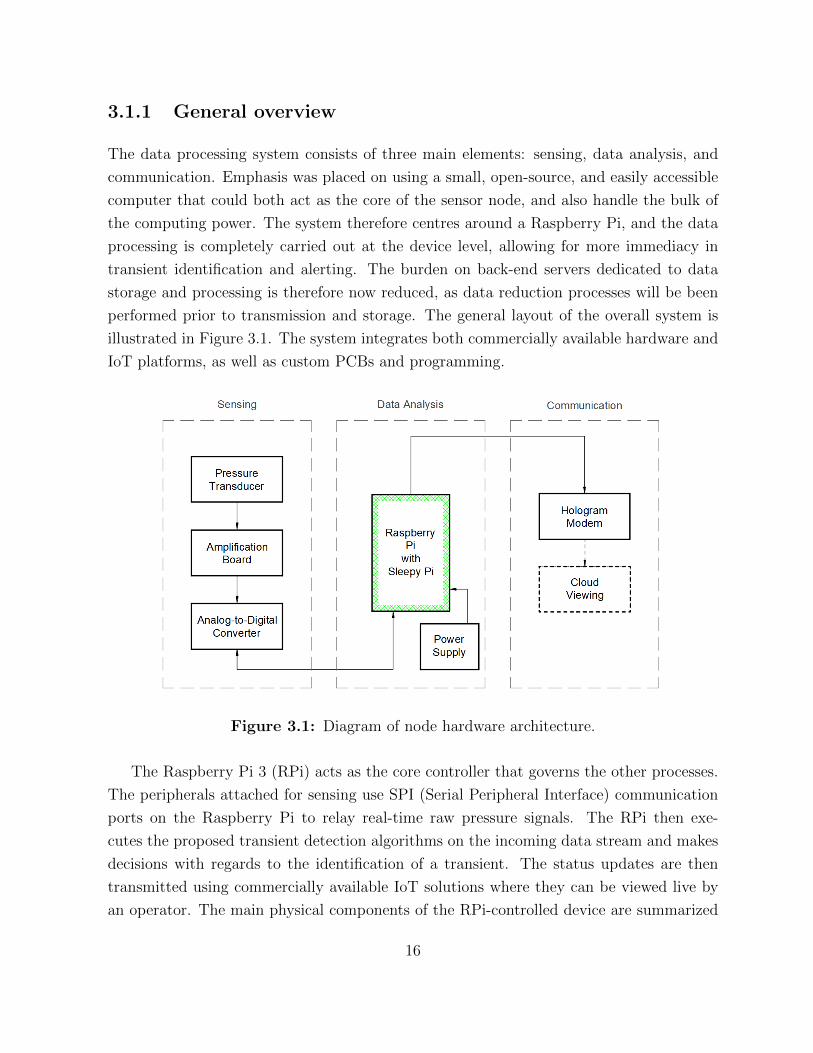
The data processing system consists of three main elements: sensing, data analysis, and

communication. Emphasis was placed on using a small, open-source, and easily accessible

computer that could both act as the core of the sensor node, and also handle the bulk of

the computing power. The system therefore centres around a Raspberry Pi, and the data

processing is completely carried out at the device level, allowing for more immediacy in

transient identification and alerting. The burden on back-end servers dedicated to data

storage and processing is therefore now reduced, as data reduction processes will be been

performed prior to transmission and storage. The general layout of the overall system is

illustrated in Figure 3.1. The system integrates both commercially available hardware and

IoT platforms, as well as custom PCBs and programming.

Figure 3.1: Diagram of node hardware architecture.

The Raspberry Pi 3 (RPi) acts as the core controller that governs the other processes.

The peripherals attached for sensing use SPI (Serial Peripheral Interface) communication

ports on the Raspberry Pi to relay real-time raw pressure signals. The RPi then exe-

cutes the proposed transient detection algorithms on the incoming data stream and makes

decisions with regards to the identification of a transient. The status updates are then

transmitted using commercially available IoT solutions where they can be viewed live by

an operator. The main physical components of the RPi-controlled device are summarized

16

in Table 3.1.

It is important that power requirements are minimized in order to facilitate long-term

field deployment. The whole system is powered by a rechargeable battery pack that does

not need frequent replacement under regular conditions. Furthermore, the RPi can also be

placed on a semi-continuous sampling schedule when the need for constant sensing is low.

The computer is fitted with a Sleepy Pi shield, an add-on board that can be programmed

using the Arduino IDE. The board makes use of a built-in RTC (real-time clock) that

controls power to the RPi according to user-programmed times set times. This conserves

energy by allowing the system to autonomously enter into sleep/low-power mode when not

in use.

Table 3.1: Main device hardware components

Component Brief Description

Raspberry Pi 3 Model B Single-board computer.

Sleepy Pi 2 Add-on board for power management.

Honeywell Model S Pressure Transducer Flush diaphragm pressure sensor.

MCP3302 ADC 13-bit, low power ADC.

Hologram Nova 2G/3G Modem Open source USB cellular modem.

Boston Power Swing 5300 Battery Pack 6 x 3.65 Volts.

3.1.2 Sensing

The primary component used for data sensing is the Honeywell Model S pressure trans-

ducer, a passive sensor whose data sheet can be found in Appendix A. The sensor is

constructed using a flush diaphragm, which minimizes buildup and bacterial growth, pro-

longing the service life as well as being sanitary for drinking water systems. The subminia-

ture size allows for its use in small pressure chambers or thin pipes where space is limited

or shared with other hardware.

There are two main sub-processes that occur in the device peripherals during sens-

ing: amplification and analog-to-digital conversion, both of which are needed in order to

17

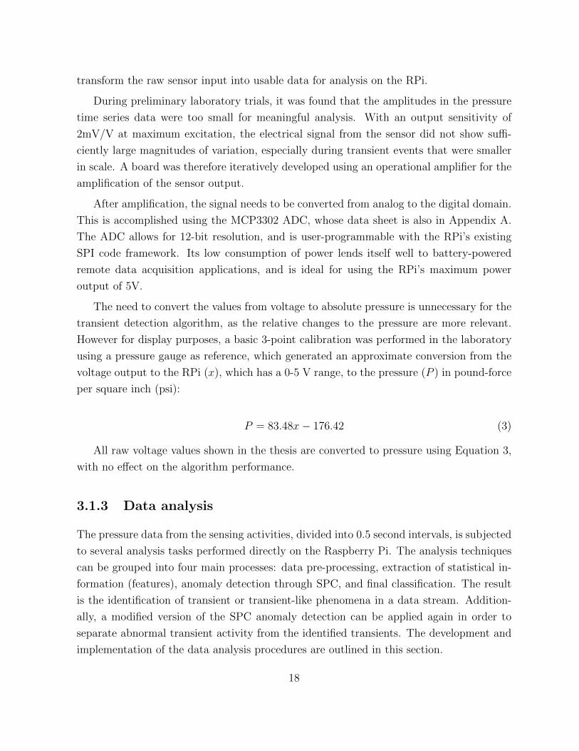
transform the raw sensor input into usable data for analysis on the RPi.

During preliminary laboratory trials, it was found that the amplitudes in the pressure

time series data were too small for meaningful analysis. With an output sensitivity of

2mV/V at maximum excitation, the electrical signal from the sensor did not show suffi-

ciently large magnitudes of variation, especially during transient events that were smaller

in scale. A board was therefore iteratively developed using an operational amplifier for the

amplification of the sensor output.

After amplification, the signal needs to be converted from analog to the digital domain.

This is accomplished using the MCP3302 ADC, whose data sheet is also in Appendix A.

The ADC allows for 12-bit resolution, and is user-programmable with the RPi’s existing

SPI code framework. Its low consumption of power lends itself well to battery-powered

remote data acquisition applications, and is ideal for using the RPi’s maximum power

output of 5V.

The need to convert the values from voltage to absolute pressure is unnecessary for the

transient detection algorithm, as the relative changes to the pressure are more relevant.

However for display purposes, a basic 3-point calibration was performed in the laboratory

using a pressure gauge as reference, which generated an approximate conversion from the

voltage output to the RPi (x), which has a 0-5 V range, to the pressure (P ) in pound-force

per square inch (psi):

P = 83.48x− 176.42 (3)

All raw voltage values shown in the thesis are converted to pressure using Equation 3,

with no effect on the algorithm performance.

3.1.3 Data analysis

The pressure data from the sensing activities, divided into 0.5 second intervals, is subjected

to several analysis tasks performed directly on the Raspberry Pi. The analysis techniques

can be grouped into four main processes: data pre-processing, extraction of statistical in-

formation (features), anomaly detection through SPC, and final classification. The result

is the identification of transient or transient-like phenomena in a data stream. Addition-

ally, a modified version of the SPC anomaly detection can be applied again in order to

separate abnormal transient activity from the identified transients. The development and

implementation of the data analysis procedures are outlined in this section.

18

3.1.3.1 Raw data and pre-processing

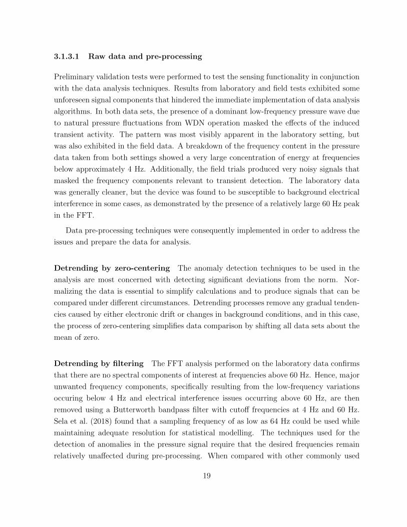
Preliminary validation tests were performed to test the sensing functionality in conjunction

with the data analysis techniques. Results from laboratory and field tests exhibited some

unforeseen signal components that hindered the immediate implementation of data analysis

algorithms. In both data sets, the presence of a dominant low-frequency pressure wave due

to natural pressure fluctuations from WDN operation masked the effects of the induced

transient activity. The pattern was most visibly apparent in the laboratory setting, but

was also exhibited in the field data. A breakdown of the frequency content in the pressure

data taken from both settings showed a very large concentration of energy at frequencies

below approximately 4 Hz. Additionally, the field trials produced very noisy signals that

masked the frequency components relevant to transient detection. The laboratory data

was generally cleaner, but the device was found to be susceptible to background electrical

interference in some cases, as demonstrated by the presence of a relatively large 60 Hz peak

in the FFT.

Data pre-processing techniques were consequently implemented in order to address the

issues and prepare the data for analysis.

Detrending by zero-centering The anomaly detection techniques to be used in the

analysis are most concerned with detecting significant deviations from the norm. Nor-

malizing the data is essential to simplify calculations and to produce signals that can be

compared under different circumstances. Detrending processes remove any gradual tenden-

cies caused by either electronic drift or changes in background conditions, and in this case,

the process of zero-centering simplifies data comparison by shifting all data sets about the

mean of zero.

Detrending by filtering The FFT analysis performed on the laboratory data confirms

that there are no spectral components of interest at frequencies above 60 Hz. Hence, major

unwanted frequency components, specifically resulting from the low-frequency variations

occuring below 4 Hz and electrical interference issues occurring above 60 Hz, are then

removed using a Butterworth bandpass filter with cutoff frequencies at 4 Hz and 60 Hz.

Sela et al. (2018) found that a sampling frequency of as low as 64 Hz could be used while

maintaining adequate resolution for statistical modelling. The techniques used for the

detection of anomalies in the pressure signal require that the desired frequencies remain

relatively unaffected during pre-processing. When compared with other commonly used

19

filter types, the Butterworth filter maximally flattens the frequency response within the

passband and rolls off to zero outside the stopbands, which maximizes the preservation of

the signal.

Due to the application of the upper stopband in the filter, the sampling frequency used

for sensing on the RPi was re-evaluated. Initially, a sampling frequency of 2048 Hz was

used in order to account for both high and low frequency components in the transient

analysis. However, since the validation trials have demonstrated fairly inconsequential

spectral components in the high-frequency ranges, the maximum frequency, or Nyquist

frequency, that is required from the signal is 64 Hz, which corresponds to a sampling rate

of 128 Hz on the RPi. The power requirements for the RPi are also reduced as a result of

this lower sampling rate.

3.1.3.2 Feature extraction and selection

A set of time series data is essentially composed of a set of values organized in time or-

der. Analysis of just the values in their original state can be inefficient and cumbersome,

therefore specific statistical information, or features, are extracted instead. Feature extrac-

tion acts as a dimensionality reduction technique, where the vector of features acts as a

summary description of the time series. A set of features should be non-redundant but

representative of the data, and can be used instead of the original data set during analysis.

The initial feature set consisted of various statistical properties commonly used for

anomaly detection in signals, as well as from existing leak detection literature such as

those presented by Gamboa-Medina et al. (2014). A subset of eleven features that show

sensitivity to transient events were chosen for use in the transient detection algorithm, and

are shown in Table 3.2. The list includes some common useful features as well as measures

of asymmetry, unpredictability, and energy. A feature vector containing all eleven values is

extracted for every half-second interval. Based on the validation time series, the selected

length of the time intervals (0.5 seconds) is sufficient for the capture of multiple cycles of

a transient wave, but short enough that the event is not diluted nor that most non-abrupt

fluctuations are misidentified.

The use and calculations for the listed features can be found in Appendix B. Some of

the features that were considered but ultimately removed from the final analyses include

the pulse factor, margin factor, and crest factor. The standard deviation could also be

omitted because the detrending and zero-centering of the data renders it fundamentally

20

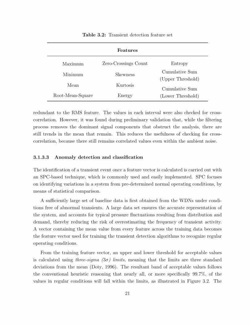
Table 3.2: Transient detection feature set

Features

Maximum Zero-Crossings Count Entropy

Minimum SkewnessCumulative Sum

(Upper Threshold)

Cumulative Sum

(Lower Threshold)

Mean Kurtosis

Root-Mean-Square Energy

redundant to the RMS feature. The values in each interval were also checked for cross-

correlation. However, it was found during preliminary validation that, while the filtering

process removes the dominant signal components that obstruct the analysis, there are

still trends in the mean that remain. This reduces the usefulness of checking for cross-

correlation, because there still remains correlated values even within the ambient noise.

3.1.3.3 Anomaly detection and classification

The identification of a transient event once a feature vector is calculated is carried out with

an SPC-based technique, which is commonly used and easily implemented. SPC focuses

on identifying variations in a system from pre-determined normal operating conditions, by

means of statistical comparison.

A sufficiently large set of baseline data is first obtained from the WDNs under condi-

tions free of abnormal transients. A large data set ensures the accurate representation of

the system, and accounts for typical pressure fluctuations resulting from distribution and

demand, thereby reducing the risk of overestimating the frequency of transient activity.

A vector containing the mean value from every feature across the training data becomes

the feature vector used for training the transient detection algorithms to recognize regular

operating conditions.

From the training feature vector, an upper and lower threshold for acceptable values

is calculated using three-sigma (3σ) limits, meaning that the limits are three standard

deviations from the mean (Doty, 1996). The resultant band of acceptable values follows

the conventional heuristic reasoning that nearly all, or more specifically 99.7%, of the

values in regular conditions will fall within the limits, as illustrated in Figure 3.2. The

21

rule is derived from properties of normally distributed data, but is still effective for use for

non-normal distributions. It can be assumed that most of the features will tend towards a

normal distribution because, regardless of the distribution of the original data, the Central

Limit Theorem states that statistical properties calculated from samples of a data set

should be normal. New data can now be compared against the thresholds to determine

whether or not an abnormal pressure change, or transient, has occurred.

Figure 3.2: Three-sigma thresholds illustrated on an example pressure time trace and on

a normal distribution.

The final classification of a pressure transient, or lack thereof, uses the ensemble of

features in a majority voting method, The number of features within each time interval

that exceed their respective three-sigma thresholds are counted, and the total number is

used to determine whether or not a transient had occurred within the interval. Combining

the decisions obtained by each feature comparison reduces the sensitivity of the overall

identification technique to misidentifications in individual features. Time intervals in which

a transient has occurred are expected to have more features that exceed the calculated

limits. Numerous exceedances in multiple successive time intervals is also indicative of a

genuine transient event.

3.1.3.4 Anomaly detection and classification for abnormal transient detection

A similar SPC process can be used specifically for identifying and assigning severity to

abnormal transients, especially those that can cause immediate harm to a WDN. In essence,

a two-tier SPC process is used, wherein the first tier separates the transient events from

22

ambient data, and the second tier separates abnormal transients from regular transient

activity resulting from general WDN use.

While ambient flow data is used to train the algorithm in the initial process, the second

tier uses the features themselves, taken from the time intervals identified in the first tier

as having experienced a pressure transient. The time intervals used in the analysis are

not separated out by feature vote threshold yet, and include all intervals in which any

number of features were triggered, with the exception of those that were determined to be

false positives. In doing so, it is assumed that the most pertinent regular transient types

are encompassed, including those induced specifically for the test, and subsequently that

statistically significant feature exceedances correspond to abnormal transients.

Not every feature will be deemed suitable for training purposes in SPC, with the primary

qualifier being the normality of their respective data sets. This is because part of the

purpose of the detection of abnormal transients is to alert WDN operators the occurrence

of pressure fluctuations that may require timely attention. Conservativeness in transient

identification is important in order to ensure that virtually no false alarms are triggered

by the system, in order to minimize wastage in time and resources. Therefore, it is more

efficient to use only the features that can classify transients with a high degree of accuracy,

and when using sigma methods in SPC it is most optimal to use normally or near-normally

distributed data.

While the Central Limit Theorem had established that features calculated from the data

would be normally distributed, this is no longer the case with the subset of the features

associated with the detected transients. This subset is effectively a truncated portion of

the parent normal distribution, and hence it is no longer inherently normally distributed.

Tests for normality on each of the transient feature subsets can be conducted by applying

probability paper plots, and the features that exhibit normality are selected for use in

identifying the abnormal transients. In some cases, a distribution may be transformed from

non-normal to normal using power transforms, most notably the Box-Cox one-parameter

transform (Box and Cox, 2018).

The resulting probability distributions of the features can be used to evaluate data

from the time intervals that have been identified as having transients, in order to obtain a

percentile value in which the data falls, for each feature. The average of these percentiles

can be used to assign a rank, or level of severity, to the detected transients. The severity

should be calibrated for different cases, but a theoretical example is summarized in Table

3.3.

23

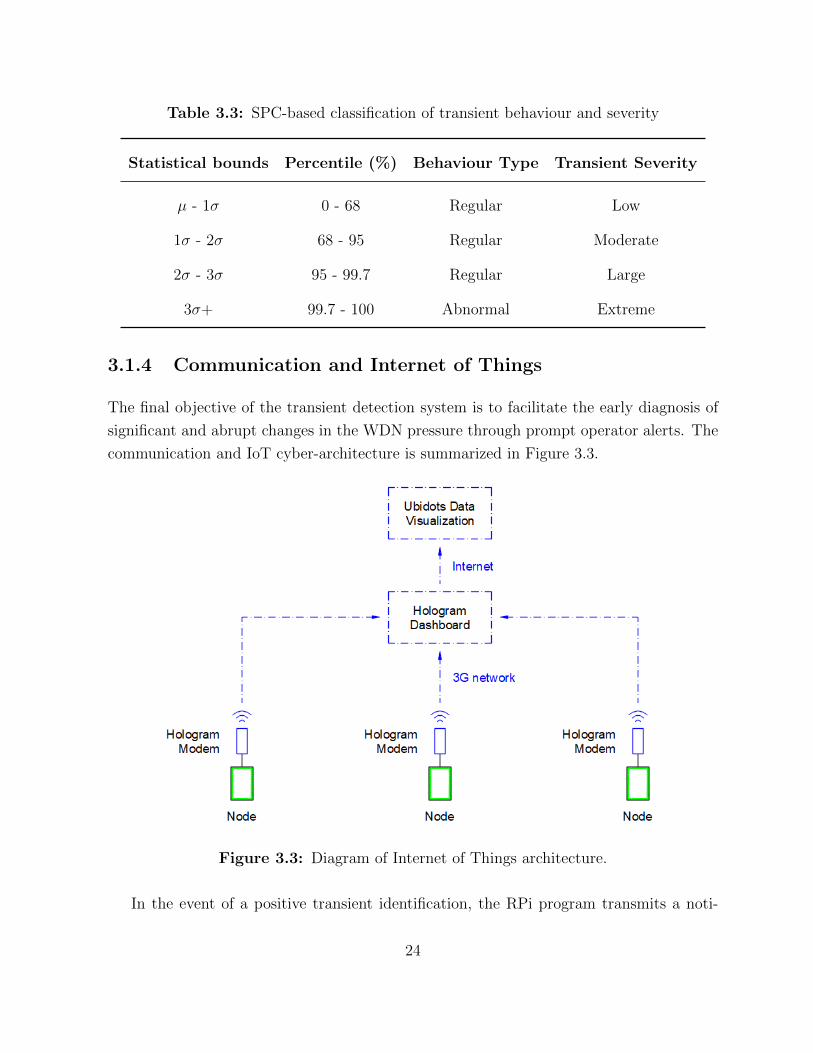
Table 3.3: SPC-based classification of transient behaviour and severity

Statistical bounds Percentile (%) Behaviour Type Transient Severity

µ - 1σ 0 - 68 Regular Low

1σ - 2σ 68 - 95 Regular Moderate

2σ - 3σ 95 - 99.7 Regular Large

3σ+ 99.7 - 100 Abnormal Extreme

3.1.4 Communication and Internet of Things

The final objective of the transient detection system is to facilitate the early diagnosis of

significant and abrupt changes in the WDN pressure through prompt operator alerts. The

communication and IoT cyber-architecture is summarized in Figure 3.3.

Figure 3.3: Diagram of Internet of Things architecture.

In the event of a positive transient identification, the RPi program transmits a noti-

24

fication to a cloud hosted by Hologram, an IoT development company. Transmission is

handled by the Hologram Nova, an open source cellular modem originally designed for the

Raspberry Pi operating system. The device operates off of the u-blox SARA-U201 modem

family, which enables the connection to the RPi via USB port and has a maximum data

rate of 480 Mb/s. Using a 2G/3G connection from an activated SIM card, SMS data

packets can be sent and viewed on the Hologram Dashboard. The messages can be tagged

according to subject, and organized by device.

The main purpose of the Hologram Dashboard is the management of the device sta-

tuses and transmissions. However, the visual display and organization of the data is not

yet supported. This is done instead on the Ubidots platform, which specializes in data

analytics and visualization for IoT frameworks. In order to reduce data transmission costs,

regular system updates are not being sent. The full data sets are stored locally on each

Raspberry Pi, though feature vectors can be sent in the event of a transient identifica-

tion. The platform is capable of transforming Hologram data packets that could contain

pressure values during transient events or otherwise, and display them graphically for the

visualization of the SPC control chart, including the thresholds. An example of the user

interface (UI) both Hologram and Ubidots is shown in Figure 3.4. Both platforms allow for

extensive user customization through their developer tools and provide APIs that easily

allow for their adaptation to the transient detection system.

Figure 3.4: Example of Internet of Things user interface: a) Hologram data packets, b)

Ubidots data visualizatio.n

25

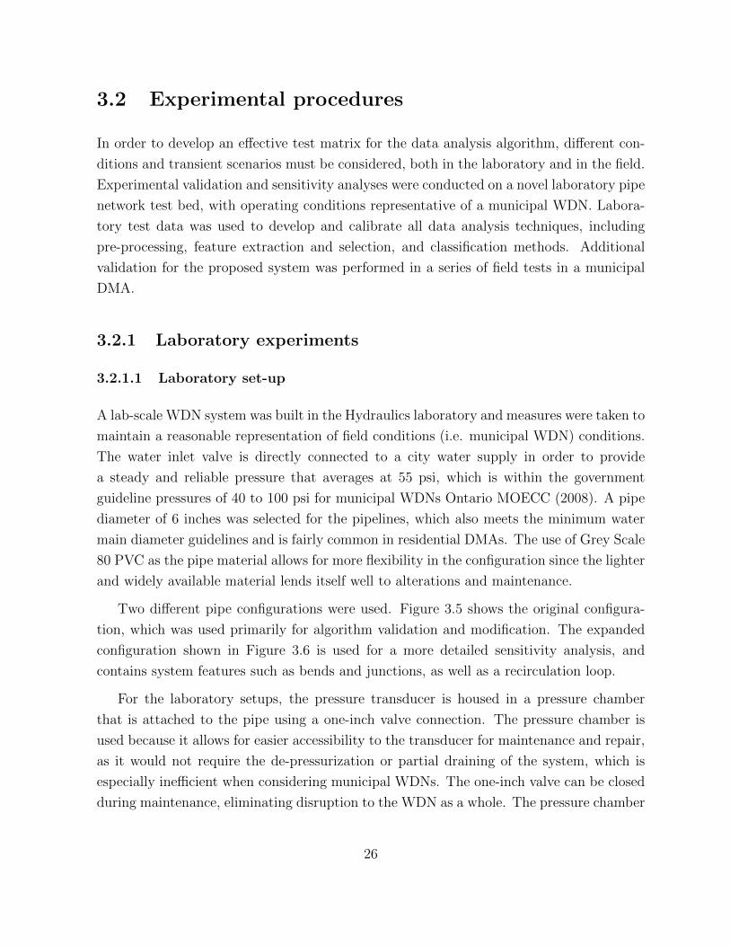
3.2 Experimental procedures

In order to develop an effective test matrix for the data analysis algorithm, different con-

ditions and transient scenarios must be considered, both in the laboratory and in the field.

Experimental validation and sensitivity analyses were conducted on a novel laboratory pipe

network test bed, with operating conditions representative of a municipal WDN. Labora-

tory test data was used to develop and calibrate all data analysis techniques, including

pre-processing, feature extraction and selection, and classification methods. Additional

validation for the proposed system was performed in a series of field tests in a municipal

DMA.

3.2.1 Laboratory experiments

3.2.1.1 Laboratory set-up

A lab-scale WDN system was built in the Hydraulics laboratory and measures were taken to

maintain a reasonable representation of field conditions (i.e. municipal WDN) conditions.

The water inlet valve is directly connected to a city water supply in order to provide

a steady and reliable pressure that averages at 55 psi, which is within the government

guideline pressures of 40 to 100 psi for municipal WDNs Ontario MOECC (2008). A pipe

diameter of 6 inches was selected for the pipelines, which also meets the minimum water

main diameter guidelines and is fairly common in residential DMAs. The use of Grey Scale

80 PVC as the pipe material allows for more flexibility in the configuration since the lighter

and widely available material lends itself well to alterations and maintenance.

Two different pipe configurations were used. Figure 3.5 shows the original configura-

tion, which was used primarily for algorithm validation and modification. The expanded

configuration shown in Figure 3.6 is used for a more detailed sensitivity analysis, and

contains system features such as bends and junctions, as well as a recirculation loop.

For the laboratory setups, the pressure transducer is housed in a pressure chamber

that is attached to the pipe using a one-inch valve connection. The pressure chamber is

used because it allows for easier accessibility to the transducer for maintenance and repair,

as it would not require the de-pressurization or partial draining of the system, which is

especially inefficient when considering municipal WDNs. The one-inch valve can be closed

during maintenance, eliminating disruption to the WDN as a whole. The pressure chamber

26

Figure 3.5: Perspective view of initial laboratory configuration.

Figure 3.6: Perspective view of expanded laboratory configuration.

hardware also includes housing for the RPi sensor device that is connected to the pressure

transducer. A diagram of the chamber is shown in Figure 3.7.

The WDN includes several quarter-inch (1/4”) valves at various locations that can

be used to simulate small leaks, as well as larger 1.5” outlet valves at pipe endings that

can simulate large leaks, water usage, or flow conditions. The transients themselves can

be induced using any of the valves, but in order to ensure an abrupt pressure change

27

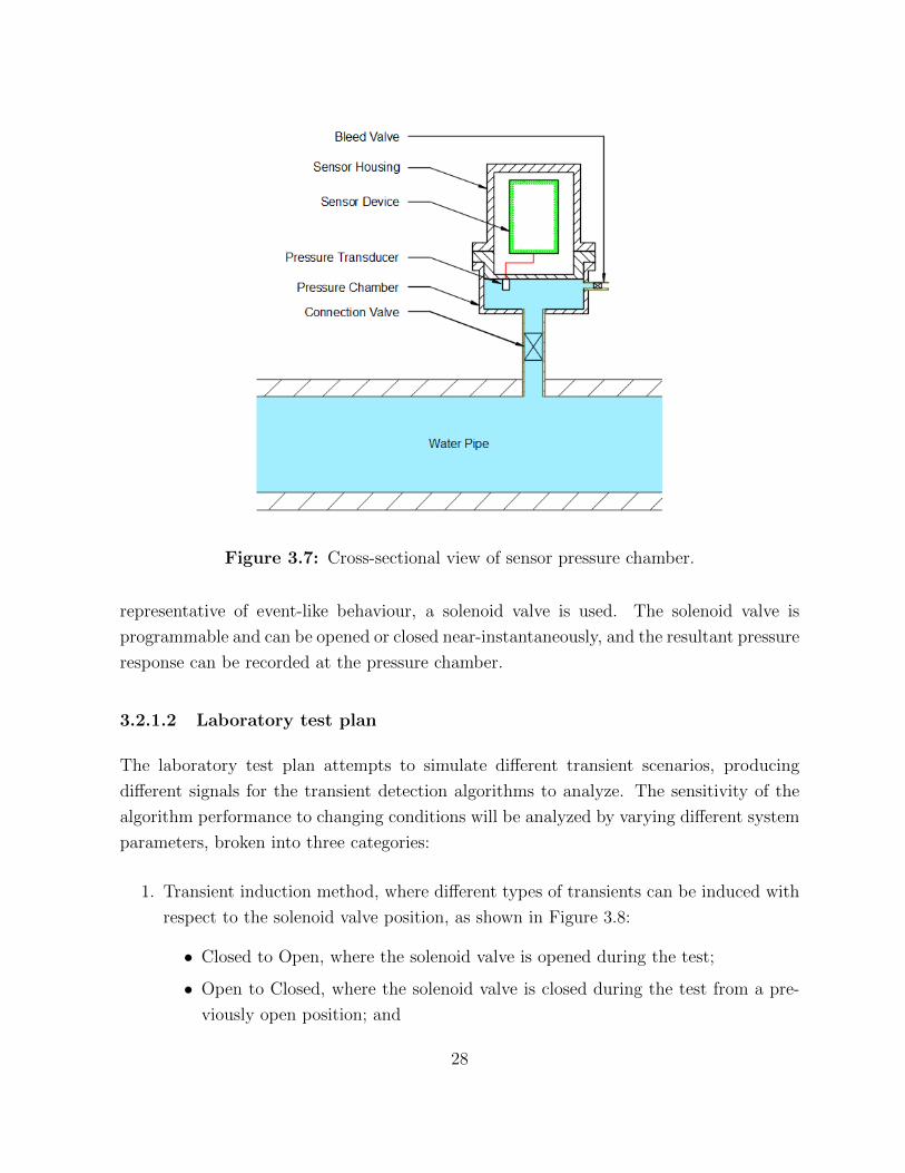
Figure 3.7: Cross-sectional view of sensor pressure chamber.

representative of event-like behaviour, a solenoid valve is used. The solenoid valve is

programmable and can be opened or closed near-instantaneously, and the resultant pressure

response can be recorded at the pressure chamber.

3.2.1.2 Laboratory test plan

The laboratory test plan attempts to simulate different transient scenarios, producing

different signals for the transient detection algorithms to analyze. The sensitivity of the

algorithm performance to changing conditions will be analyzed by varying different system

parameters, broken into three categories:

1. Transient induction method, where different types of transients can be induced with

respect to the solenoid valve position, as shown in Figure 3.8:

• Closed to Open, where the solenoid valve is opened during the test;

• Open to Closed, where the solenoid valve is closed during the test from a pre-

viously open position; and

28

• Pulse, where a quick closed-open-closed pattern is induced. A pulse, 50 ms in

duration, was selected during testing.

2. Flow conditions, which is split into two modes:

• No Flow, where the two 1.5” outlet valves are closed; and

• Flow, where the outlet valves are open.

3. Transient source location, which varies the proximity and number of connections be-

tween the transient source and the sensor by changing the solenoid valve’s placement

in the system. This is translated into the laboratory configuration as follows:

• Case 1, where the source and sensor are in line but separated by two junctions;

• Case 2: source and sensor are in line but separated by one junction;

• Case 3 where the source and sensor are separated by two junctions, where one

is a perpendicular connection

• Case 4, where the source and sensor are separated by two junctions, were both

are perpendicular connections

• Case 5, where the source and sensor are are separated by three junctions and

two directional changes.

Figure 3.8: Diagram of the solenoid valve state when inducing different transients: a)

Closed to Open, b) Open to Closed, c) Pulse.

Table 3.4 shows the overall test matrix used on the two different WDN configurations.

Multiple trials were performed for each test case.

29

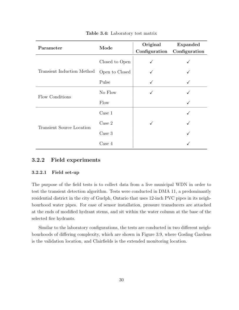
Table 3.4: Laboratory test matrix

Parameter ModeOriginal

Configuration

Expanded

Configuration

Transient Induction Method

Closed to Open X X

Open to Closed X X

Pulse X X

Flow ConditionsNo Flow X X

Flow X

Transient Source Location

Case 1 X

Case 2 X X

Case 3 X

Case 4 X

3.2.2 Field experiments

3.2.2.1 Field set-up

The purpose of the field tests is to collect data from a live municipal WDN in order to

test the transient detection algorithm. Tests were conducted in DMA 11, a predominantly

residential district in the city of Guelph, Ontario that uses 12-inch PVC pipes in its neigh-

bourhood water pipes. For ease of sensor installation, pressure transducers are attached

at the ends of modified hydrant stems, and sit within the water column at the base of the

selected fire hydrants.

Similar to the laboratory configurations, the tests are conducted in two different neigh-

bourhoods of differing complexity, which are shown in Figure 3.9, where Gosling Gardens

is the validation location, and Clairfields is the extended monitoring location.

30

Figure 3.9: Map of field test locations.

3.2.2.2 Field test plan

The Gosling Gardens location is used for algorithm validation, achieved by analyzing its

ability to detect known transients induced by flowing nearby hydrants during field tests.

The Clairfields location is used to evaluate the system performance in a more complex

neighbourhood and to draw conclusions about transient behaviour during regular use. The

background continuous monitoring conducted at Clairfields was carried out predominantly

in the early morning hours where general demand is reduced, in order for transient events

to be more apparent.

The variable parameters are similar to those of the laboratory, but some exceptions

31

are made due to limitations in the field setting. The main differences are highlighted as

follows:

1. For transient induction method, the quick pulses are difficult and possibly dangerous

to induce when flowing nearby hydrants, therefore only the controlled opening or

closing of a hydrant valve is considered.

2. For flow conditions, the water flow in the field water mains are dependent on general

use, are constantly changing, and impractical to control. The only flow setting,

therefore, will be the regular, or ’ambient’, conditions;

3. Transient source location no longer applies, and instead the focus is on sensor lo-

cation. Furthermore, the proximity of the sensors to transient sources, especially

in continuous background sampling, cannot be anticipated. The sensors are placed

throughout the neighbourhood to showcase different network features, including:

• Case 1, along a major road’s water main;

• Case 2, directly off of a looped residential road’s water main; or

• Case 3, at the end of a residential road’s water main.

The overall test plan for both locations is summarized in Table 3.5.

Table 3.5: Field test matrix

Parameter Mode Gosling Gardens Clairfields

Transient Induction MethodClosed to Open X

Open to Closed X

Sensor Location

Case 1 X X

Case 2 X

Case 3 X

Flow Conditions Ambient X X

32

Chapter 4

Results

The validation and sensitivity analysis for the proposed transient detection algorithm was

performed using the laboratory and field experiments described in the Methodology chap-

ter. The preliminary results for the abnormal transient identification process is also dis-

cussed and examined in the current chapter.

4.1 Laboratory results

The laboratory results section examines the findings from the original laboratory configu-

ration, used for validation, and the subsequently expanded configuration which was used

for a sensitivity analysis.

4.1.1 Validation - original laboratory configuration

4.1.1.1 Raw and pre-processed data

Data was collected in ten-second samples wherein a transient was induced via solenoid

valve by one of the three aforementioned methods. No other flow was generated during the

validation tests aside from through the solenoid valve itself. Figure 4.1 shows an example of

a raw data set, and one which has undergone the pre-processing detailed in Section 3.1.3.1,

taken from the original laboratory configuration in order to illustrate the effect of the first

data processing steps. The dominant low-frequency wave is apparent in the raw pressure

signal, as is the transient indicated shortly after three seconds have elapsed. The processed

33

data time series successfully removes the unwanted pressure fluctuations but retains the

effects of the transient.

Figure 4.1: Example pressure time series showing a transient occurrence in the original

laboratory configuration: a) raw data, b) pre-processed data.

Varying the transient induction method without flow and at a fixed location results in

slightly different behaviour in the resulting time series. Figure 4.2 compares the raw and

pre-processed data during the indicated transients. In the raw figures, the Closed to Open

case shows an initial drop in pressure and the Open to Closed an immediate rise at the

occurrence of a transient, which is intuitive given the drop or spike in pressure that occurs

when a valve is opened or closed, respectively. Both cases are followed by a short period of

transient-related signal oscillation, which is more apparent after pre-processing, before the

system returns to equilibrium. The Pulse case, which is effectively a rapid combination of

the previous two, shows a pronounced rapid oscillation in the signal following the transient.

Comparing the filtered signals, the behaviour and amplitude of the transient in the Open

to Closed case is similar to the Closed to Open case, while the Pulse case exhibits a more

prolonged oscillatory response and a slightly larger amplitude than the other two cases.

34

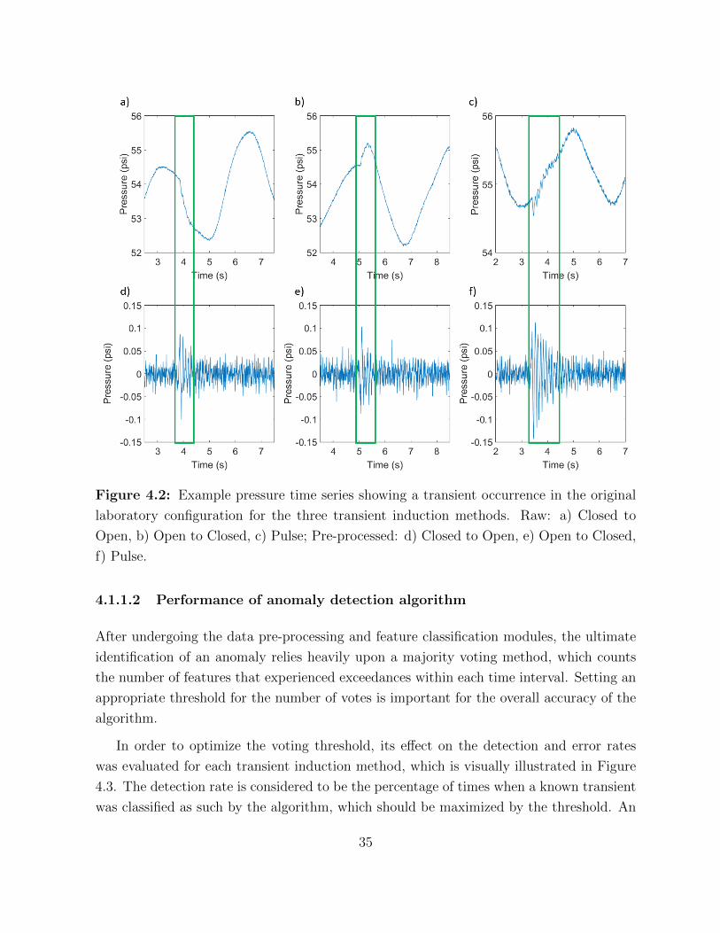
Figure 4.2: Example pressure time series showing a transient occurrence in the original

laboratory configuration for the three transient induction methods. Raw: a) Closed to

Open, b) Open to Closed, c) Pulse; Pre-processed: d) Closed to Open, e) Open to Closed,

f) Pulse.

4.1.1.2 Performance of anomaly detection algorithm

After undergoing the data pre-processing and feature classification modules, the ultimate

identification of an anomaly relies heavily upon a majority voting method, which counts

the number of features that experienced exceedances within each time interval. Setting an

appropriate threshold for the number of votes is important for the overall accuracy of the

algorithm.

In order to optimize the voting threshold, its effect on the detection and error rates

was evaluated for each transient induction method, which is visually illustrated in Figure

4.3. The detection rate is considered to be the percentage of times when a known transient

was classified as such by the algorithm, which should be maximized by the threshold. An

35

appropriate threshold would also aim to minimize the error rate, comprised predominantly

of false positives (or Type I errors), while maximizing the rate of successful transient

identifications. In this case, false positives refer to instances where a number of features

were triggered, but there was no expected or visually discernible transient. It’s important to

note that in some of these cases, there may in fact be a transient-like fluctuation in pressure.

However, the effect of these fluctuations is very small, especially when considering that the

size of the solenoid valve itself is very small compared to other potential transient sources

in a network.

Figure 4.3: Detection and error rates when using each feature vote threshold in the

original laboratory configuration for the three transient induction methods: a) Closed to

Open, b) Open to Closed, c) Pulse.

Based on the validation tests, the detection rate is most accurate when set below 6,

while the error rate is reduced when using thresholds above 3 or 4, although even the

36

highest error rate here can still maintain a confidence of 95%. The voting threshold can

be further analyzed using the test data from the expanded configuration, but the original

configuration tests show that the algorithm is successful identifying pressure transients with

a high degree of accuracy, while maintaining a low rate of errors due to false positives.

4.1.2 Sensitivity analysis - expanded laboratory configuration

With the added complexity provided by the expanded configuration, new elements were

discovered in the pressure signals that affected the algorithm performance. In some cases,

secondary transients, caused by reflections within the system, could be detected. The

occurrence of these smaller transients typically triggered fewer feature exceedances and

were not as visually discernible, as shown in Figure 4.4.

Figure 4.4: Example pressure time series showing different transient occurrences in the

expanded laboratory configuration with their corresponding feature vote.

Another element introduced by the expanded set-up is the occurrence of false negatives,

where the algorithm failed to identify a known event, typically resulting from transient

dissipation in the more complex network. The false negative can therefore be considered,

by definition, to be the complement of the detection rate. The false negatives (or Type II

errors) contribute to a slightly increased overall error rate across the thresholds.

Sensitivity analyses performed on the expanded laboratory configuration allow for a

more precise optimization of the voting threshold. The optimization of the voting threshold

would depend on the objective of a given study. For example, the threshold could be

set higher when attempting to predict pipe failure, where the only transients of interest

are large ones. Contrarily, the threshold may be set lower if the purpose is to assess

37

long-term pipe stress from water use and demand, in order to include smaller, frequently-

occurring transients. The assessment of algorithm performance can be further improved

with the consideration of additional test parameters such as the effect of flow conditions

and transient source location.

4.1.2.1 Transient induction method

Similar to tests done in the original configuration, three types of transients were induced

in order to represent different activities that would cause transients, and example pressure

time traces can be seen in Figure 4.5. Unlike in the original configuration, the behavioural

nuances and the differences in behaviour between the three methods could not be visually

discerned as easily, in either the raw or pre-processed data. However, the pressure spikes

resulting from the Pulse method were generally greater in amplitude than the other cases.

Figure 4.5: Example pressure time series showing a transient occurrence in the expanded

laboratory configuration for the three transient induction methods. Raw: a) Closed to

Open, b) Open to Closed, c) Pulse; Pre-processed: d) Closed to Open, e) Open to Closed,

f) Pulse.

38

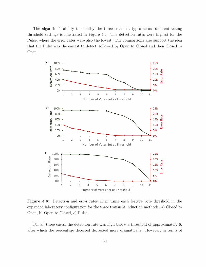
The algorithm’s ability to identify the three transient types across different voting

threshold settings is illustrated in Figure 4.6. The detection rates were highest for the

Pulse, where the error rates were also the lowest. The comparisons also support the idea

that the Pulse was the easiest to detect, followed by Open to Closed and then Closed to

Open.

Figure 4.6: Detection and error rates when using each feature vote threshold in the

expanded laboratory configuration for the three transient induction methods: a) Closed to

Open, b) Open to Closed, c) Pulse.

For all three cases, the detection rate was high below a threshold of approximately 6,

after which the percentage detected decreased more dramatically. However, in terms of

39

errors, a threshold above 7 was found to be ideal for minimizing the error rate. Given

these circumstances, the range for the optimal threshold would be rather narrow, but it

may be noted that even with the addition of the false negatives to the error, the highest

error rates still did not exceed 4%, indicating that the slightly lower thresholds may still

be ideal.

4.1.2.2 Flow conditions

The second parameter tested was flow conditions, where the presence of flow was added

by opening the two outlet valves in the system previously illustrated in Figure 3.6. The

addition of the Flow conditions also caused an overall decrease in network pressure of

approximately 35 psi compared to No Flow conditions. Figure 4.7 shows an example

of a raw and pre-processed time series with an induced transient for the two different

background condition cases. Generally, the non-transient parts of the signal for the Flow

case were noisier and exhibited a relatively higher energy. However, the reduced pressure

can also reduce the severity of the transients experienced by the system.

Figure 4.7: Example pressure time series showing a transient occurrence in the expanded

laboratory configuration for the two flow conditions. Raw: a) No Flow, b) Flow; Pre-

processed: c) No Flow, d) Flow.

40

The ability for the algorithm to detect transients within both scenarios is shown in

Figure 4.8. The added noise in the Flow case results in an approximately 10% drop

in detection rate across the thresholds. Additionally, the presence of flowing water also

greatly increased the likelihood of error because it added pressure phenomena that were

more easily misidentified as meaningful transients by the algorithm. The No Flow case

showed that a threshold below 6 would maximize its detection rate, and that virtually any

threshold at all would minimize the error rate. The Flow case was less forgiving in that

the detection rate is relatively low overall, however there is little loss in detection rate until

a threshold of 6, while the error can be kept below 5% above a threshold of 5.

Figure 4.8: Detection and error rates when using each feature vote threshold in the

expanded laboratory configuration for the two flow conditions: a) No Flow, b) Flow.

4.1.2.3 Transient source location

The last main parameter that was varied in the sensitivity analysis was the location of

the transient source, which in this case is the position of the solenoid valve. The effect of

distance and level of complexity between the sensor and the source can affect algorithm

performance. The complexity increased across the cases, with Case 1 being the simplest

and Case 4 being the most complex. For the purpose of the discussion, Solenoid 1 is

placed at the Case 1 location, Solenoid 2 at Case 2, and so forth. Each location has some

important factors to note which may affect transient propagation. Solenoids 1 and 4 are

positioned along straight sections of pipe and are relatively further from network features

such as junctions and dead ends, while Solenoids 2 and 3 are positioned in close proximity

to a junction and a dead end, respectively. Figure 4.9 shows example time traces from

the four chosen locations. From only these plots, the transient seen from Solenoid 1 had a

slightly larger amplitude than the others, while Solenoid 2 had the smallest.

41

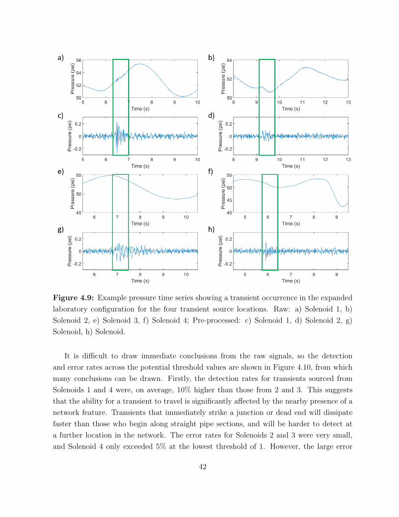
Figure 4.9: Example pressure time series showing a transient occurrence in the expanded

laboratory configuration for the four transient source locations. Raw: a) Solenoid 1, b)

Solenoid 2, e) Solenoid 3, f) Solenoid 4; Pre-processed: c) Solenoid 1, d) Solenoid 2, g)

Solenoid, h) Solenoid.

It is difficult to draw immediate conclusions from the raw signals, so the detection

and error rates across the potential threshold values are shown in Figure 4.10, from which

many conclusions can be drawn. Firstly, the detection rates for transients sourced from

Solenoids 1 and 4 were, on average, 10% higher than those from 2 and 3. This suggests

that the ability for a transient to travel is significantly affected by the nearby presence of a

network feature. Transients that immediately strike a junction or dead end will dissipate

faster than those who begin along straight pipe sections, and will be harder to detect at

a further location in the network. The error rates for Solenoids 2 and 3 were very small,

and Solenoid 4 only exceeded 5% at the lowest threshold of 1. However, the large error

42

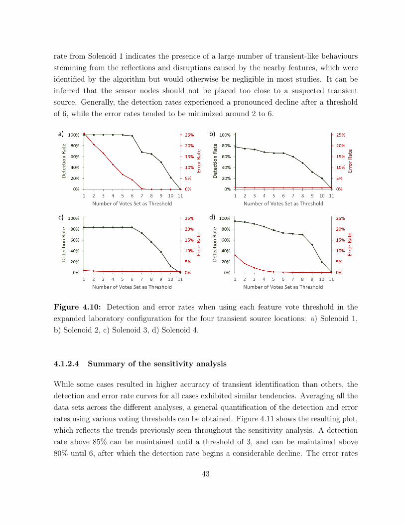
rate from Solenoid 1 indicates the presence of a large number of transient-like behaviours

stemming from the reflections and disruptions caused by the nearby features, which were

identified by the algorithm but would otherwise be negligible in most studies. It can be

inferred that the sensor nodes should not be placed too close to a suspected transient

source. Generally, the detection rates experienced a pronounced decline after a threshold

of 6, while the error rates tended to be minimized around 2 to 6.

Figure 4.10: Detection and error rates when using each feature vote threshold in the

expanded laboratory configuration for the four transient source locations: a) Solenoid 1,

b) Solenoid 2, c) Solenoid 3, d) Solenoid 4.

4.1.2.4 Summary of the sensitivity analysis

While some cases resulted in higher accuracy of transient identification than others, the

detection and error rate curves for all cases exhibited similar tendencies. Averaging all the

data sets across the different analyses, a general quantification of the detection and error

rates using various voting thresholds can be obtained. Figure 4.11 shows the resulting plot,

which reflects the trends previously seen throughout the sensitivity analysis. A detection

rate above 85% can be maintained until a threshold of 3, and can be maintained above

80% until 6, after which the detection rate begins a considerable decline. The error rates

43

are consistently low, never over 10%. A voting threshold above 3 can be used to achieve a

rate below 5%, while choosing a threshold above 6 will reduce that to near 1% while still

maintaining a reasonable detection rate.

Figure 4.11: Overall detection and error rates by feature vote threshold.

When considering field implementation, the purpose of the monitoring would help to

determine the optimal voting threshold to use, but based on the laboratory tests the ideal

range is between 3 and 7, depending on whether or not less severe transients are deemed

important for inclusion in the given test.

The results from the analysis can be used to derive probability distributions based on

the thresholds, as shown in Figures 4.12 and 4.13. This way of representing data can

be used to further investigate the effect of the individual threshold levels in identifying

pressure transients. Figure 4.12 therefore reveals that 9 features were triggered in nearly

30% of the identified transients, and that using a thresholds above 7 would account for

77% of the identified transients.

If the aim is to minimize false alarms, perhaps it is more appropriate to look at the

breakdown of the error rates. Similar to the detection rates, thresholds between 8 and 10

were the safest to use when assessing the likelihood that a real transient has occurred. In

fact, based on the laboratory data, if the system has identified a transient in which 8 to 10

features were triggered, there is a 0% chance that the identification was an error. That is,

it is definitive that a transient occurred, that it is very likely that that transient resulted

in a significant pressure change.

44

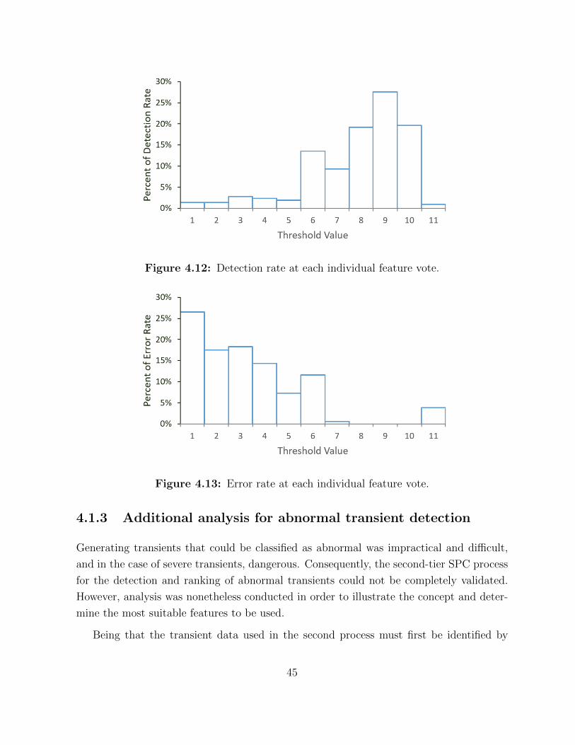
Figure 4.12: Detection rate at each individual feature vote.

Figure 4.13: Error rate at each individual feature vote.

4.1.3 Additional analysis for abnormal transient detection

Generating transients that could be classified as abnormal was impractical and difficult,

and in the case of severe transients, dangerous. Consequently, the second-tier SPC process

for the detection and ranking of abnormal transients could not be completely validated.

However, analysis was nonetheless conducted in order to illustrate the concept and deter-

mine the most suitable features to be used.

Being that the transient data used in the second process must first be identified by

45

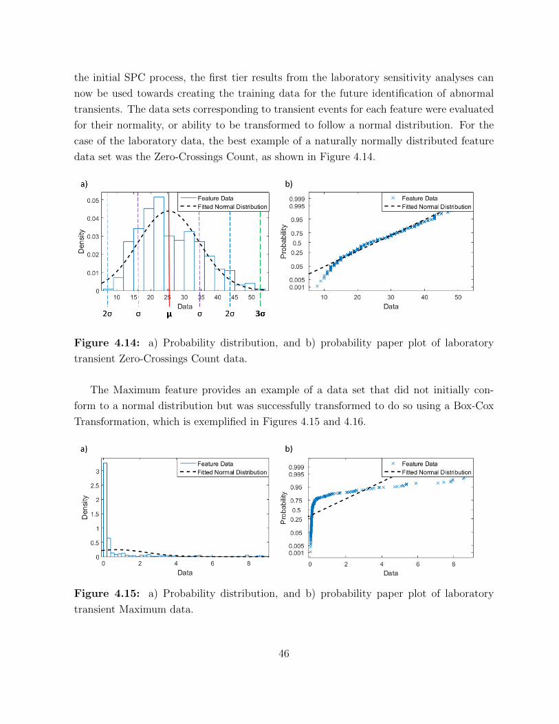
the initial SPC process, the first tier results from the laboratory sensitivity analyses can

now be used towards creating the training data for the future identification of abnormal

transients. The data sets corresponding to transient events for each feature were evaluated

for their normality, or ability to be transformed to follow a normal distribution. For the

case of the laboratory data, the best example of a naturally normally distributed feature

data set was the Zero-Crossings Count, as shown in Figure 4.14.

Figure 4.14: a) Probability distribution, and b) probability paper plot of laboratory

transient Zero-Crossings Count data.

The Maximum feature provides an example of a data set that did not initially con-

form to a normal distribution but was successfully transformed to do so using a Box-Cox

Transformation, which is exemplified in Figures 4.15 and 4.16.

Figure 4.15: a) Probability distribution, and b) probability paper plot of laboratory

transient Maximum data.

46

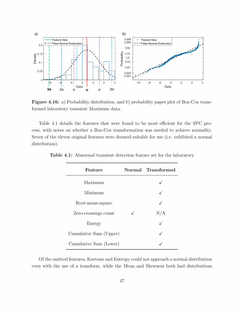
Figure 4.16: a) Probability distribution, and b) probability paper plot of Box-Cox trans-

formed laboratory transient Maximum data.

Table 4.1 details the features that were found to be most efficient for the SPC pro-

cess, with notes on whether a Box-Cox transformation was needed to achieve normality.

Seven of the eleven original features were deemed suitable for use (i.e. exhibited a normal

distribution).

Table 4.1: Abnormal transient detection feature set for the laboratory

Feature Normal Transformed

Maximum X

Minimum X

Root-mean-square X

Zero-crossings count X N/A

Energy X

Cumulative Sum (Upper) X

Cumulative Sum (Lower) X

Of the omitted features, Kurtosis and Entropy could not approach a normal distribution

even with the use of a transform, while the Mean and Skewness both had distributions

47

that resembled normal but their variances were too small and large, respectively, which

affected their uniformity when using probability paper plots for confirmation.

Despite the lack of abnormal transient data with which the method can be validated,

the distributions generated using the sensitivity analysis can allow for the deduction of

some results. There was no significant number (i.e. less than 0.3%) of transients that

exceeded the three-sigma bounds of any of the pertinent features, as would be expected

because no high-risk transients were experienced during testing. Hence, it is reasonable to

assume that any transient exhibiting feature values outside of these three sigma thresholds

can be considered abnormal and potentially dangerous.

4.2 Field results

The primary purpose of the field trials is to assess the applicability of the algorithm to

real-life situations. The results of the assessment is summarized in the following section.

4.2.1 Validation - Gosling Gardens

The Gosling Gardens field setup is a simple setup consisting of a linear water main following

a more major residential road, as shown in Figure 4.17.

Figure 4.17: Map of Gosling Gardens test location.

48

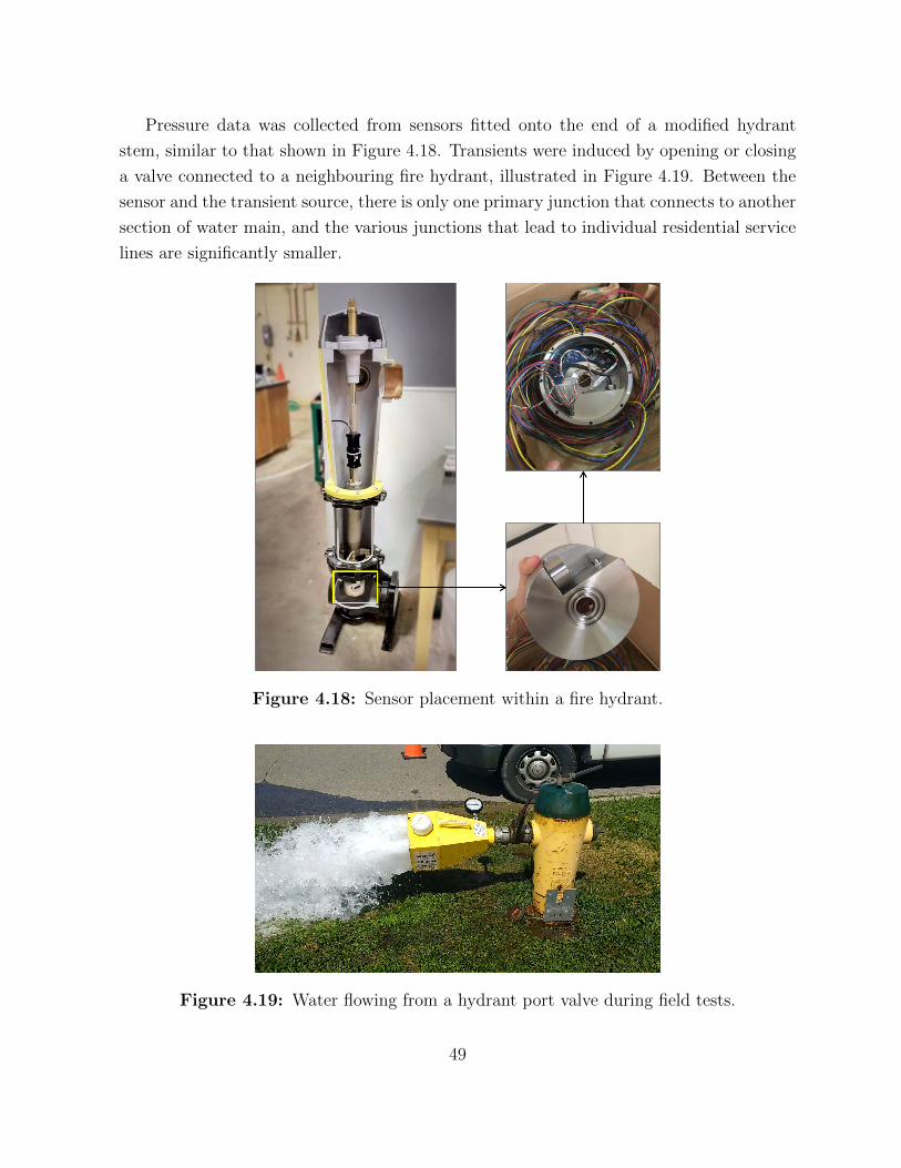
Pressure data was collected from sensors fitted onto the end of a modified hydrant

stem, similar to that shown in Figure 4.18. Transients were induced by opening or closing

a valve connected to a neighbouring fire hydrant, illustrated in Figure 4.19. Between the

sensor and the transient source, there is only one primary junction that connects to another

section of water main, and the various junctions that lead to individual residential service

lines are significantly smaller.

Figure 4.18: Sensor placement within a fire hydrant.

Figure 4.19: Water flowing from a hydrant port valve during field tests.

49

Figure 4.20 shows an example of the pressure signal from a flow test, consisting of five

minutes of data, in which three transients were induced. The first transient resulted from

initial tests with the valve, the second resulted from the valve opening and the last from the

valve closing. The algorithm successfully identified all three instances, as well as a number

of smaller transient occurrences. In this particular case, setting a threshold of 4 would

allow for the identification of all the induced transients while ignoring the smaller events.

Setting a threshold of 3 would account for all phenomena picked up by the algorithm.

Figure 4.20: Example pressure time series showing transient occurrences in the Gosling

Gardens field location: a) raw data, b) pre-processed data.

The algorithm has been shown to have the capacity to correctly identify transient events

in a real municipal WDN, while demonstrating the need to calibrate the threshold to be

more appropriate for different needs.

4.2.2 Detailed analysis - Clairfields

The Clairfields location included four sensor locations placed in a neighbourhood with a

more complex layout, which is analogous to the expanded setup in the laboratory. The

50

locations are illustrated in Figure 4.21. The four locations were chosen to represent vari-

ous features within a WDN, in order to study how pressure transients might affect them

differently. It is important to note that, since fire hydrants are typically connected to a

water main by individual valved pipes, all the sensors are technically placed at dead ends.

Flow tests were not conducted, and the focus was instead placed on deploying the system

to conduct continuous background monitoring.

Figure 4.21: Map of Clairfields test location.

The results to be displayed were taken from a time period between 2:00 a.m. and

8:00 a.m., averaged from data aggregated during the second week of November, 2018. The

examination of early morning data helps to reduce the effect of pressure fluctuations caused

by external factors and network noise, in turn helping to achieve a more accurate transient

count. Based on validation tests, two thresholds, 3 and 7, were chosen for comparison as

they had both been shown to be optimal for different monitoring objectives.

4.2.2.1 Location 1 - 38 Keys

The first sensor location is an example of a Case 2 placement type, since it is located near

a gentle bend along a water main following a relatively small road, and otherwise far from

prominent network features. Figure 4.22 shows, for each half-hour increment during the

time of study, the rate at which the transients were being identified per minute.

Based on the results, there was relatively little activity throughout the test period,

51

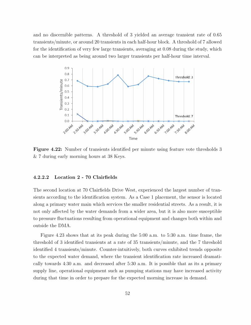
and no discernible patterns. A threshold of 3 yielded an average transient rate of 0.65

transients/minute, or around 20 transients in each half-hour block. A threshold of 7 allowed

for the identification of very few large transients, averaging at 0.08 during the study, which

can be interpreted as being around two larger transients per half-hour time interval.

Figure 4.22: Number of transients identified per minute using feature vote thresholds 3

& 7 during early morning hours at 38 Keys.

4.2.2.2 Location 2 - 70 Clairfields

The second location at 70 Clairfields Drive West, experienced the largest number of tran-

sients according to the identification system. As a Case 1 placement, the sensor is located

along a primary water main which services the smaller residential streets. As a result, it is

not only affected by the water demands from a wider area, but it is also more susceptible

to pressure fluctuations resulting from operational equipment and changes both within and

outside the DMA.

Figure 4.23 shows that at its peak during the 5:00 a.m. to 5:30 a.m. time frame, the

threshold of 3 identified transients at a rate of 35 transients/minute, and the 7 threshold

identified 4 transients/minute. Counter-intuitively, both curves exhibited trends opposite

to the expected water demand, where the transient identification rate increased dramati-

cally towards 4:30 a.m. and decreased after 5:30 a.m. It is possible that as its a primary

supply line, operational equipment such as pumping stations may have increased activity

during that time in order to prepare for the expected morning increase in demand.

52

Figure 4.23: Number of transients identified per minute using feature vote thresholds 3

& 7 during early morning hours at 70 Clairfields.

4.2.2.3 Location 3 - 10 Murphy

Location 3, at 10 Murphy Court, also experienced a substantially higher rate of transients,

though it was less than the frequency in Location 2. Unlike the 70 Clairfields location,

the trends in the morning transient activity mirrored the expected water demand for the

morning time period, as seen in Figure 4.24.

Figure 4.24: Number of transients identified per minute using feature vote thresholds 3

& 7 during early morning hours at 10 Murphy.

53

Located at the very end of the court, which is a Case 3 placement type, the sensor

location might have experienced elevated transient activity due to the transient reflec-

tions occurring in its vicinity. Figure 4.24 shows that the threshold of 3 resulted in rates

between 3 to 24 transients/minute, while the threshold of 7 reflected approximately one

transient/minute. Both curves showed a marked decline in transient-inducing activity

towards 4:00 a.m., increasing again between 6:30 to 8:00 a.m.

4.2.2.4 Location 4 - 30 Paulstown

The last location is at 30 Paulstown Crescent and experienced similar transient behaviour

to the first location, which also has a Case 2 placement on a crescent. For both Location 1

and 4, it is possible that their location away from WDN junctions and dead ends caused the

sensors to detect transients that would have mostly dissipated before reaching the hydrant

location. Furthermore, the sensors are both placed relatively far from the major road’s

water main, limiting their nearby transient sources to purely residential use.

Figure 4.25 shows that there wasn’t a dramatic trend in transient identification using

either threshold, although a very slight increase can be seen towards the 4:00 to 4:30 a.m.

time interval. Using a voting threshold of 3 resulted in an average of one transient identified

per minute, and using 7 was about half that.

Figure 4.25: Number of transients identified per minute using feature vote thresholds 3

& 7 during early morning hours at 30 Paulstown.

54

4.2.3 Field application of abnormal transient detection algorithm

The second-tier SPC process was applied to the Clairfields field data. Following the same

methodology used for the laboratory data, the analysis began by building feature probabil-

ity distributions from a training set containing all transients identified with any threshold

above zero. The resulting feature probability distributions varied by location. With the

exception of the 38 Keys location, which experienced far fewer transient events, the ma-

jority of the feature probability distributions from the remaining locations were found to

be normally distributed. This result was contradictory to the skewed distributions of the

laboratory feature set. The differences in the resulting probability distributions can be

attributed to the different constitutions of the training sets. In the laboratory, the training

data consisted solely of induced transient events, which are representative of a class of more

severe transients, whereas in the field, the training data contains transients and pressure

fluctuations of all natures, resulting in a more normally distributed transient training set.

While the probability distributions obtained from the initial field training data are

still valid for the second-tier SPC analysis, the conservativeness can be first increased by

removing transients below a certain threshold from the training data prior to distribution

fitting. Based on the results from the laboratory sensitivity analysis, a threshold of 3 was

applied to the training data as a means to remove the less severe transients, while still

allowing for enough variance in the distribution. Figure 4.26 shows the evolution of the

distribution and probability paper plots for the Maximum, using data collected from 10

Murphy.

The thresholded data reduced the span of the original distribution, and resulted in

a left-skewed distribution that did not completely follow a normal distribution, which is

similar to the behaviour previously seen in the laboratory. Applying the Box-Cox transform

then subsequently returned the distribution to normal. An analysis of each feature for each

location was performed, and the most optimal feature sets are summarized in Table 4.2.

Comparing the feature set derived from the different field locations and from the labo-

ratory set in Figure 4.1, it is clear that the features perform differently in different circum-

stances, and that training data unique to each location should be used when developing

the training set to be used for the second-tier SPC analysis. Some notable changes are

illustrated in Figures 4.27 and 4.28.

The laboratory data had found that RMS was amongst the more ideal features to be

used for analysis. However, Figure 4.27 shows that even after using a Box-Cox transform,

55

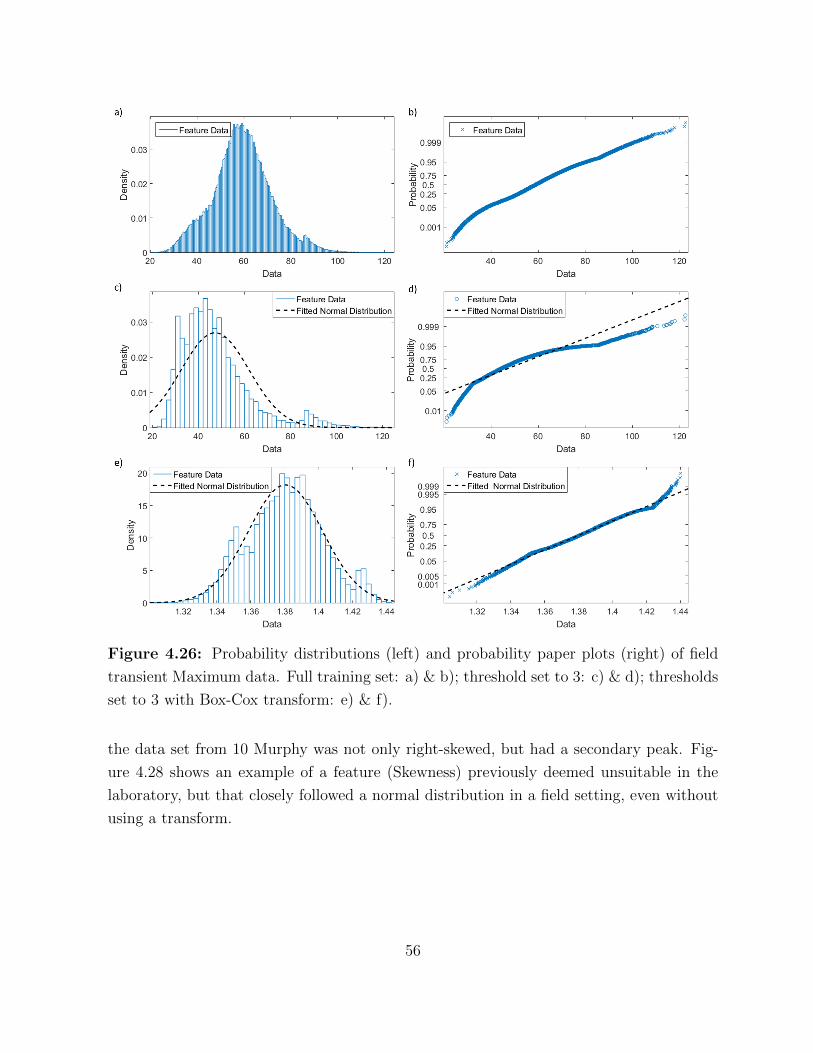
Figure 4.26: Probability distributions (left) and probability paper plots (right) of field

transient Maximum data. Full training set: a) & b); threshold set to 3: c) & d); thresholds

set to 3 with Box-Cox transform: e) & f).

the data set from 10 Murphy was not only right-skewed, but had a secondary peak. Fig-

ure 4.28 shows an example of a feature (Skewness) previously deemed unsuitable in the

laboratory, but that closely followed a normal distribution in a field setting, even without

using a transform.

56

Table 4.2: Abnormal transient detection feature set for the field locations

Feature 38 Keys 70 Clairfields 10 Murphy 30 Paulstown

Maximum X X X

Minimum X X

Mean X

Root-Mean-Square X X

Zero-crossings count X X X X

Skewness X X

Kurtosis X X X

Energy X X

Entropy X X X

Cumulative Sum (Upper) X X X

Cumulative Sum (Lower) X X

Figure 4.27: a) Probability distribution, and b) probability paper plot of Box-Cox trans-

formed field transient RMS data from 10 Murphy.

57

Figure 4.28: a) Probability distribution, and b) probability paper plot of field transient

Skewness data from 10 Murphy.

4.3 Summary

The results of the laboratory and field tests were important for algorithm adjustment and

drawing conclusions about transient behaviour in ideal and non-ideal WDNs.

Different factors contributing to algorithm performance were assessed in the laboratory,

with favourable results. The pre-processing steps were shown to successfully and effectively

remove unwanted signal components while retaining and emphasizing the occurrences of

pressure transients. The chosen features were powerful when used in combination to iden-

tify transient activity in the system, and a voting range between 3 and 7 was determined

as being optimal for the final classification step.

A higher threshold is recommended for conservative monitoring studies, where the

risk for error is lower and the goal is to identify only pressure transients that may cause

immediate damage to the system. Contrarily, a lower threshold would be used in order to

achieve the highest possible detection rate, though it also results in a higher error rate.

When monitoring for general pipe stress due to pressure, this would allow for more transient

types to be encompassed in the study, including less severe or less abrupt fluctuations.

Using the system to detect known transients in a real municipal WDN, the behaviour

of the pressure signals were found to be similar to the more complex laboratory cases. The

algorithm was shown to be adaptable for large-scale studies under non-ideal conditions. A

short-term monitoring program involving a week-long sensor deployment in various loca-

tions in a municipal DMA allowed for preliminary conclusions to be drawn about the effects

of pressure changes in different areas in a WDN. As expected, very few large transients

were detected in all locations, and some diurnal patterns could be seen in the frequency of

58

occurrence for transients in general.

A thorough validation for the abnormal transient identification process could not be

feasibly conducted, but the laboratory results showed that the SPC-based method, trained

with features from transients identified in the initial process, could be used to build prob-

ability distributions that lend themselves well to a sigma-based risk assessment. Further

application on the field data showed that the features most suitable for the analysis varied

between the different cases.

Both the laboratory and field tests showed that the algorithm can be used to illuminate

the behaviours of pressure transients in municipal WDNs.

59

Chapter 5

Conclusions and Recommendations

5.1 Conclusions

The purpose of the research was to develop a framework that could quantify the behaviour

of pressure transients in municipal WDNs and develop criteria to distinguish between nor-

mal and abnormal transients. Using different data analysis and IoT tools, the system can

be used for real-time monitoring, maintenance scheduling, and long-term asset manage-

ment decision making. The development of the proposed framework has achieved most of

the objectives, and several conclusions can be drawn from the investigations undertaken

in the laboratory and field settings.

Performance of algorithm The algorithm used for the data analysis, composed of

multiple steps, was proven to successfully detect transients in both the field and laboratory

settings. The data filtering was essential for rendering the data suitable for later analysis,

and also for comparing data from different sets and conditions. Despite its simplicity,

the SPC method was powerful for both the detection of transients, and also the potential

identification of abnormal transients subsequently. The selected features were shown to

note only perform well individually, but even more effectively when combined in a voting

method for the final classification. It was found that the optimal feature vote threshold

varied based on the purpose of a particular study, but that in the majority of cases, a

threshold could be found that could maintain the error rate below 5% and the detection

rate above 80%, with many cases performing even better. The methods used did not

require extensive processing power and were easily implemented on the Raspberry Pi.

60

Additional conclusions can be drawn concerning the sensitivity of the algorithm to

the effects of different conditions affecting transient propagation in a pipe. Firstly, the

presence of active flow in the pipes was found to decrease the detection rate and increase

the probability of error. Next, transients induced from locations farther from the sensor

had a reduced chance of detection and increased the rate of false negatives in the tests.

However, transients from locations too close to the sensor also increased the overall error,

but instead affected the false positive rate. It was found that the proximity of a transient

source to a pipe feature had a greater effect on transient propagation than the distance

from a sensor. Both in the laboratory and field settings, the presence of junctions, bends,

and dead-ends could either dramatically amplify or dampen the pressure wave signals. In

terms of the types of transients experience in a system, pulse-type valve behaviour created

stronger transients. Transients created with the abrupt opening of a valve were the most

difficult to detect, followed by transients induced with the closing of a valve. It can be

deduced that on a small scale, transients resulting from pressure surges are easier to detect

and propagate farther and than transients resulting from pressure drops.

The methodology used for abnormal transient detection proved capable of accurately

illustrating the behaviour of the transients through individual feature performance. The re-

sulting probability distributions provide a reflection of transient properties, and are further

useful when separating typical events from those worth investigating. The resulting distri-

butions for the second-tier analysis varied by location, which indicates that case-by-case

analysis should be performed in order to determine the optimal feature set.

Overall Framework Performance It was successfully proven that the use of the Rasp-

berry Pi as the control unit for the sensor nodes is a viable solution for node-level data

collection and processing. Open-source IoT solutions were integrated into the system with

ease and effectively allowed data to be transmitted using the Hologram modem, and vi-

sualized using the Ubidots platform. The node-level processing allowed for smaller data

transmission costs by reducing the raw data to only the most pertinent information. The

system proved its capability for real-time monitoring, its usefulness for remote event de-

tection, and value for WDN maintenance planning.

61

5.2 Recommendations for future work

The framework outlined in the thesis proved its effectiveness for use in transient detection.

However, there are a number of areas that can be improved, as well as studies that can

further add to the understanding of pressure transient behaviour and detection in WDNs.

The effect of transient source location was studied, but before large-scale node deploy-

ment, additional testing is needed in order to optimize the sensor placement. Studies should

be conducted to find the average distance away from a source that an individual node can

detect a transient from, to optimize sensor spacing. For both the field and laboratory,

the sensors were fixed near dead-ends for practicality purposes. However, an analysis that

varies sensor location, instead of transient source location, could be valuable for improving

the quality of data that is used for both training and analysis.

For the algorithm, the three-sigma threshold was used across all the features during

the SPC processing when identifying transients from ambient data. However, a feature-

specific sensitivity analysis should be conducted in order to improve the performance of

each feature and reduce the false negatives incurred by the current system.

The usefulness of the two-tier SPC process for abnormal transient identification has

been shown, but more tests are needed to validate and improve the process. Also, an

exploration of methods that can be used to confirm identified transients should also be

undertaken. For example, the identification of a transient across multiple consecutive time

intervals can be used as an indication of a correct transient identification. Additionally,

the proper calibration and tracking of the true pressure in the network would allow the

node to assign an accurate magnitude to each pressure change, which can factor into the

estimate of the risk that the transient poses.

More field testing is needed to better adapt the system for long-term real-world usage.

Ideally, tests similar to those done in the laboratory should be conducted in the field, or

at the very least, tests that include inducing different transients to a field WDN should

be undertaken in order to evaluate the algorithm’s performance on known transients in a

non-ideal setting. The addition of multiple sensors on a larger scale can also pave the way

for an additional level of analysis that can correlate data from different nodes and draw

conclusions based on multiple data streams.

The research summarized in the thesis can serve as an effective basis for the development

of transient detection system that can be implemented widely in municipal WDNs and

provide accurate, continuous, and real-time analyses of pressure behaviour.

62

References

Bakker, M., Jung, D., Vreeburg, J., Van De Roer, M., Lansey, K., and Rietveld, L. (2014).

Detecting pipe bursts using Heuristic and CUSUM methods. Procedia Engineering,

70:85–92.

Bergant, A., Tijsseling, A. S., Vıtkovsky, J. P., Covas, D. I., Simpson, A. R., and Lambert,

M. F. (2008). Parameters affecting water-hammer wave attenuation, shape and timing

- Part 2: Case studies. Journal of Hydraulic Research, 46(3):382–391.

Boulos, P. F., Karney, B. W., Wood, D. J., and Lingireddy, S. (2005). Hydraulic transient

guidelines for protecting water distribution systems. Journal / American Water Works

Association, 97(5):111–124.

Box, G. E. P. and Cox, D. R. (2018). An Analysis of Transformations. Journal of the

Royal Statistical Society: Series B (Methodological).

Canada, S. (2017). Freshwater in canada: A look at canada’s freshwater resources from

1971 to 2013. https://www.statcan.gc.ca/daily-quotidien/170321/g-b001-eng.

htm. Accessed: 2018-04-09.

Dobriceanu, M., Bitoleanu, A., Popescu, M., Enache, S., and Subtirelu, E. (2008). SCADA

system for monitoring water supply networks. WSEAS Transactions on Systems,

7(10):1070–1079.

Doty, L. A. (1996). Statistical Process Control: Second Edition. Industrial Press Inc., New

York, New York.

Folkman, S. (2012). Water Main Break Rates In the USA and Canada. Technical report,

Utah State University Buried Strucures Laboratory, Logan, Utah.

Folkman, S. (2018). Water Main Break Rates In the USA and Canada: A Comprehensive

Study. Mechanical and Aerospace Engineering Faculty Publications, pages 1–49.

63

Gamboa-Medina, M. M., Ribeiro Reis, L. F., and Capobianco Guido, R. (2014). Feature

extraction in pressure signals for leak detection in water networks. Procedia Engineering,

70:688–697.

Joukowsky, N. (1898). Uber den hydraulischen Stoss in Wasserleitungsrohren. Memoires

de l’Academie Imperiale des Sciences de St.-Petersbourg, 9(5):Translated by O. Simin.

(1904). Water Hammer. Proc.

Jung, D. and Lansey, K. (2014). Burst detection in water distribution system using the

extended Kalman filter. Procedia Engineering, 70:902–906.

Kim, J. H., Sharma, G., Boudriga, N., and Iyengar, S. S. (2010). SPAMMS: A sensor-based

pipeline autonomous monitoring and maintenance system. In 2010 2nd International

Conference on COMmunication Systems and NETworks, COMSNETS 2010.

Korteweg, D. J. (1878). Ueber die fortpflanzungsgeschwindigkeit des schalles in elastischen

rhren. Annalen der Physik, 241(12):525–542.

Kroon, J. R., Stoner, M. A., and Hunt, W. A. (1984). Water hammer: Causes and effects.

American Water Works Association, 76:39–45.

Mashford, J., De Silva, D., Marney, D., and Burn, S. (2009). An approach to leak detection

in pipe networks using analysis of monitored pressure values by support vector machine.

NSS 2009 - Network and System Security, pages 534–539.

Misiunas, D., Vıtkovsky, J., Olsson, G., Simpson, A., and Lambert, M. (2005). Pipeline

Break Detection Using Pressure Transient Monitoring. Journal of Water Resources

Planning and Management, 131(4):316–325.

Mounce, S. R. and Machell, J. (2006). Burst detection using hydraulic data from water

distribution systems with artificial neural networks. Urban Water Journal, 3(1):21–31.

Mounce, S. R., Mounce, R. B., and Boxall, J. B. (2011). Novelty detection for time series

data analysis in water distribution systems using support vector machines. Journal of

Hydroinformatics, 13(4):672.

Mounce, S. R., Mounce, R. B., Jackson, T., Austin, J., and Boxall, J. B. (2014). Pattern

matching and associative artificial neural networks for water distribution system time

series data analysis. Journal of Hydroinformatics, 16(3):617.

64

Ontario MOECC (2008). Design Guidelines for Drinking-Water Systems.

Ord, S. C. (2006). Water Hammer Do We Need To Protect Against It ? How To Predict

It and Prevent It Damaging Pipelines and Equipment. Symposium Series No. 151,

151:1–20.

Pothof, I. and Karney, B. (2013). Guidelines for Transient Analysis in Water Transmission

and Distribution Systems. Water Supply Systems Analysis - Selected Topics, pages 1–22.

Rizzo, P. (2010). Water and wastewater pipe nondestructive evaluation and health moni-

toring: A review. Advances in Civil Engineering, 2010.

Robles, T., Alcarria, R., Martin, D., Navarro, M., Calero, R., Iglesias, S., and Lopez, M.

(2015). An IoT based reference architecture for smart water management processes.

Journal of Wireless Mobile Networks, Ubiquitous Computing, and Dependable Applica-

tions (JoWUA), 6(1):4–23.

Romano, M., Kapelan, Z., and Savic, D. A. (2014). Automated Detection of Pipe Bursts

and Other Events in Water Distribution Systems. Journal of Water Resources Planning

and Management, 140(4):457–467.

Sadeghioon, A. M., Metje, N., Chapman, D. N., and Anthony, C. J. (2014). SmartPipes

: Smart Wireless Sensor Networks for Leak Detection in Water Pipelines. Journal of

Sensor and Actuator Networks, 3:64–78.

Sela, L., Rasekh, A., Shafiee, M. E., and Preis, A. (2018). Characterizing pressure patterns

in a water distribution network using a high-frequency monitoring system and statistical

modeling. In 1st International WDSA / CCWI 2018 Joint Conference, Kingston, ON.

Srirangarajan, S., Iqbal, M., Allen, M., Preis, A., Fu, C., Girod, L., Wong, K.-J., Lim,

H. B., and Whittle, A. (2010). Real-time burst event detection in water distribution

systems. In Proceedings of the 9th ACM/IEEE International Conference on Information

Processing in Sensor Networks - IPSN ’10, pages 444–445.

Starczewska, D., Collins, R., and Boxall, J. (2014). Transient behavior in complex distri-

bution network: A case study. Procedia Engineering, 70:1582–1591.

Stoianov, I., Nachman, L., Whittle, A., Madden, S., and Kling, R. (2006). Sensor Net-

works for Monitoring Water Supply and Sewer Systems: Lessons from Boston. Water

Distribution Systems Analysis Symposium 2006, pages 1–17.

65

Thorley, A. (1969). Pressure Transients in Hydraulic Pipelines. Journal of basic engineer-

ing, pages 453–460.

Whittle, A. J., Allen, M., Preis, A., and Iqbal, M. (2013). Sensor Networks for Monitoring

and Control of Water. The 6th International Conference on Structural Health Monitoring

of Intelligent Infrastructure, (December).

Whittle, A. J., Girod, L., Preis, A., Allen, M., Lim, H. B., Iqbal, M., Srirangarajan, S.,

Fu, C., and J., W. K. (2010). WATERWISE@SG: a tested for continuous monitoring

of the water distribution system in Singapore. Proc. ASCE Water Distrib. Syst. Anal.,

page 15.

66

APPENDICES

67

Appendix A

Hardware Datasheets

68

Subminiature, Flush Diaphragm Pressure Transducer

Model S

DESCRIPTIONHoneywell’s full line of subminiature pressure transducers

accurately measure pressure ranges from 100 psi to 15000 psi.

These gage-only subminiature pressure transducers have a high

natural frequency and utilize a flush diaphragm.

Temperature compensation is accomplished by using

temperature-sensitive components located inside the

transducers. These transducers have a small electrical zero

balance circuit board which is in the lead wire (approximately 1

in x 0.087 in thick). This balance board does not have to be in

the same temperature as the transducers. All transducers have

four (4) active bonded strain gages arranged in a Wheatstone-

bridge configuration.

FEATURES• 100psito15000psirange

• Flushmountdesign

• Nointernaldeadvolume

• Highfrequency

• mV/Voutput

• 1%accuracy

• CEapproved

2Honeywell•SensingandControl

Model SPERFORMANCE SPECIFICATIONS

Characteristic Measure

Pressure ranges

3/8-24UNFthread 100, 150, 200, 300, 500, 750, 1000, 1500, 2000, 3000, 5000, 7500, 10000, 15000 psig

7/16-20UNFthread 150, 300, 750, 1500, 7500, 15000 psig

Accuracy2 1.0%fullscale6

Non-linearityandhysteresis 1.0%fullscale2

Non-repeatability ±0.15%fullscale

Output 2mV/V6

Resolution Infinite

ENVIRONMENTAL SPECIFICATIONS

Characteristic Measure

Temperature, operating -54°Cto149°C[-65°Fto300°F]

Temperature, compensated 16°Cto71°C[60°Fto160°F]

Temperature effect, zero 0.01%fullscale/°F6

Temperature effect, span 0.02%reading/°F6

ELECTRICAL SPECIFICATIONS

Characteristic Measure

Strainedgagetype Bonded foil

Excitation(calibration) 5Vdc

Excitation(acceptable) Upto5Vdcor(Vac)

Insulation resistance 5000mOhm@50Vdc

Bridge resistance 350 ohm

Shuntcalibrationdata Included

Electricaltermination(std) Fourtwistedleads(1.83m[5ft])withexternal balance board

MECHANICAL SPECIFICATIONS

Characteristic Measure

Media Gases, liquids compatible with wetted parts

Overload, safe 50%overcapacity

Overload, burst 400%fullscale

Dead volume Flush

Wetted parts material 17-4 PH stainless steel

Weight 2 oz

Casematerial Stainlesssteel

RANGE CODES

Range Code Available rangesBR 100 psig

CJ 150 psig

CL 200 psig

CP 300 psig

CR 500 psig

CT 750 psig

CV 1000 psig

DJ 1500 psig

DL 2000 psig

DN 3000 psig

DR 5000 psig

DT 7500 psig

DV 10000 psig

EJ 15000 psig

OPTION CODES

Range Code Many range/option combinations are available in our quick-ship and fast-track manufacture pro-grams. Please see http://sensing.honeywell.com/TMsensor-ship for updated listings.

Pressure ranges100, 150, 200, 300, 500, 750, 1000, 1500, 2000, 3000, 5000, 7500, 10000, 15000 psig

Temperature compensation

1a.60°Fto160°F1b.30°Fto130°F1c.0°Fto185°F1d.-20°Fto130°F

1e.-20°Fto200°F1f.70°Fto250°F1g.70°Fto325°F1h.70°Fto400°F1i.-65°Fto250°F

Internal amplifiers

2u.Unamp.,mV/Voutput

Pressure ports3/8-24UNF7/16-20UNF(BP358)

Electrical termination

Fourtwistedleads1.83m[5ft]6d.MicrotecDR-4S-4H4-pin(max250°F)4

6e.Integralcable:Teflon

6h.Integralcable:Silicone6i.Integralunderwatercable(max180°F)4

Special calibration

9a.10point(5up/5down)20%increments@70°F9b.20point(10up/10down)10%increments@70°F

Wetted diaphragm

10e. Iconel X-750

Shock and vibration

44a.Shockandvibrationresistance

Honeywell•SensingandControl3

Subminiature, Flush Diaphragm Pressure Transducer

MOUNTING DIMENSIONS AND CHARACTERISTICS

INSTALLATION3

T (thread)

A (in)5 B (in) D (in) +.000/-.002 in

O-ring Max torque (for 17-4 PH only)

3/8-24UNF

0.47 0.30 0.445 #11 300 in-lb

7/16-20UNF

0.54 0.36 0.504 #12 500 in-lb

Order code

T (thread)

Ø A Ø D B G Dia-phragm

BP357 3/8-24UNF

7,87 mm [0.310in]

12,7 mm [0.50in]

11,43 mm[0.45in]

17,53 mm[0.69in]

Welded

BP358 7/16-20UNF

9,53mm [0.375in]

14,22 mm [0.56in]

12,7 mm[0.5in]

19,05mm[0.75in]

Welded

Forreferenceonly Transducers have a small electrical balance circuit board (approximately 1.0 in long by 0.38 in wide) located in the leadwire that is two feet from the transducer body.

TYPICAL SYSTEM DIAGRAM

SPECIAL REqUIREMENTS (CONSULT FACTORY)

Haveaspecialrequirement?Newcasepressure,differentcablelengths,electricalconnectors,ormaterials?Consultourfactorybycalling+1614-850-5000(800-848-6564).Customizationiskeytoourtestandmeasurementbusiness.Specialoutputs,wiringcodes,andcalibrationsare all standard to us.

WIRING CODES

Wire Cable, unamplifiedRed (+)excitation

Black (-) excitation

Green (-) output

White (+)output

008604-2-EN IL50 GLO August 2009Copyright © 2009 Honeywell International Inc. All rights reserved.

Model S Subminiature, Flush Diaphragm Pressure Transducer

Sensing and Control

Honeywell

1985 Douglas Drive North

Golden Valley, MN 55422

www.honeywell.com

NOTES1. Order code subject to change with varying thread, range and elec-

trical termination.2. Accuracies stated are expected for best-fit straight line for all er-

rors, including linearity, hysteresis & non-repeatability thru zero.3. Standard“S”typetransducershavestraightthreadsanduseanO-

ring for pressure sealing. To get the best seal with the O-ring on the transducer, the tapped hole should have the dimensions shown on thenextpage.Fornormaloperatingtemperatures(-54°Cto121°C[-65°Fto250°F])useBUNA-N(black)O-rings.Forhightem-peratures(121°Cto204°C[250°Fto400°F)usesilicone(red).

4. Only available on certain models, consult factory.5. “A”dimensionchangeswithdifferentthreadoptions.Consultfac-

tory for specifications for different thread options.6. Consultfactoryforspecificationsforrangeslessthan100psi.

Find out more

Honeywell serves its customers

through a worldwide network of

sales offices, representatives

anddistributors.Forapplication

assistance, current specifica-

tions, pricing or name of the

nearest Authorized Distributor,

contact your local sales office.

To learn more about Honeywell’s

test and measurement products,

call +1-614-850-5000, visit

www.honeywell.com/sensotec,

or e-mail inquiries to

info.tm@honeywell.com

Warranty. Honeywell warrants goods of its manufacture as being free of defective materials and faulty workmanship. Honeywell’s standard product warranty applies unless agreed to otherwise by Honeywell in writing; please refer to your order acknowledgement or consult your local sales office for specific warranty details. If warranted goods are returned to Honeywell during the period of coverage, Honeywell will repair or replace, at its option, without charge those items it finds defective. The foregoing is buyer’s sole remedy and is in lieu of all warranties, expressed or implied, including those of merchantability and fitness for a particular purpose. In no event shall Honeywell be liable for consequential, special, or indirect damages.

While we provide application assistance personally, through our literature and the Honeywell web site, it is up to the customer to determine the suitability of the product in the application.

WARNINGPERSONAL INJURY

•DONOTUSEtheseproductsassafetyoremergencystop devices or in any other application where failure of the product could result in personal injury.

Failure to comply with these instructions could result in death or serious injury.

WARNINGMISUSE OF DOCUMENTATION

•Theinformationpresentedinthisdatasheetisforreferenceonly.DONOTUSEthisdocumentasproductinstallation information.

•Completeinstallation,operationandmaintenanceinformation is provided in the instructions supplied with each product.

Failure to comply with these instructions could result in death or serious injury.

13-Bit Differential Input, Low Power A/D Converterwith SPI Serial Interface

FIGURE 1-1: Timing Parameters.

Data Sheet and Hardware Reference Hologram Nova Global IoT Cellular USB Modem V1.4

Issue: 04 Date: 2018-09-07

Hologram Nova Global IoT Cellular USB Modem Data Sheet and Hardware Reference

Issue 04 (2018-09-07) Page: 2

Nova Data Sheet and Hardware Reference

TABLE OF CONTENTS

1. System Block Diagrams

a. Nova

2. Input/Output Characteristics

a. USB

b. UART

3. Technical Specifications

a. Absolute Maximum Ratings (Power Inputs)

b. Operating Conditions

c. Radio Specifications

d. Mechanical Dimensions

e. LEDs

f. Antennas

4. Bill of Materials (BOM)

5. Regulatory information

a. Carrier Specific Certifications

b. Export Control Classification Number

c. RoHS Compliance

d. Interference Statement

e. FCC & IC Compliance

f. Modification Statement

g. End Product Labeling Requirements

Hologram Nova Global IoT Cellular USB Modem Data Sheet and Hardware Reference

Issue 04 (2018-09-07) Page: 3

System Block Diagrams

Block diagram of the Nova board:

Hologram Nova Global IoT Cellular USB Modem Data Sheet and Hardware Reference

Issue 04 (2018-09-07) Page: 4

Input/Output Characteristics

USB

The Hologram Nova is designed to provide easy access to the u-blox SARA-U201 and SARA-R410-02B USB interface. SARA series modules include a high-speed USB 2.0 compliant interface with maximum 480 Mb/s data rate. The module itself acts as a USB device and can be connected to any USB host. The USB is the suitable interface for transferring high speed data between SARA-U2 series and a host processor, available for AT commands. The USB_D+ / USB_D- lines carry the USB serial data and signaling. The USB interface is automatically enabled by an external valid USB VBUS supply voltage (5.0 V typical) applied on the VUSB_DET pin. For additional details, please see the following datasheets: u-blox SARA-U201 datasheet u-blox SARA-R4 Series datasheet

Hologram Nova Global IoT Cellular USB Modem Data Sheet and Hardware Reference

Issue 04 (2018-09-07) Page: 5

UART

At Hologram, we believe in providing an open platform for developers to build hardware.

To support this mission, the Nova exposes the u-blox modem's UART interface as

solderable pads on the top half of the board. For more advanced hardware devlopment,

this provides direct access to the u-blox modem which runs at 1.8V

Note: USE UART PADS AT YOUR OWN RISK. Pads are directly connected to the u-blox

modem so using these I/O or improperly handling the board runs the risk of damaging

the u-blox modem. Additionally, we do not officially provide support this interface.

Hologram Nova Global IoT Cellular USB Modem Data Sheet and Hardware Reference

Issue 04 (2018-09-07) Page: 6

Technical Specifications

Absolute Maximum Ratings (Power Inputs)

Stressing the device above one or more of the ratings listed in the Absolute Maximum Rating section may cause permanent damage. These are stress ratings only. Operating the device at these or at any conditions other than those specified in the Operating Conditions should be avoided. Exposure to Absolute Maximum Rating conditions for extended periods may affect device reliability.

Symbol Description Min. Max. Unit VCC, USB 5V Input DC voltage at VCC pins -0.30 5.50 V USB D+/D- line Input DC voltage at USB_D+/D- pins -1.00 5.35 V UBLOX_RTS UBLOX_CTS UBLOX_TXD UBLOX_RXD

Input DC voltage at u-blox digital interface pins

-0.30 3.60 V

UBLOX_RESET_N Input DC voltage at u-blox RESET_N pin -0.15 2.10 V GPIO2 GPIO3 GPIO4

Input DC voltage at u-blox GPIO pins -0.30 3.60 V

For power draw characteristics under certain cellular conditions, please view respective

u-blox datasheets.

Operating Conditions

The Hologram Nova is designed to operate within temperatures between -45°C to 85°C. It is not designed to withstand material contact with moisture or any other conductors, aside from intended use of the USB. The Hologram Nova may be installed into appropriate enclosures that can protect the device from heat, cold, moisture, and humidity for Industrial use. If handling the Nova circuit board directly, please do so in an ESD-safe environment and wear ESD protection.

Hologram Nova Global IoT Cellular USB Modem Data Sheet and Hardware Reference

Issue 04 (2018-09-07) Page: 7

Radio Specifications

The Hologram Nova platform features cellular modems which support a global list of 2G, 3G, and LTE Cat-M1/NB-IoT frequencies. Nova 3G/2G (SARA-U201)

• 3G Bands: o Americas: Band 5 (850MHz), Band 2 (1900MHz) o Europe/Asia/Africa: Band 8 (900MHz), Band 1 (2100MHz)

• 2G Bands o GSM - 850MHz o E-GSM - 900MHz o DCS - 1800 MHz o PCS - 1900 MHz

Nova LTE-M & NB-IoT (SARA-R410M-02B)

• LTE Cat-M1/N1 Bands: o LTE FDD: 1, 2, 3, 4, 5, 8, 12, 13, 17, 18, 19, 20, 25, 26, 28

Hologram Nova Global IoT Cellular USB Modem Data Sheet and Hardware Reference

Issue 04 (2018-09-07) Page: 8

Mechanical Dimensions

The Hologram Nova board without an enclosure is:

• Length: 61.58 millimeters • Width: 19.4 millimeters • Height: 5.84 millimeters (maximum height)

Below are views of the Hologram from the top and side. Top View:

Side View:

Hologram Nova Global IoT Cellular USB Modem Data Sheet and Hardware Reference

Issue 04 (2018-09-07) Page: 9

LEDs The Nova has two clear LEDs for providing power and connectivity feedback. A power LED that represents whether the modem is on or off, and a network LED that indicates the current network status.

Note: Nova LTE-M & NB-IoT modem and Nova 3G/2G modem have same placement of LED color indicators but opposite use for power/network indication. Please use below table for reference.

MODEL POWER LED NETWORK LED

Nova 3G/2G Red Blue

Nova LTE-M & NB-IoT Blue Red

• Power LED status indicator (Red – 3G/2G, Blue – LTE-M & NB-IoT) o On: USB 5V is connected and the Nova is powered on o Off: USB 5V is not connected and the Nova is not powered on (modem may

take up to 30s to boot up and power the LED) • Network LED status indicator (Blue – 3G/2G, Red – LTE-M & NB-IoT)

o On, solid: Nova connected in active data session o On, rapid blink: 3G network detected (3G/2G Nova Only) o On, double blink: 2G network detected (3G/2G Nova Only) o Off: No network detected

▪ Make sure antenna is securely connected, positioned to receive cell signal and SIM properly inserted

▪ Device can take up to 200s to detect available networks

Hologram Nova Global IoT Cellular USB Modem Data Sheet and Hardware Reference

Issue 04 (2018-09-07) Page: 10

Antennas

The Nova is made for ultimate flexibility and this extends to available antennas. Each model’s included antenna characteristics are listed below: Nova 3G/2G (SARA-U201)

• Black, flexible antenna (Sinbon A9702472) o Size: 37x7x1mm o Weight: <1g o Connector: U.FL o Mounting: Adhesive 3M tape o Temperature: -40C - +85C

Nova LTE-M & NB-IoT (SARA-R410)

• Black, flexible antenna (Pulse PN W3907B0100) o Size: 111.70x20.4x1mm o Weight: <1g o Connector: U.FL o Mounting: Adhesive 3M tape o Temperature: -40C - +85C

The Nova can also be used with additional antennas. If you'd like to use the Nova with an antenna which has an SMA connector, you need to purchase a UFL - SMA adapter.

Hologram Nova Global IoT Cellular USB Modem Data Sheet and Hardware Reference

Issue 04 (2018-09-07) Page: 11

Bill of Materials

DESIGNATOR QUANTITY MFG MPN

ANT_UFL 1 Amphenol A-1JB

C2, C6, C48 3 MURATA GRM155R61C104KA88D

C11 1 SAMSUNG CL10A225MQ8NNNC

C39 1 MURATA GRM155R71C103KA01D

C34 1 Murata GRM188R60J106ME84D

C46 1 AVX/ELCO 04025A150JAT2A

C36, C37, C38 3 MURATA GRM188R60J226MEA0D

C41, C42, C43, C44, C45 (U201 Nova Only)

5 AVX 04025A470JAT2A

C40 1 KEMET C0402C560J5GACTU

C47, C49, C50 3 AVX F950J337MBAAQ2

L7 1 Murata BLM18KG121TN1D

L5 1 Coilcraft XFL4020-102MEC

D1 1 VISHAY VLMB1500-GS08

D2 1 VISHAY VLMS1500-GS08

D3, D4, D5 3 Littlefuse PESD0402-140

Hologram Nova Global IoT Cellular USB Modem Data Sheet and Hardware Reference

Issue 04 (2018-09-07) Page: 12

DESIGNATOR QUANTITY MFG MPN

L1 1 YAEGO RC0603JR-070RL

R13 1 YAEGO RC0402FR-071ML

R3, R5 2 YAEGO RC0402FR-073KL

R4, R6, R7, R8 4 YAEGO RC0402JR-0710KL

R1, R2 2 YAEGO RC0402FR-0722RL

R11, R51 2 PANASONIC ERJ-2GEJ104X

R12 1 YAEGO RC0402FR-07150KL

R9 1 PANASONIC ERJ-2GEJ471X

U16 1 U-BLOX SARA-U260-00S

SIM1 1 GLOBAL CONNECTOR TECHNOLOGY

SIM8050-6-0-14-01-A

U2 1 TI TPS63020DSJ

Q1, Q2, Q3, Q4 4 ON Semiconductor MMBT3904LT1G

J1 1 MOLEX 480372200

Hologram Nova Global IoT Cellular USB Modem Data Sheet and Hardware Reference

Issue 04 (2018-09-07) Page: 13

Regulatory information

Carrier Specific Certifications

NOVA-U201 (3G/2G): AT&T, T-Mobile, PTCRB, GCF

NOVA-R410 (LTE-M & NB-IoT): Verizon ODI, AT&T, T-Mobile (In progress),

PTCRB, GCF

Verizon Open Development Device #7721

AT&T Network Compatibility Record: 10bkv4QCDm

Export Control Classification Number (ECCN)

ECCNs are five character alpha-numeric designations used on the Commerce

Control List (CCL) to identify dual-use items for export control purposes. An

ECCN categorizes items based on the nature of the product, i.e. type of

commodity, software, or technology and its respective technical parameters.

ECCN for All Nova Modems: 5A992.c

RoHS Compliance

The Nova modem family complies with the RoHS (Restriction of Hazardous Substances) directive of the European Union, EU Directive 2011/65/EU.

Harmonized Tariff Schedule Code (HTS)

HTS Code for All Nova Modems: 8517.62.0010

Hologram Nova Global IoT Cellular USB Modem Data Sheet and Hardware Reference

Issue 04 (2018-09-07) Page: 14

Interference Statement

This device complies with Part 15 of the FCC Rules and Industry Canada

licence-exempt RSS standards. Operation is subject to the following two

conditions: (1) This device may not cause harmful interferences, and (2) this

device must accept any interference received, including interference that may

cause undesired operation.

FCC & IC Compliance

If the modem’s antenna is located farther than 20cm from the human body and there are no proximate transmitters, the FCC/IC approvals of the constituent u-blox SARA-U201 or SARA-R410-02B can be reused by the end product.

Should the modems antenna be mounted closer than 20cm from the human body or if there are proximate transmitters, additional FCC/IC testing may be required for the end product.

Nova 3G/2G & Nova LTE-M & NB-IoT modems make use of the underlying u-blox module’s FCC & IC identification numbers below.

MODEL FCC ID IC ID (CERTIFICATION NUMBER)

Nova 3G/2G XPY1CGM5NNN 8595A-1CGM5NNN

Nova LTE-M & NB-IoT XPY2AGQN4NNN 8595A-2AGQN4NNN

Additionally, all Nova modems are compliant with FCC Part 15 Class B

Hologram Nova Global IoT Cellular USB Modem Data Sheet and Hardware Reference

Issue 04 (2018-09-07) Page: 15

Modification Statement

Hologram has not approved any changes or modifications to this device by the user. Any changes or modifications could void the user’s authorization to operate the equipment.

End Product Labeling Requirements

End products utilizing Nova 3G/2G modems should be labeled with the following information:

Device Uses Approved Radio: NOVA-U201

Contains FCC ID: XPY2AGQN4NNN Contains IC: 8595A-1CGM5NNN

This device complies with Part 15 of the FCC Rules and Industry Canada licence-exempt RSS standards. Operation is subject to the following two conditions: (1) This device may not cause harmful interferences, and (2) this device must accept any interference received, including interference that may cause undesired operation.

End products utilizing Nova LTE-M &NB-IoT modems should be labeled with the following information:

Device Uses Approved Radio: NOVA-R410

Contains FCC ID: XPY2AGQN4NNN Contains IC: 8595A-2AGQN4NNN

This device complies with Part 15 of the FCC Rules and Industry Canada licence-exempt RSS standards. Operation is subject to the following two conditions: (1) This device may not cause harmful interferences, and (2) this device must accept any interference received, including interference that may cause undesired operation.

Appendix B

List of Features

95

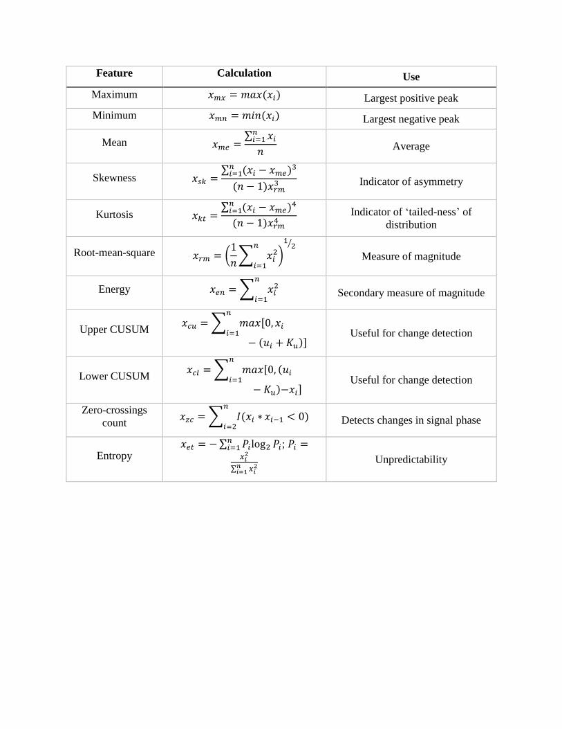
Feature Calculation Use

Maximum 𝑥𝑚𝑥 = 𝑚𝑎𝑥(𝑥𝑖) Largest positive peak

Minimum 𝑥𝑚𝑛 = 𝑚𝑖𝑛(𝑥𝑖) Largest negative peak

Mean 𝑥𝑚𝑒 =∑ 𝑥𝑖𝑛𝑖=1

𝑛 Average

Skewness 𝑥𝑠𝑘 =∑ (𝑥𝑖 − 𝑥𝑚𝑒)

3𝑛𝑖=1

(𝑛 − 1)𝑥𝑟𝑚3 Indicator of asymmetry

Kurtosis 𝑥𝑘𝑡 =∑ (𝑥𝑖 − 𝑥𝑚𝑒)

4𝑛𝑖=1

(𝑛 − 1)𝑥𝑟𝑚4

Indicator of ‘tailed-ness’ of

distribution

Root-mean-square 𝑥𝑟𝑚 = (1

𝑛∑ 𝑥𝑖

2𝑛

𝑖=1)

12⁄

Measure of magnitude

Energy 𝑥𝑒𝑛 =∑ 𝑥𝑖2

𝑛

𝑖=1 Secondary measure of magnitude

Upper CUSUM 𝑥𝑐𝑢 =∑ 𝑚𝑎𝑥[0, 𝑥𝑖

𝑛

𝑖=1

− (𝑢𝑖 + 𝐾𝑢)] Useful for change detection

Lower CUSUM 𝑥𝑐𝑙 =∑ 𝑚𝑎𝑥[0, (𝑢𝑖

𝑛

𝑖=1

− 𝐾𝑢)−𝑥𝑖] Useful for change detection

Zero-crossings

count 𝑥𝑧𝑐 =∑ 𝐼(𝑥𝑖 ∗

𝑛

𝑖=2𝑥𝑖−1 < 0) Detects changes in signal phase

Entropy 𝑥𝑒𝑡 = −∑ 𝑃𝑖log2 𝑃𝑖

𝑛𝑖=1 ; 𝑃𝑖 =

𝑥𝑖2

∑ 𝑥𝑖2𝑛

𝑖=1

Unpredictability