MARTINGALE PRICING MEASURES IN INCOMPLETEMARKETS VIA STOCHASTIC PROGRAMMING

DUALITY IN THE DUAL OF L∞

Alan King Lisa Korfkingaj@us.ibm.com korf@math.washington.edu

Mathematical Sciences Department Department of MathematicsIBM T.J. Watson Research Center University of WashingtonYorktown Heights, NY Seattle, WA

Abstract. We propose a new framework for analyzing pricing theory for incompletemarkets and contingent claims, using conjugate duality and optimization theory. Variousstatements in the literature of the fundamental theorem of asset pricing give conditionsunder which an essentially arbitrage-free market is equivalent to the existence of anequivalent martingale measure, and a formula for the fair price of a contingent claim asan expectation with respect to such a measure. In the setting of incomplete markets, thefair price is not attainable as such a particular expectation, but rather as a supremumover an infinite set of equivalent martingale measures. Here, we consider the problem asa stochastic program and derive pricing results for quite general discrete time processes.It is shown that in its most general form, the martingale pricing measure is attainableif it is permitted to be finitely additive. This setup also gives rise to a natural wayof analyzing models with risk preferences, spreads and margin constraints, and otherproblem variants. We consider a discrete time, multi-stage, infinite probability spacesetting and derive the basic results of arbitrage pricing in this framework.

Keywords: arbitrage pricing, conjugate duality, contingent claims, martingales,stochastic program, relatively complete recourse, singular multipliers, finitelyadditive measures

AMS Classification: 90C15, 90A60, 49N15, 49J99

Date: September 9, 2001

1. Introduction

Since the Nobel prize winning work of Black, Scholes and Merton [2, 13] in the 1970’sthat developed an arbitrage pricing formula for options, much attention has been de-

voted to understanding, generalizing, and applying this pricing model and its variants.Their techniques, which are still in use today, involved stochastic differential equations,

in particular relying on the assumption that the market price process (in continuoustime) behaves like geometric Brownian motion. In that setting, a unique fair option

price could be obtained in the form of a linear pricing rule. Since then, however, dif-

ferent perspectives have emerged because of the need to model market price processesthat do not necessarily conform to diffusion processes amenable to the stochastic dif-

ferential equations framework, other types of options and related financial instruments,and situations in which instead of a unique price, a range of fair prices exist.

Dominant among the new mathematical perspectives, in the 1980’s Harrison, Pliskaand Kreps [9, 8] studied the Black-Scholes formula and rederived results in a functional

analytic setting involving the representation of martingales. Harrison and Kreps [8]saw how these results could be generalized in this new setting to the relatively general

assumption that the market prices are square integrable. But one should take care tonote that the original Black-Scholes type models, which derive the price explicitly from

a partial differential equation, were not exactly being challenged by the developmentof this more general framework because the new framework did not offer a means of

obtaining the option price explicitly (or otherwise).What did come out of this new approach is what is now known as the fundamental

theorem of asset pricing, which depends on the concept of no arbitrage (i.e. no guaranteed

profit without risk; this condition was automatically satisfied in the geometric Brownianmotion setting). The theorem gives conditions under which a market is (essentially)

arbitrage-free if and only if there is an equivalent probability measure for which theprice process is a martingale. If the measure is unique, the “fair” price can then be

determined by taking an expectation with respect to it. It was shown in Harrison andPliska [9] that in the Black-Scholes model, the martingale measure exists and is unique,

hence leading to a unique price, but this is not true in general as will be seen.Also in contrast to the continuous time stochastic differential equation framework,

from the new functional analytic approach did come many variations and generalizationsin the late 1980’s and 1990’s, to problems with incomplete markets, transaction costs,

spreads and margins and other important variations as in Jouini and Kallal [10, 11].These kinds of issues were unmanageable and left relatively untouched in the stochastic

differential equations setting.In [6], Delbaen and Schachermayer extended the fundamental theorem of asset pric-

ing in the functional analytic setting to include incomplete markets in a setting of semi-

1

martingale price processes, ultimately providing a supremum formula for pricing viamartingale measures. This indicates that the pricing measure may not be attainable in

general incomplete markets. One of the main contributions of our paper is to lay out a

framework in which the pricing measure is attainable.Convexity and duality are at the heart of the functional analytic pricing results,

cf. Cvitanic and Karatzas [3]. Because the pricing problems and closely related port-folio optimization problems are so naturally cast in an optimization setting, it is our

proposal to analyze these from the perspective of conjugate duality and optimization,following [15]. This leads to the modeling of the pricing problems as well as the related

portfolio optimization problems as stochastic programs, thus offering a very rich and nat-ural framework for real problem descriptions, inclusion of additional variables (e.g. to

include the additional possibility of power production for contracts in the deregulatedenergy market), constraints, and other problem variations welcome in the stochastic pro-

gramming setting that appear unnatural in the purely functional analytic framework,and would not appear at all in a stochastic differential equations framework. Addition-

ally and perhaps most significantly, a stochastic programming framework provides anideal avenue for eventual computation, that is, a way for us to get our hands on fair

prices in a general setting.

Duality in stochastic programming on infinite dimensional spaces first appeared inthe work of Eisner and Olsen [7] and Wets [23]. Eisner and Olsen proposed an Lp,

Lq duality framework for stochastic linear programs with a very specific structure, ob-taining theorems of the type min P = sup D (where min/max indicates the solution is

attainable). At around the same time, Wets made a similar contribution in an L∞, L1

duality setting for stochastic linear programs with more general structure but no ran-

dom recourse matrix. Then in the late 1970’s, Rockafellar and Wets joined forces toproduce a series of seminal papers on stochastic programming duality for general convex

problems in an L∞, L1 setting cf. [17, 18, 16, 20]. The reason for this choice of spaces isthat one has to deal with tricky constraint qualifications in general Lp spaces unless the

problems have a special structure. Out of their work came the significance of the notionof relatively complete recourse and the related notion of induced constraints (implicit

constraints induced on past decision variables by the future) in obtaining strong dualityresults of the form inf P = max D in a very general setting with possibly unbounded

constraint sets. Additionally, they considered other duality settings such as pairing con-

tinuous functions and measures, which could be useful in a variety of applications, andstrong duality theorems (inf P = maxD) obtained in an L∞, (L∞)∗ setting where sin-

gular linear functionals play a role [19]. This latter concept is what we use to arrive atthe general results here. Portfolio optimization problems were recently analyzed in this

setting by Cvitanic, Schachermayer and Wang [4]. In 1987, Back and Pliska [1] proposeda different duality framework for continuous-time models, pairing spaces of functions of

bounded variation with a class of measures, and applying this to pricing problems. This

2

last paper is the only attempt the authors are aware of to consider arbitrage pricing inan infinite-dimensional stochastic programming duality setting.

In [12], King takes a first step toward the goal of casting pricing problems for contin-

gent claims in an optimization setting by analyzing what arbitrage and arbitrage pricingmean in discrete time, on a finite probability space, where the incomplete market pric-

ing model may be cast as a linear program. The associated dual problem is analyzedthrough linear programming duality, leading to the derivation of the generalized pricing

results comparable to those in Harrison and Kreps [8] and Harrison and Pliska [9] (butnow in a finite optimization setting). In addition, he observes that boundedness of the

portfolio optimization problem associated with a contingent claim is equivalent to the noarbitrage condition. It is then demonstrated how naturally one can add risk preferences

(utilities), spreads, margins and other variations to the problem and derive/computetheir associated (modified) pricing results simply by analyzing/solving the new dual

problems obtained. A significant aspect of this work is that the measure yielding thefair price in the dual is always attainable in the discrete time/probability space setting.

The goal of this paper is to use stochastic programming duality of L∞/(L∞)∗ type toset down a natural framework for arbitrage and arbitrage pricing in incomplete markets,

that includes attainment of the pricing measures. The approach taken is to generalize

the discrete time optimal portfolio and pricing models in King [12] to apply to moregeneral (not finite) probability spaces, to derive arbitrage pricing results for incomplete

markets in a multi-stage (discrete-time) stochastic programming duality setting.Section 2 introduces the requisite terminology from mathematical finance. The two

main problems are introduced: First, we introduce a portfolio optimization problem forthe seller (writer) of a contingent claim (e.g. an option). Then we pass to the writer’s fair

price model, which is the feasibility problem associated with the portfolio optimizationproblem. Section 3 reviews conjugate duality and optimization.

In Section 4, stochastic programming duality of L∞/(L∞)∗ type is applied to the twomain problems, to obtain relationships between the optimal values of the original prob-

lems and the optimal values of their duals. This in turn leads to equivalent expressionsof boundedness of the optimization problems in terms of feasibility of the duals.

In Section 5, it is shown that the unboundedness of the writer’s portfolio optimizationproblem is equivalent to a condition we call free lunch in the limit closely related to but

slightly weaker than (i.e. implied by) the free lunch characterization of arbitrage. It is

closely related to the concept of a free lunch with vanishing risk, described in Delbaen [5],but slightly more intuitive from an investor’s perspective. Section 6 introduces the

necessary concepts from probability theory, culminating in the definition of an equivalentfinitely additive martingale measure for a stochastic process.

Through the results in the previous sections, and an analysis of the dual portfoliooptimization problems obtained in Section 4, it is shown in Section 7 that there are

no free lunches in the limit if and only if there exists an equivalent finitely additive

3

martingale measure for the market price process, thus establishing the fundamentaltheorem of asset pricing in this setting. It is then shown through examination of solutions

to the dual pricing optimization problem that such solutions exist, and that the fair

writer’s price is given as the expectation with respect to such a solution, when consideredas an absolutely continuous finitely additive martingale measure for the market price

process.In each case, the dual variables determine the associated martingale measures, and

in this sense the measures can be broken into parts corresponding to the constraintsin the primal problem that are being dualized. Induced constraints play a role here

which warrants future investigation. A subsequent paper will develop continuous timestochastic programming models, in which trades occur at a finite number of unspecified

trading dates, where simple predictable processes are the key to the generalization.

2. The Writer’s Problems

We begin with a mathematical overview of the necessary financial terminology. Un-derlying all of our considerations is the market, by which we mean a collection of J + 1

traded assets indexed by j = 0, . . . , J . Each asset has an initial market price at timet = 0, and future market prices at times t = 1, . . . , T . The prices are described by

a nonnegative vector S0 := (S00 , . . . , S

J0 )∗ ∈ IRJ+1

+ , of initial known market prices and

nonnegative-valued random vectors St : Ξ → IRJ+1+ of future market prices, where

(Ξ,F , P ) is an underlying probability space with P -complete sigma-algebra F gener-

ated by a filtration Ft with FT = F . It is assumed that the first asset in the pricevectors is risk-free in the sense that it is always strictly positive (S0

t > 0, t = 0, . . . , T ).

We call this riskless asset the numeraire, and proceed immediately to normalize thevalues of all other assets based on the numeraire’s value and obtain the new discounted

price vectors, Zt := St/S0t . The numeraire’s value is identically one for t = 0, . . . , T ,

i.e. it is the price relative to which all other prices are measured. From here on it is

harmlessly assumed that all prices and cash flows have been similarly adjusted to reflectthis normalization. Prices in the price vector Zt are assumed Ft-measurable and essen-

tially bounded, i.e. ess sup |Zjt | < ∞ for i = 1, . . . , J . Henceforth assume all variables to

be defined up to measure zero, so that in particular Zt ∈ L∞(Ξ,Ft, P ; IRJ+1+ ). This is a

technical consideration that should be generalizable to square integrable price vectors,in keeping with the results in Harrison and Kreps [8] as well as the case of diffusion

processes, however we won’t concern ourselves with that generalization in the present

paper.A market is meaningless without the possibility of trading (buying and selling),

which we take up next. An investor may hold a portfolio of shares of assets j = 0, . . . , J ,described by a vector θt := (θ0

t , . . . , θJt )∗, t = 0, . . . , T . The investor generally has some

initial wealth to invest, and may change his or her portfolio at each time t = 0, . . . , T .

4

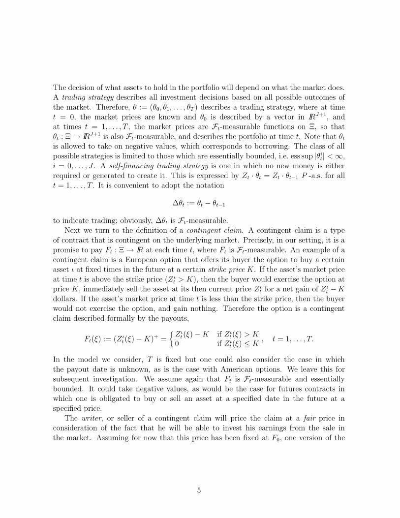
The decision of what assets to hold in the portfolio will depend on what the market does.A trading strategy describes all investment decisions based on all possible outcomes of

the market. Therefore, θ := (θ0, θ1, . . . , θT ) describes a trading strategy, where at time

t = 0, the market prices are known and θ0 is described by a vector in IRJ+1, andat times t = 1, . . . , T , the market prices are Ft-measurable functions on Ξ, so that

θt : Ξ → IRJ+1 is also Ft-measurable, and describes the portfolio at time t. Note that θt

is allowed to take on negative values, which corresponds to borrowing. The class of all

possible strategies is limited to those which are essentially bounded, i.e. ess sup |θit| < ∞,

i = 0, . . . , J . A self-financing trading strategy is one in which no new money is either

required or generated to create it. This is expressed by Zt · θt = Zt · θt−1 P -a.s. for allt = 1, . . . , T . It is convenient to adopt the notation

∆θt := θt − θt−1

to indicate trading; obviously, ∆θt is Ft-measurable.Next we turn to the definition of a contingent claim. A contingent claim is a type

of contract that is contingent on the underlying market. Precisely, in our setting, it is apromise to pay Ft : Ξ → IR at each time t, where Ft is Ft-measurable. An example of a

contingent claim is a European option that offers its buyer the option to buy a certainasset ι at fixed times in the future at a certain strike price K. If the asset’s market price

at time t is above the strike price (Z ιt > K), then the buyer would exercise the option at

price K, immediately sell the asset at its then current price Z ιt for a net gain of Z ι

t −K

dollars. If the asset’s market price at time t is less than the strike price, then the buyerwould not exercise the option, and gain nothing. Therefore the option is a contingent

claim described formally by the payouts,

Ft(ξ) := (Zιt(ξ)−K)+ =

{

Zιt(ξ)−K if Zι

t(ξ) > K0 if Zι

t(ξ) ≤ K, t = 1, . . . , T.

In the model we consider, T is fixed but one could also consider the case in which

the payout date is unknown, as is the case with American options. We leave this forsubsequent investigation. We assume again that Ft is Ft-measurable and essentially

bounded. It could take negative values, as would be the case for futures contracts inwhich one is obligated to buy or sell an asset at a specified date in the future at a

specified price.

The writer, or seller of a contingent claim will price the claim at a fair price inconsideration of the fact that he will be able to invest his earnings from the sale in

the market. Assuming for now that this price has been fixed at F0, one version of the

5

writer’s portfolio optimization problem is given by

Maximize θ E{ZT · θT }

subject to Z0 · θ0 ≤ F0

Zt ·∆θt ≤ −Ft P -a.s., t = 1, . . . , TZT · θT ≥ 0 P -a.s.,

(Pw)

where E{·} :=∫

Ξ ·dP (ξ) denotes expectation. In other words, the writer wants to

maximize the expected terminal wealth by investing the initial endowment (F0) subjectto the conditions that he cover the requisite payouts Ft through profits from trades

Zt ·∆θt and that the terminal wealth is (almost surely) nonnegative.This statement of the problem is a particular version of a more general statement

Maximize θ E{u(ZT · θT )}

subject to Z0 · θ0 ≤ F0

Zt ·∆θt ≤ −Ft P -a.s., t = 1, . . . , T,

(Pu)

where in the particular instance Pw, the utility function takes the form

uw(v) ={

v if v ≥ 0−∞ if v < 0

The requirement that the writer not lose money in the hedge is modeled by the effective

domain (denoted dom u) of the utility function, which in that case is the set [0, +∞).Bringing constraints up into the objective function in this way is standard practice (and

a powerful analytical tool) in modern convex and variational analysis, cf. [21].The generic assumptions on the utility function u(·) will be that u(·) : IR → IR is

concave, strictly increasing, and upper semi-continuous, with u(v) → ∞ as v → ∞. Inparticular this means that u(·) is a continuous function on the interior of its domain

dom u, and is continuous from the right at the boundary of dom u. In addition, thedomain dom u is either all of IR or a semi-infinite interval containing +∞, which may be

either closed or open depending on the behavior of u(v) as v approaches the boundaryof dom u from the right.

Two canonical utility functions to which our analyses will apply are the functionuw(·) as described above, and the logarithm function ul(v) = log v. Each of these fits

the assumptions and are easily handled in the framework of convex analysis. Their

domains are respectively, dom uw = [0, +∞) and dom ul = (0,∞). The boundary ofboth domains is the origin, 0. The logarithm’s value at 0 is defined to be −∞, making

that function’s hypograph closed.Associated with the problem Pw is a problem which determines the writer’s fair

price as the minimum price F0 such that Pw is feasible. This corresponds to the writer’s

6

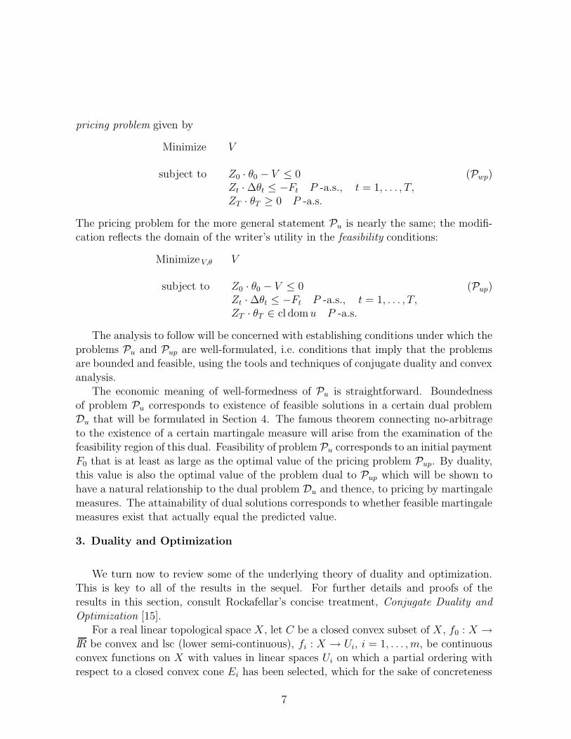
pricing problem given by

Minimize V

subject to Z0 · θ0 − V ≤ 0Zt ·∆θt ≤ −Ft P -a.s., t = 1, . . . , T,ZT · θT ≥ 0 P -a.s.

(Pwp)

The pricing problem for the more general statement Pu is nearly the same; the modifi-cation reflects the domain of the writer’s utility in the feasibility conditions:

Minimize V,θ V

subject to Z0 · θ0 − V ≤ 0Zt ·∆θt ≤ −Ft P -a.s., t = 1, . . . , T,ZT · θT ∈ cl domu P -a.s.

(Pup)

The analysis to follow will be concerned with establishing conditions under which the

problems Pu and Pup are well-formulated, i.e. conditions that imply that the problemsare bounded and feasible, using the tools and techniques of conjugate duality and convex

analysis.The economic meaning of well-formedness of Pu is straightforward. Boundedness

of problem Pu corresponds to existence of feasible solutions in a certain dual problemDu that will be formulated in Section 4. The famous theorem connecting no-arbitrage

to the existence of a certain martingale measure will arise from the examination of thefeasibility region of this dual. Feasibility of problem Pu corresponds to an initial payment

F0 that is at least as large as the optimal value of the pricing problem Pup. By duality,this value is also the optimal value of the problem dual to Pup which will be shown to

have a natural relationship to the dual problem Du and thence, to pricing by martingale

measures. The attainability of dual solutions corresponds to whether feasible martingalemeasures exist that actually equal the predicted value.

3. Duality and Optimization

We turn now to review some of the underlying theory of duality and optimization.This is key to all of the results in the sequel. For further details and proofs of the

results in this section, consult Rockafellar’s concise treatment, Conjugate Duality and

Optimization [15].For a real linear topological space X, let C be a closed convex subset of X, f0 : X →

IR be convex and lsc (lower semi-continuous), fi : X → Ui, i = 1, . . . , m, be continuousconvex functions on X with values in linear spaces Ui on which a partial ordering with

respect to a closed convex cone Ei has been selected, which for the sake of concreteness

7

and applicability we identify with a nonpositive orthant, so that ui ∈ Ei is equivalent toui ≤ 0. Consider the primal optimization problem:

Minimize f0(x) subject to x ∈ C, fi(x) ≤ 0, i = 1, . . . , m. (P)

By convention we stick to the setting of minimization, but it is easy to convert a max-imization problem into a minimization problem simply by changing the sign in the

objective. One may then apply duality in the minimization setting, and convert back tomaximization at the end.

For a linear space U , a perturbation function F : X × U → IR for P is a convexfunction satisfying

F (x, 0) =: f(x) ={

f0(x) if x ∈ C, fi(x) ≤ 0, i = 1, . . . , m,+∞ otherwise.

(1)

Thus F defines a family of convexly parameterized problems, and the original optimiza-

tion problem P may be given by the full objective function f . A common choice of Ffor P is defined on X × U , where U = ×m

i=1Ui, and given by

F (x, u) :={

f0(x) if x ∈ C, fi(x) ≤ ui, i = 1, . . . , m,+∞ otherwise.

This choice of F is clearly convex and satisfies (1), hence it is a valid perturbation

function.To the linear space U is associated a dual linear space Y along with a bilinear form

〈·, ·〉 : U × Y → IR. A topology on U is compatible with this pairing if it is a locallyconvex topology such that for each y ∈ Y , the linear functionals u 7→ 〈u, y〉 are all

continuous and every continuous linear functional on U can be represented in this form

for some y ∈ Y . Similarly, a topology on Y is compatible with the pairing if it is alocally convex topology such that for each u ∈ U , the linear functionals y 7→ 〈u, y〉 are

all continuous and every continuous linear functional on Y can be represented in thisform for some u ∈ U . It is assumed that U and Y have been equipped with compatible

topologies with respect to the given bilinear form.It is often useful to work with the Legendre-Fenchel transform. For an lsc function

f : U → IR, the Legendre-Fenchel conjugate of f (in the convex sense) is the functionf ∗ : Y → IR given by

f ∗(y) = supu∈U

{〈y, u〉 − f(u)}.

The conjugate in the concave sense just replaces “sup” with “inf.”Next we define the Lagrangian function L : X × Y → IR,

L(x, y) := inf {F (x, u) + 〈u, y〉 | u ∈ U}.

Note that L(x, y) is the negative of the conjugate of F (x, ·) evaluated at −y.

8

For the given perturbation function F above, we have

L(x, y) =

f0(x) +∑

i〈fi(x), yi〉 if x ∈ C, y ≥ 0,+∞ if x 6∈ C,−∞ if x ∈ C, y 6≥ 0,

(2)

where y ≥ 0 refers to the componentwise dual partial ordering induced by the closed

convex cones E◦i that are polar to Ei, i = 1, . . . , m. The Lagrangian function is closed

concave in y ∈ Y for each x ∈ X, closed convex in x ∈ X for each y ∈ Y , and satisfies

supy∈Y

L(x, y) ={

f0(x) if x ∈ C, fi(x) ≤ 0, i = 1, . . . , m+∞ otherwise,

i.e. the supremum over all y ∈ Y of the Lagrangian function yields the original problemP. This leads to the definition of the problem dual to P, defined on Y by

maximize g(y) so that y ≥ 0, (D)

whereg(y) := inf

x∈XL(x, y).

The concave function g is closed, cf. [15]. Properties relating P and D are intimatelytied to the convex optimal value function ϕ : U → IR defined by

ϕ(u) := infx∈X

F (x, u).

This is due to the fact that inf P, the optimal value of P is given by ϕ(0), whereas supD,the optimal value of D is equal to ϕ∗∗(u) = lim infu→0 ϕ(u), assuming P is feasible, where

u → 0 is in the designated topology. Thus duality results of the form inf P = supD

reduce to whether lim infu→0 ϕ(u) = ϕ(0). In particular, we have the following theorem.

Theorem 3.1 [15, Theorem 15]. Suppose P is feasible and lim infu→0 ϕ(u) ≥ ϕ(0).Then inf P = supD.

Attainment of dual solutions is equivalent to the subgradient of ϕ at 0 being non-

empty. A condition that ensures this is the continuity of ϕ at 0. The next theoremprovides conditions that imply the continuity of ϕ at 0, hence the existence of dual

solutions.

Theorem 3.2. Suppose there exists x ∈ C such that fi(x) ∈ int Ei, i = 1, . . . , m. Theninf P = maxD (i.e. there exists at least one y solving D).

The condition, “there exists x ∈ C such that fi(x) ∈ int Ei, i = 1, . . . , m,” is a strictfeasibility condition. In the setting in which U is a product of L∞ spaces, it corresponds

to the existence of an ε > 0 such that fi(x) ≤ −ε almost surely, i = 1, . . . , m. Stochastic

9

programming involves a particular choice of X and U that allows for the description ofthe evolving probabilistic information present in the problem, as laid out in the next

section.

4. L∞/(L∞)∗ Stochastic Programming Duality Applied to Writer’s Problems

We are now prepared to derive duality theorems for these problems which will, inSection 7, yield the existence and attainment of a finitely additive martingale measure

for the market price process, as well as a formula for the fair price of a contingentclaim in terms of this measure. The L∞/(L∞)∗ stochastic programming duality scheme

considered here was inspired by [19].Let’s return to the writer’s problem Pu first. In keeping with the duality discussion

in §3, with the solution space X now denoted by Θ for convenience, let

Θ := {θ = (θ0, . . . , θT ) | θ0 ∈ IRJ+1, θt ∈ L∞(Ξ,Ft, P ; IRJ+1), t = 1, . . . , T},

equipped with the strong product topology. Let the perturbation space U be defined by

U := {u = (u0, . . . , uT ) | u0 ∈ IR, ut ∈ L∞(Ξ,Ft, P ; IR), t = 1, . . . , T}.

The dual linear space Y is then

Y := {y = (y0, y1, . . . , yT ) | y0 ∈ IR, yt = (yt, y0t ) ∈ (L∞)∗(Ξ,Ft, P ; IR), t = 1, . . . , T},

with the compatible topologies the strong product topology on U and the weak∗ product

topology on Y .It is useful to understand how elements of (L∞)∗ behave. Each such element y may be

uniquely decomposed into an L1 component y and a singular component y0. An elementy of (L∞)∗ is singular if there exists sets En with P (En) ↘ 0 such that if z11En = 0

almost surely for some n, then 〈y, z〉 = 0.The problem which will turn out to be dual to Pu is

Minimize Y F0y0 −∑T

t=1 E{Ftyt} −∑T

t=1〈y0t , Ft〉 − (Eu)∗(yT , y0

T )

subject to E{Ztyt ·θt−1}+〈y0t , Zt ·θt−1〉=E{Zt−1yt−1 ·θt−1}+〈y

0t−1, Zt−1 ·θt−1〉

for all θt−1 ∈ L∞(Ξ,Ft−1, P ; IRJ+1), t = 1, . . . , T,y ≥ 0,

(Du)

where Eu : L∞(Ξ,F , P ; IR) → IR is the functional defined by

Eu(w) := E{u(w)},

and (Eu)∗ is the conjugate of Eu in the concave sense, defined on (L∞)∗(Ξ,F , P ; IR),

cf. §3. Here, y ≥ 0 in Y means that y0 ≥ 0, yt ≥ 0 P -almost surely, and 〈y0t , z〉 ≥ 0 for

10

all z ∈ L∞+ (Ξ,Ft, P ; IR), t = 1, . . . , T . The optimization problems under consideration

are strictly feasible if there is an ε > 0 such that the problems are still feasible when

the inequality constraints (including the implicit constraints governed by dom u) are

modified to become stricter by a factor of ε.

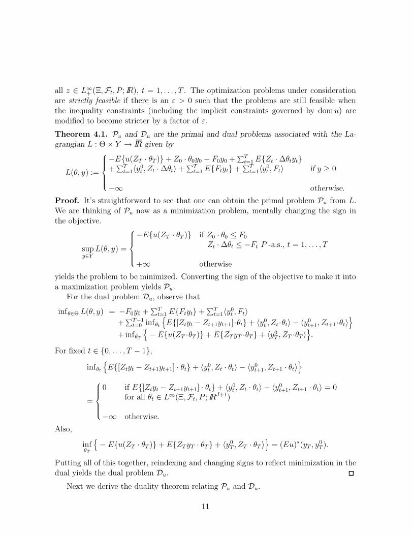
Theorem 4.1. Pu and Du are the primal and dual problems associated with the La-grangian L : Θ× Y → IR given by

L(θ, y) :=

−E{u(ZT · θT )}+ Z0 · θ0y0 − F0y0 +∑T

t=1 E{Zt ·∆θtyt}+∑T

t=1〈y0t , Zt ·∆θt〉+

∑Tt=1 E{Ftyt}+

∑Tt=1〈y

0t , Ft〉 if y ≥ 0

−∞ otherwise.

Proof. It’s straightforward to see that one can obtain the primal problem Pu from L.

We are thinking of Pu now as a minimization problem, mentally changing the sign in

the objective.

supy∈Y

L(θ, y) =

−E{u(ZT · θT )} if Z0 · θ0 ≤ F0

Zt ·∆θt ≤ −Ft P -a.s., t = 1, . . . , T

+∞ otherwise

yields the problem to be minimized. Converting the sign of the objective to make it into

a maximization problem yields Pu.For the dual problem Du, observe that

infθ∈Θ L(θ, y) = −F0y0 +∑T

t=1 E{Ftyt}+∑T

t=1〈y0t , Ft〉

+∑T−1

t=0 infθt

{

E{[Ztyt − Zt+1yt+1]·θt}+ 〈y0t , Zt ·θt〉 − 〈y

0t+1, Zt+1 ·θt〉

}

+ infθT

{

− E{u(ZT ·θT )}+ E{ZTyT ·θT}+ 〈y0T , ZT ·θT 〉

}

.

For fixed t ∈ {0, . . . , T − 1},

infθt

{

E{[Ztyt − Zt+1yt+1] · θt}+ 〈y0t , Zt · θt〉 − 〈y

0t+1, Zt+1 · θt〉

}

=

0 if E{[Ztyt − Zt+1yt+1] · θt}+ 〈y0t , Zt · θt〉 − 〈y

0t+1, Zt+1 · θt〉 = 0

for all θt ∈ L∞(Ξ,Ft, P ; IRJ+1)

−∞ otherwise.

Also,

infθT

{

− E{u(ZT · θT )}+ E{ZT yT · θT }+ 〈y0T , ZT · θT 〉

}

= (Eu)∗(yT , y0T ).

Putting all of this together, reindexing and changing signs to reflect minimization in thedual yields the dual problem Du.

Next we derive the duality theorem relating Pu and Du.

11

Theorem 4.2. Suppose Pu is strictly feasible. Then supPu = minDu.

Proof. Strict feasibility of Pu implies there exists ε > 0, θ ∈ Θ, such that

Z0 · θ0 ≤ F0 − ε,Zt ·∆θt ≤ −Ft − ε P -a.s., t = 1, . . . , t,

ZT · θT − ε ∈ cl dom u P -a.s.

Thus the assumptions of Theorem 3.2 are satisfied (with Ei the nonpositive orthant),and we immediately obtain the result supPu = minDu (translating to the setting of

maximization).

Note that Pu bounded, i.e. supPu < +∞, if and only if minDu < +∞, i.e. Du isfeasible. This fact will be used in Section 7 to obtain the fundamental theorem of asset

pricing (Theorem 7.2).Next we turn to the writer’s pricing problem Pup, recalling that it is the feasibility

problem for Pu. The solution space now contains V in addition to θ, so that

Θ := {θ = (V, θ0, . . . , θT ) | V ∈ IR, θ0 ∈ IRJ+1, θt ∈ L∞(Ξ,Ft, P : IRJ+1), t = 1, . . . , T},

equipped with the strong product topology. The perturbation space is

U := {u = (u0, . . . , uT , sT ) | u0 ∈ IR, ut ∈ L∞(Ξ,Ft, P ; IR), t = 1, . . . , T,sT ∈ L∞(Ξ, cFT , P ; IR)}.

The dual linear space is

Y := {y = (y0, y1,. . ., yT , xT ) | y0 ∈ IR, yt = (yt, y0t ) ∈ (L∞)∗(Ξ,Ft,P ; IR), t = 1,. . ., T,

xT = (xT , x0T ) ∈ (L∞)∗(Ξ,FT , P ; IR)},

with the compatible topologies the strong product topology on U and the weak∗ product

topology on Y .The problem which will turn out to be dual to Pup is

MaximizeY∑T

t=1 E{Ftyt}+∑T

t=1〈y0t , Ft〉+ E{αxT}+ 〈x0

T , α11〉

subject to E{Ztyt ·θt−1}+〈y0t , Zt ·θt−1〉=E{Zt−1yt−1 ·θt−1}+〈y

0t−1, Zt−1 ·θt−1〉

for all θt−1 ∈ L∞(Ξ,Ft−1, P ; IRJ+1), t = 1, . . . , T,x0

T = y0T , yT = xT P -a.s., y0 = 1, y ≥ 0

(Dup)

where α := inf{domu}, and 11 := 1 almost surely.

Theorem 4.3. Pup and Dup are the primal and dual problems associated with the

Lagrangian L : Θ× Y → IR given by

L(θ, y) :=

V + Z0 · θ0y0 − V y0 +∑T

t=1 E{Zt ·∆θtyt}+∑T

t=1〈y0t , Zt ·∆θt〉+

∑Tt=1 E{Ftyt}+

∑Tt=1〈y

0t , Ft〉

−E{ZT · θT xT } − 〈x0T , ZT · θT 〉+ E{αxT}+ 〈x0

T , α11〉 if y ≥ 0

−∞ otherwise.

12

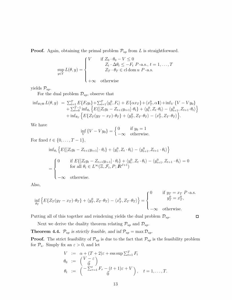
Proof. Again, obtaining the primal problem Pup from L is straightforward.

supy∈Y

L(θ, y) =

V if Z0 · θ0 − V ≤ 0Zt ·∆θt ≤ −Ft P -a.s., t = 1, . . . , TZT · θT ∈ cl dom u P -a.s.

+∞ otherwise

yields Pup.For the dual problem Dup, observe that

infθ∈Θ L(θ, y) =∑T

t=1 E{Ftyt}+∑T

t=1〈y0t , Ft〉+ E{αxT}+〈x

0T , α11〉+infV {V − V y0}

+∑T−1

t=0 infθt

{

E{[Ztyt − Zt+1yt+1]·θt}+ 〈y0t , Zt ·θt〉 − 〈y

0t+1, Zt+1 ·θt〉

}

+ infθT

{

E{ZT (yT − xT )·θT}+ 〈y0T , ZT ·θT 〉 − 〈x

0T , ZT ·θT 〉

}

.

We have

infV{V − V y0} =

{

0 if y0 = 1−∞ otherwise.

For fixed t ∈ {0, . . . , T − 1},

infθt

{

E{[Ztyt − Zt+1yt+1] · θt}+ 〈y0t , Zt · θt〉 − 〈y

0t+1, Zt+1 · θt〉

}

=

0 if E{[Ztyt − Zt+1yt+1] · θt}+ 〈y0t , Zt · θt〉 − 〈y

0t+1, Zt+1 · θt〉 = 0

for all θt ∈ L∞(Ξ,Ft, P ; IRJ+1)

−∞ otherwise.

Also,

infθT

{

E{ZT (yT − xT )·θT}+ 〈y0T , ZT ·θT 〉 − 〈x

0T , ZT ·θT 〉

}

=

0 if yT = xT P -a.s.y0

T = x0T ,

−∞ otherwise.

Putting all of this together and reindexing yields the dual problem Dup.

Next we derive the duality theorem relating Pup and Dup.

Theorem 4.4. Pup is strictly feasible, and inf Pup = maxDup.

Proof. The strict feasibility of Pup is due to the fact that Pup is the feasibility problem

for Pu. Simply fix an ε > 0, and let

V := α + (T + 2)ε + ess sup∑T

t=1 Ft

θ0 :=(

V − ε~0

)

θt :=(

−∑t

τ=1 Fτ − (t + 1)ε + V~0

)

, t = 1, . . . , T.

13

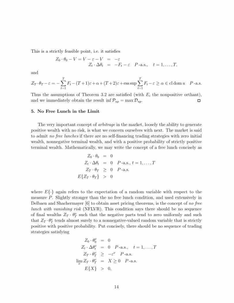
This is a strictly feasible point, i.e. it satisfies

Z0 · θ0 − V = V − ε− V = −εZt ·∆θt = −Ft − ε P -a.s., t = 1, . . . , T,

and

ZT ·θT −ε = −T∑

t=1

Ft− (T +1)ε+α+(T +2)ε+ess supT∑

t=1

Ft−ε ≥ α ∈ cl dom u P -a.s.

Thus the assumptions of Theorem 3.2 are satisfied (with Ei the nonpositive orthant),and we immediately obtain the result inf Pup = maxDup.

5. No Free Lunch in the Limit

The very important concept of arbitrage in the market, loosely the ability to generatepositive wealth with no risk, is what we concern ourselves with next. The market is said

to admit no free lunches if there are no self-financing trading strategies with zero initialwealth, nonnegative terminal wealth, and with a positive probability of strictly positive

terminal wealth. Mathematically, we may write the concept of a free lunch concisely as

Z0 · θ0 = 0

Zt ·∆θt = 0 P -a.s., t = 1, . . . , T

ZT · θT ≥ 0 P -a.s.

E{ZT · θT } > 0

where E{·} again refers to the expectation of a random variable with respect to themeasure P . Slightly stronger than the no free lunch condition, and used extensively in

Delbaen and Shachermayer [6] to obtain asset pricing theorems, is the concept of no free

lunch with vanishing risk (NFLVR). This condition says there should be no sequence

of final wealths ZT · θνT such that the negative parts tend to zero uniformly and such

that ZT · θνT tends almost surely to a nonnegative-valued random variable that is strictly

positive with positive probability. Put concisely, there should be no sequence of tradingstrategies satisfying

Z0 · θν0 = 0

Zt ·∆θνt = 0 P -a.s., t = 1, . . . , T

ZT · θνT ≥ −εν P -a.s.

limν

ZT · θνT = X ≥ 0 P -a.s.

E{X} > 0,

14

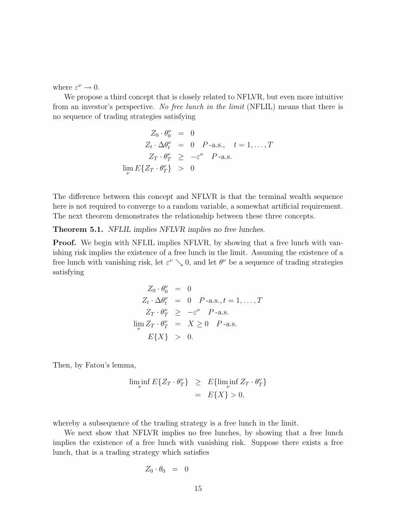
where εν → 0.We propose a third concept that is closely related to NFLVR, but even more intuitive

from an investor’s perspective. No free lunch in the limit (NFLIL) means that there is

no sequence of trading strategies satisfying

Z0 · θν0 = 0

Zt ·∆θνt = 0 P -a.s., t = 1, . . . , T

ZT · θνT ≥ −εν P -a.s.

limν

E{ZT · θνT} > 0

The difference between this concept and NFLVR is that the terminal wealth sequencehere is not required to converge to a random variable, a somewhat artificial requirement.

The next theorem demonstrates the relationship between these three concepts.

Theorem 5.1. NFLIL implies NFLVR implies no free lunches.

Proof. We begin with NFLIL implies NFLVR, by showing that a free lunch with van-

ishing risk implies the existence of a free lunch in the limit. Assuming the existence of afree lunch with vanishing risk, let εν ↘ 0, and let θν be a sequence of trading strategies

satisfying

Z0 · θν0 = 0

Zt ·∆θνt = 0 P -a.s., t = 1, . . . , T

ZT · θνT ≥ −εν P -a.s.

limν

ZT · θνT = X ≥ 0 P -a.s.

E{X} > 0.

Then, by Fatou’s lemma,

lim infν

E{ZT · θνT } ≥ E{lim inf

νZT · θ

νT}

= E{X} > 0,

whereby a subsequence of the trading strategy is a free lunch in the limit.We next show that NFLVR implies no free lunches, by showing that a free lunch

implies the existence of a free lunch with vanishing risk. Suppose there exists a freelunch, that is a trading strategy which satisfies

Z0 · θ0 = 0

15

Zt ·∆θt = 0 P -a.s., t = 1, . . . , T

ZT · θT ≥ 0 P -a.s.

E{ZT · θT} > 0.

Let θν := θ for all ν ∈ IN . This creates the desired free lunch with vanishing risk, whichcompletes the proof.

The next theorem equates NFLIL with the boundedness of the particular writer’s

portfolio optimization problem Pw, a significant feature that comes out of our approach.

Theorem 5.2. Suppose Pw is strictly feasible, with F0 > ess inf (∑T

t=1 Ft) in Pw. Thenthe following are equivalent.

(a) Pw is bounded,(b) The market admits NFLIL.

Proof. We will show that (a) ⇐⇒ (b) by contrapositive. First suppose that (a) does

not hold, i.e. Pw is unbounded (it is feasible by assumption). Then there is a sequenceof trading strategies satisfying

Z0 · θν0 ≤ F0

Zt ·∆θνt ≤ −Ft P -a.s., t = 1, . . . , T

ZT · θνT ≥ 0 P -a.s.

E{ZT · θνT} ↗ +∞.

Note that β := 1

F0−ess inf(∑

T

t=1Ft)

> 0 by assumption. Let 0 < εν := 1E{ZT ·θ

ν

T}↘ 0. Let

γν = ενβ and note in particular that γν > 0. Let

θν0 := γν

(

θν0 +

(

F0 − ess inf (∑T

t=1 Ft)− Z0 · θν0

~0

)

)

−(

εν

~0

)

,

and for t = 1, . . . , T ,

θνt := γν

(

θνt +

(

− ess inf (∑T

t=1 Ft)−∑t

t=1 Zt ·∆θνt

~0

)

)

−(

εν

~0

)

.

Then,

Z0 · θν0 = γν

(

Z0θν0 + F0 − Z0θ

ν0 − ess inf (

T∑

t=1

Ft))

− εν

= γν(

F0 − ess inf (T∑

t=1

Ft))

− εν

= εν − εν = 0.

16

Also, the self-financing condition holds:

Zt ·∆θνt = γν

(

Zt ·∆θνt − Zt ·∆θν

t

)

= 0.

The negative part of the terminal wealth sequence converges uniformly to 0, as given by

ZT · θνT = γν

(

ZT · θνT − ess inf (

T∑

t=1

Ft)−T∑

t=1

Zt ·∆θνt

)

≥ γν(

ZT · θνT − ess inf (

T∑

t=1

Ft) +T∑

t=1

Ft

)

− εν

≥ −εν.

Finally, we have that the expected terminal wealth is positive in the limit:

E{ZT · θνT} ≥ γν

(

E{ZT · θνT} − ess inf (

T∑

t=1

Ft) + E{T∑

t=1

Ft})

− εν

= β(

1 + εν(

E{T∑

t=1

Ft} − ess inf (T∑

t=1

Ft))

)

− εν,

so that

lim infν

E{ZT · θνT } ≥ β > 0.

Thus a subsequence of θνT is a free lunch in the limit, establishing (b) =⇒ (a).

Now let the market admit a free lunch in the limit θν for a sequence (εν)2 ↘ 0. By

the strict feasibility of Pw, for large enough ν, ν > ν, the problem

Maximize E{ZT · θT}subject to Z0 · θ0 ≤ F0

Zt ·∆θt ≤ −Ft P -a.s., t = 1, . . . , TZT · θT ≥ εν P -a.s.

is feasible, so let θν be such a feasible point for each ν > ν. Let θν := θν + (εν)−1θν.

Then θν is feasible for Pw, since

Z0 · θν0 = Z0 · θ

ν0 + Z0 · (ε

ν)−1θν0 ≤ F0,

and for t = 1, . . . , T ,

Zt ·∆θνt = Zt ·∆θν

t + (εν)−1Zt ·∆θνt ≤ −Ft.

17

Also,

ZT · θνT = ZT · θ

νT + (εν)−1ZT · θ

νT

≥ ZT · θνT − (εν)−1(εν)2

= εν − εν ≥ 0,

and

E{ZT · θνT} = E{ZT · θ

νT }+ (εν)−1E{ZT · θ

νT }

≥ εν + (εν)−1E{ZT · θνT }.

Since limν E{ZT · θνT } > 0, we have

limν

E{ZT · θνT } = +∞.

We have shown that supPw = +∞, i.e. Pw is unbounded, establishing (a) =⇒ (b).

It is not possible to equate the boundedness for general Pu with the no free lunch

conditions, however one may do so with some further assumptions on the utility u.

Theorem 5.3. Suppose the utility function u : IR → IR satisfies limx→α+ u(x) > −∞where α := inf{domu}, and limx→∞

u(x)x

= c > 0. Suppose Pu is strictly feasible, with

F0 > ess inf (∑T

t=1 Ft) in Pu. Then the following are equivalent.

(a) Pu is bounded,(b) The market admits NFLIL.

Proof. We proceed as in Theorem 5.2. First suppose Pu is unbounded, and let {θν}∞ν=1

be a sequence of trading strategies satisfying

Z0 · θν0 ≤ F0

Zt · [θνt − θν

t−1] ≤ −Ft P -a.s., t = 1, . . . , T

ZT · θνT ≥ 0 P -a.s.

E{u(ZT · θνT )} ↗ +∞.

E{u(ZT · θνT )} ≤ u(E{ZT · θ

νT }) by Jensen’s inequality. Thus, u(E{ZT · θ

νT}) ↗∞ for a

subsequence, whereby E{ZT · θνT} ↗ ∞ by the assumption that u(x) → ∞ as x → ∞,

and that u is strictly increasing. Appealing now to the proof in Theorem 5.2, the same

argument yields a free lunch in the limit, establishing (b) =⇒ (a).Now let the market admit a free lunch in the limit θν for a sequence (εν)2 ↘ 0. By

the strict feasibility of Pu, for large enough ν, ν > ν, the problem

Maximize E{u(ZT · θT )}subject to Z0 · θ0 ≤ F0

Zt ·∆θt ≤ −Ft P -a.s., t = 1, . . . , TZT · θT − εν ∈ cl dom u P -a.s.

18

is feasible, so let θν be such a feasible point for each ν > ν. Let θν := θν + (εν)−1θν.Then θν is feasible for Pu, since

Z0 · θν0 = Z0 · θ

ν0 + Z0 · (ε

ν)−1θν0 ≤ F0,

and for t = 1, . . . , T ,

Zt ·∆θνt = Zt ·∆θν

t + (εν)−1Zt ·∆θνt ≤ −Ft.

Also,

ZT · θνT = ZT · θ

νT + (εν)−1ZT · θ

νT

≥ ZT · θνT − (εν)−1(εν)2

= ZT · θνT − εν ∈ dom u,

and

E{ZT · θνT} = E{ZT · θ

νT }+ (εν)−1E{ZT · θ

νT }

≥ εν + (εν)−1E{ZT · θνT }.

Since limν E{ZT · θνT } > 0, we have

limν

E{ZT · θνT } = +∞.

By the assumption limx→∞u(x)

x= c > 0, for 0 < ε < c, there exists a Kε > 0 such

that x > Kε implies u(x)x

≥ c − ε, or u(x) ≥ (c − ε)x. Note that by the assumptionlimx→α+ u(x) > −∞, α > −∞, and by the upper semicontinuiuty and concavity of u,

u(α) > −∞, i.e. α ∈ dom u. Since u is strictly increasing,

E{u(ZT · θT )} = E{

u(ZT · θνT + (εν)−1ZT · θ

νT )}

≥ E{

u(α + εν + (εν)−1ZT · θνT )}

.

Let Xν := α+εν+(εν)−1ZT ·θνT . Note that Xν ≥ α P -almost surely. Since limν→∞ E{ZT ·

θνT} > 0, it follows that limν→∞ E{Xν} = +∞, and thus also limν→∞ E{Xν11Xν>K} =

+∞, for K ∈ IR. Now observe that

E{u(Xν)} = E{u(Xν)11Xν≤Kε}+ E{u(Xν)11Xν>Kε

}≥ E{u(Xν)11Xν≤Kε

}+ E{(c− ε)Xν11Xν>Kε}

≥ u(α)P (Xν ≤ Kε) + E{(c− ε)Xν11Xν>Kε}

≥ −|u(α)|+ E{(c− ε)Xν11Xν>Kε}.

Thus,limν→∞

E{u(Xν)} ≥ −|u(α)|+ limν→∞

E{(c− ε)Xν11Xν>Kε} = +∞.

19

We have thus shown that supPu = +∞, i.e. that Pu is unbounded.

6. Martingale Measures

This section reviews the definition of a martingale and equivalent representations

for martingales. Then the latter part of the section extends the notion of martingalemeasures to include finitely additive measures.

Definition 6.1. Let (Ξ,F , P ) be a probability space and {Ft} the filtration with respect

to which a vector process {Zt}Tt=0 is measurable. {Zt}

Tt=0 is a martingale under P if

E{Zt|Ft−1} = Zt−1 P -a.s., t = 1, . . . , T.

Equivalently,∫

EZtdP =

∫

EZt−1dP ∀E ∈ Ft−1, t = 1, . . . , T.

Another way of representing a martingale will be useful in the sections to follow.

Proposition 6.2. Let {Zt}Tt=0 be a vector process defined on (Ξ,F), and {Ft} the

associated filtration. Then Zt is a martingale with respect to a probability measure Pif and only if

E{Zt · θt−1} = E{Zt−1 · θt−1}, t = 1, . . . , T,

for all θt−1 ∈ L∞(Ξ,Ft−1, P ; IRJ+1), t = 1, . . . , T .

Proof. Suppose {Zt}Tt=0 is a martingale under P . Then for fixed θ = (θ0, . . . , θT ) such

that θt ∈ L∞(Ξ,Ft, P ; IRJ+1), and fixed t,

E{Zt · θt−1|Ft−1} = θt−1 · E{Zt|Ft−1}= Zt−1 · θt−1,

whereby E{Zt · θt−1} = E{Zt−1 · θt−1}.

Now suppose E{Zt · θt−1} = E{Zt−1 · θt−1} for all θt−1 ∈ L∞(Ξ,Ft−1, P ; IRJ+1),t = 1, . . . , T . Let E ∈ Ft−1 and let ei represent the Ft−1-measurable coordinate vector

with a 11E in the i’th position and 0’s elsewhere, i = 0, . . . , J . For each fixed i, withθt−1 ≡ ei, one obtains

E{Z it11E} = E{Z i

t−111E},

thus by Definition 6.1, {Zt}Tt=0 is a martingale under P .

Definition 6.3. A probability measure Q on (Ξ,F) is said to be absolutely continuous

with respect to P (denoted Q << P ) on F if P (E) = 0 implies Q(E) = 0 for all E ∈ F .

Q is said to be equivalent to P (denoted Q ∼ P ) on F if P and Q have the same zeromeasure sets, i.e. P (E) = 0 if and only if Q(E) = 0.

20

Definition 6.4. We say that a probability measure Q is a martingale measure for thevector process {Zt}

Tt=0 if Q << P and {Zt}

Tt=0 is a martingale under Q. It is an equivalent

martingale measure if in addition Q ∼ P .

A probability measure that is absolutely continuous with respect to P has an equiv-

alent representation as the Radon-Nikodym derivative of a function y ∈ L1+(Ξ,F , P ; IR)

such that∫

Ξ ydP = 1. In fact, one may translate between the space of absolutely con-

tinuous probability measures and the space of such y′s under the identification

Q(E) =∫

EydP, ∀E ∈ F .

One may express the martingale condition in terms of its equivalent representation.

Let y be the Radon-Nikodym derivative of the absolutely continuous probability measure

Q, and let yt = E{y|Ft}.

Proposition 6.5. A probability measure Q << P is a martingale measure for {Zt}Tt=0

if and only if the vector process {Ztyt}Tt=0 is a martingale under P , i.e.

E{Ztyt|Ft−1} = Zt−1yt−1 P -a.s., t = 1, . . . , T.

Equivalently,∫

EZtytdP =

∫

EZt−1yt−1dP ∀E ∈ Ft−1, t = 1, . . . , T.

Q is an equivalent martingale measure if in addition, y > 0 P -a.s..

Proof. This is immediate from the definition.

All of these considerations may be extended to the space of finitely additive proba-

bility measures.

Definition 6.6. A finitely additive probability measure Q is one that satisfies finiteadditivity, i.e. for En disjoint sets in F , n = 1, . . . , N ,

Q(N⋃

n=1

En) =N∑

n=1

Q(En),

but not necessarily countable additivity (countable additivity is a property satisfied bystandard probability measures).

Note that every countably additive probability measure is finitely additive. Thatconditional expectations with finitely additive probability measures are well-defined can

be found in Regazzini [14], along with their properties. Finitely additive measures whichare not countably additive are not as well behaved as standard probability measures,

and thus mostly avoided. However, they should not be ignored as they do arise in

21

natural contexts as we have been demonstrating. It was already stated that a probabilitymeasure has an equivalent representation as the Radon-Nikodym derivative of a function

y ∈ L1+(Ξ,F , P ; IR) such that

∫

ydP = 1. Similarly, a finitely additive probability

measure Q has an equivalent representation as the set function arising from a functiony ∈ (L∞)∗+(Ξ,F , P ; IR) such that 〈y, 11〉 = 1, i.e. under the identification

Q(E) = 〈y, 11E〉,

cf. [24]. For a finitely additive probability measure Q, let EQ{·} denote the expectationwith respect to this measure, which is well-defined when viewed with respect to this

representation. To avoid technical considerations, the definition of a finitely additivemartingale we take here parallels the representation in Proposition 6.2.

Definition 6.7. Let {Zt}Tt=0 be a vector process defined on (Ξ,F), and {Ft} the asso-

ciated filtration. Then Zt is a martingale with respect to a finitely additive probability

measure Q ifEQ{Zt · θt−1} = EQ{Zt−1 · θt−1}

for all θt−1 ∈ L∞(Ξ,Ft−1, P ; IRJ+1), t = 1, . . . , T .

Definition 6.8. A finitely additive probability measure Q on (Ξ,F) is said to be ab-

solutely continuous with respect to a (finitely or countably additive) probability measure

P (denoted Q << P ) on F if P (E) = 0 implies Q(E) = 0 for all E ∈ F . Q is said to

be equivalent to P (denoted Q ∼ P ) on F if P and Q have the same zero measure sets,i.e. P (E) = 0 if and only if Q(E) = 0.

Definition 6.9. Let (Ξ,F , P ) be the underlying probability space, where P is a count-ably additive probability measure. We say that a finitely additive probability measure

Q is a martingale measure for the vector process {Zt}Tt=0 if Q << P and {Zt}

Tt=0 is a

martingale under Q. It is an equivalent martingale measure if in addition Q ∼ P .

Recall that each element of (L∞)∗+ may be uniquely decomposed into an L1 com-ponent and a singular component. Thus the associated finitely additive measure de-

composes uniquely into a countably additive part and what is called a purely finitelyadditive part, corresponding to the singular component in (L∞)∗+. With (Ξ,F , P ) the

underlying probability space, let (y, y0) be the unique decomposition of the equiva-lent representation in (L∞)∗+ of a finitely additive probability measure Q << P . Let

yt := E{y|Ft}, and y0t be the unique singular component which is Ft-measurable and

satisfies 〈y0t , 11E〉+ E{y11E} = Q(E) for all E ∈ Ft, t = 0, . . . , T .

Proposition 6.10. A finitely additive probability measure Q << P is a finitely additivemartingale measure for {Zt}

Tt=0 if and only if

E{Ztyt · θt−1}+ 〈y0t , Zt · θt−1〉 = E{Zt−1yt−1 · θt−1}+ 〈y0

t−1, Zt−1 · θt−1〉

22

for all θt−1 ∈ L∞(Ξ,Ft−1, P ; IRJ+1), t = 1, . . . , T . Q is an equivalent finitely additivemartingale measure if and only if in addition to the above, y > 0 P -a.s..

Proof. This is a straightforward application of the definition of a finitely additive mar-

tingale measure, observing that

EQ{Zt · θt−1} = E{Ztyt · θt−1}+ 〈y0t , Zt · θt−1〉,

and

EQ{Zt−1 · θt−1} = E{Zt−1yt−1 · θt−1}+ 〈y0t−1, Zt−1 · θt−1〉.

To get the equivalence, if Q ∼ P , then y can’t be 0 on a set E of positive measure

because this would mean Q(E) = 0 while P (E) > 0, thus it must be that y > 0almost surely. Now, if y > 0 P -almost surely, and E ∈ F is such that P (E) = 0, then

Q(E) = E{11Ey}+ 〈y0, 11e〉 = 0 since 11E = 0 P -almost surely. If Q(E) = 0, this means

E{11Ey}+ 〈y0, 11E〉 = 0. Since both terms must be greater than or equal to 0, it followsthat E{11Ey} = 0. Now, using the fact that y > 0 P -almost surely, it must be true that

11Ey = 0 P -almost surely, and thus 11E = 0 P -almost surely, i.e. P (E) = 0.

7. The Fundamental Theorem of Asset Pricing

We now proceed to apply the results in the preceding sections to the pricing theoryfor contingent claims in incomplete markets.

Lemma 7.1. Du is feasible if and only if there exists an equivalent finitely additive

martingale measure.

Proof. Let y = (y0, (y1, y01), . . . , (yT , y0

T )) ∈ Y be feasible for Du. Then y satisfies the

constraints in Du:

E{Ztyt ·θt−1}+〈y0t , Zt ·θt−1〉=E{Zt−1yt−1 ·θt−1}+〈y

0t−1, Zt−1 ·θt−1〉

for all θt−1 ∈ L∞(Ξ,Ft−1, P ; IRJ+1), t = 1, . . . , T,(yT , y0

T ) ∈ dom(Eu)∗, y ≥ 0.

We begin by showing that yT > 0 almost surely. Suppose to the contrary that there is

a set E ∈ FT , P (E) > 0, such that yT11E = 0 almost surely. For y0T , let Eν ↘ be the

associated sets in FT such that P (Eν) ↘ 0 and 〈y0T , z〉 = 0 whenever z11Eν = 0 almost

surely for some ν. Choose ν large enough so that P (E \Eν) > 0. For γ ∈ dom u, λ > 0,let wT = λ11E\Eν + γ11Ec∪Eν . Then,

(Eu)∗(yT , y0T ) = infwT∈L∞(Ξ,FT ,P ;IR) {E{wTyT}+ 〈y0

T , wT 〉 − Eu(wT )}≤ E{wT yT}+ 〈y0

T , wT 〉 − Eu(wT )= γE{yT}+ γy0

T (11)− u(λ)P (E \ Eν)− u(γ)P (Ec ∪ Eν)↘ −∞ as λ ↗∞,

23

since u is strictly increasing and u(v) → ∞ as v → ∞. Thus (Eu)∗(yT , y0) = −∞,which means that (yT , y0

T ) is not in dom(Eu)∗, contradicting our choice of y as a feasible

point for Du. Thus yT > 0 almost surely, as claimed.

Now let vT := (vT , v0T ), where

vT := vT /(E{yT}+ 〈y0T , 11〉),

and

v0T := y0

T /(E{yT}+ 〈y0T , 11〉).

We proceed to show that the set function Q on FT defined by

Q(E) := 〈vT , 11E〉, E ∈ FT ,

is an equivalent finitely additive martingale measure. The finite additivity is immedi-ate from that induced by (yT , y0

T ). The requirement that Q(Ξ) = 1 follows from the

normalization,Q(Ξ) = 〈vT , 11〉

= E{vT}+ 〈v0T , 11〉

= E{yT }

(E{yT }+〈y0T

,11〉)+

〈y0T

,11〉

(E{yT }+〈y0T

,11〉)= 1.

That Q is equivalent to P follows from vT > 0. It remains to show that Q is a martingale

measure for the price process. Let vt := E{vT | Ft}, and v0t be the unique singular

component which is Ft-measurable and satisfies 〈v0t , 11E〉 + E{vT 11E} = Q(E) for all

E ∈ Ft, t = 0, . . . , T . Then by the constraints in Du (and the fact that Z0t ≡ 1,

t = 0, . . . , T ), vt = yt/(E{yT} + 〈y0T , 11〉) and v0

t = y0t /(E{yT} + 〈y0

T , 11〉). Observe thus

by the constraints in Du, for t = 1, . . . , T , θt−1 ∈ L∞(Ξ,Ft−1, P ; IRJ+1),

EQ{Zt · θt−1} = E{ZtvT · θt−1}+ 〈v0T , Zt · θt−1〉

= E{Ztvt · θt−1}+ 〈v0t , Zt · θt−1〉

= E{Zt−1vt−1 · θt−1}+ 〈v0t−1, Zt−1 · θt−1〉

= EQ{Zt−1 · θt−1},

whereby Q is an equivalent finitely additive martingale measure.Now suppose that there exists an equivalent finitely additive martingale measure Q.

Let (y, y0) ∈ (L∞)∗(Ξ,FT , P ; IR) be the representation of Q in (L∞)∗(Ξ,FT , P ; IR), let

yt := E{y| Ft}, y0t the unique Ft-measurable singular component such that

Q(E) = E{y11E}+ 〈y0t , 11E〉 for all E ∈ Ft.

Then y := (y0, (y1, y01), . . . , (yT , y0

T )) ∈ Y is a feasible solution to Du, which completes

the proof.

24

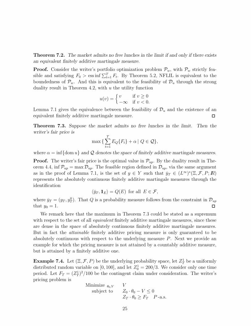
Theorem 7.2. The market admits no free lunches in the limit if and only if there existsan equivalent finitely additive martingale measure.

Proof. Consider the writer’s portfolio optimization problem Pw, with Pw strictly fea-

sible and satisfying F0 > ess inf∑T

t=1 Ft. By Theorem 5.2, NFLIL is equivalent to the

boundedness of Pw. And this is equivalent to the feasibility of Du through the strongduality result in Theorem 4.2, with u the utility function

u(v) ={

v if v ≥ 0−∞ if v < 0.

Lemma 7.1 gives the equivalence between the feasibility of Du and the existence of an

equivalent finitely additive martingale measure.

Theorem 7.3. Suppose the market admits no free lunches in the limit. Then the

writer’s fair price is

max {T∑

t=1

EQ{Ft}+ α | Q ∈ Q},

where α = inf{dom u} and Q denotes the space of finitely additive martingale measures.

Proof. The writer’s fair price is the optimal value in Pup. By the duality result in The-orem 4.4, inf Pup = maxDup. The feasible region defined in Dup, via the same argument

as in the proof of Lemma 7.1, is the set of y ∈ Y such that yT ∈ (L∞)∗(Ξ,F , P ; IR)represents the absolutely continuous finitely additive martingale measures through the

identification〈yT , 11E〉 = Q(E) for all E ∈ F ,

where yT = (yT , y0T ). That Q is a probability measure follows from the constraint in Dup

that y0 = 1.

We remark here that the maximum in Theorem 7.3 could be stated as a supremum

with respect to the set of all equivalent finitely additive martingale measures, since theseare dense in the space of absolutely continuous finitely additive martingale measures.

But in fact the attainable finitely additive pricing measure is only guaranteed to beabsolutely continuous with respect to the underlying measure P . Next we provide an

example for which the pricing measure is not attained by a countably additive measure,

but is attained by a finitely additive one.

Example 7.4. Let (Ξ,F , P ) be the underlying probability space, let Z1T be a uniformly

distributed random variable on [0, 100], and let Z10 = 200/3. We consider only one time

period. Let FT = (Z1T )2/100 be the contingent claim under consideration. The writer’s

pricing problem isMinimize θ0,V V

subject to Z0 · θ0 − V ≤ 0ZT · θ0 ≥ FT P -a.s.

25

The optimal value of the writer’s pricing problem is then given by

V ∗ = infθ00∈IR

ess sup {(Z1

T )2

100− Z1

Tθ00 +

200

3θ00}.

This value is achieved for θ00 = 1, whereby V ∗ = 200/3. By the duality theorems in

Section 4, this is also the optimal value of the dual to the writer’s pricing problem,

which is given by

Maximize yTE{FT yT}+ 〈y0

T , FT 〉subject to E{ZT yT}+ 〈y0

T , ZT 〉 = Z0

yT ≥ 0 P -a.s.

In the attempt to construct countably additive martingale measures that might yield

a solution to the dual problem, we consider certain Radon-Nikodym derivatives withrespect to the probability measure P that place as much weight as possible near the

points in Ξ where FT is largest, but still retain the martingale property. For β ≥ 1/50,let yβ

T ∈ L1(Ξ,F , P ; IR) be defined by

yβT :=

β/4 if Z1T ∈ [0, 4/3β]

β if Z1T ∈ [100− 2/3β, 100]

0 otherwise

P -a.s.

Then yβT yields a countably additive martingale measure since yβ

T ≥ 0 P -almost surely,

E{yβT} = E{

β

411Z1

T∈[0,4/3β] + β11Z1

T∈[100−2/3β,100]} =

β

4

4

3β+ β

2

3β= 1,

andE{Z1

T yβT} = E{Z1

Tβ411Z1

T∈[0,4/3β] + Z1

T β11Z1T∈[100−2/3β,100]}

=∫ 4/3β0

x100

β4dx +

∫ 100100−2/3β

x100

βdx

= 2003

= Z10 .

Taking the expectation of FT with respect to the countably additive measure obtained

through yβT yields

E{FT yβT} =

∫ 4/3β

0

x2

100

β

4dx +

∫ 100

100−2/3β

x2

100βdx =

1

675β2−

4

9β+

200

3<

200

3.

Additionally, E{FT yβT} increases to 200/3 as β →∞. However the exact pricing measure

cannot be obtained by a countably additive martingale measure. Instead we must con-

sider finitely additive measures. Let C[0, 100] denote the space of continuous functionson [0, 100], and consider the subspace of L∞(Ξ,F , P ; IR) given by

W := {w ∈ L∞(Ξ,F , P ; IR) | ∃fw ∈ C[0, 100] such that fw(Z1T ) = w P -a.s. }.

26

Define the linear functional yT on W by

〈yT , w〉 :=1

3fw(0) +

2

3fw(100).

By a version of the Hahn-Banach Theorem (cf. [22, Chapter 10, Exercise 24]), thereexists an extension y∗T of yT to L∞(Ξ,F , P ; IR) such that y∗T ≥ 0 as an element of

(L∞)∗(Ξ,F , P ; IR). In fact, y∗T is singular: For Eβ ∈ F with Eβ ↘ such that

Z1T ∈ [0,

4

3β] ∪ [100−

2

3β, 100] on Eβ P -a.s., P (Eβ) ↘ 0,

suppose that v ∈ L∞(Ξ,F , P ; IR) is such that v = 0 P -almost surely on Eβ for some β.Let β ′ > β and let w ∈ W be such that fw ∈ C[0, 100] is given by

fw(x) :=

0 if x ∈ [0, 43β′

]

[( 43β′

, 0), ( 43β

, ess sup v)] if x ∈ [ 43β′

, 43β

]

ess sup v if x ∈ [ 43β

, 100− 23β

]

[(100− 23β

, ess sup v), (100− 23β′

, 0)] if x ∈ [100− 23β

, 100− 23β′

]

0 if x ∈ [100− 23β′

, 100],

where [(a, b), (c, d)] is shorthand for the function whose graph is the line segment joining

the points (a, b) and (c, d). Then v ≤ w P -almost surely, and

〈y∗T , v〉 ≤ 〈y∗T , w〉 =1

3fw(0) +

2

3fw(100) = 0.

Similarly, 〈y∗T ,−v〉 ≤ 0, whereby 〈y∗T , v〉 = 0, which implies that y∗T is singular. (Because

there is no L1 component, the associated finitely additive measure is purely finitely

additive.)

We next show that y∗T is a finitely additive martingale measure, which follows fromthe observations that

〈y∗T , 11〉 =1

3+

2

3= 1,

which shows that y∗T defines a finitely additive probability measure and also gives the

first part of the first component of the martingale condition, that

〈y∗T , Z0T 〉 = Z0

0 .

The second component of the martingale condition follows from

〈y∗T , Z1T 〉 =

1

30 +

2

3100 =

200

3= Z1

0 .

27

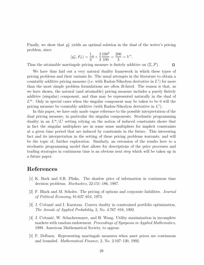
Finally, we show that y∗T yields an optimal solution in the dual of the writer’s pricingproblem, since

〈y∗T , FT 〉 =1

30 +

2

3

1002

100=

200

3= V ∗.

Thus the attainable martingale pricing measure is finitely additive on (Ξ,F).

We have thus laid out a very natural duality framework in which these types of

pricing problems and their variants lie. The usual attempts in the literature to obtain a

countably additive pricing measure (i.e. with Radon-Nikodym derivative in L1) for morethan the most simple problem formulations are often ill-fated. The reason is that, as

we have shown, the natural (and attainable) pricing measure includes a purely finitelyadditive (singular) component, and thus may be represented naturally in the dual of

L∞. Only in special cases when the singular component may be taken to be 0 will thepricing measure be countably additive (with Radon-Nikodym derivative in L1).

In this paper, we have only made vague reference to the possible interpretation of thedual pricing measure, in particular the singular components. Stochastic programming

duality in an L∞/L1 setting relying on the notion of induced constraints shows thatin fact the singular multipliers are in some sense multipliers for implicit constraints

at a given time period that are induced by constraints in the future. This interestingfact and its interpretation in the setting of these pricing problems warrants, and will

be the topic of, further exploration. Similarly, an extension of the results here to astochastic programming model that allows for descriptions of the price processes and

trading strategies in continuous time is an obvious next step which will be taken up ina future paper.

References

[1] K. Back and S.R. Pliska. The shadow price of information in continuous time

decision problems. Stochastics, 22:151–186, 1987.

[2] F. Black and M. Scholes. The pricing of options and corporate liabilities. Journal

of Political Economy, 81:637–654, 1973.

[3] J. Cvitanic and I. Karatzas. Convex duality in constrained portfolio optimization.The Annals of Applied Probability, 2, No. 4:767–818, 1992.

[4] J. Cvitanic, W. Schachermayer, and H. Wang. Utility maximization in incomplete

markets with random endowment. Proceedings of Symposia in Applied Mathematics,1999. American Mathematical Society, to appear.

[5] F. Delbaen. Representing martingale measures when asset prices are continuous

and bounded. Mathematical Finance, 2, No. 2:107–130, 1992.

28

[6] F. Delbaen and W. Schachermayer. A general version of the fundamental theoremof asset pricing. Mathematische Annalen, 300:463–520, 1994.

[7] M.J. Eisner and P. Olsen. Duality for stochastic programming interpreted as L.P.

in Lp-space. SIAM Journal of Applied Mathematics, 28-4:779–792, 1975.

[8] J.M. Harrison and D.M. Kreps. Martingales and arbitrage in multiperiod securities

markets. Journal of Economic Theory, 20, No. 3:381–408, 1979.

[9] J.M. Harrison and S.R. Pliska. Martingales and stochastic integrals in the theory of

continuous trading. Stochastic Processes and their Applications, 11:215–260, 1981.

[10] E. Jouini and H. Kallal. Arbitrage in securities markets with short-sales constraints.

Mathematical Finance, 5, No. 3:197–232, 1995.

[11] E. Jouini and H. Kallal. Martingales and arbitrage in securities markets with trans-

action costs. Journal of Economic Theory, 66:178–197, 1995.

[12] A. King. Duality and martingales: a mathematical programming perspective on

contingent claims. IBM Technical Report, T.J. Watson Research Center, Yorktown

Heights, NY, 2000.

[13] R.C. Merton. Theory of rational option pricing. Bell J. Econom. Management Sci.,

4:141–183, 1973.

[14] E. Regazzini. Finitely additive conditional probabilities. Rend. Sem. Mat. Fis.

Milano, 55:69–89, 1985.

[15] R.T. Rockafellar. Conjugate Duality and Optimization. SIAM, 1974.

[16] R.T. Rockafellar and R.J-B Wets. Nonanticipativity and L1-martingales in sto-chastic optimization problems. Mathematical Programming Study, 6:170–187, 1976.

[17] R.T. Rockafellar and R.J-B Wets. Stochastic convex programming: basic duality.Pacific Journal of Mathematics, 62-1:173–195, 1976.

[18] R.T. Rockafellar and R.J-B Wets. Stochastic convex programming: relatively com-

plete recourse and induced feasibility. SIAM J. Control and Optimization, 14-3:574–589, 1976.

[19] R.T. Rockafellar and R.J-B Wets. Stochastic convex programming: singular mul-tipliers and extended duality, singular multipliers and duality. Pacific Journal of

Mathematics, 62-2:507–522, 1976.

29

[20] R.T. Rockafellar and R.J-B Wets. The optimal recourse problem in discrete time:L1-multipliers for inequality constraints. SIAM J. Control and Optimization, 16-

1:16–36, 1978.

[21] R.T. Rockafellar and R.J-B Wets. Variational Analysis. Springer-Verlag, 1998.

[22] H.L. Royden. Real Analysis. Macmillan, New York, 1988.

[23] R.J-B Wets. Problemes duaux en programmation stochastique. Comptes Rendus

Academie des Sciences de Paris, 270:47–50, 1970.

[24] K. Yosida. Functional Analysis. Springer-Verlag, Berlin, 1980.

30