Fuzzy Clustering of Incomplete Data

Fuzzy Clusteringof Incomplete Data

Inaugural-Dissertation

zur

Erlangung des Doktorgrades der

Mathematisch-Naturwissenschaftlichen Fakultat

der Heinrich-Heine-Universitat Dusseldorf

vorgelegt von

Ludmila Himmelspach

aus Petropawlowsk

November 2015

Aus dem Institut fur Informatik

der Heinrich-Heine Universitat Dusseldorf

Gedruckt mit der Genehmigung der

Mathematisch-Naturwissenschaftlichen Fakultat der

Heinrich-Heine-Universitat Dusseldorf

Referent: Prof. Dr. Stefan Conrad

Koreferent: Prof. Dr. Martin Lercher

Tag der mundlichen Prufung: 10.12.2015

Dedicated to

Carolina

Acknowledgements

First, I would like to thank my advisor and first referee Prof. Dr. Stefan Conrad forgiving me the opportunity to write this thesis and for supporting me in my research.I am very thankful for his constructive comments and feedback, and for providing amotivating and comfortable working atmosphere. It was a great pleasure for me to workunder his supervision. I also thank the second reviewer of this thesis, Prof. Dr. MartinLercher, for his interest in my work and willingness to be the second referee.

I would like to thank my coauthors Joao Paulo Carvalho and Daniel Hommers fora good collaboration and inspiring discussions. I also thank Prof. Dr. Wilhelm Singhoffor his advise in mathematical questions.

My special compliments go to my former colleagues at the database group JohannaVompras, Hieu Quang Le, Katrin Zaiß, Sadet Alcic, Tim Schluter, Thomas Scholz, Ji-wu Zhao and to my new colleagues Magdalena Rischka, Daniel Braun, Robin Kuppers,Thi Thuy Anh Nguyen, Michael Singhof, Janine Golov, and Matthias Liebeck for anamicable atmosphere and enlightening discussions. I thank Johanna for her support atthe beginning of my work. I thank Magdalena for her patient listening and the conver-sations about the research, teaching and everything. I am also grateful to Magdalena,Daniel, Michael, and Matthias for proofreading parts of this thesis.

Furthermore, I want to thank Guido Konigstein, Sabine Freese, and Marga Potthofffor their excellent technical and administrative support.

I want to express my deepest and warmest thanks to my friends and my family,especially to my parents for their love, encouragement, and support. I am also gratefulto my brother Alexander for proofreading some of my conference papers short beforethe submission deadlines.

Finally, I deeply want to thank and dedicate this thesis to my beloved daughterCarolina, my little researcher, for bringing joy to my life, giving me motivation toaccomplish this thesis, being patient with me, cheering me up, showing how researchreally works, and her untiring interest in my work. I will always associate my work onthis thesis with your cute, smiling, interesting, sleepy baby face.

Dusseldorf, GermanyDecember, 2015 Ludmila Himmelspach

Abstract

Clustering is one of the important and primarily used techniques for the automaticknowledge extraction from large amounts of data. Its task is identifying groups, so-called clusters, of similar objects within a data set. Clustering methods are used inmany areas, including database marketing, web analysis, information retrieval, bioin-formatics, and many others. However, if clustering methods are applied on real datasets, a problem that often comes up is that missing values occur in the data sets. Sin-ce traditional clustering methods were developed to analyze complete data, there isa need for data clustering methods handling incomplete data. Approaches proposedin the literature for adapting the clustering algorithms to incomplete data work wellon data sets with equally scattered clusters. In this thesis we present a new approachfor adapting the fuzzy c-means clustering algorithm to incomplete data that takes thescatters of clusters into account. In the experiments on artificial and real data setswith differently scattered clusters we show that our approach outperforms the otherclustering methods for incomplete data.

Since the quality of the partitioning of data produced by the clustering algorithmsstrongly depends on the assumed number of clusters, in the second part of the thesis weaddress the problem of finding the optimal number of clusters in incomplete data usingcluster validity functions. We describe different cluster validity functions and adaptthem to incomplete data according to the “available-case” approach. We analyze theoriginal and the adapted cluster validity functions using the partitioning results ofseveral artificial and real data sets produced by different fuzzy clustering algorithmsfor incomplete data. Since both the clustering algorithms and the cluster validityfunctions are adapted to incomplete data, our aim is finding the factors that are crucialfor determining the optimal number of clusters on incomplete data: the adaption ofthe clustering algorithms, the adaption of the cluster validity functions, or the loss ofinformation in the data itself.

Discovering clusters of varying shapes, sizes and densities in a data set is more usefulfor some applications than just partitioning the complete data set. As a result, density-based clustering methods become more important. Recently presented approacheseither require the input parameters involving the information about the structure ofthe data set, or are restricted to two-dimensional data. In the last part of the thesis,we present a novel density-based clustering algorithm, which uses the fuzzy proximityrelations between the data objects for discovering differently dense clusters withoutany a-priori knowledge of a data set. In experiments, we show that our approach isable to correctly detect the clusters closely located to each other and clusters with widedensity variations.

Zusammenfassung

Clustering ist eine der wichtigen und primar benutzten Techniken fur die automati-sche Wissensextraktion auf großen Datenmengen. Seine Aufgabe ist es Gruppen, sogenannte Cluster, von ahnlichen Objekten auf Datenmengen zu identifizieren. Die Me-thoden der Clusteranalyse finden in vielen Bereichen ihre Anwendung, einschließlichDatabase Marketing, Web-Analyse, Information Retrieval, Bioinformatik, und vielenanderen. Wenn Clusteringmethoden jedoch auf realen Daten angewendet werden, ent-steht oft das Problem, dass fehlende Werte in Datenmengen vorkommen. Da die klas-sischen Clusteringmethoden entwickelt wurden, um auf vollstandigen Daten Analysendurchzufuhren, werden Clusteringmethoden benotigt, die mit unvollstandigen Datenumgehen konnen. Die in der Literatur vorgeschlagenen Verfahren zum Anpassen derClusteringmethoden auf unvollstandige Daten funktionieren gut auf Datenmengen mitgleichgroßen Clustern. In dieser Dissertation stellen wir ein neues Verfahren zum An-passen des Fuzzy C-Means Algorithmus an unvollstandige Daten vor, das die Streuungder Cluster berucksichtigt. In Experimenten auf kunstlichen und realen Datensatzenmit unterschiedlich großen Clustern zeigen wir, dass die Leistung unseres Verfahrensandere Clusteringmethoden fur unvollstandige Daten ubertrifft.

Da die Qualitat der Partitionierung von Daten, die von den Clusteringalgorithmenerzeugt wird, stark von der angenommenen Clusteranzahl abhangt, befassen wir unsim zweiten Teil der Doktorarbeit mit dem Problem der Bestimmung der optimalenClusteranzahl auf unvollstandigen Daten mittels Indizes zur Clustervalidierung. Wirbeschreiben unterschiedliche Gutekriterien zur Clustervalidierung und passen sie ent-sprechend der

”available-case“-Methode auf unvollstandige Daten an. Wir analysieren

die originalen und die angepassten Indizes zur Clustervalidierung unter der Benutzungder Partitionierungsergebnisse von mehreren kunstlichen und realen Datensatzen, dievon unterschiedlichen Fuzzy Clusteringalgorithmen fur unvollstandige Daten erzeugtwurden. Da sowohl die Clusteringalgorithmen als auch die Bewertungsfunktionen aufunvollstandige Daten angepasst wurden, ist es unser Ziel die Faktoren zu bestimmen,die fur die Bestimmung der optimalen Clusteranzahl auf unvollstandigen Daten aus-schlaggebend sind: das Anpassen von Clusteringalgorithmen, das Anpassen von Funk-tionen zur Clustervalidierung oder der Informationsverlust in Daten.

Fur einige Anwendungen ist die Bestimmung von Clustern unterschiedlicher Form,Große und Dichte in Datenmengen nutzlicher als die bloße Partitionierung des kom-pleten Datensatzes. Infolgedessen gewinnen die dichtebasierten Clusteringmethodenzunehmend an Bedeutung. Die jungst vorgestellten Verfahren erfordern entweder Ein-gabeparameter, die Information uber die Datensatzstruktur erfordern, oder sind aufzweidimensionale Daten beschrankt. Im letzten Teil der Doktorarbeit stellen wir einenneuen dichtebasierten Clusteringalgorithmus vor, der sich Fuzzy Proximity Relationenzwischen den Datenobjekten zu Nutze macht, um Cluster unterschiedlicher Dichte oh-

ne jedes a-priori Wissen uber den Datensatz aufzufinden. Wir zeigen in Experimenten,dass unser Verfahren fahig ist, die dicht beieinanderliegenden Cluster und Cluster starkvariierender Dichte korrekt zu bestimmen.

Contents

Contents i

1 Introduction 1

1.1 The KDD Process and Data Mining . . . . . . . . . . . . . . . . . . . . 1

1.2 Cluster Analysis . . . . . . . . . . . . . . . . . . . . . . . . . . . . . . . 4

1.3 Fuzzy Logic . . . . . . . . . . . . . . . . . . . . . . . . . . . . . . . . . 5

1.4 Contributions . . . . . . . . . . . . . . . . . . . . . . . . . . . . . . . . 7

1.5 Outline of this Work . . . . . . . . . . . . . . . . . . . . . . . . . . . . 8

2 Background 11

2.1 Fuzzy Clustering . . . . . . . . . . . . . . . . . . . . . . . . . . . . . . 11

2.1.1 Fuzzy C-Means Algorithm (FCM) . . . . . . . . . . . . . . . . . 12

2.1.2 Gustafson-Kessel Algorithm (GK) . . . . . . . . . . . . . . . . . 15

2.1.3 Fuzzy Maximum Likelihood Estimation Algorithm

(FMLE) . . . . . . . . . . . . . . . . . . . . . . . . . . . . . . . 16

2.2 Analysis of Incomplete Data . . . . . . . . . . . . . . . . . . . . . . . . 17

2.2.1 Missing-data Patterns . . . . . . . . . . . . . . . . . . . . . . . 18

2.2.2 Missing-data Mechanisms . . . . . . . . . . . . . . . . . . . . . 19

2.2.3 Methods for Handling Missing Values in Data . . . . . . . . . . 20

2.3 Fuzzy Clustering Methods for Incomplete Data . . . . . . . . . . . . . 21

2.3.1 Whole Data Strategy FCM (WDSFCM) . . . . . . . . . . . . . 21

2.3.2 Partial Distance Strategy FCM (PDSFCM) . . . . . . . . . . . 22

2.3.3 Optimal Completion Strategy FCM (OCSFCM) . . . . . . . . . 23

2.3.4 Nearest Prototype Strategy FCM (NPSFCM) . . . . . . . . . . 24

2.3.5 Distance Estimation Strategy FCM (DESFCM) . . . . . . . . . 24

2.3.6 Summary . . . . . . . . . . . . . . . . . . . . . . . . . . . . . . 26

3 Fuzzy Clustering of Incomplete Data Based on Cluster Dispersion 27

3.1 Introduction . . . . . . . . . . . . . . . . . . . . . . . . . . . . . . . . . 27

3.2 Fuzzy Clustering of Incomplete Data Based on Cluster

Dispersion . . . . . . . . . . . . . . . . . . . . . . . . . . . . . . . . . . 28

3.2.1 A New Membership Degree using Cluster Dispersion . . . . . . 30

ii CONTENTS

3.2.2 FCM for Incomplete Data based on Cluster Dispersion . . . . . 31

3.3 Data Experiments . . . . . . . . . . . . . . . . . . . . . . . . . . . . . . 32

3.3.1 Test Data . . . . . . . . . . . . . . . . . . . . . . . . . . . . . . 32

3.3.2 Missing Data Generator . . . . . . . . . . . . . . . . . . . . . . 33

3.3.3 Experimental Setup . . . . . . . . . . . . . . . . . . . . . . . . . 35

3.3.4 Experimental Results . . . . . . . . . . . . . . . . . . . . . . . . 35

3.3.4.1 Test Results for Data with Missing Values MCAR . . . 35

3.3.4.2 Test Results for Data with Missing Values MAR . . . 36

3.3.4.3 Test Results for Data with Missing Values NMAR . . . 37

3.3.5 Prototype Error and Runtime . . . . . . . . . . . . . . . . . . . 38

3.4 Conclusions and Future Work . . . . . . . . . . . . . . . . . . . . . . . 39

4 Cluster Validity for Fuzzy Clustering of Incomplete Data 43

4.1 Introduction and Related Work . . . . . . . . . . . . . . . . . . . . . . 43

4.2 Cluster Validity Indexes for Incomplete Data . . . . . . . . . . . . . . . 47

4.2.1 Cluster Validity using Membership Degrees . . . . . . . . . . . . 47

4.2.1.1 Partition Coefficient . . . . . . . . . . . . . . . . . . . 47

4.2.1.2 Partition Entropy . . . . . . . . . . . . . . . . . . . . . 48

4.2.1.3 Kim-Kim-Lee-Lee Index . . . . . . . . . . . . . . . . . 49

4.2.1.4 Overlap and Separation Index . . . . . . . . . . . . . . 51

4.2.2 Cluster Validity based on Compactness . . . . . . . . . . . . . . 53

4.2.2.1 Fuzzy Hypervolume . . . . . . . . . . . . . . . . . . . 53

4.2.2.2 Partition Density . . . . . . . . . . . . . . . . . . . . . 54

4.2.3 Cluster Validity based on Compactness and Separation . . . . . 55

4.2.3.1 Fukuyama-Sugeno Index . . . . . . . . . . . . . . . . . 56

4.2.3.2 Xie-Beni Index . . . . . . . . . . . . . . . . . . . . . . 57

4.2.3.3 Kwon Index . . . . . . . . . . . . . . . . . . . . . . . . 58

4.2.3.4 Tang-Sun-Sun Index . . . . . . . . . . . . . . . . . . . 60

4.2.3.5 Beringer-Hullermeier Index . . . . . . . . . . . . . . . 61

4.2.3.6 Zahid-Limouri-Essaid Index . . . . . . . . . . . . . . . 63

4.2.3.7 Bouguessa-Wang-Sun Index . . . . . . . . . . . . . . . 64

4.2.3.8 Partition Coefficient and Exponential Separation Index 66

4.2.3.9 Partition Negentropy Criterion . . . . . . . . . . . . . 68

4.3 Summary . . . . . . . . . . . . . . . . . . . . . . . . . . . . . . . . . . 70

5 Experiments and Evaluation 71

5.1 Test Data . . . . . . . . . . . . . . . . . . . . . . . . . . . . . . . . . . 71

5.2 Experimental Setup . . . . . . . . . . . . . . . . . . . . . . . . . . . . . 76

5.3 Experimental Results . . . . . . . . . . . . . . . . . . . . . . . . . . . . 76

CONTENTS iii

5.3.1 Experimental Results on Complete Data Sets . . . . . . . . . . 77

5.3.1.1 Cluster Validity Indexes using Membership Degrees . . 77

5.3.1.2 Cluster Validity Indexes based on Compactness . . . . 81

5.3.1.3 Cluster Validity Indexes based on Compactness and Se-

paration . . . . . . . . . . . . . . . . . . . . . . . . . . 81

5.3.1.4 Experimental Results on Real Data Sets . . . . . . . . 84

5.3.2 Evaluation of the Adapted CVIs to Incomplete Data . . . . . . 88

5.3.3 Experimental Results on Incomplete Data Sets . . . . . . . . . . 88

5.3.3.1 Cluster Validity Indexes using Membership Degrees . . 90

5.3.3.2 Cluster Validity Indexes based on Compactness . . . . 92

5.3.3.3 Cluster Validity Indexes based on Compactness and Se-

paration . . . . . . . . . . . . . . . . . . . . . . . . . . 96

5.3.3.4 Experimental Results on Real Data Sets . . . . . . . . 101


6 Density-Based Clustering using Fuzzy Proximity Relations 109

6.1 Introduction . . . . . . . . . . . . . . . . . . . . . . . . . . . . . . . . . 109

6.2 Related Work . . . . . . . . . . . . . . . . . . . . . . . . . . . . . . . . 110

6.3 Density-Based Notion of Clusters using Fuzzy Proximity

Relations . . . . . . . . . . . . . . . . . . . . . . . . . . . . . . . . . . . 111

6.4 Density-Based Clustering Algorithm using Fuzzy Proximity Relations . 115

6.4.1 The Algorithm . . . . . . . . . . . . . . . . . . . . . . . . . . . 116

6.4.2 Complexity and Efficiency Optimization . . . . . . . . . . . . . 120

6.5 Experimental Results . . . . . . . . . . . . . . . . . . . . . . . . . . . . 121


7 Conclusion and Future Work 125

7.1 Summary . . . . . . . . . . . . . . . . . . . . . . . . . . . . . . . . . . 125

7.2 Future Work . . . . . . . . . . . . . . . . . . . . . . . . . . . . . . . . . 127

References 129

List of Figures 145

List of Tables 147

A Appendix 151

B List of Own Publications 189

Introduction

1.1 The KDD Process and Data Mining

The development of possibilities for collecting and storing large volumes of data has

lead to a data overload across a wide range of areas. The huge amounts of data

are collected for many reasons. Some data are collected and stored to be used for

control or archival purposes. For example, the sales data gathered at the scanner cash

registers at the supermarkets are primary stored for understanding and evaluation of

sales. Another reason for the digital storage of data is to make them available anytime

and any place. An example here could be the data from the health care sector. In

case of emergency hospitalization the immediate access to the information about the

patient’s medical history and the drug intolerances can be lifesaving. A large amount

of data is gathered for analysis purposes concerning particular questions. Independent

from the reasons for the data collection these volumes of data can be used for the

extraction of new useful knowledge that is involved in the data. For example, the

sales data from the supermarkets can be used for revealing products that are bought

together, or for determining products that are sold well at supermarkets in particular

areas. The patients’ medical data can be used for recognizing the risk groups or for

finding the successful treatment for particular diseases. Before we obtain the interesting

knowledge, our data passes through a long process. This process is also called the

process of Knowledge Discovery in Databases (KDD). Fayyad, Piatetsky-Shapiro, and

Smyth defined KDD in [FPS96b] as follows:

Knowledge Discovery in Databases is the non-trivial process of iden-

tifying valid, novel, potentially useful, and ultimately understandable pat-

terns in data.

1

2 Introduction

Figure 1.1: The main steps of the KDD process (adapted from [FPS96b]).

The aim of the knowledge extraction from the low-level data is finding patterns that

can be either a model fitting to a set of the data or structures describing subsets of

the data set. These patterns should be valid for new data, unknown and unexpected

to the user or the application, potentially useful for the initial question. Moreover, the

patterns should be understandable (at least after a post-processing step) to be suitable

for deriving knowledge from them. As we already stated, before we gain the desired

knowledge, the raw data pass through the KDD process. The KDD process is an inter-

active and iterative process, meaning that many decisions have to be made by the user

and moving back to the previous steps of the process may be required to achieve the

best results. In the following, we briefly describe the basic steps of the KDD process,

the whole process is outlined in Figure 1.1.

Basic steps of the KKD process:

1. Understanding the application domain and identifying the goal of the

KDD process from the viewpoint of the application. This step also involves

acquiring the relevant prior application knowledge.

2. Selecting and creating a target data set: finding out which data are requi-

red, selecting data, obtaining the additional relevant data.

3. Preprocessing and cleaning: integration of data from different data sources,

resolving inconsistencies, removing noise and outliers, handling missing and un-

certain values.

4. Data transformation: selecting useful features. Using dimensionality reducti-

on or feature transformation methods in order to identify relevant variables or to

1.1 The KDD Process and Data Mining 3

obtain an invariant representation of the data.

5. Data Mining: choosing and applying the appropriate data mining algorithms

in order to extract patterns from data.

6. Evaluation/Interpretation of the found patterns: validation of mined pat-

terns, if necessary repeating the process from any of the previous steps. This

step also includes the visualization of found patterns and documentation of dis-

covered knowledge.

The fifth step, Data Mining, is often used as a synonym for the entire KDD process.

The reason is that the data mining methods are applied for extracting patterns from

data. Although the quality of the found patterns depends on the previous steps, data

mining is considered as the core of the KDD process. Data mining involves methods

at the intersection of different research areas including statistics, databases, pattern

recognition, machine learning, artificial intelligence, and high performance computing

[FPS96c, FPS96b]. Data mining techniques are applied in several research fields that

became the new distinct fields in data mining, for example, Text and Web Mining

[SW08], Multimedia Data Mining [Thu01], Spatial Data Mining [KAH96, SC03], Tem-

poral Data Mining [AO01, LOW02], and others. In our brief overview we focus on the

main tasks of data mining.

• Cluster Analysis: Clustering is an important data mining task for identifying

groups or clusters of similar data objects within a data set [EC02, Bez81, HK00].

• Classification and Prediction: The task of Classification and Prediction is

learning a function that predicts the class of new data items based on a training

set of data objects with known class membership [DHS00, HK00].

• Association Rule Mining: Association Rule Mining is a method for finding

interesting relations between the data items in large data sets and identifying

rules using different criteria for interestingness [AIS93, HGN00].

• Summarization: The goal of Summarization is creating a compact description

of a data set so that the short version retains the principal characteristic of the

original data [Mie05, FPS96a].

The data mining tasks are not used as stand-alone techniques in the KDD process.

Depending on the application they are commonly combined in the data mining step

so that some methods use the results produced by the other data mining techniques.

To discover classes within a data set, the clustering methods are often performed on

the data before classifying new data items. But there are also clustering approaches

that cluster classified data to identify subclasses within the large classes [BTK00].

4 Introduction

Some classification methods draw on the concepts of association rule mining [HLZS99,

ZLSE08]. The clustering methods are often used for summarizing large data sets

[BH67, MV13]. Beyond those there are many other interlacings between the data

mining methods. In this thesis we focus on different methods for data clustering.

1.2 Cluster Analysis

Clustering is an important and one of the primary used techniques for the automatic

knowledge extraction from large amounts of data. Its task is exploring the distribution

of objects in a data set. Generally, clustering is defined as a technique for partitioning

a data set into groups (clusters) so that

• the data items in the same cluster are as similar as possible, and

• the data items assigned to different clusters are as dissimilar as possible.

Data clustering is used in many fields, for instance, in database marketing for custo-

mer segmentation, in image processing for object extraction, or in bioinformatics for

microarray data analysis. The clustering techniques can be used in the same area for

different tasks. In text mining, for example, the clustering methods are often used for

the text summarization, but the same methods are also used for generation of author

profiles. In information retrieval, clustering is used for document grouping but also

for query expansion and visualization of search results. Depending on the application

task the discovered clusters in the data can have different characteristics. Therefore,

different clustering methods were proposed in the literature over the years. We gi-

ve a short overview of the most important techniques summarized according to the

clustering strategy:

• partition-based clustering methods partition the data set into a predefined

number of clusters which are usually represented by their cluster prototypes.

Some popular algorithms are k-Means [Mac67, Llo82], Fuzzy-C-Means [Bez81],

PAM [KR90], CLARANS [NH94], and the EM algorithm [DLR77].

• density-based clustering methods regard clusters as dense regions of data

points in the feature space separated by regions of lower density. Two established

density-based clustering algorithms are DBSCAN [EHPJX96] and DENCLUE

[HK98].

• hierarchical clustering methods create a hierarchical representation of the

data set in a dendrogram either by merging clusters (agglomerative clustering

[DE84]) or by dividing them (divisive clustering [KR90, GHJ91]).

1.3 Fuzzy Logic 5

• subspace clustering methods identify clusters of data items that are simi-

lar in some subspaces of the feature space. Depending on the search sequence

of the subspaces the subspace clustering algorithms are divided in top-down

(PROCLUST [AWY+99], ORCLUS [AY00], and COSA [FM04]) and bottom-up

(CLIQUE [AGGR98], CLTree [LXY00], and SUBCLUE [KKK04]) approaches.

Furthermore, there are also clustering methods that combine characteristics of the

aforementioned approaches. BIRCH [ZRL96] and CURE [GRS98], for instance, employ

a combination of partition-based and hierarchical clustering, and OPTICS [ABKS99]

is a density-based hierarchical clustering algorithm.

1.3 Fuzzy Logic

In the previous section we gave a definition of clustering as a technique for “partitio-

ning a data set into groups” or “identifying clusters as groups of similar data items”.

Based on this notion the clusters appear as closed sets of data objects with clear boun-

daries. In real world applications the boundaries of clusters are usually difficult to

define because it is nearly impossible to find reasonable criteria that include some data

objects into a cluster but exclude others. This problem can be explained considering

the example of customer segmentation that usually uses demographic information of

customers like age, household income, gender, education, children, debts, property,

savings, etc. A clustering algorithm partitions the data set into clusters that can be

described based on the feature values of objects within the clusters. Let us consider

the feature age. Presumably the clustering algorithm will discover a group of “young

people” using, for example, a numerical threshold 20 ≤ age ≤ 30 (compare Figure

1.2). Independently from the choice of the threshold values, the question arises: Why

are the 31-year-olds excluded from the group of “young people” although the difference

between 31 and 30 is smaller than the difference between 30 and 20? Unlike babies who

tend to “grow overnight” [VP08], people usually do not significantly change or develop

in such a short period of time at that age. The problem is the artificial thresholds that

we set to distinguish groups or clusters although the transitions between the states are

vague.

This problem was addressed by Lotfi Zadeh who is the founder of Fuzzy Logic. In

his seminal work “Fuzzy Sets” from 1965, he proposed to soften the concept of the

membership to a set [Zad65]. Instead of using the Boolean values true and false, the

basic idea of fuzzy logic is to introduce the membership degrees that range between 0

and 1 to express the membership of a data object to a set. The closer the membership

value to 1 is, the higher the grade of membership to the fuzzy set is. Formally a fuzzy

set is defined as follows [Zad65]:

6 Introduction

10 20 30 400

1

age

fA(x)

Figure 1.2: Boolean membership functionfor the set ”young people”.

10 20 30 400

1

age

fA(x)

Figure 1.3: Fuzzy membership functionfor the set ”young people”.

Definition 1. Let X be a set of objects denoted generically by x. A fuzzy set A in

X is characterized by a membership function fA(x) : X → [0, 1] which associates

with each object in X a real number in the interval [0, 1] with the value of fA(x) at x

representing the “grade of membership” of x in A.

Going back to the example of the description for the group of “young people”, in-

stead of using a bivalent set we can model soft transition between the groups using a

fuzzy set to characterize this subset. Figure 1.3 shows an example for a fuzzy mem-

bership function for the subset “young people”. As the boolean membership function

depicted in Figure 1.2 this modelling makes possible to express that a 40-year-old does

not belong to the group of “young people” (fA(40) = 0) but a 25-year-old is defini-

tely a part of it (fA(25) = 1). Unlike the boolean membership function the fuzzy

membership function is able to express that a 31-year-old still belongs to the sub-

set of “young people” but with a smaller degree than a 30-year-old or a 25-year-old

(fA(25) > fA(30) > fA(31)).

Previously we focused only on the group of “young people” but a (customer) data

set may contain several groups along the feature age. The additional groups could be

“middle-aged people” and “elderly people”. Since these subsets can not be precisely

defined either, they can also be defined as fuzzy sets. Modelling all groups as fuzzy

sets makes possible not only to describe the typical representatives for each group,

but also enables us to represent data items that belong to several groups with different

membership degrees. This preliminary example shows the basic idea of Fuzzy Clustering

[Rus69, Bez81, BEF84, HKK96] which is one of the important applications of fuzzy

logic in the data mining area.

In the previous example we used fuzzy sets to characterize vague subsets of a data

set. The fuzzy sets can also be used to describe imprecisely defined relations between

objects [Zad65, Zad75]. This kind of relations is denoted as fuzzy relations which play

an important role in the fuzzy logic theory. Formally a fuzzy relation is defined as

follows [Zad65]:

1.4 Contributions 7

Definition 2. Let X be a set of objects denoted generically by x. An n-ary fuzzy

relation in X is defined as a fuzzy set A in the Cartesian product space X×X×...×X.

The membership function for the n-ary fuzzy relation is of the form fA(x1, ..., xn), where

xi ∈ X for i = 1, ..., n.

A simple example of a fuzzy relation is the fuzzy equality (“nearly equal”) that

can be characterized by a fuzzy set A with the following representative values of the

membership function: fA(1, 100) = 0, fA(1, 1) = 1, fA(10, 15) = 0.85, etc. Another

example of a fuzzy relation describes the relational concept “is close to”. Representative

values of the corresponding membership function might be: fA(Paris,Beijing) = 0,

fA(Paris,Berlin) = 0.5, fA(Madrid,Lisbon) = 0.8, fA(Berlin,Berlin) = 1, etc.

In this introductory chapter we only outlined the basic concepts of fuzzy logic that

have been employed in this thesis. Since the introduction of fuzzy sets in 1965, the

fuzzy logic has experienced a huge development. The concepts of fuzzy logic have

found applications in many areas including control theory, image processing, artificial

intelligence, data analysis, data mining, web engineering, information retrieval, signal

processing, natural language processing and many others [HKK96, MWZ94, DP99,

KNB99, Jan07, BKKP06, LM91, Zim12, Nov92, YZ12, CBC12].

1.4 Contributions

Fuzzy Clustering is one of the important application areas of fuzzy logic in the data

mining field. This thesis addresses the problems and contributes to the fields of fuzzy

clustering and fuzzy cluster validity on incomplete data. Moreover, we propose a new

density-based clustering algorithm that uses fuzzy proximity relations. Below we briefly

summarize the main contributions of this thesis.

• The fuzzy clustering methods for incomplete data proposed in the literature per-

form poorly on incomplete data sets with differently scattered clusters [Him08,

HC10a]. For this reason, we propose an enhanced fuzzy clustering approach for

incomplete data which uses a new membership degree for missing value estimati-

on taking the cluster dispersion into account [HC10b]. Since the evaluation of the

clustering algorithms adapted to incomplete data requires both the incomplete

test data and the corresponding complete data, we developed a missing data ge-

nerator that makes a specified percentage of values in a data set absent according

to different missing data mechanisms.

• Another contribution of this work addresses the problem of finding the optimal

number of clusters on incomplete data using the cluster validity functions. We

adapted different cluster validity functions to incomplete data and evaluated them

8 Introduction

in extensive studies on incomplete test data sets with different data distributions

[HHC11, HCC12]. We reveal the factors that are crucial for the cluster validity

for fuzzy clustering of incomplete data and indicate the factors of cluster validity

functions that make them resistant against incomplete data.

• A further contribution of this thesis is the presentation of a new density-based

algorithm DENCFURE (Density-Based Clustering using Fuzzy Proximity Rela-

tions) [HC11] for discovering differently dense clusters in a data set in presence

of noise. Using the fuzzy proximity relations between data objects this algorithm

is able to detect clusters closely located to each other and clusters with wide

density variations without any a-priori knowledge of the data set.

1.5 Outline of this Work

The thesis is organized as follows. Chapter 2 provides the basic background knowledge

required to follow the approaches presented in this thesis. First we introduce the basic

concepts of fuzzy clustering and present some important partitioning fuzzy clustering

algorithms. Then we give an introduction to the analysis of incomplete data describing

some important missing-data patterns and the different types of missing-data mecha-

nisms. In the same chapter we give an overview over the methods for adapting fuzzy

clustering algorithms to incomplete data proposed in the literature.

In chapter 3, we introduce our enhanced fuzzy clustering approach for incomplete

data. Our method uses a new membership degree for estimation of missing values

taking the cluster dispersion into account. In experiments on incomplete data sets with

differently shaped and sized clusters we demonstrate the capabilities of our approach

and compare it with the existing fuzzy clustering algorithms for incomplete data.

Chapter 4 approaches the problem of finding the optimal number of clusters on

incomplete data. We give an overview over the different cluster validity functions pro-

posed in the literature and adapt them to incomplete data according to the “available-

case” approach. In chapter 5 we present the evaluation results of the adapted cluster

validity indexes in an extensive study on incomplete test data sets with different data

distributions. Furthermore, we reveal the factors of cluster validity functions that make

them resistant against incomplete data.

We introduce a new density-based algorithm DENCFURE (Density-Based Clu-

stering using Fuzzy Proximity Relations) in chapter 6. Using the fuzzy proximity

relations between data objects this algorithm discovers differently dense clusters in a

data set in presence of noise. In experiments on several test data sets we show that

our algorithm is able to detect clusters closely located to each other and clusters with

wide density variations without any a-priori knowledge of the data set.

1.5 Outline of this Work 9

Finally, chapter 7 concludes this thesis with a short summary and a discussion of

future research.

Background

Clustering is usually used as the primary technique for the automatic knowledge ex-

traction from large amounts of data. Uncertain, erroneous and missing values in data

is a challenging problem for the traditional clustering methods because they were deve-

loped to analyze complete data sets. In this thesis we address the problem of adapting

the fuzzy clustering algorithms and the validity functions to incomplete data. This

chapter provides the relevant background knowledge required to follow the approa-

ches presented in the thesis. First we give an introduction to the basic concepts of

fuzzy clustering and present some important partitioning fuzzy clustering algorithms.

Then we provide insight into the incomplete data analysis describing some important

missing-data patterns and the different missing-data mechanisms. Finally, we give an

overview over the methods for adapting fuzzy clustering algorithms to incomplete data

proposed in the literature.

2.1 Fuzzy Clustering

Clustering is an important data mining technique for the automatic exploration of the

distribution of data objects in a data set. Its aim is to partition a given data set into

groups, so called clusters, so that the data items within a cluster are as similar as

possible and the data items from different clusters are as dissimilar as possible. As

we already mentioned in the introductory chapter, over the years, different clustering

methods were proposed in the literature. The oldest and the most widely used clu-

stering techniques are the partition-based clustering methods. They partition a data

set into a predefined number of clusters which are usually represented by their cluster

prototypes. The traditional clustering techniques assign each data item to exactly one

11

12 Background

cluster which makes their results less informative. They draw no distinction between

the memberships of a typical representative of a cluster and the boundary data items.

The information about the clustering structure, like if there are overlapping clusters

in the data set, gets lost. Instead, the overlapping clusters are artificially divided by

“crisply” assigning the data points located in the overlap of clusters.

To overcome these drawbacks, in fuzzy clustering, the clusters are modelled by fuzzy

sets assigning each data item of the data set to each cluster with a membership degree

that ranges between 0 and 1. A membership degree of 1 indicates a certain assignment

of the data item to the cluster. A membership degree of 0 indicates that the data

item does not belong to the cluster. The membership degrees of data items located in

the overlap of clusters should be approximately equal to the overlapping clusters. In

this way, the fuzzy clustering methods are able to model the soft transitions between

clusters which conforms to human perception more than crisp partitioning of a data

set into clusters. Moreover, the information about the clustering structure and the

overlaps between clusters can be derived from the partitioning results produced by the

fuzzy clustering methods. Therefore, the fuzzy clustering results are of great use for

both: as the output of the data mining process and as the interim result for the further

processing.

In the following, we explain the working principle of fuzzy clustering methods on

the example of the fuzzy c-means algorithm. Besides, we present two relevant fuzzy

clustering methods: the Gustafson-Kessel algorithm and the fuzzy maximum likelihood

estimation algorithm.

2.1.1 Fuzzy C-Means Algorithm (FCM)

The objective of cluster analysis involves two requirements for an adequate partitioning

of a data set: the data items in the same cluster have to be similar and the data items

from different clusters have to be dissimilar. However, both criteria can not be always

satisfied at the same time. For example, in the case of overlapping clusters the data

points located in the overlap of clusters have approximately the same membership

degrees to the overlapping clusters. Therefore, the most clustering approaches aim to

fulfil only the requirement of the homogeneity of data items within clusters. In the

partition-based clustering approaches, each cluster is described by its representative,

so called cluster prototype. The idea to fulfil the homogeneity criterion within clusters

is to partition the data set into clusters so that the data items within clusters are

as similar as possible to the cluster prototypes. Since the similarity or rather the

dissimilarity between the data items is usually expressed by the distances between

them, the basic idea of partition-based clustering methods is to partition a data set into

clusters so that the overall distances between the data items and the cluster prototypes

2.1 Fuzzy Clustering 13

are minimal. Both fuzzy and hard partition-based clustering approaches describe the

clustering problem using an objective function that they optimize in an iterative process

satisfying constraints on its variables.

The best known and the most widely used fuzzy clustering algorithm is the fuzzy

c-means clustering algorithm (FCM) [Bez81]. Fuzzy c-means is a partitioning clu-

stering algorithm that can be considered as a fuzzy generalization of the hard k-

means algorithm [Mac67]. FCM partitions a given data set X = {x1, ..., xn} in a

d-dimensional metric data space into c clusters that are represented by their cluster

prototypes V = {v1, ..., vc}. Unlike the k-means algorithm, which assigns each data

object to exactly one cluster, fuzzy c-means algorithm assigns data items to clusters

with membership degrees [Bez81, BEF84, HKK96]. The membership degree uik ∈ [0, 1]

expresses the relative degree to which the data point xk with 1 ≤ k ≤ n belongs to the

cluster Ci, 1 ≤ i ≤ c. Fuzzy c-means algorithm is a probabilistic clustering algorithm,

which means that the sum of the membership degrees for each data item equals 1 (see

Condition (2.1)), and there are no empty clusters in the partitioning (see Condition

(2.2)).

c∑i=1

uik = 1 ∀k ∈ {1, ..., n}, (2.1)

n∑k=1

uik > 0 ∀i ∈ {1, ..., c}. (2.2)

Condition (2.1) also ensures that all data items have equal weights and, therefore, they

are equally included into the partitioning of the data set. Both constraints together

prevent assigning all data items to one single cluster in the partitioning.

The objective function of the fuzzy c-means algorithm is defined as follows:

Jm(X,U, V ) =c∑

i=1

n∑k=1

umik · d2(vi, xk) . (2.3)

The similarity between the data items and the cluster prototypes is expressed by the

Squared Euclidean function. The parameter m, m > 1, is the fuzzification parameter,

also called fuzzifier. The fuzzification parameter determines the vagueness of the re-

sulting partitioning. In the case the value of m is chosen close to unity, the assignment

of data items into clusters becomes clearer or “harder” in the partitioning. The larger

the value of m is, the softer the boundaries between the clusters are. Usually m = 2 is

chosen.

The objective function of the fuzzy c-means algorithm has to be minimized to obtain

a good partitioning of the data set. Since the objective function cannot be optimized

directly, it is minimized using an alternating optimization (AO) scheme [Bez81]. The

14 Background

objective function is alternately optimized over the membership degrees and the cluster

prototypes in an iterative process. Although the algorithm may get stuck in a local

optimum of the objective function, the alternating optimization is used in the partitio-

ning clustering algorithms due to its practicability. The objective function achieves a

local minimum when its partial derivatives in respect to its parameters, the member-

ship degrees and the cluster prototypes, equal to zero satisfying Constraints (2.1) and

(2.2). In the fuzzy c-means algorithm, the membership degrees are updated according

to Formula (2.4).

uik =

⎧⎪⎪⎪⎪⎪⎪⎪⎨⎪⎪⎪⎪⎪⎪⎪⎩

(d2(vi, xk))1

1−m

c∑j=1

(d2(vj, xk))1

1−m

if Ixk= ∅,

λ, λ ∈ [0, 1] with∑

vi∈Ixk uik = 1 if Ixk�= ∅, vi ∈ Ixk

,

0 if Ixk�= ∅, vi /∈ Ixk

,

(2.4)

where Ixk= {vi | d2(vi, xk) = 0}. The partial derivatives of the objective function in

respect to the cluster prototypes result in the following update formula for the cluster

prototypes:

vi =

∑nk=1(uik)

mxk∑nk=1(uik)m

, 1 ≤ i ≤ c . (2.5)

The computation of the cluster prototype as a weighted mean of all data items de-

pending on their membership degrees to the cluster conforms the intuition of a cluster

representative and provides the name of the fuzzy c-means algorithm. Here, we skip

the details of the derivations of the formulae for calculation of the membership degrees

and the cluster prototypes. Instead, we refer to the relevant literature [Bez81, HKK96].

The general form of the fuzzy c-means algorithm is represented in Algorithm 1.

The algorithm begins with the initialization of the cluster prototypes v′i which can

be either the first c data items of the data set or c randomly chosen data items or

c randomly chosen points in the data space. Alternatively, the membership degrees

can be initialized. In the first iteration step the membership degrees of each data

item to each cluster are calculated according to Formula (2.4). In the second iteration

step the new cluster prototypes are calculated based on all data items depending on

their membership degrees to the cluster (see Formula (2.5)). The iterative process

continues as long as the cluster prototypes change up to a value ε. Basically, the

algorithm can also be stopped when the number of iterations exceeds some predefined

number of maximal iterations. Although the fuzzy c-means algorithm is known as a

stable and robust clustering algorithm that does not often get stuck in a local optimum

[KDL07, KKW15], it is sensible to evaluate the algorithm for different initializations

to achieve the optimal partitioning results.

2.1 Fuzzy Clustering 15

Algorithm 1 FCM(X, c,m, ε)

Require: X is a d-dimensional data set with n data items, 2 ≤ c ≤ n is a number ofclusters, m > 1 is a fuzzification parameter, ε > 0 is a termination accuracy

1: Initialize the set of data centers v′ = {v′1, ..., v′c}2: v = {}3: repeat4: v = v′

5: Calculate the membership degrees uik of each data item xk to each cluster Ci

according to Formula (2.4) // Step 1

6: Calculate the set of new cluster prototypes v′ = {v′1, ..., v′c} according to For-mula (2.5) // Step 2

7: until ‖v − v′‖ < ε8: return v′

As we already mentioned above, in the probabilistic fuzzy clustering algorithms all

data items are equally included into the partitioning of the data set (see Condition

(2.1)). The partitioning results of such algorithms can be misleading in the case there

are outliers (data items that are distant from other data items) in the data set because

the membership degrees of outliers can be similar to the membership degrees of data

items located in the overlaps of clusters. One of the solutions for the problems caused by

the normalization of the membership degrees is detecting and eliminating the outliers

before clustering. Another solution is omitting Condition (2.1) and handling the mem-

bership degrees as possibility degrees of data items to be assigned to clusters. Fuzzy

clustering algorithms that use possibilistic membership degrees are referred to as possi-

bilistic fuzzy clustering algorithms [KK93, KK96, TBDK04, ZL04, PPKB05, HCJJ11].

Since we focus on the probabilistic fuzzy clustering algorithms in this thesis, we do not

expand on the possibilistic fuzzy clustering.

2.1.2 Gustafson-Kessel Algorithm (GK)

Using the Euclidean distance function as a similarity criterion the basic fuzzy c-means

algorithm partitions a data set assuming that all clusters are spherical. In [GK78]

Gustafson and Kessel proposed to use a cluster specific similarity measure that takes

the shapes of clusters into account. In the Gustafson-Kessel algorithm (GK) each

cluster Ci is described by the cluster center vi that specifies the spatial location of

the cluster in the data space, and the fuzzy covariance matrix Covi that captures the

extent of the cluster in the different dimensions. The cluster centers vi are calculated

according to Formula (2.5), the fuzzy covariance matrices Covi are calculated according

16 Background

to Formula (2.6).

Covi =

n∑k=1

(uik)m(xk − vi)(xk − vi)

T

n∑k=1

(uik)mfor 1 ≤ i ≤ c. (2.6)

The fuzzy covariance matrices are directly integrated in the calculation of the di-

stances between the data items and the cluster prototypes. The Gustafson-Kessel

clustering algorithm uses a cluster specific Mahalonobis distance function [Mah36].

Hence, the distance between the data item xk and the cluster center vi is calculated as

follows:

d2(xk, vi) =d√

det(Covi)(xk − vi)TCov−1

i (xk − vi), (2.7)

where 1 ≤ k ≤ n, 1 ≤ i ≤ c, and d is the number of dimensions of the data set

X. Using the distance function from Formula (2.7) the GK algorithm uses a sepa-

rate similarity measure for each cluster depending on its shape. Hence, the resulting

partitioning of a data set with nonspherical clusters better corresponds to the intui-

tion than the partitioning produced by the basic FCM algorithm. However, to avoid

the minimization of the objective function Jm by decreasing the covariance matrices,

the condition det(Covi) = 1 has to be satisfied. Consequently, the Gustafson-Kessel

algorithm enables the cluster shapes to be variable but the cluster sizes are fixed.

The computational costs of the Gustafson-Kessel algorithm are higher than of the

basic FCM algorithm because the covariance matrices of all clusters have to be inverted

in each iteration step. In order to decrease the computational costs, the Gustafson-

Kessel algorithm is usually initialized with the cluster prototypes produced by the basic

fuzzy c-means algorithm after few iterations.

2.1.3 Fuzzy Maximum Likelihood Estimation Algorithm

(FMLE)

The Fuzzy Maximum Likelihood Estimation algorithm (FMLE) proposed by Gath and

Geva in [GG89] creates a partitioning of a data set taking the cluster shapes, the

cluster densities, and the cluster sizes (here, the number of data items in each cluster)

into account. The algorithm partitions a data set assuming that the data set was

created as realizations of d-dimensional normally distributed random variables. Thus,

in the FMLE algorithm each cluster Ci is represented by its cluster center vi, the cluster

specific covariance matrix Covi, and the a priori probability pi for selecting this cluster.

The cluster prototypes are calculated according to Formulae (2.5), (2.6), and (2.8) for

2.2 Analysis of Incomplete Data 17

the a priori probability pi.

pi =

∑nk=1(uik)

m∑nk=1

∑cj=1(ujk)m

, 1 ≤ i ≤ c . (2.8)

Similar to the Gustafson-Kessel algorithm the algorithm proposed by Gath and Ge-

va uses a cluster specific similarity measure based on maximum likelihood estimation.

The distance between the data item xk and the cluster center vi is inversely proportio-

nal to the a posteriori probability (likelihood) that the data item xk was generated by

the normal distribution Ni with the expected value vi and the covariance matrix Covi

[Hop99]. The a posteriori probability is given in Formula (2.9).

pi√det(Covi)(2π)d

exp

(−1

2(xk − vi)

TCov−1i (xk − vi)

). (2.9)

Thus, in the fuzzy maximum likelihood estimation algorithm, the membership degrees

are updated using the distances d(xk, vi)2 that are calculated as follows:

d(xk, vi)2 =

1

pi

√det(Covi)e

12(xk−vi)

TCov−1i (xk−vi), (2.10)

where 1 ≤ k ≤ n and 1 ≤ i ≤ c. Using the cluster specific distance measure given

in Formula (2.10), the FMLE algorithm takes the variability in shapes, densities, and

sizes of clusters into account. On the other hand, using this distance function the

FMLE algorithm produces a “harder” assignment of data items into clusters [Hop99].

Therefore, it tends to get stuck in a local optimum more than the basic fuzzy c-means

or the Gustafson-Kessel algorithms. For that reason, the FMLE algorithm is usually

initialized with the cluster prototypes produced by the basic FCM or the Gustafson-

Kessel algorithms after few iterations.

2.2 Analysis of Incomplete Data

The quality of the data is one of the most important factors that might affect the

results of the overall KDD process. Problems during the data collection and data

preprocessing often lead to uncertain, erroneous or missing values in the data sets.

Since the completion or correction of data is often expensive or even impossible through

the repetition of the data collection or the data preprocessing steps, there is a need

of data analysis methods that can deal with such imperfect data. In this thesis, we

focus on the fuzzy clustering methods for dealing with incomplete data. According to

[LR02], we define a value as missing if there should be a meaningful value but it is

unknown. Since the values in data can be missing for different reason, it is useful to

18 Background

X1 X2 X3 X4 X5

(a)

X1 X2 X3 X4 X5

(b)

X1 X2 X3 X4 X5

(c)

X1 X2 X3

(d)

Figure 2.1: Missing-data patterns: (a) multivariate, (b) monotone, (c) general, and(d) file-matching [LR02].

consider the modelling of missing data for dealing with them. In this section we give

an overview of some important missing-data patterns and then we briefly describe the

different types of missing-data mechanisms. Afterwards, we describe the commonly

used approaches for handling missing values in the data analysis.

2.2.1 Missing-data Patterns

There are different reasons for values to be missing in data. The missing values can be

caused by technical problems like device failures during experiments. In questionnaires,

some questions can be unanswered due to understanding problems or lack of time or

motivation. Missing values can also occur in the data as a result of the data cleaning

process or failures during the data transfer or data coding. Although the reasons for

missingness of values are diverse, there are only few missing-data patterns that result

due to the missing values in the data sets. The missing-data patterns describe which

values are observed and which values are missing [LR02]. The missing values can

be differently arranged in the data matrix. Some clustering algorithms adapted to

incomplete data apply quite similarly to any of missing-data patterns, whereas other

algorithms are restricted to a special pattern. In general, there are four common

missing-data patterns: multivariate, monotone, general, and file-matching missing-

data patterns. Figure 2.1 (a) shows the multivariate missing-data pattern in which the

missing values occur in a group of attributes that are either completely observed or

missing. The multivariate missing-data pattern occurs, for example, in surveys where

one group of respondents gets a complete questionnaire and another groups gets a short

version of it. If missing values only occur in one attribute, the missing-data pattern

is denoted as univariate. The monotone missing values usually occur as a result of

longitudinal studies and have a stair-like arrangement of the values in the data matrix

(compare Figure 2.1 (b)). When data are joined together from several data sources, it

often happens, that the data sets from different sources have both common attributes

and the source-specific attributes. Consequently, the combined data set has completely

2.2 Analysis of Incomplete Data 19

observed attributes and the attributes that are never observed together. Figure 2.1

(d) shows the missing-data pattern for the file-matching problem. Often the missing

values are arbitrary arranged in the data matrix as shown in Figure 2.1 (c). This

pattern results in the data matrix due to ignoring or overlooking of questions in the

questionnaires, or cleaning of erroneous values, or loss of data during the transfer. If

the missing-data pattern in the data matrix does not fit either to the multivariate or to

the monotone, or to the file-matching missing-data patterns, the missing-data pattern

is denoted as general.

2.2.2 Missing-data Mechanisms

While the missing-data patterns describe which values are missing in the data matrix,

the missing-data mechanisms give information about the reasons for occurrence of

missing values in data. The missing-data mechanisms refer the relationship between

the missingness and the attribute values in the data matrix. While the missing-data

patterns indicate which data values can be used for the data analysis, the missing-data

mechanisms provide an indication how the available values should be treated during

the data analysis to achieve the best results.

Formally, Rubin and Little defined the missing-data mechanism as a probability

that a value is available or missing in the data set [LR02]. Let X = (xij) 1≤i≤n1≤j≤d

be the

data matrix. We divide X in the set Xobs of observed or available values and the set

Xmis of missing values (X = Xobs ∪ Xmis). Define the missing-data indicator matrix

M = (mij) 1≤i≤n1≤j≤d

that indicates if the data value xij ∈ X is missing (xij ∈ Xmis) or

observed (xij ∈ Xobs). Then the missing-data mechanism is defined as the conditional

probability of M given X, p(M | X,φ), where φ denotes unknown parameters. Gene-

rally, there are three different kinds of missing-data mechanisms: MCAR, MAR and

NMAR [LR02]. The missing values are called missing completely at random (MCAR),

if the missingness does not depend on the data values in the data set independently

whether they are missing or observed. That is

p(M | X,φ) = p(M | φ) for all xij ∈ X and φ. (2.11)

The missing values are denoted as missing at random (MAR), if the missingness

depends only on the observed values in the data matrix, and not on the components

that are missing:

p(M | X,φ) = p(M | Xobs, φ) for all xij ∈ Xmis and φ. (2.12)

The missing values are MAR when, for example, in a questionnaires especially young

people remain the income question unanswered. Since the missingness of values in the

20 Background

variable income does not depend on the amount of income itself but on the values of

the variable age, the condition MAR is fulfilled.

If the probability for a data value to be missing in the data set depends on the

missing value itself, then the missing-data mechanism is called not missing at random

(NMAR). That is the case when, for example, people with an over average income

refuse to reveal their income in the questionnaires. Since the missingness of values in

the variable income depends on the amount of income itself, the condition NMAR is

fulfilled.

Usually, in practice, the mechanisms that lead to missing data are not known in

advance. Nevertheless, the missing-data mechanisms can be ascertained or at least

excluded via suitable statistical test procedures such as one-sample test for missing-

data mechanism NMAR, two-sample test for missing-data mechanism MAR or the

Little’s MCAR test to verify the missing-data mechanism MCAR [Lit88]. Unlike the

tests for the missing data mechanisms MAR and NMAR the test for the missing data

mechanism NMAR requires the knowledge about the value distribution in the complete

data set, though. For more details see also [LR02, FPP98].

2.2.3 Methods for Handling Missing Values in Data

The best method for handling incomplete data during the data analysis is avoiding

the missing values in data through a better study design or the repetition of the data

collection or the data preprocessing steps. However, usually the investigation and

the repetition of working steps where the missing values occurred are too expensive

or impossible. Therefore, there is a need of methods for handling incomplete data.

Generally, there are three common approaches for dealing with missing values in data

[LR02, Wag04]:

• Elimination: As long as the amount of missing values in the data set is rela-

tively small, the common approach is ignoring the data items or the attributes

containing missing values and performing the data analysis on the available da-

ta. In the literature, this approach is denoted as the “complete-case analysis” or

the “complete-variable analysis” [LR02, Ban95]. This method is uncritical if the

missing data are missing completely at random. If the missing data are NMAR,

ignoring the attributes or the data items where the missing values occur may

cause the distortion of data and the clustering results.

• Imputation: A common technique for dealing with incomplete data is replacing

the missing values with estimated values that are usually derived from the availa-

ble data. This approach is denoted as the “missing value imputation” in the lite-

rature. The imputation techniques range from simple ones like replacing the mis-

2.3 Fuzzy Clustering Methods for Incomplete Data 21

sing values with the minimum, maximum or means, to more sophisticated approa-

ches like the regression based approaches, the expectation maximization (EM)

and the maximum likelihood (ML) approaches [LR02, Sch97, Rub04, MFK+14].

The major advantage of the imputation approach is that once the missing values

have been filled in, the standard data analysis methods can be used. However,

the drawback of the imputation is that the quality of results of the data analysis

is significantly affected by the used imputation methods because the imputed

values are treated as the observed values.

• Adaption of data analysis methods to incomplete data: An elegant ap-

proach for dealing with incomplete data is adapting the data analysis methods

so that they can handle data sets with missing values. This includes methods

that estimate missing values during the data analysis but distinguish between the

observed and imputed values. The major advantage of the adaption approach is

that all observed data can be used for the data analysis avoiding the drawbacks

of the missing value imputation.

In this thesis we address the problem of adapting the fuzzy clustering methods and

the indexes for fuzzy clustering validation so that they can handle incomplete data.

2.3 Fuzzy Clustering Methods for Incomplete Data

The fuzzy clustering algorithms presented in this chapter cannot be directly applied

to incomplete data because they require all feature values of each data item to be

present for calculation of the cluster prototypes and the distance measures. In the

literature, several approaches for adapting fuzzy clustering algorithms to incomplete

data have been proposed. In this section we describe five main strategies for adapting

the basic FCM algorithm to incomplete data. These approaches are not specified to any

missing-data patterns and they usually assume the missing-data mechanism MCAR.

Besides them, there are some proposals in the literature for adapting the GK and

the FMLE algorithms to incomplete data using the same strategies [TK98, TDK02,

Tim02]. There are also approaches for the adaption of the fuzzy clustering algorithms

to incomplete data with specific missing-data mechanisms like missing values with class

specific probabilities [TDK03, TDK04].

2.3.1 Whole Data Strategy FCM (WDSFCM)

A simple way for clustering incomplete data is first omitting the incomplete data items

and applying the FCM algorithm on the complete data items [HB01]. Afterwards,

each incomplete data item can be assigned to the cluster to which center it has the

22 Background

minimal partial distance (compare Formula (2.13)). This approach is denoted by the

whole data strategy (WDS) and the modified version of the FCM algorithm is referred

to as WDSFCM. Of course, this method can be counted as a “complete-case analysis”

because incomplete data items are not involved in the calculation of the cluster pro-

totypes. On the other hand, the incomplete data items are not totally excluded from

the data analysis. Their hard or fuzzy cluster memberships are estimated in the end

of the clustering process and can be used in the post-processing steps.

The whole data strategy can be applied for clustering of incomplete data as long

as the percentage of incomplete data items is relatively low. In [HB01], the authors

propose the limit of not less than 75% of complete data items in the data set. Since

the cluster prototypes are calculated only on the basis of the complete data items, this

strategy is recommendable only if the complete data items are representative for the

entire data set.

2.3.2 Partial Distance Strategy FCM (PDSFCM)

One of the strategies for the data analysis on incomplete data proposed by Dixon is

estimating the distances between two data items using the partial distance function

[Dix79]. The partial distance function calculates the sum of the squared Euclidean

distances between all available feature values of the data items and scales it by the

reciprocal of the proportion of values used during the calculation. If two data items

are completely available, the partial distance function calculates the squared Euclidean

distance between them. In [HB01, TDK02] the authors adapted the fuzzy c-means

algorithm according to the partial distance strategy (PDS). The resulting algorithm is

denoted by PDSFCM. In the first iteration step of the FCM algorithm the membership

degrees are updated based on the partial distances between the incomplete data items

and the cluster centers. The partial distances are calculated according to the following

Formula:

Dpart(xk, vi) =d∑d

j=1 ikj

d∑j=1

(xkj − vij)2ikj, (2.13)

where

ikj =

⎧⎨⎩1, if xkj is available

0 elsefor 1 ≤ j ≤ d, 1 ≤ k ≤ n.

In the second iteration step of the FCM algorithm the cluster prototypes are updated

only on the basis of the available feature values of data items. Thus, the calculation of

the cluster prototypes in Formula (2.5) is replaced with


vij =

∑nk=1(uik)

mikjxkj∑nk=1(uik)mikj

for 1 ≤ i ≤ c, 1 ≤ j ≤ d. (2.14)

Since the scaling factor d∑d

j=1 ikjin Dpart(xk, vi) has no effect on the calculation of

the cluster prototypes and the membership degrees are based on the relation of the

distances between the data items and the cluster prototypes, the scaling factor is

completely irrelevant and can be omitted in Formula (2.13).

In contrast to the whole data strategy the advantage of applying the partial distance

strategy to the FCM algorithm is that the resulting algorithm can be used on data sets

with a large number of missing values and even if missing values occur in all data items

and all features.

2.3.3 Optimal Completion Strategy FCM (OCSFCM)

The idea of the optimal completion strategy (OCS) is to iteratively compute the missing

values as the additional variables over which the objective function is minimized [HB01,

TDK02]. The fuzzy c-means algorithm is modified by adding an additional iteration

step where the missing values are updated. We obtain Formula (2.15) for estimation of

missing values by setting the partial derivatives of the objective function with respect

to the missing values to zero.

xkj =

∑ci=1(uik)

mvij∑ci=1(uik)m

, 1 ≤ k ≤ n and 1 ≤ j ≤ d . (2.15)

In this way, the missing values are imputed by the weighted means of all cluster centers

in each iteration step.

The algorithm begins with the initialization of cluster prototypes. Additionally, the

missing values are initialized by random values. The calculation of the membership

degrees and the cluster prototypes in the first two iteration steps works in the same

way as in the basic FCM. The available and the imputed values in the data set are

not distinguished. In the third iteration step, missing values are imputed according to

Formula (2.15). The cluster prototypes to which the incomplete data item has higher

membership degree have more influence during the estimation of missing values of the

data item. The FCM algorithm changed in this way is referred to as OCSFCM.

The advantage of this approach is that missing values are imputed during the clu-

stering process. However, the drawback of the OCSFCM is that the cluster prototypes

are computed using the estimated and the available feature values. At the same time

the missing values are imputed on the basis of these biased cluster prototypes. In this

way, the calculation of the cluster prototypes and the imputation of the missing values

influence each other. In [Tim02] the author proposed to diminish the influence of the

24 Background

imputed values to the calculation of cluster prototypes by reducing the membership

degrees of incomplete data items depending on the number of missing values. The

resulting algorithm loses the property of a probabilistic fuzzy clustering algorithm,

though.

2.3.4 Nearest Prototype Strategy FCM (NPSFCM)

The nearest prototype strategy (NPS) is a simple modification of OCSFCM. The idea

is to completely substitute the missing values of an incomplete data item by the corre-

sponding feature values of the cluster prototype to which the data item has the smallest

partial distance [HB01, TDK02]. The resulting algorithm is denoted by NPSFCM. The

algorithm results from the OCSFCM by changing the third iteration step. The missing

values of an incomplete data item are calculated as follows:

xkj = vij with Dpart(xk, vi) = min{Dpart(xk, v1), Dpart(xk, v2), ..., Dpart(xk, vc)} (2.16)

for 1 ≤ k ≤ n and 1 ≤ j ≤ d.

The drawbacks of the OCSFCM even intensify in the NPSFCM. The imputation of

missing values is influenced by their own imputation in the previous iteration. Substi-

tuting missing values by the feature values of cluster prototypes the incomplete data

items illegitimately get higher membership degrees to the clusters. In this way, they

have a greater impact on the computation of the cluster prototypes that for their part

provide the basis for the missing value imputation.

2.3.5 Distance Estimation Strategy FCM (DESFCM)

The approach proposed in [SL01] benefits from the fact that not the data items them-

selves but the distances between them and the cluster prototypes are important for the

calculation of the membership degrees. Therefore, the authors proposed not to esti-

mate the missing values but the distances between the incomplete data items and the

cluster prototypes. The algorithm is designed for the missing values missing at random

(MAR). We refer to this method here as the distance estimation strategy (DES). The

DES version of the FCM algorithm is denoted by DESFCM.

The data set X is divided into the set of incomplete data items Z and the set of

completely available data items Y , X = Z ∪ Y . Additionally, Z is divided into the set

of observed data values Zobs and the set of missing data values Zmis, Z = Zobs ∪ Zmis.

The DESFCM uses the version of the FCM algorithm that initializes the membership

degrees at the beginning. In the first iteration step the cluster prototypes are computed

based only on the completely available data items:


vi =

∑|Y |k=1(uik)

myk∑|Y |k=1(uik)m

, 1 ≤ i ≤ c , yk ∈ Y. (2.17)

In the second iteration step the membership degrees for all yk ∈ Y are calculated

according to Formula (2.4). For all incomplete data items zk ∈ Z the membership

degrees to the clusters are computed according to the same formula but replacing the

distance function d2(zk, vi) by the distance function that is defined as follows:

d2(zk, vi) = (zk1 − vi1)2 + (zk2 − vi2)

2 + ...+ (zkd − vid)2 for 1 ≤ k ≤ |Z| and 1 ≤ i ≤ c

(2.18)

with

(zkj − vij)2 =

∑|Y |k=1 uik(ykj − vij)

2∑|Y |k=1 uik

for all zkj ∈ Zmis .

In the new distance function the distances between the missing values of the incomplete

data items and the corresponding feature values of the cluster prototypes (zkj − vij)2

are imputed by the weighted mean distances between the feature values of completely

available data items and the corresponding feature values of the cluster prototypes.

To take the distance of an incomplete data item to the cluster prototype into account,

the authors assume that the weighted distance (zkj − vij)2/σ2

j is linearly dependent on

the weighted distance between zkl, ∀l �= j, and vij. Thus, they estimate the weighted

distance (zkj − vij)2/σ2

j as follows:

(zkj − vij)2/σ2

ij = w1(zk1 − vi1)2/σ2

i1 + ...+ wj−1(zk(j−1) − vi(j−1))2/σ2

i(j−1)

+ wj


2∑|Y |k=1 uik

/σ2ij + wj+1(zk(j+1) − vi(j+1))

2/σ2i(j+1)

+ ...+ wd(zkd − vid)2/σ2

id

(2.19)

where

σ2ij =


2∑|Y |k=1 uik

for 1 ≤ i ≤ c, 1 ≤ j ≤ d (2.20)

is the scatter of the cluster Ci in the jth dimension and wj, 1 ≤ j ≤ d, is the weighting

parameter that indicates the importance of the jth feature. If there is no knowledge

about the importance of the features, all features are considered to be equally import-

ant, i.e. wj = 1/d ∀j ∈ {1, ..., d} is chosen.

Unlike the other estimation strategies presented above, the DESFCM takes the

scatter of the clusters during the estimation of the distances into account because

the estimation formula of the distances between the missing values of the incomplete

26 Background

data items and the corresponding feature values of the cluster prototypes (zkj − vij)2

equals to the Formula (2.20) for the calculation of the scatter of clusters. Besides

the limitations of the DESFCM mentioned above, this approach can be applied as

long as the set of completely available data items is representative for the entire data

set because the calculation of the cluster prototypes and the estimation of distances

between the incomplete data items and the cluster prototypes are performed on the

basis of the completely available data items.

2.3.6 Summary

In this section we described different strategies for adapting the fuzzy c-means cluste-

ring algorithm to incomplete data. We discussed the advantages and the limitations of

the presented approaches. In the next chapter we present a new approach for adapting

the basic FCM algorithm to incomplete data. This method can be regarded as the ex-

tension of the OCSFCM and the NPSFCM that takes the scatter of clusters during the

estimation of missing values into account but avoids some drawbacks of the DESFCM.

Fuzzy Clustering of Incomplete

Data Based on Cluster Dispersion

Clustering algorithms are used to identify groups of similar data objects within large

data sets. Since traditional clustering methods were developed to analyze complete

data sets, they cannot be applied to many practical problems because missing values

often occur in the data sets. Approaches proposed for adapting clustering algorithms

to incomplete data work well on uniformly distributed data sets. However, in real world

applications clusters are generally differently scattered. In this chapter 1 we present a

new approach for adapting the FCM algorithm to incomplete data. It can be regarded

as an extension of the optimal completion strategy that uses the information about the

dispersion of clusters. In the experiments on artificial and real data sets we show that

our approach outperforms the other clustering methods for incomplete data.

3.1 Introduction

Clustering is an important technique for automatic knowledge extraction from large

amounts of data. Its task is to identify groups or clusters of similar objects within a

data set [HK00]. Data clustering is used in many areas, including database marketing,

web analysis, information retrieval, bioinformatics, and others. However, if clustering

methods are applied on real data sets, a problem that often comes up is that missing

values occur in the data sets. Missing values could be caused for example by problems

or failures during the data collection, data transfer, data cleaning or as a result of the

data fusion from various data sources. Depending on the cause of missingness, missing

1This chapter is a revised and updated version of [HC10b].

27

28 Fuzzy Clustering of Incomplete Data Based on Cluster Dispersion

values can be missing completely at random or depending on the values of variables in

the data set.

Traditional clustering methods were developed to analyze complete data. In cases

where the completion of data sets by repeated data collection is undesirable or im-

possible, e.g. for financial or time reasons, there is a need for data analysis methods

handling incomplete data. In the previous chapter we presented different existing fuzzy

clustering algorithms adapted to incomplete data. However, the results of the experi-

ments conducted in [Him08, HC10a] have shown that these methods work well as long

as the clusters are similarly scattered. But in real world applications clusters generally

have different dispersions. In this chapter we present a new approach for adapting the

FCM algorithm to incomplete data. Our method can be regarded as an extension of the

optimal completion strategy that takes the dispersion of clusters during the estimation

of missing values into account [HC10b]. In experiments on artificial and real data sets,

we demonstrate the capabilities of our approach and show the benefit over the basic

form of the OCSFCM on incomplete data sets with differently scattered clusters. We

give a particular attention to the analysis of the performance of the methods depending

on the different missing-data mechanisms and the percentage of missing values in the

data set.

The remainder of the chapter is organized as follows. In the next section we describe

our idea for missing data imputation using the information about the cluster scatters

and present the modified FCM algorithm. The evaluation results of our method and

the comparison with the OCSFCM are presented in Section 3.3. In Section 3.4 we close

this chapter with a short summary and the discussion of future research.

3.2 Fuzzy Clustering of Incomplete Data Based on

Cluster Dispersion

In the previous chapter we described the optimal completion and the nearest prototype

strategies to adapt the fuzzy c-means clustering algorithm to incomplete data. The

OCSFCM and the NPSFCM impute the missing values of an incomplete data item eit-

her by the weighted mean of all cluster centers or by the corresponding feature values

of the nearest cluster prototype. As we can see in Formulae (2.15) and (2.16) the mis-

sing values are estimated only depending on the distances between the incomplete data

items and the cluster centers. In the OCSFCM the influence of the cluster centers is

expressed by the membership degrees but they are based on the distances between the

data items and the cluster prototypes. Hence, the OCSFCM and the NPSFCM com-

pletely disregard the information about the scatters of clusters during the imputation

of missing values. However, real world data sets usually contain differently scattered

3.2 Fuzzy Clustering of Incomplete Data Based on ClusterDispersion 29

Figure 3.1: Two differently scattered clusters.

clusters where the data items located on the boundaries of large clusters have larger

distances to the cluster centers than the marginal data items of smaller clusters.

Figure 3.1 illustrates the problem outlined above. It shows a data set where some of

the data items contain missing values in one dimension. The data items are distributed

in two differently scattered clusters. Relying on the distances between the data items

and the cluster centers the incomplete data item with grey arrows will be correctly

assigned to the large cluster. Since the distances between the incomplete data item

with light grey arrows and the both cluster centers are equal, the missing value in this

data item will be imputed by the weighted mean of both cluster centers and it will be

correctly assigned to the large cluster. Although the incomplete data item with dark

grey arrows visually belongs to the large cluster, it will be incorrectly assigned by the

OCSFCM and the NPSFCM to the small cluster because the distance between this

data item and the center of the small cluster is smaller than the distance between the

data item and the center of the large cluster.

If missing values of incomplete data items are estimated only on the basis of the

distances between the data items and the cluster centers, it is highly possible that the

marginal data items of a large cluster are falsely assigned to the nearest small cluster.

As we already mentioned in the previous chapter, the estimation of missing values

and the calculation of the cluster centers influence each other. Therefore, ignoring

the cluster dispersions during the imputation of missing values leads to the distorted

computation of the cluster centers and consequently to inaccurate clustering results.

The results of the experiments conducted in [Him08], [HC10a] reflect this fact. The


OCSFCM and the NPSFCM produced more accurate results on uniformly distributed

data sets than on the data sets with differently scattered clusters. In order to improve

the estimation of missing values in OCSFCM and NPSFCM, in [HC10b] we proposed

a new membership degree u∗ik for the imputation of missing values. Our membership

degree determines the influence of the cluster centers taking the cluster dispersions into

account.

3.2.1 A New Membership Degree using Cluster Dispersion

We divide the data set X into Xcom, the set of completely available data items, and

Xinc, the set of data items with missing values. Furthermore, we divide the feature set

F into Fcom, the set of completely available features, and Finc, the set of features where

missing values occur. For each cluster Ci, 1 ≤ i ≤ c, we calculate the squared dispersion

s2i as a squared averaged distance of data items to their cluster centers according to

Formula (3.1).

s2i =1

| Ci ∩Xcom | −1

∑xk∈Ci∩Xcom

∑f∈Fcom

(xk.f − vi.f)2 , (3.1)

where xk ∈ Ci ⇔ uik = max{u1k, ..., uck} and | Ci ∩ Xcom |≥ 2. Instead of using the

fuzzy membership degrees for the calculation of the cluster dispersion we use the crisp

membership degrees computing the cluster dispersion similar to the sample variance.

In this way we try to avoid reducing the influence of distances between the cluster

center and the data items located between clusters.

In Formula (3.1) we calculated the cluster dispersion only on the basis of completely

available data items assuming that they are representative for the entire data set. Since

the values in completely available features are available for incomplete data items as

well, we can also include the data items with missing values during the calculation of

cluster dispersion. If missing values occur in a large number of data items but only

in few attributes, this alternative enables to include more available values during the

calculation of cluster dispersion than in Formula (3.1) described. Furthermore, in this

way we avoid the restriction that each cluster must consist at least of two completely

available data items. Then the cluster dispersion is computed as follows:

s∗2

i =1

| Ci | −1

∑xk∈Ci

∑f∈Fcom

(xk.f − vi.f)2 for 1 ≤ i ≤ c , (3.2)

where xk ∈ Ci ⇔ uik = max{u1k, ..., uck} and | Ci |≥ 2.

So far we calculated the cluster dispersion on the basis of completely available

features. In this way we tried to avoid the distortion of the cluster dispersion caused

by missing values not missing at random (NMAR). On the other hand this restriction

3.2 Fuzzy Clustering of Incomplete Data Based on ClusterDispersion 31

makes our approach inapplicable to incomplete data sets where missing values occur in

many attributes. Assuming that missing values in the data set are not NMAR, we can

compute the cluster dispersion using all available data values according to the partial

distance strategy. In this case the cluster dispersion is calculated as follows:

s∗∗2

i =1

| Ci | −1

∑xk∈Ci

Dpart(xk, vi) for 1 ≤ i ≤ c , (3.3)

where xk ∈ Ci ⇔ uik = max{u1k, ..., uck} and | Ci |≥ 2. The partial distances

Dpart(xk, vi) are computed according to Formula (2.13).

In our approach we integrate the cluster dispersion in the membership degree for-

mula for the estimation of missing values as follows:

u∗ik =

s2i d2(vi, xk)

1/(1−m)∑cj=1 s

2jd

2(vj, xk)1/(1−m), 1 ≤ k ≤ n and 1 ≤ i ≤ c . (3.4)

The larger the dispersion of the cluster and the smaller the distance between the data

item and the cluster center, the higher the new membership degree is. If all clusters are

uniformly distributed, then the membership degree u∗ik depends only on the distances

between the data item and cluster centers.

The new membership degree works with all formulae for the calculation of cluster

dispersion outlined above. Depending on the arrangement of missing values in the data

set, the cluster dispersion in Formula (3.4) can be calculated in an appropriate way

according to the Formulae (3.1) - (3.3). Since the membership degree u∗ik is normalized

by the dispersions of all clusters, the sum of the new membership degrees for each data

item equals 1. Thus, Conditions (2.1) and (2.2) are fulfilled and the resulting algorithm

maintains the property of a probabilistic clustering algorithm.

3.2.2 FCM for Incomplete Data based on Cluster Dispersion

We integrate the new membership degree for the estimation of missing values in the

OCSFCM algorithm. We refer the resulting algorithm to as Fuzzy C-Means Algorithm

for Incomplete Data based on Cluster Dispersion (FCMCD). The working principle of

FCMCD is depicted in Algorithm 2. The cluster prototypes and the missing values

are initialized at the beginning of the algorithm. The membership degrees and the

cluster prototypes are updated in the first two iteration steps in the same way as in

the OCSFCM. In the third iteration step the missing values are estimated depending

on the cluster prototypes and the dispersion of clusters according to Formula (3.5).

xkj = (c∑

i=1

(u∗ik)

mv′ij)/(c∑

i=1

(u∗ik)

m), 1 ≤ k ≤ n and 1 ≤ j ≤ d . (3.5)


Algorithm 2 FCMCD(X, c,m, ε)

Require: X is a d-dimensional incomplete data set with n data items, 2 ≤ c ≤ n isa number of clusters, m > 1 is a fuzzification parameter, ε > 0 is a terminationaccuracy

1: Initialize the set of data centers v′ = {v′1, ..., v′c}2: Initialize all missing values xkj in X with random values3: v = {}4: repeat5: v = v′

6: Calculate the membership degrees uik of each data item xk to each cluster Ci

according to Formula (2.4) // Step 1

7: Calculate the set of new cluster prototypes v′ = {v′1, ..., v′c} according to For-mula (2.5) // Step 2

8: Impute the missing values xkj according to Formula (3.5) // Step 3

9: until ‖v − v′‖ < ε10: return v′

The new membership degrees for the estimation of missing values are updated in

each iteration. As in the OCSFCM and the NPSFCM the imputation of missing values

and the calculation of cluster prototypes influence each other because the estimation

of missing values is based on the assignment of data items to clusters and the cluster

centers that are computed using the estimated and the available feature values.

The NPSFCM can also be modified using the new membership degree in a straight-

forward way. The missing values of incomplete data items are substituted by the

corresponding feature values of the cluster prototypes to which the data item has the

highest membership degree u∗ik. The comparison of the numerators of the membership

degrees u∗ik is here sufficient.

3.3 Data Experiments

3.3.1 Test Data

We have performed several experiments on artificial and real data sets to demonstrate

the capabilities of our approach. The artificial data set was generated by a composition

of three 3-dimensional Gaussian distributions. It consists of 300 data points which are

unequally distributed on three differently sized and scattered clusters with 52, 101

and 147 data items. The real world data set contains the demographic information

about 203 countries. For our experiments we only used the attributes average age,

death rate and child mortality. We tested the FCM algorithm for different numbers

of clusters and evaluated partitioning results using the cluster validity indexes NPC

[Rou78, Dav96] and the Xie-Beni index [XB91]. We achieved the best results for two

3.3 Data Experiments 33

x8,006,00

4,002,00

z10,00

8,00

6,00

4,00

2,00

y8,00

6,00

4,00

2,00

(a)

child_mortality 4,623,392,021,261,02,74,48,35,24,11

average_age

8,07

7,64

7,04

6,18

5,51

4,96

4,31

3,86

3,61

2,99

death_rate

6,74

4,81

3,79

3,15

2,77

2,40

2,14

1,86

1,51

,77

(b)

Figure 3.2: Three-dimensional representation of (a) artificial and (b) real data sets.

clusters with 46 and 157 data items. For our experiments we normalized the feature

values in both data sets to the range [0, 10]. Since dependent features do not provide

additional information for the clustering, we ensured that values of different features

are uncorrelated in both data sets. The data sets are depicted in Figure 3.2.

To generate the incomplete data sets, both data sets were modified by successive-

ly removing values in two of three features with different probabilities according to a

multivariate missing-data pattern [LR02]. The percentage of missing values was calcu-

lated in relation to all feature values in the data sets. Since missing values can cause

a random or a conditional reduction of a data set, we deleted the values from the

test data sets according to the common missing-data mechanisms MCAR, MAR and

NMAR using a missing data generator outlined below. In this way we wanted to test

whether the performance of the clustering algorithms depends on different missing-data

mechanisms.

3.3.2 Missing Data Generator

We implemented a missing data generator to create incomplete data sets from complete

data. All incomplete data sets used in experiments described in this thesis were ge-

nerated using this missing data generator. Our missing data generator removes values

from complete data sets with given probability according to the chosen missing-data

mechanism. The working principle of our generator is very similar to the missing data

generator DataZapper described in [WKN10] that was published after our generator

was already implemented and used for our first experiments.

The missing data generator supports common data formats that are supported by


the Weka machine learning platform [HFH+09] which is a standard toolkit in the ma-

chine learning environment. After loading the complete data set all relevant metadata

like attributes, number of data items, number of missing values are extracted. Since for

some experiments the correlation between the feature values is important, the Pearson

correlation coefficient between the values of different features is computed. After spe-

cifying the percentage of missing values, the user has a choice to select the attributes

where missing values should occur. Since the percentage of missing values relates to

all feature values in the data sets, the generator internally computes the percentage

of missing values per attribute evenly distributing the missing values to all selected

attributes.

The user has a choice from three supported missing-data mechanisms: MCAR,

MAR and NMAR. The default missing-data mechanism is MCAR. In the case MAR or

NMAR mechanisms are chosen, the user is requested to specify the attribute on which

values the missingness of values in the same or other attributes should be dependent. If

the missing-data mechanism MCAR is chosen, the values are removed from the entire

value range of the attributes. In the case the values should be removed according to

the missing-data mechanisms MAR or NMAR, the generator internally sorts the data

items by the attribute on which values the missingness of values in the same or the

other attributes should be dependent. Then it removes values from the upper or low

value range of the specified attributes. Theoretically, if the average feature values are

missing or the missingness of values in an attribute depends on the average values in

the other attribute, the missing values are NMAR or MAR. Unfortunately, in this case

the missing-data mechanisms MAR and NMAR cannot be verified using the statistical

test procedures without any knowledge about the complete data set. Since our aim is

to generate incomplete data sets where the missing-data mechanisms can be verified,

the missing data generator removes values from the upper or low value range of the

attributes. The range in which the feature values are removed is computed from the

percentage of missing values per attribute plus the so called gap of 10% to avoid an

artificial generation of incomplete data sets. After all feature values are removed,

the missing data generator verifies the predefined missing-data mechanism via suitable

statistical test procedures. In the case, the missing-data mechanism cannot be verified,

the missing data generator repeats the whole procedure successively reducing the gap

by 1% in each iteration until it manages to create an incomplete data set according to

the given requirements. If the missing data generator does not manage to create the

incomplete data set after zeroing the gap, it stops with a message that an incomplete

data set cannot be generated from the given complete data set satisfying the specified

requirements. Usually it is true for the MAR or NMAR missing-data mechanisms.

In this case the user can specify another attribute on which values the missingness of

values should depend, and start another attempt to generate an incomplete data set.


If the missing data generator could not create an incomplete data set with missing

values MCAR, it is highly possible that the missing-data mechanism MCAR could not

be verified for the data set with randomly removed feature values. In this case it is

advisable to start another attempt to generate an incomplete data set without any

changes.

3.3.3 Experimental Setup

In our experiments we proceeded as follows: first we clustered the complete data sets

with the basic FCM algorithm to find out the actual distribution of data items into

clusters. We used these clusterings as a baseline for the comparison. Then we clustered

the incomplete data sets with the basic versions of the OCSFCM, the NPSFCM, and

the FCMCD using Formulae (3.1) and (3.2) for the cluster dispersion. To create the

test conditions as real as possible, we initialized the cluster prototypes with random

values at the beginning of the algorithms. For the stopping criterion ‖v − v′‖ < ε we

used the Frobenius norm distance defined in Formula (3.6).

‖V − V ′‖F =

√√√√ c∑i=1

d∑j=1

|vij − v′ij|2, (3.6)

where V and V ′ are the sets of old and updated cluster centers. In all our experiments

we set the value ε to 0.0001.

3.3.4 Experimental Results

In this subsection we present the results of our experiments organized according to the

missing-data mechanisms. Since the experimental results for the modified versions of

the OCSFCM and the NPSFCM were very similar, below we present the results on the

example of the modified versions of the OCSFCM. We refer the modified OCSFCM

algorithm using Formula (3.1) to as FCMCD. The modified OCSFCM algorithm using

Formula (3.2) is referred to as FCMCD∗.

3.3.4.1 Test Results for Data with Missing Values MCAR

Figure 3.3 presents the performance results for OCSFCM, FCMCD and FCMCD∗ on

the artificial and the real data sets with missing values MCAR. To evaluate the perfor-

mance of algorithms, we compared the averaged accuracy (the percentage of correctly

classified data items) obtained over 30 trials in relation to the percentage of missing

values in the data sets. For 0% missing values, all approaches reduce to the basic FCM

algorithm and, therefore, produced the same partitionings of the data sets as the FCM


(a) (b)

Figure 3.3: Averaged results of 30 trials for the accuracy on (a) artificial and (b) realdata sets with missing values MCAR (bars indicate +/- on standard deviation).

algorithm. For 5% or more missing values in the data sets, the performance results of

FCMCD and FCMCD∗ were quite similar. The FCMCD∗ algorithm performed only

slightly better than the FCMCD algorithm for a large percentage of missing values in

the data sets. Since the missing values were MCAR, the complete data items repre-

sented the entire data set well so that the cluster dispersion could be well estimated

on the basis of the complete data items. Both algorithms produced a lower number of

misclassification errors than the basic version of the OCSFCM. The averaged accuracy

of these two algorithms exceeded 90% when the amount of missing values was not lar-

ger than 50%. Moreover, FCMCD and FCMCD∗ were considerably more stable than

OCSFCM. With a few exceptions these algorithms produced the same partitionings

of data items independent of the initial partitioning. In contrast, OCSFCM produced

from trial to trial different partitionings of data items into clusters. Consequently,

different numbers of misclassification errors were obtained by OCSFCM in each trial.

We captured the performance variations of OCSFCM with standard deviation (bars

in figures). Furthermore, the standard deviation for OCSFCM significantly increased

with the increasing number of missing values in the data sets.

3.3.4.2 Test Results for Data with Missing Values MAR

The performance results for OCSFCM, FCMCD and FCMCD∗ on both data sets with

missing values MAR are shown in Figure 3.4. All algorithms performed in a quite

similar way as long as the percentage of missing values was relatively low. We observed

the significant differences in the performance of the algorithms when the amount of

missing values in the data sets exceeded 15%. In comparison to the results on the data

sets with missing values MCAR, the algorithms performed somewhat worse on the data


(a) (b)

Figure 3.4: Averaged results of 30 trials for the accuracy on (a) artificial and (b) realdata sets with missing values MAR (bars indicate +/- on standard deviation).

with missing values MAR, especially on the real data set. This is due to the fact that

missing values MAR occurred in the data items depending on the values of available

features and thus, they occurred in the data items with particular properties. In this

way, the completely available data items did not represent the entire data set anymore.

Therefore, the computation of the cluster scatters was distorted by the complete data

items and the missing values MAR could not be estimated as well as the missing values

MCAR. Additionally, the computation of the cluster prototypes was affected by the

inaccurate imputation of missing values. All that led to more misclassifications with

the increasing number of missing values in the data sets. Since in FCMCD∗ the cluster

dispersions was computed on the basis of feature values of all data items, this algorithm

performed slightly better than the FCMCD using Formula (3.1) for the calculation of

the cluster dispersions.

3.3.4.3 Test Results for Data with Missing Values NMAR

Figure 3.5 shows the experimental results for OCSFCM, FCMCD and FCMCD∗ on

the data sets with missing values NMAR. As in the case of missing values MAR, the

performance results of the algorithms are worse than on the data sets with missing

values MCAR. Since missing values NMAR occur in the data items with particular

properties, some clusters may be affected by the absence of feature values more than

the others. In this way, these clusters may not be identified as such by the clustering

algorithms. Consequently, the clustering results produced by the algorithms on the

data sets with missing values NMAR may be different from the actual partitioning.

In our experiments, the OCSFCM split clusters with a low number of incomplete

data items in several clusters and distributed data items of clusters with a high number


(a) (b)

Figure 3.5: Averaged results of 30 trials for the accuracy on (a) artificial and (b) realdata sets with missing values NMAR (bars indicate +/- on standard deviation).

of incomplete data items to other clusters. In contrast, FCMCD and FCMCD∗ strived

to maintain the clustering structure by imputing the missing values with regard to the

cluster scatters. As Figure 3.5 shows, FCMCD and FCMCD∗ achieved better perfor-

mance results than the basic version of the OCSFCM on the data sets with missing

values NMAR. The performance of FCMCD and FCMCD∗ declined and converged to

the performance of OCSFCM only for a large number of missing values in the data

sets.

3.3.5 Prototype Error and Runtime

In our experiments we also compared the runtime (here: the mean number of iterations

to termination) of the algorithms. Table 3.1 gives the average number of iterations

required to terminate for the clustering algorithms OCSFCM, FCMCD, and FCMCD∗

obtained over 30 trials on the real data set with missing values MCAR. Like the basic

FCM all algorithms required about 8-12 iterations to termination on the complete data

sets. With the increasing number of missing values in the data set, the mean number

of iterations strongly increased. From 35% of missing values in the data set, OCSFCM

required almost the double number of iterations to termination than the other two

algorithms. There were no significant differences in the runtime between FCMCD and

FCMCD∗.

For some applications, the information about the location of clusters is as much

important as the information about the partitioning of the data items into clusters.

Therefore, we analyzed the algorithms regarding the determination of the cluster pro-

totypes in presence of missing values in the data sets. Table 3.2 gives the average

Frobenius norm distance between the terminal cluster prototypes obtained by the ba-

3.4 Conclusions and Future Work 39

Table 3.1: The average number of iterations to termination.

% mean number of iterations

missing OCSFCM FCMCD FCMCD∗

5 22.2 17.7 17.8

15 27.8 21.4 19.8

25 35.4 22.7 22.7

35 46.6 26.3 26.5

45 85.5 48.0 49.8

55 143.5 89.6 102.4

sic FCM algorithm on the complete real data set and the corresponding terminal cluster

prototypes computed by the three algorithms on the real data set with missing values

MCAR. When the percentage of missing values was not greater than 40% in the data

set, the terminal cluster prototypes obtained by FCMCD and FCMCD∗ were consi-

derably more accurate than the terminal prototypes obtained by OCSFCM. For 45%

and more of missing values in the data set, OCSFCM produced more accurate ter-

minal cluster prototypes than its extended versions. It bears mentioning that in this

range the accuracy obtained for FCMCD and FCMCD∗ was still about 10% higher

than for OCSFCM (compare Figure 3.3 (b)). This is due to the fact that OCSFCM

imputes the missing values by values, which are very close to the corresponding fea-

ture values of the nearest cluster prototype. In this way the cluster prototypes are

better maintained, but the clustering structure may get lost. In order to maintain

the clustering structure, FCMCD takes the cluster dispersions into account during the

calculation of the membership degrees and, consequently, the cluster prototypes. In

this way FCMCD produced a lower number of misclassification errors than OCSFCM,

but the terminal cluster prototypes obtained by FCMCD were less accurate in the case

of high percentage of missing values in data set.

3.4 Conclusions and Future Work

The already existing fuzzy c-means algorithms for incomplete data that impute missing

values leave the cluster dispersions out of consideration during the estimation of missing

values. For this reason, they fail to work on the incomplete data sets with differently

scattered clusters. Our approach uses a new membership degree for the missing values

imputation based on the cluster dispersion. In experiments on the artificial and the

real data sets with differently scattered clusters, we have shown that our approach


Table 3.2: The average prototype error.

% mean prototype error

missing OCSFCM FCMCD FCMCD∗

5 0.1756 0.1065 0.1043

15 0.4237 0.1504 0.1504

25 0.5467 0.1585 0.1585

35 0.7468 0.3265 0.3283

45 0.8791 1.0844 1.1387

55 1.1558 2.2040 2.1811

outperforms the basic versions of the OCSFCM and the NPSFCM. It produced less

misclassification errors, it is more stable, it required less iterations to termination,

and it produced more accurate terminal cluster prototypes in the cases, where the

percentage of missing values in the data set was not greater than 40%.

Although the data experiments have shown the promising results for our method, we

believe that we can improve them by reducing the influence of the imputed values during

the computation of cluster prototypes. In [Tim02] the authors proposed to reduce the

weight of incomplete data items while the computation of cluster centers achieving a

slightly improvement in the performance of their method. Our idea is to exclude the

missing values from the computation of cluster prototypes calculating them only on

the basis of available feature values as in the PDSFCM. In this way, the imputation

of missing values will be influenced by the cluster prototypes but the computation of

cluster prototypes will not be influenced by the imputed values. Furthermore, our

experiments showed that all clustering methods performed worse on the data sets with

missing values MAR and NMAR than on the data with missing values MCAR. In

order to improve the performance of our approach on the incomplete data sets with a

conditional absence of values, we also plan to combine our approach with an approach

presented in [TDK04] that uses class specific probabilities for missing values.

Another idea to improve the accuracy of clustering results on incomplete data is im-

puting the missing values with a sophisticated imputation technique in a preprocessing

step and clustering the completed data sets with clustering algorithms for uncertain

data. In [Him09] we imputed missing values with the EM algorithm and clustered the

completed data with the basic FCM algorithm. The performance of our approach on

data sets with equally scattered clusters was similar to the performance of PDSFCM,

OCSFCM and NPSFCM. The computational costs were, of course, much higher than

for the other approaches. Anyway, we expect a better estimation of missing values


MAR and NMAR using the regression based imputation approaches because they con-

sider the relationships between the feature values. On the other hand, the clustering

approaches for uncertain data treat the available and uncertain (in our case imputed)

values in different ways. Combining these both features we expect the more accurate

clustering results for this approach on data with conditional absence of values than for

the clustering algorithms adapted to incomplete data.

Furthermore, in all our experiments we assumed the real number of clusters to

be known because we computed it on complete data sets using the cluster validity

indexes NPC [Rou78, Dav96] and the Xie-Beni index [XB91]. However, in the real

world applications the number of clusters is generally unknown in advance. Therefore,

in the next chapter of this thesis we analyze in an extensive study to what extend the

partitioning results produced by the clustering methods for incomplete data reflect the

distribution structure of the data items and whether the optimal number of clusters

can be determined using the cluster validity indexes.

Cluster Validity for Fuzzy

Clustering of Incomplete Data

The quality of the resulting partitioning of the data produced by clustering algorithms

strongly depends on the assumed number of clusters. In this chapter, we address the

problem of finding the optimal number of clusters on incomplete data using cluster

validity functions. We describe different cluster validity functions and adapt them to

incomplete data according to the available case approach.

4.1 Introduction and Related Work

Generally, cluster analysis is defined as an unsupervised learning technique for detecting

subgroups or clusters of similar objects. Since clustering is an unsupervised process,

no a priori knowledge about the resulting distribution of data objects into clusters

can be assumed. In order to achieve an optimal partitioning of a data set, cluster

analysis is usually performed as a multi-level process that involves determining the

optimal number of clusters, partitioning data objects into clusters and validation of

found clusters. In the literature, a great number of well-performing algorithms have

been proposed that assign data objects into a pre-defined number of hard or fuzzy

partitions. However, the resulting partitioning of data produced by these methods

satisfactorily reflects the real distribution of data objects in a data set if the number

of clusters used by the clustering algorithm corresponds to the real number of clusters

in the data set.

Determining the optimal number of clusters turned out to be a difficult problem and

much effort has been done in different directions. Below we briefly describe different

43

44 Cluster Validity for Fuzzy Clustering of Incomplete Data

approaches for finding the optimal number of clusters.

• One of the best known and most commonly used methods for determining the op-

timal number of clusters in a data set is carrying out the clustering algorithm for

different numbers of clusters and to assess the partitioning results using a cluster

validity function after each trial. The data partitioning which is rated with the

best value for the Cluster Validity Index (CVI) is regarded as the optimal parti-

tioning of the data set. Since the first fuzzy clustering algorithm was developed,

a variety of post-clustering measures has been proposed. Different cluster validi-

ty functions consider different aspects of an optimal partitioning like the clarity

of the assignment, separation between clusters, compactness within clusters, etc.

and therefore they yield different results for different data distributions. Most

cluster validation indexes provide the optimal number of clusters on data with

a simple distribution structure, but they fail if some clusters partly overlap or if

clusters are hierarchically ordered building distant groups of clusters. To over-

come those problems and to determine the optimal number of clusters in data

with a complicated distribution structure, more and more complicated cluster

validation measures have been proposed.

• Another method is estimating the optimal number of clusters from the distance

matrix between data items in a pre-processing step. The idea of this approach

is to reorder the rows and columns of the dissimilarity matrix between data

items and to represent it in a grey-scale image, where the clusters are high-

lighted as dark blocks along the diagonal. The main challenge of this method

is the way of processing the dissimilarity matrix so that the final image clear-

ly highlights the cluster tendency. The idea of representing the data structure

in an image is not new, the first attempts have been made in the seventies of

the last century [Lin73]. Determining the optimal number of clusters from the

reordered dissimilarity images (RDI) found its renaissance during the last deca-

de after Bezdek and Hathaway proposed their algorithm Visual Assessment of

(Cluster) Tendency (VAT) [BH02]. Since then different and more sophisticated

improvements of the VAT method have been proposed for different types of data

[HBH05, HBH06, BHH07, SHB08, WGB+10].

• Stability based cluster validity methods represent another approach for deter-

mining the optimal number of clusters in a data set. They are based on the

assumption that the most stable partitioning of a data set under perturbation of

data contains the optimal number of clusters [Bre89, BK06]. In general, there

are two strategies for the evaluation of clustering stability: supervised and unsu-

pervised. In the supervised scheme the data set is divided into equally sized and

4.1 Introduction and Related Work 45

non-overlapping training and test sets several times. Each training set is used

for training a classifier that predicts the assignment of data items into clusters in

the corresponding test set. The average stability measure is calculated by com-

paring the predicted and the real partitionings of the test sets [LRBB04, DF02].

In the unsupervised scheme the data set is repeatedly divided into several data

subsamples with or without overlaps. Each subsample is clustered independently

and the partitioning results are cross-compared in order to obtain the average sta-

bility measure [BHEG01, LJ03, Bor07, FGP+10]. Similar to the first method the

partitioning results of a data set are compared with each other for different num-

bers of clusters. Instead of using CVIs that assess each partitioning separately,

stability based methods calculate a stability parameter comparing partitionings

of different subsamples for each number of clusters.

In our overview we only focused on methods that have been proposed recently or

are still widely used and discussed in the literature. Besides them there are several

other approaches for estimating the optimal number of clusters in the data set. Worth

to mention are methods that perform the clustering algorithms with a large number

of clusters and separately assess each cluster in the partitioning after each run. Then,

either similar and adjoining clusters are merged as in Compatible Cluster Merging

(CCM) [KF92] and Similar Cluster Merging (SCM) [Stu98] strategies or small clusters

are removed as in Competitive Agglomeration Clustering (CAC) strategy [FK97]. After

that the clustering algorithm is performed with a smaller number of clusters. Unlike

the approach using CVIs in these methods the cluster prototypes are adopted from

the partitioning results of the previous run. On the one hand this strategy yields

benefits by reducing the run time of clustering algorithms before the convergence in

each run. On the other hand, since partitioning results of clustering algorithms might

differ depending on the initialization in different trials, an inappropriate partitioning

of the data set might distort the results of all following runs and the entire cluster

validity process.

All aforementioned approaches for determining the optimal number of clusters were

developed for complete data. In this chapter we address the question to what extent the

optimal number of clusters can be found on incomplete data. Except the approach that

determines the optimal number of clusters from the reordered dissimilarity images in a

pre-processing step, all other methods presented in this section use partitioning results

produced by the clustering algorithms. In our study, we use clustering algorithms

described in the last chapter for partitioning incomplete data. We exclude approaches

that determine the optimal number of clusters from the reordered dissimilarity images

(RDI) from our consideration for two reasons. First, since those approaches are based

on the distance matrix between data items, there is no straight way of adapting them


to incomplete data. In [BH02] authors proposed to estimate the distances between

incomplete data items by partial distances [Dix79]. We consider this suggestion as

limited because the calculation of the partial distance is based on the feature values

that are available in both data items. Since data sets might contain incomplete data

items that do not have values in the same dimensions, the partial distance function

cannot be applied. Second, the experiments conducted in [Hof11] have shown that

VAT like methods are not able to determine the optimal number of clusters if some

clusters are hierarchically ordered building distant groups of clusters even if clusters

within those groups are clearly separated from each other.

We also exclude stability based cluster validity methods from the consideration. On

one side, the computational costs of those methods are very high because for each num-

ber of clusters the data set has to be repeatedly divided into several subsamples each

of which has to be clustered. Although partitioning of subsamples is less computing

intensive than partitioning of the entire data set, the number of subsamples to be parti-

tioned suspends the benefit of computational costs. Moreover, to ensure the reliability

of resulting partitionings of data subsamples the clustering algorithm has to be perfor-

med several times for different initializations of cluster prototypes. Additionally, the

partitionings of subsamples have to be compared with each other for calculation of sta-

bility measure. On the other side, empirically stability based cluster validity methods

often tend to underestimate the optimal number of clusters [Efi12, Bor07, FGP+10]

because clustering algorithms produce more stable partitionings of data for a small

number of clusters. For the same reason stability based methods detect only rough

data structures ignoring single clusters located close to each other.

We focus our consideration on the analysis and the adaption of different cluster

validity indexes. In our opinion this approach conforms to the natural perception of

clustering because the number of clusters results from the best partitioning of the data

set in a learning process. Cluster validity functions assess the structure quality of the

data partitionings and choose the one that conforms the definition of the clustering as

best. Concerning partitioning of incomplete data, some cluster validity functions use

only the information provided by the clustering methods adapted to incomplete data.

Therefore, such CVIs can be used on incomplete data without any changes. We adapt

the cluster validity indexes to incomplete data that use some additional information

like the data set for their calculation. Since both the clustering algorithms and the

cluster validity indexes are adapted to incomplete data, later in experiments we analyze

on several data sets to what extend the partitioning results produced by the clustering

methods for incomplete data reflect the distribution structure of the data items and

whether the optimal number of clusters can be determined using the original and the

adapted cluster validity indexes.

4.2 Cluster Validity Indexes for Incomplete Data 47

4.2 Cluster Validity Indexes for Incomplete Data

Since cluster validity indexes are computed using partitioning results obtained by clu-

stering algorithms, the determined optimal number of clusters depends on both clu-

stering methods and cluster validity indexes. While the cluster validity problem on

complete data has been extensively examined and different cluster validity indexes

were tested and compared with each other in the literature (see [WZ07] for exam-

ple), there are only few works that have analyzed this problem on incomplete data

[HHC11, HCC12]. In this section we present an overview of different cluster validity

indexes. We differentiate them into different categories according to the type of infor-

mation they use and the aspects of an optimal partitioning they consider. Some of the

cluster validity indexes combine the properties of more than one category. We adapt

the cluster validity indexes to incomplete data pursuing the available case approach.

The advantage of adapting the CVIs in this way is that they automatically reduce to

the original versions of the corresponding CVIs without additional computational costs

in the case of the complete data sets. So they can be used on any data set regardless

of whether it is complete or incomplete. Although some clustering algorithms adapted

to incomplete data estimate missing values in the data set, involving only available

feature values while calculation of cluster validity indexes turned out to provide better

validity results than involving estimated values [HHC11].

4.2.1 Cluster Validity using Membership Degrees

In this section we give an overview of cluster validity functions that use only member-

ship degrees of data items to clusters for the calculation. While the Partition Coef-

ficient and the Partition Entropy aggregate the membership degrees of data items to

clusters, the KKLL and the Overlap and Separation Indexes consider the geometrical

properties of a partitioning like overlap and separation between clusters. The cluster

validity indexes of this category have the advantage that they can be used on incom-

plete data without any changes because they only use information that is provided by

all clustering methods adapted to incomplete data.

4.2.1.1 Partition Coefficient

The Partition Coefficient (PC) [Bez74] rates a partitioning of a data set as optimal

if data items are clearly assigned into clusters. This means that membership degrees

should be close to 1 or close to 0. The index is defined as

VPC(U, c) =1

n

c∑i=1

n∑k=1

u2ik. (4.1)


The partition coefficient also evaluates the compactness within clusters implicitly be-

cause the membership degrees express the relative distance of data points to cluster

centers. The compacter the clusters are, the clearer is the assignment of data points

to clusters. In the optimal partitioning where all data points are clearly assigned to

clusters, the partition coefficient achieves a value of 1. In the worst case when all data

points are ambiguously assigned to clusters, i.e. the membership degrees to different

clusters are equal, the partition coefficient achieves a value of 1c. Thus, the range of the

partition coefficient is [1c, 1], where a high value indicates a good partitioning. Since

the lower bound of the partition coefficient depends on the parameter c, a clustering

with a large number of clusters can be assessed as poorer than a clustering with a small

number of clusters.

Normalized Partition Coefficient Since the partition coefficient is not normalized

to the number of clusters, the lower bound for a small c is higher than for a large c.

In this way PC has a bias towards a smaller number of clusters. To overcome this

drawback, the Normalized Partition Coefficient (NPC) was proposed in [Bac78, Rou78,

Dav96] that is defined as follows:

VNPC(U, c) = 1− c

c− 1(1− VPC(U, c)) = 1− c

c− 1

(1− 1

n

n∑k=1

c∑i=1

u2ik

). (4.2)

Unlike the partition coefficient the range of its normalized version is [0, 1]. The norma-

lized partition coefficient maintains the property of PC that in the case of an optimal

partitioning its value achieves 1:

1− c

c− 1(1− VPC(U, c)) = 1− c

c− 1(1− 1) = 1− 0 = 1.

The minimal value of NPC is 0. We get it when membership degrees of all data points

to all clusters are 1c. While PC achieves a value of 1

cin this case, NPC has a value of

0 that does not depend on the parameter c anymore:

1− c

c− 1(1− VPC(U, c)) = 1− c

c− 1

(1− 1

c

)= 1− c− 1

c− 1= 0.

4.2.1.2 Partition Entropy

The Partition Entropy (PE) is based on the idea of Shannon’s entropy [Sha48]. In infor-

mation theory, entropy is a measure of uncertainty, unpredictability or “randomness”.

Based on the equivalent notation of entropy as a measure of the average informati-

on content of a unit of data, Shannon defined the entropy H of a discrete random

variable X with m possible values {X1, ..., Xm} whose probabilities of occurrence are


p(X1), ..., p(Xm) as the expected value of the information content of X:

H(X) = E(I(X)) =m∑i=1

p(Xi)I(Xi) =m∑i=1

p(Xi) log1

p(Xi)= −

m∑i=1

p(Xi) log p(Xi)

(4.3)

with limp→0+

p log p = 0.

The meaning of entropy can be explained by taking the example of a single coin

toss experiment. In the case of a fair coin the probability of heads and tails are equal:

p(head) = p(tail) = 12. So the result of each coin toss is completely unpredictable and

the entropy is as high as possible and is equal 1.

Using the concept of entropy, the partition entropy (PE) measures the amount of un-

certainty of a clustering [Bez75, Bez81]. It interprets the probabilities p(X1), ..., p(Xm)

as the membership degrees of data points to clusters and rates a partitioning of a data

set as optimal if the clusters are clearly separated:

VPE(U, c) = − 1

n

n∑k=1

c∑i=1

uik log uik. (4.4)

As in the example above, the partition entropy achieves its highest value of log c when

all data points are ambiguously assigned into clusters, i.e. the membership degrees of

all data points to all clusters are 1c. In the case of an optimal partitioning, i.e. all data

points are clearly assigned into clusters and the amount of uncertainty is minimal, the

partition entropy obtains a value of 0. So the value range of the partition entropy is

[0, log c], where a small value indicates a good partitioning.

Normalized Partition Entropy Like in the case of the partition coefficient the

upper bound of the partition entropy depends on the parameter c which means that

clusterings with a large number of clusters can be automatically underestimated. To

overcome this drawback several normalizations were proposed in the literature [Dun77,

Bez75, BWE80]:

VNPE(U) =VPE(U)

log c. (4.5)

VMPE(U) =nVPE(U)

n− c, (4.6)

While Bezdek’s VNPE(U) is obviously normalized to the interval [0, 1] for all c, Dunn’s

VMPE(U) is very similar to the basic version of the partition entropy for c n.

4.2.1.3 Kim-Kim-Lee-Lee Index

While the partition entropy (PE) measures the amount of uncertainty of a partitioning

as the average entropy of data items, the idea of the Kim-Kim-Lee-Lee index (KKLL) is


to calculate the average overlap between pairs of clusters as a relative degree of sharing

of data points in the overlap [KKLL04]. In this way the KKLL index considers the

geometrical structure of clusterings using only the membership matrix and rates the

partitioning with the smallest degree of overlap between clusters as an optimal one.

Kim et al. define the relative degree of sharing between two fuzzy clusters Ci and

Cj at the data item xk as follows:

Srel(xk : Ci, Cj) =uik ∧ ujk

1c

c∑l=1

ulk

. (4.7)

For the calculation of the relative degree of sharing between two fuzzy clusters the

authors use a fuzzy AND operator that is defined as uik ∧ujk = min{uik, ujk} [Zad65].

The higher the membership degrees of a data item to both clusters are, the higher is the

relative degree of sharing between two clusters at that data point which means a large

overlap between clusters. In Formula (4.7) the relative degree of sharing uik ∧ ujk is

normalized by the average membership degree of the data point xk over all c clusters.

Sincec∑

l=1

ulk = 1 holds for all data points in probabilistic FCM, this term can be

neglected.

According to [KKLL04] the relative degree of sharing between two fuzzy clusters

Ci and Cj is defined as weighted sum of the relative degrees of sharing at each data

item xk between two clusters of the pair.

Srel(Ci, Cj) =n∑

k=1

c · [uik ∧ ujk]h(xk) with h(xk) = −c∑

i=1

uiklogauik. (4.8)

To reinforce the impact of vague data items in the calculation of the relative degree

of sharing between pairs of clusters, Kim et al. use the entropy of data items as a

weighting parameter. In this way the relative degree of sharing between two clusters

is the higher the more vague data items are shared by both clusters. Then the Kim-

Kim-Lee-Lee index is defined as the average relative degree of sharing of all possible

pairs of clusters:

VKKLL(U) =2

c(c− 1)

c−1∑i=1

c∑j=i+1

n∑k=1

[c · [uik ∧ ujk]h(xk)]. (4.9)

As mentioned above the KKLL cluster validity index as a separation index differs from

partition entropy (PE) because it measures not only the ambiguity of a partitioning but

also the overlap between clusters which is a geometrical property. On the other hand,

it differs from many other CVIs because it provides information about the separation

of clusters without being biased by the distances between cluster centers.


4.2.1.4 Overlap and Separation Index

The cluster validity index proposed by Le Capitaine and Frelicot in [CF11] combines

overlap and separation criteria of a partitioning and only uses the membership degree

matrix for the calculation. The idea of the Overlap and Separation Index (OSI) is to

measure the ratio of overlap and separation at each data item and to rate the clustering

of a data set regarding the average ambiguity between fuzzy clusters in the partitioning.

According to [CF11] the overlap-separation measure at data point xk ∈ X is defined

as follows:

OS⊥(uk(xk), c) =O⊥(uk(xk), c)

S⊥(uk(xk), c). (4.10)

The calculation of overlap and separation measures at the data point xk is based on

the membership degrees of this data point to all clusters in the partitioning. The

overlap measure for the data item xk evaluates the degree of overlap between different

numbers of clusters at the data point xk. Unlike other cluster validity indexes, e.g.

KKLL index, OSI calculates and compares the degrees of overlap not only between

each pair but also between each triplet up to c-tuple of clusters. Then the overlap

degree of the combination of clusters with the “highest” overlap value determines the

overall degree of overlap O⊥(uk(xk), c) for the data point xk.

O⊥(uk(xk), c) =1

⊥l=2,c

(l

⊥i=1,c

(uik)

). (4.11)

Le Capitaine and Frelicot use the l-order fuzzy OR operator (fOR-l for short) defi-

ned in [MBF08] for the calculation of the overlap measure O⊥(uk(xk), c). The l-order

fuzzy OR operator concatenates triangular norms (short: t-norms) and conorms (short:

t-conorms) which combine membership degrees in order to measure the k-order am-

biguity, i.e. the ambiguity between k fuzzy sets. Mascarilla et al. generalized the

l-order fuzzy OR operator to all triangular norms and conorms. Some basic t-norms

and t-conorms are summarized in Table 4.1. According to [MBF08] the l-order fuzzy

OR operator is defined as follows:

l

⊥i=1,c

uik = �A∈Pl−1

(⊥

j∈C\Aujk

), (4.12)

where P is the power set of C = {1, 2, ..., c} and Pl = {A ∈ P | |A| = l}. |A| is the

cardinality of the subset A.

The effect of the l-order fuzzy OR operator can be explained by taking the example

of the standard t-norm. In this case the l-order fuzzy OR operatorl

⊥(uk) calculates

the l-th largest element of uk with uk = {u1k, ..., uck} (see the proof in [MBF08]). If

we take a closer look at the overlap measure defined in Formula (4.11), we see that


the l-order fuzzy OR operator is used to determine the maximum overlap value among

all l-order overlap values for l = 2, ..., c each of which corresponds to the maximum

overlap value among all possible combinations of l clusters at the data point xk. In the

end, the overlap measure for the data point xk using the standard t-norm is defined by

the second largest element of uk with uk = {u1k, ..., uck}.

Table 4.1: Examples of T-norm (�) and T-conorm (⊥) couples.

Name a�b a⊥b

Standard (S) min(a, b) max(a, b)

Algebraic (A) ab a+ b− ab

�Lukasiewicz (L) max(a+ b− 1, 0) min(a+ b, 1)

Hamacher (Hγ)ab

γ+(1−γ)(a+b−ab)a+b−ab−(1−γ)ab

1−(1−γ)ab

Dombi (Dγ)1

1+(( 1−aa )

γ+( 1−b

b )γ)1/γ 1− 1

1+(( a1−a)

γ+( b

1−b)γ)1/γ

In contrast to the overlap measure the separation measure calculates the degree of

separation between clusters at the data item xk. In case of the standard triangular

norm it measures how well the data item xk is assigned to the cluster to which it has

the largest membership degree. According to [CF11] the separation measure at the

data point xk is defined as follows:

S⊥(uk(xk), c) =1

⊥

⎛⎜⎜⎝ 1

⊥i=1,c

uik, . . . ,1

⊥i=1,c

uik︸︷︷︸c−1 times

⎞⎟⎟⎠ . (4.13)

Formula (4.13) can be simplified using the property1

⊥i=1,c

uik = ⊥j∈C

ujk [MBF08]. While

the separation measure can be simplified to max{u1k, . . . , uck} for the standard t-norm,

the calculation of the separation measure for other triangular norms is more complica-

ted and must be normalized in accordance with the overlap measure. Since the overlap

measure in Formula (4.11) calculates the fuzzy disjunction of |l| = c−1 overlap degrees

of combinations of clusters, the authors use the fuzzy disjunction of c− 1 single1

⊥(uk)

measures in the separation measure. In this way the overlap-separation measure OS⊥for the data item xk is normalized to the interval [0, 1].

The Overlap and Separation Index (OSI) of a partitioning of a data set is defined

as the average overlap-separation value of data points in the data set:


VOSI⊥(U) =1

n

n∑k=1

OS⊥(uk(xk), c). (4.14)

Le Capitaine and Frelicot have shown in [CF11] that the overlap and separation index

(OSI) is normalized to the interval [0, 1]. Since in the optimal partitioning of a data

set the clusters should be well separated and the overlap between clusters should be

minimal, the overlap and separation index (OSI) should be minimized to find the

optimal number of clusters.

The overlap and separation index (OSI) determines the optimal number of clusters

regarding the geometrical properties of a partitioning using only the membership ma-

trix. Therefore, this index can be applied to incomplete data without any changes.

On the other hand, the high computational costs of this index limits its applicability

on large data sets. Like the other cluster validity indexes, OSI has to be computed

for several partitionings for a different number of clusters but the computational costs

exponentially increase with the increasing number of clusters. While the computation

of OSI using the standard t-norm can be drastically reduced, there is no shortcut for

the computation of OSI using other t-norms.

4.2.2 Cluster Validity based on Compactness

Cluster validity indexes of this category focus only on the consideration of the similarity

between data items within clusters. Since data objects are represented by metric

objects in the feature space and the similarity between the data items is represented

by the distances between them, the idea of CVIs of this category is to measure the

geometrical compactness of clusters as point clouds in space. As we will see later,

cluster validity functions define compactness of clusters in different ways. While the

Fuzzy Hypervolume calculates the volume of clusters, the Partition Density includes

the number of points within clusters. Since both cluster validity indexes involve the

data set in their calculation, we also give the adapted versions of them to incomplete

data.

4.2.2.1 Fuzzy Hypervolume

The idea of the cluster validity index proposed by Gath and Geva in [GG89] is that

clusters of data points should be of minimal volume in an optimal fuzzy partitioning.

In this way the Fuzzy Hypervolume (FHV) defines the compactness of a partitioning

of a data set as the sum of the volumes of its clusters.

VFHV (U,X, V ) =c∑

i=1

√det(Covi). (4.15)


The FHV uses the determinant of the covariance matrix of a cluster as a measure for

its volume:

Covi =

n∑k=1


T

n∑k=1

(uik)mfor 1 ≤ i ≤ c. (4.16)

The advantage of using the covariance matrix is that it describes the size and the shape

of clusters between pairs of dimensions. That enables fuzzy hypervolume to recognize

clusters of different sizes independent of their expansion, their location in the feature

space, and their closeness to each other. On the other hand, FHV suffers from the

monotonically decreasing tendency for c → n because the minimal volume of clusters

is achieved when each data point is in its own cluster.

Fuzzy Hypervolume for Incomplete Data As mentioned above, fuzzy hyper-

volume involves the data set in its calculation. To be precise, the calculation of the

covariance matrix demands the calculation of distances between values of data points

and cluster prototypes in each dimension. Little and Rubin proposed in [LR02] to cal-

culate the covariance matrix of a Gaussian distribution of incomplete data using only

available feature values of incomplete data items and normalizing it by the number

of used values. Using this idea in [HHC11] we already adapted the calculation of the

covariance matrix for fuzzy clusters of incomplete data in the same way as it was used

by Timm et al. in [TDK04]. In this way we adapt the FHV to incomplete data using

Formulae (4.15) and (4.17) [HCC12].

Covi(pl)(U,X, V ) =

n∑k=1

(uik)mikpikl(xkp − vip)(xkl − vil)

n∑k=1

(uik)mikpikl

for 1 ≤ i ≤ c and 1 ≤ p, l ≤ d,

(4.17)

where

ikj =

⎧⎨⎩1 if xkj ∈ Xavl

0 else.

4.2.2.2 Partition Density

The fuzzy hypervolume values the quality of a clustering only on the basis of the volume

of clusters regardless of their densities. In this way large clusters are automatically

rated as “bad” ones. To overcome this drawback, the Partition Density (PD) [GG89]

uses the idea of mass density that is defined as mass divided by volume. It seems

natural to use the number of data points belonging to a cluster as a measure for its

“mass”. Since in a fuzzy partitioning all data items are assigned to all clusters with


membership degrees, partition density relates the sum of membership degrees of data

points closely located to cluster prototypes to the volume of clusters:

VPD(U,X, V ) =Z

FHV=

Zc∑

i=1

√det(Covi)

, (4.18)

where

Z =c∑

i=1

n∑k=1

uik ∀ xk ∈ {xk | (xk − vi)TCov−1

i (xk − vi) < 1}. (4.19)

In this way, partition density maintains all properties of the fuzzy hypervolume and

relativizes the volume of clusters eliminating the preference of small clusters. But on

the other side the monotonically decreasing tendency is increased in partition density

when the number of clusters approaches n. Since the membership degrees of data points

to clusters get higher in this case, apart from the minimization of cluster volumes

more data points will be included in the calculation of parameter Z. Therefore, it

is important to determine an appropriate range [cmin, cmax] where the PD should be

maximized.

Partition Density for Incomplete Data As in the case of the fuzzy hypervolume

the data set is also involved in the calculation of the partition density. While the

covariance matrix can be calculated according to Formula (4.17), Condition (4.19) must

be adapted to incomplete data. As we already described in [HHC11], we approximate

the distance of incomplete data points to the cluster prototypes by using only available

feature values of data items and normalizing the result by the number of used values.

In this way the condition of Formula (4.19) is substituted as follows:

Z =c∑

i=1

n∑k=1

uik ∀ xk ∈

⎧⎪⎪⎪⎨⎪⎪⎪⎩xk

∣∣∣∣∣∣∣∣∣d

(ik1(xk1−vi1)

.

.ikd(xkd−vid)

)T

Cov−1i

(ik1(xk1−vi1)

.

.ikd(xkd−vid)

)d∑

j=1

ikj

< 1

⎫⎪⎪⎪⎬⎪⎪⎪⎭ , (4.20)

where ikj is defined as in Formula (4.17).

4.2.3 Cluster Validity based on Compactness and Separation

The idea of cluster validity indexes from this category is based on the the general idea

of clustering that data items within the clusters should be similar and data items from

different clusters should to be as dissimilar as possible. Since the similarity between

data items is expressed by the distances between them, cluster validity indexes of this

category consider the compactness within the clusters to meet the first requirement.


They calculate the separation between the clusters to measure the dissimilarity bet-

ween data items from different clusters. Below we give an overview of several cluster

validity indexes that differ from each other in the way how they interpret and combi-

ne the compactness and the separation criteria of a partitioning. Since almost all of

them involve the data set in their calculation, these cluster validity indexes have to be

adapted to incomplete data.

4.2.3.1 Fukuyama-Sugeno Index

One of the oldest cluster validity indexes that combine compactness and separation

between clusters is the Fukuyama-Sugeno index (FS) [FS89]. The Fukuyama-Sugeno

index uses the objective function Jm as a compactness measure and the sum of the

fuzzy weighted distances between the cluster prototypes and the grand mean of the

data set as a separation measure. According to [FS89] it is defined as follows:

VFS(U,X, V ) =n∑

k=1

c∑i=1

umik‖xk − vi‖2 −

n∑k=1

c∑i=1

umik‖vi − v‖2 with v =

c∑i=1

vi

c. (4.21)

While the compactness measure in the Fukuyama-Sugeno index measures the distances

between data items and cluster prototypes directly, the separation measure measures

the distances between cluster centers and the grand mean of the data set. On the one

hand, this strategy reduces the complexity, on the other hand, the separation degree

between clusters depends on the location of the grand mean.

Since in the optimal partitioning the compactness within clusters should be small

and the separation between clusters should be large, a small value of VFS corresponds

to a good partitioning.

Fukuyama-Sugeno Index for Incomplete Data While calculation of the separa-

tion measure in the Fukuyama-Sugeno index involves only cluster prototypes, calcula-

tion of the compactness measure is based on the squared Euclidean distances between

data items and cluster centers. In [HCC12] we already adapted the Fukuyama-Sugeno

index to incomplete data substituting the Euclidean distance function by the partial

distance function. In the case of incomplete data, the Fukuyama-Sugeno index can be

calculated according to Formula (4.22).

VFS(U,X, V ) =n∑

k=1

c∑i=1

umik

dd∑

j=1

(xkj − vij)2ikj

d∑j=1

ikj

−n∑

k=1

c∑i=1

umik‖vi − v‖2 with v =

c∑i=1

vi

c,

(4.22)


where

ikj =

⎧⎨⎩1 if xkj ∈ Xavl

0 else.

4.2.3.2 Xie-Beni Index

In the cluster validity function of Xie and Beni [XB91], the distances between the data

points and the cluster prototypes are related to the distances between the clusters:

VXB(U,X, V ) =

c∑i=1

n∑k=1

u2ik‖xk − vi‖2

n min1≤i,j≤c, i =j

‖vi − vj‖2, (4.23)

where ||.|| is the Euclidean norm. Like the Fukuyama-Sugeno index, the Xie-Beni index

uses the objective function as a compactness measure, whereas the Xie-Beni index was

initially defined for J2. The separation between clusters is determined by the distance

between the two nearest cluster prototypes. On the one hand, the Xie-Beni index favors

partitionings where all clusters are well separated from each other. On the other hand,

it tends to recognize only rough clustering structures neglecting groups of clusters. A

small value for VXB indicates an optimal c-partitioning of a data set.

The monotony properties of the Xie-Beni index were extensively examined and

discussed in the literature [Kwo98, PB95, TSS05]. Even Xie and Beni admitted in

[XB91] that their cluster validity index monotonically decreases for c → n. Since

limc→n

{‖xk − vi‖2} = 0 (4.24)

holds, VXB(U,X, V ) also converges to 0 for c → n:

limc→n

{VXB(U,X, V )} = limc→n

⎧⎪⎪⎨⎪⎪⎩

c∑i=1

n∑k=1



‖vi − vj‖2

⎫⎪⎪⎬⎪⎪⎭ = 0. (4.25)

Therefore, the authors proposed to plot their index for different c as a function and to

choose c as cmax where the function starts to decrease monotonically.

Additionally, to make their cluster validity index compatible for Jm, Xie and Beni

suggested to generalize VXB(U,X, V ) for any m > 1. In [PB95] Pal and Bezdek exami-

ned the monotony properties of the Xie-Beni index for m → ∞. They found out that

the Xie-Beni index gets unstable and unpredictable for large values of m. Since

limm→∞

⎧⎨⎩[uik =

c∑j=1

(DikA

DjkA

) 2(m−1)

]−1⎫⎬⎭ =

1

c(4.26)


and

limm→∞

⎧⎪⎪⎨⎪⎪⎩⎡⎢⎢⎣vi =

n∑k=1

(uik)mxk

n∑k=1

(uik)m

⎤⎥⎥⎦⎫⎪⎪⎬⎪⎪⎭ =

n∑k=1

(1c

)mxk

n∑k=1

(1c

)m =

(1c

)m n∑k=1

xk

n(1c

)m =

n∑k=1

xk

n= x, (4.27)

the separation measure in the Xie-Beni index converges to 0 and consequently the

Xie-Beni index converges to infinity for m → ∞:

limm→∞

{Sep(VXB)} = limm→∞

{mini =j

‖vi − vj‖2}

=

(mini =j

‖x− x‖2)

= 0. (4.28)

limm→∞

{VXB(U,X, V )} = limm→∞

⎧⎪⎪⎨⎪⎪⎩

c∑i=1

n∑k=1



‖vi − vj‖2

⎫⎪⎪⎬⎪⎪⎭

(4.28)=

limm→∞

{c∑

i=1

n∑k=1


}0

(4.26)(4.27)=

1c

n∑k=1

‖xk − x‖2

0= ∞.

Xie-Beni Index for Incomplete Data Like in the Fukuyama-Sugeno index the

compactness measure of the Xie-Beni index is also based on the squared Euclidean

distances between data items and cluster centers. To adapt the Xie-Beni index to

incomplete data, we replace the Euclidean distances by the partial distances between

the incomplete data items and the cluster prototypes [HHC11]. In this way the Xie-

Beni index is calculated on data with missing values for J2 as follows:

VXB(U,X, V ) =

c∑i=1

n∑k=1

u2ik

dd∑

l=l(xkl−vil)

2ikl

d∑

l=1

ikl


‖vi − vj‖2with ikl =

⎧⎨⎩1 if xkl ∈ Xavl

0 else.(4.29)

Since the calculation of the separation measure in the Xie-Beni index only involves the

cluster prototypes, no further changes are needed.

4.2.3.3 Kwon Index

Since the value of the objective function monotonically decreases with increasing num-

ber of clusters, the Xie-Beni index inherits this undesirable property. To avoid the

monotonically decreasing tendency of VXB(U,X, V ) for a large number of clusters, ba-

sed on the idea in [Dun77] Xie and Beni recommended to introduce an ad hoc punishing

function in their index [XB91]. In [Kwo98] Kwon extended the Xie-Beni index by ad-

ding such a punishing function to the numerator of Formula (4.23). The punishing


function in the Kwon index is another separation measure that calculates the average

distance of cluster prototypes to the mean of the data set. According to [Kwo98] the

Kwon index is defined as follows:

VKwon(U,X, V ) =

c∑i=1

n∑k=1

u2ik‖xk − vi‖2 + 1

c

c∑i=1

‖vi − x‖2

min1≤i,j≤c, i =j

‖vi − vj‖2with x =

n∑k=1

xk

n. (4.30)

The ad hoc punishing function in the numerator of VKwon(U,X, V ) prevents it from

converging to 0 for c → n:

limc→n

{VKwon(U,X, V )} = limc→n

⎧⎪⎪⎨⎪⎪⎩

c∑i=1

n∑k=1

u2ik‖xk − vi‖2 + 1

c

c∑i=1

‖vi − x‖2


‖vi − vj‖2

⎫⎪⎪⎬⎪⎪⎭

=

n∑k=1

‖xk − x‖2

nmini =j

‖xi − xj‖2.

The limit of VKwon(U,X, V ) is a function of X, so it is constant and depends only on

the data set alone. However, due to Property (4.28) the Kwon index as well as the

Xie-Beni index converges to infinity for m → ∞ which makes this cluster validity index

unstable for large values of m [TSS05].

Kwon Index for Incomplete Data Unlike the Fukuyama-Sugeno and the Xie-

Beni indexes the Kwon index uses the data set not only for the calculation of the

compactness measure but also for the calculation of the punishing function. While

we adapt the calculation of the compactness measure to incomplete data as in the

cluster validity indexes mentioned before, we calculate the mean of the data set in the

punishing function only on the basis of the available feature values. In this way the

Kwon index is calculated for incomplete data as follows:

VKwon(U,X, V ) =

c∑i=1

n∑k=1

u2ik

dd∑

l=1

(xkl−vil)2ikl

d∑

l=1ikl

+ 1c

c∑i=1

‖vi − x‖2


‖vi − vj‖2(4.31)

with

xl =

n∑k=1

iklxkl

n∑k=1

ikl

and ikl =

⎧⎨⎩1 if xkl ∈ Xavl

0 elsefor 1 ≤ l ≤ d. (4.32)


4.2.3.4 Tang-Sun-Sun Index

In [TSS05] Tang et al. proposed an improved version of the Xie-Beni index in terms of

stability for the increasing fuzzification parameter m. Similar to the Kwon index they

also use an ad hoc punishing function in the numerator of the Xie-Beni index to avoid

the decreasing tendency of the index for c → n. To solve the problem of instability

for increasing m, the Tang-Sun-Sun index (TSS) uses an additional punishing function

in the denominator that prevents it from converging to 0 for m → ∞. According to

[TSS05] the Tang-Sun-Sun index is defined as follows:

VTSS(U,X, V ) =

c∑i=1

n∑k=1

u2ik‖xk − vi‖2 + 1

c(c−1)

c∑i=1

c∑j=1j �=i

‖vi − vj‖2


‖vi − vj‖2 + 1/c. (4.33)

While the Kwon index uses a separation measure similar to the Fukuyama-Sugeno in-

dex as a punishing function, the Tang-Sun-Sun index uses a punishing function that

calculates the average distance between the cluster prototypes. As mentioned above

this approach provides more precise information about the separation between the clu-

sters in the partitioning than the separation measure used in the Fukuyama-Sugeno or

in the Xie-Beni index. Regarding the convergence behavior of the Tang-Sun-Sun index

the ad hoc punishing function in the numerator effectively eliminates the decreasing

tendency of this cluster validity index for c → n:

limc→n

{VTSS(U,X, V )} = limc→n

⎧⎪⎪⎪⎪⎨⎪⎪⎪⎪⎩

c∑i=1

n∑k=1

u2ik‖xk − vi‖2 + 1

c(c−1)

c∑i=1

c∑j=1j �=i

‖vi − vj‖2


‖vi − vj‖2 + 1/c

⎫⎪⎪⎪⎪⎬⎪⎪⎪⎪⎭

(4.24)=

0 + 1n(n−1)

n∑i=1

n∑j=1j �=i

‖xi − xj‖2

mini =j

‖xi − xj‖2 + 1/n=

nn∑

i=1

n∑j=1j �=i

‖xi − xj‖2

n2(n− 1)mini =j

‖xi − xj‖2 + 1.

An additional punishing function in the denominator of the Tang-Sun-Sun index rein-

forces the numerical stability of the index for m → ∞:

limm→∞

{VTSS(U,X, V )} = limm→∞

⎧⎪⎪⎪⎪⎨⎪⎪⎪⎪⎩

c∑i=1

n∑k=1

u2ik‖xk − vi‖2 + 1

c(c−1)

c∑i=1

c∑j=1j �=i

‖vi − vj‖2


‖vi − vj‖2 + 1/c

⎫⎪⎪⎪⎪⎬⎪⎪⎪⎪⎭

(4.26)(4.27)=

(4.28)

1c

∑nk=1 ‖xk − x‖2 + 0

0 + 1/c=

n∑k=1

‖xk − x‖2.


The limits of VTSS(U,X, V ) for c → n and for m → ∞ are both functions of X

only, so they depend on the characteristics of the data set alone. In this way, two ad

hoc punishing functions in the Tang-Sun-Sun index ensure the numerical stability of

the validation index for large values of m and prevent the monotonically decreasing

tendency of it when c approaches n. As in the Xie-Beni and the Kwon indexes the

optimal number of clusters for a data set X can be found by minimizing the Tang-Sun-

Sun index over the range [cmin, cmax].

Tang-Sun-Sun Index for Incomplete Data Like the Fukuyama-Sugeno and the

Xie-Beni index the cluster validity index of Tang et al. uses the data set for the

calculation of the objective function in the compactness measure only. Therefore, we

adapted the Tang-Sun-Sun index to data with missing values analogously to other

indexes that use the objective function. Thus, the Tang-Sun-Sun index for incomplete

data is calculated according to Formula (4.34).

VTSS(U,X, V ) =

c∑i=1

n∑k=1

u2ik

d∑d

l=l(xkl−vil)2ikl

∑dl=1 ikl

+ 1c(c−1)

c∑i=1

c∑j=1j �=i

‖vi − vj‖2


‖vi − vj‖2 + 1/c, (4.34)

where ikl is defined as in Formula (4.29).

4.2.3.5 Beringer-Hullermeier Index

The Xie-Beni index and its improved versions use the objective function as a compact-

ness measure and the minimum distance between two cluster centers as a separation

criterion. While the objective function considers the intra-cluster similarity of all clu-

sters, the inter-cluster variance (separation between clusters) is reduced to the distance

between the two nearest clusters. In order to involve the distances between all clusters

in a partitioning, Beringer and Hullermeier proposed a new separation measure that is

calculated as a sum of weighted pairwise distances between clusters [BH07]. In their se-

paration measure they also consider the variability of clusters that is defined as average

squared distance between data points and the cluster center:

Vi =

∑nk=1 uik‖xk − vi‖2∑n

k=1 uik

for i = 1, ..., c. (4.35)

The distance between two clusters is defined as a distance between their centroids

divided by the cluster variabilities.

D(Ci, Cj) =‖vi − vj‖2Vi × Vj

for i, j ∈ {1, ..., c}. (4.36)


Calculating the separation between clusters only on the basis of distances between their

prototypes ignores the overlaps between clusters. The centroids of two clusters might

be distant but if clusters have large dispersion range, they might partly overlap. In

this case the separation between clusters is small. Including the variability of clusters,

the possible overlaps between clusters are better considered in the calculation of the

distances between clusters.

According to [BH07] the Beringer-Hullermeier index (BH) for a partitioning of a

data set X is defined as follows:

VBH(U,X, V ) =1

n

c∑i=1

n∑k=1

umik‖xk − vi‖2 ×

c−1∑i=1

c∑j=i+1

1

D(Ci, Cj). (4.37)

In the Beringer-Hullermeier index (BH) the separation between clusters is used to ex-

press the similarity between clusters in the partitioning by summing up the reciprocals

of distances between each pair of clusters. In other words, the index measures the

compactness within clusters as intra-cluster similarity and the overlap between clu-

sters as inter-cluster similarity. Since in an optimal partitioning clusters should be

compact and well separated, a low value of the Beringer-Hullermeier index indicates

a good partitioning. Using the objective function Jm as a compactness measure the

Beringer-Hullermeier index inherits the undesirable monotonically decreasing tendency

when the number of clusters approaches number of data items in the data set.

Beringer-Hullermeier Index for Incomplete Data Unlike the aforementioned

cluster validity indexes that combine the compactness and the separation between clu-

sters, the Beringer-Hullermeier index uses the average distance between the data points

and the cluster prototypes in both the compactness and the separation measures. We

adapt the Beringer-Hullermeier index to incomplete data by substituting the Euclidean

distances between the incomplete data items and the cluster prototypes by the partial

distances:

VBH(U,X, V ) =1

n

c∑i=1

n∑k=1

umik

dd∑l=l

(xkl − vil)2ikl

d∑l=1

ikl

×c−1∑i=1

c∑j=i+1

1

D(Ci, Cj). (4.38)

The distance D(Ci, Cj) between two clusters is calculated according to Formula (4.36),

where we adapt the variability of clusters to incomplete data as follows:

Vi =

n∑k=1

uikd∑d

l=l(xkl−vil)2ikl

∑dl=1 ikl

n∑k=1

uik

for 1 ≤ i ≤ c, (4.39)


where ikl is defined as in Formula (4.29). An advantage of adapting the Beringer-

Hullermeier index in this way is that the calculation of the compactness and the sepa-

ration measures remains consistent, i.e. the values for the average distances between

the data points and the cluster prototypes are the same in both compactness and

separation measures.

4.2.3.6 Zahid-Limouri-Essaid Index

In [ZLE99] Zahid et al. proposed another cluster validity index that combines the

compactness and the separation criteria of a partitioning. The ratio of the separation

and the compactness is computed twice: involving the structure of the data set and

using only the membership matrix produced by the partitioning algorithm. The idea

of the Zahid-Limouri-Essaid index (ZLE) is to quantify the degree of correspondence

between the geometrical and the pure fuzzy partitioning structure of a clustering.

Similar to the Xie-Beni index [XB91] the first function SC1(X,U, V ) measures the

compactness within the clusters as the sum of distances between the data items and

the cluster prototypes. The separation in SC1(X,U, V ) is calculated similar to the

separation measure in the Fukuyama-Sugeno index [FS89] as the scatter of cluster

prototypes:

SC1(X,U, V ) =

c∑i=1

‖vi − x‖2A/cc∑

i=1

(n∑

k=1

u2ik‖xk − vi‖2/

n∑k=1

uik)with x =

n∑k=1

xk

n. (4.40)

SC1(X,U, V ) rates the partitioning of a data set as optimal if clusters are widely

scattered in the data space and the data points are close to the cluster centers.

The second function SC2(U) extracts the information about the separation and the

compactness of clustering only using the membership matrix.

SC2(U) =

c−1∑i=1

c∑j=i+1

(n∑

k=1

min(uik, ujk)2)/

n∑k=1

min(uik, ujk)

n∑k=1

(max1≤i≤cuik)2/n∑

k=1

max1≤i≤cuik

. (4.41)

SC2(U) rates the compactness of a partitioning regarding how clearly the data items

are assigned to clusters. The compactness measure in SC2(U) is calculated as the sum

of the compactness measures of all data items. Similar to the separation measure in

the Overlap and Separation Index (OSI) described in Section 4.2.1.4 in the case of the

standard t-norm, the compactness measure at a data item xk ∈ X is determined by

the largest membership degree among clusters. To compute the separation between

clusters, SC2(U) computes the overlap between each pair of clusters using the fuzzy


intersection that is defined as the minimum of the membership degrees [Zad65].

The smaller the overlap between the clusters is and the clearer the data points are

assigned to clusters in the partitioning, the smaller is the value for SC2(U). The Zahid-

Limouri-Essaid index combines both functions while function SC1(X,U, V ) should be

maximized and function SC2 should be minimized.

VZLE(U, V,X) = SC1(U, V,X)− SC2(U). (4.42)

The optimal number of clusters is obtained by maximizing VZLE(U, V,X) over the range

cmin, ..., cmax. Since the ZLE index uses the objective function J2 in the denominator of

SC1(X,U, V ), it gets unpredictable for c → n. In this case the Zahid-Limouri-Essaid

index is not able to provide useful results.

Zahid-Limouri-Essaid Index for Incomplete Data As mentioned above the

Zahid-Limouri-Essaid index calculates the ratio of the compactness and the separation

measures for a partitioning twice: involving the data set and only using the member-

ship matrix. Therefore the function SC1(U, V,X) needs to be adapted to data with

missing values for the validation of a partitioning produced on incomplete data. We

adapt the function SC1(U, V,X) in the Zahid-Limouri-Essaid index in the same way

as other cluster validity indexes using all available feature values:

SC1(X,U, V ) =

c∑i=1

‖vi − x‖2A/c

c∑i=1

⎛⎝ n∑

k=1

u2ik

dd∑

l=l(xkl−vil)2ikl

d∑

l=1

ikl

/n∑

k=1

uik

⎞⎠

with xl =

n∑k=1

iklxkl

n∑k=1

ikl

(4.43)

for 1 ≤ l ≤ d where ikl is defined as in Formula (4.29). In this way the Zahid-

Limouri-Essaid index can be calculated for a partitioning of incomplete data according

to Formula (4.42) and using Formulae (4.43) and (4.41) for calculation of functions

SC1(U, V,X) and SC2(U), respectively.

4.2.3.7 Bouguessa-Wang-Sun Index

The cluster validity index proposed by Bouguessa et al. in [BWS06] also combines

the compactness and the separation criteria of a partitioning. Unlike other CVIs of

this category the Bouguessa-Wang-Sun index (BWS) analyzes partitionings of the data

set particularly with regard to the overlaps between clusters and the variations in the

cluster density, orientation and shape. Therefore, it combines relevant properties of

the partitioning regarding the aforementioned requirements for the calculation of the

compactness and the separation measures.


As in the fuzzy hypervolume (FHV) the covariance matrix of clusters provides the

basis for the calculation of the compactness within the clusters. The advantage of using

the covariance matrix is that it considers the shape and the orientation of clusters.

Unlike the fuzzy hypervolume the Bouguessa index calculates the compactness of a

partitioning as a sum of the traces of the covariance matrices of clusters:

CompBWS(U, V,X) =c∑

i=1

tr(Covi), (4.44)

where Covi is calculated according to Formula (4.16). Bouguessa et al. adopted the

separation measure from [GSBN00] where, similar to the separation measure in the

Fukuyama-Sugeno index [FS89], it is defined as the trace of the fuzzy between-cluster

scatter matrix:

SepBWS(U, V,X) = tr

(c∑

i=1

n∑k=1

umik(vi − x)(vi − x)T

)with x =

n∑k=1

xk

n. (4.45)

The wider the cluster centers are scattered in the data space and the farther they are

from the mean of the data set, the larger is the separation between the clusters.

According to [BWS06] the Bouguessa-Wang-Sun index VBWS(U, V,X) is defined as

ratio of the separation and the compactness measures:

VBWS(U, V,X) =SepBWS(U, V,X)

CompBWS(U, V,X). (4.46)

A large value for the separation measure and a small value for the compactness measure

results in a large value for VBWS(U, V,X) and indicates compact well-separated clusters

which is a characteristic of an optimal partitioning. Therefore, the optimal number of

clusters is obtained by maximizing VBWS(U, V,X) over the range cmin, ..., cmax.

Although the authors argue in [BWS06] that the normalization of the covariance

matrix (see Formula (4.16)) prevents the compactness measure CompBWS(U, V,X) of

their cluster validity index from the monotonic decreasing for c → n, this assertion is

not true. Since the Property (4.24) holds, Covi also converges to 0 for c → n:

limc→n

{Covi} = limc→n

⎧⎪⎪⎨⎪⎪⎩

n∑k=1


T

n∑k=1

(uik)m

⎫⎪⎪⎬⎪⎪⎭

(4.24)= 0. (4.47)

As a result, the Bouguesse-Wang-Sun index gets unpredictable when the number of

clusters c approaches n:


limc→n

{VBWS(U, V,X)} = limc→n

⎧⎪⎪⎪⎪⎪⎪⎨⎪⎪⎪⎪⎪⎪⎩tr

(c∑

i=1

n∑k=1

umik(vi − x)(vi − x)T

)c∑

i=1

tr

⎛⎝ n∑

k=1(uik)m(xk−vi)(xk−vi)T

n∑

k=1

(uik)m

⎞⎠

⎫⎪⎪⎪⎪⎪⎪⎬⎪⎪⎪⎪⎪⎪⎭

(4.47)=

tr

(n∑

i=1

n∑k=1

umik(xi − x)(xi − x)T

)0

= ∞.

Bouguessa-Wang-Sun Index for Incomplete Data Similar to the Fukuyama-

Sugeno and the Zahid-Limouri-Essaid indexes the cluster validity index of Bouguessa

et al. calculates within-cluster scatter as the compactness measure and between-cluster

scatter as the separation measure. Both measures involve the data set in their calcu-

lation, so they have to be adapted to data items with missing values in the case of va-

lidating partitionings of incomplete data using the Bouguessa-Wang-Sun index. While

the calculation of the covariance matrix in the compactness measure can be adapted

to incomplete data in the same way as in the fuzzy hypervolume (FHV) using Formula

(4.17), the mean of an incomplete data set can be calculated as in the Kwon index

according to Formula (4.32). Making these changes in the calculation of the compact-

ness and the separation measures in the Bouguessa-Wang-Sun index, it can be used

for validation of partitioning of incomplete data sets.

4.2.3.8 Partition Coefficient and Exponential Separation Index

In [WY05] Wu and Yang proposed the Partition Coefficient and Exponential Separa-

tion Index (PCAES) that especially pays attention to outliers and noisy data points

while validating the partitioning results. This cluster validity index that combines the

compactness and the separation criteria of a partitioning, verifies whether all clusters

are well identified. Since outliers and noisy items identified as single clusters cause

worse results for PCAES, this cluster validity index favors partitionings in which clu-

sters are compact and well-separated, on the one hand, but, on the other hand, they

should be large enough to be identified as real clusters.

PCAES validates each single cluster regarding their compactness and separation.

According to [WY05] the compactness of a cluster is calculated using the partition

coefficient normalized by the partition coefficient of the most compact cluster in the

partitioning:


PCi(U) =

n∑k=1

u2ik

max1≤i≤c

(n∑

k=1

u2ik

) for 1 ≤ i ≤ c. (4.48)

Wu and Yang consider a cluster as the most compact one if its partitioning coefficient

is maximal among the clusters in the partitioning.1 The exponential separation mea-

sure in PCAES measures the distance between cluster Ci and its nearest neighbouring

cluster, where the nearest neighbour is the cluster whose centroid has the minimal

distance to the centroid of cluster Ci. The exponential separation measure is defined

for i = {1, . . . , c} as follows:

ESi(V ) = exp

⎛⎝−min

i =j{‖vi − vj‖2}βT

⎞⎠ with βT =

c∑l=1

‖vl − v‖2

c, (4.49)

where v is the grand mean of the data set. The nearest neighbour distance is normalized

by the between-cluster scatter βT which depends on the partitioning of the data set.

The farther the cluster prototypes are located from the grand mean of the data set, the

larger is the value of the between-cluster scatter βT . Wu and Yang use the exponential

function to strengthen the differences between small and large distances. According

to the authors this approach has proven beneficial for clustering. Unlike other cluster

validity indexes that use the between-cluster scatter in their separation measure, the

between-cluster scatter in PCAES does not use the membership matrix. Therefore, it

does not use any proximity and overlap information between the clusters themselves

which makes the separation measure of PCAES prone to give preference to rough

clustering structures neglecting the groups of clusters.

The PCAES index for cluster Ci is defined as the difference between the compactness

and the separation measures for this cluster:

PCAESi(V, U) = PCi(U)− ESi(V ) for 1 ≤ i ≤ c. (4.50)

The more compact the cluster is and the larger the distance to its neighbouring cluster

is, the larger the value of the PCAES index for this cluster is. The PCAES index for

partitioning of a data set is defined as the sum over the PCAES values of all clusters

in the partitioning:

VPCAES(V, U) =c∑

i=1

PCAESi(V, U). (4.51)

1The most compact cluster is determined by the minimal partitioning coefficient in the formula in[WY05] but this is obviously a mistake.


Since a large value of VPCAES(V, U) indicates well-identified clusters which are compact

and well separated, the optimal number of clusters is obtained by maximizing PCAES

over the range cmin, ..., cmax. In [WY05] the authors suggested to choose cmin = 2 and

cmax =√n.

Partition Coefficient and Exponential Separation Index for Incomplete Data

The PCAES index only uses the membership degrees and the cluster prototypes for

its calculation. Since all clustering algorithms adapted to incomplete data provide this

information, the PCAES index can be used on incomplete data without any changes.

4.2.3.9 Partition Negentropy Criterion

The idea of the Partition Negentropy Criterion (PNC) is to find a partitioning of a

data set with well separated clusters that conform the Gaussian distributions as much

as possible [LFSMC09]. The partition negentropy criterion measures the quality of

a partitioning of the data set using two parameters: the partition entropy and the

average negentropy of clusters:

H(C | X) + J(X | C) (4.52)

As mentioned above the partition entropy measures the amount of uncertainty of a

clustering or in other words, the averaged degree of the overlap between the clusters in

the partitioning. The second term measures the distance to the normality of clusters in

the partitioning by means of their negentropy. According to [Com94] the negentropy of

a cluster is defined as the distance between the entropy of the cluster and the entropy

of the corresponding Gaussian distribution with the same covariance matrix:

J(X | C) = H(X | C)−H(X | C), (4.53)

where H(X | C) is the differential partition entropy and H(X | C) is the differential

entropy of a normal distribution with the same covariance matrix.

H(X | C) +H(C) = H(C | X) +H(X). (4.54)

Using Property (4.54) of the conditional entropy partition negentropy criterion can be

rewritten as follows:

H(C | X) + J(X | C) = H(C | X) + H(X | C) +H(C)−H(X)−H(C | X)

= H(X | C) +H(C)−H(X).(4.55)


Since the entropy of a given data set X is constant, it can be ignored. According

to the definition of the conditional entropy the term H(X | C) can be expressed for

C = {C1, ..., Cc} as:

H(X | C) =c∑

i=1

p(Ci)H(X | C = Ci), (4.56)

where p(Ci) is the a-priori probability of cluster Ci, and H(X | C = Ci) is the diffe-

rential entropy of a normal distribution with the same covariance matrix as of cluster

Ci. According to [AG89] the entropy of the multivariate normal distribution can be

estimated as follows:

H(X | Ci) =1

2log[(2πe)d det(CovCi

)] =d

2log(2πe)+

1

2log (det(CovCi

)) for 1 ≤ i ≤ c,

(4.57)

where CovCiis the covariance matrix of cluster Ci and d is the dimension of the data

set. Since the first term is constant for a data set X, it can be ignored. Substituting

Formula (4.57) into Equation (4.55) the partition negentropy criterion (PNC) can be

rewritten as:

VPNC(X,U, V ) =1

2

c∑i=1

pi log (det(Covi))−c∑

i=1

pi log pi, (4.58)

where we write the a-priori probability of cluster Ci as pi for short. According to

[GG89] the a-priori probability of a fuzzy cluster Ci can be calculated as:

pi =

n∑k=1

umik

c∑j=1

n∑k=1

umjk

. (4.59)

Since the amount of uncertainty of an optimal partitioning should be as low as possible

and the normality of clusters should be as high as possible, a low value of the partition

negentropy criterion (PNC) indicates a good partitioning.

Partition Negentropy Criterion for Incomplete Data Although the partition

negentropy criterion (PNC) calculates the entropy of the partitioning itself which only

involves the membership matrix, it also needs the data set for the calculation of the

covariance matrix of the corresponding Gaussian distribution. As mentioned above

the clustering algorithms adapted to incomplete data provide the cluster prototypes

and the membership matrix as output. Therefore, the partition negentropy criterion

can be calculated on incomplete data using Formula (4.58), whereas the covariance


matrix of the Gaussian distribution should be estimated in the same way as in the

fuzzy hypervolume (FHV) using Formula (4.17).

4.3 Summary

In this chapter we analyzed the different cluster validity indexes from the literature

towards using them on incomplete data. Since some of the indexes only use the in-

formation provided by the clustering algorithms, they can be used for validating the

clusterings of incomplete data without any changes. The other CVIs additionally use

the data items for their calculation. We adapted them to incomplete data according to

the available case approach. Since in the most cases the problem was to calculate the

distances between the incomplete data sets and the cluster prototypes, we replaced the

Euclidean distances by the partial distances [Dix79]. Few cluster validity indexes use

the mean of the data set for their calculation, so we calculated it on the basis of the

available feature values. Furthermore, we discussed the shortages of the original cluster

validity indexes regarding the determining the optimal number of clusters. In this way

we try to avoid drawing false conclusions about the adaption of CVIs to incomplete

data in the case the CVIs fail in the experiments.

Experiments and Evaluation

In this chapter we present the evaluation results of the original and the adapted cluster

validity functions on incomplete data. We analyzed them using the partitioning results

of several artificial and real data sets produced by the different fuzzy clustering algo-

rithms for incomplete data. Although there are many publications dedicated to the

evaluation and the comparison of cluster validity indexes on complete data (see [WZ07]

for example), we first tested the described cluster validity functions on complete data

to be able to compare whether they perform on the same data sets with missing values

as well as on the complete data. Since both the clustering algorithms and the CVIs we-

re adapted to incomplete data, in this chapter, we also address the problem of finding

the factors that are crucial for the cluster validity for fuzzy clustering of incomplete

data: the adaption of the clustering algorithms, the adaption of the cluster validity

functions, or the loss of information in the data itself.

5.1 Test Data

We tested the described cluster validity functions adapted to incomplete data on several

artificial and real data sets with different numbers of clusters. Apart from knowing the

real number of clusters, the advantage of using artificial data sets is that they can

be specifically generated to analyze the interesting properties of CVIs. The first data

set series is depicted in Figure 5.1. Each of the data sets consist of 2000 data points

generated by the compositions of five 3-dimensional Gaussian distributions. The five

clusters have different magnitudes and contain different numbers of items. All data

sets in this series have the same mean value. In order to increase the overlap between

clusters, the standard deviation was gradually increased while generating the data

71

72 Experiments and Evaluation

(a) (b) (c)

Figure 5.1: Test data: (a) 3D-5-sep, (b) 3D-5-ov, (c) 3D-5-strov.

(a) (b) (c)

Figure 5.2: Test data: (a) 3D-5-h-sep, (b) 3D-5-h-ov, (c) 3D-5-h-strov.

sets. While all clusters in the data set 3D-5-sep are clearly separated from each other,

there is some overlap between clusters in the data set 3D-5-strov. Using this relatively

simple data set series, we aim to find out to which degree of overlap the cluster validity

functions can determine the correct number of clusters.

Figure 5.2 shows the data sets 3D-5-h-sep, 3D-5-h-ov and 3D-5-h-strov which were

generated from the first data set series. These data sets are formed by moving the

clusters so that two groups of two and three differently sized clusters build a hierarchical

structure in the resulting data sets. We generated this data set series in order to test

whether and which cluster validity functions are able to determine the real number of

clusters in hierarchically structured data. The gradually increasing overlap between

clusters in the data sets should make it even more difficult for CVIs to recognize the

five clusters.

In our experiments, we also wanted to find out whether the number of clusters

or features in the data set play an important role for determining the real number

of clusters. For this purpose, we generated the data set 3D-15 which contains 7500

5.1 Test Data 73

(a) (b)

Figure 5.3: Test data: (a) 3D-15, (b) 10D-10.

points distributed in 15 equally shaped and sized clusters. Like the other data sets, we

generated the data set 3D-15 by the compositions of fifteen 3-dimensional Gaussian

distributions. However, unlike the previously described the data sets, 3D-15 contains

compact and well-separated clusters. Therefore, it should be easy for the cluster validity

indexes to determine the real number of clusters. The data set 3D-15 is depicted in

Figure 5.3 (a). To test whether the number of features in the data set is an important

factor for determining the real number of clusters, we tested CVIs on the data set

10D-10 which was presented by Havens et al. in [HBP12]. The data set 10D-10 is

a 10-dimensional data set which consists of 1000 points distributed in ten clusters.

Figure 5.3 (b) shows the first three dimensions of this data set where all clusters are

clearly recognizable.

In order to analyze how the cluster validity functions react to the overlaps between

clusters without interfering factors, we generated a simple 2-dimensional data set series

depicted in Figure 5.4. The basis data set 2D-3-sep consists of 900 data items which

are distributed to three equally sized and shaped clusters. We generated this data

set by combining three 2-dimensional Gaussian distributions. Unlike other data sets,

we changed this data set only by moving the clusters to each other without changing

the standard deviations. In the first data set series, we gradually moved the middle

cluster in the direction of the right cluster producing two groups of one and two partly

overlapping clusters (cf. Figures 5.4 (b) - (d)). In the second test data series, we wanted

to produce a gradual overlap between clusters without building hierarchical structure

of clusters. For this purpose, we moved all three clusters to each other producing more

and more overlap between clusters (cf. Figures 5.4 (e) - (g)).

One of the most commonly used artificial data sets associated with cluster validity

is the beinsaid data set presented in [BHB+96]. The authors generated this data set


V1

V2

(a)

V1

V2

(b)V1

V2

(c)V1

V2

(d)

V1

V2

(e)V1

V2

(f)V1

V2

(g)

Figure 5.4: Test data: (a) 2D-3-sep, (b) 2D-3-2-tog, (c) 2D-3-2-ov, (d) 2D-3-2-strov,(e) 2D-3-3-tog, (f) 2D-3-3-ov, (g) 2D-3-3-strov.

Figure 5.5: bensaid data set.

to show the limitations of cluster validity indexes. The beinsaid data set is depicted

in Figure 5.5. This data set consists of 49 data items that are distributed in three

differently sized clusters with 3, 6, and 40 data items, respectively. The clusters are

well separated from each other but they and their number are difficult to determine

by clustering algorithms and cluster validity functions. The reason is that the data

points within clusters are uniformly distributed and not distributed according to the

Gaussian distribution. Since clustering algorithms expect clusters with accumulation

of data points around the mean value, in this data set, they fail to assign the data

items into clusters in the correct way.

In our experiments, we also used eight real data sets from the UCI Machine Learning

Repository [AN07]. On the one side, the advantage of using these data sets is that the

5.1 Test Data 75

number of classes are known. These data sets are widely used in other works for testing

and comparing different cluster validity approaches. On the downside, the number

of labeled classes does not have to correspond to the number of clusters determined

by any clustering algorithm because the class structure of these data sets could be

different from the cluster structure. While the relationships between the features in

the data set can decide about the class affiliation, the cluster shapes based on the

distance relations between the data items are important in the clustering task. Since

the number of feature dimensions of these data sets is large, the number of clusters can

not be visually assessed.

The data set ecoli describes the localization site of proteins. This data set consists

of 336 instances each with 7 attributes. The data items are distributed in 8 differently

sized classes.

The data set glass describes different properties of glass that are used for classi-

fication of the type of glass in criminological investigation. The data set consists of

214 data items. The 9 features describe the refractive index and the concentration of

different chemical components. The data items are distributed in 6 differently sized

classes that represent, for example, window glass, tableware or headlamp glass.

The ionosphere data set consists of 351 34-dimensional examples of a radar system

that records free electrons in the ionosphere. The data items are divided in two classes

that correspond to “good” and “bad” radar returns from the ionosphere depending on

whether or not some type of structure of free electrons was detected in the ionosphere.

Maybe the most popular and widely used data set in the cluster validity literature

is the iris data set. It contains 150 data items. The four features describe the sepal

length, the sepal width, the petal length and the petal width of iris plants. The data

items are distributed in three equally sized classes, where each class corresponds to

a type of iris plant. One class is clearly separated from the two other which partly

overlap. In [BKK+99] Bezdek et al. pointed to the fact that there are at least two

errors in the original iris data set presented by Fischer in [Fis36]. Since most papers

do not give any notice of which data set was used, here, we test the cluster validity

functions on both iris data sets: the original and the corrected one. We refer to the

corrected data set as iris-bezdek.

The data set sonar consists of 208 data items each with 60 features representing

sonar signals bounced off a metal cylinder or off a roughly cylindrical rock. Therefore,

the data items are divided into two approximately equally sized classes.

TheWisconsin breast cancer data set (abbreviated as wdbc) consists of 569 instances

with 30 attributes computed from a digitized image of FNA of a breast mass. The

data items are divided in two differently sized classes that correspond to malignant

and benign tumors. The “benign” class contains 357 data items, the “malignant” class

consists of 212 data items.


The data set wine consists of 178 data items, each with 13 features representing the

results of a chemical analysis of three wine types grown in the same region but derived

from three different cultivars. Corresponding to three wine types, the data items are

distributed in three classes with 59, 71 and 48 instances. According to [TDK04], only

the attributes 7, 10 and 13 are important for dividing 3 clusters. For that reason, we

also used the reduced wine-3D data set.

5.2 Experimental Setup

We tested the original and the adapted cluster validity functions on synthetic and real

data sets. We scaled all feature data in the real data sets to [−1; 1]. In order to make a

direct comparison between the performance of cluster validity indexes on complete and

incomplete data, we first tested described cluster validity functions on complete data.

In the next step, we tested the original and the adapted CVIs on the same data sets

but after removing some values. We generated incomplete data sets by removing values

in all dimensions with the probabilities of 10%, 25% and 40%, according to the most

common missing completely at random (MCAR) failure mechanism. The percentage

of missing values was calculated in relation to all values in the data set.

For each data set, complete and incomplete, we ran the fuzzy clustering algorithms

100 times for each integer c, cmin ≤ c ≤ cmax. We ran the FCM algorithm for complete

data and we clustered incomplete data sets using the algorithms PDSFCM, OCSFCM

and NPSFCM. To create the testing conditions as real as possible, we initialized the

cluster prototypes with random values at the beginning of each trial. The iterations

of all fuzzy clustering algorithms were terminated when ‖Vnew − Vold‖F < 10−4. As

in other experiments, we used the Frobenius norm distance given in Formula (3.6) in

chapter 3 for the stopping criterion. We then calculated cluster validity indexes for all

partitioning results. For each of the 100 trials of the clustering algorithms, we stored

the preferred number of clusters at the respective optimum of CVIs. Finally, for each

data set we figured out the optimal number of clusters by the majority voting rule

for each cluster validity function. For both data sets 3D-15 and 10D-10 with a large

number of clusters, we decided for cmin = 2 and cmax = 17. Since the computational

costs were very high for some CVIs, first of all for the OSI proposed by Le Capitaine

and Frelicot, we limited cmin = 2 and cmax = 10 for all other data sets.

5.3 Experimental Results

We evaluate the experimental results regarding two aspects: the cluster validity index

categories and the kind of data. First, we compare different cluster validity strategies

5.3 Experimental Results 77

with each other before comparing the single CVIs. We evaluate the cluster validity

functions regarding their performance on data sets with different data distributions like

the number of attributes, the degree of overlap between clusters, hierarchical structures

etc. For the sake of completeness, we tested CVIs on real data sets but we pay particular

attention to the experimental results on artificial data because, unlike real data sets,

we possess reliable knowledge about their real distribution. However, the tests on the

real data sets are also useful to compare the performance of cluster validity functions

on complete and incomplete data sets.

5.3.1 Experimental Results on Complete Data Sets

Tables 5.1 and 5.2 show the preferred number of clusters for all CVIs on complete arti-

ficial data sets. The subscript numbers in the tables indicate the number of iterations

in which the preferred number of clusters was obtained. All cluster validity functions,

with a few exceptions, recognized the correct number of clusters in the data set with

a large number of clusters 3D-15 and in the multi-dimensional data set 10D-10. As

expected, the high separability degree between compact clusters in the data sets plays a

greater role for determining the real number of clusters than the number of dimensions

or clusters in the data sets. In contrast, no cluster validity index managed to deter-

mine the correct number of clusters in the data set bensaid, although the clusters are

clearly separated from each other in this data set. This is due to the fact that the data

items in this data set are uniformly distributed within the clusters but the CVIs expect

compact clusters with accumulations of data points around the mean value. This is a

general problem of partitioning clustering algorithms, like the FCM. Generally, they

are not able to deal with such data sets in a proper way. A potential approach for

recognizing such inappropriate data sets could be computing the average distance for

each data item to its k-nearest neighbours. If the kNN distances of data items do not

differ much from each other, the data set should not be partitioned with a partitioning

clustering algorithm. This approach provides a valuable information about the data

set, although it is computationally expensive.

Since there are considerable differences between different kinds of CVIs in the per-

formance results, below we describe the experimental results grouped by category of

cluster validity functions.

5.3.1.1 Cluster Validity Indexes using Membership Degrees

The data set series with five differently sized and shaped clusters turned out to be

a problem for the most CVIs. While the correct number of clusters in the data set

3D-5-sep was correctly recognized by the most (normalized) cluster validity indexes

using membership degrees, all of them failed on the data sets with overlapping clusters


Table

5.1:

Preferred

number

ofclu

stersfor

differen

tvalid

ityindexes

oncom

plete

synthetic

data

sets(P

artI).

Data

Set

crea

lVPC

VNPC

VPE

VNPE

VKKLL

VOSIS

VOSIA

VOSIL

VOSIHγ

VOSIDγ

VFHV

VPD

3D-15

1515

81

1581

2100

1581

1581

1581

17100

2100

1581

1581

1581

1581

10D-10

1010

89

1089

1089

1089

1089

1089

1796

2100

1334

1089

1089

743

3D-5-sep

52100

579

2100

579

579

579

10100

2100

579

579

579

579

3D-5-ov

52100

2100

2100

2100

2100

2100

10100

2100

2100

2100

582

582

3D-5-strov

52100

2100

2100

2100

2100

2100

10100

2100

2100

2100

582

582

3D-5-h

-sep5

2100

2100

2100

2100

2100

2100

10100

2100

550

2100

550

550

3D-5-h

-ov5

2100

2100

2100

2100

2100

2100

10100

2100

2100

2100

556

556

3D-5-h

-strov5

2100

2100

2100

2100

2100

2100

10100

2100

2100

2100

563

563

2D-3-sep

33100

3100

3100

3100

3100

3100

10100

2100

745

3100

3100

3100

2D-3-2-tog

32100

3100

2100

3100

3100

3100

10100

2100

634

3100

3100

3100

2D-3-2-ov

32100

2100

2100

2100

2100

2100

10100

2100

629

2100

3100

3100

2D-3-2-strov

32100

2100

2100

2100

2100

2100

1090

2100

2100

2100

386

386

2D-3-3-tog

33100

3100

2100

3100

3100

3100

10100

2100

6100

3100

3100

3100

2D-3-3-ov

32100

3100

2100

3100

3100

3100

10100

2100

3100

3100

3100

3100

2D-3-3-strov

32100

2100

2100

3100

3100

2100

10100

2100

2100

2100

3100

3100

bensaid

3291

591

2100

1049

491

691

10100

2100

491

1085

1052

5100


Table

5.2:

Preferred

number

ofclustersfordifferentvalidityindexes

oncomplete

synthetic

datasets

(PartII).

DataSet

c rea

lVFS

VXB

VKwon

VTSS

VBH

VZLE

VBW

SVPCAES

VPNC

3D-15

1515

81

1581

1581

1470

1581

1581

1581

1581

1581

10D-10

1010

89

1089

1089

6 45

1089

1089

1089

1089

1082

3D-5-sep

55 6

12 1

00

2 100

2 100

2 100

5 79

5 79

2 100

5 61

3D-5-ov

55 6

82 1

00

2 100

2 100

2 100

5 82

5 82

4 64

5 82

3D-5-strov

55 7

42 1

00

2 100

2 100

2 100

5 82

2 100

4 68

5 82

3D-5-h-sep

55 2

62 1

00

2 100

2 100

2 100

5 50

5 50

2 100

6 41(5

33)

3D-5-h-ov

55 2

72 1

00

2 100

2 100

2 100

5 56

5 56

2 100

5 56

3D-5-h-strov

55 2

92 1

00

2 100

2 100

2 100

2 100

2 100

2 100

5 63

2D-3-sep

34 3

03 1

00

3 100

3 100

3 100

8 31

3 100

3 100

3 100

2D-3-2-tog

35 2

72 1

00

2 100

2 100

3 100

7 25/10 2

53 1

00

3 100

3 100

2D-3-2-ov

35 3

02 1

00

2 100

2 100

3 100

9 24

3 100

3 100

3 100

2D-3-2-strov

35 2

42 1

00

2 100

2 100

2 100

1031

3 86

2 100

3 86

2D-3-3-tog

33 5

43 1

00

3 100

3 100

3 100

6 50

3 100

3 100

3 100

2D-3-3-ov

33 7

63 1

00

3 100

2 100

3 100

5 100

3 100

3 100

3 100

2D-3-3-strov

33 1

00

2 100

2 100

2 100

2 100

5 100

3 100

3 100

3 100

bensaid

310

61

9 72

5 91

2 100

6 100

5 82

1050

6 100

1077


3D-5-ov and 3D-5-strov. The reason is that membership degrees alone can provide

information about the overlap and separation between clusters. This data set series

contains differently scattered clusters. In the data sets with overlapping clusters, some

data points have a larger distance to their cluster center than to the center of the nearest

cluster. In this way, the higher the overlap degree between clusters is in the data set

the more of such ambiguous data items exist. Although we can clearly recognize five

clusters by a visual assessment, the cluster validity functions based on membership

degrees assess the partitioning in five clusters as vague underestimating the correct

number of clusters.

The data set series with hierarchical structure of clusters turned out to be an

even more challenging problem for the cluster validity functions based on membership

degrees. While the most CVIs could correctly determine the correct number of clusters

in the data set 3D-5-sep, only the Overlap and Separation Index VOSIHγthat uses the

Hamacher T-norm could recognize the correct number of clusters in the data set 3D-5-

h-sep. The reason for the poor performance of cluster validity functions of this type is

that the distance between two groups of clusters and thus the separation in this data

set series is larger than the distances between five clusters. Therefore, the partitioning

in two clusters is clearer than the partitioning in five clusters.

The correct number of clusters in the two-dimensional data set 2D-3-sep with three

equally sized and shaped clusters was determined by almost all cluster validity functions

that only use membership degrees. Most CVIs that recognized the correct number of

clusters in the simple data set 2D-3-sep also determined the correct number of clusters

in the data sets where three clusters partly overlap. The indexes VNPE and VKKLL

even recognized the correct number of clusters in the data set 2D-3-3-strov with a high

degree of overlap between clusters. The same CVIs also managed to determine the

correct number of clusters in the data set 2D-3-2-tog despite the hierarchical structure

of clusters. Despite the same degree of overlap between two clusters in the data sets 2D-

3-2-ov and 2D-3-3-ov (2D-3-2-strov and 2D-3-3-strov), none of CVIs could recognize

the correct number of clusters. Since all clusters in the data set 2D-3-2-tog are clearly

separated from each other (compare Figure 5.4 (b)), the partitioning is clear enough

to recognize three clusters. However, with increasing overlap between two clusters, the

partitioning in three clusters gets more ambiguous than a partitioning in two clusters.

That results in the poor performance of CVIs based on membership degrees.

In summary, the cluster validity indexes based on membership degrees were able

to determine the correct number of clusters in the data sets with equally sized and

scattered compact and well separated clusters. They also recognized the correct number

of clusters in the data sets with hierarchical structure of clusters as long as the overlap

degree was low. The CVIs of this category had difficulties determining the correct

number of clusters in the data sets with differently sized or scattered clusters and in


the data sets with a high degree of overlap between clusters.

5.3.1.2 Cluster Validity Indexes based on Compactness

Unsurprisingly, the two cluster validity indexes based on compactness managed to

determine the correct number of clusters in all data set series. Using the covariance

matrix that takes the sizes and the shapes of clusters into account, both the FHV and

the PD indexes assessed the partitioning with the correct number of clusters as the

most compact one in the data sets with differently sized and scattered clusters. Even

the fact, that some data sets contained clusters closely located to each other building

distant groups of clusters, did not have much effect on the performance of the FHV

and the PD indexes. Since these CVIs only consider the compactness of single clusters,

the spatial arrangement of clusters plays a minor role for this cluster validity functions.

Summing up, the cluster validity functions VFHV and VPD determined the correct

number of clusters in all data sets as long as the data items within clusters were

distributed according to the Gaussian distribution.

5.3.1.3 Cluster Validity Indexes based on Compactness and Separation

The evaluation results on the synthetic data sets showed the differences between the

CVIs based on compactness and separation. The experimental results on the data set

series with five differently sized and shaped clusters already indicated the weaknesses

of some cluster validity functions. While the Xie-Beni index and its derivates VKwon,

VTSS did not recognize the real number of clusters in any of these data sets, the

Fukuyama-Sugeno index and the CVIs that use the same separation function managed

to determine the correct number of clusters, even for a high degree of overlap between

clusters. In our opinion, the reason for the poor performance of the Xie-Beni like

indexes is the separation criterion. It is defined as the distance between the two closest

cluster centers. The problem is that the clusters were widely distributed in the data

space. So the distance between clusters in a partitioning with two clusters was much

larger than the distance between two nearest clusters in the partitioning with five

clusters. On the other hand, the difference between the compactness criteria is not

that large because the clusters partly overlap in the data set. While the Fukuyama-

Sugeno index uses the same compactness criterion as the Xie-Beni index, its separation

criterion measures the distances between cluster centers and the grand mean of the data

set. In our opinion, this method describes the distribution of clusters in this data set

series better than the separation criterion in the Xie-Beni index. The cluster validity

indexes VZLE and VBWS use similar compactness and separation measures as VFS and

they also determined the correct number of clusters. While the Beringer-Hullermeier

index uses the same compactness measure as the Xie-Beni and the Fukuyama-Sugeno


indexes, it uses its own separation measure that combines the distances between the

cluster centers with the variability of clusters. Even so, this separation measure does

not seem to be appropriate for data sets with differently scattered clusters and the

BH index did not recognize the correct number of clusters in this data set series.

The evaluation results of the PCAES index on this data set series demonstrated the

problems about the compactness and the separation measures of this CVI. On the one

hand, the compactness criterion of the PCAES index is based on the PC index and

inherits its problems described above. On the other hand, the separation criterion of

the PCAES index is dominated by the distances to the nearest neighboring clusters.

Clearly, the distance between two clusters in a partitioning with two clusters is larger

than the distance between neighboring clusters in a partitioning with five clusters.

Therefore, it is no surprise that the PCAES index did not determine the correct number

of clusters in any data set of this series. Since the PNC index aims to find a partitioning

of data that conforms Gaussian distribution and this data set series was created by a

composition of Gaussian distributions, unsurprisingly, the PNC index determined the

correct number of clusters.

The evaluation results on the data set series with five clusters that build two groups

of clusters with two and three clusters, respectively, did not differ much from the results

on the previous data set series. Only the number of runs in that the CVIs recognized

the correct number of clusters decreased. Generally, the tendency to the partitioning

with two clusters could have been also observed.

Although the two-dimensional data sets with three equally sized and scattered

clusters seem to be an easy job for the cluster validity indexes at first sight, the ex-

perimental results on these data set series showed the weak points of CVIs based on

compactness and separation. The Fukuyama-Sugeno index, that performed well on the

other data sets, was not able to determine the correct number of clusters neither in the

data sets with hierarchical structure of clusters nor in the simplest data set 2D-3-sep.

In our opinion, this is due to the fact that the separation function of VFS depends on

the spatial position of the grand mean of the data set. Unlike other data sets, in the

data set 2D-3-sep the grand mean is located in the middle cluster. As a result, the

distance between the grand mean and the cluster center of the middle cluster minimizes

the separation value of the Fukuyama-Sugeno index. Although the compactness value

worsened for the partitionings with more than three clusters, the separation value got

better. That resulted in the slightly overestimation of the number of clusters by VFS

in these data sets. In the data set 2D-3-3-tog where three clusters are moved together,

the separation term did not outweigh the compactness value for a larger number of

clusters because all cluster centers were moved closer to the grand mean. The more

the clusters were moved together, the more the Fukuyama-Sugeno index tended to the

correct number of clusters. While in the data set 2D-3-3-tog the correct number of clu-


sters was determined in 54 of 100 runs, in the data set 2D-3-3-strov the correct number

of clusters was determined in all 100 runs. As we mentioned before, the cluster validity

index proposed by Zahid et al. uses similar compactness and separation functions in

its SC1 as Fukuyama-Sugeno index. So, VZLE noticeably overestimated the number of

clusters for all data sets in this series. In contrast, the Xie-Beni index and its improved

versions VKwon and VTSS recognized the correct number of clusters in the simplest data

set 2D-3-sep and even in the data sets where three clusters are moved together. Due

to a high degree of overlap in the data set 2D-3-3-strov, these indexes underestimated

the correct number of clusters. As in the other data sets with hierarchical structure

of clusters these CVIs did not determine the correct number of clusters in any of data

sets where two clusters are moved together.

While the Beringer-Hullermeier index did not recognize the correct number of clu-

sters in the data sets with differently sized and scattered clusters, it determined the

correct number of clusters in almost all data sets in this series. It underestimated

the number of clusters only in the data sets with a high degree of overlap between

clusters. As we mentioned before, the CVI proposed by Bouguesse et al. uses si-

milar compactness and separation criteria as the Fukuyama-Sugeno index. Unlike the

Fukuyama-Sugeno index, VBWS defines the separation measure as the trace of the fuzzy

between-cluster scatter matrix. In other words, it calculates the volume of the between-

cluster scatter matrix that is defined by the distances between the cluster centers and

the mean of the data set. In contrast to the Fukuyama-Sugeno index, this approach

paid off and VBWS determined the correct number of clusters in all data sets of this

series. The hierarchical structure of clusters in the data sets influenced the separation

measure of the PCAES index counterbalancing. On the one hand, the between-cluster

scatter slightly increased because two clusters moved together and the distance to the

nearest neighbour of the single cluster increased. On the other hand, the distances to

the nearest neighbour of two close clusters decreased. So, the compactness measure

played here a crucial role. As a result, the PCAES index determined the correct num-

ber of clusters in all data sets in this series except for 2D-3-2-strov, where the degree

of overlap between two clusters is high, which has a negative impact on the compact-

ness measure of the PCAES. The simultaneously moving together of three clusters

did not effect the separation criterion of the PCAES index much. On the one hand,

the between-cluster scatter decreased but, on the other hand, the nearest neighbour

distances decreased too. Therefore, the PCAES index determined the correct number

of clusters in all data sets. Although there was a high degree of overlap between clu-

sters in some data sets of this series, the PNC index determined the optimal number

of clusters in all data sets. This is due to the fact that the partitioning of the data

sets in three clusters conformed to the (compositions of three 2-dimensional) Gaussian

distributions slightly better than the partitionings in two or especially more than three


clusters.

In summary, the best cluster validity results were achieved by VBWS and VPNC .

Generally, these CVIs were able to determine the correct number of clusters in all

types of data sets. We can differentiate the remaining cluster validity indexes in three

categories. The cluster validity indexes of the first category determined the correct

number of clusters in the data sets with differently sized and scattered clusters but

their performance depended on the spatial positioning of the grand mean of the data

set. The CVIs VFS and VZLE belongs to this category. The cluster validity indexes VBH

and VPCAES form the second category of CVIs that determined the correct number of

clusters on the data sets with equally sized and scattered clusters but failed on the data

sets with differently sized and scattered clusters. The Xie-Beni index and its extensions

VKwon and VTSS belong to the third category. These indexes were able to determine

the correct number of clusters in the data sets with equally sized and scattered clusters

with a flat structure, i.e. the clusters did not build groups of clusters.

5.3.1.4 Experimental Results on Real Data Sets

Tables 5.3 and 5.4 show the performance results for the cluster validity indexes on the

complete real data sets. As we mentioned above, the evaluation of the experimental

results on the real data sets is difficult because these data sets are object of the clas-

sification task and we do not possess knowledge about the real distribution of data in

the data sets especially whether it fits to the clustering structure or not. The reason

is that these data sets are high dimensional, so the distribution of data could not be

found out by a visual assessment.

As shown in the tables, no cluster validity index could determine the real number

of clusters in the data sets ecoli and glass. The most CVIs underestimated the correct

number of classes. In contrast, almost all cluster validity indexes managed to determine

the correct number of clusters in the data sets ionosphere, sonar, and wdbc. It is

important to mention that the first two data sets contain the largest number of classes

among the real data sets and the last three data sets contain only two classes. On the

one hand, a possible reason for recognizing the correct number of classes in the data

sets with two classes may be that the data are clearly distributed in classes. On the

other hand, in our experiments we chose cmin = 2 as the lower bound of the test range

for possible numbers of clusters. Therefore, the correct determination of the number of

classes might have been due to the underestimation of the number of classes by chance.

The correct number of clusters in the data sets iris and iris-bezdek was only reco-

gnized by three cluster validity indexes: VZLE, VBWS and VPCAES. Most of the other

CVIs recognized two clusters in these data sets in our experiments. Indeed, in the li-

terature from recent years, one can find the suggestion to assume two or three clusters


Table

5.3:

Preferred

number

ofclustersfordifferentvalidityindexes

oncomplete

real

datasets

(PartI).

DataSet

c rea

lVPC

VNPC

VPE

VNPE

VKKLL

VOSI S

VOSI A

VOSI L

VOSI H

γVOSI D

γVFHV

VPD

ecoli

82 1

00

3 100

2 100

3 100

2 100

3 100

10100

2 100

2 100

10100

5 100

5 100

glass

62 1

00

2 100

2 100

2 100

2 100

2 100

10100

2 100

2 100

2 100

1099

1099

ionosphere

22 1

00

2 100

2 100

2 100

2 100

2 100

10100

2 100

2 100

10100

2 100

2 100

iris

32 1

00

2 100

2 100

2 100

2 100

2 100

10100

2 100

2 100

2 100

9 54

1052

iris-bezdek

32 1

00

2 100

2 100

2 100

2 100

2 100

10100

2 100

2 100

2 100

9 51

1058

sonar

22 1

00

2 100

2 100

2 100

2 100

2 100

10100

2 100

2 100

10100

2 100

2 100

wdbc

22 1

00

2 100

2 100

2 100

2 100

2 100

10100

2 100

2 100

10100

3 100

2 100

wine-3D

32 1

00

3 100

2 100

3 100

2 100

3 100

10100

2 100

2 100

3 51

1054

1067

wine

32 1

00

3 100

2 100

3 100

2 100

3 100

10100

2 100

2 100

10100

3 100

2 100


Table

5.4:

Preferred

number

ofclu

stersfor

differen

tvalid

ityindexes

oncom

plete

realdata

sets(P

artII).

Data

Set

crea

lVFS

VXB

VKwon

VTSS

VBH

VZLE

VBW

SVPCAES

VPNC

ecoli8

1055

3100

3100

3100

2100

2100

3100

3100

1038 (8

30 )

glass6

1099

2100

2100

2100

2100

2100

2100

2100

1099

ionosp

here

210

97

2100

2100

2100

2100

2100

2100

2100

2100

iris3

439

2100

2100

2100

2100

379

3100

3100

1082

iris-bezd

ek3

540

2100

2100

2100

2100

381

3100

3100

1078

sonar

210

100

2100

2100

2100

2100

2100

2100

267

2100

wdbc

210

100

2100

2100

2100

2100

2100

2100

2100

2100

wine-3D

3845

3100

3100

3100

3100

3100

3100

3100

1049

wine

310

100

3100

3100

3100

2100

2100

3100

3100

3100


in the iris data set. Since this data set is four-dimensional, no one knows for sure how

many clusters there are in the data set. On the other side, two- or three-dimensional

representations of these data set show three clusters where one cluster is clearly sepa-

rated from the other two clusters which partly overlap. Since in our study we treat

overlapped clusters as autonomous clusters, we assumed three clusters in this data set.

The experimental results for the two wine data sets are in general more similar

to the results on artificial data sets. A possible reason for that is that the wine data

set has a more or less simple structure that is similar to the artificial data sets. The

clusters, at least in wine-3D, only slightly overlap. The Partition Coefficient and the

Partition Entropy underestimated the real number of clusters but their normalized

versions managed to determine the correct number of clusters. As in the case of the

artificial data sets with partly overlapping clusters, VKKLL underestimated the correct

number of clusters in the wine data sets. Since the clusters in the wine data set

slightly overlap, it is of little surprise that the Overlap and Separation Index using the

standard t-norm recognized the correct number of clusters in the two wine data sets.

This cluster validity index was able to determine the correct number of clusters in the

artificial data sets with overlapping clusters.

Both cluster validity indexes based on compactness overestimated the real number

of clusters in the 3-dimensional wine data set. That might have been caused by many

single data points that are further located from the clusters. The Fuzzy Hypervolume

managed to determine the correct number of clusters in the original wine data set while

the Partition Density underestimated the real number of clusters.

Almost all CVIs based on compactness and separation determined the real number

of classes in the wine data sets. Only Fukuyama-Sugeno index recognized the correct

number of clusters neither in the complete nor in the 3-dimensional wine data set.

As in the artificial 2-dimensional data sets with three clusters, the grand mean of

the wine data set was located in one of the clusters. As we already mentioned, that

minimized the separation measure of VFS. The two cluster validity indexes VBH and

VZLE determined the correct number of clusters in the 3-dimensional wine data set

but failed on the complete data set. Since we can not visualize the complete data

set, we can not explain this fact. We can only say that the 3-dimensional wine data

set contains three clusters that neither partly overlap nor differ much in size, nor

build groups of clusters like in the iris data set. Like the Fuzzy Hypervolume, the

Partition Negentropy Criterion calculated the covariance matrices for clusters, it also

overestimated the correct number of clusters in the 3-dimensional wine data set but

was able to determine the real number of classes in the complete data set.


5.3.2 Evaluation of the Adapted CVIs to Incomplete Data

In this section, we want to examine to what extent the adaption of the original cluster

validity indexes and the missingness of values in the data sets has a negative impact on

the performance of the cluster validity indexes adapted to incomplete data. For this

purpose we applied the adapted cluster validity indexes from different categories on

the incomplete data using the clustering results, i.e. the membership degrees and the

cluster prototypes, obtained by the FCM on the corresponding complete data [HCC12].

In this way we wanted to eliminate the influence of the partitioning results produced

by the clustering algorithms adapted to incomplete data. We settled on NPC, the

Fuzzy Hypervolume, and the Fukuyama-Sugeno index. Since the CVIs based on the

membership degrees only use information provided by the clustering algorithms for

their calculation, they are irrelevant in this experiment. Nevertheless, we show the

experimental results for NPC for completeness. We decided for the FHV and the FS

indexes because they use the membership degrees as well as the cluster prototypes

in combination with the data items for their calculation. Furthermore, we performed

our experiments on two 3-dimensional data sets with five differently sized and shaped

clusters because they turned out to be the most challenging data sets for most cluster

validity functions.

Table 5.5 shows the performance results for the original NPC index and the adapted

FHV and Fukuyama-Sugeno indexes. In the table we listed the values achieved by the

CVIs for different numbers of clusters. Although the experimental settings were rather

challenging, both the FHV and the FS indexes could perfectly recognize the correct

number of clusters in the data sets. Even for a large percentage of missing values in

the data sets, for all numbers of clusters the values for the adapted cluster validity

indexes hardly differed from the values obtained on the complete data sets. In this

experiment, we showed in exemplary fashion that the adapted versions of the cluster

validity indexes maintain the properties of the original CVIs and the loss of values

in the data sets did not have much effect on the performance of the cluster validity

indexes. In further experiments we examine to what extent the CVIs are affected by

the distorted clustering results produced by different clustering algorithms adapted for

incomplete data.

5.3.3 Experimental Results on Incomplete Data Sets

Certainly, the performance of the cluster validity functions depends on the clustering

results produced by the clustering algorithms adapted to incomplete data. Furthermo-

re, the increasing percentage of missing values in the data has a negative impact on

the performance quality of clustering algorithms and CVIs as well. Therefore, we will

involve these aspects in our discussion of the experimental results. Tables summarizing


Table

5.5:Cluster

validityresultsof

clusterings

producedbyFCM

andusingcomplete

(left)

andincomplete

data(right)

[HCC12].

3D-5-h-sep

CVIs

NPC

FHV

FS

c=

20.797

53.92

-201147

c=

30.681

47.00

-226881

c=

40.671

36.76

-223743

c=

50.708

26.03

-273846

c=

60.593

29.58

-224122

c=

70.543

33.12

-216209

c=

80.503

35.01

-210778

3D-5-h-strov

c=

20.739

115.32

-170471

c=

30.574

127.26

-190852

c=

40.513

117.56

-172540

c=

50.517

103.55

-202799

c=

60.438

113.03

-168654

c=

70.401

123.33

-163122

c=

80.370

129.23

-148879

3D-5-h-sep

10%

25%

40%

CVIs

NPC

FHV

FS

NPC

FHV

FS

NPC

FHV

FS

c=

20.797

53.69

-201057

0.797

53.04

-202566

0.797

53.28

-202774

c=

30.681

46.96

-226893

0.681

46.35

-227429

0.681

46.25

-228392

c=

40.671

36.75

-223765

0.671

36.34

-224061

0.671

37.44

-223602

c=

50.708

26.02

-273874

0.708

26.17

-273982

0.708

26.25

-273696

c=

60.593

29.49

-224104

0.593

29.49

-224225

0.593

29.95

-223999

c=

70.543

33.04

-216195

0.543

33.24

-216272

0.543

33.47

-216121

c=

80.503

34.87

-210756

0.503

35.25

-210845

0.503

35.56

-210695

3D-5-h-strov

c=

20.739

115.26

-170322

0.739

114.49

-171419

0.739

113.38

-171207

c=

30.574

126.87

-190913

0.574

125.50

-191817

0.574

125.71

-191694

c=

40.513

117.67

-172435

0.513

117.02

-172921

0.513

116.67

-172399

c=

50.517

103.52

-202719

0.517

104.46

-202751

0.517

102.89

-202688

c=

60.438

112.90

-168610

0.438

114.17

-168645

0.438

112.17

-168549

c=

70.401

123.64

-163081

0.401

123.99

-163137

0.401

121.72

-163050

c=

80.370

129.90

-148835

0.370

129.43

-148922

0.370

126.94

-148835


the complete results of our experiments can be found in Appendix A. For reasons of

clarity, here, we only present the relevant parts of the tables.

In our experiments, no cluster validity index recognized the correct number of

clusters in the incomplete data set bensaid as in the case of complete bensaid data set.

Despite the high degree of separability between compact clusters, no cluster validity

index could reliably recognize the correct number of clusters in the multi-dimensional

data set 10D-10 even for a small percentage of missing values. The missing values

were homogeneously distributed in all dimensions of this data set, so the “important”

dimensions were hit by the missing values as much as all other dimensions. Therefore,

the only reason for the poor performance of the cluster validity functions and apparently

the clustering algorithms as well we see is the bias in the distance calculation caused

by the absence of values in many dimensions. For the same rate of missing values in

a multi-dimensional and in a low-dimensional data sets, the data items in the multi-

dimensional data set are more affected by the absence of values than the data items in

the low-dimensional data set. Thus, we do not mean that the cluster validity functions

and the clustering algorithms will fail on the incomplete multi-dimensional data sets

in any case, we just state that the absence of values in many dimensions has a negative

effect for the estimation of distances between the data points.

Since performance results on incomplete data sets significantly differ depending on

the kinds of CVIs, below, we describe the experimental results grouped by the category

of cluster validity functions.

5.3.3.1 Cluster Validity Indexes using Membership Degrees

The CVIs of this category only rely on the membership degrees, therefore, their per-

formance strongly depends on the partitioning results produced by the clustering algo-

rithms. Comparing the cluster validity results of the clusterings produced by PDSFCM,

OCSFCM, and NPSFCM, we observed that while for a small percentage of missing va-

lues in the data sets there was not much difference in the performance of the cluster

validity functions, the CVIs performed considerably better on the clustering results

produced by the OCSFCM and the NPSFCM when the proportion of missing values

increased in the data sets. The reason for this is that the PDSFCM estimates distan-

ces while calculating the membership degrees. The distance estimation is based on the

available case analysis which is not really aimed at considering the clustering struc-

ture. The NPSFCM and OCSFCM substitute missing values either completely by the

corresponding feature values of the nearest cluster center or depending on all cluster

centers. Therefore, they tend to strengthen the clustering structure which reflects in

the less ambiguous membership degrees. That has a positive effect on the performance

of the cluster validity indexes based on the membership degrees (compare Tables 5.6


Table 5.6: Performance results of some CVIs based on membership degrees usingpartitionings produced by PDSFCM and NPSFCM on selected synthetic data setswith 10% of missing values.

data set cPDSFCM NPSFCM

VNPE VKKLL VOSIS VOSIDγVNPE VKKLL VOSIS VOSIDγ

3D-15 15 1564 1564 1453 1545 1563 1563 1563 1563

3D-5-sep 5 583 583 468 583 582 582 582 582

2D-3-sep 3 3100 3100 3100 3100 3100 3100 3100 3100

2D-3-2-tog 3 3100 2100 3100 3100 3100 3100 3100 3100

2D-3-2-ov 3 2100 2100 2100 2100 2100 2100 2100 2100

2D-3-2-strov 3 2100 2100 2100 2100 2100 2100 2100 2100

2D-3-3-tog 3 3100 3100 3100 3100 3100 3100 3100 3100

2D-3-3-ov 3 3100 3100 3100 3100 3100 3100 3100 3100

2D-3-3-strov 3 3100 2100 2100 2100 3100 3100 2100 2100

Table 5.7: Performance results of some CVIs based on membership degrees usingpartitionings produced by PDSFCM and NPSFCM on selected synthetic data setswith 40% of missing values.



3D-15 15 1748 1757 360 1751 1522 1524 1322 1326

3D-5-sep 5 644 645 472 1040 575 573 565 575

2D-3-sep 3 3100 395 3100 3100 3100 3100 3100 3100

2D-3-2-tog 3 3100 256 3100 3100 3100 3100 3100 3100

2D-3-2-ov 3 264 2100 2100 2100 2100 2100 2100 2100

2D-3-2-strov 3 285 2100 2100 2100 2100 2100 2100 2100

2D-3-3-tog 3 1059 390 3100 396 3100 3100 3100 3100

2D-3-3-ov 3 1061 378 394 1082 3100 3100 3100 3100

2D-3-3-strov 3 1077 2100 2100 1099 1067 3100 2100 1072


and 5.7).

Comparing the performance results of the CVIs for the different kinds of data sets,

apart from the data set 10D-10, there was not much difference between the results on

the complete data sets and the data sets with 10% of missing values (compare Table 5.1

and Table 5.6). There were larger differences in the performance to report for a larger

number of missing values in the data sets. While the CVIs failed using the partitionings

produced by the PDSFCM to recognize the correct number of clusters on the data set

3D-15 with equally sized and well separated clusters, the normalized CVIs managed to

recognize the correct number of clusters on the same data set clustered by the OCSFCM

and the NPSFCM (compare Table 5.7). As in the case of the complete data sets,

the CVIs failed to recognize the correct number of clusters on the data sets with five

differently sized and scattered clusters. Only the same CVIs that recognized the correct

number of clusters in the complete data set 3D-5-sep with well separated clusters

reliably managed to determine the correct number of clusters using the partitionings

produced by the NPSFCM of the same data set even with a large percentage of missing

values. Surprisingly, the absence of values in the 2-dimensional data sets with three

equally sized and shaped clusters marginally affected the performance of the cluster

validity functions regardless the percentage of missing values in the data sets. Here,

too, the CVIs performed better on the clusterings produced by the OCSFCM and the

NPSFCM. Even the unnormalized CVIs, PC and PE, recognized the correct number

of clusters in the data sets 2D-3-sep and 2D-3-3-tog with a simple clustering structure.

In summary, it can be stated that there were hardly any differences between the

single CVIs on incomplete data. They performed analogously to the experiments on

the complete data, whereas the increasing number of missing values in the data sets

had a negative effects on the recognition of the correct number of clusters in the data

sets with a more complicated structure like large number of clusters or differently sized

and scattered clusters. However, there were significant differences in the performance

of the CVIs on the clusterings produced by different clustering algorithms adapted to

incomplete data. It has been emerged that all cluster validity indexes based on the

membership degrees performed better using the partitionings of the data sets produced

by the OCSFCM and the NPSFCM due to their tendency to strengthen the clustering

structure. The performance differences reinforced with increasing number of missing

values in the data sets.

5.3.3.2 Cluster Validity Indexes based on Compactness

Comparable to the CVIs using the membership degrees, both cluster validity functions

based on compactness performed on the data sets with a low number of missing values

as well as on complete data sets. With a few exceptions, FHV and PD managed to


determine the correct number of clusters in all kinds of data sets, of course apart

from the multi-dimensional data set 10D-10. The performance of the CVIs based on

compactness heavily declined with increasing number of missing values in the data sets.

Neither FHV nor PD managed to reliably determine the correct number of clusters in

any data set with 40% of missing values (compare Table 5.8). As we already stated

in [HHC11, HCC12], FHV and hence PD tend to overestimate the number of clusters

with increasing number of missing values in the data sets. That can be explained by

the fact that the clustering algorithms compute the cluster prototypes close to the

available data items that are taken into account for the calculation of both cluster

validity indexes. Thus, with increasing number of clusters, the distances between the

data items and the cluster prototypes get smaller and the value for FHV as well. In

this way, both cluster validity indexes based on compactness that already suffer from

the monotonically decreasing tendency for c → n overestimated the correct number of

clusters.

Similar to the CVIs based on the membership degrees, there were some differences in

the performance of FHV and PD to account for 25% of missing values in the data sets.

While both CVIs quite reliably determined the correct number of clusters in the data

set 3D-5-sep with five differently sized and shaped clusters and in all two dimensional

data sets with three equally sized and shaped clusters, apart from the data sets 2D-

3-3-strov using the clustering results produced by the OCSFCM, they failed here and

there using the clustering results produced by the PDSFCM and NPSFCM (compare

Table 5.8). A somewhat better performance on the clustering results of the OCSFCM,

comparing to the NPSFCM, can be explained by the fact that the OCSFCM estimates

missing values depending on all cluster prototypes while the NPSFCM replaces missing

values by the corresponding values of the nearest cluster center. Considering the fact

that in this algorithms the computation of cluster centers and the computation of

missing values influence each other, in this way both clustering strategies strengthen

the clustering structure but the NPSFCM does it even more. Although, comparing

to the PDSFCM, it is a beneficial for determining the correct number of clusters, this

property even intensifies the tendency to overestimate the correct number of clusters

because both CVIs based on compactness tend to favor a large number of clusters due

to their small volume.

As for the other data sets with 25% of missing values, both CVIs performed com-

parably using the clustering results produced by three clustering algorithms adapted

to incomplete data. Both cluster validity functions partially determined the correct

number of clusters in the data set 3D-15 with a large number of clusters as a local

optimum competing with cmax. Although the two CVIs based on compactness are

designed to recognize the correct number of clusters in the data sets with differently

sized and shaped clusters independently of their arrangement in the data space, neither


Table

5.8:

Perform

ance

results

ofCVIs

based

oncom

pactn

essusin

gpartition

ings

produced

byPDSFCM

andOCSFCM

onsom

eincom

plete

synthetic

data

sets.

data

setc

10%25%

40%

PDSFCM

OCSFCM

PDSFCM

OCSFCM

PDSFCM

OCSFCM

VFHV

VPD

VFHV

VPD

VFHV

VPD

VFHV

VPD

VFHV

VPD

VFHV

VPD

3D-15

1515

64

1564

1553

1553

1543

1746

1737 (15

30 )

1529 /17

29

1759

1777

1731

1730

3D-5-sep

5583

583

583

581

552

637

552

536

1063

1070

1031

1030

3D-5-ov

5588

588

589

582

674

944

640

632

1061

1070

924

1028

3D-5-strov

5587

587

587

557

671

661

537

628

1083

1085

1036

1035

3D-5-h-sep

5556

556

567

567

650

652

633

735

1073

856

1044

829

3D-5-h-ov

5573

573

571

565

660

654

649

644

1076

1060

1054

835

3D-5-h-strov

5562

664

565

552

1029

870

728

842

1079

852

1041

845

2D-3-sep

33100

3100

3100

3100

3100

382

3100

390

1050

1048

927

518 /9

18

2D-3-2-to

g3

3100

3100

3100

3100

3100

3100

3100

389

1060

1064

1049

1017

2D-3-2-ov

33100

3100

3100

3100

3100

383

3100

380

1064

1062

1042

1031

2D-3-2-strov

3386

386

385

385

375

1049

374

335

1080

1082

1051

1040

2D-3-3-to

g3

3100

3100

3100

3100

3100

355

3100

384

1064

1072

1045

1027

2D-3-3-ov

33100

3100

3100

3100

3100

1073

3100

396

1071

1088

1063

1057

2D-3-3-strov

33100

3100

3100

399

10100

10100

1035 (3

21 )

1063

1076

1071

1061

1046


FHV nor PD managed to determine the correct number of clusters in the incomplete

3-dimensional data set with five hierarchically structured clusters for 25% of missing

values. That might seem surprising at first glance because the data set 3D-5-h-sep was

created from the data set 3D-5-sep by building groups of clusters. Even if we indepen-

dently removed the values from both data sets, the results should have been somewhat

comparable. In fact, this is another example that shows how much influence the cluste-

ring results have on the cluster validity indexes. If we look back at the cluster validity

results on the complete data sets, we see that FHV and PD recognized the correct

number of clusters in 79 of 100 runs in the data set 3D-5-sep but they only determined

the correct number of clusters in 50 of 100 runs in the data set 3D-5-h-sep (compare

Table 5.1). This tendency was noticeable by all cluster validity indexes. The reason is

that the clustering algorithm produced two different kinds of the partitionings of the

data set 3D-5-h-sep for c = 5. One of them was conforming to the original structure of

the data set and was also rated as the best partitioning by FHV and PD. In the other

partitioning, the cluster partially differed from the original clustering structure. Thus,

the moderate performance of the CVIs might have been due to a moderate performan-

ce of the clustering algorithms on such kind of data. Since missing values in the data

set pose a challenge for the clustering algorithms, the poor performance of the CVIs

based on compactness can be partly justified by the poor partitioning results of the

clustering algorithms. On the other hand, as we will see later, some of the other CVIs

managed to correctly determine the number of clusters in the same data set using the

same partitioning results. Therefore, the reason for the poor performance of FHV and

PD partly lies in the functionality of these approaches themselves, particularly in their

monotonically decreasing tendency for c → n.

Summarizing, it can be said that the two analyzed cluster validity indexes based

on compactness performed on the data sets with a small percentage of missing values

as well as on the complete data. For 25% of missing values in the data sets, they

failed on the data sets with a complicated clustering structure and determined the

correct number of clusters in the simple data sets whereas the most reliable results were

achieved using the clustering results produced by the OCSFCM. Both CVIs completely

failed on all data sets with a large percentage of missing values. They overestimated the

correct number of clusters due to their monotonically decreasing tendency for c → n

which was intensified by inaccurate partitioning results produced by the clustering

algorithms. This property disqualifies FHV and PD and actually all cluster validity

indexes based on compactness for validating clustering results obtained on data with

a large percentage of missing values unless the partitioning results of the data sets can

be well determined by the clustering algorithms adapted to incomplete data.


5.3.3.3 Cluster Validity Indexes based on Compactness and Separation

Unlike the cluster validity functions of the other categories, there are considerable

differences in the performance between the CVIs based on compactness and separation

on incomplete data. Some of them hardly lost performance with increasing number of

missing values in the data sets, other CVIs totally failed on the data sets with a large

percentage of missing values. This is due to the fact that the CVIs of this category use

different measures for compactness and separation.

Like in the case of the CVIs of the other categories there were hardly any differences

in the performance of the CVIs based on compactness and separation on the data sets

with a small percentage of missing values and the complete data. With the increasing

number of missing values in the data sets, three groups of the CVIs emerged regarding

their performance. One of the groups build cluster validity indexes that use the distan-

ces between the cluster prototypes in their separation criteria. We count the Xie-Beni

index, its derivates VKwon and VTSS, the PCAES, and the Beringer-Hullermeier inde-

xes. The PCAES index additionally uses the distances between the grand mean and

the cluster prototypes in its separation criterion but it uses that only for normalization.

As a result, these indexes were able to recognize the correct number of clusters only in

the relatively simple data sets with equally sized and scattered clusters. On the other

hand, as Tables 5.9 and 5.10 show, they hardly lost performance with the increasing

number of missing values in the data sets. They managed to determine the correct

number of clusters in the 2-dimensional data sets with three clusters even for 40% of

missing values as well as in the complete data sets. Like the other CVIs, these cluster

validity indexes also had problems to recognize the correct number of clusters in the

data set 3D-15 with a large number of clusters, though. Overall, the performance of

VXB, VKwon, and VTSS was inferior to the cluster validity indexes using the membership

degrees. So, it is questionable whether the calculation effort pays off toward the per-

formance. Only the PCAES and the Beringer-Hullermeier indexes outperformed the

CVIs based on the membership degrees, although the PCAES index was more sensitive

to the partitioning results of the data sets than the other CVIs of this group. In our

experiments it totally failed using the clustering results of the data sets even with 25%

of missing values produced by the OCSFCM. The Xie-Beni index and its derivates also

performed poorer using the partitionings produced by the OCSFCM of the data sets

with a large number of missing values (compare Table 5.10). This is due to the fact

that OCSFCM tend to displace the cluster centers due to its estimation strategy. That

distorts the separation measure of the CVIs. In contrast, the Beringer-Hullermeier in-

dex turned out to be resistant against the different partitioning results produced by the

different clustering algorithms adapted to incomplete data. It performed equally using

the clusterings produced by the different clustering algorithms adapted to incomplete


Table 5.9: Performance results of some CVIs based on compactness and separationusing partitionings produced by PDSFCM and OCSFCM on selected synthetic datasets with 10% of missing values.

data set cPDSFCM OCSFCM

VXB VKwon VBH VPCAES VXB VKwon VBH VPCAES

3D-15 15 1564 1564 1564 1564 1553 1553 1553 1435(1533)

3D-5-sep 5 2100 2100 2100 2100 2100 2100 2100 276

2D-3-sep 3 3100 3100 3100 3100 3100 3100 3100 386

2D-3-2-tog 3 2100 2100 3100 3100 2100 2100 3100 372

2D-3-2-ov 3 2100 2100 3100 3100 3100 3100 3100 387

2D-3-2-strov 3 2100 2100 2100 2100 2100 2100 2100 296

2D-3-3-tog 3 3100 3100 3100 3100 3100 3100 3100 386

2D-3-3-ov 3 3100 3100 3100 3100 3100 3100 3100 387

2D-3-3-strov 3 2100 2100 2100 3100 2100 2100 2100 381

Table 5.10: Performance results of some CVIs based on compactness and separationusing partitionings produced by PDSFCM and OCSFCM on selected synthetic datasets with 40% of missing values.

data set cPDSFCM OCSFCM

VXB VKwon VBH VPCAES VXB VKwon VBH VPCAES

3D-15 15 1446 1446 1447 1433 1022 1022 446 916

3D-5-sep 5 574 574 574 457 2100 2100 295 246

2D-3-sep 3 3100 3100 3100 3100 3100 3100 3100 269

2D-3-2-tog 3 2100 2100 3100 3100 2100 2100 3100 289

2D-3-2-ov 3 2100 2100 3100 353 2100 2100 395 299

2D-3-2-strov 3 2100 2100 2100 2100 2100 2100 287 2100

2D-3-3-tog 3 3100 3100 3100 3100 3100 3100 3100 270

2D-3-3-ov 3 3100 3100 3100 3100 261 281 399 270

2D-3-3-strov 3 2100 2100 1046 3100 2100 2100 269 264


data.

The Partition Negentropy Criterion belongs to the second group of cluster validity

functions that, like the cluster validity indexes based on compactness, uses the cova-

riance matrices of clusters for its calculation. As Table 5.11 shows, PNC extremely

lost performance with the increasing number of missing values in the data sets. As

we already stated above, the clustering algorithms adapted to incomplete data tend to

strengthen the clustering structure with the increasing number of clusters. In this way,

the volumes of clusters get smaller and the covariance matrices as well. As a result,

PNC overestimated the correct number of clusters in the data sets with a large number

of missing values. As in the case of the cluster validity indexes based on compactness,

PNC achieved the best results using the clusterings produced by the OCSFCM. The

worst results were obtained using the clusterings produced by the NPSFCM. The PNC

index determined cmax as the optimal number of clusters in all data sets even with 25%

of missing values (compare Table 5.11).

The last group build the cluster validity indexes that use the distances between the

cluster prototypes and the grand mean of the data set in their separation criteria. The

indexes FS, ZLE, and BWS belong to this group. On the one hand, this turned out

to be a more appropriate separation criterion than the distances between the cluster

prototypes. On the other hand, its efficiency depends on the spatial position of the

grand mean of the data set. Unlike the other CVIs based on compactness and separa-

tion, these three CVIs generally performed better on the 3-dimensional data sets with

differently sized and scattered clusters than on the 2-dimensional data sets with three

equally sized and shaped clusters. As in the case of complete data, this was due to the

weaknesses of the separation criterion. The cluster centers in the 3-dimensional data

sets with five clusters were evenly spread in the data space while the cluster centers in

the data sets with three clusters were aligned in a line. The separation criterion was

adversely affected by this alignment of the cluster centers. Combined with the strengt-

hening of the clustering structure by the clustering algorithms, the CVIs overestimated

the correct number of clusters in the data sets with a large number of missing values

(compare Table 5.12). Comparing the performance of these three CVIs depending on

the clusterings produced by the different clustering algorithms, there was no odds-on

favorite. As Table 5.12 shows, the cluster validity indexes reliably determined the cor-

rect number of clusters in the data sets with five differently sized and scattered clusters

using the partitioning results produced by the NPSFCM. However, they failed on the

data sets with three clusters. The CVIs performed better on the data sets with three

clusters using the partitioning results produced by the OCSFCM or the PDSFCM,

however they performed considerably worse on the data sets with five clusters.

In summary, as the other cluster validity functions the CVIs based on compactness

and separation performed on the data sets with a small percentage of missing values


Table

5.11:

Perform

ance

resultsof

PNC

usingpartition

ings

producedbyPDSFCM,OCSFCM,an

dNPSFCM

onsomeincomplete

synthetic

datasets.

dataset

c10%

25%

40%

PDSFCM

OCSFCM

NPSFCM

PDSFCM

OCSFCM

NPSFCM

PDSFCM

OCSFCM

NPSFCM

3D-15

1515

64

1544

1563

1542

1747

1731

1762

1634/17 3

417

32

3D-5-sep

55 8

35 6

95 8

210

26

5 27

1036

1072

1040

1070

3D-5-ov

55 8

85 8

65 9

37 6

05 3

4/6

34

1038

1070

1032

1062

3D-5-strov

55 8

75 8

45 8

410

45

6 34(5

29)

1041

1082

1036

1070

3D-5-h-sep

55 5

65 5

95 7

410

23

6 24

9 36/10 3

610

88

1045

1079

3D-5-h-ov

55 7

35 6

95 5

85 6

96 2

410

58

1080

1056

1075

3D-5-h-strov

55 6

25 6

45 6

410

40

7 29

1055

1081

1045

1069

2D-3-sep

33 1

00

3 100

3 100

3 73

3 52

1058

1067

1041

1058

2D-3-2-tog

33 1

00

3 100

3 100

3 94

3 65

1041

1077

1047

1057

2D-3-2-ov

33 1

00

3 100

3 100

3 100

3 52

1055

1075

1048

1069

2D-3-2-strov

33 8

63 8

53 8

710

64

3 30

1063

1081

1040

1066

2D-3-3-tog

33 1

00

3 100

3 100

1063

3 50

1041

1071

1051

1073

2D-3-3-ov

33 1

00

3 100

3 100

1095

3 45

1058

1072

1051

1057

2D-3-3-strov

33 1

00

3 100

3 100

10100

1038

1070

1077

1051

1064


Table

5.12:

Perform

ance

results

oftheFSan

dtheBW

Sindexes

usin

gpartition

ings

produced

byOCSFCM

andNPSFCM

onsom

eincom

plete

synthetic

data

sets.

data

setc

10%25%

40%

OCSSFCM

NPSFCM

OCSFCM

NPSFCM

OCSFCM

NPSFCM

VFS

VBW

SVFS

VBW

SVFS

VBW

SVFS

VBW

SVFS

VBW

SVFS

VBW

S

3D-15

1515

51

1553

1563

1563

1526

1532

1441

1436

1617

1621 (15

18 )

1620

1524

3D-5-sep

5564

586

571

582

556

577

572

583

639

638 (5

34 )

552

569

3D-5-ov

5571

589

592

593

540

560

576

590

527

530

551

573

3D-5-strov

5567

294

557

584

542

282

573

588

727

253

729 (6

28 )

550

3D-5-h-sep

5549

567

542

575

541

559

552

568

530

641 (5

39 )

535 /6

35

547

3D-5-h-ov

5548

567

533

558

534

542

536

558

527

229

538

553

3D-5-h-strov

5540

2100

540

2100

534

2100

549

2100

528

287

527

538

2D-3-sep

3341

392

345

3100

342

362

339

329

335

332

437

1034

2D-3-2-to

g3

338

396

337 /4

37

3100

338

353

431

328

327

319

433

1046

2D-3-2-ov

3348

379

450

3100

433 /3

31

350

433

717 /9

17

433

1018 (3

16 )

438

1048

2D-3-2-strov

3331

380

434 /2

33

387

341

336

330

620

333

1024

422 (3

21 )

1056

2D-3-3-to

g3

357

394

360

397

339

353

451

824

329

620

620 (7

19 )

1054

2D-3-3-ov

3348

379

442

372

339

343

723

725

324

930

823

1058

2D-3-3-strov

3332

343

332

336

617 /7

17

620

721

721

522

1033

1038

1063


as well as on the complete data sets. However, no CVI of this category could recognize

the correct number of clusters in all data sets with a large number of missing values.

However, the Beringer-Hullermeier index turned out to be the most resistant CVI

against the increasing number of missing values in the data sets. It also performed in

the same way using the partitioning results of the data sets produced by the different

clustering algorithms adapted to incomplete data. The weak point of the Beringer-

Hullermeier index is that it recognized the correct number of clusters only in data

sets with a simple clustering structure. Using the partitioning results produced by the

NPSFCM, the best results on the data sets with a complicated clustering structure

were achieved by the BWS index. Even for a large number of missing values, this CVI

determined the correct number of clusters in nearly all 3-dimensional data sets with five

differently shaped and sized clusters. The weaknesses of this CVI are that it failed on

the simple data sets and its performance depends on the partitioning results produced

by the clustering algorithms. The first one is due to the limitations of the separation

criterion of the BWS index. The second one indicates the sensitivity of the index

to the small deviations in the partitioning results because the clusterings of the data

sets produced by the different clustering algorithms generally did not differ that much.

The performance of the remaining CVIs based on compactness and separation was

much more affected by the missing values in the data sets. Partially, they performed

even worse than the CVIs based on the membership degrees. In conclusion, the idea

to combine the compactness and separation in a cluster validity index is promising

regarding the incomplete data. There is only an index missing that would combine the

resistance of the Beringer-Hullermeier index against a large number of missing values

in the data sets and the ability of the BWS index to determine the correct number of

clusters in the data sets with a complicated clustering structure.

5.3.3.4 Experimental Results on Real Data Sets

Similar to the experimental results on the incomplete artificial data sets, the cluster

validity functions using the membership degrees hardly lost performance with the in-

creasing number of missing values in the data sets. There were only two indexes, NPE

and OSIDγ , that systematically failed to recognize the correct number of clusters in

the 3-dimensional version of the wine data set with a large number of missing values

(compare Table 5.15). Comparing the performance results of the CVIs depending on

the clusterings produced by the different clustering algorithms adapted to incomplete

data, the KKLL, the OSIS, and the OSIHγ indexes even managed to recognize the cor-

rect number of clusters in some data sets clustered by the OCSFCM and the NPSFCM

that they could not recognize in the complete data sets. That happened sometimes

in our other experiments too because the missingness of some values in the data set


Table 5.13: Performance results of some CVIs based on membership degrees usingpartitionings produced by PDSFCM and NPSFCM on selected real data sets with 10%of missing values.



ionosphere 2 2100 2100 2100 10100 2100 2100 2100 10100

sonar 2 295 2100 297 10100 299 2100 299 10100

wdbc 2 2100 2100 2100 10100 2100 2100 2100 10100

wine-3D 3 3100 2100 3100 1086 3100 2100 3100 1083

wine 3 3100 2100 3100 10100 3100 2100 3100 10100




ionosphere 2 2100 2100 2100 10100 2100 2100 2100 10100

sonar 2 298 2100 299 10100 2100 2100 2100 10100

wdbc 2 2100 2100 2100 10100 2100 2100 2100 2100

wine-3D 3 3100 3100 3100 354 3100 3100 3100 383

wine 3 3100 2100 3100 10100 3100 2100 3100 10100




ionosphere 2 2100 2100 2100 10100 299 299 299 1080

sonar 2 298 2100 298 10100 265 2100 271 10100

wdbc 2 2100 2100 2100 10100 2100 2100 2100 2100

wine-3D 3 1050 2100 2100 1074 1049 256 380 1070

wine 3 3100 2100 3100 10100 3100 2100 3100 398


made the clustering structure clearer. Although the performance differences between

the different clustering algorithms were not especially large, as Tables 5.13 - 5.15 show,

the results of this experiment confirms the fact that the cluster validity indexes using

the membership degrees tend to perform better using the clustering results produced

by the OCSFCM and the NPSFCM.

The performance results of the cluster validity functions based on compactness

on the incomplete real data sets seem somewhat peculiar at first view. Comparing

to complete data, these CVIs failed on few data sets with 10% and 25% of missing

values but they overperformed on the data sets with 40% of missing values (compare

Table 5.16). They even determined the correct number of clusters in the glass data set

using the clustering results produced by the NPSFCM. That contradicts the tendency

that we observed on the incomplete artificial data sets. On the one hand, this can be

due to the fact that FHV and PD determined the correct number of clusters in fewer

complete data sets than the other CVIs. On the other hand, the reason could be a

simple clustering structure of the real data sets for those the number of clusters was

correctly determined. The most real data sets, where the correct number of classes was

determined, contained only two classes. Those classes were either compact and well

separated like in the data sets ionosphere or they were not distinguishable, i.e. there

was only a single cluster like in the data set sonar. In such data sets the missingness

of values does not change the clustering structure much. For those reasons it is not

really surprising that the cluster validity indexes based on compactness hardly lost

performance with the increasing number of missing values in the data sets.

The performance results of the cluster validity indexes based on compactness and

separation on the incomplete real data sets were similar to the results obtained on the

incomplete artificial data sets. As Tables 5.17 and 5.18 show, the performance of the

CVIs declined with the increasing number of missing values in the data sets. Similar to

the experiments on the artificial incomplete data sets, the cluster validity indexes VXB,

VKwon, VBH , and VPCAES hardly lost the performance with the increasing number of

missing values in the data sets. Only the index VTSS overestimated the correct number

of clusters in few data sets with a large number of missing values especially using

the clustering results produced by the OCSFCM and the NPSFCM. Similar to the

CVIs based on compactness, VPNC has not lost much performance with the increasing

number of missing values in the real data sets. The indexes VZLE and VBWS sustained

the largest performance losses using the clusterings produced by the NPSFCM. As in

the experiments described above, they overestimated the correct number of clusters.

As the other CVIs using the partitioning results produced by the PDSFCM and the

OCSFCM, they hardly lost performance. We cannot comment on the performance

of the Fukuyama-Sugeno index because it did not determine the correct number of

clusters in any real data sets.


Table

5.16:

Perform

ance

results

ofCVIs

based

oncom

pactn

essusin

gpartition

ings

produced

byPDSFCM

andNPSFCM

onsom

eincom

plete

realdata

sets.

data

setc

10%25%

40%

PDSFCM

NPSFCM

PDSFCM

NPSFCM

PDSFCM

NPSFCM

VFHV

VPD

VFHV

VPD

VFHV

VPD

VFHV

VPD

VFHV

VPD

VFHV

VPD

glass

610

72

1069

1089

1089

843

837

853

850

1063

1078

642

640

ionosphere

22100

2100

2100

2100

2100

2100

372

2100

2100

2100

251

293

sonar

22100

2100

2100

2100

2100

2100

2100

2100

2100

2100

2100

2100

wdbc

23100

3100

5100

5100

8100

7100

3100

3100

2100

2100

393

295

wine-3

D3

1064

1076

1065

835

1075

1076

1070

1054

1057

1064

1023

730

wine

33100

2100

3100

2100

3100

288

3100

294

3100

3100

393

365


Table 5.17: Performance results of some CVIs based on compactness and separationusing partitionings produced by PDSFCM and NPSFCM on selected real data setswith 10% of missing values.


VXB VBH VBWS VPNC VXB VBH VBWS VPNC

ionosphere 2 2100 2100 2100 2100 2100 2100 2100 299

iris 3 2100 2100 3100 1083 2100 2100 399 1085

iris-bezdek 3 2100 2100 3100 1080 2100 2100 3100 1082

sonar 2 298 299 295 2100 299 2100 299 2100

wdbc 2 2100 2100 2100 2100 2100 2100 2100 2100

wine-3D 3 3100 3100 3100 1058 3100 3100 5100 1060

wine 3 3100 2100 3100 3100 3100 2100 3100 3100

Table 5.18: Performance results of some CVIs based on compactness and separationusing partitionings produced by PDSFCM and NPSFCM on selected real data setswith 40% of missing values.


VXB VBH VBWS VPNC VXB VBH VBWS VPNC

ionosphere 2 2100 2100 2100 2100 2100 2100 299 256

iris 3 2100 2100 393 931 2100 2100 443 932

iris-bezdek 3 2100 2100 3100 1055 2100 2100 3100 1039

sonar 2 299 2100 298 2100 279 287 294 2100

wdbc 2 2100 2100 2100 2100 2100 2100 2100 292

wine-3D 3 394 1047 1047 1065 374 388 1027 1045

wine 3 3100 2100 3100 983 3100 2100 3100 559


In summary, the cluster validity indexes hardly lost performance on the incomplete

real data sets comparing to the complete data. This is due to the fact that the real data

sets for those the number of clusters was correctly determined on the complete data

have a simple clustering structure. In such cases the missingness of values usually does

not change the clustering structure much. Otherwise, the performance of the cluster

validity indexes on the incomplete real data sets corresponded to the results obtained

on the incomplete artificial data sets.


The quality of the partitioning results of data produced by the clustering algorithms

strongly depends on the assumed number of clusters. In this chapter, we analyzed

the original and the adapted cluster validity functions on different artificial and real

incomplete data sets. We found out that the performance of the cluster validity indexes

adapted to incomplete data mainly depends on the clustering results produced by the

clustering algorithms. In experiments on the incomplete data, using the clustering

results obtained on complete data the adapted cluster validity indexes performed as well

as on complete data, even for a large number of missing values in the data sets. Also, for

a small number of missing values in the data sets, all cluster validity indexes performed

as well as on the complete data. With the increasing number of missing values in the

data sets, there were large differences in the performance of the CVIs to report. While

the two CVIs based on compactness, FHV and PD, and PNC totally failed on the

data sets with a large percentage of missing values, the CVIs using the membership

degrees and the CVIs based on compactness and separation that use the distances

between the cluster prototypes in their separation criteria, hardly lost performance

with the increasing number of missing values in the data sets. However, while FHV,

PD, and PNC were able to recognize the correct number of clusters in the data sets

with a complicated clustering structure, the last CVIs recognized the correct number

of clusters only in the data sets with equally sized and shaped clusters.

As mentioned above, the performance of the CVIs depends on the quality of the clu-

stering results produced by the clustering algorithms. Even though, some CVIs turned

out to be less sensitive to the variations in the clustering results than the other cluster

validity functions. The Beringer-Hullermeier index performed equally well using the

partitionings produced by the different clustering algorithms adapted to incomplete

data. The cluster validity indexes using the membership degrees performed considera-

bly better using the clustering results produced by the OCSFCM and the NPSFCM

due to their tendency to strengthen the clustering structure. The two CVIs based on

compactness and the PNC index obtained the best results using the clusterings produ-


ced by the OCSFCM because it does not tend to compact the clusters as the NPSFCM

does. In contrast, the CVIs based on compactness and separation that use the distan-

ces between the cluster prototypes in their separation criterion performed poorer using

the clusterings produced by the OCSFCM. The reason is that the OCSFCM tend to

displace the cluster centers because the computation of missing values and the com-

putation of cluster centers influence each other. Regarding the remaining three CVIs

based on compactness and separation, the FS, the ZLE, and the BWS indexes, there

were no odds-on favorite among the clustering strategies. While the CVIs performed

better on the data sets with a complicated clustering structure using the clustering

results produced by the NPSFCM, they favored the OCSFCM and the PDSFCM on

the data sets with equally sized and shaped clusters.

The performance of the cluster validity functions also depended on the clustering

structure of the incomplete data sets. Even if the most CVIs were able to reliably

determine the correct number of clusters in the complete multi-dimensional data set,

all CVIs failed on the same incomplete data set even for a small percentage of missing

values. We also observed that with the increasing number of missing values in the data

sets, the recognition rate of the correct number of clusters faster decreased on the data

sets with differently sized and scattered clusters or where some clusters were closely

located to each other building groups of clusters. As expected, the performance of

the cluster validity functions did not improve using the partitioning results produced

by the clustering algorithm FCMCD from chapter 3 on incomplete data sets with

differently sized and scattered clusters. This is due to the fact that the clustering

algorithm imputed missing values fitting to the partitionings with a particular number

of clusters. Therefore, in the future, we focus on the development of a cluster validity

index that is able to recognize the correct number of clusters in incomplete data sets

with differently sized and scattered clusters.

Considering the overall performance of the cluster validity functions the idea of

combining the compactness and separation in CVIs is very promising regarding their

application on incomplete data. Therefore, in the future we plan to develop a cluster

validity index that uses the same basic idea as the BWS index to be able to determine

the correct number of clusters in data sets with a complicated clustering structure.

To make our CVI resistant against the large number of missing values, we aim to

substitute the computation of the cluster volumes using the covariance matrix through

the variability of clusters as in the Beringer-Hullermeier index. Another idea is to

develop a multi-step approach similar to a decision tree for the recognition of the

optimal number of clusters. This approach should use the features of the existing cluster

validity functions to gain the information about a data set in single steps like whether

there are groups of clusters or overlapping clusters in the data set. Approaching in this

way, we hope to get more precise information about the structure of the data set using


step-by-step several relatively simple functions instead of bundling them together.

In our work, we focused on the analysis of the data sets with missing values MCAR.

Generally, it is the simplest failure mechanism to deal with. Depending on the reason

for the missingness of values in the data, there are data sets where the values are

missing according to the MAR or the NMAR mechanisms. In [Him09, HC10a, HC10b]

we analyzed the clustering algorithms adapted to incomplete data on the data sets with

missing values MCAR, MAR and NMAR. In [HHC11] we made the first attempts to

analyze some cluster validity functions on few relatively simple data sets with missing

values MCAR, MAR and NMAR. All our experiments showed that the clustering

results as well as the cluster validity results on the data with missing values MAR and

NMAR were noticeably worse than on the data with missing values MCAR. Therefore,

in the future, we plan to address the problem of developing a new clustering algorithm

and CVIs adapted to data with missing values MAR and NMAR. The fuzzy clustering

algorithm that uses a class specific probability presented in [TDK03] provides a good

idea for our future research in this direction.

Density-Based Clustering using

Fuzzy Proximity Relations

Discovering clusters of varying shapes, sizes and densities in a data set is still a chal-

lenging problem for density-based algorithms. Recently presented approaches either

require the input parameters involving the information about the structure of the data

set, or are restricted to two-dimensional data. In this chapter1, we present a density-

based clustering algorithm, which uses the fuzzy proximity relations between data

objects for discovering differently dense clusters without any a-priori knowledge of a

data set. In experiments, we show that our approach also correctly detects clusters

closely located to each other and clusters with wide density variations.

6.1 Introduction

Clustering is one of the primary used data analysis methods, whose task is exploring

the distribution of objects in a data set. In general, clustering is defined as a technique

for completely partitioning a data set into groups (clusters) of similar data objects.

But for some applications, for instance, in image processing, web log analysis and

bioinformatics, detection of arbitrarily shaped dense groups of data objects is more

useful than just partitioning the complete data set. As a result, the density-based

clustering methods become more important.

The basic idea of density-based clustering is that clusters are regarded as dense

regions of data points in the feature space separated by regions of lower density. Two

established density-based clustering algorithms are DBSCAN [EHPJX96] and DEN-

1This chapter is a revised and updated version of [HC11].

109

110 Density-Based Clustering using Fuzzy Proximity Relations

CLUE [HK98], which use a global density-threshold for discovering clusters in a data

set. While DBSCAN identifies clusters as sets of density-connected data points, whe-

re the minimal number of points MinPts in the ε-environment defines this concept,

DENCLUE uses standard deviation σ in the influence function of data points and

the minimum density level ξ for distinguishing between clusters and noise. These me-

thods detect clusters of different sizes and shapes, but they are not able to identify

differently dense clusters. Using global density parameters, the denser clusters are

treated as parts of less dense clusters and not as separate clusters, whereas the sparser

clusters are handled as noise. This problem was promptly perceived so that several

approaches have been proposed for discovering differently dense clusters in a data set

[ABKS99, LS09, FSS+09, ECL00, BG06]. While some of them extend DBSCAN adju-

sting density parameters for each cluster, other approaches analyze Delaunay Graph of

a data set. The algorithms based on DBSCAN have the same weaknesses as DBSCAN:

the clustering results strongly depend on the threshold parameters, which are tricky

to determine. The most methods based on Delaunay Triangulation do not require any

input parameters, but they are restricted to two-dimensional data sets. In this chap-

ter, we present a new density-based algorithm DENCFURE (Density-Based Clustering

using Fuzzy Proximity Relations) [HC11] for discovering differently dense clusters in

a data set in presence of noise. In our approach, we use the fuzzy proximity relations

between data objects to detect clusters as groups of approximately equidistant data

points in the feature space. In experiments, we show that DENCFURE is able to detect

differently dense clusters without any a-priori knowledge of a data set even if clusters

are closely located to each other or if there are wide density variations within clusters.

The remainder of this chapter is organized as follows. We give a brief overview on

recent density-based clustering approaches in Section 6.2. In Section 6.3, we present

our notion of density-based clustering using fuzzy proximity relations and introduce the

algorithm DENCFURE for discovering differently dense clusters in Section 6.4. The

evaluation results of our method are presented in Section 6.5. Section 6.6 concludes

this chapter with a short summary and discussion of future research.

6.2 Related Work

In the last decade, several density-based algorithms have been proposed for discove-

ring differently dense clusters in a data set. In general, the most effort was done in

two directions: extending DBSCAN algorithm and developing graph-based clustering

algorithms analyzing minimal spanning trees or Delaunay Graphs. In this section we

discuss these approaches.

In [ABKS99], a hierarchical density-based clustering algorithm OPTICS is presen-

6.3 Density-Based Notion of Clusters using Fuzzy ProximityRelations 111

ted. Based on DBSCAN this method creates an augmented ordering of density-based

clustering structure of a data set using several density parameters. OPTICS is a hierar-

chical clustering approach, so it is able to identify differently dense clusters only if the

clusters are clearly separated and are not contained in each other. Beside OPTICS, we

mention here two more algorithms SSDBSCAN and Enhanced DBSCAN, which adjust

density parameters for each cluster. The Semi-Supervised DBSCAN (SSDBSCAN)

finds the neighborhood radius ε for each cluster determining the length of the largest

edge of all density-connection paths between each pair of pre-labeled data points of

different clusters [LS09]. The Enhanced DBSCAN determines the neighborhood ra-

dius for each cluster as the smallest distance to the Maxpts-nearest neighbor of all

data points within the cluster [FSS+09]. Another approach LDBSCAN uses the con-

cept of local outlier factor (LOF) [BKNS00]. This algorithm discovers clusters as sets

of local-density-connected data points with similar local reachability densities (LRD)

w.r.t. input parameters LOFUB, pct and MinPts [DXG+07]. The weakness of all

these approaches is that the clustering results strongly depend on the input parame-

ters, which involve the information about the structure of the data set and are tricky

to determine.

A graph-based clustering algorithm proposed in [Stu03] creates clustering by recur-

sively breaking edges in the minimal spanning tree of a data set based on runt test

[HM92]. Apart from heuristically determining the clusters’ number, this method has

the same weaknesses as OPTICS. Other graph-based clustering algorithms identify

clusters as connected components in a Reduced Delaunay Graph [OBS92] of a data

set. While the method proposed in [PP05] uses a threshold inputted by user for re-

moving edges in Delaunay Graph, the algorithm AUTOCLUST performs clustering

automatically without any a-priori knowledge of the data set [ECL00]. Another ap-

proach CRYSTAL is proposed in [BG06]. Instead of reducing the Delaunay Graph,

CRYSTAL grows clusters starting from the point in the densest region using proximity

information in the Delaunay Triangulation. These three clustering approaches based

on Delaunay Triangulation are able to identify sparse and dense clusters closely located

to each other as well as clusters with density variations. Since a stable implementation

of Delaunay Triangulation in a three-dimensional space is still a challenging problem,

these algorithms are restricted to two-dimensional data sets.

6.3 Density-Based Notion of Clusters using Fuzzy

Proximity Relations

The basic idea of density-based clustering is that clusters are regarded as dense regions

in the feature space separated by regions of lower density. The most approaches to


density-based clustering use the definition proposed by Ester et al. in [EHPJX96], who

defined density-based clusters as sets of density-connected data objects w.r.t. density

parameters: a radius ε ∈ R and a minimum number of data points MinPts ∈ N

in ε-neighborhood (compare Figure 6.1(a)). If these density parameters are fixed as

global density-threshold such as in DBSCAN [EHPJX96], then the algorithm separates

a data set in equally dense clusters and noise (data items that do not belong to any

cluster). To detect clusters of different densities in a data set, one or both of these

density parameters are adjusted for each cluster [LS09, FSS+09, DXG+07] (compare

Figure 6.1 (b)). But the key idea remains the same: for each core data point within a

cluster the neighborhood of a given radius has to contain at least a minimum number

of data points.

(a) (b)

Figure 6.1: (a) p and q are density-connected to each other by o (adapted from[EHPJX96]), (b) two differently based clusters with different ε-radii.

We depart from this definition of density and use the concept of fuzzy proximity

relations for the definition of density-connectivity. We proceed on the assumption

that human perception of clusters depends rather on the relation of distances between

neighboring data points than on the number of data points in a given neighborhood.

The basic idea of our approach is that the distances between all neighboring data points

within a cluster are approximately equal.

Below we formalize our notion of density-based clustering. We assume that X =

{x1, ..., xn} is a given data set of n metric objects in d-dimensional feature space, and

dist is a metric distance function on the data objects in X. For each data object xi ∈ X

we considerNNk(xi), the set of its k-nearest neighbors w.r.t. the distance function dist.

Within the set of the k-nearest neighbors of xi we detect those data objects xj ∈ X,

which are approximately equidistant to xi, and refer to them as directly reachable fuzzy

neighbors of xi. We determine the equidistances between data objects using a fuzzy

membership function u that is also used in the basic fuzzy c-means algorithm (FCM)

[Bez81]. For our purpose we adapted the definition of u with u(xi, xj) ∈ [0, 1] for all

6.3 Density-Based Notion of Clusters using Fuzzy ProximityRelations 113

xi, xj ∈ X with 1 ≤ i, j ≤ n as follows

u(xi, xj) =

⎧⎪⎪⎪⎪⎪⎪⎪⎪⎪⎪⎪⎨⎪⎪⎪⎪⎪⎪⎪⎪⎪⎪⎪⎩

1 if i = j,

(dist2A(xi, xj))1

1−m

k∑l=1

(dist2A(xi, xl))1

1−m

if Ixi= ∅,

1

| Ixi| if Ixi

�= ∅, xj ∈ Ixi

0 if Ixi�= ∅, xj /∈ Ixi

(6.1)

where Ixi= {xj | distA(xi, xj) = 0, i �= j} and m > 1 is the fuzzification para-

meter. As each application requires an appropriate distance function, we do not re-

strict our approach to a specific distance function, so it works with any vector A-

norm distance function distA(xi, xj) = ‖xi − xj‖A =√

(xi − xj)TA(xi − xj). No-

te, that matrix A has to be symmetric positive definite. When A = Id×d, then

distA(xi, xj) = dist2(xi, xj) = ‖xi − xj‖2 is the Euclidean distance. As required in

[Bez81] our adapted fuzzy membership function u satisfies∑k

j=1 u(xi, xj) = 1 for all

i ∈ {1, ..., n}, i �= j.

Definition 1. (directly reachable fuzzy neighbor) A data point xj is a directly reachable

fuzzy neighbor of a data point xi if

1. xj ∈ NNk(xi) and

2. u(xi, xj) ≥ 1k.

For each data point within a cluster its directly reachable fuzzy neighbors are its

adjacent data points, i.e. data points in its nearest neighborhood. Obviously, the data

points inside a cluster have more directly reachable fuzzy neighbors than data points on

the border of a cluster or noise points. For this reason we limit the number of k nearest

neighbors for each data point to a maximum possible number of directly reachable fuzzy

neighbors for data points inside a perfectly homogeneously dense cluster. This means

that for each data point xi inside a cluster all its directly reachable fuzzy neighbors xj

are equidistant to xi. Thus, we obtain u(xi, xj) =1kfor all xj ∈ NNk(xi). All directly

reachable fuzzy neighbors of a data point xi on the border of a cluster or of a noise

point are data points from the set NNk(xi), which are approximately equidistant to

xi. We do not require an exact equidistance between data points because the distances

between neighboring data points within clusters are extremely rarely equal in real data

sets. The value for the fuzzification parameter m influences the density variance within

a cluster. The clusters are perfectly homogeneously dense for values of m near 1 and

less uniformly dense for large values of m.

The number k of nearest neighbors of a data point obviously depends on the dimen-

sionality of the data set. For example, a one-dimensional data point can have at most


two different equidistant data points, a two-dimensional data point can have at most

six such neighboring data points. In this way we limit the value for k as the maximal

number of points at the surface of a hypersphere in d-dimensional space, so that the

distances between neighboring points at the surface (i.e. the lengths of the chords) are

equal to the radius of the sphere. The value for k is equivalent to the kissing number τd

in the sphere packing theory [CSB87]. For d-dimensional Euclidean space the kissing

numbers are τ1 = 2, τ2 = 6, τ3 = 12, τ4 = 24 etc. Note, although the data point xi

is a directly reachable fuzzy neighbor of itself by definition, we regard it rather as a

special case and do not count it among its k neighbors. In the case the data point xi is

counted as its directly reachable fuzzy neighbor, the number k has to be adjusted and

the second condition in Definition 1 would be: u(xi, xj) ≥ 1k−1

.

Obviously, the directly reachable fuzzy neighborhood property is not symmetric for

each pair of data points. Each data point in a data set has at least one directly reachable

fuzzy neighbor, even noise points. But, as mentioned above, the direct neighboring data

points within a cluster have to be approximately equidistant. Therefore, the directly

reachable fuzzy neighborhood property is required to be symmetric for pairs of data

points within a cluster.

Definition 2. (direct fuzzy density-neighbor) A data point xj is a direct fuzzy density-

neighbor of a data point xi if

1. xj is a directly reachable fuzzy neighbor of xi, and

2. xi is a directly reachable fuzzy neighbor of xj.

Evidently, the direct fuzzy density-neighborhood property is symmetric and does

not depend on the distances between data points themselves. This means, if two points

are the direct fuzzy density-neighbors of each other, then the distances to their directly

reachable fuzzy neighbors are approximately equal. And exactly this property has to

be satisfied by the data points within a cluster.

Definition 3. (fuzzy density-connected) A data point xj is fuzzy density-connected to

a data point xi if there is a chain of data points xi1 , ..., xik (1 ≤ ik ≤ n), xi1 = xi,

xik = xj so that xim+1 is a direct fuzzy density-neighbor of xim.

Fuzzy density-connectivity is a fuzzy proximity relation because it is reflexive and

symmetric [Ped12]. Additionally, it is an equivalence relation because it is also tran-

sitive. Therefore, we are able to formalize the density-based notion of a cluster and

noise. Analogous to [EHPJX96], we define a cluster as a maximal set of fuzzy density-

connected data points and noise as the set of data points in X, which do not belong

to any cluster.

6.4 Density-Based Clustering Algorithm using Fuzzy ProximityRelations 115

Definition 4. (density-based cluster) Let X be a data set of n data points. A density-

based cluster C, |C| > 1, is a non-empty subset of X, satisfying:

1. ∀xi, xj ∈ C: xi is fuzzy density-connected to xj. (Connectivity)

2. ∀xi, xj ∈ X: if xi ∈ C and xj is fuzzy density-connected to xi, then xj ∈ C.

(Maximality)

Definition 5. (noise) Let C1, ..., Cl be all clusters of the data set X. The noise N

is the subset of data points in X not belonging to any cluster Ci, 1 ≤ i ≤ l, i.e.

N = {x ∈ X | ∀i : x /∈ Ci}.

According to our notion of density-based clustering, a cluster contains at least two

data points. This requirement has to be fulfilled because due to the reflexivity each

data item is fuzzy density-connected to itself by definition. Consequently, each data

item even noise points that do not have further direct fuzzy density-neighbors apart

from themselves would build a cluster. Since this property is undesirable, we require

the condition |C| > 1 to be fulfilled. Furthermore, our definition of density-based

cluster implies that equal data points build their own clusters because all data points

equal to a data point xi (apart from the data point itself) have the same membership

degrees to the data point xi. In the case when the geometrical structure of the data set

is of particular interest, it is advisable to remove all duplicates from the data set before

clustering. A further property of our notion of density-based clustering is that all data

points of a data set X can be completely assigned into clusters. This means that the

noise N can be an empty set, (N = ∅). But on the other hand, the set noise is a proper

subset of any data set X, (N � X). That is because our definition of density-based

clustering implicates that any data set X contains at least one cluster, which contains

at least two nearest data points in X. In particular, this property means that a data

set containing approximately equidistant data points will be regarded as single cluster

and not as noise.

6.4 Density-Based Clustering Algorithm using Fuz-

zy Proximity Relations

In this section, we describe the algorithm DENCFURE (DENsity-Based Clustering

using FUzzy ProximityRElations). DENCFURE is designed to detect varyingly dense

clusters and the noise in a given data set according to Definitions 4 and 5. Unlike other

density-based clustering algorithms, one of the important properties of DENCFURE

is that it does not need any input parameters, which involve information about the

structure of the data set. On the contrary, our algorithm not only detects density-based


clusters, but also outputs the information about the average density of the discovered

clusters, which can be useful for some applications. Furthermore, DENCFURE is de-

signed to separate sparse and dense clusters, which are closely located to each other.

This situation is depicted in Figure 6.2(a), where there is no clear separation between

two differently dense clusters. Three border points of a sparse cluster are closer loca-

ted to the dense cluster than to theirs. This is a challenging problem for density-based

algorithms and almost all of them fail to work because the distances between some

border points of both clusters are smaller than the average distances between neigh-

boring points in the sparse cluster. In such cases, density-based algorithms based on

DBSCAN are not able to separate such clusters correctly. They either assign border

data points of the sparse cluster to the dense cluster or merge both clusters into one.

(a)

xy

z

(b)

Figure 6.2: Two differently dense clusters closely located to each other.

6.4.1 The Algorithm

The basic idea of the DENCFURE algorithm is to construct a mixed graph with n

vertices. The vertices xi, 1 ≤ i ≤ n represent the data points of a data set X, and

there is a directed edge from vertex xi to vertex xj if data point xj is a directly

reachable fuzzy neighbor of xi, and there is an undirected edge between vertices xi and

xj if xj and xi are the direct fuzzy density-neighbors of each other. Then the connected

components of the undirected part of the graph represent clusters, and the vertices,

which do not belong to any connected component, represent the noise. We use the

directed part of the graph to differentiate between noise points and border points of

clusters, which are not clearly separated from each other as depicted in Figure 6.2.

The basic version of the DENCFURE algorithm is represented in Algorithm 3.

Note, that we focus here predominantly on the presentation of our idea omitting details

of efficient data structures and techniques. We refer to Section 6.4.2 for the discussion


Algorithm 3 DENCFURE(X,m,A)

Require: X is a d-dimensional data set with n data points, m > 1 is a fuzzificationparameter, A is a matrix for the vector distance function

1: for all xi ∈ X calculate DRFN(xi) and avg distA(xi);// Detect dense and sparse clusters closely located to each other and separate them

2: for all xi ∈ X do3: for all xj ∈ DFDN(xi)\xi do4: if (xi.avg distA < xj.avg distA && xi.avg distA < distA(xi, xj)) then5: if (SepClust(xi, xj, DFDN, avg distA)) then6: Recalculate xi.avg distA;7: end if8: end if9: end for10: end for

// Detect clusters as sets of fuzzy density-connected points11: for all xi ∈ X set xi.ClusterID = UNCLASSIFIED;12: ClusterID := nextID(UNCLASSIFIED);13: for i = 1 to n do14: if (xi.ClusterID = UNCLASSIFIED) then15: if (ExpandCluster(xi, DFDN,ClusterID)) then16: ClusterID := nextID(ClusterID);17: end if18: end if19: end for

// Validate noise20: for all xi with xi.ClusterID = UNCLASSIFIED do21: if (isNoise(xi, DRFN, avg distA) = false) then22: xi.ClusterID := NOISE;23: end if24: end for

of efficiency improving techniques and data structures. The input parameters required

by DENCFURE are a data set X, a fuzzification parameter m and a matrix A for

the vector distance function. Note, that the parameters m and A depend rather on a

given application than on the distribution of data points in a data set X. If the goal is

finding clusters with equidistant data points, then the fuzzification parameterm should

be chosen close to 1. If there are no restrictions regarding the density variations within

clusters, the fuzzification parameter should be chosen sufficiently large.

At the beginning of the algorithm, for all xi ∈ X we calculate the directly reachable

fuzzy neighborsDRFN(xi). Obviously, we can calculate the set of direct fuzzy density-

neighbors DFDN from the set DRFN . So the inclusion DFDN ⊆ DRFN holds.

Additionally, according to Formula (6.2) we calculate avg distA(xi) for all xi ∈ X

with DFDN(xi)\xi �= ∅ as the average distance from xi to all its direct fuzzy density-


Algorithm 4 boolean SepClust(xi, xj, DFDN, avg distA)

1: Calculate xi.avg distA diff and xj.avg distA diff according to Formula (6.3);2: if (|xj.avg distA − xi.avg distA| > (avg distA diff xi && avg distA diff xj))

then3: Remove xj from DRFN(xi);4: Remove xi from DRFN(xj);5: end if6: return true;

neighbors apart from the data point itself.

avg distA(xi) =

∑xk∈DFDN(xi)\xi

distA(xi, xk)

|DFDN(xi)\xi| . (6.2)

We obtain DFDN(xi)\xi = ∅ for potential noise points that do not have any direct

fuzzy density-neighbors apart from themselves and do not calculate avg distA for those.

In the next step of the algorithm, we use the average distances avg distA of data

points to detect and break bridges between dense and sparse clusters closely located

to each other as depicted in Figure 6.2(a). Here, bridges are termed as direct fuzzy

density-neighborhood relations between two border points of different clusters. In

Figure 6.2(b), there is a bridge between point z and its direct fuzzy density-neighbor

from the dense cluster (the direct fuzzy density-neighborhood relations are illustrated

with black arrows). The first indication of such a bridge between two data points

xi and xj, i �= j, is given if the average distance avg distA(xi) of xi is less than

the average distance avg distA(xj) of its direct fuzzy density-neighbor xj, and the

distance distA(xi, xj) between xi and xj is greater than avg distA(xi). The second

condition is tested using the function SepClust depicted in Algorithm 4. In this

function we go further into the question whether xi and xj both belong to an unequally

dense cluster or xi and xj are border data points of two different varyingly dense

clusters. We assume that there is a bridge between data points xi and xj, i �= j,

if the difference |avg distA(xj) − avg distA(xi)| between average distances of xi and

xj is greater than the average differences avg distA diff(xi) and avg distA diff(xj)

between avg distA(xi) (resp. avg distA(xj)) and the average distances avg distA(xk)

of all direct fuzzy density-neighbors xk of xi, xk ∈ DFDN(xi)\xi with xk �= xj (resp.

avg distA(xl) of all xl ∈ DFDN(xj)\xj with xl �= xi). We calculate avg distA diff(xi)

as follows:

avg distA diff(xi) =

∑xk∈DFDN(xi)\(xj∪xi)

|avg distA(xi)− avg distA(xk)|

|DFDN(xi)\(xj ∪ xi)| . (6.3)

If DFDN(xi)\(xj∪xi) = ∅, we define avg distA diff(xi) to be 0. This is primary true


for border points of a cluster or for noise points. If xi is a border point of a cluster, then

the distance between xi and xj should not be much larger than the average distance

of xj and its direct fuzzy density neighbours. Otherwise xi is the noise point not

far from a cluster. The calculation of avg distA diff(xj) is analogous to calculation

of avg distA diff(xi). If both conditions for the presence of a bridge are complied,

then we break the bridge removing xj from the set DRFN(xi) and xi from the set

DRFN(xj), respectively.

Algorithm 5 boolean ExpandCluster(xi, DFDN,ClId)

1: seeds := ∅;2: for all xj ∈ DFDN(xi) do3: seeds.add(xj);4: end for5: if (seeds �= ∅) then6: xi.ClusterID := ClId;7: while (seeds �= ∅) do8: currentDP := seeds.firstElement();9: currentDP.ClusterID := xi.ClusterID;10: seeds.remove(currentDP);11: for all xj ∈ DFDN(currentDP) do12: if (xj.ClusterID = UNCLASSIFIED && seeds.contains(xj) = false)

then13: seeds.add(xj);14: end if15: end for16: end while17: end if18: return true;

After breaking all bridges between closely located clusters, the algorithm assigns

data points into clusters using function ExpandCluster, which is depicted in Algorithm

5. The algorithm starts with an arbitrary unclassified data point xi and recursively

detects all data points, which are fuzzy density-connected to xi. This part of DEN-

CFURE is based on a simple algorithm for computing connected components in an

undirected graph. First it adds all direct fuzzy density neighbors of xi to a seed set.

The algorithm works the seed set off point by point by labeling them with the cluster

ID of xi. Then it removes the assigned points from the seed set and adds all their

unclassified direct fuzzy density neighbors to the seed set. Since some data points

within a cluster can share the same direct fuzzy density neighbors, first we check if

they are already in the seed set. The algorithm proceeds until the seed set is empty.

In this case the complete cluster is found and the function ExpandCluster returns to

the main algorithm.

After all clusters are detected, there may be still some unclassified data points.


Algorithm 6 boolean isNoise(xi, DRFN, avg distA)

1: for all xj with xi ∈ DRFN(xj), i �= j, DFDN(xj)\xj �= ∅ and (distA(xi, xj) ≤xj.avg distA) do

2: Find xj with maxj

(distA(xi, xj)

xj.avg distA

);

3: DRFN(xj).add(xi);4: DRFN(xi).add(xj);5: xi.avg distA := distA(xi, xj);6: xi.ClusterID := xj.ClusterID;7: Recalculate xj.avg distA;8: end for

These data points can be noise points or the endpoints of broken bridges, which do

not have any direct fuzzy density-neighborhood relation to their real cluster. But these

points can also be border points of a sparse cluster closely located to a dense one so that

from the beginning there was no direct fuzzy density-neighborhood relation to neither

dense nor sparse cluster. In Figure 6.2(b) we have this situation for points x and y,

which do not have any direct fuzzy density-neighbors (grey arrows represent the directly

reachable fuzzy neighborhood relations). Since they have more directly reachable fuzzy

neighbors in the dense cluster, they do not recognize their neighboring points from

the sparse cluster as their directly reachable fuzzy neighbors. In the last step of our

algorithm, we detect such undetected border points of clusters using function isNoise

depicted in Algorithm 6. We assign these data points to clusters testing a criterion

of average distance homogeneity. This basically means that if xi can be assigned to

more than one cluster, it will be assigned to the cluster where the distance between

xi and xj least differs from the average distance of xj. All other unclassified data

points, which could not be assigned to any cluster, are assigned to noise. Concluding,

the average density of each discovered cluster can be calculated as the average over

average distances of all points containing in the cluster.

6.4.2 Complexity and Efficiency Optimization

The main part of the DENCFURE algorithm for detecting clusters is based on the

depth-first search (DFS) algorithm. Since we store the direct fuzzy density neighbors

of all data points in a data structure, the algorithm visits each data point only one time.

So the time complexity is linear for this part of the algorithm. The noise validation

takes O(nk) time because the algorithm checks all data points for which an unclassified

data point is the direct reachable fuzzy neighbor. However, the runtime of the algorithm

is dominated by the construction and adjustment of the graph. The separation of dense

and sparse clusters closely located to each other takes O(nk2) time in the worst case. If

all clusters are clearly separated, then this part of the algorithm takes only O(nk) time.


The runtime intensive part is finding the directly reachable fuzzy neighbors for all data

points. Without using speed-up indexing structures the distances between all pairs

of data points have to be calculated. That results in the runtime complexity O(n2).

Assuming n � k2, this part determines the runtime complexity of the entire algorithm.

Since the number of directly reachable fuzzy neighbors for each data point is bounded

by the parameter k, it does not make sense to calculate the distances between all pairs of

data points. In the case that the data set is organized in a spatial tree structure like R-

tree [Gut84], only distances to data objects within bounding rectangles or neighboring

rectangles have to be calculated. Depending on the organization of the data in the

spatial tree, the run time of this part of the algorithm can be reduced to O(n log n).

6.5 Experimental Results

In this section we evaluate the performance of DENCFURE in terms of accuracy. First,

in Figure 6.3 we show the influence of the fuzzification parameter m on the clustering

results. Figure 6.3 (a) shows the original data set containing a circular uniformly dense

cluster in the middle surrounded by an unequally dense donut-shaped cluster of lower

density. Figure 6.3 (b) shows clustering results produced by DENCFURE for m =

1.1. As expected, the algorithm separated clusters of perfectly homogeneous density

dividing the donut-shaped cluster in many small clusters. In contrast, for m ≥ 2.5

DENCFURE assigned data points into clusters allowing some degree of tolerance in

density variation within clusters (compare Figure 6.3 (c)). In this case, the algorithm

assigned data points in six clusters merging small clusters into a donut-shaped one.

DENCFURE separated four small clusters on the edge of the donut-shaped cluster.

This is due to the fact that the distance between the sets of points of small marginal

clusters and the big donut-shaped cluster is greater than the average distances between

neighboring data points in both clusters. Therefore, the algorithm did not merge these

five clusters into one.

(a) (b) (c)

Figure 6.3: Influence of the fuzzification parameter m on the clustering results.


(a) (b)

Figure 6.4: Original sample data sets.

Figure 6.5 shows the clustering results produced by DENCFURE with m = 5 on

two selected sample data sets (the original data sets are shown in Figure 6.4). The

first data set contains five differently dense stripe-like clusters with no clear separation

between them. The challenge in this data set is that some points between sparse and

dense clusters have equal distances to the nearest neighbors of both clusters as the

nearest neighbor distances within clusters. The algorithm assigned data points into

clusters in the same way as a human would do it by visual assessment (compare Figure

6.5(a)). The contentious points were assigned to the dense clusters. The second data

set is depicted in Figure 6.4 (b). There are three clusters of different shapes, sizes and

densities with additional noise. In addition to no clear separation between clusters,

there are great density variations within a big cluster. This is a challenging problem

for density-based algorithms based on DBSCAN, because it is tricky to determine the

correct ε for each cluster in the sorted k-dist graph in order to separate clusters correctly

on the one hand and to discover complete clusters on the other hand. Using the fuzzy

proximity relations between data points, DENCFURE correctly discovered all clusters

and detected the noise points (represented with crosses) as showed in Figure 6.5(b).

Furthermore, the results of our experiments showed that the value for the fuzzi-

fication parameter m, which is an input parameter, does not have to be determined

for every data set such as MinPts and ε. In both data sets, which contain differently

structured clusters, DENCFURE correctly detected all clusters with the same value for

m. Moreover, we obtained the same clustering results for all m ≥ 5. This means that

a greater value for the fuzzification parameter allows the greater degree of tolerance in

density variations within clusters, but the clusters are not merged into one for m → ∞.

Figure 6.6 shows the clustering results produced by DENCFURE with m = 30 on

the bensaid data set [BHB+96]. This experiment shows the limitations of our algorithm.

While the algorithm detected two small clusters, it divided the large sparse cluster into


(a) (b)

Figure 6.5: Clustering results produced by DENCFURE with m = 5 on two sampledata sets.

several small clusters and two outliers. This is due to the fact that the distances

between small groups of data points are larger than the distances between data points

within groups. Although the aim of the DENCFURE algorithm is detecting clusters

of approximately equidistant data points, we perceive this issue as a limitation of our

algorithm because the density variations within the large cluster are tolerable from

human viewpoint. At this point it would have been desirable if the large cluster was

detected as a whole one.

Figure 6.6: Clustering results produced by DENCFURE with m = 30 on bensaiddata set.



Discovering clusters of varying shapes and densities in a data set is still a challenging

problem for density-based algorithms. In this chapter, we presented a density-based

clustering algorithm DENCFURE using fuzzy proximity relations for detecting dif-

ferently dense clusters in presence of noise in a data set. The experimental results

showed that DENCFURE is able to detect differently dense clusters without any a-

priori knowledge of the data set even if clusters are closely located to each other or if

there are wide density variations within clusters. The algorithm is designed to separa-

te differently dense clusters independent of their sizes, i.e. DENCFURE also creates

clusters of two data points if the distance between them is significantly less than the

distances to other points. It makes sense for applications detecting fine structures in

a data set. But for other applications clusters matter if they are of certain size even if

the distances between some groups of data points are larger than the distances between

data points within groups. Therefore, in the future we plan to extend DENCFURE to

create a hierarchical ordering for large clusters containing small dense clusters and to

ignore small clusters if they are not contained in any other cluster. Furthermore, we

plan to analyze and to extend our algorithm working with other distance functions e.g.

p-norm distance and other fuzzy membership functions. The challenge we see here is

that the number of nearest neighbors of a data point depends on the distance functi-

on. Moreover, we aim to parallelize our algorithm and to apply known optimization

techniques to make DENCFURE applicable to very large data sets.

Another important objective is adapting the DENCFURE algorithm to incomple-

te data. This is a challenging problem for all algorithms based on distances between

data items. In chapter 3 we mentioned the algorithm VAT for estimating the number

of clusters for partitioning cluster algorithms. The authors proposed estimating the

distances between incomplete data points by partial distances [BH02]. As we already

mentioned, this strategy does not work when data items do not have values in the same

dimensions. To avoid this problem, in our future work we plan to adapt the DENC-

FURE algorithm to incomplete data introducing a pre-clustering step. The idea is to

cluster incomplete data with a partitioning fuzzy clustering algorithm like PDSFCM or

OCSFCM and substituting missing values by the corresponding values of their cluster

prototypes. The substitution can be a total one or the missing values can be estima-

ted depending on all cluster prototypes taking the membership degrees into account.

We expect that estimating missing values in this way will not bias the results of the

DENCFURE algorithm much because it does not work with the distances between da-

ta points directly to determine the direct fuzzy density-neighborship relations. Much

more it uses the relations between distances of neighboring data points for discovering

clusters.

Conclusion and Future Work

This chapter presents the conclusion of the thesis. We summarize the contributions of

this thesis and describe the solutions of addressed problems in Section 7.1. Finally, we

discuss some future research directions in Section 7.2.

7.1 Summary

Data analysis methods have gained increasing importance with the development of

possibilities for collecting and storing large amounts of data. The volumes of data can

contain new useful knowledge that first has to be extracted within the KDD process.

Clustering represents an important and one of the primary used techniques for the

automatic knowledge extraction from large amounts of data. Its task is to partition

a data set into groups of similar data objects. Traditional clustering methods were

developed to analyze complete data sets. However, faults during the data collection,

data transfer or data cleaning often lead to missing values in data. Since the elimination

of incomplete data items or features, or the imputation of missing values may affect

the quality of the clustering results, clustering methods that can deal with incomplete

data are of great use.

The fuzzy clustering methods for incomplete data proposed in the literature perform

well as long as the clusters are similarly scattered. Therefore, in this thesis we proposed

an enhanced fuzzy clustering approach for incomplete data. Our method uses a new

membership degree for the missing value estimation that takes the cluster dispersions

into account. In the original clustering algorithm for incomplete data, the nearest

cluster centers had more influence on the imputation of missing values. In our approach,

not only the distances between the incomplete data items but also the cluster scatters

125

126 Conclusion and Future Work

are considered during the imputation of missing values. In this way the clusters with

large dispersions are fully taken into account during the imputation of missing values.

As a result, our approach aims to maintain the clustering structure while the basic

method often distorts the original clustering structure splitting the clusters with a low

number of incomplete data items in several clusters and distributing the data items of

clusters with a high number of incomplete data items to other clusters. Moreover, the

experimental results on the artificial and the real data sets with differently scattered

clusters have shown that our approach produced less misclassification errors, it was

more stable, it required less iterations to termination, and it produced more accurate

terminal cluster prototypes as long as the percentage of missing values in the data set

was not greater than 40%.

In the second part of the thesis we addressed the problem of finding the optimal

number of clusters on the incomplete data using the cluster validity functions. We

described and adapted different cluster validity functions to incomplete data according

to the available case approach. We evaluated them using the partitioning results of

several incomplete artificial and real data sets produced by different fuzzy clustering

algorithms for incomplete data. We found out that the determination of the correct

number of clusters using the cluster validity indexes adapted to incomplete data mainly

depends on the clustering results produced by the clustering algorithms. Even though,

there were large differences in the performance of the CVIs on incomplete data. While

the CVIs based on compactness totally failed on the data sets with a large percentage

of missing values, the CVIs using the membership degrees and the CVIs based on

compactness and separation that use the distances between the cluster prototypes in

their separation criteria, hardly lost performance with the increasing number of missing

values in the data sets. However, the latter CVIs recognized the correct number of

clusters only in the data sets with equally sized and shaped clusters, while the CVIs

based on compactness were able to recognize the correct number of clusters in the

data sets with a complicated clustering structure. Furthermore, we found out that

the clustering structure of the incomplete data sets is a crucial factor for finding the

optimal number of clusters. While the most CVIs reliably determined the correct

number of clusters in the complete multi-dimensional data set, all of them failed on

the same incomplete data set even with a small percentage of missing values. We also

observed that the recognition rate of the correct number of clusters faster decreased

on the data sets with a complicated clustering structure with the increasing number of

missing values in the data sets.

Since finding clusters of varying shapes, sizes and densities in a data set is more

useful for some applications than just partitioning a data set, in the last part of the

thesis, we presented a new density-based algorithm DENCFURE for discovering dif-

ferently dense clusters in a data set in presence of noise. Our algorithm uses the fuzzy

7.2 Future Work 127

proximity relations between the data items to detect clusters as groups of approxima-

tely equidistant data points in the feature space. The relative equidistance between

the data items is expressed using a fuzzy membership function which determines the

nearest neighbours of a given data item. In the main, the clusters are defined then

as groups of data items that are nearest neighbours of each other. In this way, our

clustering algorithm is able to detect differently dense clusters of varying shapes and

sizes without any input parameters that involve the information about the structure of

the data set. The fuzzy membership function alone specifies the degree of the allowed

density variations within the clusters. In experiments on different data sets, we show

that our approach is able to correctly detect the clusters closely located to each other

and clusters with wide density variations.

7.2 Future Work

In this thesis we proposed an enhanced fuzzy clustering approach for incomplete data

that takes the cluster scatters into account during the estimation of missing values.

Although the data experiments have shown promising results for our method, the

imputation of missing values and the computation of cluster prototypes influence each

other. As a result, our clustering algorithm produces less accurate cluster prototypes

for a large percentage of missing values in the data set. Therefore, in the future

we plan to avoid the influence of the imputed values on the computation of cluster

prototypes. Our idea is to completely exclude the missing values from the computation

of cluster prototypes calculating them only on the basis of the available feature values.

Furthermore, we plan to adapt our method on incomplete data sets with a conditional

missingness of values.

Another direction of future research is the development of a multi-step approach

similar to a decision tree for determining the optimal number of clusters on incomplete

data sets. Our idea is to use parts of the existing cluster validity functions that examine

the structure of the data set from different perspectives in single steps. Before deter-

mining the optimal number of clusters we aim to ascertain whether there are groups

of clusters or overlapping clusters in the data set. In this way, we hope to get more

precise information about the structure of the data set using several relatively simple

functions step-by-step instead of bundling them together.

In the last part of the thesis, we presented a new density-based algorithm DEN-

CFURE for discovering differently dense clusters in a data set in presence of noise.

The experimental results on the bensaid data set showed the limitations of our algo-

rithm. Although the data set contains three clusters according to the visual assessment,

DENCFURE divided the large cluster into several small ones. The reason is the fuzzy

128 Conclusion and Future Work

membership function that determines the allowed density variations within the clusters.

In this algorithm we used the fuzzy membership function from the FCM algorithm.

Therefore, in the future we plan to analyze and to extend our algorithm working with

other fuzzy membership functions and other distance functions. Another important

direction of future research is adapting the DENCURE algorithm to incomplete data.

This is a challenging problem for all algorithms based on the distances between the da-

ta items. The distance estimation using the partial distance function will fail when the

incomplete data items do not have values in the same dimensions. Therefore, we plan

to adapt the DENCFURE algorithm to incomplete data introducing a pre-clustering

step. Our idea is to cluster the incomplete data set with a partitioning fuzzy cluste-

ring algorithm adapted to incomplete data and substituting the missing values by the

corresponding values of their cluster centers.

References

[ABKS99] Mihael Ankerst, Markus M. Breunig, Hans-Peter Kriegel, and Jorg San-

der. OPTICS: Ordering Points To Identify the Clustering Structure. In

SIGMOD 1999, Proceedings ACM SIGMOD International Conference on

Management of Data, June 1-3, 1999, Philadelphia, Pennsylvania,USA,

pages 46 – 60, 1999.

[AG89] Nabil Ali Ahmed and D. V. Gokhale. Entropy expressions and their esti-

mators for multivariate distributions. IEEE Transactions on Information

Theory, 35(3):688–692, 1989.

[AGGR98] Rakesh Agrawal, Johannes Gehrke, Dimitrios Gunopulos, and Prabhakar

Raghavan. Automatic Subspace Clustering of High Dimensional Data for

Data Mining Applications. SIGMOD Record, 27(2):94–105, June 1998.

[AIS93] Rakesh Agrawal, Tomasz Imielinski, and Arun Swami. Mining Associa-

tion Rules Between Sets of Items in Large Databases. SIGMOD Record,

22(2):207–216, June 1993.

[AN07] A. Asuncion and D.J. Newman. UCI Machine Learning Repository, 2007.

[AO01] C. M. Antunes and A. L. Oliveira. Temporal data mining: An overview.

In KDD Workshop on Temporal Data Mining, pages 1–13, 2001.

[AWY+99] Charu C. Aggarwal, Joel L. Wolf, Philip S. Yu, Cecilia Procopiuc, and

Jong Soo Park. Fast Algorithms for Projected Clustering. SIGMOD Re-

cord, 28(2):61–72, June 1999.

[AY00] Charu C. Aggarwal and Philip S. Yu. Finding Generalized Projected

Clusters in High Dimensional Spaces. SIGMOD Record, 29(2):70–81, May

2000.

[Bac78] E. Backer. Cluster Analysis by Optimal Decomposition of Induced Fuzzy

Sets. Delftse Universitaire Pers, 1978.

[Ban95] U. Bankhofer. Unvollstandige Daten- und Distanzmatrizen in der multi-

variaten Datenanalyse. Reihe Quantitative Okonomie. Eul, 1995.

130 REFERENCES

[BEF84] James C. Bezdek, Robert Ehrlich, and William Full. FCM: The fuzzy c-

means clustering algorithm. Computers and Geosciences, 10(2):191 – 203,

1984.

[Bez74] J. Bezdek. Numerical taxonomy with fuzzy sets. Journal of Mathematical

Biology, 1(1):57–71, 1974.

[Bez75] J. C. Bezdek. Mathematical models for systematics and taxonomy. In Pro-

ceedings of 8th Annual International Conference on Numerical Taxonomy,

pages 143–166. W. H. Freeman, 1975.

[Bez81] James C. Bezdek. Pattern Recognition with Fuzzy Objective Function Al-

gorithms. Kluwer Academic Publishers, Norwell, MA, USA, 1981.

[BG06] Priyadarshi Bhattacharya and Marina L. Gavrilova. CRYSTAL - A new

density-based fast and efficient clustering algorithm. In In Proceedings

of the 3rd International Symposium on Voronoi Diagrams in Science and

Engineering, ISVD 2006, Banff, Alberta, Canada, July 2-5, 2006, pages

102 – 111, 2006.

[BH67] Geoffrey H. Ball and David J. Hall. A clustering technique for summarizing

multivariate data. Systems Research and Behavioral Science, 12(2):153–

155, 1967.

[BH02] J.C. Bezdek and R.J. Hathaway. VAT: A Tool for Visual Assessment

of (Cluster) Tendency. In Proceedings of the 2002 International Joint

Conference on Neural Networks, volume 3, pages 2225 – 2230, 2002.

[BH07] J. Beringer and E. Hullermeier. Adaptive Optimization of the Number of

Clusters in Fuzzy Clustering. In FUZZ-IEEE 2007, Proceedings of the IE-

EE International Conference on Fuzzy Systems, Imperial College, London,

UK, 23-26 July, 2007, pages 1–6, 2007.

[BHB+96] Amine Bensaid, Lawrence O. Hall, James C. Bezdek, Laurence P. Clarke,

Martin L. Silbiger, John A. Arrington, and F. Reed Murtagh. Validity-

guided (re)clustering with applications to image segmentation. IEEE

Transactions on Fuzzy Systems, 4(2):112 – 123, 1996.

[BHEG01] Asa Ben-Hur, Andre Elisseeff, and Isabelle Guyon. A stability based me-

thod for discovering structure in clustered data. In Proceedings of the

Pacific Symposium on Biocomputing, pages 6–17, 2001.

REFERENCES 131

[BHH07] J. C. Bezdek, R. J. Hathaway, and J. M. Huband. Visual Assessment of

Clustering Tendency for Rectangular Dissimilarity Matrices. IEEE Tran-

sactions on Fuzzy Systems, 15(5):890–903, October 2007.

[BK06] C. Borgelt and R. Kruse. Finding the Number of Fuzzy Clusters by

Resampling. In Proceedings of the IEEE International Conference on Fuz-

zy Systems, pages 48 – 54, 2006.

[BKK+99] J.C. Bezdek, J.M. Keller, R. Krishnapuram, L.I Kuncheva, and N.R. Pal.

Will the real iris data please stand up? IEEE Transactions on Fuzzy

Systems, 7(3):368 – 369, Jun 1999.

[BKKP06] J.C. Bezdek, J. Keller, R. Krisnapuram, and N. Pal. Fuzzy Models and

Algorithms for Pattern Recognition and Image Processing. The Handbooks

of Fuzzy Sets. Springer US, 2006.

[BKNS00] Markus M. Breunig, Hans-Peter Kriegel, Raymond T. Ng, and Jorg San-

der. LOF: Identifying Density-Based Local Outliers. In Proceedings of the

2000 ACM SIGMOD International Conference on Management of Data,

May 16-18, 2000, Dallas, Texas, USA, pages 93 – 104, 2000.

[Bor07] Christian Borgelt. Resampling for Fuzzy Clustering. International Jour-

nal of Uncertainty, Fuzziness and Knowledge-Based Systems, 15(05):595

– 614, 2007.

[Bre89] James N. Breckenridge. Replicating Cluster Analysis: Method, Consisten-

cy, and Validity. Multivariate Behavioral Research, 24(2):147–161, 1989.

[BTK00] Christian Borgelt, Heiko Timm, and Rudolf Kruse. Using fuzzy clustering

to improve naive Bayes classifiers and probabilistic networks. In Procee-

dings of Ninth IEEE International Conference on Fuzzy Systems (FUZZ

IEEE 2000), pages 53–58, 2000.

[BWE80] J. C. Bezdek, M. P. Windham, and R. Ehrlich. Statistical parameters

of cluster validity functionals. International Journal of Parallel Program-

ming, 9(4):323–336, 1980.

[BWS06] Mohamed Bouguessa, Shengrui Wang, and Haojun Sun. An objective

approach to cluster validation. Pattern Recognition Letters, 27(13):1419–

1430, October 2006.

[CBC12] J.P. Carvalho, F. Batista, and L. Coheur. A critical survey on the use of

Fuzzy Sets in Speech and Natural Language Processing. In Proceedings of

132 REFERENCES

the IEEE International Conference on Fuzzy Systems (FUZZ-IEEE 2012),

pages 1 – 8, June 2012.

[CF11] Hoel Le Capitaine and Carl Frelicot. A Cluster-Validity Index Combi-

ning an Overlap Measure and a Separation Measure Based on Fuzzy-

Aggregation Operators. IEEE Transactions on Fuzzy Systems, 19(3):580–

588, 2011.

[Com94] Pierre Comon. Independent component analysis, A new concept? Signal

Processing, 36(3):287–314, 1994.

[CSB87] J. H. Conway, N. J. A. Sloane, and E. Bannai. Sphere-packings, Lattices,

and Groups. Springer-Verlag New York, Inc., New York, NY, USA, 1987.

[Dav96] R. N. Dave. Validating fuzzy partitions obtained through c-shells cluste-

ring. Pattern Recognition Letters, 17(6):613–623, May 1996.

[DE84] William H.E. Day and Herbert Edelsbrunner. Efficient algorithms for

agglomerative hierarchical clustering methods. Journal of Classification,

1(1):7–24, 1984.

[DF02] Sandrine Dudoit and Jane Fridlyand. A prediction-based resampling me-

thod for estimating the number of clusters in a dataset. Genome Biology,

3:1–21, 2002.

[DHS00] Richard O. Duda, Peter E. Hart, and David G. Stork. Pattern Classifica-

tion (2nd Edition). Wiley-Interscience, 2000.

[Dix79] John K. Dixon. Pattern Recognition with Partly Missing Data. IEEE

Transactions on Systems, Man, and Cybernetics, 9(10):617–621, October

1979.

[DLR77] Arthur P Dempster, Nan M Laird, and Donald B Rubin. Maximum like-

lihood from incomplete data via the EM algorithm. Journal of the royal

statistical society. Series B (methodological), pages 1–38, 1977.

[DP99] Didier Dubois and Henri Prade. The Place of Fuzzy Logic in AI. In

Selected and Invited Papers from the Workshop on Fuzzy Logic in Artificial

Intelligence, IJCAI ’97, pages 9–21, London, UK, UK, 1999. Springer-

Verlag.

[Dun77] J. C. Dunn. Indices of partition fuzziness and the detection of clusters

in large data sets. In Fuzzy Automata and Decision Processes, number 2,

pages 271–284. Elsevier, New York, 1977.

REFERENCES 133

[DXG+07] Lian Duan, Lida Xu, Feng Guo, Jun Lee, and Baopin Yan. A local-

density based spatial clustering algorithm with noise. Information Sy-

stems, 32(7):978 – 986, 2007.

[EC02] Vladimir Estivill-Castro. Why So Many Clustering Algorithms: A Po-

sition Paper. ACM SIGKDD Explorations Newsletter, 4(1):65–75, June

2002.

[ECL00] Vladimir Estivill-Castro and Ickjai Lee. AUTOCLUST: Automatic Clu-

stering via Boundary Extraction for Mining Massive Point-Data Sets. In

Proceedings of the 5th International Conference on Geocomputation, pages

23 – 25, 2000.

[Efi12] Arthur Efimow. Bestimmung der optimalen Clusteranzahl fur Fuzzy Clu-

stering von unvollstandigen Daten anhand der Partitionierungsstabilitat.

Bachelor’s thesis (Bachelorarbeit), Heinrich-Heine-Universitat Dusseldorf,

April 2012.

[EHPJX96] M. Ester, Kriegel H.-P., Sander J., and Xu X. A Density-Based Algorithm

for Discovering Clusters in Large Spatial Databases with Noise. In Pro-

ceedings of the Second International Conference on Knowledge Discovery

and Data Mining (KDD-96), Portland, Oregon, USA, pages 226 – 231,

1996.

[FGP+10] M. Falasconi, A. Gutierrez, M. Pardo, G. Sberveglieri, and S. Marco. A

stability based validity method for fuzzy clustering. Pattern Recognition,

43(4):1292–1305, April 2010.

[Fis36] Ronald A. Fisher. The use of multiple measurements in taxonomic pro-

blems. Annals Eugenics, 7:179 – 188, 1936.

[FK97] Hichem Frigui and Raghu Krishnapuram. Clustering by competitive ag-

glomeration. Pattern Recognition, 30(7):1109 – 1119, 1997.

[FM04] Jerome H. Friedman and Jacqueline J. Meulman. Clustering objects on

subsets of attributes (with discussion). Journal of the Royal Statistical

Society: Series B (Statistical Methodology), 66(4):815–849, 2004.

[FPP98] D. Freedman, R. Pisani, and R. Purves. Statistics. Norton International

Student Edition Series. W.W. Norton, New York, NY, USA, 1998.

[FPS96a] Usama M. Fayyad, Gregory Piatetsky-Shapiro, and Padhraic Smyth.

From Data Mining to Knowledge Discovery in Databases. AI Magazine,

17(3):37–54, 1996.

134 REFERENCES

[FPS96b] Usama M. Fayyad, Gregory Piatetsky-Shapiro, and Padhraic Smyth.

Knowledge Discovery and Data Mining: Towards a Unifying Framework.

In Proceedings of the Second International Conference on Knowledge Dis-

covery and Data Mining (KDD-96), Portland, Oregon, USA, pages 82–88,

1996.

[FPS96c] Usama M. Fayyad, Gregory Piatetsky-Shapiro, and Padhraic Smyth. The

KDD Process for Extracting Useful Knowledge from Volumes of Data.

Communications of the ACM, 39(11):27–34, 1996.

[FS89] Y. Fukuyama and M. Sugeno. A new method for choosing the number

of clusters for the fuzzy c-means method. In Proceedings of the 5th Fuzzy

Systems Symposium, pages 247–250, 1989.

[FSS+09] Ahmed M. Fahim, Gunter Saake, Abdel-Badeeh M. Salem, Fawzy A. Tor-

key, and Mohamed A. Ramadan. An Enhanced Density Based Spatial

clustering of Applications with Noise. In Proceedings of The 2009 Inter-

national Conference on Data Mining, DMIN 2009, July 13-16, 2009, Las

Vegas, USA, pages 517 – 523, 2009.

[GG89] Isak Gath and Amir B. Geva. Unsupervised Optimal Fuzzy Clustering.

IEEE Transactions on Pattern Analysis and Machine Intelligence (TPA-

MI), 11(7):773–780, 1989.

[GHJ91] A. Guenoche, P Hansen, and B. Jaumard. Efficient algorithms for divisive

hierarchical clustering with the diameter criterion. Journal of Classifica-

tion, 8(1):5–30, 1991.

[GK78] D.E. Gustafson and W.C. Kessel. Fuzzy clustering with a fuzzy covariance

matrix. In Proceedings of the 1978 IEEE Conference on Decision and

Control including the 17th Symposium on Adaptive Processes, pages 761

– 766, Jan 1978.

[GRS98] Sudipto Guha, Rajeev Rastogi, and Kyuseok Shim. CURE: An Efficient

Clustering Algorithm for Large Databases. SIGMOD Record, 27(2):73–84,

June 1998.

[GSBN00] Amir B. Geva, Yossef Steinberg, Shay Bruckmair, and Gerry Nahum. A

comparison of cluster validity criteria for a mixture of normal distributed

data. Pattern Recognition Letters, 21(6–7):511–529, June 2000.

[Gut84] Antonin Guttman. R-trees: A Dynamic Index Structure for Spatial Sear-

ching. In Proceedings of the 1984 ACM SIGMOD International Conference

REFERENCES 135

on Management of Data, SIGMOD ’84, pages 47–57, New York, NY, USA,

1984. ACM.

[HB01] Richard J. Hathaway and James C. Bezdek. Fuzzy c-means Clustering of

Incomplete Data. IEEE Transactions on Systems, Man, and Cybernetics,

Part B, 31(5):735 – 744, 2001.

[HBH05] J. M. Huband, J. C. Bezdek, and R. J. Hathaway. bigVAT: Visual As-

sessment of Cluster Tendency for Large Data Sets. Pattern Recognition,

38(11):1875–1886, November 2005.

[HBH06] R. J. Hathaway, J. C. Bezdek, and J. M. Huband. Scalable Visual As-

sessment of Cluster Tendency for Large Data Sets. Pattern Recognition,

39(7):1315–1324, July 2006.

[HBP12] Timothy C. Havens, James C. Bezdek, and Marimuthu Palaniswami. Clu-

ster validity for kernel fuzzy clustering. In FUZZ-IEEE 2012, Proceedings

of the IEEE International Conference on Fuzzy Systems, Brisbane, Au-

stralia, June 10-15, 2012, pages 1 – 8, 2012.

[HC10a] Ludmila Himmelspach and Stefan Conrad. Clustering Approaches for Da-

ta with Missing Values: Comparison and Evaluation. In Proceedings of

the Fifth IEEE International Conference on Digital Information Manage-

ment, ICDIM 2010, July 5-8, 2010, Lakehead University, Thunder Bay,

Canada, pages 19 – 28, 2010.

[HC10b] Ludmila Himmelspach and Stefan Conrad. Fuzzy Clustering of Incomplete

Data Based on Cluster Dispersion. In Proceedings of the 13th International

Conference on Information Processing and Management of Uncertainty in

Knowledge-Based Systems, IPMU 2010, Dortmund, Germany, June 28 -

July 2, 2010, Lecture Notes in Computer Science, vol 6178, Springer, pages

59–68, 2010.

[HC11] Ludmila Himmelspach and Stefan Conrad. Density-Based Clustering using

Fuzzy Proximity Relations. In Proceedings of the 2011 Annual Meeting

of the North American Fuzzy Information Processing Society (NAFIPS),

pages 1 – 6, 2011.

[HCC12] Ludmila Himmelspach, Joao Paulo Carvalho, and Stefan Conrad. On

Cluster Validity for Fuzzy Clustering of Incomplete Data. In Proceedings

of the 6th International Conference on Scalable Uncertainty Management,

SUM 2012, Marburg, Germany, September 17-19, 2012, Lecture Notes in

Computer Science, vol 7520, Springer, pages 612–618, 2012.

136 REFERENCES

[HCJJ11] Timothy C. Havens, Radha Chitta, Anil K. Jain, and Rong Jin. Speedup of

fuzzy and possibilistic kernel c-means for large-scale clustering. In FUZZ-

IEEE 2011, Proceedings of the IEEE International Conference on Fuzzy

Systems, Taipei, Taiwan, 27–30 June, 2011, pages 463–470, 2011.

[HFH+09] Mark Hall, Eibe Frank, Geoffrey Holmes, Bernhard Pfahringer, Peter Reu-

temann, and Ian H. Witten. The WEKA Data Mining Software: An

Update. SIGKDD Explorations Newsletter, 11(1):10–18, November 2009.

[HGN00] Jochen Hipp, Ulrich Guntzer, and Gholamreza Nakhaeizadeh. Algorithms

for Association Rule Mining - a General Survey and Comparison. SIGKDD

Explorations Newsletter, 2(1):58–64, June 2000.

[HHC11] Ludmila Himmelspach, Daniel Hommers, and Stefan Conrad. Cluster Ten-

dency Assessment for Fuzzy Clustering of Incomplete Data. In Proceedings

of 6th Conference of the European Society for Fuzzy Logic and Technology

(EUSFLAT-2011), pages 290–297. Atlantis Press, 2011.

[Him08] Ludmila Himmelspach. Clustering mit fehlenden Werten: Analyse und

Vergleich. Master’s thesis (Masterarbeit), University of Dusseldorf, Ger-

many, 2008.

[Him09] Ludmila Himmelspach. Vergleich von Strategien zum Clustern von Daten

mit fehlenden Werten. In Proceedings of the 21. GI-Workshop on Founda-

tions of Databases (Grundlagen von Datenbanken), Rostock-Warnemunde,

Mecklenburg-Vorpommern, Germany, June 2-5, 2009., pages 129 – 133,

2009.

[HK98] Alexander Hinneburg and Daniel A. Keim. An Efficient Approach to

Clustering in Large Multimedia Databases with Noise. In Proceedings of

the Fourth International Conference on Knowledge Discovery and Data

Mining (KDD-98), New York City, New York, USA, August 27-31, 1998,

pages 58 – 65, 1998.

[HK00] Jiawei Han and Micheline Kamber. Data Mining: Concepts and Techni-

ques. Morgan Kaufmann Publishers Inc., San Francisco, CA, USA, 2000.

[HKK96] Frank Hoppner, Frank Klawonn, and Rudolf Kruse. Fuzzy-Clusteranalyse.

Verfahren fur die Bilderkennung, Klassifikation und Datenanalyse. View-

eg, 1996.

[HLZS99] Keyun Hu, Yuchang Lu, Lizhu Zhou, and Chunyi Shi. Integrating Clas-

sification and Association Rule Mining: A Concept Lattice Framework.

REFERENCES 137

In Proceedings of the 7th International Workshop on New Directions in

Rough Sets, Data Mining, and Granular-Soft Computing, RSFDGrC ’99,

Yamaguchi, Japan, November 9-11, 1999, pages 443–447, 1999.

[HM92] J. Hartigan and Surya Mohanty. The runt test for multimodality. Journal

of Classification, 9(1):63 – 70, 1992.

[Hof11] David Hofig. Vergleich von Strategien zur Bestimmung der optimalen Clu-

steranzahl. Bachelor’s thesis (Bachelorarbeit), Heinrich-Heine-Universitat

Dusseldorf, November 2011.

[Hop99] Frank Hoppner. Fuzzy Cluster Analysis: Methods for Classification, Data

Analysis and Image Recognition. Jossey-Bass higher and adult education

series. Wiley, 1999.

[Jan07] J. Jantzen. Foundations of Fuzzy Control. Wiley, 2007.

[KAH96] Krzysztof Koperski, Junas Adhikary, and Jiawei Han. Spatial Data Mi-

ning: Progress and Challenges. In Proceedings of the SIGMOD Workshop

on Research Issues on data Mining and Knowledge Discovery (DMKD),

pages 1 – 10, 1996.

[KDL07] Rudolf Kruse, Christian Doring, and Marie-Jeanne Lesot. Fundamentals

of Fuzzy Clustering. In Advances in Fuzzy Clustering and its Applications,

pages 1–30. John Wiley & Sons, Ltd, 2007.

[KF92] R. Krishnapuram and C.-P. Freg. Fitting an unknown number of lines

and planes to image data through compatible cluster merging. Pattern

Recognition, 25(4):385 – 400, 1992.

[KK93] R. Krishnapuram and J.M. Keller. A possibilistic approach to clustering.

IEEE Transactions on Fuzzy Systems, 1(2):98 – 110, May 1993.

[KK96] R. Krishnapuram and J.M. Keller. The possibilistic C-means algorithm:

insights and recommendations. IEEE Transactions on Fuzzy Systems,

4(3):385 – 393, Aug 1996.

[KKK04] Peer Kroger, Hans-Peter Kriegel, and Karin Kailing. Density-Connected

Subspace Clustering for High-Dimensional Data. In Proceedings of the

Fourth SIAM International Conference on Data Mining, Lake Buena Vi-

sta, Florida, USA, April 22-24, 2004, pages 246–256, 2004.

[KKLL04] Young-Il Kim, Dae-Won Kim, Doheon Lee, and Kwang H. Lee. A cluster

validation index for GK cluster analysis based on relative degree of sharing.

Information Sciences, 168(1–4):225–242, December 2004.

138 REFERENCES

[KKW15] Frank Klawonn, Rudolf Kruse, and Roland Winkler. Fuzzy clustering:

More than just fuzzification. Fuzzy Sets and Systems, 2015.

[KNB99] Rudolf Kruse, Detlef Nauck, and Christian Borgelt. Data Mining with

Fuzzy Methods: Status and Perspectives. In Proceedings of 7th Euro-

pean Congress on Intelligent Techniques and Soft Computing (EUFIT’99),

1999.

[KR90] L. Kaufman and Peter J. Rousseeuw. Finding Groups in Data: An Intro-

duction to Cluster Analysis. John Wiley, 1990.

[Kwo98] S.H. Kwon. Cluster Validity Index for Fuzzy Clustering. Electronics Let-

ters, 34(22):2176–2177, October 1998.

[LFSMC09] Luis F. Lago-Fernandez, Manuel A. Sanchez-Montanes, and Fernando J.

Corbacho. Fuzzy Cluster Validation Using the Partition Negentropy Cri-

terion. In Proceedings of the 19th International Conference on Artificial

Neural Networks - ICANN 2009, Part II, Limassol, Cyprus, September 14-

17, 2009, Lecture Notes in Computer Science, vol 5769, Springer, pages

235–244, 2009.

[Lin73] Robert L. Ling. A computer generated aid for cluster analysis. Commu-

nications of the ACM, 16(6):355 – 361, June 1973.

[Lit88] Roderick JA Little. A test of missing completely at random for mul-

tivariate data with missing values. Journal of the American Statistical

Association, 83(404):1198–1202, 1988.

[LJ03] Martin Law and Anil K. Jain. Cluster Validity by Bootstrapping Partiti-

ons. Technical Report MSU-CSE-03-5, University of Washington, Februa-

ry 2003.

[Llo82] Stuart P. Lloyd. Least squares quantization in PCM. IEEE Transactions

on Information Theory, 28(2):129–136, 1982.

[LM91] D. Lucarella and R. Morara. FIRST: Fuzzy Information Retrieval SysTem.

Journal of Information Science, 17(2):81–91, May 1991.

[LOW02] Weiqiang Lin, Mehmet A. Orgun, and Graham Williams. An Overview of

Temporal Data Mining. In Proceedings of the 1st Australian Data Mining

Workshop (AusDM02), pages 83–90. University of Technology, Sydney,

2002.

REFERENCES 139

[LR02] R.J.A. Little and D.B. Rubin. Statistical analysis with missing data. Wiley

series in probability and mathematical statistics. Probability and mathe-

matical statistics. Wiley, 2002.

[LRBB04] T. Lange, V. Roth, M. L. Braun, and J. M. Buhmann. Stability-based

validation of clustering solutions. Neural Comput., 16(6):1299–1323, June

2004.

[LS09] Levi Lelis and Jorg Sander. Semi-supervised Density-Based Clustering. In

Proceedings of the Ninth IEEE International Conference on Data Mining

(ICDM 2009), Miami, Florida, USA, 6-9 December 2009, pages 842 – 847,

2009.

[LXY00] Bing Liu, Yiyuan Xia, and Philip S. Yu. Clustering Through Decision

Tree Construction. In Proceedings of the Ninth International Conference

on Information and Knowledge Management, CIKM ’00, pages 20–29, New

York, NY, USA, 2000. ACM.

[Mac67] J. MacQueen. Some methods for classification and analysis of multivariate

observations. In Proceedings of the Fifth Berkeley Symposium on Mathe-

matical Statistics and Probability, Volume 1: Statistics, pages 281–297,

Berkeley, Calif., 1967. University of California Press.

[Mah36] Prasanta Chandra Mahalanobis. On the Generalised Distance in Statistics.

Proceedings of the National Institute of Sciences of India, 2(1):49—55,

1936.

[MBF08] Laurent Mascarilla, Michel Berthier, and Carl Frelicot. A k-order fuzzy or

operator for pattern classification with k -order ambiguity rejection. Fuzzy

Sets and Systems, 159(15):2011–2029, August 2008.

[MFK+14] G. Molenberghs, G. Fitzmaurice, M.G. Kenward, A. Tsiatis, and G. Ver-

beke. Handbook of Missing Data Methodology. Chapman & Hall/CRC

Handbooks of Modern Statistical Methods. Taylor & Francis, 2014.

[Mie05] Taneli Mielikainen. Summarization Techniques for Pattern Collecti-

ons in Data Mining. The Computing Research Repository (CoRR), ab-

s/cs/0505071, 2005.

[MV13] Michael Mampaey and Jilles Vreeken. Summarizing categorical data by

clustering attributes. Data Mining and Knowledge Discovery, 26(1):130–

173, 2013.

140 REFERENCES

[MWZ94] Willi Meier, Richard Weber, and Hans-Jurgen Zimmermann. Fuzzy data

analysis – Methods and industrial applications. Fuzzy Sets and Systems,

61(1):19 – 28, 1994.

[NH94] Raymond T. Ng and Jiawei Han. Efficient and Effective Clustering Me-

thods for Spatial Data Mining. In VLDB’94, Proceedings of 20th Inter-

national Conference on Very Large Data Bases, September 12-15, 1994,

Santiago de Chile, Chile, pages 144–155, 1994.

[Nov92] Vilem Novak. Fuzzy Sets in Natural Language Processing. In Ronald R.

Yager and Lotfi A. Zadeh, editors, An Introduction to Fuzzy Logic Appli-

cations in Intelligent Systems, volume 165 of The Springer International

Series in Engineering and Computer Science, Springer US, pages 185–200.

1992.

[OBS92] Atsuyuki Okabe, Barry Boots, and Kokichi Sugihara. Spatial Tessellati-

ons: Concepts and Applications of Voronoi Diagrams. John Wiley & Sons,

Inc., New York, NY, USA, 1992.

[PB95] N.R. Pal and J.C. Bezdek. On Cluster Validity for the Fuzzy c-Means

Model. IEEE Transactions on Fuzzy Systems, 3(3):370–379, aug 1995.

[Ped12] W. Pedrycz. Fuzzy Modelling: Paradigms and Practice. International

Series in Intelligent Technologies. Springer US, 2012.

[PP05] Giuseppe Papari and Nicolai Petkov. Algorithm That Mimics Human

Perceptual Grouping of Dot Patterns. In Proceedings of the First Inter-

national Symposium on Brain, Vision, and Artificial Intelligence (BVAI

2005), Naples, Italy, October 19-21, 2005, pages 497 – 506, 2005.

[PPKB05] Nikhil R. Pal, Kuhu Pal, James M. Keller, and James C. Bezdek. A

Possibilistic Fuzzy c-Means Clustering Algorithm. IEEE Transactions on

Fuzzy Systems, 13(4):517–530, 2005.

[Rou78] M. Roubens. Pattern classification problems and fuzzy sets. Fuzzy Sets

and Systems, 1(4):239–253, October 1978.

[Rub04] D.B. Rubin. Multiple Imputation for Nonresponse in Surveys. Wiley Clas-

sics Library. Wiley, 2004.

[Rus69] Enrique H. Ruspini. A new approach to clustering. Information and

Control, 15(1):22 – 32, 1969.

REFERENCES 141

[SC03] Shashi Shekhar and Sanjay Chawla. Spatial databases - a tour. Prentice

Hall, 2003.

[Sch97] J.L. Schafer. Analysis of Incomplete Multivariate Data. Chapman & Hall/-

CRC Monographs on Statistics & Applied Probability. CRC Press, 1997.

[Sha48] C. E. Shannon. A mathematical theory of communication. Bell system

technical journal, 27:379–423, 1948.

[SHB08] I. J. Sledge, J. M. Huband, and J. C. Bezdek. (Automatic) Cluster Count

Extraction from Unlabeled Data Sets. In Proceedings of the 2008 Fifth

International Conference on Fuzzy Systems and Knowledge Discovery –

Volume 01, FSKD ’08, pages 3–13, Washington, DC, USA, 2008. IEEE

Computer Society.

[SL01] Manish Sarkar and Tze-Yun Leong. Fuzzy K-means clustering with mis-

sing values. In AMIA 2001, Proceedings of the American Medical Infor-

matics Association Annual Symposium, Washington, DC, USA, November

3-7, 2001, pages 588 – 592, 2001.

[Stu98] C. Stutz. Partially Supervised Fuzzy c-Means Clustering with Cluster

Merging. In Proceedings of the 6th European Congress on Intelligent Tech-

niques and Soft Computing, pages 1725–1729, 1998.

[Stu03] Werner Stuetzle. Estimating the Cluster Tree of a Density by Analy-

zing the Minimal Spanning Tree of a Sample. Journal of Classification,

20(1):025 – 047, 2003.

[SW08] Min Song and Yi-Fang Brook Wu. Handbook of Research on Text and

Web Mining Technologies. Information Science Reference - Imprint of:

IGI Publishing, Hershey, PA, 2008.

[TBDK04] Heiko Timm, Christian Borgelt, Christian Doring, and Rudolf Kruse. An

extension to possibilistic fuzzy cluster analysis. Fuzzy Sets and Systems,

147(1):3–16, 2004.

[TDK02] Heiko Timm, Christian Doring, and Rudolf Kruse. Fuzzy cluster analysis

of partially missing datasets. In Proceedings of the European Symposium

on Intelligent Technologies, Hybid Systems and Their Implementation on

Smart Adaptive Systems (EUNITE 2002), Albufeira, Portugal, pages 426

– 431, 2002.

142 REFERENCES

[TDK03] Heiko Timm, Christian Doring, and Rudolf Kruse. Differentiated Treat-

ment of Missing Values in Fuzzy Clustering. In Proceedings of the 10th

International Fuzzy Systems Association World Congress on Fuzzy Sets

and Systems, IFSA 2003, pages 354 – 361, Istanbul, 2003. LNAI 2715.

[TDK04] H. Timm, C. Doring, and R. Kruse. Different Approaches to Fuzzy Clu-

stering of Incomplete Datasets. International Journal of Approximate Re-

asoning, 35(3):239–249, 2004.

[Thu01] Bhavani M. Thuraisingham. Managing and Mining Multimedia Databases.

CRC Press, Inc., Boca Raton, FL, USA, 1st edition, 2001.

[Tim02] Heiko Timm. Fuzzy-Clusteranalyse: Methoden zur Exploration von Daten

mit fehlenden Werten sowie klassifizierten Daten. Dissertation, Otto-von-

Guericke-University of Magdeburg, Germany, 2002.

[TK98] Heiko Timm and Frank Klawonn. Classification of data with missing va-

lues. In Proceedings of the 6th European Congress on Intelligent Techni-

ques and Soft Computing (EUFIT’98), Aachen, Deutschland, pages 1304

– 1308, 1998.

[TSS05] Y. Tang, F. Sun, and Z. Sun. Improved Validation Index for Fuzzy Cluste-

ring. In Proceedings of the American Control Conference, 2005, volume 2,

pages 1120–1125, june 2005.

[VP08] H. Vanderijt and F.X. Plooij. The Wonder Weeks: How to Stimulate Your

Baby’s Mental Development and Help Him Turn His 8 Predictable, Great,

Fussy Phases Into Magical Leaps Forward. KiddyWorld Promotions, 2008.

[Wag04] K. Wagstaff. Clustering with Missing Values: No Imputation Required. In

Proceedings of the Meeting of the International Federation of Classification

Societies, pages 649 – 658, 2004.

[WGB+10] L. Wang, X. Geng, J.C. Bezdek, C. Leckie, and K. Ramamohanarao.

Enhanced Visual Analysis for Cluster Tendency Assessment and Data

Partitioning. IEEE Transactions on Knowledge and Data Engineering,

22(10):1401–1414, 2010.

[WKN10] Yingying Wen, Kevin B. Korb, and Ann E. Nicholson. Generating Incom-

plete Data with DataZapper. In Proceedings of the International Confe-

rence on Agents and Artificial Intelligence, ICAART 2009, Communicati-

ons in Computer and Information Science, vol 67, Springer, pages 110–123.

2010.

REFERENCES 143

[WY05] Kuo-Lung Wu and Miin-Shen Yang. A cluster validity index for fuzzy

clustering. Pattern Recognition Letters, 26(9):1275–1291, July 2005.

[WZ07] Weina Wang and Yunjie Zhang. On fuzzy cluster validity indices. Fuzzy

Sets and Systems, 158(19):2095–2117, October 2007.

[XB91] X.L. Xie and G. Beni. A Validity Measure for Fuzzy Clustering. IEEE

Transactions on Pattern Analysis and Machine Intelligence, 13(8):841–

847, August 1991.

[YZ12] R.R. Yager and L.A. Zadeh. An Introduction to Fuzzy Logic Applications

in Intelligent Systems. The Springer International Series in Engineering

and Computer Science. Springer US, 2012.

[Zad65] Lotfi A. Zadeh. Fuzzy Sets. Information and Control, 8(3):338–353, 1965.

[Zad75] L.A. Zadeh. The concept of a linguistic variable and its application to

approximate reasoning – I. Information Sciences, 8(3):199 – 249, 1975.

[Zim12] H.J. Zimmermann. Practical Applications of Fuzzy Technologies. The

Handbooks of Fuzzy Sets. Springer US, 2012.

[ZL04] Jiang-She Zhang and Yiu-Wing Leung. Improved possibilistic C-means

clustering algorithms. IEEE Transactions on Fuzzy Systems, 12(2):209–

217, 2004.

[ZLE99] N. Zahid, M. Limouri, and A. Essaid. A new cluster-validity for fuzzy

clustering. Pattern Recognition, 32(7):1089–1097, 1999.

[ZLSE08] Abdelhamid Zemirline, Laurent Lecornu, Basel Solaiman, and Ahmed

Ech-Cherif. An Efficient Association Rule Mining Algorithm for Clas-

sification. In Proceedings of the 9th International Conference on Artificial

Intelligence and Soft Computing - ICAISC 2008, Zakopane, Poland, June

22-26, 2008, pages 717–728, 2008.

[ZRL96] Tian Zhang, Raghu Ramakrishnan, and Miron Livny. BIRCH: An Efficient

Data Clustering Method for Very Large Databases. SIGMOD Record,

25(2):103–114, June 1996.

List of Figures

1.1 The main steps of the KDD process (adapted from [FPS96b]). . . . . . 2

1.2 Boolean membership function for the set ”young people”. . . . . . . . . 6

1.3 Fuzzy membership function for the set ”young people”. . . . . . . . . . 6

2.1 Missing-data patterns: (a) multivariate, (b) monotone, (c) general, and

(d) file-matching [LR02]. . . . . . . . . . . . . . . . . . . . . . . . . . . 18

3.1 Two differently scattered clusters. . . . . . . . . . . . . . . . . . . . . . 29

3.2 Three-dimensional representation of (a) artificial and (b) real data sets. 33

3.3 Averaged results of 30 trials for the accuracy on (a) artificial and (b)

real data sets with missing values MCAR (bars indicate +/- on standard

deviation). . . . . . . . . . . . . . . . . . . . . . . . . . . . . . . . . . 36


real data sets with missing values MAR (bars indicate +/- on standard

deviation). . . . . . . . . . . . . . . . . . . . . . . . . . . . . . . . . . 37


real data sets with missing values NMAR (bars indicate +/- on standard

deviation). . . . . . . . . . . . . . . . . . . . . . . . . . . . . . . . . . 38

5.1 Test data: (a) 3D-5-sep, (b) 3D-5-ov, (c) 3D-5-strov. . . . . . . . . . . 72

5.2 Test data: (a) 3D-5-h-sep, (b) 3D-5-h-ov, (c) 3D-5-h-strov. . . . . . . . 72

5.3 Test data: (a) 3D-15, (b) 10D-10. . . . . . . . . . . . . . . . . . . . . . 73

5.4 Test data: (a) 2D-3-sep, (b) 2D-3-2-tog, (c) 2D-3-2-ov, (d) 2D-3-2-strov,

(e) 2D-3-3-tog, (f) 2D-3-3-ov, (g) 2D-3-3-strov. . . . . . . . . . . . . . . 74

5.5 bensaid data set. . . . . . . . . . . . . . . . . . . . . . . . . . . . . . . 74

6.1 (a) p and q are density-connected to each other by o (adapted from

[EHPJX96]), (b) two differently based clusters with different ε-radii. . . 112

6.2 Two differently dense clusters closely located to each other. . . . . . . 116

6.3 Influence of the fuzzification parameter m on the clustering results. . . 121

6.4 Original sample data sets. . . . . . . . . . . . . . . . . . . . . . . . . . 122

146 LIST OF FIGURES

6.5 Clustering results produced by DENCFURE with m = 5 on two sample

data sets. . . . . . . . . . . . . . . . . . . . . . . . . . . . . . . . . . . 123

6.6 Clustering results produced by DENCFURE with m = 30 on bensaid

data set. . . . . . . . . . . . . . . . . . . . . . . . . . . . . . . . . . . . 123

List of Tables

3.1 The average number of iterations to termination. . . . . . . . . . . . . 39

3.2 The average prototype error. . . . . . . . . . . . . . . . . . . . . . . . . 40

4.1 Examples of T-norm (�) and T-conorm (⊥) couples. . . . . . . . . . . 52

5.1 Preferred number of clusters for different validity indexes on complete

synthetic data sets (Part I). . . . . . . . . . . . . . . . . . . . . . . . . 78


synthetic data sets (Part II). . . . . . . . . . . . . . . . . . . . . . . . . 79


real data sets (Part I). . . . . . . . . . . . . . . . . . . . . . . . . . . . 85


real data sets (Part II). . . . . . . . . . . . . . . . . . . . . . . . . . . . 86

5.5 Cluster validity results of clusterings produced by FCM and using com-

plete (left) and incomplete data (right) [HCC12]. . . . . . . . . . . . . 89

5.6 Performance results of some CVIs based on membership degrees using

partitionings produced by PDSFCM and NPSFCM on selected synthetic

data sets with 10% of missing values. . . . . . . . . . . . . . . . . . . . 91


partitionings produced by PDSFCM and NPSFCM on selected synthetic

data sets with 40% of missing values. . . . . . . . . . . . . . . . . . . . 91

5.8 Performance results of CVIs based on compactness using partitionings

produced by PDSFCM and OCSFCM on some incomplete synthetic data

sets. . . . . . . . . . . . . . . . . . . . . . . . . . . . . . . . . . . . . . 94

5.9 Performance results of some CVIs based on compactness and separation

using partitionings produced by PDSFCM and OCSFCM on selected

synthetic data sets with 10% of missing values. . . . . . . . . . . . . . . 97


using partitionings produced by PDSFCM and OCSFCM on selected

synthetic data sets with 40% of missing values. . . . . . . . . . . . . . . 97

5.11 Performance results of PNC using partitionings produced by PDSFCM,

OCSFCM, and NPSFCM on some incomplete synthetic data sets. . . . 99

148 LIST OF TABLES

5.12 Performance results of the FS and the BWS indexes using partitionings

produced by OCSFCM and NPSFCM on some incomplete synthetic data

sets. . . . . . . . . . . . . . . . . . . . . . . . . . . . . . . . . . . . . . 100


partitionings produced by PDSFCM and NPSFCM on selected real data

sets with 10% of missing values. . . . . . . . . . . . . . . . . . . . . . . 102







5.16 Performance results of CVIs based on compactness using partitionings

produced by PDSFCM and NPSFCM on some incomplete real data sets. 104


using partitionings produced by PDSFCM and NPSFCM on selected

real data sets with 10% of missing values. . . . . . . . . . . . . . . . . . 105


using partitionings produced by PDSFCM and NPSFCM on selected

real data sets with 40% of missing values. . . . . . . . . . . . . . . . . . 105

A.1 Cluster validity results of clusterings produced by PDSFCM on synthetic

data sets with missing values 10% (Part I). . . . . . . . . . . . . . . . . 152


data sets with missing values 10%(Part II). . . . . . . . . . . . . . . . . 153

A.3 Cluster validity results of clusterings produced by PDSFCM on real data

sets with missing values 10% (Part I). . . . . . . . . . . . . . . . . . . . 154


sets with missing values 10% (Part II). . . . . . . . . . . . . . . . . . . 155











LIST OF TABLES 149







A.13 Cluster validity results of clusterings produced by OCSFCM on synthetic




A.15 Cluster validity results of clusterings produced by OCSFCM on real data




















A.25 Cluster validity results of clusterings produced by NPSFCM on synthetic




A.27 Cluster validity results of clusterings produced by NPSFCM on real data




150 LIST OF TABLES

















Appendix

In chapter 5, the performance results of cluster validity indexes adapted to incomplete

data were not fully presented in the evaluation discussion. The following tables list the

complete evaluation results.

151

152 Appendix

Table

A.1:

Cluster

validity

results

ofclu

sterings

produced

byPDSFCM

onsynthetic

data

setswith

missin

gvalu

es10%

(Part

I).

Data

Set

crea

lVPC

VNPC

VPE

VNPE

VKKLL

VOSIS

VOSIA

VOSIL

VOSIHγ

VOSIDγ

VFHV

VPD

3D-15

152100

1564

2100

1564

1564

1453

17100

2100

1564

1545

1564

1564

10D-10

102100

2100

2100

2100

2100

2100

2100

2100

2100

2100

1727

1726

3D-5-sep

52100

583

2100

583

583

468

10100

2100

577

583

583

583

3D-5-ov

52100

2100

2100

588

2100

2100

10100

2100

2100

2100

588

588

3D-5-strov

52100

2100

2100

2100

2100

2100

10100

2100

2100

2100

587

587

3D-5-h

-sep5

2100

2100

2100

2100

2100

2100

10100

2100

2100

2100

556

556

3D-5-h

-ov5

2100

2100

2100

2100

2100

2100

10100

2100

2100

2100

573

573

3D-5-h

-strov5

2100

2100

2100

2100

2100

2100

10100

2100

2100

2100

562

664

2D-3-sep

33100

3100

3100

3100

3100

3100

10100

2100

3100

3100

3100

3100

2D-3-2-tog

32100

3100

2100

3100

2100

3100

10100

2100

3100

3100

3100

3100

2D-3-2-ov

32100

2100

2100

2100

2100

2100

10100

2100

2100

2100

3100

3100

2D-3-2-strov

32100

2100

2100

2100

2100

2100

10100

2100

2100

2100

386

386

2D-3-3-tog

33100

3100

2100

3100

3100

3100

10100

2100

3100

3100

3100

3100

2D-3-3-ov

32100

3100

2100

3100

3100

3100

10100

2100

2100

3100

3100

3100

2D-3-3-strov

32100

2100

2100

3100

2100

2100

10100

2100

2100

2100

3100

3100

bensaid

32100

474

2100

1078

586

582

1099

2100

585

1083

1084

1090

Appendix 153

Table

A.2:

Cluster

validityresultsof

clusterings

producedbyPDSFCM

onsynthetic

datasets

withmissingvalues

10%(P

artII).

DataSet

c rea

lVFS

VXB

VKwon

VTSS

VBH

VZLE

VBW

SVPCAES

VPNC

3D-15

1515

64

1564

1564

1564

1564

2 100

1564

1564

1564

10D-10

102 1

00

3 78

3 100

2 100

4 22

1745

1119

2 100

1632/17 3

2

3D-5-sep

55 4

62 1

00

2 100

2 100

2 100

5 83

5 83

2 100

5 83

3D-5-ov

55 5

32 1

00

2 100

2 100

2 100

5 88

5 88

4 59

5 88

3D-5-strov

55 4

92 1

00

2 100

2 100

2 100

2 73

2 100

4 68

5 87

3D-5-h-sep

56 3

22 1

00

2 100

2 100

2 100

5 56

5 56

2 100

5 56

3D-5-h-ov

55 4

02 1

00

2 100

2 100

2 100

5 73

2 100

2 100

5 73

3D-5-h-strov

55 3

82 1

00

2 100

2 100

2 100

2 100

2 100

2 100

5 62

2D-3-sep

34 3

4(3

33)

3 100

3 100

3 100

3 100

9 25

3 100

3 100

3 100

2D-3-2-tog

34 4

52 1

00

2 100

2 100

3 100

8 28

3 100

3 100

3 100

2D-3-2-ov

34 6

52 1

00

2 100

2 100

3 100

8 30

3 100

3 100

3 100

2D-3-2-strov

32 6

02 1

00

2 100

2 100

2 100

9 35

3 86

2 100

3 86

2D-3-3-tog

34 5

5(3

45)

3 100

3 100

3 100

3 100

7 36

3 100

3 100

3 100

2D-3-3-ov

33 7

63 1

00

3 100

2 100

3 100

5 100

3 100

3 100

3 100

2D-3-3-strov

33 1

00

2 100

2 100

2 100

2 100

5 100

3 100

3 100

3 100

bensaid

310

43

5 49

5 86

2 100

6 100

6 76

1068

6 100

1072

154 Appendix

Table

A.3:

Cluster

validity

results

ofclu

sterings

produced

byPDSFCM

onreal

data

setswith

missin

gvalu

es10%

(Part

I).

Data

Set

crea

lVPC

VNPC

VPE

VNPE

VKKLL

VOSIS

VOSIA

VOSIL

VOSIHγ

VOSIDγ

VFHV

VPD

ecoli8

2100

3100

2100

3100

2100

3100

10100

2100

2100

10100

598

1054

glass6

2100

2100

2100

2100

2100

2100

10100

2100

2100

2100

1072

1069

ionosp

here

22100

2100

2100

2100

2100

2100

10100

2100

2100

10100

2100

2100

iris3

2100

2100

2100

2100

2100

2100

10100

2100

2100

2100

1063

1062

iris-bezd

ek3

2100

2100

2100

2100

2100

2100

10100

2100

2100

2100

1095

935

sonar

22100

296

2100

295

2100

297

10100

2100

2100

10100

2100

2100

wdbc

22100

2100

2100

2100

2100

2100

10100

2100

2100

10100

3100

3100

wine-3D

32100

3100

2100

3100

2100

3100

10100

2100

2100

1086

1064

1076

wine

32100

3100

2100

3100

2100

3100

10100

2100

2100

10100

3100

2100

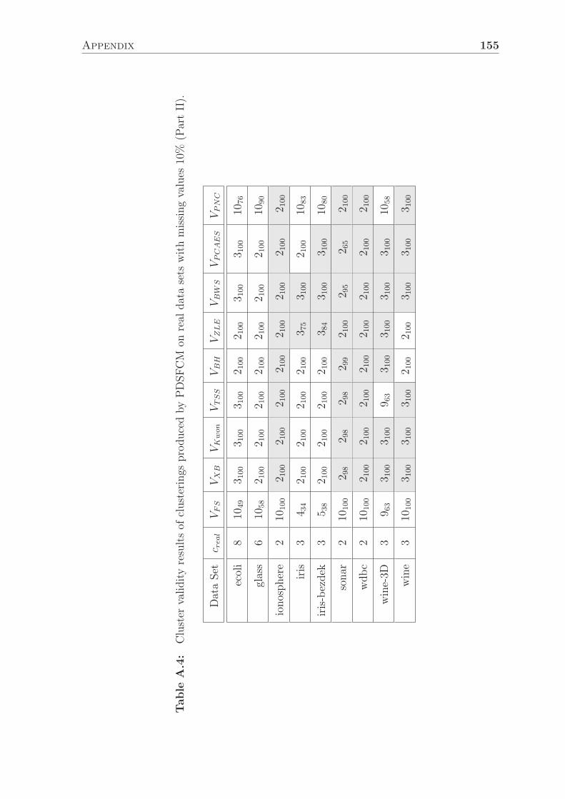
Appendix 155

Table

A.4:

Cluster

validityresultsof

clusterings

producedbyPDSFCM

onreal

datasets

withmissingvalues

10%

(PartII).

DataSet

c rea

lVFS

VXB

VKwon

VTSS

VBH

VZLE

VBW

SVPCAES

VPNC

ecoli

810

49

3 100

3 100

3 100

2 100

2 100

3 100

3 100

1076

glass

610

58

2 100

2 100

2 100

2 100

2 100

2 100

2 100

1090

ionosphere

210

100

2 100

2 100

2 100

2 100

2 100

2 100

2 100

2 100

iris

34 3

42 1

00

2 100

2 100

2 100

3 75

3 100

2 100

1083

iris-bezdek

35 3

82 1

00

2 100

2 100

2 100

3 84

3 100

3 100

1080

sonar

210

100

2 98

2 98

2 98

2 99

2 100

2 95

2 65

2 100

wdbc

210

100

2 100

2 100

2 100

2 100

2 100

2 100

2 100

2 100

wine-3D

39 6

33 1

00

3 100

9 63

3 100

3 100

3 100

3 100

1058

wine

310

100

3 100

3 100

3 100

2 100

2 100

3 100

3 100

3 100

156 Appendix

Table

A.5:

Cluster

validity

results

ofclu

sterings

produced

byPDSFCM

onsynthetic

data

setswith

missin

gvalu

es25%

(Part

I).

Data

Set

crea

lVPC

VNPC

VPE

VNPE

VKKLL

VOSIS

VOSIA

VOSIL

VOSIHγ

VOSIDγ

VFHV

VPD

3D-15

152100

725

2100

1429 (15

28 )

1541

1222

17100

2100

1636

1219 /13

19

1543

1746

10D-10

102100

2100

2100

2100

2100

2100

2100

2100

2100

2100

1735

1526 /17

26

3D-5-sep

52100

3100

2100

442 (5

39 )

3100

3100

10100

2100

2100

398

552

637

3D-5-ov

52100

2100

2100

442 (5

35 )

2100

3100

10100

2100

2100

377

674

944

3D-5-strov

52100

2100

2100

2100

2100

2100

10100

2100

2100

1099

671

661

3D-5-h

-sep5

2100

2100

2100

2100

2100

2100

10100

2100

2100

2100

650

652

3D-5-h

-ov5

2100

2100

2100

2100

2100

2100

10100

2100

2100

2100

660

654

3D-5-h

-strov5

2100

2100

2100

2100

2100

2100

10100

2100

2100

2100

1029

870

2D-3-sep

33100

3100

2100

3100

444 (3

43 )

355

10100

2100

397

345 /4

45

3100

382

2D-3-2-tog

32100

3100

2100

367

2100

297

10100

2100

2100

250

3100

3100

2D-3-2-ov

32100

2100

2100

2100

2100

2100

10100

2100

2100

2100

3100

383

2D-3-2-strov

32100

2100

2100

2100

2100

2100

10100

2100

2100

2100

375

1049

2D-3-3-tog

32100

3100

2100

3100

2100

361

10100

2100

2100

1095

3100

355

2D-3-3-ov

32100

3100

2100

1098

2100

2100

10100

2100

2100

2100

3100

1073

2D-3-3-strov

32100

2100

2100

10100

2100

2100

10100

2100

2100

10100

10100

10100

bensaid

32100

1034

2100

1059

469

441

1091

2100

472

1066

1058

1064

Appendix 157

Table

A.6:

Cluster

validityresultsof

clusterings

producedbyPDSFCM

onsynthetic

datasets

withmissingvalues

25%(P

artII).

DataSet

c rea

lVFS

VXB

VKwon

VTSS

VBH

VZLE

VBW

SVPCAES

VPNC

3D-15

1513

28

1442(15 4

1)

1442(15 4

1)

1442(15 4

1)

1442(15 4

1)

2 100

1543

1542

1542

10D-10

102 1

00

4 74

3 100

2 100

4 74

1724

1614

2 100

1733

3D-5-sep

55 3

95 8

45 8

45 8

45 8

45 6

15 8

44 6

510

26

3D-5-ov

54 4

22 1

00

2 100

2 100

2 100

5 93

5 93

4 58

7 60

3D-5-strov

55 4

32 1

00

2 100

2 100

2 100

2 100

2 100

4 56

1045

3D-5-h-sep

56 3

52 1

00

2 100

2 100

2 100

5 63

5 63

2 100

1023

3D-5-h-ov

55 4

12 1

00

2 100

2 100

2 100

5 69

2 100

2 100

5 69

3D-5-h-strov

56 3

32 1

00

2 100

2 100

2 100

2 100

2 100

2 100

1040

2D-3-sep

33 3

73 1

00

3 100

3 100

3 100

1036

3 100

3 100

3 73

2D-3-2-tog

34 3

92 1

00

2 100

2 100

3 100

1037

3 94

3 100

3 94

2D-3-2-ov

34 3

92 1

00

2 100

2 100

3 100

1049

3 100

3 100

3 100

2D-3-2-strov

32 5

52 1

00

2 100

2 100

2 100

1050

3 60

2 100

1064

2D-3-3-tog

34 6

13 1

00

3 100

3 100

3 100

8 31

3 100

3 100

1063

2D-3-3-ov

33 1

00

3 100

3 100

3 100

3 100

9 58

9 52

3 100

1095

2D-3-3-strov

35 1

00

2 100

2 100

2 100

3 100

6 100

6 51

3 100

10100

bensaid

37 3

87 4

12 6

42 1

00

7 47

1041

1049

2 100

1056

158 Appendix

Table

A.7:

Cluster

validity

results

ofclu

sterings

produced

byPDSFCM

onreal

data

setswith

missin

gvalu

es25%

(Part

I).

Data

Set

crea

lVPC

VNPC

VPE

VNPE

VKKLL

VOSIS

VOSIA

VOSIL

VOSIHγ

VOSIDγ

VFHV

VPD

ecoli8

2100

3100

2100

3100

2100

3100

10100

2100

2100

10100

1069

1058

glass6

2100

2100

2100

2100

2100

2100

10100

2100

2100

10100

843

837

ionosp

here

22100

2100

2100

2100

2100

2100

10100

2100

2100

10100

2100

2100

iris3

2100

2100

2100

2100

2100

2100

10100

2100

2100

2100

1059

874

iris-bezd

ek3

2100

2100

2100

2100

2100

2100

10100

2100

2100

2100

1051

1074

sonar

22100

299

2100

298

2100

299

10100

2100

2100

10100

2100

2100

wdbc

22100

2100

2100

2100

2100

2100

10100

2100

2100

10100

8100

7100

wine-3D

32100

3100

2100

3100

3100

3100

10100

2100

2100

354

1075

1076

wine

32100

2100

2100

3100

2100

3100

10100

2100

2100

10100

3100

288

Appendix 159

Table

A.8:

Cluster

validityresultsof

clusterings

producedbyPDSFCM

onreal

datasets

withmissingvalues

25%

(PartII).

DataSet

c rea

lVFS

VXB

VKwon

VTSS

VBH

VZLE

VBW

SVPCAES

VPNC

ecoli

810

49

3 100

3 100

3 100

2 100

2 100

3 100

3 100

1071

glass

67 3

02 1

00

2 100

2 100

2 100

2 100

2 100

2 100

1053

ionosphere

210

100

2 100

2 100

2 100

2 100

2 100

2 100

2 100

2 100

iris

36 6

32 1

00

2 100

2 100

2 100

6 72

3 100

3 100

1077

iris-bezdek

35 4

22 1

00

2 100

2 100

2 100

3 80

3 100

3 100

1077

sonar

210

100

2 100

2 100

2 100

2 100

2 100

2 99

2 68

2 100

wdbc

210

100

2 100

2 100

2 100

2 100

2 100

2 100

2 100

2 100

wine-3D

39 4

33 1

00

3 100

3 70

3 100

3 100

3 34

3 100

1082

wine

310

100

3 100

3 100

3 100

2 100

2 100

3 100

3 100

4 100

160 Appendix

Table

A.9:

Cluster

validity

results

ofclu

sterings

produced

byPDSFCM

onsynthetic

data

setswith

missin

gvalu

es40%

(Part

I).

Data

Set

crea

lVPC

VNPC

VPE

VNPE

VKKLL

VOSIS

VOSIA

VOSIL

VOSIHγ

VOSIDγ

VFHV

VPD

3D-15

152100

738

2100

1748

1757

360

17100

2100

299

1751

1759

1777

10D-10

102100

2100

2100

2100

2100

299

1796

2100

267

239

1727

1521

3D-5-sep

52100

492

2100

644

645

472

10100

2100

2100

1040

1063

1070

3D-5-ov

52100

3100

2100

743

2100

2100

10100

2100

2100

1086

1061

1070

3D-5-strov

52100

4100

2100

633

277

498

10100

2100

2100

1087

1083

1085

3D-5-h

-sep5

2100

2100

2100

298

2100

2100

10100

2100

2100

2100

1073

856

3D-5-h

-ov5

2100

2100

2100

2100

2100

2100

10100

2100

2100

298

1076

1060

3D-5-h

-strov5

2100

2100

2100

271

2100

262

10100

2100

2100

1091

1079

852

2D-3-sep

33100

3100

2100

3100

395

3100

10100

2100

350

3100

1050

1048

2D-3-2-tog

32100

3100

2100

3100

256

3100

10100

2100

354

3100

1060

1064

2D-3-2-ov

32100

2100

2100

264

2100

2100

10100

2100

1036

2100

1064

1062

2D-3-2-strov

32100

2100

2100

285

2100

2100

10100

2100

1054

2100

1080

1082

2D-3-3-tog

32100

3100

2100

1059

390

3100

10100

2100

1045

396

1064

1072

2D-3-3-ov

32100

394

2100

1061

378

394

10100

2100

1042

1082

1071

1088

2D-3-3-strov

32100

285

2100

1077

2100

2100

10100

2100

243

1099

1076

1071

bensaid

3241

931

2100

1041

726 /9

26

932

1088

2100

930

1049

725

725

Appendix 161

Table

A.10:

Cluster

validityresultsof

clusterings

producedbyPDSFCM

onsynthetic

datasets

withmissingvalues

40%(P

artII).

DataSet

c rea

lVFS

VXB

VKwon

VTSS

VBH

VZLE

VBW

SVPCAES

VPNC

3D-15

158 3

114

46

1446

1446

1447

3 100

1732

1433

1762

10D-10

102 1

00

4 100

3 100

3 100

4 100

1733

1014

3 100

1743

3D-5-sep

54 4

15 7

45 7

42 1

00

5 74

4 57

5 74

4 57

1072

3D-5-ov

55 3

92 1

00

2 100

2 100

2 100

5 74

5 85

4 67

1070

3D-5-strov

56 3

42 1

00

2 100

2 100

2 100

5 51

5 89

4 59

1082

3D-5-h-sep

55 5

22 1

00

2 100

2 100

2 100

5 61

6 58

2 100

1088

3D-5-h-ov

55 3

62 1

00

2 100

2 100

2 100

6 55

2 100

2 100

1080

3D-5-h-strov

55 3

82 1

00

2 100

2 100

2 100

5 61

2 100

2 100

1081

2D-3-sep

33 8

23 1

00

3 100

3 100

3 100

1043

1039

3 100

1067

2D-3-2-tog

34 3

62 1

00

2 100

2 100

3 100

1068

1053

3 100

1077

2D-3-2-ov

34 3

72 1

00

2 100

2 100

3 100

1073

1054

3 53

1075

2D-3-2-strov

32 5

02 1

00

2 100

2 100

2 100

1079

1071

2 100

1081

2D-3-3-tog

33 7

13 1

00

3 100

3 100

3 100

1050

1055

3 100

1071

2D-3-3-ov

38 3

03 1

00

3 100

2 100

3 100

1069

1058

3 100

1072

2D-3-3-strov

310

38

2 100

2 100

2 100

1046

1087

1081

3 100

1077

bensaid

36 2

37 3

62 3

12 1

00

7 37

1040

1048

2 48

1033

162 Appendix

Table

A.11:

Cluster

validity

results

ofclu

sterings

produced

byPDSFCM

onreal

data

setswith

missin

gvalu

es40%

(Part

I).

Data

Set

crea

lVPC

VNPC

VPE

VNPE

VKKLL

VOSIS

VOSIA

VOSIL

VOSIHγ

VOSIDγ

VFHV

VPD

ecoli8

2100

2100

2100

2100

2100

2100

10100

2100

2100

10100

1085

1090

glass6

2100

2100

2100

595

2100

2100

10100

2100

2100

10100

1063

1078

ionosp

here

22100

2100

2100

2100

2100

2100

10100

2100

2100

10100

2100

2100

iris3

2100

2100

2100

2100

2100

2100

10100

2100

2100

2100

736

727

iris-bezd

ek3

2100

2100

2100

2100

2100

2100

10100

2100

2100

2100

1032

1041

sonar

22100

298

2100

298

2100

298

10100

2100

2100

10100

2100

2100

wdbc

22100

2100

2100

2100

2100

2100

10100

2100

2100

10100

2100

2100

wine-3D

32100

3100

2100

1050

2100

2100

10100

2100

2100

1074

1057

1064

wine

32100

3100

2100

3100

2100

3100

10100

2100

2100

10100

3100

3100

Appendix 163

Table

A.12:

Cluster

validityresultsof

clusterings

producedbyPDSFCM

onreal

datasets

withmissingvalues

40%

(PartII).

DataSet

c rea

lVFS

VXB

VKwon

VTSS

VBH

VZLE

VBW

SVPCAES

VPNC

ecoli

810

54

3 100

3 100

3 100

2 100

2 100

3 100

3 81

1077

glass

69 3

92 1

00

2 100

2 100

2 100

2 100

5 100

2 100

6 35

ionosphere

210

100

2 100

2 100

2 100

2 100

2 100

2 100

2 100

2 100

iris

34 4

32 1

00

2 100

2 100

2 100

5 40

3 93

3 100

9 31

iris-bezdek

35 3

42 1

00

2 100

2 100

2 100

3 70

3 100

3 100

1055

sonar

210

100

2 99

2 99

2 99

2 100

2 100

2 98

2 65

2 100

wdbc

210

100

2 100

2 100

2 100

2 100

2 100

2 100

2 100

2 100

wine-3D

310

43

3 94

3 95

9 52

1047

9 32

1047

3 57

1065

wine

38 5

53 1

00

3 100

3 100

2 100

2 100

3 100

3 100

9 83

164 Appendix

Table

A.13:

Cluster

validity

results

ofclu

sterings

produced

byOCSFCM

onsynthetic

data

setswith

missin

gvalu

es10%

(Part

I).

Data

Set

crea

lVPC

VNPC

VPE

VNPE

VKKLL

VOSIS

VOSIA

VOSIL

VOSIHγ

VOSIDγ

VFHV

VPD

3D-15

1515

53

1553

2100

1551

1548

1553

17100

2100

1639 (15

35 )

1553

1553

1553

10D-10

10392

392

392

392

392

392

392

2100

392

392

1391

1391

3D-5-sep

52100

289

2100

586

584

584

10100

2100

576

586

583

581

3D-5-ov

52100

2100

2100

2100

2100

2100

10100

2100

2100

2100

589

582

3D-5-strov

52100

2100

2100

2100

2100

2100

10100

2100

2100

2100

587

557

3D-5-h

-sep5

2100

2100

2100

2100

2100

2100

10100

2100

653

2100

567

567

3D-5-h

-ov5

2100

2100

2100

2100

2100

2100

10100

2100

2100

2100

571

565

3D-5-h

-strov5

2100

2100

2100

2100

2100

2100

10100

2100

2100

2100

565

552

2D-3-sep

33100

3100

3100

3100

3100

3100

10100

2100

732

3100

3100

3100

2D-3-2-tog

3295

3100

2100

3100

3100

3100

10100

2100

742

3100

3100

3100

2D-3-2-ov

32100

3100

2100

3100

3100

3100

10100

2100

398

3100

3100

3100

2D-3-2-strov

32100

2100

2100

2100

2100

2100

10100

2100

2100

2100

385

385

2D-3-3-tog

33100

3100

2100

3100

3100

3100

10100

2100

695

3100

3100

3100

2D-3-3-ov

32100

3100

2100

3100

3100

3100

10100

2100

398

3100

3100

3100

2D-3-3-strov

32100

2100

2100

3100

397

2100

10100

2100

2100

2100

3100

399

bensaid

3294

475

2100

1041

479

543

1097

2100

485

1080

1071

1051

Appendix 165

Table

A.14:

Cluster

validityresultsof

clusterings

producedbyOCSFCM

onsynthetic

datasets

withmissingvalues

10%(P

artII).

DataSet

c rea

lVFS

VXB

VKwon

VTSS

VBH

VZLE

VBW

SVPCAES

VPNC

3D-15

1515

51

1553

1553

1553

1553

2 50/15 5

015

53

1435(15 3

3)

1544

10D-10

102 1

00

3 92

3 100

2 100

1392

1391

1391

2 100

1528

3D-5-sep

55 6

42 1

00

2 100

2 100

2 100

5 83

5 86

2 76

5 69

3D-5-ov

55 7

12 1

00

2 100

2 100

2 100

5 89

5 89

2 68

5 86

3D-5-strov

55 6

72 1

00

2 100

2 100

2 100

5 84

2 94

2 44

5 84

3D-5-h-sep

55 4

92 1

00

2 100

2 100

2 100

5 67

5 67

2 100

5 59

3D-5-h-ov

55 4

82 1

00

2 100

2 100

2 100

5 71

5 67

2 100

5 69

3D-5-h-strov

55 4

02 1

00

2 100

2 100

2 100

2 64

2 100

2 100

5 64

2D-3-sep

33 4

13 1

00

3 100

3 100

3 100

7 28

3 92

3 86

3 100

2D-3-2-tog

33 3

82 1

00

2 100

2 100

3 100

7 31

3 96

3 72

3 100

2D-3-2-ov

33 4

83 1

00

3 100

2 100

3 100

6 53

3 79

3 87

3 100

2D-3-2-strov

33 3

12 1

00

2 100

2 100

2 100

9 31

3 80

2 96

3 85

2D-3-3-tog

33 5

73 1

00

3 100

3 100

3 100

7 37

3 94

3 86

3 100

2D-3-3-ov

33 4

83 1

00

3 100

2 100

3 100

6 53

3 79

3 87

3 100

2D-3-3-strov

33 3

22 1

00

2 100

2 100

2 100

6 67

3 43

3 81

3 100

bensaid

37 2

35 2

62 4

62 1

00

6 25

5 33

1062

2 42

1064

166 Appendix

Table

A.15:

Cluster

validity

results

ofclu

sterings

produced

byOCSFCM

onreal

data

setswith

missin

gvalu

es10%

(Part

I).

Data

Set

crea

lVPC

VNPC

VPE

VNPE

VKKLL

VOSIS

VOSIA

VOSIL

VOSIHγ

VOSIDγ

VFHV

VPD

ecoli8

2100

3100

2100

3100

2100

3100

10100

2100

2100

10100

5100

1074

glass6

2100

2100

2100

2100

2100

2100

10100

2100

2100

2100

1088

1087

ionosp

here

22100

2100

2100

2100

2100

2100

10100

2100

2100

10100

2100

2100

iris3

2100

2100

2100

2100

2100

2100

10100

2100

2100

2100

1072

1065

iris-bezd

ek3

2100

2100

2100

2100

2100

2100

10100

2100

2100

2100

1085

1041

sonar

22100

297

2100

296

2100

298

10100

2100

2100

10100

2100

2100

wdbc

22100

2100

2100

2100

2100

2100

10100

2100

2100

10100

3100

4100

wine-3D

32100

3100

2100

389

2100

3100

10100

2100

2100

1068

1059

1047

wine

32100

3100

2100

3100

2100

3100

10100

2100

2100

10100

3100

2100

Appendix 167

Table

A.16:

Cluster

validityresultsof

clusterings

producedbyOCSFCM

onreal

datasets

withmissingvalues

10%

(PartII).

DataSet

c rea

lVFS

VXB

VKwon

VTSS

VBH

VZLE

VBW

SVPCAES

VPNC

ecoli

810

78

3 100

3 100

3 100

2 100

2 100

3 100

3 100

1071

glass

64 5

42 1

00

2 100

2 100

2 100

2 100

2 100

2 100

1078

ionosphere

210

80

2 100

2 100

2 100

2 100

2 100

2 100

2 100

2 100

iris

35 4

32 1

00

2 100

2 100

2 100

3 77

3 100

3 56

1072

iris-bezdek

35 3

82 1

00

2 100

2 100

2 100

3 79

3 100

3 100

1075

sonar

210

100

2 99

2 99

2 99

2 100

2 100

2 97

2 71

2 100

wdbc

210

100

2 100

2 100

2 100

2 100

2 100

2 100

2 100

2 100

wine-3D

39 3

53 1

00

3 100

9 46

3 100

3 100

5 84

3 100

1056

wine

310

100

3 100

3 100

3 100

2 100

2 100

3 100

3 100

3 100

168 Appendix

Table

A.17:

Cluster

validity

results

ofclu

sterings

produced

byOCSFCM

onsynthetic

data

setswith

missin

gvalu

es25%

(Part

I).

Data

Set

crea

lVPC

VNPC

VPE

VNPE

VKKLL

VOSIS

VOSIA

VOSIL

VOSIHγ

VOSIDγ

VFHV

VPD

3D-15

15287

1526

2100

1528

1735

1532

1798

2100

268

1535

1737 (15

30 )

1529 /17

29

10D-10

10398

398

398

398

398

398

398

2100

398

398

1418

1414 /16

14

3D-5-sep

52100

2100

2100

582

564

557

10100

2100

565

575

552

536

3D-5-ov

52100

2100

2100

2100

2100

2100

10100

2100

2100

2100

640

632

3D-5-strov

52100

2100

2100

2100

2100

2100

10100

2100

2100

2100

537

628

3D-5-h

-sep5

2100

2100

2100

2100

2100

2100

10100

2100

650

2100

633

735

3D-5-h

-ov5

2100

2100

2100

2100

2100

2100

10100

2100

2100

2100

649

644

3D-5-h

-strov5

2100

2100

2100

2100

2100

2100

10100

2100

2100

2100

728

842

2D-3-sep

33100

3100

3100

3100

3100

3100

10100

2100

941

3100

3100

390

2D-3-2-tog

3293

3100

2100

3100

3100

3100

10100

2100

833

3100

3100

389

2D-3-2-ov

32100

2100

2100

2100

2100

2100

10100

2100

840

2100

3100

380

2D-3-2-strov

32100

2100

2100

2100

2100

2100

2100

2100

2100

2100

374

335

2D-3-3-tog

33100

3100

2100

3100

3100

3100

10100

2100

659

3100

3100

384

2D-3-3-ov

32100

3100

2100

3100

3100

3100

10100

2100

360

3100

3100

396

2D-3-3-strov

32100

298

2100

3100

3100

2100

10100

2100

294

296

1035 (3

21 )

1063

bensaid

32100

435

2100

1033

348

348

1086

2100

457

1061

1045

1038

Appendix 169

Table

A.18:

Cluster

validityresultsof

clusterings

producedbyOCSFCM

onsynthetic

datasets

withmissingvalues

25%(P

artII).

DataSet

c rea

lVFS

VXB

VKwon

VTSS

VBH

VZLE

VBW

SVPCAES

VPNC

3D-15

1515

26

1234/13 3

412

34/13 3

412

34/13 3

415

27

2 99

1532

1227

1747

10D-10

102 1

00

3 98

3 100

2 100

3 27

1027

1215

2 100

1626

3D-5-sep

55 5

62 1

00

2 100

2 100

2 99

5 68

5 77

2 48

5 27

3D-5-ov

55 4

02 1

00

2 100

2 100

2 100

5 65

5 60

2 47

5 34/6

34

3D-5-strov

55 4

22 1

00

2 100

2 100

2 100

5 56

2 82

2 64

6 34(5

29)

3D-5-h-sep

55 4

12 1

00

2 100

2 100

2 100

6 47

5 59

2 98

6 24

3D-5-h-ov

55 3

42 1

00

2 100

2 100

2 100

5 52

5 42

2 99

6 24

3D-5-h-strov

55 3

42 1

00

2 100

2 100

2 100

2 37(5

34)

2 100

2 100

7 29

2D-3-sep

33 4

23 1

00

3 100

3 100

3 100

1039

3 62

2 65

3 52

2D-3-2-tog

33 3

82 1

00

2 100

2 100

3 100

1050

3 53

2 79

3 65

2D-3-2-ov

34 3

3(3

31)

2 100

2 100

2 100

3 100

1040

3 50

2 94

3 52

2D-3-2-strov

33 4

12 1

00

2 100

2 100

2 97

1053

3 36

2 99

3 30

2D-3-3-tog

33 3

93 1

00

3 100

3 100

3 100

8 37

3 53

2 60

3 50

2D-3-3-ov

33 3

93 1

00

3 100

2 93

3 100

1033

3 43

2 50(3

47)

3 45

2D-3-3-strov

36 1

7/7

17

2 100

2 100

2 100

2 66

8 38

6 20

2 60

1038

bensaid

34 3

13 4

82 5

2(3

48)

2 100

5 24/6

24

9 26/10 2

610

49

2 62

1048

170 Appendix

Table

A.19:

Cluster

validity

results

ofclu

sterings

produced

byOCSFCM

onreal

data

setswith

missin

gvalu

es25%

(Part

I).

Data

Set

crea

lVPC

VNPC

VPE

VNPE

VKKLL

VOSIS

VOSIA

VOSIL

VOSIHγ

VOSIDγ

VFHV

VPD

ecoli8

2100

3100

2100

3100

2100

3100

10100

2100

2100

398

939

942

glass6

2100

2100

2100

2100

2100

2100

10100

2100

2100

2100

976

973

ionosp

here

22100

2100

2100

2100

2100

2100

10100

2100

2100

10100

290

2100

iris3

2100

2100

2100

2100

2100

2100

10100

2100

2100

2100

1044

1040

iris-bezd

ek3

2100

2100

2100

2100

2100

2100

10100

2100

2100

2100

1035

1050

sonar

22100

298

2100

295

2100

299

10100

2100

2100

10100

2100

2100

wdbc

22100

2100

2100

2100

2100

2100

10100

2100

2100

10100

3100

3100

wine-3D

3295

3100

296

398

398

3100

10100

2100

387

389

1069

1056

wine

32100

3100

2100

3100

2100

3100

10100

2100

2100

10100

4100

4100

Appendix 171

Table

A.20:

Cluster

validityresultsof

clusterings

producedbyOCSFCM

onreal

datasets

withmissingvalues

25%

(PartII).

DataSet

c rea

lVFS

VXB

VKwon

VTSS

VBH

VZLE

VBW

SVPCAES

VPNC

ecoli

810

38

3 100

3 100

3 100

2 100

2 100

3 100

3 100

1075

glass

68 3

42 1

00

2 100

2 100

2 100

2 100

2 100

2 100

1092

ionosphere

210

100

2 100

2 100

2 100

2 100

2 100

2 100

2 100

2 93

iris

37 4

02 1

00

2 100

2 100

2 100

5 36(3

30)

3 95

3 100

1048

iris-bezdek

34 4

42 1

00

2 100

2 100

2 100

5 55

3 99

3 66

1057

sonar

210

100

2 99

2 99

2 99

2 100

2 100

2 97

2 63

2 100

wdbc

210

100

2 100

2 100

2 100

2 100

2 100

2 100

2 100

2 100

wine-3D

38 3

33 1

00

3 100

3 53

3 100

3 99

3 50

3 88

1069

wine

310

99

3 100

3 100

3 100

2 100

2 100

3 100

3 100

4 100

172 Appendix

Table

A.21:

Cluster

validity

results

ofclu

sterings

produced

byOCSFCM

onsynthetic

data

setswith

missin

gvalu

es40%

(Part

I).

Data

Set

crea

lVPC

VNPC

VPE

VNPE

VKKLL

VOSIS

VOSIA

VOSIL

VOSIHγ

VOSIDγ

VFHV

VPD

3D-15

152100

1116 /12

16

2100

1617 (14

15 /15

15 )

298

1618

1799

2100

286

1424

1731

1730

10D-10

10398

398

398

398

398

398

398

2100

398

398

657

651

3D-5-sep

52100

277

2100

244

372

437

10100

2100

630

353

1031

1030

3D-5-ov

52100

2100

2100

299

295

290

10100

2100

2100

298

924

1028

3D-5-strov

52100

2100

2100

2100

2100

2100

10100

2100

2100

2100

1036

1035

3D-5-h

-sep5

2100

2100

2100

299

2100

2100

10100

2100

633

2100

1044

829

3D-5-h

-ov5

2100

2100

2100

2100

2100

2100

10100

2100

2100

2100

1054

835

3D-5-h

-strov5

2100

2100

2100

2100

2100

2100

10100

2100

2100

2100

1041

845

2D-3-sep

33100

3100

3100

3100

3100

3100

380

2100

1046

3100

927

518 /9

18

2D-3-2-tog

3358

3100

2100

3100

3100

3100

1091

2100

1058

3100

1049

1017

2D-3-2-ov

32100

2100

2100

298

2100

2100

2100

2100

1058

2100

1042

1031

2D-3-2-strov

32100

2100

2100

2100

2100

2100

2100

2100

1040

2100

1051

1040

2D-3-3-tog

33100

3100

297

3100

3100

3100

10100

2100

940 /10

40

3100

1045

1027

2D-3-3-ov

32100

3100

2100

3100

3100

3100

10100

2100

944

3100

1063

1057

2D-3-3-strov

32100

2100

2100

248

369

2100

10100

2100

725 /8

25

2100

1061

1046

bensaid

3282

1032

2100

1042

923

932

1077

2100

927

1054

922

1023

Appendix 173

Table

A.22:

Cluster

validityresultsof

clusterings

producedbyOCSFCM

onsynthetic

datasets

withmissingvalues

40%(P

artII).

DataSet

c rea

lVFS

VXB

VKwon

VTSS

VBH

VZLE

VBW

SVPCAES

VPNC

3D-15

1516

17

1022

1022

1022

4 46

3 55

1621(15 1

8)

9 16

1634/17 3

4

10D-10

102 5

23 9

83 1

00

3 100

3 98

7 60

6 50

2 100

1728

3D-5-sep

56 3

92 1

00

2 100

2 100

2 95

6 39

6 38(5

34)

2 46

1040

3D-5-ov

55 2

72 1

00

2 100

2 100

2 100

5 50

5 30

2 49

1032

3D-5-strov

57 2

72 1

00

2 100

2 100

2 100

5 47

2 53

2 48

1036

3D-5-h-sep

55 3

02 1

00

2 100

2 100

2 100

6 37

6 41(5

39)

2 90

1045

3D-5-h-ov

55 2

7(6

26)

2 100

2 100

2 100

2 100

5 40

2 29(4

28)

2 86

1056

3D-5-h-strov

55 2

82 1

00

2 100

2 100

2 100

3 23/4

23

2 87

2 84

1045

2D-3-sep

33 3

53 1

00

3 100

3 100

3 100

1047

3 32

2 69

1041

2D-3-2-tog

33 2

72 1

00

2 100

2 100

3 100

1061

3 19

2 89

1047

2D-3-2-ov

34 3

32 1

00

2 100

2 100

3 95

1054

1018(3

16)

2 99

1048

2D-3-2-strov

33 3

32 1

00

2 100

2 100

2 87

1067

1024

2 100

1040

2D-3-3-tog

33 2

93 1

00

3 100

3 100

3 100

1051

6 20

2 70

1051

2D-3-3-ov

33 2

42 6

12 8

12 1

00

3 99

1053

9 30

2 70

1051

2D-3-3-strov

35 2

22 1

00

2 100

2 100

2 69

1058

1033

2 64

1051

bensaid

39 2

710

19

2 52

2 100

9 30

1035

9 28

2 73

1030

174 Appendix

Table

A.23:

Cluster

validity

results

ofclu

sterings

produced

byOCSFCM

onreal

data

setswith

missin

gvalu

es40%

(Part

I).

Data

Set

crea

lVPC

VNPC

VPE

VNPE

VKKLL

VOSIS

VOSIA

VOSIL

VOSIHγ

VOSIDγ

VFHV

VPD

ecoli8

2100

2100

2100

385

2100

3100

10100

2100

2100

397

1056

1058

glass6

2100

2100

2100

2100

2100

2100

10100

2100

2100

2100

425 (6

22 )

432 (6

22 )

ionosp

here

22100

299

2100

299

299

299

10100

2100

2100

1099

299

2100

iris3

2100

2100

2100

2100

2100

2100

10100

2100

2100

2100

830

933

iris-bezd

ek3

2100

2100

2100

2100

2100

2100

10100

2100

2100

2100

925

931

sonar

22100

271

2100

264

2100

272

10100

2100

2100

10100

2100

2100

wdbc

22100

2100

2100

2100

2100

2100

10100

2100

2100

2100

269

269

wine-3D

3289

363

2100

1027

270

374

10100

2100

263

1066

725

830

wine

32100

3100

2100

3100

2100

3100

10100

2100

2100

10100

3100

398

Appendix 175

Table

A.24:

Cluster

validityresultsof

clusterings

producedbyOCSFCM

onreal

datasets

withmissingvalues

40%

(PartII).

DataSet

c rea

lVFS

VXB

VKwon

VTSS

VBH

VZLE

VBW

SVPCAES

VPNC

ecoli

810

36

3 100

3 100

3 100

2 100

2 100

3 100

3 100

1061

glass

67 2

22 1

00

2 100

2 100

2 100

2 100

2 85

2 100

6 22

ionosphere

210

99

2 100

2 100

2 99

2 100

2 100

2 99

2 100

2 99

iris

34 3

12 1

00

2 100

2 100

2 99

5 30

3 39

3 92

1039

iris-bezdek

310

24

2 100

2 100

2 100

2 100

3 48

3 100

3 92

1038

sonar

210

100

2 81

2 81

1032(2

24)

2 84

2 100

2 97

2 65

2 100

wdbc

210

87

2 100

2 100

2 100

2 100

2 100

2 100

2 100

2 100

wine-3D

310

32

3 67

3 75

9 54

3 54

3 65

7 23

3 44

1037

wine

310

42

3 100

3 100

3 100

2 100

2 100

3 100

3 100

4 77

176 Appendix

Table

A.25:

Cluster

validity

results

ofclu

sterings

produced

byNPSFCM

onsynthetic

data

setswith

missin

gvalu

es10%

(Part

I).

Data

Set

crea

lVPC

VNPC

VPE

VNPE

VKKLL

VOSIS

VOSIA

VOSIL

VOSIHγ

VOSIDγ

VFHV

VPD

3D-15

1515

63

1563

2100

1563

1563

1563

17100

2100

1563

1563

1563

1563

10D-10

10399

399

399

399

399

399

399

2100

399

399

1734

1742

3D-5-sep

52100

582

2100

582

582

582

10100

2100

582

582

582

582

3D-5-ov

52100

2100

2100

2100

2100

2100

10100

2100

2100

2100

593

593

3D-5-strov

52100

2100

2100

2100

2100

2100

10100

2100

2100

2100

584

657

3D-5-h

-sep5

2100

2100

2100

2100

2100

2100

10100

2100

662

2100

575

575

3D-5-h

-ov5

2100

2100

2100

2100

2100

2100

10100

2100

2100

2100

558

550

3D-5-h

-strov5

2100

2100

2100

2100

2100

2100

10100

2100

2100

2100

563

550

2D-3-sep

33100

3100

3100

3100

3100

3100

10100

2100

834

3100

3100

3100

2D-3-2-tog

32100

3100

2100

3100

3100

3100

10100

2100

737 (8

35 )

3100

3100

3100

2D-3-2-ov

32100

2100

2100

2100

2100

2100

10100

2100

746

2100

3100

3100

2D-3-2-strov

32100

2100

2100

2100

2100

2100

2100

2100

2100

2100

387

387

2D-3-3-tog

33100

3100

2100

3100

3100

3100

10100

2100

698

3100

3100

3100

2D-3-3-ov

32100

3100

2100

3100

3100

3100

10100

2100

643

3100

3100

3100

2D-3-3-strov

32100

2100

2100

3100

3100

2100

10100

2100

2100

2100

3100

3100

bensaid

3293

447

2100

1066

453

549

1099

2100

475

1091

1074

1058

Appendix 177

Table

A.26:

Cluster

validityresultsof

clusterings

producedbyNPSFCM

onsynthetic

datasets

withmissingvalues

10%(P

artII).

DataSet

c rea

lVFS

VXB

VKwon

VTSS

VBH

VZLE

VBW

SVPCAES

VPNC

3D-15

1515

63

1563

1563

1563

1563

1563

1563

1563

1563

10D-10

102 1

00

3 99

3 100

2 100

1420/15 2

017

43

9 26

2 99

1751

3D-5-sep

55 7

12 1

00

2 100

2 100

2 100

5 82

5 82

2 100

5 82

3D-5-ov

55 9

22 1

00

2 100

2 100

2 100

5 93

5 93

4 71

5 93

3D-5-strov

55 5

72 1

00

2 100

2 100

2 100

5 84

5 84

4 71

5 84

3D-5-h-sep

55 4

22 1

00

2 100

2 100

2 100

5 75

5 75

2 100

5 74

3D-5-h-ov

55 3

32 1

00

2 100

2 100

2 100

5 58

5 58

2 100

5 58

3D-5-h-strov

55 4

02 1

00

2 100

2 100

2 100

2 64

2 100

2 100

5 64

2D-3-sep

33 4

53 1

00

3 100

3 100

3 100

7 24/8

24

3 100

3 100

3 100

2D-3-2-tog

33 3

7/4

37

2 100

2 100

2 100

3 100

9 32

3 100

3 100

3 100

2D-3-2-ov

34 5

02 1

00

2 100

2 100

3 100

9 37

3 100

3 98

3 100

2D-3-2-strov

34 3

4/2

33

2 100

2 100

2 100

2 100

9 38

3 87

2 82

3 87

2D-3-3-tog

33 6

03 1

00

3 100

3 100

3 100

7 44

3 97

3 100

3 100

2D-3-3-ov

34 4

23 1

00

3 100

2 100

3 100

6 85

3 72

3 100

3 100

2D-3-3-strov

33 3

22 1

00

2 100

2 100

2 100

6 68

3 36

3 100

3 100

bensaid

37 3

56 3

75 5

02 1

00

6 73

5 52

1068

6 60

1080

178 Appendix

Table

A.27:

Cluster

validity

results

ofclu

sterings

produced

byNPSFCM

onreal

data

setswith

missin

gvalu

es10%

(Part

I).

Data

Set

crea

lVPC

VNPC

VPE

VNPE

VKKLL

VOSIS

VOSIA

VOSIL

VOSIHγ

VOSIDγ

VFHV

VPD

ecoli8

2100

3100

2100

3100

2100

3100

10100

2100

2100

10100

559

1085

glass6

2100

2100

2100

2100

2100

2100

10100

2100

2100

2100

1089

1089

ionosp

here

22100

2100

2100

2100

2100

2100

10100

2100

2100

10100

2100

2100

iris3

2100

2100

2100

2100

2100

2100

10100

2100

2100

2100

1084

1048

iris-bezd

ek3

2100

2100

2100

2100

2100

2100

10100

2100

2100

2100

1076

1055

sonar

22100

299

2100

299

2100

299

10100

2100

2100

10100

2100

2100

wdbc

22100

2100

2100

2100

2100

2100

10100

2100

2100

10100

5100

5100

wine-3D

32100

3100

2100

3100

2100

3100

10100

2100

2100

1083

1065

835

wine

32100

3100

2100

3100

2100

3100

10100

2100

2100

10100

3100

2100

Appendix 179

Table

A.28:

Cluster

validityresultsof

clusterings

producedbyNPSFCM

onreal

datasets

withmissingvalues

10%

(PartII).

DataSet

c rea

lVFS

VXB

VKwon

VTSS

VBH

VZLE

VBW

SVPCAES

VPNC

ecoli

810

85

3 100

3 100

3 100

2 100

2 100

3 100

3 100

1078

glass

610

68

2 100

2 100

2 100

2 100

2 100

2 100

2 100

1093

ionosphere

210

68

2 100

2 100

2 100

2 100

2 100

2 100

2 100

2 99

iris

35 4

72 1

00

2 100

2 100

2 100

3 80

3 99

3 99

1085

iris-bezdek

36 3

12 1

00

2 100

2 100

2 100

3 75

3 100

3 100

1082

sonar

210

100

2 99

2 99

2 99

2 100

2 100

2 99

2 62

2 100

wdbc

210

100

2 100

2 100

2 100

2 100

2 100

2 100

2 100

2 100

wine-3D

39 3

53 1

00

3 100

3 58

3 100

3 100

5 100

3 100

1060

wine

310

100

3 100

3 100

3 100

2 100

2 100

3 100

3 100

3 100

180 Appendix

Table

A.29:

Cluster

validity

results

ofclu

sterings

produced

byNPSFCM

onsynthetic

data

setswith

missin

gvalu

es25%

(Part

I).

Data

Set

crea

lVPC

VNPC

VPE

VNPE

VKKLL

VOSIS

VOSIA

VOSIL

VOSIHγ

VOSIDγ

VFHV

VPD

3D-15

1514

48

1449

2100

1441

1433

1445

17100

2100

1529 /14

29

1450

1429 /15

28

1528

10D-10

10475

475

475

475

475

475

475

2100

475

475

531

533

3D-5-sep

52100

583

2100

583

583

583

10100

2100

565

583

641

1024

3D-5-ov

52100

2100

2100

2100

2100

2100

10100

2100

2100

2100

651

1036

3D-5-strov

52100

2100

2100

2100

2100

2100

10100

2100

2100

2100

1032

1046

3D-5-h

-sep5

2100

2100

2100

2100

2100

2100

10100

2100

661

2100

644

644

3D-5-h

-ov5

2100

2100

2100

2100

2100

2100

10100

2100

2100

2100

1039

851

3D-5-h

-strov5

2100

2100

2100

2100

2100

2100

10100

2100

2100

2100

1038

864

2D-3-sep

33100

3100

3100

3100

3100

3100

10100

2100

1029

3100

364

1037 (3

29 )

2D-3-2-tog

3294

3100

2100

3100

3100

3100

10100

2100

831

3100

3100

378

2D-3-2-ov

32100

2100

2100

2100

2100

2100

10100

2100

733

2100

355

336

2D-3-2-strov

32100

2100

2100

2100

2100

2100

2100

2100

2100

2100

356

928 /10

28

2D-3-3-tog

33100

3100

2100

3100

3100

3100

10100

2100

646

3100

361

336

2D-3-3-ov

32100

3100

2100

3100

3100

3100

10100

2100

653

3100

365

350

2D-3-3-strov

32100

266

2100

3100

3100

2100

10100

2100

256

377

1067

1082

bensaid

32100

434

2100

1061

352

352

1091

2100

454

1070

931

929

Appendix 181

Table

A.30:

Cluster

validityresultsof

clusterings

producedbyNPSFCM

onsynthetic

datasets

withmissingvalues

25%(P

artII).

DataSet

c rea

lVFS

VXB

VKwon

VTSS

VBH

VZLE

VBW

SVPCAES

VPNC

3D-15

1514

41

1449

1449

1449

1449

1442

1436

1437

1731

10D-10

102 1

00

4 75

3 100

2 100

4 75

1623(15 2

2)

5 59

2 100

1745

3D-5-sep

55 7

22 1

00

2 100

2 100

5 83

5 71

5 83

2 67

1036

3D-5-ov

55 7

62 1

00

2 100

2 100

2 100

5 90

5 90

2 74

1038

3D-5-strov

55 7

32 1

00

2 100

2 100

2 100

5 88

5 88

2 44(4

43)

1041

3D-5-h-sep

55 5

22 1

00

2 100

2 100

2 100

5 57

5 68

2 100

9 36/10 3

6

3D-5-h-ov

55 3

62 1

00

2 100

2 100

2 100

5 58

5 58

2 100

1058

3D-5-h-strov

55 4

92 1

00

2 100

2 100

2 100

5 65

2 100

2 100

1055

2D-3-sep

33 3

93 1

00

3 100

3 100

3 100

1042

3 29

3 100

1058

2D-3-2-tog

34 3

12 1

00

2 100

2 100

3 100

1057

3 28

3 100

1041

2D-3-2-ov

34 3

32 1

00

2 100

2 100

3 100

1043

7 17/9

17(3

16/6

16)

2 63

1055

2D-3-2-strov

33 3

02 1

00

2 100

2 100

2 100

1055

6 20

2 100

1063

2D-3-3-tog

34 5

13 1

00

3 100

3 100

3 100

8 38

8 24

3 92

1041

2D-3-3-ov

37 2

33 1

00

3 100

3 67

3 100

1048

7 25

3 100

1058

2D-3-3-strov

37 2

12 1

00

2 100

2 100

3 51(2

49)

9 35

7 21

3 100

1070

bensaid

34 3

13 5

23 5

22 1

00

7 27

1036

1060

2 86

1037

182 Appendix

Table

A.31:

Cluster

validity

results

ofclu

sterings

produced

byNPSFCM

onreal

data

setswith

missin

gvalu

es25%

(Part

I).

Data

Set

crea

lVPC

VNPC

VPE

VNPE

VKKLL

VOSIS

VOSIA

VOSIL

VOSIHγ

VOSIDγ

VFHV

VPD

ecoli8

2100

3100

2100

3100

2100

3100

10100

2100

2100

391

1062

1065

glass6

2100

2100

2100

2100

2100

2100

10100

2100

2100

2100

853

850

ionosp

here

22100

2100

2100

2100

2100

2100

10100

2100

2100

10100

372

2100

iris3

2100

2100

2100

2100

2100

2100

10100

2100

2100

2100

1051

1061

iris-bezd

ek3

2100

2100

2100

2100

2100

2100

10100

2100

2100

2100

1047

1070

sonar

22100

2100

2100

2100

2100

2100

10100

2100

2100

10100

2100

2100

wdbc

22100

2100

2100

2100

2100

2100

10100

2100

2100

2100

3100

3100

wine-3D

3294

3100

294

3100

3100

3100

10100

2100

3100

383

1070

1054

wine

32100

3100

2100

3100

2100

3100

10100

2100

2100

10100

3100

294

Appendix 183

Table

A.32:

Cluster

validityresultsof

clusterings

producedbyNPSFCM

onreal

datasets

withmissingvalues

25%

(PartII).

DataSet

c rea

lVFS

VXB

VKwon

VTSS

VBH

VZLE

VBW

SVPCAES

VPNC

ecoli

810

58

3 100

3 100

3 100

2 100

2 100

3 100

3 100

1088

glass

610

38

2 100

2 100

2 100

2 100

2 100

3 51

2 100

1069

ionosphere

210

100

2 100

2 100

2 100

2 100

2 100

2 100

2 100

3 65

iris

36 4

02 1

00

2 100

2 100

2 100

6 57

6 58

3 100

1077

iris-bezdek

35 4

3(4

42)

2 100

2 100

2 100

2 100

5 41

3 100

3 100

1056

sonar

210

100

2 100

2 100

2 100

2 100

2 100

2 100

2 59

2 100

wdbc

210

86

2 100

2 100

2 100

2 100

2 100

2 100

2 100

2 100

wine-3D

310

27(7

26)

3 100

3 100

3 49

3 100

3 74

7 38

3 99

1075

wine

310

91

3 100

3 100

3 100

2 100

2 100

3 100

3 100

4 97

184 Appendix

Table

A.33:

Cluster

validity

results

ofclu

sterings

produced

byNPSFCM

onsynthetic

data

setswith

missin

gvalu

es40%

(Part

I).

Data

Set

crea

lVPC

VNPC

VPE

VNPE

VKKLL

VOSIS

VOSIA

VOSIL

VOSIHγ

VOSIDγ

VFHV

VPD

3D-15

159/10/12

14

12/1318

2100

1522

1524

1322

17100

2100

15/16/1725

1326

1628 (15

26 )

1528

10D-10

10499

499

499

499

499

499

499

2100

499

499

451

450

3D-5-sep

52100

570

2100

575

573

565

10100

2100

734 (5

32 )

575

1057

1059

3D-5-ov

52100

2100

2100

253 (5

41 )

257

457

10100

2100

290

557

1052

1067

3D-5-strov

52100

2100

2100

2100

2100

2100

10100

2100

2100

2100

1066

1073

3D-5-h

-sep5

2100

2100

2100

281

2100

2100

10100

2100

749

2100

1067

1067

3D-5-h

-ov5

2100

2100

2100

2100

2100

2100

10100

2100

2100

2100

1071

1055

3D-5-h

-strov5

2100

2100

2100

2100

2100

2100

10100

2100

2100

2100

1066

1042

2D-3-sep

33100

3100

3100

3100

3100

3100

10100

2100

1049

3100

1053

1045

2D-3-2-tog

33100

3100

2100

3100

3100

3100

10100

2100

1051

3100

1050

1042

2D-3-2-ov

32100

2100

2100

2100

2100

2100

10100

2100

1049

2100

1060

1069

2D-3-2-strov

32100

2100

2100

2100

2100

2100

2100

2100

943

2100

1063

1061

2D-3-3-tog

33100

3100

3100

3100

3100

3100

10100

2100

1040

3100

1065

1059

2D-3-3-ov

32100

3100

2100

3100

3100

3100

10100

2100

944

3100

1053

1064

2D-3-3-strov

32100

2100

2100

1067

3100

2100

10100

2100

830

1072

1067

1069

bensaid

310

27

1041

296

1043

925

928 /10

28

1082

2100

924

1053

225

823

Table

A.34:

Cluster

validityresultsof

clusterings

producedbyNPSFCM

onsynthetic

datasets

withmissingvalues

40%(P

artII).

DataSet

c rea

lVFS

VXB

VKwon

VTSS

VBH

VZLE

VBW

SVPCAES

VPNC

3D-15

1516

20(13 1

8)

1129

1129

1129

9 16

1519

1524

1217(10 1

6)

1732

10D-10

102 7

04 9

93 1

00

3 100

4 99

4 74

4 92

2 57

1722

3D-5-sep

55 5

22 8

32 8

72 9

05 7

57 2

9(5

28)

5 69

2 38(4

36)

1070

3D-5-ov

55 5

12 1

00

2 100

2 100

2 100

5 49

5 73

2 42

1062

3D-5-strov

57 2

9(6

28)

2 100

2 100

2 100

2 100

5 43

5 50

4 61

1070

3D-5-h-sep

55 3

5/6

35

2 100

2 100

2 100

2 100

7 41

5 47

2 100

1079

3D-5-h-ov

55 3

82 1

00

2 100

2 100

2 100

6 48

5 53

2 100

1075

3D-5-h-strov

55 2

72 1

00

2 100

2 100

2 100

5 51

5 38

2 100

1069

2D-3-sep

34 3

73 1

00

3 100

3 100

3 100

1047

1034

1046

1058

2D-3-2-tog

34 3

32 1

00

2 100

2 100

3 100

1067

1046

3 100

1057

2D-3-2-ov

34 3

82 1

00

2 100

2 100

3 100

1074

1048

2 79

1069

2D-3-2-strov

34 2

2(3

21)

2 100

2 100

2 100

2 100

1081

1056

2 100

1066

2D-3-3-tog

36 2

0(7

19)

3 100

3 100

3 100

3 100

1062

1054

3 100

1073

2D-3-3-ov

38 2

33 1

00

3 100

2 100

3 100

1067

1058

3 100

1057

2D-3-3-strov

310

38

2 100

2 100

2 100

5 86

1070

1063

3 100

1064

bensaid

36 1

910

23

2 48

2 100

1035

1038

1039

2 58

9 32

Table

A.35:

Cluster

validity

results

ofclu

sterings

produced

byNPSFCM

onreal

data

setswith

missin

gvalu

es40%

(Part

I).

Data

Set

crea

lVPC

VNPC

VPE

VNPE

VKKLL

VOSIS

VOSIA

VOSIL

VOSIHγ

VOSIDγ

VFHV

VPD

ecoli8

2100

295

2100

3100

2100

3100

10100

2100

2100

390

1070

1071

glass6

2100

2100

2100

267

2100

2100

1098

2100

2100

298

642

640

ionosp

here

2299

299

2100

299

299

299

10100

2100

2100

1080

251

293

iris3

2100

2100

2100

2100

2100

2100

10100

2100

2100

2100

741

929

iris-bezd

ek3

2100

2100

2100

2100

2100

2100

10100

2100

2100

2100

1026

1032

sonar

22100

267

2100

265

2100

271

10100

2100

2100

10100

2100

2100

wdbc

22100

2100

2100

2100

2100

2100

10100

2100

2100

2100

393

295

wine-3D

3258

387

294

1049

256

380

10100

2100

388

1070

1023

730

wine

32100

3100

2100

3100

2100

3100

10100

2100

2100

398

393

365

Table

A.36:

Cluster

validityresultsof

clusterings

producedbyNPSFCM

onreal

datasets

withmissingvalues

40%

(PartII).

DataSet

c rea

lVFS

VXB

VKwon

VTSS

VBH

VZLE

VBW

SVPCAES

VPNC

ecoli

810

50

3 100

3 100

3 100

2 100

2 99

3 97

3 99

1078

glass

65 4

92 1

00

2 100

2 100

2 100

2 100

5 71

2 86

1053

ionosphere

210

51

2 100

2 100

2 99

2 100

2 99

2 99

2 100

2 56

iris

35 3

32 1

00

2 100

2 100

2 100

5 33

4 43

3 100

9 32

iris-bezdek

35 2

42 1

00

2 100

2 100

2 100

5 35

3 100

3 99

1039

sonar

210

100

2 79

2 79

4 21(6

20)

2 87

2 100

2 94

2 60

2 100

wdbc

210

91

2 100

2 100

2 100

2 100

2 100

2 100

2 100

2 92

wine-3D

310

45

3 74

3 84

9 49

3 88

9 20(3

19)

1027

3 37

1045

wine

310

27

3 100

3 100

3 100

2 100

2 100

3 100

3 100

5 59

List of Own Publications

HCC12 Ludmila Himmelspach, Joao Paulo Carvalho, and Stefan Conrad. On Cluster

Validity for Fuzzy Clustering of Incomplete Data. In Proceedings of the 6th Inter-

national Conference on Scalable Uncertainty Management, SUM 2012, Marburg,

Germany, September 17-19, 2012, Lecture Notes in Computer Science, vol 7520,

Springer, pages 612 – 618, 2012.

Ludmila Himmelspach’s contributions: idea, implementation, design and conduc-

tion of experiments, writing of the manuscript

HHC11 Ludmila Himmelspach, Daniel Hommers, and Stefan Conrad. Cluster Tenden-

cy Assessment for Fuzzy Clustering of Incomplete Data. In Proceedings of 6th

Conference of the European Society for Fuzzy Logic and Technology (EUSFLAT

– 2011), pages 290 – 297. Atlantis Press, 2011.

Ludmila Himmelspach’s contributions: idea, writing of the manuscript

HC11 Ludmila Himmelspach and Stefan Conrad. Density-Based Clustering using Fuzzy

Proximity Relations. In Proceedings of the 2011 Annual Meeting of the North

American Fuzzy Information Processing Society (NAFIPS), pages 1 – 6, 2011.



HC10b Ludmila Himmelspach and Stefan Conrad. Fuzzy Clustering of Incomplete Data

Based on Cluster Dispersion. In Proceedings of the 13th International Conference

on Information Processing and Management of Uncertainty in Knowledge-based

Systems, IPMU 2010, Dortmund, Germany, June 28 – July 2, 2010, Lecture

Notes in Computer Science, vol 6178, Springer, pages 59 – 68, 2010.

189

190 List of Own Publications



HC10a Ludmila Himmelspach and Stefan Conrad. Clustering Approaches for Data with

Missing Values: Comparison and Evaluation. In Proceedings of the Fifth IEEE

International Conference an Digital Information Management, ICDIM 2010, July

5 – 8, 2010, Lakehead University, Thunder Bay, Canada, pages 19 – 28, 2010.



Him09 Ludmila Himmelspach. Vergleich von Strategien zum Clustern von Daten mit

fehlenden Werten. In Proceedings of the 21. GI-Workshop on Foundations of

Databases (Grundlagen von Datenbanken), Rostock-Warnemunde, Mecklenburg-

Vorpommern, Germany, June 2-5, 2009, pages 129 – 133, 2009.



Fuzzy Clustering of Incomplete Data

Documents

Transcript of Fuzzy Clustering of Incomplete Data