Balanced Incomplete Factorization

BALANCED INCOMPLETE FACTORIZATION ∗

RAFAEL BRU, JOSE MARIN, JOSE MAS † AND M. TUMA‡

Abstract. In this paper we present a new incomplete factorization of a square matrix intotriangular factors in which we get standard LU or LDLT factors (direct factors) and their inverses(inverse factors) at the same time. Algorithmically, we derive this method from the approach basedon the Sherman-Morrison formula [18]. In contrast to the RIF algorithm [11], the direct and inversefactors here directly influence each other throughout the computation. Consequently, the algorithmto compute the approximate factors may mutually balance dropping in the factors and control theirconditioning in this way. For the symmetric positive definite case, we derive the theory and presentan algorithm for computing the incomplete LDLT factorization, and discuss experimental results.We call this new approximate LDLT factorization the Balanced Incomplete Factorization (BIF). Ourexperimental results confirm that this factorization is very robust and may be useful in solving difficultill-conditioned problems by preconditioned iterative methods. Moreover, the internal coupling ofcomputation of direct and inverse factors results in much shorter setup times (times to computeapproximate decomposition) than RIF, a method of a similar and very high level of robustness.We also derive and present the theory for the general nonsymmetric case, but do not discuss itsimplementation.

Key words. preconditioned iterative methods, sparse matrices, incomplete decompositions,approximate inverses

1. Introduction. We consider the linear system

Ax = b, (1.1)

where A ∈ Rn×n is a large, sparse, regular and generally nonsymmetric matrix. One ofthe intensively studied problems in scientific computing is the development of efficientpreconditioners for solving (1.1) by preconditioned iterative methods.

Incomplete factorizations represent a class of algebraic preconditioners which isimportant from both theoretical and practical points of view. Their developmentstarted by the work of Buleev at the end of fifties [19], [20]. Throughout the time, thealgorithms have achieved a considerable degree of efficiency and robustness. The firstincomplete factorizations were tightly connected to particular discretizations of partialdifferential equations by finite differences and to special matrices [49], see also [22]and [3]. An increasing amount of attention led to nice theoretical results for simplemodel problems [28], [43], [31]. Solving more complicated problems and enhancingthe convergence of the preconditioned iterative method requires tools to improve therobustness of preconditioners. To achieve this goal, a variety of approaches havebeen proposed, such as techniques to increase matrix diagonal dominance, locally orglobally, by systematic or ad hoc modifications of the decomposition [37], [41], [1],procedures to find a nearby matrix with a breakdown-free incomplete decomposition[2], or symmetric permutations of the system matrix [27], [7]. Combining droppingby value with additional enhancements (as balancing size of the preconditioner andits efficiency by sorting computed factor entries and choosing a part of them [45])can then provide preconditioners which are in many cases very powerful. A new

∗This work was supported by Spanish grants MTM 2004-02998 and MTM 2007-64477 and by theproject No. IAA100300802 of the Grant Agency of the Academy of Sciences of the Czech Republic.

†Instituto de Matematica Multidisciplinar, Universitat Politecnica de Valencia, 46022 Valencia,Spain ([email protected], [email protected], [email protected])

‡ Institute of Computer Science, Academy of Sciences of the Czech Republic, Pod vodarenskouvezı 2, 182 07 Prague 8, Czech Republic, ([email protected]).

1

2 R. BRU, J. MARIN, J. MAS AND M. TUMA

decomposition which is in the SPD case inherently breakdown-free was proposed in[48], see also [36]. Some other practical changes have significantly improved iterativepreconditioned methods by incomplete decompositions [35], [46] and led to efficientimplementations. New permutations forcing a strong diagonal of the system matrixhave become useful in this field as well [5], [32]. These permutations are based onefficient sparse algorithms and implementations to perform this task [25], [26]. Notethat here we just sketched only a small fraction of the whole development in the fieldof incomplete factorizations. For more detailed review of some of these developmentssee the survey [3].

Increasing interest in approximate inverse preconditioners was mainly motivatedby the need to enhance efficiency of iterative methods on vector and parallel computerarchitectures [24], [34]. Later it was found that sophisticated incomplete approximateinverses [30], [38], [8] offer advantages for preconditioned iterative methods also foruniprocessor and sequential implementations [9]. Further on we will mainly restrictto factorized approximate inverses being aware that unfactorized approximate in-verses can be in some cases the methods of choice. One of the explanations thatthe state-of-the-art implementations of approximate inverse preconditioners can becompetitive even in sequential computational environment is that they may capturelong interactions among matrix entries more successfully than standard incompletedecompositions [17], [10]. This motivates not only further development of sparse ap-proximate inverses but also a search for direct incomplete decompositions which arebased on approximate inverses, or which use them as auxiliary structures. One stepalong this line brought up a new robust incomplete decomposition RIF of symmetricand positive definite matrices [11]. In this case, the triangular factor is computeddirectly from the SAINV factorized approximate inverse [11]. Computation of thisapproximate factorized inverse is breakdown-free for all SPD matrices. Progress insolving difficult problems also indicates that considering the matrix inverse during thefactorization may be a right way to get better preconditioners [14], [47]. In particu-lar, the authors show in these papers that computing estimates of the inverses of thefactors can significantly increase robustness of incomplete LU factorizations.

In this paper we present a new incomplete factorization which computes thedirect and inverse factors at the same time. This factorization is derived from the fac-torized approximate decomposition AISM (Approximate Inverse Sherman-Morrison)[18]. There is a subtle relation between the AISM algorithm and the AINV decompo-sition [6], [8] on a larger matrix [15], but we do not follow this link here. Instead weget a new surprising insight into the approximate inverse factors by closely watchingthe factors produced by the AISM algorithm. Although we present the insight for de-composition of general nonsymmetric matrices, later we restrict just to SPD matrices.In this case we obtain, at the same time, the factors L, D and L−1 of the LDLT fac-torization. Computation of all these factors is interleaved and they both symbolicallyand numerically influence each other. Moreover, the order of the computation can beused to mutually balance their conditioning by dropping, hence the name BalancedIncomplete Factorization (BIF). In particular, we use the dropping rules introducedby M. Bollhofer and Y. Saad for LU factorizations and based on the theory developedby them [14], [47].

Section 2 gives the insight into the inverse Sherman-Morrison (ISM) decompo-sition, shows the structure of its factors and presents the main theoretical result ofthe paper. Section 3 deals with some additional theory which may be useful for sta-bilization of the approximate ISM (AISM) decomposition in general case. Section 4

BALANCED INCOMPLETE FACTORIZATION 3

explains the way to stabilize the computation of the the new direct triangular factorby balancing dropping rules and gives the algorithm in the form of pseudocode. Thenwe present results of the numerical experiments showing very promising behaviour ofthe new factorization, and conclude the paper by some additional notes.

2. Structure of the ISM decomposition. This section describes the newfactorization via the exact inverse Sherman-Morrison (ISM) decomposition. Supposethat the general nonsymmetric matrix A can be written as

A = A0 +n∑

k=1

xkyTk

where A0 is a nonsingular matrix and {xk}nk=1 and {yk}n

k=1 are two sets of vectors inRn. We recall that the inverse of a matrix when using the Sherman-Morrison formula(see [18] for details), is given by

A−10 −A−1 = A−1

0 UA0D−1

A0V T

A0A−1

0 ,

where UA0 and VA0 have the column vectors uk and vk given by

uk = xk −k−1∑

i=1

vTi A−1

0 xk

riui and vk = yk −

k−1∑

i=1

yTk A−1

0 ui

rivi,

respectively, and DA0 = diag(r1, . . . , rn), rk = 1 + yTk A−1

0 uk = 1 + vTk A−1

0 xk fork = 1, 2, . . . , n.When we choose, for simplicity,

A0 = sIn, s > 0, xk = ek and yk = (ak − ak0)T ,

where ak stands for the k−th row of the matrix A and ak0 stands for the k−th row of

the matrix A0, we obtain from above

uk = xk −k−1∑

i=1

(vi)k

sriui and vk = yk −

k−1∑

i=1

yTk ui

srivi, (2.1)

where (vi)k denotes the k−th component of the vector vi. Then we have

A−1 = s−1I − s−2UsD−1s V T

s ,

which expresses the inverse Sherman-Morrison (ISM) decomposition in the matrixform, where the subscript s denotes the potential dependence of the factors on theparameter s. The following lemma from [18] introduces an auxiliary unit upper trian-gular matrix W which helps to provide a better insight into the ISM decomposition.

Lemma 2.1. [18] Let Us, Vs and Ds = diag(rs1, . . . , r

sn) be the matrices com-

puted by the exact factorization algorithm ISM for some s > 0. Let U , V andD = diag(r1

1, . . . , r1n) be the matrices computed by the exact factorization algorithm

ISM for s = 1. Then,

Us = U, (2.2)

Vs = V − (s− 1)W, (2.3)


Ds = s−1D, (2.4)

where the k−th column of W is

wk = xk −k−1∑

i=1

yTk ui

r1i

wi. (2.5)

From the construction of matrices U and W it follows that both these matrices areunit upper triangular. The following theorem shows the structure of the matrix Vs

more in detail.

Theorem 2.2. Let there exist the exact ISM decomposition

A−1 = s−1I − s−2UsD−1s V T

s (2.6)

for some s > 0. Let W be the upper triangular matrix defined above. Then V Ts =

DU−1 − sWT .Proof. From (2.6) and Lemma 2.1 we get

s−1I −A−1 = s−2UsD−1s V T

s = U(s−1D−1s )(s−1V T

s ) == UD−1(s−1V T − (1− s−1)WT ). (2.7)

Taking limit s →∞ we arrive at

A−1 = UD−1WT . (2.8)

From (2.6) and (2.8) we then get

UD−1WT = s−1I − s−1UD−1V Ts .

That is

UD−1V Ts = I − sUD−1WT .

Consequently,

V Ts = DU−1 − sWT . (2.9)

Using the introduced notation for the ISM factors U , V and W computed fors = 1 we arrive at the following corollary.

Corollary 2.3. Let there exist the exact ISM decomposition (2.6) for some sand and let A = LDU be the LDU decomposition of A. Moreover, let W be definedas in (2.5). Then

L = W−T and DU = DU−1. (2.10)

Moreover,

D = D, U = U−1.


Proof. Note that from (2.8) we have

A = W−T DU−1.

Then, the result easily follows from the uniqueness of the triangular decompositionsof A and the structure of Vs described in Theorem 2.2.

For clarity, the structure of Vs for a given s can be written as follows, using theintroduced notation and the assumption of Theorem 2.2.

Corollary 2.4. We have

Vs = UT D − sL−T . (2.11)

In particular, for SPD A we have

Vs = LD − sL−T . (2.12)

Pictorially, we have (separately for the strict triangular parts of Vs and its diagonal)

Vs =

. . . −sWT ≡ −sL−T

. . .

UT D. . .

, diag (Vs) = D − sI. (2.13)

Hence, we arrived at a surprising result related to the structure of Vs. It storesboth inverse and direct triangular factors of the matrix A. One of them is scaled bya scalar, the other is scaled by the diagonal matrix D ≡ D. This fact and the wayhow we get them together inside the ISM algorithm have important consequences forpreconditioning iterative methods. Moreover, for an SPD matrix A we have all theinformation from U in V as well.

The following section will briefly discuss the approximate ISM decomposition. Inparticular, we will mention the role of the parameter s which provides an additionaldegree of freedom which we have in the ISM framework. We are motivated to discussthis subject here since the AISM procedure is guaranteed to be breakdown-free onlyfor M -matrices and H-matrices [18], [21]. Such results are parallel to those relatedto the existence of ILU, see [43] and [42]. Although the main line of this paper coversstabilization of a special case of the algorithm by sophisticated dropping rules, we arealso interested in further ways which may contribute to the efficiency of the method,especially in the nonsymmetric case.

3. Approximate ISM decomposition. As mentioned above, this section isdevoted to getting more insight into the role of the parameter s in the exact andapproximate ISM (AISM) decompositions. First, note that a redefinition of s > 0 doesnot influence the breakdown-free property of the exact ISM decomposition. Namely,we have the following simple proposition which is a corollary of Lemma 2.1.

Proposition 3.1. Let A be a square matrix. The ISM decomposition of A existsfor the positive parameter s if and only if the ISM exists for any other parametert > 0.


Proof. Observe from (2.4) that for every two positive values of the ISM parameter

Dt =s

tDs. (3.1)

Therefore, if the ISM decomposition exists for some s > 0, then it exists for anypositive parameter t. Moreover, the smaller s, the bigger diagonal entries (pivots).

The real hint for the choice of s in the ISM method follows from the structure ofVs in (2.13). Namely, the parameter s influences mutual scaling of the factors storedin the lower and upper triangles of Vs, respectively. The rule to equate approximatelynorms of both triangular factors, which we will call the scaling rule, can be usedto compute the value of s. Although we express this fact, we will not follow itsimplications here. Instead, we prefer to show the potential of the new approach in itsmost basic form.

When constructing the AISM preconditioner a dropping is used to obtain factorsU , Ds and Vs. Consider now two AISM decompositions with different parameters sand t and with the same dropping rules. Further, we assume that we do not drop thediagonal entries of the factors U and V . The following Theorem is easy to be proved.

Theorem 3.2. Let A be a square matrix such that there exist the AISM de-composition, with the same dropping rules, A−1

s = s−1I − s−2UsD−1s V T

s and A−1t =

t−1I − t−2UtD−1t V T

t for two parameters s and t, respectively. Then,

Us = Ut, sDs = tDt and tril (Vs) = tril (Vt)

where tril means the strict lower triangular part of the corresponding matrix.Using Theorem 3.2 we can bound the difference between two approximate inverses

of A induced by the two different parameters s and t for the AISM decomposition,and observe where the dependence on the parameter takes place. We can write forthe two computed inverses

A−1s = s−1I − s−2UsD

−1s V T

s and A−1t = t−1I − t−2UtD

−1t V T

t

Recall the relations in Theorem 3.2 and note that from equation (2.9) we have

V Ts = DU−1 − Zs and V T

t = DU−1 − Zt, (3.2)

where Zt and Zs represent the lower triangular part of V Tt and V T

s , respectively. Herediag Zt = tI and diag Zs = sI. Then we can write

A−1t − A−1

s =(

1t− 1

s

)I − 1

tUtt

−1D−1t V T

t +1sUss

−1D−1s V T

s

=(

1t− 1

s

)I − 1

tUD−1V T

t +1sUD−1V T

s

=(

1t− 1

s

)I − UD−1

(1tV T

t − 1sV T

s

)

by equation (3.2)

= UD−1

(1tZt − 1

sZs

).


Taking norms we arrive at

‖A−1t − A−1

s ‖ ≤ ‖U‖‖D−1‖∥∥∥∥

1tZt − 1

sZs

∥∥∥∥ .

It means that the proximity of the approximated inverses for two parameters isrelated to the difference betweeen the lower triangular parts of V T

t and V Ts (which

can be expressed via the matrix WT ) divided by the corresponding parameter. Asabove, this confirms the scaling role of the parameter s.

As we have seen above, if we face a breakdown, the new choice of s may not besufficient to get a successful decomposition even if it influences a different dropping.We typically need to use stronger modifications of A. Nevertheless, based on thestrong connection between ILU and AISM decompositions, we can proceed similarlyas in [42] for ILU, as stated in the following simple result.

Lemma 3.3. Let A be a square matrix such that the AISM decomposition doesnot exist. Then, the matrix A(α) = A + αI has AISM decomposition for some α > 0large enough.

The result implies that in practice, the decomposition can be based on an iterativeprocess in which we may increase the parameter α until a given maximum value,since the quality of the preconditioner could be adversely affected for large α. Acontemporary use of this iterative strategy for incomplete decompositions can befound in [40] where the quality of the preconditioner is analyzed as a function ofthe shift value. Note this iterative process enables to apply easily the scaling rulementioned above if we keep track of the norms of computed factors. Further potentialimprovement based on the dynamic choice of the scaling parameter is out of scope ofthis paper. In our experiments we used another way for improving incomplete factors,which is described below.

4. Balancing Incomplete Factorization in the SPD case. In this and thesubsequent section we will restrict ourselves to the symmetric and positive case. Later,we will give a few comments on practical issues related to solving general nonsym-metric problems. Our restriction is motivated by the desire to describe one particularpreconditioning approach more in detail.

Balanced incomplete factorization (BIF) LDLT of an SPD matrix is called thealgorithm to construct the lower triangular matrix L and the diagonal matrix D whichapproximate the matrices L and D, respectively, using incompletely the formulas(2.1) for k = 1, . . . , n. Both the incomplete factors D and L are stored via theapproximation Vs to the matrix Vs as shown in (2.13). In addition, we compute inthis way the matrix L−1 which is an approximation to L−1. The incompleteness iscontrolled by the dropping rules described below which mutually balance magnitudesof entries in the approximate direct and inverse triangular factors L and L−1. Notethat the scaled entries of the approximation U to U are also contained in Vs and can beretrieved from there. Once the matrix Vs is computed, only its scaled lower triangularpart and diagonal, which represent L and D, are used in the iterative method.

Let us describe our balancing dual dropping rules. Relations between directfactors from LU decomposition and inverse factors from sparse factorized inverseswere studied by M. Bollhofer and Y. Saad in [16]. Robust dropping rules based onthe resulting analysis were used in [13] and [14]. Suppose we have an incompletedecomposition A ≈ LDLT , and we intend to apply it as a preconditioner for theconjugate gradient (CG) method. It is well known, that an important role in the


preconditioned method is played by the transformed matrix which can be written asL−1AL−T . Consider dropping by value and denote the drop tolerance by τ . In [16]it is justified to drop the entries ljk of a column k of L if they satisfy

|ljk| ‖ eTk L−1 ‖≤ τ. (4.1)

Namely, for dropping in the k−th column of L we need to know the norm of the k−throw of L−1. This dropping rule then implies that the entries of the exact inverse L−1

of the computed incomplete factor L of the incomplete LDLT factorization are closeto the corresponding entries of the directly computed factorized approximate inverse.

As mentioned above, the BIF algorithm applied to the SPD matrix A computesat the same time, in addition to D, both the incomplete factors L and L−1. Considerfor a moment, that our goal is to use also L−1. Denote ˆ

jk = (L−1)jk. Then (4.1)applied to direct computation of the incomplete inverse factor L−1 implies that wedrop entries ˆ

jk of the column k of L−1 if they satisfy

|ˆjk| ‖ eTk L ‖≤ τ (4.2)

Theorem 2.2 enables us to apply both dropping rules (4.1) and (4.2) directly ifwe replace the exact quantities inside the norms by their approximations computedthroughout.

The basic scheme of the dense left-looking implementation of the BIF algorithmwith the dropping rules based on (4.1) and (4.2) is given below as Algorithm 4.1.

Algorithm 4.1. BIF algorithm

Input: A = (ai,j) (SPD matrix), dropv (drop tolerance for the auxiliary matrixV = (vi,j)), dropu (drop tolerance for the auxiliary matrix U = (ui,j)), s (scalingparameter)Output: Factors L and D of incomplete LDLT factorization of A.for k = 1, . . . , n

v1:n,k = aTk,1:n, vk,k = vk,k − s (initialize the k-th column of V )

norm l1:n = 0 (initialize norms of rows of L)for i = 1, . . . , k − 1 (update the k-th columns of U and V )

v1:n,k = v1:n,k − ak,1:nu1:n,i

sdiv1:n,i

u1:n,k = u1:n,k − vk,i

sdiu1:n,i

end fordk = vk,k/s + 1.0

norm invlk =√

vT1:k−1,kv1:k−1,k + s2/s

temp = 1.0/(dkdk)for i = k + 1, . . . , n (update norms of rows of L)

norm li = norm li + vi,kvi,k tempend fornorm lk =

√norm lk + 1.0

Keep in u1:n,k only the entries with absolute value larger than dropu

( standard dropping in U)Keep in v1:k−1,k only the entries vik with magnitudes larger than dropv/norm li

( first part of BIF dropping in V )


Keep in vk+1,n only the entries with magnitudes larger than dropv∗dk/norm invlk( second part of BIF dropping in V )

end forReturn D = diag(V + sI) and L, which is the lower triangular part of V + sI scaledby D−1 from the right.

In Algorithm 4.1 we also explicitly deal with the auxiliary matrix U which is anapproximation to U . As mentioned in Section 2, the vector u1:n,i used to update v1:n,k

can be equivalently replaced by the vector col = [vT1:i−1,i/s,−1.0, zerosT

i+1:n]T , wherezeros is the vector of all zeros of the dimension n. If we do this substitution, thematrix U is not needed at all. Even when in our experiments we obtained the sameresults with or without U , we mention it here for explanatory reasons and possiblefuture floating-point analysis of the two different algorithmic possibilities. The vectorof norms of the rows of L, which is denoted by norm l, is updated throughout thealgorithm. The vector of norms of the rows of L−1 denoted by norm invl is computedthroughout from the upper triangular part of Vs.

Let us give some details on the sparse implementation which we used in ourexperiments. Note that we will not discuss the use of matrix U which does not needto be used. In each major step, for k = 1, . . . , n, we compute one column of thematrix Vs. In order to have fully sparse implementation of the BIF algorithm weneed to store sparse Vs such that we have a fast access to both its columns and rows.The access to its columns is needed since the update of v1:n,k for i = 1, . . . , k − 1is performed by substracting a linear combination of the previous columns of Vs. Inorder to avoid the full loop from 1 to k − 1 in this update we need to know which ofthese previous columns have at least one nonzero entry in the same position as ak,1:n,which is the k-th row of A. Note that ak,1:n is accessed in the dot products used forthe update of columns of Vs. Such information is easy to get if we have a fast accessto the rows of Vs. More in detail, we get the indices of the columns of Vs with anonzero contribution to v1:n,k by unifying the structures of the rows of the current Vs

which correspond to the indices of nonzero entries of ak,1:k−1 being less than k.Consequently, we store Vs by columns in a standard compressed sparse by row

(CSR) format [33], cf. also [44]. This data structure is reallocated if needed. Inaddition, we store at most lsize entries with largest magnitudes of each row of Vs

(having thus the space for Vs stored by rows bounded by n ∗ lsize). Once a columnvk is evaluated and sparsified by dropping we check its nonzero entries, compare theirmagnitudes with those which are stored in their rows and keep only those with largestmagnitudes. Clearly, the two different data structures which store Vs by columns androws, respectively, do not necessarily contain the same information. Once the com-putation of columns of Vs, dropping its entries and update of the incomplete rowwiserepresentation of Vs are explained, the sparse implementation of the remaining linesof Algorithm 4.1 is straightforward.

The coupled computation of direct and inverse factors reflects the accumulatedexperience with AISM that U and Vs may profit from different drop tolerances usedfor them since they store mathematically rather different quantities. Taking intoaccount the theory above, different drop tolerances should be used for different partsof columns of Vs, if simpler dropping rules would be applied.

If we compare the direct and inverse factors computed by the left-looking im-plementation of the BIF algorithm with the factors which are obtained by RIF [11],we observe important differences. RIF provides in each step different quantities than


BIF. Namely, a row of the approximation L−1 to L−1 and a row of the approximationL to L, are evaluated in each step of the left-looking RIF algorithm. The factor Lobtained in RIF as a side-product of the SAINV algorithm [11] does not have anyinfluence on the computation of the factor L−1. In contrast, computation of directand inverse factors in BIF is coupled, both factors L−1 and L use information fromeach other during the whole computation and can positively influence each other.

In the following section we will present a few experimental results showing thegreat potential of the new algorithm. Even when we do not cover here the nonsym-metric case let us give a few comments on its implementation. First, to get bothincomplete lower and upper triangular factors of the LU decomposition, we need torun the process for both A and AT , similarly as in getting approximate inverses bybiconjugation [8]. If we interleave these processes, we have always available partiallyformed approximate factors and approximations of their inverses. Consequently, drop-ping rules motivated by [13] could be then applied, but we potentially double memorydemands. Or, we can compute the incomplete upper triangular factor from A, theincomplete lower triangular factor from AT , and propose a different dropping strat-egy. Our preliminary experience points out that the scaling rule may be taken intoaccount.

5. Numerical experiments. This section is devoted to numerical experimentswith the new factorization which is used as a preconditioner for the CG method.In particular, we are interested in solving large and ill-conditioned problems. Themain goal of this section is to show that the new approach is practically robust forsolving these problems, and rather cheap to compute. We will see that, in general,the new approach provides better results compared to those obtained with the RIFpreconditioner.

As a baseline method we report results for Jacobi preconditioning which maygive an idea of difficulty of the test problems. A natural competitor of the newapproach used in our comparison is the RIF preconditioner, which may be consideredas one of the methods of choice among robust approaches [11]. Moreover, the RIFpreconditioner is also based on factorized approximate inverses, and the comparisonmay be useful in order to find similarities and contrasts between both approaches.Note that standard preconditioners based on drop tolerances failed on most of theproblems, or we were not able to find parameters which would force them to run.Standard level-based preconditioners including IC(0) also failed or were extremelyinefficient, and we do not report results with them as well. Note that for most of thetest problems the factor L from IC(0), which has the same sparsity pattern as thelower triangular part of A, may be a very poor approximation of the exact Choleskyfactor L of A. This can result in the preconditioned iterative method which would berather inefficient. In addition, if A is not M -matrix or H-matrix, the decompositioncan even break down. In this case, the Jacobi preconditioner may be often preferred,especially in parallel environment, and/or if we perform only a few iterations, since theJacobi preconditioned conjugate gradient method is known to converge under weakassumptions (in exact arithmetic), and it often converges in a reasonable amountof iterations. In some sense, our experiments present a focused extension of thatconsidered in [11].

Our sparse left-looking implementation was described in the previous Section.Note that in all our experiments we chose lsize = 10. To our surprise, the numberof iterations of the preconditioned CG (PCG) method was largely insensitive to thechoice of lsize. Note that this fact is in contrast with dual dropping in the AINV


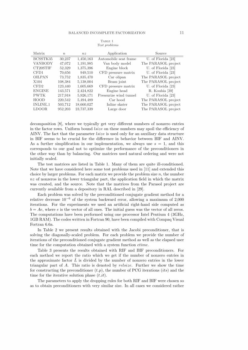
Table 1Test problems

Matrix n nz Application Source

BCSSTK35 30,237 1,450,163 Automobile seat frame U. of Florida [23]VANBODY 47,072 1,191,985 Van body model The PARASOL projectCT20STIF 52,329 1,375,396 Engine block U. of Florida [23]CFD1 70,656 949,510 CFD pressure matrix U. of Florida [23]OILPAN 73,752 1,835,470 Car olipan The PARASOL projectX104 108,384 5,138,004 Beam joint The PARASOL projectCFD2 123,440 1,605,669 CFD pressure matrix U. of Florida [23]ENGINE 143,571 2,424,822 Engine head R. Kouhia [39]PWTK 217,918 5,926,171 Pressurize wind tunnel U. of Florida [23]HOOD 220,542 5,494,489 Car hood The PARASOL projectINLINE 1 503,712 18,660,027 Inline skater The PARASOL projectLDOOR 952,203 23,737,339 Large door The PARASOL project

decomposition [8], where we typically get very different numbers of nonzero entriesin the factor rows. Uniform bound lsize on these numbers may spoil the efficiency ofAINV. The fact that the parameter lsize is used only for an auxiliary data structurein BIF seems to be crucial for the difference in behavior between BIF and AINV.As a further simplification in our implementation, we always use s = 1, and thiscorresponds to our goal not to optimize the performance of the preconditioners inthe other way than by balancing. Our matrices used natural ordering and were notinitially scaled.

The test matrices are listed in Table 1. Many of them are quite ill-conditioned.Note that we have considered here some test problems used in [11] and extended thischoice by larger problems. For each matrix we provide the problem size n, the numbernz of nonzeros in the lower triangular part, the application field in which the matrixwas created, and the source. Note that the matrices from the Parasol project arecurrently available from a depository in RAL described in [29].

Each problem was solved by the preconditioned conjugate gradient method for arelative decrease 10−6 of the system backward error, allowing a maximum of 2,000iterations. For the experiments we used an artificial right-hand side computed asb = Ae, where e is the vector of all ones. The initial guess was the vector of all zeros.The computations have been performed using one processor Intel Pentium 4 (3GHz,1GB RAM). The codes written in Fortran 90, have been compiled with Compaq VisualFortran 6.6a.

In Table 2 we present results obtained with the Jacobi preconditioner, that issolving the diagonally-scaled problem. For each problem we provide the number ofiterations of the preconditioned conjugate gradient method as well as the elapsed usertime for the computation obtained with a system function etime.

Table 3 presents the results obtained with RIF and BIF preconditioners. Foreach method we report the ratio which we get if the number of nonzero entries inthe approximate factor L is divided by the number of nonzero entries in the lowertriangular part of A. This ratio is denoted by relsize. Further we show the timefor constructing the preconditioner (t p), the number of PCG iterations (its) and thetime for the iterative solution phase (t it).

The parameters to apply the dropping rules for both RIF and BIF were chosen soas to obtain preconditioners with very similar size. In all cases we considered rather


Table 2JCG preconditioning

Matrix JCG its JCG timeBCSSTK35 464 2.38VANBODY 605 4.81CT20STIF 389 3.69

CFD1 814 6.20OILPAN 736 8.95

X104 1100 33.4CFD2 854 10.8

ENGINE 686 13.8PWTK 1178 44.8HOOD 666 27.7

INLINE 1 764 101.LDOOR 810 145.

Table 3Comparison of the RIF and BIF preconditioners

Matrix RIF BIFrelsize t p its t it relsize t p its t it

BCSSTK35 0.18 0.50 60 0.47 0.18 0.16 45 0.38VANBODY 0.07 0.75 8 0.09 0.07 0.08 7 0.08CT20STIF 0.05 1.00 62 0.69 0.05 0.06 61 0.67

CFD1 0.74 11.5 287 4.08 0.77 0.83 291 4.38OILPAN 0.08 1.20 134 1.92 0.17 0.17 141 1.97

X104 † † † † 0.24 0.88 44 1.89CFD2 0.50 5.40 372 8.40 0.55 0.62 389 8.55

ENGINE 0.06 1.48 213 4.95 0.06 0.25 208 4.88PWTK 0.21 4.03 14 0.81 0.20 1.01 26 1.39HOOD 0.07 3.36 320 16.1 0.06 0.60 319 16.3

INLINE 1 0.04 16.4 149 22.4 0.04 1.65 156 23.3LDOOR 0.05 13.9 167 34.9 0.05 2.27 168 36.0

sparse preconditioners in order to show that a reasonable efficiency can be obtainedeven with a small amount of additional information extracted from the matrix. Notethat we did not do any tuning of preconditioners for optimal performance. We can seethat both preconditioners seem to be similarly robust. Apart from one case when thecomputation of RIF failed (for a wide spectrum of parameters) since the underlyingSAINV process [4] needed excessive amount of memory, we consider both approachesefficient, having similar degree of robustness. As for the timings, the new precondi-tioner is much cheaper to compute. This can be possibly explained by combinationof two effects. First, BIF is based on cache-efficient, and primarily, columnwise im-plementation whereas in RIF we switch between two matrices stored in different datastructures. The BIF implementation is principially much simpler. Second, we believethat it is mainly caused by the dropping rules which make the factors more stable,producing larger diagonal entries and generating thus less fill-in. If we would considertotal timings, the new BIF approach would be a clear overall winner. Note that we donot consider here the intermediate memory for the SAINV process hidden inside RIF


0 1 2 3 4 5 6

x 106

0

5

10

15

20

25

time

to c

ompu

te th

e pr

econ

ditio

ner

(in s

econ

ds)

size of the preconditioner (in the number of nonzeros)

RIF BIF

Fig. 5.1. Sizes of RIF and BIF preconditioners (in numbers of their nonzeros) versus time toconstruct them (in seconds) for the matrix PWTK.

computation. We observed that this intermediate memory is typically larger than theadditional memory needed for the new approach.

We also performed some experiments with a direct method. For this purposewe used the MA57 code from the Harwell Subroutine Library with the native AMDreordering. The code was able to solve all our linear systems except for the two largestones. Even when this particular direct method provided larger timings in most testcases, we believe that one can tune both approaches to get very similar results fromthe efficiency point of view for the considered problem sizes. But we also believe thatthe classes of direct and iterative methods offer very different merits. They are inmany senses complementary, and their comparison should be always purpose-oriented.Note that one of the principial features of the direct methods is that they can get thesolution with a small backward error. In contrast, in the case of the preconditionedconjugate gradients we typically need and get only a rough approximation of thesolution, where its approximativeness is measured relatively, e.g., with respect to theoriginal backward error norm or the original residual norm.

Comparison of preconditioners is always a multivariate problem. The resultsrepresented via a table, even if the corresponding numbers are carefully selected, maynot tell us the whole story. In the following we will pay attention at the resultsobtained for the matrix PWTK.

Figure 5.1 shows the time to compute the preconditioners of different sizes.


0 1 2 3 4 5 6

x 106

0

100

200

300

400

500

600

num

ber

of it

erat

ions


RIF BIF

Fig. 5.2. Sizes of RIF and BIF preconditioners (in numbers of their nonzeros) versus numberof iterations for the conjugate gradient method preconditioned by them.

Clearly, the setup time is much smaller for all sizes of preconditioners. While wewere able to choose parameters for RIF to make the preconditioner density evenlarger (following the increase in the setup time) this was not the case of BIF. Itsdensity is naturally limited by the size of the row structures of Vs on one side, and bythe dropping rules based on the norms of rows of L and L−1 on the other side.

Figure 5.2 shows the dependence of the number of iterations of the PCG methodon the size of the preconditioner. We can see that there are regions of sizes of thepreconditioners for which the RIF preconditioner is more efficient than the BIF pre-conditioner in terms of the number of iterations for the same size. The other effectvisible in Figure 5.2 is the more uniform behavior of the curve for BIF. The jumpsin the curve seem to have more limited amplitudes. We believe that this may beattributed to the relative dropping used in BIF. In contrast to the results presentedin Table 3, the intervals of preconditioner sizes for which RIF and BIF have a verysmall number of PCG iterations are rather different for this matrix.

Finally, Figure 5.3 shows dependence of the total time on the sizes of precondi-tioners for RIF and BIF. Here, by the total time we denote the sum of the time tocompute the preconditioner and the time for PCG. Due to the very small setup time,BIF is here better, and sometimes much better, for most of its sizes. What we considereven more important is that its behavior is more uniform. The main goal of this sec-tion was to point out that the new approach is practically robust for solving difficult


0 1 2 3 4 5 6

x 106

0

5

10

15

20

25

30

35

40

tota

l tim

e (in

sec

onds

)


RIF BIF

Fig. 5.3. Sizes of RIF and BIF preconditioners (in numbers of their nonzeros) versus the totaltime (the time to compute the preconditioner plus the time for the conjugate gradient method).

problems. BIF seems to satisfy this, even when not proved to be breakdown-free. Webelieve that this behaviour is also due to the robust dropping based on the results ofM. Bollhofer and Y. Saad. We can thus obtain a high-quality preconditioner even inthe case when the SAINV process hidden inside the RIF computation generates veryhigh fill-in as in the case of matrix X104. We believe that the favourable properties ofBIF experimentally shown for solving symmetric and positive definite systems may bevery important in future extensions to nonsymmetric systems, block implementationsand iterative solvers of linear least-squares problems (cf. [12]).

6. Conclusions and future work. We have introduced a new incompleteLDLT factorization of symmetric and positive definite systems by carefully examiningthe AISM preconditioner. The new factorization is surprisingly simple. The algorithmof this new factorization closely couples computation of both the approximate factorsL and L−1 which influence each other during the course of computation. We haveshown that the dropping rules developed by M. Bollhofer and Y. Saad can be easilyapplied into the computational algorithm, and therefore the growth in both L and L−1

can be balanced. This balancing gives the name to the new approach: balanced in-complete factorization (BIF). Numerical experiments suggest that the new techniqueis reliable and can be considered as a complementary method to the RIF precondi-tioner, but having much faster setup than RIF. The extensions to preconditioning


nonsymmetric systems and linear least squares are currently under investigation.

7. Acknowledgment. We would like to thank to the anonymous referees andto Michele Benzi for their comments on the previous version which helped to improvethe paper.

REFERENCES

[1] M. A. Ajiz and A. Jennings. A robust incomplete Choleski-conjugate gradient algorithm.Internat. J. Numer. Methods Engrg., 20(5):949–966, 1984.

[2] O. Axelsson and L. Kolotilina. Diagonally compensated reduction and related preconditioningmethods. Numer. Linear Algebra Appl., 1(2):155–177, 1994.

[3] M. Benzi. Preconditioning techniques for large linear systems: a survey. J. Comput. Phys.,182(2):418–477, 2002.

[4] M. Benzi, J. K. Cullum, and M. Tuma. Robust approximate inverse preconditioning for theconjugate gradient method. SIAM J. Sci. Comput., 22(4):1318–1332, 2000.

[5] M. Benzi, J. C. Haws, and M. Tuma. Preconditioning highly indefinite and nonsymmetricmatrices. SIAM J. Sci. Comput., 22(4):1333–1353, 2000.

[6] M. Benzi, C. D. Meyer, and M. Tuma. A sparse approximate inverse preconditioner for theconjugate gradient method. SIAM J. Sci. Comput., 17(5):1135–1149, 1996.

[7] M. Benzi, D. B. Szyld, and A. van Duin. Orderings for incomplete factorization preconditioningof nonsymmetric problems. SIAM J. Sci. Comput., 20(5):1652–1670, 1999.

[8] M. Benzi and M. Tuma. A sparse approximate inverse preconditioner for nonsymmetric linearsystems. SIAM J. Sci. Comput., 19(3):968–994, 1998.

[9] M. Benzi and M. Tuma. A comparative study of sparse approximate inverse preconditioners.Appl. Numer. Math., 30(2-3):305–340, 1999.

[10] M. Benzi and M. Tuma. Orderings for factorized sparse approximate inverse preconditioners.SIAM J. Sci. Comput., 21(5):1851–1868, 2000.

[11] M. Benzi and M. Tuma. A robust incomplete factorization preconditioner for positive definitematrices. Numer. Linear Algebra Appl., 10(5-6):385–400, 2003.

[12] M. Benzi and M. Tuma. A robust preconditioner with low memory requirements for largesparse least squares problems. SIAM J. Sci. Comput., 25(2):499–512, 2003.

[13] M. Bollhofer. A robust ILU with pivoting based on monitoring the growth of the inverse factors.Linear Algebra Appl., 338:201–218, 2001.

[14] M. Bollhofer. A robust and efficient ILU that incorporates the growth of the inverse triangularfactors. SIAM J. Sci. Comput., 25(1):86–103, 2003.

[15] M. Bollhofer. Personal communication, 2004.[16] M. Bollhofer and Y. Saad. On the relations between ILUs and factored approximate inverses.

SIAM J. Matrix Anal. Appl., 24(1):219–237, 2002.[17] R. Bridson and W.-P. Tang. Ordering, anisotropy, and factored sparse approximate inverses.

SIAM J. Sci. Comput., 21(3):867–882, 1999.[18] R. Bru, J. Cerdan, J. Marın, and J. Mas. Preconditioning sparse nonsymmetric linear systems

with the Sherman-Morrison formula. SIAM J. Sci. Comput., 25(2):701–715, 2003.[19] N. I. Buleev. A numerical method for solving two-dimensional diffusion equations. Atomnaja

Energija, 6:338–340, 1959.[20] N. I. Buleev. A numerical method for solving two-dimensional and three-dimensional diffusion

equations. Matematiceskij Sbornik, 51:227–238, 1960.[21] J. Cerdan, T. Faraj, J. Marın, and J Mas. A block approximate inverse preconditioner for

sparse nonsymmetric linear systems. Technical Report No. TR-IMM2005/04, PolytechnicUniversity of Valencia, Spain, 2005.

[22] T. F. Chan and H. A. van der Vorst. Approximate and incomplete factorizations. In ParallelNumerical Algorithms, ICASE/LaRC Interdisciplinary Series in Science and EngineeringIV. Centenary Conference, D.E. Keyes, A. Sameh and V. Venkatakrishnan, eds., pages167–202, Dordrecht, 1997. Kluver Academic Publishers.

[23] T. A. Davis. The University of Florida Sparse Matrix Collection. Tech. Report REP-2007-298,CISE, University of Florida, 2007. Available online at http://www.cise.ufl.edu/∼davis.

[24] P. F. Dubois, A. Greenbaum, and G. H. Rodrigue. Approximating the inverse of a matrix foruse on iterative algorithms on vector processors. Computing, 22:257–268, 1979.

[25] I. S. Duff and J. Koster. The design and use of algorithms for permuting large entries to thediagonal of sparse matrices. SIAM J. Matrix Anal., 20:889–901, 1999.


[26] I. S. Duff and J. Koster. On algorithms for permuting large entries to the diagonal of a sparsematrix. SIAM J. Matrix Anal., 22:973–996, 2001.

[27] I. S. Duff and G. A. Meurant. The effect of ordering on preconditioned conjugate gradients.BIT, 29:635–657, 1989.

[28] T. Dupont, R. P. Kendall, and H. H. Jr. Rachford. An approximate factorization procedurefor the solving self-adjoint elliptic difference equations. SIAM J. Numer. Anal., 5:559–573,1968.

[29] N. I. M. Gould, Y. Hu, and J. A. Scott. A numerical evaluation of sparse direct solvers forthe solution of large sparse symmetric linear systems of equations. ACM Trans. Math.Software, article 10 (electronic), 33(2), 2007.

[30] M. J. Grote and T. Huckle. Parallel preconditioning with sparse approximate inverses. SIAMJ. Sci. Comput., 18(3):838–853, 1997.

[31] I. Gustafsson. A class of first order factorization methods. BIT, 18(2):142–156, 1978.[32] M. Hagemann and O. Schenk. Weighted matchings for preconditioning symmetric indefinite

linear systems. SIAM J. Sci. Comput., 28(2):403–420, 2006.[33] A. Jennings. A compact storage scheme for the solution of symmetric linear simultaneous

equations. Computing J., 9:281–285, 1966.[34] O. G. Johnson, C. A. Micchelli, and G. Paul. Polynomial preconditioners for conjugate gradient

calculations. SIAM J. Numer. Anal., 20(2):362–376, 1983.[35] M. T. Jones and P. E. Plassmann. An improved incomplete Cholesky factorization. ACM

Trans. Math. Software, 21(1):5–17, 1995.[36] I. E. Kaporin. High quality preconditioning of a general symmetric positive definite matrix

based on its UT U + UT R + RT U decomposition. Numer. Linear Algebra Appl., 5:483–509, 1998.

[37] D. S. Kershaw. The incomplete Cholesky-conjugate gradient method for the iterative solutionof systems of linear equations. J. Comp. Phys., 26:43–65, 1978.

[38] L. Yu. Kolotilina and A. Yu. Yeremin. Factorized sparse approximate inverse preconditionings.I. Theory. SIAM J. Matrix Anal. Appl., 14(1):45–58, 1993.

[39] R. Kouhia. Sparse matrices web page. available online athttp://www.hut.fi/∼kouhia/sparse.html, 2001.

[40] I. Lee, P. Raghavan, and E. G. Ng. Effective preconditioning through ordering interleaved withincomplete factorization. SIAM J. Matrix Anal. Appl., 27(4):1069–1088, 2006.

[41] T. A. Manteuffel. Shifted incomplete Cholesky factorization. In I.S. Duff and G. W. Stewart,editors, Sparse Matrix Proceedings 1978, Philadelphia, PA, 1979. SIAM Publications.

[42] T. A. Manteuffel. An incomplete factorization technique for positive definite linear systems.Math. Comp., 34:473–497, 1980.

[43] J. A. Meijerink and H. A. van der Vorst. An iterative solution method for linear systems ofwhich the coefficient matrix is a symmetric M-matrix. Math. Comp., 31:148–162, 1977.

[44] Y. Saad. SPARSKIT: A basic tool kit for sparse matrix computations. Technical Report 90–20,Research Institute for Advanced Computer Science, NASA Ames Research Center, MoffetField, CA, 1990.

[45] Y. Saad. ILUT: a dual threshold incomplete LU factorization. Numer. Linear Algebra Appl.,1(4):387–402, 1994.

[46] Y. Saad. Iterative Methods for Sparse Linear Systems. PWS Publishing Co., Boston, 1996.[47] O. Schenk, M. Bollhofer, and R. A. Romer. On large-scale diagonalization techniques for the

Anderson model of localization. SIAM J. Sci. Comput., 28(3):963–983, 2006.[48] M. Tismenetsky. A new preconditioning technique for solving large sparse linear systems.

Lin. Alg. Appl., 154–156:331–353, 1991.[49] R. S. Varga. Factorizations and normalized iterative methods. In Boundary problems in dif-

ferential equations, pages 121–142, Madison, WI, 1960. University of Wisconsin Press.

Balanced Incomplete Factorization

Documents

Transcript of Balanced Incomplete Factorization