Location distortions under incomplete information

EISEVIER Regional Science and Urban Economics 24 (1994) 409-440

Location distortions under incomplete information

Marcel Bayer*

IXpm~emen~ de Sciences Economiques et CRDE, UniversitP de Montrhl, C.P.6128,

Montrtal, Quebec, H3C 357, Canada

Jean-Jacques Laffont

GREMAQ (CNRS URA Y47) et Institut d’dconomie industrielle (IDEI). CJniversitC de

Toulouse I. Place Anaiole-France. 31042 Toulouse CEDEX, France

Philippe Mahenc

GREMAQ (CNRS URA 947). UniversitP de Toulouse 1. Place Anatole-France. 31042

Toulouse CEDEX. France

Michel Moreaux’

GREMAQ (CNRS URA 947) et Institut d’konomie industrielle (IDEI). Universit6 de

Toulouse I, Place Anatole-France, 31042 Toulouse CEDEX. France

Received December 1991, final version received March 1993

Abstract

In this paper we consider spatial competition between two firms which first choose sequentially their locations and then compete in prices, when there is mcomplete information of the second mover firm about the first mover firm’s cost advantage. We completely characterize the pure strategy equilibria and we show how the equilibrium locations differ from the complete information locations, i.e. how incomplete information affects product differentiation. The natural bound created by space

* Corresponding author.

’ We wish to thank participants in seminars at GREQE (Marseille), Universitt de Montrtal, UBC. Groupe HEC (Paris) and in the Location Theory session of the World Congress of the

Econometric Society (Barcelona) for their comments. Comments by two anonymous referees and by K. Stahl were also quite helpful in improving the paper. Financial support from FCAR,

SSHRC and CNRS is gratefully acknowledged.

0166-0462/94/$07.00 0 1994 Elsevier Science B.V. All rights reserved

SSDZ 0166.0462(93)02048-g

410 M. Boyer et al. I Regional Science and Urban Economics 24 (1994) 409-440

constraints on differentiation implies that Kreps’ intuitive criterion does not neces- sarily select the separating equilibrium as in a classical signaling model.

Key words: Location theory; Incomplete information; Perfect Bayesian equilibrium; Intuitive criterion

JEL classification: D43; D82; R30

1. Introduction

Location theory, more precisely location competition, is mainly a theory of competition under complete information.] It would be surprising, however, that the incomplete information revolution which transformed our views on imperfect competition during the last decade or so, would be without effect on this theoretical field. In this paper we start filling the incomplete information gap in location theory and consider a duopoly game on the segment line, in which one of the firms, say firm 1, may have either a high or a low constant marginal production cost, whereas the cost of the other firm takes a definite value. The two firms are involved in a two-stage game. In the first stage, when the long-run decisions are made, firm 1, knowing its cost and the cost of firm 2, moves first, choosing its location. Firm 2, not knowing the true cost of its rival, observes firm l’s location and then determines its own location. For analytical convenience, we assume that the true production cost of firm 1 is revealed before the beginning of stage two.2 In this stage, the two firms compete simultaneously in delivered prices. Hence, the location of firm 1 may be understood as a signal disclosing or not the true cost of firm 1.

The relevant equilibrium for the game (signaling game) induced by this kind of market situation is the Perfect Bayesian Equilibrium (PBE there- after), defined below. As usual in these games there exist many equilibria. Generically, the equilibrium locations differ from the complete information locations. So, first, information asymmetry matters and second, it is

‘See Greenhut et al. (1987) or Jaskold-Gabszewicz and Thisse (1986. 1989) for recent surveys. By ‘complete’ information we refer to the technical meaning of the expression which

must be distinguished from ‘perfect’ information. * A now common device since the seminal work of Milgrom and Roberts (1982) to avoid the

signaling effects of price decisions in the second stage. It makes sense in the present context. The location decisions are made under incomplete information, but competition in price will

fairly quickly reveal that information. We take here the extreme case where this information is immediately revealed.

M. Royer et al. I Regional Science and Urban Economics 24 (1994) 409-440 411

desirable to restrict the large set of equilibria. A natural candidate for restricting this set of equilibria is Kreps’ intuitive criterion” because in many cases it works well, selecting a unique equilibrium, the separating equilibrium with the least separating cost. But in the present context, due to the existence of a market center, generating natural bounds for the space of signals, a separating equilibrium does not always exist. Moreover if only pooling equilibria exist, the intuitive criterion may be ineffective. Location competition thus has distinctive characteristics under incomplete information.

The paper is organized as follows. In section 2 we formally introduce the model and characterize the complete information equilibrium, which will serve as a benchmark. We next define the PBE of the game in section 3. We show in section 4 how separating and pooling equilibria may appear according to the cost discrepancy between the two types of firm 1. In section 5 we examine how the intuitive criterion can help to restrict the set of equilibria. Last, we briefly conclude in section 6 by summarizing the main results. An appendix contains more technical derivations and the formal proofs of the propositions.

2. The model and the complete information benchmark

We consider the unitary segment [0, 11 over which there is a continuum of consumers distributed uniformly with density 1. Each consumer is willing to consume one unit of some good if its delivered price is not higher than a reservation price denoted by Y, and zero unit otherwise. The reservation price is assumed sufficiently high (r > 1 + c) so that all the market is covered whatever the locations of the firms. In stage one, each firm determines the location of a single plant. The plant locations are irreversible decisions. For both firms, the marginal production costs are constant. The transport costs are the same and equal to the distance times the quantity. There are neither fixed nor sunk costs.”

The constant average production cost of firm 1, the first mover, can take two values, either c - (Y or c, with c > 112 and (Y E (0, l/2), with prob- abilities (prior beliefs) rr E (0, 1) and 1 - V, respectively. The constant average production of cost of firm 2 is equal to c. All this is common knowledge. We denote by 8 E 0 = {c -(Y, c} the type of form 1. Before choosing its location, X, , in stage one, firm 1 discovers its type, that is what

‘See Cho and Kreps (1987). a This model is relatively standard in location theory. Its simplicity will allow US to

concentrate on the incomplete information effects on location choices.

412 M. Bayer et al. I Regional Science and Urban Economics 24 (1994) 409-440

its production cost will be. Firm 2 observes only the location of firm 1 before deciding its own location, x2.’

In stage two, the true cost of firm 1 is disclosed and the two firms compete simultaneously in delivered prices as in Hoover (1937) or, more recently, Hurter and Lederer (1985) and Lederer and Hurter (1986).6 Thus, stage two is a complete information simultaneous duopoly situation whose parameters are the two locations chosen in stage one and the type of 0 of firm 1. We are looking for a perfect equilibrium, that is an equilibrium where the decisions on prices, taken in stage two, afrer the location decisions, must constitute an equilibrium given those locations. In other words, a firm cannot make false or non-credible threats regarding its behavior or choice in stage two in order to influence the behavior of its competitor in the choice of its location in the first stage. Consider stage two: firm i’s strategy is a function pi@; x1, x2, 0) giving the delivered price quoted to the consumers located at X; this price depends on the locations selected by the two firms and the type of firm 1. In order to solve for the equilibrium, we must specify the behavior of a

consumer who is quoted the same price by both firms. Let us assume, as in Hurter and Lederer (1985), that he buys from the firm realizing the highest profit on his demand, and if both firms realize the same profit on that sale, he then buys from either one with probability l/2. Under these assump- tions, it can be shown that the following price functions constitute a Nash equilibrium of the second stage subgame:’

P1(-GXl,%, f3)=max{0+~x-x,~,c+/x-x,~}, i=1,2. (2.1)

Hence a firm always benefits from greater differentiation by its competitor since in equilibrium it may quote higher prices on a larger own market. In Fig. 1, a move from x2 to xi by firm 2 increases the market area of firm 1 from [0, X] to [0, X’] and the profit margin on its initial market by a’ - a. But the move from x2 to xi has ambiguous effects on the profits of firm 2. It increases its margin on the sales between x and 1 but reduces its margin on the sales between X’ and x and also reduces its market area from [X, l] to [X’, 11. So, given the location of firm 1, the optimal product differentiation of firm 2 will be to choose a location where the two effects are marginally balancing, if such a location exists, and if not, to locate at the end point of

’ Stackelberg location competition was studied by Anderson (1987) in a complete in-

formation context. ‘We work with delivered price competition at this second stage rather than mill price

competition in order to avoid the existence problem of subgame equilibrium (in pure strategies) when X, is sufficiently close to x,. See D’Aspremont et al. (1979) on this issue. Jacques Thisse

suggested that the other way would have been to work with convex transport costs. Preliminary

work with quadratic transport costs reveals that, mutatis mutandis, one gets the same kind of distortions in locations at the PBE of the game.

’ See Hurter and Lederer (1985); both firms choose the same delivered price schedule.

M. Boyer et al. I Regional Science and Urban Economics 24 (1994) 409-440 413

0 =I 2% 2, 2’ a 2; 1

Fig. 1.

the segment. Note also that given the locations, lower costs mean higher profits for the firm concerned and lower profits for its competitor. In Fig. 2, a drop from c to c - (Y in the marginal cost of firm 1 implies a greater market share and an increase by cy in its initial margin, and symmetrically a decrease of the same magnitude in the margin of form 2 on a reduced market share.

Given that firm 2 observes the location of firm 1 before choosing its own

414

c

c-a

M. Boyer et al. I Regional Science and Urban Economics 24 (1994) 409-440

\ --

‘\ \ -- \/

/ ” = / I I

I i I I

d”

d’

location and that the customers are evenly distributed, we may restrict x, to the first half of the segment, that is x, E [U, 1/Z] and therefore x, <x2. The subgame equilibrium profits of the firms are respectively:

M. Boyer et al. I Regional Science and Urban Economics 24 (1994) 409-440 41.5

[(1/4)(X2 -X,)(3X, +x2) f (li2)a(x, +x2) + (l/4@

nl(xr7X2, e, =

i

for0=c-a,

(1/4)(x, -x,)(3x, t x2)

for ~9 = c ,

((x2-x*)(1-(1/4)(x, t3x,))t(1i2)cy(x1 tx,)-(u+(1/4)a2

W,,x,,~)=

i

forO=c-ff,

(x2 -x,)(1 -(1/4)(x, +3x*)) for L9 =c.

(2.2)

(2.3)

Those are reduced profit functions giving the profit levels resulting from price schedule competition as functions of the parameters of the situations at the beginning of stage two, namely the locations of the firms and the type of firm 1.

Before considering explicitly the information asymmetry between firm 1 and firm 2, let us characterize the complete information perfect equilibrium, that is the location equilibrium when 0 is known to both firms. Since Ii’* is a strictly concave function of x2 for any given x,, differentiating IIZ with respect to x2 and equating the derivative to 0, we get firm 2’s reaction function, a function of x1 and 8 since the location and the production cost of firm 1 are observed by firm 2:

i2(x17 e, =

(1/3)(2+c~+x,) for8=c-cu,

(l/3)(2 +x1) for 0 = c , (2.4)

and the best response of firm 2 is an increasing function of the cost differential, II. Firm 1 knows the reaction function of firm 2 and therefore takes it into account when deciding on its own location. Using the reaction function i2(x1, 0 ) in II,, we obtain a concave function of x1. The constraint x, s l/2 is effective only when cx > l/8. Hence, firm l’s location in equilibrium is given by

1 min{(2/5)(1+ ~cx), l/2} XT(e)= 2,5

for /3 = c - (Y , for 8 = c . (2.5)

Substituting x:(0) for x1 in (2.4) gives firm 2’s location at equilibrium given the optimal location of firm 1:

min{(1/5)(4 + 3a), (l/3)(5/2+ CX} for 8 = c - CY ,

for 8 = c . (2.6)

Note that for cx < l/8, the equilibrium product differentiation decreases with cy, firm 1 moving towards l/2 and firm 2 moving towards 1 but more slowly


than firm 1. For (Y B 118, firm 1 stays at the center of the market but firm 2 keeps on moving away so that the product differentiation now increases. Using x;(0) and x:(0) in (2.2) and (2.3), we obtain the equilibrium profits:

max{(l/5)(1+ 2a)2, (l/36)(7 + 32a + 16~1~))

fortI=c-a andcr<llS,

n:(e) = min{(l/5)(1+ 2c1)~, (l/36)(7 + 32a + 16~~~))

for 0 = c - LY and CK < l/8 ,

115 for0=c,

(2.7)

fl-3~) = {

max{(3/25)(1- 3~)~, (l/12)(1 - ~cx)~} for 0-c - (Y , 3,25 for 0 = c

(2.8)

3. The incomplete information case: Definitions

To study the likely outcome of the location stage, we need a solution or equilibrium concept. The natural concept to use in such an incomplete information framework is the subgame Perfect Bayesian Equilibrium (PBE) concept which first requires that the second stage decisions be a Nash equilibrium given the outcome of the first stage and second explicitly models the treatment and updating of information by the agents.

Since the true production cost of firm 1 is disclosed at the end of the location stage, the subgame perfection condition implies that the second stage price schedules are always given by (2.1) and the profits by (2.2) and (2.3) at equilibrium. Hence, we may focus on the first, long-run, stage. Although firm 2 does not observe 0, it observes x1 and it knows that firm 1 knows 0 before choosing its location X, and therefore must have been influenced by that value of 8; hence firm 2 tries to infer from the observation of x, the particular value of 13 which firm 1 has observed. This thought process of firm 2 is well understood by firm 1 who makes the best use of its knowledge both of 0 and of the behavior of firm 2; and this is well understood also by firm 2; and so on.

The location stage is a classical ‘signaling’ game [see Cho and Kreps (1987)] that can be represented as follows. First, player ‘Nature’ draws the type 8 of firm 1 from the finite set 0 = {c, c - a} according to the probability distribution (rr, 1 - 7~). Then firm 1, the ‘sender’, observes its type or production cost [its information sets are the two singletons {c} and {c - (Y}] and selects a location [a message] X, from the set {x, (x, E [0, l/


2]}.8 Finally, firm 2, the ‘receiver’, observes firm l’s location [message] but

not firm l’s type [its information sets include two nodes (x1, c - a) and (x, , c)] and selects a best-response location, x2 E [0, 1].9 The profits (payoffs of the game) are given by (2.2) and (2.3) as functions of the moves (0, x1, x2), that is the path followed by the play of the three players. In this signaling game, a pure strategy of firm 1 is a decision function, x”, : o-+ [O, l/2], which associates some definite location choice, x,(e) E [0, l/2], by firm 1 to every draw 0 by ‘Nature’. A pure strategy of firm 2 is a function, .CZ : [0 , l/2]-+ [0, 11, which associates to every observed location x1 of firm 1 some definite location choice, X:(x,) E [0, 11, by firm 2.

In order to complete the definition of a PBE, we need to specify the way firm 2 processes the information on 8 which the observed location of firm 1 may contain, that is the posterior beliefs function of firm 2 defined on the types of firm 1. We denote by ~(0 ( xl) the probability assigned to the type 8 of firm 1 by firm 2 after the observation of firm l’s location, x, , For notational simplicity, we often write p instead of ~(c - (Y 1 x,) and 1 - p for

L4cIx,). A Perfect Bayesian Equilibrium is a triple (x”T, x”;, II*) such that: (i) firm l’s strategy, x”T, maximizes its profit given its type or production

cost 8 and its knowledge of the strategy X”t used by firm 2; (ii) firm 2’s strategy, .?I, maximizes its expected profit given xi and its

conjectures or beliefs on the types of firm 1 inferred from the observation of

xi; (iii) firm 2’s conjectures or beliefs, l.~*, are derived from the prior

distribution (r, 1 - n) and from firm l’s strategy, by using Bayes’ rule [this rule can be seen as combining optimally the old (prior) and the new (observation) information to obtain a revised information (posterior)],

/-4-aIxi)= Prob(x, 1 c - a) Prob(c - a)

Prob(x 1 )

Prob(x, ( c - a) Prob(c - (Y)

= Prob(x, 1 c - a) Prob(c - CX) + Prob(x, 1 c) Prob(c)

Prob(x, 1 c - a)~

= Prob(x, 1 c - a)~ + Prob(x, 1 c)(l - 7r) ’ (3.1)

when applicable and are arbitrary otherwise; in other words, the inference function, p*, must be cons&rent with the prior, (7~, 1 - r), and the equilibrium strategy, x7,(*), of firm 1.

8 The coordination problem pointed out by Bester et al. (1991) does not arise in this Stackelberg setting.

’ Since x1 c l/2, firm 2 never chooses a location between the origin and x, at equilibrium.


Thus, (x”T, 2;) define a Stackelberg-Nash equilibrium given the assess- ment or beliefs function, p *. Condition (iii) provides effective restrictions only when firm 2 observes equilibrium locations; for out-of-equilibrium locations, that is locations x; such that Prob(x; 1 c - a) = Prob(x; 1 c) = 0, expression (3.1) is indeterminate, being equal to O/O; that is the reason why we say that Bayes’ rule does not apply and the posterior beliefs are thus arbitrary. As we will show, it will be a source of multiplicity for equilibria.

There exist two kinds of PBE in pure strategies: separating and pooling. In a separating equilibrium, gI(c) # T1(c - (Y) so that, observing the equilibrium location of firm 1, firm 2 can infer with certainty the true type of firm 1. On the contrary, in a pooling equilibrium, x”,(c) = Z1(c - (.y) = XT so that, observing XT, firm 2 gets no additional information: the prior and posterior beliefs must be the same.” Separating equilibrium seem more appealing for an efficient firm 1. If its type is perfectly identified, it can expect more differentiation from its competitor, a greater market area, and higher margins. But as we shall see, signaling its true cost prevents firm 1 from selecting the location it would choose under complete information. On the contrary, pooling equilibria are more attractive for the less efficient firm 1. Since firm 2 cannot infer the type of firm 1, it tends to overvalue firm l’s efficiency and react less roughly by choosing a more differentiated position, leaving a greater market share to the high cost firm 1 and relaxing price competition at the second stage. But as we will see, such pooling is not always possible or profitable for the high cost firm 1.

The choice of location by firm 2 depends on x1, the observed location of firm 1, and on its beliefs, CL, that firm 1 is of type c - (Y. Let 2*(x,, p) be the best response of firm 2: I1

Straightforward calculations lead to

&(x1, /J) = (1/3)(x, + j_MY + 2) . (3.2)

Note that, given x1, the optimal location of firm 2 is an increasing function of p so that the more firm 2 believes it is competing with a low cost firm 1, the greater is the market area of firm 1 and the higher is its profit, and this whatever its type 8.

“I We will consider only pure strategy equilibria since location distortions already appear in this simpler case. Mixed strategy equilibria also exist but it can be shown, however, that neither

separating nor pooling equilibria in mixed strategies exist in the present context. The

characterization of mixed strategy equilibria is outside the scope of the present paper.

‘I Admittedly, the notation i, has been used in section 2 to denote the best response of firm 2: i.2 was then a function of X, and 0. Hence, the use of P, again here is, strict0 sensu, an abuse

of notation but since no confusion is possible, we will proceed with it.


Let us now define a(.~, , p, 0) as the profit of firm 1 of type 0 located at xl and competing against a firm 2 optimally responding to X, given the posterior beliefs F. Since

fi,(% Pu, 0) = n,(x,> W,, P), 0) >

one obtains after substitution of f,(x,, k) given by (3.2):

((1/36)(-20x; + 8(2+/_~a + 3a)x, + (2 + /..ux + 3c~)~)

fi,(x,, /-he> = for8=c-a,

(1/36)(-20x; + 8(2 + /UX)X, + (2 + P(Y)*)

for 0 =c.

(3.3)

The fil(x,, p, 0) functions are illustrated in Fig. 3(a) for the three values:

/J=O, P=tiE(O,l), and p = 1. Since afi, /ap is equal either to (l! 36)(8ax, + 2c~(2 + p.(y + 3~)) > 0 if 8 = c - LY, or to (1/36)(8ax, + 2~y(2~ + ~cx)) > if 8 = c, then to a higher posterior on the low cost type corresponds a higher profit for firm 1 of either type, whatever its location. Given p and 0, the profit function fi, is a strictly concave function of x1. Hence, there exists only one location that maximizes fi,. Since the marginal profit function is increasing with p, [a2fi1(x,, ~,0)lax, ap =2ai9>0, V8 E 01, so is the optimal location of firm 1. Letting .?,( p, 0) be the location that maximizes

fi, on the interval [0, l/2] of locations open to firm 1, we have

--;l(P7 e, = 1 min{(1/5)(2+pucu+3a),1/2} for8=c-a,

(l/5)(2 + PLY) for 8 = c . (3.4)

As expected, (3.4) gives .?*(l, c - a) and i,(O, c) as the equilibrium locations under complete information.12

Last consider some location i, and posterior @ giving fi(.~!~, fi, 0) to the type 8. For any other location x1 ZX, we can define a limit belief, denoted by p(xl, X1, fi, 0), such that a firm of type 0, locating at x1, would get at

most fi(x,, r;, 0) if, observing x,, firm 2 inferred that it was facing the low cost type with probability p s i(xl, 1,) fi, 0); and it would get more than fi(li,@.,e) if p.)p(xl,X,,fiU,O). If X,=i-,(l,e) and k=l, then E.L(x,, f,(c - a), 1, f3) = 1 since _?,(l, f3) is the only profit-maximizing location of the type 8 when identified as the low cost type and fi,(.) is increasing

” For the high cost firm 1, the constraint x, c 112 is never effective since i,(p, c) = 112 only if LY = l/2 and y = 1, i.e. if the cost discrepancy a is equal to its upper bound and firm 2 is certain to compete against the low cost firm 1. For the low cost firm 1 the constraint is ineffective when (Y < 118 and k < 1 or when a E (l/8, 116) and k < (112~1) - 3; otherwise the

constraint is tight and ,?,(p, c ~ a) = 112. Finally, a,(l, c) < a,(O, c - u), Va E (0, l/2).


with p. This case excepted, there exists a whole range of locations x, for which p < 1, as illustrated in Fig. 3(b), where this range is the interval (x,,,(ir, k, 0), l/2]. The limit belief f unction plays a crucial role in the characterization of equilibria. Clearly, if x”;(0) is the equilibrium location of type 8 and p*(c - (Y 1 x”T(O)) the equilibrium posterior beliefs, then for any x, Zx”T(0)) we must have p*(c - (Y Ix,) s p(x,, x”;(0), p*(c - a 1 g:(O)), 0). Otherwise firm 1 of type 19 would deviate from the assumed equilibrium location to x,. In a separating equilibrium where the two types choose different equilibrium locations, x”;(c) # x”T(c - a), each one revealing its true cost, we must have for any out-of-equilibrium location x,:

p*(c - (Y 1 x,) S min{G(x,, x”:(c), 0, c), p(xI, 2T(c - cu), 1, c - a)} .

(3.5)

In a pooling equilibrium, both types of firm 1 choose the same location, XT, and firm 2 gets no additional information, ~*(c - a /XT) = rr, SO that for any

x, zx;:

The properties of the limit belief function are derived in the appendix.

4. The set of pure strategy perfect Bayesian equilibria

We show in this section that for relatively small values of the cost discrepancy (Y, there exists a continuum of both separating and pooling equilibria. But for (Y sufficiently large, separating equilibria disappear. We show how to determine these equilibria and we characterize the location distortions that they imply.

4.1. The set of separating equilibria

The set of separating equilibria is characterized by the following proposition:

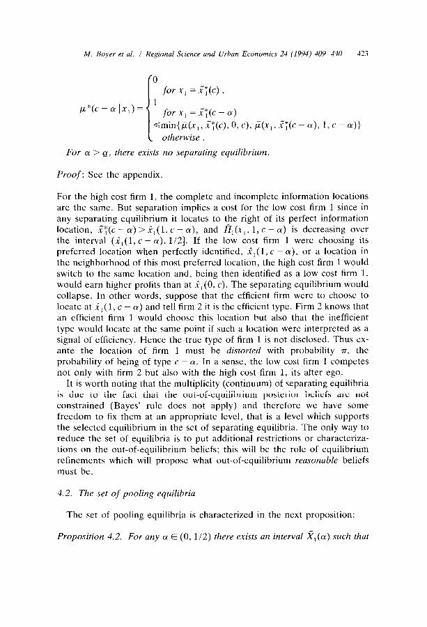
Proposition 4.1. There exists a value a such that for (Y < g [a = my] there exists a continuum of separating PBE [a unique separating PBE], (x”:(c), ?,(c - a)) such that x”:(c) =x,(0, c), and xT(c - (Y) lies in some interval X, the lower bound of which is strictly nearer the market center than 2, (1, c - a); each such equilibrium can be supported by any posterior beliefs ~*(c - (Y (x,) satisfying:


for x1 = x”;(c) )

/L*(c - (Y 1 x,) = 1

for x, = x”T(c - a)

Gmin{p(x,, x”:(c), 0, c), jL(x,, x”T(c - a), 1, c - a)}

otherwise .

For CY > a, there exists no separating equilibrium.

Proof: See the appendix.

For the high cost firm 1, the complete and incomplete information locations are the same. But separation implies a cost for the low cost firm 1 since in any separating equilibrium it locates to the right of its perfect information location, x”T(c-(~)>i~(l,c--cr), and fi,(x,, l,c-a) is decreasing over the interval (..?,( 1, c - cu), l/2]. If the low cost firm 1 were choosing its preferred location when perfectly identified, a,(l, c - CX), or a location in the neighborhood of this most preferred location, the high cost firm 1 would switch to the same location and, being then identified as a low cost firm 1, would earn higher profits than at ,?r(O, c). The separating equilibrium would collapse. In other words, suppose that the efficient firm were to choose to locate at i1 (1, c - CX) and tell firm 2 it is the efficient type. Firm 2 knows that an efficient firm 1 would choose this location but also that the inefficient type would locate at the same point if such a location were interpreted as a signal of efficiency. Hence the true type of firm 1 is not disclosed. Thus ex- ante the location of firm 1 must be distorted with probability 7r, the probability of being of type c - a. In a sense, the low cost firm 1 competes not only with firm 2 but also with the high cost firm 1, its alter ego.

It is worth noting that the multiplicity (continuum) of separating equilibria is due to the fact that the out-of-equilibrium posterior beliefs are not constrained (Bayes’ rule does not apply) and therefore we have some freedom to fix them at an appropriate level, that is a level which supports the selected equilibrium in the set of separating equilibria. The only way to reduce the set of equilibria is to put additional restrictions or characteriza- tions on the out-of-equilibrium beliefs; this will be the role of equilibrium refinements which will propose what out-of-equilibrium reasonable beliefs must be.

4.2. The set of pooling equilibria

The set of pooling equilibria is characterized in the next proposition:

Proposition 4.2. For any a E (0, l/2) there exists an interval r?, (CY) such that


any XT E X,((Y) is a pooling PBE if the prior 7~ is at least equal to a lower bound fi(xT) and if the posterior function satisfies p*(c - (Y Ix,) s

min{Ax,,xT, 7r,0), t3EO) forx,#xT.

Proof. See the appendix

The multiplicity of pooling equilibria may be seen from the following point of view. Consider a given prior rr sufficiently high, then there exists a whole range of locations (depending upon n) which may appear as pooling equilibrium locations, provided that the out-of-equilibrium beliefs verify some condition which can always be met. For example, in the extreme and degen_erate case where rr = 1 (admittedly excluded by assumption), any XT E X,(a) can be a pooling equilibrium location provided that for x, #XT, ~(c-~~Ix,)Gmin{j.Y~(x,,xT, 1, e), 8 E O}. But now let us observe that for the other extreme case, rr = 0 (also excluded by assumption), no location may be an equilibrium location: in order that the high cost firm 1 not want to deviate and locate i,(O, c), xT should be precisely a,(O, c) and, similarly, in order that the low cost firm 1 not want to deviate and locate at a,(O, c - (Y), XT would have to be precisely il(O,c - a); since _?,(O, c)< i,(O, c - a), no pooling equilibrium exists. Therefore a pooling equilibrium may exist only if r is above some bound. This lower bound, which we will denote by ~(a), is defined by

n(a) =rn~~ {max{jIL(x,, i,(O, 0), 0, f3), 0 E 0}} . (4.1)

For any rr < ~(a), whatever the location x, under consideration, it would be better for at least one of the types of firm 1, say 8’, to choose .!i, (0, f3 ‘) rather than x1; for this type, rr < I_L(x,, ,?r(O, 0’), 0,s’) implies higher profits at a,(O, 0 ‘), whatever the beliefs induced by this location, than at x, inducing the posterior rr. Next, for v = T(Q) there exists only one location which can be the pooling equilibrium location: the location at which

max{j.L(x,, i-,(0, fI), 0,0), 0 E O} . IS minimized. But for rr > r(a), there

exists a whole interval of candidate locations. We can reformulate Proposi- tion 4.2 by defining the set k,(r, a) as

where X,,,(QT, cy) is the smallest root of fiI(x,, r, c - cy) - I?,(i,(O, c - cy), 0, c - (Y) = 0 and nC,,, (7~, c~) is the largest root of I?, (x1, rr, c) -

fiI(..?,(O, c), 0, c) = 0 if such a root is less than 112, and l/2 otherwise.

Proposition 4.2’. For any T > a((~) [T = ~(a)] there exists a whole range of pooling equilibria [a unique pooling equilibrium] XT E X,(v, a), each one

M. Boyer et al. I Regional Science and Urban Economics 24 (1994) 409-440 42.5

supported by any posterior belief function /_LL*(C-a(q)< min{@(X,,Xr, 7~, 0), 0 E O}, for X, #XT.

Proof. See the appendix.

Clearly, when the equilibrium is a pooling equilibrium, for one of the types of firm 1 at least and generically for both types, the location differs from the complete information locations. The distortions are always beneficial to the high cost firm 1 since fi, (x”;, n,c)b fi,(i,(O, c),O, c) is one of the constraints that must be satisfied by the pooling equilibrium location. However, as in the separating equilibria, the efficient low cost type of firm 1 suffers a loss: in these pooling equilibria there subsists some doubt about the true type of firm 1 and this implies that firm 2 locates closer to firm 1 than under complete information, thus reducing the efficient low cost firm 1 market area and profits.

TO conclude this section we can summarize the existence results as follows: for (Y sufficiently low, a G a, and r sufficiently high, 7~ > ~(a),

there exist both separating and pooling equilibria; for (Y sufficiently low, (Y S a, and r sufficiently low, rr G ~(a), there exist only separating equilibria; for (Y sufficiently high, CY > g, and rr sufficiently high, r > ~(a), there exist only pooling equilibria; for LY sufficiently high, cx > cu, and rr sufficiently low, n G Z(U), there exists no pure strategy equilibrium; in all the equilibria, the high cost firm 1 makes as much profit as under complete information, and often (generically in ail the pooling equilibria) makes more; the efficient low cost firm 1 is, on the contrary, in a worse position, always experiencing reduced profits compared with the full information equilibrium.

5. The intuitive criterion refinement

Are all the out-of-equilibrium beliefs equally reasonable? This is the subject-matter of the so-called refinement theory.‘” Here, we apply the simplest criterion> the fairly appealing intuitive criterion developed by Kreps [see Cho and Kreps (1987)J. In the present context it eliminates, for each given cy, all but one separating equilibrium when such equilibria exist; however, it performs less efficiently in eliminating pooling equilibria when only such equilibria exist. We’ first present the particular working of the intuitive criterion in our model and then examine successively the separating and pooling equilibria.

“See, fcx example. Van Damme (1987). Fudenberg and Tirole (1991) or Laffont (1991)


5.1. The intuitive criterion

Consider an equilibrium (x”T, x”T, p *) at which firm 1 of type 0 gets the payoff II:(e). Let x, be some out-of-equilibrium location, X, ,&(x”;(0), 8 E O}. Suppose that one of the types of firm 1, say 0 ‘, locating at x, and correctly identified by firm 2, which then responds optimally, obtains higher profits than its equilibrium profits:

where 6-(0 ‘) is the perfect information binary variable: 7j(c - a) = 1 and e(c) = 0. Suppose also that the other type, 8”# 0’, earns at most its equilibrium profits at that location, whatever firm 2 conjectures about the types of firm 1 after observing x,:

V/_L E [O, l] : f&,, /J,, W) s Iiy(O”) .

Under those conditions, the deviation x, perfectly discriminates between the two types of firm 1. The intuitive equilibrium refinement criterion stipulates that it is then reasonable for firm 2 observing x, to conclude it is facing the type 8 of firm 1. But now if firm 2 observing x, is then convinced to be competing against the type 19 ‘, then firm 1 of type 19 ’ is earning more at x1 than at its equilibrium location and should locate at x1 rather than at x”T(0 ‘). So, the equilibrium considered collapses.

5.2. Refining the set of separating equilibria

We show in this subsection that the only separating equilibrium surviving the application of the intuitive criterion is the equilibrium of least separating cost for the low cost firm 1.

Proposition 5.1. The separating equilibrium robust to the application of the intuitive equilibrium refinement criterion is unique and is that separating equilibrium which implies the smallest separating cost for the low cost firm 1, i.e. the smallest location distortion.


5.3. Refining the set of pooling equilibria

Again we must distinguish according to the value of (Y. Leaving aside the non-generic case (Y = a, we show in this subsection that when (Y < cr (the region where there also exist separating equilibria), all the pooling equilibrium are eliminated by the intuitive criterion, but that when (Y > (y, things

M. Boyer et al. I Regional Science and Urbun Economics 24 (1994) 409-440 427

are more complicated: depending on the value of the prior probability n, a given pooling equilibrium may or may not survive.

Proposition 5.2. If there exist separating equilibria (CY < (y), all the pooling

equilibria are removed by the application of the intuitive criterion so that the only surviving equilibrium is the separating equilibrium of least separating cost.


Proposition 5.3. If no separating equilibrium exists (i.e. (Y > (y), then a

pooling equilibrium x’; is robust to the application of the intuitive criterion if

and only if T < tIL(xT, 112, 1, c).


If we consider the prior rr as the basic data, we know (Proposition 4.2’) that generically there exist a whole range of pooling equilibrium locations. Furthermore, in the present case (cr > LX), the pooling equilibria are the sole PBE in pure strategy. We are thus left in an uncomfortable position since either T< fi(xT, 112, 1, c), and all the pooling equilibria subsist, or rr b fi(xT, 112, 1, c), and all the equilibria are eliminated. In order to obtain existence and uniqueness, we would have to consider more powerful refinement criteria and mixed strategies. It is beyond the scope of this paper to do ~0.‘~

6. Conclusion

We have shown that incomplete information problems cannot be dis- pensed with in the analysis of spatial competition. Complete and incomplete information locations are not the same, except for the high cost firm 1 in separating equilibria. In a separating equilibrium, the efficient firm 1 is nearer the market center than under complete information, hence a loss of profits. More precisely, firm 1 being closer to the center, the products are less differentiated than under complete information, implying that the prices quoted by the two firms will be lower since less distant products mean a more stringent competition (see section 2).

Separating equilibria exist if and only if the difference in costs between

” See Boyer et al. (1994) for an analysis based on the Dl criterion proposed by Cho and Kreps

(1987). Let us simply indicate here that for any value of 7~ and LY, one and only one equilibrium survives the Dl criterion.


the more efficient type and the less efficient type of firm 1 is not too large, that is under some bound. When the difference in costs is smaller than this critical value, the type of firm 1 is revealed by its choice of location since each type chooses a specific and different location: it is profitable for the low cost type of firm 1 to move closer to the center of the market than under complete information because by doing so it makes the high cost type of firm 1 better off at its complete information location than at the location selected by the low cost type of firm 1. Hence the two types of firm 1 choose different locations and this process of location choice by firm 1 is well understood by firm 2. But if the difference in costs is larger than the critical value, the low cost type of firm 1 cannot, even by moving to the center of the market, make the high cost type of firm 1 better off at its complete information location than at the location selected by the low cost type of firm 1. It is profitable for the high cost type of firm 1 to choose the same location as the low cost type and therefore firm 2 cannot systematically infer the type of firm 1 simply by observing the location of that firm.

In a pooling equilibrium the inefficient firm 1 gets more than under revelation of its type, that is under complete information. Generally, its location will be different from its complete information location. Hence, if it were to be identified, it would get less. But the beliefs of firm 2 are sufficiently biased towards the low cost type that the misperception effect counterbalances the mislocation effect: the products are more distant, softening the price competition. For the low cost type of firm 1, pooling may be better or worse than separating. If the prior on the low cost type is high, then pooling is better. For a prior rr almost equal to 1, the equilibrium profits of the low cost type are almost equal to its complete information earnings and higher than its separating equilibrium profits. At a pooling equilibrium, the low cost type must locate in this case in the neighborhood of its complete information location, saving the cost of separation. On the contrary, if the prior is sufficiently low (but not too low since then no pooling equilibrium would exist), then either the pooling equilibrium is eliminated by the intuitive refinement criterion or there exists no pooling equilibrium. But in this last case the profits of the low cost firm 1 are lower than its complete information equilibrium profits. Therefore, except for the high cost firm 1 in separating equilibrium, incomplete information matters.

Appendix

Characterization of the limit belief function ji(*)

For a combination of locations to constitute an equilibrium, it must be the case that neither firm 1 of low and high cost type nor firm 2 wishes to


deviate given CL*. Let us take a closer look at those deviation possibilities. Consider some given pair (X1, g-i) of firm l’s location and firm 2’s posterior beliefs. Except when (X,, k) = (f,(l, f3), l), there exists a set of locations x, at which firm 1 of type 8 would earn more than I?(X, , @, 0) provided that, observing x,, firm 2 would conclude that it is facing a low cost firm 1 with a sufficiently high probability p and responds accordingly. As noted in section 3, d is increasing in Al. and strictly concave in x1; hence, this set of locations is an interval. Note that this interval can be either open or closed at each end. For example, in Fig. 3(a) the set of locations that would allow firm 1 to

get more than fi(~?~, h;, 0), provided that p is sufficiently high, is open on the left and closed on the right. Let us denote by X,(X,, +, 0) this interval. We denote by x,;,(XI, fi, 13) and x,,,(X1, G, E.L) the lower and higher bounds, respectively, of X,(I!,, k, 0).

For any location x1 E X,(X,, fi. f3) we can define a limit posterior belief p such that firm 1 of type 8 would earn more profits when located at x1 and facing a firm 2 with beliefs Al. > FL, than when located at 1, and facing a firm 2 with beliefs @. The limit is given by a function p(x,, X1, h;, 0) implicitly defined by

~,(Ir,,~,e)-ir,(X,,CL,e)=O (A.l)

if this equation has a solution p E [0, 11, in which case the solution is unique

s$rce II, is monotone in p; E.L(x,, X1, fi,tI) is equal to 0 if fiI(i,, j_i,tI)< II,(x,, 0,0), so that (A.l) has no solution p E [0, 11, as would be the case if, for example on Fig. 3, X1 were sufficiently near 0 and @ were very low implying that, in the neighborhood of i-,(0,0), we have fi,(x,, 0,0) >

II,(X,, @, 0). We extend the function h(e) on the whole segment [0, l/2] as follows:

Since 0,(x,, p, e) is continuous in x1 and p, then the function r_L(.) is

continuous. By definition:

~~,Ex,(x,,~,e):~(x,,x,,~,e)<i.

Furthermore, for XI = i-,(0,0) and C; = 0, we have

ve E 0, VX, E [o, i/2],

(A.3)

VP s cL(xl, i-,(0, e), O,e) : fi,i,(x,, P, fv G fw,(o, e),o, 0) , (A.4)


that is firm 1 of type 8 is better off at its profit-maximizing location when it is believed by firm 2 to be of type c with certainty, that is i-,(0, f3), than at any other location x1 if it is then believed to be of type c - (Y with a probability less than i(x,, a,(O, e), 0, 0).

Now consider the roots of Eq. (A.l) where fiI is given by (3.3). After calculation we obtain the following expressions for the sum of the roots:

-2(4x, + 2 + ~cv)/(Y < 0 for 8 = c - CY ,

-4(2x, + l)/(~ < 0 for /3 = c , (A.5)

so that the positive root is unique. Totally differentiating (A.l) we get

ai+, > i, > ticL, c - (.y) dfi,(x,, /L, c - a)ldx, =--

ax* ari,<q, P, c - a)/w

-40x, + 8(2 + /.LLLa + 3a)

= - ~/_LL(u~ + 2cz(4x, + 2 + 3a) ’

a/+,, -f,> /-L c> afi,(x,, CL, cl/ax, -40x, + 8(2 + /&I)

dx, =- &(x,, /_L, c)l+ = - 2pa2 + 4~1(2x, + 1) .

Hence

+ (~+/_MI+~x~)(~+/_w +4x, +3a) ’

so that

Since E,L(1,, i,, k, c - cy) = fi(X,, iI, @, c) = +, (A.6) implies that

‘mint’:19 G>C)<Xmin(i:l, G>c -a)<x,,,(xI, fiu, c,

c x,,,(X, > /-L c - a) 2 (A.7)

with the strict inequality if x,,,(L!, , fi, c) < l/2, and

ve E 0, Vx,,!zX,(a,(O, e>, 0, e>, V/L, VP.’ :

O<I*’ * ir,(x,,~,e)<-Ji(~.l(O,e),O,e)<li,(~G,(o,e),~’,e),

(A4

where X,(e) is the closure of X,(s).


Proof of Proposition 4.1. In a separating equilibrium, each type of firm 1 is, in equilibrium, perfectly identified by its location. Hence the equilibrium

payoffs are given by fil(x”,(c-~),l,c-~) for 8=c-a, and

fi,(x”,(c), 0, c) for 8 = c. Consider first the high cost firm 1. Since _?,(O, c) is the unique location maximizing fii(.r,, 0, c) and since fi,(x,, p, c) is increasing with p for any x,, we have for any p E [0, l] and x1 # a,(O, c):

ir,(x,,O,c)<~fil(~,(O,c),O,c)~~,(x”,(O,c), P,C). (A.9)

Hence, had the high cost firm 1 chosen a location x, #i-,(0, c), it would pay to deviate and locate at i,(O, c): by (A.9), whatever firm 2’s beliefs observing i,(O, c), that is whatever p, firm 1 would earn more at i-,(0, c) than at any other x1 when correctly identified, as is the case in a separating equilibrium. There is only one equilibrium location open to the high cost firm 1, its complete information location. Note, however, that in order for the high cost firm 1 to willingly remain at i-,(0, c), firm 2’s posterior beliefs must be such that [see (A.4)]:

Vx, E [O, l/2] : p(c - a IXJ 9 j&x,, i,(O, c), 0, c) .

Consider now the low cost firm 1. First, remember that, in a separating equilibrium, firm 2 observing Z1(c - a) infers that E.L(C - (Y 1 x”,(c - a)) = 1. Hence the low cost firm l’s location must be outside X,(.Y?~(O, c), 0, c) since in this interval i(xi, a,(O, c), 0, c) < 1 and therefore, had the low cost firm 1 chosen a location in this interval, then the high cost firm 1, knowing that such a location signals a low cost firm 1, would mimic the low cost type in order to obtain higher profits. Second, gl(c - a) cannot be outside X,(2-,(0, c - LY), 0, c - (.y). If it were the case, then by (A.8) the low cost firm 1 would earn more at _?,(O, c - CK) whatever the beliefs of firm 2 observing il(O, c - cu), hence it would deviate and locate at i,(O, c - a). We conclude that in a separating equilibrium the location of the low cost firm 1 must be in X7, the intersection of these two subsets (outside X,(i,(O, c), 0, c) but inside X,(.!?-,(O, c - a), 0, c - a)):

X,(c - (.y) EXY f ([O, 1/2]LX,(~-,(O, c), 0, c))

n X,&(0, c - (Y), 0, c - (Y) (A. 10)

Note that

X’; + 4 3x7 = ]x,,,(~.1(O, c), 0, c)), x,,,(i.l(o, c - (Y), 0, c - cy)] .

(A.ll)

Hence from (A.7) XT #0 if x,,, (i-,(0, c), 0, c) < l/2. Remember that x,,,(~~(O,C),O,C) is the largest root (or l/2 if this root is >1/2) of

432 M. Boyer et al. i Regional Science and Urban Economics 24 (1994) 409-440

~,(~,(o,c),o,c)-~,(x,,l,c)=O, (A. 12)

where from (2.7), fi,(x,(O, c), 0, c) = 115, and from (3.3), fi,(x,, 1, c) = (li 36)(-20x: + 8(2 + cy)x, + (2 + a)‘). Hence, defining A, = 9a(a/4 + l), we have

x,,,(x,(O, c), 0, c) = min(li2, (l/5)(2 + (Y + a)} (A. 13)

so that

(A. 14)

NOW x,,,(xl(O, c - cy), 0, c) is the largest root (or 112 if this root is >1/2) of

fi&(O, c - CY), 0, c - CX) - fi,(x,, 1, c - CY) = 0 ) (A. 15)

where from (3.3) and (3.4), fil(x,(O, c - a), 0, c - (.y) = (1/20)(3a + 2)’ if

(Y d 118 and = (1/36)(9a2 + 24~~ + 7) otherwise, and fi,(x,, 1, c - a) = (li 36)(-20x: + 8(2 + 4a)x, + (2 + ~cx)‘). Hence, defining A,_, =9a((7a/4) + l), we have

x,,,(xl(O, c - a), 0, c - (.y) = min(li2, (l/.5)(2 + ~LX + K)} ,

(A.16)

so that

if cr E (0,26 - 15fi),

, otherwise . (A. 17)

From (A.14) we conclude that the set of separating equilibria is empty for a > (y = (S/6) - 4. For LY < (y, there exists a whole range of equilibrium locations for the low cost firm 1. Note that x,(1, c - a) <x,,,(x,(O, c), 0, c) in this case, so that for the low cost type the equilibrium location is not the same as under complete information. The separating constraints result in more distant locations of the two types of firm 1. Finally, for the out-of- equilibrium locations x,, we must add ~(c - (Y Ix,) c r_L(x,, x”,(c - cu), 1, c -

ff).

Proof of Propositions 4.2 and 4.2’. In a pooling equilibrium x”,(c) = x”i(c - a) and so let us denote by XT the common location of the two types of firm 1 in equilibrium. Also prior and posterior beliefs are the same in equilibrium: &c - (Y 1 XT) = 7~. In order that the type 0 of firm 1 does not deviate from the equilibrium location XT and locates at x,(0,13), the pooling equilibrium location must lie in x,(Z,(O,0), O,@); if xT were outside x,(x-,(0,0), 0,0), then by (A.8) firm 1 of type 0 would get more profits at x,(0,0) than at XT,


whatever the posterior beliefs of firm 2 observing a,(O, 19), since for a location xT outside X,(i,(O, 0), 0, f3) we have for any p E [0, 11:

fi,(.C 1,e)<ir,(a,(O,e),o,e)~I”r,(~,(O,e), k&e>. (A.18)

Let us denote by X,(a) the intersection of the above two sets, which depends on (Y:

x,(a) = n ~,(~-,(O,~>, o,e>. (A. 19) HE8

Given the properties of X,(1,(0, e),O, 0) [see (A.7)], X,(CZ) is of the following form:

‘I(&) = [x,i,(ir(o, c - a), O, c - a)T x,,,(i*(o? c), OY c>l 7 (A.20)

where x,,,(.?~(O, c - CY), 0, c - a) is the smallest root of (A.15) (or 0 if this root is ~0); defining A:_, = 99~~’ + 24~ + 1, we have

X,i”(~.l(O, c - a), 0, c - a)

= (l/5) min((2 + 4a - c)/5, (4-t S(Y -I/m/10} . (A.21)

Note that

o<x,i”(lz,(o, c - CY), 0, c - a) < l/2 ) Va E (0,112) ) (A.22)

SO that, by (A.7), X,(a) is never empty. Let us suppose that XT E X,(CZ). For a reason similar to the above one

constraining XT to lie in X,(a), the posterior of firm 2 observing the pooling equilibrium location (i.e. the prior) must be at least equal to +(xT) defined

by

*(XT) = max{p(xT, i,(O, e), 0, e), 8 E O} . (A.23)

If not, it would be in the interest of firm 1 of type 8’ for which +(x_T) <

fi(xT, i,(O, (I’), 0, 0’) to deviate and locate at ir(O, 0’). For any XT E X,(a) we have *(XT) < 1, except when first XT =xmin(i,(O, c - CV), 0, c - CZ), !a E (0, l/2), and second x”; =x,,,,,(a,(O, c), 0, c) if (Y s p. So we define X,((Y) as follows:

(L,(~,IO’C - a), 0, c -aI, l/21 , ifcuBa.

(A.24)

If XT E X,((Y) and +(xT) s rr < 1, XT is a candidate to be a pooling equilibrium location; to be such an equilibrium, it must not pay any type of firm 1 to deviate to any other location, that is the posterior beliefs of firm 2

434 M. Royer et al. I Regional Science and Urban Economics 24 (lYY4) 409-440

observing xi #XT must satisfy ~(c-(Y Ix,)~min{E.L(x1,xT,~,8), 8 E@}. Hence Proposition 4.2. The reformulation 4.2’ follows immediately from the continuity of &Y,, a,(O, e), 0, 0) and the existence of pooling locations supported by priors rr < 1.

Proof of Proposition 5.1. We know that the equilibrium locations of the efficient type of firm 1 lie in XT defined by (A. 11). In this interval,

fil(x,, p, c) G fil(ir(O, c), 0, c), VP., with the strict inequality if x, > x,,,(.?r(O, c), 0, c) and since i,(O, c) is the equilibrium location of the high cost firm 1, then fi,(a,(O, c), 0, c) is its equilibrium profit level. Let us suppose that the equilibrium location of the low cost firm 1, x”T(c - a), is in the interior of X7 and let us consider a location x;E(x,,,(~-,(O,c),O, c),

x”T(c - LY)). Since fi, (x1, 1, c - a) is strictly decreasing on this last interval, then

ir,<x;, 1, c - a) > Q(f;(c - (I), 1, c - Ly) = n;<c - a)

Hence the low cost firm 1 wants to deviate if correctly identified and since the high cost firm 1 was shown to prefer remaining at il(O, c) rather than move to xl for any p (remember that, by assumption, for any xi EXT,

Mx;, 1, c) < fr,(_?,(O,c), 0, c) = fi,(XT(c), 0, c) with strict inequality if

x;‘x,,,(~.(O, c), 0, c), so that fi,(x;, p,c)~fi~(X”T(c),O,c) for any p E [0, l]), then it is reasonable for firm 2, observing xi, to believe that the deviation comes from the low cost firm 1 [hence ~(c - LY lx{) = 11, which then induces the low cost firm 1 to deviate to xi ; hence the equilibrium considered collapses. Clearly, the same reasoning cannot be applied to the location x max(_!i.l(O, c), 0, c) which is the least separating cost location for the low cost firm 1.

Proof of Proposition 5.2. Suppose that (Y < (y so that there also exist separating equilibria and consider any pooling equilibrium location x T. Since CY < a, then x max(~l(O,~),O,~)< l/2. In order for XT to be a pooling equilibrium location, it must lie in X,(_?,(O, c), 0, c) [if not, the high cost firm 1 would deviate and locate at i,(O, c)]. Hence x,,,(xT, 7~, c) s x,,,(?,(O, c), 0, c) < 112 so that, by (A.7), xm,,(xT, rr, c) <x,,,~,(x:, m, c - a) (see Fig. 4). Let xi E (x,,,(xT, 71, c), x,,,,,(xT, rr,c- a)). For such a location and any Al. E [0, 11, fi(x;, EL, c) < fii(xT, 7r, c) = n:(c), and

ri,(x;,l,c--)>Ijl(xT,~,c-cr)=IIT(c--(Y) and therefore the low cost firm 1 will deviate to xi, so that the equilibrium is eliminated by the intuitive criterion. Note that if GT is close to 1, the interval of profitable deviations for the low cost firm 1 is small and close to XT, which itself can be close to ii(l, c - (Y), but nevertheless always exists, so that XT cannot be an equilibrium.


III 1 I I Ill 1 I l Ill 1 I l Ill 1 I l

Proof of Proposition 5.3. For LY > g, then x,,,(i,(O, c), 0, c) = l/2 and the

set gI(cx) of locations which may appear as pooling equilibrium locations become [see (A.24)]

xI(cy)= (xmin(~l(o ,c-a),O,c-a), l/2]. (A.29

One must then distinguish two subcases according to either (Y < 6 or (Y > CT, the limit 6 being defined as the solution of


X,i”(i.l(O, c - CY), 0, c - CY) =x&(1/2, 1, c) ) (A.26)

that is, after substitution, the lowest root of 47~ + 2% - 1 = 0, that is

(Y = (1/47)(9ti - 14) (=O, 034) . (A.27)

If the cost discrepancy is lower than this limit, then ~,~,(1/2,1, c) < ~,,,~,,(ii(O, c - a), 0, c - CY) and the situation is as in Fig. 5, whereas if CY > (Y, the inequality is reversed and the situation is as in Fig. 6. In both cases some of the pooling equilibria, but not all, are eliminated by the intuitive criterion.

A I

t

xI - ,- /XI I IR x,

xm,(~,,7w)i Lx,,+r,c-a) Fig. 5. The case a <(Y < ~7.

M. Boyer et ul. I Regional Science and Urban Economics 24 (1994) 409-440

A, A

437

- I I

1- xI In x,

Fig. 6. The case Cu <LX.

(a) The subcase cx E ((y, ii). The set _%,(a) of locations which may appear as pooling equilibrik? locations may be split into two subsets. The first subset, denoted by X,(a), is defined as follows:

x, E &I) * /.I+,, l/2, 1, c) =S @(x1, a,(& c - (Y), 0, c -a>

(A.28)

438 M. Boyer et al. I Regional Science and lJrban Economics 24 (1994) 409-440

That this set is non-vacuous is clearly evident, since it includes at least some interval (x,~,(~,(O, c - (Y),O, c - (Y), xmin(-il(O, c - cr). 0, c -a) + F), E small and positive, over which p(x,, R,(O, c - a), 0, c - n) is almost equal to 1, whereas x1 > x,,,(1/2,1, c) implies that there exists some 6 > c:uch that @(x,, l/2, 1, c) < 1 - 8. The second subset, which we denote by X,((Y), is simply the complementary subset:

$(cY) = &((Y)\Z::((Y) , (A.29)

which also is non-vacuous since it includes 1,(0, c - LY) [for which ,G(S?l(O, c - cy), i,(O, c - a), 0, c - (Y) = 0, whereas p(a,(O, c - a), 112, I, c) >O] and l/2 [for which 6(1/2,1/2,1, c) = 1, whereas fi(112. i(O, c -

cw), 0, c - LY) < 11. In Fig. 5, XT E x:(cy).

(i) If XT E r?:(a), then (A.28) and the fact that rr 2 fi(x:, i,(O, c - cu), 0, c - (Y) [see (A.23) and remember that rr 3 %(x:)] imply that v 2 ,k(xy, l/ 2, 1, c). If rr> $(xt, 112, 1, c), then x,_(xT, 7~, c) < 112 so that by (A.7)

-%,,(XT, r, c) <&,,(XT, r, c - a); hence for any deviation xi E

(x,,,(x~, r, c), x,,,(xT, V, c - a>> we have

fi+;, 1, c - a) > Q(XT, ?-r, c - a) . (A.30)

fi&, /4 c) < fi,(xT, n, c) 7 VP . (A.31)

The case is illustrated in Fig. 5. If on the other hand, 7~ = ~(x~, l/2, 1, c) [in which case 7~ = F(xT, 1,(0, c - (.u), 0, c - a)], then x~,,(x:, n-, c) = x,,,,,(xT, S-, c - (Y) = l/2. Hence considering the deviation xi = 112, we get again (A.30) and

fi,(& k, c) =S fi,(& P, c) with the strict inequality if /.L < 1 .

(A.32)

From (A.30), (A.31) and (A.32) we conclude that these equilibria are not robust to the intuitive criterion.

(ii) Consider next a pooling XT E r?:(a). Then either 7~ 2 fi(xT, l/2,1, c) and for the same reason as in (i) above, the equilibrium is eliminated, or n < b(xT, 112, 1, c) and the equilibrium survives the application of the intuitive criterion. For any deviation, the high cost firm 1, if rightly identified after the deviation, would obtain strictly less than at the pooling equilibrium where some doubt subsists about its true efficiency. Any deviation that would allow the low cost firm 1, if rightly identified after its deviation, to get more than at the pooling equilibrium must lie in

(-k,(xT, 7~, c - CX), x,,,(xT, GT, c - cy)) a subinterval of (x,,,(1/2, r, c), 112). But rr < 6(x;, l/2, 1, c) implies that for any x1 E (x,,,(1/2, 7~, c), 112) and

for @ sufficiently high, Z?,(X, , p, c) > 0, (XT, rr, c). Hence no deviation can


clearly separate the two types of firm 1 and the equilibrium is robust. Note that the pooling at XT = 112 falls in this case since, by assumption, 7~ < 1 and b(l/2,1/2,1, c) = 1.

(b) The subcase a E (6,112). It is convenient here to split X,((Y) into the following subsets (see Fig. 6):

r?&) = [Xmi,(1/2, 1, c), l/2] ) (A.33)

X:)((Y) = (X,,“(i,(O ~c-(y),o,c-Ly),x~i,(112~ Ijc)). (A.34)

(i) If xy E XT(a), h t e analysis runs as paragraph (ii) of subcase (a) above. Either m 2 @(XT, l/2, 1, c) and the equilibrium is eliminated, or 7~< b(xT, l/2, 1, c) and the equilibrium survives. This completes the proof. This last case is illustrated in Fig. 6, where for any deviation xi E (xmin(xT, 7r, c - (Y), l/2] both types of firm 1 get higher than equilibrium profits if, after deviation, firm_2b believes it is facing the low cost type.

(ii) If XT E X,(a), then 7~ <6(x;, l/2,1, c) since @(XT, 112, 1, c) = 1 in this case and again, for the same reason as in paragraph (ii) of subcase (a) above, the equilibrium survives.

References

Anderson, S.P., 1987, Spatial competition and price leadership, International Journal of

Industrial Organization 5. 369-398.

D’Aspremont, C., J. Jaskold-Gabszewicz and J.F. Thisse, 1979, On Hotelling stability in

competition, Econometrica 47, 1145-1150.

Bester, H., A. De Palma. W. Leininger, E.L. Von Thadden and J. Thomas, 1991, The missing

equilibria in Hotelling’s location game. CENTER D.P 9163, Tilburg University.

Boyer. M., J.J. Laffont, P. Mahenc and M. Moreaux, 1994, Sequential Location equilibria

under incomplete information, Economic Theory, forthcoming.

Cho. I.-K. and D. Kreps, 1987. Signaling games and stable equilibria, Quarterly Journal of

Economics 102, 179-221.

Fudenberg. D. and J. Tirole, 1991, Game theory (MIT Press, Cambridge, MA). Greenhut. M.L., G. Norman and C.S. Hung, 1987, The economics of imperfect competition. A

spatial approach (Cambridge University Press, Cambridge). Hoover. E.J., 1937, Spatial price discrimination, Review of Economic Studies 4. 1X2-191.

Hurter, A.P. and P.J. Lederer, 1985. Spatial duopoly with discriminatory pricing, Regional

Science and Urban Economics 15, 541-553.

Jaskold-Gabszewicz, J. and J.F. Thisse, 1986, Spatial competition and the location of firms, in:

J. Lesourne and H. Sonnenschein, eds., Fundamentals of pure and applied economics (Harwood. London).

Jaskold-Gabszewicz, J. and J.F. Thisse, 1989, Location, CORE Discussion Paper 8928,

Universite Catholique de Louvain, forthcoming in Handbook of game theory with economic applications.

Laffont, J.J., 1991, Perfect Bayesian equilibrium, in: J.J. Laffont and M. Moreaux, eds.,

Dynamics, incomplete information and industrial economics (Basil Blackwell, Oxford).

440 M. Boyer et al. i Regional Science and Urban Economics 24 (1994) 409-440

Lederer, P. and A.P. Hurter, 1986, Competition of firms: Discriminatory pricing and location,

Econometrica 54, 623-640.

Milgrom, P. and J. Roberts, 1982, Limit pricing and entry under incomplete information,

Econometrica 50, 443-459.

Van Damme, E., 1987, Stability and perfection of Nash equilibria (Springer-Verlag, Berlin).

Location distortions under incomplete information

Documents

Transcript of Location distortions under incomplete information