DOI: 10.1007/s10287-003-0005-2

CMS 1: 75–107 (2003)

Pricing early exercise contractsin incomplete markets

A. Oberman, T. Zariphopoulou

University of Texas at Austin, Department of Mathematics, Austin, TX 78712-1082, USA(e-mail: oberman@math.utexas.edu, zariphop@math.utexas.edu)

Accepted: May 2003

Abstract. We present a utility-based methodology for the valuation of early exer-cise contracts in incomplete markets. Incompleteness stems from nontraded assetson which the contracts are written. This methodology takes into account the indi-vidual’s attitude towards risk and yields nonlinear pricing rules. The early exerciseindifference prices solve a quasilinear variational inequality with an obstacle term.They are also shown to satisfy an optimal stopping problem with criterion givenby their European indifference price counterpart. A class of numerical schemesare developed for the variational inequalities and a general approach for solvingnumerically nonlinear equations arising in incomplete markets is discussed.

Keywords: Nontraded assets, early exercise contracts, utility maximization withdiscretionary stopping, Hamilton-Jacobi-Bellman equations, quasilinear varia-tional inequalities, nonlinear asset pricing

AMS classification: 93E20, 60G40, 60J75

1 Introduction

This paper is a contribution to the valuation and risk management in incompletemarket environments. Incompleteness comes from the fact that the contracts arewritten on assets that are not traded. Such situations arise for example on optionson commodities or funds when one can at best trade another correlated asset. Inother situations, as in the case of basket options, even when one can trade the basketcomponents, for efficiency reasons one may still prefer to use a correlated indexfor pricing and risk management. In a more general picture, such situations ariseoften in the area of real options (see Dunbar 2000).

The second author acknowledges partial support from NSF Grants DMS 0102909 and DMS 0091946.

CMS Computational Management Science

© Springer-Verlag 2003

76 A. Oberman, T. Zariphopoulou

The classical approach towards contingent claim pricing consists of dynam-ically replicating a future liability by trading the assets on which the liability iswritten. This is the well known arbitrage free theory which yields the derivativeprices as (discounted) expectations of future payoffs. Expectation is taken under theso-called risk neutral measure which is unique. When nontraded assets are present,the traditional valuation approach cannot be applied and alternatives to the arbi-trage pricing must be developed in order to specify the appropriate price conceptand define the related risk management.

If it is not possible to hedge all risk, there are multiple risk neutral measures. Itthen seems natural to extend the classical valuation approach and obtain the pricesas expectations of future payoffs with respect to one of these measures, chosenunder certain optimality criteria. One may also consider different pricing criteria,like for example, the variance of the relevant random variables in order to quantifythe additional unhedged risk. This general approach is known as mean-variancehedging. The analysis can then be based on the self-financing trading strategieswith the aim of minimizing the tracking error at the terminal date only (see, forexample, Duffie and Richardson 1991). Alternatively, one can start by enlarging theclass of trading strategies to allow for an additional transfer of funds. This meansthat the usual assumption that a trading strategy should be self-financing is simplyabandoned. The aim of this approach is to focus on the minimization of the futurerisk exposure at any time, and not only at the terminal date. This method of hedgingin incomplete markets originates from work by Follmer and Sondermann (1986).Both ideas draw on the concept of arbitrage based pricing and generalizations of theclassical Black-Scholes model. There is extensive literature on the topic, we referthe interested reader to Musiela and Rutkowski (1997) and the references therein.

A very different approach to pricing and risk management is based on utilitymaximization. The underlying idea aims at incorporating an investor’s attitude to-wards the risk that cannot be eliminated. From this perspective, this utility-basedpricing method has traditionally been the approach of pricing static actuarial risks.In stochastic dynamic market environments, the utility approach borrows manycharacteristics and a lot of insight from the seminal work of Merton (1969) onstochastic models of expected utility maximization. The concept of utility-basedderivative price that takes into account transaction costs was introduced by Hodgesand Neuberger (1989) for the case of European type (fixed maturity) instruments.It was further extended and analyzed by a number of authors; see, among others,Davis et al. (1993), Davis and Zariphopoulou (1995), Barles and Soner (1998),Constantinides and Zariphopoulou (1999), (2001).

Departing from models with transaction costs, in a market environment similarto ours, Davis (1999), (2000) used the utility-based method to formulate the pricingand hedging problem of European options, considering the basis risk as the sourceof market incompleteness. He analyzed the underlying optimization problem viaits dual that, in turn, gives rise to another nonlinear problem for which no explicitsolution was given.

Pricing early exercise contracts in incomplete markets 77

From a different direction and in a more general setting, Frittelli (see Frittelli(2000a,b) analyzed the connection between entropy measures and utility-basedprices when utilities are exponential. He exposed the fundamental idea of an emerg-ing pricing measure which turns out to have the minimal relative entropy with re-spect to the real (historical) one. These measures were also studied by Rouge and ElKaroui (2000) who produced a pricing formula in terms of an alternative nonlinearoptimization problem with criteria involving the payoff and relative entropic terms.For related results see also Becherer (2002), Delbean et al. (2002) and Follmer andSchied (2002a,b).

Despite the generality of the results obtained in the above works and the useof the powerful duality method, no intuitive price formulae were produced thatwould extend the arbitrage free prices in a natural way. We recall that arbitragefree prices are given as expectation of the payoff under the risk neutral measure,a formula that is at the same time elegant and universal with two fundamentalpricing ingredients, namely, a linear pricing rule and a specific statistical vehicle(risk neutral measure). Up to now, the incomplete market analogues of these twocrucial valuation components are still lacking.

Assuming, as in Davis (2000), exponential risk preferences and European claimsbut following a different path Musiela and Zariphopoulou (2002a) produced closedform expressions for the indifference price (see Eqs. (15) and (17)), as a nonlineartransformation of a solution to a second order linear partial differential equation.It turns out that the price has two interesting features. First, it is given in terms ofa nonlinear pricing rule that has certainty equivalent characteristics. However, thisnonlinear pricing functional is not the static analogue of the certainty equivalentcorresponding to the exponential preferences. It is a distorted certainty equivalentwith the distortion depending only on the correlation of the traded and nontradedasset. The second interesting ingredient is the measure under which the indifferenceprice is computed. It turns out that it is a measure under which the stock price isa martingale. Moreover, this martingale measure has the minimal entropy withrespect to the historical one.

The results in Musiela and Zariphopoulou (2002a) indicate that the utility-basedpricing approach yields the indifference price as a nonlinear expectation under amartingale measure that minimizes the relative entropy with respect to the historicalone. In a sense, the formulae in Musiela and Zariphopoulou provide an extensionof the arbitrage free prices that are given in terms of a (linear) expectation underthe risk neutral measure. The risk neutral measure is replaced by the minimal, rel-ative to the historical, entropy martingale measure and the linear expectation by anonlinear pricing operator. A new nonlinear but, in many aspects, universal pricingconcept seems to emerge. Recent results of Musiela and Zariphopoulou (2002b)show, always in the context of European claims, that this pricing mechanism pre-serves many of the appealing characteristics of the arbitrage free prices: numeraireindependence, coherence and projection properties.

78 A. Oberman, T. Zariphopoulou

Given the recent advances in the area and the ever increasing number of morecomplex and the same time realistic applications, it is desirable to generalize theexisting results. In many situations, the claims to be priced do not have a fixedmaturity and/or are path dependent. Early exercise claims arise often in situationsin which a certain project is undertaken or abandoned (Smith and Nau 1998, Smithand McCardle 1995), executives decide when to exercise their employee stockoptions, household owners refinance their mortgages or sell certain property. Pathdependent claims arise in non traditional employee stock option models (Johnsonand Tian 2000) and development of R&D venture projects.

The scope herein is to price claims of early exercise that are written on non-traded assets. As the analysis will indicate, allowing for early exercise gives riseto stochastic optimization models of expected utility with discretionary stopping.In complete markets, expected utility problems with discretionary stopping werestudied by Karatzas and Wang (2000) who focused on optimal portfolio man-agement rather than derivative pricing. In the case of incomplete markets but inan infinite horizon setting, similar problems were analyzed by MacNair and Za-riphopoulou (2000). Early exercise claims were priced for the first time by Davisand Zariphopoulou (1995) under the assumption that the claims are written ontraded assets but with proportional transaction costs.

We assume a market environment in which the traded assets are a riskless bondand a risky stock. An early exercise claim is written on a third asset which iscorrelated with the stock. The stock is assumed to follow a lognormal process andthe nontraded asset is modelled as a diffusion process with general coefficients. Wederive the early exercise indifference price, called also American indifference price,as the solution to a quasilinear variational inequality with an obstacle constraint. Thepart of the variational inequality that is of second order is quasilinear and resemblesthe one we recover in the (quasilinear) equation of the European counterpart. Theobstacle term is given by the claim’s payoff.

We next characterize the indifference early exercise price as the solution toan optimal stopping problem of a nonlinear expectation criterion. The latter hascertainty equivalent characteristics but does not coincide with the classical staticinsurance-type pricing rule. The (nonlinear) expectation is taken under a new mea-sure that is on one hand a martingale measure for the price of the traded asset and,on the other, has the minimal relative entropy with respect to the historical measure.We see that the two main characteristics highlighted in the analysis of Musiela andZariphopoulou (2002a) for the case of European derivatives, are preserved in thecase of early exercise instruments.

Looking further at the optimal stopping problem that the indifference earlyexercise price solves, we recover another desirable property of the utility-basedpricing mechanism. Namely, the American indifference price turns out to be theoptimally stopped value of its European indifference counterpart. This fact, albeitnot at all obvious in such a nonlinear framework, is consistent with what we observein complete markets.

Pricing early exercise contracts in incomplete markets 79

Under natural assumptions on the market coefficients, we deduce that the quasi-linear variational inequalities that the indifference early exercise prices solve havea unique solution. However, one may not in general obtain explicit solutions for theprices, the optimal exercise boundary and the risk monitoring strategies. Numeri-cal approximations are then needed in order to produce results of practical interestand ultimately even test the validity of the pricing methodology. The second partof the paper is dedicated to the development of a class of pricing schemes for theequations at hand.

The overall goal however is not to produce numerical results for a specific classof applications, but rather to set the framework for a broader computational analysisof nonlinear pricing models arising in incomplete markets. Generally speaking,these models give rise to high dimensional fully nonlinear equations that do nothave in general smooth solutions. This is an immediate consequence of not only thespecific degeneracy of the model but also the potential discontinuity of the equationitself as function of its arguments. This is, for example, the case herein since theprice solves a quasilinear variational inequality with an obstacle term.

As our analysis demonstrates, one needs to go beyond the classical approxi-mation schemes and work with a weaker notion of solutions, namely, the viscositysolutions. Viscosity solutions were introduced by Crandall and Lions (1983) andby Lions (1983) for second order equations. For a general overview of the theorywe refer to Ishii and Lions (1990), the User’s Guide by Crandall, Ishii and Lions(1992) and the book of Fleming and Soner (1993). Viscosity solutions were usedfor the first time by the second author in stochastic optimization models in marketswith frictions and have by now become a standard tool of analysis in Markovianmodels of asset pricing and portfolio optimization (see for example the reviewarticle by Zariphopoulou 2001). It is this class of solutions that we use throughoutour analysis both for the theoretical as well as the numerical part of our work. First,the value functions turn out to be the unique viscosity solutions of their associatedHamilton-Jacobi-Bellman equations. This, in turn, yields, through the appropriatepricing equality, the indifference price as the unique viscosity solution of theassociated quasilinear variational pricing inequality. Sensitivity analysis is thenperformed using the comparison properties in the viscosity sense. However, themost important contribution of the viscosity theory for the problems of interest liesin the convergence of a large class of numerical schemes. Barles and Souganidis(1991) established that schemes that are stable, consistent and monotone convergeto the viscosity solution of the nonlinear equation at hand, provided that the latteradmits a strong comparison result in the viscosity sense. Even though to establishthese properties might not be a formidable task, it is not always straightforwardto actually construct such schemes. This is our contribution herein. We build ascheme in which the nonlinear terms and the obstacle are treated in a monotone andconsistent way. The scheme is explicit and the method captures the free boundary indirect and natural steps, without requiring for the optimal boundary to be tracked.We

80 A. Oberman, T. Zariphopoulou

provide an explicit condition on the time step that is used to establish the scheme’sconvergence.

The paper is organized as follows. In Sect. 2 we introduce the concept of earlyexercise indifference price and we review the existing results on European prices.In Sect. 3 we produce the pricing equation and we produce sensitivity results interms of the two important model indices, namely, the correlation, that measuresincompleteness and the risk aversion parameter, that characterizes the nonlinearinput in the pricing methodology. In Sect. 4 we relate the early exercise indifferenceprices to solutions of optimal stopping and we provide representation results ofthe American prices in terms of their European analogues. In Sect. 5 we buildthe approximation scheme and we establish its convergence. We also present thenumerical results. We provide conclusions and directions for further research inSection 6.

2 The model and pricing methodology

We assume a dynamic market setting with two risky assets, namely, a stock thatcan be traded and a nontraded asset. We model their prices as diffusion processes,denoted by S and Y, respectively.

The traded asset’s price satisfies a diffusion process with lognormal dynamics,namely, {

dSs = µSsds + σSsdW 1s , t ≤ s,

St = S > 0(1)

with µ and σ being positive constants.The level of the nontraded asset is given by{

dYs = b(Ys, s)ds + a(Ys, s)dWs, t ≤ s,

Yt = y ∈ R.(2)

The processes W 1s and Ws are standard Brownian motions defined on a proba-

bility space (�, F, (Fs) , P),where Fs is the augmented σ -algebra generated by(W 1

u , Wu, 0 ≤ u ≤ s). The Brownian motions are correlated with correlation

ρ ∈ (−1, 1). Assumptions on the drift and diffusion coefficients b and a are suchthat the above equations have a unique strong solution.

We also assume that a riskless bond B with maturity T is available for trad-ing, yielding constant interest rate r . Throughout the analysis, it is assumed thatr = 0. The results for r > 0 follow from standard rescaling arguments and are notpresented.

We now introduce a contract of early exercise time written on the nontradedasset. Its payoff g(Yτ ), at discretionary exercise time τ , is taken to be bounded. Alarger class of payoffs can be considered for more specific choices of the traded

Pricing early exercise contracts in incomplete markets 81

and nontraded asset dynamics. A standing assumption is that the payoff does notdepend on the traded asset.

The valuation method used herein is based on the comparison of maximalexpected utility payoffs corresponding to investment opportunities with and withoutinvolving the derivative. In both situations, trading occurs in the time horizon [t, T ],0 ≤ t ≤ T , and only between the two traded assets, i.e., the riskless bond B and therisky asset S. The investor starts, at time t , with initial endowment x and rebalanceshis portfolio holdings by dynamically choosing the investment allocations , sayπ0

s and πs , t ≤ s ≤ T , in the bond and the stock, respectively. It is assumedthroughout that no intermediate consumption nor infusion of exogenous funds areallowed. The current wealth, defined by Xs = π0

s + πs , t ≤ s ≤ T , satisfies thecontrolled diffusion equation{

dXs = µπsds + σπsdW 1s , t ≤ s ≤ T ,

Xt = x, x ∈ R(3)

which is derived via (1) and the assumptions on the bond dynamics (see, for ex-ample, Merton 1969). It is worth noticing that the price of the traded asset doesnot appear in the wealth state equation because of the linearity assumption onstock dynamics. The control policy πs , t ≤ s ≤ T , is deemed admissible if it is Fs-progressively measurable and satisfies the integrability condition E

∫ T

tπ2

s ds < ∞.

The set of admissible controls is denoted by Z .The individual risk preferences are modelled via an exponential utility function

U(x) = −e−γ x , x ∈ R (4)

with the risk aversion parameter γ > 0.Next, we introduce two stochastic optimization problems via which the indif-

ference price will be constructed. The first problem arises in the classical Mertonmodel of optimal investment, namely

V (x, t) = supZ

E (U(XT )/Xt = x) . (5)

In this model, the investor seeks to maximize the expected utility of terminalwealth without taking into account the possibility of employing the contract.

It is now assumed that at time t, a contract (claim) is bought. The latter yieldspayoff g(Yτ ) at the random exercise time τ . In the time interval [t, T ] no trading ofthe asset Y nor of the derivative is allowed. Following the investment policy π, thebuyer trades up to (discretionary) time τ in [t, T ] at which he decides to exercisethe claim. At exercise, the buyer’s wealth Xτ increases to Xτ + g(Yτ ), due to thecontract proceeds. After time τ, the buyer faces the same investment opportunitiesas the plain investor and continues trading between the stock and the bond till theend of the trading horizon T .

82 A. Oberman, T. Zariphopoulou

The Dynamic Programming optimality principle yields that at time τ the buyer’sexpected utility payoff is given by

J b(x, y, t; π) = E (V (Xτ + g(Yτ ), τ )/Xt = x, Yt = y) .

The latter equality reflects the fact that the value function (dynamic utility) in theabsence of the claim can be viewed as the utility functional of the buyer at thediscretionary exercise time τ.

The buyer’s value function, denoted by ub, is then defined for 0 ≤ t ≤ T , as

ub(x, y, t) = supA

J b(x, y, t; π)

= supA

E (V (Xτ + g(Yτ ), τ )/Xt = x, Yt = y) . (6)

A is the set of admissible strategies defined by A = {(π, τ ) : πs isFs−progressively measurable, E

∫ T

tπ2

s ds < ∞ and τ ∈ T[t,T ] } where T[t,T ]is the set of stopping times of filtration F . This stochastic optimization problemcombines optimal investment with discretionary stopping. It is important to ob-serve that the optimal exercise time is not exclusively defined by the early exercise(American) claim, but rather it is directly related to the buyer’s investment portfoliowhich combines the proceeds both from trading and exercising the claim. At theend of the next section, we show that as the model reduces to the one of completemarket, the optimal exercise time of (6) converges to the optimal exercise time ofthe American claim when priced by arbitrage.

We are now ready to provide the definition of the early exercise buyer’s indiffer-ence price. It is a natural extension of the one used by Musiela and Zariphopoulou(2002a) for European claims written on nontraded assets.

Definition 1. The buyer’s indifference price of the early exercise contract g (Y ),is defined as the function hb ≡ hb (x, y, t) , such that the investor is indifferenttowards the following two scenarios: optimize the utility payoff without employingthe contract and optimize his utility payoff taking into account, from one hand, thecost hb (x, y, t) at time of inscription t and, on the other, the contract proceeds atexecution. The indifference price hb must then satisfy for all (x, y, t)

V (x, t) = ub(x − hb (x, y, t) , y, t

), (7)

where V and ub are defined respectively in (5) and (6).

It is important to recall that it is the buyer of the claim who decides when thecontract is exercised. The writer of the derivative does not have this opportunity and,therefore, he will have to maximize his expected utility contingently on the buyer’soptimal actions. In a sense, the valuation problem of the writer reduces to a Europeantype one (fixed exercise time) with expiration given by the buyer’s optimally chosenexercise time. This asymmetry is not observed in complete markets where there is a

Pricing early exercise contracts in incomplete markets 83

unique price. However, in incomplete markets such asymmetries naturally emergeand give rise to realistic price spreads.

Next, we introduce a measure that will play an important role in all pricingformulae herein.

Definition 2. Let P be the historical measure and E the expectation with respectto it. Define the measure P given by

P(A) = E

(exp

(−ρ

µ

σWT − 1

2ρ2 µ2

σ 2 T

)IA

), A ∈ FW

T . (8)

Proposition 3. i) Under the measure P the stock price is a martingale. The priceof the nontraded asset solves

dYs = (b(Ys, s) − ρµ

σa(Ys, s))ds + a(Ys, s)dWs

where the process

Ws = Ws + ρµ

σs

is a Brownian motion on the probability space (�, F , (Fs), P ).ii) The measure P has the minimal entropy relative to the historical measure

P, with the relative entropy being defined as

H(P / P) = EP

(dP

dPln

dP

dP

)= E

P

(ln

dP

dP

).

(For a proof see Sect. 3 in Musiela and Zariphopoulou 2002a).We conclude this section by deriving the price of the European counterpart of

the afore introduced contracts. This case was extensively analyzed in Musiela andZariphopoulou (2002a) and we refer the reader to the latter work for the precisetechnical probabilistic and computational arguments.

When early exercise is not allowed, the optimization problem (6) reduces to

ub(x, y, t) = supA0

E (V (XT + g(YT ), T )/Xt = x, Yt = y) (9)

= supA0

E (U(XT + g(YT ))/Xt = x, Yt = y)

with U given in (4). The set A0 is the restriction of A if we take τ = T . Sincethere are no early exercise considerations, the writer’s expected utility optimizationproblem reduces in a similar way to

uw(x, y, t) = supA0

E (V (XT − g(YT ), T )/Xt = x, Yt = y) = (10)

= supA0

E (U(XT − g(YT ))/Xt = x, Yt = y) .

84 A. Oberman, T. Zariphopoulou

The above payoff reflects the liability of the writer at the fixed expiration timeT .

The above value functions satisfy the parity relation

uw(x, y, t; g) = ub(x, y, t; −g). (11)

The European writer’s (resp. buyer’s) indifference price is defined by

V (x, t) = uw(x + Hw(x, y, t), y, t) (12)

and

V (x, t) = ub(x − Hb(x, y, t), y, t). (13)

The equality (11) yields the parity relation between the indifference prices,namely,

Hw(x, y, t; g) = −Hb(x, y, t; −g). (14)

Due to the scaling properties of the exponential utility together with the specificassumptions on the dynamics of the traded asset, one may solve for uw and ub andproduce, via Eqs. (12) and (13), the relevant indifference prices.

Proposition 4. i) The writer’s indifference price of a European contract g(Y ),written on the nontraded asset Y that is correlated with the traded asset S, withdynamics given respectively by Eqs. (2) and (1), satisfies the quasilinear partialdifferential equation

Hwt +1

2a2(y, t)Hw

yy+(b(y, t)−ρµ

σa(y, t))Hw

y +1

2γ (1 − ρ2)a2(y, t)(Hw

y )2 = 0

with Hw(y, T ) = g(y). It is given by

Hw(y, t) = 1

γ(1 − ρ2

) ln EP

(eγ (1−ρ2)g(YT )/Yt = y

)(15)

where the measure P as defined in (8).ii) The buyer’s indifference price satisfies the quasilinear partial differential

equation

Hbt +1

2a2(y, t)Hb

yy+(b(y, t)−ρµ

σa(y, t))Hb

y −1

2γ (1−ρ2)a2(y, t)(Hb

y )2 = 0

(16)

with Hb(y, T ) = g(y). It is given by

Hb(y, t) = − 1

γ (1 − ρ2)ln E

P(e−γ (1−ρ2)g(YT )/Yt = y). (17)

Pricing early exercise contracts in incomplete markets 85

The key ingredient for the derivation of Eqs. (15) and (17) was a power (dis-tortion) transformation that removed certain nonlinearities in the relevant HJBequations (see Sect. 3 in Musiela and Zariphopoulou 2002a). Note however thatsuch transformations cannot be applied once the assumption on the lognormalityof stock dynamics and/or on the dependence of the payoff solely on the nontradedasset is removed.

The above indifference prices demonstrate two important consequences of theutility- based valuation approach: a nonlinear asset pricing mechanism and a spe-cific pricing measure. We see that the classical linear arbitrage free pricing operatorhas been replaced by a pricing device that has certainty equivalent characteristics.However the presence of the conditional variance factor (1 − ρ2) strongly indi-cates that the pricing algorithm is not given by a mere imitation of static certaintyequivalent criteria but, rather, by a dynamic analogue of it that takes into accountappropriate conditioning terms and distortion operators. In a sense, prices are givenin terms of a nonlinear expectation of the contract’s future payoff. The second in-triguing characteristic is the measure under which this nonlinear expectation iscomputed. The measure P is not the risk-neutral of the nested Black and Scholesneither the historical measure P. It is a measure under which the stock price is amartingale and, at the same time, its entropy relative to the historical one is min-imised. We refer the reader to the analysis in Musiela and Zariphopoulou (2002b)for further properties and comments on this new pricing mechanism.

The apparent appeal of the above pricing formulae together with certain funda-mental properties, numeraire independence, coherence and projection (see Musielaand Zariphopoulou 2002b), indicates their potential importance in the pricing andrisk management of unhedgeable risks. In what follows we explore how the resultsof Musiela and Zariphopoulou (2002a) can be extended to the case of early ex-ercise contracts. We would like to caution the reader that this extension is not atall obvious given all the relevant ingredients that enter in the specification of theutility-based price, namely, optimality of investments, discretionary stopping andrisk monitoring.

3 The early exercise indifference price

The scope of this section is to characterize the buyer’s early exercise price andanalyze its behavior with respect to the market parameters. The analysis is basedon arguments from the theory of stochastic control and nonlinear partial differen-tial equations. We first study the value functions V and ub that will determine theprice through the price equality (7). We carry out our analysis using the Hamilton-Jacobi-Bellman (HJB) equations that the value functions solve. The HJB equationsatisfied by V is well known and explicit solutions are readily derived (see Merton1969). The value function ub however is expected to satisfy a combination of a HJBequation and an obstacle problem. Such problems, known in the area of portfolio

86 A. Oberman, T. Zariphopoulou

management, as expected utility problems with discretionary stopping, are rela-tively new and only special cases have been studied so far (see Karatzas and Wang2000, MacNair and Zariphopoulou 2000). Generally speaking, these problems aredegenerate and smooth solutions might not exist. The notion of solutions needsthen to be relaxed. A class of weak solutions, the viscosity solutions, turns out to bethe appropriate vehicle to characterize the value function as the unique weak (vis-cosity) solution of the HJB equation and, moreover, to obtain convergence resultsfor a wide class of numerical schemes.

In the analysis below, we do not provide any technical arguments for the resultsinvolving the notion of viscosity solution. Moreover, for the characterization of theindifference price, we proceed as if the involved solutions were smooth. This is doneonly to ease the presentation since all related arguments can be proved in a rigorousmatter. We revert to viscosity solutions in Sect. 5 where we build our numericalschemes. For more detailed arguments and key ingredients of the viscosity theory,we refer the technically oriented reader to the review article of Zariphopoulou(2001) where an overview of the use of viscosity solutions in optimization problemsof mathematical finance is provided.

We show that the buyer’s early exercise price satisfies a quasilinear variationalinequality with an obstacle term. The nonlinearity of the operator is a direct conse-quence of the market incompleteness. As the markets become complete (ρ2 → 1)we show that the variational inequality converges to the classical obstacle problemof the American claims. We also provide a sensitivity analysis with respect to therisk aversion parameter γ and we study its asymptotic behavior for γ → 0.

To simplify the presentation, we skip the b-notation. We also introduce thedifferential operators,

L = 1

2a2(y, t)

∂2

∂y2 + b(y, t)∂

∂y(18)

and

L = 1

2a2(y, t)

∂2

∂y2 + (b(y, t) − ρµ

σa(y, t))

∂

∂y. (19)

We start with the characterization of the value functions V and u as solutionsof their HJB equations.

Proposition 5. The value function V solves the Hamilton-Jacobi-Bellman (HJB)equation

Vt + maxπ

(1

2σ 2π2Vxx + µπVx

)= 0 (20)

with V (x, T ) = −e−γ x . It is given by

V (x, t) = −e−γ xeµ2

2σ2 (T −t). (21)

Pricing early exercise contracts in incomplete markets 87

Proof. The proof follows from direct substitution of the candidate solution (21)and classical verification results. For more detailed arguments, we refer the readerto Merton (1969).

Theorem 6. The value function u is the unique viscosity solution of the Hamilton-Jacobi-Bellman equation

min

(−ut − max

π

(1

2σ 2π2uxx + π(ρσa(y, t)uxy + µux)

)− Lu , (22)

u − V (x + g(y), t)

)= 0

with

u(x, y, T ) = V (x + g(y), T ) = −e−γ (x+g(y))

in the class of functions that are concave and increasing in the spatial argument x

and bounded in y.

The proof follows closely the arguments used in Davis and Zariphopoulou(1995) and it is omitted.

We are now ready to construct the buyer’s indifference price.

Theorem 7. The buyer’s early exercise indifference price is the unique boundedviscosity solution of the quasilinear variational inequality

min

(−ht − Lh + 1

2γ (1 − ρ2)a2(y, t)h2

y, h − g(y)

)= 0 (23)

with

h(y, T ) = g(y) (24)

and L given by (19).

Proof. Using the pricing equality (7) and the HJB equation (22), evaluated at thepoint (x − h(y, t), y, t), we see that the latter becomes

min

((−Vt + µ2

2σ 2

Vx2

Vxx

)+ Vx

(−ht − Lh + 1

2γ (1 − ρ2)a2(y, t)h2

y

),

V − V (x − h + g, t)

)= 0 (25)

where all the derivatives of V are evaluated at the point (x, t).We now observe thatthe first term in the second order part above coincides with the HJB equation (20),evaluated at the optimum, and therefore it vanishes, i.e.

−Vt + µ2

2σ 2

Vx2

Vxx

= 0.

88 A. Oberman, T. Zariphopoulou

Moreover, the exact formula for V (see Eq. (21)) yields that Vx is positive and,therefore, h satisfies

−ht − Lh + 1

2γ (1 − ρ2)a2(y, t)h2

y ≥ 0, (26)

for (x, y, t) ∈ R × R × [0, T ]. On the other hand, the monotonicity of V withrespect to the spatial argument and the form of the obstacle term in (25) yield

h ≥ g (27)

for (x, y, t) ∈ R × R × [0, T ]. Combining inequalities (26) and (27) yields thedesired result.

Next, we examine the behavior of the indifference price with respect to therisk aversion parameter γ. Intuitively speaking, more risk averse buyers should bewilling to buy the claim at a lower price which implies that the price should bedecreasing with respect to γ. We establish this results in the Proposition below.

Proposition 8. The buyer’s early exercise indifference price is decreasing withrespect to the risk aversion parameter. Moreover, as γ → 0 the early exercise priceconverges to the unique bounded viscosity solution of the variational inequality

min(−h0,t − Lh0 , h0 − g(y)) = 0 (28)

with h0(y, T ) = g(y).

Proof. The proof is based on the comparison principle for viscosity solutions (seeDuffie and Zariphopoulou 1993) which yields that subsolutions of the relevantequation are dominated by its solution.

We assume that 0 ≤ γ1 ≤ γ2 and we denote by h(γ1) and h(γ2) the associatedsolutions. We note that the nonlinear term in (23) is monotone with respect to γ

while the rest of the differential expression is independent of γ . This in turn yields

0 = min

(−h

(γ1)t − Lh (γ1) + 1

2γ1(1 − ρ2)a2(y, t)(h

(γ1)y )2, h(γ1) − g(y)

)

≤ min

(−h

(γ1)t − Lh (γ1) + 1

2γ2(1 − ρ2)a2(y, t)(h

(γ1)y )2, h(γ1) − g(y)

).

The terminal condition does not depend on the risk aversion which implies, togetherwith the above differential inequality, that h(γ1)is a subsolution to the variationalinequality satisfied by h(γ2). The comparison result follows easily. Next, we examinethe behavior of the price as the risk aversion converges to zero. We first observethat h(γ ) are uniformly bounded with respect to γ and therefore converge alongsubsequences. Moreover, we readily obtain that, as functions of its arguments,

Pricing early exercise contracts in incomplete markets 89

the price equation (23) converges, locally uniformly in γ, to the linear variationalinequality

min(−h0,t − Lh0 , h0 − g(y)) = 0. (29)

Classical results from the theory of optimal stopping (see Ishii and Lions 1990),yield that the above problem has a unique viscosity solution in the class of boundedfunctions. Then, the robustness properties of viscosity solutions (see Lions 1983)yields that h → h0 locally uniformly in γ and the proof is complete.

We conclude this section by looking at the behavior of the price asρ2 → 1. In this case, the market converges to the complete one and one expects theindifference price to converge to the classical arbitrage free price that correspondsto the nested Black and Scholes model. In this case, arbitrage free arguments canbe used and the utility methodology becomes redundant. Even though intuition isclear, it is not obvious that the nonlinear incomplete market pricing mechanism isrobust when market incompleteness disappears. To facilitate the presentation, wedenote the value function and the indifference price by u(ρ) and h(ρ) respectively.We denote by h(1) the limit of h(ρ) as the market converges to the complete one(we use the same notation for ρ2 → 1 and ρ2 → −1).

Proposition 9. In the perfectly correlated case, and under the assumption that theexcess return per unit of risk is the same for both the traded and the nontradedasset, i.e. when ρ2 → 1 and

b(y, t)

a(y, t)= ρ

µ

σ, (30)

the buyer’s early exercise indifference price converges to the arbitrage free Amer-ican price solving the variational inequality

min

(−h

(1)t − 1

2a2(y, t)h(1)

yy , h(1) − g(y)

)= 0. (31)

Proof. The key ingredient of the proof comes from the stability properties of theviscosity solutions of (22). We present the proof for ρ → 1 since the case ρ → −1follows along similar arguments. To this end, we observe that in order to obtain thelimit, as ρ → 1, of h(ρ) it suffices to pass to the limit in the pricing equality (7),rewritten below for convenience

V (x, t) = u(ρ)(x − h(ρ)(y, t), y, t). (32)

The first step is to define the limit of u(ρ). To this end, we observe that, in the limitand under (30), the HJB equation (22) satisfied by u(ρ) converges to

min

(−ut− max

π

(1

2σ 2π2uxx+π(σa(y, t)uxy+µux)

)−Lu,

u − V (x+g(y), t)

)= 0, (33)

90 A. Oberman, T. Zariphopoulou

with u(x, y, T ) = −e−γ (x+g(y)). Following the arguments in Davis and Za-riphopoulou (1995), we deduce that the above problem has a unique viscositysolution in the class of functions that are concave and increasing in x and, boundedin y. The stability results of viscosity solutions will then yield that u(ρ) → u locallyuniformly. Next, we observe that a candidate solution can be constructed for (33).In fact, let

u = −e−γ xev(y,t)

with v(y, T ) = g(y). Direct calculations in (26) yield that u is a solution to (33)provided that v solves the variational inequality

min(−vt − 1

2a2(y, t)vyy, v − g(y)) = 0 .

Standard results in linear optimal stopping problems yield that the above equationhas a unique smooth solution. Therefore, u is smooth and thus a viscosity solutionof (33). The uniqueness result of viscosity solutions implies that u = u. Passing tothe limit in (32), using the form of u and the above equation we conclude.

4 Early exercise indifference prices and optimal stopping

In complete markets, the arbitrage free theory yields prices of early exercise claimsas solutions of optimal stopping problems of the (discounted) expected derivativepayoff under the risk neutral measure (see Musiela and Rutkowski 1997). In thissense, one may obtain the price of an American claim by solving its Europeancounterpart with random exercise time, aiming at the maximal price over all stop-ping times in the relevant filtration. In incomplete markets, such a representationwould be naturally desirable but, to our knowledge, is still lacking. In what fol-lows we show that early exercise indifference prices preserve this property and canbe written as solutions of an optimal stopping problem with payoff given by itsindifference price European counterpart.

Proposition 10. The early exercise indifference price satisfies, for (y, t) ∈ R ×[0, T ],

h(y, t) = supτ∈T[t,T ]

(− 1

γ (1 − ρ2)ln E

P(e−γ (1−ρ2)g(Yτ )/Yt = y)

)(34)

= supτ∈T[t,T ]

H(Yτ , τ )

where H is the European indifference price

H(y, t) = − 1

γ (1 − ρ2)ln E

P(e−γ (1−ρ2)g(YT )/Yt = y)

(cf. Eq. (17)). The pricing measure P, given in (8), is a martingale measure withthe minimal entropy with respect to the historical one.

Pricing early exercise contracts in incomplete markets 91

Proof. In order to show the results, it suffices to show that the candidate function

h(y, t) = supτ∈T[t,T ]

(− 1

γ (1 − ρ2)ln E

P(e−γ (1−ρ2)g(Yτ )/Yt = y)

)(35)

solves the same variational inequality as h and satisfies the same terminal condition.We will then conclude using the uniqueness of viscosity solutions.

To this end, we rewrite h as

h(y, t) = − 1

γ (1 − ρ2)ln f (y, t)

with

f (y, t) = infτ∈T[t,T ]

EP

(e−γ (1−ρ2)g(Yτ )/Yt = y

)

with P defined in (8) and Y solving (2). We recall the Girsanov’ s theorem whichyields that, under the measure P, the process

Ws = Ws + ρµ

σs

is a standard Brownian motion and that, under P, the dynamics of Y are given by

dYs =(b(Ys, s) − ρ

µ

σa(Ys, s)

)ds + a(Ys, s)dWs. (36)

Classical results from the theory of optimal stopping imply that f solves the obstacleproblem

max

(−ft−1

2a2 (y, t) fyy−

(b (y, t) −ρ

µ

σa (y, t)

)fy, f −e−γ (1−ρ2)g(y)

)= 0.

Then the function h solves

max

(γ(

1 − ρ2)(

ht + 1

2a2(y, t)hyy +

(b(y, t) − ρ

µ

σa(y, t)

)hy

−1

2γ (1 − ρ2)a2(y, t)h2

y, e−γ (1−ρ2)h − e−γ (1−ρ2)g(y)

)= 0.

Taking into account that γ > 0 and ρ2 < 1, the above variational inequality yields

−ht − 1

2a2(y, t)hyy −

(b(y, t) − ρ

µ

σa(y, t)

)hy + 1

2γ (1 − ρ2)a2(y, t)h2

y ≥ 0

92 A. Oberman, T. Zariphopoulou

and

h ≥ g.

Combining the above inequalities we deduce that h solves (23). The terminal con-ditions for h and h are easily verified from the properties of h and the definition ofh.

We conclude this section by providing a probabilistic representation of thelimiting prices as γ → 0 and as ρ2 → 1. We recall that the limitsh0 = limγ→0 h(γ )(y, t) and h(1)(y, t) = limρ2→1 h(ρ)(y, t) solve the variationalinequalities

min(−h0,t − Lh0 , h0 − g(y)) = 0

and

min

(−h

(1)t − 1

2a2(y, t)h(1)

yy , h(1) − g

)= 0

with h0(y, T ) = h(1)(y, T ) = g(y). The results below follow from classical repre-sentation results of classical optimal stopping problems (see, for example, Musielaand Rutkowski 1997).

Corollary 11. As γ → 0, the buyer’s early exercise indifference price convergesto the solution of the optimal stopping problem

h0(y, t) = supτ∈T[t,T ]

EP(g(Yτ )/Yt = y)

where P is the martingale measure given in (8).

Corollary 12. As ρ2 → 1 and under (30), the buyer’s early exercise indifferenceprice converges to the solution of the optimal stopping problem

h(1)(y, t) = supτ∈T[t,T ]

EP∗(g(Yτ )/Yt = y)

where P∗ is the risk neutral martingale measure of the nested Black and Scholes

model.

Pricing early exercise contracts in incomplete markets 93

5 Approximation schemes and numerical results

The purpose of this section is to construct a class of approximation schemes forthe quasilinear variational inequality (23) whose solutions yield the early exerciseindifference prices. A byproduct of the work herein and, in a sense, our overallgoal is to develop useful insights for a general computational approach for (fully)nonlinear problems arising in incomplete market models. Generally speaking, suchmodels give rise to fully nonlinear equations whose solutions represent the price of aclaim, the optimal investment strategy or the risk monitoring policy. Due to marketincompleteness, these equations are degenerate and thus do not have in generalsmooth solutions. Methodologies based on classical arguments need then to bemodified and alternative criteria to be used. As it was discussed in Sect. 2, a class ofsolutions that seems to have all necessary properties for the unique characterizationof solutions and the uniform convergence of numerical approximations are the socalled viscosity solutions (see Definition 14 below).

Using the concept of viscosity solutions, in particular, the stability property, thegeneral theory of Barles and Souganidis (1991) provides a framework for provingthe uniform convergence of numerical schemes, (see also Crandall and Lions 1991,Souganidis 1985). We refer to Zariphopoulou (2001) and the references therein fora thorough discussion of the convergence of numerical schemes with applicationsto finance. See also Barles (1997), Barles et al. (1995), Hodder et al. (2001), andTourin and Zariphopoulou (1994).

As the presentation below indicates, schemes that are stable, consistent andmonotone converge to the solution of the associated equation provided that thelatter has a unique viscosity solution. To establish these three properties and theuniqueness of viscosity solutions is not in general a formidable task, especiallyfor value functions that, at least in a Markovian framework, are expected to bethe unique solutions of their HJB equations. However, the construction of suchschemes is not always straightforward and a general methodology is still lacking.Given the plethora of nonlinear equations that arise in optimization problems inasset pricing and derivative valuation, it is highly desirable to gain some insights forthe construction of such schemes that take into account the specific characteristicsof the underlying pricing mechanism and valuation principles.

We start with reviewing the definition of viscosity solutions and the main resultsof Barles and Souganidis.

Examples of nonlinear problems that can be coherently studied in the viscositysense are the degenerate elliptic equation,

uxx + 2uxy + uyy = 0 , (37)

the fully nonlinear equation, such as the Isaac’s equation

supα

infβ

{Lα,β

} = 0 (38)

94 A. Oberman, T. Zariphopoulou

where for each α, β in some index set, Lα,β is a linear elliptic operator

Lα,βu = −n∑

i,j=1

aα,βij (x)uxixj

+n∑

i=1

bα,βi (x)uxi

− f α,β(x)

and, the obstacle problem

min{G(x, u, Du, D2u), u(x) − g(x)

}= 0 (39)

when the equation G = 0 has itself unique solutions. For more examples, seeOberman and Souganidis (2003). All these equations can be written as

F(x, u, Du, D2u) = 0

for some possibly non-smooth function F : Rn × R × Rn × N n → R, where N n

is the space of symmetric n × n matrices. Allowing for non-smoothness of the op-erator F is an important advantage of the approach because it allows for operationsof maximum and minimum, as in (38). It also allows for possibly discontinuousoperators, which in turn permits the inclusion of the boundary conditions as part ofthe equation as in (23).

A fundamental requirement for existence and uniqueness of viscosity solutionsthat the equation F(x, r, p, X) is (degenerate) elliptic, i.e.

F(x, r, p, X) ≤ F(x, s, p, Y ) (40)

for r ≤ s and Y ≤ X where Y ≤ X means that Y − X is a non-negative definitesymmetric metric. A less general definition of ellipticity is that the matrix Dxixj

F

is positive semi-definite, however the definition (40) also allows F to be non-differentiable. Notice that we include parabolic equation in this definition, by takingthe t variable to be part of the x term, and then getting an equation which isdegenerate in the t variable.

The definition of viscosity solutions is motivated by the comparison principlewhich holds when the equation F = 0 has a unique solution. We give a particularexample of the comparison principle in the parabolic case with F continuous.

Definition 13 (Comparison Principle). Let u and v be uniformly continuous so-lutions of

ut + F(t, x, u, Du, D2u) = 0 for t ∈ [0, T ) and x in Rn

where F is continuous and (degenerate) elliptic. If u(x, T ) ≤ v(x, T ) then

u ≤ v for t ∈ [0, T ] and x ∈ Rn .

Pricing early exercise contracts in incomplete markets 95

Definition 14 (Continuous Viscosity solutions). The bounded, uniformly contin-uous function u is a viscosity solution of

F(x, u, Du, D2u) = 0 in �

where F is a continuous function satisfying (40) if and only if, for all φ ∈ C2(�),if x0 ∈ � is a local maximum point of u − φ, one has

F(x0, u(x0), Dφ(x0), D2φ(x0)) ≤ 0 ,

and, for all φ ∈ C2(�), if x0 ∈ � is a local minimum point of u − φ, one has

F(x0, u(x0), Dφ(x0), D2φ(x0)) ≥ 0 .

To allow for the inclusion of boundary conditions as part of the equation, weneed to extend our definitions to allow for discontinuous equations, and sub or supersolutions.

We recall the notions of the upper semicontinuous (usc) and lower semicontin-uous (lsc) envelopes of a function z : C → Rn, where C is a closed subset of Rn.These are

z∗(x) = lim supy→xy∈C

z(y) and z∗(x) = lim infy→xy∈C

z(y) .

We now set the equation in � instead of � and include the boundary conditionsas follows

G(x, u, p, X) ={

F(x, u, p, X) if x ∈ �,

B(x, u, p, X) if x ∈ ∂� ,

where B(x, u, p, X) clearly corresponds to a (differential) description of the bound-ary conditions.

Definition 15 (Discontinuous Viscosity Solutions). A locally bounded uppersemicontinuous (usc) function u is a viscosity subsolution of the equation

G(x, u, Du, D2u) = 0 on �

if and only if, for all φ ∈ C2(�), if x0 ∈ � is a maximum point of u − φ, one has

G∗(x0, u(x0), Dφ(x0), D2φ(x0)) ≤ 0 .

A locally bounded lower semicontinuous (lsc) function u is a viscosity supersolutionof the equation

G(x, u, Du, D2u) = 0 on �

96 A. Oberman, T. Zariphopoulou

if and only if, for all φ ∈ C2(�), if x0 ∈ � is a local minimum point of u − φ, onehas

G∗(x0, u(x0), Dφ(x0), D2φ(x0)) ≥ 0 .

A viscosity solution is a function whose usc and lsc envelopes are respectivelyviscosity sub and super solutions of the equation.

A numerical scheme approximating the equation

G(x, u, Du, D2u) = 0 on � (41)

is written in the following way

S(δ, x, uδ(x), uδ) = 0 on �

where S is a real-valued function defined on R+ × � × R × B(�) where B(�) isthe set of bounded functions defined pointwise on �. We require that the schemesatisfy the following conditions.

i) Stability: For any δ > 0, the scheme has a solution uδ . Moreover, uδ is uniformlybounded, i.e. there exists a constant C > 0 such that

−C ≤ uδ ≤ C

for any δ > 0.

ii) Consistency: For any smooth function φ, one has:

lim infδ→0y→xξ→0

S(δ, y, φ(y) + ξ, φ + ξ)

δ≥ G∗(x, φ(x), Dφ(x), D2φ(x))

and

lim supδ→0y→xξ→0

S(δ, y, φ(y) + ξ, φ + ξ)

δ≤ G∗(x, φ(x), Dφ(x), D2φ(x)) .

iii) Monotonicity:

S(δ, x, t, u) ≤ S(δ, x, t, v) if u ≤ v

for any δ > 0, x ∈ �, t ∈ R and u, v ∈ B(�).

iv) Strong Comparison Result: If u is an upper semicontinuous viscosity subso-lution of the Eq. (41) and if v is a lower semicontinuous viscosity supersolution ofthe Eq. (41), then

u ≤ v on � .

We have the following theorem (see Barles and Souganidis 1991).

Pricing early exercise contracts in incomplete markets 97

Theorem 16. Under the above assumptions, the solution uδ of the scheme con-verges, uniformly on each compact subset of �, to the unique viscosity solution ofthe equation.

We note that a key requirement of a consistent scheme is monotonicity, whichis equivalent to saying that the comparison principle holds for the scheme.

Moreover, it is worth noticing that at points where the function G is continuous,as is usually the case for the ‘interior points’ of �, the consistency requirement isequivalent to

S(δ, x, φ(x), φ)

δ→ G(x, φ(x), Dφ(x), D2φ(x)) as δ → 0,

uniformly on compact subsets of �, for any smooth function φ. This is a morestandard formulation and can be checked in an easier manner.

Finally, although the scheme S(δ) is written for general maps, we will be dealingwith finite difference schemes, which are maps from a grid to a grid. We assumeimplicitly that the grid functions are injected into functions in the domain, and thatthe injection is itself monotone. This is accomplished simply by linear interpolationfrom the grid onto the domain.

To facilitate the exposition and to help the unfamiliar reader to gain someinsights we provide two examples.

We recall that the idea of approximating linear partial differential equations byfinite difference schemes, and thereby proving convergence of consistent, mono-tone approximation schemes goes back to the seminal (1928) paper of Courant,Freidrichs and Lewy (translated and reprinted in Courant et al. 1967). Their pur-pose was to derive existence results for the original problem by constructing finite-dimensional approximations of the solutions, for which the existence was clear,and then showing convergence as the dimension grows. Although the aim was notnumerical, the ideas presented in this paper played a fundamental role in numericalanalysis.

We use standard notation from numerical analysis with hnj denoting an approx-

imation of h(ndt, jdx) for n ∈ N and j ∈ Z, where dt and dx are respectivelythe mesh sizes in t and y.

The first example is taken from Courant, Freidrichs and Lewy (1967), the heatequation, and the second is a linear first order equation. We note that, in whatfollows, we work with the forward in time variation of the involved terminal valueproblems.

Example 17 (The heat equation). We consider the classical explicit scheme forapproximating the heat equation in one dimension, namely,{

ht − hyy = 0 in R × (0, T )

h = h0 on R × {0} .

98 A. Oberman, T. Zariphopoulou

Taking centered finite differences for the hyy terms and forward differences forthe ht term gives the scheme

Hn+1j − Hn

j − dt

(dy)2

(Hn

j+1 − 2Hnj + Hn

j−1

)= 0 .

The above equation should now be read as

S(δ, ((n + 1)dy, dt), Hn+1

j , {Hni }n,i

)= 0 .

In other words, the above equation is the equation of the scheme at the point((n+ 1)dy, dt) with the role of the variable Hδ being played by {Hn

i }n,i (althoughonly the nearest neighbors are needed). Taking dy and dt to be given functionsof δ fixes the discretization as a function of δ. Consistency holds by the choice ofdiscretization.

We take dy = δ, dt ≤ δ2/2 so that the Courant-Friedrichs-Lax (CFL) condition

dt ≤ dy2

2

holds. Then we see that in the solution map S for Hn+1j , the coefficients of Hn

i ,i = j , j ± 1 are all non-positive. Thus, as a map from grid points to grid points, S

is non-increasing. Stability is easily seen to hold. Moreover, solutions exist sincethe scheme is explicit and the uniform bound will be assured by monotonicity.

Example 18 (A first order linear equation). We next consider the upwind explicitscheme for the linear first order equation in one dimension{

ht − b(y, t)hy = 0 in R × (0, T ]h = h0 on R × {0} .

We discretize the spatial term by the upwind method,

b(y)hy =

b(y, t)(Hj+1 − Hj)

dyif b(y, t) ≥ 0

b(y, t)(Hj − Hj−1)

dyif b(y, t) < 0

so that the scheme becomes

Hn+1j − Hn

j + dt

(dy)2

(|bn

j |Hnj − | ± bn

j |+Hnj±1

)= 0

where |y|+ = max(y, 0). Then, letting dy = δ, the scheme is monotone if the CFLcondition

dt ≤ max(y,t)

dy

|b(y, t)|holds.

Pricing early exercise contracts in incomplete markets 99

From now on, we restrict our analysis to explicit solution schemes, and write(with a slight abuse of notation)

Hn+1j = S

(δ, (jdy, ndt), {Hn

i }n,i

) = 0 .

The schemes we will be dealing with will only use the nearest neighbors, so, infact, we can write

Hn+1j = S

(δ, (jdy, ndt), (Hn

j−1, Hnj , Hn

j+1))

= 0 .

Here dy and dt are understood to be implicitly defined as function of δ, so there isonly one parameter in the scheme.

In the previous examples, we used the fact that the linear map S : RN → RN

is monotone if the coefficients are all positive, where S is regarded as mapping gridvalues to grid values, and N is a large number corresponding to the number of gridpoints.

For nonlinear equations, we must consider nonlinear solution maps. The fol-lowing result follows from the mean value theorem.

Proposition 19 (Monotone Maps). If the mapS : RN → RN is differentiable, andthe gradient DS ≥ 0, then the map is monotone, i.e. X ≤ Y implies S(X) ≤ S(Y ).

When there are free boundaries or obstacles, as is the case with early exercisecontracts, the equation is only piecewise differentiable. Then, naturally, the solutionscheme may be only piecewise differentiable as a map. It is desirable to have a usefulcharacterization of monotone maps arising from these circumstances.

We simply note that if S1, S2 : RN → RN are monotone maps then the mapsmax(S1, S2) and min(S1, S2) (where the maximum and minimum are taken com-ponentwise) are also monotone. This is trivial to check, and more generally, amaximum or minimum over collections of monotone maps is still monotone.

We are now ready to present our scheme. We first provide a converging schemein the case of no free boundary. Next, we include the early exercise and proveconvergence of the modified scheme. We note that as a particular case, we haveprovided a provably convergent, explicit scheme for American options. Finally, weintroduce artificial boundary conditions to take into account the finite computationaldomain.

The scheme we introduce is explicit: no solution of algebraic equations is re-quired, and thus computations may be implemented easily, and solutions computedvery quickly. Our computations ran in less than one second in MATLAB, andrequired less than one hundred lines of code, including diagnostics and plottingcommands. We also provide an explicit CFL condition, which dictates the size ofthe time step required for convergence.

To this end, we first give an explicit, finite difference scheme for the equation

ht = Dhyy + Ahy + Bh2y (42)

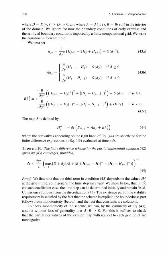
100 A. Oberman, T. Zariphopoulou

where D = D(y, t) ≥ D0 > 0, and where A = A(y, t), B = B(y, t) in the interiorof the domain. We ignore for now the boundary conditions of early exercise andthe artificial boundary conditions imposed by a finite computational grid. We writethe equation in forward time.

We next set

hyy = 1

dy2

(Hj−1 − 2Hj + Hj+1

)+ O(dy2), (43a)

Ahy =

A

dy(Hj+1 − Hj) + O(dy) if A ≥ 0

A

dy(Hj − Hj−1) + O(dy) if A < 0,

(43b)

Bh2x =

B

dy2

((|Hj+1 − Hj |+)2 + (|Hj − Hj−1|−

)2)+ O(dy) if B ≥ 0

B

dy2

((|Hj+1 − Hj |−)2 + (|Hj − Hj−1|+)2

)+ O(dy) if B < 0 .

(43c)

The map S is defined by

Hn+1j = dt

(Dhyy + Ahy + Bh2

y

)(44)

where the derivatives appearing on the right hand of Eq. (44) are shorthand for thefinite difference expressions in Eq. (43) evaluated at time ndt .

Theorem 20. The finite difference scheme for the partial differential equation (42)given by (43) converges, provided,

dt ≤ dy2

2

(max

j{D + dy|A| + |B|(|Hj+1 − Hj |+ + |Hj − Hj−1|−)}

)−1

.

(45)

Proof. We first note that the third term in condition (45) depends on the values Hnj

at the given time, so in general the time step may vary. We show below, that in theconstant coefficient case, the time step can be determined initially and remain fixed.Consistency follows from the discretization (43). The existence part of the stabilityrequirement is satisfied by the fact that the scheme is explicit, the boundedness partfollows from monotonicity (below), and the fact that constants are solutions.

To check monotonicity of the scheme, we can, by the symmetry of Eq. (43),assume without loss of generality that A, B ≥ 0. For this it suffices to checkthat the partial derivatives of the explicit map with respect to each grid point arenonnegative.

Pricing early exercise contracts in incomplete markets 101

First, checking with respect to Hj gives

∂S

∂Hj

= 1 − 2Ddt

dy2 − Adt

dy− 2B

dt

dy2

(|Hj+1 − Hj |+ + |Hj − Hj−1|−)

which is satisfied if

dt ≤ dy2

2

(max

j

{D + .5dy|A| + dy|B|(|Hj+1 − Hj |+ + |Hj − Hj−1|−)

})−1

which reduces to the CFL condition (45).We now check monotonicity in the other variables:

∂S

∂Hj−1= dt

dy2

(D + 2B|Hj+1 − Hj |+

) ≥ 0

∂S

∂Hj+1= dt

dy2

(D + 2B|Hj − Hj−1|− + A dx

) ≥ 0

Therefore the scheme is unconditionally monotone in the neighboring nodes.

Corollary 21. In the constant coefficient case D(y, t) = D, B(y, t) = B andA(y, t) = A, the finite difference scheme for the partial differential equation (42),given by (43), converges provided that

dt ≤ dy2

2

1

D + dy|A| + dyM|B| (46)

where M = maxy |hy(y, 0)|.Proof. In the case where the coefficients are constants, the solutions to (42) aresmooth, since the equation is uniformly elliptic. Therefore,

|Hj+1 − Hj |+ + |Hj − Hj−1|− = dy(|hy |+ + |hy |−) + O(dy2)

and, in fact, hy changes sign only near a local extremum, where hy = O(dy).Furthermore, standard maximum principle techniques (Berstein estimates)

show that the maximum of |hy | does not grow, and so the time step may be deter-mined from the initial data.

Up until now, our discussion has been for equations of the form (42). We wouldlike to consider American contracts, and since in practice we have only a finitecomputational domain, we need to impose boundary conditions.

Including the early exercise component gives an equation of the concise form

min{−ht + Dhyy + Ahy + Bh2

y, u − g(y)}

= 0 (47)

102 A. Oberman, T. Zariphopoulou

which is an obstacle problem and corresponds to theAmerican Option with exercisevalue g(y).

Extending the scheme from (42) to (47) involves no extra machinery. Thescheme is given by the map

Sδh = min{h + δ(Dhyy + Ahy + Bh2

y

), h − g(y)} (48)

where again the derivatives appearing on the right hand of (48) are shorthand forthe finite difference expressions in (43).

We simply note that the scheme for the (trivial) equation h − g(y) = 0 ismonotone, and that we also have a monotone scheme for the partial differentialequation. As observed in Proposition 19, minima of monotone maps are monotone,so the scheme is monotone. Further, since both the equation and the scheme arewritten as a minimum of two equations, consistency follows automatically.

We next discuss a non-rigorous heuristic for introducing artificial boundaryconditions to allow for a finite computational domain.

Restricting the computational domain to a finite grid requires introducing arti-ficial boundary conditions at the boundary. In principle, for large enough domains,the boundary conditions would not affect the values in the middle. For example, ex-amining the Gaussian kernel shows that this statement is true up to an exponentiallysmall error for the heat equation. Taking into account a finite shift in the domaindue to drift terms, we can see that it holds true for an equation with bounded drift aswell. Nevertheless, it is preferable to make a good choice of boundary conditions.Based on the heuristic that solutions of (47) are approximately linear as |y| → ∞,(when they are not equal to g(y)), we make the choice of boundary condition

hyy = 0 if h(y) > g(y). (49)

Furthermore, in the exercise region, we impose boundary conditions

h = g if h(y) ≤ g(y). (50)

The condition (50) is trivial, but for implementations it ensures that the solutiondoes not “lift off" the free boundary due to artificial boundary data.

We remark that the boundary conditions (49) may appear somewhat unortho-dox, given that standard treatments of linear second order partial differential equa-tions consider only zeroth order or first order boundary conditions. Further, in theEuropean case, this is natural, since on one side of the domain, solutions are ap-proximately linear, so the usual Neumann condition hy = 0 is not suitable. Theequation we now solve is:

min{−ht + Dhyy + Ahy + Bh2

y, h − g(y)}

= 0 if y ∈ �

hyy = 0 if y ∈ ∂� and h(y) > g(y)

h = g if y ∈ ∂� and h(y) ≤ g(y) .

Pricing early exercise contracts in incomplete markets 103

We continue with the implementation of the numerical scheme and give com-putational examples.

To begin, we introduce the change of variables y → log y. Now, a uniform gridin the new coordinates gives more accuracy near y = 1, and eliminates the possiblesingularity as y → 0. For the purposes of computations, we set a = a0y, b = b0y

which gives constant coefficients in the new coordinates, and a uniformly ellipticequation. So the equation at hand becomes

min

{−ht − 1

2a2

0hyy −(b0 − ρ

µ

σa0

)hy + 1

2a2

0γ (1 − ρ2)h2y, h − g(ez)

}= 0.

Here the Sharpe ratio µ/σ is a constant, ρ is the correlation of the nontradedasset with the traded one, b, a are the drift and volatility of the nontraded asset andγ > 0 is the risk aversion.

We set the terminal data to be that of a put, g(y) = (K − y)+, to give

h(y, T ) = (K − exp(y))+

and impose the artificial boundary conditions (49) and (50).The condition for convergence of the numerical scheme (45) becomes

dt ≤ dy2

a20 + dy(|b0 − ρ

µσa0| + a2

0γ (1 − ρ2)M)

which could be simplified to

dt ≤ 1

3min

(dy2

a20

,dy

|b0 − ρµσa0| ,

dy

a20γ (1 − ρ2)M

)

where M = maxy |hy(y, 0)|.We make some general observations about trends in the value of the option,

using the notation of (42). The value is a decreasing function of the coefficient ofthe nonlinear term, B, since h2

y > 0. The initial data is convex, outside of the freeboundary, so initially the values are increasing in the diffusion coefficient D. Withthe initial data of a put, the terminal data is decreasing, and remains so. Therefore,the value is decreasing as a function of the drift coefficient A. We note that whenA < 0 the solution lifts off the free boundary instantaneously.

We implemented the code in MATLAB, using approximately 400 nodes, anddomain the interval [e−2, e2]. In the first run, we compare the European and Amer-ican option values with Sharpe ratio equal to 1, a0 = 1, b0 = 0.3, ρ = .1, γ = 1.The results are shown in Fig. 1. The delta of the claim, and the position of thefree boundary as a function of time are shown in Fig. 2. The position of the freeboundary jumps one grid point.

Now fixing the rest of the data, we vary γ , taking γ = 0.0, 1, 5, and keepingthe other values fixed at Sharpe ratio equal to 1, a0 = .5, b0 = 0.3, ρ = .1, γ = 1.

104 A. Oberman, T. Zariphopoulou

0.5 1 1.5 2 2.5 30

0.1

0.2

0.3

0.4

0.5

0.6

0.7

0.8

Fig. 1. Comparison of European and American options after time 1, with initial data and Sharpe ratioequal to 1, a0 = 1, b0 = 0.3, ρ = 0.1, γ = 1

0 0.2 0.4 0.6 0.8 1

0.2

0.3

0.4

0.5

0.6

0.7

0.8

0.9

1Position of the free boundary

1 2 3 4 5 6 7−1

−0.8

−0.6

−0.4

−0.2

Delta of the solution

Fig. 2. Delta of the option at time 1, and position of the free boundary as a function of time, Sharperatio equal to 1, a0 = 1, b0 = 0.3, ρ = 0.1, γ = 1

0.5 1 1.5 20

0.05

0.1

0.15

0.2

0.25

0 0.2 0.4 0.6 0.8 10.7

0.75

0.8

0.85

0.9

0.95

1

Fig. 3. Value of the option (increasing as a function of γ ), and position of the free boundary as afunction of time (decreasing as a function of γ ), for γ = 0.0, 1, 5, with Sharpe ratio equal to 1,a0 = 0.5, b0 = 0.3, ρ = 0.1

Pricing early exercise contracts in incomplete markets 105

0.5 1 1.5 2 2.50

0.1

0.2

0.3

0.4

0.5

0 0.2 0.4 0.6 0.8 10.3

0.4

0.5

0.6

0.7

0.8

0.9

1

Fig. 4. Value of the option (increasing as a function of ρ), and position of the free boundary as afunction of time (decreasing as a function of ρ), for ρ = .1, .5, .8, .9, with Sharpe ratio equal to 1,a0 = .5, b0 = .3, γ = 1

The solution is decreasing in γ and the position of the free boundary is increasingin γ , as shown in Fig. 3.

Next, fixing the rest of the data, we vary ρ, taking ρ = .1, .5, .8, .9, and keepingthe other values fixed at Sharpe ratio equal to 1, a0 = .5, b0 = 0.3, γ = 1. Thesolution is increasing in ρ and at ρ = .9 the solution moves off the free boundary,as shown in Fig. 4.

6 Conclusions and future research directions

In this paper we extended the utility-based valuation approach to the case of earlyexercise contracts written exclusively on nontraded assets. We provided a differen-tial, probabilistic and computational characterization of the so called early exerciseindifference price. In a market environment with lognormal stock dynamics andgeneral dynamics for the nontraded asset, we showed that the buyer’s indifferenceprice is the unique solution to a quasilinear variational inequality with an obstacleterm, given by the contract’s payoff. We established that the early exercise indiffer-ence prices are given as solutions of optimal stopping problems of their indifferenceEuropean counterparts. This robustness result highlights the universality of the val-uation theory by indifference. Additional robustness results and price spreads wereproved as markets become complete and for limiting values of risk aversion. Wealso developed a general class of numerical schemes. We built a scheme that is sta-ble, monotone and consistent and thus converges to the unique (viscosity) solutionof the quasilinear pricing variational inequality. Numerical results were providedfor a range of the Sharpe ratio, the risk aversion and correlation.

Having provided a complete characterization of the early exercise price, weshould focus on the specification of the risk monitoring policies. One needs toconstruct the indifference analogue of the arbitrage free payoff decomposition thatyields, via the martingale representation theorem, the correct hedging strategy.

106 A. Oberman, T. Zariphopoulou

Another important task is to explore how the classical parity between the Europeanand American prices and, early exercise premium is extended to the utility-basedpricing setting.

The most challenging question however, is to understand how indifferenceprices can be represented in a model-independent manner, without any specificstructural assumptions. In order to produce a viable incomplete market pricingmechanism, one should aim at producing prices that can be written in terms of aconstitutive analogue of the risk neutral classical theory. Arbitrage free prices arerepresented as (discounted) expected payoffs under the (unique) risk neutral mea-sure. As the results herein suggest, when markets become incomplete, the utility-based valuation concept produces prices that are given in terms of a nonlinearpricing functional under a new measure, namely, the one that minimizes the rel-ative entropy with respect to the historical one. Establishing such results undervery general assumptions on the market environment and the claims is of primaryimportance.

References

Barles G (1997): Convergence of numerical schemes for degenerate parabolic equations arising infinance theory. In: Numerical Methods in Finance, Cambridge University Press, Cambridge

Barles G, Daher Ch, Romano M (1995): Convergence of numerical schemes for parabolic equationsarising in finance theory. Mathematical Models & Methods in Applied Sciences 5(1): 125–143

Barles G, Soner HM (1998): Option pricing with transaction costs and a nonlinear Black and ScholesEquation. Finance and Stochastics 2: 369–397

Barles G, Souganidis PE (1991): Convergence of approximation schemes for fully nonlinear secondorder equations. Asymptotic Analysis 4: 271–293

Becherer D (2002): Rational hedging and valuation of integrated risks under constant absolute riskaversion. (preprint)

Constantinides G, Zariphopoulou T (2001): Bounds on derivatives prices in an intertemporal settingwith proportional transaction costs and multiple securities. Mathematical Finance 11(3): 331–346

Constantinides G, Zariphopoulou T (1999): Bounds on prices of contingent claims in an intertemporaleconomy with proportional transaction costs and general preferences. Finance and Stochastics 3(3):345–369

Courant R, Friedrichs K, Lewy H (1967): On the partial difference equations of mathematical physics.IBM Journal of Research Development 11: 215–235

Crandall MG, Lions P-L (1983): Viscosity solutions of Hamilton-Jacobi equations. Transactions of theAmerican Mathematical Society 277: 1–42

Crandall MG, Lions P-L (1984): Two approximations of solutions of Hamilton-Jacobi equations. Math-ematics of Computation 43: 1–19

Crandall MG, Ishii H, Lions P-L (1992): User’s guide to viscosity solutions of second order partialdifferential equations. Bulletin of the American Mathematical Society 27: 1–67

Davis MHA (1999): Option valuation and hedging with basis risk. In: Djaferis TE, Schick IC (eds)Systems Theory: Modelling, Analysis and Control. Kluwer, Amsterdam

Davis MHA (2000): Optimal hedging with basis risk. (preprint)Davis MHA, Panas V, Zariphopoulou T (1993): European option pricing with transaction costs. SIAM

Journal on Control and Optimization 31: 470–493Davis MHA, Zariphopoulou T (1995): American options and transaction fees. Mathematical Finance,

IMA Volumes in Mathematics and Its Applications, Springer-VerlagDelbaen F, Grandits P, Rheinlander T, Samperi D, Schweizer M, Stricker C (2002): Exponential hedging

and entropic penalties. Mathematical Finance 12: 99–123Duffie D, Richardson HR (1991): Mean-variance hedging in continuous time. Annals of Applied Prob-

ability 1: 1–15

Pricing early exercise contracts in incomplete markets 107

Duffie D, Zariphopoulou T (1993): Optimal investment with undiversifiable income risk. MathematicalFinance 3: 135–148

Dunbar N (2000): The Power of Real Options. RISK 13(8): 20–22Fleming WH, Soner HM (1993): Controlled Markov Processes and Viscosity Solutions. Springer-VerlagFollmer H, Schied A (2002a): Convex measures of risk and trading constraints. Finance and Stochastics

6: 429–447Follmer H, Schied A (2002b): Robust preferences and convex measures of risk. (preprint)Follmer H, Sondermann D (1986): Hedging of non-redundant contingent claims. In: Hildenbrand W,

Mas-Colell A (eds) Contributions to Mathematical Economics in Honor of Gerard Debreu. NorthHolland, Amsterdam, 205–223

Frittelli M (2000a): The minimal entropy martingale measure and the valuation problem in incompletemarkets. Mathematical Finance 10: 39–52

Frittelli M (2000b): Introduction to a theory of value coherent with the no-arbitrage principle. Financeand Stochastics 4: 275–297

Johnson SA, Tian YS (2000): The value and incentive effects of non traditional executive stock optionplans. Journal of Financial Economics 57: 3–34

Hodder JE, Tourin A, Zariphopoulou T (2001): Numerical Schemes for Variational Inequalities Arisingin International Asset Pricing. Computational Economics 17: 43–80 (2001)

Hodges S, NeubergerA (1989): Optimal replication of contingent claims under transaction costs. Reviewof Futures Markets 8: 222–239

Ishii H, Lions P-L (1990): Viscosity solutions of fully nonlinear second-order elliptic partial differentialequations. Journal of Differential Equations 83: 26–78

Karatzas I, Wang H (2000): Utility maximization with discretionary stopping. SIAM Journal on Controland Optimization 39(1): 306–329

Lions P-L (1983): Optimal control of diffusion processes and Hamilton-Jacobi-Bellman equations. Part1: The dynamic programming principle and applications. Part 2:Viscosity solutions and uniqueness.Communications in PDE 8: 1101–1174 and 1229–1276

MacNair S, Zariphopoulou T (2000): Optimal investment models with early exercise. (preprint)Merton RC (1969): Lifetime portfolio selection under uncertainty: the continuous time model. Review

of Economic Studies 51: 247–257Musiela M, Rutkowski M (1997): Martingale Methods in Financial Modelling. Springer-VerlagMusiela M, Zariphopoulou T (2002a): An example of indifference prices under exponential preferences.

Finance and Stochastics (to appear)Musiela M, Zariphopoulou T (2002b): A valuation algorithm in incomplete markets. Finance and

Stochastics (to appear)Oberman A, Souganidis PE (2003): Convergent Schemes for Degenerate Elliptic Equations. (in prepa-

ration)Pham H, Rheinlander T, Schweizer M (1998): Mean-Variance Hedging for continuous processes: New

Proofs and Examples. Finance and Stochastics 2: 173–198Rouge R, El Karoui N (2000): Pricing via utility maximization and entropy. Mathematical Finance 10:

259–276Smith J, Nau R (1995): Valuing risky projects: Option Pricing theory and Decisions Analysis. Manage-

ment Science 41(5): 795–816Smith J, McCardle K (1998): Valuing oil properties: integrating option pricing and decision analysis

approaches. Operations Research: 198–217Souganidis PE (1985): Approximation schemes for viscosity solutions of Hamilton-Jacobi equations.

Journal of Differential Equations 59: 1–43TourinA, Zariphopoulou T (1994): Numerical schemes for investment models with singular transactions.

Computational Economics 7: 287–307Zariphopoulou T (2001): Stochastic control methods in asset pricing. In: Kannan D, Lakshmikanathan

V (eds) Handbook of Stochastic Analysis and Applications. Marcel Dekker