Discussion Papers Department of Economics University of Copenhagen

No. 07-04

Pricing and Trust

Steffen Huck Gabriele K. Ruchala Jean-Robert Tyran

Studiestræde 6, DK-1455 Copenhagen K., Denmark

Tel. +45 35 32 30 82 - Fax +45 35 32 30 00 http://www.econ.ku.dk

ISSN: 1601-2461 (online)

Pricing and Trust

STEFFEN HUCK, GABRIELE K. RUCHALA and JEAN-ROBERT TYRAN*

January 2007

Abstract

We experimentally examine the effects of flexible and fixed prices in markets for experience

goods in which demand is driven by trust. With flexible prices, we observe low prices and

high quality in competitive (oligopolistic) markets, and high prices coupled with low quality

in non-competitive (monopolistic) markets. We then introduce a regulated intermediate price

above the oligopoly price and below the monopoly price. The effect in monopolies is more or

less in line with standard intuition. As price falls volume increases and so does quality, such

that overall efficiency is raised by 50%. However, quite in contrast to standard intuition, we

also observe an efficiency rise in response to regulation in oligopolies. Both, transaction

volume and traded quality are, in fact, maximal in regulated oligopolies.

Keywords

Markets; Price competition; Price regulation; Reputation; Trust; Moral hazard; Experience

goods

JEL Classification Codes

C72, C90, D40, D80, L10

* Huck & Ruchala: Dept. of Economics and ELSE, University College London, s.huck@ucl.ac.uk / g.ruchala@ucl.ac.uk; Tyran: Dept. of Economics, University of Copenhagen, jean-robert.tyran@econ.ku.dk. Huck and Ruchala acknowledge financial support from the Economic and Social Research Council (UK) via ELSE and an additional grant on “Trust and competition.” Huck is also grateful for additional funding by the Leverhulme Trust.

1

1. Introduction

Buyers of an experience good are uncertain about its quality before they buy, but learn

(or experience) the good’s quality after having bought and consumed it. Experience goods

cover the broad middle ground between the extremes of goods involving no quality

uncertainty at all (so-called inspection or search goods) and goods for which quality is not

fully revealed even after the consumption (credence goods). Whenever contracts for the

exchange of a good are incomplete and sellers have leeway to shade its quality about which

the consumer finds out only if it is too late, the good in question is an experience good.

Hence, many are.

A key role in markets for such goods is assumed by trust. Buyers may buy an experience

good if they trust sellers to provide high quality, and will abstain if they do not. In other

words, trust induces the demand for experience goods. In contrast, lack of trust impedes

mutually advantageous transactions and results in low market efficiency.

We experimentally examine the effects of flexible and fixed prices in markets for

experience goods. To the best of our knowledge ours is the first study to investigate the role

of prices and competition for trust and market outcomes. We study two types of markets,

monopolies and four-firm oligopolies. In both cases, buyers can observe previous histories of

sellers (their reputations) and the chosen or exogenously set price before they make their

decisions.

With flexible prices, we observe low prices and high quality in competitive

(oligopolistic) markets and high prices coupled with low quality in non-competitive

(monopolistic) markets. We then introduce a regulated intermediate price roughly halfway

between the observed oligopoly and monopoly prices. The effect in monopolies is pretty

much as standard intuition would predict. As price falls, volume increases and so does the

quality of traded goods. Both effects imply a rise in efficiency of around 50%. Surprisingly,

the same effects occur when we introduce the regulated intermediate price in oligopolies. In

contrast to standard intuition, demand does not fall in reaction to the price increase and

quality rises even further, rendering the regulated oligopoly the most efficient market by far.

This counterintuitive effect of price regulation can be explained as follows. Under

unregulated Bertrand competition prices fall to a level where buyers do no longer mind that

much to buy a “lemon”. Consequently, buyers in unregulated oligopolies are rather careless.

2

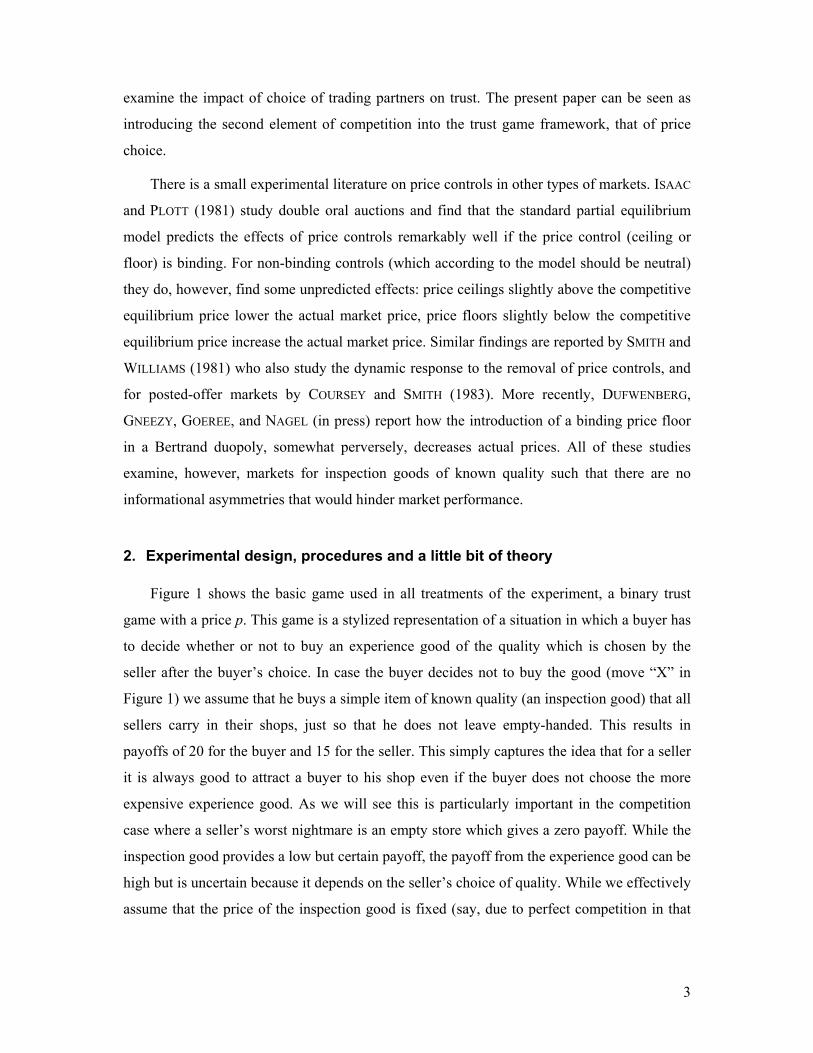
If, on the other hand, higher prices are exogenously imposed, buyers are forced to pay more

attention to reputations as buying from a low-quality firm does hurt them now substantially.

In addition, with regulated prices firms lose one of their two “marketing instruments”. The

only dimension they can now compete is quality. Thus, there are, both, demand- and supply-

induced forces that push up quality. In unregulated oligopolies almost 20% of all traded goods

are lemons (despite an accurate eBay-style feedback mechanism that allows all buyers to

track the entire history of all sellers). With price regulation the lemon share falls to just 6%.

This increase in quality also more than offsets the increase in price such that also the trade

volume is higher despite the higher price.

Thus, we do indeed find that price regulation fosters trust in markets for experience

goods but in rather subtle ways. The causal chain in monopolies has only two simple steps.

There, a lower regulated price increases demand as textbooks would have it. Given this

increase in demand it now becomes more costly for monopolists to lose the trust buyers place

in them and, consequently, they supply higher average quality. The channel through which

regulation fosters trust in oligopoly is more complex. Here, the direct effect of regulation is

that buyers become more selective. This increased sensitivity to reputations increases

trustworthiness which, finally, increases trust.1

Our finding shows how standard textbook intuition about price and demand can go wrong

in markets that suffer from informational deficiencies. In the markets we implement, these

deficiencies cause moral hazard but a similar mechanism may operate in case of adverse

selection. Regulation may directly aim at removing such deficiencies (for example by

introducing standardization, certification, or watch dogs) but in many cases such direct

regulation may be very costly. Price regulation is much cheaper to implement, administer and

enforce than most other alternatives. Yet, as we see here, it can be very effective.

Our study is the first experimental investigation into the relation of trust, competition,

and the role of prices. While there is a sizeable literature on trust games investigating how

different institutional features (such as feedback or enforcement mechanisms2) impact on

levels of trust, our previous paper (HUCK, RUCHALA, and TYRAN (2006)) is the first to

1 This complex relation between price, quality and trust is at the core of an interesting book in the management literature (SAKO (1992)) comparing inter-firm relations in Britain (low price, low trust, low quality) and Japan (high price, high trust, high quality). 2 See, e.g., KESER (2002), BOLTON, KATOK, and OCKENFELS (2004), BOHNET and HUCK (2004), BOHNET, HARMGART, HUCK, and TYRAN (2005) and FEHR and ZEHNDER (2004).

3

examine the impact of choice of trading partners on trust. The present paper can be seen as

introducing the second element of competition into the trust game framework, that of price

choice.

There is a small experimental literature on price controls in other types of markets. ISAAC

and PLOTT (1981) study double oral auctions and find that the standard partial equilibrium

model predicts the effects of price controls remarkably well if the price control (ceiling or

floor) is binding. For non-binding controls (which according to the model should be neutral)

they do, however, find some unpredicted effects: price ceilings slightly above the competitive

equilibrium price lower the actual market price, price floors slightly below the competitive

equilibrium price increase the actual market price. Similar findings are reported by SMITH and

WILLIAMS (1981) who also study the dynamic response to the removal of price controls, and

for posted-offer markets by COURSEY and SMITH (1983). More recently, DUFWENBERG,

GNEEZY, GOEREE, and NAGEL (in press) report how the introduction of a binding price floor

in a Bertrand duopoly, somewhat perversely, decreases actual prices. All of these studies

examine, however, markets for inspection goods of known quality such that there are no

informational asymmetries that would hinder market performance.

2. Experimental design, procedures and a little bit of theory

Figure 1 shows the basic game used in all treatments of the experiment, a binary trust

game with a price p. This game is a stylized representation of a situation in which a buyer has

to decide whether or not to buy an experience good of the quality which is chosen by the

seller after the buyer’s choice. In case the buyer decides not to buy the good (move “X” in

Figure 1) we assume that he buys a simple item of known quality (an inspection good) that all

sellers carry in their shops, just so that he does not leave empty-handed. This results in

payoffs of 20 for the buyer and 15 for the seller. This simply captures the idea that for a seller

it is always good to attract a buyer to his shop even if the buyer does not choose the more

expensive experience good. As we will see this is particularly important in the competition

case where a seller’s worst nightmare is an empty store which gives a zero payoff. While the

inspection good provides a low but certain payoff, the payoff from the experience good can be

high but is uncertain because it depends on the seller’s choice of quality. While we effectively

assume that the price of the inspection good is fixed (say, due to perfect competition in that

4

market) the price, p, of the experience good is, in principle, flexible but will be regulated in

some treatments.

In Figure 1, if the buyer decides to trust the seller (move “Y”), the seller can choose

between low quality (move “left”) and high quality (move “right”). Delivering low quality is

more profitable for the seller (due to lower costs) but harms the buyer. The buyer in fact

prefers not to buy the experience good at all over buying a low-quality good as long as the

price is not below 40 (which we rule out in our experiment).

Figure 1: A trust game with a variable price p

In all our experiments there are four sellers and four buyers who interact over 30 periods.

To implement monopolistic markets we randomly assign buyers to sellers. Each buyer is

assigned with probability ¼ to each seller which implies that sellers can have multiple (or no)

buyers in any given period. In oligopolistic markets buyers choose sellers, knowing each

seller’s price. In markets with endogenous prices, prices are chosen by sellers at the very

beginning of each period. In treatments with a regulated price this price-setting stage is

simply omitted.

Table 1: Treatments in the 2x2 design

partner choice no yes

no (p = 55) MON-REG OLI-REG price choice yes (40 ≤ p ≤ 85) MON-FREE OLI-FREE

We implement a 2x2 design. Table 1 gives an overview of the treatments. In MON-FREE

there is random matching and (monopolistic) sellers freely choose a price from a range

between 40 and 85. In OLI-FREE matching is endogenous, i.e., buyers choose sellers once

A

B

X Y

left . right;;

A: 60 – p points B: p – 5 points

A: 20 pointsB: 15 points

A: 85 – p points B: p – 30 points

5

sellers have chosen their prices, again with 40 ≤ p ≤ 85. In MON-REG matching is random

again but now the price is exogenously fixed to p = 55. Finally, in OLI-REG matching is

endogenous but the price is again fixed to p = 55.

We recruited 288 participants, mostly students from various fields, via the internet.3

Upon arrival subjects were provided with written instructions and randomly assigned to

cubicles in the laboratory.4 Each subject only participated in one session and we made sure

that no subject had participated in other related trust studies. The instructions employed

neutral language, avoiding terms like “trust”, “trustworthiness”, “buyer”, “seller” and “price”.

Buyer and sellers were simply called “A”-participants and “B”-participants, respectively.

Decisions were labeled as in Figure 1. In treatments with endogenous price choice “B”-

participants decided upon a “number p” at the beginning of each round. Several control

questions were included at the end of the instructions to ensure that the participants

understood the game. The experiment started after all participants had answered all the

control questions correctly and there were no further questions regarding the game. Subjects

were randomly and anonymously matched to groups of eight and were randomly assigned one

of two roles: four participants took the role of buyers and four participants the role of sellers.

Additionally, to identify participants over rounds, buyers and sellers were randomly assigned

a number between one and four. The role and the number were communicated to subjects via

the first computer screen. Matching groups of eight, roles, as well as assigned numbers stayed

constant throughout the entire experiment.

For each treatment we have nine independent matching groups with eight subjects each.

Sessions lasted on average between 60 and 90 minutes including instruction time. Participants

received a lump sum depending on their role in the experiment.5 During the experiment

payoffs were given in points which in the end were changed into Euro by a previously known

exchange rate of 1 point per 0.015 Euro. All subjects were paid anonymously.

As mentioned before, in the FREE treatments sellers chose a price p at the beginning of

each period. Prices were displayed to all buyers and sellers.6 Following this, depending on the

3 We used GREINER’s (2004) ORSEE. 4 A translation of the instructions is given in Appendix A. The original text was written in German and is available from the authors on request. The experimental software was programmed in FISCHBACHER’s (1999) z-Tree and the experiment was run in the experimental laboratory at the University of Erfurt. 5 While buyers received 150 points, sellers received 330 points. A higher lump sum fee for sellers was paid in order to provide a suitable payoff for sellers who did not very often interact with buyers. 6 We kindly asked subjects to note the respective number p on a provided blank for all buyers in all rounds.

6

matching procedure, buyers were either randomly assigned to a seller or chose one. After that

they chose between “X” or “Y”. Then sellers learned how many buyers were matched with

them as well as how many of those also decided to buy the experience good. Note that the

outside option of 15 is paid to a seller if he is first matched with a buyer who then decides not

to buy the experience good, while the seller’s payoff is zero if no buyer is matched with him.7

Then finally, given a seller had at least one buyer of the experience good, the seller had to

decide between “left” and “right” – and this decision determined the quality sold to all his

buyers, i.e., sellers could not discriminate between different buyers (who they could not

identify anyway).

At the end of each period, buyers who decided to buy the experience good were reminded

of the respective price p and informed about the choice their seller had made as well as about

the resulting payoff. Sellers were simply reminded of their price p and of the number of

buyers who bought the experience good from them, their own choice and the resulting

payoff.8 The sequence of the game with price competition is displayed in Figure 2; without

price competition, of course, the first stage is missing, i.e. sellers did not get to choose the

price p at the beginning of the game.

Figure 2: Sequence of the game with price competition

In all treatments the same feedback information is provided: all subjects (buyers and

sellers) have access to the entire history of the population game, i.e. there is a “history

window” which visualizes past decisions of sellers with respect to quality levels. This simple

graphical tool contains four columns of different colored hash (#) signs, each column

representing one seller and each row representing one period. Originally, each column

consists of thirty white hash signs, white representing the not-yet-reached future. Then,

following a given color code hash signs changed their color according to what happened in

7 Remember that even if a buyer might not trust the seller with the experience good, the seller has also an inspection good to sell which the buyer buys.

sellers choose price p

buyers choose seller / are assigned to

seller

buyers choose not to buy

“X” or to buy “Y” the

experience good

sellers choose low quality “left” or

high quality “right” for all buyers of the

experience good

sellers and buyers are informed

about actions and payoffs

history of all sellers is reproduced in the “history window”

7

the game: a hash turned black if a seller did not have a buyer; a hash turned red if a seller had

at least one buyer and chose low quality; finally, a hash turned green if a seller had at least

one buyer and chose high quality.9 Additionally, in case of the colors red or green, hash signs

were followed by a number showing how many buyers had bought the experience good from

this seller. A sample screen shot for buyers and sellers respectively is shown in Appendix B.

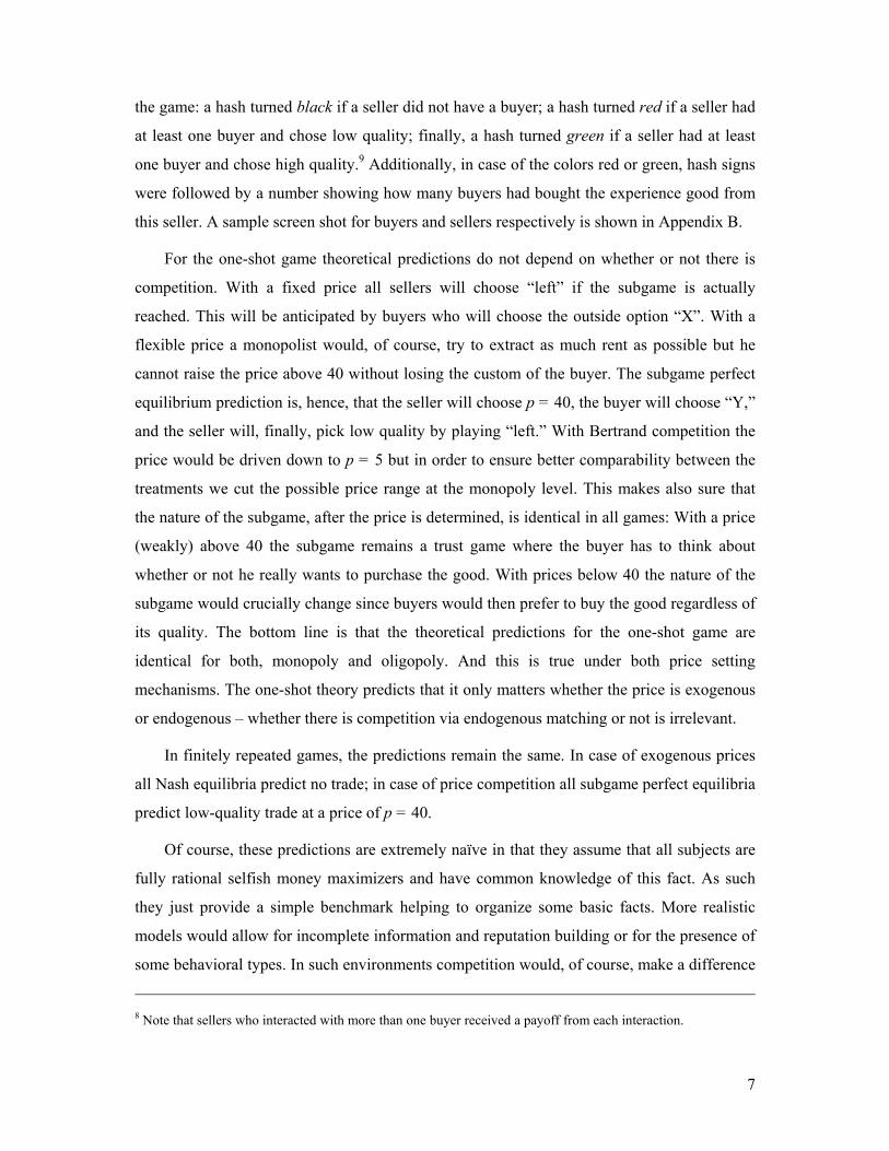
For the one-shot game theoretical predictions do not depend on whether or not there is

competition. With a fixed price all sellers will choose “left” if the subgame is actually

reached. This will be anticipated by buyers who will choose the outside option “X”. With a

flexible price a monopolist would, of course, try to extract as much rent as possible but he

cannot raise the price above 40 without losing the custom of the buyer. The subgame perfect

equilibrium prediction is, hence, that the seller will choose p = 40, the buyer will choose “Y,”

and the seller will, finally, pick low quality by playing “left.” With Bertrand competition the

price would be driven down to p = 5 but in order to ensure better comparability between the

treatments we cut the possible price range at the monopoly level. This makes also sure that

the nature of the subgame, after the price is determined, is identical in all games: With a price

(weakly) above 40 the subgame remains a trust game where the buyer has to think about

whether or not he really wants to purchase the good. With prices below 40 the nature of the

subgame would crucially change since buyers would then prefer to buy the good regardless of

its quality. The bottom line is that the theoretical predictions for the one-shot game are

identical for both, monopoly and oligopoly. And this is true under both price setting

mechanisms. The one-shot theory predicts that it only matters whether the price is exogenous

or endogenous – whether there is competition via endogenous matching or not is irrelevant.

In finitely repeated games, the predictions remain the same. In case of exogenous prices

all Nash equilibria predict no trade; in case of price competition all subgame perfect equilibria

predict low-quality trade at a price of p = 40.

Of course, these predictions are extremely naïve in that they assume that all subjects are

fully rational selfish money maximizers and have common knowledge of this fact. As such

they just provide a simple benchmark helping to organize some basic facts. More realistic

models would allow for incomplete information and reputation building or for the presence of

some behavioral types. In such environments competition would, of course, make a difference

8 Note that sellers who interacted with more than one buyer received a payoff from each interaction.

8

as sellers would compete for custom not only via price but also via their reputations (in the

REG treatments only via their reputations). From this perspective, one would expect

competition to matter in the usual way: Since endogenous matching creates incentives for

having a good reputation sellers should provide more high quality. This effect should be

unambiguous in treatments with fixed prices. Modeling the FREE treatments would be

trickier. In essence, sellers with identical reputations would again drive down the price to the

bottom. But sellers with better reputations might now not only attract more buyers but could

also be able to charge higher prices. In symmetric equilibria this would only be relevant off

the equilibrium path but would basically induce even stronger incentives for the provision of

high quality.

3. Experimental Results

Aggregate data

Table 2 summarizes the data from our experiment. The upper part of the table reports

average posted prices, trust rates (the average share of trade), quality (the average share of

high-quality among traded goods) and efficiency (the average share of buyer-seller pairings

that resulted in high quality trade).10 The lower part of the table reports tests for significance

of price regulation and competition. These MWU tests use market-level averages over 30

periods (i.e. 9 observations per treatment) as a unit of observation.

Notice first the highly significant and substantial effect of endogenous matching. Both

oligopoly treatments vastly outperform the monopolies, roughly tripling efficiency rates. This

boost is driven by, both, higher average quantity and quality. In addition, average prices are

much lower with competition (47.06) than without (59.60).

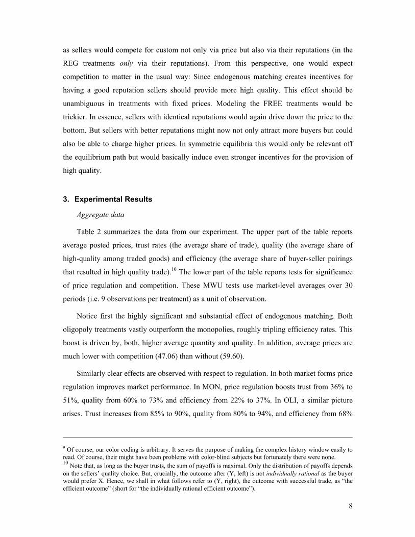
Similarly clear effects are observed with respect to regulation. In both market forms price

regulation improves market performance. In MON, price regulation boosts trust from 36% to

51%, quality from 60% to 73% and efficiency from 22% to 37%. In OLI, a similar picture

arises. Trust increases from 85% to 90%, quality from 80% to 94%, and efficiency from 68%

9 Of course, our color coding is arbitrary. It serves the purpose of making the complex history window easily to read. Of course, their might have been problems with color-blind subjects but fortunately there were none. 10 Note that, as long as the buyer trusts, the sum of payoffs is maximal. Only the distribution of payoffs depends on the sellers’ quality choice. But, crucially, the outcome after (Y, left) is not individually rational as the buyer would prefer X. Hence, we shall in what follows refer to (Y, right), the outcome with successful trade, as “the efficient outcome” (short for “the individually rational efficient outcome”).

9

to 85%. As can be seen in the bottom part of the table, all these effects are statistically

significant with the exception of the demand effect in the oligopoly treatments.

Table 2: Overview of aggregated results

Price Trust / Quantity Quality11 Efficiency

MON-FREE 59.60 (2.50)

0.36 (0.19)

0.60 (0.27)

0.22 (0.20)

MON-REG 55.00 [n.a.]

0.51 (0.16)

0.73 (0.16)

0.37 (0.19)

OLI-FREE 47.06 (5.99)

0.85 (0.16)

0.80 (0.23)

0.68 (0.26)

OLI-REG 55.00 [n.a.]

0.90 (0.07)

0.94 (0.03)

0.85 (0.07)

effect of price regulation

MON-FREE – MON-REG n.a. p = 0.039 p = 0.081 p = 0.047

OLI-FREE – OLI-REG n.a. p = 0.423 p = 0.031 p = 0.083

effect of competition

OLI-REG – MON-REG n.a. p = 0.000 p = 0.000 p = 0.000

OLI-FREE – MON-FREE p = 0.000 p = 0.000 p = 0.016 p = 0.001

Standard deviations are given in parentheses. Treatment effects are tested by one-tailed Mann-Whitney U-tests.

These unambiguous results are surprising. In one case, we observe that a lower price

improves market performance, in the other that a higher price also improves performance.

Taken together this suggests a non-monotonic relation between prices and efficiency in

markets for experience goods. With very low prices markets suffer because neither are

consumers particularly careful when selecting a good, nor are there good incentives for firms

to provide high quality: both, because consumers are less discerning and because the profit

margin of high-quality goods becomes too small. On the other hand, with very high prices

demand drops to such low levels that the incentives for reputation building are severely

reduced. Thus, market efficiency is maximal with a regulated intermediate price that is high

enough to ensure that high-quality products are profitable but at the same time not too high in

order to keep demand at levels where the incentives for high quality provision and reputation

building are maintained.

11 The reported quality corrects for the number of interactions a seller had in a period. Thus, if a seller had

4≤n buyers his quality choice enters the average n-times. If one considers each seller’s decision only once following average qualities are obtained: MON-FREE 0.58, MON-REG 0.73, OLI-FREE 0.78, and OLI-REG 0.94.

10

How do all these effects translate into payoffs for buyers and sellers? Figure 3 shows

buyers’ and sellers’ earnings averaged over all periods in the four treatments. In line with

standard intuition, forcing up prices by regulation in a competitive market harms buyers (their

average incomes fall by 21%, from 1058 to 831), but benefits sellers (their average incomes

increase by 50%, from 504 to 758). In contrast, forcing prices down by regulation benefits

both buyers and sellers in non-competitive markets (MON). Buyer incomes increase by 6%,

and, surprisingly, seller incomes also increase by 9%.12 Figure 7 also shows that, quite

remarkably, the regulated oligopoly is the most profitable market institution for sellers, while

it is, of course less surprising that Bertrand competition is best for buyers.

Figure 3: Average earnings over all periods

653

709

504

758

612649

1058

831

400450500550600650700750800850900950

100010501100

MON-FREE MON-REG OLI-FREE OLI-REG

aver

age

earn

ings

seller's earnings

buyer's earnings

Market measures over time

Figures 4a and 5 to 7 show how the measures of Table 2 behave over time. Additionally,

Figure 4b shows the distribution of posted prices in treatments with FREE price choice.

Figure 4a shows posted prices averaged over all 9 markets in the two treatments with

FREE price choice along with the regulated price of 55 as a benchmark. Competition unfolds

its effect in OLI-FREE only over time. Over the first 12 periods, posted prices continuously

12 The increase for buyers and sellers is, however, not significant in a monopolistic market (Mann-Whitney U-tests: for buyers 0.340 and for sellers 0.113, two-tailed). The change in buyer and seller payoffs in an

11

fall from 57.67 to around 45, and then remain close to this value for the rest of the periods.

While prices start out at the same level in MON-FREE as in OLI-FREE, they remain at high

levels. The average price in MON-FREE is 59.60 and in OLI-FREE it is 47.06 over all

periods. Therefore, the regulated price is about 8% below the average posted price in MON-

FREE, and about 22% above the convergence price of 45 in OLI-FREE.

Figure 4a: Average posted price in treatments with FREE prices

40

45

50

55

60

65

70

75

80

85

1 2 3 4 5 6 7 8 9 10 11 12 13 14 15 16 17 18 19 20 21 22 23 24 25 26 27 28 29 30period

aver

age

pric

e

OLI-FREE

MON-FREE

OLI-REG and MON-REG

oligopolistic market, on the other hand, is (Mann-Whitney U-tests: for buyers 0.001 and sellers 0.002, two-tailed).

12

Figure 4b: Cumulative distribution of posted prices in treatments with FREE prices

0.0

0.1

0.2

0.3

0.4

0.5

0.6

0.7

0.8

0.9

1.0

40 45 50 55 60 65 70 75 80 85posted price

cum

ulat

ive

freq

uenc

y

OLI-FREE

MON-FREE

On average, buyers were more likely to buy from sellers who posted low prices in both

treatments with FREE prices. In fact, the average transaction price was 54.18 in MON-FREE

and 42.85 in OLI-FREE over all periods. In the second half of the game, the average

transaction price in OLI-FREE falls to 40.76 with a small standard deviation of 1.35. This

illustrates how intense price competition was in OLI-FREE.

Evidence of the intensity of price competition in OLI-FREE also comes from a

comparison of the cumulative distribution of posted prices with MON-FREE (see Figure 4b).

For example, 66.57% of all posted prices are below 45 in OLI-FREE, but only 13.61% are in

MON-FREE. Prices in MON-FREE are highly concentrated between 54 and 60 (more than

40% of all prices), while only few sellers (about 7%) choose prices in this range in OLI-

FREE.

13

Figure 5: Average trust rates (average quantity) over time

0.0

0.1

0.2

0.3

0.4

0.5

0.6

0.7

0.8

0.9

1.0

1 2 3 4 5 6 7 8 9 10 11 12 13 14 15 16 17 18 19 20 21 22 23 24 25 26 27 28 29 30period

aver

age

trus

t

OLI-FREE MON-FREE OLI-REG MON-REG

Figure 5 shows that trust rates (i.e. the average share of experience goods traded) start out

at similar levels of around 50% in all treatments. While, as with prices, there are no initial

differences between the treatments already after 5 periods, demand is clearly higher in the

treatments where sellers compete for the business of buyers (i.e. in OLI) than in those without

competition, and the difference becomes more pronounced over time. In the two treatments

with oligopolistic competition, trust rates approach 100% in the last third of the experiment

while they hover around 30-40% in treatments without competition. Clearly, competition via

reputation induces trust in the sellers.

14

Figure 6: Average quality over time

0.0

0.1

0.2

0.3

0.4

0.5

0.6

0.7

0.8

0.9

1.0

1 2 3 4 5 6 7 8 9 10 11 12 13 14 15 16 17 18 19 20 21 22 23 24 25 26 27 28 29 30period

aver

age

qual

ity

OLI-FREE MON-FREE OLI-REG MON-REG

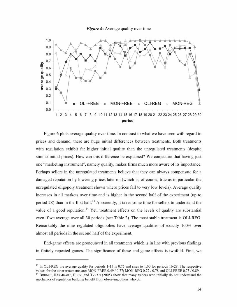
Figure 6 plots average quality over time. In contrast to what we have seen with regard to

prices and demand, there are huge initial differences between treatments. Both treatments

with regulation exhibit far higher initial quality than the unregulated treatments (despite

similar initial prices). How can this difference be explained? We conjecture that having just

one “marketing instrument”, namely quality, makes firms much more aware of its importance.

Perhaps sellers in the unregulated treatments believe that they can always compensate for a

damaged reputation by lowering prices later on (which is, of course, true as in particular the

unregulated oligopoly treatment shows where prices fall to very low levels). Average quality

increases in all markets over time and is higher in the second half of the experiment (up to

period 28) than in the first half.13 Apparently, it takes some time for sellers to understand the

value of a good reputation.14 Yet, treatment effects on the levels of quality are substantial

even if we average over all 30 periods (see Table 2). The most stable treatment is OLI-REG.

Remarkably the nine regulated oligopolies have average qualities of exactly 100% over

almost all periods in the second half of the experiment.

End-game effects are pronounced in all treatments which is in line with previous findings

in finitely repeated games. The significance of these end-game effects is twofold. First, we

13 In OLI-REG the average quality for periods 1-15 is 0.75 and rises to 1.00 for periods 16-28. The respective values for the other treatments are: MON-FREE 0.49 / 0.77; MON-REG 0.72 / 0.78 and OLI-FREE 0.75 / 0.89. 14 BOHNET, HARMGART, HUCK, and TYRAN (2005) show that many traders who initially do not understand the mechanics of reputation building benefit from observing others who do.

15

see that markets do not make people more trustworthy or more trusting in general.

Competition simply induces incentives for strategic behavior.15 Second, the end-game effect

illustrates that participants do have a proper understanding of the strategic nature of the stage

game. Sellers simply stop providing high quality when it ceases to have a beneficial effect on

their reputation. Remarkably, this only happens in the very last (and to some extent in the

next-to-last) period.

Figure 7: Average efficiency over time

0.0

0.1

0.2

0.3

0.4

0.5

0.6

0.7

0.8

0.9

1.0

1 2 3 4 5 6 7 8 9 10 11 12 13 14 15 16 17 18 19 20 21 22 23 24 25 26 27 28 29 30period

aver

age

effic

ienc

y

OLI-FREE MON-FREE OLI-REG MON-REG

Finally, Figure 7 shows the compound effects of demand and quality on market

efficiency over time. There is a clear and consistent ranking of average market efficiency in

the four treatments. Competitive markets outperform monopolies and price regulation

improves efficiency in both types of markets for experience goods.

Understanding the benefits of price regulation

The most striking finding in our experiment is the beneficial effect of price regulation in

oligopolistic markets. The flip side of this is the detrimental effects of price competition in

these markets. Price competition is fierce in OLI-FREE and quality is significantly lower in

OLI-FREE than in OLI-REG. And we have discussed the consequences of this price

15 BOHNET, FREY, and HUCK (2001) report data from a finite-horizon trust experiment where trustworthiness reaches its maximum in the very last period. A conjecture is that this is driven by the public aggregate feedback they provide.

16

differential before. With very low prices consumers are less sensitive to reputations and for

firms the profit margin of high-quality goods becomes dangerously low. But why is price

competition so fierce in OLI-FREE? In other words, why is there not more competition via

quality? The reason is that sellers had no other choice than cutting their prices to the bottom.

When sellers compete both via prices and via reputations, buyers seem to pay more attention

to prices (which are not noisy) than to reputations (which are noisy in the sense that a seller

who provided good quality in the past might still provide low quality in his next transaction).

Buyers are apparently reluctant to trade-off higher prices against higher reputations.

From whom did buyers buy? The answer is simple: from the firm with the lowest price.

This holds in 85.34% of all purchases in OLI-FREE, while only 57.55% of all goods were

bought from the seller with the best reputation.16 (As the numbers indicate, it happened quite

often that the seller with the lowest price also had the best reputation, namely in 65.46% of all

cases in which buyers bought the cheapest good.)

Buyers’ obsession with low prices forces sellers to engage in cut-throat Bertrand

competition. While sellers could reap some price premium of higher quality in MON, this was

not the case in OLI. For example, in MON, sellers who provided high quality charged prices

of 55.35 on average, while sellers who sold low quality could only charge a price of 52.55. In

contrast, the high-quality sellers in OLI charged lower prices (42.42) than the low-quality

sellers (44.35).

Fierce price competition in OLI-FREE is not only explained by the sale of relatively

unprofitable experience goods (recall from Figure 1 that at the convergence price of 45,

selling a high-quality experience goods only yields a profit of 15). Posting low prices was

attractive for sellers in OLI-FREE because it also helped to attract non-trusting buyers who

instead of choosing a good of unknown quality preferred to buy the low-value inspection

good. The profit from these buyers is also 15 (see Figure 1). Hence, at prices of 45 which are

typical in much of OLI-FREE, a seller is indifferent between selling a high-quality experience

good or an inspection good. In fact, we find that even buyers who decide not to buy the

experience good typically buy the inspection good from the seller who posts the lowest price.

It appears, thus, that buyers like the idea of fierce price competition as such. Perhaps they

want to reward low-price sellers hoping that one day these sellers will also offer high quality.

16 For our purpose, we define the seller who most frequently choose high quality for the experience good as the seller with the best reputation. Of course, one can think of several ways to match this characteristic.

17

Alas, this hope is in vain. Of course, all this happens in an environment where average quality

is with 80% pretty high. Yet, for the 20% disappointments buyers have to endure, they have

nobody to blame but their own obsession with price.

4. Conclusion

Competition has generally two elements: choice of trading partners and choice of price.

In this paper we show that while the former is unambiguously good, the latter can be

problematic in markets that suffer from informational deficiencies. In particular, we show that

in markets with experience goods (suffering from moral hazard) regulated fixed prices can

outperform endogenous prices in both, monopolistic and oligopolistic markets. This is

surprising but has, as we argued above, an intuitive reason. If both, trading partners and

prices, are endogenously chosen, price competition becomes so fierce that sellers’ incentives

to build up pristine reputations are diminished, simply because profits from high-quality

goods become too small. In other words, if consumers do not reward high quality with a

willingness to pay higher prices, they should not be surprised if quality is less than perfect.

Anecdotally, our finding seems to resemble a string of recent scandals in the German

meat market that was plagued by huge amounts of extremely low-quality meat (well past its

sell-by date, in fact, in some cases biologically hazardous). An interesting discussion ensued

with two main lines of arguments: calls for more regulation were as abundant as fierce

criticism of German consumers’ obsession with everything that is cheap. (In particular, when

it comes to non-durables Germans tend to have a low willingness to pay. For food, for

example, they spend, in relative terms, only around three quarters of what Italian consumers

spend, see SEALE, REGMI, and BERNSTEIN (2003).) In the context of our stylized study both

arguments appear to be valid. Clearly, we find that it is consumers’ choice behavior that

diminishes sellers’ incentives to provide high quality. Yet, regulation can also overcome the

problem.

But the intriguing aspect of our findings is that regulation needs not target quality. Of

course, quality regulation constitutes one way to improve market outcomes but it is

notoriously complicated and costly. Again, this is anecdotally reflected in the example of the

German meat market where quality controls differ hugely between different states and there is

no sign of reaching a consensus on how monitoring should be improved. Our study suggests

that there might be an inexpensive yet very efficient short-cut: price regulation. With higher

18

enforced prices consumers become more careful in choosing sellers. They pay more attention

to reputations and, consequently, sellers face much steeper incentives to provide high quality.

Closer to orthodox beliefs are our findings on the first aspect of competition, endogenous

choice of trading partners. In our earlier paper (HUCK, RUCHALA, and TYRAN (2006)) we have

shown that such choice on its own can improve market outcomes enormously. In that study

we show that these improvements occur under different feedback institutions. In particular,

the study shows that for choice to work it is not necessary that consumers have access to full

feedback, i.e., to the entire history of all sellers. Rather, it is sufficient that buyers simply

remember their own experience with sellers. That is, as long as sellers are not perfectly

anonymous and are identified via labels, endogenous choice of trading partners is shown to

have substantial positive effects. From the perspective of this earlier paper, the current one

establishes that the same beneficial effects of choice hold in the presence of the second

element of competition: endogenously chosen prices.

19

References

BOHNET, Iris; FREY, Bruno S. and HUCK, Steffen (2001): More Order with Less Law: On Contract Enforcement, Trust, and Crowding, American Political Science Review 95(1), 131-144.

BOHNET, Iris; HARMGART, Heike; HUCK, Steffen and TYRAN, Jean-Robert (2005): Learning Trust, Journal of the European Economic Association 3(3), 322-329.

BOHNET, Iris and HUCK, Steffen (2004): Repetition and Reputation: Implications for Trust and Trustworthiness When Institutions Change, American Economic Review 94(2), 362-366.

BOLTON, Gary; KATOK, Elena and OCKENFELS, Axel (2004): How Effective are Electronic Reputation Mechanisms? An Experimental Investigation, Management Science 50(11), 1587-1602.

COURSEY, Don L. and SMITH, Vernon L. (1983): Price Controls in a Posted Offer Market, American Economic Review 73(1), 218-221.

DUFWENBERG, Martin; GNEEZY, Uri; GOEREE, Jacob K. and NAGEL, Rosemarie (in press): Price Floors and Competition, Economic Theory.

FEHR, Ernst and ZEHNDER, Christian (2005): Reputation and Credit Market Formation, Working Paper No. 179, National Centre of Competence in Research Financial Valuation and Risk Management.

FISCHBACHER, Urs (1999): z-Tree: Zurich Toolbox for Readymade Economic Experiments, Working Paper No. 21, Institute for Empirical Research in Economics, University of Zurich.

GREINER, Ben (2004): The Online Recruitment System ORSEE 2.0 – A Guide for the Organization of Experiments in Economics, Working Paper Series in Economics 10, University of Cologne.

HUCK, Steffen; RUCHALA, Gabriele K. and TYRAN, Jean-Robert (2006): Competition Fosters Trust, Discussion Paper No. 06-22, Department of Economics, University of Copenhagen.

ISAAC, R. Marc and PLOTT, Charles R. (1981): Price Controls and the Behavior of Auction Markets: An Experimental Examination, American Economic Review 71(3), 448-459.

KESER, Claudia (2002): Trust and Reputation Building in E-Commerce, CIRANO Working Paper 2002s-75.

SAKO, Mari (1992): Price, Quality and Trust: Inter-firm Relations in Britain and Japan, Cambridge University Press, Cambridge.

SEALE, James, Jr.; REGMI, Anita and BERNSTEIN, Jason (2003): International Evidence on Food Consumption Patterns, Technical Bulletin Number 1904, Electronic Report from the Economic Research Service, United States Department of Agriculture.

SMITH, Vernon L. and WILLIAMS, Arlington W. (1981): On Nonbinding Price Controls in a Competitive Market, American Economic Review 71(3), 467-474.

20

Appendix A: Instructions (Treatment OLI-FREE)

(Original instructions were in German. They are available from the authors upon request. In treatments without choice of sellers A-participants were randomly assigned to one of the four B-participants. In the ones without price choice, i.e. with a regulated price, B-participants didn’t have to choose a number p. There, the figure in the instructions already displayed the unambiguous resulting payoffs.) Welcome to the experiment! Please read these instructions carefully! Do not speak to your neighbors and keep quiet during the entire experiment! In case you have a question raise your hand! We will then come to you. At the beginning of the experiment you are randomly separated into subpopulations of 8 participants. During the experiment you solely interact with the participants of your subpopulation. In this experiment you will repeatedly make decisions. Doing this you can earn points. Your total sum of points plus a show-up fee, which is dependent on your role in the experiment, will be converted into Euros at the end of the experiment and paid to you in cash. The show-up fee amounts to 150 points for A-participants and 330 points for B-participants. Following rule applies to the conversion of points into Euros:

1 point = 0.015 € How much you earn depends on your decisions and on the decisions of other participants in your subpopulation. All participants receive the same instructions. All decisions are made anonymously. No other participant will get to know your name and your payoff. Altogether there are (in your subpopulation) eight participants. At the beginning of the experiment all participants are randomly assigned one of two roles (A or B) which is displayed on the computer screen. There are four A-participants (A1, A2, A3 and A4) and four B-participants (B1, B2, B3 and B4). All participants keep their role and the number assigned to them throughout the experiment. At the beginning of each round each B-participant chooses a number p from 40 to 85 which is after that revealed to all A- and B-participants. This number p has an impact, as will be explained later on, on the payoffs for A- and B-participants (see also figure). Thereafter each A-participant chooses one of the four B-participants with whom he interacts in this period, this means that A-participants decide whether they want to interact with B1, B2, B3 or B4. Therefore, a B-participant can interact with zero to four A-participants in one round. This process is repeated in the next round. B-participants only learn the number of A-participants who chose them, but not who has chosen them. After the A-participants have chosen the B-participants, it is each A-participants turn to make a decision. More specifically, each A-participant has to choose between option X and Y (see figure). If he picks option X, the A-participant will earn 20 points and the B-participant chosen by him will earn 15 points from this interaction. If he picks option Y, the payoffs

21

depend on the choice of the B-participant chosen by him who has to decide whether he wants to go “left” of “right”. If he decides to pick “left”, the A-participant will earn 60 – p points and the B-participant will earn p – 5 points from this interaction. If he decides to pick “right”, the A-participant will earn 85 – p points and the B-participant will earn p – 30 points. If a B-participant is not chosen by at least one A-participant or if all A-participants who have chosen him picked X, he does not have to make a decision. Otherwise the B-participant additionally learns the number of A-participants who have chosen him and picked Y and has to make the same decision for all these A-participants, that is whether he wants to go “left” or “right” for all A-participants. A B-participant who has not been chosen by at least one A-participant earns 0 points.

Payoffs for an A-participant and a B-participant from one interaction.

(B-participants can receive payoffs from several interactions in one round.)

The experiment consists of 30 rounds. After each round you will be informed about what has happened and you will be reminded of your payoff and your total sum of points so far. Moreover, all (A- and B-) participants can keep track of the entire history of B-participants. For all participants there will be a screen depicting the history of all B-participants. For each round and each B-participant there will be a colored little # (hash) with a number behind.

• A black # indicates that the B-participant had nothing to decide because either no A-participant chose him or all A-participants who chose him picked X.

• A red # indicates that the B-participant picked “left”.

• A green # indicates that the B-participant picked “right”.

• The integer behind the # shows the number of A-participants who picked Y after choosing this B-participant.

Please note on the additionally distributed blank the respective number p of each B-participant which is displayed to you above the relevant column on the screen.

These are the rules. Your can trust us that everything will happen exactly according to these rules. Take your time going over these instructions again and feel free to ask questions. But don’t shout! Simply raise your hand.

A

B

X Y

left right

A: 60 – p points B: p – 5 points

A: 20 pointsB: 15 points

A: 85 – p points B: p – 30 points

22

Appendix B: Screenshot (Example: OLI-FREE)

A-participant’s screen

B-participant’s screen