Pricing of Complementary Goods and Network Effects*

June 2003

Nicholas Economides** and V. Brian Viard***

Abstract

We discuss the case of a monopolist of a base good in the presence of complementary goods provided either by it or by other firms. We assess and calibrate the extent of the influence on the profits from the base good that is created by the existence of complementary goods, i.e., the extent of the network effect. We establish an equivalence between a model of a base and a complementary good and a reduced-form model of the base good in which network effects are assumed in the consumers’ utility functions as a surrogate for the presence of complementary goods produced by others. We also assess and calibrate the influence on profits of the intensity of network effects and quality improvements in both goods. We evaluate the incentive that a monopolist of the base good has to improve its quality rather than that of complementary goods. Finally, based on our results, we discuss an explanation of the fact that Microsoft Office has a significantly higher price than Microsoft Windows although both products have comparable market shares. Key words: calibration; monopoly; network effects; complementary goods; software; Microsoft JEL Classification Codes: L12; L13; C63; D42; D43

* We thank Ravi Mantena and Andy Skrzypacz for useful comments. ** Stern School of Business, New York University, 44 West 4th Street, New York, NY 10012, (212) 998-0864, fax (212) 995-5218, http://www.stern.nyu.edu/networks/, e-mail: neconomi@stern.nyu.edu, and Director, NET Institute, http://www.NETinst.org . *** Graduate School of Business, Stanford University, Stanford, CA 94305, (650) 736-1098, fax (650) 725-0468, http://faculty-gsb.stanford.edu/viard/, e-mail: viard_brian@gsb.stanford.edu.

Pricing of Complementary Goods and Network Effects

1. Introduction

In the extensive literature on network effects, there are two types of models: those that attempt to derive the network effect from the detailed microeconomics of the model and those that assume the existence of network effects and discuss the consequences for market structure. The first approach has been called the “micro approach” to network economics, while the second one has been called the “macro approach.”1 In the macro approach, network effects are typically summarized by a term that influences utility positively and is increasing in sales. Rarely has there been an attempt to calibrate the size of the network effect used in the macro approach models.2 This paper attempts to fill this gap for an important class of models, where network effects arise because of the sale of complementary goods.

We examine a monopolist of a base good who benefits from a complementary good provided either by it or by other firms, as well as from other complementary goods. We assess and calibrate the extent of the positive influence (network effect) on the base good profits that is created by the existence of the two sources (internal and external) of complementary goods. We establish an equivalence between a model of a base and complementary good and a reduced form model of the base good where network effects are assumed in the utility function as a surrogate for the presence of complementary goods produced by other firms. We also assess and calibrate the influence of the intensity of network effects and quality improvements in the complementary good on profits from the base good. We evaluate the incentive that a monopolist has to improve the quality of the base good rather than that of complementary goods that it produces.

Finally, based on our results, we discuss an explanation of the fact that Microsoft Office

is significantly more expensive than Microsoft Windows. Microsoft has approximately the same market share (over 90%) in the market for operating systems for personal computers as in the market for “office applications” (a bundle of word processing, spreadsheet, presentation and database software). However, Microsoft charges a price for its Windows operating system that is significantly lower than the price of its office suite. Our calibration explains this difference.

Section 2 sets up the basic framework of our research. Section 3 develops and discusses

the five models we use in this paper, which differ in the way that network externalities and inherent product quality are modeled. Section 4 compares the equilibria of the five models. Section 5 discusses the incentives to invest in quality in either the base good or the complementary good in different ownership structures and intensities of network effects. Section 6 discusses the explanation of Microsoft’s pricing provided by our analysis. Section 7 compares our results with the empirical literature on network effects. Section 8 has concluding remarks.

1 See Economides (1996a). 2 An exception is Economides (1996b).

2

2. Basic Framework We assume that consumers are differentiated in terms of their preferences for quality of the base good (“B”) and quality of the complementary good (“C”). The second good requires the first good to provide positive utility.3 For example, we can think of the Windows operating system as the base good, and an office suite (such as Microsoft Office) as the complementary good, not necessarily produced by the same company. Let the marginal utility of quality of the base good be θ and the marginal utility of quality of the complementary good be ϕ . The pair ( )ϕθ , defines a consumer type. We assume that both θ and ϕ are distributed independently and uniformly on [0, 1]. We assume that, besides the complementary good that we explicitly model, there are potentially other complementary goods whose existence positively influences consumers’ willingness to pay for the base good. We assume that the positive consumption effects between the base good and the complementary goods reinforce each other. Thus, we summarize these effects by adding a term proportional to sales of the base good in the utility function of a typical consumer. When consuming one unit of the base good and possibly one unit of the complementary good, consumer ( )ϕθ , , receives utility

VxpqkU BBBB δαθ ++−+= ,

where is a constant, Bk Bq is the quality of the base good, is the price of the base good, V is the utility from the consumption of the complementary good, is the sales of the base good,

BpxB α

measures the intensity of network effects of other complementary goods (“additional network effects”) and δ is an indicator variable taking the value one if the complementary good is bought and zero otherwise. Thus, network effects arising out of complementary goods are summarized by an additive term in the utility function proportional to sales.4 The utility from the consumption of the complementary good is

CCC pqkV −+= ϕ ,

where is a constant, Ck Cq is the quality of the complementary good and is the price of the complementary good.

Cp

3 Since the complementary good requires the presence of the base good but not conversely, we expect that the equilibria in terms of prices and quantities will be asymmetric across firms. 4 We assume that that the influence of positive consumption (network) effects on the willingness to pay for the base good can be summarized by an additive term which is proportional to sales of the base good. This assumes that higher sales of the base good are reflected in higher sales of the complementary good and vice versa.

3

We will consider five alternative models. The first model has a base good monopolist in a market where network effects are summarized in the utility function of consumers as proportional to sales. The second model has two monopolists (independent firms), one for the base good and one for the complementary good, and assumes no other network effects. The third model adds additional network effects arising from other complementary goods to the independent firms in Model 2. The fourth model has a single monopolist (joint monopolist) producing both the base and the complementary good. The fifth model adds network effects arising from other complementary goods to the joint monopolist considered in Model 4. 3. Models 3.1 Model 1: Single Good Monopolist in a Market with Additional Network Effects We first consider a model of a single good monopolist selling the base good with network effects arising from other complementary goods. In this case, 0=δ and consumer θ who buys one unit of the base good of quality at price receives utility of Bq Bp BBB xpqU αθ +−= (1)

where 0>α measures the intensity of the additional network effect (marginal utility of network expansion).5 All consumers of type Bθθ > buy the good, where the marginal consumer is θB = (pB – αxB)/qB. (2)

Sales are

xB = (1 - θB) = 1 – (pB – αxB)/qB. (3) Inverting the demand we have xB = (qB – pB)/(qB – α, ΠB = pBxB = pB(qB – pB)/(qB – α).6 (4) Assuming zero costs, maximizing profits implies:7

pB

* = qB/2, xB* = qB/(2(qB - α)) and ΠB

* = qB2/(4(qB - α)).8 (5)

In the case of no additional network effects, i.e., when 0=α , the demand without

network effects is a pivot of the demand with network effects through the point . It is well ( Bq,0 )

5 In sections 3 through 5, in which we focus on the theoretical model, we set 0== CB kk for simplicity. 6 We require Bq<α so that the demand is download sloping. 7 We present the model with zero costs, but positive costs could easily be added. We have

( ) ( ) 02 =−−=Π αBBBBB qpqdpd and ( ) 0222 <−−=Π αBBB qdpd since α>Bq . * <x ( )q −α28 We also require that everyone does not buy the good which implies or 1B BB q> , i.e., 2Bq<α .

4

known that such pivots of linear demands lead to the same monopoly price. Thus, the equilibrium price is unaffected by additional network effects, while sales and profits are higher with them. Using the subscript 0 for the variables with no additional networks effects ( 0=α ), we have

qB

Bθθ <

B

( )[ ]αqxx BB0

*B −= , and 0

*BB pp = ( )[ ]αqqΠΠ BBB0

*B −= . (6)

3.2 Model 2: Independent Firms Without Additional Network Effects

In Model 2, we consider two independent monopolists, one for the base good and another for the complementary good, and we assume no additional network effects. By comparing the equilibrium of this model to that of Model 1, we can calibrate the intensity of network effects for the base good generated by sales of a complementary good.

There are two groups of purchasers to consider (see Figure 1). First, consumers of type Bθθ > , BUB,ϕϕ < buy the base good only, where Bθ is the marginal consumer indifferent

between buying the base good and buying nothing, i.e.

BBB qp=θ , (7) and BUB,ϕ is the marginal consumer indifferent between buying only the base good and buying both the base and complementary goods, i.e.

CCBUB qp=,ϕ . (8)

Second, consumers of types BUB,ϕϕ > , Bθθ > , as well as of types ( )θϕϕ BU> , , buy both, where ( )θϕBU is the marginal consumer of type θ indifferent between buying both goods and buying nothing, i.e. ( ) ( ) CBCBBU qqpp θθϕ −+= . (9)

The profits for the base good monopolist are

[=Π ( ) ( )( )]2/11 ,,, BUBBUBUBBUBB ϕϕϕϕθ −−−+− Bp , (10) where ( ) CCBBU qpp +=ϕ is the consumer of type 0=θ who is indifferent between buying both goods and nothing. The profits for the complementary good monopolist are

=CΠ ( ) ( ) CBBUBBUBUB p]2/1[ ,, θϕϕϕ −−− . (11)

5

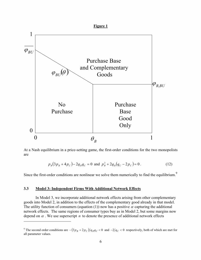
Figure 1

Purchase Base

and Complementary

Goods

No

Purchase

Purchase

Base

Good

Only

1

1 Bθ 0

0

BUB , ϕ

( ) θ ϕ BU

BU ϕ

At a Nash equilibrium in a price-setting game, the first-order conditions for the two monopolists are

( ) 0243 =−+ CBCBB qqppp and ( ) 0222 =−+ CCBB pqqp . (12) Since the first-order conditions are nonlinear we solve them numerically to find the equilibrium.9 3.3 Model 3: Independent Firms With Additional Network Effects

In Model 3, we incorporate additional network effects arising from other complementary goods into Model 2, in addition to the effects of the complementary good already in that model. The utility function of consumers (equation (1)) now has a positive α capturing the additional network effects. The same regions of consumer types buy as in Model 2, but some margins now depend on α . We use superscript n to denote the presence of additional network effects

9 The second order conditions are ( ) 023 <+− CBCB qqpp and 02 <− Cq respectively, both of which are met for all parameter values.

6

( ) BBB

nB qxp αθ −= , , (13) BUB

nBUB ,, ϕϕ =

( ) CBBCBnBU qxqpp αθϕ −−+= , ( ) CBCB

nBU qxpp αϕ −+= . (14)

Demand for the base good is given by solving for in Bx

( ) ( ) ( )( )( )2/11 ,nBB

nBUBB

nBUB

nBB xxxx θϕϕθ −−+−= . (15)

Since and are both linear functions of , this is a quadratic equation. Using the positive root, , that solves this equation, the profit function for the base good monopolist is

nBθ

nBUϕ∗Bx

Bx

( )( ) ( )( ) ( )( )[ ] BB

nB

nBUBB

nBU

nBUB

nBUBB

nB

nB pxxx ∗∗∗ −−−+−=Π θϕϕϕϕθ ,,, 2111 (16)

and for the complementary good monopolist is

( ) ( )( ) ( )[ ] CBnB

nBUBB

nBU

nBUB

nC pxx ∗∗ −−−= θϕϕϕ ,. 211Π . (17)

The first-order conditions for the two firms are nonlinear functions of the prices so we solve them numerically.10 3.4 Model 4: Joint Monopolist Without Additional Network Effects

In Model 4, the joint monopolist sells both the base and complementary goods. The marginal consumers are defined in the same manner as in Model 2, and the profit function for the joint monopolist is

( ) ( )( )( )CBBBUBBUBUBBBUBBCB ppp +−−−+−=Π+Π θϕϕϕϕθ ,,, 2111 . (18)

The joint monopolist chooses both prices to maximize its profits. The first-order conditions are

( ) 0223 =−+ CBCBB qqppp and ( ) 0222 =−− CCBB pqqp3 . (19) These can be solved to get the equilibrium prices, quantities, and profits:

32 BB qp = , 32 BCC qqp −= , (20)

10 We also verify numerically that the nonlinear second-order conditions hold and that ( )*; CBnB PPΠ is quasiconcave

in and BP ( )*; BCnC PPΠ is quasiconcave in . CP

7

( ) ( )CBCBBB qqpppx 221 +−= and ( ) ( )CBBCBC qqqppx 221 2 +−= .11 (21) Notice that the price of the base good is independent of the quality of the complementary good. This is true for general demand functions, since the marginal revenue of the joint monopolist from sales of the basic good is independent of the quality and price of the complementary good, at the optimal complementary good price.12 The joint monopolist completely internalizes in the complementary good price any changes in the quality of the complementary good, and therefore the price of the basic good remains unaffected by such quality changes.13 3.5 Model 5: Joint Monopolist With Additional Network Effects

In Model 5, we incorporate additional network effects for the base good into Model 4. The marginal consumers are defined in the same manner as in Model 3 and the profit function for the joint monopolist is

( )( ) ( )( ) ( )( )( CBB

nB

nBUBB

nBU

nBUBB

nBUBB

nB

nC

nB ppxxpx +−−−+−=Π+ ∗∗∗ θϕϕϕϕθ ,,, 2111 )Π . (22)

The first-order conditions for the firm are nonlinear functions of the prices so we solve them numerically.14 4. Equivalence Results

In this section, we calibrate the size of network effects arising from sales of complementary goods. This is possible since we have models that explicitly allow for positive effects of complementary goods sales as well as models that allow for network effects that are summarized in the utility function. Thus, we establish an equivalence between the network

11 The second-order condition is met as the Hessian is negative definite for all parameter values. 12 To see this in general, consider general demand functions for the base and complementary goods, respectively DB(pB) and DC(pB + pC). Then profits are ΠB = pB[DB(pB) + DC(pB + pC)], ΠC = pCDC(pB + pC), and joint profits are Π = ΠB + ΠC so that the first order conditions are:

(A) DB + pBDB’ + DC + (pB + pC)DC’ = 0, (B) DC + (pB + pC)DC’ = 0,

which imply DB(pB) + pBDB’(pB) = 0. Therefore for the joint monopolist the choice of price for the base good is independent of the choice of price and quality of the complementary good. 13 Also notice that, for independent firms, the first order conditions cannot be decomposed as in joint monopoly, and therefore the equilibrium prices of both the base and complementary good do depend on the quality levels of both goods. For independent firms, the first order conditions are:

(A’) DB + pBDB’ + DC + pBDC’ = 0, (B’) DC + pCDC’ = 0.

Substitution from (B’) into (A’) cannot accomplish decomposition as in joint monopoly. 14 We also verify that the second-order conditions are met. We solve over a grid of possible prices to ensure that we obtain the global maximum.

8

effects (defined as added profits to a base good monopolist) created by the presence of a complementary good and those summarized in the utility function. This is done in sections 4.1 to 4.4 for the various industry structures and for different quality levels.

4.1 Equivalence Between Additional Network Effects And The Effects Of A Complementary Good Produced By An Independent Firm (Model 1 Versus Model 2)

We start with a model of two independent monopolists, one producing the base good and

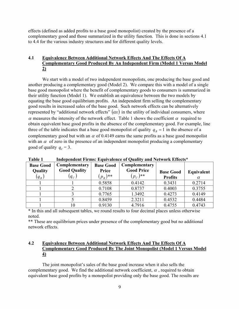
another producing a complementary good (Model 2). We compare this with a model of a single base good monopolist where the benefit of complementary goods to consumers is summarized in their utility function (Model 1). We establish an equivalence between the two models by equating the base good equilibrium profits. An independent firm selling the complementary good results in increased sales of the base good. Such network effects can be alternatively represented by “additional network effects” ( )xα in the utility of individual consumers, where α measures the intensity of the network effect. Table 1 shows the coefficient α required to obtain equivalent base good profits in the absence of the complementary good. For example, line three of the table indicates that a base good monopolist of quality 1=Bq in the absence of a complementary good but with an α of 0.4149 earns the same profits as a base good monopolist with an α of zero in the presence of an independent monopolist producing a complementary good of quality = 3. Cq Table 1 Independent Firms: Equivalence of Quality and Network Effects* Base Good

Quality ( )Bq

Complementary Good Quality

( )Cq

Base Good Price ( )Bp **

Complementary Good Price ( )Cp **

Base Good Profits

Equivalent α

1 1 0.5858 0.4142 0.3431 0.2714 1 2 0.7108 0.8737 0.4003 0.3755 1 3 0.7765 1.3492 0.4273 0.4149 1 5 0.8459 2.3211 0.4532 0.4484 1 10 0.9130 4.7916 0.4755 0.4743

* In this and all subsequent tables, we round results to four decimal places unless otherwise noted. ** These are equilibrium prices under presence of the complementary good but no additional network effects. 4.2 Equivalence Between Additional Network Effects And The Effects Of A

Complementary Good Produced By The Joint Monopolist (Model 1 Versus Model 4)

The joint monopolist’s sales of the base good increase when it also sells the

complementary good. We find the additional network coefficient, α , required to obtain equivalent base good profits by a monopolist providing only the base good. The results are

9

summarized in Table 2. This is equivalent to Table 1 but for a joint monopolist rather than for two independent firms. For example, line three of the table indicates that a monopolist producing a base good of quality q in the absence of a complementary good with an 1=B α of 0.4375 earns the same base good profits as a monopolist selling a base good of quality and a complementary good of quality with an

1=Bq3=Cq α of zero.

( )Cq

2= Cq

16

Table 2 Joint Monopolist: Equivalence of Quality and Network Effects Base Good

Quality ( )Bq

Complementary Good Quality

Base Good Price ( )Bp *

Complementary Good Price

( )Cp * Base Good

Profits Equivalent

α 1 1 0.6667 0.1667 0.4444 0.4375 1 2 0.6667 0.6667 0.4444 0.4375 1 3 0.6667 1.1667 0.4444 0.4375 1 5 0.6667 2.1667 0.4444 0.4375 1 10 0.6667 4.6667 0.4444 0.4375

* These are equilibrium prices under presence of complementary good but no additional network effects. The results in Table 2 are presented in numerical form for easy comparisons with other tables. They can also be presented in algebraic form using equations (20) - (21) as: 32 BB qp = = 2/3, 3132 −−= BCC qqp , ( ) ( )CBCBBB qqpppx 221 +−= = 2/3 and

94==Π BBB xp . Equating Π to the profits from Model 1 (a single good monopolist with additional network effects) gives (from equation (5)) the equivalent

B

α of: 742 =Π−= BBB qqα .

Comparing Tables 1 and 2, we observe that, while prices and profits for the base good are

sensitive to the quality of the complementary good for the independent monopolist, they are not for the joint monopolist. For the joint monopolist, all the variation in the quality of the complementary good is reflected in its price and the base good price is unaffected.15 This follows from the fact that the joint monopolist is able to adjust the price of the complementary good to fully reflect its adjustment in quality. Since it has both price instruments available, the joint monopolist can adjust the complementary good price so that the margin for consumers buying only the base good is not distorted by the change in complementary good quality (the Bθ margin in Figure 1). The joint monopolist does not want to alter the base good price because consumers who buy only the base good may be priced out of the market since they do not benefit from complementary good quality improvements. In contrast, the independent monopolist of the base good, in a Nash equilibrium framework, changes its price in the direction of changes in the quality of the complementary good. Thus, base good prices and profits are sensitive to quality changes of the complementary good when independent firms produce the two goods separately but not when the same firm produces them. As a result, the strength of the additional network

15 As expected, the sum of the prices is lower for the joint monopolist than for the independent monopolists.

CB pp +

10

effects (as measured by the α needed to equate the base good profits) is not sensitive to changes in the complementary good quality for the joint monopolist but is for the equilibrium of independent firms.16 4.3 Equivalence Between A Low Quality Good With Additional Network Effects And A

High Quality Good For An Independent Firm (Model 2 Versus Model 3)

We next analyze the effect of increasing the quality of the complementary good when independent firms produce the base and complementary goods. We find the increase in the degree of additional network effects that is equivalent to an increase in the quality of the complementary good. In particular, we compare increases in the quality of the complementary good in Model 2 to an increase in additional network effects (an increase in α, starting from 0) in Model 3 with a fixed complementary good quality of 1=Cq . The results are summarized in Table 3. For example, line three of the table considers a base good monopolist of quality 1=Bq in the presence of an independent complementary good monopolist with quality . If the quality of the complementary good is increased to

1=Cq5=Cq this is equivalent (in base good

profits) to increasing α from zero to 0.2792.

Table 3 Independent Firms: Equivalence of Quality Increases and Network Effects

Base Good Quality

( )Bq

Complementary Good Quality

Increase ( Cq )Base Good Price* ( )Bp

Complementary Good Price*

( )Cp

Base Good Profits at

High Quality

Equivalent α

Increase** 1 1 → 2 0.7108 0.8737 0.4003 0.1591 1 1 → 3 0.7765 1.3492 0.4273 0.2230 1 1 → 5 0.8459 2.3211 0.4532 0.2792 1 1 → 10 0.9130 4.7916 0.4755 0.3242

* These are equilibrium prices under the higher complementary good quality. ** Increase from zero.

We can also use these results to assess the incentive of the base good monopolist to invest in increasing the quality of its complementary good versus subsidizing a complementary good offered by an independent firm. An independent monopolist who produces the base good has profits of qB/4 when there is no complementary good and no additional network effects (Model 1). So an independent firm producing a base good of quality 1=Bq in the absence of a complementary good and with no additional network effects earns base good profits of 0.25. We can see from row one of Table 1 that a base good monopolist offering the same base good

16 We also observe that the equivalent α ’s are neither consistently higher nor lower for the joint monopolist relative to the independent firms. At high levels of complementary good quality the independent firms’ α -equivalent is greater, while at low quality levels the opposite is true.

11

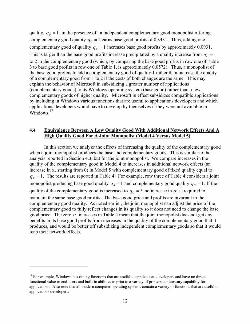
quality, , in the presence of an independent complementary good monopolist offering complementary good quality q earns base good profits of 0.3431. Thus, adding one complementary good of quality increases base good profits by approximately 0.0931. This is larger than the base good profits increase precipitated by a quality increase from

1=Bq1=C

=Cq 11=Cq

to 2 in the complementary good (which, by comparing the base good profits in row one of Table 3 to base good profits in row one of Table 1, is approximately 0.0572). Thus, a monopolist of the base good prefers to add a complementary good of quality 1 rather than increase the quality of a complementary good from 1 to 2 if the costs of both changes are the same. This may explain the behavior of Microsoft in subsidizing a greater number of applications (complementary goods) to its Windows operating system (base good) rather than a few complementary goods of higher quality. Microsoft in effect subsidizes compatible applications by including in Windows various functions that are useful to applications developers and which applications developers would have to develop by themselves if they were not available in Windows.17

1

4.4 Equivalence Between A Low Quality Good With Additional Network Effects And A

High Quality Good For A Joint Monopolist (Model 4 Versus Model 5)

In this section we analyze the effects of increasing the quality of the complementary good when a joint monopolist produces the base and complementary goods. This is similar to the analysis reported in Section 4.3, but for the joint monopolist. We compare increases in the quality of the complementary good in Model 4 to increases in additional network effects (an increase in α, starting from 0) in Model 5 with complementary good of fixed quality equal to

. The results are reported in Table 4. For example, row three of Table 4 considers a joint monopolist producing base good quality

1=Cq1=Bq and complementary good quality . If the

quality of the complementary good is increased to =Cq

5=Cq no increase in α is required to maintain the same base good profits. The base good price and profits are invariant to the complementary good quality. As noted earlier, the joint monopolist can adjust the price of the complementary good to fully reflect changes in its quality so it does not need to change the base good price. The zero α increases in Table 4 mean that the joint monopolist does not get any benefits in its base good profits from increases in the quality of the complementary good that it produces, and would be better off subsidizing independent complementary goods so that it would reap their network effects.

17 For example, Windows has timing functions that are useful to applications developers and have no direct functional value to end-users and built-in abilities to print to a variety of printers, a necessary capability for applications. Also note that all modern computer operating systems contain a variety of functions that are useful to applications developers.

12

Table 4 Joint Monopolist: Equivalence of Quality Increases and Network Effects

Base Good Quality

( )Bq

Complementary Good Quality

Increase ( Cq )Base Good Price ( )Bp *

Complementary Good Price

( )Cp *

Base Good Profits at

High Quality

Equivalent α

Increase** 1 1 → 2 0.6667 0.6667 0.4444 0 1 1 → 3 0.6667 1.1667 0.4444 0 1 1 → 5 0.6667 2.1667 0.4444 0 1 1 → 10 0.6667 4.6667 0.4444 0

* These are equilibrium prices under the higher complementary good quality. ** Increase from zero.

Comparing Tables 3 and 4, we observe that prices and profits for the base good are sensitive to quality improvements of the complementary good for the independent firms but not for the joint monopolist. As we discussed earlier, this follows from the fact that the joint monopolist is able to adjust the price of the complementary good to fully reflect its change in quality. In contrast, the independent monopolist of the base good, in a Nash equilibrium framework, changes its price in the direction of changes in the quality of the complementary good. Thus, to improve base good profits the joint monopolist should subsidize independent complementary goods and not its own, while an independent firm producing the base good benefits from both.

We can also use Tables 2 and 4 to assess the incentive of the joint monopolist to invest in increasing the quality of its complementary good versus adding a complementary good. From Model 1 we know that a monopolist producing only a base good and with no additional network effects earns base good profits of 4B

1

q . So a monopolist producing a base good of quality in the absence of a complementary good and with no additional network effects earns

base good profits of 0.25. We can see from row one of Table 2 that a joint monopolist offering the same base good quality, q , along with a complementary good of quality earns base good profits of

1=Bq

=B 1=Cq94 . Thus, adding one complementary good of quality increases

base good profits by 1=Cq

367 . From row one of Table 4 we see that increasing the quality level of the complementary good has no effect on base good profits. As discussed in Section 4.2, this is because the joint monopolist has both price instruments available and can adjust the complementary good price optimally without distorting the base good price to cost margin. This implies that the joint monopolist has an incentive to add a complementary good of minimal quality but not invest in its improvement. Note that this effect is much more pronounced than in the case of independent firms discussed in Section 4.3. Comparing Tables 1 and 3, we observe the same relative incentive for the independent monopolists, but the difference in effect on profits is much less pronounced. This is because the joint monopolist is able to internalize all of the quality increases of the complementary good through the complementary good prices while the independent firm, in a Nash equilibrium framework, only reacts to the change that the complementary good producer makes.

13

5. Effect of Quality Levels And Additional Network Effects On Profits An important question frequently posed in the network effects literature concerns the

incentive to improve the quality of products and how this is affected by the presence of complementary goods and network effects. In this section we assess the incentive for firms to invest in quality at the margin under different market structures (joint monopoly versus independent firms) and different levels of additional network effects. Although we do not explicitly model an investment stage we can assess the incentives to invest at the margin by considering the marginal effects of quality improvements on profits.

We first assess the effect on profits of quality changes in the base and complementary

goods in the presence of varying levels of additional network effects. We also contrast the effects of quality changes when independent firms produce the two products to those when a joint monopolist produces both.

We first look at the effect of changes in base good quality on the profits of the base good

monopolist with an independent monopolist providing a complementary good. The results on

B

B

dqdΠ are reported in column 1 of Table 5 for different combinations of additional network

effects, complementary good quality levels, and base good quality levels.18

Second, we assess the effect of changes in the complementary good quality on the profits of the base good monopolist with an independent monopolist providing a complementary good.

The results on C

B

dqdΠ are reported in column 2 of Table 5.

Third, we assess the effect of changes in the base good quality on the profits of the

complementary good monopolist with an independent monopolist providing the base good. The

results onB

C

dqdΠ are reported in column 3 of Table 5.

Fourth, we assess the effect of changes in the complementary good quality on the profits

of the complementary good monopolist with an independent monopolist providing the base

good. The results on C

C

dqdΠ are reported in column 4 of Table 5.

18 All derivatives are calculated based on step-sizes of 0.1 for and . Bq Cq

14

Fifth, we look at the effect of changes in base good quality on the total profits of the joint

monopolist. To avoid confusion, we use the notation JMC

JMB

JM Π+Π=Π for the profits of the

joint monopolist. Column 5 of Table 5 shows values of the derivativeB

JM

dqdΠ .

Sixth, we look at the effect of changes in complementary good quality on the total profits

of the joint monopolist. Column 6 of Table 5 provides values of C

JM

dqdΠ .

Table 5 Effects of Quality Increases on Profits (“IF” = Independent Firms, “JM” =

Joint Monopolist) 1 2 3 4 5 6 α

Base Good

Quality ( )Bq

Comple-mentary

Good Quality

( )Cq

IF

B

B

dqdΠ

IF

C

B

dqdΠ

IF

B

C

dqdΠ

IF

C

C

dqdΠ

JM

B

JM

dqdΠ

JM

C

JM

dqdΠ

0 0.2 1 0.3937 0.0077 -0.1036 0.2400 0.3148 0.2513 0 0.4 1 0.3382 0.0245 -0.0635 0.2266 0.3000 0.2554 0 0.6 1 0.2993 0.0442 -0.0435 0.2155 0.2852 0.2621 0 0.8 1 * * * * 0.2704 0.2715 0 0.5 3 0.4174 0.0059 -0.1257 0.2420 0.3198 0.2510 0 1.0 3 0.3631 0.0193 -0.0794 0.2302 0.3074 0.2540 0 1.5 3 0.3236 0.0358 -0.0553 0.2199 0.2951 0.2590 0 2.0 3 0.2938 0.0532 -0.0411 0.2113 0.2827 0.2659 0 2 10 0.4092 0.0084 -0.1175 0.2394 0.3181 0.2515 0 4 10 0.3487 0.0262 -0.0698 0.2256 0.3033 0.2559 0 6 10 0.3068 0.0469 -0.0469 0.2142 0.2885 0.2632 0 8 10 0.2763 0.0682 -0.0341 0.2052 0.2737 0.2735

0.4 1.0 1 0.2281 0.0559 -0.0419 0.2209 0.2312 0.2706 0.4 1.2 1 0.2185 0.0766 -0.0343 0.2136 0.2242 0.2847 0.4 1.4 1 0.2083 0.0966 -0.0286 0.2075 0.2140 0.3017 0.4 1.6 1 * * * * * * 0.4 0.8 3 0.3476 0.0081 -0.1202 0.2417 0.2679 0.2512 0.4 1.6 3 0.3138 0.0337 -0.0657 0.2247 0.2826 0.2586 0.4 2.4 3 0.2749 0.0617 -0.0421 0.2120 0.2686 0.2712 0.4 3.2 3 0.2462 0.0893 -0.0299 0.2024 0.2507 0.2891 0.4 2 10 0.4077 0.0074 -0.1274 0.2410 0.3117 0.2513 0.4 4 10 0.3497 0.0250 -0.0749 0.2274 0.3018 0.2557 0.4 6 10 0.3079 0.0458 -0.0502 0.2161 0.2878 0.2630 0.4 8 10 0.2773 0.0670 -0.0365 0.2071 0.2733 0.2733

* Corner solution at these values – derivative not defined.

Each row of table 5 provides these six effects at a given combination of additional network effects and quality levels. For example, row two shows that for an α of zero, base good

15

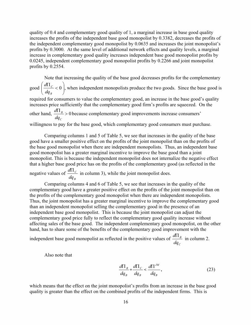
quality of 0.4 and complementary good quality of 1, a marginal increase in base good quality increases the profits of the independent base good monopolist by 0.3382, decreases the profits of the independent complementary good monopolist by 0.0635 and increases the joint monopolist’s profits by 0.3000. At the same level of additional network effects and quality levels, a marginal increase in complementary good quality increases independent base good monopolist profits by 0.0245, independent complementary good monopolist profits by 0.2266 and joint monopolist profits by 0.2554.

Note that increasing the quality of the base good decreases profits for the complementary

good

<

Π0

B

C

dqd

, when independent monopolists produce the two goods. Since the base good is

required for consumers to value the complementary good, an increase in the base good’s quality increases price sufficiently that the complementary good firm’s profits are squeezed. On the

other hand, 0>Π

C

B

dqd because complementary good improvements increase consumers’

willingness to pay for the base good, which complementary good consumers must purchase. Comparing columns 1 and 5 of Table 5, we see that increases in the quality of the base

good have a smaller positive effect on the profits of the joint monopolist than on the profits of the base good monopolist when there are independent monopolists. Thus, an independent base good monopolist has a greater marginal incentive to improve the base good than a joint monopolist. This is because the independent monopolist does not internalize the negative effect that a higher base good price has on the profits of the complementary good (as reflected in the

negative values of B

C

dqdΠ

in column 3), while the joint monopolist does.

Comparing columns 4 and 6 of Table 5, we see that increases in the quality of the complementary good have a greater positive effect on the profits of the joint monopolist than on the profits of the complementary good monopolist when there are independent monopolists. Thus, the joint monopolist has a greater marginal incentive to improve the complementary good than an independent monopolist selling the complementary good in the presence of an independent base good monopolist. This is because the joint monopolist can adjust the complementary good price fully to reflect the complementary good quality increase without affecting sales of the base good. The independent complementary good monopolist, on the other hand, has to share some of the benefits of the complementary good improvement with the

independent base good monopolist as reflected in the positive values of C

B

dqdΠ in column 2.

Also note that

B

B

dqdΠ

+B

C

dqdΠ

< B

JM

dqdΠ

, (23)

which means that the effect on the joint monopolist’s profits from an increase in the base good quality is greater than the effect on the combined profits of the independent firms. This is

16

because the joint monopolist is better able to capture the benefits of increasing the base good quality by adjusting the complementary good price optimally. We can also use our model to assess the marginal incentive to increase compatibility between the base good and complementary goods. Firms in markets with network effects, like software, often face decisions about the degree to which their product should be made compatible with other products or conform to industry standards. In our model this is equivalent to determining the effect on profits of an increase in additional network effects ( )α . We compare this incentive at different quality levels and for different market structures (independent monopolists versus a joint monopolist). First, we look at the effect of increasing additional network effects on the profits of

independent base good and complementary good monopolists. Values of αd

d BΠ are in column 1

of Table 6 and values of αd

d CΠ in column 2.19 Second, we assess the effect of increasing

additional network effects on the profits of the joint monopolist. Values of αd

d JMΠ are in column

3 of Table 6. Each row of Table 6 provides the effect at a given combination of additional network effects and quality levels. For example, row two of the table indicates that at base good quality of , complementary good quality of 1=Bq 3=Cq and additional network effects of

2.0=α , a marginal increase in compatibility (additional network effects) increases the profits of the independent base good monopolist by 0.3663, the independent complementary good monopolist by 0.1857 and the joint monopolist by 0.5436. Comparing column 3 to columns 1 and 2 of Table 6, we observe that profits are more sensitive to additional network effects for a joint monopolist than for either independent monopolist. When additional network benefits are greater the value goes up both to consumers of the base good and to consumers of the complementary good. The value of the base good goes up because of the greater availability of additional complementary goods. The value to complementary goods consumers goes up because they must buy the base good to use the complementary good and therefore also benefit indirectly from the additional complementary

goods. This is why αd

d BΠ and αd

d CΠ are both positive for the independent monopolists (columns

1 and 2 of Table 6). In fact, the complementary good monopolist receives substantial benefits from the increase of network effects from other complementary goods. However, because each of the independent firms can “free-ride” off of the other, their individual incentives to make their products more compatible is lower than the incentive of the joint monopolist to make its two products more compatible with other firms’ goods. Since consumers of both the base and complementary goods benefit, the joint monopolist captures both benefits, while in the case of the independent monopolists this benefit is shared between the two firms.

19 Derivatives are calculated based on step-sizes of 0.01 for α .

17

Table 6 Effects of the Intensity of Additional Network Effects on Profits (“IF” = Independent Firms, “JM” = Joint Monopolist)

1 2 3 α

Base Good Quality

( )Bq

Complementary Good Quality

( )Cq

IF

αdd BΠ

IF

αdd CΠ

JM

αdd JMΠ

0.1 1 3 0.3276 0.1781 0.5019 0.2 1 3 0.3663 0.1857 0.5436 0.3 1 3 0.4114 0.1901 0.5881 0.4 1 3 0.4648 0.1890 0.6356 0.5 1 3 0.5290 0.1800 0.6867 0.6 1 3 0.6066 0.1602 0.7421 0.7 1 3 0.6990 0.1281 0.8032 0.8 1 3 0.8032 0.0856 0.8723 0.9 1 3 0.9097 0.0393 0.9536 0.1 1 5 0.3132 0.2006 0.4982 0.2 1 5 0.3480 0.2102 0.5377 0.3 1 5 0.3888 0.2173 0.5807 0.4 1 5 0.4374 0.2199 0.6275 0.5 1 5 0.4964 0.2153 0.6787 0.6 1 5 0.5691 0.1998 0.7352 0.7 1 5 0.6591 0.1695 0.7982 0.8 1 5 0.7671 0.1221 0.8698 0.9 1 5 0.8877 0.0611 0.9531 0.1 1 10 0.2988 0.2250 0.4954 0.2 1 10 0.3314 0.2362 0.5334 0.3 1 10 0.3896 0.2483 0.5752 0.4 1 10 0.4396 0.2514 0.6214 0.5 1 10 0.5009 0.2465 0.6727 0.6 1 10 0.5774 0.2292 0.7299 0.7 1 10 0.6732 0.1934 0.7944 0.8 1 10 0.7913 0.1337 0.8678 0.9 1 10 0.9284 0.0490 0.9528

6. Pricing of Windows and Office

One of the puzzles of the Microsoft antitrust case was the fact that Microsoft was charging a price for its Windows operating system that was significantly lower than most economic models predict. At the same time, Microsoft was selling the Microsoft Office suite of

18

applications20 at a significantly higher price than Windows, even though Microsoft’s market share was comparable in the Windows and Office markets. Various explanations of the price difference have been offered, but none seemed to explain the low Windows price except for the possibility of very strong potential competition in the operating systems market.21

Four main failing explanations have been offered. The first explanation is that Microsoft

was keeping the price of Windows low to increase network effects, allowing it to possibly increase its price in the future. This explanation is unsatisfying given that Microsoft continued pricing Windows low even after it had gained a very high market share. A second possible explanation is that the existing installed base of Windows constrained Microsoft’s pricing because consumers who bought a new computer would uninstall Windows from their old computer and install it on the new one. However, Microsoft’s licensing requirements and the sheer complexity of uninstalling the operating system make it almost impossible for a user to uninstall a Windows operating system that was pre-installed by a computer hardware manufacturer and move it to a different (presumably new) computer. Moreover, typically, U.S. users who buy Windows pre-installed on their new computer are not given software that would allow them to install Windows to a different computer.22 So it is unlikely that the Windows installed base constrained the Windows price. A third possible explanation is that since computer systems (hardware and software) are durable, pricing of new versions of Windows is constrained by the availability of old computer system versions (including Windows). However, very rapid technological change in hardware has prompted consumers to buy new computers much faster than traditional obsolescence rates would imply and Windows was only a small part of the price of a new personal computer. Thus, it is unlikely that durability was a significant factor constraining the price of Windows. A fourth possible explanation is that the price of Windows is constrained by the possibility of consumers pirating the software. Although pirating of both Microsoft Office and Windows would have the same effect, it is more difficult to pirate Windows. Therefore, piracy issues do not explain the price difference between Windows and Microsoft Office.

Another possible explanation that has been proposed and dismissed is that Microsoft kept

the price of Windows low because this allowed Microsoft to charge more for complementary goods, such as Microsoft Office, that it produces. In the context of pure monopoly models for Windows and Microsoft Office, this explanation was insufficient to explain the very different prices charged for Windows and Office. In contrast, our model, in which a joint monopolist sets prices of the base and complementary goods in the presence or absence of additional network effects from other complementary goods, is able to explain the relative prices of Windows and Office. We can apply our Models 4 and 5, with Windows as the base good and Microsoft Office as the complementary good. A ratio of between two and four in the price of Office to Windows

20 Microsoft Office typically includes Word, a word processor; Excel, a spreadsheet; PowerPoint, a presentations tool; Outlook, a personal information management tool; and Access, a database. 21 See Economides (2001). 22 U.S. users are typically given a “recovery” CD that allows them to restore the particular computer model they own, including Windows, to the original condition when it was shipped from the factory. Such a CD is unable to install Windows on any other computer model.

19

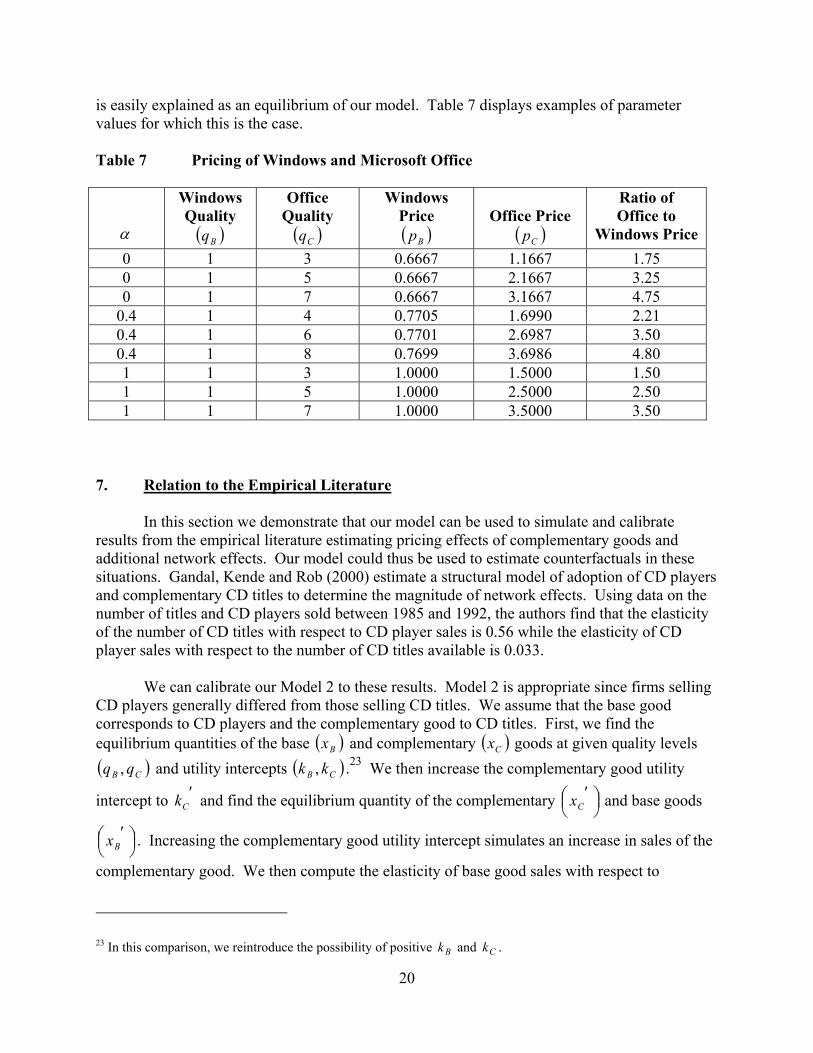
is easily explained as an equilibrium of our model. Table 7 displays examples of parameter values for which this is the case.

Table 7 Pricing of Windows and Microsoft Office

α

Windows Quality

( )Bq

Office Quality ( )Cq

Windows Price ( )Bp

Office Price

( )Cp

Ratio of Office to

Windows Price0 1 3 0.6667 1.1667 1.75 0 1 5 0.6667 2.1667 3.25 0 1 7 0.6667 3.1667 4.75

0.4 1 4 0.7705 1.6990 2.21 0.4 1 6 0.7701 2.6987 3.50 0.4 1 8 0.7699 3.6986 4.80 1 1 3 1.0000 1.5000 1.50 1 1 5 1.0000 2.5000 2.50 1 1 7 1.0000 3.5000 3.50

7. Relation to the Empirical Literature

In this section we demonstrate that our model can be used to simulate and calibrate results from the empirical literature estimating pricing effects of complementary goods and additional network effects. Our model could thus be used to estimate counterfactuals in these situations. Gandal, Kende and Rob (2000) estimate a structural model of adoption of CD players and complementary CD titles to determine the magnitude of network effects. Using data on the number of titles and CD players sold between 1985 and 1992, the authors find that the elasticity of the number of CD titles with respect to CD player sales is 0.56 while the elasticity of CD player sales with respect to the number of CD titles available is 0.033.

We can calibrate our Model 2 to these results. Model 2 is appropriate since firms selling CD players generally differed from those selling CD titles. We assume that the base good corresponds to CD players and the complementary good to CD titles. First, we find the equilibrium quantities of the base and complementary ( Bx ) ( )Cx goods at given quality levels

and utility intercepts .( CB qq ,

′

Bx

) )

( Ck,Bk 23 We then increase the complementary good utility

intercept to and find the equilibrium quantity of the complementary and base goods

. Increasing the complementary good utility intercept simulates an increase in sales of the

complementary good. We then compute the elasticity of base good sales with respect to

′Ck

′

Cx

23 In this comparison, we reintroduce the possibility of positive and . Bk Ck

20

complementary good sales:

−′

−′= BCCCBBBC xxxxxxε

′Bk C

. We simulate the elasticity of

complementary good sales with respect to base good sales in a similar manner by increasing the

base good utility intercept to (while holding k constant) and calculating

′

−′= CBBCCCB xxxxxε

=Bk

− Bx

3.0

.

=Ck 1319.0=CBε

( )Cp Cq,′

Cq

′

−′= CCCCCPq pqqppε − Cq

B

075.1=Pqε

We find that at , 1.0 , =Bq and 2=Cq we get 018.0=BCε and

which are close to the empirical results. At these values, 897.0=BP , , profits of the base good monopolist are 0.587 and profits of the complementary good monopolist are 0.462.

961.0=CP

Gandal (1995) estimates a hedonic model of personal computer database management systems (DBMS) software pricing. Using data on all major products offered from 1989 to 1991, Gandal estimates the value of a DBMS being compatible with the Lotus spreadsheet, the dominant spreadsheet at the time. Compatibility with the Lotus standard meant that the DBMS could export files in a Lotus-compatible format. Gandal finds that DBMS products compatible with the Lotus standard had a 31% higher price relative to incompatible DBMS’s, controlling for other quality variables. We simulate this using our Model 2 (since the DBMS’s and Lotus spreadsheet were produced by separate firms) and assume that the base good is a DBMS and the complementary good is the Lotus spreadsheet. First, we find the equilibrium price of the complementary good

at a given quality level for both goods ( )Bq . We then increase the quality of the

complementary good to and find the new equilibrium price of the complementary good ( )'Cp

allowing the base good price and quantity to adjust optimally. Finally, we compute the elasticity of the complementary good price with respect to the change in complementary good quality:

. We cannot calibrate our model to the empirical results

in this case since we cannot measure the quality improvement equivalent to compatibility with the Lotus standard. As an example, however, at 0== Ckk , 1=Bq and we get 2=Cq

. Brynjolfsson and Kemerer (1996) estimate a hedonic model of personal computer spreadsheet pricing on products sold between 1987 and 1992. The authors find that the elasticity of the spreadsheet price with respect to the size of the spreadsheet’s installed base is 0.75. Since we do not explicitly model the dynamics of market share formation in our model, we cannot simulate this elasticity. However, a dynamic version of Model 2 with the spreadsheet product as the base good and a compatible product, such as the operating system, as the complementary good would allow simulation of these results.

21

22

8. Concluding Remarks

This paper bridges the gap between two approaches in the network effects literature, the micro and macro approaches. In the micro approach, network effects are calculated from the sales of complementary goods explicitly defined in the model. In the macro approach, network effects are assumed in the utility functions of consumers. We develop an equivalence between these two approaches. We solve a model with two goods, a base good and a complementary good whose use requires the base good, for two alternative industry structures, joint monopoly and two independent monopolists. We then find the appropriate parameter values for network effects in a macro model that produce the same equilibrium results as a micro model. We assess the effect of changes in the inherent quality of the base and complementary goods and equate them to increases in the intensity of network effects required to maintain the same base good profits. We also evaluate the incentive to invest in either the base or complementary good quality and product compatibility. Finally, we are able to provide an economically rational explanation of Microsoft’s relative pricing of Windows and Office and demonstrate how our model can be calibrated to empirical network effects studies to perform counterfactuals. 9. References

Brynjolfsson, E. and C. Kemerer (1996), “Network Externalities in Microcomputer Software: An

Econometric Analysis of the Spreadsheet Market,” Management Science, 42, 1627 – 1647.

Economides, N. (1996a), “The Economics of Networks,” International Journal of Industrial

Organization, 14, no. 6, 673 – 699 (October 1996). Economides, N. (1996b), “Network Externalities, Complementarities, and Invitations to Enter,”

European Journal of Political Economy, 12, 211 – 232. Economides, N. (2001), “The Microsoft Antitrust Case,” Journal of Industry, Competition and

Trade: From Theory to Policy, 1, no. 1, 7 – 39 (August 2001). Gandal, N. (1995), “Competing Compatibility Standards and Network Externalities in the PC

Software Market,” The Review of Economics and Statistics, 77, 599 – 608. Gandal, N., M. Kende and R. Rob (2000), “The Dynamics of Technological Adoption in

Hardware/Software Systems: The Case of Compact Disc Players,” RAND Journal of Economics, 31, 43 – 61.