COMPLEMENTARY QUADRATIC PROGRAMMING AND ARTIFICIAL NEURAL

NETWORK FOR COMPUTATIONALLY EFFICIENT MICROGRID DISPATCH

OPTIMIZATION WITH UNIT COMMITMENT

By

NADIA VICTORIA PANOSSIAN

A thesis submitted in partial fulfillment of

the requirements for the degree of

MASTER OF SCIENCE IN MECHANICAL ENGINEERING

WASHINGTON STATE UNIVERSITY

School of Mechanical and Materials Engineering

MAY 2018

© Copyright by NADIA VICTORIA PANOSSIAN, 2018

All Rights Reserved

© Copyright by NADIA VICTORIA PANOSSIAN, 2018

All Rights Reserved

ii

To the Faculty of Washington State University:

The members of the Committee appointed to examine the thesis of NADIA VICTORIA

PANOSSIAN find it satisfactory and recommend that it be accepted.

Dustin McLarty, Ph.D., Chair

Noel Schulz, Ph.D.

Soumik Banerjee, Ph.D.

Kshitij Jerath, Ph.D.

iii

ACKNOWLEDGMENT

The author would like to recognize the help of Dr. Matthew E. Taylor for his patient guidance in

machine learning techniques, Dr. Dustin McLarty for advice on the project, and Dr. Srinivas

Katipamula at PNNL for making this work possible.

The author would also like to recognize the PNNL-WSU Distinguished Graduate Research

Program and WSU’s Research Assistantships for Diverse Scholars Program for their support of

this research.

iv

COMPLEMENTARY QUADRATIC PROGRAMMING AND ARTIFICIAL NEURAL

NETWORK FOR COMPUTATIONALLY EFFICIENT MICROGRID DISPATCH

OPTIMIZATION WITH UNIT COMMITMENT

Abstract

by Nadia Victoria Panossian, M.S.

Washington State University

May 2018

Chair: Dustin McLarty

Microgrid infrastructures allow for a cleaner energy future by reducing transmission losses,

enabling combined heat and power efficiency upgrades, employing onsite renewable generation,

and providing power stability especially when paired with energy storage devices. Microgrid

dispatch optimization allows wider implementation of microgrid infrastructures by lowering

microgrid operations costs. The computational bottleneck of dispatch optimization is unit

commitment, which is a mixed integer optimization problem. Three methods to reduce the

computational effort of unit commitment and maintain satisfactory optimality are.

Complementary Quadratic Programming (cQP), modified complementary Quadratic

Programming (mcQP), and Artificial Neural Network (ANN) with dynamic economic dispatch.

Both cQP and mcQP are capable of quickly optimizing receding horizon dispatches with storage,

creating training sets which facilitates machine learning approaches such as method three. This

thesis presents cQP and mcQP development as a means of training a neural network unit

commitment solver, and compares all three approaches to solutions of the full mixed-integer

problem using a commercial solver. Decision trees are employed for feature selection, and ANNs

v

of varying depth are compared for ANN structure selection. The mcQP method is the most

robust, and the ANN method is the most computationally efficient. All three methods outperform

the commercial solver in computational efficiency, robustness, and dispatch cost.

vi

TABLE OF CONTENTS

Page

ACKNOWLEDGEMENT………………………………………………………………………..iii

ABSTRACT……………………………………………………………………………………...iv

LIST OF TABLES……………………………………………………………………………...viii

LIST OF FIGURES……………………………………………………………………………....ix

1 Introduction…………………………………………………………………………………..1

2 Literature Review…………………………………………………………………………….4

2.1 Gradient Based Methods………………………………………………………………...4

2.2 Search Methods……………………………………………………………………….....8

2.3 Machine Learning Methods……………………………………………………………10

3 Problem Statement…………………………………………………………………………..15

4 Methodology………………………………………………………………………………...16

4.1 Problem Formulation:………………………………………………………………….16

4.1.1 Combined Cooling, Heating, and Power…………………………………………….21

4.2 Complementary Quadratic Programming……………………………………………...23

4.3 Modified Complementary Quadratic Programming…………………………………...25

4.4 Artificial Neural Network……………………………………………………………...29

4.4.1 Network Structure Selection………………………………………………………....31

4.4.2 ANN Training………………………………………………………………………..36

vii

4.4.3 Algorithm Execution and Division of Work………………………………………...38

4.5 Test Systems…………………………………………………………………………....42

5 Results………………………………………………………………………………………45

5.1 Complementary Quadratic Programming Dispatch Cost and Computational

Efficiency……………………………………………………………………………………... 45

5.2 ANN in for Unit Commitment…………………………………………………………52

5.2.1 ANN Structure Optimization………………………………………………………...52

5.2.2 ANN Implementation………………………………………………………………..61

6 Conclusion…………………………………………………………………………………..70

7 Discussion…………………………………………………………………………………...72

8 References…………………………………………………………………………………..74

9 Appendix A: Sample Source Code………………………………………………………….80

9.1 Neural Network Class………………………………………………………………….80

9.2 Single Layer ANN Training Algorithm………………………………………………..81

viii

LIST OF TABLES

Page

Table 1 Generator component parameters used in the test campus system. ................................. 43

Table 2 Chiller component parameters used in the test campus system ....................................... 44

Table 3 Energy storage components used in the test campus system ........................................... 44

Table 4 Startup costs associated with coming online. .................................................................. 44

Table 5 Summary of Winter and Summer comparison of FMI, cQP and mcQP ......................... 48

Table 6: Accuracy of decision trees for each component's unit commitment .............................. 52

Table 7: Highest level layer for input threshold for each component ........................................... 55

Table 8: Test accuracy of single and double layer ANN .............................................................. 57

Table 9: Time in seconds to complete various tasks using the mcQP method versus the ANN. . 63

Table 10: Comparison of Dispatch methods for year in receding horizon ................................... 71

ix

LIST OF FIGURES

Page

Figure 1: Artificial Neural Network basic structure ..................................................................... 10

Figure 2: Decision trees ................................................................................................................ 13

Figure 3: Conceptual depiction of generator performance and cost functions ............................. 20

Figure 4: Pseudo code for assuring feasibility when using cQP. .................................................. 24

Figure 5 Pseudo code for the elimination of combinations which are infeasible ......................... 27

Figure 6 Process for developing an ANN for unit commitment. .................................................. 30

Figure 7: Evolution of complementary Quadratic Programming algorithm and software. .......... 39

Figure 8 Electric utility rates vary throughout the week ............................................................... 44

Figure 9: Distribution of operating costs for each optimization ................................................... 46

Figure 10 Distribution of operating costs for each optimization for winter and summer ............. 47

Figure 11 Comparison of electrical dispatch of January 8th. ....................................................... 49

Figure 12 Dispatch from mcQP, cQP, and FMI methods for June 26th ....................................... 51

Figure 13: Training and testing error for each component versus training iterations ................... 58

Figure 14: Validation testing accuracy of unit commitment for each component ........................ 60

Figure 15: Training accuracy of unit commitment for each component from ANNs .................. 59

Figure 16: Dispatch Comparison for ANN1 and mcQP for the simple case microgrid ............... 62

Figure 17: ANN1 as compared to mcQP for a sample dispatch. .................................................. 64

Figure 18: The ANN is capable of eliminating shutdown of ICE. ............................................... 65

Figure 19: Cost Distribution of single layer ANN dispatch as compared to mcQP dispatch. ...... 66

Figure 20: Comparison of mcQP and ANN1 electric dispatch for August 1st ............................. 68

Figure 21: Hot thermal and cold power dispatches using mcQP and ANN1 for August 1st. ....... 69

x

Dedication

Thanks to my parents, Jack and Linda Panossian for their love and support, and thanks to my

cousin Dr. Emil Rahim for his guidance on the grad school process.

1

1. INTRODUCTION

Despite the United States’ (US) withdrawal from the Paris Climate Accords, all other

nations, many US cities, and many US states have pledged to reduce harmful carbon emissions

as part of the international effort to slow the pace of global climate change [1]. Emissions

reduction efforts focus on a switch from fossil fuel burning energy production to renewable

sources such as wind and solar, as well as a switch from gas and oil-based transportation to

electric powered vehicles [2]. In many nations, such as in Germany, legacy technology is

replaced by renewable generation from wind and solar [3]. These variable renewable sources

require a higher level of control to ensure power dispatch stability with minimized cost and

emissions. Wind and solar generated power can be curtailed or stored to assure stable power

supply at all times. Other sources such as gas turbines or fuel cells that accommodate demand

not supplied by renewables and storage must be dispatched optimally to maintain stability, lower

power generation cost, and minimize emissions.

Emissions from remaining legacy generation can be reduced by using waste heat from

generators such as gas turbines, reciprocating engines, or fuel cells. This heat can be used to

satisfy heat demand if piped over short distances in the form of steam as in the case of

Washington State University’s steam plant that is used to heat campus buildings and melt ice on

central campus walkways [4]. The heat can also be used to provide cooling when connected to an

absorption chiller as is the case at University of California, Irvine [5]. Finally, waste heat can be

used for electric generation via a steam turbine connected to a heat recovery steam generator

unit, which can be transmitted over much longer distances than thermal generation [6]. Using

2

waste heat to meet thermal demand avoids energy conversion losses, but is limited to short

supply line distances of a few miles or less as are present in microgrid infrastructures.

Microgrid infrastructures are an important part of emissions reduction plans and improve

power reliability due to their independence via an ability to disconnect from the larger power

grid [7]. High reliability is necessary for locations with high cost of power failure such as

mission critical military locations, ship-board electrical systems, and hospital campuses [8] [9].

Microgrid infrastructures can also be cost effective in large campus installations which

accumulate high power demand across many buildings such as college campuses [6]. Because

microgrids may not be able to rely on the surrounding power grid for stability, dispatch control

planning is important to provide power stability, reduce cost, and avert high emissions [6]. The

distributed generation optimization applied to microgrid systems may be applied to large grid

systems as energy generation diversifies and new generation is added to areas that were once

exclusively power demand locations.

Microgrid dispatch optimization is the process of finding set points for all power generation

components, and sometimes demand components, such that cost of generation or emissions are

minimized while still providing stable power [10]. Many components such as gas turbines, fuel

cells, and vapor compression chillers have a lower limit of generation below which they are not

self-sustaining and cannot operate. Unit commitment is the problem of optimizing which

components should be online and above the lower limit of operation, or offline with zero

production at a given time to minimize cost of generation or emissions. Unit commitment

algorithms output binary values for every component with non-zero lower limit and dispatch

optimization methods use those binary values when determining real-valued setpoints for

components.

3

Complementary Quadratic Programming can reduce the computational complexity of the

unit commitment and dispatch optimization problems to provide optimal microgrid dispatching

[11] [12]. Using a neural network for unit commitment within complementary Quadratic

Programming enables real time dispatch optimization and control allowing effective use of

renewable generation, storage, and dispatchable components for a reliable power supply with

minimized cost and emissions [13].

4

2. LITERATURE REVIEW

Dispatch optimization methods can be separated into three main approaches. Gradient-

based methods reach global optimums quickly, but are limited in the types of constraints and

efficiency curves over which they can optimize. Search based methods are more flexible in the

efficiency curves and constraints that can be accommodated, but rely on computationally

expensive search algorithms to converge to an optimal solution. Machine learning approaches

can accommodate more complex constraints and efficiency curves with low computational

demand after training, but require large training sets for robust outputs.

1.1 Gradient-Based Methods

Gradient-based methods rely on gradient descent which converges on a minimum value, in

this case generation cost, by moving in the opposite direction of the surface gradient until the

absolute value of the gradient falls below some threshold [14]. Gradient descent may not

converge to a global optimal if the problem is non-convex because all points on the surface may

not have gradients which lead towards the global minimum. Gradient-based methods require

convex and often linear relationships between power production and cost to assure global

convergence. When the problem is constrained, as is the case with power dispatch, interior-point

methods are used to limit the gradient descent search space [15] with linear and possibly

quadratic constraints. Approximating the problem as a convex function with linear constraints

creates some error between the actual and estimated costs, but allows for rapid computation by

avoiding the necessity to search and check multiple possible solutions. If gradient-based methods

are used for power flow optimization with unit commitment then they lose their computational

demand advantage, because one optimization is run for each possible unit commitment

5

combination to find a global optimum. The numeric methods discussed here are linear

programming, quadratic programming, and representation as energy hubs.

Standard form linear programming is an interior-point method where an objective, in this

case cost, is minimized subject to linear constraints [15]. Linear programming approximates

component efficiency curves as a straight line and optimizes for cost as in the equations shown

below.

min(𝐶) = ∑ 𝑃𝑖𝑐𝑖𝐵𝑖

𝑁

𝑖=1

𝑠. 𝑡. ∀𝑘 𝐷𝑒𝑚𝑎𝑛𝑑𝑘 = ∑ 𝑃𝑖𝑘

𝑁

𝑖=𝑖

Where C is the cost, P is the power from each component in the microgrid, c is the slope of the

linearized generator cost curve, B is a binary value indicating the component unit commitment,

and for all timesteps k, the demand equals the sum of generation. Linear approximation may not

have high accuracy, especially near rated power, however, it drastically simplifies the problem.

If all components have linear efficiencies, then the optimal dispatch will be the point where

marginal power is equivalent for all generators. When minimum and maximum constraints are

applied, the problem is more complex because the point at which all components have the same

marginal cost may be outside of the boundary conditions [16]. Some constraints may be removed

if the optimal solution is typically not near the boundary to reduce memory and computational

demand [16]. However, any constraint that is removed must be checked a priori to assure

feasibility. Linear programming is often paired with mixed integer problems such as unit

commitment, because of the speed with which an optimization can be performed [17] [18].

Because one mixed integer configuration can be found quickly, checking the entire domain of

unit commitment combinations may be completed rapidly for smaller systems [19].

6

Unfortunately, the unit commitment process is still NP hard, so for large networks the mixed

integer problem remains computationally expensive [20]. Linear programming is also limited in

the type of acceptable constraints. Because constraints must be linear, this method is limited to

optimization of DC power grids. Linear programming can be used to approximate a solution to

the AC problem, where linear programming finds optimal real power output from each

component and then the Newton-Raphson or other convergence method is used to find the

network flow for the AC grid, with real power generation close to the optimal value [21] [22].

Quadratic programming methods can be used for optimization of DC power grids, but are

limited to linear or quadratic constraints [14]. This means that these methods do not extend to

AC grids easily due to the non-linear relationships between active power, reactive power, and

voltage [23]. Quadratic programming methods can still be used to minimize line losses or cost of

generation. If the problem is non-convex it can still be solved using Metzler matrices and semi-

definite programming relaxation [23] [24]. The problem is approximated, as shown in the

equations below, by a quadratic curve for the relationship between generation and cost for each

generator, and by assuming that the grid is DC, eliminating the constraints for reactive power.

min(𝐶) = ∑ 𝐹(𝑃𝑖)𝐵𝑖

𝑁

𝑖=1

𝐹(𝑃𝑖) = 𝑓𝑃𝑖 + 𝐻𝑃𝑖2

𝑠. 𝑡. ∀𝑘 𝐷𝑒𝑚𝑎𝑛𝑑𝑘 = ∑ 𝑃𝑖𝑘

𝑁

𝑖=𝑖

Where the cost is quadratic function of the power output with linear f and quadratic H

coefficients. The approximation of the cost curve as a quadratic function is valid because the

inverse of most combustion engines such as gas turbines, diesel generators, or fuel cells follow a

7

convex quadratic shape near their rated power, and the optimal dispatch drives set points near

rated powers, because efficiency is often the highest near rated power. In this approximation the

only constraints are upper and lower bounds on real power, ramp rates, line losses, storage

limitations, and that generation equals demand. All constraints mentioned so far in this paragraph

are linear. The DC grid solution is often used as an approximation of the real power for an AC

grid [23]. The quadratic programming method has a high computational efficiency when not

performing unit commitment, because the convex nature of the quadratic cost functions

guarantees a global optimal. If quadratic programming methods are used for power flow

optimization including unit commitment, then it is less computationally efficient, because each

unit commitment possibility becomes a new convex optimization problem that must be solved

independently, resulting in 2G quadratic programming optimizations where G is the number of

components with non-zero generation limit.

Quadratic programming can incorporate multiple loads and demands with multiple

equality constraints [25] [26]. However, since constraints are limited to linear relationships,

modeling of co-generation plants is limited to linear relationships between fuel and heat or

electric power production and heat.

Microgrid components are often grouped into energy hubs to reduce the order of the unit

commitment and dispatch problem. In an energy hub approach energy is passed through the hub

or converted from one form to another [27]. Since hubs can represent multiple components, there

are redundant energy inputs and outputs, resulting in higher reliability and flexibility of the

optimization. Adding a natural gas network requires modeling of pump power to maintain

pressure in the gas pipelines [28]. Power flow equations and network energy carrier balance is

met with equality constraints, while system limitations such as voltage limits, power generation

8

limits, and compression limits are handled with inequality constraints [28]. Once an in-bound

solution is found for the energy hubs, the outputs from each hub are broken down by component

in a subroutine. The portion of each energy source and supply to and from each component

within an energy hub is proportional to a predetermined constant factor. Combining components

into hubs reduces computational time by reducing the number of variables. The final cost of the

solution is determined by the sum of the cost of the energy input to each component [28].

When complex power flow and real efficiency curves are included, the problem becomes

non-linear, non-convex with nonlinear constraints, preventing numerical methods from being

applied. If efficiency curves are constrained to be quadratic and constraints are approximated as

linear, then numerical methods can be used to find global optimal points.

1.2 Search Methods

The dispatch optimization and unit commitment problems are often solved with search

methods where multiple feasible solutions are found and the cost of each solution is checked.

Search methods can capture nonlinear, non-convex cost relationships, as well as nonlinear

constraints. The search methods discussed here are particle swarm optimization, teaching-

learning optimization, and multi-agent genetic algorithm.

One method for finding an optimum point is particle swarm optimization (PSO) where

particles settle on possible solutions that are checked for optimality [29] [30] [31] [32] [33].

Particles are initialized at random solutions with random velocities. All particles’ solutions are

compared using the objective function and the particles move according to a velocity and inertial

terms. Because constraints, including nonlinear power system relationships, are considered, each

9

potential solution must be checked for feasibility against the constraint boundaries before the

cost is evaluated [29].

There are several varieties of particle swarm optimizations which can be used for

dispatch optimization including Adaptive Modified Particle Swarm Optimization [34], Particle

Diffusion Optimization [35], Ant colony optimization [36] [37], and Cuckoo search algorithm

[38].

Another method for solving the optimization is through Teaching-Learning Based

Optimization (TLBO) where Pareto solutions are found using fuzzy logic and clustering, and a

final solution is selected using objective weights [39].

A multi-agent genetic algorithm (MAGA) is proposed in [28] as an optimization

approach for multi-carrier energy systems, but is constrained to optimizing for only DC grids,

eliminating reactive power elements of the problem. There are many varieties of genetic

algorithm that can be used for dispatch optimization, with varying reproduction processes

including Artificial Immune System [40] [41], Hypermutation [41], and Matrix Real-Coded

Genetic Algorithm (MRCGA) [42].

Search based methods are non-deterministic and may converge to different solutions in

successive runs. Microgrids with multiple components with similar efficiencies have several

dispatch solutions which are similarly optimal, creating flat optimization surface regions.

Employing a search based method in receding horizon dispatch may create rapid fluctuations

between similar cost solutions, creating instability on the power grid and possibly damaging

generators with rapid startups and shutdowns.

Comparison of search methods within a receding horizon dispatch optimization is beyond

the scope of this thesis.

10

1.3 Machine Learning Methods

Some machine learning methods, such as Artificial Neural Networks, are deterministic,

and thus not susceptible to the random outcomes of some search based methods caused by

multiple similar local minima. Machine learning methods use sets of input features and desired

outputs to train model parameters so that the model can reproduce desired outputs. Model

training can be computationally expensive, but once the model is trained, outputs can be

produced quickly. Artificial Neural Networks (ANN) and decision trees fit into this category.

ANNs have the potential to solve the microgrid dispatch and unit commitment problems

efficiently, and without rapid fluctuations caused by non-deterministic methods.

Artificial Neural Networks are adept at classification and have been used for medical

diagnosis [43] [44] [45], image recognition [46] [47] [48], and industrial quality control [49] [50]

[51]. ANNs were initially developed as a computational model of the human brain, where

neurons are interconnected and connections between interrelated neurons become stronger [52].

Figure 1: Artificial Neural Network basic structure: inputs are fed to the network, transformed as they pass along interconnections and through nodes, and converted into an output.

inputs

11

The basic structure of an ANN is shown in Figure 1, where inputs are fed to the network, the

input data is transformed as it is passed through the network, and an output is reached.

Features are the aspects of a problem which characterize the situation. For example,

when classifying images, a feature could be the color of a pixel. Input feature values are

multiplied by weight factors when passed along connections from node to node. All information

going into a node is summed and added to the node’s bias term before being transformed by an

operating function. The ANN structure, feature inputs, and operating functions are

predetermined, established by the user. The network’s weight and bias terms are learned to

minimize the error between the desired and actual outputs of a training set. ANNs must be

provided with examples of inputs and desired outputs, called training examples. When an ANN

is initialized its weights and biases are not tuned to generate accurate outputs, so training is

necessary. The inputs from each training example is fed through the network and the ANN

output is compared to the desired output. If the output classification deviates from the desired

classification, then the weights and biases are altered using a learning method. Back propagation,

the learning method used here, is further described in section 1.7.2. Training a network to

achieve high accuracy outputs requires significant computation, with long training times, using

large training, testing, and validation data sets, but once the network has been optimized, use of

the network is computationally efficient.

ANN’s can also be used in dispatch optimization. ANNs have been used for renewable

generation forecasting [53] [54], load forecasting [55] [56], load shedding [53], and replication

of quadratic programming optimization [57]. In the case of renewable generation and load

forecasting, weather data, as well as solar production, wind production, and electrical demand

historical data is often logged at generation sites, so large training sets can be created easily from

12

these historical profiles [53] [54] [55] [56]. In the case of load shedding decisions, the ANN was

trained from load shedding simulations run on a cloud based Graphics Processing Unit because

of the large computing and memory demands involved with creating a large set of training data

[53]. In the case of quadratic programming optimization replication, generator cost functions

were represented as piecewise quadratic, convex functions, and all components were assumed to

be online to facilitate rapid creation of a training set using quadratic programming [57]. The

assumption of that all components are always online, eliminates the unit commitment problem

completely, reducing computational time of training set creation, but restricting the solution from

turning any component off. This case also does not employ energy storage, so quadratic

programming optimizations can be conducted for individual timesteps, instead of over a receding

horizon. This no-storage, non-unit commitment case, facilitates rapid creation of training

examples.

This thesis evaluates use of a neural network for unit commitment over a receding

horizon with storage as trained by mcQP, with decision tree to facilitate neural network structure

optimization. Modified complementary Quadratic Programming is demonstrated to rapidly create

training examples for cases with energy storage and unit commitment.

Decision trees are useful for classification, but also require implementation with an

optimization method with real valued outputs for dispatch optimization [58]. Decision trees are

series of nodes with thresholds on features values. Each node has one feature threshold. The

outcome (above or below the value) of the threshold comparison determines the branch that the

example follows to the next node. This process of thresholding and branching is repeated until

the example reaches a node with no branches, called a leaf node. Each leaf node is associated

with a classification and the example is classified according to the leaf node where it ends.

13

Decision tree thresholds and node structures are created by sorting training examples. All

training examples start in one group at the root node, and a threshold is determined that will

effectively separate the examples into two groups.

The method for determining which feature and what threshold value is variable. The algorithm

ID3 for threshold determination is described in Section 1.7.1. The process of selecting a

threshold and separating the training examples is repeated until all examples at a node are of the

same classification. Once all examples at a node are of the same classification, the node is said to

be “pure” and becomes a leaf node.

Decision trees are very flexible and can be used for classifications with complex

boundaries and mixed integer features. Decision trees have been used to optimize islanding for

blackout prevention as trained by mixed-integer non-linear programming solutions [59], active

power and thermal generation security and contingency planning [60], and fault response

stability determination as trained by multi-objective biogeography-based optimization [61].

Decision trees are classification structures where all examples begin at the root node and are

separated along branches by a threshold on one feature. Each node that contains examples of

more than one class is split further until all nodes only contain one class type. Most algorithms

stop before all nodes are pure or employ some form of pruning to prevent overfitting. Pruning

involves removing nodes which contain few examples to prevent overfitting. Following the ID3

Figure 2: Decision trees classify examples using thresholds on important features. The ID3

algorithm selects feature thresholds which create the highest information gain.

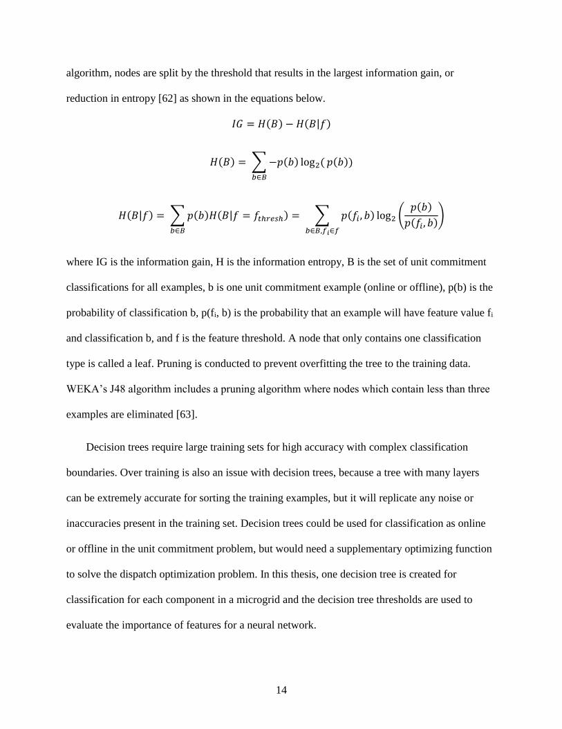
14

algorithm, nodes are split by the threshold that results in the largest information gain, or

reduction in entropy [62] as shown in the equations below.

𝐼𝐺 = 𝐻(𝐵) − 𝐻(𝐵|𝑓)

𝐻(𝐵) = ∑ −𝑝(𝑏) log2( 𝑝(𝑏))

𝑏∈𝐵

𝐻(𝐵|𝑓) = ∑ 𝑝(𝑏)𝐻(𝐵|𝑓 = 𝑓𝑡ℎ𝑟𝑒𝑠ℎ) = ∑ 𝑝(𝑓𝑖 , 𝑏) log2 (𝑝(𝑏)

𝑝(𝑓𝑖, 𝑏))

𝑏∈𝐵,𝑓𝑖∈𝑓𝑏∈𝐵

where IG is the information gain, H is the information entropy, B is the set of unit commitment

classifications for all examples, b is one unit commitment example (online or offline), p(b) is the

probability of classification b, p(fi, b) is the probability that an example will have feature value fi

and classification b, and f is the feature threshold. A node that only contains one classification

type is called a leaf. Pruning is conducted to prevent overfitting the tree to the training data.

WEKA’s J48 algorithm includes a pruning algorithm where nodes which contain less than three

examples are eliminated [63].

Decision trees require large training sets for high accuracy with complex classification

boundaries. Over training is also an issue with decision trees, because a tree with many layers

can be extremely accurate for sorting the training examples, but it will replicate any noise or

inaccuracies present in the training set. Decision trees could be used for classification as online

or offline in the unit commitment problem, but would need a supplementary optimizing function

to solve the dispatch optimization problem. In this thesis, one decision tree is created for

classification for each component in a microgrid and the decision tree thresholds are used to

evaluate the importance of features for a neural network.

15

3. PROBLEM STATEMENT

A reliable dispatch optimization system with high computational efficiency is required to

enable real time optimization and control of generation systems. The computational bottleneck of

the dispatch optimization process is unit commitment. Unit commitment involves selecting

which components will be online for the minimal cost dispatch. A reliable dispatch optimization

is desired with low computational demand for unit commitment. An artificial neural network

trained by modified complementary quadratic programming is proposed to meet computational

and reliability requirements for real time dispatch optimization. The accuracy of various artificial

neural network feature and depth configurations are compared to assess the minimum

computational resources needed for high accuracy output.

This thesis describes generation and storage dispatch optimization by breaking it down into

two problems: unit commitment, and dispatch optimization.

16

4. METHODOLOGY

1.4 Problem Formulation:

The cost function to be minimized is defined as:

min 𝐶 = ∑ { ∑ 𝐹(𝑃𝑖) + 𝐹(𝑃𝑔𝑟𝑖𝑑)𝐺𝑖=1 }𝑁

𝑘=1 + ∑ {𝐹(𝑆𝑂𝐶𝑟)}𝑁 𝑆𝑟=1 (1)

Where there are N time steps, k = 1, 2, 3,…, and G dispatchable generators whose cost, F(Pi), is

a function of their power output, Pi. Connection to an external electric grid, represented by Pgrid,

is assigned a time dependent price for either purchasing or selling power, F(Pgrid).

Dispatch cost estimates typically include the cost of storing energy by dividing the average

cost of energy generation by the round-trip efficiency of the storage system. This energy storage

cost estimate fails to account for the degrading round-trip efficiency with the duration of storage

and the time dependence of cost of generation for storage. In this problem formulation, power

put into or coming from energy storage devices, S, incurs cost only at the time it was generated,

Pi, or purchased, Pgrid. The charging efficiency, ηc, is included in the round trip efficiency loss

term (9), because there is some power lost during the charging process. Any residual state-of-

charge, SOC, must have some value; otherwise the SOC would always be driven to zero at the

end of the dispatch horizon. Assigning the residual SOC value instead of mandating an ending

SOC set point allows more flexibility so that if the forecast changes, the storage use can be

adapted. Assigning value only to the final state of charge assures that storage is discharged

during peak pricing periods, because it allows flexibility by avoiding artificial price assignments.

If value was assigned to stored energy at all timesteps, then storage devices would discharge as

soon as the cost of energy was above the assigned storage value, which may deplete the stored

energy before peak pricing hours. The function describing the value of this residual charge, (2),

17

is a convex quadratic such that the first kWh of storage is valued slightly more, 1+δ, than the

highest marginal cost dispatchable generation, and the last kWh of storage is valued less than,

1/(1+δ), the smallest marginal cost of generation [11]. The discharge efficiency, ηd, is included

because only the energy that can be extracted has value.

( ) ( ) ( )2212

1NrNrNr SOCaSOCaSOCF += (2)

Where: ( )( )

+−=

dP

PdFa i

id max11 (3)

( )( )

( )( ) max2

2 min1

1max1 i

i

i

i

id P

dP

PdF

dP

PdFa

+−

+=

(4)

The steep negative slope, a1, at zero SOC implies a preference to use the most expensive

generator before fully depleting the storage. Similarly, the less negative, or possibly positive,

slope at full SOC, a1 + a2, suggests a preference to discharge storage before using the least

expensive dispatchable generator. This method does not assign cost or value to stored energy at

intermediate time steps, thus ensuring maximizing utilization within the dispatch horizon.

It is important to avoid an optimal solution which fully charges or discharges the energy

storage when it is relied upon to provide the moment-to-moment balancing of generation and

demand, because of uncertainty in forecasting loads. Over charging or over discharging energy

storage may also damage or reduce the life of the system. The most straightforward approach

would optimize the middle 80% of the available capacity, leaving 10% as a buffer for

uncertainty. This approach may underutilize the storage device. A second approach adds soft

buffers through the cost function that grow stronger as the storage approaches 100% charged or

fully discharged. The buffer can be proportional, Π, to the maximum capacity of the storage, or a

18

fixed value. Two pseudo-states, l and u, are given quadratic costs, the severity of which

determines the relative ‘softness’ of the boundary (5-6). The soft constraints (5) and (6) can be in

addition to the hard capacity constraint (19). Soft constraints act as buffers in the receding

horizon control by placing a thumb on the scale in the modified cost function (9) as the storage

approaches full or empty.

𝛱 ∙ 𝑆𝑂𝐶𝑟𝑚𝑎𝑥 ≥ −(𝑆𝑂𝐶𝑟)𝑘 − 𝑙𝑘 & 𝑙𝑘 ≥ 0 (5)

𝛱 ∙ 𝑆𝑂𝐶𝑟𝑚𝑎𝑥 ≥ (𝑆𝑂𝐶𝑟)𝑘 − 𝑢𝑘 & 𝑢𝑘 ≥ 0 (6)

The minimization of (1) is constrained by:

Energy balance: for each energy demand category at every time step, k = 1,2,3….

∀𝑘 {∑ 𝑃𝑖 + 𝑃𝑔𝑟𝑖𝑑 + ∑ (𝑃𝑟 − ∅𝑟) 𝑆𝑟=1

𝐺𝑖=1 } = {𝐿 − 𝑃𝑢𝑛𝑐𝑡𝑟𝑙 + 𝑃𝑣𝑒𝑛𝑡}𝑘 (7)

Each energy demand category, e.g. DC power, heating, cooling, or steam production, has a

separate energy balance. There is a subset of generators, G, and storage devices, S. The power

supplied to or extracted from energy storage devices, (8), includes the round-trip energy loss, ϕr,

(9). The discharging power of the storage system, Pr, is calculated from the change in state-of-

charge, SOC and a self-discharge factor 𝜅. The charging loss term, ϕr, accounts for both charging

and discharging losses and is strictly non-negative. The indirect cost of producing additional

energy to satisfy the energy balance (5) ensures this charging loss is equal to, not greater than,

the actual round-trip energy losses. The energy storage charging and discharging efficiencies,

represented by ηc and ηd, are constant.

(𝑃𝑟)𝑘 = −{(𝑆𝑂𝐶𝑟)𝑘−(1−𝜅∗∙∆𝑡𝑘)∙(𝑆𝑂𝐶𝑟)𝑘−1−𝜅}∙𝜂𝑑

∆𝑡𝑘 (8)

19

( ) ( ) ( ) ( ) 0&11

−−− krkd

ckrkrkr tSOCSOC

(9)

The load, L determines the net sink of power from the generators and transmission lines

at each node. Any uncontrollable power generation, such as rooftop solar PV, is captured in the

term Punctrl. Curtailment is not considered here, so all solar or wind generation is considered must

take power. The Pvent term captures any excess production of heat, cooling, or steam that is

vented instead of used or stored. In some cases, such as the Savona Microgrid, there is no bypass

valve for heat created by CHP generators, so Pvent is zero for heat [11]. The inability to vent extra

heat production creates an additional constraint on generators, because it means that CHP

generators may not operate at a setpoint which overproduces heat, even if the microgrid must use

a utility for electrical power supply. Linear conversion from one energy category to another, e.g.

DC power to cooling power, is represented as a negative generator in the source energy balance,

-Pi, and a positive term in the converted energy category, Pi·β, where β represents the conversion

efficiency

Capacity constraints on dispatchable energy systems, energy storage systems, and grid

connections respectively assure that these components do not exceed their rated power or operate

below their self-sustaining lower limit.

maxmin

iii PPP (10)

maxmin

rrr SOCSOCSOC (11)

maxmin

gridgridgrid PPP (12)

20

Ramping constraints on dispatchable energy systems and charging/discharging limits on

energy storage systems assure that all components can safely reach their optimal setpoints in the

amount of time given.

( ) ( ) kikiki trPP −−

max

1 (13)

max

,

max

, drrcr PPP − (14)

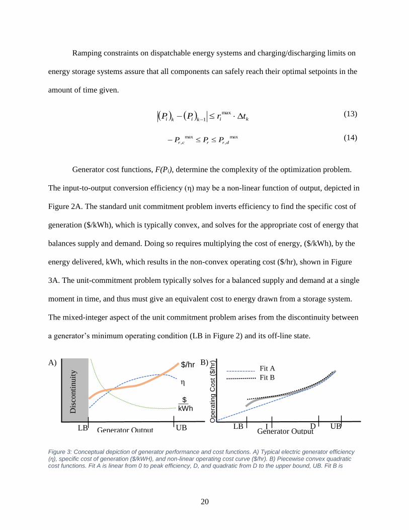
Generator cost functions, F(Pi), determine the complexity of the optimization problem.

The input-to-output conversion efficiency (η) may be a non-linear function of output, depicted in

Figure 2A. The standard unit commitment problem inverts efficiency to find the specific cost of

generation ($/kWh), which is typically convex, and solves for the appropriate cost of energy that

balances supply and demand. Doing so requires multiplying the cost of energy, ($/kWh), by the

energy delivered, kWh, which results in the non-convex operating cost ($/hr), shown in Figure

3A. The unit-commitment problem typically solves for a balanced supply and demand at a single

moment in time, and thus must give an equivalent cost to energy drawn from a storage system.

The mixed-integer aspect of the unit commitment problem arises from the discontinuity between

a generator’s minimum operating condition (LB in Figure 2) and its off-line state.

Figure 3: Conceptual depiction of generator performance and cost functions. A) Typical electric generator efficiency (η), specific cost of generation ($/kWH), and non-linear operating cost curve ($/hr). B) Piecewise convex quadratic cost functions. Fit A is linear from 0 to peak efficiency, D, and quadratic from D to the upper bound, UB. Fit B is

D

isco

nti

nuit

y

η

$ kWh

LB UB Generator Output

A) $/hr B)

LB Generator Output

(kW)

UB D I

Fit A

Fit B

Opera

ting C

ost ($

/hr)

21

discontinuous from 0 to the lower bound, LB, linear from LB to the cost curve inflection point, I, and quadratic from I to UB.

It is common practice in optimization approaches to estimate convex functions with a series of

linear segments to linearize the optimization. The methodology described in this paper optimizes

the cost function (1) representing each generator operating cost, F(Pi), with a piecewise convex

quadratic function. Fit A represents the best possible piecewise convex quadratic that avoids the

lower bound discontinuity and has zero cost at zero output. Fit B is more accurate and includes

the discontinuity and has a non-zero initial cost. Limiting the cost functions to convex quadratics

enables a gradient-based interior-point search method to quickly converge on a global minimum

cost for the entire time horizon. Convex quadratic functions better approximate generator

efficiency curves than linear fits and avoid artificially guiding the optimization as would occur

with piecewise linear optimizations. The optimal dispatch points when using piecewise linear fits

are driven toward the junctions between piecewise linear segments. Constraining the piecewise

convex quadratics to have smooth junctions, eliminates the artificial bias toward junction points.

Most generators have peak operational efficiencies at or near rated capacity, in which case a

linear approximation is equivalent to Fit A. However, chillers, fuel cells and other distributed

energy systems operate more efficiently at part load. In the instances where part load is most

efficient, a piecewise quadratic cost drives the solution towards these non-upper bound optimal

operating conditions, where a linear fit would not.

1.4.1 Combined Cooling, Heating, and Power

Combined heating and power, CHP, generators’ outputs appear in two energy balances.

The secondary heating output does not alter the cost of the generator, and must be linearly

proportional to the primary output, i.e. Pi·β. This may over or under represent actual heat co-

production in the case of a partially loaded CHP unit. Generally, there is a greater tolerance for

22

variance in heating than electricity, so an increase or decrease in demand during the subsequent

forecast optimization accommodates any deviation in heat supplied.

A piecewise linear fit of the heat co-generation can be employed to achieve a more

accurate representation in partially loaded cases, but the optimal location of the end-points

between pieces is subjective and may drastically alter the dispatch of the problem. If heat

demand is a significant portion of total demand, then the optimal dispatch setpoints will tend

toward the end points of the piecewise representation, artificially emphasizing those setpoints

above other, more continuous solutions.

Electric chillers typically represent a non-linear conversion of electrical power to cooling

power not captured by a constant coefficient of performance, COP. Without cold thermal

storage, there is little flexibility in meeting the thermal demand, and chillers are often run at non-

optimal performance. In this scenario, it is preferable to first optimize the chiller dispatch

independent of other systems, where the linear and quadratic cost terms represent the non-linear

electric power consumption, then add the resulting electric demand to net electric load and

proceed with the optimization of the remaining energy systems.

With cold energy storage, it becomes feasible to use chiller loads to balance the electric

demand, and thus dispatch all systems concurrently. In this scenario, the chillers have no direct

costs, i.e. F(Pi) = 0. The chillers appear in the electric energy balance as a load, -Pi, and in the

cooling energy balance as a generator, Pi · COP. The cost of operating a chiller is accounted for

in the cost of electric power it consumes. Given the flexibility in dispatch afforded by the

thermal storage, it is generally preferable to operate all chillers at their design condition, thus

justifying the assumption of constant COP.

23

1.5 Complementary Quadratic Programming

Generally, the problem formulation of 4.1 is a mixed-integer problem with 2N·G states for

the generators to be online or offline at each time step. The number of on/off decision variables

quickly increases beyond what is practical to solve. Complementary Quadratic Programming is a

modified dynamic economic dispatch solution strategy applicable to district energy systems, with

a focus on microgrids with energy storage and is applicable to a receding horizon control

approach. The optimization strategy is part of an open-source platform for the design, simulation,

and control of district energy systems. Complementary Quadratic Programming greatly reduces

the mixed-integer aspect of the optimization problem by separating the problem into three steps:

Step 1. Estimation

Step 2. Unit Commitment

Step 3. Dispatch Optimization

Complementary quadratic programming’s base theory significantly reduces the burden of

the mixed-integer unit commitment problem.

Step 1: Estimation

The optimization of (1) is solved with Fit A, which results in a close approximation of the true

optimal operation without the need to solve the mixed-integer unit commitment problem. Fit A

assumes that all generators can come online or go offline without unit commitment because there

is no discontinuity between the lowest operating point and zero. It is likely only one component

of each energy type is dispatched within the region of Fit A between zero and the component’s

24

lower bound, since the slope of each component’s linear segment is unique. The ramping

constraints may force two or more components into this region for short periods of time when a

component is transitioning between on and offline states.

Step 2: Unit Commitment

The part-loaded component/s as estimated in Step 1 may be operating in the discontinuity

between offline and the lower bound. Either the part loaded component/s must shut down and

allow other systems to pick up the slack, or the part loaded component/s stay on with other

systems operating at part-load to accommodate the extra capacity. Unit commitment defaults to

all components above their lower bound in the estimation step are online, while all components

below their lower bound in the estimation step are offline. If the unit commitment is infeasible,

then the threshold between online and offline is incrementally lowered until a feasible solution is

reached. Figure 4 outlines the relaxation of the on/off threshold for the unit commitment

problem. Lowering the threshold for determining the on/off status does not impact the lower

operating constraint. It may force a generator that was initially dispatched at 15% power to be

online and operating above its 20% minimum.

attempt = 1; %initialize first threshold at the lower bound

percent_of_LB = [1, 0.9, 0.5, 0.1, 0, -1]; %array of thresholds

%continue to lower the threshold, until a feasible solution is found

while Feasible == False && attempt <6

%if the estimated dispatch setpoint is above the threshold, set that component online

Unit_Commitment = Estimation> LB*percent_of_LB(attempt)

[Feasible] = checkFeasibility(Unit_Commitment);

attempt = attempt+1;

end

Figure 4: Pseudo code for assuring feasibility when using cQP.

25

Feasibility with all components online is the last check because it is the most expensive.

Gradual threshold relaxation assures feasibility and reduces the computational demand of the

unit commitment problem from 2NG to a small finite number of threshold steps.

Step 3: Dispatch Optimization

With the resulting unit commitment schedule of generator operation known, the optimization

(1) can be re-solved using Fit B to reach a better approximation of the marginal cost of each

component.

Estimating the solution of (1) with Fit A, checking the feasibility of the part-loaded

component/s, then solving (1) with Fit B replaces the mixed-integer optimization with two

straightforward quadratic optimizations. This approach is valid for most simple arrangements of

generators and storage devices. Arrangements that are more complex may still require solving a

portion of the mixed-integer problem as described in Section 1.6.

1.6 Modified Complementary Quadratic Programming

For complex or highly constrained district energy systems it may be beneficial to check a

broader set of feasible operating conditions between the optimizations with Fit A and Fit B. The

error between Fit A and the actual cost at part-load, varies by component. The start-up and re-

start costs are not captured in (1). Vastly varying equipment sizes may mean that accommodating

a large generator results in shutting down one or more smaller units. These additional costs and

26

complications can be accommodated in a more robust unit commitment step.

Step 1: Estimation

This step is the same as the estimation step for cQP, but it is used to estimate the storage use

over the horizon. The preliminary optimization over the horizon using Fit A is used to estimate

use of storage. The estimate of storage power output is then subtracted from the demand at each

timestep and each timestep is optimized individually. Storage planning is the reason for

optimizing over the entire horizon simultaneously. Estimating storage use with Fit A reduces the

unit commitment problem from 2NG to N∙2G, because each timestep can be optimized

independently.

Step 2: Unit Commitment

The intermediate unit commitment step formulates a set of optimizations of (1) at each

discrete time step. Each optimization considers a feasible arrangement of the 2G generator

combinations available at that time. Combinations in which either the lower bound of the

combination of generators is above the demand, or in which the upper bound of the combination

of generators is below the demand are eliminated, before optimization and comparisons are made

according to Figure 5.

27

Figure 5 Pseudo code for the elimination of combinations which are infeasible for meeting demand

The algorithm in Figure 5 eliminates combinations that are infeasible because they either

cannot produce enough power to meet demand, or cannot all be online without over producing

power.

All combinations that do not meet ramp rate conditions are also eliminated before

optimizations are run and compared. The set of feasible combinations is often much smaller than

the set of all combinations. The cost differential between the feasible alternatives and the original

combination of generators is then compared to any start-up costs avoided by changing the unit

commitment schedule from the first optimization of (1).

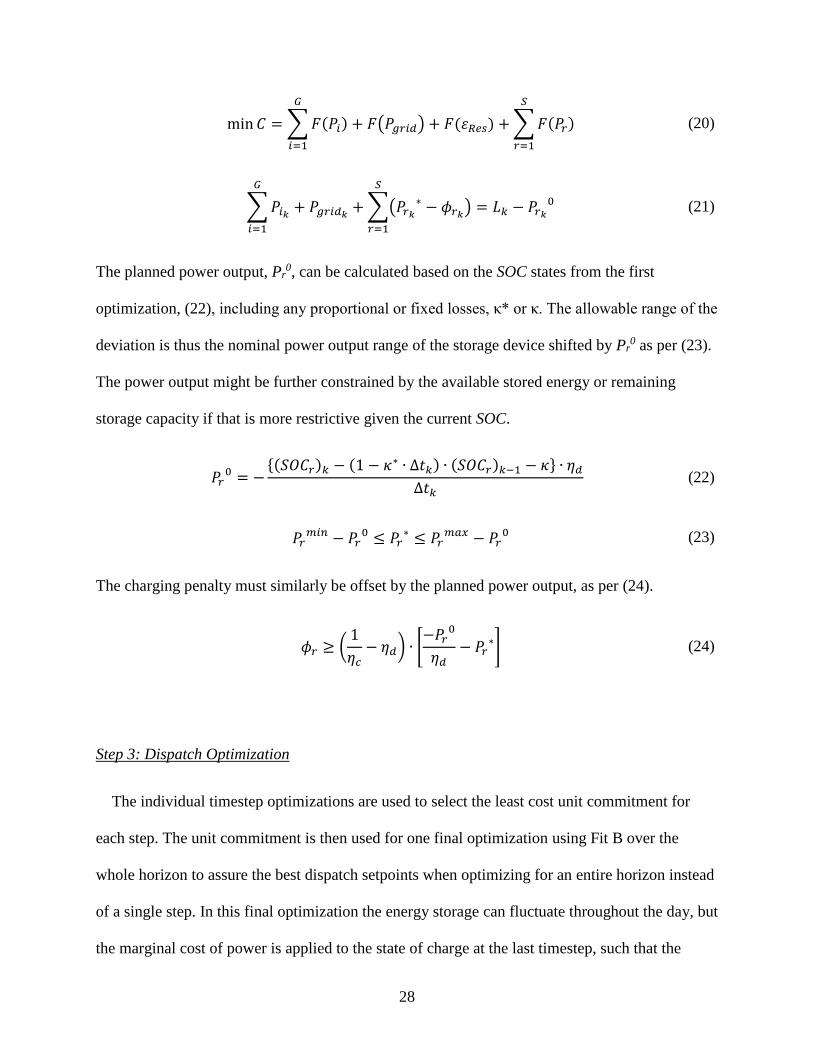
When optimizing a single time step, (20), energy storage lacks the ‘big-picture’ perspective of

the simultaneous optimization. This perspective is incorporated by using the SOC determined by

the first optimization to set the nominal discharge target, Pr0. A quadratic cost constrains

deviations from the original storage, but allows for deviations when significant savings can

accrue. The energy balance at each step thus becomes (21). The planned power output from the

storage is placed on the right-hand-side as a constant, reducing apparent load. The deviation from

this power, and the charging penalty remain on the left hand.

for all_Combinations

if sum(UB(this_Combination)) < Demand

remove this_Combination

elseif sum(LB(thisCombination)) > Demand

remove this_Combination

end

end

28

min 𝐶 = ∑ 𝐹(𝑃𝑖)

𝐺

𝑖=1

+ 𝐹(𝑃𝑔𝑟𝑖𝑑) + 𝐹(𝜀𝑅𝑒𝑠) + ∑ 𝐹(𝑃𝑟)

𝑆

𝑟=1

(20)

∑ 𝑃𝑖𝑘

𝐺

𝑖=1

+ 𝑃𝑔𝑟𝑖𝑑𝑘+ ∑(𝑃𝑟𝑘

∗ − 𝜙𝑟𝑘)

𝑆

𝑟=1

= 𝐿𝑘 − 𝑃𝑟𝑘

0 (21)

The planned power output, Pr0, can be calculated based on the SOC states from the first

optimization, (22), including any proportional or fixed losses, κ* or κ. The allowable range of the

deviation is thus the nominal power output range of the storage device shifted by Pr0 as per (23).

The power output might be further constrained by the available stored energy or remaining

storage capacity if that is more restrictive given the current SOC.

𝑃𝑟0 = −

{(𝑆𝑂𝐶𝑟)𝑘 − (1 − 𝜅∗ ∙ ∆𝑡𝑘) ∙ (𝑆𝑂𝐶𝑟)𝑘−1 − 𝜅} ∙ 𝜂𝑑

∆𝑡𝑘 (22)

𝑃𝑟𝑚𝑖𝑛 − 𝑃𝑟

0 ≤ 𝑃𝑟∗ ≤ 𝑃𝑟

𝑚𝑎𝑥 − 𝑃𝑟0 (23)

The charging penalty must similarly be offset by the planned power output, as per (24).

𝜙𝑟 ≥ (1

𝜂𝑐− 𝜂𝑑) ∙ [

−𝑃𝑟0

𝜂𝑑− 𝑃𝑟

∗] (24)

Step 3: Dispatch Optimization

The individual timestep optimizations are used to select the least cost unit commitment for

each step. The unit commitment is then used for one final optimization using Fit B over the

whole horizon to assure the best dispatch setpoints when optimizing for an entire horizon instead

of a single step. In this final optimization the energy storage can fluctuate throughout the day, but

the marginal cost of power is applied to the state of charge at the last timestep, such that the

29

storage unit is not constrained to an end SOC, but maintains stored energy that can be used in

future horizons.

1.7 Artificial Neural Network

Although modified complementary quadratic programming is a more optimal method of

dispatch than complementary quadratic programming or search based methods and maintains a

much lower computational demand than traditional numerical methods, the optimization may be

out-of-date before it can be solved and setpoints implemented. This computational time

constraint prevents the mcQP from solving highly complex problems or problems with high

frequency (e.g. sub minute) receding horizon updates.

A machine learning approach can send dispatch signals at the desired frequency, but

machine learning systems require large training sets before outputs reach a robust representation

of the optimal.

Developing training sets with full mixed-integer solvers would be

prohibitively time and resource consuming. Thus, mcQP, with its balance between

reliability and efficiency, can quickly generate the large training sets necessary for

machine learning methods. The efficiency and reliability of mcQP are key in

allowing an Artificial Neural Network to train on the full range of seasonal, weekly,

and diurnal market and demand input fluctuations.

Neural Network methods are amenable to classification problems, so the neural network

developed for this work acts as a classifier for unit commitment. An ANN, trained from mcQP

solutions for specific loads, classifies each component as either online or offline, reducing the

unit commitment step computational time. Dispatch constraints, feasibility, and robustness are

30

maintained by using the unit commitment solution from the ANN as the equipment status for a

quadratic programming optimization using Fit B, thus replacing the first two steps of both cQP

and mcQP. Real time control can be achieved with an ANN that reduces the order of the problem

from 2NG to constant time.

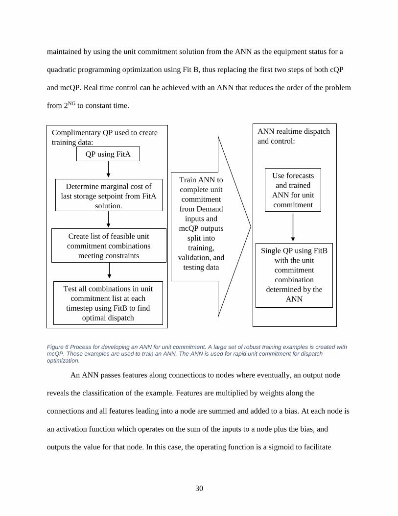
Figure 6 Process for developing an ANN for unit commitment. A large set of robust training examples is created with mcQP. Those examples are used to train an ANN. The ANN is used for rapid unit commitment for dispatch

optimization.

An ANN passes features along connections to nodes where eventually, an output node

reveals the classification of the example. Features are multiplied by weights along the

connections and all features leading into a node are summed and added to a bias. At each node is

an activation function which operates on the sum of the inputs to a node plus the bias, and

outputs the value for that node. In this case, the operating function is a sigmoid to facilitate

Complimentary QP used to create

training data:

QP using FitA

Determine marginal cost of

last storage setpoint from FitA

solution.

Create list of feasible unit

commitment combinations

meeting constraints

Test all combinations in unit

commitment list at each

timestep using FitB to find

optimal dispatch

Train ANN to

complete unit

commitment

from Demand

inputs and

mcQP outputs

split into

training,

validation, and

testing data

ANN realtime dispatch

and control:

Use forecasts

and trained

ANN for unit

commitment

Single QP using FitB

with the unit

commitment

combination

determined by the

ANN

31

binary classification. The sigmoid has asymptotes at zero and one with a steep slope for input

values between -1 and 1. This shape facilitates binary classification by pushing inputs toward

either online (one) or offline (zero). All nodes employ the sigmoid activation function (25) to

emphasize any deviation from normal, so that small changes in the middle range have large

impacts, while outliers are prevented from dominating the characterization of an example.

𝑦 =1

𝑒𝑥+1 𝑥 = 𝑏 − ∑ 𝑤𝑖 ∗ 𝑓𝑖

𝐹𝑖=1 (25)

where y is the output of the node, b is the bias at the node, wi is the weight corresponding

to the ith connection, fi is the feature or input corresponding to the ith connection, and F is the

number of input features.

The output from mcQP can be re-organized into a training set where non-zero component

setpoints map to the online class, while setpoints at zero map to the offline class. Feature

selection is more flexible and is explained further in Section 1.7.1 Network Structure Selection.

1.7.1 Network Structure Selection

There are several challenges in accurately training an ANN, specifically determining the

features to consider as inputs and determining the number of layers. Feature selection is a

challenge because unimportant features, those whose weighting would eventually train to zero,

significantly add to the training time and obfuscate the training of more significant parameters

until the weighting reaches zero. Features must be carefully selected to reduce training time and

prevent obfuscation, while still capturing all aspects of the problem. A decision tree as described

on page 35 is used for feature selection.

The available features from the dispatch estimation include:

32

● Estimated component set point from the previous dispatch for each component at each

step in the horizon

● Estimated energy storage input/output for each storage device at each step in the horizon

● Market price of energy at each step in the horizon:

○ Price of electricity from the grid

● Forecasted Energy demand at each step in the horizon:

○ Electric, Cooling, and Heating demand

● Forecasted renewable energy production at each step in the horizon

● Upper and lower bounds of each component at each step in the horizon

○ The upper and lower bounds change at each timestep because the generation from

each component is limited by a ramp rate

The market prices for fuel are not included because they are assumed to be constant

values throughout the year, while the market price of electricity varies throughout the day and

seasonally. Static values such as the generator efficiency curve constants and generator types are

not considered for features, because these characteristics are static. Training to static features

obfuscates the learning of important features. The upper and lower bounds of each component

are not static values because they change depending on component initial condition and ramp

rate.

Instead of including the estimated hourly dispatch for each component at each timestep

into the horizon, timesteps 1, 2, 3, 6, 12, 18, and 23 were selected to reveal the value of including

estimated dispatches farther into the future without incurring the computational slowdown

associated with including all timesteps from 1 to 23. The estimations do not reach timestep 24,

because they are provided by the previous dispatch, and the last step of the previous dispatch is

33

timestep 23 of the current dispatch. Power from storage devices is only included at the previous

timestep, instead of all estimated timesteps, because the power from the previous step has

already been implemented and is not an estimated value. Also, reducing the features from all

estimated timesteps to only the previous timestep reduces computational time for the decision

tree.

The accuracy of the ANN is also dependent on the number of layers, also known as the

ANN’s depth. Deep ANN’s can achieve high accuracy, but deep learning requires a longer

training time to propagate through all the layers, and more training examples to accurately define

the classification boundary without overfitting as compared to shallow ANNs. Unit commitment

has a more predictable behavior than common problems that employ deep learning, such as

complex image recognition [64] or human behavior recognition [65], so it is assumed that the

problem will require few layers. When there are few layers, the accuracy varies more quickly

with the number of layers. A single layer ANN will not capture any interaction between features,

while a two layered ANN will capture feature interaction. The difference between one and two

layers is large while the difference between 99 and 100 layers is smaller because with many

layers, complex interactions are already captured without the addition of another layer. The

depth of the ANN is more crucial when assuming a shallow ANN is sufficient, because an extra

layer will add a significant percentage to the training time, while too few layers will fail to

capture the complexity of the problem.

Feature and layer selection is challenging because a rigorous search of all configurations

would require training, testing, and comparing test accuracy for D·2F different ANNs for each

component, where D is the number of different ANN depths to check and F is the number of

features. The case study of this thesis, 6 possible depths and 10 possible features, would result in

34

6144 ANN’s that would be trained and substituted for the unit commitment problem. Six

possible ANN layer depths were compared because the ANN layers were increased until

accuracy did not improve at all for any unit commitment validation accuracy. The ten possible

features include all possible features with varying values as described in the list above. Instead of

testing all combinations of features, a decision tree selects the features for training ANNs with 1

to 6 layer depths. MATLAB’s Neural Network Toolbox is used to train and evaluate neural

networks with 2 to 6 layers, but the toolbox does not support single layer ANNs, so an author

created open-source algorithm for training and evaluation of a single layer ANN is used for an

ANN with one layer.

Network structure selection is conducted using the complex campus system described in

Section 1.8 Test Systems. The complex system encompasses all possible features for the simple

system. Training examples were created from optimal dispatches of the complex case using

mcQP. The optimal dispatches span a full year with a receding horizon of 24 hours, timesteps of

one hour, predictions updated every hour, and 24 hours to establish initial conditions resulting in

365*24*24+24 = 210264 training examples. Training solutions are the unit commitment state of

the dispatchable components, such that a component with an output of 0 is offline, and a

component with an output above its minimum self-sustaining threshold is online. The component

lower bound constraint assures that no components have outputs between 0 and the minimum

self-sustaining threshold.

All inputs are normalized by subtracting the minimum value and dividing by the

maximum value. Normalization (26-33) prevents large inputs from overpowering smaller inputs

and facilitates the use of a sigmoid function for binary classification. The predicted power from

35

the storage devices is found from the predicted state of charge at the current timestep minus the

predicted state of charge at the previous timestep (28).

𝑓𝑑𝑒𝑚𝑎𝑛𝑑 =𝐷𝑒𝑚𝑎𝑛𝑑−𝑋𝑟𝑒𝑛𝑒𝑤

max(𝐷𝑒𝑚𝑎𝑛𝑑) (26)

𝑓𝑐𝑜𝑠𝑡 = 𝐶(

𝑈𝑡𝑖𝑙𝑖𝑡𝑦

𝑑𝑡)

max(𝐶(𝑈𝑡𝑖𝑙𝑖𝑡𝑦

𝑑𝑡))

(27)

𝑓𝑠𝑡𝑜𝑟𝑒𝑑𝑃𝑜𝑤𝑒𝑟 = (𝑆𝑂𝐶𝑡−1𝐴 − 𝑆𝑂𝐶𝑡𝐴)/𝑈𝐵𝑠𝑡𝑜𝑟𝑎𝑔𝑒 (28)

fUB = min(𝑈𝐵, 𝑋𝑡−1𝐴 + 𝑅𝑎𝑚𝑝𝑅𝑎𝑡𝑒) /𝑈𝐵 (29)

𝑓𝐿𝐵 = max(𝐿𝐵, 𝑋𝑡−1𝐴 − 𝑅𝑎𝑚𝑝𝑅𝑎𝑡𝑒) /𝑈𝐵 (30)

𝑓𝑝𝑟𝑒𝑑𝑖𝑐𝑡𝑒𝑑𝑆𝑡𝑎𝑡𝑒−1 = 𝑋𝑡−1𝐴/𝑈𝐵 (31)

𝑓𝑝𝑟𝑒𝑑𝑖𝑐𝑡𝑒𝑑𝑆𝑡𝑎𝑡𝑒 1 = 𝑋𝑡+1𝐴/𝑈𝐵 (32)

𝑓𝑝𝑟𝑒𝑑𝑖𝑐𝑡𝑒𝑑𝑆𝑡𝑎𝑡𝑒 0 = 𝑋𝑡/𝑈𝐵 (33)

Where f is the normalized feature input, X is the predicted state of the component, C(Utility)*dt

is the cost of electricity from the utility in the form of $/kWh at an hourly timestep, SOC is the

state of charge of an energy storage device, UB is the absolute upper limit on component

production or stored energy, and LB is the lower limit on power output or stored energy when

the component is online.

The features of the ANN are determined according to accuracy associated with decision

trees for each component in the unit commitment problem to reduce the computational effort

involved in finding the most effective ANN structure.

36

A decision tree trained from the inputs listed above and the solutions as given by the final

unit commitment from mcQP is used for the selection of valuable features. If an input is never

thresholded in the tree, then that input is not useful for deciding if the generator is online. If an

input is thresholded in a node near the top of the tree, then that input is very important, because it

provides the most information gain for all examples. Using a decision tree for input evaluation is

more efficient than the exhaustive search of all ANN inputs, because it only requires the training

of one tree per dispatchable component.

WEKA’s J48 decision tree algorithm is used to conduct unit commitment for each

dispatchable component given the described set of features [63]. Trees are made with 10-fold

cross validation. The trees are generated with a smaller sample size of 21,137 labeled examples

for each component, which is one tenth of the available example set. Only one tenth of the full

set is used to train the decision tree to improve training time. The J48 implementation follows the

ID3 algorithm where the node is split along the feature with the highest information gain. One

tree is created for each component.

1.7.2 ANN Training

The ANN is trained using batch learning and back propagation to 0.0001 maximum

square error or 10,000 training iterations, whichever comes first during back propagation. A

maximum square error of 0.0001 is chosen because inputs include forecasted demands and

generator limits which are often values accurate to four decimal places, so this small square error

value maintains the importance of all significant figures. For example, a forecasted demand of

1001 kW is distinct from a forecast of 1000 kW if you have two generators with maximum

capacities at 1000 kW. The threshold of 10,000 training iterations is chosen, because this is the

point at which accuracy reaches saturation. For a more detailed accuracy curve see Section

37

1.10.1 ANN Structure Selection. Back propagation alters the weights and biases using gradient

descent starting with the output layer and working backwards in the network. The weights and

biases of the layer in question are updated according to the error between expected output and

actual output.

𝑑𝑤

𝑑𝐸= −2𝑥 𝐸𝑦 (1 − 𝑦)

∆𝑤𝑗 =𝑑𝑤

𝑑𝐸𝑒𝑟𝑟𝑜𝑟

𝑎

100+

𝑚

100∆𝑤𝑗−1

𝑑𝑏

𝑑𝐸= −

2

𝐹∑ 𝑒𝑟𝑟𝑜𝑟𝑖 𝑦𝑖 (1 − 𝑦𝑖)

𝐹

𝑖=1

∆𝑏𝑗 =𝑑𝑏

𝑑𝐸

𝑎

100+

𝑚

100∆𝑏𝑗−1

Learning rate, a, of 1 is divided by 100 to prevent overshooting the minimal error

solution. Momentum factor, m, of 0.25 is employed to increase speed of learning at points of

high change in error.

A Hessian training approach was attempted to increase accuracy and speed up

convergence, but the large multi-parameter dependency of the output prevents the inversion of

the sparse Hessian matrix, preventing learning. Biases are necessary to realize the non-zero

minimum effect of parameters such as temperature and forecasted demand. The sigmoid

activation function facilitates rapid training to the binary off/on problem in unit commitment

because it has asymptotes at 0 and 1 with a region of steep slope around an input value of zero.

Sample source code for the neural network learning algorithm and the neural network

class definition can be found in APPENDIX A: SAMPLE SOURCE CODE.

38

1.7.3 Algorithm Execution and Division of Work

A robust execution of the optimization algorithms was developed through different

contributors across several years. The evolution of software and algorithms, as well as the

division of work is detailed in Figure 7. Blue text indicates software that was developed without

author involvement, purple text indicates software that was developed with author collaboration,

and red text indicates software that was developed by the author independently.

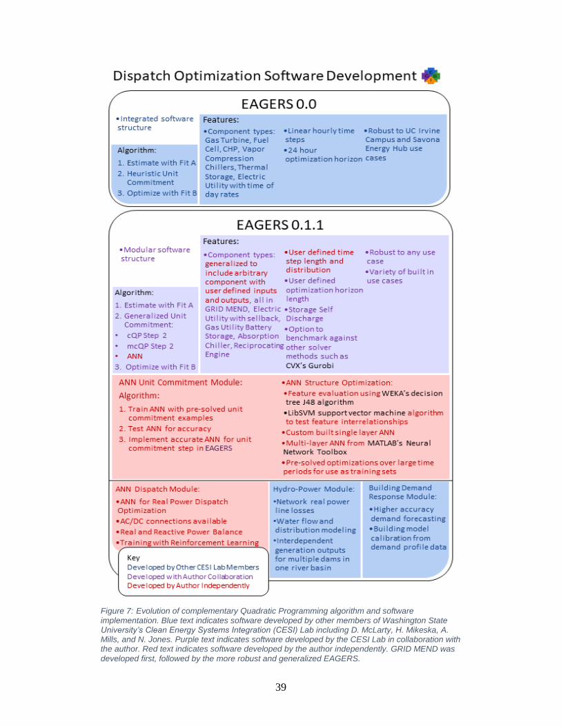
39

Figure 7: Evolution of complementary Quadratic Programming algorithm and software implementation. Blue text indicates software developed by other members of Washington State University’s Clean Energy Systems Integration (CESI) Lab including D. McLarty, H. Mikeska, A. Mills, and N. Jones. Purple text indicates software developed by the CESI Lab in collaboration with the author. Red text indicates software developed by the author independently. GRID MEND was

developed first, followed by the more robust and generalized EAGERS.

40

The software Efficient Allocation of Grid Energy Resources including Storage (EAGERS

0.0), which was developed by D. McLarty prior to 2015, followed an algorithm where unit

commitment was conducted using heuristic rules which accommodated the UC Irvine Campus

use case and the Savona Energy Hub use case. Version 0.0 accommodated CHP gas turbines,

CHP fuel cells, vapor compression chillers, thermal storage units, and electric utilities with time

of use rates.

EAGERS underwent restructuring, feature expansion, and generalization starting when

the author joined Washington State University’s Clean Energy Systems Integration Lab in 2015.

The new modular, more robust, generalized algorithm became the open source software

EAGERS 0.1.1. The algorithm was generalized such that different processes can be used for unit

commitment. There are currently three algorithm options for unit commitment implemented in

EAGERS. The first option follows cQP as described in Section 1.4 Theory Development. The

second option follows mcQP as described in Section 1.6 Modified Complementary

Programming. The third option uses an artificial neural network for unit commitment as

described in Section 1.7 Artificial Neural Network.

The modular structure of EAGERS 0.1.1 is more adaptable to new microgrid

components, new power demand types, new optimization implementations for benchmarking,

and new features. The algorithm was generalized such that optimization timesteps could have

any arbitrary value and span an arbitrary horizon length. Timesteps longer than an hour and

horizons longer than 24-hours enable optimization of long term phenomenon, such as power

storage at a dam [66]. Timesteps shorter than one hour enable higher resolution optimization,

bringing the algorithm one step closer to bridging the gap between optimization and control.

41

Non-linear timesteps can be used in scenarios where the near future requires high resolution, but

the far-future forecast has high uncertainty.

The robustness of the new algorithm and implementation in EAGERS 0.1.1 is important

for creating training sets for neural network training. Machine learning methods require large

training sets to capture the entire space of an optimization. Other robust algorithms that search

larger unit commitment spaces run slowly, making training set generation prohibitive. CVX’s

Gurobi is a commercial mixed integer quadratic programming solver, but its long run time makes

creating large training sets prohibitive. This aspect of the computational advantage of EAGERS

0.1.1 is further described in Section 1.7 Artificial Neural Network.

The artificial neural network for unit commitment method was developed by the author

independently. Artificial neural network structure optimization is available using WEKA’s J48

decision tree algorithm for feature selection, and MATLAB’s Neural Network Toolbox for ANN

depth evaluation. Single layer ANNs are available for unit commitment using author generated

class structure, training, and unit commitment algorithm. These single layer ANNs improve

training time, require fewer training examples, reduce memory use, and improve output

computation time. For multi-layer ANNs, MATLAB’s Neural Network Toolbox is used for

training and dispatch within the unit commitment method. Large training example sets were

created using EAGERS’s mcQP option as applied to scenarios further described in Section 1.8

Test Systems.

Future work includes extending the neural network to include dispatch optimization for

real power, then adapting a neural network for dispatch optimization including reactive power

control and AC/DC connections. The ANN for reactive power control would be trained using

reinforcement learning. Future work is described in more detail in Section 7 Future Work.

42

EAGERS is open source and free to download at https://github.com/CESI-Lab/EAGERS

or by contacting the author. Sample source code is shown in APPENDIX A: SAMPLE SOURCE

CODE.

1.8 Test Systems

Two test systems are used for training and testing optimization methods to show the

exponential increase in computational efficiency with increasing microgrid complexity. The

simple microgrid is dispatched for one week and is used to validate the optimization of the neural

network approach, since it is more difficult to determine if a complex system has been

dispatched optimally, than if a simple system has been dispatched optimally. The complex

system is dispatched for a full year, allowing for a full generalized training set for the ANN. This

system is used to benchmark computational demands of different methods and verify that a

neural network can accommodate complex systems.

The first system includes 5 components: an electric utility, a gas utility, an internal

combustion engine, a gas turbine, and a hot water thermal energy storage unit. Both the internal

combustion engine and the gas turbine are combined heat and power units. This system has

electrical and heat demand.

The complex microgrid system consists of 18 components: an electric utility, a natural

gas utility, a diesel supply, two combined heat and power gas turbines with dissimilar efficiency

curves, two combined heat and power fuel cells with dissimilar efficiency curves, one battery, a

rooftop solar PV array, two large chillers with dissimilar efficiency curves, two small chillers

with dissimilar efficiency curves, one diesel generator, a cold thermal storage water tank, a hot

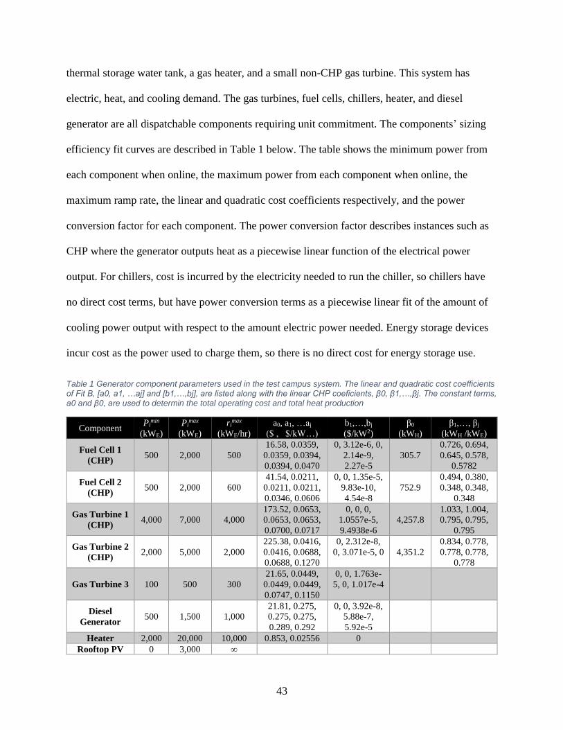
43

thermal storage water tank, a gas heater, and a small non-CHP gas turbine. This system has

electric, heat, and cooling demand. The gas turbines, fuel cells, chillers, heater, and diesel

generator are all dispatchable components requiring unit commitment. The components’ sizing

efficiency fit curves are described in Table 1 below. The table shows the minimum power from

each component when online, the maximum power from each component when online, the

maximum ramp rate, the linear and quadratic cost coefficients respectively, and the power

conversion factor for each component. The power conversion factor describes instances such as

CHP where the generator outputs heat as a piecewise linear function of the electrical power

output. For chillers, cost is incurred by the electricity needed to run the chiller, so chillers have

no direct cost terms, but have power conversion terms as a piecewise linear fit of the amount of

cooling power output with respect to the amount electric power needed. Energy storage devices

incur cost as the power used to charge them, so there is no direct cost for energy storage use.

Table 1 Generator component parameters used in the test campus system. The linear and quadratic cost coefficients of Fit B, [a0, a1, …aj] and [b1,…,bj], are listed along with the linear CHP coeficients, β0, β1,…,βj. The constant terms, a0 and β0, are used to determin the total operating cost and total heat production

Component Pi

min

(kWE)

Pimax

(kWE)

rimax

(kWE/hr)

a0, a1, …aj

($ , $/kW…)

b1,…,bj

($/kW2)

β0

(kWH)

β1,…, βj

(kWH /kWE)

Fuel Cell 1

(CHP) 500 2,000 500

16.58, 0.0359,

0.0359, 0.0394,

0.0394, 0.0470

0, 3.12e-6, 0,

2.14e-9,

2.27e-5

305.7

0.726, 0.694,

0.645, 0.578,

0.5782

Fuel Cell 2

(CHP) 500 2,000 600

41.54, 0.0211,

0.0211, 0.0211,

0.0346, 0.0606

0, 0, 1.35e-5,

9.83e-10,

4.54e-8

752.9

0.494, 0.380,

0.348, 0.348,

0.348

Gas Turbine 1

(CHP) 4,000 7,000 4,000

173.52, 0.0653,

0.0653, 0.0653,

0.0700, 0.0717

0, 0, 0,

1.0557e-5,

9.4938e-6

4,257.8

1.033, 1.004,

0.795, 0.795,

0.795

Gas Turbine 2

(CHP) 2,000 5,000 2,000

225.38, 0.0416,

0.0416, 0.0688,

0.0688, 0.1270

0, 2.312e-8,

0, 3.071e-5, 0 4,351.2

0.834, 0.778,

0.778, 0.778,

0.778

Gas Turbine 3 100 500 300

21.65, 0.0449,

0.0449, 0.0449,

0.0747, 0.1150

0, 0, 1.763e-

5, 0, 1.017e-4

Diesel

Generator 500 1,500 1,000

21.81, 0.275,

0.275, 0.275,

0.289, 0.292

0, 0, 3.92e-8,

5.88e-7,

5.92e-5

Heater 2,000 20,000 10,000 0.853, 0.02556 0

Rooftop PV 0 3,000 ∞

44

Table 2 Chiller component parameters used in the test campus system. Chiller costs are incurred as the electrical power used by each chiller, determined by the linear energy conversion factors β.

Component Pi

min

(kWC)

Pimax

(kWC)

rimax

(kWC/hr) β0 (kWE)

β1,…, βj

(kWE / kWC)

Chiller 1 2,000 10,000 3,000 183.1 0.133, 0.161, 0.304

Chiller 2 1,500 10,000 2,000 186.1 0.135, 0.157, 0.305

Chiller 3 2,500 7,500 5,000 199.6 0.150, 0.151, 1.52, 0.238, 0.368

Chiller 4 2,000 7,500 2,000 182.9 0.166, 0.222, 0.390

Table 3 Energy storage components used in the test campus system. Energy storage costs are incurred as the power used to charge the device, so there is no direct costs for energy storage.

Component SOCr

max

(MWhr) Pi

min (kW) Pimax (kW) κ* (%/hr) , κ (kW) ηc , ηd (%)

Battery 25.5 -14,900 7,540 0.0 , 3.41 99.48 , 99.48

Cold Thermal Storage 20 -50,000 50,000 0.0 , 123.75 99 , 99

Hot Thermal Storage 7.5 -30,000 30,000 0.0 , 330 99 , 99

Table 4 The fuel cells, gas turbines, diesel generator, and chillers have startup costs associated with coming online.

Fuel

Cell 1

Fuel

Cell 2

Gas

Turbine 1

Gas

Turbine 2

Gas

Turbine 3

Diesel

Generator

Chiller

1

Chiller

2

Chiller

3

Chiller

4

$300 $250 $1000 $300 $10 $100 $150 $200 $50 $50

Figure 8 Electric utility rates vary throughout the week and are dependent on season. From June 1st through September 30th summer rates are used, while from October 1st through May 31st winter rates apply. Peak pricing is during the middle of the day on weekdays

The electric utility pricing varies by season, day of the week, and hour of the day. Pricing

schedules are split into two seasons: summer which is from June 1st through September 30th, and

winter which is from October 1st through May 31st. The profiles for winter and summer pricing

are shown in Figure 8. These pricing profiles are representative of a typical time of use schedule

where the highest price for electricity occurs mid-day during summer weekdays.

45

5. RESULTS

1.9 Complementary Quadratic Programming Dispatch Cost and Computational Efficiency

The cQP method is benchmarked against mcQP, and the full mixed integer approach as

implemented by CVX’s Gurobi mixed-integer quadratic programming optimizer. The second,

complex microgrid setup is used for benchmarking the cQP method to demonstrate its

computational efficiency when applied to complex systems.

A historic energy profile for electric, heating, and cooling demand for a college campus

in California for a full year at one hour intervals is used for the demand. The historical demand

profile is surface fit for demand versus time of day and temperature to simulate forecasting and

include forecasting error where the actual demand is the historic data and the forecasted demand

is the surface fit for that temperature and time of day. Forecasting error is important to include

for testing the robustness of the receding horizon method, because it tests that the dispatch

method can adapt to errors in demand forecasts as well as adjust to new information in the

dispatch in the receding horizon. The hourly dispatch profile for one year allows for the creation

of 8760 optimizations from both cQP and mcQP methods on real data. The large dispatch set

allows for comparison of computational time, dispatches, and cost at all ranges in time of day,

weekly, and seasonal profiles. Full year energy profiles for electric, heating, and cooling

demands collected at a college campus in California are used for the loads, resulting in 8760

optimizations from both cQP and mcQP methods. This allows for comparison of computational

time, dispatches, and cost at all ranges in time of day, weekly, and seasonal profiles. The cQP is

able to optimize a 24 hour dispatch in an average of 1.6 seconds, while the mcQP method takes

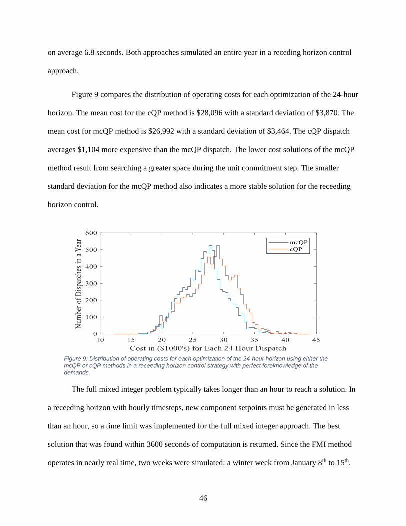
46

on average 6.8 seconds. Both approaches simulated an entire year in a receding horizon control

approach.

Figure 9 compares the distribution of operating costs for each optimization of the 24-hour

horizon. The mean cost for the cQP method is $28,096 with a standard deviation of $3,870. The

mean cost for mcQP method is $26,992 with a standard deviation of $3,464. The cQP dispatch

averages $1,104 more expensive than the mcQP dispatch. The lower cost solutions of the mcQP

method result from searching a greater space during the unit commitment step. The smaller

standard deviation for the mcQP method also indicates a more stable solution for the receeding

horizon control.

The full mixed integer problem typically takes longer than an hour to reach a solution. In

a receeding horizon with hourly timesteps, new component setpoints must be generated in less

than an hour, so a time limit was implemented for the full mixed integer approach. The best

solution that was found within 3600 seconds of computation is returned. Since the FMI method

operates in nearly real time, two weeks were simulated: a winter week from January 8th to 15th,

Figure 9: Distribution of operating costs for each optimization of the 24-hour horizon using either the mcQP or cQP methods in a receeding horizon control strategy with perfect foreknowledge of the demands.

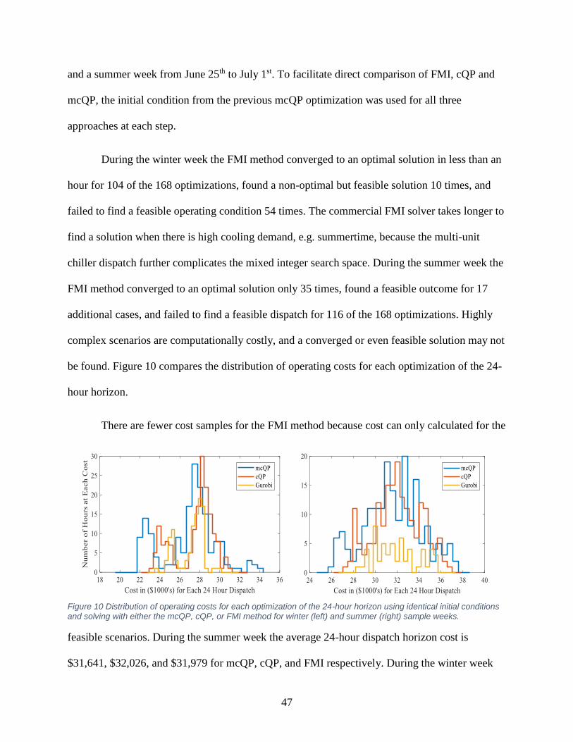
47

and a summer week from June 25th to July 1st. To facilitate direct comparison of FMI, cQP and

mcQP, the initial condition from the previous mcQP optimization was used for all three

approaches at each step.

During the winter week the FMI method converged to an optimal solution in less than an

hour for 104 of the 168 optimizations, found a non-optimal but feasible solution 10 times, and

failed to find a feasible operating condition 54 times. The commercial FMI solver takes longer to

find a solution when there is high cooling demand, e.g. summertime, because the multi-unit

chiller dispatch further complicates the mixed integer search space. During the summer week the

FMI method converged to an optimal solution only 35 times, found a feasible outcome for 17

additional cases, and failed to find a feasible dispatch for 116 of the 168 optimizations. Highly

complex scenarios are computationally costly, and a converged or even feasible solution may not

be found. Figure 10 compares the distribution of operating costs for each optimization of the 24-

hour horizon.

There are fewer cost samples for the FMI method because cost can only calculated for the

feasible scenarios. During the summer week the average 24-hour dispatch horizon cost is

$31,641, $32,026, and $31,979 for mcQP, cQP, and FMI respectively. During the winter week

Figure 10 Distribution of operating costs for each optimization of the 24-hour horizon using identical initial conditions and solving with either the mcQP, cQP, or FMI method for winter (left) and summer (right) sample weeks.

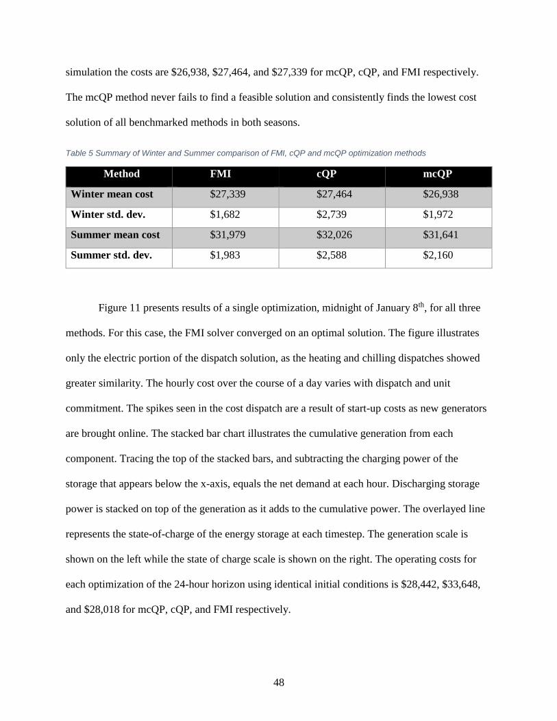
48

simulation the costs are $26,938, $27,464, and $27,339 for mcQP, cQP, and FMI respectively.

The mcQP method never fails to find a feasible solution and consistently finds the lowest cost

solution of all benchmarked methods in both seasons.

Table 5 Summary of Winter and Summer comparison of FMI, cQP and mcQP optimization methods

Method FMI cQP mcQP

Winter mean cost $27,339 $27,464 $26,938

Winter std. dev. $1,682 $2,739 $1,972

Summer mean cost $31,979 $32,026 $31,641

Summer std. dev. $1,983 $2,588 $2,160

Figure 11 presents results of a single optimization, midnight of January 8th, for all three

methods. For this case, the FMI solver converged on an optimal solution. The figure illustrates

only the electric portion of the dispatch solution, as the heating and chilling dispatches showed

greater similarity. The hourly cost over the course of a day varies with dispatch and unit

commitment. The spikes seen in the cost dispatch are a result of start-up costs as new generators

are brought online. The stacked bar chart illustrates the cumulative generation from each

component. Tracing the top of the stacked bars, and subtracting the charging power of the

storage that appears below the x-axis, equals the net demand at each hour. Discharging storage

power is stacked on top of the generation as it adds to the cumulative power. The overlayed line

represents the state-of-charge of the energy storage at each timestep. The generation scale is

shown on the left while the state of charge scale is shown on the right. The operating costs for

each optimization of the 24-hour horizon using identical initial conditions is $28,442, $33,648,

and $28,018 for mcQP, cQP, and FMI respectively.

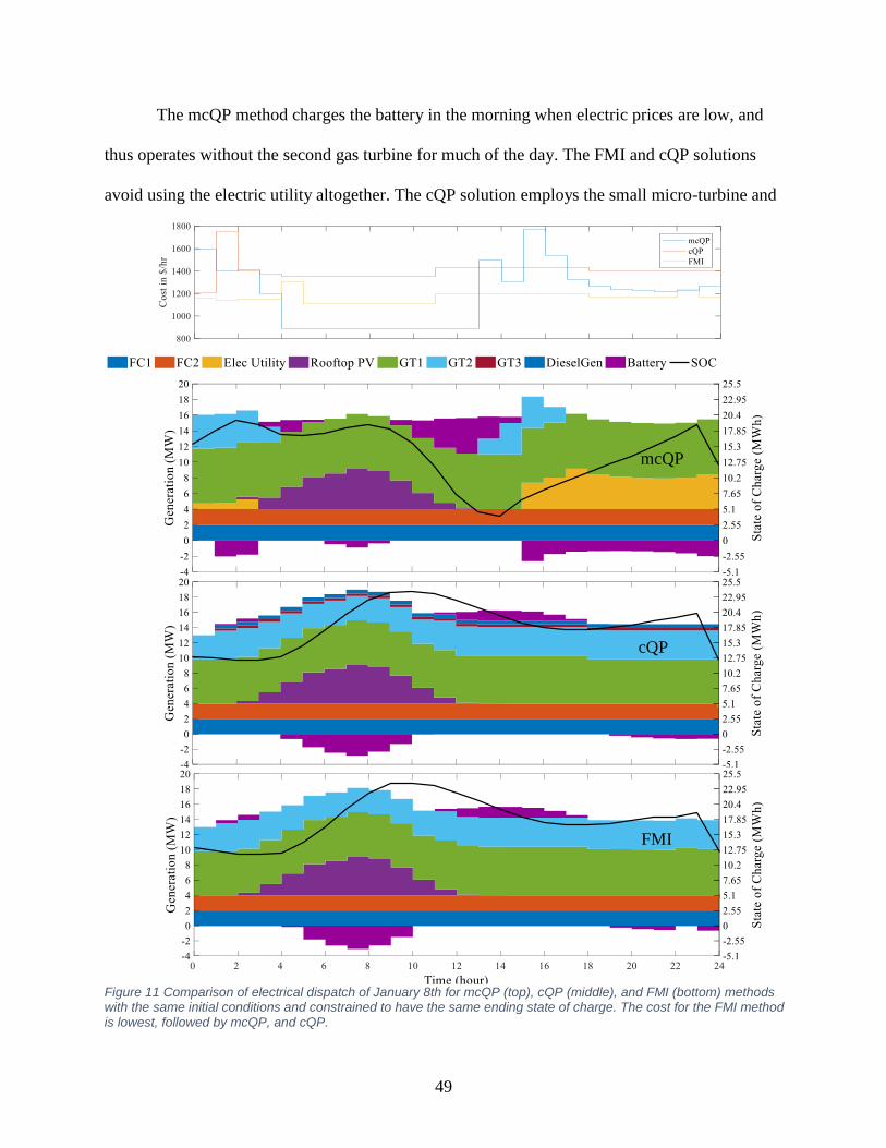
49

The mcQP method charges the battery in the morning when electric prices are low, and

thus operates without the second gas turbine for much of the day. The FMI and cQP solutions

avoid using the electric utility altogether. The cQP solution employs the small micro-turbine and

mcQP

cQP

FMI

Figure 11 Comparison of electrical dispatch of January 8th for mcQP (top), cQP (middle), and FMI (bottom) methods with the same initial conditions and constrained to have the same ending state of charge. The cost for the FMI method is lowest, followed by mcQP, and cQP.

50

diesel reciprocating engine to make-up additional power, which accounts for the majority of the

additional cost. Additional control logic bespoke to this system could improve the general cQP

approach by forcing a check of the microturbine and diesel generator operating status. Generally

the cQP approach more closely approximates mcQP, and this particular optimization may be one

of the outliers of Figure 10.

51

Figure 12 presents results of a single optimization, midnight of June 26th, for all three

methods. The operating costs for each optimization of the 24-hour horizon using identical initial

mcQP

cQP

FMI

Figure 12 Dispatch from mcQP (top), cQP (middle), and FMI (bottom) methods for June 26th. The cost at each hour for each method is shown at the top.

52

conditions is $34,693, $35,751, and $35,141 for mcQP, cQP, and FMI respectively. The costs

and dispatches produced by all three aproaches are similar. This particular summer optimization

is simpler than most, as evidenced by the FMI method’s ability to reach a feasible solution.

Unlike mcQP, the cQP method keeps the second gas turbine off from 7-8am, 10am-1pm, and

from 6-7pm. During the middle of the day, the cQP method brings GT3 online and relies on the

battery and electric utility to compensate for not using GT2. This significantly changes the

battery discharge dynamics. The cQP method also reduces the time that the first gas turbine is

online. The reduction in use of the larger two gas turbines results in a higher overall cost for

cQP, as the utility is more heavily relied on.

1.10 ANN in for Unit Commitment

1.10.1 ANN Structure Optimization

A decision tree was created for each component to determine which features should be

used for ANN inputs.

The first two rows of Table 6 show the accuracy and number of nodes in each respective

component tree. The percent of examples that belong to the majority class is shown in the bottom

row for comparison to the accuracy.

Table 6: Accuracy of decision trees for each component's unit commitment. The accuracy must be high in comparison to the percent of training examples that are of one class to show that the problem is well defined by the

features included.

GT 1 GT 2 Fuel

Cell 1

Fuel

Cell 2

Small

GT

Diesel

Gen

Heater Chiller 1 Chiller 2 Chiller 3 Chiller

4

Accuracy 98.46 92.13 100 100 93.63 100 90.40 98.22 95.35 96.83 98.55 Number

of Nodes 217 857 1 1 599 1 1103 171 403 303 151

Percent

One Class 93.16 73.96 100 100 88.60 100 55.95 92.64 66.91 68.47 90.16

53

The first fuel cell is online for every timestep in the year, the second fuel cell is online for

every timestep except one, and the diesel generator is offline for every timestep in the year when

dispatched using the mcQP method. These three components do not require a decision tree or

neural network evaluation, because they always remain online due to the fuel cells’ high

efficiency, or offline due to the diesel generator’s low efficiency combined with high cost of

fuel.

All component trees have high accuracies above the percentage of training examples

belonging to one class, indicating that the problem is well represented by the trees with the

features used for thresholds. If the component tree accuracy were high, but below the percentage

of examples in one class, then the tree would perform worse than always outputting one class,

indicating a poorly represented problem. The comparison between accuracy and examples in one

class is important here because some components have a high percentage of examples in one

class. The trees for GT2, the Small GT, and the heater have lower accuracy because they are all

components which come online when there is not enough power provided by other components,

so their behaviors are more difficult to predict.

The decision trees are used to provide insight into which features are valuable and which

ones are not important when structuring an ANN. The features which appear near the top of

many components’ trees are more valuable than the features that appear at the bottom of the

trees, because thresholds are selected based on the feature that reduces information entropy the

most, so features near the top of the tree immediately provide value to the classification problem,

while features near the bottom of the tree may only separate a few examples from the group.

Features that do not appear in the tree at all are not important for component unit commitment.

54

All component trees have more than 150 nodes indicating that the problem has complex

behavior. The trees with more nodes have more complex relationships between the features and

unit commitment classification. The behavior of GT1 is relatively easy to predict comparing to

the behavior of the heater as evidenced by the larger decision tree needed to predict the heater

unit commitment.

The priority of each feature can be determined by its initial presence in the decision tree.

Features appearing earlier in the tree provide more immediate information gain. Table 7 shows

the highest layer at which each feature appears for each component. The estimations for the

current timestep, the next timestep, and the third timestep always appear in the fourth layer or

higher, meaning they are very important for all components. The importance of the components’

estimated dispatch is high because this can be used to estimate the online/offline state, similarly

to the cQP method. The upper and lower bounds either do not appear at all in the component

decision trees or are thresholded near the bottom of the tree, showing low importance of these

features. The low importance of the upper and lower bound features is likely because they are

captured by other features such as the initial condition and estimated dispatch. Estimation of

component dispatch states further into the future, from t = 6 to t= 23 do not show as high

importance as other features and are sometimes not included in component decision trees. The

power from storage devices shows lower importance than near future estimated dispatch, but

higher importance than far future estimated dispatch.

55

Table 7: Highest level layer for input threshold for each component with a decision tree. A level of 0 denotes that this feature was thresholded at the root node. A threshold level of None denotes that this feature was never thresholded for this component, so it is not an important feature in deciding the online status of the component. Etimations of future states are provided by the previous steps horizon dispatch. The estimation states only go out to t=23 because the previous dispatch does not include this timestep’s t = 24.

Thresholds GT 1 GT 2 Small GT Heater Chiller 1 Chiller 2 Chiller 3 Chiller 4

Electric Demand 7 4 4 7 10 11 7 10 Heat Demand 3 5 7 11 None 5 17 3 Cooling Demand 5 5 9 7 17 13 5 None Utility Cost 9 6 4 3 6 6 8 None Initial Condition 7 3 2 4 5 8 5 None Power from Battery 9 7 5 3 7 6 12 7 Power from Hot

Thermal Storage 4 4 3 2 None 2 2 10

Power from Cold

Thermal Storage 4 4 5 6 3 8 5 8

Estimation of t = 1 0 3 1 1 1 1 6 0

Estimation of t = 2 1 2 0 0 0 0 0 1

Estimation of t = 3 1 1 3 2 3 3 4 1

Estimation of t = 6 3 9 3 6 5 7 10 8

Estimation of t = 12 8 4 7 5 9 9 6 None

Estimation of t = 18 None 3 4 6 15 8 8 None

Estimation of t = 23 None 3 2 6 4 None 12 None

Upper Bound None 5 4 4 9 5 5 None Lower Bound None None 8 None None 7 18 None

Some components’ trees include thresholds on the estimated output from other

components with similar generation near the top of the tree. The importance of the estimated

output from other components with similar generation is intuitive, because an inefficient

component will not come online unless a more efficient component is unable to meet the full

demand.

Based on the information gathered from the decision tree structures, the following features

are selected for training the ANN:

56

• Estimated component set point from the previous dispatch for each component for

timesteps t = 1, t = 2, and t = 3

• Initial condition of each component for the current timestep

• Predicted energy storage input/output for each storage device at the current timestep

• Price of Electricity from the Grid at the current timestep

• Net Electric, Heating, and Cooling demand at the current timestep

Feature selection was conducted before training so that the optimal number of ANN layers is

found using the most effective set of features. Feature selection is conducted using decision trees,

while layer evaluation is conducted by testing ANNs with 1 through 6 layers with important

training features.

Neural Networks with layers ranging from 1 to 6 were compared to determine the

minimum number of layers necessary for acceptable accuracy. The unit commitment problem

follows logistic principles, so an ANN with few layers is sufficient. MATLAB’s Neural Network

toolbox is used for multi-layer neural network testing. This toolbox is a starting point for

validation because it does not support networks with less than one hidden layer, or two layers

total. An independently constructed ANN is needed to test the accuracy of a single layer ANN.

The ANNs are trained with 10-fold cross validation using the full training set of one year

and two days. The training set is two days longer than a year to assure that dispatches from the

end of one year to the beginning of the next year are included. There are 24 dispatches per day,

with 24 timesteps per dispatch, for 367 days excluding the initial condition dispatch which is 25

hours: 24 x 24 x 367 – 25 = 211,367 labeled examples.

57

The pattern recognition ANN algorithm from MATLAB’s Neural Network Toolbox was

used to train multi-layer ANNs for unit commitment using the features found to be important

from the decision tree. ANN’s were trained with 10-fold cross validation on training sets of

190,231 examples. The validation testing set is taken from the full 211,367 examples for the year

sampled at every tenth timestep to assure even representation of each hour of the day, day of the

week, month and season without aliasing. The validation test set size is 21,137 examples. The

validation testing set is removed from the total set, leaving behind an evenly distributed, but

distinct training set. Both sets are shuffled to avoid emphasizing any season. A threshold of 0.5

was used to sort the ANN outputs into the two distinct classes, with any output above 0.5

considered online, and any output below or equal to 0.5 considered offline.

The percentage of training and testing examples which are of one class are shown in

Table 8. Any decision process accuracy should exceed the percentage of examples in one class,

because always locking a component online or offline would meet the accuracy of examples in

one class.

Table 8: Test accuracy of single and double layer ANN when evaluated on the test set for each component unit commitment and the percent of training and testing examples that are of one class for each component.

GT 1 GT 2 Fuel Cell 1

Fuel Cell 2

Small GT

Diesel Gen

Heater Chiller 1 Chiller 2 Chiller 3 Chiller 4

ANN 1 Test

Accuracy

98.15 90.62 99.94 99.91 94.12 99.8

7

82.94 97.33 92.65 95.52 97.50

ANN 2 Test

Accuracy

99.01 93.39 1 1 94.67 1 92.04 98.12 96.33 97.44 99.02

Training

Percent One

Class

93.00 72.45 100 100 88.66 100 55.84 92.82 66.65 68.81 88.76

Testing

Percent One

Class

93.76 72.21 100 100 88.64 100 55.61 92.24 66.37 68.79 90.55

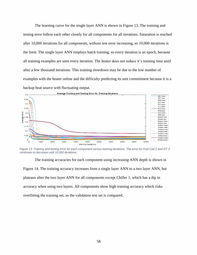
58

The learning curve for the single layer ANN is shown in Figure 13. The training and

testing error follow each other closely for all components for all iterations. Saturation is reached

after 10,000 iterations for all components, without test error increasing, so 10,000 iterations is

the limit. The single layer ANN employs batch training, so every iteration is an epoch, because

all training examples are seen every iteration. The heater does not reduce it’s training time until

after a few thousand iterations. This training slowdown may be due to the low number of

examples with the heater online and the difficulty predicting its unit commitment because it is a

backup heat source with fluctuating output.

The training accuracies for each component using increasing ANN depth is shown in

Figure 14. The training accuracy increases from a single layer ANN to a two layer ANN, but

plateaus after the two layer ANN for all components except Chiller 1, which has a dip in

accuracy when using two layers. All components show high training accuracy which risks

overfitting the training set, so the validation test set is compared.

Figure 13: Training and testing error for each component versus training iterations. The error for Fuel Cell 2 and GT 3 continues to decrease until 10,000 iterations.

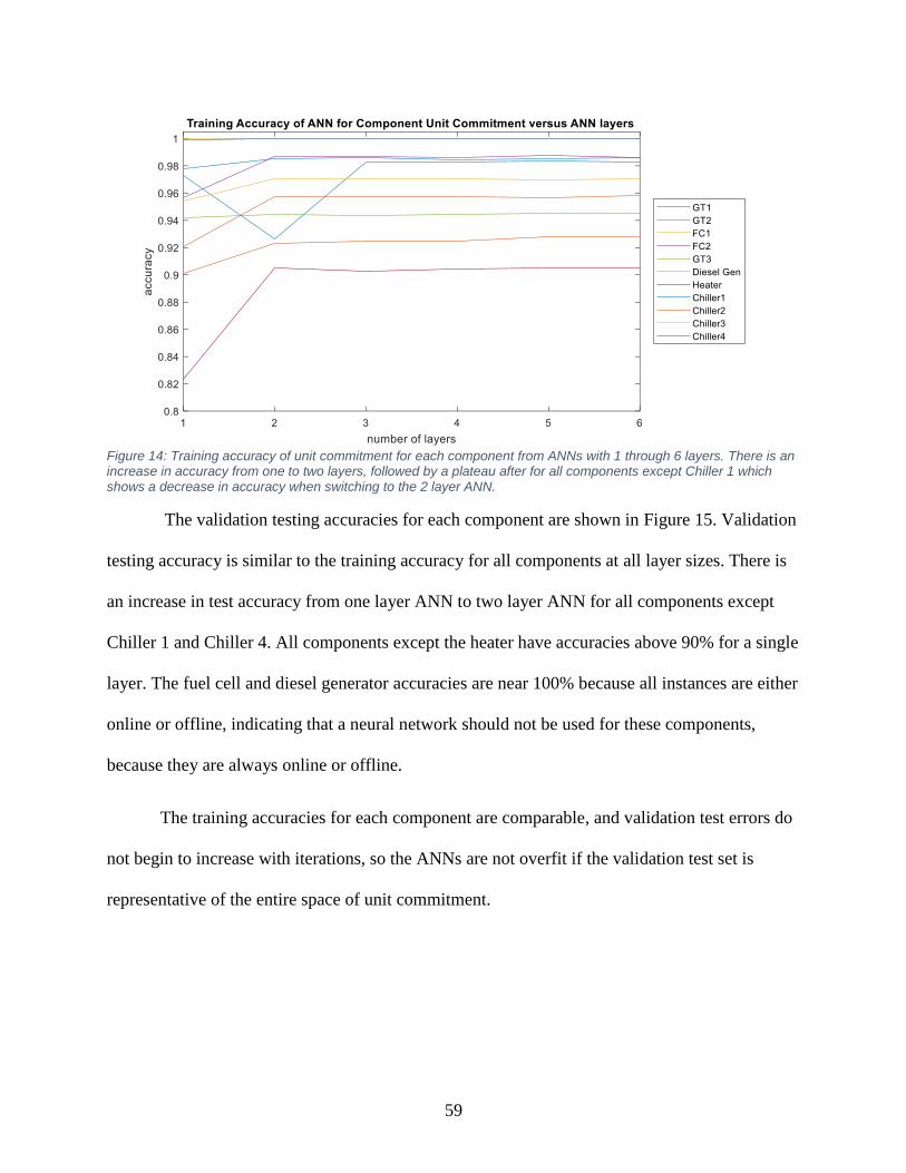
59

The validation testing accuracies for each component are shown in Figure 15. Validation

testing accuracy is similar to the training accuracy for all components at all layer sizes. There is

an increase in test accuracy from one layer ANN to two layer ANN for all components except

Chiller 1 and Chiller 4. All components except the heater have accuracies above 90% for a single

layer. The fuel cell and diesel generator accuracies are near 100% because all instances are either

online or offline, indicating that a neural network should not be used for these components,

because they are always online or offline.

The training accuracies for each component are comparable, and validation test errors do

not begin to increase with iterations, so the ANNs are not overfit if the validation test set is

representative of the entire space of unit commitment.

Figure 14: Training accuracy of unit commitment for each component from ANNs with 1 through 6 layers. There is an increase in accuracy from one to two layers, followed by a plateau after for all components except Chiller 1 which shows a decrease in accuracy when switching to the 2 layer ANN.

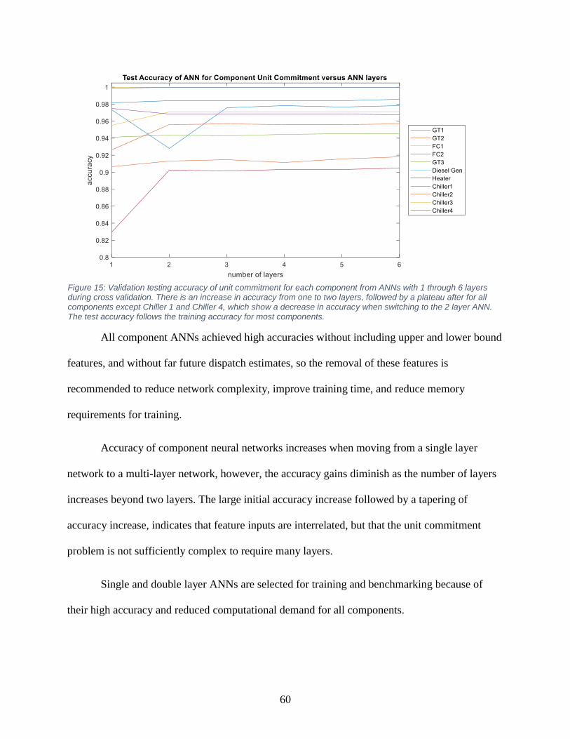
60

All component ANNs achieved high accuracies without including upper and lower bound

features, and without far future dispatch estimates, so the removal of these features is

recommended to reduce network complexity, improve training time, and reduce memory

requirements for training.

Accuracy of component neural networks increases when moving from a single layer

network to a multi-layer network, however, the accuracy gains diminish as the number of layers

increases beyond two layers. The large initial accuracy increase followed by a tapering of

accuracy increase, indicates that feature inputs are interrelated, but that the unit commitment

problem is not sufficiently complex to require many layers.

Single and double layer ANNs are selected for training and benchmarking because of

their high accuracy and reduced computational demand for all components.

Figure 15: Validation testing accuracy of unit commitment for each component from ANNs with 1 through 6 layers during cross validation. There is an increase in accuracy from one to two layers, followed by a plateau after for all components except Chiller 1 and Chiller 4, which show a decrease in accuracy when switching to the 2 layer ANN. The test accuracy follows the training accuracy for most components.

61

1.10.2 ANN Implementation

A single layer ANN, ANN1, is implemented for unit commitment in the dispatch

optimization problem. The ANN is implemented on the simple case microgrid to show optimal

solution output and the complex case to show robustness and benchmark it against the mcQP

method.

For the simple case, mcQP is used to create a training set from one week’s worth of

historical demand data with added Gaussian noise. Only one week is used so that the network is

more closely trained to the near future scenario. Gaussian noise is added to the training set, so

that actual historical demand profiles can be used for test dispatches without having identical

examples for training and testing. The simple case is not analyzed statistically, because it was

only run for one week, so the analysis would not be representative of the full year stresses.

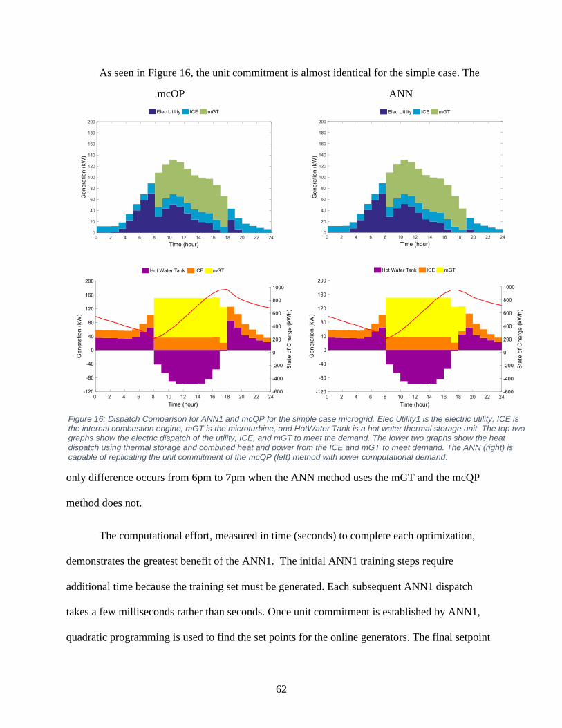
62

As seen in Figure 16, the unit commitment is almost identical for the simple case. The

only difference occurs from 6pm to 7pm when the ANN method uses the mGT and the mcQP

method does not.

The computational effort, measured in time (seconds) to complete each optimization,

demonstrates the greatest benefit of the ANN1. The initial ANN1 training steps require

additional time because the training set must be generated. Each subsequent ANN1 dispatch

takes a few milliseconds rather than seconds. Once unit commitment is established by ANN1,

quadratic programming is used to find the set points for the online generators. The final setpoint

Figure 16: Dispatch Comparison for ANN1 and mcQP for the simple case microgrid. Elec Utility1 is the electric utility, ICE is the internal combustion engine, mGT is the microturbine, and HotWater Tank is a hot water thermal storage unit. The top two graphs show the electric dispatch of the utility, ICE, and mGT to meet the demand. The lower two graphs show the heat dispatch using thermal storage and combined heat and power from the ICE and mGT to meet demand. The ANN (right) is capable of replicating the unit commitment of the mcQP (left) method with lower computational demand.

mcQP ANN

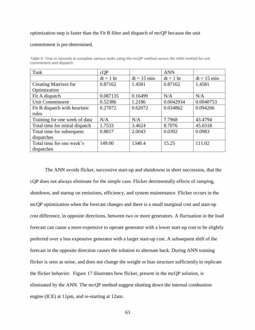
63

optimization step is faster than the Fit B filter and dispatch of mcQP because the unit

commitment is pre-determined.

Table 9: Time in seconds to complete various tasks using the mcQP method versus the ANN method for unit commitment and dispatch.

Task cQP ANN

dt = 1 hr dt = 15 min dt = 1 hr dt = 15 min

Creating Matrixes for

Optimization

0.87162 1.4581 0.87162 1.4581

Fit A dispatch 0.087135 0.16499 N/A N/A

Unit Commitment 0.52386 1.2186 0.0042934 0.0040753

Fit B dispatch with heuristic

rules

0.27072 0.62072 0.034862 0.094266

Training for one week of data N/A N/A 7.7968 43.4794

Total time for initial dispatch 1.7533 3.4624 8.7076 45.0318

Total time for subsequent

dispatches

0.8817 2.0043 0.0392 0.0983

Total time for one week’s

dispatches

149.00 1348.4 15.25 111.02

The ANN avoids flicker, successive start-up and shutdowns in short succession, that the

cQP does not always eliminate for the simple case. Flicker detrimentally effects of ramping,

shutdown, and startup on emissions, efficiency, and system maintenance. Flicker occurs in the

mcQP optimization when the forecast changes and there is a small marginal cost and start-up

cost difference, in opposite directions, between two or more generators. A fluctuation in the load

forecast can cause a more expensive to operate generator with a lower start-up cost to be slightly

preferred over a less expensive generator with a larger start-up cost. A subsequent shift of the

forecast in the opposite direction causes the solution to alternate back. During ANN training

flicker is seen as noise, and does not change the weight or bias structure sufficiently to replicate

the flicker behavior. Figure 17 illustrates how flicker, present in the mcQP solution, is

eliminated by the ANN. The mcQP method suggest shutting down the internal combustion

engine (ICE) at 11pm, and re-starting at 12am.

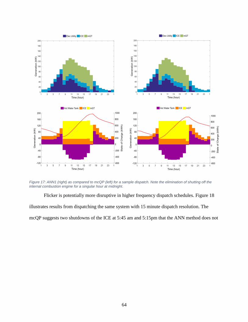
64

Figure 17: ANN1 (right) as compared to mcQP (left) for a sample dispatch. Note the elimination of shutting off the

internal combustion engine for a singular hour at midnight.

Flicker is potentially more disruptive in higher frequency dispatch schedules. Figure 18

illustrates results from dispatching the same system with 15 minute dispatch resolution. The

mcQP suggests two shutdowns of the ICE at 5:45 am and 5:15pm that the ANN method does not

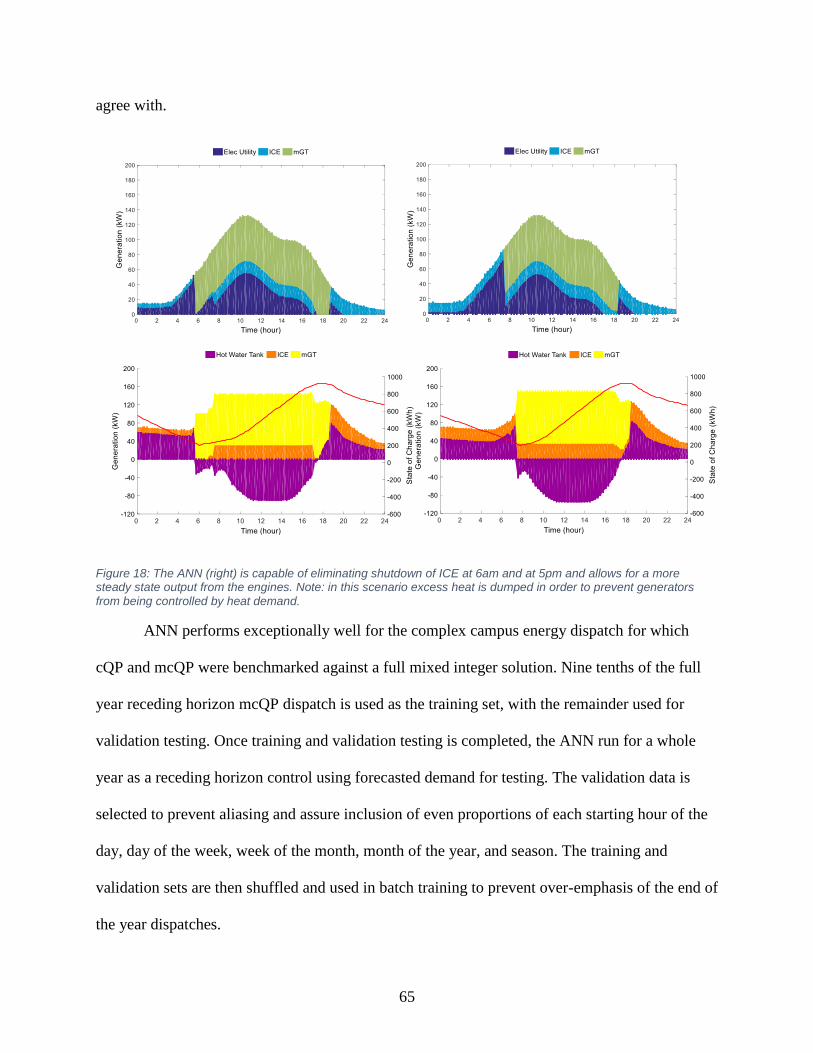
65

agree with.

Figure 18: The ANN (right) is capable of eliminating shutdown of ICE at 6am and at 5pm and allows for a more steady state output from the engines. Note: in this scenario excess heat is dumped in order to prevent generators

from being controlled by heat demand.

ANN performs exceptionally well for the complex campus energy dispatch for which

cQP and mcQP were benchmarked against a full mixed integer solution. Nine tenths of the full

year receding horizon mcQP dispatch is used as the training set, with the remainder used for

validation testing. Once training and validation testing is completed, the ANN run for a whole

year as a receding horizon control using forecasted demand for testing. The validation data is

selected to prevent aliasing and assure inclusion of even proportions of each starting hour of the

day, day of the week, week of the month, month of the year, and season. The training and

validation sets are then shuffled and used in batch training to prevent over-emphasis of the end of

the year dispatches.

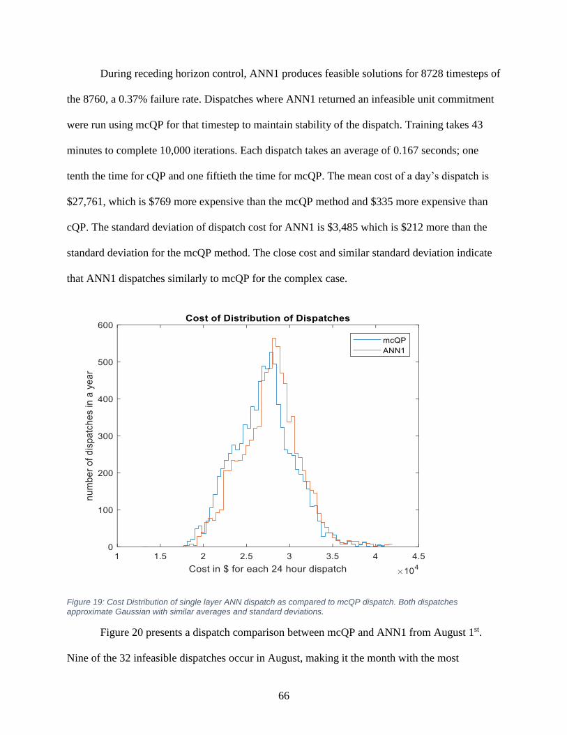
66

During receding horizon control, ANN1 produces feasible solutions for 8728 timesteps of

the 8760, a 0.37% failure rate. Dispatches where ANN1 returned an infeasible unit commitment

were run using mcQP for that timestep to maintain stability of the dispatch. Training takes 43

minutes to complete 10,000 iterations. Each dispatch takes an average of 0.167 seconds; one

tenth the time for cQP and one fiftieth the time for mcQP. The mean cost of a day’s dispatch is

$27,761, which is $769 more expensive than the mcQP method and $335 more expensive than

cQP. The standard deviation of dispatch cost for ANN1 is $3,485 which is $212 more than the

standard deviation for the mcQP method. The close cost and similar standard deviation indicate

that ANN1 dispatches similarly to mcQP for the complex case.

Figure 19: Cost Distribution of single layer ANN dispatch as compared to mcQP dispatch. Both dispatches approximate Gaussian with similar averages and standard deviations.

Figure 20 presents a dispatch comparison between mcQP and ANN1 from August 1st.

Nine of the 32 infeasible dispatches occur in August, making it the month with the most

67

infeasible dispatches. August has the highest cooling demand and often requires the use of all

chillers and cold thermal energy storage. Since the fourth chiller is rarely dispatched and is used

mostly as a backup component, the ANN had difficulty replicating the fluctuating behavior of

the chillers when the cooling demand reached high levels. The ANN1 dispatch is infeasible for

1.25% of the attempted optimizations in August. The cost of ANN1 for August 1st is higher than

mcQP for all hours except 11pm to midnight when mcQP brings GT2 back online and pays a

startup cost. ANN1 keeps GT2 on for the whole day instead of using the utility and battery

storage during the middle of the day, thus the higher operating costs throughout the day. The

difference in GT2’s unit commitment is also seen in the thermal dispatch in Figure 21, because it

is a CHP generator. ANN1 does not dispatch Chiller 3 and instead pushes Chillers 1 and 2 to

higher setpoints and uses the cold water storage tank for the middle of the day demand.

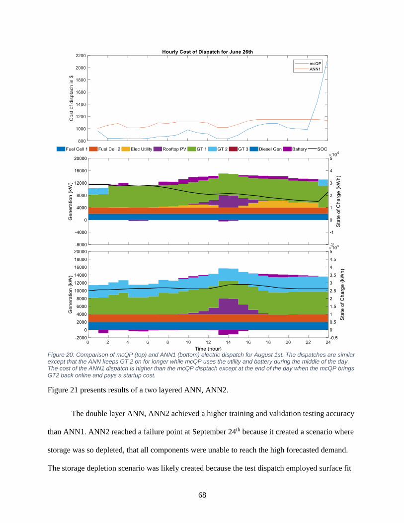
68

Figure 20: Comparison of mcQP (top) and ANN1 (bottom) electric dispatch for August 1st. The dispatches are similar except that the ANN keeps GT 2 on for longer while mcQP uses the utility and battery during the middle of the day. The cost of the ANN1 dispatch is higher than the mcQP disptach except at the end of the day when the mcQP brings

GT2 back online and pays a startup cost.

Figure 21 presents results of a two layered ANN, ANN2.

The double layer ANN, ANN2 achieved a higher training and validation testing accuracy

than ANN1. ANN2 reached a failure point at September 24th because it created a scenario where

storage was so depleted, that all components were unable to reach the high forecasted demand.

The storage depletion scenario was likely created because the test dispatch employed surface fit

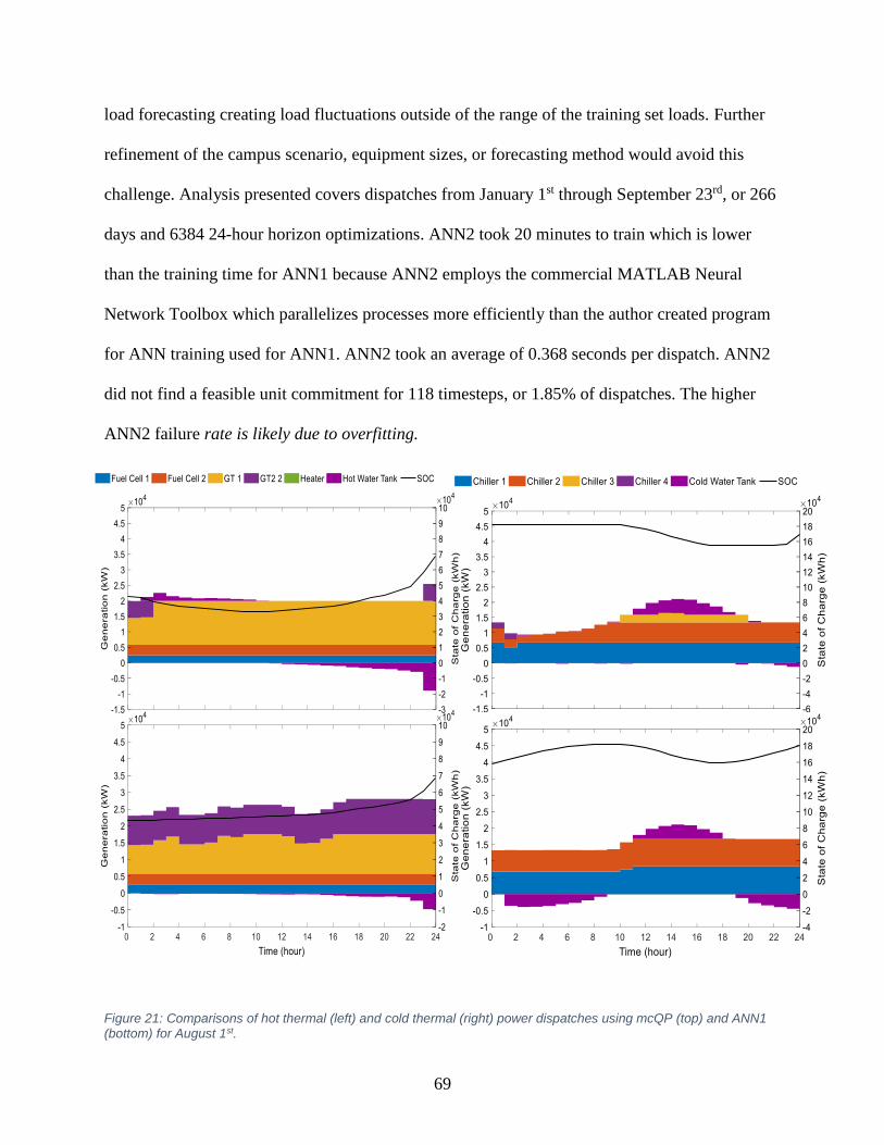
69

load forecasting creating load fluctuations outside of the range of the training set loads. Further

refinement of the campus scenario, equipment sizes, or forecasting method would avoid this

challenge. Analysis presented covers dispatches from January 1st through September 23rd, or 266

days and 6384 24-hour horizon optimizations. ANN2 took 20 minutes to train which is lower

than the training time for ANN1 because ANN2 employs the commercial MATLAB Neural

Network Toolbox which parallelizes processes more efficiently than the author created program

for ANN training used for ANN1. ANN2 took an average of 0.368 seconds per dispatch. ANN2

did not find a feasible unit commitment for 118 timesteps, or 1.85% of dispatches. The higher

ANN2 failure rate is likely due to overfitting.

Figure 21: Comparisons of hot thermal (left) and cold thermal (right) power dispatches using mcQP (top) and ANN1 (bottom) for August 1st.

70

6. CONCLUSION

Dispatch optimization with mcQP is reliable and a dramatic improvement over full

mixed-integer solutions in both computational time and reliability, where reliability is measured

as the percentage feasibility when faced with the dispatch of a complex microgrid. The method is

highly suitable to design of micro-grid systems, and large time-step, e.g. hourly, dispatch

optimizations. The exponential increase in effort for complex systems, may limit its use as a real-

time controller when higher frequency dispatches are required. Dispatch optimization with cQP

is sufficiently fast, but reaches less optimal solutions and is applicable only for systems that do

not require complex unit commitment. Dispatch optimization with Gurobi’s CVX is unreliable

for complex cases, and is not a viable option for either dispatch optimization or training set

generation, because of the excessive computational time requirement and high failure rate.

Unit commitment with an ANN trained by mcQP provides sufficient reliability and is

computationally efficient. A single layer ANN achieves a sufficiently high accuracy replicating

mcQP unit commitment for complex cases without overfitting. To avoid computational slow

down and prevent excessive memory requirements, ANN input features should be limited to:

• Net electric demand: total electric demand minus solar PV electric generation

• Heat demand

• Cooling demand

• Market price of electricity at the current timestep

• Estimated power from each storage device at the current timestep

• Estimated dispatch at the previous timestep for each dispatchable component

• Estimated dispatch at the current timestep for each dispatchable component

71

• Estimated dispatch at the next timestep for each dispatchable component

• Power from energy storage at the current timestep

Other features such as estimated dispatch at future timesteps in the horizon, and upper and lower

bounds should not be incorporated, because they are not valuable features and obfuscate the

impact of important features, slowing learning, and even reducing accuracy in some cases.

Table 10: Comparison of Dispatch methods for year in receding horizon. The full mixed integer (FMI) method took longer than an hour to complete a single dispatch, so it was unable to run through a full year. The two layer ANN method (ANN2) crashed in September of the full year dispatch and its cost is not compared. The training time is lower for ANN2 than ANN1 because ANN2 employs a commercial training algorithm, while ANN1 employs an author created training algorithm that is likely less optimally parallelized.

FMI cQP mcQP ANN1 ANN2

Feasibility 100% 100% 99.63% 99.15%*

Time (s/dispatch) >3600 1.6 6.8 0.167 0.368

Training Time (s) N/A N/A N/A 43 min 20 min

Mean Cost ($) 28,096 26,992 27,761

Standard

Deviation Cost ($)

3,870 3,464 3,485

Single layer ANNs reduce flicker in dispatches as well as improving computational speed.

A multi-layer ANN likely leads to overfitting in energy dispatch applications.

The mcQP method is well suited for dispatch optimization and training set generation. The

cQP method should be used for less complex cases for training set generation and dispatch

optimization, because it can create dispatches quickly and reliably. The single layer ANN should

be used for real time optimization and control or for dispatch optimization because, once trained,

it rapidly solves the unit commitment problem.

72

7. DISCUSSION

The five methods benchmarked here, mcQP, cQP, FMI, ANN1, and ANN2 show a range in

dispatch reliability and computational speed. In general, there is a tradeoff between reliability

and speed, however, the mcQP method creates dispatches more reliably and faster than the

traditional FMI method. Also, ANN1 creates dispatches similar to the mcQP method reliably if

provided with a wide enough range of training examples.

The reliability and speed of both mcQP and ANN1 methods have the potential to close the

gap between optimization at large timesteps, and real time control. If generation setpoints can be

optimized in real time, then microgrid operating costs could be reduced enabling higher

penetration of technologies like combined heat and power, energy storage, and on site renewable

generation. The speed with which robust training sets can be created with mcQP also opens the

door to more machine learning techniques which require large training sets.

A single layer ANN is very similar in nature to non-linear regression. The weights and biases

are the fitting parameters, and back propagation with a single layer is similar to iterations in

regression. The high reliability and accuracy of the single layer ANN demonstrates that the unit

commitment problem is simple enough for regression methods. It also demonstrates that

complex methods such as multi-layer ANNs or deep learning machine learning methods are not

suitable for this problem, because they will not provide noise filtering and would be too

computationally demanding considering the problem at hand.

Further investigations of expansions to the Artificial Neural Network should be investigated.

The next step is to test the accuracy of an ANN trained for the entire dispatch problem including

unit commitment and dispatch optimization. The training sets can once again be taken from pre-

73

solved dispatches using the mcQP method, however input features would only be data input to

mcQP and training solutions would be the real valued set point for each component instead of

just the unit commitment decision. If an ANN can achieve high accuracy with this method, then

a reinforcement learning method should be tested where an ANN would be trained without a pre-

solved training set with feedback from the cost function. Since solutions to this problem are

known, the ANN’s solutions could be tested against known values for optimal solutions to

determine accuracy and robustness.

The high level of reliability, accuracy, and computational speed from ANN1 means that it

should be investigated for real and reactive power control. The extension to include reactive

power creates non-linear constraints, so solutions are not known a priori since cQP and mcQP

are limited to linear constraints. Reinforcement learning would avert the need for an established

training set, expanding the set of optimizable problems from convex mixed integer with linear

constraints to non-convex mixed integer with non-linear constraints. The success of the ANN

would be measured with the objective function and a tested against all constraints. A violation of

any constraint would result in an extremely high cost, guiding the ANN away from constraint

violation scenarios.

The potential for a neural network to train to a complex non-convex optimization

problem and create dispatches with high computational speed could open the door to

optimization and control unification for real power systems with transmission effects and

reactive power demands. Computationally efficient methods such as ANN1 are crucial for

reducing the operating costs of systems with renewables and energy storage allowing the

advancement of a cleaner power generation infrastructure.

74

REFERENCES

[1] C40 Cities Climate Leadership Group, Inc., "C40 Cities," 2018. [Online]. Available:

http://www.c40.org/cities . [Accessed 19 May 2018].

[2] United Nations Climate Change, "Conference of the Parties serving as the meeting of the

Parties to the Paris Agreement," United Nations Framework Convention on Climate

Change, Paris, 2014.

[3] U.S. Energy Information Administration, "Germany's renewables electricity generation

grows in 2015, but coals still dominant," eia, Washington, DC, 2016.

[4] Washington State University, "Steam plant starting up," 26 August 2004. [Online].

Available: https://news.wsu.edu/2004/08/20/steam-plant-starting-up/. [Accessed 19 March

2018].

[5] D. McLarty, C. Sabate, J. Brouwer and F. Jabbari, "Micro-grid energy dispatch

optimization and predictive control algorithms; A UC Irivine case study," Electrical Power

and Energy Systems, vol. 65, pp. 179-190, 2015.

[6] F. Farzan, S. Lahiri and M. Kleinberg, "Microgrids for Fun and Profit: The Economics of

Installation Investments and Operations," IEEE Power and Energy Magazine, Vols. July-

Aug, pp. 52-58, 2013.

[7] United States White House, "United States Mid-Century Strategy for Deep

Decarbonization," United Nations Framework Convention on Climate Change, Marrakech,

2016.

[8] S. Van Broekhoven, N. Judson, N. SV and W. Ross, "Microgrid Study: Energy Security for

DoD Installations," Defence Technical Information Center, 2012.

[9] N. Hatziargyriou, "Guest Editorial Special Section on Microgrids for Sustainable Energy

Systems," IEEE Transactions on Sustainable Energy, vol. 5, no. 4, p. 1309, 2014.

[10] Z. Yang, H. Zhong, Q. Xia and C. Kang, "Fundamental Review of the OPF Problem:

Challenges, Solutions, and State-of-the-Art Algorithms," Journal of Energy Engineering,

vol. 144, no. 1, 2018.

[11] D. McLarty, A. Traverso, N. Panossian and F. Jabbari, "Dynamic Economic Dispatch using

Complementary Quadratic Programing," TBD, 2018.

75

[12] D. McLarty, J. Brouwer and C. Ainschough, "Development of an open access tool for

design, simulated dispatch, and economic assessment of distributed generation

technologies," Energy and Buildings, vol. 105, no. 15, pp. 314-325, 2015.

[13] N. Panossian and D. McLarty, "Artificial Neural Network Trained with Complementary

Quadratic Progrmaming for Realtime Unit Commitment and Microgrid Dispatch

Optimization," TBD, 2018.

[14] S. Boyd and L. Vandenberghe, "Interior-point methods," in Convex Optimization,

Cambridge, Cambridge University Press, 2004, pp. 561-622.

[15] S. Boyd and L. Vandenberghe, "Gradient Descent Method," in Convex Optimization,

Cambridge, Cambridge Universtiy Press, 2004, p. 4660475.

[16] A. Ardakani and F. Bouffard, "Identification of Umbrella Constraints in DC-Based

Security-Constrained Optimal Power Flow," IEEE Transactions on Power Systems, vol.

28, no. 4, pp. 3924-3934, 2013.

[17] M. Nemati, M. Braun and S. Tenbohlen, "Optimization of unit commitment and economic

dispatch in microgrids based on genetic algorithm and mixed integer linear programming,"

Applied Energy, vol. 210, pp. 944-963, 2018.

[18] C. Zhao, J. Wang, J. Watson and Y. Guan, "Multi-Stage Robust Unit Commitment

Considering Wind and Demand Response Uncertainties," IEEE Transactions on Power

Systems, vol. 28, no. 3, pp. 2708-2717, 2013.

[19] A. Castillo, C. Laird, C. Silva-Monroy, W. JP and R. O'Neill, "The Unit Commitment

Problem with AC Optimal Power Flow Constraints," IEEE Transactions on Power

Systems, vol. 31, no. 6, 2016.

[20] J. Jian, K. Meng, Y. Xu and Z. Dong, "A novel projected two-binary-variable formulation

for unit commitment in power systems," Applied Energy , vol. 187, pp. 732-745, 2017.

[21] A. Farag, A. Al-Baiyat and T. Cheng, "Economic Load Dispatch Multiobjective

Optimization Procedures Using Linear Programming Techniques," IEEE Transactions on

Power Systems, vol. 10, no. 2, pp. 731-738, 1995.

[22] A. Castillo, P. Lipka, J. Watson, S. Oren and R. O'Neill, "A successive linear programming

approach to solving the iv-acopf," IEEE Transactions on Power Systems, vol. 31, no. 4,

2015.

[23] J. Lavei, A. Rantzer and S. Low, "Power Flow Optimization Using Positive Quadratic

Programming*," IFAC Proceedings Volumes, vol. 44, no. 1, pp. 10481-10486, 2011.

76

[24] E. Erseghe and S. Tomasin, "Power Flow Optimization for Smart Microgrids by SDP

Relaxation on Linear Networks," IEEE Trans Smart Grid, vol. 4, no. 2, pp. 751-762, 2013.

[25] C. Wu, P. Jiang, Y. Sun, C. Shang and W. Gu, "Economic dispatch with CHP and wind

power using probabilistic sequence theory and hybrid heuristic algorithm," AIP Journal of

Renewable and Sustainable Energy, vol. 9, 2017.

[26] E. Alvarez, J. Gomez-Aleixandre, N. de Abajo and A. Campos Lopez, "Algorithm for

microgrid on-line central dispatch of electrical power and heat," in Universities Power

Engineering Conference, Glasgow, 2009.

[27] M. Geidl and G. Andersson, "Optimal Power Flow of Mutiple Energy Carriers," IEEE

Transactions on Power Systems, vol. 22, no. 1, 2007.

[28] M. Moeini-Aghtaie, A. Abbaspour, M. Fotuhi-Firusabad and H. Ehsan, "A Decomposed

Solution to Multiple-Energy Carriers Optimal Power Flow," IEEE Transactions on Power

Systems, vol. 29, no. 2, pp. 707-716, 2014.

[29] M. Abido, "Optimal Power Flow Using Particle Swarm Optimization," International

Journal of Electrical Power and Energy Systems, vol. 24, no. 7, pp. 563-571, 2002.

[30] Z. Feng, W. Niu, J. Zhou and C. CT, "Multiobjective Operation Optimization of a

Cascaded Hydropower System," Journal of Water Resources Planning and Management,

vol. 143, no. 10, 2017.

[31] R. Arul, S. Velusami and G. Ravi, "A new algorithm for combined dynamic economic

emission dispatch with security constraints," Energy, vol. 28, no. 4, pp. 3924-3934, 2013.

[32] D. Aydin, S. Ozyon, C. Yasar and T. Liao, "Artificial bee colony algorithm with dynamic

population size to combined economic and emission dispatch problem," International

Journal of Electrical Power and Energy Systems, vol. 54, pp. 144-153, 2014.

[33] H. Wu, X. Liu and M. Ding, "Dynamic Economic Dispatch of a Microgrid: Mathematical

Models and Solution Algorithm," International Journal of Electrical Power and Energy

Systems, vol. 63, pp. 336-346, 2014.

[34] A. Moghaddam, A. Seifi, T. Niknam and M. Pahlavani, "Multi-objective operation

management of renewable MG (micro-grid) with back-up micro-turbine/fuel cell/battery

hybrid power source," Energy, vol. 36, no. 11, pp. 6490-6507, 2011.

[35] L. Han, C. Romero and Z. Yao, "Economic dispatch optimization algorithm based on

particle diffusion," Energy Conversion and Management, vol. 105, pp. 1251-1260, 2015.

77

[36] S. Pothiya, I. Ngamroo and W. Kongprawechon, "Ant colony optimisation for economic

dispatch problem with non-smooth cost functions," International Journal of Electrical

Power and Energy Systems, vol. 32, no. 5, pp. 478-487, 2010.

[37] Y. Song, C. Chou and T. Stonham, "Combined heat and power economic dispatch by

improved ant colony search algorithm," Electric Power Systems Research, vol. 52, no. 2,

pp. 115-121, 1999.

[38] M. Basu and A. Chowhury, "Cuckoo Search Algorithm for Economic Dispatch," Energy

60, pp. 99-108, 2013.

[39] A. Shabanpour-Haghighi, A. Reza Seifi and T. Niknam, "A modified teaching-learning

based optimization for multi-objective optimal power flow problem," Energy Conversion

and Management, vol. 77, pp. 597-607, 2014.

[40] M. Basu, "Artificial immune system for combined heat and power economic dispatch,"

International Journal of Electrical Power and Energy Systems, vol. 43, no. 1, pp. 1-5,

1012.

[41] S. Hemamalini and S. Simon, "Dynamic economic dispatch using artificial immune system

for units with valve-point effect," International Journal of Electrical Power and Energy

Systems, vol. 33, no. 4, pp. 868-874, 2011.

[42] C. Chen, S. Duan, T. Cai, B. Liu and G. Hu, "Smart Energy Management System for

Optimal Microgrid Economic Operation," IET Renewable Power Generation, vol. 5, no. 3,

pp. 258-267, 2011.

[43] C. Aguilar, E. Westman, J. Muehlboeck, P. Mecocci, B. Vellas, M. Tsolaki, I. Kloszewska,

H. Soininen, S. Lovestone, C. Spenger, A. Simmons and L. Wahlund, "Different

multivariate techniques for automated classification of MRI data in Alzheimer's disease

and mild cognitive impairment," Psychiatry Res, pp. 89-98, 2013.

[44] M. Binder, A. Steiner, M. Schwartz, S. Knollmayer and K. P. H. Wolff, "Application of an

Artificial Neural-Network in Epiluminescence Microscopy Pattern-Analysis of Pigmented

Skin-Lesions - A Pilot-Study," British Journal of Dermatology, vol. 130, no. 4, pp. 460-

465, 1994.

[45] C. Heath, S. Cooper, K. Murray, A. Lowman, C. Henry, M. MacLeod, G. Stewart, M.

Zeidler, J. MacKenzie, J. Ironside, D. Summers, R. Knight and R. Will, "Validation of

diagnostic criteria for variant Creutzfeldt-Jakob disease," Annals of Neurology, vol. 67, no.

6, pp. 761-770, 2010.

[46] D. Ciregan, U. Meier and J. Schmidhuber, "Multi-column deep neural networks for image

classification," in IEEE Conference on Computer Vision and Pattern Recognition,

Providence, RI, 2012.

78

[47] G. Birajdar and V. Mankar, "Subsampling-Based Blind Image Forgery Detection Using

Support Vector Machine and Artificial Neural Network Classifiers," Arabian Journal for

Science and Engineering, vol. 43, no. 2, pp. 555-568, 2017.

[48] S. Kuter, S. Akyurek and G. Weber, "Retrieval of fractional snow covered area from

MODIS data by multivariate adaptive regression splines," Remote Sensing of Environment,

vol. 205, pp. 236-252, 2018.

[49] R. Furferi and L. Governi, "Machine vision tool for real-time detection of defects on textile

raw fabrics," Journal of the Textile Institute, vol. 99, no. 1, pp. 57-66, 2008.

[50] I. Lopez-Juarez, R. Rios-Cabrera, S. Hsieh and M. Howarth, "A hybrid non-invasive

method for internal/external quality assessment of potatoes," European Food Research and

Technology, vol. 244, no. 1, pp. 161-174, 244.

[51] R. Rojas-Moraleda, N. Valous, A. Gowen, C. Esquerre, S. Hartel, L. Salinas and C.

O'Donnell, "A frame-based ANN for classification of hyperspectral images: assessment of

mechanical damage in mushrooms," Neural Computing and Applications, vol. 28, no. 1,

pp. S969-S981, 2017.

[52] M. Kentardzic, "Artificial Neural Networks," in Data Mining: Concepts, Models, Methods,

and Algorithms, Institute of Electrical and Electronics Engineers, John Wiley and Sons,

Inc., 2011, pp. 199-235.

[53] G. Capizzi, G. Lo Sciuto, C. Napoli and E. Tramontana, "An advanced neural network

based solution to enforce dispatch continuity in smart grids," Applied Soft Computing, vol.

62, pp. 768-775, 2018.

[54] B. Doucoure, K. Agbossou and A. Cardenas, "Time series preiction using artificial wavelet

neural network and multi-resolution analysis: Application to wind speed data," Renewable

Energy, vol. 92, pp. 202-211, 2016.

[55] A. Khotanzad, R. Afkhami-Rohani, T. Lu, A. Abaye, M. Davis and D. Maratukulam,

"ANNSTLF - A Neural-Network-Based Electric Load Forecasting System," IEEE

Transactions on Neural Networks, vol. 8, no. 4, pp. 835-846, 1997.

[56] D. Chaturvedi, A. Sinha and O. Malik, "Short term load forecast using fuzzy logic and

wavelet transform integrated generalized in neural network," International Journal of

Electrical Power and Energy Systems, vol. 67, pp. 230-237, 2015.

[57] J. Park, Y. Kim, I. Eom and K. Lee, "Economic load dispatch for piecewise quadratic cost

function using Hopfield neural network," IEEE Transactions on Power Systems, vol. 8, no.

3, pp. 1030-1038, 1993.

[58] H. I. Duame, A Course in Machine, self published, 2017.

79

[59] S. Kamail and T. Amraee, "Blackout prediction in interconnected electric energy systems

considering generation re-dispatch and energy curtailment," Applied Energy, vol. 187, no.

1, pp. 50-61, 2017.

[60] D. Costa, M. Nunez, J. Vieira and U. Bezerra, "Decision tree-based security dispatch

application in integrated electric power and natural-gas networks," Electric Power Systems

Research, vol. 141, pp. 442-449, 2016.

[61] H. Mohammadi, G. Khademi, D. Simon and M. Dehghani, "Multi-objective optimization

of decision trees for power system voltage security assessment," in IEEE SysCon, Orlando,

FL, 2016.

[62] R. Quinlan and M. Kaufmann, "C4.5 Programs for Machine Learning," Kluwer Academic

Publishers, vol. 16, no. 4, 1994.

[63] E. Frank, M. Hall and I. Witten, The WEKA Workbench. Onlne Appendix for "Data

Mining : Practical Machine Learning Tools and Techniques, 4th ed., Morgan Kaufmann,

2016.

[64] W. Rawat and Z. Wang, "Deep Convolutional Neural Networks for Image Classification: A

Comprehensive Review," Massachusetts Institute of Technology Neural Computation, vol.

29, no. 9, 2017.

[65] C. Ronao and S. Cho, "Human activity recognition with smartphone sensors using deep

learning neural networks," Expert Systems with Applications, vol. 59, pp. 235-244, 2016.

[66] A. Mills and D. McLarty, "Large Scale Network Optimization of the Columbia River

Basin," TBD, 2018.

[67] F. Shariatzadeh, N. Kumar and A. Srivastava, "Optimal Control Algorithms for

Reconfiguration of Shipboard Microgrid Distribution System Using Intelligent

Techniques," IEEE Transactions on Industry Applications, vol. 53, pp. 474-482, 2017.

80

8. APPENDIX A: SAMPLE SOURCE CODE

1.11 Neural Network Class

classdef Neural_Network

properties

%define structure parameters

inputLayerSize

outputLayerSize

%define wieght parameters

Wlayer1

%define bias

blayer1

%define scale factor for how complex you want to allow your system

%to be

lambda

%is it a classification network (generators off/on)

classify

%constant for node function

nodeconst

%statistical stuff to update with more info

avrginputs

stddev

end

methods

function obj = Neural_Network(inputLayerSize, outputLayerSize, varargin)

%initialization

%inputs include UpperBound, LowerBound, Demand, quadratic

%portion of cost, linear portion of cost, cost/kWh from grid

%for each generator, so inputlaysize is 4*#ofgenerators+2

if isnumeric(inputLayerSize)

obj.inputLayerSize = inputLayerSize;

obj.Wlayer1 = rand(obj.inputLayerSize,outputLayerSize);%give a

different weight to each input's connection to each node

end

if isnumeric(outputLayerSize)

obj.outputLayerSize = outputLayerSize;

obj.blayer1 = rand(1,outputLayerSize);

end

%default conditions

obj.lambda = .0001;

obj.classify = false;

obj.nodeconst = 1;

obj.avrginputs = [];

obj.stddev = [];

if length(varargin)==1%the first input is if it is a classification

network, then node const, then lambda

81

classify = iscellstr(varargin);

lambda = isnumeric(varargin);

obj.lambda = varargin(lambda);

obj.classify = (nnz(classify)>0);

elseif length(varargin)==2

obj.classify = strcmp(varargin{1},'classify');

obj.nodeconst = varargin{2};

end

end

function yHat = forward(self, X)

%forward propogate inputs, X is the inputs, this must be in a

%genparameters x number of outputs size

if sum(size(X')==size(self.Wlayer1))==2%if inputs directly allow

multiplication

z2 = X.*self.Wlayer1';

yHat = sum(z2,2)+self.blayer1';

else%if only one row of inputs, or one row of inputs per timestep

yHat = (X*self.Wlayer1 + self.blayer1);

end

yHat = activationf(self, yHat); %use the activation function scaled by 1

end

function a2 = activationf(self,yHat)

%apply activation function

%if it is a classifyer use a sigmoid function

if self.classify

a2 = 1./(1+exp(-self.nodeconst*yHat));

if nnz(isnan(a2))>0

a2(and(isnan(a2),yHat>0)) = 1;%if numbers are too big inf/inf,

make a2=1

a2(isnan(a2)) = 0;%if numbers are to negative -inf/-inf, make a2=0

end

else %if it is a numeric output network don't include activation

a2 = yHat*self.nodeconst;

end

end

end

end

1.12 Single Layer ANN Training Algorithm

function [Net,sqrerror] = trainNetwork(Net,desiredOut, inputs)

%this does forward propagation for a one layer network for a set of

%generators and a demand

%inputs: network, desiredOut: desired network output when using forward

%funnction in the form of a vertical vector, inputs: matrix of inputs of

%size inputlength x number of outputs

%inputs in order: ub, lb, f, H for each generator, demand, $/kWgrid

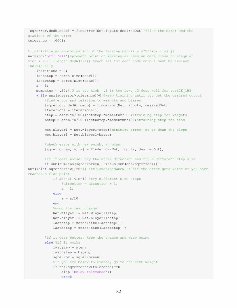
82

[sqrerror,dedW,dedb] = finderror(Net,inputs,desiredOut);%find the error and the

gradient of the error

tolerance = .0001;

% initialize an approximation of the Hessian matrix = d^2f/(dx_i dx_j)

warning('off','all')%prevent print of warning as Hessian gets close to singular

%for i = 1:1:length(dedW(1,:)) %each set for each node output must be trained

individually

iterations = 0;

laststep = zeros(size(dedW));

lastbstep = zeros(size(dedb));

a = 1;

momentum = .25;%.3 is too high, .1 is too low, .2 does well for test2E_1BS

while nnz(sqrerror>tolerance)>0 %keep training until you get the desired output

%find error and relation to weights and biases

[sqrerror, dedW, dedb] = finderror(Net, inputs, desiredOut);

iterations = iterations+1;

step = dedW.*a/100+laststep.*momentum/100;%training step for weights

bstep = dedb.*a/100+lastbstep.*momentum/100;%training step for bias

Net.Wlayer1 = Net.Wlayer1-step;%minimize error, so go down the slope

Net.blayer1 = Net.blayer1-bstep;

%check error with new weight an bias

[sqrerrornew, ~, ~] = finderror(Net, inputs, desiredOut);

%if it gets worse, try the other direction and try a different step size

if sum(sum(abs(sqrerrornew)))>=sum(sum(abs(sqrerror))) ||

nnz(isinf(sqrerrornew))>0%|| nnz(isnan(dedWnew))>0%if the error gets worse or you have

reached a flat point

if abs(a) <1e-12 %try different size steps

%direction = direction + 1;

a = 1;

else

a = a/10;

end

%undo the last change

Net.Wlayer1 = Net.Wlayer1+step;

Net.blayer1 = Net.blayer1+bstep;

laststep = zeros(size(laststep));

lastbstep = zeros(size(lastbstep));

%if it gets better, keep the change and keep going

else %if it works

laststep = step;

lastbstep = bstep;

sqrerror = sqrerrornew;

%if you are below tolerance, go to the next weight

if nnz(sqrerrornew>tolerance)==0

disp('below tolerance');

break

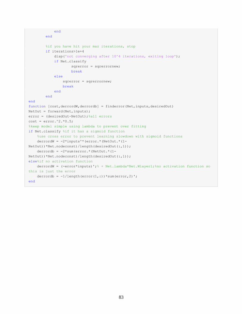
83

end

end

%if you have hit your maz iterations, stop

if iterations>1e+4

disp('not converging after 10^4 iterations, exiting loop');

if Net.classify

sqrerror = sqrerrornew;

break

else

sqrerror = sqrerrornew;

break

end

end

end

function [cost,derrordW,derrordb] = finderror(Net,inputs,desiredOut)

NetOut = forward(Net,inputs);

error = (desiredOut-NetOut);%all errors

cost = error.^2.*0.5;

%keep model simple using lambda to prevent over fitting

if Net.classify %if it has a sigmoid function

%use cross error to prevent learning slowdown with sigmoid functions

derrordW = -2*inputs'*(error.*(NetOut.*(1-

NetOut))*Net.nodeconst)/length(desiredOut(:,1));

derrordb = -2*sum(error.*(NetOut.*(1-

NetOut))*Net.nodeconst)/length(desiredOut(:,1));

else%if no activation function

derrordW = (-error*inputs)';% + Net.lambda*Net.Wlayer1;%no activation function so

this is just the error

derrordb = -1/length(error(1,:))*sum(error,2)';

end