BJPS - A

ccep

ted M

anus

cript

Submitted to the Brazilian Journal of Probability and Statistics

arXiv: math.PR/0000000

The complementary exponential power series distribution

Jose Flores D.a,c, Patrick Borgesb, Vicente G. Cancho c , Francisco Louzadac

aPontificia Universidad Catolica del PerubUniversidade Federal de Sao Carlos

cUniversidade de Sao Paulo

Abstract. In this paper, we introduce the complementary exponential power series

distributions, with failure rate either increasing, which is complementary to the

exponential power series model proposed by Chahkandi & Ganjali (2009). The new

class of distribution arises on a latent complementary risks scenarios, where the

lifetime associated with a particular risk is not observable, rather we observe only the

maximum lifetime value among all risks. This new class contains several distributions

as particular case. The properties of the proposed distribution class are discussed such

as quantiles, moments and order statistics. Estimation is carried out via maximum

likelihood. Simulation results on maximum likelihood estimation are presented. An

real application illustrate the usefulness of the new distribution class.

1 Introduction

The exponential distribution is widely used for modeling many problems in lifetimetesting and reliability studies. However, the exponential distribution does not provide areasonable parametric fit for some practical applications where the underlying failure ratesare nonconstant, presenting monotone shapes. Recently, new distributions to model thefailure rate have appeared in the literature, such as those obtained by compounding theexponential distribution with several discrete distributions. For example, a distributionwith a decreasing failure rate has been obtained by assuming the minimum of a randomsample of the exponential distribution and a random sample size. In order to do this thegeometric, the Poisson and the logarithmic distributions were considered by Adamidis& Loukas (1998), Kus (2007) and Tahmashi & Rezaei (2008), respectively. These workswere generalized by Chahkandi & Ganjali (2009) by showing that the composition ofthe exponential distribution with the power series distribution yields a distribution witha decreasing failure rate, the exponential power series (EPS) distribution. Later Morais

AMS 2000 subject classifications. Primary 60K35, 60K35; secondary 60K35

Keywords and phrases. Complementary risks, Exponential Distribution, Increasing failure rate, Power

series distribution, Exponential power series distribution.

1imsart-bjps ver. 2010/04/27 file: BJPS-FinalVersion.tex date: November 26, 2011

BJPS - A

ccep

ted M

anus

cript

2 Flores et al.

& Barreto-Souza (2011) replaced the exponential distribution by the Weibull generatingdistributions with decreasing failure rates when the form parameter is lower or equal than1 and different types of failure rates when the form parameter is greater than 1. Thedistribution proposed by Kus (2007) was generalized by including a power parameterin his distribution, by Barreto-Souza & Cribari-Neto (2009). A different approach, thatconsiders the maximum, instead of the minimum, has been also considered. In this casethe distributions obtained have increasing failure rates. The geometric distribution wasconsidered by Adamidis et al. (2005), later generalized in Silva et al. (2010) by including apower parameter in his distribution. The Poisson distribution was assumed to be obtainedthe distribution of Cancho et al. (2011), which later was generalized in Cordeiro et al.(2011) by assuming a COMPoisson distribution. by including a power parameter in hisdistribution The power series distribution however has not been considered yet when themaximum number of competing causes is considered, leading to a complementary riskscenario. In this paper, assuming a power series distribution, we propose a new familydistribution based on a complementary risk problem (Basu & J., 1982) in presence oflatent risks. We assume that there is no information about which factor was responsiblefor the component failure but only the maximum lifetime value among all risks is observedinstead of the minimum lifetime value among all risks as in Chahkandi & Ganjali (2009)and Morais & Barreto-Souza (2011). The new distribution is a counterpart of the EPSdistribution and then, hereafter it shall be called complementary exponential power series(CEPS) distribution.

The paper is organized as follows. In Section 2, we define the CEPS distribution. InSection 3 the survival and failure rate function, the quantiles, moments, order statisticsand moments of the order statistics are provided. In Section 4 some special cases arestudied in details and are compared the graphics of failure rate functions of these caseswith the ones analogues EPS distributions for some particular parameters. Estimation ofthe parameters by maximum likelihood is given in the section 5. In Section 6 presents theresults of an simulation study. In Section 7 an application to one real data set is provided.Final remarks in the Section 8 concludes the paper.

2 The CEPS distribution

In the classical complementary risks scenarios (Basu & J., 1982) the lifetime associatedwith a particular risk is not observable, rather we observe only the maximum lifetime valueamong all risks. simplistically, in reliability, we observe only the maximum component

imsart-bjps ver. 2010/04/27 file: BJPS-FinalVersion.tex date: November 26, 2011

BJPS - A

ccep

ted M

anus

cript

The complementary exponential power series distribution 3

lifetime of a parallel system. That is, the observable quantities for each component aremaximum lifetime value to failure among all risks, and the cause of failure. Complementaryrisks problems arise in several areas, such as medical, industrial and financial ones(interested readers can refer to Lawless (2003), Crowder et al. (1991) and Cox & Oakes(1984)).

A difficulty arises if the risks are latent in the sense that there is no information aboutwhich factor was responsible for the component failure, which can be often observed in fielddata. We call these latent complementary risks data. On many occasions this informationis not available or it is impossible that the true cause of failure is specified by an expert.In reliability, the components can be totally destroyed in the experiment. Further, the truecause of failure can be masked from our view. In modular systems, the need to keep a systemrunning means that a module that contains many components can be replaced without theidentification of the exact failing component. Goetghebeur & Ryan (1995) addressed theproblem of assessing covariate effects based on a semi-parametric proportional hazardsstructure for each failure type when the failure type is unknown for some individuals.Reiser et al. (1995) considered statistical procedures for analyzing masked data, but theirprocedure can not be applied when all observations have an unknown cause of failure. Lu &Tsiatis (2001) presents a multiple imputation method for estimating regression coefficientsfor risk modeling with missing cause of failure. A comparison of two partial likelihoodapproaches for risk modeling with missing cause of failure is presented in Lu & Tsiatis(2005).

The proposed distribution can be derived as follows. Let Z be a random variable denotingthe number of failure causes, z = 1, 2, . . . and considering Z following a power seriesdistribution (truncated at zero) with probability function given by

P [Z = z; θ] =azθ

z

A(θ), z = 1, 2, . . . , θ ∈ (0, s), (1)

where a1, a2, . . . is a sequence of nonnegative real numbers, where at least one of themis strictly positive, s is a positive number no greater than the ratio of convergence of thepower series

∑∞z=1 azθ

z, and A(θ) =∑∞z=1 azθ

z, ∀ θ ∈ (0, s). Notice, in particular, thatA is positive and infinitely many differentiable. For more details on the power series classof distributions, see Johnson et al. (2005). Table 2.1, reported in Morais & Barreto-Souza(2011), shows useful quantities of some power series distributions (truncated at zero) suchas Poisson, logarithmic, geometric and binomial (with m being the number of replicas)distributions. The quantities A′(θ) and A′′(θ) are the derivation of A(θ) and A′(θ) with

imsart-bjps ver. 2010/04/27 file: BJPS-FinalVersion.tex date: November 26, 2011

BJPS - A

ccep

ted M

anus

cript

4 Flores et al.

respect to θ, respectively. The quantile A−1(θ) is the inverse function of A(θ).

Table 2.1 Useful quantities of some power series distributions.

Distribution az A(θ) A′(θ) A′′(θ) A−1(θ) s

Poisson z!−1 eθ − 1 eθ eθ log(1 + θ) ∞Logarithmic z−1 − log(1− θ) (1− θ)−1 (1− θ)−2 1− e−θ 1Geometric 1 θ(1− θ)−1 (1− θ)−2 2(1− θ)−3 θ(1 + θ)−1 1

Binomial(mz

)(1 + θ)m − 1 m(1 + θ)m−1 m(m−1)

(1+θ)2−m (θ − 1)1/m − 1 ∞

Let’s also consider Y1, Y2 . . . , be a sequence of independent, identically distributed,continuous random variables, independent of Z, with exponential distribution withparameter β > 0, that is, the probability density function (pdf) is given by

f(y;β) = β exp{−βy}, y > 0. (2)

These random variables represent the lifetimes associated with the failure causes. In thelatent complementary risks scenario, the number of causes Z and the lifetime Yi associatedwith a particular cause are not observable (latent variables), but only the maximum lifetimeX among all independent causes is usually observed. So, we only observe the randomvariable given by

X = max{Y1, . . . , YZ}. (3)

Then, f(x|z;β) = zβe−βx(1− e−βx

)z−1and the marginal pdf X is

f(x; θ, β) =∞∑z=1

f(x|z, β)P (Z = z; θ)

=∞∑z=1

zβe−βx(1− e−βx

)z−1 azθz

A(θ)

=∞∑z=1

azzθβe−βx

[θ(1− e−βx

)]z−1

A(θ)(4)

but∞∑z=1

azzθβe−βx

[θ(1− e−βx

)]z−1=

∂

∂xA(θ(1− e−βx

)).

So

f(x; θ, β) =∂∂xA

(θ(1− e−βx

))A(θ)

=θβe−βxA′

(θ(1− e−βx

))A(θ)

, x > 0, θ, β > 0, (5)

imsart-bjps ver. 2010/04/27 file: BJPS-FinalVersion.tex date: November 26, 2011

BJPS - A

ccep

ted M

anus

cript

The complementary exponential power series distribution 5

where A′(θ(1− e−βx

))is the derivative of A(·) evaluated at θ(1 − e−βx). We denote a

random variable X following CEPS distribution with parameters θ, β by X ∼ CEPS(θ, β).Notice by equation (4) that pdf of the CEPS distribution can be written as a mixture ofdensities as follows

f(x) =∞∑z=1

azθz

A(θ) fz(x), (6)

where fz is the pdf of the maximum of a sample of size z of a exponential distribution withparameter β, that is,

fz(x) = zβe−βx(1− e−βx)z−1, x > 0. (7)

3 Some properties of the CEPS distribution

3.1 The distribution, survivor, failure rate functions

Let X a nonnegative random variable denoting the lifetime of a component in somepopulation with CEPS distribution with parameters θ and β, i.e., X ∼ CEPS(θ, β). Thedistribution function is given by

F (x; θ, β) =A(θ(1− e−βx

))A(θ)

, x > 0, (8)

and the survival function is

S(x; θ, β) = 1−A(θ(1− e−βx

))A(θ)

, x > 0. (9)

The following proposition shows that our distribution has exponential distribution aslimiting distribution, when a1 > 0.

Proposition 3.1. If a1 > 0, the exponential distribution with parameter β is a limitingspecial case of the CEPS distribution when θ → 0+. In general, lim

θ→0+F (x; θ, β) =

(1− e−βx)k, with k = min{n ∈ N+ : an > 0}.

Proof. Considering equation (8) and using The L’Hospital’s rule k times, it follows that

limθ→0+

F (x; θ, β) = limθ→0+

(1− e−βx)kA(k)(θ(1− e−βx

))A(k)(θ)

=(1− e−βx)kak

ak= (1− e−βx)k.

imsart-bjps ver. 2010/04/27 file: BJPS-FinalVersion.tex date: November 26, 2011

BJPS - A

ccep

ted M

anus

cript

6 Flores et al.

The failure rate function is given by

h(x; θ, β) =f(x; θ, β)S(x; θ, β)

=θβe−βxA′

(θ(1− e−βx

))A(θ)−A (θ (1− e−βx))

, x > 0. (10)

Proposition 3.2. The failure rate function is increasing for x sufficiently large.

Proof. The derivative of the failure rate function is given by

h′(x) =θβ2e−βxw(x)

[A(θ)−A( θ(1− e−βx) ) ]2,

where

w(x) =[−A′(θ(1− e−βx)) + θe−βxA′′(θ(1− e−βx) )

][A(θ)−A(θ(1− e−βx))

]+θe−βx[A′(θ(1− e−βx))]2

Notice that limx→∞

w(x) = 0. Therefore the claim follows by showing that w′(x) < 0, for x

sufficiently large. But w′(x) = θβe−βxw1(x), with

w1(x) =[− 2A′′(θ(1− e−βx)) + θe−βxA′′′(θ(1− e−βx))

][A(θ)−A(θ(1− e−βx))

]+θe−βxA′′(θ(1− e−βx))A′(θ(1− e−βx))

and limx→∞

w1(x) = 0. Then it’s sufficient to show that w′1(x) is positive for x sufficiently

large. Notice that w′1(x) = θβe−βxw2(x), with

w2(x) =[− 3A′′′(θ(1− e−βx)) + θe−βxA(iv)(θ(1− e−βx))

][A(θ)−A(θ(1− e−βx))

]+A′′(θ(1− e−βx))A′(θ(1− e−βx)) + θe−βx

[A′′(θ(1− e−βx))

]2and lim

x→∞w2(x) = A′′(θ)A′(θ) > 0. Then w2(x) and w′1(x) are positive for x sufficiently

large.

The following proposition gives the initial and long-term values for the failure ratefunction. This follows by (10).

Proposition 3.3. The failure rate function has the following limits

limx→0+

h(x) =a1θ

A(θ)β and lim

x→∞h(x) = β.

Notice that limx→0+

h(x) ≤ limx→∞

h(x).

imsart-bjps ver. 2010/04/27 file: BJPS-FinalVersion.tex date: November 26, 2011

BJPS - A

ccep

ted M

anus

cript

The complementary exponential power series distribution 7

3.2 Quantiles, moments, mean residual and order statistics

From (8) the quantile γ of the CEPS distribution, xγ = F−1(γ; θ, β), is given by

xγ = −β−1 log{

1− θ−1A−1 (γA(θ))}

, (11)

where A−1(·) is the inverse function of A(·).An expression for the moments of a CEPS distribution can be derived as following.

Proposition 3.4. The rth moment of CEPS(θ, β) distribution is finite and is given by

E(Xr) = Γ(r+1)βrA(θ)

∞∑z=1

z−1∑j=0

azθzz(z−1j

)(−1)j 1

(j+1)r+1 (12)

Proof. Since A ′ is a non decreasing function, A ′( θ(1 − e−βx)) ≤ A ′(θ). Hence by (5) itfollows that f(x) ≤ A′(θ)

A(θ) θβe−βx, which implies that E(Xr) is finite.

By Equation (6), that describes the density CEPS as a mixture, it follows

E(Xr) =∞∑z=1

azθz

A(θ)E(Y rz ),

where Yz has fz as its density function, defined in (7). Equation (12) follows from this

equality and that E(Y rz ) = Γ(r+1)

βr

z−1∑j=0

z(z−1j

)(−1)j 1

(j+1)r+1 .

An expression for the mean residual of a CEPS distribution can be derived as following.

Proposition 3.5. The mean residual, given the survival to time x, until the time of failure,of the CEPS distribution can be obtained as follows:

m(x) = E(X − x|X ≥ x) =1

β A(θ)S(x)

∞∑z=1

z−1∑j=0

azθzz(z−1j

)(−1)j−1 e−β(j+1)x

(j+1)2. (13)

Proof. Since the conditional density of X − x0 given X ≥ x0 is f(x + x0)/S(x0) then

E(X − x|X ≥ x) = 1S(x)

∞∫0

yf(y + x)dy and the claim follows by writing f as a mixture of

the density functions fz as in (7).

An explicit expression for the density of the ith order statistic Xi:n, say fi:n(x), in arandom sample of size n from the CEPS distribution is derived in the sequel. It is well-known that

fi:n(x) =1

B(i, n− i+ 1)f(x)F i−1(x)(1− F (x))n−i,

imsart-bjps ver. 2010/04/27 file: BJPS-FinalVersion.tex date: November 26, 2011

BJPS - A

ccep

ted M

anus

cript

8 Flores et al.

for i = 1, . . . , n, where B(·, ·) is the beta function. Using the binomial expansion in the lastequation, fi:n(x) becomes

fi:n(x) =n−i∑k=0

(−1)k

B(i, n− i+ 1)

(n− ik

)f(x)F i+k−1(x), (14)

where f(·) and F (·) are pdf and cdf given by (5) and (8), respectively. By inserting theseequations in (14) we obtain for x > 0

fi:n(x; θ, β) =θβe−βxA′

(θ(1− e−βx

))A(θ)B(i, n− i+ 1)

n−i∑k=0

(−1)k(n− ik

)A(θ(1− e−βx

))A(θ)

i+k−1

. (15)

The moments of the CEPS distribution order statistics are obtained by using a result dueto Barakat & Abdelkader (2004) applied to the independent and identically distributed(iid) case, leading to

E[Xri:n; θ, β] = r

n∑k=n−i+1

(−1)k−n+i−1

(k − 1n− i

)(n

k

)∫ ∞0

xr−1Sk(x;β, p)dx

= rn∑

k=n−i+1

(−1)k−n+i−1

(k − 1n− i

)(n

k

)∫ ∞0

xr−1

1−A(θ(1− e−βx

))A(θ)

kdx. (16)

4 Special cases

In this Section we present some special cases of the CEPS distribution. Expressions formean, variance and mean residual are presented.

4.1 Complementary exponential binomial distribution

The complementary exponential binomial (CEB) distribution is defined from the cdf (5)with A(θ) = (1 + θ)m − 1, which is given by

F (x; θ, β) =

(1 + θ

(1− e−βx

))m− 1

(1 + θ)m − 1, x > 0, (17)

where m is integer positive.The associated pdf and failure rate function are given, respectively, by

f(x; θ, β) =θβe−βxm

(1 + θ

(1− e−βx

))m−1

(1 + θ)m − 1

imsart-bjps ver. 2010/04/27 file: BJPS-FinalVersion.tex date: November 26, 2011

BJPS - A

ccep

ted M

anus

cript

The complementary exponential power series distribution 9

and

h(x; θ, β) =θβe−βxm

(1 + θ

(1− e−βx

))m−1

(1 + θ)m − (1 + θ (1− e−βx))m,

for x > 0.

The mean, variance and mean residual of the CEB distribution are given, respectively,by

E[X] =(1 + θ)m

β ((1 + θ)m − 1)

m∑z=1

(−1)z+1

z

(m

z

)(θ

1 + θ

)z,

V ar[X] =(1 + θ)m

β2 ((1 + θ)m − 1)

[2

m∑z=1

(−1)z+1

z2

(m

z

)(θ

1 + θ

)z

− (1 + θ)m

(1 + θ)m − 1

(m∑z=1

(−1)z+1

z

(m

z

)(θ

1 + θ

)z)2

and

m(x) =(1 + θ)m

β[ (1 + θ)m − (1 + θ(1− e−βx))m ]

m∑z=1

(−1)z

z

(m

z

) (θe−βx

1 + θ

)x.

4.2 Complementary exponential Poisson distribution

The complementary exponential Poisson (CEP) distribution was introduced by Canchoet al. (2011). The pdf and survival function are given by

f(x; θ, β) =θβe−βx−θe

−βx

1− e−θand S(x; θ, β) =

1− e−θe−βx

1− e−θ,

for x > 0, respectively. The next Proposition gives us another characterization of the CEPdistribution.

Proposition 4.1. The CEP distribution can be obtained as limiting of CEB distributionwith cdf given by (17), if mθ → λ > 0, when m→∞ and θ → 0+.

Proof. We shall show that the survival function of the CEB distribution converges to thesurvival function of the CEP distribution under conditions of the Proposition, that is,

limm→∞θ→0+

1−

(1 + θ

(1− e−βx

))m− 1

(1 + θ)m − 1=

1− e−λe−βx

1− e−λ.

imsart-bjps ver. 2010/04/27 file: BJPS-FinalVersion.tex date: November 26, 2011

BJPS - A

ccep

ted M

anus

cript

10 Flores et al.

The claim follows by the following limits

limm→∞θ→0+

(1 + θ

(1− e−βx

))m= lim

m→∞θ→0+

1 +mθ

(1− e−βx

)m

= eλ(1−e−βx)

andlimm→∞θ→0+

(1 + θ)m = limm→∞θ→0+

(1 +

mθ

m

)m= eλ.

The failure rate function of the CEP distribution is given by

h(x; θ, β) =θβe−βx

eθe−βx − 1, x > 0.

The mean, variance and mean residual of the CEP distribution are given, respectively,by

E[X] =θ

β (1− e−θ)F2,2 ([1, 1], [2, 2],−θ) ,

V ar[X] =2θ

β2 (1− e−θ)

[2F3,3 ([1, 1, 1], [2, 2, 2],−θ)− θ

1− e−θF 2

2,2 ([1, 1], [2, 2],−θ)]

and

m(x) =θe−βx

λ(1− e−θe−βx)F2,2

([1, 1], [2, 2],−θe−βx

),

where Fp,q(n,d, λ) is the generalized hypergeometric function. This function is also knownas Barnes’s extended hypergeometric function. The definition of Fp,q(n,d, λ) is

Fp,q(n,d, λ) =∞∑k=0

λk∏pi=1 Γ(ni + k)Γ−1(ni)

Γ(k + 1)∏qi=1 Γ(di + k)Γ−1(di)

,

where n = [n1, n2, . . . , np], p is the number of operands of n, d = [d1, d2, . . . , dq] and q isthe number of operands of d. The generalized hypergeometric function is quickly evaluatedand readily available in standard software such as Maple or R (R Development Core Team(2008)).

4.3 Complementary exponential geometric distribution

The complementary exponential geometric (CEG) distribution, introduced by Adamidiset al. (2005), is defined by the cdf (5) with A(θ) = θ(1− θ)−1, which is given by

F (x; θ, β) =(1− θ)(1− e−βx)(1− θ (1− e−βx))

, x > 0, θ ∈ (0, 1).

imsart-bjps ver. 2010/04/27 file: BJPS-FinalVersion.tex date: November 26, 2011

BJPS - A

ccep

ted M

anus

cript

The complementary exponential power series distribution 11

The associated pdf and failure rate function are given, for x > 0, respectively by

f(x; θ, β) =(1− θ)βe−βx

(1− θ (1− e−βx))2 and h(x; θ, β) =(1− θ)β

1− θ(1− e−βx).

The mean, variance and mean residual are given, respectively, by

E[X] = − 1θβ

log(1− θ) , V ar[X] = − 2θβ2

[2Li2( θ

θ−1) +1θlog2(1− θ)

]

and m(x) = − 1− θ(1− e−βx)βθe−βx

[log(1− θ)− log(1− θ(1− e−βx))

],

where Lis(z) is the polylogarithm function defined by

Lis(z) =z

Γ(s)

∞∫0

us−1e−u

1− ze−udu, z < 1, s > 0.

The polylogarithm function is quickly evaluated in standard software such as R.

4.4 Complementary exponential logarithmic distribution

The cdf of the complementary exponential logarithmic (CEL) distribution is defined by(5) with A(θ) = − log(1− θ), 0 < θ < 1. The associated pdf and failure rate function are

f(x; θ, β) = − θβe−βx

log(1− θ) (1− θ (1− e−βx))

and

h(x; θ, β) = − θβe−βx

log(

1−θ1−θ(1−e−βx)

)(1− θ(1− e−βx))

,

for x > 0, respectively.The mean, variance and mean residual of the CEL distribution are given, respectively, by

E[X] =1

β log(1− θ)Li2( θ

θ−1),

V ar[X] =2

β2log(1− θ)Li3( θ

θ−1)− 1β2log2(1− θ)

Li22( θθ−1)

and

m(x) =1

β [ log(1− θ)− log(1− θ(1− e−βx)) ]Li2( θ

θ−1 e−βx) .

imsart-bjps ver. 2010/04/27 file: BJPS-FinalVersion.tex date: November 26, 2011

BJPS - A

ccep

ted M

anus

cript

12 Flores et al.

The Figure 4.1 shows the behavior of failure rate functions of the EPS and CEPSdistributions for some values of the parameters. The CEPS failure rate function increaseswhile the EPS failure rate function decreases with x, but both converge to β when x→∞corroborating Proposition 3.3.

0 2 4 6 8 10

0.0

0.5

1.0

1.5

2.0

x

Haz

ard

θθ=0.01θθ=0.1θθ=0.5θθ=0.99

CEB distribution

EB distribution

0 2 4 6 8 10

0.0

0.5

1.0

1.5

2.0

x

Haz

ard

θθ=0.01θθ=0.1θθ=0.5θθ=0.99

CEP distribution

EP distribution

0 2 4 6 8 10

0.0

0.5

1.0

1.5

2.0

x

Haz

ard

θθ=0.01θθ=0.1θθ=0.5θθ=0.99

CEG distribution

EG distribution

0 2 4 6 8 10

0.0

0.5

1.0

1.5

2.0

x

Haz

ard

θθ=0.01θθ=0.1θθ=0.5θθ=0.99

CEL distribution

EL distribution

Figure 4.1 Comparing the failure rate function of the EPS and CEPS distributions for same fixed θ values.We fixed β = 1.0.

imsart-bjps ver. 2010/04/27 file: BJPS-FinalVersion.tex date: November 26, 2011

BJPS - A

ccep

ted M

anus

cript

The complementary exponential power series distribution 13

5 Inference

5.1 Maximum likelihood estimation

Let x = (x1, . . . , xn) be a random sample of the CEPS distribution with unknownparameter vector ξ = (θ, β). The log-likelihood l = l(ξ; x) is given by

l = n log(θβ)− βn∑i=1

xi +n∑i=1

log(A ′( θ(1− e−βxi) )

)− n log(A(θ)). (18)

The maximum likelihood estimations (MLEs) of θ and β can be derived directly eitherfrom the log-likelihood (18) or by solving the following nor-linear system:

∂l(ξ; x)

∂θ=

n

θ− nA ′(θ)

A(θ)+

n∑i=1

(1− e−βxi)A ′′(θ(1− e−βxi)

)A′(θ(1− e−βxi)

) = 0, (19)

∂l(ξ; x)

∂β=

n

β−

n∑i=1

xi + θn∑i=1

xi e−βxiA ′′

(θ(1− e−βxi)

)A ′(θ(1− e−βxi)

) = 0, (20)

Large sample inference for the parameters can be based, in principle, on the MLEs andtheir estimated standard errors. According to (Cox & Hinkley, 1974), it can be showed,under suitable regularity conditions, the following convergence in distribution

√n( θ − θ, β − β ) D→ N2

(0, I−1

(θ, β)

),

where I(θ, β) is Fisher information matrix, i.e,

I(θ, β) = −

E(∂2L(θ, β;X)

∂θ2

)E(∂2L(θ, β;X)

∂θ∂β

)E(∂2L(θ, β;X)

∂θ∂β

)E(∂2L(θ, β;X)

∂β2

) ,where L(θ, β ;x) = log(f(x; θ, β)) is the logarithm of density CEPS(θ, β) distribution(given by equation 5), then the second derivatives are given by

∂2L(θ, β ;x)∂θ2

=− 1θ2− A ′′(θ)A(θ)−A ′ 2(θ)

A2(θ)+b2(x)[A ′′′(θb(x))A ′(θb(x))−A ′′ 2(θb(x)) ]

A ′ 2(θb(x))∂2L(θ, β ;x)

∂θ∂β=

xe−βx

A ′ 2(θb(x)){A ′(θb(x))

[A ′′(θb(x)) + θb(x)A ′′′(θb(x))

]− θb(x)A ′′

2(θb(x))

}∂2L(θ, β ;x)

∂β2=− 1

β2− θx2e−βx

A ′ 2(θb(x)){A ′(θb(x))

[A ′′(θb(x))− θe−βxA ′′′(θb(x))

]+ θe−βxA ′′

2(θb(x))

},

where where A′′′(θb(x)

)is the third derivative of A(·) evaluated at b(x) and b(x) =

θ(1− e−βx).

imsart-bjps ver. 2010/04/27 file: BJPS-FinalVersion.tex date: November 26, 2011

BJPS - A

ccep

ted M

anus

cript

14 Flores et al.

6 Simulation study

This section presents the results of a simulation study carried out to assess the accuracyof the approximation of the variance and covariance of the MLEs determined from theFisher information matrix. Five thousand samples of sizes n = 20, 30, 50, 100 and 200 weregenerated from a Binomial-Exponential distribution (with m = 13) for each combination ofthe parameter values (θ;β) = (0, 1; 2), (0, 3; 2), (0, 5; 2), (0, 7; 2), (0, 9; 2), (0, 1; 6), (0, 3; 6),(0, 5; 6), (0, 7; 6) and (0, 9; 6). Overall, 50 different set ups were considered.

Table 6.1 Mean of the variances and covariances of the MLEs, mean square error (mse) of the MLEsand coverage probabilities of the 95% confidence intervals for the parameters.

Simulated Expected Information Observed Information Coverage

n (θ; β) θ β Var(θ) Var(β) mse(θ) mse(β)Cov(θ, β) Var(θ) Var(β)Cov(θ, β) Var(θ)Var(β)Cov(θ, β) θ β20 (0,1;2) 0.151 2.228 0.020 0.420 0.022 0.472 0.063 0.015 0.401 0.061 0.022 0.447 0.071 0.999 0.953

(0,3;2) 0.390 2.128 0.051 0.221 0.059 0.237 0.073 0.026 0.198 0.053 0.065 0.220 0.077 0.985 0.955(0,5;2) 0.609 2.078 0.069 0.142 0.081 0.148 0.064 0.063 0.148 0.070 0.143 0.160 0.100 0.964 0.968(0,7;2) 0.763 2.032 0.057 0.099 0.061 0.100 0.043 0.145 0.131 0.103 0.209 0.133 0.115 0.956 0.978(0,9;2) 0.857 1.979 0.039 0.071 0.041 0.072 0.026 0.305 0.125 0.149 0.248 0.115 0.118 0.953 0.982

30 (0,1;2) 0.129 2.140 0.011 0.261 0.012 0.280 0.038 0.010 0.268 0.041 0.012 0.290 0.045 0.998 0.958(0,3;2) 0.356 2.079 0.031 0.151 0.034 0.157 0.049 0.018 0.132 0.035 0.032 0.142 0.045 0.978 0.954(0,5;2) 0.587 2.052 0.053 0.099 0.061 0.102 0.049 0.042 0.099 0.047 0.085 0.104 0.064 0.964 0.960(0,7;2) 0.760 2.024 0.049 0.069 0.053 0.070 0.036 0.097 0.088 0.068 0.140 0.088 0.078 0.954 0.976(0,9;2) 0.861 1.978 0.033 0.049 0.034 0.050 0.022 0.203 0.083 0.099 0.172 0.077 0.082 0.953 0.979

50 (0,1;2) 0.118 2.084 0.006 0.162 0.006 0.169 0.023 0.006 0.161 0.025 0.007 0.167 0.026 0.986 0.955(0,3;2) 0.333 2.050 0.015 0.087 0.017 0.090 0.027 0.011 0.079 0.021 0.015 0.083 0.024 0.975 0.949(0,5;2) 0.558 2.037 0.035 0.062 0.038 0.063 0.033 0.025 0.059 0.028 0.043 0.062 0.035 0.966 0.962(0,7;2) 0.756 2.027 0.037 0.043 0.040 0.044 0.026 0.058 0.053 0.041 0.083 0.053 0.047 0.963 0.976(0,9;2) 0.874 1.980 0.025 0.030 0.026 0.030 0.015 0.122 0.050 0.060 0.110 0.047 0.052 0.957 0.979

100 (0,1;2) 0.107 2.035 0.003 0.078 0.003 0.079 0.012 0.003 0.080 0.012 0.003 0.082 0.013 0.980 0.962(0,3;2) 0.315 2.023 0.006 0.041 0.006 0.041 0.011 0.005 0.040 0.011 0.006 0.040 0.011 0.966 0.956(0,5;2) 0.529 2.022 0.017 0.031 0.017 0.032 0.016 0.013 0.030 0.014 0.017 0.030 0.016 0.966 0.954(0,7;2) 0.741 2.018 0.026 0.024 0.028 0.024 0.017 0.029 0.026 0.021 0.039 0.027 0.023 0.961 0.969(0,9;2) 0.882 1.985 0.018 0.016 0.018 0.016 0.010 0.061 0.025 0.030 0.057 0.024 0.027 0.960 0.976

200 (0.1;2) 0.102 2.016 0.002 0.042 0.002 0.042 0.006 0.001 0.040 0.006 0.002 0.041 0.006 0.961 0.956(0,3;2) 0.307 2.010 0.003 0.020 0.003 0.020 0.006 0.003 0.020 0.005 0.003 0.020 0.005 0.962 0.956(0,5;2) 0.518 2.012 0.008 0.015 0.008 0.015 0.008 0.006 0.015 0.007 0.007 0.015 0.008 0.962 0.956(0,7;2) 0.728 2.015 0.015 0.013 0.016 0.013 0.010 0.015 0.013 0.010 0.018 0.013 0.011 0.965 0.965(0,9;2) 0.891 1.993 0.012 0.009 0.012 0.009 0.007 0.031 0.012 0.015 0.030 0.012 0.014 0.963 0.979

20 (0,1;6) 0.149 6.666 0.018 3.677 0.020 4.120 0.174 0.015 3.613 0.184 0.021 3.985 0.21 0.999 0.961(0,3;6) 0.385 6.353 0.051 2.010 0.058 2.134 0.217 0.026 1.781 0.158 0.065 1.987 0.231 0.981 0.958(0,5;6) 0.615 6.248 0.069 1.256 0.082 1.317 0.188 0.063 1.334 0.210 0.147 1.448 0.307 0.969 0.970(0,7;6) 0.771 6.111 0.056 0.883 0.061 0.895 0.130 0.145 1.182 0.308 0.212 1.191 0.346 0.958 0.980(0,9;6) 0.854 5.943 0.040 0.661 0.042 0.664 0.085 0.305 1.123 0.447 0.246 1.035 0.352 0.946 0.980

30 (0,1;6) 0.128 6.411 0.011 2.348 0.012 2.516 0.114 0.010 2.408 0.123 0.012 2.595 0.134 0.999 0.965(0,3;6) 0.358 6.243 0.032 1.317 0.035 1.376 0.144 0.018 1.187 0.105 0.033 1.274 0.136 0.980 0.951(0,5;6) 0.594 6.185 0.054 0.882 0.063 0.916 0.147 0.042 0.889 0.140 0.088 0.946 0.195 0.967 0.966(0,7;6) 0.761 6.081 0.048 0.598 0.052 0.605 0.106 0.097 0.788 0.205 0.140 0.797 0.234 0.961 0.978(0,9;6) 0.862 5.924 0.033 0.429 0.034 0.435 0.063 0.203 0.749 0.298 0.172 0.691 0.245 0.954 0.982

50 (0,1;6) 0.115 6.248 0.006 1.420 0.006 1.481 0.069 0.006 1.445 0.074 0.007 1.532 0.078 0.986 0.960(0,3;6) 0.332 6.161 0.015 0.779 0.016 0.805 0.077 0.011 0.712 0.063 0.015 0.748 0.073 0.976 0.953(0,5;6) 0.559 6.123 0.035 0.531 0.038 0.546 0.094 0.025 0.533 0.084 0.043 0.559 0.106 0.968 0.961(0,7;6) 0.755 6.070 0.038 0.388 0.041 0.392 0.079 0.058 0.473 0.123 0.083 0.479 0.142 0.958 0.974(0,9;6) 0.869 5.938 0.026 0.269 0.027 0.273 0.047 0.122 0.449 0.179 0.108 0.423 0.155 0.951 0.980

100 (0,1;6) 0.106 6.099 0.003 0.750 0.003 0.760 0.037 0.003 0.723 0.037 0.003 0.745 0.038 0.981 0.958(0,3;6) 0.314 6.074 0.006 0.374 0.006 0.379 0.034 0.005 0.356 0.032 0.006 0.365 0.034 0.967 0.953(0,5;6) 0.531 6.072 0.016 0.269 0.017 0.274 0.047 0.013 0.267 0.042 0.017 0.274 0.048 0.972 0.956(0,7;6) 0.738 6.043 0.025 0.212 0.026 0.214 0.050 0.029 0.236 0.062 0.038 0.240 0.069 0.963 0.969(0,9;6) 0.880 5.959 0.018 0.152 0.018 0.153 0.032 0.061 0.225 0.089 0.057 0.216 0.082 0.961 0.979

200 (0,1;6) 0.104 6.058 0.002 0.366 0.002 0.369 0.019 0.001 0.361 0.018 0.002 0.367 0.019 0.957 0.955(0,3;6) 0.307 6.039 0.003 0.183 0.003 0.184 0.016 0.003 0.178 0.016 0.003 0.181 0.016 0.962 0.954(0,5;6) 0.515 6.040 0.007 0.133 0.008 0.134 0.023 0.006 0.133 0.021 0.007 0.135 0.022 0.965 0.958(0,7;6) 0.726 6.035 0.016 0.120 0.016 0.121 0.032 0.015 0.118 0.031 0.018 0.120 0.034 0.963 0.959(0,9;6) 0.893 5.981 0.012 0.076 0.012 0.077 0.020 0.031 0.112 0.045 0.030 0.110 0.043 0.962 0.960

The simulated values of V ar(θ), V ar(β) and Cov(θ, β) as well as their approximate

imsart-bjps ver. 2010/04/27 file: BJPS-FinalVersion.tex date: November 26, 2011

BJPS - A

ccep

ted M

anus

cript

The complementary exponential power series distribution 15

values obtained by averaging the corresponding values obtained from the expectedand observed information matrices are presented in Table 6.1. It is observed that theapproximate values determined from the expected and observed information matricesare close to the simulated values for large values of n. Furthermore, it is noted thatthe approximation becomes quite accurate as n increases. Additionally, variances andcovariances of MLEs obtained from the observed information matrix are quite close fromthe variances and covariances obtained from the expected information matrix for large valueof n. Also, the simulation study include the mean square error (mse) of the MLEs, as wellas the empirical coverage probabilities of the 95% confidence intervals for the parametersθ and β, which are closer to the nominal coverage as the sample size increases.

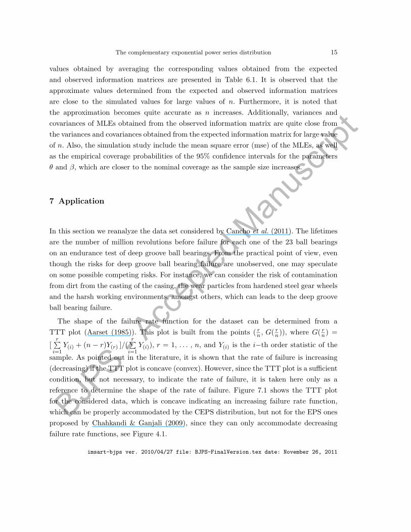
7 Application

In this section we reanalyze the data set considered by Cancho et al. (2011). The lifetimesare the number of million revolutions before failure for each one of the 23 ball bearingson an endurance test of deep groove ball bearings. From the practical point of view, eventhough the risks for deep groove ball bearing failure are unobserved, one may speculateon some possible competing risks. For instance, we can consider the risk of contaminationfrom dirt from the casting of the casing, the wear particles from hardened steel gear wheelsand the harsh working environments, amongst others, which can leads to the deep grooveball bearing failure.

The shape of the failure rate function for the dataset can be determined from aTTT plot (Aarset (1985)). This plot is built from the points ( rn , G( rn)), where G( rn) =

[r∑i=1

Y(i) + (n − r)Y(r) ]/(r∑i=1

Y(i)), r = 1, . . . , n, and Y(i) is the i−th order statistic of the

sample. As pointed out in the literature, it is shown that the rate of failure is increasing(decreasing) if the TTT plot is concave (convex). However, since the TTT plot is a sufficientcondition, but not necessary, to indicate the rate of failure, it is taken here only as areference to determine the shape of the rate of failure. Figure 7.1 shows the TTT plotfor the considered data, which is concave indicating an increasing failure rate function,which can be properly accommodated by the CEPS distribution, but not for the EPS onesproposed by Chahkandi & Ganjali (2009), since they can only accommodate decreasingfailure rate functions, see Figure 4.1.

imsart-bjps ver. 2010/04/27 file: BJPS-FinalVersion.tex date: November 26, 2011

BJPS - A

ccep

ted M

anus

cript

16 Flores et al.

0.0 0.2 0.4 0.6 0.8 1.0

0.0

0.2

0.4

0.6

0.8

1.0

r/n

G(r

/n)

Figure 7.1 Empirical scaled TTT-Transform for the data.

Therefore, the dataset may be fitted by the CEPS distribution. Thus, the Poisson,geometric, logarithmic and binomial distributions can be used for this purpose. Themaximum likelihood estimation is obtained by direct maximization of (18) via theoptim function of the R program (R Development Core Team (2008)). For complementaryexponential-binomial model it is taken m = 5, value that determines the CEB model withgreatest likelihood. Also, for sake of comparison, we fit more one usual lifetime distributiongenerally used for fitting dataset with increasing failure rate function: the Weibulldistribution. As well known, the Weibull distribution is indexing by two parameters asit is the case for the CEPS distribution. The density functions of the Weibull distributions,with parameters θ and β is given by θβθxθ−1 exp(−(βx)θ), respectively. Table (7.1) showsthe MLEs and their standard errors for the CEPS distribution parameters as well as forthe Weibull distribution parameters.

Table 7.1 MLEs and their standard errors (in brackets) for the parameters of the fitted distributions.

Distribution θ β

CEB 600 (280.3460) 0.0315 (0.0036)CEP 7.3259 (2.594) 0.0358 (0.0061)CEG 0.9447 (0.0415) 0.0436 (0.0094)CEL 0.9982 (0.0077) 0.0516 (0.0215)Weibull 2.1026 (0.3437) 0.0122 (0.0014)

We compare the fitting of the CEPS particular distributions and the Weibull one

imsart-bjps ver. 2010/04/27 file: BJPS-FinalVersion.tex date: November 26, 2011

BJPS - A

ccep

ted M

anus

cript

The complementary exponential power series distribution 17

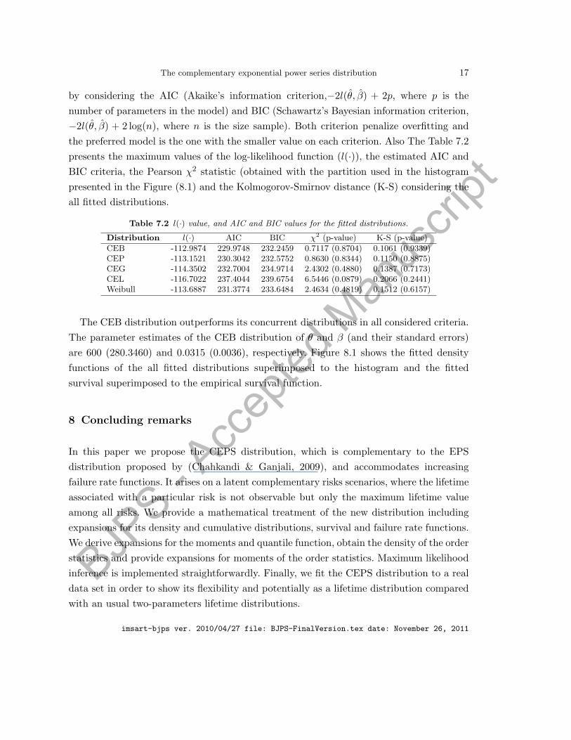
by considering the AIC (Akaike’s information criterion,−2l(θ, β) + 2p, where p is thenumber of parameters in the model) and BIC (Schawartz’s Bayesian information criterion,−2l(θ, β) + 2 log(n), where n is the size sample). Both criterion penalize overfitting andthe preferred model is the one with the smaller value on each criterion. Also The Table 7.2presents the maximum values of the log-likelihood function (l(·)), the estimated AIC andBIC criteria, the Pearson χ2 statistic (obtained with the partition used in the histogrampresented in the Figure (8.1) and the Kolmogorov-Smirnov distance (K-S) considering theall fitted distributions.

Table 7.2 l(·) value, and AIC and BIC values for the fitted distributions.

Distribution l(·) AIC BIC χ2 (p-value) K-S (p-value)

CEB -112.9874 229.9748 232.2459 0.7117 (0.8704) 0.1061 (0.9339)CEP -113.1521 230.3042 232.5752 0.8630 (0.8344) 0.1150 (0.8875)CEG -114.3502 232.7004 234.9714 2.4302 (0.4880) 0.1387 (0.7173)CEL -116.7022 237.4044 239.6754 6.5446 (0.0879) 0.2066 (0.2441)Weibull -113.6887 231.3774 233.6484 2.4634 (0.4819) 0.1512 (0.6157)

The CEB distribution outperforms its concurrent distributions in all considered criteria.The parameter estimates of the CEB distribution of θ and β (and their standard errors)are 600 (280.3460) and 0.0315 (0.0036), respectively. Figure 8.1 shows the fitted densityfunctions of the all fitted distributions superimposed to the histogram and the fittedsurvival superimposed to the empirical survival function.

8 Concluding remarks

In this paper we propose the CEPS distribution, which is complementary to the EPSdistribution proposed by (Chahkandi & Ganjali, 2009), and accommodates increasingfailure rate functions. It arises on a latent complementary risks scenarios, where the lifetimeassociated with a particular risk is not observable but only the maximum lifetime valueamong all risks. We provide a mathematical treatment of the new distribution includingexpansions for its density and cumulative distributions, survival and failure rate functions.We derive expansions for the moments and quantile function, obtain the density of the orderstatistics and provide expansions for moments of the order statistics. Maximum likelihoodinference is implemented straightforwardly. Finally, we fit the CEPS distribution to a realdata set in order to show its flexibility and potentially as a lifetime distribution comparedwith an usual two-parameters lifetime distributions.

imsart-bjps ver. 2010/04/27 file: BJPS-FinalVersion.tex date: November 26, 2011

BJPS - A

ccep

ted M

anus

cript

18 Flores et al.

Time

Den

sity

func

tion

0 40 80 120 160 200 240

0.00

00.

002

0.00

40.

006

0.00

80.

010

0.01

20.

014

CEBCEPCEGCELWeibull

Time

Sur

vivi

ng fu

nctio

n

0 40 80 120 160

0.0

0.2

0.4

0.6

0.8

1.0

CEBCEPCEGCELWeibull

Figure 8.1 Left panel: The plots of the fitted CEB, CEP, CEG, CEL and Weibull densities. Right panel:Kaplan-Meir curve together with the fitted survival functions.

Acknowledgments: The authors are grateful to the anonymous referees for theirimportant comments, suggestions and criticisms. Jose Flores D. is supported by thePontificia Universidad Catolica del Peru and the University of Sao Paulo. The researchesof Francisco Louzada and Vicente G. Cancho are supported by the Brazilian organizationCNPq.

References

Aarset, M. V. (1985). The null distribution for a test of constant versus “bathtub” failure rate. Scandinavian

Journal of Statistics, 12(1), 55–68.

Adamidis, K. & Loukas, S. (1998). A lifetime distribution with decreasing failure rate. Statistics &

Probability Letters, 39(1), 35–42.

Adamidis, K., Dimitrakopoulou, T. & Loukas, S. (2005). On an extension of the exponential-geometric

distribution. Statistics and Probability Letters, 73(3), 259 – 269.

Barakat, H. M. & Abdelkader, Y. H. (2004). Computing the moments of order statistics from nonidentical

random variables. Statistical Methods and Applications, 13, 15–26.

Barreto-Souza, W. & Cribari-Neto, F. (2009). A generalization of the exponential-poisson distribution.

Statistics and Probability Letters, 79, 2493–2500.

Basu, A. & J., K. (1982). Some recent development in competing risks theory. Survival Analysis, Edited by

Crowley, J. and Johnson, R. A, Hayvard:IMS , 1, 216–229.

imsart-bjps ver. 2010/04/27 file: BJPS-FinalVersion.tex date: November 26, 2011

BJPS - A

ccep

ted M

anus

cript

The complementary exponential power series distribution 19

Cancho, V. G., Louzada-Neto, F. & Barriga, G. D. (2011). The poisson-exponential lifetime distribution.

Computational Statistics & Data Analysis, 55, 677 – 686.

Chahkandi, M. & Ganjali, M. (2009). On some lifetime distributions with decreasing failure rate.

Computational Statistics and Data Analysis, 53, 4433–4440.

Cordeiro, G., Rodrigues, J. & de Castro, M. (2011). The exponential com-poisson distribution. Statistical

Papers, pages 1–12. 10.1007/s00362-011-0370-9.

Cox, D. R. & Hinkley, D. V. (1974). Theoretical statistics. Chapman and Hall, London.

Cox, D. R. & Oakes, D. (1984). Analysis of Survival Data. Chapman & Hall.

Crowder, M., Kimber, A., Smith, R. & Sweeting, T. (1991). Statistical Analysis of Reliability Data.

Chapman & Hall.

Goetghebeur, E. & Ryan, L. (1995). A modified log rank test for competing risks with missing failure type.

Biometrics, 77, 207–211.

Johnson, N. L., Kemp, A. W. & Kotz, S. (2005). UnivariateDiscreteDistribution. New Jersey.

Kus, C. (2007). A new lifetime distribution. Computational Statistics and Data Analysis, 51, 4497–4509.

Lawless, J. F. (2003). Statistical Models and Methods for Lifetime Data, volume second edition. Wiley.

Lu, K. & Tsiatis, A. A. (2001). Multiple imputation methods for estimating regression coefficients in the

competing risks model with missing cause of failure. Biometrics, 54, 1191–1197.

Lu, K. & Tsiatis, A. A. (2005). Comparision between two partial likelihood approaches for the competing

risks model with missing cause of failure. Lifetime Data Analysis, 11, 29–40.

Morais, A. L. & Barreto-Souza, W. (2011). A compound class of weibull and power series distributions.

Computational Statistics & Data Analysis, 55(3), 1410–1425.

Reiser, B., Guttman, I., Lin, D., Guess, M. & Usher, J. (1995). Bayesian inference for masked system

lifetime data. Applied Statistics, 44, 79–90.

R Development Core Team (2008). R: A Language and Environment for Statistical Computing . R

Foundation for Statistical Computing, Vienna, Austria.

Silva, R. B., Barreto-Souza, W. & Cordeiro, G. M. (2010). A new distribution with decreasing, increasing

and upside-down bathtub failure rate. Computational Statistics and Data Analysis, 54(4), 935 – 944.

Tahmashi, R. & Rezaei, S. (2008). A two-parameter lifetime distribution with decreasing failure rate.

Computational Statistics and Data Analysis, 52, 3889–3901.

Jose Flores D.

DAC - Pontificia Universidad Catolica del Peru,

Lima, Peru

E-mail: jfdelgad@pucp.edu.pe

Patrick Borges

DEs, Universidade Federal de Sao Carlos,

SP, Brazil

E-mail: patrickborges@yahoo.com.br

Vicente G. Cancho

ICMC - Universidade de Sao Paulo,

Sao Carlos - SP, Brazil

E-mail: garibay@icmc.usp.br

Francisco Louzada

ICMC - Universidade de Sao Paulo,

SP, Brazil

E-mail: louzada@icmc.usp.br

imsart-bjps ver. 2010/04/27 file: BJPS-FinalVersion.tex date: November 26, 2011