Department of Applied MathematicsFaculty of EEMCS

tUniversity of Twente

The Netherlands

P.O. Box 2177500 AE Enschede

The Netherlands

Phone: +31-53-4893400Fax: +31-53-4893114

Email: memo@math.utwente.nl

www.math.utwente.nl/publications

Memorandum No. 1776

Two exponential neighborhoods for

single machine scheduling

T. Brueggemann and J.L. Hurink

September, 2005

ISSN 0169-2690

Two Exponential Neighborhoods For Single

Machine Scheduling

Tobias Brueggemann 1,∗, Johann L. Hurink 2

Department of Applied Mathematics, University of Twente,P.O. Box 217, 7500 AE Enschede, The Netherlands

Abstract

We study the problem of minimizing total completion time on a single machinewith the presence of release dates. We present two different approaches leading toexponential neighborhoods in which the best improving neighbor can be determinedin polynomial time. Furthermore, computational results are presented to get insightin the performance of the developed neighborhoods.

Key words: exponential neighborhoods, local search, single machine.MSC2000: 90B35, 68M20.

1 Introduction

Many optimization problems in the practical world are computational in-tractable. It would simply cost too much time to solve them to optimality.Hence, there is need for a practical approach to solve such problems. A waytoo achieve this is the development of heuristic (approximation) algorithmsthat are able to find satisfying solutions within a reasonable amount of com-putational time. In the literature concerning heuristic algorithms two differentclasses can be distinguished. The first class of heuristic algorithms consists ofconstructive algorithms. These algorithms build solutions by assigning values

∗ Corresponding author.Email addresses: t.brueggemann@math.utwente.nl (Tobias Brueggemann),

j.l.hurink@math.utwente.nl (Johann L. Hurink).1 supported by the Netherlands Organization for Scientific Research (NWO) grant613.000.225 (Local Search with Exponential Neighborhoods).2 supported by BSIK grant 03018 (BRICKS: Basic Research in Informatics forCreating the Knowledge Society).

1

to one or more decision variables at a time. The second class are the im-provement algorithms, that start with a feasible solution and iteratively tryto advance to a better solution. In this class, local search resp. neighborhoodsearch algorithms play a big role.

A local search heuristic starts, roughly spoken, with some solution and itera-tively replaces the current solution by some solution in a neighborhood of thissolution. Thus, for a local search approach, a method for calculating an initialsolution, a neighborhood structure of a given solution and a method to selecta solution from the neighborhood of a given solution is needed.

The neighborhood structure of a given solution has an important influenceon the efficency of the local search heuristic. The structure determines thenavigation through the solution space during the iterations of the local searchmethod and the computation time of one iteration is affected by the choiceof the neighborhood structure as well. Therefore, one expects that the size ofthe neighborhood has influence on the quality of the final solution of a localsearch approach, because a larger neighborhood covers a bigger amount ofsolutions and of course, affects the running time. So, there has to be found acompromise between size, quality and running time.

A possible way to do this, is to restrict the neighborhood of a solution topromising solutions, i.e. to solutions which may have a good objective value.Another possibility is to develop efficient methods to find the best solutionin a given neighborhood, which is often an interesting optimization problemitself.

Over the last time, large-scale neighborhoods were considered that can be ex-hausted in reasonable time. These large-scale neighborhoods mostly containan exponential number of solutions but allow a polynomial exploration. Anice survey about large-scale neighborhood techniques is given by Ahuja et al.[1]. They categorize large-scale neighborhoods into three not necessarily dis-tinct classes. Their first category of neighborhood search algorithms consists ofvariable-depth methods. These algorithms partially exploit exponential-sizedneighborhoods using heuristics. The second category consists of network flowbased improvement algorithms. These methods use network flow techniques toidentify improving neighbors. Finally, their third category consists of neigh-borhoods for NP-hard problems received by subclasses or restrictions thatcan be solved in polynomial time.

Although, the concept of large scale neighborhoods sounds promising, thepractical relevance of these neighborhoods is not so clear (see e.g. Hurink [6]).In this paper we develop two large scale neighborhoods for a single machinescheduling problem and study their usage in local search. The goal is to presentfor one problem different concepts to reach large scale neighborhoods and to

2

get some more insight under which conditions large scale neighborhoods maybe of practical use.

More precisely, we present two different approaches for receiving a large-scaleneighborhood for the problem of scheduling n jobs with release dates ri andprocessing times pi on a single machine in order to minimize total completiontime

∑Ci without preemption. In the classical scheduling notation by Graham

et al. [5], this problem is denoted by 1|ri|∑ Ci. It is strongly NP-hard as statedin Lenstra et al. [7]. Since for a fixed sequence π there is an efficient method forcalculating the best schedule with respect to the objective function in O(n),local search may be applied by considering sequences as solutions.

The first neighborhood we present is an extension of the adjacent pairwiseinterchange neighborhood (API ). This extension is based on the idea of com-bining independent operations. Congram et al. [3] and Potts and van de Velde[8] applied the idea of combining independent SWAP -operations to the singlemachine total weighted tardiness scheduling problem and the TSP, respec-tively. They call their approach iterated dynasearch. In the paper of Congramet al. [3], the authors show that the size of their neighborhood is O(2n−1)and they give a dynamic programming recursion to find the best neighbor inO(n3). Hurink [6] applies compounded API -operations in the context of onemachine batching problems and shows, that an improving neighbor can beobtained in O(n2) by calculating a shortest path in an improvement graph,that is a structure, defined by the possibility of combining API -operationsand their change of the objective value.

We examine, in which situations we may combine several API -operations tomodify a sequence π describing a solution for 1|ri|∑ Ci. By looking on howto find a best combined move to a neighboring solution it turns out, that thiscan be done by calculating a shortest path in an improvement graph similarlyas described by Hurink [6]. According to Ahuja et al. [1], this extension of theAPI -neighborhood belongs to their second category of large scale neighbor-hoods.

The second neighborhood we introduce is based on a dominance rule for se-quences, that may also be used in a branch-and-bound algorithm for solvingthe considered problem. This dominance rule uses that for a given solution,the problem is locally not very different from it’s relaxation 1||∑ Ci, whichcan be solved by the shortest processing time first (SPT) rule from Smith [10].This second neighborhood belongs to the third category of Ahuja et al. [1].

The outline of this text is as follows. In Section 2 we give a brief description ofthe problem and introduce some notations. The next section describes the twolarge-scale neighborhoods and their main conceptual differences. Afterwards,in Section 4 we give some computational results for these neighborhoods and

3

dicuss the possibilities and limitations of the two concepts. Finally, some con-cluding remarks are given.

2 Problem Description

We consider a one-machine-scheduling problem, where n jobs 1, . . . , n withnon-negative release dates r1, . . . , rn and processing times p1, . . . , pn are given.A job i is not available before time ri and needs to be processed for pi time-units without preemption. W.l.o.g. we reorder the jobs such that r1 ≤ . . . ≤ rn

and, if ri = ri+1, that pi ≤ pi+1.

A schedule for this problem can be described by a vector S of starting timesSi, i = 1, . . . , n. It is called a feasible schedule, if and only if:

• Si ≥ ri for i = 1, . . . , n,• either Sj ≥ Si + pi or Si ≥ Sj + pj for all pairs i, j = 1, . . . , n with i �= j.

Furthermore, by C we denote the vector of completion times for a feasibleschedule S, i.e. Ci := Si + pi for i = 1, . . . , n.

The goal is to find a feasible schedule S, such that the objective function

f(S) :=n∑

i=1

Ci (1)

is minimized. This problem, denoted by 1|ri|∑ Ci, is NP-hard, (see Lenstraet al. [7]), and thus computational intractable.

Solutions of this problem can be characterized by sequences of jobs, which rep-resents a processing-order of the jobs. For a given sequence π we can calculatea corresponding feasible schedule S by:

Sπ(1) := rπ(1) and

Sπ(i) := max{rπ(i), Sπ(i−1) + pπ(i−1)} for i = 2, . . . , n.(2)

The calculation of the schedule belonging to a sequence needs O (n) time.From now on let π be a given sequence and Sπ the corresponding feasibleschedule. Often, we omit π if it is clear, which sequence is considered.

4

3 Large Scale Neighborhoods

In this section we present two large scale neighborhoods for problem 1|ri|∑ Ci.The neighborhoods rely on two different principles. First, in Subsection 3.1,we build up neighbored solutions by combining several independent pair-interchange operators to one compounded neighborhood operator. Next, inSubsection 3.2, we use a reordering of subsequences as the base of building upa neighborhood structure. Both neighborhoods have of up to an exponentialnumber of neighbors and can be searched efficiently. Finally, in Subsection 3.3,we compare the two approaches.

3.1 Compounded API

In this subsection we develop a neighborhood which is based on adjacent-pair-interchanges (API) for sequences. First, we analyze the effects of a single API-operation. The questions, which jobs are affected by a single move and howthis affects the objective function, are answered. Later on, this will be used tocombine several API-operations to a compounded operation, which results ina neighborhood up to exponential size that can be searched in polynomial time.Before presenting the mentioned results, we first introduce some notations.

For a given sequence π = (π(1), . . . , π(n)) and the resulting schedule S sets ofjobs, called blocks, occur. A block consists of jobs that are scheduled withoutidle-times, such that the first job of this block starts after an idle periodat it’s release date and all other jobs start at the completion time of theirpredecessor. More precisely, a block is a set of jobs B := {π(i), . . . , π(i + k)}with i ∈ {1, . . . , n− 1} and i+ k ≤ n, such that the following conditions hold:

• either i = 1 or Cπ(i−1) < Sπ(i),• Cπ(j) = Sπ(j+1) for j = i, . . . , i + k − 1,• either i + k = n or Cπ(i+k) < Sπ(i+k+1).

A given sequence π of jobs leads to a unique decomposition into blocks. Wedenote by b(π) the number of blocks and by B1, . . . , Bb(π) the blocks of theform Bβ = {π(iβ), . . . , π(iβ + kβ)} with iβ + kβ + 1 = iβ+1.

Additionally, we denote by gβ the amount of idle-time between job π(iβ) andπ(iβ−1 + kβ−1) if β ≥ 2 or the idle-time before the job π(1), if β = 1, i.e.

gβ :=

⎧⎨⎩

Sπ(iβ) − Cπ(iβ−1+kβ−1) if β ≥ 2,

Sπ(1) if β = 1

In Figure 1 an example for blocks and their gaps in a schedule is given.

5

S π(1) π(3) π(4) π(5) π(6) . . .

Block B1 B2 B3

time

π(2)

g1

0

g3g2

Fig. 1. Blocks and gaps in a schedule S

The API-neighborhood consist of adjacent-pair interchange operatorsAPI1, . . . , APIn−1, where operator APIj interchanges the elements in posi-tion j and j + 1 of a sequence, i.e.

APIj(π) := (π(1), . . . , π(j − 1), π(j + 1), π(j), π(j + 2), . . . , π(n))

The operator API is called adjacent-pair-interchange.

In the following we examine, how a single API-operation affects a given solu-tion. Considering the two jobs π(j) and π(j+1) involved in an API -operation,there are different cases to handle, depending on the position of job π(j) inthe block and the release date rπ(j+1) of job π(j + 1).

Consider an API -operator APIj where index j belongs to a position of blockBβ = {π(ibeta), . . . , π(ibeta+kbeta)}. Clearly, if j = ibeta+kbeta, the application ofAPIj leads to an increase of the objective value since the job π(ibeta+kbeta+1)is the first job of the next block and, therefore, starts at it’s release date. Thus,if we are interested in operators APIj which may lead to better solutions, weonly have to consider j ∈ {ibeta, . . . , ibeta + kbeta − 1}. Because of the block-structure we have for the schedule S of π:

Sπ(j) + pπ(j) = Sπ(j+1).

In order to calculate the consequences of the exchange of the jobs π(j) andπ(j + 1), let S ′ be the schedule of APIj(π) and let

• σ := Sπ(j+1) − S ′π(j+1),

• γ := S ′π(j) − Sπ(j).

• δ := C ′π(j) − Cπ(j+1).

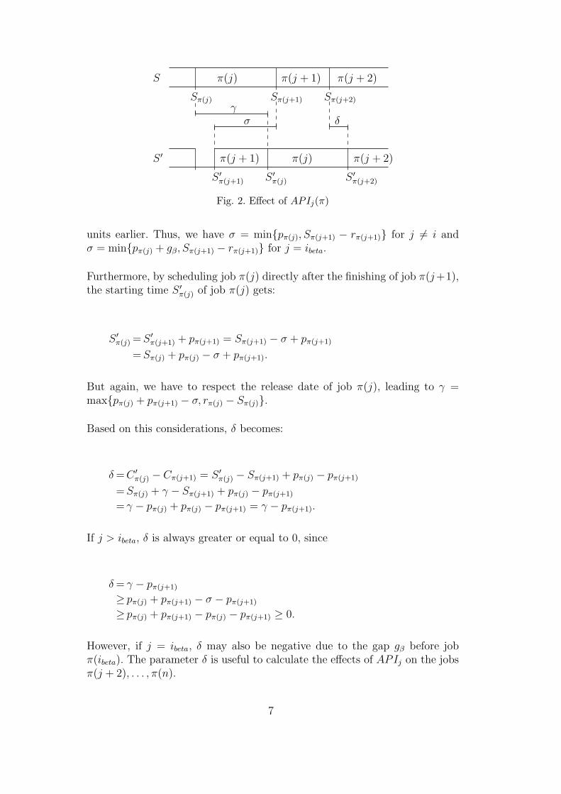
Herewith, σ describes the absolute value of the change in starting time ofjob π(j + 1), γ gives the change for job π(j) and δ presents the effect of theexchange for the succeeding jobs π(j + 2), . . . , π(n) (see Figure 2).

If we take the job π(j) out of the schedule, i.e. the time-period [Sπ(j), Sπ(j) +pπ(j)] becomes idle-time, we have pπ(j) (or pπ(j) + gβ for j = ibeta) units ofidle before job π(j + 1). Thus, we can schedule the job π(j + 1) this amountearlier, if we do not have to respect the release date rπ(j+1). However, if we haveCπ(j−1) < rπ(j+1) ≤ Sπ(j+1), the job π(j + 1) can start only by Sπ(j+1) − rπ(j+1)

6

π(j + 2)π(j)π(j + 1)

δσ

Sπ(j)γ

Sπ(j+1) Sπ(j+2)

π(j + 2)π(j + 1)π(j)

S ′π(j+1) S ′

π(j) S ′π(j+2)

S ′

S

Fig. 2. Effect of APIj(π)

units earlier. Thus, we have σ = min{pπ(j), Sπ(j+1) − rπ(j+1)} for j �= i andσ = min{pπ(j) + gβ, Sπ(j+1) − rπ(j+1)} for j = ibeta.

Furthermore, by scheduling job π(j) directly after the finishing of job π(j+1),the starting time S ′

π(j) of job π(j) gets:

S ′π(j) = S ′

π(j+1) + pπ(j+1) = Sπ(j+1) − σ + pπ(j+1)

= Sπ(j) + pπ(j) − σ + pπ(j+1).

But again, we have to respect the release date of job π(j), leading to γ =max{pπ(j) + pπ(j+1) − σ, rπ(j) − Sπ(j)}.

Based on this considerations, δ becomes:

δ =C ′π(j) − Cπ(j+1) = S ′

π(j) − Sπ(j+1) + pπ(j) − pπ(j+1)

=Sπ(j) + γ − Sπ(j+1) + pπ(j) − pπ(j+1)

= γ − pπ(j) + pπ(j) − pπ(j+1) = γ − pπ(j+1).

If j > ibeta, δ is always greater or equal to 0, since

δ = γ − pπ(j+1)

≥ pπ(j) + pπ(j+1) − σ − pπ(j+1)

≥ pπ(j) + pπ(j+1) − pπ(j) − pπ(j+1) ≥ 0.

However, if j = ibeta, δ may also be negative due to the gap gβ before jobπ(ibeta). The parameter δ is useful to calculate the effects of APIj on the jobsπ(j + 2), . . . , π(n).

7

Applying operator APIj changes the objective value by

Δj := f(S ′) − f(S) =n∑

μ=1(S ′

π(μ) + pπ(μ) − Sπ(μ) − pπ(μ))

= γ − σ +n∑

μ=j+2S ′

π(μ) − Sπ(μ)

(3)

It remains to calculate

penalty :=n∑

μ=j+2

S ′π(μ) − Sπ(μ).

As mentioned before, the effects of APIj on the jobs π(j + 2), . . . , π(n) ischaracterized by δ. If δ = 0, then penalty := 0. Otherwise, we consider firstthe directly affected block Bβ.

If δ > 0, we have to move all jobs π(μ) with ibeta +kbeta ≥ μ ≥ j +2 by δ unitsto the right, resulting in penalty := δ(iβ +kβ−j−1). If δ > gβ+1, the shift alsoaffects the next block. We then have to shift the jobs π(iβ+1), . . . , π(iβ+1+kβ+1)by δ′ := δ − gβ+1 units. If again the value of δ′ is bigger than the gap gβ+2 wealso have to shift the block Bβ+2. This continues until the remaining value δvalue is 0.

On the other hand if δ < 0, we have to shift jobs to the left in the newschedule, beginning with job π(j + 2). The affected jobs are only the jobsj + 2, . . . , iβ + kβ and the calculation of penalty has to be done by calculatingfor all these jobs their new starting times by applying formula (2). Note, thatin this case the penalty is negative and the block Bβ may split into severalblocks and/or partially join the block Bβ−1.

All in all the effects of such an API -operation are computable in time O(n),however in the average we expect a much lower running time. Since the API -neighborhood has size O(n), we need in the worst case O(n2) to compute thebest API-neighbor of a solution.

In the following we investigate the possibility of combining API operators.More precisely, we search for pairs of operators APIi and APIj, where theconsecutive application of these two operators to a sequence π leads to a changeof Δi + Δj in the objective value. Such an independence of operations allowsa combined execution of several different APIs in one iteration of the localsearch algorithm and so gives a compounded neighborhood. To find candidatesfor combined operators, we have to analyze, which APIs do not have an effecton each other.

Consider indices i and j with 1 ≤ i < j ≤ n−1 and i+2 ≤ j. We are interestedin those cases, where the effect of APIj(APIi(π)) and APIi(APIj(π)) are

8

equal to Δi + Δj , i.e. we look for indices i and j where

f(Sπ) + Δi + Δj = f(SAPIj(APIi(π))),

(Sπ denotes the schedule for π and SAPIj(APIi(π)) denotes the schedule forthe sequence obtained by applying APIi to π and the APIj to the resultingsequence). An necessary condition for this independency is that after applyingAPIi to π the resulting schedule around the jobs in position j and j + 1 mustbe the same as in π. To formalize this, we introduce a variable Fi denotingthe first position after i + 1 where the application of APIi to π has no effect.

If APIi(π) changes the schedule in such a way, that the starting time ofjob π(i + 2) in the schedules π and APIi(π) remains the same and the newcompletion time of π(j) is equal to the old completion time of π(j + 1), onlythe two jobs π(i) and π(i + 1) change their positions in the schedule withoutany effect on the succeeding jobs and the block structure of the schedule. Inthis case we define Fi := i + 2.

On the other hand, if the starting time of job π(i+2) or the idle period beforeπ(i + 2) is changed by applying APIi to π, we have to consider the index ofthe last affected job

Li := max{k : i ≤ k ≤ n, Sππ(k) �= S

APIi(π)π(k) },

i.e. the last job, that changes it’s starting time. This job π(Li) can easilybe determined during the calculations of penalty, as described before. Sincethe job π(Li) is scheduled earlier or later in the schedule corresponding toAPIi(π), the effects of APIj(APIi(π)) may get different to Δj + Δi for allindices j from i + 1 to Li + 1. However, the effects of APIj(APIi(π)) are stillequal to Δj +Δi for j ≥ Li +2. Therefore, in this case we define Fi := Li +2.

Based on the above considerations, we call APIj π-independent of APIi if thefollowing conditions hold:

• neither π(i) nor π(j) is a last job of it’s block,• j ≥ Fi.

Additionally, we call APIi and APIj π-independent if either APIj is π-independent of APIi or APIi is π-independent of APIj.

Summarizing, for two π-independent operations APIi and APIj we have

f(Sπ) + Δi + Δj = f(SAPIj(APIi(π))).

An important property of π-independency is it’s transitivity. If for i < j < kAPIj is π-independent of APIi and APIk is π-independent of APIj then also

9

APIk is π-independent of APIi. Thus, we call a set M ⊆ {1, . . . , n − 1} π-independent if the API -operators belonging to the elements of M are pairwiseπ-independent.

Hence, for a given π-independent set M := {v1, . . . , vk} ⊆ {1, . . . , n−1} we cancalculate the objective value of the schedule APIvk

◦APIvk−1◦ . . . ◦APIv1(π)

by

f(SAPIvk◦APIvk−1

◦...◦APIv1(π)) = f(Sπ) +∑i∈M

Δi.

In the following we develop an efficient method to calculate a set of indepen-dent operations, that gives the best gain in the objective value over all possibleindependent operations. For this, we define a structure called improvementgraph which depends strongly on the given sequence π.

For a given sequence π let Gπ = (V, Aπ) be a graph with vertices V ={0, 1, . . . , n − 1, ∗} and a set Aπ ⊆ V × V of directed arcs, where each arc(i, j) ∈ Aπ receives a cost cij . The vertices 0 and ∗ are called source resp. sink.The set Aπ contains the following arcs.

• arcs (0, i) with cost c0i = Δi for all 1 ≤ i ≤ n − 1 where π(i) is not a lastjob of a block in Sπ,

• arcs (i, j) with cost cij = Δj for all 1 ≤ i < j ≤ n − 1 where APIj isπ-independent of APIi,

• arcs (i, ∗) with cost ci∗ = 0 for all 0 ≤ i ≤ n − 1.

An arc leading to a vertex i ≤ n − 1 corresponds to an application of theoperation APIi. Furthermore, a directed path P = (0, v1, . . . , vk, ∗) with 1 ≤vi ≤ n−1 corresponds to a combined operation APIvk

◦APIvk−1◦. . .◦APIv1(π)

of π-independent operations and the sum of the costs of the arcs on the pathdescribes the gain to the objective value. Hence, if we have a shortest directedpath from the source to the sink, this determines the best possible combinedoperation of π-independent operations.

Because our graph has no directed cycles, we can use Dijkstra’s algorithm toobtain a shortest-path in this graph. With this algorithm we are able to calcu-late the best possible combined operation of π-independent APIi operationsin O(n2). There can be up to exponential many paths from the source to thesinks. Thus we have an exponential neighborhood that can be exploited inpolynomial time. We call this neighborhood CAPI.

10

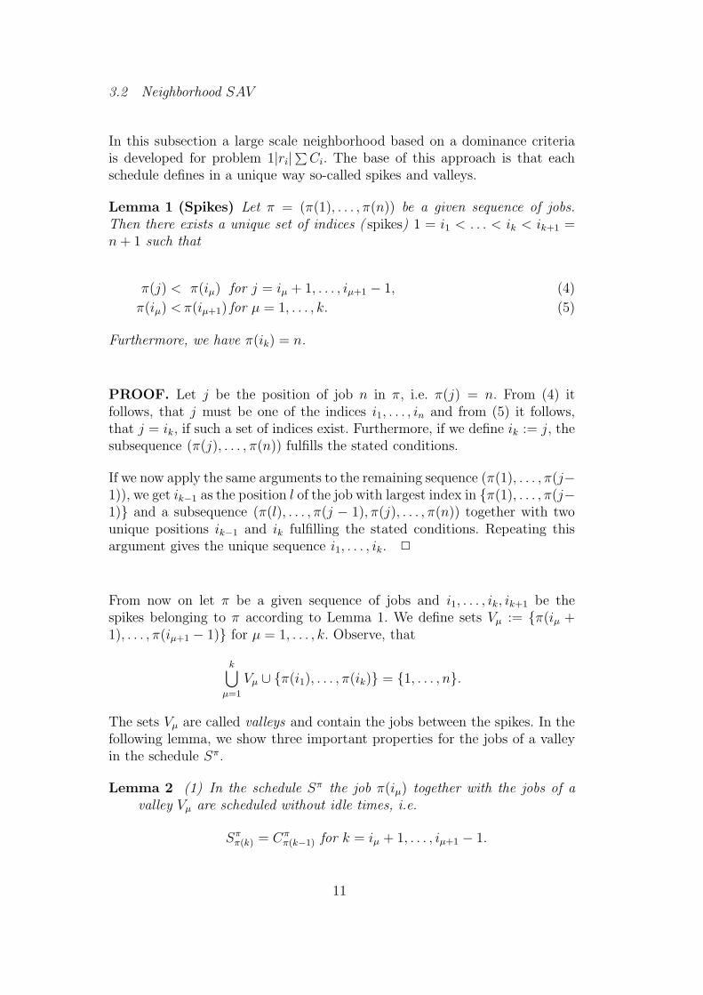
3.2 Neighborhood SAV

In this subsection a large scale neighborhood based on a dominance criteriais developed for problem 1|ri|∑ Ci. The base of this approach is that eachschedule defines in a unique way so-called spikes and valleys.

Lemma 1 (Spikes) Let π = (π(1), . . . , π(n)) be a given sequence of jobs.Then there exists a unique set of indices ( spikes) 1 = i1 < . . . < ik < ik+1 =n + 1 such that

π(j) < π(iμ) for j = iμ + 1, . . . , iμ+1 − 1, (4)

π(iμ) < π(iμ+1) for μ = 1, . . . , k. (5)

Furthermore, we have π(ik) = n.

PROOF. Let j be the position of job n in π, i.e. π(j) = n. From (4) itfollows, that j must be one of the indices i1, . . . , in and from (5) it follows,that j = ik, if such a set of indices exist. Furthermore, if we define ik := j, thesubsequence (π(j), . . . , π(n)) fulfills the stated conditions.

If we now apply the same arguments to the remaining sequence (π(1), . . . , π(j−1)), we get ik−1 as the position l of the job with largest index in {π(1), . . . , π(j−1)} and a subsequence (π(l), . . . , π(j − 1), π(j), . . . , π(n)) together with twounique positions ik−1 and ik fulfilling the stated conditions. Repeating thisargument gives the unique sequence i1, . . . , ik. �

From now on let π be a given sequence of jobs and i1, . . . , ik, ik+1 be thespikes belonging to π according to Lemma 1. We define sets Vμ := {π(iμ +1), . . . , π(iμ+1 − 1)} for μ = 1, . . . , k. Observe, that

k⋃μ=1

Vμ ∪ {π(i1), . . . , π(ik)} = {1, . . . , n}.

The sets Vμ are called valleys and contain the jobs between the spikes. In thefollowing lemma, we show three important properties for the jobs of a valleyin the schedule Sπ.

Lemma 2 (1) In the schedule Sπ the job π(iμ) together with the jobs of avalley Vμ are scheduled without idle times, i.e.

Sππ(k) = Cπ

π(k−1) for k = iμ + 1, . . . , iμ+1 − 1.

11

(2) Considering all sequences resulting from π by a reordering of the jobs of avalley Vμ, the sequence obtained by reordering these jobs by non-decreasingprocessing-times has minimal objective value.

(3) Reordering the jobs of Vμ ∪ {π(iμ)} by non-decreasing processing-timesdoes not increase the objective value.

PROOF.

(1) For all l ∈ {iμ + 1, . . . , iμ+1 − 1} equation (4) implies l < iμ, i.e.rl ≤ riμ . This again implies Cj ≥ rl for all j, l ∈ Vμ leading toSπ

π(l) = max{rπ(l), Cππ(l−1)} = Cπ

π(l−1) for all l ∈ {iμ + 1, . . . , iμ+1 − 1}.(2) Due to part (1) of the lemma, the jobs of Vμ are scheduled in Sπ in the

interval

I = [Sππ(iμ+1), S

ππ(iμ+1) +

∑j∈Vμ

pj ].

Furthermore, we have rj ≤ Sππ(iμ) for all j ∈ Vμ. Thus, reordering the jobs

of Vμ still allows to schedule the jobs of Vμ in I. According to Smith’srule, a reordering to non-decreasing processing-times is best possible.

(3) Due to part (2) we first may reorder the jobs of Vμ by non-decreasingprocessing-times without increasing the objective value. Since rj ≤ rπ(iμ),interchanging job π(iμ) with jobs of Vμ which have a smaller processingtime leads to a decrease of the objective value. �

Consider a given initial sequence π, spikes i1, . . . , ik, ik+1 and valleys V1, . . . , Vk.Based on part (2) of the lemma it is possible to find a best sequence respectingthe spikes and valleys in time O (n log n) by simply sorting the jobs of Vμ byincreasing processing-times. If we allow a change in the spikes and valleys,we even might get a better solution by sorting the whole sets Vμ ∪ {π(iμ)}.In the latter case, it may happen, that the new sequence does not have thesame spikes and valleys as before and, therefore, again may be optimized byresorting the valleys.

Summarizing, if spikes i1, . . . , ik, ik+1 and valleys V1, . . . , Vk are given, we caneasily find an optimal sequence π that respects these spikes and valleys. How-ever, as the next theorem shows, it is not easy to find an optimal sequence πrespecting given spikes i1, . . . , ik, ik+1 without the knowledge of the valleys.

Theorem 3 Let 1 = i1 < . . . < ik < ik+1 = n + 1 be a given set of integers.The problem of finding a sequence π with

π(j) < π(iμ) for j = iμ + 1, . . . , iμ+1 − 1,

π(iμ) < π(iμ+1) for μ = 1, . . . , k.

12

for the jobs 1, . . . , n with release dates ri, (r1 ≤ . . . ≤ rn) and processing-timespi, which minimizes the objective function

∑Ci is NP-hard in the strong

sense.

PROOF. The proof is based on an analysis of the reduction which maybe used to proof that problem 1|ri|∑ Ci is NP-hard in the strong sense.Therefore, we only give a short sketch of the proof and leave details to thereader.

The NP-hardness proof for problem 1|ri|∑ Ci reduces a general instance of3-Partition to an instance of 1|ri|∑ Ci in such a way that a set of dummyjobs have to occupy certain fixed intervals and that for the remaining jobs(which correspond to the items of 3-Partition) only t intervals of length bremain open (t and b are the number of items and the size of each partitionset of 3-Partition). Defining all the dummy jobs as spikes, does not have anyeffect on the reduction and, thus, the problem stated in the theorem is alsoNP-hard in the strong sense. �

The second large scale neighborhood we define in the following is called SAV(Spike And Valley) and relies on the results of Lemma 2. Given a solution πwith corresponding spikes and valleys a neighbored solution is achieved in twosteps: first the solution is ’manipulated’ in such a way that a new sequenceπ′ is achieved which in general has a different spike and valley structure thanπ and, second, the order of jobs within valleys of π′ is changed. For the firststep we use Lemma 2 (3); i.e. we resort all sets Vμ ∪ {π(iμ)}, μ = 1, . . . , k bynon-decreasing processing-times. Since this is a deterministic procedure, thisfirst step is the same for all neighbored solutions. The second step is based onLemma 2 (2): we allow a reordering of jobs within valleys. As a consequenceneighbored solutions differ only in the ordering of the jobs within the valleysof π′. Lemma 2 (2) states that a best neighbor is achieved by sorting the jobsof these valleys by non-decreasing processing-times.

Summarizing, the SAV neighborhood has up to exponential size depending onthe instance and the sequence, especially the amount of spikes in the sequenceπ′ after the first step. To calculate the best neighbor of a solution in theSAV -neighborhood we two times have to sort the valleys by non-decreasingprocessing times which can be realized in O(n log n). Note, that after applyingthis neighborhood operation once, in the first step of the next neighboringoperator the jobs within each valley are already sorted and only the spike infront of a valley has to be inserted in the valley on the base of its processingtime (which can be realized in linear time). Furthermore, if in this first stepall spikes have a processing time smaller or equal to the minimum processingtime in their valley, the choice of the best neighbor will not change the given

13

solution π; i.e. we are in a local minimum.

3.3 Comparison of the two neighborhoods

The two approaches, CAPI together with the block structure and SAV withit’s spikes and valleys, are somehow related. The jobs that belong to a blockare processed without idle-times as well as the jobs of a valley defined by thespikes. The difference lies in the fact, that there are at least as many valleysthan blocks for a given sequence π, but there may be more. This results fromthe fact, that in a schedule valleys for two adjacent spikes may be scheduledwithout idle-time in between, whereas two blocks are always separated by anidle-time.

However, the underlying ideas to develop the large scale neighborhoods arequite different. The CAPI neighborhood is build upon the simple API neigh-borhood and has in principle the same navigation behavior as that neighbor-hood. The only difference to the API neighborhood is that the API-operatorsare not chosen and executed sequentially but in parallel. Thus, from qualitypoint of view, we may expect from CAPI only a better behavior than API,if the parallel choice fits better to the problem. From computational point ofview, both neighborhoods have a worst case complexity of O(n2) to computea best neighbor. But since the chosen operator of CAPI may contain sev-eral API operators, one may suppose that the total time to reach a certainquality may be shorter for CAPI. Both of these aspects are investigated viacomputational tests which are reported in the next section.

The SAV neighborhood is based on a local priority criteria, which allows theinterchange of two jobs under certain conditions (first job has larger process-ing time and after the interchange the first scheduled job does not start later).Thus, in principle this neighborhood also relies on the API neighborhood.However, in contrast to the CAPI neighborhood we do not restrict to inde-pendent operators but allow a complete reordering of certain subsets of jobs.This may indicate that the SAV neighborhood is able to reach (good) localoptima in short time. On the other hand, if one has reached a local optima,the SAV neighborhood may not be a good choice to navigate further, sincewithin this neighborhood always a job with larger processing time than its suc-cessor is interchanged with this successor; i.e. we have a monotone behavior.Note, that under the API neighborhood also an interchange with a succeed-ing job with larger processing time may lead to an improving neighbor. Again,computational results have to give insight to these questions.

14

4 Results

In this section we report on computational experiments to indicate how thetwo approaches perform regarding solution quality and running time for smalland large instances. Furthermore, we compare the results with optimal solu-tions found by a branch-and-bound algorithm for smaller instances. We usethe branch-and-bound algorithm of Yanai and Fujie [4] to obtain these exactsolutions. As an initial heuristic we use besides some simple priority basedmethods the APRTF -heuristic which was presented by Chu [2].

The problem instances were generated as described by Yanai and Fujie [4]and Chu [2]. The processing times were uniform randomly chosen between1 and 100. The release dates were generated between 0 and 101nλ

2where λ

is a parameter and n the number of jobs. Hereby, λ is some sort of densityfactor. The tests done by Yanai and Fujie [4] show, that the hardest instancesare received for 0.6 ≤ λ ≤ 1.1. For several values of λ (0.2, 0.4, . . . , 2.0) andn = 100 we randomly generated each 100 instances. Since we were not able toobtain for every instance an optimal solution (i.e. for values of λ between 0.6and 1.1 we left these very difficult instance out of consideration. For example,for λ = 0.8 we only had optimal solutions for 95 out of the 100 instances. Forall the other λ-values we had at least 97 optimal solved instances.

In order to compare the quality of two solutions, we need a useful attribute.We don’t use the objective value

∑Ci for comparing two solutions but use

the so called total waiting time of the jobs∑

(Si − ri). The total waiting timediffers from the objective value

∑Ci by the additive constant

∑(ri + pj) and,

therefore, reflects better how good the decision space is used by a solution. Ifwe denote with Si the starting times of the jobs in some solution and with S∗

i

the starting times of the jobs in an optimal solution, we measure the qualityof the approximating solution by the average deviation which we calculate as:

∑(Si − ri) − (S∗

i − ri)∑(S∗

i − ri)=

∑(Si − S∗

i )∑(S∗

i − ri).

The achieved average optimal total waiting time values for the generated in-stances are given in Figure 3 for different values of λ.

In order to test the effectiveness of the neighborhoods in practice, we imple-mented them in ANSI-C. We decided to use best fit API, i.e. choose the bestpossible API neighbor (BAPI for short) of the current solution as was de-scribed before. Furthermore we implemented CAPI and SAV as introduced.Because it turned out very soon that SAV as a stand-alone neighborhoodwould not suffice, we decided to combine SAV and BAPI as a fourth neigh-borhood. This means, that we try to find a better solution in the SAV -neighborhood and if this is not possible, we use the BAPI -neighborhood for

15

0

20000

40000

60000

80000

100000

120000

140000

0.2 0.4 0.6 0.8 1 1.2 1.4 1.6 1.8 2

tota

l wai

ting

time

lambda

average total waiting time

Fig. 3. Optimal total waiting values

one iteration. A local optima in the SAV neighborhood is achieved if the pro-cessing time of every spike is smaller or equal to the processing time of the firstjob of the corresponding valley and the valleys are sorted by non-decreasingprocessing times. In such a case, SAVBAPI will then apply a BAPI step.

Furthermore, as local search method we use iterative improvement. We havechosen not to use tabu search or simulated annealing since we are interestedin the structural behavior of the neighborhoods and not in the potentials oflocal search methods. We tested the given neighborhoods exhaustively withdifferent initial solutions.

First, we use the APRTF -heuristic as initial solution and iterative improve-ment. The local optimal solutions obtained by the neighborhoods in averagediffer only slightly. The solutions are similar in structure and there is notmuch difference to the initial solution. This may be caused by the fact thatthe heuristic delivers often a local optima resp. a solution of good quality.

In Figure 4 the performance of the considered approaches are given. For dif-ferent values of λ the average deviation of the total waiting time value of thesolutions to the optimal total waiting time value is given.

The upper line shows the average deviation of the solutions received by it-erative improvement using the SAV -neighborhood. Since a solution receivedby the APRTF -heuristic is mostly local optimal in the SAV -neighborhood,

16

the lines of the APRTF -heuristic and for iterative improvement using theSAV -neighborhood are almost identical in average. The second line shows theaverage deviations of the solutions received by the iterative improvement pro-cedure using the BAPI, CAPI and SAVBAPI -neighborhood. Here again, thelines are nearly identical in average. Hence, the first observations are that theCAPI -neighborhood performs no better than the BAPI -neighborhood andthat in the iterative improvement using the SAVBAPI -neighborhood mainlythe BAPI -operator is used if we start from a solution of good quality.

This at first indicates, that for problem 1|ri|∑ Ci the possibility of the expo-nential neighborhood to combine several moves and to look at their overallperformance does not help for navigation. To get more insight in the naviga-tional behavior of the neighborhoods, we added an extra component to thelocal search approach.

After iterative improvement with one of the neighborhood approaches stopswe give the resulting local optima a kick and restart the iterative improvementprocedure. This kick simply takes one of the jobs not starting at it’s releasedate and reinserted it at a position in the sequence so that this job will startat it’s release date. With this slightly perturbed solution, which is not neces-sarily better than the original local optimal solution, we again start iterativeimprovement possibly arriving at a better solution. We apply the kick to everyjob where it is possible and the best received solution from this kick followedby iterative improvement is taken as next solution. We iterated this process aslong as a kick to any job followed by iterative improvement leads to no bettersolution.

The average solution quality received by using the kick method is also pre-sented in Figure 4. Here one can see that the kick method has in general abig impact on solution quality. Although, the SAV -neighborhood was hardlyable to improve the initial solution given by the APRTF -heuristic, it now im-proves this solution considerably. Again, kick-BAPI and kick-CAPI performnearly the same as was the case for BAPI and CAPI. But, combining SAVwith BAPI and using kicks (kick-SAVBAPI ) leads to the best solution qualityespecially for higher λ values.

The above mentioned test give some indications of the navigation behavior ofthe neighborhoods in regions of high quality solutions. In a further series oftests, we investigate how they behave if a weak initial solution is chosen. Forthis we use an initial solution called RSORT obtained by sorting the jobs byincreasing release dates. In Figure 5 we compare the initial solutions and localoptima with the optimal solution for the generated instances. As one can see,although iterative improvement is not a very clever local search algorithm,the solutions achieved by this algorithm using one of our neighborhoods are ofnoticeable improvement compared to the initial solution and get into the re-

17

0

0.01

0.02

0.03

0.04

0.05

0.2 0.4 0.6 0.8 1 1.2 1.4 1.6 1.8 2

aver

age

devi

atio

n fr

om o

ptim

al o

bjec

tive

valu

e

lambda

APRTF-heuristic/ SAV-neighborhoodBAPI/CAPI/SAVBAPI-neighborhood

kick-SAV-neighborhoodkick-BAPI/CAPI-neighborhood

kick-SAVBAPI-neighborhood

Fig. 4. Comparison with optimal solution

gion of the APRTF -heuristic. Hereby, the SAVBAPI -neighborhood performssignificantly better than the BAPI - or CAPI -neighborhood, which delivernearly the same solutions. Because of the nature of the SAV -neighborhood,an initial solution received by the RSORT -heuristic is already an optimum inthe SAV -neighborhood and thus, iterative improvement with only the SAV -neighborhood has no effect.

Again, we tested how the different neighborhoods behave after giving thelocal optimal solution a kick. In Figure 6 we compare the quality of the re-trieved local optimal solutions with each other. In order to be able to have areference point, the local optimal solutions received by the simple SAVBAPI -neighborhood without using kicks are also shown. Here one can see, that usingkicks on local optimal solutions again improves the quality. Especially the it-erative improvement method using the neighborhoods kick-BAPI, kick-CAPIand kick-SAVBAPI are performing well, although iterative improvement withrestarts using small changed solutions is not a very clever local search heuris-tic. One can see that, if we start with a rather bad initial solution receivedby the constructive heuristic RSORT, we are able to end up with solutionsof comparable quality to the APRTF -heuristic. Moreover, kick-SAVBAPI isable to beat APRTF for λ in the range [1.0, 2.0].

The additional tests confirm, that the navigation behavior of the exponentialneighborhood CAPI is not better than that of the underlying basic neigh-borhood API. Taking always in a greedy way the best API -move in general

18

0

0.1

0.2

0.3

0.4

0.5

0.6

0.7

0.8

0.2 0.4 0.6 0.8 1 1.2 1.4 1.6 1.8 2

aver

age

devi

atio

n fr

om o

ptim

al o

bjec

tive

valu

e

lambda

RSORT-heuristic/ SAV-neighborhoodBAPI/CAPI-neighborhood

SAVBAPI-neighborhoodAPRTF-heuristic

Fig. 5. Using RSORT as initial solution for iterative improvement

0

0.05

0.1

0.15

0.2

0.25

0.2 0.4 0.6 0.8 1 1.2 1.4 1.6 1.8 2

aver

age

devi

atio

n fr

om o

ptim

al o

bjec

tive

valu

e

lambda

kick-SAV-neighborhoodSAVBAPI-neighborhood

kick-BAPI/CAPI-neighborhoodkick-SAVBAPI-neighborhood

APRTF-heuristic

Fig. 6. Using RSORT as initial solution and restarts for iterative improvement

19

n BAPI CAPI SAV SAVBAPI

100 0.01 0.01 0.00 0.01

200 0.04 0.05 0.01 0.07

400 0.32 0.43 0.01 0.49

1000 4.93 7.17 0.01 7.17

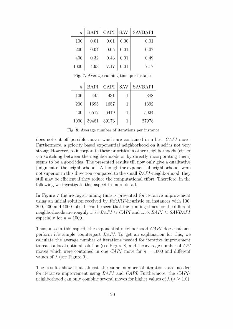
Fig. 7. Average running time per instance

n BAPI CAPI SAV SAVBAPI

100 445 431 1 388

200 1695 1657 1 1392

400 6512 6419 1 5024

1000 39481 39173 1 27978

Fig. 8. Average number of iterations per instance

does not cut off possible moves which are contained in a best CAPI -move.Furthermore, a priority based exponential neighborhood on it self is not verystrong. However, to incorporate these priorities in other neighborhoods (eithervia switching between the neighborhoods or by directly incorporating them)seems to be a good idea. The presented results till now only give a qualitativejudgment of the neighborhoods. Although the exponential neighborhoods werenot superior in this direction compared to the small BAPI -neighborhood, theystill may be efficient if they reduce the computational effort. Therefore, in thefollowing we investigate this aspect in more detail.

In Figure 7 the average running time is presented for iterative improvementusing an initial solution received by RSORT -heuristic on instances with 100,200, 400 and 1000 jobs. It can be seen that the running times for the differentneighborhoods are roughly 1.5×BAPI ≈ CAPI and 1.5×BAPI ≈ SAVBAPIespecially for n = 1000.

Thus, also in this aspect, the exponential neighborhood CAPI does not out-perform it’s simple counterpart BAPI. To get an explanation for this, wecalculate the average number of iterations needed for iterative improvementto reach a local optimal solution (see Figure 8) and the average number of APImoves which were contained in one CAPI move for n = 1000 and differentvalues of λ (see Figure 9).

The results show that almost the same number of iterations are neededfor iterative improvement using BAPI and CAPI. Furthermore, the CAPI -neighborhood can only combine several moves for higher values of λ (λ ≥ 1.0).

20

λ 0.6 0.7 0.8 0.9 1.0 1.1 1.2 1.4 1.6 1.8 2.0

API 1.0 1.0 1.0 1.0 1.4 2.7 4.0 6.5 7.8 10.1 11.1

Fig. 9. Average moves per iteration in CAPI -neighborhood

λ 0.4 0.6 0.7 0.8 0.9 1.0 1.1 1.2 1.4 1.6

% 80.5 80.3 80.3 80.2 80.0 80.5 83.0 85.4 89.3 91.4

Fig. 10. Average use of BAPI per iteration in SAV -neighborhood

This is because for higher values of λ we get a wider range of release dates.This results in instances and feasible solutions with a greater amount of blocksthat do not interfere and allow simultaneous moves.

Finally, we calculated for n = 1000 in how many cases the BAPI -neighborhoodhas to be applied if the combined neighborhood SAVBAPI is used (see Figure10). Again, the average need for BAPI in every iteration increases for highervalues of λ because of the structure of theses instances and the chosen initialsolution RSORT. In order to receive solutions that are not optimal regardingthe SAV -neighborhood by applying neighborhood search on the consideredinitial solution there is need for some BAPI -moves to enlarge the valleys.Hence, it takes some iterations using BAPI -moves before an SAV -move givesan improvement. This is specially the case for instance with higher values ofλ. These instances have a wider range of release dates and hence it is veryunlikely to receive non-empty valleys. And if a non-empty valley is obtainedby an BAPI -move, mostly either the valley and the corresponding spike arealready sorted by processing times or it would not improve the objective valueif this sorting is done by an SAV -move. Another reason for this effect is theasymptotic decreasing number of iterations needed with increasing λ. For ex-ample from 113977 iterations for λ = 0.2 over 18074 for λ = 0.9 down to347 for λ = 1.6. With a less number of iterations the structure of the initialsolution will not be destroyed enough to allow a lot of SAV -moves.

For decreasing values of λ we see that the rate of BAPI -moves stays around80.3%. Additional tests for small values of λ show a drop in the rate of usedBAPI -moves beginning at λ = 0.01 with a rate of 78.8% and for λ = 0.005a rate of 77.4%. For very small values of λ we receive dense instances. Insuch instances, the chance that new valley structures occur is higher thanfor instances where the release dates are spread over a larger interval. Thisexplains why more often SAV -moves are used.

21

5 Conclusions

The exponential neighborhood CAPI received by combining independentAPI -moves does not automatically lead to solutions of better quality. Alsothe hope for a faster running time of iterative improvement because of theexecution of several moves at once did not come out. In fact, CAPI was notable to combine such an amount of moves in any testing we did, that it beatsBAPI regarding computational time.

Furthermore, the second exponential neighborhood SAV alone was not ableto deliver good results. This neighborhood is only useful to bring any randomfeasible solutions to some better solution in a very fast way. It does not succeedon solutions of good quality since these solutions have a near optimal structureregarding the SAV -neighborhood. But in combining BAPI and SAV, iterativeimprovement was able to improve significantly an initial solution received byRSORT in comparison to the stand-alone BAPI -neighborhood. Hence, SAVis only useful in combination with other neighborhoods.

Of course, iterative improvement is not a clever local search algorithm anddepends strongly on the initial solution. Therefore, we tried to restart itera-tive improvement by perturbing the received local optima. By doing this weobserved a vast increasing in solution quality. Hence, with other methods assimulated annealing or tabu search it will perhaps be possible to receive betterlocal optima with the two introduced neighborhoods. This can be a furtherstep to research for which some more investigation has to take place, especiallyhow to avoid tabu moves with the introduced neighborhoods.

The results of this paper somehow confirm the conclusions drawn by otherson the practical use of exponential neighborhoods (see e.g. Hurink [6]). Ex-ponential neighborhoods are not good on beforehand for making local searchefficient. Based on our experiences, we may conclude that the size of the neigh-borhood does not guarantee a better quality. Only if structural properties ofthe considered problem make it useful to combine different neighborhood op-erators, exponential neighborhoods may be successful. This means that thesecombined neighborhood operators lead to different and better solutions as asequence of (greedy) chosen neighborhood steps in the underlying basic neigh-borhood (for our problem, this was not the case!). On the other hand, largeneighborhoods resulting from dominance rules are not useful as stand alonemethods. Only in combination with other neighborhoods, they may help toimprove the quality.

A second possible advantage of exponential neighborhoods consisting of com-bined operators of a basic neighborhood can be a speed up in computationaltime. Based on our results, we may conclude that this can only be the case if

22

most of the executed combined neighborhood operators combine several basicneighborhood operators, and if the extra computational effort for searchingthe combined neighborhood in comparison with the basic neighborhood is notlarge.

All in all, we suggest to develop and use exponential neighborhoods of theconsidered types only if problem specific properties or computational argu-ments on beforehand give an indication that the exponential neighborhoodshave some potential to be a success.

References

[1] R.K. Ahuja, E. Ozlem, J. B. Orlin, A.P. Punnen [2002]: A survey of very large-scale neighborhood search techniques. In: Discrete Applied Mathematics 123,75-102.

[2] C. Chu [1992]: A branch-and-bound algorithm to minimize total flow time withunequal release dates. In: Naval Research Logistics 39, 859-875.

[3] R.K. Congram, C.N. Potts, S.L. van de Velde [2002]: An iterated dynasearchalgorithm for the single-machine total weighted tardiness scheduling problem.In: INFORMS Journal on Computing, vol. 14, no.1, 52-67.

[4] S. Yanai, T. Fujie [2004]: On a Dominance Test for the Single MachineScheduling Problem with Release Dates to Minimize Total Flow Time. In:Journal of the Operations Research Society of Japan 47 (2004), No. 2, 96-111.

[5] R.L. Graham, E.L. Lawler, J.K. Lenstra, A.H.G. Rinnooy Kan [1979]:Optimization and approximation in deterministic sequencing and scheduling:A survey. In: Annals of Discrete Mathematics 5, 287-326.

[6] J. Hurink [1999]: An exponential neighborhood for a one machine batchingproblem. In: OR Spektrum 21, 461-476.

[7] J.K. Lenstra, A.H.G. Rinnooy Kan, P.Brucker [1977]: Complexity of machinescheduling problems. In: Annals of Discrete Mathematics 1, 343-362.

[8] C.N. Potts, S.L. van de Velde [1995]: Dynasearch- Iterative local improvementby dynamic programming. part 1. The traveling salesman problem. TechnicalReport, University of Twente, The Netherlands, 1995.

[9] A.H.G. Rinnooy Kan [1976]: Machine Scheduling Problems: Classification,complexity and computations. Martinus Nijhoff, The Hague, 79-88.

[10] W.E. Smith [1956]: Various optimizers for single-stage production. In: NavalResearch Logistics Quarterly 3, 59-66.

23