Towards Scheduling Evolving Applications

Cristian KLEIN and Christian PÉREZ

INRIA/LIP, ENS de Lyon, Francecristian.klein@inria.fr, christian.perez@inria.fr

Abstract. Most high-performance computing resource managers onlyallow applications to request a static allocation of resources. However,evolving applications have resource requirements which change (evolve)during their execution. Currently, such applications are forced to makean allocation based on their peak resource requirements, which leadsto an inefficient resource usage. This paper studies whether it makessense for resource managers to support evolving applications. It focuseson scheduling fully-predictably evolving applications on homogeneousresources, for which it proposes several algorithms and evaluates thembased on simulations. Results show that resource usage and applicationresponse time can be significantly improved with short scheduling times.

1 Introduction

High-Performance Computing (HPC) resources, such as clusters and super-computers, are managed by a Resource Management System (RMS) which isresponsible for multiplexing computing nodes among multiple users. Commonly,users get an exclusive access to nodes by requesting a static allocation of re-sources (i.e., a rigid job [1]), characterized by a node-count and a duration.Scheduling is mostly done using First-Come-First-Serve (FCFS) combined withbackfilling rules such as EASY [2] or CBF [3]. Once the allocation has started,it cannot be grown nor shrunken.

As applications are becoming more complex, they exhibit evolving resourcerequirements, i.e., their resource requirements change during execution. For ex-ample, Adaptive Mesh Refinement (AMR) [4] simulations change the working setsize as the mesh is refined/coarsened. Applications which feature both temporaland spatial compositions [5, 6] may have non-constant resource requirements ascomponents are activated/deactivated during certain phases of the computation.Unfortunately, using only static allocations, evolving applications are forced toallocate resources based on their maximum requirements, which may lead to aninefficient resource utilisation.

We define three types of evolving applications. Fully-predictably evolv-ing applications know their complete evolution at submittal. Marginally-predictable can predict changes in their resource requirements only some timein advance. Non-predictably evolving applications cannot predict their evo-lution at all.

inria

-006

0935

3, v

ersi

on 1

- 18

Jul

201

1Author manuscript, published in "CoreGRID/ERCIM Workshop on Grids, Clouds and P2P Computing (2011)"

This paper does an initial study to find out whether it is valuable for RMSsto support evolving applications. It focuses on fully-predictably evolving appli-cations. While we agree that such an idealized case might be of limited practicaluse, it is still interesting to be studied for two reasons. First, it paves the wayto supporting marginally-predictably evolving applications. If little gain can bemade with fully-predictably evolving applications, where the system has com-plete information, it is clear that it makes little sense to support marginally-predictable ones. Second, the developed algorithms might be extensible to themarginally- and non-predictable case. Each time an application submits a changeto the RMS, the scheduling algorithm for fully-predictable applications could bere-run with updated information.

The contribution of this paper is threefold. First, it presents a novel schedul-ing problem: dealing with evolving applications. Second, it proposes a solutionbased on a list scheduling algorithm. Third, it evaluates the algorithm and showsthat significant gains can be made. Therefore, we argue that RMSs should beextended to take into account evolving resource requirements.

The remaining of this article is structured as follows. Section 2 presentsrelated work. Section 3 gives a few definitions and notations used throughoutthe paper and formally introduces the problem. Section 4 proposes algorithmsto solve the stated problem, which are evaluated using simulations in Section 5.Finally, Section 6 concludes this paper and opens up perspectives.

2 Related Work

Increased interest has been devoted to dynamically allocate resources to appli-cations, as it has been shown to improve resource utilization [7]. If the RMS canchange an allocation during run-time, the job is called malleable. How to writemalleable applications [8, 9] and how to add RMS support for them [10, 11] hasbeen extensively studied.

However, supporting evolving applications is different from malleability.In the latter case, it is the RMS that decides when an application has togrow/shrink, whereas in the former case, it is the application that requestsmore/fewer resources, due to some internal constraints.

The Moab Workload Manager supports so-called “dynamic” jobs [12]: theRMS regularly queries each application what its current load is, then decideshow resources are allocated. This feature can be used to dynamically allocateresources to interactive workloads, but is not suitable for batch workloads. Forexample, let us assume that there are two evolving applications in the system,each using half of the platform. If, at one point, both of them require additionalresources, a dead-lock occurs, as each application is waiting for the requestedresources. Instead, the two applications should be launched one after the other.

In the context of Cloud computing, resources may be acquired on-the-fly.Unfortunately, this abstraction is insufficient for large-scale deployments, suchas those required by HPC applications, because “out-of-capacity” errors may beencountered [13]. Thus, the applications’ requirements cannot be guaranteed.

inria

-006

0935

3, v

ersi

on 1

- 18

Jul

201

1

3 Problem Statement

To accurately define the problem studied in this paper, let us first introducesome mathematical definitions and notations.

3.1 Definitions and Notations

Let an evolution profile (EP) be a sequence of steps, each step being char-acterized by a duration and a node-count. Formally, ep = {(d1, n1), (d2, n2), . . . ,(dN , nN )}, where N is the number of steps, di is the duration and ni is thenode-count during Step i.

An evolution profile can be used to represent three distinct concepts. First,a resource EP represents the resource occupation of a system. For example,if 10nodes are busy for 1200 s, afterwards 20 nodes are busy for 3600 s, thenepres = {(1200, 10), (3600, 20)}.

Second, a requested EP represents application resource requests. For ex-ample, epreq = {(500, 5), (3600, 10)} models a two-step application with the firststep having a duration of 500 s and requiring 5nodes and the second step havinga duration of 3600 s and requiring 10nodes. Non-evolving, rigid applications canbe represented by an EP with a single step.

Third, a scheduled EP represents the number of nodes actually allocatedto an application. For example, an allocation of nodes to the previous two-step application might be eps = {(2000, 0), (515, 5), (3600, 10)}. The applicationwould first have to wait 2000 s to start its first step, then it would have to waitanother 15 s (= 515 s − 500 s) to start its second step.

We define the expanded and delayed EPs of ep = {(d1, n1), . . . , (dN , nN )}as follows: ep′ = {(d′1, n1), . . . , (d

′N , nN )} is an expanded EP of ep, if ∀i ∈

{1, . . . , N}, d′i > di; ep′′ = {(d0, 0), (d1, n1), . . . , (dN , nN )} is a delayed EP ofep, if d0 > 0.

For manipulating EPs, we use the following helper functions:

– ep(t) returns the number of nodes at time coordinate t,i.e., ep(t) = n1 for t ∈ [0, d1), ep(t) = n2 for t ∈ [d1, d1 + d2), etc.

– max(ep, t0, t1) returns the maximum number of nodes between t0 and t1,i.e., max(ep, t0, t1) = maxt∈[t0,t1) ep(t), and 0 if t0 = t1.

– loc(ep, t0, t1) returns the end-time of the last step containing the maximum,restricted to [t0, t1],i.e., loc(ep, t0, t1) = t ⇒ max(ep, t0, t) = max(ep, t0, t1) > max(ep, t, t1).

– delay(ep, t0) returns an evolution profile that is delayed by t0.– ep1 + ep2 is the sum of the two EPs, i.e., ∀t, (ep1 + ep2)(t) = ep1(t)+ ep2(t).

3.2 An RMS for Fully-Predictably Evolving Applications

To give a better understanding on the core problem we are interested in, thissection briefly describes how fully-predictably evolving applications could bescheduled in practice.

inria

-006

0935

3, v

ersi

on 1

- 18

Jul

201

1

Let us consider that the platform consists of a homogeneous cluster of nnodes

computing nodes, managed by a centralized RMS. Fully-predictably evolvingapplications are submitted to the system. Each application i expresses its re-source requirements by submitting a requested EP1 ep(i) (ep(i)(t) ≤ nnodes,∀t).The RMS is responsible for deciding when and which nodes are allocated toapplications, so that their evolving resource requirements are met.

During run-time, each application maintains a session with the RMS. If fromone step to another the application increases its resource requirements, it keepsthe currently allocated nodes and has to wait for the RMS to allocate additionalnodes to it. Note that, the RMS can delay the allocation of additional nodes,i.e., it is allowed to expand a step of an application. However, we asssume thatduring the wait period the application cannot make any useful computations:the resources currently allocated to the application are wasted. Therefore, thescheduled EP (the EP representing the resources effectively allocated to theapplication) must be equal to the requested EP, optionally expanded and/ordelayed.

If from one step to another the node-count decreases, the application has torelease some nodes to the system (the application may choose which ones). Theapplication is assumed fully-predictable, therefore, it is not allowed to contractnor expand any of its steps at its own initiative.

A practical solution to the above problem would have to deal with severalrelated issues. An RMS-Application protocol would have to be developed. Pro-tocol violations should be detected and handled, e.g., an application which doesnot release nodes when it is required to should be killed. However, these issuesare outside the scope of this paper.

Instead, this paper does a preliminary study on whether it is meaningful todevelop such a system. For simplicity, we are interested in an offline schedulingalgorithm that operates on the queued applications and decides how nodes areallocated to them. It can easily be shown that such an algorithm does not need tooperate on node IDs: if for each application, a scheduled EP is found, such thatthe sum of all scheduled EPs never exceeds available resources, a valid mappingcan be computed at run-time. The next section formally defines the problem.

3.3 Formal Problem StatementBased on the previous definitions and notations, the problem can be stated asfollows. Let nnodes be the number of nodes in a homogeneous cluster. napps appli-cations having their requested EPs ep(i) (i = 1 . . . napps) queued in the system(∀i,∀t, ep(i)(t) ≤ nnodes). The problem is to compute for each application i ascheduled EP ep

(i)s , such that the following conditions are simultaneously met:

C1 ep(i)s is equal to ep(i) or a delayed/expanded version of ep(i) (see above why);

C2 resources are not overflown (∀t,∑napps

i=1 ep(i)s (t) ≤ nnodes).

Application completion time and resource usage should be optimized.1 Note that this is in contrast to traditional parallel job scheduling, where resource

requests only consist of a node-count and a wall-time duration.

inria

-006

0935

3, v

ersi

on 1

- 18

Jul

201

1

4 Scheduling Fully-Predictably Evolving Applications

This section aims at solving the above problem in two stages. First, a list-scheduling algorithm is presented, which transforms requested EPs into sched-uled EPs. It requires a fit function which operates on two EPs at a time. Second,several algorithms for computing a fit function are described.

4.1 An Algorithm for Offline Scheduling of Evolving Applications

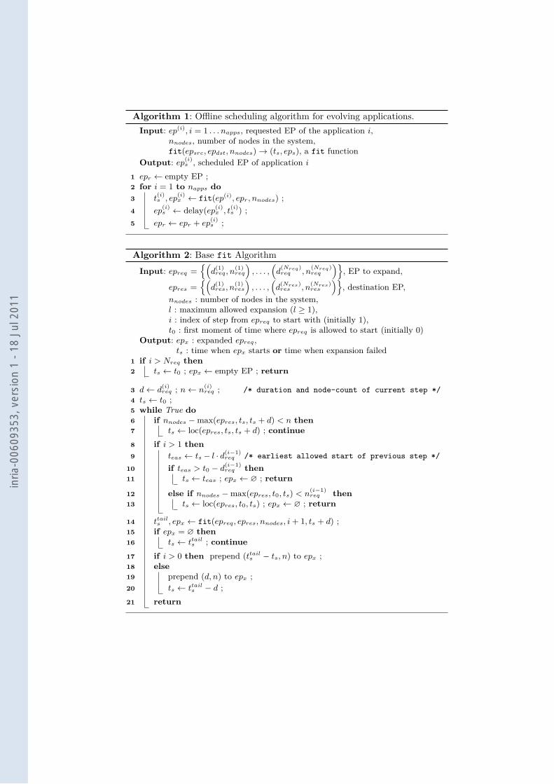
Algorithm 1 is an offline scheduling algorithm that solves the stated problem. Itstarts by initializing epr, the resource EP, representing how resource occupationevolves over time, to the empty EP. Then, it considers each requested EP, po-tentially expanding and delaying it using a helper fit function. The resultingscheduled EP ep

(i)s is added to epr, effectively updating the resource occupation.

The fit function takes as input the number of nodes in the system nnodes,a requested EP epreq and a resource EP epres and returns a time coordinate tsand epx an expanded version of epreq, such that ∀t, epres(t)+delay(epx, ts)(t) ≤nnodes. A very simple fit implementation consists in delaying epreq such thatit starts after epres.

Throughout the whole algorithm, the condition ∀t, epr(t) ≤ nnodes is guaran-teed by the post-conditions of the fit function. Since at the end of the algorithmepr =

∑napps

i=1 ep(i)s , resources will not be overflown.

4.2 The fit Function

The core of the scheduling algorithm is the fit function, which expands a re-quested EP over a resource EP. It returns a scheduled EP, so that the sum ofthe resource EP and scheduled EP does not exceed available resources.

Because it can expand an EP, the fit function is an element of the effi-ciency of a schedule. On one hand, a step can be expanded so as to interleaveapplications, potentially reducing their response time. On the other hand, whena step is expanded, the application cannot perform useful computations, thusresources are wasted. Hence, there is a trade-off between the resource usage, theapplication’s start time and its completion time.

In order to evaluate the impact of expansion, the proposed fit algorithmtakes as parameter the expand limit. This parameter expresses how manytimes the duration of a step may be increased. For example, if the expand limitis 2, a step may not be expanded to more than twice its original duration. Havingan expand limit of 1 means applications will not be expanded, while an infiniteexpand limit does not impose any limit on expansion.

Base fit Algorithm Algorithm 2 aims at efficiently computing the fit func-tion, while allowing to choose different expand limits. It operates recursively foreach step in epreq as follows:

inria

-006

0935

3, v

ersi

on 1

- 18

Jul

201

1

Algorithm 1: Offline scheduling algorithm for evolving applications.Input: ep(i), i = 1 . . . napps, requested EP of the application i,

nnodes, number of nodes in the system,fit(epsrc, epdst, nnodes)→ (ts, eps), a fit function

Output: ep(i)s , scheduled EP of application i

epr ← empty EP ;1for i = 1 to napps do2

t(i)s , ep

(i)x ← fit(ep(i), epr, nnodes) ;3

ep(i)s ← delay(ep(i)x , t

(i)s ) ;4

epr ← epr + ep(i)s ;5

Algorithm 2: Base fit AlgorithmInput: epreq =

{(d(1)req, n

(1)req

), . . . ,

(d(Nreq)req , n

(Nreq)req

)}, EP to expand,

epres ={(

d(1)res, n

(1)res

), . . . ,

(d(Nres)res , n

(Nres)res

)}, destination EP,

nnodes : number of nodes in the system,l : maximum allowed expansion (l ≥ 1),i : index of step from epreq to start with (initially 1),t0 : first moment of time where epreq is allowed to start (initially 0)

Output: epx : expanded epreq,ts : time when epx starts or time when expansion failed

if i > Nreq then1ts ← t0 ; epx ← empty EP ; return2

d← d(i)req ; n← n

(i)req ; /* duration and node-count of current step */3

ts ← t0 ;4while True do5

if nnodes −max(epres, ts, ts + d) < n then6ts ← loc(epres, ts, ts + d) ; continue7

if i > 1 then8teas ← ts − l · d(i−1)

req /* earliest allowed start of previous step */9

if teas > t0 − d(i−1)req then10

ts ← teas ; epx ← ∅ ; return11

else if nnodes −max(epres, t0, ts) < n(i−1)req then12

ts ← loc(epres, t0, ts) ; epx ← ∅ ; return13

ttails , epx ← fit(epreq, epres, nnodes, i+ 1, ts + d) ;14if epx = ∅ then15

ts ← ttails ; continue16

if i > 0 then prepend (ttails − ts, n) to epx ;17else18

prepend (d, n) to epx ;19ts ← ttails − d ;20

return21

inria

-006

0935

3, v

ersi

on 1

- 18

Jul

201

1

1. find ts, the earliest time coordinate when the current step can be placed, sothat nnodes is not exceeded (lines 4 – 7);

2. test if this placement forces an expansion on the previous step, which exceedsthe expand limit (lines 8 – 11) or exceeds nnodes (lines 12 – 13);

3. recursively try to place the next step in epreq, starting at the completiontime of the current step (line 14);

4. prepend the expanded version of the current step in epx (line 17). The firststep is delayed (i.e., ts is increased) instead of being expanded (line 20).

The recursion ends when all steps have been successfully placed (lines 1–2).Placement of a step is first attempted at time coordinate t0, which is 0 for

the first step, or the value computed on line 14 for the other steps. After everyfailed operation (placement or expansion) the time coordinate ts is increased sothat the same failure does not repeat:

– if placement failed, jump to the time after the encountered maximum (line 7);– if expansion failed due to the expand limit, jump to the first time which

avoids excessive expansion (computed on line 11, used on line 16).– if expansion failed due to insufficient resources, jump to the time after the

encountered maximum (computed on line 13, used on line 16);Since each step, except the first, is individually placed at the earliest possible

time coordinate and the first step is placed so that the other steps are notdelayed, the algorithm guarantees that the application has the earliest possiblecompletion time. However, resource usage is not guaranteed to be optimal.

Post-processing Optimization (Compacting) In order to reduce resourcewaste, while maintaining the guarantee that the application completes as earlyas possible, a compacting post-processing phase can be applied. After a firstsolution is found by the base fit algorithm, the expanded EP goes through acompacting phase: the last step of the applications is placed so that it ends at thecompletion time found by the base algorithm. Then, the other steps are placedfrom right (last) to left (first), similarly to the base algorithm. In the worst case,no compacting occurs and the same EP is returned after the compacting phase.

The base fit algorithm with compacting first optimizes completion timethen start time (it is optimal from expansion point-of-view), but because it actsin a greedy way, it might expand steps with high node-count, so it is not alwaysoptimal for resource waste.

4.3 DiscussionsThis section has presented a solution to the problem stated in Section 3.3. Thepresented strategies attempt to minimize both completion time and resourcewaste. However, these strategies treat applications in a pre-determined orderand do not attempt to do a global optimization. This allows the algorithm tobe easier to adapt to an online context in future work for two reasons. First,list scheduling algorithms are known to be fast, which is required in a scalableRMS implementation. Second, since the algorithms treat application in-order,starvation cannot occur.

inria

-006

0935

3, v

ersi

on 1

- 18

Jul

201

1

5 EvaluationThis section evaluates the benefits and drawbacks of taking into account evolvingresource requirements of applications. It is based on a series of experiments donewith a home made simulator developed in Python. The experiments are firstdescribed, then the results are analyzed.

5.1 Description of ExperimentsThe experiments compare two kinds of scheduling algorithms: rigid, which doesnot take into account evolution, and variations of Algorithm 1. Applications areseen by the rigid algorithm as non-evolving: the requested node-cound is themaximum node-count of all steps and the duration is the sum of the durationsof all steps. Then, rigid schedules the resulting jobs in a CBF-like manner.

Five versions of Algorithm 1 are considered to evaluate the impact of itsoptions: base fit with no expansion (noX), base fit with expand limit of 2 withoutcompacting (2X) and with compacting (2X+c), base fit with infinite expansionwithout compacting (infX) and with compacting (infX+c).

Two kinds of metrics are measured: system-centric and user-centric. Thefive system-centric metrics considered are: (1) resource waste, the resource area(nodes×duration, expressed as percent of total resources), which has been al-located to applications, but has not been used to make computations (see Sec-tion 3.2); (2) resource utilisation, the resource area that has been allocated toapplications; (3) effective resource utilisation, the resource area (expressed aspercent of total resources) that has been effectively used for computations; (4)makespan, the maximum of the completion times; (5) schedule time, the com-putation time taken by a scheduling algorithm to schedule one test on a laptopwith an Intel R©CoreTM2 Duo processor running at 2.53GHz.

The five user-centric metrics considered are: (1) per-test average applicationcompletion time (Avg. ACT); (2) per-test average application waiting time (Avg.AWT); (3) the number of expanded applications (num. expanded) as a percentageof the total number of applications in a test; (4) by how much was an applicationexpanded (App Expansion) as a percentage of its initial total duration; (5) per-application waste as a percentage of resources allocated to the application.

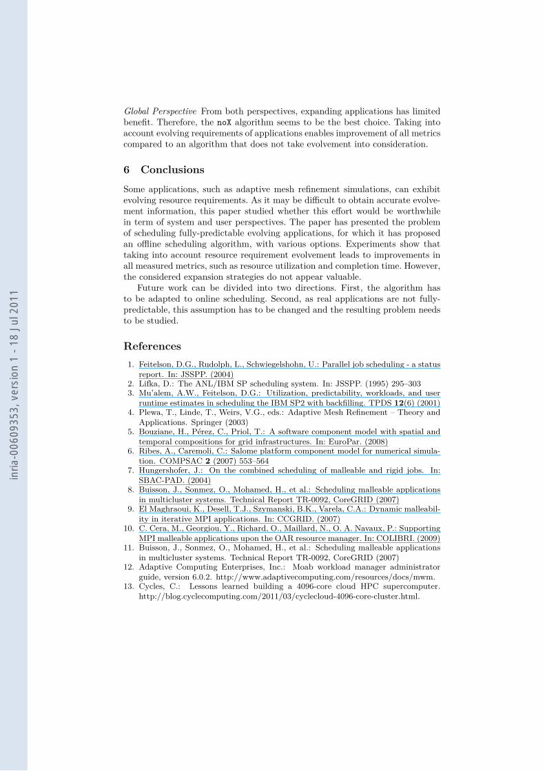
As we are not aware of any public archive of evolving application workloads,we created synthetic test-cases. A test case is made of a uniform random choiceof the number of applications, their number of steps, as well as the durationand requested node-count of each step. We tried various combinations that gavesimilar results. Table 1 and 2 respectively present the results for the system-and user-centric metrics of an experiment made of 1000 tests. The number ofapplications per test is within [15, 20], the number of steps within [1, 10], a stepduration within [500, 3600] and the node-count per step within [1, 75].

5.2 AnalysisAdministrator’s Perspective rigid is outperformed by all other strategies. Theyimprove effective resource utilisation, reduce makespan and drastically reduce

inria

-006

0935

3, v

ersi

on 1

- 18

Jul

201

1

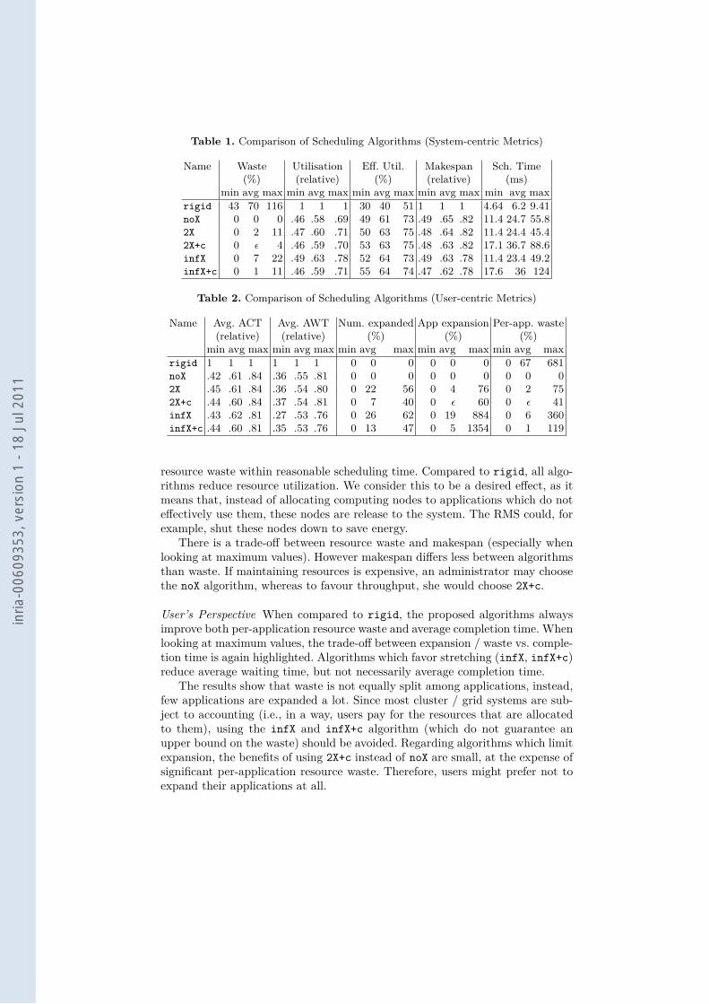
Table 1. Comparison of Scheduling Algorithms (System-centric Metrics)

Name Waste Utilisation Eff. Util. Makespan Sch. Time(%) (relative) (%) (relative) (ms)

min avg max min avg max min avg max min avg max min avg maxrigid 43 70 116 1 1 1 30 40 51 1 1 1 4.64 6.2 9.41noX 0 0 0 .46 .58 .69 49 61 73 .49 .65 .82 11.4 24.7 55.82X 0 2 11 .47 .60 .71 50 63 75 .48 .64 .82 11.4 24.4 45.42X+c 0 ε 4 .46 .59 .70 53 63 75 .48 .63 .82 17.1 36.7 88.6infX 0 7 22 .49 .63 .78 52 64 73 .49 .63 .78 11.4 23.4 49.2infX+c 0 1 11 .46 .59 .71 55 64 74 .47 .62 .78 17.6 36 124

Table 2. Comparison of Scheduling Algorithms (User-centric Metrics)

Name Avg. ACT Avg. AWT Num. expanded App expansion Per-app. waste(relative) (relative) (%) (%) (%)

min avg max min avg max min avg max min avg max min avg maxrigid 1 1 1 1 1 1 0 0 0 0 0 0 0 67 681noX .42 .61 .84 .36 .55 .81 0 0 0 0 0 0 0 0 02X .45 .61 .84 .36 .54 .80 0 22 56 0 4 76 0 2 752X+c .44 .60 .84 .37 .54 .81 0 7 40 0 ε 60 0 ε 41infX .43 .62 .81 .27 .53 .76 0 26 62 0 19 884 0 6 360infX+c .44 .60 .81 .35 .53 .76 0 13 47 0 5 1354 0 1 119

resource waste within reasonable scheduling time. Compared to rigid, all algo-rithms reduce resource utilization. We consider this to be a desired effect, as itmeans that, instead of allocating computing nodes to applications which do noteffectively use them, these nodes are release to the system. The RMS could, forexample, shut these nodes down to save energy.

There is a trade-off between resource waste and makespan (especially whenlooking at maximum values). However makespan differs less between algorithmsthan waste. If maintaining resources is expensive, an administrator may choosethe noX algorithm, whereas to favour throughput, she would choose 2X+c.

User’s Perspective When compared to rigid, the proposed algorithms alwaysimprove both per-application resource waste and average completion time. Whenlooking at maximum values, the trade-off between expansion / waste vs. comple-tion time is again highlighted. Algorithms which favor stretching (infX, infX+c)reduce average waiting time, but not necessarily average completion time.

The results show that waste is not equally split among applications, instead,few applications are expanded a lot. Since most cluster / grid systems are sub-ject to accounting (i.e., in a way, users pay for the resources that are allocatedto them), using the infX and infX+c algorithm (which do not guarantee anupper bound on the waste) should be avoided. Regarding algorithms which limitexpansion, the benefits of using 2X+c instead of noX are small, at the expense ofsignificant per-application resource waste. Therefore, users might prefer not toexpand their applications at all.

inria

-006

0935

3, v

ersi

on 1

- 18

Jul

201

1

Global Perspective From both perspectives, expanding applications has limitedbenefit. Therefore, the noX algorithm seems to be the best choice. Taking intoaccount evolving requirements of applications enables improvement of all metricscompared to an algorithm that does not take evolvement into consideration.

6 ConclusionsSome applications, such as adaptive mesh refinement simulations, can exhibitevolving resource requirements. As it may be difficult to obtain accurate evolve-ment information, this paper studied whether this effort would be worthwhilein term of system and user perspectives. The paper has presented the problemof scheduling fully-predictable evolving applications, for which it has proposedan offline scheduling algorithm, with various options. Experiments show thattaking into account resource requirement evolvement leads to improvements inall measured metrics, such as resource utilization and completion time. However,the considered expansion strategies do not appear valuable.

Future work can be divided into two directions. First, the algorithm hasto be adapted to online scheduling. Second, as real applications are not fully-predictable, this assumption has to be changed and the resulting problem needsto be studied.

References1. Feitelson, D.G., Rudolph, L., Schwiegelshohn, U.: Parallel job scheduling - a status

report. In: JSSPP. (2004)2. Lifka, D.: The ANL/IBM SP scheduling system. In: JSSPP. (1995) 295–3033. Mu’alem, A.W., Feitelson, D.G.: Utilization, predictability, workloads, and user

runtime estimates in scheduling the IBM SP2 with backfilling. TPDS 12(6) (2001)4. Plewa, T., Linde, T., Weirs, V.G., eds.: Adaptive Mesh Refinement – Theory and

Applications. Springer (2003)5. Bouziane, H., Perez, C., Priol, T.: A software component model with spatial and

temporal compositions for grid infrastructures. In: EuroPar. (2008)6. Ribes, A., Caremoli, C.: Salome platform component model for numerical simula-

tion. COMPSAC 2 (2007) 553–5647. Hungershofer, J.: On the combined scheduling of malleable and rigid jobs. In:

SBAC-PAD. (2004)8. Buisson, J., Sonmez, O., Mohamed, H., et al.: Scheduling malleable applications

in multicluster systems. Technical Report TR-0092, CoreGRID (2007)9. El Maghraoui, K., Desell, T.J., Szymanski, B.K., Varela, C.A.: Dynamic malleabil-

ity in iterative MPI applications. In: CCGRID. (2007)10. C. Cera, M., Georgiou, Y., Richard, O., Maillard, N., O. A. Navaux, P.: Supporting

MPI malleable applications upon the OAR resource manager. In: COLIBRI. (2009)11. Buisson, J., Sonmez, O., Mohamed, H., et al.: Scheduling malleable applications

in multicluster systems. Technical Report TR-0092, CoreGRID (2007)12. Adaptive Computing Enterprises, Inc.: Moab workload manager administrator

guide, version 6.0.2. http://www.adaptivecomputing.com/resources/docs/mwm.13. Cycles, C.: Lessons learned building a 4096-core cloud HPC supercomputer.

http://blog.cyclecomputing.com/2011/03/cyclecloud-4096-core-cluster.html.

inria

-006

0935

3, v

ersi

on 1

- 18

Jul

201

1