303

PRICING WEATHER DERIVATIVES USING THEINDIFFERENCE PRICING APPROACH

Patrick L. Brockett,* Linda L. Golden,† Min-Ming Wen,‡ and Charles C. Yang§

ABSTRACT

This paper adopts an incomplete market pricing model—the indifference pricing approach—toanalyze valuation of weather derivatives and the viability of the weather derivatives market in ahedging context. It incorporates price risk, weather/quantity risk, and other risks in the financialmarket. In a mean-variance framework, the relationship between the actuarial price and the in-difference price of weather derivatives is analyzed, and conditions are obtained concerning whenthe actuarial price does not provide an appropriate valuation for weather derivatives. Conditionsfor the viability of the weather derivatives market are examined. This paper also analyzes the effectsof partial hedging, natural hedges, basis risk, quantity risk, and price risk on investors’ indifferenceprices by examining the distributional impacts of the stochastic variables involved.

1. INTRODUCTION

Weather derivatives represent a recent development in hedging the risk arising from uncertain weatherconditions. According to the results of a 2006 survey for the Weather Risk Management Associationconducted by PriceWaterhouseCoopers, the notional value of weather derivatives traded on the ChicagoMercantile Exchange (CME) and the over-the-counter market for the summer and winter seasons of2004–2005 was $9.697 billion, and this grew to $45.244 billion for the summer and winter seasons of2005–2006. The CME reported 1,041,439 trades in summer 2005 and winter 2005–2006 combined,with 2005–2006 CME trades up over 300% compared to 2004–2005.

Weather derivatives are important in weather risk management for several reasons.1 First, globalbusinesses have large exposure to increasingly uncertain global weather conditions. For example, be-yond the energy and power industries where weather derivatives started, other industries such as ag-riculture, insurance, tourism, and retail businesses are also directly or indirectly affected by weather(e.g., Dischel 1998; Zeng 2000). The U.S. Department of Commerce has estimated that the weatheraffects about one-third of the U.S. economy. Second, compared to weather-related insurance products,weather derivatives are more economical and flexible and require no proof of loss (Dischel 1998).Furthermore, as noted by many authors (e.g., Zeng 2000; Platen and West 2004), the correlationbetween weather derivatives and other financial instruments appears to be low enough to make themattractive assets for diversification and portfolio formation (Brockett et al. 2006). Despite its phenom-enal growth in recent years, the development of the weather derivatives market is still impeded by thescarcity of widely accepted standard pricing techniques (e.g., Dischel 1998; Platen and West 2004).

* Patrick L. Brockett is Gus Wortham Chair in Risk Management and Insurance in the Department of Information, Risk and Operations Man-agement, Red McCombs School of Business, Global Research Fellow, IC2 Institute, University of Texas at Austin, Austin, TX 78712,brockett@mail.utexas.edu.† Linda L. Golden is Marlene and Morton Myerson Centennial Professor in Business in the Department of Marketing, Red McCombs School ofBusiness, Global Research Fellow, IC2 Institute, University of Texas at Austin, Austin, TX 78712, linda.golden@mccombs.utexas.edu.‡ Min-Ming Wen is Assistant Professor in Finance in the Department of Finance and Law, California State University, Los Angeles, CA 90032,mwen2@exchange.calstatela.edu.§ Charles C. Yang is Assistant Professor in Insurance and Risk Management in the Department of Finance, Barry Kaye College of Business,Florida Atlantic University, Boca Raton, FL 33431, cyang1@gau.edu.1 See Brockett, Wang, and Yang (2005) for a detailed description and overview of the weather derivatives market.

304 NORTH AMERICAN ACTUARIAL JOURNAL, VOLUME 13, NUMBER 3

Not surprisingly, the quest for new pricing techniques is imperative for the weather derivatives market(e.g., Dornier and Queruel 2000; Cao and Wei 2003).

The most distinctive feature of weather derivatives is that, unlike conventional derivatives, theirpayoffs are linked to weather events rather than the price of an underlying security or commodity. Thecommonly used underlying weather indexes—for example, heating degree days (HDDs) and coolingdegree days (CDDs)2—are nontradable, and there is typically little liquidity in the weather derivativesmarket (Davis 2001). Accordingly the traditional no-arbitrage pricing models of financial derivatives,such as the Black-Scholes (1973) model, cannot be directly applied to the pricing of weather derivatives(see, e.g., Dischel 1998; Zeng 2000; Cao and Wei 2003). Dornier and Queruel (2000) also note thatapplying the idea of delta hedging to create an equivalent risk-neutral portfolio for pricing weatherderivatives in an incomplete market without an underlying traded asset is not possible.

On the other hand, although actuarial valuation approaches have been very successful in the insur-ance market, they are not appropriate for pricing weather derivatives (Sloan, Palmer, and Burrow2002). One striking feature of the actuarial valuation principles is that they are formulated within aframework that generally ignores the financial market. However, weather events evidently affect theprices of some liquid assets in the financial market, and weather derivatives can therefore be partiallyhedged by these liquid assets that are stochastically related to the payoff of weather derivatives (Craft1998; Hirshleifer and Shumway 2003; Kamstr, Kramer, and Levi 2000; Roll 1984; Saunders 1993).

The weather derivatives market is a classic incomplete market (Davis 2001). In principle, incompletemarket pricing models are more appropriate for the valuation of weather derivatives because theyacknowledge both the hedgeable and unhedgeable parts of a risk. Various alternative pricing mecha-nisms have been developed for the incomplete market, such as super-replication (El Karoui and Quenez1995), quadratic approaches (Follmer and Sondermann 1986; Schweizer 1988, 1991; Bouleau andLamberton 1989; Duffie and Richardson 1991), quantile hedging and shortfall minimization (Follmerand Leukert 1999, 2000; Cvitanic 1998), marginal utility approach (Davis 1998), and indifferencepricing (Hodges and Neuberger 1989; Davis, Panas, and Zariphopoulou 1993).

The particular problem of valuation of weather derivatives has also been explored in the literature.For example, Cao and Wei (2003) propose and implement an equilibrium representative agent frame-work for pricing weather derivatives. They generalize the Lucas (1978) model to include weather as afundamental variable in the economy. Davis (2001) gives an exploration of weather derivative pricingusing the marginal utility approach from mathematical economics, based on the idea that agents inthe weather derivatives market are not representative but face very specific risks related to the effectof weather on their business. Based on a utility maximization point of view, Barrieu and El Karoui(2002) determine the optimal profile and value of a derivative written on an illiquid asset, such as acatastrophic or a weather event.

The purpose of this paper is to apply the indifference pricing approach to value weather derivativesand use weather futures/forwards and weather options as examples to illustrate the model. This papervalues weather derivatives in a hedging context, in which hedgers use weather derivatives to hedgetheir weather risks and maximize their expected utility. In practice, weather derivatives are commonlyvalued by the expected payoff under the physical measure, discounted at the riskless rate (Davis 2001):that is, they are valued by the actuarial approach.

This paper extends the literature by incorporating price risk, weather/quantity risk, and other risksin the financial market by analyzing the relationship between the actuarial price and the indifferenceprice of weather derivatives and by examining the conditions under which the actuarial price does notyield an appropriate valuation for weather derivatives. The viability of the weather derivatives market

2 Because one need not heat if the temperature is above 65�F, daily HDD � Max(0, 65�F � daily average temperature). Similarly, because onedoes not need to cool if the temperature is below 65�F, daily CDD � Max(0, daily average temperature � 65�F). Weather derivatives are basedon the accumulation of HDDs or CDDs during a certain period (contract period), e.g., one calendar month, or a winter/summer season. Tocalculate the degree days over a period, simply aggregate the daily degree days of each day in that period.

PRICING WEATHER DERIVATIVES USING THE INDIFFERENCE PRICING APPROACH 305

is also analyzed by examining the indifference prices of investors in this market. The weather derivativemarket is a new derivative market and still immature, and the examination of market viability providesimportant insights for the investors in the weather derivative market. In addition, the indifferenceprices derived in this research can serve as important benchmark prices for the market players.

Partial hedging, natural hedges, and basis risk are all important issues in corporate hedging. However,to the best of our knowledge none of the previous research has examined their impacts on the valueof weather derivatives.3 Weather derivatives can be hedged partially in the financial markets by thoseliquid assets that are stochastically related to weather indexes. A natural hedge occurs when one riskis offset by another one in the hedger’s business. For instance, a company whose commodity price andquantity demand move in the opposite directions holds a natural hedge. Basis risk occurs when aweather contract is written in a different location than the area that a hedger wishes to cover. Byexamining the distributional impacts of the stochastic variables involved, this paper also extends theliterature by analyzing the effects of partial hedging, natural hedges, and basis risk, as well as quantityrisk and price risk on an investors’ indifference prices.

The next section introduces the general indifference pricing approach and presents the specificindifference pricing model used in this research. The results of the derivations of indifference pricesand market viability are also provided in this section. Section 3 analyzes the distributional impacts ofthe stochastic variables on both linear and nonlinear weather contracts. We conclude with a summaryand some ideas for future research.

2. MODEL SPECIFICATION AND INDIFFERENCE PRICES OF WEATHER DERIVATIVES

The indifference pricing approach stems from the basic principle of equivalent utility.4 This method isbased on expected utility arguments and produces the reservation prices. It is built around the inves-tors’ preferences toward risks that cannot be eliminated because of market incompleteness. The indif-ference pricing approach has been applied to pricing traditional financial derivatives in incompletemarket (e.g., Hodges and Neuberger 1989; Davis, Panas, and Zariphoupoulou 1993; Eydeland and Ge-man 1999; Henderson 2002; Owen 2001; Zariphopoulou 2001), to pricing insurance products in thefinancial market (e.g., Moore and Young 2003; Young and Zariphopoulou 2002; Moller 2003; Young2003), and to pricing some other derivatives with exotic underlyings (e.g., Barrieu and El Karoui 2002;Musiela and Zariphopoulou 2002).

To illustrate the general indifference pricing approach,5 this paper assumes a dynamic market settingthat consists of two assets, a stock with a price process S � (St)0�t�T, where T is a fixed finite timehorizon, and a savings account with a price process that is constant and equal to one, as well as anontraded asset Yt on which a European-type claim is written. The payoff of this European derivative isdenoted by g(Yt), payable at time T. Moreover, no trading of the derivative is allowed after its inscrip-tion/purchase. The individual risk preferences are modeled via a utility function u. In this model theinvestor seeks to maximize the expected utility of terminal wealth with and without taking into accountthe European claim.

The optimization problem without considering this financial claim is the classical Merton model ofoptimal investment (Merton 1969, 1971), namely,

T

V(w) � sup Eu(w � � � dS ), (2.1)t t0�

where w denotes the initial wealth of the investor and �t represents his or her investment strategy (orthe composition of his or her investment portfolio of the risky asset and the risk-free asset at time t).

3 Golden, Wang, and Yang (2007) examine credit and basis risk for weather derivatives, and Golden, Yang, and Zou (2009) discuss theeffectiveness of using basis derivatives for managing weather-related risks.4 See Gerber and Pafumi (1998) for a detailed overview of the principle of equivalent utility.5 In the introduction of the general indifference pricing approach, this paper presents the continuous-time model. The discrete-time modeladopted in this paper will be presented later as a special case.

306 NORTH AMERICAN ACTUARIAL JOURNAL, VOLUME 13, NUMBER 3

Considering the possibility of buying/selling � units of this financial claim, the buyer’s and seller’soptimization problems are defined, respectively, by

Tb bV (w) � sup Eu w � � � dS � �� � �g(Y ) (2.2)� �t t T

0�

and

Ts sV (w) � sup Eu w � � � dS � �� � �g(Y ) , (2.3)� �t t T

0�

where �b and �s denote the prices of buying and selling one unit of this financial claim, respectively.The seller’s (buyer’s) indifference price of the European claim g(YT) is defined as �s(�b), such that

the investor is indifferent to the following two scenarios: (1) optimize his or her expected utility withoutemploying the derivative and (2) optimize his or her expected utility taking into account, on one hand,the liability (payoff) g(YT) at expiration T and, on the other hand, the compensation �s (cost �b).Therefore, the indifference prices �s(�b) must satisfy

T Tssup Eu w � � � dS � sup Eu w � � � dS � �� � �g(Y ) (2.4)� � � �t t t t T

0 0� �

and

T Tbsup Eu w � � � dS � sup Eu w � � � dS � �� � �g(Y ) . (2.5)� � � �t t t t T

0 0� �

The most popular weather derivatives are based on temperature indexes such as HDDs, CDDs, andcumulative average temperature (CAT). Weather derivatives are designed to hedge weather risks for aspecific time period (a contract term). The most popular contract terms are a week, a month, or aseason. The HDD or CDD index values are the sum of each daily HDD or CDD value, whereas the CATindex is the accumulation of each daily average temperature, during a specific contract term. Becauseof this structure of weather derivatives, hedgers generally hold weather derivatives for the whole con-tract term (or the hedging period) till maturity.6 Therefore, this paper adopts a two-date model thatis more appropriate than the multiperiod or the continuous-time setting for this research.

In this two-date model, the financial market consists of two assets, a risky asset (such as a stock,the market portfolio, or a subset of the market portfolio) with a random rate of return r at date 1 anda savings account with a gross risk-free rate of return rf, as well as a random weather index y on whicha weather derivative can be written. The payoff of this weather derivative is denoted by Ry. In thisresearch the investors’ risk preferences are modeled by the mean-variance utility function

2u(x) � E(x) � �� (x), (2.6)

with the risk aversion parameter � � 0. Higher expected wealth improves firm value, whereas highervolatility imposes costs due to increases in the likelihood of financial distress and/or effects on futureinvestment incentives. The mean-variance utility function has been widely used in the literature (e.g.,Duffie and Richardson 1991; Vukina, Li, and Holthausen 1996; Doherty and Richter 2002; Bessem-binder and Lemmon 2002); however, other objective functions such as the exponential utility and thepower utility could be applied similarly.

In our models the investor seeks to maximize the mean variance of his or her terminal wealth atdate 1 under the scenarios with and without taking into account the weather derivative. The buyer (or

6 Even assuming that the weather derivative is bought/sold initially and the position in that single instrument is unchanged, it is certainlypossible that the investor may dynamically rebalance the weights in other securities in the portfolio. We leave the impact of the dynamicrebalancing to future work. We are using a static model because it is also mathematically simpler, and possibly easier to implement.

PRICING WEATHER DERIVATIVES USING THE INDIFFERENCE PRICING APPROACH 307

hedger)7 considered in this research is typified by an electric power provider with random powerdemand q and random unit power price p at date 1,8 and the seller (or issuer) of weather derivativescan be an investment bank, an insurance company, or an energy trading company. Our model incor-porates price risk (p), weather/quantity risk (q), and other risks (r) in the financial market and valuesweather derivatives in a hedging context in which hedgers use weather derivatives to hedge theirweather risks and maximize their utility of terminal wealth.

First, we analyze the buyer’s indifference prices of weather derivatives. Without weather hedging, theoptimal portfolio choice problem of the buyer is

bV � Max u[(w � a)r � ar � pq], (2.7)1 fa

where (w � a)rf � ar � pq is the buyer’s terminal wealth at date 1, in which a is the amount investedin the risky asset, w � a is the amount invested in the risk-free asset, w denotes the initial wealth ofthe investor, and pq is the buyer’s revenue from power supply. Taking into consideration using a weatherderivative to hedge the weather risk, the optimal portfolio choice problem of the buyer becomes

b bV � Max u[(w � �� )r � a(r � r ) � pq � �R ], (2.8)2 f f ya

where �b is the buying price of the weather derivative. Under the mean-variance utility function, thebuyer’s indifference price of the weather derivative is

b b� ( � r � 2� � � �� � )1 r,R r f r,pq r,Ry yb b 2 b� � � �� � � 2� � � . (2.9)� �R R pq,Ry y y 2r �f r

Because of the prominent role of the risk aversion parameter �, the investors’ indifference pricescan be highly subjective. Generally, one participant’s indifference price should not be used to determinethe general viability of a market. However, the weather derivatives transactions are mostly over-the-counter customized deals between a buyer and a seller even though some weather derivatives are listedfor trading at some exchanges such as the CME. Investors’ indifference prices provide important bench-marks to the market players in the customized weather derivatives markets.9

For the market to be viable, the market price of the weather derivative must be between the seller’sindifference price and the buyer’s indifference price: that is, the market price is no higher than thebuyer’s indifference price. Therefore, if the buyer’s indifference risk premium—the difference between�b and the risk-free-rate discounted price /rf —is negative:Ry

b b� ( � r � 2� � � �� � )1 r,R r f r,pq r,Ry yb 2 b�� � � 2� � � � 0, (2.10)� �R pq,Ry y 2r �f r

7 Generally, hedgers take a short position in forwards/futures, and the payoff of a long position in a forward/future is y � K. In this paper thepayoff of a long position in a forward/future is specified as K � y so that hedgers buy long (issuers sell short) both forwards/futures and putoptions, which then can be analyzed in a single buyer’s model. Otherwise we have to present two models for hedgers alone: one for buyingput options and the other one for selling forwards/futures (and for issuers: one model for selling put options and the other one for buyingforwards/futures). This avoids much clumsiness by presenting fewer models/equations. However, this specification does not affect our analysesof the indifference prices of weather contracts.8 p and q are introduced separately because weather derivatives are designed to hedge quantity risk instead of price risk.9 Indifference prices are also very important even for the exchange market. Hedgers have to know their indifference prices to determine ifparticipating in the exchanges’ market will achieve their hedging objectives and maximize their utility. In this sense the market makers haveto set the market clearing price in the range of investors’ subjective prices (i.e., indifference prices) to attract enough participants for themarket to be viable. However, the market clearing price will be determined by indifference prices of a majority of investors instead of only afew potential participants.

308 NORTH AMERICAN ACTUARIAL JOURNAL, VOLUME 13, NUMBER 3

that is,b 2 2 2 2� [�(� � � � ) � 2(� � � � � )] � � ( � r ), (2.11)r,R r R r,R r,pq r pq,R r,R r fy y y y y

then �M � /rf : the market price of the weather derivative, �M, must be lower than its expectedRy

discounted value discounting at the risk-free rate and under the physical measure (actuarial price),and thus the actuarial price is not an appropriate valuation of the weather derivative.

Consider a weather forward contract with tick size of $1 and delivery price K. The buyer’s (orhedger’s) payoff for this contract is specified as Ry � K � y, where y is the weather index. The indif-ference price of the weather forward can be expressed as

b b� ( � r � 2� � � �� � )1 r,y r f r,pq r,yb b 2 b� � (K � ) � �� � � 2� � � . (2.12)� �f y y pq,y 2r �f r

The indifference forward price Fb is the value of K that makes equal to 0, that is,b�f

b b� ( � r � 2� � � �� � )r,y r f r,pq r,yb b 2 bF � � �� � � 2� � � . (2.13)y y pq,y 2�r

Similarly, for the market to be viable, the market forward price must be no lower than the buyer’sindifference forward price. Therefore, if the buyer’s indifference forward risk premium is positive:

b b� ( � r � 2� � � �� � )r,y r f r,pq r,yb 2 b�� � � 2� � � � 0, (2.14)y pq,y 2�r

that is,b 2 2 2 2� [�(� � � � ) � 2(� � � � � )] � � ( � r ), (2.15)y r r,y r,y r,pq r pq,y r,y r f

then FM � y. Hence the market forward price of the weather index, FM, must be higher than itsexpected value under the physical measure.

Next, we analyze the seller’s indifference price of weather derivatives. Without taking into accounta weather derivative, the optimal portfolio choice problem for the seller is

sV � Max u[wr � a(r � r )]. (2.16)1 f fa

Taking into account a weather derivative, the optimal portfolio choice problem for the seller becomess sV � Max u[(w � �� )r � a(r � r ) � �R ], (2.17)2 f f y

a

where �s is the selling price of the weather derivative. Accordingly, under the mean-variance utilityfunction, the seller’s indifference price of the weather derivative is

s� ( � r � � �� )1 r;R r f r,Ry ys s 2� � � � �� � . (2.18)� �R Ry y 2r �f r

For the market to be viable, the market price of the weather derivative must be no lower than theseller’s indifference price. Therefore, if the seller’s indifference risk premium is positive:

s� ( � r � � �� )r,R r f r,Ry ys 2� �� � � 0, (2.19)Ry 2�r

that is,

� ( � r )r,R r fys� � , (2.20)2 2 2�(� � � � )R r r,Ry y

PRICING WEATHER DERIVATIVES USING THE INDIFFERENCE PRICING APPROACH 309

then �M � /rf. Thus, the market price of the weather derivative, �M, must be higher than itsRy

expected discounted value discounting at the riskless rate and under the physical measure. This in-equality holds when � 0. Hence, when the return of the risky asset and the payoff of the weatherr,Ry

derivative are negatively correlated, the actuarial price is not an appropriate market price for thisweather derivative.

Similar results apply to the seller’s (or issuer’s) indifference forward price. The seller’s indifferenceprice for a weather forward with payoff Ry � K � y can be expressed as

s� ( � r � � �� )1 r,y r f r,ys s 2� � K � � � �� � . (2.21)� �y y 2r �f r

The indifference forward price iss� ( � r � � �� )r,y r f r,ys s 2F � � � �� � . (2.22)y y 2�r

In a viable market the market forward price must be no higher than the seller’s indifference forwardprice. Therefore, if the seller’s indifference forward risk premium is negative:

s� ( � r � � �� )r,y r f r,ys 2� �� � � 0, (2.23)y 2�r

that is,

� ( � r )r,y r fs� � , (2.24)2 2 2�(� � � � )r,y y r

then FM � y, the market forward price of the weather index, FM, must be lower than its expectedvalue under the physical measure, if the market does exist. This inequality holds when (r; y) � 0:when weather events have a positive impact on the return of the risky asset in the financial market,actuarial forward price is not an appropriate market forward price in the weather derivatives market.

Clearly a weather derivative market transaction is possible only if the buyer’s indifference price is nolower than the seller’s indifference price. Therefore, another necessary condition for market viabilityshould be �b � �s. This necessary condition can be stated as

2b s 2� � � 2� �� � � r,R r,pq pq,R ry y� . (2.25)b 2 2 2� �� � � ��R r r,Ry y

3. DISTRIBUTIONAL IMPACTS OF THE STOCHASTIC VARIABLES

This section analyzes the effects of partial hedging, natural hedges, basis risk, quantity risk, and pricerisk on the buyer’s indifference forward premium and indifference prices of put options. Specificallywe analyze the distributional impacts of the stochastic variables involved. Distributional impacts on theseller’s indifference forward premium and indifference prices of put options can be analyzed similarly.

For a weather forward contract with tick size of $1, delivery price of K, and payoff Ry � K � y, wherey is the weather index, the buyer’s indifference forward premium, FPb, is

b b� ( � r � 2� � � �� � )r,y r f r,pq r,yb b b 2 bFP � F � � �� � � 2� � � . (3.1)y y pq,y 2�r

For simplicity and without loss of generality, let � � 1 and �b � 1. Restated in the volatility of thestochastic variables and their correlations, the indifference forward premium can be expressed as

310 NORTH AMERICAN ACTUARIAL JOURNAL, VOLUME 13, NUMBER 3

� rr fb 2 2FP � (1 � )� � � � 2� � � 2� � . (3.2)r,y y y r,y y r,y r,pq pq y pq,y pq�r

Assume that the stochastic variables are multivariate normally distributed (other distributional mod-els can be analyzed by conducting a series of simulations). Following Vukina, Li, and Holthausen (1996),

� � � p q q,y q p p,y � (3.3)pq,y �pq

and

� � � p q q,r q p p,r � . (3.4)pq,r �pq

Therefore,

� rr fb 2 2FP � (1 � )� � � � 2 � � � 2 � � r,y y y r,y p y q q,y q y p p,y�r

� 2 � � � 2 � � . (3.5)p y q r,y q,r q y p r,y p,r

Weather derivatives are designed to hedge weather risks, which are primarily considered as volume/quantity risks caused by weather events.10 Basis risk occurs when a weather derivative is written onan index that is calibrated in a different location than the area that a hedger wishes to cover. Basisrisk of the weather forward contract can be represented by the correlation coefficient between theweather index and the quantity demanded, q,y (higher q,y indicates lower basis risk). Note that�FPb/�q,y � �2p�q�y � 0. Therefore, ceteris paribus, the buyer’s indifference forward premiumincreases in basis risk (decreases in q,y): the higher the basis risk, the lower the buyer’s indifferenceforward premium.

A dirty hedge occurs when a derivative security cannot be fully hedged with liquid exchange-tradedsecurities and/or its risk exposure changes over time or in response to changes in a secondary under-lying variable. Weather derivatives can also be used as a ‘‘dirty hedge’’ of power price risk if the cor-relation between the power price and the weather index is not zero (p,y � 0). Note that �FPb/�p,y ��2q�p�y � 0. Therefore, ceteris paribus, the buyer’s indifference forward premium decreases in thecorrelation between the power price and the weather index p,y (increases in the basis risk of this ‘‘dirtyhedge’’).

In our model a natural hedge happens when q,yp,y � 0. For a power provider, it is very likely thatthe correlation between the weather index and the quantity demanded is positive (q,y � 0). Therefore,a natural hedge occurs when the correlation between the weather index and the power price is negative(p,y � 0), whereas there is no natural hedge if p,y is also positive. Ceteris paribus, the buyer’s indif-ference forward premium is higher in the case when a natural hedge exists than that when there is nonatural hedge for the power provider.

Weather derivatives can be hedged partially in the financial markets by those liquid assets that arestochastically related to the payoff of weather derivatives. This partial hedging effect can be character-ized by the correlation coefficient y,r. Similarly, the hedging effects on the power provider’s price riskand quantity risk using the risky asset in the financial market can be characterized by the correlationcoefficients p,r and q,r, respectively.11 Note that

10 The volume/quantity risk is the risk that results from a change in the demand for goods due to a change in the weather.11 Weather risks are primarily quantity risks. Instead of treating the hedger’s income as one general random endowment, we introduce priceand quantity risk separately so that we are modeling quantity risk or weather risk explicitly. This makes the paper specifically related to weatherderivatives or the modeling of weather risks.

PRICING WEATHER DERIVATIVES USING THE INDIFFERENCE PRICING APPROACH 311

b�FP� 2 � � , (3.6)p q y r,y�q,r

b�FP� 2 � � . (3.7)q p y r,y�p,r

Therefore, if r,y � 0, ceteris paribus, the buyer’s indifference forward premium increases in q,r andp,r, vice versa. When �FPb/(�r,y) � 0, that is,

� � � rq p r f � � � , (3.8)r,y q,r p p,r q� � 2� �y y y r

ceteris paribus, the buyer’s indifference forward premium increases in r,y. Otherwise the buyer’s in-difference forward premium decreases in r,y: that is, the buyer’s indifference forward premium initiallyincreases and then decreases in r,y.

The results also indicate how the price risk and quantity risk are related to the buyer’s indifferenceforward premium. Note that

b�FP� 2 � ( � ), (3.9)p y q,r r,y q,y��q

b�FP� 2 � ( � ). (3.10)q y p,r r,y p,y��p

Therefore, if r,yq,r � q,y, ceteris paribus, the indifference forward premium increases in the standarddeviation of the quantity demanded �q, and vice versa. If r,yp,r � p,y, ceteris paribus, the indifferenceforward premium increases in the standard deviation of the power price �p, and vice versa. We can alsosee that, ceteris paribus, if weather events have a positive impact on the return of the risky asset inthe financial market (r,y � 0), the buyer’s indifference forward premium decreases in the market priceof risk of the risky asset, r � rf/�r, and vice versa.

Similar distributional impacts apply to the buyer’s indifference prices of put options. For a weatherput option with tick size of $1, strike price K, and payoff � max(K � y, 0), the buyer’s indifferencepRy

price, isb� ,p

b bp p� ( � r � 2� � � �� � )1 r,R r f r,pq r,Ry yb b 2 b

p p p� � � �� � � 2� � � . (3.11)� �p R R pq,R 2y y yr �f r

Because of the nonlinear structure of weather put options, the effects of the determinants (such asthe correlation among the stochastic variables involved) of the indifference price cannot be clearlyidentified from the closed-form formula itself. Therefore, a series of simulations are conducted to clearlyillustrate the effects of the determinants of a buyer’s indifference price of a put option.

We assume that the stochastic variables are multivariate normally distributed. Without loss of gen-erality, rf, �, and �b are all assumed to be 1. The buyer’s indifference price of a put option is computedfrom 20,000 simulation realizations of (r, y, p, and q).12 As in Bessembinder and Lemmon (2002), themagnitude of the simulated indifference prices can be made arbitrarily large or small by varying relatedparameters. However, the simulations are useful in terms of clarifying the determinants of indifferenceprices.

12 5,000, 10,000, 20,000, and 50,000 simulations are all tried, and 20,000 simulations are large enough to have a good convergence of theMonte Carlo.

312 NORTH AMERICAN ACTUARIAL JOURNAL, VOLUME 13, NUMBER 3

Table 1A Buyer’s Indifference Price of a Put Option at Different Levels of �q,y and �p,y

�q,y

0.0 0.1 0.2 0.3 0.4 0.5 0.6 0.7 0.8

0.0 �9.33 �7.90 �6.64 �5.59 �3.92 �2.30 �1.03 0.83 2.230.1 �8.43 �5.83 �4.84 �3.50 �2.43 �0.56 1.05 2.27 3.410.2 �6.15 �5.96 �3.60 �2.31 �0.46 0.67 2.91 3.95 4.850.3 �5.07 �3.28 �1.95 �0.54 0.40 2.26 3.42 5.03 6.43

p,y 0.4 �3.98 �1.62 �0.53 1.08 2.05 4.17 4.52 7.12 7.660.5 �2.33 �0.58 1.38 1.69 3.28 4.75 6.45 7.45 9.220.6 �0.87 0.41 2.01 3.59 5.20 6.59 7.59 8.98 10.170.7 0.82 3.11 3.84 5.61 6.46 7.82 8.72 10.42 11.920.8 2.58 4.16 5.32 6.55 7.79 9.12 10.58 11.36 13.25

Note: r, y, p, and q are assumed to be multivariate normally distributed. r � N(1.05,0.22), y � N(100,202), q � N(15,32), and p � N(2.5,0.52).r,y � 0.5, p,r � 0.5, q,r � 0.5, and p,q � 0.5. K � y � 100. All estimates are computed using 20,000 simulation runs.

Table 2A Buyer’s Indifference Price of a Put Option at Different Levels of �r,y, �q,r , and �p,r

�r,y

0.0 0.1 0.2 0.3 0.4 0.5 0.6 0.7 0.8

0.0 11.67 11.17 11.06 10.79 11.04 11.55 12.28 — —0.1 11.37 11.12 10.62 10.47 10.33 10.68 11.20 — —

q,r0.2 11.39 10.70 10.31 10.13 10.09 10.24 10.27 — —

(p,r � 0.5)0.3 11.29 10.67 10.25 9.61 9.26 9.24 9.51 — —0.4 11.49 10.59 9.75 9.36 8.84 8.57 8.55 — —0.5 11.49 10.48 9.39 8.69 8.05 7.70 7.57 — —0.6 11.30 10.29 8.99 8.20 7.48 6.93 6.43 — —

0.0 11.48 11.23 11.19 10.83 11.05 11.53 12.15 13.00 14.260.1 11.56 11.18 10.84 10.27 10.65 10.90 11.04 11.86 12.880.2 11.48 10.92 10.22 10.04 9.89 10.12 10.25 10.55 11.62

p,r 0.3 11.81 10.54 9.89 9.53 9.32 9.39 9.34 9.88 10.31(q,r � 0.5) 0.4 11.38 10.39 9.90 9.19 8.67 8.30 8.12 8.81 9.13

0.5 11.44 10.40 9.47 8.41 7.86 7.93 7.50 7.70 8.080.6 11.62 10.32 9.17 8.40 7.20 6.86 6.24 6.79 6.840.7 11.66 10.11 8.67 7.88 7.18 6.18 5.74 5.46 5.54

Note: r, y, p, and q are assumed to be multivariate normally distributed. r � N(1.05,0.22), y � N(100,202), q � N(15,32), and p � N(2.5,0.52).q,y � 0.7, p,y � 0.5, and p,q � 0.5. K � y � 100. All estimates are computed using 20,000 simulation runs.

Table 1 displays the buyer’s indifference price of a put option under different levels of q,y and p,y.13

The results indicate that the buyer’s indifference price of a put option increases in both the correlationcoefficient of y and p and that of y and q. This reflects that hedgers are willing to pay more for weatherderivatives with less basis risk. The results also indicate that the sensitivity of this indifference priceto the correlation coefficient of y and p(q) is almost the same at different levels of q,y(p,y).

Table 2 reports the buyer’s indifference price of a put option under different levels of y,r, q,r, andp,r. The simulation results suggest that the buyer’s indifference price of a put option decreases in p,r

and q,r when y,r � 0, and the sensitivity is greater when y,r is larger. The intuition is that, wheny,r � 0, a larger value in p,r or q,r implies a higher risk of the buyer’s portfolio, and thus a lower

13 In the simulations some indifference prices are negative under some scenarios. Negative indifference prices indicate that a ‘‘buyer’’ wouldlike to ‘‘get paid’’ to ‘‘buy’’ a weather contract instead of paying a price. One possible explanation is that using this weather contract to‘‘hedge’’ weather risk will actually increase the hedger’s total risk level. Therefore, the hedger will not use this weather contract for hedgingor will require to get paid to ‘‘buy’’ this weather contract for taking a higher risk. It is obvious that the market will never exist under thesescenarios, and no arbitrage will occur because most probably no seller is willing to ‘‘pay’’ to ‘‘sell’’ a weather contract with a nonnegativepayoff to the buyer.

PRICING WEATHER DERIVATIVES USING THE INDIFFERENCE PRICING APPROACH 313

Table 3A Buyer’s Indifference Price of a Put Option at Different Levels of �q,y and �q

�q,y

0.0 0.1 0.2 0.3 0.4 0.5 0.6 0.7 0.8 0.9

2.00 �0.46 0.63 0.90 1.88 3.12 4.06 5.05 5.60 6.70 7.992.25 �0.79 0.00 1.05 2.15 2.92 4.24 5.50 6.32 7.31 8.042.50 �1.41 0.17 1.29 2.63 3.21 4.73 5.86 7.12 8.25 8.85

�q 2.75 �1.66 �0.16 0.98 2.15 3.67 4.68 6.14 7.46 8.39 9.82(p � 2.5) 3.00 �1.96 �0.46 1.15 2.07 3.82 4.74 6.51 7.67 9.31 10.41

3.25 �2.36 �0.48 1.00 2.15 3.97 5.40 6.88 8.52 9.57 10.993.50 �2.73 �1.22 �0.02 2.51 4.05 5.64 7.30 8.42 10.50 11.813.75 �3.21 �1.01 0.57 2.03 4.15 6.02 7.77 9.26 11.03 12.974.00 �3.26 �1.38 0.59 2.41 4.27 5.83 8.13 10.01 11.68 13.53

Note: r, y, p, and q are assumed to be multivariate normally distributed. r � N(1.05,0.22), y � N(100,202), q � 15, and �p � 0.5. r,y � 0.5,p,r � 0.5, p,y � 0.5, q,r � 0.5, and (p;q) � 0.5. K � y � 100. All estimates are computed using 20,000 simulation runs.

Table 4A Buyer’s Indifference Price of a Put Option at Different Levels of �p,y and �p

�p,y

0.0 0.1 0.2 0.3 0.4 0.5 0.6 0.7 0.8 0.9

0.1 3.99 4.60 4.78 4.57 5.39 5.59 5.99 5.85 6.02 6.570.2 2.99 4.11 4.65 5.03 5.50 5.90 6.59 7.17 7.48 8.310.3 2.13 3.61 4.01 4.99 5.63 6.42 7.31 8.11 9.13 9.97

�p 0.4 1.60 3.17 4.21 5.34 5.96 7.38 8.01 9.32 10.12 11.48(q � 15) 0.5 0.89 2.04 4.46 5.43 6.28 7.51 9.45 10.34 11.48 12.94

0.6 0.62 1.71 3.14 4.60 6.55 8.48 10.07 11.70 12.53 14.920.7 �0.46 1.61 2.80 5.73 7.30 9.31 11.10 12.58 14.61 16.110.8 �1.03 1.36 2.85 5.22 7.39 9.94 11.38 14.09 16.14 18.250.9 �1.76 0.37 2.53 5.03 8.12 10.12 12.55 15.23 17.23 19.90

Note: r, y, p, and q are assumed to be multivariate normally distributed. r � N(1.05,0.22), y � N(100,202), �q � 3, and p � 2.5. r,y � 0.5,p,r � 0.5, q,y � 0.7, q,r � 0.5, and p,q � 0.5. K � y � 100. All estimates are computed using 20,000 simulation runs.

indifference price that the buyer is willing to pay for this put option. Similarly, the buyer’s indifferenceprice for the put option increases in p,r and q,r when y,r � 0. The results also indicate that the buyer’sindifference price for the put option initially decreases and then increases, in y,r.

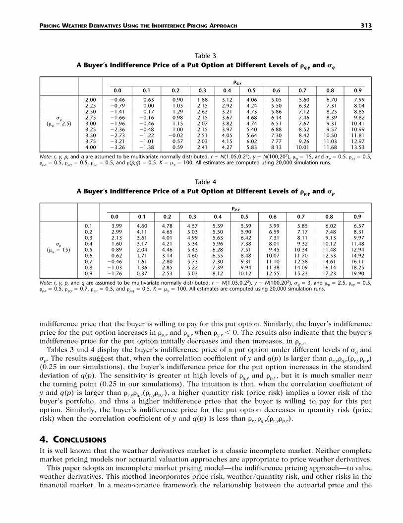
Tables 3 and 4 display the buyer’s indifference price of a put option under different levels of �q and�p. The results suggest that, when the correlation coefficient of y and q(p) is larger than r,yq,r(r,yp,r)(0.25 in our simulations), the buyer’s indifference price for the put option increases in the standarddeviation of q(p). The sensitivity is greater at high levels of q,y and p,y, but it is much smaller nearthe turning point (0.25 in our simulations). The intuition is that, when the correlation coefficient ofy and q(p) is larger than r,yq,r(r,yp,r), a higher quantity risk (price risk) implies a lower risk of thebuyer’s portfolio, and thus a higher indifference price that the buyer is willing to pay for this putoption. Similarly, the buyer’s indifference price for the put option decreases in quantity risk (pricerisk) when the correlation coefficient of y and q(p) is less than r,yq,r(r,yp,r).

4. CONCLUSIONS

It is well known that the weather derivatives market is a classic incomplete market. Neither completemarket pricing models nor actuarial valuation approaches are appropriate to price weather derivatives.

This paper adopts an incomplete market pricing model—the indifference pricing approach—to valueweather derivatives. This method incorporates price risk, weather/quantity risk, and other risks in thefinancial market. In a mean-variance framework the relationship between the actuarial price and the

314 NORTH AMERICAN ACTUARIAL JOURNAL, VOLUME 13, NUMBER 3

indifference price of weather derivatives is analyzed, and some conditions are obtained concerning whenthe actuarial price is not an appropriate valuation notion for weather derivatives. Conditions for theviability of the weather derivatives market are also examined. These conditions relate an investor’s riskaversion to the distributional characteristics of the stochastic variables involved. Important and inter-esting findings are documented. For example, it is shown that when weather events have a positiveimpact on the return of the risky asset in the financial market, the actuarial price is not an appropriatemarket price for weather derivatives.

This paper also analyzes the impacts of partial hedging, natural hedges, basis risk, quantity risk, andprice risk on an investor’s indifference price. The results indicate that a hedger’s indifference forwardpremium increases in basis risk, and it is higher when a natural hedge exists than when there is nonatural hedge for the hedger. The results also indicate that a hedger’s indifference forward premiuminitially increases, and then decreases as a function of the correlation coefficient between the weatherindex and the return of the risky asset in the financial market. It increases in the correlation coefficientbetween the hedger’s quantity demanded (or power price) and the return of the risky asset when theweather index and the return of the risky asset are positively correlated, and vice versa. Similar distri-butional impacts apply to a hedger’s indifference prices of put options.

There are still numerous outstanding issues to be addressed before the method of the paper couldbe applied in practice, such as parameterization of the indifference pricing model, and the impact ofdynamic rebalancing of an investor’s portfolio on weather derivatives pricing. In addition, even thoughthe analyses and results in this paper apply under the theoretical assumptions employed (such as mean-variance investors, or linearity of pricing relationships) and provide important insights about weatherderivatives pricing and viability of the weather derivatives market, we expect the results would probablydiffer under different assumptions and suggest that investors adopt other objective functions and dis-tributions of random variables if more appropriate when applying the indifference pricing model pro-posed in this paper. It would be interesting to empirically examine the pricing behavior of weatherderivatives using other distributional models for the stochastic variables and other incomplete marketpricing models, such as the super-replication approach and the quadratic approach. We leave explo-ration of the indifference pricing approach (especially for pricing weather derivatives) under othertheoretical assumptions to future work.

REFERENCES

BARRIEU, P., AND N. EL KAROUI. 2002. Optimal Design of Derivatives in Illiquid Assets. Quantitative Finance 2(3): 181–88.BESSEMBINDER, H., AND M. LEMMON. 2002. Equilibrium Pricing and Optimal Hedging in Electricity Forward Markets. Journal of Finance

57(3): 1347–82.BLACK, F., AND M. SCHOLES. 1973. The Pricing of Options and Corporate Liabilities. Journal of Political Economy 81: 637–55.BOULEAU, N., AND D. LAMBERTON. 1989. Residual Risks and Hedging Strategies in Markovian Markets. Stochastic Processes and Their

Applications 33: 131–50.BROCKETT, P., M. WANG, AND C. YANG. 2005. Weather Derivatives and Weather Risk Management. Risk Management and Insurance

Review 8(1): 127–40.BROCKETT, P., M. WANG, C. YANG, AND H. ZOU. 2006. Portfolio Effects and Valuation of Weather Derivatives. Financial Review 41: 55–

76.CAO, M., AND J. WEI. 2003. Weather Derivatives Valuation and Market Price of Weather Risk. Journal of Futures Markets 24: 1065–

90.CRAFT, E. 1998. The Value of Weather Information Services for Nineteenth-Century Great Lakes Shipping. American Economic Review

88(5): 1059–76.CVITANIC, J. 1998. Minimizing Expected Loss of Hedging in Incomplete and Constrained Markets. Preprint, Columbia University.DAVIS, M. 1998. Option Pricing in Incomplete Markets. In Mathematics of Derivative Securities. New York: Cambridge University Press.———. 2001. Pricing Weather Derivatives by Marginal Value. Quantitative Finance 1: 1–4.DAVIS, M., V. PANAS, AND T. ZARIPHOUPOULOU. 1993. European Option Pricing with Transaction Costs. SIAM Journal on Control and

Optimization 31: 470–93.DISCHEL, B. 1998. Weather Sensitivity, Weather Derivatives and a Pricing Model. Focus (Nov.)DOHERTY, N., AND A. RICHTER. 2002. Moral Hazard, Basis Risk and Gap Insurance. Journal of Risk and Insurance 69(1): 9–24.

PRICING WEATHER DERIVATIVES USING THE INDIFFERENCE PRICING APPROACH 315

DORNIER, F., AND M. QUERUEL. 2000. Weather Derivatives Pricing: Caution to the Wind. Energy & Power Risk Management (Aug.):30–32.

DUFFIE, D., AND H. RICHARDSON. 1991. Mean-Variance Hedging in Continuous Time. Annals of Applied Probability 1: 1–15.EL KAROUI, N., AND M. QUENEZ. 1995. Dynamic Programming and Pricing of Contingent Claims in an Incomplete Market. SIAM Journal

on Control and Optimization 33: 29–66.EYDELAND, A., AND H. GEMAN. 1999. Pricing Power Derivatives. Risk 71–74.FOLLMER, H., AND P. LEUKERT. 1999. Quantile Hedging. Finance and Stochastics 3: 251–73.———. 2000. Efficient Hedging: Cost versus Shortfall Risk. Finance and Stochastics 4: 117–46.FOLLMER, H., AND D. SONDERMANN. 1986. Hedging of Non-redundant Contingent Claims. In Contributions to Mathematical Economics.

Amsterdam: North-Holland.GERBER, H. U., AND G. PAFUMI. 1998. Utility Functions: From Risk Theory to Finance. North American Actuarial Journal 2(3): 74–

100.GOLDEN, L., M. WANG, AND C. YANG. 2007. Handling Weather Related Risks through Financial Markets: Considerations of Credit Risk,

Basis Risk, and Hedging. Journal of Risk and Insurance 74(2): 319–46.GOLDEN, L., C. YANG, AND H. ZOU. 2009. The Effectiveness of Using a Basis Derivative Hedging Strategy to Mitigate the Financial

Consequences of Weather-Related Risks. Working paper, University of Texas at Austin, Center for Risk Management and Insur-ance Research.

HENDERSON, V. 2002. Valuation of Claims on Non-traded Assets Using Utility Maximization. Mathematical Finance 12(4): 351–73.HIRSHLEIFER, D., AND T. SHUMWAY. 2003. Good Day Sunshine: Stock Returns and the Weather. Journal of Finance 58(3): 1009–32.HODGES, S., AND A. NEUBERGER. 1989. Optimal Replication of Contingent Claims under Transaction Costs. Review of Futures Markets

8: 222–39.KAMSTR, M., L. KRAMER, AND M. LEVI. 2000. Losing Sleep at the Market: The Daylight- Savings Anomaly. American Economic Review

12: 1005–1000.LUCAS, R. 1978. Asset Prices in an Exchange Economy. Econometrica 46: 1429–45.MERTON, R. 1969. Lifetime Portfolio Selection under Uncertainty: The Continuous Time Case. Review of Economics and Statistics

51: 247–57.———. 1971. Optimum Consumption and Portfolio Rules in a Continuous-Time Model. Journal of Economic Theory 3: 373–413.MOLLER, T. 2003. Indifference Pricing of Insurance Contracts in a Product Space Model. Finance and Stochastics 7(2): 197–217.MOORE, K. S., AND V. R. YOUNG. 2003. Pricing Equity-Linked Pure Endowments via the Principle of Equivalent Utility. Insurance:

Mathematics and Economics 33(3): 497–516.MUSIELA, M., AND T. ZARIPHOPOULOU. 2002. Indifference Prices and Related Measures. Technical report, University of Texas at Austin.OWEN, M. 2001. Utility Based Optimal Hedging in Incomplete Markets. Preprint, University of Technology, Vienna, Austria.PLATEN, E., AND J. WEST. 2004. A Fair Pricing of Weather Derivatives. Asia-Pacific Financial Market 11(1): 23–53.ROLL, R. 1984. Orange Juice and Weather. American Economic Review 74(5): 861–80.SAUNDERS, E. 1993. Stock Prices and Wall Street Weather. American Economic Review 83(5): 1337–45.SCHWEIZER, M. 1988. Hedging of Options in a General Semimartingale Model. Ph.D. diss., ETHZ no. 8615, Zurich, Switzerland.———. 1991. Option Hedging for Semimartingales. Stochastic Processes and Their Applications 37: 339–63.SLOAN, D., L. PALMER, AND H. BURROW. 2002. A Broker’s View. Global Reinsurance (Feb.).VUKINA, T., D. LI, AND D. HOLTHAUSEN. 1996. Hedging with Crop Yield Futures: A Mean-Variance Analysis. American Journal of Agri-

cultural Economics 78: 1015–25.YOUNG, V. R. 2003. Equity-Indexed Life Insurance: Pricing and Reserving Using the Principle of Equavelent Utility. North American

Actuarial Journal 7(1): 68–86.YOUNG, V. R., AND T. ZARIPHOPOULOU. 2002. Pricing Dynamic Insurance Risks Using the Principle of Equivalent Utility. Scandinavian

Actuarial Journal 4: 246–79.ZARIPHOPOULOU, T. 2001. A Solution Approach to Valuation with Unhedgeable Risks. Finance and Stochastics 5: 61–82.ZENG, L. 2000. Pricing Weather Derivatives. Journal of Risk Finance 1(3): 72–78.

Discussions on this paper can be submitted until January 1, 2010. The authors reserve the right to reply toany discussion. Please see the Submission Guidelines for Authors on the inside back cover for instructionson the submission of discussions.