1

Heuristic Biases and Knightian Uncertainty: the Prior Indifference Fallacy

Massimo Fuggetta, April 2015

www.massimofuggetta.com

Summary

This paper shows that seemingly unrelated heuristic biases – Representativeness, Anchoring, Availability

and Hindsight – can be explained by a common underlying bias, which we call the Prior Indifference Fallacy.

Prior Indifference can in turn be seen as deriving from Knightian uncertainty. The main difference among

the four biases is in the type of evidence used to update beliefs.

1. Bayes’ Theorem and the Inverse Fallacy

Bayes’ Theorem describes the relationship between a hypothesis H, which can be true or false, and

evidence E, which can be positive (present) or negative (absent):

))H(P)(notH|E(P)H(P)H|E(P

)H(P)H|E(P

)E(P

)H(P)H|E(P)E|H(P

1 (1)

We rewrite (1) as:

)BR(FPRBRTPR

BRTPRPP

1 (2)

with terms defined as in Table 1.

Table 1 Definitions

P(H) BR Base Rate; Prior Probability

P(E|H) TPR True Positive Rate

P(not E|H) FNR=1-TPR False Negative Rate; Miss Rate; Probability of Type I error

P(E|not H) FPR False Positive Rate; False Alarm Rate; Probability of Type II error

P(not E|not H) TNR=1-FPR True Negative Rate

P(H|E) PP Posterior Probability

If the two error rates are equal (FPR=FNR), we call evidence symmetric and (2) becomes:

BR)BR(TPR

BRTPRPP

112 (3)

2

We call evidence confirmative if PP>BR: the probability that H is true in the light of E is higher than its prior

probability. From (2), this occurs if TPR>FPR: the evidence is more likely when the hypothesis is true than

when it is false. Similarly, evidence is disconfirmative if PP<BR, i.e. TPR<FPR, and unconfirmative if PP=BR,

i.e. TPR=FPR.

We call Accuracy the average of the True Positive Rate and the True Negative Rate:

A=(TPR+TNR)/2=0.5+(TPR-FPR)/2 (4)

Accordingly, A is greater than 0.5 with confirmative evidence, smaller than 0.5 with disconfirmative

evidence and equal to 0.5 with unconfirmative evidence. Notice that, with symmetric evidence (FPR=FNR),

we have A=TPR.

Bayes’ Theorem can be written in odds form as:

PO = LR ∙ BO (5)

where PO=PP/(1-PP) are Posterior Odds, LR=TPR/FPR is the Likelihood Ratio and BO=BR/(1-BR) are Prior (or

Base) Odds. Notice that confirmative evidence has LR>1, disconfirmative evidence has LR<1 and

unconfirmative evidence has LR=1.

A special case of (2) occurs if BR=0.5. We call it Prior Indifference. Under Prior Indifference, (2) becomes:

FPRTPR

TPRPP

(6)

and PO=LR in odds form. Notice that if, as it is normally the case, the size of two error rates is similar, the

denominator in (6) is close to 1, and therefore PP is close to TPR. Under symmetric evidence the two error

rates are exactly equal and therefore PP=TPR.

Therefore, if BR=0.5, then P(H|E), the probability of the hypothesis given the evidence, is close to or, under

symmetry, exactly equal to P(E|H), the probability of the evidence given the hypothesis. The more BR

differs from 0.5, the more P(H|E) differs from P(E|H). Under symmetry, the relationship between PP and

TPR can be depicted as in Figure 1.

Figure 1

3

PP is equal to TPR at the two extremes of the probability spectrum: TPR=0 and TPR=1. Otherwise, the

relationship is convex if BR<0.5, and increasingly so as BR tends to 0. It is concave if BR>0.5, and

increasingly so as BR tends to 1. It is linear, i.e. PP=TPR (or PP≈TPR with asymmetric evidence) only under

Prior Indifference: BR=0.5. The further away is BR from the 0.5 indifference level, the more PP differs from

TPR.

Confusing PP=P(H|E) with TPR=P(E|H) when BR differs from 0.5 is a common mistake, known as the Inverse

Fallacy. As we have just seen, the Inverse Fallacy is a Prior Indifference Fallacy: assuming BR=0.5 when it is

not the case.

2. Representativeness

A well-known example of Inverse Fallacy is Tversky and Kahneman’s cab problem1:

A cab was involved in a hit and run accident at night. Two cab companies, the Green and the Blue,

operate in the city. You are given the following data:

85% of the cabs in the city are green and 15% are blue.

A witness identified the cab as blue. The Court tested the reliability of the witness under the same

circumstances that existed on the night of the accident and concluded that the witness correctly

identified each one of the two colours 80% of the time and failed 20% of the time.

What is the probability that the cab involved in the accident was blue rather than green?

The common, and wrong, answer is 80%: go along with the witness. In our notation, BR=15% is the prior

probability of a Blue Cab and TPR=80% is the probability that the witness says that the cab is Blue, given

that it is Blue. This is a case of symmetric evidence, with FPR=FNR=20%. Hence, from (3), PP – the posterior

probability that the cab is Blue in the light of the witness evidence – is 41%, much lower than 80%. The

mistake is due to Prior Indifference, which in this context is known as Base Rate neglect.

A similar example is Linda’s problem:

Linda is 31 years old, single, outspoken, and very bright. She majored in philosophy. As a student,

she was deeply concerned with issues of discrimination and social justice, and also participated in

anti-nuclear demonstrations.

Is Linda:

1. A bank employee

2. A Greenpeace supporter.

This is a slightly updated version of another well-known Kahneman and Tversky experiment2. In this case, E

is Linda’s description which, as in the cab problem, is not accurate enough to answer the question with

certainty. The problem is best looked at in odds form:

1

2

1

2

1

2

BO

BO

LR

LR

PO

PO (7)

1 Tversky, Kahneman (1982), Kahneman (2011), Chapter 16. 2 Tversky, Kahneman (1984), Kahneman (2011), Chapter 15.

4

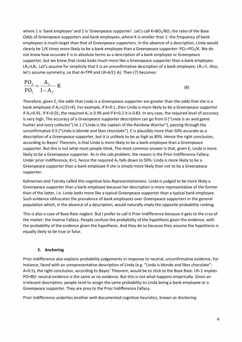
where 1 is ‘bank employee’ and 2 is ‘Greenpeace supporter’. Let’s call K=BO2/BO1 the ratio of the Base

Odds of Greenpeace supporters and bank employees, where K is smaller than 1: the frequency of bank

employees is much larger than that of Greenpeace supporters. In the absence of a description, Linda would

clearly be 1/K times more likely to be a bank employee than a Greenpeace supporter: PO1=PO2/K. We do

not know how accurate E is in absolute terms as a description of a bank employee or Greenpeace

supporter, but we know that Linda looks much more like a Greenpeace supporter than a bank employee:

LR2>LR1. Let’s assume for simplicity that E is an unconfirmative description of a bank employee: LR1=1. Also,

let’s assume symmetry, so that A=TPR and LR=A/(1-A). Then (7) becomes:

KA

A

PO

PO

2

2

1

2

1 (8)

Therefore, given E, the odds that Linda is a Greenpeace supporter are greater than the odds that she is a

bank employee if A2>1/(1+K). For example, if K=0.1, then Linda is more likely to be a Greenpeace supporter

if A2>0.91. If K=0.01, the required A2 is 0.99 and if K=0.2 it is 0.83. In any case, the required level of accuracy

is very high. The accuracy of a Greenpeace supporter description can go from 0 (“Linda is an avid game

hunter and ivory collector”) to 1 (“Linda is the captain of the Rainbow Warrior”), passing through the

unconfirmative 0.5 (“Linda is blonde and likes chocolate”). E is plausibly more than 50% accurate as a

description of a Greenpeace supporter, but it is unlikely to be as high as 80%. Hence the right conclusion,

according to Bayes’ Theorem, is that Linda is more likely to be a bank employee than a Greenpeace

supporter. But this is not what most people think. The most common answer is that, given E, Linda is more

likely to be a Greenpeace supporter. As in the cab problem, the reason is the Prior Indifference Fallacy.

Under prior indifference, K=1, hence the required A2 falls down to 50%: Linda is more likely to be a

Greenpeace supporter than a bank employee if she is simply more likely than not to be a Greenpeace

supporter.

Kahneman and Tversky called this cognitive bias Representativeness. Linda is judged to be more likely a

Greenpeace supporter than a bank employee because her description is more representative of the former

than of the latter, i.e. Linda looks more like a typical Greenpeace supporter than a typical bank employee.

Such evidence obfuscates the prevalence of bank employees over Greenpeace supporters in the general

population which, in the absence of a description, would naturally imply the opposite probability ranking.

This is also a case of Base Rate neglect. But I prefer to call it Prior Indifference because it gets to the crux of

the matter: the Inverse Fallacy. People confuse the probability of the hypothesis given the evidence, with

the probability of the evidence given the hypothesis. And they do so because they assume the hypothesis is

equally likely to be true or false.

3. Anchoring

Prior indifference also explains probability judgements in response to neutral, unconfirmative evidence. For

instance, faced with an unrepresentative description of Linda (e.g. “Linda is blonde and likes chocolate”:

A=0.5), the right conclusion, according to Bayes’ Theorem, would be to stick to the Base Rate. LR=1 implies

PO=BO: neutral evidence is the same as no evidence. But this is not what happens empirically. Given an

irrelevant description, people tend to assign the same probability to Linda being a bank employee or a

Greenpeace supporter. They are prey to the Prior Indifference Fallacy.

Prior indifference underlies another well-documented cognitive heuristics, known as Anchoring.

5

One of the experiments used to illustrate Anchoring involved two groups of visitors at the San Francisco

Exploratorium3. Members of the first group were asked: ‘Is the height of the tallest redwood more or less

than 1,200 feet?’, while members of the second group were asked: ‘Is the height of the tallest redwood

more or less than 180 feet?’. Subsequently, members of both groups were asked the same question: ‘What

is your best guess about the height of the tallest redwood?’ As it turned out, the mean estimate was 844

feet for the first group and 282 feet for the second group. People were anchored to the value specified in

the first, priming question. The anchoring index was (844-282)/(1200-180)=55%, roughly in the middle

between no anchoring and full anchoring. This index level is typical of other similar experiments.

Why is judgement influenced by irrelevant information? It is for the same reason why, in Linda’s

experiment, an unconfirmative description is not equivalent to no description. Among visitors, there were

people who had quite a good sense of the height of the tallest redwood (it is called Hyperion and it is 379

feet high), some people who had only a vague sense and some other who had no idea. The less one knows

about redwoods, the closer one is to Prior Indifference. Under Prior Indifference, the number in the priming

question acts as a neutral reference point, around which the probability that the tallest redwood is

higher/shorter is deemed to be 50/50. Asked to give a number, people with little or no knowledge of

redwoods will choose one around the reference point, thus skewing the group average towards it.

In the redwoods experiment the priming question may be thought to contain a modicum of information –

uninformed people may take the number as an indication of the average height of redwoods. But anchoring

works even when priming information is unequivocally insignificant. In another experiment, a wheel of

fortune with numbers from 0 to 100 was rigged to stop only at 10 or 65. Participants were asked to spin the

wheel and annotate their number, and then were asked: ‘What is your best guess of the percentage of

African nations in the United Nations?’ The average answer of those who saw 10 was 25%, while the

average of those who saw 65 was 45%. Prior indifference is seen here in its clearest and most disturbing

capacity.

We crave for and absorb information without necessarily being aware of it. Bayesian updates on

unconfirmative evidence should be inconsequential: LR=1. But inconsequential evidence can influence our

thoughts, estimates, choices and decisions much more than we would like to think. To protect against such

danger, we should not only try to focus on relevant evidence, but also actively shield ourselves against

irrelevant evidence – an increasingly arduous task in our age of information superabundance.

4. Availability

Another prominent cognitive heuristic is Availability4. The availability heuristics is the process of judging

frequency based of the ease with which instances come to mind. The area in which Availability has been

most extensively studied is risk perception5.

As an example, let’s take aviophobia. When someone is terrified of flying, there is no point telling him that

airplanes are safer than cars. The safest means of transportation – is the typical reply – is a car driven by

me. This illusion of control is caused by an obviously improper comparison between innumerable memories

of safe car driving and many vivid episodes of catastrophic plane crashes.

Like Representativeness and Anchoring, Availability is a probability update in the light of new evidence. But

with Availability evidence comes from within: our own memory. Far from being a passive and faithful

repository of objective reality, memory is a highly reconstructive process, heavily influenced by feelings and

3 Jacowitz, Kahneman (1995), Kahneman (2011), Chapter 11. 4 Tversky, Kahneman (1973), Kahneman (2011), Chapter 12 and 13. 5 Slovic (2000).

6

emotions. As we try to assess the relative odds of a fatal plane accident versus a fatal car accident, we may

well be aware that airplane crashes are more infrequent than car crashes. But when we update Base Rates

by retrieving evidence from memory, we find that instances of plane crashes are more easily available than

instances of car crashes.

This is essentially equivalent to Linda’s problem. Here we have BO1=Prior Odds of fatal car accidents and

BO2=Prior Odds of fatal airplane accidents, with BO1>BO2: car travel is statistically riskier than air travel.

Evidence consist of retrieved memory. Let’s again assume symmetry, hence A=TPR. Just as Linda’s

description can be a more or less accurate portrayal of a Greenpeace supporter or a bank employee, the

availability of instances of airplane or car accidents defines the accuracy of our memory. Again mirroring

Linda’s example, let’s assume LR1=1: memory is neutral with respect to car accidents. A2, the availability of

fatal airplane accidents, is higher than A1. But how much higher should it be, for air travel to be perceived

as riskier than car travel? Again, the limit is given by (8), where K is the relative riskiness of air travel versus

car travel. If air travel were as risky as car travel (K=1), all that would be necessary for airplanes to be

perceived as riskier than cars would be more than neutrally available memories of airplane accidents:

A2>50%. But for lower values of K the required A2 is higher. For instance, if K=0.1 (as seems to be the case in

the US)6, A2 needs to be higher than 0.9 – which may be the reason why aviophobia is confined to a

minority of exceedingly impressionable types (such as, apparently, Joseph Stalin).

5. Hindsight

Our last bias to be seen in the light of prior indifference is Hindsight: the tendency to regard events as

predictable after they have occurred7.

How could US intelligence fail to prevent 9/11? How could the Federal Reserve fail to detect the US housing

bubble? How could the SEC fail to spot Bernard Madoff?

As events happen, they require explanations. We want to know why they happened. Explanations make

sense of events, linking them to preceding events in a causal chain that gives us a satisfactory account of

what turned out to be the case. But causes can only be seen after the events. Before events happen, all we

can see are other events – evidence whose links to what happened was only probable. 9/11 was the result

of a countless number of preceding events, none of which was bound to happen for certain. High house

prices were not destined to cause the 2008 recession. As hard as it is to believe after the fact, Madoff did

not look like an obvious fraud.

Nothing that happens is bound to do so. Everything is the result of a long chain of more or less probable

events. As common sense as this is, it runs counter to the Principle of Sufficient Reason, according to which

there is no such thing as chance: everything is destined to occur in the only possible way, according to its

causes. The Hindsight Bias is a corollary of the Principle of Sufficient Reason.

Let’s take Madoff. Before the scandal broke out, Madoff Investment Securities was one of the largest

broker-dealer firms on Wall Street and Madoff was one of the best-respected hedge fund managers, who

was a using a proprietary strategy, called split-strike conversion, allowing him to earn 15% returns year

after year, with little volatility and no management fee. So let’s go back a few years and test the hypothesis

‘Madoff is a crook’. As we know, PO=LR∙BO. In this case, our evidence is the split-strike conversion strategy.

Let’s take a very sceptical view of it and say TPR=100%: the probability that Madoff would use that strategy,

given that he is a crook, is 100%; and FPR=5%: the probability that he would use the strategy, given that he

is not a crook, is only 5%. Hence LR=20: the evidence is highly confirmative of the hypothesis that Madoff is

6 http://en.wikipedia.org/wiki/Transportation_safety_in_the_United_States.

7 Fischhoff (1980), Kahneman (2011), Chapter 19.

7

a crook. But in order to measure the probability that Madoff is a crook, given that he uses the strategy, we

need to multiply LR by BO: the prior probability that Madoff is a crook. If we did not know who Madoff was,

it would be reasonable to assume BO=1, which gives PO=20 and therefore PP=95%: Madoff is almost

certainly a crook. But for thousands of wealthy investors and sophisticated advisors, who were counting on

Madoff’s excellent reputation, the prior probability that Madoff was a crook was very small: let’s say one in

a thousand. From Bayes’ Theorem, this implies that the probability that Madoff is a crook, in the light of his

investment strategy, is only 2% – in fact much less than that if we choose a higher FPR: with FPR=20%, for

example, LR=5 and PP=0.5%. In that case, even after increasing BR to a more circumspect 1%, PP would still

be less than 5%.

This is not to not justify anybody’s gullibility. But to conclude that they were all utter dunces or, worse, that

many of them ‘could not have possibly ignored’ who Madoff was, and were therefore in cahoots with him,

is wrong. The mistake is caused by the Hindsight Bias: once events happen – Madoff’s fraud is discovered –

we tend to ignore the state of knowledge on which prior beliefs were formed. Once we find out that

Madoff was a crook, we forget that he was a highly respected professional, and mistakenly conclude that

his dishonesty was highly predictable. This is a backward Prior Indifference Fallacy: blinded by the evidence

of our discovery, we inadvertently shift our and everybody else’s past priors to 50%. In Madoff’s case, these

would have been much better priors. But we can only say so with the benefit of hindsight.

In addition, hindsight makes evidence appear more accurate than it was before the event. As we have seen,

starting from a low prior of dishonesty, even a very sceptical view of the split-strike conversion strategy was

not enough to conclude that Madoff was a crook. After the event, however, we tend to regard the same

evidence as conclusive, and retrospectively drop FPR all the way to zero: there was no way that Madoff

would have used that strategy if he were not a crook. It can indeed be argued that a closer look at Madoff’s

strategy should have convinced anyone that its FPR was virtually 0%: there was near-perfect evidence that

Madoff was dishonest, irrespective of his outstanding reputation. And there is no denying that the prospect

of hefty returns and advisory fees made some people’s scrutiny not as diligent as it should have been. But

for most people this become clear only with the benefit of hindsight.

Backward prior indifference, combined with the spurious accuracy of retrospective evidence, make

hindsight a particularly powerful bias. This is bad news for decision makers. No matter how well designed

their decision process might be, the occurrence of a bad outcome – always a possibility in risky conditions –

may be taken as a proof that the process was not well designed. Therefore, the Hindsight Bias promotes

the design of excessively risk averse decision processes. Left to their own devices, decision makers have an

incentive to impose a high cost of a False Alarm on others, in order to avoid the cost of a Miss on

themselves – including the cost of self-blame and regret.

6. Prior Indifference as Knightian uncertainty

Prior Indifference amounts to perfect ignorance: we have no clue at all about whether H is true or false.

Imagine an urn containing 100 balls, black and white, in unknown proportions. What is the probability of

extracting a white ball? The immediate answer is: no idea, we just don’t know. This feeling of helplessness

is what is known as Knightian uncertainty8. We would rather not answer the question but, if forced to, our

thinking may be: there are 99 equiprobable proportions, ranging from 1 white/99 black to 99 white/1 black.

Hence we take their average: 50%. Under the circumstances, it is clearly the best answer. It is the same

answer we would give if we knew that the balls were 50% white and 50% black. But under Knightian

8 Knight (1921).

8

uncertainty we don’t know the actual proportion – in fact we know that it is almost surely different from

50/50. It is precisely such ignorance that motivates our answer.

Despite the equivalence, if we had to choose between betting on the extraction of a white ball from an urn

with a known 50/50 proportion and an urn with an unknown proportion, we would prefer the former. This

is known as Ellsberg paradox, or ambiguity aversion9. We prefer known risk to unknown uncertainty. But

Prior Indifference is the starting point of both. So BR=0.5 does not necessarily mean that we know that the

prior probability of the hypothesis is 50%. It simply means that we know nothing at all – nothing that allows

us to differentiate between true and false: perfect ignorance.

Why is Prior Indifference a fallacy? Because it is hardly ever true that we have no idea. Most times our

priors already contain plenty of background evidence that we wrongly ignore. As ex US Secretary of

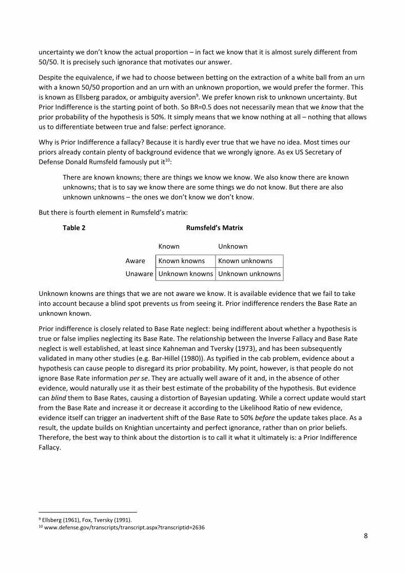
Defense Donald Rumsfeld famously put it10:

There are known knowns; there are things we know we know. We also know there are known

unknowns; that is to say we know there are some things we do not know. But there are also

unknown unknowns – the ones we don’t know we don’t know.

But there is fourth element in Rumsfeld’s matrix:

Table 2 Rumsfeld’s Matrix

Known Unknown

Aware Known knowns Known unknowns

Unaware Unknown knowns Unknown unknowns

Unknown knowns are things that we are not aware we know. It is available evidence that we fail to take

into account because a blind spot prevents us from seeing it. Prior indifference renders the Base Rate an

unknown known.

Prior indifference is closely related to Base Rate neglect: being indifferent about whether a hypothesis is

true or false implies neglecting its Base Rate. The relationship between the Inverse Fallacy and Base Rate

neglect is well established, at least since Kahneman and Tversky (1973), and has been subsequently

validated in many other studies (e.g. Bar-Hillel (1980)). As typified in the cab problem, evidence about a

hypothesis can cause people to disregard its prior probability. My point, however, is that people do not

ignore Base Rate information per se. They are actually well aware of it and, in the absence of other

evidence, would naturally use it as their best estimate of the probability of the hypothesis. But evidence

can blind them to Base Rates, causing a distortion of Bayesian updating. While a correct update would start

from the Base Rate and increase it or decrease it according to the Likelihood Ratio of new evidence,

evidence itself can trigger an inadvertent shift of the Base Rate to 50% before the update takes place. As a

result, the update builds on Knightian uncertainty and perfect ignorance, rather than on prior beliefs.

Therefore, the best way to think about the distortion is to call it what it ultimately is: a Prior Indifference

Fallacy.

9 Ellsberg (1961), Fox, Tversky (1991). 10 www.defense.gov/transcripts/transcript.aspx?transcriptid=2636

9

7. Conclusions

The idea that the accumulation of evidence leads to the truth is a powerful engine of progress. People may

start from different priors but, as long as they look at the same evidence, they should, and normally do

converge to the same truth. Right from the start11, we are natural Bayesians, innately predisposed to learn

about the world through observation and experience.

Yet, if Bayesian updating worked perfectly, the world would be a different place – not necessarily better,

perhaps, but surely not one still fraught with illusions, faulty reasoning and wrong beliefs. Combating these

flaws requires a clear understanding of where and why Bayesian updating gets its cramps.

The Inverse Fallacy is a distortion of Bayesian updating. Different terms have been used to denote it.

Among others: Invalid inversion, Error of the transposed conditional, Base Rate fallacy or neglect,

Prosecutor’s or Juror’s fallacy12. But we have claimed here that the best way to think about it is to call it

what it ultimately is: a Prior Indifference Fallacy. Prior indifference is closely related to Base Rate neglect:

being indifferent about whether a hypothesis is true or false implies ignoring its Base Rate. But the crucial

attribute of faulty thinking is not inattention or neglect of evidence. Like optical illusions, prior indifference

persists despite our full attention. It is there not because we ignore evidence, but because we are blinded

by it.

Seen in this light, Prior Indifference helps us understand not only Representativeness, to which Base Rate

neglect is usually associated, but also seemingly unrelated heuristic biases, such as Anchoring, Availability

and Hindsight.

The Prior Indifference Fallacy should not be seen as a systematic flaw or an automatic reflex. People are not

stupid – Bayesian updating works well in most circumstances. But when it doesn’t, the phenomenon cannot

be simply dismissed as a casualty of semantic confusion or ineffective communication, vanishing once it is

made transparent through a more explicit description13. As with optical illusions, we can and do understand

that we are making a mistake. But the illusion does not go away once we understand it. This is what makes

prior indifference particularly insidious.

What should we do to avoid Prior Indifference? We should resist the sirens of Knightian uncertainty and

properly place new evidence within the confines of what we already know. Correct priors guard us against

perfect ignorance, keep us closer to the truth and prevent us from getting blinded by evidence. Of course,

correct priors are just a good starting point. They are neither a necessary nor a sufficient condition for

convergence to the truth. Unless we can find conclusive evidence, convergence can only occur as a result of

a thorough tug of war between confirmative and disconfirmative evidence, making sure that we gather

plenty of it on both sides of the rope.

References

M. Bar-Hillel (1980), The Base Rate Fallacy in Probability Judgments, Acta Psychologica, 44, 211-233.

L. Cosmides, J. Tooby (1996), Are Humans Good Intuitive Statisticians After All? Rethinking Some

Conclusions from the Literature on Judgment and Uncertainty, Cognition, 58(1), 1-73.

D. Ellsberg (1961), Risk, Ambiguity, and the Savage Axiom, Quarterly Journal of Economics, 75, 643-669.

11 Gopnik (2009). 12 Bar-Hillel (1980), Thompson, Schumann (1987), Koehler (1996), Villejoubert, Mandel (2002). 13 As claimed in Cosmides, Tooby (1996), Koehler (1996).

10

B. Fischhoff (1980), For Those Condemned to Study the Past: Heuristics and Biases in Hindsight, in

Kahneman, Slovic, Tversky, Eds. (1982), 23.

C. Fox, A. Tversky (1995), Ambiguity Aversion and Comparative Ignorance, Quarterly Journal of Economics,

110, 3, 585-603. In Kahneman, Tversky, Eds. (2000), 30.

T. Gilovich, D. Griffin, D. Kahneman, Eds. (2002), Heuristics and Biases. The Psychology of Intuitive

Judgment, Cambridge University Press.

A. Gopnik (2009), The Philosophical Baby, Random House.

K.E. Jacowitz, D. Kahneman (1995), Measures of Anchoring in Estimation Tasks, Personality and Social

Psychology Bulletin, 21, 1161-1166.

D. Kahneman, P. Slovic, A. Tversky, Eds. (1982), Judgment under Uncertainty: Heuristics and Biases,

Cambridge University Press.

D. Kahneman, A. Tversky (1973), On the Psychology of Prediction, in Kahneman, Slovic, Tversky, Eds. (1982),

4.

D. Kahneman, A. Tversky, Eds. (2000), Choices, Values, and Frames, Cambridge University Press.

D. Kahneman (2011), Thinking, Fast and Slow, Allen Lane.

F.H. Knight (1921), Risk, Uncertainty and Profit, BeardBooks.

J.J. Koehler (1996), The Base Rate Fallacy Reconsidered: Descriptive, Normative, and Methodological

Challenges, Behavioral and Brain Sciences, 19, 1-17.

P. Slovic (Ed.) (2000), The Perception of Risk, Earthscan Publications.

W.C. Thompson, E.L. Schumann (1987), Interpretation of Statistical Evidence in Criminal Trials – The

Prosecutor’s Fallacy and the Defense Attorney’s Fallacy, Law and Human behaviour, 11, 167-187.

A. Tversky, D. Kahneman (1973), Availability: A Heuristic for Judging Frequency and Probability, in

Kahneman, Slovic, Tversky, Eds. (1982), 8.

A. Tversky, D. Kahneman (1980), Causal Schemas in Judgments under Uncertainty, in Kahneman, Slovic,

Tversky, Eds. (1982), 11.

A. Tversky, D. Kahneman (1982), Evidential Impact of Base Rates, in Kahneman, Slovic, Tversky, Eds. (1982),

10.

A. Tversky, D. Kahneman (1984), Extensional versus Intuitive Reasoning: The Conjunction Fallacy, in

Probability Judgment, in Gilovich, Griffin, Kahneman, Eds. (2002), 1.

G. Villejoubert, D.R. Mandel (2002), The Inverse Fallacy: An Account of Deviations from Bayes’s Theorem

and the Additivity Principle, Memory and Cognition, 30 (2), 171-178.