Voter Biases in the US Electoral College
22
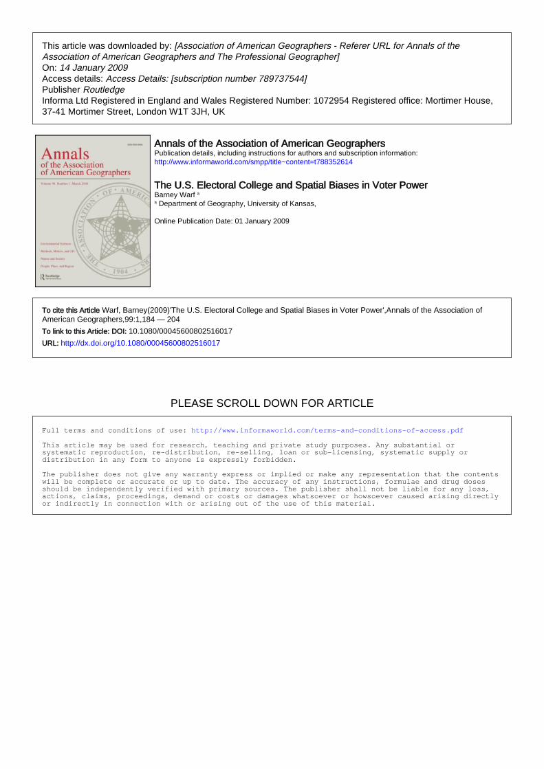
PLEASE SCROLL DOWN FOR ARTICLE This article was downloaded by: [Association of American Geographers - Referer URL for Annals of the Association of American Geographers and The Professional Geographer] On: 14 January 2009 Access details: Access Details: [subscription number 789737544] Publisher Routledge Informa Ltd Registered in England and Wales Registered Number: 1072954 Registered office: Mortimer House, 37-41 Mortimer Street, London W1T 3JH, UK Annals of the Association of American Geographers Publication details, including instructions for authors and subscription information: http://www.informaworld.com/smpp/title~content=t788352614 The U.S. Electoral College and Spatial Biases in Voter Power Barney Warf a a Department of Geography, University of Kansas, Online Publication Date: 01 January 2009 To cite this Article Warf, Barney(2009)'The U.S. Electoral College and Spatial Biases in Voter Power',Annals of the Association of American Geographers,99:1,184 — 204 To link to this Article: DOI: 10.1080/00045600802516017 URL: http://dx.doi.org/10.1080/00045600802516017 Full terms and conditions of use: http://www.informaworld.com/terms-and-conditions-of-access.pdf This article may be used for research, teaching and private study purposes. Any substantial or systematic reproduction, re-distribution, re-selling, loan or sub-licensing, systematic supply or distribution in any form to anyone is expressly forbidden. The publisher does not give any warranty express or implied or make any representation that the contents will be complete or accurate or up to date. The accuracy of any instructions, formulae and drug doses should be independently verified with primary sources. The publisher shall not be liable for any loss, actions, claims, proceedings, demand or costs or damages whatsoever or howsoever caused arising directly or indirectly in connection with or arising out of the use of this material.
Transcript of Voter Biases in the US Electoral College
PLEASE SCROLL DOWN FOR ARTICLE
This article was downloaded by: [Association of American Geographers - Referer URL for Annals of theAssociation of American Geographers and The Professional Geographer]On: 14 January 2009Access details: Access Details: [subscription number 789737544]Publisher RoutledgeInforma Ltd Registered in England and Wales Registered Number: 1072954 Registered office: Mortimer House,37-41 Mortimer Street, London W1T 3JH, UK
Annals of the Association of American GeographersPublication details, including instructions for authors and subscription information:http://www.informaworld.com/smpp/title~content=t788352614
The U.S. Electoral College and Spatial Biases in Voter PowerBarney Warf a
a Department of Geography, University of Kansas,
Online Publication Date: 01 January 2009
To cite this Article Warf, Barney(2009)'The U.S. Electoral College and Spatial Biases in Voter Power',Annals of the Association ofAmerican Geographers,99:1,184 — 204
To link to this Article: DOI: 10.1080/00045600802516017
URL: http://dx.doi.org/10.1080/00045600802516017
Full terms and conditions of use: http://www.informaworld.com/terms-and-conditions-of-access.pdf
This article may be used for research, teaching and private study purposes. Any substantial orsystematic reproduction, re-distribution, re-selling, loan or sub-licensing, systematic supply ordistribution in any form to anyone is expressly forbidden.
The publisher does not give any warranty express or implied or make any representation that the contentswill be complete or accurate or up to date. The accuracy of any instructions, formulae and drug dosesshould be independently verified with primary sources. The publisher shall not be liable for any loss,actions, claims, proceedings, demand or costs or damages whatsoever or howsoever caused arising directlyor indirectly in connection with or arising out of the use of this material.
The U.S. Electoral College and Spatial Biasesin Voter Power
Barney Warf
Department of Geography, University of Kansas
The United States does not provide for direct election of its chief executive but utilizes the Electoral Collegeto represent voter choices. Central to this institution is the “winner-take-all” model by which electoral votesin all states but two are awarded to the candidate who garners a plurality of that state’s popular vote. As gametheorists have long pointed out, this system introduces several biases in voter power that differentially rewardor punish voters based on each state’s population or electorate. This article offers a historical overview of theElectoral College and the geographic biases in voter power it introduces. It extends the influential binomialmodel of voter power proposed by Banzhaf in the 1960s to include a multinomial approach sensitive to thepresence of more than two parties, the absolute and relative margins of victories, and the number of electoralvotes in each state. It then applies this approach to U.S. presidential elections from 1960 to 2004 utilizing a seriesof cartograms. Next, the article examines voter power differentials between the two major political parties, fiveethnic groups, rural and urban areas, and ten religious denominations in the 2000 and 2004 elections. Finally, itlinks contemporary discussions of voter power to theories of democracy, arguing that the electoral power can onlybe understood in contingent, temporally fluid, and geographically specific terms. Key Words: elections, ElectoralCollege, electoral geography, political geography.
La eleccion del presidente de Estados Unidos no se hace por voto directo sino a traves del Colegio Electoral,entidad a la que corresponde representar la eleccion hecha por los votantes. La esencia de esta institucion es laregla de “el ganador se lleva todo”, segun la cual los votos electorales en todos los estados, menos dos, se adjudicanal candidato que acumule una mayorıa relativa del voto popular de un estado dado. Como lo han indicado desdehace mucho tiempo los teoricos de juegos, este sistema comporta varios sesgos en el poder del voto, premiando ocastigando diferencialmente a los votantes segun el tamano de la poblacion o electorado del estado. En el artıculose presenta un recuento historico sucinto del Colegio Electoral y de los sesgos geograficos que aquel crea en el poderdel voto. Se extiende la discusion hasta el influyente modelo binomial del poder de voto propuesto por Banzhafen los anos 1960, para incluir un enfoque multinomio sensible a la presencia de mas de dos partidos, los margenesde victorias absolutos y relativos, y el numero de votos electorales para cada estado. Luego, el enfoque se aplica alas elecciones presidenciales de E.U. de 1960 a 2004, con la ilustracion de una serie de cartogramas. El artıculoexamina enseguida las diferenciales del poder de voto entre los dos principales partidos polıticos, cinco gruposetnicos, las areas rurales y urbanas, y diez denominaciones religiosas, en las elecciones de los anos 2000 y 2004.Por ultimo, se relacionan las discusiones contemporaneas sobre el poder del voto, con las teorıas de la democracia,
Annals of the Association of American Geographers, 99(1) 2009, pp. 184–204 C© 2009 by Association of American GeographersInitial submission, January 2008; revised submission, April 2008; final acceptance, April 2008
Published by Taylor & Francis, LLC.
Downloaded By: [Association of American Geographers - Referer URL for Annals of the Association of American Geographers and The Professional Geographer] At: 20:38 14 January 2009
The U.S. Electoral College and Spatial Biases in Voter Power 185
arguyendose que el poder electoral solo puede entenderse en terminos contingentes, temporalmente fluidos ygeograficamente especıficos. Palabras clave: elecciones, Colegio Electoral, geografıa electoral, geografıa polıtica.
The impacts of individuals and groups of voterson national elections in the United States havebeen the object of enormous popular and aca-
demic scrutiny, in part because the forces that shapethis phenomenon are institutionalized in highly unevenways geographically through the Electoral College. Thistopic is richly deserving of the attention of anyone in-terested in the dynamics of American politics and theways in which democratic politics are constituted overtime and space.
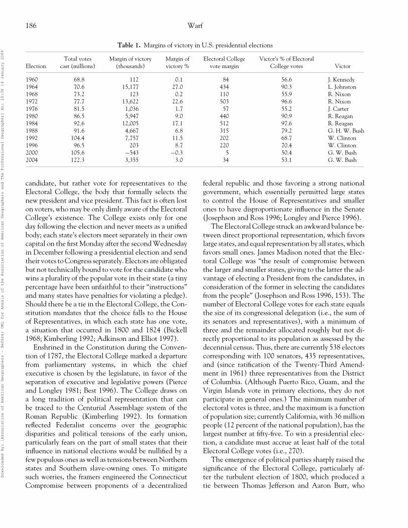
U.S. presidential elections have ranged from sweep-ing, decisive victories to excruciatingly close races de-cided by a handful of voters. Since World War II, themargin of victory has fluctuated from 112,000 votes(or 0.1 percent) in 1960, when Kennedy squeaked pastNixon, to a resounding 15 million votes, or 27 per-cent, when Johnson trounced Goldwater four years later(Table 1). In the infamous election of 2000, the winnerof the popular vote, Al Gore, nonetheless lost the Elec-toral College vote to George W. Bush. The outcomesof these elections reflected the highly uneven distribu-tion of votes among states as well as the temporally andspatially uneven web of capacities to shape nationalraces as voter preferences were differentially magnifiedor reduced through the Electoral College.
Despite a wide consensus that the Electoral Col-lege generates biases in individuals’ and states’ ca-pacities to shape national elections, geographers havecontributed remarkably little to the debate concern-ing this institution. Electoral geography, with a longand distinguished history (e.g., Prescott 1959), com-prised the core of political geography in the 1980s butcurrently finds itself awkwardly poised between a tradi-tion of uncritical, atheoretical empiricism on the onehand and a resurgent, theoretically self-conscious re-naissance on the other. Classic works in this genre typi-cally described how spatial variations in elections reflectelectoral apportionments, economic and demographicfactors, and the campaign strategies of parties and candi-dates (Taylor 1973; Taylor and Johnston 1979; Swauger1980; Johnston 1982, 2002; Archer, Murauskas, andShelley 1985; Archer and Shelley 1986, 1988; Archer1988; Johnston, Shelley, and Taylor 1990). A relatedapproach reflects the discipline’s abiding concern withthe state, social relations, and the sociospatial contextof ideology, in which elections are seen as the exer-cise of subjectivity within structural constraints rang-ing from the local scale to the world system (Agnew1996; Flint 2001; Johnston and Pattie 2003). The vast
majority of such works focused on the United States,with a few notable examples drawn from Europe (Ag-new 1995; Johnston and Pattie 2006; Adams 2007).This literature has offered a rich, detailed portrait of thespatiality of elections at the national and local levels;redistricting and gerrymandering; shifts in voter pref-erences, turnout rates, and correlations with varioussocioeconomic variables; and neighborhood effects onpolitical behavior. Despite this wealth of insights, thegeographic literature specifically concerning the Elec-toral College is dismayingly limited, although insightfulanalyses of its role in shaping the outcomes of the 2000and 2004 elections were made by Johnston, Rossiter,and Pattie (2005, 2006), who observed the efficiencywith which the spatial distributions of votes for thecandidates affected the outcome.
This article examines the changing geography ofvoter power within the Electoral College system. Itopens with a historical overview of the institution, howit shapes American presidential elections, argumentsin its favor as well as for its abolition, and the allegedspatial biases it generates. Next, it offers a mathemati-cal exegesis of a famous combinatorial approach to thisissue, the Banzhaf model, and its descendents; it thenextends this line of thought using a more complex multi-nomial model that incorporates more than two politi-cal parties and margins of victory in each state. Third,it presents a cartographic overview of the results ofthis methodology using data pertaining to presidentialelections from 1960 to 2004, illustrating the changingdistribution of relative voter power by state. Fourth,it utilizes this approach to examine potential biases in-duced by the Electoral College regarding political party,ethnicity, rural or urban residence, and religious denom-ination. Fifth, it embeds these topics within a widerconceptual discussion of power, democracy, and votingrights, arguing that elections and democratic processescannot be fruitfully understood as an abstract, aspatialdiscourse but as one rooted in the constantly shifting,geographically differentiated web of relations throughwhich voter preferences are manifested in republicansystems of governance.
The Electoral College: Strengths andWeaknesses in Historic Context
Unlike in most industrial democracies, votersin America do not directly choose a presidential
Downloaded By: [Association of American Geographers - Referer URL for Annals of the Association of American Geographers and The Professional Geographer] At: 20:38 14 January 2009
186 Warf
Table 1. Margins of victory in U.S. presidential elections
Total votes Margin of victory Margin of Electoral College Victor’s % of ElectoralElection cast (millions) (thousands) victory % vote margin College votes Victor
1960 68.8 112 0.1 84 56.6 J. Kennedy1964 70.6 15,177 27.0 434 90.3 L. Johnston1968 73.2 123 0.2 110 55.9 R. Nixon1972 77.7 13,622 22.6 503 96.6 R. Nixon1976 81.5 1,036 1.7 57 55.2 J. Carter1980 86.5 5,947 9.0 440 90.9 R. Reagan1984 92.6 12,005 17.1 512 97.6 R. Reagan1988 91.6 4,667 6.8 315 79.2 G. H. W. Bush1992 104.4 7,757 11.5 202 68.7 W. Clinton1996 96.5 203 8.7 220 70.4 W. Clinton2000 105.6 −543 −0.3 5 50.4 G. W. Bush2004 122.3 3,355 3.0 34 53.1 G. W. Bush
candidate, but rather vote for representatives to theElectoral College, the body that formally selects thenew president and vice president. This fact is often loston voters, who may be only dimly aware of the ElectoralCollege’s existence. The College exists only for oneday following the election and never meets as a unifiedbody; each state’s electors meet separately in their owncapital on the first Monday after the second Wednesdayin December following a presidential election and sendtheir votes to Congress separately. Electors are obligatedbut not technically bound to vote for the candidate whowins a plurality of the popular vote in their state (a tinypercentage have been unfaithful to their “instructions”and many states have penalties for violating a pledge).Should there be a tie in the Electoral College, the Con-stitution mandates that the choice falls to the Houseof Representatives, in which each state has one vote,a situation that occurred in 1800 and 1824 (Bickell1968; Kimberling 1992; Adkinson and Elliot 1997).
Enshrined in the Constitution during the Conven-tion of 1787, the Electoral College marked a departurefrom parliamentary systems, in which the chiefexecutive is chosen by the legislature, in favor of theseparation of executive and legislative powers (Pierceand Longley 1981; Best 1996). The College draws ona long tradition of political representation that canbe traced to the Centurial Assemblage system of theRoman Republic (Kimberling 1992). Its formationreflected Federalist concerns over the geographicdisparities and political tensions of the early union,particularly fears on the part of small states that theirinfluence in national elections would be nullified by afew populous ones as well as tensions between Northernstates and Southern slave-owning ones. To mitigatesuch worries, the framers engineered the ConnecticutCompromise between proponents of a decentralized
federal republic and those favoring a strong nationalgovernment, which essentially permitted large statesto control the House of Representatives and smallerones to have disproportionate influence in the Senate(Josephson and Ross 1996; Longley and Pierce 1996).
The Electoral College struck an awkward balance be-tween direct proportional representation, which favorslarge states, and equal representation by all states, whichfavors small ones. James Madison noted that the Elec-toral College was “the result of compromise betweenthe larger and smaller states, giving to the latter the ad-vantage of electing a President from the candidates, inconsideration of the former in selecting the candidatesfrom the people” (Josephson and Ross 1996, 153). Thenumber of Electoral College votes for each state equalsthe size of its congressional delegation (i.e., the sum ofits senators and representatives), with a minimum ofthree and the remainder allocated roughly but not di-rectly proportional to its population as assessed by thedecennial census. Thus, there are currently 538 electorscorresponding with 100 senators, 435 representatives,and (since ratification of the Twenty-Third Amend-ment in 1961) three representatives from the Districtof Columbia. (Although Puerto Rico, Guam, and theVirgin Islands vote in primary elections, they do notparticipate in general ones.) The minimum number ofelectoral votes is three, and the maximum is a functionof population size; currently California, with 36 millionpeople (12 percent of the national population), has thelargest number at fifty-five. To win a presidential elec-tion, a candidate must accrue at least half of the totalElectoral College votes (i.e., 270).
The emergence of political parties sharply raised thesignificance of the Electoral College, particularly af-ter the turbulent election of 1800, which produced atie between Thomas Jefferson and Aaron Burr, who
Downloaded By: [Association of American Geographers - Referer URL for Annals of the Association of American Geographers and The Professional Geographer] At: 20:38 14 January 2009
The U.S. Electoral College and Spatial Biases in Voter Power 187
had seventy-three electoral votes each; after thirty-sixrounds, the House chose Jefferson. This crisis led tothe subsequent passage of the Twelfth Amendment in1801, which requires presidential and vice presidentialcandidates to run on the same ticket, a measure thatfirst came into play in the election of 1804. The result-ing institution has withstood two centuries of a rapidlychanging nation, the expansion of suffrage, the rise ofthe party convention system, and the steady national-ization of politics through media such as television.
The overriding characteristic of this institution isthe “winner-take-all,” or “unit rule” system, in whichcandidates who receive a plurality of the popular votein a state acquire all of its Electoral College votes(an analogous system is practiced in the House ofCommons in the United Kingdom, although obviouslywithout an electoral college). Article Two of theConstitution gives each state considerable latitudein deciding how its electors will be chosen. Virginiawas the first to adopt the winner-take-all system in1800, and all but two states eventually followed suit.Maine, starting in 1972, and Nebraska, starting in1991, are exceptions, giving two electoral votes to thewinner of the statewide popular vote and allocatingthe remainder to the winner of the popular vote withineach congressional district.1 Under the winner-take-allsystem, any vote exceeding the plurality necessaryto win that state is effectively “wasted,” or maderedundant. As Abbott and Levine (1991, 83) note,“The only votes a winning candidate really needs arethose necessary to guarantee that candidate an unchal-lengeable margin over the opposition.” The unit rulehas been declared unconstitutional for statewide officesbut not presidential ones (Josephson and Ross 1996).
The relative merits and demerits inherent in theElectoral College have been hotly debated. Earlyadvocates argued that it was necessary for a republicanstructure of government to have a layer of repre-sentation between the populace and the state. Lesscharitably, Elbridge Gerry, Massachusetts foundingfather of gerrymandering fame, noted the college wasnecessary because “the people are uninformed andwould be misled by a few designing men” without it(quoted in Pierce and Longley 1981, 21). In this view,the Electoral College’s electors are better informed thanthe average voter and are more capable of selecting the“optimal” candidate. Supporters maintain that the Elec-toral College forces presidential candidates to engage instate-by-state “retail” campaigns and remain sensitive tolocal political issues, in effect creating 51 separate races(Hardaway 1994; Best 1996). Indeed, the very origins
of the Electoral College lay in attempts by the framersof the Constitution to overcome the nation’s deep ge-ographical divisions by forcing candidates to constructgeographically diverse bases of support. Candidatesmust win states, not simply votes, and winners must seekconsensus by building broad coalitions of local intereststhat stretch across state boundaries. Defense of theElectoral College is thus predicated on a faith in federal-ism and the two-party political system as a guarantee ofstability and continuity (Gregg 2001). Defenders arguethat despite its imperfections, the system works as partof a broader web of subtle checks and balances. Elimina-tion of the Electoral College, it is argued, would weakenthe political party system, enhance the importance oftelevision campaigning, promote splinter parties, trig-ger numerous contingency elections and interminablerecounts, encourage electoral fraud, and undermine theelectoral system (Adkinson and Elliott 1997). Aboli-tion would facilitate presidential candidates who repre-sent narrow geographical, ideological, or ethnic bases ofsupport and reduce the influence of small states and ruralinterests. Proponents argue that the Electoral Collegeencourages a politics of moderation; under the directvote alternative, minor parties could attempt to forcerunoffs to flex their political muscles. Abolition wouldalso annihilate geographic diversity in state require-ments governing challenges and recounts, centralizingcontrol in a national presidential election commission.Thus, faith in the Electoral College also representsthe abiding American concern with local control ofgovernment.
The Electoral College has also been strongly criti-cized on several grounds, objections that underpin re-peated attempts at its reform or abolition, includingmore than 700 proposals in Congress since its foun-dation to reform or eliminate it (Josephson and Ross1996). Some argue that it unfairly forces presidentialcandidates to concentrate their campaign efforts on afew battleground states at the expense of voters else-where. Others maintain that it is an archaic, anachro-nistic institution that runs contrary to the principlesof democratic government (Michener 1969; Abbottand Levine 1991; McCaughey 1993). Critics allegethat the Electoral College may contribute to low voterturnout and reinforce one-partyism in selected states.Researchers (Longley and Dana 1984, 1992; Ross andJosephson 1996) note that the Electoral College gener-ates four sources of systematic bias that distort the re-sults of the popular vote: the allocation of a minimumof three electoral votes to states regardless of popula-tion, the winner-take-all or unit rule, the allocation ofD
ownloaded By: [Association of American Geographers - Referer URL for Annals of the Association of American Geographers and The Professional Geographer] At: 20:38 14 January 2009
188 Warf
electors on the basis of population rather than voterturnout, and the delays in electoral vote allocation in-duced by decennial censuses.
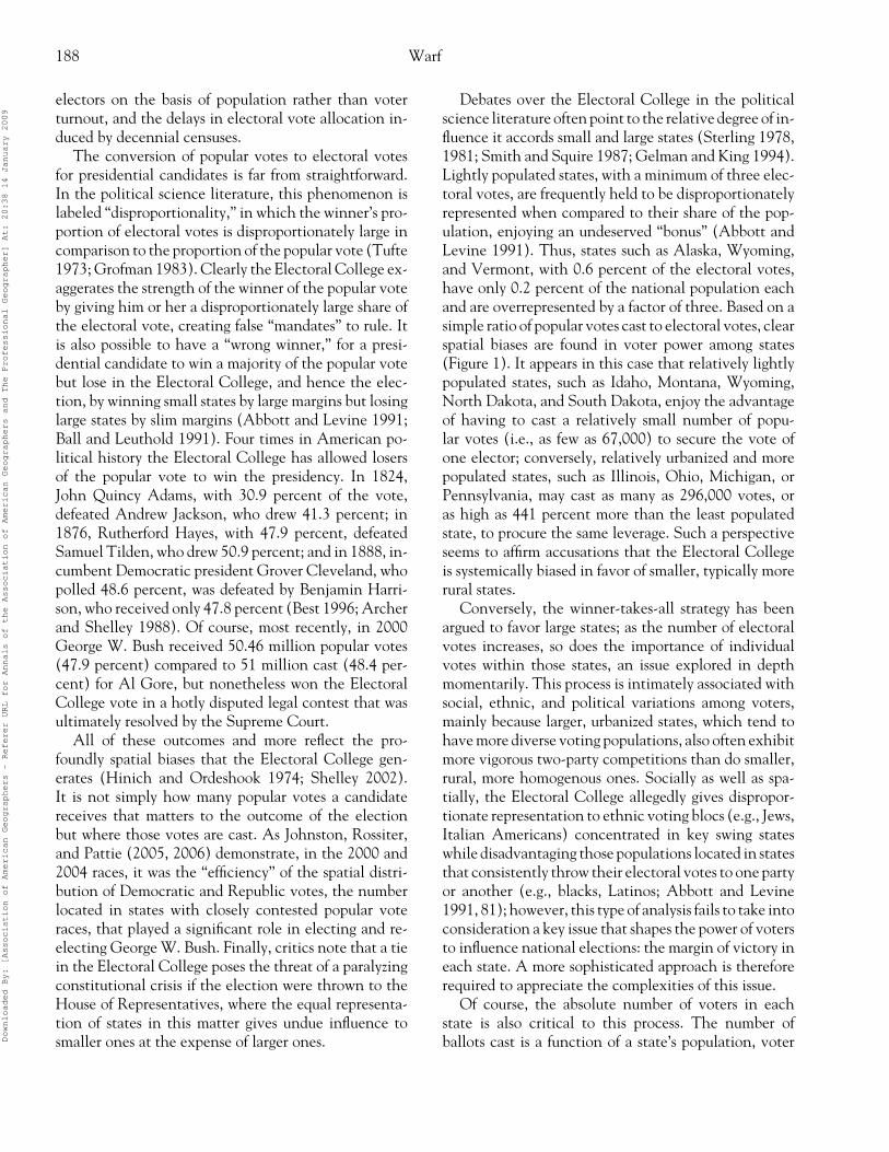
The conversion of popular votes to electoral votesfor presidential candidates is far from straightforward.In the political science literature, this phenomenon islabeled “disproportionality,” in which the winner’s pro-portion of electoral votes is disproportionately large incomparison to the proportion of the popular vote (Tufte1973; Grofman 1983). Clearly the Electoral College ex-aggerates the strength of the winner of the popular voteby giving him or her a disproportionately large share ofthe electoral vote, creating false “mandates” to rule. Itis also possible to have a “wrong winner,” for a presi-dential candidate to win a majority of the popular votebut lose in the Electoral College, and hence the elec-tion, by winning small states by large margins but losinglarge states by slim margins (Abbott and Levine 1991;Ball and Leuthold 1991). Four times in American po-litical history the Electoral College has allowed losersof the popular vote to win the presidency. In 1824,John Quincy Adams, with 30.9 percent of the vote,defeated Andrew Jackson, who drew 41.3 percent; in1876, Rutherford Hayes, with 47.9 percent, defeatedSamuel Tilden, who drew 50.9 percent; and in 1888, in-cumbent Democratic president Grover Cleveland, whopolled 48.6 percent, was defeated by Benjamin Harri-son, who received only 47.8 percent (Best 1996; Archerand Shelley 1988). Of course, most recently, in 2000George W. Bush received 50.46 million popular votes(47.9 percent) compared to 51 million cast (48.4 per-cent) for Al Gore, but nonetheless won the ElectoralCollege vote in a hotly disputed legal contest that wasultimately resolved by the Supreme Court.
All of these outcomes and more reflect the pro-foundly spatial biases that the Electoral College gen-erates (Hinich and Ordeshook 1974; Shelley 2002).It is not simply how many popular votes a candidatereceives that matters to the outcome of the electionbut where those votes are cast. As Johnston, Rossiter,and Pattie (2005, 2006) demonstrate, in the 2000 and2004 races, it was the “efficiency” of the spatial distri-bution of Democratic and Republic votes, the numberlocated in states with closely contested popular voteraces, that played a significant role in electing and re-electing George W. Bush. Finally, critics note that a tiein the Electoral College poses the threat of a paralyzingconstitutional crisis if the election were thrown to theHouse of Representatives, where the equal representa-tion of states in this matter gives undue influence tosmaller ones at the expense of larger ones.
Debates over the Electoral College in the politicalscience literature often point to the relative degree of in-fluence it accords small and large states (Sterling 1978,1981; Smith and Squire 1987; Gelman and King 1994).Lightly populated states, with a minimum of three elec-toral votes, are frequently held to be disproportionatelyrepresented when compared to their share of the pop-ulation, enjoying an undeserved “bonus” (Abbott andLevine 1991). Thus, states such as Alaska, Wyoming,and Vermont, with 0.6 percent of the electoral votes,have only 0.2 percent of the national population eachand are overrepresented by a factor of three. Based on asimple ratio of popular votes cast to electoral votes, clearspatial biases are found in voter power among states(Figure 1). It appears in this case that relatively lightlypopulated states, such as Idaho, Montana, Wyoming,North Dakota, and South Dakota, enjoy the advantageof having to cast a relatively small number of popu-lar votes (i.e., as few as 67,000) to secure the vote ofone elector; conversely, relatively urbanized and morepopulated states, such as Illinois, Ohio, Michigan, orPennsylvania, may cast as many as 296,000 votes, oras high as 441 percent more than the least populatedstate, to procure the same leverage. Such a perspectiveseems to affirm accusations that the Electoral Collegeis systemically biased in favor of smaller, typically morerural states.
Conversely, the winner-takes-all strategy has beenargued to favor large states; as the number of electoralvotes increases, so does the importance of individualvotes within those states, an issue explored in depthmomentarily. This process is intimately associated withsocial, ethnic, and political variations among voters,mainly because larger, urbanized states, which tend tohave more diverse voting populations, also often exhibitmore vigorous two-party competitions than do smaller,rural, more homogenous ones. Socially as well as spa-tially, the Electoral College allegedly gives dispropor-tionate representation to ethnic voting blocs (e.g., Jews,Italian Americans) concentrated in key swing stateswhile disadvantaging those populations located in statesthat consistently throw their electoral votes to one partyor another (e.g., blacks, Latinos; Abbott and Levine1991, 81); however, this type of analysis fails to take intoconsideration a key issue that shapes the power of votersto influence national elections: the margin of victory ineach state. A more sophisticated approach is thereforerequired to appreciate the complexities of this issue.
Of course, the absolute number of voters in eachstate is also critical to this process. The number ofballots cast is a function of a state’s population, voterD
ownloaded By: [Association of American Geographers - Referer URL for Annals of the Association of American Geographers and The Professional Geographer] At: 20:38 14 January 2009

The U.S. Electoral College and Spatial Biases in Voter Power 189
Figure 1. Spatial biases in the Electoral College as measured by popular votes cast per Electoral College vote, 2004.
registration, and turnout rates. Voters in states with lowturnout rates are effectively “rewarded” by the ElectoralCollege compared to those with high turnout rates, asmeasured by the ratio of electoral to popular votes ineach. States with rapidly growing populations, whosenumber of electoral votes reflects census statistics upto a decade old, may also have a representation in theElectoral College smaller than they deserve.
Although extended discussion of alternatives to theElectoral College is beyond the scope of this article,it is worth noting that the most commonly suggestedsubstitute is the direct vote plan, which would abolishthe institution and provide for the election of the pres-ident by a plurality of the popular vote, the system usedin gubernatorial and senatorial races. Appealing in itssimplicity, in such a system each vote is equally influ-ential regardless of where it is cast. Repeated opinionsurveys indicate that the voting public would prefer itto the system currently in place (Longley and Braun1972; Ball and Leuthold 1991; Best 1996). Others ar-gue that direct voting would reduce the influence oflightly populated states, undermining federalism, or fallvictim to state variations in voter registration require-ments based on age, length of residency, and citizenshipqualifications (Zeidenstein 1973; Best 1975). Alterna-
tive, less well-known approaches include the districtand proportional election plans, which would retainthe Electoral College but allocate electoral votes onthe basis of congressional districts within each state oras a reflection of each candidate’s share of the popu-lar vote, respectively (Amy 1993). Under such systems,large states are likely to lose influence as their electoralvotes are split among different candidates. Yet anotheralternative suggests retaining the 538 Electoral Collegevoters but adding an additional pool of electoral votesawarded to the candidate who wins the largest shareof the popular vote (Twentieth Century Fund TaskForce 1978). No alternative, however, has yet musteredthe political support required for passage of a consti-tutional amendment necessary to change the currentsystem.
This article is not concerned with such issues, im-portant as they are, but rather their consequences giventhe current system of electoral representation in U.S.presidential elections. How does the Electoral Collegegenerate spatial biases in the power of voters in differentstates to affect national races? Within any given state,voters by definition have equal power to influence races(although obviously political preferences vary markedlyby age, ethnicity, religion, class, and gender), but givenD
ownloaded By: [Association of American Geographers - Referer URL for Annals of the Association of American Geographers and The Professional Geographer] At: 20:38 14 January 2009
190 Warf
the uneven distribution of voters among states, as wellas profound spatial differences in statewide margins ofvictory, the ability of voters to shape national outcomesby throwing their state’s electors to one party or anotheris highly variable geographically.
Voter Power and the Mathematics of theElectoral College
The power of voters to shape national outcomes isnotoriously difficult to estimate. In the simplest, ran-dom case, one can take a single vote and divide bythe total number of votes cast. In the 2000 presiden-tial election, for example, in which roughly 100 millionvotes were cast, the probability that any one of themdecided the outcome is about .00000001. Mulligan andHunter (2003) note that a single vote is almost neverpivotal in an election: In more than 40,000 electionsthey analyzed in the twentieth century, comprising onebillion votes, only seven races were decided by a singlevote. Indeed, given the extremely low impact that in-dividual voters have on races and the time and effortinvolved, it is remarkable that as many people botherto cast ballots as they do: Anthony Downs (1957), inhis famous treatise An Economic Theory of Democracyexamining the costs and benefits of voting, concludedthat under some circumstances it is not rational to vote.Such a view, however, does not take into account thecomplex dynamics of the Electoral College and howit may amplify some voters’ abilities to sway nationaloutcomes.
Starting in the 1960s, game theoreticians and math-ematicians became intrigued by this very issue (Riker1962; Mann and Shapley 1964). Drawing heavily onthese works, the most famous and influential analysisof this topic was proposed by Banzhaf (1968), who in-troduced combinatorial analysis to the study of voting.Banzhaf’s approach viewed voter power as a function ofpossible voting combinations that voters in a given statecould achieve by throwing their state’s electoral votesto one candidate or another. Thus, voter power was afunction of (1) the probability that a citizen’s vote couldchange a state’s votes for a given candidate, and (2) theprobability that the state’s electoral votes could decidethe outcome of the national election. Voter power wasthus held to be “the chance that any voter has of affect-ing the election of the President through the mediumof his [sic] state’s electoral votes” (Banzhaf 1968, 313);that is, the leverage enjoyed by voters purely due totheir geographic location of residence. For analytical
convenience, Banzhaf assumed that for a voter to makea difference, votes must be equally split between thetwo major parties, a view that allows the use of a bino-mial model of voter power. By measuring the factori-als of state votes, he calculated voter power in state sas
VPs = ns !(ns − ds )!ds !
∗ EVs , (1)
where VPs is voter power in state s, ns is total votesin state s, ds is votes for one political party in state s ,and EVs is electoral votes of state s . This approachholds that distribution of votes follows a binomial dis-tribution with a mean of 0.5. For large populations, thecentral limit theorem allows the binomial to be approx-imated accurately using a normal distribution with thesame mean and variance, which, when simplified, canbe stated as
VP = sqrt(2/nπ). (2)
Banzhaf (1968) argued that voter power rises roughlyas the inverse of the square root of the size of the statepopulation. Contrary to widespread impressions thatthe Electoral College favors small states, the systemactually rewards their counterparts in larger ones. Al-though the smaller states have more electoral votes perresident, this does not give them a net advantage underthe existing system because the unit-vote rule measuresvoters’ choices in each state to vote as a group. Thedecrease in each individual voter’s effectiveness as amember of a large electorate was more than offset bythe larger number of electoral votes he or she can af-fect. The title of his article, “One Man, 3.312 Votes,”reflected his finding that a voter in New York State had3.312 times more ability to affect the outcome of presi-dential elections than did a voter in the least powerfulstate. Banzhaf (1968) concluded that “the current Elec-toral College system falls short of even an approxima-tion of equality in voter power” (306). He concludedby calling for direct presidential elections. Banzhaf’spaper was enormously influential. Several state legis-latures adopted it as the criterion for establishing theexistence of equitable voter power among local legisla-tive districts as well as the validity of different weightedvoting systems under the “one man, one vote” principle(Grofman 1981). In 1970, Indiana’s scheme of single-and multiple-member districts for its state legislaturewas challenged in the Supreme Court, which, in Whit-comb v. Chavis, decisively rejected Banzhaf’s argumentD
ownloaded By: [Association of American Geographers - Referer URL for Annals of the Association of American Geographers and The Professional Geographer] At: 20:38 14 January 2009

The U.S. Electoral College and Spatial Biases in Voter Power 191
on the grounds that its simplifying assumptions wereabsurd: Of particular concern was the assumption thatvoters must tie for marginal voters to have any effectat all; with n voters in the district, this situation wouldoccur only once out of 2n possible coalitions of voters.Justice Harlan noted that even minor departures fromthe assumption that p = 0.5 could produce dramaticallydifferent results.
The key weakness to Banzhaf’s (1968) originalformulation, therefore, is that it does not sufficientlyaccount for the relative closeness of races withineach state—the margin of victory—in effect assumingthat voters are effective only when the two partiesare effectively tied. As noted earlier, however, theprobability of exact ties in the popular vote is extremelyremote, a fact that renders his portrayal of voter powerinconveniently unrealistic. Banzhaf’s work unleashedconsiderable criticism (e.g., Margolis 1983) as wellas extensions and modifications. It is also importantto note that a disadvantage of this approach is thatit is strictly post facto in its approach and, becausethe outcomes of electoral contests are contingentand highly variable over time, this method offerslittle utility as a tool to predict voter power in thefuture.
Because some states are more closely contested thanothers, a more accurate reflection of the power of vot-ers must include the distribution of votes among partieswithin states, a view that incorporates the power ofswing voters to decide outcomes. Ceteris paribus, votersin close races will exercise more influence over elec-toral outcomes than do those in races in which onecandidate is far ahead of his or her opponent. Politicalparties recognize this fact by allocating disproportionateshares of their limited resources (i.e., television adver-tising funds, candidate campaign time) to influencingvoters in “battleground” states, especially large ones,that are “up for grabs,” because the outcome is too closeto predict accurately or there is a reasonable likelihoodof swaying undecided voters (Colantoni, Levesque, andOrdeshook 1975; Shaw 1999). In some races, the mar-gin of victory may be less than the margin of errorintroduced by flawed voting technologies (Warf 2006).Conversely, states with lopsided support for either partycan safely be ignored by both.
Merrill (1978) overcame the critical, unrealistic as-sumption of the Banzhaf model that voters are tiedin each state by reformulating the binomial approachto measure voter power using differential percentagesof votes cast for political candidates. For example,in a two-party presidential race (i.e., Democrats and
Republicans),
VPs = ns !(ns − ds )!ds !
∗ pds ∗ q r
s ∗ EVs (3)
where VPs is voter power in state s , ns is total numberof popular votes in state s, ds is votes for Democraticpolitical candidate in state s, rs is votes for Republicanpolitical candidate in state s, ps is proportion of totalpopular vote for Democratic political candidate instate s , qs = proportion of total popular vote forRepublican politician candidate in state s, and EVs =electoral votes of state s . Critically, in this approachthe magnitude of voter power is inversely related to(but not entirely determined by) the margin of victoryin a given state, and loosely proportionate to thenumber of electoral votes involved.
To illustrate this concept, consider the race betweenRepublican George H. W. Bush and Democrat MichaelDukakis in 1988. In New York, with thirty-six electoralvotes, Dukakis took 2,974,190 votes out of a total of6,201,708, or 48 percent, leaving 3,227,518 (52 per-cent) to George H. W. Bush. In this case, the powerof each New York voter to shape the national electionwas
VP = 6,201,708!2,974,190! ∗ 3,227,518!
∗ (.48)2,974,190 ∗
× (.52)3,227,518 ∗ 36 = .011542 (4)
In contrast, in the same race in a small state, Wyoming,with three electoral votes and 173,891 popular votes, inwhich George H. W. Bush won by a significant margin(106,814, or 61 percent), each voter’s relative influencein the national presidential contest may be estimatedas
VP = 173,891!106,814! ∗ 67,077!
∗ (.39)67,077
× (.61)106,814 ∗ 3 = .00590. (5)
In this situation, the VP of New York voters is 1.95times that of voters in Wyoming; that is, each NewYork voter was almost twice as likely to influence thenational presidential contest. The VP measure signifieslittle as an absolute number in and of itself; rather,its meaning becomes clear only in a relative contextcomparing two or more states.
Merrill (1978) found that the disparities in individ-ual voter power varied among states by as much as afactor of ten, with the highest values found in large,D
ownloaded By: [Association of American Geographers - Referer URL for Annals of the Association of American Geographers and The Professional Geographer] At: 20:38 14 January 2009

192 Warf
urbanized Northeastern states and the lowest ones inrural, Southern ones. He noted that voter power alsoreflected the internal homogeneity or heterogeneity ofstates: Large states with relatively diverse, metropolitanpopulations tend to exhibit increased voter power, andsmaller, homogeneous ones had lower degrees of influ-ence; however, his analysis was confined to two politicalparties.
Subsequent mathematical treatments attempting todemonstrate the degree to which the institution dif-ferentially rewards or punishes voters across geographicspace have not deviated substantially from Banzhaf’sand Merrill’s approach (Hinich and Ordeshook 1974;Owen 1975; Levesque 1984; Enelow and Hinich 1990;Garand and Parent 1991; Natapoff 1996; Grofman,Brunell, and Campagna 1997), most of which mutateinto various game theoretic approaches. The focus ofsuch works is primarily on the elegant mathematicsrather than empirical applications; moreover, they holdlittle regard for issues of spatiality. Surprisingly, therehas been no attempt to date to apply this line of method-ology geographically, that is, to the spatial dynam-ics of the Electoral College over multiple presidentialelections.
A key limitation to both Banzhaf’s and Merrill’s workis the assumption that only two political parties are op-erative. Despite the predominance of the two majorparties in the United States, the binomial representa-tion of the power of voters to affect national electionsis too simple because third political parties and can-didates can and do often play important roles, takinga significant part of the popular vote and on occasioneven winning the electoral votes of some states. Forexample, in 1968 George Wallace’s American Inde-pendent Party secured 13.5 percent of the popular voteand forty-five electoral votes in five Southern states.Ross Perot, in 1992, acquired 19 percent of the vote butno electoral votes because he did not carry a plurality inany given state. To incorporate differential probabili-ties based on respective party shares of the vote—whichweights the power of voters for the winning party sothat their supporters are more likely to cast the decid-ing vote—somewhat more elaborate mathematics arerequired; that is, a multinomial model, of which thebinomial is a simplification:
VPs = ns !�x1! . . . xk!
∗ px11 px2
2 . . . pxkk ∗ EVs , (6)
where VPs is voter power in state s , ns is total numberof popular votes in state s , xi s is number of votes for
political party i in state s , ks is number of politicalparties in any given election in state s , pi is proportionof total popular vote in state s accounted for by party i,and EVs is electoral votes of state s .
This approach improves on Banzhaf’s original con-ception in three ways. First, following Merrill (1978),it incorporates the closeness of political races in eachstate (i.e., the margin of victory), whereas Banzhaf as-sumed the distribution of votes between them to beequal (i.e., p = q = 0.5). Second, whereas Banzhaf usedstate populations, not voters, in his calculations, this ar-ticle utilizes the electorate. Third, whereas Banzhaf andMerrill limited their approach to two political parties,this method allows for multiple candidates in one state.
Because the measurement of voter power has littleintuitive appeal, in this analysis absolute estimatesof this variable were converted into relative ones, orrelative voter power, by dividing each state’s estimatedvoter power by the national average for the yearinvolved. Thus,
RVPs t = VPs t/VPus .t ∗ 100, (7)
where RVPs t is the relative voter power in state s attime t, VPs t is the voter power in state s at time tas defined in Equation 6, and VPus .t is the weightednational average voter power in the United States attime t .
Because relative voter power is central to the empiri-cal analysis that follows, it is important that its meaningand significance are clear. Relative voter power reflectsthe influence on the national election of the voters whoprovided the margin of victory for a given presidentialcandidate in a given state in comparison to the “av-erage” voter nationally. This measure of voter powersuffers from the fewest simplifying assumptions and yetallows for a reasonable approximation of the biases gen-erated by the Electoral College.
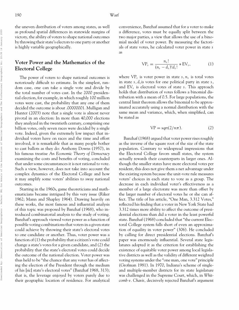
To what extent is the measure of relative voter powerutilized here real, or, conversely, to what extent is it sim-ply an artifact of the methodology? In other words, canthe measure of relative voter power proposed here serveas a reliable indicator of spatial biases in the ElectoralCollege, or is it simply a proxy for other forces? Onthe basis of the approach outlined earlier, the relativepower of voters to sway elections may be expected tobe a function of two variables, the margin of victory ineach state in each presidential election and the numberof electoral votes involved. As Figure 2 indicates, as pre-dicted, relative voter power is indeed correlated—butnot synonymous—with the margin of victory in eachD
ownloaded By: [Association of American Geographers - Referer URL for Annals of the Association of American Geographers and The Professional Geographer] At: 20:38 14 January 2009
The U.S. Electoral College and Spatial Biases in Voter Power 193
Figure 2. Scattergram of margin of victory and relative voter power, 1960–2004 presidential elections.
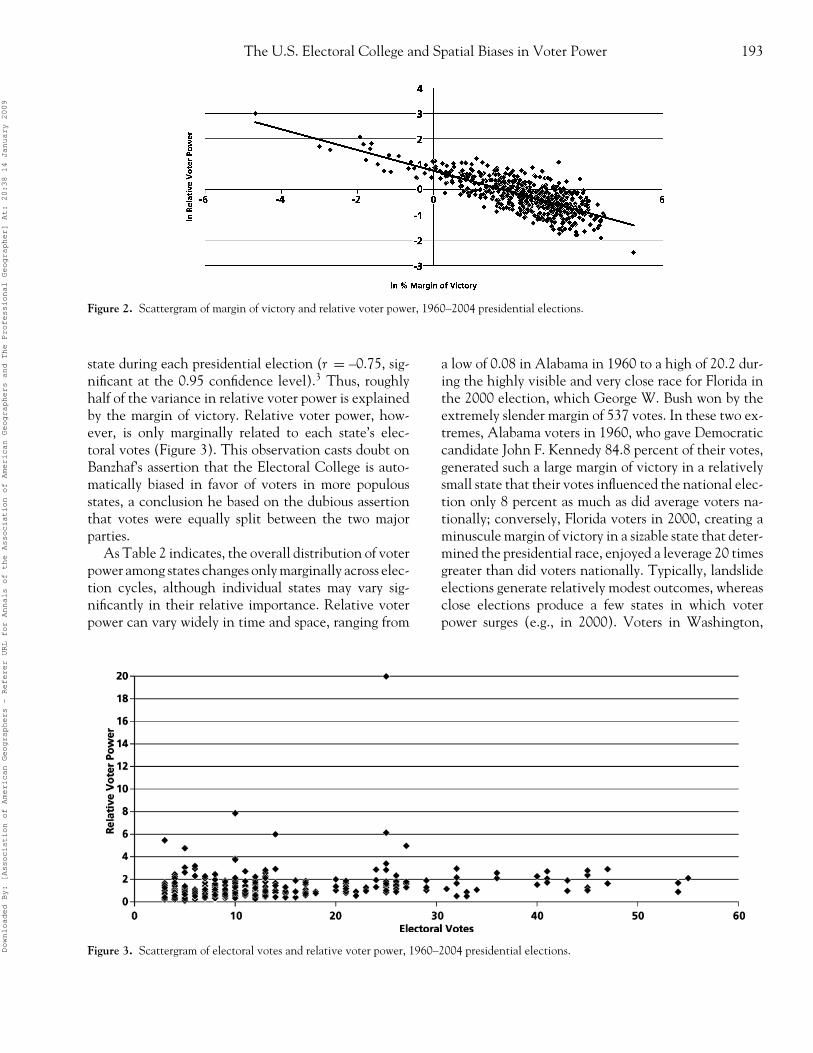
state during each presidential election (r = –0.75, sig-nificant at the 0.95 confidence level).3 Thus, roughlyhalf of the variance in relative voter power is explainedby the margin of victory. Relative voter power, how-ever, is only marginally related to each state’s elec-toral votes (Figure 3). This observation casts doubt onBanzhaf’s assertion that the Electoral College is auto-matically biased in favor of voters in more populousstates, a conclusion he based on the dubious assertionthat votes were equally split between the two majorparties.
As Table 2 indicates, the overall distribution of voterpower among states changes only marginally across elec-tion cycles, although individual states may vary sig-nificantly in their relative importance. Relative voterpower can vary widely in time and space, ranging from
a low of 0.08 in Alabama in 1960 to a high of 20.2 dur-ing the highly visible and very close race for Florida inthe 2000 election, which George W. Bush won by theextremely slender margin of 537 votes. In these two ex-tremes, Alabama voters in 1960, who gave Democraticcandidate John F. Kennedy 84.8 percent of their votes,generated such a large margin of victory in a relativelysmall state that their votes influenced the national elec-tion only 8 percent as much as did average voters na-tionally; conversely, Florida voters in 2000, creating aminuscule margin of victory in a sizable state that deter-mined the presidential race, enjoyed a leverage 20 timesgreater than did voters nationally. Typically, landslideelections generate relatively modest outcomes, whereasclose elections produce a few states in which voterpower surges (e.g., in 2000). Voters in Washington,
Figure 3. Scattergram of electoral votes and relative voter power, 1960–2004 presidential elections.Downloaded By: [Association of American Geographers - Referer URL for Annals of the Association of American Geographers and The Professional Geographer] At: 20:38 14 January 2009
194 Warf
Table 2. Summary of distribution of relative voter power (RVP) by election cycle
Number of states with RVP
<1.0 1.0–1.9 2.0–2.99 3.0–3.99 > 4.00 Minimum Maximum
1960 35 11 2 0 2 .08 (AL) 5.45 (HI)1964 32 16 2 1 0 .34 (DC) 3.05 (AZ)1968 36 10 4 1 0 .24 (DC) 3.39 (TX)1972 36 13 2 0 0 .50 (UT) 2.36 (CA)1976 33 15 1 1 1 .20 (DC) 6.13 (OH)1980 34 13 2 1 1 .19 (UT) 5.98 (MA)1984 37 10 2 1 1 .33 (DC) 7.85 (MN)1988 33 13 5 0 0 .30 (DC) 2.90 (CA)1992 33 13 5 0 0 .29 (DC) 2.55 (GA)1996 33 13 5 0 0 .28 (DC) 2.79 (GA)2000 45 3 1 0 2 .12 (VT) 20.2 (FL)2004 32 15 3 1 0 .30 (DC) 3.73 (WI)
DC, often suffer from being the least influential in thecountry in that they tend to cast their votes for Demo-cratic candidates by large margins and offer only threeelectoral votes.
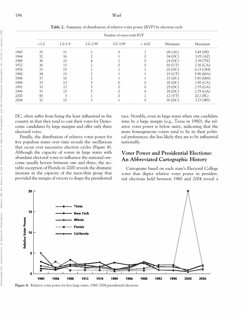
Finally, the distribution of relative voter power forfive populous states over time reveals the oscillationsthat occur over successive election cycles (Figure 4).Although the capacity of voters in large states withabundant electoral votes to influence the national out-come usually hovers between one and three, the no-table exception of Florida in 2000 reveals the dramaticincrease in the capacity of the razor-thin group thatprovided the margin of victory to shape the presidential
race. Notably, even in large states when one candidatewins by a large margin (e.g., Texas in 1980), the rel-ative voter power is below unity, indicating that themore homogeneous voters tend to be in their politi-cal preferences, the less likely they are to be influentialnationally.
Voter Power and Presidential Elections:An Abbreviated Cartographic History
Cartograms based on each state’s Electoral Collegevotes that depict relative voter power in presiden-tial elections held between 1960 and 2004 reveal a
Figure 4. Relative voter power for five large states, 1960–2004 presidential elections.Downloaded By: [Association of American Geographers - Referer URL for Annals of the Association of American Geographers and The Professional Geographer] At: 20:38 14 January 2009

The U.S. Electoral College and Spatial Biases in Voter Power 195
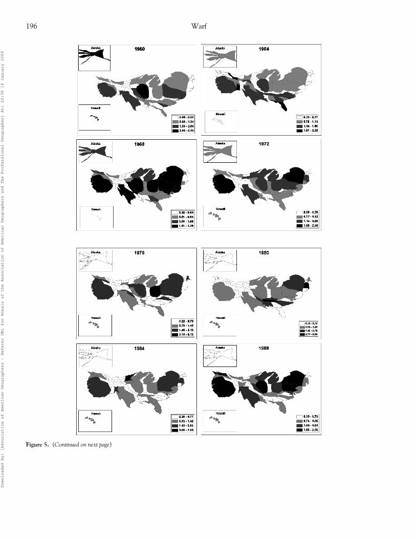
complex, shifting landscape in which voter power wasnot concentrated in a single group of states—large orsmall—but alternated among them (Figure 5). Thesecartograms represent two variables simultaneously: Thesize of each state is proportional to its total electoralvotes, whereas its shade represents relative voter power.It is worth emphasizing that the results portrayed heredo not measure the popularity of particular candidatesor parties; rather, they reflect the relative ability of vot-ers in different states to shape national elections asthe dynamics of statewide voting margins are reflectedthrough the peculiarities of the Electoral College.
Thus, in the extremely close race of 1960, John F.Kennedy defeated Richard Nixon by 34,220,984 to34,108,185, a mere 112,827 votes, or 0.16 percent ofthe total cast. Voters in Illinois, which gave its twenty-seven electoral votes to Kennedy by a 0.19 percentmargin of victory, enjoyed a leverage five times greaterthan their average counterparts did nationally (how-ever, contrary to much received opinion, Kennedy, with303 electoral votes, would have won even without thetwenty-seven votes from Illinois). In the 1964 race, inwhich Lyndon Johnson soundly defeated Barry Gold-water, voters in Florida and Idaho, which Johnson wonby a hair, and Arizona, Goldwater’s home state (whichhe carried by 1 percent), were roughly three times asinfluential as those nationally. The Arizona case is il-lustrative of the counterintuitive notion that even vot-ers in states that support losing presidential candidatesmay enjoy high levels of influence; voter power in thiscontext is not synonymous with support for the winner.
The 1968 presidential election, complicated byGeorge Wallace’s American Independence Party vic-tories in much of the South by large margins, simulta-neously reduced the relative influence of those statesnationally (although Texas and Arkansas were partic-ularly influential) and elevated the power of votes castin Ohio, Missouri, and California to double the na-tional level. Nonetheless, a broad coalition of statesunited behind Richard Nixon led to his victory overHubert Humphrey. The 1968 election initiated a long-term shift of the region away from the Democratic Partyin the wake of the Civil Rights Act and led the South,which gave successive Republican candidates large mar-gins of victory, to become relatively marginal in termsof voter power until Bill Clinton’s campaigns in the1990s put several states back into play.
In 1972, Nixon trounced George McGovern by 18million votes, or 22.6 percent, carrying every stateexcept Massachusetts and the District of Columbia.Voter power shifted toward the Northeast and Mid-
west, in which the margins of victories were small-est and large electoral blocs were at stake: New York,Pennsylvania, Michigan, and Illinois, as well as increas-ingly important California, all large states in whichNixon’s margins of victory were lower than average,saw their relative voter power rise to 1.5 to 2.4 timesthat of the national average. In Jimmy Carter’s suc-cessful 1976 bid for the presidency, a 0.2 percent mar-gin of victory in Ohio over Gerald Ford, coupled withtwenty-five electoral votes, elevated the significance ofvoters in that state to a level six times higher thanthe national average; California and Oregon were alsoimportant in this regard. Throughout the 1970s, thelightly populated states of the Midwest and intermoun-tain West, which generally gave large margins of victoryto Republican candidates, receded significantly in voterpower.
By 1980, when Carter’s reelection bid was defeatedby Ronald Reagan, the latter’s slim margins of vic-tory in New York, Massachusetts, Arkansas, and Ten-nessee raised voters’ relative power in those states tolevels two to six times as high as nationally. In 1984,Reagan’s landslide reelection victory over DemocratWalter Mondale made the voters of Minnesota—theonly state (other than the District of Columbia) to voteagainst him—enjoy a leverage 7.85 times greater thanthe national average, an indication that voters may berelatively influential even if they cast their votes for acandidate who loses. California, despite its enormoussize, endorsed Reagan twice with such large marginsof victory that its electoral votes were never in doubt,greatly reducing relative voter power there. The victoryof George H. W. Bush in 1988 over Michael Dukakis,the first by a sitting vice president since 1837, likewiseconferred considerable relative voter power to statesthat opposed him, such as New York, as well as somethat supported him, albeit by thin margins, such as Illi-nois and California.
Two victories by Bill Clinton, in 1992 and 1996, pro-duced almost identical maps of voter power, with thehighest levels of relative voter power found in Texas,Georgia, Virginia, and Kentucky (which opposed him),and Nevada (which supported him by a very narrowmargin), indicating that his base of support remainedremarkably constant in size and spatial distribution dur-ing that period. The 1992 race, of course, was compli-cated by Ross Perot, who did not win electoral votes butwas a significant presence in some states. A Southerner,Clinton managed to attract sufficiently large supportthroughout the South to erode or even overcome Re-publican margins of victory, greatly elevating relativeD
ownloaded By: [Association of American Geographers - Referer URL for Annals of the Association of American Geographers and The Professional Geographer] At: 20:38 14 January 2009
196 Warf
Figure 5. (Continued on next page)
Downloaded By: [Association of American Geographers - Referer URL for Annals of the Association of American Geographers and The Professional Geographer] At: 20:38 14 January 2009

The U.S. Electoral College and Spatial Biases in Voter Power 197
Figure 5. (continued.) Cartograms of relative voter power, 1960–2004 presidential elections. (Note: Size of states is proportional to thenumber of Electoral College votes.)
voter power in the region (e.g., in Kentucky, Tennessee,Arkansas, and Louisiana).
The 2000 election, of course, stands in a class byitself, not only because the Electoral College victor,George W. Bush, failed to acquire the majority of thepopular vote, but also because the extremely close mar-gin of victory in Florida (537 votes amid a hotly con-tested recount), with twenty-seven electoral votes atstake, elevated voters’ relative power there to a leveltwenty times greater than voters nationally, an un-precedented, unique maximum of influence in Ameri-can political history. Likewise, voters in New Mexicowere also more powerful than voters nationally by afactor of almost five. The presence on the ballot ofRalph Nader, who won 2.8 million votes (2.7 per-cent), and Pat Buchanan (448,000, or 0.4 percent),likewise was critical to the outcome in several keystates. By 2004, Bush’s reelection victory focused enor-mous media attention on Ohio, which he won by 2percent, generating relative voter power 3.8 times ashigh the national average; Wisconsin, Iowa, New Mex-ico, and California were also significant in this regard.Conversely, in both 2000 and 2004, large Republicanmajorities throughout the Great Plains reduced voterpower there to levels less than one-half of the nationalaverage.
What do these maps tell us? Clearly the spatial bi-ases generated by the Electoral College extend wellbeyond the simple dichotomy of large versus smallstates, as theorized by Banzhaf and others, as well asthe popular “red versus blue” bifurcation utilized bythe media. Neither are these maps simply reflectionsof popular margins of victory, for small margins instates with few electoral votes fail to generate sub-stantial increases in relative voter power. Rather, thesepatterns speak to the complex interplay of voter pref-erences and the distortions created by the ElectoralCollege, in which relative voter power is produced inways that are contingent, spatially uneven, and oftenunpredictable.
Is the Electoral College Biased for orAgainst Particular Social Groups?
In addition to the spatial biases that the ElectoralCollege generates for and against individual states, thereare grounds for suspecting that these tendencies play dif-ferentially to the advantage or disadvantage of particu-lar social groups of voters as defined by political party,ethnicity, urban or rural location, or religion. Follow-ing Longley and Dana (1984), the relative voter powerD
ownloaded By: [Association of American Geographers - Referer URL for Annals of the Association of American Geographers and The Professional Geographer] At: 20:38 14 January 2009
198 Warf
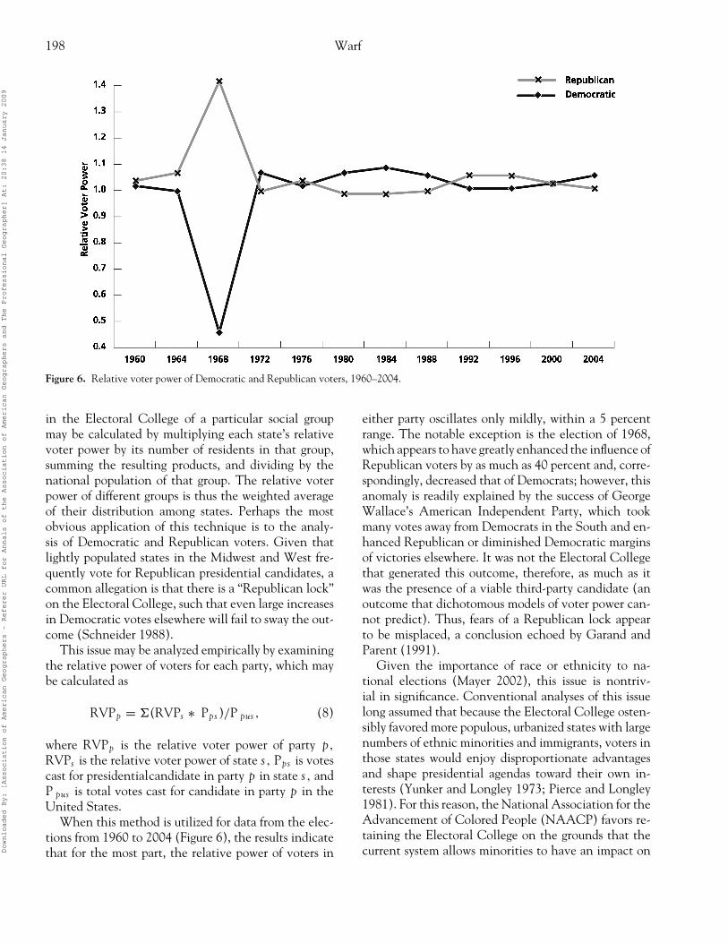
Figure 6. Relative voter power of Democratic and Republican voters, 1960–2004.
in the Electoral College of a particular social groupmay be calculated by multiplying each state’s relativevoter power by its number of residents in that group,summing the resulting products, and dividing by thenational population of that group. The relative voterpower of different groups is thus the weighted averageof their distribution among states. Perhaps the mostobvious application of this technique is to the analy-sis of Democratic and Republican voters. Given thatlightly populated states in the Midwest and West fre-quently vote for Republican presidential candidates, acommon allegation is that there is a “Republican lock”on the Electoral College, such that even large increasesin Democratic votes elsewhere will fail to sway the out-come (Schneider 1988).
This issue may be analyzed empirically by examiningthe relative power of voters for each party, which maybe calculated as
RVPp = �(RVPs ∗ Pps )/P pus , (8)
where RVPp is the relative voter power of party p,
RVPs is the relative voter power of state s, Pps is votescast for presidentialcandidate in party p in state s, andP pus is total votes cast for candidate in party p in theUnited States.
When this method is utilized for data from the elec-tions from 1960 to 2004 (Figure 6), the results indicatethat for the most part, the relative power of voters in
either party oscillates only mildly, within a 5 percentrange. The notable exception is the election of 1968,which appears to have greatly enhanced the influence ofRepublican voters by as much as 40 percent and, corre-spondingly, decreased that of Democrats; however, thisanomaly is readily explained by the success of GeorgeWallace’s American Independent Party, which tookmany votes away from Democrats in the South and en-hanced Republican or diminished Democratic marginsof victories elsewhere. It was not the Electoral Collegethat generated this outcome, therefore, as much as itwas the presence of a viable third-party candidate (anoutcome that dichotomous models of voter power can-not predict). Thus, fears of a Republican lock appearto be misplaced, a conclusion echoed by Garand andParent (1991).
Given the importance of race or ethnicity to na-tional elections (Mayer 2002), this issue is nontriv-ial in significance. Conventional analyses of this issuelong assumed that because the Electoral College osten-sibly favored more populous, urbanized states with largenumbers of ethnic minorities and immigrants, voters inthose states would enjoy disproportionate advantagesand shape presidential agendas toward their own in-terests (Yunker and Longley 1973; Pierce and Longley1981). For this reason, the National Association for theAdvancement of Colored People (NAACP) favors re-taining the Electoral College on the grounds that thecurrent system allows minorities to have an impact onD
ownloaded By: [Association of American Geographers - Referer URL for Annals of the Association of American Geographers and The Professional Geographer] At: 20:38 14 January 2009

The U.S. Electoral College and Spatial Biases in Voter Power 199
Table 3. Relative voter power (RVP) of fiveethnic groups, 2000 and 2004
RVP
2000 2004 % of voters
White 0.98 1.00 74.3Black 1.02 0.87 11.6Latino or Hispanic 0.64 1.77 9.5Asian 1.19 0.95 3.1Native American 0.69 1.34 1.5
the electoral process by being the deciding factor in se-lected states (Best 1996). The relative voter power offive major ethnic groups may be estimated as
RVPe = �(RVPs ∗ Pes )/Pe us, (9)
where RVPe is the relative voter power of ethnic groupe (whites, blacks, Native Americans, Latinos, Asians),RVPs is the relative voter power of state s, Pes is thepopulation of ethnic group e in state s, and Peus is thepopulation of ethnic group e in the United States.
The results of this exercise for the 2000 and 2004elections are indicated in Table 3, using 2000 Censusdata. Whites, who comprise the vast majority of thepopulation and voters, exhibited relative voter powerroughly equal to the national average. African Ameri-cans enjoyed approximately the national average rela-tive voter power in 2000, but a decline to 87 percentin 2004, reflecting their concentration in states withrelatively little impact, including much of the South.Native Americans and Latinos and Hispanics revealedsubstantial fluctuations in power over the two elections:They were by far the most relatively disenfranchisedgroups in 2000 (with 69 persent and 64 percent of thenational average, respectively), only to witness a risein 2004 to 1.34 and 1.77, respectively, in large part be-cause they were clustered in battleground states suchas California and New Mexico. Finally, Asian Amer-ican voters, who enjoyed an average 19 percent morepolitical leverage in 2000 than the national average,returned to roughly the average in 2004 as the sites ofmaximum voter power shifted to states with relativelysmaller proportions of voters in that group (e.g., Ohio).In short, ethnic minorities do not appear to enjoy anyconsistent advantage in the Electoral College, a con-clusion that mirrors similar analyses of ethnicity andvoter power (e.g., Longley and Dana 1984).
Voting differences between large, highly urbanizedcounties, which lean Democratic, and smaller, more ru-
Table 4. Relative voter power (RVP) of voters inmetropolitan and nonmetropolitan counties, 2000
and 2004 elections
RVP
Region 2000 2004 % of voters
Metropolitan 1.10 1.03 80.4Nonmetropolitan 0.60 0.87 19.6
ral areas, which tend to support Republicans, are amongthe central differences in recent presidential elections(Fife and Miller 2002). The voting power of populationsresiding in metropolitan and nonmetropolitan countiesmay be estimated using the relation
RVPm,nm = �(RVPs ∗ Pm,nm.s )/Pm,nm.us , (10)
where RVPm,nm is the relative voting power ofmetropolitan or nonmetropolitan populations, RVPs isthe relative voter power of state s, Pm,nm.s is the popula-tion of metropolitan or nonmetropolitan areas in states, and Pm,nm.us is the population of metropolitan ornonmetropolitan areas in the United States.
The results (Table 4) indicate that in the 2000 elec-tion, voters in metropolitan areas were almost twice asinfluential as those living in nonmetropolitan areas, inlarge part due to the extremely relative voter power inhighly urbanized Florida, in which 93 percent of thepopulation lives in metropolitan areas. By 2004, thisdiscrepancy decreased slightly, although voters in largemetropolitan regions still retained a slight edge (3 per-cent); the change reflected the decline in relative voterpower in Florida but a rise in Ohio, Minnesota, NewYork, and California.
In the same vein, the relative power of different reli-gious denominations may be calculated. Organized reli-gion plays an increasingly important role in Americanpresidential politics, a phenomenon of which the re-cent rise of politically conservative Protestants withinthe Republican Party is perhaps the most visible face(Fowler et al. 2004; Green, Rozell, and Wilcox 2006;Wald and Calhoun-Brown 2007). The source of data re-garding membership in religious denominations was the2000 census published by the Glenmary Research Cen-ter (2002); nondenominational and nonreligious voterswere excluded from this analysis. The voter power of dif-ferent religious groups of voters may be estimated usingthe equation
RVPr = �(RVPr s ∗ Pr s )/Pr us, (11)Downloaded By: [Association of American Geographers - Referer URL for Annals of the Association of American Geographers and The Professional Geographer] At: 20:38 14 January 2009
200 Warf
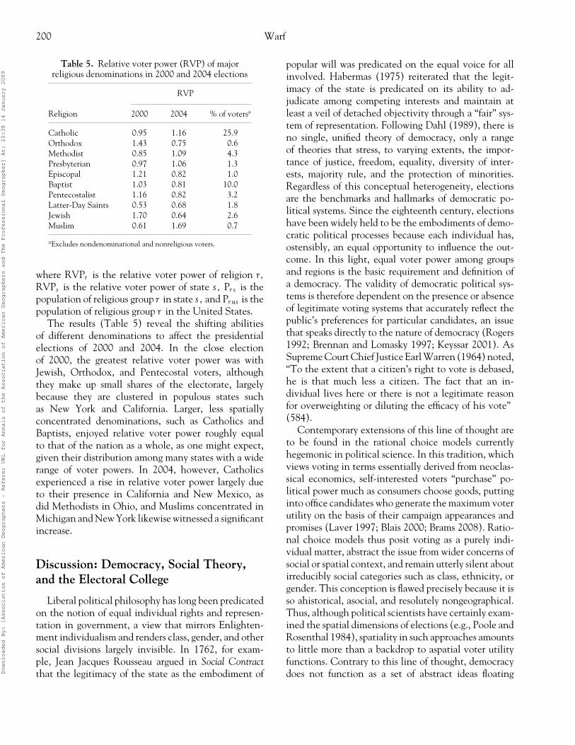
Table 5. Relative voter power (RVP) of majorreligious denominations in 2000 and 2004 elections
RVP
Religion 2000 2004 % of votersa
Catholic 0.95 1.16 25.9Orthodox 1.43 0.75 0.6Methodist 0.85 1.09 4.3Presbyterian 0.97 1.06 1.3Episcopal 1.21 0.82 1.0Baptist 1.03 0.81 10.0Pentecostalist 1.16 0.82 3.2Latter-Day Saints 0.53 0.68 1.8Jewish 1.70 0.64 2.6Muslim 0.61 1.69 0.7
aExcludes nondenominational and nonreligious voters.
where RVPr is the relative voter power of religion r,RVPs is the relative voter power of state s, Pr s is thepopulation of religious group r in state s, and Pr us is thepopulation of religious group r in the United States.
The results (Table 5) reveal the shifting abilitiesof different denominations to affect the presidentialelections of 2000 and 2004. In the close electionof 2000, the greatest relative voter power was withJewish, Orthodox, and Pentecostal voters, althoughthey make up small shares of the electorate, largelybecause they are clustered in populous states suchas New York and California. Larger, less spatiallyconcentrated denominations, such as Catholics andBaptists, enjoyed relative voter power roughly equalto that of the nation as a whole, as one might expect,given their distribution among many states with a widerange of voter powers. In 2004, however, Catholicsexperienced a rise in relative voter power largely dueto their presence in California and New Mexico, asdid Methodists in Ohio, and Muslims concentrated inMichigan and New York likewise witnessed a significantincrease.
Discussion: Democracy, Social Theory,and the Electoral College
Liberal political philosophy has long been predicatedon the notion of equal individual rights and represen-tation in government, a view that mirrors Enlighten-ment individualism and renders class, gender, and othersocial divisions largely invisible. In 1762, for exam-ple, Jean Jacques Rousseau argued in Social Contractthat the legitimacy of the state as the embodiment of
popular will was predicated on the equal voice for allinvolved. Habermas (1975) reiterated that the legit-imacy of the state is predicated on its ability to ad-judicate among competing interests and maintain atleast a veil of detached objectivity through a “fair” sys-tem of representation. Following Dahl (1989), there isno single, unified theory of democracy, only a rangeof theories that stress, to varying extents, the impor-tance of justice, freedom, equality, diversity of inter-ests, majority rule, and the protection of minorities.Regardless of this conceptual heterogeneity, electionsare the benchmarks and hallmarks of democratic po-litical systems. Since the eighteenth century, electionshave been widely held to be the embodiments of demo-cratic political processes because each individual has,ostensibly, an equal opportunity to influence the out-come. In this light, equal voter power among groupsand regions is the basic requirement and definition ofa democracy. The validity of democratic political sys-tems is therefore dependent on the presence or absenceof legitimate voting systems that accurately reflect thepublic’s preferences for particular candidates, an issuethat speaks directly to the nature of democracy (Rogers1992; Brennan and Lomasky 1997; Keyssar 2001). AsSupreme Court Chief Justice Earl Warren (1964) noted,“To the extent that a citizen’s right to vote is debased,he is that much less a citizen. The fact that an in-dividual lives here or there is not a legitimate reasonfor overweighting or diluting the efficacy of his vote”(584).
Contemporary extensions of this line of thought areto be found in the rational choice models currentlyhegemonic in political science. In this tradition, whichviews voting in terms essentially derived from neoclas-sical economics, self-interested voters “purchase” po-litical power much as consumers choose goods, puttinginto office candidates who generate the maximum voterutility on the basis of their campaign appearances andpromises (Laver 1997; Blais 2000; Brams 2008). Ratio-nal choice models thus posit voting as a purely indi-vidual matter, abstract the issue from wider concerns ofsocial or spatial context, and remain utterly silent aboutirreducibly social categories such as class, ethnicity, orgender. This conception is flawed precisely because it isso ahistorical, asocial, and resolutely nongeographical.Thus, although political scientists have certainly exam-ined the spatial dimensions of elections (e.g., Poole andRosenthal 1984), spatiality in such approaches amountsto little more than a backdrop to aspatial voter utilityfunctions. Contrary to this line of thought, democracydoes not function as a set of abstract ideas floatingD
ownloaded By: [Association of American Geographers - Referer URL for Annals of the Association of American Geographers and The Professional Geographer] At: 20:38 14 January 2009

The U.S. Electoral College and Spatial Biases in Voter Power 201
in the minds of individuals inhabiting some ahistori-cal, aspatial vacuum but as complex, contingent, andpower-laden networks deeply rooted in social relationsconstituted at multiple spatial scales. Elections are em-bedded in a broader civic epistemology, “the culturesand practices of knowledge production and validationthat characterize public life and civic institutions inmodern democratic societies” (Miller 2004, 1), a webof formal and informal relations that extends beyondthe voting booth to the judiciary, election bureaucra-cies, schools, and the media.
The analysis offered here indicates that the abil-ity of American voters to influence the outcome ofpresidential elections is intimately bound up with thegeographic dynamics of the Electoral College. Spatialbiases are not idiosyncratic but generic to its organiza-tion. Where voters are located, the size of their electoralblocs, and the statewide margin of victory in presiden-tial races are all central to shaping the relative powerof voters in different states to influence the choice ofthe chief executive. To the extent that the ElectoralCollege generates uneven geographies of voter power,therefore, it is a fundamentally antidemocratic and an-tiliberal institution.
Moreover, because power is such a notoriously slip-pery phenomenon to measure empirically, this approachoffers a means to operationalize it mathematically, lend-ing methodological rigor to the analysis of an issuethat has enjoyed little such advantage in the literature.Clearly the assessment of power is highly contingent onits specification via a particular model. The most suc-cessful approach to this issue to date, the Banzhaf model,“does not take account of the political competitivenessof the states” (Rabinowitz and MacDonald 1986, 77.)In contrast, by introducing the margin of victory intothis issue, the approach advocated here significantlyamplifies the differentials in voter power among states.Voter margins of victory reflect the collective prefer-ences of large groups of people whose intentions (asmanifested in the popular vote) are funneled into thewinner-take-all system that ultimately determines thewinning candidate for the presidency; thus, electoralgeography can engage productively with the analysis ofvoter subjectivity, incorporating contingency into itsanalysis of electoral outcomes and avoiding the mech-anistic stance that long plagued the field. In short, thelegacy of an eighteenth-century political system thattried to accommodate small and large states, the hap-penstance of voter location, and the unintentional pro-duction of margins of victory all conspire within theElectoral College to produce relative voter power in
spatially uneven ways, generating geographies of influ-ence that fluctuate markedly from one election cycle toanother. Such a critique allows the liberal view aboutequal access to state power to be reconceptualized in amanner that complements, but does not substitute for,predominant Marxist and Foucauldian notions, whichtend to ignore electoral politics. In this reading, theability to shape the power of the national governmentvia elections is far more unstable, ephemeral, and con-tingent than that generated by relations of class, eth-nicity, and gender, which tend to be deeply embeddedin arenas outside of the state, such as the division oflabor and cultural norms.
Concluding Thoughts
The Electoral College is an institution that reflectsthe unique historical and political circumstances of theUnited States. Critics maintain that it systematicallydistorts the meaning of the popular vote, to the ex-tent that more than once candidates have won thepresidency without winning a majority of ballots cast.Presidential political campaigns are acutely sensitiveto the uneven landscapes of power that the Collegegenerates and structure their spatial allocations of lim-ited resources and candidate time accordingly. Popu-lar understandings of this topic simplistically point tothe overrepresentation of lightly populated states in theElectoral College. Conversely, game theorists, seekingto shed mathematical light on this issue, have con-sistently maintained that voters in larger states holdrelatively more power to sway the national race byvirtue of the large blocs of electoral votes they con-trol. Drawing on the seminal work of Banzhaf (1968),who introduced game theory in the form of a model oftwo political parties that split the popular vote evenly,this analysis offered an empirically tractable, multino-mial extension of his model of relative voter power,which reflects the total number of votes cast in eachstate in each election, the number and proportion ofvotes cast for each candidate, the margin of victoryof the winner, and the number of electoral votes atstake.
Applying this analysis to U.S. presidential electionsfrom 1960 to 2004 reveals that relative voter power var-ied markedly among states and over time. Unexpect-edly, voter power was not consistently related to thesize of states but reflected a complex interplay shapedby the margin of victory in each state and the winner-take-all dynamics of the Electoral College. UtilizingD
ownloaded By: [Association of American Geographers - Referer URL for Annals of the Association of American Geographers and The Professional Geographer] At: 20:38 14 January 2009

202 Warf
the same framework to analyze the abilities of the twomajor political parties, five major ethnic groups, ruralor urban residence, and ten religious denominationsto shape national elections likewise indicates that theElectoral College does not consistently exaggerate thevoter power of any single group, with the exception ofvoters in metropolitan regions, who tend to be con-centrated in large states that are often electoral battle-grounds. Thus, allegations that the Electoral Collegeexhibits a “Republican lock” that it is weighted in fa-vor of large states, or that it protects the interests ofwhite men, or, conversely, allows minorities to shapepresidential priorities, are all equally unfounded. Voterpower is much more complex than any simple or sim-plistic assertions will admit.
Rather than the portrait of power as stable anddurable across time and space, a concept found through-out many conventional treatments, this analysis indi-cates that voter power is highly contingent, ephemeral,transitory, and unpredictable. Such a conclusion speaksto the role of elections as the embodiment of popu-lar political preferences (e.g., via margins of victory),yet acknowledges that the winner-take-all system thatis the defining feature of the Electoral College impartsspatial distortions that differentially enhance the powerof voters in some states at the expense of others.
Acknowledgment
The author thanks Shawn Lewers and DarinGrauberger for their assistance with the graphics.
Notes1. Although Maine and Nebraska do not strictly abide by
the winner-take-all system, for analytical convenience inthis analysis they are considered to operate on that basis.For more on the Maine–Nebraska or Mundt–Coudertsystem, see Johnston, Rossiter, and Pattie (2006).
2. The empirical calculation of large factorials such as thoseinvolved in the application of Equation 5 to voting datapresents a formidable methodological obstacle. Fortu-nately, factorials may be estimated closely using Ster-ling’s formula, which holds that for any number m, m!= e−mmm sqrt(2πm). For numbers larger than 100, thisformula is accurate within 0.1 percent; for very largenumbers, such as the ones used here, the difference be-tween the estimated and actual factorials is infinitesi-mally small. Banzhaf (1968) used Sterling’s approxima-tion throughout his paper. Even this estimate may bechallenging for all but the most sophisticated of com-puters, however. An easier approach is to use naturallogarithms: Ln m! = –m + m * ln m + ln sqrt(2πm).This technique is employed throughout this article.
3. The regression equation was ln(RVP) = 0.733 – 0.409ln(margin of victory), r 2 = 0.569, N = 611.
References
Abbott, D., and J. Levine. 1991. Wrong winner: The comingdebacle in the Electoral College. New York: Praeger.
Adams, P. 2007. Atlantic reverberations: French representationsof an American presidential election. London: Ashgate.
Adkinson, D., and C. Elliott. 1997. The Electoral College:A misunderstood institution. Political Science and Politics30:77–80.
Agnew, J. 1995. The rhetoric of regionalism: The NorthernLeague in Italian politics. Transactions of the Institute ofBritish Geographers 20:156–72.
———. 1996. Mapping politics: How context counts in elec-toral geography. Political Geography 15:129–46.
Amy, D. 1993. Real choices/new voices: The case for proportionalrepresentation elections in the United States. New York:Columbia University Press.
Archer, J. 1988. Macrogeographical versus microgeographi-cal cleavages in American presidential elections: 1940–1984. Political Geography Quarterly 7:111–26.
Archer, J., G. Murauskas, and F. Shelley. 1985. Coun-ties, states, sections, and parties in the 1984 pres-idential election. Professional Geographer 37:279–87.
Archer, J., and F. Shelley. 1986. American electoral mo-saics. Washington, DC: Association of American Ge-ographers.
———. 1988. The geography of U.S. presidential elections.Scientific American 259:44–53.
Ball, W., and D. Leuthold. 1991. Estimating the likelihoodof an unpopular verdict in the Electoral College. PublicChoice 70:215–24.
Banzhaf, J. 1968. One man, 3.312 votes: A mathematicalanalysis of the Electoral College. Villanova Law Review13:304–32.
Best, J. 1975. The case against direct election of the president:A defense of the Electoral College. Ithaca, NY: CornellUniversity Press.
———. 1996. The choice of the people? Debating the ElectoralCollege. Lanham, MD: Rowman & Littlefield.
Bickel, A. 1968. Reform and continuity: The Electoral College,the convention and the party system. New York: Harperand Row.
Blair, D. 1979. Electoral College reform and the distributionof voter power. Public Choice 34:201–15.
Blais, A. 2000. To vote or not to vote: The merits and limitsof rational choice theory. Pittsburgh, PA: University ofPittsburgh Press.
Brams, S. 2008. Mathematics and democracy: Designing bettervoting and fair-division procedures. Princeton, NJ: Prince-ton University Press.
Brennan, G., and L. Lomasky, eds. 1997. Democracy and de-cision: The pure theory of electoral preference. Cambridge,UK: Cambridge University Press.
Colantoni, C., T. Levesque, and P. Ordeshook. 1975. Cam-paign resource allocations under the Electoral College.American Political Science Review 69:141–54.
Dahl, R. 1989. Democracy and its critics. New Haven, CT:Yale University Press.D
ownloaded By: [Association of American Geographers - Referer URL for Annals of the Association of American Geographers and The Professional Geographer] At: 20:38 14 January 2009
The U.S. Electoral College and Spatial Biases in Voter Power 203
Downs, A. 1957. An economic theory of democracy. New York:Harper.
Enelow, J., and M. Hinich, eds. 1990. Advances in the spatialtheory of voting. Cambridge, UK: Cambridge UniversityPress.
Fife, B., and G. Miller. 2002. Political culture and voting systemsin the United States: An examination of the 2000 presidentialelection. New York: Praeger.
Flint, C. 2001. A timespace for electoral geography:Economic restructuring, political agency and therise of the Nazi party. Political Geography 20:301–29.
Fowler, R., A. Hertzke, L. Olson, and K. den Dulk. 2004.Religion and politics in America: Faith, culture, and strategicchoices. Boulder, CO: Westview.
Garand, J., and T. Parent. 1991. Representation, swing,and bias in U.S. presidential elections, 1872–1988. American Journal of Political Science 35:1011–31.
Gelman, A., and G. King. 1994. A unified method of eval-uating electoral systems and districting plans. PoliticalScience 12:158–67.
Glenmary Research Center. 2002. Religious congregations &membership in the United States. Atlanta, GA: GlenmaryResearch Center.
Green, J., M. Rozell, and C. Wilcox, eds. 2006. The val-ues campaign? The Christian right and the 2004 elections.Washington, DC: Georgetown University Press.
Gregg, G., ed. 2001. Securing democracy: Why we have anelectoral college. Wilmington, DE: ISI Books.
Grofman, B. 1981. Fair apportionment and the Banzhaf in-dex. American Mathematical Monthly 88:1–5.
———. 1983. Measures of bias and proportionality in seats–votes relationships. Political Methodology 9:295–327.
Grofman, B., T. Brunell, and J. Campagna. 1997. Distinguish-ing between the effects of swing ratio and bias on out-comes in the U.S. Electoral College, 1900–1992. Elec-toral Studies 16:471–87.
Habermas, J. 1975. Legitimation crisis. Boston: Beacon Press.Hardaway, R. 1994. The Electoral College and the Constitu-
tion: The case for preserving federalism. Westport, CT:Praeger.
Hinich, M., and P. Ordeshook. 1974. The Electoral College:A spatial analysis. Political Methodology 1 (Summer): 1–29.
Johnston, R. 1982. The changing geography of voting in theUnited States: 1946–1980. Transactions of the Institute ofBritish Geographers 7:187–204.
———. 2002. Census counts and apportionment: The poli-tics of representation in the United States . . . continued.Environment and Planning D: Society and Space 20:619–28.
———. 2005. Anglo-American electoral geography: Sameroots and same goals, but different means and ends? Pro-fessional Geographer 57:580–87.
Johnston, R., and C. Pattie. 2003. Representative democracyand electoral geography. In A companion to political geog-raphy, ed. J. Agnew, K. Mitchell, and G. Toal, 337–55.Oxford, UK: Blackwell.
———. 2006. Putting voters in their place: Geography and elec-tions in Great Britain. New York: Oxford University Press.
Johnston, R., D. Rossiter, and C. Pattie. 2005. Disproportion-ality and bias in US presidential elections: How geogra-
phy helped Bush defeat Gore but couldn’t help Kerrybeat Bush. Political Geography 24:952–68.
———. 2006. Changing the scale and changing the result:Evaluating the impact of an electoral reform on the 2000and 2004 US presidential elections. Political Geography25:557–69.
Johnston, R., F. Shelley, and P. Taylor, eds. 1990. Develop-ments in electoral geography. London: Routledge.
Josephson, W., and B. Ross. 1996. Repairing the ElectoralCollege. Journal of Legislation 22 (9): 145–93.
Keyssar, A. 2001. The right to vote: The contested history ofdemocracy in the United States. New York: Basic Books.
Kimberling, W. 1992. The Electoral College. Washington,DC: National Clearinghouse on Election Administra-tion, Federal Election Commission. http://www.fec.gov/pdf/eleccoll.pdf (last accessed 21 October 2008).
Laver, M. 1997. Private desires, political action: An invitation tothe politics of rational choice. Newbury Park, CA: Sage.
Levesque, T. 1984. Measuring state power in presidentialelections. Public Choice 42 (3): 295–310.
Longley, L., and A. Braun. 1972. The politics of Electoral Col-lege reform. New Haven, CT: Yale University Press.
Longley, L., and J. Dana. 1984. New empirical estimates ofthe biases of the Electoral College for the 1980s. WesternPolitical Quarterly 37:157–75.
———. 1992. The biases of the electoral college in the 1990s.Polity 25:123–45.
Longley, L. and N. Pierce. 1996. The Electoral College primer.New Haven, CT: Yale University Press.
Mann, I., and L. Shapley. 1964. The a priori voting strengthof the electoral college. In Game theory and related ap-proaches to social behavior, ed. M. Shubik, 19–31. NewYork: Wiley.
Margolis, H. 1983. The Banzhaf fallacy. American Journal ofPolitical Science 27:321–26.
Mayer, J. 2002. Running on race: Racial politics in presidentialcampaigns 1960–2000. New York: Random House.
McCaughey, E. 1993. Democracy at risk: The dangerous flawsin the Electoral College. Policy Review 63:79–81.
Merrill, S. 1978. Citizen voter power under the ElectoralCollege: A stochastic model based on state voting pat-terns. SIAM Journal on Applied Mathematics 34:376–90.
Michener, J. 1969. Presidential lottery: The reckless gamble inour electoral system. New York: Random House.
Miller, C. 2004. Interrogating the civic epistemology ofAmerican democracy. Social Studies of Science 34:501–30.
Mulligan, C., and C. Hunter. 2003. The empirical frequencyof a pivotal vote. Public Choice 116 (1–2): 31–54.
Natapoff, A. 1996. A mathematical one-man one-vote ratio-nale for Madisonian presidential voting based on max-imum individual voter power. Public Choice 88:259–73.
Owen, G. 1975. Evaluation of a presidential election game.American Political Science Review 69:947–53.
Pierce, N., and L. Longley. 1981. The people’s president: TheElectoral College in American history and the direct votealternative. New Haven, CT: Yale University Press.
Poole, K., and H. Rosenthal. 1984. U.S. presi-dential elections 1968–80: A spatial analy-sis. American Journal of Political Science 28:282–312.D
ownloaded By: [Association of American Geographers - Referer URL for Annals of the Association of American Geographers and The Professional Geographer] At: 20:38 14 January 2009
204 Warf
Prescott, J. 1959. The function and methods of electoral geog-raphy. Annals of the Association of American Geographers49:296–304.
Rabinowitz, G., and S. MacDonald. 1986. The power of thestates in U.S. presidential elections. American PoliticalScience Review 80:65–87.
Riker, W. 1962. The theory of political coalitions. New Haven,CT: Yale University Press.
Rogers, D. 1992. Voting and the spirit of Americandemocracy: Essays on the history of voting and vot-ing rights in America. Urbana: University of IllinoisPress.
Ross, B., and W. Josephson. 1996. The Electoral Collegeand the popular vote. Journal of Law and Politics 12:665–747.
Schneider, W. 1988. An insider’s view of the election. At-lantic Monthly 262:29–57.
Shaw, D. 1999. The methods behind the madness: Presiden-tial Electoral College strategies, 1988–1996. Journal ofPolitics 61:893–913.
Shelley, F. 2002. The Electoral College and the election of2000. Political Geography 21:79–83.
Smith, R., and P. Squire. 1987. Direct election of the presi-dent and the power of the states. Western Political Quar-terly 40:31–44.
Sterling, C. 1978. The Electoral College biases revealed,the conventional wisdom and game theory modelsnotwithstanding. Western Political Quarterly 31:159–77.
———. 1981. Electoral College misrepresentation—A geo-metric analysis. Polity 13:425–49.
Swauger, J. 1980. Regionalism in the 1976 presidential elec-tion. Geographical Review 70:157–66.
Taylor, P. 1973. Some implications of the spatial organiza-tion of elections. Transactions of the Institute of BritishGeographers 60:121–36.
Taylor, P., and R. J. Johnston. 1979. Geography of elections.London: Penguin.
Tufte, E. 1973. The relationship between seats and votesin two-party systems. American Political Science Review67:540–54.
Twentieth Century Fund Task Force on Reform of the Pres-idential Election Process. 1978. Winner take all. NewYork: Holmes and Meier.
Wald, K., and A. Calhoun-Brown. 2007. Religion and politicsin the United States. 5th ed. Lanham, MD: Rowman &Littlefield.
Warf, B. 2006. Voting technologies and residual ballots in the2000 and 2004 presidential elections. Political Geography27:664–77.
Warren, E. 1964. Reynolds v. Sims (The opinion of theCourt). United States Reports 377:533–87.
Yunker, J., and L. Longley. 1973. The biases of the ElectoralCollege: Who really is advantaged? In Perspectives onpresidential selection, ed. D. Matthews, 172–203. Wash-ington, DC: Brookings Institution.
Zeidenstein, H. 1973. Direct election of the president. Lexing-ton, MA: Lexington Books.
Correspondence: Department of Geography, University of Kansas, Lawrence, KS 66045, e-mail: [email protected].
Downloaded By: [Association of American Geographers - Referer URL for Annals of the Association of American Geographers and The Professional Geographer] At: 20:38 14 January 2009