Biases and information in analysts' recommendations: The European experience

Biases and Information in Analysts’ Recommendations: The European Experience

Sarah Azzi, University of Technology Sydney

Email: [email protected]

Ron Bird*, University of Technology Sydney and Bocconi University


Paolo Griringhelli, Bocconi University


Emanuele Rossi, University of Udine


First Draft: December, 2004

*Corresponding Author: Emeritus Professor Ron Bird School of Finance and Economics

University of Technology Sydney PO Box 123 Broadway NSW 2007 Australia

Phone: +612 9514 7716 Fax: +612 9514 7711 Email: [email protected]

JEL Classifications: G13, G14

mailto:[email protected]





2


Abstract:

Financial analysts are viewed as playing an important intermediary role in gathering and interpreting data and

thus converting it into useful information for the investment community. However, in recent years, it has

become more apparent that the analysts come under much internal and external pressure when making their

forecasts and recommendations. Jegadeesh et al (2004) have highlighted that this results in US equity analysts

being biased towards large, high momentum growth stocks when making their recommendations which

presumedly causes them to add little or no value in their own right. However, they find that the analysts’

recommendations changes do provide useful incremental investment insights. Azzi and Bird (2005) when

evaluating Australian analysts similarly found that it was only the recommendation changes that provided useful

information to investors. However, they also found evidence to suggest that the analysts attempt to adjust the

biases in their recommendations over the market cycle. The implication being that biases identified in the

Jegadeesh et al study may have been as much a reflection of the analysts pursuing the types of stocks that were

performing well during the period rather than any long-term bias in these recommendations.

In this paper, we extend the analysis to consider the recommendations made by the European analysts. We find

that as a group their recommendations have a similar strong bias towards large high momentum stocks and a

weaker bias towards growth stocks. Over the sample period of 10 years commencing April 1994, it proves that

neither their recommendations nor changes in these recommendations provide any useful information to

investors. When we divide our sample period up into the boom years of the 1990’s and the gloom years of the

early 2000’s, we do find some weak evidence of the European analysts adjusting their recommendations

particularly towards value stocks that performed best during the gloom years. We found that the

recommendations did provide useful insights to investors during the boom years but this only reflected the

biases in the recommendations suggesting little contribution from the analysts. We also found that the

recommendation changes provided useful information to investors during the gloom years but in this instance

the evidence suggested that this was reflective of some special skills of the analysts. At the country/region level,

we did find some evidence of variation in the biases impacting on analysts’ recommendations with the English

analysts displaying a strong preference for small cap stocks and the English, German and Italian analysts

appearing neutral with respect to the growth/value stock choice. The analysis of the recommendations made by

both the German and Italian analysts suggested that they could provide useful insights as to future stock

performance over and above that reflected by the biases in their recommendations. The news was no where near

as good for the UK and French analysts whose recommendations seemed to provide the market with

disinformation as to future stock returns. Overall the European findings, suggested that one would have to take

care in extending the original Jegadeesh et al findings to both other markets and other time periods.

3


Section 1: Introduction

In an innovative US study covering the period from 1985 through to 1998, Jegadeesh et al (2004) found that

analysts recommendation were biased towards large, high momentum growth stocks. Once they controlled for

these inherent biases in analyst recommendations, the authors found that the recommendations provided no

incremental information although there was additional information to be gleamed from changes in these

recommendations. The results in the Jegadeesh et al study should probably come as no surprise as the economics

of the broking industry post the deregulation of fees in 1975 resulted in US analysts becoming more a marketing

arm of not only of their firm’s broking operations but also its investment banking activities. The outcome being

that the analysts were driven less towards providing useful information to investors and more towards making

recommendations with the objective of both attracting and retaining corporate clients. Of course, the analysts

came under close scrutiny after the collapse of both the market and many large companies in the early 2000’s

resulting in legislation designed to redirect the focus of analyst back towards providing independent, useful

information to investors (Sarbanes-Oxley Act of 2002).

The focus of this study is on extending the Jegadeesh et al study to evaluate the recommendations of analysts in

15 European countries over the 10 year period commencing April 1994. In this study we not only investigate

whether the biases affecting the US analysts extended to their European colleagues during the 1990’s when the

markets in both Continents were on a sharp upward path but we also consider whether any biases that impacted

on the European analysts during this boom market carried over to the early 2000’s when the market experienced

a severe correction phase. The Jegadeesh et al data set ended in 1998 and so only covered a period during which

the market was in a consistent uptrend favouring the large, high momentum growth stocks to which the US

analysts were found to be drawn. Barber et al [2001, 2003] found that stocks favoured by the analysts performed

extremely well during the period from 1986 to 1999 but the opposite was the case during 2000 and 2001, the

first two year of the market correction. Azzi and Bird (2005) in a study of Australian analysts found evidence to

suggest that the biases identified by Jegadeesh et al might simply reflect that they are drawn to the best

performing stocks at a particular point in time and so the Jegadeesh et al findings cannot be generalised to all

stages of the market cycle.

We initially undertake our study of the biases influencing the European analyst and the information content of

their recommendations by aggregating the data from the 15 markets and conduct our analysis over our entire 10

year sample period. However, we then divide this sample period up into the first six years ending April 2002

(the boom years) and the subsequent four years (the gloom years) and repeat the analysis in order to see whether

the European analysts, like their Australian colleagues, attempt to vary the biases in their recommendations in

line with market conditions. We are also interested to see the extent to which the US findings and the Australian

4

finings extend to other countries/regions so we again repeat our analysis at the country/region level. In order to

ensure the maintenance of a sufficient sample size we do not examine the 15 countries separately but rather

examine four countries (the UK, France, Germany and Italy) and two regions (Other Europe and Scandinavia).

We find that over the entire sample period the recommendations of the European analysts display a strong bias

towards large, high momentum stocks and a slightly weaker bias towards growth stocks. These identified biases

are entirely consistent with the behavioural traits and external pressures that have been suggested to influence

their decisions. We do find evidence to suggest that the European analysts make some attempt to move their

recommendations towards the better performing value stocks during the gloom years. However, this move is far

less obvious than it was for the Australian analysts and a slight bias towards growth stocks still remains during

these years. It proves that when evaluated over the entire sample period that neither the recommendations nor

changes in these recommendations provide any worthwhile (incremental) information in relation to future stock

returns either when evaluated alone or after controlling for the biases in their recommendations. We obtain a

different picture when we evaluate the information value of the analysts’ recommendations over the two sub-

periods. During the boom years, the recommendations (but not the recommendation changes) prove to provide

useful insights into future stock returns when considered in isolation but it proves that any added value comes

more from the bias towards well-performing large, high momentum, growth stocks during this period rather

than the inherent skill of the analysts. In contrast during the gloom years it was the recommendation changes

that provided useful insights into future stock returns. To a certain extent this reflected the fact that analysts

were marginally moving their recommendations towards the well performing value stocks but it proved that the

recommendations changes during the gloom years provided information over and above the performance due to

any biases inherent in these recommendation changes. Finally, the preference for large high momentum growth

stocks was found generally to apply across analysts in each of the four countries and two regions evaluated with

the one exception being the UK market where the analysts displayed a preference for small, high momentum

stocks. There was a preference for growth stocks over value stocks in all countries/regions but there was

significant variation with its strength which was found to be strongest in Scandinavia and weakest in Germany.

There was also a fair degree of variation in the apparent information provided by the recommendations and

recommendation changes emanating from the various countries/regions. There is relatively strong evidence to

suggest that the recommendations made by both the German and Italian analysts provided useful information to

the market even after account is taken of the biases inherent in these recommendations. There is equally strong

evidence that the recommendations of the French analysts provided negative information to the market and also

some suggestion that this might also be the case for the UK analysts1. In terms of recommendation changes, the

only country/region where there was discernable evidence that these changes provided a source of useful

1 We have previously found at the aggregated level that the recommendations provide no incremental information to investors. This clearly did not apply at the country/region level but simply reflected that the positive information in some countries was offset by some negative information in others.

5

information was in Germany and even there it seemed to be purely a reflection of the bias in the

recommendation changes towards the better performing high momentum, value stocks. On the negative side,

the news was bad for the UK analysts whose recommendation changes clearly provided negative information to

the market which only became greater when account was taken of the biases inherent in these changes.

The findings of this paper are relevant for several cross-sections of the community. This paper contributes to

the existing literature on analyst biases and the information content of their recommendations and may lead to

further avenues of research in these areas. Financial practitioners and the wider investing community are able to

make better use of analyst recommendations through greater understanding of their relationship with future

returns and this may be useful in creating more lucrative trading strategies. Regulators may also find this paper of

interest as it is can be observed that recommendations are not always made in the interest of the investing public.

Similarly, financial analysts may be able to improve their performance through gaining a greater understanding of

the biases that frequently enter into their recommendations.

In Section 2 of the paper we provide some background as to the motivation of this study and we proceed in

Section 3 to describe our data and provide some insights in to the method that we employ. In Section 4 we

initially outline our findings for our entire data set which incorporates the boom years of the late 1990’s and the

gloom years of the early 2000’s. In Section 5 we repeat much of our analysis after splitting our sample between

pre- and post-April 2000 in order to evaluate whether the information content of analyst recommendations

varies under different market conditions. We repeat much of our previous analysis at the level of individual

countries/regions in order to examine the degree of commonality in the biases and information content

associated with analyst recommendations across the various European countries/regions. We complete our

study in Section 6 where we summarise our major findings and consider their implications for future research.

Section 2: Background

The assumed role of the financial analyst is to both gather and interpret information and to pass their findings

on to market participants in the form of forecasts and recommendations. As such they have the potential to play

an important intermediary role in these markets by creating a better informed and so more efficient market than

would otherwise be the case. Indeed, there is evidence to suggest that the speed of dissemination of information

about a company within a market is a function of the extent to which analysts cover the company (Hong et al,

2000). However, the extent to which analysts make a positive contribution to a better informed market has come

under significant scrutiny in recent times with there being concerns as to the effect of biases, underlying

incentives, compensation structures and cognitive traits on the information worthiness of the analyst forecast

and recommendations.

The focus in this paper is on examining the question as to whether factors other than future prospects and

current valuation levels influence the recommendations made by analysts. Importantly, studies have found

6

r

evidence to suggest that investors and analysts prefer stocks with particular characteristics. Analysts tend to be

optimistic about stocks that have performed well in the past and pessimistic about firms that have performed

poorly (Doukas, Chansog and Pantzalis, 2002). This finding is consistent with another well-known human trait,

the tendency to over-extrapolate the past, and suggests that analysts would favour growth stocks over value

stocks. Other forms of selection bias observed by analysts include a preference for positive momentum (Boni

and Womack, 2003) and for large capitalisation stocks (Womack, 1996).

These selection biases towards large, high momentum growth stocks would also appear to be consistent with

three other factors that influence analysts’ recommendations: career concerns, cognitive biases and internal

pressures. Hong and Kubrik (2003) analysed the career conce ns of analysts during 1983 to 2000, using 12,000

analysts from 600 brokerage houses. The authors found that accuracy is well rewarded, with accurate analysts

experiencing a 52% increase in the probability of improving their job position. However they also found that

once one controlled for analyst accuracy, it was the analysts that issued the more optimistic forecast that were

most likely to be promoted and be assigned to cover more attractive stocks.

Amir and Ganzach (1998) suggested that leniency, representativeness and anchoring, and adjustment are some of

the cognitive biases that affect analyst forecasts. They find that representativeness leads to overreaction;

anchoring and adjustment creates underreaction; while leniency, on the other hand, leads to optimistic

predictions2. Another characteristic that has been found a feature of analyst recommendations is their tendency

to herd, where one adheres to convention and follows the consensus (Scharfstein and Stein 1990). Welch (2000)

found that recommendation revisions of security analysts impacted upon the recommendations of the following

two analysts with this herding behaviour being more prominent under positive market conditions. He also found

that herding was not a consequence of efficient information gathering as analysts continued to bias their

recommendations to the consensus despite inaccurate consensus recommendations.

Our analysis is based on the recommendations of broker analysts who are likely to be subject to employer

pressures. One pressure applied to sell-side analysts is the need to generate broker commissions. Irvine (2002)

applied a theoretical model developed by Hayes (1998) to derive hypotheses relating analyst forecasts to trading

volume. Using Toronto Stock exchange data for the largest 100 companies during September 1993 and August

1994, analysts are found to bias recommendations, as opposed to forecasts, to induce trading volume. Irvine

(2002) contends that buy recommendations were a more effective means of increasing commission revenue than

sell recommendations.

The internal and external influences on analyst as outlined above suggest that a number of factors other than

valuations may influence their recommendations. Their influences provide an explanation for such phenomena

2 These findings are supported by Easterwood and Nutt (1999) who identified that analysts overreact to positive information and underreact to negative information.

7

as the paucity of sell recommendations, why the analysts tend to move their recommendations in the one

direction (i.e. herd) and why they are attracted towards recommending stock with particular characteristics. It is

this last point that is critical to this paper and we will address whether the European analyst has the same

preference for large, high momentum growth stocks that has been found to be the case for the US analysts

(Jegadeesh et al, 2004) and the Australian analysts (Azzi and Bird, 2005). We will then consider the implications

of the biases that we identify for the information content of the recommendations and recommendation

changes.

Section 3: Data

The discussion in the previous section leads us to suggest that there are likely to be some inherent biases in

broker recommendations: specifically we would expect analyst to favour large, high momentum, growth stocks.

In order to evaluate the extent to which these characteristics impact on analyst recommendations and the extent

to which this impacts on their performance, we need data to characterise stocks, stock returns and analyst

recommendations

General Information

This paper is designed to assess the recommendations made by European analysts with the data on these

recommendations being obtained from the Institutional Brokers Estimate System (I/B/E/S) database3. We use

the consensus analyst recommendation, calculated by I/B/E/S as the mean of the individual analyst

recommendations where I/B/E/S assigns recommendations a rating of 1-Strong Buy, 2-Buy, 3-Hold, 4-

Underperform, 5-Sell. The financial data used in the computation of financial variables, including earnings per

share, operating revenue, current assets, cash, capital expenditure, current liabilities, depreciation and

amortization, total assets, and shareholders equity is obtained from Worldscope. The market data provided by

GMO Europe included monthly returns, monthly prices, and market capitalisation.

The sample period is from April 1994 to April 2004. The analysis uses all consensus recommendations which

are based on three or more individual recommendations and for which there was corresponding financial and

market data. The analysis is conducted twice yearly at the end of April and the end of October in order to best

correspond with the release of financial data by European firms. In much of our analysis portfolios are formed

at these twice-yearly intervals based on either the current consensus recommendations or recommendation

changes and held for six-months.

There are 15 countries included in our sample: the UK, France, Germany, Italy, Austria, Belgium, Greece,

Ireland, the Netherlands, Portugal, Spain, Denmark, Finland, Norway and Sweden. We initially conduct the

analysis on a total Europe basis combining the data for all of the 15 countries and undertaking the analysis across

3 The authors wish to thank Thompson Financial for supporting our research by providing the I/B/E/S data on analyst recommendations.

8

the whole 10-year data period. We then spilt our aggregated sample into two sub-periods: when the markets were

rapidly advancing (pre-April 2000) and a period of market decline (post-April 2004) in order to identify any

differences in behaviour during these two periods within the market cycle. Finally, we investigated the extent of

diversity within Europe by splitting our data into four countries (the UK, France Germany and Italy) and two

regions: Other Europe consisting of Austria, Belgium, Greece, Ireland, the Netherlands, Portugal, and Spain

and Scandinavia consisting of Denmark, Finland, Norway and Sweden.

Recommendation Measures

Analyst recommendations are defined as the consensus recommendation. For the purpose of this study,

recommendations are reverse-scored with a rating of 5-Strong Buy, 4-Buy, 3-Hold, 2-Underperform and 1-Sell.

This is purely for ease of interpretation by the reader, as intuitively one would assign a higher score to a better

rating. Given the small number of sell recommendations made over the entire ten year period, Sell and

Underperform recommendations were combined to produce the Sell recommendation rating. This is a

limitation, as the combining of Underperform and Sell recommendations, whilst still an appropriate measure

results in lose of information content inherent in the individual measures.

Recommendation changes are computed as the current consensus recommendation minus the consensus

recommendation six months prior. Whilst the changes in the consensus recommendation scores over any six-

month period range from -2.43 to +1.89, we choose to classify a downward revision in recommendations as a

change of less or equal to -0.25, an upward revisions as a change that is greater than or equal to +0.25 with any

score in between these two levels being classified as no change.

Descriptive Statistics

The merging of the three data bases resulted in a dataset of 11,537 consensus recommendations, and 11,168

recommendation changes. Table 1 provides more detail on both the number and nature of the consensus

recommendations and the changes in recommendations for the entire sample and subsets of the sample. There

were approximately twice as many observations on average during each six month period when the markets were

declining (post-April 2000) compared with during the six-month periods when the markets were rising (pre-April

2000]. This reflects that the companies for which I/B/E/S collected data was relatively sparse initially but

rapidly grew beyond 1998. There is relatively good coverage across the various countries/regions with the

possible exception of Italy with 841 total observations and Germany with 1,264 total observations. We see from

Panel A of Table 2 that the majority of the recommendations were either a Buy or a Hold with a relative small

number of consensus recommendations being classified as a Strong Buy or Sell. There is a similar picture with

the changes in consensus recommendations during the six-month periods with slightly more than 50% being

classified as No Change with a fairly equal proportion of the remainder being classified as an Increase or a

Decrease.

9

Table 1: Sample Distribution This table provides descriptive statistics on the number of firm-observations during the sample period. The total, average, minimum and maximum number of observations per semi-annual period is observed. Recommendations are observed from April 1994 to October 2003. Changes are reported from October 1994 to October 2003.

Panel A: Consensus Recommendations

Sample

Total Obs

Mean Obs

Min Obs

Max Obs

Total Sample 11537 576.85 11 951 Pre2000 4849 404.08 11 948 Post2000 6688 836 788 951

UK 2059 102.95 2 249 France 1908 95.4 3 162

Germany 1264 70.222 0 156 Italy 841 42.05 1 63

Scandinavia 2871 159.5 0 218 Rest of Europe 2594 129.7 4 193

Panel B: Recommendation Changes

Sample

Total Obs

Mean Obs

Min Obs

Max Obs

Total Sample 11168 587.79 24 927 Pre2000 4662 423.82 24 924 Post2000 6506 813.25 764 927

UK 2008 105.68 5 247 France 1886 99.263 3 162

Germany 1217 67.611 0 148 Italy 825 43.421 1 61

Scandinavia 2716 150.89 0 209 Rest of Europe 2516 132.42 15 190

Table 2 : Description of Analyst Recommendations and Recommendation Changes Panel A (B) examines the recommendation level (changes) over the whole sample period. The average number of observations, mean, minimum and maximum recommendation score across the portfolios formed semi-annually.

Panel A: Consensus Recommendation Level

Mean Obs Mean Min Max SB ≥ 4.5 24.111 4.663 4.5 4.97 Buy ≥ 3.5 to <4.5 290.4 3.8825 3.516 4.428 Hold ≥ 2.5 to <3.5 231.15 3.0798 2.53 3.459 Sell < 2.5 33.6 2.1398 1.416 2.4375

Panel B: Recommendation Change

Mean Obs Mean Min Max Increase ≥ 0.25 120.16 0.50084 0.25 1.49

Hold > -0.25 to < 0.25 307.79 -0.00429 -0.2421 0.22368 Decrease ≤ -0.25 159.84 -0.53879 -1.6611 -0.26053

10

Investment Variables and Return

In Section 2, we hypothesised that there may be a bias in the analysts’ recommendations towards large, high

momentum growth stocks. In order to ascertain whether this is the case, we identified a number of investment

variables that are associated with size, momentum and value/growth which other writers have also found to

have some predictive power in terms of future returns. In this study, we propose to use these measures to

identify any biases in analysts’ recommendations and to determine whether the recommendations and changes in

the recommendations have any information content after controlling for the identified biases. The predictive

variables that we have chosen to use in our study are briefly discussed below and set out in more detail in

Appendix 1.

Size Variable

Despite prior findings that small firms tend to outperform large firms, controversy still surrounds this anomaly.

Banz (1981) examined the returns during 1926 to 1980 for stocks listed on the NYSE and found that small firms

outperformed larger firms and other indexes. Reinganum (1992), however, finds that the small-firm effect is

volatile and tends to reverse itself. Indeed, more recent evidence would question the persistence of a size effect

in most markets. We only use one size variable which is:

1. The log of each stocks market capitalisation which consistent with earlier evidence we will assume is

negatively correlated with future returns

Momentum Variables

Price4 and earnings momentum has been well documented in past literature. The price momentum effect refers

to the persistence in recent market performance where stocks that have performed well in the recent past

(referred to as winners) continue to perform well for several months in the future while likewise stocks that have

performed poorly in the recent past (referred to as losers) continue to underperform for the next several months

(Jegadeesh and Titman 1993; Rouwenhorst 1998). Similarly, earnings momentum has been extensively cited in

prior studies (Chan et al 1996; Latane and Jones 1979). By earnings momentum, we mean that stocks whose

earnings have exceeded (fallen short of) expectations generally outperform (underperform) the market over the

next several months.

We use two measures of price momentum:

2. Returns over the previous six months (RETP) which previous studies have suggested should be

positively associated with future market performance

3. Return over the six months prior to the last six months (RET2P) which previous studies have suggested

should also be positively associated with future market performance

We use two measures of earnings momentum:

4 We shall use the commonly used term price momentum even though we are actually considering momentum in total returns rather than in prices.

11

4. Standardised Unexpected Earnings (SUE) which provides a measure of earnings surprise which previous

studies have suggested should be positively correlated with future returns.

5. The change in the analysts’ consensus earnings forecast over the past six month standardised by price

(FREV) is another earnings momentum measure which prior studies suggest should also be positively

correlated with future returns

Value/Growth Variables

The existence of a value premium across a wide range of markets has been identified in a number of studies. We

use two of the valuation multiples that have been found to best be able to differentiate between value and

growth stocks (Lakonishok et al, 1994):

6. Book-to-price (BP) has been found to be positively associated with future returns

7. Earnings-to-Price (EP) has also found to be positively associated with future returns

Two other variables used in our study found to be highly correlated with value and growth stocks and provide

good contrarian indicators of future performance.

8. Turnover is calculated as the proportion of a company’s shares that turnover in a particular month

(TURN). Lee and Swaninathan (2000) found that low turnover was associated with value stocks and so

provided another good contrarian indicator of future performance. Therefore, we propose a negative

relationship between turnover and future performance.

9. Sales growth is calculated as the growth in sales over the past 12 months (SG). Lakonishok et al (1994)

found that poor sales growth was typical of value stocks and also provided a good contrarian indicator

of future performance. This suggests that there should be a negative relationship between sales growth

and future returns.

The final two variables that we include are both fundamental variables that are highly associated with growth

stocks:

10. Total accruals are measured as the difference between accounting income and cash flow income

standardised by total assets (TA). Chan et al (2001) found both that high accruals were more associated

with growth stocks and typically preceded poor market performance. This suggests a negative

association between accruals and future performance

11. Capital expenditure is standardised by total assets (CAPEX). Beneish et al (2001) not only confirmed

that high CAPEX was typically associated with growth stocks but also that it provided an indicator of

poor future performance. Hence, we propose a negative relationship between CAPEX and future

market performance.

Future Returns

In our analysis, portfolios are formed based upon the analysts’ consensus recommendations, changes in these

consensus recommendations and the 11 investment variables outlined above. The market adjusted returns are

12

then calculated for these portfolios over a six month holding period. The market adjusted return is estimated as

the difference between the return on the stock over the holding period and that on a market weighted index over

the same period that we calculated using all the available stocks in our sample. If an analyst sought to develop a

strategy with the objective of outperforming the market (i.e. realising a positive market adjusted return), prior

evidence would suggest that they would favour large, high momentum, value stocks. However, our discussion in

the previous section would suggest that analysts are likely to favour large, high momentum, growth stocks. In the

following section we use a combination of tests to address whether analysts recommendations and changes in

recommendations are biased towards particular types of stocks and the impact of any such biases on the

usefulness of the information that they provide.

Section 4: Total Sample Results

The main objective in this section and the following two sections is to identify any biases in the analyst

recommendations and recommendation changes, and ascertain the information content of the analyst

recommendations and recommendation changes. Analysis will be undertaken to determine the predictive ability

of first analyst recommendations and then other investment signals as a forerunner of determining the extent to

which recommendations are influenced by these variables. This study will then delve into the information

content and consequent incremental value, provided by recommendations after controlling for these variables.

In this section, the analysis is undertaken using the aggregated information across all of the markets for the entire

sample period. In Section 5, we still use the aggregated data but this time attempt to analyse whether the findings

are somewhat dependent on the market circumstances by splitting our sample up into a period when the market

was on a solid upward path (pre-April 2000) and a period of market correction (post-April 2000). Finally, in

Section 6, we examine whether the findings differ across markets by separately examining the behaviour of four

countries and two regions.

Predictive Ability of Analyst Recommendations

Table 3 Panel A reports the Spearman rank correlation between future returns and the recommendation

measures. The evidence is suggestive of a positive relationship between consensus recommendations and future

returns which would appear to be stronger in the case of recommendation changes. Panel B and C report the

mean market-adjusted return of portfolios formed on the basis of consensus recommendation (and

recommendation changes) as at the end of April and October each year and held for the subsequent six months.

Panel B reports that a strategy of going long the Buy portfolio and shorting the Sell portfolio yields an

insignificant 3.29% return over a six month holding period. Panel C finds that a similar strategy based on

recommendation changes yields a statistically significant return of 4.81% over a six months holding period.

These findings further question the information content of analyst recommendations and confirm that

recommendation changes are perceived to be a far superior predictor of returns (Stickel 1995; Womack 1996).

13

Table 3: Recommendations and Returns Panel A reports the Spearman Rank Correlation between each recommendation measure and future returns. Continuous Explanatory Variable refers to the actual value of the recommendations, whilst Categorical Explanatory Variable uses the score of the recommendation. Panel B (C) reports future returns grouped by recommendations (changes). We compute the statistics in the table each 6 months and report the mean of the time series. *, **, *** indicates statistical significance at 10%, 5% and 1% level, respectively.

Panel A: Spearman Rank Correlations with Future Returns

Explanatory Variable Mean Cont Variable Mean Categ Variable Consensus Recommendation Level 0.0354 0.0457**

Consensus Change 0.0581*** 0.0513***

Panel B: Consensus Recommendation Level: Market-adjusted Returns Portfolio Mean

Strong Buy -0.047836 Buy -0.038724 Hold -0.055723 Sell -0.080753

BUY-SELL 0.032918

Panel C: Consensus Recommendation Change: Market-adjusted Returns Portfolio Mean Increase -0.024643

Hold -0.042667 Decrease -0.072694

INCREASE-DECREASE 0.04805***

Predictive Ability of Individual and Aggregate Investment Signals

Individual Investment Variables

The analysis proceeds to evaluate the predictive ability of the 11 investment variables that we have chosen to

investigate any biases in analyst recommendations and changes in recommendations. As mentioned previously,

there is an established relationship in the literature between each of these variables and future returns. In Table 4

we present evidence on this relationship in the European markets during the period covered by our sample. The

second column of Table 4 reports the correlation between each of the variables and future returns. One

distinctive feature of our evidence is that it clearly indicates that the larger stocks did better in these markets over

our sample period. Consistent with previous findings for momentum, we see a strong positive correlation for

both six-month price momentum (RETP), the prior six-month price momentum (RET2P) and analysts forecast

revisions (FREV). Although there proved to be no significant relations between earnings surprise (SUE) and

future returns, the weight of evidence suggests that momentum type strategies would have performed well when

assessed over the total period covered by this sample. As for the value parameters, we find both significant and

expected relationships for the two valuation variables (BP and EP) and for the two fundamental variables (TA

and CAPEX). The two contrarian variables (TURN and SG) prove to be insignificant but the overall findings

suggest that value stocks are likely to have performed well over the period examined. We are likely to gain

14

greater insights into the performance of value stocks in the next section when we split our sample according to

prevailing market conditions.

In order to be able to calculate aggregated scores for both momentum and value, and an overall score that also

includes size, we assign each stock a score of either 1 or 0 in line with the definitions outlined in column 3 of

Table 4. The scoring system is based on the accepted relationship in the literature between each variable and

future return and so designed with the expectation of a positive relationship between each stock’s score and

future return. To gauge the effectiveness of separate strategies based on each of these 11 variables we both

calculate the correlation between the binary scores and future returns and the mean net portfolio return, defined

as the mean difference in future returns between the top performing (a binary of one) and bottom performing (a

binary of 0) firms over the 20 six monthly periods. Based on the correlations, the only variable with an

unexpected (negative) and significant correlation is SIZE with all other correlations having the expected

(positive) sign and most of them being significant. The mean six-monthly returns of the investment strategies

based on each of these variables all generate the expected positive returns although these returns prove to be

significant only in the case of RETP, SG and TA. The general conclusion that one can draw from the findings

reported in Table 4 is that with the possible exception of size, the remaining variables all displayed the expected

relationship with future returns.

Aggregated Variables

The summary Qscore, Momentum, and Contrarian measures are created through combining the binary scores of

the individual investment signals according to the definition for each as outlined in Table 4. The Qscore

measure is calculated as the sum of the 11 binary investment variables. The Momentum measure is calculated as

the sum of the four momentum variables, whilst the Contrarian measure is the sum of the remaining six

investment variables. Table 5 Panel A reports the correlation of each variable with future returns. The Qscore,

Contrarian and Momentum measures are all revealed to be significantly and positively correlated with returns.

The significant and positive relationship between the summary measures and returns is further observed in

Panels B, C and D of Table 5. In each case, firms are sorted into portfolios according to the sum of their binary

score for each of the investment variables that form part of the summary measures. The expectation being that

the portfolio constructed of stocks with the higher scores in each of the summary measures would yield a greater

return than those portfolios constructed of stocks with the lower scores. As can be seen in Table 5, the market

adjusted return to a Qscore strategy yields a mean market adjusted return of 10.28% over a six month holding

period. Although the winning stocks as identified by the momentum score outperformed the losing stocks by an

average of almost 5% over the 20 six-month periods, this difference did not prove to be significant. In contrast

the value stocks outperformed the growth stocks by an average of almost 12% each six months which proved to

be significant and indicative that value stocks were the main driver of the performance of the Qscore measure.

15

Table 4: Investment Signals and Future Returns Table 4 reports the Spearman Rank Correlation between returns and the explanatory variable. A binary variable is then allocated to each variable depending on its relationship with future returns. Binary correlation refers to the Spearman Rank correlation between returns and the binary variable. Net portfolio return is the mean difference in future returns between the portfolio of top firms and the portfolio of bottom firms within each variable. % Positive Portfolio Returns reports the percentage of the semi-annual periods in which the net portfolio return was above 0. *, **, *** indicates statistical significance at 10%, 5% and 1% level, respectively.

Explanatory Variable

Continuous Explanatory

Variable Definition Binary

Correlation

Mean Net Portfolio return

% Positive Return

SIZE 0.0372***

1if less than the median 0 otherwise

-0.0314*** 0.0061 55

RETP 0.1279***

1if greater than the median 0

otherwise

0.0772*** 0.0531** 75

RET2P 0.0592***


otherwise

0.0472*** 0.0213 60

SUE 0.0138


otherwise

0.0103 0.0057 65

FREV 0.0239**


otherwise

0.0483*** 0.0125 80

BP 0.0332***


otherwise

0.0120 0.0342 65

EP 0.0441*** 1if greater than the median 0

otherwise 0.0349*** 0.0172 60

TURN -0.0132


0.0250*** -0.0016 55

SG -0.0064


0.0515*** 0.0361** 70

TA -0.0444***


0.0401*** 0.0403*** 85

CAPEX -0.0305***


0.0179* 0.0027 55

Table 5: Summary Measures and Future Returns

Panel A reports the Spearman Rank correlation between the summary measures and future returns. Panel B, C, and D report the future returns grouped according to summary measure ratings. We compute the statistics in the table each 6 months and report the mean of the time series.*, **, *** indicates statistical significance at 10%, 5% and 1% level, respectively.

Panel A: Spearman Rank Correlation with Future Returns Summary Measure Mean

Qscore 0.1072** Momentum 0.0855** Contrarian 0.0818**

Panel B: Market-adjusted Returns by Qscore Rating

Qscore Obs per 6 months Mean Best=8,9,10,11 62.3 0.025634

Medium=4,5,6,7 444.95 -0.0477 Worst=0,1,2,3 69.6 -0.07714

BEST-WORST 0.10277*

Panel C: Market-adjusted Returns by Momentum Rating Momentum Obs per 6 months Mean

Best-4 53.55 -0.01331 Medium-3,2,1 465.55 -0.04619

Worst-0 57.75 -0.06294 BEST-WORST 0.049629

Panel D: Market-adjusted Returns by Contrarian Rating

Contrarian Obs per 6 months Mean Best- 5,6 66.7 0.026142

Medium-2,3,4 444.9 -0.05213 Worst-0,1 65.25 -0.09205

BEST-WORST 0.1182**

Recommendations and Investment signals

Having established the relationship between the 11 investment variables and future returns, the next important

step is to determine the extent to which analysts favour stocks with these characteristics when making both

recommendations and changes in the recommendations. This relationship is examined by using a pooled

regression first with the consensus recommendations as the dependent variable and then the changes in these

recommendation changes. In each case the explanatory variables are composed of the 11 investment variables.

These equations are set out below and our findings are reported in table 6:

iiiiiiiiiiiiii CAPEXTASGTURNEPBPFREVSUEPRETRETPSIZEcom εβββββββββββα ++++++++++++= 1110987654321 2Re

iiiiiiiiiiiiii CAPEXTASGTURNEPBPFREVSUEPRETRETPSIZEChanges εβββββββββββα ++++++++++++= 1110987654321 2

16

Table 6: Regression of Recommendation Measures on Investment Variables This table displays the results of a regression on the predictive variables. In Panel A (B) the dependent variable of Recommendations (Changes) is regressed on the eleven predictive variables. *, **, *** indicates statistical significance at 10%, 5% and 1% level, respectively.


Statistics Value R Squared 11.31%

Adjusted R Squared 11.22% F Statistic 133.55

Parameter Normative Direction Actual Direction Intercept +3.180***

SIZE - +0.055*** Momentum Variables

RETP + +0.169*** RET2P + +0.229***

SUE + +0.051*** FREV + +0.000

Contrarian Variables BP + -0.055*** EP + +0.026**

TURN - +0.000*** SG - -0.001 TA - +0.439***

CAPEX - +0.369***

Panel B: Consensus Recommendation Change

Statistics Value R Squared 5.30%

Adjusted R Squared 5.21% F Statistic 56.77

Parameter Normative Direction Actual Direction Intercept -0.051***

SIZE - +0.007*** Momentum Variables

RETP + +0.241*** RET2P + +0.043***

SUE + -0.025*** FREV + 0.000

Contrarian Variables BP + -0.010 EP + +0.002

TURN - +0.000*** SG - -0.005** TA - -0.097**

CAPEX - +0.012

17

18

In panel A of Table 6 we present evidence on the typical characteristics of the stocks recommended by analysts

as evidenced from the regression of the recommendations against our 11 investment variables. In the second

column we present the relationship between each of these variables and future returns that have commonly been

found in previous studies and largely documented in our study. The third column presents the coefficients that

we have found between the analyst recommendations and these same 11 variables. Not surprisingly, we find that

they the analysts favour large companies as evidenced by the positive and significant coefficient on the size

variable. We also find that the coefficients on the two price momentum variables and one of the earnings

momentum variables are also positive and significant suggesting that as expected analysts recommendations tend

to favour high momentum stocks. Perhaps surprisingly, there is some conflict when it comes to the valuations

multiples as the significant and positive coefficient on BP suggests that analysts recommendations tend to favour

growth stocks but then the negative coefficient on EP suggests that they favour value stocks. This conflict is

somewhat resolved when one examines the coefficients on the remaining four variables as in three instances they

suggest a bias towards growth stocks while in the other case the coefficient is not significant. The overall

conclusion that one can draw from the information contained in panel A of Table 6 is that analysts’

recommendations were tilted towards large, high momentum growth stocks over our sample period. In Section 2

we concluded that these are just the biases that one might expect to see in analyst recommendations. However,

Azzi and Bird (2004) have found that Australian analysts tend to adjust their preference for stocks with particular

characteristics in line with market conditions and we will get greater insights as to whether this applies to

European analysts when we report on the split sample in the next section.

In panel B of Table 6, the focus is on the characteristics of stocks towards which the analysts are moving their

recommendations. It is clear that the preference towards large stocks is maintained throughout the same period.

On balance, it would also appear that the recommendation changes are also in the direction of high momentum

stocks with significant and positive coefficients attached to the two price momentum variables partially balanced

by a significant negative coefficient attached to one of the earnings momentum variables. As for the value

variables, neither valuation multiple proves to be significant with recommendation changes, both contrarian

variables are significant with only one having the expected sign, and finally only one of the fundamental variables

has a significant coefficient but it has the opposite sign to what was expected. The net result being that it is hard

to discern a preference for growth or value stocks based on the changes in recommendations by the analysts

over the sample period. In summary, by the analysts’ recommendation changes would appear to display a strong

bias towards large cap stocks, a somewhat weaker bias towards high momentum stocks and to be fairly neutral in

terms of any bias towards value and growth stocks

Incremental value

In this section we explore the incremental value provided by analyst recommendations, and recommendation

changes after controlling for either each stock’s binary momentum and contrarian scores or its value for each of

the 11 investment variables. In Table 8 Panel A we report the results for the following three pooled regressions5:

Model A1: iiii commturns εβα ++= ReRe 1

Model A2: iiiiii ContrarianMomentumcommturns εβββα ++++= 321 ReRe

Model A3:

iii

iiiiiiiiiiii

CAPEXTASGTURNEPBPFREVSUEPRETRETPSIZEcommturns

εββββββββββββα

+++++++++++++=

1211

10987654321 2ReRe

The overwhelming impression that one gets from the results reported in panel A of Table 8 is that over our

sample period the recommendations provided by the European analysts are of little value to investors when

either considered in isolation (Model A1) or in combination with either the binary scores (Model A2) or the

eleven investment variables (Model A3). Panel A, Model A1, reports an insignificant T statistic on the

recommendation coefficient where future returns are regressed on the consensus recommendation scores. Model

A2 extends the regression by adding the Momentum and the Contrarian scores as independent variables. Whilst

the recommendation coefficient remains insignificant, those on both the other two scores are positive and highly

significantly confirming that both the Momentum and Contrarian scores have strong predictive power in terms

of future performance. From Model A3, we see that the relationship between each of our 11 investment

variables and future returns are as reported in Table 4 with the majority of them being significant. Again the

insignificant coefficient on the recommendations implies that they provide no incremental information as to

future returns.

In panel B of Table 8, we report on similar regressions as in panel A but now with recommendation changes

substituting for recommendations as one of the explanatory variables. The overall findings suggested by the

regression reported in Panel B are almost identical to those reported in panel A. In none of the three regressions

is their any evidence to suggest that the changes in recommendations provide useful information to investors.

Panel B confirms that information in the momentum and contrarian scores while Panel C reports that the same

six investment variables have significant coefficients. This analysis is repeated in the next section on a split

sample which will provide an insight as to whether there are periods in the market cycle when the

recommendations and recommendation changes provided by the analysts might be of use to investors.

195 To adjust for the possible violation of the independence of the error term a Newey-West test is used.

Table 7: Regression of Returns on Recommendations and Explanatory Variables This table reports the results for a regression of returns on recommendations and explanatory variables. Model A1 (B1) reports a regression of returns on the recommendations (changes). Model A2 (B2) reports a regression of returns on categorical recommendations (changes) and Momentum and Contrarian variables. Model A3 (B3) reports a regression of returns on recommendations (changes) and the eight binary variables. *, **, *** indicates statistical significance at 10%, 5% and 1% level, respectively.


Model A1 Analysts Alone

Model A2 Analysts and

Momentum and Contrarian

Model A3 Analysts and Binary

Signals

Parameter Estimate Estimate Estimate Intercept -0.070*** -0.161*** -0.169***

RECOMM 0.009 0.007 0.009 Momentum 0.018*** Contrarian 0.020***

SIZE 0.016* RETP 0.041***

RET2P 0.005 FREV 0.021** SUE 0.007 EP 0.021** BP 0.008

TURN 0.015 SG 0.029*** TA 0.031***

CAPEX 0.008






Signals

Parameter Estimate Estimate Estimate Intercept -0.061*** -0.144*** -0.144***

CHGCON 0.008 0.004 0.001 Momentum 0.018*** Contrarian 0.019***

SIZE 0.018** RETP 0.041***

RET2P 0.006 FREV 0.021** SUE 0.008 EP 0.021* BP 0.007

TURN 0.012 SG 0.028*** TA 0.030***

CAPEX 0.007

20

21

Recommendation value for subsets of stocks

We have seen that the analyst recommendations would appear to not provide useful information to investors but

maybe this finding does not apply across all stocks. In Table 8 we first divide stocks up on the basis of their

Qscores using the same categorisation of Best, Worst and Medium as used in Table 5. Within each division of

these three category Qscores, we then further divide the stocks up in accordance with the analyst

recommendations. The investment returns generated by forming portfolios in this way with a six month holding

period are reported in Panel A of Table 8. The findings confirm that Qscores are useful in identifying the best

stocks in which to invest and to avoid. Within the division of Qscores, the level of consensus recommendation

would appear to have some success in differentiating between stocks but this has to be tempered by the fact that

none of the added value is significant. One finding that is significant is that the stocks with a high Qscore and a

Strong Buy recommendation outperform those with a low Qscore and a Sell recommendation by a significant

20.8% over a six month holding period. In Panel B we repeat the exercise but this time use the changes in

analyst recommendations to further divide the stocks already categorised by their Qscore. In this case the results

are quite encouraging as the recommendation changes would appear to do a good job in differentiating between

the stocks already segregated according to their Qscore, especially for those stocks with relatively poor

investment prospects as evidenced by a low to average Qscore.

The analysis reported in Panels A and B has all been conducted where the portfolios are held for a six-month

holding period. In panels C and D we extend the analysis to consider holding periods of between one month and

12 months. In Panel C we report the returns on a strategy within each division of Qscore of going long those

stocks that are a Strong Buy and short those that are a Sell. The results largely confirm that the

recommendations do little to supplement the information that is already contained in the Qscores but it does

suggest that any improvement in performance from using the recommendations would require a holding period

of six to 12 months. The returns from a similar analysis where the stocks divided by Q scores are further divided

on the basis of recommendation changes are reported in Panel D. The findings confirm the potential usefulness

of recommendations for differentiating between the stocks with the relatively poor prospects, particularly over

relatively short holding periods of three- to six-months.

22

TABLE 8: Cumulative Excess Returns Over Various Holding Periods Panel A (B) sorts stocks into their Qscore divisions and consensus recommendation (change) division. Panel A and B are constructed using data from April 1994 to April 2004. Panel C then reports the excess return to a Buy-Sell recommendation strategy within each Qscore division. Panel B reports the excess return to an Increase-Decrease recommendation change strategy within each Qscore division. Panel B and C calculate results 1, 3, 6,9,12 month holding periods, using data from October 1994 to April 2004. *, **, *** indicates statistical significance at 10%, 5% and 1% level, respectively. Mean market adjusted Return difference between extreme recommendation score within each Qscore.

Panel A: Consensus Recommendation Quartile Qscore Sell StrongBuy SB-Sell

WORST=LOW -0.17015 -0.07306 -0.08251 -0.10218 0.067978 Medium -0.081178 -0.05309 -0.04 -0.051913 0.029264

BEST=HIGH -0.028117 -0.02746 0.026188 0.037937 0.066054 High-Low 0.14204* 0.045601 0.1087* 0.14011***

Buy-Sell 0.032918

High-Low 0.10277* DISAGREE= LowandBuy-HighandSell -0.074059

AGREE=HighandBuy-LowandSell 0.20809**

Panel B: Consensus Recommendation Change Qscore Decrease Increase Increase-Decrease

WORST=LOW -0.0888 -0.06967 -0.04151 0.047253* Medium -0.0684 -0.0403 -0.04164 0.026779**

BEST=HIGH -0.0437 -0.02408 0.070659 0.11438 High-Low 0.0450 0.045587 0.11217

Buy-Sell 0.0481***

High-Low 0.0584 DISAGREE= LowandBuy-HighandSell 0.0022

AGREE=HighandBuy-LowandSell 0.1594

Panel C: Consensus Recommendation Holding Period Within Qscore Worst 0,1,2,3 Medium 4,5,6,7 Best 8,9,10,11

1M -0.015818 0.016731 0.0091981 3M 0.042417 0.040674 0.030453 6M 0.073315 0.054979* 0.074532 9M 0.11556 0.051942 0.086669

12M 0.092649 0.093068* 0.10029

Panel D: Recommendation Change Holding Period Within Qscore Worst 0,1,2,3 Medium 4,5,6,7 Best 8,9,10,11

1M 0.02915** -0.0012882 0.012582 3M 0.05175** 0.019004* 0.02087 6M 0.054405* 0.026664** 0.12075 9M 0.0073017 0.017237 0.21995

12M -0.025084 0.0089722 -0.010589

23

Section 5: Different Market Conditions

Although the average increase across the markets included in this study was a fairly low 6% pa over the ten years

covered in our sample, this was composed of a healthy 20% pa over the six years ending April 2000 (which we

shall refer to as the boom years) and a very poor -12% pa over the remaining four year (which we shall refer to

as the gloom years). We have seen over the entire sample period that analysts favoured large high momentum

growth stocks but then this was in tune with the market conditions during the boom years of the late 90’s. The

questions that we want to address in this section of the paper is whether analysts adjust the overall characteristics

of the stocks that they favour in accordance with the prevailing market conditions and whether the information

content of their recommendations and/or recommendation changes alter under different market conditions. In

order to address these issues we repeat much of the analysis reported in the previous section but this time

generating separate results for the boom and the gloom years.

Predictive Ability of Analyst Recommendations

Table 9 Panel A reports the Spearman correlation between future returns and the recommendation measures.

These results highlight that analyst recommendations performed much better during the boom years than during

the gloom years which is consistent with the previous findings for the US (Barber et al, 2001 and 2003) and the

Australian market (Azzi and Bird, 2005). In contrast, the relationship between the recommendation changes and

future stocks returns is both positive and significant over both time periods.

Panel B (C) report the mean market-adjusted return of equally weighted portfolios formed on the basis of

consensus recommendation (and recommendation changes) formed as at the end of April and October each year

and held for the subsequent six months. The findings in Panel B confirm that the analyst recommendation

provided useful information to investors during the period of a rapidly rising market but that the

recommendations at best were of no value to investors during the period of market correction. In contrast,

Panel C reports that a similar strategy based on recommendation changes yields a statistically significant positive

return over both of the sub-periods evaluated. Overall, one might conclude from this analysis that

recommendations only provide useful information during periods in the market cycle that favour the stocks

towards which the analysts recommendations are biased while changes in recommendations may well be used as

a useful information source throughout all stages of the market cycle.

24

Table 9: Recommendations and Returns Panel A reports the Spearman Rank correlation between each recommendation measure and future returns for the boom and gloom periods. Panel B (C) reports future returns grouped by recommendations (changes) over the two periods. *, **, *** indicates statistical significance at 10%, 5% and 1% level, respectively.

Panel A: Spearman Rank Correlation with Future Returns

Explanatory Variable Correlation 1994 – 1999 2000-2002 Cont Categ Cont Categ

Consensus Recommendation Level 0.0618 0.0751** -0.0042 0.0017 Consensus Change 0.0572** 0.0515*** 0.0587** 0.0510*

Panel B: Consensus Recommendation Level: Market-adjusted Returns

Portfolio Return (% per six months) 1994 - 1999 2000-2002

Strong Buy -0.0460 -0.0507 Buy -0.0675 0.0045 Hold -0.1077 0.0222 Sell -0.1264 -0.0123

BUY-SELL 0.0804* -0.0383

Panel C: Consensus Recommendation Change: Market-adjusted Returns Portfolio Return

1994 - 1999 2000-2002 Increase -0.0626 0.0322

Hold -0.0805 0.0140 Decrease -0.1143 -0.0104

INCREASE-DECREASE 0.0517* 0.0426*

Predictive Ability of Aggregate Investment Variables

We evaluated the ability of the three summary measures derived from the 11 investment variables to be able to

differentiate between stocks on the basis of their future performance during the two sub-periods. Our findings

are reported in Table 10. In Panel A of this table, we report the correlation between each stock’s Qscore,

momentum score and contrarian score with its future performance. We find that the there was no significant

relationship between each stock’s Qscore and its future performance during the boom years but that there is a

strong positive relationship during the gloom years. Not surprisingly during the boom years, stocks with a high

momentum score performed very well while in a relative sense value (contrarian) stocks languished. Finally, the

success of the composite measure (Qscore) during the gloom years to differentiate between stocks was

undoubtedly due to the fact the value (contrarian) component of the composite score performed so well as

indicated by a very significant positive correlation with future returns.

In Panels B through D, we report the returns earned on portfolios formed on the basis of their Qscore,

Momentum score and Contrarian score over the two sub-periods. Our findings confirm that Qscore proved a

good way of differentiating between stocks in the gloom years as evidenced by the fact that a long-short strategy

based upon the Qscores would have realised a highly significant 15.3% every six-months. Although the same

strategy based on the momentum score performed far better in the boom years than the gloom years, in neither

period did the performance prove to be significant. In contrast, a long/short strategy based on the contrarian

score based on the six value investment variables would have realised an exceptional market-adjusted return of

18% over a six-month holding period during the gloom period.

The evidence presented in Table 10 demonstrates the analysts’ bias towards large, high momentum growth

stocks would have served them well during the boom years. This is what we determined to be the dominant bias

of the analysts and so it is not surprising that their recommendations performed well during this period. One

explanation for why their recommendations performed poorly during the gloom years might be that they largely

left this bias unaltered during a period when neither momentum nor growth performed well. We will gain

insights into this possible explanation when we soon turn our attention to the recommendations changes.

Table 10: Summary Measures and Future Returns Panel A reports the Spearman Rank correlation between the summary measures and future returns for the boom and gloom periods. Panel B, C, and D report the future returns grouped according to summary measure ratings. We compute the statistics in the table each 6 months and report the mean of the time series.*, **, *** indicates statistical significance at 10%, 5% and 1% level, respectively.

Panel A: Spearman Rank Correlation with Future Returns 1994-1999 2000-2003

Summary Measure Mean Mean Qscore 0.0694 0.1641***

Momentum 0.0991** 0.0651 Contrarian 0.0265 0.1647***


1994-1999 2000-2003 Qscore Obs 6 months Mean Obs 6 months Mean

Best=8,9,10,11 41.25 -0.01322 93.875 0.083911 Medium=4,5,6,7 316.58 -0.08748 637.5 0.011971 Worst=0,1,2,3 46.25 -0.08246 104.63 -0.069161

BEST-WORST 0.069238 0.15307**

Panel C: Market-adjusted Returns by Momentum Rating 1994-1999 2000-2003

Momentum Obs 6 months Mean Obs 6 months Mean Best-4 37.917 -0.037 77 0.022217

Medium-3,2,1 326.58 -0.08284 674 0.0087718 Worst-0 39.583 -0.11251 85 0.011417

BEST-WORST 0.075515 0.0108

Panel D: Market-adjusted Returns by Contrarian Rating 1994-1999 2000-2003

Contrarian Obs 6 months Mean Obs 6 months Mean Best- 5,6 44.75 -0.01597 99.625 0.089309

Medium-2,3,4 316.5 -0.0951 637.5 0.012336 Worst-0,1 42.833 -0.09321 98.875 -0.090324

BEST-WORST 0.077237 0.17963***

25

Recommendations and investment variables

The relationship between the 11 investment variables and first the recommendations and then the change in

recommendations are ascertained through a pooled regression analysis and reported in Table 12. The regression

equations are:

iiiiiiiiiiiiii CAPEXTASGTURNEPBPFREVSUEPRETRETPSIZEcom εβββββββββββα ++++++++++++= 1110987654321 2Re

iiiiiiiiiiiiii CAPEXTASGTURNEPBPFREVSUEPRETRETPSIZEChanges εβββββββββββα ++++++++++++= 1110987654321 2

Table 12 Panel A reports the coefficient estimates where the dependent variable is the level of consensus

recommendations. We have previously found that analysts’ recommendations provide no useful information to

investors over the 10 year sample period. However, the new findings indicate that when considered alone that

they provided very useful insights as to future returns in the boom years but negative information in the gloom

years. However, both the positive and negative signals provided quickly dissipate once one incorporates either

the momentum and contrarian scores or the 11 investment variables as explanatory variables. In other words, the

success of the recommendations is attributable to the biases in the analysts’ recommendations to which they

have little or nothing to add. This is an important finding which emphasises that the Jegadeesh et al (2004)

findings for the US analysts which were confined to the boom years may not be reflective of the information

content of their recommendations at other stages in the market cycle.

Similarly, Table 12 Panel B reports results for a regression where recommendation changes are regressed on the

11 investment variables. These results are particularly instructive as they indicate the direction of analysts’

preferences with respect to these 11 variables during each of the two periods. During the boom period, the

changes in recommendations display a drift in analyst preferences towards growth stocks displaying short-term

momentum; while during the gloom period, the drift is now to value stocks displaying price and earnings

momentum. These findings suggest that although analysts through their recommendations demonstrate a

consistent disposition towards large, high momentum growth stocks in line with the biases as hypothesised in

Section 2 of this paper, that they do have some flexibility in these preferences as indicated by the fact that the

changes that they make to these recommendations would appear to be geared more to stock characteristics that

are currently performing best in the market. This finding is more in line with previous finding that the

recommendations contain no incremental information while there would appear to be information in the

recommendation changes. Indeed, one proposition is that the inherent biases in analysts’ recommendations

often detract from their information but that one can get a better insight into the true preferences of the analysts

by observing their recommendation changes.

26

Table 11: Regression of Recommendation Measures on Predictive Variables This table displays the results of a regression on the predictive variables in the boom and gloom periods. In Panel A (B) the dependent variable of Recommendations (Changes) is regressed on the eleven predictive variables. *, **, *** indicates statistical significance at 10%, 5% and 1% level, respectively.

Panel A: Consensus Recommendation Level 1994-1999 2000-2004

Statistics R Squared 15.28% 10.75%

Adjusted R Squared 15.09% 10.60% F Statistic 79.30 73.10

1994-1999 2000-2004 Parameter Normative Direction Actual Direction Intercept 3.191*** 3.246***

SIZE - +0.054*** +0.046*** Momentum Variables

RETP + +0.273*** +0.119*** RET2P + +0.371*** +0.181***

SUE + +0.045*** +0.053*** FREV + +0.000 +0.000

Contrarian Variables BP + -0.178*** -0.047*** EP + +0.588*** +0.030**

TURN - +0.000*** +0.000 SG - +0.001 -0.011 TA - +0.487*** +0.400***

CAPEX - +0.430*** +0.301** Panel B: Consensus Recommendation Change

1994-1999 2000-2004 Statistics R Squared 5.48% 6.22%

Adjusted R Squared 5.26% 6.06% F Statistic 24.50 39.14

1994-1999 2000-2004 Parameter Normative Direction Actual Direction Intercept 0.010 -0.065**

SIZE - 0.007 0.006* Momentum Variables

RETP + 0.332*** 0.222*** RET2P + 0.051* 0.046***

SUE + -0.020*** -0.027*** FREV + 0.000 0.000

Contrarian Variables EP + -0.171* 0.002 BP + 0.002 -0.009

TURN - -0.000 -0.000*** SG - -0.002* -0.020 TA - -0.034 -0.120**

CAPEX - -0.145 0.126*

Incremental value

In this section will explore the incremental value of the information provided by analyst recommendations, and

recommendation changes after controlling for the predictive variables. In each of the panels we report the results

for the following three pooled regressions: 27

Model A1: iiii commturns εβα ++= ReRe 1

Model A2: iiiiii ContrarianMomentumcommturns εβββα ++++= 321 ReRe

Model A3:

iii

iiiiiiiiiiii

CAPEXTASGTURNEPBPFREVSUEPRETRETPSIZEcommturns

εββββββββββββα

+++++++++++++=

1211

10987654321 2ReRe

These models are repeated (B1 to B3) with recommendation changes as the dependent variable.

In Panels A Table 12 we report our findings based upon the level of the recommendations (REC) for the

periods, 1994-1999 and 2000-2004, respectively. Interestingly it proves that the consensus recommendations

which were found to provide little in the way of useful information over the entire sample period, do appear to

provide very useful insights as to future stock performance when considered in isolation during the 1994-1990

period. However, the information attributable to the recommendations dissipates once the momentum and

contrarian scores are introduced as explanatory variables and disappears completely with the introduction of the

11 investment variables. These results are not all that unexpected as during the boom period the inherent biases

in the analyst recommendations were being rewarded and so captured by the recommendations when they were

included as the sole explanatory variable. However, it proved that the recommendations provided little in the

way of incremental information with the introduction of the other explanatory variables. The analysis also

confirms that many of the eight predictive variables and the summary scores based on these variables provide

useful insights into future returns, especially in the gloom period when value stocks performed particularly well

(see Models A2 and A3).

We previously found that at the margin European analysts have a proclivity to move their recommendations

towards stocks whose characteristics that are performing best at that point in time. It is this type of behaviour

that caused the recommendation changes by Australian analysts to be a far superior signal for investors than the

recommendations themselves (Azzi and Bird, 2005). In Panel B we report our findings based upon the level of

the recommendations changes (CHGCON) for the periods, 1994-1999 and 2000-2004, respectively. The

findings suggest some similarities between the usefulness of the information provided by the European and that

provided by the Australian analysts. During the boom years when the best performing stocks had the

characteristics favoured by the analysts (i.e. large, high momentum, growth stocks), their recommendation

changes provided no useful information to investors. However during the gloom years when our previous

analysis was suggestive of a drift in the consensus recommendations towards value stocks, their recommendation

changes did provide useful insights for investors. Again the value of this information dissipated but did not

disappear with the introduction of the other explanatory variables reflecting both the importance of these factors

in explaining stock performance and the ability of the analysts to generate useful incremental information.

28

Table 12: Regression of Returns on Recommendations and Explanatory Variables

This table reports the results for a regression of returns on the categorical measure of recommendations and explanatory variables. Model A1 (B1) reports a regression of returns on the recommendations (changes). Model A2 (B2) reports a regression of returns on recommendations (changes) and Momentum and Contrarian variables. Model A3 (B3) reports a regression of returns on recommendations (changes) and the eight binary variables. *, **, *** indicates statistical significance at 10%, 5% and 1% level, respectively.






Signals

Parameter Estimate Estimate Estimate 1994-99 2000-04 1994-99 2000-04 1994-99 2000-04

Intercept -0.202*** +0.040* -0.189*** -0.116*** -0.196*** -0.128*** REC +0.031*** -0.012* +0.017* -0.006 +0.017 -0.003

Momentum +0.024*** +0.011** Contrarian -0.009 +0.040***

SIZE +0.023 +0.016** RETP +0.057*** +0.025***

RET2P +0.005 -0.001 SUE +0.023 -0.003

FREV +0.014 +0.026*** BP -0.042** +0.043*** EP -0.007 +0.044***

TURN -0.027 +0.048*** SG +0.001 +0.047*** TA +0.024 +0.032***

CAPEX -0.009 +0.018***






Signals

Parameter Estimate Estimate Estimate 1994-99 2000-04 1994-99 2000-04 1994-99 2000-04

Intercept -0.146*** -0.024* -0.153*** -0.148*** -0.156*** -0.151*** CHGCON +0.012 +0.019*** +0.006 +0.014** +0.004 +0.011* Momentum +0.026*** +0.008** Contrarian -0.011 +0.039***

SIZE +0.023 0.019** RETP +0.057*** +0.020**

RET2P +0.008 -0.004 SUE +0.025 -0.003

FREV +0.014 +0.025*** BP -0.044** +0.044*** EP -0.006 +0.043***

TURN -0.033 +0.047*** SG -0.000 +0.046*** TA 0.022 +0.031***

CAPEX -0.010 +0.018**

29

30

Section 6: The Individual Markets

The analysis to date has all been at the aggregate level combining the information relating to analyst

recommendations across all of the European markets. In this section, we break the analysis down into four

countries (the UK, France, Germany and Italy) and two regions (Scandinavia and Other Europe). First we take

an overview of the usefulness of the recommendations (and changes) for forecasting future investment returns

as we did at the aggregate level in Table 3. As we see from Table 13, there is little evidence of the

recommendations or recommendation changes providing much in the way of useful information in any of the

countries/regions. The most likely instances of where the analysts may provide useful information are in Italy,

Scandinavia and Other Europe. The findings in relation to the other countries are not significant but it would

appear that the recommendation in the UK and possibly France may be of negative value to investors.

In Table 14 we report on the success of both the Momentum and Contrarian scores and also the combined

Qscore for differentiating between the stocks on the basis of their future returns. We found that the Qscore

proves useful for this purpose in every country other than France. Indeed, in France it would appear that neither

momentum nor value investment styles would have performed well across our sample period although this does

not deny that one or both may have performed well in the boom or gloom years. Other points worth noting are

that both momentum and value appeared to have performed very well in Italy while momentum seems to have

performed exceptionally well in Germany.

Recommendations and investment variables

We next turn to consider whether the recommendations and recommendation changes made by the analysts in

the various countries/regions would appear to be biased towards stocks with particular characteristics. In order

to determine this we regress the recommendations (changes) across the various countries/regions against the 11

investment variables and our findings are reported in Panel A (B) of Table 15. From Panel A we find that with

the exception of the UK, the analysts in all other countries/regions display the traditional strong preference

towards large cap stocks. Also consistent with all previous findings, the analysts across the various

countries/regions would appear to have a strong preference for high momentum stocks. We have previously

seen when aggregating all European analysts that their bias towards growth stocks is much weaker than any bias

they display towards large cap stocks and/or high momentum stocks. Therefore, it is not surprising that only the

recommendations by the analysts in France, Scandinavia and Other Europe display a slight bias towards growth

stocks with the analysts in the other three countries seemingly neutral on this issue. Perhaps the major findings

in our analysis of the biases inherent in the analysts recommendations across the various countries/ regions is

the preference of UK analysts for small cap stocks and the lack of any bias towards growth stocks in the

recommendations made by the UK, German and Italian analysts.

Table 13: Recommendations and Returns Panel A reports the Spearman Rank correlation between each recommendation measure and future returns for the individual countries. Panel B (C) reports future returns grouped by recommendations (changes) for the countries. *, **, *** indicates statistical significance at 10%, 5% and 1% level, respectively.

Panel A: Spearman Rank Correlation with Future Returns

Explanatory Variable UK France Germany Italy Scandinavia Other Europe Cont Categ Cont Categ Cont Categ Cont Categ Cont Categ Cont Categ

Recommendation -0.062825 -0.031686 -0.077743 -0.01548 0.001144 0.083398 0.20715** 0.20339** 0.019587 0.043896 0.016647 0.013247 Recomm Change 0.02175 0.025199 0.05033 0.088834 0.055079 -0.033649 0.15613** 0.14375** 0.052603** 0.045771* 0.037791 0.027946

Panel B: Consensus Recommendation Level: Market-adjusted Returns

UK France Germany Italy Scandinavia Other EuropeStrong Buy -0.0502 -0.0433 -0.0731 -0.0833 -0.0111 -0.0759

Buy -0.0308 -0.0362 -0.0514 -0.0537 -0.0345 -0.0559Hold -0.0518 -0.0392 -0.0435 -0.0843 -0.0671 -0.0445Sell 0.1791 0.0291 -0.1336 -0.0913 -0.0912 -0.0829

BUY-SELL -0.2293 -0.0724 0.0605 0.0080 0.080097* 0.0069

Panel C: Recommendation Change: Market-adjusted Returns UK France Germany Italy Scandinavia Other Europe

Increase -0.0402 -0.0233 -0.0286 0.0006 -0.0213 -0.0549Hold -0.0237 -0.0477 -0.0521 -0.0853 -0.0475 -0.0452

Decrease -0.0410 -0.0616 -0.0709 -0.0671 -0.0690 -0.0905INCR-DECR 0.0008 0.0383 0.0423 0.0677 0.0477 0.035636**

Table14: Summary Measures and Future Returns Panel A reports the Spearman Rank correlation between the summary measures and future returns for the individual countries. Panel B, C, and D report the future returns grouped according to summary measure ratings. We compute the statistics in the table each 6 months and report the mean of the time series.*, **, *** indicates statistical significance at 10%, 5% and 1% level, respectively.

Panel A: Spearman Rank Correlation with Future Returns Summary Measure UK Mean France

Mean Germany

Mean Italy Mean Scandinavia Mean

OtherEurope Mean

Qscore 0.026899 0.072829 -0.013815 0.062372 0.068142 0.16463*** Momentum -0.0033961 0.077182 -0.015219 0.045637 0.06718* 0.091225** Contrarian 0.060807 0.049133 0.07462 0.11706 0.046178 0.12843**


QScore UK France Germany Italy Scandinavia OtherEurope Best=8,9,10,11 0.0077 -0.0314 0.0171 -0.0171 0.0101 -0.0153

Medium=4,5,6,7 -0.0392 -0.0159 -0.0608 -0.0641 -0.0514 -0.0564 Worst=0,1,2,3 -0.0860 -0.0380 -0.0980 -0.1023 -0.1059 -0.0741

BEST-WORST 0.0936** 0.0066 0.11514* 0.085171** 0.11597* 0.058748*

Panel C: Market-adjusted Returns by Momentum Rating Momentum UK France Germany Italy Scandinavia OtherEurope

Best-4 -0.0038 -0.0238 -0.0047 0.0024 -0.0383 -0.0021 Medium-3,2,1 -0.0392 -0.0213 -0.0695 -0.0684 -0.0452 -0.0609

Worst-0 -0.0611 -0.0378 -0.0795 -0.0775 -0.0583 -0.0637 BEST-WORST 0.0573 0.0140 0.0748 0.079945* 0.0200 0.0616

Panel D: Market-adjusted Returns by Contrarian Rating

Contrarian UK France Germany Italy Scandinavia OtherEurope Best- 5,6 -0.0289 -0.0418 0.0005 -0.0261 0.0204 -0.0441

Medium-2,3,4 -0.0310 -0.0253 -0.0385 -0.0632 -0.0604 -0.0540 Worst-0,1 -0.0778 -0.0412 -0.1455 -0.0939 -0.0660 -0.0838

BEST-WORST 0.0489 -0.0005 0.14601*** 0.067779* 0.0865 0.0398

Table 15: Regression of Recommendation Measures on Predictive Variables

This table displays the results of a regression on the predictive variables for the individual countries. In Panel A (B) the dependent variable of Recommendations (Changes) is regressed on the eleven predictive variables. *, **, *** indicates

statistical significance at 10%, 5% and 1% level, respectively.


Statistics UK France Germany Italy Scandinavia OtherEurope R Squared 0.1496 19.55 19.46 18.08 7.95 19.95

Adjusted R Squared 0.1450 19.08 18.76 17.00 7.60 19.61 F Statistic 32.7378 41.89 27.51 16.63 22.46 58.50

Parameter Normative UK France Germany Italy Scandinavia OtherEurope Intercept +*** +*** +*** +*** +*** +***

SIZE - -*** +*** +*** +*** +*** +*** Momentum Variables

RETP + +*** +** +*** +*** +*** +*** RET2P + +* +*** +*** +*** +*** +*** FREV + -*** -*** +*** +*** +*** +*** SUE + +*** +*** +*** +*** +*** +***

Contrarian Variables

EP + + + +* +*** +*** - BP + -*** -*** -** -*** -*** -**

TURN - -*** - -** -*** - + SG - +** +** + +*** + - TA - - + +*** +*** + +***

CAPEX - +*** + - - + +***


Statistics UK France Germany Italy Scandinavia OtherEurope R Squared 4.47 13.19 11.14 3.83 4.39 7.13

Adjusted R Squared 3.95 12.68 10.33 2.52 4.00 6.72 F Statistic 8.50 25.89 13.74 2.94 11.29 17.48

Parameter Normative UK France Germany Italy Scandinavia OtherEurope Intercept + + - - -** +

SIZE - + +** +** +* +** - Momentum Variables

RETP + +*** +*** +*** +* +*** +*** RET2P + - +*** - +** +* +** FREV + -*** -*** + +*** +** -*** SUE + - -*** -*** - -*** -***

Contrarian Variables

EP + - - - -** + - BP + + -* + + - -

TURN - -*** -*** -* -*** -** - SG - - - -* +** - -*** TA - - -* -** + - -

CAPEX - + -** -** + + -

33

34

Incremental value

The findings in relation to recommendation changes reported in Panel B are somewhat mixed. One finding that

is conclusive is that over the period of our sample, there has been a consistent movement of the

recommendations towards large cap stocks. However, the movement towards high momentum stocks was only

found to hold in Italy and the Scandinavian countries. In the case of the other countries/region, the relationship

between the recommendation changes and momentum would appear to be fairly neutral with a preference

towards price movement being balanced by a movement away from earnings momentum. With the exception of

Italy, the analysts in all countries show a preference to move their recommendations towards value stocks. This

is consistent with the trend that we found at the aggregate level during the gloom years when value stocks

performed exceptionally well which suggests that the analysts in most of the countries/regions may be wiling to

switch any preference for growth relative to value to take account of current market conditions.

The incremental value of the consensus recommendations (and recommendation changes) is reported in Panel A

(B) of Table 16. It is interesting to see if our previous finding that the recommendations provide no incremental

information at the aggregated level also applies to the various countries/regions. Indeed, it appears that this

finding does not generalise to the individual countries/regions as there is strong evidence to suggest that the

recommendations by both the German and Italian analysts do provide information even after one adjusts for the

biases in their recommendations6. The recommendation variable has a positive sign which proves insignificant

for both Scandinavia and OtherEurope suggesting that the recommendations by analysts in these regions

provide little in the way of information, particularly when account is taken of the biases inherent in their

recommendations. There is clear evidence that the consensus recommendations of the French analysts provide

disinformation to investors with respect to future stock performance both before and after the

momentum/contrarian scores and the 11 investment variables are introduced into the analysis. Finally for the

UK, there is some evidence consistent with that contained in Table 13 that the consensus recommendations of

the UK analysts are if anything of negative value.

Previous studies conducted in the US and Australia have found that recommendation changes by analysts

provide useful information to investors which is a finding that we could not replicate when examining these

changes at the aggregate level across all European analysts. From table 16, Panel B we see that it is only the

recommendations changes of the German analysts that would appear to provide useful information as to future

stock returns and even here the value disappeared once account is taken of the biases in these recommendations

changes towards large, value stocks. In the case of Italy, the Scandinavian countries and Other Europe, the sign

on the recommendation changes is always positive yet never significant whereas for France it is always negative

but never significant. Finally, for the UK there is clear evidence to suggest that the changes in the consensus

6 In both Germany and Italy, the analysts favour large, high momentum stocks but display no bias on value/growth.

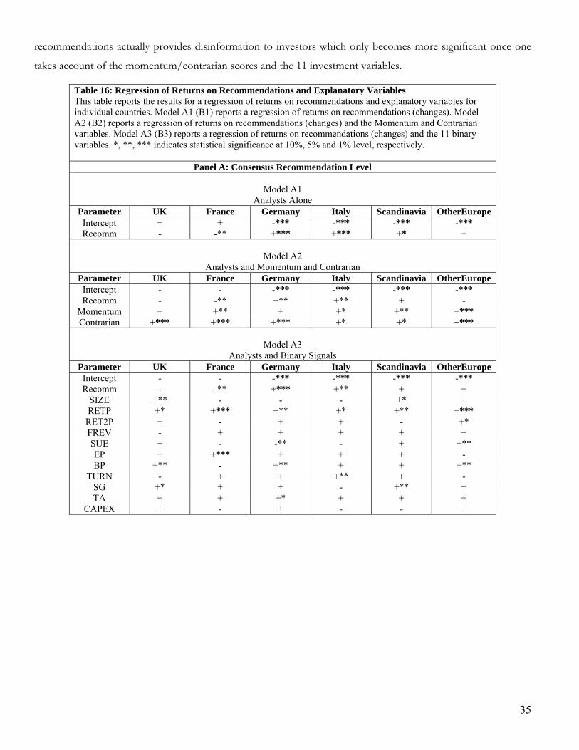
35

recommendations actually provides disinformation to investors which only becomes more significant once one

takes account of the momentum/contrarian scores and the 11 investment variables.

Table 16: Regression of Returns on Recommendations and Explanatory Variables This table reports the results for a regression of returns on recommendations and explanatory variables for individual countries. Model A1 (B1) reports a regression of returns on recommendations (changes). Model A2 (B2) reports a regression of returns on recommendations (changes) and the Momentum and Contrarian variables. Model A3 (B3) reports a regression of returns on recommendations (changes) and the 11 binary variables. *, **, *** indicates statistical significance at 10%, 5% and 1% level, respectively.



Parameter UK France Germany Italy Scandinavia OtherEurope Intercept + + -*** -*** -*** -*** Recomm - -** +*** +*** +* +

Model A2

Analysts and Momentum and Contrarian Parameter UK France Germany Italy Scandinavia OtherEurope Intercept - - -*** -*** -*** -*** Recomm - -** +** +** + -

Momentum + +** + +* +** +*** Contrarian +*** +*** +*** +* +* +***

Model A3

Analysts and Binary Signals Parameter UK France Germany Italy Scandinavia OtherEurope Intercept - - -*** -*** -*** -*** Recomm - -** +*** +** + +

SIZE +** - - - +* + RETP +* +*** +** +* +** +***

RET2P + - + + - +* FREV - + + + + + SUE + - -** - + +** EP + +*** + + + - BP +** - +** + + +**

TURN - + + +** + - SG +* + + - +** + TA + + +* + + +

CAPEX + - + - - +


Model A1

Analysts Alone Parameter UK France Germany Italy Scandinavia OtherEurope Intercept + - -*** -*** -** -*** Change -* - +** + + +

Model A2

Analysts and Momentum and Contrarian Parameter UK France Germany Italy Scandinavia OtherEurope Intercept -* -*** -*** -*** -** -*** Change -** - + + + +

Momentum + +* +** +** +* +*** Contrarian +*** +*** +*** +* + +***

Model A3

Analysts and Binary Signals Parameter UK France Germany Italy Scandinavia OtherEurope Intercept -** -** -*** -*** -** -*** Change -** - + + + + SIZE +** - - - +* + RETP + +*** +** +* +** +***

RET2P + - +* + - +* FREV - + +* +* + - SUE + - -** - + +** EP + +*** + + + - BP +** - +** + + +**

TURN - + + +** + - SG +** +** + - +** + TA + + + + + +

CAPEX + - + - - +

36

37

Section 6: Summary

Consistent with previous findings for both the US and Australian analysts, the recommendations of European

analysts are shown to be significantly biased towards large, high momentum stocks with a slightly less strong bias

towards growth. The identified biases are what one might expect given the common behavioural traits (e.g. over-

extrapolation and over-confidence) and the conflicts of interest faced by the analysts (e.g. the need to generate

brokerage and attract institutional clients). In contrast to the findings for their US and Australian colleagues

where the recommendation changes were found to provide useful information to investors, neither the

recommendations by European analysts nor changes in these recommendations were found to provide investors

with any useful information. It may be thought that this poor performance may be due to the fact that their

slight preferences for growth stocks did not stand them in good stead over the 10 year period covered by this

study. However, it proved that the analysts were unable to provide useful information even when one controlled

for the biases in their recommendations and recommendation changes. An isolated instance of where the

analysts appeared to be to provide incremental information was when using their recommendations changes as a

means to differentiate between stocks that were viewed to have poor investment prospects as measured by their

Qscore.

Our sample period extended for 10 years from April 1994 which covered two distinct periods in the market

cycle. In order to evaluate the extent to which our initial findings could be generalised across an entire market

cycle, we repeated our analysis on these two distinct sub-periods: the period from April 1994 to March 2000

when stocks were generally rising (the “boom” period) and from April 2000 to April 2004 which was a period of

market correction (the “gloom” period). Although we did not find any significant change in the consensus

recommendations across the two periods in terms of their bias towards large, high momentum, growth stocks,

we did find minimal evidence during the gloom years to suggest a minor switch away from growth stocks

towards value stocks. As previously found for both US and Australian analysts, the recommendations by the

European analysts during the boom years did appear to provide useful insights into future stock returns but this

proved to be a consequence of the biases towards stocks with particular characteristics rather than any special

insights provided by the analysts. In contrast it did appear that the recommendation changes of the analysts

during the gloom years provided useful information to investors over and above that attributable to the biases

towards particular types of stocks inherent in these recommendation changes. This finding of the usefulness of

the recommendation changes by the European analysts is weaker than that previously found for US and

Australian analysts where recommendation changes proved to be a good investment signal during the boom

years as well as the gloom years.

Finally, we saw significant variation across countries/regions in both the biases in the stock preferences of the

European analysts and the information contained in their recommendations and recommendation changes. In

38

contrast to all other countries examined, the recommendations by the UK analysts displayed a definite towards

small cap stocks. At the overall level we had seen that the bias towards growth stocks was weaker in Europe than

previous evidence suggests to be the case in both the US and Australia. Indeed, the recommendations by the

analysts in the UK, Germany and Italy would appear to be neutral in terms of growth and value. Further in most

countries/regions, there was a discernible drift towards value stocks which suggests that the growth/value aspect

of any bias in their recommendations may simply be reflected through simply favouring the style that was

performing best at a particular point in time. In contrast to our initial findings at the aggregated level that

recommendations and recommendation changes by the European analysts provided no useful information to

investors, we did find both positive and negative instances at the country/region levels on the usefulness of this

information. On the positive side, we found that the recommendations by both the German and Italian analysts

provided useful information to investors over and above that attributable to the biases inherent in the

recommendations. On the negative side, it appears that the UK and French analysts provided misinformation by

their recommendations and/or recommendation changes.

Our findings do suggest several avenues for future research. One of the major questions that we have addressed

for which we only obtained limited support is the ability of analysts by their recommendations to predict future

stock returns. However, there is the related question as to the extent to which particularly changes in analysts’

recommendations simply are a reaction to past returns. We have definite evidence in this study that analysts tend

to adjust their recommendations in response to stock performance over the previous six months. However, it

would be instructive to undertake further research to determine the extent to which stock price movements

influence analyst recommendations as opposed to the extent to which analysts’ recommendations anticipate

stock price movements. A further extension would be to divide the sample up in accordance with a number of

categories (e.g industries) in order to determine whether analysts are capable of identifying certain characteristics

of firms, and as such make more accurate recommendations for particular stocks or industries. Finally, it would

be interesting to repeat the Jegadeesh et al analysis of the US analysts to see whether their findings were just

specific to a period in the market cycle when stocks were strongly advancing. This would be of particular

importance given both the findings in this study and those in Azzi and Bird on Australian analysts and the recent

draft of regulatory changes in the US aimed at increasing the independence of the US analysts. The one thing

that we can predict with a high degree of certainly is that analysts’ forecast and recommendations will provide a

very active vehicle for academic research for many years to come.

References

Amir, E., and Ganzach, Y. 1998. Overreaction and Underreaction in Analysts’ Forecasts, Journal of Economic Behavior and Organization: 37, 3.

Azzi, S. and Bird, R. 2005. Prophets during Gloom and Doom Downunder, Global Finance Journal, forthcoming

39

Banz, RW. 1981. The Relationship between Market Value and Return of Common Stocks. Journal of Financial Economics: 9, 1.

Barber, B., Lehavy, R., McNichols, M and Trueman, B. 2001. Can Investors Profit from the Prophets? Security Analyst Recommendations and Stock Returns. The Journal of Finance: 56, 2.

Barber, B., Lehavy, R., McNichols, M and Trueman, B. 2003. Prophets And Losses: Reassessing the Returns To Analysts' Stock Recommendations, Forthcoming, Financial Analysts Journal: 59, 2.

Benesih, M., Lee C. and Tarpley, R. 2001. Comntextual Fundamental Analysis Through the Prediction of Extreme Returns. Review of Accounting Studies, 6, 2-3.

Boni, L, and Womack, K. 2003. Analysts, Industries, and Price Momentum. Working Paper, University of New Mexico and Dartmouth College.

Chan, L., Jegadeesh, N and Lakonishok, J. 1996. Momentum Strategies, Journal of Finance: 51, 5.

Chan, L.., Chan, K., Jegadeesh, N and Lakonishok, J. 2001. Earnings Quality and Stock Returns. University of Illinois Working Paper.

Doukas, JA., Chansog, FK., and Pantzalis, C. 2002. A Test of the Errors-in-Expectations Explanation of the Value/Glamour Stock Returns Performance: Evidence from Analysts' Forecasts. Journal of Finance: 57, 5.

Easterwood, J., and Nutt, SR. 1999. Inefficiency in Analysts Forecasts: Systematic Misreaction or Systematic Optimism. Journal of Finance: 54, 5.

Hayes, R. 1998. The Impact of Trading Commission Incentives on Analysts’ Stock Coverage Decisions and Earnings Forecasts. Journal of Accounting Research: 36, 2.

Hong, H., Lim, T. and Stein, J. 2000. Bad News Travel Slowly: Size, Analyst Coverage and the Size of Momentum Profits. Journal of Finance. 55, 1.

Hong, H. and Kubrik, J. 2003. Analyzing the Analysts: Career Concerns and Biased Earnings Forecasts Journal of Finance: 58, 1.

Irvine, P. 2002. Analysts’ Forecasts and Brokerage-Firm Volume, Working paper: Emory University - Goizueta Business School.

Jegadeesh, N and Titman, 1993. S. Profitability of Momentum Strategies: An Evaluation of Alternative Explanations, Journal of Finance: 56, 2.

Jegadeesh, N., Kim, J., Krische, SD, and Lee, CM. 2004. Analyzing the Analysts: When Do Recommendations Add Value? Journal of Finance. forthcoming

Lakonishok, J., Shleifer, A., and Vishny RW. 1994. Contrarian investments, extrapolation, and risk, Journal of Finance: 49, 5

Latane, H. and Jones, C. Standardized Unexpected Earnings: 1971-77, Journal of Finance: 34, 3.

Lee, C. and Swaminathan, B. 2000. Price Momentum and Trading Volume. Journal of Finance. 55, 5.

Reinganum, MR. 1992. A Revival of the Small-firm Effect. Journal of Portfolio Management. 18, 3.

Rouwenhorst, KG. 1998. International Momentum Strategies. Journal Of Finance. 53, 1..

Scharfstein, David S., and Jeremy C. Stein. 1990. Herd behavior and investment. American Economic Review 80, 3.

Stickel, SE. 1995. The Anatomy of the Performance of Buy and Sell Recommendations. Financial Analysts Journal: 51, 5.

Welch, I. 2000. Herding among security analysts. Journal of Financial Economics 58, 3.

Womack, KL. 1996. Do Brokerage Analysts' Recommendations Have Investment Value? The Journal of Finance 51, 1.

Appendix 1: Investment Variables

In Section 3 of the paper we introduced the 11 investment variables that are used throughout the paper. In this

Appendix we define how we calculate these variables:

Size Variable

1. Size (SIZE)- The natural log of a firm’s market capitalization at the end of the reporting period

ln ( Pt * Shares Outstanding

t)

t= six month period when recommendations were collected

Momentum Variables

This fall into two categories: price momentum and earnings momentum:

Price Momentum

2. Cumulative Market Adjusted Returns for preceding six months (0 through to -5) of the recommendation date (RETP)

}1)]1({[}1)]1({[ 55CC

−−−+−−+

m

m

m

mnonthyreturtedmarketmvalueweighurnMonthlyret

• m= month end of the 6 month period t

3. Cumulative Market Adjusted Returns for second preceding six months (-7 through to -12) of the recommendation date

(RET2P)

}1)]1({[}1)]1({[ 11

6

11

6 CC−

−

−

−−+−−+

m

m

m

mnonthyreturtedmarketmvalueweighurnMonthlyret

• m= month end of the 6 month period t

Earnings momentum

4. Standardised Unexpected Earnings (SUE) - The unexpected earnings for the semi-annual period of the

recommendation, standardized by the time series standard deviation over the three preceding semi-annual

periods

s

1-ss

S)EPS - (EPS

s = most recent 6 month period for which an earnings announcement was made a minimum two months prior

to the end of the 6 month period ending on m.

EPSs – EPS

s-1= unexpected earnings for the 6 month period

Ss = standard deviation of unexpected earnings over three preceding 6 month periods.

40

7. Analysts’ Forecast Revisions (FREV) – The change in the analysts’ consensus forecast over the past six

months standardised by the stock’s price.

s

1-ss

P)FEST - (FEST

FESTs – FESTs-1 = Change in consensus analyst forecast over previous six months

Ps = Current share price

Value/Growth Variables

The existence of a value premium across a wide range of markets has been identified in a number of studies.

These can be broken down into two valuation multiples, two contrarian indicators and two fundamental

variables:

Valuation multiples

6. Book-to-Price (BP)

t

s

CapMarket equitycommon of Book value

s = Most recent 6 month period for which an earnings announcement was made a minimum of two months

prior to the end of the 6 month period ending on m.

Market Capt = P

t * Shares Outstanding

t = price at the end of the 6 month period m multiplied by common

shares outstanding at the end of the 6 month period.

7. Earnings-to-Price (EP)

t

s

P)(EPS

EPSs = earnings per share before extraordinary items for the 6 month period

s = Most recent 6 month period for which an earnings announcement was made a minimum of two months

prior to the end of the 6 month period ending on m.

t = six month period when recommendations were collected

41

Contrarian indicators

8. Turnover (TURN) – Monthly volume over the previous month standardised by the number of shares

t

t

NoofSharesVolume

t = six month period when recommendations were collected

9. Sales Growth (SG) - Sales growth rate over the previous year.

1-s

s

SalesSales

• s = Most recent 6 month period for which an earnings announcement was made a minimum of two

months prior to the end of the 6 month period ending on m.

10. Accruals to Total Assets (TA)- The difference between accounting income and cash flow income

standardised by total assets (TA).

s

ss

sTotalAssetnsomOperatioCashFlowfrncomeOperatingI −



Fundamental variables

11. Capital Expenditure(CAPEX) – The level of capital expenditure over the past year standardised by the

average total assets held during the year

)/2sTotalAssetts(TotalAsseCAPEX

1-ss

s

+



42

Biases and information in analysts' recommendations: The European experience

Documents

Transcript of Biases and information in analysts' recommendations: The European experience