Selection biases in sociological data

SOCIAL SCIENCE RESEARCH 11, 352-398 (1982)

Selection Biases in Sociological Data

RICHARD A. BERK AND SUBHASH C. RAY

University of California, Santa Barbara

Textbook discussions of the general linear model typically skirt the issue of sampling. If the regressors are assumed to be fixed, all results are simply given conditional status and generalization then proceeds by replication or theoretical extrapolation (e.g., Kmenta, 1971, p. 297; Pin- dyck and Rubinfeld, 1981, p. 48). Because, with the exception of experimental social science, regressors are likely to be stochastic, researchers are alternatively counseled either to retain the approach that any results are conditional on the particular regressor values observed or to add two assumptions: (1) the explanatory variables are independent of the regression parameters, and (2) the explanatory variables are independent of the error term (Johnston, 1972, pp. 274-278; Pindyck and Rubinfeld, 1981, p. 134). The former addresses external validity and guarantees that one’s estimates are not conditional on the regressor values. The latter addresses internal validity and guarantees that the estimates of the regression coefficients are unbiased.’

The apparent sampling-free nature of the general linear model has led to all manner of confusions in the sociological literature about when statistical inference is appropriate and how correct interpretations should be made (Morrison and Henkel, 1970; Berk and Brewer, 1978). Put a bit crudely, many sociologists cannot accept the conclusion that if the two assumptions listed above are correct, the sources of the data have no statistical implications. On the one hand, this reflects a certain inability

Thanks go to Andy Anderson, Eleanor Weber-Burden, Kenneth C. Land, Karl F. Schuessler, and especially Thomas F. Cooley and Steven Klepper for comments on an earlier draft of this paper, and to David Rauma for comments on that draft, drawing the figures, and for developing the software to do the “Greene-Tobit” estimation. Thanks also go to Anthony Shih and Jimy Sanders for help with the “citizen feedback” analysis and to Leslie Wilson for typing the equations. Finally. work on this manuscript was supported by the National Institute of Justice (Grant 80-IJ-CX-0037).

’ The assumptions provided by Pindyck and Rubinfeld are basically a more explicit way of saying that if, for each sample of regressors, the results are conditional, but we place no restrictions on which regressor values may appear. we are really claiming that the results hold for any sample of regressors (cf. Kmenta. 1971, pp. 299-300).

352

0049-089X/82/040352-47$02.00/0 Copyright 0 1982 by Academic Pres. Inc. All rights of reproduction in any form reserved.

SELECTION BIASES IN SOCIOLOGICAL DATA 353

to fully comprehend the statistical procedures being used. But on the other hand, the sociological instincts are essentially correct. Yes, if the assumptions are true, sampling problems disappear. However, for most data sets available to sociologists, the assumptions are often false.

Building on the pioneering work of James Tobin (1958) a number of econometricians have of late confronted the fact that sampling can make a difference, and that in particular, inappropriate sampling procedures can introduce inconsistency into least squares estimates. Yet, with a few exceptions (e.g., Tuma, Hannan, and Groenveld, 1979; Rossi, Berk, and Lenihan, 1980; Berk, Rossi, and Lenihan, 1980; Berk and Rossi, 1982), this work has not filtered into sociological practice, and, to our knowledge, there is no review of the recent material in the sociological literature. In this manuscript, therefore, we consider current work in econometrics loosely organized under the rubric of “sample selection bias.” In addition to examining the nature of the problem and possible solutions, we provide some examples, based on real data, of how one can proceed in practice. To anticipate a bit and motivate the material that follows, we are not “just” saying that poor sampling procedures jeopardize external validity; we are saying that internal validity is threatened as well through the introduction of fundamental specification errors.

AN INTUITIVE INTRODUCTION TO THE PROBLEM

While the literature on sample selection bias can be somewhat demanding, the problem in its simplest form can be explained rather easily. Suppose that one is interested in urban, civil disorders and the relationship between the amount of property damage (measured in dollars) and a city’s unemployment rate. Assume that the relationship is positive and that, therefore, one might observe a scatter plot something like the one shown in Fig. 1. The “true” population regression line is also represented, and it is apparent that a positive slope exists; the greater the unemployment rate, the greater the property damage. We will also assume that our theory makes the amount of damage a function of unemployment rate; we are imposing structure on the joint distribution of the two variables.

Now suppose that the data on the amount of property damage comes from archival sources based on newspaper and other media accounts. Not all disorders are included, and small disorders with little damage are especially likely to be neglected. Put in terms we will use extensively later, one might hypothesize that the amount of damage must exceed some “threshold” before the disorder receives significant media attention. And without media attention, the incident will not be archived. Should this hypothesis essentially prove correct, disorders with little or no damage will not appear in the archival data set; neither unemployment nor property damage will be, therefore, “observable.” The consequences

BERKANDRAY 354

I I

Regression Line

Before Selection

X FIG. 1. An example of “explicit” selection.

of this selectivity for external validity are apparent; one must be careful not to generalize automatically any findings to all urban, civil disorders. Moreover, the selection process implies that the lower edge of the scatter plot is unavailable for study. In Fig. 1, the shaded area is missing, and as a result the scatter plot will generate an estimate of the true regression line that is too flat. In other words, there is a systematic attenuation in the regression line as a result of the process by which some observations are discarded.

While we will be more specific shortly, it is important to emphasize that there are two generic problems. First, the regression line for all civil disorders does not correspond to the regression line for the subset of larger disorders. This is a problem of external validity; the regression parameters now differ depending on the data available. Second, the distorted scatter plot implies that the unemployment variable is now correlated negatively (in this illustration) with the error term. Note that once the bottom of the scatter plot is removed, the disturbances for the original regression line no longer have expectations of zero, and disturbances with larger expectations are associated with lower rates of unemployment. Internal validity, therefore, is equally threatened, even if


one were prepared to focus exclusively on larger disorders. In other words, even if all findings are reported conditional upon the particular, nonrandom subset of disorders for which data are available, any linear regression of the amount of property damage on the unemployment rate confounds the impact of the unemployment rate with the impact of the error term.

With a few moments thought, a number of more complicated selection processes can be postulated. For example, perhaps the question of significant media coverage depends alternatively (or in addition) on whether one of the wire services has an office in the city where the disorder occurs. Without the office, coverage is strictly local. Clearly, this is another kind of selection process that does not depend on the endogenous variable (i.e., the amount of damage), but on a variable having nothing directly to do with the unrest. Nevertheless, one risks distorting the scatter plot and producing inappropriate estimates of the regression parameters. For example, if smaller municipalities are less likely to have both a wire service office and disorders with extensive damage, the lower portion of the scatter plot in Fig. 1 may be affected once again, depending on factors discussed in detail below. And once again, both external and internal validity are involved.

With the civil disorder example in mind, large bodies of the substantive literature in sociology become suspect. In the criminal justice field, for example, each step from arrest to sentencing necessarily involves a win- nowing process in which certain kinds of individuals are systematically discarded. In the status attainment tradition, alternatively, one only ob- serves the destination occupation of individuals who enter the labor force. Or in the family literature, studies of husband-wife interactions necessarily ignore adults who are single, separated or divorced. Again, the problem is not just external validity. Internal validity is also in jeopardy.

It is no doubt hard to imagine that on such grounds decades of sociological research are completely without merit and, in fact, the sample selection problem is not universal. The problem is hardly a mere tech- nicality, however, or an exotic statistical malady. Many important research traditions are vulnerable. The nature of that vulnerability is the question to which we now turn.

A FORMAL MODEL OF EXPLICIT SELECTION

Before launching into a rather lengthy, technical discussion, there are three qualifications that warrant brief mention. First, while we will be emphasizing rather recent work in econometrics, the generic issues are hardly new. At the turn of the century Pearson and Lee (1!908), for instance, were worrying about “truncated” distributions, and over the past two decades a number of statisticians have been developing tools

356 BERK AND RAY

for the analysis of “survival data” subject to “censoring” (for a recent discussion see Kalbfleisch and Prentice, 1980).

Second, there are a number of different expositional strategies that might have been employed. Our approach will, with a few small detours. move from the simple to the complex. We discarded the alternative of presenting a rather general formulation and then discussing a number of special cases for fear of burying intuitive insights beneath a mountain of statistical notation.

Finally, the distortions produced by certain kinds of selection processes look a lot like more commonly recognized ceiling and floor effects. That is, scatter plots are flattened because of inherent boundaries on the variable in question. The length of jail terms for misdemeanors, for example, should (in principle) fall between 0 and 12 months. However, such ceiling and floor effects do not derive from excluded observations, and therefore, the statistical issues differ; with one exception (see foot- note 15), they will not be considered in this paper.

Having dispensed with preliminaries, we turn to what Goldberger (1980) has recently dubbed “explicit selection.” Although explicit selection was first recognized by Tobin (1958) over 20 years ago, and has since been formulated as a special case from a more general model (Heckman, 1976; 1979), we will for didactic purposes proceed initially within Goldberger’s framework (cf. for example, Amemiya, 1973; Heck- man, 1980).

Goldberger’s discussion begins with a conventional linear regression equation applied to some “original” population. That is,

y = x’p + u, u - N(O,o’), u independent of x. (1)

Since the regressors are assumed to be independent of the disturbance term, Goldberger is asserting that in the original population, the equation is properly specified. Any omitted variables are uncorrelated with the regressors that are included, and the linear form is appropriate. If the story ended here, there would be a happy ending.

One is unable in principle, however, to observe all of the original population because one only can obtain access to observations for which y falls outside (or inside) of some threshold Y. Y is fixed for each ob- servational unit, but, as a subset of the real line, can vary across units: Y is a vector of real numbers. It is important to stress that when y does not exceed (or exceeds) Y, data are missing on both the endogenous variable and the full set of regressors, and that observations that are retained define the “selected” population. Note also, that by focusing initially on an original and selected population, Goldberger can avoid getting sidetracked into a discussion of estimators.2

’ Since Goldberger is at this point not interested in sample estimators, he focuses on the originai population and the selected population. In practice, of course, we must work


Goldberger’s initial formulation is rather general since there are absolutely no restrictions on what real values Y may include. For example, one may be interested in classroom performance where students are transferred to a special tutorial program if their reading scores have declined by one standard deviation or more compared to their reading scores the year before. Thus, one only can obtain observations for students whose reading scores have not dropped dramatically. The full group of students defines some original population while the subset remaining after screening defines a selected population.

What are the consequences of this quite general, explicit selection? Goldberger begins by distinguishing between the linear regression function for y given x (i.e., the usual regression “line”) and the conditional expectation function for y given x (i.e., the expected value of y given x). In the original population, the two functions correspond; both will

Ogenerate the same numbers for the expected values of y. However, in the selected population, the linear regression function (with vectors boldfaced) can be represented by

L” (J(x) = a* + x’p*, (2)

where according to the usual normal equations (again, with vectors boldfaced)

a* = t$. - P:‘P*, W

z.,$* = a:>,, Ub)

and where the CL’s represent the population means of y and the x vector, respectively, C represents the variance-covariance matrix of the x’s, and u represents the covariance between the x vector and y. Asterisks indicate that the moments come from the selected population.

Perhaps the most immediate difficulty is that in the selected population, the linear regression function will typically not correspond to the conditional expectation function (Goldberger, 1981, p. 358). That is, the linear regression function will usually not generate the desired expectations for y. This is no small problem, since it is the conditional expectation function that the linear regression function is exactly supposed to capture. The latter is but a theory-based “short-cut” to the former that

succeeds in the original population. When it fails, however, internal

with a sample, and the problem is that the sample is drawn from the selected population. It will turn out, however, that once we consider the consequences of the selection process for the population regression parameters, sample estimators are easy enough to construct. It is also important to note that if we had been selecting on one or more regressors instead of the endogenous variable, we would basically come away unscathed. Assuming that some variance remains in the regressors, the only price is (perhaps) a loss in efficiency (Muthen and Joreskog, 1981, p. 3).

358 BERKANDRAY

validity goes by the boards; one has basically specified the wrong model. And the linear regression model is the wrong model even in the selected population. In other words, one cannot wriggle out of the problem by focusing exclusively on the selected subset of observations. Statements conditioned upon the selected units will not suffice. While we will soon be far more specific for important special cases of explicit selection, the selection process introduces an additional term into the conditional expectation function that the linear regression function ignores. As Heck- man has observed (1979, p. IS), one consequence is the classic missing variable specification error.

Equally problematic, however, is external validity: the relationship between the linear regression functions in the original and selected populations. Goldberger proceeds by adding the assumption (1981, p. 359) that the regressors are random variables drawn from a multivariate nor-. ma1 distribution. The normality represents an absolutely critical condition on which many later expressions of the selection effects depend, but is not formally required for the regression model shown in Eq. (1). Gold- berger imposes the assumption of multivariate normality because of the instructive implications that follow. In practice, of course, many variables common in sociological data sets are not normally distributed (e.g., binary variables), but we will postpone a discussion of real world problems until the statistical theory is clear. Goldberger also assumes that the regressors all have expectations of zero, but this is a harmless simplification with no implications for the generality of the derivation (because the variables can all be expressed as deviations from their means).

Looking back at the normal equations, it is apparent that all of the moments in the selected population are suspect, and Goldberger sets about trying to find expressions for these moments in terms of the moments in the original population. To the degree that this can be accom- plished, relationships between the regression parameters in the original and selected population can be derived.

Goldberger’s trick is to build on the fact that nonrandom selection does not alter the conditional distribution of an x given y. In other words, nonrandom selection via the endogenous variable (i.e., y), has no effect on the distribution of the regressors (i.e., the x’s), conditional upon the selected values of the endogenous variable (see again Fig. I). This immediately permits expressions in terms of the original population moments for (1) the conditional expectations of the x’s given y, (2) the variance of these conditional means, and (3) the mean of the conditional variances. For readers familiar with analysis of variance terminology, the second is analogous to a “between” variance while the third is analogous to a “within” variance.

With these in hand, the next step is to assemble the pieces. The “between” and “within” variances are summed to yield the “total”


variance-covariance matrix for the regressors in the selected population. The conditional means of x given y, when “co-varied” with y, produce the covariance between x and y which, because it is symmetric, gives the covariance between y and x. Finally, a bit of algebraic manipulation yields an expression for the relationships between the regression parameters in the original population and the selected population.

where

p* = w, (4) cf* = (1 - Ap2)&, (5)

pz = xp2, (f-9

and

A = Ml - p2(1 - (3% (7)

8 = v*(yycr2. (8) From Eq. (4) (we will define the symbols as we proceed), it is clear

that the regression coefficients in the selected population (where, in general, the asterisks refer to the selected population) are proportional to the regression coefficients in the original population, and that the constant of proportionality is A. In other words, all of the suspect regression coefficients are altered by the same proportion relative to the proper regression coefficients. Equation (6) indicates that the square of the multiple correlation coefficient is subject to the identical proportional distortion. Finally, Eq. (5) shows that the intercept in the selected population is a function of (1-X) and that, therefore, the intercept is shifted in the opposite direction of the regression coefficients for given values of the other parameters.

A key to the impact of selection, therefore, is A. From Eq. (7), A is seen to be a function of the coefficient of determination (i.e., p2) in the original population and 8. From Eq. (8), 0 is shown as the ratio of the variance of the endogenous variable in the selected population to the variance of the endogenous variable in the original population (i.e., m2, a nonnegative number). Putting Eqs. (7) and (8) together, and assuming that p is neither 1.0 nor 0.0, when 8 is greater than 1.0, A is greater than 1 .O, and the regression coefficients in the selected population are inflated. When 0 is less than 1.0, A is less than 1.0, and the regression coefficients in the selected population are attenuated. When the ratio equals 1.0, the two sets of regression coefficients correspond.3 In short, the critical element is whether the variance of y in the selected population is greater

3 Similar arguments can be made for the other regression parameters from Eqs. (5) and (6).

360 BERK AND RAY

than, equal to, or smaller than, the variance ofy in the original population. And given the very general kind of explicit selection discussed so far, one cannot make any general statements about the proportionality constant.

The importance of p’ (the coefficient of determination in the original population) is that it alters the effect of 0. At the extreme p2 of 1.0, the expression for A equals 1.0, and there are no problems with selection. Put a bit differently, since for all practical purposes there are no residuals, there is no error term to be correlated with the regressors. There can be, as a consequence, no potential for distortions. At the extreme p’ of 0.0, the expression for A equals 0. Of course, in virtually all real situations, the p* will not fall at either pole.

To summarize, the regression coefficients and the p2 in the selected population are distorted by the same proportion. The intercept in the selected population is also distorted but in a more complicated fashion. In practice, this means that sample data drawn from the selected population (even at random) will ordinarily produce inconsistent estimates of the regression parameters in the original population with the degree of inconsistency a function of A. Clearly, the inconsistency can be very severe. A A of SO, for instance, implies that the estimated coefficients will be too small by approximately 50%.

THE SPECIAL CASE OF TRUNCATION

Goldberger’s general approach to explicit selection on the endogenous variable most often surfaces in practice as the special case of “truncation.” Instead of Y (i.e., the selection criterion) being any point on the real line, Y is some constant “c” serving as aJixed threshold. Note that it is still the endogenous variable in the equation of interest that provides the information on which selection is based and that, as before, entire cases are discarded. We will discuss later a less complete form of selection under the rubric of “censoring.”

Consider the following example. Suppose that one were interested in modeling the amount of insurance money claimed in automobile accidents as a function of the nature of the accident. Are larger claims, for example. likely to come from accidents involving mid-size American-made cars compared to accidents involving compact American-made cars? The particular insurance company in question charges very high premiums for full collision insurance, however; virtually all customers buy collision insurance with the first $100 dollars “deductible.” Consequently, damage claims of less than $100 are not reported, and data are not available on collisions falling below the threshold of $100. Thus, one is left with a selected (nonrandom) population which in turn will jeopardize both external and internal validity should the usual linear regression model be applied.


Sociological examples are easily generated. For instance, studies of the performance of college students measured by their grade point average rest on the subpopulation of all admitted students (and that is another problem we will address shortly) whose grade point average exceeds the level necessary to remain in school. Clearly, all studies of the behavior of people processed by formal organizations are similarly implicated to the degree that the endogenous variables of interest also serve as a criteria for “membership.” Readers interested in obtaining a visual sense of the problem when there is truncation from below should reexamine Fig. 1, keeping in mind that we are still emphasizing an original population (i.e., the full scatter plot) and a selected population (i.e., the subset that exceeds the threshold).

The truncation does not have to be from below. For example, a study of the earnings of households below the “poverty line” will surely risk serious problems since households with earnings above the poverty threshold will not be included. In Fig. 1 the only difference is that the upper part of the scatter plot is lost.

Once again, it is possible under certain assumptions to be far more specific about the distortions. Beginning with 120 assumptions about the distribution of the regressors, Goldberger presents the well-known expression for the conditional expectation function under truncation as

E*(ylx) = x’f3 - or(z), (9)

where

and

z = (c - x’pyw, (10)

r(e) = j-(.)/F(*). (11)

All of the symbols in Eqs. (9) through (11) that have already been defined retain those definitions (e.g., w is the standard deviation of the disturbances in Eq. (l)), and new terms will be explained as we proceed. Thus, Eq. (9) indicates that after selection, the conditional expectation of the endogenous variable depends not only on the usual linear combination of regressors, but on a function “r” of a new variable “z” weighted by the standard deviation of the error term from the initial equation in the original population (i.e., Eq. (1)). The standard deviation weight serves much the same role as a regression coefficient and for present purposes needs little discussion. Other things equal, the weight will be less important if the error variance is smaller (i.e., if more variance is “explained”). This observation parallels our observations above about the role of p* under the general form of explicit selection. Such weights will figure significantly, however, in our later discussions of estimators.

Equation (10) shows that the new variable z is a standardized version

362 BERK AND RAY

of the usual linear combination of regressors subtracted from the constant threshold. From Eq. (ll), the function r is the ratio of z’s probability density to z’s cumulative density, both based on the standard normal. This ratio is the widely cited “hazard rate” popularized in Heckman’s work (1976; 1979), and widely used for over two decades in biometric analyses of survival data (Kalbfleisch and Prentice, 1980).

What are the properties of the hazard rate variable? First, if the regression hyperplane in the original population is parallel to the regressor hyperplane, the hazard rate is a constant that only has implications for the intercept in the selected population. Second, if the regression hy- pet-plane is vertical to the regressor hyperplane, the hazard rate is un- defined. Of course, both configurations are highly unlikely in practice. It follows, then, that whatever the difficulties created by the hazard rate, they cannot just be ignored.

There are at least two different ways in concrete terms to think about the hazard rate. First, the hazard rate reflects the “risk” that observations will be discarded. When for a given observation the ratio of the density to the cumulative is large, the likelihood of not being selected is large. When the ratio of the density to the cumulative is small, the likelihood of not being selected is small. Thus, the hazard rate captures the risk of not exceeding the threshold; the “hazard” in question is “exclusion.” This parallels the biometric literature in which the “hazard function” is the instantaneous rate of failure (e.g., death) at time t, conditional upon not failing up to time t (Kalbfleisch and Prentice, 1980, P. 6).

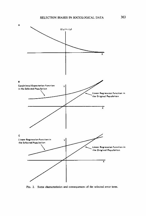
Second, the ratio of the density to the cumulative can be understood as the expected value of the error term after selection has occurred. Before selection (and assuming no specification errors), the expected value of the error for each observation is constant and (usually) zero. The selection process creates an error term whose expectation for each observation is no longer zero. Furthermore, Muthen and Joreskog (1981) point out that there is a monotonic and negative relationship between the linear combination of the regressors and the expected value of the error term (although their discussion rests on a more general formulation). Given a relationship like the one shown in Fig. 1, Fig. 2A illustrates one kind of pattern that Muthtn and Joreskog (1981) discuss. Note that the expected value of the error term declines as x becomes large, but at a less rapid rate.

It should be clear that, by definition, the linear regression function in the selected population is misspecified. The expected value of the error term represents a nonorthogonal regressor that the linear regression function ignores. At the same time, this means that regressors in the linear regression function are correlated with the postselection error term. In short, even if one is prepared to report all results conditional upon the


A

E(u)=r(z)

in

c Linear RegressionFunction in Y the Selected Population

y \ Linear Regression Function in

the Original Population

FIG. 2. Some characteristics and consequences of the selected error term

364 BERKANDRAY

subset of cases represented by the selected population, the linear regression function is the wrong model. The whole of Eq. (9) captures the expected values of y, while the linear regression function rests only on the first, righthand-side term. Internal validity has been sacrificed.

Some important implications of the postselection error term for external validity can be seen in Fig. 2B. In particular, while as x becomes large the conditional expectation function in the selected population con- verges to the linear expectation function in the original population, by and large, the two functions do not correspond. The disparity between the two functions results from the additive effect of the postselection error term, and the message is clear: Causal relationships are different in the selected population.4

An alternative way to think about the impact of the postselection error term can be seen in Fig. 2C where the linear regression function in the original population is compared to the linear regression function in the selected population. As suggested in Fig. 1, the linear regression function in the selected population is attenuated. However, we can now add that the linear regression function in the selected population is attenuated because it reflects a linear approximation of the nonlinear conditional expectation function shown in Fig. 2B.

Under certain assumptions, the relationship between the two linear regression functions in Fig. 2C can be characterized more precisely. To begin, the conditional expectation function in Eq. (9) and illustrated in Fig. 2B is highly nonlinear, which complicates the expression of the selection distortions. Goldberger, however, is able to build on the well- known result that when the slopes of the conditional expectation function are evaluated at given x values, all of the slopes are attenuated by the same proportion with respect to the slopes of the linear expectation function in the original population. In other words, when we focus on the conditional expectation function and assume that the error term in Eq. (1) is normally distributed, we find a proportional attenuation in all of the slopes for given values of x. We need to evaluate the slopes at specific values of x because the slopes are nonlinear. This implies that if Fig. 2B included two regressors (in three dimensions) and the slopes of the conditional expectation function for given values of the two regressors were compared to the appropriate slopes of the linear regression function (in the original population), the two slopes of the conditional expectation function would be attenuated by the same proportion.

4 We will see later, however, that estimators can be developed that capture the nonlinear conditional expectation function and allow one to properly model the linear regression function in the original population. To anticipate a bit, the key element is to construct an estimate of the omitted variable from the data on hand and add that variable to one’s regression analysis. That is, one needs an estimate of the expected value of the postselection error term that can be used as a new regressor.


We are in practice more likely to be interested in the linear regression function than the conditional expectation function; we are usually trying to extract causal inferences by regressing y and X. Unfortunately, since the conditional expectation function and the linear regression function will not correspond in the selected population (as discussed above), we need information on the distortions introduced by the explicit selection process for the linear regression function. In response, Goldberger dem- onstrates that in contradiction to some assertions in the literature, there are no general results for the linear regression function in the selected population unless one assumes that the regressors are multivariate normal. If this assumption holds, all of the slopes for the linear regression function are proportionally attenuated (relative to the slopes in the original population). If multivariate normality does not hold, neither proportionality nor attenuation are guaranteed.5 Under multivariate normality, then (and remembering that u is the standard deviation of the endogenous variable in the original population)

and

p; = -ur(c/u) (W

e = 1 + FJ(c/u). (13)

Equation (12) indicates that the mean of the endogenous variable in the selected population will almost certainly be altered. Consistent with common sense, the mean will be increased when the truncation is from below and decreased when the truncation is from above. Equation (13) provides an expression for 8 which is guaranteed to fall within the unit interval. And since p* is also a fraction, h in Eq. (7) is bounded by 0.0 and 1.0 as well. Thus, there is proportional attenuation in Eqs. (4) and (6) (i.e., for the regression coefficients and p*). Not surprisingly, this has important implications for a correct estimation procedure that will be discussed later.

To summarize the issues with respect to external validity, in the selected population, the conditional expectation function will not correspond to the original linear regression function. This is bad because the two are supposed to correspond. For given values of the regressors, the slopes of the conditional expectation function are attenuated. Note that in Fig. 2B, the slope of the conditional expectation function is always less steep than the slope of the linear regression function. In addition, the linear regression function in the selected population approximates the nonlinear conditional expectation function with the result that the former also fails properly to represent the linear regression function in

’ On the other hand, Greene (1981~) argues that even without multivariate normality, most empirical situations will produce attenuation in practice.

366 BERK AND RAY

the original population. If one assumes that the regressors are multivariate normal, proportional attenuation results (as in Fig. 2C). In the absence of multivariate normality, no statements can be made about attenuation or proportionality (although the lack of correspondence remains). Similar arguments can be made about the other regression parameters.

Before moving on, one final observation needs to be made about the truncation form of explicit selection. It is sometimes possible and de- sirable to include partial data on cases that would otherwise be totally lost. When time comes for estimation, statistical efficiency can be improved because of the additional information provided (Muthen and Jo- reskog, 1981, pp. 23-35). In the usual instance, data are fully available on all of the regressors but not fully available on the endogenous variable. That is, the explicit selection only affects one’s ability to observe the endogenous variable. It is common to call this form of explicit selection “censoring” (e.g., Heckman, 1979).6 Under these conditions, one can code the missing observations on the endogenous variable to the threshold value and then proceed “as if” there were no selection effects. However, this is actually nothing more than the “Tobit Form” (1958) of the selection model: virtually all of Goldberger’s conclusions about truncation hold. While the expressions for the distortions are a bit different (Greene, 1981c), the same sorts of proportionality results follow.

Recall the insurance company example. One could turn a truncation problem into a censoring problem if, for claims less than $100, (a) data are available on all the regressors, and (b) in these cases the value of $100 is inserted for the size of the claim. We will see later that censored data such as these are comparatively “friendly” and that especially convenient estimation procedures exist.

THE CASE OF INCIDENTAL SELECTION

To this point, the selection process has hinged on the endogenous variable whose variation is the subject of interest. Observations are discarded or not depending on whether y falls above (or below) Y. How- ever, selection can also occur not as a function of y and Y, but as a function of some other variable and its selection criterion. This leads directly to the two-equation framework for sample selection bias developed by Heckman (1976, 1979) where there is one equation of substantive

6 The terminology in the sample selection literature is at best inconsistent. We are comfortable, however, with the following distinction. Drawing from Kendall and Stuart (1963), a population (or sample) is “truncated” if, for certain cases, there are no observations on both the endogenous variable and all the exogenous variables. A population (or sample) is “censored” if, for certain cases, there are no observations only on the endogenous variable and data are fully available on all the exogenous variables. The former is sometimes called the truncated regression model while the latter is sometimes called the Tobit model (e.g., Greene, 1981~).


interest and one equation to model the selection process. In other words, there are now two distinct causal models that need to be properly specified. When the substantive and selection process can be captured in the same equation, one is returned to the explicit selection models we have considered above (cf. Heckman, 1979, p. 155). In effect, the process by which the threshold is exceeded (or not) is the same as the process that determines the value of the endogenous variable for cases that exceed the threshold.

Incidental selection takes many forms whose formal properties can produce a wide variety of distortions in the scatter plot for the selected population. While we will be far more specific shortly, Fig. 3 provides one illustration of how incidental selection sometimes works.

In Fig. 3A an example of the incidental selection mechanism is shown. There exists a selection process in which observations on some “selection” endogenous variable falling below a fixed threshold (indicated by the horizontal, dotted line) are discarded. Therefore, the original population represented by the full set of observations is no longer available for study; the first, second, fifth, and eighth cases are lost. The remaining observations constitute the selected population, and it is apparent from Fig. 3B that when the regression line for the “substantive” endogenous variable is considered, the regression line in the selected population will not correspond to the regression line in the original population.

X2

FIG. 3. An example of “incidental” selection.

368 BERK AND RAY

Consider the standard study of sentences given out to convicted felons. It is surely no surprise that a condition for sentencing is a conviction. Put a bit differently, if the evidence points to guilt beyond a reasonable doubt, a conviction is obtained. In other words, there exists an evidential threshold which, if exceeded, establishes a conviction. Convicted felons are then selected from among all tried felons for the next step of sentencing.

It is clear that convicted felons are a selected population from the population of all alleged felons who are tried.’ When time comes then to build and estimate models of the sentences given, one risks both kinds of distortions we have been considering; both internal and external validity are potentially involved. (The conditions under which the potential is realized will be discussed shortly.) Now the selection is “incidental,” however, because when sentence length is modeled, the selection process is a function of the evidence “beyond a reasonable doubt.” The selection is nof a function of sentence length.

As with the earlier selection problems, there are many examples in sociological work. Studies of medical care typically focus on the subset of people who seek treatment. Studies of small business are usually limited to enterprises that manage to avoid bankruptcy. Studies of rev- olutions often neglect stable countries and/or historical periods. Indeed, it is difficult to think of a literature that is immune. More formally, consider two equations in Goldberger’s notation for the full (i.e., not selected) population,

yl = X’P, + UI, y2 = X’PZ + u2, (14)

where

and where

x - N(0, Lx), u = (u142)’ - iw,R), (15)

(16)

In order to make this exposition comparable to Goldberger’s earlier efforts, assume that all of the variables, including both y’s and all the X’S, are multivariate normal. There is now a second equation, however, whose role needs to be considered. To begin, Eqs. (14) through (16) look tame enough. Indeed, they represent nothing more than a traditional, seemingly unrelated equations framework (with the distributional assumption of the regressors added). Note that according to the

’ Those tried are a selected population of those indicted, and so on. The criminal justice system is an excellent example of a sequential selection process that needs to be modeled in its entirety. We will briefly cite some relevant literature later.


R matrix, there is a nonzero covariance between the disturbances of the 2 equations.

It is important to emphasize that in the original population both equations are properly specified. This means that any omitted variables are uncorrelated with the regressors included and that the (here) linear functional form is correct. Thus, any difficulties that may surface in the selected population do not derive from misspecification of the relationships in the original population.

Suppose, however, that the original population is vulnerable to incidental selection. Assume that the second y has to exceed some fixed threshold in order for observations on the first y (and the regressor values associated with it) to be available (see especially Heckman, 1979, pp. 154-155). In our example, the second y is the strength of the evidence, while the fixed constant is evidence “beyond a reasonable doubt.”

What are the consequences of this selection process for the relationships in the selected population? Focusing first on the conditional expectation function, Goldberger, like Heckman (1976), indicates that the mean of y is a function not just of the usual linear combination of regressors (which suffices in the original population), but a hazard rate capturing the impact of the selection equation. Thus,

where

E* (Y,lx) = x’h - (~,hdT(zzh (17)

z2 = cc2 - x’P*)h. (18)

Given our earlier discussion of the conditional expectation function under truncation, it is apparent that Eqs. 17 and 18 are just generalizations of Eqs. (9) through (11) (i.e., explicit selection). Thus, the new z variable is the usual linear combination of regressors subtracted from the threshold constant and standardized by the appropriate error variance. The twist is that Eq. (18) is derived from a separate selection equation. The function “r” is again the ratio of the density of z to the cumulative, given the assumption that the two disturbances are bivariate normal. It is, therefore, a hazard rate much as in the single-equation case. Finally, the ratio of the covariance between the two disturbances to the standard deviation of the selection (i.e., second) equation error term serves as a weight, and is literally a regression coefficient. Perhaps more instructive, the ratio can be reexpressed as the product of two terms: the standard deviation of the disturbance for the first equation in the original population and the correlation between the disturbances across equations (Heckman, 1979, p. 157). The latter, consequently, determines the sign of the regression coefficient and is especially useful in substantive interpretations (e.g., Heckman, 1980, p, 230); when a positive correlation exists between the disturbances, the regression coefficient associated with the hazard rate will be positive (and vice versa).

370 BERKANDRAY

The generalization implied by Eqs. (17) and (18) produces at least two complications beyond those discussed earlier. First, under incidental selection, if the covariance between the error terms in the selection and substantive equation is zero, the regression weight associated with the hazard rate is zero, and ull incidental selection problems evaporate. This is a fundamental result that will figure significantly in the pages ahead. Note that under explicit selection, there is a single equation (i.e., the selection and substantive equations are collapsed) with a single error density. For incidental selection, however, the selection process is fun- neled into the substantive equation through the cross-equation error covariance. If the funnel is removed, selection artifacts cannot materialize. Consequently, the practical question is for what kinds of empirical phenomena will the covariance be nonzero and nontrivial. We will return to this point later.

The second complication involves the interpretation of the hazard rate. As before, the hazard rate reflects the likelihood that an observation will be discarded. If the hazard rate is large, the likelihood of exclusions is large (and vice versa). Because the selection process is contained within its own equation, however, the threshold implicates a distinct selection variable. In addition, the hazard rate is again the expectation of an error term after selection, but it is now the error term of a separate substantive equation. Readers interested in an excellent discussion of these issues coupled with instructive graphics should consult the work of Muthen and Joreskog (1981).8

Turning to external validity, we can consider, as before, whether, under multivariate normality incidental selection leads to proportional distortions in the usual regression parameters. As in the case of truncation, the conditional expectation function is highly nonlinear, and the proportionality issue must be addressed for particular values of the regressors. However, Goldberger shows that even with multivariate normality, “no presumption of proportionality arises” (1981, p. 364). In other words, while it is clear that incidental selection can produce a conditional expectation function that departs dramatically from the linear regression function in the original population, the slope of the conditional expectation function will not be altered by some proportionality constant.

The news is no better for the linear regression function. The expression for the relationship between the linear regression function in the original population and the linear regression function in the selected population is

* It should be apparent that one kind of estimator to adjust for incidental selection artifacts could rest on a means of constructing an estimate of the postselection error term in the substantive equation. With this in hand, the missing variable in the substantive equation would not have to be missing.


where

$ = (1 - e2m - PXl - WI

and

f3* = v*(y*yu: = 1 + r’ (c*/u*).

It is apparent from Eq. (19) that the second term on the righthand side reflects the selection effect, and the fact that subtraction is involved means that there is “neither proportionality nor attenuation” (Goldber- ger, 1981, p. 364). In summary, under incidental selection, the selection effects are not simply described, even if multivariate normality is assumed.

Where does this leave us? First, we have provided formal models for explicit selection, truncation as a special case of explicit selection, and incidental selection. Second, we have shown that in all three cases after selection, the conditional expectation function and the linear regression function do not formally correspond. This means that the usual linear regression formulation is in error, even conditional upon the selected units. Third, we have provided a summary of how selection artifacts lead to a disparity between the regression parameters in the selected and original populations. Under multivariate normality, explicit selection usually produces for the selected population either a proportional attenuation or inflation in the regression parameters of interest. Under multivariate normality, the special case of truncation usually produces attenuation in the regression coefficients and R* coupled with a positive or negative change in the intercept. Without multivariate normality, however, the precise nature of the distortions from explicit selection and/or truncation cannot be anticipated. And for incidental selection, there are no simple expressions for the distortions, even under multivariate normality. Finally, the discussion implies that when the usual least squares procedures are applied to a sample (even a random sample) from the selected population, biased and inconsistent estimates may often follow. One may obtain biased and inconsistent estimates not only of the parameters for the original population, but for the selected population as well.

It should now be apparent that selection problems are in principle pervasive throughout the sociological literature. Moreover, since virtually any data set can be viewed as a selected subset from some larger population, empirical work is subject to an almost infinite selection regress. For example, any random sample of American adults excludes the nonrandom subset of individuals who fail to live into adulthood. A study of resistance to illness, consequently, risks the kinds of distortions we have described. We will argue at greater length later, therefore, that one needs to consider selection problems with the same kind of humility that

372 BERKANDRAY

is appropriate for other kinds of vulnerabilities in all empirical work. One never claims that there is no measurement errors. Rather, one worries at some length about the nature of the measurement errors, the distortions that can result, and what can be done about them. Likewise, one never claims that a causal model is perfectly specified. Rather, one worries about the nature of the specification errors, the distortions that can result, and what can be done about them. Selection problems would seem to require the same perspective.

ESTIMATORS UNDER MULTIVARIATE NORMALITY

One of the convenient consequences of Goldberger’s formulation of the selection problem is that it leads rather directly to a handy class of estimators. Simply put, once an expression is derived for the relationship between the regression parameters in the original population and the regression parameters in the selected population, the remaining task is to capitalize properly on information in the sample. Because the sample is drawn from the selected population (if we had a random sample from the original population, we would not be worrying about selection effects), the trick is to construct estimators to get from the selected sample to the selected population and then on to the original population,

To our knowledge, no one has yet formally derived estimators for Goldberger’s most general form, although Amemiya (1973, p. 997) ob- serves that a constant threshold, Tobit model (without multivariate normality) could with a “slight modification” be developed for the case of a variable threshold. In contrast, thanks to a series of papers by William H. Greene (198la, 1981b, 1981c), there are consistent estimators for Goldberger’s special case of truncation under the assumption of multivariate normality. However, there is also Monte Carlo simulation evidence and growing experience that the procedures are very robust to the assumption of multivariate normality (Greene, 1981~; Berk, Berk, Loseke, and Rauma, 1981a). Moreover, while Greene’s estimators are a bit less efficient than maximum likelihood approaches, they are much less costly to compute.

Greene begins by distinguishing between instances in which explicit selection affects only the endogenous variable and instances in which explicit selection affects both the endogenous and exogenous variables. In the first case, one has the classic Tobit formulation in which the missing data on the endogenous variable are coded to the constant threshold (e.g., $100 in our insurance example). This is also the case with which there is the most practical experience and that has appeared most in the empirical literature. For ease of exposition and to be consistent with Greene’s terms, we will refer to this case as the “Tobit Model.” Alternatively, such models are said to result from “censoring.” In the second case, whole rows in the cases-by-variables data matrix are miss-


ing, and, consistent with Greene, we will refer to this formulation as the “truncated regression model.” Statistical procedures for the truncated regression model (under explicit selection) are quite recent (e.g., Ame- miya, 1973; Olsen, 1980a; Greene, 1981a, 1981~) and have yet to be widely employed in practice. Part of the problem is that by failing to include information on the regressors, some statistical efficiency is lost (Muthen and Joreskog, 1981, pp. 22-25). In addition, most researchers to date have managed to obtain observations on the regressors for all relevant cases.9

Greene (1981a, 1981b, 1981~) proceeds by deriving the relationships between the linear regression parameters in the original population and the linear regression parameters in the selected population, much as Goldberger does. While there are some differences in terms, notation, and exposition, the ultimate results will suffice for our purposes. More- over, because for the truncated, explicit selection problem discussed earlier we focused on what we are now calling the “truncated regression model,” we will now emphasize the “Tobit” form (i.e., the “censored” form). This will not only help to broaden the discussion, but will highlight a formulation that has a long history and that has proved quite popular.

Greene’s Tobit Model

Greene prefers to think in terms of a “latent regression model” be- lieved to accurately reflect what is actually occurring in the population of interest. In Table 1, we have shown this model under the first heading. Note that the latent regression model is the classic linear regression equation. The catch is that, under the Tobit selection process, we are only able to observe the endogenous variable when that variable exceeds a threshold of 0 (although the value of the threshold could be set at any constant). Thus, while we would like to observe the full range of the endogenous variable under Eq. (l), we are limited to a “censored” version as a result of Eq. (2). In a next step, Greene shifts to the problem of estimation and, in particular, what would follow should the usual least squares procedures be applied to a sample drawn at random from a population subject to the Tobit form of explicit selection. Under the third heading, we have provided expressions for the most common regression statistics. Recalling the Goldberger exposition, the regression statistics will consistently estimate the linear regression function in the selected population which is (a) probably not the population of interest, and (b) does not usually capture the conditional expectation function in any case.

Greene then derives the relationship between the sample estimators and the parameters of interest in the original population (i.e., the parameters in the latent regression model). Under the fourth heading, we

’ The Amemiya estimator does not require regressor multivariate normality.

TABLE 1 Greene’s Tobit Model

I. The latent regression model y: = a + p’xi + u, u, - N(0.u’)

E(u,,u,) = 0 (i # 3, i,j= I ,..., M.

II. The Tobit (T) selection process y: = 0 ify: 5 0 yJ = YT i fvf > 0

III. Regression estimates in the selected sample c = s,:‘s,, (regression coefficients) a z.z jl - c’ji (intercept)

R’ = C’S,,/&, (coefficient of determination) S’ = S,,.(i - R’) (variance of error term)

IV. Probability limits of regression estimates in the selected sample a: @*(a + u*A*) c: P@*

R2: Pi@*/E* S’: U*@,(E, - pir@*/l - PS,

(1)

(2)

where 6, = l.4~~ (the ratio of the mean of yt to its standard deviation) +* = m*) (the density value of 8*) @* = W*) (the cumulative value of 6*) A* = +*I@* (the hazard rate of 6,) e* = 1 - A*@* + A,) E* = e* + (I - @*)(A* + 6,)’

V. Moment estimators A. Ancillary parameters

6 = P = sample proportion of nonlimit observations 6, = d = W’(P) = inverse of cumulative normal at P

& = f = $(d) = density at d

c, = e =ffP = hazardrateatdandp

6, = t = 1 - e(d + t)

8*=c =r+(l-P)(e+dJ’ B. Estimators

ii = c/P 6; = R:/P

i?Z, = SJPe

6’ = a;(1 - fiz,)

8 = a/P - C*(f/P) jL+ = 6,d

(regression coefficients) (coefficient of determination)

(variance of y:)

(variance of error term)

(intercept) (mean of y*)

[Cl - P/PI M c c’

1 (standard errors of p)

where

and O*(c) = (xx,-‘&xrx,-’

A = (l,& ,=I i

yi - a - c’x, x,x:

374


show the results, and the story is much the same as we saw earlier for the truncated regression form. The biases, however, for the regression coefficients are even easier to express. For the regression coefficients the constant of proportionality is just the probability of exceeding the threshold. For example, if this probability is .30, the estimated regression coefficients are too small by a factor of -30. It is also apparent that the estimate of the coefficient of determination is too small, although the expression for the bias is not nearly so simple. The estimates for the intercept and the error variance can be either too small or too large.

A careful examination of the expressions under the fourth heading will indicate that with the regression estimates from the sample in hand, one needs just two additional parameter estimates to get from the sample to the original population; one needs an estimate of the coefficient of determination in the original population and probability of exceeding the threshold (Greene, 1981~). Under the fifth heading, we have provided the appropriate estimators and shown how they are then used to obtain consistent estimates of the latent regression parameters in the original population. Perhaps the most pleasing result is that the probability of exceeding the threshold is estimated by the proportion of nonlimit observations. For example, if 75% of the observations exceed the threshold (and are therefore observed), the estimate of the probability is .75. Then, consistent estimates of the regression coefficients in the latent regression model can be obtained by just dividing each of the estimated regression coefficients by .75. What could be easier?

While the other estimators are a bit more complicated, all but the estimator for the standard errors can be calculated with the usual least squares output from the selected sample (with the threshold inserted for missing values on the endogenous variable), a hand-held calculator, and a table of z scores. The expression for the correct standard errors requires some matrix manipulations best done by computer, but in practice the estimated standard errors from the inconsistent, sample regression will rarely be off by more than about 20%.I” In short, with the aid of a hand- held calculator, a table of z scores, and the usual regression printout from the selected sample, one can obtain consistent estimates of all the necessary parameters with the exception of the standard errors, and even here, the inconsistent OLS estimates may often suffice for a quick fix.

An Example for a Tobit Model

Since the bias in the usual OLS regression coefficients from a Tobit selected sample is a direct translation of the proportion of nonlimit ob-

” It is important to note that the errors in the Tobit model are heteroskedastic. The estimator for the standard errors proposed by Greene (1981 b; 1981c), while producing consistent standard error estimates, is inefficient. The standard error estimator, however, rests on a rather general formulation derived by Halbert White (1980) that Greene (1981~) has used as the basis for GLS procedures.

376 BERKANDRAY

servations, it is clear that the biases are often quite large. Consider the following example. In a recent study, the senior author and three colleagues (Berk et al., 1981a) were concerned with the injuries received in incidents of domestic disturbances. The research focused on assaults between married adults or adults who were otherwise “romantically” linked. Data were collected on 262 incidents coming to the attention of the police, with primary documents from the police and district attorney’s office serving as the sources of information on the incident and reported injuries.

The study is instructive in part because of the selection problems not addressed. Perhaps most important, there were clear selection difficulties in the cases coming to the attention of the police. Obviously, an enormous number of incidents never reach the criminal justice system. And as we have stressed, both internal validity and external validity are, therefore, threatened. Suffice to say, it was apparent that some kind of incidental selection was implicated, but we could not obtain the data necessary to model the incidental selection. Recalling our earlier discussion, we would have at least needed measures on one or more selection variables.” In any case, we will return to the question of incidental selection shortly.

Several related issues were addressed in the research, including whether the man or the woman was more likely to be injured and whether the man or the woman was more likely to be seriously injured. The presence or absence of injuries was captured with a simple dummy variable while the severity of injuries was measured with an S-point scale coded (with very high reliability) from the primary source material. At the bottom of the scale was “no injuries” and at the top of the scale was homicide. There were, however, no homicides in our sample (although there was one homicide shortly after we stopped collecting data), and the empirical upper level was a “combination” of internal injuries, broken bones, and damage to sense organs such as eyes or ears (e.g., a perforated eardrum).

From simple descriptive statistics, it was clear that women were over- whelmingly the victims of domestic violence. For example, in over 94% of the incidents it was the woman who was injured. These and other findings corroborated conclusions from the National Crime Survey and allowed us to ultimately focus solely on a causal model for the severity of injuries the woman receives.

Thinking back to the sources of our data on injuries, an injury must

‘I In work currently underway, funded by the NIMH Center for the Study of Crime and Delinquency (Grant MH34616-021, data are being collected in part to address the question of why some cases come to the attention of the criminal justice system while others do not. The key, of course, is to obtain data on households where the criminal justice system becomes involved and households where it does not. The analysis of this filtering process will be of interest in its own right and also provide the basis for modeling the selection problem faced in our analysis of injuries from spousal violence incidents.


come to the attention of the police for it to be recorded on police reports. In other words, it is plausible to postulate an “injury threshold” in which some level of severity must be exceeded before the police document it. This leads directly to a model of explicit selection. The explicit selection is of the Tobit kind because even if injuries are not recorded by the police, there are still data on all other variables for the full set of incidents in which the police were called. For example, a bruise hidden by clothing and unacknowledged by the parties in the dispute will be unrecorded. In contrast, regardless of whether or not injuries are recorded, there will be information from police “field cards” on such things as whether both parties were present when the police arrived, the number of witnesses, the ethnicity of the parties, who called the police and the like. Consequently, it is possible to code “zero” for the severity of “injuries” that are undocumented by the police and proceed with a causal analysis of the severity of injuries using the full sample of incidents. The problem, then, is how to estimate the causal parameters of the latent regression model.

Table 2 shows the usual OLS results and the Greene-corrected OLS results (P = .43) for an equation addressing the severity of the woman’s injuries. The equation is for didactic purposes a simplified version of the analysis actually reported, but the simplification is unimportant here. Using the .05 level of statistical significance for a one-tail test, it appears from the OLS results that two of the causal variables have nonchance effects. When the couple is divorced or separated, the woman is injured less severely by about half a unit. Thus, there appears to be evidence

Variable

TABLE 2 Uncorrected and Corrected OLS Results for Female Injuries

OLS Corrected OLS

Coefficient t Value Coefficient t Value

Intercept Male’s No. Alcohol priors More than two people in-

volved (dummy) Divorced or separated

(dummy) Male white-female hispanic

(dummy) Male white (dummy) Male’s No. spouse/child

abuse priors R2

- 0.27 - 1.41 -0.64 - 1.46

-

0.98 8.60 0.10 (I

0.13 1.54 0.31 2.14

0.59 -3.30

2.32 3.32 5.39 3.76 0.20 1.35 0.47 1.35

0.19 0.83 .12

- 1.37 -4.09

0.44 1.25 .I7

Note. N = 262. ’ Estimator not yet developed.

378 BERKANDRAY

for the common claim that “a marriage license is a hitting license” when it is men who are the offenders. In addition, the data indicate that Hispanic women married to Anglo men are especially likely to be severely injured. This finding was predicted a priori from the premise that in relationships where the man is especially dominant, the woman is placed at special risk. All of the other causal effects are in the predicted direction, and readers interested in the substantive issues should consult the cited work.

When the Greene-corrected OLS results are considered, we find nearly a 50% increase in the amount of variance explained, and all of the regression coefficients are more than doubled. In addition, the effect of the male’s number of prior convictions for alcohol abuse is now statistically significant. Given the claims and counterclaims about the role of alcohol in spouse abuse, the surfacing of the alcohol variable is perhaps the most important finding in the analysis.‘* To help put this in context, offenders with one prior for alcohol abuse typically have several others. This means that a comparison between the modal individual with no priors and the modal individual with any priors translates into about 2 units on our 8-point injury scale (e.g., the difference between bruises and internal injuries). l3

While it is clear that the corrected OLS results are very different from the uncorrected OLS results, there remains the important question of the validity of the Tobit approximation. First, as mentioned earlier, the presence of dummy variables as regressors does not seem in practice to lead to serious problems; the assumption of multivariate normality is apparently quite robust.

Second, the underlying explicit selection model seems plausible. Of course, if some other form of selection is more appropriate, the equation has been misspecified, and the corrections are inappropriate. That is, the validity of the statistical correction depends fundamentally on one’s theory of the selection process. This implies the need to carefully consider the kind of selection (e.g., explicit) and all of the usual issues associated with the proper specification of any causal model (e.g., missing variables,

‘* The central question is whether the causal role of problem drinking is spurious. Our more extensive analysis (Berk et al., 1981a) suggests that spuriousness is quite likely. Simply put, “unhappy” men drink and “unhappy” men also beat their wives, but drinking itself does not cause the violence. For example, we find no evidence that drinking at the time of the domestic disturbance has any impact on whether or not the wife is injured or how serious those injuries are.

I3 Technically, the scale of injuries is just ordinal. Much the same substantive story appears, however, when the scale is dichotomized, and, in addition, there is no evidence of gross violations of the equal interval assumption. In principle, however, it might have been possible to employ a generalization of the probit model for ordinal endogenous variables (e.g., McKeIvey and Zaviana, 1975). Under ordinal probit assumptions, the Tobit selection problem disappears. We will speak briefly to the Tobit-Probit relationship shortly.


functional form). In this case, we are unaware of any fatal flaws, but that is not to say that none could exist.

Third, and with this in mind, beside the explicit selection process modeled, there is the possibility that the corrected results are still inconsistent through a failure to handle the incidental selection process by which some family violence cases come to the attention of the police. The likely severity of this problem will be addressed below.

Finally, there is in this data a special problem with the meaning of “zero” on the injury scale. A zero can represent either a iegitimate absence of any injury or the censoring to zero of an unobserved injury. Yet, the Tobit model assumes that observations at the threshold are selection artifacts. The result here is that we have “overcorrected” to some unknown (but probably not serious) degree.

Some Extensions under Multivariate Normality

From our earlier discussion, one can under multivariate normality apply very similar procedures for the truncated regression form of explicit selection. Interested readers should consult Greene (1981a; 1981~) or Olsen (1980a). However, there is also the prospect of other rather straightforward extensions of either the censored or truncated regression model. For example, the senior author has in one substantive study (Berk and Rossi, 1982) suggested a simple two-sided Tobit estimator. The estimator addresses the case in which there are two selection con- stants, and the scatter plot is “flattened” both from above and below. In another study (Berk, Berk, Loseke, and Rauma, 1981b), there is a second simple extension to the time series case where, due to a lagged endogenous variable, there is a censored variable on both sides of the equal sign.

Still more generally, since it is possible to obtain consistent estimates of the regression coefficients for censored and truncated single equation models, one should in principle be able to move to a wide variety of multiple equation formulations that use single equation models as building blocks (e.g., two-stage least squares). While we have not seen any formal consideration of multiple equations models under Goldberger’s general framework (cf. MuthCn and Joreskog, 1981), there may well be no special obstacles, with perhaps the exception of expressions for the standard errors.

As Greene’s most recent work clearly indicates (Greene, 1981c), the Tobit and truncated regression forms of explicit selection are also closely related to the probit model. The same latent regression formulation is appropriate in all three cases, and in each there is an explicit selection effect via some constant threshold. While in the Tobit and truncated regression instances at least some of the latent values of the endogenous variable are observable, however, in the probit case, all one can observe

380 BERK AND RAY

is whether or not the threshold is exceeded. That is, if the threshold is exceeded, there is one outcome (e.g., got a job), and if the threshold is not exceeded, there is another outcome (e.g., did not get a job). Under multivariate normality, this perspective leads directly to a consistent estimator (Greene, 1981~) much like the two already discussed. That is, one begins with inconsistent regression estimates and, through rather straightforward series of adjustments, obtains the desired (consistent) estimates.

ESTIMATORS WITHOUT MULTIVARIATE NORMALITY

Goldberger’s work highlights the importance of the assumption of multivariate normality if general statements are to be made about the distortions that result from explicit selection. The absence of multivariate normality, however, does not eliminate inconsistency, it just makes it more difficult to characterize. Moreover, multivariate normality buys nothing under incidental selection; even under multivariate normality, proportional selection effects do not surface and, as a consequence, Greene-like estimators are not forthcoming. Clearly, there is a need for estimators not resting on multivariate normality.

Estimators under Explicit Selection

While we are in this paper not concerned especially with estimators for nominal, endogenous variables, we have briefly noted that they can be approached within a selection framework. More important, we will need shortly estimation procedures for nominal, endogenous variables when we turn to the practical side of incidental selection. Hence, it is important to know that as a direct competitor to Greene’s probit estimator, there exists the usual probit estimator that makes no assumptions about the distribution of the regressors (e.g., Hanushek and Jackson, 1977, Chap. 7; Pindyck and Rubinfeld, 1981, Chap. 10; Daganzo, 1979). Within the traditional likelihood function in which sample values on the endogenous variable are coded “1” for the presence of some state of the world (e.g., arrested) and “0” for the presence of the complement (e.g., not arrested),

1 = ProWe,~~,

Equation (22) indicates that for a total of “M” observations on the endogenous variable, the likelihood of obtaining the sample is simply the product of the likelihood of obtaining each observation in the sample. That still leaves the problem, however, of specifying the probability


density (or distribution). If one is prepared to assume that the error term in the latent regression model is normally distributed, the probability associated with each observation is

P, = 1/(2~)“* 1:: exp( - &2)du. (23)

Under the specification shown in Eqs. (22) and (23), maximum likelihood estimation easily follows. The major practical problem is that with large samples even relatively simple single-equation models will often be pro- hibitively expensive to compute. Recall that it is precisely such costs that in part motivated Greene’s work.

Once one no longer has to worry about the distribution of the regressors, the error term carries the full weight of any distributional assumptions. And while the normality assumption is certainly common and often reasonable, it is hardly sacred. Indeed, the logistic distribution has of late proved at least as popular depending on the underlying substantive theory (e.g., Manski, 1981). Thus, instead of using Eq. (23) to obtain the likelihood of observing any given outcome, one uses the following “logit” formulation:‘4

P, = 1

1 + exp( - xp)’

Maximum likelihood Tobit procedures flow from a very similar logic (e.g., Amemiya, 1973). Again, there is precisely the same latent regression model. However, the explicit selection process implies that the likelihood of obtaining any given observation on the endogenous variable is a function of (a) the chances of exceeding the threshold and (b) the chances of obtaining a particular endogenous variable value given that the threshold is exceeded. This two-part process leads to the following likelihood function

1 = II 1/427FY* N-d - i&y - xP)*lI * lJ{ /I= & I

ew - &Y - x1.3)’ 3 I & 7 (25)

where the first term corresponds to those observations for which we observe the endogenous variable, and the second term corresponds to those observations for which all we know is whether or not the threshold of “c” is exceeded. Note that consistent with the latent regression model,

” For an excellent discussion of the tradeoffs between probit and logit models see Manski (1981) and Judge and his colleagues (1980, pp. 583409). Superior introductory material can be found in Hanushek and Jackson (1977, Chap. 7) and in Pindyck and Rubinfeld (1981, Chap. 1). In practice, however, it would be very unusual for the substantive results from one model to differ from the substantive results of the other model.

382 BERKANDRAY

the maximum likelihood procedures assume that the error term is normally distributed. Beyond the kinds of assumptions one usually makes about the exogenous variables in regression models, however, no special restrictions on the regressors are imposed. Finally, it is the maximum likelihood estimates derived from Eq. (25) that Greene’s Tobit estimator is meant to approximate.

Not surprisingly, there is also a maximum likelihood approach to the truncated regression formulation (Amemiya, 1974, pp. 1015-1016). While Greene (1981~) uses this MLE formulation as a target for his OLS- corrected estimators, the truncated regression model in general and the MLE procedures in particular have not proved nearly as popular as other perspectives. As we noted earlier, more efficient methods are available when data can be collected on the regressors, and to date, most researchers have been able to obtain such information.

In summary, it is apparent that when the latent regression model is subject to explicit selection, there are, depending on the nature of the selection process, several different estimators available. Maximum likelihood estimators are in general to be preferred since they make no additional assumptions about the regressors and are know to be asymp- totically efficient by the usual econometric criteria. If, however, (a) the maximum likelihood software is not available, and/or (b) the computational costs are prohibitive, there is the option of using estimators such as Greene’s based on Goldberger’s formulation. Moreover, while these estimators formally require multivariate normality among the regressors, there is growing evidence that the normality assumption is quite robust. For example, unless the distribution is highly skewed, nominal regressors appear to create no special problems. On the other hand, should one be uneasy, there is Amemiya’s (1973) consistent, instrumental variable estimator for both the Tobit and truncated case. Since many instructive comparisons and applications can be found in the works of Greene, Olsen, and others, there seems no need to pursue these issues any further here.

Estimators under Incidental Selection

Even under the assumption of multivariate normality, there are with incidental selection no general proportionality relationships for the linear regression function in the original and selected populations. Therefore, there are apparently no simple estimators that “fall out.” Other kinds of estimators, however, exist.

Consider again Eq. (14), which represents a two-equation model of incidental selection. If the second y exceeds some threshold, we are able to observe the first y. Recall the example of prison sentence length and the fact that one could only observe sentence length if the available evidence was beyond the threshold of “reasonable doubt” (i.e., a con-


viction was obtained). The strength of the evidence was represented by the second y, and the sentence length was represented by the first y.

The key to an estimator, however, can be found in Eqs. (16)-( 18). First, in the conditional expectation function for the first y, the initial, right-hand-side term reflects precisely the population parameters of interest (see Eq. (17)). Thus, if some way could be found to take the second, right-hand-side term into account, an estimator might be obtained.

Second, the problematic term is the product of a ratio and a function of a ratio. The more critical element in the ratio is the numerator: the covariance between the error terms in the two original equations (see Eq. (16)). If the covariance is zero, the troublesome product drops out. If, however, the covariance is not zero, the ratio (at least) cannot be ignored. The ratio associated with the function is the density divided by the cumulative for what is a standardized, linear combination of the regressors from the second (selection) equation. On closer inspection, Eq. (18) indicates that the “z” is nothing more than a standardized, linear transformation of the predicted values from the selection equation. As discussed earlier, the second z captures the risk that an observation will in the selection equation not exceed the threshold. Therefore, the function of the z looks a lot like an instrument that one might construct in a hierarchical, nonrecursive model. In short, the second, right-hand- side term in Eq. (17) is basically controlling for incidental selection effects.

If at least some observations are not available on the first y because of incidental selection via the second y, there will be variance in the function “r”; there will be variance in the selection variable. Attention then shifts to the covariance between the two equations’ error terms, and it is important to understand in practical terms what the covariance is meant to represent. Note that in Eq. (15), the expectations for both error terms are zero. This means that in the original population, both equations are properly specified. The covariance between the two equations does not come about because either (or both) equations are misspecified in the original population. The errors covary despite proper model specification. In essence then, both equations are affected (in part) by the same random perturbations (or random perturbations that tend to covary) .

Consider the sentence length example. In the original population, there would be an equation for the strength of the evidence (i.e., the selection equation) and an equation for the length of the sentence (i.e., the substantive equation). These two equations would both be properly specified; all of the systematic effects are captured by the regressors that are included. Yet, there would be unsystematic factors (i.e., whose effects have expectations of zero) shared by the two equations. Examples might include the local and transitory climate surrounding crime, the aggres- siveness of the prosecutor on a particular day, the current case load of

384 BERKANDRAY

the public defender, and the like. Note that some random factors would likely affect one equation and not the other. The mood of the judge, for instance, might affect the sentence length but not strength of the evidence presented (although one could make the argument that both would be affected).

The critical point is that the covariance between the errors in the two equations does not reflect a specification error, and, if that covariance is zero, problems with incidental selection disappear. Put a bit differently, if the covariance is not zero because of some specification error shared by the two equations, the formulations of Goldberger, Heckman, and others are inappropriate. If there is reason, for instance, to believe that both the judge and jury routinely give first offenders the benefit of the doubt, and if prior record is left out of the two equations, there will be correlated errors across the two equations through a joint misspecification. But this falls outside of the selection models we have been considering. Before one addresses the question of selection effects, there is a specification error that needs to be corrected.

Steven Klepper argues, however (personal communication), that often a more interesting and substantive story can be told about the cross- equation covariance (see also Heckman, 1980, p. 230). There may well be circumstances in which, for the original population, an important causal variable (or several) has been omitted from both equations. In other words, some systematic variation in both endogenous variables has been neglected. Because, however, the omitted variable is uncorrelated with the regressors that have been included, all is well. If there were no selection, unbiased estimates could be easily obtained. Unfor- tunately, because the omitted variable produces a correlation between the disturbances in the two equations, the selection process generates the kinds of distortions we have been considering. Klepper’s point is that when such omitted variables can be designated, the source of the cross-equation covariance can be explained in a substantively instructive manner. Of course, this all depends on the assumption that the omitted variable is really uncorrelated with the other regressors. Again, when the omitted variable is correlated with the other regressors, one first must deal with the consequences of more traditional misspecification.

Klepper also argues, however, that even when the omitted variable technically produces traditional misspecification, it is useful to point out that as a result of selection, there are now two sources of inconsistency. Moreover, there may well be circumstances in which relatively small biases from traditional omitted variable misspecification are enormously inflated via selection. That is, specification errors that one may be prepared to accept under usual conditions become devastating as a result of selection. This is a very important observation, although again, the solution lies in improving the specification for the original population model.


We have dwelt on the covariance between the error terms for at least three reasons. First, there was, in contrast, no covariance about which to worry in our lengthy discussion of explicit selection. Put a bit differently, under explicit selection, the two error terms are identical and consequently correspond perfectly (Heckman, 1979, p. 155). Under incidental selection, the selection effects are produced in a more subtle manner (compare Figs. 1 and 3).

Second, whether or not one is likely in practice to suffer from incidental selection effects depends fundamentally on the cross-equation, error covariance. Thinking in terms of correlations instead of covariances, it is clear that correlations near zero mean that incidental selection effects are minor. Correlations over .80 are grounds for serious concern. But the problem is that there is not likely to be any prior empirical information on the correlation in question, especially since it will probably fall some- where between extremely high and low values. Moreover, one cannot expect much help from sociological theory that, at best, may have something to say about the systematic parts of the two equations. Our position, therefore, is that one must do some very hard thinking about how one’s data were collected.

For example, when the substantive and selection processes occur within the same organization and/or at about the same time, the likelihood of correlated errors is probably increased. The conviction-sentencing instance is an excellent illustration. Similarly, there is good reason to be uneasy with causal models of earnings because the error processes that determine whether or not a job is obtained are likely to be closely related to the error processes that determine wages once a job is obtained (e.g., the demeanor of the job seekers, the particular needs of companies, or the company’s affirmative action policies). In contrast, there is little reason to believe that the error processes affecting families’ decisions to establish state residency are closely related to the error processes affecting the grade point average of students enrolled in public univer- sities. That is, rne incidental selection through establishing state residency will probably not alter models of student performance among “in-state” students.

Third, concern with the covariance leads rather directly to the details of various estimation procedures. In the two-step approach we emphasize, it is common to estimate first an equation based on the full sample to determine the factors influencing the probability of exceeding or not exceeding the threshold. Then, one takes information from this first equation and constructs a variable that will control for the incidental selection effect. Finally, it is possible to estimate for the incidentally selected subset of observations a second equation including the new selection variable. The first equation is, therefore, the selection equation while the second equation is the substantive equation. However, the

386 BERK AND RAY

precise form of these steps depends on what one is prepared to assume about the error distributions underlying the cross-equation covariance.

If, as in the Goldberger exposition, one assumes a joint normal distribution for the errors, the two-step procedures developed by James Heckman (1976, 1979, including the addendum), immediately follow. In the first step, one estimates on the full sample a probit equation with the endogenous variables coded IL I ” if the observation is included and “0” if the observation is not included. The predicted values from this equation are then used to construct the hazard rate instrument. In the second step, one inserts the hazard rate instrument as a new regressor and estimates the substantive equation with ordinary least squares. Con- sistent estimates follow for the regression coefficients and intercept.

Given the probit-linear regression combination, the regression equation will be formally identified even if the same regressors are included in both equations. This, however, is a very fragile basis for identification, and high variance estimates typically result. It is also quite common to find substantial multicollinearity between the hazard rate instrument and the other regressors in the substantive equation when the regressor matrices in the two equations are actually somewhat different. This often makes it difficult to determine how important the selection effects really are. Finally, if one is unable to explain much of the variation in the selection process (via the selection equation), the hazard rate instrument will have very little variance. One important consequence is high col- linearity with the intercept in the substantive equation; in effect, a second constant term has been added.

Besides Heckman’s own efforts, there are now many instructive applications of his procedures in the literature (e.g., Lee, 1978; Smith, 1980; Leuthold, 1981). What too often is overlooked in applied studies, however, is that the simple two-step approach produces heteroskedastic errors in the substantive equation, and that there are implied restrictions and additional information in the data that, when ignored, introduce inefficiency (Heckman, 1976, p. 483). While this is certainly not grounds for discrediting the applied literature, it is a source of concern. The effect of the hazard rate instrument has sometimes been small, and the associated f tests hardly overwhelming. It is precisely under such conditions that heteroskedasticity, unused information, and neglected restrictions may lead to incorrect conclusions.

One improvement is to employ GLS procedures that at least respond to the heteroskedastic residuals (e.g., Heckman, 1976, p. 483). Better efficiency can also be obtained through maximum likelihood procedures using the two-step results for start values (Heckman, 1980). On the other hand, the full set of implied restrictions have yet to be built in. For example, there is a need to restrict the square of the correlation between the residuaIs in the two equations to be less than 1.0 (Heckman, 1976, p. 483).


Before moving on to other incidental selection estimators, it is important to recall that Heckman’s two-equation model includes the Tobit formulation as a special case. And as one might expect, Heckman’s two- step approach can be used to produce consistent Tobit estimates. The primary alteration is that the same endogenous variable is involved in both equations. In the selection equation, the endogenous variable is coded “1” if a nonthreshold value is observed and “0” otherwise. Then, in the substantive equation, the observed values of the endogenous variable are used in a regression analysis for the subset of cases initially coded “1”. Interested readers should consult Heckman’s 1976 article. Equally important, Heckman’s framework can be extended so that the selection equation by itself has a Tobit form, while the substantive equation retains its incidental selection framework. In this instance, the selection equation takes on interesting substantive properties of its own (Heckman, 1976). We shall not consider such generalizations here.

As an alternative to the assumption of bivariate normality, one can assume that (a) the errors in the selection equation follow a rectangular distribution, and (b) the errors in the substantive equation are a linear function of the errors in the selection equation (Olsen, 1980b). While this might seem to be a strange pair of assumptions, they lead to a particularly convenient result. For the selection equation, one can apply the usual linear probability model (e.g., Pindyck and Rubinfeld, 1981, pp. 274-280), but with inclusion in the sample coded as 0 and exclusion from the sample coded 1 (i.e., the reverse of the coding for the probit approach). The “hazard rate” instrument that follows is then simply a vector of the equation’s predicted probabilities with 1.0 subtracted from each. This is the instrument that is inserted in the substantive equation. Again, however, there is the implicit cross-equation restriction on the correlation between the residuals and the problem of heteroskedastic errors. To our knowledge, these difficulties have not been formally addressed. More- over, identification can now be a significant complication because both the selection and substantive equations are linear; the two regressor matrices cannot be the same. Finally, what published evidence that exists (e.g., Olsen, 1980b) suggests that much the same story unfolds under either the Heckman or Olsen procedures. This may result in part from the modest variance in both instruments or from modest selection effects per se.

Yet a third approach is to assume that the errors have a bivariate logistic distribution. Since the density for the logistic is very similar to the normal (which makes sense since the logistic and cumulative normal are much alike), there may be little to choose between the two of them on either theoretical or empirical grounds. Furthermore, the assumption that the errors are bivariate logistic leads to a very convenient two-step estimator. In the first equation, one applies a logistic rather than either

388 BERK AND RAY

a probit or linear probability model (with inclusion coded 0 and exclusion coded 1). The logit formulation is typically much less expensive to compute than the probit and avoids the well-known problems connected with the linear probability model (e.g., predicted values outside of the O-I range). The “hazard rate” instrument that results is simply the equation’s predicted probability. Finally, the predicted probabihty serves as the new regressor in the usual second step. Justifications for this approach can be found in Ray, Berk, and Bielby (1980).

There are at least two problems with the logit-based procedures. First, there is an implicit restriction that the correlation between the two errors falls between plus and minus .304. The presence of a restriction on the correlation by itself presents no new problems; the other two approaches we have reviewed also require restrictions on the same correlation. The difficulty is that the restricted value is so low. However, the restriction does not seem to matter much in practice (Ray ef al. (1980). Perhaps more important, one should be a bit uneasy with cross correlations much in excess of .30. As we noted earlier, the residual correlation is not the result of a specification error, and, while large residual correlations can in principle exist without shared specification errors in the two equations, we suspect that they are rare. In short, if the correlation is large, incidental selection is probably the least of one’s problems, and there is a good chance that fundamental specification errors need to be addressed before selection effects are considered.

A second difficulty is that heteroskedasticity is present once again. While to our knowledge no formal solution yet exists, empirically based adjustments appear to be useful in practice (e.g., Park, 1966).

To summarize, there are at least three incidental selection estimators that rest on the two-step format, but vary because of the postulated relationship between the two equations’ error terms. Fortunately, it may make little difference in practice which of the estimators one uses. Sim- ulation work (Ray et al., 1980) suggests that any reasonable “hazard rate” instrument will most likely correlate well over .90 with any other, which means that substantive conclusions will almost certainly be un- affected by one’s choice of instrument (see also Olsen, 1980b). Therefore, one may well be free to choose from convenience: computational cost, available software, interpretability, and the like. However, the definition of how large the variation in results across estimators has to be before it is considered “large” is a difficult judgment call, and some authors are very uneasy about the impact of different distributional assumptions (e.g., Barnow, Cain, and Goldberger, 1980, pp. 55-56).

Other things roughly equal, therefore, perhaps the safest course rests on an assumption of bivariate normality and the probit-regression combination. This strategy has been the most widely used to date, and one can, consequently, draw on a growing body of practical experience pro-


viding a convenient yardstick from which to judge one’s results. For example, unreasonable estimates can sometimes surface (e.g., Heckman, 1976, pp. 485-490) that may be difficult to diagnose without information about the sorts of problems other researchers have previously experienced.

There is also the option of moving beyond the two-step estimators to maximum likelihood procedures. Indeed, the two-step results provide excellent start values for some of the available software. At the very least, maximum likelihood techniques will enhance one’s statistical efficiency, although experience to date suggests that the gains are not dramatic (e.g., Muthen and Joreskog, 1981). And as noted above, maximum likelihood procedures are more costly even when the software is readily available.

An Example Assuming That the Errors Are Bivariate Logistic

Since there are already examples in the literature of studies using either Heckman’s or Olsen’s procedures, it may prove instructive to illustrate the two-step approach to incidental selection through the techniques suggested by Ray et al. (1980, 1981). The research in question involves efforts to provide better feedback to criminal justice agencies about how well they are doing. In particular, the project rests on surveys of individuals who have had recent contact with criminal justice per- sonnel. For several months, citizens who had interacted with police officers serving the local university and immediate surroundings, who had been called for jury duty, who had been served by a local victim/ witness program, or who had been provided with legal counsel through the Public Defender’s Office were mailed a short questionnaire designed to tap assessments of their experiences. There were separate questionnaires for each agency.

We anticipated that no more than half of the respondents would return the questionnaire and that, therefore, any overall survey results would be subject to incidental selection effects. To counter this problem, official records from each criminal justice agency were coded for each respondent. For example, regardless of whether or not a questionnaire was returned, we knew for all local police contacts the respondent’s ethnicity, age, sex, residence, occupation, and kind of police call (among other things). This information, in turn, could be used in a selection equation for who returned the mailed questionnaire. Finally, a “hazard rate” instrument could then be constructed and inserted in any substantive equations we chose to estimate.

The results for a summary question asked of individuals who had interacted with police are shown in Table 3. The question read “All things considered, how satisfied are you with your treatment by the police.” Response categories included: “very satisfied, somewhat satisfied, somewhat dissatisfied, and very dissatisfied.” Note that this is

390 BERK AND RAY

TABLE 3 Analysis of Satisfaction with Police

I. Selection equation (1 = did not return the questionnaire) Variable Logit coefficient X2 P

Intercept 2.00 43.11 Incorrect mailing address (dummy) 3.35 10.83 Citizen initiated contact (dummy) -0.35 1.89 Lives on campus (dummy) -0.98 13.03 Student (dummy) -0.26 1.41 Female (dummy) - 0.50 4.86 Witness (dummy) - 0.60 4.03 Minority (dummy) 0.49 1.71

N = 503. D = .14, x2 81.51 (df = 7, P = 0.0)

.oooo

.OOlO

.1688

.0003

.2343

.0275

.0446

.1910

II. Substantive equation (dissatisfaction with police treatment: 4 = very dissatisfied) Corrected Uncorrected

Variable Coefficient t Value Coefficient t Value

Intercept 2.38 9.79 2.43 15.44 Minority (dummy) 0.70 2.46 0.69 2.48 Female (dummy) -0.23 -1.40 -0.21 -1.46 Student (dummy) 0.02 0.10 -0.03 0.18 Citizen initiated contact (dummy) -0.99 -4.91 -0.97 -5.73 Hazard rate (instrument) -0.31 0.27 - -

N = 150 i? = .26 N = 150 ii’ = .26

just the kind of “mushy” assessment that could well be subject to selection effects. For example, one could argue a priori that the self- selected group of individuals who returned the questionnaire would overrepresent individuals whose recent experience with the police was unpleasant; the people with grievances would be more likely to take the time to respond. (The questionnaire was very short, but with mailing considered still took about 15 min of the respondent’s time.) And to the degree that these feelings were the sort of transient affect likely to be captured in the error terms of both equations, adjustments for sample selection would be necessary. More generaliy, of course, the model of incidental selection depends on a large number of such stochastic perturbations stemming from different sources but nevertheless introducing a cross-equation correlation in the errors.

Section I in Table 3 shows the logit selection equation for the full sample of 503 individuals to whom questionnaires were mailed. Four variables are statistically significant at the .05 level for a two-tailed test. When the mailing address was incorrect, there was a dramatic increase (not surprisingly) in the probability of not returning the questionnaire. Indeed, for almost any reasonable configuration of regressors, the likely result of having a wrong address was a “missing” case. It also appears


that females, witnesses (as opposed to victims or offenders), and respondents living on campus were more likely to return their questionnaires. At the 50-50 tipping point, for instance, women were about 13% more cooperative, witnesses were about 15% more cooperative, and respondents living on campus were about 25% more cooperative (holding constant whether or not the respondent was a student).

Section II in Table 3 shows the results for the substantive equation with and without the “hazard rate” instrument included. Under the logit-regression formulation, the instrument represents the probability of not returning the questionnaire. Both equations were estimated with ordinary least squares.

Perhaps the most important overall conclusion is that the correction for sample selection bias does not in this instance make much of a difference despite the fact that 70% of the questionnaires were not returned. The instrument’s regression coefficient is not statistically significant, and whether or not the instrument is included does little to alter the overall substantive story. In both instances, minorities are about 0.7 unit more dissatisfied with the police (on a 4-point scale) while respondents whose contact with the police was citizen initiated were about 1 unit less dissatisfied. There is also a hint that female respondents were about 0.20 units less dissatisfied. It is useful to stress, however, that such variation occurs in a sample from which 60% report being very satisfied with how they were treated by police and another 20% report being somewhat satisfied; overall, the police seem to be scoring high on “consumer appeal.”

Yet, the instrument’s regression coefficient of - .3 1 is perhaps of some interest. While its impact is small, the direction of the impact seems reasonable. Respondents who are more likely to return the questionnaire are less dissatisfied with the police; complainers do not respond, other things equal. In this context, the role of potential multicollinearity needs to be considered, and there are apparently some difficulties, especially between the instrument and the intercept. Using diagnostics recommended by Belsley, Kuh, and Welsh (1980), the condition index for the relevant eigenvector is over 14, and both terms load with variance proportions of over .75. This means that the estimate of the selection effect is somewhat “degraded.” The dramatic drop in the sample size and the modest amount of explained variance in the logit equation (which reduces the variance of the instrument) are additional obstacles. In short, the results highlight the all too common multicollinearity that often follows even when the regressor matrices in the two equations are rather different and when the first equation is nonlinear. There is a hint of selection effects, but it is little more than that. On the one hand, this may reflect a correct result; the correlation between the errors in two equations is too small for important selection effects to materialize. On the other hand, we may

392 BERK AND RAY

be victims of weak statistical power.15 If it is any consolation, Olsen and Heckman procedures (both OLS and GLS) applied to the same models produced virtually the same substantive results subject to the same technical problems. (Indeed, the three instruments correlated well over .95 with one another.)

It is also important to emphasize that the logit-regression procedures (like all we have discussed) assume that both the selection and substantive equations are properly specified with respect to the original population. In other words, if there were no selection effects, all would be well. While there is not space here to dwell on the justifications for the model specification, a wide variety of competing model specifications lead to virtually identical results in terms of the near absence of incidental selection effects. Of course, this hardly proves that the particular two- equation formulation is correct; we were limited as in most studies by the array of variables available. Consequently, while we doubt that for this survey there are important incidental selection effects, there is certainly the possibility that some exist.16

In summary, despite our best guess that incidental effects would be severe, little support for that view was forthcoming. Perhaps a stronger case would have surfaced with greater statistical power. Perhaps the problem is specification error in the selection equation, substantive equation, or both. It is entirely possible, however, that there are no substantial selection effects, resting as they must on a nontrivial correlation between the residuals. We have had similar experiences with incidental selection in other settings (Rossi et al., 1980) and would not be surprised if our findings are quite close to the mark. The more general

I5 There is another complication that raises an important issue. The response to the survey question included but four categories. It is clear, therefore, that since all four categories were used, the scatter plot is necessarily flattened at the upper and lower end. On the one hand, this looks a lot like a two-sided, Tobit model; responses that exceed one threshold (i.e., the highest response category) or fail to exceed another threshold (i.e.. the lowest response category) cannot be observed. On the other hand, the upper and lower bounds may well reflect real limits to people’s assessments. In this case there is no selection. explicit or otherwise. Rather, there is a natural upper and lower boundary to the response function. There remain, however. heteroskedastic errors to consider and perhaps more important, the possibility of some nonlinear functional form to properly model floor and ceiling effects. For example, it might make sense to fit a logistic equation that is asymptotic at the lower and upper bounds. The general point is that there is a fundamental difference between an endogenous variable with natural boundaries and an endogenous variable with apparent boundaries resulting from explicit or incidental selection. Different statistical procedures are required.

” It may be comforting to know that for virtually all of the survey items from the police questionnaire, there was no evidence of selection effects. Each of the estimation efforts, however, were hindered by multicollinearity, and we have yet to analyze the survey data from the other three questionnaires (i.e.. for jury duty, the victim/witness assistance program, and the public defender’s office).


point, then, is that there may sometimes be a wide gap between the prospect of selection biases and the reality of selection biases. The key is in the cross correlation between the error terms which under properly specified models (or reasonably close approximations) may turn out to be small. In these instances, selection artifacts will be small as well. For example, our reading of some simulation studies by Muthen and Joreskog (1981, pp, 22-25) is that even with the cross correlation fixed as high as plus or minus .50, many of the coefficient estimates are not far off the mark (especially when the standard errors are taken into account), and cross correlations that large may well be rare when the original population model is properly specified.

With this example, we end our discussion of estimators. A more de- tailed consideration would take us well beyond the scope of this paper. We have, however, provided in Table 4 a brief description of leading contenders in the estimators derby. Most of them have been at least mentioned above, and those that have been neglected rest on principles that we have covered.

At the same time, we do not want to give the impression that all of the literature on selection artifacts has been cited. In particular, we have ignored the work on selection in (a) simultaneous equation models (e.g., Amemiya and Boskins, 1974; Sickles and Schmidt, 1978; Heckman, 1979), including generalizations to “switching regressions” (e.g., Lee, 1979; Lee, Maddala, and Trost, 1980); (b) experimental settings (e.g., Barnow et al., 1980); and (c) confirmatory factory analysis from the Joreskog tradition (Muthen and Jdreskog, 1981). This is important (and demanding) material, but cannot be surveyed here. Again, however, the basic principles we have discussed are the foundation on which these more complicated procedures rest.” Finally, there is some related work on specification tests for Tobit Models (Nelson, 1981) that has practical import for current research, and with extensions to more general models may generate a significant set of new diagnostic tools.18 The principles behind these tests can be found in Hausman’s recent efforts (Hausman, 1978).

CONCLUSIONS

Long papers are perhaps best served by short conclusions. In this case, in addition, the conclusions come as no surprise. First, the potential is enormous for selection artifacts in sociological research. It is hard to imagine a literature that is in principle immune.

” There is also a growing literature on multiple and/or sequential selection effects much as one might find in the criminal justice system (e.g., Klepper er al., 1982; Tunali, 1980). So far, however, this has involved relatively straightforward (though certainly nontrivial) extensions of material we have discussed.

” Olsen (1980a) provides a related diagnostic tool for the truncated regression case.

394 BERK AND RAY

TABLE 4 Summary of Estimators and Their Key Assumptions

Model

Explicit selection (Tobit) (e.g., Greene. 198la)

Explicit selection (Tobit) (e.g.. Tobin, 1958)

Explicit selection (Tobit) (e.g., Amemiya, 1973)

Explicit selection (Tobit) (e.g., Heckman, 1976)

Explicit selection (Tobit) (e.g., Amemiya and Boskin, 1974)

Explicit selection (Truncated regression) (e.g., Amemiya, 1973)

Explicit selection (Truncated regression) (e.g.. Olsen, l980a)

Explicit selection (Truncated regression) (e.g.. Greene, 1981~)

Incidental selection (e.g.. Heckman. 1976)

Incidental selection (e.g., Olsen, l980b)

Incidental selection (e.g., Ray et al., 1981)

Repressors

Multivariate Normal

Usual Regression

Usual Regression

Usual Regression

Usual Regression

Usual Regression

Multivariate Normal

Multivariate Normal

Usual Regression

Usual Regression

Usual Regression

Errors

Univariate Normal

Univariate Normal

Univariate Normal

Univariate Normal

Log Normal

Univariate Normal

Univariate Normal

Univariate Normal

Bivariate Normal

UI retangular, U, a linear

function of u2

Bivariate Logistic

Comments

Cheap, consistent, MLE approximation

Inconsistent MLE due to poor start values

Consistent MLE due to good start values

Consistent “special case” of incidental selection in Probit- regression form

True MLE for log normal errors

Consistent non- MLE estimator

Cheap, inconsistent (But close) MLE approximation

Cheap, consistent MLE approximation

Probit-regression consistent estimator

Linear probability model-regression consistent estimator

Logit-regression consistent estimator

Second, the selection problem and all of its solutions rest fundamentally on one’s ability to properly model both the substantive process and the selection process in the original population. While it is appropriate to conceptualize the selection problem as a specification error in the selected population, this is a postselection artifact. In short, one needs theory about the substantive phenomena in question and about how the selection operates.


Third, given a correct specification, the importance of explicit selection is determined relatively easily. Goldberger’s work can be used to obtain a precise characterization of one’s problems when multivariate normality among the regressors is a reasonable assumption. When multivariate normality cannot be asserted with confidence, Goldberger’s results may still be sufficiently accurate for a first cut at the problem. Then, since estimators for all but the most general kind of explicit selection are readily available (with many cheap for compute), corrections for explicit selection artifacts are easily undertaken.

Fourth, it is difficult to know how widespread explicit selection problems actually are in the sociological literature. While isolated examples are common, few would claim that whole literatures are automatically discredited. Our hunch is the explicit selection is not the dominant sampling artifact. There is some irony in the reality that explicit selection, which is rather easily handled, may be the least worrisome kind of selection problem.

Fifth, incidental selection clearly constitutes the more widespread threat to sociological research, but its actual significance is difficult to determine. Much rests on the size of the correlation between error processes in the substantive and selection equations. There are no doubt some important research traditions in which this correlation is high despite excellent model specifications in the original population. We suspect that incidental selection biases will eventually and properly take their place along side of specification and measurement errors as problems whose seriousness is a question of degree and for which full and com- pelling solutions are rare. This does not mean that incidental selection artifacts should be just swept under the ceteris paribus rug; it means that they should be directly addressed with a sense of humility and the best analytic tools available.

Sixth, the more difficult problem of incidental selection is coupled with weaker diagnostic procedures and more finicky statistical corrections. Recall that even under multivariate normality, there was no evidence of straightforward proportionality selection effects. And it is not an absence of estimators that hinders remedial efforts; it is that a number of practical hurdles often intervene, undermining the effectiveness of these estimators. On top of the need for proper specification of both the selection and substantive equations, there are often frustrating problems with multicollinearity that at the very least “degrade” the regression coefficient for the selection instrument. There is also the question of how robust the various estimators are to violations in an assumed joint density for the substantive and selection error terms. We suspect that even modest violations are unimportant in practice, but there are others who would disagree.

Finally, there is the issue of how research designs can be improved to minimize selection artifacts in advance. Perhaps most important, prob-

396 BERK AND RAY

ability sampling whenever possible will surely improve matters as long as it is fully understood that because of the infinite regress problem mentioned earlier, there will always be some original population from which a nonrandomly selected population has been culled. In other words, potential selection problems can be dramatically reduced but never fully eliminated. The one exception is when through randomized experiments or their approximations (e.g., regression discontinuity procedures), I9 “treatments” can be made orthogonal (on the average) to all potentially confounded main effects. For much sociological research, however, randomized experiments are not a viable option. In short, the threat of selection artifacts has long been with us and is apparently here to stay.

REFERENCES Amemiya, T. (l973), “Regression analysis when the dependent variable is truncated nor-

mal,” Econometrica, 41, 6, 997-1016. Amemiya, T. (1974), “Multivariate regression and simultaneous equation models when the

dependent variables are truncated normal,” Econometrica 42, 6, 999-1010. Barnow, B. S., Cain, G. G., and Goldberger. A. S. (i980), “Issues in the analysis of

selectivity bias, ” in Evaluation Studies Review Annual (E. Stromsdorfer and G. Far- kus, Eds), Vol. 5, Sage, Beverly Hills, Calif.

Belsley, D. A., Kuh, E., and Welsh, R. E. (1980), Regression Diagnostics, Wiley, New York.

Berk, R. A., Berk, S. F., Loseke, D. R., and Rauma, D. (1981), “Mutual combat and other family violence myths,” Paper presented at conference on Family Violence at the University of New Hampshire, July 1981. (a)

Berk, R. A., Berk, S. F., Loseke, D. R., and Rauma. D. (1981), “Throwing the cops back

out: The decline of a program to make the criminal justice system more responsive to incidents of family violence.” Social Science Research 11, 3, 245-279. (b)

Berk, R. A., and Brewer, M. (1978). “Feet of clay in hobnail boots: An assessment of statistical inference in applied research,” in Evaluation Studies Review Annual (T. P. Cook, Ed), Vol. 3, Sage, Beverly Hills, Calif.

Berk, R. A., and Rauma, D. (1983). “Capitalizing on nonrandom assignment to treatments: A regression discontinuity evaluation of a crime control program,” Journal of the American Statistical Association, in press.

Berk, R. A., and Rossi, P. H. (1982), “A retrospective on prison reform and state elites.” in Measuring Social Judgements: A Factorial Survey Approach (S. Neck, Ed.), Sage, Beverly Hills, Calif.

Berk, R. A., Rossi, P. H. and Lenihan, K. J. (1980), “Crime and poverty: Some experimental evidence for exoffenders,” American Sociological Review 45, 5, 766-800.

Daganzo, C. (1979), Multinomial Probit, Academic Press, New York. Goldberger, A. S. (1981). “Linear regression after selection,” Journal of Econometrics

15, 2, 357-366.

I9 Regression discontinuity designs rest on full knowledge of a deterministic selection process; there are not even any stochastic factors operating. For a recent discussion and application of a regression discontinuity design, see Berk and Rauma (1983). The basic point is that if one has full knowledge of a deterministic selection process. one can eliminate bias caused by the cross-equation correlation between the substantive and selection equation error terms.


Greene, W. H. (1981), “On the asymptotic bias of the ordinary least squares estimator of the tobit model,” Econometrica 49, 2, 505-513. (a)

Greene, W. H. (1981), “Computing an asymptotic covariance matrix for a moment estimator of the tobit model,” Mimeo, Department of Economics, Cornell University. (b)

Greene, W. H. (1981), “Estimation of some limited dependent variable models using least squares and the method of moments,” Mimeo, Department of Economics, Cornell University. (c)

Hanushek, E. A., and Jackson, J. E. (1977), Statistical Methods for Social Scientists. Academic Press, New York.

Hausman, J. A. (1978), “Specification tests in econometrics,” Econometrica 46, 6, 1251-1272.

Heckman, J. (1976), “The common structure of statistical models of truncation, sample selection and limited dependent variables and a simple estimator for such models,” Annuals of Economic and Social Measurement 5, 3, 475-492.

Heckman, J. (1979), “Sample selection bias as a specification error,” Econometrica 45, 1, 153-161.

Heckman, J. (1980), “Sample selection bias as a specification error,” in Female Labor Supply: Theory and Estimation (J. P. Smith, Ed.), Princeton Univ. Press.

Johnston, J. (1972), Econometric Methods, McGraw-Hill, New York. Judge, G. G., Griffiths, W. E., Hill, R. C., and Lee, T. (1980) The Theory and Practice

of Econometrics, Wiley, New York. Kalbfleisch, J. D., and Prentice, R. L. (1980), The Statistical Analysis of Failure Time

Data, Wiley, New York. Kendall, M. G., and Stuart, A. (1963), The Advanced Theory of Statistics, Vol. 1 (3rd

ed.), Griffin, London. Klepper, S., Nagin, D., and Tierney, L. (1981). “Discrimination in the criminal justice

system: A critical appraisal of the literature and suggestions for future research,” Social Science Department, Carnegie-Mellon University.

Kmenta. J. (1971), Elements of Econometrics, Macmillan, New York. Leuthold, J. H. (1981), “Taxation and the value of nonmarket time,” Social Science

Research 10, 3, 267-281. Lee, L. (1975), “Identification and estimation in binary choice models with limited (cen-

sored) dependent variables,” Econometrica 47, 4, 977-996. Lee, L., Maddala, G. S., and Trost, R. P. (1980) “Asymptotic covariance matrices of

two-stage probit and two-stage tobit methods for simultaneous equation models with selectivity,” Econometrica 48, 2, 491-504.

McKelvey, R. D., and Zavoina, W. (1975), “A statistical model for the analysis of ordinal level dependent variables,” Journal of Mathematical Sociology 4, 1, 103-120.

Manski, C. F. (1981), “Structural models for discrete data: The analysis of discrete choice,” in Sociological Methodology, 1981 (S. Leinhardt, Ed.), Jossey-Bass, San Francisco.

Muthen, B., and Joreskog, K. G. (1981). “Selectivity problems in quasi-experimental studies,” Mimeo, Department of Statistics, University of Uppsala.

Morrison, D. E., and Henkel, R. E. (1970), The Significance Test Controversy, Aldine, Chicago.

Nelson, F. D. (1981), “A test for misspecification in the censored normal model,” Econ- ometrica 49, 5, 1317-1329.

Olsen, R. (1980), “Approximating a truncated normal regression with the method of moments,” Econometrica 48, 5, 1099-1105. (a)

Olsen, R. (1980), “A least squares correction for selectivity bias,” Econometrica 48, 7, 1815-1820. (b)

Park, R. E. (1966), “Estimation with heteroscedastic error terms,” Econometrica 34, 4, 888.

398 BERKANDRAY

Pearson, K.. and Lee, A. (1908), “Generalized probable error in multiple normal correlation,” Biometrica 6, 1, 59-68.

Pindyck, R. S., and Rubinfeld, D. L. (1981), Econometric Models and Economic Forecasts, 2nd ed.. McGraw-Hill. New York.

Ray, S. C.. Berk, R. A., and Bielby, W. T. (1980). “Correcting for sample selection bias for a bivariate logistic distribution of disturbances,” Paper presented at the 1980 meetings of the American Statistical Association.

Ray, S. C., Berk. R. A., and Bielby, W. T. (1982), ‘Correcting for sample selection bias: Some further results when the disturbances have a bivariate logistic distribution.” Mimeo, Department of Economics, University of California at Santa Barbara.

Rossi, P. H., Berk, R. A., and Lenihan, K. J. (1980). Money, Work, and Crime: Some Experimental Results, Academic Press, New York.

Schmidt. P.. and Witte, A. D. (1980), “Evaluating correctional programs: Models of criminal recidivism and illustrations of their use.” Evaluation Review 4, 5, 585-600.

Sickles, R. C., and Schmidt, P. (1978), ‘Simultaneous equation models with truncated dependent variables: A simultaneous tobit model,” Journal of Economics and Business 33, 1. 11-21.

Tobin. J. (1958), “Estimation of relationships for limited dependent variables,” Econo- metrica 26, 1, 24-36.

Tuma, N. B., Hannan, M. T., and Groenveld, L. P. (1979), “Dynamic analysis of event histories,” American Journal of Sociology 84, 4, 820-854.

Tunali, F. I., Behrman, J. R.. and Wolfe, B. L. (1980), “Identification, estimation and prediction under double selection,” Paper presented at the 1980 meetings of the American Statistical Association.

White, H. (1980). “A heteroskedasticity-consistent covariance estimator and a direct test for heteroskedasticity,” Econometrica 48, 4. 817-838.

Selection biases in sociological data

Documents

Transcript of Selection biases in sociological data