Quantifying Cognitive Biases in Analyst Earnings Forecasts

Geoffrey Friesen*

University of Nebraska-Lincoln

gfriesen2@unl.edu

Paul A. Weller**

University of Iowa

paul-weller@uiowa.edu

September 2005

* Department of Finance, University Of Nebraska-Lincoln, 237 CBA, Lincoln, NE 68588-0490. Tel: 402.472.2334. Fax:

402.472.5140 ** Department of Finance, Henry B. Tippie College of Business, University of Iowa, Iowa City, IA 52242-

1000. Tel: 319.335.1017. Fax: 319.335.3690. We would like to thank Gene Savin, Matt Billett, Anand Vijh, Ashish

Tiwari, Gary Koppenhaver, Jim Schmidt and seminar participants at the University of Iowa, University of Nebraska-Lincoln,

Iowa State University, Northern Illinois, SUNY at Albany and the 2003 FMA Annual Meeting for helpful comments. We are

grateful to I/B/E/S International Inc. for providing the earnings forecast data under their Academic Research Program.

Quantifying Cognitive Biases in Analyst Earnings Forecasts

Abstract

This paper develops a formal model of analyst earnings forecasts that discriminates between

rational behavior and that induced by cognitive biases. In the model, analysts are Bayesians who issue

sequential forecasts that combine new information with the information contained in past forecasts. The

model enables us to test for cognitive biases, and to quantify their magnitude. We estimate the model

and find strong evidence that analysts are overconfident about the precision of their own information

and also subject to cognitive dissonance bias. But they are able to make corrections for bias in the

forecasts of others. We show that our measure of overconfidence varies with book-to-market ratio in a

way consistent with the findings of Daniel and Titman (1999). We also demonstrate the existence of

these biases in international data.

Quantifying Cognitive Biases in Analyst Earnings Forecasts

Introduction

Earnings forecasts are an important source of information for security valuation. Almost

all valuation models use such forecasts explicitly or implicitly as an input in some way or

another. Analyst forecasts have been shown to be more accurate than univariate time series or

other naïve forecast methods (Brown and Rozeff, 1978; Fried and Givoly, 1982; Brown et al.,

1987) and to have economic value for investors (Givoly and Lakonishok, 1984). But many

investigators have found that the forecasts are biased (overly optimistic) (for example Stickel

1990, Abarbanell 1991, Brown, 1997; Easterwood and Nutt 1999) and inefficient in the way that

they incorporate new information (DeBondt and Thaler, 1990; Abarbanell, 1991; LaPorta, 1996;

Zitzewitz, 2001a). Our focus in this paper is explicitly on the latter source of bias. Our aim is to

throw further light on the nature of the inefficiency and on its economic significance.

More specifically, we present evidence relevant for assessing recent asset pricing models

that have relaxed the assumption of full rationality in order to provide explanations for certain

persistent features of the data that are not adequately explained by the standard theory (Daniel,

Hirshleifer and Subrahmanyam, 1998, 2001; Odean, 1998; Barberis, Shleifer and Vishny, 1998).

Daniel, Hirshleifer and Subrahmanyam (1998) develop a behavioral model based on the

assumption that investors display overconfidence and self-attribution bias with respect to their

private information about stock returns. Overconfidence causes them to attach excessive weight

to private relative to public information. Self-attribution bias refers to the tendency to attribute

success to skill and failure to misfortune and accentuates the effect of overconfidence in the short

run. The model generates asset prices that display short-horizon momentum and long-horizon

mean reversion. It also predicts that the magnitude of the short-horizon momentum effect will

depend upon the severity of the investor’s overconfidence and self-attribution bias.

If investors are overconfident in their assessment of private information, then we would

expect to observe similar biases in the way that security analysts process information to produce

earnings forecasts. Our model of security analyst earnings forecasts contrasts rational and biased

forecasts. In addition to overconfidence we consider another bias extensively documented in the

psychology literature, that of cognitive dissonance. An individual who is overconfident

overestimates the precision of his private information. Cognitive dissonance can be characterized

1

by the proposition that individuals tend to acquire or perceive information to conform with a set

of desired beliefs.1 Thus if an analyst issues an optimistic earnings forecast on the basis of

favorable private information, she will have a tendency to interpret subsequent information in

such a way as to support or conform to the prior belief.2 We develop a series of tests that

identify and measure both the information content and cognitive biases in earnings forecasts.

Notably, both of these measures are independent of asset prices and the momentum effect.3

Using data on individual analyst forecasts, we estimate the model and find strong evidence of

both overconfidence and cognitive dissonance in analyst earnings forecasts.

I. An Empirical Measure of Forecast Inefficiency

To provide some initial motivation we consider a simple atheoretic approach to

measuring forecast inefficiency. A fundamental property of an optimal forecast is that it is not

possible to improve the accuracy of the forecast by conditioning on any information available at

the time the forecast is made. In particular, if we observe a sequence of earnings forecasts, then

we should not be able to increase the precision of the ith forecast by conditioning on earlier

forecasts.

We examine this question by comparing the precision of the ith quarterly earnings

forecast with that of forecasts conditioned also on earlier forecasts. If analyst forecasts are

efficient, then the ith forecast will be the optimal predictor of actual time t earnings, . In

particular, the i

ittF 1, − tA

th forecast will efficiently combine information from past forecasts ittF 1, −

111,

−=−

ij

jttF , as well as the ith analyst’s own private information. The precision of the ith forecast

will therefore exceed the precision obtainable by mechanically combining past forecasts, 111,

−=−

ij

jttF . Also, since the ith forecast optimally combines past forecasts and the ith analyst’s own

private information, it will not be possible to improve upon the ith forecast by mechanically

combining the ith forecast with past forecasts.

We look at the precision of three forecasting variables, where precision is defined as the

inverse mean squared forecast error (Greene, 1997).4 The first forecasting variable, labeled

, is simply the i11, −ttFV th analyst’s forecast of time t earnings, . The second forecasting

variable, labeled , is a predictor of time t earnings obtained by regressing time t earnings

ittF 1, −

21, −ttFV

2

on lagged forecasts 111,

−=−

ij

jttF , all of which are observable when the ith analyst issues her forecast

. The third variable, labeled , is a predictor of time t earnings obtained by regressing

time t earnings on lagged forecasts and the i

ittF 1, −

31, −ttFV

th analyst’s forecast. Forecasting parameters for

and are re-estimated each quarter, using all earnings data from previous quarters. 21, −ttFV 3

1, −ttFV

The precisions are plotted sequentially by forecast order in Figure 1. The figure

demonstrates that the ith analyst’s forecast precision is lower than the forecast precision

obtainable by either mechanical forecasting method. Figure 2 plots the percentage difference

between (the i11, −ttFV th analyst’s forecast) and (which recombines the i3

1, −ttFV th analyst’s

forecast and past forecasts). The magnitude of the loss of accuracy in the forecast is large,

ranging from around 10% for early forecasts to over 20% for late forecasts. The models

developed in Sections III and IV provide an explanation for the observed inefficiency in terms of

cognitive biases.

II. Related Literature

A. Optimistic Forecast Bias

Some research suggests that analyst forecasts exhibit an optimistic bias. That is, the

average analyst earnings forecast exceeds actual earnings (Stickel 1990, Abarbanell 1991,

Easterwood and Nutt 1999). The apparent optimistic bias may be due to incentive conflicts,5

may be rational,6 or may simply reflect measurement error.7 The bias has been identified in

consensus forecasts (Lim 2001) and is more pronounced at longer forecast horizons (e.g. one

year) than at shorter horizons (e.g. one month) (Richardson et al. 1999). We find evidence of an

optimistic bias consistent with previous work but our primary focus is on biases of over- or

underreaction.

B. Inefficient Use of Information

The second set of biases involves over- and underreaction to information. That is, when

analysts incorporate new information into their forecasts, the new information does not receive

the rational Bayesian weight. This phenomenon may be due to cognitive biases or incentive

conflicts.

3

Several theoretical papers have focused explicitly on the effects of performance-based

incentives on analyst forecast behavior. Predictions tend to be sensitive to the assumptions of the

model. Trueman (1994) finds that analysts will display a tendency to “herd” on the consensus,

underweighting their own information. Other papers identify different circumstances under

which one would observe either herding or exaggeration (Ehrbeck and Waldmann, 1996;

Ottaviani and Sorensen, 2001).

Empirical evidence is also mixed. Lamont (1995) and Hong, Kubik and Solomon (2000)

find a relationship between job tenure and herding among forecasters, in which the less

experienced are more likely to follow the herd. Graham (1999) in contrast examines asset

allocation recommendations of investment newsletters and finds evidence that the incentive to

herd increases with analyst reputation. Zitzewitz (2001a) argues that analysts systematically

exaggerate their difference from the consensus.

A number of studies have also suggested that cognitive biases cause analysts to deviate

from rational Bayesian updating. DeBondt and Thaler (1990) argue that analysts tend to

overreact and form extreme expectations. Others find that current analyst forecasts are

predictable from past stock returns (Klein 1990) or past analyst forecast errors (Mendenhall

1991, Abarbanell and Bernard 1992), and suggest that analysts tend to underreact to new

information. Easterwood and Nutt (1999) and Chen and Jiang (2005) find that analysts overreact

to positive news but underreact to negative news, thus appearing systematically overoptimistic.

Shane and Brous (2001) find evidence of correlation between forecast revisions and both prior

forecast errors and prior forecast revisions, and conclude that analysts use non-earnings

information to correct prior underreaction to information about future earnings. This diversity of

findings has not gone unnoticed by advocates of market efficiency. Fama (1998, p. 306) surveys

the anomalies literature and argues that “in an efficient market, apparent underreaction will be

about as frequent as overreaction. If anomalies are split randomly between underreaction and

overreaction, they are consistent with market efficiency.”

We choose to focus solely on the task of discriminating between rational forecasting

behavior and that influenced by cognitive biases. However, we recognize that in certain

circumstances the incentives to exaggerate private information or herd with the consensus may

be difficult to distinguish from such cognitive biases since they induce analysts to report

4

forecasts which differ from their true expectations. We return to consider alternative

explanations for our empirical findings in Section V.

III. The Rational Model

Analyst forecasts represent combinations of various pieces of public and private

information. In this paper, we think of private information as encompassing traditional forms of

private information (e.g. proprietary research) as well as the skillful interpretation of publicly

available information. After time earnings are announced, analysts sequentially issue one-

quarter-ahead forecasts of time t earnings . To capture public information about A

1−t

tA t available at

time t-1, we introduce a statistical forecast of At which we denote : 1,ˆ

−ttA

(1) ( publictttt IAEA 11, |ˆ−− = )

1− Here, pI contains any public information known to be able to forecast earnings, which

of course includes lagged earnings. We model the sequential nature of forecasts by assuming that

each analyst observes her own private signal as well as all forecasts previously issued.

ublict

8 The

earnings innovation conditional on the public information used to generate the forecast 1,ˆ

−ttA is

denoted tε . Thus

(2) tttt AA ε+= −1,ˆ

and tε , which can also be interpreted as a forecast error, is uncorrelated with . We assume

that

1,ˆ

−ttA

tε is normally distributed with mean zero and variance . Then each analyst’s private

information is represented by a signal about

2εσ

tε . Let

(3) 11,itt

ittS −− += ηε

represent the ith private signal in order observed by the ith analyst. The signal is observed at some

point during period , and provides information about the innovation 1−t tε . We assume that

is normally distributed with mean zero and variance it 1 −η ( )2i

ησ , and is uncorrelated with tε and

with , jt 1−η ij ≠ . This particular form for the signal is a convenient way of capturing the fact that

and ittS 1, − tε are correlated random variables, as of course must be true of any informative signal.

It does not imply that tε has been realized at time 1−t .

5

We also assume that is public information, thus abstracting from the possibility that

there may exist an incentive to provide an informative signal about as a measure of skill.

iησ

iησ

9 In

models where is not public information, optimal forecasts may deviate from the rational

forecast as we define it (see for example Trueman 1994; Ehrbeck and Waldmann 1996). One

may then want to think of what we call the rational model as the

iησ

unbiased model. In Section V

we consider the possibility that our results represent rational incentive-driven behavior.

The ith analyst, having observed all previous forecasts, now updates her prior in the light

of her private signal. Her Bayesian forecast of earnings at time t issued during period 1−t is

denoted . It is convenient at this point to introduce the notation ittF 1, − ( )21 ii

ηη σπ ≡ for the

precision of the ith private signal, and 21 εε σπ ≡ for the precision of the earnings innovation tε .

Here, we assume that the analyst's loss function is such that the rational forecast equals the

analyst's posterior expectation.10

Introducing the notation

∑=

+= i

j

j

i

iw

1ηε

η

ππ

π (4)

forecasts of earnings changes can be expressed in the following way (see Appendix A.1):

( )( ) 11,111,11

11,

ˆ1 −−−−− +−−=− tttttttt SwAAwAF

( )( ) ittit

ittit

itt SwAFwAF 1,1

11,11, 1 −−

−−−− +−−=− …,2=i (5)

This has a straightforward interpretation. Bayesian forecasts can be expressed as

weighted averages of prior mean and observed signal. In a world in which all analysts make

rational forecasts, private information is correctly incorporated into each forecast. Thus each

analyst will treat the immediately preceding forecast as her prior mean and earlier forecasts will

have no independent effect on the current forecast. Even though signals are private information,

it is sufficient that only the forecasts are observable for all information to be efficiently

incorporated into successive forecasts.

Substituting for we can rewrite (5) as: ittS 1, −

( ) 11111,1

11,

ˆ1 −−− ++−= tttttt wAwAwF η

6

( ) ititi

itti

itt wAwFwF 1

11,1, 1 −

−−− ++−= η …,2=i (6)

These equations relate successive forecasts to realized earnings and place strong

restrictions on the various coefficients, both within and across equations. The variances of the

error terms are constrained both because of the appearance of the coefficient as a

multiplicative factor and because is a nonlinear function of the variances of all preceding

private signal error terms. Note that the error term in (6) is uncorrelated with all right-hand-side

independent variables. It is therefore a well-defined regression equation despite the

unconventional appearance of the forecasted variable on the right-hand-side. Moreover, the

error term represents the individual analyst’s surprise after controlling for information contained

in all previous forecasts. Thus, the error terms should not exhibit the serial correlation

documented in Keane and Runkle (1998).

itiw 1−η iw

iw

tA

Since the weight is a function of signal precisions, which can be estimated from the

variances of the error terms in (6), the rational model imposes restrictions on parameter estimates

that allow us to test it against an alternative model with cognitive biases, which we describe in

the next section.

iw

IV. The Model with Cognitive Biases

A. The model with overconfidence

We retain the same basic structure laid out in Section III of the paper. Analysts observe

previous forecasts and combine them with their own private information to produce their own

forecasts. However we now assume that analyst i either over- or underestimates the precision of

her own private signal. The analyst perceives her private signal precision to be where

measures the degree of bias. If the analyst overestimates the precision of the signal,

and if she underestimates it. We describe these situations respectively as overconfidence

and underconfidence, as in Daniel, Hirshleifer and Subrahmanyam (1998). The first analyst

issues a forecast which misweights the first private signal,

iia ηπ)1( +

ia 0>ia

0<ia

( )( ) ( ) ( )

( )1

111

11

1,11

11

1,1,1, 1

1ˆ1

1ˆ−−−− ++

++−

++

+=− tttttt

Btt a

aAA

aa

AF ηππ

πππ

π

ηε

η

ηε

η (7)

where the superscript B on the forecast stands for “biased”.

7

Defining

( )( ) 1

1

11

1 11

ηε

η

πππa

awB

++

+= (8)

we can rewrite (7) as:

( ) 1111,11,

1,1,

ˆˆ−−−− +−=− t

Bttt

Btt

Btt wAAwAF η (9)

To describe how subsequent forecasts are made we need an assumption about whether

analysts recognize the presence of bias in others. We consider the implications of the two

possibilities.

If analysts are unaware of the presence of bias in others they will treat previous forecasts

as fully rational. We have shown in the previous section that this implies that analysts will form

forecasts as weighted averages of the immediately preceding forecast change and the private

signal, as in (5).

( )( ) itt

Bitt

iBtt

Bitt

iBtt SwAFwAF 1,1,

1,1,1,

,1,

ˆ1ˆ−−

−−−− +−−=− (10)

In this situation the natural way to specify the “rational” weight is to base it on the

empirical precision of the biased forecast. So if analysts are overconfident they will attach

greater weight to the private signal than would be justified by the empirical precision.

If on the other hand analysts recognize that the forecasts of others are biased, they will be

able to make appropriate correction for the bias. Then one can show that forecasts take the form:

( )( ) itt

Bitt

itt

Bitt

iBtt SwAFwAF 1,1,

11,1,

,1,

ˆ1ˆ−−

−−−− +−−=− (11)

where

( )

( )∑−

=

+++

+= 1

11

1i

j

ii

j

iiB

i

a

aw

ηηε

η

πππ

π

(see Appendix A.2) This has a natural interpretation. If analysts recognize that the forecasts of

others are biased, then simply by observing past data on actual earnings changes and forecasts

they can infer the magnitude of the bias. This allows them to correct for the presence of the bias

and to infer what the unbiased forecast, , would be. We also show in the Appendix that the

efficient forecasts depend on the biased forecasts in the following way:

11,

−−

ittF

( ) ( 21,

1

11,1,

1

111, 1 −

−−

−−−

−

−−− ⎟⎟

⎠

⎞⎜⎜⎝

⎛−+= i

ttBi

iiBttB

i

iitt F

wwF

wwF ) (12)

8

By recursively substituting (12) into (11) one obtains an expression for the ith observed forecast

that depends upon all previously observed forecasts. The weights on past forecasts decline in an

approximately geometric fashion. For example, if 1=επ , and for all i, we find

that the pattern of weights on past forecasts is as shown in Figure 3.

1.0=iηπ 1=ia

This gives us a simple way to distinguish between the two hypotheses. We regress the ith

forecast earnings change on all previous forecast changes and the actual earnings change. If

analysts view the forecasts of others as unbiased then only the immediately preceding forecast

and the actual earnings change should have non-zero coefficients. On the other hand, if analysts

recognize and compensate for the bias in preceding forecasts, we will find non-zero coefficients

on earlier forecasts. We report in Section V the results of such a test showing clearly that prior

forecasts are not treated as if they were unbiased. That is, analysts recognize the existence of

bias in others, but not in themselves.

B. Biases of Self-deception: Cognitive Dissonance

Cognitive dissonance describes the psychological discomfort that accompanies evidence

that contradicts one’s prior beliefs or world-view. To avoid this psychological discomfort, people

tend to ignore, reject or reinterpret any information that conflicts with their prior beliefs. There

are many studies that document this effect. For example, a study of the banking industry found

that bank executive turnover predicted both provision for loan loss and the write-off of bad loans

(Staw, Barsade and Koput, 1997). Higher turnover was associated with higher loan loss

provision and more write-offs. The authors interpret this as evidence that the individuals

responsible for making the original loan decisions exhibited systematic bias in their

interpretation of information about the status of the loans. Scherbina and Jin (2005) describe a

similar effect among mutual fund managers. New fund managers are more likely to sell

momentum losers that they have inherited from their predecessors since they are not as

committed to the investment decisions that led to those holdings. We hypothesize that earnings

forecasts will be subject to a similar bias. If an analyst forms a favorable opinion of a company

and issues an optimistic forecast, subsequent information will tend to be interpreted in a positive

light, and conversely.

To incorporate cognitive dissonance, we introduce a distinction between the true or

objective signal and the perceived signal. The perceived signal is influenced by whether the

9

analyst has observed particularly favorable or unfavorable signals in the past. We model this

effect by assuming that the perceived private signal differs from the objective signal by a

mean shift that is a linear function of the forecast error in the previous period.

iBttS ,

1, −

( ) ( )12,111,12,11,,

1,ˆ

−−−−−−−−−− −++−=−+= ti

ttittttt

itt

itt

iBtt AFkAAAFkSS η (13)

Thus a positive forecast error generated by an unduly optimistic forecast causes the analyst to

interpret her private signal next period too favorably. The size of the bias is measured by the

coefficient k. The theory of cognitive dissonance predicts that k will be positive.

With biases of overconfidence and cognitive dissonance the first analyst’s one-period-

ahead forecast is

( )( 11,

2,11

11,1

1,1,11,

1,1,

ˆ

ˆ

−−−−−

−−−

−++−=

=−

tB

ttttttB

Btt

Btt

Btt

AFkAAw

SwAF

η ) (14)

where is defined as before.Bw111

Then the first efficient forecast is:

(( 11,

2,111,1,1,

1

11,

11,

ˆˆ−−−−−−− −−−=− t

Btt

Btt

BttBtttt AFkwAF

wwAF )) (15)

If the second analyst recognizes the presence of both biases in the previous forecast, her forecast

will be

( ) ( )( )

( )( )211

2,2,11,2

11,

2,111,1,1,

1

121,

2,1,

ˆ

ˆ1ˆ

−−−−−

−−−−−−−

+−+−+

⎟⎟⎠

⎞⎜⎜⎝

⎛−−−−=−

ttB

tttttB

tB

ttB

ttBttB

Btt

Btt

AFkAAw

AFkwAFwwwAF

η

(16)

In general then the forecast of analyst i will depend on all prior forecasts for the current period

and on the corresponding lagged forecasts.

V. Estimation of the Rational Model

A. Data

Our data set consists of all quarterly earnings forecasts from the I/B/E/S Detail History

database from 1993-1999. Actual earnings are obtained from the I/B/E/S Actuals File. To ensure

a minimum level of accuracy in our parameter estimates, firms must have at least twelve quarters

of seasonally differenced earnings data to be included in our study. To eliminate potential

outliers, we follow the literature and apply several cumulative data filters. Because the forecast

10

properties of “penny-stocks” may differ from the general sample, we remove observations when

the stock price is below $5 (Filter A). To ensure that the forecasts in our study come from

analysts actively following the forecasted firms, we remove observations for analysts who issue

fewer than 25 forecasts over the entire sample period. We also remove forecasts occurring on

multiple-forecast days, which we use as a proxy for large new pieces of public information

(Filter B).12 We restrict our sample to all quarterly earnings forecasts issued since the most

recent quarterly earnings announcement (Filter C). Finally, to mitigate concerns about the

influence of outliers13, we eliminate forecasts more than 6 standard deviations from actual (Filter

D). Eliminating the inexperienced analysts and “penny” stocks has virtually no impact on our

results. Including multiple forecast days or extreme observations (forecasts more than 6 standard

deviations from actual) makes our estimates noisier, but does not affect the qualitative nature of

our results.

B. Pooling of Data

Earnings vary considerably in both magnitude and volatility across firms. In addition,

there exists significant cross-sectional variation in the firm-specific slope parameters in equation

(11). It is common to adjust seasonally-differenced earnings by price (Rangan and Sloan 1998;

Easterwood and Nutt 1999; Keane and Runkle 1998) or by a rolling 8-period estimate of

standard deviation (Bernard and Thomas 1990; Chan, Jegadeesh and Lakonishok 1996).

However, Friesen (2005) shows that cross-sectional variation in both the regression parameters

and the scale of the underlying regression variables can lead to biased regression parameters.

Friesen demonstrates that in many instances, normalizing by price fails to remove this

variability, and as a result regression parameters estimated with price-normalized data may be

biased. Therefore, we normalize the data using a more stable firm-specific volatility measure as

follows: For each firm, we fit an AR(2) model to seasonally differenced earnings.14 In particular,

for each firm j, we estimate parameters for the model:

( ) ( ) tjjtjtjjjtjtjjtjjtj AAAAAA ,6,2,2,5,1,1,4,, εμρμρμ +−−+−−++= −−−−− (17)

where ( )2,, ,~ εσε jtj oN . Following Bernard and Thomas (1990), we use the entire sample period

to estimate the parameters. The estimated standard deviation, , is then used to normalize the

firm’s earnings. We refer to data normalized in this way as sigma-normalized data.

εσ ,j

11

A possible objection to this method is that the normalizing factor is estimated using data

not available at the time the forecast is made, possibly introducing a look-ahead bias. If we were

using the estimated normalizing factor to help forecast future realizations of a variable, this

might indeed induce a look-ahead bias. However, our regressions simply decompose the ith

observed forecast into a weighted average of lagged forecasts and actual earnings. A second

criticism is that our normalizing factor might be biasing the parameter estimates themselves.

The key issue here is whether the normalizing factor, , is correlated with the regression

parameter,

εσ ,j

jβ . We have checked this and found that the factor is uncorrelated with model

parameters.

Because our model predicts a specific relationship between forecast error variance and

regression error variance, pooled parameter estimates must be based upon appropriately

normalized data. Both price-normalized and actual data have cross-sectional heteroskedasticity

approximately four to seven times as severe as that of sigma normalized data. In light of this

statistic and the results of Friesen (2005), we feel that our methodology is the most sensible way

to achieve stability in the scale of variables across firms, while maintaining the relative

dispersions required for calculating valid measures of within-firm variance.

Table I provides some basic sample statistics for our data. Panel A uses actual data, and

panel B gives identical statistics for sigma-normalized data. Of particular interest is that moving

from Filter C to Filter D has minimal impact on the mean, median and standard deviation of most

variables, but the minimum and maximum values of analyst forecast and forecast error are

significantly affected. Note the minimal impact on extreme values of actual earnings. Keane and

Runkle (1998) eliminate outliers by removing actual earnings observations greater than 4

standard deviations from the mean. By contrast, we eliminate all observations associated with

forecast errors greater than 6 standard deviations from the mean.15 The most extreme values of

actual earnings are unaffected, suggesting that analysts were able to forecast those extreme

values no less accurately. Eliminating outliers based on extreme forecast errors removes the

biggest true surprises.

C. A Comparison of the Rational and Cognitive Bias Models

We are interested in distinguishing between three separate hypotheses: (i) forecasts are

rational (ii) forecasts are biased and individuals do not recognize the bias in others (iii) forecasts

12

are biased but individuals do recognize the bias in others. Previous work has not explicitly

attempted to discriminate between (ii) and (iii). However, our analysis in the previous section has

shown that it is important to do this if we are to have a properly specified model.

We first run the regressions described at the end of Section IV.A. We regress the iPth

forecast earnings change on all previous forecast changes and the actual earnings change. As we

argued above, if analysts view the forecasts of others as rational then only the immediately

preceding forecast and the actual earnings change should have non-zero coefficients. The results

presented in Table II show that this is clearly not the case. The weights on past forecasts decline

in a way that is qualitatively similar to those illustrated in Figure 3, which were derived from a

numerical example. This is evidence against both hypothesis (i) and hypothesis (ii). It also allows

us to conduct a formal test to discriminate between (i) and (iii) using the generalized method of

moments (GMM). Since the rational and non-rational models are nested we can use the Newey-

West (1987) D-test to discriminate between them. The difference between the models is that in

the rational model, the overconfidence and cognitive dissonance variables (a and k) are

constrained to equal zero. Technical details on the estimation procedure, including moment

conditions and the specification of the D-test are contained in Appendix B.

Estimating the models requires us to make several assumptions. First, we assume that

cognitive bias parameters are constant across analysts and through time. As such, our estimates

can be interpreted as measures of the average level of cognitive bias among analysts. Second,

private signal precision is aggregated across analysts, again yielding an estimate of the average

signal precision for each ordered forecast. Third, we ignore the effect of dissonance bias other

than for the issuer of the current forecast. That is, analyst i exhibits overconfidence and

cognitive dissonance, and also recognizes and adjusts for overconfidence in previous forecasts.

Analyst i does not adjust for the cognitive dissonance bias in other analyst forecasts.16 Fourth, in

the biased model, the efficient consensus is calculated endogenously as a weighted average of all

previously issued forecasts, where the weights are functions of the estimated cognitive bias

parameters, as well as the estimated weights each past analyst placed on her private information.

The results from estimating the rational model and the model with cognitive biases are

presented in Table III.17 The equations of the model are estimated with a constant to allow us to

identify optimism bias. We find clear evidence of such a bias, although it declines steadily over

the quarter and has disappeared by the eighth forecast and is replaced by a pessimism bias. Its

13

magnitude is very similar in both models. The most striking difference between the parameter

estimates generated by the two models occurs for private signal precision. Figures for the

rational model are consistently much larger than those for the model with bias. To understand

this result, it is helpful to think intuitively about the source of the parameter estimates. In both

models, the current (ith) forecast is generated by a weight on the efficient consensus and a weight

on the private signal. The weight on the private signal, along with the estimated regression error

variance, yields an unbiased estimate of the precision of the ith signal. The rational model

imposes the additional restriction that private signal precision be internally consistent with the

actual weight attached to the private signal. If the actual weight is set too high then this will

introduce an upward bias in the estimate of private signal precision.

The values of the cognitive bias parameters a and k are both positive and highly

significant. The Newey-West D-test resoundingly rejects the rational model (p-value < 10-20).

The parameter a has a value of 0.937 and a standard error of 0.027. This means that analysts

attach roughly double the rational weight to their private information. The parameter k has a

value of 0.079 and a standard error of 0.007. Thus an analyst’s past forecast error has an effect

on her current forecast in the direction predicted by the theory of cognitive dissonance. If the

previous forecast error was positive, indicating that the analyst’s private information was

relatively favorable, the beliefs formed on the basis of this information induce a positive bias in

the perception of the current private signal.

However, the economic significance of the two variables differs. We can illustrate this by

calculating the impact of overconfidence alone on forecast accuracy. We compare the precision

of the ith ordered forecast with the precision of the ith efficient consensus forecast. The (ith)

efficient forecast is a weighted average of the current (ith) and past forecasts, with weights

calculated according to equation (11). The difference between the efficient forecast precision

and the actual forecast precision represents the efficiency loss due to overweighting private

information and cognitive dissonance biases. Figure 4 expresses this efficiency loss as a

percentage of the actual forecast precision. The effect of analyst bias is dramatic, reducing

forecast precision by 5% to 30% depending on forecast order. In contrast, the isolated effect of

the dissonance parameter k is limited. If we look at the distribution of (non-normalized) forecast

errors in our sample, we find that three quarters of all forecasts have an absolute error of 7 cents

or less per share. For these forecasts a value of k = 0.1 produces a bias of less than one penny per

14

share. Five per cent of all forecasts have absolute errors of more than 28 cents. For these

forecasts the bias is two cents per share or more.

An interesting feature of our results is that analysts do not view the forecasts of others as

fully rational, but do not extend this perception to correct the bias in their own forecasts. This is

consistent with psychological theories that emphasize self-serving bias in causal attribution

(Miller and Ross, 1975). This bias involves individuals attributing their own successes to skill

and their failures to chance. The reason for the existence of such a bias may be that it enhances

self-esteem and protects from the negative impact of a sense of failure. Additionally, it has been

argued that there may be an effect working through expectations. If outcomes are as expected

they are attributed to ability, and if they are not they are attributed to chance. Miller and Ross

argue that people are more likely to expect to succeed rather than to fail in task-oriented

situations, hence the tendency to believe that success is due to ability. The presence of such a

bias provides an explanation for the fact that individuals find it much more difficult to learn

about biases in their own behavior than about those in others.

VI. Testing Predictions of the Cognitive Bias Model

A. Theoretical Predictions of Incentive-Based and Psychological Models

Our analysis of forecasting behavior assumes that analysts issue forecasts that correspond

to their true expectations. However, several authors have argued that there may be various

incentives which lead analysts to issue forecasts that deviate systematically from their true

expectations. This question is typically examined in an environment in which analysts differ in

ability. Those with low skill want to appear like those with high skill, but the latter want to

differentiate themselves from the low skill group. Trueman (1994) constructs a model in which

such incentives induce analysts to underweight their own private information and to display a

propensity to “follow the herd”. If analysts are indeed subject to this pressure, then our measure

of overconfidence is biased downwards, since our results demonstrate that the net effect of

rational incentives and overconfidence leads to overweighting. There are a number of other

papers not focused explicitly on analysts’ forecasts that also conclude that there are pressures to

engage in herding behavior when actions such as investment decisions reveal information about

ability (Scharfstein and Stein 1990, Prendergast and Stole 1996).

15

Ehrbeck and Waldmann (1996) show that under different assumptions it is possible for a

rational incentive for overweighting private information to emerge. However, in their model

analysts make forecasts only over one or two periods. In such a situation using forecast accuracy

as a measure of ability is relatively uninformative, since there is a large amount of sampling error

and there is scope for the deviation of a forecast from the consensus to transmit significant

additional information about private signal precision. So there is a tradeoff between the incentive

to forecast accurately and the incentive to overweight one’s private information to signal that the

information is more precise than it really is. However one would expect such an incentive to

decline rapidly in significance the more forecasts an analyst makes.18 We include analysts in our

sample only if they have made at least 25 forecasts. Many have made several hundred. For

example, of the 3,594 analysts in our sample, the mean analyst issues 85 forecasts. Twenty-five

percent of our sample, or about 900 analysts, have issued at least 111 forecasts, while ten percent

of our sample, or 359 analysts, have issued at least 213 forecasts. In these circumstances it is not

obvious why any significant incentive to exaggerate should persist. We have shown above in

Figures 4 and 5 that the effect of overconfidence on forecast accuracy is large. Given analysts’

clear incentive to issue accurate forecasts (Mikhail, Walther and Willis (1999) find that lower

relative forecast accuracy increases an analyst’s chances of being fired), it would be implausible

to attribute the observed behavior solely to signaling of ability.

We turn to considering additional implications of the cognitive bias model. The

psychology literature consistently demonstrates that overconfidence tends to be most pronounced

in situations where information is ambiguous and predictability is low (Griffin and Tversky

1992) and the task is of moderate to extreme difficulty (Fischoff, Slovic and Lichtenstein, 1982).

Similarly, Clark's (1960) signal detection research suggests that individuals are most prone to

overconfidence when the precision of a signal is low. If our empirical estimates represent

overconfidence, then cross-sectional variation in the estimates should be consistent with these

findings. Based on these studies, we hypothesize that overconfidence will be most pronounced

for firms where information is ambiguous and the quality of information is low.

Daniel and Titman (1999) use this prediction to generate an indirect test of the asset

pricing model of Daniel, Hirshleifer and Subrahmanyam (1998) based on overconfidence. They

argue that since valuation of low book-to-market (B-M) firms involves a greater degree of

uncertainty and ambiguity, the findings from the psychology literature cited above imply that

16

overconfidence should be greater for this group of firms. The model predicts that momentum

effects should be higher the higher the level of overconfidence, leading to the hypothesis that

such effects should be higher for low B-M firms than for high B-M firms. They find strong

evidence that this is the case. If their argument is correct we should find that our measure of

overconfidence is higher among low B-M firms than high B-M firms.

To examine this issue, we obtain B-M data from the Compustat Industrials file, and

define the B-M ratio as the book value of equity (item 60) divided by the market value of equity

(item 24 times item 25). Forecasts are divided into high, low, and medium B-M quartiles based

on the cross-sectional distribution of B-M ratios as of the previous fiscal year end.19 Following

Fama and French (1992), we include a six-month lag between the previous fiscal year-end and

our forecasts. Thus, for a firm with a December fiscal year-end, the firm's forecasts issued

between July 1 of year t and June 30 of year 1+t are sorted based on the firm's B-M ratio as of

the previous fiscal year-end ( ). 1−t

Table IV contains parameter estimates, and reveals a significant association between

overconfidence and B-M ratios. The value of a for low B-M firms is 1.04 with a standard error

of 0.046, while for high B-M firms it is 0.75 with a standard error of 0.050. Likewise, the

cognitive dissonance bias is nearly twice as strong amongst low B-M firms. The value of k for

low B-M firms is 0.103 with a standard error of 0.014 versus a value for high B-M firms of 0.028

with a standard error of 0.015. Thus, the subset of firms for which Daniel and Titman (1999)

find the strongest momentum effect also have the strongest cognitive biases.

B. Asymmetric Cognitive Dissonance Bias

As with overconfidence, some studies have suggested that the correlation between current

and lagged forecast errors, which we attribute to cognitive dissonance, may be due to incentives.

For instance, Chan, Jegadeesh and Lakonishok (1996, p.1710) suggest that “analysts are

especially slow in revising their estimates in the case of companies with the worst performance.

This may possibly be due to their reluctance to alienate management.” This leads one to predict

that analysts will update their beliefs too slowly when their past forecasts have been too high, but

will rationally update their beliefs when their forecasts have been too low. In contrast, cognitive

dissonance theory suggests that analysts will be slow to update their beliefs regardless of the sign

of past forecast error. Easterwood and Nutt (1999) and Kasznick and McNichols (2002) find

17

evidence consistent with the incentive argument: when analyst forecasts are too high, subsequent

forecasts tend to stay too high; but when analyst forecasts are too low, subsequent forecasts are

either unbiased (Kasznick and McNichols 2002), or become too high (Easterwood and Nutt

1999).

Following the methodology in Easterwood and Nutt (1999), we divide our sample into

quartiles based on the sign and magnitude of lagged forecast errors. We define lagged forecast

error as lagged forecast minus lagged actual earnings. We label the top quartile of observations

“High Positive Lagged Error”, the bottom quartile “High Negative Lagged Error” and the middle

two quartiles “Low Lagged Error”. We estimate the model separately for each sub-sample, and

present the results in Table V. Overconfidence levels are highest among the high positive and

high negative quartiles of lagged error, and there is no significant difference between the two

groups. Thus we see no evidence that overreaction to new information, which is the defining

characteristic of overconfidence, is influenced in the way that an incentive-based argument

would suggest. What we do observe is that the level of overconfidence is significantly lower in

the Low Lagged Error subsample and that the quality of private information as measured by

private signal precision is higher. This is consistent with the experimental findings cited above in

which individuals are found to be more overconfident in situations where information is of lower

quality.

Cognitive dissonance is most evident among the low lagged forecast errors (i.e. when

lagged absolute forecast errors are relatively small). The dissonance bias is also significant

among high negative lagged error forecasts (i.e. when the lagged analyst forecast was “too

pessimistic”). The dissonance bias is insignificant among high positive lagged error forecasts

(i.e. when the lagged analyst forecast was “too optimistic”). These findings run counter to the

incentive-based predictions of Chan, Jegadeesh and Lakonishok (1996) but the cause of the

observed asymmetry remains obscure.

C. International Evidence

Experimental studies have revealed systematic cross-cultural variations in

overconfidence. Asian subjects regularly display higher levels of overconfidence than their

Western counterparts (Wright et al. 1978, Lee et al. 1995). Among Asian subjects the Japanese

display lower levels of overconfidence (Yates et al. 1989, 1990). In a detailed survey on cultural

18

perceptions of overconfidence, Yates et al. (1996) find that most Americans express surprise, and

sometimes skepticism, when told that Asians are more overconfident than Americans.

Moreover, while many studies measure overconfidence using general knowledge questions,

Yates et al. (1998) demonstrate that the same cross-cultural variations exist in practical decision-

making contexts. If the analyst behavior documented in section IV is indeed due to

overconfidence, then we should expect our estimates of overconfidence to vary across countries

in a manner consistent with the psychological evidence.

C.1. International Data Sources

Our data set consists of all annual earnings forecasts from the I/B/E/S International Detail

History database and I/B/E/S Domestic Detail History database from 1993-1999. Whereas

analysts in the United States tend to issue both quarterly and annual earnings forecasts for firms,

most international forecasts are issued only for annual earnings. Thus, while previous sections of

the paper used quarterly US earnings forecasts to estimate the model, this section utilizes annual

US forecasts to provide a consistent basis for comparison with other countries.

To ensure a minimum level of accuracy in our parameter estimates, firms must have at

least four years of annually-differenced earnings data to be included in our study. To eliminate

potential outliers, we apply the same data filters as for quarterly data. Filter C is appropriately

modified to apply to annual earnings forecasts so that our sample is restricted to all annual

forecasts issued since the most recent annual earnings announcement.

We normalize the data using a firm-specific volatility measure as follows: for each firm j,

we calculate the variance of annually-differenced earnings ( )1,,2, −−= tjtjj AAVarεσ . As before,

we use the entire sample period to estimate the parameters. The estimated standard deviation,

j,εσ , is then used to normalize the firm’s earnings. We refer to data normalized in this way as

sigma-normalized data.

C.2. Estimation Results for Annual US Forecasts

Table VI contains parameter estimates for annual US earnings forecasts. Comparing the

results of Table VI to those of Table II (quarterly US earnings forecasts) reveals that the

properties of quarterly and annual US forecasts are similar. As with quarterly forecasts, the

unconditional annual consensus forecast precision increases sequentially with forecast order (in

19

both data sets, the forecast precision of the 15th ordered forecasts is about double the forecast

precision of the second forecast).20

Overconfidence parameter estimates are higher with annual data (a = 1.141) than with

quarterly data (a = 0.937). Given the increase in uncertainty associated with annual forecasts this

finding is consistent with the experimental evidence cited above. In the next section, we compare

the properties of annual US earnings forecasts to those of international earnings forecasts.

C.3. Cross-Country Parameter Estimates

Table VI presents parameter estimates from annual earnings forecasts for the US and

Japan. The sequential increase in consensus forecast precision in Japan is similar to patterns in

US data. This precision increases with each sequential forecast. Private signal precisions are in

general substantially higher in the US than in Japan, suggesting that Japanese analysts have

relatively less private information than US analysts.

Analysts in Japan exhibit higher levels of overconfidence than their American

counterparts. The overconfidence parameter in Japan is 1.575 with a standard error of 0.147. We

also find that the level of private signal precision is overall substantially lower in Japan. This

means that there are potentially confounding effects on the measured level of overconfidence. On

the one hand, poorer quality of information will tend to increase overconfidence, whereas the

international experimental evidence cited above (Yates et al. 1989, 1990) would lead one to

expect lower levels of overconfidence in Japan than in the US.

We also look at cognitive bias parameter estimates for other East Asian nations and for

Western Europe. We calculate estimates from a pooled sample of annual earnings forecasts from

China, Hong Kong, India, Indonesia, Malaysia, the Philippines, Singapore, Taiwan, South Korea

and Thailand. Overconfidence among these countries is somewhat higher than in the US (a =

1.382 with a standard error of 0.107) although the difference is not significant. Given that levels

of private signal precision are broadly comparable with those in the US (details omitted), this

finding is (weakly) consistent with the experimental evidence.

In the case of Western Europe, the results from estimating the model on aggregate data

give an estimate of 1.006 for the overconfidence parameter with a GMM standard error of 0.062.

Thus we find that the results from our analysis of international data confirm the general finding

20

for the US, that analysts display overconfidence and that this has a substantial impact on earnings

forecasts.

VII. Conclusion We have presented a model of sequential earnings forecasts that enables us to use

information on the second moment of forecast errors to test whether the forecasts are unbiased.

We find strong evidence to suggest that analysts place too much weight on their private

information, consistent with the model of investor overconfidence in Daniel, Hirshleifer and

Subrahmanyam (1998). We also show that past forecast errors influence current forecasts in a

manner predicted by the theory of cognitive dissonance. We argue that these results are unlikely

to have arisen solely as a result of a rational response to incentives, and present evidence to

support the view that the misweighting stems from cognitive biases. Our results are consistent

with findings in other fields. As Hirshleifer (2001) points out in his review of investor

psychology, experts in many fields systematically suffer from these biases. We show also that

the bias generated by overconfidence is sufficiently large to be of economic significance.

Analysts place twice as much weight on their private information as is justified by rational

Bayesian updating.

In our framework in which analysts issue forecasts sequentially it becomes important to

address the issue of how analysts interpret the forecasts of others. Our model delivers a simple

test to determine whether analysts view other forecasts as unbiased or not. The test indicates that

analysts make corrections for bias in the forecasts of others even though their own forecasts are

subject to the same biases.

We examine the way in which information quality proxied by the book-to-market ratio

influences our measures of overconfidence and cognitive dissonance, and find strong effects

consistent with experimental findings in the psychology literature. We show that the level of

overconfidence varies with the firm’s book-to-market ratio in a manner consistent with the

model of Daniel, Hirshleifer and Subrahmanyam (1998) and the empirical findings of Daniel and

Titman (1999). We also look at international data on the level of overconfidence and find some

weak evidence that our measure varies as predicted by psychological experiments.

Our model enables us to quantify cognitive biases across a large cross-section of stocks.

This, in turn, will allow us to address a further series of questions relevant for assessing asset

21

pricing models based on investor overconfidence. Are the biases we measure associated with the

presence of price momentum? Does the magnitude of average cognitive bias vary with price-

dividend or price-earnings ratios through time? These questions are ones we intend to pursue in

future research.

22

References

Abarbanell, J.S., 1991, Do analysts' forecasts incorporate information in prior stock price

changes? Journal of Accounting and Economics, 14, 147-165.

Abarbanell, J.S.and Victor Bernard, 1992, Tests of analysts’ overreaction/underreaction to

earnings information as an explanation for anomalous stock price behavior, Journal of

Finance, 47, 1181-1208.

Abarbanell, J. and R. Lehavy, 2000, Differences in commercial database reported earnings:

Implications for inferences concerning analyst forecast rationality, the association between

prices and earnings, and firm reporting discretion, Working Paper, University of North

Carolina.

Akerlof, G. A. and W. T. Dickens, 1982, The economic consequences of cognitive dissonance,

The American Economic Review, 72, 307-319.

Barberis, Nicholas, Andrei Shleifer and Robert Vishny, 1998, A model of investor sentiment,

Journal of Financial Economics, 49, 308-343.

Berg, E., May 15, 1990, Risks for analysts who dare say sell, New York Times, pp. C1,C6.

Bernard, Victor, and Jacob Thomas, 1990, Evidence that stock prices do not fully reflect the

implications of current earnings for future earnings, Journal of Accounting and Economics,

13, 305-341.

Brown, L, and M. Rozeff, 1978, The superiority of analyst forecasts as measures of expectations:

evidence from earnings, Journal of Finance, 33, 1-16.

Brown, L., L. Hagerman, P. Griffin, and M. Zmijewski, 1987, Security analyst superiority

relative to univariate time-series models in forecasting quarterly earnings. Journal of

Accounting and Economics, 9, 61-87.

Brown, L, 1997, Analyst forecasting errors: additional evidence, Financial Analysts Journal, 53,

81-89.

Chan, L., Jegadeesh, N., Lakonishok, J., 1996, Momentum strategies. Journal of Finance 51,

1681–1713.

Chen, Qi, and Wei Jiang, 2005, Analysts’ Weighting of private and public information, Review

of Financial Studies, forthcoming.

Clark, F. R., 1960, Confidence ratings, second-choice responses and confusion matrices in

intelligibility tests, Journal of the Acoustical Society of America, 32, 35-46.

23

Cochrane, John, 2001, Asset Pricing, Princeton University Press: Princeton, NJ.

Cooper, Rick A., Theodore E. Day and Craig M. Lewis, 2001, Following the Leader: A Study of

Individual Analysts' Earnings Forecasts, Journal of Financial Economics. Volume 61(3),

383-416.

Daniel, Kent D., David Hirshleifer and Avanidhar Subrahmanyam, 1998, Investor psychology

and security market under- and overreactions, Journal of Finance, 53, 1839-1885.

Daniel, Kent D., David Hirshleifer, and Avanidhar Subrahmanyam, “Overconfidence, Arbitrage

and Equilibrium Asset Pricing,” Journal of Finance, 56, 2001, 921-965.

Daniel, Kent D. and Sheridan Titman, 1999, Market Efficiency in an Irrational World, Financial

Analysts’ Journal 55, 28-40.

DeBondt, W.F.M., Thaler, R.H., 1990. Do security analysts overreact? American Economic

Review, 80, 52-57.

Easterwood, J., and S. Nutt, 1999, Inefficiency in analysts’ earnings forecasts: systematic

misreaction or systematic optimism?, Journal of Finance, 54, 1777-1797.

Ehrbeck, T., and R. Waldmann, 1996, Why are professional forecasters biased? Agency versus

behavioral explanations, Quarterly Journal of Economics, 111, 21-40.

Fama, Eugene F., 1998, Market efficiency, long-term returns, and behavioral finance, Journal of

Financial Economics 49, 283-306.

Fama, Eugene F., and Kenneth French, 1992, The cross-section of expected stock returns,

Journal of Finance, 47, 427-465.

Festinger, L., 1957, A theory of cognitive dissonance. Evanston, IL: Row, Peterson.

Fischoff, B., P. Slovic and S. Lichtenstein, 1982, Calibration of probabilities: The state of the art

to 1980, in Daniel Kahneman, Paul Slovic and Amos Tversky, ed.: Judgement under

Uncertainty: Heuristics and Biases (Cambridge University Press, Cambridge).

Fried, D., and D. Givoly, 1982, Financial Analysts’ forecasts of earnings: A better surrogate for

market expectations, Journal of Accounting and Economics, 4, 85-107.

Friesen, G., 2005, A note on the dangers of analyzing price-normalized earnings forecasts,

Working Paper, University Of Nebraska-Lincoln

Givoly, D., Lakonishok, J., 1984. The quality of analysts’ forecasts of earnings, Financial

Analysts Journal, 40, 40-47.

24

Gleason, C. and C. Lee, 2002, Characteristics of price informative analyst forecasts, working

paper, University of Arizona.

Goetzmann, W. and N. Peles, 1997, Cognitive dissonance and mutual fund investors, Journal of

Financial Research, 20, 145-158.

Graham, J.R., 1999, Herding among investment newsletters: Theory and evidence, Journal of

Finance, 54, 237-268.

Greene, W.H., 1997, Econometric Analysis, Prentice Hall: Upper Saddle River, NJ.

Griffin, D., Tversky, A., 1992. The weighing of evidence and the determinants of confidence,

Cognitive Psychology, 24, 411–435.

Hansen, L. P., 1982, Large sample properties of generalized method of moments estimators,

Econometrica, 50, 1029-1054.

Hirshleifer, David, 2001, Investor psychology and asset pricing, Journal of Finance, 56, 1533-

1597.

Hong, Harrison, Jeffery Kubik and Amit Solomon, 2000, Security analysts’ career concerns and

herding of earnings forecasts, RAND Journal of Economics, 31, 121-144.

Jones, E. E. (1985). Major developments in social psychology during the past five decades. In G.

Lindzey & E. Aronson (Eds.), The handbook of social psychology (3rd ed., pp. 47-108).

New York: Random House.

Kasznick, R. and M. McNichols, 2002, Does meeting expectations matter? Evidence from

analyst forecast revisions and share prices, Journal of Accounting Research, 40, 727-759.

Keane, M., and D. Runkle, 1998, Are financial analysts’ forecasts of corporate profits rational?,

Journal of Political Economy, 106, 768-805.

Klein, A., 1990, A direct test of the cognitive bias theory of share price reversals, Journal of

Accounting and Economics, 13, 155-166.

Lamont, O., 1995, Macroeconomic forecasters and microeconomic forecasts, NBER Working

Paper #5284.

LaPorta, R., 1996, Expectations and the cross-section of stock returns, Journal of Finance, 51,

1715-1742.

Lee, J., J. F. Yates, H. Shinotsuka, R. Singh, M. L. U. Onglatco, N. S. Yen, M. Gupta, D.

Bhatnagar, 1995, Cross-national differences in overconfidence, Asian Journal of

Psychology, 1, 63-69.

25

Lim, T., 2001, Rationality and analysts’ forecast bias, Journal of Finance, 56, 369-385.

Mendenhall, R., 1991, Evidence on the possible underweighting of earnings-related information,

Journal of Accounting Research, 29, 170-179.

McNichols, M. and P. O’Brien, and J. Francis, 1997, Self-selection and analyst coverage,

Journal of Accounting Research, 35, 167-208.

Michaely and Womack, 1999, Conflict of interest and credibility of underwriter analyst

recommendations, Review of Financial Studies, 12, 653-686.

Mikhail, M., B. Walther and R. Willis, 1999, Does forecast accuracy matter to security analysts?,

The Accounting Review, 74, 185-200.

Miller, D.T. and M. Ross, 1975, Self-serving biases in the attribution of causality: fact or fiction?

Psychological Bulletin 82, 213 -25.

Newey, Whitney, and Kenneth West, 1987, Hypothesis testing with efficient method of

moments, International Economic Review, 28, 777-787.

Odean, Terrance, 1998, Volume, volatility, price and profit when all traders are above average,

Journal of Finance, 53, 1887-1934.

Ottaviani, M., and P. N. Sorensen, 2001, The strategy of professional forecasting, Working

Paper, University College London.

Prendergast, Canice and Lars Stole, 1996, Impetuous youngsters and jaded old-timers:

Acquiring a reputation for learning, Journal of Political Economy, 104, 1105-1131.

Rangan, S., and R. Sloan. "Implications of the Integral Approach to Quarterly Reporting for the

Post-Earnings-Announcement Drift." The Accounting Review (July 1998): 353-371.

Richardson, S., S. Teoh and P. Wysocki, 1999, Tracking analysts’ forecasts over the annual

earnings horizon: Are analysts’ forecasts optimistic or pessimistic? working paper,

University of Michigan.

Scharfstein, D. and J. Stein, 1990, Herd behavior and investment, The American Economic

Review, 80, 465-479.

Scherbina, Anna and Jin, Li, 2005, "Change is Good or the Disposition Effect Among Mutual

Fund Managers," EFA 2005 Moscow Meetings Paper.

Schultz, E., April 23, 1990, Analysts who write lukewarm sometimes get burned, The Wall Street

Journal.

26

Shane, Philip and Peter Brous, 2001, Investor and (value line) analyst underreaction to

information about future earnings: The corrective role of non-earnings-surprise information,

Journal of Accounting Research, 39, 387-404.

Siconolfi, M. 1995. Many companies press analysts to steer clear of negative ratings. Wall Street

Journal (July 25, 1995): A1, C6.

Staw, Barry M., Sigal G. Barsade and Kenneth W. Koput, (1997) “Escalation at the Credit

Window: A Longitudinal Study of Bank Executives’ Recognition and Write-Off of Problem

Loans,” Journal of Applied Psychology 82, 130-142.

Stickel, Scott, 1990, Predicting individual analyst earnings forecasts, Journal of Accounting

Research, 28, 409-417.

Trueman, B., 1994, Analysts forecasts and herding behavior, Review of Financial Studies, 7, 97-

124.

Wright, G. N., L. D. Phillips, P. C. Whalley, G. T. Choo, K. O. Ng, I. Tan and A. Wisudha,

1978, Cultural differences in probabilistic thinking, Journal of Cross-Cultural Psychology,

15, 239-257.

Yates, J. F., Y. Zhu, D. L. Ronis, D. F. Wang, H. Shinotsuka and M. Toda, 1989, Probability

judgment accuracy: China, Japan and the United States, Organizational Behavior and

Human Decision Processes, 43, 145-171.

Yates, J. F., J.-W. Lee, K. R. Levi and S. P. Curley, 1990, Measuring and analyzing probability

judgement accuracy in medicine, Philippine Journal of Internal Medicine, 28 (Suppl. 1), 21-

32.

Yates, J. F., J.-W. Lee and H. Sinotsuka, 1996, Beliefs about overconfidence, including its cross-

national variation, 1996, Organizational Behavior and Human Decision Processes, 65, 138-

147.

Yates, J. F., J.-W. Lee, H. Sinotsuka, A. L. Ptalano and W. R. Sieck, 1998, Cross-cultural

variations in probability judgement accuracy: Beyond general knowledge overconfidence?

Organizational Behavior and Human Decision Processes, 74, 89-117.

Zitzewitz, E., 2001a, Measuring herding and exaggeration by equity analysts, Working Paper,

MIT mimeo.

Zitzewitz, E., 2001b, Opinion-producing agents: career concerns and exaggeration, MIT mimeo.

27

Appendix A.1

We derive the results contained in (6). Since the first forecast during period 1−t is

conditioned only on and the first private signal, it can be written publictI 1−

( 111

11

1,1

1

1,1

1,ˆ

−−−− ++

=+

=− tttttttt SAF ηεππ

πππ

π

ηε

η

ηε

η ) (A.1.1)

To show how the first forecast can be transformed into an unbiased signal about tε , we

can write it as

( ) 111,

11,1

1ˆ

−−− +=−+

tttttt AF ηεπππ

η

ηε (A.1.2)

The forecast of the second analyst will combine the second private signal with the forecast

already issued. Using the rules for Bayesian updating, her expected earnings innovation is

[ ] ( ) 21,2

1

2

1,1

1,1

1

2

1

11

1,2

1,ˆ,| −

=

−−

=

−−

∑∑ ++

⎥⎥⎦

⎤

⎢⎢⎣

⎡−

+

+= tt

j

jtttt

j

jttttt SAFFSE

ηε

η

η

ηε

ηε

η

ππ

ππππ

ππ

πε

( ) ( ) 212

1

2

1,2

1

2

1,1

1,2

1

1ˆˆ

−

=

−

=

−−

=∑∑∑ +

+−+

+−+

+= t

j

jttt

j

jtttt

j

jAAAF η

ππ

π

ππ

π

ππ

ππ

ηε

η

ηε

η

ηε

ηε (A.1.3)

Remembering that

∑=

+= i

j

j

i

iw

1ηε

η

ππ

π (A.1.4)

and noting that

(A.1.5) [ 11,

21,1,

21, ,|ˆ

−−−− += ttttttttt FSEAF ε ]we find that

( ) 2122

11,2

21, 1 −−− ++−= tttttt wAwFwF η (A.1.6)

and that in general

( ) ititi

itti

itt wAwFwF 1

11,1, 1 −

−−− ++−= η (A.1.7)

which is the form of equation (6) in the text.

28

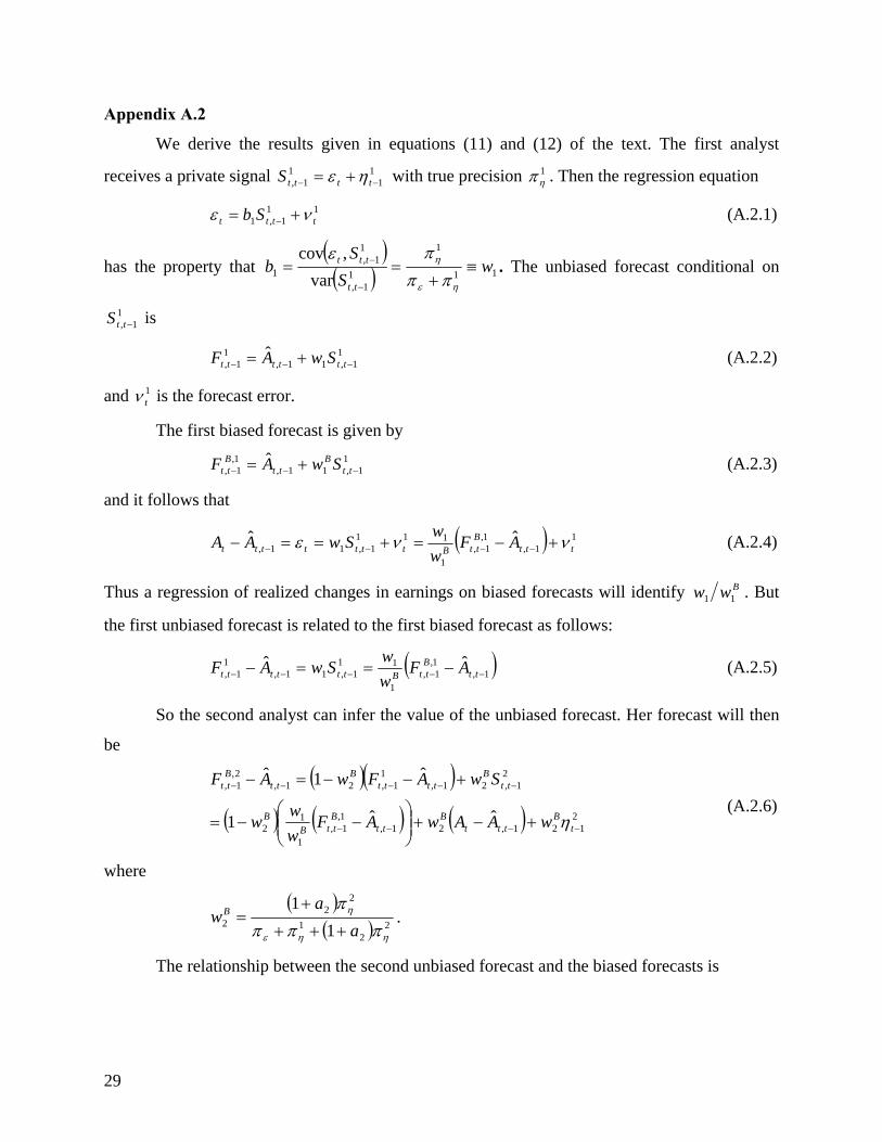
Appendix A.2

We derive the results given in equations (11) and (12) of the text. The first analyst

receives a private signal with true precision . Then the regression equation 11

11, −− += ttttS ηε 1

ηπ

111,1 tttt Sb νε += − (A.2.1)

has the property that ( )( ) 11

1

11,

11,

1 var,cov

wS

Sb

tt

ttt ≡+

==−

−

ηε

η

πππε

. The unbiased forecast conditional on

is 11, −ttS

(A.2.2) 11,11,

11,

ˆ−−− += tttttt SwAF

and 1tν is the forecast error.

The first biased forecast is given by

(A.2.3) 11,11,

1,1,

ˆ−−− += tt

Btt

Btt SwAF

and it follows that

( ) 11,

1,1,

1

1111,11,

ˆˆttt

BttBttttttt AF

ww

SwAA ννε +−=+==− −−−− (A.2.4)

Thus a regression of realized changes in earnings on biased forecasts will identify Bww 11 . But

the first unbiased forecast is related to the first biased forecast as follows:

( )1,1,1,

1

111,11,

11,

ˆˆ−−−−− −==− tt

BttBtttttt AF

ww

SwAF (A.2.5)

So the second analyst can infer the value of the unbiased forecast. Her forecast will then

be

( )( )

( ) ( ) ( ) 2121,21,

1,1,

1

12

21,21,

11,21,

2,1,

ˆˆ1

ˆ1ˆ

−−−−

−−−−−

+−+⎟⎟⎠

⎞⎜⎜⎝

⎛−−=

+−−=−

tB

tttB

ttBttB

B

ttB

ttttB

ttBtt

wAAwAFwww

SwAFwAF

η (A.2.6)

where

( )

( ) 22

1

22

2 11

ηηε

η

ππππ

aa

wB

+++

+= .

The relationship between the second unbiased forecast and the biased forecasts is

29

( ) ( ⎟⎟⎠

⎞⎜⎜⎝

⎛−⎟⎟

⎠

⎞⎜⎜⎝

⎛−+−=− −−−−−− 1,

1,1,

1

1

2

21,

2,1,

2

21,

21,

ˆ1ˆˆtt

BttBBtt

BttBtttt AF

ww

wwAF

wwAF ) (A.2.7)

where 21

2

2ηηε

η

ππππ

++=w is the unbiased weight for the private signal of the second analyst.

In general, the ith observed forecast will be given by

( )( ) itt

Bitt

itt

Bitt

iBtt SwAFwAF 1,1,

11,1,

,1,

ˆ1ˆ−−

−−−− +−−=− (A.2.8)

where

( )

( )∑−

=

+++

+= 1

11

1i

j

ii

j

iiB

i

a

aw

ηηε

η

πππ

π

and

( ) ( 21,

1

11,1,

1

111, 1 −

−−

−−−

−

−−− ⎟⎟

⎠

⎞⎜⎜⎝

⎛−+= i

ttBi

iiBttB

i

iitt F

wwF

wwF ). (A.2.9)

which are the expressions in (11) and (12) of the text.

Appendix B

This section contains technical details for the GMM estimation of the rational and

cognitive bias models. The fundamental moment conditions are the same for both models, with

the rational model imposing several parameter restrictions, described below. The four

fundamental moment conditions, in general form, are:

[ ] 0,1, =−−−

it

iBtt AFE μ (B.1)

{ } 011

1

2,1, =

⎥⎥⎥⎥

⎦

⎤

⎢⎢⎢⎢

⎣

⎡

+−−−

∑−

=

− i

j

j

it

iBtt AFE

ηε ππμ (B.2)

( )[ ] 0)1( 12,111,,01, =−−−−−− −−−

−−− t

itt

Bit

Bi

itt

Bii

itt AFkwAwFwbFE (B.3)

( ){ } ( ) ( )[ ] 0)1( 12212,1

11,,01, =⋅−−−−−−−

−

−−−−−−

iBit

itt

Bit

Bi

itt

Bii

itt wAFkwAwFwbFE ηπ (B.4)

where i = 1, 2,…, 16. The parameter measures the average forecast error for the iiμ th ordered

forecast, thus controlling for any optimism or pessimism bias in the ith ordered forecast. All

30

other parameters are as defined in the text. Moment conditions (B.1) through (B.4) are estimated

separately for each ordered forecast, yielding a total of 64 moment conditions. The first and

second sets of moment conditions yield estimates of sequential forecast bias and consensus

forecast precision. The third set of moment conditions represents the basic regression equation,

and to obtain consistent estimates for the regression parameters, we cross-multiply each of the

moment conditions in the third set by the instrument vector [ ]tiB

ttt AFZ ,,1 ,1, −= , which produces 32

additional moment conditions, for a total of 96 moment conditions. Recall that the orthogonality

of At with the regression error term follows from the model. The fourth set of moment

conditions produces sequential estimates of private signal precision. The following parameter

restriction is imposed by both the rational model and the model with overconfidence and

cognitive dissonance:

i

i

j

j

iBi

a

aw

ηηε

η

πππ

π

)1(

)1(1

1+++

+=

∑−

=

(B.5)

The rational model imposes two additional restrictions:

a = 0 (B.6)

k = 0 (B.7)

Thus, the model with cognitive biases contains two more variables than the rational model.

Estimation

Write the set of all moment conditions as

( )[ ] 0, =θtxfE (B.8)

where represents the data and the vector of parameters to be estimated. The first-stage of

our GMM procedure requires the minimization of the quadratic form of the following term:

tx θ

( ) (∑=

≡N

itN xf

Ng

1

,1 θθ ) . (B.9)

That is, the parameter estimates are given by:

( ) ( )θθθ NN Wgg ′≡= q whereq, minargˆ . (B.10)

As a first step, we estimate unrestricted parameters, using 1̂θ NNIW ×= . These initial parameter

estimates are consistent but inefficient, and are used to construct the asymptotically efficient

31

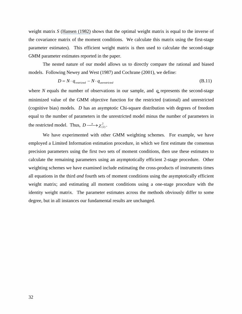
weight matrix S (Hansen (1982) shows that the optimal weight matrix is equal to the inverse of

the covariance matrix of the moment conditions. We calculate this matrix using the first-stage

parameter estimates). This efficient weight matrix is then used to calculate the second-stage

GMM parameter estimates reported in the paper.

The nested nature of our model allows us to directly compare the rational and biased

models. Following Newey and West (1987) and Cochrane (2001), we define:

(B.11) edunrestrictrestricted qNqND ⋅−⋅=

where N equals the number of observations in our sample, and represents the second-stage

minimized value of the GMM objective function for the restricted (rational) and unrestricted

(cognitive bias) models. D has an asymptotic Chi-square distribution with degrees of freedom

equal to the number of parameters in the unrestricted model minus the number of parameters in

the restricted model. Thus, .

•q

2)2(χ⎯→⎯aD

We have experimented with other GMM weighting schemes. For example, we have

employed a Limited Information estimation procedure, in which we first estimate the consensus

precision parameters using the first two sets of moment conditions, then use these estimates to

calculate the remaining parameters using an asymptotically efficient 2-stage procedure. Other

weighting schemes we have examined include estimating the cross-products of instruments times

all equations in the third and fourth sets of moment conditions using the asymptotically efficient

weight matrix; and estimating all moment conditions using a one-stage procedure with the

identity weight matrix. The parameter estimates across the methods obviously differ to some

degree, but in all instances our fundamental results are unchanged.

32

Footnotes

1 The theory was first expounded by Festinger (1957). It has been described as one of the most influential theories in social psychology (Jones, 1985) and has been the stimulus for a great number of experimental studies. 2 The theory of cognitive dissonance has been applied in an economic context in Akerlof and Dickens (1982) and in a financial context in Goetzmann and Peles (1997). 3 In the context of our model, the information content is implicitly measured by the improvement in forecast precision relative to the previously issued forecast. This approach differs from other studies that use a market-based measure of information content. For example, Gleason and Lee (2002) and Cooper, Day and Lewis (2001) study the properties of analyst forecast revisions. In those studies, each forecast’s information content is measured using market-based responses (excess returns or volume) to the forecast revision. 4 Because we are examining the precision of the forecasts themselves, and not the precision of the parameters used to generate the forecasts, the mean squared forecast error is calculated by dividing the sum of the squared forecast errors by the number of observations (see Greene 1997, pp. 372-373). However, the number of observations in our sample is so large that even if a loss of degrees of freedom in the regression parameters translated into a loss of degrees of freedom in the mean squared forecast error, the relative performance of the predictors would remain unchanged. 5 Firms may punish analysts who issue negative or pessimistic forecasts by excluding them from conference calls (or other forms of direct contact with management), terminating correspondence, and even threatening legal or physical harm (Siconolfi 1995; Schultz 1990; Berg 1990). Michaely and Womack (1999) suggest that an analyst may issue more favorable forecasts for firms that have an underwriting relationship with the analyst’s company. 6 Lim (2001) develops a model in which analyst forecast bias is fully rational, because it induces firm management to provide better information to the optimistic analyst. The improved information is sufficient to decrease the analyst’s mean squared forecast error. 7 McNichols, O’Brien and Francis (1997) find that analysts tend to drop coverage of firms that they expect to do poorly rather than retain them and issue negative comments. This incentive not to release unfavorable forecasts truncates the left tail of the forecast distribution, producing observationally biased forecasts even when the true forecast distribution is unbiased. Other studies suggest that the observed upward bias is the result of discretionary asset write-downs (Keane and Runkle 1998) or skewed data (Abarbanell and Lehavy 2000). 8Information on forecasts is easily accessible. I/B/E/S, Zack’s and First Call, the main providers of earnings forecast information, all offer real-time web-based access to forecast data. 9 However we argue below that such incentives are likely to be insignificant in the context we consider. 10 This would include a loss function equal to the mean squared forecast error. 11 This assumes for notational simplicity that each analyst’s forecast appears at the same point in the forecast order in successive quarters. We do not assume that this is the case in the empirical analysis. 12 We assume that large pieces of new public information are followed by two or more simultaneous forecasts. By eliminating multiple forecast days from our regressions (though still including them in the information set of all subsequent forecasts), we aim to isolate the effect of private information on forecasts. 13 Keane and Runkle (1998) find that including all earnings forecast observations in their analysis leads to rejection of the hypothesis of rational forecasts. However, after eliminating outliers they can no longer reject the rational hypothesis.

33

14 Bernard and Thomas (1990) show that pooled, seasonally-differenced earnings are predictable using lagged values of differenced earnings, particularly at lags 1 and 2. Clearly, earnings for some firms will be more predictable than others. Thus, we extend Bernard and Thomas (1990) by fitting separate AR(2) models for each firm. 15 Results are virtually identical when we eliminate observations +/- 4 standard deviations from the mean. 16 This considerably simplifies the expression for the ith analyst’s forecast. While this could theoretically bias our estimates, we doubt this is the case for two reasons. First, since the median forecast error in our sample is zero, the lagged forecast errors of analysts j=1,2,…,i-1 may tend to cancel each other out, and incorporating them individually into the ith forecast may yield little benefit. Second, as we demonstrate below, the economic significance of the cognitive dissonance bias is fairly small, and ignoring the cognitive dissonance bias in other forecasts would likely have little effect on the ith analyst’s own forecast precision. In contrast, we also show below that the overconfidence bias is quite significant, both economically and statistically. 17 In Table III, we utilize a consensus measure equal to a weighted average of all previously issued forecasts, where the weights are functions of the estimated cognitive bias parameters, as well as the estimated weights each past analyst placed on her private information. We have also estimated the table with consensus measures equal to the average of all existing forecasts; the average of the most recent two, three or four forecasts; the most recent existing forecast; and the average of all forecasts issued in the past 30 days. In all cases, the results are similar. 18 Zitzewitz (2001b) does allow the analyst to make multiple forecasts within a period, and shows that the incentive to overweight private information declines with the number of forecasts made. 19 Firms with negative B-M ratios are excluded from the low B-M quartile, since firms with negative B-M ratios have properties very different from firms with small, positive B-M ratios. 20 The large jump in precision from the 15th ordered forecast the "16th+" forecasts occurs because the "16th+" category contains not only the 16th forecasts, but all subsequent forecasts, whose precision continues to sequentially increase. The pooled precision estimates are therefore higher than the precision for the 16th ordered forecasts alone.

34

Table I Sample Statistics for Raw and Sigma-Normalized Data

Full sample includes all one- and two-quarter-ahead quarterly earnings forecasts in the I/B/E/S Domestic Detail File over the 1993-1999 period. Actual earnings data are taken from the domestic I/B/E/S Actuals File. To be included in the full sample, a firm must have at least 12 seasonally-differenced quarterly earnings observations. Additional cumulative data filters are applied as follows: Filter A eliminates observations with Price < $5 per share. Filter B eliminates observations from analysts with fewer than 25 total forecasts during the sample period, as well as all forecasts issued on multiple-forecast days (days on which 2 or more forecasts are issued). Filter C excludes forecasts made before the most recent past quarterly earnings announcement. Filter D eliminates forecasts more than six standard deviations from actual reported earnings, where firm-specific standard deviations are estimated by fitting an AR(2) model to actual earnings over the entire sample period. It also eliminates forecasts for which no prior forecasts exist.

Panel A: Raw Data Panel B: Sigma-Normalized Data Variable

Data Filter

N. obs in sample

Mean

Median

Std. Dev

Min.

Max.

Mean

Median

Std. Dev

Min.

Max.

Actual Earnings Forecasted Earnings Analyst Forecast Error

Full Filter A Filter B Filter C Filter D

Full

Filter A Filter B Filter C Filter D

Full

Filter A Filter B Filter C Filter D

989,967 909,046 624,144 389,233 307,532

989,967 909,046 624,144 389,233 307,532

989,967 909,046 624,144 389,233 307,532

0.298 0.322 0.323 0.323 0.336

0.374 0.360 0.361 0.346 0.356

0.075 0.037 0.038 0.024 0.020

0.235 0.255 0.250 0.253 0.268

0.250 0.270 0.270 0.260 0.273

0.000 0.000 0.000 0.000 0.000

1.444 1.386 1.574 1.558 1.218

36.986 1.354 1.535 1.513 1.184

36.968 0.582 0.667 0.717 0.405

-363.650 -249.900 -249.900 -249.900 -39.000

-250.000 -250.000 -250.000 -250.000 -11.667

-247.200 -247.200 -247.200 -247.200 -22.130

125.970 125.970 125.970 125.970 125.970 36875.0 143.060 143.060 143.060 131.050 36874.3 218.400 218.400 218.400 65.730

3.784 4.024 3.883 3.838 4.013

3.922 4.157 4.014 3.896 4.057

0.138 0.132 0.131 0.059 0.044

2.245 2.459 2.372 2.359 2.482

2.342 2.551 2.463 2.379 2.500

0.000 0.000 0.000 0.000 0.000

5.506 5.641 5.469 5.382 5.519

8.451 5.626 5.489 5.458 5.437

6.552 1.297 1.382 1.469 0.712

-10.254 -10.254 -10.254 -10.254 -10.254

-283.404 -283.404 -283.404 -283.404 -10.928

-280.230 -280.230 -280.230 -280.230 -5.975

63.321 63.321 63.321 63.321 63.076

6384.46 582.781 582.781 582.781 61.165

6384.30 576.953 576.953 576.953 5.974

Table II Regression of ith Analyst Forecast on Lagged Forecasts

Table presents regression slope coefficients from a regression of the ith observed forecast, , on lagged forecast

changes , j=1,2,…,i-1 and actual time-t earnings changes, . Regressions include an intercept term, which is omitted for brevity. For the 8

ittF 1, −

1,1,ˆ

−− − ttjtt AF 1,

ˆ−− ttt AA

th and later ordered forecasts, we report only the coefficients on the first seven lagged forecasts. Data reflect Filter D (see Table I). is calculated using, and all data are normalized by, firm-specific AR(2) standard errors. White Heteroskedasticity consistent standard errors reported in parentheses.

1,ˆ

−ttA

Slope Coefficients

Forecast order

i

i-1

i-2

i-3

i-4

i-5

i-6

i-7

1,ˆ

−− ttt AA

2 0.791 0.2039 (0.002) (0.002)

3 0.489 0.353 0.157 (0.004) (0.004) (0.003)

4 0.408 0.236 0.197 0.158 (0.005) (0.005) (0.005) (0.003)

5 0.347 0.205 0.156 0.125 0.166 (0.006) (0.005) (0.006) (0.005) (0.003)

6 0.331 0.192 0.136 0.095 0.080 0.166 (0.006) (0.006) (0.006) (0.006) (0.006) (0.004)

7 0.330 0.180 0.145 0.089 0.046 0.050 0.157 (0.007) (0.007) (0.007) (0.007) (0.007) (0.007) (0.004)

8 0.281 0.248 0.114 0.072 0.044 0.030 0.044 0.167 (0.008) (0.008) (0.007) (0.008) (0.008) (0.007) (0.007) (0.005)

9 0.312 0.195 0.129 0.079 0.065 0.041 0.020 0.157 (0.010) (0.009) (0.009) (0.008) (0.009) (0.009) (0.008) (0.006)

10 0.297 0.184 0.113 0.099 0.074 0.037 0.036 0.161 (0.011) (0.011) (0.010) (0.011) (0.011) (0.010) (0.010) (0.007)

11 0.236 0.175 0.181 0.095 0.070 0.040 0.016 0.186 (0.013) (0.013) (0.013) (0.013) (0.012) (0.011) (0.011) (0.008)

12 0.237 0.223 0.113 0.116 0.100 0.057 0.005 0.147 (0.015) (0.016) (0.016) (0.015) (0.015) (0.015) (0.012) (0.009)

13 0.227 0.159 0.154 0.134 0.050 0.081 0.023 0.171 (0.016) (0.016) (0.017) (0.017) (0.016) (0.015) (0.014) (0.010)

14 0.187 0.310 0.110 0.091 0.075 0.074 0.018 0.133 (0.002) (0.018) (0.019) (0.020) (0.019) (0.019) (0.018) (0.013)

15 0.179 0.219 0.089 0.149 0.119 0.229 0.072 0.148 (0.024) (0.027) (0.022) (0.021) (0.023) (0.020) (0.020) (0.015)

16+ 0.192 0.113 0.189 0.119 0.139 0.034 0.071 0.142 (0.017) (0.016) (0.016) (0.016) (0.015) (0.015) (0.014) (0.011)

Table III GMM Estimation and Model Comparison

Regressions below estimate (i) the rational model equation ( ) ititi

ittii

itt wAwFwbF 11,,01, 1 −−− ++−+= η , and (ii) the

equation for the model with cognitive bias ( ) ( ) it

Bit

iBtt

Bit

Bi

iBtt

Bii

iBtt wAFkwAwFwbF 11

,2,1

,1,,0

,1, 1 −−−−−− +−++−+= η

where ( ) is the iittF 1, −

iBttF ,

1, −th sequential analyst forecast, i

ttF 1, − ( iBttF ,

1, − ) is the consensus defined as a weighted average of all previously issued forecasts, where the weights are functions of the estimated cognitive bias parameters, as well as the estimated weights each past analyst placed on her private information., and is the actual quarterly earnings reported at time t. Data reflect Filter D (see Table I). All data are normalized by firm-specific AR(2) standard errors. See text and Appendix for details of GMM estimation. The Newey-West D-statistic equals N times the minimized value of the GMM objective function in the restricted (rational) model, minus the same statistic from the unrestricted model. This statistic has an asymptotic chi-squared distribution with 2 degrees of freedom. GMM standard errors are reported in parentheses.

tA

Rational Model Model with Cognitive Bias

Forecast

order

Constant

Consensus precision

Private signal

precision

Implied iw

Constant

Consensus precision

Private signal

precision

Implied B

iw

1 0.106 1.512 0.417 0.22 0.112 1.528 0.168 0.18 (0.005) (0.023) (0.015) (0.004) (0.020) (0.007)

2 0.089 1.813 0.428 0.19 0.099 1.706 0.166 0.16 (0.004) (0.038) (0.025) (0.004) (0.023) (0.008)

3 0.076 2.049 0.397 0.16 0.087 1.825 0.180 0.16 (0.004) (0.032) (0.017) (0.004) (0.022) (0.007)

4 0.028 2.215 0.805 0.27 0.035 1.911 0.217 0.18 (0.004) (0.040) (0.044) (0.003) (0.023) (0.010)

5 0.052 2.356 0.523 0.18 0.060 2.027 0.222 0.18 (0.004) (0.047) (0.026) (0.004) (0.029) (0.010)

6 0.043 2.565 0.601 0.19 0.047 2.195 0.243 0.18 (0.004) (0.057) (0.032) (0.004) (0.035) (0.012)

7 0.035 2.902 0.574 0.17 0.036 2.372 0.264 0.18 (0.004) (0.080) (0.041) (0.004) (0.044) (0.017)

8 -0.009 3.057 1.487 0.33 -0.011 2.496 0.319 0.20 (0.004) (0.092) (0.133) (0.004) (0.046) (0.022)

9 -0.026 3.168 1.430 0.31 -0.027 2.565 0.322 0.20 (0.004) (0.109) (0.149) (0.004) (0.052) (0.027)

10 -0.033 3.513 1.864 0.35 -0.036 2.845 0.376 0.20 (0.004) (0.140) (0.233) (0.005) (0.065) (0.034)

11 -0.046 3.870 2.225 0.37 -0.050 3.171 0.565 0.26 (0.005) (0.181) (0.288) (0.006) (0.094) (0.059)

12 -0.052 4.142 1.763 0.30 -0.054 3.354 0.495 0.22 (0.006) (0.236) (0.283) (0.006) (0.118) (0.066)

13 -0.064 4.509 2.279 0.34 -0.067 3.737 0.648 0.25 (0.007) (0.278) (0.384) (0.007) (0.161) (0.091)

14 -0.074 4.723 2.380 0.34 -0.080 4.135 0.755 0.26 (0.008) (0.329) (0.491) (0.007) (0.221) (0.145)

15 -0.084 5.517 2.607 0.32 -0.095 4.696 0.881 0.27 (0.010) (0.472) (0.592) (0.008) (0.0311 (0.189)

16+ -0.010 6.108 3.429 0.36 -0.115 5.138 1.090 0.29 (0.010) (0.892) (1.24) (0.009) (0.538) (0.325) D

statistic 1,713.43

(p-val <10-20)

Cognitive bias

parameters

a 0.937 (0.027) k 0.079 (0.0073)

Table IV GMM Estimation of Model with Cognitive Biases

High and Low Book-to-Market Firms Each year t, firms are divided into high, low and medium B-M categories based on the cross-sectional distribution of B-M ratios as of the previous fiscal year-end (t - 1). Following Fama and French (1992), we include a six-month lag between the previous fiscal year-end and our forecasts. Thus, forecasts issued between July of year t and June 30 of year t + 1 are sorted according to the B-M ratio as of the previous fiscal year-end (t - 1). For instance, using the 1993 fiscal-year-end B-M ratios for each firm, we calculate the cross-sectional distribution of these ratios, and group firms according to their relative position. All forecasts issued between 7/1/94 and 6/30/95 are then assigned to the appropriate subsample based on the firm's B-M ratio as of 1993 year end. This process is repeated for each year in the sample. B-M data are obtained from the Compustat Industrials file, and equal the book value of equity (items 60) divided by the market value of equity (item 24 times item 25). The model is estimated separately for each group. The model and estimation procedure are as described in the notes to Table II. GMM standard errors are reported in parentheses under coefficient estimates.

Low Book-to-Market Firms

Medium Book-to-Market Firms

High Book-to-Market Firms

Forecast

Order

Consensus Precision

Private Signal

Precision

Consensus Precision

Private Signal

Precision

Consensus Precision

Private Signal

Precision 2 1.726 0.170 1.685 1.685 1.719 0.174 (0.038) (0.012) (0.033) (0.011) (0.057) (0.017)

3 1.815 0.175 1.853 1.852 1.803 0.178 (0.042) (0.012) (0.030) (0.010) (0.066) (0.018)

4 1.879 0.193 1.951 1.951 1.918 0.248 (0.042) (0.017) (0.033) (0.015) (0.083) (0.035)

5 1.854 0.208 2.107 2.107 2.175 0.280 (0.051) (0.018) (0.039) (0.014) (0.094) (0.036)

6 2.007 0.192 2.294 2.294 2.314 0.285 (0.061) (0.018) (0.050) (0.017) (0.119) (0.040)

7 2.082 0.197 2.475 2.475 2.701 0.316 (0.072) (0.021) (0.062) (0.021) (0.163) (0.051)

8 2.114 0.220 2.690 2.691 2.687 0.327 (0.068) (0.026) (0.070) (0.034) (0.184) (0.061)

9 2.038 0.201 2.738 2.739 3.069 0.443 (0.070) (0.026) (0.075) (0.043) (0.227) (0.083)

10 2.398 0.305 3.082 3.082 3.170 0.465 (0.102) (0.043) (0.091) (0.053) (0.308) (0.112)

11 2.589 0.443 3.344 3.344 4.007 0.866 (0.145) (0.078) (0.117) (0.079) (0.446) (0.225)

12 3.090 0.470 3.469 3.469 3.440 0.732 (0.198) (0.092) (0.147) (0.069) (0.435) (0.284)

13 3.120 0.464 4.086 4.086 4.228 1.381 (0.224) (0.092) (0.237) (0.107) (0.628) (0.385)

14 3.844 0.568 4.045 4.045 5.505 1.016 (0.373) (0.220) (0.285) (0.122) (0.990) (0.505)

15 3.991 0.984 4.857 4.827 5.993 0.997 (0.495) (0.399) (0.447) (0.251) (1.301) (0.539)

16+ 3.696 0.814 5.781 5.780 10.678 8.075 (1.131) (0.604) (0.604) (0.411) (2.220) (3.447)

Cognitive Bias

Parameters

a 1.040 0.908 0.752 (0.046) (0.035) (0.050) k 0.103 0.074 0.028 (0.014) (0.009) (0.015)

Avg. B-M ratio 0.139 0.465 0.962

Table V

Full-Information GMM Estimation of Model with Cognitive Biases Positive and Negative Lagged Forecast Error

Following Easterwood and Nutt (1999), we use the distribution of lagged errors to partition the sample into quartiles based upon the sign and magnitude of the lagged error. Lagged forecast error is defined as lagged forecast minus lagged actual earnings. We label the top quartile of observations "High Positive Lagged Error", the middle two quartiles "Low Lagged Error", and the bottom quartile "High Negative Lagged Error". The model is estimated separately for each group. The model and estimation procedure are as described in the notes to Table II. GMM standard errors are reported in parentheses under coefficient estimates.

High Positive Lagged Error

Low Lagged Error High Negative Lagged Error

Forecast

Order

Consensus Precision

Private Signal

Precision

Consensus Precision

Private Signal

Precision

Consensus Precision

Private Signal

Precision 2 1.194 0.108 2.460 0.240 1.804 0.182 (0.033) (0.008) (0.053) (0.014) (0.042) (0.012)

3 1.365 0.102 2.539 0.280 1.892 0.174 (0.031) (0.008) (0.061) (0.018) (0.051) (0.013)

4 1.404 0.094 2.646 0.343 2.138 0.285 (0.035) (0.009) (0.071) (0.026) (0.062) (0.025)

5 1.546 0.121 2.849 0.375 2.199 0.244 (0.046) (0.012) (0.086) (0.028) (0.074) (0.020)

6 1.625 0.132 3.037 0.389 2.450 0.298 (0.054) (0.013) (0.106) (0.030) (0.091) (0.028)

7 1.706 0.137 3.324 0.469 2.790 0.284 (0.061) (0.017) (0.128) (0.044) (0.115) (0.035)

8 1.759 0.135 3.799 0.663 2.944 0.503 (0.068) (0.016) (0.177) (0.078) (0.147) (0.074)

9 1.771 0.123 3.812 0.580 3.150 0.451 (0.074) (0.014) (0.208) (0.079) (0.183) (0.077)

10 1.820 0.139 4.205 0.613 3.600 0.594 (0.083) (0.019) (0.249) (0.100) (0.225) (0.105)

11 2.010 0.225 4.487 0.792 3.910 0.871 (0.111) (0.041) (0.307) (0.138) (0.261) (0.153)

12 2.480 0.188 4.163 0.571 4.171 0.818 (0.192) (0.050) (0.325) (0.109) (0.394) (0.191)

13 2.479 0.191 5.105 1.161 4.592 0.721 (0.209) (0.045) (0.414) (0.241) (0.419) (0.172)

14 2.348 0.149 5.759 1.076 4.780 0.834 (0.226) (0.046) (0.500) (0.227) (0.481) (0.237)

15 2.553 0.182 6.879 1.093 4.551 0.887 (0.241) (0.048) (0.782) (0.324) (0.591) (0.305)

16+ 3.363 0.331 6.752 1.372 3.993 0.700 (0.282) (0.080) (0.995) (0.462) (0.858) (0.344)

Cognitive Bias

Parameters

a 1.229 0.777 1.280 (0.047) (0.033) (0.056) k 0.008 0.202 0.071 (0.011) (0.075) (0.016)

Mean Forecast Error 0.864 -0.053 -0.887

Table VI GMM Estimation of Model with Cognitive Biases

Annual I/B/E/S Earnings Forecasts - United States and Japan Parameter estimates are obtained by estimating the equation for the model with cognitive bias

( ) ( ) it

Bit

iBtt

Bit

Bi

iBtt

Bii

iBtt wAFkwAwFwbF 11

,2,1

,1,,0

,1, 1 −−−−−− +−++−+= η where is the iiB

ttF ,1, −

th sequential analyst forecast, iB

ttF ,1, − is the consensus, equal to a weighted average of past forecasts, as specified in section 3 of the paper, and is the

actual annual earnings reported at time t. Data reflect Filter D (see Table I). All data are normalized by firm-specific standard errors. See text and Appendix for details of GMM estimation.

tA

United States

Japan

Forecast Order

Consensus Precision

Private Signal Precision

Consensus Precision

Private Signal Precision

2 3.025 0.466 2.741 0.218 (0.139) (0.058) (0.183) (0.045)

3 3.481 0.663 3.101 0.288 (0.255) (0.080) (0.247) (0.068)

4 4.834 1.767 3.739 0.313 (0.506) (0.266) (0.290) (0.079)

5 3.216 0.651 3.991 0.333 (0.282) (0.108) (0.367) (0.094)

6 4.475 0.829 4.652 0.548 (0.253) (0.114) (0.417) (0.159)

7 4.582 0.662 4.885 0.441 (0.324) (0.123) (0.539) (0.143)

8 5.541 1.191 5.322 0.870 (0.332) (0.237) (0.771) (0.378)

9 5.055 2.185 6.457 0.703 (0.740) (0.406) (0.935) (0.254)

10 5.678 1.773 4.713 0.417 (0.623) (0.400) (0.822) (0.240)

11 6.015 1.626 5.254 0.563 (0.614) (0.373) (1.258) (0.340)

12 6.369 1.813 6.052 1.069 (0.597) (0.496) (0.809) (0.435)

13 6.632 2.305 11.911 5.054 (0.687) (0.455) (2.911) (2.382)

14 7.511 1.628 7.445 0.481 (0.591) (0.414) (1.483) (0.132)

15 7.146 1.883 9.580 1.026 (0.765) (0.588) (1.674) (0.548)

16+ 8.063 2.436 10.902 1.465 (0.740) (0.529) (1.427) (0.351)

Cognitive Bias

Parameters

a 1.141 1.575 (0.065) (0.147) k 0.024 0.038 (0.014) (0.036)

Num. Obs. 148,244 11,672

Forecast Precision by Forecast Order

1.0

1.5

2.0

2.5

3.0

3.5

4.0

4.5

5.0

5.5

2 3 4 5 6 7 8 9 10 11 12 13 14 15 16+Forecast Order

Prec

isio

n

FV1 FV2 FV3 Figure 1: Forecast Precision by Forecast Order Figure plots the forecast precision for three forecasting variables of actual time t earnings. The forecasting variables are labeled through . The current (i1

1, −ttFV 31, −ttFV th) analyst’s actual forecast is labeled . is generated by

regressing actual earnings on observable lagged forecasts,

11, −ttFV 2

1, −ttFV111,

−=−

ij

jttF . is generated by regressing actual earnings

on observable lagged forecasts,

31, −ttFV

111,

−=−

ij

jttF , as well as the current (ith) analyst’s actual forecast. Forecast precision is equal

to the inverse sample mean-squared forecast error for each ordered forecast. Forecasting parameters are re-estimated each quarter, using all earnings data from previous quarters. Any difference in forecast precision between and is due to mis-weighting of information contained in the current and lagged forecasts.

11, −ttFV 3

1, −ttFV

Efficiency Loss in Forecast Precision Due ToMis-Weighting

-25%

-20%

-15%

-10%

-5%

0%

2 3 4 5 6 7 8 9 10 11 12 13 14 15 16+

Forecast Order

Difference in forecast precision Figure 2: Efficiency Loss in Forecast Precision Due to Analyst Cognitive Biases Figure expresses the percentage difference between the forecast precision of the current (ith) analyst’s actual forecast

and . The reported values are equal to the precision divided by the precision of minus

one. The current (i

11, −ttFV 3

1, −ttFV 11, −ttFV 3

1, −ttFVth) analyst’s actual forecast is labeled .

is generated by regressing actual earnings on

observable lagged forecasts,

11, −ttFV 3

1, −ttFV111,

−=−

ij

jttF , as well as the current (ith) analyst’s actual forecast. Forecasting parameters are re-

estimated each quarter, using all earnings data from previous quarters. Any difference in forecast precision between and is due to mis-weighting of information contained in the current and lagged forecasts. 1

1, −ttFV 31, −ttFV

Efficient Weights on Lagged Forecasts

0.53

0.25

0.12

0.060.03 0.01 0.01

0.00

0.10

0.20

0.30

0.40

0.50

0.60

i-1 i-2 i-3 i-4 i-5 i-6 i-7

Lagged Forecast

Wei

ght

Figure 3. Consensus Forecast: Theoretical Weights on Lagged Forecasts. The figure plots the efficient Bayesian weights placed on lagged forecasts to form an efficient consensus forecast. The actual weights on lagged forecasts are described in equation (11) in the text, and in general depend upon the precision of the initial information set, precision of past analyst private signals, and the degree of overconfidence exhibited by each past analyst. The weights above illustrate a special case with initial precision , constant private signal

precision and constant overconfidence (a=1).

0.1=επ10.0=i

ηπ

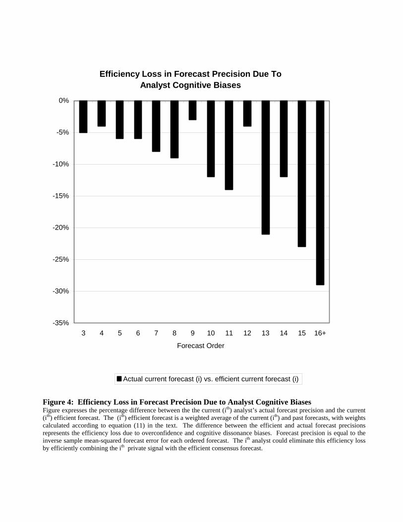
Efficiency Loss in Forecast Precision Due ToAnalyst Cognitive Biases

-35%

-30%

-25%

-20%

-15%

-10%

-5%

0%

3 4 5 6 7 8 9 10 11 12 13 14 15 16+

Forecast Order

Actual current forecast (i) vs. efficient current forecast (i)

Figure 4: Efficiency Loss in Forecast Precision Due to Analyst Cognitive Biases Figure expresses the percentage difference between the the current (ith) analyst’s actual forecast precision and the current (ith) efficient forecast. The (ith) efficient forecast is a weighted average of the current (ith) and past forecasts, with weights calculated according to equation (11) in the text. The difference between the efficient and actual forecast precisions represents the efficiency loss due to overconfidence and cognitive dissonance biases. Forecast precision is equal to the inverse sample mean-squared forecast error for each ordered forecast. The ith analyst could eliminate this efficiency loss by efficiently combining the ith private signal with the efficient consensus forecast.