arX

iv:2

005.

0354

0v1

[st

at.A

P] 7

May

202

0

Sequential Aggregation of Probabilistic Forecasts

- Applicaton to Wind Speed Ensemble Forecasts

Michael Zamo1,3, Liliane Bel2, and Olivier Mestre1,3

1Meteo-France, Direction des Operations pour la Production, 42avenue Gaspard Coriolis, 31057 Toulouse cedex 07, France.

2Universite Paris-Saclay, AgroParisTech, INRAE, UMRMIA-Paris, 75005, Paris, France

3CNRM/GAME, Meteo-France/CNRS URA 1357, Toulouse,France

May 8, 2020

Abstract

In the field of numerical weather prediction (NWP), the probabilisticdistribution of the future state of the atmosphere is sampled with Monte-Carlo-like simulations, called ensembles. These ensembles have deficien-cies (such as conditional biases) that can be corrected thanks to statisticalpost-processing methods. Several ensembles exist and may be correctedwith different statistiscal methods. A further step is to combine theseraw or post-processed ensembles. The theory of prediction with expertadvice allows us to build combination algorithms with theoretical guar-antees on the forecast performance. This article adapts this theory to thecase of probabilistic forecasts issued as step-wise cumulative distributionfunctions (CDF). The theory is applied to wind speed forecasting, by com-bining several raw or post-processed ensembles, considered as CDFs. Thesecond goal of this study is to explore the use of two forecast performancecriteria: the Continous ranked probability score (CRPS) and the Jolliffe-Primo test. Comparing the results obtained with both criteria leads toreconsidering the usual way to build skillful probabilistic forecasts, basedon the minimization of the CRPS. Minimizing the CRPS does not neces-sarily produce reliable forecasts according to the Jolliffe-Primo test. TheJolliffe-Primo test generally selects reliable forecasts, but could lead toissuing suboptimal forecasts in terms of CRPS. It is proposed to use bothcriterion to achieve reliable and skillful probabilistic forecasts.

1

1 Introduction

As a chaotic dynamical system, the atmosphere has an evolution that is in-trinsically uncertain (Malardel, 2005; Holton and Hakim, 2012) and should bedescribed in a probabilistic form. In the field of numerical weather predic-tion (NWP), this probabilistic form is not a probability distribution but aset of deterministic forecasts whose aim is to assess the forecast uncertainty(Leutbecher and Palmer, 2008). Such a set of deterministic forecasts is calledan ensemble forecast and each individual deterministic forecast is called a mem-ber. The members are usually obtained by running the same NWP model withdifferent initial conditions and different parametrizations of the model physics(Descamps et al., 2011). Forecast uncertainty can then be derived from themembers as a probability distribution with statistical estimation techniques andconsidering the members are a random sample from an unknown multivariateprobability distribution .

Being often biased and under-dispersed for surface parameters (Hamill and Colucci,1998; Buizza et al., 2005), the ensemble forecast systems may be post-processedwith statistical methods, called ensemble model output statistics (EMOS) to getmore skillful forecast distributions (Wilson et al., 2007; Thorarinsdottir and Gneiting,2010; Moller and Scheuerer, 2013; Zamo et al., 2014; Baran and Lerch, 2015;Taillardat et al., 2016).

Nowadays, several ensemble forecast systems are available routinely (Bougeault et al.,2010; Descamps et al., 2014). Combining, or “aggregating”, several forecastsmay improve the predictive performance compared to the most skillful post-processed ensemble (Allard et al., 2012; Gneiting et al., 2013; Baudin, 2015;Baran and Lerch, 2016; Moller and Groß, 2016; Bogner et al., 2017). The the-ory of prediction with expert advice (Cesa-Bianchi et al., 2006; Stoltz, 2010)shows how to efficiently aggregate in real-time several forecasts based on theirrespective past performances. This theory studies the mathematical propertiesof aggregation algorithms of several forecasting systems (called “experts” in thisframework), and has been applied mostly to point forecasts.

The first goal of the present work is to apply the theory of prediction with expertadvice to probabilistic forecasts represented as step-wise cumulative distributionfunctions (CDF) with any number of steps. Two previous studies (Baudin, 2015;Thorey, 2017) used this theory for specific cases of probabilistic forecasts. InBaudin (2015), the experts are the ordered individual members of pooled en-sembles. Each expert’s forecast is a stepwise cumulative distribution functionwith one step. In this case the experts are not identifiable over time althoughit is required by the theory. For instance, at different times, the lowest forecastvalue comes from a different member of a different ensemble. Thorey (2017)applies the theory of prediction with expert advice to forecasts of photovoltaicelectricity production. The experts are ensemble forecasts or built from ensem-ble or deterministic forecasts thanks to statistical regression methods. Eachexpert is treated as a different deterministic forecast, even though some of them

2

are members of the same ensemble. Other experts are built thanks to quantileregression methods. As such, the set of forecast quantiles could be consideredas a specific probabilistic expert, but each forecast quantile is again consideredas a separate deterministic expert. In this study, contrary to Baudin (2015) andThorey (2017), each expert is a whole (raw or post-processed) ensemble, andis thus actually identifiable over time. This work extends the work of Baudin(2015) in the sense that the formulae established in this article reduce to theones in Baudin (2015) if considering step-wise CDFs with a single step. Ina nutshell, the aggregated forecast is a linear combination of the CDFs of theexperts. Since the aggregated forecast must be a CDF, only convex aggregationstrategies are investigated: the weights are constrained to be positive and tosum up to one.

The second goal of this work is to compare two model selection approacheswhen dealing with probabilistic forecasting systems (Collet and Richard, 2017).The first approach is based on “reliability” (or “calibration”) and “sharpness”(Gneiting et al., 2007; Jolliffe and Stephenson, 2011). A forecasting system isreliable if the conditional probability distribution of the observation given theforecast distribution is equal to the forecast distribution. A forecasting sys-tem is sharper when, on average, it predicts a lower dispersion of the observa-tion. According to the sharpness-calibration paradigm of Gneiting et al. (2007) aforecasting system should aim at providing reliable probabilistic forecasts thatare the sharpest (i.e. less dispersed) possible. A practical motivation of thissharpness-calibration paradigm is that decisions based on such a forecastingsystem would be optimal due to the reliability of the forecast and less uncertaindue to the forecast’s low dispersion, which improves its value for economicaldecisions (Richardson, 2001; Zhu et al., 2002; Mylne, 2002). Among severalreliable forecasting systems, one should thus select the sharpest. The secondapproach to model selection among probabilistic forecasting systems is basedon a scoring rule, such as the Continuous Ranked Probabilistic Score (CRPS,Matheson and Winkler 1976): the selected model is the one that has the bestvalue of the scoring rule (highest or lowest value depending on the scoring rule).The two approaches to model selection do not yield equivalent forecasts, as pre-viously mentioned in different studies (Collet and Richard, 2017; Wilks, 2018).For instance, minimizing the CRPS may lead to forecasts that are not reliable.To solve this problem, Wilks (2018) proposes to minimize the CRPS penalizedwith a term quantifying the unreliability of the forecast. Collet and Richard(2017) introduces a post-processing method that, under quite strong assump-tions, yields reliable forecasts without degrading too much the CRPS comparedto the CRPS-minimizing approach. We do not use any of these solutions herebut compare the two model selection approaches and their properties on a casestudy. Both approaches are used to select the best forecasting system amongseveral experts and aggregated forecasts. In the first approach, reliability isimposed by using the Jolliffe-Primo flatness test (JP test, Jolliffe and Primo(2008)). As for the second approach, forecast performance is measured with theCRPS.

3

In Section 2, the theory of prediction with expert advice is presented, alongwith notations. It is shown how this theory can be straightforwardly applied tostep-wise CDFs. The CRPS and JP test are also introduced with more detailsand their use is further motivated. Section 3 presents the different aggregationmethods investigated. Some are empirical, while others exhibit interesting the-oretical properties. Section 4 describes the use-case of this study and the datait uses: four ensemble forecasts, two EMOS methods used to post-process theensembles, and the wind speed observation. The results of the comparison of theaggregation methods are presented in Section 5. These results motivate a moretheoretical comparison of the two approaches to model selection among proba-bilistic forecasts, in Section 6. Finally, Section 7 concludes with a summary ofthe results and perspectives.

2 Theoretical Framework and Performance As-

sessment Tools

The desired properties of forecast aggregation are two-fold. The first one is toyield an aggregated forecast that performs better than any of the forecasts thatare used in the aggregation. According to the theory of prediction with expertadvice (Cesa-Bianchi et al., 2006; Stoltz, 2010), some algorithms used to sequen-tially aggregate forecasts exhibits theoretical guarantees of performance. Theseguarantees state that the aggregated forecast will not perform much worse thansome skillful reference forecast, called the oracle. In practice, the aggregatedforecast may even outperform the oracle. This motivates using the theory ofprediction with expert advice. The second desired property is to dynamicallytackle changes in the forecasts’ generating process (such as modification in NWPmodel’s code). These changes may strongly affect the performance of the rawor post-processed forecasts. A good aggregation method should quickly detectchanges in the performance of the individual forecasts and adapt the aggregationweights to discard the bad ones and favor the good ones. Being a sequential ag-gregation framework based on the recent performance of the experts, the theoryof prediction with expert advice may help in reaching this second goal.

2.1 Sequential Aggregation of Step-Wise CDFs

The situation tackled by the theory of prediction with expert advice is the fol-lowing: a forecaster has to forecast some parameter of interest by using onlypast observations of the parameter and past and current forecasts of the pa-rameter steming from several sources. These sources whose forecasts are to beaggregated are called “experts” in this theory. In this very general frameworkno assumption is made on the generating process of the observations and theexperts.

4

More formally, at time t, before the observation yt ∈ Y is revealed, let us supposeavailable the forecast of the E ∈ N

∗ experts and of the past observations (notedyj=1,...,t−1). An expert is any means, in a very general sense (NWP model,human expertise, . . . ), to produce a forecast of yt at each time t, before theobservation yt is known. The forecast of expert e ∈ 1, . . . , E at time t is

noted ye;t ∈ Y, with Y the value set of the forecasts. Although the predictionwith expert advice has been mostly used with experts issuing point forecasts(Y ⊆ R), let us stress that the experts yield forecasts of any type, not necessarilypoint forecasts. The theory straightforwardly adapts to probabilistic forecastsas will be shown below. Someone or something, called the “forecaster” in thetheory, produces an aggregated forecast yt as a linear combination of the experts’current forecasts

yt =E∑

e=1

ωe;tye;t, (1)

where ωe;t ∈ Ω ⊆ R is the aggregation weight of expert e at time t. The ag-gregation weights are computed using only information available at the presenttime, namely the past and present experts’ forecasts ye;j with e = 1, . . . , E andj = 1, . . . , t, and the past observations yj, with j = 1, . . . , t − 1. The aggrega-tion is usually initialized with equal weights, that is, ωe;1 = 1

E, ∀e = 1, . . . , E.

The weights ωe;t can be computed with many algorithms (called aggregationmethods), some of which are presented in Section 3.

When the observation yt is revealed, the forecaster suffers a loss, quantified witha function ℓ : Y × Y → R. The most general goal of the forecaster would be tobuild the best possible forecast, that is, to minimize its cumulative loss over aperiod of time t = 1, . . . , T . This minimization is not possible for all sequences(ye,t, yt)e,t, since it is always theoretically possible to build a sequence of obser-vations that makes the forecaster’s cumulative loss arbitrarily high. Therefore,a more realistic goal is to build the best possible forecast relatively to the bestelement from some class of reference forecasts. Let us note C such a class ofreference forecasts, whose elements are written

yt =

E∑

e=1

ωe;tye;t, (2)

In this case the weights ωe;t may be computed by using the present and futureinformation (that is on the whole period t′ ∈ 1, . . . , T ). Hence the aggregatedforecast delivered by the forecaster may be different from the best aggregatedforecast in class C (called the oracle). Two examples of class C are the set of theavailable experts, or the set of linear combination of the experts’ forecasts withconstant weighting computed with some chosen aggregation method. The com-putation of the oracle uses all the information for the whole period. Thus, theoracle cannot be used for real-time applications, but may be used as a referencein order to evaluate aggregation methods. The regret RC

T of the forecaster rela-tively to the class C is the cumulative additional loss suffered by the forecaster

5

who used its own aggregated forecast instead of the oracle of class C:

RCT =

T∑

t=1

ℓ(yt, yt)− infyt∈C

T∑

t=1

ℓ(yt, yt). (3)

According to the theory of prediction with expert advice there exists aggregationmethods available to the forecaster such that the regret relative to class C is sub-linear in T

supRCT ≤ o(T ), (4)

where the supremum is taken over all possible sequences of the observation andexperts. Let’s point out that the regret is not lower bounded, and so may benegative for some datasets. Since the upper bound on the regret holds for anysequence of observation and forecasts, this sublinearity property ensures to theforecaster good forecast performances. In most cases, this property only re-quires that the chosen loss ℓ be convex in its first argument, and no assumptionis required about the observation or the experts (Cesa-Bianchi et al., 2006). Inspecific cases where some information is known about the experts, such as acorrelation structure between the experts’ forecasts, this information may beused to design better aggregation methods (see supplement in Swinbank et al.(2016)). Adjakossa et al. (2020) uses assumptions about the experts’ gener-ating process to improve aggregation methods for point forecasts. Here onlythe general case is treated. Mallet et al. (2007) and Gerchinovitz et al. (2008)review many aggregation methods of expert advice, with numerical algorithmsthereof. Both articles describe the case of experts issuing point forecasts (Y ⊆ R)and real observations (Y ⊆ R), along with theoretical bounds for the L2-loss(ℓ(yt, yt) = (yt − yt)

2), when they exist.

Applying this theory for probabilistic forecasts expressed as step-wise CDF isstraightforward. The observation is supposed real-valued (Y ⊆ R). The forecast

space Y is the set of step-wise CDF, that is the set of piece-wise constant, non-decreasing functions taking their values in [0; 1]. Each expert forecast ye;t isa step function with jumps of heights pme

e (called weights) at Me ∈ N∗ values

xme

e;t ∈ Y. For instance the values xme

e;t may come from an ensemble forecastwith Me members. The weights are such that pme

e > 0, for me = 1, . . . ,Me, and∑Me

me=1 pme

e = 1. Then each expert’s forecast is the step-wise CDF

ye;t =

Me∑

me=1

pme

e H(x− xme

e;t ) (5)

where H is the Heaviside function, and x ∈ Y. Without loss of generality, thexme

e;t are supposed sorted in ascending order for each expert and at each time t,

so that xme

e;t may be considered as the quantile of order τme

e =∑me

m′

e=1 p

m′

e

e of a

random variable Ye;t ∈ Y.The aggregated forecast CDF, yt, is a step function at the pooled values xme

e;t ;me =

6

1, . . . ,Me, e = 1, . . . , E such that the jump of height ωe;tpme

e is associated tothe value xme

e;t , thus

yt(xme

e;t ) =

E∑

e′=1

ωe′;t

Me′∑

m′

e′=1

pm′

e′

e′ H(xme

e;t − xm′

e′

e′;t )

= τme

e;t . (6)

In other words, xme

e;t may be considered as the quantile of order τme

e;t of some

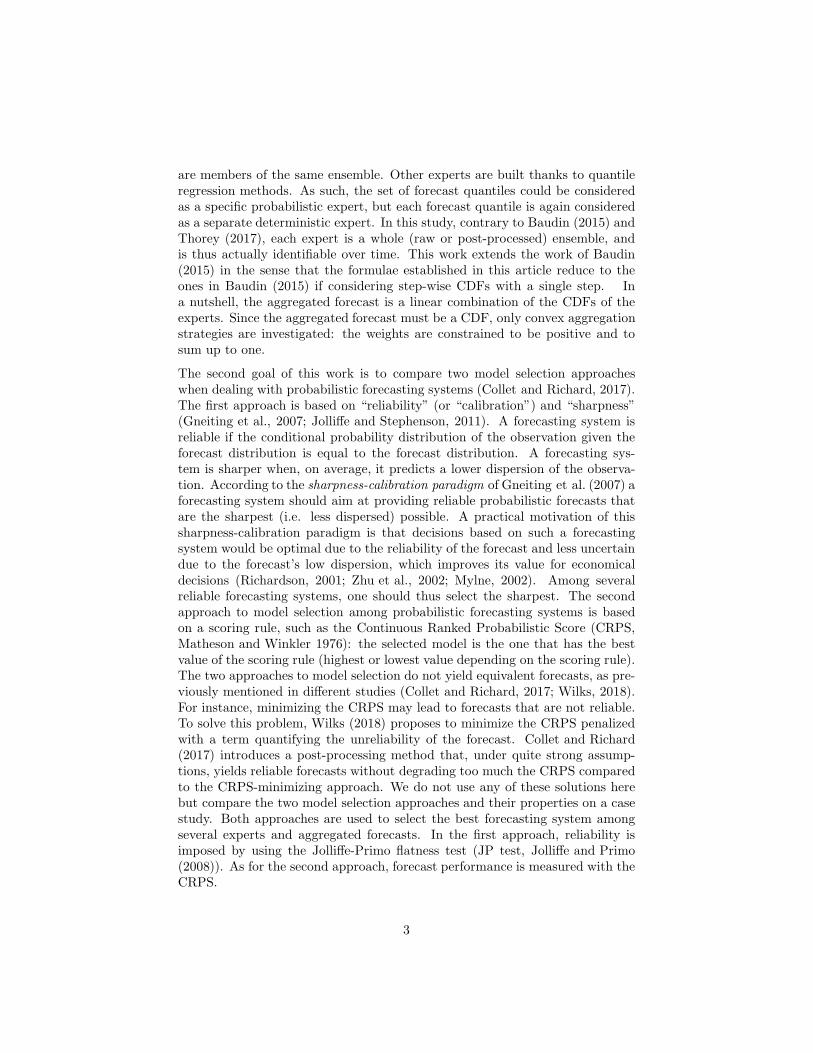
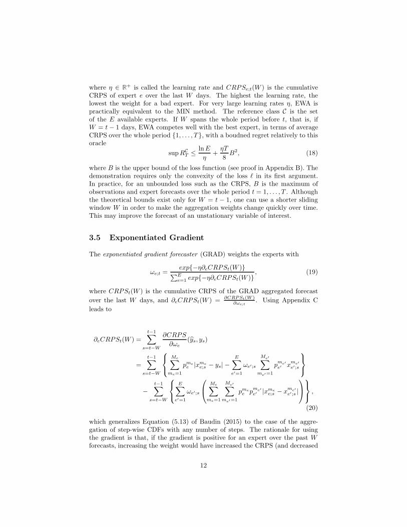
random variable Yt ∈ Y, whose computation is illustrated in Figure 1. Toproduce a valid step-wise CDF, the aggregation method must produce aggre-gation weights that are all non negative and sum up to 1 at fixed t. Thus, theaggregated forecast is a convex combination of the expert forecasts.

0.0

0.2

0.4

0.6

0.8

1.0

x

CD

F

xe=1m1=1 xe=1

m1=2 xe=2m2=1 xe=1

m1=3 xe=2m2=2 xe=2

m2=3

pe=1m1=1

pe=1m1=2

pe=1m1=3

pe=2m2=1

pe=2m2=2

pe=2m2=3

Figure 1 – Example of aggregation of E = 2 CDFs. The forecast CDFs (bluecontinuous line for expert e = 1, red dashed line for expert e = 2) are knownonly through a set of M1 = M2 = 3 values xme

e with associated jumps pme

e = 13 .

Following Equation (6), since x12 is greater than x1

1 and x21, it is the quantile of

order τ12;t = ω1;t(p11 + p21) + ω2;tp

12 = 2

3ω1;t +13ω2;t of yt. If ω1;t = ω2;t =

12 , then

τ12;t = 12 . In this case, the aggregated step-wise CDF is the black continuous

line.

7

2.2 Performance Assessment Tools

Among the several attributes of performance of probabilistic forecast systems,reliability and resolution are most useful (Murphy, 1993; Winkler et al., 1996).A probabilistic forecast system is reliable if the conditional distribution of the(random) observation Y given the forecast distribution F , noted [Y |F ], is equalto the forecast distribution: [Y |F ] = F . Resolution refers to the ability of theforecast system to issue forecast distributions very different from the marginaldistribution of the observations. If a forecast is reliable, decisions can then bemade by considering the observation will be drawn from the forecast distribu-tion. For a reliable forecasting system, the higher is its resolution, the moreuseful it is useful for economical decision taking (Richardson, 2001).

In order to compare the two approaches of probabilistic forecast selection, asstated in the Introduction, two tools are used: the Continuous Ranked Proba-bility Score which is a global measure of performance, and the rank histogramwhich is linked to reliability.

The Continuous Ranked Probability Score (CRPS, Matheson and Winkler 1976)is a scoring rule that quantifies the forecast performance of a probabilistic fore-casts expressed as a CDF F with a scalar observation y ∈ Y ⊆ R

ℓ(F, y) =

∫

x∈Y

(F (x)−H(x− y))2dx. (7)

The CRPS being convex in its first argument, the existence of theoretical boundsfor the regret is ensured for some aggregation methods by the theory of pre-diction with expert advice. Since the experts are step-wise CDFs with steps atxme

e;t , the information about the underlying forecast CDF F is incomplete, whichmakes some estimators of the CRPS biased, as investigated in Zamo and Naveau(2018). This last article shows that, in order to get an accurate estimate of theCRPS, one has to choose an estimator of the CRPS according to the nature ofthe xme

e;t (a sample from F or a set of quantiles from F ). This recommendationwas followed in this study. For a forecast CDF built as the empirical CDF of anM -random sample xi=1,...,M (such as a raw ensemble), the CRPS is estimatedwith

CRPSINT (M) =1

M

M∑

i=1

|xi − y| − 0.5

M2

M∑

i,j=1

|xi − xj | (8)

and for a forecast CDF defined from a set ofM quantiles xi=1,...,M with regularlyspaced orders (such as a post-processed ensemble), the following estimator isused

CRPSPWM (M) =1

M

M∑

i=1

|xi − y| − 0.5

M(M − 1)

M∑

i,j=1

|xi − xj | (9)

The expectation of the CRPS can be decomposed into three terms that quantifydifferent properties of a forecasting system or the observation distribution: the

8

reliability (RELI), the resolution (RES) and the uncertainty (UNC) terms:

EF,Y ℓ(F, Y ) = RELI −RES + UNC (10)

Let us note π = [Y ] the marginal distribution of the observation Y and πF =[Y |F ] the conditional distribution of the observation Y given the forecast dis-tribution F . Then the three terms are defined as in Brocker (2009) by

RELI = EF,Y∼πF

(ℓ(F, Y )− ℓ(πF , Y )

)(11)

RES = EF,Y∼πF

(ℓ(π, Y )− ℓ(πF , Y )

)(12)

UNC = EY∼πℓ(π, Y ) (13)

The reliability term is the average difference of CRPS between forecasts F

and πF when forecasting observations distributed according to πF . It is neg-atively oriented with a minimum of 0 for a perfectly reliable forecast system(πF = F ∀F ). The resolution term is the average difference of CRPS be-tween forecasts π and πF when forecasting observations distributed accordingto πF . It is positively oriented and the more F is different form π the higher itis. For a reliable forecast system, it is essentially equivalent to the sharpness.The uncertainty term is linked to the dispersion of the marginal distributionof the observation and does not depend on the forecast. Hersbach (2000) givesa method to estimate these terms from an ensemble forecast. Based on thisdecomposition, good CRPS can be obtained with a bad reliability (high RELI)provided that the resolution is good enough (high RES). By minimizing theCRPS as a forecast selection criterion, one may thus select a forecast systemthat has a low CRPS but is not reliable (Wilks, 2018). The solution proposedby Wilks (2018) is to minimize the CRPS modified with a penalty proportionalto the reliability term. Although this may indeed decrease the reliability term,there is no way to check if it is low enough.

Collet and Richard (2017) proposed a post-processing method that enforces thereliability of the forecast. To have a more general forecast selection method,it is proposed here to check that a forecasting system is reliable by testing thehypothesis that its rank histogram is flat. This procedure may be used as longas one can build a rank histogram from the forecast, which is generally thecase. The rank histogram of an ensemble forecast, simultaneously introducedby Anderson (1996), Hamill and Colucci (1996) and Talagrand et al. (1997), isthe histogram of the rank of the observation when it is pooled with its corre-sponding forecast members. For a reliable ensemble, the observation and themembers must have the same statistical properties, resulting in a flat rank his-togram. The type of deviation from flatness gives indications about the flaws ofan ensemble. For instance, an L-shape histogram means the forecasts are con-sistently too high, while a J-shape histogram indicates consistently too low fore-casts. A U-shape histogram reveals the forecast distribution is under-dispersedor conditionally biased. Hamill (2001) showed on synthetic data that a flat rankhistogram can be obtained for an unreliable ensemble. Producing a flat rank his-togram is thus a necessary but not sufficient condition for a forecasting system

9

to be reliable. Although the rank histogram was initially designed for ensembleforecasts, it can be used for forecasts in the form of quantiles. If the quantiles’ or-ders are regularly spaced between 0 and 1 (excluded), then the histogram shouldalso be flat if the forecasting system is reliable. The flatness of a rank histogramcan be statistically tested thanks to the Jolliffe-Primo tests of flatness describedin Jolliffe and Primo (2008) and summarized in Appendix A. These tests assessthe existence of some specific deviations from flatness in a rank histogram, suchas a slope, a convexity and a wave shape1. In this study we apply the threeflatness tests to each rank histogram at several locations where forecasts andobservations are available, which leads to a multiple testing procedure. In orderto take into account this multiple testing, the false discovery rate is controlledthanks to the Benjamini-Hochberg procedure (Benjamini and Hochberg, 1995;Benjamini and Yekutieli, 2001) with an alpha of 0.01. Brocker (2018) showedthat when the observation ranks are serially dependent, the JP tests should beadapted to take into account this temporal dependency. In this study, the lag-1autocorrelation of the rank has a median of 0.2 over all the studied locationsand lead times and is lower than 0.4 for most of the forecasting systems (raw,post-processed and aggregated alike). This correlation was judged low enoughso the modified procedure proposed by Brocker (2018) was not used.

3 Aggregation Methods

Five aggregation methods are introduced, from simple empirical ones to moresophisticated ones derived from the theory of prediction with expert advice.

3.1 Inverse CRPS Weighting

The inverse CRPS weighting method (INV) gives to each expert’s forecast aweight inversely proportional to its average CRPS over the last W days:

ωe;t =(CRPSe;t)

−1(W )∑E

e=1(CRPSe;t)−1(W )(14)

where CRPSe;t(W ) is the average CRPS of expert e during the W days beforetime t.

1The p-values of the Jolliffe-Primo test for slope and convexity have been computed basedon a modified version of the function TestRankhist in the R package SpecsVerification

(Siegert, 2015). The function has been modified to compute also the p-value for the Jolliffe-Primo test for a wave shape, introduced in this study.

10

3.2 Sharpness-Calibration Paradigm

The sharpness-calibration paradigm (SHARP) of Gneiting et al. (2007) can beused as an aggregation method to select at each time one expert. The ag-gregated forecast is the forecast of the expert whose range of the central 90%interval IQ90, averaged over the last W days is the lowest, among the expertswhose reliability term, as computed in Hersbach (2000), is lower than a chosenthreshold Relith over the last W days. The aggregated forecast gives an aggre-gation weight of 1 to the sharpest reliable expert’s forecast and of 0 to the otherexperts’ forecast:

ωe;t = 1

(e = argmin

e|Relie;t(W )<Relith

IQ90e;t(W )

), (15)

where Relie;t(W ) is the reliability term of expert e over the W days beforetime t, and IQ90e;t(W ) is the average range of the interval between quantilesof orders 0.95 and 0.05, forecasted by the expert e over the W days before timet. If no expert has a reliability term lower than the reliability threshold Relithover the last W days, the aggregated forecast is just the expert with the lowestmean CRPS over the last W days.

The three following methods are derived from the theory of prediction withexpert advice, and bounds for the regret may be computed.

3.3 Minimum CRPS

The minimum CRPS method (MIN) chooses the best recent expert in terms ofCRPS, that is, the aggregation weight is 1 for the expert with the lowest averageCRPS over the last W days, and 0 for all the other experts:

ωe;t = 1(e = e⋆t (W )), (16)

where e⋆t (W ) is the index of the expert with the minimum average CRPS duringthe last W days. The reference class C is the set of the E available experts, sothat the oracle for this method is the expert with the lowest CRPS averagedover the period 1, . . . , T , e⋆T (T ). This aggregation method is called “follow-the-best-expert” in Cesa-Bianchi et al. (2006), who prove that, under severalassumptions on the loss, the regret of the aggregated forecast relatively to theoracle is o(ln(T )).

3.4 Exponential Weighting

The exponentially weighted average forecaster (EWA) computes the aggregationweights as

ωe;t =exp−ηCRPSe;t(W )

∑Ee=1 exp−ηCRPSe;t(W )

, (17)

11

where η ∈ R+ is called the learning rate and CRPSe;t(W ) is the cumulative

CRPS of expert e over the last W days. The highest the learning rate, thelowest the weight for a bad expert. For very large learning rates η, EWA ispractically equivalent to the MIN method. The reference class C is the setof the E available experts. If W spans the whole period before t, that is, ifW = t− 1 days, EWA competes well with the best expert, in terms of averageCRPS over the whole period 1, . . . , T , with a boudned regret relatively to thisoracle

supRCT ≤ lnE

η+

ηT

8B2, (18)

where B is the upper bound of the loss function (see proof in Appendix B). Thedemonstration requires only the convexity of the loss ℓ in its first argument.In practice, for an unbounded loss such as the CRPS, B is the maximum ofobservations and expert forecasts over the whole period t = 1, . . . , T . Althoughthe theoretical bounds exist only for W = t − 1, one can use a shorter slidingwindow W in order to make the aggregation weights change quickly over time.This may improve the forecast of an unstationary variable of interest.

3.5 Exponentiated Gradient

The exponentiated gradient forecaster (GRAD) weights the experts with

ωe;t =exp−η∂eCRPSt(W )

∑Ee=1 exp−η∂eCRPSt(W )

, (19)

where CRPSt(W ) is the cumulative CRPS of the GRAD aggregated forecast

over the last W days, and ∂eCRPSt(W ) = ∂CRPSt(W )∂ωe;t

. Using Appendix C

leads to

∂eCRPSt(W ) =

t−1∑

s=t−W

∂CRPS

∂ωe

(ys, ys)

=

t−1∑

s=t−W

Me∑

me=1

pme

e |xme

e;s − ys| −E∑

e′=1

ωe′;s

Me′∑

me′=1

pm

e′

e′ xm

e′

e′;s

−t−1∑

s=t−W

E∑

e′=1

ωe′;s

Me∑

me=1

Me′∑

me′=1

pme

e pm

e′

e′ |xme

e;s − xm

e′

e′ ;s |

,

(20)

which generalizes Equation (5.13) of Baudin (2015) to the case of the aggre-gation of step-wise CDFs with any number of steps. The rationale for usingthe gradient is that, if the gradient is positive for an expert over the past W

forecasts, increasing the weight would have increased the CRPS (and decreased

12

the performance) of the aggregated forecast. So for incoming forecasts, givingthis expert a low weight should improve the forecast performance. The reverseis true for a negative gradient.

For this aggregation method, the reference class C is the set of convex combina-tions with constant weights over the whole period 1, . . . , T , that is, such thatωe;t = ωe, ∀e ∈ 1, . . . , E and t ∈ 1, . . . , T . The oracle is the best, in termsof cumulative CRPS, constant convex combination of experts. This is usuallya better oracle than the best expert. If W = t − 1 days, the following boundimmediately follows from Mallet et al. (2007) or Baudin (2015)

supRCT ≤ lnE

η+

ηT

2C2, (21)

where C = maxt∈1,...,T,e∈1,...,E|∂CRPS∂ωe

(yt, yt)|. Although the oracle forGRAD is better than for EWA, the bounds may be larger, so that EWA mayactually perform better than GRAD. In practice, one has to try both methodsto know which one performs best.

4 The Experts and the Observation

In this work, aggregation is applied to ensemble forecasts of the 10 m wind speedover France. Forecasting surface wind is quite difficult due to complex inter-actions between phenomena at different spatio-temporal scales. For instance,wind speed is influenced by large scale atmospheric structures such as cyclonesand anticyclones, but also by local orography and surface friction. Local atmo-spheric effects such as downward drifts under convective clouds also contributeto the direction and speed of wind. National weather services need to haveskillful wind speed forecasts to issue early warnings to the population and civilsecurity services. Also, wind speed influences many economic activities, suchas sailing, windpower generation, construction,... that need good forecasts fordecision making.

This section presents the 28 experts used in this study and the wind speedobservation used to assess the forecasts.

4.1 The Four Experts based on TIGGE

The International Grand Global Ensemble, formerly the THORPEX Interac-tive Grand Global Ensemble (TIGGE), was an international project aiming,among other things, to provide ensemble prediction data from leading opera-tional forecast centers (Bougeault et al., 2010; Swinbank et al., 2016). Although

13

the TIGGE data set2 includes 10 ensemble NWP models, only the four ensem-ble models available on a daily basis at Meteo-France have been retained (seeTable 1) as experts, so that the aggregation methods may later be used inoperations at Meteo-France.

The TIGGE ensembles are available on a grid size is 0.5. Over France thisamounts to a total of 267 grid points. The study period goes from the 1st

January, 2011 to the 31st December, 2014 (so T = 1461 in the notations ofSection 2). The lead times go from 6 h to 54 h depending on the ensemble, witha timestep of 6 h. The forecast are done at 1800 UTC for lead times h from 6 hto 48 h, with a time step of 6 h. This implies that for experts based on CMCand ECMWF, whose runtime is 1200 UTC, the actual lead time is h + 6 (seeTable 1).

Each ensemble is an expert whose forecast CDF Fe;t is the empirical CDF of themembers associated with the same weight pme

e = 1M, where M is the number of

members in the ensemble.

Table 1 – Ensembles from TIGGE used in this study, with some of their char-acteristics.

Weather service Members Hour of the run used (UTC) Lead times

Canadian Meteorological Center(CMC)

21 1200 12h to 54h

European Center for Medium-RangeWeather Forecasts (ECMWF)

51 1200 12h to 54h

Meteo-France (MF) 35 1800 6h to 48hUS National Centers for Environmen-tal Prediction (NCEP)

21 1800 6h to 48h

4.2 The Twenty Four Experts built with EMOS Methods

Each ensemble is post-processed with two kinds of EMOS: non-homogeneousregression (NR, Gneiting et al. 2005, Hemri et al. 2014) and quantile randomforest (QRF, Meinshausen 2006, Zamo et al. 2014, Taillardat et al. 2016).

The forecast CDF produced with NR is parametric. Following Hemri et al.(2014), the square root of the forecast wind speed ft is supposed to follow anormal distribution truncated at 0

√ft ∼ N 0(a+ bxt, c

2 + d2sdt) (22)

where xt and sdt are the mean and standard deviation of the square-root of theassociated ensemble values, forecasted at time t. The four paremeters (a, b, cand d) are optimized by maximizing the log-likelihood3 over the last Wtr fore-

2The TIGGE data set can be retrieved from the ECMWF athttp://apps.ecmwf.int/datasets or from the Chinese Meteorological Administration athttp://wisportal.cma.gov.cn/wis/

3With the function optim in R (R Core Team, 2015).

14

cast days. In order to build several NR-post-processed ensembles with differentreaction time to the raw ensemble’s performance changes, five sizes of the train-ing window Wtr are used, as summarized in Table 2. These parametric CDFscan not be used as such in the framework of step-wise CDF aggregation. A step-wise ye;t is built from the squared quantiles of orders 0, 1

100 , . . . ,99100 , 0.999 of

the parametric CDF produced by NR. The last order is not 1 in order to avoidinfinite values.

QRF is a non parametric machine learning method that produces a set of quan-tiles of chosen order. A random forest is a set of regression trees built on abootstrapped version of the training data (Zamo et al., 2016). While buildingeach tree, the observations are split in two most homogeneous groups (in termsof variance of the observation), according to a splitting criterion over an explana-tory variable. At each split (or node) only a random subset of the complete setof explanatory variables are tested, until a stopping criterion is reached (such asa maximum number of final nodes, called leaves). When a forecast is required, astep-wise CDF is produced by going down the forest with the vector of explana-tory variables, computing the step-wise CDF of the observations associated toeach leaf and averaging those CDFs. In practice, one requests a set of quantileorders and gets the corresponding quantiles4. The requested quantile orders arethe same as for NR, except the last order which is 1, because QRF cannot pro-duce infinite values. Since the forecast CDF is a step-wise function, the obtainedquantiles may contain many ties, that are suppressed by linearily interpolatingbetween the points defining the CDF’s steps, as explained in Zamo and Naveau(2018).

The post-processing and aggregation methods are trained separately for each ofthe eight lead times and each grid point. Since NR is a parametric method withonly four parameters, it can be trained with few data, thus a sliding-windowtraining period is used. QRF, being a non parametric method, requires moretraining data to define the many splits in each tree. It is thus trained with 4-foldcross-validation: each year is successively used as a test sample, the reminaingthree being used as the training sample.

From each of the four ensembles seven experts are built: the raw ensemble,the QRF-post-processed ensemble and five NR-post-processed versions of theensemble (each with a different size of the training window, Table 2). Altogether,28 experts are aggregated.

4.3 The Observation

The observation is the 10 m average wind speed analysis built in Zamo et al.(2016), at 267 grid points over France. Those grid points are the same as theensemble datasets presented in Section 4.1.

4In the R packages quantregForest or ranger.

15

Table 2 – Summary description of the EMOS methods used to post-process eachensembe.

Quantile Regression Forest (QRF)

Forecast distribution Non-parametric (set of quantiles).Explanatory variables Control member, ensemble mean, ensemble 0.1 and

0.9 quantiles, month.Training method 4-fold cross-validation (3 training years, 1 test year).Orders of the forecastquantiles

0, 1100 , . . . ,

99100 , 1.

Non-homogeneous Regression (NR)

Forecast distribution Parametric (truncated normal distribution for thesquare-root of wind speed).

Explanatory variables Mean and standard deviation of the raw ensemble.Training method Likelihood maximization on a sliding window over

the Wtr previous days. Five windows are used:Wtr = 7, 30, 90, 365, t− 1 days

Orders of the forecastquantiles

0, 1100 , . . . ,

99100 , 0.999.

5 Results

The five aggregation methods presented in Section 3 have been investigated,with different values of the tuning parametersW and η. The values of the tuningparameters tested in the study are listed in Table 3. When two parameters arelisted, all combinations have been tried.

Table 3 – Sets of tried values for the parameters of the aggregation methods.When two parameters are given, all the possible combinations of values havebeen tried.

Aggregation method Parameters’ values

Minimum CRPS or InverseCRPS

W = 7, 15, 30, 90, 365, t− 1 days

Sharpness-calibration W = 7, 15, 30, 90, 365, t − 1 days,Relith = 0.1 m/s

Exponentiated weighting or Ex-ponentiated gradient weighting

W = 7, 15, 30, 90, 365, t − 1 days, η =10−1.5, 10−1, 10−0.5, 1, 100.5, 101.5, 102

Hereafter the best expert and the best aggregation method is selected followingthe two approaches mentioned above: the minimization of the average CRPSor the maximization of the proportion of grid points with a rank histogramdeemed flat by the three flatness tests. The best forecasting system in terms of

16

minimum CRPS is called the most skillful. The forecasting system which getsthe maximum proportion of grid points with a flat rank histogram is called themost reliable.

5.1 CRPS and Reliability

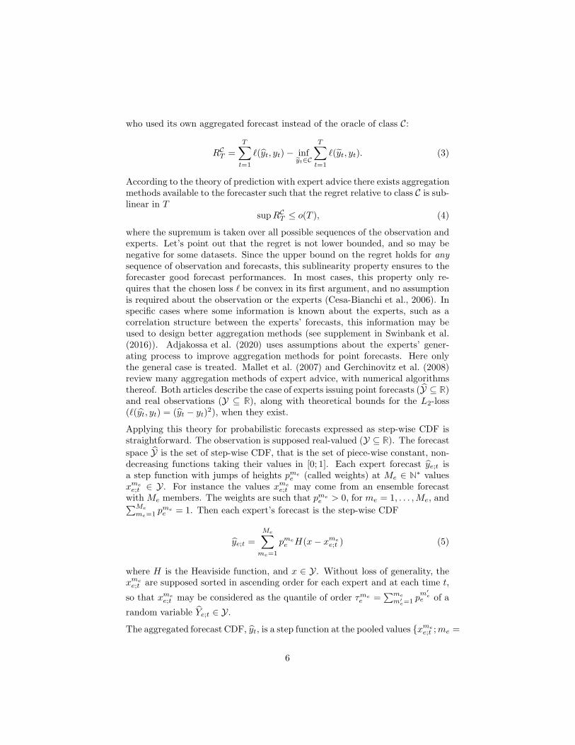
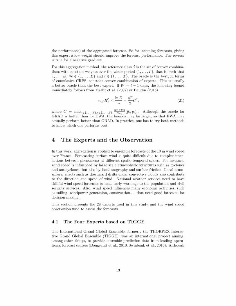
From Table 4, the most skillful expert is the QRF-post-processed ECMWFensemble (it is an oracle). The time series of the regret of each most skillful orreliable aggregation method of each type relatively to the QRF-post-processedECMWF ensemble is drawn in Figure 2, for lead time 24 h. Whereas the mostskillful setting of the SHARP aggregation method gets a consistently higherCRPS than the most skillful expert, the other aggregation methods manageto outperform the latter at least for some part of the four years. The mostskillful settings of EWA and GRAD even get a negative regret relatively to themost skillful expert. The regret exhibits a trend and a diurnal cycle with thelead times (not shown), and so does the averaged CRPS (see Table 4): theforecast performance decreases with increasing lead times, particularly duringthe late afternoon when the wind strengthens. The main point is that, interms of CRPS, post-processing improves performance, and aggregation furtherimproves performance. According to the minimization of the CRPS, the chosenforecast method would be the most skillful GRAD setting, that is log10(η) = −1and W = t− 1 days.

Lead time: 24 h

Valid date

Cum

ulat

ed a

vera

ge r

egre

t (m

/s)

0

50

100

2012 2013 2014

SHARP

2012 2013 2014

EWA

2012 2013 2014

GRAD

2012 2013 2014

INV

2012 2013 2014

MIN

skillful reliable

Figure 2 – Time series of the cumulative spatially-averaged regret, at lead time24 h, for each aggregation method, relatively to the most skillful expert (QRF-post-processed ECMWF ensemble). At each valid date, the regret relatively tothe QRF-post-processed ECMWF ensemble is averaged over the 267 grid-points.For each aggregation method, two settings are used to compute the regret: themost skillful one (blue continuous line) and the most reliable one (pink dashedline).

If one uses the flatness of rank histograms as the selection criterion, the bestraw ensemble is CMC, the best expert is QRF-post-processed MF and the best

17

Table 4 – CRPS averaged over the four years and the 267 grid points for sev-eral forecasting systems. The average CRPS of the most skillful raw ensemble(ECMWF) is indicated in the first line. Then, for each model selection ap-proach, the best expert is indicated followed by the best setting of each aggre-gation method. For each selection approach, the forecasting system with thelowest CRPS is in bold.

Method Parameters Lead time (h)log10(η) W all 6 12 18 24 30 36 42 48

RAWECMWF

0.76 0.79 0.79 0.73 0.73 0.78 0.78 0.73 0.74

Selection: most skillful forecasting system.expert(QRFECMWF)

0.49 0.47 0.46 0.48 0.50 0.49 0.49 0.52 0.53

SHARP 1095 0.55 0.52 0.52 0.55 0.56 0.55 0.55 0.59 0.60GRAD -1 t-1 0.47 0.44 0.44 0.46 0.47 0.47 0.47 0.51 0.51

EWA -1 365 0.48 0.44 0.44 0.47 0.48 0.47 0.48 0.52 0.52INV 7 0.49 0.46 0.46 0.47 0.48 0.49 0.49 0.52 0.52MIN 365 0.51 0.47 0.47 0.51 0.52 0.50 0.51 0.56 0.56

Selection: most reliable forecasting system.expert(QRFMF)

0.50 0.46 0.47 0.51 0.50 0.49 0.50 0.55 0.53

SHARP 1095 0.55 0.52 0.52 0.55 0.56 0.55 0.55 0.59 0.60GRAD 0.5 t-1 0.50 0.46 0.46 0.50 0.50 0.49 0.50 0.54 0.54EWA 0.5 30 0.50 0.46 0.46 0.50 0.50 0.50 0.50 0.55 0.54INV 7 0.49 0.46 0.46 0.47 0.48 0.49 0.49 0.52 0.52

MIN 365 0.51 0.47 0.47 0.51 0.52 0.50 0.51 0.56 0.56

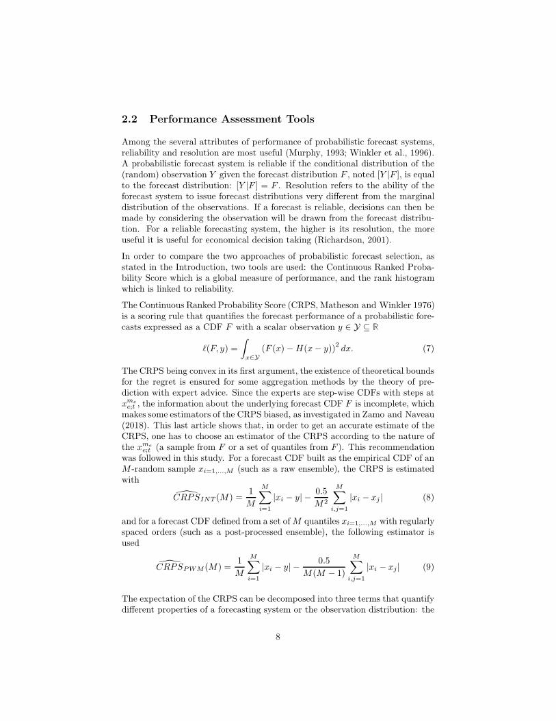
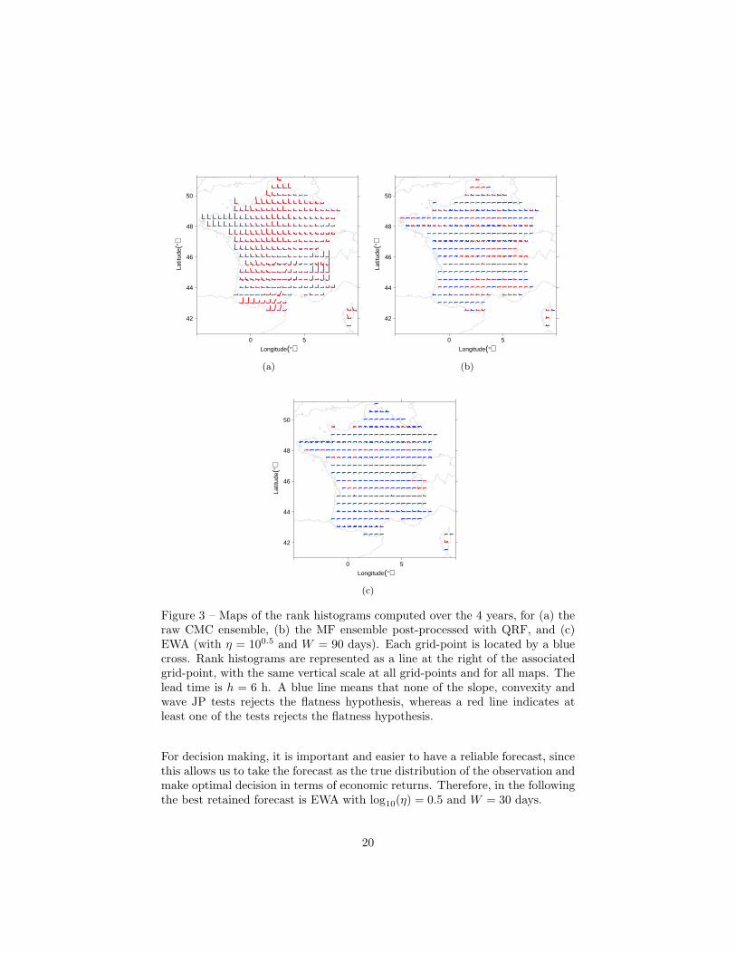
aggregated forecast is EWA with log10(η) = 0.5 and W = 30 days (see Table 5).Raw CMC is not a very reliable ensemble, as shown in Figure 3 (a) for leadtime h = 6 h: the ensemble is consistently biased with too strong forecastwind speeds in the north-west of France and too weak forecast wind speedsover the Alps and the Pyrenees. Elsewhere, although the ensemble is muchless biased, the rank histogram is not deemed flat due to an obvious U-shape.The rank histograms at the other lead times and for the other raw ensemblesexhibit similar features (not shown). For the most reliable expert and aggregatedforecasts, the rank histograms are computed with the nine forecast deciles. Asillustrated in Figure 3 (b), the QRF-post-processed version of the MF ensembleyields a higher number of flat rank histograms than the raw CMC ensemble.Finally, Figure 3 (c) shows that, the JP tests do not reject the flatness hypothesisat many more grid-points for the most reliable EWA forecast. Table 5 confirmsquantitatively that the most reliable EWA outperforms the most reliable expertin terms of flatness of the rank histogram, at each lead time.The most reliable

18

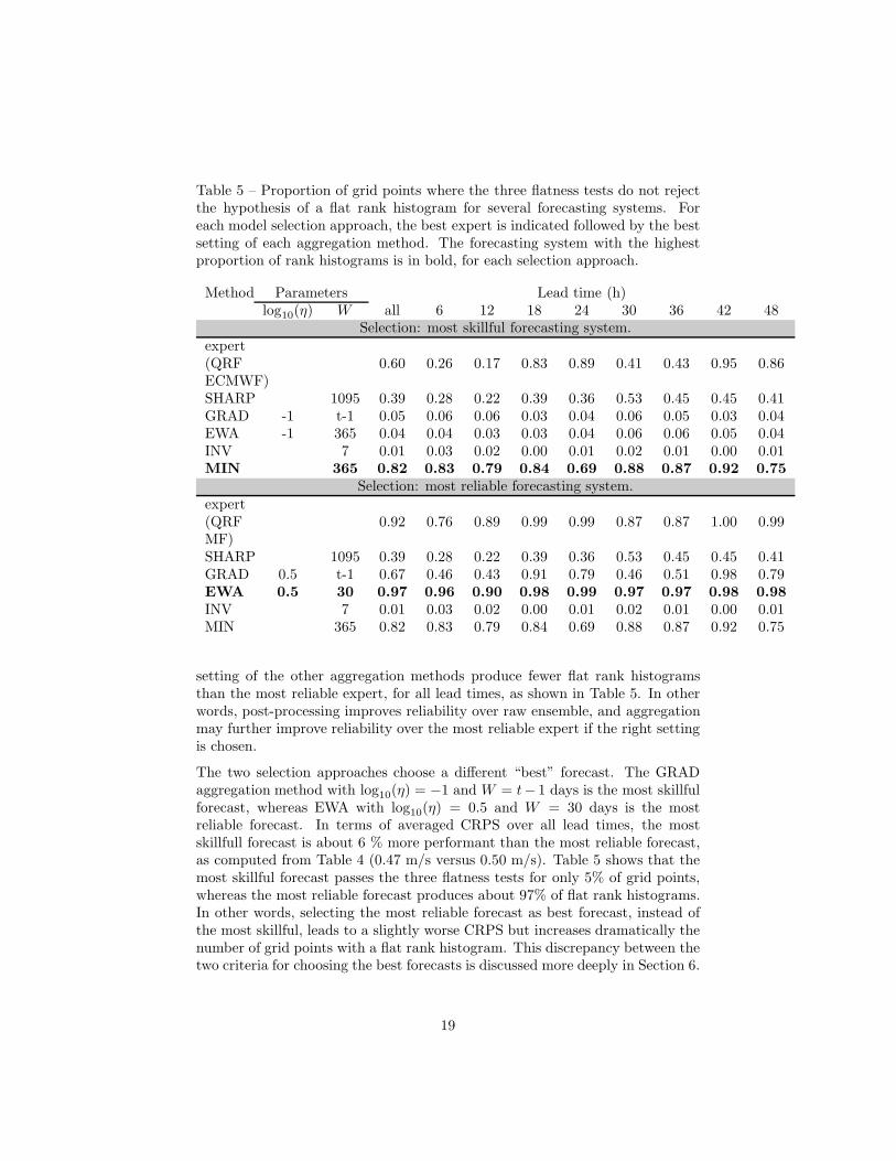
Table 5 – Proportion of grid points where the three flatness tests do not rejectthe hypothesis of a flat rank histogram for several forecasting systems. Foreach model selection approach, the best expert is indicated followed by the bestsetting of each aggregation method. The forecasting system with the highestproportion of rank histograms is in bold, for each selection approach.

Method Parameters Lead time (h)log10(η) W all 6 12 18 24 30 36 42 48

Selection: most skillful forecasting system.expert(QRFECMWF)

0.60 0.26 0.17 0.83 0.89 0.41 0.43 0.95 0.86

SHARP 1095 0.39 0.28 0.22 0.39 0.36 0.53 0.45 0.45 0.41GRAD -1 t-1 0.05 0.06 0.06 0.03 0.04 0.06 0.05 0.03 0.04EWA -1 365 0.04 0.04 0.03 0.03 0.04 0.06 0.06 0.05 0.04INV 7 0.01 0.03 0.02 0.00 0.01 0.02 0.01 0.00 0.01MIN 365 0.82 0.83 0.79 0.84 0.69 0.88 0.87 0.92 0.75

Selection: most reliable forecasting system.expert(QRFMF)

0.92 0.76 0.89 0.99 0.99 0.87 0.87 1.00 0.99

SHARP 1095 0.39 0.28 0.22 0.39 0.36 0.53 0.45 0.45 0.41GRAD 0.5 t-1 0.67 0.46 0.43 0.91 0.79 0.46 0.51 0.98 0.79EWA 0.5 30 0.97 0.96 0.90 0.98 0.99 0.97 0.97 0.98 0.98

INV 7 0.01 0.03 0.02 0.00 0.01 0.02 0.01 0.00 0.01MIN 365 0.82 0.83 0.79 0.84 0.69 0.88 0.87 0.92 0.75

setting of the other aggregation methods produce fewer flat rank histogramsthan the most reliable expert, for all lead times, as shown in Table 5. In otherwords, post-processing improves reliability over raw ensemble, and aggregationmay further improve reliability over the most reliable expert if the right settingis chosen.

The two selection approaches choose a different “best” forecast. The GRADaggregation method with log10(η) = −1 and W = t− 1 days is the most skillfulforecast, whereas EWA with log10(η) = 0.5 and W = 30 days is the mostreliable forecast. In terms of averaged CRPS over all lead times, the mostskillfull forecast is about 6 % more performant than the most reliable forecast,as computed from Table 4 (0.47 m/s versus 0.50 m/s). Table 5 shows that themost skillful forecast passes the three flatness tests for only 5% of grid points,whereas the most reliable forecast produces about 97% of flat rank histograms.In other words, selecting the most reliable forecast as best forecast, instead ofthe most skillful, leads to a slightly worse CRPS but increases dramatically thenumber of grid points with a flat rank histogram. This discrepancy between thetwo criteria for choosing the best forecasts is discussed more deeply in Section 6.

19

Longitude(°)

Latit

ude(

°)

42

44

46

48

50

0 5

+ +

+ +

+ +

+ +

+ +

+ +

+ +

+ +

+ +

+ +

+ +

+ +

+

+ +

+

+

+

+

+

+

+

+

+

+

+

+

+

+

+ +

+

+

+

+

+

+ +

+

+ +

+ +

+ +

+ +

+ +

+ +

+

+ +

+ +

+ +

+ +

+

+ +

+ +

+ +

+ +

+ +

+ +

+ +

+

+ +

+

+

+

+

+

+

+

+

+

+

+

+ +

+ +

+

+

+

+

+

+

+

+

+

+

+

+

+

+

+ +

+

+ +

+ +

+

+

+

+

+

+

+

+

+

+

+

+

+

+ +

+ +

+

+

+

+

+

+

+

+

+

+

+

+

+

+

+

+ +

+ +

+

+

+

+

+

+

+

+

+

+

+

+

+ +

+

+

+

+

+

+

+

+

+

+

+

+

+ +

+ +

+

+

+

+

+

+

+

+

+

+

+

+

+

+

+

+

+

+

+

+

+

+

+

+

+

+

+

+

+

+

+

+

+

+

+

+

+

+

+

+

+

+

+

+

+

+

+

+

+

+

+

+

+

+

+

+

+

+

+

+

+

+

+

+

+

+

+

+

+

+ +

+

+

+

+

(a)

Longitude(°)

Latit

ude(

°)

42

44

46

48

50

0 5

+ +

+ +

+ +

+ +

+ +

+ +

+ +

+ +

+ +

+ +

+ +

+ +

+

+ +

+

+

+

+

+

+

+

+

+

+

+

+

+

+

+ +

+

+

+

+

+

+ +

+

+ +

+ +

+ +

+ +

+ +

+ +

+

+ +

+ +

+ +

+ +

+

+ +

+ +

+ +

+ +

+ +

+ +

+ +

+

+ +

+

+

+

+

+

+

+

+

+

+

+

+ +

+ +

+

+

+

+

+

+

+

+

+

+

+

+

+

+

+ +

+

+ +

+ +

+

+

+

+

+

+

+

+

+

+

+

+

+

+ +

+ +

+

+

+

+

+

+

+

+

+

+

+

+

+

+

+

+ +

+ +

+

+

+

+

+

+

+

+

+

+

+

+

+ +

+

+

+

+

+

+

+

+

+

+

+

+

+ +

+ +

+

+

+

+

+

+

+

+

+

+

+

+

+

+

+

+

+

+

+

+

+

+

+

+

+

+

+

+

+

+

+

+

+

+

+

+

+

+

+

+

+

+

+

+

+

+

+

+

+

+

+

+

+

+

+

+

+

+

+

+

+

+

+

+

+

+

+

+

+

+ +

+

+

+

+

(b)

Longitude(°)

Latit

ude(

°)

42

44

46

48

50

0 5

+ +

+ +

+ +

+ +

+ +

+ +

+ +

+ +

+ +

+ +

+ +

+ +

+

+ +

+

+

+

+

+

+

+

+

+

+

+

+

+

+

+ +

+

+

+

+

+

+ +

+

+ +

+ +

+ +

+ +

+ +

+ +

+

+ +

+ +

+ +

+ +

+

+ +

+ +

+ +

+ +

+ +

+ +

+ +

+

+ +

+

+

+

+

+

+

+

+

+

+

+

+ +

+ +

+

+

+

+

+

+

+

+

+

+

+

+

+

+

+ +

+

+ +

+ +

+

+

+

+

+

+

+

+

+

+

+

+

+

+ +

+ +

+

+

+

+

+

+

+

+

+

+

+

+

+

+

+

+ +

+ +

+

+

+

+

+

+

+

+

+

+

+

+

+ +

+

+

+

+

+

+

+

+

+

+

+

+

+ +

+ +

+

+

+

+

+

+

+

+

+

+

+

+

+

+

+

+

+

+

+

+

+

+

+

+

+

+

+

+

+

+

+

+

+

+

+

+

+

+

+

+

+

+

+

+

+

+

+

+

+

+

+

+

+

+

+

+

+

+

+

+

+

+

+

+

+

+

+

+

+

+ +

+

+

+

+

(c)

Figure 3 – Maps of the rank histograms computed over the 4 years, for (a) theraw CMC ensemble, (b) the MF ensemble post-processed with QRF, and (c)EWA (with η = 100.5 and W = 90 days). Each grid-point is located by a bluecross. Rank histograms are represented as a line at the right of the associatedgrid-point, with the same vertical scale at all grid-points and for all maps. Thelead time is h = 6 h. A blue line means that none of the slope, convexity andwave JP tests rejects the flatness hypothesis, whereas a red line indicates atleast one of the tests rejects the flatness hypothesis.

For decision making, it is important and easier to have a reliable forecast, sincethis allows us to take the forecast as the true distribution of the observation andmake optimal decision in terms of economic returns. Therefore, in the followingthe best retained forecast is EWA with log10(η) = 0.5 and W = 30 days.

20

5.2 Temporal Variation of the Weights

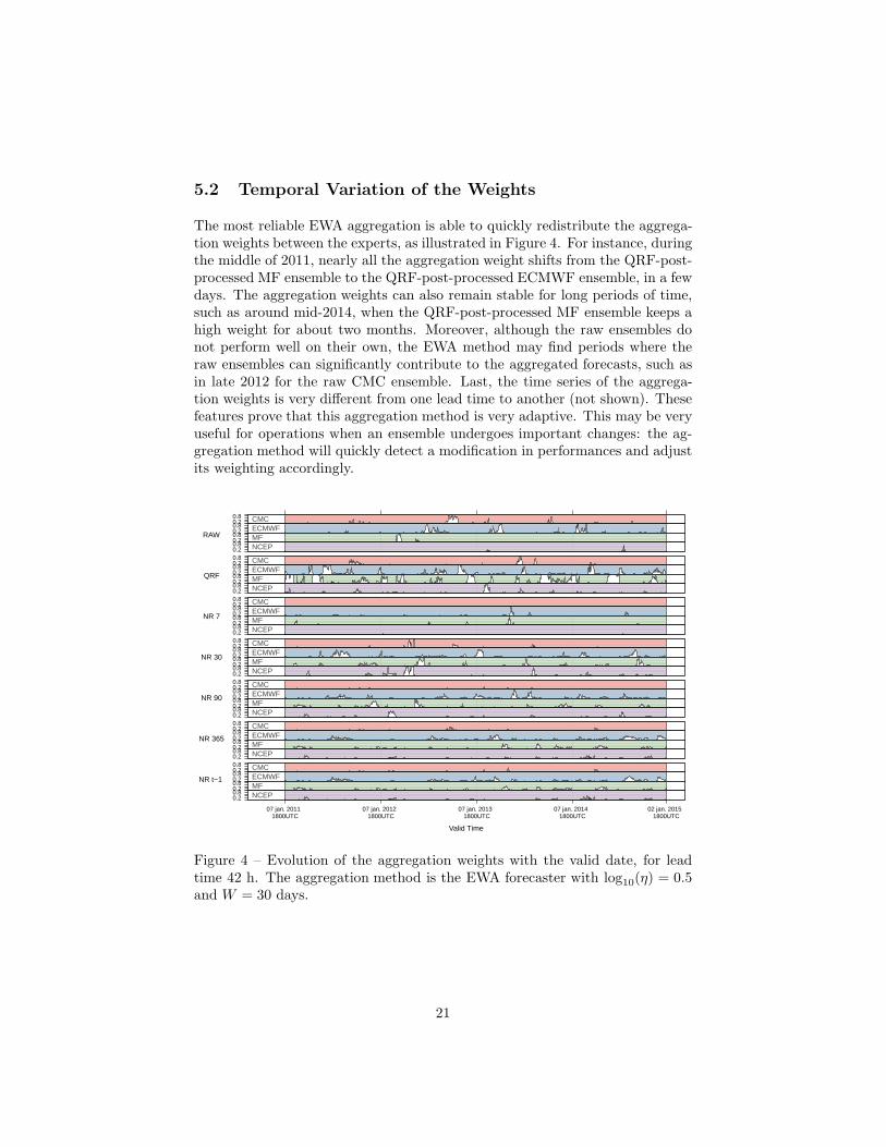
The most reliable EWA aggregation is able to quickly redistribute the aggrega-tion weights between the experts, as illustrated in Figure 4. For instance, duringthe middle of 2011, nearly all the aggregation weight shifts from the QRF-post-processed MF ensemble to the QRF-post-processed ECMWF ensemble, in a fewdays. The aggregation weights can also remain stable for long periods of time,such as around mid-2014, when the QRF-post-processed MF ensemble keeps ahigh weight for about two months. Moreover, although the raw ensembles donot perform well on their own, the EWA method may find periods where theraw ensembles can significantly contribute to the aggregated forecasts, such asin late 2012 for the raw CMC ensemble. Last, the time series of the aggrega-tion weights is very different from one lead time to another (not shown). Thesefeatures prove that this aggregation method is very adaptive. This may be veryuseful for operations when an ensemble undergoes important changes: the ag-gregation method will quickly detect a modification in performances and adjustits weighting accordingly.

Valid Time

NR t−1

NR 365

NR 90

NR 30

NR 7

QRF

RAW

0.20.8 CMC

0.20.8 ECMWF

0.20.8 MF

0.20.8 NCEP

0.20.8 CMC

0.20.8 ECMWF

0.20.8 MF

0.20.8 NCEP

0.20.8 CMC

0.20.8 ECMWF

0.20.8 MF

0.20.8 NCEP

0.20.8 CMC

0.20.8 ECMWF

0.20.8 MF

0.20.8 NCEP

0.20.8 CMC

0.20.8 ECMWF

0.20.8 MF

0.20.8 NCEP

0.20.8 CMC

0.20.8 ECMWF

0.20.8 MF

0.20.8 NCEP

0.20.8 CMC

0.20.8 ECMWF

0.20.8 MF

0.20.8

07 jan. 20111800UTC

07 jan. 20121800UTC

07 jan. 20131800UTC

07 jan. 20141800UTC

02 jan. 20151800UTC

NCEP

Figure 4 – Evolution of the aggregation weights with the valid date, for leadtime 42 h. The aggregation method is the EWA forecaster with log10(η) = 0.5and W = 30 days.

21

5.3 Aggregation of individual sorted experts

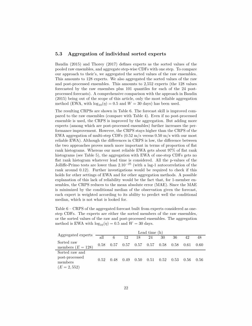
Baudin (2015) and Thorey (2017) defines experts as the sorted values of thepooled raw ensembles, and aggregate step-wise CDFs with one step. To compareour approach to their’s, we aggregated the sorted values of the raw ensembles.This amounts to 128 experts. We also aggregated the sorted values of the rawand post-processed ensembles. This amounts to 2,552 experts (the 128 valuesforecasted by the raw ensembes plus 101 quantiles for each of the 24 post-processed forecasts). A comprehensive comparison with the approach in Baudin(2015) being out of the scope of this article, only the most reliable aggregationmethod (EWA, with log10(η) = 0.5 and W = 30 days) has been used.

The resulting CRPSs are shown in Table 6. The forecast skill is improved com-pared to the raw ensembles (compare with Table 4). Even if no post-processedensemble is used, the CRPS is improved by the aggregation. But adding moreexperts (among which are post-processed ensembles) further increases the per-formance improvement. However, the CRPS stays higher than the CRPS of theEWA aggregation of multi-step CDFs (0.52 m/s versus 0.50 m/s with our mostreliable EWA). Although the differences in CRPS is low, the difference betweenthe two approaches proves much more important in terms of proportion of flatrank histograms. Whereas our most reliable EWA gets about 97% of flat rankhistograms (see Table 5), the aggregation with EWA of one-step CDFs gets noflat rank histogram whatever lead time is considered. All the p-values of theJolliffe-Primo tests are lower than 2.10−25 (with a lag-1 autocorrelation of therank around 0.12). Further investigations would be required to check if thisholds for other settings of EWA and for other aggregation methods. A possibleexplanation of this lack of reliability would be the fact that, for 1-member en-sembles, the CRPS reduces to the mean absolute error (MAE). Since the MAEis minimized by the conditional median of the observation given the forecast,each expert is weighted according to its ability to predict well the conditionalmedian, which is not what is looked for.

Table 6 – CRPS of the aggregated forecast built from experts considered as one-step CDFs. The experts are either the sorted members of the raw ensembles,or the sorted values of the raw and post-processed ensembles. The aggregationmethod is EWA with log10(η) = 0.5 and W = 30 days.

Aggregated expertsLead time (h)

all 6 12 18 24 30 36 42 48Sorted rawmembers (E = 128)

0.58 0.57 0.57 0.57 0.57 0.58 0.58 0.61 0.60

Sorted raw andpost-processedmembers(E = 2, 552)

0.52 0.48 0.49 0.50 0.51 0.52 0.53 0.56 0.56

22

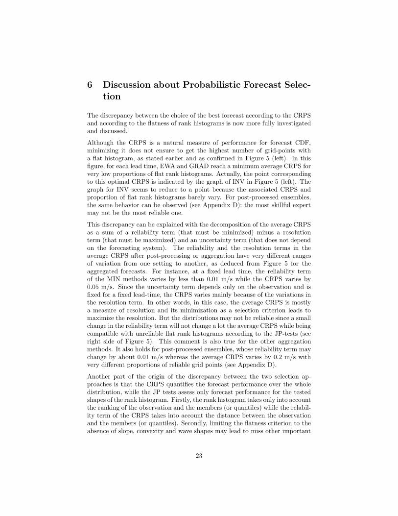
6 Discussion about Probabilistic Forecast Selec-

tion

The discrepancy between the choice of the best forecast according to the CRPSand according to the flatness of rank histograms is now more fully investigatedand discussed.

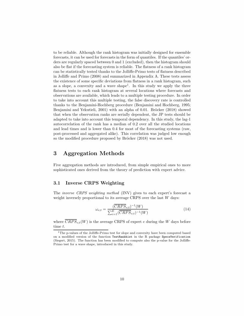
Although the CRPS is a natural measure of performance for forecast CDF,minimizing it does not ensure to get the highest number of grid-points witha flat histogram, as stated earlier and as confirmed in Figure 5 (left). In thisfigure, for each lead time, EWA and GRAD reach a minimum average CRPS forvery low proportions of flat rank histograms. Actually, the point correspondingto this optimal CRPS is indicated by the graph of INV in Figure 5 (left). Thegraph for INV seems to reduce to a point because the associated CRPS andproportion of flat rank histograms barely vary. For post-processed ensembles,the same behavior can be observed (see Appendix D): the most skillful expertmay not be the most reliable one.

This discrepancy can be explained with the decomposition of the average CRPSas a sum of a reliability term (that must be minimized) minus a resolutionterm (that must be maximized) and an uncertainty term (that does not dependon the forecasting system). The reliability and the resolution terms in theaverage CRPS after post-processing or aggregation have very different rangesof variation from one setting to another, as deduced from Figure 5 for theaggregated forecasts. For instance, at a fixed lead time, the reliability termof the MIN methods varies by less than 0.01 m/s while the CRPS varies by0.05 m/s. Since the uncertainty term depends only on the observation and isfixed for a fixed lead-time, the CRPS varies mainly because of the variations inthe resolution term. In other words, in this case, the average CRPS is mostlya measure of resolution and its minimization as a selection criterion leads tomaximize the resolution. But the distributions may not be reliable since a smallchange in the reliability term will not change a lot the average CRPS while beingcompatible with unreliable flat rank histograms according to the JP-tests (seeright side of Figure 5). This comment is also true for the other aggregationmethods. It also holds for post-processed ensembles, whose reliability term maychange by about 0.01 m/s whereas the average CRPS varies by 0.2 m/s withvery different proportions of reliable grid points (see Appendix D).

Another part of the origin of the discrepancy between the two selection ap-proaches is that the CRPS quantifies the forecast performance over the wholedistribution, while the JP tests assess only forecast performance for the testedshapes of the rank histogram. Firstly, the rank histogram takes only into accountthe ranking of the observation and the members (or quantiles) while the relabil-ity term of the CRPS takes into account the distance between the observationand the members (or quantiles). Secondly, limiting the flatness criterion to theabsence of slope, convexity and wave shapes may lead to miss other important

23

deviations to flatness in the rank histogram. One could use more flatness teststo add constraints on the forecasting system selected on a reliability criterion.It would be interesting investigate how it changes the solution.

Finally, the sampling noise may add further differences between the solutionsselected by the two approaches. The CRPS and the flatness tests may not reactin the same way to this sampling. The JP-test being hypothesis testing it hasthe same limit as every tests. Rejection of the flatness hypothesis may be dueto other features than a lack of reliability (Wasserstein et al., 2019).

In conclusion, the selection of the best forecast should not be made only byminimizing the CRPS, but also by taking care of the actual reliability of theforecasts, as tested with the JP tests. Both performance critera should be used.Being only focused on the CRPS may lead to choosing a forecasting systemthat is not optimal in terms of reliabilty as shown here and earlier studies(Collet and Richard, 2017; Wilks, 2018). But relying only on the JP flatnesstests may also be misleading. Indeed, always forecasting the climatology leadsto a very good reliability but a very low resolution. Consequently, a forecastermay be tempted to forecast the climatology in order to get a good forecast,instead of issuing a forecast he might consider more likely but too different fromthe climatology, and too risky to issue. Choosing a forecast based on the JPtests only may lead to such hedging strategies. In this study, hedging is avoidedby using the CRPS to tune the experts and the aggregation. But the reliabilityof the chosen forecast is ensured by using the JP tests.

7 Conclusion and Perspectives

The first goal of the present study was to adapt the theory of prediction withexpert advice to the case of experts issuing probabilistic forecasts as step-wiseCDFs with any number of steps. Contrary to the work of Baudin (2015) whoaggregated unidentifiable experts built by pooling and sorting members of sev-eral ensembles, each expert used in the present work is identifiable over timeas required by the theoretical framework of prediction with expert advice: theaggregation weights for the members or quantiles of the same expert are con-strained to be equal. Some formulae of Baudin (2015) valid for step-wise CDFswith one step have been generalized to the case of step-wise CDFs with anynumber of steps.

Several aggregation methods to combine step-wise forecast CDFs have beenpresented and compared in terms of reliability and CRPS. The reliability hasbeen assessed by using the Jolliffe-Primo tests, which detect the presence inthe rank histogram of typical deviations from flatness. The systematic use ofthe Jolliffe-Primo flatness test highlights that the minimization of the CRPSas the main criterion to calibrate or aggregate may not produce the maximumnumber of flat rank histograms. It is also shown that choosing the best forecast

24

by maximizing the proportion of rank histograms ensures reliable forecasts,without significantly increasing the CRPS.

On a real wind speed data set, the best aggregation method, in terms of propor-tion of flat rank histograms, is the exponentially weighted average forecaster,with a learning rate η = 100.5 and an aggregation window W = 30 days. Thisaggregated forecast has a similar CRPS as the most skillful expert in terms ofCRPS, and produces many more flat rank histograms than the most reliableexpert. The method can produce weights with very different temporal patterns:rapidly evolving weighting of the experts, long period of constant weighting,short period with large weights for the raw ensembles. With the use of expertsfitted over sliding windows of different size, this flexibility may help to solve arecurrent problem in post-processing: important changes in the NWP modelsthat may make the post-processing equation inadequate for the new version ofthe NWP model. Although EWA is the selected aggregation method in thisstudy, this must not be taken as a result valid for other observations and/or ge-ographical domains. To the best of our knowledge, no theoretical results allowus to tell among the many available aggregation methods which one will be thebest on a given dataset.

As for the perspectives, it is planned to study the same and other aggregationmethods by pooling data in blocks of nearby grid-points. This may improve thefit by enlarging the training sample or, at the very least, speed up operationson finer grids with thousands of points, as was demonstrated for deterministicforecasts (Zamo et al., 2016). Since post-processing of other meteorological pa-rameters, such as temperature and rainfall, has been already tested internallyat Meteo-France, aggregation methods will be tried on these variables too. Amore comprehensive study of the discrepancy between the CRPS and the pro-portion of flat rank histograms as a performance criterion and its implicationon post-processing and aggregation constitutes a more theoretical perspective.A further line of research would be to expand on the proposed approach topost-processing and aggregation. Indeed, the retained criterion in this study(maximizing the number of grid points with a flat rank histogram) does not al-low us to choose a different forecast for each grid point, which may be desirableto further improve forecast performance.

25

Proportion of flat rank histograms

Ave

rage

CR

PS

(m

/s)

0.5

0.6

0.7

0.0 0.4 0.8

EW

A

0.0 0.4 0.8 0.0 0.4 0.8 0.0 0.4 0.8

GR

AD

0.5

0.6

0.7

0.5

0.6

0.7

INV

MIN

0.5

0.6

0.7

0.5

0.6

0.7

6

SH

AR

P

0.0 0.4 0.8

12 18

0.0 0.4 0.8

24 30

0.0 0.4 0.8

36 42

0.0 0.4 0.8

48

log10(η)

−1.5−1

−0.50

0.51

1.52

Proportion of flat rank histograms

Ave

rage

rel

iabi

lity

(m/s

)

0.010.020.030.04

0.0 0.4 0.8

EW

A

0.0 0.4 0.8 0.0 0.4 0.8 0.0 0.4 0.8

GR

AD

0.010.020.030.04

0.010.020.030.04

INV

MIN

0.010.020.030.04

0.010.020.030.04

6

SH

AR

P

0.0 0.4 0.8

12 18

0.0 0.4 0.8

24 30

0.0 0.4 0.8

36 42

0.0 0.4 0.8

48

log10(η)

−1.5−1

−0.50

0.51

1.52

Figure 5 – CRPS averaged over space and time (left) and reliability term (right),versus the proportion of flat rank histograms. Each row corresponds to oneaggregation method. Each column corresponds to one lead time. Inside eachindividual panel, the line is obtained by varying the aggregation window W .For EWA and GRAD, several lines are drawn, each associated with a differentvalue of η (as indicated in the upper color legend).For INV, the variations areso small that it appears almost as a point.

26

Appendix

A Statistical Tests of Flatness of a Rank His-

togram

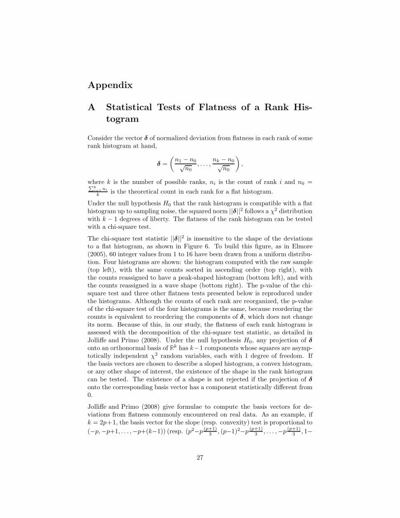
Consider the vector δ of normalized deviation from flatness in each rank of somerank histogram at hand,

δ =

(n1 − n0√

n0, . . . ,

nk − n0√n0

),

where k is the number of possible ranks, ni is the count of rank i and n0 =∑k

i=1ni

kis the theoretical count in each rank for a flat histogram.

Under the null hypothesis H0 that the rank histogram is compatible with a flathistogram up to sampling noise, the squared norm ||δ||2 follows a χ2 distributionwith k − 1 degrees of liberty. The flatness of the rank histogram can be testedwith a chi-square test.

The chi-square test statistic ||δ||2 is insensitive to the shape of the deviationsto a flat histogram, as shown in Figure 6. To build this figure, as in Elmore(2005), 60 integer values from 1 to 16 have been drawn from a uniform distribu-tion. Four histograms are shown: the histogram computed with the raw sample(top left), with the same counts sorted in ascending order (top right), withthe counts reassigned to have a peak-shaped histogram (bottom left), and withthe counts reassigned in a wave shape (bottom right). The p-value of the chi-square test and three other flatness tests presented below is reproduced underthe histograms. Although the counts of each rank are reorganized, the p-valueof the chi-square test of the four histograms is the same, because reordering thecounts is equivalent to reordering the components of δ, which does not changeits norm. Because of this, in our study, the flatness of each rank histogram isassessed with the decomposition of the chi-square test statistic, as detailed inJolliffe and Primo (2008). Under the null hypothesis H0, any projection of δonto an orthonormal basis of R

k has k−1 components whose squares are asymp-totically independent χ2 random variables, each with 1 degree of freedom. Ifthe basis vectors are chosen to describe a sloped histogram, a convex histogram,or any other shape of interest, the existence of the shape in the rank histogramcan be tested. The existence of a shape is not rejected if the projection of δonto the corresponding basis vector has a component statistically different from0.

Jolliffe and Primo (2008) give formulae to compute the basis vectors for de-viations from flatness commonly encountered on real data. As an example, ifk = 2p+1, the basis vector for the slope (resp. convexity) test is proportional to

(−p,−p+1, . . . ,−p+(k−1)) (resp. (p2−p(p+1)

3 , (p−1)2−p(p+1)

3 , . . . ,−p(p+1)

3 , 1−

27

1 3 5 7 9 11 13 15

RankC

ount

s0

24

68

χ2 : 0.679, slope : 0.179convexity : 0.935, wave: 0.191

1 3 5 7 9 11 13 15

Rank

Cou

nts

02

46

8

χ2 : 0.679, slope : 0.001convexity : 0.662, wave: 0.734

1 3 5 7 9 11 13 15

Rank

Cou

nts

02

46

8

χ2 : 0.679, slope : 0.823convexity : 0.002, wave: 0.87

1 3 5 7 9 11 13 15

RankC

ount

s0

24

68

χ2 : 0.679, slope : 0.014convexity : 0.956, wave: 0.03

Figure 6 – Illustration of the Jolliffe-Primo flatness tests of a rank histogram.The p-value of four flatness tests (chi-square, and three Jolliffe-Primo tests) arereproduced.

p(p+1)

3 , . . . , p2 − p(p+1)

3 )). In our study, three tests are used, the slope and con-vexity tests, and the “wave” test not described in Jolliffe and Primo (2008).This last test assesses the presence of a deviation from flatness in the shapeof a tilde, that was frequently observed in the literature (Scheuerer et al., 2015;Baran and Lerch, 2016; Taillardat et al., 2016) and in internal studies at Meteo-France. The corresponding basis vector is built thanks to the Grahm-Schmidtprocess as follows: the vector (0, sin( 2π

k−1 ), sin(2π2

k−1 ), . . . , sin(2πk−2k−1 ), 0) is made

orthogonal to the slope basis vector, and the resulting vector is normalized toget the basis vector for testing the presence of a wave shape. In Figure 6, thep-values for the test of existence of a slope, a convexity or a wave are in agree-ment with the shape of the histograms. For instance, the low p-value of theslope test (top right) rejects flatness against slope as expected.

B Proof of the Bounds for the Regret of the

Exponentially Weighted Average Forecaster

The proof closely follows the proof of theorem 2.2 in Cesa-Bianchi et al. (2006).

Let ℓ : Y × Y → [a; b] be a real-valued, bounded loss function. ℓ is supposedconvex in its first argument.

28

The EWA weights at time t are computed as

ωEWAe;t =

exp−ηLe;t∑Ee=1 exp−ηLe;t

,

with Le;t =∑t−1

s=1 ℓ(ye;s, ys) the cumulative loss of expert e at time t, and withthe convention Le;1 = 0 so that ωEWA

e,1 = 1E

∀e.

Let us define Wt =∑E

e=1 exp−ηLe;t∀t ≥ 1 and W0 = E. At all timest = 1, . . . , T , and using the convention that a sum over 0 elements is 0 (fort = 1, such that ωEWA

e,0 = 1E

∀e),

lnWt

Wt−1= ln

∑Ee=1 exp−ηℓ(ye;t, yt)exp−ηLe;t−1∑E

e′=1 exp−ηLe′;t−1

= ln

∑Ee=1 ω

EWAe;t−1 exp−ηℓ(ye;t, yt)∑E

e′=1 ωEWAe′;t−1

. (23)

The proof now needs Hoeffding’s inequality (Hoeffding, 1963). Let a, b ∈ R witha < b. Let Z be a bounded random variable with values in [a; b], then, ∀s ∈ R,Hoeffding’s inequality states that

lnE[esZ]≤ sE[Z] +

s2

8(b − a)2.

Using Equation (23) and Hoeffding’s inequality for the random variable Z tak-ing the values ℓ(ye;t, yt) with discrete probability ωEWA

e;t−1 , taking s = −η andsumming over t = 1, . . . , T leads to

lnWT

W0≤− η

T∑

t=1

E∑

e=1

ωEWAe;t ℓ(ye;t, yt) +

η2

8(b− a)2T

≤− η

T∑

t=1

ℓ

(E∑

e=1

ωEWAe;t ye;t, yt

)+

η2

8(b− a)2T

=− η

T∑

t=1

ℓ (yt, yt) +η2

8(b− a)2T,

after using the convexity of the loss function ℓ in its first argument, and thedefinition of the EWA forecast.

Noting that the following relationship also holds

lnWT

W0= ln

(E∑

e=1

exp−ηLe;T)

− lnE

≥ ln

(max

e=1,...,Eexp−ηLe;T

)− lnE

=− η mine=1,...,E

Le;T − lnE,

29

and combining it with the previous relationship leads to

−η mine=1,...,E

Le;T − lnE ≤ −η

T∑

t=1

ℓ (yt, yt) +η2

8(b − a)2T.

Finally, dividing by −η results in the following bound of the regret of the ag-gregated forecast relatively to the best expert

T∑

t=1

ℓ (yt, yt)− mine=1,...,E

Le;T ≤ lnE

η+

η

8(b− a)2T. (24)

Noting that this bound for the regret holds for any bounded loss function ℓ

convex in its first argument, which is a propery of the CRPS, concludes thedemonstration.

C Formula for the Gradient of the CRPS

Baudin (2015) considers the aggregation of step-wise CDFs with one singlestep (Me = 1 ∀e ∈ 1, . . . , E). We generalize equations (5.10) and (5.13) ofBaudin (2015) for, respectively, the CRPS and gradient thereof, to an aggrega-tion of step-wise CDFs with any number of steps.

Dropping the time index t in the notations, the aggregated CDF at time t is

y(x) =

E∑

e=1

ωe

[Me∑

me=1

pme

e Hxmee

(x)

],

with the notation Ha(x) = H(x− a).

Therefore, the CRPS of the aggregated CDF at time t is

CRPS(y, y) =

∫

R

Hy(x)−

E∑

e=1

ωe

[Me∑

me=1

pme

e Hxmee

(x)

]2

dx

=

∫ Γ

γ

Hy(x)−

E∑

e=1

ωe

[Me∑

me=1

pme

e Hxmee

(x)

]2

dx,

where γ = min(y, x11, . . . , x

ME

E ) and Γ = max(y, x11, . . . , x

ME

E ).

30

By developing the square inside the integral,

CRPS(y, y) =

∫ Γ

γ

Hy(x)dx

− 2

∫ Γ

γ

E∑

e=1

ωe

[Me∑

me=1

pme

e Hxmee

(x)Hy(x)

]dx

+

∫ Γ

γ

E∑

e=1

ωe

[Me∑

me=1

pme

e Hxmee

(x)

]

E′∑

e′=1

ωe′

Me′∑

me′=1

pme

e Hxm

e′

e′

(x)

dx.

Noting that Ha(x)Hb(x) = Hmax(a,b)(x), and∫ Γ

γHa(x)dx = Γ− a ∀a ∈ [γ; Γ],

then

CRPS(y, y) =Γ− y

− 2

E∑

e=1

ωe

Me∑

me=1

pme

e [Γ−max(xme

e , y)]

+E∑

e,e′=1

ωeωe′

Me∑

me=1

Me′∑

me′=1

pme

e pm

e′

e′

[Γ−max(xme

e , xm

e′

e′ )]

=− y

+ 2

E∑

e=1

ωe

[Me∑

me=1

pme

e max(xme

e , y)

]

−E∑

e,e′=1

ωeωe′

Me∑

me=1

Me′∑

me′=1

pme

e pm

e′

e′ max(xme

e , xm

e′

e′ )

,

because∑E

e=1 ωe = 1, and∑Me

me=1 pme

e = 1 ∀e ∈ 1, . . . , E.

31

Since max(a, b) = 12 (a+ b+ |a− b|),

CRPS(y, y) =− y

+

E∑

e=1

ωe

[Me∑

me=1

pme

e (xme

e + y + |xme

e − y|)]

− 1

2

E∑

e,e′=1

ωeωe′

Me∑

me=1

Me′∑

me′=1

pme

e pm

e′

e′ (xme

e + xm

e′

e′ + |xme

e − xm

e′

e′ |)

=E∑

e=1

ωe

[Me∑

me=1

pme

e (xme

e + |xme

e − y|)]

− 1

2

E∑

e,e′=1

ωeωe′

Me∑

me=1

Me′∑

me′=1

pme

e pm

e′

e′ (xme

e + xm

e′

e′ + |xme

e − xm

e′

e′ |)

.

(25)

The derivation with respect to ωe results in

∂CRPS

∂ωe

(y, y) =

Me∑

me=1

pme

e (xme

e + |xme

e − y|)

−E∑

e′=1

ωe′

Me∑

me=1

Me′∑

me′=1

pme

e pm

e′

e′ (xme

e + xm

e′

e′ + |xme

e − xm

e′

e′ |)

.

Finally, recalling that∑E

e=1 ωe = 1, and∑Me

me=1 pme

e = 1 ∀e ∈ 1, . . . , E

∂CRPS

∂ωe

(y, y) =

Me∑

me=1

pme

e |xme

e − y| −E∑

e′=1

ωe′

Me′∑

me′=1

pm

e′

e′ xm

e′

e′

−E∑

e′=1

ωe′

Me∑

me=1

Me′∑

me′=1

pme

e pm

e′

e′ |xme

e − xm

e′

e′ |

. (26)

Formulae (25) and (26) generalize equations (5.10) and (5.13), respectively, ofBaudin (2015).

D Relationship between the experts’ CRPS and

the reliability term with the JP tests

The expert with the minimum CRPS may not be the most reliable, accordingto the proportion of flat rank histograms in view of the JP tests. For instance

32

in Figure 7, at lead time 36 h, the QRF-post-processed ECMWF ensemblehas the lowest CRPS among the experts, but exhibits less than 40% of flathistograms despite the low significance threshold chosen for the JP tests thatallows important departure from flatness. At the same lead time, the NR-post-processed version of the CMC ensemble (with W = 90 days) has nearly 80% offlat histograms for a slightly higher CRPS.

As for the aggregation methods, the CRPS of the post-processed ensembles ismainly driven by the resolution term. Whereas the reliability term varies byless than 0.01 m/s, the average CRPS may change by up to 0.1 m/s from oneto the other. For post-processed ensembles, the average CRPS is thus mostly ameasure of resolution only.

33

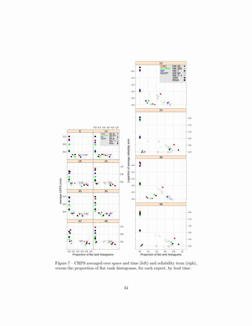
Proportion of flat rank histograms

Ave

rage

CR

PS

(m

/s)

0.6

0.8

1.0

60.0 0.2 0.4 0.6 0.8 1.0

12

18

0.6

0.8

1.0

24

0.6

0.8

1.0

30 36

0.0 0.2 0.4 0.6 0.8 1.0

42

0.6

0.8

1.0

48

CMCECMWFMFNCEP

NR 30NR 365NR 7NR 90NR T−1QRFRAW

Proportion of flat rank histograms

Loga

rithm

of a

vera

ge r

elia

bilit

y te

rm

−3.0

−2.5

−2.0

−1.5

−1.0

−0.5

12

−3.0

−2.5

−2.0

−1.5

−1.0

−0.5

24

−3.0

−2.5

−2.0

−1.5

−1.0

−0.5

36

0.0 0.2 0.4 0.6 0.8 1.0

−3.0

−2.5

−2.0

−1.5

−1.0

−0.5

48

CMCECMWFMFNCEP

NR 30NR 365NR 7NR 90NR T−1QRFRAW

Figure 7 – CRPS averaged over space and time (left) and reliability term (righ),versus the proportion of flat rank histograms, for each expert, by lead time.

34

References

Adjakossa, E., Goude, Y., and Wintenberger, O. (2020). Kalman RecursionsAggregated Online. arXiv preprint arXiv:2002.12173.

Allard, D., Comunian, A., and Renard, P. (2012). Probability aggregationmethods in geoscience. Mathematical Geosciences, 44(5):545–581.

Anderson, J. L. (1996). A method for producing and evaluating probabilisticforecasts from ensemble model integrations. Journal of Climate, 9(7):1518–1530.

Baran, S. and Lerch, S. (2015). Log-normal distribution based Ensemble ModelOutput Statistics models for probabilistic wind-speed forecasting. QuarterlyJournal of the Royal Meteorological Society.

Baran, S. and Lerch, S. (2016). Mixture EMOS model for calibrating ensembleforecasts of wind speed. Environmetrics, 27:116–130.

Baudin, P. (2015). Prevision sequentielle par agregation d’ensemble: applica-tion a des previsions meteorologiques assorties d’incertitudes. PhD thesis,Universite Paris-Saclay.

Benjamini, Y. and Hochberg, Y. (1995). Controlling the false discovery rate:a practical and powerful approach to multiple testing. Journal of the Royalstatistical society: series B (Methodological), 57(1):289–300.

Benjamini, Y. and Yekutieli, D. (2001). The control of the false discovery ratein multiple testing under dependency. Annals of statistics, 29(4):1165–1188.

Bogner, K., Liechti, K., and Zappa, M. (2017). Combining quantile forecasts andpredictive distributions of streamflows. Hydrology and Earth System Sciences,21(11):5493–5502.

Bougeault, P., Toth, Z., Bishop, C., Brown, B., Burridge, D., Chen, D. H.,Ebert, B., Fuentes, M., Hamill, T. M., Mylne, K., et al. (2010). The THOR-PEX interactive grand global ensemble. Bulletin of the American Meteoro-logical Society, 91(8):1059.

Brocker, J. (2009). Reliability, sufficiency, and the decomposition of properscores. Quarterly Journal of the Royal Meteorological Society, 135(643):1512–1519.

Brocker, J. (2018). Assessing the reliability of ensemble forecasting systems un-der serial dependence. Quarterly Journal of the Royal Meteorological Society,144(717):2666–2675.

Buizza, R., Houtekamer, P., Pellerin, G., Toth, Z., Zhu, Y., and Wei, M. (2005).A comparison of the ECMWF, MSC, and NCEP global ensemble predictionsystems. Monthly Weather Review, 133(5):1076–1097.

35

Cesa-Bianchi, N., Lugosi, G., et al. (2006). Prediction, learning, and games,volume 1. Cambridge University Press Cambridge.

Collet, J. and Richard, M. (2017). A Generic Method for Density ForecastsRecalibration. In Forecasting and Risk Management for Renewable Energy,pages 147–166. Springer.

Descamps, L., Labadie, C., and Bazile, E. (2011). Representing modeluncertainty using the multiparametrization method. In Proceedings ofECMWF Workshop on Representing Model Uncertainty and Error in Numer-ical Weather and Climate Prediction Models, 20-24 June 2011, pages 175–182.

Descamps, L., Labadie, C., Joly, A., Bazile, E., Arbogast, P., and Cebron, P.(2014). PEARP, the Meteo-France short-range ensemble prediction system.Quarterly Journal of the Royal Meteorological Society, 141(690):1671–1685.

Elmore, K. L. (2005). Alternatives to the chi-square test for evaluating rankhistograms from ensemble forecasts. Weather and forecasting, 20(5):789–795.

Gerchinovitz, S., Mallet, V., and Stoltz, G. (2008). A further look at sequentialaggregation rules for ozone ensemble forecasting. Rapport technique, INRIAParis-Rocquencourt et Ecole normale superieure, Paris.

Gneiting, T., Balabdaoui, F., and Raftery, A. (2007). Probabilistic forecasts,calibration and sharpness. Journal of the Royal Statistical Society: Series B(Statistical Methodology), 69(2):243–268.

Gneiting, T., Raftery, A., Westveld III, A., and Goldman, T. (2005). Calibratedprobabilistic forecasting using ensemble model output statistics and minimumCRPS estimation. Monthly Weather Review, 133(5):1098–1118.

Gneiting, T., Ranjan, R., et al. (2013). Combining predictive distributions.Electronic Journal of Statistics, 7:1747–1782.

Hamill, T. (2001). Interpretation of rank histograms for verifying ensembleforecasts. Monthly Weather Review, 129(3):550–560.

Hamill, T. and Colucci, S. (1998). Evaluation of Eta-RSM ensemble probabilisticprecipitation forecasts. Monthly Weather Review, 126(3):711–724.

Hamill, T. M. and Colucci, S. J. (1996). Random and systematic error inNMC’s short-range Eta ensembles. In Preprints, 13th Conf. on Probability andStatistics in the Atmospheric Sciences, San Francisco, CA, Amer. Meteor.Soc, pages 51–56.

Hemri, S., Scheuerer, M., Pappenberger, F., Bogner, K., and Haiden, T. (2014).Trends in the predictive performance of raw ensemble weather forecasts. Geo-physical Research Letters, 41(24):9197–9205.

Hersbach, H. (2000). Decomposition of the continuous ranked probability scorefor ensemble prediction systems. Weather and Forecasting, 15(5):559–570.

36

Hoeffding, W. (1963). Probability inequalities for sums of bounded randomvariables. Journal of the American statistical association, 58(301):13–30.

Holton, J. R. and Hakim, G. J. (2012). An introduction to dynamic meteorology,volume 88. Academic press.

Jolliffe, I. and Stephenson, D. (2011). Forecast verification: a practioner’s guidein atmospheric science, second edition. Wiley-Blackwell.

Jolliffe, I. T. and Primo, C. (2008). Evaluating rank histograms using decompo-sitions of the chi-square test statistic. Monthly Weather Review, 136(6):2133–2139.

Leutbecher, M. and Palmer, T. N. (2008). Ensemble forecasting. Journal ofComputational Physics, 227(7):3515–3539.

Malardel, S. (2005). Fondamentaux de meteorologie: a l’ecole du temps, vol-ume 45. Cepadues.

Mallet, V., Mauricette, B., and Stoltz, G. (2007). Description of Sequential Ag-gregation Methods and their Performances for Ozone Ensemble Forecasting.Technical report, Ecole normale superieure, DMA and CEREA.

Matheson, J. E. and Winkler, R. L. (1976). Scoring rules for continuous prob-ability distributions. Management science, 22(10):1087–1096.

Meinshausen, N. (2006). Quantile regression forests. The Journal of MachineLearning Research, 7:983–999.

Moller, A. and Groß, J. (2016). Probabilistic temperature forecasting basedon an ensemble autoregressive modification. Quarterly Journal of the RoyalMeteorological Society, 142(696):1385–1394.

Moller, D. and Scheuerer, M. (2013). Postprocessing of Ensemble Forecasts forWind Speed over Germany. PhD thesis, Diploma thesis, Faculty of Math-ematics and Computer Science, Heidelberg University. Available online athttp://www.rzuser.uni-heidelberg.de/˜kd4/files/Moeller2013.pdf.

Murphy, A. (1993). What is a good forecast? an essay on the nature of goodnessin weather forecasting. Weather and Forecasting, 8(2):281–293.

Mylne, K. R. (2002). Decision-making from probability forecasts based on fore-cast value. Meteorological Applications, 9(3):307–315.

R Core Team (2015). R: A Language and Environment for Statistical Comput-ing. R Foundation for Statistical Computing, Vienna, Austria.

Richardson, D. S. (2001). Measures of skill and value of ensemble predictionsystems, their interrelationship and the effect of ensemble size. QuarterlyJournal of the Royal Meteorological Society, 127(577):2473–2489.

37

Scheuerer, M., Moller, D., et al. (2015). Probabilistic wind speed forecastingon a grid based on ensemble model output statistics. The Annals of AppliedStatistics, 9(3):1328–1349.

Siegert, S. (2015). SpecsVerification: Forecast Verification Routines for theSPECS FP7 Project. R package version 0.4-1.

Stoltz, G. (2010). Agregation sequentielle de predicteurs: methodologie generaleet applications a la prevision de la qualite de l’air et a celle de la consommationelectrique. Journal de la Societe Francaise de Statistique, 151(2):66–106.

Swinbank, R., Kyouda, M., Buchanan, P., Froude, L., Hamill, T. M., Hewson,T. D., Keller, J. H., Matsueda, M., Methven, J., Pappenberger, F., et al.(2016). The TIGGE project and its achievements. Bulletin of the AmericanMeteorological Society, 97(1):49–67.

Taillardat, M., Mestre, O., Zamo, M., and Naveau, P. (2016). Calibrated Ensem-ble Forecasts using Quantile Regression Forests and Ensemble Model OutputStatistics. Monthly Weather Review, 144(6):2375–2393.

Talagrand, O., Vautard, R., and Strauss, B. (1997). Evaluation of probabilisticprediction systems. In Proc. ECMWF Workshop on Predictability, pages 1–25.

Thorarinsdottir, T. L. and Gneiting, T. (2010). Probabilistic forecasts of windspeed: ensemble model output statistics by using heteroscedastic censoredregression. Journal of the Royal Statistical Society: Series A (Statistics inSociety), 173(2):371–388.

Thorey, J. (2017). Prevision d’ensemble par agregation sequentielle appliquee ala prevision de production d’energie photovoltaıque. PhD thesis, INRIA. tobe submitted (in English).

Wasserstein, R., Schirm, A., and N., L. (2019). [Special Issue]Statistical Infer-ence in the 21st Century: A World Beyond p ¡ 0.05. The American Statisti-cian, 73(1).

Wilks, D. S. (2018). Enforcing calibration in ensemble postprocessing. QuarterlyJournal of the Royal Meteorological Society, 144(710):76–84.

Wilson, L. J., Beauregard, S., Raftery, A. E., and Verret, R. (2007). Calibratedsurface temperature forecasts from the Canadian ensemble prediction systemusing Bayesian model averaging. Monthly Weather Review, 135(4):1364–1385.

Winkler, R., Munoz, J., Cervera, J., Bernardo, J., Blattenberger, G., Kadane,J., Lindley, D., Murphy, A., Oliver, R., and Rıos-Insua, D. (1996). Scoringrules and the evaluation of probabilities. Test, 5(1):1–60.

Zamo, M., Bel, L., Mestre, O., and Stein, J. (2016). Improved gridded wind-speed forecasts by statistical post-processing of numerical models with blockregression. Weather and Forecasting, 31(6):1929–1945.

38

Zamo, M., Mestre, O., Arbogast, P., and Pannekoucke, O. (2014). A benchmarkof statistical regression methods for short-term forecasting of photovoltaicelectricity production. Part II: Probabilistic forecast of daily production. SolarEnergy, 105:804–816.

Zamo, M. and Naveau, P. (2018). Estimation of the Continuous Ranked Proba-bility Score with Limited Information and Applications to Ensemble WeatherForecasts. Mathematical Geosciences, 50(2):209–234.

Zhu, Y., Toth, Z., Wobus, R., Richardson, D., and Mylne, K. (2002). Theeconomic value of ensemble-based weather forecasts. Bulletin of the AmericanMeteorological Society, 83(1):73.

39