Ceiling & Visibility Forecasts via Neural Nets

Ceiling & Visibility Forecasts via Neural Nets

Caren Marzban1,2∗, Steve Leyton1, and Brad Colman3

1 Center for Analysis and Prediction of Storms

University of Oklahoma, Norman, OK

2 Department of Statistics, University of Washington, Seattle, WA

3 National Weather Service, Seattle, WA

∗Corresponding author. Email: [email protected]

1

Abstract

Statistical postprocessing of model output can improve forecast quality, espe-

cially when model output is combined with surface observations. In this article, the

development of nonlinear postprocessors for the prediction of ceiling and visibility is

discussed. The statistical model is a neural network, 39 of which are developed for

various TAF stations in the Northwest US. The performance of these postprocessors

is shown to be generally superior to logistic regression and MOS.

2

1 Introduction

Coastal locations around the US are susceptible to marine stratus and low ceilings.

Occasionally, the stratus extends to the surface, resulting in dense fog conditions and

a significant reduction in horizontal visibility. When these adverse conditions occur,

they often disrupt daily activities, such as aviation and shipping interests, sometimes

to the point of jeopardizing human safety. It is imperative, then, to provide forecasters

with the most accurate guidance for these high-impact weather phenomena.

Marine stratus is especially problematic along the West Coast of the US during

the summer months. This is primarily due to a semi-permanent area of high pres-

sure over the northern Pacific Ocean during the summer months, the continuous flow

of relatively cool ocean waters southward along the West Coast via the California

Current and the warm daytime temperatures of inland locations in this region. This

cycle of marine stratus development is explained in more detail by Hilliker and Fritsch

(1999). In addition, Hilliker and Fritsch (1999) displayed the frequency of occurrence

of these marine stratus events through an annual number of Instrument Flight Rules

(IFR) events at various airports across the US. It is shown that San Francisco In-

ternational Airport experiences nearly 200 IFR events per year while Seattle-Tacoma

International Airport experiences about 125 events per year.

In addition to the very common inland intrusions of marine fog and stratus

are episodes of inland basin (radiational) fog. During spells of prolonged ridging

over the western US in the cool season, shallow layers of persistent fog form in the

3

inner basins, including the Columbia river basin, and the Sacramento valley. These

events are hazardous to all kinds of transportation and commerce, but especially to

aviation. Additionally, recurring winter storms bring restricted flying conditions to

all terminals across the Pacific Northwest. These events include strong wind, rain,

fog, snow and freezing precipitation.

Traditionally, the primary source of guidance for forecasting surface weather

conditions has been statistically postprocessed numerical model output. In particular,

Model Output Statistics (MOS) derived from the Nested Grid Model (NGM) and

Aviation Model (AVN) provide forecasts of weather parameters at three-hour intervals

out to 60 hours.

This type of forecasting guidance has at least two defects: 1) the models are

run only a few times daily, allowing forecasts to become several hours old before

an updated product is made available, and 2) the MOS equations are linear. To

alleviate the first limitation, studies have been undertaken to investigate the use of an

observations-based forecasting system (Vislocky and Fritsch 1997). In this system, a

network of surface observations is used as predictors in a multiple regression technique.

It was demonstrated that this approach could improve the accuracy of ceiling and

visibility forecasts for the hours between the times that the output from the numerical

models is released (Leyton and Fritsch 2002a,b).

To overcome the linearity of the MOS equations, nonlinear generalizations of

multiple regression have been utilized to model the full nonlinearity and interactions

4

of the underlying processes. For example, temperature forecasts from the Advanced

Regional Prediction System (ARPS) have been postprocessed via neural networks,

displaying a reduction in bias and error variance of the forecasts (Marzban 2003).

As such, the statistical postprocessing yields temperature forecasts that are more

accurate than the model forecasts.

Here, these two solutions have been combined to produce superior forecasts.

In other words, a nonlinear postprocessor has been developed that takes as input

(i.e., predictors) not only model data but also surface observations, and it produces

forecasts of ceiling and visibility. In fact, 39 postprocessors are developed for 39 Ter-

minal Aerodrome Forecast (TAF) stations. TAF forecasters rely heavily on statistical

postprocessors, because not all of the parameters included in TAF are directly output

by numerical weather prediction models. Specifically, explicit information about vis-

ibility, cloud and fog layers, is generally absent. Forecasters thus rely on experience,

climatology, and statistical tools. The numerical model for which postprocessors are

developed is the 5th Generation PSU-NCAR Mesoscale Model (MM5). The MM5

real-time mesoscale weather prediction system run by the Northwest Modeling Con-

sortium and the University of Washington is one of the longest running and mature

regional modeling efforts in existence.1 In what follows, the development of these

NNs is outlined in detail, and it is shown that their performance is generally supe-

rior to that of logistic regression and MOS derived from GFS. As shown below, the

1While nationally produced statistical guidance products, from nationally run models, will remain

an important part of the forecast process, regional tools are also needed.

5

exceptions include stations where insufficient data exist for a proper development of

a nonlinear postprocessor.

2 Data

Four data sets are employed. The first is an archive of standard hourly surface obser-

vations (SAO) from 2001 to 2005, acquired from the National Center of Atmospheric

Research (NCAR). These observations include reports of temperature, dew point,

wind speed and direction, cloud cover, ceiling, visibility and precipitation.

The second data set is an archive of standard hourly surface (ASOS and AWOS)

data, also acquired from NCAR. This data set includes reports of temperature, dew

point, wind speed and direction, cloud cover, visibility and precipitation. While some

differences exist between the methods by which the observations are taken in each data

set (most notably cloud cover and visibility), studies have found that the observations

are comparable from a climatological perspective. Therefore, this difference should

have minimal effect on this study. The surface observations employed for the analysis

span the dates 11/7/2001-1/31/2005. Although the data are available on an hourly

basis, only the 00Z values are used, except for ceiling and visibility, which are used

at 06Z, and 12Z - the valid times.

The third data set is an archive of MM5 data. The MM5 has been run at the

University of Washington on a twice-daily basis since late 1997. The standard con-

6

figuration includes a triple nest of 36, 12, and 4-km grids. The current configuration

consists of a 12-km grid that covers a broad area of the Pacific Northwest, extending

from western Montana to the coast and southward to northern Nevada and Califor-

nia. An archive of 12-km runs provides the model data used in the study. The model

data were archived for the period 11/7/2001-3/31/2005, and were used every 6 hours.

The last data set consists of MOS forecasts derived from the GFS model, span-

ning the dates 11/1/2001-2/28/2005.2 MOS forecasts are issued at 0Z, are categorical,

and are available every 6 hours. This data set is utilized as a benchmark for comparing

the performance of the neural network.

The categories for ceiling and visibility are given in Table 1. The categories

defined in MOS are finer, and so, in order to compare the neural nets developed

here with MOS, the categories in the latter are combined into larger categories that

coincide with those adopted here.

The list of the TAF stations for which specific neural nets are developed is given

in Table 2. They are scattered across, Washington, Oregon, Idaho, Montana, Nevada,

and California; see Figure 1.

2The data archive for MOS NGM are highly incomplete, and for that reason, the NNs will be

compared with the MOS GFS forecasts for which the data archive is quite complete.

7

3 Methodology

Recently, there has been a surge of interest in the use of Neural Networks (NNs)

among meteorologists (Hsieh and Tang 1998). Among the numerous applications,

postprocessing of model output has been beneficial (Casaioli et al. 2000, Marzban

2003). Given that NNs belong to the class of nonlinear statistical models, the post-

processing activity can be considered a nonlinear version of MOS. Although the choice

of a nonlinear method is not unique, NNs are generally useful because in addition to

being able to approximate a large class of functions, compared to many other models

they are less prone to overfit data. 3

The prediction of ceiling and visibility can be cast into a classification problem.

The NN is designed to produce a probability of belonging to one of the classes/categories

shown in Table 1, given the atmospheric conditions at the time; the latter are quan-

tified by the predictors, namely the model output variables and surface observations.

The development of the NNs requires substantial preprocessing of the data.

Seasonal cycles in the data are removed by subtracting the monthly average of each

3Overfitting can occur when a statistical model has sufficient flexibility to fit features in the data

that are purely statistical fluctuations. As such, a statistical model that has overfit some data set

is likely to perform poorly on data not represented in that data set. The number of parameters in

a statistical model is one measure of model flexibility, and so a model with too many parameters

is more likely to overfit a data set than another model with less parameters. For example, the

number of parameters in polynomial regression grows exponentially with the number of independent

variables (i.e., predictors); by contrast, for NNs the growth is only linear.

8

variable from the data on that variable. More sophisticated techniques (e.g., seasonal

differencing) for filtering out periodicity were examined, but showed no significant

difference. Outliers are removed by simply excluding any data beyond 5 standard

deviations of the mode. For variables with highly skewed distributions, outliers are

identified visually. Square-root and cube-root transformations are applied to the

inputs to render their distribution more normal. Pairwise correlations between the

predictors are employed to exclude one member of highly correlated pairs. Principal

components of the data were considered as inputs to the NN, but no significant

improvement was detected.

After this preprocessing, 20 predictors remain, and the surviving sample size

is 878. The predictors are normalized a la z-scores (i.e., the mean of each variable

is subtracted from each case, and the result is divided by the standard deviation of

that variable). Jitter (or gaussian noise) with a mean of 0 and standard deviation of

0.2 is added to each variable. In order to inflate the sample size, this is repeated 10

times, increasing the sample size from 878 to 8780.4

Some NN-specific matters are as follows: The number of input nodes is 20,

and the number of output nodes is 4 or 3, respectively, for ceiling or visibility. The

number of hidden nodes is determined via bootstrapping.5 The number of bootstrap

4This manner of increasing sample size may seem like trickery; however, it is a relatively standard

technique in nonlinear modeling, with the sole purpose of restraining overfitting. The choice of 0.2 for

the standard deviation of the jitter, and 10 for the multiplication factor, are based on trial-and-error.

The final results are generally insensitive to the specific values of these quantities.5In its simplest version bootstrapping calls for repeated partitioning of the data into a training

9

trials is 4.

One way of displaying many of these quantities is through a TV-diagram (Marzban

2000) which is basically a scatterplot of training and validation performance numbers

for different hidden nodes and different bootstrap trials (e.g., Figure 6).

The activation functions for all the nodes is the logistic function, and the error

function being minimized is cross-entropy. This set-up assures that the outputs of the

NN represent the posterior probability of belonging to a certain category of ceiling

or visibility, given the inputs. In other words, the outputs of the NN are forecast

probabilities.

As mentioned previously, for some stations the occurrence of the lowest ceiling

and visibility classes is extremely rare. So rare, in fact, that no satisfactory NN can

be developed. For these stations, categories of ceiling (and visibility) are combined

to render it binary; the highest category is considered as a distinct class, and the

remaining categories are combined into a second class. The NNs based on this revised

data set are referred to as “2-class”, and the NNs based on the non-combined classes

are labeled as “4-class” or “3-class” depending on whether the predictand is ceiling

or visibility, respectively.

The performance of the NN is compared with that of logistic regression and

MOS in terms of several measures of performance. For the 2-class NNs, in addi-

set and a validation set. The number of hidden nodes is taken to be that which minimizes the

average of the validation errors over the bootstrap trials.

10

tion to Receivers Operating Characteristic (ROC) diagrams, performance is gauged

within the framework of probabilistic forecasting developed by Murphy and Winkler

(1987, 1992) - specifically: reliability, discrimination, refinement, resolution, and at-

tributes diagrams. Some scalar measures representing the quality of the probabilistic

forecasts are also computed, including cross-entropy, and Ranked Probability Score.

Since MOS forecasts are categorical, some scalar (nonprobabilistic) measures of per-

formance are also computed, e.g., the Heidke Skill Scores (HSS); this measure has

been advocated as a relatively “healthy” measure (Marzban 1998), and has a natural

generalization to non-binary classes, and so, is utilized to asses the performance of

the 3-class and 4-class NNs.

Two sets of NNs are developed for two different valid times - 06Z and 12Z. The

former utilize the model predictors at 06Z, and the surface observations at 00Z. These

NNs produce forecasts with a lead time of 6 hours. The NNs producing forecasts with

a 12-hr lead time are developed on model predictors at 12Z, and surface observations

at 00Z. These NNs produce forecasts of ceiling and visibility at 12Z.6

The number of NNs developed here is unwieldy. 39 stations, binary and non-

binary classes, ceiling and visibility, 5 different hidden nodes (0,2,4,6,8), 4 seeds, 6Z

and 12Z forecasts, altogether yield 6,240 NNs. The verification task is even more com-

plex because each of these NNs can be assessed in terms of a multitude of verification

6In principle, it is possible to arrange for model and surface observation variables to be at 00Z,

while the predictand is at the valid time. That possibility has been examined in Marzban, Sandgathe,

Kalnay (2005).

11

measures. Here, only a sample of all the results is presented.

4 Results from Preprocessing

The initial variables available for analysis numbered in the hundreds. However, after

the preprocessing only 20 remain; eleven from MM5 and 8 from surface observations.

The final list of variables is shown in Table 3. Of course, in addition to these pre-

dictors, the data include measurements of ceiling and visibility at every station and

at 6-hr intervals. The variables in the table are self-explanatory; the only ones that

call for further clarification are variables 14-16. The variable “Sky” refers to sky

coverage, and takes the following values: Clear, Few, Scattered, Broken, Overcast,

and Obscured. Variable 15 is binary and labels the occurrence or non-occurrence of

precipitation. Wind Direction is recorded as NE, E, SE, S, SW, W, NW, and N.

As mentioned previously, for some stations the data contain an exceedingly

small number of low ceilings or low visibility. Figure 2 shows the climatological

frequency (in percent) of the lowest categories at 06Z and at 12Z.7 Low ceiling and

visibility occurs most frequently at KACV, KCEC, KEUG, KOLM, and KSKA, with

some variability between 06Z and 12Z. The stations at which these conditions occur

least frequently depend more strongly on the time of day; at 06Z, they are KBFI,

KDLS, KEKO, KPDX, KSUN, KTTD, KWMC, and KYKM; at 12Z, they are KBKE,

7The stations with low climatological frequency of low ceiling and visibility are those farther away

from a body of water.

12

KBNO, KBOI, KDLS, KEKO, KPSC, KRDD, KSUN, KTTD, KWMC, and KYKM.

The stations with the lowest occurrence of ceiling and visibility are expected to have

poorly performing NNs.

As discussed in Marzban et al. (1999), the notion of a “best predictor” is ill-

defined, at least outside of the framework of a statistical model. Nevertheless, this is a

natural place in the analysis to explore the relationships among the various variables

in more detail. Figure 3 shows the linear correlation coefficient between each of the

predictors at 0Z and the predictands - ceiling and visibility - at 12Z for KOLM.

Evidently, all of the predictors of ceiling have generally equal strength (within the

error-bars). The exceptions are T2, Q2, and Q which have near-zero correlation with

ceiling. However, this does not imply that they are poor predictors as far as the NN

is concerned, because, first, their correlations may be nonlinear, and second, their

interaction with the other variables may be important for predicting ceiling. This is

why they are not excluded as inputs to the NNs. The best predictors of visibility

again have comparable strength, with the exception of Sky (sky coverage) which is

highly correlated with visibility. The weakest predictors are T2, and Dew point, but

they are not excluded from the analysis for the aforementioned reasons.

A more complete representation of predictive strength is given in terms of con-

ditional distributions. Figure 4 shows the conditional distribution of the predictors

for low-ceiling and high-ceiling, separately.8 It can be seen, for example, that x1 (Sea

8It is possible to plot the conditional distributions for all 4 classes of ceiling, but the results are

visually unappealing.

13

level Pressure) is a poor predictor, while x4 (wind u-component at 10m) is a relatively

good predictor. Note that a binary variable such as x15 (precipitation occurrence)

appears as a continuous quantity, because of the jitter introduced in the data (see the

Method section). Such plots provide a more meaningful assessment of the predictive

strength of the predictors, but they are still univariate in nature, and so, are not

utilized in determining the inputs to the NN.

5 Results

In order to compare the NNs with MOS, the HSS scores for MOS are computed first.

Figure 5 shows the HSS scores for 12Z, 12 hour MOS forecasts. The HSS is computed

from 4×4 contingency tables, i.e., for the classes adopted here (Table 1). Each station

has two bars - one for the training set and one for the validation set. The error-bars

on each bar are computed from bootstrapping. The left figure is for ceiling and the

right figure for visibility. Note that MOS performs differently for ceiling and visibility.

For example, the best ceiling forecasts occur at KEAT and KRDD, while, the best

visibility forecasts take place at KPDT and KRDM. Moreover, the uncertainty in the

HSS values (i.e. error-bars) is not consistent across stations. For example, for ceiling,

whereas stations like KBKE, KCEC and KYKM are consistently in the high-HSS

range, KEKO and KRDD display a large variability in performance.

As mentioned previously, the optimal number of hidden nodes is determined via

14

bootstrapping. The data from different stations have different amount of nonlinearity,

leading to different number of hidden nodes. The TV-diagrams, with cross-entropy

as the performance measure, for three stations and three bootstrap trials are shown

in Figure 6. KACV, for example, has lower training and validation errors for more

hidden nodes. This suggests a highly nonlinear relationship between the predictors

and the predictand (here, ceiling).9 KEUG, however, shows a strong preference for

an NN with 6 hidden nodes; larger NNs lead to lower training but higher validation

errors for each of three bootstrap trials. By contrast, any amount of nonlinearity

introduced in the NN for KMSO causes overfitting.10

The discrimination diagram for the NN and logistic regression are shown in

Figure 7. These figures are for KNUW; the forecasts are 12hr forecasts of ceiling for

12Z, and the NN has 6 hidden nodes (the optimal for that station). It can be seen

that the NN makes more discriminatory forecasts, i.e., the conditional distribution of

the forecasts is concentrated around small values for cases with high ceiling, and the

distribution for low ceiling is concentrated around high values (∼ 0.9). By contrast,

logistic regression has broader distributions for low and high ceilings, leading to a

greater overlap between the two.

The attributes diagram for the NN and logistic regression are shown in Figure

8. The station and the NN are the same as those described for Figure 7. Both the NN

9As a final step, in order to avoid overfitting, the largest allowed number of hidden nodes is 8.10A NN with zero hidden nodes is equivalent to logistic regression; for clarity, the performance

measures for logistic regression are shown in later figures.

15

and logistic regression produce highly reliable forecasts, as evident from the overlap

of the reliability curve and the diagonal line. One difference is that whereas the NN

produces reliable forecasts (at least within the error-bars) even when the probability

of low ceiling is in the 0.9 range, logistic regression produces no forecasts in that range

at all. Moreover, a comparison of the error-bars between the two figures suggests that

the NN’s forecasts are more certain than those of logistic regression.

The bell-shaped curve in Figure 7 is often called the refinement diagram, and

is simply the distribution of the forecasts without regard to low or high ceilings. Its

skewed nature is simply a reflection of the rare nature of low ceiling conditions.

Figure 9 shows the ROC curves for the NN and logistic regression. Here, the

training and validation curves are plotted separately. The most concave curves cor-

responds to three different training sets (i.e., seeds), and the intermediate curves are

the associated validation sets. The least concave curves are for logistic regression; the

training and validation curves are not as distinguishable as the NN curves. Again, it

is evident that the NN outperforms logistic regression.

To compare NN, logistic, and MOS, simultaneously, ceiling and visibility must

be binary, since logistic regression models only 2-class predictands. Furthermore, since

MOS does not produce probabilistic forecasts, a categorical verification measure, such

as HSS, must be employed. The TV-diagrams showing HSS for 3 stations are shown in

Figure 10. The top diagram illustrates that for 3 bootstrap trials, the NN outperforms

logistic regression, which in turn outperforms MOS. This conclusion follows because

16

the training and validation HSS values for the 3 NNs (regardless of the number of

hidden nodes) are all superior to those of logistic regression; moreover, more hidden

nodes lead to better performance on the training and validation sets. The middle

figure illustrates a situation where MOS and logistic regression are comparable in

their performance, but the NNs still outperform both. An ambiguous situation that

does arise is exemplified in the bottom figure. Here, MOS displays validation HSS

values that are superior to both logistic regression and NN, in spite of the latter’s wide

spread in the training HSS values. As such, it is not possible to assess the relative

performance of the three models.

Analogous figures for all 30 stations have been produced, but are not shown

here.11 To distill that information, a course categorization of the results is in or-

der. Given that logistic regression is an NN with zero hidden nodes, an analysis

of such figures for all 39 stations allows for a course comparison of NN with MOS.

Labeling the above-mentioned three situations as “significantly”, “moderately”, and

“questionably”, Table 4 lists the stations falling in each category.

HSS allows a comparison of the various models when ceiling and visibility are

not binary. The results for above-mentioned 3 stations are shown in Figure 11, but an

analysis of the figures for all 39 stations suggests that the difference in performance

between the NN and MOS is generally smaller than in the binary case. Nevertheless,

the NN does generally outperform MOS for many of the stations. For some stations,

11All the figures can be found in the Appendix of the web-version of this article; it can be found

at http://www.stat.washington.edu/www/research/reports/tr489.pdf.

17

however, MOS outperforms NN. For instance, binary MOS forecasts of 06Z ceiling

for KEUG are superior to the NN forecasts. All of these comparisons are shown in

Table 5. The letter “N” implies that the NN outperforms MOS, and the letter “O”

implies the opposite. Meanwhile, there are many situations where it is not at all clear

which forecasts are best, and these are labeled “-”; the cases where the comparison

is ambiguous are generally when the amount of data is exceedingly small, and the

occurrence of low ceiling and visibility is exceedingly rare.

6 Conclusion and Discussion

MM5 model output and surface observations at 39 TAF stations are utilized to develop

NNs for predicting ceiling and visibility with 6 and 12 hour lead time. A number of

verification measures are employed to compare the performance of these NNs with

logistic regression and with traditional MOS. It is shown that for stations for which

sufficient data exists for developing an NN, the NN outperforms logistic regression and

MOS, with the degree of improvement depending on a number of factors including

lead time, and the choice of the station itself. This suggests that the NNs should

be employed in realtime, especially because they are developed to produce highly

reliable and discriminatory probabilistic forecasts (in contrast to MOS’s categorical

forecasts).

The comparison of statistical models is contingent on the data at hand, and

18

therefore, the above conclusions are valid only for the data employed herein. In fact,

the manner in which the NNs are developed is apt to render their performance posi-

tively biased. Specifically, although a number of steps are taken to avoid overfitting,

it is still possible that some degree of overfitting has occurred. This is mostly because

the training and validation bootstrap data are not entirely independent of one an-

other; although seasonal effects are removed, some autocorrelation is apt to remain,

thereby rendering a given training set and validation set dependent. This may appear

to unfairly favor NN over MOS; however, it must be pointed out that the regression

models underlying the MOS forecasts employed here are likely developed on the same

data used for comparing MOS with NN. In other words, the MOS forecasts are also

positively biased. A better comparison of MOS and NN would involve truly inde-

pendent data; these data are being currently archived, and the comparison will be

reported at a later time.

Changes to MM5 can be accommodated in several ways: 1) by running an older

postprocessor on new model output, 2) developing a new postprocessor developed

from only new data produced from new runs of the new model, and on 3) new runs

of the new model on archived data. A priori it is not clear which approach would

produce better forecasts. These options will be tested in the future.

Other future work involves developing separate models for warm and cool sea-

sons, more sophisticated preprocessing (e.g., removal of autocorrelations) and variable

selection (e.g., using principal components of the data as inputs).

19

A more promising direction is the development of NNs that utilize the relation-

ship between ceiling and visibility to improve the forecasts. All of the NNs described

here were designed to predict either ceiling or visibility. There is, however, some

evidence that a NN that predicts multiple predictands (e.g., ceiling and visibility)

simultaneously may outperform separate NNs designed to predict each predictand,

separately. The advantage of the former is most evident when the predictands are

correlated. A typical conditional (on ceiling) probability distribution between ceiling

and visibility is:

Visibility

35% 32% 33% 100%

Ceiling 5% 18% 77% 100%

1% 7% 92% 100%

0.04% 0.33% 99.63% 100%

The structure of this table implies that when ceiling is high, then visibility is

high as well. By contrast, a low ceiling does not imply low visibility. The complex

nature of the association between ceiling and visibility is ideal for developing an NN

that predicts both ceiling and visibility, simultaneously. This idea will be examined

in the future.

Acknowledgements

The authors are grateful to Patrick Tewson of the Applied Physics Laboratory,

University of Washington, for providing the MM5 data. Partial funding for this work

was provided under a cooperative agreement between the National Oceanic and At-

20

mospheric Administration (NOAA) and the University Corporation for Atmospheric

Research (UCAR). The views expressed herein are those of the authors and do not

reflect the views of NOAA, its subagencies, or UCAR.

21

7 References

Casaioli, M., R. Mantovani, F. P. Scorzoni, S. Puca, E. Ratini, and A. Speranza,

2001: Post-processing of numerical surface temperature with neural networks.

Nonlinear Processes in Geophysics; in press. Available at krishna.phys.uniroma1.it.

Hilliker, J. L., and J. M. Fritsch, 1999: An observations-based statistical system for

warm-season hourly probabilistic forecasts of low ceiling at the San Francisco

International Airport. J. Appl. Meteor., 38, 1692-1705.

Hsieh, William W., and B. Tang, 1998: Applying Neural Network Models to Predic-

tion and Data Analysis in Meteorology and Oceanography. Bull. Amer.Meteo.

Soc., 79, pp. 1855.

Leyton, S. M., and J. M. Fritsch, 2002a: Short-term probabilistic forecasts of ceiling

and visibility utilizing high-density surface weather observations. Wea. Fore-

casting, in press. ??

Leyton, S. M., and J. M. Fritsch, 2002b: The impact of high-frequency surface

weather observations on short-term probabilistic forecasts of ceiling and visibil-

ity. J. Appl. Meteor., in press. ??

Marzban, C., 2003: A Neural Network for Post-processing Model Output: ARPS.

Monthly Weather Review, in press.

Marzban, C., 2000: A Neural Network for Tornado Diagnosis. Neural Computing

and Applications, 9, 133-141.

22

Marzban, C. 1998: Scalar measures of performance in rare-event situations, Wea.

Forecasting, 13, 753-763.

Marzban, C., S. Sandgathe, E. Kalnay 2005: MOS, Perfect Prog, and Reanalysis

Data. Accepted by Mon. Wea. Rev.

Marzban, C., E. D. Mitchell, and G. Stumpf, 1999: The notion of “best predictors:”

An application to tornado prediction. Wea. Forecasting, 14, 1007-1016.

Murphy, A. H., and R. L. Winkler, 1992: Diagnostic verification of probability

forecasts. Int. J. Forecasting, 7, 435-455.

Murphy, A. H., and R. L. Winkler, 1987: A general framework for forecast verifica-

tion. Mon. Wea. Rev., 115, 1330-1338.

Vislocky, R. L., and J. M. Fritsch, 1997: An automated, observations-based system

for short-term prediction of ceiling and visibility. Wea. Forecasting, 12, 31-43.

23

Table 1. The categories for ceiling and visibility adopted here.

class (category) ceiling (feet) visibility (miles)

1 ≤ 500 ≤ 1

2 500 - 1000 1 - 3

3 1000 - 3000 ≥ 3

4 ≥ 3000

24

Table 2. List of TAF stations.

Arcata KACV Moses Lake KMWH

Walla Walla KALW Whidbey KNUW

Astoria KAST Olympia KOLM

Boeing Field (Seattle) KBFI Paine Field (Everett) KPAE

Baker city KBKE Pendleton KPDT

Bellingham KBLI Portland int KPDX

Burns KBNO Pasco KPSC

Boise KBOI Redding KRDD

Crescent City KCEC Redmond KRDM

Port Angeles KCLM Seattle-Tacoma Int. KSEA

Coeur D’Alene KCOE Felts Field (Spokane) KSFF

Dalles KDLS Fairchild AFB KSKA

Wenatchee KEAT Salem KSLE

Elko KEKO Sun Valley KSUN

Eugene KEUG McChord KTCM

Geiger Field (Spokane) KGEG Troutdale KTTD

Hoquium KHQM Twin Falls KTWF

Klamath Falls KLMT Winnemucca KWMC

Medford KMFR Yakima KYKM

Missoula KMSO

25

Table 3. List of the predictors after variable selection.

x1. Sea-level Pressure (PSEALVLC)

x2. Temperature at 2m (T2)

x3. Mixing Ratio at 2m (Q2)

x4. Wind u-component at 10m (U10)

x5. Wind v-component at 10m (V10)

x6. Total precipitation since initialization (RAINTOT)

x7. Geopotential Height at 850mb (H)

x8. Mixing Ratio at 850mb (Q)

x9. Temperature at 850mb (T)

x10. Wind u-component at 850mb (U)

x11. Wind v-component at 850mb (V)

x12. Sin of julian day (sin)

x13. Cos of julian day (cos)

x14. Sky

x15. Precipitation Occurrence (Precip)

x16. Wind Direction (Wind D)

x17. Wind Speed (Wind S)

x18. Dewpoint

x19. Dewpoint Depression

x20. Relative Humidity

26

Table 4. A course classification of the stations according to how significantly

the NN outperforms MOS. The forecasts are 12hr forecasts for 12Z, and ceiling is

binary (i.e. takes 2 classes).

Significantly Moderately Questionably

KACV KALW KBNO

KAST KBKE KBOI

KBFI KCEC KEKO

KBLI KCOE KEUG

KCLM KGEG KMSO

KDLS KMWH KRDM

KEAT KOLM KSUN

KHQM KPDT KTCM

KLMT KPDX KWMC

KMFR KPSC

KNUW KSKA

KPAE KSLE

KRDD

KSEA

KSFF

KTTD

KTWF

KYKM

27

Table 5. A course comparison of NN (“N”) and MOS (“O”) at all stations, for

forecasts of ceiling and visibility at 06Z and 12Z.

28

Ceiling Visibility

12Z 06Z 12Z 06Z

2-class 4-class 2-class 4-class 2-class 3-class 2-class 3-class

KACV N N - N N N - -

KALW N N - - - - - -

KAST N N N N N N N -

KBFI N N - N N N N -

KBKE N - - - N N - -

KBLI N N N N N N - -

KBNO - - - - - - - -

KBOI N N - - - - - -

KCEC N N O - N - - -

KCLM N N - - N N - -

KCOE N - - - N N N -

KDLS N - - - N - - -

KEAT N - N - N - - -

KEKO N N N - N N N -

KEUG - N O - - - - -

KGEG N - - O N - - -

KHQM N N N N N N N -

KLMT N N - - N N - -

KMFR N N - N - - - -

KMSO N N - N N - - -

KMWH N N - - N N - -

KNUW N N - - N N N N

KOLM N N - - N - - -

KPAE N N - - N N - -

KPDT N N - - N - - -

KPDX N N O - N N - -

KPSC N N - - N N - -

KRDD N N - - N N - -

KRDM - N - - - - - -

KSEA N N N - N N - -

KSFF N N N - N N N -

KSKA N - - O - - - O

KSLE N N O - N N - -

KSUN - N N - N N N N

KTCM N N O - N - - -

KTTD N N - - N N - -

KTWF N N - - N N - -

KWMC - - - - N - N -

KYKM N N N - N - - -

29

Figure 1. A map of the 39 TAF stations superimposed over the Northwest

region of the US.

HQM

CLMBLI

PAEBFISEA

OLM

EATMWH

GEGSFF

PSCYKM

ALW

NUW

TCM

SKA

AST

PDXTTD

DLS PDT

SLE

EUG RDMBKE

BNO

MFR LMT

COE

BOI

TWF

SUN

MSO

EKOWMCACV

CEC

RDD

-124 -122 -120 -118 -116 -114

42

44

46

48

30

Figure 2. The climatological frequency (in percent) of the lowest category of

ceiling (left) and visibility (right), at 06Z (top) and 12Z (bottom). The vertical lines

at 5% and 10% are drawn for visual aid.

KACVKALW

KASTKBFI

KBKEKBLI

KBNOKBOI

KCECKCLM

KCOEKDLS

KEATKEKO

KEUGKGEG

KHQMKLMT

KMFRKMSO

KMWHKNUW

KOLMKPAE

KPDTKPDX

KPSCKRDD

KRDMKSEA

KSFFKSKA

KSLEKSUN

KTCMKTTD

KTWFKWMC

KYKM

010

2030

400 5

10 15

20

Percent

KACVKALW

KASTKBFI

KBKEKBLI

KBNOKBOI

KCECKCLM

KCOEKDLS

KEATKEKO

KEUGKGEG

KHQMKLMT

KMFRKMSO

KMWHKNUW

KOLMKPAE

KPDTKPDX

KPSCKRDD

KRDMKSEA

KSFFKSKA

KSLEKSUN

KTCMKTTD

KTWFKWMCKYKM

010

2030

400 2 4 6 8

10 12 14 16 18

20

Percent

KACVKALW

KASTKBFI

KBKEKBLI

KBNOKBOI

KCECKCLM

KCOEKDLS

KEATKEKO

KEUGKGEG

KHQMKLMT

KMFRKMSO

KMWHKNUW

KOLMKPAE

KPDTKPDX

KPSCKRDD

KRDMKSEA

KSFFKSKA

KSLEKSUN

KTCMKTTD

KTWFKWMC

KYKM

010

2030

400 5

10 15

20

Percent

KACVKALW

KASTKBFI

KBKEKBLI

KBNOKBOI

KCECKCLMKCOE

KDLSKEAT

KEKOKEUG

KGEGKHQM

KLMTKMFR

KMSOKMWHKNUW

KOLMKPAE

KPDTKPDX

KPSCKRDD

KRDMKSEA

KSFFKSKA

KSLEKSUN

KTCMKTTD

KTWFKWMC

KYKM

010

2030

400 5

10 15

20

Percent

31

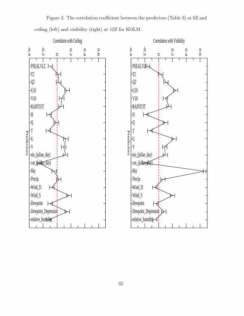
Figure 3. The correlation coefficient between the predictors (Table 3) at 0Z and

ceiling (left) and visibility (right) at 12Z for KOLM.

PSEALVLCT2Q2U10V10RAINTOTHQTUVsin_(julian_day)cos_(julian_day)SkyPrecipWind_DWind_SDewpointDewpoint_Depressionrelative_humidity

Pred

icto

rs

-0

.4

-0

.2 0

0.2

0.4

0.6

Correlation with Ceiling

PSEALVLCT2Q2U10V10RAINTOTHQTUVsin_(julian_day)cos_(julian_day)SkyPrecipWind_DWind_SDewpointDewpoint_Depressionrelative_humidity

Pred

icto

rs

-0

.4

-0

.2 0

0.2

0.4

0.6

Correlation with Visibility

32

Figure 4. The conditional distribution of the predictors (Table 3) at 0Z, condi-

tioned on low (black) and high (red) ceiling at 12Z.

-4 -2 0 2 4x1

0

0.1

0.2

0.3

0.4

0.5

-4 -2 0 2 4x2

0

0.1

0.2

0.3

0.4

0.5

-4 -2 0 2 4x3

0

0.1

0.2

0.3

0.4

0.5

-4 -2 0 2 4x4

0

0.1

0.2

0.3

0.4

0.5

-4 -2 0 2 4x5

0

0.1

0.2

0.3

0.4

0.5

-4 -2 0 2 4x6

0

0.5

1

1.5

2

-4 -2 0 2 4x7

0

0.1

0.2

0.3

0.4

0.5

-4 -2 0 2 4x8

0

0.1

0.2

0.3

0.4

0.5

-4 -2 0 2 4x9

0

0.1

0.2

0.3

0.4

0.5

-4 -2 0 2 4x10

0

0.1

0.2

0.3

0.4

0.5

33

Figure 4. Continued.

-4 -2 0 2 4x11

0

0.1

0.2

0.3

0.4

0.5

0.6

-4 -2 0 2 4x12

0

0.1

0.2

0.3

0.4

0.5

-4 -2 0 2 4x13

0

0.1

0.2

0.3

0.4

0.5

-4 -2 0 2 4x14

0

0.5

1

1.5

-4 -2 0 2 4x15

0

0.5

1

1.5

2

-4 -2 0 2 4x16

0

0.2

0.4

0.6

0.8

-4 -2 0 2 4x17

0

0.1

0.2

0.3

0.4

0.5

0.6

0.7

-4 -2 0 2 4x18

0

0.1

0.2

0.3

0.4

0.5

-4 -2 0 2 4x19

0

0.1

0.2

0.3

0.4

0.5

-4 -2 0 2 4x20

0

0.1

0.2

0.3

0.4

0.5

34

Figure 5. HSS values according to MOS forecasts of ceiling (right) and visibility

(left), for training (black) and validation (red) sets, separately. The error-bars are

derived from bootstrapping.

KACVKALWKASTKBFIKBKEKBLIKBNOKBOIKCECKCLMKCOEKDLSKEATKEKOKEUGKGEGKHQMKLMTKMFRKMSOKMWHKNUWKOLMKPAEKPDTKPDXKPSCKRDDKRDMKSEAKSFFKSKAKSLEKSUNKTCMKTTDKTWFKWMCKYKM

0

0.1

0.2

0.3

0.4

0.5

HSS_MOS

KACVKALWKASTKBFIKBKEKBLIKBNOKBOIKCECKCLMKCOEKDLSKEATKEKOKEUGKGEGKHQMKLMTKMFRKMSOKMWHKNUWKOLMKPAEKPDTKPDXKPSCKRDDKRDMKSEAKSFFKSKAKSLEKSUNKTCMKTTDKTWFKWMCKYKM

0

0.1

0.2

0.3

0.4

0.5

HSS_MOS

35

Figure 6. TV-diagrams, with cross-entropy as the performance measure, for

three stations with different levels of nonlinearity in the data - extreme (top), midrange

(middle), and no nonlinearity (bottom).

2

46

8

2

4

6

8

2

4

6

8

6000 6500 7000 7500Training Performance

3100

3200

3300

3400

3500

3600

Valid

ation P

erform

ance

KACV12nc.eps

2

4

6

82

4

6

8 2

4

6

8

4000 4500 5000 5500 6000 6500 7000Training Performance

3800

4000

4200

4400

Valid

ation P

erform

ance

KEUG12nc.eps

2

4

6

8

24

6

8

2

4

6

8

1000 1500 2000 2500 3000 3500 4000Training Performance

2500

2600

2700

2800

2900

3000

3100

3200

Valid

ation P

erform

ance

KMSO12nc.eps

36

Figure 7. Discrimination diagrams for NN (top) and logistic regression (bottom)

forecasts for KNUW. The forecasts are for 12Z ceiling, and the (optimal) number of

hidden nodes is 6.

0 0.2 0.4 0.6 0.8 1Probability of Low Ceiling

0

1

2

3

4

5

6

7

High Ceiling

Low Ceiling


0

0.5

1

1.5

2

2.5

3

High Ceiling

Low Ceiling

37

Figure 8. Attributes diagrams for NN (top) and logistic regression (bottom)

forecasts for KNUW. The forecasts are for 12Z ceiling, and the (optimal) number of

hidden nodes is 6.


0

0.2

0.4

0.6

0.8

1

Obse

rved

Frac

tion


0

0.2

0.4

0.6

0.8

1

Obse

rved

Frac

tion

38

Figure 9. ROC curves for NN and logistic regression, separately for training

and validation data, and for 3 different seeds (see text).

0 0.2 0.4 0.6 0.8 1False Alarm Rate

0

0.2

0.4

0.6

0.8

1

Prob

abili

ty o

f D

etec

tion

NN_trn

NN_vld

Logistic_trn_vld

39

Figure 10. TV diagrams displaying HSS values of NNs with 2, 4, 6, and 8

hidden nodes, Logistic regression (“L”), and MOS (“M”), for three bootstrap trials

(labeled 1, 2, and 3). The underlying forecasts are 2-class.

2

46

8

24

6 8

2

46

8

L1L2L3

M1

M2

M3

0 0.2 0.4 0.6 0.8 1Training Performance

0

0.2

0.4

0.6

0.8

1Va

lidatio

n Perf

ormanc

e

KAST12-c.eps

24

6

8

2

4 6

8

2

4

68

L1L2L3

M1

M2M3


0

0.2

0.4

0.6

0.8

1

Valid

ation P

erform

ance

KBKE12-c.eps

2

468

2

4

6

8

2

4 6

8

L1L2L3

M1

M2

M3


0

0.2

0.4

0.6

0.8

1

Valid

ation P

erform

ance

KWMC12-c.eps

40

Figure 11. Same as Figure 10, but for ceiling having four classes.

24

6 8

2

46

8

2 4

6 8

L1L2L3

M1M2M3


0

0.2

0.4

0.6

0.8

1

Valid

ation P

erform

ance

KRDM12nc.eps

24

6 8

2 4 6

8

24

6

8

L1L2L3

M1M2M3


0

0.2

0.4

0.6

0.8

1

Valid

ation P

erform

ance

KDLS12nc.eps

2 4

6 8

24

68

24 6

8

L1L2L3

M1

M2M3


0

0.2

0.4

0.6

0.8

1

Valid

ation P

erform

ance

KSKA12nc.eps

41

Appendix

The following are all the figures for the 39 stations, comparing their performance

in terms of HSS. M stands for MOS, L stands for Logistic. The numbers labels 1, 2,

3, refer to three bootstrap trials. The numbers 2, 4, 6, and 8, refer to the number

of hidden nodes in the NN. The notation appearing in the upper left conveys the

following information: station name, forecast time; “-c” refers to 2-class ceiling, and

“nc” refers to 4-class ceiling. The same convention applies to visibility.

42

2 46 8

2 46

8

2 46

8

L1L2L3

M1

M2M3


0

0.2

0.4

0.6

0.8

1

Val

idat

ion

Perf

orm

ance

KACV12-c.eps

24 6

8

24

6 8

24 6

8

L1L2L3

M1

M2

M3


0

0.2

0.4

0.6

0.8

1

Val

idat

ion

Perf

orm

ance

KALW12-c.eps

2

46

8

24

6 8

2

46

8

L1L2L3

M1

M2

M3


0

0.2

0.4

0.6

0.8

1

Val

idat

ion

Perf

orm

ance

KAST12-c.eps

2

4 6

8

2

4 68

24

68

L1L2L3

M1

M2

M3


0

0.2

0.4

0.6

0.8

1

Val

idat

ion

Perf

orm

ance

KBFI12-c.eps

24

6

8

2

4 6

8

2

4

68

L1L2L3

M1

M2M3


0

0.2

0.4

0.6

0.8

1

Val

idat

ion

Perf

orm

ance

KBKE12-c.eps

2

46 8

2

46

8

2

46

8

L1L2L3

M1

M2

M3


0

0.2

0.4

0.6

0.8

1

Val

idat

ion

Perf

orm

ance

KBLI12-c.eps

2

4 68

2

46

8

24 6

8

L1L2L3

M1M2

M3


0

0.2

0.4

0.6

0.8

1

Val

idat

ion

Perf

orm

ance

KBNO12-c.eps

2 4

68

2 4

6 8

2 4

6 8

L1L2L3

M1M2M3


0

0.2

0.4

0.6

0.8

1

Val

idat

ion

Perf

orm

ance

KBOI12-c.eps

24 6

8

2

4 6

8

24 6

8

L1L2L3M1M2

M3


0

0.2

0.4

0.6

0.8

1

Val

idat

ion

Perf

orm

ance

KCEC12-c.eps

43

24

6 8

2

46

8

24

6

8

L1L2L3M1M2M3


0

0.2

0.4

0.6

0.8

1

Val

idat

ion

Perf

orm

ance

KCLM12-c.eps

24

68

2 4

6 8

24

68

L1L2L3

M1

M2M3


0

0.2

0.4

0.6

0.8

1

Val

idat

ion

Perf

orm

ance

KCOE12-c.eps

2 4 6 82 4

68

24 6 8

L1L2L3

M1

M2

M3


0

0.2

0.4

0.6

0.8

1

Val

idat

ion

Perf

orm

ance

KDLS12-c.eps

24

6 8

2 4

6 8

24

6 8

L1L2L3

M1M2

M3


0

0.2

0.4

0.6

0.8

1

Val

idat

ion

Perf

orm

ance

KEAT12-c.eps

2

46

8

2

46

8

2

4

6 8

L1L2L3

M1

M2

M3


0

0.2

0.4

0.6

0.8

1

Val

idat

ion

Perf

orm

ance

KEKO12-c.eps

2

4 6 8

24 6

8

2

46 8

L1L2L3

M1

M2M3


0

0.2

0.4

0.6

0.8

1

Val

idat

ion

Perf

orm

ance

KEUG12-c.eps

24

68

24

6 8

2 46

8

L1L2L3M1

M2

M3


0

0.2

0.4

0.6

0.8

1

Val

idat

ion

Perf

orm

ance

KGEG12-c.eps

2

46 8

2 46

8

24

68

L1L2L3

M1M2M3


0

0.2

0.4

0.6

0.8

1

Val

idat

ion

Perf

orm

ance

KHQM12-c.eps

2

46

8

2

46 8

2

46

8

L1L2L3

M1

M2M3


0

0.2

0.4

0.6

0.8

1

Val

idat

ion

Perf

orm

ance

KLMT12-c.eps

44

2

4 6 8

2

4

68

24

6

8

L1L2L3

M1M2M3


0

0.2

0.4

0.6

0.8

1

Val

idat

ion

Perf

orm

ance

KMFR12-c.eps

2

46

8

24

6 8

2 4

68

L1L2L3

M1

M2

M3


0

0.2

0.4

0.6

0.8

1

Val

idat

ion

Perf

orm

ance

KMSO12-c.eps

2

4

6

8

24

6

8

24 6

8

L1L2L3

M1

M2

M3


0

0.2

0.4

0.6

0.8

1

Val

idat

ion

Perf

orm

ance

KMWH12-c.eps

2 4

6 8

2 4

6

8

2 4

6 8

L1L2L3

M1M2

M3


0

0.2

0.4

0.6

0.8

1

Val

idat

ion

Perf

orm

ance

KNUW12-c.eps

2 46

8

24 6

8

2 46 8

L1L2L3M1

M2M3


0

0.2

0.4

0.6

0.8

1

Val

idat

ion

Perf

orm

ance

KOLM12-c.eps

24

6

8

24

6

8

24 6

8

L1L2L3

M1

M2M3


0

0.2

0.4

0.6

0.8

1

Val

idat

ion

Perf

orm

ance

KPAE12-c.eps

24

6

8

2

4 6 8

2

4 6 8

L1L2L3M1

M2M3


0

0.2

0.4

0.6

0.8

1

Val

idat

ion

Perf

orm

ance

KPDT12-c.eps

2

46

8

2

4

6 8

2

4

6

8

L1L2L3

M1

M2

M3


0

0.2

0.4

0.6

0.8

1

Val

idat

ion

Perf

orm

ance

KPDX12-c.eps

24

68

2 4 6

82

4 68

L1L2L3

M1

M2

M3


0

0.2

0.4

0.6

0.8

1

Val

idat

ion

Perf

orm

ance

KPSC12-c.eps

45

2

46 8

2

4

6 8

2 46

8

L1L2L3

M1

M2

M3


0

0.2

0.4

0.6

0.8

1

Val

idat

ion

Perf

orm

ance

KRDD12-c.eps

24

6 82

4 68

2

4 6

8

L1L2L3

M1

M2M3


0

0.2

0.4

0.6

0.8

1

Val

idat

ion

Perf

orm

ance

KRDM12-c.eps

2 4

68

2

4 6

8

2

46 8

L1L2L3

M1

M2

M30 0.2 0.4 0.6 0.8 1

Training Performance

0

0.2

0.4

0.6

0.8

1

Val

idat

ion

Perf

orm

ance

KSEA12-c.eps

2 4

6 8

2 4

6 8

2 4

6 8

L1L2L3

M1

M2

M3


0

0.2

0.4

0.6

0.8

1

Val

idat

ion

Perf

orm

ance

KSFF12-c.eps

24 6 8

2 4

68

2 4 6 8

L1L2L3M1

M2M3


0

0.2

0.4

0.6

0.8

1

Val

idat

ion

Perf

orm

ance

KSKA12-c.eps

24

6

8

2 46

8

2

4 6

8

L1L2L3

M1

M2M3


0

0.2

0.4

0.6

0.8

1

Val

idat

ion

Perf

orm

ance

KSLE12-c.eps

2 46 8

2 4

6 82

4 68

L1L2L3

M1

M2

M3


0

0.2

0.4

0.6

0.8

1

Val

idat

ion

Perf

orm

ance

KSUN12-c.eps

24

6

8

24

6

8

2

4

68

L1L2L3

M1M2

M3


0

0.2

0.4

0.6

0.8

1

Val

idat

ion

Perf

orm

ance

KTCM12-c.eps

24

6 8

2

46

8

2 4

6

8

L1L2L3M1M2M3


0

0.2

0.4

0.6

0.8

1

Val

idat

ion

Perf

orm

ance

KTTD12-c.eps

46

2

46

8

2 4

6 8

24

68

L1L2L3

M1

M2

M3


0

0.2

0.4

0.6

0.8

1

Val

idat

ion

Perf

orm

ance

KTWF12-c.eps

2

468

2

4

6

8

2

4 6

8

L1L2L3

M1

M2

M3


0

0.2

0.4

0.6

0.8

1

Val

idat

ion

Perf

orm

ance

KWMC12-c.eps

24

6

82

4

6 8

2

4 6 8

L1L2L3

M1

M2

M3


0

0.2

0.4

0.6

0.8

1

Val

idat

ion

Perf

orm

ance

KYKM12-c.eps

47

2

46

8

2

46

8

2

46

8

L1L2L3

M1M2M3


0

0.2

0.4

0.6

0.8

1

Val

idat

ion

Perf

orm

ance

KACV12nc.eps

2

4

6

8

2

4

68

24

6 8

L1L2L3

M1M2

M3


0

0.2

0.4

0.6

0.8

1

Val

idat

ion

Perf

orm

ance

KALW12nc.eps

24

6 8

24

6 8

24

6 8

L1L2L3

M1

M2

M3


0

0.2

0.4

0.6

0.8

1

Val

idat

ion

Perf

orm

ance

KAST12nc.eps

2

46 8

2

468

2

4 6

8

L1L2L3

M1

M2M3


0

0.2

0.4

0.6

0.8

1

Val

idat

ion

Perf

orm

ance

KBFI12nc.eps

2

4

6

8

2

4

68

2

46

8

L1L2L3

M1M2M3


0

0.2

0.4

0.6

0.8

1

Val

idat

ion

Perf

orm

ance

KBKE12nc.eps

2

4

6 8

2

46

8

2

4

68

L1L2L3

M1M2

M3


0

0.2

0.4

0.6

0.8

1

Val

idat

ion

Perf

orm

ance

KBLI12nc.eps

2

4 6

8

2

4

68

2

46

8

L1L2L3

M1

M2

M3


0

0.2

0.4

0.6

0.8

1

Val

idat

ion

Perf

orm

ance

KBNO12nc.eps

2

46 8

2

46

8

2

4

6

8

L1L2L3

M1M2M3


0

0.2

0.4

0.6

0.8

1

Val

idat

ion

Perf

orm

ance

KBOI12nc.eps

24 6

8

24 6

8

2

46 8

L1L2L3

M1M2

M3


0

0.2

0.4

0.6

0.8

1

Val

idat

ion

Perf

orm

ance

KCEC12nc.eps

48

2

46

8

2

46

8

2

46

8

L1L2L3

M1M2M3


0

0.2

0.4

0.6

0.8

1

Val

idat

ion

Perf

orm

ance

KCLM12nc.eps

2

468

2

46 8

2

46

8

L1L2L3

M1

M2

M3


0

0.2

0.4

0.6

0.8

1

Val

idat

ion

Perf

orm

ance

KCOE12nc.eps

24

6 8

2 4 6

8

24

6

8

L1L2L3

M1M2M3


0

0.2

0.4

0.6

0.8

1

Val

idat

ion

Perf

orm

ance

KDLS12nc.eps

24

6 82

46 8

2 46 8

L1L2L3

M1M2M3


0

0.2

0.4

0.6

0.8

1

Val

idat

ion

Perf

orm

ance

KEAT12nc.eps

2

46

8

2

4

6

8

2

4

68

L1L2L3

M1M2

M3


0

0.2

0.4

0.6

0.8

1

Val

idat

ion

Perf

orm

ance

KEKO12nc.eps

2

4 68

2

46 8

2

4 68

L1L2L3

M1

M2

M3


0

0.2

0.4

0.6

0.8

1

Val

idat

ion

Perf

orm

ance

KEUG12nc.eps

24

6 8

24

6 8

2 46 8

L1L2L3

M1

M2

M3


0

0.2

0.4

0.6

0.8

1

Val

idat

ion

Perf

orm

ance

KGEG12nc.eps

24

68

2

46

8

24 6

8

L1L2L3

M1

M2M3


0

0.2

0.4

0.6

0.8

1

Val

idat

ion

Perf

orm

ance

KHQM12nc.eps

2

4

6 8

2

4

6 8

2

46

8

L1L2L3

M1M2

M3


0

0.2

0.4

0.6

0.8

1

Val

idat

ion

Perf

orm

ance

KLMT12nc.eps

49

24 6

8

24 6

8

24

6 8

L1L2L3

M1M2M3


0

0.2

0.4

0.6

0.8

1

Val

idat

ion

Perf

orm

ance

KMFR12nc.eps

2

4

6

8

2

46

8

2

4

6 8

L1L2L3

M1

M2

M3


0

0.2

0.4

0.6

0.8

1

Val

idat

ion

Perf

orm

ance

KMSO12nc.eps

2

4 6 8

2

46

8

2

4

6

8

L1L2L3

M1M2

M3


0

0.2

0.4

0.6

0.8

1

Val

idat

ion

Perf

orm

ance

KMWH12nc.eps

2 4

68

24

68

2

4 6

8

L1L2L3

M1

M2

M3


0

0.2

0.4

0.6

0.8

1

Val

idat

ion

Perf

orm

ance

KNUW12nc.eps

2

46

8

2

4 6 8

24

68

L1L2L3

M1M2M3


0

0.2

0.4

0.6

0.8

1

Val

idat

ion

Perf

orm

ance

KOLM12nc.eps

2

46

8

24

6 8

2

4 6

8

L1L2L3

M1M2

M3


0

0.2

0.4

0.6

0.8

1

Val

idat

ion

Perf

orm

ance

KPAE12nc.eps

24

6 8

24

6 8

2

46

8

L1L2L3

M1M2M3


0

0.2

0.4

0.6

0.8

1

Val

idat

ion

Perf

orm

ance

KPDT12nc.eps

2

4

68

2

4

6 8

2

4

68

L1L2L3

M1M2

M3


0

0.2

0.4

0.6

0.8

1

Val

idat

ion

Perf

orm

ance

KPDX12nc.eps

2

4 6

8

2

4 6

8

2

46

8

L1L2L3

M1

M2

M3


0

0.2

0.4

0.6

0.8

1

Val

idat

ion

Perf

orm

ance

KPSC12nc.eps

50

24

68

24

6

8

24

68

L1L2L3

M1M2

M3


0

0.2

0.4

0.6

0.8

1

Val

idat

ion

Perf

orm

ance

KRDD12nc.eps

24

6 8

2

46

8

2 4

6 8

L1L2L3

M1M2M3


0

0.2

0.4

0.6

0.8

1

Val

idat

ion

Perf

orm

ance

KRDM12nc.eps

2

46

8

24 6

8

24

6 8

L1L2L3

M1

M2M3


0

0.2

0.4

0.6

0.8

1

Val

idat

ion

Perf

orm

ance

KSEA12nc.eps

2

46

8

2

4 68

2

46

8

L1L2L3

M1

M2

M3


0

0.2

0.4

0.6

0.8

1

Val

idat

ion

Perf

orm

ance

KSFF12nc.eps

2 4

6 8

24

68

24 6

8

L1L2L3

M1

M2M3


0

0.2

0.4

0.6

0.8

1

Val

idat

ion

Perf

orm

ance

KSKA12nc.eps

2

4

6

8

2

4

68

2

4

68

L1L2L3

M1

M2

M3


0

0.2

0.4

0.6

0.8

1

Val

idat

ion

Perf

orm

ance

KSLE12nc.eps

2

4

6 8

2

4 6

8

2

4

6 8

L1L2L3

M1M2M3


0

0.2

0.4

0.6

0.8

1

Val

idat

ion

Perf

orm

ance

KSUN12nc.eps

2

46

8

2

46 8

2

4

68

L1L2L3

M1M2

M3


0

0.2

0.4

0.6

0.8

1

Val

idat

ion

Perf

orm

ance

KTCM12nc.eps

24 6

8

2 4

6 8

24

68

L1L2L3

M1M2

M3


0

0.2

0.4

0.6

0.8

1

Val

idat

ion

Perf

orm

ance

KTTD12nc.eps

51

2

4

68

2

46

8

2

4

6

8

L1L2L3

M1

M2M3


0

0.2

0.4

0.6

0.8

1

Val

idat

ion

Perf

orm

ance

KTWF12nc.eps

2

46

8

2

4 6

8

2

4

6 8

L1L2L3

M1

M2M3


0

0.2

0.4

0.6

0.8

1

Val

idat

ion

Perf

orm

ance

KWMC12nc.eps

2

4 68

2 4

6

82

4 68

L1L2L3

M1M2M3


0

0.2

0.4

0.6

0.8

1

Val

idat

ion

Perf

orm

ance

KYKM12nc.eps

52

24

242 4

L1

L2L3

M1M2

M3


0

0.2

0.4

0.6

0.8

1

Val

idat

ion

Perf

orm

ance

KACV06-c.eps

2

4

2 42 4L1L2L3

M1

M2

M3


0

0.2

0.4

0.6

0.8

1

Val

idat

ion

Perf

orm

ance

KALW06-c.eps

24

2

4

24

L1L2L3

M1

M2

M3


0

0.2

0.4

0.6

0.8

1

Val

idat

ion

Perf

orm

ance

KAST06-c.eps

24

24

24

L1L2L3

M1

M2

M3


0

0.2

0.4

0.6

0.8

1

Val

idat

ion

Perf

orm

ance

KBFI06-c.eps

24

242

4

L1L2L3

M1

M2

M3


0

0.2

0.4

0.6

0.8

1

Val

idat

ion

Perf

orm

ance

KBKE06-c.eps

2 42

42 4

L1L2L3

M1

M2

M3


0

0.2

0.4

0.6

0.8

1

Val

idat

ion

Perf

orm

ance

KBLI06-c.eps

2 42

4

24

L1L2L3

M1

M2

M3


0

0.2

0.4

0.6

0.8

1

Val

idat

ion

Perf

orm

ance

KBNO06-c.eps

2

42 42

4

L1L2L3 M1

M2

M3


0

0.2

0.4

0.6

0.8

1

Val

idat

ion

Perf

orm

ance

KBOI06-c.eps

24

2

42

4

L1L2L3

M1

M2M3


0

0.2

0.4

0.6

0.8

1

Val

idat

ion

Perf

orm

ance

KCEC06-c.eps

53

2 42

424

L1L2L3

M1M2

M3


0

0.2

0.4

0.6

0.8

1

Val

idat

ion

Perf

orm

ance

KCLM06-c.eps

2 42 42 4

L1L2L3

M1

M2

M3


0

0.2

0.4

0.6

0.8

1

Val

idat

ion

Perf

orm

ance

KCOE06-c.eps

2

4

24

2

4

L1L2L3

M1

M2

M3


0

0.2

0.4

0.6

0.8

1

Val

idat

ion

Perf

orm

ance

KDLS06-c.eps

242

42 4

L1L2L3

M1M2

M3


0

0.2

0.4

0.6

0.8

1

Val

idat

ion

Perf

orm

ance

KEAT06-c.eps

2

4

2

4

2

4

L1L2

L3

M1

M2

M3


0

0.2

0.4

0.6

0.8

1

Val

idat

ion

Perf

orm

ance

KEKO06-c.eps

242 42 4

L1L2L3

M1M2

M3


0

0.2

0.4

0.6

0.8

1

Val

idat

ion

Perf

orm

ance

KEUG06-c.eps

2 42 42

4

L1L2L3

M1

M2

M3


0

0.2

0.4

0.6

0.8

1

Val

idat

ion

Perf

orm

ance

KGEG06-c.eps

2

4

24

24

L1L2L3

M1

M2M3


0

0.2

0.4

0.6

0.8

1

Val

idat

ion

Perf

orm

ance

KHQM06-c.eps

2

4

2

4

2

4

L1L2L3

M1

M2M3


0

0.2

0.4

0.6

0.8

1

Val

idat

ion

Perf

orm

ance

KLMT06-c.eps

54

24

24

2 4

L1L2L3

M1M2M3


0

0.2

0.4

0.6

0.8

1

Val

idat

ion

Perf

orm

ance

KMFR06-c.eps

242 4

24

L1L2L3

M1

M2

M3


0

0.2

0.4

0.6

0.8

1

Val

idat

ion

Perf

orm

ance

KMSO06-c.eps

2 42

42 4

L1L2L3

M1

M2

M3


0

0.2

0.4

0.6

0.8

1

Val

idat

ion

Perf

orm

ance

KMWH06-c.eps

2 42

4

24

L1L2L3

M1

M2

M3


0

0.2

0.4

0.6

0.8

1

Val

idat

ion

Perf

orm

ance

KNUW06-c.eps

2

4

2

4

2

4

L1L2L3

M1

M2M3


0

0.2

0.4

0.6

0.8

1

Val

idat

ion

Perf

orm

ance

KOLM06-c.eps

242 4

2 4

L1L2L3

M1

M2M3


0

0.2

0.4

0.6

0.8

1

Val

idat

ion

Perf

orm

ance

KPAE06-c.eps

2 42

42 4L1L2L3

M1M2

M3


0

0.2

0.4

0.6

0.8

1

Val

idat

ion

Perf

orm

ance

KPDT06-c.eps

2

4

2

4

2

4

L1L2L3

M1

M2

M3


0

0.2

0.4

0.6

0.8

1

Val

idat

ion

Perf

orm

ance

KPDX06-c.eps

24

24

24

L1L2L3

M1

M2

M3


0

0.2

0.4

0.6

0.8

1

Val

idat

ion

Perf

orm

ance

KPSC06-c.eps

55

2 424

2 4

L1L2L3M1

M2

M3


0

0.2

0.4

0.6

0.8

1

Val

idat

ion

Perf

orm

ance

KRDD06-c.eps

24

242 4

L1L2L3

M1

M2

M3


0

0.2

0.4

0.6

0.8

1

Val

idat

ion

Perf

orm

ance

KRDM06-c.eps

24

2

4

2

4

L1L2L3

M1

M2

M3


0

0.2

0.4

0.6

0.8

1

Val

idat

ion

Perf

orm

ance

KSEA06-c.eps

2

42

4

24

L1L2L3

M1

M2M3


0

0.2

0.4

0.6

0.8

1

Val

idat

ion

Perf

orm

ance

KSFF06-c.eps

2

42

42

4

L1L2L3

M1

M2M3


0

0.2

0.4

0.6

0.8

1

Val

idat

ion

Perf

orm

ance

KSKA06-c.eps

2

4

2

42

4

L1L2L3

M1

M2

M3


0

0.2

0.4

0.6

0.8

1

Val

idat

ion

Perf

orm

ance

KSLE06-c.eps

2 42 42 4

L1L2L3

M1M2

M3


0

0.2

0.4

0.6

0.8

1

Val

idat

ion

Perf

orm

ance

KSUN06-c.eps

2

4

2

4

2

4

L1L2L3

M1M2M3


0

0.2

0.4

0.6

0.8

1

Val

idat

ion

Perf

orm

ance

KTCM06-c.eps

2

4

2

4

2

4

L1L2L3

M1

M2

M3


0

0.2

0.4

0.6

0.8

1

Val

idat

ion

Perf

orm

ance

KTTD06-c.eps

56

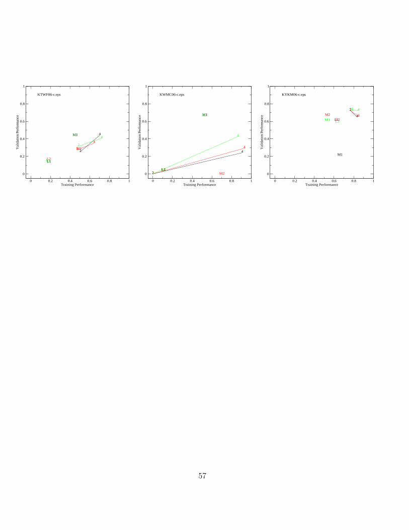
2

4

2

42

4

L1L2L3

M1

M2

M3


0

0.2

0.4

0.6

0.8

1

Val

idat

ion

Perf

orm

ance

KTWF06-c.eps

2

4

2

4

2

4

L1L2L3

M1

M2

M3


0

0.2

0.4

0.6

0.8

1

Val

idat

ion

Perf

orm

ance

KWMC06-c.eps

2

4

2

4

2 4

L1L2L3

M1

M2

M3


0

0.2

0.4

0.6

0.8

1

Val

idat

ion

Perf

orm

ance

KYKM06-c.eps

57

2

4

2424

L1L2L3

M1

M2M3


0

0.2

0.4

0.6

0.8

1

Val

idat

ion

Perf

orm

ance

KACV06nc.eps

24

2

4

24

L1L2L3

M1

M2

M3


0

0.2

0.4

0.6

0.8

1

Val

idat

ion

Perf

orm

ance

KALW06nc.eps

24

242

4

L1L2L3

M1M2M3


0

0.2

0.4

0.6

0.8

1

Val

idat

ion

Perf

orm

ance

KAST06nc.eps

24

2

4

2

4

L1L2L3

M1M2

M3


0

0.2

0.4

0.6

0.8

1

Val

idat

ion

Perf

orm

ance

KBFI06nc.eps

242 4

2 4

L1L2L3

M1

M2

M3


0

0.2

0.4

0.6

0.8

1

Val

idat

ion

Perf

orm

ance

KBKE06nc.eps

24

2

4

2

4

L1L2L3

M1

M2

M3


0

0.2

0.4

0.6

0.8

1

Val

idat

ion

Perf

orm

ance

KBLI06nc.eps

2

4

2

4

2

4

L1L2L3

M1M2M3


0

0.2

0.4

0.6

0.8

1

Val

idat

ion

Perf

orm

ance

KBNO06nc.eps

2

4

2

4

24

L1L2L3

M1M2

M3


0

0.2

0.4

0.6

0.8

1

Val

idat

ion

Perf

orm

ance

KBOI06nc.eps

24

24

24

L1L2L3

M1M2

M3


0

0.2

0.4

0.6

0.8

1

Val

idat

ion

Perf

orm

ance

KCEC06nc.eps

58

2

4

2

4

2

4

L1L2L3

M1M2M3


0

0.2

0.4

0.6

0.8

1

Val

idat

ion

Perf

orm

ance

KCLM06nc.eps

24 24

2

4

L1L2L3

M1M2M3


0

0.2

0.4

0.6

0.8

1

Val

idat

ion

Perf

orm

ance

KCOE06nc.eps

24

24

2

4

L1L2L3

M1

M2

M3


0

0.2

0.4

0.6

0.8

1

Val

idat

ion

Perf

orm

ance

KDLS06nc.eps

2

4

2

4

2

4

L1L2L3

M1

M2M3


0

0.2

0.4

0.6

0.8

1

Val

idat

ion

Perf

orm

ance

KEAT06nc.eps

2

4

2

4

2

4

L1L2L3

M1M2

M3


0

0.2

0.4

0.6

0.8

1

Val

idat

ion

Perf

orm

ance

KEKO06nc.eps

24

24

2

4

L1L2L3

M1M2

M3


0

0.2

0.4

0.6

0.8

1

Val

idat

ion

Perf

orm

ance

KEUG06nc.eps

24

2

4

24

L1L2L3

M1M2

M3


0

0.2

0.4

0.6

0.8

1

Val

idat

ion

Perf

orm

ance

KGEG06nc.eps

2

4

2

4

2

4

L1L2L3

M1M2M3


0

0.2

0.4

0.6

0.8

1

Val

idat

ion

Perf

orm

ance

KHQM06nc.eps

2

4

2

4

2

4

L1L2L3

M1M2M3


0

0.2

0.4

0.6

0.8

1

Val

idat

ion

Perf

orm

ance

KLMT06nc.eps

59

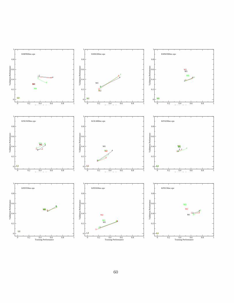
242

42

4

L1L2L3

M1M2

M3


0

0.2

0.4

0.6

0.8

1

Val

idat

ion

Perf

orm

ance

KMFR06nc.eps

2

4

2

4

2

4

L1L2L3

M1

M2M3


0

0.2

0.4

0.6

0.8

1

Val

idat

ion

Perf

orm

ance

KMSO06nc.eps

2

42

42

4

L1L2L3

M1M2

M3


0

0.2

0.4

0.6

0.8

1

Val

idat

ion

Perf

orm

ance

KMWH06nc.eps

2

4

2 42

4

L1L2L3

M1M2M3


0

0.2

0.4

0.6

0.8

1

Val

idat

ion

Perf

orm

ance

KNUW06nc.eps

2

4

2

42

4

L1L2L3

M1

M2M3


0

0.2

0.4

0.6

0.8

1

Val

idat

ion

Perf

orm

ance

KOLM06nc.eps

24

24

2

4

L1L2L3

M1M2M3


0

0.2

0.4

0.6

0.8

1

Val

idat

ion

Perf

orm

ance

KPAE06nc.eps

2

4

2

4

2

4

L1L2L3

M1M2M3


0

0.2

0.4

0.6

0.8

1

Val

idat

ion

Perf

orm

ance

KPDT06nc.eps

2

4

2

4

2

4

L1L2L3

M1

M2

M3


0

0.2

0.4

0.6

0.8

1

Val

idat

ion

Perf

orm

ance

KPDX06nc.eps

24

2 42

4

L1L2L3

M1

M2

M3


0

0.2

0.4

0.6

0.8

1

Val

idat

ion

Perf

orm

ance

KPSC06nc.eps

60

242 4

2 4

L1L2L3

M1

M2M3


0

0.2

0.4

0.6

0.8

1

Val

idat

ion

Perf

orm

ance

KRDD06nc.eps

2

424

2

4

L1L2L3

M1M2

M3


0

0.2

0.4

0.6

0.8

1

Val

idat

ion

Perf

orm

ance

KRDM06nc.eps

2 4

2

42

4

L1L2L3

M1

M2

M3


0

0.2

0.4

0.6

0.8

1

Val

idat

ion

Perf

orm

ance

KSEA06nc.eps

2

42

4

2

4

L1L2L3

M1M2

M3


0

0.2

0.4

0.6

0.8

1

Val

idat

ion

Perf

orm

ance

KSFF06nc.eps

2

4

2

4

2

4

L1L2L3

M1

M2M3


0

0.2

0.4

0.6

0.8

1

Val

idat

ion

Perf

orm

ance

KSKA06nc.eps

2

4

2

4

2

4

L1L2L3

M1M2

M3


0

0.2

0.4

0.6

0.8

1

Val

idat

ion

Perf

orm

ance

KSLE06nc.eps

2

42

42 4

L1L2L3

M1M2M3


0

0.2

0.4

0.6

0.8

1

Val

idat

ion

Perf

orm

ance

KSUN06nc.eps

2

4

24

2

4

L1L2L3

M1

M2M3


0

0.2

0.4

0.6

0.8

1

Val

idat

ion

Perf

orm

ance

KTCM06nc.eps

24

2

42

4

L1L2L3

M1M2M3


0

0.2

0.4

0.6

0.8

1

Val

idat

ion

Perf

orm

ance

KTTD06nc.eps

61

2

42

4

24

L1L2L3

M1M2

M3


0

0.2

0.4

0.6

0.8

1

Val

idat

ion

Perf

orm

ance

KTWF06nc.eps

2

4

2

4

2

4

L1L2L3

M1M2

M3


0

0.2

0.4

0.6

0.8

1

Val

idat

ion

Perf

orm

ance

KWMC06nc.eps

24

2

42

4

L1L2L3

M1

M2

M3


0

0.2

0.4

0.6

0.8

1

Val

idat

ion

Perf

orm

ance

KYKM06nc.eps

62

2

4

6

2

4

6

2

46

L1L2L3

M1

M2

M3


0

0.2

0.4

0.6

0.8

1

Val

idat

ion

Perf

orm

ance

KACV12-v.eps

24

6

2

4 62

4

6

L1L2L3

M1

M2

M3


0

0.2

0.4

0.6

0.8

1

Val

idat

ion

Perf

orm

ance

KALW12-v.eps

2

46

2

4

6

2

4

6

L1L2L3M1M2

M3


0

0.2

0.4

0.6

0.8

1

Val

idat

ion

Perf

orm

ance

KAST12-v.eps

2

46

2 46

2

4 6

L1L2L3

M1

M2

M3


0

0.2

0.4

0.6

0.8

1

Val

idat

ion

Perf

orm

ance

KBFI12-v.eps

2

4

6

2

4

6

2

4

6

L1L2L3M1

M2

M3


0

0.2

0.4

0.6

0.8

1

Val

idat

ion

Perf

orm

ance

KBKE12-v.eps

2

462 4

6

24

6

L1L2L3

M1

M2

M3


0

0.2

0.4

0.6

0.8

1

Val

idat

ion

Perf

orm

ance

KBLI12-v.eps

2

4

6

2

4

6

2

4

6

L1L2L3

M1M2

M3


0

0.2

0.4

0.6

0.8

1

Val

idat

ion

Perf

orm

ance

KBNO12-v.eps

2

4

6

2

4

6

2

4

6

L1L2L3

M1

M2

M3


0

0.2

0.4

0.6

0.8

1

Val

idat

ion

Perf

orm

ance

KBOI12-v.eps

24

6

2 4

6

24

6

L1L2L3

M1

M2M3


0

0.2

0.4

0.6

0.8

1

Val

idat

ion

Perf

orm

ance

KCEC12-v.eps

63

2

4

6

2

4

6

2

4

6

L1L2L3 M1

M2

M3


0

0.2

0.4

0.6

0.8

1

Val

idat

ion

Perf

orm

ance

KCLM12-v.eps

24

6

2

4

6

2

46

L1L2L3M1M2M3


0

0.2

0.4

0.6

0.8

1

Val

idat

ion

Perf

orm

ance

KCOE12-v.eps

2

4 6

2

4 6

24

6

L1L2L3

M1

M2

M3


0

0.2

0.4

0.6

0.8

1

Val

idat

ion

Perf

orm

ance

KDLS12-v.eps

2

4 6

2

46

2

4 6

L1L2L3

M1M2

M3


0

0.2

0.4

0.6

0.8

1

Val

idat

ion

Perf

orm

ance

KEAT12-v.eps

2

46

2

4

6

2

46

L1

L2

L3

M1M2M3


0

0.2

0.4

0.6

0.8

1

Val

idat

ion

Perf

orm

ance

KEKO12-v.eps

24

6

24

6

2

4

6

L1L2L3

M1M2

M3


0

0.2

0.4

0.6

0.8

1

Val

idat

ion

Perf

orm

ance

KEUG12-v.eps

2

4

6

2

4

6

2

4 6

L1L2L3

M1

M2M3


0

0.2

0.4

0.6

0.8

1

Val

idat

ion

Perf

orm

ance

KGEG12-v.eps

2

4

6

2

4 6

2

4

6

L1L2L3

M1

M2

M3


0

0.2

0.4

0.6

0.8

1

Val

idat

ion

Perf

orm

ance

KHQM12-v.eps

2 4

6

24

6

24 6

L1L2L3M1

M2

M3


0

0.2

0.4

0.6

0.8

1

Val

idat

ion

Perf

orm

ance

KLMT12-v.eps

64

2 46

2 4 62

4 6

L1L2L3

M1

M2M3


0

0.2

0.4

0.6

0.8

1

Val

idat

ion

Perf

orm

ance

KMFR12-v.eps

2

46

24

6

2

4 6

L1L2L3

M1

M2M3


0

0.2

0.4

0.6

0.8

1

Val

idat

ion

Perf

orm

ance

KMSO12-v.eps

2

4 6

2

4 6

2

4

6

L1L2

L3

M1

M2M3


0

0.2

0.4

0.6

0.8

1

Val

idat

ion

Perf

orm

ance

KMWH12-v.eps

2

4

6

2

4

6

24

6

L1L2L3M1

M2

M3


0

0.2

0.4

0.6

0.8

1

Val

idat

ion

Perf

orm

ance

KNUW12-v.eps

24

624

62 4 6

L1L2L3

M1

M2M3


0

0.2

0.4

0.6

0.8

1

Val

idat

ion

Perf

orm

ance

KOLM12-v.eps

24 6

2

46

24

6

L1L2L3

M1

M2

M3


0

0.2

0.4

0.6

0.8

1

Val

idat

ion

Perf

orm

ance

KPAE12-v.eps

2

4 6

2

4 6

24 6

L1L2L3

M1

M2M3


0

0.2

0.4

0.6

0.8

1

Val

idat

ion

Perf

orm

ance

KPDT12-v.eps

2

4

6

2

46

2

4 6

L1L2L3

M1M2M3


0

0.2

0.4

0.6

0.8

1

Val

idat

ion

Perf

orm

ance

KPDX12-v.eps

2

46

2

4

6

2

4

6

L1L2L3

M1M2

M3


0

0.2

0.4

0.6

0.8

1

Val

idat

ion

Perf

orm

ance

KPSC12-v.eps

65

2

46

2

4

6

2

4 6

L1L2

L3

M1M2

M3


0

0.2

0.4

0.6

0.8

1

Val

idat

ion

Perf

orm

ance

KRDD12-v.eps

24

6

2

4

6

24

6

L1L2L3 M1

M2M3


0

0.2

0.4

0.6

0.8

1

Val

idat

ion

Perf

orm

ance

KRDM12-v.eps

2 46

24 62

46

L1L2L3

M1

M2M3


0

0.2

0.4

0.6

0.8

1

Val

idat

ion

Perf

orm

ance

KSEA12-v.eps

2

4

6

2

46

2

4

6

L1L2L3M1M2M3


0

0.2

0.4

0.6

0.8

1

Val

idat

ion

Perf

orm

ance

KSFF12-v.eps

2

4 6

2

4 6

2

46

L1L2L3

M1

M2M3


0

0.2

0.4

0.6

0.8

1

Val

idat

ion

Perf

orm

ance

KSKA12-v.eps

2

46

24

6

24

6

L1L2L3

M1

M2

M3


0

0.2

0.4

0.6

0.8

1

Val

idat

ion

Perf

orm

ance

KSLE12-v.eps

2

46

2

4 6

2

46

L1

L2L3

M1M2M3


0

0.2

0.4

0.6

0.8

1

Val

idat

ion

Perf

orm

ance

KSUN12-v.eps

24

6

2

46

24 6

L1L2L3

M1

M2

M3


0

0.2

0.4

0.6

0.8

1

Val

idat

ion

Perf

orm

ance

KTCM12-v.eps

2

4

6

2

4

6

2

4

6

L1L2L3M1M2M3


0

0.2

0.4

0.6

0.8

1

Val

idat

ion

Perf

orm

ance

KTTD12-v.eps

66

2

4

6

2

4

6

2

4 6

L1L2L3 M1

M2

M3


0

0.2

0.4

0.6

0.8

1

Val

idat

ion

Perf

orm

ance

KTWF12-v.eps

2 462 462 46

L1 L2L3M1M2M3


0

0.2

0.4

0.6

0.8

1

Val

idat

ion

Perf

orm

ance

KWMC12-v.eps

2

4 6

2

46

2

4

6

L1L2L3

M1

M2

M3


0

0.2

0.4

0.6

0.8

1

Val

idat

ion

Perf

orm

ance

KYKM12-v.eps

67

24

6

2

4

6

2

4

6

L1L2L3

M1M2M3


0

0.2

0.4

0.6

0.8

1

Val

idat

ion

Perf

orm

ance

KACV12nv.eps

2 4 6

2

46

2

4

6

L1L2L3

M1M2

M3


0

0.2

0.4

0.6

0.8

1

Val

idat

ion

Perf

orm

ance

KALW12nv.eps

2

4

6

2

46

2

4

6

L1L2L3M1

M2

M3


0

0.2

0.4

0.6

0.8

1

Val

idat

ion

Perf

orm

ance

KAST12nv.eps

2

46

24

6

24

6

L1L2L3

M1

M2

M3


0

0.2

0.4

0.6

0.8

1

Val

idat

ion

Perf

orm

ance

KBFI12nv.eps

2

4

6

2

4

6

2

4

6

L1L2L3

M1M2

M3


0

0.2

0.4

0.6

0.8

1

Val

idat

ion

Perf

orm

ance

KBKE12nv.eps

24

62

46

24

6

L1L2L3

M1

M2

M3


0

0.2

0.4

0.6

0.8

1

Val

idat

ion

Perf

orm

ance

KBLI12nv.eps

2

4

6

2

4

6

2

4

6

L1L2L3

M1M2

M3


0

0.2

0.4

0.6

0.8

1

Val

idat

ion

Perf

orm

ance

KBNO12nv.eps

2

4

6

2

4

6

2

4

6

L1L2L3

M1M2

M3


0

0.2

0.4

0.6

0.8

1

Val

idat

ion

Perf

orm

ance

KBOI12nv.eps

2

4 6

2

4

6

2

4

6

L1L2L3

M1

M2M3


0

0.2

0.4

0.6

0.8

1

Val

idat

ion

Perf

orm

ance

KCEC12nv.eps

68

2

46

2

4

6

24

6

L1L2L3

M1

M2

M3


0

0.2

0.4

0.6

0.8

1

Val

idat

ion

Perf

orm

ance

KCLM12nv.eps

2

4

6

2

4

6

2

4

6

L1L2L3 M1

M2

M3


0

0.2

0.4

0.6

0.8

1

Val

idat

ion

Perf

orm

ance

KCOE12nv.eps

2

4

6

2

4

6

2

4

6

L1L2L3

M1M2

M3


0

0.2

0.4

0.6

0.8

1

Val

idat

ion

Perf

orm

ance

KDLS12nv.eps

2

4

6

2

4

6

2

46

L1L2L3

M1

M2M3


0

0.2

0.4

0.6

0.8

1

Val

idat

ion

Perf

orm

ance

KEAT12nv.eps

2

4

6

2

46

2

4

6

L1L2L3M1

M2

M3


0

0.2

0.4

0.6

0.8

1

Val

idat

ion

Perf

orm

ance

KEKO12nv.eps

2

46

2

4 6

2

4 6

L1L2L3

M1M2

M3


0

0.2

0.4

0.6

0.8

1

Val

idat

ion

Perf

orm

ance

KEUG12nv.eps

2

4

6

2

4

6

2

4

6

L1L2L3

M1

M2M3


0

0.2

0.4

0.6

0.8

1

Val

idat

ion

Perf

orm

ance

KGEG12nv.eps

2

4

6

2

4

6

2

4

6

L1L2L3

M1

M2

M3


0

0.2

0.4

0.6

0.8

1

Val

idat

ion

Perf

orm

ance

KHQM12nv.eps

246

2 4 62 4

6

L1L2L3

M1

M2

M3


0

0.2

0.4

0.6

0.8

1

Val

idat

ion

Perf

orm

ance

KLMT12nv.eps

69

2 46

24

6

2

46

L1L2L3

M1

M2M3


0

0.2

0.4

0.6

0.8

1

Val

idat

ion

Perf

orm

ance

KMFR12nv.eps

2

46

2

4

6

2

4

6

L1L2L3

M1M2

M3


0

0.2

0.4

0.6

0.8

1

Val

idat

ion

Perf

orm

ance

KMSO12nv.eps

2

4 6

2

4

6

2

4 6

L1L2L3

M1

M2

M3


0

0.2

0.4

0.6

0.8

1

Val

idat

ion

Perf

orm

ance

KMWH12nv.eps

2

4

6

2

4

6

2

4

6

L1L2L3

M1M2

M3


0

0.2

0.4

0.6

0.8

1

Val

idat

ion

Perf

orm

ance

KNUW12nv.eps

2

4

6

24

6

2

46

L1L2L3

M1

M2M3


0

0.2

0.4

0.6

0.8

1

Val

idat

ion

Perf

orm

ance

KOLM12nv.eps

2

4

62

4

6

2 4

6

L1L2L3

M1

M2

M3


0

0.2

0.4

0.6

0.8

1

Val

idat

ion

Perf

orm

ance

KPAE12nv.eps

24

6

24 6

2 46

L1L2L3

M1

M2

M3


0

0.2

0.4

0.6

0.8

1

Val

idat

ion

Perf

orm

ance

KPDT12nv.eps

2

46

2

4

6

2

4

6

L1L2L3

M1

M2

M3


0

0.2

0.4

0.6

0.8

1

Val

idat

ion

Perf

orm

ance

KPDX12nv.eps

2

4

6

2

46

2

4

6

L1L2L3

M1

M2

M3


0

0.2

0.4

0.6

0.8

1

Val

idat

ion

Perf

orm

ance

KPSC12nv.eps

70

2

4

6

2

4

6

2

4

6

L1L2L3

M1

M2

M3


0

0.2

0.4

0.6

0.8

1

Val

idat

ion

Perf

orm

ance

KRDD12nv.eps

2

4 6

2

4 6

2

4 6

L1L2L3

M1

M2

M3


0

0.2

0.4

0.6

0.8

1

Val

idat

ion

Perf

orm

ance

KRDM12nv.eps

2 4

6

24

6

2

4

6

L1L2L3

M1M2

M3


0

0.2

0.4

0.6

0.8

1

Val

idat

ion

Perf

orm

ance

KSEA12nv.eps

2

4

6

2

4

6

2

4

6

L1L2L3 M1

M2

M3


0

0.2

0.4

0.6

0.8

1

Val

idat

ion

Perf

orm

ance

KSFF12nv.eps

2

4

6

2

4

6

2

46

L1L2L3

M1

M2

M3


0

0.2

0.4

0.6

0.8

1

Val

idat

ion

Perf

orm

ance

KSKA12nv.eps

24

6

24 6

24

6

L1L2L3 M1

M2

M3


0

0.2

0.4

0.6

0.8

1

Val

idat

ion

Perf

orm

ance

KSLE12nv.eps

2

4

6

2

46

2

46

L1L2L3

M1M2

M3


0

0.2

0.4

0.6

0.8

1

Val

idat

ion

Perf

orm

ance

KSUN12nv.eps

24

6

24

6

24 6

L1L2L3

M1

M2

M3


0

0.2

0.4

0.6

0.8

1

Val

idat

ion

Perf

orm

ance

KTCM12nv.eps

2

46

2

4

6

2

4 6

L1L2L3

M1M2

M3


0

0.2

0.4

0.6

0.8

1

Val

idat

ion

Perf

orm

ance

KTTD12nv.eps

71

2

4

6

2

4

6

2

4

6

L1L2L3

M1M2

M3


0

0.2

0.4

0.6

0.8

1

Val

idat

ion

Perf

orm

ance

KTWF12nv.eps

2 462

462 46

L1L2L3

M1

M2

M3


0

0.2

0.4

0.6

0.8

1

Val

idat

ion

Perf

orm

ance

KWMC12nv.eps

2

4

6

2

4

6

2

4

6

L1L2L3

M1

M2

M3


0

0.2

0.4

0.6

0.8

1

Val

idat

ion

Perf

orm

ance

KYKM12nv.eps

72

2

4

2

4

2

4

L1L2L3

M1M2

M3


0

0.2

0.4

0.6

0.8

1

Val

idat

ion

Perf

orm

ance

KACV06-v.eps

24

2

4

2

4

L1L2L3

M1

M2M3


0

0.2

0.4

0.6

0.8

1

Val

idat

ion

Perf

orm

ance

KALW06-v.eps

2

4

2

4

2 4

L1L2L3M1M2 M3


0

0.2

0.4

0.6

0.8

1

Val

idat

ion

Perf

orm

ance

KAST06-v.eps

2

4

2

4

2

4

L1L2L3 M1

M2

M3


0

0.2

0.4

0.6

0.8

1

Val

idat

ion

Perf

orm

ance

KBFI06-v.eps

2

424

2

4

L1

L2L3

M1M2

M3


0

0.2

0.4

0.6

0.8

1

Val

idat

ion

Perf

orm

ance

KBKE06-v.eps

2

42

4

2

4

L1L2L3

M1

M2

M3


0

0.2

0.4

0.6

0.8

1

Val

idat

ion

Perf

orm

ance

KBLI06-v.eps

2

42 42

4

L1L2

L3

M1

M2

M3


0

0.2

0.4

0.6

0.8

1

Val

idat

ion

Perf

orm

ance

KBNO06-v.eps

2

42

4

2 4

L1L2L3

M1M2

M3


0

0.2

0.4

0.6

0.8

1

Val

idat

ion

Perf

orm

ance

KBOI06-v.eps

2

4

2

4

2

4

L1L2L3

M1

M2

M3


0

0.2

0.4

0.6

0.8

1

Val

idat

ion

Perf

orm

ance

KCEC06-v.eps

73

2

4

2

4

2

4

L1L2L3 M1

M2

M3


0

0.2

0.4

0.6

0.8

1

Val

idat

ion

Perf

orm

ance

KCLM06-v.eps

2

4

2

4

2

4

L1L2L3M1M2M3


0

0.2

0.4

0.6

0.8

1

Val

idat

ion

Perf

orm

ance

KCOE06-v.eps

2

4

2

4

2

4

L1

L2

L3

M1M2

M3


0

0.2

0.4

0.6

0.8

1

Val

idat

ion

Perf

orm

ance

KDLS06-v.eps

2

4

2

4

2

4

L1L2L3

M1

M2

M3


0

0.2

0.4

0.6

0.8

1

Val

idat

ion

Perf

orm

ance

KEAT06-v.eps

2

4

2

4

2

4

L1L2L3

M1M2M3


0

0.2

0.4

0.6

0.8

1

Val

idat

ion

Perf

orm

ance

KEKO06-v.eps

2

4

2

42 4L1L2

L3

M1

M2

M3


0

0.2

0.4

0.6

0.8

1

Val

idat

ion

Perf

orm

ance

KEUG06-v.eps

2

4

2

4

2

4

L1L2L3

M1M2

M3


0

0.2

0.4

0.6

0.8

1

Val

idat

ion

Perf

orm

ance

KGEG06-v.eps

2

4

2

4

2

4

L1L2L3M1M2M3


0

0.2

0.4

0.6

0.8

1

Val

idat

ion

Perf

orm

ance

KHQM06-v.eps

2

4

2

4

2

4

L1L2L3

M1

M2

M3


0

0.2

0.4

0.6

0.8

1

Val

idat

ion

Perf

orm

ance

KLMT06-v.eps

74

2

42 4

2 4

L1L2

L3

M1

M2

M3


0

0.2

0.4

0.6

0.8

1

Val

idat

ion

Perf

orm

ance

KMFR06-v.eps

2

424

24L1

L2L3

M1

M2

M3


0

0.2

0.4

0.6

0.8

1

Val

idat

ion

Perf

orm

ance

KMSO06-v.eps

2

4

2

4

2

4

L1L2L3

M1

M2

M3


0

0.2

0.4

0.6

0.8

1

Val

idat

ion

Perf

orm

ance

KMWH06-v.eps

2

4

2

4

2

4

L1L2L3

M1

M2

M3


0

0.2

0.4

0.6

0.8

1

Val

idat

ion

Perf

orm

ance

KNUW06-v.eps

24

24

24

L1L2L3

M1

M2

M3


0

0.2

0.4

0.6

0.8

1

Val

idat

ion

Perf

orm

ance

KOLM06-v.eps

2

42

42 4

L1L2

L3

M1

M2

M3


0

0.2

0.4

0.6

0.8

1

Val

idat

ion

Perf

orm

ance

KPAE06-v.eps

2

42

4

2

4

L1L2L3

M1

M2

M3


0

0.2

0.4

0.6

0.8

1

Val

idat

ion

Perf

orm

ance

KPDT06-v.eps

2

4

2

4

2

4

L1L2

L3

M1

M2

M3


0

0.2

0.4

0.6

0.8

1

Val

idat

ion

Perf

orm

ance

KPDX06-v.eps

2

42

42 4

L1 L2L3

M1

M2

M3


0

0.2

0.4

0.6

0.8

1

Val

idat

ion

Perf

orm

ance

KPSC06-v.eps

75

2

4

2

4

2

4

L1L2L3

M1

M2

M3


0

0.2

0.4

0.6

0.8

1

Val

idat

ion

Perf

orm

ance

KRDD06-v.eps

2

4

2

4

2

4

L1L2L3

M1

M2

M3


0

0.2

0.4

0.6

0.8

1

Val

idat

ion

Perf

orm

ance

KRDM06-v.eps

2

4

2

4

2

4

L1L2L3

M1M2

M3


0

0.2

0.4

0.6

0.8

1

Val

idat

ion

Perf

orm

ance

KSEA06-v.eps

2

4

2

4

2

4

L1L2L3

M1

M2

M3


0

0.2

0.4

0.6

0.8

1

Val

idat

ion

Perf

orm

ance

KSFF06-v.eps

2 4

2

4

2

4

L1L2L3

M1

M2M3


0

0.2

0.4

0.6

0.8

1

Val

idat

ion

Perf

orm

ance

KSKA06-v.eps

2

4

2 4

2

4

L1 L2L3

M1

M2

M3


0

0.2

0.4

0.6

0.8

1

Val

idat

ion

Perf

orm

ance

KSLE06-v.eps

2

4

2

4

2

4

L1L2

L3

M1 M2

M3


0

0.2

0.4

0.6

0.8

1

Val

idat

ion

Perf

orm

ance

KSUN06-v.eps

2

4

2

4

2

4

L1L2L3

M1

M2

M3


0

0.2

0.4

0.6

0.8

1

Val

idat

ion

Perf

orm

ance

KTCM06-v.eps

2

4

2

4

24

L1L2L3

M1M2

M3


0

0.2

0.4

0.6

0.8

1

Val

idat

ion

Perf

orm

ance

KTTD06-v.eps

76

2

4

2

42

4

L1L2L3

M1

M2

M3


0

0.2

0.4

0.6

0.8

1

Val

idat

ion

Perf

orm

ance

KTWF06-v.eps

2

4

242

4

L1L2L3M1M2M3


0

0.2

0.4

0.6

0.8

1

Val

idat

ion

Perf

orm

ance

KWMC06-v.eps

2

4

2

4

2

4

L1

L2 L3

M1

M2

M3


0

0.2

0.4

0.6

0.8

1

Val

idat

ion

Perf

orm

ance

KYKM06-v.eps

77

2

42

4

2

4

L1L2L3

M1

M2M3


0

0.2

0.4

0.6

0.8

1

Val

idat

ion

Perf

orm

ance

KACV06nv.eps

2

42 4

24

L1L2L3

M1M2

M3


0

0.2

0.4

0.6

0.8

1

Val

idat

ion

Perf

orm

ance

KALW06nv.eps

2

4

2

4

2

4

L1L2L3

M1

M2

M3


0

0.2

0.4

0.6

0.8

1

Val

idat

ion

Perf

orm

ance

KAST06nv.eps

2

4

2

4

2

4

L1L2L3

M1

M2

M3


0

0.2

0.4

0.6

0.8

1

Val

idat

ion

Perf

orm

ance

KBFI06nv.eps

2

4

2 4

2

4

L1L2L3

M1

M2

M3


0

0.2

0.4

0.6

0.8

1

Val

idat

ion

Perf

orm

ance

KBKE06nv.eps

2

42

42

4

L1L2L3

M1

M2M3


0

0.2

0.4

0.6

0.8

1

Val

idat

ion

Perf

orm

ance

KBLI06nv.eps

24

2 42 4

L1L2L3

M1

M2

M3


0

0.2

0.4

0.6

0.8

1

Val

idat

ion

Perf

orm

ance

KBNO06nv.eps

2 42

4

2

4

L1L2L3

M1M2

M3


0

0.2

0.4

0.6

0.8

1

Val

idat

ion

Perf

orm

ance

KBOI06nv.eps

2 4

2

4

2

4

L1L2L3

M1M2

M3


0

0.2

0.4

0.6

0.8

1

Val

idat

ion

Perf

orm

ance

KCEC06nv.eps

78

2

4

2

4

2

4

L1L2L3

M1

M2

M3


0

0.2

0.4

0.6

0.8

1

Val

idat

ion

Perf

orm

ance

KCLM06nv.eps

24

2

4

2

4

L1L2L3

M1

M2

M3


0

0.2

0.4

0.6

0.8

1

Val

idat

ion

Perf

orm

ance

KCOE06nv.eps

2

4

2

4

2

4

L1L2L3

M1

M2

M3


0

0.2

0.4

0.6

0.8

1

Val

idat

ion

Perf

orm

ance

KDLS06nv.eps

2

4

2

4

2

4

L1L2L3

M1

M2

M3


0

0.2

0.4

0.6

0.8

1

Val

idat

ion

Perf

orm

ance

KEAT06nv.eps

2

4

2

4

2

4

L1L2L3

M1

M2M3


0

0.2

0.4

0.6

0.8

1

Val

idat

ion

Perf

orm

ance

KEKO06nv.eps

24

2

4

2 4

L1L2L3

M1M2

M3


0

0.2

0.4

0.6

0.8

1

Val

idat

ion

Perf

orm

ance

KEUG06nv.eps

2

4

2

4

2

4

L1L2L3

M1

M2

M3


0

0.2

0.4

0.6

0.8

1

Val

idat

ion

Perf

orm

ance

KGEG06nv.eps

2

4

2

4

2

4

L1L2L3 M1M2

M3


0

0.2

0.4

0.6

0.8

1

Val

idat

ion

Perf

orm

ance

KHQM06nv.eps

2

4

2

4

2

4

L1L2L3

M1

M2M3


0

0.2

0.4

0.6

0.8

1

Val

idat

ion

Perf

orm

ance

KLMT06nv.eps

79

242

4

24

L1L2L3

M1M2

M3


0

0.2

0.4

0.6

0.8

1

Val

idat

ion

Perf

orm

ance

KMFR06nv.eps

2

4

2

4

2

4

L1L2L3

M1M2M3


0

0.2

0.4

0.6

0.8

1

Val

idat

ion

Perf

orm

ance

KMSO06nv.eps

2

4

2

4

2

4

L1L2L3

M1

M2

M3


0

0.2

0.4

0.6

0.8

1

Val

idat

ion

Perf

orm

ance

KMWH06nv.eps

2

4

2 4

2

4

L1L2L3

M1

M2

M3


0

0.2

0.4

0.6

0.8

1

Val

idat

ion

Perf

orm

ance

KNUW06nv.eps

2 4242 4

L1L2L3

M1

M2

M3


0

0.2

0.4

0.6

0.8

1

Val

idat

ion

Perf

orm

ance

KOLM06nv.eps

24

2

4

2

4

L1L2L3

M1

M2

M3


0

0.2

0.4

0.6

0.8

1

Val

idat

ion

Perf

orm

ance

KPAE06nv.eps

24

2 42 4

L1L2L3

M1M2

M3


0

0.2

0.4

0.6

0.8

1

Val

idat

ion

Perf

orm

ance

KPDT06nv.eps

2

4

2

4

2

4

L1L2L3

M1

M2

M3


0

0.2

0.4

0.6

0.8

1

Val

idat

ion

Perf

orm

ance

KPDX06nv.eps

24

2

4

2

4

L1L2L3 M1

M2

M3


0

0.2

0.4

0.6

0.8

1

Val

idat

ion

Perf

orm

ance

KPSC06nv.eps

80

2

4

2

4

2

4

L1L2L3

M1M2

M3


0

0.2

0.4

0.6

0.8

1

Val

idat

ion

Perf

orm

ance

KRDD06nv.eps

24

2

4

2

4

L1L2L3

M1

M2

M3


0

0.2

0.4

0.6

0.8

1

Val

idat

ion

Perf

orm

ance

KRDM06nv.eps

2

42

4

2

4

L1L2L3

M1

M2

M3


0

0.2

0.4

0.6

0.8

1

Val

idat

ion

Perf

orm

ance

KSEA06nv.eps

2

4

2

4

2

4

L1L2L3

M1

M2

M3


0

0.2

0.4

0.6

0.8

1

Val

idat

ion

Perf

orm

ance

KSFF06nv.eps

2

4

2

4

2

4

L1L2L3

M1

M2

M3


0

0.2

0.4

0.6

0.8

1

Val

idat

ion

Perf

orm

ance

KSKA06nv.eps

2

4

2

4

2

4

L1L2L3

M1

M2

M3


0

0.2

0.4

0.6

0.8

1

Val

idat

ion

Perf

orm

ance

KSLE06nv.eps

2

4

2

4

2

4

L1L2L3

M1

M2

M3


0

0.2

0.4

0.6

0.8

1

Val

idat

ion

Perf

orm

ance

KSUN06nv.eps

2

4

242

4

L1L2L3

M1M2

M3


0

0.2

0.4

0.6

0.8

1

Val

idat

ion

Perf

orm

ance

KTCM06nv.eps

24

24

2

4

L1L2L3

M1

M2M3


0

0.2

0.4

0.6

0.8

1

Val

idat

ion

Perf

orm

ance

KTTD06nv.eps

81

2

4

2

4

2

4

L1L2L3

M1

M2

M3


0

0.2

0.4

0.6

0.8

1

Val

idat

ion

Perf

orm

ance

KTWF06nv.eps

2

4

24

2

4

L1L2L3

M1

M2M3


0

0.2

0.4

0.6

0.8

1

Val

idat

ion

Perf

orm

ance

KWMC06nv.eps

2

4

2

4

2

4

L1L2L3

M1

M2

M3


0

0.2

0.4

0.6

0.8

1

Val

idat

ion

Perf

orm

ance

KYKM06nv.eps

82

Ceiling & Visibility Forecasts via Neural Nets

Documents

Transcript of Ceiling & Visibility Forecasts via Neural Nets