DISCUSSION PAPER SERIES

IZA DP No. 14624

Sarmistha PalPrabal Roy ChowdhuryZoya Saher

Land Ceiling Legislations, Land Acquisition and De-industrialisation: Theory and Evidence from the Indian States

JULY 2021

Any opinions expressed in this paper are those of the author(s) and not those of IZA. Research published in this series may include views on policy, but IZA takes no institutional policy positions. The IZA research network is committed to the IZA Guiding Principles of Research Integrity.The IZA Institute of Labor Economics is an independent economic research institute that conducts research in labor economics and offers evidence-based policy advice on labor market issues. Supported by the Deutsche Post Foundation, IZA runs the world’s largest network of economists, whose research aims to provide answers to the global labor market challenges of our time. Our key objective is to build bridges between academic research, policymakers and society.IZA Discussion Papers often represent preliminary work and are circulated to encourage discussion. Citation of such a paper should account for its provisional character. A revised version may be available directly from the author.

Schaumburg-Lippe-Straße 5–953113 Bonn, Germany

Phone: +49-228-3894-0Email: publications@iza.org www.iza.org

IZA – Institute of Labor Economics

DISCUSSION PAPER SERIES

IZA DP No. 14624

Land Ceiling Legislations, Land Acquisition and De-industrialisation: Theory and Evidence from the Indian States

JULY 2021

Sarmistha PalUniversity of Surrey and IZA

Prabal Roy ChowdhuryIndian Statistical Institute, Delhi Centre

Zoya SaherUniversity of Nottingham

ABSTRACT

IZA DP No. 14624 JULY 2021

Land Ceiling Legislations, Land Acquisition and De-industrialisation: Theory and Evidence from the Indian States*

We examine the impact of legislated land ceiling size on capital investment and

industrialisation in the Indian states. India’s land ceiling legislations of 1960s and 1970s

imposed a ceiling on maximum land holdings and redistributed above-ceiling lands. These

ceiling legislations, effectively implemented or not, had increased land fragmentation and

increased transactions costs of acquiring land for both strategic and non-strategic reasons.

States with smaller ceiling size are thus likely to have (i) lower capital investment; (ii) less

factories and lower industrialisation too. Ceteris paribus, estimates of both relative (post-

1971 ceiling legislations relative to pre-1971 ones) and aggregate effects of legislated

ceiling size lend support to these hypotheses, after eliminating competing explanations.

These results offer insights about how to reduce transactions costs of land acquisition,

policies that we claim are also applicable beyond India.

JEL Classification: H70, K11, L38, O14, Q15

Keywords: land reform, land acquisition, land ceiling size, transaction costs of land acquisition, investment in capital, industrialisation, India

Corresponding author:Sarmistha PalSurrey Business SchoolUniversity of SurreyStag HillGuildford GU2 7XHUnited Kingdom

E-mail: s.pal@surrey.ac.uk

* We gratefully acknowledge the support of the University of Surrey and the Indian Statistical Institute, Delhi Centre, where most of this research was done. We are extremely grateful to Dilip Mookherjee for his insightful comments on an earlier version of the paper. We would also like to thank Emmanuelle Auriol, Indraneel Dasgupta, Oded Galor, Katsushi Imai, Ashok Kotwal, Yanan Li, Michael Lipton, Bansi Malde, Ron Masulis, Abhiroop Mukhopadhyay, Tiago Pinheiro, Imran Rasul, Bibhas Saha, Justin Tumlinson, and also the participants at the PhD annual workshop at the University of Surrey, Surrey-IFABS conference, Growth and Development conference at the Indian Statistical Institute Delhi, West Bengal Growth Workshop in Kolkata, Asian Bureau of Finance and Economic Research Annual Conference, Singapore, American Economic Association Annual Meeting, Boston, Royal Economic Society Annual Meeting, European Economic Association meeting for many constructive comments on earlier drafts. The usual disclaimer applies.

1 Introduction

Many developing and emerging economies never had their own industrial revolutions - they have ex-perienced falling manufacturing shares in both employment and real value added. Rodrik (2016) la-belled this phenomenon premature deindustrialisation and attributed it to globalisation and labour-saving technological progress. While Rodrik (2016) finds that such deindustrialisation was less sig-nificant for Asian countries, Amirapu and Subramanian (2015) document that between 1980-2000,the Indian economy also underwent a similar slowdown of the industrial sector.1 The present paperargues that in the Indian context, such deindustrialisation can be traced, among other reasons, towell-meaning policies like land reforms, land ceiling legislations to be precise, that predate this pe-riod. Such ceiling legislations had led to fragmentation of land, which in turn increased transactionscosts of land acquisition, thereby slowing down the process of industrialization.

Successive Indian governments have introduced a large body of land reform legislations in thepost-independence period. This encompassed (1) the abolition of intermediaries; (2) tenancy re-forms; (3) fixing ceilings on land holdings; and (4) consolidation of landholdings. There is a sig-nificant literature that examine the e�cacy of these land reform legislations. Bardhan (1970) hasargued that an unenthusiastic implementation has muted some of the benefits, especially for thepoor. Using panel data on the sixteen main Indian states from 1958 to 1992, Besley and Burgess(2000) had, however, documented that states with large volume of legislated land reforms had ex-perienced a significant decline in poverty, attributing this result to land reforms that change theterms of land contracts (especially that relating to security of tenure), rather than actual redistri-bution of land. However the study also found a negative e↵ect on agricultural productivity. Onecan possibly attribute this to the gap between legislations and their implementation as highlightedby Bardhan (1970). Studying the case of West Bengal, a state where tenancy reforms were imple-mented very thoroughly, Banerjee, Gertler and Ghatak (2002) concluded that tenancy reforms hadimproved agricultural productivity. Without denying any of these beneficial e↵ects of land reforms,the present paper identifies an unintended consequence of land reforms–land ceiling legislationsleading to increased transaction costs of land acquisition–that remains unexplored in the literature.

At its extreme, such transactions cost is manifested in the conflicts associated with land ac-quisition in many countries, especially populous emerging economies like India, Brazil and China(Alston et al., 2000; Deininger and Nagarajan, 2007; Deininger et al. 2011; Ding and Lichtenberg,2011). As highlighted by the conflict surrounding land acquisition for the Nano project in India,the so-called 1 lakh rupee car, land acquisition can sometimes lead to violence, political interfer-ence and even the scrapping of the concerned projects.2 While the reasons behind such conflictsare complex, anecdotal evidence suggests that the consequences of these conflicts are both sizeableand visible: projects are delayed, relocated, or cancelled. As of 2009, delays in land acquisition for

1Both Rodrik (2016) and Amirapu and Subhamanain (2015) find that deindustrialisation was accompanied bya growth of the service sector. Amirapu and Subramanian (2015) argue however that the potential for key servicesub-sectors including finance, insurance and real estate to assume the role of manufacturing is limited. This is becausethese sub-sectors are highly skill intensive where India lacks a comparative advantage. The focus of the present paperhowever is on deindustrialisation, rather than the service sector growth.

2Initiated in 2007 by the Tata group, the project required acquisition of 997 acres (4.03 sq. km) of farmland inSingur (in the Indian state of West Bengal). Following opposition by unwilling farmers (the undervaluation of multi-cropped land playing a large role in this, see Ghatak et al. 2013), opposition parties, and environmental activists,the project was ultimately scrapped, and the factory was relocated.

1

industrial projects were threatening investments worth USD 100 billion all over India.3,4

We argue that in India these transactions costs were quite large to begin with, and the processof land reforms, in particular land ceiling legislations, exacerbated these costs. These legislationstypically imposed a ceiling on the maximum amount of land a landowner can hold, with the ceilingsize varying across the states and over time as legislations were modified in the 1960s and then againin the 1970s. After 1971, such ceilings were imposed on family land holding and varied with soilfertility so that more fertile land tends to have a lower ceiling size. The excess land over and abovethe ceiling was then redistributed among the landless though the e↵ectiveness of redistributionvaried across states (Appu 1972; Venkatsubramanian 2013). In case the ceiling legislations wereimplemented well, land was redistributed from a few big owners to numerous small owners, therebyincreasing land fragmentation. Even when these legislations were not implemented e↵ectively bythe state, the fear of such legislations had led to benami5 transfers of land to third parties so as toprevent the government from taking possession of excess land (Appu 1972). Using the agriculturalcensus data, we show that states with smaller land ceiling size tend to have lower average cultivableland size (per household, as well as per individual) in a state, indicating greater land fragmentationand therefore higher transaction costs of acquiring land.6 We elaborate on these issues, in particularthat of mala fide transfers, further in Section 3.

One likely though unintended consequence of such increased fragmentation would be an increasein the per unit transaction costs of buying land. This is because with smaller plot sizes, a firmlooking to acquire a plot of a given size has to negotiate with a larger number of owners. Thiscan add to land acquisition costs via various channels, both non-strategic, as well as strategic. Thenon-strategic reasons can be located at the intersection of various legal-bureaucratic factors. Inparticular, given that there are fixed costs of writing any contract (e.g. stamp duties, as well asregistration fees, see Alm et al., 2004), no matter how small the amount of land involved, the aggre-gate legal costs of buying any given amount of land is increasing in the number of sellers who holdthat land. This cost can be even higher in case some of the land owners were recipients of benamitransfers, given the legal ramifications of such transfers (Venkatsubramanian, 2013). Such legal-bureaucratic costs are likely to be quite salient in India, given its out-dated land records,7 improperidentification of de facto, as well as de jure owners in land surveys (Lindsay, 2012; Feder and Feeny,1991; Ghatak amd Mookherjee, 2014), mis-classification of land quality (Ghatak, Mookherjee andNath, 2013),8 and a slow moving and expensive legal justice system.

3This is from a 2016 report by the Rights and Resources Initiative (RRI), a global coalition of non-profit organizations, and the Indian School of Business (ISB). See, https://rightsandresources.org/wp-content/uploads/2016/11/Land-Disputes-and-Stalled-Investments-in-India-November-2016.pdf. Also see:https://www.constructionweekonline.in/land-acquisition- delays-costing-us100-bln-study which states that ac-cording to an assessment report released by the Indian Steel Ministry, 22 major steel projects in the country worthUSD 82 billion are being held up because of several reasons, including public protests.

4Such delay has sometimes led policy makers to resort to the legal expropriation of agricultural land, convertingthese to non-agricultural uses under various industrial promotions programmes (Kazmin, 2015).

5Benami literally means under someone else’s name. In case it is a false name then it is not just benami, but also“farzi”, i.e. fraudulent.

6At the same time land consolidation was slow because of lack of updated land records, and also because itwas resisted by small and marginal landowners, as well as by tenants and sharecroppers (for fear of displacement).Eastwood et al. (2010), among others, discuss how the land reform process might have a↵ected the smallness of plotsin India.

7Caused, among other reasons, by high stamp duty and registration costs (Mishra and Suhag, 2017), so thatbuyers often skip registration of land purchase.

8Such weak property rights is an important reason why land markets are thin in most LDCs, see Binswanger et

2

Moreover there can be strategic reasons why fragmentation can increase transactions costs, inparticular the holdout problem that arises when one buyer bargains with multiple sellers (RoyChowdhury (2012); Roy Chowdhury and Sengupta, 2012). For example, Roy Chowdhury (2012)has argued that this problem becomes more serious when land gets more fragmented, developing anargument that is based on the landowners’ inability to manage large sums of money (and consequentlack of consumption smoothing following the sale of land). Further, in case of private bargaining,ill-defined property rights force buyers to deal with not just owners, but also non-owners, possiblyleading to conflict (Banerjee et al., 2007).9,10 Finally, in Appendix 2 we develop a theory of holdoutthat does not depend on any inability on part of the landowners to manage large sums of money.One reduced form way of capturing this aspect would be to say that an increase in fragmentationincreases the per unit cost of acquiring land.

We develop a general equilibrium framework with two consumer goods, agricultural and indus-trial, and two factors of production, capital and land. The industrial sector uses a CES productionfunction, where the elasticity of substitution between land and capital is not too small, capturingthe idea that land acts as a constraint on the amount of capital that can be gainfully employed.Further, given that our interest is in less developed economies, we assume that the land market is im-perfect. Formally, industrial firms have to pay a premium over and above that paid by agriculturalfirms, thereby creating a role for transactions costs and consequently land ceiling legislations. Wedemonstrate that land ceiling legislations can, via an increase in transaction costs, dis-incentivisefirms from investing in capital, thereby leading to a shrinkage in the size of the industrial sector.11

This holds whenever the transactions costs are su�ciently large to begin with, which is realis-tic given that land markets in LDCs are rife with imperfections (see Section 3). The theoreticalframework generates two key hypotheses regarding the e↵ect of ceiling size on capital, and firmprofits for our sample states: Hypothesis 1 - total capital increases with ceiling size; and Hypothesis

2 - industrial output increases with ceiling size. In other words, restrictions on land ceiling sizefollowing the imposition of land ceiling legislations are likely to limit both capital investment andindustrialisation.

The rest of the paper focuses on testing the empirical validity of these hypotheses using historicalstate-level data from India, the key explanatory variable being land ceiling size. We shall examinethe e↵ect of a change in ceiling size on two the selected outcome variables, total capital, as wellas indices of industrialisation, namely, share of manufacturing and registered number of factories.Given that ceiling size was laid down by various state legislations in the 1960s and 1970s (undercentral guidelines), being a function of the area under cash crops in the pre-1971 years, and of soilfertility in the post-1971 years (see Section 3), we construct two sets of ceiling sizes for each state,one between 1960-71, and another from 1972-1985.12 The temporal variation in land ceiling sizesacross the sample states provides us with a useful exogenous variation to exploit. This exogeneityarises because of a number of reasons. First, soil quality is given exogenously for individual plotsand to some extent by the fact that historical state boundaries for the sample states that did

al., 1995. As argued by Alston et al. (2012), the absence of de jure property rights – as was the case in frontierregions of several countries, including Australia, Brazil and the U.S. – led to problems in land acquisition.

9In Brazil, there were conflicts between landowners and squatters over property rights (Alston et al., 2000).

10There is evidence of inter-state variation in land records, land tittling and land registration fee all of which addto transaction costs of land acquisition (Mishra and Suhag, 2017).

11See, for example, Ghatak et al. (2013), who argue that in the the automobile sector there was actually a reductionin the amount of capital invested post these legislations.

12We also consider a variant where we extend the sample from 1960 to 2015 so that the two ceilings for each statespan 1960-1971, and 1972-2015.

3

not change over 1960-85. Second, the decision about what kind of crops to grow, i.e. whetherfood, or cash crop, is largely up to the individual land-users and not determined by the state.Third, and more importantly, the timings of the introduction of ceiling legislations were determinedby the central Ministry of Agriculture and were thus random for the individual states. Giventhat the central government issued nationally applicable guidelines pertaining to ceiling sizes since1972 (Venkatsubramanian, 2013),13 the ability of the states to manipulate ceiling size is likely tobe limited. Finally all our regressions control for a number of state-level time-varying observedcharacteristics plus state and year dummies account for state- and year-level unobserved trends.Taken together, we take ceiling size to be largely exogenous to the indices of capital investmentused as the key outcomes in our analysis.

All Indian states experienced changes in mandated ceiling size after 1971, with 14 out of the 16sample states experiencing a drop after 1971, whereas the remaining two states, namely MadhyaPradesh and Rajasthan, had experienced increases. We, therefore, start by exploring the ceilinge↵ects in a comparative perspective: (a) e↵ect of post 1971 ceiling size relative to pre-1971 level; wefind that the post-1971 ceiling legislations had adversely impacted both investment in total capitaland total number of registered factories relative to pre-1971 ones. (b) In order to further explain theresults in (a), we next consider the e↵ects of a decline in ceiling size relative to an increase withina di↵erence-in-di↵erence framework. Our analysis shows that states experiencing a fall in ceilingsize after 1971 (relative to those experiencing an increase) had significantly lower total capital andalso lower registered factories than those that did not, lending support to Hypotheses 1 and 2.

Second, we pool our state-level data to assess the aggregate ceiling e↵ects as well within a pooledOLS framework: in particular, we regress various outcomes on ceiling size (average or that on ceilingon most fertile land) among other controls. Ceteris paribus, states with lower ceiling size tends tohave lower total capital invested, as well as lower number of registered firms, which is consistentwith our central hypothesis 1. We also document that states with smaller ceiling sizes tend to havesmaller share of manufacturing output, thereby indicating a link between legislated ceiling size anddeindustrialisation in our baseline sample 1960-85 (a period when much of the ceiling legislationswere introduced). Further, we show that the baseline results hold, albeit somewhat weakly, evenwhen we use an extended state-level panel data for the period 1960-2015.

We perform several additional exercises to test for the robustness of the results. Among pos-sible sources of confounding, we first examine the likelihood that states may di↵er in their zeal inimplementing land legislations, thus generating policy uncertainty for investors. To this end weinclude an additional control variable - the cumulative total number of land legislations by a statein a given year. Second, capital investment could be a↵ected by other state level policies, e.g. thosepertaining to labour unrest, as well as state politics. As a proxy for a state’s ability in controllinglabour unrest, we include man days lost in a year as an additional variable. Finally, to control forstate-level politics, we include the vote percentage of the Indian National Congress (the dominantpolitical party during the relevant period) as an additional variable. Of course, some time-varyingunobservables, e.g., pro-business attitudes or role of green revolution, may still be present and wetry to eliminate the possibility that these time-varying unobservables may influence our results.In a bid to examine any e↵ect of pro-business attitude of some states, we re-estimate the modelafter dropping the two key pro-business states, Gujarat and Maharashtra. To test for any possibleconfounding arising from the Green Revolution, we examine the implications after dropping Pun-jab, and Haryana, the two key states that benefitted from this agricultural revolution. The central

13National guidelines issued in 1972 specified that the land ceiling limit would be: (i) 10 acres for the best land,(ii) 18-27 acres for the second class of land; and (iii) 27-54 acres for the rest, with a slightly higher limit in the hilland desert areas.

4

result that states with smaller ceiling size had lower capital investment remains robust to all theseadditional considerations.

While land reforms of course had many positive consequences, results from this study o↵er somepolicy implications to lower the transaction costs of land acquisition. The first one relates to prop-erty rights reform- initiating registration and digitisation of all land records- to ease transferabilityof land thereby lowering the non-strategic transaction costs of land acquisition. Second, given thevariations in soil quality, farm size and alternative non-farm opportunities across the Indian states,there is a need for a local rather than a ‘national’ consent clause for land acquisition as in the recentLand Bill 2015 to lower the strategic transaction costs. Finally, these land acquisition policies canbe complemented by accompanying policies like reform of labour laws (Besley and Burgess 2004),development of road and transport infrastructure (Asher and Novosad, 2020), as well as ensuringaccess to credit (Banerjee and Duflo, 2010) to boost capital investment.

2 Literature Review and Contributions

To the best of our knowledge, this is the first paper to argue, using both theory and empirics, thatthe imposition of ceiling size restrictions in India had an unexpected detrimental impact on capitalinvestment, and also on the pace of industrialisation. Our results contribute to various strands of theexisting literature. There is now a growing literature on how various public policy interventions maya↵ect investment, productivity and earnings in developing countries. One central theme is that welldefined property rights lower transaction costs, improve resource allocation, and boost investment(Ding and Lichtenberg, 2011; Galliani and Schargrodsky, 2011). Along this line, Besley and Burgess(2000) showed that Indian states with more land reform legislations experienced greater povertyreduction. Our paper complements this literature: we study a scenario where not only are propertyrights ill-defined, but land markets are imperfect too, thus generating significant transaction costsfor land acquisition. Land ceiling legislations can thus exacerbate such transactions costs, withpossible implications for capital investment and industrialisation. Further, our focus is on legislatedland ceiling size, rather than the number of land legislations per state as in Besley and Burgess(2000).

Second, there is an emerging literature on land acquisition for industrial/infrastructural use.In particular, Banerjee et al. (2007) and Sarkar (2007) make the case that the use-value of landmay be higher than its sale-price, while Ghatak and Banerjee (2009) suggest that such discrepancycan arise because of incomplete markets. Ghatak and Mookherjee (2014) further argue that thefarmers displaced by acquisition of agricultural land ought to be over-compensated. Finally, RoyChowdhury (2012) considered the role of the holdout problem (that typically arises when one buyerfaces multiple sellers) in a setting where the landowners’ find it di�cult to manage large sums ofmoney. Our paper adds to this literature by providing a connection between land ceiling legislationsand transaction costs of land acquisition on the one hand, and between such transactions costs andthe extent of capital investment and industrialization on the other.

Third, the industrial location literature identifies the importance of wage, access to road, elec-tricity, power, market, corporate taxes, labour and bankruptcy regulations (Besley and Burgess2004; Lall and Chakravorty, 2005; Deichmann et al. 2008; Tarantino 2013) for industrialisation.There is also some literature (Lucas, 2000; Ngai, 2004) that attributes the persistence of povertyin some countries to their delay in initiating the process of industrialisaiton. Gollin et al. (2002)examine why industrialisation may start at di↵erent dates in di↵erent countries, and why it can beslow; their analysis, in particular, highlight the role of agricultural productivity in economic devel-opment. Henderson and Turner (2020) highlight the slow process of urbanisation in south Asia even

5

when urban income and wages are significantly higher. Our paper complements this literature byfinding yet another link between agriculture and industry - one that runs from ceiling legislationsto inadequate transfer of land from agriculture to industry (even when agricultural productivity islower than that in industry), thus impeding the process of industrialisation and urbanisation too.

Fourth, our paper connects to the broader literature on the e↵ect of ceiling legislations on farmsize and agricultural productivity. Adamopoulos and Restuccia (2017; 2019; 2020) demonstratethat the widespread use of ceiling legislations in many countries has generally led to fall in farmsize around the world. In fact, Adamapoulos and Restuccia (2014) argue that farm size is animportant factor in unravelling the low productivity problem in agriculture in poor countries. Ouranalysis another implication of reduced farm size, and its e↵ect on industrial productivity.

Finally, our findings contribute to the emerging literature on premature deindustrialisation, seee.g. Rodrik (2015) and Amirapu and Subramanian (2015). In particular, our analysis links theceiling legislations to the hypothesis of premature deindustrialisation documenting that restrictedceiling size that may increase the costs of land acquisition for industries may cause total capitaland manufacturing output share to fall.

3 Land ceiling, land fragmentation and land acquisition for in-dustries in India

In this section we discuss various aspects of the Indian land ceiling legislations, as well as the Indianexperience with land acquisition.

Ceiling legislations and land fragmentation: Starting in the early 1950s the Indian govern-ment induced various state governments14 to pass a slew of legislations with a view to abolishlandlordism, distribute land through imposition of ceilings, protect tenants and consolidate land-holdings. Among these, our analysis focuses on land ceiling legislations. These legislations attemptto create surplus land by taking possession of land in excess of the ceiling, with the objective ofredistributing such land among landless labourers, which would give rise to land fragmentationand multiple small landholders. While such ceiling legislations were passed in all states by 1961-62,there was a lot of heterogeneity in implementation.15 In the interest of uniformity, a new policy wasintroduced in 1971 (Venkatasubramanian, 2013). In this legislation, all land was divided into threecategories: (i) dry land; (ii) single-cropped; and (iii) multi-cropped, with a lower ceiling-height be-ing applied to relatively more fertile land. Further, it fixed ceiling-height based on landholding perhousehold, rather than per individual members of a household, and also attempted to fix loopholesin earlier legislations by (a) allowing for fewer exemptions from ceilings, (b) making retrospective“benami” transactions illegal, and (c) mandating that one could not move the courts on ground ofinfringement of fundamental rights.

The ceiling regulations however were not implemented very e�ciently in all Indian states.16 Infact, only 0.91 million hectares of surplus land was distributed till 1980-81 (Bandopadhyay, 1986).Further, till the beginning of the Seventh Five Year Plan, while the area declared surplus was 72

14Land is under the state list of the Indian constitution.

15The height of the ceiling varied from state to state, and was di↵erent for food and cash crops. The unit ofapplication also di↵ered across states: in some states ceiling restrictions were imposed on the ‘land holder’, whereasin others such restrictions were imposed on the ‘family’.

16The sixth 5 year plan of India (1980-85) stated, “Often, the necessary determination has been lacking to e↵ectivelyundertake action, particularly in the matter of implementation of ceiling laws,· · · .” (quoted in Bandopadhyay, 1986).

6

lakh acres, the area actually distributed was only 44 lakh acres (Venkatasubramanian, 2013).17 Wewould argue however that despite this ine�ciency in implementation, ceiling legislations had led toa significant amount of land fragmentation.

Such fragmentation can be attributed to the pre-emptive transfer of land by landowners whowere apprehensive of losing their land following such legislations, such transfers being wide spreadand often mala fide. In an illuminating report, the Directorate of Land Records and Surveys, WestBengal (1968) document the ways such Benami transfers – either to relatives, or even non-relatives– were arranged.18 While many states tried to prevent such transfers, e.g. by banning transfersafter a certain cuto↵ date (at least among relatives), such restrictions were not too e↵ective becauseof various reasons. First, much of the mischief had already been done by the time these restrictionswere put into place.19 Second, such malfeasance was not only hard to catch, but also di�cult toprove in courts given the use of various shady practices, e.g. unregistered sale of land, joint pattas,and complex chain of transfers.20 Such transfers were of course easier if the land ceilings wereimposed on individuals rather than families, and it did not help that many states were actuallydoing precisely that prior to the 1971 legislations.21

By their very nature, o�cial estimates of mala fide transfers are hard to get. Nonethelessan indirect estimate of their magnitude can be found in Bandopadhyay (1986). Based on theagricultural census, he reports that the operational agricultural area had decreased by 12.93 millionhectares between 1970-71 (when the new ceiling laws were introduced) and 1980-81. Bandopadhyay(1986) attributes this decrease to “conscious and wilful dispersion of land, obviously with a view toavoiding the ceiling laws,” arguing that this decrease cannot be attributed to devolution given thatthe number of operational holdings has gone down by 0.62 million over the same period, ratherthan going up (Table 2, Bandopadhyay, 1986).22

Taken together, we argue that an immediate e↵ect of land ceiling legislations was land fragmen-tation, irrespective of whether these legislations were implemented e�ciently or not. To that end,Figure 2 (panels (a) and (b)) demonstrates that there is a positive relationship between ceiling size(average, or that on most fertile land) and the average size of cultivable landholding per household(available from the agricultural census data) in our sample. Further Table 1A compares averagecultivable land holding size in low ceiling states before and after 1971.23 Thus we find that average

17Of this, 16 lakh acres were reserved for specific public purposes. The process involved in the distribution of surplusland was complicated and time consuming thanks to the intervention of the courts. Many land owners surrenderedonly inferior and uncultivable land. The allottees, in many cases, could not make proper use of the land as they didnot have the money to improve the soil.

18Quoted in Ghosh and Nagaraj (1978).

19To quote Haque and Sirohi (1986), “Between verbal discussion, introduction of ceiling legislation and final passingof the bill in the form of an Act, there was such a time-gap that people could always conveniently make nami orbenami transfer of all land above the expected ceiling.”

20One could use ‘amalnamas’ (unregistered sale of land) so as to establish that land transfers were made prior to anycritical cut-o↵ date. Further, such transfers could involve complex transfers - X transfers land to Y (a third person)who re-conveys the same to X’s son-in-law, etc. In states like Assam where joint pattas were allowed, landownerswould get land registered in joint pattas including people who have acreage below the ceiling limit.

21Not all fragmentation was because of mala fide transfers of course and could also arise, for example, in casezamindari families governed by the Mitakshara school of inheritance distributed their land among all living membersof their family. There are other ways of avoiding ceiling laws that need not lead to increased fragmentation, e.g.deliberate suppression of the amount of land held, the recording of agricultural land as fisheries, or orchards, etc.

22See Section 6.2 for more discussion.

23Since we do not have comparable information for pre-1960 years, we cannot do the same before/after comparisonfor the 1960s legislations.

7

cultivable landholding, both per household and per person, were significantly lower after the 1971legislation (further discussion in Section 7.5). Further, according to the 1971 legislation ceiling sizevaries inversely with soil fertility. Thus states with more fertile land tend to have smaller aver-age cultivable landholding because of greater land fragmentation there. As argued earlier in theIntroduction, such land fragmentation would be to increase transaction costs of land acquisition.

Large transaction costs of land acquisition: We next argue that transactions costs in the landmarket were significant to begin with. In the absence of any direct estimate of transaction costs,we start by observing that the land market in India is not very active (Chakrabarty 2013), a factthat is consistent with transactions cost of land acquisition being large. The thinness of Indianland markets can be traced to various institutional infirmities. For one, not only is registrationof property not mandatory, costs of doing so are high, and include a registration fee, along withstamp duty, both of which are on the higher side (Mishra and Suhag 2017). Stamp duty rates varybetween 4% and 10% across Indian states, whereas in other countries these rates typically rangebetween 1%-4%. Further, registration fee is an additional 0.5% to 2%, on average. Since theserates are calculated on the cost of the property, these could end up being fairly big amounts incases of high property values. Consequently, property transfers are often not registered, with suchopacity adding to the transaction costs of land acquisition. This is especially problematic since inIndia land ownership is presumptive in nature, being established through various documents, inparticular registered sale deeds (see further discussion in subsection 7.5).

Land acquisition: Till 2013, land acquisition in India was governed by the Land Acquisition Actof 1894, which was later amended in 2013. There was a further amendment in 2015 (proposed bythe ruling BJP government): the proposed amendments removed requirements for approval fromfarmers to proceed with land acquisition under five broad categories of projects. This has facedtough resistance from key opposition parties, who have called the proposed amendments “antifarmer” and “anti poor”.24 While the bill was passed in Lok Sabha, it stalled in the Rajya Sabha.Despite promises to sort out land acquisition problems, nothing has been been done after 2015.

In India land acquisition has proven to be quite unpopular; in fact, public protests about suchacquisitions are common and further add to the costs as these protests also tend to delay production,recall the Nano agitations discussed earlier. Such protests against land acquisition have been takingplace all over India - in Nandigram, West Bengal against building a chemical hub (Banerjee etal., 2007), in Orissa against the building of a steel plant by Posco (Chandra, 2008), against theJharkhand government for building a steel plant and also a power project in Khuntia district (Basu,2008), against the Himachal Pradesh government for building an international airport along withair cargo hub at Gagret in Una district (Panwar, 2008), etc.

An important reason behind such protests is that the amount paid as compensation is quitelow relative to the current indices of prices prevailing in the economy. Such low compensation canbe traced to several factors, the greater bargaining power of large industrialists vis-a-vis small andmarginal land owners, an unsympathetic bureaucracy,25 the practice of land prices being based onthe value recorded in the sale deeds etc.26 Forcible dispossession with little compensation, reneging

24For Industrial corridors, Public Private Partnership projects, Rural Infrastructure, A↵ordable housing and defenseprojects, the amendment waives the consent clause of farmers, which requires “approval of the 70% of the land ownersfor PPP projects and 80% for the private entities.” Further the bill recommended that in the event of a family sellingits land, one member of the family would be o↵ered a job in the concerned project. families would be much higherin states with greater soil fertility because these states faced lower ceiling size, which in turn meant that they hadlower average size of cultivable land.

25In fact, relative to the bureaucracy, the judiciary has awarded higher compensations on the average (Singh 2013).

26As far as compensation for land acquisition is concerned, the government only compensates actual landowners,

8

on promises of resettlement, and even defrauding by middlemen and contractors are common.27

The consequences of land acquisition in India are therefore manifold. On the one hand, it may,and often does, lead to landlessness, joblessness, and marginalisation of landowners with resultante↵ects on food insecurity, morbidity and mortality. This raises serious concerns about the extentto which land acquisition can provide long-term benefits to local populations and contribute tosustainable development, as well as poverty reduction (e.g., Deininger et al. 2011). On the otherhand, failed or stalled attempts at land acquisition delays projects significantly, thus slowing downthe pace of industrialization, and failing to generate employment opportunities.

4 Framework

Consider an economy populated by a representative consumer, and competitive profit-maximizingfirms that produce either of two consumption goods, agricultural (A), or industrial (I). The profitsfrom these firms, if any, goes to the consumer. There are two factors of production, land (h), andcapital (k).28 Including land in the production function is part of our key insight that in manyless developed countries, including India, land acts as a bottle-neck in the production process. Inorder to formalise this idea we shall assume that land and capital are gross complements, i.e. theelasticity of substitution between land and capital is not “too large”. The aggregate supply of landis constant and given by H.

Production. While industry uses both factors of production, combining them using a CEStechnology, agriculture only uses land. This formulation captures the fact that industry is morecapital intensive vis-a-vis agriculture in a fashion that is expositionally convenient. Letting hi

denote the amount of land used in sector i, i = {A, I}, and k denote capital input into industry,the production functions of the industrial and the consumption goods are given by:

I(k, hI) = [k⇢ + h⇢I ]

1⇢ , (1)

A(hA) = Y hA, (2)

where Y (> 0) is total factor productivity in agriculture and ⇢ < 0. Given that ⇢ < 0, the elasticityof (factor) substitution in industry � (= 1

1�⇢) satisfies 0 < � < 1. The fact that capital and landare gross complements (i.e. � < 1) captures the fact that land essentially acts as a constraint onthe size of a plant that a firm can build, so that the elasticity of substitution between them is small.Recall that a Cobb-Douglas production function has � = 1, whereas � = 0 for a Leontief productionfunction. Thus we focus on technologies having elasticity of substitution between capital and landthat lie in between these two cases.

We shall use the notations Ik = @I@k , Ih = @I

@hI, Ikk = @2I

@k2 , Ihh = @2I@h2

Iand Ikh = @2I

@k@hI.

For later reference, we note that Ik =�Ik

� 1� , Ih =

�IhI

� 1� , Ikk = 1

�

�Ik

� 1�⇥1I

�Ik

� 1� � 1

k

⇤, Ihh =

1�

�IhI

� 1�⇥1I

�IhI

� 1� � 1

hI

⇤, Ikh = 1

�I

�Ik

� 1��

IhI

� 1� .

and does not consider those who do not own land, but are still adversely a↵ected by land acquisition, e.g. landlesslabourers, fishermen, and artisans. Thus the poorest of the poor, in particular tribals, bear a disproportionately largefraction of the costs of displacement, with roughly one in ten Indian tribal being a displaced person.

27In China the matter has been made worse by the fact that farmers do not have land ownership rights (only userrights), and they are much more at the mercy of the arbitrary decisions of local government o�cials in collusion withcommercial developers.

28In Appendix 1 we introduce labour as well, finding that the results in this section remain qualitatively robust.

9

Firms are price takers in both factor, as well as product markets. Let p be the price of theindustrial good, with the price of the agricultural good being normalized to 1. We assume that theland market is imperfect,29 in that acquiring land for industrial use involves a per unit price thatis ⌧ times its price in the agricultural sector, where ⌧ > 1. As discussed earlier, the imposition ofland ceiling laws would increase fragmentation, thereby increasing the per unit transactions costs⌧ . Thus, in our comparative statics exercises, we shall let an increase in ⌧ capture the e↵ects ofland ceiling laws. Moreover, industry imports capital from the rest of the world30 at a price of r.Letting sA (respectively sI) denote the price for agricultural land (respectively industrial land), wetherefore have that:

sI = ⌧sA. (3)

Thus the profit function in industry is given by

⇡I(k, hI) = p[k⇢I + h⇢I ]

1⇢ � sIhI � rk, (4)

while that in agriculture is⇡A(hA) = Y hA � sAhA. (5)

Profit maximization ensures that factor prices equal their respective marginal revenue products:

r = pIk = p

✓I

k

◆ 1�

, (6)

sI = pIh = p

✓I

hI

◆ 1�

, (7)

sA = Y. (8)

Using (3), (7) and (8), we have that

⌧Y = pIh. (9)

Consumption. The utility function of the representative consumer is

U = � log cA + (1� �) log cI , (10)

where cA (respectively cI) denotes consumption of the agricultural (respectively industrial) good,and 0 < � < 1. Her income comprises of profits (which, given competitive firms, is zero) andincome from sale of land sIhI + sAhA, so that her budget constraint is given by:

cA + pcI = sIhI + sAhA. (11)

29That the land market in LDCs are typically thin has been remarked upon by Morris and Pandey (2009), andSarkar (2007), among others. This thinness can be traced among other reasons to poor land records, and a slowmoving legal-justice system.

30This captures the reality that less developed countries import a significant fraction of their capital requirements.In India, for example, capital and intermediate goods constituted 29.93% and 35.44% of total import respectively in1960-61. The corresponding figures were 35.44% and 36.14% in 1965-66, 23.76% and 52.84% in 1970-71, and 15.09%and 63.58% in 1974-75 (Pitre, 1981, Table 6). Even as late as 2015, capital goods constituted 0.6% of GDP (Agarwaland Sengupta, 2017).

10

Her consumption levels are therefore:

cA = �[sIhI + sAhA], (12)

cI = (1� �)sIhI + sAhA

p. (13)

Market clearing conditions. The factor market for land, as well as the two goods markets mustclear. Factor market clearing entails:

H = hA + hI . (14)

Turning to the goods market, the market clearing condition in agriculture is

A = cA, (15)

while that in industry isI = cI . (16)

Equilibrium. An allocation (k, hI , hA, cA, cI) and a price vector (p, sI , sA) constitutes an equi-librium if (a) (k, hI) maximizes industry profits, and hA maximizes agricultural profits, so that (6),(7) and (8) hold, (b) (cA, cI) maximizes consumer utility, so that (12) and (13) are satisfied, (c) thefactor and goods markets clear, i.e. (14), (15) and (16) hold, and (d) the transaction cost condition(3) is satisfied.

5 The Equilibrium Analysis with Comparative Statics

In this section we begin by characterising the equilibrium and then examine how a change intransaction costs ⌧ a↵ects the variables of interest, i.e. capital, land use, and the capital outputratio in industry, i.e. k, hI , and

kI(k,hI)

.

We can simplify (3), (6), (7), (8), (12), (13), and (14) to obtain (6) and (9). Further fromWalras’s law, it is su�cient to consider market clearing in agriculture (15), which, given (2) and(12), simplifies to

Y (H � hI) = �[sIhI + sAhA]. (17)

Thus the equilibrium is characterized by the system of three equations (6), (9) and (17) in the threeendogenous variables k, hI and p.31

We then turn to comparative statics. Totally di↵erentiating equations (6), (9) and (17) withrespect to p, k, hI and ⌧ , we have that

pIkkdk + pIkhdhI +�Ik

� 1� dp = 0, (18)

pIkhdk + pIhhdhI +�

IhI

� 1� dp = Y d⌧, (19)

Z0dhI = �Y hId⌧, (20)

31Given that production technologies and utility functions are well behaved, standard arguments show that anequilibrium exists, see e.g. Mas-colell et al., 1995, Section 17.C.

11

where Z0 = �Y [1� �+ �⌧ ] < 0. We next introduce some notations that simplify the exposition:

D ⌘

�������

pIkk pIkh

�Ik

� 1�

pIkh pIhh

�IhI

� 1�

0 Z0 0

�������, D

h⌧ ⌘

�������

pIkk 0�Ik

� 1�

pIkh Y�

IhI

� 1�

0 �hIY 0

�������, and D

k⌧ ⌘

�������

0 pIkh

�Ik

� 1�

Y pIhh

�IhI

� 1�

�hIY Z0 0

�������.

Using (9), straightforward calculations show that

D =Z

0p

�k

�Ik

� 1�� I

hI

� 1� =

Z0⌧Y

�k

�Ik

� 1� < 0, (21)

Dh⌧ =

p�hIY

�k

�Ik

� 1�� I

hI

� 1� =

⌧�hIY2

�k

�Ik

� 1� > 0, (22)

and, Dk⌧ = ��Ik

� 1� Y

2[1� �+ �⌧(1� 1

�)⇤. (23)

We next turn to comparative statics on ⌧ . To begin with,

dhI

d⌧=

Dh⌧

D=

�hIY

Z 0 < 0, (24)

since Z0< 0. Thus, as is intuitive, an increase in ⌧ makes land acquisition by industry costlier,

thereby reducing land use in industry.

We next examine the e↵ect of a change in ⌧ on k:

dk

d⌧=

Dk⌧

D= �Y �k

Z 0⌧[1� �+ �⌧(1� 1

�)⇤. (25)

Thus whenever transactions cost ⌧ is su�ciently large to begin with, i.e. ⌧ > ⌧ ⌘ 1���

�1�� ,

an increase in ⌧ reduces investment in industry. Assuming that ⌧ is not too small, may not beunrealistic in the context of developing countries. This is for several reasons. First, with landmarkets in LDCs being imperfect, land acquisition is di�cult and ⌧ is likely to be large. Second, ⌧is increasing in �. Thus this condition is more likely to be satisfied if the elasticity of substitution� is small, which is likely to hold given that land acts as a constraint on industry.

Note that for ⌧ > ⌧ , both k and hI declines with an increase in ⌧ . Thus total industrial outputdeclines as well.

Proposition 1. An increase in transactions cost ⌧ :

(a) reduces capital use k whenever ⌧ is not too small to begin with, i.e. ⌧ > ⌧ = 1���

�1�� ;

(b) reduces land use in industry hI ; further, it reduces industrial output I(k, hI) whenever ⌧ > ⌧ .

We next examine the e↵ect of a change in Y , i.e. total factor productivity in agriculture oncapital and industrial output. While a change in ⌧ remains our focus, these results help us sharpenthe predictions that we take to data. Totally di↵erentiating equations (6), (9) and (17) with respect

12

to p, k, hI and Y , we have that

pIkkdk + pIkhdhI +�Ik

� 1� dp = 0, (26)

pIkhdk + pIhhdhI +�

IhI

� 1� dp = ⌧dY, (27)

ZdhI = 0. (28)

Define X ⌘ [hI(1 + �⌧)�H], where we note that X is negative from (17). As before we define:

DhY ⌘

�������

pIkk 0�Ik

� 1�

pIkh ⌧�

IhI

� 1�

0 0 0

�������= 0, and, D

kY ⌘

�������

0 pIkh

�Ik

� 1�

⌧ pIhh

�IhI

� 1�

0 Z 0

�������= ⌧Z

�Ik

� 1� < 0,

since Z is negative. We therefore have that dkdA > 0 and dhI

dA = 0, i.e. an increase in agriculturalproductivity has no e↵ect on industrial land use, and increases the amount of capital use.

Proposition 2. An increase in agricultural total factor productivity Y :

(a) increases capital use k, but has no e↵ect on land use hI ;

(b) increases industrial output.

Remark 1. In Appendix 1, we extend the analysis to allow for labour, in addition to capital and

land. Further, we allow for a feature of the labour market that is of importance to many countries,

namely minimal wage regulations. In India, such regulations can be traced back to the Minimum

Wages Act 1948. This was followed by the Payment of Bonus Act, 1965, the Equal Remuneration

Act, 1976, and the Code on Wages, 2019. Minimal wage regulations however have a long history

even outside of India, with some form of living/minimum wages being legislated as far back as 1894

in New Zealand (the Industrial Conciliation and Arbitration Act), 1907 in Australia (the Harvester

decision) and 1917 in Mexico (Article 123, VI of the Federal Constitution). We find that the

comparative statics results, i.e. Propositions 1 and 2, are robust to this extension.

Remark 2. In Appendix 2, we illustrate how, in the presence of the holdout problem, the price

paid by the monopoly firm is higher under land fragmentation. In order to focus on the issue of

bargaining, in this exercise we abstract from general equilibrium aspects of the problem and consider

a simple monopoly firm that uses land and labour in a generalized Leontief technology. We find that

the ceiling laws, working via land fragmentation, can increase land price, thereby reducing firm

profits, and also the amount invested in both land and capital.

5.1 Testable hypotheses

We next discuss some testable implications of Propositions 1 and 2, relating them to the landceiling legislations in India in particular. As we discuss earlier in sections 1 and 3, the impact ofthese legislations is to increase fragmentation of land, either directly, or indirectly, because of thetransfers induced by such legislation. This makes the acquisition of land by firms more di�cult,thereby increasing the transactions cost of purchasing land, i.e. ⌧ . Let us compare two hypotheticalregions, say A and B, where suppose A is more fertile relative to B, so that after imposition of landfertility based ceiling legislation, region A ends up being relatively more fragmented. What are theempirical implications of land ceiling legislations in these two regions?

13

• First consider capital investment. Proposition 1(a) shows that, after controlling for soil fer-tility, the amount of capital invested in region A would be lower. Whereas Proposition 2(a)suggests that, after controlling for ⌧ , the amount of capital is likely to be higher in region Asince Y would be larger. Taken together, we have that while an increase in ⌧ reduces capitalinvestment if soil fertility is controlled for (H1), the e↵ect however is ambiguous if one doesnot control for soil fertility (H1(a)).

• Next Proposition 1(b) suggests that such land ceiling legislation can slow down the pace ofindustrialization, and may even lead to exit, which is our second testable hypothesis H2.

Summarizing the preceding discussion we have the following testable hypotheses:

H1: After controlling for soil fertility, imposition of land ceiling legislations lowers investment inindustry.

H2: After controlling for soil fertility, imposition of land ceiling legislations slows down firm entryand lead to exit of firms, thus lowering the number of firms.

We now take to the data to test the empirical validity of these hypotheses in our sample.

6 Data and Empirical Model

6.1 Data

From our earlier discussion recall that most of the major Indian states had passed at least two ceilinglegislations, one during 1960-1971, and another after 1971. We thus have two sets of observationson ceiling size for each state: one for the period 1960-71, and another for 1972 onwards.32 Thisleads to di↵erences in ceiling sizes not only across states, but also over time for a given state (seeAppendix 3 and Figure 1). It is also evident from Figure 1 that 14 out of 16 sample states hadexperienced a drop in ceiling size after 1971 (more on this later). Accordingly, we consider theaverage ceiling size for the full sample period (either 1960-1985 or 1960-2015, see discussion later);as an alternative we also redo the analysis using ceiling size on most fertile land for the post-1971years (see further discussion below).

We collate ceiling size variables from various sources including Chaudhuri (1960), Besley andBurgess (2000), and Government of India (2014). Appendix 3 provides further information onceiling size data (see note on ceiling size). We have compiled other state-level data from a varietyof o�cial sources including Ozler et al. (1996), and Besley and Burgess (2000). The primary datais collected for 16 major Indian states33 for a period of 26 years starting from 1960 to 1985 duringwhich much of the land ceiling legislations were introduced, yielding a sample of about 416 state-year observations. We also extend the baseline 1960-85 data to 2015 to consider the long-termimpact of legislated land ceiling size on capital investment and pace of industrialisation. This isdone by using various o�cial data sources including Central Statistical O�ce, Annual Survey ofIndustries, O�ce of the Registrar General and Census Commissioner and the Reserve Bank of IndiaHandbook on State Statistics. In Appendix 4, Table A4.1 summarises the variable definitions and

32Section 3 has a more detailed discussion of these legislations.

33The States Reorganisation Act, 1956 reorganised the states based on linguistic lines resulting in the creation ofa number of new states. The sample states included in our study include 16 major states formed by 1960, whichnaturally excludes the north-eastern and other states formed afterwards. Haryana split from the Punjab in 1965 and,after this date, we include Haryana as a separate observation.

14

data sources in our sample for the 1960-85 sample, and Table A4.2 does the same for the extended1960-2015 sample.34 We focus on sixteen major Indian states.

Using the Orbis database available from Bureau van Djik, we also consider the firm-level datafor the period 1996-2012. We start by plotting the location of the head quarters of the listedfirms across the Indian states in 2012. Consider Figure A3.1 in Appendix 3. The green dotsshow the locational distribution of the head-o�ces of the listed firms. Evidently, there is a highconcentration of firms head-quartered in the western states of Gujarat, Maharashtra, and also inand around Delhi/Haryana/Punjab. In contrast there is a dearth of manufacturing firms along theGangetic plain. Although firm location can be influenced by many factors (e.g., see Deichman et al.2008), a higher concentration of listed Indian firms in the western and north-western states (whereland is arid or semi-arid relative to that in the Gangetic plains) is noteworthy. This motivates usto examine the impact of legislated land ceiling size on capital investment in the Indian states. Inthe rest of the paper, we empirically assess the impact of land ceiling size on the observed capitalinvestment indices (total capital, as well as capital output ratios), registered number of factoriesand share of manufacturing output in the Indian states, after accounting for other observed factorsand some unobserved fixed e↵ects too that may influence these outcome variables.

6.2 Empirical Strategy

In this sub-section we describe the key regression variables and also explain our empirical strategy.For testing hypothesis H1, the outcome variable of interest is the total capital in state s in year

t. We use the natural logarithm of total capital, abbreviated as Ln(Totalcapital), so as to allow forany possible non-linearity. The source of the state-level data on fixed capital, working capital, aswell as total value added, is the Annual Survey of Industries (ASI). Using a panel data framework,we can therefore trace the change in these measures of capital across states and over time.

For hypothesis H2, the outcome variables of interest are firm entry/exit in state s in year t.In the absence of information on firm entry/exit at the state-level, we proxy it by the numberof factories registered under the Payment of Wages Act 1936 (Factory), also available from theASI data-base. We use the natural logarithm of total number of registered factories (abbreviatedas Ln(factory)) to allow for any possible non-linearity. As an alternative outcome variable we alsoconsider the share of manufacturing (both registered and unregistered) output in net state domesticproduct (shmfg in short).35

Key explanatory variables: Our key explanatory variable is land ceiling size – the maximumarea (in hectares, ha for short) of land that a household/individual can hold in a state over time– as laid down by various land ceiling legislations. Recall that in the 1960s, ceiling size was basedon share of cash crops, so that we do not have information on ceiling sizes for land categorizedon the basis of fertility - arid, single-cropped, and multi-cropped. Accordingly, we construct twoceiling size variables: (i) AverageCeilingsst: It is the simple mean of ceiling sizes on all land –most fertile, less fertile and dry/infertile land – in state s in year t after 1971. (ii) As a robustnessexercise we also use an alternative ceiling size variable MostFertileCeilingsst (available only from1971) that indicates the ceiling size on most fertile land. We collate the data on ceiling size fromvarious sources including Chaudhuri (1960), Besley and Burgess (2000), and Government of India(see Appendix 3). Mean ceiling size on most fertile land is 15 ha (hectare) and the median ceiling

34Although Bihar, MP and UP were respectively split into Bihar and Jharkhand, MP and Chhatisgarh and UPand Uttarakhand in 2001, we continue to treat them as Bihar, MP and UP as before.

35Information on net state domestic product and also net state domestic product from manufacturing is availablefrom India’s national accounts for various years.

15

size is 13 ha (1972-85); average ceiling size on any land is 17 ha, while the median ceiling size is 16ha (1960-85). Unsurprisingly, the ceiling size on most fertile land is smaller relative to the averageceiling size. We find that there is su�cient time-series and cross-section variations in ceiling size(see Appendix 3 Figure A3.1 for a sample of states). Since we have only 16 states in our samplethat limits the degree of variation in ceiling size, we also consider the corresponding farm-level datawith more cross-section units, ensuring more variations in the chosen outcome variables.

E↵ects of ceiling legislations on ceiling size: We next demonstrate that the various ceiling legis-lations did a↵ect ceiling size, thus validating our use of ceiling size as an explanatory variable. Tothat end Figure 2 plots ceiling size against the variables used in various ceiling laws, in particularshare of land used for cash crops (between 1960-71), and soil fertility (between 1972-85). (i) Thetop panel plots the fitted line between ceiling size (both average and that on ceiling on most fertileland) and cultivable land across the sample states over 1960-1985, finding that both ceiling sizevariables increase monotonically with an increase in average cultivable land per household. (ii) Themiddle panel shows the relationship between ceiling size and share of land used for cash crops inthe pre-1972 years. Evidently, both measures of ceiling size decline with an increasing share of landused for cash crops in the 1960s. (iii) The final panel shows the relationship between ceiling sizeand soil fertility in the post-1971 years. In this case too the fitted relationships between these twoceiling size variables turn out to be negative, indicating that ceiling size fell with increasing soilfertility.

Exogeneity of ceiling variables: We then expand on our earlier discussion (in the Introduction) toargue that the outcomes of interest are unlikely to a↵ect ceiling size. First, the legislated ceiling sizewas related to nature of the crop produced until 1971, and soil fertility from 1972 onwards (under theguidance of the central government) as documented earlier. Second, the timings of the legislationsimposed by the Centre are likely to be random for the states and are unlikely to be influenced bythe future industrialisation policies of successive state governments. However, since there couldstill be important omitted factors, we therefore control for observed state characteristics (Xst), aswell as state (Ss) and year (✓t) fixed e↵ects (see below). Finally, we also test for the presence ofpre-trends, if any, in our outcomes (a la Borusyak and Jaravel, 2017) before 1972, treating it as anevent (see Appendix 5 for the construction of F-statistic).36 (a) All the F-statistics (see Table 3)reject the null hypothesis that there are pre-trends in the outcomes of interest before the event date1972. (b) We also use the same F-test for testing pre-trends in both soil fertility and populationdensity (panel g) before 1972. The F-statistics are respectively 10.70 and 29.61 for soil fertilityand population density, thereby rejecting the null hypothesis that there are pre-trends in the databefore 1972.

6.3 Relative e↵ects of ceiling size

A comparison of ceiling sizes in the 1960s and 1970s shows that all states experienced changes inmandated ceiling size after 1971, with 14 out of the 16 sample states experiencing a drop after1971, whereas the remaining two states, namely, Madhya Pradesh and Rajasthan had experiencedincreases (See Figure 1). These changes induce us to explore the nature of the ceiling e↵ects withina comparative perspective: (a) e↵ect of post 1971 ceiling size relative to pre-1971 level; (b) e↵ectof a decline in ceiling size relative to the rest.

(a) We start by assessing the e↵ect of post-1971 ceiling size (relative to its earlier level) onselected outcomes of interest in various states as per our hypotheses. In doing so, we run the

36We could not do the same for the 1960 legislations since we do not have the data prior to 1960.

16

following regression on selected outcomes Yst as follows:

Yst = ↵0+↵1Ceilingsizest+↵2Post1971t+↵3Ceilingsizest⇥Post1971t+↵4X1st+Ss+vst, (29)

where Ceilingsizest, Xst, ✓t and Ss carry the same interpretations as in (31), and Post1971t = 1 fort � 1972 and 0 otherwise. Note that X1st includes all other control variables including soil fertilityas in (31). Note that the year dummies will now be subsumed in the Post1971 dummy. Thecoe�cient of interest is ↵3 associated with the interaction term between Ceilingsize and Post1971.The estimated coe�cient captures the e↵ect of post-1971 ceiling size (relative to its pre-1972 level)on the set of outcomes. As such the estimated interaction coe�cient accounts for the relative ceilingsize e↵ect on selected outcomes in our sample.

Control Variables: We also include Xst , a set of control variables, lagged by one period so asto minimise the potential omitted variable bias, if any, of the estimates:

• Log (state output): This variable is the natural log of Net State Domestic Product availablefrom the World Bank. This allows us to control for the heterogeneity in economic prosperityacross the sample states over time.

• Population density: Population density is the ratio of total state-level population to geo-graphic size of the state in each year using Population Census data (Census of India, RegistrarGeneral and Census Commissioner, Government of India). Inclusion of this variable allowsus to account for time-varying population pressure on land arising from in/out migration, aswell as refugee inflow in certain states (e.g., Punjab in the west and Bengal in the east) inthe post independence years, that may influence land price premium and therefore capitalinvestment. It would also address any potential concern that states where landholdings weretrending downwards because of population pressure may set lower land ceilings.

• Percentage share of SC/ST Population: Scheduled castes (SC) and scheduled tribes (ST)tend to be over-represented among the Indian poor. Traditionally they are less educated aswell. Hence states with higher SC/ST population shares could be major beneficiaries of theland redistribution programme, while their predominance in a state may also indicate lowerhuman capital status of the state which may discourage corporate investment.

• Percentage share of Urban to Rural population: In general more urbanised states are moreindustrialised and more developed, with better human and physical infrastructure includingaccess to road, river, ports. These states may therefore be better placed for attracting capital.

• Literacy rate (Total number of literates

total population ⇤ 100): State-level literacy rate reflects the humancapital of the state which is a major determinant of capital investment and productivity.

• Net sown area share: Given that there is little or no systematic data on soil fertility, weuse the ratio of net sown area to total land area in a state as a proxy. We find that thecorrelation between this variable and ceiling size, especially after the 1971 ceiling legislationsis only 0.01 in our samples (statistically significant at 1% level), for both 1960-85 and 1960-2015 samples. The variance inflation factor is therefore close to 1, which is much less thanthe bench mark value 4 over which multicollinearity poses estimation problems. Includingthis variable therefore does not pose any such issue in our sample. The reason for this lowcorrelation may lie in the fact that while ceiling size is based on soil quality since 1971, theshare of net sown area in a state not only depends on soil fertility, but also on access to otherfactors of production including irrigation, credit, labour, seeds, fertilisers, etc., with both

17

HYV seeds, and fertilisers becoming increasingly common from around mid-60s, especially incertain states adopting green revolution in the mid-60s or so.

• Dummy variables: Equation (31) also includes two dummies, namely year-level (✓t) and state(Ss) level dummies to account respectively for the unobserved aggregate time-varying andstate-level time-invariant factors that may also influence the outcomes of interest. As suchwe focus on within state variation in outcomes, thus eliminating the concern for inter-statemigration, for example. While year-level dummies ✓t account for the aggregate unobservedyear-specific trends (e.g., policy changes at the centre) common to all the states, (Ss) wouldaccount for the state-level unobserved time-invariant factors a↵ecting a state’s history (e.g.,presence of a successful business community), geography (access to port, di�cult terrain, aridweather or success of land consolidation programmes), culture, institutions, all of which mayalso influence the outcomes of interest.

In addition to the baseline controls X, we re-estimate the model including several additionalcontrols in a bid to rule out competing explanations:

• Policy uncertainty: This is proxied by the cumulative total number of land laws legislated ina state s in year t. This variable accounts for the states’ proactiveness in land legislationswhich may increase policy uncertainty in securing land in the state s in year t and thereforemay lower capital investment.

• Labour militancy: We proxy this by the man days lost in a state in a year due to strikes andother union activities (note that this information is only available for the period 1960-85).The variable accounts for the political unrest in the state s in year t. Inclusion of this controlallows us to exclude the possibility that the observed ceiling e↵ect on capital investmentindices is net of the labour militancy in the state.

• Political support for social democracy: This is proxied by the percentage of votes won bythe Indian National Congress (INC) in a state s in year t. Congress is one of the nationalpolitical parties in India whose social democratic platform is generally considered in the centreto centre-left of Indian politics. Inclusion of the variable would account for the role of socialdemocracy on land acquisition and therefore on capital investment in our analysis.

(b) Given that ceiling size fell in 14 out of 16 sample states, we further assess the impact offall in ceiling size (relative to its increase) in the post 1972 years in our sample. To this end,we estimate the following equation to assess its e↵ects on Yst as follows:

Yst = �0+�1Ceiling fallst+�2Post1971t+�3Ceiling fallst⇥Post1971t+�4Xst+Ss+wst,

(30)where Ceiling fallst is a binary variable taking a value 1 if the s-th state experienced a dropin ceiling size in year t and 0 otherwise. Among other factors, we include Ceiling fallst,Post1971t and their interactions in each column. We include the same set of X variables(including soil fertility) as in (29). Year dummies are therefore absorbed in the post-1971dummy. As before, we are particularly interested in �3, controlling for all other factors. Incontrast to equation (29), (30) accounts for the relative e↵ect of a drop in ceiling size (vis-a-visa rise) on the selected outcome variables Yst in our sample. These estimates are analysed inthe next section.

18

6.4 Aggregate e↵ects of ceiling size

Finally, we consider the aggregate e↵ects of ceiling size on selected outcomes of interest overthe whole sample period with state and year fixed e↵ects.

The regression for determining any outcome variable Yst in the s-th state in the t-th year,now takes the following form:

Yst = �0 + �1Ceilingsizest + �2SoilFertilityst + �3Xst + Ss + ✓t + ust, (31)

where Xst is a set of control variables, and Ss and ✓t are respectively state and year dummies.The variables Ceilingsizest and SoilFertilityst are of course self-explanatory.

The coe�cient of interest for us is the estimated coe�cient of the ceiling size variable thataccounts for the marginal e↵ect of ceiling size on the selected outcomes pertaining to capitalinvestments in our sample, ceteris paribus.

Inclusion of these additional controls allows us to eliminate the possibilities that the observedceiling e↵ects on capital investment indices are not due to policy uncertainty, labour militancy,political support for social democracy.

• Green revolution: We also eliminate the possibility that the observed ceiling e↵ects could bedue to green revolution that started in the mid-60s that enhanced soil fertility of land; onepossibility is that successful green revolution is likely to raise the return from agriculture, thusinducing farmers away from industry. Since green revolution had primarily a↵ected two ofthe Indian states, namely, Punjab and Haryana, we re-estimate our equations after droppingPunjab and Haryana.

• Pro-business policies: We attempt to eliminate the possibility that the observed ceiling ef-fects are an artefact of the pro-business policies followed by some states. Since Gujarat andMaharashtra are the two states perceived to be most pro-business in the pre-1990s years, were-estimate the baseline regression after dropping Gujarat and Maharashtra.

7 Empirical Findings

In this section, we test the empirical validity of our hypotheses H1 and H2. We expect that higher(lower) ceiling size would increase (decrease) total capital (H1), as well as the number of registeredfactories and the share of manufacturing output (H2). We start with the sample for 1960-85 duringwhich most ceiling laws were legislated and then extend the sample to 1960-2015 to explore if thebaseline e↵ects also hold over the longer run. As before, we consider both the relative and aggregateceiling e↵ects on the outcomes of interest as per our hypotheses.

7.1 Baseline estimates: 1960-85

Recall that hypothesis H1 predicts that total capital is lower in states with lower ceiling size. Forthe states in the top 10-th and bottom 10-th percentile in the distribution of average ceiling size(states with large and small ceilings respectively), we compare the means (average) of total capital,total factories and also share of manufacturing sdp in total sdp before and after the introductionof the 1972 ceiling legislations (Table 1). While, we find no significant mean di↵erence for anycapital investment measures between states with large and small ceilings sizes before 1972, themean di↵erence in total capital is positive and also becomes statistically significant after 1971. In

19

other words, after 1971, mean ln(total capital) is significantly larger in the states with larger ceilingsize, indicating a positive relationship between average ceiling size and total capital in the post-1971years.37 Although the e↵ect is similar for ln(total factories), the di↵erence between low and highceiling states remain statistically insignificant in this case.

***********Insert Table 1 here **************

Given that these are only simple comparisons of outcomes between low/high ceiling states, wenext move on to multiple regression framework to examine if these mean comparisons hold aftercontrolling for other factors that may also influence the outcomes of interest.

7.2 Relative E↵ects of ceiling size

As indicated in Figure 1, after 1971 legally mandated ceiling size changed in all sample states,allowing us to exploit a di↵erence-in-di↵erence framework. Accordingly, we consider two cases ofrelative e↵ects of ceiling size: (a) e↵ects of ceiling size after 1971 relative to that in earlier years ina state, and (b) e↵ects of a fall in ceiling size (relative to a rise) after 1971 as 14 out of 16 samplestates experienced a drop in ceiling size. All control variables are lagged by one period to minimisepotential simultaneity bias, if any and all standard errors are clustered at the state level.

Table 2 summarises the e↵ects of the post-1971 changes in ceiling size on selected outcomevariables, namely, the natural logarithm of total capital (column 1), as well as two indices ofindustrialisation (share of manufacturing output in column 2, and natural logarithm of registeredfactories in column 3) using equation (29).

****Insert Table 2 here ****Of particular interest to us is the coe�cient of the interaction term Ceilingsizest⇥Post1971t.

Panel a shows the estimates using ceiling size on most fertile land. Ceteris paribus, the estimatedcoe�cients of the interaction term are positive and statistically significant for ln(total capital) incolumn (1) and ln(registered factories) in column (3) though it is only statistically significant forln(total capital); the estimated interaction coe�cients remained statistically insignificant for shareof manufacturing (column 2) and ln(total registered factories) in column (3).

Panel b shows the corresponding e↵ects using the average ceiling size variable. In this case theestimated interaction term is positive and statistically significant for ln(total capital) and also forln(total registered factories), but remained statistically insignificant for share of manufacturing incolumn 2.

****Insert Table 3 here ****Table 3 further tests the robustness of these results by including additional controls, namely,

natural logarithm of man days lost due to strikes, voter turnout, Congress vote percentage, cumu-lative number of land reform legislations in a state in a year; the latter reflects the proactiveness ofthe state in land reform legislaitons and may enhance the policy uncertainty for an investor; totalnumber of land legislations vary between 0 to 11 across the sample states over the years. Otherthings remaining unchanged, we obtain very similar estimates of the interaction coe�cients: stateswith higher ceiling size in the post-1971 years (relative to earlier years) had significantly highertotal capital and also total number of registered factories; these e↵ects are more pronounced whenusing average ceiling size in our sample.

****Insert Table 4 here ****

37Note, however, that we are unable to do similar comparisons for years before/after 1960/61 aswe do not have observations prior to 1960.

20

Table 4 then uses the extended sample 1960-2015 to test further robustness tests of these es-timates. Columns (1)-(3) show the estimates using ceiling size on most fertile land while columns(4)-(6) show the corresponding estimates using average ceiling size. Note that the estimated coef-ficients of the interaction terms are all positive in columns (1)-(6), but these estimated coe�cientsare only statistically significant when using average ceiling size.

Taken together, these estimates confirm the validity of H1 and H2 in that states with lowerceiling size on land – on the average, as well as the most fertile – after 1971 (relative to pre-1972years) tend to have lower total capital and lower total registered factories. Results are somewhatweaker for the extended sample though we still find support for H1 and H2 using average ceilingsize variable. Evidently, these results reflect the fact that there has been a drop in ceiling size in14 out of 16 samples states after 1971, which is further assessed below using Equation (30).

dNext, we compare the selected outcome variables in states that experienced a fall in ceiling size

after 1971 (relative to those that did not) using Equation (30). Table 5 shows the e↵ects of a fallin ceiling size after 1971 (irrespective of whether we use average ceiling size or ceiling size on mostfertile land) on selected outcome variables, namely, ln(total capital), share of manufacturing andln(total registered factories) in state s in year t respectively in columns (1)-(3). Panel a shows theestimates using ceiling size on most fertile land while panel b shows those using average ceiling size.

****Insert Table 5 here ****As before, the coe�cient of interest is the one associated with the interaction term Ceiling fallst⇥

Post1971t. The estimated coe�cient of the interaction term is negative in all columns (1)-(3), butis statistically significant only in the determination of ln(total capital) irrespective of the choice ofceiling size variable. In other words, these estimates highlight the presence of a second order e↵ectof a drop in ceiling size (relative to an increase) on total capital, thus further strengthening theresults shown in Table 2 and Table 3.

7.3 Aggregate e↵ects of ceiling size

Finally, we consider the estimates of equation (31) to determine the aggregate e↵ects of ceilingsize on selected outcome variables in our sample. As before, all control variables are lagged byone period to minimise any potential simultaneity bias of our estimates and all standard errors areclustered at the state level.

Estimates using average ceiling size. We first report on the estimates using the average ceilingsize variable for the period 1960-85, controlling for various observable economic variables, as well asstate and year dummies to account for the unobserved state and year fixed e↵ects. Table 6 showsthe e↵ects of average ceiling size on selected outcome variables, namely, natural logarithm of totalcapital (columns 1-2) and indices of industrialisation (share of manufacturing output in columns 3and 4 and also natural logarithm of registered factories in columns 5 and 6 respectively). Columns1, 3, 5 show the estimates using linear average ceiling size variable while columns 2, 4, 6 showthose using linear spline of average ceiling size variable, namely, if ceiling size is greater than itsfirst quartile value in the sample. Panel a shows the baseline estimates while panel b shows theestimates with additional controls (see discussion below).

***********Insert Table 6 here **************Estimates using linear average ceiling size variable suggest that the coe�cient estimates of

average ceiling size variable is positive and statistically significant only for share of manufacturing.The latter indicates that smaller (greater) ceiling size would significantly lower (increase) share ofmanufacturing, thus highlighting the adverse e↵ects of limited ceiling size on manufacturing output

21

and lending support to H2. However, the same does not hold when we replace the average ceilingsize variable by its spline in column (4) of the table. The e↵ects of average ceiling size on ln(totalcapital) and ln(total factories) turn out to be negative but statistically insignificant here. We,however, get strong positive e↵ects of average ceiling size on ln(total capital) and ln(total factories)in columns (2) and (6) respectively, only when we replace the linear average ceiling size variable byits spline: average ceiling size being greater than its first quartile value Q1.

As expected, the estimated coe�cients of both variables are positive and statistically significantat 1% or lower value. Thus, states with larger than the Q1 value of average ceiling size will havesignificantly larger total capital (supporting H1) and also more registered factories (supportingH2) in our sample, but only when we use the linear spline of the average ceiling size variable.Taken together, the relationships between average ceiling size and the outcomes could be linear ornon-linear depending on the outcomes of interest.

Panel b augments Panel a results by augmenting the baseline regression with a number of controlvariables. First, we include CLR, which is the cumulative sum of total number of land legislationsmade in a state s in year t. CLR accounts for the states’ proactiveness in land legislations whichmay increase uncertainty in securing land and therefore may lower capital investment.The estimatedcoe�cient of lagged CLR is negative for total capital, thus supporting our conjecture that proactivestates in this respect tend to su↵er from lack of capital investment. Second, we include the voteswon by the socially democratic Indian National Congress (INC) party. Ceteris paribus, Congressvote percentage remains statistically insignificant for any outcome variables in any specification.Further we include the ln(number of man days lost) to account for strike actions in the state,which may discourage capital investment; the estimated coe�cient however remains statisticallyinsignificant in all specifications. More importantly, inclusion of these additional control factorsdoes not alter our key result pertaining to the e↵ect of ceiling size on selected outcomes. Using thelinear average ceiling size variable: states with smaller ceiling size tend to have significantly lowertotal capital (column 2) and also lower share of manufacturing (column 3); while the relationshipbetween average ceiling size and share of manufacturing is linear, the corresponding coe�cient ispositive and statistically significant for ln(total capital) only when we replace the linear averageceiling size variable by it spline, namely, average ceiling size being greater than its first quartilevalue Q1. The estimated coe�cient is positive for ln(factory), but remains weakly significant inthis case. Taken together, the augmented equation still lend support to hypotheses H1 and H2 inour sample.

Estimates using ceiling size on most fertile land. Table 7 shows the e↵ects of ceiling size onmost fertile land on selected outcome variables, namely, natural logarithm of total capital (columns1-2) and indices of industrialisation (share of manufacturing output in columns 3 and 4 and alsonatural logarithm of registered number of factories in columns 5 and 6 respectively). Ceiling sizeon most fertile land is the key explanatory variable here: columns 1, 3, 5 show the estimates usinglinear ceiling size variable on most fertile land while columns 2, 4, 6 show those using linear splineof the same ceiling size variable, namely, if ceiling size on most fertile land is greater than itsmedian value. All regressions include control for a number of factors that may also influence theoutcome variables as per (29): net state domestic product, population density, share of populationof scheduled castes and tribes, share of urban population, literacy rate, land Gini, soil fertility aswell as the state and year dummies. Panel b shows the estimates with additional controls CLR,total mandays lost and also total Congress vote percentage.

***********Insert Table 7 here **************Using the linear ceiling size on most fertile land as the key explanatory variable, its estimated

coe�cient is positive for ln(total capital), share of manufacturing and ln(total registered factories),

22

though it is statistically significant only for share of manufacturing; the latter indicates that stateswith smaller ceiling size tend to have significantly smaller share of manufacturing, controlling forall other factors.

If, however, we consider the linear spline of ceiling size on most fertile land, the estimatedcoe�cients are positive for all selected outcome variables as before, but statistically significant onlyfor ln(total registered factories). Taken together, these estimates lend support to both hypothesesH1 and H2, after controlling for soil fertility among others.

Panel b then shows the estimates of the augmented model with additional controls for the cumu-lative sum of all land laws legislated (CLR) in a state s in year t, man days lost as well as Congressvote percentage. Our central results pertaining to the e↵ects of ceiling size are confirmed afterincluding the additional controls. While the linear ceiling size variable is positive and statisticallysignificant for the share of manufacturing output, ceiling size on most fertile land being greater thanits median value Q2 is statistically significant in determining ln(total capital) as well as ln(totalregistered factories). Again, these results confirm the robustness of our ceiling size estimates to theinclusion of additional controls, while lending support to our key hypotheses H1 and H2.

Taken together, there is evidence from our sample that lower ceiling size on most fertile landtends to significantly constrain investment in total capital, total number of registered factories aswell as share of manufacturing output. These results are, therefore, broadly in line with the resultsusing average ceiling size variable (Table 6) and support our key hypotheses H1 and H2, aftercontrolling for soil fertility among others.

7.4 Eliminating competing explanations

In this sub-section we argue that our results are not confounded by other competing factors thatmay influence the outcomes of interest.

Policy uncertainty : As discussed earlier, proactivity on part of states in implementing landlegislations may create policy uncertainty in acquiring land for industries and could therefore a↵ectcapital investment. To eliminate the possibility that our ceiling e↵ects are not biased by this factor,we control for the number of land legislations issued by a state s in year t (abbreviated by CLRst).As panels b of Tables 6 and 7 demonstrate, our central results continue to hold even after controllingfor CLRst, respectively using average ceiling size and ceiling size on most fertile land.

Pro-labour policies: It is also possible that capital investment in the sample states are influencedby pro- or anti-labour policies pursued by them. While we cannot quantify such labour policies,we do observe the number of man days lost due to worker strikes for each state in a year. Suchloss of man days indicates the presence of strong labour unions and could be a proxy for pro-labourpolicies followed by the states. We therefore include the log of man days lost because of workerstrike as an additional control to eliminate the possibility that the observed ceiling e↵ects reflectthis. The results, summarised in panel b of Tables 6 and 7, continue to lend support to our keyhypotheses H1 and H2, suggesting that our results are not an artefact of the presence of statespersuing pro-labour policies.

Pro-business policies: Table A4.3 in Appendix 4 presents the estimates of selected outcomes inour sample after dropping Gujarat and Maharashtra (using average ceiling size variable). Thesestates are traditionally known to be pro-business and it is possible that they were introducingpolicies to boost capital investment concomitantly with ceiling legislations, which in turn couldbias the ceiling e↵ects of capital estimates.38 Evidently, these new estimates are compatible with

38In Gujarat, industrialisation was boosted by the establishment of an Indian Institute of Management in 1961,

23

our baseline results in Tables 6 and 7, suggesting that these results cannot be attributed to thepresence of pro-business states.

E↵ects of green revolution: Finally, Table A4.4 in Appendix 4 shows the estimates after droppingPunjab and Haryana, two states that largely benefitted from the introduction of the Indian greenrevolution that started around the mid-60s. This is of interest because the green revolution wasaccompanied by increasing irrigation, use of high-yielding variety seeds, chemical fertiliser, all ofwhich may boost soil fertility and therefore may confound the baseline estimates pertaining tocapital investment for industries. Table A4.5 however confirms that our central results still gothrough thus lending support to hypotheses H1 and H2; these results also reject the possibility thatthese results are an artefact of the presence of Punjab and Haryana in the sample.

Evidence from extended sample 1960-2015 : Our analysis of aggregate e↵ects of ceiling size wasso far based on sample data from 1960-85. We next extend the analysis to the period 1960-2015,with a view to assessing the long-run e↵ects of ceiling size on indices of capital investment, if any.

***********Insert Table 8 here **************Panel a shows the estimates using average ceiling size and Panel b shows those using ceiling

size on most fertile land. Columns (1)-(3) summarise the estimates of the three outcome variables,namely, natural logarithm of total capital (column 1), share of manufacturing output (column 2)and natural logarithm of registered factories (column 3), central to the hypotheses of interest.

Evidently, capital investment measures are significantly lower when linear average ceiling size islower in the extended sample too (see panel a). The corresponding e↵ects using ceiling size on mostfertile land tend to be weaker. In this case, the linear ceiling size e↵ect is positive for all three capitalinvestment indices, but turns out to be statistically significant only for ln(total factories). For shareof manufacturing, however, we identify some non-linear ceiling size (on most fertile land) e↵ect. Inother words, the ceiling size e↵ect on ln(total capital) is somewhat weaker in the extended samplerelative to that for the 1960-85 period; however, it continues to be highly significant for both shareof manufacturing as well as ln(total registered factories) irrespective of the choice of the ceiling sizevariable. These extended sample results lend support to H2 that states with smaller ceiling sizelend to have lower level of industrialisation as reflected in lower total number of registered factoriesas well as lower share of manufacturing.

7.5 Empirical validity of the transaction cost hypothesis

Section 7.1 argues that states with low ceiling size not only have significantly lower investment incapital, but also less factories and lower share of manufacturing output, results that are consistentwith our predictions in H1 and H2. As per our theoretical model, we attribute these results tothe higher transaction costs of acquiring land in states with lower ceiling size because of greaterland fragmentation after introduction of ceiling legislations (see Section 3 and Appendix 2). Inthis section, we shall now assess the relevance of the land fragmentation and transaction costshypothesis in the light of available information.

Non-strategic costs of acquisition: Earlier in the Introduction we discussed both the non-strategicand the strategic costs of acquiring land for industries. Non-strategic costs include legal costs ofwriting a contract, including stamp duties, as well as registration fees.39 By international standards,

GIDC in 1962, Dairy Development Board in 1965, etc. Similarly, in the 1960s and the 1970s Maharashtra gainedfrom its transport infrastructure, concentration of commercial bank branches, as well as a stable power situation.Some of these relative advantages were of course whittled away in the 1980s as other states started doing better.

39A stamp duty is a tax on the value of instruments used in various business transactions. There are two sub-classifications: judicial stamp duties and nonjudicial stamp duties. Judicial stamp duties are fees collected from

24

Indian stamp duties, in particular non-judicial stamp duties, are very high, often in excess of 10%,thus imposing a high cost of compliance. Further, the process for the payment of stamp duties(and the registration of the sale deed) is exceptionally complex and time-consuming. Consequently,stamp duties have been subject to a good deal of evasion and fraud, with under declaration of landbeing very common. While there are small variations in stamp duties across the states (imposedcentrally), the stamp duties remained largely invariant during 1960-85 (Alm et al. 2004) - mostchanges in stamp duties came in the 1990s. Because of high non-strategic costs of acquiring land,e.g. high stamp duty, registration fees, etc. property transfers are often not registered, with suchopacity adding to the transaction costs of land acquisition (see Mishra and Suhag, 2017). Thesecosts get multiplied if a buyer has to acquire multiple plots of land; the latter in turn may causedelays and legal conflicts in land acquisition pushing up transactions costs further.

Strategic costs of acquisition: As discussed in the Introduction, conflicts in the process of landacquisition for industries are common in many economies, though systematic long-term data ishard to come by. A report by RRI and TISS40 analyzes 289 ongoing land conflicts—around 25-40 percent of active and substantive land conflicts in India. It found that these conflicts haveimpacted 3.2 million people and posed a risk to over Rs. 12 trillion (US$179 billion) worth ofinvestments.41 Singh (2013) also documents conflicts over land acquisition recorded in the HighCourts of Punjab and Haryana. Most of these disputes pertain to the amount of compensation,in particular those granted by government o�cer. Besides, some disputes related to compensationfor the other properties such as the superstructures, trees, wells, etc. Also, there were a few casesof dispute over ownership of the land acquired, condonation in filing the application, grant ofcompensation on account of severance, apportionment of compensation and disagreement on theland type.

Given the lack of systematic and direct data in this respect, we now seek to provide someindirect evidence for the transactions cost hypothesis. In particular, we argue that there is anegative relation between legislated ceiling size and average landholding in a state. In other words,states with smaller ceiling size had more land fragmentation and hence smaller landholding size,which, we argue, increases the transactions costs of land acquisition.

***********Insert Table 9 here **************First, consider states which are not too fertile, i.e not in the top 10% in the distribution of ceiling

size on most fertile land. Using the information available from successive agricultural censusesbetween 1961-91 in India, Table 9 compares the average cultivable land holding per household, aswell as per person, before and after 1972 for these states. We have already shown that ceiling sizedropped in fourteen out of sixteen sample states after 1971 (see Figure 1). It is evident from Table9 that the mean cultivable land holding per household, as well as that per person, was significantlylower in the states with very small ceiling size after 1971 (relative to earlier years) in our sample.

Second, this trend is also evident from Figure 3 that shows the relationship between ceilingsize (average, as well as that on most fertile land) and average cultivable land per household. Therelationship is distinctly upward sloping, indicating that the size of land holding per household is

litigants in courts, and are best viewed as court fees. For most states, judicial stamp duties are relatively small inmagnitude. Non-judicial stamp duties are typically a one-time charge on the transfer of immovable property; becausethe charge is a one-time payment whose tax base is the value of the transaction, it can appropriately be seen as a taxon the transaction.

40“Land Conflicts in India: An Interim Analysis” by RRI and TISS.

41Three-quarters of these land-related conflicts involved common lands. More than 40 percent of all land-relatedconflicts analyzed involved forest lands, the majority of which occurred in regions where the state has failed torecognize the customary rights of tribal communities.

25

smaller in states with lower ceiling size. The positive relationship between ceiling size and averagelandholding holds irrespective of the choice of the ceiling size variable (average, or on most fertileland).

***********Insert Table 10 here **************Finally, Table 10 shows the parametric estimates of ceiling size on land holding size in our sample

states, both cultivable and total land holding. Columns (1)-(2) show the estimates for cultivablelandholding per household, while columns (3)-(4) show the estimates for total landholding perhousehold over 1960-85. We find that for each case, average landholding is increasing in ceilingsize, irrespective of the choice of the ceiling variable – average ceiling size or ceiling size on mostfertile land.

Evidently these findings are compatible with those made by Bandyopadhyay (1986): (i) between1970-71 to 1980-81, there has been an increase in small (those who own 1-2 ha land) and marginalfarmers (those who own less than 1 ha), though the extent varies across the states. (ii) Between1970-71 to 1980-81, there has been a drop in the size of operational holding of large farmers in mostIndian states, even if marginally.

Taken together, the available evidence lends support to our conjecture of land fragmentation,which in turn increases transactions costs.

8 Conclusion

Transferring land from (relatively low productivity) agriculture to industry has proved to be di�cultin many developing and emerging economies. We went further to show that land ceiling legislationsin India too had reduced farm size, which in turn enhanced transaction costs of land acquisition forfactories. We argue that this can be one contributory factor to the premature deindustrialisationseen in many such economies (as documented by Rodrik (2016) in general, and by Amirapu andSubramanian (2015) in the Indian context). Ours is the first paper to document the role of legislatedceiling size in explaining these trends.

Departing from the existing literature, the present paper argues that land ceiling legislations,an important component of land reforms in many countries including India, can lead to greaterfragmentation, thereby making land acquisition more costly, and hence reducing capital investment,as well as the pace of industrialization. Moreover, note that such ceiling legislations have beenadopted not just in India, but in many populous emerging countries: Bangladesh in 1984, Ethiopiain 1975, South Korea in 1950, Pakistan in 1972 and 1977, Sri Lanka in 1972, and Philippines in1988 in Asia; many poor southern American countries too adopted ceiling legislations at variouspoints in time.42

The paper therefore speaks to both the deindustrialisation, and the transfer puzzle in general,and not just in the Indian context, but beyond the Indian border. In so doing, it brings togethertwo issues that are critical to the development of such economies - land acquisition and land reform.

We exploit the variation in land ceiling size legislations across states and over time to arguethat, irrespective of whether ceiling legislations were implemented e↵ectively or not, these wereimportant exogenous drivers of capital investment and pace of industrialisation. In particular, weexamine how these legislations a↵ected total capital investment and pace of industrialisation withina state. First of all the timings of these legislations are taken to be random. Also, we control for

42Further, there was a substantial decrease in average farm size and labour productivity in all these countries withina decade or two of these reforms (Adamopoulos and Restuccia (2014); Adamopoulos and Restuccia (2019)). Thelatter links to the issue identified in this paper, namely deindustrialisation triggered by well-meaning land ceilinglegislations.

26

various time-varying state characteristics, and state and year fixed e↵ects, as well as rule out thepossibility of pre-trends in the outcome variables prior to the 1971 legislations. Results identifyingboth relative and aggregate e↵ects of ceiling size on selected capital investment measures suggestthat states with more fertile land (and therefore with lower legislated ceiling size, especially after1971) tend to have lower investment in total corporate capital. Such states also have a lower numberof registered factories, and hence a lower pace of industrialisation as well, thus supporting bothhypotheses H1 and H2.

These results, coupled with the fact that states with smaller ceiling size had faced greater landfragmentation (as reflected in lower average landholding size per household and per individual),suggest that the channel via which ceiling legislations a↵ected capital investment and industriali-sation does indeed involve land fragmentation. Finally our results o↵er at least two sets of policies:first, registration and digitisation of all land records to lower the non-strategic transaction costsof land acquisition. Second, we advocate for a ‘local’ rather than a ‘national’ consent clause forland acquisition to lower the strategic transaction costs. Of course, these policies need to be ac-companied by complementary policies, e.g., reform of labour laws, development of transport andinfrastructure as well as ensuring easy access to credit, to boost capital investment.

References

[1] Adamopoulos, T and D Restuccia (2014), The size distribution of farms and internationalproductivity di↵erences, American Economic Review 104(6): 1667–97.

[2] Adamopoulos, T and D Restuccia (2019), The e↵ects of land reforms on farm size and agri-cultural productivity”, Vox Development: https://voxdev.org/topic/agriculture/e↵ects-land-reforms-farm-size-and-agricultural-productivity.

[3] Adamapoulos, T and D. Restuccia (2020), Land Reform and Productivity: A QuantitativeAnalysis with Micro Data, American Economic Journal: Macroeconomics 12(3): 1-39.

[4] Agarwal, A. and S. and Sengupta, S. (2017) Seizing India’s Capital Goods Oppor-tunity. From https://www.mckinsey.com/featured-insights/india/seizing-indias-capital-goods-opportunity, accessed on 20.6.2020.

[5] Alm, J., P. Annez and A. Modi. (2004) Stamp duties in Indian States, Discussion Paper, WorldBank, Washington D.C.

[6] Alston, L., E. Harris and B. Mueller (2012). The development of property rights on frontiers:endowments, norms, and politics, Journal of Economic History, 72(3), 741.

[7] Alston, L.J., G.D. Libecap, and B. Mueller (2000). Land reform policies, the sources of violentconflict, and implications for deforestation in the Brazilian Amazon, Journal of EnvironmentalEconomics and Management 39, 162-188.

[8] Appu, P. S. (1972). Ceiling on Agricultural Holdings. Ministry of Agriculture, Government ofIndia, New Delhi.

[9] Asher, S. and Novosad, P. (2020). Rural roads and Local Economic Development. AmericanEconomic Review 110, 797-823.

[10] Bandyopadhyay, D. 1986. Land Reforms in India: An Analysis, Economic and Political Weekly(21): 21-28.

27

[11] Banerjee, A.V., P. J. Gertler, and M. Ghatak (2002): aAIJEmpowerment and E�cienncy:Tenancy Reform in West BengalaAI, Journal of Political Economy 110 (2): 239-280

[12] Banerjee, A., and E. Duflo. (2005). Growth Theory through the Lens of Development Eco-nomics, Handbook of Economic Growth, Vol. 1 A, P. Aghion and eds. (Amsterdam: Elsevier,Chap. 7).

[13] Banerjee, A.V., P. Bardhan, K. Basu, M.D. Chaudhury, M. Ghatak, A. S. Guha, M. Majum-dar, D. Mookherjee and D. Ray (2007). Beyond Nandigram: industrialization in West BengalEconomic and Political Weekly April 28, 1487-1489.

[14] Banerjee, A.V. and L. Iyer (2005). Tenure Systems in India. The American Economic Review,95 (4), 1190-1213.

[15] Banerjee, A.V. and E. Duflo (2010). Giving Credit Where It Is Due’. Journal of EconomicPerspectives, 24 (3), 61-80

[16] Basu, M. (2008). Arcelor-Mittal in Jharkhand, Economic and Political Weekly November 29,22-23.

[17] Besley, T. and R. Burgess (2000). Land reform, poverty reduction, and growth: Evidence fromindia. Quarterly Journal of Economics, 115(2): 389–430.

[18] Besley, T. J. and R. Burgess (2004). Can labour regulation hinder economic performance?Evidence from India. Quarterly Journal of Economics, 119(1): 91-134.

[19] Binswanger, H. P., Deininger, K., and Feder, G. (1995). Power, distortions, revolt and reformin agricultural land relations. Handbook of development economics, 3, 2659-2772.

[20] Blamestorm, M., Lipsey, R. E., & Zejan, M. (1993). Is fixed investment the key to economicgrowth? (No. w4436). National Bureau of Economic Research.

[21] Borusyak, K., and Jaravel, X. (2017). Revisiting event study designs. Available at SSRN2826228.

[22] Chandra, N.K. (2008). Tata motors in Singur: a step towards industrialization and pauperiza-tion, Economic and Political Weekly December 13, 36-51.

[23] Chaudhuri, P. (1960). Ceiling on Landholdings, Economic and Political Weekly, March 19.

[24] Deichmann, U., Lall, S.V., Redding, S.J. and Venables, A.J. (2008). Industrial location indeveloping countries. The World Bank Research Observer, 23(2), pp.219-246.

[25] Deininger, K. and H. Nagarajan. (2007). Land policies and land reforms in India: Progressand implications for the future, World Bank Washington DC.

[26] Deininger, K and D. Byerlee (with J. Lindsay, A. Norton, H. Selod, and M. Stickler). (2011)Rising Global Interest in Farmland - Can It Yield Sustainable and Equitable Benefits? WorldBank, Washington DC.

[27] Ding, C. and Lichtenberg, E. (2011). Land and urban economic growth in China, Journal ofRegional Science, 51(2):299–317.

28

[28] Duranton, G., E. Ghani, A. Grover Goswami and W. Kerr. (2015a). The misallocation of landand other factors of production in India. World Bank Working Paper 7221.

[29] Duranton, G., E. Ghani, A. Grover Goswami and W. Kerr. (2015b). E↵ects of Land Misallo-cation on Capital Allocations in India World Bank Policy Research Working Paper 7451.

[30] Eastwood, R., Lipton, M., and Newell, A. (2010). Farm size. Handbook of agricultural eco-nomics, 4, 3323-3397.

[31] Feder, G., and D. Feeny (1991). Land tenure and property rights: Theory and implications fordevelopment policy The World Bank Economic Review, 5(1), 135-153.

[32] Galiani, S. and Schargrodsky, E. (2011). Land property rights and resource allocation, TheJournal of Law and Economics, 54(S4):S329–S345.

[33] Ghatak, M. and D. Mookherjee. (2014). Land acquisition for industrialization and compensa-tion of displaced farmers, Journal of Development Economics 110: 303-12.

[34] Ghatak, M. and S. Roy (2007). Land reform and agricultural productivity in India: a reviewof the evidence, Oxford Review of Economic Policy 23 (2), 251–269.

[35] Ghatak, M., and Bannerji, S. (2009). No way out of this plot. Financial Express September,30.

[36] Ghatak, M., Mitra, S., Mookherjee, D. and Nath, A. (2013) Land acquisition and compensationin Singur: what really happened? Working Paper. Coventry, UK: Department of Economics,University of Warwick. CAGE Online Working Paper Series, Volume 2013 (Number 121).

[37] Ghosh, R. and K. Nagaraj. 1978. Land reforms in West Bengal, Social Scientist 6, 50-67.

[38] Gollin, D., Parente, S., & Rogerson, R. (2002). The role of agriculture in development. Amer-ican economic review, 92(2), 160-164.

[39] Government of India. (2014) Agricultural Statistics at a Glance, Department of Land Re-sources, Government of India, New Delhi.

[40] Haque, T. and Sirohi, A.S. (1986). Agrarian Reforms and Institutional Changes in India,Concept Publishing Company, New Delhi.

[41] Henderson, V. and M. Turner. (2020) Urbanization in the Developing World: Too Early orToo Slow? Journal of Economic Perspectives 34(3): 150-173

[42] Hsieh, C-T and P.J. Klenow. (2009). Misallocation and manufacturing TFP in China andIndia. Quarterly Journal of Economics, 124(4): 1403-1448.

[43] Kazmin, A. (2015) India - Land in Demand. Financial Times July 7,https://www.ft.com/content/2bba915c-18fa-11e5-a130-2e7db721f996

[44] Kaplan, S. N. and L. Zingales (1997). Do investment-cash flow sensitivities provide usefulmeasures of financing constraints? The Quarterly Journal of Economics, 169–215.

[45] Klenow, Peter J., and Andres Rodriguez-Clare. (1997). The Neoclassical Revival. In NBERMacroeconomics Annual, J. Rotemberg, eds. Cambridge, MA: MIT Press.

29

[46] Lall, S. V. and S. Chakravorty (2005). Industrial location and spatial inequality: Theory andevidence from India, Review of Development Economics 9 (1), 47–68.

[47] Ladejinsky, W. (1972). Land Ceilings and Land Reform. Economic and Political Weekly, vol7: 401-08.

[48] Lindsay, J. M. (2012). Compulsory acquisition of land and compensation in infrastructureprojects. PPP Insights, 1(3), 1-10.

[49] Lucas, Robert E. Some Macroeconomics for the 21st Century. Journal of Economic Perspec-tives, 2000, 14(1), 159 – 68.

[50] Mas-Colell, A., Whinston, M. D., and Green, J. R. (1995). Microeconomic theory (Vol. 1).New York: Oxford university press.

[51] McKinsey Global Institute. 1998. Productivity: Key to an Accelerated Development Path forBrazil, Washington, DC: McKinsey Global Institute).

[52] Mishra, P. and R. Suhag. (2017). Land records and titles in India. Ideas for India.

[53] Morris, S., and Pandey, A. (2009). Land markets in India: Distortions and issues. India In-frastructure Report.

[54] Ngai, R. (2004) Barriers and the transition to modern growth, Journal of Monetary Economics.Elsevier, vol. 51(7), 1353-1383.

[55] Ozler, B., G. Dutt and M. Ravallion (1996) A Database on Poverty and Growth in India,mimeo, Policy Research Department, World Bank·

[56] Panwar, T.S. (2008). Nailing the Himachal Pradesh government’s lies. Economic and PoliticalWeekly, December 13, 14-15.

[57] Pitre, Vidya (1981). A study of trends in India’s imports, 1960-61 to 1974-75. Economic andPolitical Weekly, 16, May 9, 1981.

[58] Reserve Bank of India. 2018. Handbook of State Statistics in India. Mumbai.https://m.rbi.org.in/Scripts/AnnualPublications.aspx?head=Handbook+of+Statistics+on+Indian+States

[59] Roy Chowdhury, P. (2012). Land Acquisition: Political intervention, fragmentation and voice,Journal of Economic Behaviour and Organization, 85, 63-78.

[60] Roy Chowdhury, P. and Sengupta, K. (2012). Transparency, complementarity and holdout,Games and Economic Behavior 75, 598-612.

[61] Sarkar, A. (2007). Development and displacement: Land acquisition in West Bengal. Economicand Political Weekly, 1435-1442.

[62] Singh, G. (2016). Land in India: Market price vs. fundamental value, Ideas for India Column,International Growth Centre. http://www.ideasforindia.in/article.aspx?article id=1586

[63] Singh, R. (2013). Litigation over Eminent Domain Compensation, Working paper, Interna-tional Growth Centre.

[64] Tarantino, E. (2013). Bankruptcy law and corporate investment decisions, Journal of Bankingand Finance 37(7): 2490-2500.

30

[65] Venkatasubramanian, K. (2013). Land Reforms Remain An Unfinished Business, PlanningCommission, India.

31

32

Tables Table 1. Mean comparisons of the capital investment before and after 1971 ceiling law, 1960-85

The table below compares indices of mean capital investment in low (bottom 10th percentile) and high (top 10th percentile ceiling states before and after 1971 ceiling laws. In addition to ln(total capital), we consider ln(total number of registered factories) and share of manufacturing output in state net domestic product as the relevant capital investment indices. Significance level: *** p<0.01, ** p<0.05, * p<0.1

Before 1972

Large ceilings (top 10th percentile)

Small ceilings (bottom 10th percentile)

Mean difference- T-statistics

Ln(Total capital) 7.35 7.44 -0.3348 Ln(Total factory) 6.35 7.16 - 1.7633 Share of mfg. 0.09 0.13 -1.9506 After 1971 Ln(Total capital) 7.89 7.48 2.8759*** Ln(Total factory) 7.80 7.11 1.5668 Share of mfg. 0.10 0.13 1.5148

33

Table 2. Difference-in-difference pre-post 1971 effects of ceiling size on selected outcomes, 1960-85

The table shows the effect of 1971 changes in ceiling size (relative to that prior to 1971) on selected outcome variables, namely, natural logarithm of total capital (column 1) and indices of industrialisation (share of manufacturing output in column 2 and also natural logarithm of registered factories in column 3). Panel A shows the estimates using ceiling size on most fertile land while Panel B show the corresponding estimates using average ceiling size variable. Post1971 is a binary variable taking a value 1 if years>=1972 and 0 otherwise. We also include an interaction of ceiling size with Post1971 in both Panel a and Panel b. All regressions include other controls: net state domestic product, population density, share of population of scheduled castes and tribes, share of urban population, literacy rate, land Gini, soil fertility, natural logarithm of man days lost due to strikes. All control variables are lagged by one year to minimise any potential simultaneity bias. All regressions also include state dummies; year dummies are absorbed in Post1971 dummy. Standard errors are clustered at the state level. Significance level: *** p<0.01; ** p<0.05; * p<0.1.

Panel a (1) (2) (3) VARIABLES Ln(totalcapital) Sh. Mfg output Ln(factory) MostfertileCeilings 0.1693 0.0604*** -0.4090**

(0.208) (0.011) (0.158) post1971 -1.8434** 0.0186 -0.4929

(0.714) (0.019) (0.422) MostfertileXPost1971 0.1130** -0.0007 0.0273

(0.045) (0.001) (0.028) Constant 2.1617 -0.9574*** 11.2524***

(3.387) (0.174) (2.443) Observations 344 336 318 R-squared 0.354 0.922 0.956 Panel b Ln(totalcapital) Sh. Mfg output Ln(factory) Average ceiling -0.0081 -0.0001 -0.0033*

(0.006) (0.000) (0.002) Post1971 -1.2696*** 0.0087 -0.6843***

(0.396) (0.008) (0.196) AveragenCeilingxPost1971 0.0785*** -0.0002 0.0422***

(0.025) (0.001) (0.012) Constant 4.7068 -0.1052 6.3542***

(3.466) (0.076) (1.505) Observations 344 336 318 R-squared 0.384 0.922 0.963 Other controls Yes Yes Yes State dummies Yes Yes Yes

34

Table 3. Difference-in-difference pre-post 1971 effects of ceiling size on selected outcomes, 1960-85 - with additional controls

The table shows the effect of 1971 changes in ceiling size (relative to that prior to 1971) on selected outcome variables, namely, natural logarithm of total capital (column 1) and indices of industrialisation (share of manufacturing output in column 2 and also natural logarithm of registered factories in column 3). Panel a shows the estimates using ceiling size on most fertile land while Panel b show the corresponding estimates using average ceiling size variable. Post1971 is a binary variable taking a value 1 if years>=1972 and 0 otherwise. We also include an interaction of ceiling size with Post1971 in both Panel a and Panel b. All regressions include controls: net state domestic product, population density, share of population of scheduled castes and tribes, share of urban population, literacy rate, land Gini, soil fertility, natural logarithm of man days lost due to strikes, voter turnout, Congress vote %, cumulative number of land reform legislations in a state in a year. All control variables are lagged by one year to minimise any potential simultaneity bias. All regressions also include state dummies; year dummies are absorbed in Post1971 dummy. Standard errors are clustered at the state level. Significance level: *** p<0.01; ** p<0.05; * p<0.1.

(1) (2) (3) VARIABLES Ln(totalcapital) Sh. Mfg Ln(factory) Panel a Most fertile ceilings 0.1862 0.0640*** -0.3941**

(0.188) (0.011) (0.170) Post 1971 -1.8505** 0.0132 -0.5000

(0.666) (0.016) (0.455) MostfertilexPost1971 0.1168** -0.0004 0.0280

(0.041) (0.001) (0.029) Constant -0.1651 -0.982*** 11.3347***

(3.721) (0.152) (2.888) Observations 335 327 312 R-squared 0.360 0.923 0.953 Panel b Ln(totalcapital) Sh. Mfg Ln(factory) Average ceilings -0.0095 -0.0001 -0.0032*

(0.005) (0.000) (0.002) Post 1971 -1.2671*** 0.0078 -0.6728***

(0.403) (0.008) (0.186) AveragexPost1971 0.0822*** -0.0001 0.0417***

(0.022) (0.001) (0.011) Constant 2.0651 -0.0853 6.7312***

(4.239) (0.080) (1.578) Observations 335 327 312 R-squared 0.396 0.923 0.960

35

Table 4. Difference-in-difference estimates of pre-post 1971 effects of ceiling size on selected outcomes in extended sample 1960-2015

The table shows the effect of 1971 changes in ceiling size (relative to that prior to 1971) on selected outcome variables, namely, natural logarithm of total capital (column 1) and indices of industrialisation (share of manufacturing output in column 2 and also natural logarithm of registered factories in column 3) using 1960-15 data. Columns (1)-(3) show the estimates using ceiling size on most fertile land while columns (4)-(6) show the corresponding estimates using average ceiling size variable. Post1971 is a binary variable taking a value 1 if years>=1972 and 0 otherwise. We also include an interaction of ceiling size with Post1971 in both Panel a and Panel b. All regressions include controls: net state domestic product, population density, share of population of scheduled castes and tribes, share of urban population, literacy rate, soil fertility, cumulative number of land reform legislations in a state in a year. All control variables are lagged by one year to minimise any potential simultaneity bias. All regressions also include state dummies; year dummies are absorbed in Post1971 dummy. Standard errors are clustered at the state level. Significance level: *** p<0.01; ** p<0.05; * p<0.1.

(1) (2) (3) (4) (5) (6) VARIABLES Ln(totalcapital) Share of mfg Ln(factory) Ln(totalcapital) Share of mfg Ln(factory) Most fertile ceilings 0.6700*** -0.016*** 0.4835***

(0.186) (0.004) (0.064) Post1971 2.2011 -0.0067 0.1601 0.7457 -0.0133 -0.2907

(1.505) (0.036) (0.490) (0.757) (0.015) (0.247) Most fertilexPost1971 0.0349 0.001 0.004

(0.108) (0.002) (0.031) Average ceiling -0.0217 -0.0006* -0.009***

(0.014) (0.000) (0.003) AveragexPost1971 0.0622* 0.0012 0.0347**

(0.044) (0.001) (0.015) Constant -8.4890** 0.3114*** 1.5054 1.8513** 0.1031*** 8.5746***

(3.165) (0.078) (1.140) (0.766) (0.027) (0.235) Other controls Yes Yes Yes Yes Yes Yes State dummies Yes Yes Yes Yes Yes Yes Year dummies Yes Yes Yes Yes Yes Yes Observations 594 829 635 594 829 635 R-squared 0.914 0.791 0.945 0.916 0.795 0.947

36

Table 5. Difference-in-difference estimates of relative fall in ceiling size after 1971 on selected outcome variables

This table shows the estimates of a fall in ceiling size after 1971 on selected outcome variables in our sample, within a difference-in-difference framework. Ceiling_fall is a binary variable taking a value 1 for the states that experienced a fall in ceiling size. Post1971 is a binary variable taking a value 1 if years>=1972 and 0 otherwise. All regressions in panel a also control for lagged values of a number of control factors: net state domestic product, population density, share of population of scheduled castes and tribes, share of urban population, literacy rate, soil fertility. Panel b estimates include additional controls: natural logarithm of man days lost due to strikes, voter turnout, Congress vote %, cumulative number of land reform legislations in a state in a year. All control variables are lagged by one year to minimise the potential simultaneity bias. All regressions also include state dummies; year dummies are subsumed in Post1971. Standard errors are clustered at the state level. Significance: *** p<0.01; ** p<0.05; * p<0.1.

Panel a (1) (2) (3) VARIABLES Ln(totalcapital) Share of mfg Ln(factory) Ceiling fall 0.4657 -0.0811*** 0.4755 (0.951) (0.017) (0.435) post1971 0.3946 -0.0170 1.8592 (1.342) (0.031) (1.082) Ceiling fall*post1971 -0.8392*** -0.0042 -0.2858 (0.228) (0.009) (0.278) Constant 2.0515 -0.0770 6.6188** (4.173) (0.110) (2.870) Other controls Yes Yes Yes State dummies Yes Yes Yes Observations 344 336 318 R-squared 0.489 0.935 0.970 Panel b Ln(totalcapital) Share of mfg Ln(factory) Ceiling fall 0.3819 -0.0554** 0.7676 (1.063) (0.019) (0.543) post1971 0.7376 0.0059 2.0819* (1.133) (0.031) (1.110) Ceiling fallxPost1971 -0.8446*** -0.0059 -0.2862 (0.252) (0.010) (0.259) Constant -0.9845 -0.0368 6.8718** (4.490) (0.108) (2.840) Other controls Yes Yes Yes State dummies Yes Yes Yes Observations 335 327 312 R-squared 0.517 0.936 0.969

37

Table 6. Aggregate effects of average ceiling size on selected outcome variables, 1960-85 - Pooled OLS estimates

The table shows the effect of average ceiling size on selected outcome variables, namely, natural logarithm of total capital (columns 1-2) and indices of industrialisation (share of manufacturing output in columns 3 and 4 and also natural logarithm of registered number of factories in columns 5 and 6 respectively). Average ceiling size on most fertile land is the key explanatory variable here: columns 1, 3, 5 show the estimates using linear average ceiling size variable while columns 2, 4, 6 show those using linear spline of average ceiling size variable, namely, if ceiling size is greater than its first quartile value. All regressions shown in top panel a include control for a number of factors that may also influence the outcome variables: net state domestic product, population density, share of population of scheduled castes and tribes, share of urban population, literacy rate, land Gini and soil fertility. Regressions shown in the bottom panel b include additional controls, namely, total number of land laws legislated in a state s in year t as measured by the variable CLR, total mandays lost and also total Congress vote percentage. All control variables are lagged by one year to minimise any potential simultaneity bias. All regressions also include state and year dummies. Standard errors are clustered at the state level. Significance level: *** p<0.01; ** p<0.05; * p<0.1.

Panel a (1) (2) (3) (4) (5) (6) VARIABLES Ln(totcapital) Ln(totcapital) Sh of mfg Sh of mfg Ln(factory) Ln(factory) Average ceiling size -0.0131 0.0031*** -0.0172

(0.015) (0.001) (0.020) Average ceilings>Q1 1.3470*** -0.0357 2.5659***

(0.514) (0.024) (0.827) Constant 3.8735 1.5959 -0.2516* -0.1182 7.4843* 4.4607

(2.527) (2.207) (0.119) (0.118) (3.642) (2.845) State & Year dummies Yes Yes Yes Yes Yes Yes Observations 344 344 336 336 318 318 R-squared 0.434 0.434 0.934 0.934 0.968 0.968 Panel b With additional controls Average ceilings -0.0154 0.0030*** -0.0289 (0.015) (0.001) (0.023) Average ceilings>Q1 1.6578** -0.0559 0.8028* (0.737) (0.050) (0.492) Constant 7.157*** 6.7452*** -0.2080* -0.1284 12.1967** 11.4251** (2.529) (2.312) (0.100) (0.104) (5.467) (4.914) State & Year dummies Yes Yes Yes Yes Yes Yes Observations 335 335 327 327 312 312 R-squared 0.571 0.571 0.933 0.933 0.968 0.968

38

Table 7. Aggregate effects of ceiling size on most fertile land on selected outcome variables, 1960-85 - Pooled OLS estimates

The table shows the effect of ceiling size on most fertile land on selected outcome variables, namely, natural logarithm of total capital (columns 1-2) and indices of industrialisation (share of manufacturing output in columns 3 and 4 and also natural logarithm of registered factories in columns 5 and 6 respectively). Ceiling size on most fertile land is the key explanatory variable here: columns 1, 3, 5 show the estimates using linear ceiling size on most fertile land while columns 2, 4, 6 show those using linear spline of the same ceiling size variable, namely, if ceiling size is greater than its median value. All regressions in Panel a include control for a number of factors that may also influence the outcome variables: net state domestic product, population density, share of population of scheduled castes and tribes, share of urban population, literacy rate, land Gini, soil fertility. All control variables are lagged by one year to minimise any potential simultaneity bias. Regressions shown in the bottom panel b include additional controls, namely, total number of land laws legislated in a state s in year t as measured by the variable CLR, total mandays lost and also total Congress vote percentage. All regressions also include state and year dummies. Standard errors are clustered at the state level. T-statistics are shown in the parentheses; significance level: *** p<0.01; ** p<0.05; * p<0.1.

Panel a (1) (2) (3) (4) (5) (6) VARIABLES Ln(totalcapital) Ln(totalcapital) Sh of mfg Sh of mfg Ln(factory) Ln(factory) MostfertileCeilings 0.4305 0.0609*** 0.1179

(0.619) (0.010) (0.376) MostfertileCeilng>Q2 1.3470* 0.0459 2.5659***

(1.771) (0.047) (0.827) Constant -2.5026 2.1769 -1.0062*** -0.1998** 5.3758 4.4607

(6.575) (7.842) (0.198) (0.076) (3.348) (2.845) State & Year FE Yes Yes Yes Yes Yes Yes Observations 344 344 336 336 318 318 R-squared 0.434 0.434 0.934 0.934 0.968 0.968 Panel b With additional controls MostFertileCeilings -1.0721* 0.0603*** -0.2878 (0.529) (0.011) (0.532) Mostfertile ceiling>Q2 2.4493** 0.0559 3.0643*** (0.950) (0.050) (0.833) Constant 21.7548* 4.2959 -0.973*** -0.18** 15.454 8.361* (11.450) (4.993) (0.195) (0.071) (12.208) (4.403) State & year FE Yes Yes Yes Yes Yes Yes Observations 335 335 327 327 312 312 R-squared 0.571 0.571 0.933 0.933 0.968 0.968

39

Table 8. Aggregate long-term impact of ceiling size on selected outcomes, 1960-2015- Pooled OLS

The table shows the long-run effects of ceiling size on indices of capital investment in our sample over 1960-2015. Panel A shows the estimates using average ceiling size and Panel B shows those using ceiling size on most fertile land. Columns (1)-(3) summarise the estimates of the three outcome variables, namely, natural logarithm of total capital (column 1), share of manufacturing output (column 2) and natural logarithm of registered factories (column 3). Q1, Q2, Q3 respectively refer to the first, second and third quartiles of the distribution of land ceiling size (average or that on most fertile land) in our sample. All regressions also control for net state domestic product, population density, share of population of scheduled castes and tribes, share of urban population, literacy rate, soil fertility. All control variables are lagged by one year to minimise the potential simultaneity bias. All regressions also include state and year dummies. Standard errors are clustered at the state level. Significance level: *** p<0.01; ** p<0.05; * p<0.1.

(1) (2) (3) VARIABLES Ln(totalcapital) Ln(factory) Sh. Of mfg Panel A Average ceilings>Q1 0.6652* 0.3896** 0.0399***

(0.350) (0.152) (0.012) Constant 3.3515*** 8.1559*** 0.0465*

(0.223) (0.325) (0.024) Other controls Yes Yes Yes State &year dummies Yes Yes Yes Observations 596 637 830 R-squared 0.979 0.966 0.850 Panel B Most fertile ceiling 0.0976 0.3950*** (0.064) (0.077) Most fertile Q1 0.0525***

(0.016) Most fertile Q2 0.0273

(0.022) Most fertile Q3 0.0700**

(0.025) Constant 3.3515*** 8.1559*** 0.0465*

(0.223) (0.325) (0.024) Other controls Yes Yes Yes State &year dummies Yes Yes Yes Observations 596 637 830 R-squared 0.979 0.966 0.850

40

Table 9. Mean comparisons of average cultivable landholding in low ceiling states before and after 1971 ceiling law for those below 90th percentile 1960-85

The table compares average cultivable land holding (per household and per person) before and after the 1971 ceiling law in low ceiling states, i.e., when the ceiling size is below the 90th percentile value (i.e., p90=0). Levels of significance: *** p<0.01; ** p<0.05; * p<0.1.

States with small ceilings (p90=0) t-statistics Before 1971 After 1971 State-level data Average cultivable landholding per household (ha)

0.035 0.028 2.2339**

Average cultivable landholding per person (ha)

1.35*10-9 8.34*10-10 5.6410***

Table 10. Effect of ceiling size on average landholding (total and cultivable), 1960-85 years

The table shows the relationship between ceiling size and land holding size, both total and cultivable land holding. Other controls are as in Table 3: net state domestic product, population density, share of population of scheduled castes and tribes, share of urban population, literacy rate, land Gini, soil fertility, natural logarithm of man days lost due to strikes. All control variables are lagged by one year to minimise the potential simultaneity bias. All regressions also include state and year dummies. Standard errors are clustered at the state level. Significance level: *** p<0.01; ** p<0.05; * p<0.1.

(1) (2) (3) (4)

VARIABLES Average

cultivable land Average

cultivable land Average land

holding Average land

holding Average ceilings 0.0014*** 0.0288***

(0.000) (0.006) Most fertile ceilings 0.0089** -0.2751**

(0.004) (0.118) Mostfertile>Q3 1.8694***

(0.430) Constant 0.0213 -0.0662 1.1939 5.8139**

(0.071) (0.053) (1.320) (2.537) other controls Yes Yes Yes Yes State dummies Yes Yes Yes Yes Year dummies Yes Yes Yes Yes Observations 194 194 194 194 R-squared 0.993 0.993 0.998 0.998

41

Figures

Gujarat

Maharashtra

Punjab

Haryana

Madhya Pradesh

Rajasthan

Kerala

West Bengal

Figure 1. Inter-state variations in ceiling size in our sample over 1960-85

The figure plots the ceiling size among selected states over 1960-85. Note that fourteen out of sixteen sample states (with the exception of MP and Rajasthan) had experienced a drop in ceiling size after 1972.

1015

2025

30C

eilin

g_Si

ze_a

v

1960 1965 1970 1975 1980 1985year

1415

1617

18Ce

iling_

Size

_av

1960 1965 1970 1975 1980 1985year

1415

1617

18Ce

iling_

Size

_av

1960 1965 1970 1975 1980 1985year

1415

1617

18Ce

iling_

Size

_av

1960 1965 1970 1975 1980 1985year

1011

1213

1415

Ceilin

g_Si

ze_a

v

1960 1965 1970 1975 1980 1985year

1015

2025

30Ce

iling_

Size

_av

1960 1965 1970 1975 1980 1985year

68

1012

Ceilin

g_Si

ze_a

v

1960 1965 1970 1975 1980 1985year

68

1012

14Ce

iling_

Size

_av

1960 1965 1970 1975 1980 1985year

42

Panel a1

Panel a2

Panel b1: Pre-1971

Panel b2: Pre-1971

Panel c1: Post-1971

Panel c2: Post-1971

Figure 2. Empirical validity of ceiling legislations in determining ceiling size

Panels (a)-(c) show the correspondence between ceiling size (average on the left panel and that on most fertile land on the right panel on the vertical axis) on the one hand and respectively average cultivable land, share of cash crop area (in the pre-1971 years) and proxy for soil fertility (post-1971 years) on the other in our sample.

1020

3040

50

0 .05 .1 .15Average cultivable land per household

average ceiling size Fitted values

1012

1416

1820

0 .05 .1 .15Average cultivable land per household

ceiling size on most fertile land Fitted values

1020

3040

50

0 10 20 30cashcroparea/nsa1

average ceiling size Fitted values

1012

1416

18

0 10 20 30cashcroparea/nsa1

ceiling size on most fertile land Fitted values

1020

3040

50

0 50 100 150croparea37/nsa1

average ceiling size Fitted values

1012

1416

18

0 50 100 150croparea37/nsa1

ceiling size on most fertile land Fitted values

43

Panel a. Average cultivable land holding

Panel b. Average cultivable landholding

Figure 3. Effect of ceiling size on average landholding per household The figure shows the effect of ceiling size, average and that on most fertile land, on average cultivable land per household (on the vertical axis).

0.0

5.1

.15

10 20 30 40 50average ceiling size

Average cultivable land per household Fitted values

0.0

5.1

.15

10 12 14 16 18ceiling size on most fertile land

Average cultivable land per household Fitted values

1 Appendix 1: Production with land, labour and capital

We now introduce labour into the production process, which of course is realistic. Further, thisallows us to introduce another feature that is of importance for many countries, including India,namely minimal wage restrictions. We modify the baseline model so as to allow for these aspects.Thus we consider an economy with two consumption goods, A and I, and three factors of production,labour (l), land (h), and capital (k). The representative consumer has a labour supply of L =1 which she supplies inelastically to the two sectors. While industry uses all three factors ofproduction, agriculture does not use capital, and only uses land and labour. With some abuse ofnotation we let I(k, hI , lI) denote industrial, and A(hA, lA) denote agricultural output:

I(k, hI , lI) = [k⇢ +min{lI , hI}⇢]1⇢ , (1)

A(hA, lA) = Y min� lA↵,hA

�

, (2)

where ↵,� > 0 and ⇢ < 0. Note that the specific functional form adopted for I(k, hI , lI) keeps theanalysis tractable, as well as allows us to focus on capital as the critical input into industry.

As earlier, capital is rented from abroad at a gross rental rate of r, and the land market isimperfect in that sI = ⌧sA. In the labour market the government fixes a minimal wage of w. Weassume that minimal wage restrictions are are relatively harder to enforce in agriculture which is inthe non-formal sector. For tractability, we assume that w is strictly enforced in industry, but notin agriculture. At this wage, industry utilizes lI , and the remaining labour 1 � lI remains in theagricultural sector. We assume that there is surplus labour in agriculture, in that labour demandin agriculture lA < 1� lI , driving down agricultural wages to zero. Thus the profit function of firmsin the industrial sector is given by

⇡I = p[k⇢ +min{lI , hI}⇢]1⇢ � rk � wlI � sIhI , (3)

while that in the agricultural sector is

⇡A = Y min� lA↵,hA

�}� sAhA. (4)

Note that e�ciency entails that in industry hI = lI , while in agriculture lA↵ = hA

� . Thus theprofit functions can be re-written as

⇡I = p[k⇢ + h⇢I ]

1⇢ � rk � (w + sI)hI , (5)

⇡A = YhA

�� sAhA. (6)

The profit maximization exercises yield, as usual, that factor prices equal their respectivemarginal revenue products:

r = pIk, (7)

w + ⌧sA = pIh, (8)

sA =Y

�. (9)

As before let (10, in the main text) denote the utility function of the representative consumer.

1

She now earns wages from industrial labour, as well as rental income, so that her total income isgiven by

wlI + sA(H � hI) + ⌧sAhI .

Thus her consumption of agricultural good is given by cA = �[wlI + sA(H � hI) + ⌧sAhI ]. Thusfrom demand supply equality in the agricultural sector, i.e. cA = A(hA, lA), and using the factsthat lA

↵ = hA� , lI = hI and sA = Y

� , we have that

�[w(H � hI) + sA(H � hI) + ⌧sAhI ] = Y(H � hI)

�= sA(H � hI). (10)

Clearly, a solution to (7), (8) and (10) in the three variables k, hI and p is an equilibrium ofthis economy. We can then totally di↵erentiate (7), (8) and (10) with respect to k, hI , p and ⌧ toobtain:

pIkkdk + pIkhdhI +�Ik

� 1� dp = 0, (11)

pIkhdk + pIhhdhI +�

IhI

� 1� dp = sAd⌧, (12)

ZdhI = �sAhId⌧, (13)

where Z = �[sA � �(sA + w) + �⌧sA]. Moreover, from (10) we have that Z < 0.As before we define

D =

�������

pIkk pIkh

�Ik

� 1�

pIkh pIhh

�IhI

� 1�

0 Z 0

�������, D

h⌧ =

�������

pIkk 0�Ik

� 1�

pIkh sA�

IhI

� 1�

0 �sAhI 0

�������, and D

k⌧ =

�������

0 pIkh

�Ik

� 1�

sA pIhh

�IhI

� 1�

�sAhI Z 0

�������.

It is straightforward to check that

D =Zp

�k

�Ik

� 1�� I

hI

� 1� < 0, D

h⌧ =p�sAhI

�k

�Ik

� 1�� I

hI

� 1� > 0.

We therefore have that dhId⌧ = dlI

d⌧ = Dh

D< 0. Thus an increase in transactions cost not only reduces

land use in industry, it also reduces labour movement to industry.Moreover, note that

Dk⌧ = sA(

I

k)1� [�sA + �(sA + w)� �⌧sA +

�

�(w + ⌧sA)]. (14)

Thus there exists ⌧⇤ ⌘ �1��

sA��(sA+w)��w�

�sAsuch that Dk

> 0, and consequently dkd⌧ < 0, i↵ ⌧ > ⌧

⇤.

Proposition 1. Consider an economy with three factors of production, land, labour and capital.An increase in transactions cost ⌧ :

(a) reduces capital use k, as well as aggregate industrial production whenever ⌧ is not too small

to begin with, i.e. ⌧ > ⌧⇤, where ⌧

⇤ ⌘ �1��

sA��(sA+w)��w�

�sA; and

(b) reduces both land use hI , as well as labour absorption lI in industry.

We finally examine the e↵ect of a change in Y on capital, and the capital-output ratio. Using the

2

fact that Y = �sA, we can equivalently consider the e↵ect of a change in sA. Totally di↵erentiating(7), (8) and (10) with respect to k, hI , p and sA we obtain:

pIkkdk + pIkhdhI +�Ik

� 1� dp = 0, (15)

pIkhdk + pIhhdhI +�

IhI

� 1� dp = ⌧dsA, (16)

ZdhI = NdsA, (17)

where N = �⌧hI � hA(1� �), where N < 0 from (10).Define

Dh⌧ =

�������

pIkk 0�Ik

� 1�

pIkh ⌧�

IhI

� 1�

0 N 0

�������= 0, and D

kY =

�������

0 pIkh

�Ik

� 1�

⌧ pIhh

�IhI

� 1�

N Z 0

�������=�Ik

� 1� [⌧ Z +

N

�hI(w + ⌧sA)] < 0,

since N and Z are both negative. Thus dhIdsA

= dlIdsA

= 0, i.e. a change in agricultural productivity

has no e↵ect on land use pattern, or labour absorption in industry, dkdsA

> 0, i.e. an increase inagricultural productivity increases capital investment.

Proposition 2. Consider an economy with three factors of production, land, labour and capital.An increase in agricultural total factor productivity Y :

(a) increases capital use k.

Note that the comparative statics predictions on k, hI and I(.) remains unchanged even whenwe allow for labour in production. Consequently, the testable hypotheses in section 4.1 remain thesame as well.

2 Appendix 2

In this appendix we illustrate how, in the presence of the holdout problem, the ceiling laws, workingvia land fragmentation, can reduce firm profits, and also the amount invested in both land andcapital. In order to focus on the bargaining aspect, we abstract from several aspects of the problemconsidered in our baseline framework. In particular we adopt a partial equilibrium framework, aswell as focus on the industrial good sector alone.

A monopoly firm produces a good q using both capital, denoted k, and land, denoted h. Theproduction function is given by

q = f(min{k, h}), (18)

where f(x) is strictly increasing and concave, i.e. fx(x) > 0 and fxx(x) < 0, whenever x > 0, andalso satisfies the Inada conditions. Note that this formulation, while less general than that in thebaseline model, captures our essential thesis that the amount of land h acts as a constraint on theamount of capital k that can be gainfully employed. The inverse market demand function is givenby

p = D(q), (19)

where p is the market price, and D(q) is negatively sloped.

3

As in the baseline framework, capital can be imported at an exogenous per unit price of r. Letthe opportunity cost of 1 unit of land be Y . Thus the monopoly firm solves the following problem:

maxk,h

⇡(k, h) ⌘ D(f(min{k, h}))f(min{k, h})� rk � zh, (20)

where z is the per unit price of land which will be endogenously solved via a bargaining mechanism(to be described shortly). Given the nature of the production function, it is clear that the equi-librium must involve an equal amount of k and h, so that the monopoly problem simplifies to thefollowing:

maxh

⇡(h, h) ⌘ D(f(h))f(h)� (r + z)h. (21)

As we know from the literature, the holdout problem manifests itself in one buyer many sellerbargaining situations in the presence of super-additivity in the production process. In order todefine the idea of super-additivity in production, we define the optimal gross profit of a firm thathas already acquired one (resp. 1/2) unit of land, denoting it by ⇡m(1) (resp. ⇡m(1/2)). Clearly,

⇡m(1) = f(1)D(f(1))� r, (22)

⇡m(1/2) = f(1/2)D(f(1/2))� r/2. (23)

Note that ⇡m(1) and ⇡m(1/2) does not include any price already paid for land. Super-additivityin the production process is now captured via the assumption that

⇡m(1)

2> ⇡m(1/2).

Moreover, in order to formalise the e↵ect of ceiling laws, in particular land fragmentation, weshall consider two scenarios. Under the first scenario, the firm faces a single seller who has exactlyone unit of land. This formalises the pre-ceiling legislation scenario. Under the second scenario,because of land fragmentation following the ceiling laws, the firm faces two sellers, each having oneplot of land each of size 1

2 .

Scenario 1 (pre-fragmentation). Let the firm bargain with a single seller who has 1 unit of landfor sale. The bargaining outcome is given by a symmetric Nash bargaining solution, where theaggregate surplus in case of agreement is ⇡m(1), the dis-agreement payo↵ of the firm is zero, andthat of the landowner is Y . Clearly, post the bargaining process, the profit of the firm is

⇡m(1)� Y

2. (24)

Scenario 2 (post-fragmentation). Next suppose that because of land ceiling acts, the single unitof land is split into two, with two di↵erent sellers holding a plot of size 1

2 each, that yields them areturn of Y

2 each. Further, land is acquired via a two stage sequential bargaining process with thetwo sellers, using symmetric Nash bargaining in every stage:

Stage 1: The firm bargains with seller 1 for her plot of land (of size 12), using the symmetric Nash

bargaining solution. In this stage, the aggregate surplus in case of agreement is given by thefirm’s expected income in stage 2.

4

Stage 2: The firm bargains with seller 2 using a symmetric Nash bargaining solution.1

As is usual, we solve this game backwards.

Stage 2: Suppose the firm has already acquired seller 1’s plot, and have paid her the agreed upon price.The firm is now bargaining with seller 2. The dis-agreement payo↵ of the firm is ⇡m(1/2),and that of the seller is Y/2. Thus the firm’s payo↵ at this stage is given by:

⇡m(1) + ⇡m(1/2)� Y2

2. (25)

Whereas in case the firm had not acquired seller 1’s plot in stage 1, its payo↵ in stage 2 isgiven by

⇡m(1/2)� Y2

2. (26)

Stage 1: We now consider the bargaining process with seller 1. In case the firm manages to acquireseller 1’s plot, then the game goes to stage 2. From (25), recall the firm’s continuation payo↵

is given by ⇡m(1)+⇡m(1/2)�Y/22 , which therefore constitutes the gross surplus that seller 1 and

the firm bargain over. The dis-agreement payo↵ of the firm is ⇡m(1/2)�Y/22 from (26), and that

of the seller is Y/2. Thus the firm’s payo↵ is given by

⇡m(1)+⇡m(1/2)�Y/22 + ⇡m(1/2)�Y/2

2 � Y/2

2. (27)

It is clear that the firm’s profit is higher in case there is no fragmentation of land, i.e.

⇡m(1)� Y

2>

⇡m(1)+⇡m(1/2)�Y/22 + ⇡m(1/2)�s/2

2 � s/2

2, (28)

whenever ⇡m(1)2 > ⇡m(1/2), which is true given the super-additivity of the production process. Note

that, given that firm’s profit is lower under fragmentation, the average per unit price paid by thefirm for land is higher under fragmentation.

Finally, assume that the firm has an opportunity cost given by X, where

⇡m(1)� Y

2> X >

⇡m(1)+⇡m(1/2)�Y/22 + ⇡m(1/2)�Y/2

2 � Y/2

2. (29)

Thus in this example, prior to ceiling legislations, the firm was operating profitably, earning anet profit of ⇡m(1)�Y

2 > X, and employing a positive amount of both land and capital. Followingfragmentation, the firm however shutdowns, so that there is a reduction in both the amount ofland, as well as capital employed.

1The results do not change if, instead, in each stage there is a non-cooperative bargaining protocol, where eachagent gets to be the proposer with equal probability. Following the proposal the responder just says accept or reject.

5

6

Appendix 3: Ceiling legislations

A note on ceiling legislations and ceiling sizes in India

Besley and Burgess (2002) give and account of various land reforms legislations pertaining to abolition of intermediaries, land ceiling, land consolidation passed in the 16 major states since the early 1950s. The present paper focuses on the land ceiling acts that set the size of land ceiling in the Indian states in our sample. This is couched in terms of Chaudhuri (1960), Besley and Burgess (2000) and Government of India (2014).

Land is under the state list of the Indian constitution and by 1961-62, ceiling legislations were passed in most states. The maximum ceiling size varied from state to state, and was different for food and cash crops. The unit of application also differed across states: in some states ceiling restrictions were imposed on the `land holder', whereas in others such restrictions were imposed on the `family'. In order to bring about uniformity and comparability, a new policy was introduced in 1972 based on the fertility of land. Different land ceilings were imposed on three categories of land: (i) land cultivated with two crops; (ii) land cultivated with one crop; (iii) dry land, with the ceiling being lowest for more fertile land. Here we provide a summary account of the ceiling size between 1960-85 in our sample.

The Andhra Ceilings Bill 1958 empowers the prescribed authority in each local area to determine the extent of land ordinarily sufficient to yield a prescribed income- It is, however, higher at Rs. 5,100 per annum for each class of land in each kind of soil in that area. Since 1972, the ceiling size varies from 4.05 ha to 21.85 hectares (ha) depending on the soil fertility.

The Assam Fixation of Ceiling on Land Holdings Act, 1956 (as amended) came into force with effect from 15th February, 1958 in all the Plain Districts of Assam. The level of Ceiling was 19.87 ha plus allowable areas for orchard up to 3.645 ha. Since 1972, the ceiling was fixed 6.74 ha irrespective of whether land was fertile or not.

The Bihar Ceilings Bill 1959 lays down the ceiling area of land of different classes: ceiling size: varied between 9.71- 29.14 ha during 1960-1971 and 6.07-18.21 ha since 1972.

Gujarat imposed ceiling on landholdings of 4.05-53.14 ha until 1971; the ceiling size was set at 4.05-21.85 ha since 1972.

Haryana set a ceiling of 18.26 ha until 1971; since 1972, the ceiling varied between 7.25 ha to 21.80 ha.

J&K: J&K was the first Indian state to introduce land reform legislations as early as 1948 when it abolished all feudal institutions including Jagirs and Mukkarrarree. The ceiling size was fixed at 9.21 ha per household during 1960-71, while it varied between 3.60 ha to 9.20 ha since 1972, depending on soil fertility.

Karnataka: Ceiling size on landholdings was set at 15 ha until 1971 and varied between 4.05 ha and 21.85 ha since 1972.

Kerala: Ceiling on landholdings was 6.07-15.18 ha during 1960-1972 and 4.86-6.07 ha since 1972.

MP: Imposed ceiling on landholdings was 10.12 hectares during 1960-1972; the ceiling was 7.28-21.85 ha since 1972.

Maharashtra: The Bombay Ceilings Bill 1959 focuses on income criterion and empowers the State Government to determine for each class of land in each local region, the area sufficient to yield a net income (which is equivalent to 50 per cent of gross produce) of Rs 3,600 per annum. This area, which

7

will vary from region to region and land to land, will be the ceiling. Since 1972, the ceiling size varies between 7.28 and 21.85 ha depending on soil fertility.

Orissa: Ceiling act was initially passed in 1960 and the size was set between 8.09-32.37 ha. Since 1972, the ceiling varies between 4.05-18.21 ha.

Punjab: Land reforms act 1972: Permissible limit (ceiling) was 7 ha. Since 1972, the ceiling size varies between 7 ha and 20.50 ha.

Rajasthan: The Rajasthan Ceiling Bill 1958 puts the ceiling area for a family consisting of five or less than five members at 30 standard acres (=12.15 Ha) of land. A 'standard acre' is the area of land which, with reference to its productive capacity, situation, soil classification and other prescribed particulars, is found likely to yield 10 maunds of wheat yearly. It became 7.28 ha since 1972 for irrigated land with two crops and the maximum ceiling size was 21.85 ha for dry land.

Tamil Nadu instituted a land ceiling of 12.14-48.56 hectares during 1960-1971; it was changed to 4.86-24.28 hectares from 1972.

UP: Ceiling on landholdings varied between 16.19-32.37 hectares during 1960-1971; since 1972 it was 7.30-18.25 hectares depending on soil fertility.

West Bengal: First land reforms act was introduced in 1955, amended 1970, 1971, 1977. According to the 1955 act, in the case of tiller (the raiyats) and the under-raiyats, the government is empowered to acquire any agricultural land in excess of 33 acres (=13.36 Ha) per individual. There were a few amendments of the law to restrict transfer of land to avoid ceiling subsequently. Since 1972, the ceiling was set at 5 ha for irrigated land with one/two crops and 7 ha for dry land.

While the land reform legislations including land ceiling ones were implemented with different effectiveness across the Indian states (see Deininger and Nagarajan, 2007), our analysis makes use of the ceiling size as per land ceiling legislations.

8

Table A3.1: Data sources

Variables Source: 1960-85 Dependant Variable : Fixed Capital share

Annual Survey of Industries (ASI)

Dependant Variable : Total Capital share

Annual Survey of Industries (ASI)

Dependant Variable : Ln(Total Capital)

Annual Survey of Industries (ASI)

Dependant Variable : Ln(no of factories)

Annual Survey of Industries (ASI)

Dependant Variable : share of manufacturing net (Sdp)

Annual Survey of Industries (ASI)

Key explanatory Variables

Size Of Ceilings (in hecacres)

Chaudhuri (1960), Besley and Burgess (2000) and Government of India

Land irrigated with two crops i.e. Most fertile Land

Chaudhuri (1960), Besley and Burgess (2000) and Government of India

Average ceiling size (1960-1985)

Chaudhuri (1960), Besley and Burgess (2000) and Government of India

Average ceiling size (1973-1985)

Chaudhuri (1960), Besley and Burgess (2000) and Government of India

Controls

Log(state Output)

World Bank

Population density

Census of India, Registrar General and Census Commissioner, Government of India

Literacy rate %

Census of India, Registrar General and Census Commissioner, Government of India

Share (SC/ST) Population

Census of India, Registrar General and Census Commissioner, Government of India

Share (Urban/Rural) Population

Census of India, Registrar General and Census Commissioner, Government of India

Log (Labour Militancy)

Census of India, Registrar General and Census Commissioner, Government of India

Soil fertility

Census of India, Registrar General and Census Commissioner, Government of India

Note: We compile the 1960-85 data from various sources including Chaudhuri (1960), Besley and Burgess (2000), Ozler et al. (1996). We used data from Central Statistical Office, Annual Survey of Industries, Office of the Registrar General and Reserve Bank of India Handbook on State Statistics to update the 1960-85 sample to 2015.

9

Figure A3.1. Location of sample firms across the Indian states

10

Appendix 4. Additional Results

Table A4.1: Summary Statistics, 1960-85

Variables Observation Mean Std. Dev. Dependant Variable : Fixed Capital share 416 1.773 0.892 Dependant Variable : Total Capital share 416 3.007 0.937 Dependant Variable : Ln(Total Capital) 416 7.511 0.534 Dependant Variable : Ln(no of factories) 377 7.6609 1.0524 Dependant Variable : share of manufacturing net sdp

402 0.1330 0.0566

Key explanatory Variables Size Of Ceilings (in hectares) Land irrigated with two crops i.e. Most fertile Land

416 15.2 2.7232

Average ceiling size (1960-1985) 416 16.90 11.561 Average ceiling size (1973-1985) 208 27.3125 9.9546 Controls

Log(state Output) 404 12.3842 1.0398 Population density 411 558.22 343.47 Literacy rate % 372 62.16591 8.0026 Share (SC/ST) Population 411 0.2147 0.0817 Share (Urban/Rural) Population 410 0.2006 0.0733 Log (Labour Militancy) 405 12.7444 1.9909 Soil fertility 416 0.0595 0.0413

Table A4.2: Summary Statistics 1960-2015

Variables Observation Mean Std. Dev. Dependant Variable : Fixed Capital share 636 2.943 2.048 Dependant Variable : Total Capital share 636 3.867 2.253 Dependant Variable : Ln(Total Capital) Dependant Variable : Ln(no of factories) 658 8.444 1.038 Dependant Variable : share net sdp, manufacturing

879 0.1361 0.0575

Key explanatory Variables Size Of Ceilings (in hectares) Land irrigated with two crops i.e. Most fertile Land (1973 onwards)

896 15.2 2.7232

Average ceiling (1973 onwards) 692 25.2948 11.7774 Average ceiling size (1960-2015) 896 16.90 11.561 Controls Log(state Output) 892 14.068 2.031 Population density 896 631.96 1340.48 Literacy rate % 840 60.31 30.263 Share (ST/SC) pop 896 0.24 0.088 Share (Urban/Rural) Pop. 892 0.127 0.150 Soil fertility 885 0.055 0.033

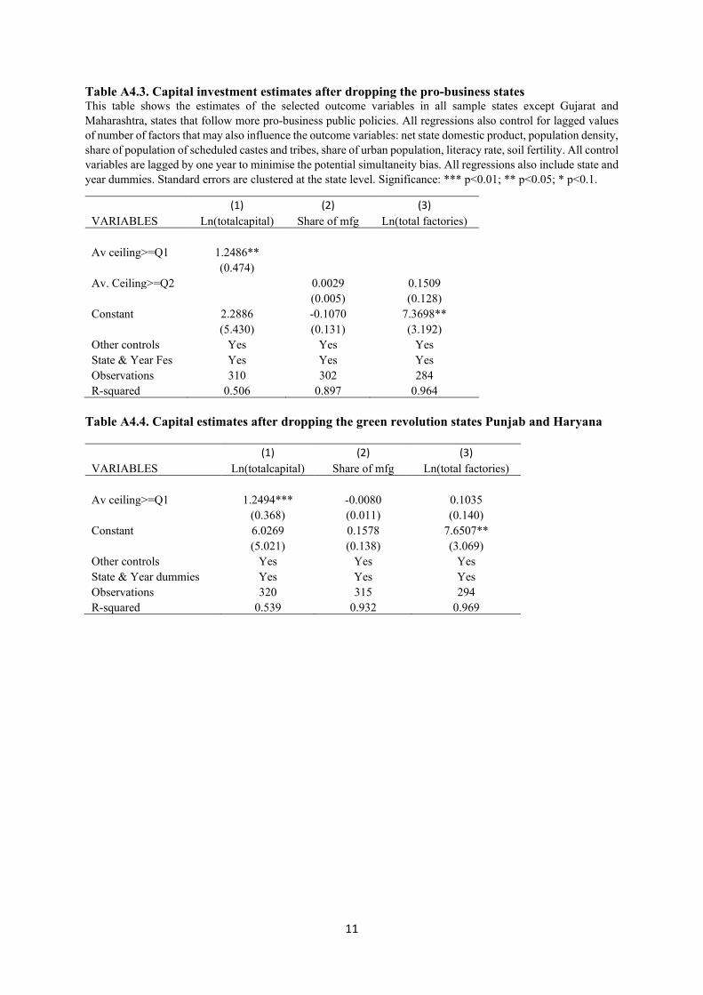
11

Table A4.3. Capital investment estimates after dropping the pro-business states This table shows the estimates of the selected outcome variables in all sample states except Gujarat and Maharashtra, states that follow more pro-business public policies. All regressions also control for lagged values of number of factors that may also influence the outcome variables: net state domestic product, population density, share of population of scheduled castes and tribes, share of urban population, literacy rate, soil fertility. All control variables are lagged by one year to minimise the potential simultaneity bias. All regressions also include state and year dummies. Standard errors are clustered at the state level. Significance: *** p<0.01; ** p<0.05; * p<0.1.

(1) (2) (3) VARIABLES Ln(totalcapital) Share of mfg Ln(total factories) Av ceiling>=Q1 1.2486**

(0.474) Av. Ceiling>=Q2 0.0029 0.1509

(0.005) (0.128) Constant 2.2886 -0.1070 7.3698**

(5.430) (0.131) (3.192) Other controls Yes Yes Yes State & Year Fes Yes Yes Yes Observations 310 302 284 R-squared 0.506 0.897 0.964

Table A4.4. Capital estimates after dropping the green revolution states Punjab and Haryana

(1) (2) (3) VARIABLES Ln(totalcapital) Share of mfg Ln(total factories) Av ceiling>=Q1 1.2494*** -0.0080 0.1035

(0.368) (0.011) (0.140) Constant 6.0269 0.1578 7.6507**

(5.021) (0.138) (3.069) Other controls Yes Yes Yes State & Year dummies Yes Yes Yes Observations 320 315 294 R-squared 0.539 0.932 0.969

12

Appendix 5. Test of pre-trends

We follow Borusyak and Jaravel (2017) to test that there are no pre-trends in the outcome variables among the states in the years leading to the event date 1971 and we use an F-test to do this as follows. Let Kit = t – Ei (E being the event date) denote the “relative time”—the number of years relative to the event date. The indicator variable for being treated can therefore be written as

'LW� ���^W���(L`� ���^.LW����`� <LW� �Įi ��ȕt ��Ȉf k=-f Ȗk �^.LW� �N`���İit i (1)

A common way to check for pre-WUHQGV�LV�WR�SORW�WKH�SDWK�RI�ȖÖN�EHIRUH�DQG�DIWHU�WUHDWPHQW��6RPHWLPHV�this is called the event study approach.

+HUH�^Ȗ�k`�IRU�N�����FRUUHVSRQG�WR�SUH-WUHQGV��DQG�IRU�N�����WR�G\QDPLF�HIIHFWV�N�SHULRGV�DIWHU�WKH�HYHQW�E.

Įi DQG�ȕt DUH�XQLW�DQG�SHULRG�IL[HG�HIIHFWV��UHVSHFWLYHO\��DQG�İit is random noise. We call equation (1) the fully dynamic specification.

We perform a test for identifying the pre-trends. Start from the fully dynamic regression (1) for any outcome variable Y and drop any two terms corresponding to k1; k2 < 0. This is the minimum number of restrictions for point identification, to pin down a constant and a linear term in Kit. The F-test compares the residual sums of squares under the restricted and unrestricted specifications, where the former is always semi-dynamic, and the latter is fully dynamic with two restrictions. Precisely due to under-identification, the fully dynamic specification with two restrictions is effectively unrestricted and its fit is identical for any k1 and k2, so the F-statistic will be invariant to k1 and k2 even in finite samples. If the F-stat is significant, it means that we reject the null (i.e., fully dynamic specification) in favour of the restricted dynamic specification.