FACTOR MODEL FORECASTS OF EXCHANGE RATES

FACTOR MODEL FORECASTS OF EXCHANGE RATES

Charles EngelUniversity of Wisconsin

Nelson C. MarkUniversity of Notre Dame

Kenneth D. WestUniversity of Wisconsin

November 2008Last revised September 2010

ABSTRACT

We construct factors from a cross section of exchange rates and use the idiosyncratic deviationsfrom the factors to forecast. In a stylized data generating process, we show that such forecasts can beeffective even if there is essentially no serial correlation in the univariate exchange rate processes. Weapply the technique to a panel of bilateral U.S. dollar rates against 17 OECD countries. We forecast usingfactors, and using factors combined with any of fundamentals suggested by Taylor rule, monetary andpurchasing power parity (PPP) models. For long horizon (8 and 12 quarter) forecasts, we tend to improveon the forecast of a “no change” benchmark in the late (1999-2007) but not early (1987-1998) parts of oursample.

We thank Wallice Ao, Roberto Duncan, Lowell Ricketts and Mian Zhu for exceptional researchassistance, and seminar audiences at the European Central Bank and the IMF for helpful comments. Wethank the National Science Foundation for financial support. Note to referees and editor: the AdditionalAppendix that is referenced in the paper has been submitted as a two separate documents (Appendix Aand Appendix B) that are not intended for publication.

1

1. INTRODUCTION

In predictions of floating exchange rates between countries with roughly similar inflation rates, a

random walk model works very well. The random walk forecast is one in which the (log) level of the

nominal exchange rate is predicted to stay at the current log level; equivalently, the forecast is one of “no

change” in the exchange rate. This forecast works well at various horizons, from one day to three years.

It does well in the following sense: the out of sample mean squared (or mean absolute) error in predicting

exchange rate movements generally is about the same, and often smaller, than that of models that use

“fundamentals” data on variables such as money, output, inflation, productivity, and interest rates.

Classic references are Meese and Rogoff (1983a,b); a recent update is Cheung, Chinn and Pascual (2005).

Whether or not this stylized regularity is bad news for economic theory is unclear. Some

economists think the regularity is very bad news. Bacchetta and van Wincoop (2006,p552) describe it as

“...the major weakness of international macroeconomics.” On the other hand, Engel and West (2005)

argue that a near random walk is expected under certain conditions.1

Whether or not one thinks the empirical finding of near random walk behavior is bad news for

economic theory, it is of interest to try to tease out connections (if any) between a given exchange rate

and other data. A small literature has used panel data techniques to forecast exchange rates, finding

relatively good success (Mark and Sul (2001), Rapach and Wohar (2004), Groen (2005), Engel et al.

(2007)). A very large literature has found that factor models do a good job forecasting basic macro

variables.2 The present paper predicts exchange rates, via factor models, in the context of panel data

estimation, and compares the predictions to those of a random walk via root mean squared prediction

error.

The panel consists of quarterly data on 17 bilateral US dollar exchange rates with OECD

countries, 1973-2007. We construct factors from the exchange rates. We take the literature on

predicting exchange rates to suggest that the exchange rate series themselves have information that is hard

2

to extract from observable fundamentals. This information might be hard to extract because standard

measures of fundamentals (e.g., money supplies and output) are error ridden, or because we simply lack

any direct measures of non-standard fundamentals such as risk premia or noise trading.3

We compare four different forecasting models to a benchmark model that makes a “no change”

forecast–the random walk model. One of our four models uses factors but no other variables to forecast.

The other three use factors along with some measures of observable fundamentals. The three measures of

observable fundamentals are: (1)those of a “Taylor rule” model; (2)those of a monetary model;

(3)deviations from purchasing power parity (PPP). Our measure of forecasting performance is root mean

squared prediction error (root MSPE).

On balance, these models have lower MSPE than does a random walk model for long (8 and 12)

quarter horizon predictions over the late part of our forecasting sample (1999-2007). These differences,

however, are usually not significant at conventional levels. Predictions that span the entire two decades

(1987-2007) or the early part (1987-1998) of our forecast sample generally have higher MSPE than does

a no change forecast. (Different samples involve different currencies, because of the introduction of the

Euro in 1999.) The basic factor model, and the factor model supplemented by PPP fundamentals, do best.

We recognize that the good performance in the recent period may be ephemeral. But we are hopeful that

our approach will prove useful in other datasets.

We close this introduction with some cautions. First, we make no attempt to justify or defend the

use of out of sample analysis. We and others have found such analysis useful and informative. But we

recognize that some economists might disagree. Second, judgment (sometimes rather arbitrary) has been

used at various stages, so we’re not (yet) proposing a completely replicable strategy. Third, our exercise

is not “true” out of sample. For example, revised rather than real time data are used in some

specifications. We use revised data because we are using out of sample analysis as a model evaluation

tool, and the models presume that the best available data are used. More importantly, perhaps, our

3

exercise is not true out of sample because we have relied on research that has already examined exchange

rates during parts of our forecasting sample. The most pertinent reference is Engel et al. (2007), which

used similar data, spanning 1973-2005 (vs. 1973-2007).

Section 2 presents a stylized model that illustrates analytically why our approach might predict

well. Section 3 describes our empirical models, section 4 our data and forecast evaluation techniques.

Section 5 presents empirical results. Section 6 concludes. Some appendices available on request present

detailed empirical results omitted from the paper to save space.

2. WHY A FACTOR MODEL MAY FORECAST WELL

In this section, we present a factor model and a simple data generating process that motivates its

use.

Our basic presumption is that the deviation of the exchange rate from a measure of central

tendency will help predict subsequent movements in the exchange rate. Algebraically, let

(2.1) sit = log of exchange rate in country i in period t,

zit = measure of central tendency defined below.

For concreteness, we note that sit is measured as log(foreign currency units/U.S. dollar), though that is not

relevant to the present discussion. Algebraically, our basic presumption is that for a horizon h, sit+h-sit can

be predicted by zit-sit, maybe using two different measures of z in a single regression.

Many papers have relied on the same presumption (that sit+h-sit can be predicted by zit-sit). For

example, Mark (1995) sets zit in accordance with the “monetary model”, so that zit depends on money

supplies and output levels; Molodstova and Papell (2008) set zit in accordance with a “Taylor rule”

model, so that zit depends on the exchange rate, inflation rates, output gaps and parameters of monetary

policy rules; Engel et al. (2008) set zit in accordance with PPP, so that zit depends on price levels. Some

4

papers (see references above) have used these specifications of zit in the context of panel data. Our twist

is to construct one measure of zit from factors estimated from the panel of exchange rates.

To exposit the idea, consider the following example. Suppose that the i’th exchange rate follows

the process

(2.2) sit = Fit + vit.

Here, Fit is the effect the factor has on currency i; in a one factor model, for example Fit = δif1t where f1t is

the factor and δi is the factor loading for currency i. The idiosyncratic shock vit is uncorrelated with Fit.

For simplicity, make as well some further assumptions not required in our empirical work, namely, that

Fit follows a random walk and that vit is i.i.d.:

(2.3) Fit = Fit-1 + εit, εit ~ i.i.d. (0, σ2ε), vit ~ i.i.d. (0, σ2

v), Eεitvis=0 all t, s.

An i subscript is omitted from the variances σ2ε and σ2

v for notational simplicity.

Then Δsit = εit + vit - vit-1 and the univariate process followed by Δsit is clearly an MA(1), say

(2.4) Δsit = ηit + θηit-1, Eη2it/σ

2η, |θ|<1.

Here, ηit is the Wold innovation in Δsit. The variance of ηit and the value of θ can be computed in

straightforward fashion from the values of σ2ε and σ2

v.4

Let us compare population forecasts of Δsit+1 using the factor model (2.2), the MA(1) model

(2.4), and a random walk model. Let “MSPE” denote “mean squared prediction error.” Unless otherwise

stated, in this section MSPE refers to a population rather than sample quantity. (This contrasts to the

discussion of our empirical work below, in which MSPE refers to a sample quantity.) To forecast using

(2.2), observe that Δsit+1 = ΔFit+1 + Δvit+1 = εit+1 + vit+1 - vit Y EtΔsit+1 = -vit / Fit-sit Y

(2.5) forecast error from factor model = εit+1 + vit+1, MSPEfactor = σ2ε + σ2

v.

5

The MSPE from the univariate model (2.4) is of course σ2η. With a little bit of algebra, and using the

formula for σ2η given in the previous footnote, it may be shown that σ2

ε+σ2v < σ2

η. Hence the factor model

has a lower MSPE than the MA(1) model.

But the relevant issue is whether the improvement (i.e., the fall) in the MSPE is notable, for a

plausible data generating process. A plausible DGP would be one in which there is very little serial

correlation in Δsit. Put differently, if the DGP is such that the MSPE from the MA(1) model is

essentially the same as that from a random walk model, is it still possible that the MSPE from the factor

model is substantially smaller than that of the random walk?

In our empirical work, we use Theil’s U-statistic to compare (sample) MSPEs relative to that of a

random walk. These are square roots of the ratios of (sample MSPE alternative forecast / sample MSPE

forecast of no change). The forecast error of the random walk model is the actual change in Δsit =εit

+vit-vit-1; the corresponding population MSPE is σ2ε+2σ2

v. In the context of the present section (population

rather than MSPEs), define population U-statistics as

(2.6) Ufactor = [ (σ2ε+σ

2v)/ (σ

2ε+2σ2

v) ] ½, UMA = [ σ2

η/(σ2ε+2σ2

v) ] ½.

For select values of the first order autocorrelation of Δsit (which is approximately the MA parameter θ

introduced in (2.4)), these are as follows:

(2.7a) corr(Δsit, Δsit-1) -0.01 -0.02 -0.03 -0.04 -0.05 -0.10(2.7b) UMA 0.99995 0.9998 0.9996 0.9992 0.9987 0.9949(2.7c) Ufactor 0.995 0.990 0.985 0.980 0.975 0.949

The factor model improves on the moving average model by an order of magnitude. For example, when

the first order autocorrelation of Δsit is -0.10, the population root MSPE for the MA model is only .5%

lower than for the random walk (because .9949 is about .5% smaller than 1), while the population root

MSPE for the factor model is about 5% lower than the random walk.5

6

We further note that the population values for UMA in (2.7b) are so near 1 that in practice, for any

of the values of the autocorrelations, one would not be surprised if sampling error in estimation of an

MA(1) model led to sample U-statistics above 1. Hence we view the figures in the table as consistent

with the well-established finding that no univariate model predicts better than a random walk. But clearly

the factor model has the potential to predict better, even accepting the point that in practice the best

univariate model is a random walk.

In the simple DGP consisting of (2.2) and (2.3), whether a factor model will have lower MSPE

than a model that uses information not only on exchange rates but also on fundamentals such as prices

and output depends on whether the additional variables help pin down vit. To allow for this possibility,

our empirical work combine factors with observable fundamentals, as discussed in the next section.

3. EMPIRICAL MODELS

We use models with one, two or three factors. We will use the three factor model for illustration.

The one and two factor models are analogous. In the three factor model, we first estimate a set of three

factors and factor loadings from the exchange rates. For currency i, i=1, ...,17, the model is

(3.1) sit = constant + δ1i f1t + δ2i f2t + δ3i f3t + vit

/ constant + Fit + vit.

The factors (the f’s) are unobserved I(1) variables. Here and throughout, we do not attempt to test for unit

roots in the factors or any other variable for that matter. See Bai (2004) on estimation of factor models

with unit root data.

Let Fit = δ1i f1t + δ2i f2t + δ3i f3t. We aim to use (estimates of) Fit to forecast sit. In contrast to

much work with factors, the factors are not constructed from a set of additional variables. For example,

in Groen’s (2006) work on exchange rates, factors are constructed from data on real activity and prices,

7

and take the place of traditional measures of real and nominal activity. We take the literature on

predicting exchange rates to suggest that the exchange rate series themselves may have low frequency

information on common trends that is hard to extract from observable fundamentals. This low frequency

information might be buried in standard, but noisy, measures of fundamentals such as relative money

supplies and relative outputs. Or this information might be embedded in non-standard measures of

fundamentals that are sufficiently persistent that they function in part to drive common trends; examples

are persistent risk premia or persistent noise trading. Put differently, we use factors to parsimoniously

capture co-movements of exchange rates that are not well-captured by observable fundamentals. Crudely,

we posit that a weighted average of the log levels of exchange rates represents a central tendency for the

log level a given exchange rate, and use this weighted average to help forecast.

Mechanics are as follows. We assume that the factors component soak up a common unit root

component in the s’s. That is, we assume that Fit-sit is stationary, and may be useful in predicting

(stationary) future changes in sit. We do not attempt to test stationarity of vit; our selection of number of

factors was based on presumed limitations of a panel of cross-section dimension 17.6 The factors f1t, f2t

and f3t are uncorrelated by construction. We normalize the f’s to have mean zero and unit variance.

So this first stage produces a time series for ^f1t, ^f2t and ^f3t and factor loadings, ^δ1i, i=1,...,17; ^δ2i,

i=1,...,17; ^δ3i, i=1,...,17. In our simplest specification, the measure of central tendency zit that was

introduced in (2.1) is

(3.3) zit = ^δ1i ^f1t + ^δ2i

^f2t + ^δ3i ^f3t / ^Fit.

In this simplest specification, with ^Fit / ^δ1i ^f1t + ^δ2i

^f2t + ^δ3i ^f3t , for quarterly horizons h=1, 4, 8, and 12

we use standard panel data estimator (least squares with dummy variable) to estimate and forecast. For

example, with a horizon of h=4 quarters, we estimate

(3.4) sit+4-sit = αi + β( ^Fit-sit) + uit+4,

8

where αi is a fixed effect for country i. We then use ^αi and ^β to predict (some details below). Here, and in

all of our specifications, there is no “time effect” (in the jargon of panel data): the factors are dynamic

versions of time effects (we hope).

Our three other specifications combine factors with observables. The other three specifications

are all of the form

(3.5) sit+h-sit = αi + β( ^Fit - sit) + γ(zit-sit) + uit+h

for three different zit’s. Let country 0 refer to the USA. The three zit’s are:

(3.6) Taylor rule: zit = 1.5(πit-π0t)+0.5(~yit-~y0t)+sit; π = inflation, ~y = output gap;

zit-sit = 1.5(πit-π0t)+0.5(~yit-~y0t);

(3.7) monetary model: zit = (mit-m0t)-(yit-y0t); m = ln(money), y=ln(output);

(3.8) PPP model: zit = pit-p0t; p=ln(price level).

The Taylor rule model builds on the recently developed view that interest rates rather than money

supplies are the instrument of monetary policy. Expositions may be found in Benigno and Benigno

(2006), Engel and West (2006) and Mark (2008). The monetary model was for many years the workhorse

of international monetary economics; see, for example the textbook exposition in Mark (2001) or the

abbreviated summary in Engel and West (2005). The PPP model (3.6) presumes convergence of price

levels.

4. DATA AND FORECASTING EVALUATION

We use quarterly, data 1973:1-2007:4, with the out of sample period beginning in 1987:1. The

basic data source is International Financial Statistics, supplemented on occasion by national sources.

Exchange rates are end of quarter values of the US dollar vs. the currencies of 17 OECD countries:

9

Australia, Austria, Belgium, Canada, Denmark, Finland, France, Germany, Japan, Italy, Korea,

Netherlands, Norway, Spain, Sweden, Switzerland, and the United Kingdom. (See below on how we

handled conversion to the Euro in 1999:1.) The price level is the CPI in the last month of quarter; output

is industrial production in last month of quarter; money is M1 (with some complications); the output gap

is constructed by HP detrending, computed recursively, using only data from periods prior to forecast

period. Because some of the data appeared to display seasonality, we seasonally adjusted prices, output

and money by taking a four quarter average of the log levels before doing any empirical work. For

example the price level in country i is pit = ¼[log(CPIit) + log(CPIit-1) + log(CPIit-2) + log(CPIit-3)].

To explain the mechanics of our forecasting work, let us illustrate for the four quarter horizon

(h=4), for the first forecast, and for the model that uses only factors but not in addition observable

fundamentals. As depicted in (4.1) below, we use data from 1973:1 to 1986:4 to estimate factors and

factor loadings, and construct ^Fit for i=1,...,17.

(4.1) --------------data used to estimate factors-------------- ----data used to estimate panel regression----|___________________________________|_____|_____|

85:4 86:4 87:4

We then use right hand side data from 1973:1 to 1985:4 to estimate panel data regression

(4.2) sit+4-st = αi + β( ^Fit-sit) + uit+4, t=1973:1, ..,1985:4.

We use 1986:4 data to predict the 4 quarter change in s:

(4.3) Prediction of (si,1987:4-si,1986:4) = ^αi + ^β( ^Fi,1986:4-si,1986:4).

We then add an observation to the end of the sample, and repeat.

As is indicated by this discussion, the recursive method is used to generate predictions:

observations are added to the end of the estimation sample, so that the sample size used to estimate factors

10

and panel data regressions grows. The direct (as opposed to iterated) method is used to make multiperiod

predictions. The estimation technique is maximum likelihood, assuming normality.

An analogous setup is used for other horizons and for models with observable fundamentals.

For a given date, factors and r.h.s. variables are identical across horizons: for given t, the same

values of ^Fit-sit are used. However, the l.h.s. variable is different (h period difference in st), and

regression samples are smaller for larger h. This means that the regression coefficients (^αi, ^β) and

predictions vary with h.

For the 9 non-Euro currencies (Australia, Canada, Denmark, Japan, Korea, Norway, Sweden,

Switzerland, and the United Kingdom), we report “long sample” forecasting statistics for a 1987-2007

sample. For all 17 currencies, we report “early” sample forecasting statistics for a 1987-1998 sample. For

the 9 non-Euro currencies and the Euro, we report “late sample” forecasting statistics for a 1999-2007

sample. Early sample statistics involve forecasts whose forecast base begins in 1986:4 and ends in

1998:4. Towards the end of the early sample, the forecast occurs in the pre-Euro era, while the realization

occurs during the Euro era. We rescaled Euro area currencies so that there was no discontinuity. See

Table 1 for the exact number of forecasts for each sample and horizon, as well as a summary listing of

models.

In all samples (long, early and late), we use data from all 17 countries to construct factors and

panel data estimates. For post-1999 data, the left hand side variable in both factor and panel data

estimation is identical for all 8 Euro area countries. But because all samples include some pre-1999 data

in estimation, there are differences across countries in estimates of the factor ^Fit, and of course the

measures of prices, output and money used in the PPP, monetary and Taylor rule models. This means

that the forecasts are different for the Euro countries. We construct a Euro forecast by simple averaging

of the 8 different forecasts.

Our measure of forecast performance is root mean squared prediction error (RMSPE). (Here and

11

through the rest of the paper, all references to MSPE and RMSPE refer to sample rather than population

values.) We compute Theil’s U-statistic, the ratio of the RMSPE from each of our models to the RMSPE

from a random walk model. We summarize results by reporting the median (across 17 countries) of the

U-statistic, and the number of currencies for which the ratio is less than one (since a value less than one

means our model had smaller RMSPE than did a random walk). Individual currency results are available

on request.

A U-statistic of 1 indicates that the (sample) RMSPEs from the factor model and from the random

walk are the same. As argued by Clark and West (2006, 2007), this is evidence against the random walk

model. If, indeed, a random walk generates the data, then the factor model introduces spurious variables

into the forecasting process. In finite samples, attempts to use such variables will, on average, introduce

noise that inflates the variability of the forecasting error of the factor model. Hence under a random walk

null, we expect sample U-statistics greater than 1, even though that null implies that population ratios of

RMSPEs are 1.

We report 10 percent level one sided hypothesis tests on H0: RMSPE(our model) =

RMSPE(random walk) against HA: RMSPE(our model) < RMSPE(random walk). (Here,“our model”

refers to any one of the four models given in (3.4) or (3.6)-(3.8): factor model, factor model plus Taylor

rule, factor model plus monetary or factor model plus PPP.) These hypothesis tests are conducted in

accordance with Clark and West (2006), who develop a test procedure that accounts for the potential

inflation of the factor model’s RMSPE noted in the previous paragraph. Of course, with many currencies

(17, in our early sample), it is very possible that one or more test statistics will be significant even if none

in fact predict better than a random walk. We guarded against this possibility by testing H0: RMSPE(our

model) = RMSPE(random walk) for all currencies against HA: RMSPE(our model) > RMSPE(random

walk) for at least one currency, using the procedure in Hubrich and West (2010).7 This statistic, however,

rarely had a p-value less than 0.10. We therefore do not report it, to keep down the number of figures

12

reported.

5. EMPIRICAL RESULTS

For the largest sample used (1973-2007), Figure 1 plots the estimates of the three factors, while

Table 2 presents the factor loadings. The factor loadings in Table 2 are organized so that the first block

of six currencies (Austria, ..., Switzerland) includes ones in the one-time German mark area. The next

block of four currencies (Finland, ..., Spain) are Euro area countries not included in the first block. The

final block (Australia, ..., UK) lists the seven remaining countries.

The factor loadings suggest that the second factor reflects a central tendency of countries in the

former German mark area. (If the factor loading on the second factor was zero for countries not in the

mark area, then this second factor would literally be a weighted average of countries in the mark area.8

The coefficients are not zero on all non-mark countries, so the second factor is only roughly an average of

mark countries.) By similar logic, the first factor seems to represent an average of everybody except

countries in the former German mark area. The third factor is hard to label.

Of course this breakdown is not precise. Denmark’s factor loading on what we have labeled the

“mark” factor is smaller than is Japan’s (0.68 vs. 0.78), and its factor loading on the first factor is, in

absolute value, larger than Japan’s (0.70 vs. -0.55).

Tables 3 and 4 present some forecasting results. What we present in these tables is summaries of

results over all currencies. We present the median U statistic across the currencies in the sample, the

number of U-statistics less than 1 and the number of t-statistics greater than 1.282. (Recall that a U

statistic less than 1 means that the model’s had a lower MSPE than did a random walk.) Currency by

currency results are available on request.

Table 3 presents results for r=2 factors, both for the model that uses only factors, and for the

models that also include observable fundamentals. To read the table, consider the entry at the top of the

13

table for model = ^Fit-sit, sample = 87-07. The figure of “1.003" for “median U” and horizon “h=1” means

that of the 9 currencies, half had U-statistics above 1.003, half had U-statistics below 1.003. The figures

of “1(0)” immediately below the figure of “1.003” means that only 1 of the 9 U-statistics was below 1,

and that 0 of the t-statistics rejected the null of equal MSPE at the 10% level.9

One’s eyes (or at least our eyes) are struck by the preponderance of median U-statistics that are

above 1. In the long sample, 13 of the 16 the median U-statistics are above one (the three exceptions are

for ^Fit-sit + PPP for the h=4, 8 and 12 quarter horizons). In the early sample, it is again the case that 13

of the 16 the medians are above one (the exceptions in this case being ^Fit-sit + PPP for h=1 and 4, and ^Fit-

sit + monetary for h=1). In the late sample, however, 9 of the 16 medians are above 1, with the models

doing consistently better than a random walk (median U<1) at 8 and 12 quarter horizons. Note in

particular that in this sample, 8 of the 10 U-statistics were below 1 for ^Fit-sit and ^Fit-sit + monetary, and 9

or 10 were below 1 for ^Fit-sit + PPP.

Table 4 illustrates how varying the number of factors affects the simplest model, that of ^Fit-sit;

results for models that include Taylor rule, monetary or PPP fundamentals are similar. The Table

indicates that for the long sample, r=3 performs a little better and the r=1 model a little worse than does

the r=2 model presented in Table 3. In the early sample, the r=2 model is the worst performing; the r=1

model is the best performing. In the late sample, the r=2 and r=3 models perform similarly, with the r=1

model performing distinctly more poorly than either of the other models.

To depict visually what underlies a U-statistic of various values, let us focus on the United

Kingdom, r=3 factors, model = ^Fit-sit, long sample. The U-statistics happen to be: 1.003 (h=1), 0.996

(h=4), 0.979 (h=8) and 0.969 (h=12). (These U-statistics, as well as other individual currency U-statistics

discussed below, are not reported in any table.) A scatter plot of the recursive estimates of ^Fit-sit, and of

the subsequent h-quarter change in the exchange rate, is in Figure 2. The values of 0.979 and 0.968 for

the U-statistics for h=8 and h=12 imply a reduction in root MSPE relative to a no-change forecast of

14

about 2-3%. Despite the seemingly small reduction, the figures for h=8 and h=12 depict an

unambiguously positive relation between the deviation from the factor ^Fit-sit and the subsequent change in

the exchange rate. On the other hand, there clearly is a lot of variation in a relation that is positive on

average.

Our predictions fared especially poorly for the Japanese yen, which generally had one of the

highest U-statistics in each sample and model. For example, the U-statistics for Japan, r=2 factors, model

= ^Fit-sit, long sample were: 1.008 (h=1), 1.051 (h=4), 1.085 (h=8) and 1.160 (h=12). That the yen does

not quite fit into the same mold as the other currencies in our study is perhaps suggested by the large

negative weight of -0.55 for the yen on the first factor (see Table 2). In the late sample, continental

currencies (Denmark, Norway, Sweden, Switzerland) and, to a lesser extent, the Euro were generally well

predicted by our models. For example, the figures for the Euro for r=2 factors, model = ^Fit-sit, late

sample were: 1.009 (h=1), 1.015 (h=4), 0.939 (h=8) and 0.816 (h=12).

Over all specifications and horizons (1, 2 and 3 factors; long, early and late samples; horizons of

1, 4, 8 and 12 quarters), only the ^Fit-sit+PPP model had median U-statistics less than 1 in over 50 percent

of the forecasts.

We checked the robustness of these results in two ways. First, we estimated by principal

components rather than by maximum likelihood. Overall, results were comparable, with one technique

doing a little better (occasionally, a lot better) in one specification and the other doing a little better

(occasionally, a lot better) in other specifications. Second, we used the British pound rather than the U.S.

dollar as the base currency. Estimation was by maximum likelihood. Here, results were comparable for

the early sample, somewhat worse for the long and late samples.

A detailed summary of the robustness checks is in an appendix available on request. To illustrate,

let us take two lines form Table 3, and present analogous results from principal components estimation,

and from estimation with the British pound as the base currency. These lines are chosen because they are

15

representative:

h=1 h=4 h=8 h=12(5.1a) ^Fit-sit, early / N=17, maximum likelihood, U.S. dollar (Table 3) 6(0) 7(0) 4(0) 3(0)(5.1b) ^Fit-sit, early / N=17, principal components, U.S. dollar 4(2) 4(3) 7(4) 8(2)(5.1c) ^Fit-sit, early / N=17, maximum likelihood, British pound 6(1) 6(1) 4(2) 4(0)

(5.2a) ^Fit-sit+PPP, late / N=10, maximum likelihood, U.S. dollar (Table 3) 4(0) 5(0) 8(0) 9(5)(5.2b) ^Fit-sit+PPP, late / N=10, principal components, U.S. dollar 3(3) 3(3) 7(2) 9(4)(5.2c) ^Fit-sit+PPP, late / N=10, maximum likelihood, British pound 3(0) 1(0) 1(0) 1(0)

We see in (5.1a) and (5.1b) that in terms of the number of U-statistics less than one, principal

components improves over maximum likelihood at h=12 (8 versus 3 U-statistics less than 1), while the

converse is true at h=4 (4 versus 7 U-statistics less than 1). Results for the British pound in (5.1c)

similarly are better at some horizons, worse at other horizons. We see in (5.2a) and (5.2b) that principal

and components and the maximum likelihood generate very similar numbers, while (5.2c) illustrates that

with the British pound as the base currency, results degrade for the late sample.

6. CONCLUSIONS

This first pass at extracting factors from the cross-section of exchange rates yielded mixed results.

Results for late samples (1999-2007) were promising, at least for horizons of 8 or 12 quarters. With

occasional exceptions for models that relied not only on factors but PPP fundamentals as well, other

results suggested no ability to improve on a “no change,” or random walk, forecast.

Late samples allow larger sample sizes for estimation of factors. While that may be part of the

reason for good results for late samples, that is not a sufficient condition for good results because our

robustness checks found that the when the British pound is the base currency, late samples perform worse

than early samples. Indeed, it remains to be seen whether our results for late samples are spurious. In any

event, the framework here can be extended in a number of ways. It would be desirable to allow different

slope coefficients across currencies, to allow more flexible specification of parameters in monetary and

16

Taylor rule models, and to use a data dependent method of selecting the number of factors. Such

extensions are priorities for future work. It would also be desirable to compare our predictions to not only

a random walk model, but to other models that have been compared to the random walk in earlier studies.

17

1. The Engel and West (2005) argument is not that a random walk is produced by an efficient market;indeed the simple efficient markets model implies that exchange rate changes are predicted by interestrate differentials and any variables correlated with interest rate differentials. Rather, the argument relatesto the behavior of an asset price that is determined by a present value model with a discount factor near 1.

2. See Stock and Watson (2006). We use “factor” to refer to a DGP driven by factors, even if theestimation technique involves principal components.

3. See Diebold et al. (1994) for another attempt, with methodology very different from ours, to predictexchange rates using a cross section of exchange rates.

4. Specifically, let γ=σ2ε+2σ2

v denote the variance of Δs. Then σ2η = 0.5[γ+(γ2-4σ4

v)½], θ=-σ2

v/σ2η.

5. The figures for the MA model may appear surprisingly small. But consider, for example, when theautocorrelation is -0.1 (rightmost column in the table), and suppose we forecast using an AR(1). Thepopulation R2 is (-.1)2 = .01. This means that the variance of the forecast error is 99% of the variance ofΔs, with implied U-statistic of about .995 (since .9952 . .99). The MA(1) model does very slightly better:To be precise, the variance of the MA(1) forecast error expressed as a percentage is 98.9898 < 99. Ininterpreting the table in the text, it may help to observe that the first order autocorrelation of Δs pins downthe ratio of σ2

ε to σ2v, which is all that is needed to compute the other figures in the table.

6. In principle, one could use techniques to determine cointegrating rank to determine the number of I(1)factors and the factor loadings. We take results such as Ho and Sorensen (1996) to indicate that the finitesample performance of such techniques is likely to be poor, when the cross-section dimension is 17.

7. Although we report ratios of RMSPEs for convenience of interpretation, the Clark and West (2006)and Hubrich and West (2008) tests work off the arithmetic difference of MSPEs, evaluating whether thisdifference is statistically different from zero. The null hypothesis is that the random walk generates thedata. These tests begin by adjusting the MSPE difference to account for noise that is present in thealternative (the non-random walk model) under the null hypothesis. For Clark and West (2006), thestandard Diebold-Mariano-West (DMW) statistic is then computed for the adjusted MSPE difference. For Hubrich and West (2009), a parametric bootstrap is executed, under the assumption of normality. Wedid 10,000 repetitions in this bootstrap. See West (1996, 2006) for basic theory and further discussion.

8. See Stock and Watson (2006) on algebra relating factor loadings, factors, and data used to estimatefactors.

9. The fact the median U was 1.003, but only 1 U-statistic was below 1 of course means that the U-statistics were tightly clustered near 1.

FOOTNOTES

REFERENCES

Bacchetta, Philippe and Eric van Wincoop, 2006, “Can Information Heterogeneity Explain the ExchangeRate Determination Puzzle?,” American Economic Review 96(3), 552-576.

Bai, Jushan, 2004, “Estimating Cross-Section Common Stochastic Trends in Nonstationary Panel Data,”Journal of Econometrics, 137-183.

Benigno, Gianluca, and Pierpaolo Benigno, 2006, “Exchange Rate Determination under Interest RateRules,” manuscript, London School of Economics.

Cheung, Yin-Wong, Menzie Chinn and Antonio Garcia Pascual , 2005, “Empirical Exchange RateModels of the Nineties: Are Any Fit to Survive?” Journal of International Money and Finance24,1150-1175.

Clark, Todd E. and Kenneth D. West, 2006, “Using Out-of-Sample Mean Squared Prediction Errors toTest the Martingale Difference Hypothesis,” Journal of Econometrics 135 (1-2), 155-186.

Clark, Todd E. and Kenneth D. West, 2007, “Approximately Normal Tests for Equal Predictive Accuracyin Nested Models,” Journal of Econometrics, 138(1), 291-311.

Diebold, Francis X.,, Javier Gardeazabal, and Kamil Yilmaz, 1994, “ On Cointegration and ExchangeRate Dynamics,” Journal of Finance XLIX, 727-735.

Engel, Charles and Kenneth D. West, 2005, Exchange Rates and Fundamentals, Journal of PoliticalEconomy 113, 485-517.

Engel, Charles and Kenneth D. West, 2006, “Taylor Rules and the Deutschemark-Dollar Real ExchangeRate,” Journal of Money, Credit and Banking 38, 1175-1194.

Engel, Charles, Nelson M. Mark and Kenneth D. West, 2007, “Exchange Rate Models Are Not As BadAs You Think,”, 381-443 in NBER Macroeconomics Annual, 2007, D. Acemoglu, K. Rogoff and M.Woodford (eds.), Chicago: University of Chicago Press.

Groen, Jan J.J., 2005, “Exchange Rate Predictability and Monetary Fundamentals in a Small Multi-Country Panel,” Journal of Money, Credit and Banking 37, 495-516.

Groen, Jan J. J., 2006, “Fundamentals Based Exchange Rate Prediction Revisited,” manuscript, Bank ofEngland.

Hubrich, Kirstin and Kenneth D. West, 2010, “Forecast Comparisons for Small Nested Model Sets,”Journal of Applied Econometrics. 25, 574-594.

Ho, Mun S. and Bent E. Sørensen, 1996, “Finding Cointegration Rank in High Dimensional SystemsUsing the Johansen Test: An Illustration Using Data Based Monte Carlo Simulations,” Review ofEconomics and Statistics, 726-732.

Mark, Nelson A., 1995, “Exchange Rates and Fundamentals: Evidence on Long-Horizon Predictability,”American Economic Review 85, 201--218

Mark, Nelson A., 2001, International Macroeconomics and Finance: Theory and Empirical Methods,New York: Blackwell.

Mark, Nelson A., 2008, “Changing Monetary Policy Rules, Learning and Real Exchange RateDynamics,” manuscript, University of Notre Dame.

Mark, Nelson A., and Donggyu Sul, 2001, “Nominal Exchange Rates and Monetary Fundamentals:Evidence from a Small Post-Bretton Woods Sample,” Journal of International Economics 53, 29-52.

Meese, Richard A., and Kenneth Rogoff, 1983a, “Empirical Exchange Rate Models of the Seventies: DoThey Fit Out of Sample?”, Journal of International Economics 14, 3-24.

Meese, Richard A., and Kenneth Rogoff, 1983b, “The Out-of-Sample Failure of Empirical Exchange RateModels: Sampling Error or Misspecification”, in J. A. Frenkel, (ed.) Exchange Rates and InternationalMacroeconomics (Chicago: University of Chicago Press).

Molodtsova, Tanya, and David Papell, 2008, “Taylor Rules with Real-time Data: a Tale of Two Countriesand One Exchange,” Journal of Monetary Economics 55, S63-S79 .

Rapach, David E., and Mark E. Wohar, 2002, Testing the Monetary Model of Exchange RateDetermination: New Evidence from a Century of Data, Journal of International Economics, 58, 359-385.

Rapach, David E., and Mark E. Wohar, 2004, “Testing the Monetary Model of Exchange RateDetermination: A Closer Look at Panels,” Journal of International Money and Finance, 23(6), 841-865.

Stock, James H. and Mark W. Watson, 2006, “Forecasting with Many Predictors,” 515-550 in Handbookof Economic Forecasting, Vol 1, G. Elliott, C.W.J. Granger and A. Timmermann (eds), Amsterdam:Elsevier.

West, Kenneth D., 1996, “Asymptotic Inference About Predictive Ability,” Econometrica 64 ,1067-1084.

West, Kenneth D., 2006, “Forecast Evaluation,” 100-134 in Handbook of Economic Forecasting, Vol. 1,G. Elliott, C.W.J. Granger and A. Timmerman (eds), Amsterdam: Elsevier.

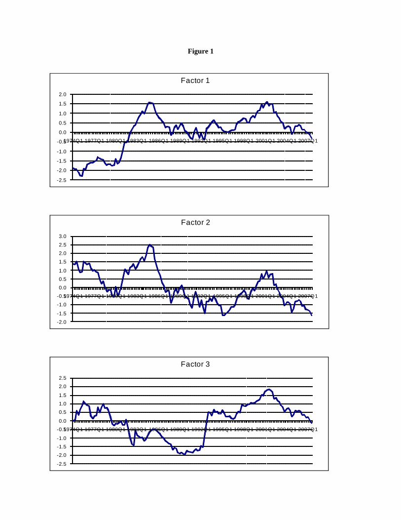
Figure 1

-2.5

-2.0

-1.5

-1.0

-0.5

0.0

0.5

1.0

1.5

2.0

1974Q1 1977Q1 1980Q1 1983Q1 1986Q1 1989Q1 1992Q1 1995Q1 1998Q1 2001Q1 2004Q1 2007Q1

Factor 1

-2.0-1.5

-1.0-0.50.00.51.0

1.52.02.53.0

1974Q1 1977Q1 1980Q1 1983Q1 1986Q1 1989Q1 1992Q1 1995Q1 1998Q1 2001Q1 2004Q1 2007Q1

Factor 2

-2.5

-2.0-1.5-1.0

-0.50.0

0.51.01.5

2.02.5

1974Q1 1977Q1 1980Q1 1983Q1 1986Q1 1989Q1 1992Q1 1995Q1 1998Q1 2001Q1 2004Q1 2007Q1

Factor 3

Figure 2

‐0.6

‐0.5

‐0.4

‐0.3

‐0.2

‐0.1

0.0

0.1

0.2

0.3

0.4

‐1.5 ‐1 ‐0.5 0 0.5 1 1.5 2 2.5

Fhat‐S vs. DS(+1) (United Kingdom)

‐0.6

‐0.5

‐0.4

‐0.3

‐0.2

‐0.1

0.0

0.1

0.2

0.3

0.4

‐1.5 ‐1 ‐0.5 0 0.5 1 1.5 2 2.5


‐0.6

‐0.5

‐0.4

‐0.3

‐0.2

‐0.1

0.0

0.1

0.2

0.3

0.4

‐1.5 ‐1 ‐0.5 0 0.5 1 1.5 2 2.5


‐0.6

‐0.5

‐0.4

‐0.3

‐0.2

‐0.1

0.0

0.1

0.2

0.3

0.4

‐1.5 ‐1 ‐0.5 0 0.5 1 1.5 2


Table 1

List of Currencies and Models

A. Number of Quarterly Observations in Prediction Sample

Prediction Sample ----- Horizon h ------1 4 8 12

Long Sample (1986:4+h) - 2007:4 84 81 77 73Early Sample (1986:4+h) - (1998:4+h) 49 49 49 49Late Sample (1999:1+h) - 2007:4 35 32 28 24

B. Currencies

Long sample N=9 Australia, Canada, Denmark, Japan, Korea, Norway, Sweden,Switzerland, United Kingdom

Early sample N=17 The long sample countries plus: Austria, Belgium, Finland, France,Germany, Italy, Netherlands and Spain

Late Sample N=10 The long sample countries plus the Euro

C. Models

^Fit-sit^Fit is the estimated factor component of currency i, estimated from 17currencies in each sample (with identical Euro values appearing post-1998 for the 8 Euro area currencies).

^Fit-sit + Taylor Taylor rule fundamentals (3.6) also included as a regressor

^Fit-sit + Monetary Monetary model fundamentals (3.7) also included as a regressor

^Fit-sit + PPP Purchasing power parity fundamentals (3.8) also included as a regressor

Notes:

1. The sample period for estimation of models runs from 1973:1 to the forecast base. Models areestimated recursively. Factors are estimated using N=17 currencies, for all samples.

2. In the late sample, Euro area forecasts are made by averaging forecasts from the 8 Euro countries.

3. Long horizon forecasts are made using the direct method.

Table 2

Factor Loadings, 1973-2007 Sample

^δ1i ^δ2i ^δ3i

Austria -0.06 1.00 0.02Belgium 0.53 0.83 -0.11Denmark 0.70 0.68 -0.16Germany -0.03 1.00 0.01Netherlands 0.08 1.00 -0.02Switzerland -0.31 0.93 -0.03

Finland 0.88 0.23 0.34France 0.85 0.50 -0.16Italy 0.97 -0.14 0.15Spain 0.98 -0.08 0.12

Australia 0.87 -0.31 0.16Canada 0.80 -0.11 0.29Japan -0.55 0.78 -0.16Korea 0.84 -0.27 0.28Norway 0.95 0.19 0.12Sweden 0.96 -0.07 0.22UK 0.84 0.13 -0.01

Notes:

1. The fitted model is sit = const. + ^δ1i ^f1t + ^δ2i

^f2t + ^δ3i ^f3t + ^vit / ^Fit + ^vit;

^f1t, ^f2t and ^f3t are estimated

factors.

Table 3

Two Factor (r=2) Results

Model Sample/ No. Statistic --- Horizon h ---Currencies 1 4 8 12

^Fit-sit long / N=9 median U 1.003 1.008 1.056 1.108#U<1 or (t>1.282) 1(0) 4(0) 4(0) 4(0)

^Fit-sit + Taylor long / N=9 median U 1.010 1.047 1.089 1.129#U<1 or (t>1.282) 1(0) 0(0) 1(0) 4(0)

^Fit-sit + Monetary long / N=9 median U 1.010 1.071 1.202 1.474#U<1 or (t>1.282) 3(2) 3(2) 3(2) 3(3)

^Fit-sit + PPP long / N=9 median U 1.003 0.996 0.953 0.938#U<1 or (t>1.282) 3(0) 5(0) 6(2) 5(0)

^Fit-sit early / N=17 median U 1.001 1.006 1.049 1.164#U<1 or (t>1.282) 6(0) 7(0) 4(0) 3(0)

^Fit-sit + Taylor early / N=17 median U 1.012 1.048 1.086 1.156#U<1 or (t>1.282) 1(0) 2(0) 1(0) 3(0)

^Fit-sit + Monetary early / N=17 median U 0.996 1.012 1.116 1.216#U<1 or (t>1.282) 10(3) 8(4) 7(3) 6(4)

^Fit-sit + PPP early / N=17 median U 0.999 0.983 1.027 1.128#U<1 or (t>1.282) 9(0) 13(1) 5(1) 3(0)

^Fit-sit late / N=10 median U 1.009 1.014 0.934 0.835#U<1 or (t>1.282) 3(1) 3(0) 7(0) 8(3)

^Fit-sit + Taylor late / N=10 median U 1.010 1.035 0.979 0.836#U<1 or (t>1.282) 2(1) 2(0) 6(0) 8(2)

^Fit-sit + Monetary late / N=10 median U 1.013 1.034 0.978 1.105#U<1 or (t>1.282) 3(1) 4(1) 6(3) 5(3)

^Fit-sit + PPP late / N=10 median U 1.006 1.000 0.891 0.727#U<1 or (t>1.282) 4(0) 5(0) 8(0) 9(5)

Notes:

1. Table 1 defines the long, early and late sample periods, lists the currencies in each sample, anddescribes the models.

2. The U statistic is = (RMSPE Model/RMSPE random walk); U<1 means that the model had a smallerMSPE than did a random walk model. “median U” presents the median value of this ratio across 9, 17 or10 currencies. “#U<1” gives the number of currencies for which U<1, a number that can range from 0 tothe number of currencies N.

3. t is test of H0: U=1 (equality of RMSPEs) against one-sided HA: U<1 (RMSPE Model is smaller),using the Clark and West (2006) procedure. The number of currencies in which this test rejected equalityat the 10 percent level is given in the (t>1.282) entry.

Table 4

Results for ^Fit-sit, Varying Number of Factors r

No. of Sample/ No. Statistic --- Horizon h ---Factors (r) Currencies 1 4 8 12

1 long / N=9 median U 1.011 1.037 1.083 1.154#U<1 or (t>1.282) 1(0) 1(0) 1(0) 1(0)



1 early / N=17 median U 0.996 0.969 0.995 1.103#U<1 or (t>1.282) 9(3) 10(3) 9(1) 3(0)



1 late / N=10 median U 1.021 1.081 1.179 1.294#U<1 or (t>1.282) 1(0) 1(0) 1(0) 1(1)



Notes:

1. The results for r=2 in this table repeat, for convenience, those for ^Fit-sit in Table 3.

2. See notes to Table 3.

FACTOR MODEL FORECASTS OF EXCHANGE RATES

Documents

Transcript of FACTOR MODEL FORECASTS OF EXCHANGE RATES