Real Exchange Rates, Commodity Prices andStructural Factors in Developing Countries

V. Bodart, B. Candelon and J-F. Carpantier

Discussion Paper 2011-45

REAL EXCHANGE RATES, COMMODITY PRICES AND STRUCTURALFACTORS IN DEVELOPING COUNTRIES1

Vincent Bodart2 Bertrand Candelon3 Jean-Francois Carpantier4

Abstract

This paper provides new empirical evidence about the relationship that may existbetween real exchange rates and commodity prices in developing countries that arespecialized in the export of a main primary commodity. It investigates how structuralfactors like the exchange rate regime, the degree of financial and trade openness, thedegree of export concentration and the type of the commodity exports affect thestrength of the commodity price-real exchange rate dependence.

Keywords: Real exchange rates * commodity prices * exchange rate regime * fi-nancial openness * panel analysis.

JEL Classification: C32, C33, E31, F32, 011.

1The authors thank the participants of the fifth annual Method in International Finance Network(MIFN) workshop at Orleans. Vincent Bodart and Jean-Franois Carpantier acknowledge the financialsupport of the Belgian French speaking community (convention ARC 09/14-018 on Sustainability) resp.D. de la Croix. The usual disclaimers apply.

2Universite Catholique de Louvain, IRES, B-1348 Louvain-La-Neuve, Belgium.3University of Maastricht, Department of Economics, PO Box 616, 6200 MD Maastricht, The Nether-

lands.4Universite Catholique de Louvain, CORE and IRES, B-1348 Louvain-La-Neuve, Belgium.

1

1 Introduction

This paper provides new empirical evidence about the relationship that may exist betweenreal exchange rates and commodity prices in developing countries that are specialized in theexport of a main primary commodity. It is largely documented that for many developingcountries that are dependent on the production of primary commodities, commodity priceshocks may have important economic implications, either positive or negative1. As shownby the literature on the ”Dutch disease”2, the principal channel through which commodityprice shocks may affect a country’s economic performances is the real exchange rate. Forthat reason, the dependence of real exchange rates on commodity prices (or, more gener-ally, on terms of trade) has been the subject of numerous empirical studies, that usuallyfind that increases in the world price of commodity prices are associated with an appre-ciation of the real exchange rate3. With a very few exceptions, the focus of these studiesis strictly limited to the estimation of the real exchange rate response to commodity priceshocks. However, what determines the magnitude of the real exchange rate reaction is notexamined in these studies. It is the purpose of our paper to fill this gap. We do that byexploring the role played by several structural factors in shaping the real exchange rate -commodity price relationship.

Our analysis focuses on five structural features : the exchange rate regime, the degree offinancial openness, the degree of trade openness, the degree of export diversification andthe type of the main commodity exported by the country. From a policy stand point, un-derstanding the role of these factors is particularly important given that many developingcountries have been or are faced with questions such as which exchange rate regime tochoose, how and by how much open the capital account, and whether and how reduce theconcentration of exports on a few products. As shown in the next Section, the choice ofthese factors is also dictated by theoretical considerations.

Despite its narrow focus, our analysis is at the cross-section of two important topics ofthe literature about the determinants of economic growth in developing countries. As re-minded above, the first one is about the impact that commodity price shocks may haveon the economic performances of developing countries that are specialized in the export

1For instance, the literature on the ”Natural Resource Curse” suggests that increases in commodityprices have adverse, rather than positive, effects on the economic growth of commodity producing countries.For a recent survey on this topic, see Frankel (2010)

2The term ”Dutch disease” usually refers to the decline in the production of several sectors that iscaused by a favorable shock such as a large natural resource discovery or a rise in the world market priceof a primary commodity. The main source of the decline in sectoral output is an appreciation of the realexchange rate. For a nice non-technical discussion of the ”Dutch disease” phenomenon, see Brahmbhatt,Canuto, and Vostroknutova (2010). For more detailed analyses, see Corden (1984) and Corden and Neary(1982).

3Recent studies are Chen and Rogoff (2003), Broda (2004), Cashin, Cespedes, and Sahay (2004),Coudert, Couharde, and Mignon (2008) and Bodart, Candelon, and Carpantier (2011). Coudert, Couharde,and Mignon (2008) provides a comprehensive survey of these studies.

2

of primary products as many small African countries are. The second topic is about theinfluence of structural factors such as the exchange rate regime or the degree of financialopenness on economic growth.

Existing empirical evidence on what determines the strength of the real exchange rate -commodity price relationship is very scarce. To our knowledge, it is almost limited toBroda (2004) who examines whether the response of real exchange rates to terms-of-tradeshocks differ systematically across exchange rate regimes4. He shows that in response toa fall in terms-of-trade, there is a small and slow depreciation of the real exchange ratein developing countries with a currency peg but a large and immediate real exchange ratedepreciation in country where the exchange rate is floating. His analysis also concludesthat the response of the real exchange rate does not differ significantly across regimes whenthe terms-of-trade shock is positive. The role played by structural factors in shaping therelationship between real exchange rates and commodity prices is also evoked by Chen andRogoff (2003) who estimate such a relationship for Australia, Canada and New Zealand.They find that the relation is strong for Australia and New Zealand but less robust forCanada, and they suggest that this difference is due to the fact that the Canadian dollaris de facto tied to the US dollar, while the Australia and NZ dollars are floating. A secondexplanation that they put forward is that commodities constitute a smaller share of theCanadian exports compared to Australia and New Zealand. Their tentative explanationsare however not tested formally.

Admittedly, the issue that we intend to explore in this paper is empirically relevant onlyif there is enough variation across countries about the impact of commodity prices on realexchange rates. Evidence in support of our analysis is provided in Table 1 where we re-port, for 33 developing countries that produce a primary commodity that counts for atleast 20 percent of their total exports, estimates of the long-run (cointegrating) relation-ship between their real exchange rate and the world market price of their main commodityexport. The estimates of the long-run commodity price elasticity of the real exchange rateare significant for 17 countries. More importantly, we observe that they vary considerablyacross countries, ranging from -0.17 (Dominica Republic) to 10.39 (Ghana), with a medianvalue of 0.215. So we can proceed further with our analysis, whose purpose is thus to findout what factors explain these differences across countries.

4An analysis similar to that of Broda (2004) has been realized recently for 9 East Asian countries by Daiand Chia (2008). Edwards (2011) and Edwards and Yeyati (2003) also examine empirically the economicimpact of terms of trade disturbances under alternative exchange rate regimes, but their evidence is limitedto the impact on GDP growth.

5To our knowledge, the only published study that provides estimates of the commodity price elasticityof the real exchange rate for a large number of countries is Cashin, Cespedes, and Sahay (2004), whoreport long-run (cointegrating) elasticity estimates for 19 countries. Their elasticity estimates range from0.16 to 2.03, with a median value of 0.42

3

Tab

le1:

Dat

asu

mm

ary

Com

dty

Country

βcoin

tCurrency

Reg

Fin

Opnss

Trade

Opnss

Div

Cdty

Type

12

31

23

12

3W

ght

Cat

1O

ilA

lgeri

a0.3

90

27

128

00

325

046.4

2E

nerg

y2

Oil

Bahra

in0.0

928

00

00

28

00

28

23.2

1E

nerg

y3

Coff

ee

Buru

ndi

0.6

5***

423

128

00

24

40

54.5

3A

gri

4O

ilC

am

ero

on

0.0

328

00

18

10

014

14

040.7

2E

nerg

y5

Copp

er

Chile

0.0

72

25

118

37

127

029.7

1M

eta

l6

Oil

Colo

mbia

0.1

50

28

024

40

28

00

20.6

1E

nerg

y7

Cocoa

Cote

d’I

v.

-0.1

328

00

18

10

00

26

234.5

2A

gri

8B

ananas

Dom

inic

a-0

.17***

28

00

820

00

028

27.8

1A

gri

9O

ilE

cuador

0.2

010

711

024

40

28

038.6

2E

nerg

y10

Coff

ee

Eth

iopia

0.0

010

18

028

00

24

40

47.4

2A

gri

11

Oil

Gab

on

0.1

3*

28

00

12

16

00

919

74.3

3E

nerg

y12

Cocoa

Ghana

10.3

9***

013

15

26

20

812

833.7

2A

gri

13

Coff

ee

Hondura

s0.7

85

22

19

19

00

14

14

23.5

1A

gri

14

Oil

Iran

1.5

9***

026

220

80

18

10

079.7

3E

nerg

y15

Tea

Kenya

2.9

5***

719

216

012

028

021.4

1A

gri

16

Oil

Kuw

ait

0.0

8**

523

00

028

06

22

58.7

3E

nerg

y17

Tobacco

Mala

wi

0.7

2***

312

13

27

10

026

258.5

3A

gri

18

Gold

Mali

1.1

4***

28

00

12

16

00

28

052.3

3M

eta

l19

Fis

hM

auri

tania

0.5

2**

028

027

10

09

19

33.8

2A

gri

20

Ura

niu

mN

iger

0.2

0***

28

00

12

16

013

15

040.5

2M

eta

l21

Oil

Nig

eri

a0.4

80

18

10

15

13

05

22

195.5

3E

nerg

y22

Cott

on

Pakis

tan

1.2

2**

226

028

00

28

00

21.1

1A

gri

23

Oil

Papua

N.

G.

0.0

6***

10

18

09

19

00

028

22.9

1E

nerg

y24

Soya

Para

guay

0.9

9***

025

310

99

413

11

32.7

2A

gri

25

Oil

Qata

r0.1

3***

28

00

00

28

020

846.1

2E

nerg

y26

Oil

Saudi

Ar.

0.1

628

00

00

28

023

574.9

3E

nerg

y27

Oil

Sudan

-0.0

58

20

019

90

25

30

25.4

1E

nerg

y28

Oil

Syri

a0.3

8*

028

028

00

523

054.4

3E

nerg

y29

Gold

Tanzania

1.8

70

25

325

30

424

022.5

1M

eta

l30

Oil

UA

E0.0

527

10

00

28

01

27

37.8

2E

nerg

y31

Coff

ee

Uganda

0.2

23

16

914

410

25

30

40.7

2A

gri

32

Oil

Venezuela

0.2

13

13

12

515

82

26

064.4

3E

nerg

y33

Copp

er

Zam

bia

0.6

8***

14

23

16

012

028

059.7

3M

eta

lM

ean

0.7

943.6

Med.

0.2

140.5

All

352

465

107

500

222

202

231

471

222

Notes.

Beta

coin

tegra

tion

coeffi

cie

nts

are

com

pute

dby

FM

OL

Sin

auniv

ari

ate

sett

ing

on

annual

data

.*,

**

and

***

hold

for

signifi

cance

at

10%

,5%

and

1%

.C

urr

ency

regim

eis

ade

facto

cla

ssifi

cati

on

into

3cate

gori

es

from

1(fi

x)

to3

(flexib

le).

Sin

ce

acountr

ycurr

ency

regim

ecan

change

over

tim

e,

figure

scorr

esp

ond

toth

enum

ber

of

years

ineach

regim

e.

Fin

ancia

lop

enness

,base

don

Kaop

en

index,

iscla

ssifi

ed

into

3cate

gori

es

from

1(c

lose

d)

to3

(op

en).

Sin

ce

financia

lop

enness

can

change

over

tim

e,

figure

scorr

esp

ond

toth

enum

ber

of

years

ineach

regim

e.

Tra

de

op

enness

iscom

pute

dby

div

idin

gth

esu

mof

exp

ort

sand

imp

ort

son

GD

P.

Tra

de

op

enness

iscla

ssifi

ed

into

3cate

gori

es

from

1(c

lose

d)

to3

(op

en).

Sin

ce

acountr

ycan

change

of

cate

gory

over

tim

e,

figure

scorr

esp

ond

toth

enum

ber

of

years

ineach

cate

gory

.T

he

degre

eof

div

ers

ificati

on,

pro

xie

dby

the

weig

ht

(in

%)

of

the

dom

inant

com

modit

yin

the

exp

ort

s,is

cla

ssifi

ed

into

3cate

gori

es

from

1(h

igh

div

ers

ificati

on)

to3

(low

div

ers

ificati

on).

The

weig

ht

avera

ge

of

the

dom

inant

com

modit

yis

by

defi

nit

ion

not

changin

gover

tim

e.

Com

modit

yty

pe

refe

rsto

the

natu

reof

the

com

modit

y,

from

lab

or

low

inte

nsi

ve

(energ

y)

tola

bor

hig

hin

tensi

ve

(agri

cult

ura

l).

4

To achieve our analysis, we use panel data covering 33 small developing countries over theperiod 1980-2007. Our main findings can be summarized as follows. First, we find evidencethat the real exchange rate of countries specialized in the production of a main primarycommodity is related in the long-run to the international price of the main commoditythat they export. Second, we find evidence suggesting that the long-run commodity priceelasticity of the real exchange rate varies with the exchange rate regime, the degree of tradeopenness, the degree of export diversification and the type of the primary commodity thatis exported. Conversely, our evidence suggests that the degree of financial openness doesnot affect the long-run response of real exchange rates to international commodity pricedisturbances.

The rest of the paper is structured as follows. In Section 2, we outline a simple theoreticalmodel to illustrate how the exchange rate regime, the degree of financial and trade open-ness, the extent of export concentration and the type of commodity exported may affectthe relation between a country’s real exchange rate and the world market price of its pri-mary commodity exports. Section 3 describes the data while the econometric methodologyand the results are presented in Section 4. Conclusions and policy implications are drawnin Section 5.

2 Theoretical considerations

The purpose of this Section is to illustrate with a simple theoretical framework how struc-tural factors like the exchange rate regime or the degree of financial openness may affectthe relationship between the real exchange rate of a small commodity exporting countryand the price of the main commodity exported by that country .

To do so, we present a model of a small open economy composed of a tradable and a nontradable sectors6. In addition of being quite standard, this model has the advantage ofbeing simple enough to be analytically tractable but rich enough to provide interestinginsights. The main features of the model are as follows. It is assumed that the economyproduces two goods, a primary commodity that is not consumed locally, and a nontrad-able good that is only available to domestic consumer. Private agents can also consume animported consumer good. They therefore derive their utility from the consumption of thenontradable good produced domestically and the imported good. Domestic agents takethe world market price of the exported commodity and of the imported consumer goodas given. As our empirical analysis is only concerned with the long-run relationship thatmay exist between real exchange rates and commodity prices, our model has no dynamics.7

6The model developed in this Section is derived from the model developed by Gregorio and Wolf(1994). For a detailed presentation of small open economy models with tradable and non tradable goods,see Dornbusch (1980) and Obstfeld and Rogoff (1996)

7As shown in details by Corden (1984), we are conscious that the conclusions delivered by small open

5

In what follow, the exported, nontradable and imported goods are denoted respectively bythe suffix X, N , and M .

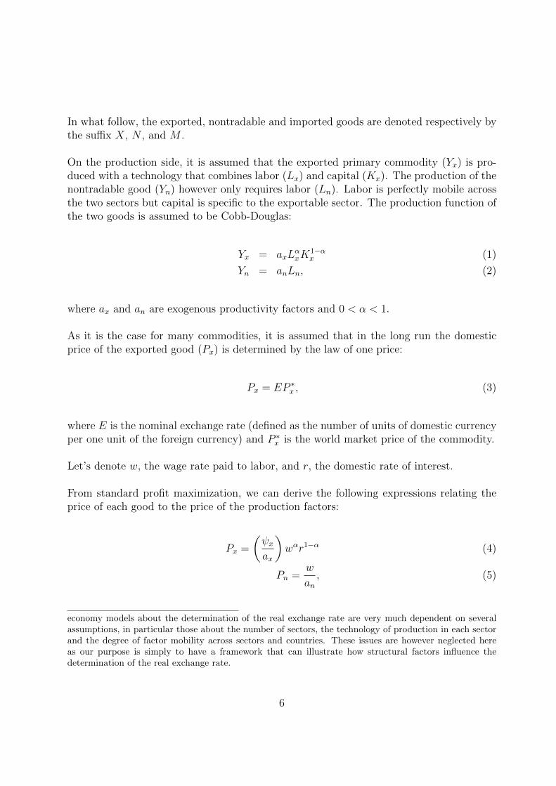
On the production side, it is assumed that the exported primary commodity (Yx) is pro-duced with a technology that combines labor (Lx) and capital (Kx). The production of thenontradable good (Yn) however only requires labor (Ln). Labor is perfectly mobile acrossthe two sectors but capital is specific to the exportable sector. The production function ofthe two goods is assumed to be Cobb-Douglas:

Yx = axLαxK

1−αx (1)

Yn = anLn, (2)

where ax and an are exogenous productivity factors and 0 < α < 1.

As it is the case for many commodities, it is assumed that in the long run the domesticprice of the exported good (Px) is determined by the law of one price:

Px = EP ∗x , (3)

where E is the nominal exchange rate (defined as the number of units of domestic currencyper one unit of the foreign currency) and P ∗x is the world market price of the commodity.

Let’s denote w, the wage rate paid to labor, and r, the domestic rate of interest.

From standard profit maximization, we can derive the following expressions relating theprice of each good to the price of the production factors:

Px =

(ψxax

)wαr1−α (4)

Pn =w

an, (5)

economy models about the determination of the real exchange rate are very much dependent on severalassumptions, in particular those about the number of sectors, the technology of production in each sectorand the degree of factor mobility across sectors and countries. These issues are however neglected hereas our purpose is simply to have a framework that can illustrate how structural factors influence thedetermination of the real exchange rate.

6

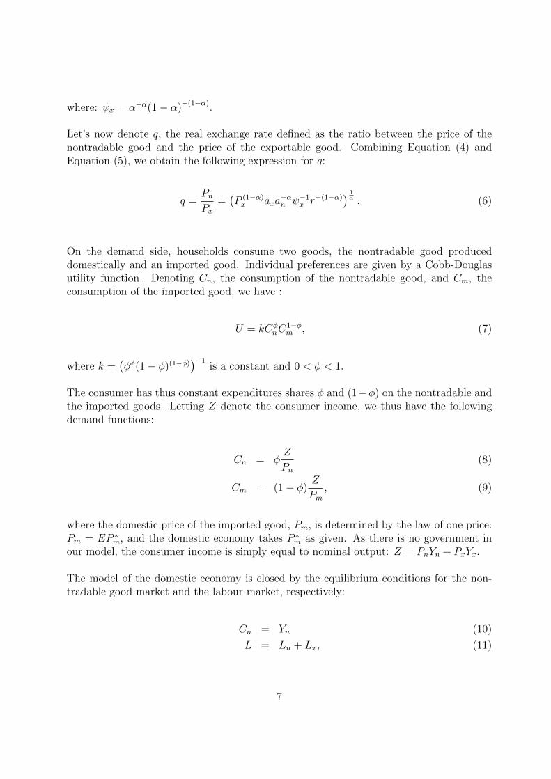
where: ψx = α−α(1 − α)−(1−α).

Let’s now denote q, the real exchange rate defined as the ratio between the price of thenontradable good and the price of the exportable good. Combining Equation (4) andEquation (5), we obtain the following expression for q:

q =PnPx

=(P (1−α)x axa

−αn ψ−1x r−(1−α)

) 1α . (6)

On the demand side, households consume two goods, the nontradable good produceddomestically and an imported good. Individual preferences are given by a Cobb-Douglasutility function. Denoting Cn, the consumption of the nontradable good, and Cm, theconsumption of the imported good, we have :

U = kCφnC

1−φm , (7)

where k =(φφ(1 − φ)(1−φ)

)−1is a constant and 0 < φ < 1.

The consumer has thus constant expenditures shares φ and (1−φ) on the nontradable andthe imported goods. Letting Z denote the consumer income, we thus have the followingdemand functions:

Cn = φZ

Pn(8)

Cm = (1 − φ)Z

Pm, (9)

where the domestic price of the imported good, Pm, is determined by the law of one price:Pm = EP ∗m, and the domestic economy takes P ∗m as given. As there is no government inour model, the consumer income is simply equal to nominal output: Z = PnYn + PxYx.

The model of the domestic economy is closed by the equilibrium conditions for the non-tradable good market and the labour market, respectively:

Cn = Yn (10)

L = Ln + Lx, (11)

7

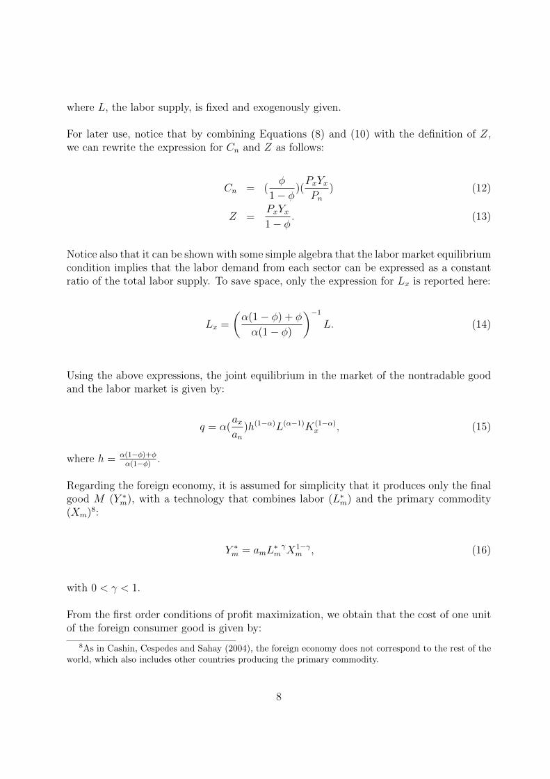
where L, the labor supply, is fixed and exogenously given.

For later use, notice that by combining Equations (8) and (10) with the definition of Z,we can rewrite the expression for Cn and Z as follows:

Cn = (φ

1 − φ)(PxYxPn

) (12)

Z =PxYx1 − φ

. (13)

Notice also that it can be shown with some simple algebra that the labor market equilibriumcondition implies that the labor demand from each sector can be expressed as a constantratio of the total labor supply. To save space, only the expression for Lx is reported here:

Lx =

(α(1 − φ) + φ

α(1 − φ)

)−1L. (14)

Using the above expressions, the joint equilibrium in the market of the nontradable goodand the labor market is given by:

q = α(axan

)h(1−α)L(α−1)K(1−α)x , (15)

where h = α(1−φ)+φα(1−φ) .

Regarding the foreign economy, it is assumed for simplicity that it produces only the finalgood M (Y ∗m), with a technology that combines labor (L∗m) and the primary commodity(Xm)8:

Y ∗m = amL∗mγX1−γ

m , (16)

with 0 < γ < 1.

From the first order conditions of profit maximization, we obtain that the cost of one unitof the foreign consumer good is given by:

8As in Cashin, Cespedes and Sahay (2004), the foreign economy does not correspond to the rest of theworld, which also includes other countries producing the primary commodity.

8

P ∗m =

(ψmam

)w∗γP ∗x

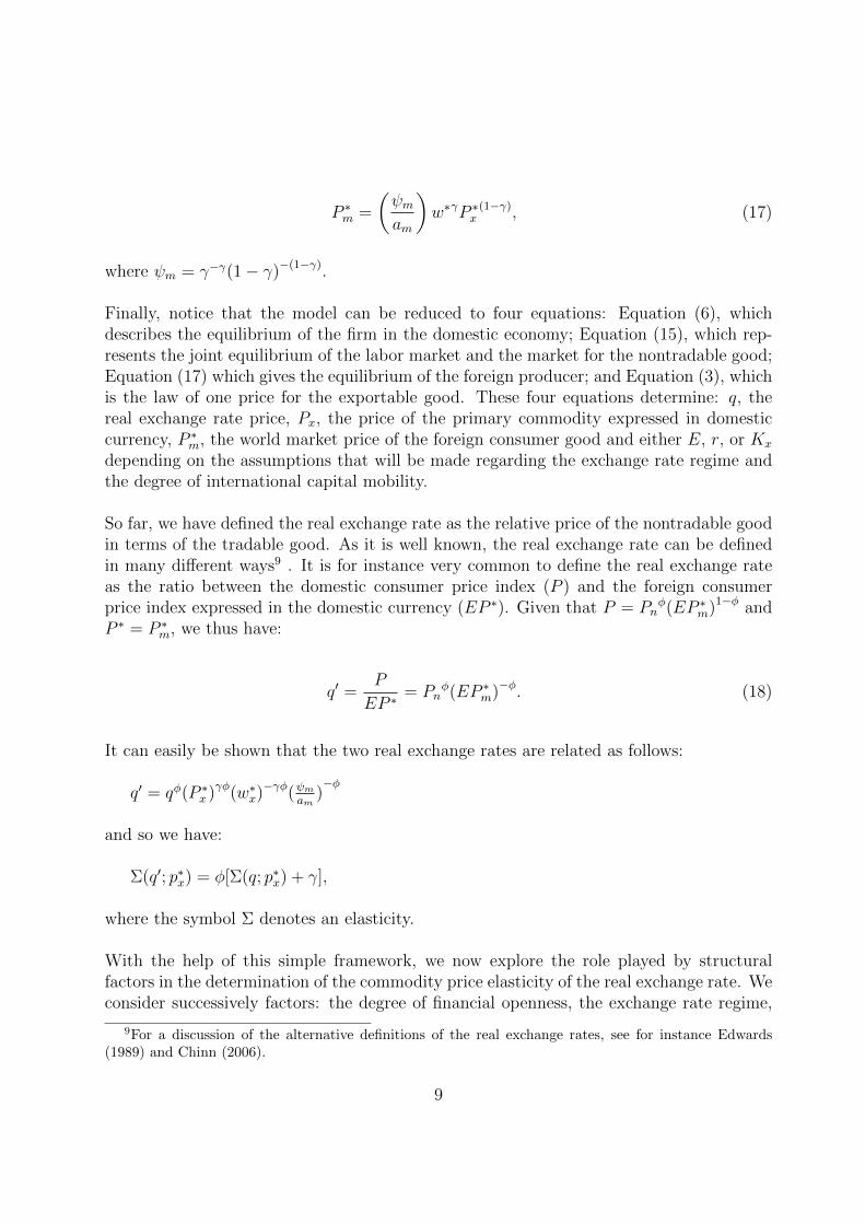
(1−γ), (17)

where ψm = γ−γ(1 − γ)−(1−γ).

Finally, notice that the model can be reduced to four equations: Equation (6), whichdescribes the equilibrium of the firm in the domestic economy; Equation (15), which rep-resents the joint equilibrium of the labor market and the market for the nontradable good;Equation (17) which gives the equilibrium of the foreign producer; and Equation (3), whichis the law of one price for the exportable good. These four equations determine: q, thereal exchange rate price, Px, the price of the primary commodity expressed in domesticcurrency, P ∗m, the world market price of the foreign consumer good and either E, r, or Kx

depending on the assumptions that will be made regarding the exchange rate regime andthe degree of international capital mobility.

So far, we have defined the real exchange rate as the relative price of the nontradable goodin terms of the tradable good. As it is well known, the real exchange rate can be definedin many different ways9 . It is for instance very common to define the real exchange rateas the ratio between the domestic consumer price index (P ) and the foreign consumerprice index expressed in the domestic currency (EP ∗). Given that P = Pn

φ(EP ∗m)1−φ andP ∗ = P ∗m, we thus have:

q′ =P

EP ∗= Pn

φ(EP ∗m)−φ. (18)

It can easily be shown that the two real exchange rates are related as follows:

q′ = qφ(P ∗x )γφ(w∗x)−γφ(ψm

am)−φ

and so we have:

Σ(q′; p∗x) = φ[Σ(q; p∗x) + γ],

where the symbol Σ denotes an elasticity.

With the help of this simple framework, we now explore the role played by structuralfactors in the determination of the commodity price elasticity of the real exchange rate. Weconsider successively factors: the degree of financial openness, the exchange rate regime,

9For a discussion of the alternative definitions of the real exchange rates, see for instance Edwards(1989) and Chinn (2006).

9

the type of the exportable commodity, the degree of trade openness, and the degree ofexport diversification.

2.1 Financial openness

In the analysis that follows, financial openness is given by the degree of international cap-ital mobility. To simplify the analysis, we assume in this Subsection that E is fixed (andset arbitrarily equal to 1).

We start by assuming that capital is perfectly mobile internationally. Under this assump-tion, the domestic rate of interest (r) is tied to the world interest rate (r∗) through theuncovered interest parity condition. With E fixed, we thus have: r = r∗, and the domesticeconomy takes the world interest rate as given. In this case, as shown in numerous pa-pers (see for instance Gregorio and Wolf (1994) or Obstfeld and Rogoff (1996)), the realexchange rate is uniquely determined by Equation (6) and thus depends only on the pro-ductivity parameters and the world interest rate. Demand conditions have no impact on q.The intuition is straightforward. As Px and r are given, it follows that the wage rate, w, isdetermined by Equation (4). Furthermore, as shown by Equation (5), the wage rate is theonly determinant of the price of the nontradable good (Pn). As the real exchange rate isequal to the ratio between the price of the nontradable good and the price of the exportablegood, it therefore depends only on P ∗x , ax, an, and r∗. As it appears from Equation (6),an increase in the world market price of the exportable commodity leads to an increase(appreciation) of the real exchange rate: Σ(q; p∗x) = 1−α

α. Indeed, an increase in Px leads to

a more than proportional increase in the wage rate and the price of the nontradable good.We can also notice that the lower is α, the stronger is the response of q to a variation in P ∗x .

Let’s now assume that capital is not mobile internationally. In this case, r is no longerexogenously given by the world interest rate but is determined endogenously from domesticconditions. The capital stock now becomes exogenous. In this case, q is determined byEquation (15) while Equation (6) is solved for r. It therefore appears that in response toa change in Px, q remains unchanged. Indeed, as Kx is now fixed, the production of thetradable good, Yx, becomes also fixed. The marginal productivity of capital and labor inthe tradable sector is therefore fixed which implies that any increase in the price of theexportable good leads to a proportional increase in the domestic rate of interest and thewage rate. In turn, the price of the nontradable good increases in the same proportion, soleaving unchanged the real exchange rate. Alternatively, notice from Equation (12) thatwith Yx given, the consumer demand of the nontradable good depends only on q. As Yn isconstant, the equilibrium condition for the nontradable good market requires that Cn beconstant as well, which imposes that q be invariant.

When we use the alternative definition of the real exchange rate (q′), the reaction of thereal exchange rate to a change in the world market price of the primary commodity is givenby the following elasticities: (i) φ

(1−αα

+ γ)

when there is perfect capital mobility and (ii)

10

φγ in case of zero capital mobility.

The analysis in this Subsection therefore suggests that the response of the real exchangerate to a commodity price shock is more pronounced in more financially open economies.

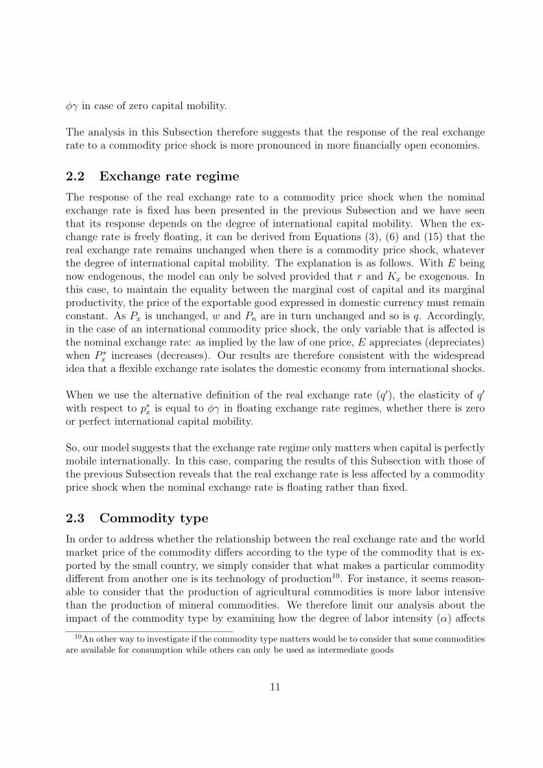
2.2 Exchange rate regime

The response of the real exchange rate to a commodity price shock when the nominalexchange rate is fixed has been presented in the previous Subsection and we have seenthat its response depends on the degree of international capital mobility. When the ex-change rate is freely floating, it can be derived from Equations (3), (6) and (15) that thereal exchange rate remains unchanged when there is a commodity price shock, whateverthe degree of international capital mobility. The explanation is as follows. With E beingnow endogenous, the model can only be solved provided that r and Kx be exogenous. Inthis case, to maintain the equality between the marginal cost of capital and its marginalproductivity, the price of the exportable good expressed in domestic currency must remainconstant. As Px is unchanged, w and Pn are in turn unchanged and so is q. Accordingly,in the case of an international commodity price shock, the only variable that is affected isthe nominal exchange rate: as implied by the law of one price, E appreciates (depreciates)when P ∗x increases (decreases). Our results are therefore consistent with the widespreadidea that a flexible exchange rate isolates the domestic economy from international shocks.

When we use the alternative definition of the real exchange rate (q′), the elasticity of q′

with respect to p∗x is equal to φγ in floating exchange rate regimes, whether there is zeroor perfect international capital mobility.

So, our model suggests that the exchange rate regime only matters when capital is perfectlymobile internationally. In this case, comparing the results of this Subsection with those ofthe previous Subsection reveals that the real exchange rate is less affected by a commodityprice shock when the nominal exchange rate is floating rather than fixed.

2.3 Commodity type

In order to address whether the relationship between the real exchange rate and the worldmarket price of the commodity differs according to the type of the commodity that is ex-ported by the small country, we simply consider that what makes a particular commoditydifferent from another one is its technology of production10. For instance, it seems reason-able to consider that the production of agricultural commodities is more labor intensivethan the production of mineral commodities. We therefore limit our analysis about theimpact of the commodity type by examining how the degree of labor intensity (α) affects

10An other way to investigate if the commodity type matters would be to consider that some commoditiesare available for consumption while others can only be used as intermediate goods

11

the elasticity between q (q′) and P ∗x . From the analysis above, it turns out that when theexchange rate is flexible or when there is zero capital mobility, the elasticity is independentof α and thus invariant to the type of commodities exported by the country. Conversely,when the exchange rate is fixed and capital is perfectly mobile internationally, the elasticityis a negative function of α. Our model therefore suggests that the impact of internationalcommodity price shocks on the real exchange rate will be lower for countries that arespecialized in the export of a commodity whose production is more labor intensive (e.g.agricultural commodities) than for countries which produce capital-intensive commodities(e.g. mineral goods).

2.4 Degree of trade openness

In our model, the degree of trade openness can be captured by the parameter (φ), whichmeasures the share of the nontradable good, compared to the foreign imported good, intotal consumption. It follows from our model that the extent to which the real exchangerate is affected by world commodity price shocks does depend on the country’s degree oftrade openness only when the real exchange rate is given by q′. When those conditionshold, it appears that the higher is the degree of trade openess (the lower is φ), the lower isthe appreciation (depreciation) of q′ in response to a rise (fall) of world commodity prices.

2.5 Export diversification

In order to investigate whether the degree of export diversification affects the magnitude ofthe reaction of the real exchange rate to international commodity price shocks, we extendour model to include the production of a second tradable good. We assume that this newtradable good is a manufacturing good, produced but not consumed domestically. Wealso assume that the production of the manufacturing good (Yd) involves two intermediateinputs, the primary commodity (Xd) and an intermediate input produced by the foreigneconomy (G∗d):

Yd = adXdβG∗d

1−β. (19)

It is straightforward to show that, in equilibrium, the price of the manufacturing good isdetermined as follows:

Pd =ψdadPx

βPf1−β, (20)

where Pf is the price of the foreign intermediate good in domestic currency with Pf = EP ∗f ,

and ψd = β−β(1 − β)−(1−β).

12

In this new framework, we redefine the real exchange rate q as the ratio between the priceof the nontradable good and a composite price of the two exportable goods, q = Pn

Pt, where

Pt = PxεPd

(1−ε).

In what follows, the analysis is limited to the case when the exchange rate is fixed andcapital is perfectly mobile internationally. Under these assumptions, we obtain throughseveral straightforward substitutions that the elasticity of q with respect to P ∗x is given by:

Σ(q; p∗x) =(1−αα

)+ (1 − β)(1 − ε).

This elasticity is then larger than the corresponding elasticity obtained in the model withone exportable good. So our model does indicate that the degree of export diversificationmay influence the magnitude of the real exchange rate variation in response to a worldcommodity price shock. In particular, our model implies that when commodity prices in-crease (decrease), countries whose exports are largely diversified should register a strongerappreciation (depreciation) of their real exchange rate than countries whose exports areweakly diversified. This results comes from the fact that variation in Px leads to a lessthan proportional variation in Pd (see Equation (20)).

Notice that the inclusion of a second good does not affect the expression of q′ and so, theelasticity Σ(q′; p∗x) is independent of the degree of export diversification.

3 Data

In our empirical investigation, we focus on developing and emerging countries that arespecialized in the export of a main commodity. We examine whether their real exchangerate is related to the world market price of their main commodity export and whether therelationship is dependent on structural factors. To address those questions, we use annualdata covering the period 1980-200711. The selection of the countries and the dataset arediscussed in this Section. Data sources are provided in the Appendix.

3.1 Selection of countries and commodities

Our dataset is composed only of countries that are specialized in the export of a leadingcommodity. Using the results of Bodart, Candelon, and Carpantier (2011), we considerthat a country is specialized in the export of a main commodity if that commodity accountsfor at least 20 percent of its total exports12. From an initial sample of 65 developing and

11The end of the sample period is set in 2007 because data on the classification of exchange rate regimesare only available until 2007.

12Bodart, Candelon, and Carpantier (2011) finds that a commodity specialization of at least 20 percentis necessary to have cointegration between the real exchange rate and the international price of the leading

13

emerging countries that, according to the IMF, are considered as commodity producingcountries13, we found 33 countries that satisfy that criteria. The selected countries arelisted in Table 1. We indicate in front of each country what is its main commodity exportand what is the share of that commodity in the total exports of the country14. One cannotice that our dataset is mainly composed of African and Latin american countries andinclude 12 different commodities. More details about the selection of countries are givenin the Appendix.

3.2 Real exchange rates and commodity prices

In line with many studies on the determination of the real exchange rate, the exchange rateseries is the IMF’s real effective exchange rate based on consumer prices. As in Cashin,Cespedes, and Sahay (2004), commodity prices are expressed in real terms, by deflating theUS dollar price of each commodity by the IMF’s index (of the unit value) of manufacturedexports (MUV )15. Real exchange rates (REER) and real commodity prices (COMP ) areindices with base January 1995=100.

3.3 Structural factors

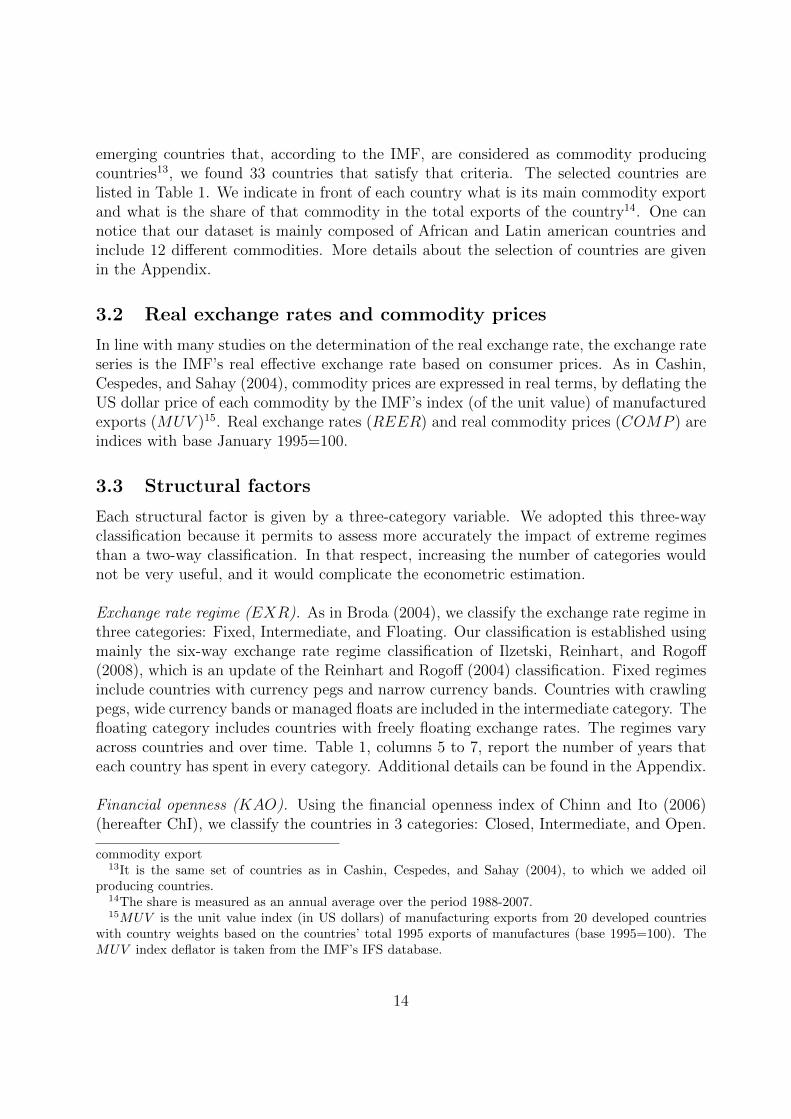
Each structural factor is given by a three-category variable. We adopted this three-wayclassification because it permits to assess more accurately the impact of extreme regimesthan a two-way classification. In that respect, increasing the number of categories wouldnot be very useful, and it would complicate the econometric estimation.

Exchange rate regime (EXR). As in Broda (2004), we classify the exchange rate regime inthree categories: Fixed, Intermediate, and Floating. Our classification is established usingmainly the six-way exchange rate regime classification of Ilzetski, Reinhart, and Rogoff(2008), which is an update of the Reinhart and Rogoff (2004) classification. Fixed regimesinclude countries with currency pegs and narrow currency bands. Countries with crawlingpegs, wide currency bands or managed floats are included in the intermediate category. Thefloating category includes countries with freely floating exchange rates. The regimes varyacross countries and over time. Table 1, columns 5 to 7, report the number of years thateach country has spent in every category. Additional details can be found in the Appendix.

Financial openness (KAO). Using the financial openness index of Chinn and Ito (2006)(hereafter ChI), we classify the countries in 3 categories: Closed, Intermediate, and Open.

commodity export13It is the same set of countries as in Cashin, Cespedes, and Sahay (2004), to which we added oil

producing countries.14The share is measured as an annual average over the period 1988-2007.15MUV is the unit value index (in US dollars) of manufacturing exports from 20 developed countries

with country weights based on the countries’ total 1995 exports of manufactures (base 1995=100). TheMUV index deflator is taken from the IMF’s IFS database.

14

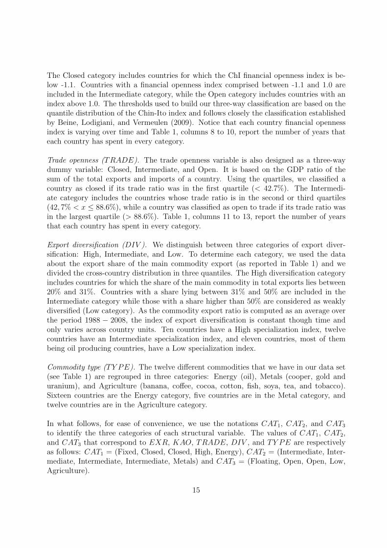
The Closed category includes countries for which the ChI financial openness index is be-low -1.1. Countries with a financial openness index comprised between -1.1 and 1.0 areincluded in the Intermediate category, while the Open category includes countries with anindex above 1.0. The thresholds used to build our three-way classification are based on thequantile distribution of the Chin-Ito index and follows closely the classification establishedby Beine, Lodigiani, and Vermeulen (2009). Notice that each country financial opennessindex is varying over time and Table 1, columns 8 to 10, report the number of years thateach country has spent in every category.

Trade openness (TRADE). The trade openness variable is also designed as a three-waydummy variable: Closed, Intermediate, and Open. It is based on the GDP ratio of thesum of the total exports and imports of a country. Using the quartiles, we classified acountry as closed if its trade ratio was in the first quartile (< 42.7%). The Intermedi-ate category includes the countries whose trade ratio is in the second or third quartiles(42, 7% < x ≤ 88.6%), while a country was classified as open to trade if its trade ratio wasin the largest quartile (> 88.6%). Table 1, columns 11 to 13, report the number of yearsthat each country has spent in every category.

Export diversification (DIV ). We distinguish between three categories of export diver-sification: High, Intermediate, and Low. To determine each category, we used the dataabout the export share of the main commodity export (as reported in Table 1) and wedivided the cross-country distribution in three quantiles. The High diversification categoryincludes countries for which the share of the main commodity in total exports lies between20% and 31%. Countries with a share lying between 31% and 50% are included in theIntermediate category while those with a share higher than 50% are considered as weaklydiversified (Low category). As the commodity export ratio is computed as an average overthe period 1988 − 2008, the index of export diversification is constant though time andonly varies across country units. Ten countries have a High specialization index, twelvecountries have an Intermediate specialization index, and eleven countries, most of thembeing oil producing countries, have a Low specialization index.

Commodity type (TY PE). The twelve different commodities that we have in our data set(see Table 1) are regrouped in three categories: Energy (oil), Metals (cooper, gold anduranium), and Agriculture (banana, coffee, cocoa, cotton, fish, soya, tea, and tobacco).Sixteen countries are the Energy category, five countries are in the Metal category, andtwelve countries are in the Agriculture category.

In what follows, for ease of convenience, we use the notations CAT1, CAT2, and CAT3to identify the three categories of each structural variable. The values of CAT1, CAT2,and CAT3 that correspond to EXR, KAO, TRADE, DIV , and TY PE are respectivelyas follows: CAT1 = (Fixed, Closed, Closed, High, Energy), CAT2 = (Intermediate, Inter-mediate, Intermediate, Intermediate, Metals) and CAT3 = (Floating, Open, Open, Low,Agriculture).

15

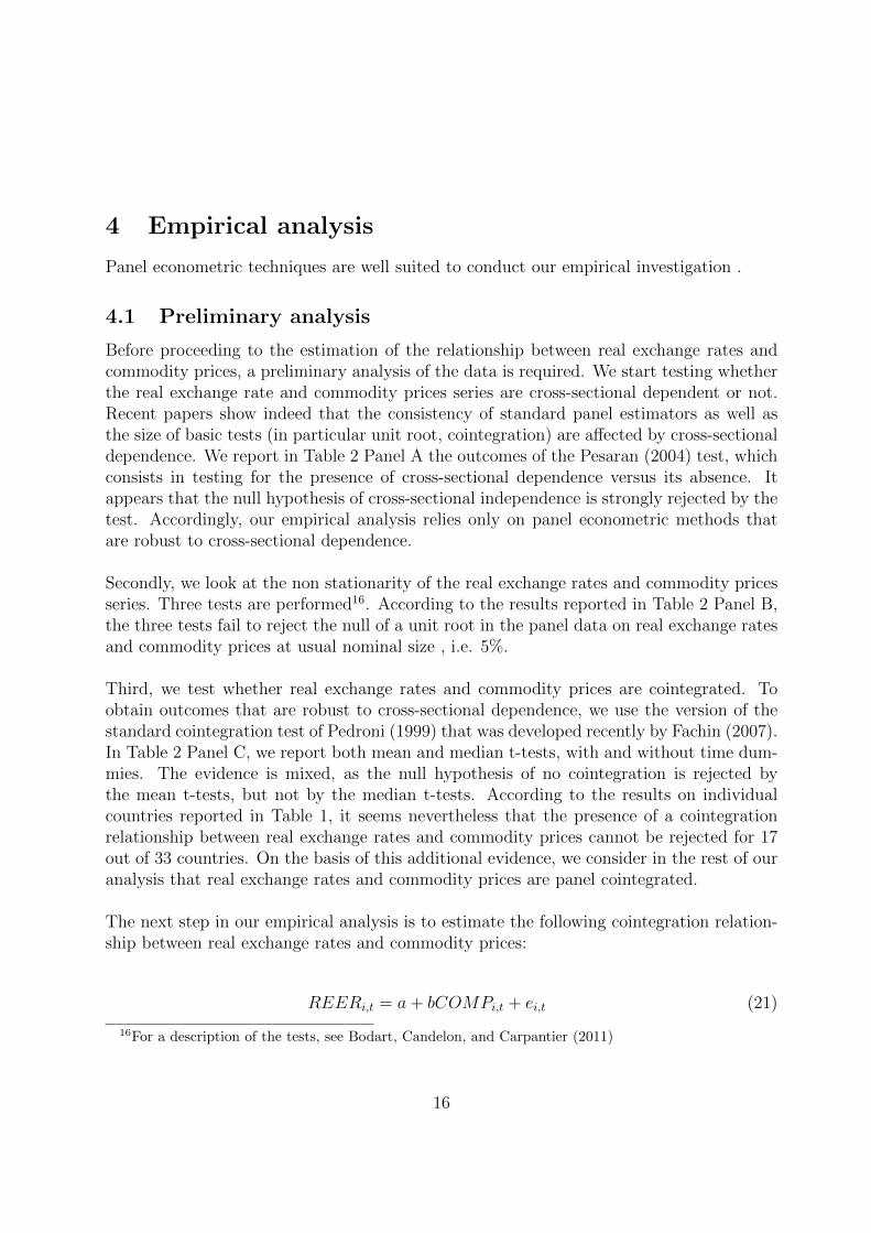
4 Empirical analysis

Panel econometric techniques are well suited to conduct our empirical investigation .

4.1 Preliminary analysis

Before proceeding to the estimation of the relationship between real exchange rates andcommodity prices, a preliminary analysis of the data is required. We start testing whetherthe real exchange rate and commodity prices series are cross-sectional dependent or not.Recent papers show indeed that the consistency of standard panel estimators as well asthe size of basic tests (in particular unit root, cointegration) are affected by cross-sectionaldependence. We report in Table 2 Panel A the outcomes of the Pesaran (2004) test, whichconsists in testing for the presence of cross-sectional dependence versus its absence. Itappears that the null hypothesis of cross-sectional independence is strongly rejected by thetest. Accordingly, our empirical analysis relies only on panel econometric methods thatare robust to cross-sectional dependence.

Secondly, we look at the non stationarity of the real exchange rates and commodity pricesseries. Three tests are performed16. According to the results reported in Table 2 Panel B,the three tests fail to reject the null of a unit root in the panel data on real exchange ratesand commodity prices at usual nominal size , i.e. 5%.

Third, we test whether real exchange rates and commodity prices are cointegrated. Toobtain outcomes that are robust to cross-sectional dependence, we use the version of thestandard cointegration test of Pedroni (1999) that was developed recently by Fachin (2007).In Table 2 Panel C, we report both mean and median t-tests, with and without time dum-mies. The evidence is mixed, as the null hypothesis of no cointegration is rejected bythe mean t-tests, but not by the median t-tests. According to the results on individualcountries reported in Table 1, it seems nevertheless that the presence of a cointegrationrelationship between real exchange rates and commodity prices cannot be rejected for 17out of 33 countries. On the basis of this additional evidence, we consider in the rest of ouranalysis that real exchange rates and commodity prices are panel cointegrated.

The next step in our empirical analysis is to estimate the following cointegration relation-ship between real exchange rates and commodity prices:

REERi,t = a+ bCOMPi,t + ei,t (21)

16For a description of the tests, see Bodart, Candelon, and Carpantier (2011)

16

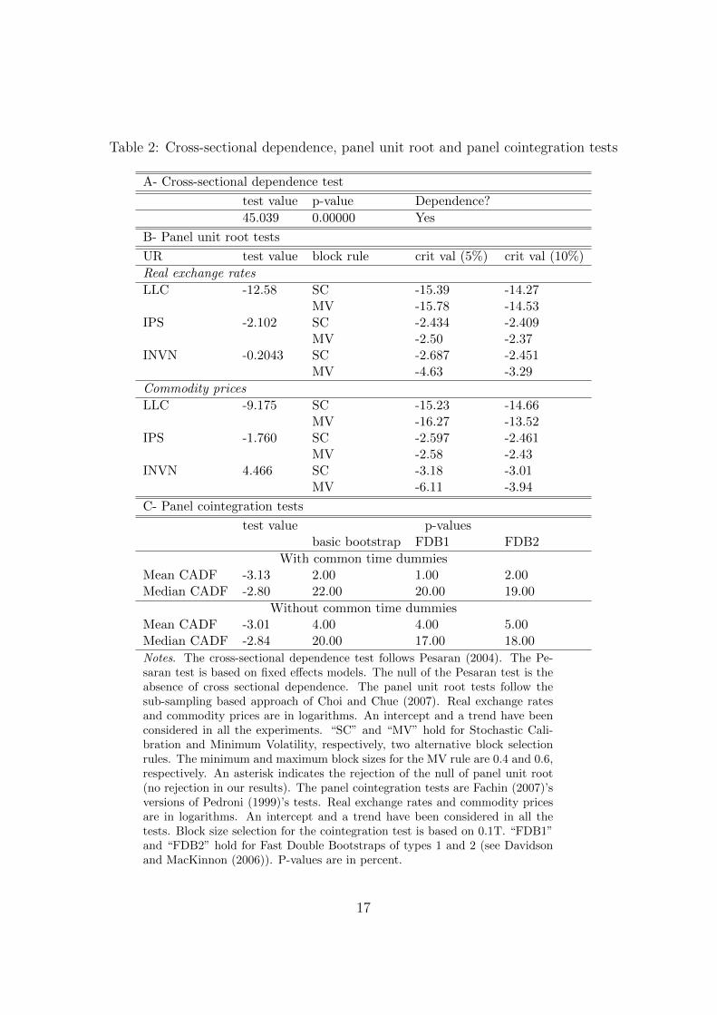
Table 2: Cross-sectional dependence, panel unit root and panel cointegration tests

A- Cross-sectional dependence test

test value p-value Dependence?

45.039 0.00000 Yes

B- Panel unit root tests

UR test value block rule crit val (5%) crit val (10%)

Real exchange rates

LLC -12.58 SC -15.39 -14.27MV -15.78 -14.53

IPS -2.102 SC -2.434 -2.409MV -2.50 -2.37

INVN -0.2043 SC -2.687 -2.451MV -4.63 -3.29

Commodity prices

LLC -9.175 SC -15.23 -14.66MV -16.27 -13.52

IPS -1.760 SC -2.597 -2.461MV -2.58 -2.43

INVN 4.466 SC -3.18 -3.01MV -6.11 -3.94

C- Panel cointegration tests

test value p-valuesbasic bootstrap FDB1 FDB2

With common time dummiesMean CADF -3.13 2.00 1.00 2.00Median CADF -2.80 22.00 20.00 19.00

Without common time dummiesMean CADF -3.01 4.00 4.00 5.00Median CADF -2.84 20.00 17.00 18.00

Notes. The cross-sectional dependence test follows Pesaran (2004). The Pe-saran test is based on fixed effects models. The null of the Pesaran test is theabsence of cross sectional dependence. The panel unit root tests follow thesub-sampling based approach of Choi and Chue (2007). Real exchange ratesand commodity prices are in logarithms. An intercept and a trend have beenconsidered in all the experiments. “SC” and “MV” hold for Stochastic Cali-bration and Minimum Volatility, respectively, two alternative block selectionrules. The minimum and maximum block sizes for the MV rule are 0.4 and 0.6,respectively. An asterisk indicates the rejection of the null of panel unit root(no rejection in our results). The panel cointegration tests are Fachin (2007)’sversions of Pedroni (1999)’s tests. Real exchange rates and commodity pricesare in logarithms. An intercept and a trend have been considered in all thetests. Block size selection for the cointegration test is based on 0.1T. “FDB1”and “FDB2” hold for Fast Double Bootstraps of types 1 and 2 (see Davidsonand MacKinnon (2006)). P-values are in percent.

17

where REERi,t is the (log) real exchange rate of country i at time t, and COMPi,t is the(log) real price at time t of the leading commodity exported by country i.

Several techniques have been proposed to estimate such a long run relationship, the mostpopular being DOLS and FMOLS. Nevertheless Bai, Kao, and Ng (2009) (BKN hereafter)prove that traditional estimators are biased in presence of cross-sectional dependence gen-erated by unobserved global stochastic trends. They introduce common factors to controlfor cross unit dependence, and thus propose an iterative procedure to extract the commonfactor and to estimate the equation simultaneously. The results are reported in Table 3column 1. It turns out that the price of the dominant commodity has a long-run impacton the real exchange rate with an elasticity of 12.5% which is in line with the Bodart,Candelon, and Carpantier (2011)’s analysis, the only one so far to implement the BKNapproach in this context.

4.2 Estimates of the impact of structural factors

Once this preliminary analysis achieved, let us now turn to the paper’s core, i.e. how theselected structural factors might affect the long-run commodity price elasticity of the realexchange rate. To this aim, Equation (21) is augmented by an interaction term betweenthe commodity price variable and the three-way variable representing each structural factor(see Section 3). In practice, we explore the impact of each structural factor by interactingthe commodity price variable with two dummy variables, a dummy D2 (that takes thevalue 1 when observations are in the 2nd category (CAT2) and zero otherwise) and adummy D3 (that takes the value 1 when observations are in the 3rd category (CAT3)and zero otherwise). Let us note that we did not include a D1 dummy to avoid the lineardependence between the interaction terms and the variable COMPi,t. The category definedby D1 will thus be considered as the baseline. This gives the following relationship:

REERi,t = a+ bCOMPi,t + c1(Dj,2,t ∗ COMPi,t) + c2(Dj,3,t ∗ COMPi,t) + ei,t (22)

The estimation of Equation (22) thus amounts to estimate the long-run relationship be-tween real exchange rates and commodity prices, conditional on each factor. The impactof each factor on the long-run commodity price elasticity of the real exchange rate is deter-mined by testing the hypothesis that each cj (j = 1, 2) is significantly different from zero(H0: cj = 0).

The estimation outcomes of Equation (22) are reported in Table 3 columns (2) to (6).Before analyzing the impact of the structural factors on the real exchange rate-commodityprice relationship, let us make two remarks. First, it is noticeable that the baseline coeffi-cient b only varies marginally from one specification to the other, lying between 0.101 and

18

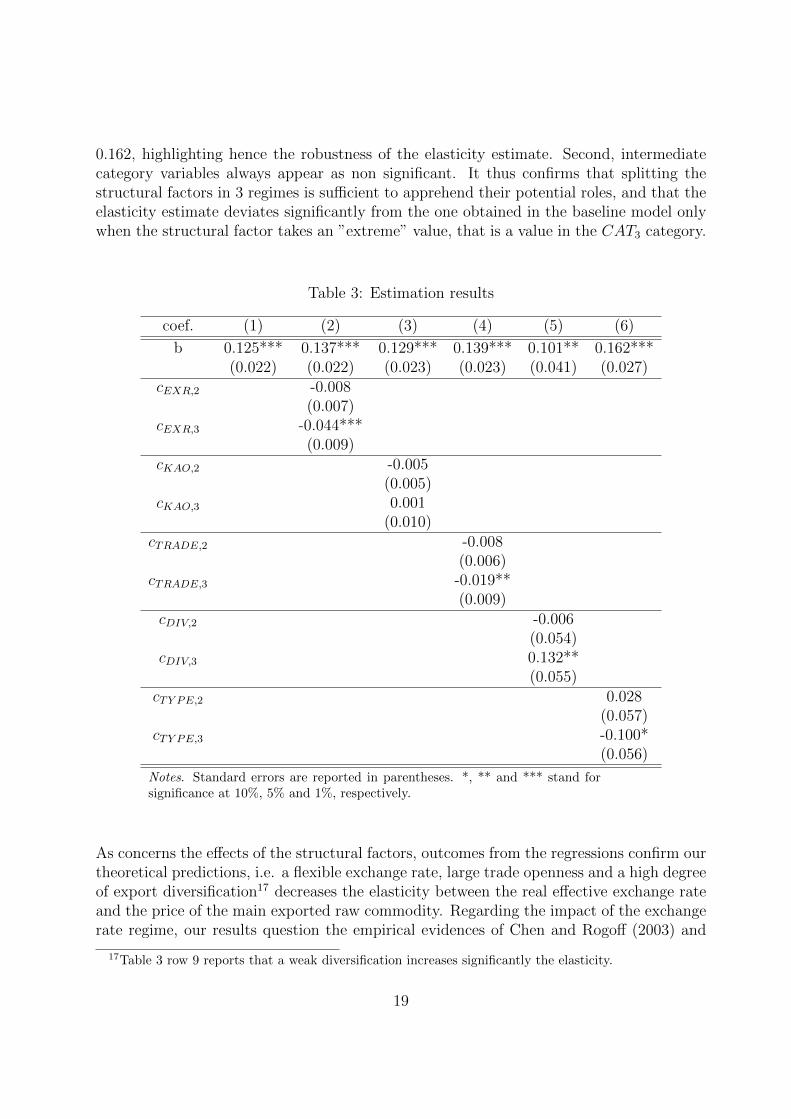
0.162, highlighting hence the robustness of the elasticity estimate. Second, intermediatecategory variables always appear as non significant. It thus confirms that splitting thestructural factors in 3 regimes is sufficient to apprehend their potential roles, and that theelasticity estimate deviates significantly from the one obtained in the baseline model onlywhen the structural factor takes an ”extreme” value, that is a value in the CAT3 category.

Table 3: Estimation results

coef. (1) (2) (3) (4) (5) (6)

b 0.125*** 0.137*** 0.129*** 0.139*** 0.101** 0.162***(0.022) (0.022) (0.023) (0.023) (0.041) (0.027)

cEXR,2 -0.008(0.007)

cEXR,3 -0.044***(0.009)

cKAO,2 -0.005(0.005)

cKAO,3 0.001(0.010)

cTRADE,2 -0.008(0.006)

cTRADE,3 -0.019**(0.009)

cDIV,2 -0.006(0.054)

cDIV,3 0.132**(0.055)

cTY PE,2 0.028(0.057)

cTY PE,3 -0.100*(0.056)

Notes. Standard errors are reported in parentheses. *, ** and *** stand forsignificance at 10%, 5% and 1%, respectively.

As concerns the effects of the structural factors, outcomes from the regressions confirm ourtheoretical predictions, i.e. a flexible exchange rate, large trade openness and a high degreeof export diversification17 decreases the elasticity between the real effective exchange rateand the price of the main exported raw commodity. Regarding the impact of the exchangerate regime, our results question the empirical evidences of Chen and Rogoff (2003) and

17Table 3 row 9 reports that a weak diversification increases significantly the elasticity.

19

Broda (2004) who, conversely, find that the impact of world commodity prices on the realexchange rate is weaker when the exchange rate is fixed. We also find that when the ex-ported commodity is an agricultural good, the elasticity becomes higher, corroborating ourfinding that real exchange rate and commodity prices are strongly linked for labor intensiveactivity sectors. Interestingly, column (3) does not show any effect of financial openness.This result, which does not match the predictions of theoretical models, may be due tothe difficulty to measure properly this structural variable. However, to our knowledge,the Chinn and Ito (2006) index remains the most accurate and used measure of financialopenness.

4.3 Robustness check

In order to evaluate the robustness of our findings, three investigations are performed.Since the construction of the dummy variables representing the degree of trade opennessand the degree of export diversification is obviously ad hoc, we first replicate the analysisof the previous section using an alternative construction of the variables TRADE andDIV 18. Instead of using quartiles to classify trade values into three categories, we nowuse quintiles. We then classify a country as Closed if its trade ratio is in the first quintile(< 38.0%) and Open if it is in the largest quintile (> 94.0%) . The Intermediate categoryincludes the countries whose trade ratio is in the second, third and fourth quintiles. Thenew trade dummy variable is denoted TRADEn. Similarly, the new DIV n dummy is builtupon quartiles. A country is then in the High diversification category if the share of theexports of its main commodity in total exports is in the first quartile (< 38%) while it isin the Low diversification category if the commodity exports share is in the fourth quartile(> 94.0%). When the commodity export ratio lies in the second and third quartiles, thecountry is classified in the Intermediate diversification category. Results obtained withthese new variables are reported in Table 4. It appears that they are qualitatively compa-rable to those obtained previously (Table 3 columns (4) and (5)).

Since our sample includes several African countries belonging to the CFA Franc Zone(Cameroon, Ivory Coast, Gabon, Mali and Niger), we next investigate whether our resultsare influenced by the 50 percent devaluation of the CFA Franc that took place in January1994. We do so by adding in our specification a 1994 dummy which is equal to 1 for CFAcountries in 1994 and which is equal to zero otherwise19. The new results are reported inTable 5. One can observe that the estimators are very close to those obtained in Table 3,so supporting again the robustness of our conclusions.

18As regards the construction of the variables representing the degree of flexibility of the exchange rateregime and the degree of financial openness, since it is taken from existing studies, we consider that it isless subject to debate

19The BKN methodology has a preliminary step where the series are first regressed on a constant and atrend. In order to test the robustness of our results to the 1994 devaluation in CFA countries, we add the1994 dummy to the regressors in the preliminary regression.

20

Table 4: Robustness check: modification of the trade openness and export diversificationdummies

b ci,2 ci,3i = TRADEn 0.161*** (0.023) -0.013** (0.006) -0.023** (0.009)i = DIV n 0.125*** (0.045) 0.004 (0.054) 0.134** (0.060)

Notes. Standard errors in parentheses. *, ** and *** stand for significance at10%, 5% and 1%, respectively.

Table 5: Robustness check: accounting for the January 1994 devaluation of the CFA Franc

coef. (1) (2) (3) (4) (5) (6)

b 0.1405*** 0.130*** 0.1100*** 0.1489*** 0.1136*** 0.1535***(0.022) (0.021) (0.027) (0.023) (0.041) (0.027)

cEXR,2 -0.006372(0.007)

cEXR,3 -0.04277 ***(0.009)

cKAO,2 0.002692(0.005)

cKAO,3 0.01206(0.010)

cTRADE,2 -0.008557(0.006)

cTRADE,3 -0.01842 **(0.009)

cDIV,2 -0.02766(0.054)

cDIV,3 0.08265(0.055)

cTY PE,2 0.02532(0.057)

cTY PE,3 -0.09739*(0.056)

Notes. Standard errors are reported in parentheses. *, ** and *** stand forsignificance at 10%, 5% and 1%, respectively.

21

Finally, we conduct the analysis by region. We split our sample of countries in two groups,Sub-Saharan Africa and Latin Americia. Estimations (1) to (6) are repeated separately foreach group and the results are reported in Panels A and B of Table 6. Overall, the resultsobtained for each group are qualitatively similar to those in the full sample (see Table 3).The real exchange rate is positively related to world commodity prices in both regions, andthe relationship is shaped by almost the same structural factors. There are however twonoticeable differences. First, the impact of the degree of financial openness is positive andstatistically significant for Africa while it is non significant in Latin America and in the fullsample. For Africa, this means that the higher is international capital mobility, the higheris the commodity price elasticity of the real exchange rate. Second, the results regardingthe impact of the commodity type are different between Africa and Latin America andthey are also different from the results in the full sample. For Africa, the impact is notsignificant. A possible explanation of this result is the low diversification of commodityexports as half of the countries in the Sub-Saharan panel have an agricultural commodityas their main commodity export.

5 Conclusions

As it is demonstrated by the literature on the ”Dutch” disease, commodity prices are po-tentially an important determinant of the real exchange rate of countries that produce andexport primary commodities. For that reason, the dependence of real exchange rates oncommodity prices (or, more generally, on terms of trade) has been the focus of numerousempirical studies. In most of these studies, the empirical evidence consists only of econo-metric estimates of the real exchange rate response to commodity price shocks. Whatdetermines the magnitude of the real exchange rate reaction is however not investigated.This issue is the main subject of this paper. We first showed with a simple theoreticalframework that several structural or institutional characteristics may contribute to shapethe relationship that exists in the long-run between a country’s real exchange rate andthe world price of the main commodity that it exports. We emphasized the role of fivestructural factors: the exchange rate regime, the degree of trade openness, the degree ofexport diversification, the type of the commodity export, and the degree of financial open-ness. We then subjected the role of these factors to econometric scrutiny by conductingan empirical investigation involving 33 developing countries specialized in the export of amain primary commodity.

Using panel cointegration methods robust to cross-sectional dependence, we found thatfour of the five factors, namely the exchange rate regime, the degree of trade openness, thedegree of export diversification and the type of the commodity exported, have a significantimpact on the long-run commodity price elasticity of the real exchange rate. More precisely,we report that the elasticity is reduced when a country operates a floating exchange rate(rather than a fixed exchange rate). It is also smaller when the country is strongly opened

22

Table 6: Robustness check: Estimations by region

A - Sub-Saharan African countries

coef. (1) (2) (3) (4) (5) (6)b 0.210*** 0.151*** 0.163*** 0.155*** 0.039 0.157***

(0.036) (0.027) (0.029) (0.030) (0.046) (0.037)cEXR,2 0.003

(0.010)cEXR,3 -0.068***

(0.012)cKAO,2 0.010*

(0.006)cKAO,3 0.040***

(0.012)cTRADE,2 0.004

(0.008)cTRADE,3 -0.030**

(0.012)cDIV,2 0.030

(0.079)cDIV,3 0.221***

(0.061)cTY PE,2 -0.046

(0.082)cTY PE,3 0.016

(0.064)

B - Latin American countries

coef. (1) (2) (3) (4) (5) (6)b 0.089*** 0.120*** 0.102*** 0.224*** - 0.122***

(0.028) (0.031) (0.034) (0.031) - (0.034)cEXR,2 -0.006

(0.012)cEXR,3 -0.029**

(0.013)cKAO,2 0.006

(0.008)cKAO,3 0.013

(0.014)cTRADE,2 -0.063***

(0.008)cTRADE,3 -0.058***

(0.012)cDIV,2 -

-cDIV,3 -

-cTY PE,2 0.211**

(0.088)cTY PE,3 0.145

(0.104)

Notes. Countries included in Panel A are Burundi, Cameroon, Cote d’Ivoire,Ethiopia, Gabon, Ghana, Kenya, Malawi, Mali, Mauritania, Niger, Nigeria, Su-dan, Tanzania, Uganda and Zambia. Countries included in Panel B are Chile,Colombia, Dominica, Ecuador, Honduras, Paraguay and Venezuela. Standarderrors are reported in parentheses. *, ** and *** stand for significance at 10%,5% and 1%, respectively.

23

to external trade (rather than closed) and when its exports are highly diversified (ratherthan specialized on a few products). We also find that the elasticity is smaller when the pri-mary commodity is an agricultural good, but is higher when it is oil. Conversely, it appearsfrom our analysis that the degree of financial openness does not influence significantly theextent to which real exchange rates and world commodity prices are related in the long-run.

The analysis by regions show some differences with these main results. The first differ-ence concerns the impact of the commodity type in the determination of the real exchangerate-commodity pricer relationship. For Sub-saharan African countries, the type of themain exported commodity does not matter and, in Latin America, the elasticity is smallerwhen the primary commodity is oil and higher when it is metals. Second, it appears thatfor Africa, the degree of financial openness is a significant determinant of the long-runcommodity price elasticity of the real exchange rate.

Our results have several policy implications. They suggest in particular that countrieswhich are concerned by the adverse impact that world commodity price fluctuations mayhave on their competitiveness, in other words countries that wish to reduce ”Dutch disease”effects, should adopt a floating exchange rate instead of a fixed exchange rate. Theyalso suggest that developing countries whose exports are concentrated on a few primarycommodities can reduce the dependance of their real exchange rate on world commodityprices by having more diversified exports. According to our results, diversification towardsagricultural products would isolate further the real exchange rate from world commodityprice shocks. Countries can also protect their competitiveness from fluctuations in worldcommodity prices by being more opened to external trade. Finally, Sub-Saharan Africancountries could attenuate the dependence o f their real exchange rate on world commodityprices by being less opened to international capital flows.

24

Appendix: description of the data

To proceed to the selection of the countries included in our dataset, we recovered from theUN Comtrade database the annual US$ export value of 42 commodities for 65 countriesover the period 1988-2007. The initial set of 65 countries corresponds to the sample ofdeveloping and emerging countries selected by Cashin, Cespedes, and Sahay (2004) on thebasis of the International Monetary Fund classification of developing countries accordingto the composition of their export earnings, to which we added oil producing countries.For each country, we computed the 1988-2007 annual average of the US$ export receiptof each individual commodity and we expressed the resulting value as a share of the totalUS$ export receipts of the country. We then kept the countries for which at least onecommodity had a share in total exports of at least 20 percent. From the resulting list ofcountries, we removed Mozambique because the export share of its aluminium exports wasmore than 50% after 2001 but about zero before 2000. A few other countries were excludedfrom our analysis because of the unavailability of data for all the variables of our model.

Real exchange rates are IMF real effective exchange rates based on consumer prices20. Thedata are extracted from the IMF’s Information Notice System (INS) database.

Commodity prices are taken from the International Financial Statistics (IFS) database ofthe IMF. Two series, Tobacco and Gold, were not available in IFS and were taken fromDatastream (with respective codes: USI76M.ZA and GOLDBLN). Details about each se-ries are provided in Table 7.

Data on exchange rate regimes are taken from two databases. The first database, IRR,is provided by Ilzetski, Reinhart, and Rogoff (2008) and is an update of the Reinhart andRogoff (2004) exchange rate regime classification. The IRR exchange rate regime classifi-cation is a de facto classification based on market-determined exchange rates. It providesmonthly and annual classification data over the period 1940-2007. Classification by 6 and15 categories are available. The second database, LY S, was established by Levy-Yeyatiand Sturzenegger (2005) on the basis of data on nominal exchange rates volatility andinternational reserves volatility (de facto classification). It covers 183 countries for theperiod 1974-2004. Classification by 3 and 5 categories are available. Both databases haveadvantages and weaknesses. One advantage of the LY S database is to provide a 3-categoryclassification, but it has no data for 2005 and later. On the contrary, the IRR databasecovers the period 1980-2007, but it has only 6- and 15-category classifications. Our pa-per uses mainly the IRR 6-regime classification to benefit from the longest time coverage(1980-2007). It contains however missing values. When possible, we solved this problemby replacing the missing value by the value found in the LY S 3-category classification.When no data were available in the LY S database, we replaced the missing value by the

20See Desruelle and Zanello (1997) for details regarding the construction of the real effective exchangerates.

25

value of the previous year. We converted the IRR 6-regime classification into 3 exchangerate regime categories as follows: our Fixed Regime category corresponds to IRR category1; our Intermediate Regime category corresponds to categories 2 and 3 of IRR; and ourFlexible Regime category includes categories 4, 5 and 6 of IRR.

The financial openness dummy variable used in our analysis is based upon the financialopenness index of Chinn and Ito (2006). The Chinn-Ito index measures the degree ofopenness of a country’s capital account. It is based on binary dummy variables thatcodify the tabulation of restrictions on cross-border financial transactions reported in theInternational Monetary Fund’s Annual Report on Exchange Arrangements and ExchangeRestrictions. This index is thus a de jure measure of financial openness. The index isnot smoothly distributed. Values range between -1.9 and 2.6, with about one third of theobservations having a value of -1.13. Three values were missing in the Chinn-Ito database:Dominica in 1980 and 1981 and Sudan in 2006. We filled the gaps by setting the 1980 and1981 Dominica indices equal to the 1982 Dominica index, and by setting the 2006 Sudanindex equal to the 2005 Sudan index (which is the same as the 2007 index).

GDP, export and import data used to construct the trade openness dummy variable areall taken from the World Bank. All the data are in current US$.

26

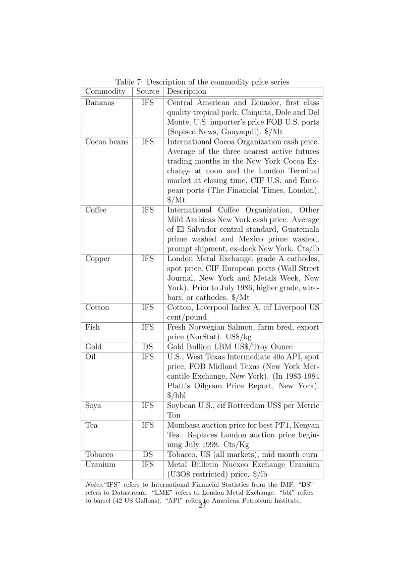
Table 7: Description of the commodity price seriesCommodity Source Description

Bananas IFS Central American and Ecuador, first classquality tropical pack, Chiquita, Dole and DelMonte, U.S. importer’s price FOB U.S. ports(Sopisco News, Guayaquil). $/Mt

Cocoa beans IFS International Cocoa Organization cash price.Average of the three nearest active futurestrading months in the New York Cocoa Ex-change at noon and the London Terminalmarket at closing time, CIF U.S. and Euro-pean ports (The Financial Times, London).$/Mt

Coffee IFS International Coffee Organization, OtherMild Arabicas New York cash price. Averageof El Salvador central standard, Guatemalaprime washed and Mexico prime washed,prompt shipment, ex-dock New York. Cts/lb

Copper IFS London Metal Exchange, grade A cathodes,spot price, CIF European ports (Wall StreetJournal, New York and Metals Week, NewYork). Prior to July 1986, higher grade, wire-bars, or cathodes. $/Mt

Cotton IFS Cotton, Liverpool Index A, cif Liverpool UScent/pound

Fish IFS Fresh Norwegian Salmon, farm bred, exportprice (NorStat). US$/kg

Gold DS Gold Bullion LBM US$/Troy OunceOil IFS U.S., West Texas Intermediate 40o API, spot

price, FOB Midland Texas (New York Mer-cantile Exchange, New York). (In 1983-1984Platt’s Oilgram Price Report, New York).$/bbl

Soya IFS Soybean U.S., cif Rotterdam US$ per MetricTon

Tea IFS Mombasa auction price for best PF1, KenyanTea. Replaces London auction price begin-ning July 1998. Cts/Kg

Tobacco DS Tobacco, US (all markets), mid month curnUranium IFS Metal Bulletin Nuexco Exchange Uranium

(U3O8 restricted) price. $/lbNotes.“IFS” refers to International Financial Statistics from the IMF. “DS”refers to Datastream. “LME” refers to London Metal Exchange. “bbl” refersto barrel (42 US Gallons). “API” refers to American Petroleum Institute.

27

References

Bai, J., C. Kao, and S. Ng (2009): “Panel cointegration with global stochastic trends,”Journal of Econometrics, 149(1), 82–99.

Beine, M., E. Lodigiani, and R. Vermeulen (2009): “Remittances and FinancialOpenness,” CREA Discussion Paper Series 09-09, Center for Research in EconomicAnalysis, University of Luxembourg.

Bodart, V., B. Candelon, and J. F. Carpantier (2011): “Real exchanges rates incommodity producing countries : a reappraisal,” CORE Discussion Papers 2011006, Uni-versit catholique de Louvain, Center for Operations Research and Econometrics (CORE).

Brahmbhatt, M., O. Canuto, and E. Vostroknutova (2010): “Dealing with DutchDisease,” World Bank - Economic Premise, (16), 1–7.

Broda, C. (2004): “Terms of trade and exchange rate regimes in developing countries,”Journal of International Economics, 63(1), 31–58.

Cashin, P., L. F. Cespedes, and R. Sahay (2004): “Commodity Currencies and theReal Exchange Rate,” Journal of Development Economics, 75(1), 239–268.

Chen, Y.-c., and K. Rogoff (2003): “Commodity currencies,” Journal of InternationalEconomics, 60(1), 133–160.

Chinn, M. (2006): “A Primer on Real Effective Exchange Rates: Determinants, Over-valuation, Trade Flows and Competitive Devaluation,” Open Economies Review, 17(1),115–143.

Chinn, M. D., and H. Ito (2006): “What matters for financial development? Capitalcontrols, institutions, and interactions,” Journal of Development Economics, 81(1), 163–192.

Choi, I., and T. K. Chue (2007): “Subsampling Hypothesis Tests for NonstationaryPanels with Applications to Exchange Rates and Stock Prices,” Journal of AppliedEconometrics, 22(2), 233–264.

Corden, W. M. (1984): “Booming Sector and Dutch Disease Economics: Survey andConsolidation,” Oxford Economic Papers, 36(3), 359–80.

Corden, W. M., and J. P. Neary (1982): “Booming Sector and De-Industrialisationin a Small Open Economy,” Economic Journal, 92(368), 825–48.

Coudert, V., C. Couharde, and V. Mignon (2008): “Do Terms of Trade Drive RealExchange Rates? Comparing Oil and Commodity Currencies,” Working Papers 2008-32,CEPII research center.

28

Dai, C. Y., and W. M. Chia (2008): “Terms of trade shocks and exchange rate regimes inEast Asian countries,” in 4th Asia-Pacific Economic Association Conference at Beijing,China.

Davidson, R., and J. G. MacKinnon (2006): “Improving the Reliability of Boot-strap Tests with the Fast Double Bootstrap,” Working Papers 1044, Queen’s University,Department of Economics.

Desruelle, D., and A. Zanello (1997): “A Primer on the IMF’s Information NoticeSystem,” IMF Working Papers 97/71, International Monetary Fund.

Dornbusch, R. (1980): Open Economy Macroeconomics. New-York: Basic Books.

Edwards, S. (1989): “The Liberalization of the Current Capital Accounts and the RealExchangeRate,” NBER Working Papers 2162, National Bureau of Economic Research,Inc.

(2011): “Exchange Rates in Emerging Countries: Eleven Empirical Regularitiesfrom Latin America and East Asia,” NBER Working Papers 17074, National Bureau ofEconomic Research, Inc.

Edwards, S., and E. L. Yeyati (2003): “Flexible Exchange Rates as Shock Absorbers,”NBER Working Papers 9867, National Bureau of Economic Research, Inc.

Fachin, S. (2007): “Long-Run Trends in Internal Migrations in Italy: a Study in PanelCointegration with Dependent Units,” Journal of Applied Econometrics, 22(2), 401–428.

Frankel, J. A. (2010): “The Natural Resource Curse: A Survey,” NBER Working Papers15836, National Bureau of Economic Research, Inc.

Gregorio, J. D., and H. C. Wolf (1994): “Terms of Trade, Productivity, and the RealExchange Rate,” NBER Working Papers 4807, National Bureau of Economic Research,Inc.

Ilzetski, E., C. M. Reinhart, and K. S. Rogoff (2008): “Exchange Rate Arrange-ments Entering the 21st Century: Which Anchor Will Hold?,” .

Levy-Yeyati, E., and F. Sturzenegger (2005): “Classifying exchange rate regimes:Deeds vs. words,” European Economic Review, 49(6), 1603–1635.

Obstfeld, M., and K. S. Rogoff (1996): Foundations of International Macroeco-nomics. MIT.

Pedroni, P. (1999): “Critical Values for Cointegration Tests in Heterogeneous Panelswith Multiple Regressors,” Oxford Bulletin of Economics and Statistics, 61, 653–70.

29

Pesaran, M. (2004): “General Diagnostic Tests for Cross Section Dependence in Panels,”Cambridge Working Papers in Economics 0435, Faculty of Economics, University ofCambridge.

Reinhart, C. M., and K. S. Rogoff (2004): “The Modern History of Exchange RateArrangements: A Reinterpretation,” The Quarterly Journal of Economics, 119(1), 1–48.

30

ISSN 1379-244X D/2011/3082/045