0

COMMODITY PRICES IN ARGENTINA:WHAT DOES MOVE THE WIND?*

Diego BastourreBanco Central de la República Argentina

Universidad Nacional de La Plata

Jorge CarreraBanco Central de la República Argentina

Universidad Nacional de La Plata

Javier IbarluciaBanco Central de la República Argentina

Universidad Nacional de La Plata• 4 de junio 2007

Abstract

The increase in the international commodity prices exported by Argentina are usually presented as a tailwind that explains the strong growth and the good external conditions that have benefited this countrysince 2004. This paper investigates which are the drivers of an index of the real prices of the eight maincommodities of Argentina. We discuss different theoretical approaches and present a VECM in order tomake a multivariate empirical analysis. Our estimations indicate that effective real exchange rate of US,the real interest rate, the international liquidity, and the factors that represent industrial demand for rawmaterials are significant determinants of Argentinean commodities in the long run. The key conclusion ofthe paper is that the factors that explain the behaviour of commodity prices are very similar to those thataffect capital account movements. This could help to understand why we observe a positive correlationbetween nominal and real shocks in emerging markets in general and, particularly, in Argentina.

JEL Codes: C32, F42, Q11

Keywords: commodity prices, international liquidity, VEC models,

Palavras-chave: preco de commodities, liquidez internacional, modelos VEC

Área 6 - Economia Internacional

• and Universidad Nacional de La Plata. Corresponding author: jorgecarrera@bcra.gov.ar

1

Commodity Prices in Argentina. What does move the wind?

1. Introduction

There is a widespread feeling that favorable winds are blowing in the direction of many emerging economiesin the last years. This “tail wind” has essentially two components: low interest rate environment, and highprices of various primary commodities. But in contrast to the 90s, the emphasis is now more on the secondcomponent at least in South America and, particularly, in Argentina. In the later case, much of the recentgrowth performance is usually attributed to an unusual situation of commodity prices and the terms of trade.Commodity prices shocks are an important source of growth, volatility and uncertainty in a small and openeconomy like Argentina. Economic intuition tells us that the degree of exportable sector diversification isinversely linked to the macroeconomic importance of specific commodity prices. According to 2007 data1

approximately one-third of Argentinean exports are primary products, and a similar percentage correspondsto agricultural manufactures like vegetable oils, soybean meal, beef, diary products, oil, or metals like cooperor aluminum. This means about sixty-five percent of Argentinean export basket depends directly or indirectlyon international commodity markets.High commodity dependence influences almost every policy stance in a small and open economy. Volatileprices impose not only macroeconomic restrictions over fiscal, monetary, and exchange rate policies, but alsoinfluence consumers purchasing power, private and public savings, commercial policies and opennessstrategies, agricultural policies, natural resources utilization, and investment allocation among economicsectors.From the Argentinean perspective, commodity prices influence the economy through a variety of channels.We could think in four main channels.Firstly, high commodity prices were, historically, the basic way to obtain external liquidity to enhanceeconomic growth. That is why much of the economic analysis until the financial openness of the seventiesrested on the behavior of commodity prices to explain cyclical patterns and external constraints. This channellost preeminence once the economy opened to financial markets at least from a theoretical standpoint2.However, it continues to be relevant in practice since crisis were recurrent in the last thirty years, andconsequently international financial restrictions were frequent.Secondly, the incidence of commodity prices over the fiscal stance is direct. Even when tax structure havechanged in Argentina, high external prices were historically a source of direct (exports taxes) or indirect(income taxes) revenues for the public sector.Thirdly, in contrast with other commodity producer economies, the Argentinean domestic consumptionbasket contains large numbers of products that are part of the export basket. For this reason, the ups anddowns of commodity prices create important distributive effects and directly affect poverty line calculations.This fact also differentiates Argentina from developed countries where volatile price of food and energy arepartially ignored in monetary policy formulation based on the analysis of core CPI inflation3. Argentinean

1Preliminary figures based on 2007 first quarter data of INDEC.2In open countries there is also an indirect effect of commodity prices over external finance. In a primary producercountry, commodity prices affect agents’ expectations of future wealth changing debt sustainability analysis. Therefore,current prices could affect both the cost (sovereign spread) and the availability of finance, and result a important elementin building expectations.3See D´ Amato et. al (2006) for a recent review of core inflation indexes published by different Central Banks.

2

monetary policy formulation could not easily ignore these items since their direct and indirect weights in CPIis extremely high.Finally, commodity prices and terms of trade could impact the real exchange rate (RER). Carrera and Restout(2007) have recently shown that an increase in the terms of trade leads to a real exchange rate appreciation inSouth America.Despite of its importance, the academic interest in the subject of commodity prices has changed over time.Following seminal papers of Prebisch (1950) and Singer (1950), a series of works have tried to assert theexistence of trends and/or structural breaks in commodity prices data. But only recently the subject hasrecover part of it past strength. In Frankel (2006) words “commodities prices are back with a vengeance”.The recent historical nominal records of many commodity prices such as cooper, nickel or crude oil hasmotivated additional research on this field focusing on both the consequences for developed countries and theeffects in commodity producers economies.In this regard, there is well documented evidence of the importance of commodity prices and terms of tradeshocks over long run growth4 and macroeconomic volatility5 in the international economic literature. Manyscholars have analyzed commodity dependence highlighting that is something not too different to a curse.The so called “resource curse” in the growth literature (Sachs and Wagner, 1995) establishes that countrieswith abundant natural resources tend to grow slower than resource-scarce economies. Economic theory hasproposed no less than three channels of transmission. In the fist place, high commodity prices could lead toDutch Disease effects through the previously mentioned real exchange rate link. In the second place,countries with more natural resources are probably more exposed to volatility which, in turns, impacts ongrowth6. Finally, commodity dependence could have adverse effects on governance7.Commodity prices could also influence growth from a political economy point of view. In a period of pricebooms policymakers could think that the economic situation is so good as to alter it, but during depressionsthere are no means as to change primary products dependence even when policymakers have the purpose todo it.Even good luck has been mentioned as a main factor driving economic performance of primary producerscountries. Diaz Alejandro (1984) proposed the “commodity lottery” idea which emphasized that, from ahistorical perspective, the exportable resources of each country were basically determined by geography andprevious experience with global integration. But later economic development was a result of the economic,political and institutional attributes of each commodity. In fact, the long run temporal behavior ofcommodities is far from being homogeneous. To take some quick examples of heterogeneity in commodityprices, consider the following growth rates8 over the period 1900-2000 according to Ocampo and Parra(2003): lamb 399%; beef 135%; tobacco 100%; cotton -66%; rice -67%; and rubber -94%.All the above mentioned reasons partially explain why the study of both the stochastic properties ofcommodity prices, i.e. trends, volatility and cyclical properties, and their economic determinants has been amayor issue for many economists for the last sixty years. In addition, this also helps to appreciate why 4Harberger (1950) and Laursen and Metzler (1950) pioneering works suggested that a fall in the terms of trade will reducenational income and consequently decrease savings in order to smooth consumption. Later on this effect became knowas the Harberger-Laursen-Metzler effect. Subsequent works of Obstfeld (1982) and Kent and Cashin (2003) extended theidea, and demonstrated that longer persistence and duration of negative terms of trade shocks result in lower investmentrates and higher saving.5Deaton (1999) for instance, documents a strong comovement between commodity prices and growth rates in Africa,while Mendoza (1997) describes the links between terms of trade uncertainty and economic growth. Moreover, Bastourreand Carrera (2004) find that terms of trade volatility increases output volatility using a panel data approach.6See Ramey and Ramey (1995).7Lane and Tornell (1996) and Tornell and Lane (1999).

3

explaining and forecasting commodity prices continues being a relevant concern from a policymaker point ofview.From this introduction we hope to have convinced the reader that commodity prices, i.e. the wind, are a keyfactor affecting a small open economy similar to Argentina. Since we are aware of the central role ofcommodity prices, our next step will be trying to answer a related question: What moves this wind?Thus, this paper aims at identifying global macroeconomic determinants of commodity prices of Argentineanexport basket. To this end it has been employed a vector error correcting model (VECM) to explore the linksbetween of variable of interest and its drives.The structure of this study is as follows. In the next section we describe macroeconomic determinants of pricemovements. We also briefly survey empirical work done in this area. In the second section we analyze timeseries properties of argentinean terms of trade and commodity prices. Following this, we present theempirical model to be estimated and the empirical results. Our focus will be posed on both the economic longrun relationships among the considered variables and the short run responses of commodity prices to varioustypes of macroeconomic shocks. We also extend our basic empirical model to study the relationship ofArgentinean export prices and its terms of trade with macroeconomic global factors. The paper endsdiscussing conclusions and policy recommendations.

2. Drivers of Commodity Prices.

In one of the most controversial thesis in the field of international economics of the past century, Prebisch(1950) and Singer (1950) claimed that, contrary to classical view, primary products would fall relative toindustrial products9. Since productivity had tended to growth faster in industry than in agricultural or miningsectors during 1876-1947, Prebish argued that there existed a fundamental asymmetry in the internationaldivision of labor: while center countries would had kept all the gains of its productivity increases, “theperiphery” would had conceded the benefits of it own technological progress.For a developing country with a non-diversified and traditional export structure it is quite obvious that existsa positive link between terms of trade and commodity prices. That is why much of the empirical research onthe Prebisch-Singer hypothesis is not a direct test over terms of trends per se, but instead a test over fallingcommodity prices over time in nominal and/or real terms. By and large, this has been the common way toempirically approach to commodity prices10.Other important branch of this literature states that it is incorrect to discuss long run trends since in the shortand medium term volatility dominates by far the behavior of commodity prices. According to Deaton (1999),what commodity prices lack in trend, they make up for in variance. In this respect, Cashin and McDermott(2002) find that volatility of commodity prices has increased notably since Bretton Woods breakdown at thebeginning of the seventies.But contrary to focus on time properties of prices series as such, a smaller group of scholars has raised adifferent question: Are there some accepted macroeconomic determinants of commodity prices?

8All these commodity price figures are deflated by the Manufacturing Unit Value (MUV) index developed by the UnitedNations.9The classic wisdom due to Ricardo and Mill was that because of diminishing returns of land the relative price ofagricultural products was bound to rise in the long run.10There are many papers that analyzed long run behavior of commodity prices. Grilli and Yang (1988) devised severalseries for the period 1900-1986, and found that non-fuel primary commodities prices had felt 0.6% p.a. relative tomanufactures. Among others, the works of Cuddington and Urzúa (1989); Powell (1991); Bleaney and Greenaway(1993); Lutz (1999), Cashing and McDermott (2002); and Ocampo and Parra (2003) had tried to confirm or reject Grilliand Yang (1988) results. The general picture that emerges from these papers is that negative growth rates tend to prevailin the very long run. However there is not a clear consensus. While some works argue in favor of a trend that moves at aconstant peace, other papers find that more important factors are structural negative shifts that are not fully recoveredduring the upward phase of commodity prices cycles.

4

The clearest message that has emerged from this literature is that fluctuations in the value of the dollar haveimplications on the real value of primary commodities. The pioneering model of Ridler and Yandle (1972)uses comparative static analysis in a single-good model to demonstrate that an increase in the value of thedollar (i.e. a real appreciation) should result in a fall in dollar commodity prices. Moreover, the magnitude ofthis negative elasticity should be less than one in absolute value since a %100 general appreciation will causea )%1(*100 iv− change in commodity i , where iv measures the relative significance of US as a producer

and consumer of this good11. This is the so called “denomination effect” that have been discussed many timessince then.A second intuitive driver of commodity prices proposed by literature is world income. Dornbusch (1985) forinstance sets out a two country market cleaning model to describe external influences on relative commodityprices. Market cleaning equilibrium requires that the sum of domestic (U.S.) and foreign demand ( D and

*D ) equals global supply ( S ) which is assumed exogenous. In turns, each demand depends on both relative

domestic prices measured in its respective currency (PPc and

**

PPc ) and income levels (Y and *Y ).

(1) ⎟⎠⎞

⎜⎝⎛+⎟

⎠⎞

⎜⎝⎛= *,

**

*, YPP

DYPP

DS cc

Due to full arbitrage in commodity markets, the general solution for our variable of interest is:

(2) );;*

*,,( SeP

PYYHPPc = ;0, 21 >HH 03 <H

This means real commodity prices in dollars are positive related to domestic (U.S.) and foreign activity and

negatively influenced by the U.S. effective real exchange rate (*eP

P)12.

Apart from real exchange rate and industrial production, a third variable has been suggested as a determinantof commodity prices namely the real interest rate. In explaining the excess of co-movement amongcommodity prices with respect to fundamentals, Pindyck and Rotemberg (1987) have considered that thesemovements are the result of herd behavior in financial markets since its participants could have the belief thatall commodities tend to move together. As storable assets, commodities are affected by expectations. Interest

11It could be argued that it is not consistent to use a partial equilibrium model for each good without considering allpossible commodity prices interactions. It would not be correct to compute, for instance, the effect of real exchange rateof the dollar on the price of copper holding the price of aluminum constant, and then to calculate the effect of the samechange on the price of aluminum holding the price of copper constant (Gilbert, 1989). This led Chambers and Just (1979)to a multi-commodity generalization of Ridler and Yandle (1972) model. In this context, the assumption of grosssubstitutability in production and consumption is sufficient to assure that the dollar exchange rate to commodity priceselasticity remain within the unit interval.12As in the case of the Ridler and Yandle (1972) model it could be showed that the elasticity of commodity prices to realexchange rate would be less than one in absolute value. To reach such result take the partial derivative of expression (1)with respect to the real exchange rate to have:

(2’)

⎟⎟⎠

⎞⎜⎜⎝

⎛+

−=⎟⎠⎞

⎜⎝⎛∂

⎟⎠⎞

⎜⎝⎛∂

**

*

*ln

ln

βηβηβ

ePPPPc

where η and *η are the domestic and foreign price elasticities of commodity demand and β and *β are the sharesof home country and the rest of the world in total demand. As it is clear from (2’) the left side elasticity should be afraction. Moreover, if demand elasticities are the same commodity price response to U.S. real exchange rate isproportional to the importance of U.S as global buyer in that good.

5

rates might affect the rates of investment or harvest in a number of commodities changing future supplies andso current prices. It could also affect expectations about future economic activity and then future commoditydemands wich, again, impacts on current prices.As part of a general model of North-South interdependence, Beenstock (1988) pointed out two componentsof commodity demand, a flow element that reflects consumption of raw materials in the production process,and a stock element related to speculative activity. Supply of commodities negatively depends on the price ofoil since energy in required in the production process. Therefore, in theory relative commodity prices are apositive function of total demand and the price of oil and a negative function of the change in the nominalinterest rate.According to Frankel (2006) rising interest rates are transmitted to commodity prices through for threechannels: i) by increasing the incentive for extraction (or production) today rather than tomorrow; ii) bydecreasing the desire of firms to carry inventories; and iii) by encouraging speculators to shift out ofcommodity contracts and into treasury bills. The three channels of transmission work to reduce spot prices ofcommodities. This means it would be expected a negative relationship between commodity prices and realinterest rates from an theoretical point of view. In fact, Frankel (2006) point out that recent nominal recordsin some commodities could be a signal that monetary policy has been loose.

2.1. The empirical evidence. Where we stand?

Considering the models previously reviewed, the conclusion about commodity prices determinants isstraightforward. They should rise with global income, and fall with real exchange rate appreciation of thedollar and with real interest rates. However, this simple picture that emerges from theory has not been easilymirrored in empirical studies.Several caveats make hard to survey the available empirical research. In the first place, the number ofestimations is not too large and the majority of them are from the eighties, where these literature had itsmomentum. In the second place, the available calculations are methodologically not totally comparable.Finally, both the dependent variables and the explanatory variables are often dissimilar.The most puzzling result up to now refers to the value of the real exchange rate elasticity of commodityprices. Most of the empirical studies found a negative coefficient as theory predict, but its absolute value ishigher than one. Several explanations have been hypothesized to explain this result, particularly Dornbusch(1985) pointed out that there could be measurement problems with the real exchange rate. Particularly Gilbert(1989) suggested that the widely used IMF MERM index is inappropriate since it gives disproportionateweight to the Canadian Dollar. More recently, De Gregorio et al. (2005) have found that RER elasticity ofcopper price also overshoots its theoretical value, but they have not proposed a full explanation to this fact.Both the demand and supply sides of the model have also been problematic. It is clear that in a generalequilibrium setting prices and quantities should be modeled simultaneously. However, this is not an easy taskand the empirical literature have follow basically two strategies. The first one is to estimate pure demand sideempirical models. In this case, industrial production of developed countries have been the preferred proxy.Alternatively, some authors have augmented this demand side benchmark using supply side proxies.Borenstein and Reinhart (1994) for instance, have assumed an exogenous supply of commodities in theirtheoretical model but they have incorporated two supply factors in the empirical specification: industrial

6

production of former Soviet Union, and a dummy variable for the debt crisis of the eighties. Also Gilbert(1989) has included debt services as a supply shift variable13.Regarding real interest rates, Frankel (2006) shows fresh evidence that appears to confirm a negativecoefficient of the real U.S interest rate representing global monetary policy according to this author. Thisresult was established in previous works of Gilbert (1989) and De Gregorio el al. (2005). Pindyck andRotemberg (1987) had found a negative link between nominal interest rates and various commodities prices.In sum, there are not a great number of empirical studies and also they results are not totally comparable. Toshed some light in this international literature is another reason to explore the empirical counterpart of thetheory of commodity prices determinants in the particular case of Argentinean external prices.

3. The stylized facts of the external prices of Argentina

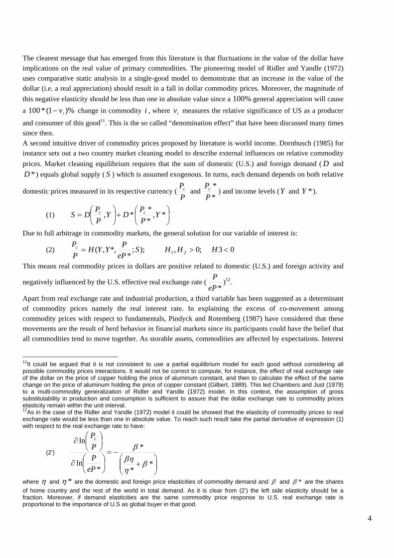
As part of a global tendency described in the introduction, the issue of terms of trade and commodity priceshas recovered a central place in the economic debate in Argentina. However in many occasions, this debatestarts with ideas that are not totally supported by the data. For instance, it has been occasionally said thatcurrent terms of trade are the highest in Argentinean history but this is not true from a long run view.Alternatively, some observers tend to study commodities as a homogenous market when there are cleardisparities in the behavior of commodity groups. Moreover, short run analysis usually focus only on nominalprices making not connection with real prices, as if both variables were the same.In order to clarify ideas it will be helpful to start the empirical analysis by describing both the general trendsand the recent outcomes in commodity prices and the terms of trade. This is an important step in order tomove to the analysis of the role of international drivers of argentinean commodity prices.In Graph 1 below we have draw a long series for the Argentinean terms of trade. The first notable visualfeature is its high volatility.Regarding long run trends, we could see four phases. From the beginning of the series in 1875 to the crisis ofthe 30s approximately there is a period of decaying terms of trade. Around the Second World War period weobserve a recovery of the terms of trade explained by sharp commodity prices increases. Then there is aperiod of low terms of trade from 1940 to approximately 1970. In the later years the terms of trade peaked asa consequence of the oil shocks. However, this events did not structurally altered the behavior of the seriesand so they acted more as an jump shift rather than as a step shift. Hence, from 1973 to 1986 volatility tendedto prevail.Only from 1987 on we detect an upward trend with some degree of persistence. This later period have raisedan important debate among economists.In this debate, some observers suggested that current terms of trade are in a extraordinary unique situation,while others said that around the years 2000-2001 there was a structural negative break in the terms of tradethat jeopardized the convertibility plan. Nevertheless, when historical data is analyzed we conclude thatrecent fluctuations have been relatively small, and that stable and slightly rising terms of trade are not a novelcharacteristic in Argentinean economy but an outcome that have been taken place during the last twentyyears.

13The idea is that debt crisis endogenously created incentives to increase commodity supply and so prices plummeted in1982-85.

7

Graph 1. The very long run of Argentinean terms of trade

50.0

70.0

90.0

110.0

130.0

150.0

170.0

190.0

1875 1883 1891 1899 1907 1915 1923 1931 1939 1947 1955 1963 1971 1979 1987 1995 2004

Source: ECLAC Office in Buenos Aires based on INDEC, Ministry of Finance and BCRA and others

As the most volatile component of the terms of trade series, commodity prices evolution is different to someextent. In the case of international prices we will focus in the last twenty years of data which is the risingterms of trade cycle previously identified. Our analysis of main commodity prices of Argentina will beconducted using the variable IPCom 8 which is a summary measure of the eight principal internationalcommodities that Argentina exports. A full description of this variable will be giving in the section one of theappendix in conjunction with the rest of the variables that take part in the empirical model (section two of theappendix). For this moment we have draw two commodity series one in nominal terms and the other in realterms using in the later case the U.S GDP deflator.

8

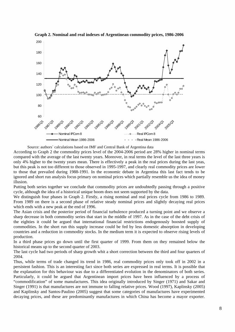
Graph 2. Nominal and real indexes of Argentinean commodity prices, 1986-2006

60

80

100

120

140

160

180

200

1986

Q1

1987

Q3

1989

Q1

1990

Q3

1992

Q1

1993

Q3

1995

Q1

1996

Q3

1998

Q1

1999

Q3

2001

Q1

2002

Q3

2004

Q1

2005

Q3

Nominal IPCom 8 Real IPCom 8

Nominal Mean 1986-2006 Real Mean 1986-2006

Source: authors´ calculations based on IMF and Central Bank of Argentina dataAccording to Graph 2 the commodity prices level of the 2004-2006 period are 28% higher in nominal termscompared with the average of the last twenty years. Moreover, in real terms the level of the last three years isonly 4% higher to the twenty years mean. There is effectively a peak in the real prices during the last yeas,but this peak is not too different to those observed in 1995-1997, and clearly real commodity prices are lowerto those that prevailed during 1988-1991. In the economic debate in Argentina this last fact tends to beignored and short run analysis focus primary on nominal prices which partially resemble us the idea of moneyillusion.Putting both series together we conclude that commodity prices are undoubtedly passing through a positivecycle, although the idea of a historical unique boom does not seem supported by the data.We distinguish four phases in Graph 2. Firstly, a rising nominal and real prices cycle from 1986 to 1989.From 1989 on there is a second phase of relative steady nominal prices and slightly decaying real priceswhich ends with a new peak at the end of 1996.The Asian crisis and the posterior period of financial turbulence produced a turning point and we observe asharp decrease in both commodity series that start in the middle of 1997. As in the case of the debt crisis ofthe eighties it could be argued that international financial restrictions endogenously boosted supply ofcommodities. In the short run this supply increase could be fed by less domestic absorption in developingcountries and a reduction in commodity stocks. In the medium term it is expected to observe rising levels ofproduction.In a third phase prices go down until the first quarter of 1999. From them on they remained below thehistorical means up to the second quarter of 2003.The last cycle had two periods of sharp growth whit a short correction between the third and four quarters of2004.Thus, while terms of trade changed its trend in 1986, real commodity prices only took off in 2002 in apersistent fashion. This is an interesting fact since both series are expressed in real terms. It is possible thatthe explanation for this behaviour was due to a differentiated evolution in the denominators of both series.Particularly, it could be argued that Argentinean import prices have been influenced by a process of“commodification” of some manufactures. This idea originally introduced by Singer (1971) and Sakar andSinger (1991) is that manufactures are not immune to falling relative prices. Wood (1997), Kaplinsky (2005)and Kaplinsky and Santos-Paulino (2005) suggest that some categories of manufactures have experimenteddecaying prices, and these are predominantly manufactures in which China has become a mayor exporter.

9

This effect could help to explain the fact that Argentinean nominal import prices remains practicallyunchanged in the last ten years, a period in which China and other developing countries increased their sharein Argentinean imports. Contrary to this effect, GDP deflator of the U.S has experimented an independenttemporal evolution of steadily low growth.

4. The empirical model

The objective of this section is to evaluate the empirical validity of the models revisited in section 2. Thesemodels showed commodity price determination for Argentina’s main exports during the 1986Q1-2003Q3period.Besides the determinants already studied by literature (interest rate, U.S real exchange rate, the worldindustrial production), we think it is also important to study the role of global liquidity.Monetary conditions of international economy have not usually been taken into account in a direct way in theexplanation of commodity price behaviour (see Graph A.2.2 in the Appendix). However, some studies, likeHSBC (2007) and Dooley and Garber (2002) have pointed out that global liquidity is the key variable inorder to explain the remarkable growth of world economy and the recent good performance in emergingmarkets financial assets. Because of these reasons, commodity values are expected to be influenced by theglobal liquidity level, beyond the effect captured by interest rate.Regarding world demand, China’s industrial production has been added to the developed countries industrialproduction with the objective of evaluating the role played by this new actor in raw materials markets.As the objective of this paper are, on one hand, to establish if any long run relationships exist betweencommodity prices and the previously pointed out global factors, and on the other, to know commodity priceshort run dynamics in the presence of different shocks, we propose to estimate a vector error correctingmodel (VECM). Besides satisfying the objectives above, this methodology does not present the typicalproblems of univariate modelling.We propose to estimate the model based on the following equation:

(3) tit

p

iitt XXAX ε+Δ∏+Π+=Δ −

−

=− ∑

1

110

Where the endogenous variables vector tX is corresponds to the price index of eight main Argentinean

commodities, the US real exchange rate, the financial return of the US treasury bond (one year), a globalliquidity measure, and a developing countries plus china industrial production index. Details of data sourcesand time evolution of the variables are provided in section A.2 of the appendix.In the long run equation we have added a time trend in order to control for the possibility of a Prebish-Singereffect. As we have used a US GDP implicit price index to deflate commodity prices and this index has a highcomponent of services and manufactures, the hypothesis would be that, given OECD demand, the pass-through of rising productivity to international prices has been more intense in commodity goods than inmanufacture goods and tradable services.

5. The empirical results

The first methodological step in the VECM is to determine the order of integration of the series to beincluded in it. To this end, we have employed standard augmented unit root test of Dickey and Fuller (1979).In section A.3 of the appendix we show the results. As it could be inferred from them, it is not possible toreject the null hypothesis of a unit root in all the variables that enters in the VECM.Since all the series are I(1), we proceed to estimate an unrestricted vector autoregressive model (VAR) inlevels to determine the appropriate lag length and check the properties of the residuals. We follow thepractical rule of considering the seasonal lag plus one, and so our unrestricted VAR is estimated whit five

10

lags. We next proceed to check the absence of serial autocorrelation and heteroskedasticity in the residuals.This results are shown in section A.4 of the appendix.We following the Johansen (1991 and 1995) methodology in order to test the possibility of one or morecointegration relationships among our variables. In Table 1 we present the results of the trace ( traceλ ) andmaximum eigenvalues ( maxλ ) statistics. In this respect, it is important to remind that a deterministic trend hasbeen included in the cointegration equation for the reasons presented in the previous section. In the firstcolumn of this table we place the number of cointegration equations under the null hypothesis. Followingthis, we can find the value of each statistic, the corresponding critical value, and finally the associatedprobability.

Table 1. Results of the cointegration testsTrace Test

Number of CointegrationEquations Trace Statistic 5% Critical Value Probability**

None* 0.3917 107.35 0.0012At most 1* 0.2653 66.08 0.0322At most 2 0.2164 40.49 0.0856At most 3 0.1524 20.24 0.2138At most 4 0.0754 6.51 0.3981

Maximun Eigenvalues Test

Number of CointegrationEquations Max-Eigen Statistic 5% Critical Value Probability**

None* 0.3917 41.27 0.0223At most 1 0.2653 25.59 0.2531At most 2 0.2164 20.24 0.2292At most 3 0.1524 13.73 0.2726At most 4 0.0754 6.51 0.3981

*Denotes rejection of the null hypothesis at the 0.05 significance level**P Values based on MacKinnon et. al (1999)

As we observe from the table both test produce different results. Trace test indicates the presence of twocointegration equations while maximum eigenvalues test suggests one equation. When the coefficients of thefirst cointegration equation are normalized we obtain the coefficients and the t statistics of the long runequation which are presented in Table 2. In this table, the left hand side variable is the commodity pricesindex.

Table 2. Long run relationship between commodity prices and its drivers

Real exchangerate** Interest rate* International

liquidity*Industrial

production* Time trend*

Coefficient 0.4922 -5.5945 2.2011 -4.6324 -0.0189

t statistic (-1.6744) (2.7607) (-5.1067) (5.0944) (2.8349)

p-value 0.100 0.008 0.000 0.000 0.006

*Denotes rejection of the null hypothesis at the 0.05 significance level**Denotes rejection of the null hypothesis at the 0.10 significance level

Previous to the analysis of the economic consequences of the econometric results showed in Table 2, we haveopted to introduce the short run dynamics of the VECM. We then discuss simultaneously both long and shortrun implications of our model.

11

In the next sequence of graphs the results of the impulse-response analysis are presented. It is important totake into consideration two things. Firstly, these graphs make reference to accumulated impulse-responsefunctions. Secondly and more important, in order to identify the structural innovations we have employed theCholesky factorization based on some economic intuition regarding the order of the variables. We haveassumed that liquidity shocks of the VECM in reduced form are identical to the structural shocks. Thus,liquidity is the most exogenous variable in the sense that its instantaneous impact over the remainingvariables is no null. The remaining variables are put in the following order: real interest rate, real exchangerate, industrial production, and finally real commodity prices. As it is usual, results are measured as apercentage of change in the variable that receives the shock and the magnitude of it is one standard deviationof each variable.

Graph 3. Accumulated responses of real commodity prices to a real exchange rate shock

-0.015

-0.01

-0.005

0

0.005

0.01

0.015

1 3 5 7 9 11 13 15 17 19 21 23

Periods

Graph 4. Accumulated responses of real commodity prices to a real interest rate shock

-0.06

-0.05

-0.04

-0.03

-0.02

-0.01

0

0.01

1 3 5 7 9 11 13 15 17 19 21 23

Periods

12

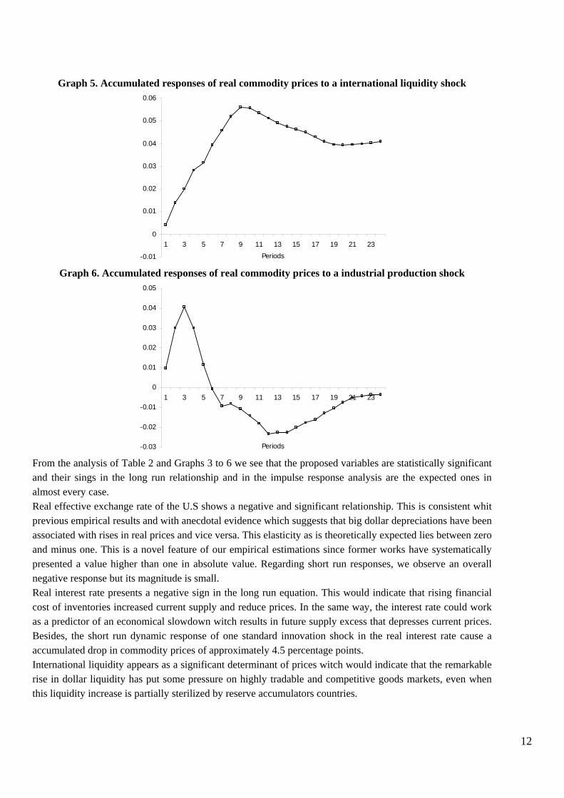
Graph 5. Accumulated responses of real commodity prices to a international liquidity shock

-0.01

0

0.01

0.02

0.03

0.04

0.05

0.06

1 3 5 7 9 11 13 15 17 19 21 23Periods

Graph 6. Accumulated responses of real commodity prices to a industrial production shock

-0.03

-0.02

-0.01

0

0.01

0.02

0.03

0.04

0.05

1 3 5 7 9 11 13 15 17 19 21 23

Periods

From the analysis of Table 2 and Graphs 3 to 6 we see that the proposed variables are statistically significantand their sings in the long run relationship and in the impulse response analysis are the expected ones inalmost every case.Real effective exchange rate of the U.S shows a negative and significant relationship. This is consistent whitprevious empirical results and with anecdotal evidence which suggests that big dollar depreciations have beenassociated with rises in real prices and vice versa. This elasticity as is theoretically expected lies between zeroand minus one. This is a novel feature of our empirical estimations since former works have systematicallypresented a value higher than one in absolute value. Regarding short run responses, we observe an overallnegative response but its magnitude is small.Real interest rate presents a negative sign in the long run equation. This would indicate that rising financialcost of inventories increased current supply and reduce prices. In the same way, the interest rate could workas a predictor of an economical slowdown witch results in future supply excess that depresses current prices.Besides, the short run dynamic response of one standard innovation shock in the real interest rate cause aaccumulated drop in commodity prices of approximately 4.5 percentage points.International liquidity appears as a significant determinant of prices witch would indicate that the remarkablerise in dollar liquidity has put some pressure on highly tradable and competitive goods markets, even whenthis liquidity increase is partially sterilized by reserve accumulators countries.

13

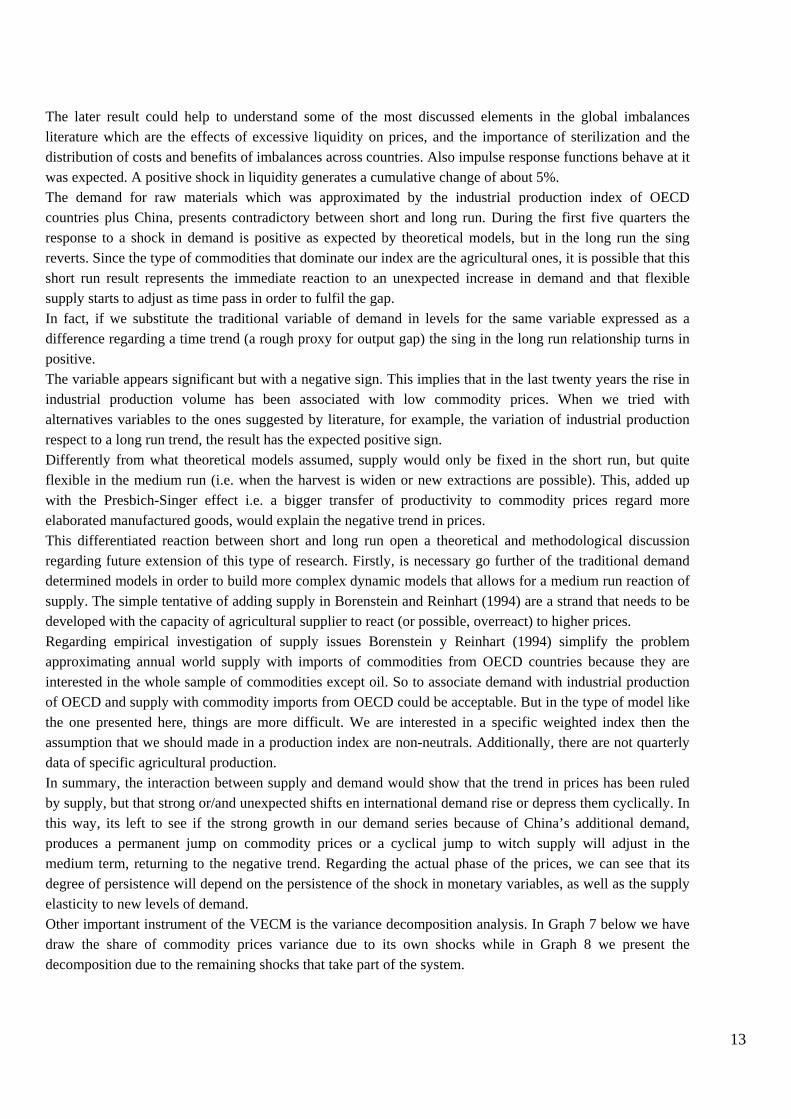
The later result could help to understand some of the most discussed elements in the global imbalancesliterature which are the effects of excessive liquidity on prices, and the importance of sterilization and thedistribution of costs and benefits of imbalances across countries. Also impulse response functions behave at itwas expected. A positive shock in liquidity generates a cumulative change of about 5%.The demand for raw materials which was approximated by the industrial production index of OECDcountries plus China, presents contradictory between short and long run. During the first five quarters theresponse to a shock in demand is positive as expected by theoretical models, but in the long run the singreverts. Since the type of commodities that dominate our index are the agricultural ones, it is possible that thisshort run result represents the immediate reaction to an unexpected increase in demand and that flexiblesupply starts to adjust as time pass in order to fulfil the gap.In fact, if we substitute the traditional variable of demand in levels for the same variable expressed as adifference regarding a time trend (a rough proxy for output gap) the sing in the long run relationship turns inpositive.The variable appears significant but with a negative sign. This implies that in the last twenty years the rise inindustrial production volume has been associated with low commodity prices. When we tried withalternatives variables to the ones suggested by literature, for example, the variation of industrial productionrespect to a long run trend, the result has the expected positive sign.Differently from what theoretical models assumed, supply would only be fixed in the short run, but quiteflexible in the medium run (i.e. when the harvest is widen or new extractions are possible). This, added upwith the Presbich-Singer effect i.e. a bigger transfer of productivity to commodity prices regard moreelaborated manufactured goods, would explain the negative trend in prices.This differentiated reaction between short and long run open a theoretical and methodological discussionregarding future extension of this type of research. Firstly, is necessary go further of the traditional demanddetermined models in order to build more complex dynamic models that allows for a medium run reaction ofsupply. The simple tentative of adding supply in Borenstein and Reinhart (1994) are a strand that needs to bedeveloped with the capacity of agricultural supplier to react (or possible, overreact) to higher prices.Regarding empirical investigation of supply issues Borenstein y Reinhart (1994) simplify the problemapproximating annual world supply with imports of commodities from OECD countries because they areinterested in the whole sample of commodities except oil. So to associate demand with industrial productionof OECD and supply with commodity imports from OECD could be acceptable. But in the type of model likethe one presented here, things are more difficult. We are interested in a specific weighted index then theassumption that we should made in a production index are non-neutrals. Additionally, there are not quarterlydata of specific agricultural production.In summary, the interaction between supply and demand would show that the trend in prices has been ruledby supply, but that strong or/and unexpected shifts en international demand rise or depress them cyclically. Inthis way, its left to see if the strong growth in our demand series because of China’s additional demand,produces a permanent jump on commodity prices or a cyclical jump to witch supply will adjust in themedium term, returning to the negative trend. Regarding the actual phase of the prices, we can see that itsdegree of persistence will depend on the persistence of the shock in monetary variables, as well as the supplyelasticity to new levels of demand.Other important instrument of the VECM is the variance decomposition analysis. In Graph 7 below we havedraw the share of commodity prices variance due to its own shocks while in Graph 8 we present thedecomposition due to the remaining shocks that take part of the system.

14

As we could see the more important source of shocks in this model are the financial variables related tointernational liquidity and the interest rate. This confirms that financial factors are not only importantdeterminants of commodity prices long run values but also main drives of short run dynamics.

Graph 7. Accumulated responses of real commodity prices to a industrial production shock

0.00

10.00

20.00

30.00

40.00

50.00

60.00

70.00

80.00

90.00

100.00

1 2 3 4 5 6 7 8 9 10 11 12 13 14 15 16 17 18 19 20 21 22 23 24

Graph 8. Accumulated responses of real commodity prices to each type of shocks

0.00

8.00

16.00

24.00

32.00

1 2 3 4 5 6 7 8 9 10 11 12 13 14 15 16 17 18 19 20 21 22 23 24ERER USA Real Interest RateReal International Liquidity Industrial Production

6. Conclusions

High commodity prices have gained weight as an explanation of recent growth cycle in Argentina and LatinAmerica. If we take an index that reflexes commodity price dynamics of Argentina’s main eight commodityexports, we could see that prices between 2005-2006 are 28% higher in nominal terms, than it’s average of 20last years. In real terms, this figure is only a 5% increase. In real terms, commodity prices are today similar tothose observed in 1995-1997 but inferior to those of the 1988-1991 phase. An analysis of the recentcommodity prices cycle shows that after an abrupt fall provoked by the Asian crisis in 1997-8, prices haveexperimented a sustained recovery.In this paper we have tried to deduce which are the main determinants of the prices of Argentina’s maincommodities. For that, we have explored different theoretical explanations and constructed an empirical

15

multivariate model (VECM) that takes into account the interaction between the variables and also short andlong run relationships.Theoretical evidence indicates that commodity prices are mainly determined by the real effective exchangerate of the dollar (with a negative sign) and by the demand of raw materials by consumer countries (with apositive sign). In some models interest rate is added, basically because its effect on speculative demand: alower rate of interest stimulates speculators to buy commodities as an alternative to financial assets. Thisphenomenon has grown in recent years and this could be reflecting what is called the "financialization” ofcommodity14. This implies that commodities have become an increasingly important part in investments fundportfolios. Most existing models are in general demand determined, where supply is assumed to be given andalso perfect competition in international commodity markets.However, from our perspective is relevant to complete theoretical ideas with the vision that emerges of theliterature related to the deterioration trend of raw material prices regard industrial goods. The existence ofauction markets for raw materials and customer markets for industrial goods and tradable services makes thatproductivity growth transfers to prices at different speeds.In our empirical model we have taken into account the effect of time through a specific trend variable.Finally, we have also introduced a variable that represents real international liquidity in dollars, thatcomplements interest rate as an indicator of global liquidity conditions.The VECM model establishes that a cointegration relationship exists among the determinants previouslymentioned and commodity prices. In this long run relationship, all variables are significant and adjust toequilibrium correctly while its signs are the expected in most cases.In particular, the real exchange rate has a negative sign and its elasticity is lower than one as it is anticipatedin the models.The increases in global liquidity is associated with the higher prices of commodity, this could be highly forthe last part of the sample.Real interest rate represent the opportunity cost of stocking commodities, it presents the expected negativesign that an increase reduce the incentive to accumulate more commodities in the portfolio and by doing so,makes prices fall.The global demand of raw material is captured by the level of industrial production index of OECD countriesplus China. It is the only variable that shows an opposite sign between the short and the long run. The formeris positive, as it is expected, and the later is negative which could indicate a reaction of supply to higherprices in the previous year.Finally, the trend that represents the Presbich-Singer effects is significant and negative evidencing a fastervelocity of transmission of productivity shocks to prices in commodity competitive markets than inmanufactures customer markets.As a general conclusion of our empirical model we have that most of the macroeconomic variables thatdetermine commodity prices and perceived value for the exporting economy are the same that influencecapital flows from the centre to the periphery. Such is the case of the U.S real exchange rate, the interest rateand the global liquidity. These variables, of a monetary nature, coordinate the exogenous cycle in countrieslike Argentina and act by two channels: the commercial and the financial channels (Carrera, Féliz andPanigo, 2000; Canova, 2005). This source of positive correlation between channel increase exogenousvolatility received from the centre.Hence, for a developing country more international liquidity, less interests rates and a dollar depreciationgenerate higher commodity prices, enhanced sustainability and risk perception, attract more capital flows andinvestment, and produce more growth alongside with inflationary and appreciatory pressures. When globaleconomic conditions change in the centre, all of this effects reverted and it is possible to find overshooting incommodity prices fall (Frankel, 2006).Since international variables that determine commercial and financial cycles in a open economy likeArgentina overlap, it is difficult to cushion real commercial shocks using international financial markets. Ifthe fall in prices were caused by monetary tightening and dollar appreciation it would be more difficult tofinance the shortfall in domestic income with external finance. This suggests that a good domestic strategy

14 According to Domanski and Heat (2006) the number of outstanding contracts on gold and commodities in millions ofdollars has more than doubled between 2003 y 2006.

16

should take into account developing domestic measures to smooth external cycles when prices are in highlevels.Regarding policy recommendations designated to such end, there are some that belong to the macroeconomicfield and other that are structural measures.Among the first ones, they should reduce cycle volatility smoothing transitory elements. We can list some ofthem: keeping a flexible exchange rate, accumulate international reserve, avoid real exchange rateovershooting respect to its long run equilibrium, implement a tax-subsidies system to exports accordingly thephase of external price cycle, establish fiscal funds to stabilize expenditure and adopt countercyclicalregulations of short term capital flows. Other more innovative measures are the hedging proposals made byCaballero (2002) to create financial funds that take into account the correlation of commodities to otherfinancial asset and Frankel’s recommendation to use as a monetary policy target an export price index.Structural policy measures should try to deal with the declining trend in prices. Thus, increasingdiversification in commodity exports as well as enhancing production chains for each raw material through anindustrialization process would help to reduce price volatility. Other fronts of policy should be posed indeveloping infrastructure and also stimulates local financial instruments intended to diminish futureuncertainty. Finally, coordination between producer countries could collaborate to stabilize markets eventough its implementation seem rather difficult.The last paragraph is again devoted the current high prices phase. Accordingly to our analysis, is still valid tosay that the force that moves the price wind is the great liquidity existing in the world, even when increasingdemand of commodities from countries like China and India, and the long way that could take to thiscountries to catch up the developed world in terms of commodities consumption, are considered. As variablesthat represent liquidity had changed many times in the past, it is possible that they can do it once again. Inother words, it is probable that an important part of the recent positive shock reflects transitory conditions.Countries like Argentina should profit this period to minimize the costs of future reversions.

References

Bastourre, D. A. and J. E. Carrera (2004) “Could the Exchange Rate Regime Reduce MacroeconomicVolatility”, Annals of Latin American Meeting of the Econometric Society, Santiago, 27-30 July.

Beenstock, M. (1988) “An Econometric Investigation of North-South Interdependence”, in D. Currie and D.Vines (eds.), Macroeconomic Interactions between North and South, Great Britain, CUP.

Bleaney M. and D. Greenaway (1993) “Long-Run Trends in the Relative Price of Primary Commodities andin the Terms of Trade of Developing Countries”, Oxford Economic Papers, New Series, Vol. 45. No. 3, pp349-363.

Borensztein E. and C. M. Reinhart (1994) “The Macroeconomic Determinants of Commodity Prices”, IMFStaff Papers, Vol. 41, No. 2, 236-258.

Canova, F. (2005) “The transmission of US shocks to Latin America”, Journal of Applied Econometrics, 20,229-251.

Carrera, J. Féliz, M. and Panigo, D. (2000) “Asymmetric Monetary Union and Real Volatility. The Case ofArgentina”. Anales de la AAEP. Córdoba, 2000. ISBN 950-9836-07-9.

Carrera, J. E. and R. Restout (2007) “Lon Run Determinants of Real Exchange Rate in Latin America”,Mimeo, Central Bank of Argentina, 2007.

Cashin, P. and C. J. McDermott (2002) “The Long-Run Behavior of Commodity Prices: Small Trends andBig Variability”, IMF Staff Papers, Vol. 49, No. 2, 175-199.

Chambers R. G. and R. E. Just (1979) “A Critique of Exchange Rate Treatment in Agricultural TradeModels”, American Journal of Agricultural Economics, Vol. 61, pp. 249-257.

Cuddington, J. T. and C. M. Urzúa (1989) “Trends and Cycles in the Net Barter Terms of Trade: a NewApproach” Economic Journal, Vol. 99, pp. 426-442.

D´Amato, L., L. Sanz and J. M. Sotes Paladino “Evaluación de Medidas Alternativas de InflaciónSubyacente” Serie Estudios BCRA, No. 1, Marzo de 2006.

17

De Gregorio, J., H. Gonzáles and F. Jaque (2005) “Fluctuaciones del Dólar, Precio del Cobre y Términos delIntercambio”, Documento de Trabajo del Banco Central de Chile No. 310, Febrero de 2005.

Deaton, A. (1999) “Commodity Prices and Growth in Africa”, Journal of Economic Perspectives, Vol. 13,No. 3, pp. 23-40.

Diaz Alejandro, C. (1984) “Latin America in the 1930s”, In R. Thorp (ed.) Latin America in the 1930s, NewYork, Macmillan, pp. 17-49.

Dickey, D. and W. A. Fuller (1979) “Distribution of the Estimates for Autoregressive Time Series whit aUnit Root”, Journal of the American Statistical Association, Vol. 74, pp. 427-431.

Domanski, D. and Heat, A. (2006) “Financial Investors and Commodity Markets”. BIS Quarterly Review, pp53-67.

Dooley ,M. P. and P. Garber (2005) “Is It 1958 or 1968? Three Notes on the Longevity of the RevivedBretton Woods System”, Brookings Papers on Economic Activity, forthcoming.

Dornbusch, R. (1985) “Policy and Performance Links Between LDC Debtors and Industrial Nations”,Brookings Papers on Economic Activity, Vol. 1985, No. 2, pp. 303-368.

Frankel, J. A. (2006) “The Effect of Monetary Policy on Real Commodity Prices”, NBER Working PaperNo. 12713.

Gilbert, C. L. (1989) “The Impact of Exchange Rates and Developing Country Debt on Commodity Prices”,The Economic Journal, Vol. 99, pp. 773-784.

Grilli, E. R. and M. C. Yang (1988) “Primary Commodity Prices, Manufactured Goods, Prices and Terms ofTrade of Developing Countries: What the Long Run Shows” World Bank Economic Review, Vol. 2, No. 1,pp. 1-48.

Harberger, A. (1950) “Currency Depreciation, Income and the Balance of Trade”, Journal of PoliticalEconomy, Vol. 58, pp. 47-60.

HSBC (2007) When all the boats floated (a true story). Emerging markets primal research. February 2007.

Kaplinsky, R. (2005) “Revisiting the Revisited Terms of Trade: Will China Make a Difference”, WorldDevelopment, forthcoming.

Kaplinsky, R. and A. Santos-Paulino (2005) “Innovation and Competitiveness: Trends in Unit Prices inGlobal Trade”, Oxford Development Studies, Vol. 33, No. 3-4, pp. 333-355.

Kent, C. and P. Cashin (2003) “The Response of the Current Account to Terms of Trade Shocks: PersistenceMatters”, IMF Working Papers 03/143.

Lane, P. R. and A. Tornell (1996) “Power, Growth and the Voracity Effect”, Journal of Economic Growth,Vol. 1, pp. 213-241.

Laursen, S. and L. Metzler (1950) “Flexible Exchange Rates and the Theory of Employment”, Review ofEconomic and Statistics, Vol. 32, pp. 281-299.

Lutz M. G. (1999) “A General Test of the Prebisch-Singer Hypothesis”, Review of Development Economics,Vol. 3, No. 1, pp. 44-57.

Mendoza, E. (1997) “Terms of Trade Uncertainty and Economic Growth”, Journal of DevelopmentEconomics, Vol. 54, pp. 323-356.

Obstfeld, M. (1982) “Aggregate Spending and the Terms of Trade: Is There a Laursen-Metzler Effect?,Quarterly Journal of Economics, Vol. 97, pp. 251-270.

Ocampo, J. A. and M. A. Parra (2003) “Returning to a Eternal Debate: The Terms of Trade in the TwentiethCentury”, Serie Estudios e Informes Especiales No. 5, CEPAL, Santiago.

Pindyck, R. S. and J. J. Rotemberg (1987) “The Excess of Co-Movement of Commodity Prices”, NBERWorking Paper No. 1987.

18

Powell, A. (1991) “Commodity and Developing Countries Terms of Trade: What Does the Long RunShows?, Economic Journal, Vol. 101, pp. 1485-1496.

Prebisch, R. (1950) “The Economic Development of Latin America and Its Principal Problems”, New York,United Nations; Reprinted in Spanish in Desarrollo Económico, Vol. 26., No 103, pp. 251-502.

Ramey, G. and V. A. Ramey (1995) “Cross-Country Evidence on the Link Between Volatility and Growth”,American Economic Review, Vol. 85, No. 5, pp. 1138-1151.

Ridler, D. and Ch. Yandle (1972) “A Simplified Method of Analyzing the Effects of Exchange Rates onExports of a Primary Commodity”, IMF Staff Papers Vol.19, No 3, pp. 559-578.

Sachs, J. D. and A. M. Warner (1995) “Natural Resource Abundance and Economic Growth”, NBERWorking Paper No. 5398.

Sarkar, P. and H. W. Singer (1991) “Manufactured Exports of Developing Countries and their Terms ofTrade”, World Development, Vol. 19, No.4, pp. 333-340.

Singer, H. W. (1950) “The Distribution of Gains between Investing and Borrowing Countries”, AmericanEconomic Review, Vol. 40, No. 2, pp. 473-485.

Singer, H. W. (1971) “The Distribution of Gains Revisited”, reprinted in A. Cairncross and M. Puri (eds.)(1975), The Strategy of International Development, London: Macmillan.

Tornell, A. and P.R. Lane (1999) “The Voracity Effect”, American Economic Review, Vol. 89, No.1, pp. 22-46.

Wood, A. (1997) “Openness and Wage Inequality in Developing Countries: the Latin American Challenge toEast Asian Conventional Wisdom”, World Bank Economic Review, Vol. 11, No 1, pp. 33-57.

Appendix

A.1. Commodity prices indexWe have constructed an index of the prices of the eight main commodities exported by Argentina (IPCom8).The following table shows the commodities considered as well as their shares in the total exports ofArgentina in 2006. The weight of each commodity in the index is calculated according to these figures

Table A. 1. Construction of the Argentinean Commodity Price Index

CommodityShare in Total

ExportsPrice Index

Weight

Soybeans 3.8 13.3

Soybeans oil 6.0 20.9

Soybeans meal 9.3 32.6

Maize 2.7 9.5

Wheat 3.2 11.1

Aluminium 0.8 2.6

Metals 0.5 1.7

Beef 2.4 8.3Total 28.7 100.0

Our index contains the same products included in Index of commodity prices published by the BCRA, butdifferently to that index we use fixed weights along the whole period considered, particularly thosecorresponding to the year 2006. The main justification of that is that BCRA index is a chained Laspeyresindex where the weights are updated every year. Since part of the evolution of that index reflects changes inshares and we want to capture the pure price effect. But more important to this is the fact that we haveexcluded oil and cooper in comparison with the index of the BCRA. The reason is that we want to focus onhighly consolidated export sectors that are related to the traditional comparative advantages, and has room togrowth in the near future.The nominal prices are taken from International Financial Statistics (IMF). In the econometric analysis theIPCom8 is deflated by the GDP implicit price deflator of USA (IFS-IMF).

19

A.2. Description of the international variables

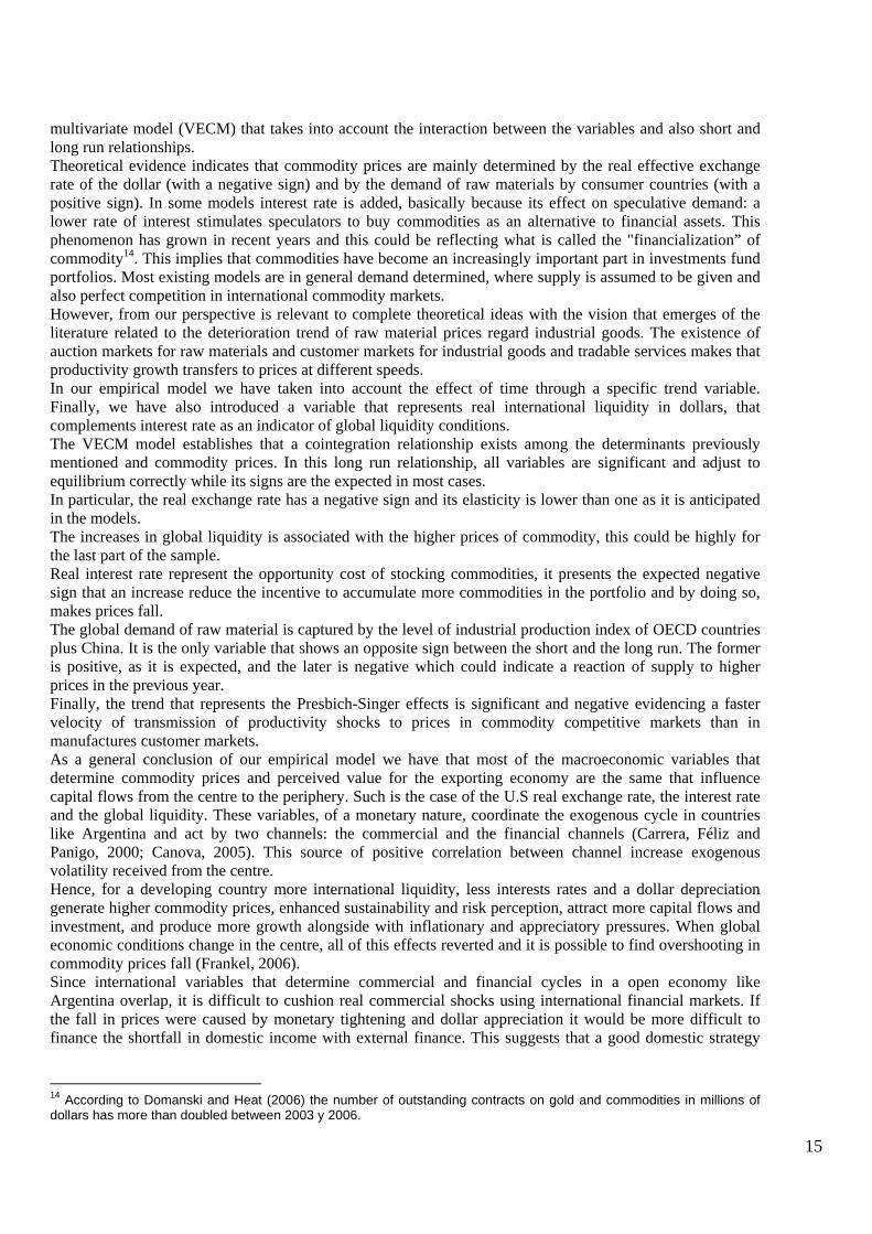
In this part, construction and sources of global commodity price determinants are explained in detail. We usequarterly data for the period 1986-2006. All variables were seasonally adjusted (except for the interest rateand real global liquidity) by the X-12 Arima method and are expressed in logarithms.

US Multilateral Real Exchange Rate

The broad multilateral real exchange rate index series from the Federal Reserve Bank of New York was used.

Real Global LiquidityThis series is the result of the sum of the US monetary base and international reserves held by central banksall over the world. The seasonally adjusted monetary base from the Board of Governors of the FederalReserve System and the world total reserve series from the International Financial Statistics (IFS-IMF) wereused in its construction. ““001.1..SZF...” To deflate the variable the USA GDP implicit price deflator wasused (“11199BIRZF...” IFS series).

Real Interest Rate

The 1-Year Treasury Constant Maturity Rate from the Board of Governors of the Federal Reserve Systemwas utilized and deflated by the USA GDP deflator.

Industrial Production IndexA developed countries plus China industrial production index was built. As there is no industrial productionindex for the last country, we used the industrial added value employing IFS and World DevelopmentIndicators (World Bank) data as an approximate measure. For developed economies IFS IPI series(“11066..IZF...” series) was used. Both indexes were weighted by the respective industrial added value.

Graph A.2.1 Multilateral Real Exchange Rate Graph A.2.2 Real Global Liquidity (logarithmic scale)

70

75

80

85

90

95

100

105

110

1986

Q1

1987

Q3

1989

Q1

1990

Q3

1992

Q1

1993

Q3

1995

Q1

1996

Q3

1998

Q1

1999

Q3

2001

Q1

2002

Q3

2004

Q1

2005

Q3

1313,213,413,613,8

1414,214,414,614,8

15

1986

Q1

1987

Q3

1989

Q1

1990

Q3

1992

Q1

1993

Q3

1995

Q1

1996

Q3

1998

Q1

1999

Q3

2001

Q1

2002

Q3

2004

Q1

2005

Q3

20

Graph A.2.3 Real Interest Rate Graph A.2.4 Industrial Production

1

1,02

1,04

1,06

1,08

1,1

1986

Q1

1987

Q4

1989

Q3

1991

Q2

1993

Q1

1994

Q4

1996

Q3

1998

Q2

2000

Q1

2001

Q4

2003

Q3

2005

Q2

60

70

80

90

100

110

120

1986

Q1

1987

Q3

1989

Q1

1990

Q3

1992

Q1

1993

Q3

1995

Q1

1996

Q3

1998

Q1

1999

Q3

2001

Q1

2002

Q3

2004

Q1

2005

Q3

A.3. Unit root testsTable A.2. Summary of the Augmented Dickey-Fuller test

Deterministic regressorsVariable

None Constant Constant and trend

IPCom8 0.4602 0.1937 0.1168MRER USA 0.7279 0.3954 0.6943Real Global Liquidity 0.9999 0.9999 0.2687Real Interest Rate 0.3093 0.2927 0.0336Industrial Production Index 0.9994 0.9786 0.1736

A.4. Unrestricted VAR residuals

Table A.3. VAR Residual: Serial Correlation LM testH0: no serial correlation at lag order hSample: 1986Q1 2006Q4Included observations: 83

Lags LM-Stat Prob1 32.90498 0.133462 32.27370 0.150243 34.15704 0.104594 37.07791 0.056765 19.66240 0.764306 34.25041 0.102667 31.09528 0.185888 22.77168 0.590899 24.23186 0.50601

10 17.95039 0.8444911 31.10532 0.1855512 30.49116 0.20642

Table A.4. VAR Residual: White Heteroskedasticity TestH0: no heteroskedasticitySample: 1986Q1 2006Q4Included observations: 83

Chi-sq df Prob.726.62940 750 0.72326