Excessive commodity price volatility: Macroeconomic effects ...
Upload
khangminh22Category
view
0download
0
Capacitated Network Design–
Multi-Commodity Flow Formulations, Cutting Planes,and Demand Uncertainty
vorgelegt vonDipl.-Math. Christian Raack
aus Berlin
Von der Fakultät II – Mathematik und Naturwissenschaftender Technischen Universität Berlin
zur Erlangung des akademischen Grades
Doktor der Naturwissenschaften– Dr. rer. nat. –
genehmigte Dissertation
Promotionsausschuss
Vorsitzender: Prof. Dr. Andreas UnterreiterBerichter: Prof. Dr. Martin Grötschel
Prof. Dr. Arie Koster
Tag der wissenschaftlichen Aussprache: 26.06.2012
Berlin 2012D 83


Abstract
In this thesis, we develop methods in mathematical optimization to dimensionnetworks at minimal cost. Given hardware and cost models, the challenge is toprovide network topologies and efficient capacity plans that meet the demandfor network traffic (data, passengers, freight). We incorporate crucial aspects ofpractical interest such as the discrete structure of available capacities as well as theuncertainty of demand forecasts. The considered planning problems typically arisein the strategic design of telecommunication or public transport networks and alsoin logistics.
One of the essential aspects studied in this work is the use of cutting planes toenhance solution approaches based on multi-commodity flow formulations. Pro-viding theoretical and computational evidence for the efficacy of inequalities basedon network cuts, we extend existing theory and algorithmic work in different di-rections.
First, we prove that special-purpose techniques, originally designed to solve capaci-tated network design problems, can be successfully integrated into general-purposemixed integer programming (MIP) solvers. Our approach relies on an automaticdetection of network structure within the constraint matrix of general mixed in-teger programs. More precisely, we identify multi-commodity (MCF) networksub-matrices and resolve the isomorphisms of the commodity blocks as well as theoriginal graph structure. In the subsequent separation framework, we guide theconstraint aggregation of available cutting plane procedures (e. g. based on mixedinteger rounding) to produce strong cutting planes that reflect the structure of theconstructed network. The new MCF-separator integrates network design specificmethodology into general optimization tools which is of particular importance forpractitioners that tend to use MIP solvers as black boxes.
Extensive computational tests show that our network detection procedure operatesaccurately and reliably. Moreover, due to the generated cutting planes, we achievean average speed-up of a factor of two for pure network design problems on the MIPsolvers Scip and Cplex. Many of these instances can only be solved to optimalityin reasonable time if the new MCF-separator is active. In 9% of the instances ofgeneral MIP test sets we find consistent embedded networks and generate violatedinequalities. In this case the computation time decreases by 18% on average withalmost no degradation for unaffected instances.
iii
Second, we generalize concepts, models, and cutting planes from deterministicnetwork design to robust network design, incorporating the uncertainty of trafficdemands. We enhance and compare strategies that are able to handle a polyhedralset of different traffic scenarios. In particular, we consider two correlated solutionmethods, based on separating extreme demand scenarios and dualizing the lineardescription of the demand polytope, respectively.
We consider robust network design as part of the more general framework of two-stage robust optimization with recourse. First stage capacity decisions are fixedfor all scenarios while the second stage flow depends on the realized demands. Inthis respect, in order to reroute the traffic as a function of the demand dynamics,we consider three alternative recourse actions, namely, static, affine, and dynamicrouting. We analyze properties of the new affine routing and show (theoreticallyand computationally) that it combines advantages of the well-known static anddynamic models.
Using the concept of robust cut-set polyhedra and the corresponding lifting theo-rems, we develop several classes of facet-defining inequalities based on network cutsthat can be used to further accelerate solution strategies for robust network design.Among them are the well-known cut-set and flow cut-set inequalities, which wegeneralize from single demand scenarios to general demand polytopes, but also newclasses of potential cutting planes, so-called envelope inequalities, that exploit thespecial structure of the considered uncertainty sets. The practical importance ofthe developed cutting planes is revealed by a series of computational tests. Similarto the results for the MCF-separator we achieve speed-ups of two and more forgeneralized cut-set inequalities. Also robust flow cut-set inequalities turn out tobe useful in further decreasing computation times.
To evaluate the robustness of solutions that are computed with our framework weuse real-life measurements of traffic dynamics from different existing telecommu-nication networks, among them data from the German and the European researchnetwork. Our results indicate that traffic peaks do not necessarily occur all simul-taneously with respect to different source-destination pairs, which is of practicalimportance for the design of uncertainty sets. It is, in particular, not necessary todimension networks for a scenario that assumes all source-destination traffic is atits peak simultaneously. With our solutions we save up to 20% of the correspond-ing solution cost compared to this artificial scenario and achieve comparable levelsof robustness.
iv

Acknowledgments
I am extremely grateful for any help in typo- and proof-reading of this thesis.My biggest and sincere thanks go to Tobias Achterberg, Andreas Bley, ManuelKutschka, Sara Mattia, Michael Poss, Jonad Pulaj, Domenico Salvagnin, Jacque-line Schönborn, Jonas Schweiger, Axel Werner, Roland Wessäly, and Kati Wolter.Without underestimating the work of the rest, I have to thank in particular Tobi,Andreas, and Axel as they read extremely large parts of this thesis without everrejecting or complaining. In the last couple of months, Axel even took over manyof my jobs and duties taking away some of the stress and leaving me to concentrateon writing. I truly appreciate this generous help.
I would also like to give special thanks to all my co-authors of articles relatedto this thesis. Thank you Tobias Achterberg, Sanjeeb Dash, Oktay Günlük, ArieKoster, Manuel Kutschka, and Michael Poss! It was a pleasure to work with youguys.
v

Contents
Introduction 1The problem: Capacitated network design . . . . . . . . . . . . . . . . . 1The methodology: Mixed integer programming . . . . . . . . . . . . . . 3
I Concepts 11
1 Mixed integer programming 131.1 Basics . . . . . . . . . . . . . . . . . . . . . . . . . . . . . . . . . . 141.2 Branch-and-cut . . . . . . . . . . . . . . . . . . . . . . . . . . . . . 161.3 Mixed integer rounding: A pivotal cutting plane technique . . . . . 211.4 Computationally successful cutting plane separators . . . . . . . . 29
2 Capacitated network design 352.1 Graphs and flows . . . . . . . . . . . . . . . . . . . . . . . . . . . . 352.2 A base model . . . . . . . . . . . . . . . . . . . . . . . . . . . . . . 382.3 Cutting planes . . . . . . . . . . . . . . . . . . . . . . . . . . . . . 452.4 Capacity models . . . . . . . . . . . . . . . . . . . . . . . . . . . . 542.5 Computational impact of cut-based inequalities . . . . . . . . . . . 65
II Capacitated networks within mixed integer programs 67
3 Introductory remarks Part II 69
4 Detecting networks in general mixed integer programs 754.1 Identifying multi-commodity flow matrices . . . . . . . . . . . . . . 794.2 Arc detection . . . . . . . . . . . . . . . . . . . . . . . . . . . . . . 824.3 Node detection . . . . . . . . . . . . . . . . . . . . . . . . . . . . . 834.4 Network construction . . . . . . . . . . . . . . . . . . . . . . . . . . 864.5 Inconsistency issues . . . . . . . . . . . . . . . . . . . . . . . . . . . 88
5 Aggregating constraints for cutting plane separation 915.1 Algorithmic framework . . . . . . . . . . . . . . . . . . . . . . . . . 915.2 Extensions . . . . . . . . . . . . . . . . . . . . . . . . . . . . . . . . 95
6 The MCF-separator: Computational impact 99
vii

6.1 Success of the network detection . . . . . . . . . . . . . . . . . . . 1006.2 Success of the separation . . . . . . . . . . . . . . . . . . . . . . . . 1026.3 The impact of inconsistencies . . . . . . . . . . . . . . . . . . . . . 1086.4 The impact of aggressive separation . . . . . . . . . . . . . . . . . . 110
7 Concluding remarks Part II 113
III Demand uncertainty: Design of robust networks 115
8 Introductory remarks Part III 117
9 Solving robust network design problems 1259.1 Recourse actions: Dynamic vs. static routing . . . . . . . . . . . . 1259.2 Uncertainty sets . . . . . . . . . . . . . . . . . . . . . . . . . . . . . 133
10 Cut-based inequalities for robust network design 14310.1 Robust cut-set and flow cut-set inequalities . . . . . . . . . . . . . 14410.2 Envelope inequalities for the Γ-model . . . . . . . . . . . . . . . . . 15210.3 Computational insights . . . . . . . . . . . . . . . . . . . . . . . . . 164
11 Affine policies: between static and dynamic routing 17911.1 Properties of affine routings . . . . . . . . . . . . . . . . . . . . . . 18211.2 Computational insights . . . . . . . . . . . . . . . . . . . . . . . . . 194
12 Concluding remarks Part III 205
A Tables Part II 209A.1 Used instances . . . . . . . . . . . . . . . . . . . . . . . . . . . . . 209A.2 Results – Network Detection . . . . . . . . . . . . . . . . . . . . . 220A.3 Results – Separation – MCF-cuts . . . . . . . . . . . . . . . . . . . 231
B Tables Part III 245B.1 Used instances . . . . . . . . . . . . . . . . . . . . . . . . . . . . . 245B.2 Results – Separation – Robust cut-set inequalities . . . . . . . . . . 247B.3 Results – Separation – Robust flow cut-set inequalities . . . . . . . 252B.4 Results – Separation – Robust envelope inequalities . . . . . . . . . 254
C Notation 257
D Abbreviations 261
List of tables 264
List of figures 266
List of algorithms 267
Bibliography 283
viii

Introduction
In this thesis, we focus on several aspects arising in the context of optimizing andplanning the core of nation-wide telecommunication networks. Most of the modelsand methodology, however, are based on the general notion of capacitated networksand multi-commodity flows such that the main findings and new approaches arealso useful for applications in public transport and logistics. More generally, wewere able to enhance some of the most successful approaches to the level of generaloptimization software handling all kinds of different applications. Solvers such asCplex [140], Scip [227], and Gurobi [131] now scan the problem structure andapply our methods or similar techniques in case they can find network designsubstructures.
The results in this work have been developed within the German research projectEibone–Efficient Integrated Backbone and the Matheon project Integrated plan-ning of multi-layer telecommunication networks at the Zuse Institute Berlin, par-tially in cooperation with industry partners such as IBM-ILOG and Nokia-SiemensNetworks.
The problem: Capacitated network design
The Internet is evolving as the common platform for all classical communicationservices such as telephony, mailing, and broadcasting TV or radio. Due to itsimmense flexibility, it has also created new multi-media services, as for instanceonline-gaming, video-on-demand, (video) instant messaging, and file sharing. Thishas resulted in an ever increasing demand for higher bit-rates. The rapid de-velopment of communication technologies is, as a consequence, constantly puttingpressure on telecommunication network operators and service providers to increasenetwork speed and capacity and to efficiently design their infrastructure. In gen-eral one has to face the following trade-off: On the one hand, as end-users, weare interested in high Quality of Service (QoS), that is, we want fast connections,high throughput, no latency, no packet loss, and no interrupts when using ap-plications that require constant data streams. On the other hand, resources arelimited. Network carriers are interested in minimizing capital expenditures (capex)for the necessary technology and equipment but also expenditures for operating
1

Introduction
500 km
Seattle
Indianapolis
Atlanta
Chicago
San Francisco
Washington DC
Houston
Denver
Los Angeles
New York City
Kansas City
(a) IP network
500 km
Seattle
Indianapolis
Atlanta
Chicago
San Francisco
Washington DC
Houston
Denver
Los Angeles
New York City
Kansas City
(b) Optical network
Figure 1: Capacitated networks connecting US cities based on the Abilene topology [224] (exemplary).The thickness of the links and nodes corresponds to their capacity expansion. Both networks arestrongly correlated. Links in the upper IP (Internet Protocol) layer are realized as tunneled light-pathsin the optical network layer below.
the network (opex). In particular, the energy consumption of telecommunicationinfrastructure has recently moved more into the focus of political and public at-tention.
This situation creates the classical capacitated network design problem: Planningtelecommunication networks essentially means to connect locations in a given re-gion and to provide enough capacity in the resulting network in order to meetthe demand for bandwidth. That is, one has to provide sufficiently capacitatedconnections between the locations at minimum-cost (with respect to capex and/oropex) such as to be capable of simultaneously routing given origin-to-destinationcommunication demands without ever exceeding any of the installed capacities(which ensures QoS), see Figure 1. We will refer to locations as network nodes andto connections as network links in the following.
At this point we have already introduced two essential concepts in networks: thecapacities at network nodes and links and the flow of data on links between the
2

Introduction
connected nodes. Different capacities in telecommunication correspond to differenttransmission technologies, different bit-rates, and the size and amount of installedequipment: routers, cables, fibers, interface cards. Flow corresponds to the trans-port of data using the resources provided by the capacitated devices.
Decisions about the provided capacities and the network topology belong to thestrategic long-term planning process of a network operator. This process involvesthe choice of architectures and technologies, the design of connections, the upgradeor installation of the equipment, and the configuration of devices. Also the trafficroutes, that is, the paths taken by data-streams in the network are configured atthis early stage. However, network flow is re-optimized on a regular basis in theshort term operational planning of a network provider, a task which in practice isknown as traffic engineering. This is typically based on observations of the trafficdynamics. Routes are changed to improve efficiency and network performance.
Both in the network engineering community and in the mathematical optimizationcommunity, dimensioning networks is known to be extremely challenging alreadyin the setting described above, that is, the task to create a capacitated network anda network flow supporting a single matrix of traffic demands. However, from thepractical point of view, we cannot completely ignore the following additional aspectthat gets particular attention in this thesis and even increases the complexity ofcapacitated network design.
We can never expect to have full knowledge of the traffic demand at the timethe design capacity decisions are made. In long-term planning, networks shouldbe dimensioned to meet the future demand. This demand is uncertain. As aconsequence, decisions about the actual capacity design are typically made basedon traffic estimations, and very often, to avoid bottlenecks and shortages, the trafficis over-estimated. Over-estimated demand creates over-provisioned networks whichin turn results in costly designs and a wastage of resources.
In order to create and operate more resource- and cost-efficient networks the un-certainty of future demand has to be taken into account already in the strategiccapacity design process. Robust network design tries to address this issue and over-come the mentioned problems. Instead of (over-)estimating a single deterministictraffic scenario, a set of realistic traffic scenarios is assumed. Network solutionsare then only accepted if they are robust, that is, they are feasible for all theconsidered scenarios.
The methodology: Mixed integer programming
To solve different problems in the design of networks we develop techniques inmath-ematical programming. In general, this optimization discipline stands for findingthe best solution among a set of admissible alternatives. The set of alternatives,also called the feasible region or solution space, can typically not be given explic-
3
Introduction
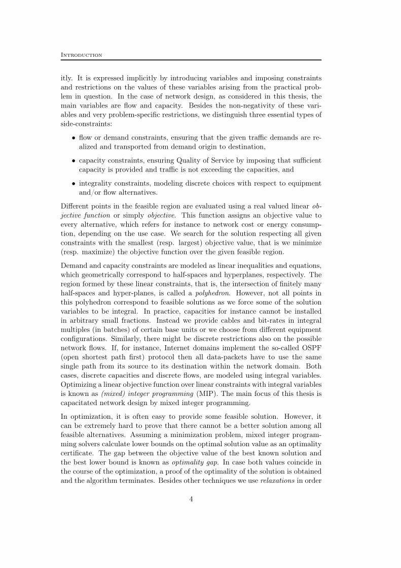
itly. It is expressed implicitly by introducing variables and imposing constraintsand restrictions on the values of these variables arising from the practical prob-lem in question. In the case of network design, as considered in this thesis, themain variables are flow and capacity. Besides the non-negativity of these vari-ables and very problem-specific restrictions, we distinguish three essential types ofside-constraints:
• flow or demand constraints, ensuring that the given traffic demands are re-alized and transported from demand origin to destination,
• capacity constraints, ensuring Quality of Service by imposing that sufficientcapacity is provided and traffic is not exceeding the capacities, and
• integrality constraints, modeling discrete choices with respect to equipmentand/or flow alternatives.
Different points in the feasible region are evaluated using a real valued linear ob-jective function or simply objective. This function assigns an objective value toevery alternative, which refers for instance to network cost or energy consump-tion, depending on the use case. We search for the solution respecting all givenconstraints with the smallest (resp. largest) objective value, that is we minimize(resp. maximize) the objective function over the given feasible region.
Demand and capacity constraints are modeled as linear inequalities and equations,which geometrically correspond to half-spaces and hyperplanes, respectively. Theregion formed by these linear constraints, that is, the intersection of finitely manyhalf-spaces and hyper-planes, is called a polyhedron. However, not all points inthis polyhedron correspond to feasible solutions as we force some of the solutionvariables to be integral. In practice, capacities for instance cannot be installedin arbitrary small fractions. Instead we provide cables and bit-rates in integralmultiples (in batches) of certain base units or we choose from different equipmentconfigurations. Similarly, there might be discrete restrictions also on the possiblenetwork flows. If, for instance, Internet domains implement the so-called OSPF(open shortest path first) protocol then all data-packets have to use the samesingle path from its source to its destination within the network domain. Bothcases, discrete capacities and discrete flows, are modeled using integral variables.Optimizing a linear objective function over linear constraints with integral variablesis known as (mixed) integer programming (MIP). The main focus of this thesis iscapacitated network design by mixed integer programming.
In optimization, it is often easy to provide some feasible solution. However, itcan be extremely hard to prove that there cannot be a better solution among allfeasible alternatives. Assuming a minimization problem, mixed integer program-ming solvers calculate lower bounds on the optimal solution value as an optimalitycertificate. The gap between the objective value of the best known solution andthe best lower bound is known as optimality gap. In case both values coincide inthe course of the optimization, a proof of the optimality of the solution is obtainedand the algorithm terminates. Besides other techniques we use relaxations in order
4

Introduction
Figure 2: A cutting hyperplane (in red) reducing a linear relaxation (in gray) by removing infeasiblefractional regions (in light-gray). The cutting plane does not cut into the convex hull (in blue) of theintegral feasible solutions (dark grid points). Instead, in this case, it defines a facet (dark red).
to provide such optimality certificates. The essential idea of this approach is toincrease the solution space and to solve the resulting relaxed problem instead ofthe original problem itself. The objective value of a cost-minimal solution to a re-laxation clearly defines a lower bound on the optimal cost of the original problem.The trick is to use relaxations that are tight in the sense that they only slightlyincrease the feasible region which provides good lower bounds, and secondly, relax-ing should substantially simplify the problem to be able to provide lower boundsquickly.
In mixed integer programming we use linear programming (LP) relaxations whichare obtained by removing the integrality restrictions from the original problem.The LP relaxations are then tightened by iteratively adding cutting planes to theformulation and re-optimizing the relaxation. These additional linear inequalitiesare supposed to cut off infeasible fractional regions from the increased solutionspace while keeping all feasible integral solutions, see Figure 2. State-of-the-artMIP solvers integrate an LP relaxation based cutting plane algorithm into anenumeration framework called branch-and-bound . Branching divides the solutionspace into smaller subproblems. The resulting combined algorithm is often referredto as branch-and-cut .
There is a trade-off between improving the lower bound by adding more cuttingplanes and deteriorating the LP re-optimization by adding too many additionalconstraints which typically slows down the overall algorithm. At this point itis crucial to provide strong cutting planes that cut off large infeasible portionsfrom the relaxation without cutting off feasible points. Translating this propertyto the mathematical terminology means that cutting planes should define high-dimensional faces of the polyhedron defined by the convex hull of all feasible solu-tions, see Figure 2. In the best case, we provide facet-defining inequalities. For thedesign of successful cutting plane separators a deep knowledge of the mathematicalstructure of the problem and the resulting polyhedra is indispensable.
Large parts of this thesis concentrate on cutting plane techniques and polyhedralstudies applied to network design problems. We provide cutting planes that in-corporate the different variables in network design, capacity and flow, and thatexploit aspects such as discrete capacity models and demand uncertainty as de-
5

Introduction
scribed above. We thereby study the strength of the developed inequalities theo-retically and computationally, that is, we show that the studied inequalities definefacets but we also evaluate their algorithmic impact. Our approach is two-fold.We provide cutting plane techniques that can be used to design tailored algorithmsto solve specific network design problems. On the other hand, we aim at improv-ing general purpose MIP solvers by including successful special purpose cuttingtechniques stemming from network design.
Most of the strong inequalities in network design have been derived by studyingthe problem for very small networks or network substructures. The main idea is tofully understand the mathematical structure and the problem-defining polyhedrafor these small instances and to describe (all) important facet-defining inequalities.In a second step, these inequalities are generalized and made available for theoriginal problem.
Following this approach, the inequalities in this thesis are mostly based on net-work cuts. A network cut is a set of links connecting two independent parts ofthe network, meaning that taking away these links disconnects the network, seeFigure 3 on the next page. A cut-based inequality essentially states a restrictionon the capacity and/or flow on the links defining the network cut. It might forinstance force sufficient cut-capacity. It is well known that cutting planes derivedby network cuts are among the most effective when used within branch-and-cutframeworks to solve network design problems. Cut-based inequalities also definefacets of the corresponding polyhedra under only mild conditions. Shrinking eachside of a cut to a single node obviously results in a two-node network. In thisrespect, deriving strong cut-based inequalities is related to understanding networkdesign polyhedra for problems with only two-nodes, also known as cut-set poly-hedra. We highlight that the concept of studying the facial structure of cut-setpolyhedra leads to the well-known and strong cut-set inequalities, flow cut-set in-equalities, flow-cover inequalities, or Steiner cut inequalities. We study cut-setpolyhedra in different contexts incorporating side-constraints such as demand un-certainty, thereby enhancing and generalizing some of the mentioned cut-basedinequalities to these contexts.
Main contributions and structure of this document
This thesis consists of three major parts. Their content is as follows.
In Part I, we introduce the general concepts and notation used in the rest of thisthesis. The chapter is two-fold. On the one hand we formally introduce the no-tion of capacity, routing, and multi-commodity flows in networks and describevariations of capacitated network design problems. We present mixed integer pro-gramming formulations as well as cutting planes used to tighten the correspondinglinear programming relaxations. We start with a basic link-flow formulation andintegral link capacity variables. We then show how the models can be extended or
6

Introduction
500 km
Seattle
Indianapolis
Atlanta
Chicago
San Francisco
Washington DC
Houston
Denver
Los Angeles
New York City
Kansas City
Figure 3: A network cut (in red) disconnecting the three cities on the left from the rest of the network.The two shores of the cut (in blue) can be seen as two artificial nodes connected by the cut linkscreating a two-node network.
modified to handle different requirements on the network flow and capacity such asfractional, integral, and single-path flows, unidirectional and bidirectional capaci-ties, as well as multiple link or node capacity modules. For all of these variationswe show how to formulate strong cutting planes and review the corresponding liter-ature. The focus is on cut-based inequalities. In this respect, so-called single-nodeflow sets and cut-set polyhedra are introduced. It is highlighted that cut-basedinequalities define facets and can be very effective computationally. That is, theaverage time to solve network design problems can be reduced substantially andthere are many instances that can only be solved in a reasonable amount of timeif the mentioned strong inequalities are used as cutting planes.
On the other hand, we focus on solution technology to deal with mixed integerprogramming formulations in general. As most of the results in this work are re-lated to cutting planes we introduce this methodology in a more general form. Wework out how strong inequalities that can be obtained by constraint aggregationtechniques in combination with rounding techniques such as mixed integer round-ing (MIR). We introduce the concept of complemented mixed integer rounding(c-MIR) as implemented in state-of-the-art MIP solvers. We review crucial knownfacts but also provide some new insights about the size of MIR aggregations. Inparticular we give a short alternative proof of a recent result of Andersen, Cor-nuéjols, and Li [11] that any split or MIR cut can be obtained from a subset oflinearly independent constraints of the given system.
Part II provides the detailed algorithmic framework of the MCF separator (MCFstands for multi-commodity flow) which combines both areas, that is, successfulcutting planes for special purpose network design problems as well as aggregationand separation techniques for general purpose MIP. The MCF separator is now anintegral part of the MIP solvers Cplex [140] and Scip [227]. A similar approachbased on single-commodity flows and so-called network inequalities is now alsoavailable in Gurobi [125]. The MCF separator integrates network design specificmethodology into these optimization tools which is of particular importance for
7

Introduction
practitioners that tend to use MIP solvers as black boxes.
The key idea of the MCF-separator is to scan the constraint matrix of generalMIP formulations in order to find a substructure that is common to many modelsfor network design problems. This structure consists of a series of similar blockscorresponding to network matrices defining a multi-commodity flow and a couplingof these flow-blocks by capacity constraints. In case of a successful detection, theMCF-separator constructs a network from the obtained information and appliesseparation methods similar to those from Part I. To obtain inequalities defined oncuts in the detected network, rows of the original system are aggregated accord-ingly. In this respect, the MCF-separator essentially provides an alternative aggre-gation framework that is used to provide cut-based base inequalities. These baseinequalities are then strengthened by mixed integer rounding. In Part II we answerthe question of how to detect and construct a network from a multi-commodityflow formulation as well as the question of how to generate valid cut-based in-equalities without precisely knowing the network structure. We also report on thecomputational success of the separator using Scip and Cplex. Through extensivecomputational tests we show that the proposed separation scheme speeds-up thecomputation for a large set of network design problems by a factor of two on av-erage. Many of these problems can only be solved if the separator is switched on.In roughly 9% of general MIP instances we find consistent embedded networksand generate violated inequalities. For these instances the computation time isdecreased by 18–30% on average, depending on the solver and test set. For allother instances there is almost no degradation of the optimization performance.
In Part III we study the problem of designing networks without precisely knowingthe traffic demand. We discuss how this demand uncertainty can be modeled andreview and discuss different demand uncertainty sets. It is shown how the con-cept of uncertainty affects the methodology to solve capacitated network designproblems. Assuming polyhedral uncertainty sets, we highlight that there are dif-ferent ways of solving the corresponding robust network design problems based ondualization or decomposition techniques. In detailed polyhedral studies we workon the resulting models and robust counterparts. In this respect, we extend theapproaches from Part I to the design of robust networks, thereby generalizing andstrengthening the strong inequalities from Part I and II. We extend the conceptof cut-set polyhedra to robust network design and present facet-defining cut-basedinequalities. We provide computational insights comparing different solution ap-proaches, showing progress by separating cutting planes, but also evaluating therobustness of solutions using real-life measurements from IP networks.
Since there is a set of traffic scenarios to be considered, robust network design is atwo-stage process. In the first stage we determine capacities. In the second stagewe are allowed to change the flow observing realized demands. The flexibility inthe second stage, known as recourse actions or recovery, can be restricted leadingto different routing schemes, static and dynamic routing being the most extensivelystudied. Following this line, we embed robust network design into the more general
8
Introduction
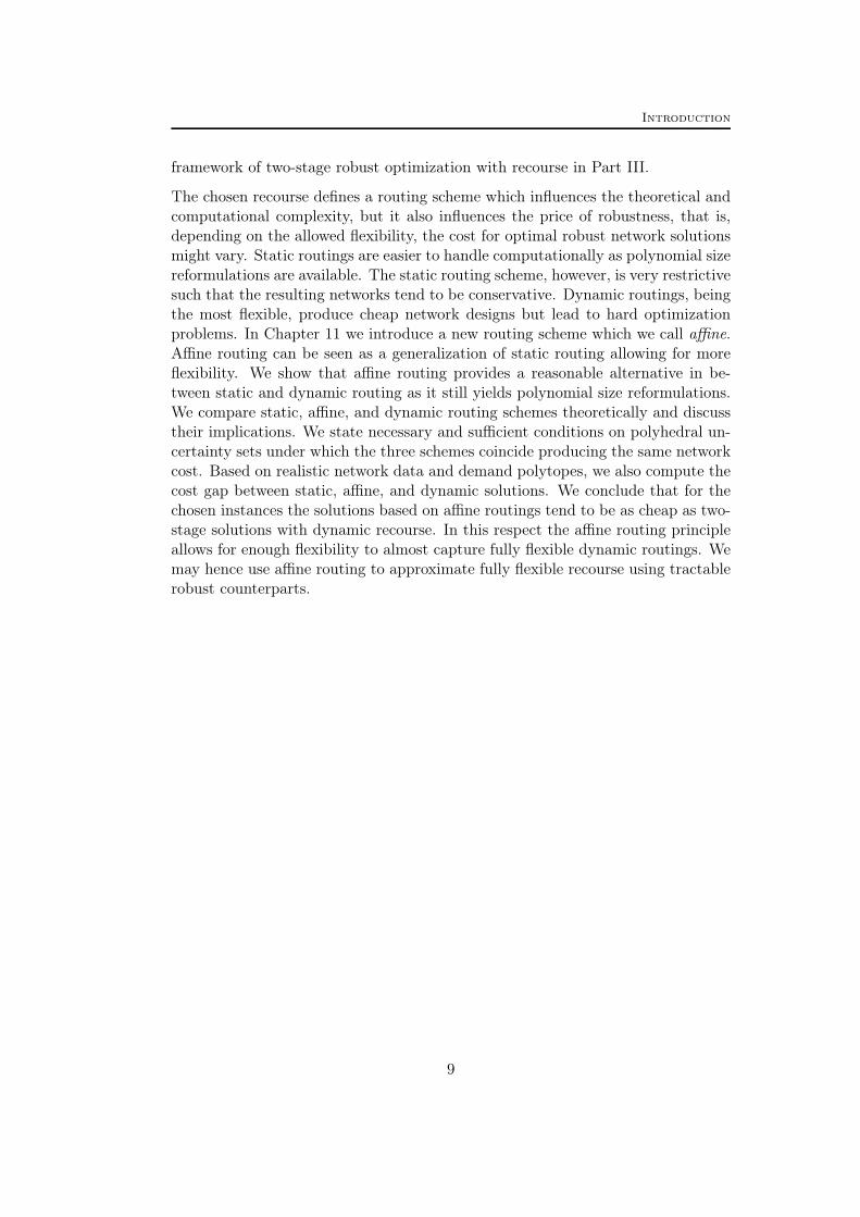
framework of two-stage robust optimization with recourse in Part III.
The chosen recourse defines a routing scheme which influences the theoretical andcomputational complexity, but it also influences the price of robustness, that is,depending on the allowed flexibility, the cost for optimal robust network solutionsmight vary. Static routings are easier to handle computationally as polynomial sizereformulations are available. The static routing scheme, however, is very restrictivesuch that the resulting networks tend to be conservative. Dynamic routings, beingthe most flexible, produce cheap network designs but lead to hard optimizationproblems. In Chapter 11 we introduce a new routing scheme which we call affine.Affine routing can be seen as a generalization of static routing allowing for moreflexibility. We show that affine routing provides a reasonable alternative in be-tween static and dynamic routing as it still yields polynomial size reformulations.We compare static, affine, and dynamic routing schemes theoretically and discusstheir implications. We state necessary and sufficient conditions on polyhedral un-certainty sets under which the three schemes coincide producing the same networkcost. Based on realistic network data and demand polytopes, we also compute thecost gap between static, affine, and dynamic solutions. We conclude that for thechosen instances the solutions based on affine routings tend to be as cheap as two-stage solutions with dynamic recourse. In this respect the affine routing principleallows for enough flexibility to almost capture fully flexible dynamic routings. Wemay hence use affine routing to approximate fully flexible recourse using tractablerobust counterparts.
9


Part I
Concepts
11


Chapter 1
Mixed integer programming
In this chapter, we introduce the basic notation and main concepts of linear andmixed integer programming. We will in particular highlight mixed integer rounding(MIR) as a central cutting plane technique used throughout this thesis.
The presentation is not meant to be self-contained. In particular, we expect basicknowledge in polyhedral theory, combinatorial optimization, and integer program-ming. We recommend the books Grötschel, Lovász, and Schrijver [121], Cook,Cunningham, Pulleyblank, and Schrijver [80], and Korte and Vygen [149] for in-troductions to combinatorial optimization as well as polyhedral combinatorics in-cluding the basic notion of polyhedra as we need them here. For complexity theoryand the notion of polynomial solvable and NP-hard problems, we refer to Gareyand Johnson [108] and Grötschel et al. [121]. The books Nemhauser and Wolsey[180], Wolsey [219], and Schrijver [205] serve as standard references to linear pro-gramming, integer programming and cutting planes. A very nice survey of historyand state-of-the-art in integer programming is provided by Jünger et al. [143]. Ex-cellent overviews about the state-of-the-art of cutting plane theory are given byMarchand, Martin, Weismantel, and Wolsey [169], Cornuéjols [82], and Conforti,Cornuéjols, and Zambelli [77]. For computational aspects and recent progress inmixed integer programming, we refer to Bixby and Rothberg [55], Bixby et al. [57],Achterberg [1], and Lodi [159]. For benchmarking and MIP libraries consult theweb-sites [178, 226].
The concepts presented in this chapter are all well-known. Most of the resultscan be found in the mentioned text books. If not, we will refer the reader to theoriginal articles within the text. In Section 1.3 we present a simple alternativeproof of a result by Andersen et al. [11] and Balas and Perregaard [28] who showthat all split cuts can be generated as so-called intersection cuts [26]. Our proofof Theorem 1.8 on page 28, which is joint work with Sanjeeb Dash and OktayGünlük, uses the equivalence of split cuts and MIR cuts. Instead of relying on themore complicated framework of split disjunctions we make explicit use of the MIRfunction as introduced in Section 1.3.
13
1 Mixed integer programming
1.1 Basics
We denote by R, Q and Z the sets of real, rational, and integral numbers. Toexclude negative numbers we write R+, Q+ and Z+. We set N := Z+ \ 0. LetK be any set of numbers. Given a finite set N , all column vectors with n = |N |entries in K are given by the set KN ≡ Kn. The transposition of x ∈ KN
is given by the row vector xT. For arbitrary subsets S ⊆ N we abbreviatex(S) :=
∑j∈S xj . The inequality x ≥ y for two vectors x, y ∈ KN is meant to hold
component-wise.
Given a matrix A ∈ Rm×n, the letters N and M denote the column and row indexsets of A with |N | = n and |M | = m. The matrix entry corresponding to rowi ∈ M and column j ∈ N is Aij ∈ R. For a subset S ⊆ N , the term A·S denotesthe submatrix of A obtained by removing all columns in N \ S. Similarly, thesubmatrix AS· corresponds to all rows S ⊆ M . We abbreviate A·j := A·j andAi· := Ai· to denote column j and row i, respectively. The identity matrix ofappropriate dimension is denoted by I.
Given a real number a ∈ R, its ceil dae is the smallest integer larger than or equalto a. Similarly, the floor bac is the largest integer smaller than or equal to a. Weset a+ := max(0, a) and a− := min(0, a). Given two real numbers a, c ∈ R withc 6= 0, the remainder of the division of a by c is given by r(a, c) := a− cbac c. Forthe fractional part of a we abbreviate r(a) := r(a, 1) = a− bac.
Given k real vectors x1, . . . , xk ∈ Rn with k ∈ N and multipliers λ ∈ Rk, we callx :=
∑ki=1 λix
i a linear combination of the vectors xi. We say that x is anaffine combination if
∑ki=1 λ = 1 and a convex combination if both λ ≥ 0
and∑k
i=1 λ = 1. Given a non-empty subset S ⊆ Rn, we denote by aff(S) theaffine hull of S which refers to all affine combinations of finitely many vectorsin S. Analogously, we denote by conv(S) the convex hull of the set S. We setaff(∅) := conv(∅) := ∅. The dimension of S denoted by dim(S) is defined asthe dimension of its affine hull which is an affine space. We say that the vectorsxi, . . . , xk are linearly independent if there is no λ 6= 0 such that
∑ki=1 λix
i = 0.They are affinely independent if there is no λ 6= 0 with
∑ki=1 λix
i = 0 and∑ki=1 λi = 0.
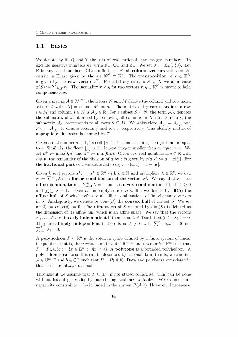
A polyhedron P ⊆ Rn is the solution space defined by a finite system of linearinequalities, that is, there exists a matrix A ∈ Rm×n and a vector b ∈ Rm such thatP = P (A, b) := x ∈ Rn : Ax ≥ b. A polytope is a bounded polyhedron. Apolyhedron is rational if it can be described by rational data, that is, we can findA ∈ Qm×n and b ∈ Qm such that P = P (A, b). Data and polyhedra considered inthis thesis are always rational.
Throughout we assume that P ⊆ Rn+ if not stated otherwise. This can be donewithout loss of generality by introducing auxiliary variables. We assume non-negativity constraints to be included in the system P (A, b). However, if necessary,
14
1.1 Basics
we might exclude the non-negativity constraints from the system Ax ≥ b andwrite P = P+(A, b) := x ∈ Rn : Ax ≥ b, x ≥ 0. Sometimes we assume equalitysystems yielding P = P=(A, b) := x ∈ Rn : Ax = b, x ≥ 0.We say that an inequality aTx ≥ β with a ∈ Rn and β ∈ R is valid for P if thehalf-space x ∈ Rn : aTx ≥ β contains P . Every valid inequality for P inducesa face F = x ∈ P : aTx = β. A singleton face F = v is called a vertex. Wedenote by vert(P ) the set of vertices of P . Inclusion-wise maximal faces F 6= Pare called facets. Inequalities inducing facets of P are called facet-defining. Forevery facet F it holds dim(F ) = dim(P )− 1.
Given a valid inequality aTx ≥ β and a point x? ∈ Rn, we call aTx? the activ-ity and β − aTx? the violation of the inequality with respect to the point x?.Inequality aTx ≥ β is violated by x? if the violation is positive. The Euclideandistance from x? to the hyperplane x ∈ Rn : aTx = β with a 6= 0 is given by|β − aTx?|/ ‖a‖, where ‖·‖ denotes the Euclidean norm in Rn.
Given two inequalities aTx ≥ β and a′Tx ≥ β′ valid for P ⊆ Rn+, we say thataTx ≥ β dominates a′Tx ≥ β′ if
x ∈ Rn+ : aTx ≥ β ⊆ x ∈ Rn+ : a′Tx ≥ β′,
see for instance Wolsey [219]. Inequality aTx ≥ β strictly dominates a′Tx ≥ β′
if in addition the two inequalities do not define the same hyperplane.
The task to minimize a linear function κTx with κ ∈ Qn over a polyhedron P (A, b)is called a linear programming problem (LP) with primal program :
(P) minκTx : x ∈ Rn, Ax ≥ b. (1.1)
We denote optimal solutions of (1.1) by x?. The set of optimal solutions to (1.1)is a face of P (A, b). The corresponding dual program is given by
(D) maxbTµ : µ ∈ Rm, ATµ = κ, µ ≥ 0. (1.2)
By linear programming duality it holds that if (1.1) has an optimal solution thenalso (1.2) has an optimal solution and the solution values coincide, that is,
minκTx : x ∈ Rn, Ax ≥ b = maxbTµ : µ ∈ Rm, ATµ = κ, µ ≥ 0
Restricting a subset I ⊆ N of the variables to integer values, we obtain the mixedinteger set PI := P ∩ x ∈ Rn : xj ∈ Z, ∀j ∈ I. Optimizing linear functionsover mixed integer sets is known as mixed integer programming (MIP). Incase I = N we speak of pure integer programming (IP). If P is a polytope or arational polyhedron then also conv(PI) is a rational polyhedron [175], see Figure 2on page 5. In this case, we have
(MIP) minκTx : x ∈ PI = minκTx : x ∈ conv(PI). (1.3)
15

1 Mixed integer programming
P
conv(PI)
(a)
P
conv(PI)
(b)
P 1 P 2
(c)
Figure 1.1: Cut and branch: (a) LP relaxation (b) Cutting plane (c) Branching
We speak of (1.1) being the linear programming relaxation (LP relaxation) of(1.3), referring to a relaxation of the problem. Similarly, we speak of P being thelinear programming relaxation of PI , in this case, referring to a relaxation of thesolution space.
Linear programming is tractable both from the theoretical and computational pointof view. There exist algorithms solving (1.1) that are polynomial in the encodinglength of the data given by the constraint matrix A, the right-hand side b, andthe objective coefficients κ, see [121, 145, 146]. Modern LP solvers implement veryefficient variants of the simplex and interior point methods going back to Dantzig[91] and Karmarkar [145], respectively, see [52] for a progress report.
In contrast, mixed integer programming is known to be strongly NP-hard [108].All known algorithms are worst-case exponential in the problem size. However, ithas been made a significant progress in the last decades in solving MIPs in practicestemming mainly from a better understanding of the underlying mathematics anda consequent implementation of new ideas and theoretical insights. For recentcomputational progress see Bixby and Rothberg [55], Bixby et al. [57] and for athorough history of the breakthroughs in integer programming and applicationswe refer to Applegate, Bixby, Chvàtal, and Cook [14] and Jünger et al. [143].
1.2 Branch-and-cut
The two fundamental concepts for solving MIPs in practice are currently LP basedbranch-and-bound and the cutting plane method. In its general form goingback to Land and Doig [156], branch-and-bound is an enumeration method follow-ing the algorithmic divide-and-conquer paradigm. The term branching refersto recursively splitting the problem and solution space into smaller sub-problemsthat can be solved more efficiently. This creates a branching tree (or search tree)which is processed in the course of the algorithm. Nodes of this tree correspond tothe created sub-problems with the root node being the original problem. In MIPwe mainly use single variable branches also called splits of the form P = P 1 ∪ P 2
16
1.2 Branch-and-cut
with
P 1 = P ∩ x ∈ Rn : xj ≥ z and P 2 = P ∩ x ∈ Rn : xj ≤ z − 1 (1.4)
for j ∈ I and z ∈ Z, see Figure 1.1(c) on the previous page. To avoid a completerecursion and hence an enumeration of all solutions it is necessary to implementan additional bounding framework. Upper (primal) bounds are given by feasiblesolutions which are provided by heuristics or solutions to sub-problems. If vectorx is feasible, that is, x ∈ PI , then clearly
minκTx : x ∈ PI ≤ κTx.
On the other hand, lower (dual) bounds are provided by optimal solutions x? tothe LP relaxations of the individual sub-problems, e. g., for the root node problemit holds
κTx? ≤ minκTx : x ∈ PI,
where κTx? = minκTx : x ∈ P. If the objective value of the LP solutionof a sub-problem is not smaller than the best known global upper bound, thecorresponding solution sub-space cannot contain an optimal solution and hencethe corresponding node in the branching tree can be pruned. See Wolsey [219]for a classification of pruning methods. LP solutions not only guide the pruning,they also guide the branching decisions as the index j and the value z in (1.4) aretypically determined from a fractional value x?j /∈ Z, j ∈ I, of an LP solution x?
setting z = dx?je. For more details on branching, in particular different branchingstrategies and their impact, we refer to Achterberg [1].
By minκTx : x ∈ PI = minκTx : x ∈ conv(PI) we know that there existsa linear program with the same optimal solution value as the given MIP. More-over, the vertices of conv(PI) are contained in PI , which means that the simplexalgorithm will find an optimal solution to (1.3) if applied to a linear description ofconv(PI). However, a complete linear inequality description of conv(PI) is typicallynot given. In the cutting plane method, we construct this description iteratively.Using valid inequalities for the linear relaxation P of PI and the integrality of thevariables in I we determine valid inequalities for PI .
We define a cutting plane or simply cut to be an inequality aTx ≥ β that isvalid for PI but not valid for P , that is, it holds aTx ≥ β for all x ∈ PI but thereexist points x? in the LP relaxation P such that aTx? < β. We say that x? isseparated from conv(PI). A cutting plane thus cuts off or separates infeasiblefractional portions from the LP relaxation of an MIP instance. A simplified cuttingplane scheme is stated in Algorithm 1.1 on the next page.
The problem to solve in Step 5 and 6 of Algorithm 1.1 on the following page isknown as the separation problem w. r. t. conv(PI). Often we are not faced withthe separation problem in this general form but with the problem of finding aninequality from a specific class of valid inequalities for PI violated by x?.
17

1 Mixed integer programming
1 Solve the LP relaxation (1.1).2 if (1.1) is infeasible then stop; // (1.3) is infeasible3 if (1.1) is unbounded then stop; // (1.3) is infeasible or unbounded4 else Let x? be an optimal solution of (1.1).5 if x? ∈ PI then stop; // x? is optimal for (1.3)6 else Find a cutting plane aTx ≥ β that separates x? from conv(PI)7 Add aTx ≥ β to the original formulation Ax ≥ b and go to Step 1.
Algorithm 1.1: The cutting plane method
The cutting plane method dates back to the 1950s and the pioneering work ofGeorge Dantzig and Ralph Gomory. George Dantzig together with Ray Fulkersonand Selmer Johnson [93, 95] developed the cutting plane method to tackle thefamous traveling salesman problem (TSP) [14] thereby establishing the field ofinteger programming. While their algorithmic scheme was based on special purposecutting planes, Gomory [112, 113] introduced a fully generic cutting plane methodbased on the famous Gomory mixed integer cuts (short: Gomory cuts), seeSection 1.4. He also proved that his method converges after a finite number ofsteps in case of a pure integer program and rational data. See Zanette, Fischetti,and Balas [223] for a recent discussion on the convergence of the pure cutting planemethod based on Gomory cuts. Notice that no finite cutting plane algorithm isknown for general MIP.
Branch-and-bound and cutting planes have been combined first by Hong [138]while the term branch-and-cut (see Figure 1.1 on page 16) was first used byPadberg and Rinaldi [191, 192], see [78]. Branch-and-cut is state-of-the-art andimplemented in modern commercial MIP solvers such as Cplex [140], Gurobi[131], or Xpress [103], as well as academic codes such as Scip [227] and CBC[74]. In branch-and-cut globally or locally valid cutting planes are added to all sub-problem formulations in the search tree to tighten the relaxations and to improvethe dual bounds. In case cuts are only used in the root node of the tree beforebranching we speak of cut-and-branch.
It has been observed very early that a deep knowledge of the facial structure ofPI is crucial for the design of successful special purpose branch-and-cut schemes.To cut deep into the LP relaxation the inequalities used for cutting should, inthe best case, define facets of PI or at least high-dimensional faces. In general,we cannot expect to know all linear inequalities defining PI . Nevertheless, givena particular problem, it is usually possible to identify at least certain classes of(strong) valid inequalities. After early successes by Grötschel [118], Grötscheland Padberg [119, 120] and many others in understanding the TSP polytope andsolving larger TSP instances by branch-and-cut, the research on cutting planesexperienced a rapid growth attacking all kinds of different problems by polyhedralmethods and devising problem specific codes with tailored cutting planes, see [14,80, 87, 121, 149].
18

1.2 Branch-and-cut
Despite the success of branch-and-cut for combinatorial optimization problems,cutting planes have long been ignored in the context of solving general MIP in-stances with general purpose solvers. For almost 40 years Gomory cuts have beenbelieved to be a theoretical tool only, causing numerical instabilities and slow con-vergence in practice. Hence early MIP codes mainly focused on efficient LP basedbranch-and-bound. The situation changed only in the late nineties with a publi-cation of Balas, Ceria, Cornuéjols, and Natraj [32] who show that Gomory cutscan be embedded effectively into a branch-and-cut framework to solve 0, 1-MIPs(integral variables are restricted to the values 0 or 1). One of the new observationsof Balas et al. [32] was that adding sets of cuts clearly outperforms adding just asingle violated cut in every separation step as proposed by Algorithm 1.1 on theprevious page. For 0, 1-MIPs, they also showed how Gomory cuts can be sharedacross the branches of the search tree by a simple lifting procedure. In a recentinteresting historical note, Cornuéjols [81] pointed out that the computational re-sults in [32] were so unexpected that the authors had problems to publish theirarticle: “[. . . ] One referee commented that ’there is nothing new’ while anotherwas so suspicious of the results that he requested a copy of the code. [. . . ]”
Shortly after the Balas et al. [32] paper, the Cplex team released version 6.5 oftheir general purpose MIP solver including separators for the mentioned Gomorycuts and other classes of strong inequalities. Bixby et al. [57] reported an averagespeedup of 22.3 from version 6.0 to 6.5 using an internal test set. This speedupwas mainly caused by the introduction of cutting planes, in particular Gomorycuts. Later in [159], the step from version 6.0 to 6.5 was shown to have the biggestimpact on the speed in the history of Cplex (version 1.2 to 11.0).
Cutting planes in practice
Nowadays it is common knowledge that cutting planes are one of the most impor-tant ingredients of a MIP solver speed-wise. Bixby and Rothberg [55] showed thatswitching off all separators in Cplex 8.0 results in a mean performance degrada-tion of 53.7 compared to 10.8 for (root) presolving and 1.8 for primal heuristics.
In addition to Gomory cuts, several classes of general cutting planes have been de-veloped over the years and tested with respect to their computational impact. Wecannot introduce all these classes in detail here but refer the reader to overviewsgiven by Marchand et al. [169], Cornuéjols [82], and Conforti et al. [77]. Alsosee Wolter [221]. However, we want to highlight that most of the successful cut-ting plane separators used in modern branch-and-cut codes follow an algorithmicscheme which can be summarized as follows:
• Aggregation: Construct an inequality aTx ≥ β valid for P by aggregatingconstraints of the original system Ax ≥ b.
• Cut generation: Find a cutting plane that separates the point x? fromQI = x ∈ RN\I × ZI : aTx ≥ β
19

1 Mixed integer programming
That is, instead of directly working on the facial structure of PI we work on a sin-gle row relaxation QI of PI . Strong inequalities that are explicitly constructedthis way and used for instance in Cplex or Scip include Gomory cuts [112] (Sec-tion 1.4), strong Chvàtal-Gomory cuts [157], knapsack cover inequalities [27], flowcover inequalities [193] (Section 2.4), 0, 1/2-cuts [64], c-MIR inequalities [168](both Section 1.4), and MCF cuts (Part II of this thesis).
The hope is that strong or even facet-defining inequalities for simple polyhedrasuch as conv(QI) might also be strong for PI and can be used efficiently in generalbranch-and-cut codes. This has led to a detailed study of the facial structure ofso-called knapsack sets, mixed integer knapsack sets, and single node flow sets, seefor instance [17, 18, 22, 27, 193, 195, 217]. In addition to the integrality of variablesand the validity of aTx ≥ β, these sets and hence the corresponding cut generationexploit information such as simple, variable, or generalized bound constraints andspecial properties of the coefficients in aTx ≥ β such as divisibility [195].
Note that there is a recent trend to generalize the framework of single row relax-ations by generating cuts from multiple rows of the simplex tableau, see Andersen,Louveaux, Weismantel, and Wolsey [12], Cornuéjols and Margot [84]. The com-putational impact of this idea still needs to be investigated, see Espinoza [102] forfirst results.
Despite the success of cutting planes in commercial codes, their generation is im-plemented in a highly heuristic fashion, very often with almost no theoreticaljustification. Little is known about how to select cuts from a large set of violatedinequalities and about the interaction of different families of cutting planes. Imple-mentation and tuning is typically based on excessive computational tests on largesets of instances, see [1] and the references therein. Cutting plane generation inpractical codes is also a heuristic with respect to numerical accuracy and floatingpoint arithmetic. It might simply happen that feasible solutions are cut off evenin case of very conservative strategies, see Margot [170].
In practice, cutting planes are generated in rounds mainly in the root node of thebranching tree. Given a solution x? of the current LP relaxation, a list of separatorsis asked to produce violated inequalities in Step 6 of Algorithm 1.1 on page 18.Violated inequalities enter the so-called cut-pool [1, 13]. Only a certain numberof the best cuts from the pool are then allowed to enter the LP formulation. Themain selection criterion in branch-and-cut codes in this context (despite the knownweaknesses, see for instance [216]) is the Euclidean distance (β−aTx?)/ ‖a‖ of thepoint x? to the violated cutting hyperplane aTx ≥ β which is also referred to asthe efficacy of the cut, see [1, 13, 219].
Bixby and Rothberg [55] as well as Wolter [221] and Achterberg [1] reported on per-formance measures for the individual cutting plane classes implemented in Cplexand Scip, respectively. Without providing detailed numbers as these tests arebased on different codes and test sets, we can easily identify the two main winnersin the sense that deactivating these separators leads to the largest performance
20

1.3 Mixed integer rounding: A pivotal cutting plane technique
f
x
β
Figure 1.2: The MIR inequality (in red) and its base inequality (in black) in two dimensions.
degradations: these are the mentioned Gomory cuts and the complemented mixedinteger rounding (c-MIR) cuts from Marchand and Wolsey [168], see Section 1.4. Itis remarkable that both separators (and others) use the same rounding techniqueknown as MIR, which we believe to be pivotal for mixed integer programming.This technique is also used for the new MCF separator described in Part II of thisthesis. Moreover, all the special purpose facet-defining inequalities in the remain-ing chapters of this thesis can be shown to be obtained by MIR. Consequently, wewill introduce mixed integer rounding in more detail in the following.
After introducing MIR as a cut generation scheme in Section 1.3, Section 1.4focuses on aggregation techniques that are successfully used in combination withMIR in state-of-the-art branch-and-cut codes.
1.3 Mixed integer rounding: A pivotal cutting planetechnique
The term and methodMixed integer rounding (MIR) goes back to the work ofGomory [112, 113]. Considered to be only a theoretical tool for a long time, it hasbeen rediscovered computationally only recently by Balas et al. [32] and Marchandand Wolsey [168]. There is quite some confusion in the literature on how to defineMIR as a procedure. Different versions of the same inequality are available and theprocess of revising and establishing MIR also led to descriptions that are in factweaker than the original inequality of Gomory. Gomory used MIR only for rowsof the simplex tableau (see Section 1.4). The term mixed integer rounding wasfirst used by Nemhauser and Wolsey [180] while the most general version of MIRwas introduced in Nemhauser and Wolsey [181] strengthening the weaker MIRprocedure from [180]. For a state-of-the-art presentation and a thorough overviewabout the different versions of MIR with historical notes we refer to Dash, Günlük,and Lodi [96].
There is a strong relation of MIR cuts to the theoretical frameworks of split cuts,intersection cuts, disjunctive cuts, and also lift-and-project cuts. We will work
21

1 Mixed integer programming
out some of these relations below but refer to Conforti, Cornuéjols, and Zambelli[76], Cornuéjols [82] for comprehensive reviews.
To introduce MIR it suffices to consider a mixed two-variable set defined by a singleconstraint with a general integer variable and a non-negative continuous variable,see Figure 1.2 on the previous page. The basic MIR inequality turns out to definethe only non-trivial facet of this set [168, 219].
Lemma 1.1 (Wolsey [219]). Let QI := (f, y) ∈ R × Z : f + y ≥ β, f ≥ 0.The basic MIR inequality
f + ry ≥ rdβe (1.5)
with r := r(β) = β − bβc is valid for QI and defines a facet of conv(QI) if r > 0.
Proof. Inequality (1.5) is trivially valid if r = 0. Let r > 0 and assume first thaty ≥ dβe. In this case f + ry ≥ rdβe by the non-negativity of f . Otherwise, ify ≤ bβc then we rewrite the inequality f + y ≥ β as f + ry ≥ bβc+ r− y(1− r) ≥bβc+ r− bβc(1− r) = rdβe. Inequality (1.5) connects the two points (0, dβe) and(r, bβc) which are clearly affinely independent if r > 0. Hence (1.5) defines a facetof conv(QI) in this case.
Based on Lemma 1.1, we will in the sequel develop general rank-1 MIR inequalitiesvalid for PI with P = P (A, b) or P = P+(A, b) following presentations in [82, 96,219]. We will provide two definitions of a general MIR inequality depending onwhether non-negativity constraints are included in the system Ax ≥ b or not.These two definitions are equivalent [96].
First we introduce a general valid base inequality by constraint aggregation. Lets ∈ Rm, s ≥ 0 be the vector of slacks corresponding to the system Ax ≥ b, that is,s = Ax− b. Choosing row multipliers λ ∈ Rm the equation
−λTs+ λTAx = λTb (1.6)
is valid for P . To simplify notation we set aj := λTA·j We also set rj := r(aj) andr := r(β) with β := λTb.
Let us first assume we have a formulation P = P+(A, b) with non-negativity con-straints not included in the system Ax ≥ b and hence not used in the aggregation.Relaxing (1.6) gives(
−∑i∈M
λ−i si +∑j∈N\I
a+j xj +
∑j∈I′
rjxj)
+(∑j∈Ibajcxj +
∑j∈I\I′
xj)≥ β. (1.7)
for some I ′ ⊆ I. Notice that aj = bajc + rj . Also notice that we increase thecoefficients for all j ∈ I \ I ′ to the value (bajc + 1) ≥ aj . Similarly, coefficientsfor continuous variables are increased to a+
j and −λ−i , respectively. Here we makeexplicit use of the non-negativity of the variables. As the first part of inequality(1.7) is non-negative and the second part is integral we can apply Lemma 1.1. Theresulting inequality turns out to be strongest in case I ′ := j ∈ I : rj < r. Werewrite and obtain:
22

1.3 Mixed integer rounding: A pivotal cutting plane technique
Proposition 1.2 (Dash et al. [96], Nemhauser and Wolsey [181]). Let P =P+(A, b). Inequality
−∑i∈M
λ−i si +∑j∈N\I
a+j xj +
∑j∈I
(rbajc+ min(rj , r))xj ≥ rdβe (1.8)
is valid for PI for all λ ∈ Rm.
We call (1.8) theMIR inequality generated by the row weights λ . Inequality(1.7) is the base inequality for (1.8). Notice that by resubstituting the slackvariables, inequality (1.8) can be expressed in the space of the x variables. Wemay restrict the multipliers λi to non-negative values which gives the simpler MIRinequality ∑
j∈N\Ia+j xj +
∑j∈I
(rbajc+ min(rj , r))xj ≥ rdβe.
Notice that setting λ ≥ 0 is equivalent to not introducing slacks in (1.6) andthen applying MIR. However, it has been observed by Dash et al. [96] that sucha simplified procedure does not give all possible MIR inequalities and hence leadsto a different closure:
Definition 1.3. The set MirClosure(P, I) ⊆ P is the set of points x ∈ P ⊆ Rn+that satisfy all MIR inequalities (1.8) that can be generated by some λ ∈ Rm. Wecall MirClosure(P, I) the (first) MIR closure of P with respect to I.
Clearly it holdsPI ⊆MirClosure(P, I) ⊆ P.
We also know that MirClosure(P, I) is a rational polyhedron [79, 96]. Any MIRinequality valid for MirClosure(P, I) is said to be of rank 1. Taking theclosure recursively leads to higher rank MIR inequalities and higher rank closures.However, this does not give conv(PI) in a finite number of steps for general (P, I),see Cook et al. [79]. But it is true in case all variables are integral, that is,I = N , which is related to the corresponding convergence result for Gomory cuts[112, 113]. It also holds in the mixed binary case, that is, if xj ∈ 0, 1 for j ∈ I,see for instance [82, 83, 180].
The so-called Chvátal-Gomory cut (short: CG cut) for the all-integer caseN = I and the corresponding CG closure is obtained from (1.8) by relaxingto∑
j∈N rdajexj ≥ rdβe and considering all row weights λ ∈ Rm+ . Notice that(rbajc+ min(rj , r)) ≤ rdaje, that is, the MIR cut may dominate the CG cut.
Let us now assume we have a formulation of the form P = P (A, b) with non-negativity constraints included in the system Ax ≥ b. Starting from (1.6) werestrict the set of row multipliers to
Φ = λ ∈ Rm : λTA·j ∈ Z for all j ∈ I, λTA·j = 0 for all j /∈ I. (1.9)
For λ ∈ Φ and x ∈ PI it now holds λTAx ∈ Z. Also −λ−i si ≥ 0 for all i ∈M . Wemay thus apply Lemma 1.1 giving the following MIR inequality valid for PI :
23

1 Mixed integer programming
Proposition 1.4 (Dash et al. [96], Nemhauser and Wolsey [181]). Let P =P (A, b). Inequality
−∑i∈M
λ−i si + r∑j∈I
ajxj ≥ rdβe (1.10)
is valid for PI for all λ ∈ Φ.
In contrast to Proposition 1.2, the non-negativity of the variables has not beenused explicitly in Proposition 1.4. But notice that both conditions λTA·j ∈ Z andλTA·j = 0 can be achieved easily by tuning the row multipliers corresponding tothe non-negativity constraints of the variables j ∈ N . We refer to Dash et al. [96]to see that the MIR inequalities (1.8) and (1.10) and the corresponding definitionsof the MIR closure are equivalent. This is based on the transformation P =P+(A, b) = P (A, b) with A = (I,A) and bT = (0, bT). In this case row multipliersλ ∈ Rm for (1.8) translate to row multipliers λ ∈ Φ for (1.10) and vice versa. Wewill use MIR-inequality (1.8) or (1.10), whichever form is more handy.
The CG closure for the all-integer case N = I is obtained from (1.10) by restrict-ing the used multipliers to all non-negative λ ∈ Φ which results in the CG cuts∑
j∈N ajxj ≥ dβe with aj ∈ Z, j ∈ N . Both definitions of the CG closure areequivalent.
MIR functions and subadditivity
Mixed integer rounding can be expressed as an operator acting on the coefficientsand right-hand side of a valid inequality. This operator has some crucial properties.It turns out that these properties suffice to get valid inequalities for PI in general,see Nemhauser and Wolsey [180]. Let us define the MIR function Fβ : R → Rwith α 7→ Fβ(α) := r(β)bαc+ min(r(α), r(β)), see Figure 1.3 on the facing page.Setting Fβ(α) := α+ we rewrite the MIR inequality (1.8) as∑
i∈MFβ(−λi)si +
∑j∈N\I
Fβ(aj)xj +∑j∈IFβ(aj)xj ≥ Fβ(β). (1.11)
The function Fβ is non-decreasing with Fβ(0) = 0 and Fβ is subadditive, thatis, Fβ(α1) + Fβ(α2) ≥ Fβ(α1 + α2) for all α1, α2 ∈ R [180, 181]. It also holdsthat Fβ(α) = limt0
Fβ(αt)t for all α ∈ R. It turns out that any function Fβ with
these properties generates a valid inequality for PI of the form (1.11). Moreover,any valid inequality for PI is generated by some subadditive valid inequality [180,Theorem 7.8]. Notice that the presentation in [180] is for superadditive functionsand valid “≤” inequalities which can be translated easily to our setting.
Often we use the same inequality (1.7) with different multipliers 1/γ, γ > 0, beforederiving the MIR inequality (1.11). For this purpose we introduce the function
Fβ,γ(α) := γFβ(α/γ) = γr(β/γ)bα/γc+ γmin(r(α/γ), r(β/γ))
= r(β, γ)bα/γc+ min(r(α, γ), r(β, γ)).
24
1.3 Mixed integer rounding: A pivotal cutting plane technique
−1 −0.5 0.5 1 1.5 2
−0.5
0.5
1
F0.5(α)
α
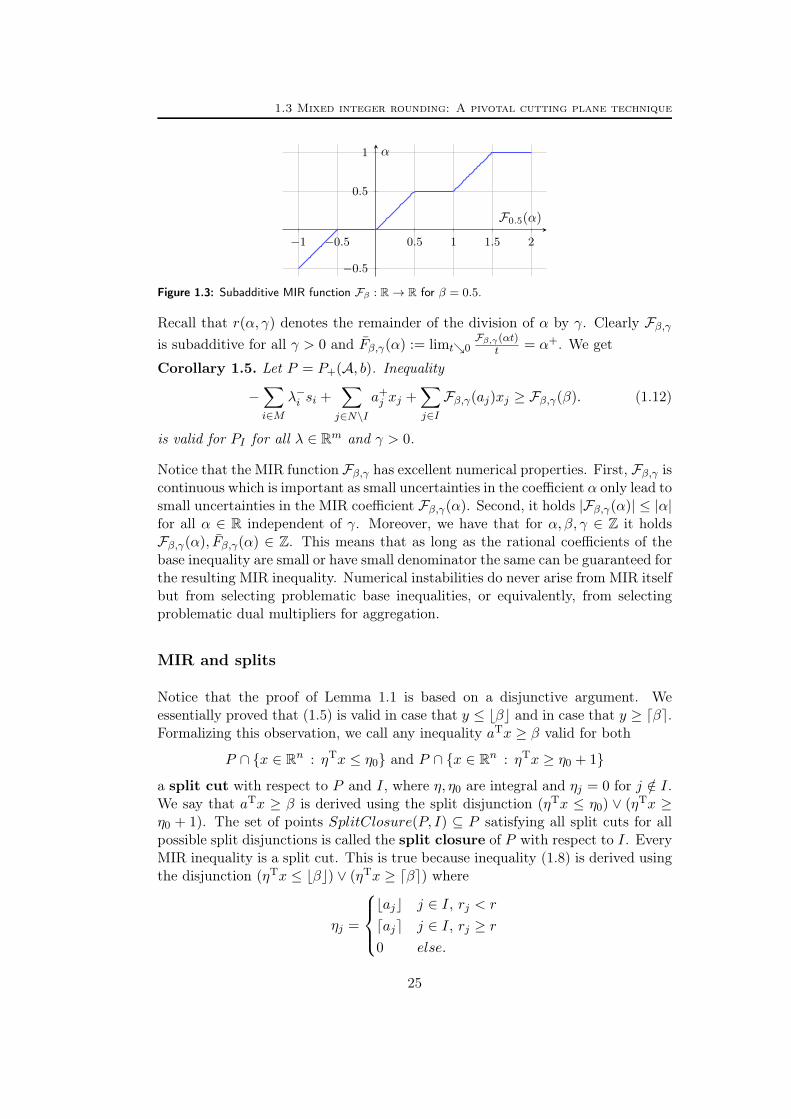
Figure 1.3: Subadditive MIR function Fβ : R→ R for β = 0.5.
Recall that r(α, γ) denotes the remainder of the division of α by γ. Clearly Fβ,γis subadditive for all γ > 0 and Fβ,γ(α) := limt0
Fβ,γ(αt)t = α+. We get
Corollary 1.5. Let P = P+(A, b). Inequality
−∑i∈M
λ−i si +∑j∈N\I
a+j xj +
∑j∈IFβ,γ(aj)xj ≥ Fβ,γ(β). (1.12)
is valid for PI for all λ ∈ Rm and γ > 0.
Notice that the MIR function Fβ,γ has excellent numerical properties. First, Fβ,γ iscontinuous which is important as small uncertainties in the coefficient α only lead tosmall uncertainties in the MIR coefficient Fβ,γ(α). Second, it holds |Fβ,γ(α)| ≤ |α|for all α ∈ R independent of γ. Moreover, we have that for α, β, γ ∈ Z it holdsFβ,γ(α), Fβ,γ(α) ∈ Z. This means that as long as the rational coefficients of thebase inequality are small or have small denominator the same can be guaranteed forthe resulting MIR inequality. Numerical instabilities do never arise from MIR itselfbut from selecting problematic base inequalities, or equivalently, from selectingproblematic dual multipliers for aggregation.
MIR and splits
Notice that the proof of Lemma 1.1 is based on a disjunctive argument. Weessentially proved that (1.5) is valid in case that y ≤ bβc and in case that y ≥ dβe.Formalizing this observation, we call any inequality aTx ≥ β valid for both
P ∩ x ∈ Rn : ηTx ≤ η0 and P ∩ x ∈ Rn : ηTx ≥ η0 + 1a split cut with respect to P and I, where η, η0 are integral and ηj = 0 for j /∈ I.We say that aTx ≥ β is derived using the split disjunction (ηTx ≤ η0) ∨ (ηTx ≥η0 + 1). The set of points SplitClosure(P, I) ⊆ P satisfying all split cuts for allpossible split disjunctions is called the split closure of P with respect to I. EveryMIR inequality is a split cut. This is true because inequality (1.8) is derived usingthe disjunction (ηTx ≤ bβc) ∨ (ηTx ≥ dβe) where
ηj =
bajc j ∈ I, rj < r
daje j ∈ I, rj ≥ r0 else.
25

1 Mixed integer programming
Similarly (1.10) is a split cut derived by the disjunction (λTAx ≤ bβc)∨ (λTAx ≥dβe). Surprisingly also every split cut is an MIR cut [181] such that
MirClosure(P, I) = SplitClosure(P, I).
The split closure is surprisingly strong. It has been shown to nicely approximatethe integer hull PI for practical instances by Balas and Saxena [29] (Dash et al.[96]). These authors formulated the problem of separating a given point fromthe split closure (MIR closure) as a MIP. Notice that this problem is NP-hard ingeneral [65]. It could be shown that the integrality gap closed by all rank-1 splitcuts amounts to 82% on average for 33 MIPs from the Miplib 3.0 [56] and 71%on average for 24 pure integer programs from the same library.
The MIR closure and basic relaxations
Exactly solving the separation problem for split cuts as in [29, 96] is too timeconsuming to be used in practical codes. It remains a challenging problem how toselect a subset of efficient split cuts from the immense collection of available cuts,that is, how to approximate the MIR closure for effective branch-and-cut codes.This relates to the question of finding appropriate split disjunctions or appropriateaggregators λ to generate split or MIR cuts, respectively.
Before we will introduce three different aggregation schemes for MIR cuts, suc-cessfully used in state-of-the-art codes, namely Gomory cuts, c-MIR cuts, and0, 1/2-cuts, we will briefly sketch a couple of related theoretical questions.
In particular, we will give a proof of the fact that all important split cuts areso-called intersection cuts [26] corresponding to a basis of the LP relaxation Pand a split disjunction, that is, the set of row multipliers λ to be considered in theseparation of MIR cuts reduces to those that correspond to an LP basis.
Separating from the MIR closure. Recall that the separation problem forsplit cuts is NP-hard in general. However, given a point x? ∈ P and a split(ηTx ≤ bβc) ∨ (ηTx ≥ dβe) with η integral and ηj = 0 for j /∈ I such thatηTx? = β /∈ Z, the most violated split inequality for this split can be found inpolynomial time by solving the so-called cut generating LP. The correspondingtheoretical framework is known as lift-and-project, see [28, 30, 31]. Balas andPerregaard [28] showed that the (higher dimensional) cut generating LP can besolved by pivoting in the original simplex tableau, that is, lift-and-project can beseen as a framework to find the best basis from which to generate the split cut.
Similarly, given a basis of the LP relaxation corresponding to a fractional extremesolution x?, we can easily state a split such that the vertex is cut off by the corres-ponding split cut. This is done in polynomial time by generating a Gomory cut as
26

1.3 Mixed integer rounding: A pivotal cutting plane technique
we will see in Section 1.4. But notice that this feature is restricted to extreme so-lutions of P . It does not contradict NP-hardness of the general separation problemfor split cuts.
Row multipliers. We know that MirClosure(P, I) is a polyhedron [79, 96]which implies that the number of vectors λ needed to obtain the MIR closureis finite. Dash et al. [96] explicitly established a finite set of vectors leading toMirClosure(P, I). Here we state their result for the pure integer case. Assume(by scaling) matrix A and right-hand side b have integral entries and let N = I.
Proposition 1.6 (Dash et al. [96]). MirClosure(P, I) with P = P+(A, b) isthe set of points that satisfy all MIR inequalities (1.8) generated by λ ∈ Rm whereλi ∈ [0, 1) is rational with denominator equal to a sub-determinant of the matrix(A, b).Corollary 1.7 (Dash et al. [96]). MirClosure(P, I) with P = P (A, b) is theset of points that satisfy all MIR inequalities (1.10) generated by λ ∈ Φ whereλi ∈ (−1, 1) is rational with denominator equal to a sub-determinant of the matrix(A, b).
Proposition 1.6 and Corollary 1.7 state the same result for the two different versionsof MIR inequalities (1.8) and (1.10) (either assuming non-negativity constraints tobe part of the system Ax ≥ b or not). Corollary 1.7 follows from the correspondingtransformation of the row multipliers given in [96]. This result can be generalizedto the mixed integer case, see [96]. It is crucial for the choice of potential λ inpractical implementations of MIR procedures, see Section 1.4.
Notice that to obtain the CG closure for P = P (A, b) with N = I we simplyrestrict the multipliers to λ ∈ Φ ∩ [0, 1)m in Corollary 1.7.
Basic relaxations. Proposition 1.6 limits the necessary vectors λ to obtain theMIR closure in terms of the numbers λi to use as multipliers for rows i ∈M . Nextwe show that we can also restrict λ with respect to the (number of) rows i forwhich λi 6= 0. It suffices to consider linear independent rows for MIR aggregations.Notice that such rows correspond to a basis of the LP relaxation P . The resultsbelow are based on the presentation by Dash, Günlük, and Raack [97].
Given a subset S of the rows M , the relaxation of P corresponding to S is:
P (S) := x ∈ Rm : Ai·x ≥ bi, i ∈ SClearly P = P (M). In case the vectors Ai·, i ∈ S are linearly independent, we callthe relaxation P (S), a basic relaxation of P . Let B be the collection of subsetsof M that give basic relaxations of P . Andersen et al. [11] showed that all splitcuts can be generated from basic relaxations of P , that is,
SplitClosure(P, I) =⋂B∈B
SplitClosure(P (B), I). (1.13)
27

1 Mixed integer programming
This result implies that all split cuts, and hence all MIR cuts, can be obtainedas so-called intersection cuts [26]. Equivalence between split cuts and intersectioncuts has been shown earlier for mixed binary sets by Balas and Perregaard [28].In the following we give a short proof of the general result of Andersen et al. [11]by showing that
MirClosure(P, I) =⋂B∈B
MirClosure(P (B), I).
Here we assume MIR inequalities of the form (1.10) with row multipliers restrictedto the set Φ defined in (1.9). For λ ∈ Φ we denote by A(λ) and b(λ) the collectionof rows i of A and b for which λi 6= 0. Hence the MIR inequality generated by λis in fact an MIR inequality for the relaxation
PI(λ) = x ∈ RN\I × ZI : A(λ)x ≥ b(λ)
Theorem 1.8. Let x ∈ P \MirClosure(P, I), then x violates an MIR inequalitygenerated by λ ∈ Φ such that A(λ) has full-row rank.
Proof. The proof is by contradiction. Let ΦB = λ ∈ Φ : A(λ) has full-row rank.Assume that there is a point x ∈ P \ MirClosure(P, I) that satisfies all MIRinequalities that are generated by λ ∈ ΦB. For the point x, define the violation ofan MIR inequality (1.10) generated by λ ∈ Φ as
vio(λ) = rdλTbe − rλTAx+∑i∈M
λ−i si
where s = b−Ax and r = λTb−bλTbc. Remember that 0 < r < 1 for any violatedMIR inequality.
Let λ ∈ Φ \ ΦB give the most violated MIR inequality for x. In other words,vio(λ) > 0 and vio(λ) ≥ vio(λ) for all λ ∈ Φ. Furthermore, assume that fromamong the MIR inequalities that are violated by vio(λ), the vector λ yields amatrix A(λ) with the fewest number of rows. In other words, for any λ ∈ Φ, weassume that either (i) vio(λ) > vio(λ), or, (ii) vio(λ) = vio(λ) and A(λ) has atleast as many rows as A(λ). Furthermore, let λ have k > 0 non-zero elementsand without loss of generality assume that the first k elements of λ are non-zero.Consequently, A(λ) and b(λ) have k rows and A = (A(λ),A′)T and b = (b(λ), b′)T.
As A(λ) does not have full-row rank, there exists a vector θ ∈ Rk such that θ 6= 0and θTA(λ) = 0. Let θ ∈ Rm be defined by θ := (θ, 0)T. We will next argue thatfor some ε 6= 0, the vector (λ + ε θ) is in Φ and it either yields a more violatedMIR inequality, or, gives a matrix A(λ+ ε θ) with strictly fewer rows than A(λ),which is a contradiction.
For convenience, let γ = θTb = θTb(λ) and assume that γ ≥ 0. Note that this canbe done without loss of generality by replacing θ with −θ, if necessary. In fact,
28
1.4 Computationally successful cutting plane separators
we can assume that γ > 0 as the proof is similar for γ = 0. First note that byconstruction θTA = 0 and therefore for any ε ∈ R we have (λ + ε θ)TA = λTAand consequently (λ+ ε θ) ∈ Φ. Next, note that λTb is not integral and thereforedλTbe = d(λ+ε θ)Tbe for ε satisfying (1−r)/γ > ε > −r/γ where r = λTb−bλTbc.Therefore, for all ε such that |ε| < ε0 = min(1− r)/γ, r/γ, we have
∆(ε) := vio(λ)− vio(λ+ ε θ) = (r− r′)(dλTbe− λTAx) +∑i∈M
(λ−i − (λi + ε θi)−)si
where r′ = (λ+ε θ)Tb−b(λ+ε θ)Tbc, and hence r−r′ = −ε θTb. Furthermore, for|ε| < ε1 := mini:θi 6=0|λi/θi| we have that λ−i is non-zero if and only if (λi+ε θi)
−
is non-zero. Hence
∆(ε) = −ε θTb(dλTbe − λTAx) + ε θTs,
for any ε such that |ε| < minε0, ε1, where θi := θi if λ−i is non-zero and θi = 0otherwise. It turns out that ∆(ε) is linear in ε. As the starting MIR inequalitygiven by λ is a most violated one, we have both ∆(ε),∆(−ε) ≥ 0 and therefore∆(ε) = 0. Thus λ+ ε θ also gives a most violated MIR inequality. In fact, λ+ ε θgives a most violated MIR inequality for all ε > 0 such that ε < (1 − r)/γ, andε < |λi/θi| for all i such that λi, θi 6= 0 and have opposing signs. But then, ε > 0can be increased, while keeping vio(λ) = vio(λ+ ε θ) until either (i) ε = (1− r)/γ,which implies that the original inequality is not violated, or (ii) ε = λi/θi for somei, which gives a vector λ + ε θ that has strictly fewer non-zero elements than λ.Both cases contradict the starting assumptions on λ and therefore the proof iscomplete.
We have introduced mixed integer rounding as a cutting plane technique and wehave highlighted the general concept of constraint aggregation to obtain singlerow relaxations of the original system Ax ≥ b. We showed that it suffices toconsider linearly independent rows in the aggregation for MIR and we showed thatuseful row multipliers λi are limited to a particular finite set related to the sub-determinants of the matrix (A, b). However, separating from the MIR closure, thatis, finding the vector λ that yields the most violated MIR cut, remains NP-hard. Inthe following we will present three computationally successful separation schemesthat are based on MIR aggregations.
1.4 Computationally successful cutting plane separa-tors
In this section, we briefly sketch the main concepts of three different cutting planeseparators. These separators are all based on MIR and successfully used in state-of-the-art MIP solvers. In particular, we highlight the corresponding constraintaggregation schemes. Some of these concepts will influence the design of the MCF-separator in Part II of this thesis. The MCF separator is based on an alternativeconstraint aggregation scheme.
29
1 Mixed integer programming
Simplex tableaux and Gomory cuts
The most practical MIR cut derived from a basic relaxation of P is the Gomorymixed integer cut, see [55]. By introducing slacks if necessary we consider thesystem P = P=(A, b) = x ∈ Rn : Ax = b, x ≥ 0, where matrix A has m linearlyindependent rows with m < n. Let x? be a basic solution of the system Ax = b,e. g., a vertex of P . We denote by B the indices of the corresponding basic variableswith |B| = m and by J the indices of the non-basic variables with |J | = n −msuch that x?j ≥ 0 for j ∈ B and x?j = 0 for j ∈ J . Let us assume that the vectorλT corresponds to row k of the basis inverse A−1
·B . For k ∈ B we have
xk +∑j∈J
akjxj = x?k (1.14)
with akj = λTA·j for j ∈ J and x?k = λ
Tb. Hence equation (1.14) is precisely (1.6),
that is, we have simply used a row of the basis inverse corresponding to x? foraggregation. The system (1.14) for all k ∈ B is known as the simplex tableaufor basis B.
Assume that (1.14) corresponds to a basic integral variable, that is k ∈ B ∩ I.Applying MIR to (1.14) as in Proposition 1.2 gives
rxk +∑j∈J\I
a+kjxj +
∑j∈J∩I
(rbakjc+ min(rj , r))xj ≥ rdx?ke. (1.15)
with r being the fractional part of x?k and rj the fractional part of akj . Inequality(1.15) is known as a Gomory mixed integer cut. Assuming x?k /∈ Z and hencer > 0, the Gomory cut is very often given in a different form where (1.14) iscombined with (1.15) using multipliers −1/(1 − r) and 1/(r(1 − r)) respectively,see for instance [82, 168]. This way the Gomory cut can be expressed with non-basic variables only and normalized to a right-hand side value of 1:∑j∈J\I:akj>0
akjrxj −
∑j∈J\I:akj≤0
akj(1− r)xj +
∑j∈J∩I:rj≤r
rjrxj +
∑j∈J∩I:rj>r
(1− rj)(1− r) xj ≥ 1.
Let us have a closer look at the aggregation that yields the simplex tableau (1.14).The system Ax = b is typically obtained from Ax ≥ b with A ∈ Qm×(n−m) byintroducing slacks s = Ax − b, that is, x =
(sx
)and A = (−I, A). In this case
λi 6= 0 only for rows with non-basic slacks since (1.14) does not contain basic slackvariables. That is, these rows are tight: A(λ)x? = b(λ). In this respect and usingthe terminology from Section 1.3, the Gomory cut is obtained as an MIR inequalityfrom the basic relaxation defined by the basic solution x? =
(s?
x?
)where the rows
A(λ) correspond to the non-basic slacks of the system Ax ≥ b.A crucial feature of the Gomory cut is to provably cut off the solution x? in casethe chosen row of the simplex tableau corresponds to a basic integer variable xk
30
1.4 Computationally successful cutting plane separators
that has fractional value x?k. Notice that (1.15) is violated by x? in case thatx?k /∈ Z since x?j = 0 for j ∈ J . This feature is unique among all aggregation andseparation schemes used in MIP solvers. Every optimal but fractional LP solutionx? directly leads to violated Gomory cuts (1.8). Besides all numerical difficulties,if separated in rounds and selected carefully, Gomory cuts are nowadays amongthe most important ingredients of state-of-the-art MIP solvers [55, 159, 221].
0, 1/2-cuts
In the sequel let P = P (A, b), where all coefficients in A and all entries in bare integral. We further assume that all rows of (A, b) are relatively prime. Ofcourse both assumptions influence the chosen row multipliers λ in practice as theyare achieved by scaling. We also assume the all-integer case, that is, N = I.From Corollary 1.7 we know that all important MIR-inequalities (1.10) for P withN = I can be generated by a finite set of rational row weights in λ ∈ (−1, 1)m.Restricting to λ ∈ [0, 1)m gives all important CG-cuts. Restricting the possibleweights even further, we call an MIR-inequality (1.10) generated by λ ∈ 0, 1/2ma 0,1/2-cut. Setting λ = (2λ) ∈ 0, 1m, inequality (1.10) reduces to∑
j∈N(a′j/2)xj ≥ dβ′/2e, (1.16)
where a′j = λTA·j for all j ∈ N and β′ = λTb. The 0, 1/2-cuts introduced byCaprara and Fischetti [64] are a special case of the so-calledmod-k cuts defined byCaprara, Fischetti, and Letchford [66] which in turn are CG-cuts. 0, 1/2-cuts areof particular interest as they generalize many classes of strong and facet-defininginequalities for important combinatorial optimization problems. For instance, theblossom inequalities for the matching polytope, the comb inequalities for the TSPpolytope, the odd cycle inequalities for the stable set polytope, and the Möbiusladder inequalities for the linear ordering polytope, all can be seen as 0, 1/2-cutsusing appropriate relaxations P = P (A, b) for these problems, see [64, 151] andthe references therein.
By the definition of (1.10) we have (a′j/2) ∈ Z, that is, a′j is even for all j ∈ N .Moreover (1.16) is violated only if β′ is odd. As λ ∈ 0, 1m these conditionsexclusively depend on the parity of the entries in the matrix A and right-hand sideb. Hence given a solution x? and setting s? = Ax? − b, finding a most violated0, 1/2-cut reduces to the problem
z? := minλTs? : λ ∈ 0, 1M , λTb odd, and λTA·j even for all j ∈ N. (1.17)
Here (A, b) denotes the binary support of (A, b). An entry in (A, b) is either0 or 1 depending on whether the corresponding entry in (A, b) is even or odd,respectively. Inequality (1.16) generated by λ ∈ 0, 1m is violated by x? if andonly if z? < 1. The corresponding violation is given by (1− z?)/2, see [13, 66].
31

1 Mixed integer programming
The problem (1.17) is NP-hard in general [64]. It can be simplified from thecomputational point of view by preprocessing the system (A, b), see [13, 64, 151].We can for instance remove all columns from A with x?j = 0. Similarly rows i withs?i ≥ 1 can be removed. If A has at most two odd entries per row, then (1.17)can be solved in polynomial time by finding a minimum weight odd cycle in anauxiliary graph [64]. Andreello et al. [13] studied heuristic aggregation algorithmsbased on this observation and based on relaxing A to a matrix with two odd entriesper row.
Removing all rows i from (A, b) with slack s?i 6= 0 changes problem (1.17) to thefeasibility problem of finding a maximally violated 0, 1/2-cut [66], that is,a 0, 1/2-cut with violation 1/2 or proving that it does not exists. This can bedone in polynomial time by a Gaussian elimination modulo 2, see [66]. Koster et al.[151] presented heuristics to construct aggregators λ ∈ 0, 1m that are based onpreprocessing and Gaussian elimination to eliminate rows and columns in (A, b).They also consider solving (1.17) exactly by formulating the separation problemas an integer program.
Both studies by Caprara et al. [66] and Koster et al. [151] show promising resultsin particular for MIPs with combinatorial structure as common in practice. Forthis reason 0, 1/2-cut separators based on techniques proposed in [66, 151] arenow available in solvers such as Cplex and Scip.
Complemented MIR
For the validity of the general MIR inequality (1.8) we made the assumption thatP ∈ Rn+ which means that all variables have to be non-negative. This is of coursenot always the case. However, typically we know that variables are bounded, thatis, P is contained in a hyper cube given by
lj ≤ xj ≤ uj , j ∈ N.
For integral variables j ∈ N we can assume that lj , uj ∈ Z. These bounds areeither explicitly given or they are obtained by preprocessing, probing, and domainpropagation techniques, see for instance [1].
We can use the variable bounds to transform P (A, b) into a system with non-negative variables. This transformation process is typically called Complement-ing. It refers to substituting a variable xj with its complement xj in a given validinequality of type (1.7) before MIR. Here the complement is either given by one ofthe equations xj − xj = lj or xj + xj = uj with finite lower or upper bound, re-spectively. Hence xj ≥ 0 is the slack of a simple bound constraint. In this respect,complementing is just a special case of constraint aggregation. The weight vectorλ ∈ RM is chosen in such a way that the variable xj disappears from the baseinequality. The difference to the procedure described above is that the slack xj is
32

1.4 Computationally successful cutting plane separators
1 Aggregation: Find row weights λ ∈ Rm for constraint aggregationresulting in a single constraint of the form (1.7)
2 Bound substitution: Substitute a subset of the continuous variablesN \ I with non-zero coefficient using variable or simple bounds.
3 Complementing: Complement a subset of the integral variables I withnon-zero coefficient using simple bounds
4 Scaling loop: For all scalars γ > 0 in a given set ∆, use γ to derive theMIR cut (1.12) from the (modified) base constraints (1.7).
5 Recomplement, resubstitute, and select violated inequalities.
Algorithm 1.2: Complemented mixed integer rounding
treated as an integral variable in case xj is integral. Notice that if all variables arecomplemented the resulting inequality has non-negative variables only.
Complementing can be generalized to bound substitution which uses variablelower or upper bounds of the form
xj ≥ ljxk or xj ≤ ujxk, j, k ∈ N, j 6= k
to remove variable xj from a base inequality introducing the slack xj ≥ 0 corres-ponding to either xj − xj = ljxk or xj + xj = ujxk. Such a substitution is ofparticular interest in case xj is a continuous variable and xk is integral.
Marchand and Wolsey [168] introduced a procedure that is based on constraintaggregation, bound substitution, complementing, and MIR known as comple-mented mixed integer rounding, also see [160, 166, 167]. We sketch thisprocedure in Algorithm 1.2. Marchand and Wolsey [168] devise the c-MIR proce-dure based on the observation that many well-known strong and also facet-defininginequalities for certain mixed integer sets can be obtained as c-MIR inequalities.This is for instance true for arc-residual capacity inequalities [164], knapsack par-tition inequalities [195], (mixed) knapsack cover inequalities [17, 18, 27, 217], orflow cover inequalities [126, 160, 193]. It also holds for the cut-set inequalities andflow cut-set inequalities [16, 50, 72] for network design problems studied in thisthesis in different variants, see Chapter 2 and Chapter 10.
The heuristic c-MIR approach is one of the most successful separation schemes incomputational mixed integer programming. As a general cutting plane machinery,together with Gomory cuts, it outperforms all other separators on general test sets[55, 221]. The implementation of c-MIR in Scip together with computational testshas been described in [1, 221]. A computational c-MIR study concerning the CutGeneration Library (CGL) of the COIN-OR-initiative [75] has been provided by[114]. Results on the performance of c-MIR in Cplex can be found in [55].
Marchand and Wolsey [168] proposed heuristics for each of the four operationsin Algorithm 1.2, also see [166, 167]. These heuristics use information from the
33
1 Mixed integer programming
current solution of the linear programming relaxation x?. The main motivation be-hind the heuristics for aggregation and bound substitution is to obtain constraintsthat are sparse with only a few (basic) continuous variables. The base constraintshould also be tight with respect to x?. Integral variables xj are typically com-plemented with respect to the bound that is closer to x?j . In general, all variableswith a lower bound different from zero are substituted by one of the lower boundconstraint to introduce non-negative variables.
The set of multipliers in Step 4 of Algorithm 1.2 is initialized using the absolutevalues of non-zero coefficients of the (basic and integral) variables after Step 3.The main motivation behind this choice is Proposition 1.6. Assuming integralcoefficients aj , the scalars 1/aj are among the important weights to obtain theMIR closure of the single row relaxation defined by the base constraint.
It is natural to impose a conservative limit on the maximal number of inequalitiesconsidered for aggregation since this limit appears in the exponent of the runningtime function. Moreover, it is very likely that the generated inequalities becomevery dense if too many inequalities are aggregated. In Marchand and Wolsey [168],aggregation starts with a constraint from the original formulation and then iter-atively adds single constraints calculating a c-MIR inequality in each step. Thealgorithms tested in [168] and also [114] used a maximum number of 6 rows for ag-gregation, that is, |A(λ)| ≤ 6. Wolter [221] used |A(λ)| ≤ 7 for the implementationin Scip. The corresponding number for Cplex is in the same order of magnitude[2].
Concluding remarks
We have introduced the necessary notation and methodology w. r. t. mixed inte-ger programming and cutting plane techniques used throughout this thesis. Wehave also learned that some of the most successful separators in state-of-the-artMIP solvers apply different (heuristic) constraint aggregation schemes before doingmixed integer rounding. In Part II, we will establish a new aggregation scheme forMIR that is based on exploiting a matrix structure which is common to formula-tions stemming from capacitated network design problems. Before presenting theresulting separator we will introduce the notion of capacitated network design indetail in the next chapter. This includes the corresponding MIP models and itsvariations, solution methods, and successful special purpose cutting planes.
34
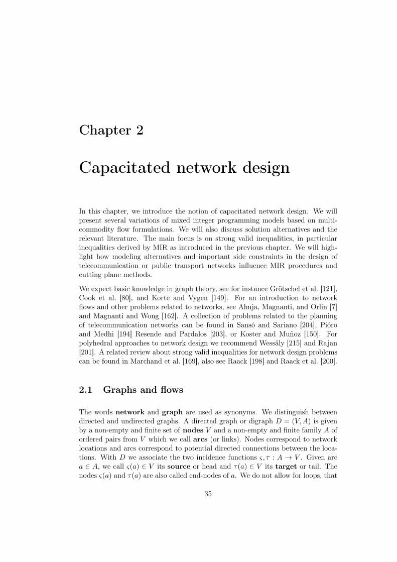
Chapter 2
Capacitated network design
In this chapter, we introduce the notion of capacitated network design. We willpresent several variations of mixed integer programming models based on multi-commodity flow formulations. We will also discuss solution alternatives and therelevant literature. The main focus is on strong valid inequalities, in particularinequalities derived by MIR as introduced in the previous chapter. We will high-light how modeling alternatives and important side constraints in the design oftelecommunication or public transport networks influence MIR procedures andcutting plane methods.
We expect basic knowledge in graph theory, see for instance Grötschel et al. [121],Cook et al. [80], and Korte and Vygen [149]. For an introduction to networkflows and other problems related to networks, see Ahuja, Magnanti, and Orlin [7]and Magnanti and Wong [162]. A collection of problems related to the planningof telecommunication networks can be found in Sansó and Sariano [204], Pióroand Medhi [194] Resende and Pardalos [203], or Koster and Muñoz [150]. Forpolyhedral approaches to network design we recommend Wessäly [215] and Rajan[201]. A related review about strong valid inequalities for network design problemscan be found in Marchand et al. [169], also see Raack [198] and Raack et al. [200].
2.1 Graphs and flows
The words network and graph are used as synonyms. We distinguish betweendirected and undirected graphs. A directed graph or digraph D = (V,A) is givenby a non-empty and finite set of nodes V and a non-empty and finite family A ofordered pairs from V which we call arcs (or links). Nodes correspond to networklocations and arcs correspond to potential directed connections between the loca-tions. With D we associate the two incidence functions ς, τ : A → V . Given arca ∈ A, we call ς(a) ∈ V its source or head and τ(a) ∈ V its target or tail. Thenodes ς(a) and τ(a) are also called end-nodes of a. We do not allow for loops, that
35

2 Capacitated network design
is, for every arc a ∈ A it holds ς(a) 6= τ(a). However, there might be parallelarcs with the same source and the same target. A digraph without parallel arcs iscalled simple. We often write a = (v, w) instead of ς(a) = v and τ(a) = w. Wecall two arcs a, a′ ∈ A anti-parallel in case ς(a) = τ(a′) and ς(a′) = τ(a).
An undirected graph G = (V,E) is defined by a non-empty and finite set of nodesV and a non-empty and finite family E of unordered pairs from V which we calledges (or links). Edges correspond to undirected network connections. With Gwe associate an incidence function ψ : E → V (2). Given edge e ∈ E, we denoteby ψ(e) = vw the two end-nodes of e and abbreviate vw := v, w. Edgesare parallel if they have the same end-nodes. A graph without parallel edges issimple. We write e = vw instead of ψ(e) = vw. The digraph D(G) = (V,A(E))associated with G = (V,E) is the one obtained by replacing each edge by twoanti-parallel arcs with the same end-nodes. If not ambiguous we denote by e+, e−
the two anti-parallel arcs in A(E) corresponding to e ∈ E.
Let S ⊆ V . Given a digraph D, we denote by D[S] = (S,A[S]) the inducedsubgraph of D defined by the node-set S and all arcs A[S] ⊆ A that have bothend-nodes in S. A similar notation applies to undirected graphs. The cut δD(S)respectively δG(S) corresponding to S is the set of arcs inD respectively edges in Gwith one end-node in S and one end-node in V \S. We omit the subscriptsD and Gif it is clear from the context. The two shores of a cut are the subgraphs induced byS and V \S. For digraphs the set δ+(S) ⊆ δ(S) respectively δ−(S) ⊆ δ(S) denotesall cut arcs with source respectively target in S. We abbreviate δ(v), δ+(v), δ−(v)for δ(v), δ+(v), δ−(v), respectively. We call a graph or digraph connectedif all cuts corresponding to non-empty and proper subsets of V are non-empty.Digraphs are called strongly connected if both δ+(S) and δ−(S) are non-emptyfor all ∅ 6= S ( V .
A (directed) path in the (directed) graph G with the end-nodes v0, vk ∈ V is asequence p = (v0e1v1 . . . ekvk) of nodes v0, . . . , vk and edges (arcs) e1, . . . , ek suchthat ei = vi−1vi (ei = (vi−1, vi)) for 1 ≤ i ≤ k and all nodes in the sequenceare distinct. We speak of a v0vk-path in the undirected and a (v0, vk)-path in thedirected case. If source v0 and target vk of the sequence are identical we speak ofa cycle in G.
Given a directed graph D = (V,A), a set of commodities K, and vectors bk ∈ QV
with∑
v∈V bk = 0 for all k ∈ K, a multi-commodity flow (or simply flow) is a
vector f ∈ RA×K+ satisfying flow conservation∑a∈δ+(v)
fka −∑
a∈δ−(v)
fka = bkv for all v ∈ V, k ∈ K, (2.1)
that is, for every commodity k ∈ K and for every node v ∈ V the flow leaving v onall outgoing arcs minus the flow entering v on all incoming arcs equals the valuebkv . The condition bk(V ) = 0 ensures that no flow leaves the network or entersit from outside. The sub-vectors fk ∈ RA+ are called single-commodity flows.
36
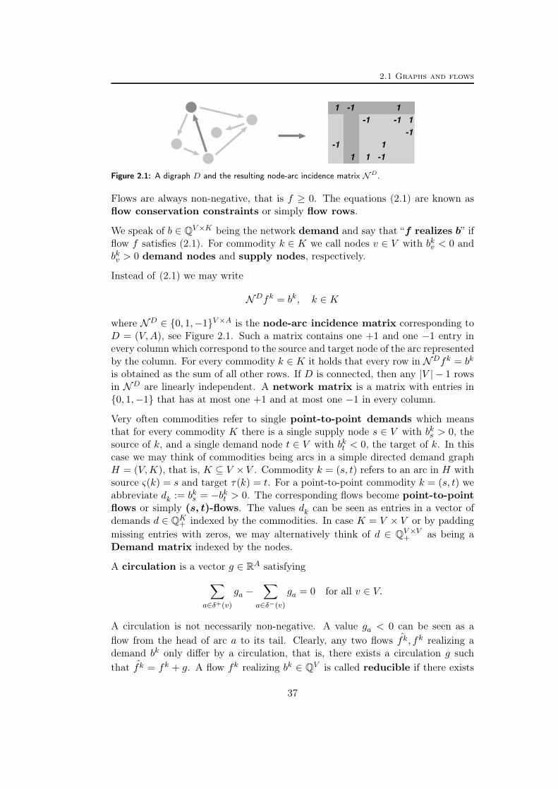
2.1 Graphs and flows
1
-1
1 1
1
1
-1
-1
-1
-1 1
-1
Figure 2.1: A digraph D and the resulting node-arc incidence matrix ND.
Flows are always non-negative, that is f ≥ 0. The equations (2.1) are known asflow conservation constraints or simply flow rows.
We speak of b ∈ QV×K being the network demand and say that “f realizes b” ifflow f satisfies (2.1). For commodity k ∈ K we call nodes v ∈ V with bkv < 0 andbkv > 0 demand nodes and supply nodes, respectively.
Instead of (2.1) we may write
NDfk = bk, k ∈ K
where ND ∈ 0, 1,−1V×A is the node-arc incidence matrix corresponding toD = (V,A), see Figure 2.1. Such a matrix contains one +1 and one −1 entry inevery column which correspond to the source and target node of the arc representedby the column. For every commodity k ∈ K it holds that every row in NDfk = bk
is obtained as the sum of all other rows. If D is connected, then any |V | − 1 rowsin ND are linearly independent. A network matrix is a matrix with entries in0, 1,−1 that has at most one +1 and at most one −1 in every column.
Very often commodities refer to single point-to-point demands which meansthat for every commodity K there is a single supply node s ∈ V with bks > 0, thesource of k, and a single demand node t ∈ V with bkt < 0, the target of k. In thiscase we may think of commodities being arcs in a simple directed demand graphH = (V,K), that is, K ⊆ V ×V . Commodity k = (s, t) refers to an arc in H withsource ς(k) = s and target τ(k) = t. For a point-to-point commodity k = (s, t) weabbreviate dk := bks = −bkt > 0. The corresponding flows become point-to-pointflows or simply (s, t)-flows. The values dk can be seen as entries in a vector ofdemands d ∈ QK
+ indexed by the commodities. In case K = V × V or by paddingmissing entries with zeros, we may alternatively think of d ∈ QV×V
+ as being aDemand matrix indexed by the nodes.
A circulation is a vector g ∈ RA satisfying∑a∈δ+(v)
ga −∑
a∈δ−(v)
ga = 0 for all v ∈ V.
A circulation is not necessarily non-negative. A value ga < 0 can be seen as aflow from the head of arc a to its tail. Clearly, any two flows fk, fk realizing ademand bk only differ by a circulation, that is, there exists a circulation g suchthat fk = fk + g. A flow fk realizing bk ∈ QV is called reducible if there exists
37
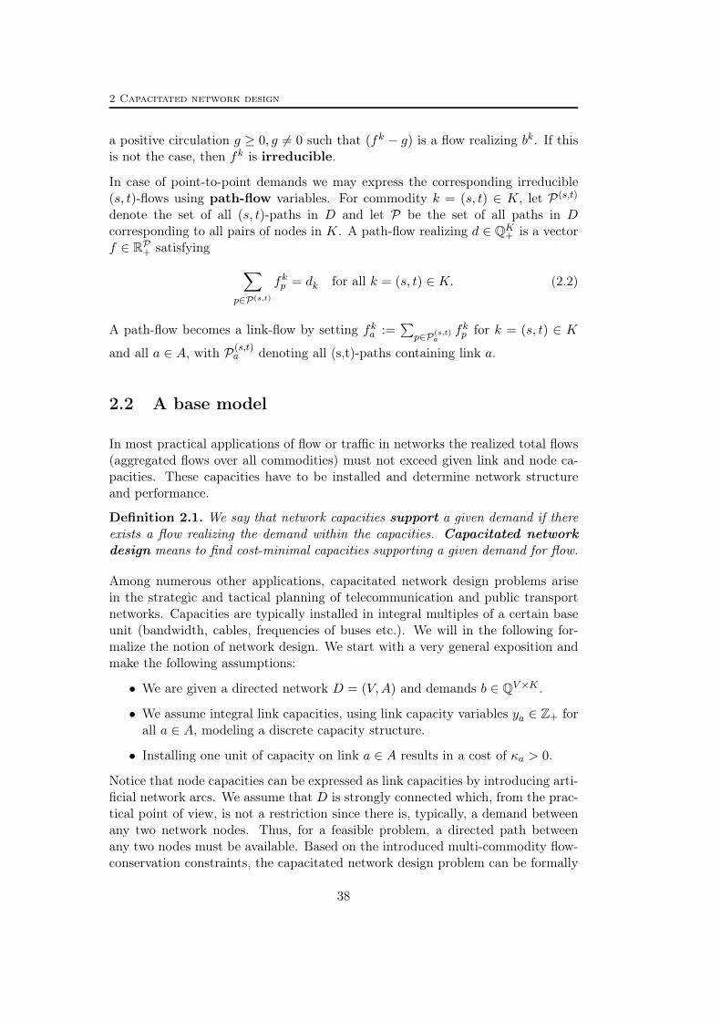
2 Capacitated network design
a positive circulation g ≥ 0, g 6= 0 such that (fk − g) is a flow realizing bk. If thisis not the case, then fk is irreducible.
In case of point-to-point demands we may express the corresponding irreducible(s, t)-flows using path-flow variables. For commodity k = (s, t) ∈ K, let P(s,t)
denote the set of all (s, t)-paths in D and let P be the set of all paths in Dcorresponding to all pairs of nodes in K. A path-flow realizing d ∈ QK
+ is a vectorf ∈ RP+ satisfying ∑
p∈P(s,t)
fkp = dk for all k = (s, t) ∈ K. (2.2)
A path-flow becomes a link-flow by setting fka :=∑
p∈P(s,t)a
fkp for k = (s, t) ∈ Kand all a ∈ A, with P(s,t)
a denoting all (s,t)-paths containing link a.
2.2 A base model
In most practical applications of flow or traffic in networks the realized total flows(aggregated flows over all commodities) must not exceed given link and node ca-pacities. These capacities have to be installed and determine network structureand performance.
Definition 2.1. We say that network capacities support a given demand if thereexists a flow realizing the demand within the capacities. Capacitated networkdesign means to find cost-minimal capacities supporting a given demand for flow.
Among numerous other applications, capacitated network design problems arisein the strategic and tactical planning of telecommunication and public transportnetworks. Capacities are typically installed in integral multiples of a certain baseunit (bandwidth, cables, frequencies of buses etc.). We will in the following for-malize the notion of network design. We start with a very general exposition andmake the following assumptions:
• We are given a directed network D = (V,A) and demands b ∈ QV×K .
• We assume integral link capacities, using link capacity variables ya ∈ Z+ forall a ∈ A, modeling a discrete capacity structure.
• Installing one unit of capacity on link a ∈ A results in a cost of κa > 0.
Notice that node capacities can be expressed as link capacities by introducing arti-ficial network arcs. We assume that D is strongly connected which, from the prac-tical point of view, is not a restriction since there is, typically, a demand betweenany two network nodes. Thus, for a feasible problem, a directed path betweenany two nodes must be available. Based on the introduced multi-commodity flow-conservation constraints, the capacitated network design problem can be formally
38
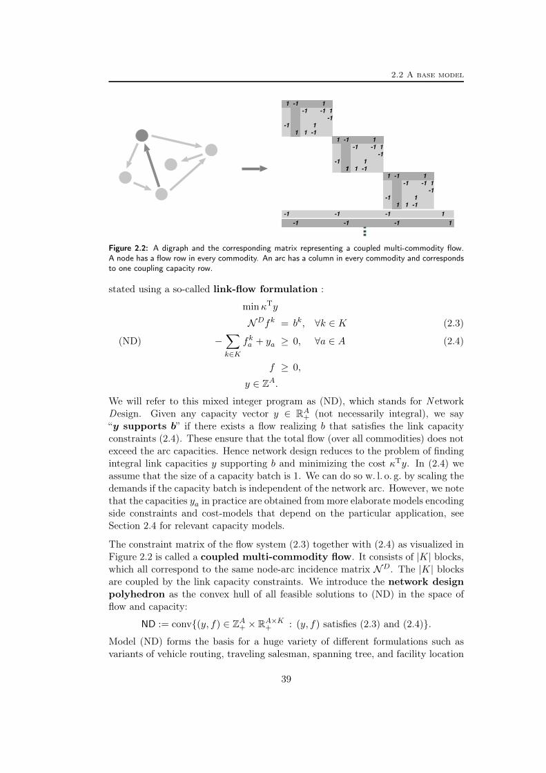
2.2 A base model
-1
1
-1 1
1
-1
1 1
1
1
-1
-1
-1
-1 1
-1
1
-1
-1
1
1
1
-1
-1
-1
-1 1
-1
1
-1
1 1
1
1
-1
-1
-1
-1 1
-1
-1 -1 -1 1
1
Figure 2.2: A digraph and the corresponding matrix representing a coupled multi-commodity flow.A node has a flow row in every commodity. An arc has a column in every commodity and correspondsto one coupling capacity row.
stated using a so-called link-flow formulation :
minκTy
NDfk = bk, ∀k ∈ K (2.3)
(ND) −∑k∈K
fka + ya ≥ 0, ∀a ∈ A (2.4)
f ≥ 0,
y ∈ ZA.
We will refer to this mixed integer program as (ND), which stands for N etworkDesign. Given any capacity vector y ∈ RA+ (not necessarily integral), we say“y supports b” if there exists a flow realizing b that satisfies the link capacityconstraints (2.4). These ensure that the total flow (over all commodities) does notexceed the arc capacities. Hence network design reduces to the problem of findingintegral link capacities y supporting b and minimizing the cost κTy. In (2.4) weassume that the size of a capacity batch is 1. We can do so w. l. o. g. by scaling thedemands if the capacity batch is independent of the network arc. However, we notethat the capacities ya in practice are obtained from more elaborate models encodingside constraints and cost-models that depend on the particular application, seeSection 2.4 for relevant capacity models.
The constraint matrix of the flow system (2.3) together with (2.4) as visualized inFigure 2.2 is called a coupled multi-commodity flow. It consists of |K| blocks,which all correspond to the same node-arc incidence matrix ND. The |K| blocksare coupled by the link capacity constraints. We introduce the network designpolyhedron as the convex hull of all feasible solutions to (ND) in the space offlow and capacity:
ND := conv(y, f) ∈ ZA+ × RA×K+ : (y, f) satisfies (2.3) and (2.4).Model (ND) forms the basis for a huge variety of different formulations such asvariants of vehicle routing, traveling salesman, spanning tree, and facility location
39

2 Capacitated network design
problems, see Magnanti and Wong [162] and Ahuja et al. [7] for surveys. Many ap-plications from telecommunication, transport, scheduling, logistics, and productionplanning use (ND) as a building block, which is why understanding the structureof ND is of importance. In Section 2.4, we provide some variations and possibleextensions of the standard model. Also the models in Part III of this thesis arebased on (ND).
Clearly, ND 6= ∅ since D is strongly connected. Furthermore, there are also nomore implied equations than those given by the |K|(|V | − 1) linearly independentconstraints among (2.3). We obtain the following well-known fact.
Proposition 2.2. Given a strongly connected digraph D = (V,A), the polyhedronND has dimension |A|(|K|+ 1)− |K|(|V | − 1).
It is known that the lower bound obtained from the LP relaxation of ND can be veryweak. In fact, the integrality gap, that is, the relative distance between the LP dualbound and the actual optimal solution value, can be arbitrarily large. Removingthe integrality constraints, the problem reduces to a series of |K| shortest pathproblems (assuming |K| point-to-point demands), that is, the optimal solutionof the LP is given by sending each demand on a shortest path from its sourceto its destination w. r. t. the arc costs κ. The relaxed problem decomposes as thecoupling constraints (2.4) can be removed, and we are in fact minimizing the cost ofarc flows. Such a continuous uncapacitated flow problem is computationally eveneasier than the well-known and polynomially solvable multi-commodity minimum-cost flow problem [7]. Introducing the integrality requirements in (ND) completelychanges the structure of the problem and increases its (computational) complexityby several orders of magnitude. However, this strongly depends on the givendata. We may consider the following two extreme scenarios assuming point-to-point demands d ∈ QK
+ .
Observation 2.3. If all demands are integral, i. e., dk ∈ Z+ for all k ∈ K, thenthe optimal solution to (ND) is given by the LP solution.
Assuming all demands to be integral means that they are multiples of the basecapacity unit 1. In this case it does not pay off to split the flows or use longpaths. We can remove the integrality constraints and also (2.4) and solve a seriesof shortest path problems. In this scenario the integrality gap is zero.
Observation 2.4. If the demands are small with∑
k∈K dk ≤ 1, then problem(ND) becomes a connectivity problem: Minimize the cost for opened arcs (arcs awith ya = 1) such as to connect all demand end-nodes.
In this second scenario the integrality gap is huge and it further increases whendecreasing the demand values. With small demands, or alternatively big-M arc-capacities, (ND) relates to the uncapacitated fixed charge network flowproblem [162, 163, 188, 202]. In particular, as there is no cost for flow, it gener-alizes the NP-hard Steiner tree problem [70, 71, 108].
40

2.2 A base model
Corollary 2.5 (Chopra et al. [72]). Capacitated network design is strongly NP-hard.
Uncapacitated fixed charge network flow formulations have been used and studiedearly in the context of network design but also in the context of transportationproblems, facility location, production planning, and lot-sizing, see Magnanti andWong [162], Magnanti et al. [163] and the references therein. The notion of connec-tivity, inherent in these formulations, is of particular importance for telecommu-nication networks as it relates to resilience and survivability. Grötschel, Monma,and Stoer [122, 124] introduced and studied uncapacitated connectivity problemsand compute optimal topologies for networks that survive node or link failures.
However, from a practical perspective, fixed charge problems as in Observation 2.4ignore the relation of realized flows to the capacity design and the cost for capacity.Also Observation 2.3 is based on artificial extreme scenarios. In applications fromtelecommunications, for instance, the unit of the demands is typically smaller thanthe unit of the smallest capacity batch (e. g., demands are given in multiples of 100Mbps, capacities in multiples of 10 Gbps), but the sum of all demands is largerthan the smallest batch. Capacitated network design in practice means to haveproblem instances in between the two uncapacitated (and easier) extremes above,shortest path problems and connectivity problems.
As model (ND) is compact, that is, the number of constraints and variables ispolynomial in the network size, we can, in principle, simply pass it to an MIP-solver implementing a general purpose LP based branch-and-cut scheme. However,as mentioned, the LP bounds can be weak which leads to huge branch-and-boundtrees and slow convergence. Moreover, since the number of commodities can be inthe order of O(|V |2), model (ND) can become extremely large, both in terms ofconstraints and variables, already for medium sized networks.
Remark 2.6. Given point-to-point demands d ∈ QV×V+ , instead of defining a
commodity for every individual demand, we may aggregate demands with acommon source node to reduce the number of commodities to O(|V |). To constructcommodity k ∈ V we simply set
bkv :=
−d(k,v) k 6= v∑
w∈V d(k,w) k = v
for all v ∈ V , where d(vv) = 0 for all v ∈ V . In general, aggregating demandsprovides much smaller models that scale well with the size of the graph. As longas the capacity model remains unchanged the LP relaxation of ND provides thesame dual bound. However, for uncapacitated fixed charge problems (such asthe Steiner tree problem) disaggregated formulations can be used to derive muchstronger LP relaxations by adjusting the arc capacities, see for instance Rardinand Wolsey [202].
We will in the following discuss various alternatives for solving the capacitated
41

2 Capacitated network design
network design problem. There are several approaches to avoid at least some ofthe mentioned problems. These include:
1. Branch-and-cut based on (ND) and strong problem specific cutting planes,
2. Column (and cut) generation using a path-flow formulation,
3. Benders decomposition using metric inequalities,
4. Branch-and-bound based on Lagrangian relaxations.
In this thesis, we concentrate on branch-and-cut based approaches that use link-flow formulations and add strong cutting planes in order to improve the lowerbounds coming from the LP relaxations. Before introducing facet-defining in-equalities for ND that can be used to strengthen formulation (ND) in a branch-and-cut scheme, we will briefly sketch possible decomposition methods in casea pure branch-and-cut approach fails. This might happen if the network or thenumber of commodities becomes to large.
Below we assume that all commodities are given as point-to-point demands.
Path generation. Instead of using a link-flow formulation we can also state thenetwork design problem by using path-flow variables combining constraints (2.2)and (2.4). The number of flow-variables in such a path-flow formulation is expo-nential and thus typically treated implicitly by column generation techniques. Aslong as there are no additional side-constraints the corresponding pricing problemis a shortest path problem. That is, to solve the LP relaxation we can start with asmall subset of the paths P(s,t) for every commodity (s, t) ∈ K and add additionalpaths (LP columns) iteratively by solving shortest path problems. Path formula-tions typically offer more flexibility with respect to restricting the set of admissiblepaths, e. g., using length or hop restrictions. Very often the set of admissible pathsis limited to a small number and the resulting model is used without generatingfurther columns, e. g. the k-shortest (s, t)-paths are used with some k ≥ 1.
Benders decomposition. Another decomposition method is based on the fea-sibility condition for multi-commodity flows known as the Japanese Theorem.
Theorem 2.7 (Iri [142], Onaga and Kakusho [183]). A capacity vector y ∈RA+ supports the demand matrix d ∈ QK
+ if and only if∑a∈A
µaya ≥∑k∈K
lµ(k)dk, for all µ ∈ RA+, (2.5)
where lµ(k) is the length of a shortest path in D = (V,A) between the end-nodesof k and with respect to the weights µ.
The Japanese theorem is a generalization of the max-flow min-cut duality for single-commodity flows. It is a direct consequence of strong duality (Farkas’ Lemma)
42
2.2 A base model
applied to the LP relaxation of ND. From Theorem 2.7 follows that the projectionof ND onto the space of capacity variables is given by
NDy := convy ∈ Z+ : y satisfies (2.5). (2.6)
We may restrict the necessary weights µ in (2.5) to the extreme rays of the cone
M(D) := µ ∈ RA+ : The length of the shortest (s, t)-pathw.r.t µ is µ(s,t) if (s, t) ∈ A.
If µ ∈ M(D), then the shortest path lengths lµ : V × V → R+, (s, t) 7→ lµ(s, t)satisfy the triangle inequalities lµ(s, t) ≤ lµ(s, v)+lµ(v, t) for all s, t, v ∈ V , which iswhy we call M(D) the metric cone and (2.5) are known as metric inequalities.Since all data is rational we may even further restrict our attention to integralweights µ ∈ M(D). In fact, all facet-defining inequalities of the linear relaxationof NDy are metric inequalities of type (2.5) with µ ∈ ZA+ ∩ M(D). We refer toBienstock, Chopra, Günlük, and Tsai [51] and Avella, Mattia, and Sassano [23] formore details about the metric cone and metric inequalities.
Since y is integral we may round the right-hand side of (2.5) if µ ∈ ZA+ and get
µTy ≥ dlµTde (2.7)
as a valid inequality for NDy, a so-called rounded metric inequality. Theseinequalities are not necessarily strong. However, it can be shown that all facet-defining inequalities of NDy have metric left-hand side, more precisely:
Proposition 2.8 (Avella et al. [23]). All facet-defining inequalities of NDy aretight metric inequalities of the form
µTy ≥ ρ (2.8)
where µ ∈ M(D) and ρ := minµTy : y ∈ ZA+ supports d. If µ ∈ ZA+ is anextreme ray of M(D) such that the entries of µ have greatest common divisor 1,then ρ = dlµTde, that is, (2.8) is a rounded metric inequality.
The relaxation of NDy has exponentially many facets even if we restrict inequalities(2.5) to the rays of the metric cone. They can, however, be handled implicitly byseparation. Solving a satellite LP based on triangle inequalities either proves thata given capacity vector y supports b or a metric µ violating (2.5) can be generated.The satellite LP simply maximizes the violation of a metric inequality given afixed capacity vector y. This approach is a special case of the well-known Bendersdecomposition, see Benders [45]. Metric inequalities can be seen as a special caseof the Benders feasibility cuts. We refer to Costa, Cordeau, and Gendron [85] fora discussion on metric and Benders inequalities. Also see [129, 171–173, 186, 215]for applications and extensions of metric inequalities.
43
2 Capacitated network design
Lagrangian relaxations. Instead of relying on LP relaxations of ND in a branch-and-bound framework, it is also possible to use Lagrangian relaxations, whichmight yield stronger dual bounds. Lagrangian relaxations are obtained by remov-ing difficult constraints (e. g., coupling constraints) from the constraint system,and instead, penalizing their violation in the objective function using dual mul-tipliers. This is of particular interest if the remaining problem decomposes intosmall polynomially solvable sub-problems. Lagrangian relaxations for combinato-rial problems have been used first by Held and Karp [133, 134] to solve TSPs. Foran introduction to Lagrangian relaxations for integer programming and networkflows, the reader is referred to Geoffrion [110] (republished in [111]) and Ahujaet al. [7], respectively. Lagrangian based approaches to solve (fixed charge) net-work design problems have been studied for instance by Gendron, Crainic, andFrangioni [109], [86] and Holmberg and Yuan [137].
In the case of formulation (ND) we might either dualize the flow conservation con-straints (2.3) or the coupling constraints (2.4). Penalizing the capacity constraints(2.4) with dual multipliers µa ∈ R+, a ∈ A yields the following Lagrangian relax-ation of (ND):
L1(µ) = minκTy +∑a∈A
µa(∑k∈K
fka − ya) : (y, f) ∈ ZA+ × RA×K+ ,
NDfk = bk, ∀k ∈ K
This problem decomposes into a series of |K| shortest path problems using µ asarc weights. Clearly L1(µ) ≤ minκTy : (y, f) ∈ ND for any vector µ ∈ RA+. Itis also easy to see that the set of dual multipliers yielding the largest dual boundis given by µ = κ, more precisely
maxµ∈RA+
L1(µ) = L1(κ),
that is, in this particular case we precisely obtain the solution of the LP relaxationof ND. The problem of maximizing L1(µ) is known as the Lagrangian dual. Thevalue of the Lagrangian dual coincides with the value of the LP relaxation if wecan drop the integrality restriction in the Lagrangian relaxation without changingthe problem, that is, the Lagrangian relaxation has the integrality property,see [110]. This is the case above.
For an alternative Lagrangian relaxation, assume we are given upper bounds uk > 0for all arc flow variables fka :
−fka ≥ −uk, a ∈ A, k ∈ K. (2.9)
In case of point-to-point demands and flows we can safely set uk = dk for k =(s, t) ∈ K since the (s, t)-flow cannot exceed the point-to-point demand dk unlessthe flow contains a positive circulation. Removing such circulations can only im-prove the solution value. For general commodities we set uk =
∑v∈V (bkv)
+ usingthe same argument. Assume the redundant bound constraints (2.9) are added to(ND).
44

2.3 Cutting planes
Dualizing the flow conservation constraints (2.3) using multipliers µkv ∈ R for v ∈ Vand k ∈ K gives the alternative Lagrangian relaxation
L2(µ) = minκTy +∑k∈K
µk(NDfk − bk) : (y, f) ∈ ZA+ × RA×K+ ,∑k∈K
fka ≤ ya, fka ≤ uk, ∀a ∈ A.
This problem decomposes into simple polynomially solvable sub-problems for everynetwork arc, see Magnanti et al. [164], Magnanti, Mirchandani, and Vachani [165].Here the upper bound constraints (2.9) improve the Lagrangian lower bound L2(µ)although they are redundant for problem (ND). Moreover, this Lagrangian relax-ation does not satisfy the integrality condition and is in general stronger than thecorresponding LP-relaxation. In particular, Magnanti et al. [165] proved that thedual bound maxµ L
2(µ) is the same that can be obtained from the LP-relaxationafter adding all so-called arc-residual capacity inequalities. These inequalities areintroduced in the next section.
Lagrangian relaxations of type L1(µ) or L2(µ) can be used to approach capacitatednetwork design problems, see [86, 109, 137]. For fixed multipliers, these relaxationsare solved easily also for large-scale networks. However, determining the optimalmultipliers µ can be a challenge. This can be done for instance by using subgradientor bundle methods, see [86] and the references therein. We refer to [110] on howto embed Lagrangian relaxations into branch-and-cut frameworks.
We have learned that there are different methods to solve capacitated networkdesign problems. In the following, we will introduce strong valid inequalities thatcan be used as cutting planes in branch-and-cut approaches.
2.3 Cutting planes
Network design polyhedra have been studied extensively by several authors fordifferent models. Most of the strong valid inequalities for ND and related polyhedrastudied in the literature and used in branch-and-cut-codes are based on simple sub-structures of the network such as single arcs, cuts, 3-partitions or, more general,k-partitions. They have been derived as facets of relaxations related to thesesub-structures, so-called cut-set polyhedra, multi cut-set polyhedra, or arc-set polyhedra. A central approach is to enumerate all corresponding facets andto lift the resulting inequalities to the original variable space. Known classes ofnon-trivial facet-defining inequalities for ND obtained in this way include
• cut-set and flow cut-set inequalities derived from cut-set polyhedra,
• k-partition inequalities derived from multi cut-set polyhedra, and
• arc-residual capacity inequalities derived from arc-set polyhedra,
45

2 Capacitated network design
(a) Arc-residual capacity inequalities [20,135, 164]
(b) 3-partition inequalities [51, 164]
(c) 4-partition inequalities [5, 6] (d) Flow cut-set inequalities [16, 198, 200]
Figure 2.3: Small networks with their corresponding polyhedral studies and strong valid inequalities.
see Figure 2.3. Cut-set inequalities are defined on a network cut, i. e., a 2-partitionof the network, and they contain capacity variables only. The more general net-work k-partitions with k ≥ 3 yield k-partition inequalities. Flow cut-set inequali-ties generalize cut-set inequalities to the space of capacity and flow on a networkcut. Arc-residual capacity inequalities are defined in the variable space of a singlearc. Magnanti and Mirchandani [161] and Magnanti et al. [164, 165] initiated thestudy of network design polyhedra and introduce cut-set inequalities, 3-partitioninequalities and arc-residual capacity inequalities. Generalizing the work in [164],Hoesel et al. [135] and Atamtürk and Rajan [20] considered single arcs and thecorresponding arc-set polyhedra based on different variants of single arc capac-ity constraints. Just like Magnanti et al. [164] for the undirected case, Bienstocket al. [51] gave a complete description of ND projected to the space of the capacityvariables in case |V | = 3. Agarwal [5] identified facet-defining inequalities for thecapacity formulation of a four node network and gave a complete description in[6]. Bienstock and Günlük [50] considered a generalization of cut-set inequalitiesto simple flow cut-set inequalities. General flow cut-set inequalities have been in-troduced by Chopra et al. [72]. They have been studied in detail by Atamtürk [16]and Raack et al. [200].
In the following, we will review some of the results on strong valid inequalities forcapacitated network design. We will concentrate on rank-1 MIR inequalities (1.8)and present the necessary dual weights λ used to aggregate the system (ND), seeSection 1.3. We refer to Marchand et al. [169] for another review of strong validinequalities for network design problems as well as lot sizing and facility location.
Cut-set polyhedra and flow cut-set inequalities
Let S be a nonempty proper subset of the nodes V and let δ+(S) be the corres-ponding dicut. Now it obviously holds that the cut demand is bounded by the cut
46

2.3 Cutting planes
1
-1
1 1
1
1
-1
-1
-1
-1 1
-1
S
δ(S)
S
δ(S)
Figure 2.4: The cut δ(S) obtained by aggregating the flow rows of a node-set S
capacity, that is, informally:
capacity(δ+(S)) ≥ demand(S → V \ S). (2.10)
Similarly the demand of S (which is the supply of V \S) cannot exceed the capacityon δ−(S). Observation (2.10) is crucial both from the theoretical and practicalpoint of view. In practice, if inequality (2.10) is tight, then the network cut δ(S)can be considered being a bottleneck. In theory, (2.10) follows from LP dualityand relates to the max-flow-min-cut theorem [7] and the Japanese theorem, seeSection 2.2. Our main motivation here is to derive cutting planes from (2.10).
To develop cut-based inequalities we regard the structure DS = (S, V \ S, δ(S))as a two-node network and restrict ourselves to consider the flow across the cut(the flow between S and V \ S) and the capacity provided on the cut δ(S). Wedenote by bk(S) :=
∑v∈S b
kv the total demand (supply) over the cut with respect
to commodity k ∈ K and define
K+S := k ∈ K : bk(S) > 0 and K−S := k ∈ K : bk(S) < 0.
We only consider cuts with non-zero cut demand, i. e., we assumeK+S 6= ∅ w. l. o. g..
Aggregating all flow equations (2.3) corresponding to S and restricting the capacityconstraints (2.4) to the cut δ(S) results in the following two-node cut-set relaxationof the formulation (ND), see Figure 2.4:∑
a∈δ+(S)
fka −∑
a∈δ−(S)
fka = bk(S), ∀k ∈ K (2.11)
−∑k∈K
fka + ya ≥ 0, ∀a ∈ δ(S) (2.12)
The key to derive strong valid cut-based inequalities for network design problemsas facets of ND is to study the convex hull of the corresponding solution space.This structure is known as a cut-set polyhedron :
CS := conv(y, f) ∈ Zδ(S)+ × Rδ(S)×K
+ : (y, f) satisfies (2.11) and (2.12).
The following result by Raack [198] establishes the relation between facets of CSand facets of ND, also see [5, 200].
Theorem 2.9 (Cut-set lifting theorem). Let ∅ 6= S ( V . Any facet-defininginequality for CS defines a facet of ND if both D[S] and D[V \ S] are stronglyconnected.
47

2 Capacitated network design
S
Figure 2.5: A directed network cut δ(S) with selected arc subsets A+ ⊆ δ+(S) and A− ⊆ δ−(S)
The result also holds in more general contexts such as multi-facility problems andthere is a version for undirected formulations, see Section 2.4.
Before studying the convex hull of CS we introduce some more notation. For asubset Q ⊆ K+
S we write bQ(S) :=∑
k∈Q bk(S) and fQa :=
∑k∈Q f
ka for all a ∈ A.
Consider fQa ∈ R+ as a single variable. Further, we choose subsets A+ ⊆ δ+(S),A− ⊆ δ−(S), and set A+ := δ+(S) \ A+, see Figure 2.5. For all a ∈ A, we denoteby sa ≥ 0 the slack of the capacity constraint (2.12), that is, sa := ya −
∑k∈K f
ka .
Summing up all equations (2.11) for k ∈ Q (with weight 1) as well as all capacityconstraints (2.12) for a ∈ A+ (with weight 1) and a ∈ A− (with weight −1), weobtain
−s+∑a∈A−
sa +∑a∈A+
fQa +∑a∈A+
ya −∑a∈A−
ya ≥ bQ(S), (2.13)
where −s subsumes all remaining (slack and structural) variables that are contin-uous and have negative coefficient. By Proposition 1.2, the corresponding MIRinequality∑
a∈A+
fQa −∑a∈A−
fQa +∑a∈A+
rQya +∑a∈A−
(1− rQ)ya ≥ rQdbQ(S)e (2.14)
is valid for CS and ND. Here rQ := r(bQ(S)) denotes the fractional part of bQ(S).Inequalities (2.14) are known as flow cut-set inequalities [72]. In the single-commodity case there are no further non-trivial facet-defining inequalities:
Theorem 2.10 (Atamtürk [16]). Assume |K| = 1. It holds that
CS = (y, f) ∈ 2Rδ(S)+ : (y, f) satisfies (2.11), (2.12), and (2.14).
Inequality (2.14) defines a facet if and only if rQ > 0 and A+ 6= ∅.
The flow cut-set inequalities (2.14) are also strong in the multi-commodity case.But not all combinations of Q, A+, and A− result in a facet-defining inequality forCS. We refer to Atamtürk [16] and Raack et al. [200] for a comprehensive collectionof necessary and sufficient conditions. Combining these results with Theorem 2.9yields sufficient conditions for flow cut-set inequalities to define facets of ND. Thereare two important facet-defining sub-classes of (2.14). We speak of simple flowcut-set inequalities in case A− = ∅:∑
a∈A+
fQa +∑a∈A+
rQya ≥ rQdbQ(S)e. (2.15)
48

2.3 Cutting planes
If additionally A+ = δ+(S) and Q = K+S they reduce to the well-known cut-set
inequalities ∑a∈δ+(S)
ya ≥ db+e, (2.16)
with b+ := bK+S (S). In case both D[S] and D[V \ S] are strongly connected
and b+ /∈ Z, inequality (2.16) defines a facet of both ND and NDy. The cut-setinequality (2.16) is a tight metric inequality of the form (2.8) w. r. t. the integralextreme ray µ of the metric cone M(D) given by µa = 1 if a ∈ δ+(S) and µa = 0else. Cut-set inequalities turn out to be among the most effective cutting planesfor network design in practice, see [16, 50, 51, 129, 200].
For single-commodity uncapacitated fixed-charge network design problems withb+ < 1 for all nonempty S ( V (Observation 2.4) we have db+e = 1 and r(b+) =b+. Hence inequality (2.14) reduces to the mixed dicut inequality with outflowby Ortega and Wolsey [188]:∑
a∈A+
fa −∑a∈A−
fa +∑a∈A+
b+ya +∑a∈A−
(1− b+)ya ≥ b+,
with the special case of a mixed dicut inequality without outflow (simple flow cut-set inequality) and the basic dicut inequality (Steiner cut-set inequality) given by∑
a∈A+
fa +∑a∈A+
b+ya ≥ b+ and∑
a∈δ+(S)
ya ≥ 1,
respectively.
Because of the simpler structure, but also because they dominate general flowcut-set inequalities with respect to computational impact, branch-and-cut codestypically implement cut-set inequalities and sometimes also simple flow cut-set in-equalities to solve systems of type (ND). We will study variants of these inequalitiesin Section 2.4 and in Chapter 10.
Separation. Given a fractional point (y?, f?), the separation problem for flowcut-set inequalities is to simultaneously determine a node-set S ( V , a commod-ity subset Q ⊆ K, and arc subsets A+ ⊆ δ+(S), A− ⊆ δ−(S), leading to amost-violated inequality (2.14). The complexity of this general problem remainsunknown. Even for fixed cut-sets S it is unknown how to select Q, A+, and A−
simultaneously.
However, there are complexity results for a number of related problems. For single-commodity flow cut-set inequalities with K = Q = k, where k = (s, t) is a point-to-point commodity, the right-hand side of (2.14) reduces to the value r(dk)ddkefor every (s, t)-cut. Atamtürk [16] showed that in this case minimizing the ac-tivity of the left hand is a min-cut problem. As the corresponding weights canbe negative, solving the separation problem is NP-hard [108]. However, from the
49

2 Capacitated network design
construction in [16] also follows that by assuming A− = ∅ the weights becomenon-negative. Consequently, separating simple flow cut-set inequalities (2.15) andcut-set inequalities (2.16) in the single-commodity case can be done in polynomialtime. The separation for cut-set inequalities in the multi-commodity case is knownto be NP-hard, see [51].
Fixing the node-set S and the commodity subset Q, the most violated flow cut-setinequality (2.14) can be found in linear time by iterating all arcs and using sets
A+ := a ∈ δ+(S) : rQy?a < f?Qa and A− := a ∈ δ−(S) : (1− rQ)y?a < f?Qa .
Similarly, we can decide in linear time whether there exists a violated flow cut-setinequalities for the case that S and A+, A− are fixed, which follows from a similarlinear time separation rule by for arc-residual capacity inequalities, see [16, 20] andSection 2.3.
Most branch-and-cut approaches for network design problems in the literature im-plementing cut-set and flow cut-set inequalities decompose the actual separationproblem. Very often the necessary subset of the nodes, commodities, and arcsare restricted in cardinality and then enumerated. Many authors, for instance,add all cut-set inequalities corresponding to singleton node-sets S to the initialformulation. Magnanti et al. [165] proposed an enumeration strategy for cut-setsincreasing the size of |S| iteratively. They add arc-residual capacity inequalitiesand 3-partition inequalities if no cut-set inequality can be found. Considering acapacity formulation, Barahona [34] presented a separation routine for cut-set in-equalities that is based on a heuristic for the max-cut problem. Bienstock et al.[51] enumerated “critical” cut-sets with the property that the two correspondingshores are strongly connected, see Theorem 2.9. If the corresponding cut-set in-equality is violated or tight, then they also checked simple flow cut-set inequalitiesfor violation. A similar strategy based on enumerating critical cut-sets was usedby Bienstock and Günlük [50]. They checked cut-set inequalities, 3-partition in-equalities (see below) and simple flow cut-set inequalities in a hierarchical mannersimilar to [165]. If no cut-set inequalities can be found, 3-partition inequalitieswere tested for violation, and only if the latter fails simple flow cut-set inequalitieswere generated with |Q| ≤ 2. Atamtürk [16] enumerated all cuts with |S| ≤ 2 and,given a cut, he considered all singleton commodity subsets Q and the set Q = K+
S
to test for violated flow cut-set inequalities.
In addition to enumeration schemes, Bienstock et al. [51] introduced a very fastheuristic to generate subsets S that is based on a graph contraction procedure.Variants of this procedure have been successfully applied by Günlük [129], Ortegaand Wolsey [188], and Raack et al. [200]. A similar approach is used in Part IIof this thesis to integrate the generation of flow cut-set inequalities into generalpurpose MIP solvers. Also in Part III we will adapt these approaches for robustnetwork design. We will see that graph contraction can be a crucial ingredient ofseparation frameworks to solve different network design problems.
50
2.3 Cutting planes
Multi cut-set polyhedra and k-partition inequalities
The notion of cut-set and flow cut-set inequalities is based on a 2-partition of thenetwork nodes. Flow cut-set inequalities define facets for network design polyhe-dra based on two-node networks. This can be generalized to k-partitions and thecorresponding multi cut-sets. For k ∈ Z,k ≥ 2 let (S1, . . . , Sk) be a partitionof the nodes V into k disjoint and non-empty node subsets. The correspond-ing multi cut-set is denoted by δ(S1, . . . , Sk−1) :=
⋃1≤i≤k−1 δ(Si). The multi
cut-set polyhedron MCS(k), as a generalization of the cut-set polyhedron, isobtained by considering the network design polyhedron for the k-node digraphDS1,...,Sk−1
= (S1, . . . , Sk, δ(S1, . . . , Sk−1)). Non-trivial inequalities valid formulti cut-set polyhedra are called k-partition inequalities. They form a super-class of flow cut-set inequalities.
The cut-set lifting Theorem 2.9 extends to multi cut-set using the same argu-ments as in [200]. See Agarwal [5] for the same result but for undirected capacityformulations.
Theorem 2.11 (Multi cut-set lifting theorem). For k ≥ 2 let (S1, . . . , Sk) bea partition of V into k disjoint and non-empty node subsets. Any facet-defininginequality for MCS(k) defines a facet of ND if all induced subgraphs D[Si], 1 ≤ i ≤k, are strongly connected.
We have seen that the facial structure of cut-set polyhedra is very rich alreadyin the single-commodity case. As k-partition inequalities generalize cut-set in-equalities and flow cut-set inequalities, this is in particular true for multi cut-setpolyhedra. Classes of facet-defining k-partition inequalities have mainly been de-veloped in the space of the capacity variables as facets of NDy and for small k.Magnanti et al. [164], Bienstock and Günlük [50] and Bienstock et al. [51] de-veloped 3-partition inequalities, also see Günlük [129]. Facet-defining 4-partitioninequalities were studied by Agarwal [5, 6]. Rajan [201] considered 3-partitioninequalities in the space of flow and capacity.
For every node-set S = Si, 1 ≤ i ≤ k, we may formulate a cut-set inequality of theform (2.16), which can be facet-defining for MCS(k) under certain conditions. Inthe following we give two examples for strong 3-partition inequalities in the spaceof the capacity variables that are different from cut-set inequalities. Both classesare introduced in [51]. Let k = 3 and let all commodities be given by point-to-point demands. For i, j ∈ 1, 2, 3 we denote by Aij all arcs with source in Si andtarget in Sj . Similarly, all commodities with source in Si and target in Sj are givenby Kij . Summing up the demands corresponding to Kij gives dij :=
∑k∈Kij dk.
In the following we assume that Aij 6= ∅ and all subgraphs D[Si] are stronglyconnected, for i, j ∈ 1, 2, 3. If these conditions do not hold, the following in-equalities are not necessarily tight metric inequalities, and, in particular they arenot necessarily facet-defining for ND or NDy. The first inequality is a rank-1 MIRinequality. We first aggregate all flow conservation constraints (2.3) for nodes in
51

2 Capacitated network design
S1 and commodities in K12 ∪K13 (with weight 1) similar to the derivation of thecut-set inequality (2.16) for S = S1. In addition we add all flow conservationconstraints for nodes in S2 and commodities in K32 (with weight -1). Eventu-ally adding all capacity constraints for arcs in A12 ∪A13 ∪A32 and applying MIR(Proposition 1.2) gives ∑
a∈A12∪A13∪A32
ya ≥ dd12 + d13 + d32e. (2.17)
This is a tight metric inequality (2.8) corresponding to the extreme ray µ ∈ ZA+ ofthe metric cone M(D) given by setting µa = 1 if a ∈ A12 ∪ A13 ∪ A32 and µa = 0else. Inequality (2.17) defines a facet of ND and NDy if (d12 + d13 + d32) /∈ Z.There are 6 different 3-partition inequalities of type (2.17) corresponding to thepermutations of 1, 2, 3.
Another facet-defining inequality for NDy is obtained by considering the tightmetric inequality (2.8) corresponding to the metric µ with µa = 1 for all arcs a inthe multi-cut δ(S1, S2) and µa = 0 else, which gives∑
a∈δ(S1,S2)
ya ≥ ρ (2.18)
with ρ = minµTy : y ∈ ZA+ supports demand d, see Proposition 2.8. In generalρ > dd12 + d21 + d13 + d31 + d23 + d32e. In particular, inequality (2.18) is nota rank-1 MIR inequality. Also notice that the corresponding metric µ is not anextreme ray of M(D) as it combines cut-set metrics and metrics to obtain (2.17).According to [51], inequality (2.18) can be obtained as a CG inequality combiningcut-set inequalities (2.16) corresponding to the node-sets Si and V \Si, i ∈ 1, 2, 3with inequalities of type (2.17). For instance, adding up all 6 cut-set inequalities,dividing by 2 and applying MIR gives the 0, 1/2-cut∑
a∈δ(S1,S2)
ya ≥⌈
12 (dd12 + d13e+ dd21 + d23e+ dd32 + d31e
+ dd31 + d21e+ dd12 + d32e+ dd13 + d23e)⌉.
However, this right-hand side can still be smaller than ρ, see [51].
Theorem 2.12 (Bienstock et al. [51]). The projection of MCS(3) onto the spaceof capacity variables is completely described by the corresponding cut-set inequal-ities, the 3-partition inequalities of type (2.17), and the total capacity inequality(2.18).
In principle, inequalities (2.17) and also (2.18) can be generalized to facet-defining3-partition inequalities in the space of flow and capacity variables which is beyondthe scope of this survey. We refer the reader for instance to Rajan [201] for mixed3-partition inequalities.
52

2.3 Cutting planes
Separation. The separation for k-partition inequalities is well studied in thecase of uncapacitated connectivity problems, see for instance [25, 33, 34, 70, 123].There is, however, not much known about the separation of k-partition inequalitiesfor capacitated problems as studied here. Bienstock et al. [51] showed that onecan identify in polynomial time violated partition inequalities if the k-partition isfixed. The approaches used to separate 3-partition inequalities in [50, 51, 165] areall based on heuristics and combined with the separation of cut-set inequalities.3-partitions are generated depending on the success of the corresponding cut-setinequalities. Bienstock and Günlük [50] also considered enumeration strategies for“critical” 3-partitions, see Theorem 2.11. For such partitions the correspondingthree shores are strongly connected. Agarwal [5] enumerated all 2, 3, 4-partitioninequalities for a small graph.
Arcset polyhedra and arc-residual capacity inequalities
We assume that the upper bounds (2.9) are already contained in the system (ND).
Arc-residual capacity inequalities are obtained as facets of arc-set polyhedra whichare defined by the capacity constraint (2.4) of a single arc, all bounds (2.9), and theintegrality of the arc capacity variable. This structure arises when removing theflow-conservation constraints from (ND), e. g. by Lagrangian relaxation as above.For every arc a ∈ A we consider the arc-set polyhedron
AS := conv(ya, fa) ∈ Z+ × RK+ : (ya, fa) satisfies (2.4) and (2.9).
Combining results from Magnanti et al. [164] and Magnanti et al. [165] we see thatfacets of AS may result in facets of the original network design polyhedron ND:
Theorem 2.13 (Arcset lifting theorem). Any facet-defining inequality for ASdefines a facet of ND if a ∈ A is not a bridge arc, i. e., the digraph D remainsstrongly connected after removal of a.
To develop facet-defining inequalities of AS we choose a commodity subset Q ⊆ Kand denote by sk ≥ 0 the slacks of the upper bound constraints (2.9). Nowaggregating the single capacity constraint (2.4) and all bound constraints (weight-1) corresponding to k ∈ Q gives
ya − s+∑k∈Q
sk ≥∑k∈Q
uk,
where −s subsumes all flow variables with negative coefficient. Applying MIR(Proposition 1.2) and resubstituting the slacks gives the arc-residual capacity in-equality
rQya − fQa ≥ rQduQe − uQ (2.19)
valid for AS [164], where uQ :=∑
k∈Q uk and rQ := r(uQ) denotes the fractional
part of uQ. Together with all trivial facets, arc-residual capacity inequalities sufficeto completely describe AS:
53
2 Capacitated network design
Theorem 2.14 (Magnanti et al. [164]).
AS = (ya, fa) ∈ R+ × RK+ : (ya, fa) satisfies (2.4), (2.9), and (2.19).
Inequality (2.19) defines a facet of AS if and only if either |Q| = 1 or both rQ > 0and uQ > 1.
The dual LP bound obtained by adding all arc-residual capacity inequalities to(ND) is identical to the Lagrangian dual obtained from relaxing the flow conser-vation constraints and moving them to the objective function, see Section 2.2.
Separation. Atamtürk and Rajan [20] showed that minimizing linear functionsover arc-set polyhedra can be done in time O(|K| log|K|). They also proved thatthe corresponding separation problem can be solved in linear time. For every arca ∈ A it holds that given a point (y?, f?) with y? fractional, either (y?, f?) violates(2.19) for
Q := k ∈ K : f?ka /uk > r(y?a), (2.20)
or there is no arc-residual capacity inequality for arc a violated by (y?, f?). Hencearc-residual capacity inequalities can be separated by choosing Q according to rule(2.20) for every arc a ∈ A and testing (2.19) for violation.
We have presented the most important cutting planes for capacitated network de-sign problems, cut-set inequalities, flow cut-set inequalities, arc-residual capacityinequalities, and k-partition inequalities. In the following we will show how certainmodel variations, such as undirected models, multi-facility problems, and boundedcapacity variables, influence the appearance of these cutting planes. In this con-text, we will for instance highlight how cut-based knapsack cover and flow coverinequalities relate to cut-set and flow cut-set inequalities.
2.4 Capacity models
Undirected capacity models
From the technical point of view, data flows in telecommunications are alwaysdirected, they have a unique source and a unique target in the network. Alsothe installed capacities can typically not be used in both directions. However,depending on the technologies behind, it is common in telecommunication networkdesign to use undirected models. This is feasible because in many cases we canmake the following assumptions:
• Capacities are installed bidirectionally, that is, if a = (v, w) ∈ A then alsothe corresponding anti-parallel arc a′ = (w, v) is present and ya = ya′ .
54

2.4 Capacity models
• All (t, s)-demands are realized just like the corresponding (s, t)-demands butin the opposite direction, that is, for all pairs of anti-parallel commoditiesk, k′ ∈ K with k = (s, t) and k′ = (t, s), and, for all a ∈ A it holds fka /dk =fk′
a′ /dk′ where a and a′ are anti-parallel.
• The demands are symmetric, that is, for every k = (s, t) ∈ K with demanddk there exists the anti-parallel commodity k′ = (t, s) ∈ K with dk′ = dk.
It might also happen that the demands are not symmetric but by technologicalrestrictions or for a simpler network management, it is nevertheless required thatevery (t, s)-demand uses the same paths with the same splitting of flow as thecorresponding (s, t)-demand.
Clearly, in such cases we can save variables by using undirected graphs and vari-ables. In particular, capacities become undirected. Let G = (V,E) be an undi-rected graph and let D(G) = (V,A(E)) be the associated digraph, see Section 2.1.Demands and commodities are defined as in the previous sections. We consider anundirected capacity model as follows:
minκTy
ND(G)fk = bk, ∀k ∈ K (2.21)
(NDun) −∑k∈K
(fke+ + fke−) + ye ≥ 0, ∀e ∈ E (2.22)
y, f ≥ 0,
y ∈ Ze,
where ND(G) denotes the node-arc incidence matrix corresponding to D(G) ande+, e− ∈ A(E) are the two anti-parallel arcs corresponding to e ∈ E. (NDun)stands for undirected N etwork Design.
Observation 2.15. We may exchange the role of fke+ , fke− by reversing individual
demands without changing model (NDun). In particular, −ND(G) is ND(G) afterpivoting of columns. We can choose bk or −bk as the right-hand side of (2.21).In fact, the direction of the demands is arbitrary for model (NDun). Multiplyingindividual flow rows with −1 is called reflecting.
Bienstock and Günlük [50] introduced a variation of (NDun) known as the bidi-rected capacity model using the capacity constraints
−max(∑k∈K
fke+ ,∑k∈K
fke−) + ye ≥ 0, e ∈ E (2.23)
instead of (2.22), which results in the formulation (NDbi). Reflecting individualflow rows is not feasible in the bidirected case. The direction of the demandsmatters for (NDbi). Clearly, we can express (2.23) with two linear constraints for
55

2 Capacitated network design
every edge e ∈ E. The corresponding network design polyhedra are given by
NDun := conv(y, f) ∈ ZE+ × RA(E)×K+ : (y, f) satisfies (2.21) and (2.22)
NDbi := conv(y, f) ∈ ZE+ × RA(E)×K+ : (y, f) satisfies (2.21) and (2.23)
The facial structure of NDun and NDbi is similar to that of ND. All of the presentedclasses of valid inequalities for ND have their undirected (bidirected) counterpart.In principle, also the corresponding MIR procedures are identical.
The lifting results for cut-set polyhedra, multi cut-set polyhedra, and arc-set poly-hedra carry over to the undirected and bidirected setting by exchanging “stronglyconnected” with “connected” in Theorem 2.9, 2.11, and 2.13. Notice that G isconnected if and only if D(G) is strongly connected.
To translate strong inequalities for ND to strong inequalities for NDun and NDbi
we can use the following projection:
Observation 2.16. Consider the network design polytope ND corresponding toD(G), introducing the artificial anti-parallel capacity variables ye+ , ye− for arcse+, e− ∈ A(E). We obtain NDbi as a projection of ND by setting ye := ye+ = ye−for every e ∈ E. Clearly, NDbi is a relaxation of NDun. It follows that any validinequality for ND based on the associated digraph of G yields a valid inequality forNDbi and NDun using this projection.
Facet-defining inequalities for the directed case do not necessarily translate tofacets for the bidirected case with the projection above. Similarly, not every facet-defining inequality for NDbi defines a facet for NDun. There are also facet-defininginequalities for NDbi or NDun that are not obtained by the projection of facets ofND. Below we will provide some examples.
Given S ( V , the (projected) general flow cut-set inequality valid for NDun as wellas NDbi is given by∑
e∈E1
fQe+−∑e∈E2
fQe− +
∑e∈E1
rQye +∑e∈E2
(1− rQ)ye ≥ rQdbQ(S)e (2.24)
where E1, E2 ⊆ δ(S), E1 := δ(S) \ E1, Q ⊆ K+S , and fQ
e+refers to flow from
S to V \ S while fQe− is flow in the reverse direction. Notice that in contrast to
the directed flow cut-set inequality (2.14), the edge sets E1, E2 are not necessarilydisjoint. Undirected models together with cut-set inequalities were consideredin [161, 164, 165]. Bienstock and Günlük [50] studied cut-set and simple flowcut-set inequalities for bidirected models, see also Günlük [129]. Raack et al.[200] introduced (2.24) and presented general flow cut-set inequalities for all threecapacity models, directed, undirected, and bidirected in a unified way. They alsoprovided necessary and sufficient conditions for these inequalities to define facets.
The projection of the cut-set inequality (2.16) yields the same left-hand side in-dependent of the considered shore of the cut δ(S). That is, the strongest cut-set
56

2.4 Capacity models
inequality for NDbi corresponding to δ(S) is given by∑a∈δ(S)
ye ≥ max(db+e, db−e), (2.25)
where b+ :=∑
k∈K+Sbk(S) and b− := |∑k∈K−S
bk(S)|. In the undirected case wemay (implicitly) reflect all commodities in K−S = ∅ using Observation 2.15. Itfollows that the strongest cut-set inequalities for NDun corresponding to δ(S) is∑
a∈δ(S)
ye ≥ db+ + b−e. (2.26)
Theorem 2.10 does not hold in the undirected setting. Flow cut-set inequalities(2.24) do not suffice to completely describe the undirected (bidirected) cut-setpolyhedra in the single-commodity case. In fact, Raack et al. [200] introduced aclass of facet-defining cut-based inequalities valid for NDun and NDbi, so-called cut-set residual capacity inequalities, which are not obtained by projecting a strongdirected counterpart. Instead these inequalities can be seen as MIR inequalitiesof rank 2: We select a nonempty and proper subset E1 ( E and set E2 := E1.Adding to the corresponding flow cut-set inequality (2.24) all flow conservationconstraints corresponding to Q and S (with weight −1) and the cut-set inequality∑
e∈E ye ≥ dbQ(S)e (with weight (1− rQ)) gives∑e∈E1
fQe− −
∑e∈E1
fQe+
+∑e∈E1
ye +∑e∈E1
2(1− rQ)ye ≥ (1− rQ).
We introduce the slack s(E1) :=∑
e∈E1 ye −∑
e∈E1 fQe+≥ 0, which refers to
adding the corresponding capacity constraints. Dividing the resulting inequalityby 2(1 − rQ), applying MIR (Proposition 1.8), and resubstituting the slack givesthe cut-set residual capacity inequality∑
e∈E1
fQe− −
∑e∈E1
fQe+
+∑e∈E1
ye +∑e∈E1
(1− rQ)ye ≥ (1− rQ),
which has been shown to be facet-defining for Q = K+S in [200].
By Observation 2.16, we obtain arc-set polyhedra for every arc in A(E) withthe corresponding (forward and backward) arc-residual capacity inequalities (2.19)(substituting subscript a with subscript e+ or e− for flow variables and with sub-script e for capacity variables). However, these inequalities can be strengthenedin the undirected case by setting fke := fke+ + fke− and considering undirectedarc-set polyhedra for every edge in E based on capacity constraints of the form∑
k∈K fke ≤ ye. The corresponding undirected arc-residual capacity inequalities
are obtained by substituting subscript a with subscript e for all variables in (2.19).In fact, the original arc-residual capacity inequality from Magnanti et al. [164]has been developed for an undirected model. We refer to [135, 136] for studying
57
2 Capacitated network design
the edge-set polyhedra for undirected and bidirected models assuming single pathflows.
Similar to Bienstock et al. [51] for directed models, Magnanti et al. [164] andBienstock and Günlük [50] introduced 3-partition inequalities in the space of thecapacity variables for NDun and NDbi, respectively. Projecting inequality (2.17)yields ∑
e∈δ(S1,S2)
ye ≥ dd12 + d13 + d32e.
However, this inequality is not necessarily strong as it is dominated by the projec-tion of the total capacity inequality (2.18)∑
e∈δ(S1,S2)
ye ≥ ρ,
which is a tight metric inequality with ρ := min∑e∈δ(S1,S2) ye : y supports d.In fact, projecting the 6 different 3-partition inequalities of type (2.17) yields thesame left-hand side and 6 possible right-hand sides. Let θ1 ≤ ρ be the maximumpossible right-hand side obtained in this way. By combining all 3 undirected cut-setinequalities (2.26) we obtain another possible right-hand side value θ2 ≤ ρ with
θ2 =⌈
12(dd12 +d13 +d21 +d31e+ dd21 +d23 +d12 +d32e+ dd31 +d32 +d13 +d23e)
⌉.
Similarly, combining all 3 bidirected cut-set inequalities (2.25) gives the right-handside
θ2 =⌈
12
(max(dd12 + d13e, dd21 + d31e) + max(dd21 + d23e, dd12 + d32e)
+ max(dd31 + d32e, dd13 + d23e)) ⌉.
It turns out that in the undirected case ρ = θ2 ≥ θ1 [164] and in the bidirectedcase ρ = max(θ1, θ2) [50]. Moreover, the total capacity inequality provides theonly non-trivial 3-partition inequality for NDun and NDbi different from cut-setinequalities [50, 164].
Discrete capacity models
By restricting the arc variables y to non-negative integral values we implicitly as-sume (by scaling) that arc capacities are installed in integral multiples of a givenbase unit c > 0, that is, we consider a single-facility problem. This assumptioncan be restrictive. In line planning for public transport networks, different vehicletypes (bus, metro, cable car, etc.) with different passenger capacities can be pro-vided using the same network path with potentially also different line frequencies.In communication networks different bit-rates are available which, in principle,can be installed in parallel (multi-rate networks). In SDH (Synchronous Digital
58

2.4 Capacity models
Hierarchy) networks, for instance, there is a hierarchy of so-called STM-N (Syn-chronous Transport Module) capacities used to establish connections. An STM-16link has capacity 2.5 Gbps, STM-64 refers to 10 Gbps, and so on. Modern back-bone and metro networks using IP (Internet Protocol) or Carrier-Grade Ethernettechnologies provide connections with 10, 40, or even 100 Gbps. Since low-speedconnections are often aggregated and mapped to higher capacity channels, forsome technologies larger capacity values are multiples of the smaller capacities,e. g., 2.5 Gbps, 10 Gbps, and 40 Gbps. In such a case we speak of the divisibilityproperty.
To generalize the link capacity model in (ND) to the multi-facility case, weintroduce a set of admissible facilities Ta for every arc a ∈ A. Elements of Ta arealso called link designs. We set T := ∪a∈ATa. Facility t ∈ T has capacity ct ∈ Z,ct > 0. Also all demands are assumed to be integral (by scaling). We rewrite thelink capacity constraint (2.4) for a ∈ A as
−∑k∈K
fka +∑t∈Ta
ctyta ≥ 0, (2.27)
where yta ∈ Z+ denotes the number of link designs of type t installed on arc a. Weset ca :=
∑t∈Ta c
t and ya :=∑
t∈Ta yta for every arc a ∈ A.
The total number of link designs of a certain type can be limited. For every arca ∈ A and facility t ∈ Ta we allow to bound the facility variables using
yta ≤ uta, (2.28)
where uta ∈ Z ∪ ∞, uta ≥ 1. If we write uta = ∞, then yta is considered tobe unbounded. The set of admissible link designs might depend on the link, forinstance because of length or hop restrictions that depend on the bit-rate. If thisis not the case we omit the subscript a for the capacity variables and bounds.
So far we assumed that every facility corresponds to a base unit of capacity thatis installed in multiples (up to a certain limit). It might however be reasonable toassume that only one of the given link designs can be installed. In such a case,the set of facilities Ta rather corresponds to a finite set of possible link capacityscenarios and we impose the generalized upper bound (GUB) constraint∑
t∈Tayta ≤ 1 (2.29)
for every arc a ∈ A, which guarantees that only one of the available link designs isinstalled on the link. With (2.29) the bound constraints (2.28) become redundant.Capacity models using GUB constraints for telecommunication network designhave been introduced by Dahl and Stoer [89, 90].
According to the terminology of the Sndlib [187, 228], a library of network de-sign instances, unbounded link capacity variables correspond to modular link
59

2 Capacitated network design
capacities (installing multiples of a base unit) while a model with GUB con-straints corresponds to explicit link capacities (selecting from an explicit list ofalternatives). A discussion of these models can be found in Wessäly [215].
The key to generalize the strong single-facility inequalities introduced in Sec-tion 2.3 is to study the (mixed) integer set defined by the corresponding generalizedbase inequalities and the additional bound constraints. We will exemplary con-sider generalizations of flow cut-set inequalities. Again we concentrate on rank-1MIR inequalities. The same (MIR) procedures can, in principle, be applied toarc-residual capacity inequalities and k-partition inequalities as well. Considerthe multi-facility network design polyhedron NDmulti obtained by exchanging thesingle-facility capacity constraint (2.4) with its multi-facility version (2.27) and,depending on the model, by adding the bound constraints (2.28) or (2.29). Sim-ilarly, we define the cut-set polyhedron CSmulti by exchanging (2.12) with (2.27)and adding bound constraints if necessary.
Unbounded facility variables. We first study the case where uta = ∞ forall a ∈ A and t ∈ T . In the unbounded scenario the cut-set lifting theoremTheorem 2.9 extends to the multi-facility case, see Raack et al. [200], that is,facets of CSmulti translate to facets of NDmulti if both D[S] and D[V \ S] arestrongly connected.
We start by introducing multi-facility cut-set inequalities. For ease of notation, weassume a set of link-independent facilities T and set β := b+, where b+ correspondsto all demands with source in S and target in V \ S. We also abbreviate zt :=∑
a∈δ+(S) yta. Using the same constraint aggregation as for (2.16) we obtain the
cut-set base inequality ∑t∈T
ctzt ≥ β. (2.30)
Inequality (2.30) defines an integer knapsack cover set
X := z ∈ ZT+ : z satisfies (2.30).
If for the capacities ct, t ∈ T the divisibility property holds, then a completedescription of conv(X) is given by Pochet and Wolsey [195] based on MIR inequal-ities. For the general case the knowledge about the facial structure of conv(X) inthis setting (with unbounded variables) is limited. However, it is known that theMIR inequality ∑
t∈TFβ,γ(ct)zt ≥ Fβ,γ(β), (2.31)
with γ = ct for some t ∈ T , defines a facet of conv(X) under certain conditions, see[174, 195, 222]. Inequality (2.31) is obtained by multiplying (2.30) with 1/γ andapplying MIR, see Section 1.3 and Corollary 1.5. Also recall that by Proposition 1.6the row weights 1/ct are among the important multipliers to obtain the first MIR
60

2.4 Capacity models
closure of the LP relaxation of X. For every cut δ+(S), we obtain |T | potentiallydifferent cut-set inequalities (2.31), one for every available capacity module.
Generalizing (2.31) to flow cut-set inequalities by applying the same MIR functionFβ,γ to the multi-facility version of (2.13) gives∑a∈A+
fQa −∑a∈A−
fQa +∑a∈A+
∑t∈TaFβ,γ(ct)yta +
∑a∈A−
∑t∈Ta
(ct +Fβ,γ(−ct))yta ≥ Fβ,γ(β),
(2.32)where β = bQ(S) for some Q ⊆ K+
S , γ = ct for some t ∈ T , and A−, A+ aresubsets of δ−(S), δ+(S), respectively. Atamtürk [16] introduced these inequalitiesby lifting facility variables starting from the single-facility flow cut-set inequality(2.14). It turns out that the subadditive lifting functions developed in [16] are MIRfunctions based on Fβ,γ , see [200]. Atamtürk [16] showed that (2.32) defines a facetfor the cut-set polyhedron CSmulti under certain conditions, see Raack et al. [200]for the undirected and bidirected version of (2.32). Combining these results withthe cut-set lifting theorem we obtain facets of ND, NDun, and NDbi respectively. Inparticular, inequalities (2.32) generalize all the previous two and three-facility ver-sions of facet-defining cut-set inequalities and flow cut-set inequalities introducedin [50, 72, 161, 165].
Notice that in case that A− = ∅ (cut-set inequalities and simple flow cut-setinequalities) all coefficients in (2.32) are non-negative. We may hence reduce thecoefficients of capacity variables to the value of the right-hand side. Since Fβ,γis non-decreasing, applying this strengthening and MIR can be exchanged, moreprecisely, min(Fβ,γ(β),Fβ,γ(ct)) = Fβ,γ(min(β, ct)), see also [16, 200, 222]. Astronger version of (2.31) is thus given by∑
t∈TFβ,γ(min(β, ct))zt ≥ Fβ,γ(β). (2.33)
Bounded facility variables. The presented cut-set inequalities and flow cut-set inequalities clearly remain valid if we impose upper bounds on the capacityvariables. However, these inequalities might become weak and the cut-set liftingtheorem does not hold anymore. In the following we consider inequalities thatexplicitly exploit the given bounds. We assume one arc-dependent facility withcapacity ca, a ∈ A. Consider the following single-commodity relaxation of CSmulti:∑
a∈δ+(S)
fQa −∑
a∈δ−(S)
fQa = bQ(S), (2.34)
fQa − caya ≤ 0, ∀a ∈ δ(S) (2.35)ya ≤ ua ∀a ∈ δ(S). (2.36)
Notice that we treat fQa =∑
k∈Q fa as a single variable. The corresponding mixedinteger set
SNF := conv(y, f) ∈ Zδ(S)+ × Rδ(S)
+ : (y, f) satisfies (2.34), (2.35), and (2.36).
61
2 Capacitated network design
is known as a single node flow set [15, 126, 127, 167, 193, 210, 213] and hasbeen studied extensively in the literature, in particular for the case that ya is abinary variable, i. e., ua = 1 for all a ∈ A. This case is interesting not only becausemany 0,1-mixed IP applications have fixed charge network sub-structures butalso because single node flow sets arise as natural relaxations of single rows ingeneral MIPs [213]. Here we perceive single node flow sets as corresponding tonetwork cuts.
A large class of valid inequalities for SNF, which incorporate the bounds on thecapacity variables, is given by flow cover inequalities [126, 193, 213]. Marc-hand and Wolsey [167, 168] and recently Louveaux and Wolsey [160] observed thatstrong valid lifted flow cover inequalities can be obtained by MIR. Among others,this observation led to the development of the c-MIR framework described in Sec-tion 1.4. Starting from an inequality similar to (2.13), we allow to complementa subset C of the capacity variables using the upper bounds ua before applyingMIR. As shown by Louveaux and Wolsey [160] this may lead to flow cover in-equalities dominating those introduced for instance by Van Roy and Wolsey [213].Following the presentation in [160], we emphasize here that flow cover inequalities(simultaneously lifted by using subadditive MIR functions) can be derived in thesame way as flow cut-set and mixed dicut inequalities with the additional featureof complementing simple bounds.
We introduce partitions of the cut arcs δ+(S) and δ−(S) into (C+, C+, A+) and(C−, C−, A−), respectively. Assuming A+ = C+∪ C+ and A− = C−∪ C− we mayrewrite inequality (2.13) as∑
a∈C−∪C−sa +
∑a∈A+
fQa +∑
a∈C+∪C+
caya −∑
a∈C−∪C−caya ≥ bQ(S). (2.37)
The solution space corresponding to (2.37) together with the bound constraints(2.36) is known as a mixed (integer) knapsack set , see [17, 167] and thereferences therein. Before applying MIR we will use the given simple bounds tocomplement all capacity variables corresponding to C+ and C−. For variable yalet ya = ua − ya denote its complement. However, complementing is not done forarbitrary subsets (C+, C−).
Definition 2.17. We call (C+, C−) a flow cover for SNF if∑a∈C+
caua −∑a∈C−
caua − bQ(S) = β > 0
Note the symmetry in this presentation. We can think of the value∑
a∈C+ caua−∑a∈C− caua “covering” the value b
Q(S). Alternatively we could speak of (C−, C+)being a flow pack (a reverse flow cover) [15, 167] with respect to the value −bQ(S).The notions of flow covers and flow packs are equivalent here by switching betweenthe single node flow set for S and V \ S (by reflection).
62

2.4 Capacity models
Now suppose that (C+, C−) is a flow cover for SNF as defined above. Comple-menting the flow cover in (2.37) gives∑a∈C−
caya −∑a∈C−
caya −∑a∈C+
caya +∑a∈C+
caya +∑a∈A+
fQa +∑
a∈C−∪C−sa ≥ −β.
We choose a multiplier 1/γ ∈ Z+ with γ > β and apply MIR (Corollary 1.5) usingthe MIR function F−β,γ :∑
a∈C−F−β,γ(ca)ya +
∑a∈C−
F−β,γ(−ca)ya +∑a∈C+
F−β,γ(−ca)ya
+∑a∈C+
F−β,γ(ca)ya +∑a∈A+
fQa +∑
a∈C−∪C−sa ≥ 0 (2.38)
Inequality (2.38) is the MIR flow cover inequality of Louveaux and Wolsey [160,Proposition 9]. For comparability add the flow conservation constraint (2.34) to(2.38) (with weight −1). Also set (C1, L1, R1) := (C+, C+, A+), (C2, L2, R2) :=(C−, C−, A−), b := bQ(S), and observe that βF ( caγ ) = ca − F−β,γ(ca), where F isthe MIR function used in [160].
In principle, we can choose the scalar γ from the set of facility capacities as wedid for the unbounded case above. Louveaux and Wolsey [160, Corollary 2 and 3]showed that if γ is chosen from the available coefficients ca and is large enough,then (2.38) is at least as strong as the so-called generalized flow cover inequalitiesGFC1 and GFC2, which have been shown to define facets for single node flowsets by Van Roy and Wolsey [213]. To compare (2.38) with known flow coverinequalities use that F−β,γ(−ca) = −(ca − β)+ and F−β,γ(ca) = min(γ − β, ca) ifγ ≥ ca and γ > β. It is possible to derive even stronger inequalities by lifting, see[126, 127, 160, 167] and the references therein.
Inequality (2.38) reduces to a flow cut-set inequality (2.32) if C+ = C− = ∅. Alsoin the single-facility case with ca = 1 > β for all a ∈ δ(S), inequality (2.38) isidentical to flow cut-set inequality (2.14), see [169, 198]. Flow cover inequalitiesgeneralize flow cut-set inequalities to the context of bounded facilities via the ad-ditional feature of complementing bounded variables. Notice that for flow cut-setinequalities and for flow cover inequalities we start from the same cut-based baseinequality obtained by the same constraint aggregation. This is in line with thec-MIR framework from Section 1.4. Flow cover inequalities for multi-facility prob-lems, so-called additive flow cover inequalities, have been introduced by Atamtürket al. [22], also see Raack [198].
Flow cover inequalities also generalize the concept of cover inequalities as wellas pack inequalities for knapsack sets [18, 27, 214, 217]. To see this, assumebounds ua = 1 for a ∈ δ(S). We set A+ = δ(S), A− = ∅ in (2.37) and considerthe knapsack set X = y ∈ 0, 1δ+(S) :
∑a∈δ+(S) caya ≥ bQ(S), a relaxation of
SNF. Choosing γ as the largest capacity in C+, that is γ := maxa∈C+ ca, inequality
63

2 Capacitated network design
(2.38) reduces to the (complemented) cut-set inequality∑a∈C+
−(ca − β)+ya +∑a∈C+
F−β,γ(ca)ya ≥ 0. (2.39)
Fixing all variables in C+ to zero, inequality (2.39) becomes∑a∈C+
(ca − β)+ya ≤ 0,
a knapsack pack inequality (or weight inequality [214]) valid for the restrictionX(C+) = y ∈ 0, 1C+
:∑
a∈C+ caya ≥ bQ(S) (not valid for X). It forcesall arc facility variables in C+ with ca ≥ β to their upper bound. This ensuressufficient cut capacity as
∑a∈C+ caua = bQ(S) + β > 0, which is the (flow) cover
condition. Inequality (2.39) lifts the pack inequality to a valid inequality for Xand hence also valid for SNF and ND. The lifting is done simultaneously by usinga subadditive MIR function.
Now assume that bQ(S) < 0. Setting A− = δ−(S) and A+ = ∅ in (2.37) wemay consider the knapsack set X = y ∈ 0, 1δ−(S) :
∑a∈δ−(S) caya ≥ −bQ(S).
Further assume that ca > β for all a ∈ C− and choose γ as the largest coefficientin C−. After adding the flow conservation constraint (2.34) (with weight −1),inequality (2.38) reduces to∑
a∈C−(F−β,γ(ca)− ca)ya +
∑a∈C−
βya ≥ β, (2.40)
which is a lifted knapsack cover inequality dominating∑a∈C−
ya ≥ 1 or equivalently∑a∈C−
ya ≤ |C−| − 1. (2.41)
By the (flow) pack condition∑
a∈C− caua < −bQ(S) we have to install at least oneunit of capacity in C− to ensure sufficient cut capacity. The condition ca > β, a ∈C− used above is simply the minimality condition for C−, which guarantees that(2.41) defines a facet of the convex hull of the restriction X(C−) = y ∈ 0, 1C− :∑
a∈C− caya ≥ β obtained from X by fixing all variables in C− to their upperbound. Inequality (2.40) lifts the minimal cover inequality.
Inequalities (2.39) and (2.40) are strong for X (and also SNF) but not necessarilyfacet-defining as the lifting is not exact. See [18, 160, 167] for exact lifting andalso for subadditive valid lifting functions different from the MIR functions above.
The examples above indicate that the residual β should be small, which relatesto minimality conditions for covers [18]. However, notice that the minimality ofcovers is not necessary for mixed cover inequalities to induce facets, which is incontrast to the pure integer case [18, 167, 169]. To mimic the generation of well-known classes of lifted (flow) cover inequalities one should consider large capacitiesfrom the available coefficients in the base constraints for scaling.
64
2.5 Computational impact of cut-based inequalities
We close this presentation with the remark that the concept of flow cover and knap-sack cover inequalities can be extended to the so-called GUB cover inequalities[218] exploiting the additional GUB constraints (2.29). The band inequalities ofDahl and Stoer [89, 90] for network design problems with explicit link capacitiesare cut-set GUB cover inequalities after variable transformation, see also [215]. Inprinciple, valid GUB cover inequalities can be generated by the MIR proceduresabove, if GUB constraints instead of simple bound constraints are used for com-plementing, that is, the GUB constraints are used in the constraint aggregationintroducing the (binary) slack of (2.29).
2.5 Computational impact of cut-based inequalities
Before introducing the MCF-separator in Part II of this thesis, we make a fewremarks about the impact of cut-based inequalities such as (multi-facility) cut-setand flow cut-set inequalities when used as cutting planes within a branch-and-cutscheme to solve capacitated network design problems. The following observationsserved as the main motivation for the development of the MCF-separator.
It is a well-known fact that cut-set inequalities are among the most effective cuttingplanes in the context of solving capacitated network design problems with branch-and-cut approaches, outperforming the effect of general flow cut-set inequalities,arc-residual capacity inequalities, and k-partition inequalities. For computationalevidence see for instance [20, 50, 165, 188, 199, 200].
Using Cplex 9.0 and 10.0 and focusing on flow cut-set inequalities, Raack et al.[199, 200] provided computational experiments based on 52 instances from theSurvivable Network Design Library (Sndlib) [187, 228] using directed, undirectedand bidirected capacity models (formulations (ND), (NDun), or (NDbi)) with eithera modular capacity structure and unbounded capacity variables or an explicitcapacity structure with binary capacity variables and GUB constraints. The sameSndlib test set is used again in the following chapters, see Table 6.1 on page 100.
Given an LP solution (y?, f?), Raack et al. [199, 200] decomposed the actual sepa-ration problem for flow cut-set inequalities into the problems of finding a node-setS ( V , a commodity subset Q ⊆ K, arc-sets A+ ⊆ δ+(S), A− ⊆ δ−(S), and anMIR multiplier γ. These problems were solved sequentially, yielding a potentiallyviolated inequality (2.32). The network cut selection scheme in [199, 200] focusedon a fast graph contraction heuristic exploiting the given LP solution. The usedheuristic has been first proposed by Bienstock et al. [51] and Günlük [129], see alsoOrtega and Wolsey [188]. The best results were achieved by generating flow cut-setinequalities in a hierarchical manner. General flow cut-set inequalities were separ-ated more conservatively and only if no violated cut-set inequalities (2.33) couldbe found. Raack et al. [199, 200] in particular showed that the latter subclass ofcutting planes, which contains only capacity variables but no flow variables, wasresponsible for most of the progress, which is in line with observations for instance
65
2 Capacitated network design
in [50]. However, an additional speed-up could be obtained in particular cases byadding other types of flow cut-set inequalities.
For nearly all of the easy Sndlib instances (instances that could be solved tooptimality in one hour) the computation time was drastically reduced. On averageRaack et al. [199, 200] saved up to 90% and up to 70% of computation timefor modular and explicit instances, respectively. For harder instances it could beshown that the cutting planes most often significantly reduce the gaps, sometimesby more than 90%. On average the final endgap was decreased by more than35%. As expected, the impact of cut-set inequalities and flow cut-set inequalitieswas larger for modular instances with unbounded variables. However, Raack et al.[199] also showed excellent results for models with explicit link capacities, whichis unexpected because flow cut-set inequalities do not exploit the fact that thecapacity variables are binary.
Concluding remarks
Starting from a generic multi-commodity flow based model, we have introduced thenotion of capacitated network design including modeling alternatives and differentsolution methods. We presented variations of the generic model to include addi-tional aspects such as undirected formulations and discrete multi-facility modelsas common in practice.
We introduced several classes of strong valid inequalities based on small networksub-structures such as single arcs or network cuts. Most of these inequalities turnedout to be rank-1 MIR-cuts. We highlighted the corresponding constraint aggre-gation. We have shown that the presented inequalities carry over to undirectedmodels, multi-facility problems, and also to problems with bounded capacity vari-ables. The same constraint aggregation schemes can be used to obtain generalizedbase constraints. When multiple facilities are available, the corresponding capaci-ties can be used as scalars in MIR procedures such as Algorithm 1.2 on page 33. Incase of bounds there is the additional freedom of complementing a carefully chosensubset (a cover) of the facility variables.
The strong impact of cut-based inequalities in improving the performance of branch-and-cut approaches to solve capacitated network design problems that is demon-strated by the results in [199, 200] was one of the main motivations for the theo-retical and computational studies presented in parts of this thesis. In particular,it was responsible for the development of the MCF-separator presented in thefollowing chapters. The MCF-separator essentially combines mixed integer pro-gramming techniques from Chapter 1, such as constraint aggregation and mixedinteger rounding, with successful cutting plane techniques for capacitated networkdesign as presented above.
66

Part II
Capacitated networks withinmixed integer programs
67


Chapter 3
Introductory remarks Part II
In this part of the thesis, we present a novel separation heuristic for general mixedinteger programs, which we call the MCF-separator. We will refer to the cor-responding cutting planes as MCF-cuts. The acronym MCF stands for multi-commodity flow. The separator has been implemented for Scip 1.1.0.8 [227] andCplex 12.1 [140]. So-called network inequalities, designed for single-commoditysubstructures and available in Gurobi since version 3.0, are based on similar ideas[125]. In the following we will give a detailed description of the implementationof MCF-cuts in Scip. The material in this part of the thesis is joint work withTobias Achterberg. Most of it has been published in Achterberg and Raack [3].
The MCF-separator identifies a coupled multi-commodity arc-flow formulation inthe constraint matrix and constructs the corresponding network. It then generatesinequalities based on cuts in the detected network. The focus is on cut-basedinequalities as introduced in Chapter 2. Our separation scheme makes use of thec-MIR approach [166–168], see Section 1.4. Instead of using the default aggregationheuristic of the c-MIR separator (see Algorithm 1.2 on page 33 and [1, 221]), weaggregate inequalities in such a way that the resulting base inequalities correspondto cuts of the detected network. In this context our approach can be considered asan alternative c-MIR aggregation heuristic which exploits combinatorial structure.If the considered MIP instance contains a network structure, e. g., if it correspondsto a network design problem, our implementation is able to identify it and toproduce strong valid special-purpose cuts which help to improve the dual boundand to accelerate the branch-and-cut solver. In addition, our implementation candecide whether the detected structure is consistent or not. In particular, we do notgenerate cutting planes if the structure is not consistent. This way we introducealmost no overhead for instances that do not fit into our framework, following aremark from Bixby and Rothberg [55]:
It may also be tempting to consider a new method in the contextof a single problem class. While an idea that provides a big benefit forone problem class can be quite useful, both for solving problems of that
69

3 Introductory remarks Part II
class and for developing insights into generalizations of such methods,one practical difficulty is that MIP practitioners are typically unawarethat they are confronting a problem of that class. At a minimum, amethod should be able to recognize models to which it can be applied,ideally introducing little or no overhead when the model does not fit themold.
Based on the notation and methodology introduced in Chapter 1 we consider ageneral mixed integer program (MIP) of the form
min κTx
Ax ≥ b (3.1)xj ∈ Z, ∀j ∈ I
where the linear constraints of the system (3.1) are given either as equations or asinequalities. Upper and lower bounds on variables are assumed to be included inthe constraint system. Recall that the matrix A = (Aij)i∈M,j∈N is rational, has mrows, n columns, and z non-zero entries. Row and column indices are denoted byM and N , respectively. The set of integer variables is given by I ⊆ N . The mixedinteger set associated with (3.1) is PI := x ∈ RN\I ×ZI : Ax ≥ b containing allfeasible solutions. The LP relaxation of PI is given by P = P (A, b).
Motivation
Despite the fact that MIR inequalities and c-MIR inequalities are generated inScip and also Cplex, computational results suggest that important cut-basedMIR inequalities for capacitated network design problems are rarely found withthe default aggregation heuristics. Raack et al. [200] and others showed that MIPsolvers such as Cplex 10.0 can be sped up by a factor of 10 and more for particularnetwork design instances if flow cut-set inequalities are generated in addition toall the default cutting planes. Even for models with bounds on integral variables(not exploited by flow cut-set inequalities) the speed up may exceed a factor of 4,see [200].
This has mainly two reasons. First, the network structure is not known to thesolvers. To emphasize this fact we quote a remark from Bixby and Fourer [54]made in the context of linear programming and network simplex methods:
In principle, a person who is familiar with a linear program’s for-mulation should know which constraints are network flows, and shouldbe able to communicate this information to a computer system thatsolves embedded network linear programs. In practice, however, largesystems of sparse linear constraints have complex structures that tendto obscure their networks. Thus our algorithms sometimes find a rea-sonably large network where none is immediately obvious in the originalapplication.
70
3 Introductory remarks Part II
Second, row aggregations to obtain inequalities on network cuts might involve toomany rows of the original system (3.1). It is natural to impose a conservativelimit on the maximal number of inequalities considered for aggregation in generalpurpose MIR or Chvátal-Gomory based procedures since this limit appears in theexponent of the running time function. Moreover, it is very likely that (withoutadditional information) the generated inequalities become very dense if too manyinequalities are aggregated. For these reasons, the default c-MIR aggregation limitin Scip has been set to 7 inequalities. A similar value is used in Cplex [2]. In prin-ciple, all the facet-defining cut-based inequalities from Chapter 2 for capacitatednetwork design problems can be obtained as c-MIR inequalities. However, theaggregation for cut-based inequalities may involve a huge number of flow conser-vation and capacity constraints. Assuming a medium sized network with 50 nodesand only 100 commodities, the number of constraints involved in an aggregationto obtain a base inequality of the form (2.10) may exceed 2500. Nevertheless, sincethe support of the resulting base constraint corresponds to a cut of the detectednetwork, the aggregated constraint tends to be very sparse. In fact, the sparsity ofthe resulting cutting plane depends mainly on the number of arcs in the networkcut.
General algorithmic idea
In Chapter 2, we saw that there is a vast variety of approaches to model and solvenetwork design problems depending on the requirements to incorporate. Withour network detection and cutting plane approach we focus on mixed integer pro-gramming models containing a coupled multi-commodity flow, see Figure 2.2 onpage 39. These are formulations of type (ND) (page 39) with flow conservationconstraints of the form (2.3) and capacity constraints similar to (2.4) coupling thecommodity flow network matrices, see Figure 2.2.
Our implementation of the MCF separator in Scip consists of two main parts, anetwork detection heuristic and a separation heuristic. The network detection iscarried out once at the beginning of the branch-and-cut algorithm within the firstapplication of the cutting plane loop of Scip (see Section 1.2, Algorithm 1.1 onpage 18, and also [1, 221]) and can be summarized as follows:
• Scan the matrix A to identify a coupled multi-commodity flow, that is, asubsystem of the form (ND).
• Construct a digraph D = (V,A) and a set of commodities K from A, thatis, resolve the structure given in Figure 2.2 backwards.
• Map network nodes and commodities to the corresponding flow conservationconstraints.
• Map network arcs to the corresponding capacity constraints.
• Decide whether the identified network structure is consistent or not.
71

3 Introductory remarks Part II
Details are given in Chapter 4. If a consistent network is found, a separationheuristic is applied in every round of the cutting plane loop in the root node of thebranch-and-bound tree. The separation scheme we use essentially follows Algo-rithm C in Raack et al. [200] to generate (multi-facility) flow cut-set inequalities.However, it is important to understand that our framework is not explicitly gener-ating cutting planes. It solely proposes interesting aggregations for MIR. We usethe c-MIR framework given by Algorithm 1.2 on page 33 and the correspondingimplementation in Scip [221]. We skip the default c-MIR aggregation heuristicand instead construct the vector of row multipliers λ ∈ Rm for MIR based on themappings from network elements to constraints in the system Ax ≥ b:Following [200], we calculate interesting node-sets S ( V , commodity subsetsQ ⊆ K, and arc subsets A+ ⊆ δ+(S). As in [200] we favor cut-set inequalities overflow cut-set inequalities. In our implementation we set A− := ∅ which means thatwe concentrate on simple flow cut-set inequalities, mixed dicut inequalities, or flowcover inequalities without inflow, see Section 2.3. To generate a base inequalityof the form (2.13), we then propose the following row multipliers λi, i ∈M to thec-MIR framework:
• λi = 1 if row i ∈M corresponds to a flow conservation constraint for a nodein S and a commodity in Q,
• λi = 1 if row i ∈M corresponds to an arc capacity constraint for arc a ∈ A+,
• λi = 0 else.
The detailed aggregation and separation scheme is described in Chapter 5 andAlgorithm 5.7 on page 93. Clearly, the corresponding aggregation might involve alarge number of constraints already for small sized networks. The remaining steps,that is, the actual aggregation, bound substitution, complementing, scaling, andMIR, following Algorithm 1.2, are carried out by the generic c-MIR functions ofScip as implemented by Wolter [221] and Achterberg [1].
The presented high-level aggregation scheme to generate MCF-cuts includes cut-set inequalities and flow cut-set inequalities independent of the actual capacitymodel (single-facility, multi-facility, modular, explicit), see Section 2.4. Also un-capacitated fixed charge models together with the corresponding (mixed) dicutand Steiner cut inequalities are considered. Since bounded capacity variables arepotentially complemented by the c-MIR approach, our separation scheme mightalso result in MIR knapsack cover and MIR flow cover inequalities. Moreover,as violated MCF-cuts enter the LP relaxation and k-partition inequalities canbe obtained by combining cut-set inequalities, see Section 2.3, these inequalitiesmight be generated automatically in a subsequent round by the default c-MIRseparator. We do not consider the generation of arc-residual capacity inequalities(Section 2.3). Recall that these cutting planes are MIR inequalities based on asingle capacity constraint and upper bounds on flow variables. No sophisticatedaggregation scheme is required. Thus, it is very likely that arc-residual capacityinequalities are generated already as a result of the default c-MIR heuristic.
72
3 Introductory remarks Part II
Related work
For a comprehensive literature review on general mixed integer programming,mixed integer rounding, and in particular the computational framework c-MIR,we refer to Chapter 1. For alternative aggregation frameworks see Section 1.4.The considered strong valid inequalities based on network cuts have been intro-duced in Chapter 2 together with successful separation schemes.
The problem of finding and maximizing embedded networks in matrices is a wellestablished problem. Sophisticated heuristics as well as exact approaches are avail-able. Given some matrix, the task is essentially to identify a submatrix that is thenode-arc incidence matrix of a graph up to scaling of rows and columns. Themotivation behind most of the previous work in this direction was to acceleratethe solution of linear programs. If a linear program contains many network con-straints it can be solved faster if the network structure is exploited accordingly, e. g.by network simplex or related methods, see [61, 88, 94] and the references therein.All of the algorithms developed in the literature concentrate on single-commoditynetwork detection. Potential multi-commodity block-structure is not exploited.
Bixby and Cunningham [53] studied the problem of converting a complete linearprogram into a network flow problem by elementary row operations (aggregationand scaling) and column scaling. They presented an algorithm that converts theconstraint matrix or decides that such a conversion is impossible. The algorithmhas running time in O(mz), where m is the number of rows and z the number ofnon-zeros of the matrix. Submatrices, however, are not considered.
Brown and Wright [62] introduced the problem of maximizing embedded purenetwork structure within the constraint matrix of a linear program, that is, theygeneralized the problem to finding maximal subsets of rows with the desired struc-ture. Brown and Wright [62] allowed for row-scaling only. Multiplying a row (withentries in 0,+1,−1 only) by −1 was explicitly allowed and called reflection. Themaximization problem was shown to be NP-hard. Some heuristics were based onearlier studied GUB (generalized upper bounds) detection. A GUB structure refersto a subset of the rows with at most one non-zero entry in every column. Brownand Wright [62] also introduced the concept of row-scanning deletion, which meansto start with a subset of the rows and to successively examine and delete conflictingrows. They used upper bounds to verify the quality of their detection methods.The heuristics were shown to be effective on real-world instances. Brown, McBride,and Wood [63] studied the generalized problem of maximizing row subsets with atmost two entries in every column. The problem was shown to be NP-hard as welland heuristic row-scanning addition (start with an empty set and successively addnon-conflicting rows) as well as row deletion schemes were developed.
Bixby and Fourer [54] provided a very detailed algorithmic and implementationalstudy for network detection. They introduced sophisticated preprocessing andscaling heuristics to obtain subsystems with only 0,+1,−1 entries allowing for
73

3 Introductory remarks Part II
the scaling of rows as well as columns. Based on these systems they comparedrow-scanning deletion, row-scanning addition, as well as column scanning deletionschemes (successively examine the columns and delete intersecting rows that causeconflicts). Addition methods tend to be the fastest while deletion methods seemto find larger networks more reliably. However, the picture is not clear. Bixby andFourer [54] suggested making several runs with different types of implementations.
Gülpinar, Gutin, Mitra, and Zverovitch [128] and Gutin and Zverovitch [132] usedthe concept of signed graphs for network detection. A signed graph is a graphwith the notion of positive and negative edges. Gutin and Zverovitch [132] estab-lished a connection between maximizing an embedded network in a 0,+1,−1-matrix (allowing for the reflection of rows) and finding maximum stable sets insigned graphs. Essentially, the graphs are constructed such that nodes correspondto rows and edges encode row conflicts. Maximum stable sets in the constructedgraphs correspond to maximum conflict-free subsets of the rows. The authors useda heuristic to construct suitable signed graphs and to find maximum stable sets.
Eventually, Figueiredo, Labbé, and de Souza [104] developed an integer program-ming formulation that solves the problem of maximizing embedded networks in0,+1,−1-matrices exactly. Their formulation is based on signed graphs and theresults from [128]. Binary variables indicate whether rows belong to the desiredsubset or not. The authors studied the convex hull of all feasible solutions anddeveloped cutting planes that are used in a branch-and-cut framework.
Structure
This part of the thesis is organized as follows. In Chapter 4, we explain our al-gorithmic approach in detail with the sub-procedures of the network detectionin Sections 4.1 – 4.4. The separation framework based on the detected networkstructure, the aggregation of model constraints, and mixed integer rounding ispresented in Chapter 5. Although the network design model (ND) and the cor-responding c-MIR aggregation are already rather general, we have to considermodel variations which are frequently used in practice. These are in particularthe multi-facility problems and undirected capacity models from Section 2.4, butalso single-path-flow formulations. In Section 5.2, we explain how these extensionsand variants are incorporated into our framework. In Chapter 6 we report on ourcomputational experiments with the MCF-separator of Scip and Cplex. We firstevaluate the quality of the detection algorithm in Section 6.1 using a large set ofpublicly available network design instances. We then study the impact of MCF-cuts on the performance of the MIP solvers in Section 6.2. These experiments arecarried out with the mentioned network design instances and in addition using theMiplib 3.0 [56], Miplib 2003 [4], Miplib 2010 [148], the MIP instances of HansMittelmann [178], and a Cplex-internal test set. We conclude with some remarksin Chapter 7.
74

Chapter 4
Detecting networks in generalmixed integer programs
In this chapter, we present our multi-commodity network detection strategy. Westart by introducing the related single-commodity problem together with com-plexity results. We then give a high-level presentation of the multi-commoditydetection. Thereafter we will explain the corresponding sub-procedures in moredetail. Notice that we have not necessarily implemented our algorithms in the waywe present them here. Our aim is to describe the core idea of our implementa-tion. To obtain a fast and stable algorithm one has to introduce more involveddata structures. We will point out necessary improvements and implementationalissues in the detailed description of the sub-procedures whenever possible.
A network matrix is characterized by a 0,+1,−1-matrix such that each columncontains at most one +1 and at most one −1 entry, see Figure 2.2 on page 39. Werefer to the rows as flow rows as they correspond to flow conservation constraints.A subset of the rows of A will be called an embedded network if it forms anetwork matrix, up to scaling of individual rows. Scaling with negative values iscalled reflection. The maximum embedded network problem introduced byBrown and Wright [62] is to find an inclusion-wise maximum embedded networkin A.Proposition 4.1 (Brown and Wright [62]). The maximum embedded networkproblem is NP-hard.
Proposition 4.1 was proven in [62] by reduction from the maximum independentset problem. Let us assume we identified the maximum embedded network fora particular instance. Constructing the corresponding digraph together with itsincidence functions is straightforward as rows correspond to nodes and columnsto arcs. However, in the multi-commodity case, the matrix block structure resultsin a network with multiple independent components, see Figure 4.1 on the nextpage. In the perfect case, these components are isomorphic and represent the dif-
75

4 Detecting networks in general mixed integer programs
1
1
-1
1 1
1
1
-1
-1
-1
-1 1
-1
1
-1
1
1
1
-1
-1
-1
-1 1
-1
1
-1
1 1
1
1
-1
-1
-1
-1 1
-1
1
Figure 4.1: Flow Detection resulting in a disconnected graph with one component per commodity
-1
1
-1 1
1
-1
1 1
1
1
-1
-1
-1
-1 1
-1
1
-1
-1
1
1
1
-1
-1
-1
-1 1
-1
1
-1
1 1
1
1
-1
-1
-1
-1 1
-1
-1 -1 -1 1
1
2
2
2
2
2
2
2
Figure 4.2: Arc Detection: using capacity constraints to assign arc-ids
ferent commodities of the problem. In principle, to recover the original graph, wehave to solve a series of graph isomorphism problems depending on the number ofcommodities. Notice that the problem of deciding whether two graphs are isomor-phic has not yet been proven to be polynomially solvable or to be NP-complete[108]. However, since in practice the different commodity components are usuallynot identical due to user and solver preprocessing as explained in Section 4.5, itis more important in our context to decide whether one (commodity) graph iscontained in another or to maximize the largest common subgraph of two given(commodity) graphs. Both these problems are NP-complete (NP-hard) [108].
We use a collection of fast heuristics to first maximize the embedded networkand then to solve the isomorphism problems. We distinguish between four sub-
76

4 Detecting networks in general mixed integer programs
1
1
-1
1 1
1
1
-1
-1
-1
-1 1
-1
1
-1
1
1
1
-1
-1
-1
-1 1
-1
1
-1
1 1
1
1
-1
-1
-1
-1 1
-1
1
2
2
2
1
5
1
5
1
5
1
1
1
2
2
2 5
5
5
1
1
1
1
1
1
Figure 4.3: Node Detection: Compare arc-id patterns in the different commodities and assign thesame node-id to (almost) identical patterns
-1
1
-1 1
1
-1
1 1
1
1
-1
-1
-1
-1 1
-1
1
-1
-1
1
1
1
-1
-1
-1
-1 1
-1
1
-1
1 1
1
1
-1
-1
-1
-1 1
-1
-1 -1 -1 1
1
1
5
1
5
1
5
5
1
Figure 4.4: Network Construction: Ask flow-variables for source and target node, construct incidencefunction according to majority vote, minority votes are inconsistencies
procedures:
• flow detection (Figure 4.1),
• arc detection (Figure 4.2),
• node detection (Figure 4.3), and
• network construction (Figure 4.4).
Let us start with a high-level presentation of these sub-procedures.
Our flow detection procedure (see Figure 4.1) is based on a row scanning addi-tion algorithm introduced by Bixby and Fourer [54], see also Brown and Wright
77
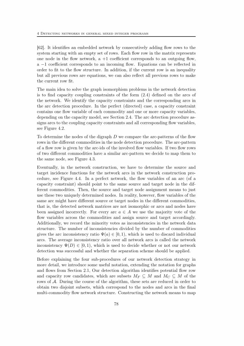
4 Detecting networks in general mixed integer programs
[62]. It identifies an embedded network by consecutively adding flow rows to thesystem starting with an empty set of rows. Each flow row in the matrix representsone node in the flow network, a +1 coefficient corresponds to an outgoing flow,a −1 coefficient corresponds to an incoming flow. Equations can be reflected inorder to fit to the flow structure. In addition, if the current row is an inequalitybut all previous rows are equations, we can also reflect all previous rows to makethe current row fit.
The main idea to solve the graph isomorphism problems in the network detectionis to find capacity coupling constraints of the form (2.4) defined on the arcs ofthe network. We identify the capacity constraints and the corresponding arcs inthe arc detection procedure. In the perfect (directed) case, a capacity constraintcontains one flow variable of each commodity and one or more capacity variables,depending on the capacity model, see Section 2.4. The arc detection procedure as-signs arcs to the coupling capacity constraints and all corresponding flow variables,see Figure 4.2.
To determine the nodes of the digraph D we compare the arc-patterns of the flowrows in the different commodities in the node detection procedure. The arc-patternof a flow row is given by the arc-ids of the involved flow variables. If two flow rowsof two different commodities have a similar arc-pattern we decide to map them tothe same node, see Figure 4.3.
Eventually, in the network construction, we have to determine the source andtarget incidence functions for the network arcs in the network construction pro-cedure, see Figure 4.4. In a perfect network, the flow variables of an arc (of acapacity constraint) should point to the same source and target node in the dif-ferent commodities. Then, the source and target node assignment means to justuse these two uniquely determined nodes. In reality, however, flow variables of thesame arc might have different source or target nodes in the different commodities,that is, the detected network matrices are not isomorphic or arcs and nodes havebeen assigned incorrectly. For every arc a ∈ A we use the majority vote of theflow variables across the commodities and assign source and target accordingly.Additionally, we record the minority votes as inconsistencies in the network datastructure. The number of inconsistencies divided by the number of commoditiesgives the arc inconsistency ratio Ψ(a) ∈ [0, 1), which is used to discard individualarcs. The average inconsistency ratio over all network arcs is called the networkinconsistency Ψ(D) ∈ [0, 1), which is used to decide whether or not our networkdetection was successful and whether the separation scheme should be applied.
Before explaining the four sub-procedures of our network detection strategy inmore detail, we introduce some useful notation, extending the notation for graphsand flows from Section 2.1, Our detection algorithm identifies potential flow rowand capacity row candidates, which are subsets MF ⊆ M and MC ⊆ M of therows of A. During the course of the algorithm, these sets are reduced in order toobtain two disjoint subsets, which correspond to the nodes and arcs in the finalmulti-commodity flow network structure. Constructing the network means to map
78

4.1 Identifying multi-commodity flow matrices
the rows and columns of the matrix A to network elements and commodities. Themappings are
rowcom : M → K ∪ 0, i 7→ rowcom(i)
colcom : N → K ∪ 0, j 7→ colcom(j)
rowarc : M → A ∪ 0, i 7→ rowarc(i)
colarc : N → A ∪ 0, j 7→ colarc(j)
rownode : M → V ∪ 0, i 7→ rownode(i),
where rowcom and colcom map rows and columns of the flow system to commodi-ties, the functions rowarc and colarc map the coupling (capacity) constraints andthe flow variables to arcs of the network, and rownode assigns a node to every flowrow. A mapping to 0 means that the corresponding row or column has not beenassigned. To construct the graph D = (V,A) we will use the source and targetincidence functions ς, τ : A→ V .
All of our algorithms, based on data structures provided by Scip, rely on sparsearray representations of the rows and columns of the matrix A. Whenever iteratingrows or columns, we in fact iterate all corresponding non-zeros. For a subsetN ′ ⊆ N of the column indices, the set M [N ′] := i ∈M : ∃j ∈ N ′ with Aij 6= 0contains all row indices with a non-zero entry in one of the columns ofN ′. Similarly,for a row index set M ′ ⊆ M , the set N [M ′] := j ∈ N : ∃i ∈ M ′ with Aij 6= 0corresponds to all columns with a non-zero entry in one of the rows of M ′. Weabbreviate M [j] := M [j] and call M [j] the support of column j. Similarly,N [i] := N [i] denotes the support of row i.
4.1 Identifying multi-commodity flow matrices
The goal of the flow detection Algorithm 4.3 on the following page is to findan embedded network in A that is inclusion-wise maximal with respect to therows. For finding the embedded network we use a modified row-scanning-additionalgorithm [54]. Roughly speaking, this algorithm starts with an empty set of flowrows and adds rows until a maximal embedded network has been built.
Prior to calling Algorithm 4.3 we identify a potential set of flow row candidatesMF among all rows M . Initially, the set MF contains all rows in A that have,up to scaling, entries in the set 0,+1,−1. Note that in contrast to Bixby andFourer [54] we do not allow for scaling of columns in order to obtain a 0,−1, 1system. All non-zero coefficients of a row in MF have the same absolute value.We do not explicitly scale rows but keep track of the scaling factors. The actualscaling is carried out by the weighted aggregation in the c-MIR procedure. Sincein practice the degree of network nodes is relatively small and for efficiency reasonswe do not allow for flow rows with more than 10 % non-zeros, that is, we limit thenode degree to 0.1|A| (in the single-commodity case).
79

4 Detecting networks in general mixed integer programs
Input : flow row candidates MF , scoring sF : MF → R+
Output : set of commodities K, mappings rowcom : M → K ∪ 0,colcom : N → K ∪ 0
1 Sort MF in non-increasing order of sF2 Initialize rowcom(i) := 0 for all i ∈M3 Initialize k := 04 for i ∈MF with rowcom(i) = 0 do // Scan flow row candidates5 k := k + 1 // Create new commodity6 i′ := i7 rowcom(i′) := k // Add row i′ to commodity k8 colcom(j) := k for all j ∈ N [i′] // Add non-zero columns
// of i′ to commodity k9 for j with colcom(j) = k do // Search for adjacent rows
10 for i′ ∈M [j] with rowcom(i′) = 0 do11 if row i′ fits to system MF (k) then goto 7; // i′ is best row12 end13 end14 if flow system MF (k) is too small then // Delete commodity k15 colcom(j) := 0 for all j ∈ NF (k)16 rowcom(i′) := 0 for all i′ ∈MF (k)17 k := k − 1
18 end19 end20 MF := MF \ i ∈MF : rowcom(i) = 0 // Rm unassigned candidates21 NF := N [MF ]
Algorithm 4.3: Flow Detection
Our flow detection algorithm is strongly driven by a scoring of the flow row candi-dates. To every row i in MF we assign a score sF (i) ∈ R+. The larger sF (i), themore we trust row i to be part of a flow system. The following properties of row i(in decreasing order of their importance) increase its score sF (i):
• Row i does not need to be scaled, i. e., its coefficients are among 0,−1,+1.• All variables (with non-zero coefficient) are continuous (corresponding to
splittable flows).
• All variables in row i (with non-zero coefficient) are integer or all variables inrow i (with non-zero coefficient) are binary (corresponding to integer split-table or single-path flows).
• Row i has both positive and negative coefficients. (There are both inflowand outflow variables)
• Row i is an equation.
80

4.1 Identifying multi-commodity flow matrices
We use the number of non-zeros and the absolute dual value of row i in the initialsolution of the LP relaxation for tie-breaking. The larger these values are, theearlier the flow row candidate is considered: scanning and evaluation of the flowrow candidates in Steps 4 and 10 of Algorithm 4.3 are carried out in non-increasingorder of sF .
The submatrix defined by the flow rows might contain independent blocks, i. e., thecorresponding network is not necessarily connected. These different blocks, thatis, the corresponding rows and columns, are assigned to different commodities.In contrast to the row-scanning-addition algorithm of Bixby and Fourer [54] ourprocedure constructs the flow system of every commodity one by one (Steps 5–13).We denote by MF (k) all flow rows that are assigned to commodity k, MF (k) :=i ∈ MF : rowcom(i) = k. Similarly, the set NF (k) := N [MF (k)] contains allflow variables assigned to commodity k. If MF (k) cannot be increased, a newcommodity is created until all potential flow row candidates have been considered.In Step 14 of Algorithm 4.3 we say that a finished commodity k is too small if|MF (k)| < 3 or there exists a commodity k′ such that |MF (k)| < 0.5|MF (k′)|. Inthis case the commodity mappings for the corresponding rows and columns arereleased. These rows can then indeed be used again for new commodities. Butnotice that every row is considered at most once as the starting row of a commodityin Step 4, which guarantees the termination of the algorithm.
Every step of the addition method results in a feasible flow system (an embed-ded and connected sub-network) for the current commodity k. Given a flow rowcandidate i ∈MF \MF (k), we say that i fits to MF (k), if
• i is adjacent toMF (k), i. e., the intersection of NF (k) and N [i] is non-empty,
• the augmented system MF (k) ∪ i is an embedded network, i. e., it has atmost one +1 and at most one −1 entry in every column (up to scaling andreflection).
In Steps 9–13 we scan all columns of MF (k) for adjacent flow rows. For efficiencyreasons we take the first row that fits. But note that this row has the largest scorew. r. t. the current column. To accelerate the loop 9–13 we consider only thosecolumns j in Step 9 that have exactly one entry in MF (k). This is achieved byintroducing arrays that count the number of +1 and −1 entries in the currentcommodity for every column. In our implementation these arrays are also used fortesting if a row fits to MF (k), also see [54].
To fit a row into a flow system one can reflect it, i. e., multiply it by −1. Since ourseparation approach (see Chapter 5) relies on aggregating flow rows, this operationcan be applied as long as the current row i is an equation (or similarly, every rowof the current systemMF (k) is an equation). In case there is a ≥-inequality amongMF (k) and a ≥-constraint has to be reflected in Step 11 to make it fit to MF (k),we decrease its score such that it is considered later in the loop 10–12. This waywe avoid to introduce slacks when aggregating subsets of the rows of (3.1) in thec-MIR procedure by summing up ≥ and ≤-constraints.
81
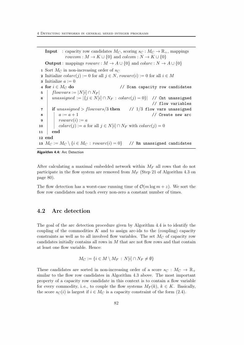
4 Detecting networks in general mixed integer programs
Input : capacity row candidates MC , scoring sC : MC → R+, mappingsrowcom : M → K ∪ 0 and colcom : N → K ∪ 0
Output : mappings rowarc : M → A ∪ 0 and colarc : N → A ∪ 01 Sort MC in non-increasing order of sC2 Initialize colarc(j) := 0 for all j ∈ N , rowarc(i) := 0 for all i ∈M3 Initialize a := 04 for i ∈MC do // Scan capacity row candidates5 flowvars := |N [i] ∩NF |6 unassigned := |j ∈ N [i] ∩NF : colarc(j) = 0| // Cnt unassigned
// flow variables7 if unassigned > flowvars/3 then // 1/3 flow vars unassigned8 a := a+ 1 // Create new arc9 rowarc(i) := a
10 colarc(j) := a for all j ∈ N [i] ∩NF with colarc(j) = 0
11 end12 end13 MC := MC \ i ∈MC : rowarc(i) = 0 // Rm unassigned candidates
Algorithm 4.4: Arc Detection
After calculating a maximal embedded network within MF all rows that do notparticipate in the flow system are removed from MF (Step 21 of Algorithm 4.3 onpage 80).
The flow detection has a worst-case running time of O(m logm+ z). We sort theflow row candidates and touch every non-zero a constant number of times.
4.2 Arc detection
The goal of the arc detection procedure given by Algorithm 4.4 is to identify thecoupling of the commodities K and to assign arc-ids to the (coupling) capacityconstraints as well as to all involved flow variables. The set MC of capacity rowcandidates initially contains all rows in M that are not flow rows and that containat least one flow variable. Hence:
MC := i ∈M \MF : N [i] ∩NF 6= ∅
These candidates are sorted in non-increasing order of a score sC : MC → R+
similar to the flow row candidates in Algorithm 4.3 above. The most importantproperty of a capacity row candidate in this context is to contain a flow variablefor every commodity, i. e., to couple the flow systems MF (k), k ∈ K. Basically,the score sC(i) is largest if i ∈MC is a capacity constraint of the form (2.4).
82

4.3 Node detection
Properties that influence the score of capacity row candidates are given in the fol-lowing in decreasing order of their importance. Note that capacity row candidatesgiven as equations can always be reflected. For simplicity we assume that they aregiven as ≥-inequalities in the following. We increase sC(i)
• for every covered commodity, i. e., for every k ∈ K with N [i] ∩NF (k) 6= ∅,• if i contains (close to) one flow variable per commodity, i. e., if the number
of flow variables |N [i] ∩NF | divided by the number of covered commodities|k ∈ K : N [i] ∩NF (k) 6= ∅| is close to 1,
• if i is a (capacity) constraint bounding flow from above, i. e., it holds thatAij < 0 for all j ∈ N [i] ∩NF and Aij > 0 for all j ∈ N [i] \NF ,
• if Aij = −1 for all j ∈ N [i] ∩NF without scaling, or
• if Aij = −1 for all j ∈ N [i] ∩NF by scaling.
We use the absolute dual values of the capacity row candidates for tie-breaking.As for flow rows we keep track of the necessary scaling factors. These will be usedas weights in the c-MIR aggregation, see Chapter 5.
Algorithm 4.4 simply assigns an arc-id to every capacity row candidate and allunassigned flow variables in the support of the capacity row candidate if one thirdof the flow variables is still unassigned. Note that in a perfect network all capacityconstraints are disjoint w. r. t. the flow variables hence the flow variables are allunassigned in Step 7. Here we allow for some overlap between capacity constraints,for example to cope with presolving reductions. The loop 4 is carried out in non-increasing order of sC . Eventually, all capacity rows without an arc-id are removedfromMC . Algorithm 4.4 terminates with a bijection rowarc : MC ↔ A of capacityrows to arc-ids. Flow variables j ∈ NF with colarc(j) = 0 are considered to beuncapacitated since they do not have a supporting capacity constraint. For thesevariables we will create (uncapacitated) arcs in a final step after the constructionof the network, see below.
The arc detection has a worst-case running time of O(m logm + z). We sort thecapacity row candidates and touch every non-zero a constant number of times.
4.3 Node detection
Algorithm 4.5 on the next page uses the incidence information given by the arc-idmapping colarc to identify (almost) isomorphic nodes in the different commodities.Two flow rows in different commodities are considered to belong to the same nodeif they have a similar incidence pattern w. r. t. their arc-ids.
Algorithm 4.5 on the following page scans all flow rows in non-increasing order ofsF . In the single-commodity case every flow row simply gets a different node-id.Given a flow row i ∈ MF belonging to commodity k in the case |K| > 1, we try
83

4 Detecting networks in general mixed integer programs
Input : flow row candidates MF , mappings rowcom : M → K ∪ 0 andcolarc : N → A ∪ 0
Output : mapping rownode : M → V ∪ 01 Initialize rownode(i) := 0 for all i ∈M2 Initialize v := 03 for i ∈MF with rownode(i) = 0 do // Scan flow rows4 v := v + 1 // Create new node5 rownode(i) := v // Assign node v to flow row i6 if |K| = 1 then continue7 k = rowcom(i)8 pattern := PatternOf(i)9 for i′ ∈MF with rowcom(i′) 6= k do // Scan flow rows of
10 k′ := rowcom(i′) // commodities k′ 6= k11 score := ComparePattern(pattern, PatternOf(i′))12 Remember bestrow(k′) with largest score for k′
13 end14 for k′ ∈ K \ k do // Assign v to rows with15 rownode(bestrow(k′)) := v // closest arc-pattern to i16 end17 end
Algorithm 4.5: Node Detection
to identify flow rows in all commodities k′ 6= k with a similar arc-pattern. Tocalculate the arc-pattern of a flow row i we count for every arc a, how often itappears as an outgoing and incoming arc in the support of the constraint, i. e.,how many flow variables with positive and negative coefficients in the support ofi are assigned to arc a.
If the problem formulation is of the ideal form (ND) and if we managed to de-tect the flow system and arcs correctly in Algorithm 4.3 and Algorithm 4.4, thenPatternOf(i) returns an incidence vector in 0,+1,−1A giving all outgoing andincoming arcs of the flow row i. Due to inconsistencies in the system or matrixpreprocessing the entries might differ from 0, +1, or −1.
In Step 11 of Algorithm 4.5 we compare all arc-patterns of flow rows i′ of com-modities k′ 6= k with the pattern of row i of commodity k using the functionComparePattern. Notice that it suffices to scan only those flow rows i′ in the loop9-13 that are coupled with i by a capacity constraint. Hence we consider only rowsi′ ∈ MF in Step 9 that have at least one arc in common with i. The functionComparePattern returns the (weighted) overlap of the two arc-patterns. As a tie-breaker we use the number of non-overlapping entries of the two pattern vectorsdivided by the number of columns of the matrix A. As already mentioned, theremight be uncapacitated flow variables that have no arc-id. In our implementation
84

4.3 Node detection
Input : flow row i
Output : pattern ∈ ZA
1 pattern(a) = 0 for all a ∈ A // Initialize arc-pattern of row i2 for j ∈ N [i] do3 a = colarc(j)4 if a = 0 then continue // Uncapacitated flow variable5 if Aij > 0 then pattern(a) = pattern(a) + 1 // Outgoing arc6 if Aij < 0 then pattern(a) = pattern(a)− 1 // Incoming arc7 end8 return pattern
Function PatternOf(i)
Input : arc-patterns pattern1, pattern2
Output : score ∈ R+
1 Initialize score := 02 for a ∈ A do3 if pattern1(a) · pattern2(a) > 0 then // Patterns overlap and
// signs match
4 score := score+ min(pattern1(a)pattern2(a) ,
pattern2(a)pattern1(a)) // Inc score
5 end6 Calculate tiebreaker 0 ≤ ε 17 score := score− ε8 end9 return score
Function ComparePattern(pattern1, pattern2)
we also count the number of these uncapacitated flow variables (both with positiveand negative sign) in the two flow rows and use this information as an additionaltie-breaker when comparing two patterns. Hence flow rows should have a similarnumber of uncapacitated flow variables in addition to a similar arc-pattern to re-ceive a large score. It should be mentioned that every individual commodity flowsystem MF (k) can be reflected once, which means to reflect every flow row in thesystem. This has to be considered when comparing the arc-patterns.
Subsequent to the node-detection procedure we perform a cleanup of the networkinformation obtained so far. We remove commodities that have no arcs (no flowvariable with an arc-id) or too few nodes (too few flow rows assigned to differentnodes). A commodity has too few nodes if its total number is smaller than 3 or ithas less then 50 % of the nodes of the largest commodity. In general one wishes tohave commodity systems of almost the same size. Removing a commodity means
85

4 Detecting networks in general mixed integer programs
to release the corresponding data structures and assignments to nodes and arcs.
In principle, the running time of the node detection may be in the order of O(mz)assuming that we compare every pair of rows by scanning the corresponding non-zero elements. In this respect, the node detection dominates all four steps inthe network detection with respect to computational complexity. However, inpractice, this procedure runs much faster. The main trick, as mentioned above, is toconsider only those rows for comparison that are coupled by a capacity constraint.Moreover, only those rows are considered that have not been assigned to a node ina previous iteration. Also recall that in the flow detection we selected only sparseflow rows as candidates for MF .
4.4 Network construction
For constructing a digraph D based on the node-set V and arc-set A it remains toconstruct the source and target incidence functions ς, τ : A→ V . The correspond-ing information is hidden in our data structures. Given a flow variable j ∈ NF
assigned to some arc a ∈ A, there are at most two flow rows in MF having j intheir support, one with positive and one with negative coefficient. These flow rowsare assigned to nodes. It follows that every flow variable, if assigned to an arc, hasa source and a target node.
Algorithm 4.6 on the facing page iterates all arcs in A and asks all the correspond-ing flow variables for their source and target node. Due to inconsistencies in theformulation or in the network detection the flow variables of the same arc mightanswer differently. Based on the majority of the votes the incidence functions ςand τ are constructed. The minority votes are counted as arc inconsistencies, seeStep 22 of Algorithm 4.6. We further discuss inconsistencies in the next section.
The running time of the network construction depends linearly on the number ofnon-zeros in the capacity constraints, that is, it is in the order of O(z).
It remains to show what happens with uncapacitated flow variables that couldnot be assigned to arcs in the arc detection Algorithm 4.4 on page 82. For thesevariables we try to create uncapacitated arcs in a procedure following the networkconstruction. We create a new uncapacitated arc (v, w) for v, w ∈ V if there areenough uncapacitated flow variables in different commodities having v as sourceand w as target node. More precisely, if for the number uncap(v,w) of uncapacitatedflow variables corresponding to (v, w) it holds that uncap(v,w) ≥ d0.8|K|e we createa new arc a = (v, w). Notice that for (v, w) there can only be one matching flowvariable for every commodity. For the single-commodity case this means that wecreate a new arc for each uncapacitated flow variable in the flow system.
The constructed graph D = (V,A) might be disconnected for two reasons. First,the arc-capacity constraints do not necessarily couple all commodity flow systemsbut only subsets of them. Second, the network might get disconnected by deleting
86

4.4 Network construction
Input : nodes V, arcs A, mappings rowarc : M → A ∪ 0 andcolcom : N → K ∪ 0
Output : digraph D = (V,A) with incidence functions ς : A→ V andτ : A→ V , network inconsistency Ψ(D) ∈ [0, 1)
1 Initialize inconsistencies := 02 for a ∈ A do3 i := rowarc−1(a) // Capacity row of arc a4 for k ∈ K do // # Flow-vars of commodity k5 nvars(k) := |j ∈ N [i] : colcom(j) = k| // in cap-row i6 end7 ncom := |k ∈ K : nvars(k) > 0| // # Commodities in row i
// Ask all flow variables for source and target node8 Initialize scount(v) := 0, tcount(v) := 0 for all v ∈ V9 for j ∈ N [i] with colcom(j) > 0 do
10 k := colcom(j)11 for i′ ∈M [j] ∩MF do // Flow variable j has at most12 v := rownode(i′) // two incident flow-rows13 if Ai′j > 0 then // Increase source count for v14 scount(v) := scount(v) + 1/nvars(k)15 else // Increase target count for v16 tcount(v) := tcount(v) + 1/nvars(k)17 end18 end19 end
// Majority vote wins, assign best source/target to a20 ς(a) := argmaxscount(v) : v ∈ V, scount(v) ≥ tcount(v)
τ(a) := argmaxtcount(v) : v ∈ V, tcount(v) ≥ scount(v)// Minority votes give arc inconsistency
21 totalcount :=∑
v∈V (scount(v) + tcount(v))22 Ψ(a) := (totalcount− scount(ς(a))− tcount(τ(a)))/2 · ncom
Ψ(D) := Ψ(D) + Ψ(a)/|A| // Network inconsistency23 end24 for a ∈ A do25 if Ψ(a) > Ψmax
a then A := A \ a; // Delete inconsistent arcs26 end
Algorithm 4.6: Network Construction
inconsistent arcs. Our separation procedure is applied to every individual com-ponent of D. Each of these components might correspond to a multi-commoditysystem. For simplicity, in the rest of this paper we assume that there is only onesuch component in the sequel, i. e., D is connected.
87

4 Detecting networks in general mixed integer programs
Before we present the constraint aggregation and separation scheme of the MCF-separator in Chapter 5, let us have a look at possible reasons for network incon-sistencies. It turns out that inconsistency is not necessarily caused by a wrongdetection but is intrinsic to multi-commodity arc-flow formulations.
4.5 Inconsistency issues
For every arc a ∈ A we evaluate its inconsistency Ψ(a) ∈ [0, 1) in Step 22 ofAlgorithm 4.6 on the preceding page, where Ψ(a) corresponds to the number ofminority votes divided by the number of involved commodities. Inconsistent arcs,that is, arcs a with Ψ(a) > Ψmax
a , are deleted. In our implementation we donot allow for arcs with individual inconsistency ratio Ψ(a) greater than Ψmax
a =0.5. The mean of the arc inconsistencies defines the network inconsistency ratioΨ(D) ∈ [0, 1). This ratio is used to decide about the quality of the detected networkstructure. If Ψ(D) = 0 we detected a consistent coupled multi-commodity flownetwork. The commodity network matrices can be considered being isomorphicand we correctly assigned arcs and nodes to rows and columns. If, however, Ψ(D)is close to 1 our detection failed or there is no consistent embedded network in theconstraint matrix. The network inconsistency is not allowed to exceed Ψmax = 0.02in our implementation. If Ψ(D) > Ψmax, then all network data structures arereleased and it is not tried to generate cutting planes based on the detection,see Algorithm 5.7 on page 93. That is, the MCF-separator is switched off. Theinfluence of the parameters Ψmax and Ψmax
a is tested in Section 6.3.
There are several reasons for potential inconsistencies. First, our detection algo-rithm is a heuristic. Its success largely depends on a proper identification and or-dering of flow and capacity rows. But already the formulation of the concrete MIPinstance can be “corrupted” even if it corresponds to a coupled multi-commodityflow. As a consequence, the detection procedures cannot expect pure and isomor-phic network matrices. The same node or the same arc does not need to be presentin every commodity. Moreover, an arc does not necessarily have both a source anda target node, that is, the corresponding flow rows might be missing:
User presolving
It is known that the rank of a network matrix corresponding to a directed connectednetwork D = (V,A) is exactly |V | − 1. For every commodity, an arbitrary row inthe system (2.3) on page 39 can be omitted. To save constraints, this preprocessingis sometimes already carried out by the modeler and results in deleting a node fromD for every commodity, see Figure 4.5(a) on the facing page. Moreover, the nodethat is deleted typically differs from commodity to commodity. For example, if eachcommodity has a single source node, it is common to omit the flow conservationconstraint of this source node from the formulation.
88
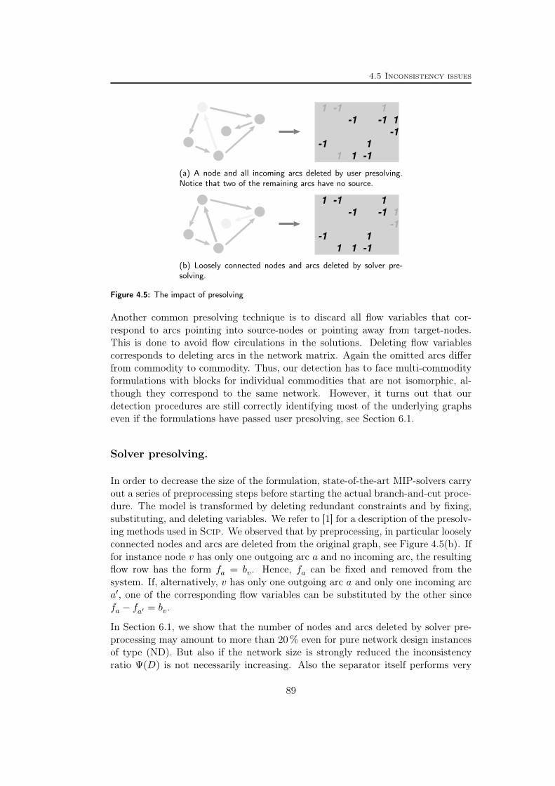
4.5 Inconsistency issues
1
-1
1 1
1
1
-1
-1
-1
-1 1
-1
(a) A node and all incoming arcs deleted by user presolving.Notice that two of the remaining arcs have no source.
1
-1
1 1
1
1
-1
-1
-1
-1 1
-1
(b) Loosely connected nodes and arcs deleted by solver pre-solving.
Figure 4.5: The impact of presolving
Another common presolving technique is to discard all flow variables that cor-respond to arcs pointing into source-nodes or pointing away from target-nodes.This is done to avoid flow circulations in the solutions. Deleting flow variablescorresponds to deleting arcs in the network matrix. Again the omitted arcs differfrom commodity to commodity. Thus, our detection has to face multi-commodityformulations with blocks for individual commodities that are not isomorphic, al-though they correspond to the same network. However, it turns out that ourdetection procedures are still correctly identifying most of the underlying graphseven if the formulations have passed user presolving, see Section 6.1.
Solver presolving.
In order to decrease the size of the formulation, state-of-the-art MIP-solvers carryout a series of preprocessing steps before starting the actual branch-and-cut proce-dure. The model is transformed by deleting redundant constraints and by fixing,substituting, and deleting variables. We refer to [1] for a description of the presolv-ing methods used in Scip. We observed that by preprocessing, in particular looselyconnected nodes and arcs are deleted from the original graph, see Figure 4.5(b). Iffor instance node v has only one outgoing arc a and no incoming arc, the resultingflow row has the form fa = bv. Hence, fa can be fixed and removed from thesystem. If, alternatively, v has only one outgoing arc a and only one incoming arca′, one of the corresponding flow variables can be substituted by the other sincefa − fa′ = bv.
In Section 6.1, we show that the number of nodes and arcs deleted by solver pre-processing may amount to more than 20 % even for pure network design instancesof type (ND). But also if the network size is strongly reduced the inconsistencyratio Ψ(D) is not necessarily increasing. Also the separator itself performs very
89

4 Detecting networks in general mixed integer programs
well, see Section 6.2. The remaining graphs after presolving seem to reflect the coreof the network such that generated cut-based inequalities still capture importantstructural information.
Concluding remarks.
We showed how to detect a network D = (V,A) and commodity set K in a sys-tem of the form Ax ≥ b and we learned how to construct functions of the formrowarc : M → A, rowcom : M → K, and rownode : M → V that map rows of Ato network elements and commodities. We first scan the matrix A for an embeddedflow system. The remaining three sub-procedures of the network detection try toresolve the isomorphism of commodity blocks using coupling capacity constraints.A crucial feature of our implementation is to compute a network consistency mea-sure, which can be used to decide about the quality of the network detection. Inthe next chapter, we will show how to exploit the new structural information in aspecial constraint aggregation and cutting plane scheme.
90

Chapter 5
Aggregating constraints forcutting plane separation
In this chapter, we introduce the separation framework to generate network cut-based inequalities using the network structure detected by the procedures presentedin the previous chapter. We also explain how we incorporate the c-MIR procedureto generate strong cutting planes by a proper constraint aggregation. We start withthe general framework in Section 5.1 and explain some extensions in Section 5.2.
5.1 Algorithmic framework
If the network detection scheme described in the previous chapter identified anetwork D = (V,A) with inconsistency Ψ(D) > Ψmax, then either our detectionheuristics failed or the MIP model is not based on network design and does simplynot contain a coupled multi-commodity flow. If, however, Ψ(D) ≤ Ψmax we applythe following aggregation and separation scheme exploiting the consistent networkstructure. Our separation heuristic relies on calculating a weight vector λ ∈ Rmthat is used to aggregate original constraints of the system (3.1) based on theconstructed mappings. For every such weight vector we additionally provide aset ∆ of scalars γ > 0 chosen among the (absolute values of the) coefficients ofinteger variables in the capacity coupling constraints i ∈ MC with λi 6= 0, seeCorollary 1.5 and Algorithm 1.2 on page 33. The final base mixed integer rows aregiven by −(1/γ)λTs + (1/γ)λTAx = (1/γ)λTb for all γ ∈ ∆, where s = Ax − bis the vector of slacks corresponding to the constraint system Ax ≥ b, also seeSection 1.3.
The vector λ and γ ∈ ∆ are passed to the c-MIR framework which carries out theaggregation and scaling and also performs bound substitution and complementingif possible. In Algorithm 5.7 below we denote the corresponding function callby cMIR(λ,γ) (which in Scip relates to calling the procedure SCIPcalcMIR). We
91
5 Aggregating constraints for cutting plane separation
choose the vector λ such that the resulting inequality corresponds to a cut in thedetected network. The vector λ already incorporates the necessary scaling andreflecting of flow and capacity rows from the network detection procedures. Inthe following description we ignore this fact and assume that all flow and capacityrows are correctly scaled, that is, λi ∈ 0, 1 for all i ∈ M . To select constraintsfor aggregation based on the network structure we make use of the calculatedmappings rowarc : MC → A, rowcom : MF → K, and rownode : MF → V . Fromrowarc we construct a function arcrow : A→MC ∪0 that returns the capacityconstraint for every arc a ∈ A or 0 if arc a is uncapacitated. From rownode androwcom we construct a function nodecomrow : V ×K → MF ∪ 0 that returnsthe flow row corresponding to node v ∈ V and commodity k ∈ K or 0 if node v(and hence the corresponding flow row) is not existing for commodity k. Noticethat our detection algorithm ensures that there can be at most one capacity rowfor every arc and at most one flow row for every node and commodity.
The high-level aggregation scheme of our implementation is given by Algorithm 5.7below. Our network cut selection strategy is very close to procedures proposedin [50, 51, 129, 188, 200] which have been successfully used in branch-and-cutframeworks to solve different types of network design problems. Essentially, weuse a variation of Algorithm C presented in Raack et al. [200]. We favor thegeneration of cut-based inequalities in the space of the capacity variables overthe generation of mixed inequalities containing both flow and capacity variables.This is based on experimental observations that the latter are not as efficient inimproving the dual bounds and performance, see for instance [50, 188, 200] andalso Chapter 10.
Algorithm 5.7 starts by calculating a set of cuts in the detected network (seebelow for details). If node-set S is in the list C, then also the reverse direction isconsidered, i. e., V \S ∈ C (for the undirected case see Section 5.2). For every node-set S we determine the set of supply commodities K+
S , i. e., the set of commoditiesthat has to be routed from V to S \V . We set the weights λ such that in the idealcase a cut-set inequality of the form (2.16) (or its multi-facility version (2.33)) isgenerated by the c-MIR framework (Step 18 of Algorithm 5.7). This inequalitycontains only capacity variables since flow variables for arcs in δ+(S) are canceledout by the corresponding capacity constraints and flow variables for arcs in δ−(S)get a zero-coefficient by MIR. Several such inequalities might be generated becausewe try different scaling factors γ > 0. In our implementation we use a maximumof 20 from the largest multipliers in ∆. Two multipliers γ1 ≥ γ2 are consideredto be identical if γ1/γ2 < 1.001. The coefficient scaling loop in Step 17–20 ofAlgorithm 5.7 is similar to the one of the c-MIR separator, cf. Algorithm 1.2 onpage 33.
To get tight base inequalities (having no slack) we only accept tight flow rowsfor aggregation in Step 10 of Algorithm 5.7, and we are not accepting capacityrows with a slack greater than 0.1 (the largest coefficient being normalized to 1)in Step 14. Recall that in the ideal case flow rows are equations. The node-sets
92
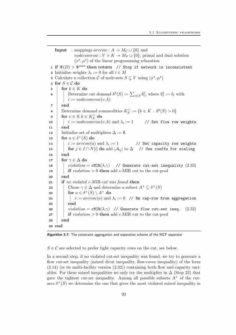
5.1 Algorithmic framework
Input : mappings arcrow : A→MC ∪ 0 andnodecomrow : V ×K →MF ∪ 0, primal and dual solution(x?, µ?) of the linear programming relaxation
1 if Ψ(D) > Ψmax then return // Stop if network is inconsistent2 Initialize weights λi := 0 for all i ∈M3 Calculate a collection C of node-sets S ( V using (x?, µ?)4 for S ∈ C do5 for k ∈ K do6 Determine cut demand bk(S) :=
∑v∈S b
kv , where bkv := bi with
i := nodecomrow(v, k)
7 end8 Determine demand commodities K+
S := k ∈ K : bk(S) > 09 for v ∈ S, k ∈ K+
S do10 i := nodecomrow(v, k) and λi := 1 // Set flow row weights11 end12 Initialize set of multipliers ∆ := ∅.13 for a ∈ δ+(S) do14 i := arcrow(a) and λi := 1 // Set capacity row weights15 for j ∈ I ∩N [i] do add |Aij | to ∆ // Use coeffs for scaling16 end17 for γ ∈ ∆ do18 violation = cMIR(λ,γ) // Generate cut-set inequality (2.33)19 if violation > 0 then add c-MIR cut to the cut-pool20 end21 if no violated c-MIR-cut was found then22 Chose γ ∈ ∆ and determine a subset A+ ⊆ δ+(S)23 for a ∈ δ+(S) \A+ do24 i := arcrow(a) and λi := 0 // Rm cap-row from aggregation25 end26 violation = cMIR(λ,γ) // Generate flow cut-set ineq. (2.32)27 if violation > 0 then add c-MIR cut to the cut-pool28 end29 end
Algorithm 5.7: The constraint aggregation and separation scheme of the MCF separator
S ∈ C are selected to prefer tight capacity rows on the cut, see below.
In a second step, if no violated cut-set inequality was found, we try to generate aflow cut-set inequality (mixed dicut inequality, flow-cover inequality) of the form(2.14) (or its multi-facility version (2.32)) containing both flow and capacity vari-ables. For these mixed inequalities we only try the multiplier in ∆ (Step 22) thatgave the tightest cut-set inequality. Among all possible subsets A+ of the cut-arcs δ+(S) we determine the one that gives the most violated mixed inequality in
93

5 Aggregating constraints for cutting plane separation
Steps 22–25. This can be done by using the linear separation rule for arc subsetsand flow cut-set inequalities described in Section 2.3 and also [16, 188, 200]. Weheuristically assume that the right-hand side of the capacity constraints is zero,i. e., there is no pre-installed capacity on δ+(S) and no variable is complemented orsubstituted. In this case the right-hand side of the base inequality does not dependon the chosen subset A+. It follows that the MIR coefficients do not depend on A+.Hence the change of the violation of the MIR inequality can be pre-calculated forevery arc a that is removed from A+. The most violated inequality w. r. t. A+ andthe scaling factor γ ∈ ∆ is obtained by removing all arcs a from A+ that decreasethe activity of the resulting MIR ≥-inequality. Notice that removing a from A+
relates to removing the corresponding capacity constraint from the aggregation.
Network cut selection
It remains to explain our cut selection strategy in Step 3 of Algorithm 5.7. Weuse a variation of the cut selection scheme described by Raack et al. [200], also see[51, 129, 188]. That is, we consider all node-sets S with |S| = 1 or |V \ S| = 1as candidates for the cut-collection C. In addition we apply a graph contractionheuristic, which has been first proposed by Bienstock et al. [51], Günlük [129]. Ingeneral, there might be parallel arcs in the graph. Consequently, this heuristic isbased on node-pair weights as opposed to the arc-weights used in the schemes of[51, 129, 188, 200]. To every node-pair v, w ∈ V (2), for which an arc a = (v, w)or a = (w, v) exists, we assign a weight λv,w ∈ R and iteratively contract thetwo nodes (see [121]) with the largest weight until the contracted graph has k ≥ 2nodes corresponding to a partition of the nodes in the original graph of size k.We enumerate all cuts in the contracted graph and consider the two correspondingshores to be added to C, which results in a maximum number of 2k − 2 additionalnode-sets. By Theorem 2.9 and Theorem 2.11 a crucial condition for a cut-basedinequality to be strong (to define a facet) is that the two shores of the cut are(strongly) connected. In our implementation we only add node-sets S to the listC if both D[S] and D[V \ S] are connected. The connectivity check is carried outusing a breadth first search algorithm on these graphs. Note, however, that everyindividual shore in the network partition obtained by contraction is connected sincewe start with a connected network. The weight of a node-pair v, w is initializedwith the minimum of all corresponding arc-weights λa defined by
λa := s?a − |µ?a|,
where s?a denotes the slack value of the capacity constraint arcrow(a) with respectto the solution x?. Similarly, µ?a denotes the dual value of the row arcrow(a).Recall that s?a · µ?a = 0 due to complementary slackness. We set λa to infinity ifarc a is uncapacitated. The weights are not adapted after node contraction.
With contraction weights defined this way, cuts are preferred that have many arcswith small slack and large absolute dual. If (all of) the capacity constraints in the
94

5.2 Extensions
cut are tight then also the base inequality will be tight. For tight base constraints,it is more likely to derive a violated MIR inequality. Subtracting the dual valuesfor tight arcs is based on the heuristic argument that the inequalities we generateincrease the capacity on the cut. Hence, they introduce slacks in the capacityconstraints on the cut. It follows that using large absolute duals should maximallyimprove the dual bound. With weights that can be positive and negative, thiscontraction scheme is a fast max-cut heuristic.
Obviously, the number of considered cuts increases exponentially with the size ofk. In our default implementation we use a value of k = 5. The effect of theparameter k is evaluated in Section 6.4.
5.2 Extensions
Our implementation also incorporates different model alternatives of the standardmodel (ND) (page 39). In Section 2.4, we already introduced several possiblevariations and extensions of (ND) w. r. t. the capacity model. In the following weshow how these variations influence our detection and cutting plane procedure.
Multi-facility models
Let us first assume that the capacity on an arc is not given by a single (integral)capacity variable as in the capacity constraints (2.4) but given by a multi-facilityinstallation, that is, the scalar product of different facility capacities and the cor-responding facility variables, as in the multi-facility arc capacity constraints (2.27),also see [16, 22, 200]. Such a generalized capacity model does not influence ouralgorithms. In fact, the introduced detection framework is independent from thestructure of the capacity variables and their coefficients in the capacity constraints.It only relies on the fact that (almost) all arc-flow variables appear in the couplinginequality, which is the case for both (2.4) and (2.27). The separation frameworkis affected only in Step 15 of Algorithm 5.7 above as the set of multipliers dependson the coefficients of integral variables in the coupling constraints which typicallycorrespond the facility capacities, see Section 2.4.
Unsplittable flow models
Many applications require that the commodity flow is unsplittable, that is, theflow of a point-to-point commodity has to use a single path from its source to itsdestination [20, 60, 135, 136]. To model unsplittable flow one typically introducesbinary flow variables hka that state whether or not the flow of commodity k uses arca. Additionally, the flow conservation constraints (2.3) for commodity k = (s, t) ∈
95

5 Aggregating constraints for cutting plane separation
V × V are formulated as∑a∈δ+(v)
hka −∑
a∈δ−(v)
hka = ψkv ∀v ∈ V, k ∈ K,
where ψkv = 1 if v = s, ψkv = −1 if v = t, and ψkv = 0 else. We also speak ofh ∈ 0, 1A×K being a flow template, see Part III. For the actual arc flow fka itholds fka = dkh
ka, where dk > 0 is the point-to-point-demand that has to be routed
on a single path from s to t. The capacity constraints (2.4) change to:∑k∈K
dkhka − ya ≤ 0 ∀a ∈ A. (5.1)
This results in capacity constraints with coefficients for flow template variables thatare commodity dependent. Note that the same formulation alternative can be usedin the context of splittable flow and single-source, single-target commodities. Inthis case the flow template hka denotes the fraction of flow routed on arc a forcommodity k. Such a formulation does not affect any of the detection proceduresin Sections 4.1 – 4.4 since none of them evaluates the coefficients in the capacityconstraints. Because of a potentially smaller score, capacity rows of type (5.1) willbe considered later in the arc detection Algorithm 4.4 on page 82. But this is onlyof interest if there are both capacity rows of type (2.4) and (5.1) among MC thatcover all commodities.
While this model variant has no influence on the network detection, we have toadapt the weights in the separation scheme. The aim to add the capacity con-straints for δ+(S) to the aggregated flow system is to cancel out the correspond-ing flow variables and to introduce cut capacity variables in the base constraint(2.13). Since the coefficients of flow variables in the constrains (5.1) depend onthe commodities we have to scale the flow rows for every commodity accordingly.Before applying Algorithm 5.7 on page 93 we heuristically normalize all capac-ity constraints in such a way that the coefficients for flow variables of the samecommodity are identical. Let us assume that the coefficient of the single-source,single-target commodity k = (s, t) is dk in all capacity constraints after normal-ization. In this case, every flow row for commodity k has to be scaled by dk whichis carried out in Step 10 of Algorithm 5.7. Notice that normalization and scalinghas no effect on the standard model with capacity constraints of type (2.4).
We refer to Brockmüller et al. [60] for MIR cut-set inequalities and the case thatthe flow is unsplittable.
Undirected capacity models
In case of undirected models as introduced in Section 2.4 we have capacity con-straints of type (2.22) with two flow variables for every commodity. While theflow-system is still directed, the direction of the flow is arbitrary and the capaci-tated network can be considered being undirected.
96
5.2 Extensions
Our implementation is able to distinguish directed and undirected capacity models.Basically one can think of two different implementations. The user is able to decidewhich algorithm to use by setting a model type parameter. In the default settingwe try to detect the model type automatically.
The flow detection Algorithm 4.3 on page 80 is identical for both model types,directed or undirected. If the user is not explicitly claiming either of the twodetection variants, we decide about the model type when assigning the score tothe potential capacity rows just before the arc detection Algorithm 4.4 on page 82.If, on average, the number of flow variables per commodity in the capacity row isgreater than or equal to two we switch to the undirected detection algorithm. Thescoring is modified accordingly. In the arc detection procedure we then constructedges instead of arcs. Again, every edge corresponds to either exactly one capacityconstraint or it is uncapacitated. The node detection in Algorithm 4.5 on page 84is adapted in the way that the incidence pattern of a node does not depend onthe direction of the incident arcs. We only compare the arc-ids of two flow rowsbut not their +1,−1 pattern. When constructing the incidence functions inAlgorithm 4.6 on page 87 we do not distinguish between source and target nodecount but consider the sum count(v) := scount(v) + tcount(v) and simply assignthe two nodes with largest count(v) to be source and target of edge a.
Given a node-set S, the separation scheme Algorithm 5.7 on page 93 considersthe set of cut-edges δ(S) for undirected models. Since the generated inequalitiesare identical for S and V \ S we only add one of the two node-sets to the list C.Since the direction of traffic is arbitrary we calculate and use the commodity setK+S ∪K−S . Flow rows corresponding to K−S are reflected, i. e., we set λi = −1 for
i = nodecomrow(v, k) with v ∈ S and k ∈ K−S . Hence, the right-hand side value inthe base constraint (2.13) (the cut demand) is
∑k∈K+
Sbk(S)−∑k∈K−S
bk(S) > 0.For flow cut-set inequalities we consider a subset A∗ of the cut-edges δ(S) insteadof the set A+. For more details on general flow cut-set inequalities and undirectedmodels the reader is referred to Section 2.4 and [200].
Variable bounds and additional cut generation procedures
Given the valid base inequality corresponding to the constraint aggregation of theMCF-separator, the c-MIR scheme automatically incorporates simple and vari-able bounds by complementing and bound substitution, as already explained inSection 1.4. This is however done in a purely heuristic fashion. Beyond c-MIR,both Scip and Cplex contain procedures to generate strong (mixed) knapsack-cover inequalities, GUB cover inequalities, or flow-cover inequalities using exactand heuristic lifting methods, provided that the base inequality is already in therequired form or can be relaxed accordingly. In principle, any cutting plane tech-nique that works on a single row relaxation of the original problem and incorporatesadditional information, such as bounds on variables or integrality, can be used tostrengthen the valid base inequalities provided by the MCF-separator.
97

5 Aggregating constraints for cutting plane separation
Our Scip implementation of the MCF-separator tries to generate exactly liftedknapsack-cover inequalities (based on knapsack-covers) in addition to applying de-fault c-MIR to inequalities of the form (2.13), see Section 2.4. We have not triedthe flow-cover inequalities of Scip. Notice that the corresponding implementa-tion in Scip also uses the c-MIR framework but with a different complementingheuristic based on flow-covers, see Section 2.4 and [160, 221].
Concluding remarks
We have presented a network detection framework with the procedures flow detec-tion, arc detection, node detection, and network construction. We also establisheda separation framework based on the network detection. The MCF-separator con-sists of both ingredients. While the network detection is carried out once at thebeginning of branch-and-cut, the separation algorithm is applied in every roundof the cutting plane loop in the root node of the search tree. We showed how therespective sub-procedures have to be adapted in case of multi-facility problems, sin-gle path flow models, or undirected formulation. All of the corresponding decisionsare made automatically by the MCF-separator. In particular, the MCF-separatoris able to recognize the models to which it can be applied. Only if the detectednetworks show few inconsistencies the separator tries to generate inequalities basedon network cuts.
We conclude this part of the thesis by investigating the computational impact ofthe MCF-separator in the following chapter. We study both the efficiency of thenetwork detection in terms of resolving hidden network structure and the impactof the resulting cutting plane machinery in improving the performance of state-of-the-art MIP solvers.
98

Chapter 6
The MCF-separator:Computational impact
In this chapter we report on the computational impact of the MCF-separator. InSection 6.1, we discuss the success of our network detection scheme introduced inSections 4.1 – 4.4 and in Section 6.2 we report on the success of the MCF-separatorin improving the performance of Scip as well as Cplex based on the aggregationframework described in Chapter 5.
For our tests we selected publicly available network design instances as well as largetest sets with general MIP instances. Table 6.1 on the following page summarizesthe corresponding test sets. It states the name of the test set, its source, andthe number of instances contained. For the network design instances we alsogive details about the used formulations within the test set. For possible modelvariations see Section 2.3, Section 2.4, and Section 5.2. There are single-commodity(SCF) (|K| = 1) and multi-commodity (MCF) (|K| > 1) instances. The flow canbe splittable (S) or unsplittable (US). The capacity formulation can be directed(DI) or undirected (UN) with a single arc facility (SF), multiple arc facilities (MF),or a big-M capacity (M) in case of uncapacitated problems. The capacity variablesare either binary (BIN), with an additional generalized upper bound constraint(BIN+GUB), or they are integer (INT). Some instances are randomly generated(RG).
The miplib03 test set contains all instances from the Miplib 3 [56] and Miplib2003 [4] libraries. The miplib10 test set includes all instances from the new Miplib2010 library [148, 226]. The mittelmann test set subsumes instances available onthe website of Hans Mittelmann [178, January 2009] used to benchmark MIP-solvers. These test sets are not disjoint. However, from mittelmann we removedinstances that were already contained in miplib03 and fctp. The cplex test setcontains a confidential set of general MIP instances used by the Cplex team tointernally evaluate the performance of their solver.
99

6 The MCF-separator: Computational impact
test set size source paper problem description
arc.set 35 A. Atamtürk, [19] [20] MCF, S, US, BIN, DI, SFcut.set 15 A. Atamtürk, [19] [16] MCF, INT, DIfc 20 A. Atamtürk, [19] [15] SCF, BIN, DI, SF, RGfctp 32 J. Gottlieb, [115] – SCF, BIN, DI, SF, bipartite graphsavub 60 A. Atamtürk, [19] [22] SCF, BIN, DI, MF, RGsndlib 52 ZIB, [228] [187] MCF, INT, BIN+GUB, DI, UN, MFufcn 83 L.A. Wolsey, [220] [188] SCF, BIN, DI, Mmiplib03 92 ZIB, [226] [4, 56] general MIP instancesmiplib10 87 ZIB, [226] [148] general MIP instancesmittelmann 59 H. Mittelmann, [178] – general MIP instancescplex 1266 T. Achterberg – general MIP instances
Table 6.1: Publicly available network design instances with different formulations and general MIPtest sets
For all the network design instances except for the cut.set test set we know orcould determine the underlying graph, that is, we know the correct number ofnodes, arcs, and commodities. Thus the quality of the network detection can beevaluated by comparing the detected networks with the original networks.
Table A.1 on page 220 in Appendix A provides a complete list of the consideredinstances with more detailed information (except for the cplex test set). It providesinformation about the number of rows (rows) and columns (vars) in the model,the value of the LP relaxation (lp), and the best dual (bestdual) and primal (best-primal) bounds obtained during all the computational tests for this chapter.Most of the results presented in this chapter correspond to our implementation inScip 1.1.0.8 using Cplex 11.2.1 as linear programming solver. This developmentversion can be made available on request by the author. The corresponding Scipruns were done on a 64bit 3.00GHz Quad-Core machine with 6144 KB of cache and8 GB of RAM using a single CPU. Deviating from our publication Achterberg andRaack [3], we also provide computations using the Miplib 2010 library togetherwith Scip version 2.1.1 and Cplex 12.4 as LP solver. These more recent tests havebeen carried out single-threaded on a 3.2 GHz Intel Xeon with 48 GB RAM. InSection 6.2, in addition to the Scip results using the same framework, we presentresults using Cplex 12.1. These results have been provided by Tobias Achterberg[2]. For the Cplex 12.1 tests a single CPU of a 64bit 3.33GHz Quad-Core machinewith 6144 KB of cache and 16 GB of RAM was used.
6.1 Success of the network detection
In the following we discuss the success of our detection strategy. The detailedcomputational results for the network detection are presented in Appendix A.2 withTable A.2 and Table A.3 giving the results for instances with known and unknownoriginal network, respectively. Table 6.2 on the next page summarizes these results.We performed two tests. First, we switched off the preprocessing of Scip such that
100

6.1 Success of the network detection
no presolve presolve
test set # nets nice max(Ψ) V A K nets nice max(Ψ) V A Kmean diff % mean diff %
arc.set 35 35 35 0.009 0.0 0.0 0.7 35 35 0.008 20.1 13.4 0.9cut.set 15 15 0 0.403 - - - 15 0 0.366 - - -fc 20 20 20 0.000 0.0 0.0 0.0 20 20 0.002 23.3 11.5 0.0fctp 32 30 30 0.000 3.1 3.3 6.7 30 30 0.000 3.1 3.3 6.7avub 60 60 60 0.000 0.3 0.4 0.0 60 60 0.002 26.9 21.8 0.0sndlib 52 52 52 0.000 0.3 0.0 0.0 52 51 0.023 0.4 0.1 0.0ufcn 83 83 83 0.018 3.8 4.2 0.0 83 83 0.009 9.3 8.3 0.0miplib03 92 46 20 0.669 - - - 57 23 0.656 - - -miplib10 87 66 12 0.668 - - - 64 15 0.928 - - -mittelmann 59 41 2 0.712 - - - 41 6 0.621 - - -
Table 6.2: Network detection results – summary – Scip 1.1.0.8
our network detection procedures worked on the original formulation (no presolve).But note that the original formulation might already contain model reductions byuser presolving as explained in Section 4.5. In the second test, Scip was run inits default settings with preprocessing switched on (presolve). For both tests andevery test set, Table 6.2 reports on the number of instances for which we detect anetwork (nets), the number of instances with a detected network and inconsistencyratio of at most Ψmax = 0.02 (nice), and the maximum inconsistency ratio amongall instances in the test set (max(Ψ)). Recall that the value Ψmax is used in ourframework as a default parameter to decide whether or not to separate. In case theoriginal network is available, we compare it with the detected network by takingthe arithmetic mean (mean diff %) of the percentage deviation from the originalnumber of nodes (V ), arcs (A), and commodities (K). A single node deviation, forinstance, is given by the ratio 100 · ||V |−|V ?||/|V ?|, where |V ?| and |V | correspondto the number of nodes in the original and detected network, respectively.
Let us first discuss the results for the network design instances. With solver pre-solving switched off we find a consistent network in almost all of the instances. Theinconsistency ratio is close to zero on average and the deviations from the originalnetwork are insignificant. There are only a few exceptions. Two fctp-networks arenot detected (bk4x3 and gr4x6), and one detected fctp-network significantly differsfrom the original one (ran4x64). All other fctp-networks are correctly identified,see Table A.2 on page 226. It turns out that some of the fctp flow rows are rejectedbecause they have a density exceeding 10% of the total number of variables, whichis done by the flow-detection procedure for efficiency reasons, see above. Note thatthe fctp instances are based on complete bipartite graphs which can result in denseflow rows. In addition, the proposed algorithm is not able to identify consistentnetworks in the cut.set instances. We observed that the algorithm already fails inthe flow-detection procedure. For individual cut.set instances we do not know theoriginal network but according to Atamtürk [16] the set consists of problems with19 to 29 nodes and 23 to 93 commodities. In contrast, our flow-detection proceduredetects 1 to 6 commodities with up to 168 nodes (see Table A.3 on page 230). The
101

6 The MCF-separator: Computational impact
matrix is not correctly decomposed into commodity blocks caused by additionalcoupling constraints that are misleadingly used as flow rows.
If presolving is switched on, the detected networks obviously differ in size fromthe original ones. The mean deviation in the number of nodes and arcs exceeds20% for arc.set , fc, and avub while the number of commodities is stable for allnetwork design instances. For most of the instances the network size is decreasedbecause of deleted flow rows or flow variables, see Section 4.5. This does howevernot mean that these networks are less consistent. Only for the sndlib test set theinconsistency ratios are noticeably increasing.
For roughly two thirds of the general MIP instances (miplib03 , miplib10 , andmittelmann) we detect a network but only a few of them are consistent. The in-consistency ratio can be close to one in general, which is not surprising. It is,however, remarkable that with presolving switched on the number of detected net-works and also the number of consistent networks increases. For the miplib03 andmittelmann test set the maximum inconsistency ratio even decreases. It seemsthat some networks can be identified easier if redundant rows and columns are re-moved from the system. There are 223 different MIP instances in the three generaltest sets. Notice that miplib10 is not disjoint from miplib03 and mittelmann. Ifpresolving is switched off we detect a network with consistency ratio less than orequal to Ψmax = 0.02 in 28 cases, which refers to roughly 13% of the instances.With default presolving there are 37 such instances. This amounts to 17% generalMIP instances with a consistent embedded network in the (presolved) constraintmatrix.
6.2 Success of the separation
In this section, we evaluate the performance of the MCF-separator implementedin Scip and Cplex. We start by comparing the solvers in their default settings(mcf ) with the MCF-separator being switched off (nomcf ) which is summarizedon the following pages in Table 6.3 and Table 6.4 for Scip as well as Table 6.5for Cplex. Detailed results for Scip can be found in Appendix A.3 (Tables A.4to A.5 on pages 239–243)
For the maximum performance of our separation strategy we fixed a series ofparameters based on extensive computational tests. We intended to accelerate thesolvers by an order of magnitude for the network design instances without cuttingtoo aggressively and without decreasing the performance for general MIPs. For themain test mcf versus nomcf we fixed the inconsistency parameters to Ψmax = 0.02and Ψmax
a = 0.5 and set k = 5. The effect of changing Ψmaxa and Ψmax is studied
in Section 6.3. In Section 6.4, we report on the impact of the parameter k whichrelates to the number of network cuts used for separation.
The MCF-separator is called with the default cutting strategy, that is, it is called
102

6.2 Success of the separation
in every pass of the solver but only in the root node. For all tests we fixed the timelimit to one hour and the memory limit to 6 GB. We will distinguish easy andhard instances in our exposition. Hard instances cannot be solved to optimalityby the considered solver within the time limit regardless of whether the separatoris switched on or off. All other instances are considered to be easy. Notice thatthis definition depends on the solver.
Table 6.3 and Table 6.5 below contain 2–3 rows for every individual test set, whererow all refers to all instances, row sep corresponds to those instances for which theMCF-separator was switched on and found at least one violated inequality, androw nosep summarizes the results for the rest of the instances (no network found,network inconsistent, or no inequality found). The respective number of instancesis given in the third column (#). If there are no instances in sep or nosep thecorresponding rows are omitted.
For the instances that are easy (Scip: Table 6.3, Cplex: Table 6.5) we report onthe shifted geometric means of the CPU time in seconds (time) and the exploredbranch-and-bound nodes (nodes) used to solve the problems (shifting all timevalues by 1 second and all node values by 100 nodes). For the Scip runs inTable 6.3 we additionally provide the arithmetic means of the closed root gapin % (root) which is defined as
100 · (root − lp)/(bestprimal − lp),
where lp denotes the value of the initial LP relaxation, bestprimal the best primalsolution value from all runs and root the value of the LP at the root node aftercutting but before branching. Table A.1 on page 220 in Appendix A.1 providesthe used lp and bestprimal values. All mean values are given for both the mcf andnomcf runs. The last four columns in Tables 6.3 and 6.5 (mcf/nomcf ) compare themcf and nomcf runs with respect to the number of wins (wins) and the numberof time or memory limit hits (t-outs), and they provide the time (time) and node(nodes) ratios of the respective shifted geometric means. Notice that in case oneof the two runs hits the time limit with fewer branch-and-bound nodes, for a faircomparison, we take the maximum of the two node values in the calculation ofthe geometric means. If by switching on the MCF-separator the time to solvethe problem is decreased by at least 10% we say that the mcf -run “wins”. If itincreases by at least 10% the nomcf -run “wins”. That is, entry 20/4 in columnwins of Table 6.3 on the next page means that for 20 instances the MCF-separatorcould decrease (significantly) the computation time and for 4 instances the timeincreased (significantly) by switching on the MCF-separator.
For the hard instances (Scip: Table 6.4) we report on the arithmetic mean ofthe closed root gaps (root), the closed dual gaps (dual), the closed primal gaps(primal), and the endgaps (endgap). All gaps are given in %. The closed root gapis defined as above. The closed dual and closed primal gaps are defined as
100 · (dual − lp)/(bestprimal − lp)
103
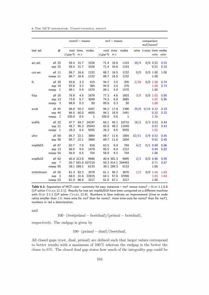
6 The MCF-separator: Computational impact
nomcf – means mcf – means comparisonmcf/nomcf
test set # root time nodes root time nodes wins t-outs time nodescl.gap% in s cl.gap% in s ratio ratio
arc.set all 25 58.4 31.7 3326 71.4 16.6 1103 20/4 0/0 0.52 0.33sep 25 58.4 31.7 3326 71.4 16.6 1103 0.52 0.33
cut.set all 11 88.7 16.6 1232 88.7 16.5 1232 0/0 0/0 1.00 1.00nosep 11 88.7 16.6 1232 88.7 16.5 1232 1.00
fc all 20 93.6 3.3 415 94.2 3.5 305 2/10 0/0 1.08 0.74sep 19 93.8 3.2 384 94.5 3.4 276 1.08 0.72
nosep 1 89.1 5.9 1570 89.1 5.9 1570 1.00
fctp all 16 76.9 4.5 1679 77.3 4.6 1603 3/5 0/0 1.02 0.95sep 13 73.8 6.7 3049 74.3 6.8 2885 1.02 0.95
nosep 3 89.9 0.3 50 89.9 0.3 50 1.06
avub all 45 86.8 55.2 4267 94.2 17.8 1396 25/8 0/14 0.32 0.33sep 44 86.5 60.0 4658 94.1 18.9 1491 0.32 0.32
nosep 1 100.0 0.5 1 100.0 0.6 1 1.20
sndlib all 22 47.7 84.7 24197 64.1 45.1 10710 18/2 0/3 0.53 0.44sep 21 48.7 95.3 25943 65.8 49.2 11049 0.52 0.43
nosep 1 26.3 6.4 5555 26.3 6.5 5555 1.02
ufcn all 58 85.7 22.1 3984 89.7 11.6 1804 32/11 0/9 0.52 0.45sep 58 85.7 22.1 3984 89.7 11.6 1804 0.52 0.45
miplib03 all 67 62.7 7.0 816 62.5 6.9 784 4/2 0/1 0.99 0.96sep 13 86.5 9.0 1479 85.5 8.4 1212 0.94 0.82
nosep 54 56.9 6.5 704 56.9 6.5 704 1.00
miplib10 all 62 40.4 312.9 9946 40.4 301.3 9495 2/1 0/0 0.96 0.95sep 7 50.7 581.8 427218 50.3 414.1 284493 0.71 0.67
nosep 55 39.1 289.1 6133 39.1 289.3 6133 1.00
mittelmann all 56 61.3 82.2 3579 61.1 85.2 3676 1/2 0/0 1.04 1.03sep 3 68.0 31.6 22815 64.1 57.8 37098 1.83 1.63
nosep 53 61.0 86.8 3217 61.0 87.1 3217 1.00
Table 6.3: Separation of MCF-cuts – summary for easy instances – mcf versus nomcf – Scip 1.1.0.8(LP solver Cplex 11.2.1). Results for test set miplib2010 have been computed on a different machinewith Scip 2.1.1 (LP solver Cplex 12.4). Numbers in blue indicate an improvement (time or noderatios smaller than 1.0, more wins for mcf than for nomcf , more time-outs for nomcf than for mcf ),numbers in red a deterioration.
and100 · (bestprimal − bestdual)/(primal − bestdual),
respectively. The endgap is given by
100 · (primal − dual)/|bestdual|.
All closed gaps (root, dual, primal) are defined such that larger values correspondto better results with a maximum of 100% whereas the endgap is the better thecloser to 0%. The closed dual gap states how much of the integrality gap could be
104

6.2 Success of the separation
nomcf – means mcf – means comparisonmcf/nomcf
test set # root dual primal endgap root dual primal endgap wins endgapclosed gap in % in % closed gap in % in % ratio
arc.set all 10 33.9 59.3 86.9 1.4 35.6 61.8 86.5 1.3 2/1 0.93sep 10 33.9 59.3 86.9 1.4 35.6 61.8 86.5 1.3 0.93
cut.set all 4 58.0 68.0 100.0 12.6 58.0 68.0 100.0 12.6 0/0 1.00nosep 4 58.0 68.0 100.0 12.6 58.0 68.0 100.0 12.6
fctp all 16 21.2 24.0 97.1 24.9 21.3 24.1 97.5 24.8 0/0 0.99sep 16 21.2 24.0 97.1 24.9 21.3 24.1 97.5 24.8 0.99
avub all 15 31.1 37.7 29.1 83.9 72.5 75.6 91.7 10.2 14/0 0.12sep 15 31.1 37.7 29.1 83.9 72.5 75.6 91.7 10.2 0.12
sndlib all 30 31.9 56.5 90.5 7.6 42.0 63.8 94.2 6.2 17/2 0.82sep 29 32.7 57.8 90.5 8.5 43.2 65.3 94.3 6.9 0.81
nosep 1 9.6 20.4 91.7 0.2 9.6 20.4 91.7 0.2
ufcn all 25 74.5 80.9 84.5 10.7 81.8 87.7 91.5 7.2 19/2 0.67sep 25 74.5 80.9 84.5 10.7 81.8 87.7 91.5 7.2 0.67
miplib03 all 25 19.0 36.3 38.2 15.9 19.0 36.5 38.2 15.9 0/0 1.00sep 3 11.4 28.8 99.7 14.8 11.5 30.2 99.7 14.2 0.97
nosep 22 20.0 37.3 32.0 16.1 20.0 37.4 32.0 16.1
miplib10 all 21 31.5 60.5 57.1 5.6 32.0 61.5 57.1 5.3 2/1 0.95sep 3 51.3 82.1 66.7 12.6 54.4 89.2 66.7 8.8 0.70
nosep 18 28.2 56.9 55.6 4.8 28.2 56.9 55.6 4.9
mittelmann all 3 19.6 52.4 100.0 2.7 19.6 52.4 100.0 2.7 0/0 1.00nosep 3 19.6 52.4 100.0 2.7 19.6 52.4 100.0 2.7
Table 6.4: Summary for hard instances – mcf versus nomcf – Scip 1.1.0.8 (LP solver Cplex 11.2.1).Results for test set miplib2010 have been computed on a different machine with Scip 2.1.1 (LP solverCplex 12.4). Numbers in blue indicate an improvement (endgap ratios smaller than 1.0, more winsfor mcf than for nomcf ), numbers in red a deterioration.
closed by the dual bound at termination. Similarly, the closed primal gap stateshow much gap towards the best known solution could be closed by the given primalsolution. The values lp and bestprimal are defined as above and can be found inTable A.1 on page 220 together with the bestdual, which refers to the best knowndual bound. The numbers primal and dual correspond to the primal and dualbound at the end of the optimization. Note that in case that primal = bestdualfor an individual run we set the closed primal gap to 100%. If the LP value isalready optimal (lp = bestprimal = bestdual), then rootgap as well as dualgapare considered to be 100%. If primal or dual bounds are not finite or in case thatbestdual = 0, the corresponding gaps are not defined and hence not consideredin the calculation of the mean. Again all mean values are given for both the mcfand nomcf runs. The last two columns in Table 6.4 (mcf/nomcf ) compare the mcfand nomcf runs with respect to the number of wins (wins) and the endgap. If byswitching on the MCF-separator the endgap decreases by at least 10% we say that
105

6 The MCF-separator: Computational impact
nomcf – means mcf – means comparisonmcf/nomcf
test set # time nodes time nodes wins t-outs time nodesin s in s ratio ratio
arc.set all 25 14.9 3244 10.2 1258 15/4 0/0 0.70 0.39sep 23 16.9 3344 11.2 1194 0.68 0.36
nosep 2 3.2 2286 3.2 2286 1.01 1.00
cut.set all 12 12.7 892 12.7 1232 0/0 0/0 1.00 1.00nosep 12 12.7 892 12.7 1232 1.00 1.00
fc all 20 1.5 270 1.6 260 5/7 0/0 1.04 0.97sep 20 1.5 270 1.6 260 1.04 0.97
fctp all 17 3.9 751 4.1 687 3/5 1/0 1.04 0.92sep 15 5.0 1329 5.3 1202 1.05 0.91
nosep 2 0.1 1 0.1 1 1.00 1.00
avub all 41 4.6 413 1.8 163 18/2 0/3 0.50 0.33sep 40 4.8 454 1.9 175 0.49 0.32
nosep 1 0.1 1 0.1 1 1.00 1.00
sndlib all 25 93.3 20353 41.1 7427 18/1 0/4 0.45 0.37sep 22 81.1 15624 31.8 4967 0.40 0.32
nosep 3 258.5 141400 258.4 141400 1.00 1.00
ufcn all 67 3.3 349 3.5 404 8/11 0/0 1.05 1.15sep 59 3.4 379 3.6 448 1.05 1.18
nosep 8 2.6 186 2.6 186 1.01 1.00
miplib03 all 67 3.0 558 2.9 556 3/1 0/0 0.99 1.00sep 8 5.7 1060 5.2 1023 0.93 0.97
nosep 58 2.7 511 2.7 511 1.00 1.00
mittelmann all 56 23.2 1101 22.4 1073 3/2 0/0 0.97 0.98sep 6 73.2 5232 52.2 4135 0.72 0.79
nosep 50 20.1 912 20.2 912 1.00 1.00
cplex all 1266 34.9 1201 34.2 1170 45/35 5/5 0.98 0.97sep 115 42.8 6665 34.9 5006 0.82 0.75
nosep 1151 34.1 1011 34.2 1011 1.00 1.00
cplex10s all 780 132.5 3225 128.8 3118 30/25 5/5 0.97 0.97sep 77 142.9 15230 106.8 10856 0.75 0.71
nosep 703 131.4 2719 131.5 2719 1.00 1.00
cplex100s all 411 504.4 8989 484.1 8589 20/13 5/5 0.96 0.96sep 42 546.3 38192 365.8 24486 0.67 0.64
nosep 369 499.8 7623 499.8 7623 1.00 1.00
Table 6.5: Summary for easy instances – mcf versus nomcf – Cplex 12.1. Numbers in blue indicatean improvement (time or node ratios smaller than 1.0, more wins for mcf than for nomcf , moretime-outs for nomcf than for mcf ), numbers in red a deterioration.
the mcf -run wins. If it increases by at least 10% the nomcf -run wins.
In Table 6.3, it can be seen that our implementation of the MCF-separator in Scipdrastically reduces the computation times and branch-and-bound nodes for almost
106
6.2 Success of the separation
all of the network design instances. In particular for the test sets arc.set , avub,sndlib, and ufcn we save between 55% and 67% of the tree nodes and between 47%and even 68% of the solving time on average. Moreover, 14 avub, 3 sndlib, and9 ufcn instances can be solved within the time limit of one hour only if the MCF-separator is switched on. Table 6.4 shows similar effects for the hard instances ofthese 4 test sets. The average endgap is decreased and the mcf -run wins in mostof the cases. The results for the hard avub instances are remarkable. We decreasethe endgap from 83.9% to 10.2% on average which is caused by improving boththe dual and the primal bounds. Already at the root node we close the optimalitygap by 72.5% compared to 31.1% without the MCF-separator. For the very easytest sets fc and also fctp (excluding the n37* instances) with an average solvingtime of less than 5s we decrease the number of nodes but slightly increase thesolving time (from 3.3s to 3.5s and from 4.5s to 4.6s on average), see Table 6.3.For these instances it does not pay off to tighten the relaxation. Our separatorhas no effect on the hard fctp n37* instances (see Table 6.4) and for the (hard andeasy) cut.set instances the MCF-separator is switched off because the networks arenot consistent, also compare with Table 6.2 on page 101.
The results for the easy mittelmann are not conclusive since the number of affectedinstances is too small. The performance slightly degrades for 2 out of 3 easymittelmann instances. However, we observe a remarkable improvement for easymiplib03 andmiplib10 instances. Time and branch-and-bound nodes are decreasedby 1–5% on average for these test sets. This is caused by a significant speedupon a subset of only 13 and 7 instances, respectively. One miplib03 instance (tr12-30) can only be solved in the mcf -run. For 3 hard miplib03 and 3 hard miplib10instances we decrease the endgap on average by 3% and 30%, respectively.
Table 6.5 on the previous page shows that the results for Cplex are comparable tothe results for Scip with respect to the easy network design instances. The effectis not as dramatic since Cplex is already very fast without the MCF-separator(compare the average nomcf computation times in Table 6.3 and Table 6.5). Butthe decrease of the computation time is still between 30% and 55% for the arc.set ,avub, and sndlib instances with 61%-67% saved branch-and-bound nodes. Incontrast to Scip the time increases for the ufcn test set but these instances arevery easy for Cplex with average solving times below 5s in the nomcf run similarto the fc and fctp test sets. The results for the sndlib test set are in line withthe results from [199, 200], which show a possible time reduction of 70–90% withCplex 10.0 using flow cut-set inequalities (knowing the networks before-hand), cf.Section 2.5.
Let us discuss the results in Table 6.5 for the general MIP instances and Cplex.We can trust these values since the overall test set is very large with a reasonablenumber of affected instances. In addition to the miplib03 and mittelmann testsets we consider an internal Cplex-library containing 1266 easy instances (cplex ).The subsets cplex10s and cplex100s correspond to those instances within cplex thatneed at least 10s and 100s of CPU time to be solved, respectively, by the slower
107

6 The MCF-separator: Computational impact
Ψmax = 0.02? Ψmax = 0.02? Ψmax =∞ Ψmax =∞Ψmaxa = 0.5? Ψmax
a =∞ Ψmaxa = 0.5? Ψmax
a =∞test set # sep wins time sep wins time sep wins time sep wins time
Scip
miplib03 67 13 4/2 0.99 13 4/2 0.99 18 5/3 0.98 20 5/6 0.99mittelmann 56 3 1/2 1.04 3 1/2 1.03 9 3/3 1.03 10 6/3 1.01
Cplex
miplib03 67 8 3/1 0.99 8 3/1 0.99 11 3/2 0.99 12 3/2 0.99mittelmann 56 6 3/2 0.97 6 2/2 0.97 9 3/4 0.98 10 3/5 1.00cplex 1266 115 45/35 0.98 115 46/33 0.98 214 78/80 0.99 247 84/99 1.00cplex10s 780 77 30/25 0.97 77 31/24 0.97 146 58/56 0.98 166 62/71 0.99cplex100s 411 42 20/13 0.96 43 20/11 0.96 81 35/28 0.96 90 39/34 1.01
Table 6.6: Impact of inconsistency – Scip 1.1.0.8 and Cplex 12.1 – easy instances. Default valuesmarked with ?. In every row, we highlight in blue the best time ratio and the largest difference ofwins(mcf ) minus wins(nomcf ).
of the two versions, mcf and nomcf . Among all 1389 MIP instances (miplib03 ,mittelmann, and cplex ) 129 instances or 9.3% are affected by the MCF-separator.We save 17.9% of the computation time and 23.6% of the search tree nodes onaverage for these 129 instances which refers to 2% time and 2.8% node savingsover the whole test set. Moreover, it turns out that the harder the instances are tosolve the larger are the benefits of the MCF-separator. The saved time amounts to25% for the 77 affected instances in cplex10s and to even 33% for the 42 affectedinstances in cplex100s.
In all cases (Scip, Cplex, easy and hard), if the separator is switched off or doesnot find violated inequalities there is almost no degradation of the computationtime, cf. the nosep rows. This means that the detection as well as the separationprocedures are very fast. Summarizing it can be said that using the MCF-separatormany instances can now be solved within 1 hour that could not be solved before.For the instances the separator is designed for a significant reduction in the com-putation time and the branch-and-bound nodes is observed which is driven byimproved dual bounds at the root node. Whenever the solvers struggle in solvinga specific problem class switching on the MCF-separator gives substantial benefits(e.g. avub, sndlib for Scip and sndlib, cplex100s for Cplex).
6.3 The impact of inconsistencies
The two parameters Ψmaxa and Ψmax control our algorithm with respect to incon-
sistent or not existing networks in the constraint matrix. If violated inequalitiesare identified these are always valid since our framework relies on aggregatingoriginal constraints and on applying MIR to aggregations. But the larger the in-consistency in the network the lower the chance to produce base inequalities that
108

6.3 The impact of inconsistencies
0 0.005 0.05 0.5
0
20
40
Maximum network inconsistency ratio Ψmax
Num
ber
ofin
stan
ces
nicesepwins(mcf)wins(nomcf)
Figure 6.1: Impact of inconsistency – Scip 1.1.0.8 – easy instances in miplib03 . Ψmaxa = ∞. nice:
Detected networks with inconsistency ratio Ψ(D) ≤ Ψmax, sep: At least one violated MCF-cut. Thenumber of instances which benefit from the MCF-separator is relatively constant (wins(mcf)). Theseinstances have small inconsistency ratio Ψ(D). The performance is deteriorated if large inconsistencyratios are allowed (wins(nomcf) increases).
correspond to network cuts or to have any relation to a network. For very largeinconsistency we basically simulate randomized aggregation. Moreover, since thenumber of considered original constraints can be very large (in contrast to the de-fault c-MIR heuristics) and because there is not necessarily a proper cancellationof flow variables in case of inconsistency we might produce dense and unstablecutting planes.
Increasing Ψmaxa means to increase the size of the networks (and hence the size of
the aggregations) by allowing for more inconsistent arcs (and the correspondingcapacity constraints). These are arcs with uncertain source or target assignment.On the other hand, increasing Ψmax means to consider more instances for sepa-ration. In the first test we released both parameters Ψmax
a and Ψmax individuallyand simultaneously. Table 6.6 on the facing page reports on the results for allconsidered general MIP instances for both Scip and Cplex. The third columnin Table 6.6 gives the total number of easy instances in the test set. For everyrun there are three columns providing the number of affected instances (sep), theratio of the wins (wins), and the time ratio (time). The ratios compare the respec-tive mcf -run with the nomcf -run. The time ratios are based on shifted geometricmeans over the whole test set (not only the affected instances). The number ofclusters k is fixed to 5 in all runs. Columns 4–6 in Table 6.6 summarize the valuesfor the default settings for comparison. These are precisely the values you canalready find in Table 6.3 on page 104 and Table 6.5 on page 106 for Scip andCplex, respectively. The results for the test sets miplib03 and mittelmann shouldnot be overrated since the number of affected instances is small.
It can be seen that releasing the maximum arc inconsistency ratio Ψmaxa alone
(Columns 7–9) does not remarkably change the behavior of the solver. Recall thatthe network inconsistency ratio Ψ(D) is defined as the mean of the arc inconsis-tency ratios Ψ(a). Hence in case of a very small value Ψ(D) there cannot be manyinconsistent arcs such that releasing Ψmax
a while keeping Ψmax small has not a
109

6 The MCF-separator: Computational impact
great impact on our algorithm. On the other hand, relaxing the maximum net-work inconsistency ratio Ψmax while keeping Ψmax
a = 0.5 (Column 10–12) alreadydeteriorates the performance. There are more instances considered for separationbut the wins and time ratios degrade at least for the larger cplex test sets. Asshown in Columns 13–15 of Table 6.6, releasing both inconsistency parameterseven worsens the performance in terms of wins and time ratios while the numberof affected instances is again increasing. It turns out that the arc inconsistencyratio is not as important as the network inconsistency ratio, but releasing both re-strictions gives the worst results. In a second test, we study the impact of differentvalues for Ψmax while fixing Ψmax
a =∞. We restrict our attention to the Scip testsand the easy instances within the miplib03 test set. Figure 6.1 on the previouspage shows the number of instances that are considered to contain a consistent net-work (nice) and the number of instances for which at least one violated inequalitywas found (sep). The values wins(mcf) and wins(nomcf) refer to the number ofinstances for which the computation time was decreased (wins(mcf)) or increased(wins(nomcf)) by at least 10% switching on the MCF-separator. There are 14 easyinstances in miplib03 with an embedded network and Ψ(D) = 0. For 11 of theseinstances we found at least one violated inequality. It is no surprise that the num-ber of considered instances increases with Ψmax. Since the largest inconsistencyratio in miplib03 is 0.656 (compare with Table 6.2 on page 101) a value Ψmax = 0.8means that the MCF-separator is switched on for all 40 easy miplib03 instancescontaining an embedded network. But it is remarkable that the number of affectedinstances only slightly increases to 20. For most of the instances with very large in-consistency ratios the generated inequalities are not violated such that separationbased on the network detection has no effect. Moreover, for values of Ψmax largerthan 0.05 there are more and more instances for which using the MCF-separatorincreases the computation time. Notice that wins(nomcf) increases. Hence even ifviolated inequalities are found they do not help.
Summarizing the observed phenomena from Table 6.6 and Figure 6.1 on the pre-vious page, both mechanisms for refusing inconsistent networks or network com-ponents help to improve the overall performance of the separator and can be usedalone. But the best results are obtained with a small maximum network inconsis-tency ratio Ψmax. We decided to use a more conservative default setting with bothΨmaxa and Ψmax being active. For Ψmax a good trade-off between performance and
the number of affected instances seems to be between 0.02 and 0.05. Based on anumber of similar test scenarios we fixed Ψmax
a to 0.5.
6.4 The impact of aggressive separation
By changing the value of k we control the size of the partition used to enumeratenetwork cuts and thus the size of the network cut collection C, see Chapter 5.For directed networks the number of considered cuts amounts to a maximum of2k − 2, but recall that we allow for cut-sets only if both cut-shores are connected.
110

6.4 The impact of aggressive separation
k = 3 k = 5? k = 7 k = 9
test set # sep wins time cuts wins time cuts wins time cuts wins time cuts
arc.set 25 25 20/3 0.53 110 20/4 0.52 133 19/3 0.57 169 20/0 0.50 205fc 20 19 3/13 1.13 423 2/10 1.08 464 6/11 1.10 620 3/14 1.24 819fctp 16 13 3/3 0.99 424 3/5 1.02 455 4/3 0.98 506 3/6 0.99 699avub 45 44 27/8 0.32 249 25/8 0.32 256 25/8 0.36 278 22/11 0.34 329sndlib 22 21 18/2 0.64 102 18/2 0.53 144 15/4 0.38 220 16/2 0.37 296ufcn 58 58 29/11 0.52 118 32/11 0.52 135 30/13 0.53 202 24/16 0.54 358miplib03 67 13 4/1 0.99 54 4/2 0.99 58 3/3 0.99 66 4/3 1.00 73mittelmann 56 3 1/2 1.03 6 1/2 1.04 8 0/3 1.04 5 0/2 1.04 5
Table 6.7: Impact of the partition size k – Scip 1.1.0.8 – easy instances. Default value markedwith ?. In every row, we highlight in blue the best time ratio and the largest difference of wins(mcf )minus wins(nomcf ).
The parameter k should be large enough to produce enough interesting cut-setsand cut-based inequalities. But setting it too large can result in unacceptablecomputation times for calculating the inequalities itself and also for solving theLP relaxations since too many violated inequalities might be added.
In the test reported in Table 6.7 we increased the value k from 3 to 9 fixing theinconsistency parameters Ψmax and Ψmax
a to their default values. Table 6.7 containsall test sets except for cut.set for which no inequalities are separated independentof k. We report on the number of easy instances contained in each of the test sets(#) as well as the number of affected instances (sep) which is constant over theconsidered scenarios. For every run we report on the ratio of the wins (wins), theshifted geometric mean of the time ratios (time), and the arithmetic mean of thenumber of inequalities added to the LP (#cuts). The means are taken over alleasy instances of the test set.
First it can be observed that the number of generated cutting planes increaseswith k but the increase is not exponential. The number of added inequalitiesapproximately doubles from k = 3 to k = 9. Only the sndlib instances reallybenefit from a large k value. For this test set the time ratio decreases from 0.64for k = 3 to 0.37 for k = 9. The performance is slightly deteriorated for fc, avub,ufcn, miplib03 , and mittelmann while it is slightly improved for arc.set and fctp.We decided to fix k to the conservative value 5. However, for certain classes ofnetwork design instances it can be crucial to cut more aggressively.
111

Chapter 7
Concluding remarks Part II
Because cut-based MIR inequalities can be used to drastically reduce computationtimes and gaps when generated within branch-and-cut procedures to solve networkdesign problems and because these strong inequalities are not detected by state ofthe art MIP solvers, we proposed a separation framework for general MIP that isnow implemented in Scip and Cplex. This algorithm consists of two main steps.
First, we try to identify the block structure of a multi-commodity flow formula-tion in the constraint matrix of a general MIP. Coupling capacity constraints areused to resolve the isomorphism of the graphs represented by the network matri-ces of individual commodity blocks and the corresponding underlying network isconstructed.
Second, we derive cutting planes based on the identified network structure. Usingmappings from network elements to rows of the original MIP formulation, wereplace the default aggregation heuristic of the c-MIR separator implemented inScip and Cplex. In our framework, rows are aggregated such that the resultingbase inequalities correspond to network cuts. These base inequalities are then usedto generate MIR cut-set inequalities, flow-cover inequalities, dicut inequalities, andthe like, depending on the type of capacity constraints and variables. In contrastto the default aggregation of the c-MIR separator, the number of aggregated rowsdepends on the size of the network and can be in the order of hundreds. However,the calculated base inequalities are sparse due to the +1,−1 pattern in thedetected network matrices.
A key-feature of our implementation is the ability to determine the consistencyof the detected networks. Only if the calculated overall network inconsistencyratio is very small we trust the detected structures and generate cutting planes.We also delete inconsistent network elements in order to work on the consistentnetwork core only. With this machinery we are able to recognize network designtype models for which the methods are successful, introducing almost no overheadfor other models.
113

7 Concluding remarks Part II
We showed, through extensive computational tests, that the proposed separationscheme speeds-up the computation for a large set of network design problems bya factor of two on average. Many of these problems can only be solved within onehour of CPU time if the MCF-separator is switched on. For 17% of general MIPinstances we detected consistent network structure based on flow matrices. In 9–12% of all cases we generated violated structural cutting planes. The computationtime could be decreased by 18% (Cplex with internal test set) to 29% (Scip withMiplib 2010) on average for affected MIP instances with almost no degradationfor unaffected instances.
Given these results and the fact that state-of-the-art MIP solvers have almost noknowledge about the underlying problem, one might consider a new paradigm ofexploiting structure in MIP solving. Many known and very successful approaches(cutting planes, heuristics, branching rules) for special purpose problems couldbe used within the MIP solver if the constraint matrices are scanned for knownstructures.
114

Part III
Demand uncertainty: Design ofrobust networks
115

Chapter 8
Introductory remarks Part III
In this part of the thesis, we extend the concepts of capacitated network designfrom Chapter 2 to include demand uncertainty. The task is to dimension networkswithout precise knowledge about the actual traffic demands. One has to designnetwork capacities that are robust enough to handle different demand scenariosand traffic dynamics. As a methodology, we apply the recently established ro-bust optimization framework which deals with data uncertainties in mathematicalprogramming. In particular, we will study the case where all possible demandscenarios lie in a predefined demand polytope. On the one hand, we study for-mulations, solution methods, and cutting planes for the extended problem. Inparticular, we generalize cut-based inequalities from Chapter 2 and provide facetproofs. On the other hand, we consider different rerouting strategies to cope withtraffic dynamics and work out properties of the resulting solution spaces. We alsoprovide computations comparing different approaches to robust network design.Based on realistic scenarios and measurements from real networks, we evaluatethe resulting robustness of the solutions. The material in this part of the thesis ispartially joint work with Michael Poss [196, 197] and with Arie Koster and ManuelKutschka [152–155].
Motivation
In the classical capacitated network design problem, as studied in Chapter 2, trafficdemands are given as nominal values between pairs of network nodes. Givena potential topology D = (V,A), we typically assume a given demand matrixd ∈ QV×V
+ , where the entries dk ≥ 0 for k = (s, t) ∈ V ×V correspond to a demandfor flow between the source s ∈ V and the target t ∈ V of commodity k. The goalis to provide minimum-cost capacities that support the given demand matrix d,that is, the capacitated network has to accommodate the demands by a multi-commodity flow. This classical approach assumes that all demands are knownwith precision and do not (dramatically) change over time. However, varying the
117
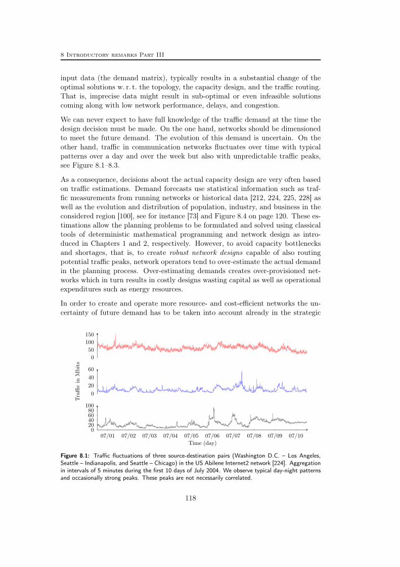
8 Introductory remarks Part III
input data (the demand matrix), typically results in a substantial change of theoptimal solutions w. r. t. the topology, the capacity design, and the traffic routing.That is, imprecise data might result in sub-optimal or even infeasible solutionscoming along with low network performance, delays, and congestion.
We can never expect to have full knowledge of the traffic demand at the time thedesign decision must be made. On the one hand, networks should be dimensionedto meet the future demand. The evolution of this demand is uncertain. On theother hand, traffic in communication networks fluctuates over time with typicalpatterns over a day and over the week but also with unpredictable traffic peaks,see Figure 8.1–8.3.
As a consequence, decisions about the actual capacity design are very often basedon traffic estimations. Demand forecasts use statistical information such as traf-fic measurements from running networks or historical data [212, 224, 225, 228] aswell as the evolution and distribution of population, industry, and business in theconsidered region [100], see for instance [73] and Figure 8.4 on page 120. These es-timations allow the planning problems to be formulated and solved using classicaltools of deterministic mathematical programming and network design as intro-duced in Chapters 1 and 2, respectively. However, to avoid capacity bottlenecksand shortages, that is, to create robust network designs capable of also routingpotential traffic peaks, network operators tend to over-estimate the actual demandin the planning process. Over-estimating demands creates over-provisioned net-works which in turn results in costly designs wasting capital as well as operationalexpenditures such as energy resources.
In order to create and operate more resource- and cost-efficient networks the un-certainty of future demand has to be taken into account already in the strategic
0
50
100
150
0
20
40
60
Tra
ffic
inM
bit
s
07/01 07/02 07/03 07/04 07/05 07/06 07/07 07/08 07/09 07/100
20406080100
Time (day)
Figure 8.1: Traffic fluctuations of three source-destination pairs (Washington D.C. – Los Angeles,Seattle – Indianapolis, and Seattle – Chicago) in the US Abilene Internet2 network [224]. Aggregationin intervals of 5 minutes during the first 10 days of July 2004. We observe typical day-night patternsand occasionally strong peaks. These peaks are not necessarily correlated.
118

8 Introductory remarks Part III
Mo, 30th Mo, 6th Mo, 13th Mo, 20th
2
3
4
·104
Time (day)
Trafficin
Mbits
Figure 8.2: Total traffic in the European research network Geant [212, 228] (sum over all source-destination pairs). Aggregation in intervals of 1 hour during 4 weeks in June 2005. Traffic is high onbusiness days and around noon, while the demand is low on weekends and in the early morning.
01:00
03:00
05:00
07:00
09:00
11:00
12:00
13:00
15:00
17:00
19:00
23:00
0
0.2
0.4
0.6
0.8
1·104
Time (hour)
Trafficin
Mbits
(a) Geant network
01:00
03:00
05:00
07:00
09:00
11:00
12:00
13:00
15:00
17:00
19:00
23:00
0
0.2
0.4
0.6
0.8
1·104
Time (hour)
Trafficin
Mbits
(b) DFN network
Figure 8.3: Total traffic in the European research network Geant [212, 228] and in the Germanresearch network DFN [98, 228] (sum over all source-destination pairs). Aggregation in intervals of15 minutes (Geant) and 5 minutes (DFN) during day 2005/05/05 (Geant) and 2005/15/02 (DFN).We observe a typical day-night traffic pattern.
capacity design process. In mathematical programming, we distinguish two mainframeworks to incorporate the uncertainty of data into optimization models. Theseare stochastic optimization and robust optimization. Stochastic programming, go-ing back to Dantzig [92], uses probabilities for the possible realizations of theuncertain data. Instead of (estimated) nominal values, a probabilistic distributionof the data is taken as input of the problem. A typical goal is to minimize theexpectation of some cost-function of the decision and random variables. That is,the average cost (over all scenarios and weighted using the given probabilities)is optimized. Often so-called chance constraints [208, Chapter 4] are introducedwhich consider solutions to be feasible if they satisfy a certain constraint (e.g. a ca-pacity constraint) with high probability (w. r. t. the given distribution). However,stochastic programs can become computationally demanding compared to theirdeterministic counterparts. Furthermore, the required probabilistic distributionsare not always known and thus are very often estimated.
In contrast, in robust optimization [41, 42, 47, 48, 209], the framework we adapthere, the distribution of the uncertain data is completely ignored. Instead, asolution is said to be feasible if it satisfies the considered constraints for all (possible
119

8 Introductory remarks Part III
2010 2011 2012 2013 2014 20150
0.2
0.4
0.6
0.8
1·104
Time (year)
Trafficin
Petab
ytepe
rmon
th
VideoP2PTVOther
Figure 8.4: Cisco forecast for Western Europe [73]: consumer IP traffic evolution – 2010-2015 –file sharing (P2P); Internet video, video communications (Video); managed TV services (TV); Web,Data, Email, Gaming (Other)
or considered) realizations of data. The predefined set of considered data scenariosis called the uncertainty set. In the context of robust capacitated network design,we will consider capacity designs as feasible if they support all demand matricesin a given demand uncertainty set D. In this thesis, we will mainly restrict ourattention to the case where D is a polytope (although some theoretical resultsextend to more general bounded convex sets).
Definition 8.1. We say that network capacities support a given set D of demandscenarios if there exists a flow for every scenario d ∈ D realizing the demandwithin these capacities. Robust capacitated network design means to find cost-minimal capacities supporting D.
Notice that we do not further restrict the notion of capacities in this definition,similar to Definition 2.1 for deterministic capacitated network design. We refer toSection 2.4 for possible realistic capacity models. In the sequel, we will mainlyconsider integral capacities. However, to better understand the structure of theproblems we also study the continuous case, which is helpful in developing LPbased branch-and-cut codes.
At first sight, robust network design seems to be conservative since we considermore than just a single scenario and hence reduce the number of feasible solutionswhich might increase the optimal cost. However, as explained above, in order to ob-tain robust solutions using deterministic tools, practitioners tend to over-estimatethe demand which in turn means using a single and artificial peak scenario outsidethe actual uncertainty set D, see Figure 8.5. In fact, explicitly incorporating allrealistic scenarios in D might instead reduce the cost for robust solutions. Clearly,the shape of the used uncertainty set D has a strong impact on the quality androbustness of the solution. In particular, this set should reflect typical patternsand observed phenomena from historical data.
120

8 Introductory remarks Part III
0 d1
d2observed peak for d2
observed peak for d1
artificial peak scenario
Figure 8.5: Exemplary traffic scenarios over time and the corresponding artificial worst case peakscenario w. r. t. two different source destination pairs, commodities 1 and 2.
Related work
For a survey on stochastic and robust optimization we refer to Shapiro et al. [208]and Ben-Tal, El Ghaoui, and Nemirovski [44], respectively.
The general concept of robust linear programming has been introduced by Soyster[209] assuming uncertain coefficients in the constraint matrix of a linear program.Significant progress has been made by Ben-Tal and Nemirovski [40, 41, 42] andalso Bertsimas and Sim [48] using different convex and bounded uncertainty sets.These authors also introduced the notion of robust counterparts for uncertainlinear programs. Ben-Tal and Nemirovski [40] showed how to solve robust linearprograms using reformulations that depend on the given uncertainty set. Forexample, a robust linear program reduces to another deterministic linear programif the uncertainty set is polyhedral and it reduces to a deterministic conic quadraticprogram if the uncertainty set is ellipsoidal.
Recourse and routing. In the original framework of Soyster [209] all problemvariables have to be fixed, independent of the realization of the data. Introducingmore flexibility and allowing for less conservative solutions, two-stage robust op-timization, as introduced by Ben-Tal et al. [43] and following the well establishedconcept of multi-stage stochastic programming [208, Chapters 2 and 3], allows anadjustment of a subset of the problem variables only after observing the actualrealization of the data. This second stage adjusting procedure is called recourse.For general two-stage robust network design see Atamtürk and Zhang [21].
In fact, it is natural to apply the two-stage approach to network design. Long-term capacity design decisions are made in the first stage, while the actual flow isadjusted based on observed user demands in the second stage. In telecommunica-tions, this second stage adjusting procedure is well established and known as trafficengineering. Unrestricted second stage recourse in robust network design is calleddynamic routing, see for instance [68, 130], and [172]. Dynamic routing allows
121
8 Introductory remarks Part III
for full flexibility in rerouting the traffic if the demand changes. That is, given afixed design, the commodity flow can be changed arbitrarily as a function of thedemand d ∈ D. Gupta et al. [130], Chekuri et al. [68], and Minoux [177] showedthat allowing for dynamic routing makes robust network design intractable. Moreprecisely, it is co-NP-complete to decide whether a capacitated network allows fora dynamic routing of demands when the uncertainty set D of all possible demandvectors is a polytope. This is true even if D is described by polynomially manyinequalities. We refer to Mattia [172] on how to handle the corresponding hardnessof the separation problem in Benders decomposition when solving robust networkdesign problems with dynamic routing.
More generally, Ben-Tal et al. [43] observed that two-stage robust linear program-ming with free recourse is computationally intractable and suggested to limitthe flexibility in the second stage by affine functions which makes the problemtractable. Chen and Zhang [69] extended this idea by using extended formula-tions of uncertainty sets and by applying affine policies in the resulting higher-dimensional variable spaces.
Interestingly, this limitation in the flexibility of the second stage has been usedearlier in robust network design without relating it to two-stage optimization. Ben-Ameur and Kerivin [38, 39] introduced the concept of static routing which is alsoknown as oblivious routing [116, 182, 185] or stable routing [39, 67]. Static routingmeans that for every commodity k = (s, t) and independent of the size of thedemand dk the same (s, t)-paths are used with the same flow splitting among thepaths. We speak of a (static) routing template used by all demand realizations.In this respect, the flow of a commodity is allowed to change but it is a linearfunction of the demand dk for every commodity k ∈ K. Static routing has beenused extensively since then, as it makes robust network design tractable but alsobecause it relates to routing schemes used in practice such as the OSPF (openshortest path first) protocol in IP (Internet protocol) networks, see [58].
The restriction of routing templates for every commodity makes the problemtractable but it is more conservative in terms of capacity cost compared to dy-namic routing. Recently there have been several attempts to handle less restric-tive routing principles most of which could be shown to be intractable just like thedynamic case. Ben-Ameur [37] partitioned the demand uncertainty set into two(or more) subsets using hyperplanes and devises specific routings for each subset.The resulting optimization problem is NP-hard when no assumptions are made onthe hyperplanes. Scutellá [206, 207] introduced a generalization of the procedurefrom [37] by allowing for two (or more) routing templates to be used conjointlyand proved NP-hardness of the corresponding robust network design problem.
As an alternative to these NP-hard approaches, Ouorou and Vial [190] and Babon-neau, Klopfenstein, Ouorou, and Vial [24] directly applied the affine decision rulesfrom [43] to network design problems using particular uncertainty sets. The result-ing restrictive routing scheme is referred to as affine routing and can be seen as ageneralization of static routing. In this context, affine routing provides an alterna-
122

8 Introductory remarks Part III
tive in between static and dynamic routing yielding tractable robust counterpartsin contrast to the schemes used in [37, 206].
Polyhedral uncertainty sets. The cost for robust solutions strongly dependson the shape of the uncertainty set. Ben-Ameur and Kerivin [39] considered staticrouting and demands that may vary within a polytope D in the space of the com-modities. For telecommunication network design problems the concept of poly-hedral demand uncertainty sets has mainly been applied using the Hose-model,which is of practical relevance as it appears naturally in the context of designingvirtual private networks [99]. In its symmetric version, the Hose-model definesupper bounds on the sum of the incoming and outgoing node traffic for all loca-tions. Hence the Hose polytope is defined by inequalities at the customer nodes.This model has attracted a lot of attention in recent years, in particular, withrespect to theoretical and algorithmic properties assuming continuous capacities.We refer to [67, 68, 117, 130, 139, 182] for complexity results and approximation.
Another compact but less studied description of uncertainty of traffic in telecom-munication networks is obtained by applying the framework of Bertsimas and Sim[48] to network design problems. The polyhedral model of Bertsimas and Sim [48]allows to control the price of robustness by varying the number Γ of coefficientsin a row of the given linear program that are allowed to deviate from its nominalvalues simultaneously. By changing this parameter Γ, the practitioner is enabledto regulate the trade-off between the degree of uncertainty taken into account andthe cost of this additional feature. As demand uncertainty essentially arises in thecoefficients of the capacity constraints of network design formulations, a restrictionon the number of coefficients to deviate simultaneously translates to a restrictionon the number of simultaneous traffic peaks. The corresponding polyhedral de-mand uncertainty set, which we call the Γ-model, provides a meaningful alternativeto the Hose-model. Given that in realistic traffic scenarios it is unlikely to haveall demands at their peak at the same time, the number of simultaneous peaks isrestricted to a (small) non-negative value Γ. Adjusting Γ relates to adjusting therobustness and the level of conservatism of the solutions which provides additionalflexibility.
Computational work. Altin, Amaldi, Belotti, and Pinar [8] developed a com-pact integer linear programming model for virtual private network design withcontinuous capacities and single path routing using the Hose-model and staticrouting. They presented a branch-and-price-and-cut algorithm and computationalexperience. Altin, Yaman, and Pinar [9] studied the robust network design problemwith static routing assuming splittable flow and integer capacities with a generalpolyhedral uncertainty set. They derived a reformulation along the lines of Soyster[209]. For the case of the Hose-model, a polyhedral investigation and computa-tional evaluation of this model has been carried out. Using the Hose-model, Mat-tia [172] provided the first realistic branch-and-cut approach for robust network
123
8 Introductory remarks Part III
design with dynamic routing and provides computations using the Hose-modelfor demands. Altin et al. [8] applied the Γ-model to network design problemswith single-path flows and continuous capacities. Belotti, Capone, Carello, andMalucelli [35] used a simplification of the Γ-model for the special case Γ = 1 andsolve a robust network design problem by Lagrangian relaxation. Klopfenstein andNace [147] considered bandwidth packing using the Γ-model focusing on the robustknapsack problem given by link capacity constraints. Finally Belotti, Kompella,and Noronha [36] solved real-world network design problems taking into accountdemand uncertainty using the Γ-model. They computationally compared differentlayer architectures with respect to equipment cost for different values of Γ.
Domination. Oriolo [185] introduced the concept of domination of demand ma-trices. Matrices are dominated if they can be removed from the uncertainty setwithout changing the problem. Oriolo [185] classified domination for pairs of de-mand matrices and static as well as dynamic routing.
Structure and Contribution
In Chapter 9, we start by introducing the general concept of robust network de-sign. We introduce and compare mathematical models and formally define staticand dynamic routings. In Section 9.2, we make some remarks about possible poly-hedral uncertainty sets that will receive particular attention in this part of thethesis, the Hose-model and the Γ-model. We provide a detailed analysis of thefacial structure of robust network design polyhedra in Chapter 10. In particular,we generalize cut-set and flow cut-set inequalities to the context of demand un-certainty. Section 10.3 reveals the impact of these inequalities in solving robustnetwork design problems. In this computational part we also compare differentapproaches to deal with multiple demand scenarios, based on dualization or sepa-ration. Finally, we analyze the robustness of the computed solutions using realisticnetworks and traffic measurements from real-life IP networks.
Chapter 11 consists of a theoretical and empirical study of robust network designunder the affine routing principle for general polyhedral demand uncertainty setsD. We embed affine routing into the context of two-stage network design withrecourse and compare it to its natural counterparts, static and dynamic routing. InSection 11.1, we develop properties of affine routings and describe necessary as wellas sufficient conditions on D under which affine routing is equivalent to static ordynamic routing, respectively. As a by-product, we obtain that static and dynamicroutings are equivalent under certain assumptions on D. Finally, Section 11.2presents numerical comparisons of dynamic, affine and static routings carried outon instances from Sndlib, see [228]. It turns out that for these instances the affinerouting principle is numerically very close to the dynamic second stage decisionrule. In fact, it provides enough flexibility to approximate the cost for optimaltwo-stage solutions.
124

Chapter 9
Solving robust network designproblems
This chapter serves as an introduction to the general concept of robust networkdesign, the corresponding notation, and possible mathematical models. All ofthe mentioned results are well-known but correspond to very recent and relevantresearch. In particular, we embed robust network design into the more generalframework of two-stage robust optimization. We distinguish first-stage decisionsabout the capacity design and second-stage decisions on the network flow. In thisrespect, we introduce the concepts of static and dynamic routing in Section 9.1,which allow different levels of flexibility in the second-stage flow. Notice thatthese routing strategies will be complemented by the new affine routing later inChapter 11.
We will also distinguish two different approaches of handling demand uncertaintybased on either considering all possible extreme demand scenarios implicitly byseparation or, alternatively, using compact extended formulations obtained by ex-plicitly dualizing the uncertainty set. We will refer to these correlated approachesas Separate and Dualize, respectively.
We close this chapter in Section 9.2 with some remarks about possible polyhedraluncertainty sets that will receive particular attention in this part of the thesis, thepolyhedral Hose-model and the polyhedral Γ-model.
9.1 Recourse actions: Dynamic vs. static routing
We start by specifying the notation used in this part of the thesis. As in Chap-ter 2, we consider a strongly connected directed graph D = (V,A) and a set ofcommodities K. We will consider point-to-point demands throughout, that is, ev-ery commodity k = (s, t) ∈ K comes with a demand value dk ≥ 0 and corresponds
125

9 Solving robust network design problems
to an arc in a directed digraph H = (V,K) with K ⊆ V × V . The vector d ∈ RK+of point-to-point demands is uncertain but we assume that it can only be a pointin the uncertainty set D ⊆ RK+ .
Multi-commodity flows realize individual elements (demand matrices) in D. Gen-eralizing the definitions from Chapter 2 to multiple demand scenarios, a rout-ing is a function f : D → RA×K+ that assigns a realizing multi-commodity flowf(d) ∈ RA×K+ to every d ∈ D. The corresponding |K| sub-vectors of single-commodity flows are denoted by fk(d) ∈ RA+. The flow on arc a w. r. t. scenariod ∈ D and commodity k is given by fka (d) ≥ 0. We say that “f realizes D” andcall f a dynamic routing if there is no further restriction on the routing. Givena capacity allocation y ∈ RA+ we say that “y supports D” if y supports everyindividual demand matrix d ∈ D.Given a set of demand matrices D, we introduce the set of fractional feasiblecapacity allocations
U(D) := y ∈ RA+ : y supports D.
Robust network design now aims at providing a capacity vector in U(D) ∩ ZA+ atminimum cost. That is, formally we solve minκTy : y ∈ U(D) ∩ ZA+, which canbe written as the following mixed integer program with potentially infinitely manyvariables and constraints, generalizing the deterministic model (ND) (page 39):
minκTy
NDfk(d) = dkψk, ∀k ∈ K, d ∈ D (9.1)
(RND) −∑k∈K
fka (d) + ya ≥ 0, ∀a ∈ A, d ∈ D (9.2)
fka (d) ≥ 0, ∀a ∈ A, k ∈ K, d ∈ D (9.3)
y ∈ ZA,
where the vector ψk ∈ ZV for point-to-point commodity k = (s, t) is defined bysetting ψkv := 1 if v = s, ψkv := −1 if v = t, and ψkv := 0 else. Recall that ND
denotes the node arc incidence matrix of the graph D. Abbreviation (RND) standsfor Robust N etwork Design. (RND) is also called the robust counterpart (see[40]) of the deterministic formulation (ND) on page 39.
Model (RND) has to be read in the following way: Every d ∈ D determines aflow f(d) ∈ RA×K+ and for all d ∈ D with realizing flows f(d) ≥ 0, all constraints(9.1) and (9.2) have to be satisfied simultaneously. That is, we essentially have |D|copies of the deterministic model (ND) (page 39). However, the capacity designy ∈ ZA is fixed over all scenarios. In this respect, robust network design is atwo-stage robust program with recourse, following the more general frameworkdescribed by Ben-Tal et al. [43]. The capacity design has to be fixed in the firststage, and, observing a demand realization d ∈ D, we are allowed to adjust theflow f(d) that is realizing d in the second stage.
126

9.1 Recourse actions: Dynamic vs. static routing
When D is not finite, model (RND) contains an infinite number of variables andinequalities. However, it is well-known that we can replace D by the set of itsextreme points.
Lemma 9.1. Let D = (V,A) be a digraph and K ⊆ V × V . Assume D ⊆ RK+ andy ∈ RA. It holds: y supports D ⇐⇒ y supports conv(D).
Proof. ⇐: D ⊆ conv(D). ⇒: Consider y supporting D. Now let d ∈ conv(D) be aconvex combination of di ∈ D, i = 1, . . . , n. We construct a flow f(d) realizing dwithin the capacities y by taking the convex combination of flows realizing di, i =1, . . . , n within y using the same multipliers.
Lemma 9.1 shows that the set of demand matrices supported by a fixed capacityallocation y is convex. Similarly, it is easy to see that the set U(D) of capacityallocations supporting a fixed set D of demand scenarios is convex. In Section 2.2we learned that all capacity allocations supporting a single demand matrix d ∈ RK+can be described by so-called metric inequalities. We may apply the JapaneseTheorem 2.7 to every individual scenario d ∈ D which gives the following result:
Lemma 9.2 (Mattia [172]). Let D = (V,A) be a digraph, K ⊆ V × V , and D acompact set in RK . Given µ ∈ RA, let lµ(k) be the length of a shortest path in Dbetween the end-nodes of k and with respect to the weights µ. Inequality
∑a∈A
µaya ≥ maxd∈D
(∑k∈K
lµ(k)dk
)(9.4)
is valid for all y ∈ U(D). Moreover, U(D) = y ∈ RA+ : y satisfies (9.4) ∀µ ∈ RA.
We denote by NDy(D) the convex hull of all feasible solutions to (RND) in thespace of the capacity variables, that is
NDy(D) := convy ∈ ZA+ : y supports D = conv(U(D) ∩ ZA+).
In case D is a polytope, NDy(D) and U(D) are polyhedra and U(D) becomesthe linear programming relaxation of NDy(D). As a generalization of capacitatednetwork design, robust network design remains stronglyNP-hard, see Corollary 2.5.In the following we will see that in contrast to the LP-relaxation of (ND), whichrefers to a shortest path problem, removing the integrality constraints in (RND)does not necessarily give a tractable problem. In particular, optimizing over U(D)is co-NP-hard.
In what follows we assume that D is a non-empty polytope. In view of Lemma 9.1,this is equivalent to assuming that D is a non-empty finite set. We denote byvert(D) the set of vertices of D. Lemma 9.1 implies that (RND) can be dis-cretized by restricting the model to the extreme demand scenarios that correspondto vertices of D yielding a finite mixed integer programming model (RND). Inthe following we say that a linear formulation is compact if both the number ofvariables and constraints is polynomial in the number of nodes |V |.
127

9 Solving robust network design problems
Corollary 9.3. Let D = (V,A) and K ⊆ V × V . If D is a polytope in RK+ withpolynomially many vertices in |V |, then (RND) is compact.
In particular, it follows that we can solve the LP relaxation of (RND) in polynomialtime as long as the number of vertices ofD is polynomial in the size of the graph. Ofcourse, in general, D may have an exponential number of vertices and hence (RND)may be exponential in size. Moreover, it turns out that (RND) is intractable evenif the uncertainty polytope D is given by a polynomial system of inequalities.
Proposition 9.4 (Gupta et al. [130]). Let D = (V,A) be a digraph and K ⊆V × V . If D is a polytope in RK+ described by a linear system of inequalities, thendeciding whether y supports D is co-NP-complete.
Proposition 9.4 has been proven in [130] for directed graphs and the asymmet-ric Hose-model, see Section 9.2. Chekuri et al. [68] proved the same result forundirected graphs. For robust network design and NP-hardness results see Mi-noux [177]. Proposition 9.4 refers to the membership problem for U(D). By theequivalence of optimization and separation [121], we cannot expect to solve robustnetwork design problems with general uncertainty polytopes in polynomial timeeven if we relax the integrality constraints for the arc capacities (unless P = co-NP).We can also not expect to derive a compact reformulation of (RND) as long asthere is no restriction on the second stage routing decision. We refer to Mattia[172] on how to solve the separation problem for U(D) and optimize over U(D)and NDy(D).
Static routing
Ben-Tal et al. [43] point out that allowing for arbitrary recourse very often makesrobust optimization problems intractable and propose to restrict the recourse byaffine functions. In fact, most of the robust network design studies [8, 9, 39, 152,179, 184] assume a simpler version of (RND) introducing a restriction on the secondstage recourse. Each of the commodity flows fk : D → RA+ is forced to be a linearfunction of dk:
fka (d) := hkadk for some hka ∈ R, a ∈ A, k ∈ K, d ∈ D. (9.5)
We call a routing f realizing D and satisfying (9.5) a static routing (also calledoblivious or stable routing). Notice that by (9.5) the flow for k is not changing ifwe perturb the demand for k ∈ K with k 6= k. By combining (9.1) and (9.5) itfollows that the multipliers h ∈ RA×K+ define a multi-commodity percentage flow.They decide, for every commodity, which paths are used to route the demand andwhat is the percentage splitting among these paths. In this respect, the vector his called a routing template and hk ∈ RA+ is a flow template for commodityk ∈ K. The flow templates have to be used by all demand scenarios d ∈ D underthe static routing scheme.
128
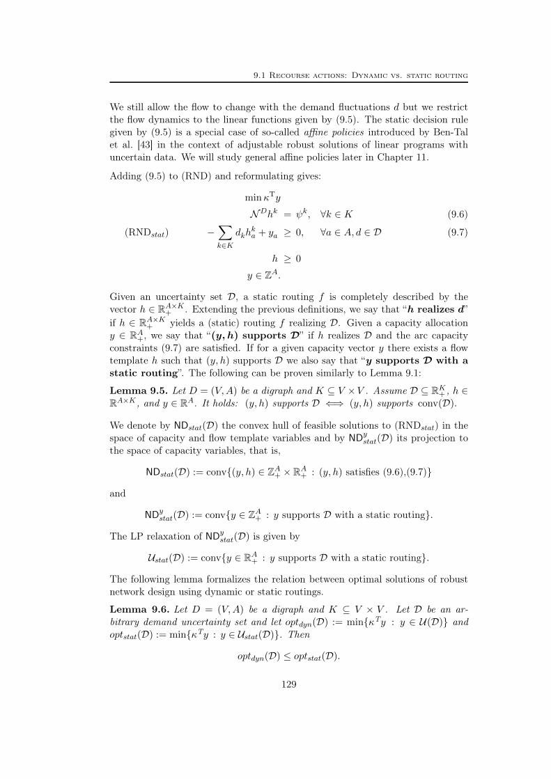
9.1 Recourse actions: Dynamic vs. static routing
We still allow the flow to change with the demand fluctuations d but we restrictthe flow dynamics to the linear functions given by (9.5). The static decision rulegiven by (9.5) is a special case of so-called affine policies introduced by Ben-Talet al. [43] in the context of adjustable robust solutions of linear programs withuncertain data. We will study general affine policies later in Chapter 11.
Adding (9.5) to (RND) and reformulating gives:
minκTy
NDhk = ψk, ∀k ∈ K (9.6)
(RNDstat) −∑k∈K
dkhka + ya ≥ 0, ∀a ∈ A, d ∈ D (9.7)
h ≥ 0
y ∈ ZA.
Given an uncertainty set D, a static routing f is completely described by thevector h ∈ RA×K+ . Extending the previous definitions, we say that “h realizes d”if h ∈ RA×K+ yields a (static) routing f realizing D. Given a capacity allocationy ∈ RA+, we say that “(y, h) supports D” if h realizes D and the arc capacityconstraints (9.7) are satisfied. If for a given capacity vector y there exists a flowtemplate h such that (y, h) supports D we also say that “y supports D with astatic routing”. The following can be proven similarly to Lemma 9.1:
Lemma 9.5. Let D = (V,A) be a digraph and K ⊆ V ×V . Assume D ⊆ RK+ , h ∈RA×K , and y ∈ RA. It holds: (y, h) supports D ⇐⇒ (y, h) supports conv(D).
We denote by NDstat(D) the convex hull of feasible solutions to (RNDstat) in thespace of capacity and flow template variables and by NDy
stat(D) its projection tothe space of capacity variables, that is,
NDstat(D) := conv(y, h) ∈ ZA+ × RA+ : (y, h) satisfies (9.6),(9.7)
and
NDystat(D) := convy ∈ ZA+ : y supports D with a static routing.
The LP relaxation of NDystat(D) is given by
Ustat(D) := convy ∈ RA+ : y supports D with a static routing.
The following lemma formalizes the relation between optimal solutions of robustnetwork design using dynamic or static routings.
Lemma 9.6. Let D = (V,A) be a digraph and K ⊆ V × V . Let D be an ar-bitrary demand uncertainty set and let optdyn(D) := minκTy : y ∈ U(D) andoptstat(D) := minκTy : y ∈ Ustat(D). Then
optdyn(D) ≤ optstat(D).
129

9 Solving robust network design problems
v1
v2
v3
3
2
2
(a)
v1
v2
v3
2
2
(b)
v1
v2
v3
1
2
1
(c)
Figure 9.1: Arc costs and optimal capacity allocations for robust network design with dynamic andstatic routing. Let K = k1, k2 = (v1, v2), (v1, v3) and D = (2, 1), (1, 2), (1, 1). (a) Arc costvector κ. (b) Optimal capacity allocation y using static routing with total cost 10. (c) Optimalcapacity allocation y using dynamic routing with total cost 9.
This result follows from Ustat(D) ⊆ U(D). In particular, the metric inequalities(9.4) might be weak for Ustat(D). There are, however, trivial cases for whichUstat(D) = U(D) and thus optstat(D) = optdyn(D) :
Lemma 9.7. Let D = (V,A) be a digraph and K ⊆ V × V . Let D be a demandpolytope in RK+ . If |D| = 1 or |K| = 1 or |P(s,t)| = 1 for all k = (s, t) ∈ K or|V | = 2, then U(D) = Ustat(D) and hence optstat(D) = optdyn(D).
Proof. If D is a singleton, then given any dynamic solution, the routing for thesingle demand vector defines a static routing template. In the single commoditycase the polytope D is an interval, and we can remove all scenarios except forthe largest without changing the (static or dynamic) problem, see the remarksabout domination in Section 9.2. If there exists only one path from s to t for acommodity k = (s, t) ∈ K, then static, and dynamic routings coincide for thiscommodity. Eventually assume that |V | = s, t. Let y ∈ U(D) and let f bethe corresponding dynamic routing. Let K+, K− denote the (s,t)-commoditiesand (t,s)-commodities, respectively. Similarly, let A+, A− be the set of (s,t)-arcsand (t,s)-arcs, respectively. By removing circulations we can assume that for allscenarios d ∈ D it holds that fka (d) = 0 for a ∈ A− and k ∈ K+, as well asfka (d) = 0 for a ∈ A+ and k ∈ K−. Let d? := argmax∑k∈K+
Sdk : d ∈ D and let
∆∗ :=∑
k∈K+Sd?k. We set ha :=
∑k∈K f
ka (d?)/∆∗ for all a ∈ A. The vector h ∈ RA
provides a feasible flow template for all commodities in K+. A flow template forall k ∈ K− is constructed in the same way. The resulting static routing is notexceeding the capacities given by y.
It is, however, also easy to construct examples with optdyn(D) < optstat(D), seeFigure 9.1. There are some theoretical results related to the (worst-case) gap be-tween optdyn(D) and optstat(D). For general polytopes D, Chekuri [67] showed
130

9.1 Recourse actions: Dynamic vs. static routing
that this gap is in O(log|V |) (undirected graphs) and Goyal et al. [116] showedthat this bound is tight. In particular, they stated a class of instances (usingthe asymmetric single-sink Hose-model) for which optdyn(D) ∈ O(|V |) whileoptstat(D) ∈ Ω(|V | log|V |). Mattia [172] provided computational evidence thatthe gap is relatively small for practical instances from the Sndlib [228] using theHose-model, also see Chapter 11.
It turns out that the large linear program coming from the discretization of D canbe sensibly simplified for static routings (and also for affine routings, see Chap-ter 11). Namely, if D is defined by a polynomial number of inequalities, Soyster[209] showed how to use linear programming duality to obtain a formulation thatcontains the deterministic variables and constraints plus an additional polynomialnumber of variables and constraints, and that is equivalent to the robust semi-infinite program (RNDstat).
For problem (RNDstat) we observe that the data uncertainty only affects the ca-pacity constraints (9.7). From the computational perspective there are two mainapproaches to treat the uncertainty of the coefficients. One may either Dualizeor Separate the extreme scenarios. We may rewrite (9.7) as
maxd∈D
∑k∈K
dkhka ≤ ya, ∀a ∈ A. (9.8)
Since D is a non-empty polytope the maximization in (9.8) refers to a (feasibleand bounded) linear program. LetM be a finite set of row indices and lets assumethat D ⊆ RK+ is defined by the linear system Ad ≤ α. That is,
D := P+(−A,−α) = d ∈ RK+ : Ad ≤ α
with A ∈ QM×K and α ∈ QM , m = |M | ≥ 1. See Chapter 1 for notation andduality theory w. r. t. inequality systems and linear programs.
Dualize. The dualization of constraints is a central technique in robust opti-mization, see [41, 42, 44, 47, 48]. Given arc a ∈ A, we may dualize the linearprogram (see Chapter 1) in (9.8) following the duality transformation already es-tablished by Soyster [209]. Fixing a ∈ A and using dual variable µia for everyi ∈M we obtain the dual program
min∑i∈M
αiµia s.t.
∑i∈MAikµia ≥ hka, ∀k ∈ K (9.9)
corresponding to the (feasible and bounded) linear program in the left-hand sideof (9.8). As the optimal values of both programs coincide we obtain the following
131

9 Solving robust network design problems
equivalent formulation for (RNDstat):
minκTy
NDhk = ψk, ∀k ∈ K(RND?
stat) −∑i∈M
αiµia + ya ≥ 0, ∀a ∈ A (9.10)∑
i∈MAikµia − hka ≥ 0, ∀a ∈ A, k ∈ K (9.11)
h, µ ≥ 0
y ∈ ZA.
Constraints (9.7) have been substituted by (9.10) and (9.11). Notice that in con-straint (9.10) we omitted the min of the dual objective. This can be done becausewe are minimizing the capacities ya with non-negative weights. The same formu-lation has been obtained by Altin et al. [9]. Despite the size of the digraph andthe number of commodities, the size of (RND?
stat) only depends on the cardinalityof M , the number of inequalities used to describe the polyhedral set D.Corollary 9.8. Let D = (V,A) be a digraph and K ⊆ V × V . If D is a polytopein RK+ with polynomially many facets in |V |, then (RND?stat) is compact.
Combining Corollary 9.3 and Corollary 9.8, it follows that we can either use for-mulation (RNDstat) or (RND?
stat) and obtain compact models when D has poly-nomially many vertices or facets, respectively.
Before dualizing (RNDstat) to obtain (RND?stat), we may remove dominated ver-
tices to change the size and shape of D. See Section 9.2 for the concept of domi-nation. Moreover, instead of a formulation for D in R|K| it is also possible to usecompact extended formulations of D to derive compact robust counterparts, seeSection 9.2 and Chapter 11.
We denote by Dualize any algorithmic approach that is based on solving therobust counterpart (RND?
stat) obtained by dualizing the capacity constraints.
Separate. Instead of dualizing the capacity constraints we can also use theoriginal formulation (RNDstat) and treat the potentially exponential number ofcapacity constraints (9.7) implicitly by separation. For network design problemsand polyhedral uncertainty this approach has been followed first by Ben-Ameur andKerivin [39]. We remove the capacity constraints (9.7) from the system (RNDstat)(or keep a subset) and add them dynamically. Non-redundant model constraintsthat are generated “on the fly” are also referred to as lazy constraints. Theseparation problem in (9.8) has to be solved in every iteration and for every arc.More precisely, given a solution (y?, h?) to an incomplete formulation, for everyarc a ∈ A, we solve the problem
max∑k∈K
dkh?ka s.t. d ∈ D
132

9.2 Uncertainty sets
obtaining an optimal solution d? ∈ D. Given flow template h?, the vector d? refersto the worst case demand realization in D for arc a. In case
∑k∈K d
?kh
?ka > y?a
we add the corresponding capacity constraint∑
k∈K d?kh
ka ≤ ya to formulation
(RNDstat) and resolve.
If we can solve this separation problem in polynomial time, then the LP relaxationof (RNDstat) can be solved in polynomial time.
Corollary 9.9. Let D = (V,A) be a digraph and K ⊆ V ×V . Let D be a polytopein RK+ . If a linear function over D can be minimized in polynomial time in |V |, thenalso deciding whether a capacity vector y ∈ RA supports D with a static routingcan be done in polynomial time.
We can in particular optimize over D in polynomial time in |V | if D is eitherdescribed by polynomially many vertices or by polynomially many facets in |V |.Notice that these results follow from more general insights into two-stage robustlinear programming and affine decision rules, see [43] and also Chapter 11.
We refer to any approach based on separating the capacity constraints of extremescenarios as algorithm Separate.
9.2 Uncertainty sets
The design of uncertainty sets has a strong impact on the quality and robustness ofthe solutions. There are many criteria for selecting uncertainty sets for a particularapplication. We believe that the following issues should receive particular atten-tion. First, any uncertainty set should reflect observed data uncertainty, that is, inour case, D should contain the observed (non-dominated) demand fluctuations thathappen with high probability, and it should not contain demand realizations thatare highly unlikely. Second, data to formulate and parametrize the uncertainty setshould be available. For sensitivity analysis and network design case studies, it isdesirable to be able to tune the shape of D in a meaningful way. And last butnot least, the resulting formulations or reformulations should be computationallytractable and scale well with the size of instances.
Domination
For problem (RNDstat) we observe that the data uncertainty only affects the capac-ity constraints (9.7). As pointed out earlier, we may restrict these constraints tothe extreme scenarios of D. However, not all points in vert(D) must be considered.For instance, if 0 ∈ D, it is an extreme point of D that any capacity allocationsupports. This intuitive idea can be formalized using the concept of dominationintroduced by Oriolo [185]. We may remove vectors from the uncertainty set thatare dominated without changing the problem.
133

9 Solving robust network design problems
Given two demand vectors d1 and d2, we say that d1 weakly dominates d2 ifany capacity allocation y ∈ RA+ supporting d1 also supports d2. Clearly, in thiscase, we may remove d2 from D without changing the dynamic model (RND). Weobtain the following beautiful characterization of weak domination:
Lemma 9.10 (Oriolo [185]). Matrix d1 ∈ D weakly dominates d2 ∈ D if andonly if d1, regarded as a capacity allocation in the demand graph H = (V,K),supports d2.
However, even if d1 weakly dominates d2 there is not necessarily a static routingrealizing these demands within the same capacities. We might have to change therouting template. In contrast, a vector d1 ∈ D is said to totally dominate avector d2 ∈ D if any pair (y, h) ∈ RA+ × RA×K+ supporting d1 also supports d2.In this case we may safely remove vertex d2 from D without changing the set offeasible solutions to the static model (RNDstat).
Total domination implies weak domination. Whenever we speak of domination inthe following, we will for simplicity always refer to total domination.
Lemma 9.11 (Oriolo [185]). Matrix d1 ∈ D totally dominates d2 ∈ D if andonly if d1
k ≥ d2k for all k ∈ K.
That is, if a capacity vector supports a polyhedron D (with a static routing), thenit also supports its anti-dominant
ant(D) := d2 ∈ RK+ : ∃d1 ∈ D with d2 ≤ d1,
see Figure 9.2 on page 136.
The Hose-model
For network design problems, a polyhedral demand uncertainty set meeting mostof the mentioned criteria has received particular attention: the Hose-model.Introduced in the context of virtual private networks (VPN) by Duffield et al. [99],the Hose-model defines upper bounds on the node traffic for all network nodes,also see [39]. In the asymmetric version of the Hose-model the incoming andoutgoing traffic is bounded by uinv ∈ Q+ and uoutv ∈ Q+ for all nodes v ∈ V ,respectively. This results in the asymmetric Hose polytope
DA := d ∈ RK+ :∑
k=(s,v)∈Kdk ≤ uinv ,
∑k=(v,t)∈K
dk ≤ uoutv for all v ∈ V .
For the symmetric version we define node bounds uv > 0 for v ∈ V and considerthe symmetric Hose polytope
DS := d ∈ RK+ :∑
k=(s,v)∈Kdk +
∑k=(v,t)∈K
dk ≤ uv for all v ∈ V .
134

9.2 Uncertainty sets
The Hose-model model is very popular in network optimization and has a strongrelation to the practice of telecommunication network design. It does not requireto estimate pairwise point-to-point traffic but describes feasible traffic realizationby estimates on single nodes only. This data is typically available to the networkpractitioner [99, 105]. For theoretical results for robust network design assumingcontinuous capacities and the Hose-model see [67, 68, 117, 130, 139].
Dualize. It is easy to see that the number of vertices of DS is in general ex-ponential, the number of facets, however, is linear in |V |. It follows that thereis a compact MIP model for robust network design with static routing using theHose-model, see the previous section and Corollary 9.8. Assuming the symmetricHose-model DS , model (RND?
stat) reduces to
minκTy
NDhk = ψk, ∀k ∈ K(HND) −
∑v∈V
uvµva + ya ≥ 0, ∀a ∈ A
µsa + µta − hka ≥ 0, ∀a ∈ A, k = (s, t) ∈ Kh, µ ≥ 0
y ∈ ZA,
where variables µva correspond to the traffic upper bound for node v ∈ V for all arcsa ∈ A. Clearly, model (HND) is compact. Compared to the (singleton scenario)deterministic network design model (ND) (page 39) we have |A||V | additionalvariables and |A||K| additional constraints.Solving (HND) relates to the Dualize approach for robust network design withstatic routing and the symmetric Hose-model. We refer to Altin et al. [9], Mattia[171] and Ben-Ameur and Kerivin [39] solving this problem and algorithms Dual-ize and Separate, respectively. Altin et al. [9] provided a third algorithm that isbased on projecting (HND) to the space (y, µ) of capacity and dual variables.
Separate. To apply the Separate approach to the Hose-model we have tosolve the maximization problem in (9.8). That is, given a flow template h?, forevery arc a ∈ A, we have to determine the scenario d ∈ D that maximizes theflow
∑k∈K dkh
?ka . As observed by Erlebach and Ruegg [101], Jüttner, Szabó, and
Szentesi [144] this can be done by solving a min-cost flow problem in the followingway. Assuming the asymmetric Hose-model, we construct an auxiliary digraphD′ = (V ′, A′). Node-set V ′ contains two artificial nodes s, t and two copies v′, v′′
for every node v ∈ V in the original graph. The arc-set A′ contains arcs from sto all v′ with cost 0 and capacity uoutv as well as arcs from v′′ to t with cost 0 andcapacity uinv . In addition, for all k = (v, w) ∈ K, we construct arcs from v′ to w′′
with cost −h?ka . Clearly, every (s,t)-flow describes a demand scenario d ∈ D and
135

9 Solving robust network design problems
0 d1
d2
d1 + d1d1
d2 + d2
d2
(a)
0 d1
d2
d1 + d1d1
d2 + d2
d2
(b)
Figure 9.2: The polyhedral Γ-model for two commodities and Γ = 1. Exemplary scenarios in darkgreen, the uncertainty set in green, and its anti-dominant in light green. Nominal and peak valuesto parametrize the Γ-model can be based on observed mean and peak values. Any capacity vectorsupporting the given uncertainty set automatically supports its anti-dominant (with a static routing).(a) The original Γ-model based on upward and downward deviations described by DΓ. (b) TheΓ-model with only upward deviations described by DΓ
+. Compare with Figure 8.5 on page 121.
vice versa. The demand value dk is simply the flow on arc (v′, w′′). Hence themin-cost (s,t)-flow problem in the auxiliary graph is equivalent to the mentionedseparation problem.
Describing traffic by node demands simplifies the notion of traffic matrices since thetraffic fluctuations are aggregated at the network nodes. Whenever point-to-pointtraffic data is available or can be calculated from real-life measurements in networks[187, 212, 224, 225] or from population statistics [100], it becomes desirable to workwith more flexible uncertainty sets that reflect the observed characteristics anddynamics of the point-to-point traffic to allow for more accurate network designs.
The Γ-model
For general linear and integer programs, Bertsimas and Sim [47, 48] proposeda polyhedral uncertainty set together with a simple way to adjust the price ofrobustness (i. e., the increase of the objective value of a robust solution comparedto its non-robust counterpart) by tuning the shape of the set. In their modelthe coefficients of the constraint matrix of a linear program may vary arounda given nominal value but the number of deviating coefficients is bounded by a(small) number Γi for every row i of the constraint matrix. Adjusting Γi meansto control the price of robustness. Because of its simplicity, this concept has beenused extensively in robust optimization for many different applications [8, 21, 47–49, 147].
As data uncertainty for (RNDstat) only appears in the capacity constraints (9.7)
136

9.2 Uncertainty sets
with uncertain coefficients dk, k ∈ K, applying the framework of Bertsimas andSim [47] to (RNDstat) means to restrict the number of commodity demands thatdeviate from a given nominal demand value dk simultaneously. In particular, thenumber of simultaneous demand peaks is bounded. This assumption has a strongrelation to telecommunications since in typical traffic patterns, in particular in IP(Internet Protocol) networks, traffic peaks do not occur simultaneously w. r. t. allsource-destination pairs, cf. Figure 8.1 on page 118. However, the main justificationfor a meaningful application of the Γ-model to our problem is the huge numberof coefficients in the uncertain capacity constraints (9.7). The situation can bedifferent for other applications.
In the following we introduce the Γ-model for (RNDstat) in detail. Similar uncer-tainty models have been used in [8], [10] and [147] applied to different versions ofnetwork design and demand packing problems. We assume that the demand forcommodity k ∈ K varies around a given nominal demand dk with a maximalpossible deviation of 0 ≤ dk ≤ dk, that is,
dk ∈ [dk − dk, dk + dk] for all k ∈ K. (9.12)
We call dk+dk the peak demand of commodity k ∈ K. Now we limit the possibledeviations from the nominal value:∑
k∈K
|dk − dk|dk
≤ Γ, (9.13)
where Γ ∈ 0, . . . , |K|, see Figure 9.2 on the previous page. Clearly, inequality(9.13) restricts the number of commodities k ∈ K that admit their peak demandsimultaneously to the value Γ. We use the same Γ for all capacity constraints (9.7)since the coefficients (the demand scenarios) are independent of the arcs.
The corresponding uncertainty polytope can be described in RK directly usingexponentially many inequalities or alternatively using a compact extended formu-lation. For the latter, we rewrite dk = dk + (σk+ − σk−)dk and let (σ+, σ−) ∈ DΓ,where
DΓ := (σ+, σ−) ∈ R2|K|+ :
∑k∈K
(σk+ + σk−) ≤ Γ and σk+ + σk− ≤ 1 for all k ∈ K.
The set DΓ corresponds to all possible deviation scenarios from the nominal vectord. The number of simultaneous deviations is restricted independently of beingdownward or upward deviations.
However, the Γ-model can also be described in the original space RK with a familyof inequalities of polynomial size by exploiting the concept of domination, see aboveand [185]. In fact, it is possible to remove all vertices from DΓ that correspond todownward deviations, see Figure 9.2. This is true independent of whether static ordynamic routing is assumed. Since only the worst-case arc-flow determines the arc-capacity, the problem remains the same if the actual demand is assumed to be in
137

9 Solving robust network design problems
the interval [dk, dk+dk], instead of the interval [dk−dk, dk+dk] for k ∈ K. Demandvectors containing downward deviations from the nominal are totally dominated.For the concept of domination see above. We may hence assume that σk− = 0 forall k ∈ K without changing the problem.
In this case dk = dk + σkdk for all k ∈ K and we consider uncertain upwarddeviations σ ∈ DΓ
+, where
DΓ+ := σ ∈ RK+ :
∑k∈K
σk ≤ Γ and σk ≤ 1 for all k ∈ K.
Of course DΓ+ is a projection of DΓ. Notice that DΓ
+ is only implicitly describing thedemand uncertainty. For the static and dynamic routing principle it is equivalent touseDΓ orDΓ
+. Static as well as dynamic solutions supportingDΓ+ will automatically
support DΓ.
By domination we might even force∑
k∈K σk = Γ which removes the origin from
DΓ+ corresponding to the all-nominal demand vector d. This observation, however,
is not improving on the robust counterpart (RNDstat) such that we stick to thefull-dimensional description of DΓ
+. Setting Γ = 0, the polytope DΓ+ reduces to a
singleton, the origin. In this case (RNDstat) reduces to the deterministic problem ofoptimizing against the single vector d. Similarly, in case Γ = |K| model (RNDstat)reduces to the problem of optimizing against the worst-case all-peak scenario d+ d.By varying Γ in 0, . . . , |K| we may adjust the level of robustness.
Remark 9.12. The Γ-model can be generalized to the case that Γ is non-integral,see [47, 48]. In this case one assumes that bΓc commodities k may realize their peakdk+ dk simultaneously while one of the commodities realizes the value dk+r(Γ)dk,where r(Γ) denotes the fractional part of Γ.
Remark 9.13. We also remark that a simple compact alternative to the definedΓ-model that can be described in the original space is to use (9.12) plus a relaxationof (9.13): ∑
k∈K
dk − dkdk
≤ Γ.
In this case there might be more than Γ upward deviations if compensated byan appropriate number of downward deviations and vice versa. This results in arelaxed uncertainty set potentially giving more conservative solutions.
Similar to the Hose polytopes, the Γ-polytope DΓ+ has exponentially many vertices
but it is described by polynomially many facets. We will assume 0 < Γ < |K| inthe following. In this case the polytope DΓ
+ is full-dimensional and has(|K|
Γ
)many
non-dominated vertices. These vertices correspond to extreme scenarios where|Γ| many commodities have σk = 1 and hence admit the peak demand dk + dksimultaneously.
138

9.2 Uncertainty sets
Dualize. Using the Γ-model, model (RND?stat) reads as
minκTy
NDhk = ψk, ∀k ∈ K(ΓND) −
∑k∈K
dkhka −
∑k∈K
µka − Γπa + ya ≥ 0, ∀a ∈ A (9.14)
πa + µka − dkhka ≥ 0, ∀a ∈ A, k ∈ K (9.15)h, µ, π ≥ 0
y ∈ ZA,
where, for every arc a ∈ A, dual variable πa corresponds to (9.13) and dual vari-ables µka correspond to the individual upper bound constraints for the demand ofthe commodities k ∈ K. Model (ΓND) is compact. As the number of facets of DΓ
+
is in O(|K|) in contrast to O(|V |) for the Hose polytopes DS and DA, reformula-tion (ΓND) has typically more variables than (HND). Compared to the (singletonscenario) deterministic network design model (ND) (page 39) we have |A|+ |A||K|additional variables and |A||K| additional constraints in (ΓND). Notice that forthe case that Γ = 0, we can fix µka to zero for all k ∈ K and a ∈ A since wecan set πa large enough. Constraints (9.15) become redundant. That is, model(ΓND) reduces to (ND) for the nominal demand scenario d. Similarly, if Γ ≥ |K|we can assume that πa = 0 and µka = dkh
ka, which means that (ΓND) reduces to
(ND) for the peak demand scenario d + d. We denote by ΓND the convex hull ofall feasible solutions of model (ΓND) and by ΓNDy,π the projection of ΓND ontothe (y, π) space. The following directly follows from the corresponding results forthe deterministic model and the fact that D = (V,A) is strongly connected, seeProposition 2.2
Lemma 9.14. Let D = (V,A) be a strongly connected digraph and K ⊆ V × V .The polyhedron ΓND has dimension 2|A|+ 2|A||K| − (|V | − 1)|K| whereas ΓNDy,π
is full-dimensional.
We will compare the two approaches Separate and Dualize computationally inChapter 10.3 assuming the Γ-model and using the methodology described above.
Separate. Using the deviation uncertainty set DΓ+ and given arc a ∈ A, the
arc capacity constraint (9.7) for the Γ-model with static routing reduces to
−∑k∈K
dkhka −
∑k∈Q
dkhka + ya ≥ 0, ∀Q ⊆ K, |Q| ≤ Γ (9.16)
or equivalently
−∑k∈K
dkhka − max
σ∈DΓ+
∑k∈K
σkdkhka + ya ≥ 0. (9.17)
The capacity of a link has to be determined subject to at most Γ commoditiesdeviating from the nominal demand value. For each deviating commodity, the
139

9 Solving robust network design problems
peak value dk + dk describes the worst-case (the extreme traffic scenario) capacity-wise. In the Separate approach for the Γ-model we have to solve the linearprogram in (9.17) for every arc a, given a solution (y?, h?) to (RNDstat). Thisproblem, however, can be solved directly by sorting the commodities with respectto the value dkh?ka . The Γ largest values determine the worst-case commoditysubset Q ⊆ K with |Q| = Γ for arc a ∈ A maximizing the left-hand side of (9.17).
Properties of the Γ-model. In the following, we will prove properties of staticsolutions using the Γ-model which we will study further and verify numerically inSection 10.3 and Section 11.2. For this we have to introduce some notation. Forfixed K, we define the numbers Φ(Γ),Γ? ∈ Z+ which depend on the structure ofthe network and commodities.
Definition 9.15. For Γ ≥ 0 and an optimal static solution S = (y, h) with objec-tive value optstat(DΓ), let Φ(Γ, S) denote the largest number of commodities usingthe same arc in the solution S, that is,
Φ(Γ, S) := max|k ∈ K : hka > 0| : a ∈ A.
We set Φ(Γ) := minΦ(Γ, S) : S static optimal, that is, Φ(Γ) gives the smallestvalue Φ(Γ, S) among all optimal static solutions S. Moreover, fixing commodityset K we define
Γ? := minΓ : Γ ∈ Z+,Γ ≥ Φ(Γ).
In any solution S at most |K| many commodities can meet. It follows Φ(Γ) ≤Φ(Γ, S) ≤ |K|. We also conclude that Φ(Γ) ≥ 1 since in all solutions at least onearc is used (as long as K is not empty). It follows directly that 1 ≤ Γ? ≤ |K|.In the following we essentially show that for fixedK and increasing Γ at some pointthe optimal solution value optstat(DΓ) remains constant and is based on a shortestpath solution, that is, an optimal static solution can be obtained by routing allcommodities on a shortest path with respect to the arc costs κa, a ∈ A. Thecorresponding threshold for Γ is precisely Γ?.
Lemma 9.16. For a given network D = (V,A), a commodity set K 6= ∅ andΓ ≥ Γ? it holds
• optstat(DΓ) = optstat(DΓ∗),
• Φ(Γ) = Φ(Γ?) ≤ Γ, and
• Instance (K,Γ) has an optimal static solution with a shortest path template.
Proof. Let S be an optimal static solution for (K,Γ?) such that Φ(Γ?, S) = Φ(Γ?).There are at most Φ(Γ?) ≤ Γ? commodities meeting on every individual arc inthis solution. Hence, for every arc, all the commodities can be at their peaksimultaneously. It follows that solution S is also optimal for any instance (K,Γ)with Γ ≥ Γ? with the same objective, that is, optstat(DΓ) = optstat(DΓ∗) for
140

9.2 Uncertainty sets
all Γ ≥ Γ?. To see this, notice that for arbitrary instances and solutions thesolution value cannot decrease if we increase Γ. For solution S and instances (K,Γ)with Γ ≥ Γ? the solution value can also not increase as we have to consider allcommodities at their peak anyway. Also Φ(Γ) = Φ(Γ?) for all Γ ≥ Γ?. OtherwiseΦ(Γ?, S) was not minimal for instance (K,Γ?). To prove the third claim observethat optstat(D|K|) = optstat(DΓ∗). But every optimal static solution S′ = (y, h)to instance (K, |K|) is based on a shortest path template h. These shortest pathsolutions are obviously optimal for any instance (K,Γ) with Γ ≥ Γ?.
Note that as a consequence of Lemma 9.16 there always exists a shortest pathtemplate for set K where at most Φ(Γ?) commodities meet on every arc.
Concluding remarks
This chapter has served as an introduction to the notion of demand uncertaintyand robust network design. The presented facts are all well-known. Extendingconcepts for deterministic network design with a single given demand scenario,we showed that one may distinguish two correlated solution methods for robustnetwork design, namely Dualize and Separate, which are based on dualizing orseparating a given set of demand scenarios, respectively. We presented models forthe case that the given uncertainty set is polyhedral. We also showed that robustnetwork design is naturally embedded in the more general framework of two-stagerobust optimization with recourse. Capacities are fixed in the first stage. Observ-ing the uncertain demand fluctuations, the network flow can be adjusted in thesecond stage. We introduced two opposed rerouting schemes, static and dynamicrouting, allowing for different levels of freedom in reorganizing the flow. Eventu-ally, we introduced two polyhedral uncertainty sets that have a strong relation tothe design of telecommunication networks. In particular, the Γ-model will receiveattention in the following chapters. We also established the concept of dominationw. r. t. demand scenarios, which turns out to influence the design of appropriateuncertainty sets.
In the following, we will develop cutting planes that can be used to enhance branch-and-cut approaches to solve robust capacitated network design problems. We will,in particular, generalize the well-known cut-set and flow cut-set inequalities to thiscontext.
141

Chapter 10
Cut-based inequalities for robustnetwork design
In deterministic network design, cut-based inequalities have been proven to be ofparticular importance, cf. Section 2.3, Section 2.5, and Part II. They define facetsof the corresponding polyhedra and they can be shown to improve on the perfor-mance of branch-and-cut based approaches to solve network design problems. Inthis chapter, we generalize the cut-set and flow cut-set inequalities from Section 2.3to incorporate the concept of polyhedral demand uncertainty. In Section 10.1 weintroduce cut-set and flow cut-set inequalities for general robust network design.We will also generalize the cut-set lifting theorems from Section 2.3. Moreover, inSection 10.2 we develop cut-set inequalities that exploit the special structure ofthe Γ-model introduced in Section 9.2.
One might well ask whether there is need to develop cutting planes and special-purpose separation frameworks for robust network design and why the MCF-separator developed in Part II is not simply doing the job. Both presented ap-proaches for capacitated robust network design, Separate and Dualize, rely onmulti-commodity flow formulations. Thus, in principle, the MCF-separator shouldbe able to detect the flow system. However, it turns out that the it either failsto resolve the graph isomorphisms of the commodity blocks or it generates weakinequalities. The necessary information is hidden too deep in the constraint ma-trices. In case of Separate, the capacity constraints (9.7), necessary to resolvethe graph isomorphisms, are generated on the fly. They are not present when theMCF-separator is scanning the matrix. Even if the initial system already containsa subset of the capacity constraints and the network can be detected correctly, theMCF-separator relies on a single capacity constraint per network arc. Thus, thegenerated cut-set inequalities will be weak as they correspond to a single demandscenario only. Using the dualized model (RND?
stat), the information about thecoupling of the commodities is present from the beginning but hidden in a combi-nation of the constraints (9.11) and (9.10). That is, this information is unavailable
143
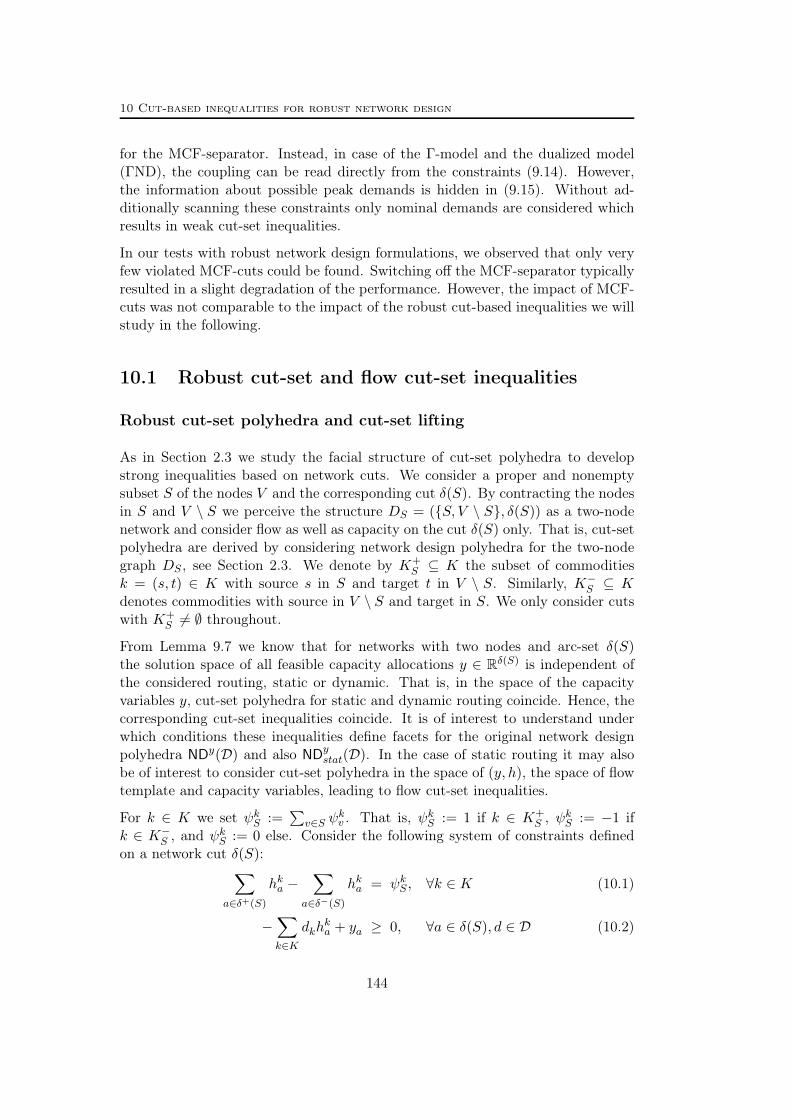
10 Cut-based inequalities for robust network design
for the MCF-separator. Instead, in case of the Γ-model and the dualized model(ΓND), the coupling can be read directly from the constraints (9.14). However,the information about possible peak demands is hidden in (9.15). Without ad-ditionally scanning these constraints only nominal demands are considered whichresults in weak cut-set inequalities.
In our tests with robust network design formulations, we observed that only veryfew violated MCF-cuts could be found. Switching off the MCF-separator typicallyresulted in a slight degradation of the performance. However, the impact of MCF-cuts was not comparable to the impact of the robust cut-based inequalities we willstudy in the following.
10.1 Robust cut-set and flow cut-set inequalities
Robust cut-set polyhedra and cut-set lifting
As in Section 2.3 we study the facial structure of cut-set polyhedra to developstrong inequalities based on network cuts. We consider a proper and nonemptysubset S of the nodes V and the corresponding cut δ(S). By contracting the nodesin S and V \ S we perceive the structure DS = (S, V \ S, δ(S)) as a two-nodenetwork and consider flow as well as capacity on the cut δ(S) only. That is, cut-setpolyhedra are derived by considering network design polyhedra for the two-nodegraph DS , see Section 2.3. We denote by K+
S ⊆ K the subset of commoditiesk = (s, t) ∈ K with source s in S and target t in V \ S. Similarly, K−S ⊆ Kdenotes commodities with source in V \ S and target in S. We only consider cutswith K+
S 6= ∅ throughout.From Lemma 9.7 we know that for networks with two nodes and arc-set δ(S)the solution space of all feasible capacity allocations y ∈ Rδ(S) is independent ofthe considered routing, static or dynamic. That is, in the space of the capacityvariables y, cut-set polyhedra for static and dynamic routing coincide. Hence, thecorresponding cut-set inequalities coincide. It is of interest to understand underwhich conditions these inequalities define facets for the original network designpolyhedra NDy(D) and also NDy
stat(D). In the case of static routing it may alsobe of interest to consider cut-set polyhedra in the space of (y, h), the space of flowtemplate and capacity variables, leading to flow cut-set inequalities.
For k ∈ K we set ψkS :=∑
v∈S ψkv . That is, ψkS := 1 if k ∈ K+
S , ψkS := −1 if
k ∈ K−S , and ψkS := 0 else. Consider the following system of constraints definedon a network cut δ(S):∑
a∈δ+(S)
hka −∑
a∈δ−(S)
hka = ψkS , ∀k ∈ K (10.1)
−∑k∈K
dkhka + ya ≥ 0, ∀a ∈ δ(S), d ∈ D (10.2)
144

10.1 Robust cut-set and flow cut-set inequalities
This system is obtained by aggregating the flow conservation constraints (9.6) fornodes in S and by restricting the capacity constraints (9.7) to the cut δ(S). Therobust cut-set polyhedron CSstat(D) is defined as
CSstat(D) := conv(y, h) ∈ Z|δ(S)|+ × R|δ(S)||K|
+ : (y, h) satisfies (10.1) and (10.2).
Its projection to the space of the capacity variables is given by
CSy(D) := convy ∈ Z|δ(S)|+ : ∃h ∈ R|δ(S)||K|
+ such that (y, h) ∈ CSstat(D).
Notice that we omit the subscript stat for the projection CSy(D) as this polyhe-dron is independent of the routing scheme as mentioned above. Since the digraphD = (V,A) is strongly connected we have δ+(S), δ−(S) 6= ∅. it follows that bothCSstat(D) and CSy(D) are non-empty. It is also easy to see that CSy(D) is full-dimensional since we can arbitrarily increase capacity for all arcs a ∈ δ(S). ForCSstat(D) there are no more implied equations than those given by (10.1).
Lemma 10.1. Let D = (V,A) be a strongly connected digraph and K ⊆ V × V .Given a non-empty node-set S ( V , the polyhedron CSy(D) is full-dimensional andthe dimension of CSstat(D) is |δ(S)|+ |δ(S)||K| − |K|.
Before studying facets of CSy(D) and CSstat(D) we prove a lifting theorem forrobust cut-set inequalities as a generalization of the cut-set lifting Theorem 2.9 fordeterministic cut-set inequalities.
Theorem 10.2 (Robust cut-set lifting theorem). Assume that D = (V,A) isa strongly connected digraph and K ⊆ V ×V . Given a non-empty node-set S ( V ,any facet-defining inequality for CSstat(D) defines a facet of NDstat(D) if both D[S]and D[V \ S] are strongly connected.
Proof. Let us assume that ∑a∈δ(S)
µaya +∑a∈δ(S)
αkahka ≥ β (10.3)
defines a facet FS of CSstat(D) and let F be the face of NDstat(D) defined by(10.3). There are n := |δ(S)| + |δ(S)||K| − |K| many affinely independent points(y(i), h(i)) ∈ FS . For every i ∈ 1, . . . , n let y(i) ∈ RA+ be such that y(i)
a = y(i)a if
a ∈ δ(S) and y(i)a = M else, whereM is large number. For every commodity k ∈ K
we extend the template hk(i) ∈ Rδ(S) to a flow template hk(i) ∈ RA for k. This canbe done by solving flow problems in the strongly connected graphs D[S] and D[S]
such that hk(i)a = h
k(i)a for a ∈ δ(S). Recall that flow templates are flows itself.
Since we did not change values on the cut and we provided enough capacity in theremaining arcs (D is bounded) we get p(i) := (y(i), h(i)) ∈ NDstat(D). We furtherconsider the point p(1) +ea ∈ NDstat(D) for every a ∈ A\δ(S), where ea is the unitvector corresponding to the capacity variable of arc a ∈ A. All constructed pointsare clearly on the face F . Consider the strongly connected shore D[S] = (S,A[S])
145

10 Cut-based inequalities for robust network design
and choose a spanning arborescence T ⊆ A[S], which exists since D[S] is stronglyconnected. We assign a unique cycle to every arc in A[S] \ T in the following way.If arc a forms a cycle with arcs of T only, we assign this cycle to a. Then allarcs with this property are added to T . This process is repeated until every arc inA[S] \ T has its cycle. Notice that as long as A[S] \ T is non-empty, arcs with thementioned property always exist because we start with a spanning arborescenceand because D[S] is strongly connected. Also notice that all constructed cyclesare different. Now we perturbate the point p(1) by adding a circulation to hk(1) forevery commodity k and w. r. t. the cycle assigned to a ∈ A[S] \ T . The resultingpoint is on the face F . It is feasible since adding a circulation to a templateresults in a feasible template again and since we can assume that y(1) ∈ ZA+ withenough capacity in D[S]. Doing the same in the shore D[V \ S] results in a totalof |A| + |A||K| − |K|(|V | − 1) many affinely independent points in F . Since FSis a proper face of CSstat(D), there is a point in CSstat(D) that is not on the faceFS . From this point we may construct a point in NDstat(D) that is not on theface F using the construction above, which shows that F is a proper face. As thedimension of a proper face of NDstat(D) cannot exceed |A|+ |A||K| − |K|(|V | − 1)we showed that F is a facet.
Theorem 10.2 implies the same result for inequalities defined in the space of thecapacity variables. For the case of dynamic routings and undirected formulationsa similar result is stated in Mattia [172]. Here we consider the directed case andboth static and dynamic routings.
Corollary 10.3. Let D = (V,A) be a strongly connected digraph and K ⊆ V ×V . Given a non-empty node-set S ( V , any facet-defining inequality for CSy(D)defines a facet of NDy(D) and also NDy
stat(D) if both D[S] and D[V \S] are stronglyconnected.
Proof. We prove that under the given condition any facet-defining inequality∑a∈δ(S)
µaya ≥ β (10.4)
for CSy(D) defines a facet of NDystat(D). The result for NDy(D) follows since both
NDy(D) and NDystat(D) are full-dimensional, NDy
stat(D) ⊆ NDy(D) and (10.4) isvalid for NDy(D). Let y(i) ∈ CSy(D), 1 ≤ i ≤ |δ(S)| be affinely independentand satisfy (10.4) at equality. For every i ∈ 1, . . . , |δ(S)| let h(i) be a feasibletemplate and let (y(i), h(i)) ∈ NDstat(D) be constructed as in the proof of Theo-rem 10.2. Hence y(i) ∈ NDy
stat(D). Further, for every arc a ∈ A \ δ(S) consider thepoint (y(1) + ea) ∈ NDy
stat(D), where ea is the unit vector for index a in RA. Weconstructed |A| many affinely independent points in NDy
stat(D) satisfying (10.4)at equality. Moreover, (10.4) defines a proper face of NDy
stat(D) since it defines aproper face of CSy(D).
146

10.1 Robust cut-set and flow cut-set inequalities
Robust cut-set inequalities
From Corollary 10.3 follows that by studying the facial structure of CSy(D) weobtain facets of NDy(D) as well as NDy
stat(D). This result comes as a surprisesince in the last section we learned that there can be a gap between optdyn(D) andoptstat(D), cf. Figure 9.1 on page 130. In particular, the metric inequalities (9.4)can be weak for NDy
stat(D) in general. However, Corollary 10.3 establishes thatinequalities based on cut metrics for cuts with strongly connected shores are strongfor NDy
stat(D). As for the deterministic case there are only two non-trivial cut-setinequalities for CSy(D), based on the two non-trivial cut metrics for δ+(S) andδ−(S). Before we show under which conditions the resulting cut-set inequalitiesdefine facets we need some more notation.
Definition 10.4. For subset Q ⊆ K+S and scenario d ∈ D we define d(Q) :=∑
k∈Q dk and call d ∈ D maximal w. r. t. Q if d(Q) = maxd∈D(d(Q)). Thescenario d is said to be strictly maximal w. r. t. Q if d(Q) > d(Q) for all d ∈ Dwith d 6= d. We abbreviate
d+ := maxd∈D
(d(K+S )) and d− := max
d∈D(d(K−S )).
By symmetry, we only state the result for δ+(S) here.
Theorem 10.5. Let D = (V,A) be a strongly connected digraph and K ⊆ V × V .Given ∅ 6= S ( V , let D[S] and D[V \ S] be strongly connected. The robustcut-set inequality ∑
a∈δ+(S)
ya ≥ dd+e (10.5)
defines a facet of NDstat(D) if d+ /∈ Z. It defines a facet of the projections NDy(D)and NDy
stat(D) if d+ > 0.
Proof. By Theorem 10.2 and Corollary 10.3 it suffices to prove that (10.5) defines afacet of CSstat(D) and CSy(D), respectively. Choosing a+ ∈ δ+(S) and a− ∈ δ−(S)we construct a point p = (y , h) ∈ CSstat(D) by setting ya+ = dd+e, ya = M forall a ∈ δ−(S), hka+ = 1 for k ∈ K+
S , and hka− = 1 for k ∈ K−S . All other variables
are set to 0. Clearly, the point is feasible as the worst case flow for arc a+ is d+
and M can be chosen large enough. Point p is on the face defined by (10.5). Weconsider the following additional points:
• p(a)1 := p+ ea for all a ∈ δ−(S),
• p(a)2 := p− ea+ + ea −
∑k∈K+
Sψeka+ +
∑k∈K+
Sψeka for all a ∈ δ+(S), a 6= a+,
• p(a,k)3 := p+ εeka+ + εeka for all a ∈ δ−(S) and k ∈ K,
• p(a,k)4 := p
(a)2 + εeka + εeka− for all a ∈ δ+(S), a 6= a+ and k ∈ K,
where ε > 0 is small enough, ψ := r+/d+ with r+ := d+ − (dd+e − 1), thatis, r+ = r(d+) (the fractional part of d+) if d+ /∈ Z and r+ = 1 else. Hence
147

10 Cut-based inequalities for robust network design
∑k∈K+
Sψdk ≤ r+ for all d ∈ D. The vector ea refers to the unit vector for the
capacity variable of arc a and eka refers to the unit vector of the template variablefor arc a and commodity k. All points are affinely independent and satisfy (10.5)at equality. Point p(a)
1 is clearly feasible as we only increase capacity in δ−(S).As long as d+ > 0 point p(a)
2 is feasible since ψ ≤ r+ ≤ 1. In case d+ /∈ Z andhence r+ < 1 points p(a,k)
3 and p(a,k)4 become feasible for small ε. We constructed
|δ(S)|+ (|δ(S)| − 1)|K| many affinely independent points on the face of CSstat(D)defined by (10.5). Together with Theorem 10.2 we have shown that (10.5) definesa facet of NDstat(D). As long as d+ > 0, the capacities defined with p
(a)1 and
p(a)2 provide |δ(S)| many affinely independent points on the face of CSy(D). Thus
together with Corollary 10.2 also the second statement holds.
Mattia [172] states Theorem 10.5 for NDy(D). The robust cut-set inequality (10.5)is a rank-1 MIR inequality corresponding to the systems (RND) and (RNDstat).It generalizes the deterministic cut-set inequality (2.16). As already mentioned,assuming strongly connected shores, (10.5) provides the only non-trivial cut-basedinequality for NDy(D) and NDy
stat(D) together with its symmetric counterpart∑a∈δ−(S) ya ≥ dd−e. In the following we show how (10.5) can be generalized to
robust flow cut-set inequalities for NDstat(D).
Robust flow cut-set inequalities
As in Section 2.3 we choose a subset A+ ⊆ δ+(S) and set A+ := δ+(S) \ A+. Wealso select Q ⊆ K. Consider a fixed scenario d ∈ D. Summing up all equations(10.2) for k ∈ Q (with weight dk) as well as all capacity constraints (10.1) fora ∈ A+ (with weight 1) yields
−s+∑a∈A+
∑k∈Q
dkhka +
∑a∈A+
ya ≥ d(Q), (10.6)
where s subsumes all continuous variables with negative coefficient. After applyingMIR (Proposition 1.2) we obtain∑
a∈A+
∑k∈Q
dkhka +
∑a∈A+
rQya ≥ rQdd(Q)e. (10.7)
Here rQ := r(d(Q)) denotes the fractional part of d(Q). We call (10.7) a simple(robust) flow cut-set inequality . It generalizes the deterministic simple flowcut-set inequality (2.15) and is valid for NDstat(D) for all d ∈ D. Clearly, settingQ := K+
S and A+ := δ+(S) we obtain (10.5) if d is maximal w. r. t.K+S . Intuitively,
also in case A+ 6= δ+(S) the scenario d should be maximal w. r. t. Q for (10.7) todefine a facet. Except for the special case that d(Q) < 1 this is true and formalizedby the following theorem stating necessary conditions for (10.7) to define a facet.
148

10.1 Robust cut-set and flow cut-set inequalities
Theorem 10.6. Let D = (V,A) be a strongly connected digraph and Q ⊆ K ⊆V × V . Given a non-empty node-set S ( V , assume A+ 6= δ+(S) and assumethat (10.7) defines a facet of NDstat(D) different from a non-negativity constraint.It follows that A+ 6= ∅, d(Q) /∈ Z, and either |Q| = 1 with maxd∈D d(Q) < 1 orscenario d is maximal w. r. t. Q with d(Q) > 1.
Proof. If d(Q) ∈ Z, then rQ = 0 and (10.7) becomes a non-negativity con-straint. If A+ = ∅ and rQ > 0, then (10.7) is dominated by the flow constraint∑
a∈δ+(S)
∑k∈Q dkh
ka ≥ d(Q) because rQdd(Q)e = d(Q)− (dd(Q)e − 1)(1− rQ) ≤
d(Q). Assume A+ 6= ∅ and rQ < 0. If both |Q| > 1 and d(Q) < 1, then (10.7)becomes the sum of the simple robust flow cut-set inequalities corresponding tothe commodity subsets Qk = k for all k ∈ Q. Assume that scenario d withd(Q) /∈ Z, d(Q) > 1 is not maximal w. r. t. Q. It follows that there exists d ∈ Dwith d(Q) < d(Q). We consider a point (y, h) on the face defined by (10.7). Forease of notation, we set h :=
∑a∈A+
∑k∈Q h
ka, h(d) :=
∑a∈A+
∑k∈Q dkh
ka, and
y :=∑
a∈A+ ya. Since (10.7) is not a non-negativity constraint we can assumethat h(d) > 0. It follows from (10.7) that y < dd(Q)e. But subtracting equationh(d)+rQy = rQdd(Q)e from (10.6) yields y = bd(Q)c and thus h(d) = rQ. Writing(10.6) for scenario d gives
h(d) ≥ d(Q)− bd(Q)c = d(Q)− d(Q) + rQ.
Using h(d) = rQ gives h(d − d) = h(d) − h(d) ≥ d(Q) − d(Q). It follows that∑a∈A+ hka = 1 for all k ∈ Q. Hence h(d) = d(Q) > 1 > rQ which is a contradiction.
Let us eventually assume that |Q| = 1 and d(Q) < 1 ≤ d(Q) for some d ∈ D.Inequality (10.7) divided by rQ then writes h + y ≥ 1 since d(Q) = rQ anddd(Q)e = 1. If d(Q) = 1 this is simply the base inequality (10.6) written forscenario d. If d(Q) > 1, we assume that (y, h) had been chosen such that y > 0.We can assume y ≥ 1 which gives y = 1 and h = 0. But this point then violatesthe base inequality (10.6) for scenario d.
The following theorem provides a proof for the fact that (10.7) yields a large classof facet-defining inequalities for NDstat(D).
Theorem 10.7. Let D = (V,A) be a strongly connected digraph and K ⊆ V × V .Given a non-empty node-set S ( V , let D[S] and D[V \ S] be strongly connected.Let ∅ 6= A+ ( δ+(S) and Q ⊆ K+
S . The simple flow cut-set inequality (10.7)defines a facet of NDstat(D) if d(Q) /∈ Z and either |Q| = 1 with maxd∈D d(Q) < 1or scenario d is strictly maximal w. r. t. Q with d(Q) > 1.
Proof. By Theorem 10.2 it suffices to prove that (10.7) defines a facet of CSstat(D).Set Q := K+
S \Q. We choose a+ ∈ A+, a+ ∈ A+, and a− ∈ δ−(S) and construct apoint p = (y , h) ∈ CSstat(D) by setting ya+ = dd(Q)e, ya = M for all a ∈ δ(S)\A+,hka+ = 1 for k ∈ Q, hka+ = 1 for k ∈ Q and hka− = 1 for k ∈ K−S . All other variablesare set to 0. Clearly, the point is feasible asM can be chosen large enough and the
149

10 Cut-based inequalities for robust network design
worst case flow for arc a+ is maxd∈D d(Q) ≤ dd(Q)e. Point p also satisfies (10.7)at equality. We define ψ := rQ/d(Q). Based on the points defined in the proof ofTheorem 10.5 we consider the following additional points:
• p(a)1 for all a ∈ δ(S) \A+,
• p(a)2 for all a ∈ δ+(S), a 6= a+,
• p(a,k)3 for all a ∈ δ−(S) and k ∈ K,
• p(a,k)4 for all a ∈ A+, a 6= a+ and k ∈ K, and for all a ∈ A+ and k ∈ K \Q.
These points can be shown to be affinely independent and on the face defined by(10.7) just like in the proof of Theorem 10.5. The proof is complete in case |Q| = 1.Notice that for p(a)
2 to be feasible we need maxd∈D d(Q) < 1 in this case since allthe flow for Q is routed on a with capacity 1. As there is slack on a also p(a,k)
4 isfeasible. Now assume that |Q| > 1 and d(Q) > 1. It follows that dd(Q)e ≥ 2 and0 < ψ = rQ/d(Q) < 1. Consider point p(a)
2 for arc a ∈ A+. For the correspondingflow templates it holds 0 < hka = ψ < 1 and 0 < hka+ = 1 − ψ for all k ∈ Q.That is, on arc a ∈ A+ we can both decrease and increase the flow for all scenariosw. r. t. commodities in Q. Notice that worst case flow (scenario d ∈ D) on a is rQ
while the capacity is 1. Arc a+ has capacity d(Q)− rQ. That is, in the worst casescenario d ∈ D arc a+ is tight. However, since scenario d is strictly maximal wecan slightly increase the flow on a+ for all scenarios d ∈ D with d 6= d. Choose anarbitrary commodity k ∈ Q and for all a ∈ A+ and k ∈ Q with k 6= k perturb p(a)
2
as follows:p
(a,k)5 := p
(a)2 − ε
dkeka + ε
dk
eka + εdkeka+ − ε
dk
eka+ .
We only add a small circulation for commodities k and k to point p(a)2 using arcs
a and a+. If ε > 0 is small enough, then the perturbed flow templates result infeasible flows since both arcs a and a+ are not tight for scenarios different fromd. For the maximal scenario d the total flow on both arcs is not changing. Thisalso proves that p(a,k)
5 is on the face defined by (10.7). We constructed |δ(S)| +(|δ(S)| − 1)|K| many affinely independent points on the face of CSstat(D) definedby (10.7) which completes the proof.
Notice that we exchanged the necessary condition d is maximal w. r. t. Q fromTheorem 10.6 by the condition that d is strictly maximal w. r. t. Q. Claiming thelatter essentially means that d is the only vertex of D that maximizes the linearobjective
∑k∈Q dk. We cannot prove that this stronger assumption is necessary
for (10.7) to define a facet. In fact, it is easy to construct examples where allscenarios d maximizing
∑k∈Q dk yield facet-defining inequalities of type (10.7).
Inequality (10.7) is a simple flow cut-set inequality and does not contain variablesfor the backward cut arcs in δ−(S). However, it can be generalized to flow cut-setinequalities of type (2.14) by using a similar aggregation procedure and applyingMIR. For scenarios d that are (strictly) maximal w. r. t. Q and by extending the
150

10.1 Robust cut-set and flow cut-set inequalities
corresponding proofs in Atamtürk [16] and Raack [198], the resulting general robustflow cut-set inequalities can be shown to define facets.
Separation
Most of the remarks from page 49 about the separation of cut-set and flow cut-set inequalities in the deterministic single scenario case carry over to the robustmulti-scenario setting. The main difference is that whenever we fix a commoditysubset Q we have to maximize the scenario d ∈ D w. r. t.
∑k∈Q dk according
to Theorem 10.6. For instance, in the single-commodity case, the separation forsimple flow cut-set inequalities (10.7) can be done in polynomial time. We first findthe maximal scenario d ∈ D w. r. t. Q = k and then apply a min-cut procedureas described in [16]. Similarly, first fixing the cut δ(S) and and an arbitrarycommodity subset Q, we can find the most violated robust flow cut-set inequalityin polynomial time. In this case, we first maximize the objective
∑k∈Q dk over
the polytope D to fix a scenario d ∈ D and then we decide about the arc subsetsas described on page 49, see also [16, 200].
Generalizing cut-set and flow cut-set inequalities
All presented classes of facet-defining cut-based inequalities are valid for directedcapacity models. However, similar to deterministic cut-set and flow cut-set inequal-ities, the presented inequalities for robust network design, that is, robust cut-setinequalities (10.5) and robust flow cut-set inequalities (10.7) have their undirectedcounterpart in case of undirected (or bidirected) capacity models. As discussedin Section 2.4, demands can be flipped in the undirected case without changingthe model. The maximum cut demand over all scenarios, given an undirected cutδ(S), is hence given by
d? := maxd∈D
(d(K+S ∪K−S )) ≤ d+ + d−,
cf. Definition 10.4. The undirected counterpart of the robust cut-set inequality(10.5) then reads ∑
e∈δ(S)
ye ≥ dd?e.
The mentioned inequalities can also be easily generalized to the multi-facilitycase by using the flexibility of scaling and mixed integer rounding as described inSection 2.4, see also Section 1.3. In case of multiple facilities the (directed) robustcut-set base inequality may be ∑
a∈δ+(S)
∑t∈Ta
ctyta ≥ d+, (10.8)
151

10 Cut-based inequalities for robust network design
where Ta defines the set of facilities installable at arc a with capacity ct and ytadenotes the corresponding integral facility variable, see Section 2.4. Any coefficient,that is, any of the available cut capacities, in this knapsack constraint can be usedas a scalar for MIR, similar to the coefficient scaling loops of the c-MIR and MCF-separator, see Section 1.4 (Algorithm 1.2 on page 33) and Chapter 5 (Algorithm 5.7on page 93), respectively.
We have seen that the cut-set and flow cut-set inequalities from Section 2.3 fordeterministic network design can be generalized to robust cut-set and flow cut-setinequalities for network design problems with multiple demand scenarios. Theessential concept in this context is that of (strictly) maximal demand scenariosw. r. t. commodity subsets, cf. Definition 10.4. The presented results are independ-ent of the routing scheme, static or dynamic, and they are independent of thechosen uncertainty set D. In fact, the lifting theorems and also Theorem 10.5 andTheorem 10.7 hold for general compact convex sets D. For well-defined (strictly)maximal scenarios d ∈ D following Definition 10.4 we only need to be able tomaximize a linear function over D.In the next section we will develop facet-defining cut-based inequalities for a par-ticular polyhedral uncertainty set, namely the Γ-model introduced in Section 9.2
10.2 Envelope inequalities for the Γ-model
In this section, we will generalize the robust cut-set inequality (10.5) from theprevious section to exploit the special structure of the demand polytope DΓ
+ cor-responding to the Γ-model introduced in Section 9.2. We will develop cut-setinequalities that are facet-defining for the dualized model (ΓND) (page 139) andthe corresponding polyhedron ΓND. The reader is referred to Altin et al. [9] for asimilar study assuming the Hose-model and formulation (HND) (page 135).
The base inequality corresponding to the robust cut-set inequality (10.5) is∑a∈δ+(S)
ya ≥ d+, (10.9)
where d+ is maximal w. r. t. K+S , cf. Definition 10.4. In case of the Γ-model this
means thatd+ =
∑k∈K+
S
dk + maxσ+∈DΓ
+
∑k∈K+
S
σk+dk
Thus, inequality (10.9) states that the capacity on the cut should be at least thenominal cut demand plus the Γ largest deviations among K+
S . Notice that theright-hand side is independent of the realized flow. The value d+ only dependson the node-set S and the value of Γ. Inequality (10.5) defines a facet of ΓNDif d+ < dd+e and the two shores D[S] and D[V \ S] are strongly connected,
152

10.2 Envelope inequalities for the Γ-model
which is only a small variation of Theorem 10.5. In the rest of this section wewill generalize this essential result to a more general class of inequalities in thespace of the y and π variables. To generalize (10.5) we will introduce the robustcut-set polyhedron corresponding to the dualized formulation (ΓND) in the space(y, h, π, µ) of capacity, flow template, and dual variables. We will then furthersimplify and project the feasible region to the space (y, π). The resulting two-variable set is studied in detail providing a complete description and all facet-defining inequalities. These inequalities are then lifted back to facets of the originalpolytope ΓND.
Given a cut δ(S), consider the following robust cut-set polyhedron correspondingto formulation (ΓND) (page 139):
ΓCS := conv(y, h, π, µ) ∈ Z|δ(S)|+ × R|δ(S)||K|
+ × R|δ(S)|+ × R|δ(S)||K|
+ :
(y, h, π, µ) satisfies (9.14), (9.15), and (10.1).ΓCS is obtained from ΓND by considering the two-node network DS = (S, V \S, δ(S)). The dimension of ΓCS is 2|δ(S)|+ 2|δ(S)||K| − |K| which follows fromLemma 9.14. The cut-set lifting theorem also holds for ΓCS with the same argu-ments as in the proof of Theorem 10.2:
Corollary 10.8. Let D = (V,A) be a strongly connected digraph and K ⊆ V × V .Given a non-empty node-set S ( V , any facet-defining inequality for ΓCS definesa facet of ΓND if both shores D[S] and D[V \ S] are strongly connected.
We will consider a projection of ΓCS to the variable space (y, π) on the dicut δ+(S):
ΓCSy,π+ := (y+, π+) ∈ R2|δ+(S)|+ :∃(y−, π−) ∈ R2|δ−(S)|
+ and (h, µ) ∈ R2|δ(S)||K|+
such that (y+, π+, y−, π−, h, µ) ∈ ΓCS.Clearly, ΓCSy,π+ is full-dimensional since we may arbitrarily increase ya and πavalues for every arc a ∈ δ(S).
Let us start by generalizing the base cut-set inequality (10.9). LetQ be an arbitrarybut nonempty subset of the cut-commodities K+
S . We write d(Q) :=∑
k∈Q dk andd(Q) :=
∑k∈Q dk. Consider the following aggregation of the system (ΓND). We
add up
• all flow conservation constraints (10.1) with weight (dk + dk) for k ∈ Q,
• all flow conservation constraints (10.1) with weight dk for all k ∈ K+S \Q,
• all dualized capacity constraints (9.14) with weight 1 for all a ∈ δ+(S), and
• all inequalities (9.15) with weight 1 for all a ∈ δ+(S) and k ∈ Q,
This yields the following aggregated inequality valid for ΓCS and ΓND:∑a∈δ+(S)
ya +∑
a∈δ+(S)
(|Q| − Γ)πa ≥ d(K+S ) + d(Q), (10.10)
153

10 Cut-based inequalities for robust network design
0 y
π
dd0e dd0e+ 1 dd0e+ 2
d0 − d−1
d1 − d0y ≥ dd0e
(10.15) lower region
(10.14)
upper region(10.16)
Figure 10.1: Lower and upper region (dark gray) together with facet-defining envelope inequalities(dark blue). The 6 base inequalities y + iπ ≥ di, i ∈ J are given in light gray. In this case we haveΓ = 2 and |K+
S | = 5. Hence J = −2,−1, 0, 1, 2, 3.
where continuous variables with negative coefficient have been omitted. In thefollowing we will see that (10.10) generalizes the cut-set base inequality (10.9).The left-hand side of (10.10) is not changing as long as the cardinality of thesubset Q is constant. Hence among all subsets of Q with cardinality |Q| the onemaximizing d(Q) gives the strongest inequality (10.10). To state this inequalitywe have to introduce some new notation handling subsets of K+
S corresponding tolarge deviations.
Definition 10.9. We sort the commodities in K+S non-increasingly with respect to
the value dk. Let J = −Γ, . . . ,Θ with Θ := |K+S | −Γ. For i ∈ J we define Qi to
be the subset of commodities k ∈ K+S that correspond to the i+Γ largest deviations
dk. Ties are broken arbitrarily. For i ∈ J we abbreviate di := d(K+S ) + d(Qi).
By Definition 10.9, the value di denotes the total nominal demand plus the i+ Γlargest deviation demands across the cut. Setting d0 := d+ this definition isconsistent with the definition of d+ in (10.9). The value dΘ = d(K+
S ) + d(K+S )
corresponds to the all peak demand scenario across the cut.
Using this notation, inequality (10.10) reduces to∑a∈δ+(S)
ya +∑
a∈δ+(S)
iπa ≥ di. (10.11)
It is valid for all i ∈ J . For i = 0 we obtain (10.9). Consider the polyhedron
ΓXS = conv(y, π) ∈ Z|δ+(S)|
+ × R|δ+(S)|
+ : (y, π) satisfies (10.11) ∀i ∈ JClearly, ΓCSy,π+ ⊆ ΓXS. Every valid inequality for ΓXS is also valid for the Γ-robustmodel ΓND. In the following we will completely describe ΓXS providing all facet-defining inequalities. Since all coefficients in (10.11) are identical for all arcs in
154

10.2 Envelope inequalities for the Γ-model
δ+(S) it suffices to study the two-dimensional case with inequalities
y + iπ ≥ di (10.12)
and the polyhedron
ΓX = conv(y, π) ∈ Z+ × R+ : (y, π) satisfy (10.12) for all i ∈ J,also see Figure 10.1 on the previous page.
Note that ΓXS is obtained from ΓX by copying variables and forcing non-negativityfor the copied variables. It follows that every facet for ΓX translates into a facet forΓXS and vice versa except for the non-negativity constraints. In fact a completedescription of ΓX determines a complete description of ΓXS and vice versa.
Lemma 10.10. Every facet-defining inequality αy+ απ ≥ β for ΓX with α, α, β ∈R different from a non-negativity constraint translates into a facet-defining inequal-ity ∑
a∈δ+(S)
αya +∑
a∈δ+(S)
απa ≥ β (10.13)
for ΓXS. Moreover, all facets of ΓXS defined by inequalities different from non-negativity constraints are of the form (10.13). and correspond to a facet-defininginequality αy + απ ≥ β for ΓX. We have ΓX = ΓXS if and only if |δ+(S)| = 1.
In the following we will not distinguish facet-defining inequalities of ΓX and ΓXSas long as different from non-negativity constraints.
Definition 10.11. Let us divide the index set J into the sets J− = −Γ, . . . ,−1and J+ := 1, . . . ,Θ such that J = J− ∪ 0 ∪ J+. Accordingly, the upperregion of ΓX corresponds to indices in J− and the lower region of ΓX correspondsto indices in J+, see Figure 10.1. More precisely, the upper region is given byΓX∩π ≥ d0−d−1 whereas we define the lower region of ΓX as ΓX∩π ≤ d1−d0.
Notice that the upper region is always non-empty. The lower region is non-emptyif and only if Θ ≥ 1 and d1 > d0.
We call valid inequalities for ΓX trivial if they are non-negativity constraints orif they are of type (10.12). In the following we are only interested in non-trivialfacets of ΓX as these will translate to facets of ΓND. Lower and upper region aresimilar in structure. The lower region, however, is cut by π ≥ 0 which leads to oneadditional type of facet. We will see that besides the cut-set facet y ≥ dd0e thereare two classes of non-trivial inequalities describing the lower region and one classof non-trivial inequalities describing the upper region facets.
Setting ri := r(di) and applying mixed integer rounding (Lemma 1.1) to (10.12)yields
riy + max(0, i) · π ≥ riddie (10.14)
valid for ΓX. Recall that ri = di− bdic is the fractional part of di with 0 ≤ ri < 1.If ri = 0, then inequality (10.14) reduces to a non-negativity constraint. For ri > 0and i = 0 inequality (10.14) reduces to the robust cut-set inequality (10.5).
155

10 Cut-based inequalities for robust network design
Lemma 10.12. Inequality (10.14) defines a facet of ΓX if i = 0 and ri > 0.
Proof. Consider ε > 0 and the two affinely independent points (dd0e, d0−d−1) and(dd0e, d0 − d−1 + ε) which both satisfy (10.14) with equality. To see feasibility ofthe two points we show that they are in ΓCSy,π+ ⊆ ΓXS. Notice that d0 − d−1 ≥ 0
gives the commodity k with the Γ largest deviation demand dk among commoditiesk in K+
S . We set
ya = dd0e, πa = d0 − d−1, µka = max(dk − πa, 0), and hka = 1 for k ∈ K+S
for some arc a ∈ δ+(S). Demands for K−S are routed on arcs a ∈ δ−(S) whichcan be done if ya and πa are set large enough. We obtain a feasible point for ΓCS.Hence (dd0e, d0 − d−1) ∈ ΓCSy,π+ ⊆ ΓXS. The point has a slack of 1 − r0 in thecapacity constraint (9.14) for arc a since Γπa +
∑k∈K µ
ka +
∑k∈K dkh
ka = d0. As
1 > r0 > 0 it follows also that the second point (dd0e, d0 − d−1 + ε) is feasible forΓX for ε < 1− r0.
For i ∈ J−, inequalities (10.14) are obviously dominated by (10.5). For i ∈ J+
inequality (10.14) connects the two points (bdic, ri/i) and (ddie, 0) in case ri > 0.We get
Lemma 10.13. Assume J+ 6= ∅ and ddΘe > dd0e. Set i = argmaxrj/j : j ∈J+ with ddje = ddΘe. Inequality (10.14) defines a facet of ΓX if ri > 0.
Proof. Let π′ := max(rk/k : k ∈ J+). Since bdic ≥ dd0e the two points (bdic, π′)and (ddie, 0) are feasible. They satisfy (10.14) with equality and are affinely inde-pendent.
Inequality (10.14) for i = 0 reduces to a cut-set inequality in the space of thecapacity variables. Inequality (10.14) for i ∈ J+ will be called a lower envelopeinequality as by Lemma 10.13 it may define a facet of the lower region, see alsoFigure 10.1 on page 154. In general, the two inequalities from Lemma 10.12 andLemma 10.13 do not suffice to provide a complete description of ΓX. To get acomplete description of the lower region of ΓX we have to consider two arbitraryinequalities y + iπ ≥ di and y + jπ ≥ dj with i, j ∈ J+, i < j. Its intersection hasy-value
bi,j := (jdi − idj)/(j − i).Now we have to connect the two points (bbi,jc, (di − bbi,jc)/i) and (dbi,je, (dj −dbi,je)/j). Let ri,j be the remainder of the division of jdi − idj by (j − i), that is,ri,j := r(jdi − idj , j − i) = (j − i)r(bi,j). For convenience, we set bi,j = ri,j = 0 ifi = j.
Lemma 10.14. For i, j ∈ J+ with i ≤ j, the following inequality is valid for ΓX:
(i+ ri,j)y + ijπ ≥ ri,jdbi,je+ idj (10.15)
156

10.2 Envelope inequalities for the Γ-model
Proof. Inequality (10.15) reduces to (10.12) if i = j. Assume i < j. We scale thetwo inequalities with j and i, respectively:
jy + jiπ ≥ jdi and iy + ijπ ≥ idj .
Introducing the slack sj := iy+ijπ−idj ≥ 0 of the second constraint and combiningthe two inequalities gives
(j − i)y + sj ≥ jdi − idj ,
Applying MIR (Lemma 1.1) and re-substituting results in (10.15).
We also call (10.15) a lower envelope inequality.
In a similar way we combine two base constraints for i, j ∈ J− to get valid inequal-ities for the upper region of ΓX.
Lemma 10.15. For i, j ∈ J− with i ≤ j, the following inequality is valid for ΓX:
(−j + ri,j)y − ijπ ≥ ri,jdbi,je − jdi (10.16)
Proof. It holds i, j < 0. Inequality (10.16) reduces to (10.12) if i = j. Assumei < j. We multiply the base constraints for i and j by −j and −i, respectively:
−jy − jiπ ≥ −jdi and − iy − ijπ ≥ −idj .
Introducing the slack si := −jy − jiπ + jdi ≥ 0 for the first constraint andcombining gives
(j − i)y + si ≥ jdi − idj ,
Applying MIR (Lemma 1.1) and resubstituting results in (10.16).
We call (10.16) an upper envelope inequality. In case bi,j is fractional, in-equalities (10.15) and (10.16), respectively, cut off the fractional intersection point(bi,j , π) with π = (di−bi,j)/i of the two inequalities (10.12) corresponding to i andj. Note that, by construction of the demand values di, it holds that bi,i+1 ≥ bi+1,i+2
for 0 > i ∈ J− and bi,i+1 ≤ bi+1,i+2 for 0 < i ∈ J+. If bi,j is not fractional theninequality (10.15) and (10.16) reduce to (10.12). Of course not every pair (i, j)results in a facet. In fact, only linearly many of the inequalities (10.15) and (10.16)are non-redundant, cf. Figure 10.1 on page 154. Let us define the function
π(i, y) := (di − y)/i for all i ∈ J− ∪ J+ and y ∈ R+.
We now consider an arbitrary interval [y, y + 1] with y ∈ Z, y ≥ dd0e and easilydetermine the indices i, j that yield an inequality of (10.15) resp. (10.16) domi-nating all others of this type on the chosen interval by simply maximizing (resp.minimizing) the value π(i, y) and π(i, y + 1). Doing so for all relevant values of ywe get all (non-trivial) facets of the lower (resp. upper region):
157

10 Cut-based inequalities for robust network design
Lemma 10.16. Assume J+ 6= ∅ and ddΘe ≥ dd0e+ 2. For y ∈ Z with dd0e ≤ y ≤ddΘe − 2 let i := argmaxπ(i, y) : i ∈ J+ and j := argmaxπ(i, y+ 1) : i ∈ J+.The lower envelope inequality (10.15) defines a facet of ΓX.
Proof. Inequality (10.15) connects the two points (y, π(i, y)) and (y + 1, π(j, y +1)). These points are affinely independent and they satisfy inequality (10.15) atequality. For feasibility we have to check if both points are non-negative and satisfy(10.12). We show feasibility of the first point as feasibility of the second point canbe shown in a similar way. It holds y ≥ d0 ≥ 0. Since y ≤ |dΘ| − 2 and i ≥ 0we have π(i, y) ≥ 0. That is, the point (y, π(i, y)) is non-negative and (10.12) issatisfied for i = 0. For i ∈ J+ it holds y + iπ(i, y) ≥ y + iπ(i, y) = di by definitionof i. For i ∈ J− we have y + iπ(i, y) ≥ d0 + i(di − d0)/i ≥ d0 + i(di − d0)/i = di
where the first inequality follows from y ≥ d0 and the second inequality followsfrom i < 0 < i and the definition of the demands di. Notice that the differencedi − di−1 is non-increasing with i.
Lemma 10.16 describes facets of the lower region for dd0e ≤ y ≤ ddΘe − 2. For thelower region and ddΘe − 1 ≤ y ≤ ddΘe we get a facet of type (10.14). If y ≥ ddΘewe have π ≥ 0 as a facet. These inequalities together completely describe thelower region. A complete description of the upper region of ΓX is obtained withthe following Lemma which can be proven similar to the proof of Lemma 10.16.
Lemma 10.17. For y ∈ Z with y ≥ dd0e let i = argminπ(i, y + 1) : i ∈ J−and j = argminπ(i, y) : i ∈ J−. The upper envelope inequality (10.16) definesa facet of ΓX.
Notice that for y ≥ db−Γ,−Γ+1e the inequality (10.12) for i = −Γ is the only facet.
We have established different classes of facet-defining inequalities for ΓX. It turnsout that all these inequalities together with the trivial constraints completely de-scribe ΓX. This essentially follows already from the above since we stated thedominant inequalities for all intervals [y, y + 1] with y ≥ dd0e.Completeness also follows from a result of Miller and Wolsey [176] who study atwo-dimensional set similar to ΓX. Applying [176, Theorem 3] for the lower regionor upper region (using an appropriate variable transformation) we get
Corollary 10.18.
ΓX = (y, π) ∈ R× R : (y, π) satisfies the constraints(10.12), (10.14), (10.15), (10.16), and π ≥ 0.
Lifting envelope inequalities to facets of the original problem
We have provided a complete and non-redundant description of ΓX and thus of ΓXS.Next, we show how facets of ΓXS translate to facets of the cut-set polyhedron ΓCS
158

10.2 Envelope inequalities for the Γ-model
and the original network design polyhedron ΓND. We also prove that the set ΓXSis identical to the projection of the cut-set polyhedron ΓCS to the space of the yand π variables if the cut contains a single arc.
Lemma 10.19. ΓCSy,π+ ⊆ ΓXS. ΓCSy,π+ = ΓXS if and only if |δ+(S)| = 1.
Proof. From any (y, π) ∈ ΓCSy,π+ we may construct a point in ΓCS. Hence (y, π)satisfies inequalities (10.11) valid for ΓCS. This gives (y, π) ∈ ΓXS and ΓCSy,π+ ⊆ΓXS. Let δ+(S) = a. Given (y, π) ∈ ΓXS we set hka := 1 and µka := max(0, dk −πa) for all k ∈ K+
S . For some arc a in δ−(S) we set ya and πa large enough toroute all the demand for K−S using arc a across the cut. All other variables areset to zero. The extended vector (y, h, π, µ) is non-negative and obviously satisfies(10.1) and (9.15). Moreover, it holds that
Γπa +∑k∈K+
S
dkhka +
∑k∈K+
S
µka = Γπa +∑k∈K+
S
dk +∑k∈K+
S
max(0, dk − πa)
= Γπa + d(K+S ) + d(Qi)− (i+ Γ)πa
≤ ya
for some i ∈ J using Definition 10.9 and (10.11). It follows that (y, h, π, µ) satis-fies (9.14) and hence (y, h, π, µ) ∈ ΓCS. Consequently, (y, π) restricted to the dicutδ+(S) gives a point in ΓCSy,π+ . It remains to show that ΓCSy,π+ 6= ΓXS if |δ+(S)| > 1.Let a1, a2 ∈ δ+(S). There is a point (y, h, π, µ) in ΓCS with ya1
, πa1 > 0 andya2
, πa2 = 0. We simply route all traffic on a1 and set ya1, πa1 large enough. For
this point it holds (y, π) ∈ ΓXS as already shown. We modify this point by shiftingthe capacity from a1 to a2 but keeping the value πa1 such that ya1
= 0 and πa1 > 0.This gives a vector (y, π) ∈ ΓXS\ΓCSy,π+ since inequalities (10.11) are still satisfiedbut (9.14) is violated for a1.
We say that a point (y, π) is defined on a single arc if there exists a ∈ δ+(S) suchthat yf = πf = 0 for all f ∈ δ+(S), f 6= a. From Lemma 10.19 follows that points(y, π) defined on a single arc are valid for ΓXS if and only if they are valid forΓCSy,π+ . We will use this fact several times below.
Lemma 10.20. Every facet-defining inequality for ΓXS that is different from anon-negativity constraint defines a facet of ΓCSy,π+ .
Proof. By Lemma 10.10 we can assume that the facet of ΓXS is defined by (10.13).Consider 2|δ+(S)| affinely independent points (yi, πi) ∈ ΓXS for i = 1, . . . , 2|δ+(S)|satisfying (10.13) at equality. Given an arbitrary arc f ∈ δ+(S) we construct apoint (yi, πi) for every i = 1, . . . , 2|δ+(S)| by shifting all entries to arc f , moreprecisely yif :=
∑a∈δ+(S) y
ia and πif :=
∑a∈δ+(S) π
ia. All other entries are set to
zero: yia := πia := 0 for all a ∈ δ+(S)\f. The points (yi, πi) are valid for ΓXS andthey satisfy (10.13) at equality. Moreover, since (yi, πi) is defined on a single arcit holds (yi, πi) ∈ ΓCSy,π+ . Notice that (yi, πi) 6= 0 as there is at least one demand
159

10 Cut-based inequalities for robust network design
across the cut. There must exist at least two affinely independent points among(yi, πi), otherwise the points (yi, πi) cannot be affinely independent. Assume thesepoints are (y1, π1) and (y2, π2). The proof is complete for |δ+(S)| = 1. In case|δ+(S)| > 1 we can assume that either y1
f > 0 or y2f > 0, and similarly either π1
f > 0
or π2f > 0. Otherwise the original points (yi, πi) are all contained in the face defined
by∑
a∈δ+(S) ya ≥ 0 resp.∑
a∈δ+(S) πa ≥ 0, which is a contradiction as the sum ofnon-negativity constraints cannot define a facet. Now we vary f ∈ δ+(S) whichgives 2|δ+(S)| affinely independent points, all in ΓCSy,π+ and on the face definedby (10.13).
Lemma 10.21. If (10.13) defines a facet for ΓCSy,π+ then it also defines a facetfor ΓXS.
Proof. Since ΓCSy,π+ ⊆ ΓXS and ΓCSy,π+ is full-dimensional we only have to showthat (10.13) is valid for ΓXS. Assume the contrary. We take a point in ΓXSwhich violates (10.13). We modify this point by shifting everything to one arc.The constructed point is also valid for ΓCSy,π+ as shown above but violates thefacet-defining inequality which is a contradiction.
We call facet-defining inequalities for ΓCSy,π+ non-trivial if they are non-trivial forΓXS, that is, they are different from non-negativity constraints and different from(10.11).
Theorem 10.22. Every non-trivial facet-defining inequality (10.13) for ΓCSy,π+
also defines a facet of ΓCS if there exists a feasible point (y, h, π, µ) on the face ofΓCS defined by (10.13) such that the arc capacity constraint (9.14) for some arca ∈ δ+(S) is not tight.
Proof. We assume that (10.13) does not define a facet for ΓCS. Hence every point(y, h, π, µ) ∈ ΓCS satisfying (10.13) at equality must be contained in a facet of ΓCSdefined by∑
a∈δ(S)
αaya +∑a∈δ(S)
αaπa +∑a∈δ(S)
∑k∈K
γkaµka +
∑a∈δ(S)
∑k∈K
γkahka. ≥ β (10.17)
There exists a feasible point (y, h, π, µ) on the face of ΓCS defined by (10.13) suchthat for a ∈ δ+(S) the capacity constraint is not tight. By adding flow conservationconstraints to (10.17) we conclude that γka = 0 for the same arc a ∈ δ+(S) and allk ∈ K. We may arbitrarily increase the capacity ya on arcs in δ−(S). Similarlywe may increase µka and πa for all a ∈ δ−(S). If these values are large enough alsothe flow on every arc in δ−(S) can be increased if we increase the flow on arc aaccordingly. Since with these perturbations we never leave the face, we concludethat αa = αa = γka = γka = 0 for all a ∈ δ−(S) and k ∈ K. By increasing µkawe get γka = 0 for all k ∈ K. Sending a circulation flow on a and some arc inδ−(S) we get γka = 0. The proof is complete for |δ+(S)| = 1. Now assume that|δ+(S)| ≥ 2. We can shift capacity and flow from a to a 6= a without leaving
160

10.2 Envelope inequalities for the Γ-model
the face defined by (10.13). We may hence assume that for a ∈ δ+(S), a 6= athe capacity constraint is not tight. By increasing µka and by sending circulationflows on a and δ−(S) we conclude that γka = γka = 0 for all arcs a ∈ δ+(S) andcommodities k ∈ K. Since (10.13) defines a facet of ΓCSy,π+ , 2|δ+(S)| affinelyindependent points on the facet exist. These points can be lifted to points in ΓCSremaining affinely independent in the (y, π) space and satisfying (10.13) as wellas (10.17) at equality. We showed that only the 2|δ+(S)| coefficients in (10.17)corresponding to the ya and πa variables with a ∈ δ+(S) are non-zero. Hence(10.17) is (10.13) up to scaling and up to a linear combination of flow conservationconstraints. It follows that (10.13) defines a facet of ΓCS.
Knowing the complete description of ΓXS and knowing under which conditionsfacets of ΓXS translate to facets of ΓND, we can now, as a central result of thissection, argue that the presented envelope inequalities define facets of ΓND. Thefollowing corollaries state the corresponding result for the four different types offacets of ΓXS. We start with the vertical cut-set inequality in the space of thecapacity variables.
Corollary 10.23. Let D = (V,A) be a strongly connected digraph and K ⊆ V ×V .Given a non-empty node-set S ( V such that the two shores of the correspondingcut are strongly connected, the cut-set inequality (10.5) defines a facet of ΓND ifr(d0) > 0.
Proof. By Lemma 10.12 and Lemma 10.20 inequality (10.5) defines a facet ofΓCSy,π+ . Fixing arc a ∈ δ+(S) we construct a point valid for ΓCS as in Lemma 10.12.This point has a slack in the capacity constraint for a and satisfies (10.5) at equality.By using Theorem 10.22 and Corollary 10.8 we get the desired result.
Corollary 10.24. Let D = (V,A) be a strongly connected digraph and K ⊆ V ×V .Given a non-empty node-set S ( V such that the two shores of the correspondingcut are strongly connected and J+ 6= ∅ as well as ddΘe > dd0e, the lower envelopeinequality ∑
a∈δ+(S)
riya +∑
a∈δ+(S)
i+πa ≥ riddie (10.18)
defines a facet of ΓND if i = argmaxrj/j : j ∈ J+ with ddje = ddΘe and ri > 0.
Proof. By Lemma 10.13 and Lemma 10.20 inequality (10.18) defines a non-trivialfacet of ΓCSy,π+ . Fixing a ∈ δ+(S) we consider the following point (y, h, π, µ) onthe face of ΓCS defined by (10.18)
ya = ddΘe, πa = 0, µka = dk, and hka = 1 for k ∈ K+S .
Demands for K−S are routed arbitrarily on arcs a ∈ δ−(S) setting variables ya andπa large enough. All other variables are set to zero. The point protects against alldemands in K+
S at their peak. There is a slack of at least 1 − ri in the capacityconstraint for arc a. By using Theorem 10.22 and Corollary 10.8 we get the desiredresult.
161

10 Cut-based inequalities for robust network design
Corollary 10.25. Let D = (V,A) be a strongly connected digraph and K ⊆ V ×V .Given a non-empty node-set S ( V such that the two shores of the correspondingcut are strongly connected, the upper envelope inequality∑
a∈δ+(S)
(−j + ri,j)ya −∑
a∈δ+(S)
ijπa ≥ ri,jdbi,je − jdi (10.19)
defines a facet of ΓND if i, j ∈ J−, i < j, such that i = argminπ(i, y+1) : i ∈ J−and j = argminπ(i, y) : i ∈ J− with ri,j < 1 and y ∈ Z with y ≥ dd0e.
Proof. By Lemma 10.17 and Lemma 10.20 inequality (10.19) defines a facet ofΓCSy,π+ . From ri,j < 1 follows that i < j and that the break point bi,j is fractional.Hence (10.19) is non-trivial for ΓCSy,π+ . Let F be the face of ΓCS defined by (10.19).There is a point (y, π) ∈ R2
+ with y < y < y + 1 in the linear relaxation of ΓXcut off by (10.19). Using a single arc a we may lift this point to a valid point(y, h, π, µ) of the linear relaxation of ΓCS. Set α = (−j + ri,j), α = −ij, andβ = ri,jdbi,je − jdi. The point (y, π) with y = β−απ
α > y is in ΓX and lies on thefacet. Moreover p1 := (y, h, π, µ) ∈ F such that for the selected single arc a thecapacity constraint is not tight. However p1 is not feasible as y with y < y < y+ 1is not integral. Consider the two points (y, π(j, y)) and (y + 1, π(i, y + 1)) on thefacet of ΓX and denote by p2 and p3 the two corresponding points lifted to ΓCS onthe face F . We can assume that p2 and p3 have non-zero values only on arc a andthat p1 is a convex combination of p2 and p3. Hence at least one of p2 or p3 is nottight in the capacity constraint of a. By using Theorem 10.22 and Corollary 10.8the claim follows.
Corollary 10.26. Let D = (V,A) be a strongly connected digraph and K ⊆ V ×V .Given a non-empty node-set S ( V such that the two shores of the correspondingcut are strongly connected and J+ 6= ∅ as well as ddΘe ≥ dd0e + 2. The lowerenvelope inequality∑
a∈δ+(S)
(i+ ri,j)ya + i∑
a∈δ+(S)
jπa ≥ ri,jdbi,je+ idj (10.20)
defines a facet of ΓND if i, j ∈ J+, i < j, such that i := argmaxπ(i, y) : i ∈ J+and j := argmaxπ(i, y + 1) : i ∈ J+ with ri,j < 1 and y ∈ Z with dd0e ≤ y ≤ddΘe − 2.
Proof. Similar to the proof of Corollary 10.25.
Separation
Given a cut δ+(S), the separation problem for the envelope inequalities (10.5),(10.18), (10.19), and (10.20) boils down to determining the “interesting” part of the
162

10.2 Envelope inequalities for the Γ-model
lower and upper region, see Figure 10.1 on page 154. Lower envelope inequalitiesmay define facets as long as for the cut capacity y :=
∑a∈δ+(S) ya it holds
dd0e ≤ y ≤ ddΘe = dd|K+S |−Γe,
compare with the conditions in Corollary 10.24 and Corollary 10.26. Upper enve-lope inequalities may define facets if
dd0e ≤ y ≤ db−Γ,−Γ+1e = d−Γ + Γ(d−Γ − d−Γ+1).
To compute the corresponding region we have to calculate all values of di fori ∈ J = −Γ, . . . ,Θ with Θ := |K+
S |−Γ, see Definition 10.9 and Definition 10.11.This can be done by sorting the commodities k ∈ K+
S with respect to the theirdeviation dk, which yields the subsets Qi, i ∈ J and the corresponding cut demandsdi corresponding to the i+ Γ largest deviations.
Given these values, we compute the indices argmaxπ(i, y) : i ∈ J+ for ally ∈ dd0e, dd0e + 1, . . . , ddΘe. Recall that π(i, y) was defined by π(i, y) := (di −y)/i. Applying Corollary 10.26 and Corollary 10.24, we can now generate all lowerenvelope inequalities for the intervals dd0e ≤ y ≤ ddΘe−1 and ddΘe−1 ≤ y ≤ ddΘe,respectively. We proceed in a similar way for the upper region.
Notice that, in principle, one could simply combine all pairs i, j ∈ J = −Γ, . . . ,Θwith i < j to generate all possible upper and lower envelope inequalities (10.19) and(10.20). Similarly we could test all lower envelope inequalities of type (10.18) forall i ∈ J = −Γ, . . . ,Θ for violation. However, as explained above, most of theseinequalities are redundant, e. g., there is only one facet-defining inequality (10.18)of the lower region. The procedure above helps to reduce the computational effortand to concentrate on the facet-defining inequalities. The worst case running timeto generate all non-redundant envelope inequalities, however, remains in O(|K+
S |2).
Generalizing envelope inequalities
All presented classes of facet-defining cut-based inequalities are valid for directedcapacity models. However, similar to the concluding remarks in Section 10.1, thepresented inequalities for the Γ-model, the robust cut-set inequalities (10.5), andthe lower and upper envelope inequalities (10.18), (10.20), and (10.19), have theirundirected counterpart in case of undirected (or bidirected) capacity models. Infact, in [152–155] we consider undirected models. The mentioned inequalities canalso be easily generalized to the multi-facility case by using the flexibility of scal-ing and mixed integer rounding as described in Section 2.4, see also Section 10.1.Again, the main trick to handle multiple facilities is to assume the same constraintaggregation as in the single-facility case which leads to a multi-facility base con-straint. Additional facility capacities are then used as additional scalars in theMIR procedure applied to the base constraint, see Section 2.4, Section 1.4 andChapter 5.
163

10 Cut-based inequalities for robust network design
We have studied robust cut-set and flow cut-set inequalities for general polyhedraluncertainty sets D thereby generalizing their deterministic counterparts. We alsodeveloped so-called envelope inequalities valid and facet-defining for the polyhedralΓ-model. All presented inequalities are based on network cuts and can all be usedas cutting planes in branch-and-cut approaches for robust network design. In thefollowing we will evaluate the numerical impact of these inequalities in detail.
10.3 Computational insights
In this section, we verify the computational impact of the robust cut-based in-equalities introduced in the previous sections. We consider the robust networkdesign problem with static routing and the Γ-model as polyhedral uncertainty set.That is, we assume that demand uncertainty is described by the demand deviationpolytope DΓ
+ as introduced in Section 9.2.
We also compare the two different approaches Dualize and Separate to solvethe corresponding design problems, see Section 9.1. In the Dualize approach wesolve the compact dualized model (ΓND) (page 139). In the Separate approachwe use model (RNDstat) (page 129) and handle the lazy capacity constraints oftype (9.16) implicitly by separation as explained in Section 9.1 and 9.2.
Eventually we verify the robustness of the resulting robust network designs usingreal-life measurements from IP networks.
We use Cplex 12.3 as a branch-and-cut framework. For both approaches, Du-alize and Separate, we try to improve the performance of Cplex by addingcutting planes iteratively in the root node of the branch-and-bound tree. That is,we compare four different methods to solve the same problem. Cutting planes aswell as the lazy constraints (9.16) (in case of the Separate approach) are addedto the LP using Cplex callbacks and the Concert C++ API. Notice that noneof the added constraints (cutting planes or lazy constraints) is later removed fromthe LP.
All computations in this section were carried out single-threaded on a 3.2 GHzIntel Xeon with 48 GB RAM. We used a time limit of 4 hours for each probleminstance. We decreased the integrality tolerance of Cplex from 10−5 to 10−6. Allother solver settings were left at their defaults. In particular, the MCF-separatorfrom Part II was switched on in all our tests but with only marginal effect asexplained at the beginning of this chapter.
Instances
We used 28 instances from the Sndlib [187] available at sndlib.zib.de [228].From the data in this library we considered all the available topologies. For allinstances the link capacity and cost structure as defined by the Sndlib is kept.
164
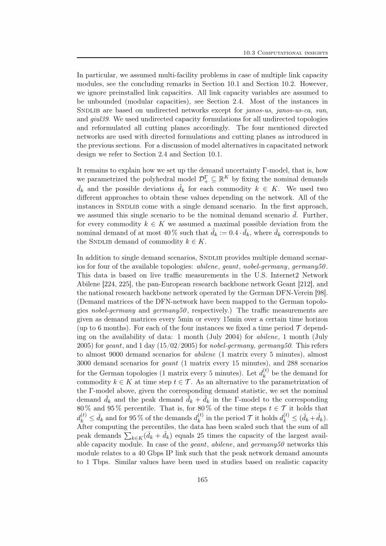
10.3 Computational insights
In particular, we assumed multi-facility problems in case of multiple link capacitymodules, see the concluding remarks in Section 10.1 and Section 10.2. However,we ignore preinstalled link capacities. All link capacity variables are assumed tobe unbounded (modular capacities), see Section 2.4. Most of the instances inSndlib are based on undirected networks except for janos-us, janos-us-ca, sun,and giul39. We used undirected capacity formulations for all undirected topologiesand reformulated all cutting planes accordingly. The four mentioned directednetworks are used with directed formulations and cutting planes as introduced inthe previous sections. For a discussion of model alternatives in capacitated networkdesign we refer to Section 2.4 and Section 10.1.
It remains to explain how we set up the demand uncertainty Γ-model, that is, howwe parametrized the polyhedral model DΓ
+ ⊆ RK by fixing the nominal demandsdk and the possible deviations dk for each commodity k ∈ K. We used twodifferent approaches to obtain these values depending on the network. All of theinstances in Sndlib come with a single demand scenario. In the first approach,we assumed this single scenario to be the nominal demand scenario d. Further,for every commodity k ∈ K we assumed a maximal possible deviation from thenominal demand of at most 40 % such that dk := 0.4 · dk, where dk corresponds tothe Sndlib demand of commodity k ∈ K.
In addition to single demand scenarios, Sndlib provides multiple demand scenar-ios for four of the available topologies: abilene, geant , nobel-germany , germany50 .This data is based on live traffic measurements in the U.S. Internet2 NetworkAbilene [224, 225], the pan-European research backbone network Geant [212], andthe national research backbone network operated by the German DFN-Verein [98].(Demand matrices of the DFN-network have been mapped to the German topolo-gies nobel-germany and germany50 , respectively.) The traffic measurements aregiven as demand matrices every 5min or every 15min over a certain time horizon(up to 6 months). For each of the four instances we fixed a time period T depend-ing on the availability of data: 1 month (July 2004) for abilene, 1 month (July2005) for geant , and 1 day (15/02/2005) for nobel-germany, germany50. This refersto almost 9000 demand scenarios for abilene (1 matrix every 5 minutes), almost3000 demand scenarios for geant (1 matrix every 15 minutes), and 288 scenariosfor the German topologies (1 matrix every 5 minutes). Let d(t)
k be the demand forcommodity k ∈ K at time step t ∈ T . As an alternative to the parametrization ofthe Γ-model above, given the corresponding demand statistic, we set the nominaldemand dk and the peak demand dk + dk in the Γ-model to the corresponding80 % and 95 % percentile. That is, for 80 % of the time steps t ∈ T it holds thatd
(t)k ≤ dk and for 95 % of the demands d(t)
k in the period T it holds d(t)k ≤ (dk+ dk).
After computing the percentiles, the data has been scaled such that the sum of allpeak demands
∑k∈K(dk + dk) equals 25 times the capacity of the largest avail-
able capacity module. In case of the geant , abilene, and germany50 networks thismodule relates to a 40 Gbps IP link such that the peak network demand amountsto 1 Tbps. Similar values have been used in studies based on realistic capacity
165
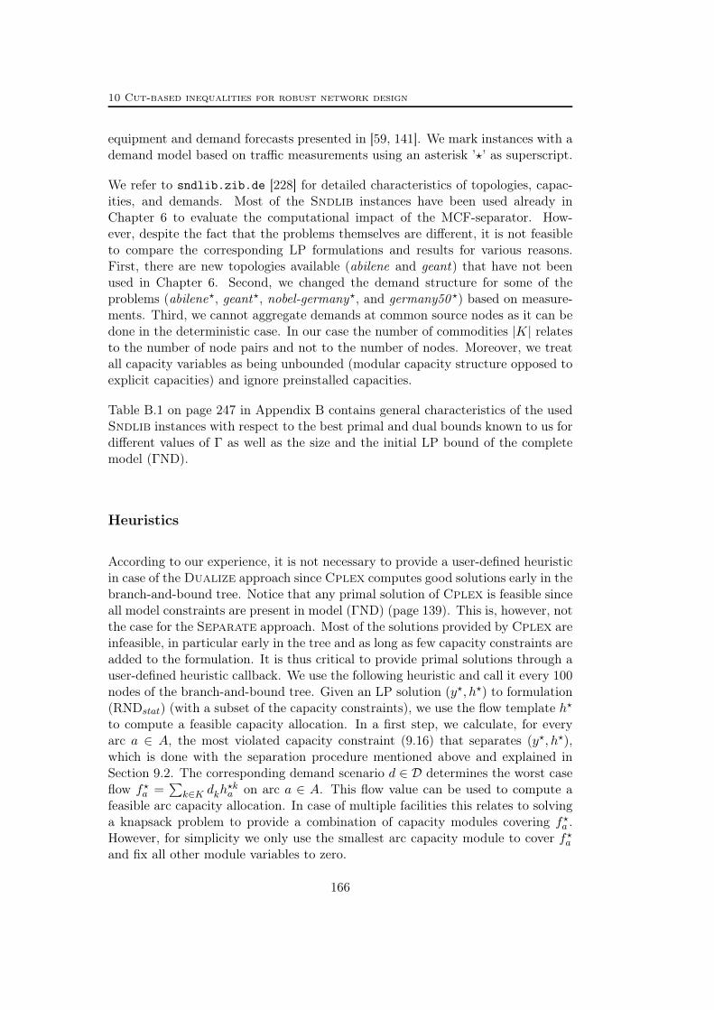
10 Cut-based inequalities for robust network design
equipment and demand forecasts presented in [59, 141]. We mark instances with ademand model based on traffic measurements using an asterisk ’?’ as superscript.
We refer to sndlib.zib.de [228] for detailed characteristics of topologies, capac-ities, and demands. Most of the Sndlib instances have been used already inChapter 6 to evaluate the computational impact of the MCF-separator. How-ever, despite the fact that the problems themselves are different, it is not feasibleto compare the corresponding LP formulations and results for various reasons.First, there are new topologies available (abilene and geant) that have not beenused in Chapter 6. Second, we changed the demand structure for some of theproblems (abilene?, geant?, nobel-germany?, and germany50 ?) based on measure-ments. Third, we cannot aggregate demands at common source nodes as it can bedone in the deterministic case. In our case the number of commodities |K| relatesto the number of node pairs and not to the number of nodes. Moreover, we treatall capacity variables as being unbounded (modular capacity structure opposed toexplicit capacities) and ignore preinstalled capacities.
Table B.1 on page 247 in Appendix B contains general characteristics of the usedSndlib instances with respect to the best primal and dual bounds known to us fordifferent values of Γ as well as the size and the initial LP bound of the completemodel (ΓND).
Heuristics
According to our experience, it is not necessary to provide a user-defined heuristicin case of the Dualize approach since Cplex computes good solutions early in thebranch-and-bound tree. Notice that any primal solution of Cplex is feasible sinceall model constraints are present in model (ΓND) (page 139). This is, however, notthe case for the Separate approach. Most of the solutions provided by Cplex areinfeasible, in particular early in the tree and as long as few capacity constraints areadded to the formulation. It is thus critical to provide primal solutions through auser-defined heuristic callback. We use the following heuristic and call it every 100nodes of the branch-and-bound tree. Given an LP solution (y?, h?) to formulation(RNDstat) (with a subset of the capacity constraints), we use the flow template h?
to compute a feasible capacity allocation. In a first step, we calculate, for everyarc a ∈ A, the most violated capacity constraint (9.16) that separates (y?, h?),which is done with the separation procedure mentioned above and explained inSection 9.2. The corresponding demand scenario d ∈ D determines the worst caseflow f?a =
∑k∈K dkh
?ka on arc a ∈ A. This flow value can be used to compute a
feasible arc capacity allocation. In case of multiple facilities this relates to solvinga knapsack problem to provide a combination of capacity modules covering f?a .However, for simplicity we only use the smallest arc capacity module to cover f?aand fix all other module variables to zero.
166

10.3 Computational insights
Separation
Capacity constraints. Given a solution to (RNDstat) with a subset of the neces-sary exponential capacity constraints (9.16), the corresponding separation problemcan be solved in time O(|A||K| log|K|) by sorting the commodities for every arca ∈ A and computing the maximum possible arc flow based on the nominal flowand the Γ largest deviation commodity flows, see Section 9.2. In our implementa-tion of Separate the initial formulation (RNDstat) already contains one capacityconstraint per arc corresponding to the all-nominal demand scenario d ∈ D, thatis, we start with model (RNDstat) restricted to the capacity constraints
−∑k∈K
dkhka + ya ≥ 0 ∀a ∈ A. (10.21)
For a feasible Separate algorithm it suffices to separate all infeasible primal so-lutions generated by Cplex during branch-and-cut using violated capacity con-straint (9.16). If no violated capacity constraint can be found, then the primalsolution is feasible. However, it turned out to be more effective to separate LPsolutions (in the root node of the branch-and-bound tree) in addition to primalsolutions. In this respect, our lazy constraint handler acts as an additional cuttingplane separator in the cutting plane loop of the root node. All violated capacityconstraints are added to the LP relaxation.
Cut-based inequalities. For both approaches, Dualize and Separate, wegenerate strong valid cut-based inequalities in the root node of the branch-and-bound tree and add the corresponding cutting planes to the LP. This includes thecut-set inequalities of type (10.5) in the space of the capacity variables and flowcut-set inequalities of type (10.7) in the space of capacity and flow. In addition,we check the cut-based envelope inequalities (10.18), (10.19), and (10.20). Theseinequalities are, however, limited to the Dualize approach as they are defined inthe space of capacity and dual π variables.
However, in contrast to the simple single-facility form of these inequalities, as pre-sented in the last sections, we incorporate multiple arc capacities facilities. More-over, we respect undirected capacity models, see Section 2.4 and the concludingremarks in Section 10.1 and Section 10.2.
The strategy to separate cut-based inequalities for both approaches Dualize andSeparate follows, in principle, the strategy of the MCF separator as described inChapter 5 and Algorithm 5.7 on page 93, also see Section 2.5. We concentrate onthe separation of cut-set inequalities. If we cannot find violated cut-set inequalitieswe also try to find violated flow cut-set or envelope inequalities.
We start by calculating a set of network cuts. As in Algorithm 5.7, we considercuts around single nodes and in addition cuts obtained by a graph contractionheuristic. As for the MCF separator the contraction is designed to provide cuts
167
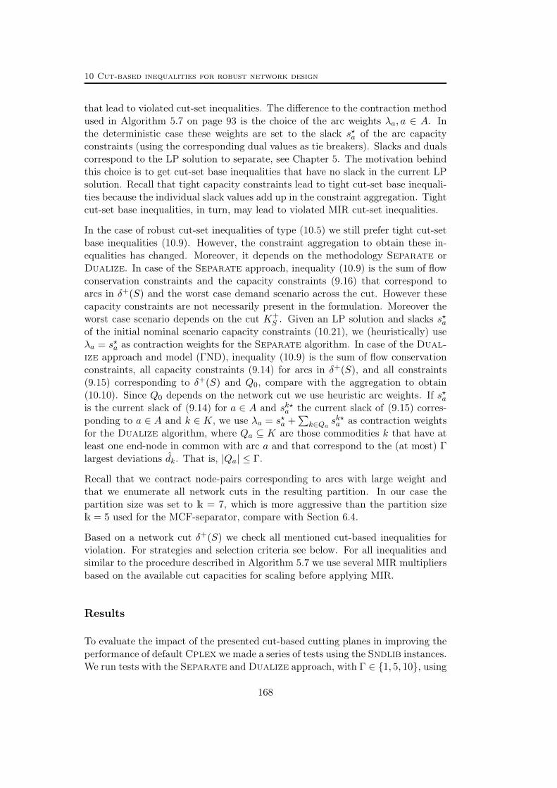
10 Cut-based inequalities for robust network design
that lead to violated cut-set inequalities. The difference to the contraction methodused in Algorithm 5.7 on page 93 is the choice of the arc weights λa, a ∈ A. Inthe deterministic case these weights are set to the slack s?a of the arc capacityconstraints (using the corresponding dual values as tie breakers). Slacks and dualscorrespond to the LP solution to separate, see Chapter 5. The motivation behindthis choice is to get cut-set base inequalities that have no slack in the current LPsolution. Recall that tight capacity constraints lead to tight cut-set base inequali-ties because the individual slack values add up in the constraint aggregation. Tightcut-set base inequalities, in turn, may lead to violated MIR cut-set inequalities.
In the case of robust cut-set inequalities of type (10.5) we still prefer tight cut-setbase inequalities (10.9). However, the constraint aggregation to obtain these in-equalities has changed. Moreover, it depends on the methodology Separate orDualize. In case of the Separate approach, inequality (10.9) is the sum of flowconservation constraints and the capacity constraints (9.16) that correspond toarcs in δ+(S) and the worst case demand scenario across the cut. However thesecapacity constraints are not necessarily present in the formulation. Moreover theworst case scenario depends on the cut K+
S . Given an LP solution and slacks s?aof the initial nominal scenario capacity constraints (10.21), we (heuristically) useλa = s?a as contraction weights for the Separate algorithm. In case of the Dual-ize approach and model (ΓND), inequality (10.9) is the sum of flow conservationconstraints, all capacity constraints (9.14) for arcs in δ+(S), and all constraints(9.15) corresponding to δ+(S) and Q0, compare with the aggregation to obtain(10.10). Since Q0 depends on the network cut we use heuristic arc weights. If s?ais the current slack of (9.14) for a ∈ A and sk?a the current slack of (9.15) corres-ponding to a ∈ A and k ∈ K, we use λa = s?a +
∑k∈Qa s
k?a as contraction weights
for the Dualize algorithm, where Qa ⊆ K are those commodities k that have atleast one end-node in common with arc a and that correspond to the (at most) Γlargest deviations dk. That is, |Qa| ≤ Γ.
Recall that we contract node-pairs corresponding to arcs with large weight andthat we enumerate all network cuts in the resulting partition. In our case thepartition size was set to k = 7, which is more aggressive than the partition sizek = 5 used for the MCF-separator, compare with Section 6.4.
Based on a network cut δ+(S) we check all mentioned cut-based inequalities forviolation. For strategies and selection criteria see below. For all inequalities andsimilar to the procedure described in Algorithm 5.7 we use several MIR multipliersbased on the available cut capacities for scaling before applying MIR.
Results
To evaluate the impact of the presented cut-based cutting planes in improving theperformance of default Cplex we made a series of tests using the Sndlib instances.We run tests with the Separate and Dualize approach, with Γ ∈ 1, 5, 10, using
168

10.3 Computational insights
either default Cplex (default) or generating cut-based inequalities in the root nodeof the branch-and-bound tree (cutset). Detailed statistics for all runs can be foundin Appendix B.
We compare easy and hard instances (independent of the value of Γ). Instances areeasy if they could be solved with one of the approaches (Dualize or Separate,separators on/off) for one of the Γ values. All other instances are considered to behard. With this definition we have 11 easy and 17 hard instances from Sndlib.
Impact of robust cut-set inequalities. In a first test, we study the impactof robust cut-set inequalities. All other network cut-based inequalities (flow cut-set and envelope inequalities) are switched off. For cut-set inequalities we usea minimum relative violation of 0.0001, which refers to the minimum Euclideandistance of the point to separate to the separating hyper-plane, see the definitionin Section 1.1 on page 15.
Tables B.2 to B.3 on pages 249–252 in Appendix B provide all details of thisstudy. Table 10.1 on the next page summarizes the results for easy instances andTable 10.2 on page 171 those for hard instances. Columns default – means reporton average performance measures for the default Cplex run and columns cutset– means provide the same values for the run with cut-set inequalities switched on.The results are presented in the same way as the results for the MCF-separator inTables 6.3 to 6.4 on pages 104–105, cf. Section 6.2, with the only difference thatin addition we provide the average number of generated cut-set inequalities (cuts)and generated lazy capacity constraints (lazy).
For easy instances, we report in Table 10.1 on the next page on the size of the test-set (#), the arithmetic mean of the closed root gaps in % (root), the geometricmean of the CPU time in seconds (time) (using a shift of 1 second), and thegeometric mean of the explored branch-and-bound nodes (nodes) (using a shiftof 100 nodes) used to solve the problems. The closed root gap is defined as inSection 6.2 and is based on the best known primal and dual bounds known to us,see Table B.1 on page 247. All mean values are given for both the default andthe cutset run. The last four columns in Table 10.1 on the next page comparethe two runs with respect to the number of wins (wins) and the number of timelimit hits (t-outs), and they provide the time (time) and node (nodes) ratios ofthe respective geometric means. In case one of the two runs hits the time limitwith fewer branch-and-bound nodes, for a fair comparison, we take the maximumof the two node values in the calculation of the shifted geometric means. One ofthe two runs, default or cutset, “wins” if it could solve the problem with at least10% less CPU time.
For hard instances, we report in Table 10.2 on the size of the test-set (#), theaverage closed root gap (root), dual gap (dual), and primal gap (primal), as wellas the average endgap (endgap). All gaps are given as arithmetic means in %and defined as in Section 6.2. Recall that all closed gaps (root, dual, primal) are
169

10 Cut-based inequalities for robust network design
default – means cutset – means comparisoncutset/default
Algorithm # root time nodes lazy root time nodes lazy cuts wins t-outs time nodescl.gap% in s cl.gap% in s ratio ratio
Γ = 1
Dualize 11 91.1 431 29253 - 94.5 173 10860 - 27 8/1 1/4 0.40 0.37Separate 11 91.3 245 28110 127 94.9 111 10518 121 59 9/1 0/2 0.45 0.37
Γ = 5
Dualize 11 92.4 242 13246 - 94.9 198 8650 - 27 6/0 2/2 0.82 0.65Separate 11 92.6 383 18603 851 95.5 276 11750 766 71 7/2 2/2 0.72 0.63
Γ = 10
Dualize 11 90.8 323 15091 - 94.4 175 6485 - 38 5/2 1/1 0.54 0.43Separate 11 91.2 1068 16132 1416 94.4 779 7361 1664 79 4/2 3/4 0.73 0.46
Table 10.1: Summary for the separation of robust cut-set inequalities – Cplex 12.3 – easy Sndlibinstances. Numbers in blue indicate an improvement (time or node ratios smaller than 1.0, more winsfor cutset than for default, more time-outs for default than for cutset).
defined such that larger values correspond to better results with a maximum of100% whereas the endgap is the better the closer to 0%. Again all mean values aregiven for both the default and the cutset run. The last two columns in Table 10.2compare the two runs with respect to the number of wins (wins) and the endgap.One of the two runs, default or cutset, “wins” if the corresponding endgap is atleast 10% smaller.
All mentioned performance measures are given for each of the two approachesSeparate and Dualize and for all Γ ∈ 1, 5, 10.
It can be seen that we strongly improve the performance of Cplex when generatingrobust cut-set inequalities for both the Dualize and the Separate approach. Foreasy instances, the CPU time is decreased on average by 18–60% for Dualizeand by 27–55% for Separate if robust cut-set inequalities are generated. Thenumber of branch-and-bound nodes even decreases by 35–63% (Dualize) and 37–63% (Separate). Comparing the time limit hits in Table 10.1, we observe thatmany instances can only be solved within the time limit if our cut-set separator isswitched on. The number of wins is in general larger in this case for both easy andhard instances. These results are based on a better approximation of the convexhull of the solution space, which can be seen by comparing the average closed rootgaps in Tables 10.1 and 10.2. Roughly 3–4% more of the integrality gap is closedby using robust cut-set inequalities. But also primal solutions tend to improve.The closed primal gap strongly increases in most cases. Eventually, improved dualand improved primal bounds both are responsible for a decrease of the averageendgap by 7–22% (Dualize) and 10–37% (Separate) for hard instances.
Before we will compare the performance of the different solution methods Dualize
170

10.3 Computational insights
default – means cutset – means comparisoncutset/default
Algorithm # root dual primal endgap lazy root dual primal endgap lazy cuts wins endgapclosed gap in % in % closed gap in % in % ratio
Γ = 1
Dualize 17 35.1 44.1 77.0 5.9 - 37.2 45.4 79.2 5.5 - 37 6/2 0.93Separate 17 34.6 44.1 74.9 5.4 395 38.5 46.3 76.0 4.8 396 61 6/2 0.90
Γ = 5
Dualize 17 30.6 39.2 70.4 5.8 - 34.2 42.3 80.5 4.7 - 36 6/0 0.82Separate 17 31.7 37.4 52.9 9.0 2160 34.5 40.5 63.2 7.5 1966 73 8/0 0.83
Γ = 10
Dualize 17 29.6 38.4 76.7 5.6 - 34.8 41.8 85.8 4.4 - 37 8/1 0.78Separate 17 30.2 33.8 34.5 16.3 5265 35.1 39.4 47.1 10.3 4303 82 9/1 0.63
Table 10.2: Summary for the separation of robust cut-set inequalities – Cplex 12.3 – hard Sndlibinstances. Numbers in blue indicate an improvement (endgap ratios smaller than 1.0, more wins forcutset than for default.
and Separate using the results from Tables 10.1 and 10.2, let us first study theimpact of flow cut-set inequalities and envelope inequalities if separated in additionto cut-set inequalities.
Impact of flow cut-set and envelope inequalities. In two individual testswe study the additional impact of flow cut-set inequalities or envelope inequalitiesin reducing computation times and gaps.
The general form of a flow cut-set inequality contains cut-set inequalities as a spe-cial case. Even more, the most violated flow cut-set inequality (for commodity setK+S ) is most of the time not a cut-set inequality. However, cut-set inequalities typi-
cally clearly outperform flow cut-set inequalities in terms of computational success,see [50, 200]. To our experience, the number of violated flow cut-set inequalitiescan be very large such that they have to be selected carefully. We generate flowcut-set inequalities only if no violated cut-set inequality could be found in the lastseparation round of the root node. This is in line with the separation approachesin [50, 200] and the separation framework of the MCF separator, see Section 2.5and Chapter 5.
We use the same set of network cuts as for cut-set inequalities (single node cuts andcuts from the contraction heuristic). Given a network cut δ+(S), we have to fix asubset A+ of δ+(S), a subset Q of the cut commoditiesK+
S , and a demand scenariod ∈ D, in order to generate a (simple) robust flow cut-set inequality of type (10.7),see Section 2.3 and Section 10.1. We use two different types of commodity subsets,the full set Q = K+
S as in Algorithm 5.7 on page 93 and additionally all singletonsets Q = k with k ∈ K+
S . After fixing the commodity subset we compute the
171
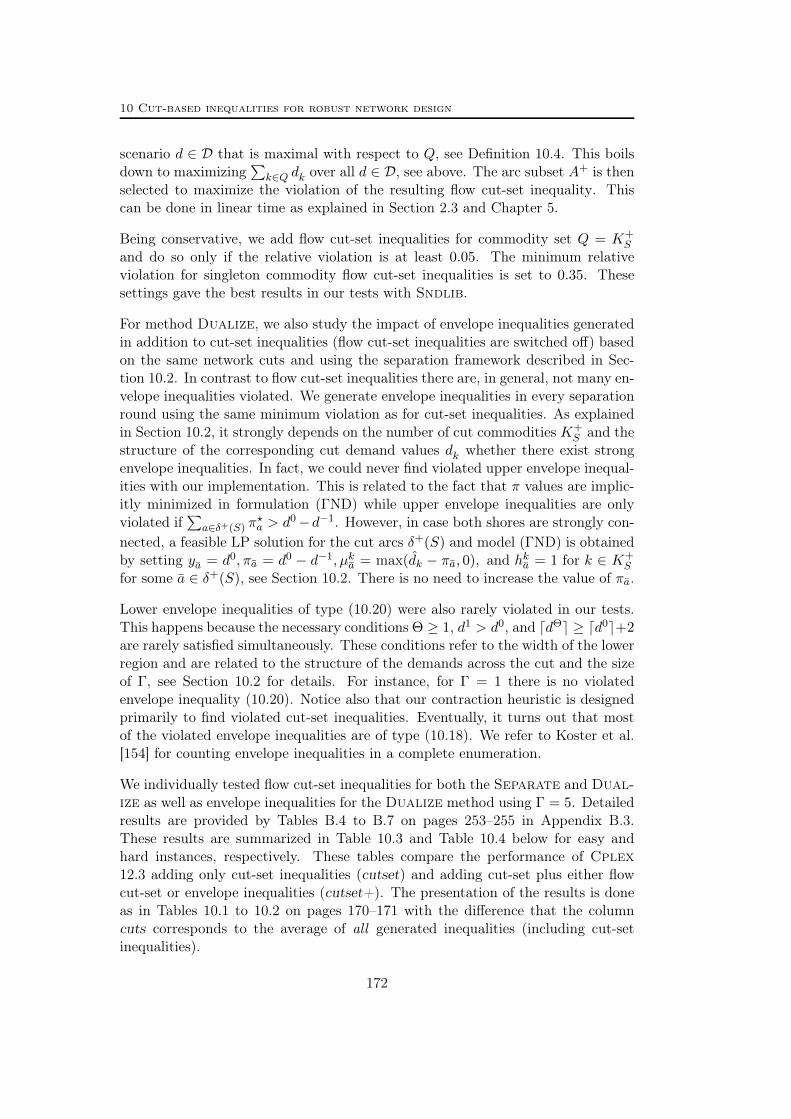
10 Cut-based inequalities for robust network design
scenario d ∈ D that is maximal with respect to Q, see Definition 10.4. This boilsdown to maximizing
∑k∈Q dk over all d ∈ D, see above. The arc subset A+ is then
selected to maximize the violation of the resulting flow cut-set inequality. Thiscan be done in linear time as explained in Section 2.3 and Chapter 5.
Being conservative, we add flow cut-set inequalities for commodity set Q = K+S
and do so only if the relative violation is at least 0.05. The minimum relativeviolation for singleton commodity flow cut-set inequalities is set to 0.35. Thesesettings gave the best results in our tests with Sndlib.
For method Dualize, we also study the impact of envelope inequalities generatedin addition to cut-set inequalities (flow cut-set inequalities are switched off) basedon the same network cuts and using the separation framework described in Sec-tion 10.2. In contrast to flow cut-set inequalities there are, in general, not many en-velope inequalities violated. We generate envelope inequalities in every separationround using the same minimum violation as for cut-set inequalities. As explainedin Section 10.2, it strongly depends on the number of cut commodities K+
S and thestructure of the corresponding cut demand values dk whether there exist strongenvelope inequalities. In fact, we could never find violated upper envelope inequal-ities with our implementation. This is related to the fact that π values are implic-itly minimized in formulation (ΓND) while upper envelope inequalities are onlyviolated if
∑a∈δ+(S) π
?a > d0−d−1. However, in case both shores are strongly con-
nected, a feasible LP solution for the cut arcs δ+(S) and model (ΓND) is obtainedby setting ya = d0, πa = d0 − d−1, µka = max(dk − πa, 0), and hka = 1 for k ∈ K+
S
for some a ∈ δ+(S), see Section 10.2. There is no need to increase the value of πa.
Lower envelope inequalities of type (10.20) were also rarely violated in our tests.This happens because the necessary conditions Θ ≥ 1, d1 > d0, and ddΘe ≥ dd0e+2are rarely satisfied simultaneously. These conditions refer to the width of the lowerregion and are related to the structure of the demands across the cut and the sizeof Γ, see Section 10.2 for details. For instance, for Γ = 1 there is no violatedenvelope inequality (10.20). Notice also that our contraction heuristic is designedprimarily to find violated cut-set inequalities. Eventually, it turns out that mostof the violated envelope inequalities are of type (10.18). We refer to Koster et al.[154] for counting envelope inequalities in a complete enumeration.
We individually tested flow cut-set inequalities for both the Separate and Dual-ize as well as envelope inequalities for the Dualize method using Γ = 5. Detailedresults are provided by Tables B.4 to B.7 on pages 253–255 in Appendix B.3.These results are summarized in Table 10.3 and Table 10.4 below for easy andhard instances, respectively. These tables compare the performance of Cplex12.3 adding only cut-set inequalities (cutset) and adding cut-set plus either flowcut-set or envelope inequalities (cutset+). The presentation of the results is doneas in Tables 10.1 to 10.2 on pages 170–171 with the difference that the columncuts corresponds to the average of all generated inequalities (including cut-setinequalities).
172

10.3 Computational insights
cutset – means cutset+ – means comparisoncutset+/cutset
Algorithm # root time nodes lazy cuts root time nodes lazy cuts wins t-outs time nodescl.gap% in s cl.gap% in s ratio ratio
flow cut-set inequalitiesDualize 11 94.9 198 8578 - 27 95.0 182 8379 - 33 3/0 2/2 0.92 0.98Separate 11 95.5 276 11235 766 71 95.3 296 11897 702 102 0/3 2/2 1.07 1.06
envelope inequalitiesDualize 11 94.9 198 8354 - 27 94.8 198 8648 - 31 2/2 2/2 1.00 1.04
Table 10.3: Summary for adding robust flow cut-set inequalities or robust envelope inequalities inaddition to robust cut-set inequalities – Cplex 12.3 – easy Sndlib instances. Γ = 5 fixed. Numbersin blue indicate an improvement (time or node ratios smaller than 1.0, more wins for cutset+ thanfor cutset, more time-outs for cutset than for cutset+), numbers in red a deterioration.
cutset – means cutset+ – means comparisoncutset+/cutset
Algorithm # root dual primal endgap lazy cuts root dual primal endgap lazy cuts wins endgapclosed gap in % in % closed gap in % in % ratio
flow cut-set inequalitiesDualize 17 34.2 42.3 80.5 4.7 - 36 34.1 41.9 86.3 4.1 - 53 3/1 0.86Separate 17 34.5 40.5 63.2 7.5 1966 73 34.4 40.1 61.6 7.8 1986 107 2/4 1.05
envelope inequalitiesDualize 17 34.2 42.3 80.5 4.7 - 36 34.2 42.0 77.8 4.8 - 37 1/1 1.02
Table 10.4: Summary for adding robust flow cut-set inequalities or robust envelope inequalities inaddition to robust cut-set inequalities – Cplex 12.3 – hard Sndlib instances. Γ = 5 fixed. Numbersin blue indicate an improvement (endgap ratios smaller than 1.0, more wins for cutset+ than forcutset), numbers in red a deterioration.
We observe that by generating flow cut-set inequalities in addition to cut-set in-equalities we can still improve on the computation times and endgaps in the caseof Dualize. There is a decrease of the average CPU time decrease of 8% for easyinstances and an average decrease of the endgap by even 14% on average. It isremarkable that the latter results for hard instances are caused by improved primalsolutions rather than by improving on the dual bounds. In fact 8 of 17 instancesbenefit from flow cut-set inequalities in terms of primal bounds, cf. Table B.5 onpage 254. We even find the best known solutions in 3 cases. For the Separateapproach adding flow cut-set inequalities does not pay off with our settings. TheCPU times, node ratios, and endgaps increase. This is obviously caused by tooaggressive separation. It seems that flow cut-set inequalities have to be tuned in adifferent way for the Separate approach. In particular, the interaction with theseparation of lazy capacity constraints has to be taken into account properly.
The results for envelope inequalities are not conclusive. On average, there are onlyfew inequalities actually added to the LP in addition to cut-set inequalities, see the
173

10 Cut-based inequalities for robust network design
0 20 40 600
50
100
150
200
250
Γ
CP
Uti
me
ins
SeparateDualize
(a) abilene? instance with |K| = 66 commodi-ties
0 5 10 15 20 250
200
400
600
Γ
CP
Uti
me
ins
SeparateDualize
(b) pdh-UUM instance with |K| = 24 commodi-ties
Figure 10.2: Solving time in seconds as a function of Γ for the Dualize and Separate approach.The solving time for Dualize is independent of Γ. It clearly depends on the number of vertices ofthe uncertainty set in case of Separate.
remarks above. In fact, only a small number of instances is affected (see Table B.6and B.7 on page 255). The number of wins is balanced both for easy and hardinstances. Sometimes we improve by adding envelope inequalities, sometimes wedeteriorate the performance. For hard instances this results in a small decrease ofthe average endgap. However, for easy instances we loose 4% of the CPU time.
Summarizing, flow cut-set inequalities clearly help to further improve the perfor-mance of our branch-and-cut algorithms if generated carefully. However, for theSeparate we need to find a better tuning. In contrast, violated envelope inequal-ities are rarely found and do not seem to help a lot even if a reasonable numbercan be generated.
Impact of the solution method. Comparing the Dualize and Separate ap-proach, Tables 10.1 to 10.2 on pages 170–171 clearly show that the Separateapproach outperforms Dualize for Γ = 1. Easy instances are solved in about65% of the CPU time on average (111 s compared to 173 s for cutset) and also theaverage endgap for hard instances is smaller if capacity constraints are separatedrather than dualized (4.8% compared to 5.5% for cutset). However, increasing Γstrongly decreases the performance of Separate while the performance of Dual-ize is (almost) independent of Γ. For Γ = 10, Separate is already more than 4times slower than Dualize (779 s compared to 175 s for cutset) for easy instances.Also the average endgap for hard instances is poor in this case.
This behavior can be explained easily. Assume 0 < Γ < |K|. The size of the(resulting) formulation for Separate strongly depends on the size of Γ in contrastto Dualize. Recall that Γ corresponds to the number of commodities that maydeviate from their nominal value simultaneously. The number of necessary capacityconstraints (9.16) for Separate is proportional to the number of non-dominated
174

10.3 Computational insights
vertices of the uncertainty polytope DΓ+. These are
(|K|Γ
)many, corresponding to
all subsets of K with cardinality Γ. Hence, for Γ = 1, the complete Separateformulation is relatively small. The formulation, however, increases exponentiallyas long as Γ < |K|/2. Observe that in Tables 10.1 to 10.2 on pages 170–171 thenumber of lazy capacity constraints (column lazy) increases exponentially withΓ. These constraints are necessary to obtain a feasible root formulation. Noticethat with Separate we achieve the same level of closed root gap (column root)compared to the Dualize approach. However, the linear programs become toolarge and hard to solve such that the overall solution process slows down. Thisresults in large CPU times for easy problems and poor dual as wells as primalbounds for hard instances.
By the above arguments the Separate approach should become competitive againif Γ is chosen close to |K|. To illustrate this effect we compare the solving times ofDualize and Separate for two easy instances and all values of Γ in 0, . . . , |K|in Figure 10.2 on the previous page. The computation times for Dualize arerelatively independent of the value of Γ while the solution times for Separateroughly follow the shape of
(|K|Γ
)as a function of Γ. We conclude that the approach
Separate should be used only for small values of Γ or (|K|−Γ). Notice that theseresults are in contrast to those in Fischetti and Monaci [106] for uncertain linearprograms and robust set covering problems.
Robustness of network designs. We close this chapter by briefly commentingon the quality of the computed optimal robust network designs. For detailedstudies on the robustness of solutions and how to parametrize the Γ-model werefer to Koster et al. [152, 155].
We investigate two aspects as quality criteria: the cost of an optimal robust net-work design and the realized robustness with respect to a given set of traffic ma-trices. Exemplary, we consider the abilene? and geant? instances as defined above.Recall that we parametrized the Γ-model for these instances using life traffic mea-surements from IP networks. Given traffic scenarios every 5min over one month(abilene?) and every 15min over one month (geant?), we used nominal and peakvalues based on the 80% and 95% percentile. That is, whenever we speak of ’peak’in the following we refer to the 95% percentile.
Figure 10.3(a) and Figure 10.3(b) on the next page report on the optimal solutionvalue for both instances and all values of Γ in 0, . . . , 40. We first observe thatby increasing Γ the solution cost increases. The gap of the solution value betweenthe two extremes, that is, Γ = 0 referring to the 80% percentile demand matrixand Γ = |K+
S | referring to the 95% percentile scenario, is 28.4% and 26.7% forabilene? and geant?, respectively. However, the solution value for Γ = |K| isachieved already for small Γ. Lets call the corresponding threshold Γ?. In case ofabilene for Γ? = 21 < |K| = 66 and in case of geant? for Γ? = 40 < |K| = 228 themaximum possible network cost is attained. This is related to the size of nominal
175

10 Cut-based inequalities for robust network design
0 10 20 30 403.5
4
4.5
5
5.5
6·104
Cost of all-peak scenario
Full robustness
Γ
Opt
imal
valu
e
(a) abilene? instance, optimal solution value as afunction of Γ
0 10 20 30 403.5
4
4.5
5·104
Cost of all-peak scenario
Full robustness
Γ
Opt
imal
valu
e
(b) geant? instance, optimal solution value as afunction of Γ
0 10 20 30 400
10
20
30
40
50
Full robustness
Γ
Infe
asib
leti
me
step
s
Single linkcongestion:
0.01 %1 %5 %10 %20 %30 %
(c) abilene? instance, percentage of infeasible timesteps as a function of Γ
0 10 20 30 400
10
20
30
40
50
Full robustness
Γ
Infe
asib
leti
me
step
s
Single linkcongestion:
0.01 %1 %5 %10 %20 %30 %
(d) geant? instance, percentage of infeasible timesteps as a function of Γ
Figure 10.3: The price of robustness: Increasing Γ means increasing the robustness and increasing thecost. Reasonable levels of robustness are obtained already for small values of Γ in 5, . . . , 15 withsignificant cost saving compared to the worst case scenario (Γ = |K|). Depending on the choice ofnominal and peak values to parametrize the Γ-model not all traffic matrices outside to the uncertaintyset D can be routed. In this case, around 5% of the matrices can not be realized even for large Γ.The Γ-model has been parametrized by using the 80% and 95% percentile for nominal and peakvalues, respectively.
demands dk and peak demands dk + dk for individual commodities. If the valuedk is large only for a small number of commodities, then protecting against thesimultaneous peak of these commodities means protecting against the peak of allcommodities (with the given capacity structure). It turns out that in data fromreal networks only a small number of commodities realizes peaks simultaneously. Arelated consequence of these observations is the maximum number of commoditiesthat meet on a single arc in an optimal solution. Essentially, if this number issmaller than Γ, then we can increase Γ without changing the solution value. Recallthat we have already formalized this observation in Section 9.2 together with apossible definition of Γ?, see Definition 9.15 and Lemma 9.16.
176

10.3 Computational insights
0 5 10 15 20 25 30
0.4
0.6
0.8
1·105
Cost of all-peak scenario
Full robustness
Γ
Opt
imal
valu
e
(a) abilene? instance, optimal solution value as afunction of Γ
0 5 10 15 20 25 300
10
20
30
40
50
Full robustness
Γ
Infe
asib
leti
me
step
s
Single linkcongestion:
0.01 %1 %5 %10 %20 %30 %
(b) abilene? instance, percentage of infeasibletime steps as a function of Γ
Figure 10.4: The price of robustness: Increasing Γ means increasing the robustness and increasingthe cost. Reasonable levels of robustness are obtained already for small values of Γ in 1, . . . , 5 withsignificant cost saving compared to the worst case scenario (Γ = |K|). Depending on the choice ofnominal and peak values to parametrize the Γ-model not all traffic matrices outside to the uncertaintyset D can be routed. In this case, around 1% of the matrices can not be realized even for large Γ.The Γ-model has been parametrized by using the 80% and 99% percentile for nominal and peakvalues, respectively.
In Figure 10.3(c) and 10.3(d) we show how many of the traffic matrices in the1 month period (|T | = 8928 matrices for abilene? and |T | = 2976 matrices forgeant?) can be realized in the optimal solution (y, h) for Γ ∈ 0, . . . , 40. Forevery point in time t ∈ T we try to route the given traffic matrix using the staticflow template h within the capacities y. We count the number of matrices intime horizon T that can be routed without exceeding individual link capacitiesby more than p% with p ∈ 0.01, 1, 5, 10, 20, 30. All other time steps t ∈ Tare said to be infeasible. The individual link congestion for arc a in time stept ∈ T is defined as pa := 1 − (ya/f
(t)a ), where f (t)
a refers to the realized arc flow.Setting p := maxa∈A pa, a time step becomes infeasible if at least one of the linksfails. Figure 10.3(c) and Figure 10.3(d) provide the percentage of infeasible timesteps w. r. t. |T |. Notice that even setting Γ = |K+
S | does not necessarily give 0%infeasibility over time as we removed 5% of the largest demands by assuming thepeak demand dk + dk to be the 95 % percentile over time for all k ∈ K.
Figure 10.3 shows that, similar to the solution cost as a function of Γ, also thenumber of infeasible time steps decreases if we increase Γ. And also the maximalpossible robustness (with the given parametrization of the Γ-model) is achievedalready for very small Γ. Let q(Γ) be the percentage of matrices with at least onelink having congestion more than 1%. If q(Γ) = q(|K|) ± 0.5 % we say that thesolution corresponding to Γ is fully robust. We denote by Γ?? the smallest Γwith this property. In case of abilene? Γ?? = 6 with q(Γ??) = 4.8 % and for geant?
Γ?? = 15 with q(Γ??) = 4.6 %. Clearly, for both instances we have Γ?? < Γ?. Itfollows that we achieve full robustness before we achieve the maximum cost. Thecost savings compared to the (artificial) scenario Γ = |K+
S | are in between 2–10%
177

10 Cut-based inequalities for robust network design
of the total cost for abilene? and geant?, respectively.
To increase the number of feasible time steps we have to include more trafficscenarios into our uncertainty set. In Figure 10.4 on the previous page we reusedinstance abilene? and the corresponding traffic measurements but parametrizedthe Γ-model by setting nominal and peak values to the 80% and 99% percentile,respectively. In this case, there remain around 1% of the matrices that cannot berealized within the capacities of the global robust solution. Already for Γ?? = 3the percentage of matrices with at least one link having congestion more than 1%drops below q(|K|) = 1.3 % and then remains in this order of magnitude. Theworst case solution value is obtained with Γ? = 28. We save 20.1% of the costwhen optimizing with Γ = Γ? rather than Γ = Γ?? and obtain the same level ofrobustness.
Concluding remarks
We have generalized the well-known cut-set and flow cut-set inequalities to robustnetwork design with general polyhedral uncertainty sets. We showed under whichconditions these inequalities define facets and we proved that these inequalitiescan be used in a similar way as cutting planes with a comparable computationalimpact as their deterministic counterparts. We also provided detailed numericaltests w. r. t. different solution methods for robust network design and w. r. t. therobustness of the resulting capacitated networks.
Surprisingly, the presented cut-set inequalities (in the space of the capacity vari-ables) define facets independent of the assumed recourse scheme, static or dynamicrouting. Recall that the respective polyhedra are contained in each other. Inthe remaining chapter we will investigate a new routing scheme, so-called affinerouting. The focus will be on general properties and on conditions of polyhedraluncertainty sets that result in affine routings being static or dynamic routings be-ing affine. However, note that because affine routing is a restriction of dynamicrouting and a relaxation of static routing, the mentioned results about cut-set in-equalities also hold for this new recourse scheme. In particular, Theorem 10.3 andTheorem 10.5 can be easily generalized to the context of affine routings.
178

Chapter 11
Affine policies: between staticand dynamic routing
In this chapter, we study an alternative to routing schemes dynamic and staticintroduced in Chapter 8, which we call affine routing. The focus is not on solvingthe corresponding design problems but on theoretical aspects and properties of theresulting solution spaces. In this respect, we mainly focus on continuous capacitiesrather than a discrete capacity structure. It turns out that the solution costfor robust network designs with affine routing is in between the cost for robustnetwork design with static and dynamic routing. Moreover, affine routings enablepolynomial reformulations just like static routings. In this respect we follow therecent remark made by Goyal et al. [116]:
[ . . . ] for at least some robust network design problems of practicalinterest, the routing model used may have a serious impact on thesolution cost. While completely dynamic routing is typically infeas-ible for reasons mentioned previously, it is plausible that some tradeoff between the two extremes of dynamic and oblivious routing couldproduce significantly better results while remaining practical. [. . . ]
Recall that oblivious routing is just a different name for static routing.
Affine routings are based on applying the framework of affine decision rules ofBen-Tal et al. [43] developed for general linear programming to multi-commodityflows and demand uncertainty. Ben-Tal et al. [43] show that affinely-adjustablerobust counterparts may provide tractable alternatives to (two-stage) robust pro-grams with arbitrary (dynamic) recourse.
In Section 11.1, we compare the new affine routing scheme to the well-studied staticand dynamic routing schemes for robust network design. We will show that affinerouting can be seen as a generalization of the widely used static routing while stillbeing tractable and providing cheaper solutions. We investigate properties on thedemand polytope D under which affine routings reduce to static routings and also
179
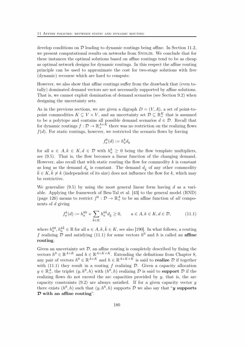
11 Affine policies: between static and dynamic routing
develop conditions on D leading to dynamic routings being affine. In Section 11.2,we present computational results on networks from Sndlib. We conclude that forthese instances the optimal solutions based on affine routings tend to be as cheapas optimal network designs for dynamic routings. In this respect the affine routingprinciple can be used to approximate the cost for two-stage solutions with free(dynamic) recourse which are hard to compute.
However, we also show that affine routings suffer from the drawback that (even to-tally) dominated demand vectors are not necessarily supported by affine solutions.That is, we cannot exploit domination of demand scenarios (see Section 9.2) whendesigning the uncertainty sets.
As in the previous sections, we are given a digraph D = (V,A), a set of point-to-point commodities K ⊆ V × V , and an uncertainty set D ⊆ RK+ that is assumedto be a polytope and contains all possible demand scenarios d ∈ D. Recall thatfor dynamic routings f : D → RA×K+ there was no restriction on the realizing flowsf(d). For static routings, however, we restricted the scenario flows by forcing
fka (d) := hkadk
for all a ∈ A, k ∈ K, d ∈ D with hka ≥ 0 being the flow template multipliers,see (9.5). That is, the flow becomes a linear function of the changing demand.However, also recall that with static routing the flow for commodity k is constantas long as the demand dk is constant. The demand d
kof any other commodity
k ∈ K, k 6= k (independent of its size) does not influence the flow for k, which maybe restrictive.
We generalize (9.5) by using the most general linear form having d as a vari-able. Applying the framework of Ben-Tal et al. [43] to the general model (RND)(page 126) means to restrict fk : D → RA+ to be an affine function of all compo-nents of d giving
fka (d) := hk0a +
∑k∈K
hkka dk ≥ 0, a ∈ A, k ∈ K, d ∈ D, (11.1)
where hk0a , h
kka ∈ R for all a ∈ A, k, k ∈ K, see also [190]. In what follows, a routing
f realizing D and satisfying (11.1) for some vectors h0 and h is called an affinerouting.
Given an uncertainty set D, an affine routing is completely described by fixing thevectors h0 ∈ RA×K and h ∈ RA×K×K . Extending the definitions from Chapter 8,any pair of vectors h0 ∈ RA×K and h ∈ RA×K×K is said to realize D if togetherwith (11.1) they result in a routing f realizing D. Given a capacity allocationy ∈ RA+, the triplet (y, h0, h) with (h0, h) realizing D is said to support D if therealizing flows do not exceed the arc capacities provided by y, that is, the arccapacity constraints (9.2) are always satisfied. If for a given capacity vector ythere exists (h0, h) such that (y, h0, h) supports D we also say that “y supportsD with an affine routing”.
180

11 Affine policies: between static and dynamic routing
As for static and dynamic routings, the set of demand vectors supported by acapacity allocation with an affine routing is convex which allows to state demandpolytopes either by an outer facet description or an inner vertex description.
Lemma 11.1. Let D ⊆ RK+ , h ∈ RA×K×K h0 ∈ RA×K , and y ∈ RA. The triple(y, h0, h) supports D if and only if it supports conv(D).
The following lemma formalizes the relation between optimal solutions for robustnetwork design using dynamic, affine, or static routings. Affine routing generalizesstatic routing allowing for more flexibility in reacting to demand fluctuations, butit is not as flexible as dynamic routing, cf. Lemma 9.6.
Lemma 11.2. Let D be an arbitrary demand uncertainty set and let optdyn(D),optaff (D), optstat(D) be the cost of the optimal solution to the LP relaxation of(RND) where f is allowed to be dynamic (no restriction), affine (forcing (11.1)),or static (forcing (9.5)), respectively. Then
optdyn(D) ≤ optaff (D) ≤ optstat(D).
Proof. Trivially any routing f is a dynamic routing. The number of possibleroutings realizing D is restricted by imposing (11.1) hence optdyn(D) ≤ optaff (D).Moreover, we see immediately that static routing can be obtained from (11.1) bysetting hk0
a = 0 and hkka = 0 for each a ∈ A and all k, k ∈ K with k 6= k yieldingoptaff (D) ≤ optstat(D).
For trivial properties on the graph and the set of commodities yielding optstat(D) =optdyn(D) and hence optdyn(D) ≤ optaff (D) ≤ optstat(D) see the remarks in Sec-tion 9.1. Also recall that the ratio of optstat(D) and optdyn(D) is at most O(log|V |)[67, 116]. In this chapter, we do not establish optimality gaps between the threerouting principles. We rather focus on studying properties of the demand scenar-ios D that either yield optstat(D) = optaff (D) or optaff (D) = optdyn(D). Ourcomputational experiments in Section 11.2 suggest that for realistic networks anddemand scenarios the static/dynamic optimality gap is small in practice (also see[172]), and if there is a gap, the cost for affine solutions tends to be very close tothe cost for dynamic solutions. In fact in most cases optaff (D) ≈ optdyn(D) in ourcomputations.
In what follows, we will assume that D is a full-dimensional polytope, if not ex-plicitly stated otherwise. Notice, however, that some results in the next sectioncan be easily generalized to D being some bounded set in RK+ . Recall that vert(D)denotes the set of extreme points of the polytope D.
As already mentioned in Section 9.1, static, affine and dynamic routings coincidefor any commodity k = (s, t) ∈ K if there exists only one path from s to t. In thefollowing, we assume that for all k = (s, t) ∈ K there exist at least two distinctpaths p1, p2 in D from s to t, that is, two paths that differ by at least one arc.
181
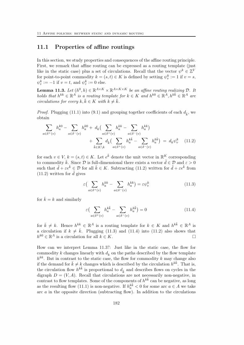
11 Affine policies: between static and dynamic routing
11.1 Properties of affine routings
In this section, we study properties and consequences of the affine routing principle.First, we remark that affine routing can be expressed as a routing template (justlike in the static case) plus a set of circulations. Recall that the vector ψk ∈ ZVfor point-to-point commodity k = (s, t) ∈ K is defined by setting ψkv := 1 if v = s,ψkv := −1 if v = t, and ψkv := 0 else.
Lemma 11.3. Let (h0, h) ∈ RA×K ×RA×K×K be an affine routing realizing D. Itholds that hkk ∈ RA is a routing template for k ∈ K and hk0 ∈ RA, hkk ∈ RA arecirculations for every k, k ∈ K with k 6= k.
Proof. Plugging (11.1) into (9.1) and grouping together coefficients of each dk, we
obtain∑a∈δ+(v)
hk0a −
∑a∈δ−(v)
hk0a + dk
( ∑a∈δ+(v)
hkka −∑
a∈δ−(v)
hkka)
+∑k∈K\k
dk( ∑a∈δ+(v)
hkka −∑
a∈δ−(v)
hkka)
= dkψkv (11.2)
for each v ∈ V, k = (s, t) ∈ K. Let ek denote the unit vector in RK correspondingto commodity k. Since D is full-dimensional there exists a vector d ∈ D and ε > 0such that d + εek ∈ D for all k ∈ K. Subtracting (11.2) written for d + εek from(11.2) written for d gives
ε( ∑a∈δ+(v)
hkka −∑
a∈δ−(v)
hkka)
= εψkv (11.3)
for k = k and similarly
ε( ∑a∈δ+(v)
hkka −∑
a∈δ−(v)
hkka)
= 0 (11.4)
for k 6= k. Hence hkk ∈ RA is a routing template for k ∈ K and hkk ∈ RA isa circulation if k 6= k. Plugging (11.3) and (11.4) into (11.2) also shows thathk0 ∈ RA is a circulation for all k ∈ K.
How can we interpret Lemma 11.3?: Just like in the static case, the flow forcommodity k changes linearly with dk on the paths described by the flow templatehkk. But in contrast to the static case, the flow for commodity k may change alsoif the demand for k 6= k changes which is described by the circulation hkk. That is,the circulation flow hkk is proportional to d
kand describes flows on cycles in the
digraph D = (V,A). Recall that circulations are not necessarily non-negative, incontrast to flow templates. Some of the components of hkk can be negative, as longas the resulting flow (11.1) is non-negative. If hkka < 0 for some arc a ∈ A we takearc a in the opposite direction (subtracting flow). In addition to the circulations
182

11.1 Properties of affine routings
v1
v2
v3
3
2
2
(a)
v1
v2
v3
1
2
1
(b)
v1
v2
v3
1/3
2/3
2/3
(c)
v1
v2
v3
1/3
−1/3
−1/3
(d)
v1
v2
v31
(e)
Figure 11.1: Optimal capacity allocation for robust network design with affine routing, cf. Figure 9.1 onpage 130 and Example 11.4. Let K = k1, k2 = (v1, v2), (v1, v3) and D = (2, 1), (1, 2), (1, 1).(a) Arc cost vector κ. (b) Optimal capacity allocation y using affine (or dynamic) routing with totalcost 9. The optimal affine routing is given by (c) flow template hk1k1 , (d) circulation hk1k2 , and (e)flow template hk2k2 . Negative values correspond to flows in the opposite direction.
hkk for all k 6= k that may change the template hkka , there is a constant circulationshift described by variables hk0, which is independent of the demand scenarios.
As already mentioned, also a dynamic routing for commodity k could be describedby one (representative) routing template and circulations depending on the de-mand fluctuations. However, in the dynamic case, the circulations can be chosenarbitrarily while in the affine case the actual flow changes according to (11.1). Weillustrate this concept in Example 11.4 and Figure 11.1 which shows that affinerouting can be as good as dynamic routing in terms of the cost for capacity alloca-tion. Example 11.4 also highlights that h0 and hkk may not describe circulationswhen D is not full-dimensional.
Example 11.4. Consider the network design problem from Figure 11.1. Fig-ures 11.1(c)–11.1(e) describe coefficients hkk for an affine routing feasible for thecapacity allocation in Figure 11.1(b). This capacity allocation has cost 9 and coin-cides with the optimal dynamic capacity allocation while the optimal static capacityallocation has cost 10, cf. Figure 9.1 on page 130. If we remove d3 = (1, 1) fromthe set of extreme points, the dimension of the uncertainty set reduces to 1. Theaffine routing prescribed by hk2k2
(v1,v3) = 1, hk10(v1,v2) = 3, and hk1k2
(v1,v2) = −1 realizes alldemands in the convex hull of d1 = (2, 1) and d2 = (1, 2) but hk10 and hk1k2 do notdescribe a circulation.
A compact reformulation
Recall that a formulation is said to be compact if the number of variables and con-straints is polynomial in the number of nodes |V |. A valid formulation for robustnetwork design using affine routing is obtained by adding (11.1) to the general
183

11 Affine policies: between static and dynamic routing
formulation (RND) (page 126). By Lemma 11.1, a compact linear formulation forthe robust network design problem with affine routing can be prescribed when-ever the number of (non-dominated) vertices of D is polynomial in the number ofnodes since we can restrict (RND) to these vertices. In the following we providea compact linear reformulation for the case that D has a compact inequality de-scription, that is, the polytope D has a linear description in RK+ , where the numberof defining inequalities is polynomial in the number of nodes. The reformulationextends the dualized formulation (RND?
stat) (page 132) for robust network designwith static routing. As in Chapter 9, let polytope D ⊆ RK+ be given implicitly bya system of linear constraints:
D := P+(−A,−α) = d ∈ RK+ : Ad ≤ α
with A = (Aik) ∈ QM×K and α ∈ QM , m = |M | ≥ 1.
Proposition 11.5. The robust network design problem (RND) with affine routingrespecting all scenarios in D is equivalent to the following linear program and robustcounterpart denoted by (RND?aff ) in the following:
minκTy
NDhkk = ψk, ∀k ∈ K (11.5)
NDhkk = 0, ∀k, k ∈ K, k 6= k (11.6)
NDhk0 = 0, ∀k ∈ K (11.7)
(RND?aff ) −∑k∈K
hk0a −
m∑i=1
αiµia + ya ≥ 0 a ∈ A (11.8)
m∑i=1
Aikµia −∑k∈K
hkka ≥ 0 a ∈ A , k ∈ K (11.9)
−m∑i=1
αiλika + hk0
a ≥ 0 a ∈ A , k ∈ K (11.10)
m∑i=1
Aikλika + hkka ≥ 0 a ∈ A, k ∈ K, k ∈ K (11.11)
h0, h, µ, λ ≥ 0
y ∈ ZA. (11.12)
Proof. It has been shown in Lemma 11.3 that the flow balance constraints (9.1)reduce to (11.5)-(11.7) using (11.1). The capacity constraint (9.2) can be rewrittenas
−∑k∈K
hk0a −max
d∈D
∑k∈K
∑k∈K
dkhkka + ya ≥ 0 (11.13)
Dualizing the maximization problem in the constraint for every a ∈ A using theinequality description of D gives (11.8) and (11.9), where µia is the dual variable
184
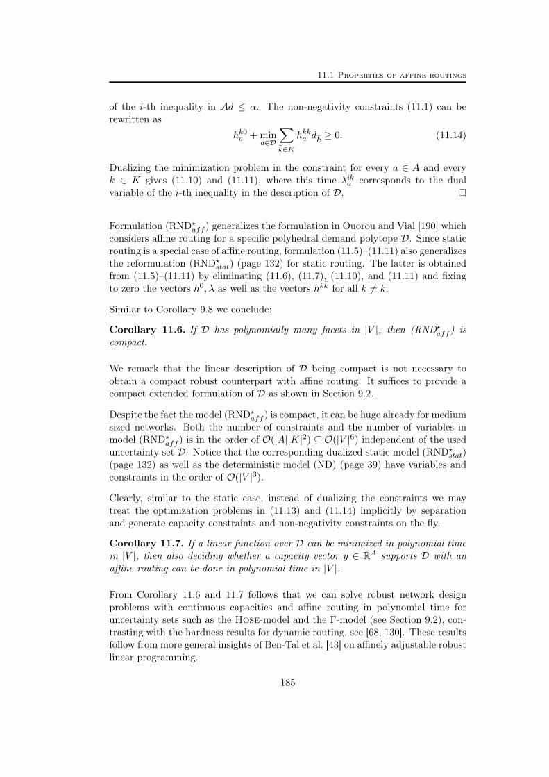
11.1 Properties of affine routings
of the i-th inequality in Ad ≤ α. The non-negativity constraints (11.1) can berewritten as
hk0a + min
d∈D
∑k∈K
hkka dk ≥ 0. (11.14)
Dualizing the minimization problem in the constraint for every a ∈ A and everyk ∈ K gives (11.10) and (11.11), where this time λika corresponds to the dualvariable of the i-th inequality in the description of D.
Formulation (RND?aff ) generalizes the formulation in Ouorou and Vial [190] which
considers affine routing for a specific polyhedral demand polytope D. Since staticrouting is a special case of affine routing, formulation (11.5)–(11.11) also generalizesthe reformulation (RND?
stat) (page 132) for static routing. The latter is obtainedfrom (11.5)–(11.11) by eliminating (11.6), (11.7), (11.10), and (11.11) and fixingto zero the vectors h0, λ as well as the vectors hkk for all k 6= k.
Similar to Corollary 9.8 we conclude:
Corollary 11.6. If D has polynomially many facets in |V |, then (RND?aff ) iscompact.
We remark that the linear description of D being compact is not necessary toobtain a compact robust counterpart with affine routing. It suffices to provide acompact extended formulation of D as shown in Section 9.2.
Despite the fact the model (RND?aff ) is compact, it can be huge already for medium
sized networks. Both the number of constraints and the number of variables inmodel (RND?
aff ) is in the order of O(|A||K|2) ⊆ O(|V |6) independent of the useduncertainty set D. Notice that the corresponding dualized static model (RND?
stat)(page 132) as well as the deterministic model (ND) (page 39) have variables andconstraints in the order of O(|V |3).
Clearly, similar to the static case, instead of dualizing the constraints we maytreat the optimization problems in (11.13) and (11.14) implicitly by separationand generate capacity constraints and non-negativity constraints on the fly.
Corollary 11.7. If a linear function over D can be minimized in polynomial timein |V |, then also deciding whether a capacity vector y ∈ RA supports D with anaffine routing can be done in polynomial time in |V |.
From Corollary 11.6 and 11.7 follows that we can solve robust network designproblems with continuous capacities and affine routing in polynomial time foruncertainty sets such as the Hose-model and the Γ-model (see Section 9.2), con-trasting with the hardness results for dynamic routing, see [68, 130]. These resultsfollow from more general insights of Ben-Tal et al. [43] on affinely adjustable robustlinear programming.
185
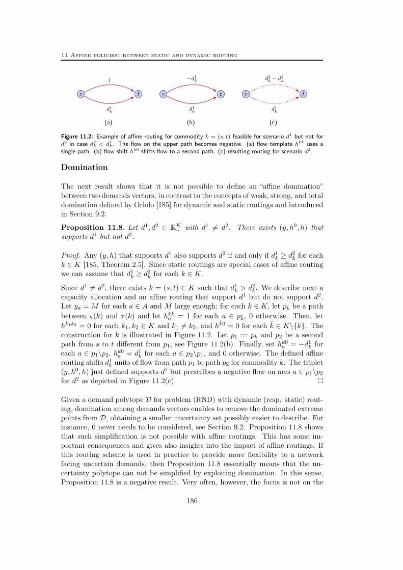
11 Affine policies: between static and dynamic routing
s t
1
d1k
(a)
s t
−d1k
d1k
(b)
s t
d2k − d1k
d1k
(c)
Figure 11.2: Example of affine routing for commodity k = (s, t) feasible for scenario d1 but not ford2 in case d2
k < d1k. The flow on the upper path becomes negative. (a) flow template hkk uses a
single path. (b) flow shift hk0 shifts flow to a second path. (c) resulting routing for scenario d2.
Domination
The next result shows that it is not possible to define an “affine domination”between two demands vectors, in contrast to the concepts of weak, strong, and totaldomination defined by Oriolo [185] for dynamic and static routings and introducedin Section 9.2.
Proposition 11.8. Let d1, d2 ∈ RK+ with d1 6= d2. There exists (y, h0, h) thatsupports d1 but not d2.
Proof. Any (y, h) that supports d1 also supports d2 if and only if d1k ≥ d2
k for eachk ∈ K [185, Theorem 2.5]. Since static routings are special cases of affine routingwe can assume that d1
k ≥ d2k for each k ∈ K.
Since d1 6= d2, there exists k = (s, t) ∈ K such that d1k > d2
k. We describe next acapacity allocation and an affine routing that support d1 but do not support d2.Let ya = M for each a ∈ A and M large enough; for each k ∈ K, let pk be a pathbetween ς(k) and τ(k) and let hkka = 1 for each a ∈ pk, 0 otherwise. Then, lethk1k2 = 0 for each k1, k2 ∈ K and k1 6= k2, and hk0 = 0 for each k ∈ K\k. Theconstruction for k is illustrated in Figure 11.2. Let p1 := pk and p2 be a secondpath from s to t different from p1, see Figure 11.2(b). Finally, set hk0
a = −d1k for
each a ∈ p1\p2, hk0a = d1
k for each a ∈ p2\p1, and 0 otherwise. The defined affinerouting shifts d1
k units of flow from path p1 to path p2 for commodity k. The triplet(y, h0, h) just defined supports d1 but prescribes a negative flow on arcs a ∈ p1\p2
for d2 as depicted in Figure 11.2(c).
Given a demand polytope D for problem (RND) with dynamic (resp. static) rout-ing, domination among demands vectors enables to remove the dominated extremepoints from D, obtaining a smaller uncertainty set possibly easier to describe. Forinstance, 0 never needs to be considered, see Section 9.2. Proposition 11.8 showsthat such simplification is not possible with affine routings. This has some im-portant consequences and gives also insights into the impact of affine routings. Ifthis routing scheme is used in practice to provide more flexibility to a networkfacing uncertain demands, then Proposition 11.8 essentially means that the un-certainty polytope can not be simplified by exploiting domination. In this sense,Proposition 11.8 is a negative result. Very often, however, the focus is not on the
186

11.1 Properties of affine routings
actual realized routing but on a feasible capacity design at low cost. In this contextaffine routing can be seen and used as an approximation scheme to (RND) withdynamic routing, the latter being very difficult computationally. Proposition 11.8now tells us that removing the dominated extreme points from D may reduce thecapacity cost for affine routings, and therefore, may yield a cheaper network thatis still (dynamically) feasible and hence a better approximation to (RND) withfree recourse. More precisely, assume that D+ is obtained from D after removingall totally dominated demand scenarios. It holds:
optdyn(D) = optdyn(D+) ≤ optaff (D+) ≤ optaff (D) ≤ optstat(D) = optstat(D+)
Observe that optaff (D+) might be closer to value optdyn(D) than optaff (D). Forthis reason we consider both uncertainty sets D and D+ for affine routing in ournumerical experiments in Section 11.2.
Relation to static routing
The results from the previous section imply that all extreme points of D must beconsidered when using affine routing, in particular extreme points correspondingto very small demand realization. Also 0 ∈ D, if required, cannot be removedfrom the uncertainty set. This comes from the non-negativity constraints (11.14),which impose important restrictions on the circulation variables hk0 and hkk. Un-fortunately it turns out that affine routings reduce to static routings whenever Dcontains very small demand realization as we will show in the following. In whatfollows let ek be the k-th unit vector in RK+ .
Lemma 11.9. If 0 ∈ D then hk0 ∈ RA+ describes a non-negative circulation in Dfor all k ∈ K. If εek ∈ D for some ε > 0 and k ∈ K and hk0 = 0 for k 6= k ∈ Kthen hkk ∈ RA+ describes a non-negative circulation in D.
Proof. Writing (11.1) for 0 ∈ D gives hk0a ≥ 0 for all a ∈ A and k ∈ K and hence by
Lemma 11.3 hk0 is a non-negative circulation. Similarly, writing (11.1) for εek ∈ Dwe get hk0
a + εhkka ≥ 0 for all a ∈ A and k ∈ K. If hk0 = 0 for k 6= k we get thathkk is a non-negative circulation by Lemma 11.3.
It is clear that the non-negative circulations mentioned in Lemma 11.9 do notyield useful affine routings because they increase the capacity requirement with-out providing additional flexibility. If the flow fk(d) ∈ RA for demand matrix dand commodity k contains a positive circulation, that is, there exists a positivecirculation g ∈ RA such that fk(d)− g is a flow for k, then fk(d) can be reducedto fk(d) − g without changing the flow balance constraints. Recall that we callsingle-commodity flows fk(d) irreducible if they cannot be reduced this way, cf.Section 2.1. Clearly, if a routing f : D → RA×K+ results in a positive circulationfor some d ∈ D and k ∈ K we can construct a second routing f realizing D byremoving this single circulation. The routing f may require less capacity than f .
187
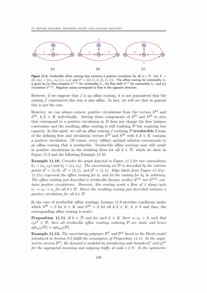
11 Affine policies: between static and dynamic routing
v1
v2
v3 v41
1
(a)
v1
v2
v3 v41
1
−1
(b)
v1
v2
v3 v4−1
1
1
(c)
Figure 11.3: Irreducible affine routing that contains a positive circulation for all d ∈ D. Let K =k1, k2 = (v1, v2), (v1, v3) and D = (2, 1), (1, 2), (1, 1). The affine routing for commodity k1
is given by (a) flow template hk1k1 for commodity k1, (b) flow shift hk10 for commodity k1, and (c)circulation hk1k2 . Negative values correspond to flow in the opposite direction.
However, if we suppose that f is an affine routing, it is not guaranteed that therouting f constructed this way is also affine. In fact, we will see that in generalthis is not the case.
However, we can always remove positive circulations from the vectors hk0 andhkk, k, k ∈ K individually. Setting those components of hk0 and hkk to zerothat correspond to a positive circulation in D does not change the flow balanceconstraints and the resulting affine routing is still realizing D but requiring lesscapacity. In this spirit, we call an affine routing f realizing D irreducible if noneof the defining flow and circulation vectors hk0 and hkk with k, k ∈ K containsa positive circulation. Of course, every (affine) optimal solution corresponds toan affine routing that is irreducible. Irreducible affine routings may still resultin positive circulations in the resulting flows for all d ∈ D, which we show inFigure 11.3 and the following Example 11.10.
Example 11.10. Consider the graph depicted in Figure 11.3 for two commoditiesk1 = (v1, v2) and k2 = (v1, v3). The uncertainty set D is described by the extremepoints d1 = (1, 2), d2 = (2, 1), and d3 = (1, 1). Edge labels from Figure 11.3(a)–11.3(c) represent the affine routing for k1 and let the routing for k2 be arbitrary.The affine routing just described is irreducible because neither hk10 nor hk1k2 con-tains positive circulations. However, this routing sends a flow of 1 along cyclev1 → v4 → v1 for all d ∈ D. Hence the resulting routing just described contains apositive circulation for all d ∈ D.
In the case of irreducible affine routings, Lemma 11.9 provides conditions underwhich hk0 = 0 for k ∈ K and hkk = 0 for all k, k ∈ K, k 6= k and thus, thecorresponding affine routing is static:
Proposition 11.11. If 0 ∈ D and for each k ∈ K there is εk > 0 such thatεke
k ∈ D, then all irreducible affine routings realizing D are static and henceoptaff (D) = optstat(D).
Example 11.12. The uncertainty polytopes DS and DA based on the Hose-modelintroduced in Section 9.2 fulfill the assumption of Proposition 11.11. In the asym-metric version DA, the demand is modeled by introducing node bounds uinv and uoutv
for the aggregated incoming and outgoing traffic at node v ∈ V . In the symmetric
188

11.1 Properties of affine routings
version DS there is just one bound uv for the total traffic at node v ∈ V . Aslong as uinv > 0 and uoutv > 0 (uv > 0) for all v ∈ V , respectively, DA (DS)fulfills the assumptions of Proposition 11.11 so that all irreducible affine rout-ings realizing DA (DS) are static and hence optaff (DS) = optstat(DS) as wellas optaff (DA) = optstat(DA). This is true as long as the Hose-model is not com-bined with additional lower bounds on point-to-point or aggregated node traffic, seefor instance [10].
Proposition 11.11 also highlights that affine routing suffers from a drawback relatedto Proposition 11.8. Adding dominated vectors to D might restrict the set offeasible affine routings.
In the rest of this section, let Dk0 denote the set obtained from D by removing d ∈ Dwith dk > 0, that is, Dk0 := d ∈ D : dk = 0. Whenever D is acyclic, we show inthe next proposition that the condition in Proposition 11.11 on the structure of Dcan be relaxed to dim(Dk0) = |K| − 1 for all k ∈ K. Moreover, we show below thatdim(Dk0) = |K| − 1 for all k ∈ K is a necessary and sufficient condition for staticroutings to be affine in acyclic graphs, while it is only a necessary condition forstatic routings to be affine in general graphs. Sufficiency and necessity are shown inProposition 11.13 and Theorem 11.14, respectively. Notice that for acyclic graphs,all affine routings are irreducible.
Proposition 11.13. Let D be an acyclic network. If dim(Dk0) = |K|−1 for all k ∈K, then all affine routings realizing D are static and hence optaff (D) = optstat(D).
Proof. Let k ∈ K be a given commodity. For all d ∈ Dk0 , any flow fk(d) musteither be equal to 0 or describe a positive circulation. The latter is impossiblebecause D is acyclic, so that fk(d) = 0 for all d ∈ Dk0 . Let d1, . . . , d|K| be a setof affinely independent vectors included in Dk0 . Any affine flow for k must satisfy
hk0a +
∑k∈K
hkka dik = hk0
a +∑
k∈K\khkka d
ik = 0, 1 ≤ i ≤ |K|, (11.15)
for all a ∈ A, which is a system of |K| independent linear equations with |K|variables. Therefore, its unique solution is 0 and the affine routing must be static.
In the following we prove that for general graphs the condition dim(Dk0) = |K| − 1for all k ∈ K is necessary for all irreducible affine routings to be static. This meansthat in all other cases there exists irreducible affine routings that are not static.But notice that from the latter it does not follow that optaff (D) < optstat(D) asshown in Example 11.15.
Theorem 11.14. If all irreducible affine routings realizing D are static then forall k ∈ K dim(Dk0) = |K| − 1.
189
11 Affine policies: between static and dynamic routing
Proof. Let k = (s, t) ∈ K be such that dim(Dk0) < |K| − 1. We construct anirreducible affine routing for commodity k (all other commodities are routed ar-bitrarily). Consider two distinct paths p1 and p2 in D from s to t. Let hkk bethe routing template that splits the flow equally between p1 and p2, that is, hkkais equal to 0.5 for a ∈ p1 ∪ p2\(p1 ∩ p2), 1 for a ∈ p1 ∩ p2, and 0 otherwise. Wewill construct an affine perturbation for k using the cycles formed by p2\p1 andp1\p2 where arcs in p1\p2 will be taken in the reverse direction (their flows will benegative). If Dk0 is non-empty, let p−1 be its dimension, with 1 ≤ p ≤ |K|−1, andlet d1, . . . , dp be a set of affinely independent vectors spanning Dk0 . It followsthat the system of equations
x0 +∑k∈K\k
dikxk = 0, 1 ≤ i ≤ p (11.16)
has a solution x 6= 0. In case Dk0 is empty we choose the vector x 6= 0 arbitrarily.We construct next an affine perturbation for the flow of commodity k based on x.
Given ε > 0, let hk0a = εx0 for a ∈ p2\p1, hk0
a = −εx0 for a ∈ p1\p2, and hk0a = 0
otherwise. Similarly, given k 6= k, we set hkka = εxk for all arcs a in p2\p1,hkka = −εxk for a ∈ p1\p2 and hkka = 0 otherwise. Combining these circulationvariables with the routing template hkk defined above yields an irreducible affinerouting fk realizing D.It remains to show that ε > 0 can be chosen such that the flow fk(d) is non-negative on all arcs for all d ∈ D. Because of Lemma 9.1 we can restrict ourselvesto the finite set vert(D) of extreme points of D. Consider first d ∈ vert(D) withdk = 0. By definition, fka (d) = 0 for each a ∈ A\(p1 ∪ p2), and fka (d) = dk = 0for each a ∈ p1 ∩ p2. Assume a ∈ p2\p1. The vector d can be written as anaffine combination of the vectors in d1, . . . , dp, that is, d =
∑pi=1 λid
i for somemultipliers λi ∈ R with
∑pi=1 λi = 1. Hence the flow on arc a ∈ p2\p1 for demand
d satisfies
fka (d) = ε
x0 +∑k∈K\k
dkxk
= ε
p∑i=1
λi
x0 +∑k∈K\k
dikxk
= 0,
where the last equation follows from (11.16). Similarly, the flow can be shown tobe zero for a ∈ p1\p2.
Now let d ∈ vert(D) be such that dk > 0. Again fka (d) = 0 for a ∈ A\(p1∪p2)∪(p1∩p2) by definition. For a ∈ p2\p1 and a ∈ p1\p2 it holds that fka (d) = 0.5dk + εg(d)
and fka (d) = 0.5dk − εg(d), respectively, where g(d) = x0 +∑
k∈K\k dkxk. These
flows are obviously positive if either g(d) = 0 or ε < dk/|2g(d)| for all d ∈ vert(D)with g(d) 6= 0. Such an ε exists since vert(D) is finite.
Combining Proposition 11.13 with Theorem 11.14, we have completely describedpolytopes for which affine routings and static routings are equivalent, assuming
190
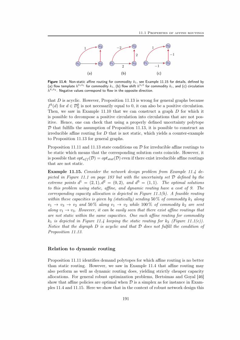
11.1 Properties of affine routings
v1
v2
v3
1
(a)
v1
v2
v3
−2
2
2
(b)
v1
v2
v3
1
−1
−1
(c)
Figure 11.4: Non-static affine routing for commodity k1, see Example 11.15 for details, defined by(a) flow template hk1k1 for commodity k1, (b) flow shift hk10 for commodity k1, and (c) circulationhk1k2 . Negative values correspond to flow in the opposite direction.
that D is acyclic. However, Proposition 11.13 is wrong for general graphs becausefk(d) for d ∈ Dk0 is not necessarily equal to 0, it can also be a positive circulation.Then, we saw in Example 11.10 that we can construct a graph D for which itis possible to decompose a positive circulation into circulations that are not pos-itive. Hence, one can check that using a properly defined uncertainty polytopeD that fulfills the assumption of Proposition 11.13, it is possible to construct anirreducible affine routing for D that is not static, which yields a counter-exampleto Proposition 11.13 for general graphs.
Proposition 11.11 and 11.13 state conditions on D for irreducible affine routings tobe static which means that the corresponding solution costs coincide. However, itis possible that optaff (D) = optstat(D) even if there exist irreducible affine routingsthat are not static.
Example 11.15. Consider the network design problem from Example 11.4 de-picted in Figure 11.1 on page 183 but with the uncertainty set D defined by theextreme points d1 = (2, 1), d2 = (0, 2), and d3 = (1, 1). The optimal solutionsto this problem using static, affine, and dynamic routing have a cost of 9. Thecorresponding capacity allocation is depicted in Figure 11.1(b). A feasible routingwithin these capacities is given by (statically) sending 50 % of commodity k1 alongv1 → v3 → v2 and 50 % along v1 → v2 while 100 % of commodity k2 are sentalong v1 → v3. However, it can be easily seen that there exist affine routings thatare not static within the same capacities. One such affine routing for commodityk1 is depicted in Figure 11.4 keeping the static routing for k2 (Figure 11.1(e)).Notice that the digraph D is acyclic and that D does not fulfill the condition ofProposition 11.13.
Relation to dynamic routing
Proposition 11.11 identifies demand polytopes for which affine routing is no betterthan static routing. However, we saw in Example 11.4 that affine routing mayalso perform as well as dynamic routing does, yielding strictly cheaper capacityallocations. For general robust optimization problems, Bertsimas and Goyal [46]show that affine policies are optimal when D is a simplex as for instance in Exam-ples 11.4 and 11.15. Here we show that in the context of robust network design this
191
11 Affine policies: between static and dynamic routing
condition is also necessary. In view of Lemma 9.1, we can restrict our attention toroutings realizing the set of extreme points vert(D) in the following.
Proposition 11.16. All dynamic routings realizing vert(D) are affine routings ifand only if D is a simplex with dimension n ≤ |K|.
Proof. Given a subset D′ ⊆ D of demand scenarios, we consider an arbitraryrouting f serving all d ∈ D′. We further consider the linear equation system
hk0a +
∑k∈K
dkhkka = fka (d), d ∈ D′ (11.17)
for every a ∈ A and k ∈ K, where the right hand sides correspond to the chosenroutings f(d) for d ∈ D′.If D is a simplex, then all its vertices are affinely independent, which impliesthat the left hand side rows of system (11.17) with D′ = vert(D) are linearlyindependent. It follows that for D′ = vert(D) system (11.17) has a solution.Hence, by the definition of affine routings, every routing f serving the verticesvert(D) of a simplex D is affine.
Let us assume D is not a simplex and let us first assume D is full-dimensional.Hence D has at least |K|+2 vertices. To construct a routing f which is not affine westart with an affine routing for a subset D′ of the extreme points. Let D′ ⊆ vert(D)be a subset of |K|+1 affinely independent vectors in vert(D). For every commodityk = (s, t) ∈ K we take arbitrary flows fk(d), d ∈ D′, realizing the individualvertices D′ and solve the system (11.17) which, for every a ∈ A, has a uniquesolution (hk0
a , hka). This procedure yields an affine routing f realizing D′ together
with the defining multipliers (h0, h). Notice that any affine routing realizing D′can be constructed this way. Now for d ∈ vert(D)\D′ we choose arbitrary flowsfk(d) realizing d. These flows might fulfill the corresponding equations in (11.17)such that the constructed affine routing also realizes vert(D)\D′. However, sincethere exists at least two paths between s and t we may construct a flow fk(d) fork ∈ K and d ∈ vert(D)\D′ such that fk(d) 6= hk0 +
∑k∈K dkh
kk. This way we canalways construct a routing realizing all vertices vert(D) that is not affine.
If dim(D) = n < |K|, D is included in an affine space defined by |K|−n independ-ent linear equations. We can use these equations to express |K| − n componentsof the demand as affine functions of the others:
dk =∑k∈Q
αkkdk, k ∈ K\Q, (11.18)
where |Q| = n. Plugging (11.18) into the definition of an affine routing (11.1),any affine routing realizing D can be expressed as an affine function of n variables.Since D is not a simplex, it has at least n + 2 extreme points. We choose D′ asan arbitrary subset of n + 1 affinely independent vectors in vert(D) and the restof the proof is similar.
192

11.1 Properties of affine routings
Proposition 11.16 does not imply that all dynamic routings realizing a simplexD are affine. Indeed, any dynamic routing described by a non-linear functionf : D → RA×K+ cannot be described by an affine routing. For instance, considerD = [0, 1] and the dynamic routing that routes d ∈ [0, 0.5] along p1 and d ∈]0.5, 1]along p2. This routing is not affine as it is not described by a continuous function.However, there exists an affine routing (in the same capacities) that yields thesame flow for each d ∈ vert(D) = 0, 1. This affine routing is simply the staticrouting that routes any demand vector along p2.
Example 11.17 shows that when the conditions of Propositions 11.11 and 11.16 arenot fulfilled, that is, D is not a simplex and does not contain the origin, capacityallocation costs required by static, affine, and dynamic routings can be strictlydifferent.
Example 11.17. Consider the network design problem from Example 11.4 depictedin Figure 11.1 on page 183 but with the uncertainty set D defined by the extremepoints d1 = (3, 0), d2 = (0, 3), d3 = (2, 2), and d4 = (0.5, 0.5). The optimalcapacity allocation costs with static, affine, and dynamic routings are, 13+ 1
2 , 13+ 13 ,
and 13, respectively. Notice that moving d4 along the segment (0, 0)− (1, 1) leavesstatic and dynamic optimal capacity allocations unchanged while the affine solutioncost moves between 13 and 13 + 1
2 . In particular, if d4 is set to (0, 0), the affineand static costs are the same, which we knew already from Proposition 11.11. Ifd4 is in convd1, d2, d3, (1, 1), the affine and dynamic costs are the same.
Propositions 11.11 and 11.16 relate theoretically affine routing to the well-knownstatic and dynamic routings. Combining these results we obtain conditions on thedemand set D which yield that dynamic routings are static and which establishthat optstat(D) = optdyn(D).
Corollary 11.18. Let the demand polytope D be the convex hull of 0∪εkek, k ∈K with εk > 0 for all k ∈ K. Then, all dynamic routings realizing vert(D) arestatic routings.
Note that there exists other situations in which dynamic routing is not better thanstatic routing. The set D in Example 11.15 does not satisfy the hypothesis fromCorollary 11.18 but optstat(D) = optdyn(D) in this case. We refer to Frangioni,Pascali, and Scutellá [107] for providing conditions on D for optstat(D) = optdyn(D)to hold. Besides the structure of D these situations, however, also depend on thetopology of D and the design cost function κ.
We have established theoretical relations between static, affine, and dynamic rout-ings. In the following we will examine these relations numerically.
193

11 Affine policies: between static and dynamic routing
11.2 Computational insights
In this section we investigate the objective gaps between optimal network de-signs using static, affine, and dynamic routings, respectively, facing networks fromthe Sndlib ([228]). That is, we study the gaps between optdyn(D), optaff (D),and optstat(D) using realistic network topologies. Here optdyn(D), optaff (D), andoptstat(D) correspond to the value of an optimal solution to the robust networkdesign problem with continuous capacities and dynamic, affine, or static routing,respectively.
We point out that our objective here is to solve these models with the black-boxsolvers of Cplex 12.1 [140]. We do not intend to compare more advanced solutiontechniques such as Benders’ decomposition [45] or column generation. However,this could be an interesting topic for future research.
Uncertainty sets and data
Two polyhedral uncertainty sets and their variations receive most of the attentionamong robust network design practitioners, the Hose-model going back to Duffieldet al. [99] and a restricted interval uncertainty set based on Bertsimas and Sim[47, 48], which we refer to as the Γ-model. Both models have been introduced inSection 9.2.
One of the key advantages of the Hose-model with demand polytope DS (sym-metric Hose-model) or DA (asymmetric Hose-model) is the fact that it does notrequire any estimates of pairwise demands. The potential demands are describedby upper bounds on the traffic at the source respectively target nodes. How-ever, as there are no implied lower bounds we conclude in Example 11.12 thatoptstat(DS) = optaff (DS) as well as optstat(DA) = optaff (DA) based on Proposi-tion 11.11. We can in general not expect any improvements on the network costfor the Hose-model when using affine routing unless we explicitly impose lowerbounds on the traffic as for instance done in [10].
For this reason we use the Γ-model with uncertainty polytope DΓ (page 137),which imposes both upper and lower bounds on point-to-point traffic. In thisrespect Proposition 11.11 does not holds in general and we can expect to haveoptstat(DΓ) > optaff (DΓ). In Section 9.2 we learned that for the static and dy-namic routing principle, by domination, it is equivalent to optimize using the poly-tope of all possible upward and downward deviations DΓ or using the polytope DΓ
+
which considers upward deviations only. Static as well as dynamic solutions sup-porting DΓ
+ will automatically support DΓ. Moreover, static and dynamic routingsmight even cover demand-scenarios outside the actual deviation polytope DΓ aslong as these are (totally) dominated, e.g., demand vectors with dk = ε for allk ∈ K and ε > 0 small enough. See Section 9.2 for the concept of domination.
194
11.2 Computational insights
By Proposition 11.8, this is not true for the affine routing principle. It can not besaid a priori whether or not affine solutions supporting DΓ
+ will support deviationsin DΓ. All possible downward variations have to be included in the uncertaintydefinition since the feasibility of an affine routing can only be ensured if demand-deviations never leave the given uncertainty set. In the sequel we will use the setDΓ
+ for static and dynamic scenarios. But in the case of affine policies we willstudy optimal solutions for both the uncertainty set DΓ
+ and DΓ. Notice that forΓ > 0 both DΓ
+ and DΓ are full-dimensional since they contain εkek with εk > 0for each k ∈ K and the origin.
We selected the three directed Sndlib instances janos-us, sun, and giul39 fromSndlib [228] which we already used in Section 10.3. More characteristics andstatistics can be found on the Sndlib website [228]. Similar to Section 10.3 weparametrize the Γ-model by using the single demand scenario from Sndlib asnominal demand dk and by fixing the maximum deviation to dk := 0.4dk for everycommodity. That is, we made the assumption that the demand deviates by atmost 40% from the nominal value. To reduce the size of the formulations and tobe able to do a series of runs we considered the largest 10 to 50 commodities k withrespect to the value dk, that is, |K| takes values in 10, 20, 30, 50. We consideredall values Γ in 1, . . . , 7. Notice that small values of Γ are reasonable as theyalready introduce a relatively high level of robustness, see the computations inSection 10.3 and also check the values in Table 11.2 on page 199.
Robust counterparts
The demand uncertainty polytope DΓ has 2|K| variables and |K| + 1 constraints(not counting non-negativity constraints). For DΓ
+ the number of variables reducesto |K|. Consequently, the corresponding static and affine robust counterpartsare compact, as shown in Section 9.1 (static routing) and in Section 11.1 (affinerouting). For the static case we use the reformulation (ΓND) (page 139) which has2|A||K|+ 2|A| variables and |K|(|V | − 1) + (|K|+ 1)|A| constraints. Notice thatalways one flow conservation constraint per commodity can be omitted.
To set up the affine robust counterpart we dualized the capacity constraints andthe flow non-negativity constraints following model (RND?
aff ) (page 184) in Sec-tion 11.1. Notice that DΓ is described in dimension 2|K| which increases thenumber of rows of the dualization and hence the number of rows of the model(RND?
aff ). The resulting affinely adjustable robust network design formulation(RND?
aff ) for the Γ-model with uncertainty set DΓ has 2|A||K|2 + 3|A||K|+ 2|A|variables and (|K|2 + |K|)(|V |−1)+2|A||K|2 +3|A||K|+ |A| constraints. If the setDΓ
+ is used instead, the number of constraints reduces to (|K|2 + |K|)(|V | − 1) +|A||K|2 + 2|A||K| + |A|. Again we can omit one flow conservation constraint percommodity in the routing template (11.5). Also one flow conservation constraintper commodity of the flow cycle conditions (11.6) and (11.7) is redundant.
195

11 Affine policies: between static and dynamic routing
To calculate dynamic optimal solutions we used model (RND) (page 126) restrictedto those d ∈ D that correspond to the vertices of the demand uncertainty polytopeDΓ
+. As explained above it suffices to consider non-dominated vertices correspond-ing to extreme upward deviations scenarios. These are the demand-vectors whereΓ out of |K| commodities are at their peak values dk + dk and the remaining|K| − Γ commodities are at their nominal values dk. More precisely, for everysubset Q ⊆ K with |Q| = Γ we have to consider the vertex σ+ ∈ DΓ
+ with σk+ = 1
for k ∈ Q and σk+ = 0 for k ∈ K \ Q, which results in(|K|
Γ
)many vertices (to-
tally dominating all other vertices of DΓ+). Consequently, the resulting exponential
model to solve the dynamic robust network design problem has(|K|
Γ
)|A||K| + |A|
variables and(|K|
Γ
)(|K|(|V | − 1) + |A|) constraints. Notice that we can sensibly
reduce the problem size for the dynamic case, by aggregating commodities with acommon source node [50, 158]. For our instances |K| could be reduced from 50 to18 (resp. 10 and 6) for janos-us (resp. giul39 and sun).
For comparison purposes we summarize the sizes of the three different modelsin Table 11.1 on the next page. Notice that all models are linear programs aswe assume continuous arc capacities y ∈ RA. In this respect we solve the LPrelaxations of (RND) for the respective routing schemes.
Remark 11.19. As we can conclude from Table 11.1, affine and dynamic modelscan be very large already for medium sized instances. In general it might be wise touse decomposition methods to solve the corresponding problems which is beyondthe scope of this paper. Very few publications in robust network design (beyondstatic routing) consider algorithmic issues or present solutions. Implementing well-engineered solution algorithms for (RND) with affine respectively dynamic routingremains a challenging task. However, a few steps in this direction have been carriedout. Ouorou and Vial [190] use a path-flow model and column generation to solvethe affine robust counterpart using the Γ-model. Babonneau et al. [24] solve asimilar problem after restricting the set of admissible paths and also restrictingthe number of affine decision variables. For the intractable design problem withintegral capacities and dynamic routing, using the Hose-model, Mattia [172] showsthat small to medium sized instances can be solved in a reasonable amount of timewhen using a branch-and-cut approach based on Benders decomposition [45]. Tosolve the separation problem for robust metric inequalities (9.4), Mattia [172] usesmixed integer programs with big-M coefficients.
Results
Our numerical results are summarized in Table 11.2 and Table 11.3 below. Forour computations we used the interior point (barrier) solver of Cplex 12.1 [140]on a 64bit 3.0GHz Quad-Core CPU with 8GB of memory allowing for 4 threadsand 8 hours of CPU time for every individual run. Since we are only interested inthe objective value of the optimal solution we switched off the crossover of Cplex.
196
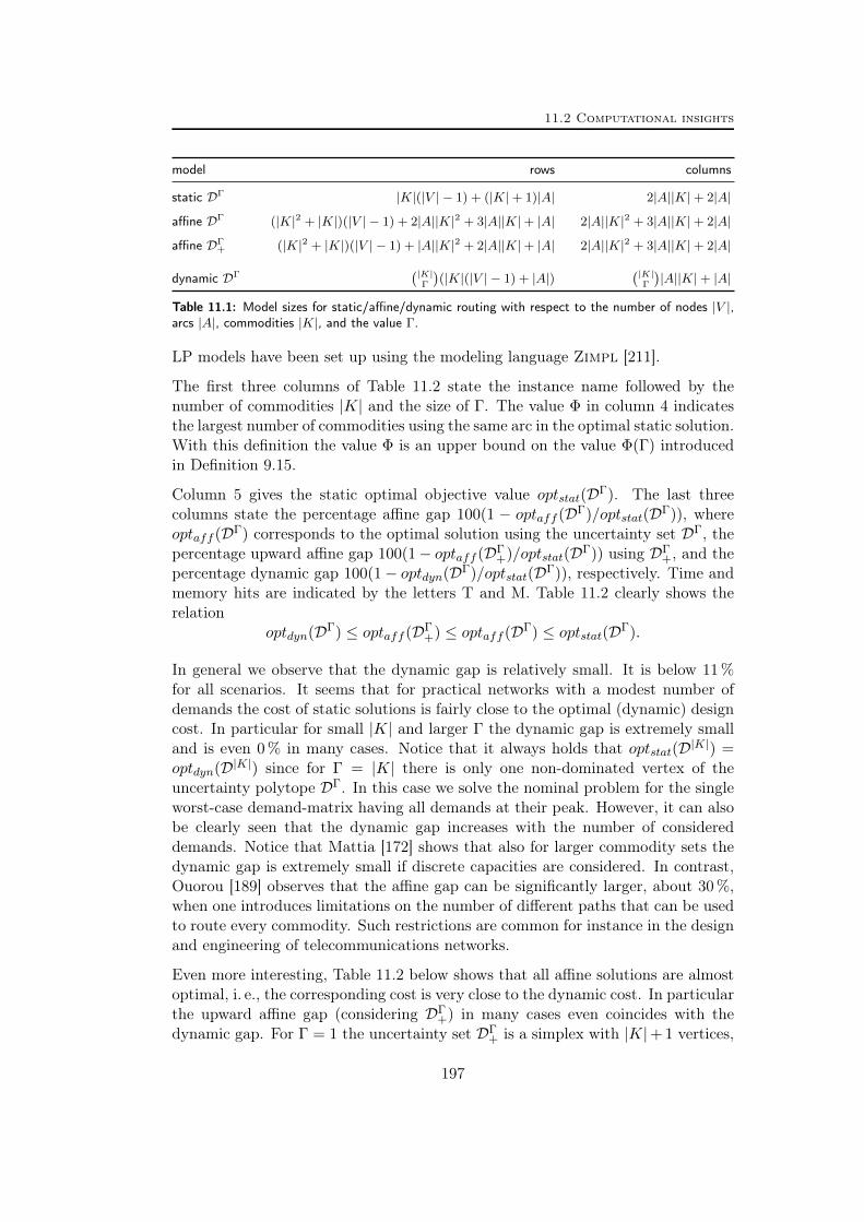
11.2 Computational insights
model rows columns
static DΓ |K|(|V | − 1) + (|K|+ 1)|A| 2|A||K|+ 2|A|affine DΓ (|K|2 + |K|)(|V | − 1) + 2|A||K|2 + 3|A||K|+ |A| 2|A||K|2 + 3|A||K|+ 2|A|affine DΓ
+ (|K|2 + |K|)(|V | − 1) + |A||K|2 + 2|A||K|+ |A| 2|A||K|2 + 3|A||K|+ 2|A|
dynamic DΓ(|K|
Γ
)(|K|(|V | − 1) + |A|)
(|K|Γ
)|A||K|+ |A|
Table 11.1: Model sizes for static/affine/dynamic routing with respect to the number of nodes |V |,arcs |A|, commodities |K|, and the value Γ.
LP models have been set up using the modeling language Zimpl [211].
The first three columns of Table 11.2 state the instance name followed by thenumber of commodities |K| and the size of Γ. The value Φ in column 4 indicatesthe largest number of commodities using the same arc in the optimal static solution.With this definition the value Φ is an upper bound on the value Φ(Γ) introducedin Definition 9.15.
Column 5 gives the static optimal objective value optstat(DΓ). The last threecolumns state the percentage affine gap 100(1 − optaff (DΓ)/optstat(DΓ)), whereoptaff (DΓ) corresponds to the optimal solution using the uncertainty set DΓ, thepercentage upward affine gap 100(1− optaff (DΓ
+)/optstat(DΓ)) using DΓ+, and the
percentage dynamic gap 100(1− optdyn(DΓ)/optstat(DΓ)), respectively. Time andmemory hits are indicated by the letters T and M. Table 11.2 clearly shows therelation
optdyn(DΓ) ≤ optaff (DΓ+) ≤ optaff (DΓ) ≤ optstat(DΓ).
In general we observe that the dynamic gap is relatively small. It is below 11%for all scenarios. It seems that for practical networks with a modest number ofdemands the cost of static solutions is fairly close to the optimal (dynamic) designcost. In particular for small |K| and larger Γ the dynamic gap is extremely smalland is even 0 % in many cases. Notice that it always holds that optstat(D|K|) =optdyn(D|K|) since for Γ = |K| there is only one non-dominated vertex of theuncertainty polytope DΓ. In this case we solve the nominal problem for the singleworst-case demand-matrix having all demands at their peak. However, it can alsobe clearly seen that the dynamic gap increases with the number of considereddemands. Notice that Mattia [172] shows that also for larger commodity sets thedynamic gap is extremely small if discrete capacities are considered. In contrast,Ouorou [189] observes that the affine gap can be significantly larger, about 30%,when one introduces limitations on the number of different paths that can be usedto route every commodity. Such restrictions are common for instance in the designand engineering of telecommunications networks.
Even more interesting, Table 11.2 below shows that all affine solutions are almostoptimal, i. e., the corresponding cost is very close to the dynamic cost. In particularthe upward affine gap (considering DΓ
+) in many cases even coincides with thedynamic gap. For Γ = 1 the uncertainty set DΓ
+ is a simplex with |K|+ 1 vertices,
197

11 Affine policies: between static and dynamic routing
hence optaff (DΓ+) = optdyn(DΓ) by Proposition 11.16. But also for Γ > 1 it holds
that optaff (DΓ+) ≈ optdyn(DΓ). As mentioned above the corresponding affine
routing does not necessarily support demands in DΓ \ DΓ+. But even considering
downward deviations by using the uncertainty set DΓ does not remarkably decreasethe corresponding gap. Affine solutions for DΓ are still very close to the dynamicsolutions and improve on the static solutions in terms of capacity cost.
static affine Dσ affine Dσ+ dynamicinstance |K| Γ Φ optstat(D) gap in % gap in % gap in %
janos-us
10 1 2 3.149202e+05 4.9 5.7 5.710 2 1 3.323827e+05 0.0 0.0 0.020 1 3 4.657367e+05 6.4 7.2 7.220 2 2 5.125317e+05 5.1 6.2 6.520 3 2 5.125317e+05 0.1 0.9 2.520 4 2 5.125317e+05 0.0 0.0 0.020 5 2 5.125317e+05 0.0 0.0 M30 1 4 6.127240e+05 6.8 7.5 7.530 2 5 6.722822e+05 7.5 8.3 8.730 3 5 6.988964e+05 5.7 6.6 7.030 4 3 6.992080e+05 1.4 2.4 M30 5 3 6.992080e+05 0.0 0.0 M40 1 5 6.729093e+05 7.5 8.2 8.240 2 5 7.324675e+05 7.5 8.4 8.840 3 5 7.631223e+05 5.6 6.7 M40 4 4 7.659107e+05 1.9 2.9 M40 5 4 7.659107e+05 0.0 0.2 M40 6 4 7.659107e+05 0.0 0.0 M50 1 5 7.311094e+05 7.7 8.4 8.450 2 5 7.925296e+05 7.8 8.7 9.150 3 5 8.266402e+05 6.3 7.4 M50 4 5 8.369683e+05 3.7 4.8 M50 5 4 8.386076e+05 1.1 2.1 M50 6 4 8.386076e+05 0.0 0.0 M
sun
10 1 3 2.616416e+02 7.5 9.8 9.810 2 3 2.740441e+02 0.6 2.7 3.010 3 2 2.753181e+02 0.0 0.0 0.410 4 2 2.753181e+02 0.0 0.0 0.010 5 2 2.753181e+02 0.0 0.0 0.010 6 2 2.753181e+02 0.0 0.0 0.010 7 2 2.753181e+02 0.0 0.0 0.020 1 5 4.314919e+02 8.1 9.9 9.920 2 5 4.666696e+02 6.1 8.9 9.220 3 5 4.821624e+02 3.2 5.5 6.420 4 5 4.867587e+02 0.8 2.0 3.520 5 4 4.878762e+02 0.3 0.7 M20 6 4 4.878762e+02 0.0 0.2 M20 7 4 4.878762e+02 0.0 0.0 M30 1 7 5.563141e+02 8.0 9.2 9.230 2 7 6.029896e+02 8.1 10.1 10.530 3 8 6.303494e+02 6.6 8.8 9.630 4 7 6.400667e+02 3.6 5.6 M30 5 7 6.465764e+02 1.8 3.1 M
continued on next page
198

11.2 Computational insights
static affine Dσ affine Dσ+ dynamicinstance |K| Γ Φ optstat(D) gap in % gap in % gap in %
30 6 7 6.491593e+02 0.9 1.8 M30 7 6 6.500533e+02 0.4 0.8 M40 1 9 6.688681e+02 7.4 8.5 8.540 2 10 7.230139e+02 8.6 10.3 10.640 3 11 7.578679e+02 8.1 10.1 10.840 4 9 7.783114e+02 6.7 8.8 M40 5 9 7.906376e+02 5.1 7.1 M40 6 9 7.964860e+02 3.5 5.5 M40 7 9 7.989951e+02 2.0 4.1 M50 1 10 7.342829e+02 T 8.0 8.050 2 12 7.916815e+02 T 10.1 10.450 3 12 8.299185e+02 T 10.4 M50 4 12 8.533162e+02 T 9.6 M50 5 12 8.704549e+02 T 8.6 M50 6 13 8.809769e+02 T 7.3 M50 7 10 8.862691e+02 T 6.2 M
giul39
10 1 3 2.682375e+01 2.6 2.6 2.610 2 3 3.046875e+01 0.9 2.3 2.310 3 3 3.063375e+01 0.0 0.0 0.510 4 3 3.063375e+01 0.0 0.0 0.020 1 5 4.996563e+01 4.3 4.7 4.720 2 5 5.529969e+01 5.3 6.1 6.120 3 5 5.787094e+01 3.6 4.4 5.120 4 5 5.970656e+01 1.5 2.2 3.120 5 5 6.052813e+01 0.0 0.2 M20 6 5 6.052813e+01 0.0 0.0 M30 1 7 7.894656e+01 5.6 6.0 6.030 2 7 8.494313e+01 6.6 7.3 7.330 3 7 8.976938e+01 6.5 7.6 7.830 4 7 9.350938e+01 5.5 7.1 M30 5 7 9.565781e+01 3.1 5.0 M30 6 7 9.633750e+01 0.3 2.3 M30 7 7 9.668750e+01 0.0 0.0 M40 1 9 1.059966e+02 T 6.8 6.840 2 10 1.136150e+02 T 8.2 8.340 3 9 1.195538e+02 T 8.5 M40 4 9 1.235375e+02 T 8.0 M40 5 9 1.267484e+02 T 7.1 M40 6 8 1.283469e+02 T 5.2 M40 7 8 1.291969e+02 T 3.4 M50 1 10 1.233091e+02 M 7.9 7.950 2 10 1.325416e+02 M 9.8 10.250 3 10 1.385434e+02 M 9.7 M50 4 10 1.432656e+02 M 9.7 M50 5 10 1.468328e+02 M 9.0 M50 6 9 1.493625e+02 M 7.8 M50 7 9 1.502844e+02 M 5.8 M
Table 11.2: Comparing static, affine, and dynamic routing in terms of the solution cost. Γ-modelwith Γ ∈ 1, . . . , 7 and |K| ∈ 10, 20, 30, 40, 50. We removed rows whenever objective values andgaps did not differ from the previous row.
199

11 Affine policies: between static and dynamic routing
This result shows that affine routing allows for enough flexibility to almost capturefree recourse. It also suggests the following general approach. Given a general un-certainty polytope D, in order to calculate a cheap network together with a feasibledynamic routing, one may compute the cost-minimal affine solution (capacity androuting) for D instead. For an even cheaper still (dynamically) feasible capacityallocation one might remove all vertices from D that are (totally) dominated andthen compute the cost-minimal affine solution. In the latter case the resultingaffine routing is not necessarily feasible for D but there exists a dynamic routingfor the computed capacity allocation, and this capacity allocation can be consid-ered as being almost optimal. In fact, if only the capacity allocation and its costare of interest, affine policies with such a reduced uncertainty set can be used toapproximate the cost for free recourse. Notice that in our case, using the Γ-model,the affine robust counterpart (RND?
aff ) for the reduced set Dσ+ was much easierto solve than (RND?
aff ) for the original set DΓ, see Table 11.3 below.
Using definition Definition 9.15 and comparing the value Γ and the value Φ incolumns 3 and 4 of Table 11.2 on the preceding page, we observe that Γ? =2, 2, 4, 4, 5 for network janos-us and |K| = 10, 20, 30, 40, 50, respectively. For Γ ≥Γ? the cost for static solutions remains constant, see Lemma 9.16. For network sunand giul39 we have Γ? = 3, 5, 7 for |K| = 10, 20, 30, respectively. For all networksthe values Γ? are very small but increasing with the number of commodities. Noticethat since optstat(DΓ∗) = optstat(D|K|) the worst-case objective for the Γ-model(together with a shortest path solution) is obtained already early (for small Γ)with static routing. This is in line with the observations from Section 10.3, seeFigure 10.3 on page 176. Affine and dynamic solutions tend to admit the worstcase later (for larger Γ).
Table 11.3 below reports on the computational complexity of the solved models.The first three columns of Table 11.3 again indicate the instance followed by thenumber of commodities |K| and the size of Γ. Additionally, there are columns forevery considered routing principle stating the number of non-zeros (nonz) in thelinear programming model and the time in seconds (time) to solve the problem. Itcan be seen that all static models can be solved within 1 second of CPU time. Thenumber of non-zeros for the static and affine models is independent of the value Γand increases polynomially with the number of considered commodities. The affinemodels however are very large already for small values of |K| with a huge numberof non-zeros (in the order of 106 already for |K| = 30, 40, 50). We could still solveall affine counterparts corresponding to DΓ
+ in less than one hour for janos-us andsun and in less than two hours for giul39 . In contrast, we observed time andmemory hits when solving (RND?
aff ) for DΓ when |K| ≥ 40 (giul39 ) and |K| ≥ 50
(sun). As expected the affine robust counterpart for the reduced set DΓ+ is much
easier to solve because of a smaller LP, also see Table 11.1 on page 197. As long asthe number of non-zeros is modest the dynamic models seem to be easier to solvethan their affine counterparts. However, the number of non-zeros is exponentialboth in the number of commodities and in the size of Γ. It exceeds 109, 1010, 1011
200

11.2 Computational insights
for Γ = 7 and |K| = 30, 40, 50, respectively, such that we can provide dynamicsolutions only for very small values of Γ or small values of |K|. In all other casesthe memory limit was hit either already when setting up the LPs using Zimpl orlater in the barrier algorithm.
static affine Dσ affine Dσ+ dynamicinstance |K| Γ nonz time nonz time nonz time nonz time
in s in s in s in s
janos-us
10 1 5978 1 116998 27 81718 5 15540 110 2 5978 1 116998 15 81718 5 69930 110 3 5978 1 116998 16 81718 2 186480 110 4 5978 1 116998 4 81718 4 326340 210 5 5978 1 116998 3 81718 3 391608 210 6 5978 1 116998 3 81718 5 326340 210 7 5978 1 116998 2 81718 12 186480 120 1 11786 1 450786 240 313026 32 45800 120 2 11786 1 450786 336 313026 153 435100 420 3 11786 1 450786 279 313026 79 2610600 3820 4 11786 1 450786 238 313026 22 11095050 11120 5 11786 1 450786 248 313026 163 35504160 M20 6 11786 1 450786 247 313026 180 88760400 M20 7 11786 1 450786 261 313026 192 177520800 M30 1 17594 1 1001534 1389 694094 88 76140 330 2 17594 1 1001534 1847 694094 153 1104030 1330 3 17594 1 1001534 2161 694094 191 10304280 21330 4 17594 1 1001534 2490 694094 255 69553890 M30 5 17594 1 1001534 1802 694094 135 361680228 M30 6 17594 1 1001534 1693 694094 157 1507000950 M30 7 17594 1 1001534 1557 694094 141 5166860400 M40 1 23410 1 1769570 3021 1225250 265 150640 740 2 23410 1 1769570 5362 1225250 407 2937480 4940 3 23410 1 1769570 7823 1225250 672 37208080 M40 4 23410 1 1769570 13192 1225250 802 344174740 M40 5 23410 1 1769570 6657 1225250 672 2478058128 M40 6 23410 1 1769570 6051 1225250 476 14455339080 M40 7 23410 1 1769570 5282 1225250 467 70211646960 M50 1 29220 1 2754420 6316 1906020 1031 225100 1450 2 29220 1 2754420 13331 1906020 1818 5514950 9850 3 29220 1 2754420 15007 1906020 2848 88239200 M50 4 29220 1 2754420 17181 1906020 3225 1036810600 M50 5 29220 1 2754420 19075 1906020 3413 9538657520 M50 6 29220 1 2754420 12814 1906020 2867 71539931400 M50 7 29220 1 2754420 11557 1906020 2333 449679568800 M
sun
10 1 7278 1 142278 5 99438 3 13020 110 2 7278 1 142278 5 99438 3 58590 510 3 7278 1 142278 4 99438 4 156240 110 4 7278 1 142278 4 99438 2 273420 210 5 7278 1 142278 3 99438 2 328104 210 6 7278 1 142278 4 99438 3 273420 210 7 7278 1 142278 3 99438 2 156240 120 1 14338 1 547938 99 380658 33 32040 120 2 14338 1 547938 100 380658 68 304380 5
continued on next page
201

11 Affine policies: between static and dynamic routing
static affine Dσ affine Dσ+ dynamicinstance |K| Γ nonz time nonz time nonz time nonz time
in s in s in s in s
20 3 14338 1 547938 134 380658 61 1826280 4720 4 14338 1 547938 80 380658 59 7761690 29220 5 14338 1 547938 59 380658 67 24837408 M20 6 14338 1 547938 83 380658 38 62093520 M20 7 14338 1 547938 59 380658 50 124187040 M30 1 21404 1 1217384 627 844064 147 57000 430 2 21404 1 1217384 677 844064 173 826500 1430 3 21404 1 1217384 722 844064 192 7714000 22930 4 21404 1 1217384 777 844064 175 52069500 M30 5 21404 1 1217384 741 844064 286 270761400 M30 6 21404 1 1217384 603 844064 205 1128172500 M30 7 21404 1 1217384 493 844064 153 3868020000 M40 1 28474 1 2150714 2480 1489754 470 76000 140 2 28474 1 2150714 2796 1489754 512 1482000 3140 3 28474 1 2150714 2613 1489754 612 18772000 76240 4 28474 1 2150714 2866 1489754 591 173641000 M40 5 28474 1 2150714 3251 1489754 588 1250215200 M40 6 28474 1 2150714 3187 1489754 757 7292922000 M40 7 28474 1 2150714 2594 1489754 885 35422764000 M50 1 35550 1 3348150 28000 2317950 1212 95000 150 2 35550 1 3348150 28000 2317950 1381 2327500 5650 3 35550 1 3348150 28000 2317950 1525 37240000 M50 4 35550 1 3348150 28000 2317950 1711 437570000 M50 5 35550 1 3348150 28000 2317950 1796 4025644000 M50 6 35550 1 3348150 28000 2317950 2133 30192330000 M50 7 35550 1 3348150 28000 2317950 2369 189780360000 M
10 1 12640 1 240520 9 168280 7 30500 110 2 12640 1 240520 9 168280 6 137250 1210 3 12640 1 240520 6 168280 6 366000 310 4 12640 1 240520 6 168280 7 640500 610 5 12640 1 240520 5 168280 6 768600 510 6 12640 1 240520 5 168280 6 640500 410 7 12640 1 240520 4 168280 8 366000 2
giul39
20 1 24594 1 925834 144 643754 91 71200 320 2 24594 1 925834 185 643754 84 676400 620 3 24594 1 925834 157 643754 111 4058400 9820 4 24594 1 925834 182 643754 147 17248200 71720 5 24594 1 925834 183 643754 95 55194240 M20 6 24594 1 925834 161 643754 118 137985600 M20 7 24594 1 925834 145 643754 87 275971200 M30 1 36564 1 2057124 1987 1427604 574 152520 1530 2 36564 1 2057124 1910 1427604 504 2211540 3630 3 36564 1 2057124 2160 1427604 539 20641040 94230 4 36564 1 2057124 1649 1427604 513 139327020 M30 5 36564 1 2057124 2619 1427604 463 724500504 M30 6 36564 1 2057124 1845 1427604 630 3018752100 M30 7 36564 1 2057124 1076 1427604 652 10350007200 M40 1 48524 1 3633804 28000 2519244 1791 203360 3640 2 48524 1 3633804 28000 2519244 1961 3965520 82
continued on next page
202
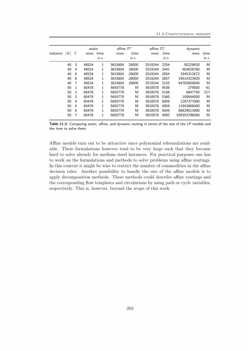
11.2 Computational insights
static affine Dσ affine Dσ+ dynamicinstance |K| Γ nonz time nonz time nonz time nonz time
in s in s in s in s
40 3 48524 1 3633804 28000 2519244 2254 50229920 M40 4 48524 1 3633804 28000 2519244 2441 464626760 M40 5 48524 1 3633804 28000 2519244 2054 3345312672 M40 6 48524 1 3633804 28000 2519244 2657 19514323920 M40 7 48524 1 3633804 28000 2519244 2155 94783859040 M50 1 60478 1 5655778 M 3918578 4536 279500 6150 2 60478 1 5655778 M 3918578 5188 6847750 21750 3 60478 1 5655778 M 3918578 5360 109564000 M50 4 60478 1 5655778 M 3918578 6858 1287377000 M50 5 60478 1 5655778 M 3918578 4959 11843868400 M50 6 60478 1 5655778 M 3918578 5044 88829013000 M50 7 60478 1 5655778 M 3918578 4992 558353796000 M
Table 11.3: Comparing static, affine, and dynamic routing in terms of the size of the LP models andthe time to solve them
Affine models turn out to be attractive since polynomial reformulations are avail-able. These formulations however tend to be very large such that they becomehard to solve already for medium sized instances. For practical purposes one hasto work on the formulations and methods to solve problems using affine routings.In this context it might be wise to restrict the number of commodities in the affinedecision rules. Another possibility to handle the size of the affine models is toapply decomposition methods. These methods could describe affine routings andthe corresponding flow templates and circulations by using path or cycle variables,respectively. This is, however, beyond the scope of this work.
203


Chapter 12
Concluding remarks Part III
In this part of the thesis, we generalized the concepts of deterministic network de-sign from Part I and in particular Chapter 2 in order to deal with the uncertaintyof demands. We enhanced and compared methods that handle a polyhedral set ofrealistic traffic scenarios thereby analyzing suitable models and algorithms. Basedon extensive polyhedral studies we provided different classes of facet-defining in-equalities, revealing their practical importance by a series of computational tests.We also theoretically embedded robust network design into the more general frame-work of two-stage robust optimization with recourse considering three alternativererouting schemes. We analyzed properties of the new affine routing and showed(theoretically and computationally) that it combines features of the well-knownstatic and dynamic routing.
We started by introducing the general concepts of two-stage robust network designtogether with a discussion on models, possible polyhedral uncertainty sets, as wellas suitable algorithms. In particular we showed how to apply the two correlatedsolution methods, Separate and Dualize, handling the uncertainty of demandsin a different way.
We then generalized the notion of cut-set polyhedra to robust network design.Using rank-1 MIR aggregations as discussed in Part I and Part II, we introducedrobust cut-set as well as flow cut-set inequalities for general polyhedral uncer-tainty sets generalizing their deterministic counterparts. We provided necessaryand sufficient conditions for these inequalities to define facets. These results areindependent of the assumed recourse scheme, static, affine, or dynamic. In a sec-ond polyhedral study we present facet-defining cut-set inequalities that exploit thespecial structure of the Γ-model. This polyhedral demand model going back toBertsimas and Sim [47, 48] allows to adjust the number of point-to-point demandsthat deviate from a given nominal value simultaneously by changing a param-eter Γ > 0. We derived multiple classes of facet-defining cut-based inequalities,so-called envelope inequalities, by exploiting the extra variables available in the du-alized robust counterparts. We were also able to completely describe a projection
205

12 Concluding remarks Part III
of the robust cut-set polyhedron with only a single arc.
In detailed computational tests, we showed that the resulting inequalities, whenused as cutting planes in a branch-and-cut framework, are responsible for a speed-up of more than a factor of two compared to default Cplex settings. Cut-setinequalities are responsible for most of the progress followed by flow cut-set in-equalities. Envelope inequalities, however, seem not to be effective in reducingsolving times or gaps. We also prove computationally that the performance ofSeparate versus Dualize strongly depends on the shape of the polyhedral de-mand uncertainty set D, that is, on the number of vertices versus facets of D.For the polyhedral Γ-model with polynomially many defining facets, increasingthe number of vertices (by increasing Γ) leads to a decrease of the performance ofSeparate. The Dualize approach (using a dual formulation of D) shows con-stant performance when tuning the level of robustness by changing the value Γ.However, Separate outperforms Dualize for very small Γ.
To evaluate the robustness of solutions that are computed with our framework weused real-life measurements from Sndlib taken in the U.S. IP network Abilene[224] and the European research network Geant [212] to parametrize the Γ-model.We could then show that already small values of Γ suffice to provide a reasonablelevel of robustness w. r. t. traffic fluctuations in the given time periods, which relatesto the fact that traffic peaks do not occur all simultaneously in our data. It is, inparticular, not necessary to dimension networks against a scenario that assumesall commodities at their peak. With our solutions we save up to 20% of thecorresponding solution cost with the same level of robustness.
In a supplementary theoretical study we analyzed a new recourse scheme for robustnetwork design, so-called affine routing. We showed that this scheme provides areasonable alternative to the well-studied static and dynamic routing. When Dis full-dimensional, affine routings decompose into a combination of cycles andpaths, that is, a routing template for every commodity can be affinely adjustedusing a set of cycles, whenever a different commodity is perturbed within thefeasible demand region. We investigated the three routing principles with respectto their flexibility depending on the structure of the given demand uncertainty setD. Fixing the demand polytope D, the cost of optimal affine solutions is alwaysbetween the cost for optimal static and optimal dynamic solutions. We developednecessary and sufficient conditions on D under which affine routings reduce tostatic routings and also develop properties of uncertainty sets leading to dynamicroutings being affine.
Eventually, in Section 11.2, we computed the cost gap between static, affine, anddynamic solutions based on networks from Sndlib and the Γ-model. We concludedthat for these instances the solutions based on affine routings tend to be as cheapas two-stage solutions with dynamic routing. In this respect, the affine routingprinciple allows enough flexibility to almost capture dynamic routings. We remarkthat in contrast to static and maybe also dynamic routing, affine routing is atheoretical and computational tool only. It is unlikely that affine routing will
206

12 Concluding remarks Part III
be implemented in practice as it is too complex to describe. However, as it isin general NP-hard to compute an optimal network design with dynamic routing(even if capacities and flows are assumed to be continuous), the affine principlemight be very useful in approximating a free recourse of flow and, moreover, thecomputations can be done using tractable robust counterparts.
207


Appendix A
Tables Part II
In this chapter, we provide detailed numbers for all tests carried out to test theperformance of the MCF-separator. For the corresponding presentation and asummary of the results see Chapter 6.
A.1 Used instances
Table A.1 below contains all instances used in the computational tests presentedin Chapter 6 except for the Cplex-internal test set. We report on the number ofrows (rows), the number of columns (vars), the value of the linear programmingrelaxation (lp), and the values of the best dual (bestdual) and primal bounds (best-primal) we found in all tests carried out by the author for this thesis. These valuesare used to calculate the measures rootgap, primalgap, and dualgap presented inTable A.4 on page 239 and Table A.5 on page 243 and summarized in Table 6.3on page 104 and Table 6.4 on page 105.
The instances in the sndlib test set are marked with either ’UUM’, ’UUE’, ’DBM’,’DBM’, ’DDM’, or ’DDE’. The first two letters correspond tho the demand andlink capacity model. Letter ’U’ stands for undirected while letter ’B’ and ’D’ standfor bidirected and directed. The last letter indicates whether we assume a modular(’M’) or explicit (’E’) link capacity structure, see [187, 228] and Section 2.4.
problem rows vars lp bestdual bestprimal
arc.setns25-pr12 2313 5868 52957.5 53905 53905ns25-pr3 2210 8601 29920 30575 30575ns25-pr4 1138 3393 16175 16705 16705ns25-pr6 2639 6919 25362.5 26175 26175ns25-pr9 2220 7350 29175 29430 29430ns4-pr12 2313 5868 63911 64072 64072
continued on next page
209
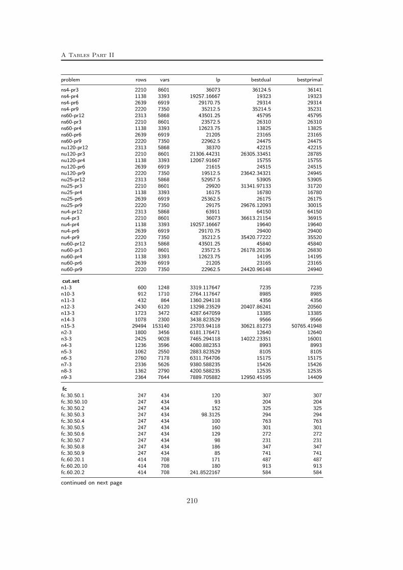
A Tables Part II
problem rows vars lp bestdual bestprimal
ns4-pr3 2210 8601 36073 36124.5 36141ns4-pr4 1138 3393 19257.16667 19323 19323ns4-pr6 2639 6919 29170.75 29314 29314ns4-pr9 2220 7350 35212.5 35214.5 35231ns60-pr12 2313 5868 43501.25 45795 45795ns60-pr3 2210 8601 23572.5 26310 26310ns60-pr4 1138 3393 12623.75 13825 13825ns60-pr6 2639 6919 21205 23165 23165ns60-pr9 2220 7350 22962.5 24475 24475nu120-pr12 2313 5868 38370 42215 42215nu120-pr3 2210 8601 21306.44231 26305.33451 28785nu120-pr4 1138 3393 12067.91667 15755 15755nu120-pr6 2639 6919 21615 24515 24515nu120-pr9 2220 7350 19512.5 23642.34321 24945nu25-pr12 2313 5868 52957.5 53905 53905nu25-pr3 2210 8601 29920 31341.97133 31720nu25-pr4 1138 3393 16175 16780 16780nu25-pr6 2639 6919 25362.5 26175 26175nu25-pr9 2220 7350 29175 29676.12093 30015nu4-pr12 2313 5868 63911 64150 64150nu4-pr3 2210 8601 36073 36613.21154 36915nu4-pr4 1138 3393 19257.16667 19640 19640nu4-pr6 2639 6919 29170.75 29400 29400nu4-pr9 2220 7350 35212.5 35420.77222 35520nu60-pr12 2313 5868 43501.25 45840 45840nu60-pr3 2210 8601 23572.5 26178.20136 26830nu60-pr4 1138 3393 12623.75 14195 14195nu60-pr6 2639 6919 21205 23165 23165nu60-pr9 2220 7350 22962.5 24420.96148 24940
cut.setn1-3 600 1248 3319.117647 7235 7235n10-3 912 1710 2764.117647 8985 8985n11-3 432 864 1360.294118 4356 4356n12-3 2430 6120 13298.23529 20407.86241 20560n13-3 1723 3472 4287.647059 13385 13385n14-3 1078 2300 3438.823529 9566 9566n15-3 29494 153140 23703.94118 30621.81273 50765.41948n2-3 1800 3456 6181.176471 12640 12640n3-3 2425 9028 7465.294118 14022.23351 16001n4-3 1236 3596 4080.882353 8993 8993n5-3 1062 2550 2883.823529 8105 8105n6-3 2760 7178 6311.764706 15175 15175n7-3 2336 5626 9380.588235 15426 15426n8-3 1362 2790 4200.588235 12535 12535n9-3 2364 7644 7889.705882 12950.45195 14409
fcfc.30.50.1 247 434 120 307 307fc.30.50.10 247 434 93 204 204fc.30.50.2 247 434 152 325 325fc.30.50.3 247 434 98.3125 294 294fc.30.50.4 247 434 100 763 763fc.30.50.5 247 434 160 301 301fc.30.50.6 247 434 129 272 272fc.30.50.7 247 434 98 231 231fc.30.50.8 247 434 186 347 347fc.30.50.9 247 434 85 741 741fc.60.20.1 414 708 171 487 487fc.60.20.10 414 708 180 913 913fc.60.20.2 414 708 241.8522167 584 584
continued on next page
210
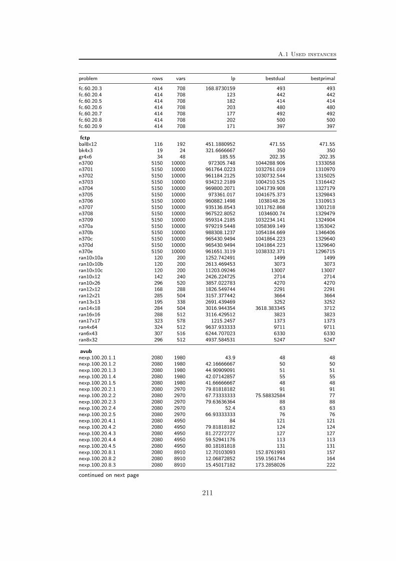
A.1 Used instances
problem rows vars lp bestdual bestprimal
fc.60.20.3 414 708 168.8730159 493 493fc.60.20.4 414 708 123 442 442fc.60.20.5 414 708 182 414 414fc.60.20.6 414 708 203 480 480fc.60.20.7 414 708 177 492 492fc.60.20.8 414 708 202 500 500fc.60.20.9 414 708 171 397 397
fctpbal8x12 116 192 451.1880952 471.55 471.55bk4x3 19 24 321.6666667 350 350gr4x6 34 48 185.55 202.35 202.35n3700 5150 10000 972305.748 1044288.906 1333058n3701 5150 10000 961764.0223 1032761.019 1310970n3702 5150 10000 961184.2125 1030732.544 1315025n3703 5150 10000 934212.2189 1004210.525 1316442n3704 5150 10000 969800.2071 1041739.908 1327179n3705 5150 10000 973361.017 1041675.373 1329843n3706 5150 10000 960882.1498 1038148.26 1310913n3707 5150 10000 935136.8543 1011762.868 1301218n3708 5150 10000 967522.8052 1034600.74 1329479n3709 5150 10000 959314.2185 1032234.141 1324904n370a 5150 10000 979219.5448 1058369.149 1353042n370b 5150 10000 988308.1237 1054184.669 1346406n370c 5150 10000 965430.9494 1041864.223 1329640n370d 5150 10000 965430.9494 1041864.223 1329640n370e 5150 10000 961651.3119 1038332.371 1296715ran10x10a 120 200 1252.742491 1499 1499ran10x10b 120 200 2613.469453 3073 3073ran10x10c 120 200 11203.09246 13007 13007ran10x12 142 240 2426.224725 2714 2714ran10x26 296 520 3857.022783 4270 4270ran12x12 168 288 1826.549744 2291 2291ran12x21 285 504 3157.377442 3664 3664ran13x13 195 338 2691.439469 3252 3252ran14x18 284 504 3016.944354 3618.383345 3712ran16x16 288 512 3116.429512 3823 3823ran17x17 323 578 1215.2457 1373 1373ran4x64 324 512 9637.933333 9711 9711ran6x43 307 516 6244.707023 6330 6330ran8x32 296 512 4937.584531 5247 5247
avubnexp.100.20.1.1 2080 1980 43.9 48 48nexp.100.20.1.2 2080 1980 42.16666667 50 50nexp.100.20.1.3 2080 1980 44.90909091 51 51nexp.100.20.1.4 2080 1980 42.07142857 55 55nexp.100.20.1.5 2080 1980 41.66666667 48 48nexp.100.20.2.1 2080 2970 79.81818182 91 91nexp.100.20.2.2 2080 2970 67.73333333 75.58832584 77nexp.100.20.2.3 2080 2970 79.63636364 88 88nexp.100.20.2.4 2080 2970 52.4 63 63nexp.100.20.2.5 2080 2970 66.93333333 76 76nexp.100.20.4.1 2080 4950 84 121 121nexp.100.20.4.2 2080 4950 79.81818182 124 124nexp.100.20.4.3 2080 4950 81.27272727 127 127nexp.100.20.4.4 2080 4950 59.52941176 113 113nexp.100.20.4.5 2080 4950 80.18181818 131 131nexp.100.20.8.1 2080 8910 12.70103093 152.8761993 157nexp.100.20.8.2 2080 8910 12.06872852 159.1561744 164nexp.100.20.8.3 2080 8910 15.45017182 173.2858026 222
continued on next page
211
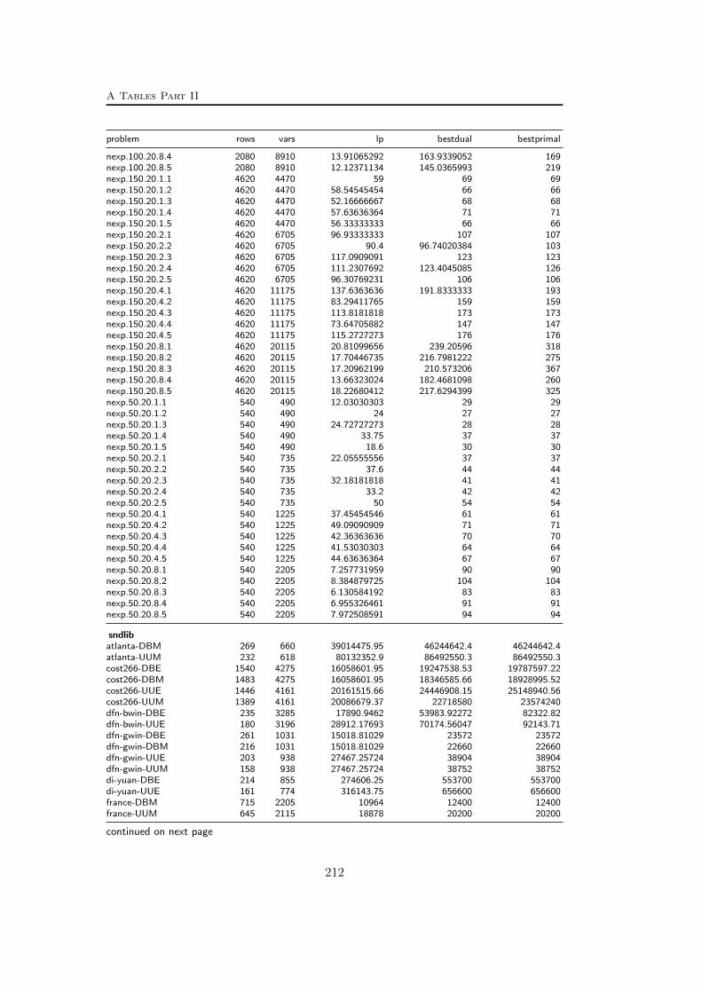
A Tables Part II
problem rows vars lp bestdual bestprimal
nexp.100.20.8.4 2080 8910 13.91065292 163.9339052 169nexp.100.20.8.5 2080 8910 12.12371134 145.0365993 219nexp.150.20.1.1 4620 4470 59 69 69nexp.150.20.1.2 4620 4470 58.54545454 66 66nexp.150.20.1.3 4620 4470 52.16666667 68 68nexp.150.20.1.4 4620 4470 57.63636364 71 71nexp.150.20.1.5 4620 4470 56.33333333 66 66nexp.150.20.2.1 4620 6705 96.93333333 107 107nexp.150.20.2.2 4620 6705 90.4 96.74020384 103nexp.150.20.2.3 4620 6705 117.0909091 123 123nexp.150.20.2.4 4620 6705 111.2307692 123.4045085 126nexp.150.20.2.5 4620 6705 96.30769231 106 106nexp.150.20.4.1 4620 11175 137.6363636 191.8333333 193nexp.150.20.4.2 4620 11175 83.29411765 159 159nexp.150.20.4.3 4620 11175 113.8181818 173 173nexp.150.20.4.4 4620 11175 73.64705882 147 147nexp.150.20.4.5 4620 11175 115.2727273 176 176nexp.150.20.8.1 4620 20115 20.81099656 239.20596 318nexp.150.20.8.2 4620 20115 17.70446735 216.7981222 275nexp.150.20.8.3 4620 20115 17.20962199 210.573206 367nexp.150.20.8.4 4620 20115 13.66323024 182.4681098 260nexp.150.20.8.5 4620 20115 18.22680412 217.6294399 325nexp.50.20.1.1 540 490 12.03030303 29 29nexp.50.20.1.2 540 490 24 27 27nexp.50.20.1.3 540 490 24.72727273 28 28nexp.50.20.1.4 540 490 33.75 37 37nexp.50.20.1.5 540 490 18.6 30 30nexp.50.20.2.1 540 735 22.05555556 37 37nexp.50.20.2.2 540 735 37.6 44 44nexp.50.20.2.3 540 735 32.18181818 41 41nexp.50.20.2.4 540 735 33.2 42 42nexp.50.20.2.5 540 735 50 54 54nexp.50.20.4.1 540 1225 37.45454546 61 61nexp.50.20.4.2 540 1225 49.09090909 71 71nexp.50.20.4.3 540 1225 42.36363636 70 70nexp.50.20.4.4 540 1225 41.53030303 64 64nexp.50.20.4.5 540 1225 44.63636364 67 67nexp.50.20.8.1 540 2205 7.257731959 90 90nexp.50.20.8.2 540 2205 8.384879725 104 104nexp.50.20.8.3 540 2205 6.130584192 83 83nexp.50.20.8.4 540 2205 6.955326461 91 91nexp.50.20.8.5 540 2205 7.972508591 94 94
sndlibatlanta-DBM 269 660 39014475.95 46244642.4 46244642.4atlanta-UUM 232 618 80132352.9 86492550.3 86492550.3cost266-DBE 1540 4275 16058601.95 19247538.53 19787597.22cost266-DBM 1483 4275 16058601.95 18346585.66 18928995.52cost266-UUE 1446 4161 20161515.66 24446908.15 25148940.56cost266-UUM 1389 4161 20086679.37 22718580 23574240dfn-bwin-DBE 235 3285 17890.9462 53983.92272 82322.82dfn-bwin-UUE 180 3196 28912.17693 70174.56047 92143.71dfn-gwin-DBE 261 1031 15018.81029 23572 23572dfn-gwin-DBM 216 1031 15018.81029 22660 22660dfn-gwin-UUE 203 938 27467.25724 38904 38904dfn-gwin-UUM 158 938 27467.25724 38752 38752di-yuan-DBE 214 855 274606.25 553700 553700di-yuan-UUE 161 774 316143.75 656600 656600france-DBM 715 2205 10964 12400 12400france-UUM 645 2115 18878 20200 20200
continued on next page
212

A.1 Used instances
problem rows vars lp bestdual bestprimal
germany50-DBM 2526 8189 438028 461662.2689 474700germany50-UUM 2088 6971 597932.5 617513.2 628490giul39-DDE 1865 7052 1706.732812 2050.952458 2761janos-us-DDM 760 2184 1488134.75 1490871.1 1493112janos-us-ca-DDM 1643 4758 1488681.897 1490273.263 1492416newyork-DBE 403 1568 41753.8 824721.6604 999702newyork-DBM 354 1568 41753.8 846739.7 999702newyork-UUE 338 1470 74943.8 864347.1473 999702newyork-UUM 289 1470 74943.8 852034.6 999702nobel-eu-DBE 879 3771 570687.5 601505.1037 610910nobel-eu-UUE 838 3771 817152.5 840162.4697 863900nobel-ger-DBE 333 1771 115406 126070.7711 129940nobel-ger-UUE 307 1770 147488 156094.3439 162420norway-DBE 882 2754 84836.5925 331034.6295 383890norway-DBM 831 2754 84836.5925 333307.2 383890norway-UUE 804 2652 162715.395 412130.1817 452680norway-UUM 753 2652 162715.395 415215.0786 452680pdh-DBE 212 703 4489313.45 9689062 9689062pdh-DBM 178 703 4489313.45 9615107 9615107pdh-UUE 145 527 4593661.173 11114202 11114202pdh-UUM 111 527 4593661.173 10903843 10903843pioro40-DBM 1738 6942 254029.2926 254632.7885 255454pioro40-UUM 1649 6942 412076.045 412774.4549 414045polska-DBM 168 396 14948.55627 15717 15717polska-UUM 150 396 22633.7508 23619 23619sun-DDM 264 695 684.6945 859.3029916 897.72ta1-DBE 621 2606 2344400.755 5896728 5896728ta1-DBM 566 2606 2344400.755 4686829.552 5896728ta1-UUE 494 2288 3693674.557 6855895 7533070ta1-UUM 439 2288 3693674.557 5331466 7621520ta2-DBE 3055 10101 36065210.45 36471255.99 36471255.99ta2-DBM 2947 10101 36065210.45 36471255.99 36471255.99ta2-UUE 2687 9241 36964014.23 37871728.59 37871728.59ta2-UUM 2579 9241 36964014.18 37534290 37871728.59zib54-DBE 2430 6748 2224025.844 9773826.66 9773826.66zib54-UUE 1809 5150 4081019.858 10334015.82 10334015.82
ufcnbeasleyC1 1750 2500 52 85 85beasleyC2 1750 2500 47.33333333 144 144beasleyC3 1750 2500 237.9878049 653.7467057 779beavma 372 390 293174.2758 383284.9997 383284.9997berlin 2704 5304 130.0666667 1008.759977 1044brasil 3364 6612 2208.708333 12976.96639 13680fixnet6 600 1000 3192.042 3983 3983g150x1100 1250 2200 34562.12 67197.96497 71827g150x1650 1800 3300 31884.515 63313.75911 69130g180x666 846 1332 496101.2425 624632 624632g200x740 940 1480 34077.54267 43807.57406 44316g200x740b 940 1480 145993.88 178286.1284 179279g200x740c 940 1480 655765.895 680124 680124g200x740d 940 1480 548918.9429 586038 586038g200x740e 940 1480 559469.2194 600396 600396g200x740f 940 1480 572132.2166 617872 617872g200x740g 940 1480 7911.513 36249.13905 45308g200x740h 940 1480 86698.8429 125673.348 131639g200x740i 940 1480 2292.465 25884.70859 31175g40x132 172 264 13997.266 26629 26629g50x170 220 340 10711.592 25576 25576g55x188 243 376 9178.605 24487 24487
continued on next page
213

A Tables Part II
problem rows vars lp bestdual bestprimal
g55x188c 243 376 22549.394 35464 35464h50x2450 2549 4900 11147.73151 32906.88083 32906.88083h50x2450b 2549 4900 2822.584647 3030.198086 3030.198086h50x2450c 2549 4900 3400.372829 4896.196619 4896.196619h50x2450d 2549 4900 3251.877445 4639.264786 4639.264786h50x2450e 2549 4900 2999.379052 4077.684199 4077.684199h80x6320b 6558 12640 5086.547046 6003.179413 6003.179413h80x6320c 6558 12640 5461.33783 6273.627361 6273.627361h80x6320d 6558 12640 5325.160104 6382.09905 6382.09905k10x90 100 180 399.73 568 568k14x182 196 364 3995.514 8491 8491k14x182b 196 364 4442.844 11042 11042k15x210 225 420 1982.74 16128 16128k15x420 435 840 350.08 819 819k15x630 645 1260 449.89 936 936k16x240 256 480 2769.838 10072.41885 10674k16x240b 256 480 3320.771 11146.48643 11393k20x380 400 760 952.566 1941 1941k20x380b 400 760 1764.92 11343 11343k20x380c 400 760 1858.48 17159 17159k20x380d 400 760 1937.75 20979 20979k20x380e 400 760 2013.35 6904 6904l121x232 353 464 169104.5134 192446 192446l451x885 1336 1770 399355.0014 431050 431050l451x885b 1336 1770 530266.6196 560847 560847l61x114 175 228 56275.99471 60085 60085mc11 1920 3040 608.8443396 9711.1359 12008mc7 1920 3040 367.7573964 3167.928932 3696mc8 1920 3040 91.76470588 1284.278026 1615mtest4ma 1174 1950 33968.06567 52148 52148p100x588 688 1176 3957.217778 8711.17038 8999p100x588b 688 1176 5554.011111 43614.81892 48793p100x588c 688 1176 97579.11063 172770 172770p100x588d 688 1176 1.899352402 5 5p200x1188 1388 2376 5575.126667 11109.11095 11396p200x1188b 1388 2376 7860.811111 50630.07781 56403p200x1188c 1388 2376 5678.607089 15078 15078p500x2988 3488 5976 59130.6729 71280.72127 71917p500x2988b 3488 5976 61188.729 160303.2449 179975p500x2988c 3488 5976 14122.96285 15215 15215p500x2988d 3488 5976 2.161832061 6 6p50x288 338 576 4178.478 6134 6134p50x288b 338 576 5818.04 21753 21753p50x576 626 1152 12203.142 19407 19407p50x864 914 1728 11284.682 19007 19007p80x400 480 800 4824.65 8458.861661 8548p80x400b 480 800 6418.8 36136.80479 39915r20x100 120 200 6747.217 15603 15603r20x200 220 400 5088.257 14783 14783r30x160 190 320 10608.074 21827 21827r50x360 410 720 575.02 1653 1653r80x800 880 1600 3651.48 5150.009169 5338sp100x200 300 400 18517.54178 34507 34507sp150x300 450 600 13333.96896 30918 30918sp150x300b 450 600 38.09703259 56 56sp150x300c 450 600 406383.7402 560735.9965 560735.9965sp150x300d 450 600 34.1089901 68.99999927 68.99999927sp50x100 150 200 49287.62252 50968 50968sp80x160 240 320 14573.39492 19549 19549sp90x180 270 360 58915.83556 68862 68862
continued on next page
214

A.1 Used instances
problem rows vars lp bestdual bestprimal
sp90x250 340 500 18733.09473 23571 23571
miplib1030n20b8 576 18380 1.566407646 302 302acc-tight5 3052 1339 0 0 0aflow40b 1442 2728 1005.664817 1168 1168air04 823 8904 55535.43639 56137 56137app1-2 53467 26871 -264.6016505 -41 -41ash608gpia-3col -1 -1 0 0 0bab5 4964 21600 -124657.6414 -106411.8401 -106411.8401beasleyC3 1750 2500 40.42682927 754 754biella1 1203 7328 3060037.431 3065005.78 3065005.78bienst2 576 505 11.72413793 54.6 54.6binkar10_1 1026 2298 6637.188027 6742.200024 6742.200024bley_xl1 175620 5831 154.3902 190 190bnatt350 4923 3150 0 0 0core2536-691 2539 15293 688.476034 689 689cov1075 637 120 17.14285714 20 20csched010 351 1758 332.4227273 408 408danoint 664 521 62.63728042 65.66666667 65.66666667dfn-gwin-UUM 158 938 27467.25724 38752 38752eil33-2 32 4516 811.2789961 934.007916 934.007916eilB101 100 2818 1075.247691 1216.920174 1216.920174enlight13 169 338 0 71 71enlight14 -1 -1 0 0 0ex9 40962 10404 81 81 81glass4 396 322 800002400 1200012600 1200012600gmu-35-40 424 1205 -2406943.556 -2406733.369 -2406733.369iis-100-0-cov 3831 100 16.66666667 29 29iis-bupa-cov 4803 345 26.49721688 36 36iis-pima-cov 7201 768 26.62038939 33 33lectsched-4-obj 14163 7901 0 4 4m100n500k4r1 100 500 -25 -25 -25macrophage 3164 2260 0 374 374map18 328818 164547 -932.7826848 -847 -847map20 328818 164547 -998.8364187 -922 -922mcsched 2107 1747 193774.7537 211913 211913mik-250-1-100-1 151 251 -79842.42363 -66729 -66729mine-166-5 8429 830 -821763677.7 -566395707.9 -566395707.9mine-90-10 6270 900 -887165318.5 -784302337.6 -784302337.6msc98-ip 15850 21143 19520966.15 19839497.01 19839497.01mspp16 561657 29280 341 363 363mzzv11 9499 10240 -22945.23963 -21718 -21718n3div36 4484 22120 114333.3747 130800 130800n3seq24 6044 119856 52000 52200 52200n4-3 1236 3596 4080.882353 8993 8993neos-1109824 28979 1520 278 378 378neos-1337307 5687 2840 -203123.9739 -202319 -202319neos-1396125 1494 1161 388.5523998 3000.045337 3000.045337neos-1601936 3131 4446 1 3 3neos-476283 10015 11915 406.2447077 406.363207 406.363207neos-686190 3664 3660 5134.81383 6730 6730neos-849702 1041 1737 0 0 0neos-916792 1909 1474 26.20359581 31.87039837 31.87039837neos-934278 11495 23123 259.5 260 260neos13 20852 1827 -126.1783778 -95.47480656 -95.47480656neos18 11402 3312 7 16 16net12 14021 14115 17.24947917 214 214netdiversion 119589 129180 230.8 242 242newdano 576 505 11.72413793 65.666667 65.666667
continued on next page
215
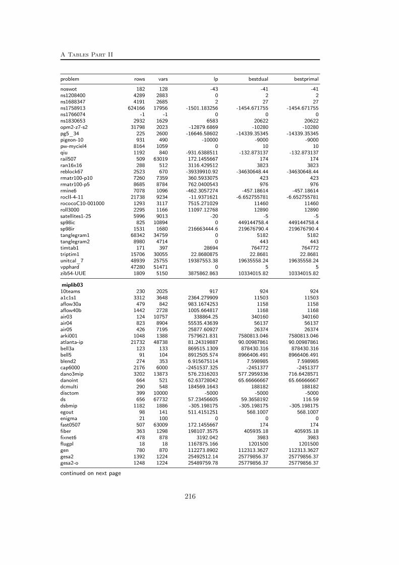
A Tables Part II
problem rows vars lp bestdual bestprimal
noswot 182 128 -43 -41 -41ns1208400 4289 2883 0 2 2ns1688347 4191 2685 2 27 27ns1758913 624166 17956 -1501.183256 -1454.671755 -1454.671755ns1766074 -1 -1 0 0 0ns1830653 2932 1629 6583 20622 20622opm2-z7-s2 31798 2023 -12879.6869 -10280 -10280pg5_34 225 2600 -16646.58602 -14339.35345 -14339.35345pigeon-10 931 490 -10000 -9000 -9000pw-myciel4 8164 1059 0 10 10qiu 1192 840 -931.6388511 -132.873137 -132.873137rail507 509 63019 172.1455667 174 174ran16x16 288 512 3116.429512 3823 3823reblock67 2523 670 -39339910.92 -34630648.44 -34630648.44rmatr100-p10 7260 7359 360.5933075 423 423rmatr100-p5 8685 8784 762.0400543 976 976rmine6 7078 1096 -462.3057274 -457.18614 -457.18614rocII-4-11 21738 9234 -11.9371621 -6.652755781 -6.652755781rococoC10-001000 1293 3117 7515.271029 11460 11460roll3000 2295 1166 11097.12768 12890 12890satellites1-25 5996 9013 -20 -5 -5sp98ic 825 10894 0 449144758.4 449144758.4sp98ir 1531 1680 216663444.6 219676790.4 219676790.4tanglegram1 68342 34759 0 5182 5182tanglegram2 8980 4714 0 443 443timtab1 171 397 28694 764772 764772triptim1 15706 30055 22.8680875 22.8681 22.8681unitcal_7 48939 25755 19387553.38 19635558.24 19635558.24vpphard 47280 51471 0 5 5zib54-UUE 1809 5150 3875862.863 10334015.82 10334015.82
miplib0310teams 230 2025 917 924 924a1c1s1 3312 3648 2364.279909 11503 11503aflow30a 479 842 983.1674253 1158 1158aflow40b 1442 2728 1005.664817 1168 1168air03 124 10757 338864.25 340160 340160air04 823 8904 55535.43639 56137 56137air05 426 7195 25877.60927 26374 26374arki001 1048 1388 7579621.831 7580813.046 7580813.046atlanta-ip 21732 48738 81.24319887 90.00987861 90.00987861bell3a 123 133 869515.1309 878430.316 878430.316bell5 91 104 8912505.574 8966406.491 8966406.491blend2 274 353 6.915675114 7.598985 7.598985cap6000 2176 6000 -2451537.325 -2451377 -2451377dano3mip 3202 13873 576.2316203 577.2959336 716.6428571danoint 664 521 62.63728042 65.66666667 65.66666667dcmulti 290 548 184569.1643 188182 188182disctom 399 10000 -5000 -5000 -5000ds 656 67732 57.23456605 59.3658192 116.59dsbmip 1182 1886 -305.198175 -305.198175 -305.198175egout 98 141 511.4151251 568.1007 568.1007enigma 21 100 0 0 0fast0507 507 63009 172.1455667 174 174fiber 363 1298 198107.3575 405935.18 405935.18fixnet6 478 878 3192.042 3983 3983flugpl 18 18 1167875.166 1201500 1201500gen 780 870 112273.8902 112313.3627 112313.3627gesa2 1392 1224 25492512.14 25779856.37 25779856.37gesa2-o 1248 1224 25489759.78 25779856.37 25779856.37
continued on next page
216

A.1 Used instances
problem rows vars lp bestdual bestprimal
gesa3 1368 1152 27846437.46 27991042.65 27991042.65gesa3_o 1224 1152 27844600.02 27991042.65 27991042.65glass4 396 322 800002400 1200012600 1200012600gt2 29 188 20146.7613 21166 21166harp2 112 2993 -74325169.34 -73899813 -73899813khb05250 101 1350 95919464 106940226 106940226l152lav 97 1989 4656.363636 4722 4722liu 2178 1156 560 560 1138lseu 28 89 947.9572368 1120 1120manna81 6480 3321 -13297 -13164 -13164markshare1 6 62 0 1 1markshare2 7 74 0 1 1mas74 13 151 10482.79528 11801.18573 11801.18573mas76 12 151 38893.90364 40005.05414 40005.05414misc03 96 160 1910 3360 3360misc06 820 1808 12841.68939 12850.86074 12850.86074misc07 212 260 1415 2810 2810mitre 2054 10724 114782.4674 115155 115155mkc 3411 5325 -605.25 -566.33 -557.206mod008 6 319 290.9310727 307 307mod010 146 2655 6532.083333 6548 6548mod011 4480 10958 -62081950.29 -54558535.01 -54558535.01modglob 291 422 20430947.62 20740508.09 20740508.09momentum1 42680 5174 79192.66721 109143.4935 109143.4935momentum2 24237 3732 10696.11156 12314.21959 12314.21959momentum3 56822 13532 94175.457 95161.32147 236426.335msc98-ip 15850 21143 19530897.71 19839497.01 19839497.01mzzv11 9499 10240 -22944.98755 -21718 -21718mzzv42z 10460 11717 -21622.99848 -20540 -20540net12 14021 14115 68.39787582 214 214noswot 182 128 -43 -41 -41nsrand-ipx 735 6621 49667.89226 51200 51200nw04 36 87482 16310.66667 16862 16862opt1217 64 769 -20 -16 -16p0033 16 33 2838.546739 3089 3089p0201 133 201 7125 7615 7615p0282 241 282 246740.1476 258411 258411p0548 176 548 7740.671835 8691 8691p2756 755 2756 2704.482763 3124 3124pk1 45 86 0 11 11pp08a 136 240 2748.345238 7350 7350pp08aCUTS 246 240 5480.606156 7350 7350protfold 2112 1835 -41.95744681 -31 -31qiu 1192 840 -931.6388569 -132.873137 -132.873137qnet1 503 1541 14274.10267 16029.69268 16029.69268qnet1_o 456 1541 12557.24792 16029.69268 16029.69268rd-rplusc-21 125899 622 100 165395.2753 165395.2753rentacar 6803 9557 28928379.62 30356760.98 30356760.98rgn 24 180 48.79999856 82.19999765 82.19999765roll3000 2295 1166 11099.05045 12890 12890rout 291 556 981.8642857 1077.56 1077.56set1ch 492 712 35118.10985 54537.75 54537.75seymour 4944 1372 403.8464741 414.4202538 423sp97ar 1761 14101 652560391.1 659537423 661670441.4stein27 118 27 13 18 18stein45 331 45 22 30 30stp3d 159488 204880 481.8777862 482.4321875 500.736swath 884 6805 334.4968581 467.407491 467.407491t1717 551 73885 134531.0214 135582.8176 170195.1timtab1 171 397 157896.0366 764772 764772
continued on next page
217
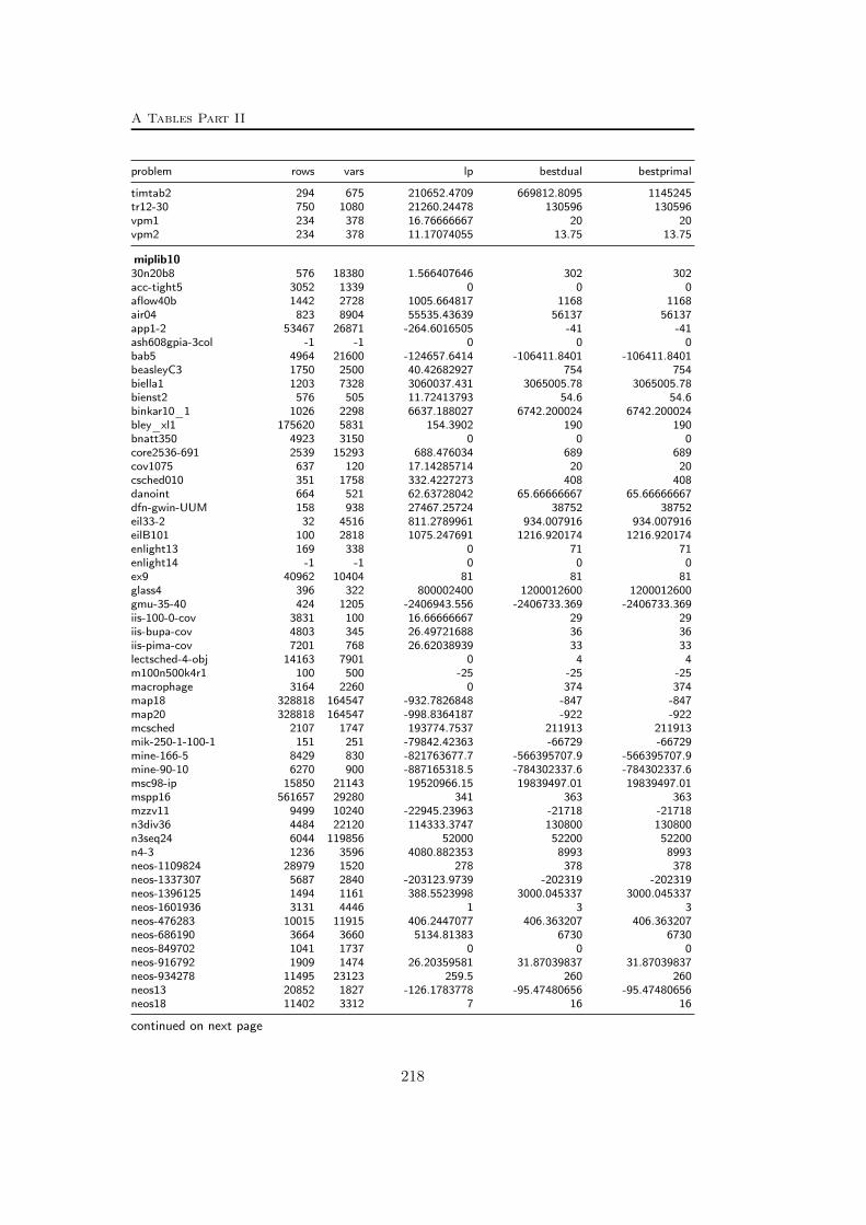
A Tables Part II
problem rows vars lp bestdual bestprimal
timtab2 294 675 210652.4709 669812.8095 1145245tr12-30 750 1080 21260.24478 130596 130596vpm1 234 378 16.76666667 20 20vpm2 234 378 11.17074055 13.75 13.75
miplib1030n20b8 576 18380 1.566407646 302 302acc-tight5 3052 1339 0 0 0aflow40b 1442 2728 1005.664817 1168 1168air04 823 8904 55535.43639 56137 56137app1-2 53467 26871 -264.6016505 -41 -41ash608gpia-3col -1 -1 0 0 0bab5 4964 21600 -124657.6414 -106411.8401 -106411.8401beasleyC3 1750 2500 40.42682927 754 754biella1 1203 7328 3060037.431 3065005.78 3065005.78bienst2 576 505 11.72413793 54.6 54.6binkar10_1 1026 2298 6637.188027 6742.200024 6742.200024bley_xl1 175620 5831 154.3902 190 190bnatt350 4923 3150 0 0 0core2536-691 2539 15293 688.476034 689 689cov1075 637 120 17.14285714 20 20csched010 351 1758 332.4227273 408 408danoint 664 521 62.63728042 65.66666667 65.66666667dfn-gwin-UUM 158 938 27467.25724 38752 38752eil33-2 32 4516 811.2789961 934.007916 934.007916eilB101 100 2818 1075.247691 1216.920174 1216.920174enlight13 169 338 0 71 71enlight14 -1 -1 0 0 0ex9 40962 10404 81 81 81glass4 396 322 800002400 1200012600 1200012600gmu-35-40 424 1205 -2406943.556 -2406733.369 -2406733.369iis-100-0-cov 3831 100 16.66666667 29 29iis-bupa-cov 4803 345 26.49721688 36 36iis-pima-cov 7201 768 26.62038939 33 33lectsched-4-obj 14163 7901 0 4 4m100n500k4r1 100 500 -25 -25 -25macrophage 3164 2260 0 374 374map18 328818 164547 -932.7826848 -847 -847map20 328818 164547 -998.8364187 -922 -922mcsched 2107 1747 193774.7537 211913 211913mik-250-1-100-1 151 251 -79842.42363 -66729 -66729mine-166-5 8429 830 -821763677.7 -566395707.9 -566395707.9mine-90-10 6270 900 -887165318.5 -784302337.6 -784302337.6msc98-ip 15850 21143 19520966.15 19839497.01 19839497.01mspp16 561657 29280 341 363 363mzzv11 9499 10240 -22945.23963 -21718 -21718n3div36 4484 22120 114333.3747 130800 130800n3seq24 6044 119856 52000 52200 52200n4-3 1236 3596 4080.882353 8993 8993neos-1109824 28979 1520 278 378 378neos-1337307 5687 2840 -203123.9739 -202319 -202319neos-1396125 1494 1161 388.5523998 3000.045337 3000.045337neos-1601936 3131 4446 1 3 3neos-476283 10015 11915 406.2447077 406.363207 406.363207neos-686190 3664 3660 5134.81383 6730 6730neos-849702 1041 1737 0 0 0neos-916792 1909 1474 26.20359581 31.87039837 31.87039837neos-934278 11495 23123 259.5 260 260neos13 20852 1827 -126.1783778 -95.47480656 -95.47480656neos18 11402 3312 7 16 16
continued on next page
218

A.1 Used instances
problem rows vars lp bestdual bestprimal
net12 14021 14115 17.24947917 214 214netdiversion 119589 129180 230.8 242 242newdano 576 505 11.72413793 65.666667 65.666667noswot 182 128 -43 -41 -41ns1208400 4289 2883 0 2 2ns1688347 4191 2685 2 27 27ns1758913 624166 17956 -1501.183256 -1454.671755 -1454.671755ns1766074 -1 -1 0 0 0ns1830653 2932 1629 6583 20622 20622opm2-z7-s2 31798 2023 -12879.6869 -10280 -10280pg5_34 225 2600 -16646.58602 -14339.35345 -14339.35345pigeon-10 931 490 -10000 -9000 -9000pw-myciel4 8164 1059 0 10 10qiu 1192 840 -931.6388511 -132.873137 -132.873137rail507 509 63019 172.1455667 174 174ran16x16 288 512 3116.429512 3823 3823reblock67 2523 670 -39339910.92 -34630648.44 -34630648.44rmatr100-p10 7260 7359 360.5933075 423 423rmatr100-p5 8685 8784 762.0400543 976 976rmine6 7078 1096 -462.3057274 -457.18614 -457.18614rocII-4-11 21738 9234 -11.9371621 -6.652755781 -6.652755781rococoC10-001000 1293 3117 7515.271029 11460 11460roll3000 2295 1166 11097.12768 12890 12890satellites1-25 5996 9013 -20 -5 -5sp98ic 825 10894 0 449144758.4 449144758.4sp98ir 1531 1680 216663444.6 219676790.4 219676790.4tanglegram1 68342 34759 0 5182 5182tanglegram2 8980 4714 0 443 443timtab1 171 397 28694 764772 764772triptim1 15706 30055 22.8680875 22.8681 22.8681unitcal_7 48939 25755 19387553.38 19635558.24 19635558.24vpphard 47280 51471 0 5 5zib54-UUE 1809 5150 3875862.863 10334015.82 10334015.82
mittelmann30:70:4_5:0_5:100 12050 10772 8.1 9 930:70:4_5:0_95:100 12526 10976 3 3 330:70:4_5:0_95:98 12471 10990 11.5 12 12acc-1 2286 1620 0 0 0acc-2 2520 1620 0 0 0acc-3 3249 1620 0 0 0acc-4 3285 1620 0 0 0acc-5 3052 1339 0 0 0acc-6 3047 1335 0 0 0bc1 1913 1751 2.146801502 3.338362548 3.338362548bienst1 576 505 11.72413793 46.75 46.75bienst2 576 505 11.72413793 54.6 54.6binkar10_1 1026 2298 6637.188027 6742.200024 6742.200024dano3_3 3202 13873 576.2316203 576.344633 576.344633dano3_4 3202 13873 576.2316203 576.4352247 576.4352247dano3_5 3202 13873 576.2316203 576.924916 576.924916lrn 8491 7253 44246903.22 44482699.34 44482699.34markshare_4_0 4 34 0 1 1markshare_5_0 5 45 0 0 2mik.250-20-75.1 195 270 -59156.75737 -49716 -49716mik.250-20-75.2 195 270 -59987.19637 -50768 -50768mik.250-20-75.3 195 270 -60670.36664 -52242 -52242mik.250-20-75.4 195 270 -61651.2271 -52301 -52301mik.250-20-75.5 195 270 -60527.43721 -51532 -51532neos1 5020 2112 15.5 19 19
continued on next page
219

A Tables Part II
problem rows vars lp bestdual bestprimal
neos10 46793 23489 -1196.333333 -1135 -1135neos11 2706 1220 6 9 9neos12 8317 3983 9.411612426 13 13neos13 20852 1827 -126.1783778 -95.47480656 -95.47480656neos14 552 792 32734.11478 74333.34334 74333.34334neos17 486 535 0.0006814985015 0.1500025774 0.1500025774neos2 1103 2101 -4407.097239 454.864697 454.864697neos20 2446 1165 -475 -434 -434neos21 1085 614 2.216483516 7 7neos22 5208 3240 777191.4286 779715 779715neos23 1568 477 56 137 137neos3 1442 2747 -6158.209105 368.842751 368.842751neos4 38577 22884 -4.860344075e+10 -4.860344075e+10 -4.860344075e+10neos5 63 63 13 15 15neos6 1036 8786 83 83 83neos648910 1491 814 16 32 32neos7 1994 1556 562977.4297 721934 721934neos8 46324 23228 -3725 -3719 -3719neos808444 18329 19846 0 0 0neos818918 2450 2750 1680 1700 1700neos823206 709 1830 19.81417814 83.86019578 83.86019578neos897005 11612 44630 14 14 14neos9 31600 81408 780 798 798ns1648184 806 705 -1260.954861 -1234.666667 -1231.31746ns1671066 316 2840 7.634607843 7.634607843 7.634607843ns1688347 4191 2685 15.11176471 27 27ns1692855 4562 3047 15.11176471 26 30nug08 912 1632 203.5 214 214prod1 208 250 -84.41587189 -56 -56prod2 211 301 -86.98076893 -62 -62qap10 1820 4150 332.5662276 340 340seymour1 4944 1372 403.8464741 410.7637014 410.7637014swath2 884 6805 334.4968581 385.1996929 385.1996929swath3 884 6805 334.4968581 397.7613437 397.7613437
Table A.1: General information for all used instances in Part II ordered by their respective test set.At most 10 digits are shown.
A.2 Results – Network Detection
Table A.2 below presents the results of the network detection for those instancesfor which the original network is known. It reports on the number of nodes (|V |),the number of arcs (|A|), and the number of commodities (|K|) in the originalnetwork (original). For the detected networks with the presolving of Scip switchedoff respectively on (detection – no presolve respectively detection – presolve) thenetwork inconsistency (Ψ(D)) and the difference in the network size (nodes |V |,arcs |A|, commodities |K|) compared with the original network is provided. Ifno network has been found the corresponding entries are marked with ‘-’. Forevery test set we present the arithmetic mean of the (absolute) difference of theoriginal and the detected network elements. The detection results are summarizedin Table 6.2 on page 101.
220
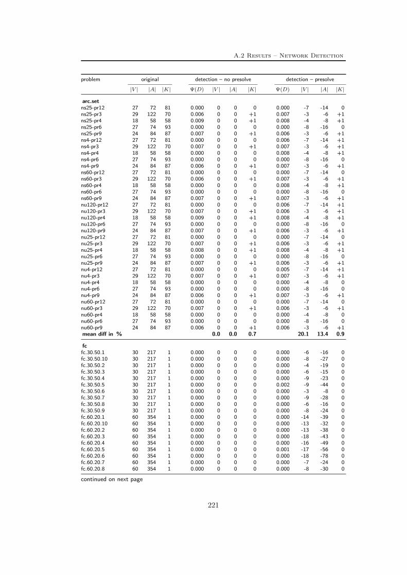
A.2 Results – Network Detection
problem original detection – no presolve detection – presolve
|V | |A| |K| Ψ(D) |V | |A| |K| Ψ(D) |V | |A| |K|
arc.setns25-pr12 27 72 81 0.000 0 0 0 0.000 -7 -14 0ns25-pr3 29 122 70 0.006 0 0 +1 0.007 -3 -6 +1ns25-pr4 18 58 58 0.009 0 0 +1 0.008 -4 -8 +1ns25-pr6 27 74 93 0.000 0 0 0 0.000 -8 -16 0ns25-pr9 24 84 87 0.007 0 0 +1 0.006 -3 -6 +1ns4-pr12 27 72 81 0.000 0 0 0 0.006 -7 -14 +1ns4-pr3 29 122 70 0.007 0 0 +1 0.007 -3 -6 +1ns4-pr4 18 58 58 0.000 0 0 0 0.008 -4 -8 +1ns4-pr6 27 74 93 0.000 0 0 0 0.000 -8 -16 0ns4-pr9 24 84 87 0.006 0 0 +1 0.007 -3 -6 +1ns60-pr12 27 72 81 0.000 0 0 0 0.000 -7 -14 0ns60-pr3 29 122 70 0.006 0 0 +1 0.007 -3 -6 +1ns60-pr4 18 58 58 0.000 0 0 0 0.008 -4 -8 +1ns60-pr6 27 74 93 0.000 0 0 0 0.000 -8 -16 0ns60-pr9 24 84 87 0.007 0 0 +1 0.007 -3 -6 +1nu120-pr12 27 72 81 0.000 0 0 0 0.006 -7 -14 +1nu120-pr3 29 122 70 0.007 0 0 +1 0.006 -3 -6 +1nu120-pr4 18 58 58 0.009 0 0 +1 0.008 -4 -8 +1nu120-pr6 27 74 93 0.000 0 0 0 0.000 -8 -16 0nu120-pr9 24 84 87 0.007 0 0 +1 0.006 -3 -6 +1nu25-pr12 27 72 81 0.000 0 0 0 0.000 -7 -14 0nu25-pr3 29 122 70 0.007 0 0 +1 0.006 -3 -6 +1nu25-pr4 18 58 58 0.008 0 0 +1 0.008 -4 -8 +1nu25-pr6 27 74 93 0.000 0 0 0 0.000 -8 -16 0nu25-pr9 24 84 87 0.007 0 0 +1 0.006 -3 -6 +1nu4-pr12 27 72 81 0.000 0 0 0 0.005 -7 -14 +1nu4-pr3 29 122 70 0.007 0 0 +1 0.007 -3 -6 +1nu4-pr4 18 58 58 0.000 0 0 0 0.000 -4 -8 0nu4-pr6 27 74 93 0.000 0 0 0 0.000 -8 -16 0nu4-pr9 24 84 87 0.006 0 0 +1 0.007 -3 -6 +1nu60-pr12 27 72 81 0.000 0 0 0 0.000 -7 -14 0nu60-pr3 29 122 70 0.007 0 0 +1 0.006 -3 -6 +1nu60-pr4 18 58 58 0.000 0 0 0 0.000 -4 -8 0nu60-pr6 27 74 93 0.000 0 0 0 0.000 -8 -16 0nu60-pr9 24 84 87 0.006 0 0 +1 0.006 -3 -6 +1mean diff in % 0.0 0.0 0.7 20.1 13.4 0.9
fcfc.30.50.1 30 217 1 0.000 0 0 0 0.000 -6 -16 0fc.30.50.10 30 217 1 0.000 0 0 0 0.000 -8 -27 0fc.30.50.2 30 217 1 0.000 0 0 0 0.000 -4 -19 0fc.30.50.3 30 217 1 0.000 0 0 0 0.000 -6 -15 0fc.30.50.4 30 217 1 0.000 0 0 0 0.000 -9 -23 0fc.30.50.5 30 217 1 0.000 0 0 0 0.002 -9 -44 0fc.30.50.6 30 217 1 0.000 0 0 0 0.000 -3 -8 0fc.30.50.7 30 217 1 0.000 0 0 0 0.000 -9 -28 0fc.30.50.8 30 217 1 0.000 0 0 0 0.000 -6 -16 0fc.30.50.9 30 217 1 0.000 0 0 0 0.000 -8 -24 0fc.60.20.1 60 354 1 0.000 0 0 0 0.000 -14 -39 0fc.60.20.10 60 354 1 0.000 0 0 0 0.000 -13 -32 0fc.60.20.2 60 354 1 0.000 0 0 0 0.000 -13 -38 0fc.60.20.3 60 354 1 0.000 0 0 0 0.000 -18 -43 0fc.60.20.4 60 354 1 0.000 0 0 0 0.000 -16 -49 0fc.60.20.5 60 354 1 0.000 0 0 0 0.001 -17 -56 0fc.60.20.6 60 354 1 0.000 0 0 0 0.000 -18 -78 0fc.60.20.7 60 354 1 0.000 0 0 0 0.000 -7 -24 0fc.60.20.8 60 354 1 0.000 0 0 0 0.000 -8 -30 0
continued on next page
221

A Tables Part II
problem original detection – no presolve detection – presolve
|V | |A| |K| Ψ(D) |V | |A| |K| Ψ(D) |V | |A| |K|fc.60.20.9 60 354 1 0.000 0 0 0 0.000 -20 -67 0mean diff in % 0.0 0.0 0.0 23.3 11.5 0.0
fctpbal8x12 20 96 1 0.000 0 0 0 0.000 0 0 0bk4x3 7 12 1 - - - - - - - -gr4x6 10 24 1 - - - - - - - -n3700 150 5000 1 0.000 0 0 0 0.000 0 0 0n3701 150 5000 1 0.000 0 0 0 0.000 0 0 0n3702 150 5000 1 0.000 0 0 0 0.000 0 0 0n3703 150 5000 1 0.000 0 0 0 0.000 0 0 0n3704 150 5000 1 0.000 0 0 0 0.000 0 0 0n3705 150 5000 1 0.000 0 0 0 0.000 0 0 0n3706 150 5000 1 0.000 0 0 0 0.000 0 0 0n3707 150 5000 1 0.000 0 0 0 0.000 0 0 0n3708 150 5000 1 0.000 0 0 0 0.000 0 0 0n3709 150 5000 1 0.000 0 0 0 0.000 0 0 0n370a 150 5000 1 0.000 0 0 0 0.000 0 0 0n370b 150 5000 1 0.000 0 0 0 0.000 0 0 0n370c 150 5000 1 0.000 0 0 0 0.000 0 0 0n370d 150 5000 1 0.000 0 0 0 0.000 0 0 0n370e 150 5000 1 0.000 0 0 0 0.000 0 0 0ran10x10a 20 100 1 0.000 0 0 0 0.000 0 0 0ran10x10b 20 100 1 0.000 0 0 0 0.000 0 0 0ran10x10c 20 100 1 0.000 0 0 0 0.000 0 0 0ran10x12 22 120 1 0.000 0 0 0 0.000 0 0 0ran10x26 36 260 1 0.000 0 0 0 0.000 0 0 0ran12x12 24 144 1 0.000 0 0 0 0.000 0 0 0ran12x21 33 252 1 0.000 0 0 0 0.000 0 0 0ran13x13 26 169 1 0.000 0 0 0 0.000 0 0 0ran14x18 32 252 1 0.000 0 0 0 0.000 0 0 0ran16x16 32 256 1 0.000 0 0 0 0.000 0 0 0ran17x17 34 289 1 0.000 0 0 0 0.000 0 0 0ran4x64 68 256 1 0.000 -63 -252 +2 0.000 -63 -252 +2ran6x43 49 258 1 0.000 0 0 0 0.000 0 0 0ran8x32 40 256 1 0.000 0 0 0 0.000 0 0 0mean diff in % 3.1 3.3 6.7 3.1 3.3 6.7
avubnexp.100.20.1.1 100 990 1 0.000 0 0 0 0.000 -61 -388 0nexp.100.20.1.2 100 990 1 0.000 0 0 0 0.000 -59 -356 0nexp.100.20.1.3 100 990 1 0.000 0 0 0 0.000 -66 -457 0nexp.100.20.1.4 100 990 1 0.000 0 0 0 0.000 -64 -447 0nexp.100.20.1.5 100 990 1 0.000 0 0 0 0.000 -65 -431 0nexp.100.20.2.1 100 990 1 0.000 0 0 0 0.000 -61 -388 0nexp.100.20.2.2 100 990 1 0.000 0 0 0 0.000 -54 -325 0nexp.100.20.2.3 100 990 1 0.000 0 0 0 0.000 -63 -414 0nexp.100.20.2.4 100 990 1 0.000 0 0 0 0.000 -51 -313 0nexp.100.20.2.5 100 990 1 0.000 0 0 0 0.000 -58 -351 0nexp.100.20.4.1 100 990 1 0.000 0 0 0 0.000 0 -102 0nexp.100.20.4.2 100 990 1 0.000 0 0 0 0.000 0 -107 0nexp.100.20.4.3 100 990 1 0.000 0 0 0 0.000 0 -92 0nexp.100.20.4.4 100 990 1 0.000 0 0 0 0.000 0 -85 0nexp.100.20.4.5 100 990 1 0.000 0 0 0 0.000 0 -133 0nexp.100.20.8.1 100 990 1 0.000 0 0 0 0.000 0 -102 0nexp.100.20.8.2 100 990 1 0.000 0 0 0 0.000 0 -107 0nexp.100.20.8.3 100 990 1 0.000 0 0 0 0.000 0 -119 0nexp.100.20.8.4 100 990 1 0.000 0 0 0 0.000 0 -85 0nexp.100.20.8.5 100 990 1 0.000 0 0 0 0.000 0 -133 0
continued on next page
222
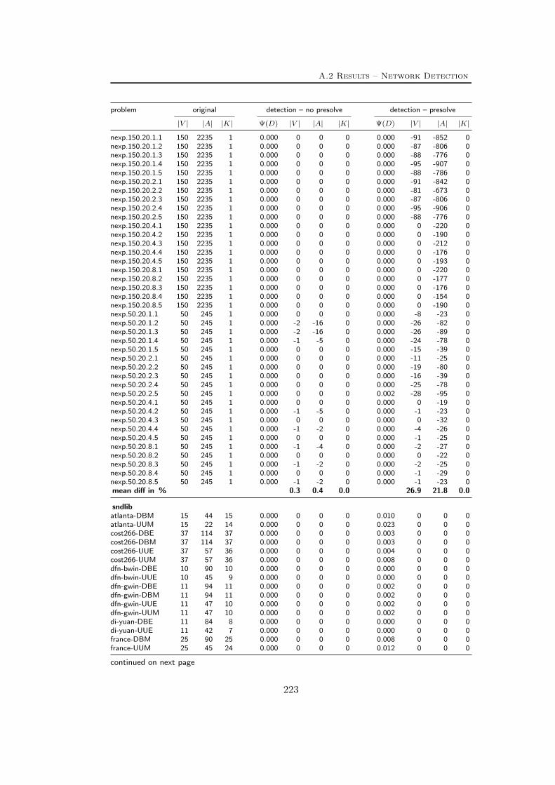
A.2 Results – Network Detection
problem original detection – no presolve detection – presolve
|V | |A| |K| Ψ(D) |V | |A| |K| Ψ(D) |V | |A| |K|nexp.150.20.1.1 150 2235 1 0.000 0 0 0 0.000 -91 -852 0nexp.150.20.1.2 150 2235 1 0.000 0 0 0 0.000 -87 -806 0nexp.150.20.1.3 150 2235 1 0.000 0 0 0 0.000 -88 -776 0nexp.150.20.1.4 150 2235 1 0.000 0 0 0 0.000 -95 -907 0nexp.150.20.1.5 150 2235 1 0.000 0 0 0 0.000 -88 -786 0nexp.150.20.2.1 150 2235 1 0.000 0 0 0 0.000 -91 -842 0nexp.150.20.2.2 150 2235 1 0.000 0 0 0 0.000 -81 -673 0nexp.150.20.2.3 150 2235 1 0.000 0 0 0 0.000 -87 -806 0nexp.150.20.2.4 150 2235 1 0.000 0 0 0 0.000 -95 -906 0nexp.150.20.2.5 150 2235 1 0.000 0 0 0 0.000 -88 -776 0nexp.150.20.4.1 150 2235 1 0.000 0 0 0 0.000 0 -220 0nexp.150.20.4.2 150 2235 1 0.000 0 0 0 0.000 0 -190 0nexp.150.20.4.3 150 2235 1 0.000 0 0 0 0.000 0 -212 0nexp.150.20.4.4 150 2235 1 0.000 0 0 0 0.000 0 -176 0nexp.150.20.4.5 150 2235 1 0.000 0 0 0 0.000 0 -193 0nexp.150.20.8.1 150 2235 1 0.000 0 0 0 0.000 0 -220 0nexp.150.20.8.2 150 2235 1 0.000 0 0 0 0.000 0 -177 0nexp.150.20.8.3 150 2235 1 0.000 0 0 0 0.000 0 -176 0nexp.150.20.8.4 150 2235 1 0.000 0 0 0 0.000 0 -154 0nexp.150.20.8.5 150 2235 1 0.000 0 0 0 0.000 0 -190 0nexp.50.20.1.1 50 245 1 0.000 0 0 0 0.000 -8 -23 0nexp.50.20.1.2 50 245 1 0.000 -2 -16 0 0.000 -26 -82 0nexp.50.20.1.3 50 245 1 0.000 -2 -16 0 0.000 -26 -89 0nexp.50.20.1.4 50 245 1 0.000 -1 -5 0 0.000 -24 -78 0nexp.50.20.1.5 50 245 1 0.000 0 0 0 0.000 -15 -39 0nexp.50.20.2.1 50 245 1 0.000 0 0 0 0.000 -11 -25 0nexp.50.20.2.2 50 245 1 0.000 0 0 0 0.000 -19 -80 0nexp.50.20.2.3 50 245 1 0.000 0 0 0 0.000 -16 -39 0nexp.50.20.2.4 50 245 1 0.000 0 0 0 0.000 -25 -78 0nexp.50.20.2.5 50 245 1 0.000 0 0 0 0.002 -28 -95 0nexp.50.20.4.1 50 245 1 0.000 0 0 0 0.000 0 -19 0nexp.50.20.4.2 50 245 1 0.000 -1 -5 0 0.000 -1 -23 0nexp.50.20.4.3 50 245 1 0.000 0 0 0 0.000 0 -32 0nexp.50.20.4.4 50 245 1 0.000 -1 -2 0 0.000 -4 -26 0nexp.50.20.4.5 50 245 1 0.000 0 0 0 0.000 -1 -25 0nexp.50.20.8.1 50 245 1 0.000 -1 -4 0 0.000 -2 -27 0nexp.50.20.8.2 50 245 1 0.000 0 0 0 0.000 0 -22 0nexp.50.20.8.3 50 245 1 0.000 -1 -2 0 0.000 -2 -25 0nexp.50.20.8.4 50 245 1 0.000 0 0 0 0.000 -1 -29 0nexp.50.20.8.5 50 245 1 0.000 -1 -2 0 0.000 -1 -23 0mean diff in % 0.3 0.4 0.0 26.9 21.8 0.0
sndlibatlanta-DBM 15 44 15 0.000 0 0 0 0.010 0 0 0atlanta-UUM 15 22 14 0.000 0 0 0 0.023 0 0 0cost266-DBE 37 114 37 0.000 0 0 0 0.003 0 0 0cost266-DBM 37 114 37 0.000 0 0 0 0.003 0 0 0cost266-UUE 37 57 36 0.000 0 0 0 0.004 0 0 0cost266-UUM 37 57 36 0.000 0 0 0 0.008 0 0 0dfn-bwin-DBE 10 90 10 0.000 0 0 0 0.000 0 0 0dfn-bwin-UUE 10 45 9 0.000 0 0 0 0.000 0 0 0dfn-gwin-DBE 11 94 11 0.000 0 0 0 0.002 0 0 0dfn-gwin-DBM 11 94 11 0.000 0 0 0 0.002 0 0 0dfn-gwin-UUE 11 47 10 0.000 0 0 0 0.002 0 0 0dfn-gwin-UUM 11 47 10 0.000 0 0 0 0.002 0 0 0di-yuan-DBE 11 84 8 0.000 0 0 0 0.000 0 0 0di-yuan-UUE 11 42 7 0.000 0 0 0 0.000 0 0 0france-DBM 25 90 25 0.000 0 0 0 0.008 0 0 0france-UUM 25 45 24 0.000 0 0 0 0.012 0 0 0
continued on next page
223

A Tables Part II
problem original detection – no presolve detection – presolve
|V | |A| |K| Ψ(D) |V | |A| |K| Ψ(D) |V | |A| |K|germany50-DBM 50 176 47 0.000 0 0 0 0.002 0 0 0germany50-UUM 50 88 40 0.000 0 0 0 0.003 0 0 0giul39-DDE 39 172 39 0.000 0 0 0 0.000 0 0 0janos-us-DDM 30 84 26 0.000 -4 0 0 0.004 -4 0 0janos-us-ca-DDM 39 122 39 0.000 0 0 0 0.004 0 0 0newyork-DBE 16 98 16 0.000 0 0 0 0.001 0 0 0newyork-DBM 16 98 16 0.000 0 0 0 0.001 0 0 0newyork-UUE 16 49 15 0.000 0 0 0 0.001 0 0 0newyork-UUM 16 49 15 0.000 0 0 0 0.001 0 0 0nobel-eu-DBE 28 82 27 0.000 0 0 0 0.006 0 0 0nobel-eu-UUE 28 41 27 0.000 0 0 0 0.009 0 0 0nobel-ger-DBE 17 52 15 0.000 0 0 0 0.012 0 0 0nobel-ger-UUE 17 26 15 0.000 0 0 0 0.015 0 0 0norway-DBE 27 102 27 0.000 0 0 0 0.001 0 0 0norway-DBM 27 102 27 0.000 0 0 0 0.001 0 0 0norway-UUE 27 51 26 0.000 0 0 0 0.002 0 0 0norway-UUM 27 51 26 0.000 0 0 0 0.003 0 0 0pdh-DBE 11 68 10 0.000 0 0 0 0.000 0 0 0pdh-DBM 11 68 10 0.000 0 0 0 0.000 0 0 0pdh-UUE 11 34 7 0.000 0 0 0 0.000 0 0 0pdh-UUM 11 34 7 0.000 0 0 0 0.000 0 0 0pioro40-DBM 40 178 39 0.000 0 0 0 0.000 0 0 0pioro40-UUM 40 89 39 0.000 0 0 0 0.000 0 0 0polska-DBM 12 36 11 0.000 0 0 0 0.008 0 0 0polska-UUM 12 18 11 0.000 0 0 0 0.010 0 0 0sun-DDM 27 102 6 0.000 0 0 0 0.003 0 0 0ta1-DBE 24 110 19 0.000 0 0 0 0.002 0 0 0ta1-DBM 24 110 19 0.000 0 0 0 0.002 0 0 0ta1-UUE 24 55 16 0.000 0 0 0 0.003 0 0 0ta1-UUM 24 55 16 0.000 0 0 0 0.003 0 0 0ta2-DBE 65 216 42 0.000 0 0 0 0.002 -1 -2 0ta2-DBM 65 216 42 0.000 0 0 0 0.003 -1 -2 0ta2-UUE 65 108 38 0.000 0 0 0 0.003 -1 -1 0ta2-UUM 65 108 38 0.000 0 0 0 0.005 -1 -1 0zib54-DBE 54 162 42 0.000 0 0 0 0.005 -1 -2 0zib54-UUE 54 81 32 0.000 0 0 0 0.006 -1 -1 0mean diff in % 0.3 0.0 0.0 0.4 0.1 0.0
ufcnbeasleyC1 500 1250 1 0.000 0 0 0 0.000 -193 -386 0beasleyC2 500 1250 1 0.000 0 0 0 0.000 -190 -380 0beasleyC3 500 1250 1 0.000 -1 -2 0 0.000 -199 -398 0beavma 89 195 1 0.000 0 0 0 0.000 -11 -15 0berlin 52 2652 1 0.000 0 0 0 0.000 0 0 0brasil 58 3306 1 0.000 0 0 0 0.000 0 0 0fixnet6 100 500 1 0.000 0 0 0 0.000 -1 -51 0g150x1100 150 1100 1 0.000 0 0 0 0.000 0 0 0g150x1650 150 1650 1 0.000 0 0 0 0.000 0 0 0g180x666 180 666 1 0.000 0 0 0 0.000 0 0 0g200x740 200 740 1 0.000 0 0 0 0.000 0 0 0g200x740b 200 740 1 0.000 0 0 0 0.000 0 0 0g200x740c 200 740 1 0.000 0 0 0 0.000 0 0 0g200x740d 200 740 1 0.000 0 0 0 0.000 0 0 0g200x740e 200 740 1 0.000 0 0 0 0.000 0 0 0g200x740f 200 740 1 0.000 0 0 0 0.000 0 0 0g200x740g 200 740 1 0.000 0 0 0 0.000 0 0 0g200x740h 200 740 1 0.000 0 0 0 0.000 0 0 0g200x740i 200 740 1 0.000 0 0 0 0.000 0 0 0g40x132 40 132 1 0.000 0 0 0 0.000 0 0 0
continued on next page
224

A.2 Results – Network Detection
problem original detection – no presolve detection – presolve
|V | |A| |K| Ψ(D) |V | |A| |K| Ψ(D) |V | |A| |K|g50x170 50 170 1 0.000 0 0 0 0.000 0 0 0g55x188 55 188 1 0.000 0 0 0 0.000 0 0 0g55x188c 55 188 1 0.000 0 0 0 0.000 0 0 0h50x2450 50 2450 1 0.000 0 -49 0 0.000 0 -49 0h50x2450b 50 2450 1 0.000 0 -49 0 0.000 0 -49 0h50x2450c 50 2450 1 0.000 0 -49 0 0.000 0 -49 0h50x2450d 50 2450 1 0.000 0 -49 0 0.000 0 -49 0h50x2450e 50 2450 1 0.000 0 -49 0 0.000 0 -49 0h80x6320b 80 6320 1 0.000 0 -79 0 0.000 0 -79 0h80x6320c 80 6320 1 0.000 0 -79 0 0.000 0 -79 0h80x6320d 80 6320 1 0.000 0 -79 0 0.000 0 -79 0k10x90 10 90 1 0.000 0 0 0 0.000 0 0 0k14x182 14 182 1 0.000 0 0 0 0.000 0 0 0k14x182b 14 182 1 0.000 0 0 0 0.000 0 0 0k15x210 15 210 1 0.000 0 0 0 0.000 0 0 0k15x420 15 420 1 0.000 0 0 0 0.000 0 0 0k15x630 15 630 1 0.000 0 0 0 0.000 0 0 0k16x240 16 240 1 0.000 0 0 0 0.000 0 0 0k16x240b 16 240 1 0.000 0 0 0 0.000 0 0 0k20x380 20 380 1 0.000 0 0 0 0.000 0 0 0k20x380b 20 380 1 0.000 0 0 0 0.000 0 0 0k20x380c 20 380 1 0.000 0 0 0 0.000 0 0 0k20x380d 20 380 1 0.000 0 0 0 0.000 0 0 0k20x380e 20 380 1 0.000 0 0 0 0.000 0 0 0l121x232 121 232 1 0.000 0 0 0 0.006 -6 -36 0l451x885 451 885 1 0.000 0 0 0 0.004 -9 -129 0l451x885b 451 885 1 0.000 0 -1 0 0.004 -9 -134 0l61x114 61 114 1 0.000 0 -1 0 0.009 -5 -20 0mc11 400 1520 1 0.000 0 0 0 0.000 0 0 0mc7 400 1520 1 0.000 0 0 0 0.000 0 0 0mc8 400 1520 1 0.000 0 0 0 0.000 0 0 0mtest4ma 100 975 1 0.000 0 0 0 0.000 0 0 0p100x588 100 588 1 0.000 0 0 0 0.000 0 0 0p100x588b 100 588 1 0.000 0 0 0 0.000 0 0 0p100x588c 100 588 1 0.000 0 0 0 0.000 0 0 0p100x588d 100 588 1 0.000 0 0 0 0.000 0 0 0p200x1188 200 1188 1 0.000 0 0 0 0.000 0 0 0p200x1188b 200 1188 1 0.000 0 0 0 0.000 0 0 0p200x1188c 200 1188 1 0.000 0 0 0 0.000 0 0 0p500x2988 500 2988 1 0.000 0 0 0 0.000 0 0 0p500x2988b 500 2988 1 0.000 0 0 0 0.000 0 0 0p500x2988c 500 2988 1 0.000 0 0 0 0.000 0 0 0p500x2988d 500 2988 1 0.000 0 0 0 0.000 0 0 0p50x288 50 288 1 0.000 0 0 0 0.000 0 0 0p50x288b 50 288 1 0.000 0 0 0 0.000 0 0 0p50x576 50 576 1 0.000 0 0 0 0.000 0 0 0p50x864 50 864 1 0.000 0 0 0 0.000 0 0 0p80x400 80 400 1 0.000 0 0 0 0.000 -2 -4 0p80x400b 80 400 1 0.000 0 0 0 0.000 -2 -4 0r20x100 20 100 1 0.000 0 0 0 0.000 -1 -2 0r20x200 20 200 1 0.000 0 0 0 0.000 0 0 0r30x160 30 160 1 0.000 0 0 0 0.000 -4 -8 0r50x360 50 360 1 0.000 0 0 0 0.000 -1 -2 0r80x800 80 800 1 0.000 0 0 0 0.000 0 0 0sp100x200 100 200 1 0.000 -60 -124 0 0.000 -76 -136 0sp150x300 150 300 1 0.000 -52 -105 0 0.000 -89 -143 0sp150x300b 150 300 1 0.000 -23 -53 0 0.000 -79 -110 0sp150x300c 150 300 1 0.000 -13 -30 0 0.000 -68 -85 0sp150x300d 150 300 1 0.000 0 -4 0 0.000 -86 -86 0
continued on next page
225
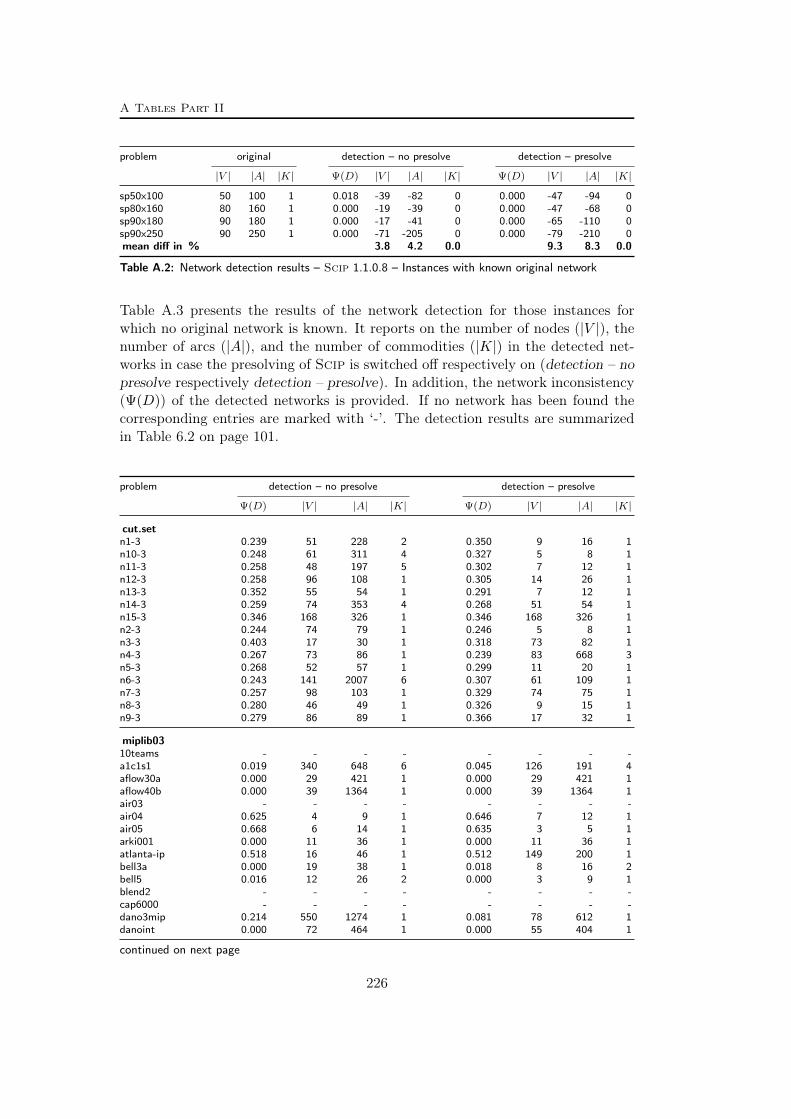
A Tables Part II
problem original detection – no presolve detection – presolve
|V | |A| |K| Ψ(D) |V | |A| |K| Ψ(D) |V | |A| |K|sp50x100 50 100 1 0.018 -39 -82 0 0.000 -47 -94 0sp80x160 80 160 1 0.000 -19 -39 0 0.000 -47 -68 0sp90x180 90 180 1 0.000 -17 -41 0 0.000 -65 -110 0sp90x250 90 250 1 0.000 -71 -205 0 0.000 -79 -210 0mean diff in % 3.8 4.2 0.0 9.3 8.3 0.0
Table A.2: Network detection results – Scip 1.1.0.8 – Instances with known original network
Table A.3 presents the results of the network detection for those instances forwhich no original network is known. It reports on the number of nodes (|V |), thenumber of arcs (|A|), and the number of commodities (|K|) in the detected net-works in case the presolving of Scip is switched off respectively on (detection – nopresolve respectively detection – presolve). In addition, the network inconsistency(Ψ(D)) of the detected networks is provided. If no network has been found thecorresponding entries are marked with ‘-’. The detection results are summarizedin Table 6.2 on page 101.
problem detection – no presolve detection – presolve
Ψ(D) |V | |A| |K| Ψ(D) |V | |A| |K|
cut.setn1-3 0.239 51 228 2 0.350 9 16 1n10-3 0.248 61 311 4 0.327 5 8 1n11-3 0.258 48 197 5 0.302 7 12 1n12-3 0.258 96 108 1 0.305 14 26 1n13-3 0.352 55 54 1 0.291 7 12 1n14-3 0.259 74 353 4 0.268 51 54 1n15-3 0.346 168 326 1 0.346 168 326 1n2-3 0.244 74 79 1 0.246 5 8 1n3-3 0.403 17 30 1 0.318 73 82 1n4-3 0.267 73 86 1 0.239 83 668 3n5-3 0.268 52 57 1 0.299 11 20 1n6-3 0.243 141 2007 6 0.307 61 109 1n7-3 0.257 98 103 1 0.329 74 75 1n8-3 0.280 46 49 1 0.326 9 15 1n9-3 0.279 86 89 1 0.366 17 32 1
miplib0310teams - - - - - - - -a1c1s1 0.019 340 648 6 0.045 126 191 4aflow30a 0.000 29 421 1 0.000 29 421 1aflow40b 0.000 39 1364 1 0.000 39 1364 1air03 - - - - - - - -air04 0.625 4 9 1 0.646 7 12 1air05 0.668 6 14 1 0.635 3 5 1arki001 0.000 11 36 1 0.000 11 36 1atlanta-ip 0.518 16 46 1 0.512 149 200 1bell3a 0.000 19 38 1 0.018 8 16 2bell5 0.016 12 26 2 0.000 3 9 1blend2 - - - - - - - -cap6000 - - - - - - - -dano3mip 0.214 550 1274 1 0.081 78 612 1danoint 0.000 72 464 1 0.000 55 404 1
continued on next page
226

A.2 Results – Network Detection
problem detection – no presolve detection – presolve
Ψ(D) |V | |A| |K| Ψ(D) |V | |A| |K|dcmulti - - - - - - - -disctom - - - - - - - -ds - - - - - - - -dsbmip - - - - - - - -egout 0.016 11 15 1 0.000 8 21 1enigma - - - - - - - -fast0507 - - - - - - - -fiber 0.015 28 44 11 0.005 23 38 11fixnet6 0.000 100 448 1 0.000 99 449 1flugpl - - - - - - - -gen 0.000 52 55 5 0.486 16 18 2gesa2 0.000 24 24 13 0.000 24 24 13gesa2-o 0.000 24 24 1 0.000 24 24 1gesa3 0.093 36 70 12 0.093 35 70 11gesa3_o 0.020 26 28 1 0.022 25 50 1glass4 - - - - - - - -gt2 - - - - - - - -harp2 - - - - - - - -khb05250 0.000 76 100 1 0.000 76 100 1l152lav - - - - - - - -liu - - - - - - - -lseu - - - - - - - -manna81 0.190 46 51 7 0.190 46 51 7markshare1 - - - - - - - -markshare2 - - - - - - - -mas74 - - - - - - - -mas76 - - - - - - - -misc03 - - - - 0.417 5 4 1misc06 0.041 8 14 1 0.099 6 6 1misc07 - - - - 0.438 6 5 1mitre - - - - - - - -mkc 0.095 319 319 1 0.271 7 6 24mod008 - - - - - - - -mod010 - - - - - - - -mod011 - - - - 0.445 19 24 3modglob - - - - - - - -momentum1 0.021 74 184 1 0.026 311 658 1momentum2 0.003 287 1375 1 0.002 285 1193 1momentum3 0.000 502 4519 1 0.005 898 4035 1msc98-ip 0.529 186 345 1 0.535 143 303 1mzzv11 0.669 6 7 1 0.645 10 23 1mzzv42z 0.661 10 17 2 0.656 7 11 2net12 0.209 12 17 2 0.395 20 32 1noswot 0.250 6 5 1 0.250 6 5 1nsrand-ipx - - - - 0.322 11 17 5nw04 - - - - - - - -opt1217 - - - - - - - -p0033 - - - - - - - -p0201 - - - - 0.561 4 3 2p0282 - - - - 0.089 8 9 5p0548 - - - - 0.137 4 6 3p2756 - - - - 0.195 11 14 1pk1 - - - - - - - -pp08a 0.000 72 162 1 0.000 69 154 1pp08aCUTS 0.095 72 132 1 0.091 69 121 1protfold 0.479 142 368 1 0.499 140 263 1qiu - - - - - - - -qnet1 0.478 13 49 5 0.313 8 28 6qnet1_o 0.213 36 103 24 0.000 10 37 24
continued on next page
227
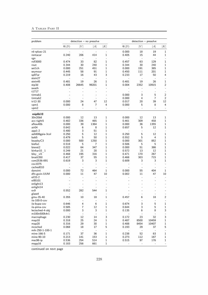
A Tables Part II
problem detection – no presolve detection – presolve
Ψ(D) |V | |A| |K| Ψ(D) |V | |A| |K|rd-rplusc-21 - - - - 0.000 18 19 1rentacar 0.240 206 414 1 0.405 15 44 1rgn - - - - - - - -roll3000 0.474 33 82 1 0.457 63 129 1rout 0.344 30 240 1 0.344 30 240 1set1ch 0.000 251 451 1 0.000 191 385 1seymour 0.445 58 91 1 0.450 111 201 1sp97ar 0.219 16 43 3 0.233 17 50 4stein27 - - - - - - - -stein45 0.481 19 26 1 0.481 19 26 1stp3d 0.408 26645 99201 1 0.004 2352 10915 2swath - - - - - - - -t1717 - - - - - - - -timtab1 - - - - 0.000 3 5 2timtab2 - - - - 0.000 4 7 2tr12-30 0.000 24 47 12 0.017 20 39 12vpm1 0.000 8 7 4 0.000 5 8 4vpm2 - - - - - - - -
miplib1030n20b8 0.000 12 13 1 0.000 12 13 1acc-tight5 0.482 336 465 1 0.461 309 458 1aflow40b 0.000 39 1364 1 0.000 36 1355 1air04 0.642 6 8 1 0.657 5 12 1app1-2 0.480 3 51 1 - - - -ash608gpia-3col 0.250 5 12 1 0.250 5 12 1bab5 0.479 5 50 1 0.552 5 4 1beasleyC3 0.000 500 1250 1 0.000 301 852 1biella1 0.518 5 7 1 0.506 5 5 1bienst2 0.022 64 347 1 0.000 51 386 1binkar10_1 0.249 21 20 1 0.572 13 12 1bley_xl1 0.468 195 316 1 0.471 170 267 1bnatt350 0.417 37 55 1 0.468 303 715 1core2536-691 0.619 3 3 1 0.609 3 3 1cov1075 - - - - - - - -csched010 - - - - - - - -danoint 0.000 72 464 1 0.000 55 404 1dfn-gwin-UUM 0.000 11 47 10 0.002 11 47 10eil33-2 - - - - - - - -eilB101 - - - - - - - -enlight13 - - - - - - - -enlight14 - - - - - - - -ex9 0.552 282 544 1 - - - -glass4 - - - - - - - -gmu-35-40 0.355 10 18 1 0.457 6 18 2iis-100-0-cov - - - - - - - -iis-bupa-cov 0.646 4 6 1 0.674 3 5 1iis-pima-cov 0.585 7 12 1 0.644 3 5 1lectsched-4-obj 0.000 3 3 1 0.135 6 8 3m100n500k4r1 - - - - - - - -macrophage 0.230 12 14 3 0.172 23 32 3map18 0.318 25 24 1 0.487 8500 10459 1map20 0.316 29 30 1 0.488 8454 10407 1mcsched 0.068 18 17 5 0.193 29 37 5mik-250-1-100-1 - - - - - - - -mine-166-5 0.171 37 36 1 0.238 52 63 1mine-90-10 0.213 141 153 1 0.273 112 167 1msc98-ip 0.536 254 514 1 0.515 97 176 1mspp16 0.183 256 661 1 - - - -
continued on next page
228

A.2 Results – Network Detection
problem detection – no presolve detection – presolve
Ψ(D) |V | |A| |K| Ψ(D) |V | |A| |K|mzzv11 0.668 6 7 1 0.516 39 44 2n3div36 - - - - - - - -n3seq24 0.668 3 58 1 0.668 3 58 1n4-3 0.278 58 60 1 0.406 14 26 1neos-1109824 0.025 20 190 1 0.025 20 190 1neos-1337307 0.189 48 101 10 0.287 116 166 4neos-1396125 0.284 117 406 1 0.512 258 584 1neos-1601936 0.629 7 8 1 0.637 11 15 1neos-476283 - - - - - - - -neos-686190 0.002 62 3438 1 0.002 63 3439 1neos-849702 0.578 4 4 1 0.670 5 4 1neos-916792 - - - - - - - -neos-934278 0.595 881 1420 1 0.547 23 22 1neos13 - - - - - - - -neos18 0.309 524 1104 1 0.474 17 103 1net12 0.211 12 17 2 0.397 21 37 1netdiversion 0.000 10002 20001 2 0.000 10001 19901 2newdano 0.022 64 347 1 0.000 51 386 1noswot 0.250 6 5 1 0.250 6 5 1ns1208400 0.521 81 104 1 0.561 77 89 1ns1688347 0.341 151 305 1 0.466 49 142 1ns1758913 0.489 357 526 1 0.497 362 785 1ns1766074 0.000 20 90 1 0.000 20 90 1ns1830653 0.608 4 6 1 0.495 4 8 1opm2-z7-s2 0.011 413 414 1 0.001 1040 1042 1pg5_34 - - - - - - - -pigeon-10 - - - - - - - -pw-myciel4 0.500 24 196 1 0.500 447 874 1qiu - - - - - - - -rail507 - - - - - - - -ran16x16 0.000 32 256 1 0.000 32 256 1reblock67 0.166 38 40 1 0.103 65 72 2rmatr100-p10 0.245 91 174 1 0.245 91 176 1rmatr100-p5 0.250 94 177 1 0.250 94 177 1rmine6 0.107 287 288 1 0.095 358 368 1rocII-4-11 0.270 52 148 9 0.379 41 167 5rococoC10-001000 0.333 10 41 33 0.020 10 41 74roll3000 0.472 33 82 1 0.425 9 34 1satellites1-25 0.603 206 424 1 0.224 164 2272 12sp98ic - - - - - - - -sp98ir - - - - - - - -tanglegram1 0.369 17 42 4 0.313 16 35 7tanglegram2 0.452 4 7 1 0.454 4 6 1timtab1 - - - - 0.000 3 5 2triptim1 0.502 157 287 1 0.928 24 24 1unitcal_7 0.396 420 668 1 0.352 135 158 1vpphard 0.285 103 553 1 0.483 75 747 7zib54-UUE 0.000 54 81 32 0.006 53 80 32
mittelmann30:70:4_5:0_5:100 0.404 91 104 1 0.416 176 201 130:70:4_5:0_95:100 0.424 108 128 1 0.421 108 129 130:70:4_5:0_95:98 0.418 50 62 1 0.411 58 69 1acc-1 0.514 293 764 1 0.515 155 673 1acc-2 0.517 116 422 1 0.514 155 673 1acc-3 0.373 149 168 1 0.407 175 220 1acc-4 0.374 169 204 1 0.387 180 225 1acc-5 0.488 250 334 1 0.469 286 440 1acc-6 0.466 238 355 1 0.473 287 470 1
continued on next page
229
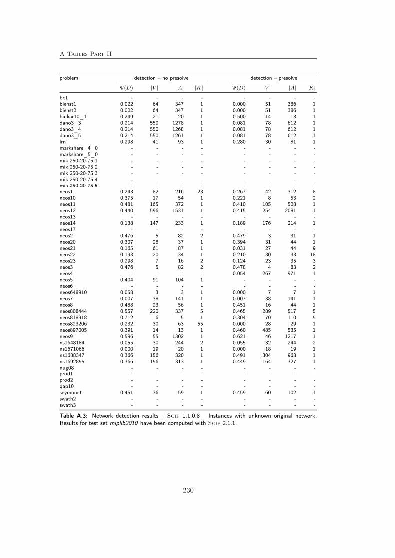
A Tables Part II
problem detection – no presolve detection – presolve
Ψ(D) |V | |A| |K| Ψ(D) |V | |A| |K|bc1 - - - - - - - -bienst1 0.022 64 347 1 0.000 51 386 1bienst2 0.022 64 347 1 0.000 51 386 1binkar10_1 0.249 21 20 1 0.500 14 13 1dano3_3 0.214 550 1278 1 0.081 78 612 1dano3_4 0.214 550 1268 1 0.081 78 612 1dano3_5 0.214 550 1261 1 0.081 78 612 1lrn 0.298 41 93 1 0.280 30 81 1markshare_4_0 - - - - - - - -markshare_5_0 - - - - - - - -mik.250-20-75.1 - - - - - - - -mik.250-20-75.2 - - - - - - - -mik.250-20-75.3 - - - - - - - -mik.250-20-75.4 - - - - - - - -mik.250-20-75.5 - - - - - - - -neos1 0.243 82 216 23 0.267 42 312 8neos10 0.375 17 54 1 0.221 8 53 2neos11 0.481 165 372 1 0.410 105 528 1neos12 0.440 596 1531 1 0.415 254 2081 1neos13 - - - - - - - -neos14 0.138 147 233 1 0.189 176 214 1neos17 - - - - - - - -neos2 0.476 5 82 2 0.479 3 31 1neos20 0.307 28 37 1 0.394 31 44 1neos21 0.165 61 87 1 0.031 27 44 9neos22 0.193 20 34 1 0.210 30 33 18neos23 0.298 7 16 2 0.124 23 35 3neos3 0.476 5 82 2 0.478 4 83 2neos4 - - - - 0.054 267 971 1neos5 0.404 91 104 1 - - - -neos6 - - - - - - - -neos648910 0.058 3 3 1 0.000 7 7 1neos7 0.007 38 141 1 0.007 38 141 1neos8 0.488 23 56 1 0.451 16 44 1neos808444 0.557 220 337 5 0.465 289 517 5neos818918 0.712 6 5 1 0.304 70 110 5neos823206 0.232 30 63 55 0.000 28 29 1neos897005 0.391 14 13 1 0.460 485 535 1neos9 0.596 55 1302 1 0.621 46 1217 1ns1648184 0.055 30 244 2 0.055 32 244 2ns1671066 0.000 19 20 1 0.000 18 19 1ns1688347 0.366 156 320 1 0.491 304 968 1ns1692855 0.366 156 313 1 0.449 164 327 1nug08 - - - - - - - -prod1 - - - - - - - -prod2 - - - - - - - -qap10 - - - - - - - -seymour1 0.451 36 59 1 0.459 60 102 1swath2 - - - - - - - -swath3 - - - - - - - -
Table A.3: Network detection results – Scip 1.1.0.8 – Instances with unknown original network.Results for test set miplib2010 have been computed with Scip 2.1.1.
230
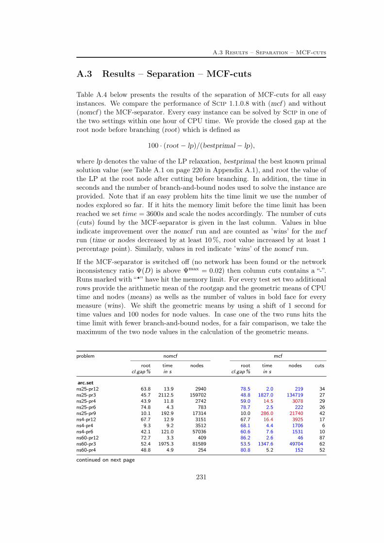
A.3 Results – Separation – MCF-cuts
A.3 Results – Separation – MCF-cuts
Table A.4 below presents the results of the separation of MCF-cuts for all easyinstances. We compare the performance of Scip 1.1.0.8 with (mcf ) and without(nomcf ) the MCF-separator. Every easy instance can be solved by Scip in one ofthe two settings within one hour of CPU time. We provide the closed gap at theroot node before branching (root) which is defined as
100 · (root − lp)/(bestprimal − lp),
where lp denotes the value of the LP relaxation, bestprimal the best known primalsolution value (see Table A.1 on page 220 in Appendix A.1), and root the value ofthe LP at the root node after cutting before branching. In addition, the time inseconds and the number of branch-and-bound nodes used to solve the instance areprovided. Note that if an easy problem hits the time limit we use the number ofnodes explored so far. If it hits the memory limit before the time limit has beenreached we set time = 3600s and scale the nodes accordingly. The number of cuts(cuts) found by the MCF-separator is given in the last column. Values in blueindicate improvement over the nomcf run and are counted as ’wins’ for the mcfrun (time or nodes decreased by at least 10 %, root value increased by at least 1percentage point). Similarly, values in red indicate ’wins’ of the nomcf run.
If the MCF-separator is switched off (no network has been found or the networkinconsistency ratio Ψ(D) is above Ψmax = 0.02) then column cuts contains a “-”.Runs marked with “?” have hit the memory limit. For every test set two additionalrows provide the arithmetic mean of the rootgap and the geometric means of CPUtime and nodes (means) as wells as the number of values in bold face for everymeasure (wins). We shift the geometric means by using a shift of 1 second fortime values and 100 nodes for node values. In case one of the two runs hits thetime limit with fewer branch-and-bound nodes, for a fair comparison, we take themaximum of the two node values in the calculation of the geometric means.
problem nomcf mcf
root time nodes root time nodes cutscl.gap% in s cl.gap% in s
arc.setns25-pr12 63.8 13.9 2940 78.5 2.0 219 34ns25-pr3 45.7 2112.5 159702 48.8 1827.0 134719 27ns25-pr4 43.9 11.8 2742 59.0 14.5 3078 29ns25-pr6 74.8 4.3 783 78.7 2.5 222 26ns25-pr9 10.1 192.9 17314 10.0 286.0 21740 42ns4-pr12 67.7 12.9 3151 67.7 16.4 3925 17ns4-pr4 9.3 9.2 3512 68.1 4.4 1706 6ns4-pr6 42.1 121.0 57036 60.6 7.6 1531 10ns60-pr12 72.7 3.3 409 86.2 2.6 46 87ns60-pr3 52.4 1975.3 81589 53.5 1347.6 49704 62ns60-pr4 48.8 4.9 254 80.8 5.2 152 52
continued on next page
231
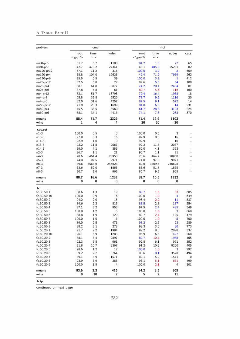
A Tables Part II
problem nomcf mcf
root time nodes root time nodes cutscl.gap% in s cl.gap% in s
ns60-pr6 61.7 6.7 1190 84.2 1.8 27 65ns60-pr9 42.7 478.2 27341 43.1 405.0 25251 82nu120-pr12 67.1 11.2 316 100.0 3.9 2 609nu120-pr4 38.8 104.0 12628 49.4 71.9 7959 262nu120-pr6 95.5 6.5 39 100.0 3.9 1 412nu25-pr12 82.5 6.8 72 82.6 5.6 54 100nu25-pr4 58.1 64.8 8877 74.2 20.4 2484 81nu25-pr6 87.8 4.8 61 82.7 5.6 116 160nu4-pr12 72.1 51.7 13798 79.4 16.4 1988 18nu4-pr4 65.8 35.8 9526 78.7 9.2 1116 20nu4-pr6 82.0 31.6 4257 87.5 9.1 572 14nu60-pr12 71.9 20.3 1699 94.8 6.3 14 531nu60-pr4 45.5 38.5 3560 61.7 28.8 3193 224nu60-pr6 58.1 34.1 4416 74.1 7.8 233 370
means 58.4 31.7 3326 71.4 16.6 1103wins 1 4 4 20 20 20
cut.setn1-3 100.0 0.5 3 100.0 0.5 3 -n10-3 97.9 0.3 16 97.9 0.3 16 -n11-3 92.9 1.0 10 92.9 1.0 10 -n13-3 92.2 11.8 2067 92.2 11.8 2067 -n14-3 89.0 4.1 353 89.0 4.1 353 -n2-3 96.7 1.1 21 96.7 1.1 21 -n4-3 78.6 464.4 28958 78.6 464.7 28958 -n5-3 74.8 97.5 9971 74.8 97.8 9971 -n6-3 89.6 3568.6 246628 89.6 3569.5 246628 -n7-3 83.6 52.0 1865 83.6 51.7 1865 -n8-3 80.7 9.6 965 80.7 9.5 965 -
means 88.7 16.6 1232 88.7 16.5 1232wins 0 0 0 0 0 0
fcfc.30.50.1 88.6 1.3 19 89.7 1.5 33 685fc.30.50.10 100.0 0.9 6 100.0 1.0 4 649fc.30.50.2 94.2 2.0 15 93.4 2.2 11 537fc.30.50.3 84.6 2.3 815 88.5 2.3 137 554fc.30.50.4 97.1 3.2 953 97.5 2.4 495 549fc.30.50.5 100.0 1.2 5 100.0 1.6 3 668fc.30.50.6 88.8 1.9 129 89.7 2.4 125 479fc.30.50.7 100.0 1.0 6 100.0 1.9 5 700fc.30.50.8 89.0 2.5 471 93.2 2.5 23 289fc.30.50.9 98.2 3.1 278 98.3 3.0 90 773fc.60.20.1 91.7 9.2 1994 92.2 8.3 2028 337fc.60.20.10 96.1 6.9 1283 96.9 6.5 497 268fc.60.20.2 88.1 8.4 2897 89.7 10.4 1988 465fc.60.20.3 92.3 5.8 961 92.8 6.1 961 352fc.60.20.4 91.8 10.7 8367 91.2 10.3 8260 405fc.60.20.5 98.6 1.2 12 100.0 1.6 3 292fc.60.20.6 89.2 9.7 3764 88.6 8.1 3578 494fc.60.20.7 89.1 5.9 1571 89.1 5.9 1571 0fc.60.20.8 93.9 3.9 288 93.1 5.1 651 499fc.60.20.9 100.0 1.5 4 100.0 2.1 4 301
means 93.6 3.3 415 94.2 3.5 305wins 0 10 2 5 2 11
fctp
continued on next page
232
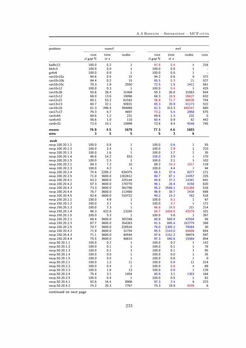
A.3 Results – Separation – MCF-cuts
problem nomcf mcf
root time nodes root time nodes cutscl.gap% in s cl.gap% in s
bal8x12 100.0 0.2 1 97.8 0.4 4 216bk4x3 100.0 0.0 1 100.0 0.0 1 -gr4x6 100.0 0.0 1 100.0 0.0 1 -ran10x10a 94.6 0.5 15 94.2 0.6 9 372ran10x10b 84.4 0.2 15 85.5 0.3 21 527ran10x10c 70.3 1.9 2550 72.5 1.5 1411 561ran10x12 100.0 0.3 1 100.0 0.4 1 425ran10x26 55.6 28.4 31469 55.3 26.8 31563 844ran12x12 68.0 13.6 19096 68.3 16.9 26827 632ran12x21 60.1 53.2 61542 58.8 71.7 88530 744ran13x13 60.7 32.1 50831 65.3 26.9 41173 522ran16x16 61.3 296.4 394888 62.3 313.3 440247 680ran17x17 76.3 6.7 4697 73.2 5.4 2958 575ran4x64 69.8 1.2 231 69.8 1.3 231 0ran6x43 56.6 1.0 110 60.4 0.9 82 442ran8x32 72.0 10.1 10999 72.8 9.4 9248 745
means 76.9 4.5 1679 77.3 4.6 1603wins 3 5 5 5 3 6
avubnexp.100.20.1.1 100.0 0.8 1 100.0 0.6 1 55nexp.100.20.1.2 100.0 2.4 1 100.0 2.9 1 210nexp.100.20.1.3 100.0 1.6 1 100.0 1.7 1 35nexp.100.20.1.4 86.6 14.2 933 100.0 3.9 1 170nexp.100.20.1.5 100.0 2.3 1 100.0 2.1 1 102nexp.100.20.2.1 89.3 7.2 10 89.2 24.3 1817 119nexp.100.20.2.3 100.0 4.2 1 100.0 4.4 2 94nexp.100.20.2.4 75.4 2295.2 634375 86.3 37.4 8277 171nexp.100.20.2.5 71.0 3600.0 1302612 80.7 87.1 14457 225nexp.100.20.4.1 63.2 3600.0 325144 94.6 37.2 14341 641nexp.100.20.4.2 67.3 3600.0 178770 96.1 28.4 4158 620nexp.100.20.4.3 73.3 3600.0 361786 95.2 2546.1 531289 516nexp.100.20.4.4 76.7 3600.0 112480 96.9 38.7 2434 698nexp.100.20.4.5 82.6 3600.0 310722 99.2 15.2 762 518nexp.150.20.1.1 100.0 4.9 1 100.0 6.1 1 67nexp.150.20.1.2 100.0 3.1 1 100.0 3.7 1 172nexp.150.20.1.3 100.0 7.3 1 96.8 24.5 201 214nexp.150.20.1.4 86.3 422.8 13165 84.7 1454.5 43179 321nexp.150.20.1.5 100.0 5.3 1 100.0 5.6 1 267nexp.150.20.2.1 69.4 3600.0 302168 80.8 589.9 42504 56nexp.150.20.2.3 67.7 3600.0 354263 91.5 885.4 162779 268nexp.150.20.2.5 70.7 3600.0 228516 76.0 1305.2 78584 30nexp.150.20.4.2 71.9 3600.0 31754 95.5 2143.0 85008 854nexp.150.20.4.3 71.1 3600.0 40544 97.6 1151.2 39474 597nexp.150.20.4.4 75.5 3600.0 46633 97.3 440.6 15564 854nexp.50.20.1.1 100.0 0.2 1 100.0 0.2 1 142nexp.50.20.1.2 100.0 0.1 1 100.0 0.1 1 76nexp.50.20.1.3 100.0 0.1 1 100.0 0.1 1 95nexp.50.20.1.4 100.0 0.0 1 100.0 0.0 1 35nexp.50.20.1.5 100.0 0.5 1 100.0 0.6 1 0nexp.50.20.2.1 100.0 1.2 11 100.0 0.9 11 214nexp.50.20.2.2 100.0 0.4 1 100.0 0.6 4 68nexp.50.20.2.3 100.0 1.8 13 100.0 0.9 1 129nexp.50.20.2.4 75.4 3.1 1454 80.9 3.1 1303 164nexp.50.20.2.5 100.0 0.4 1 100.0 0.5 1 62nexp.50.20.4.1 82.6 16.4 8906 97.3 2.4 6 223nexp.50.20.4.2 75.2 20.3 7767 75.3 19.9 9209 6
continued on next page
233

A Tables Part II
problem nomcf mcf
root time nodes root time nodes cutscl.gap% in s cl.gap% in s
nexp.50.20.4.3 86.7 15.6 7242 90.0 11.4 3778 174nexp.50.20.4.4 85.9 8.7 2710 87.6 6.0 902 64nexp.50.20.4.5 97.4 2.4 8 100.0 0.7 1 131nexp.50.20.8.1 77.5 585.8 325852 83.4 273.4 156790 172nexp.50.20.8.2 78.2 3600.0? 2533846? 94.9 60.4 23889 582nexp.50.20.8.3 82.8 829.5 602812 94.3 8.2 1799 496nexp.50.20.8.4 83.2 3600.0 2656207 93.7 26.5 10430 703nexp.50.20.8.5 85.1 192.1 99668 83.4 458.7 218807 122
means 86.8 55.2 4267 94.2 17.8 1396wins 3 8 9 23 25 21
sndlibatlanta-DBM 49.4 6.3 3474 71.6 1.9 829 34atlanta-UUM 26.3 6.4 5556 26.3 6.5 5556 -dfn-gwin-DBE 60.7 82.4 20260 67.3 61.4 10855 216dfn-gwin-DBM 66.7 56.6 16285 69.4 44.9 8923 74dfn-gwin-UUE 64.7 76.1 40495 66.8 61.6 24978 146dfn-gwin-UUM 64.5 287.5 214582 66.5 107.3 60790 54di-yuan-DBE 51.5 62.0 19753 57.6 43.2 9449 283di-yuan-UUE 64.8 168.0 109972 69.4 62.3 24589 215france-DBM 44.3 407.4 132148 54.9 166.5 42159 64france-UUM 31.1 130.9 69384 64.0 15.6 5123 28pdh-DBE 56.1 49.6 22184 59.3 51.8 21442 287pdh-DBM 56.9 60.3 26828 62.4 41.6 16895 157pdh-UUE 71.7 23.7 12629 75.6 16.1 6649 304pdh-UUM 74.4 16.0 10149 76.0 11.4 5289 60polska-DBM 53.0 0.8 659 56.4 1.1 942 16polska-UUM 35.8 7.4 13897 49.2 3.5 5799 16ta1-DBE 27.2 3600.0? 1608597? 87.6 812.7 488521 86ta2-DBE 21.1 14.9 250 100.0 2.6 1 32ta2-DBM 0.0 47.5 1769 27.5 16.4 384 2ta2-UUE 0.0 3600.0? 181005? 47.4 2620.2 207059 16zib54-DBE 72.1 3238.2 153710 80.2 3600.0 121784 661zib54-UUE 57.2 1599.0 105420 73.7 547.6 27183 434
means 47.7 84.7 24197 64.1 45.1 10710wins 0 2 2 21 18 18
ufcnbeasleyC1 74.5 1.9 17 75.5 3.0 58 9beasleyC2 73.4 241.5 103685 70.1 429.3 205234 29beavma 88.4 0.9 31 100.0 0.6 7 270fixnet6 82.0 1.4 7 82.0 1.4 7 2g180x666 67.2 3600.0 1407689 96.3 226.1 97553 523g200x740c 77.1 15.0 7493 79.8 8.8 2283 109g200x740d 68.2 3600.0 2038110 85.9 242.4 116280 378g200x740e 62.4 3600.0 1783097 89.5 1479.1 752118 487g200x740f 62.2 3600.0 1838978 93.8 40.4 17293 609g40x132 88.7 6.1 9379 90.0 4.8 7634 121g50x170 88.8 26.4 40826 88.7 78.6 121031 140g55x188c 92.8 1.2 31 100.0 0.7 2 109h50x2450 88.2 3600.0 512965 94.0 646.9 62232 293h50x2450b 87.8 36.9 1942 100.0 3.6 1 361h50x2450c 87.0 1888.2 241900 95.0 23.4 402 284h50x2450d 88.0 3600.0 628139 96.0 22.9 300 367h50x2450e 93.9 19.2 50 95.6 18.3 7 389h80x6320b 93.6 38.0 518 93.6 35.9 273 25h80x6320c 87.8 314.2 45656 87.9 208.7 28161 23
continued on next page
234
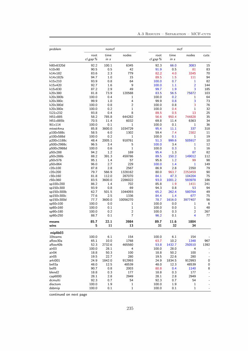
A.3 Results – Separation – MCF-cuts
problem nomcf mcf
root time nodes root time nodes cutscl.gap% in s cl.gap% in s
h80x6320d 92.2 100.1 6345 92.3 66.0 3083 15k10x90 90.5 0.5 42 91.9 0.5 81 83k14x182 83.6 2.3 779 82.2 4.0 3345 70k14x182b 94.7 1.0 15 89.5 1.5 111 94k15x210 93.9 0.8 64 100.0 0.7 1 82k15x420 92.7 1.6 9 100.0 1.1 2 144k15x630 87.2 2.9 49 99.7 1.9 3 185k20x380 81.8 73.9 120588 83.5 56.5 75872 103k20x380b 100.0 0.4 1 100.0 0.2 1 64k20x380c 99.9 1.0 4 99.9 0.8 3 73k20x380d 100.0 0.8 2 100.0 0.8 3 76k20x380e 100.0 0.2 1 100.0 0.4 1 32l121x232 93.8 0.4 8 89.5 0.5 13 25l451x885 58.2 785.8 644282 56.6 950.4 744828 35l451x885b 70.5 11.4 6032 69.8 11.4 6363 34l61x114 100.0 0.1 1 100.0 0.1 1 36mtest4ma 85.8 3600.0 1034729 95.4 11.1 337 318p100x588c 58.5 6.0 1302 59.4 7.4 2302 11p100x588d 100.0 0.2 1 100.0 0.1 1 19p200x1188c 48.4 2005.1 918761 51.3 999.6 505917 10p500x2988c 96.5 3.4 5 100.0 3.4 1 12p500x2988d 100.0 0.6 1 100.0 0.3 1 16p50x288 94.2 1.2 169 95.4 1.3 87 82p50x288b 88.2 391.3 459786 89.5 150.2 149012 112p50x576 95.1 1.4 57 95.6 1.2 99 98p50x864 96.0 2.7 229 100.0 1.4 1 149r20x100 87.8 2.8 2567 86.9 2.8 2350 79r20x200 79.7 566.9 1328162 80.0 963.7 2253459 90r30x160 81.8 112.0 287070 84.1 47.3 104204 75r50x360 83.5 3600.0 2286022 93.0 1001.2 593978 186sp100x200 86.2 1.4 702 85.8 1.9 1411 241sp150x300 93.9 0.8 69 94.3 0.8 53 94sp150x300b 62.7 501.5 1044093 65.2 262.4 580764 49sp150x300c 77.6 2.5 1336 84.4 1.4 677 75sp150x300d 77.7 3600.0 10056270 78.7 1616.0 3977407 56sp50x100 100.0 0.0 1 100.0 0.0 1 6sp80x160 100.0 0.1 1 100.0 0.0 1 48sp90x180 100.0 0.2 2 100.0 0.3 2 267sp90x250 88.7 0.1 7 96.2 0.1 4 77
means 85.7 22.1 3984 89.7 11.6 1804wins 5 11 13 31 32 34
miplib0310teams 100.0 6.1 154 100.0 6.1 154 -aflow30a 65.1 10.0 1768 63.7 10.2 1348 967aflow40b 52.3 2732.6 465560 53.8 1432.7 250510 1392air03 100.0 28.1 4 100.0 28.0 4 -air04 18.8 50.3 100 18.8 50.2 100 -air05 19.5 22.7 280 19.5 22.6 280 -arki001 24.9 1842.0 912993 24.9 1834.5 912993 0bell3a 48.0 12.5 48539 48.0 12.3 48539 0bell5 90.7 0.8 2003 80.8 0.4 1140 8blend2 18.8 0.3 177 18.8 0.3 177 -cap6000 28.1 2.8 2949 28.1 2.8 2949 -dcmulti 92.3 0.7 54 92.3 0.7 54 -disctom 100.0 1.9 1 100.0 1.9 1 -dsbmip 100.0 0.1 1 100.0 0.1 1 -
continued on next page
235
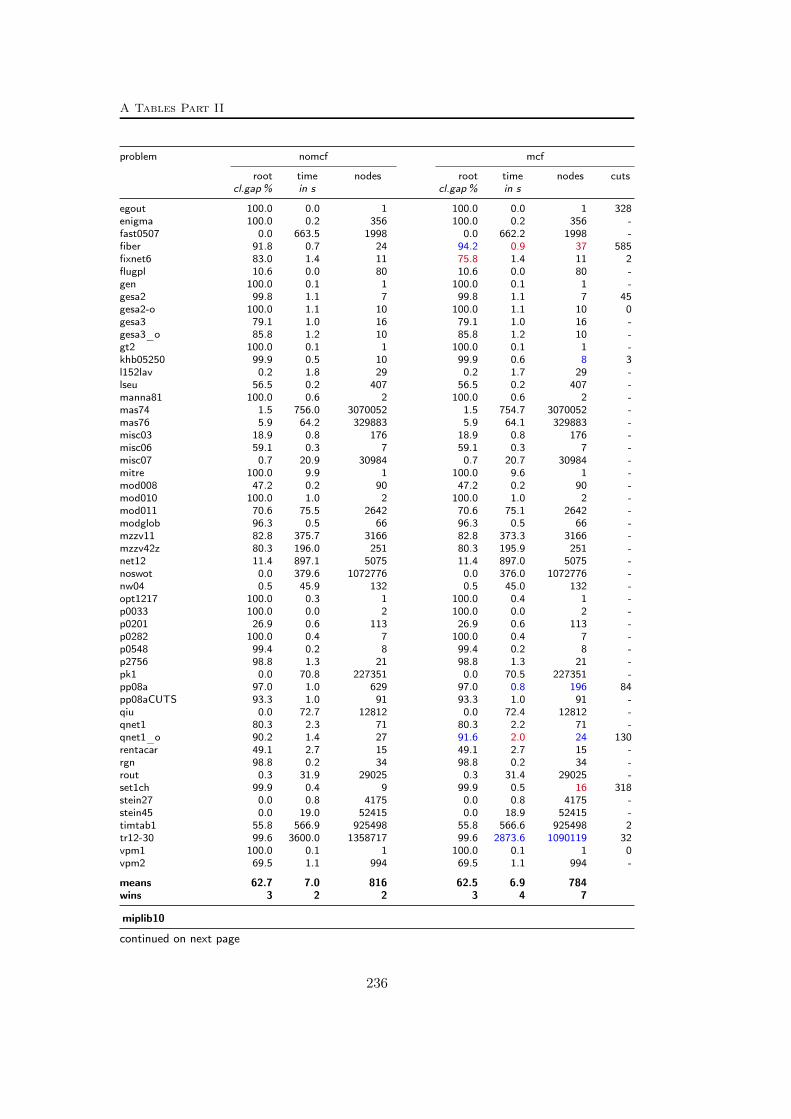
A Tables Part II
problem nomcf mcf
root time nodes root time nodes cutscl.gap% in s cl.gap% in s
egout 100.0 0.0 1 100.0 0.0 1 328enigma 100.0 0.2 356 100.0 0.2 356 -fast0507 0.0 663.5 1998 0.0 662.2 1998 -fiber 91.8 0.7 24 94.2 0.9 37 585fixnet6 83.0 1.4 11 75.8 1.4 11 2flugpl 10.6 0.0 80 10.6 0.0 80 -gen 100.0 0.1 1 100.0 0.1 1 -gesa2 99.8 1.1 7 99.8 1.1 7 45gesa2-o 100.0 1.1 10 100.0 1.1 10 0gesa3 79.1 1.0 16 79.1 1.0 16 -gesa3_o 85.8 1.2 10 85.8 1.2 10 -gt2 100.0 0.1 1 100.0 0.1 1 -khb05250 99.9 0.5 10 99.9 0.6 8 3l152lav 0.2 1.8 29 0.2 1.7 29 -lseu 56.5 0.2 407 56.5 0.2 407 -manna81 100.0 0.6 2 100.0 0.6 2 -mas74 1.5 756.0 3070052 1.5 754.7 3070052 -mas76 5.9 64.2 329883 5.9 64.1 329883 -misc03 18.9 0.8 176 18.9 0.8 176 -misc06 59.1 0.3 7 59.1 0.3 7 -misc07 0.7 20.9 30984 0.7 20.7 30984 -mitre 100.0 9.9 1 100.0 9.6 1 -mod008 47.2 0.2 90 47.2 0.2 90 -mod010 100.0 1.0 2 100.0 1.0 2 -mod011 70.6 75.5 2642 70.6 75.1 2642 -modglob 96.3 0.5 66 96.3 0.5 66 -mzzv11 82.8 375.7 3166 82.8 373.3 3166 -mzzv42z 80.3 196.0 251 80.3 195.9 251 -net12 11.4 897.1 5075 11.4 897.0 5075 -noswot 0.0 379.6 1072776 0.0 376.0 1072776 -nw04 0.5 45.9 132 0.5 45.0 132 -opt1217 100.0 0.3 1 100.0 0.4 1 -p0033 100.0 0.0 2 100.0 0.0 2 -p0201 26.9 0.6 113 26.9 0.6 113 -p0282 100.0 0.4 7 100.0 0.4 7 -p0548 99.4 0.2 8 99.4 0.2 8 -p2756 98.8 1.3 21 98.8 1.3 21 -pk1 0.0 70.8 227351 0.0 70.5 227351 -pp08a 97.0 1.0 629 97.0 0.8 196 84pp08aCUTS 93.3 1.0 91 93.3 1.0 91 -qiu 0.0 72.7 12812 0.0 72.4 12812 -qnet1 80.3 2.3 71 80.3 2.2 71 -qnet1_o 90.2 1.4 27 91.6 2.0 24 130rentacar 49.1 2.7 15 49.1 2.7 15 -rgn 98.8 0.2 34 98.8 0.2 34 -rout 0.3 31.9 29025 0.3 31.4 29025 -set1ch 99.9 0.4 9 99.9 0.5 16 318stein27 0.0 0.8 4175 0.0 0.8 4175 -stein45 0.0 19.0 52415 0.0 18.9 52415 -timtab1 55.8 566.9 925498 55.8 566.6 925498 2tr12-30 99.6 3600.0 1358717 99.6 2873.6 1090119 32vpm1 100.0 0.1 1 100.0 0.1 1 0vpm2 69.5 1.1 994 69.5 1.1 994 -
means 62.7 7.0 816 62.5 6.9 784wins 3 2 2 3 4 7
miplib10
continued on next page
236

A.3 Results – Separation – MCF-cuts
problem nomcf mcf
root time nodes root time nodes cutscl.gap% in s cl.gap% in s
acc-tight5 100.0 195.5 870 100.0 196.1 870 0aflow40b 52.9 1610.7 311571 53.2 1959.8 380156 1302air04 18.8 48.4 598 18.8 49.3 598 0app1-2 94.2 3150.4 12934 94.2 3115.1 12934 0biella1 2.9 212.3 2673 2.9 212.6 2673 0bienst2 51.0 112.2 108442 48.9 111.8 109772 221binkar10_1 63.9 263.6 196269 63.9 262.5 196269 0bley_xl1 100.0 167.8 3 100.0 166.7 3 0bnatt350 100.0 3011.4 33288 100.0 3004.6 33288 0core2536-691 0.0 36.8 51 0.0 36.9 51 0csched010 32.9 3241.2 993796 32.9 3226.9 993796 0danoint 1.7 3295.5 1143205 1.7 3192.6 1090128 17dfn-gwin-UUM 65.2 246.3 239021 65.0 59.2 43484 52eil33-2 8.7 59.5 7903 8.7 59.3 7903 0eilB101 48.1 126.5 5915 48.1 126.3 5915 0ex9 100.0 98.6 1 100.0 98.4 1 0iis-100-0-cov 2.4 1980.6 105412 2.4 1984.2 105412 0iis-pima-cov 2.1 576.5 9055 2.1 564.9 9055 0lectsched-4-obj 100.0 59.1 4464 100.0 58.5 4464 0map18 24.1 326.6 487 24.1 328.7 487 0map20 22.6 248.3 337 22.6 249.5 337 0mcsched 0.0 304.9 40532 0.0 305.6 40532 0mik-250-1-100-1 73.9 286.0 1473349 73.9 286.7 1473349 0mine-166-5 85.5 25.9 2993 85.5 25.9 2993 0mine-90-10 49.8 473.4 152416 49.8 476.2 152416 0mzzv11 77.0 174.3 1565 77.0 173.8 1565 0n4-3 75.7 684.0 70112 75.7 681.9 70112 0neos-1109824 80.0 190.8 36153 80.0 190.1 36153 0neos-1396125 57.6 175.2 45770 57.6 174.7 45770 0neos-1601936 100.0 1759.6 5723 100.0 1762.7 5723 0neos-476283 0.0 342.9 1409 0.0 342.2 1409 0neos-686190 4.1 72.0 7043 4.1 72.9 7043 0neos-849702 100.0 1202.7 67922 100.0 1202.6 67922 0neos-916792 1.4 397.9 84750 1.4 400.9 84750 0neos-934278 0.0 283.3 92 0.0 283.0 92 0neos13 0.0 116.5 233 0.0 117.6 233 0neos18 66.7 39.6 7001 66.7 39.5 7001 0net12 34.6 1116.4 5194 34.6 1115.9 5194 0netdiversion 29.6 428.5 13 29.6 432.4 13 0noswot 0.0 302.7 971220 0.0 303.3 971220 0ns1208400 0.0 964.9 3719 0.0 965.4 3719 0ns1688347 84.0 907.2 13344 84.0 905.1 13344 0ns1758913 100.0 3378.3 227 100.0 3370.7 227 0ns1830653 35.9 836.0 85904 35.9 836.1 85904 0opm2-z7-s2 0.0 412.1 3027 0.0 412.9 3027 0pg5_34 98.8 1015.0 339456 98.8 1014.9 339456 0qiu 0.0 40.9 9613 0.0 40.7 9613 0rail507 0.0 318.6 1657 0.0 318.8 1657 0ran16x16 60.8 206.1 352290 62.7 185.8 349503 864reblock67 51.4 196.9 93091 51.4 196.0 93091 0rmatr100-p10 0.0 49.5 856 0.0 49.6 856 0rmatr100-p5 0.0 84.8 435 0.0 84.5 435 0rmine6 4.5 1907.5 467964 4.5 1916.9 467964 0rocII-4-11 39.8 168.7 19939 39.8 168.4 19939 0rococoC10-001000 61.4 1998.3 1083094 58.4 718.2 295517 235satellites1-25 0.0 485.2 4123 0.0 485.9 4123 0sp98ir 1.8 173.2 6875 1.8 172.8 6875 0tanglegram1 0.1 394.4 23 0.1 393.1 23 0
continued on next page
237
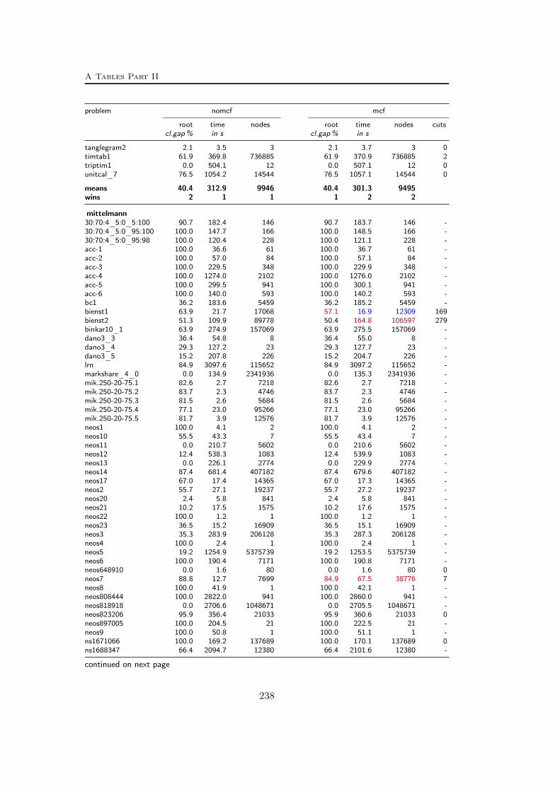
A Tables Part II
problem nomcf mcf
root time nodes root time nodes cutscl.gap% in s cl.gap% in s
tanglegram2 2.1 3.5 3 2.1 3.7 3 0timtab1 61.9 369.8 736885 61.9 370.9 736885 2triptim1 0.0 504.1 12 0.0 507.1 12 0unitcal_7 76.5 1054.2 14544 76.5 1057.1 14544 0
means 40.4 312.9 9946 40.4 301.3 9495wins 2 1 1 1 2 2
mittelmann30:70:4_5:0_5:100 90.7 182.4 146 90.7 183.7 146 -30:70:4_5:0_95:100 100.0 147.7 166 100.0 148.5 166 -30:70:4_5:0_95:98 100.0 120.4 228 100.0 121.1 228 -acc-1 100.0 36.6 61 100.0 36.7 61 -acc-2 100.0 57.0 84 100.0 57.1 84 -acc-3 100.0 229.5 348 100.0 229.9 348 -acc-4 100.0 1274.0 2102 100.0 1276.0 2102 -acc-5 100.0 299.5 941 100.0 300.1 941 -acc-6 100.0 140.0 593 100.0 140.2 593 -bc1 36.2 183.6 5459 36.2 185.2 5459 -bienst1 63.9 21.7 17068 57.1 16.9 12309 169bienst2 51.3 109.9 89778 50.4 164.8 106597 279binkar10_1 63.9 274.9 157069 63.9 275.5 157069 -dano3_3 36.4 54.8 8 36.4 55.0 8 -dano3_4 29.3 127.2 23 29.3 127.7 23 -dano3_5 15.2 207.8 226 15.2 204.7 226 -lrn 84.9 3097.6 115652 84.9 3097.2 115652 -markshare_4_0 0.0 134.9 2341936 0.0 135.3 2341936 -mik.250-20-75.1 82.6 2.7 7218 82.6 2.7 7218 -mik.250-20-75.2 83.7 2.3 4746 83.7 2.3 4746 -mik.250-20-75.3 81.5 2.6 5684 81.5 2.6 5684 -mik.250-20-75.4 77.1 23.0 95266 77.1 23.0 95266 -mik.250-20-75.5 81.7 3.9 12576 81.7 3.9 12576 -neos1 100.0 4.1 2 100.0 4.1 2 -neos10 55.5 43.3 7 55.5 43.4 7 -neos11 0.0 210.7 5602 0.0 210.6 5602 -neos12 12.4 538.3 1083 12.4 539.9 1083 -neos13 0.0 226.1 2774 0.0 229.9 2774 -neos14 87.4 681.4 407182 87.4 679.6 407182 -neos17 67.0 17.4 14365 67.0 17.3 14365 -neos2 55.7 27.1 19237 55.7 27.2 19237 -neos20 2.4 5.8 841 2.4 5.8 841 -neos21 10.2 17.5 1575 10.2 17.6 1575 -neos22 100.0 1.2 1 100.0 1.2 1 -neos23 36.5 15.2 16909 36.5 15.1 16909 -neos3 35.3 283.9 206128 35.3 287.3 206128 -neos4 100.0 2.4 1 100.0 2.4 1 -neos5 19.2 1254.9 5375739 19.2 1253.5 5375739 -neos6 100.0 190.4 7171 100.0 190.8 7171 -neos648910 0.0 1.6 80 0.0 1.6 80 0neos7 88.8 12.7 7699 84.9 67.5 38776 7neos8 100.0 41.9 1 100.0 42.1 1 -neos808444 100.0 2822.0 941 100.0 2860.0 941 -neos818918 0.0 2706.6 1048671 0.0 2705.5 1048671 -neos823206 95.9 356.4 21033 95.9 360.6 21033 0neos897005 100.0 204.5 21 100.0 222.5 21 -neos9 100.0 50.8 1 100.0 51.1 1 -ns1671066 100.0 169.2 137689 100.0 170.1 137689 0ns1688347 66.4 2094.7 12380 66.4 2101.6 12380 -
continued on next page
238

A.3 Results – Separation – MCF-cuts
problem nomcf mcf
root time nodes root time nodes cutscl.gap% in s cl.gap% in s
nug08 100.0 41.8 1 100.0 41.8 1 -prod1 34.3 17.5 23482 34.3 17.6 23482 -prod2 32.7 81.4 68500 32.7 81.4 68500 -qap10 18.5 167.9 5 18.5 168.2 5 -seymour1 12.2 453.0 5772 12.2 452.5 5772 -swath2 14.7 61.4 5157 14.7 61.5 5157 -swath3 11.4 866.1 140698 11.4 871.5 140698 -
means 61.3 82.2 3579 61.1 85.2 3676wins 2 2 2 0 1 1
Table A.4: Results for the MCF-separator – Scip 1.1.0.8 – easy instances. Results for test setmiplib2010 have been computed with Scip 2.1.1. Values in blue indicate an improvement (wins ofmcf ), values in red a deterioration (wins of nomcf ).
Table A.5 below presents the results of the separation of MCF-cuts for all hardinstances. We compare the performance of Scip 1.1.0.8 with (mcf ) and without(nomcf ) the MCF-separator. Every hard instance cannot be solved by Scip inboth settings within one hour of CPU time. We provide the closed gap at the rootnode before branching (rootgap) defined as
100 · (root − lp)/(bestprimal − lp),
the closed dual gap after optimization (dualgap) given by
100 · (dual − lp)/(bestprimal − lp),
the closed primal gap after optimization (primalgap) given by
100 · (bestprimal − bestdual)/(primal − bestdual),
the endgap defined as
100 · (primal − dual)/|bestdual|,
and the number of cuts (cuts) found by the MCF-separator. The numbers primaland dual correspond to the primal and dual bound at the end of the optimiza-tion. The value lp denotes the value of the initial LP relaxation, bestprimal andbestdual are the best known primal and dual bounds (see Table A.1 on page 220in Appendix A.1), and root is the value of the LP at the root node after cut-ting and before branching. In case that primal = bestdual for an individualrun we set the closed primal gap to 100%. If the LP value is already optimal(lp = bestprimal = bestdual) then rootgap as well as dualgap are considered tobe 100%. If primal or dual bounds are not finite or in case that bestdual = 0the corresponding gaps are not defined and marked with “-”. Values in blue indi-cate improvement over the nomcf run and are counted as ’wins’ for the mcf run(endgap decreased by at least 10 %, closed root, dual, or primal gap increased by
239

A Tables Part II
at least 1 absolute percentage point). Similarly, values in red indicate ’wins’ of thenomcf run.
If the MCF separator is switched off (no network has been found or the networkinconsistency ratio Ψ(D) is above Ψmax = 0.02) then column cuts contains a “-”.Runs marked with “?” have hit the memory limit. For every test set two additionalrows provide the arithmetic means of the gaps (means) and the number of valuesin bold face for every measure (wins).
problem nomcf mcf
root dual primal endgap root dual primal endgap cutsclosed gaps in % in % closed gaps in % in %
arc.setns4-pr3 15.6 71.8 100.0 0.1 17.3 71.3 84.6 0.1 5ns4-pr9 0.0 5.4 100.0 0.0 0.0 8.3 100.0 0.0 12nu120-pr3 37.0 61.1 100.0 11.1 38.6 64.1 93.9 10.8 392nu120-pr9 43.1 76.0 100.0 5.5 43.2 72.3 79.8 7.8 328nu25-pr3 62.1 72.2 47.4 2.9 66.9 78.8 70.9 1.7 86nu25-pr9 32.0 56.4 62.9 1.9 35.0 59.6 64.1 1.8 135nu4-pr3 42.5 64.1 89.6 0.9 42.2 61.5 100.0 0.9 1nu4-pr9 20.5 47.1 83.2 0.5 19.6 51.1 100.0 0.4 21nu60-pr3 52.2 73.5 86.7 3.7 54.2 77.3 73.1 3.7 299nu60-pr9 34.4 65.4 99.0 2.8 39.1 73.7 99.0 2.1 351
means 33.9 59.3 86.9 1.4 35.6 61.8 86.5 1.3wins 0 2 4 1 6 7 4 2
cut.setn12-3 71.6 93.7 100.0 2.2 71.6 93.7 100.0 2.2 -n15-3 24.3 24.5 100.0 66.7 24.3 24.5 100.0 66.7 -n3-3 70.2 76.2 100.0 14.5 70.2 76.2 100.0 14.5 -n9-3 65.7 77.4 100.0 11.4 65.7 77.4 100.0 11.4 -
means 58.0 68.0 100.0 12.6 58.0 68.0 100.0 12.6wins 0 0 0 0 0 0 0 0
fc
fctpn3700 18.7 20.0 96.8 28.6 19.1 19.9 100.0 27.7 1307n3701 18.5 19.8 100.0 27.1 18.8 20.3 100.0 26.9 1363n3702 18.8 19.6 98.1 28.1 18.9 19.7 98.1 28.1 1377n3703 16.8 18.3 100.0 31.1 16.6 17.6 100.0 31.4 1108n3704 18.9 19.8 100.0 27.5 19.2 20.1 100.0 27.4 1242n3705 18.0 19.2 95.8 28.9 17.9 18.8 95.8 29.0 2059n3706 21.0 22.1 96.2 27.3 20.6 22.1 98.3 26.7 2280n3707 19.6 20.7 100.0 28.7 19.6 20.9 100.0 28.6 1145n3708 17.1 18.3 100.0 28.6 17.3 18.5 100.0 28.5 1294n3709 18.8 19.5 100.0 28.5 19.0 19.9 100.0 28.4 1969n370a 19.9 21.2 100.0 27.8 20.2 21.1 100.0 27.9 1427n370b 17.4 18.2 95.5 29.1 17.5 18.4 100.0 27.7 1191n370c 19.6 20.4 95.3 29.2 19.8 21.0 95.4 29.0 1220n370d 19.6 20.4 95.3 29.2 19.8 21.0 95.4 29.0 1220n370e 22.2 22.9 100.0 24.9 21.9 22.6 97.3 25.7 1345ran14x18 53.6 83.9 80.3 3.7 54.7 83.8 80.3 3.7 1031
means 21.2 24.0 97.1 24.9 21.3 24.1 97.5 24.8wins 0 0 1 0 1 0 3 0
continued on next page
240
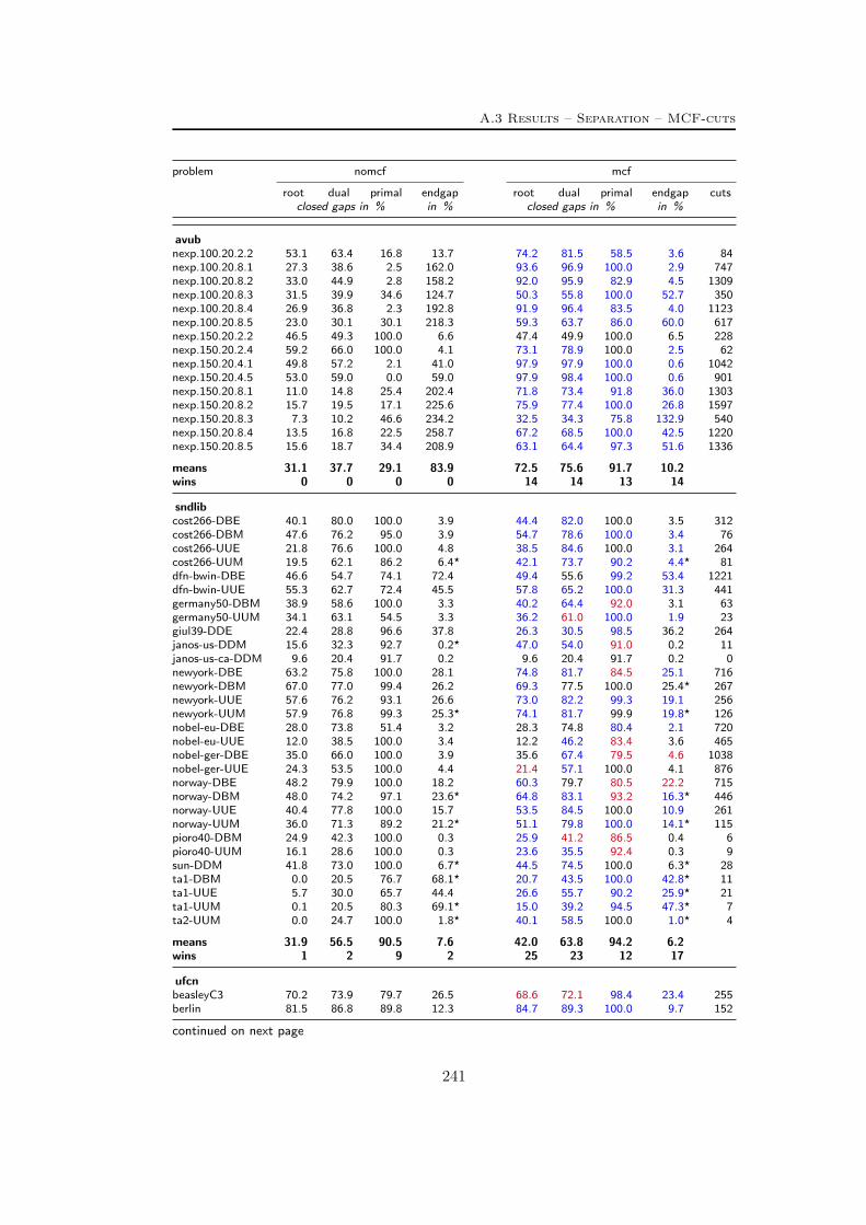
A.3 Results – Separation – MCF-cuts
problem nomcf mcf
root dual primal endgap root dual primal endgap cutsclosed gaps in % in % closed gaps in % in %
avubnexp.100.20.2.2 53.1 63.4 16.8 13.7 74.2 81.5 58.5 3.6 84nexp.100.20.8.1 27.3 38.6 2.5 162.0 93.6 96.9 100.0 2.9 747nexp.100.20.8.2 33.0 44.9 2.8 158.2 92.0 95.9 82.9 4.5 1309nexp.100.20.8.3 31.5 39.9 34.6 124.7 50.3 55.8 100.0 52.7 350nexp.100.20.8.4 26.9 36.8 2.3 192.8 91.9 96.4 83.5 4.0 1123nexp.100.20.8.5 23.0 30.1 30.1 218.3 59.3 63.7 86.0 60.0 617nexp.150.20.2.2 46.5 49.3 100.0 6.6 47.4 49.9 100.0 6.5 228nexp.150.20.2.4 59.2 66.0 100.0 4.1 73.1 78.9 100.0 2.5 62nexp.150.20.4.1 49.8 57.2 2.1 41.0 97.9 97.9 100.0 0.6 1042nexp.150.20.4.5 53.0 59.0 0.0 59.0 97.9 98.4 100.0 0.6 901nexp.150.20.8.1 11.0 14.8 25.4 202.4 71.8 73.4 91.8 36.0 1303nexp.150.20.8.2 15.7 19.5 17.1 225.6 75.9 77.4 100.0 26.8 1597nexp.150.20.8.3 7.3 10.2 46.6 234.2 32.5 34.3 75.8 132.9 540nexp.150.20.8.4 13.5 16.8 22.5 258.7 67.2 68.5 100.0 42.5 1220nexp.150.20.8.5 15.6 18.7 34.4 208.9 63.1 64.4 97.3 51.6 1336
means 31.1 37.7 29.1 83.9 72.5 75.6 91.7 10.2wins 0 0 0 0 14 14 13 14
sndlibcost266-DBE 40.1 80.0 100.0 3.9 44.4 82.0 100.0 3.5 312cost266-DBM 47.6 76.2 95.0 3.9 54.7 78.6 100.0 3.4 76cost266-UUE 21.8 76.6 100.0 4.8 38.5 84.6 100.0 3.1 264cost266-UUM 19.5 62.1 86.2 6.4? 42.1 73.7 90.2 4.4? 81dfn-bwin-DBE 46.6 54.7 74.1 72.4 49.4 55.6 99.2 53.4 1221dfn-bwin-UUE 55.3 62.7 72.4 45.5 57.8 65.2 100.0 31.3 441germany50-DBM 38.9 58.6 100.0 3.3 40.2 64.4 92.0 3.1 63germany50-UUM 34.1 63.1 54.5 3.3 36.2 61.0 100.0 1.9 23giul39-DDE 22.4 28.8 96.6 37.8 26.3 30.5 98.5 36.2 264janos-us-DDM 15.6 32.3 92.7 0.2? 47.0 54.0 91.0 0.2 11janos-us-ca-DDM 9.6 20.4 91.7 0.2 9.6 20.4 91.7 0.2 0newyork-DBE 63.2 75.8 100.0 28.1 74.8 81.7 84.5 25.1 716newyork-DBM 67.0 77.0 99.4 26.2 69.3 77.5 100.0 25.4? 267newyork-UUE 57.6 76.2 93.1 26.6 73.0 82.2 99.3 19.1 256newyork-UUM 57.9 76.8 99.3 25.3? 74.1 81.7 99.9 19.8? 126nobel-eu-DBE 28.0 73.8 51.4 3.2 28.3 74.8 80.4 2.1 720nobel-eu-UUE 12.0 38.5 100.0 3.4 12.2 46.2 83.4 3.6 465nobel-ger-DBE 35.0 66.0 100.0 3.9 35.6 67.4 79.5 4.6 1038nobel-ger-UUE 24.3 53.5 100.0 4.4 21.4 57.1 100.0 4.1 876norway-DBE 48.2 79.9 100.0 18.2 60.3 79.7 80.5 22.2 715norway-DBM 48.0 74.2 97.1 23.6? 64.8 83.1 93.2 16.3? 446norway-UUE 40.4 77.8 100.0 15.7 53.5 84.5 100.0 10.9 261norway-UUM 36.0 71.3 89.2 21.2? 51.1 79.8 100.0 14.1? 115pioro40-DBM 24.9 42.3 100.0 0.3 25.9 41.2 86.5 0.4 6pioro40-UUM 16.1 28.6 100.0 0.3 23.6 35.5 92.4 0.3 9sun-DDM 41.8 73.0 100.0 6.7? 44.5 74.5 100.0 6.3? 28ta1-DBM 0.0 20.5 76.7 68.1? 20.7 43.5 100.0 42.8? 11ta1-UUE 5.7 30.0 65.7 44.4 26.6 55.7 90.2 25.9? 21ta1-UUM 0.1 20.5 80.3 69.1? 15.0 39.2 94.5 47.3? 7ta2-UUM 0.0 24.7 100.0 1.8? 40.1 58.5 100.0 1.0? 4
means 31.9 56.5 90.5 7.6 42.0 63.8 94.2 6.2wins 1 2 9 2 25 23 12 17
ufcnbeasleyC3 70.2 73.9 79.7 26.5 68.6 72.1 98.4 23.4 255berlin 81.5 86.8 89.8 12.3 84.7 89.3 100.0 9.7 152
continued on next page
241

A Tables Part II
problem nomcf mcf
root dual primal endgap root dual primal endgap cutsclosed gaps in % in % closed gaps in % in %
brasil 77.2 84.2 94.7 14.3 87.6 92.7 75.8 8.2 114g150x1100 68.1 78.2 68.4 15.3 77.2 87.6 96.8 7.1 196g150x1650 66.4 75.0 83.7 16.5 73.6 82.3 95.2 10.9 193g200x740 67.4 73.7 99.8 6.1 85.3 93.9 99.8 1.4 370g200x740b 72.3 82.2 69.4 3.6 87.0 96.5 100.0 0.6 297g200x740g 68.5 69.4 80.7 37.5 73.4 74.3 89.5 29.4 584g200x740h 77.4 81.1 84.3 7.6 82.8 86.0 75.9 6.5 561g200x740i 71.4 72.4 52.5 49.3 78.7 80.6 64.9 32.7 487g55x188 82.2 97.1 100.0 1.8 83.3 96.7 100.0 2.0 139k16x240 75.4 92.1 100.0 6.2 76.2 90.8 100.0 7.2 126k16x240b 77.9 93.9 100.0 4.4 79.9 94.2 100.0 4.2 152mc11 51.7 53.6 77.9 61.2 78.4 79.3 92.1 26.3 532mc7 39.0 41.4 45.2 81.8 81.6 83.0 61.0 28.6 474mc8 58.3 64.0 94.8 44.0 75.7 77.3 98.5 27.3 447p100x588 88.0 93.2 99.3 4.0 88.7 93.8 99.7 3.6 227p100x588b 82.5 85.6 78.7 17.5 83.5 86.7 96.0 13.7 340p200x1188 89.0 94.0 83.4 3.7 89.6 94.5 100.0 2.9 205p200x1188b 82.5 85.6 90.1 15.1 84.1 88.1 82.0 13.9 292p500x2988 87.2 93.7 92.2 1.2 88.9 95.0 82.6 1.1 349p500x2988b 80.5 82.3 78.5 16.5 81.3 82.8 96.5 13.2 440p80x400 86.1 95.5 100.0 2.0 88.7 96.7 100.0 1.5 162p80x400b 82.4 87.5 87.2 13.2 83.2 88.7 95.8 10.9 205r80x800 79.4 85.7 83.2 5.4 83.4 88.5 86.6 4.3 262
means 74.5 80.9 84.5 10.7 81.8 87.7 91.5 7.2wins 1 2 4 2 18 18 15 19
miplib03a1c1s1 67.8 84.6 0.0 13.7 67.8 84.6 0.0 13.7 -atlanta-ip 0.4 55.5 0.0 6.6 0.4 56.1 0.0 6.5 -dano3mip 0.6 0.8 99.9 24.2 0.6 0.8 99.9 24.2 -danoint 1.7 37.9 100.0 2.9 1.9 42.3 100.0 2.7 28ds 0.3 3.6 19.3 498.7 0.3 3.6 19.3 498.7 -glass4 0.0 25.0 0.0 58.3 0.0 25.0 0.0 58.3 -harp2 35.1 99.9 100.0 0.0 35.1 99.9 100.0 0.0 -liu 0.0 0.0 68.8 150.0 0.0 0.0 68.8 150.0 -markshare1 0.0 0.0 0.0 400.0 0.0 0.0 0.0 400.0 -markshare2 0.0 0.0 0.0 1500.0 0.0 0.0 0.0 1500.0 -mkc 42.7 81.0 100.0 1.6 42.7 81.0 100.0 1.6 -momentum1 56.9 59.1 - - 56.9 59.1 - - -momentum2 0.5 7.2 0.0 12.2 0.5 7.2 0.0 12.2 0momentum3 0.7 0.7 - - 0.7 0.7 - - 21msc98-ip 55.7 55.7 0.0 1.0 55.7 55.7 0.0 1.0 -nsrand-ipx 27.3 63.3 0.0 5.8 27.3 63.3 0.0 5.8 -protfold 14.5 46.6 0.0 38.2 14.5 46.6 0.0 38.2 -rd-rplusc-21 0.0 0.0 0.0 99.9 0.0 0.0 0.0 99.9 0roll3000 76.2 96.1 100.0 0.5 76.2 96.1 100.0 0.5 -seymour 22.6 55.2 89.6 2.3 22.6 55.2 89.6 2.3 -sp97ar 8.6 40.1 13.0 3.0 8.6 40.2 13.0 3.0 -stp3d 0.2 2.0 - - 0.2 2.9 - - 0swath 29.0 41.8 0.0 20.9 29.0 41.8 0.0 20.9 -t1717 1.5 2.9 49.4 51.7 1.5 2.9 49.4 51.7 -timtab2 31.8 47.7 99.4 73.5 31.8 47.7 99.4 73.4 2
means 19.0 36.3 38.2 15.9 19.0 36.5 38.2 15.9wins 0 0 0 0 0 1 0 0
miplib1030n20b8 40.6 49.7 100.0 50.0 40.6 49.7 100.0 50.0 0
continued on next page
242

A.3 Results – Separation – MCF-cuts
problem nomcf mcf
root dual primal endgap root dual primal endgap cutsclosed gaps in % in % closed gaps in % in %
bab5 93.9 95.0 0.0 1.1 93.9 95.0 0.0 1.1 0beasleyC3 76.1 79.4 0.0 21.1 85.6 88.3 0.0 13.0 382cov1075 30.0 45.3 100.0 7.8 30.0 45.3 100.0 7.8 0enlight13 8.7 43.0 100.0 57.0 8.7 43.1 100.0 56.9 0glass4 0.0 70.0 0.0 39.2 0.0 70.0 0.0 39.2 0gmu-35-40 9.4 12.5 0.0 0.0 9.4 12.5 0.0 0.0 0iis-bupa-cov 1.4 68.5 100.0 8.3 1.4 68.5 100.0 8.3 0m100n500k4r1 100.0 100.0 0.0 4.0 100.0 100.0 0.0 4.0 0macrophage 49.2 72.0 0.0 30.9 49.2 72.0 0.0 30.9 0msc98-ip 57.1 57.5 100.0 0.7 57.1 58.5 100.0 0.7 0mspp16 - - - -F - - - -F -n3div36 6.5 32.2 100.0 8.5 6.5 31.8 100.0 8.6 0n3seq24 0.0 0.0 100.0 0.4 0.0 0.0 100.0 0.4 0neos-1337307 2.3 95.5 100.0 0.0 2.3 95.5 100.0 0.0 0newdano 38.5 73.8 100.0 21.5 38.1 92.0 100.0 6.6 417pigeon-10 0.0 0.0 100.0 11.1 0.0 0.0 100.0 11.1 0pw-myciel4 40.0 90.0 100.0 10.0 40.0 90.0 100.0 10.0 0roll3000 69.3 93.8 0.0 0.9 69.3 93.8 0.0 0.9 0sp98ic 0.0 99.0 0.0 2.0 0.0 99.0 0.0 2.0 0vpphard 0.0 0.0 0.0 340.0 0.0 0.0 0.0 340.0 0zib54-UUE 39.3 93.0 100.0 4.4 39.5 87.3 100.0 7.9 42
means 31.5 60.5 57.1 5.6 32.0 61.5 57.1 5.3wins 0 1 0 1 1 3 0 2
mittelmannmarkshare_5_0 0.0 0.0 100.0 - 0.0 0.0 100.0 - -ns1648184 5.7 84.2 100.0 0.4 5.7 84.2 100.0 0.4 -ns1692855 53.0 73.1 100.0 15.4 53.0 73.1 100.0 15.4 -
means 19.6 52.4 100.0 2.7 19.6 52.4 100.0 2.7wins 0 0 0 0 0 0 0 0
Table A.5: Results for the MCF-separator – Scip 1.1.0.8 – hard instances. Results for test setmiplib2010 have been computed with Scip 2.1.1. Values in blue indicate an improvement (wins ofmcf ), values in red a deterioration (wins of nomcf ).
243


Appendix B
Tables Part III
In this chapter, we provide detailed numbers for all tests carried out to test theperformance of cut-set inequalities, flow cut-set inequalities, and envelope inequal-ities for robust network design. For the corresponding presentation and a summaryof the results see Section 10.3.
B.1 Used instances
Table B.1 contains all instances used in the computational tests presented in Sec-tion 10.3. We report on the value of Γ corresponding to the number of allowedsimultaneous peaks, the number of rows (rows), the number of columns (vars), thevalue of the linear programming relaxation (lp), and the values of the best dual(bestdual) and primal bounds (bestprimal) we found in all tests carried out by theauthor for this thesis. The row and column numbers as well as the LP bound referto the dualized formulation (ΓND) (page 139) using the Γ-uncertainty model.
The Sndlib instances are marked with either ’UUM’, or ’DDM’. The first twoletters correspond tho the demand and link capacity model. Letter ’U’ and ’D’stand for undirected demands/capacities or directed demands/capacities, respec-tively. The last letter ’M’ means that we always assumed a modular link capacitystructure. For most instances we used the single demand scenario provided in therespective Sndlib instance. We assumed this value to be the nominal demandto parametrize the Γ-model and assumed a possible maximal deviation 40%. Forinstances marked with an asterisk ’?’ we constructed the demands based on trafficmeasurements also provided in Sndlib, see Section 10.3.
problem Γ rows vars lp bestdual bestprimal
abilene?-UUM 1 2787 3015 41224.98964 43364 433645 2787 3015 47933.64164 50036 50036
10 2787 3015 51161.57705 53687 53687
continued on next page
245

B Tables Part III
problem Γ rows vars lp bestdual bestprimal
abilene-UUM 1 2787 3015 232555.4994 235178 2351785 2787 3015 260834.3339 262252 262252
10 2787 3015 268744.9459 269867 269867atlanta-UUM 1 6217 7015 98213669.61 102858738.9 102858738.9
5 6217 7015 113611566.2 116638573.9 116638573.910 6217 7015 118370307.5 121459290.8 121459290.8
cost266-UUM 1 100623 114114 8291272.263 10478073.86 11587773.325 100623 114114 8919178.97 10873544.49 12192681.81
10 100623 114114 9448311.48 11168213.95 12568812.99dfn-bwin-UUM 1 4545 8595 40474.91332 78731.43479 88643.5
5 4545 8595 40474.91332 83087.41324 89252.4810 4545 8595 40474.91332 83778.83048 99074.59
dfn-gwin-UUM 1 5822 7894 33102.84841 39352 393525 5822 7894 37256.88895 44724 44724
10 5822 7894 37603.40836 46556 46556di-yuan-UUM 1 1628 2562 385878.125 683900 683900
5 1628 2562 394015.625 753200 75320010 1628 2562 394015.625 753200 753200
france-UUM 1 34545 40590 19788.17275 21200 212005 34545 40590 21845.97372 23200 23200
10 34545 40590 23397.4846 24400 24400geant?-UUM 1 21468 24696 33291.35819 43586 43586
5 21468 24696 39896.56016 46412 4641210 21468 24696 41433.04988 47115 47115
geant-UUM 1 21750 25020 135481.5456 139732 1397325 21750 25020 156625.2449 165019 165019
10 21750 25020 162582.4881 168153 168153germany50?-UUM 1 32968 38984 257325.3017 291326.6156 310310
5 32968 38984 294362.847 323104.5076 34880010 32968 38984 310404.2795 333482.7692 368970
germany50-UUM 1 102708 127952 637191.756 652263.5777 6718405 102708 127952 678593.9589 694755.1291 709750
10 102708 127952 688604.3895 703652.7987 725920giul39-DDM 1 537765 733924 1738.291667 2233.02474 4907
5 537765 733924 1831.939063 2272.387846 508210 537765 733924 1913.968099 2300.30586 5260
janos-us-ca-DDM 1 419528 542656 1575707.043 1575862.136 15790315 419528 542656 1711435.181 1711469.946 1713138
10 419528 542656 1796329.339 1796341.129 1798477janos-us-DDM 1 126184 163968 1629009.694 1629909.189 1632610
5 126184 163968 1817080.943 1817362.124 181865410 126184 163968 1894180.981 1894794.907 1895845
newyork-UUM 1 12651 16709 78348.96542 876288.3698 9862945 12651 16709 88984.93625 890382.6878 986294
10 12651 16709 91744.625 869971.6433 1011670nobel-eu-UUM 1 33626 40173 856514.6675 877199.9596 892690
5 33626 40173 922538.1621 936230.45 96600010 33626 40173 961511.5112 979963.6929 998360
nobel-ger?-UUM 1 7728 9776 3174419.587 3177351.242 31831305 7728 9776 3627368.69 3629071.073 3632050
10 7728 9776 3811720.67 3814020.451 3817220nobel-ger-UUM 1 7413 9542 160589.25 168951.3691 173580
5 7413 9542 175917.375 181558.9308 18918010 7413 9542 182492.4583 189562.3141 195190
nobel-us-UUM 1 5117 6594 2610631.277 2611964.014 26184405 5117 6594 3029389.461 3029901.303 3033200
10 5117 6594 3273535.818 3273576.6 3276380norway-UUM 1 45126 53652 166856.6312 374653.4093 477390
5 45126 53652 179188.799 376513.8973 47209010 45126 53652 190155.1225 367214.4985 466810
continued on next page
246

B.2 Results – Separation – Robust cut-set inequalities
problem Γ rows vars lp bestdual bestprimal
pdh-UUM 1 1930 2584 6422518.178 12776618 127766185 1930 2584 6422518.178 14022345 14022345
10 1930 2584 6422518.178 14046890 14046890pioro40-UUM 1 170129 208527 418111.4123 418480.3738 419939
5 170129 208527 437259.6275 437489.9406 43852310 170129 208527 455966.1269 456171.3582 457079
polska-UUM 1 3186 3618 24081.48318 24870 248705 3186 3618 28094.4169 28558 28558
10 3186 3618 30907.72887 31414 31414sun-DDM 1 14355 19482 774.244825 923.688631 966.5
5 14355 19482 895.6960958 1045.015968 1134.3210 14355 19482 914.5095 1094.417067 1168.65
ta1_peak_140 1 20589 25347 4378153.641 7562553.66 7562553.665 20589 25347 4964464.188 8225935.29 8225935.29
10 20589 25347 5094748.14 8350922.336 8358611.78ta2_peak_140 1 226875 262261 11994852.65 14438286.54 16835156.95
5 226875 262261 13528087.01 15959036.85 20402675.6910 226875 262261 14124741.17 16545243.79 21950567.05
zib54_peak_140 1 95964 112320 4283303.631 9342672.265 10334015.825 95964 112320 4818559.456 9498746.401 10997397.72
10 95964 112320 4984847.738 9364384.375 11203783.2
Table B.1: General information for all used instances from Sndlib in Part III. At most 10 digits areshown.
B.2 Results – Separation – Robust cut-set inequalities
Table B.2 below presents the results of the separation of robust cut-set inequalitiesfor all easy Sndlib instances. We compare the performance of Cplex 12.3 with(cutset) and without (default) adding robust cut-set inequalities as presented inSection 10.1. For a summary of the results see Section 10.3. Every easy instancecan be solved by Cplex in one of the two settings and for one of the values Γ in1, 5, 10 within 4 hours of CPU time. The presentation of the results is done asin Appendix A.3 for the MCF-separator with the difference that the column cutscorresponds to the number of generated robust cut-set inequalities. Moreover, weprovide the number of added lazy capacity constraints (non-zero in case of theSeparate approach) in column lazy . The closed root gap (root) is defined as inAppendix A.3 and based on the values in Table B.1. For every Sndlib instance weprovide the results for both the Separate and Dualize approach and all valuesof in 1, 5, 10.Values in blue indicate improvement over the default run and are counted as ’wins’for the cutset run (time or nodes decreased by at least 10 %, root value increasedby at least 1 percentage point). Similarly, values in red indicate ’wins’ of thedefault run.
247
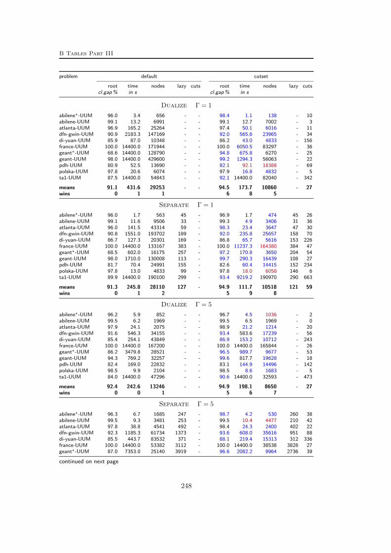
B Tables Part III
problem default cutset
root time nodes lazy cuts root time nodes lazy cutscl.gap% in s cl.gap% in s
Dualize Γ = 1
abilene?-UUM 96.0 3.4 656 - - 98.4 1.1 138 - 10abilene-UUM 99.1 13.2 6991 - - 99.1 12.7 7002 - 3atlanta-UUM 96.9 165.2 25264 - - 97.4 50.1 6016 - 11dfn-gwin-UUM 90.9 2183.3 147169 - - 92.0 565.6 23965 - 34di-yuan-UUM 85.9 87.0 10348 - - 86.2 43.0 4833 - 156france-UUM 100.0 14400.0 171944 - - 100.0 6050.5 83297 - 36geant?-UUM 68.6 14400.0 128790 - - 94.8 675.8 6270 - 25geant-UUM 98.0 14400.0 429600 - - 99.2 1294.3 56063 - 22pdh-UUM 80.9 52.5 13690 - - 82.1 92.1 18388 - 69polska-UUM 97.8 20.6 6074 - - 97.9 16.8 4832 - 5ta1-UUM 87.5 14400.0 54843 - - 92.1 14400.0 82040 - 342
means 91.1 431.6 29253 - - 94.5 173.7 10860 - 27wins 0 1 1 6 8 5
Separate Γ = 1
abilene?-UUM 96.0 1.7 563 45 - 96.9 1.7 474 45 26abilene-UUM 99.1 11.6 9506 33 - 99.3 4.9 3406 31 36atlanta-UUM 96.0 141.5 43314 59 - 98.3 23.4 3647 47 30dfn-gwin-UUM 90.8 1551.0 193702 189 - 92.0 235.8 25657 158 70di-yuan-UUM 86.7 127.3 20301 169 - 86.8 65.7 5616 153 226france-UUM 100.0 14400.0 133167 383 - 100.0 11237.3 164380 384 47geant?-UUM 68.5 602.0 16175 257 - 97.2 170.8 3650 204 54geant-UUM 98.0 1710.0 130008 113 - 99.7 290.3 16439 108 27pdh-UUM 81.7 70.4 24991 155 - 82.6 60.4 14415 152 234polska-UUM 97.8 13.0 4833 99 - 97.8 18.0 6058 146 6ta1-UUM 89.9 14400.0 190100 299 - 93.4 9219.2 190970 290 663
means 91.3 245.8 28110 127 - 94.9 111.7 10518 121 59wins 0 1 2 5 9 8
Dualize Γ = 5
abilene?-UUM 96.2 5.9 852 - - 96.7 4.5 1036 - 2abilene-UUM 99.5 6.2 1969 - - 99.5 6.5 1969 - 0atlanta-UUM 97.9 24.1 2075 - - 98.9 21.2 1214 - 20dfn-gwin-UUM 91.6 546.3 34155 - - 93.4 583.6 17239 - 56di-yuan-UUM 85.4 254.1 43849 - - 86.9 153.2 10712 - 243france-UUM 100.0 14400.0 167200 - - 100.0 14400.0 165844 - 26geant?-UUM 86.2 3479.8 28521 - - 96.5 989.7 9677 - 53geant-UUM 94.3 769.2 32257 - - 99.6 817.7 19628 - 18pdh-UUM 82.4 169.0 22832 - - 83.1 144.9 14496 - 142polska-UUM 98.5 9.9 2104 - - 98.5 8.6 1683 - 5ta1-UUM 84.0 14400.0 47296 - - 90.6 14400.0 32593 - 473
means 92.4 242.6 13246 - - 94.9 198.1 8650 - 27wins 0 0 1 5 6 7
Separate Γ = 5
abilene?-UUM 96.3 6.7 1685 247 - 98.7 4.2 530 260 38abilene-UUM 99.5 9.3 3481 253 - 99.5 10.4 4477 210 42atlanta-UUM 97.8 38.8 4541 492 - 98.4 24.3 2400 402 22dfn-gwin-UUM 92.3 1185.3 61734 1373 - 93.6 608.0 35616 951 88di-yuan-UUM 85.5 443.7 83532 371 - 88.1 219.4 15313 312 336france-UUM 100.0 14400.0 53382 3112 - 100.0 14400.0 38538 3828 27geant?-UUM 87.0 7353.0 25140 3919 - 96.6 2082.2 9964 2736 39
continued on next page
248

B.2 Results – Separation – Robust cut-set inequalities
problem default cutset
root time nodes lazy cuts root time nodes lazy cutscl.gap% in s cl.gap% in s
geant-UUM 94.7 1270.0 32414 1184 - 99.7 860.7 17330 1005 71pdh-UUM 83.5 292.1 47089 872 - 83.8 409.8 34708 1410 249polska-UUM 98.2 27.8 2649 969 - 98.5 23.1 4351 385 13ta1-UUM 83.5 14400.0 112093 884 - 93.5 14400.0 44478 1441 849
means 92.6 383.6 18603 851 - 95.5 276.2 11750 766 71wins 0 2 2 6 7 7
Dualize Γ = 10
abilene?-UUM 95.8 10.5 1750 - - 96.3 10.6 1334 - 10abilene-UUM 99.7 2.9 544 - - 99.8 5.2 734 - 5atlanta-UUM 97.7 198.3 15114 - - 98.8 31.5 1153 - 21dfn-gwin-UUM 92.9 2584.6 109671 - - 94.8 293.8 8886 - 42di-yuan-UUM 87.5 96.7 18989 - - 88.1 98.2 17180 - 253france-UUM 100.0 862.2 12680 - - 100.0 196.3 2436 - 17geant?-UUM 89.1 3173.5 16751 - - 96.6 3624.1 16254 - 63geant-UUM 96.6 9901.5 141640 - - 99.7 1793.2 24491 - 27pdh-UUM 84.4 140.2 21983 - - 84.5 114.1 10984 - 207polska-UUM 98.3 33.2 6626 - - 98.3 33.8 6550 - 6ta1-UUM 56.5 14400.0 57632 - - 81.5 14400.0 27191 - 462
means 90.8 323.9 15091 - - 94.4 175.1 6485 - 38wins 0 2 1 5 5 6
Separate Γ = 10
abilene?-UUM 95.9 97.0 4430 2019 - 96.6 77.0 2991 2005 48abilene-UUM 99.7 14.7 1705 811 - 99.7 13.9 1049 1238 25atlanta-UUM 97.7 270.4 18797 912 - 98.8 149.6 2719 1742 36dfn-gwin-UUM 93.1 14400.0 165837 5255 - 95.0 3023.4 33449 6140 116di-yuan-UUM 87.5 96.5 18989 0 - 88.1 98.3 17180 0 253france-UUM 100.0 10742.9 16298 6270 - 100.0 14400.0 1012 13100 43geant?-UUM 90.9 14400.0 3919 13143 - 97.0 14400.0 403 36040 63geant-UUM 96.8 14400.0 14484 14322 - 99.7 14400.0 22149 7714 79pdh-UUM 85.3 658.7 61855 1839 - 84.8 145.6 14799 775 275polska-UUM 98.2 167.4 13930 1196 - 98.3 195.8 13933 1364 13ta1-UUM 58.1 14400.0 32959 2271 - 80.2 14400.0 23846 2657 786
means 91.2 1068.3 16132 1416 - 94.4 779.2 7361 1664 79wins 0 2 0 5 4 5
Table B.2: Results for robust cut-set inequalities– Cplex 12.3 – easy Sndlib instances. Values inblue indicate an improvement (wins of cutset), values in red a deterioration (wins of default).
Table B.3 below presents the results of the separation of robust cut-set inequal-ities for all hard instances. We compare the performance of Cplex 12.3 with(cutset) and without (default) adding robust cut-set inequalities as presented inSection 10.1. For a summary of the results see Section 10.3. Every hard instancecannot be solved by Cplex in both settings and for none of the values of Γ in1, 5, 10 within 4 hours of CPU time. The presentation of the results is done asin Appendix A.3 for the MCF-separator with the difference that the column cutscorresponds to the number of generated robust cut-set inequalities. Moreover, weprovide the number of added lazy capacity constraints (non-zero in case of theSeparate approach) in column lazy . The closed root gap (rootgap), closed pri-mal gap primalgap, and closed dual gap dualgap are defined as in Appendix A.3
249

B Tables Part III
and based on the values in Table B.1 on page 247. For every Sndlib instance weprovide the results for both the Separate and Dualize approach and all valuesof in 1, 5, 10.Values in blue indicate improvement over the default run and are counted as ’wins’for the cutset run (endgap decreased by at least 10 %, closed root, dual, or primalgap increased by at least 1 absolute percentage point). Similarly, values in redindicate ’wins’ of the default run.
problem default cutset
root dual primal endgap lazy cuts root dual primal endgap lazy cutsclosed gap in % in % closed gap in % in %
Dualize Γ = 1
cost266-UUM 55.6 58.6 74.0 16.7 - - 58.2 61.1 88.2 13.7 - 173dfn-bwin-UUM 60.8 72.4 31.0 44.9 - - 62.8 72.1 79.2 20.4 - 329germany50?-UUM 38.0 60.1 100.0 7.3 - - 39.7 59.1 80.6 9.0 - 19germany50-UUM 38.2 43.3 95.8 3.1 - - 38.3 43.5 91.9 3.3 - 23giul39-DDM 15.1 15.1 100.0 120.5 - - 15.3 15.3 100.0 120.2 - 108janos-us-ca-DDM 3.5 4.7 74.4 0.3 - - 3.5 4.7 74.4 0.3 - 0janos-us-DDM 11.7 25.0 99.9 0.2 - - 11.7 25.0 99.9 0.2 - 0newyork-UUM 69.1 80.8 99.8 19.9 - - 77.8 84.6 100.0 15.9 - 185nobel-eu-UUM 36.1 42.0 44.7 4.6 - - 36.9 41.9 22.0 8.7 - 251nobel-ger?-UUM 6.0 21.4 93.1 0.2 - - 6.3 21.6 87.0 0.2 - 64nobel-ger-UUM 20.4 38.5 84.3 5.2 - - 28.1 47.1 100.0 4.1 - 354nobel-us-UUM 14.5 16.2 97.7 0.3 - - 14.5 17.1 100.0 0.2 - 10norway-UUM 57.7 63.3 69.3 42.6 - - 61.2 64.0 73.5 39.7 - 92pioro40-UUM 12.3 20.2 100.0 0.3 - - 13.4 18.5 82.2 0.4 - 2sun-DDM 48.8 69.9 62.5 9.1 - - 50.3 73.5 80.6 6.6 - 8ta2-UUM 42.2 42.3 5.2 324.0 - - 43.7 43.7 5.2 323.5 - 145zib54-UUM 65.9 75.5 77.1 19.0 - - 70.5 79.2 81.8 15.8 - 66
means 35.1 44.1 77.0 5.9 - - 37.2 45.4 79.2 5.5 - 37wins 0 1 5 2 10 6 7 6
Separate Γ = 1
cost266-UUM 57.8 61.6 88.7 13.4 650 - 61.2 66.3 100.0 10.6 604 72dfn-bwin-UUM 63.5 79.4 25.2 50.0 409 - 65.5 75.6 31.8 41.9 421 800germany50?-UUM 37.3 56.0 93.6 8.4 1355 - 41.5 57.3 69.6 10.6 1430 81germany50-UUM 37.4 40.8 47.5 6.5 409 - 37.4 41.1 50.9 6.0 449 17giul39-DDM 15.4 15.4 92.6 129.6 2805 - 15.5 15.5 92.6 129.5 2638 67janos-us-ca-DDM 2.8 3.7 100.0 0.2 289 - 2.8 3.7 92.6 0.2 272 4janos-us-DDM 8.3 17.3 100.0 0.2 194 - 8.3 17.5 82.7 0.2 193 3newyork-UUM 72.4 83.4 99.8 17.2 240 - 79.8 87.9 100.0 12.6 250 219nobel-eu-UUM 35.4 40.5 36.3 5.6 196 - 36.3 43.7 100.0 2.3 183 164nobel-ger?-UUM 2.9 20.3 39.8 0.5 151 - 4.9 18.6 47.3 0.4 121 154nobel-ger-UUM 18.9 39.3 84.3 5.2 82 - 47.9 63.5 71.3 3.9 92 698nobel-us-UUM 9.8 11.4 65.2 0.4 104 - 9.8 12.2 77.8 0.3 127 24norway-UUM 56.8 62.8 95.7 32.1 1220 - 62.1 65.4 100.0 28.7 1222 152pioro40-UUM 11.1 14.6 63.0 0.6 930 - 12.5 14.6 69.2 0.5 919 8sun-DDM 49.9 76.2 100.0 4.9 377 - 54.5 75.9 93.1 5.4 392 17ta2-UUM 42.2 46.3 69.6 25.3 655 - 44.2 47.9 37.6 45.0 659 187zib54-UUM 66.0 79.9 72.1 17.1 357 - 69.8 80.5 76.2 15.9 342 57
means 34.6 44.1 74.9 5.4 395 - 38.5 46.3 76.0 4.8 396 61wins 0 2 6 2 11 7 9 6
continued on next page
250

B.2 Results – Separation – Robust cut-set inequalities
problem default cutset
root dual primal endgap lazy cuts root dual primal endgap lazy cutsclosed gap in % in % closed gap in % in %
Dualize Γ = 5
cost266-UUM 44.3 47.4 77.9 19.3 - - 48.1 53.4 89.1 15.5 - 164dfn-bwin-UUM 70.7 79.6 16.5 49.5 - - 75.4 85.3 89.0 9.5 - 559germany50?-UUM 32.7 49.1 75.6 11.1 - - 36.5 44.0 90.0 10.3 - 45germany50-UUM 42.5 46.5 76.6 3.1 - - 44.9 49.6 75.0 3.0 - 32giul39-DDM 12.5 12.5 100.0 125.2 - - 12.5 12.5 100.0 125.2 - 64janos-us-ca-DDM 0.0 2.0 100.0 0.1 - - 0.0 2.0 100.0 0.1 - 0janos-us-DDM 4.0 13.1 62.6 0.1 - - 8.0 17.9 94.8 0.1 - 1newyork-UUM 70.2 80.5 100.0 19.7 - - 80.2 87.5 100.0 12.6 - 213nobel-eu-UUM 24.9 29.6 60.3 5.4 - - 24.8 31.5 95.9 3.3 - 306nobel-ger?-UUM 17.2 36.2 69.8 0.1 - - 18.0 36.2 83.9 0.1 - 51nobel-ger-UUM 20.3 32.4 76.9 6.2 - - 31.0 42.5 76.9 5.5 - 433nobel-us-UUM 0.0 5.4 62.3 0.2 - - 0.0 5.4 57.6 0.2 - 0norway-UUM 57.0 59.4 46.3 61.0 - - 64.7 67.2 49.5 51.4 - 115pioro40-UUM 7.9 18.0 100.0 0.2 - - 7.9 18.1 100.0 0.2 - 0sun-DDM 30.4 62.1 88.1 9.8 - - 36.3 62.6 96.6 8.8 - 32ta2-UUM 25.7 25.7 8.6 329.6 - - 30.1 30.5 8.6 327.6 - 134zib54-UUM 60.3 67.6 74.9 26.4 - - 63.5 72.2 62.1 27.7 - 49
means 30.6 39.2 70.4 5.8 - - 34.2 42.3 80.5 4.7 - 36wins 0 1 3 0 11 10 8 6
Separate Γ = 5
cost266-UUM 51.2 52.1 78.7 17.7 2637 - 55.1 58.7 68.9 17.9 2572 69dfn-bwin-UUM 74.1 80.8 12.2 64.5 1356 - 78.7 83.9 15.2 51.0 1405 810germany50?-UUM 33.2 42.4 68.9 13.3 7220 - 39.3 44.0 65.4 13.6 9814 77germany50-UUM 42.6 45.7 40.2 5.6 2013 - 42.7 46.6 65.6 3.5 1742 18giul39-DDM 12.8 12.8 92.1 135.3 2804 - 13.1 13.1 92.1 134.9 2786 73janos-us-ca-DDM 0.0 0.5 9.0 1.1 1889 - 0.0 0.0 8.6 1.1 1792 16janos-us-DDM 0.9 12.1 57.3 0.1 1275 - 5.2 14.7 89.3 0.1 1034 6newyork-UUM 74.0 82.8 99.9 17.4 1047 - 81.2 89.3 99.8 10.8 792 230nobel-eu-UUM 25.8 28.7 28.5 11.3 1935 - 26.8 28.3 35.1 9.2 1269 160nobel-ger?-UUM 25.5 35.7 36.0 0.2 1130 - 26.3 36.4 38.7 0.2 1511 360nobel-ger-UUM 19.2 30.0 54.8 8.6 2901 - 24.3 36.4 52.6 8.4 1984 678nobel-us-UUM 0.0 5.4 52.3 0.2 925 - 0.0 13.4 100.0 0.1 705 21norway-UUM 57.2 60.7 56.3 50.3 4545 - 59.9 62.9 73.1 38.2 4187 150pioro40-UUM 4.8 4.8 0.7 35.4 3613 - 5.0 5.1 0.7 35.5 3708 9sun-DDM 31.2 46.4 88.4 13.4 1871 - 35.1 52.9 81.4 12.7 2433 27ta2-UUM 26.3 26.9 42.0 69.9 5693 - 31.0 32.1 95.9 30.5 2827 187zib54-UUM 60.2 67.6 82.2 24.5 1286 - 63.1 70.1 92.7 20.7 1362 57
means 31.7 37.4 52.9 9.0 2160 - 34.5 40.5 63.2 7.5 1966 73wins 0 0 4 0 11 11 9 8
Dualize Γ = 10
cost266-UUM 41.0 47.8 100.0 14.6 - - 42.9 48.7 69.2 19.9 - 133dfn-bwin-UUM 65.1 72.1 41.0 45.7 - - 67.8 73.9 100.0 18.3 - 647germany50?-UUM 29.8 37.5 97.6 11.2 - - 32.3 39.4 100.0 10.6 - 23germany50-UUM 36.3 39.0 96.3 3.4 - - 37.1 40.3 100.0 3.2 - 11giul39-DDM 10.9 10.9 100.0 129.5 - - 10.9 10.9 100.0 129.6 - 54janos-us-ca-DDM 0.0 0.5 100.0 0.1 - - 0.0 0.5 100.0 0.1 - 0janos-us-DDM 6.6 36.8 93.6 0.1 - - 22.4 36.8 95.5 0.1 - 1newyork-UUM 69.6 78.3 78.0 27.6 - - 79.1 83.0 82.7 21.4 - 179nobel-eu-UUM 22.5 32.8 42.5 5.1 - - 39.5 50.1 65.4 2.9 - 284nobel-ger?-UUM 16.8 32.0 67.1 0.1 - - 16.8 32.0 88.2 0.1 - 52nobel-ger-UUM 24.3 38.1 78.2 5.0 - - 30.2 46.8 100.0 3.6 - 298nobel-us-UUM 0.0 1.4 90.9 0.1 - - 0.0 0.0 79.3 0.1 - 2
continued on next page
251
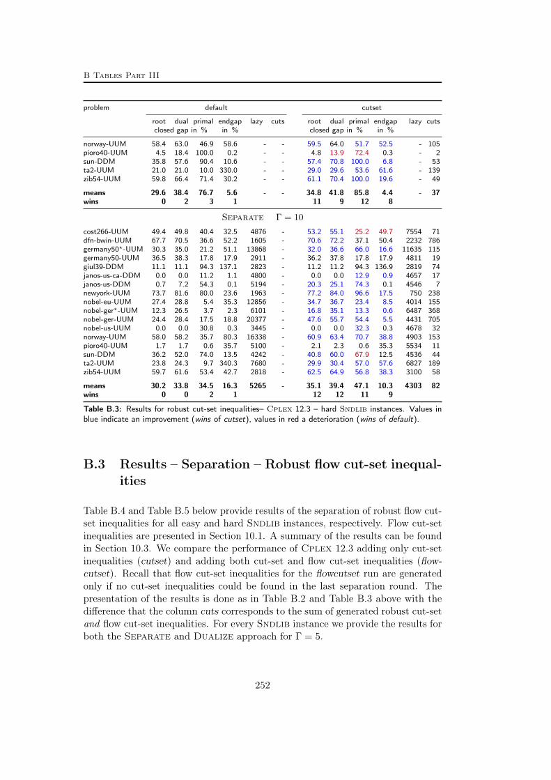
B Tables Part III
problem default cutset
root dual primal endgap lazy cuts root dual primal endgap lazy cutsclosed gap in % in % closed gap in % in %
norway-UUM 58.4 63.0 46.9 58.6 - - 59.5 64.0 51.7 52.5 - 105pioro40-UUM 4.5 18.4 100.0 0.2 - - 4.8 13.9 72.4 0.3 - 2sun-DDM 35.8 57.6 90.4 10.6 - - 57.4 70.8 100.0 6.8 - 53ta2-UUM 21.0 21.0 10.0 330.0 - - 29.0 29.6 53.6 61.6 - 139zib54-UUM 59.8 66.4 71.4 30.2 - - 61.1 70.4 100.0 19.6 - 49
means 29.6 38.4 76.7 5.6 - - 34.8 41.8 85.8 4.4 - 37wins 0 2 3 1 11 9 12 8
Separate Γ = 10
cost266-UUM 49.4 49.8 40.4 32.5 4876 - 53.2 55.1 25.2 49.7 7554 71dfn-bwin-UUM 67.7 70.5 36.6 52.2 1605 - 70.6 72.2 37.1 50.4 2232 786germany50?-UUM 30.3 35.0 21.2 51.1 13868 - 32.0 36.6 66.0 16.6 11635 115germany50-UUM 36.5 38.3 17.8 17.9 2911 - 36.2 37.8 17.8 17.9 4811 19giul39-DDM 11.1 11.1 94.3 137.1 2823 - 11.2 11.2 94.3 136.9 2819 74janos-us-ca-DDM 0.0 0.0 11.2 1.1 4800 - 0.0 0.0 12.9 0.9 4657 17janos-us-DDM 0.7 7.2 54.3 0.1 5194 - 20.3 25.1 74.3 0.1 4546 7newyork-UUM 73.7 81.6 80.0 23.6 1963 - 77.2 84.0 96.6 17.5 750 238nobel-eu-UUM 27.4 28.8 5.4 35.3 12856 - 34.7 36.7 23.4 8.5 4014 155nobel-ger?-UUM 12.3 26.5 3.7 2.3 6101 - 16.8 35.1 13.3 0.6 6487 368nobel-ger-UUM 24.4 28.4 17.5 18.8 20377 - 47.6 55.7 54.4 5.5 4431 705nobel-us-UUM 0.0 0.0 30.8 0.3 3445 - 0.0 0.0 32.3 0.3 4678 32norway-UUM 58.0 58.2 35.7 80.3 16338 - 60.9 63.4 70.7 38.8 4903 153pioro40-UUM 1.7 1.7 0.6 35.7 5100 - 2.1 2.3 0.6 35.3 5534 11sun-DDM 36.2 52.0 74.0 13.5 4242 - 40.8 60.0 67.9 12.5 4536 44ta2-UUM 23.8 24.3 9.7 340.3 7680 - 29.9 30.4 57.0 57.6 6827 189zib54-UUM 59.7 61.6 53.4 42.7 2818 - 62.5 64.9 56.8 38.3 3100 58
means 30.2 33.8 34.5 16.3 5265 - 35.1 39.4 47.1 10.3 4303 82wins 0 0 2 1 12 12 11 9
Table B.3: Results for robust cut-set inequalities– Cplex 12.3 – hard Sndlib instances. Values inblue indicate an improvement (wins of cutset), values in red a deterioration (wins of default).
B.3 Results – Separation – Robust flow cut-set inequal-ities
Table B.4 and Table B.5 below provide results of the separation of robust flow cut-set inequalities for all easy and hard Sndlib instances, respectively. Flow cut-setinequalities are presented in Section 10.1. A summary of the results can be foundin Section 10.3. We compare the performance of Cplex 12.3 adding only cut-setinequalities (cutset) and adding both cut-set and flow cut-set inequalities (flow-cutset). Recall that flow cut-set inequalities for the flowcutset run are generatedonly if no cut-set inequalities could be found in the last separation round. Thepresentation of the results is done as in Table B.2 and Table B.3 above with thedifference that the column cuts corresponds to the sum of generated robust cut-setand flow cut-set inequalities. For every Sndlib instance we provide the results forboth the Separate and Dualize approach for Γ = 5.
252

B.3 Results – Separation – Robust flow cut-set inequalities
problem cutset flowcutset
root time nodes lazy cuts root time nodes lazy cutscl.gap% in s cl.gap % in s
Dualize Γ = 5
abilene?-UUM 96.7 4.5 1036 - 2 96.7 4.7 1036 - 2abilene-UUM 99.5 6.5 1969 - 0 99.5 6.4 1969 - 0atlanta-UUM 98.9 21.2 1214 - 20 98.9 21.4 1214 - 20dfn-gwin-UUM 93.4 583.6 17239 - 56 93.4 582.4 17239 - 56di-yuan-UUM 86.9 153.2 10712 - 243 86.7 139.9 15244 - 249france-UUM 100.0 14400.0 165844 - 26 100.0 14400.0 198202 - 34geant?-UUM 96.5 989.7 9677 - 53 96.6 752.6 6946 - 118geant-UUM 99.6 817.7 19628 - 18 99.6 525.0 16392 - 45pdh-UUM 83.1 144.9 14496 - 142 83.2 128.5 13129 - 147polska-UUM 98.5 8.6 1683 - 5 98.5 8.8 1683 - 5ta1-UUM 90.6 14400.0 32593 - 473 92.1 14400.0 36389 - 481
means 94.9 198.1 8578 - 27 95.0 182.8 8379 - 33wins 0 0 1 1 3 2
Separate Γ = 5
abilene?-UUM 98.7 4.2 530 260 38 98.7 4.1 530 260 38abilene-UUM 99.5 10.4 4477 210 42 99.5 10.6 4477 210 42atlanta-UUM 98.4 24.3 2400 402 22 98.4 24.9 2400 402 22dfn-gwin-UUM 93.6 608.0 35616 951 88 93.6 607.0 35616 951 88di-yuan-UUM 88.1 219.4 15313 312 336 88.0 287.4 17056 383 345france-UUM 100.0 14400.0 38538 3828 27 100.0 14400.0 82490 2287 44geant?-UUM 96.6 2082.2 9964 2736 39 96.6 2387.7 14849 1963 284geant-UUM 99.7 860.7 17330 1005 71 99.7 1329.6 24222 902 326pdh-UUM 83.8 409.8 34708 1410 249 84.0 375.3 28079 1636 262polska-UUM 98.5 23.1 4351 385 13 98.5 23.2 4351 385 13ta1-UUM 93.5 14400.0 44478 1441 849 91.7 14400.0 36713 1006 821
means 95.5 276.2 11235 766 71 95.3 296.5 11897 702 102wins 1 3 3 0 0 1
Table B.4: Results for adding robust flow cut-set inequalities in addition to cut-set inequalities–Cplex 12.3 – easy Sndlib instances. Values in blue indicate an improvement (wins of flowcutset),values in red a deterioration (wins of cutset).
problem cutset flowcutset
root dual primal endgap lazy cuts root dual primal endgap lazy cutsclosed gap in % in % closed gap in % in %
Dualize Γ = 5
cost266-UUM 48.1 53.4 89.1 15.5 - 164 48.6 52.9 100.0 14.2 - 236dfn-bwin-UUM 75.4 85.3 89.0 9.5 - 559 75.4 85.2 100.0 8.7 - 559germany50?-UUM 36.5 44.0 90.0 10.3 - 45 36.7 48.3 77.5 11.0 - 53germany50-UUM 44.9 49.6 75.0 3.0 - 32 44.7 49.7 80.1 2.8 - 51giul39-DDM 12.5 12.5 100.0 125.2 - 64 12.5 12.5 100.0 125.1 - 124janos-us-ca-DDM 0.0 2.0 100.0 0.1 - 0 0.0 2.0 100.0 0.1 - 0janos-us-DDM 8.0 17.9 94.8 0.1 - 1 8.0 17.9 94.8 0.1 - 1newyork-UUM 80.2 87.5 100.0 12.6 - 213 81.8 87.4 99.9 12.7 - 285nobel-eu-UUM 24.8 31.5 95.9 3.3 - 306 24.8 31.5 100.0 3.2 - 306nobel-ger?-UUM 18.0 36.2 83.9 0.1 - 51 18.0 36.2 77.6 0.1 - 51nobel-ger-UUM 31.0 42.5 76.9 5.5 - 433 31.0 42.5 70.8 5.9 - 433nobel-us-UUM 0.0 5.4 57.6 0.2 - 0 0.0 5.4 64.1 0.2 - 0
continued on next page
253
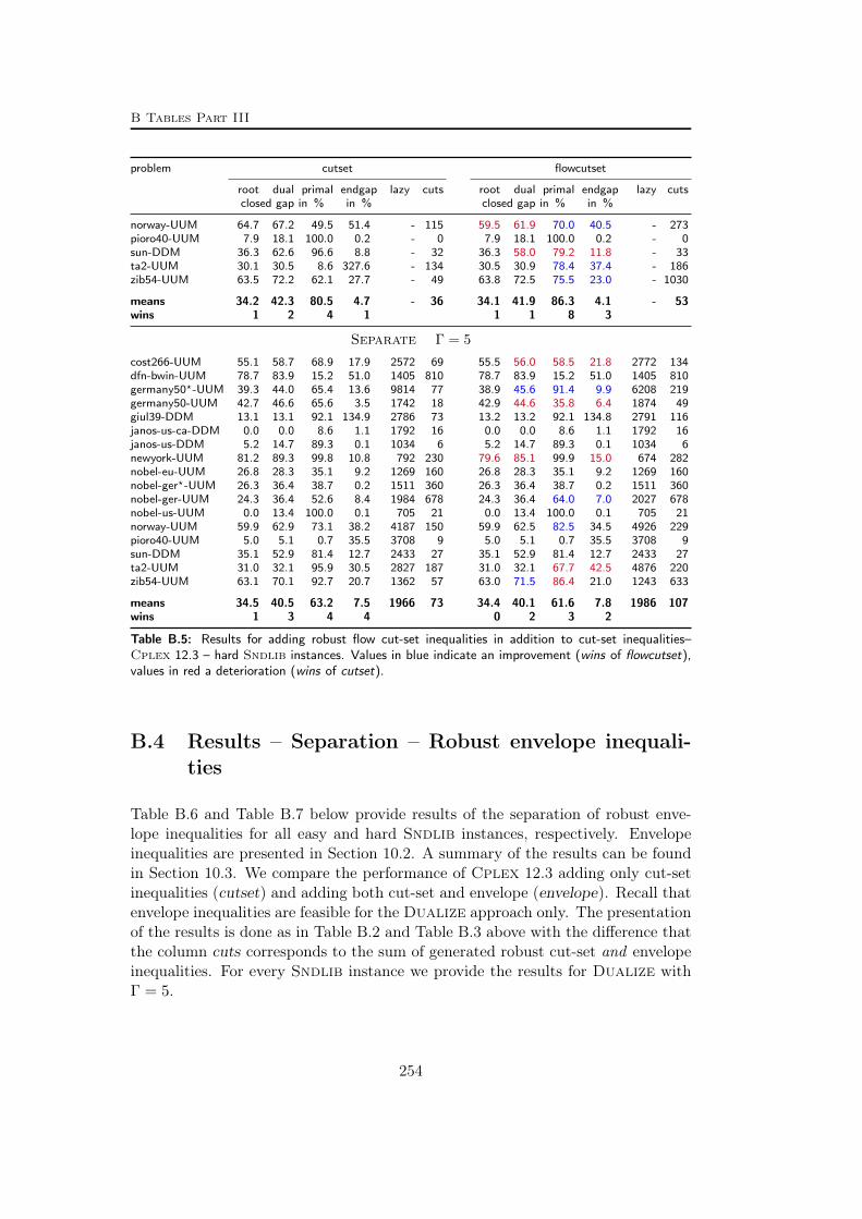
B Tables Part III
problem cutset flowcutset
root dual primal endgap lazy cuts root dual primal endgap lazy cutsclosed gap in % in % closed gap in % in %
norway-UUM 64.7 67.2 49.5 51.4 - 115 59.5 61.9 70.0 40.5 - 273pioro40-UUM 7.9 18.1 100.0 0.2 - 0 7.9 18.1 100.0 0.2 - 0sun-DDM 36.3 62.6 96.6 8.8 - 32 36.3 58.0 79.2 11.8 - 33ta2-UUM 30.1 30.5 8.6 327.6 - 134 30.5 30.9 78.4 37.4 - 186zib54-UUM 63.5 72.2 62.1 27.7 - 49 63.8 72.5 75.5 23.0 - 1030
means 34.2 42.3 80.5 4.7 - 36 34.1 41.9 86.3 4.1 - 53wins 1 2 4 1 1 1 8 3
Separate Γ = 5
cost266-UUM 55.1 58.7 68.9 17.9 2572 69 55.5 56.0 58.5 21.8 2772 134dfn-bwin-UUM 78.7 83.9 15.2 51.0 1405 810 78.7 83.9 15.2 51.0 1405 810germany50?-UUM 39.3 44.0 65.4 13.6 9814 77 38.9 45.6 91.4 9.9 6208 219germany50-UUM 42.7 46.6 65.6 3.5 1742 18 42.9 44.6 35.8 6.4 1874 49giul39-DDM 13.1 13.1 92.1 134.9 2786 73 13.2 13.2 92.1 134.8 2791 116janos-us-ca-DDM 0.0 0.0 8.6 1.1 1792 16 0.0 0.0 8.6 1.1 1792 16janos-us-DDM 5.2 14.7 89.3 0.1 1034 6 5.2 14.7 89.3 0.1 1034 6newyork-UUM 81.2 89.3 99.8 10.8 792 230 79.6 85.1 99.9 15.0 674 282nobel-eu-UUM 26.8 28.3 35.1 9.2 1269 160 26.8 28.3 35.1 9.2 1269 160nobel-ger?-UUM 26.3 36.4 38.7 0.2 1511 360 26.3 36.4 38.7 0.2 1511 360nobel-ger-UUM 24.3 36.4 52.6 8.4 1984 678 24.3 36.4 64.0 7.0 2027 678nobel-us-UUM 0.0 13.4 100.0 0.1 705 21 0.0 13.4 100.0 0.1 705 21norway-UUM 59.9 62.9 73.1 38.2 4187 150 59.9 62.5 82.5 34.5 4926 229pioro40-UUM 5.0 5.1 0.7 35.5 3708 9 5.0 5.1 0.7 35.5 3708 9sun-DDM 35.1 52.9 81.4 12.7 2433 27 35.1 52.9 81.4 12.7 2433 27ta2-UUM 31.0 32.1 95.9 30.5 2827 187 31.0 32.1 67.7 42.5 4876 220zib54-UUM 63.1 70.1 92.7 20.7 1362 57 63.0 71.5 86.4 21.0 1243 633
means 34.5 40.5 63.2 7.5 1966 73 34.4 40.1 61.6 7.8 1986 107wins 1 3 4 4 0 2 3 2
Table B.5: Results for adding robust flow cut-set inequalities in addition to cut-set inequalities–Cplex 12.3 – hard Sndlib instances. Values in blue indicate an improvement (wins of flowcutset),values in red a deterioration (wins of cutset).
B.4 Results – Separation – Robust envelope inequali-ties
Table B.6 and Table B.7 below provide results of the separation of robust enve-lope inequalities for all easy and hard Sndlib instances, respectively. Envelopeinequalities are presented in Section 10.2. A summary of the results can be foundin Section 10.3. We compare the performance of Cplex 12.3 adding only cut-setinequalities (cutset) and adding both cut-set and envelope (envelope). Recall thatenvelope inequalities are feasible for the Dualize approach only. The presentationof the results is done as in Table B.2 and Table B.3 above with the difference thatthe column cuts corresponds to the sum of generated robust cut-set and envelopeinequalities. For every Sndlib instance we provide the results for Dualize withΓ = 5.
254

B.4 Results – Separation – Robust envelope inequalities
problem cutset envelope
root time nodes lazy cuts root time nodes lazy cutscl.gap% in s cl.gap% in s
Dualize Γ = 5
abilene?-UUM 96.7 4.5 1036 - 2 96.7 4.7 1036 - 2abilene-UUM 99.5 6.5 1969 - 0 99.5 6.5 1969 - 0atlanta-UUM 98.9 21.2 1214 - 20 98.9 21.2 1214 - 20dfn-gwin-UUM 93.4 583.6 17239 - 56 93.4 389.1 17786 - 123di-yuan-UUM 86.9 153.2 10712 - 243 87.5 218.9 14588 - 263france-UUM 100.0 14400.0 165844 - 26 100.0 14400.0 165892 - 26geant?-UUM 96.5 989.7 9677 - 53 96.5 1160.8 9993 - 55geant-UUM 99.6 817.7 19628 - 18 99.6 698.3 23076 - 20pdh-UUM 83.1 144.9 14496 - 142 83.1 143.3 12415 - 243polska-UUM 98.5 8.6 1683 - 5 98.5 8.8 1683 - 5ta1-UUM 90.6 14400.0 32593 - 473 88.6 14400.0 30300 - 467
means 94.9 198.1 8354 - 27 94.8 198.0 8648 - 31wins 1 2 2 0 2 1
Table B.6: Results for adding robust envelope inequalities in addition to cut-set inequalities– Cplex12.3 – easy Sndlib instances. Sndlib instances. Values in blue indicate an improvement (wins ofenvelope), values in red a deterioration (wins of cutset).
problem cutset envelope
root dual primal endgap lazy cuts root dual primal endgap lazy cutsclosed gap in % in % closed gap in % in %
Dualize Γ = 5
cost266-UUM 48.1 53.4 89.1 15.5 - 164 48.1 53.4 89.1 15.5 - 164dfn-bwin-UUM 75.4 85.3 89.0 9.5 - 559 75.4 83.3 60.9 14.6 - 625germany50?-UUM 36.5 44.0 90.0 10.3 - 45 36.5 44.0 90.0 10.3 - 45germany50-UUM 44.9 49.6 75.0 3.0 - 32 44.9 51.8 83.3 2.6 - 34giul39-DDM 12.5 12.5 100.0 125.2 - 64 12.5 12.5 100.0 125.2 - 64janos-us-ca-DDM 0.0 2.0 100.0 0.1 - 0 0.0 2.0 100.0 0.1 - 0janos-us-DDM 8.0 17.9 94.8 0.1 - 1 8.0 15.9 65.8 0.1? - 1newyork-UUM 80.2 87.5 100.0 12.6 - 213 80.2 87.5 100.0 12.6 - 213nobel-eu-UUM 24.8 31.5 95.9 3.3 - 306 24.8 31.5 95.9 3.3 - 306nobel-ger?-UUM 18.0 36.2 83.9 0.1 - 51 18.0 36.2 77.6 0.1 - 51nobel-ger-UUM 31.0 42.5 76.9 5.5 - 433 31.0 42.4 80.4 5.2 - 433nobel-us-UUM 0.0 5.4 57.6 0.2 - 0 0.0 5.4 64.1 0.2 - 0norway-UUM 64.7 67.2 49.5 51.4 - 115 64.7 67.2 49.5 51.4 - 115pioro40-UUM 7.9 18.1 100.0 0.2 - 0 7.9 18.1 100.0 0.2 - 0sun-DDM 36.3 62.6 96.6 8.8 - 32 36.3 60.4 96.1 9.4 - 33ta2-UUM 30.1 30.5 8.6 327.6 - 134 30.1 30.5 8.6 327.6 - 134zib54-UUM 63.5 72.2 62.1 27.7 - 49 63.5 72.2 62.1 27.7 - 49
means 34.2 42.3 80.5 4.7 - 36 34.2 42.0 77.8 4.8 - 37wins 0 3 3 1 0 1 3 1
Table B.7: Results for adding robust envelope inequalities in addition to cut-set inequalities– Cplex12.3 – hard Sndlib instances. Sndlib instances. Values in blue indicate an improvement (wins ofenvelope), values in red a deterioration (wins of cutset).
255


Appendix C
Notation
General
R,R+ set of (non-negative) real numbers
Q,Q+ set of (non-negative) rational numbers
Z,Z+ set of (non-negative) integral numbers
M , N index set for constraints/rows and variables/columns, re-spectively
I,B, J index set for integral, basic, and non-basic variables, respec-tively
i, j row and column index, respectively
m,n number of rows and columns, respectively, |M | = m, |N | =n
x variables, variable vector x ∈ RN
s slack variables, slack vector s ∈ RM
µ, π, λ dual variables or row weights
P polyhedron
bac the floor of a real number a, bac ∈ Zdae the ceil of a real number a, dae ∈ Zr(a, c) the remainder of the division of a by c
r(a) the fractional part of a real number a, r(a) = r(a, 1)
a+ a+ := max(0, a)
x(S) sum over all indices in S, that is, x(S) :=∑
j∈S xj
u upper bounds
continued on next page
257

C Notation
l lower bounds or lengths
e unit vector
P class of polynomially solvable problems
NP class of non-deterministic polynomially solvable problems
O(f(n)) class of algorithms with asymptotic running time of at mostf(n), n→∞
Fβ,γ MIR function w. r. t. a right hand side β and a multiplier γ
Graphs
D directed graph
G undirected graph
V set of nodes
v, w single nodes
A set of directed arcs
a single directed arc
ς(a), τ(a) source and target of arc a
(v, w) directed arc with head v and tail w
E set of undirected edges
e single undirected edge
ψ(e) end-nodes of edge e
vw undirected edge with end-nodes v, w
P, P(s,t) set of paths, set of paths with end-nodes s,t
S node subset
δ(S), δG(S) a cut-set or network cut w. r. t. node-set S (and graph G)
δ+(S), δ−(S) network dicuts
δ(S1, . . . , Sk−1) multi cut-set w. r. t. k-partition (S1, . . . , Sk) of the nodes
(Robust) Network design
K set of commodities
k, k single commodities
Q subset of the commodities
bkv net demand of general commodity k at node v, bkv ∈ Q
continued on next page
258
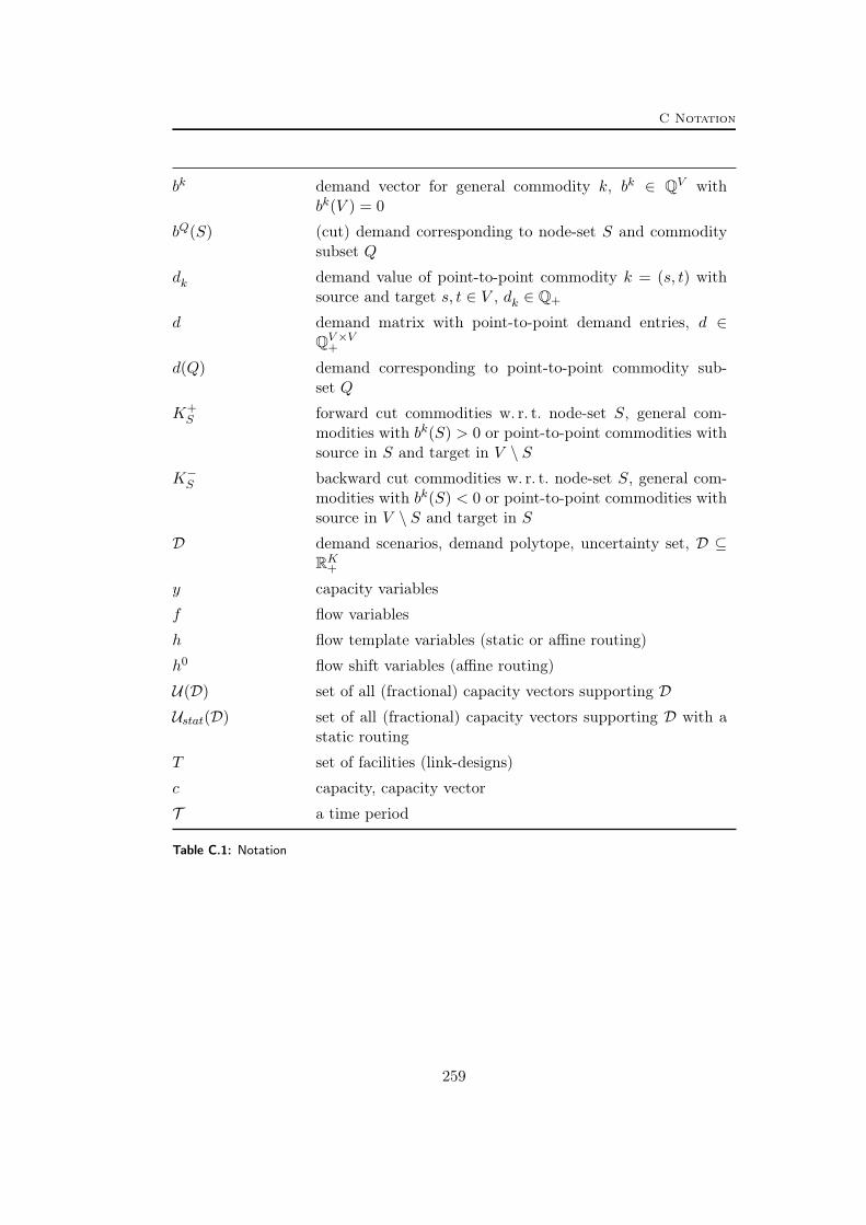
C Notation
bk demand vector for general commodity k, bk ∈ QV withbk(V ) = 0
bQ(S) (cut) demand corresponding to node-set S and commoditysubset Q
dk demand value of point-to-point commodity k = (s, t) withsource and target s, t ∈ V , dk ∈ Q+
d demand matrix with point-to-point demand entries, d ∈QV×V
+
d(Q) demand corresponding to point-to-point commodity sub-set Q
K+S forward cut commodities w. r. t. node-set S, general com-
modities with bk(S) > 0 or point-to-point commodities withsource in S and target in V \ S
K−S backward cut commodities w. r. t. node-set S, general com-modities with bk(S) < 0 or point-to-point commodities withsource in V \ S and target in S
D demand scenarios, demand polytope, uncertainty set, D ⊆RK+
y capacity variables
f flow variables
h flow template variables (static or affine routing)
h0 flow shift variables (affine routing)
U(D) set of all (fractional) capacity vectors supporting DUstat(D) set of all (fractional) capacity vectors supporting D with a
static routing
T set of facilities (link-designs)
c capacity, capacity vector
T a time period
Table C.1: Notation
259

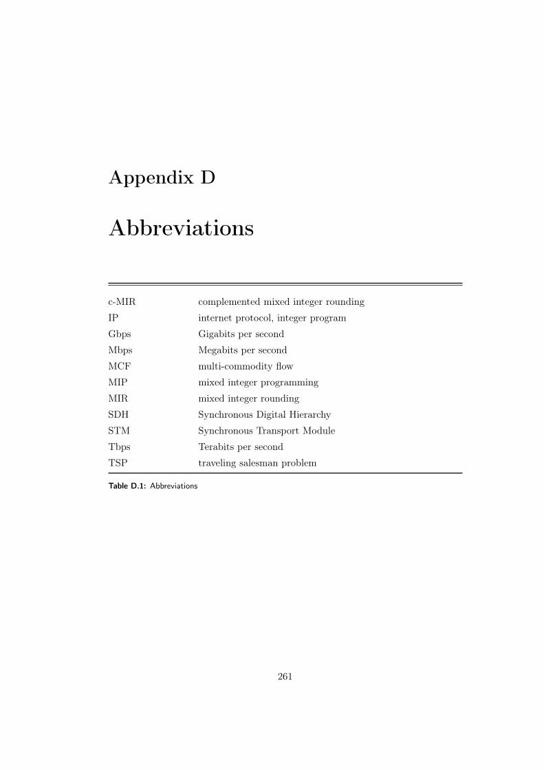
Appendix D
Abbreviations
c-MIR complemented mixed integer rounding
IP internet protocol, integer program
Gbps Gigabits per second
Mbps Megabits per second
MCF multi-commodity flow
MIP mixed integer programming
MIR mixed integer rounding
SDH Synchronous Digital Hierarchy
STM Synchronous Transport Module
Tbps Terabits per second
TSP traveling salesman problem
Table D.1: Abbreviations
261


List of Tables
Part II: Capacitated networks within mixed integer programs 69
6.1 Testsets: network design and general MIPs . . . . . . . . . . . . . . 1006.2 Network detection results – summary . . . . . . . . . . . . . . . . . 1016.3 Separation results MCF cuts – summary for easy instances . . . . . 1046.4 Separation results MCF cuts – summary for hard instances . . . . 1056.5 Separation results MCF cuts in Cplex– summary for easy instances 1066.6 The impact of inconsistency . . . . . . . . . . . . . . . . . . . . . . 1086.7 The impact of aggressive separation . . . . . . . . . . . . . . . . . . 111
Part III: Demand uncertainty: Design of robust networks 117
10.1 Separation results robust cut-set inequalities – summary for easy in-stances . . . . . . . . . . . . . . . . . . . . . . . . . . . . . . . . . . 170
10.2 Separation results robust cut-set inequalities – summary for hardinstances . . . . . . . . . . . . . . . . . . . . . . . . . . . . . . . . . 171
10.3 Separation results robust flow cut-set and envelope inequalities –summary for easy instances . . . . . . . . . . . . . . . . . . . . . . 173
10.4 Separation results robust flow cut-set and envelope inequalities –summary for hard instances . . . . . . . . . . . . . . . . . . . . . . 173
11.1 Model sizes for static/affine/dynamic routing . . . . . . . . . . . . 19711.2 Comparing static/affine/dynamic routing – solution cost . . . . . . 19911.3 Comparing static/affine/dynamic routing – computation time . . . 203
Appendix A: Tables Part II 209
A.1 All instances – general information . . . . . . . . . . . . . . . . . . 220A.2 Network detection results – details . . . . . . . . . . . . . . . . . . 226A.3 Network detection results – details . . . . . . . . . . . . . . . . . . 230A.4 Separation results MCF cuts – details for easy instances . . . . . . 239A.5 Separation results MCF cuts – details for hard instances . . . . . . 243
263
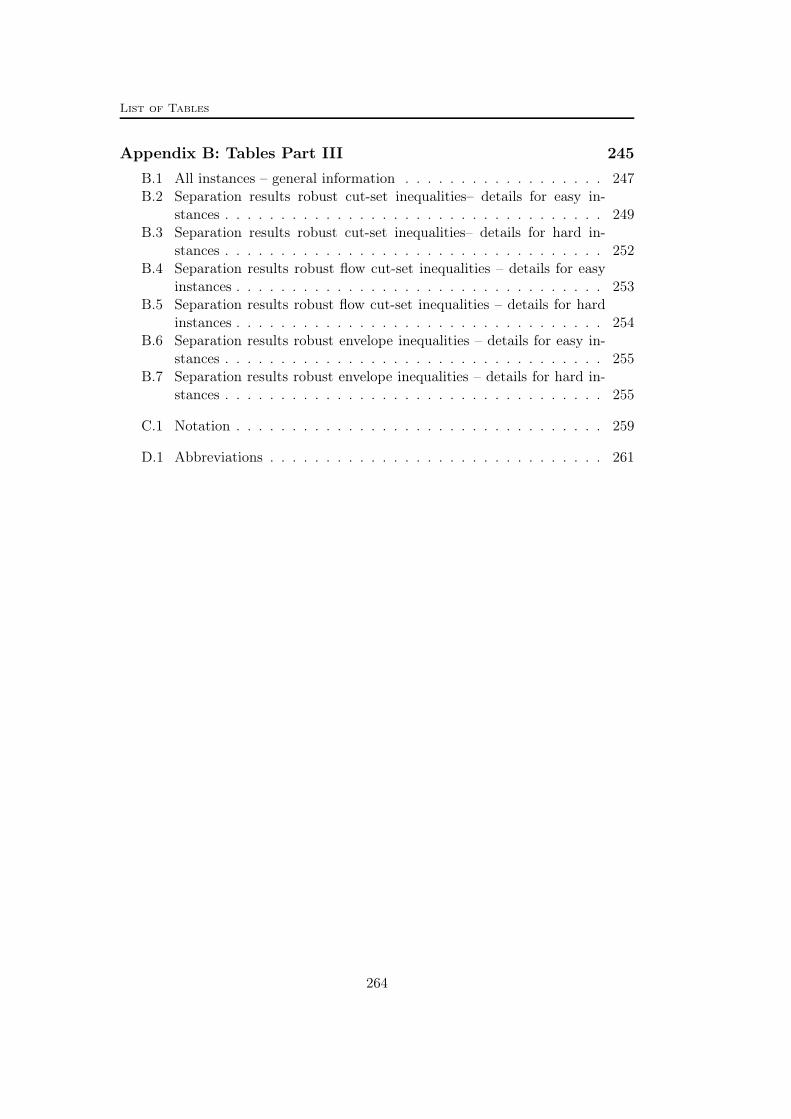
List of Tables
Appendix B: Tables Part III 245B.1 All instances – general information . . . . . . . . . . . . . . . . . . 247B.2 Separation results robust cut-set inequalities– details for easy in-
stances . . . . . . . . . . . . . . . . . . . . . . . . . . . . . . . . . . 249B.3 Separation results robust cut-set inequalities– details for hard in-
stances . . . . . . . . . . . . . . . . . . . . . . . . . . . . . . . . . . 252B.4 Separation results robust flow cut-set inequalities – details for easy
instances . . . . . . . . . . . . . . . . . . . . . . . . . . . . . . . . . 253B.5 Separation results robust flow cut-set inequalities – details for hard
instances . . . . . . . . . . . . . . . . . . . . . . . . . . . . . . . . . 254B.6 Separation results robust envelope inequalities – details for easy in-
stances . . . . . . . . . . . . . . . . . . . . . . . . . . . . . . . . . . 255B.7 Separation results robust envelope inequalities – details for hard in-
stances . . . . . . . . . . . . . . . . . . . . . . . . . . . . . . . . . . 255
C.1 Notation . . . . . . . . . . . . . . . . . . . . . . . . . . . . . . . . . 259
D.1 Abbreviations . . . . . . . . . . . . . . . . . . . . . . . . . . . . . . 261
264

List of Figures
1 Capacitated US network Abilene . . . . . . . . . . . . . . . . . . . 22 A cutting plane . . . . . . . . . . . . . . . . . . . . . . . . . . . . . 53 A network cut . . . . . . . . . . . . . . . . . . . . . . . . . . . . . . 7
Part I: Concepts 13
1.1 Cut and branch . . . . . . . . . . . . . . . . . . . . . . . . . . . . . 161.2 The MIR inequality . . . . . . . . . . . . . . . . . . . . . . . . . . 211.3 The MIR function . . . . . . . . . . . . . . . . . . . . . . . . . . . 25
2.1 Digraph and node-arc incidence matrix . . . . . . . . . . . . . . . . 372.2 A coupled multi-commodity flow . . . . . . . . . . . . . . . . . . . 392.3 Small networks and polyhedral studies . . . . . . . . . . . . . . . . 462.4 A network cut and constraint aggregation . . . . . . . . . . . . . . 472.5 A directed network cut with selected arc subsets . . . . . . . . . . 48
Part II: Capacitated networks within mixed integer programs 69
4.1 The MCF-separator: Flow Detection . . . . . . . . . . . . . . . . . 764.2 The MCF-separator: Arc Detection . . . . . . . . . . . . . . . . . . 764.3 The MCF-separator: Node Detection . . . . . . . . . . . . . . . . . 774.4 The MCF-separator: Network Construction . . . . . . . . . . . . . 774.5 The impact of presolving . . . . . . . . . . . . . . . . . . . . . . . . 89
6.1 The impact of inconsistency . . . . . . . . . . . . . . . . . . . . . . 109
Part III: Demand uncertainty: Design of robust networks 117
8.1 Traffic in the Abilene network during 10days . . . . . . . . . . . . . 1188.2 Traffic in the Geant network during 4 weeks . . . . . . . . . . . . . 1198.3 Traffic in the Geant and DFN network during 1 day . . . . . . . . 1198.4 Cisco traffic forecast . . . . . . . . . . . . . . . . . . . . . . . . . . 1208.5 Realized traffic scenarios and artificial worst case peak scenario . . 121
265

List of Figures
9.1 Optimal solutions for static/dynamic routing . . . . . . . . . . . . 1309.2 The polyhedral Γ-model and the concept of domination . . . . . . 136
10.1 Lower and upper region in the space (y, π) . . . . . . . . . . . . . . 15410.2 Solving time as a function of Γ – Dualize and Separate . . . . . 17410.3 The price of robustness – 95%percentile peaks . . . . . . . . . . . . 17610.4 The price of robustness – 99%percentile peaks . . . . . . . . . . . . 177
11.1 Optimal solution for affine routing . . . . . . . . . . . . . . . . . . 18311.2 No domination with affine routings . . . . . . . . . . . . . . . . . . 18611.3 Irreducible affine routing that contains a positive circulation . . . . 18811.4 Non-static affine routing . . . . . . . . . . . . . . . . . . . . . . . . 191
266

List of Algorithms
Part I: Concepts 13
1.1 The cutting plane method . . . . . . . . . . . . . . . . . . . . . . . . 181.2 Complemented mixed integer rounding . . . . . . . . . . . . . . . . 33
Part II: Capacitated networks within mixed integer programs 69
4.3 Flow Detection . . . . . . . . . . . . . . . . . . . . . . . . . . . . . . 804.4 Arc Detection . . . . . . . . . . . . . . . . . . . . . . . . . . . . . . 824.5 Node Detection . . . . . . . . . . . . . . . . . . . . . . . . . . . . . . 84- Function PatternOf(i) . . . . . . . . . . . . . . . . . . . . . . . . . . 85- Function ComparePattern(pattern1, pattern2) . . . . . . . . . . . . 854.6 Network Construction . . . . . . . . . . . . . . . . . . . . . . . . . . 87
5.7 The constraint aggregation and separation scheme of the MCF sepa-rator . . . . . . . . . . . . . . . . . . . . . . . . . . . . . . . . . . . 93
267


Bibliography
[1] Tobias Achterberg. Constraint Integer Programming. PhD thesis, Technische Uni-versität Berlin, 2007. Cited on pages 13, 17, 20, 32, 33, 69, 71, 72, 89.
[2] Tobias Achterberg. Personal communication, 2011. Cited on pages 34, 71, 100.[3] Tobias Achterberg and Christian Raack. The MCF-Separator – Detecting and Ex-
ploiting Multi-Commodity Flows in MIPs. Mathematical Programming Computa-tion, 2:125–165, July 2010. Cited on pages 69, 100.
[4] Tobias Achterberg, Thorsten Koch, and Alexander Martin. MIPLIB 2003. Opera-tions Research Letters, 34(4):1–12, 2006. doi: 10.1016/j.orl.2005.07.009. Cited onpages 74, 99, 100.
[5] Yogesh K. Agarwal. k-Partition-based facets of the network design problem. Net-works, 47(3):123, 2006. Cited on pages 46, 47, 51, 53.
[6] Yogesh K. Agarwal. Polyhedral structure of the 4-node network design problem.Networks, 54(3):139–149, 2009. Cited on pages 46, 51.
[7] Ravindra K. Ahuja, Thomas L. Magnanti, and James B. Orlin. Network Flows:Theory, Algorithms, and Applications. Prentice-Hall, Inc., 1993. Cited on pages 35,40, 44, 47.
[8] Ayşegül Altin, Eduardo Amaldi, Pietro Belotti, and Mustafa Pinar. Provisioningvirtual private networks under traffic uncertainty. Networks, 49(1):100–115, 2007.Cited on pages 123, 124, 128, 136, 137.
[9] Ayşegül Altin, Hande Yaman, and Mustafa Pinar. The Robust Network LoadingProblem Under Hose Demand Uncertainty: Formulation, Polyhedral Analysis, andComputations. INFORMS Journal on Computing, 23(1):75–89, 2011. Cited onpages 123, 128, 132, 135, 152.
[10] Ayşegül Altin, Hande Yaman, and Mustafa Pinar. A Hybrid Polyhedral Uncer-tainty Model for the Robust Network Loading Problem . In Nalân Gülpinar, PeterHarrison, and Berç Rustem, (Eds.), Performance Models and Risk Management inCommunications Systems, Springer Optimization and Its Applications, pages 157–172. Springer, 2011. Cited on pages 137, 189, 194.
[11] Kent Andersen, Gérard Cornuéjols, and Yanjun Li. Split closure and intersectioncuts. Mathematical programming, 102(3):457–493, 2005. Cited on pages 7, 13, 27,28.
[12] Kent Andersen, Quentin Louveaux, Robert Weismantel, and Laurence A. Wolsey.Inequalities from two rows of a simplex tableau. Integer Programming and Combi-natorial Optimization IPCO 2007, pages 1–15, 2007. Cited on page 20.
[13] Giuseppe Andreello, Alberto Caprara, and Matteo Fischetti. Embedding 0, 12-Cutsin a Branch-and-Cut Framework: A Computational Study. INFORMS Journal onComputing, 19(2):229–238, 2007. Cited on pages 20, 31, 32.
269
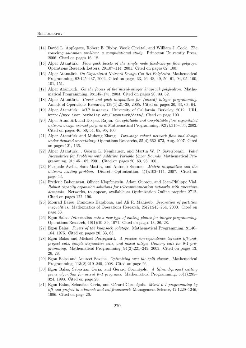
Bibliography
[14] David L. Applegate, Robert E. Bixby, Vasek Chvàtal, and William J. Cook. Thetraveling salesman problem: a computational study. Princeton Universtiy Press,2006. Cited on pages 16, 18.
[15] Alper Atamtürk. Flow pack facets of the single node fixed-charge flow polytope.Operations Research Letters, 29:107–114, 2001. Cited on pages 62, 100.
[16] Alper Atamtürk. On Capacitated Network Design Cut-Set Polyhedra. MathematicalProgramming, 92:425–437, 2002. Cited on pages 33, 46, 48, 49, 50, 61, 94, 95, 100,101, 151.
[17] Alper Atamtürk. On the facets of the mixed-integer knapsack polyhedron. Mathe-matical Programming, 98:145–175, 2003. Cited on pages 20, 33, 62.
[18] Alper Atamtürk. Cover and pack inequalities for (mixed) integer programming.Annals of Operations Research, 139(1):21–38, 2005. Cited on pages 20, 33, 63, 64.
[19] Alper Atamtürk. MIP instances. University of California, Berkeley, 2012. URLhttp://www.ieor.berkeley.edu/~atamturk/data/. Cited on page 100.
[20] Alper Atamtürk and Deepak Rajan. On splittable and unsplittable flow capacitatednetwork design arc–set polyhedra. Mathematical Programming, 92(2):315–333, 2002.Cited on pages 46, 50, 54, 65, 95, 100.
[21] Alper Atamtürk and Muhong Zhang. Two-stage robust network flow and designunder demand uncertainty. Operations Researchs, 55(4):662–673, Aug. 2007. Citedon pages 121, 136.
[22] Alper Atamtürk, , George L. Nemhauser, and Martin W. P. Savelsbergh. ValidInequalities for Problems with Additive Variable Upper Bounds. Mathematical Pro-gramming, 91:145–162, 2001. Cited on pages 20, 63, 95, 100.
[23] Pasquale Avella, Sara Mattia, and Antonio Sassano. Metric inequalities and thenetwork loading problem. Discrete Optimization, 4(1):103–114, 2007. Cited onpage 43.
[24] Frédéric Babonneau, Olivier Klopfenstein, Adam Ouorou, and Jean-Philippe Vial.Robust capacity expansion solutions for telecommunication networks with uncertaindemands. Networks, to appear, available as Optimization Online preprint 2712.Cited on pages 122, 196.
[25] Mourad Baïou, Francisco Barahona, and Ali R. Mahjoub. Separation of partitioninequalities. Mathematics of Operations Research, 25(2):243–254, 2000. Cited onpage 53.
[26] Egon Balas. Intersection cuts-a new type of cutting planes for integer programming.Operations Research, 19(1):19–39, 1971. Cited on pages 13, 26, 28.
[27] Egon Balas. Facets of the knapsack polytope. Mathematical Programming, 8:146–164, 1975. Cited on pages 20, 33, 63.
[28] Egon Balas and Michael Perregaard. A precise correspondence between lift-and-project cuts, simple disjunctive cuts, and mixed integer Gomory cuts for 0-1 pro-gramming. Mathematical Programming, 94(2):221–245, 2003. Cited on pages 13,26, 28.
[29] Egon Balas and Anureet Saxena. Optimizing over the split closure. MathematicalProgramming, 113(2):219–240, 2008. Cited on page 26.
[30] Egon Balas, Sebastian Ceria, and Gérard Cornuéjols. A lift-and-project cuttingplane algorithm for mixed 0–1 programs. Mathematical Programming, 58(1):295–324, 1993. Cited on page 26.
[31] Egon Balas, Sebastian Ceria, and Gérard Cornuéjols. Mixed 0-1 programming bylift-and-project in a branch-and-cut framework. Management Science, 42:1229–1246,1996. Cited on page 26.
270

Bibliography
[32] Egon Balas, Sebastian Ceria, Gérard Cornuéjols, and N. Natraj. Gomory cutsrevisited. Operations Research Letters, 19:1–9, 1996. Cited on pages 19, 21.
[33] Francisco Barahona. Separating from the dominant of the spanning tree polytope.Operations research letters, 12(4):201–203, 1992. Cited on page 53.
[34] Francisco Barahona. Network Design Using Cut Inequalities. SIAM Journal onOptimization, 6:823–837, 1996. Cited on pages 50, 53.
[35] Pietro Belotti, Antonio Capone, Giuliana Carello, and Frederico Malucelli. Multi-layer MPLS network design: The impact of statistical multiplexing. Computer Net-works, 52(6):1291–1307, 2008. Cited on page 124.
[36] Pietro Belotti, Kireeti Kompella, and Lloyd Noronha. A comparison of OTNand MPLS networks under traffic uncertainty. IEEE/ACM Trans. on Net-working, submitted. URL http://myweb.clemson.edu/~pbelott/papers/robust-opt-network-design.pdf. Cited on page 124.
[37] Walid Ben-Ameur. Between fully dynamic routing and robust stable routing. In Pro-ceedings of the 6th International Workshop on Design and Reliable CommunicationNetworks (DRCN 2007), 2007. Cited on pages 122, 123.
[38] Walid Ben-Ameur and Hervé Kerivin. New Economical Virtual Private Networks.Communications of ACM, 46(6):69–73, 2003. Cited on page 122.
[39] Walid Ben-Ameur and Hervé Kerivin. Routing of uncertain traffic demands. Opti-mization and Engineering, 6(3):283–313, 2005. Cited on pages 122, 123, 128, 132,134, 135.
[40] Aharon Ben-Tal and Arkadi Nemirovski. Robust solutions of uncertain linear pro-grams. Operations Research Letters, 25(1):1–14, 1999. Cited on pages 121, 126.
[41] Aharon Ben-Tal and Arkadi Nemirovski. Robust solutions of linear programmingproblems contaminated with uncertain data. Mathematical Programming, 88(3):411–424, 2000. Cited on pages 119, 121, 131.
[42] Aharon Ben-Tal and Arkadi Nemirovski. Robust optimization–methodology and ap-plications. Mathematical Programming, 92(3):453–480, 2002. Cited on pages 119,121, 131.
[43] Aharon Ben-Tal, Alexander Goryashko, E. Guslitzer, and Arkadi Nemirovski. Ad-justable robust solutions of uncertain linear programs. Mathematical Programming,99(2):351–376, 2004. Cited on pages 121, 122, 126, 128, 129, 133, 179, 180, 185.
[44] Aharon Ben-Tal, Laurent El Ghaoui, and Arkadi Nemirovski. Robust optimization.Princeton University Press, Princeton, NJ, 2009. Cited on pages 121, 131.
[45] J.F. Benders. Partitioning procedures for solving mixed-variables programming prob-lems. Numerische Mathematik, 4(1):238–252, 1962. Cited on pages 43, 194, 196.
[46] Dimitris Bertsimas and Vineet Goyal. On the power and limitations of affinepolicies in two-stage adaptive optimization. Mathematical Programming, to ap-pear, published online, 2011. URL http://www.springerlink.com/content/2u016h08582m5024/. Cited on page 191.
[47] Dimitris Bertsimas and Melvyn Sim. Robust discrete optimization and networkflows. Mathematical Programming, 98(1):49–71, 2003. Cited on pages 119, 131,136, 137, 138, 194, 205.
[48] Dimitris Bertsimas and Melvyn Sim. The price of robustness. Operations Research,52(1):35–53, 2004. Cited on pages 119, 121, 123, 131, 136, 138, 194, 205.
[49] Dimitris Bertsimas and Aurelie Thiele. A robust optimization approach to inventorytheory. Operations Research, 54(1):150–168, 2006. Cited on page 136.
271

Bibliography
[50] Daniel Bienstock and Oktay Günlük. Capacitated Network Design – PolyhedralStructure and Computation. INFORMS Journal on Computing, 8:243–259, 1996.Cited on pages 33, 46, 49, 50, 51, 53, 55, 56, 58, 61, 65, 66, 92, 171, 196.
[51] Daniel Bienstock, Sunil Chopra, Oktay Günlük, and Chih-Yang Tsai. MinimumCost Capacity Installation for Multicommodity Network Flows. Mathematical Pro-gramming, 81:177–199, 1998. Cited on pages 43, 46, 49, 50, 51, 52, 53, 58, 65, 92,94.
[52] Robert E. Bixby. Solving Real-World Linear Programs: A Decade and More ofProgress. Operations Research, 50(1):3–15, 2002. Cited on page 16.
[53] Robert E. Bixby and William H. Cunningham. Converting linear programs to net-work problems. Mathematics of Operations Research, 5(3):321–357, 1980. Cited onpage 73.
[54] Robert E. Bixby and Robert Fourer. Finding embedded network rows in linearprograms I. Extraction heuristics. Management Science, 34(3):342–376, 1988. Citedon pages 70, 73, 74, 77, 79, 81.
[55] Robert E. Bixby and Edward Rothberg. Progress in computational mixed integerprogramming – A look back from the other side of the tipping point. Annals ofOperations Research, 149(1):37–41, 2007. Cited on pages 13, 16, 19, 20, 30, 31, 33,69.
[56] Robert E. Bixby, Sebastian Ceria, Cassandra M. McZeal, and Martin W. P. Savels-bergh. An Updated Mixed Integer Programming Library: MIPLIB 3.0. Optima,58:12–15, June 1998. URL http://www.caam.rice.edu/~bixby/miplib/miplib.html. Cited on pages 26, 74, 99, 100.
[57] Robert E. Bixby, Mary Fenelon, Zonghao Gu, Edward Rothberg, and Robert Wun-derling. Mixed integer programming: A progress report. In M. Grötschel, (Ed.), TheSharpest Cut: The impact of Manfred Padberg and his work, MPS-SIAM Series inOptimization, chapter 18, pages 309—-326. SIAM, 2004. Cited on pages 13, 16, 19.
[58] Andreas Bley. Routing and Capacity Optimization for IP Networks. PhD thesis,TU Berlin, 2007. URL http://opus.kobv.de/tuberlin/volltexte/2007/1553.Cited on page 122.
[59] Andreas Bley, Ullrich Menne, Roman Klähne, Christian Raack, and RolandWessäly.Multi-layer network design – A model-based optimization approach. In Proceedingsof the PGTS 2008, Berlin, Germany, pages 107–116, Berlin, Germany, 2008. Polish-German Teletraffic Symposium. Cited on page 166.
[60] Beate Brockmüller, Oktay Günlük, and Laurence A. Wolsey. Designing privateline networks: polyhedral analysis and computation. Transactions on OperationalResearch, 16:7–24, 2004. Cited on pages 95, 96.
[61] Gerald G. Brown and Michael P. Olson. Dynamic factorization in large-scale opti-mization. Mathematical Programming, 64(1):17–51, 1994. Cited on page 73.
[62] Gerald G. Brown and William G. Wright. Automatic identification of embeddednetwork rows in large-scale optimization models. Mathematical Programming, 29:41–56, 1984. Cited on pages 73, 75, 78.
[63] Gerald G. Brown, Richard D. McBride, and R. Kevin Wood. Extracting embeddedgeneralized networks from linear programming problems. Mathematical Program-ming, 32(1):11–31, 1985. Cited on page 73.
[64] Alberto Caprara and Matteo Fischetti. 0, 12-Chvátal-Gomory Cuts. MathematicalProgramming, 74(3):221–235, 1996. Cited on pages 20, 31, 32.
[65] Alberto Caprara and Adam N. Letchford. On the separation of split cuts and relatedinequalities. Mathematical Programming, 94(2):279–294, 2003. Cited on page 26.
272

Bibliography
[66] Alberto Caprara, Matteo Fischetti, and Adam N. Letchford. On the separationof maximally violated mod-k cuts. Mathematical Programming, 87(1):37–56, 2000.Cited on pages 31, 32.
[67] Chandra Chekuri. Routing and network design with robustness to changing or uncer-tain traffic demands. ACM SIGACT News, 38(3):106–129, 2007. Cited on pages 122,123, 130, 135, 181.
[68] Chandra Chekuri, F. Bruce Shepherd, Gianpolo Oriolo, and Maria G. Scutellá.Hardness of robust network design. Networks, 50(1):50–54, 2007. Cited on pages 121,122, 123, 128, 135, 185.
[69] Xin Chen and Yin Zhang. Uncertain linear programs: Extended affinely adjustablerobust counterparts. Operations Research, 57(6):1469–1482, 2009. Cited on page 122.
[70] Sunil Chopra and Mendu Rammohan Rao. The Steiner tree problem I: Formu-lations, compositions and extension of facets. Mathematical Programming, 64(1):209–229, 1994. Cited on pages 40, 53.
[71] Sunil Chopra and Mendu Rammohan Rao. The Steiner tree problem II: Propertiesand classes of facets. Mathematical Programming, 64(1):231–246, 1994. Cited onpage 40.
[72] Sunil Chopra, Itzhak Gilboa, and S. Trilochan Sastry. Source sink flows with capacityinstallation in batches. Discrete Applied Mathematics, 86:165–192, 1998. Cited onpages 33, 41, 46, 48, 61.
[73] Cisco. Cisco Visual Networking Index: Forecast and Methodology, 2012. URLhttp://www.cisco.com/en/US/solutions/collateral/ns341/ns525/ns537/ns705/ns827/white_paper_c11-481360_ns827_Networking_Solutions_White_Paper.html. Cited on pages 118, 120.
[74] COmputational INfrastructure for Operations Research (COIN-OR). Coin-orBranch and Cut (CBC), 2012. URL https://projects.coin-or.org/Cbc. Citedon page 18.
[75] COmputational INfrastructure for Operations Research (COIN-OR). Cut Genera-tion Library (CGL), 2012. URL https://projects.coin-or.org/Cgl. Cited onpage 33.
[76] Michele Conforti, Gérard Cornuéjols, and Giacomo Zambelli. Polyhedral approachesto mixed integer linear programming. In Michael Jünger, Thomas Liebling, DenisNaddef, George L. Nemhauser, William R. Pulleyblank, Gerhard Reinelt, GiovanniRinaldi, and Laurence A. Wolsey, (Eds.), 50 Years of Integer Programming 1958-2008, chapter 11, pages 343–385. Springer, 2010. Cited on page 22.
[77] Michele Conforti, Gérard Cornuéjols, and Giacomo Zambelli. Polyhedral Approachesto Mixed Integer Linear Programming. In Michael Jünger, Thomas Liebling, DenisNaddef, George L. Nemhauser, William R. Pulleyblank, Gerhard Reinelt, GiovanniRinaldi, and Laurence A. Wolsey, (Eds.), 50 Years of Integer Programming 1958-2008, chapter 11, pages 343–385. Springer, 2010. Cited on pages 13, 19.
[78] William J. Cook. Fifty-Plus Years of Combinatorial Integer Programming. InMichael Jünger, Thomas Liebling, Denis Naddef, George L. Nemhauser, William R.Pulleyblank, Gerhard Reinelt, Giovanni Rinaldi, and Laurence A. Wolsey, (Eds.),50 Years of Integer Programming 1958-2008, chapter 12, pages 387–430. Springer,2010. Cited on page 18.
[79] William J. Cook, Ravi Kannan, and Alexander Schrijver. Chvátal closures for mixedinteger programming problems. Mathematical Programming, 47(1):155–174, 1990.Cited on pages 23, 27.
273

Bibliography
[80] William J. Cook, William H. Cunningham, William R. Pulleyblank, and AlexanderSchrijver. Combinatorial Optimization. John Wiley & Sons, 1998. Cited on pages 13,18, 35.
[81] Gérard Cornuéjols. Revival of the Gomory cuts in the 1990s. Annals of OperationsResearch, 149(1):63–66, 2007. Cited on page 19.
[82] Gérard Cornuéjols. Valid inequalities for mixed integer linear programs. Mathemat-ical Programming, 112(1):3–44, 2008. Cited on pages 13, 19, 22, 23, 30.
[83] Gérard Cornuéjols and Yanjun Li. On the Rank of Mixed 0,1 Polyhedra. Mathe-matical Programming A, 91:391–397, 2002. Cited on page 23.
[84] Gérard Cornuéjols and Francois Margot. On the facets of mixed integer programswith two integer variables and two constraints. Mathematical Programming, 120:429–456, 2009. Cited on page 20.
[85] Alysson M. Costa, Jean-François Cordeau, and Bernard Gendron. Benders, metricand cutset inequalities for multicommodity capacitated network design. Computa-tional Optimization and Applications, 42(3):371–392, 2009. Cited on page 43.
[86] Teodor Gabriel Crainic, Antonio Frangioni, and Bernard Gendron. Bundle-basedrelaxation methods for multicommodity capacitated fixed charge network design. Dis-crete Applied Mathematics, 112(1-3):73–99, 2001. Cited on pages 44, 45.
[87] Harlan Crowder, Ellis L. Johnson, and Manfred W. Padberg. Solving large-scalezero-one linear programming problems. Operations Research, 31(5):803–834, 1983.Cited on page 18.
[88] William H. Cunningham. A network simplex method. Mathematical Programming,11(1):105–116, 1976. Cited on page 73.
[89] Geir Dahl and Mechthild Stoer. A Polyhedral Approach to Multicommodity Surviv-able Network Design. Numerische Mathematik, 68:149–167, 1994. Cited on pages 59,65.
[90] Geir Dahl and Mechthild Stoer. A Cutting Plane Algorithm for MulticommoditySurvivable Network Design Problems. INFORMS Journal on Computing, 10:1–11,1998. Cited on pages 59, 65.
[91] George B. Dantzig. Programming in a linear structure. U.S. Air Force, Comptroller,Washington, DC, Feb. 1948. Cited on page 16.
[92] George B. Dantzig. Linear programming under uncertainty. Management Science,1(3/4):197–206, 1955. Cited on page 119.
[93] George B. Dantzig. Discrete-variable extremum problems. Operations Research, 5:266–277, 1957. Cited on page 18.
[94] George B. Dantzig. Linear programming and extensions. Princeton University Press.princeton, New Jersey, 1963. Cited on page 73.
[95] George B. Dantzig, Ray Fulkerson, and Selmer Johnson. Solution of a large-scale traveling-salesman problem. Operations Research, 2:393–410, 1954. Citedon page 18.
[96] Sanjeeb Dash, Oktay Günlük, and Andrea Lodi. MIR closures of polyhedral sets.Mathematical Programming, 121:33–60, June 2009. Cited on pages 21, 22, 23, 24,26, 27.
[97] Sanjeeb Dash, Oktay Günlük, and Christian Raack. A note on the MIR closure andbasic relaxations of polyhedra. Operations Research Letters, 39(3):198–199, May2011. Cited on page 27.
[98] DFN. Deutsche Forschungsnetz. http://www.dfn.de, 2012. Cited on pages 119,165.
274

Bibliography
[99] Nick G. Duffield, Pawan Goyal, Albert Greenberg, Partho Mishra, Kadangode K.Ramakrishnan, and Jacobus E. van der Merwe. A flexible model for resource man-agement in virtual private networks. ACM SIGCOMM Computer CommunicationReview, 29(4):95–108, 1999. Cited on pages 123, 134, 135, 194.
[100] Anurag Dwivedi and Richard E. Wagner. Traffic model for USA long-distance opticalnetwork. In Proceedings of the Optical Fiber Communication Conference (OFC),volume TuK1, pages 156–158. Optical Society of America, 2000. Cited on pages 118,136.
[101] Thomas Erlebach and Maurice Ruegg. Optimal bandwidth reservation in hose-modelVPNs with multi-path routing. In INFOCOM 2004. Twenty-third Annual JointConference of the IEEE Computer and Communications Societies, volume 4, pages2275–2282. IEEE, 2004. Cited on page 135.
[102] Daniel G. Espinoza. Computing with multi-row Gomory cuts. Operations ResearchLetters, 38(2):115–120, 2010. Cited on page 20.
[103] FICO. Xpress Optimizer, 2012. URL http://www.fico.com/en/Products/DMTools/xpress-overview/Pages/Xpress-Optimizer.aspx. Cited on page 18.
[104] Rosa M. V. Figueiredo, Martine Labbé, and Cid C. de Souza. An exact approachto the problem of extracting an embedded network matrix. Computers & OperationsResearch, 38(11):1483–1492, 2011. Cited on page 74.
[105] J. Andrew Fingerhut, Subhash Suri, and Jonathan S. Turner. Designing least-costnonblocking broadband networks. Journal of Algorithms, 24(2):287–309, 1997. Citedon page 135.
[106] Matteo Fischetti and Michele Monaci. Robustness by cutting planes and the Uncer-tain Set Covering Problem. Technical report, ARRIVAL project, 2008. Cited onpage 175.
[107] Antonio Frangioni, Fausto Pascali, and Maria G. Scutellá. Static and dynamicrouting under disjoint dominant extreme demands. Operations Research Letters, 39(1):36–39, Jan. 2011. Cited on page 193.
[108] Michael R. Garey and David S. Johnson. Computers and Intractability: A Guide tothe Theory of NP-Completeness. Freeman and Company, New York, 1979. Citedon pages 13, 16, 40, 49, 76.
[109] Bernard Gendron, Teodor Gabriel Crainic, and Antonio Frangioni. Multicommoditycapacitated network design. In B. Sans and P. Sariano, (Eds.), TelecommunicationsNetwork Planning, chapter 1, pages 1–19. Kluwer Academic Publishers, 1999. Citedon pages 44, 45.
[110] Arthur M. Geoffrion. Lagrangean relaxation for integer programming. Approachesto Integer Programming, 2:82–114, 1974. Cited on pages 44, 45.
[111] Arthur M. Geoffrion. Lagrangean relaxation for integer programming. In MichaelJünger, Thomas Liebling, Denis Naddef, George L. Nemhauser, William R. Pul-leyblank, Gerhard Reinelt, Giovanni Rinaldi, and Laurence A. Wolsey, (Eds.), 50Years of Integer Programming 1958-2008, chapter 9, pages 243–281. Springer, 2010.Cited on page 44.
[112] Ralph Gomory. Outline of an algorithm for integer solutions to linear programs.Bulletin of the American Mathematical Society, 64(5):275–278, 1958. Cited onpages 18, 20, 21, 23.
[113] Ralph Gomory. An algorithm for the mixed integer problem. Technical ReportResearch Memorandum RM 2597, RAND Corporation, Santa Monica, USA, 1960.Cited on pages 18, 21, 23.
275
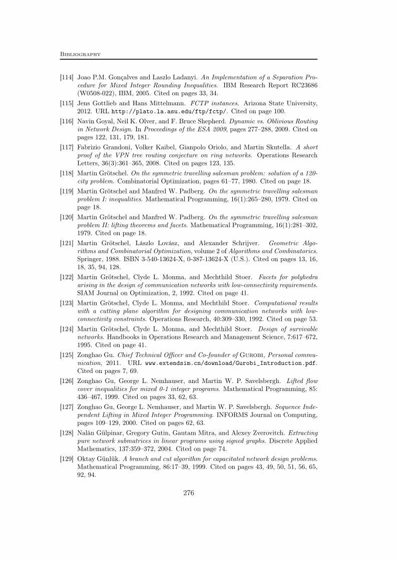
Bibliography
[114] Joao P.M. Gonçalves and Laszlo Ladanyi. An Implementation of a Separation Pro-cedure for Mixed Integer Rounding Inequalities. IBM Research Report RC23686(W0508-022), IBM, 2005. Cited on pages 33, 34.
[115] Jens Gottlieb and Hans Mittelmann. FCTP instances. Arizona State University,2012. URL http://plato.la.asu.edu/ftp/fctp/. Cited on page 100.
[116] Navin Goyal, Neil K. Olver, and F. Bruce Shepherd. Dynamic vs. Oblivious Routingin Network Design. In Proceedings of the ESA 2009, pages 277–288, 2009. Cited onpages 122, 131, 179, 181.
[117] Fabrizio Grandoni, Volker Kaibel, Gianpolo Oriolo, and Martin Skutella. A shortproof of the VPN tree routing conjecture on ring networks. Operations ResearchLetters, 36(3):361–365, 2008. Cited on pages 123, 135.
[118] Martin Grötschel. On the symmetric travelling salesman problem: solution of a 120-city problem. Combinatorial Optimization, pages 61–77, 1980. Cited on page 18.
[119] Martin Grötschel and Manfred W. Padberg. On the symmetric travelling salesmanproblem I: inequalities. Mathematical Programming, 16(1):265–280, 1979. Cited onpage 18.
[120] Martin Grötschel and Manfred W. Padberg. On the symmetric travelling salesmanproblem II: lifting theorems and facets. Mathematical Programming, 16(1):281–302,1979. Cited on page 18.
[121] Martin Grötschel, Lászlo Lovász, and Alexander Schrijver. Geometric Algo-rithms and Combinatorial Optimization, volume 2 of Algorithms and Combinatorics.Springer, 1988. ISBN 3-540-13624-X, 0-387-13624-X (U.S.). Cited on pages 13, 16,18, 35, 94, 128.
[122] Martin Grötschel, Clyde L. Monma, and Mechthild Stoer. Facets for polyhedraarising in the design of communication networks with low-connectivity requirements.SIAM Journal on Optimization, 2, 1992. Cited on page 41.
[123] Martin Grötschel, Clyde L. Monma, and Mechthild Stoer. Computational resultswith a cutting plane algorithm for designing communication networks with low-connectivity constraints. Operations Research, 40:309–330, 1992. Cited on page 53.
[124] Martin Grötschel, Clyde L. Monma, and Mechthild Stoer. Design of survivablenetworks. Handbooks in Operations Research and Management Science, 7:617–672,1995. Cited on page 41.
[125] Zonghao Gu. Chief Technical Officer and Co-founder of Gurobi, Personal commu-nication, 2011. URL www.extendsim.cn/download/Gurobi_Introduction.pdf.Cited on pages 7, 69.
[126] Zonghao Gu, George L. Nemhauser, and Martin W. P. Savelsbergh. Lifted flowcover inequalities for mixed 0-1 integer programs. Mathematical Programming, 85:436–467, 1999. Cited on pages 33, 62, 63.
[127] Zonghao Gu, George L. Nemhauser, and Martin W. P. Savelsbergh. Sequence Inde-pendent Lifting in Mixed Integer Programming. INFORMS Journal on Computing,pages 109–129, 2000. Cited on pages 62, 63.
[128] Nalân Gülpinar, Gregory Gutin, Gautam Mitra, and Alexey Zverovitch. Extractingpure network submatrices in linear programs using signed graphs. Discrete AppliedMathematics, 137:359–372, 2004. Cited on page 74.
[129] Oktay Günlük. A branch and cut algorithm for capacitated network design problems.Mathematical Programming, 86:17–39, 1999. Cited on pages 43, 49, 50, 51, 56, 65,92, 94.
276
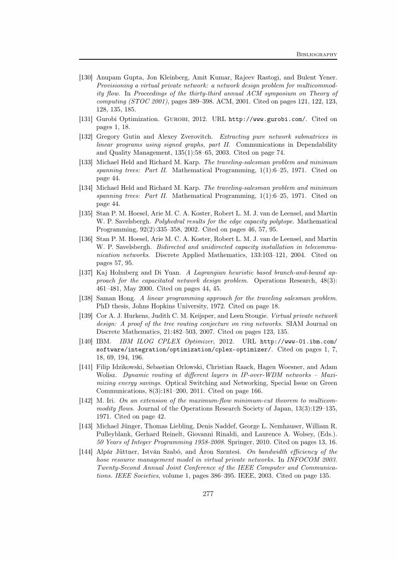
Bibliography
[130] Anupam Gupta, Jon Kleinberg, Amit Kumar, Rajeev Rastogi, and Bulent Yener.Provisioning a virtual private network: a network design problem for multicommod-ity flow. In Proceedings of the thirty-third annual ACM symposium on Theory ofcomputing (STOC 2001), pages 389–398. ACM, 2001. Cited on pages 121, 122, 123,128, 135, 185.
[131] Gurobi Optimization. Gurobi, 2012. URL http://www.gurobi.com/. Cited onpages 1, 18.
[132] Gregory Gutin and Alexey Zverovitch. Extracting pure network submatrices inlinear programs using signed graphs, part II. Communications in Dependabilityand Quality Management, 135(1):58–65, 2003. Cited on page 74.
[133] Michael Held and Richard M. Karp. The traveling-salesman problem and minimumspanning trees: Part II. Mathematical Programming, 1(1):6–25, 1971. Cited onpage 44.
[134] Michael Held and Richard M. Karp. The traveling-salesman problem and minimumspanning trees: Part II. Mathematical Programming, 1(1):6–25, 1971. Cited onpage 44.
[135] Stan P. M. Hoesel, Arie M. C. A. Koster, Robert L. M. J. van de Leensel, and MartinW. P. Savelsbergh. Polyhedral results for the edge capacity polytope. MathematicalProgramming, 92(2):335–358, 2002. Cited on pages 46, 57, 95.
[136] Stan P. M. Hoesel, Arie M. C. A. Koster, Robert L. M. J. van de Leensel, and MartinW. P. Savelsbergh. Bidirected and unidirected capacity installation in telecommu-nication networks. Discrete Applied Mathematics, 133:103–121, 2004. Cited onpages 57, 95.
[137] Kaj Holmberg and Di Yuan. A Lagrangian heuristic based branch-and-bound ap-proach for the capacitated network design problem. Operations Research, 48(3):461–481, May 2000. Cited on pages 44, 45.
[138] Saman Hong. A linear programming approach for the traveling salesman problem.PhD thesis, Johns Hopkins University, 1972. Cited on page 18.
[139] Cor A. J. Hurkens, Judith C. M. Keijsper, and Leen Stougie. Virtual private networkdesign: A proof of the tree routing conjecture on ring networks. SIAM Journal onDiscrete Mathematics, 21:482–503, 2007. Cited on pages 123, 135.
[140] IBM. IBM ILOG CPLEX Optimizer, 2012. URL http://www-01.ibm.com/software/integration/optimization/cplex-optimizer/. Cited on pages 1, 7,18, 69, 194, 196.
[141] Filip Idzikowski, Sebastian Orlowski, Christian Raack, Hagen Woesner, and AdamWolisz. Dynamic routing at different layers in IP-over-WDM networks – Maxi-mizing energy savings. Optical Switching and Networking, Special Issue on GreenCommunications, 8(3):181–200, 2011. Cited on page 166.
[142] M. Iri. On an extension of the maximum-flow minimum-cut theorem to multicom-modity flows. Journal of the Operations Research Society of Japan, 13(3):129–135,1971. Cited on page 42.
[143] Michael Jünger, Thomas Liebling, Denis Naddef, George L. Nemhauser, William R.Pulleyblank, Gerhard Reinelt, Giovanni Rinaldi, and Laurence A. Wolsey, (Eds.).50 Years of Integer Programming 1958-2008. Springer, 2010. Cited on pages 13, 16.
[144] Alpár Jüttner, István Szabó, and Áron Szentesi. On bandwidth efficiency of thehose resource management model in virtual private networks. In INFOCOM 2003.Twenty-Second Annual Joint Conference of the IEEE Computer and Communica-tions. IEEE Societies, volume 1, pages 386–395. IEEE, 2003. Cited on page 135.
277

Bibliography
[145] Narendra Karmarkar. A new polynomial-time algorithm for linear programming. InProceedings of the sixteenth annual ACM symposium on Theory of computing, pages302–311. ACM, 1984. Cited on page 16.
[146] Leonid G. Khachiyan. A Polynomial Algorithm in Linear Programming. SovietMathematics Doklady, 20:191–194, 1979. Cited on page 16.
[147] Olivier Klopfenstein and Dritan Nace. Valid inequalities for a robust knapsack poly-hedron – Application to the robust bandwidth packing problem. In Proceedings of the4th International Network Optimization Conference (INOC 2009), Pisa, Italy, 2009.Cited on pages 124, 136, 137.
[148] Thorsten Koch, Tobias Achterberg, Erling Andersen, Oliver Bastert, Timo Berthold,Robert E. Bixby, Emilie Danna, Gerald Gamrath, Ambros M. Gleixner, StefanHeinz, Andrea Lodi, Hans Mittelmann, Ted Ralphs, Domenico Salvagnin, Daniel E.Steffy, and Kati Wolter. MIPLIB 2010. Mathematical Programming Computation,3(2):103–163, 2011. Cited on pages 74, 99, 100.
[149] Bernhard Korte and Jens Vygen. Combinatorial Optimization. Theory and applica-tions. 3rd ed. Springer, 2006. Cited on pages 13, 18, 35.
[150] Arie M. C. A. Koster and Xavier Muñoz. Graphs and Algorithms in CommunicationNetworks. Springer, 2009. Cited on page 35.
[151] Arie M. C. A. Koster, Adrian Zymolka, and Manuel Kutschka. Algorithms to Sep-arate 0, 12-Chvátal-Gomory Cuts. In Proceedings of the 15th annual Europeanconference on Algorithms (ESA 2007), pages 693–704, 2007. Cited on pages 31, 32.
[152] Arie M. C. A. Koster, Manuel Kutschka, and Christian Raack. Towards RobustNetwork Design using Integer Linear Programming Techniques. In Proceedings of theNGI 2010, Paris, France, Paris, France, June 2010. Next Generation Internet. URLhttp://ieeexplore.ieee.org/xpl/freeabs_all.jsp?arnumber=5534462. Citedon pages 117, 128, 163, 175.
[153] Arie M. C. A. Koster, Manuel Kutschka, and Christian Raack. Cutset Inequalitiesfor Robust Network Design. In Proceedings of the 5th International Network Opti-mization Conference (INOC 2011), Lecture Notes in Computer Science – NetworkOptimization, pages 118–123, Hamburg, Germany, 2011. Springer.
[154] Arie M. C. A. Koster, Manuel Kutschka, and Christian Raack. Robust NetworkDesign: Formulations, Valid Inequalities, and Computations. ZIB Report 11-34,Zuse Institute Berlin, Takustr.7, 14195 Berlin, 2011. submitted to Networks. Citedon page 172.
[155] Arie M. C. A. Koster, Manuel Kutschka, and Christian Raack. On the robustness ofoptimal network designs. In Proceedings IEEE International Conference on Com-munications, ICC 2011, pages 1–5. IEEE Xplore, 2011. Cited on pages 117, 163,175.
[156] Ailsa H. Land and Alison G. Doig. An automatic method of solving discrete program-ming problems. Econometrica: Journal of the Econometric Society, pages 497–520,1960. Cited on page 16.
[157] Adam N. Letchford and Andrea Lodi. Strengthening Chvátal-Gomory cuts andGomory fractional cuts. Operations Research Letters, 30(2):74–82, 2002. Cited onpage 20.
[158] Abdel Lisser, Adam Ouorou, Jean-Philippe Vial, Jacek Gondzio, et al. Capacityplanning under uncertain demand in telecommunication networks. Technical Report99.13, École des hautes études commerciales de Genève, Genève, Switzerland, 1999.Cited on page 196.
278
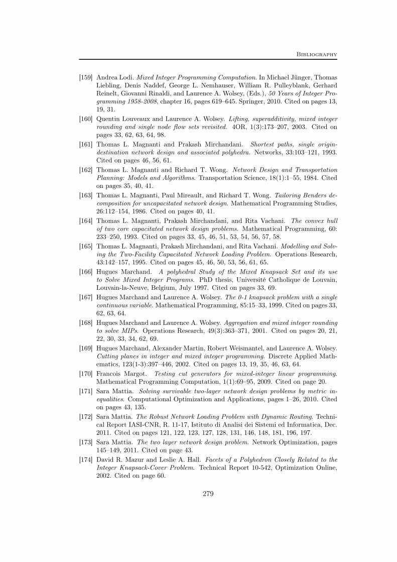
Bibliography
[159] Andrea Lodi. Mixed Integer Programming Computation. In Michael Jünger, ThomasLiebling, Denis Naddef, George L. Nemhauser, William R. Pulleyblank, GerhardReinelt, Giovanni Rinaldi, and Laurence A. Wolsey, (Eds.), 50 Years of Integer Pro-gramming 1958-2008, chapter 16, pages 619–645. Springer, 2010. Cited on pages 13,19, 31.
[160] Quentin Louveaux and Laurence A. Wolsey. Lifting, superadditivity, mixed integerrounding and single node flow sets revisited. 4OR, 1(3):173–207, 2003. Cited onpages 33, 62, 63, 64, 98.
[161] Thomas L. Magnanti and Prakash Mirchandani. Shortest paths, single origin-destination network design and associated polyhedra. Networks, 33:103–121, 1993.Cited on pages 46, 56, 61.
[162] Thomas L. Magnanti and Richard T. Wong. Network Design and TransportationPlanning: Models and Algorithms. Transportation Science, 18(1):1–55, 1984. Citedon pages 35, 40, 41.
[163] Thomas L. Magnanti, Paul Mireault, and Richard T. Wong. Tailoring Benders de-composition for uncapacitated network design. Mathematical Programming Studies,26:112–154, 1986. Cited on pages 40, 41.
[164] Thomas L. Magnanti, Prakash Mirchandani, and Rita Vachani. The convex hullof two core capacitated network design problems. Mathematical Programming, 60:233–250, 1993. Cited on pages 33, 45, 46, 51, 53, 54, 56, 57, 58.
[165] Thomas L. Magnanti, Prakash Mirchandani, and Rita Vachani. Modelling and Solv-ing the Two-Facility Capacitated Network Loading Problem. Operations Research,43:142–157, 1995. Cited on pages 45, 46, 50, 53, 56, 61, 65.
[166] Hugues Marchand. A polyhedral Study of the Mixed Knapsack Set and its useto Solve Mixed Integer Programs. PhD thesis, Université Catholique de Louvain,Louvain-la-Neuve, Belgium, July 1997. Cited on pages 33, 69.
[167] Hugues Marchand and Laurence A. Wolsey. The 0-1 knapsack problem with a singlecontinuous variable. Mathematical Programming, 85:15–33, 1999. Cited on pages 33,62, 63, 64.
[168] Hugues Marchand and Laurence A. Wolsey. Aggregation and mixed integer roundingto solve MIPs. Operations Research, 49(3):363–371, 2001. Cited on pages 20, 21,22, 30, 33, 34, 62, 69.
[169] Hugues Marchand, Alexander Martin, Robert Weismantel, and Laurence A. Wolsey.Cutting planes in integer and mixed integer programming. Discrete Applied Math-ematics, 123(1-3):397–446, 2002. Cited on pages 13, 19, 35, 46, 63, 64.
[170] Francois Margot. Testing cut generators for mixed-integer linear programming.Mathematical Programming Computation, 1(1):69–95, 2009. Cited on page 20.
[171] Sara Mattia. Solving survivable two-layer network design problems by metric in-equalities. Computational Optimization and Applications, pages 1–26, 2010. Citedon pages 43, 135.
[172] Sara Mattia. The Robust Network Loading Problem with Dynamic Routing. Techni-cal Report IASI-CNR, R. 11-17, Istituto di Analisi dei Sistemi ed Informatica, Dec.2011. Cited on pages 121, 122, 123, 127, 128, 131, 146, 148, 181, 196, 197.
[173] Sara Mattia. The two layer network design problem. Network Optimization, pages145–149, 2011. Cited on page 43.
[174] David R. Mazur and Leslie A. Hall. Facets of a Polyhedron Closely Related to theInteger Knapsack-Cover Problem. Technical Report 10-542, Optimization Online,2002. Cited on page 60.
279

Bibliography
[175] R. R. Meyer. On the existence of optimal solutions to integer and mixed-integerprogramming problems. Mathematical Programming, 7(1):223–235, 1974. Cited onpage 15.
[176] Andrew J. Miller and Laurence A. Wolsey. Tight formulations for some simplemixed integer programs and convex objective integer programs. Mathematical Pro-gramming, 98(1):73–88, 2003. Cited on page 158.
[177] Michele Minoux. Robust network optimization under polyhedral demand uncer-tainty is NP-hard. Discrete Applied Mathematics, 158(5):597–603, 2010. Citedon pages 122, 128.
[178] Hans Mittelmann. Benchmarks for Optimization Software, 2012. URL http://plato.asu.edu/bench.html. Cited on pages 13, 74, 99, 100.
[179] Supakom Mudchanatongsuk, Fernando Ordóñez, and Jie Liu. Robust solutions fornetwork design under transportation cost and demand uncertainty. Journal of theOperational Research Society, 59(5):652–662, 2008. Cited on page 128.
[180] George L. Nemhauser and Laurence A. Wolsey. Integer and Combinatorial Op-timization. Wiley-Interscience Series in Discrete Mathematics and Optimization.John Wiley & Sons, New York, 1988. Cited on pages 13, 21, 23, 24.
[181] George L. Nemhauser and Laurence A. Wolsey. A recursive procedure to generate allcuts for 0–1 mixed integer programs. Mathematical Programming, 46(1):379–390,1990. Cited on pages 21, 23, 24, 26.
[182] Neil K. Olver. Robust Network Design. PhD thesis, Department of Mathematicsand Statistics, McGill University, 2010. Cited on pages 122, 123.
[183] K. Onaga and O. Kakusho. On feasibility conditions of multicommodity flows innetworks. Transactions on Circuit Theory, 18(4):425–429, 1971. Cited on page 42.
[184] Fernando Ordóñez and Jiamin Zhao. Robust capacity expansion of network flows.Networks, 50(2):136–145, 2007. Cited on page 128.
[185] Gianpolo Oriolo. Domination Between Traffic Matrices. Mathematics of OperationsResearch, 33(1):91–96, 2008. Cited on pages 122, 124, 133, 134, 137, 186.
[186] Sebastian Orlowski. Optimal Design of Survivable Multi-layer TelecommunicationNetworks. PhD thesis, Technische Universität Berlin, May 2009. Cited on page 43.
[187] Sebastian Orlowski, Michal Pióro, Artur Tomaszewski, and Roland Wessäly. SNDlib1.0–Survivable Network Design Library. Networks, 55(3):276–286, 2010. Cited onpages 59, 65, 100, 136, 164, 209.
[188] Francisco Ortega and Laurence A. Wolsey. A branch-and-cut algorithm for thesingle-commodity, uncapacitated, fixed-charge network flow problem. Networks, 41:143–158, 2003. Cited on pages 40, 49, 50, 65, 92, 94, 100.
[189] Adam Ouorou. Affine Decision Rules for Tractable Approximations to Robust Ca-pacity Planning in Telecommunications. In Proceedings of the 5th InternationalNetwork Optimization Conference (INOC 2011), Lecture Notes in Computer Sci-ence – Network Optimization, pages 277–282, Hamburg, Germany, 2011. Cited onpage 197.
[190] Adam Ouorou and Jean-Philippe Vial. A model for robust capacity planning fortelecommunications networks under demand uncertainty. In Proceedings of the 6thInternational Workshop on Design and Reliable Communication Networks (DRCN2007), pages 1–4, 2007. Cited on pages 122, 180, 185, 196.
[191] Manfred W. Padberg and Giovanni Rinaldi. Optimization of a 532-city symmetrictraveling salesman problem by branch and cut. Operations Research Letters, 6:1–7,1987. Cited on page 18.
280

Bibliography
[192] Manfred W. Padberg and Giovanni Rinaldi. A branch-and-cut algorithm for theresolution of large-scale symmetric traveling salesman problems. SIAM review, 33:60–100, 1991. Cited on page 18.
[193] Manfred W. Padberg, Tony J. Van Roy, and Laurence A. Wolsey. Valid LinearInequalities for Fixed Charge Problems. Operations Research, 33(4):842–861, 1985.Cited on pages 20, 33, 62.
[194] Michal Pióro and Deepankar Medhi. Routing, Flow, and Capacity Design in Com-munication and Computer Networks. Morgan Kaufmann Publishers, 2004. Citedon page 35.
[195] Yves Pochet and Laurence A. Wolsey. Integer knapsack and flow covers with divisiblecoefficients. Discrete Applied Mathematics, 59:57–74, 1995. Cited on pages 20, 33,60.
[196] Michael Poss and Christian Raack. Affine recourse for the robust network designproblem: between static and dynamic routing. In Proceedings of the 5th Interna-tional Network Optimization Conference (INOC 2011), Lecture Notes in ComputerScience – Network Optimization, pages 150–155, Hamburg, Germany, 2011. Citedon page 117.
[197] Michael Poss and Christian Raack. Affine recourse for the robust network designproblem: between static and dynamic routing. ZIB Report 11-04, Zuse InstituteBerlin, Takustr.7, 14195 Berlin, 2011. submitted to Networks. Cited on page 117.
[198] Christian Raack. Employing Mixed-Integer Rounding in Telecommunication Net-work Design. Diploma thesis, Technische Universität Berlin, December 2005.URL http://www.zib.de/groetschel/students/masterstudents.html. Citedon pages 35, 46, 47, 63, 151.
[199] Christian Raack, Arie M. C. A. Koster, Sebastian Orlowski, and Roland Wessäly.Capacitated network design using general flow-cutset inequalities. In Proceedingsof the 3rd International Network Optimization Conference (INOC 2007), Spa,Belgium, 2007. URL http://www.zib.de/Publications/abstracts/ZR-07-14.Cited on pages 65, 66, 107.
[200] Christian Raack, Arie M. C. A. Koster, Sebastian Orlowski, and Roland Wessäly.On cut-based inequalities for capacitated network design polyhedra. Networks, 57(2):141–156, March 2011. Cited on pages 35, 46, 47, 48, 49, 50, 51, 56, 57, 60, 61, 65,66, 70, 72, 92, 94, 95, 97, 107, 151, 171.
[201] Deepak Rajan. Designing capacitated survivable networks: Polyhedral analysis andalgorithms. PhD thesis, University of California, Berkeley, 2004. Cited on pages 35,51, 52.
[202] Ronald L. Rardin and Laurence A. Wolsey. Valid inequalities and projecting themulticommodity extended formulation for uncapacitated fixed charge network flowproblems. European Journal of Operational Research, 71(1):95–109, 1993. Cited onpages 40, 41.
[203] Mauricio G. C. Resende and Panos M. Pardalos, (Eds.). Handbook of Optimizationin Telecommunications. Springer, 2006. Cited on page 35.
[204] Brunilde Sansó and Patrick Sariano. Telecommunications network planning. KluwerAcademic Publishers, 1999. Cited on page 35.
[205] Alexander Schrijver. Theory of Linear and Integer Programming. Interscience seriesin discrete mathematics and optimization. John Wiley & Sons, 1998. Cited onpage 13.
[206] Maria G. Scutellá. On improving optimal oblivious routing. Operations ResearchLetters, 37(3):197–200, 2009. Cited on pages 122, 123.
281

Bibliography
[207] Maria G. Scutellá. Hardness of some optimal oblivious routing generalizations. Tech-nical Report TR-10-05, Universitá di Pisa, 2010. Cited on page 122.
[208] Alexander Shapiro, Darinka Dentcheva, and Andrzej Ruszczyński. Lectures onstochastic programming: modeling and theory, volume 9 of MSP-SIAM series onoptimization. SIAM, 2009. Cited on pages 119, 121.
[209] Allen L. Soyster. Convex programming with set-inclusive constraints and applica-tions to inexact linear programming. Operations research, 21(5):1154–1157, Sept.1973. Cited on pages 119, 121, 123, 131.
[210] Jan I.A. Stallaert. The complementary class of generalized flow cover inequalities.Discrete Applied Mathematics, 77(1):73–80, 1997. Cited on page 62.
[211] Zuse Institute Berlin Thorsten Koch. Zimpl, 2012. URL http://zimpl.zib.de.Cited on page 197.
[212] Steve Uhlig, Bruno Quoitin, Jean Lepropre, and Simon Balon. Providing public in-tradomain traffic matrices to the research community. ACM SIGCOMM ComputerCommunication Review, 36(1):83–86, 2006. Cited on pages 118, 119, 136, 165, 206.
[213] Tony J. Van Roy and Laurence A. Wolsey. Valid Inequalities for mixed 0-1 programs.Discrete Applied Mathematics, 14:199–213, 1986. Cited on pages 62, 63.
[214] Robert Weismantel. On the 0/1 knapsack polytope. Mathematical Programming,77:49–68, 1997. Cited on pages 63, 64.
[215] Roland Wessäly. Dimensioning Survivable Capacitated NETworks. PhD thesis,Technische Universität Berlin, April 2000. Cited on pages 35, 43, 60, 65.
[216] Franz Wesselmann. Generating general-purpose cutting planes for mixed-integerprograms. PhD thesis, Universität Paderborn, 2011. Cited on page 20.
[217] Laurence A. Wolsey. Faces for a linear inequality in 0-1 variables. MathematicalProgramming, 8:165–178, 1975. Cited on pages 20, 33, 63.
[218] Laurence A. Wolsey. Valid inequalities for 0-1 knapsacks and MIPs with generalisedupper bound constraints. Discrete Applied Mathematics, 29(2-3):251–261, 1990.Cited on page 65.
[219] Laurence A. Wolsey. Integer Programming. John Wiley & Sons, 1998. Cited onpages 13, 15, 17, 20, 22.
[220] Laurence A. Wolsey. UFCN instances. Université Catholique de Louvain, Louvain-la-Neuve, Belgium, 2012. URL http://www.core.ucl.ac.be/wolsey/ufcn.htm.Cited on page 100.
[221] Kati Wolter. Implementation of Cutting Plane Separators for Mixed Integer Pro-grams. Master’s thesis, Technische Universität Berlin, 2006. Cited on pages 19, 20,31, 33, 34, 69, 71, 72, 98.
[222] Hande Yaman. The integer knapsack cover polyhedron. SIAM Journal on DiscreteMathematics, 21:551, 2007. Cited on pages 60, 61.
[223] Arrigo Zanette, Matteo Fischetti, and Egon Balas. Lexicography and degeneracy:can a pure cutting plane algorithm work. Mathematical Programming, pages 1–24,2009. Cited on page 18.
[224] Yin Zhang. 6 months of Abilene traffic matrices, 2012. URL http://www.cs.utexas.edu/~yzhang/research/AbileneTM/. Cited on pages 2, 118, 136, 165, 206.
[225] Yin Zhang, Matthew Roughan, Nick G. Duffield, and Albert Greenberg. Fast accu-rate computation of large-scale IP traffic matrices from link loads. ACM SIGMET-RICS Performance Evaluation Review, 31(1):206–217, 2003. Cited on pages 118,136, 165.
282

Bibliography
[226] Zuse Institute Berlin. MIPLIB 2010, 2012. URL http://miplib.zib.de/. Citedon pages 13, 99, 100.
[227] Zuse Institute Berlin. Scip - Solving Constraint Integer Programs, 2012. URLhttp://scip.zib.de/. Cited on pages 1, 7, 18, 69.
[228] Zuse Institute Berlin. SNDlib – Survivable Network Design Library, 2012. URLhttp://sndlib.zib.de/. Cited on pages 59, 65, 100, 118, 119, 124, 131, 164, 166,194, 195, 209.
283

Index
Symbols0, 1/2-cut . . . . . . . . . . . . . . . . . . . . . . . . . 19, 31–32k-partition inequality . . . . . . . . . . . . . . . . . . . . . . 45
Aactivity . . . . . . . . . . . . . . . . . . . . . . . . . see inequalityaffine combination . . . . . . . . . . . . . . . . . . . . . . . . . 14affine hull . . . . . . . . . . . . . . . . . . . . . . . . . . . . . . . . . . 14affine routing . . . . . . . . . . . . . . . . . . . . . . . . . 179–203affinely independent . . . . . . . . . . . . . . . . . . . . . . . . 14anti-parallel arcs . . . . . . . . . . . . . . . . . . . . . . . . . . . 36arc flow formulation . see link-flow formulationarc inconsistency . . . . . . . . . . . . see inconsistencyarc pattern. . . . . . . . . . . . . . . . . . . . . . . . . .78, 83–85arc-residual capacity inequality . . 45, 52–54, 57arc-set polyhedra. . . . . . . . . . . . . . . . . . . . . . . . . . .45associated digraph . . . . . . . . . . . . . . . . . . see graph
Bbasic relaxation . . . . . . . . . . . . . . . . . . . . . . . . . . . . 27basis . . . . . . . . . . . . . . . . . . . . . . .see linear programBenders decomposition . . . . . . . . . . . . . . . . . . . . . 42bound substitution . . . . . . . . . . . . . . . . . . . . . . . . . 32branch-and-bound. . . . . . . . . . . . . . . . . . . . . . . . . .16branch-and-cut . . . . . . . . . . . . . . . . . . . . . . . . . . . . .18branching . . . . . . . . . . . . . . . . . . . . . . . . . . . . . . . . . . 16
branching tree . . . . . . . . . . . . . . . . . . . . . . . . 16
Cc-MIR . . . . . . .see complemented mixed integer
roundingcapacitated network design . . . . . . . . . . . . 38, 120CG . . . . . . . . . . . . . . . . . . . . . . see Chvátal-GomoryChvàtal-Gomory . . . . . . . . . . . . . . . . . . . . . . . . . . . 19
closure . . . . . . . . . . . . . . . . . . . . . . . . . . . . . . . . 23inequality, cut . . . . . . . . . . . . . . . . . . . . . 19, 23
circulation. . . . . . . . . . . . . . . . . . . . . . . .37, 182, 183column generation . . . . . . . . . . . . . . . . . . . . . . . . . 42commodity . . . . . . . . . . . . . . . . . . . . . . . . . . . . . . . . . 36compact formulation . . 127, 132, 135, 137–139,
183–185complemented mixed integer rounding . . . . . 19,
32–34contraction . . . . . . . . . . . . . see graph contractionconvex combination . . . . . . . . . . . . . . . . . . . . . . . . 14
convex hull. . . . . . . . . . . . . . . . . . . . . . . . . . . . . . . . .14coupled multi-commodity flow. . . . . . . . . . . . . .39Cplex . . . . . . . 18, 19, 33, 64, 69, 100, 102–110,
164–178, 197–203cut . . . . . . . . . . . . . . . . . . . . . . . . . . see cutting planecut-and-branch. . . . . . . . . . . . . . . . . . . . . . . . . . . . .18cut-pool. . . . . . . . . . . . . . . . . . . . . . . . . . . . . . . . . . . .20cut-set . . . . . . . . . . . . . . . . . . . . . . . .see network cutcut-set inequality . . . . . . 45–50, 56, 60, 147–152,
169–171cut-set lifting theorem . . . . . . . . . . . . 47, 145–146cut-set polyhedron . . . . . . . 45, 47, 144, 145, 153cut-set residual capacity inequality . . . . . . . . . 56cutting plane . . . . . . . . . . . . . . . . . . . . . . . . . . . 17–20
separation . . . . . . . . . . . . . . . . . see separationcutting plane method . . . . . . . . . . . . . . . . . . . . . . 16cut generating LP. . . . . . . . . . . . . . . . . . . . . . . . . . 26
Ddemand . . . . . . . . . . . . . . . . . . . . . . . . . . . . . . . . . . . . 36
deviation. . . . . . . . . . . . . . . . . . . . . . . . . . . . .137domination . . . . . . . . . . . . . . . . . 130, 133–134
total. . . . . . . . . . . . . . . . . . . . . . . . . . . . . . .134weak . . . . . . . . . . . . . . . . . . . . . . . . . . . . . . 134
nominal . . . . . . . . . . . . . . . . . . . . . . . . . 136, 137peak . . . . . . . . . . . . . . . . . . . . . . . . . . . . . . . . . 137scenario
extreme . . . . . . . . . . . . . . . . . . 131, 133, 138maximal . . . . . . . . . . . . . . . . . . . . . . . . . . . 147strictly maximal . . . . . . . . . . . . . . . . . . . 147
demand polytope . . . . . . . . . . see uncertainty setΓ-model . . . . . .136–141, 152–164, 194–203Hose-model . . . . . . . . . . . . . . . . . . . . . .134–136
dicut inequality . . . . . . . . . . . . . . . . . . . . . . . . . . . . 49digraph . . . . . . . . . . . . . . . . . . . . . . . . . . . . . see graphdual multiplier . . . . . . . . . . . . . . . . see row weightsdual program . . . . . . . . . . . . . . see linear programdual weigts . . . . . . . . . . . . . . . . . . . see row weightsduality. . . . . . . . . . . . . . . . . . . . .see linear programdualization . . . . . . . . . . . . . 131–132, 135, 138, 184dynamic routing . . . . . . .126, 180, 181, 191–193,
195–203
Eembedded network . . . . . . . . . . . . . . . . . . 75, 79–82
285

Index
envelope inequality . . . . . . . . . . 155–164, 171–174lower . . . . . . . . . . . . . . . . . . . . . . . . . . . . 156, 157upper . . . . . . . . . . . . . . . . . . . . . . . . . . . . . . . . 157
Ethernet . . . . . . . . . . . . . . . . . . . . . . . . . . . . . . . . . . . 58explicit link capacities . . . . . . . . . . . . . . . . . . . . . .59extended formulation . . . . . . . . . . . . . . . . . . . . . 137extreme scenario . . . . . . see demand, see vertex
Fface . . . . . . . . . . . . . . . . . . . . . . . . . . . see polyhedronfacet . . . . . . . . . . . . . . . . . . . . . . . . . . see polyhedronfacet-defining . . . . . . . . . . . . . . . . . . . see inequalityfacility . . . . . . . . . . . . . . . . . . . . . . . . . . . . . 58–64, 151flow . . . . . . . . . . . . . . . . . . . . . . . . . . . . . . . . . . . . . . . . 36
irreducible . . . . . . . . . . . . . . . . . . . . . . . . . . . . 37link-flow . . . . . . . . . . . . . . . . . . . . . . . . . . . . . . 39multi-commodity . . . . . . . . . . . . . . . . . . . . . . 36path-flow. . . . . . . . . . . . . . . . . . . . . . . . . . . . . .37point-to-point, (s, t) . . . . . . . . . . . . . . . . . . . 37reducible . . . . . . . . . . . . . . . . . . . . . . . . . . . . . . 37single-commodity . . . . . . . . . . . . . . . . . . . . . 36
flow conservation constraint . . . . . . . . . . . . . . . . 36flow cover . . . . . . . . . . . . . . . . . . . . . . . . . . . . . . . . . . 62flow cover inequality . . . . . . . . . . . . . . . . 19, 61–64flow cut-set inequality . 45–50, 56, 60, 148–152,
171–174flow row . . . . . . see flow conservation constraintflow system . . . . . . . . see network matrix, 80–81flow template . . . . . . . . . . . . . . . . . . . . . . . . 128, 180fractional part . . . . . . . . . . . . . . . . . . . . . . . . . . . . . 14
GΓ-model . . . . . . . . . . 136–141, 152–164, 194–203generalized upper bound . . . . . . . . . . . . . . . . . . . 59Gomory cut . . . . see Gomory mixed integer cutGomory mixed integer cut . . . . . . . . . . 18, 29–30graph . . . . . . . . . . . . . . . . . . . . . . . . . . . . . . . . . . . . . . 35
associated (digraph) . . . . . . . . . . . . . . . 36, 54connected . . . . . . . . . . . . . . . . . . . . . . . . . . . . . 36contraction . . . . . . . . . . . 65, 94–95, 167–168directed, digraph . . . . . . . . . . . . . . . . . . . . . . 35simple . . . . . . . . . . . . . . . . . . . . . . . . . . . . . . . . 35strongly connected (digraph) . . . . . . . . . . 36undirected . . . . . . . . . . . . . . . . . . . . . . . . . . . . 35
graph isomorphism . . . . . . . . . . . . . . . . . . . . . . . . . 75GUB. . . . . . . . . . . . .see generalized upper boundGUB cover inequality . . . . . . . . . . . . . . . . . . . . . . 64Gurobi . . . . . . . . . . . . . . . . . . . . . . . . . . . . . . . 18, 69
HHose-model . . . . . . . . . . . . . . . . . . . . . . 134–136, 194
Iincidence function . . . . . . . . . . . . . . . . . . . . . . 36, 86
inconsistency. . . . . . . . . . .78, 86, 88–90, 108–110inequality
activity . . . . . . . . . . . . . . . . . . . . . . . . . . . . . . . 15domination. . . . . . . . . . . . . . . . . . . . . . . . . . . .15efficacy. . . . . . . . . . . . . . . . . . . . . . . . . . . . . . . .20facet-defining . . . . . . . . . . . . . . . . . . . . . . . . . 15projection . . . . . . . . . . . . . . . . . . . . . . . . . 55–57rank . . . . . . . . . . . . . . . . . . . . . . . . . . . . . . . . . . 23separation . . . . . . . . . . . . . . . . . see separationstrictly dominates . . . . . . . . . . . . . . . . . . . . . 15valid . . . . . . . . . . . . . . . . . . . . . . . . . . . . . . . . . . 14violation . . . . . . . . . . . . . . . . . . . . . . . . . . . . . . 15
integer program . . . . . . . . . . . . . . . . . . . . . . . . . . . . 15integrality gap . . . . . . . . . . . . . . . . . . . . . . . . . . . . . 40integrality property . . . . . . . . . . . . . . . . . . . . . . . . 44intersection cut . . . . . . . . . . . . . . . . . . . . . . . . . . . . 26IP (Internet Protocol) network . . . . . . 2, 58, 137
JJapanese Theorem . . . . . . . . . . . . . . . . . . . . . . . . . 42
Kk-partition inequality . . . . . . . . . . . . 50–52, 57–58knapsack cover inequality . . . . . . . . . . . 19, 63–64
LLagrangian dual. . . . . . . . . . . . . . . . . . . . . . . . . . . .44Lagrangian relaxation . . . . . . . . . . . . . . . . . . . . . . 43lazy constraints . . . . . . . . 132, 164, 167, 169, 175lift-and-project . . . . . . . . . . . . . . . . . . . . . . . . . . . . . 26linear combination . . . . . . . . . . . . . . . . . . . . . . . . . 14linear program . . . . . . . . . . . . . . . . . . . . . . . . . . . . . 15
basis . . . . . . . . . . . . . . . . . . . . . . . . . . . 26, 29–30dual . . . . . . . . . . . . . . . . . . . . . . . . . . 15, 42, 131primal . . . . . . . . . . . . . . . . . . . . . . . . . . . . . . . . 15
linear programming relaxation . . . . . . . . . . . . . 15linearly independent . . . . . . . . . . . . . . . . . . . . . . . 14link design . . . . . . . . . . . . . . . . . . . . . . . . . see facilitylink-flow formulation . . . . . . . . . . . . . . . . . . . 39, 69lower envelope inequality . . . . . . . . . see envelope
inequalitylower region. . . . . . .see envelope inequality, 155LP. . . . . . . . . . . . . . . . . . . . . . . . .see linear program
Mmax-flow min-cut . . . . . . . . . . . . . . . . . . . . . . . . . . 42maximal demand scenario. . . . . . . . .see demandmaximum embedded network problem. . . . . .75MCF . . . . . . . . . . . . . . . see multi-commodity flowMCF-cut . . . . . . . . . . . . . . . . . . . . . . . . . . 19, 69–114MCF-separator . . . . . . . . . . . . . . . . . . . . . . . . 69–114metric cone . . . . . . . . . . . . . . . . . . . . . . . . . . . . . . . . 43metric inequalities . . . . . . . . . . . . . . . . . . . . . . . . . 43metric inequality . . . . . . . . . . 42, 48–52, 127, 130
286
Index
MIP . . . . . . . . . . . . . . . see mixed integer programMiplib . . . . . . . . . . . . . . . . . . . . . . . . . 100, 102–111MIR . . . . . . . . . . . . . . see mixed integer roundingmixed dicut inequality . . . . . . . . . . . . . . . . . . . . . 49mixed integer knapsack set . . . . . . . . . . . . . . . . . 61mixed integer program . . . . . . . . . . . . . . . . . . . . . 15mixed integer rounding . . . . . . . . . . . . . . . . . 21–29
closure . . . . . . . . . . . . . . . . . . . . . . . . . . . . . . . . 23function . . . . . . . . . . . . . . . . . . . . . . . . . . . . . . . 24inequality, cut . . . . . . . . . . . . . . . . . . . . . . . . . 21rank . . . . . . . . . . . . . . . . . . . . . . . . . . . . . . . . . . 23
mixed integer set . . . . . . . . . . . . . . . . . . . . . . . . . . .15modular link capacities . . . . . . . . . . . . . . . . . . . . .59multi cut-set polyhedron . . . . . . . . . . . . . . . . . . . 45multi-commodity flow . . . . . . . . . . . . . . . . see flowmulti-facility . . . . . . . . . . . . . . . . . . . . . . . . . . 58, 151
Nnetwork. . . . . . . . . . . . . . . . . . . . . . . . . . . . .see graphnetwork cut . . . . . . . . . . . . . . . . . . . . . . . . . . . . . . . . 36
shore. . . . . . . . . . . . . . . . . . . . . . . . . . . . . . . . . .36network design polyhedron . . . . . . . . . . . . . . . . . 39network inequalities . . . . . . . . . . . . . . . . . . . . . . . . 69network matrix . . . . . . . . . . . . . . . . . . . . . . . . . 37, 75node-arc incidence matrix . see network matrix
Ooblivious routing . . . . . . . . . . . . see static routing
Ppoint-to-point demand . . . . . . . . . . . . . . . . . . . . . 37polyhedron. . . . . . . . . . . . . . . . . . . . . . . . . . . . . . . . .14
anti-dominant . . . . . . . . . . . . . . . . . . . . . . . .134dimension . . . . . . . . . . . . . . . . . . . . . . . . . . . . . 14face . . . . . . . . . . . . . . . . . . . . . . . . . . . . . . . . . . . 15facet . . . . . . . . . . . . . . . . . . . . . . . . . . . . . . . . . . 15projection. .42, 52, 55, 135, 138, 139, 145,
147, 153, 159rational . . . . . . . . . . . . . . . . . . . . . . . . . . . . . . . 14vertex . . . . . . . . . . . . . . . . . . . . . . . . . . . . . . . . . 15
polytope . . . . . . . . . . . . . . . . . . . . . . . . . . . . . . . . . . . 14projection . . . . . . . . . . . . . . . . . . . . . see polyhedron
Rrecourse . . . . . . . . . . . . . . . . . . . . . . . . . . . . . . 126, 128reflection . . . . . . . . . . . . . . . . . . . . . . . . . . . . . . . 75, 81robust cut-set polyhedron . . . . . . . . . . . . . . . . . 145robust counterpart 126, 132, 184, 185, 195–196robust cut-set inequality . . . . . . . . . . . . . . 147–152robust envelope inequality. . . . . . . .see envelope
inequalityrobust flow cut-set inequality . . . . . . . . . 148–152robust network design. . . . . . . . . . . . . . . . . . . . .120root node . . . . . . . . . . . . . . . . . . see branching tree
rounded metric inequality . . . . . . . . . . . . . . . . . . 43routing . . . . . . . . . . . . . . . . . . . . . . . . . . . . . . . . . . . 126
affine . . . . . . . . . . . . . . . . . . . . . . . . . . . . 179–203dynamic . . . . . . 180, 181, 191–193, 195–203static . . . . . . . . . 179–181, 187–191, 195–203
routing template . . . . . . . . . . . . . . . . 128, 182, 183row multiplier . . . . . . . . . . . . . . . . see row weightsrow scanning addition algorithm . . . . . . . . 77, 79row weights. . . . . . . . . . . . . . . . . . . . . .22–34, 91–94
SScip . . . . . . . . . . . . . 18, 19, 33, 69, 100, 102–111SDH . . . . . . . see Synchronous Digital Hierarchysearch tree . . . . . . . . . . . . . . . . . see branching treeseparation49, 52, 53, 91–95, 132–133, 135, 139,
151, 167problem. . . . . . . . . . . . . . . . . . . . . . . . . . . . . . . 26
separation problem. . . . . . . . . . . . . . . . . . . . . . . . .17shore . . . . . . . . . . . . . . . . . . . . . . . . . see network cutsigned graph . . . . . . . . . . . . . . . . . . . . . . . . . . . . . . . 74simple flow cut-set inequality . . . . . . . . . . 48, 148simplex tableau . . . . . . . . . . . . . . . . . . . . . . . . . . . . 30single node flow set . . . . . . . . . . . . . . . . . . . . . . . . 61single row relaxation . . . . . . . . . . . . . . . . . . . . . . . 19Sndlib . . . . . . .100, 102–111, 164–178, 195–203split . . . . . . . . . . . . . . . . . . . . . . . . . . . . . . . . . . . . . . . 16
closure . . . . . . . . . . . . . . . . . . . . . . . . . . . . . . . . 23inequality, cut . . . . . . . . . . . . . . . . . . . . . . . . . 25rank . . . . . . . . . . . . . . . . . . . . . . . . . . . . . . . . . . 23
stable routing . . . . . . . . . . . . . . . see static routingstatic routing . 128, 179–181, 187–191, 195–203Steiner cut-set inequality . . . . . . . . . . . . . . . . . . 49Steiner tree problem. . . . . . . . . . . . . . . . . . . . 40, 41STM. . . . . . see Synchronous Transport Modulestrictly maximal demand scenario . see demandsubadditivity . . . . . . . . . . . . . . . . . . . . . . . . . . . 24–25Synchronous Digital Hierarchy . . . . . . . . . . . . . 58Synchronous Transport Module . . . . . . . . . . . . 58
Ttight metric inequality . . . . . . . . . . . . . . 43, 48–52
Uuncapacitated fixed charge network flow prob-
lem . . . . . . . . . . . . . . . . . . . . . . . . . . . . . . 40uncertainty set. . . . . . . . . . . . . .122, 126, 134–141
domination . . . . . . . . . . . . . . . . . . . . . . 133–134upper envelope inequality . . . . . . . . see envelope
inequalityupper region . . . . . . see envelope inequality, 155
Vvertex . . . . . . . . . . . . . . . . . . . . . . . . . see polyhedronviolation . . . . . . . . . . . . . . . . . . . . . . . . see inequality
287
Copyright © 2022 FDOKUMEN