
Merchant Operations: Real Option Management of Commodity ...
156
Foundations and Trends R in sample Vol. xx, No xx (2013) 1–151 c 2013 Tepper Working Paper 2013-E3; May 2013; prepared for Foundations and Trends in Technology, Information and Operations Management DOI: xxxxxx Merchant Operations: Real Option Management of Commodity and Energy Conversion Assets Nicola Secomandi 1 and Duane J. Seppi 2 1 Tepper School of Business, Carnegie Mellon University, 5000 Forbes Av- enue, Pittsburgh, PA 15213-3890, USA, [email protected] 2 Tepper School of Business, Carnegie Mellon University, 5000 Forbes Av- enue, Pittsburgh, PA 15213-3890, USA, [email protected] Abstract The value chain for energy and other commodities entails physical con- versions through refineries, power plants, storage facilities, and trans- portation and other capital-intensive infrastructure. When the opera- tion of such commodity conversion assets occurs alongside liquid mar- kets for the input and output commodities, the operating flexibility of conversion assets can be managed as real options on the underlying commodity prices. Merchant operations is an integrated trading and operations approach that (i) buys and sells commodities to support market-value maximizing optimal, or at least near-optimal, operating policies and (ii) values conversion assets, for capital budgeting, based on the cash flows such policies produce. This monograph introduces the concept of merchant operations, presents the basic principles of op- tion valuation, surveys foundational models of commodity and energy
-
Upload
khangminh22 -
Category
Documents
-
view
0 -
download
0
Transcript of Merchant Operations: Real Option Management of Commodity ...
Foundations and TrendsR© insampleVol. xx, No xx (2013) 1–151c© 2013 Tepper Working Paper 2013-E3; May2013; prepared for Foundations and Trendsin Technology, Information and OperationsManagementDOI: xxxxxx
Merchant Operations: Real OptionManagement of Commodity and Energy
Conversion Assets
Nicola Secomandi1 and Duane J. Seppi2
1 Tepper School of Business, Carnegie Mellon University, 5000 Forbes Av-enue, Pittsburgh, PA 15213-3890, USA, [email protected]
2 Tepper School of Business, Carnegie Mellon University, 5000 Forbes Av-enue, Pittsburgh, PA 15213-3890, USA, [email protected]
Abstract
The value chain for energy and other commodities entails physical con-versions through refineries, power plants, storage facilities, and trans-portation and other capital-intensive infrastructure. When the opera-tion of such commodity conversion assets occurs alongside liquid mar-kets for the input and output commodities, the operating flexibility ofconversion assets can be managed as real options on the underlyingcommodity prices. Merchant operations is an integrated trading andoperations approach that (i) buys and sells commodities to supportmarket-value maximizing optimal, or at least near-optimal, operatingpolicies and (ii) values conversion assets, for capital budgeting, basedon the cash flows such policies produce. This monograph introducesthe concept of merchant operations, presents the basic principles of op-tion valuation, surveys foundational models of commodity and energy
price evolution, analyzes the structure of optimal operating policies forcommodity conversions (focusing specifically on inventory and otherintertemporal linkages in storage, inventory acquisition and disposal,and swing assets), considers a variety of heuristic storage operatingpolicies, and discusses future trends in this multidisciplinary area ofresearch and business applications.
Contents
1 Aim and Scope 1
2 Commodity Conversion Assets and MerchantOperations 3
2.1 Commodities and Energy Sources 32.2 Physical and Financial Markets 52.3 Conversion Assets and Merchant Operations 72.4 Commodity Conversion Assets as Real Options 92.5 Outline of this Monograph 132.6 Notes 14
3 Real Option Valuation 16
3.1 Statically Complete Markets 193.2 Dynamically Complete Markets 213.3 Dynamically Incomplete Markets 293.4 Calibration 303.5 Summary 31
i
ii Contents
3.6 Notes 32
4 Modeling Commodity and Energy Prices 33
4.1 Spot-price Evolution Models 414.2 Futures Term Structure Models 504.3 Equilibrium Models 564.4 Empirical Research on Commodity Prices 584.5 Summary 594.6 Notes 60
5 Modeling Storage Assets 61
5.1 Model 665.2 Basestock Optimality 715.3 Price Monotonicity of the Optimal Basestock Targets 805.4 Computation 835.5 The Value of Optimally Interfacing Operational and
Trading Decisions 855.6 Conclusions 925.7 Notes 92
6 Benchmarking the Practice Based Management ofStorage Assets 95
6.1 Valuation Problem and Exact SDP 996.2 Practice-based Heuristics 1026.3 ADP Model 1066.4 Upper Bounds 1106.5 Numerical Results 1116.6 Conclusions 1186.7 Notes 119
7 Modeling Other Conversion Assets 121
7.1 An Inventory Disposal Asset 1227.2 An Inventory Acquisition Asset 125
Contents iii
7.3 Swing Assets 1277.4 Conclusions 1307.5 Notes 130
8 Trends 133
8.1 Financial Hedging 1338.2 Analysis of Other Commodity Conversion Assets 1348.3 Approximate Dynamic Programming 1358.4 Price Model Error 1368.5 Price Impact 1368.6 Equilibrium Asset Pricing 1378.7 Capacity Choice 137
Acknowledgements 139
References 140
1
Aim and Scope
Commodity conversion assets perform various transformation pro-cesses, including the production, refining, industrial and commercialconsumption, and distribution of physical commodities and energysources, such as grains, metals, coal, crude oil, and natural gas. Thismonograph deals with the management and valuation of conversionassets. Commodities and energy are traded on physical markets. It isthus natural to approach the management of commodity conversionassets from the perspective of merchant operations. This approach ad-justs the level of the conversion activities to profit from the dynamicsof commodity prices.
Managing merchant operations to maximize the market value ofcommodity conversion assets is a complex task. It requires both mod-els of the evolution of commodity prices and stochastic optimizationmodels of the conversion activities. The existence of traded contractson commodities and energy sources allows commodity conversion assetsto be interpreted as real options on the prices of the underlying com-modities. This real option interpretation greatly facilitates formulatingthe necessary mathematical models.
The valuation of real options shares the same theoretical founda-
1
2 Aim and Scope
tions as the valuation of financial options. The specific real options val-uation complications that arise in the context of merchant operationsare distinguished from financial options valuation problems by one ormore of the following features: decisions at multiple dates, intertempo-ral linkages across decisions, payoffs determined by operational costsand contractual provisions, engineering-based constraints on operat-ing decisions, and quantity decisions rather than binary exercise/no-exercise decisions. The valuation of Bermudan financial options alsoinvolves decisions at multiple dates and intertemporal linkages acrossdecisions, but the other features in this list are largely unique to mer-chant operations. Moreover, even when the structure of an optimaloperating (exercise) policy can be explicitly characterized, determiningsuch a policy typically involves numerical computation and approxi-mations. Closed-form solutions are thus rare in merchant operations,while they are more widespread in the valuation of financial options.
The aim of this monograph is to present the basic tenets of merchantoperations, that is, the management of commodity conversion assets asreal options on commodity prices. The focus here is on the foundationalprinciples that underlie the valuation of real options, on basic modelsof both the evolution of commodity and energy prices and commodityconversion assets, and on optimal and heuristic operating policies.
In terms of current research, the scope of this monograph is lim-ited to models that represent the foundations of merchant operations.There are many models in the current literature that pass this test.The limited number of pages available to this monograph thus furtherreduces its scope. In addition, this monograph includes a discussion offuture trends in merchant operations research and applications.
2
Commodity Conversion Assets and MerchantOperations
This chapter briefly introduces the basic commodity groups in §2.1,and illustrates the trading of commodities in physical and financialmarkets in §2.2. This discussion provides the necessary elements forintroducing the concepts of commodity conversion assets and merchantoperations in §2.3. This chapter also shows that merchant operationscan be usefully cast in the framework of real options in §2.4, providingsome examples of the real option management of commodity conversionassets. Some of these examples are substantial simplifications of howcommodity conversion assets are operated in practice, but they setthe stage for more realistic models. The discussion of these examplesprovides a point of departure for the rest of this monograph, which isoutlined in §2.5. Section 2.6 offers pointers to the existing literature.
2.1 Commodities and Energy Sources
According to the Webster’s New Universal Unabridged Dictionary[201], a commodity is “any unprocessed or partially processed good.”Commodities can be grouped according to three basic categories: agri-culturals, metals, and energy sources. Each of the groups includes sev-
3
4 Commodity Conversion Assets and Merchant Operations
eral commodity types, for example:
• Agriculturals: grains (corn, oats, rice, and wheat), oil andmeal (soybean, soyoil, and soymeal), livestock (pork andbeef), foodstuff (cocoa, coffee, orange juice, potatoes, andsugar), textiles (cotton), and forest products (lumber andpulp).
• Metals: gold, silver, platinum, palladium, copper, and alu-minum.
• Energy sources: coal, crude oil, heating oil, gasoline, naturalgas, propane gas, and electricity.
Commodity types can be further categorized according to grade andquality. In addition, due to limited transportation and storage capacity,the same commodity type at different locations and/or times effectivelyconstitutes separate commodities. For instance, consider natural gas attwo ends of a pipeline that transports it, or the availability of naturalgas in a storage facility at two different dates. Thus, location and timeare defining attributes of commodity types.
Commodities are basic inputs to production, distribution, and con-sumption activities. They thus play important economic roles. For ex-ample, natural gas is extensively used for heating, e.g., by about 50%of the households in the United States (Casselman [46]), and electricitygeneration, e.g., about 30% of worldwide electricity production is basedon natural gas (Geman [91]); it is also increasingly the fuel of choice fornew electricity generation projects, due in part to the recent shale gasboom (Smith [183]); it is having an impact on the worldwide liquefiednatural gas trade (Davis and Gold [60]) and the planning of new majorpipeline constructions (Chazan [52], Gold [97]); and it is an input toseveral manufacturing processes, including the refining of oil, and theproduction of chemicals, ammonia and methanol, steel and aluminum,and paper (Kaminski and Prevatt [118]).
Although energy is just one commodity group, it is emphasized inthe title of this section and throughout this monograph because thereis a substantial literature that deals with the application of real optionmethods to energy.
2.2. Physical and Financial Markets 5
2.2 Physical and Financial Markets
Commodities are traded in physical and financial markets. In bothcases, transactions can be on a spot or forward basis. Spot transac-tions involve the immediate, or at least very near term (e.g. , nextday), transfer of the physical commodity or financial ownership thereof.With forward transactions this transfer occurs at a specified date in thefuture.
Physical trading eventually leads to the transfer of a commodityfrom one party to another party. For example, the same lot of naturalgas for next day delivery may be purchased and sold several timesduring a given day, but this lot must be transfered from a seller to abuyer on the delivery date.
Financial markets for commodities, such as the Chicago Mercan-tile Exchange (CME), the New York Mercantile Exchange (NYMEX),the IntercontinentalExchange (ICE), and the London Metal Exchange(LME) trade various contracts that specify different commodity own-ership structures. Futures contracts specify obligations to deliver orreceive a given amount of a commodity, at a given price, and at a givenmaturity. (One month maturity futures typically have the highest vol-ume.) Selling and purchasing, respectively, a futures contract entailsthe obligation to deliver and receive a commodity. However, most fu-tures traders typically close out their positions via an offsetting tradebefore maturity. Thus, futures trading need not lead to physical han-dling of a commodity. Futures prices are set for each delivery date tomake the value of the futures contract zero. Hence, there is a singlefutures price for each delivery date.
Options contracts on futures specify the right to purchase or sella given futures contracts at a given price and maturity. Call and putoptions on futures, respectively, given their owners the right to purchaseand sell a futures at a contractually specified strike price. The payoff ofa call option is the positive part of the difference between the futuresprice at the option maturity and the strike price. The payoff of a putoption is the positive part of the difference between the strike price andthe futures price at maturity. Typically, there are options traded withmany strikes and expiries.
6 Commodity Conversion Assets and Merchant Operations
Additional types of options include calendar spread options on fu-tures contracts. These options give their owners the right to exchangea futures contract with a given maturity for a futures contract witha different maturity at a given strike price. Effectively, these optionsgiven their owners the right to purchase or sell the difference betweentwo futures prices at a given maturity and strike price. The payoff ofa call calendar spread option is the maximum between zero and thedifference between the spread between the two futures prices and thestrike price. The payoff of a put spread option is defined in an analogousmanner.
The options so far described are of the European types, meaningthat contractually they can be exercised only at maturity. American(respectively, Bermudan) versions of these options given their ownersthe right to exercise them at any time (respectively, a set of predeter-mined times) before maturity.
Futures, call and put options, and call and put calendar spread op-tion are traded on organized financial exchanges, such as CME, ICE,LME, and NYMEX, which guarantee the clearing of every trade. Thatis, these trades are insured by the exchange against the risk of counter-party default. These contracts and additional contracts are also tradedon over-the-counter (OTC) markets. Trades on OTC markets are di-rectly exposed to greater counterparty default risk.
Physical trading has an obvious use, as it supports the functioningof production, distribution, and consumption processes. The prices ofcommodities and contracts on commodities are variable and uncertain.They exhibit both seasonality (deterministic variability) and volatility(stochastic variability). Some theories explain the existence of financial(futures) markets based on price-risk aversion/control arguments (see,e.g., Keynes [124], Duffie [75]). Others rely on transaction costs princi-ples (Williams [202, 203]). In the context of this monograph, financialmarkets play a useful role in terms of the management of commod-ity conversion assets in the face of variable and uncertain commodityprices, as explained in §§2.3-2.4.
2.3. Conversion Assets and Merchant Operations 7
2.3 Conversion Assets and Merchant Operations
Commodities are produced and used for further processing, consump-tion, and distribution. In this monograph, the industrial facilities thatperform these transformation processes are called commodity conver-sion assets. Conversion here is used in a broad sense. It refers to
• The production of a commodity, such as the extraction ofnatural gas from underground wells;
• A physical transformation of a commodity, such as the refin-ing of crude oil, into another commodity, such as gasoline,jet fuel, and naphtha; or
• A change in availability of a commodity, such as the trans-portation of this commodity in between different locationsor its storage over time.
Managing commodity conversion assets thus requires performing oneor more operational activities, such as the production, processing, re-fining, transportation, storage, distribution, and physical trading ofcommodities.
Consider, for example, a storage asset, such as a grain or metalwarehouse, or an underground natural gas storage facility. Storage isused to help match the supply and demand of a given commodity overtime. Storage assets feature limited space, and may also exhibit limitson the amount of inventory that can be acquired or disposed of dur-ing a given time period. Managing a commodity storage asset requiresdetermining an inventory trading policy subject to space and possiblycapacity constraints.
As another example, consider a refining asset, such as a crude oilrefinery. A crude oil refinery includes various storage tanks for both theinputs, that is, various grades of crude oil, and the intermediate prod-ucts and outputs. Managing this refinery requires a joint inventory andproduction policy that determines the inventory levels in these tanksand how the inputs are converted and blended into refined products.In addition, shipping and transportation policies support the sourcingof crude oil and the distribution of refined products.
8 Commodity Conversion Assets and Merchant Operations
In practice, the owners of the capacity of a given commodity conver-sion assets often rent all or part of this capacity to third parties, suchas commodity and energy merchants, for given time periods throughcontracts. This occurs in the natural gas industry in the United States,where, by federal regulation, the owners of interstate pipelines and stor-age facilities must make their capacity available to shippers on an openaccess basis. Tolling agreements play a similar role in the power genera-tion industry whereby physical generator owners can sell off generationrevenue to investors. In this monograph, contracts on the capacity ofa commodity conversion assets are themselves considered commodityconversion assets. In addition to determining an optimal operating pol-icy for such assets, the determination of their market value is an impor-tant practical problem, as it forms the basis for contract negotiation.
Commodity conversion assets are embedded in a market environ-ment for the commodities that they convert. Indeed, commodity con-version assets are the building blocks of both physical and financialcommodity markets. Commodity production and storage assets, as wellas transportation assets, such as pipelines, ships, and related loadingand unloading facilities at ports, play a central role in the determina-tion of spot and futures prices (Williams and Wright [204]). Commodityconversion assets can thus be managed taking a merchant perspective,which involves the adjustment of the level of the conversion activities toreflect the dynamics of commodity prices. For example, the decision torefine crude oil into refined products depends on the respective spreadsbetween the prices of these products and the price of crude oil. Thelabel merchants operations refers to this approach to the managementof commodity conversion assets.
The optimal management of merchant operations thus requiresmanaging operational activities in the face of variable and uncertaincommodity prices. The valuation of these operational policies also isimportant. In general, these are difficult tasks. Interpreting conversionassets as real options facilitates the execution of these tasks.
2.4. Commodity Conversion Assets as Real Options 9
2.4 Commodity Conversion Assets as Real Options
Managerial flexibility in projects can be viewed as embedded real op-tions. Managerial flexibility in merchant operations is linked to theuncertain evolution of commodity and energy prices. For example, theability of oil and natural gas producers to drill or shut down wells de-pending on the prevailing oil and natural gas prices can be interpretedas a real option on these prices. Other commodity conversion assetshave analogous interpretations as real options on commodity prices.This means that merchant operations of managing commodity conver-sion assets amounts to optimally exercising specific real options. Tomake this concept more concrete, it is useful to discuss some examples.
Simplified commodity production assets and call options.Consider a natural gas well. Let c be the cost of producing one unit ofgas; st be the spot price of natural gas at time t; and Q the rate of pro-duction. For simplicity, ignore the cost of shutting down and resumingproduction, the time required to do so, and any other intertemporalconsiderations (e.g., the ability of the asset manager to time the sale ofnatural gas). Then, the optimal merchant management policy for thissimplified natural gas production asset is to produce and sell Q unitsof natural gas at time t when the spot price of natural gas st exceedsthe marginal production cost c, and do nothing otherwise. The payoffof this policy at time t is
maxst − c, 0 ·Q, (2.1)
which is also the payoff of a call option on Q units of the time t spotprice of natural gas st with strike price equal to c. This observationjustifies thinking of the simplified natural gas well at time t as a realcall option on the spot price with a strike price equal to the marginalproduction cost and notional amount equal to the production rate (thenotional amount of an option is the “number” of such options ownedby a trader). The merchant operations of this asset thus amounts tothe optimal exercise of this option.
The time t futures price with maturity t, Ft,t, is identical to thetime t spot price, st. The payoff (2.1) is thus also the payoff of Q call
10 Commodity Conversion Assets and Merchant Operations
options on the time t futures price with maturity t and strike pricec. As discussed in §2.2, such options are traded on exchanges, such asNYMEX. Thus, the current market value of this simplified commodityproduction asset, when managed at time t as a merchant operations,can be observed from NYMEX.
Transportation assets and spread options. Consider a pipelinethat transports natural gas from Houston, Texas, to New York City,New York. Suppose that a merchant rents an amount Q of the capacityof this pipeline for a given time period, say one year starting at timet. This merchant can maximize the market value of this capacity byoptimally trading natural gas on the Houston and New York City spotmarkets for natural gas over the year. Namely, at time t this merchantcan optimally purchase an amount of natural gas equal to the rentedpipeline capacity on the Houston spot market, ship this natural to NewYork City using this capacity, and sell the shipped natural gas on theNew York City spot market if the New York City natural gas priceexceeds the Houston natural gas price net of the shipping cost.
Let s1,t and s2,t be the spot prices at time t for the Houston andNew York City markets. Denote by c the marginal shipping cost. Thetime t payoff of the optimal shipping policy is
maxs2,t − s1,t − c, 0 ·Q. (2.2)
This payoff assumes that natural gas is simultaneously injected into thepipeline in Houston and delivered in New York City at time t. This isrealistic because the entire pipeline from Houston to New York City isfilled up with natural gas, but it is clear that the delivered natural gasis not physically the same injected natural gas. In addition, the payoff(2.2) ignores the fuel that is used by the pipeline compressors to shipnatural gas.
The payoff (2.2) corresponds to the payoff of Q call spread optionson the spot prices s1,t and s2,t with strike price c. Different from thepayoff (2.1) for the simplified natural gas production asset, the payoff(2.2) involves two distinct commodities: natural gas in Houston at timet and natural gas in New York City at time t. A contract on naturalgas pipeline capacity is thus a cross-commodity conversion asset, which
2.4. Commodity Conversion Assets as Real Options 11
can be interpreted as a real call spread option on the time t spot pricesin Houston and New York City with strike price equal to the marginalshipping cost and notional amount equal to the rented pipeline capac-ity. The merchant operations of this asset corresponds to the optimalexercise of this option.
Other transportation assets share this feature with natural gaspipelines. Examples include power grids, as well as crude oil tankersand trains that haul coal rail cars. The difference between the latter as-sets and power grids and natural gas pipelines is that tanker and trainpayoffs are defined on commodity prices at both multiple location anddates, due to the longer transportation lead time. Transportation as-sets can also entail multiple sourcing and delivery locations. This aspectcan be characterized as a rainbow option, that is, an option to chooseamong multiple prices.
Exchanges such as NYMEX and ICE trade basis swaps for severallocations in the United States. These contracts are essentially futurescontracts on the difference between the futures price at a given loca-tion and the futures price at Henry Hub, the delivery location for theNYMEX natural gas futures contract. The time t spot prices for Hous-ton and New York City, s1,t and s2,t, should be identical to the sum ofthe Henry Hub futures price and the Houston and New York City basisswaps’ prices, respectively. Denote these sums by F1,t,t and F2,t,t. Thus,the payoff (2.2) is that of a spread option on the difference between thefutures prices F2,t,t and F1,t,t net of the strike price c.
Cross-commodity spread options are not directly traded onNYMEX or ICE (but they may be traded on OTC markets). However,the time 0 < t market value of these options can be determined usingthe techniques discussed in Chapter 3, based on a stochastic modelof the joint evolution of the prices F1,·,t and F2,·,t during the time in-terval [0, t]. This valuation amounts to the computation of a specificmathematical expectation.
Simplified consumption assets and put options. Commodityconsumption assets play the opposite role of commodity productionassets. Consider a firm that employs a given commodity as its majorinput to its manufacturing process. For example, the input commodity
12 Commodity Conversion Assets and Merchant Operations
could be copper for a company that manufactures pipes. For simplic-ity, suppose that the firm can sell its production at time t at the fixedprice K (this is not entirely realistic, as the firm could adjust its pricingpolicy according to the input price, but represents a situation whereoutput prices are fixed in the short term). This price is net of other(nonrandom) variable manufacturing costs. Suppose that this produc-tion is known with certainty and is equal to Q. Also assume that thefirm does not carry inventory of the input commodity, another simpli-fying assumption.
The manufacturer’s optimal production policy is to purchase thecommodity, produce, and sell its output at time t if the output priceexceeds the input price. The payoff of this policy is
maxK − st, 0 ·Q, (2.3)
The payoff (2.3) is also the payoff of Q European put options on the spotprice at time t. This observation justifies interpreting the commodityconsumption asset as a real put option on the time t spot price of thecommodity with strike price equal to the output price and notionalequal to the manufacturing capacity Q. The merchant operations ofthe manufacturing asset is identical to the optimal exercise of this putoption.
The time t price of a futures contract with maturity at time t is equalto the spot price at this time, that is, Ft,t = st. The time 0 < t marketvalue of the manufacturing asset managed as a merchant operationsis thus the time 0 value of this futures option. Similar to Europeancall options on commodity futures prices, European put options oncommodity futures prices are also traded on exchanges (such as LME).The time 0 value of the commodity conversion asset when managed asa merchant operations at time t can thus be observed from the market,as it amounts to the value of the futures put option multiplied by theproduction capacity for time t.
These examples illustrate that interpreting commodity conversionassets as real options and the merchant operations of such assets as theoptimal exercise of specific real options is useful because it leads to themaximization of the market values of these assets.
2.5. Outline of this Monograph 13
2.5 Outline of this Monograph
In some cases, managing a commodity conversion asset as merchantoperations is simple, such as in the examples discussed in §2.4. However,for most commodity conversion assets this requires the development ofmathematical models that maximize the market value of the merchantoperating policy of such an asset based on a stochastic representationof the evolution of commodity and energy prices, subject to certainmarket pricing consistency criteria. Specifically, the merchant operatingpolicy prescribes how to optimally exercise the managerial flexibilityembedded in the commodity conversion asset, that is, the real optionsthat this asset represents, and the market pricing consistency criteriaensure that this policy maximizes the market value of this asset.
In theory, the development and use of such real option models re-quires the existence of frictionless financial markets for commodity con-tracts. Some commodity and energy industries come close to satisfy-ing these requirements, e.g., grains, soybean, natural gas, and oil allhave fairly liquid financial markets (e.g., CME, ICE, NYMEX). Thereal option modeling approach remains useful in practice even whenthese requirements are not perfectly satisfied, as it provides a consis-tent framework for devising operating policies that strive to maximizethe market value of an asset. Chapter 3 outlines the theory behind thevaluation of real options. Chapter 4 illustrates basic models of the evo-lution of commodity and energy prices that can be used when applyingthis theory.
The transportation assets discussed in §2.4 are fairly realistic repre-sentations of how these assets are operated in practice. In contrast, thecommodity production and consumption assets presented in §2.4 sim-plify many important aspects of how such assets are managed. In par-ticular, these simplified assets neglect a basic aspect that distinguishesmost storable commodity conversion assets: inventory. For commod-ity production assets, inventory represents the reserve of commoditythat can be produced and sold over time. For commodity consump-tion assets, inventory is the input stored in tanks or stockpiles that isavailable for use in the manufacturing process. Refining assets featuresmultiple types of inventory, both for inputs and outputs, but also, pos-
14 Commodity Conversion Assets and Merchant Operations
sibly, for intermediate products; that is, in this case storage is bundledwith cross-commodity transformations. Inventory is important becauseit links decisions across multiple dates and can lead to nontrivial opti-mal quantity decisions, that is, decisions about a commodity conversionasset operating scale. Switching costs incurred to alter the scale of op-erations of a commodity conversion asset can also impose intertemporallinkages across decisions.
From this perspective, storage is a foundational element of com-modity conversion assets. In a simplified model, a single commodity ispurchased from the market at the prevailing spot price, held in stockat a warehouse, and resold back to the spot market at a future date.Chapters 5-6 deal with the structure of the optimal policy for the com-modity storage asset and the benchmarking of policies used to managesuch assets in practice, respectively. Chapter 7 shows that the optimalpolicy structure for a commodity storage asset remains relevant for themerchant operations of other assets, including inventory disposal andacquisition assets and swing assets. In contrast, realistic real optionmodeling of more complicated commodity conversion assets remainsan open area of research and applications. This is one of the trendsdiscussed in Chapter 8.
2.6 Notes
The categorization of commodity groups and types in §2.1 is from Ge-man [91, Table 1, p. 13]. Geman [91] discusses in detail the marketsfor the commodity groups introduced in §2.1. Schofield [166] providesa detailed account of commodity markets and derivatives. Clewlowand Strickland [55], Eydeland and Wolyniec [79], Geman [91], Pilipovic[155], and Burger et al. [36] illustrate various contracts traded in com-modity financial markets, as well as real options models for valuationand risk management of energy derivatives and assets. Hull [110, p. 587]is a comprehensive introduction to derivatives contracts, including fu-tures and options. The collection edited by Ronn [162] includes severalcontributions on the use of real options in energy management. Lep-pard [135] provides a nontechnical introduction to energy derivativesand their role in the risk management of energy assets.
2.6. Notes 15
The real option literature is vast, and no attempt is made hereto provide a comprehensive coverage. Dixit and Pindyck [71] and Tri-georgis [194] provide introductions to real option concepts. Luenberger[141], Clewlow and Strickland [55], Ronn [162], Eydeland and Wolyniec[79], Kaminski [116], Geman [91], and Hull [110] present various com-modity and/or energy applications. Smith and McCardle [182] discusspractical applications of real option concepts in the energy industry.Benth et al. [12] is an advanced treatment of energy price evolutionmodels, a topic discussed in Chapter 4.
The link between the management of commodity conversion assetsas merchant operations and the management of real options is implicitin most of this literature. In practice, the merchant operations approachto managing commodity conversion assets has been embraced by com-mercial banks (see, e.g., Davis [59]) and energy merchants (Ronn [162],Kaminski [116]).
The discussion of the commodity conversion assets considered in§2.4 is based on the work of Brennan and Schwartz [32] on the realoption valuation of natural resource production, the research of Denget al. [67], Eydeland and Wolyniec [79, pp. 59-62], Fleten et al. [86],and Secomandi [170] on the real option valuation of electricity andnatural gas transportation infrastructure, and the paper by McDonaldand Siegel [145] on the real option valuation of manufacturing firms.Secomandi and Wang [176] consider a more realistic model of naturalgas transport assets.
The material at the beginning of §2.5 is based on the chapter bySick [179] and the paper by Smith [180]. Sick [179] emphasizes that theoptimal management of commodity and energy real options often givesrise to stochastic dynamic programs whose formulation must satisfymarket consistency criteria. Such criteria are based on assumptionsthat can be restrictive in applications. Smith [180] points out thateven when these assumptions are not fully satisfied, enforcing thesecriteria provides a consistent framework for informing and supportingmanagerial decision making.
3
Real Option Valuation
Our goal in this chapter is to develop a framework for pricing futurecash flows paid off by real (or financial) commodity options. In partic-ular, the goal is to compute market valuations; that is to say, optionvaluations which are consistent with the market prices of related tradedsecurities.
Option valuation depends, in general, on the probability beliefs andpreferences of the market and on the option payoff function. For com-modity options, the option payoffs are contingent on commodity prices.The evolution of commodity prices can be represented formally as func-tions on a probability space (Ω,F , P ) where Ω is the set of all possiblestates, F = Ft is a filtration which describes the possible evolutionof information about the realized state ω ∈ Ω, and P is a probabilitymeasure over informational states ωt ∈ Ft. Given the probability space,let c∗T denote an option payoff at a future expiration date T where theonly restriction on c∗T is that it must be measurable with respect to FT .In other words, c∗T only depends on commodity price information thatwill be known at date T . For commodity options, the payoffs c∗T aredetermined contractually (as with exchange-traded and OTC call andput options) or operationally (as with real options which must be run
16
17
according to an operating policy which is feasible given physical engi-neering constraints and measurable with respect to information Ft). Inthe absence of arbitrage, a non-negative function ϕ(ωT |ωt) exists suchthat any measurable payoff function c∗T can be valued at date t < T
as1
ct =∫
ωT∈FT
c∗T (ωT )ϕ(ωT |ωt)dωT (3.1)
where ωT is a possible future state given the information FT at dateT , ωt is the state given current information Ft at date t, and ϕ(ωT |ωt)is a state price density giving the market value in state ωt at date t
of a state-contingent dollar in state ωT at date T . The state pricesincorporate everything that matters at date t for valuing future ωT -contingent cash. In particular, state prices depend on the time-value-of-money between dates t and T , the market’s beliefs about the probabilityof state ωT occurring at T given that ωt is the current state at t, andthe market’s preferences in state ωt for state-contingent cash in thefuture state ωT . For example, the market may have a preference forinsurance in some futures states (e.g., down market states in a CAPMworld) but not in others (e.g., up market states). If riskless interestrates are a constant r, the state price valuation equation (3.1) can bemanipulated as
ct =
[∫
ωT∈FT
c∗T (ωT )ϕ(ωT |ωt)∫
ωT∈FTϕ(ωT |ωt)dωT
dωT
][∫
ωT∈FT
ϕ(ωT |ωt)dωT
]
=[∫
ωT∈FT
c∗T (ωT )qRN (ωT |ωt)dωT
]e−r (T−t) (3.2)
to obtain the risk neutral valuation equation2
ct = ERNt [c∗T ]e−r (T−t). (3.3)
The second equality in (3.2) follows from i) the fact that the integral ofthe state prices
∫ωT∈FT
ϕ(ωT |ωt)dωT equals the price of a riskless dis-count bond e−r (T−t) (i.e., of a riskless payoff of $1 in each possible state
1See Harrison and Kreps [104] and Duffie [76] chapters 1 and 6 for more on multi-periodasset pricing and state prices.
2See Schwartz [167], Miltersen and Schwartz [147] and Casassus and Collin-Dufresne [44]for models of commodity option pricing with stochastic interest rates.
18 Real Option Valuation
ωT at T ) and ii) an interpretation of scaled state prices as preference-adjusted risk neutral probabilities qRN (ωT |ωt). The RN probabilitiesare non-negative and integrate to 1 but differ from the objective prob-abilities because the RN probabilities are constructed from state priceswhich depend on market preferences as well as on objective probabili-ties.3
A practical use of RN valuation is that equation (3.3) provides atractable numerical procedure for computing the value of options whenanalytic formulas for option prices are not available. First, N realiza-tions of the underlying state ωT are simulated under the RN probabilitymeasure using Monte Carlo. Second, option payoffs c∗T (i) are computedfor each simulated realization i = 1, . . . , N of the state ωT (i), averaged,and discounted to get an estimated valuation:
ct =∑N
i=1 c∗T (i)N
e−r (T−t). (3.4)
Since averages are unbiased estimators of expected values, the MonteCarlo estimate ct is an unbiased estimate of the option price ct.
Real options often have cash flows, not at just a single date, butrather a stream of cash flows c∗1, c
∗2, . . ., c∗M at a sequence of dates
T1, T2, . . ., TM . Using RN valuation, the value of a sum of cash flows is
ct =M∑
i=1
ERNt [c∗Ti
]e−r (Ti−t). (3.5)
For example, mines generate streams of net profits over time tied tomineral prices. Electric power plants produce streams of operating prof-its tied to the spark spread between power and fuel prices. Natural gasstorage yields a stream of negative cash flows (in months in which gasis purchased and stored) and positive cash flows (in months in whichstored gas is withdrawn and sold).
The purpose of an option pricing model is to specify the risk neu-tral probabilities with which to value future state-contingent cash flows.
3Sometimes RN probabilities are decomposed as qRN (ωT |ωt) = p(ωT |ωt)m(ωT |ωt) wherep(ωT |ωt) is the objective probability and m(ωT |ωt) is called the pricing kernel and rep-resents the equilibrium pricing impact of investor preferences.
3.1. Statically Complete Markets 19
Since existence of state prices – and, hence, of RN probabilities – is en-sured by absence of arbitrage, the focus in this chapter is on two relatedissues: When are RN probabilities unique? And how are RN probabil-ities identified? In particular, this chapter reviews three approachesto identify risk-neutral probabilities. The first approach is possible ina statically complete market. The second is possible in a dynamicallycomplete market. The third requires price-of-risk assumptions when themarket is incomplete. While the discussion here is exposited in termsof commodities, the uniqueness and identification of the RN dynamicsof an option’s underlying variable are generic issues. They arise withoptions on any tradable asset (e.g., stocks, bonds) and on underlyingswhich are not directly tradable (e.g, interest rates, weather, defaultevents).
A key consideration in option pricing is what exactly constitute a“state.” In general, an informational state ωt ∈ Ft in a commodityoption pricing model includes the current spot price st and also anyother factors (i.e., other variables like stochastic volatility) that affectthe dynamics of future spot prices plus the prior history of all statevariables. Equation (3.3) shows that the properties of option pricesfollow directly from the option payoff formula and the RN dynamics ofthe state variables driving the commodity price filtration. This chapterpresents generic approaches to option pricing. Chapter 4 then describesa variety of different commodity option pricing models in terms of theirspecific representations of states, price dynamics, and RN probabilities.
The rest of this chapter proceeds as follows. Section 3.1 explains riskneutral valuation in statically complete markets. Section 3.2 describesrisk neutral valuation in dynamically complete markets based on Blackand Scholes [20] and Black [19]. Section 3.3 discusses the role of Priceof Risk assumption in risk neutral valuation in incomplete markets.Section 3.4 discusses model calibration. Section 3.5 summarizes. Section3.6 includes pointers to the literature.
3.1 Statically Complete Markets
Traded securities are bundles of future state-contingent cash flows invarious future dates and future states. A market is statically complete if
20 Real Option Valuation
any combination of future state-contingent payoffs can be constructedusing buy-and-hold positions in market-traded securities. In particular,a market is statically complete if there are as many traded securitieswith linearly independent cash flows as there are states.
In a statically complete market, state prices can be recovered fromthe prices of traded securities. Let t0 denote the current date and lett1, . . . , tM denote discrete future payment dates. Let Kj denote the to-tal number of discrete (for simplicity) possible states at future paymentdate tj . The total number of future date/state pairs are K =
∑Mj=1 Kj .
Let ϕk denote the state price at date t0 of a state-contingent dollarin the kth possible future state/date pair. Let CFi,k denote the futurecash flow paid off by a particular traded security i in a possible fu-ture date/state k and let Pi,t0 denote the price at date t0 of securityi. State prices equate the values of the future security cash flows withthe current date t0 security prices. If we have N traded securities withlinearly independent future cash flows, then the market prices of thesesecurities imply the system of linear equations
P1,t0 = ϕ1 CF1,1 + ϕ2 CF1,2 + · · ·+ ϕK CF1,K , (3.6)
P2,t0 = ϕ1 CF2,1 + ϕ2 CF2,2 + · · ·+ ϕK CF2,K ,
· · ·PN,t0 = ϕ1 CFN,1 + ϕ2 CFN,2 + · · ·+ ϕK CFN,K .
The solution for the ϕks in (3.6) is unique if the number of tradedsecurities with linearly independent future cash flows, N , equals thenumber of future dates/states K. However, in practice, there are typi-cally many more future states/dates than traded securities, so marketsare rarely statically complete. Hence, state prices cannot be uniquelyidentified algebraically from an under-determined system of N equa-tions in K > N unknowns.
State prices still exist in incomplete markets, in the absence of ar-bitrage, but they are not uniquely identified by traded security prices.There are multiple possible state price vectors which are each con-sistent with the traded security prices. Option pricing models imposeadditional structure on state prices in order to determine state prices inan incomplete market. An option pricing model is correct if its assumed
3.2. Dynamically Complete Markets 21
additional structure on state prices is consistent with the structure infact imposed on state prices by the actual economics of the market
3.2 Dynamically Complete Markets
Markets which are statically incomplete may still be dynamically com-plete if there are dynamic trading strategies with traded securitieswhich can replicate any state-contingent payoff. The link between dy-namic completeness and option pricing was first recognized in Black andScholes [20]. There are two approaches to commodity option pricing indynamically complete markets. The first assumes that the underlyingcommodity is itself a traded asset. This approach applies to commodi-ties like gold which are investable stores of value over time. The secondapproach, due to Black [19], assumes that a traded commodity futurescontract is available.
Commodities which are traded assets: The Black-Scholes ap-proach to identify RN dynamics follows from two key assumptions.First, the underlying commodity is assumed to be an investible asset(e.g., like gold). Second, the objective dynamics of the spot price of thecommodity st are assumed to be the following general Ito process:4
dst = µ(st, t)st dt + v(st, t)st dZt. (3.7)
The assumption of an univariate Ito process for spot prices means thatthe spot price st itself is the only state variable needed to describecommodity price dynamics. Given these two assumptions, generalizedBlack-Scholes RN dynamics can be derived in two steps.
The first step is the derivation of the Black-Scholes partial differ-ential equation. Over time only two things change in a Black-Scholeseconomy – the spot price st and the date t. As a result, option pricesare functions c(st, t) of st and t, where everything else at date t isparametrically fixed by assumption (e.g., interest rates, the forms ofthe local drift and volatility functions µ(·, ·) and v(·, ·)), contractually
4These dynamics generalize the original Black and Scholes [20] derivation for GeometricBrownian Motion prices (i.e., with constant local drifts and volatilities, µ and σ). SeeShreve [178] for more on Ito processes.
22 Real Option Valuation
fixed (e.g., option strike prices and expiration dates), and historicallyfixed (e.g., the path of prior spot prices before date t). However, thevaluation function c(st, t) must be consistent with absence of arbitrage.This no-arbitrage condition imposes restrictions on the types of func-tions c which value commodity price-contingent future cash flows.
Consider a portfolio consisting of a long position in a given optioncombined with a short position of −∆ units of the underlying com-modity. In particular, this is only possible if the commodity is a non-perishable, storable, and, hence, investible asset that can be includedin an investment portfolio. At date t this portfolio is worth ct −∆ st.Since ct is a function c(st, t), Ito’s Lemma tells us how this portfolio’svalue changes in response to the passage of time dt and changes dst inthe underlying spot price:5
dct −∆dst =(
∂c
∂t+
12v2(st, t)s2
t
∂2c
∂s2
)dt +
∂c
∂sdst −∆dst. (3.8)
The portfolio value dynamics have two components: Adeterministic part due to the nonrandom passage of time[∂c/∂t + (1/2)v2(st, t)s2
t ∂2c/∂s2
]dt and a risky part due to ran-
dom changes in the spot price (∂c/∂s−∆) dst. Setting the commodityposition ∆ = ∂c/∂s makes the combined option/commodity portfolioriskless. In particular, the implicit exposure to spot price risk throughthe option, ∂c/∂s, is offset by the direct exposure from the short∆ = ∂c/∂s commodity position. Thus, to avoid arbitrage between thisriskless option/commodity portfolio and riskless t-bills, the functionc(st, t) must satisfy
dct − ∂c
∂sdst =
(ct − ∂c
∂sst
)rdt. (3.9)
In words, the change in the value of the hedged option/commodityportfolio must be the same as would be earned if an equal amount ofmoney, ct − (∂c/∂s)st, were instead invested at the riskless rate. This
5The function c(st, t) is parameterized by everything that is fixed at date t including processparameters, contractual payoff terms, and (for path-dependent options) the history of pastspot prices. For an explanation of Ito’s Lemma, see Shreve [178] or Hull [110].
3.2. Dynamically Complete Markets 23
leads to the Black-Scholes partial differential equation
∂c
∂t+
12v2(st, t)s2
t
∂2c
∂s2=
(ct − ∂c
∂sst
)r. (3.10)
This equation has infinitely many solutions c. To pick out the specificfunction which prices a given option, a boundary condition is imposedon (3.10) requiring that the function c(sT , T ) equals the payoff functionc∗T on the payoff date T .
As an aside, note that the payoffs of any commodity option canbe exactly replicated, under the Black-Scholes assumptions, by a self-financing dynamic trading strategy. Rearranging (3.9)
dct =∂c
∂sdst +
(ct − ∂c
∂sst
)rdt (3.11)
says that the dollar price change in an option dct over each instant dt
is exactly mirrored by a portfolio consisting of ∂c/∂s units of the com-modity and ct− (∂c/∂s)st dollars in riskless bonds. This demonstratesthat the Black-Scholes market is, indeed, dynamically complete sincethe option payoff c∗T in the PDE boundary condition can be any mea-surable function of ωT since states in Black-Scholes are generated bythe evolution of spot prices. It also means that, in practice, a discretizedversion of (3.11) can be used to hedge options in a Black-Scholes mar-ket.
The second step of the Black-Scholes identification of the RN com-modity price dynamics uses the Black-Scholes PDE to identify so-calledequivalent economies and then makes a convenient choice. In the Black-Scholes model, an economy is described by a collection U , µ, v, r, s0consisting of investor preferences U (i.e., investor utilities), an Ito pro-cess (3.7) for the underlying commodity under the objective measure,a risk-free interest rate r and an initial commodity spot price s0 at abeginning date t0. We know that option prices depend on s0, v(·, ·), andr since they appear explicitly in the Black-Scholes PDE – together withthe strike price, expiration date, etc. and any other contractual termsin the associated boundary condition cT = c∗T – but option prices donot depend directly on either the underlying commodity’s drift µ(·, ·)
24 Real Option Valuation
or on investor risk preferences U . Because the option/commodity ver-sus bonds arbitrage is riskless, neither µ nor U affect the option pricingfunctions c implicitly described by the Black-Scholes PDE.
This last observation leads to a key insight: Option prices in the trueeconomy U , µ, v, r, s0 are unchanged in any alternate (i.e., imaginary)economy Ualt, µalt, v, r, s0 with different investor preferences Ualt andspot price drift µalt(·, ·) but where the local volatility function v(·, ·),interest rate r, and initial spot price s0 are unchanged. This followssince both economies have the same Black-Scholes PDE. Accordingly,we can define a set of equivalent economies with different preferencesUalt and drifts µalt in which all option prices are the same as in thetrue economy.
Options can be priced numerically either by arbitrage (i.e., evalu-ating the replicating portfolio by solving the PDE) or by DiscountedCash Flows (DCF).6 When using DCF to price options, we are free tosearch for a convenient equivalent economy in which the risk-adjusteddiscount rate (unlike in the true economy) is known a priori – thatis, we pick preferences Ualt for which we know how to discount. Sincethe Black-Scholes PDE still holds in this chosen equivalent economy,option prices computed there by DCF are, by construction, identicalto option prices in the true economy.
A convenient choice of an equivalent economy is a risk neutral econ-omy URN , µRN , v, r, s0. With risk neutrality, all expected future cashflows (including those of risky options) are just discounted for time-value-of-money at the risk-free rate. Moreover, the risk-free rate in theequivalent RN economy is the same as in the actual economy by the def-inition of equivalent economies. For the equivalent RN spot commoditymarket to clear (i.e., for supply to equal demand) the RN expected re-turn on investable commodities must equal the risk-free rate, µRN = r.If not, there would be infinite demand either to buy the commodity andborrow (if µRN > r) or short the commodity and lend (if µRN < r).
To summarize, DCF in the equivalent RN economy implies that the
6Discounted Cash Flows values future cash flows as their expected value under the objectivemeasure discounted at the appropriate risk-adjusted discount rate. In contrast, RN valu-ation values future cash flows as their expected value under the RN measure discountedat the risk-free rate. For more on DCF, see any introductory finance textbook.
3.2. Dynamically Complete Markets 25
price of any commodity derivative with a payoff c∗T that is measurablewith respect to date T commodity price information is
ct = cRNt = ERN
t [c∗T ]e−r(T−t) (3.12)
where the underlying spot commodity price follows the equivalent RNprocess
dst = rst dt + v(st, t) st dZt. (3.13)
Later in this chapter we shall see that a so-called price of risk assump-tion is needed to identify the RN dynamics in dynamically incompletemarkets, but no such POR assumption is needed here in the Black-Scholes RN identification. That is part of the appeal of the Black-Scholes approach. However, many commodities – electricity, naturalgas during peak demand times – are not investible assets and, thus,the riskless hedge step in the Black-Scholes identification of the RNdynamics is not possible. Moreover, as will be seen in Chapter 4, thenon-asset nature of many commodities makes the properties of the RNBlack-Scholes spot price process (3.13) inappropriate for valuing op-tions on non-asset commodities.
Commodity futures prices as the underlying variable: A futurescontract with delivery at date τ specifies a futures price which the longinvestor in the futures contract pays to the short investor to buy aunit of a commodity. No money changes hands at initiation, so thefutures price Ft,τ at date t is set to make the date t value of the futurescontract equal to zero. Over the life of the futures contract the futuresprice is reset with payments between the long and short sides equal,in continuous time, to the instantaneous change in the market futuresprice dFt,τ .7 Black [19] developed a riskless hedge argument for pricingoptions whose terminal payoff c∗T at an expiration date T is measurablewith respect to information generated by the futures price Ft,τ for aspecific delivery date τ > T . In other words, the payoff is measurablewith respect to the filtration induced by the futures price Ft,τ alone. Ingeneral, this single-futures price filtration is less informative that thefull commodity spot price filtration Ft.
7 In practice, this settlement/payment process happens daily rather than continuously.
26 Real Option Valuation
The Black argument does not assume that the underlying com-modity is an investible asset – i.e., the commodity can be non-storable/perishable – but it does assume that the futures contract withdate τ delivery is traded and that the objective dynamics of the futuresprice for date τ delivery are8
dFt,τ = µ(Ft,τ , t)Ft,τ dt + v(Ft,τ , t)Ft,τ dZt (3.14)
In the Black model, the futures price Ft,τ is the only underlying statevariable, along with time t, needed to describe its own dynamics. Inthis sense, the information content of a “state” in the Black model isweaker than in Black-Scholes where the filtration fully describes com-modity price dynamics. The Black option price is a function c(Ft,τ , t)of the futures price and time with everything else again parametrically,contractually, or historically fixed. To find valuation functions c whichare consistent with the absence of arbitrage, we consider a portfolioconsisting of a long position in one option combined with a short po-sition −∆ in the date-τ delivery futures contract. Since futures pricesare set on date t to make futures contracts have zero market value, thisportfolio at date t is worth ct −∆0 = ct. Ito’s Lemma and a variationon the Black-Scholes riskless hedge logic imply that, to avoid arbitrage,the Black partial differential equation must hold
∂c
∂t+
12v2(Ft,τ , t)F 2
t,τ
∂2c
∂F 2= ct r. (3.15)
In the Black PDE, there is no analogue to the (∂c/∂s)st term in theBlack-Scholes PDE since futures contracts, by definition, have a marketvalue of 0 at each date t.9
Continuing with the RN identification argument, the Black PDEidentifies a set of equivalent economies Ualt, µalt, v, r, Ft0,τ with po-tentially different investor preferences Ualt and futures price driftµalt(Ft,τ , t) than in the actual economy. Once again, a conve-nient choice of an equivalent economy is a risk neutral economy
8This is a generalization of Black [19] which originally assumed the futures price follows aGeometric Brownian Motion.
9The replicating equation with futures which is analogous to (3.11) is dct = (∂c/∂F )dFt,τ +ctrdt. This says that the change in the option price here is replicated by a position ∂c/∂Fin the futures contract and ct dollars in t-bills.
3.2. Dynamically Complete Markets 27
URN , µRN , v, r, Ft0,τ so that expected option cash flows are just dis-counted for time-value-of-money at the risk-free rate. Since futures havea zero up-front investment cost, the RN expected futures price driftmust be µRN = 0 for markets to clear at the futures price Ft0,τ . Thus,the price of any commodity derivative with a payoff c∗T that is mea-surable with respect to the filtration induced by the futures price Ft,τ
is a discounted RN expectation (i.e, as in (3.3) but where now c∗T isrestricted to functions measurable with respect to the Ft,τ filtration)where the underlying futures price follows the RN process
dFt,τ = v(Ft,τ , t) Ft,τ dZt. (3.16)
An important limitation of the Black approach is the restrictionto valuing option payoffs c∗T which are measurable with respect to thefiltration of one particular futures price. The Black model for a givenfutures price Ft,τ cannot be used – without additional assumptions –to price options on the spot commodity at expiration dates other thandate τ (at which time the instantaneous futures price Fτ,τ equals thespot price sτ ) or to price options whose payoffs depend on informationdefined by the filtration for spot prices generally (e.g., paths of spotprices) or for futures prices Ft,τ ′ for other delivery dates τ ′ 6= τ . Toextend the Black approach to price general payoffs measurable withrespect to commodity spot prices at any date, or futures prices forarbitrary delivery dates, requires a model of the dynamics of the entireterm structure of futures prices (see Section 4.2).
Using a commodity option to identify RN dynamics: The limi-tation of option pricing in the single-futures contract Black approach isthat the connection from the futures price (whose RN dynamics dFt,T
are known a priori) back to the more primitive state space inducedby the underlying RN commodity price dynamics is not known. Inother words, the futures price function Ft,τ (st, t) relating Ft,τ and st isnot known. However, if this relation is monotone and known a priori,then we can again uniquely identify the RN commodity price dynam-ics. Moreover, this point is not limited just to futures. It applies toall derivatives subject to a natural monotonicity condition. To see this,suppose that the objective dynamics of the underlying commodity spot
28 Real Option Valuation
price – where the commodity is not an investible asset – are known tobe
dst = µ(st, t)dt + v(st, t)dZt (3.17)
and that there is an option with expiry T with a known pricing functionc(st, t) relating the option valuation and the spot price where ∂c/∂s 6=0. From Ito’s lemma, the dynamics of the known option price are
dct =[∂c
∂t+
12
v2(st, t)∂2c
∂s2+
∂c
∂sµ(st, t)
]dt +
∂c
∂sv(st, t) dZt. (3.18)
Given these assumptions, the question is: what are the RN com-modity spot price dynamics?
dst = µRN (st, t) dt + vRN (st, t) dZt (3.19)
Since the quadratic variation of an Ito process is unchanged under theRN measure, we have vRN (st, t) = v(st, t). Turning to the RN drift,since options are assets, the known option’s RN expected return is therisk-free rate; which implies
∂c
∂t+
12
v2(st, t)∂2c
∂s2+
∂c
∂sµRN (st, t) = r c(st, t) (3.20)
which, when rearranged, gives
µRN (st, t) =rc(st, t)− ∂c/∂t− (1/2) v2(st, t)∂2c/∂s2
∂c/∂s(3.21)
where, since the function c(st, t) is known, all of the partial deriva-tives on the RHS of (3.21) are known, and, thus, the RN commodityprice drift is determined. Given the RN spot price dynamics, we cannow use RN valuation, as in equation (3.5) to value any stream ofcommodity-linked cash flows over time that are measurable with re-spect to the commodity price process. (In addition, the known optioncan be used to hedge dst induced randomness in any other commodity-linked derivative.) Unfortunately, it is rare that the valuation functionc is known a priori for even one option. As a result, this approach andthe RN identification in (3.21) is typically not of practical use.
3.3. Dynamically Incomplete Markets 29
3.3 Dynamically Incomplete Markets
Suppose that spot prices follow a jump-diffusion process
dst = µ(xt− , t)dt + v(xt− , t)dZt + ξ(xt− , t)dJt (3.22)
driven by (continuous) Brownian motion increments dZt and (discon-tinues) Poisson or Compound Poisson jumps dJt where xt is a vectorof state variables (with their own Ito or jump-diffusion dynamics dxt)which affect the spot price drift µ(xt− , t), diffusion volatility v(xt− , t),and the predictable jump magnitudes ξ(xt− , t) and jump probabilityintensities (where the spot price st itself can be one of the state vari-ables).10 Markets are dynamically incomplete when the Brownian mo-tions, jumps, or any of the state variables are not tradable.11 The prob-lem with non-traded randomness in spot price dynamics is that thereare no market prices from which to infer the market preferences whichadjust the objective probabilities into RN probabilities. Equivalently,we cannot construct riskless hedged option/underlying portfolios as inthe Black-Scholes RN identification. In a dynamically incomplete mar-ket, option pricing models therefore impose specific structure on marketrisk preferences in order to compute state prices. These so-called Price-of-Risk (POR) assumptions specify the difference between objectiveand RN probabilities for the underlying commodity price dynamics.Models then assume that the same POR are consistently embedded
10 Jump processes lead to discontinuities in the spot price process and possibly in the statevariables. The t− notation means that local drifts, volatilities and the jump moments donot depend on state variables at date t (which would include any unpredictable jumpsin the state variables occurring at date t) but rather on the limiting values limτ→t xτ ofthe state variables as they approach date t. The realized magnitudes of the jumps dJt
can be either known in advance (e.g., normalized to 1 so that ξ(xt− , t) is the jump size)or they can be i.i.d. random variables (normalized with a mean 1 so that ξ(xt− , t) is theconditional expected jump size). See Chapter 4 and Shreve [178] for more on Poisson andCompound Poisson processes.
11The discussion here is exposited in terms of the physical availability of securities withwhich to trade the state variables and jumps. A market can also be epistemologicallyincomplete if sufficient securities are physically traded, but their dynamics are not knownto the individual wanting an option pricing model. In non-statically complete markets,simply knowing the current prices of traded securities is not sufficient for a market to bedynamically complete. The future dynamics of the traded securities must also be knownin order to recover the implicit underlying RN dynamics. This generalizes the point maderegarding the RN identification in (3.21) in the previous subsection.
30 Real Option Valuation
in all derivative prices. One model of incomplete market option pric-ing differs from another model because of the different particular PORassumptions they make.
Suppose again that the underlying commodity is a non-asset andthat, while there may be observed market prices for some commodityderivatives, there is no traded derivative whose price function is knowna priori. In this case, there is not enough information to pin down theRN spot price dynamics, and derivatives can only be priced given anauxiliary price of risk (POR) assumption. For example, if objective spotprice dynamics are given by (3.17), then a common pricing procedureis to assume RN dynamics
dst = µRN (st, t) dt + v(st, t) dZt, (3.23)
where the RN drift is
µRN (st, t) = µ(st, t) + λ(st, t; θ) (3.24)
where the price-of-risk λ(st, t, θ) is typically assumed to have a func-tional form that makes the RN dynamics qualitatively similar to theobjective dynamics (which can be empirically estimated) and where θ
is a set of parameters which must be calibrated (see §3.4). In contrastto RN asset drifts, non-asset RN drifts have no necessary relation tothe risk-free interest rate.
Although the market in the previous paragraph was not dynamicallycomplete a priori, once we can condition on an assumed POR, themarket may be complete. In particular, given the POR, any optionwith a non-zero sensitivity ∂c/∂s can be used to dynamically synthesizeand price any other measurable commodity state-contingent cash flow.Of course, this only works if the POR assumption is correct. Thus,dynamic replication based on an assumed ad hoc POR is subject toconsiderable potential model risk.
3.4 Calibration
Once the functional form of the RN dynamics has been specified, it stillmust be parametrically calibrated. There are two ways RN dynamicsare calibrated. If parameters are the same under both the objective
3.5. Summary 31
and RN measures, then one approach is to estimate them statisticallyusing historical data. This, of course, assumes that the objective datagenerating process in the future is the same as it was in the past. Statis-tically estimated parameters are also estimated with error. A popularalternative approach is implied calibration. If θ denotes the parametersof the RN dynamics,
dst = µRN (st, t; θ) dt + vRN (st, t; θ) dZt, (3.25)
then the prices of traded commodity-contingent securities depend im-plicitly on θ
ct(θ) = ERNt [c∗T ; θ]e−r (T−t). (3.26)
Implied calibration involves solving numerically for values of θ thatequate one or more model prices ct(θ) with observed market securityprices cMKT
t .
3.5 Summary
This chapter has reviewed how commodity RN price dynamics are iden-tified and the connection with market completeness. A key idea implicitin this discussion was what defines a “state” for commodity price dy-namics. The generalized Black-Scholes model assumes that the date andspot price (st, t) constitute the state variables for describing RN com-modity spot price dynamics. Given this assumption, any Ft-measurablecommodity option payoff can be priced. In contrast, states in the single-futures price Black model are defined based on time and the futuresprice for a particular fixed delivery date T . Given this coarser defini-tion of the driving state variables, (Ft,T , t), the Black model can onlyvalue option payoffs that are measurable with respect to a restrictedfiltration induced just by the particular futures price Ft,T .
When the spot price (or futures price) dynamics depend on factorsother than just the spot price (or futures prices) themselves, then iden-tification of the RN spot price process typically requires price of riskassumptions for the identification of any RN non-asset factor processes.This issue is discussed further in the context of specific multi-factormodels in Chapter 4.
32 Real Option Valuation
3.6 Notes
The existence, uniqueness, and identification of state prices, or equiv-alently RN probabilities, is more general than the application to com-modities. In particular, the same identification issues arise when pricingoptions in incomplete markets for other non-asset underlying variables.This includes option valuation when the underlying variables are inter-est rates, weather, and events such as corporate defaults.
The general theory for dynamic state-contingent claim valuationwas first worked out in Harrison and Kreps [104]. Duffie [76] is a morerecent exposition. Continuous-time models of option pricing rely on themathematics of stochastic calculus. Shreve [178] provides a systematicintroduction to Brownian motions, Ito processes, jump processes, andtheir application to option pricing. When option valuations do not haveanalytic expressions, option price are computed numerically either us-ing tree and lattice methods or via Monte Carlo simulation. Hull [110]gives a description of tree and finite difference methods. Glasserman[94] is a comprehensive reference on Monte Carlo methods in finance.
Our discussion of option pricing in incomplete markets implicitlyassumes that introduction of a new option (which needs to be priced)does not change the fundamental economics of valuation. However,this is a non-trivial assumption. In general, introducing new (non-redundant) securities in an incomplete market increases the span oftradable states which, in turn, can potentially change investor assetsdemands and, thus, can change market-clearing traded securities prices.In this case, the new option needs to be priced to be consistent withthe new post-option-introduction traded security prices, not the pre-introduction prices. A related set of issues has to do with option pricingwhen liquidity is priced. In this case, the state prices implicit in activelytraded securities may include a premium for liquidity which would notcarry over to the valuation of illiquid real options (see Vayanos andWang [197] for a general survey on liquidity and asset pricing). Lastly,it should be noted that Black-Scholes and Black both assume trade oc-curs in frictionless markets (i.e., no bid-ask spreads, transaction costs).Option pricing with frictions is generally difficult.
4
Modeling Commodity and Energy Prices
The valuation of options and derivatives of any type requires specifi-cations for the dynamics of the underlying state variables driving thepayoff cash flows. In the case of real options to physically store andtransform commodities, spot and futures prices at which commoditiescan be bought and sold are natural state variables. Indeed, some realoption pricing models (e.g., Black-Scholes in Chapter 3) just take thespot price as the only state variable. More fundamentally, however,any factor which affects the dynamics of the future supply and demandcurves, and, thus, future prices, is, in principle, a potential state vari-able. Thus, much of this chapter will focus on multi-factor models ofoption pricing.
Commodity price processes are defined formally on a probabilityspace (Ω,F , P ) where Ω is the set of all possible states, F = Ft is afiltration which describes the possible evolution of information aboutthe realized state ω ∈ Ω, and P is a probability measure. More con-cretely, the dynamics of commodity prices are induced by the dynamicsof supply and demand. From standard microeconomics, the spot pricest of a commodity at date t is the market-clearing price which equatesphysical supply and demand. This is illustrated in the familiar diagram
33
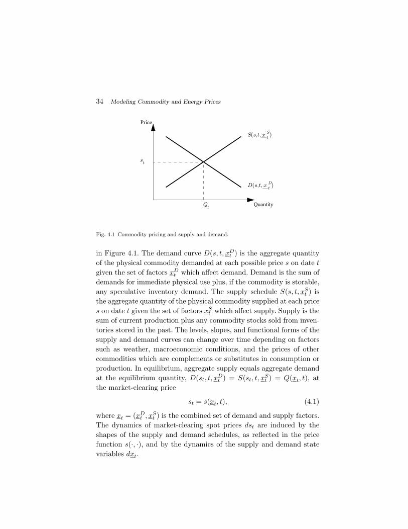
34 Modeling Commodity and Energy Prices
!
"
Price
Quantity
#
!$!% %"#
&
!$!% %"&
Fig. 4.1 Commodity pricing and supply and demand.
in Figure 4.1. The demand curve D(s, t, xDt ) is the aggregate quantity
of the physical commodity demanded at each possible price s on date t
given the set of factors xDt which affect demand. Demand is the sum of
demands for immediate physical use plus, if the commodity is storable,any speculative inventory demand. The supply schedule S(s, t, xS
t ) isthe aggregate quantity of the physical commodity supplied at each prices on date t given the set of factors xS
t which affect supply. Supply is thesum of current production plus any commodity stocks sold from inven-tories stored in the past. The levels, slopes, and functional forms of thesupply and demand curves can change over time depending on factorssuch as weather, macroeconomic conditions, and the prices of othercommodities which are complements or substitutes in consumption orproduction. In equilibrium, aggregate supply equals aggregate demandat the equilibrium quantity, D(st, t, x
Dt ) = S(st, t, x
St ) = Q(xt, t), at
the market-clearing price
st = s(xt, t), (4.1)
where xt = (xDt , xS
t ) is the combined set of demand and supply factors.The dynamics of market-clearing spot prices dst are induced by theshapes of the supply and demand schedules, as reflected in the pricefunction s(·, ·), and by the dynamics of the supply and demand statevariables dxt.
35
The stochastic processes followed by the state variables xt =(x1,t, . . . , xK,t) are typically represented as a system of stochastic dif-ferential equations like the following:
dxk,t = [mk(xt− , t)− ξk(xt− , t)λ(xt− , t)] dt + vk(xt− , t) dZt
+ξk(xt− , t)dJ t, ∀k = 1, . . . , K, (4.2)
where the instantaneous change dxk,t in the k-th state variable at date t
is driven by potentially three building blocks: The deterministic passageof time dt, the random instantaneous increments of a vector of Brown-ian motions dZt, and the random instantaneous increments of a vectorof Poisson or Compound Poisson jump processes dJ t with possiblystate-dependent jump probability intensities λ(xt− , t) and jump mag-nitudes which are either fixed (and normalized to 1 so that ξ
k(xt− , t) is
the vector of local jump sizes for the k-th state variable) or i.i.d. ran-dom vectors Y t (with mean vector Et[Y t] normalized to the unit vectorso that ξ
k(xt− , t) gives the expected local jump sizes for the k-th state
variable) defined at a discrete set of jump dates (i.e., dates on whichdJ t 6= 0).1 Since Brownian motions are continuous, the Brownian mo-tion increment represents the gradual arrival of incremental news. Thejumps represent the potential arrival of dramatic news which causes dis-continuous changes in the state variables and, thus, in prices. The mag-nitudes of the impacts of these building blocks on dxk,t are determinedby the expressions multiplying them: mk(xt− , t) is the predictable localdrift, vk(xt− , t) is a vector of loadings which scale the local volatili-ties of the Brownian motions, and ξ
k(xt− , t) is a vector which scales
the jump magnitudes. The local drifts, volatility, and jump intensitiesand magnitudes can all depend on the state variables and on time t.Time-dependence in price levels, volatilities, and other dynamics canbe due to predictable seasonalities (e.g., harvests, weather patterns) orpredictable macroeconomic, demographic, or technological trends (e.g.,time to build new power plants, technology adoption dynamics). Thet− notation means that drifts, volatilities and the jump moments donot depend on state variables at exactly date t (which would includeany unpredictable jumps in the state variables occurring at date t) but
1See Shreve [178] for properties of Brownian motions and Poisson processes.
36 Modeling Commodity and Energy Prices
2003 2004 2005 2006 2007 2008 2009 2010 2011 2012
400
600
800
1000
1200
1400
1600
1800
2000
$/T
roy
Oun
ce
Year
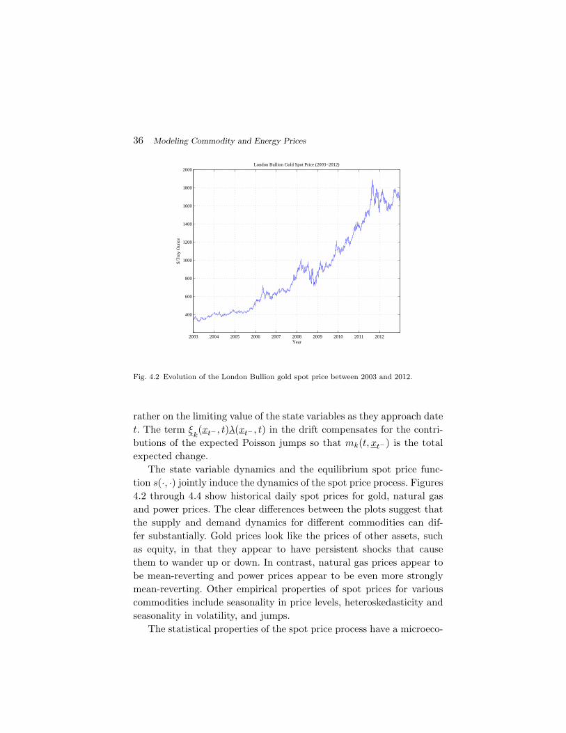
London Bullion Gold Spot Price (2003−2012)
Fig. 4.2 Evolution of the London Bullion gold spot price between 2003 and 2012.
rather on the limiting value of the state variables as they approach datet. The term ξ
k(xt− , t)λ(xt− , t) in the drift compensates for the contri-
butions of the expected Poisson jumps so that mk(t, xt−) is the totalexpected change.
The state variable dynamics and the equilibrium spot price func-tion s(·, ·) jointly induce the dynamics of the spot price process. Figures4.2 through 4.4 show historical daily spot prices for gold, natural gasand power prices. The clear differences between the plots suggest thatthe supply and demand dynamics for different commodities can dif-fer substantially. Gold prices look like the prices of other assets, suchas equity, in that they appear to have persistent shocks that causethem to wander up or down. In contrast, natural gas prices appear tobe mean-reverting and power prices appear to be even more stronglymean-reverting. Other empirical properties of spot prices for variouscommodities include seasonality in price levels, heteroskedasticity andseasonality in volatility, and jumps.
The statistical properties of the spot price process have a microeco-
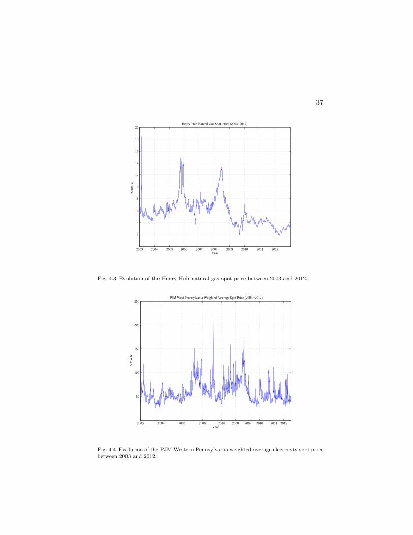
37
2003 2004 2005 2006 2007 2008 2009 2010 2011 2012
2
4
6
8
10
12
14
16
18
20$/
mm
Btu
Year
Henry Hub Natural Gas Spot Price (2003−2012)
Fig. 4.3 Evolution of the Henry Hub natural gas spot price between 2003 and 2012.
2003 2004 2005 2006 2007 2008 2009 2010 2011 2012
50
100
150
200
250
$/M
Wh
Year
PJM West Pennsylvania Weighted Average Spot Price (2003−2012)
Fig. 4.4 Evolution of the PJM Western Pennsylvania weighted average electricity spot pricebetween 2003 and 2012.
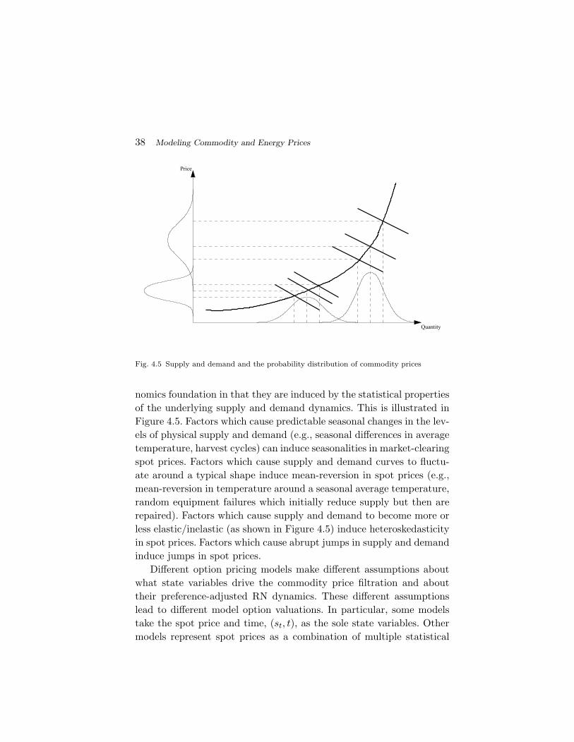
38 Modeling Commodity and Energy Prices
Price
Quantity
Fig. 4.5 Supply and demand and the probability distribution of commodity prices
nomics foundation in that they are induced by the statistical propertiesof the underlying supply and demand dynamics. This is illustrated inFigure 4.5. Factors which cause predictable seasonal changes in the lev-els of physical supply and demand (e.g., seasonal differences in averagetemperature, harvest cycles) can induce seasonalities in market-clearingspot prices. Factors which cause supply and demand curves to fluctu-ate around a typical shape induce mean-reversion in spot prices (e.g.,mean-reversion in temperature around a seasonal average temperature,random equipment failures which initially reduce supply but then arerepaired). Factors which cause supply and demand to become more orless elastic/inelastic (as shown in Figure 4.5) induce heteroskedasticityin spot prices. Factors which cause abrupt jumps in supply and demandinduce jumps in spot prices.
Different option pricing models make different assumptions aboutwhat state variables drive the commodity price filtration and abouttheir preference-adjusted RN dynamics. These different assumptionslead to different model option valuations. In particular, some modelstake the spot price and time, (st, t), as the sole state variables. Othermodels represent spot prices as a combination of multiple statistical
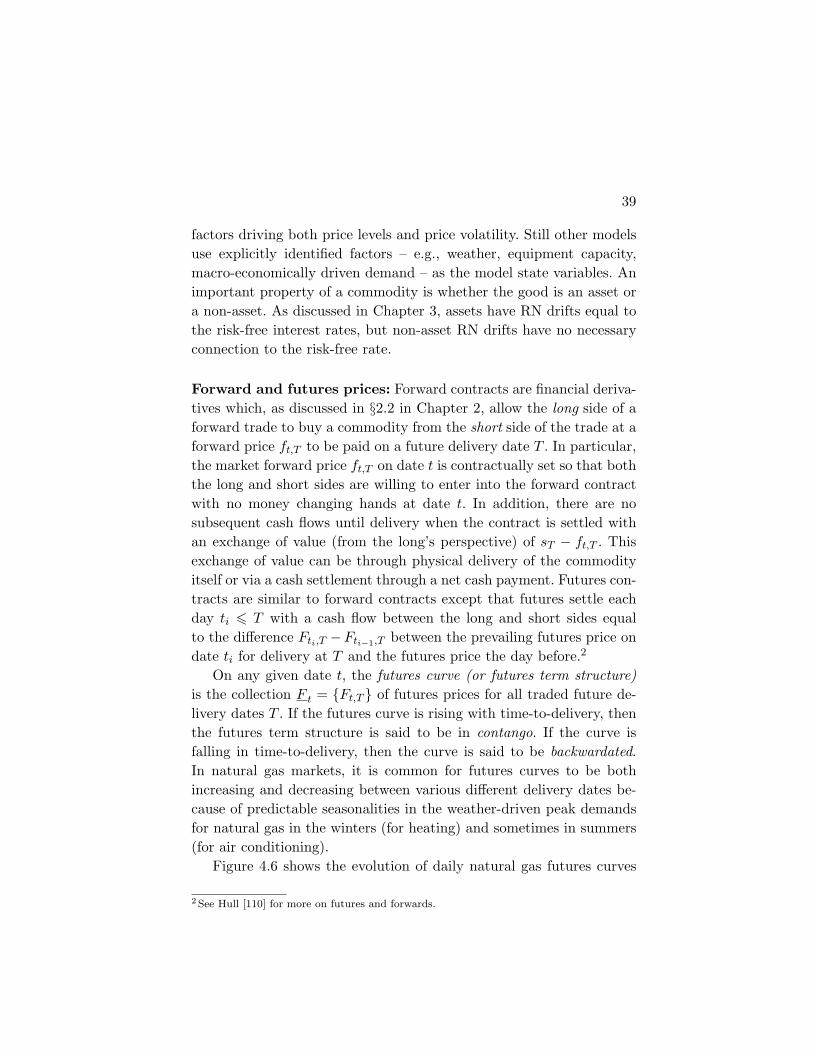
39
factors driving both price levels and price volatility. Still other modelsuse explicitly identified factors – e.g., weather, equipment capacity,macro-economically driven demand – as the model state variables. Animportant property of a commodity is whether the good is an asset ora non-asset. As discussed in Chapter 3, assets have RN drifts equal tothe risk-free interest rates, but non-asset RN drifts have no necessaryconnection to the risk-free rate.
Forward and futures prices: Forward contracts are financial deriva-tives which, as discussed in §2.2 in Chapter 2, allow the long side of aforward trade to buy a commodity from the short side of the trade at aforward price ft,T to be paid on a future delivery date T . In particular,the market forward price ft,T on date t is contractually set so that boththe long and short sides are willing to enter into the forward contractwith no money changing hands at date t. In addition, there are nosubsequent cash flows until delivery when the contract is settled withan exchange of value (from the long’s perspective) of sT − ft,T . Thisexchange of value can be through physical delivery of the commodityitself or via a cash settlement through a net cash payment. Futures con-tracts are similar to forward contracts except that futures settle eachday ti 6 T with a cash flow between the long and short sides equalto the difference Fti,T −Fti−1,T between the prevailing futures price ondate ti for delivery at T and the futures price the day before.2
On any given date t, the futures curve (or futures term structure)is the collection F t = Ft,T of futures prices for all traded future de-livery dates T . If the futures curve is rising with time-to-delivery, thenthe futures term structure is said to be in contango. If the curve isfalling in time-to-delivery, then the curve is said to be backwardated.In natural gas markets, it is common for futures curves to be bothincreasing and decreasing between various different delivery dates be-cause of predictable seasonalities in the weather-driven peak demandsfor natural gas in the winters (for heating) and sometimes in summers(for air conditioning).
Figure 4.6 shows the evolution of daily natural gas futures curves
2See Hull [110] for more on futures and forwards.
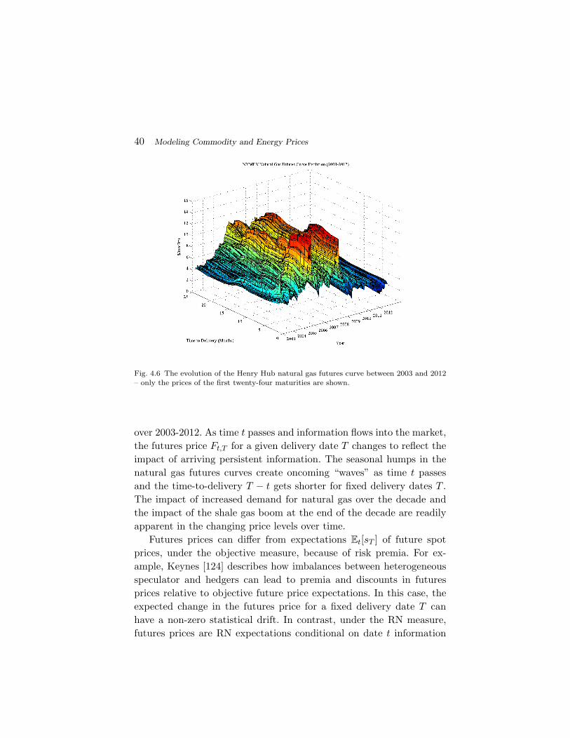
40 Modeling Commodity and Energy Prices
Fig. 4.6 The evolution of the Henry Hub natural gas futures curve between 2003 and 2012– only the prices of the first twenty-four maturities are shown.
over 2003-2012. As time t passes and information flows into the market,the futures price Ft,T for a given delivery date T changes to reflect theimpact of arriving persistent information. The seasonal humps in thenatural gas futures curves create oncoming “waves” as time t passesand the time-to-delivery T − t gets shorter for fixed delivery dates T .The impact of increased demand for natural gas over the decade andthe impact of the shale gas boom at the end of the decade are readilyapparent in the changing price levels over time.
Futures prices can differ from expectations Et[sT ] of future spotprices, under the objective measure, because of risk premia. For ex-ample, Keynes [124] describes how imbalances between heterogeneousspeculator and hedgers can lead to premia and discounts in futuresprices relative to objective future price expectations. In this case, theexpected change in the futures price for a fixed delivery date T canhave a non-zero statistical drift. In contrast, under the RN measure,futures prices are RN expectations conditional on date t information
4.1. Spot-price Evolution Models 41
of future date T spot prices:
Ft,T = ERNt [sT ] (4.3)
and, thus, futures prices are martingales under the RN measure
ERNt [dFt,T ] = 0. (4.4)
The martingale property of RN futures price dynamics follows fromiterated expectations and the daily settlement mechanics.
In practice, two main approaches used to model commodity prices:reduced-form spot price evolution models and reduced-form modelingof the term structure of futures prices. These approaches are presentedin §4.1 and §4.2, respectively. A third approach, less flexible but moreconceptually grounded in the underlying economics, is based on equilib-rium pricing models. Section 4.3 gives an overview of this equilibriumapproach. Section 4.4 then gives a brief review of the empirical evi-dence on commodity prices. Section 4.5 summarizes. Section 4.6 offersgeneral pointers to the literature.
4.1 Spot-price Evolution Models
One widely-used type of reduced-form model is the spot price evolu-tion approach where the RN spot price dynamics are modeled withoutexplicit reference to the underlying microeconomic drivers.
Generalized Black-Scholes: In §3.3, we saw that the local Black-Scholes drift can be any function µ(st, t) under the objective measure,but that the RN drift is the risk-free rate r (see equations (3.7) and(3.13)). While possibly a reasonable approximation for stock prices andasset-like commodities (e.g., gold), these dynamics are problematic fornon-asset commodities. In particular, the generalized Black-Scholes RNdynamics have constant expected returns equal to the risk-free interestrate, no seasonality, and no jumps. In contrast, actual commodity spotprices often exhibit mean-reversion, seasonalities, and jumps. Whilethese statistical properties are characteristics of the objective measureobserved in real-world price data, they also seem to carry over to the
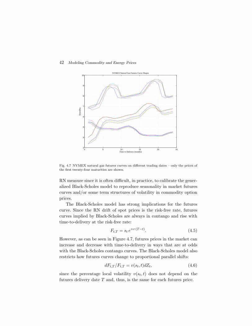
42 Modeling Commodity and Energy Prices
0 5 10 15 20 253
4
5
6
7
8
9
10
$/m
mB
tu
Time to Delivery (months)
NYMEX Natural Gas Futures Curve Shapes
Fig. 4.7 NYMEX natural gas futures curves on different trading dates – only the prices ofthe first twenty-four maturities are shown.
RN measure since it is often difficult, in practice, to calibrate the gener-alized Black-Scholes model to reproduce seasonality in market futurescurves and/or some term structures of volatility in commodity optionprices.
The Black-Scholes model has strong implications for the futurescurve. Since the RN drift of spot prices is the risk-free rate, futurescurves implied by Black-Scholes are always in contango and rise withtime-to-delivery at the risk-free rate:
Ft,T = st e+r (T−t). (4.5)
However, as can be seen in Figure 4.7, futures prices in the market canincrease and decrease with time-to-delivery in ways that are at oddswith the Black-Scholes contango curves. The Black-Scholes model alsorestricts how futures curves change to proportional parallel shifts:
dFt,T /Ft,T = v(st, t)dZt, (4.6)
since the percentage local volatility v(st, t) does not depend on thefutures delivery date T and, thus, is the same for each futures price.
4.1. Spot-price Evolution Models 43
Subsequent research in commodity option pricing has worked to de-velop tractable models with more realistic commodity price dynamics.One variant of the Black-Scholes RN dynamics includes a deterministiclocal convenience yield, denoted by y(t), in the drift:
dst = [r − y(t)] st dt + v(t, st) st dZt. (4.7)
The convenience yield y(t) is like a non-monetary dividend represent-ing a flow of services assumed to accrue to the owners of physical com-modities. This variant of Black-Scholes can then be calibrated to fitany initial commodity futures curve by recursively choosing the con-venience yields to set RN expected future spot prices at each deliverydate equal to the corresponding market futures price:
Ft,T = st e+r (T−t)−∫ Tτ=t y(τ)dτ . (4.8)
If the convenience yield is greater than the risk free rate, y(T ) > r, thenthe futures curve will be decreasing at delivery date T and if y(T ) < r,then the futures curve will be increasing. However, conditional on therealized spot price st, the futures curve on any date t is not random.In particular, random shocks to the futures curve again lead to parallelshifts.
The Black-Scholes model also has strong implications for the termstructure of volatility. Since i) price changes are serially uncorrelatedover time in Black-Scholes and ii) using the fact that log price changesare additive, the volatility of the cumulative log price change over atime interval T − t is
vart [ln(sT /st)] = vart
[∫ T
τ=td ln(sτ )
]=
∫ T
τ=tv2t,τdτ, (4.9)
where v2t,τ is the variance of the instantaneous date τ log spot price
changes conditional on date t information.3 This implies that cumu-lative price change variances are weakly increasing in T . However, ifthe objective and RN price changes are negatively correlated (e.g., as
3The conditional variances, v2t,τ , are different from the future local variances, v(τ, sτ ), in
that the v(τ, sτ )s can depend on prevailing future prices sτ whereas the v2t,τ s can only
depend on the spot price st at date t but not on the realized future spot prices.
44 Modeling Commodity and Energy Prices
with a mean-reverting price process), then heteroskedasticity and/orchanging speeds of mean-reversion can cause the cumulative returnvariance – both empirically and implied from market option prices –to be non-monotone in the time interval T − t.
Another even more general variant of Black-Scholes allows the con-venience yield to depend on the prevailing spot price level as well ason time:
dst = [r − y(t, st)] st dt + v(t, st) st dZt. (4.10)
Now the shape of the futures curve can change stochastically in waysthat are empirically more realistic. For example, high spot prices canbe associated with backwardated futures curves if y(t, st) > r whenst is high and in contango if y(t, st) < r when st is low. However,this randomness is driven entirely by the spot price, which means thatknowing st and the date t is sufficient to know the shape of the futurescurve.
While convenience yields improve the fit of Black-Scholes to marketcommodity derivative prices, there are two conceptual problems withthis modeling approach. First, when the underlying variable is a tradedasset, the Black-Scholes RN dynamics are derived from a no-arbitrageargument without price of risk assumptions. However, the no-arbitrageargument is valid only if the underlying variable is a traded asset.Consequently, when the various variants of Black-Scholes are applied tonon-asset commodities, the RN dynamics in (3.13), (4.7), and (4.10) areeffectively assumed, not derived. In this sense, while the mathematics ofthe RN dynamics can be assumed to have a generalized Black-Scholesform, the conceptual justification for these RN dynamics is absent whenthe Black-Scholes model is used to price non-asset commodity options.
The second problem specifically concerns convenience yields. Unlikestocks which pay actual dividends, ownership of a barrel of oil or anmmBtu of natural gas do not pay any interim cash flows to commodityowners. Commodity ownership may entail storage costs (negative divi-dends), but no positive cash flows accrue to owners of commodities overtime. Similarly, a short position in equity involves paying dividends, butshort positions in commodities do not receive any negative dividends.In short, convenience yields may be a convenient model-fitting device,
4.1. Spot-price Evolution Models 45
but pseudo-dividends have no physical basis in cash flows in the realworld to put any restrictions on the commodity RN drift.
Gibson-Schwartz: This is a two-factor model of RN spot price dy-namics:
dst = [r − yt] st dt + σ st dZ1,t, (4.11)
dyt = α[λ− yt] dt + ξ dZ2,t.
Spot prices follow a process similar to a Geometric Brownian Motionexcept that now a stochastic convenience yield is subtracted from thethe risk-free rate in the RN spot price drift. The convenience yieldfollows an Ornstein-Uhlenbeck process which mean-reverts to a long-run mean of λ which impounds both the objective long-run mean plus apossible risk premium. The Brownian motions dZ1,t and dZ2,t drivingthe two processes can be correlated as needed. The dZ1,t Brownianmotion represents persistent shocks to commodity supply and demand,while the mean-reverting convenience yield causes spot prices to deviatefrom constant-drift paths.
In terms of fitting observed market derivative prices, this approachhas additional flexibility in that, given the spot price, the shapes offutures curves are now random. The short end of the futures curve willbe locally increasing (decreasing) if the current convenience yield yt isless (greater) than the risk-free rate r. Whether or not the futures curveis increasing or decreasing at distant future delivery dates depends onwhether the long-run mean convenience yield λ is less than or greaterthan r. Once again, as in the generalized Black-Scholes model, since theRN commodity price process appears to have a RN drift equal to therisk-free rate after adjusting for the convenience yield – i.e., the sameRN drift as for asset prices – the suggestion that commodity prices areasset prices is a somewhat misleading intuition.
Affine models: Schwartz [167] extends the two-factor Gibson andSchwartz [93] model to a three-factor model which also includes aspot interest rate process. Casassus and Collin-Dufresne [44] furtherextend the specification of the multi-factor spot rate models and in-vestigate their empirical fit. In particular, log commodity spot prices
46 Modeling Commodity and Energy Prices
under the RN measure are assumed to follow a maximal affine functionof three mean-reverting state variables.4 With the additional identify-ing assumptions that (i) the stochastic risk-free spot interest rate is anOrnstein-Uhlenbeck process:
drt = κr (θr − rt) dt + σr dZr,t, (4.12)
and (ii) commodities are traded assets with convenience yields, theresulting RN dynamics for spot prices and convenience yields are
dyt = [κy,0 + κy,rrt + κyy(t) + κy,p ln(st)] dt + σy dZy,t, (4.13)
dst = [rt − y(t)] st dt + σp st dZs,t,
where the κs, θs, and σs are model parameters. In this model the con-venience yield is not just correlated with the spot price via potentiallycorrelated Brownian motions dZy,t and dZs,t; rather now the conve-nience yield dynamics depend directly on spot prices as a factor.
Pilipovic/Schwartz-Smith: Pilipovic [155] and Schwartz and Smith[168] dispense with treating imperfectly storable commodities as tradedassets with RN expected returns equal to the risk-free interest rate.5
Instead, they simply posit an incomplete market setting in which theRN spot price dynamics include permanent and transitory components:
st = Lt eεt , (4.14)
dLt = µRN Lt dt + σ Lt dZL,t,
dεt = α[λ− εt] dt + ξ dZε,t,
where the two Brownian motions, dZL,t and dZε,t, are potentially corre-lated. The Geometric Brownian Motion Lt represents persistent long-run price trends due to persistent shocks to long-term supply anddemand (e.g., technology, discoveries of new deposits). The mean-reverting process εt then causes the market-clearing spot price to wan-der away from the long-term price due to short-lived supply and de-
4Dai and Singleton [58] define an affine model as being “maximal” if it has the maximumnumber of identifiable parameters given futures prices alone.
5Ross (1997) models RN spot prices with mean-reversion but no persistent shocks.
4.1. Spot-price Evolution Models 47
mand shocks (e.g., weather). Futures prices are also available in closed-form:
Ft,T = Lt exp
e−α(T−t)εt + [1− e−α(T−t)]λ + A(T − t)
, (4.15)
where A(T − t) is a function of the futures time-to-maturity that de-pends on the other parameters of the model. Note that, although Lt
and εt are unobserved latent variables, once the model parameters areknown, the two factors can be recovered (i.e., implied) from any twofutures prices.
One significant fact – proven in Schwartz and Smith [168] – is thatthe Gibson-Schwartz and Pilipovic/Schwartz-Smith models are math-ematically equivalent “rotations” of each other. For each calibrationof the Pilipovic/Schwartz-Smith RN dynamics in (4.14), there is amathematically equivalent calibration of the Gibson-Schwartz dynam-ics in (4.11). Thus, the critique of the dividend interpretation of theGibson-Schwartz convenience yield is not a criticism of the mathemat-ics per se; but rather a critique of the economic motivation for themathematics and its connection to real-world economics. In contrast,the Pilipovic/Schwartz-Smith model does not suggest that commodityprices have anything to do with asset prices. Rather, it simply startswith the premise that RN commodity price dynamics have persistentand transitory components qualitatively like those in the objective priceprocess.
This model is easily adapted to include multiple transitory factors:
st = Lt eε1t+ε2t , (4.16)
dLt = µRN Lt dt + σ Lt dZL,t,
dεit = αi[λi − εit] dt + ξi dZi,t, i = 1, 2
with the speeds of mean reversion operating on potentially differenttime scales, α1 6= α2. For example, ε1t may be a rapidly mean-revertingprocess due to equipment failure while ε2t could be a somewhat slowermean-reverting process due to weather.
One limitation of the Pilipovic/Schwartz-Smith model is that it isnot automatically consistent with an arbitrary initial market futurescurve. To the extent that it implies that current market futures are
48 Modeling Commodity and Energy Prices
inconsistent with each other, we say that the model is not arbitrage-free.6 However, the model can be made arbitrage-free if it is modifiedto include a deterministic time-dependent drift. For example, if themean-reverting drift pulls the transitory component to different levelsλ(t) over time,
st = Lt eεt , (4.17)
dLt = µRN Lt dt + σ Lt dZL,t,
dεt = α[λ(t)− εt] dt + ξ dZε,t.
then λ(t) can be calibrated to ensure that the RN expected future spotprices agree with any current futures price term structure.
Jaillet-Ronn-Tompaidis: This is a one-factor mean-reverting RNspot price model with a deterministic seasonal price level:
st = g(t) eεt , (4.18)
dεt = α[λ− εt] dt + σ dZt.
In this specification there are no persistent random shocks to prices.All randomness comes from short-term temporary deviations from aseasonally-adjusted normal price g(t). The associated futures pricesare given by
Ft,T = g(t) exp
e−α(T−t)εt + [1− e−α(T−t)]λ + [1− e−2α(T−t)]σ2
4α
.
(4.19)
Stochastic volatility: An alternative to price- and time-dependentheteroskedasticity are spot price models with stochastic volatility factoras in
dst = α[θ(t)− st] dt + v(xt) st dZs,t, (4.20)
dxt = κ[λ(t)− xt] dt + σdZx,t.
The spot prices here are mean-reverting with time-dependent meanprice levels and the local volatility is a function of one, or possibly
6Since Gibson-Schwartz is mathematically equivalent to Pilipovic/Schwartz-Smith, thesame limitation applies there too.
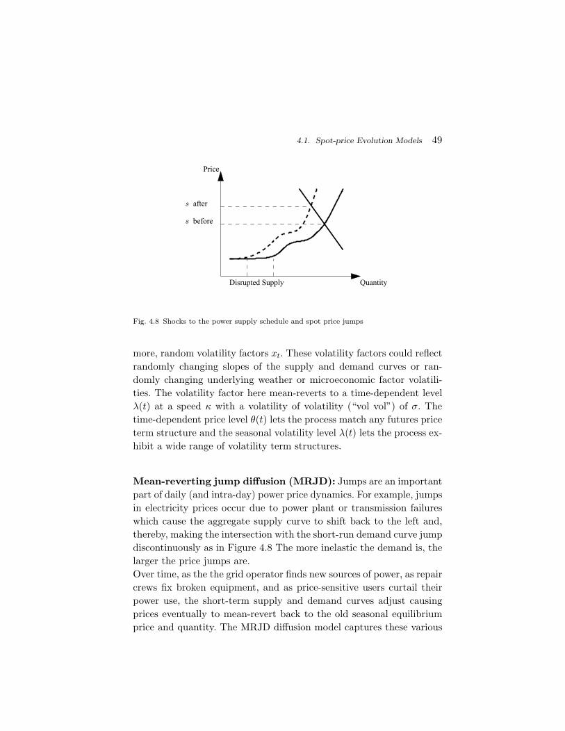
4.1. Spot-price Evolution Models 49
before
after
Disrupted Supply
Price
Quantity
Fig. 4.8 Shocks to the power supply schedule and spot price jumps
more, random volatility factors xt. These volatility factors could reflectrandomly changing slopes of the supply and demand curves or ran-domly changing underlying weather or microeconomic factor volatili-ties. The volatility factor here mean-reverts to a time-dependent levelλ(t) at a speed κ with a volatility of volatility (“vol vol”) of σ. Thetime-dependent price level θ(t) lets the process match any futures priceterm structure and the seasonal volatility level λ(t) lets the process ex-hibit a wide range of volatility term structures.
Mean-reverting jump diffusion (MRJD): Jumps are an importantpart of daily (and intra-day) power price dynamics. For example, jumpsin electricity prices occur due to power plant or transmission failureswhich cause the aggregate supply curve to shift back to the left and,thereby, making the intersection with the short-run demand curve jumpdiscontinuously as in Figure 4.8 The more inelastic the demand is, thelarger the price jumps are.Over time, as the the grid operator finds new sources of power, as repaircrews fix broken equipment, and as price-sensitive users curtail theirpower use, the short-term supply and demand curves adjust causingprices eventually to mean-revert back to the old seasonal equilibriumprice and quantity. The MRJD diffusion model captures these various
50 Modeling Commodity and Energy Prices
qualitative features:
dst = α[θ(t)− st] dt + v(st, t) dZt + ξ(st, t) dJt. (4.21)
Prices wander around a seasonal price level θ(t) driven by heteroskedas-tic Brownian Motion shocks and Poisson jumps with state-dependentjump intensities λ(st, t) and jump magnitudes ξ(st, t).
4.2 Futures Term Structure Models
Another widely-used approach for commodity option valuation directlymodels the RN dynamics of the entire term structure of futures prices.There are two general points to make here. The first is that the dy-namics of the futures curve represents the dynamics of arriving new in-formation and the intertemporal linkages between supply and demandat different delivery dates. Different types of information can have dif-ferent impacts on spot price expectations for different future deliverydates. Some events cause persistent shifts to future supply and demandwhich cause the whole term structure of future prices to shift up anddown (e.g., development of new technologies like hydraulic fracking orincreased construction of natural gas powered power plants). Otherevents have supply and demand effects which are more transitory and,thus, move the spot price and short-dated futures prices more thanlonger-dated futures prices (e.g., short-run weather patterns).
The second general point is that futures curve dynamics imply spotprice dynamics and vice versa. For example, if futures prices for earlydelivery dates shift more than long-dated futures prices, that impliesthat the impact of that particular piece of news is transitory and thatits effect on spot prices will predictably mean-revert away. Conversely,if a shock to spot prices is expected to mean revert away over time,then that predictable decay should be reflected in longer-dated futuresprices reacting less than short-dated futures prices. Although the twoapproaches are isomorphic, the term structure modeling approach hassome tractability advantages over the spot price modeling approach. Inpractice, the drift of the RN spot price process must typically includecalibrated time-dependent deterministic functions – for example, λ(t) inthe modified Pilipovic/Schwartz-Smith model (4.17) – to be arbitrage-
4.2. Futures Term Structure Models 51
free given the initial futures curve observed in the market. In contrast,since futures term structure models are specified in terms of futuresprice changes, setting the initial term structure equal to the observedcurrent futures automatically ensures that the future RN futures areconsistent with the current futures curve.
The modeling of correlated futures curve dynamics draws heavily onmodeling techniques first developed in an interest rate context. Heath,Jarrow, and Morton [106] derived an arbitrage-free model of the risk-neutral dynamics for a vector of instantaneous forward rates. Their keyinsight is that the RN drifts of forward rates are pinned down by theforward rate volatility function and the fact that forward rates must beconsistent with RN expected bond returns being equal to spot interestrates. Brace, Gatarek, and Musiela [28] and Jamshidian [113] deriveda version of HJM – called the market model – which is specified notin terms of instantaneous forward rates but in terms of a collectionof discrete-term forward rates. This modification was motivated by thefact that, in practice, fixed income traders work with vectors of discreteforward rates. Kennedy [122, 121], Goldstein [98], and Longstaff, Santa-Clara and Schwartz [139] develop and work with string models whichhave the same dimensionality as the set of forward rates. This lets theforward rate model be consistent both with the initial futures curveand with the empirical correlation structure of forward rates.
There is, however, at least one significant difference between mod-eling term structures of forward rates and modeling term structuresof commodity futures prices. Futures prices are RN martingales. Thus,the mathematical complications associated with specifying RN forwardinterest rate drifts that are consistent with RN bond price dynamics donot arise in a futures price term structure model. This greatly simplifiescommodity futures term structure modeling.
Black model: The Black [19] model, discussed in §3.3, represents theRN dynamics of futures prices over time for a particular single fixedfuture delivery date T as a driftless Ito process:
dFt,T = v(Ft,T , t) Ft,T dZt. (4.22)
This can be generalized to a model of futures curve dynamics if this
52 Modeling Commodity and Energy Prices
equation is assumed to hold for any delivery date T . In particular, if theBrownian motion increment is not specific to a particular maturity T
but rather affects all futures maturities, then the Black term structuremodel implies that changes in futures prices for all delivery dates arelocally perfectly correlated due to their common dependence on dZt.In the special case of delivery-date-independent and time- and spotprice-contingent local futures price volatility,
dFt,T = v(st, t) Ft,T dZt, ∀T, (4.23)
the futures curve has proportional parallel shifts. Comparing this withequation (4.6) shows that the equal volatility Black futures term struc-ture model is consistent with the generalized Black-Scholes spot pricemodel.
Multi-factor term structure model: The RN futures dynamics canbe made richer than perfectly correlated local shifts by introducingmultiple factors and allowing futures prices for different delivery datesto load differently on the various factors (the number of which is takento be N):
dFt,T =
N∑
j=1
vj(t, xt;T ) dZj,t
Ft,T . (4.24)
The factor loading notation vj(t, xt; T ) is interpreted as follows: Thedependence on T in vj(t, xt;T ) means that futures prices for differentdelivery dates T along the futures curve on a given date t can responddifferently to shocks to a particular factor dZj,t. The dependence on t
means that the sensitivity of a future price for a given (fixed) deliverydate T to factor dZj,t can change over time t because of seasonalities orbecause factor sensitivities change as the time until delivery T − t getsshorter. For example, the Samuelson effect – an empirical regularitythat futures volatility tends to be greater for short time-to-delivery fu-tures prices than for long time-to-delivery futures prices – is consistentwith factor loadings which are decreasing in T − t.7 The dependenceon a volatility factor xt (or set of factors) allows for the possibility
7The exponential specification dFt,T /Ft,T = σ exp[−α(T − t)]dZt with α > 0 in Clewlowand Strickland [55] is an example of such a decaying factor loading.
4.2. Futures Term Structure Models 53
that the factor sensitives depend not just on time effects, but also onother random factors (e.g., the futures term structure itself or stochas-tic volatility factors). If xt is a non-futures state variable, then RNdynamics for dxt must also be specified.
Cortazar and Schwartz [57] is an example of this approach. In theirmodel, the cross-delivery-date covariances depend on both t and thedelivery date T . In the special case in which the factor loading arestable over time and just depend on maturity T − t, the factor loadingsare often empirically calibrated using Principal Component Analysis.
In practice, a small number of factors is often sufficient for a factormodel to reproduce a large part of the empirical covariability of fu-tures term structures. Litterman and Scheinkman [137] show that level,slope, and curvature factors explain over 90 percent of interest rate termstructure variability. Secomandi, Lai, Margot, Scheller-Wolf, and Seppi[175] find that slope and curvature explain over 90 percent of naturalgas futures term structure variability. Working with low-dimensionalfactor models can sometimes improve computational tractability.
The dynamics of futures prices induce dynamics of spot prices. Tosee this, consider the log spot price at any date t after the current datet0:
ln st = lnFt,t (4.25)
= lnFt0,t +∫ t
τ=t0
d ln Fτ,t.
From (4.24) and Ito’s Lemma, holding t fixed and allowing the timeindex τ to vary over time between t0 and t gives the dynamics forfutures prices Fτ,t with a fixed delivery date t:
d lnFτ,t = −12
N∑
j=1
v2j (τ, xτ ; t)
dτ +
N∑
j=1
vj(τ, xτ ; t) dZj,τ . (4.26)
Substituting (4.26) into (4.25) gives
ln st = ln Ft0,t − 12
N∑
j=1
[∫ t
τ=t0
v2j (τ, xτ ; t) dτ
](4.27)
54 Modeling Commodity and Energy Prices
+N∑
j=1
[∫ t
τ=t0
vj(τ, xτ ; t) dZj,τ
].
Applying Ito’s lemma again, now allowing the time index t to change,gives a stochastic differential equation for (log) spot prices:
d ln st =
∂ ln Ft0,t
∂t− 1
2
N∑
j=1
v2j (t, xt; t) (4.28)
−12
N∑
j=1
[∫ t
τ=t0
∂v2j (τ, xτ ; t)
∂tdτ
]
+N∑
j=1
[∫ t
τ=t0
∂vj(τ, xτ ; t)∂t
dZj,τ
] dt
+N∑
j=1
vj(t, xt; t) dZj,t.
The four components in the drift can be interpreted as follows:8 First,the slope of the past futures curve observed on date t0 for the deliverydate t reflects predictable (e.g., seasonal) changes in the spot price at afuture date t. The next two terms in the spot price drift are Ito (Jensen’sinequality) adjustments due to the log transformation. The fourth termin the drift reflects any predictable autocorrelation in how spot pricesrespond to factor shocks over time. At date t the spot price st reflectsthe impact of factor shocks on prior dates τ between dates t0 and t asreflected in changes in prior futures prices Fτ,t with delivery at time t.Similarly, on a date t+∆t (for a small ∆t > 0) the spot price st+∆t alsoreflects those same past factor shocks on dates τ but as reflected in thechanges in the prior futures prices Fτ,t+∆t with delivery at t + ∆t. Thederivative ∂vj(τ, xτ ; t)/∂t represents the differential impact of thosepast shocks on the date t + ∆t delivery futures prices relative to theimpact on the date t delivery futures prices. Note also that, to the
8Spot price changes d ln st can depend on current and past values of the factor xt, butthey do not include contemporaneous dxt shocks just like the spot price changes dst in astochastic volatility model (see (4.20)) do not include volatility shocks dxt.
4.2. Futures Term Structure Models 55
extent that the integrals in the third and fourth terms in the driftdepend on the realized sequence of factor values xτ (which includespossible dependence on the path of futures prices and/or spot prices)and Brownian motion shocks dZj,τ over time, the spot price processwill be non-Markovian.9
String models: If the number of factors is smaller than the dimensionof the variance-covariance matrix of the futures curve, then the factormodel imposes restrictions on the futures variance-covariance matrixsince the futures matrix’s rank is less than its dimension. In practice,option traders sometimes want models which allow for some amountof independent variation at each point along the futures curve. Thestring model approach – drawing on Kennedy [122, 121], Goldstein [98],and Longstaff, Santa-Clara, and Schwartz [139] – allows for imperfectlycorrelated variability along the full term structure:
dFt,T = v(t, xt; T ) Ft,T dZt,T . (4.29)
This model looks similar to the proportional parallel shift Black termstructure model (4.23) except that here there is a separate Brown-ian motion, dZt,T , corresponding to each maturity T along the futurescurve as opposed to a single Brownian motion dZt driving the entirecurve. However, rather than independent Brownian motions driving dif-ferent futures prices along the term structure, the different Brownianmotions in the string model are potentially correlated. One empiricaladvantage of a string model is that the correlation structure of factorsin a string model for N futures prices and constant correlations is ex-actly identified by the empirical correlation matrix. In particular, thereare (N −1)N/2 correlations to be specified in the string model and thesame number of distinct correlations in the empirical correlation ma-trix. In contrast, a factor model with N factors has N2 factor loadings.Consequently, additional structure must be assumed to identify an N
factor model.
9See Carverhill [43] who gives sufficient conditions for Markovian dynamics.
56 Modeling Commodity and Energy Prices
4.3 Equilibrium Models
Spot price evolution models and futures term structure models repre-sent the reduced-form statistical properties of commodity price dynam-ics. The focus in much of “reduced form” modeling is to develop flexibleforms which can be used to price real and financial commodity deriva-tives. Along side this work, a large body of research explicitly modelsthe underlying economic drivers of commodity supply and demand andtheir impact on the equilibrium properties of commodity prices.
The early seminal work on equilibrium commodity pricing was byKaldor [114], Working [205, 206], Telser [188], and Samuelson [165].Later developments on commodity pricing are in Wright and Williams[207], Williams and Wright [204], Brennan [31], Deaton and Laroque[64, 65], Litzenberger and Rabinowitz [138], Routledge, Spatt, andSeppi [164], and Tayur and Yang [186] among others. Much of thiswork goes under the name theory of storage because of its focus onthe dynamics of storage and how storage moderates the price impactof transitory – random or seasonal – shocks to commodity productionand consumption.
The key idea in the theory of storage is that physical storage givesspeculators an American-style timing option of when to use the com-modity. The result is that prices and aggregate storage inventories arejointly determined. Buying by speculators at date t raises spot pricesat date t (since less is available for current consumption) and lowersexpected future prices at later dates t′ > t (as future inventory with-drawals augment future production). The price impact of inventoryaffects the profitability of inventory at date t. In a competitive equi-librium, inventory at date t adjusts the spot price at date t and theprobability distribution of future spot prices until either i) speculatorsare indifferent about acquiring the final marginal unit of inventory or ii)physical constraints on the maximum or minimum aggregate inventorybind. In particular, one important constraint is that inventory cannotbe negative. When inventory hits zero, this is called a stock-out. In astock-out, the futures curve will be backwardated because, even thoughinvestors would like to withdraw more inventory to sell even more ofthe commodity in the market (i.e., if current spot prices are above
4.3. Equilibrium Models 57
expected future spot prices), they are unable to do so once inventoryis empty. In addition, the possibility of future stock-outs can lead tobackwardation in the futures curve at future delivery dates. Thus, themodels provide a theory for backwardation. In addition, the theory ofstorage implies that commodity price volatility will tend to be high instock-outs and backwardated markets due to the absence or shortageof inventory to buffer demand and supply shocks.
Recent research has also modeled commodity production. Carlson,Khokher, and Titman [40] extend the theory of storage approach tothe pricing and optimal extraction of an exhaustible commodity inwhich natural commodity deposits in the ground are viewed as a typeof storage subject to extraction frictions. Casassus, Collin-Dufresne,and Routledge [45] show how lumpy irreversible investment in com-modity production capacity (e.g., development of oil reserves) leads toregime-switching between different endogenous commodity price dy-namics. Kogan, Livdan, and Yaron [127] show how irreversible invest-ment in commodity production can cause non-monotonicities in therelation between the convenience yield curve slope and volatility.
Equilibrium models of commodity prices often assume that themarginal consumers and investors in the market have risk neutral pref-erences with respect to commodity prices. This may be a plausibleassumption for commodities which are a relatively small part of theaggregate consumption bundle. However, it is possible that oil andother major commodities directly affect market pricing. Recent researchseeks to understand the role of preferences in commodity pricing andrisk premia in commodity-linked investments. For example, motivatedby dramatic changes in commodity prices in the mid 2000s, Baker andRoutledge [6] show how changes in endowments and preferences canlead to dramatic changes in the shape of the futures curve and futuresopen interest in an endowment economy with heterogeneous agents,multiple consumption goods, and recursive preferences.10 Ready [159]shows that commodity production frictions increase commodity risk
10Recursive preferences are a departure from expected utility preferences in that the utilityu(ct, Vt) at each date t depends on both current consumption ct and on the value Vt ofexpected future utility. See Epstein and Zin [78] and Kreps and Porteus [130] and thesurvey paper by Backus, Routledge, and Zin [5].
58 Modeling Commodity and Energy Prices
premia but moderate stock risk premia in a two-good long-run riskmodel (see Bansal and Yaron [7]).
4.4 Empirical Research on Commodity Prices
There is a large literature on empirical commodity pricing. A thoroughsurvey of all of this research is beyond the scope of this chapter, butwe do give pointers to work on several big research questions. Ourfocus here is on general empirical issues and on tests of specific pricingmodels.
One major research question concerns whether there are risk pre-mia in commodity futures prices. A common empirical methodology toinvestigate this question uses predictive regressions of spot prices onprior futures prices:
st+n − st = a0 + a1[Ft,t+n − st] + εt+n (4.30)
where the change in the spot price between date t and a date t +n (i.e., over n periods) is regressed on the date t futures-spot pricebasis, Ft,t+n− st, for the futures price with delivery on date t + n. Theexplanatory variable in the regression can be decomposed as follows:
Ft,t+n − st = [Ft,t+n − EMt (st+n)] + [EM
t (st+n)− st] (4.31)
where EMt (st+n) − st is the market’s belief about the objective ex-
pected change in the spot price based on date t information and whereFt,t+n−EM
t (st+n) represents any market risk premium (or discount) infuture prices set at date t relative to the market’s expected future spotprice.11 If the risk premium is non-random and if the market is infor-mationally efficient – i.e., in that the market’s expectation EM
t (st+n)properly reflects any predictability in pt+n – then the true value of theregression coefficient a1 is 1. Thus, if the estimated slope a1 is sta-tistically different from 1, that suggests that futures prices are infor-mationally inefficient and/or that futures prices include time-varyingrisk premia. Fama and French [80] find that the estimated slope co-efficients are positive for many (but not all) commodities, but often
11The EM notation allows for the possibility of market inefficiency if the market’s expecta-tions differ from the true objective expectations. Since EM refers to the markets beliefsabout objective expectations, it should not be confused with RN expectations ERN .
4.5. Summary 59
seem to be less than 1. These results are consistent with the existenceof time-varying risk premia in futures prices. Other work on commod-ity risk premia is in Bessembinder [16], Bessembinder and Chan [17],and Gorton, Hayashi, and Rouwenhorst [99]. Closely related issues arethe idea in Keynes [124] that commodity futures pricing is affected bythe changing imbalances between speculators and hedgers (see Dewally,Ederington, and Fernanado [70] and references therein) and, more re-cently, the pricing impact of the financialization of commodities (see,for example, Buyuksahin, Haigh, Harris, Overdahl, and Robe, [37], andTang and Xiong [185]).
A second question concerns the behavior of commodity price ran-domness. Schwartz [167] and Kogan, Livdan, and Yaron [127] study theterm structure of commodity futures price volatility. Pan [154] uses therisk-neutral price distribution inferred using the Breeden and Litzen-berger [30] method to document time variation in commodity pricevolatility (and in higher moments) and shows that this time varia-tion is correlated with factors reflecting dispersion of beliefs. Fama andFrench [81] investigate the effect of the macroeconomic business cycleon commodity prices.
A third research question concerns the impact of model error, dueto model misspecification or incorrect model calibration, on real optionpricing and hedging. Secomandi, Lai, Margot, Scheller-Wolf, and Seppi[175] show that empirically likely misspecifications of the RN futurescurve dynamics do not have a major impact on natural gas storage val-uation, but that different hedging strategies – which, in the absence ofmodel error, are equivalent – have large differences in their sensitivitiesto even small model error.
4.5 Summary
This chapter reviewed the three approaches to modeling commodityprices and valuing commodity-linked real assets and derivatives: Spotprice evolution models, futures term structure models, and equilib-rium asset pricing. These models differ in their conceptual justification,complexity, and statistical fit. However, these different approaches arenot mutually inconsistent. For example, each RN spot price model im-
60 Modeling Commodity and Energy Prices
plies a corresponding model of futures curve dynamics and vice versa.Reduced-form models rely on replication (when commodities are assetsor when the entire futures curve and its dynamics are known) to iden-tify the RN dynamics or simply posit RN spot price dynamics based onprice of risk assumptions. Equilibrium models derive endogenous mar-ket prices via explicit assumptions about investor preferences. Withineach of these three approaches, we presented a variety of specific single-and multi-factor models of commodity prices. Empirical evidence oncommodity pricing was also reviewed.
4.6 Notes
General references for stochastic calculus and option valuation areShreve [178], Hull [110], and Duffie [76]. References for each of thespecific models discussed here are given in body of this chapter. Seppi[177] is another high level discussion of issues in commodity price mod-eling.
5
Modeling Storage Assets
For a storable commodity, the economic interpretation of storage is theamount of commodity carried over to the next period from the cur-rent period; that is, storage from the prior period plus the differencebetween the commodity production and consumption in the currentperiod (Williams and Wright [204]). Professional commodity storers,hereafter referred to as merchants, trade this surplus in wholesale mar-kets where they behave as price takers. For example, such a setting isthe natural gas market at Henry Hub, Louisiana, the delivery locationof the New York Mercantile Exchange (NYMEX) natural gas futurescontract.
Merchants need access to storage facilities to support their com-modity trading activities. They may own such facilities themselves, orhold rental contracts on their capacity. In this chapter, a storage as-set refers to the facility where a commodity can be physically stored,or a contractual agreement that entitles its owner to usage of a por-tion of such a facility. Storage assets feature two distinctive charac-teristics. On the operational side, while the storage technology maytake many forms (from conventional warehouses and tanks to under-ground depleted reservoirs, aquifers, and salt domes for natural gas),
61
62 Modeling Storage Assets
minimum/maximum inventory levels (space) and injection/withdrawalcapacity limits are ubiquitous. On the financial side, commodity pricesare notoriously variable and volatile (Chapter 4), and storage assetsgive merchants the real option to buy the commodity at one point intime, store it, and sell it at a later point in time to exploit intertemporalprice variability and volatility.
The merchant management of a commodity storage asset requiresdetermining an inventory trading policy that, given the current com-modity spot and futures prices and inventory available in the storagefacility, tells the merchant how much commodity to buy from the whole-sale market and inject into this facility, or withdraw from this facilityand sell into the wholesale market. This is a foundational problem inthe merchant management of commodities, which has been studied inthe literature on the warehouse problem. Cahn [38] introduces thisproblem as follows:
Given a warehouse with fixed capacity and an initialstock of a certain product, which is subject to knownseasonal price and cost variations, what is the opti-mal pattern of purchasing (or production), storage andsales?
The fixed capacity attribute that Cahn mentions refers to a finitesize warehouse without restrictions on how fast it can be filled up oremptied. In addition, storage facilities in practice often feature injec-tion/withdrawal capacity constraints. That is, they are often capac-itated in addition to having finite size. For example, this occurs innatural gas storage (see, e.g., Kobasa [126, pp. 8-9], Tek [187, Chapter3], Maragos [143, p. 435], Geman [91, pp. 304-307]). As shown in thischapter, these additional constraints are critical.
This chapter formulates the warehouse problem as a finite-horizonperiodic review Markov decision process (MDP, Stokey and Lucas [184],Puterman [158], Heyman and Sobel [107], and Bertsekas [14]). Thisformulation encompasses both the fast storage asset case and the slowstorage asset case: a fast storage asset features only space constraints,while a slow storage asset features both space and capacity constraints.
63
In each stage, the state of the MDP includes both the merchant’savailable inventory and the current commodity spot price, with thisprice evolving as an exogenous single factor Markov process. (Model-ing this price evolution with more than one factor would require in-cluding in the state the futures price term structure or more broadlyother information, such as weather and operating conditions.) In gen-eral, the state space is uncountable. This MDP optimizes the marketvalue of the inventory trading policy of a price-taking merchant sub-ject to space and possibly capacity limits. The presence of both spaceand capacity limits gives rise to kinked injection/withdrawal capacityfunctions of inventory. The formulation of this MDP is based on riskneutral valuation.
This chapter analyzes this real option formulation to bring to light(i) the structure of the optimal inventory trading policy, (ii) the com-putation of an optimal policy, and (iii) the managerial relevance of in-terfacing inventory trading and operation decisions. The main resultsand insights of this analysis are now summarized.
The structure of the optimal inventory trading policy. Theoptimal policy in the fast asset case has a simple BI/DN/WS structure:in each stage, given the current price, it is optimal to trade to withdrawand sell (WS) to empty the asset or to buy and inject (BI) to fill itup, or to do nothing (DN) otherwise. This is a simple type of criticallevel, or, equivalently, basestock level inventory trading policy, in whichthe same type of action, BI/DN/WS, is optimal independent of theinventory level, given a stage and a spot price. In other words, theinventory affects how much must be bought or sold to fill up or emptythe asset, but not when it is optimal to buy or sell. Put differently, thereare two critical stage-dependent prices, a BI price and a WS price, suchthat in a given stage it is optimal to fill-up (empty) the storage whenthe current price is below (above) the BI (WS) price, and do nothingotherwise.
In the slow asset case, a modified critical level, that is, basestocktarget, policy is optimal. In a given stage and for a given spot price,this policy is characterized by two dependent basestock targets, theBI and the WS targets, which partition the available inventory into
64 Modeling Storage Assets
three regions, where the BI, DN, and WS actions are respectively op-timal. When a BI/WS action is optimal, it is optimal to buy-and-inject/withdraw-and-sell that amount of inventory that brings the cur-rent inventory level as close as possible to the BI/WS target. That is,these critical inventory-level functions are targets because they maynot be reachable from some inventory levels. This BI/DN/WS struc-ture is more complex than the BI/DN/WS structure in the fast assetcase, because in the fast case only one of these regions is nonempty in agiven stage and for a given spot price. In other words, in a given stage,for a slow asset the it is in general impossible to identify two optimalBI and WS prices.
The optimal basestock targets are functions of the stage and thespot price. Under some assumptions on the risk neutral dynamics of thespot price, in every stage the optimal basestock levels/targets decreasein the spot price. In every stage, the inventory and spot price space isthus partitioned into three ordered BI, DN, and WS regions.
The computation of an optimal policy. In some cases of practicalrelevance, the optimal basestock levels/targets can be easily computed:the operational parameters of the storage asset must satisfy a benigntechnical condition and the spot price dynamics are modeled using alattice representation. In this case, the MDP formulation of the ware-house problem reduces to a discrete state stochastic dynamic program(SDP), which can be solved by backward dynamic programming. Thisfacilitates further numerical analysis.
The managerial relevance of interfacing inventory trading andoperation decisions. The BI/DN/WS structure is nontrivial in theslow asset case because at the same commodity price and stage the typeof the merchant’s optimal action can depend on its inventory availabil-ity. That is, at the same commodity price and stage the BI, DN, andWS actions can each be optimal at different inventory levels. This non-triviality is a direct consequence of the kinked capacity functions, wherethe kinks arise from the limited inventory adjustment capacity relativeto the available space. In particular, due to this limited capacity, themanager of a slow storage asset may optimally decide to make partial
65
inventory adjustments at times with less lucrative cash flows comparedto the case of a fast asset. Put differently, this manager is concernedwith managing “left over” space, that is, the available space minus theinventory adjustment capacity. This issue disappears in the fast assetcase: the left over space is always zero in this case. Thus, trading atcapacity is generally suboptimal with a slow asset, while it is optimalwith a fast asset. Moreover, capacity underutilization can optimally oc-cur at every inventory level for which trading (BI or WS) is optimal. Incontrast, optimal capacity underutilization can only occur at a triviallevel with a fast asset; that is, when it is optimal to do nothing.
It is also insightful to interpret the nontriviality of the BI/DN/WSstructure in the slow asset case in terms of high and low commodityprices. The key insight here is that at a given decision time a merchantmanaging a slow asset cannot always tell whether a given commod-ity price is high (and inventory should be sold) or low (and inventoryshould be bought) independently of its own inventory availability. Inother words, at this given time, the same price can be both high and lowat different inventory levels. This insight is markedly different from theinventory-independent price qualification in the fast asset case. Thisresult occurs even if the merchant is risk neutral and a price taker.Thus, nonlinearities in the operations of a commodity storage assetcan fundamentally condition a merchant qualification of high and lowcommodity prices. The relevant nonlinearities in the storage asset op-erations are brought about by the interplay between the space andcapacity limits that give rise to kinked capacity functions in the slowasset case.
The nontrivial nature of the BI/DN/WS structure for a slow assetimplies that the interface between inventory trading and operationaldecisions is in general nontrivial: these choices cannot be optimally de-coupled by letting the inventory trader decide at what price to buy/sell(that is, set the optimal BI and WS prices in a given stage) and the op-erations manager inject/withdraw at capacity, as if the asset were fast.This chapter uses natural gas data to quantify the likely loss yielded bydecoupling these choices in practice. It is shown here that while the ad-dition of constraining injection/withdrawal capacity, and hence kinkedcapacity functions, does not dramatically reduce the value of a storage
66 Modeling Storage Assets
asset given an optimal operating policy, mismanaging the trading andoperations interface can yield substantial value losses. Moreover, incor-rect inventory trading decisions magnify these losses when the injectioncapacity is increased.
The surprising part of these results is that they hold even whenthe addition of constraining injection/withdrawal capacity does notdramatically reduce the value of optimally managed storage, which isdue to the fact that in these cases the asset is operated at similar flowrates. Thus, nonlinear capacity functions make managing a commoditystorage asset a genuinely difficult problem.
The results and insights of this chapter have relevance for the man-agement of natural gas storage assets, as well as of storage assets forother (partially) storable commodities, such as oil, metals, and agri-cultural products (see, e.g., Geman [91]). While the facilities used tostore these commodities may feature less stringent engineering restric-tions in terms of injection/withdrawal capacities, in such cases capac-ity limitations equivalent to those studied in this paper can arise as aconsequence of logistical and market constraints that limit how fast amerchant can effectively fill up or empty a facility.
This chapter proceeds by formulating the warehouse problem as anMDP in §5.1. Sections 5.2 and 5.3 study the structure of the optimalinventory trading policy. The computation of this policy is investigatedin §5.4. Section 5.5 quantifies the value of interfacing trading and oper-ational decisions. Section 5.6 concludes. Section 5.7 provides pointersto the literature.
5.1 Model
This section describes a periodic review model where inventory trad-ing decisions are made at N given equally spaced points in time. SetI = 0, . . . , N − 1 indexes them; that is, the i-th decision, i ∈ I, ismade at time Ti. An action is denoted as a: a positive action corre-sponds to a purchase followed by an injection, a negative action to awithdrawal followed by a sale, and zero is the do-nothing action. The
5.1. Model 67
operational action, that is, an injection or a withdrawal, correspond-ing to a decision made at time Ti is executed during the time intervalin between times Ti and Ti+1. This means that the receipt/deliveryleadtime is zero, so that commodity purchased/sold at time Ti is avail-able/unavailable in storage at time Ti+1. For the most part, a buy-and-inject or withdraw-and-sell action will be simply referred to as aninjection or a withdrawal, or, more generally, a trade. The monetarypayoff of the i-th trade occurs at time Ti. This modeling choice reflectstypical practice, not only in commodity markets, where financial pay-offs are accounted for at specific points in time, even though physicaloperations often occur as flows over time. Moreover, if the length of thereview period is set sufficiently short, this modeling set-up can closelyapproximate cases where financial payoffs occur simultaneously withthe operational execution of the trades.
The storage asset has minimum and maximum inventory levels, x
and x ∈ <+, with x < x (x > 0 is common in energy applications).Hence, the feasible inventory set is X := [x, x]. There are constant in-jection and withdrawal capacities CI > 0 and CW < 0, respectively, onthe maximum amount of inventory that can be injected into and with-drawn out of the facility in each review period (to be strict this appliesto the absolute value of CW ). It is assumed that both CI and −CW
belong to set (0, x − x]. This implies that the storage asset featuresinventory-dependent injection and withdrawal capacity functions of in-ventory a(x) : X → [0, CI ∧ (x− x)] and a(x) : X → [CW ∨ (x− x), 0]defined as
a(x) := CI ∧ (x− x), (5.1)
a(x) := CW ∨ (x− x), (5.2)
where ·∧ · ≡ min·, · and ·∨ · ≡ max·, ·. They express the maximumamount of commodity that can be injected and withdrawn, respectively,into and out of the facility during each review period starting frominventory level x ∈ X while keeping the inventory level in set X (strictlyspeaking this comment applies to the absolute value of a(x)). The fastasset case arises when CI = −CW = x− x.
Figure 5.1 illustrates the capacity functions in these cases. In theslow facility case, the kinks in these functions (at x = x − CI and
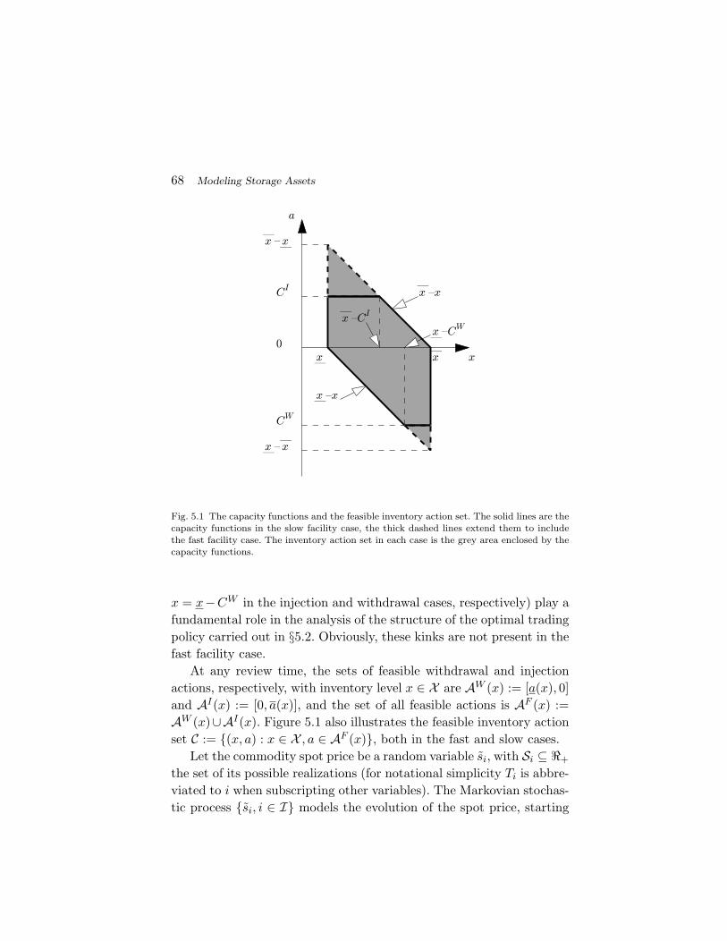
68 Modeling Storage Assets
! "
!
#!
!"
#!
!
" !"
" "!
""!
!"
$
"
!" "
!
"!
!"
Fig. 5.1 The capacity functions and the feasible inventory action set. The solid lines are thecapacity functions in the slow facility case, the thick dashed lines extend them to includethe fast facility case. The inventory action set in each case is the grey area enclosed by thecapacity functions.
x = x−CW in the injection and withdrawal cases, respectively) play afundamental role in the analysis of the structure of the optimal tradingpolicy carried out in §5.2. Obviously, these kinks are not present in thefast facility case.
At any review time, the sets of feasible withdrawal and injectionactions, respectively, with inventory level x ∈ X are AW (x) := [a(x), 0]and AI(x) := [0, a(x)], and the set of all feasible actions is AF (x) :=AW (x)∪AI(x). Figure 5.1 also illustrates the feasible inventory actionset C := (x, a) : x ∈ X , a ∈ AF (x), both in the fast and slow cases.
Let the commodity spot price be a random variable si, with Si ⊆ <+
the set of its possible realizations (for notational simplicity Ti is abbre-viated to i when subscripting other variables). The Markovian stochas-tic process si, i ∈ I models the evolution of the spot price, starting
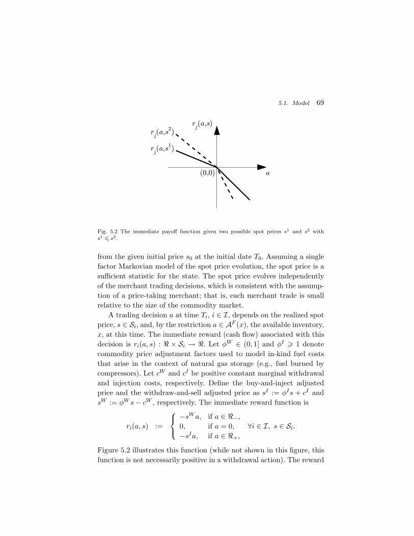
5.1. Model 69
!
!""#$
# !""#$
!""#$
$ !"$
Fig. 5.2 The immediate payoff function given two possible spot prices s1 and s2 withs1 6 s2.
from the given initial price s0 at the initial date T0. Assuming a singlefactor Markovian model of the spot price evolution, the spot price is asufficient statistic for the state. The spot price evolves independentlyof the merchant trading decisions, which is consistent with the assump-tion of a price-taking merchant; that is, each merchant trade is smallrelative to the size of the commodity market.
A trading decision a at time Ti, i ∈ I, depends on the realized spotprice, s ∈ Si, and, by the restriction a ∈ AF (x), the available inventory,x, at this time. The immediate reward (cash flow) associated with thisdecision is ri(a, s) : < × Si → <. Let φW ∈ (0, 1] and φI > 1 denotecommodity price adjustment factors used to model in-kind fuel coststhat arise in the context of natural gas storage (e.g., fuel burned bycompressors). Let cW and cI be positive constant marginal withdrawaland injection costs, respectively. Define the buy-and-inject adjustedprice and the withdraw-and-sell adjusted price as sI := φIs + cI andsW := φW s− cW , respectively. The immediate reward function is
ri(a, s) :=
−sW a, if a ∈ <−,
0, if a = 0,
−sIa, if a ∈ <+,
∀i ∈ I, s ∈ Si.
Figure 5.2 illustrates this function (while not shown in this figure, thisfunction is not necessarily positive in a withdrawal action). The reward
70 Modeling Storage Assets
function is kinked in the action at zero, as sW 6 sI . In contrast to thekinks in the capacity functions, this kink does not play an importantrole in the analysis of §5.2, in the sense that the structural characteri-zation of the optimal policy would persist even without this kink (thatis, if the immediate payoff function were linear in the action).
A unit cost h for physically holding (but not financing) inventory ischarged at each time Ti, i ∈ I, against the inventory x ∈ X availableat this time. Cash flows are discounted from time Ti back to time Ti−1,i ∈ I\0, using the deterministic risk-free discount factor δi−1 ∈ (0, 1].Notationally it is useful to define δ0 := 1.
An optimal inventory trading policy can be obtained by solving afinite horizon MDP. Set I indexes the stages and the state space instage i is X × Si. Let Aπ
i (xi, si) be the decision rule of policy π instage i. Denote by Π the set of all the feasible policies. Let xπ
i be therandom variable that denotes the inventory level available in stage i
when following policy π. The objective is to find an optimal policy forthe following problem:
maxπ∈Π
N−1∑
i=0
i∏
j=0
δj
ERN [ri (Aπ
i (xπi , si), si) | x0, s0] , (5.3)
where ERN [· | x0, s0] denotes the risk neutral expectation given theinitial inventory x0 and spot price s0.
Problem (5.3) can be equivalently reformulated as an SDP. Such areformulation is useful both for deriving the structure of an optimal pol-icy and computing such a policy. Denote by Vi(x, s) the optimal valuefunction in stage i and state (x, s). The SDP formulation of problem(5.3) is
VN−1(x, s) := maxa∈AFW (x)
−sW a− hx, ∀(x, s) ∈ X × Si, (5.4)
Vi(x, s) = maxa∈AF (x)
vi(x, a, s), ∀i ∈ I \ N − 1, (x, s) ∈ X × Si,
(5.5)
vi(x, a, s) := ri(a, s)− hx + δiERNi [Vi+1(x + a, si+1)] , (5.6)
where ERNi [·] := ERN [· | si = s] is the time Ti risk neutral conditional
expectation given spot price s ∈ Si, ∀i ∈ I. This formulation is inter-
5.2. Basestock Optimality 71
preted as follows. In the last stage, only the withdraw-and-sell action isavailable. In prior stages, both the buy-and-inject and withdraw-and-sell actions are available, but at most one of these actions is performed.(This modeling choice is shown to be without loss of generality in §5.2.)
5.2 Basestock Optimality
This section analyzes the structure of an optimal inventory tradingpolicy at a given stage given the spot price.
Before proceeding, it is important to point out that the immediatereward function ri(a, s) is superadditive with respect to two actionswith opposite signs for each given spot price; that is, given aW <
0 < aI it holds that ri(aW , s) + ri(aI , s) 6 ri(aW + aI , s), ∀i ∈ I,s ∈ Si. This property, which can be easily proven, implies that it isnever optimal to perform two opposite trades in the same stage, sothat MDP formulation (5.4)-(5.6) is without loss of generality.
It is useful to define the discount factors δi,i := 1, ∀i ∈ I \ N − 1,and δi,j := δi,j−1δj−1, ∀i ∈ I \ N − 1, j ∈ I, with j > i. Thefollowing natural assumption on the expected discounted spot priceholds throughout. It ensures that the optimal value function is finitein every stage and state.
Assumption 1 (Expected discounted spot price). It holds thatδj,kERN [sk|si = si] < ∞, ∀i ∈ I \ N − 1, k ∈ J , with k > j, andsi ∈ Si.
In the ensuing analysis, properties of functions should be interpretedin the weak sense. It is useful to define the continuation value functions
WN−1(x, s) := 0, ∀(x, s) ∈ X × SN−1, (5.7)
Wi(x, s) := δiERN [Vj+1(x, sj+1)|si = s],
∀i ∈ I \ N − 1, (x, s) ∈ X × Si.
(5.8)
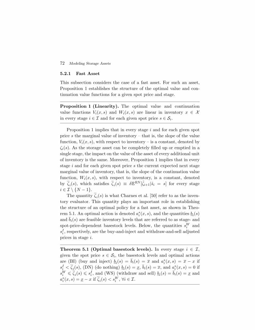
72 Modeling Storage Assets
5.2.1 Fast Asset
This subsection considers the case of a fast asset. For such an asset,Proposition 1 establishes the structure of the optimal value and con-tinuation value functions for a given spot price and stage.
Proposition 1 (Linearity). The optimal value and continuationvalue functions Vi(x, s) and Wi(x, s) are linear in inventory x ∈ Xin every stage i ∈ I and for each given spot price s ∈ Si.
Proposition 1 implies that in every stage i and for each given spotprice s the marginal value of inventory – that is, the slope of the valuefunction, Vi(x, s), with respect to inventory – is a constant, denoted byζi(s). As the storage asset can be completely filled up or emptied in asingle stage, the impact on the value of the asset of every additional unitof inventory is the same. Moreover, Proposition 1 implies that in everystage i and for each given spot price s the current expected next stagemarginal value of inventory, that is, the slope of the continuation valuefunction, Wi(x, s), with respect to inventory, is a constant, denotedby ζi(s), which satisfies ζi(s) ≡ δERN [ζi+1|si = s] for every stagei ∈ I \ N − 1.
The quantity ζi(s) is what Charnes et al. [50] refer to as the inven-tory evaluator. This quantity plays an important role in establishingthe structure of an optimal policy for a fast asset, as shown in Theo-rem 5.1. An optimal action is denoted a∗i (x, s), and the quantities bi(s)and bi(s) are feasible inventory levels that are referred to as stage- andspot-price-dependent basestock levels. Below, the quantities sW
i andsIi , respectively, are the buy-and-inject and withdraw-and-sell adjusted
prices in stage i.
Theorem 5.1 (Optimal basestock levels). In every stage i ∈ I,given the spot price s ∈ Si, the basestock levels and optimal actionsare (BI) (buy and inject) bi(s) = bi(s) = x and a∗i (x, s) = x − x ifsIi < ζi(s), (DN) (do nothing) bi(s) = x, bi(s) = x, and a∗i (x, s) = 0 if
sWi 6 ζi(s) 6 sI
i , and (WS) (withdraw and sell) bi(s) = bi(s) = x anda∗i (x, s) = x− x if ζi(s) < sW
i , ∀i ∈ I.
5.2. Basestock Optimality 73
)WS ( !"#"!$"
!"#"!$
"%"#
!$!!$%
)DN (
!"#"!$" "& !"#"!$ "&%"
#&!'!' !!$%
)BI (
!"#"!$"
!"#"!$ "%"
'!(!!$%
#!
'!
$/unit
Fig. 5.3 Illustration of the determination of the optimal basestock levels for a given stageand spot price in the case of a fast asset; the stage subscript is suppressed.
Figure 5.3 illustrates the result established in Theorem 5.1 for agiven stage and spot price. The determination of an optimal actionclearly involves comparing the inventory evaluator, ζi(si), against thebuy-and-inject or withdraw-and-sell adjusted prices, sI
i or sWi . In par-
ticular, it is optimal to buy-and-inject or withdraw-and-sell when theinventory evaluator exceeds the buy-and-inject spot price or when thewithdraw-and-sell spot price exceeds the inventory evaluator, and todo nothing otherwise. As the inventory evaluator does not depend onthe inventory level, the same type of action is optimal at all inventorylevels. Consequently, it is optimal to purchase inventory to fill the assetup to inventory level x if the buy-and-inject adjusted price is less thanthe inventory evaluator, withdraw inventory to empty the asset downto inventory level x if the withdraw-and-sell adjusted price exceeds theinventory evaluator, and do nothing otherwise.
This is a simple BI/DN/WS structure, in which if BI is optimal theoptimal basestock levels bi(s) and bi(s) are both equal to x, if WS isoptimal they are both equal to x, and if DN is optimal then the BIbasestock level bi(s) and bi(s) is equal to x and the WS basestock levelbi(s) is equal to x.
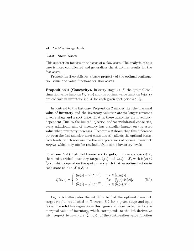
74 Modeling Storage Assets
5.2.2 Slow Asset
This subsection focuses on the case of a slow asset. The analysis of thiscase is more complicated and generalizes the structural results for thefast asset.
Proposition 2 establishes a basic property of the optimal continua-tion value and value functions for slow assets.
Proposition 2 (Concavity). In every stage i ∈ I, the optimal con-tinuation value function Wi(x, s) and the optimal value function Vi(x, s)are concave in inventory x ∈ X for each given spot price s ∈ Si.
In contrast to the fast case, Proposition 2 implies that the marginalvalue of inventory and the inventory valuator are no longer constantgiven a stage and a spot price. That is, these quantities are inventory-dependent. Due to the limited injection and/or withdrawal capacities,every additional unit of inventory has a smaller impact on the assetvalue when inventory increases. Theorem 5.2 shows that this differencebetween the fast and slow asset cases directly affects the optimal bases-tock levels, which now assume the interpretations of optimal basestocktargets, which may not be reachable from some inventory levels.
Theorem 5.2 (Optimal basestock targets). In every stage i ∈ I,there exist critical inventory targets bi(s) and bi(s) ∈ X , with bi(s) 6bi(s), which depend on the spot price s, such that an optimal action ineach state (x, s) ∈ X × Si is
a∗i (x, s) =
(bi(s)− x) ∧ CI , if x ∈ [x, bi(s)),0, if x ∈ [bi(s), bi(s)],(bi(s)− x) ∨ CW , if x ∈ (bi(s), x].
(5.9)
Figure 5.4 illustrates the intuition behind the optimal basestocktarget results established in Theorem 5.2 for a given stage and spotprice. The solid line segments in this figure are the expected next stagemarginal value of inventory, which corresponds to the left derivativewith respect to inventory, ζi(x, s), of the continuation value function
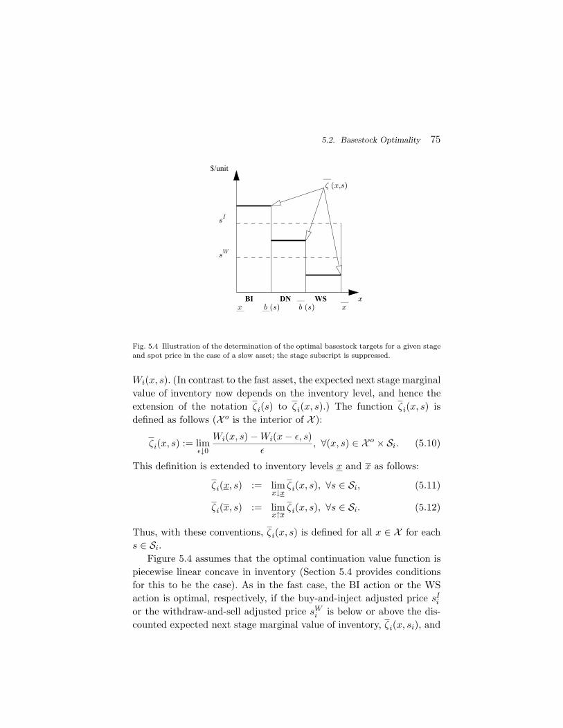
5.2. Basestock Optimality 75
!"!#"
"
" "!$
" "!"$
$/unit
%"
&"
DNBI WS
Fig. 5.4 Illustration of the determination of the optimal basestock targets for a given stageand spot price in the case of a slow asset; the stage subscript is suppressed.
Wi(x, s). (In contrast to the fast asset, the expected next stage marginalvalue of inventory now depends on the inventory level, and hence theextension of the notation ζi(s) to ζi(x, s).) The function ζi(x, s) isdefined as follows (X o is the interior of X ):
ζi(x, s) := limε↓0
Wi(x, s)−Wi(x− ε, s)ε
, ∀(x, s) ∈ X o × Si. (5.10)
This definition is extended to inventory levels x and x as follows:
ζi(x, s) := limx↓x
ζi(x, s), ∀s ∈ Si, (5.11)
ζi(x, s) := limx↑x
ζi(x, s), ∀s ∈ Si. (5.12)
Thus, with these conventions, ζi(x, s) is defined for all x ∈ X for eachs ∈ Si.
Figure 5.4 assumes that the optimal continuation value function ispiecewise linear concave in inventory (Section 5.4 provides conditionsfor this to be the case). As in the fast case, the BI action or the WSaction is optimal, respectively, if the buy-and-inject adjusted price sI
i
or the withdraw-and-sell adjusted price sWi is below or above the dis-
counted expected next stage marginal value of inventory, ζi(x, si), and
76 Modeling Storage Assets
the DN action is optimal otherwise. However, given the spot price,since the marginal value of inventory decreases in inventory, this func-tion brackets the buy-and-inject and the withdraw-and-sell spot pricesat no more than two critical inventory levels. These critical inventorylevels are the basestock targets bi(s) and bi(s). The BI basestock tar-get is less than the WS basestock target because the withdraw-and-selladjusted price is less than the buy-and-inject spot price. These tar-gets thus partition the feasible inventory set into no more than threecontiguous regions, where the BI, DN, and WS actions are respectivelyoptimal. These regions are the sets [x, bi(s)), [bi(s), bi(s)], and (bi(s), x].
This is an extended version of the BI/DN/WS structure that holdsfor the fast asset case. With a slow asset, the optimal basestock targetsin a given stage and for a given spot price are not necessarily equalto the minimum or maximum inventory levels. This is why they aretargets rather than levels.
These observations yield the following insights. First, in the slowasset case, at the same spot price any type of action can be optimal ina given stage depending on the available inventory. Thus, in general,it is impossible to provide an absolute characterization of a spot pricein a given stage as low or high; that is, one at which BI or WS isoptimal, respectively. Any such statement must be made relative toinventory availability. In contrast, in the fast facility case in a givenstage it is indeed possible to define a price as low, intermediate (thatis, DN is optimal at this price), and high independently of the availableinventory.
Second, in the fast asset case, when trading (BI or WS) is optimal,it is optimal to fully utilize the capacity functions, in the sense that anoptimal BI action is equal to injection capacity function (5.1) and anoptimal WS action is equal to the withdrawal capacity (5.2). In con-trast, in the slow asset case, when trading is optimal, it is in generaloptimal to underutilize the available capacity, as expressed by the ca-pacity functions, at some inventory levels. What may be less clear isthat this capacity underutilization can occur at every inventory levelfor which trading is optimal. Example 1 illustrates this possibility.
Example 1 (Slow injection capacity). In this example there are
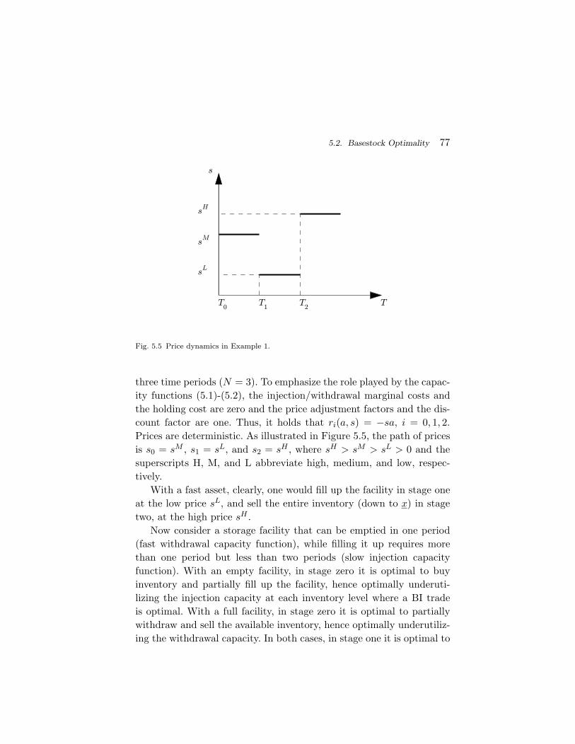
5.2. Basestock Optimality 77
!
"
!"
#"
$"
"
Fig. 5.5 Price dynamics in Example 1.
three time periods (N = 3). To emphasize the role played by the capac-ity functions (5.1)-(5.2), the injection/withdrawal marginal costs andthe holding cost are zero and the price adjustment factors and the dis-count factor are one. Thus, it holds that ri(a, s) = −sa, i = 0, 1, 2.Prices are deterministic. As illustrated in Figure 5.5, the path of pricesis s0 = sM , s1 = sL, and s2 = sH , where sH > sM > sL > 0 and thesuperscripts H, M, and L abbreviate high, medium, and low, respec-tively.
With a fast asset, clearly, one would fill up the facility in stage oneat the low price sL, and sell the entire inventory (down to x) in stagetwo, at the high price sH .
Now consider a storage facility that can be emptied in one period(fast withdrawal capacity function), while filling it up requires morethan one period but less than two periods (slow injection capacityfunction). With an empty facility, in stage zero it is optimal to buyinventory and partially fill up the facility, hence optimally underuti-lizing the injection capacity at each inventory level where a BI tradeis optimal. With a full facility, in stage zero it is optimal to partiallywithdraw and sell the available inventory, hence optimally underutiliz-ing the withdrawal capacity. In both cases, in stage one it is optimal to
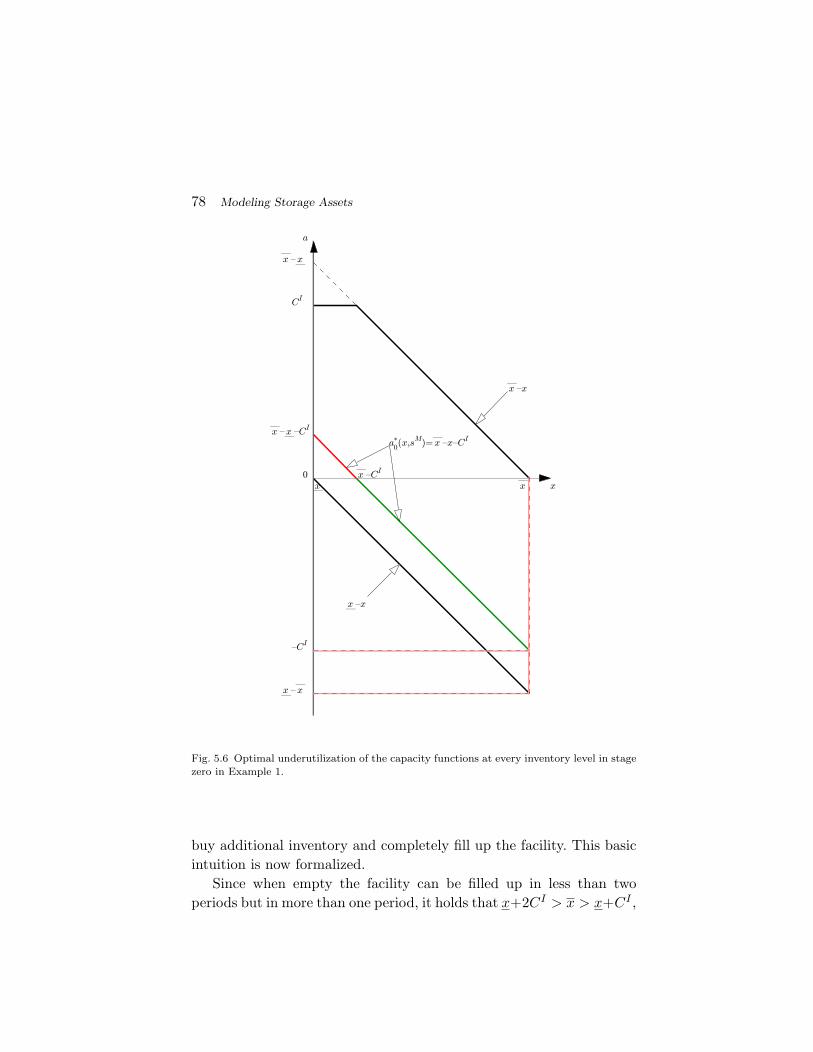
78 Modeling Storage Assets
!
! "
!
! " "
!"#
#"$%$
%
&
! !" "
!
!
!" "!
" "!
&
"!" "!
"!
!"
%
" !"
Fig. 5.6 Optimal underutilization of the capacity functions at every inventory level in stagezero in Example 1.
buy additional inventory and completely fill up the facility. This basicintuition is now formalized.
Since when empty the facility can be filled up in less than twoperiods but in more than one period, it holds that x+2CI > x > x+CI ,
5.2. Basestock Optimality 79
which can be rewritten as
CI < x− x < 2CI . (5.13)
In stage two, it holds that V2(x, sH) = sH(x − x) because AFW (x) =[x−x, 0], ∀x ∈ X . In stage one, with x ∈ X and a ∈ [x−x,CI∧(x−x)],it is easy to verify that v1(x, a, sL) = (sH − sL)a + sH(x − x). Sincev1(x, a, sL) increases in a, it follows that a∗1(x, sL) = CI ∧ (x− x) andV1(x, sL) = (sH − sL)[CI ∧ (x − x)] + sH(x − x), ∀x ∈ X . Finally,consider stage zero and focus on inventory level x. For a ∈ [0, x − x],it holds that v0(x, a, sM ) = (sH − sM )a + (sH − sL)[CI ∧ (x− x− a)].Since
CI ∧ (x− x− a) =
CI , if a ∈ [0, x− x− CI),x− x− a, if a ∈ [x− x− CI , x− x],
it follows that
v0(x, a, sM ) =
(sH − sM )a + (sH − sL)CI , if a ∈ [0, x− x− CI),(sL − sM )a + (sH − sL)(x− x), if a ∈ [x− x− CI , x− x].
It holds that x − x − CI =: a¦0(x, sM ) ∈ arg maxa∈[0,x−x] v0(x, a, sM )and, by (5.13), 0 < a¦0(x, sM ) < CI = a(x). Thus, in stage zero at in-ventory level x it is optimal to buy and inject without fully utilizing theinjection capacity. Moreover, it holds that a(x) < −CI =: a¦0(x, sM ) ∈arg maxa∈[x−x,0] v0(x, a, sM ). Thus, in stage zero at inventory level x itis optimal to withdraw and sell without fully utilizing the withdrawalcapacity. Since x + a¦0(x, sM ) = x − CI and x + a¦0(x, sM ) = x − CI ,it holds that b0(sM ) = b0(sM ) = x − CI and a∗0(x, sM ) = x − x − CI ,∀x ∈ X . Thus, in stage zero it is optimal to buy and inject withoutfully utilizing the injection capacity at every inventory level in the in-terval [x, x−CI), and it is optimal to withdraw and sell without fullyutilizing the withdrawal capacity at every inventory level in the inter-val (x− CI , x]. Figure 5.6 displays the behavior of this optimal actionfunction and relates it to those of the injection and withdrawal capacityfunctions.
This example illustrates a general feature of an optimal basestocktarget structure for a slow storage asset: limited inventory adjustment
80 Modeling Storage Assets
capacity forces the manager of a storage asset to partially shift thedecision to adjust the inventory level in a given stage to stages withless attractive cash flows. In other words, the nontriviality of an optimalbasestock target structure arises from the need to manage “left over”space or inventory arising from limited capacity. In Example 1, thespace left over is the difference between the available space and theinjection capacity, that is, (x− x)− CI .
5.3 Price Monotonicity of the Optimal Basestock Targets
This section characterizes the behavior of the optimal basestock targetsin the spot price in every given stage. For simplicity of exposition, theensuing analysis only uses the basestock target terminology, but thisanalysis also applies to the fast asset case, that is, when these targetsare basestock levels reachable from any inventory level.
The optimal basestock targets are said to be monotonic in the spotprice if they decrease in the spot price in each stage. Example 2 showsthat an optimal basestock target does not always satisfy this property.
Example 2 (Nonmonotonic optimal BI basestock target). LetN = 2, x = 0, and x = 1. Suppose that φI = φW = 1, cI = 0.04,cW = 0, δ1 = 1, h = 0, and CI = −CW = 1. This is a fast asset,so that V1(x, s) = xs and W0(x, s) = xs1|0(s), where, with a slightabuse of notation, s1|0(s) := E[s1|s0 = s]. Assume that there are fourpossible spot prices in stage zero, those in set S0 = 0.01, 2, 9, 12,and that s1|0(s) is equal to 0.0149, 2.1922, 9.0375, and 11.8498for s = 0.01, 2, 9, and 12, respectively. In stage zero, b0(s) andb0(s) are optimal solutions to maxy∈[0,1][s1|0(s) − (s + 0.04)]y andmaxy∈[0,1][s1|0(s)− s]y, respectively. Thus, b0(s) is equal to 0 if the BIunit margin, s1|0(s)− (s + 0.04), is negative and to 1 if this quantity ispositive; and b0(s) is equal to 0 if the WS unit margin, s1|0(s) − s, isnegative and to 1 if this quantity is positive. Table 5.1 displays the BIand WS unit margins and their associated optimal basestock targetsand type of action for all possible spot prices in stage one. This tableshows that b0(s) behaves nonmonotonically in s.
What makes the function b1(s) nonmonotonic in s in Example 2
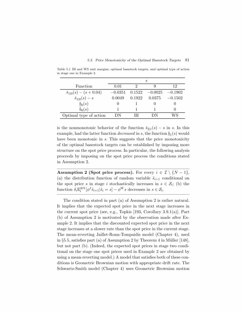
5.3. Price Monotonicity of the Optimal Basestock Targets 81
Table 5.1 BI and WS unit margins, optimal basestock targets, and optimal type of actionin stage one in Example 2.
s
Function 0.01 2 9 12s1|0(s)− (s + 0.04) −0.0351 0.1522 −0.0025 −0.1902
s1|0(s)− s 0.0049 0.1922 0.0375 −0.1502b0(s) 0 1 0 0b0(s) 1 1 1 0
Optimal type of action DN BI DN WS
is the nonmonotonic behavior of the function s2|1(s) − s in s. In thisexample, had the latter function decreased in s, the function b1(s) wouldhave been monotonic in s. This suggests that the price monotonicityof the optimal basestock targets can be established by imposing morestructure on the spot price process. In particular, the following analysisproceeds by imposing on the spot price process the conditions statedin Assumption 2.
Assumption 2 (Spot price process). For every i ∈ I \ N − 1,(a) the distribution function of random variable si+1 conditional onthe spot price s in stage i stochastically increases in s ∈ Si; (b) thefunction δiERN
i [φI si+1|si = s]− φW s decreases in s ∈ Si.
The condition stated in part (a) of Assumption 2 is rather natural.It implies that the expected spot price in the next stage increases inthe current spot price (see, e.g., Topkis [193, Corollary 3.9.1(a)]. Part(b) of Assumption 2 is motivated by the observation made after Ex-ample 2. It implies that the discounted expected spot price in the nextstage increases at a slower rate than the spot price in the current stage.The mean-reverting Jaillet-Ronn-Tompaidis model (Chapter 4), usedin §5.5, satisfies part (a) of Assumption 2 by Theorem 4 in Muller [148],but not part (b). (Indeed, the expected spot prices in stage two condi-tional on the stage one spot prices used in Example 2 are obtained byusing a mean-reverting model.) A model that satisfies both of these con-ditions is Geometric Brownian motion with appropriate drift rate. TheSchwartz-Smith model (Chapter 4) uses Geometric Brownian motion
82 Modeling Storage Assets
to represent long-term variations in commodity prices and Schwartzand Smith [168] suggest that it may be an appropriate model for thevaluation of long-term real options. However, part (b) of Assumption2 is not necessary for the optimal basestock targets to be monotonic inprice, as it is easy to verify that b1(s) is monotonic in s in Example 2when cI is zero.
Theorem 5.3 establishes the price monotonicity of the optimal base-stock targets when Assumption 2 holds.
Theorem 5.3 (Price monotonicity). If Assumption 2 holds, thenin every stage i ∈ I the optimal basestock target functions bi(s) andbi(s) decrease in the spot price s ∈ Si.
To appreciate this result, focus on the slow asset case and Figure5.4 (an analogous argument holds in the fast asset case). As the spotprice s increases, both the buy-and-inject and the withdraw-and-selladjusted prices sI and sW increase and, under Assumption 2, it ispossible to show that the discounted expected next stage marginal valueof inventory, that is, the function ζi(y, ·), also increases. It is thus notobvious that the optimal basestock targets decrease in the spot price.However, this would occur if the functions ζi(y, s)−sI and ζi(y, s)−sW
decreased in the spot price s (for each given stage j and inventory levely), which is the case under Assumption 2. This is the main idea inestablishing Theorem 5.3.
In words, this result follows from showing that the discounted ex-pected next stage marginal value of inventory net of its marginal ac-quisition cost and marginal disposal “cost” decreases in the spot price.Consequently, the optimal basestock targets decrease in the spot price,or, equivalently, the optimal amount of inventory bought and injected(respectively, withdrawn and sold) in each stage decreases (respectively,increases) in the spot price. This is consistent with the discussion ofcomplementarity in Topkis [193, pp. 92-93].
When Assumption 2 holds, Theorem 5.3 brings to light the structureof the optimal policy illustrated in Figure 5.7: in every stage i ∈ I, theoptimal basestock targets bi(s) and bi(s) partition the state space X×Si
into disjoint BI, DN, and WS regions. How these functions decrease in

5.4. Computation 83
DN
!
! ""
! " "
! !
WS
BI BI
DN
!"!
WS
"
"
"
!!"
"" "
"
!!"# !"!!
!!"# !
"!!
(a) Slow Asset (b) Fast Asset
Fig. 5.7 Illustration of the price monotonicity of the optimal basestock targets under As-sumption 2; s and s are hypothetical minimum and maximum spot prices and the stagesubscript is suppressed.
the spot price can differ significantly in the slow and fast facility cases,as shown in panels (a) and (b) of Figure 5.7.
5.4 Computation
Consider a Markov process that in each stage can only take on a finitenumber of values, for example using a lattice model such as in Jaillet etal. [112] (see also Luenberger [141, Chapter 12] and Hull [108, Chapter16]). Thus, in the following, the spot price is assumed to evolve asstated in Assumption 3.
Assumption 3 (Finite spot price sets). In every stage i ∈ I, thespot price set Si is finite.
This assumption implies that the random next price si+1 condi-tional on each spot price s ∈ Si in stage i has a discrete probability
84 Modeling Storage Assets
distribution, ∀i ∈ I \ N − 1.Under Assumption 3, an optimal policy in the fast storage asset
case can be computed by dynamic programming backward recursion,despite set X being uncountable. This is so because determining theinventory evaluator in every stage and for each given spot price onlyrequires computing the optimal value function at the two inventorylevels x and x for each possible spot price in the next stage.
The remaining part of this section focuses on the slow asset case.Proposition 3 establishes a useful property of the optimal value functionunder Assumption 3.
Proposition 3 (Piecewise linearity). If Assumption 3 holds, then,in every stage i ∈ I, the optimal value function Vi(x, s) of a slow storageasset is piecewise linear and continuous in x ∈ X for each s ∈ Si.
Under Assumption 3, computing the optimal basestock targets for aslow storage asset is simplified by the capacities, −CW and CI , and theinventory limits, x and x, being integer multiples of some real number.In this case, Proposition 4 establishes two useful properties of the op-timal value function and basestock targets by leveraging the propertyestablished in Proposition 3.
Proposition 4 (Restricted capacities and inventory limits).Suppose that Assumption 3 holds and that there exists a maximalnumber Q ∈ <+ such that −CW , CI , x, and x are all integer multiplesof Q. In this case, in every stage i ∈ I and for each given spot prices ∈ Si, (a) the optimal value function Vi(x, s) can change slope ininventory x only at inventory levels that are integer multiples of Q,and (b) the optimal basestock levels/targets bi(s) and bi(s) can betaken to be integer multiples of Q.
The properties established in Proposition 4 are useful because onecan compute the optimal basestock targets in every stage for each spotprice by restricting attention to a finite number of feasible inventorylevels, namely those that are multiples of the quantity Q, which canbe interpreted as a lot size. Thus, one needs to compute the optimal
5.5. The Value of Optimally Interfacing Operational and Trading Decisions 85
value function in each stage and for each possible spot price only for the1+(x−x)/Q feasible inventory levels x, x+Q, x+2Q, . . . , x. This canbe easily done by optimally solving a discrete space MDP by standardbackward recursion.
Proposition 4 always holds for a fast asset by redefining x as 0 andx as x − x, since in this case this Proposition holds with Q = x − x.For a slow storage asset, The assumption on the quantities x, x, CW ,and CI in Proposition 4 can be relaxed by redefining x as 0 and x asx− x and requiring that CW , CI , and x− x be integer multiples of Q.
5.5 The Value of Optimally Interfacing Operational andTrading Decisions
This section quantifies the managerial relevance of the BI/DN/WSstructure in the slow asset case through a computational analysis inthe context of natural gas storage. The issue being investigated is therelevance of taking the capacity limits into account when determin-ing a trading policy; that is, of optimally interfacing operational andinventory trading decisions.
The analysis here assumes that the natural gas price evolves as asingle factor mean-reverting process with deterministic monthly sea-sonality factors as in the Jaillet-Ronn-Tompaidis model discussed in§4.1 in Chapter 4. Recall that in this model the spot price at time t, st,is the exponential of a single mean reverting factor, εt, multiplied by adeterministic monthly seasonality factor, g(t): st = g(t) exp(εt). Thatis, the single factor, εt, is the natural logarithm of the deseasonalizedspot price. This factor evolves in continuous time and space accordingto the stochastic differential equation
dεt = κ(λ− εt)dt + σdZt, (5.14)
where λ, κ > 0, and σ > 0, respectively, are the long term meanreversion level, the speed of mean reversion, and the volatility of εt,and dZt is an increment to a standard Brownian motion. The dynamicsin (5.14) are under the risk neutral measure. One could also assumethe dynamics of the single factor under the objective measure are alsomean-reverting but with a different mean-reversion level.
86 Modeling Storage Assets
Table 5.2 Estimates of the seasonal mean-reverting price model parameters based on cali-brating the parameters of this model to daily NYMEX natural gas futures and option pricesobserved in February 2006.
Parameter EstimateLong term log level (λ) 1.9740Speed of mean reversion (κ) 0.7200Volatility (σ) 0.6610Monthly Seasonality Factors EstimateJanuary 1.1932February 1.1948March 1.1412April 0.9142May 0.8984June 0.8998July 0.9113August 0.9219September 0.9287October 0.9412November 1.0252December 1.1049
Table 5.2 displays the estimates of the parameters of this modelemployed in this analysis – these estimates are obtained by calibratingthe parameters of this model to daily NYMEX natural gas futures andoption prices observed in February 2006 using the approach describedby Jaillet et al. [112].
The minimum and maximum inventory levels x and x are 0 and 10,respectively. (The normalized unit of measurement of inventory shouldbe interpreted as an appropriate mmBtu multiple, where 1 mmBtu =1,000,000 British thermal units.) In practice, the number of days neededto fill up and empty different types of natural gas storage facilitiesvaries considerably, between 20-250 and 10-150, respectively (FERC[83, p. 7]). The monthly injection and withdrawal capacities are thusvaried from 10% to 100% of the maximum available space (10 units)in increments of 10%. This setting covers several cases of practical
5.5. The Value of Optimally Interfacing Operational and Trading Decisions 87
8.5
9
9.5
10
10.5
11
11.5
0 5 10 15 20 25
$/m
mB
tu
Maturity
Fig. 5.8 NYMEX natural gas futures prices for the first 24 maturities on 2/1/2006.
interest since it corresponds to varying the number of days required tofill-up/empty a facility roughly between 30 and 300.
The injection fuel loss factor is set equal to 0.01, and there is noloss associated with withdrawals, so that φI = 1/0.99 and φW = 1.The injection fuel loss factor accounts for the natural gas used by thefacility pump to inject natural gas into the storage facility. No pumpingis assumed for withdrawals. The withdrawal and injection marginalcosts cW and cI are both set equal to $0.02/mmBtu. These values arerealistic (Secomandi [171]). Consistent with how natural gas storageassets are leased in the U.S. the holding cost is zero: h = $0/mmBtu.
The analysis here features an MDP formulation with 24 stages(N = 24) corresponding to a monthly partition of a two year timeperiod. The first stage corresponds to the beginning of March and theremaining ones to the beginning of each of the next 23 months. Theevolution of the spot price during these months is represented by a tri-nomial lattice calibrated by standard methods (Jaillet et al. [112]) tothe first 24 NYMEX natural gas futures prices observed at the end of2/1/2006 illustrated in Figure 5.8. Since this trinomial lattice is built
88 Modeling Storage Assets
using the risk neutral measure, these initial futures prices are the con-ditional expectations of the spot price in each remaining stage underthe risk neutral measure given the spot price in the first stage. Herethe initial price is $8.723/mmBtu, the closing price for the March 2006contract on 2/1/2006. The trinomial lattice models the stochastic vari-ability around the expected spot price. The monthly discount factoris 0.9958, which corresponds to an annual risk free interest rate of 5%with continuous discounting. Each SDP is optimally solved using thestructural results in Proposition 4, whose underlying assumptions aresatisfied by the setting of this section.
Three types of policies are considered to measure the importance ofoptimally interfacing operational and inventory trading decisions. Thegoal is to understand the impact of capacity on a trading policy. Thisanalysis varies the “speed” of the storage asset by using different valuesfor the injection/withdrawal capacity scale factors (ICSFs/WCSFs),defined as CI/(x− x) and |CW |/(x− x), respectively.
(1) The fast capacity optimal policy (FCOP) that assumes thatICSFs and WCSFs are both 100%.
(2) The slow capacity optimal policy (SCOP).(3) A decoupled operations and trading policy (DOTP) that uses
the FCOP buying and selling price thresholds in each stage,but where the quantities traded are restricted by the capac-ity constraints. In other words, this policy buys and sellswhenever FCOP does so, but its actions are constrained bythe capacity functions, so that it does trades at capacity butit cannot always empty/fill-up the asset in a single stage.Thus, this policy mismanages the interface between opera-tional and trading decisions in the merchant management ofthe storage asset.1
The following discussion compares the relevant value functions andother quantities of interest in stage one given the spot price in this stageand zero initial inventory. The value function in this stage and stateunder a given policy is refereed to as the total asset value under this
1The value function of this policy can be easily computed.
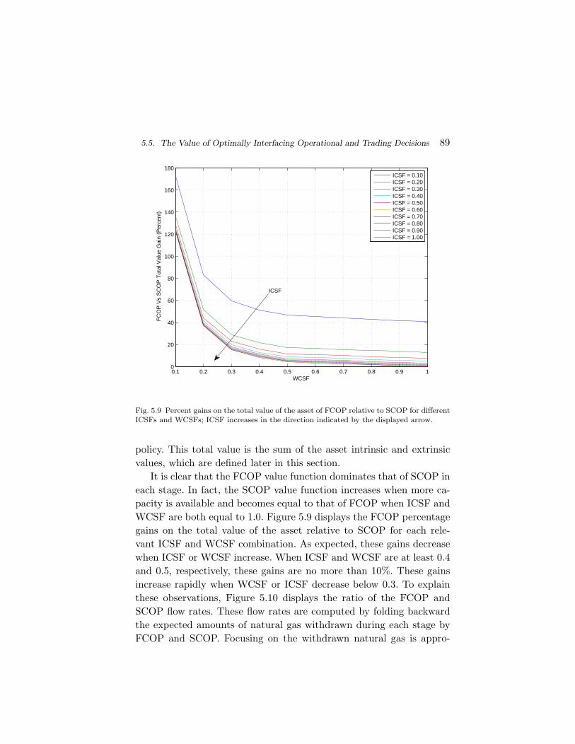
5.5. The Value of Optimally Interfacing Operational and Trading Decisions 89
0.1 0.2 0.3 0.4 0.5 0.6 0.7 0.8 0.9 10
20
40
60
80
100
120
140
160
180
WCSF
FC
OP
Vs
SC
OP
Tot
al V
alue
Gai
n (P
erce
nt)
ICSF = 0.10ICSF = 0.20ICSF = 0.30ICSF = 0.40ICSF = 0.50ICSF = 0.60ICSF = 0.70ICSF = 0.80ICSF = 0.90ICSF = 1.00
ICSF
Fig. 5.9 Percent gains on the total value of the asset of FCOP relative to SCOP for differentICSFs and WCSFs; ICSF increases in the direction indicated by the displayed arrow.
policy. This total value is the sum of the asset intrinsic and extrinsicvalues, which are defined later in this section.
It is clear that the FCOP value function dominates that of SCOP ineach stage. In fact, the SCOP value function increases when more ca-pacity is available and becomes equal to that of FCOP when ICSF andWCSF are both equal to 1.0. Figure 5.9 displays the FCOP percentagegains on the total value of the asset relative to SCOP for each rele-vant ICSF and WCSF combination. As expected, these gains decreasewhen ICSF or WCSF increase. When ICSF and WCSF are at least 0.4and 0.5, respectively, these gains are no more than 10%. These gainsincrease rapidly when WCSF or ICSF decrease below 0.3. To explainthese observations, Figure 5.10 displays the ratio of the FCOP andSCOP flow rates. These flow rates are computed by folding backwardthe expected amounts of natural gas withdrawn during each stage byFCOP and SCOP. Focusing on the withdrawn natural gas is appro-
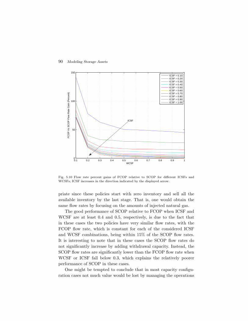
90 Modeling Storage Assets
0.1 0.2 0.3 0.4 0.5 0.6 0.7 0.8 0.9 10
50
100
150
WCSF
FC
OP
Vs
SC
OP
Flo
w R
ate
Gai
n (P
erce
nt)
ICSF = 0.10ICSF = 0.20ICSF = 0.30ICSF = 0.40ICSF = 0.50ICSF = 0.60ICSF = 0.70ICSF = 0.80ICSF = 0.90ICSF = 1.00
ICSF
Fig. 5.10 Flow rate percent gains of FCOP relative to SCOP for different ICSFs andWCSFs; ICSF increases in the direction indicated by the displayed arrow.
priate since these policies start with zero inventory and sell all theavailable inventory by the last stage. That is, one would obtain thesame flow rates by focusing on the amounts of injected natural gas.
The good performance of SCOP relative to FCOP when ICSF andWCSF are at least 0.4 and 0.5, respectively, is due to the fact thatin these cases the two policies have very similar flow rates, with theFCOP flow rate, which is constant for each of the considered ICSFand WCSF combinations, being within 15% of the SCOP flow rates.It is interesting to note that in these cases the SCOP flow rates donot significantly increase by adding withdrawal capacity. Instead, theSCOP flow rates are significantly lower than the FCOP flow rate whenWCSF or ICSF fall below 0.3, which explains the relatively poorerperformance of SCOP in these cases.
One might be tempted to conclude that in most capacity configu-ration cases not much value would be lost by managing the operations
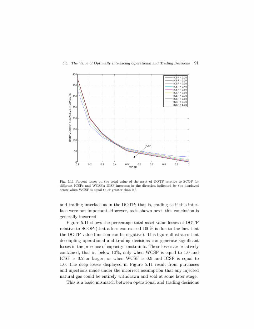
5.5. The Value of Optimally Interfacing Operational and Trading Decisions 91
0.1 0.2 0.3 0.4 0.5 0.6 0.7 0.8 0.9 10
50
100
150
200
250
300
350
400
WCSF
DO
TP
Vs
SC
OP
Tot
al V
alue
Los
s (P
erce
nt)
ICSF = 0.10ICSF = 0.20ICSF = 0.30ICSF = 0.40ICSF = 0.50ICSF = 0.60ICSF = 0.70ICSF = 0.80ICSF = 0.90ICSF = 1.00
ICSF
Fig. 5.11 Percent losses on the total value of the asset of DOTP relative to SCOP fordifferent ICSFs and WCSFs; ICSF increases in the direction indicated by the displayedarrow when WCSF is equal to or greater than 0.5.
and trading interface as in the DOTP; that is, trading as if this inter-face were not important. However, as is shown next, this conclusion isgenerally incorrect.
Figure 5.11 shows the percentage total asset value losses of DOTPrelative to SCOP (that a loss can exceed 100% is due to the fact thatthe DOTP value function can be negative). This figure illustrates thatdecoupling operational and trading decisions can generate significantlosses in the presence of capacity constraints. These losses are relativelycontained, that is, below 10%, only when WCSF is equal to 1.0 andICSF is 0.2 or larger, or when WCSF is 0.9 and ICSF is equal to1.0. The deep losses displayed in Figure 5.11 result from purchasesand injections made under the incorrect assumption that any injectednatural gas could be entirely withdrawn and sold at some later stage.
This is a basic mismatch between operational and trading decisions
92 Modeling Storage Assets
in the presence of capacity limits. As a consequence of this mismatch,more injection capacity is not necessarily beneficial for a given level ofwithdrawal capacity, when the latter capacity is “low.” For example,this can occur for WCSFs between 0.1 and 0.4. In other words, when theoperations manager and the trader do not coordinate their decisions, itcan be better to have a tighter injection capacity when the withdrawalcapacity is “too low” because limited injection capacity avoids excessiveinventory build up. Instead, a higher withdrawal capacity appears tobe always beneficial, since it helps to dispose of previously accumulatedinventory.
5.6 Conclusions
This chapter deals with the modeling of commodity storage assets. Theanalysis is based on an MDP formulation of the classical warehouseproblem that encompasses both the fast and the slow storage assetcases. This analysis focuses on (i) the structure of an optimal policyto this MDP, (ii) its computation, and (iii) the managerial relevance ofcoordinating inventory trading and operational decisions. The findingsof this analysis are as follows: (i) an optimal policy has a basestock levelstructure in the fast asset case and a basestock target structure in theslow asset case; under some assumptions on the spot price dynamics,the optimal basestock levels/targets decrease in the spot price in eachgiven stage; (ii) when the spot price dynamics follow a discrete spaceprocess, the optimal basestock levels in the fast case can be easilycomputed, while the computation of the optimal basestock targets inthe slow case requires an additional and natural assumption on theoperational parameters of the asset; (iii) coordinating inventory tradingand operational decisions when managing a slow storage asset is ofsubstantial managerial importance.
5.7 Notes
Bellman [9] presents a deterministic price dynamic programming for-mulation of the warehouse problem for a fast asset, and Charnes andCooper [49] discuss network flow formulations of this problem. Charnes
5.7. Notes 93
et al. [50] consider the case of stochastic prices. Rempala [160] focuseson the case of limited (slow) injection capacity. The MDP model pre-sented in §5.1 is discussed by Secomandi [171].
Dreyfus [73] shows that the optimal policy of the model of Bellman[9] has a structure analogous to that discussed in §5.2.1. Charnes etal. [50] generalize the analysis of Dreyfus [73] to the case of stochasticprices. Rempala [160] establishes a basestock structure for the case oflimited injection capacity. Secomandi [171] shows the optimality of thebasestock target structure in the general case when both the injectionand the withdrawal capacities are slow. Secomandi [172] provides anopportunity cost view of basestock optimality.
The basestock structure is related to the basestock results availablein the inventory management literature (Zipkin [212], Porteus [156]),whose focus is on managing inventory to provide adequate service levelsto customers in the face of demand uncertainty, rather than optimizingthe inventory trading decisions of merchants that operate in wholesalecommodity markets to take advantage of price fluctuations.
The analysis of the price monotonicity of the optimal basestocktargets and their computation in §§5.3-5.4 is from Secomandi [171].Secomandi et al. [175] show that it is possible to generalize Proposi-tion 4 by dispensing of Assumption 3. That is, Secomandi et al. [175]establish that so long as the capacity limits and the minimum andmaximum inventory levels are integer multiples of the lot size Q, thenthe optimal value function is piecewise linear concave in inventory withbreak points that are integer multiple of Q even if Assumption 3 isnot satisfied. It then follows that the optimal basestock targets can betaken to be integer multiples of Q even without making this assump-tion. That is, Assumption 3 is superfluous in Proposition 4. However,this assumption is critical to make model (5.4)-(5.6) a discrete spaceMDP, which can be solved by backward dynamic programming.
Charnes et al. [50] characterize the intercept and slope of both theoptimal value function and the the optimal continuation value functionfor a fast storage asset, that is, the marginal values of space and inven-tory in a given stage and the discounted next stage marginal values ofspace and inventory. For brevity, this chapter does not emphasize this
94 Modeling Storage Assets
characterization. Secomandi [173] generalizes this characterization tothe slow storage asset case.
The analysis of the managerial relevance of coordinating inventorytrading and operational decisions is from Secomandi [171]. In partic-ular, the estimates of the parameters of the mean reverting model re-ported in Table 5.2 and used in this analysis are from Wang [199].Other authors that have used such a model in the context of naturalgas storage valuation include de Jong and Walet [63], Boogert and deJong [23], and Manoliu [142]. Chen and Forsyth [54], Kaminski et al.[117], Thompson et al. [192], and Carmona and Ludkovski [42] valuenatural gas storage using continuous-time stochastic control methods.
Zhou et al. [210] study the storage of electricity, the price of whichcan be negative, and generalize the work of Charnes et al. [50]. Kimand Powell [125] and Zhou et al. [211], among others, investigate thevalue of storage for a wind-based power generator. Lai et al. [133] con-sider liquefied natural gas storage by modeling the shipping, storage,and regasification of liquefied natural gas. Guigues et al. [102] develop astochastic programming approach to manage liquefied natural gas con-tracts modeling storage and cancellation provisions. Jafarizadeh [111]models oil storage.
The notation used in this chapter is an adaptation of the one used inSecomandi [171] and Lai et al. [132]. For consistency, the same notationis used in Chapter 6, which is based on Lai et al. [132]. The price tobe paid for this consistency is that the notation of this monograph isnot entirely consistent with either the notation of Secomandi [171] orthe one of Lai et al. [132].
6
Benchmarking the Practice Based Managementof Storage Assets
In North America, current federal regulation separates ownership ofnatural gas storage facilities from the control of their capacity. Thatis, the owners of this capacity must make it available to users in anopen access fashion via storage contracts. This chapter deals with thebenchmarking of methods used to value and manage these contracts inpractice. That is, in this chapter the storage asset is a rental contractfor the capacity of a natural gas storage facility.
Natural gas merchants manage such contracts as real options onnatural gas prices, whose values derive from the intertemporal trad-ing of natural gas allowed by storage. Organized markets such as theNew York Mercantile Exchange (NYMEX) and the IntercontinentalEx-change (ICE) trade natural gas related financial instruments, includingfutures and options on futures. Practitioners can use them to hedgeand price natural gas storage contracts using risk-neutral valuationtechniques (Chapter 3). Valuing a storage contract entails dynamic op-timization of inventory trading decisions with capacity constraints inthe face of uncertain natural gas price dynamics.
As discussed in Chapter 5, stochastic dynamic programming(Stokey and Lucas [184], Puterman [158], Heyman and Sobel [107],
95
96 Benchmarking the Practice Based Management of Storage Assets
Bertsekas [14]) is the natural approach to this valuation problem. How-ever, this approach is tractable only when a low-dimensional spot pricemodel is employed to describe the stochastic evolution of the price ofnatural gas (see Chapter 4).
Natural gas storage traders do not appear to like this low dimen-sional approach, due to doubts that the futures and option price dy-namics implied by such price models are consistent with the dynamicsof the NYMEX or ICE futures and options they trade to hedge pricerisk. For example, in discussing the viability of using stochastic dy-namic programming for natural gas storage valuation, Eydeland andWolyniec [79, p. 367] make the following observations:
Great care must be taken when specifying and calibrat-ing spot processes for the use in optimization, so thatthey are consistent with the hedging strategy to be pur-sued. Additionally, even for a given set of forward in-formation, the critical surface may exhibit unstable be-havior that renders it of limited use as a hedging tool.
According to the practice-based literature (Maragos [143, pp. 449-453], Eydeland and Wolyniec [79, pp. 351-367], Gray and Khandel-wal [101, 100]), the preferred modeling approach for many naturalgas storage traders is to model the full dynamics of the futures termstructure using high-dimensional futures price evolution models, suchas those discussed in Chapter 4. Unfortunately, this modeling choicemakes stochastic dynamic programming computationally intractableand necessitates the use of alternative valuation approaches based onsuboptimal but computationally tractable operating policies. Accord-ing again to this practice-based literature, practitioners typically valuenatural gas storage based on heuristic operating policies. Interestingly,commercial software products for the valuation of natural gas storage(see, e.g., FEA [82], KYOS [131]) include heuristic valuation modelsthat can accommodate the high-dimensional futures price evolutionmodels.
One such heuristic combines linear programming and spread optionvaluation methods with or without periodic reoptimization embeddedin Monte Carlo simulation; we label the two resulting heuristics LP
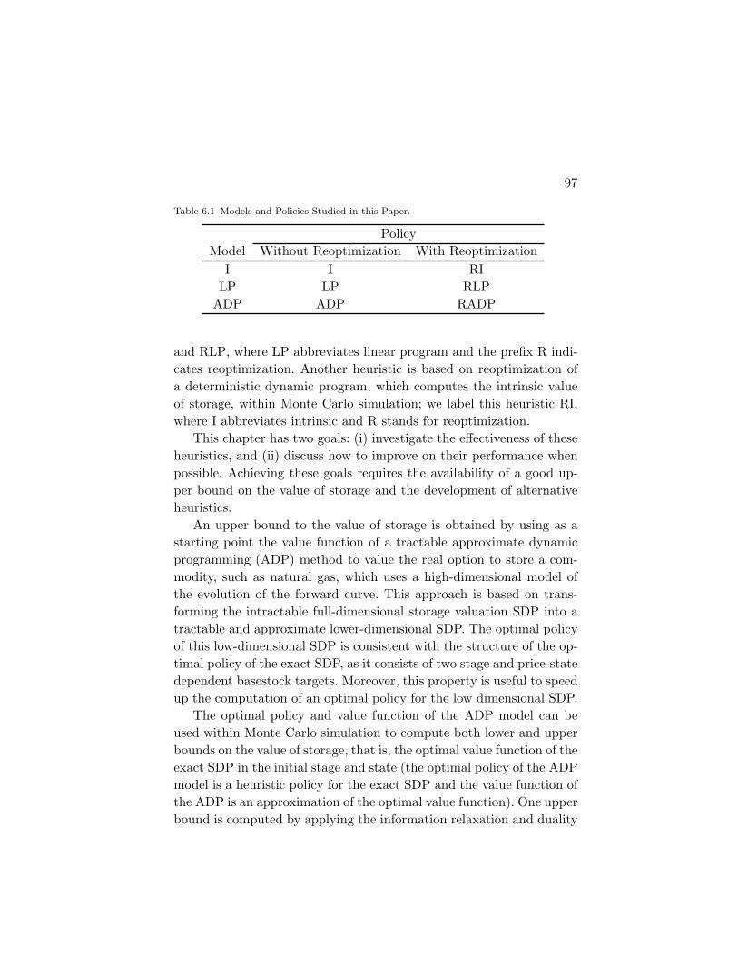
97
Table 6.1 Models and Policies Studied in this Paper.
PolicyModel Without Reoptimization With Reoptimization
I I RILP LP RLP
ADP ADP RADP
and RLP, where LP abbreviates linear program and the prefix R indi-cates reoptimization. Another heuristic is based on reoptimization ofa deterministic dynamic program, which computes the intrinsic valueof storage, within Monte Carlo simulation; we label this heuristic RI,where I abbreviates intrinsic and R stands for reoptimization.
This chapter has two goals: (i) investigate the effectiveness of theseheuristics, and (ii) discuss how to improve on their performance whenpossible. Achieving these goals requires the availability of a good up-per bound on the value of storage and the development of alternativeheuristics.
An upper bound to the value of storage is obtained by using as astarting point the value function of a tractable approximate dynamicprogramming (ADP) method to value the real option to store a com-modity, such as natural gas, which uses a high-dimensional model ofthe evolution of the forward curve. This approach is based on trans-forming the intractable full-dimensional storage valuation SDP into atractable and approximate lower-dimensional SDP. The optimal policyof this low-dimensional SDP is consistent with the structure of the op-timal policy of the exact SDP, as it consists of two stage and price-statedependent basestock targets. Moreover, this property is useful to speedup the computation of an optimal policy for the low dimensional SDP.
The optimal policy and value function of the ADP model can beused within Monte Carlo simulation to compute both lower and upperbounds on the value of storage, that is, the optimal value function of theexact SDP in the initial stage and state (the optimal policy of the ADPmodel is a heuristic policy for the exact SDP and the value function ofthe ADP is an approximation of the optimal value function). One upperbound is computed by applying the information relaxation and duality
98 Benchmarking the Practice Based Management of Storage Assets
approach developed by Brown et al. [35]. Denote this upper bound byDUB, where D and UB abbreviate dual and upper bound, respectively.A simpler approach is to compute a perfect information upper bound,labeled PIUB. PIUB serves as a benchmark for DUB. An additionallower bound is obtained by reoptimizing the ADP model within MonteCarlo simulation. Thus, one obtains two ADP-based lower bounds, theADP and the RADP lower bounds. Table 6.1 summarizes the modelsand policies analyzed in this chapter.
Results. On a set of realistic instances based on NYMEX price dataand additional data available in the energy trading literature, DUBis found to be much tighter than PIUB. DUB is thus used to bench-mark the practice-based heuristics and the two ADP and RADP lowerbounds on these instances. The intrinsic value of storage accounts for arelatively small amount of the total value of storage, but its computa-tion is extremely fast. The LP heuristic is also very fast and capturessignificantly more value than the intrinsic value of storage, but its sub-optimality is large when compared to DUB. The ADP lower boundexhibits less suboptimality, in most cases, but higher computationalrequirement than these heuristics.
Reoptimization improves the valuation performance of all the poli-cies. In almost all the instances, the RLP, RI, and RADP lower boundsare all nearly optimal when compared to DUB. Thus, DUB is a fairlytight upper bound and plays a critical role in benchmarking the vari-ous heuristics. Of course, all these reoptimized lower bounds are moreexpensive to compute. In particular, the computational requirement ofthe RADP lower bound is higher than those of the other lower bounds.Overall, the RI heuristic strikes the best compromise between compu-tational efficiency and valuation quality on our instances. However, insome cases the RADP policy can improve on the performance of theRI policy at the expense of increase computational effort.
The results discussed in this chapter are useful for natural gas stor-age traders because they provide scientific validation, support, andguidance for the use of heuristic storage valuation models in prac-tice. Moreover, these results remain substantially similar, provided that
6.1. Valuation Problem and Exact SDP 99
reoptimization is used, when the seasonality in the NYMEX naturalgas forward curves used to obtain them is (artificially) eliminated.This finding suggests that the insight into the benefit of reoptimiza-tion has potential relevance for the valuation of the real option tostore other commodities, whose forward curves do not exhibit the pro-nounced seasonality of the natural gas forward curve, e.g., metals, oil,and petroleum products (Geman [91]).
The remainder of this chapter is organized as follows. Section 6.1presents the natural gas storage valuation problem and an exact SDPformulation of this problem. Section 6.2 introduces the practice-basedheuristics. Section 6.3 illustrates the ADP model and the upper boundsDUB and PIUB. Section 6.5 discusses numerical results. Section 6.6concludes. Section 6.7 provides pointers to the literature.
6.1 Valuation Problem and Exact SDP
This section describes the natural gas storage valuation problem andformulates an exact SDP of this problem that extends the SDP pre-sented in §5.1 in Chapter 5 A natural gas storage contract gives amerchant the right to inject, store, and withdraw natural gas at a stor-age facility up to given limits during a finite time horizon. The injectionand withdrawal capacity limits are expressed in million British ther-mal units (mmBtus) per unit of time, e.g., day. There are also limits onthe minimum and maximum amounts of the natural gas inventory thatthe merchant can hold under such a contract. There are proportionalcharges and fuel losses associated with injections and withdrawals.
The wholesale natural gas market in North America features aboutone hundred geographically dispersed markets for the commodity.NYMEX and ICE trade financial contracts associated with about fortyof these markets. The most liquid market is Henry Hub, Louisiana,which is the delivery location of the NYMEX natural gas futures con-tract. NYMEX also trades options on this contract. Moreover, NYMEXand ICE trade basis swaps, which are financially settled forward loca-tional price differences relative to Henry Hub. Thus, these financialinstruments make practical the risk-neutral valuation of natural-gas
100 Benchmarking the Practice Based Management of Storage Assets
related cash flows.The quantity of interest is the value of a given natural gas storage
contract at the time of its inception. This value depends on how thenatural gas price changes over time because a merchant uses storage tosupport his trading activity in the natural gas market: buying naturalgas and injecting it into the storage facility at a given point in time,storing it for some time, and withdrawing it out of the facility andselling it at a later point in time. A storage contract can be valued asthe discounted risk-neutral expected value of the cash flows from opti-mally operating it during its tenor, while also respecting its operationalconstraints (Chapter 3).
Of primary interest to traders is the value of the “forward” or“monthly-volatility” component of a storage contract (Maragos [143,p. 440], Eydeland and Wolyniec [79, p. 365]). The value of this compo-nent can be hedged by trading futures contracts, and corresponds tothe value of the cash flows associated with making natural gas trad-ing decisions on a monthly basis. Thus, attention is restricted to thevaluation of such cash flows.
The contract tenor spans N futures maturities in set I ≡0, . . . , N − 1. Inventory trading decisions are made at each matu-rity time Ti with i ∈ I. The notation FTi,Tj denotes the futures priceat time Ti with maturity at time Tj , ∀i, j ∈ I, j > i; FTi,Ti is the spotprice at time Ti. With some abuse of notation, for the most part thenotation FTi,Tj is replaced with the alternative notation Fi,j to simplifythe exposition: the former notation is useful when dealing with contin-uous time dynamics of futures prices, the latter simplifies the writingof discrete time dynamic programs. Define the forward curve at timeTi as Fi := (Fi,j , j ∈ I, j > i), ∀i ∈ I; by convention FN := 0. Noticethat Fi includes the spot price at time Ti. Define the forward curve attime Ti without including the spot price as F′i := (Fi,j , j ∈ I, j > i),∀i ∈ I \ N − 1; F′N−1 := 0.
The numerical experiments in this chapter are based on a stringmodel of futures price evolution (§4.2 in Chapter 4). This approach isrepresentative of the high-dimensional forward models discussed in thepractice-based literature. The risk-neutral dynamics of the prices of thenatural gas futures associated with each maturity Ti are described by a
6.1. Valuation Problem and Exact SDP 101
driftless Geometric Brownian motion, with maturity-specific constantvolatility σi > 0 and standard Brownian motion increment dZi,t. More-over, the standard Brownian motion increments corresponding to twodifferent maturity times Ti and Tj are instantaneously correlated withconstant correlation coefficient ρi,j ∈ [−1, 1], and ρi,i := 1. This modelis
dFt,Ti
Ft,Ti
= σidZi,t, ∀i ∈ I (6.1)
dZi,tdZj,t = ρi,jdt, ∀i, j ∈ I, i 6= j. (6.2)
The storage valuation problem is formulated as an SDP by mod-ifying the one-factor spot-price SDP (5.4)-(5.6) presented in Chapter5. The inventory review period is monthly, so that each review timecorresponds to a futures price maturity. The states in stage i of SDP(5.4)-(5.6) is modified by replacing the spot price si with the forwardcurve Fi, so that the optimal value function in stage i is written asVi(x,Fi). According to the practice-based literature, natural gas stor-age contracts typically do not seem to include a holding cost. Thus,the unit holding cost, h, is set to zero. For simplicity, let the one-stagerisk-free discount factor be constant across stages, and denote it by δ.
The minimum inventory level is normalized to 0, x := 0. Thus, theset of feasible inventory levels is X = [0, x]. The feasible injection actionset at each inventory level is identical to the one defined in Chapter5. In contrast, since the minimum inventory level is zero, the feasiblewithdrawal action set at inventory level x, AW (x), is [CW ∨ (−x), 0].The feasible action set is updated accordingly.
The modified SDP for storage valuation is
VN (xN ,FN ) := 0, ∀xN ∈ X , (6.3)
Vi(xi,Fi) = maxa∈A(xi)
r(a, si) + δERN[Vi+1(xi + a, Fi+1)|F′i
],
∀i ∈ I, (xi,Fi) ∈ X × <N−i+ , (6.4)
where expectation ERN in (6.4) is taken with respect to the risk-neutraldistribution of random vector Fi+1 conditional on Fi. In the remainderof this chapter, and consistent with the notation used in Chapter 5, atilde on top of a symbol denotes a random entity.
102 Benchmarking the Practice Based Management of Storage Assets
In practice, the number of maturities N associated with natural gasstorage contracts is at least twelve, so that model (6.3)-(6.4) is compu-tationally intractable because of its high-dimensional state space.
6.2 Practice-based Heuristics
This section describes the practice-based policies LP and I, and theirreoptimization versions RLP and RI.
6.2.1 Model Based on Spread Options
The LP policy is based on spread option valuation and linear program-ming (as explained below, it also includes a spot sale of inventory attime T0). A spread option is an option on the difference between twoprices with a positive strike price (see §2.4). The LP policy uses spreadoptions on the difference between two futures prices Fi,j and Fi,i on afuture date Ti, with i < j, adjusted for the time value of money andfuel, and strike price equal to the sum of the values of the time Ti in-jection and withdrawal marginal costs. Refer to such an option as thei-j spread option. Its time T0 value is
δiERN
[δj−iφW Fi,j − φI Fi,i −
(δj−icW + cI
)+|F0,i, F0,j
], (6.5)
and is denoted by Si,j0 (F0,i, F0,j). This is the time T0 value of inject-
ing one unit of natural gas at time Ti and withdrawing it at timeTj provided that the value of this trade is nonnegative at time Ti
(·+ := max·, 0).The LP policy works with portfolios of spread options qi,j , i, j ∈
I, i < j; here qi,j is the notional amount of natural gas associatedwith spread option i-j. Such a portfolio includes notional amounts forspread options whose injections and withdrawals are associated withmaturities 0, 1, . . ., N − 2, and 1, 2, . . ., N − 1, respectively. The LPpolicy also includes a spot sale y0 that allows one to sell some or all ofthe inventory available at time T0.1
1Typically storage contracts do not entail a positive initial inventory, but this decisionvariable is useful in the reoptimization version of this linear program.
6.2. Practice-based Heuristics 103
The initial step of the LP policy is to approximate the value ofstorage at time T0 by constructing a portfolio of spread options anda spot sale as an optimal solution to the linear program (6.6)-(6.14)below. The decision variables in this linear program are the notionalamounts in set qi,j , i, j ∈ I, i < j; the inventory levels in set xi, i ∈I \ 0 ∪ N; and the spot sale y0. This linear program, which onlydepends on the time T0 information set x0,F0, is
ULP0 (x0,F0) := max
y0,q,xs0y0 +
∑
i∈I
∑
j∈I,i<j
Si,j0 (F0,i, F0,j)qi,j (6.6)
s.t. xi+1 = xi +∑
j∈I,j>i
qi,j − y01i = 0
−∑
j∈I,j<i
qj,i, ∀i ∈ I, (6.7)
xi 6 x, ∀i ∈ I \ 0 ∪ N, (6.8)∑
j∈I,j>i
qi,j 6 CI , ∀i ∈ I \ N − 1, (6.9)
y0 6 −CW , (6.10)∑
i∈I,i<j
qi,j 6 −CW , ∀j ∈ I \ 0, (6.11)
y0 > 0, (6.12)
qi,j > 0, ∀i, j ∈ I, i < j, (6.13)
xi > 0, ∀i ∈ I \ 0 ∪ N. (6.14)
The objective function (6.6) is the value of the portfolio of spot saleand spread options. Constraint sets (6.7) and (6.8) express inventorybalance and bounding conditions, respectively (1· in (6.7) is the in-dicator function, which is equal to 1 if its argument is true and 0 oth-erwise). Constraint sets (6.9)-(6.11) enforce capacity constraints. Con-straint sets (6.12)-(6.14) pose nonnegativity conditions on the decisionvariables.
Model (6.6)-(6.14) requires prices for the spread options that appearin the objective function (6.6). Once these prices are known, this modelcan be optimally solved very efficiently. These prices can be obtainedin two ways: from (i) market quotes or (ii) a model. Market prices arenot available initially if a liquid market for these spread options is not
104 Benchmarking the Practice Based Management of Storage Assets
active. In addition, spread option prices are not available for futurestages when using the reoptimized version of model (6.6)-(6.14) withina Monte Carlo simulation of the forward curve (see 6.2.3). Hence, inthese cases spread option prices must be obtained from a model. Whenusing the string model (6.1)-(6.2), there is no closed form formula forcomputing these prices. However, they can be numerically computedor, alternatively, they can be approximated using closed form formulas,such as Kirk’s formula (Carmona and Durrleman [41]), which is usedin §6.5.
Let yLP0 (x0,F0) and qLP
i,j (x0,F0), i, j ∈ I, i < j be an optimalportfolio, that is, an optimal solution to model (6.6)-(6.14). This port-folio can be used to construct a feasible policy for model (6.3)-(6.4).This is the LP policy.
To describe this policy, define the following quantities:
qLP,+i,j (Fi,i, Fi,j) :=
0, if δj−iφW Fi,j
− (φIFi,i + δj−icW + cI
)60,
−qLPi,j (x0,F0), otherwise.
(6.15)These quantities depend on x0,F0, but this dependence is suppressedfrom the notation for ease of exposition. Given Fi := (Fj)i
j=0, thesequence of forward curves observed up to and including time Ti, theLP policy uses the quantities defined by (6.15) and the optimal spot-sale yLP
0 (x0,F0) to obtain the following action at time Ti:
−yLP0 (x0,F0)1i = 0−
∑
j∈I,j<i
qLP,+j,i (Fj,j , Fj,i)+
∑
j∈I,j>i
qLP,+i,j (Fi,i, Fi,j).
(6.16)This action does not depend on the inventory level xi. Neverthelessthe LP policy is feasible for model (6.3)-(6.4) as shown in Proposition5. Denote the time T0 value of the LP policy by V LP
0 (x0,F0), whichcan be estimated using Monte Carlo simulation of the forward curveevolution.
Proposition 5 shows that the optimal objective function value ofmodel (6.6)-(6.14) is no greater than the value of the LP policy, andthat both of these values are lower bounds on V0(x0,F0).
6.2. Practice-based Heuristics 105
Proposition 5 (LP policy value). It holds that ULP0 (x0,F0) 6
V LP0 (x0,F0) 6 V0(x0,F0).
The basic idea behind the first inequality in Proposition 5 is showingthat constraint sets (6.7)-(6.14) are sufficient for the feasibility of theLP policy for model (6.3)-(6.4). The second inequality follows fromobserving that the objective function (6.6) underestimates the value ofthe LP policy, because it “double counts” the injection or withdrawalcosts of the LP policy, and that this policy is feasible but not necessarilyoptimal for model (6.3)-(6.4).
6.2.2 Model Based on Forward Contracts
Another model of interest is the so called intrinsic value model, whichcomputes the value of storage that can be attributed to seasonality, asexpressed by the forward curve in the initial stage. This model is thefollowing deterministic dynamic program:
U IN (xN ;F0) := 0, ∀xN ∈ X , (6.17)
U Ii (xi;F0) := max
a∈A(xi)r(a, F0,i) + δU I
i+1(xi + a;F0), ∀i ∈ I,∀xi ∈ X .
(6.18)
This model computes an optimal policy that only considers the infor-mation available at time T0. This is the I policy, which corresponds to asequence of purchases-and-injections or withdrawals-and-sales, one foreach stage, determined based on the information available at the initialtime. The cash flows associated with this policy can be secured at timeT0 by transacting in the forward market for natural gas at this time.The time T0 value of the I policy is U I
0 (x0;F0).
6.2.3 Models Based on Reoptimization
It is typically possible to improve the performance of the LP and I poli-cies by reoptimizing their associated linear and dynamic programs ateach maturity to take advantage of the price and inventory informationthat becomes available over time, implementing the action pertainingto the maturity when the reoptimization is performed, and repeating
106 Benchmarking the Practice Based Management of Storage Assets
this process up to and including the last maturity. For brevity, the de-tails of this process are not discussed here. The time T0 values of thereoptimization versions of the LP and I policies, that is, the RLP andRI policies, are clearly lower bounds on the value of storage and canbe estimated by Monte Carlo simulation of the forward curve.
6.3 ADP Model
This section discuss the ADP model, some structural results for thismodel, and how it can be used to compute lower and upper bounds onthe value of storage.
6.3.1 ADP Policy
To reduce the computationally intractable and exact model (6.3)-(6.4)to a computationally tractable and approximate model, the approachdiscussed below uses information and value function approximations,which allow one to reduce the high dimensionality of model (6.3)-(6.4)and compute an approximate and feasible policy for this model.
The ADP model is introduced by reformulating the exact model.To this aim, define the forward curve at time Ti excluding the spotand prompt month futures prices as F′′i := (Fi,j , j ∈ I, j > i + 1), ∀i ∈I \N−2, N−1; F′′N−2 := 0. Also define as follows the expected valuefunction in stage i and state (xi,Fi) given that the stage i inventorylevel xi and spot price si and the stage i − 1 forward curve F′′i−1 areknown but the stage i forward curve F′i is unknown:
V ′i (xi, si,F′′i−1) := ERN
[Vi(xi, si, F′i) | si,F′′i−1
], (6.19)
for all i ∈ I \0 and (xi, si,Fi) ∈ X ×<N−i+ . Thus, the recursion (6.4)
in stage i ∈ I \N−1 and state (xi,Fi) can be equivalently expressedas
Vi(xi,Fi) = maxa∈A(xi)
r(a, si) + δERN[Vi+1(xi + a, Fi+1)|F′i
]
= maxa∈A(xi)
r(a, si)
6.3. ADP Model 107
+δERN
E
RN[Vi+1(xi + a, si+1, F′i+1)|si+1 = si+1,F′′i
]
︸ ︷︷ ︸V ′i+1(xi+a,si+1,F′′i )
|Fi,i+1
= maxa∈A(xi)
r(a, si) + δERN[V ′
i+1(xi + a, si+1,F′′i )|Fi,i+1
]. (6.20)
The maximization in (6.20) is computationally intractable but itcan be made tractable based on the following approximations:
(1) Information: Replace F′′i in (6.20) with (F0,i+2, . . . , F0,N−1),which is information known at time T0. This effec-tively reduces the dimensionality of maximization (6.20)because the third argument of the function V ′
i+1(·, ·, ·),(F0,i+2, . . . , F0,N−1), is known at time T0.
(2) Value function: Replace the unknown functionV ′
i+1(·, ·, (F0,i+2, . . . , F0,N−1)) with the function UADPi+1 (·, ·),
which is recursively defined as follows.
At the final stage the boundary conditions are
UADPN (xN , sN ) := 0, ∀xN ∈ X . (6.21)
At earlier stages introduce the approximate value function
uADPi (xi, si, Fi,i+1) := max
a∈A(xi)r(a, si)
+δERN[UADP
i+1 (xi + a, si+1) | Fi,i+1
],
(6.22)
for all i ∈ I and (xi, si, Fi,i+1) ∈ X ×<2+, and, paralleling (6.19), define
UADPi (xi, si) := ERN
[uADP
i (xi, si, Fi,i+1) | si, F0,i+1
], (6.23)
for all i ∈ I and (xi, si) ∈ X × <+, with F0,N = FN−1,N := 0.Expressions (6.21)-(6.23) define the ADP model, which can be used
to generate a feasible policy for the exact model (6.3)-(6.4) through themaximization in the right-hand side of (6.22). Call the resulting heuris-tic policy the ADP policy. Denote by aADP
i (xi, si, Fi,i+1) the action of
108 Benchmarking the Practice Based Management of Storage Assets
this policy in stage i and state (xi, si, Fi,i+1); if the set
arg maxa∈A(xi)
r(a, si) + δERN[UADP
i+1 (xi + a, si+1) | Fi,i+1
], (6.24)
is not a singleton, the action aADPi (xi, si, Fi,i+1) is set equal to the
element in this set with the smallest absolute value.Making this ADP approach computationally tractable requires (i)
using finite sets for the possible values of the spot prices si and si+1
and the futures price Fi,i+1; (ii) suitably discretizing the dynamics ofthis futures price into the next stage spot price; (iii) interpolating toobtain values of UADP
i+1 (xi+a, ·) that are otherwise unavailable; and (iv)mapping the pair (si, Fi,i+1) ∈ <2
+ to one of the available correspondingpairs (see Lai et al. [132] for details).
Denote the value of the ADP policy by UADP0 (x0,F0). This value
can be estimated by Monte Carlo simulation of the forward curve, whichis needed because the approximate value function computed by theADP model (6.22)-(6.23) is not necessarily equal to the value functionof the ADP policy when this policy is evaluated under the full informa-tion available in model (6.3)-(6.4). In other words, when implementingthe ADP policy one has access to all the relevant price information,that is, the entire forward curve at a given time; when computing thispolicy in the ADP model only partial information is available, that is,the current spot and prompt month futures prices at a given time andthe forward curve in the initial stage.
The following result holds because the ADP policy is feasible forthe exact model.
Proposition 6 (ADP policy value). It holds that V ADP0 (x0,F0) 6
V0(x0,F0).
The computational implementation of the ADP model can benefitfrom the properties of the optimal value function and policy of thismodel. Lai et al. [132] show that the optimal policy of model ADP hasa stage and price-state dependent basestock target structure analogousto the policy established in Theorem 5.2 in Chapter 5. That is, in eachstage there exist two basestock targets, which depend on the available
6.3. ADP Model 109
price information, that is, the pair (si, Fi,i+1), such that it is optimalto buy-and-inject (respectively, withdraw-and-sell) to get as close aspossible to the lower (respectively, higher) target from any inventorylevel below (respectively, above) such target; doing nothing is optimalat inventory levels in between these targets.
Moreover, these targets decrease in the spot price si for each givenstage i and futures price Fi,i+1. This parallels the property establishedin Theorem 5.3 in Chapter 5. Further, suppose that the distributionof the spot price in the next stage conditional on the prompt monthfutures price in the current stage, denoted by Φ(si+1|Fi,i+1), stochasti-cally increases in the latter quantity; that is, this distribution satisfiesthe property that 1 − Φ(si+1|Fi,i+1) increases in Fi,i+1 for each givensi+1. For example, this assumption is satisfied by the multidimensionalBlack model (6.1)-(6.2). Then, these targets increase in the futuresprice Fi,i+1 for each given stage i and spot price si. These propertiescan be interpreted as follows: as the spot price increases it is opti-mal to purchase less and sell more; as the prompt month futures priceincreases it is optimal to purchase more and sell less. These naturalcomplementarity relationships (Topkis [193, pp. 92-93]) are consistentwith the monotonicity results discussed in §5.3 in Chapter 5.
6.3.2 RADP Policy
The ADP policy is computed once at time T0. The reoptimization ver-sion of the ADP policy (the RADP policy) involves re-solving the ADPmodel in each stage after the initial stage given the information avail-able at that time. In other words, model ADP is reoptimized at eachtime Tj , j ∈ I \ 0, by using the futures curve Fj in place of F0.Specifically, F0,i+1 is replaced with Fj,i+1 in (6.23). The time T0 valueof the resulting RADP policy is typically different, and in fact higher,than that of the ADP policy. In other words, the RADP policy cantypically benefit from sequential reoptimization. Since the RADP pol-icy is feasible for the full model, its time T0 value is a lower bound onV0(x0,F0).
110 Benchmarking the Practice Based Management of Storage Assets
6.4 Upper Bounds
The optimal value function of the ADP model can be used to computean upper bound on the value of storage. Following Brown et al. [35],define the penalty terms
pADPi (xi, a, si+1, Fi,i+1) := UADP
i+1 (xi + a, si+1)
−ERN[UADP
i+1 (xi + a, si+1) | Fi,i+1
],
(6.25)
for all i ∈ I and (xi, a) ∈ X × A(xi), which are based on the optimalvalue function of the ADP model computed at time T0.
These penalty terms have an appealing interpretation in terms ofadditional value of perfect information. Consider performing action a
given inventory level xi and the prompt month futures price Fi,i+1.If the next stage spot price si+1 is known, then the value in stagei + 1 of the resulting inventory level xi + a according to the op-timal policy of the ADP model is UADP
i+1 (xi + a, si+1). If this spotprice is not known, the value of this inventory level is the expecta-tion ERN
[UADP
i+1 (xi + a, si+1) | Fi,i+1
]. The additional value of perfect
information is thus the difference in the right hand side of (6.25). Thesequantities are used to penalize the availability of hindsight informationin the dual upper bound model discussed next; that is, they serve thepurpose of “Lagrange” multipliers (duals) on information one is notsupposed to know.
Denote by P0 a sequence of pairs of spot and prompt-month futureprices for maturities 0 through N − 1; that is, P0 := ((si, Fi,i+1))
N−1i=0 .
Given P0, solve the following dual upper bound DUB model:
UDUBN (xN ; P0) := 0, ∀xN ∈ X , (6.26)
UDUBi (xi; P0) = max
a∈A(xi)r(a, si)− pADP
i (xi, a, si+1, Fi,i+1)
+δUDUBi+1 (xi + a;P0),
∀i ∈ I, xi ∈ X . (6.27)
This is a perfect price information model whose immediate rewards arepenalized according to the penalty terms (6.25). An upper bound on
6.5. Numerical Results 111
the value of storage is obtained in the manner stated in Proposition 7,which follows from Brown et al. [35].
Proposition 7 (DUB). Define
V DUB0 (x0,F0) := ERN
[UDUB
0 (x0; P0) | F0
]. (6.28)
It holds that V0(x0,F0) 6 V DUB0 (x0,F0).
Intuitively, V DUB0 (x0,F0) is an upper bound on the value of storage
because it is obtained from averaging the value functions of perfectinformation models in which hindsight information is penalized usingterms that average to zero. The upper bound V DUB
0 (x0,F0) can beestimated by Monte Carlo simulation of the forward curve.
A different upper bound on the value of storage can be obtained bysetting the penalty terms defined in (6.25) equal to zero and proceedinganalogously to the computation of upper bound (6.28). This yields theperfect information upper bound on the value of storage, labeled PIUB(this follows from Brown et al. [35]). This upper bound provides abenchmark for the performance of the upper bound V DUB
0 (x0,F0).
6.5 Numerical Results
This section discusses the performance of the models and policies pre-sented in §§6.2-6.3 on a set of realistic benchmark instances.
6.5.1 Instances
The benchmark instances are based on market data and parametervalues reported in the energy trading literature.
The two top panels of Figure 6.1 illustrate four forward curves thatinclude the Henry Hub spot price and futures prices of the first 23maturities (Henry Hub is the delivery location of the NYMEX naturalgas futures contract). These curves were observed on four days, eachcorresponding to one of the four seasons of the year: 3/1/2006 (Spring),6/1/2006 (Summer), 8/31/2006 (Fall), and 12/1/2006 (Winter). Thepronounced seasonality in the natural gas forward curve is evident inthese panels.
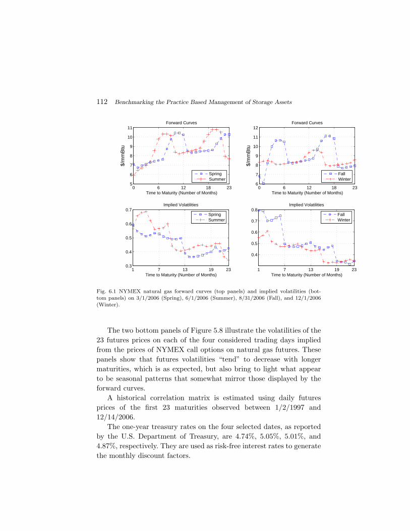
112 Benchmarking the Practice Based Management of Storage Assets
0 6 12 18 235
6
7
8
9
10
11
Time to Maturity (Number of Months)
$/m
mB
tuForward Curves
0 6 12 18 236
7
8
9
10
11
12
Time to Maturity (Number of Months)
$/m
mB
tu
Forward Curves
1 7 13 19 230.3
0.4
0.5
0.6
0.7Implied Volatilities
Time to Maturity (Number of Months)1 7 13 19 23
0.4
0.5
0.6
0.7
0.8
Time to Maturity (Number of Months)
Implied Volatilities
SpringSummer
FallWinter
SpringSummer
FallWinter
Fig. 6.1 NYMEX natural gas forward curves (top panels) and implied volatilities (bot-tom panels) on 3/1/2006 (Spring), 6/1/2006 (Summer), 8/31/2006 (Fall), and 12/1/2006(Winter).
The two bottom panels of Figure 5.8 illustrate the volatilities of the23 futures prices on each of the four considered trading days impliedfrom the prices of NYMEX call options on natural gas futures. Thesepanels show that futures volatilities “tend” to decrease with longermaturities, which is as expected, but also bring to light what appearto be seasonal patterns that somewhat mirror those displayed by theforward curves.
A historical correlation matrix is estimated using daily futuresprices of the first 23 maturities observed between 1/2/1997 and12/14/2006.
The one-year treasury rates on the four selected dates, as reportedby the U.S. Department of Treasury, are 4.74%, 5.05%, 5.01%, and4.87%, respectively. They are used as risk-free interest rates to generatethe monthly discount factors.
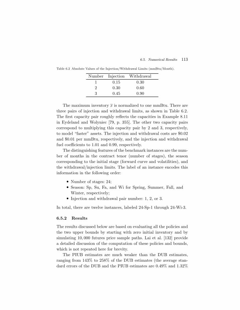
6.5. Numerical Results 113
Table 6.2 Absolute Values of the Injection/Withdrawal Limits (mmBtu/Month).
Number Injection Withdrawal1 0.15 0.302 0.30 0.603 0.45 0.90
The maximum inventory x is normalized to one mmBtu. There arethree pairs of injection and withdrawal limits, as shown in Table 6.2.The first capacity pair roughly reflects the capacities in Example 8.11in Eydeland and Wolyniec [79, p. 355]. The other two capacity pairscorrespond to multiplying this capacity pair by 2 and 3, respectively,to model “faster” assets. The injection and withdrawal costs are $0.02and $0.01 per mmBtu, respectively, and the injection and withdrawalfuel coefficients to 1.01 and 0.99, respectively.
The distinguishing features of the benchmark instances are the num-ber of months in the contract tenor (number of stages), the seasoncorresponding to the initial stage (forward curve and volatilities), andthe withdrawal/injection limits. The label of an instance encodes thisinformation in the following order:
• Number of stages: 24;• Season: Sp, Su, Fa, and Wi for Spring, Summer, Fall, and
Winter, respectively;• Injection and withdrawal pair number: 1, 2, or 3.
In total, there are twelve instances, labeled 24-Sp-1 through 24-Wi-3.
6.5.2 Results
The results discussed below are based on evaluating all the policies andthe two upper bounds by starting with zero initial inventory and bysimulating 10, 000 futures price sample paths. Lai et al. [132] providea detailed discussion of the computation of these policies and bounds,which is not repeated here for brevity.
The PIUB estimates are much weaker than the DUB estimates,ranging from 143% to 258% of the DUB estimates (the average stan-dard errors of the DUB and the PIUB estimates are 0.49% and 1.32%
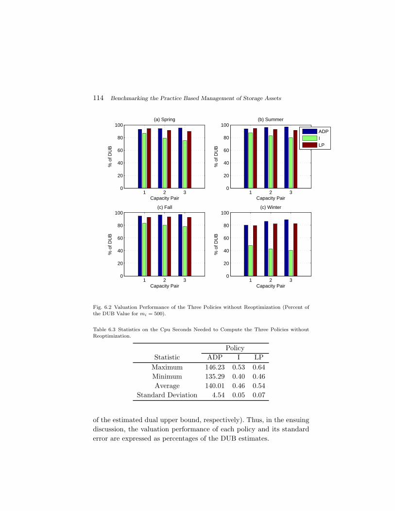
114 Benchmarking the Practice Based Management of Storage Assets
1 2 30
20
40
60
80
100(a) Spring
Capacity Pair
% o
f DU
B
1 2 30
20
40
60
80
100(b) Summer
Capacity Pair
% o
f DU
B
1 2 30
20
40
60
80
100(c) Fall
Capacity Pair
% o
f DU
B
1 2 30
20
40
60
80
100(c) Winter
Capacity Pair
% o
f DU
B
ADPILP
Fig. 6.2 Valuation Performance of the Three Policies without Reoptimization (Percent ofthe DUB Value for mi = 500).
Table 6.3 Statistics on the Cpu Seconds Needed to Compute the Three Policies withoutReoptimization.
PolicyStatistic ADP I LP
Maximum 146.23 0.53 0.64Minimum 135.29 0.40 0.46Average 140.01 0.46 0.54
Standard Deviation 4.54 0.05 0.07
of the estimated dual upper bound, respectively). Thus, in the ensuingdiscussion, the valuation performance of each policy and its standarderror are expressed as percentages of the DUB estimates.
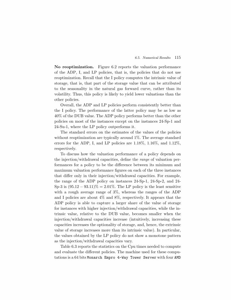
6.5. Numerical Results 115
No reoptimization. Figure 6.2 reports the valuation performanceof the ADP, I, and LP policies, that is, the policies that do not usereoptimization. Recall that the I policy computes the intrinsic value ofstorage, that is, that part of the storage value that can be attributedto the seasonality in the natural gas forward curve, rather than itsvolatility. Thus, this policy is likely to yield lower valuations than theother policies.
Overall, the ADP and LP policies perform consistently better thanthe I policy. The performance of the latter policy may be as low as40% of the DUB value. The ADP policy performs better than the otherpolicies on most of the instances except on the instances 24-Sp-1 and24-Su-1, where the LP policy outperforms it.
The standard errors on the estimates of the values of the policieswithout reoptimization are typically around 1%. The average standarderrors for the ADP, I, and LP policies are 1.18%, 1.16%, and 1.12%,respectively.
To discuss how the valuation performance of a policy depends onthe injection/withdrawal capacities, define the range of valuation per-formances for a policy to be the difference between its minimum andmaximum valuation performance figures on each of the three instancesthat differ only in their injection/withdrawal capacities. For example,the range of the ADP policy on instances 24-Sp-1, 24-Sp-2, and 24-Sp-3 is (95.12− 93.11)% = 2.01%. The LP policy is the least sensitivewith a rough average range of 3%, whereas the ranges of the ADPand I policies are about 4% and 8%, respectively. It appears that theADP policy is able to capture a larger share of the value of storagefor instances with higher injection/withdrawal capacities, while the in-trinsic value, relative to the DUB value, becomes smaller when theinjection/withdrawal capacities increase (intuitively, increasing thesecapacities increases the optionality of storage, and, hence, the extrinsicvalue of storage increases more than its intrinsic value). In particular,the values obtained by the LP policy do not show a monotone patternas the injection/withdrawal capacities vary.
Table 6.3 reports the statistics on the Cpu times needed to computeand evaluate the different policies. The machine used for these compu-tations is a 64 bits Monarch Empro 4-Way Tower Server with four AMD
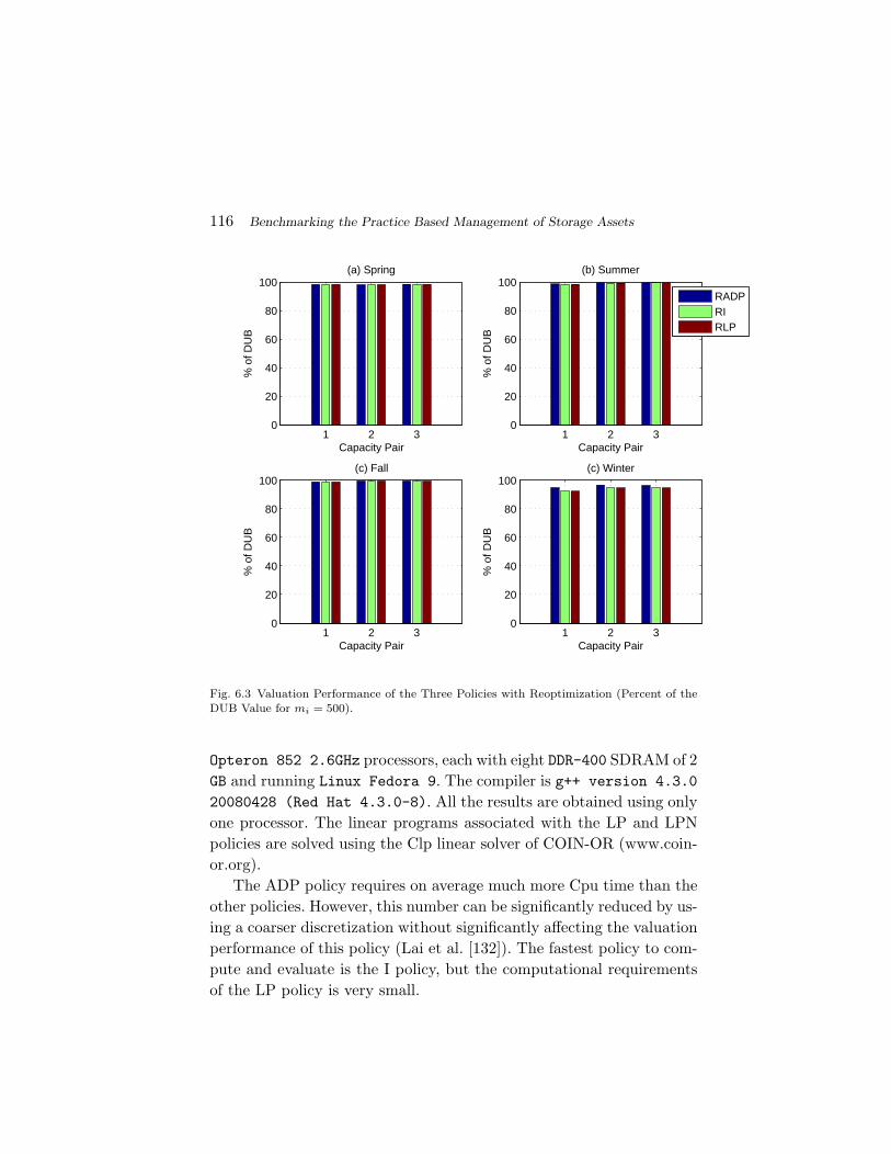
116 Benchmarking the Practice Based Management of Storage Assets
1 2 30
20
40
60
80
100(a) Spring
Capacity Pair
% o
f DU
B
1 2 30
20
40
60
80
100(b) Summer
Capacity Pair
% o
f DU
B
RADPRIRLP
1 2 30
20
40
60
80
100(c) Fall
Capacity Pair
% o
f DU
B
1 2 30
20
40
60
80
100(c) Winter
Capacity Pair
% o
f DU
B
Fig. 6.3 Valuation Performance of the Three Policies with Reoptimization (Percent of theDUB Value for mi = 500).
Opteron 852 2.6GHz processors, each with eight DDR-400 SDRAM of 2GB and running Linux Fedora 9. The compiler is g++ version 4.3.0
20080428 (Red Hat 4.3.0-8). All the results are obtained using onlyone processor. The linear programs associated with the LP and LPNpolicies are solved using the Clp linear solver of COIN-OR (www.coin-or.org).
The ADP policy requires on average much more Cpu time than theother policies. However, this number can be significantly reduced by us-ing a coarser discretization without significantly affecting the valuationperformance of this policy (Lai et al. [132]). The fastest policy to com-pute and evaluate is the I policy, but the computational requirementsof the LP policy is very small.
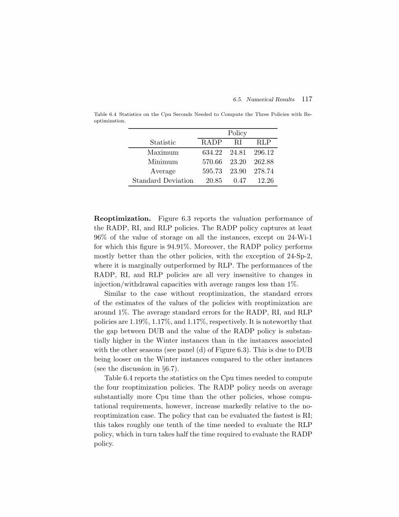
6.5. Numerical Results 117
Table 6.4 Statistics on the Cpu Seconds Needed to Compute the Three Policies with Re-optimization.
PolicyStatistic RADP RI RLP
Maximum 634.22 24.81 296.12Minimum 570.66 23.20 262.88Average 595.73 23.90 278.74
Standard Deviation 20.85 0.47 12.26
Reoptimization. Figure 6.3 reports the valuation performance ofthe RADP, RI, and RLP policies. The RADP policy captures at least96% of the value of storage on all the instances, except on 24-Wi-1for which this figure is 94.91%. Moreover, the RADP policy performsmostly better than the other policies, with the exception of 24-Sp-2,where it is marginally outperformed by RLP. The performances of theRADP, RI, and RLP policies are all very insensitive to changes ininjection/withdrawal capacities with average ranges less than 1%.
Similar to the case without reoptimization, the standard errorsof the estimates of the values of the policies with reoptimization arearound 1%. The average standard errors for the RADP, RI, and RLPpolicies are 1.19%, 1.17%, and 1.17%, respectively. It is noteworthy thatthe gap between DUB and the value of the RADP policy is substan-tially higher in the Winter instances than in the instances associatedwith the other seasons (see panel (d) of Figure 6.3). This is due to DUBbeing looser on the Winter instances compared to the other instances(see the discussion in §6.7).
Table 6.4 reports the statistics on the Cpu times needed to computethe four reoptimization policies. The RADP policy needs on averagesubstantially more Cpu time than the other policies, whose compu-tational requirements, however, increase markedly relative to the no-reoptimization case. The policy that can be evaluated the fastest is RI;this takes roughly one tenth of the time needed to evaluate the RLPpolicy, which in turn takes half the time required to evaluate the RADPpolicy.
118 Benchmarking the Practice Based Management of Storage Assets
Summary. The results discussed in this section bring to light thebenefit of combining reoptimization and Monte Carlo simulation fornatural gas storage valuation. This approach allows one to compute anear optimal policy in a rather simple and relatively fast fashion, forexample, by sequentially reoptimizing model I, which is a deterministicand dynamic model that can be optimized very efficiently. Reoptimizingmodel ADP, which is a stochastic and dynamic model, yields a slightlybetter policy at the expense of significantly higher Cpu requirements.Reoptimizing model LP, which is a stochastic and static model, alsogenerates a very good policy and is faster than reoptimizing modelADP. Hence, the choice of which model to sequentially reoptimize isimportant in order to obtain near optimal valuation of natural gas stor-age contracts by sequential reoptimization coupled with Monte Carlosimulation.
6.6 Conclusions
The valuation of the real option to store natural gas is an impor-tant problem in practice. Exact valuation of this real option using themultidimensional models of the evolution of the natural gas forwardcurve that seem to be used in practice is an intractable problem. Thus,practitioners typically value storage using heuristics. This chapter dis-cusses an ADP approach to benchmark the effectiveness of a set of suchheuristics on realistic instances and possibly improve on their valuationperformance. Unlike these heuristics or methods that are available inthe extant literature, this ADP approach yields both lower and upperbounds on the value of storage using the multidimensional representa-tion of the dynamics of the natural gas forward curve that seem to beused in practice.
The estimated upper bounds appear to be fairly tight. The analyzedpractice-based heuristic policies are very fast to compute but also sig-nificantly suboptimal, and are dominated by the ADP policy. However,when employed in a reoptimization fashion within Monte Carlo simula-tion, the valuation performances of all but one of these policies becomenearly optimal. The price to be paid for this improvement is a signifi-cantly higher computational burden. Overall, sequential reoptimization
6.7. Notes 119
within Monte Carlo simulation of a deterministic model that computesthe intrinsic value of storage strikes a good balance between valuationquality and computational requirements. However, in some cases theRADP policy can improve on the performance of the RI policy, butrequires more time to compute.
These results have immediate relevance for natural gas storagetraders. The findings with reoptimization remain substantially similarwhen (artificially) removing the seasonality from the employed natu-ral gas forward curves (Lai et al. [132]). This suggests that the resultsbased on reoptimization have potential relevance for traders involvedin the valuation of the real option to store other commodities, whoseforward curves do not exhibit the marked seasonality of the natural gasforward curve.
6.7 Notes
This chapter is based on Lai et al. [132]. As mentioned in §5.7, thenotation used in this chapter is not fully consistent with the notationof Lai et al. [132], but it is consistent with the notation of Chapter 5.
Eydeland and Wolyniec [79, p. 362] and Gray and Khandelwal [100]discuss versions of the practice-based heuristics considered in this chap-ter. Specifically, Eydeland and Wolyniec [79, p. 362] presents the LPpolicy, and Gray and Khandelwal [101] consider the I, RI, LP, andRLP heuristics. Gray and Khandelwal [101] refer to the RI as therolling-intrinsic policy, and the LP and RLP heuristics as the staticand dynamic basket-of-spreads policies.
Bjerksund et al. [18] and Wu et al. [209] also analyze the perfor-mance of the rolling intrinsic policy. Secomandi [173] investigates struc-tural properties of the intrinsic and basket-of-spreads policies and theirrolling versions, and provides theoretical support for the near optimalperformance of the policies with reoptimization observed in this chap-ter.
Nadarajah et al. [150] obtain stronger upper bounds for the in-stances considered in this chapter. They show that on the Winter in-stances the upper bounds used in this chapter are between 2.46% and2.82% larger than those that they compute. This implies that the RI,
120 Benchmarking the Practice Based Management of Storage Assets
RLP, and RADP policies are near optimal also on these instances.The approach of Nadarajah et al. [150] is based on the approximate
linear programming approach to MDPs (de Farias and Van Roy [62] andAdelman [1]) and subsumes the ADP model used in this chapter. Theheuristics considered in this chapter are examples of control algorithms,which are optimization-based ADP models that compute heuristic con-trol policies for intractable MDPs (Secomandi [169]). Other ADP ap-proaches include regression and Monte Carlo simulation (Longstaff andSchwartz [140], Bertsekas and Tsitsiklis [15]), Monte Carlo simulationand math programming (Powell [157]), rollout policies (Bertsekas [14,Chapter 6]), and Monte Carlo simulation and optimization algorithms(Chang et al. [48]). Boogert and de Jong [23, 24], Carmona and Lud-kovski [42], Nascimento and Powell [153], and Nadarajah et al. [149]value natural gas storage using ADP methods based on Monte Carlosimulation. Boogert and Mazieres [25] and Thompson [189] apply ra-dial basis function techniques to value natural gas storage. Felix andWeber [85] approach the same problem using recombining trees. Desaiet al. [68] develop a pathwise optimization approach to the valuationof Bermudan options. Bonnans et al. [21] develop a stochastic dualdynamic programming approach to value energy contracts.
The upper bound used in this chapter is based on the theory de-veloped by Brown et al. [35], who generalize the work of Davis andKaratzas [61], Rogers [161], Andersen and Broadie [3], and Haugh andKogan [105] on pricing American options (see Glasserman [94, Chapter8] for a review). Recent work includes the papers by Belomestny et al.[10], Bender [11], Chandramouli and Haugh [47], and Meinshausen andHambly [146].
7
Modeling Other Conversion Assets
This chapter deals with the optimal management of commodity con-version assets other than storage. These assets are an inventory dis-posal asset, an inventory acquisition asset, and swing assets. Inventorydisposal/acquisition assets are similar to storage assets, except thatthey are one-sided with only sale decisions for inventory disposal as-sets and purchase decisions for inventory acquisition assets. Anotherdifference from the storage asset is that they also have constraints onthe amount of inventory that must be disposed-of/acquired by a givendate. This implies that the feasible inventory set is stage dependent.Swing assets also are related to storage assets, but their payoffs repre-sent savings/gains from the contractual rights to buy/sell a commodityat prices that differ from market prices.
The goal of this chapter is to illustrate how the basestock struc-ture that characterizes the optimal inventory trading policy for stor-age can be modified for the optimal management of inventory dis-posal/acquisition and swing assets. Thus, the formulations of theseproblems as MDPs and their analysis rely substantially on the formu-lation of the storage asset as an MDP and the analysis carried out inChapter 5. In addition, this chapter points out that such modified base-
121
122 Modeling Other Conversion Assets
stock structures share the same nontriviality of the optimal basestockstructure for storage assets, as well as, under natural assumptions onthe relevant operational parameters, its lot size characterization statedin part (b) of Proposition 4 in §5.4 in Chapter 5.
The results in this chapter emphasize the generality of basestocktarget structures for optimally managing commodity conversion assetsas real options. In particular, the nontriviality of these structures stemsfrom nonlinearities that arise from the interaction between operationalaspects of commodity conversion assets. As a result, the operating pol-icy is not of the bang-bang type.
Sections 7.1 and 7.2 focus on the inventory disposal and acquisitionassets, respectively. Section 7.3 deals with swing assets. Section 7.4concludes. Section 7.5 provides pointers to the literature.
7.1 An Inventory Disposal Asset
Consider a merchant who has acquired a given amount of a storablecommodity and wants to unwind this position in a fixed time horizon.For instance, this might be a merchant of a particular metal, suchas, whose inventory is stored in a warehouse on its account (Geman[91, Chapter 8]). Sales from inventory are marked at the prevailingspot price when each sale occurs. There is a limit on the amount ofcommodity that the merchant can sell per unit of time, e.g., due tothe warehouse operational constraints. This merchant thus owns aninventory disposal asset with an embedded timing option about whento sell.
Different from the storage asset studied in Chapter 5, for whichthere is no constraint on the amount of inventory to be held at the endof the planning horizon, the manager of an inventory disposal assetmust sell all of the initial inventory by the end of the planning horizon.Hence, the terminal inventory level is constrained to be zero.
The problem of managing an inventory disposal asset can be formu-lated as an MDP. The time horizon is [0, T ]. Inventory disposal deci-sions are made at each time Ti, with i ∈ I := 0, . . . , N−1, T0 ≡ 0, andTN−1 ≡ T . The stage set is I. The initial inventory is x. The maximumamount of inventory that can be sold in each stage is the positive num-
7.1. An Inventory Disposal Asset 123
ber C. The feasible inventory set in stage i is Xi := [0, x ∧ (N − i)C],since the initial inventory must be entirely sold off by time T and thecapacity C limits how much inventory can be sold in each stage.
Selling an amount of inventory a, a nonnegative quantity, in stage i
generates the cash flow (si − c) a, where c is a marginal operational cost.The holding cost h is charged against each unit of inventory availablein a given stage.
Given a feasible inventory level x in stage i, a feasible action a
must be nonnegative, cannot exceed the selling capacity C, a positivequantity less than or equal to x, and must result in a feasible inventorylevel in the next stage, that is, a value in set Xi+1:
0 6 a 6 C,
0 6 x− a 6 x ∧ ((N − i− 1)C) .
The resulting feasible action set is
Ai(x) := [(x− (x ∧ (N − i− 1)C)) ∨ 0, x ∧ C] .
For simplicity, assume that the spot price in the current stage is theonly information available about the distribution of spot prices in laterstages. This assumption can be easily relaxed for the purposes of theanalysis performed in this section. As in §5.1 in Chapter 5, let Aπ
i (xi, si)be the decision rule of policy π in stage i, Π the set of all the feasiblepolicies, and xπ
i the random variable that denotes the inventory levelavailable in stage i when following policy π. Denote by δ the (constant)per stage risk-free discount factor and by ERN risk-neutral expectation.
The initial inventory level in stage 0 is x. The objective is to solvethe following problem:
maxπ∈Π
N−1∑
i=0
δiERN [(si − c) Aπi (xπ
i , si)− hxi | x, s0] . (7.1)
To understand the structure of the optimal policy of problem (7.1),ignore the requirement that the initial inventory must be entirely soldby time T . In this case the inventory disposal asset is analogous tothe storage asset discussed in Chapter 5 with respective injection andwithdrawal capacities equal to zero and −C, marginal injection and
124 Modeling Other Conversion Assets
withdrawal costs equal to infinity and c, and fuel loss factors equal toone. (The minus sign in front of C here is due to the withdrawal ac-tion and capacity being modeled as negative quantities in Chapter 5.)It thus follows from the analysis of Chapter 5 that the optimal policyfor such an inventory disposal asset has a basestock target structure.Specifically, in every stage and for a given spot price realization, the BIbasestock target can be defined to be zero and the only relevant bases-tock target is the WS target. In every stage and for a given spot price,the feasible inventory level is partitioned into at most two regions: ado nothing region for inventory levels below the sell-down-to basestocktarget and a selling region for inventory levels above this target.
This discussion suggests that adding the constraint that the entireinitial inventory be sold by the end of the planning horizon shouldnot fundamentally change the optimal policy structure. Proposition 8formally shows that this structure is of the single basestock target type.
Proposition 8 (Inventory disposal asset). The optimal policy forproblem (7.1) is of the basestock target type. In every stage i ∈ Igiven the spot price si ∈ <+ there exists a critical inventory levelbi(si) ∈ Xi such that an optimal action in state (xi, si) ∈ Xi × <+ isa∗i (xi, si) = 0 ∨ ((xi − bi(si)) ∧ C).
Proposition 8 relies on the basic intuition behind the basestockstructure for storage assets established in Theorem 5.2 in Chapter 5.In a given stage and for a given spot price, the optimal continuationvalue function of the equivalent formulation of problem 7.1 as an SDP,which is not shown here for brevity, is concave in inventory. The lin-earity of the immediate payoff function in the action then implies thestated basestock target structure.
Analogous to storage assets, the computation of an optimal inven-tory disposal policy is greatly simplified by the capacity C and themaximum inventory level x being integer multiples of a give lot size Q.Indeed, in this case each optimal basestock target also can be takento be an integer multiple of Q. That is, the optimal basestock targetstructure has a lot size characterization.
Example 1 in §5.2.2 in Chapter 5 shows the general nontriviality of
7.2. An Inventory Acquisition Asset 125
the optimal basestock target structure for a slow storage asset; namely,that the optimal slow storage policy is not of the bang-bang type.The same is true for the optimal policy of a slow (C < x) inventorydisposal asset. This feature can be seen by tailoring this example tosuch an asset.
Specifically, consider the medium, low, and high deterministic spotprice path illustrated in Figure 5.5 in §5.2.2 of Chapter 5. Set the totalinventory to be sold x equal to 1, the discount factor δ equal to 1,the selling capacity C equal to 2/3, and the marginal cost c and theholding cost h to be zero. This means that the lot size Q is equal to1/3. Given that the initial inventory level is 1, it is clearly optimal tosell 1/3 of it in stage 0 and 2/3 of it in stage 2. This means that theoptimal basestock targets are 2/3 in stage 0, 1 in stage 1, and 0 in stage2. The selling capacity is thus optimally underutilized when selling instage 0.
Similar to Example 1 in §5.2.2 in Chapter 5 that brings to light thenotion of left over space for a slow storage asset, this example illustratesthat left over inventory is a general feature of an optimal basestocktarget structure with a slow inventory disposal asset. The inventoryleft over in stage 0 is 1/3, which is the difference between the initialinventory to be sold and the selling capacity per stage: x−C = 1−2/3.
7.2 An Inventory Acquisition Asset
An inventory acquisition asset is the flip-side of an inventory disposalasset. It models the situation in which a merchant has agreed to delivera given amount of commodity by a certain date, and thus must acquirethis amount during a given time horizon. In doing so, the merchanthas the flexibility (timing option) of choosing when to purchase thecommodity from the spot market, holding it until the delivery date.
This problem can be formulated as an MDP. The time horizon is[0, T ]. The merchant must have available an amount x of commodityat time T . Purchases can be made at each of a given number of datesTi in set [0, T ], with i ∈ I (this set is defined as in §7.1). The stage setis I. Due to operational constraints, there is a capacity C (a positivenumber less than or equal to x) that limits the amount of commodity
126 Modeling Other Conversion Assets
that can be purchased at each such date. The cash flow associated withthe purchase of an amount of commodity a in stage i is − (si + c) a,where c is a marginal operational cost. The holding cost h is assessedon each inventory unit available in a given stage.
The requirement on the amount of inventory to be procured bytime TN ≡ T and the limit on the amount that can be purchased ateach time Ti imply that the feasible inventory set in each stage i isXi := [0 ∨ (x− (N − i) C) , x]. A feasible purchase in stage i when theavailable inventory level is x ∈ Xi must satisfy
0 6 a 6 C,
0 ∨ (x− (N − i− 1)C) 6 x + a 6 x.
These inequalities imply that the corresponding set of feasible pur-chases is
Ai(x) := [0 ∨ ((0 ∨ (x− (N − i− 1)C))− x) , (x− x) ∧ C] .
Like the inventory disposal asset, suppose for simplicity that thedistribution of the spot price in the next stage only depends on thespot price in the current stage. The initial inventory level in stage 0 iszero. Reusing the notation used to formulate problem 7.1, the problemto be solved is
minπ∈Π
N−1∑
i=0
δiERN [(si + c) Aπi (xπ
i , si) + hxi | 0, s0] . (7.2)
As the inventory disposal asset, the inventory acquisition asset isrelated to the storage asset, but the requirement that a given amountof commodity be procured by a given date is critical to make the prob-lem nontrivial. In other words, if there were no such requirement, theoptimal policy would be trivially equal to doing nothing in every stagefor every spot price realization. In contrast, this is not the case for theinventory disposal asset when it lacks the requirement that the entireinitial inventory be sold by the end of the time horizon.
Proposition 9 states that the optimal inventory acquisition policyfor problem (7.2) has a basestock target structure.
7.3. Swing Assets 127
Proposition 9 (Inventory acquisition asset). The optimal policyfor MDP (7.2) is of the basestock target type. In every stage i ∈ I givena spot price si ∈ <+ there exists a critical inventory level bi(si) ∈ Xi
such that an optimal action in state (xi, si) ∈ Xi × <+ is a∗i (xi, si) =0 ∨ ((bi(si)− xi) ∧ C).
As with Proposition 8, the intuition behind Proposition 9 is theconcavity in inventory of the optimal continuation value function of theformulation of problem (7.2) as an SDP, not shown here for brevity,in each given stage and for a given spot price, and the linearity inthe amount of purchased inventory of the immediate payoff function.Moreover, the optimal basestock structure for an inventory acquisitionasset shares the nontriviality and lot size characterization of the optimalpolicy for an inventory disposal asset.
7.3 Swing Assets
Swing contracts are widespread in energy, especially electricity and nat-ural gas, industries. In these industries, producers or buyers often trans-act via contracts that specify minimum and maximum total amountsof energy to be sold or purchased at a fixed price during a given timeperiod. Moreover, these contracts specify a maximum, and possibly aminimum, amount of energy transacted on each given trading date.Thus, a producer or a buyer that owns such a contract is obligatedto deliver or purchase at least a given amount of energy, but retainsthe flexibility to decide how to do so during the given time period.In other words, the owners of such contracts have available a givennumber of “swings” and must decide how to optimally exercise themduring the contract life. The distinction here is between sale-swing andpurchase-swing contracts.
The existence of energy spot markets means that producers or buy-ers could transact on such markets at the prevailing market price, ratherthan through a given swing contract. Thus, the valuation and manage-ment of swing contracts can be determined by optimally managing thegains/savings that accrue to the owner of a swing contract relative
128 Modeling Other Conversion Assets
to trading in the spot market. Consequently, the dynamics of energyspot prices are fundamental in the valuation and management of swingcontracts.
Sale-Swing asset. Consider an energy producer that has agreed todeliver at least x but no more than x units of energy during the timeinterval [0, T ] to a given buyer. Sales can be made at each of a givennumber of dates Ti with i ∈ I (the same set used in §7.1). Each salecan be made at a contractually fixed unit price equal to K. There is alimit C, a positive number, on the amount of each sale (the possibilityof a minimum sale quantity per date is ignored for simplicity).
If a sale a is made at time Ti, then the producer gains the amount(K − si)a. This is because the producer could have sold the amount ofenergy a on the spot market for a cash flow equal to sia, and ownershipof the sale contract gives the producer the ability to obtain additionalvalue relative to transacting on the spot market.1 This is a key insightthat allows one to formulate the problem of managing a sale-swingcontract as an MDP.
The stage set of this MDP is the set I. The total amount of energysold by time Ti since time 0 is denoted by xi and represents the amountof energy already sold up to stage i, a type of “inventory.” The feasibleinventory set in stage i is Xi := [0 ∨ (x− (N − i)C) , x].
Given the feasible inventory level x in stage i, a feasible action mustsatisfy the following constraints:
0 6 a 6 C,
0 ∨ (x− (N − i− 1)C) 6 x + a 6 x.
These inequalities imply that this action must belong to the followingset:
Ai(x) := [0 ∨ (x− (0 ∨ (x− (N − i− 1)C))) , (x− x) ∧ C] .
As in §§7.1-7.2, assume for simplicity that the current spot price isthe only information available about future spot price dynamics. The
1The implicit assumption here is that the operational cost of executing the sale is the sameunder both modes of operations.

7.3. Swing Assets 129
initial inventory level in stage 0 is 0. Reusing the notation used in §§7.1-7.2, optimally managing a sale-swing asset entails solving the followingproblem:
maxπ∈Π
N−1∑
i=0
δiERN [(K − si) Aπi (xπ
i , si)− hxi | 0, s0] . (7.3)
On the surface, problem (7.3) resembles problem (7.1) once thedecision rule Aπ
i (xπi , si) is expressed as −(−Aπ
i (xπi , si)) and the selling
price K is replaced with the marginal cost c. Notwithstanding someremaining differences in the definition of the feasible inventory andaction sets of these problems, this observation suggests that the optimalpolicy for a sale-swing asset is of the basestock target type. Proposition10 demonstrates that this is indeed the case.
Proposition 10 (Sale-swing asset). The optimal policy for prob-lem (7.3) is of the basestock target type. In every stage i ∈ I given aspot price si there exists a critical inventory level bi(si) ∈ Xi suchthat an optimal action in state (xi, si) ∈ Xi × <+ is a∗i (xi, si) =0 ∨ ((xi − bi(si)) ∧ C).
Proposition 10 relies on the same intuition that underlies Proposi-tions 8 and 9 in this chapter. Moreover, the optimal policy of a sale-swing asset shares the same nontriviality and lot size characterizationof the optimal policies of the inventory disposal and acquisition as-sets (the lot size characterization holds under the assumption that thequantities x, x, and C are all integer multiples of some number Q).
Purchase-swing asset. A purchase swing-asset is the analogue of asale-swing asset for an energy buyer. This buyer has agreed to purchaseat least x but no more than x units of energy during the time interval[0, T ] from a given producer. On each of a given number of dates Ti
with i ∈ I, this buyer can purchase energy up to the limit C at agiven unit price K. The difference between the sale-swing asset andthe purchase-swing asset is the benefit obtained by the buyer whena purchase is made. This per unit gain on a purchase made at timeTi is (si −K), and represents the savings obtained by the buyer when
130 Modeling Other Conversion Assets
purchasing using the purchase-swing asset rather than the spot market.Replacing the term (K− si) with this per unit gain in problem (7.3) isthe only modification that needs to be made to this problem to modelthe optimal management of the purchase-swing asset. It follows that theanalogue of Proposition 10 in this section and the properties discussedafter this result hold for the purchase-swing asset.
7.4 Conclusions
This chapter considers the management of inventory dis-posal/acquisition assets and swing assets. Inventory dis-posal/acquisition assets are relevant for a merchant that mustsell/procure a given amount of inventory by a certain date, and hasthe flexibility to decide when to sell/purchase this inventory. Swingassets are widespread in the energy industry and provide quantityflexibility to energy producers and users.
This chapter shows that variants of the basestock target structurethat characterize the optimal management of storage assets remainoptimal for the management of the assets considered here. Moreover,these variants of the basestock target structure retain the nontrivialityand the lot size characterization of the storage optimal basestock targetstructure.
7.5 Notes
The inventory disposal asset without the condition that the entire ini-tial inventory be sold by the end of the finite horizon represents a natu-ral resource production asset, e.g., a natural gas or petroleum reservoiror a coal mine; that is, the initial inventory represents the amount ofavailable natural resource, e.g., oil, natural gas, or coal. In such casesthe dynamics of the natural resource availability may deserve moredetailed modeling. For instance, after an initial transitory period, thenatural gas or petroleum that can be extracted from a reservoir ina given time period has ben observed to exhibit exponential declineas the total natural gas or petroleum in the reservoir depletes. Suchdecline may also be characterized by stochastic behavior. Smith and
7.5. Notes 131
McCardle [181] and Enders et al. [77], among others, model oil andnatural gas production assets as SDPs. Brown and Smith [34] take abandit approach to the management of oil and gas production assets.Cortazar et al. [56] apply the least squares Monte Carlo approach tovalue a copper mine.
The inventory acquisition asset can be modified to model a con-sumption asset, whereby the amount of acquired commodity is used asan input to a manufacturing or a distribution stage. In this case, therequired amount of commodity may not be known with certainty, thatis, the demand for the commodity may be random, and excess supplycan be carried in inventory to satisfy demand in later periods. Nasci-mento and Powell [152] and Secomandi and Kekre [174] discuss modelsin which the commodity/energy requirement is stochastic (in the modelof Secomandi and Kekre [174] energy purchases can be made both inspot and forward markets incurring differential transaction costs). Ka-lymon [115], Gavirneni [90], Goel and Gutierrez [95, 96], Berling andVictor Martınez-de-Albeniz [13], and Kouvelis et al. [128, 129] presentcommodity inventory management models with stochastic demand andpurchase prices (Goel and Gutierrez [96] do this in a multiechelon set-ting).
This chapter does not deal with cross-commodity conversion assetsthat involve the physical conversion of one commodity into one or morecommodities. Examples include refinery assets that convert petroleuminto gasoline, naphta, and jet fuel, corn or sugarcane into ethanol, soy-bean into soyoil and soymeal; electricity generation assets that use nat-ural gas as an input; and the processing of cattle into beef products.Power plants are often subject to pollution emission caps which limittheir operations. Operation of a power plant then involves choosingwhich days will be the most profitable – given the spark spread betweenpower and fuel prices – to produce power and use up the available emis-sion permits. This decision has a similar timing option structure as aninventory disposal asset. If emission permits are tradable, as with SOXin the US or carbon in Europe, then operation of a power plant is avariation on a storage option in which an inventory of emission permitscan be bought, sold, and also used over time. Coal and natural gas fired
132 Modeling Other Conversion Assets
power plants have also access to storage of their fuels. In the case ofnatural gas, in addition to underground natural gas storage facilities,the pipeline linepack can also be used for short-term storage. Liquefiednatural gas terminals also provide short-term storage opportunities.
Research on the management of cross-commodity conversion assestsincludes the work of Adkins and Paxson [2], Arvesen et al. [4], Boyabatliet al. [26], Brandao et al. [29], Devalkar et al. [69], Dockendorf andPaxson [72], Hahn and Dyer [103], Kazaz and Webster [120], Thompsonet al. [191], Thompson [190], Tseng and Barz [195], Tseng Lin [196],and Wu and Chen [208].
Fleten and Kristoffersen [87], Nasakkala and Keppo [151], and De-nault et al. [66] consider hydropower production asset. Relevant workin this area, but not from a real options perspective, includes that ofDrouin et al. [74] and Lamond et al. [134]. Wallace and Fleten [198]review the related literature on energy stochastic optimization models.
The swing assets considered in this chapter are based on the de-scription of swing contracts in Geman [91, p. 294]. The insight that aswing contract can be valued and managed relative to the strategy thatonly operates in the spot markets appears novel. Ghiuvea et al. [92],Jaillet et al. [112], Keppo [123], Barrera-Esteve et al. [8], Ross and Zhu[163], and Nadarajah et al. [149], among others, discuss the valuationand management of swing contracts.
8
Trends
This chapter briefly discusses a nonexhaustive list of trends for furtherresearch in the area of merchant operations: financial hedging (§8.1),the analysis of other commodity conversion assets (8.2), approximatedynamic programming methods (§8.3), price model error (8.4), endo-geneity of the price process in determining an operating policy (§8.5),equilibrium asset pricing (§8.6), and the choice of capacity levels (§8.7).
8.1 Financial Hedging
In addition to being the basic principle underlying risk neutral val-uation in dynamically complete markets, the ability to construct dy-namic portfolios of traded securities (typically, commodity and energyfutures contracts) that replicate the cash flows generated by commod-ity conversion assets is an important risk management tool (Hull [109]).Merchants can use these replicating portfolios for financial hedging.
Specifically, shorting and periodically rebalancing a replicatingportfolio amounts to eliminating the change over time of the marketvalue of a given asset. This approach yields a financial hedging policy,known as delta hedging. Delta hedging can be used to reduce/eliminate
133
134 Trends
risk capital charges that a merchant might incur in some costly statesof nature.
Due to the lack of explicit representations for optimal, or near-optimal, operating policies for most commodity conversion assets,closed-form expressions for the compositions of these portfolios, theso called deltas, are rare. Numerical computation of the deltas is thusthe norm. Monte Carlo simulation is a useful tool in this respect. Boyleet al. [27], Broadie and Glasserman [33], and Fu and Hu [89] discuss theestimation of the Greeks by Monte Carlo simulation. Glasserman [94,Chapter 7] provides a more recent review of this literature. Wang etal. [200] is a recent addition to this literature. Kaniel et al. [119], Chenand Liu [53], and Caramellino and Zanette [39] focus on the estimationof Greeks for options with multiple exercise dates.
Secomandi and Wang [176] and Secomandi et al. [175] use derivativeestimation techniques to compute the deltas of natural gas transportand storage assets using term structure price models. Secomandi et al.[175] also test their approach on natural gas data. Bonnans et al. [22]compute the price sensitivities of the values of energy contracts in astochastic programming setting. Fleten and Wallace [88] and Li andKleindorfer [136] consider the delta hedging of hydropower generationassets and spark spread options.
More research is needed to develop delta estimation techniques un-der alternative price models and benchmark the performance of theresulting estimators in realistic situations. This research direction isparticularly important in dynamically incomplete markets, for whichrisk neutral valuation depends on price of risk assumptions.
8.2 Analysis of Other Commodity Conversion Assets
This monograph examines in detail only a small number of applications:storage and inventory disposal/acquisition/swing assets. As discussedin §2.6 in Chapter 2 and in §7.5 in Chapter 7, the ideas and methods ofmerchant operations have much wider applicability beyond these ap-plications. Important commodity conversion assets that have receivedsubstantial attention in the literature, but are ignored in this mono-graph, include power plants and a variety of commodity processing
8.3. Approximate Dynamic Programming 135
assets that embed portfolios of spread/rainbow and switching options.The structure of the optimal operating policies of these assets is
typically not well understood in the literature. In particular, unlike theoptimal policy of the assets that are the focus of this monograph, theoptimal policy structure for these other assets is unlikely to be of thebasestock . Deepening our understanding of the structure of their op-timal policies is a fruitful area for additional research. Although thecomputation of optimal policies is typically an intractable task, knowl-edge of these structures might inform the development of practical andeffective methods for the computation of near-optimal policies.
8.3 Approximate Dynamic Programming
As illustrated in Chapter 6, practitioners use high-dimensional com-modity price evolution models. Even though one may not want to usea full dimensional market model of the futures curve evolution, a modelwith three factors would already be considered high dimensional for theexact computation of optimal operating policies. Both practitioners andscholars have thus turned to approximations that allow for the efficientcomputations of near-optimal operating policies.
Due to the dynamic and stochastic nature of most merchant opera-tions problems, these approximations involve some form of approximatedynamic programming algorithm. Glasserman [94, Chapter 7] discussesthe literature on the Monte Carlo pricing of American options, includ-ing approximate dynamic programming methods. This material is rel-evant to merchant operations problems, which tend to have an Amer-ican (Bermudan) structure. Moreover, as discussed in §6.7 in Chapter6, the literature includes several approximate dynamic programmingmethods. Refining these methods via their application to merchant op-erations problems is an interesting area for additional research.
Approximate dynamic programming typically focuses on the com-putation of near optimal policies and lower bounds (to a maximizationproblem). As demonstrated in Chapter 6, good upper bounds are es-sential to assess the performance of heuristic policies. As discussed in§6.7 in Chapter 6, there is an active stream of recent research thatdeals with upper bound estimation in financial and real options valua-
136 Trends
tion. Continuing this line of work in the area of merchant operations,in which optimization problem are more complicated than stoppingproblems, is a promising are for additional research.
8.4 Price Model Error
Merchant operations relies in a fundamental manner on models of theevolution of commodity and energy prices. It is inevitable that thesemodels are only approximations of the dynamics of these prices. Inother words, these models embed errors. It is thus important to assessthe impact of model errors on the merchant management of differ-ent commodity conversion assets. The impact here can be in terms ofasset valuation, which merchants use to decide how much to bid toacquire an asset, the asset operating policy and, when relevant, the as-set financial hedging policy, which affect the operational and financialcash flows earned by a merchant when managing an asset. When thisimpact is practically important, developing methods to mitigate thenegative consequences of this impact is relevant. This type of researchthus combines empirical and methodological aspects. Secomandi et al.[175] investigate these issues in the context of merchant commoditystorage. It would be interesting to investigate the topic of price modelerror in the context of different commodity conversion assets.
8.5 Price Impact
A key underlying assumption behind this monograph is that a mer-chant’s trading decisions to not affect market prices. That is, the ca-pacity of the commodity conversion asset under a merchant’s control is“small’ relative to the market size or, equivalently, commodity marketsare sufficiently liquid. In such a setting, market liquidity considerationsdo not play a role in optimizing the operating policy of a conversion as-set, and a price-taker modeling approach is justified. However, liquidityin physical spot markets can be limited. In these cases, the price-takerapproach is not justified and may generate suboptimal operating poli-cies once liquidity constraints are taken into account. Studying the ex-tent of this suboptimality and developing merchant operations methods
8.6. Equilibrium Asset Pricing 137
in the presence of limited liquidity are interesting avenue for additionalresearch. Some research along these directions includes the papers ofMartınez-de-Albeniz and Vendrell Simon [144], Felix et al. [84], andChaton and Durand-Viel [51].
8.6 Equilibrium Asset Pricing
Reduced-form models like Pilipovic/Schwartz-Smith or future termstructure factor models (see §4.1 and §4.2 in Chapter 4) simply takecommodity price dynamics as exogenously given. As such, reduced-formmodels make strong assumptions about the stationarity of commodityprice processes over time. In contrast, equilibrium models derive thedynamics of commodity price from the statistical properties of randomenvironmental shocks and the joint endogenous production, storage,and consumption behavior of optimizing producers, merchants, andconsumers. By relating commodity prices to deeper economic funda-mentals, equilibrium models have at least some hope of being able toaccount for changing statistical properties of commodity prices. Sec-tion 4.3 in Chapter 4 gives pointers to recent theoretical work on therelationship between investor preferences and commodity risk premiaand to recent empirical work on the macroeconomic and microeco-nomic drivers of commodity prices. While option valuation theory isconcerned with computing market prices, merchant traders frequentlytrade on views of future changes in fundamentals that differ from theprevailing market view. Commodity pricing when agents have strategicmarket power or private information and the impact of market seg-mentation between physical and financial markets for commodities arerelatively unexplored topic that are not well understood.
8.7 Capacity Choice
This monograph assumes that the capacity of a commodity commod-ity conversion asset is given. That is, a merchant has already decidedhow to size the assets that it controls, e.g., how much space and injec-tion/withdrawal capacity of a given natural gas storage asset to rentand for how long. This capacity choice problem is an important one
138 Trends
in practice when a merchant faces risk capital charges, that is, thereare frictions in capital markets. In this situation, a merchant might notbe able to fund all the available projects, that is, a merchant mighthave to choose which projects to select and their size. The resultingproblem might resemble a portfolio optimization problem, even thoughprojects might be selected in a sequential manner rather than simulta-neously. It would be interesting to conduct exploratory research aimedat learning and documenting the institutional details of how merchantscurrently address this project selection and sizing problem, and inves-tigating whether optimization techniques might be relevant to supportmerchants in solving such problem.
Acknowledgements
Yunfan Gu offered insightful comments on Chapters 3 and 4. SelvaNadarajah helped producing some of the figures in Chapter 4. Chapter5 uses by permission content from N. Secomandi, Optimal Commod-ity Trading with a Capacitated Storage Asset, Management Science,56, 3, 2010, 449-467, Copyright 2010, The Institute for OperationsResearch and the Management Sciences, 7240 Parkway Drive, Suite300, Hanover, MD 21076 USA. Chapter 6 uses by permission contentfrom G. Lai, F. Margot, N. Secomandi, An Approximate Dynamic Pro-gramming Approach to Benchmark Practice-based Heuristics for Nat-ural Gas Storage Valuation, Operations Research, 58, 3, 2010, 564-582,Copyright 2010, The Institute for Operations Research and the Man-agement Sciences, 7240 Parkway Drive, Suite 300, Hanover, MD 21076USA. This work was in part supported by NSF grant CMMI 1129163.
139
References
[1] D. Adelman. Math programming approaches to approximate dynamic pro-gramming. Tutorial, INFORMS Annual Meeting, Pittsburgh, PA, USA, 2006.
[2] R. Adkins and D. Paxson. Reciprocal energy-switching options. Journal ofEnergy Markets, 4:91–120, 2011.
[3] L. Andersen and M. Broadie. Primal-dual simulation algorithm for pric-ing multidimensional American options. Management Science, 50:1222–1234,2004.
[4] O. Arvesen, V. M. ø, S.-E. Fleten, and A. T. S. Westgaard. Linepack storagevaluation under price uncertainty. Energy, 52:155–164, 2013.
[5] D. Backus, B. Routledge, and S. Zin. Exotic preferences for macroeconomists.NBER Macroeconomics Annual, 19:319–390, 2004.
[6] S. Baker and B. Routledge. The price of oil risk. Working Paper, 2012.[7] R. Bansal and A. Yaron. Risks for the long run: A potential resolution of
asset pricing puzzles. Journal of Finance, 59:1481–1509, 2004.[8] C. Barrera-Esteve, F. Bergeret, C. Dossal, E. Gobet, A. Meziou, R. Munos,
and D. Reboul-Salze. Numerical methods for the pricing of swing options: Astochastic control approach. Methodology And Computing In Applied Proba-bility, 8:517–540, 2006.
[9] R. Bellman. On the theory of dynamic programming – a warehousing problem.Management Science, 2:272–275, 1956.
[10] D. Belomestny, C. Bender, and J. Schoenmakers. True upper bounds forbermudan products via non-nested monte carlo. Mathematical Finance, 19:53–71, 2009.
[11] C. Bender. Dual pricing of multi-exercise options under volume constraints.Finance and Stochastics, 15:1–26, 2011.
140
References 141
[12] F. E. Benth, J. S. Benth, and S. Koekebakker. Stochastic Modeling of Elec-tricity and Related Markets. World Scientific Publishing, Singapore, 2008.
[13] P. Berling and V. Martınez-de-Albeniz. Optimal inventory policies when pur-chase price and demand are stochastic. Operations Research, 59:109–124,2011.
[14] D. P. Bertsekas. Dynamic Programming and Optimal Control – Volume I.Athena Scientific, Belmont, MA, USA, third edition, 2005.
[15] D. P. Bertsekas and J. N. Tsitsiklis. Neuro-Dynamic Programming. AthenaScientific, Belmont, MA, USA, 1996.
[16] H. Bessembinder. Systematic risk, hedging pressure, and risk premiums infutures markets. Review of Financial Studies, 5:637–667, 1992.
[17] H. Bessembinder and K. Chan. Time varying risk premia and forecastablereturns in futures markets. Journal of Financial Economics, 32:169–193, 1992.
[18] P. Bjerksund, G. Stensland, and F. Vagstad. Gas storage valuation: Pricemodeling v. optimization models. The Energy Journal, 32:203–227, 2011.
[19] F. Black. The pricing of commodity contracts. Journal of Financial Eco-nomics, 3:167–179, 1976.
[20] F. Black and M. Scholes. The pricing of options and corporate liabilities.Journal of Political Economy, 81:637–654, 1973.
[21] J. F. Bonnans, Z. Cen, and T. Christel. Energy contracts management bystochastic programming techniques. Annals of Operations Research, 200:199–222, 2012.
[22] J. F. Bonnans, Z. Cen, and T. Christel. Sensitivity analysis of energy contractsby stochastic programming techniques. In R. Carmona, P. D. Moral, P. Hu,and N. Oudjane, editors, Numerical Methods in Finance, Springer Proceedingsin Mathematics, pages 447–471. Springer-Verlag, Berlin Heidelberg, 2012.
[23] A. Boogert and C. de Jong. Gas storage valuation using a Monte Carlomethod. Journal of Derivatives, 15:81–98, 2008.
[24] A. Boogert and C. de Jong. Gas storage valuation using a multifactor priceprocess. Journal of Energy Markets, 4:29–52, 2011/12.
[25] A. Boogert and D. Mazieres. A radial basis function approach to gas storagevaluation. Working Paper, Birkbeck University of London, London, UK, 2011.
[26] O. Boyabatli, P. R. Kleindorfer, and S. R. Koontz. Integrating long-term andshort-term contracting in beef supply chains. Management Science, 57:1771–1787, 2011.
[27] P. P. Boyle, M. Broadie, and P. Glasserman. Monte Carlo methods for securitypricing. Journal of Economic Dynamics and Control, 21:1267–1321, 1997.
[28] A. Brace, D. Gatarek, and M. Musiela. The market model of interest ratedynamics. Mathematical Finance, 7:127–147, 1997.
[29] L. E. T. Brandao, G. Master Penedo, and C. Bastian-Pinto. The value ofswitching inputs in a biodiesel production plant. European Journal of Finance,pages 1–15, 2011.
[30] D. Breeden and R. Litzenberger. Prices of state-contingent claims implicit inoption prices. Journal of Business, 51:621–651, 1978.
142 References
[31] M. J. Brennan. Stochastic models and option models. In D. L. and B. Ok-sendal, editors, The price of convenience and the valuation of commodity con-tingent claims, pages 33–71. North Holland, North Holland, Amsterdam, 1991.
[32] M. J. Brennan and E. S. Schwartz. Evaluating natural resource investments.Journal of Business, 58:135–157, 1985.
[33] M. Broadie and P. Glasserman. Estimating security price derivatives usingsimulation. Management Science, 42:269–285, 1996.
[34] D. B. Brown and J. E. Smith. Optimal sequential exploration: Bandits, clair-voyants, and wildcats. Operations Research, Forthcoming, 2012.
[35] D. B. Brown, J. E. Smith, and P. Sung. Information relaxation and dualityin stochastic dynamic programs. Operations Research, 58:785–801, 2010.
[36] B. Burger, B. Graeber, and G. Schindlmay. Managing Energy Risk: An In-tegrated View on Power and Other Energy Markets. John Wiley & Sons,Chichester, UK, 2007.
[37] B. Buyuksahin, M. S. Haigh, J. H. Harris, J. A. Overdahl, and M. A. Robe.Fundamentals, trader activity and derivative pricing. Working Paper, 2008.
[38] A. S. Cahn. The warehouse problem. Bulletin of the American MathematicalSociety, 54:1073, 1948.
[39] L. Caramellino and A. Zanette. Monte Carlo methods for pricing and hedgingAmerican options in high dimensions. Risk and Decision Analysis, 2:207–220,2010/2011.
[40] M. Carlson, Z. Khokher, and S. Titman. Equilibrium exhaustible resourceprice dynamics. Journal of Finance, 62:16631703, 2007.
[41] R. Carmona and V. Durrleman. Pricing and hedging spread options. Societyfor Industrial and Applied Mathematics Review, 45:627–685, 2003.
[42] R. Carmona and M. Ludkovski. Valuation of energy storage: An optimalswitching approach. Quantitative Finance, 10:359–374, 2010.
[43] A. Carverhill. When is the short rate markovian? Mathematical Finance,4:305–312, 1994.
[44] J. Casassus and P. Collin-Dufresne. Stochastic convenience yields implied frominterest rates and commodity futures. Journal of Finance, 60:2283–2331, 2005.
[45] J. Casassus, P. Collin-Dufresne, and B. R. Routledge. Equilibrium commod-ity prices with irreversible investment and non-linear technologies. WorkingPaper, 2008.
[46] B. Casselman. Natural-gas forecast is hot. The Wall Street Journal, June 23,2008.
[47] S. Chandramouli and M. B. Haugh. A unified approach to multiple stoppingand duality. Operations Research Letters, 40:258–264, 2012.
[48] S. H. Chang, M. C. Fu, J. Hu, and S. I. Marcus. Simulation-based Algorithmsfor Markov Decision Processes. Springer, London, UK, 2007.
[49] A. Charnes and W. W. Cooper. Generalization of the warehousing problem.Operational Research Quarterly, 6:131–172, 1955.
[50] A. Charnes, J. Dreze, and M. Miller. Decision and horizon rules for stochasticplanning problems: A linear example. Econometrica, 34:307–330, 1966.
References 143
[51] C. Chaton and L. Durand-Viel. Real asset valuation under imperfect compe-tition: Can we forget about market fundamentals? Journal of Economics &Management Strategy, 22:125–139, 2013.
[52] G. Chazan. Russia outflanks EU’s pipeline plan. The Wall Street Journal,June 16, 2008.
[53] N. Chen and Y. Liu. American option sensitivities estimation via a general-ized IPA approach. Working Paper, Department of Systems Engineering andEngineering Management, The Chinese University of Hong Kong, 2012.
[54] Z. Chen and P. A. Forsyth. A semi-Lagrangian approach for natural gas stor-age valuation and optimal operation. SIAM Journal on Scientific Computing,30:339–368, 2007.
[55] L. Clewlow and C. Strickland. Energy Derivatives: Pricing and Risk Manage-ment. Lacima Publications, London, UK, 2000.
[56] G. Cortazar, M. Gravet, and J. Urzua. The valuation of multidimensionalAmerican real options using the LSM simulation method. Computers & Op-erations Research, 35:113–129, 2008.
[57] G. Cortazar and E. S. Schwartz. The valuation of commodity-contingentclaims. Journal of Derivatives, 1:27–39, 1994.
[58] Q. Dai and K. J. Singleton. Specification analysis of affine term structuremodels. Journal of Finance, 55:1943–1978, 2000.
[59] A. Davis. Morgan Stanley trades energy the old-fashioned way: In barrels.The Wall Street Journal, March 2, 2005.
[60] A. Davis and R. Gold. Surge in natural-gas price stoked by new global trade.The Wall Street Journal, April 18, 2008.
[61] M. Davis and I. Karatzas. A deterministic approach to optimal stopping, withapplications. In P. Kelly, editor, Probability, Statistics and Optimization: ATribute to Peter Whittle, pages 255–466. John Wiley & Sons, Chichester, UK,1994.
[62] D. P. de Farias and B. V. Roy. The linear programming approach to approx-imate dynamic programming. Operations Research, 51:850–865, 2003.
[63] C. de Jong and K. Walet. Gas storage management. In Managing Energy PriceRisk, pages 631–647. Risk Publications, London, UK, third edition, 2004.
[64] A. Deaton and G. Laroque. On the behaviour of commodity prices. Reviewof Economic Studies, 59:1–23, 1992.
[65] A. Deaton and G. Laroque. Competitive storage and commodity price dy-namics. Journal of Political Economy, 104:896–923, 1996.
[66] M. Denault, J. G. Simonato, and L. Stentoft. A simulation-and-regressionapproach for stochastic dynamic programs with endogenous state variables.Working Paper G-2011-24, Les Cahiers du GERAD, HEC Montreal, Montreal,Canada, 2011.
[67] S. J. Deng, B. Johnson, and A. Sogomonian. Exotic electricity options and thevaluation of electricity generation and transmission assets. Decision SupportSystems, 30(3):383–392, 2001.
[68] V. V. Desai, V. F. Farias, and C. C. Moallemi. Pathwise optimization foroptimal stopping problems. Management Science, 58:2292–2308, 2012.
144 References
[69] S. K. Devalkar, R. Anupindi, and A. Sinha. Integrated optimization of pro-curement, processing and trade of commodities in a network environment.Operations Research, 59:1369–1381, 2011.
[70] M. Dewally, L. Ederington, and C. Fernando. Determinants of trader profitsin commodity futures markets. Working Paper, University of Oklahoma, 2009.
[71] A. K. Dixit and R. S. Pindyck. Investment under Uncertainty. PrincetonUniversity Press, Princeton, NJ, USA, 1994.
[72] J. Dockendorf and D. Paxson. Continuous rainbow options on commodityoutputs: what is the real value of switching facilities? European Journal ofFinance, 4, Forthcoming.
[73] S. E. Dreyfus. An analytic solution of the warehouse problem. ManagementScience, 4:99–104, 1957.
[74] N. Drouin, A. Gautier, B. F. Lamond, and P. Lang. Piecewise affine approx-imations for the control of a one-reservoir hydroelectric system. EuropeanJournal of Operational Research, 89:53–69, 1996.
[75] D. Duffie. Futures Markets. Prentice Hall, Englewood Cliffs, NJ, USA, 1989.[76] D. Duffie. Dynamic Asset Pricing Theory. Princeton University Press, Prince-
ton, NJ, USA, 2001.[77] P. Enders, A. Scheller-Wolf, and N. Secomandi. Interaction between tech-
nology and extraction scaling real options in natural gas production. IIETransactions, 49:643–655, 2010.
[78] L. Epstein and S. Zin. Substitution, risk aversion, and the temporal behaviorof consumption growth and asset returns i: A theoretical framework. Econo-metrica, 57:937–969, 1989.
[79] A. Eydeland and K. Wolyniec. Energy and Power Risk Management: NewDevelopments in Modeling, Pricing, and Hedging. John Wiley & Sons, Inc.,Hoboken, NJ, USA, 2003.
[80] E. Fama and K. French. Commodity futures prices: Some evidence on forecastpower, premiums and the theory of storage. Journal of Business, 60:55–73,1987.
[81] E. Fama and K. French. Business cycles and the behavior of metals prices.Journal of Finance, 43:1075–1093, 1988.
[82] FEA. @ENERGY/Storage – Pricing, hedging andoptimization of gas storage contracts and facilities.http://www.fea.com/products/pdf/fea energy storage.pdf, 2007.
[83] Federal Energy Regulatory Commission. Current State of and Issues Concern-ing Underground Natural Gas Storage. Staff Report, Docket No. AD04-11-000,Federal Energy Regulatory Commission, Washington, DC, USA, 2004.
[84] B. Felix, O. Woll, and C. Weber. Gas storage valuation under limited marketliquidity. European Journal of Finance, Forthcoming, 2013.
[85] J. Felix and C. Weber. Gas storage valuation applying numerically constructedrecombining trees. European Journal of Operational Research, 216:178–187,2012.
[86] S.-E. Fleten, A. M. Heggedal, and A. Siddiqui. Transmission capacity betweennorway and germany – a real options analysis. Journal of Energy Markets,4:121–147, 2011.
References 145
[87] S.-E. Fleten and T. K. Kristoffersen. Short-term hydropower production plan-ning by stochastic programming. Computers & Operations Research, 35:2656–2671, 2008.
[88] S.-E. Fleten and S. W. Wallace. Delta-hedging a hydropower plant us-ing stochastic programming. In K. J., P. M. Pardalos, S. Rebennack, andM. Scheidt, editors, Optimization in the Energy Industry, pages 507–524.Springer, Berlin, Germany, 2003.
[89] M. C. Fu and J. Hu. Sensitivity analysis for Monte Carlo simulation of optionpricing. Probability in the Engineering and Information Sciences, 9:417–449,1995.
[90] S. Gavirneni. Periodic review inventory control with fluctuating purchasingcosts. Operations Research Letters, 32:374–379, 2004.
[91] H. Geman. Commodities and Commodity Derivatives: Modeling and Pricingfor Agriculturals, Metals and Energy. John Wiley & Sons, Chichester, UK,2005.
[92] C. S. Ghiuvea, J. P. Lehoczky, and D. Seppi. Pricing swing and other gener-alized American options. Working Paper, Carnegie Mellon University, Pitts-burgh, PA, USA, 2003.
[93] R. Gibson and E. S. Schwartz. Stochastic convenience yield and the pricingof oil contingent claims. Journal of Finance, 45:959976, 1990.
[94] P. Glasserman. Monte Carlo Methods in Financial Engineering. Springer,New York, NY, USA, 2004.
[95] A. Goel and G. Gutierrez. Integrating commodity markets in the optimal pro-curement policies of a stochastic inventory system. Working Paper, Universityof Texas, Austin, TX, USA, 2009.
[96] A. Goel and G. Gutierrez. Multiechelon procurement and distribution policiesfor traded commodities. Management Science, 57:2228–2244, 2011.
[97] R. Gold. ConocoPhillips, BP plan pipeline for Alaska gas. The Wall StreetJournal, April 9, 2008.
[98] R. Goldstein. The term structure of interest rates as a random field. Reviewof Financial Studies, 13:365–384, 2000.
[99] G. Gorton, F. Hayashi, and K. G. Rouwenhorst. The fundamentals of com-modity futures returns. Working Paper 07-08, Yale International Center forFinance, 2008.
[100] J. Gray and P. Khandelwal. Realistic gas storage models II: Trading strategies.Commodities Now, pages 1–5, September 2004.
[101] J. Gray and P. Khandelwal. Towards a realistic gas storage model. Commodi-ties Now, pages 1–4, June 2004.
[102] V. Guigues, C. Sagastizabal, and J. P. Zubelli. Robust management andpricing of liquefied natural gas contracts with cancelation options. Journal ofOptimization Theory and Applications, Forthcoming, 2013.
[103] W. J. Hahn and J. S. Dyer. Discrete time modeling of mean-reverting stochas-tic processes for real option valuation. European Journal of Operational Re-search, 184(2):534–548, 2008.
[104] M. Harrision and D. Kreps. Martingales and arbitrage in multi-period secu-riteis markets. Journal of Economic Theory, 20:381–408, 1979.
146 References
[105] M. B. Haugh and L. Kogan. Pricing American options: A duality approach.Operations Research, 52:258–270, 2004.
[106] D. Heath, R. Jarrow, and A. Morton. Bond pricing and the term structure ofinterest rates: A new methodology for contingent claim valuation. Economet-rica, 60:77–105, 1992.
[107] D. P. Heyman and M. J. Sobel. Stochastic Models in Operations Research:Volume II, Stochastic Optimization. Dover Publications, Inc., Mineola, N.Y.,USA, 2004.
[108] J. C. Hull. Options, Futures, and Other Derivatives Securities. Prentice Hall,Englewood Cliffs, NJ, USA, fourth edition, 2000.
[109] J. C. Hull. Risk Management and Financial Institutions. Prentice Hall,Boston, MA, USA, second edition, 2010.
[110] J. C. Hull. Options, Futures, and Other Derivatives Securities. Prentice Hall,Englewood Cliffs, NJ, USA, eight edition, 2012.
[111] B. Jafarizadeh. Analysis of oil-storage trading using two-factor price modeland simulation. International Journal of Engineering Management and Eco-nomics, 2:20–38, 2011.
[112] P. Jaillet, E. I. Ronn, and S. Tompaidis. Valuation of commodity-based swingoptions. Management Science, 50:909–921, 2004.
[113] F. Jamshidian. LIBOR and swap market models and measures. Finance andStochastics, 1:293–330, 1997.
[114] N. Kaldor. Speculation and economic stability. Review of Economic Studies,7:1–27, 1939.
[115] B. A. Kalymon. Stochastic prices in a single-item inventory purchasing model.Operations Research, 19:1434–1458, 1971.
[116] V. Kaminski, editor. Managing Energy Price Risk. Risk Publications, London,UK, third edition, 2004.
[117] V. Kaminski, Y. Feng, and Z. Pang. Value, trading strategies and financialinvestment of natural gas storage assets. Working Paper, 2008.
[118] V. Kaminski and R. Prevatt. The natural gas market. In Managing EnergyPrice Risk, pages 263–323. Risk Publications, London, UK, third edition, 2004.
[119] R. Kaniel, S. Tompaidis, and A. Zemlianov. Efficient computation of hedgingparameters for discretely exercisable options. Operations Research, 56:811–826, 2008.
[120] B. Kazaz and S. Webster. The impact of yield-dependent trading costs onpricing and production planning under supply uncertainty. Manufacturing &Service Operations Management, 13:404–417, 2011.
[121] D. Kennedy. Characterizing gaussian models of the term structure of interestrates. Mathematical Finance, 7:107118, 1997.
[122] D. P. Kennedy. The term structure of interest rates as a Gaussian randomfield. Mathematical Finance, 4:247–258, 1994.
[123] J. Keppo. Pricing of electricity swing options. Journal of Derivatives, 11:26–43, 2004.
[124] J. M. Keynes. A Treatise on Money. 1930. volume 2, (MacMillan, London).[125] J. H. Kim and W. B. Powell. Optimal energy commitments with storage and
intermittent supply. Operations Research, 59:1347–1360, 2011.
References 147
[126] J. D. Kobasa. Management’s perspective on underground gas storage. InM. R. Tek, editor, Underground Storage of Natural Gas: Theory and Practice,pages 3–13. Kluwer Academic Publishers, Norwell, MA, USA, 1988.
[127] L. Kogan, D. Livdan, and A. Yaron. Oil futures prices in a production economywith investment constraints. Journal of Finance, 64:13451375, 2009.
[128] P. Kouvelis, R. Li, and Q. Ding. Managing storable commodity risk: Roleof inventories and financial hedges. In P. Kouvelis, O. Boyabatli, L. Dong,and R. Li, editors, Handbook of Integrated Risk Management in Global SupplyChains, pages 127–156. John Wiley & Sons, Inc., Hoboken, NJ, USA, 2011.
[129] P. Kouvelis, R. Li, and Q. Ding. Managing storable commodity risks: Therole of inventory and financial hedge. Manufacturing and Service OperationsManagement, Forthcoming.
[130] D. Kreps and E. Porteus. Temporal resolution of uncertainty and dynamicchoice theory. Econometrica, 46:185–200, 1978.
[131] KYOS. MayStore-Gas storage valuation – Opti-mal trading decisions in forward and spot markets.http://www.kyos.com/upload/Modeling/MayStore Brochure 2009.pdf,2009.
[132] G. Lai, F. Margot, and N. Secomandi. An approximate dynamic program-ming approach to benchmark practice-based heuristics for natural gas storagevaluation. Operations Research, 58:564–582, 2010.
[133] G. Lai, F. Margot, and N. Secomandi. Valuation of storage at a liquefiednatural gas terminal. Operations Research, 59:602–616, 2011.
[134] B. F. Lamond, S. L. Monroe, and M. J. Sobel. A reservoir hydroelectricsystem: Exactly and approximately optimal policies. European Journal ofOperational Research, 81:535–542, 1995.
[135] S. Leppard. Energy Risk Management: A Non-technical Introduction to EnergyDerivatives. Risk Books, London, UK, 2005.
[136] L. Li and P. R. Kleindorfer. On hedging spark spread options in electricitymarkets. Risk and Decision Analysis, 1:211–220, 2009.
[137] R. Litterman and J. Scheinkman. Common factors affecting bond returns.Journal of Fixed Income, 1:54–61, 1991.
[138] R. H. Litzenberger and N. Rabinowitz. Backwardation in oil futures markets:Theory and empirical evidence. Journal of Finance, 50:1517–1545, 1995.
[139] F. A. Longstaff, P. Santa-Clara, and E. S. Schwartz. The relative valuationof caps and swaptions: Theory and empirical evidence. Journal of Finance,56:2067–2109, 2001.
[140] F. A. Longstaff and E. S. Schwartz. Valuing American options by simulation:A simple least-squares approach. Review of Financial Studies, 14:113–147,2001.
[141] D. G. Luenberger. Investment Science. Oxford University Press, New York,NY, USA, 1998.
[142] M. Manoliu. Storage options valuation using multilevel trees and calendarspreads. International Journal of Theoretical and Applied Finance, 7:425–464, 2004.
148 References
[143] S. Maragos. Valuation of the operational flexibility of natural gas storagereservoirs. In E. Ronn, editor, Real Options and Energy Management UsingOptions Methodology to Enhance Capital Budgeting Decisions, pages 431–456.Risk Publications, London, UK, 2002.
[144] V. Martınez-de-Albeniz and J. M. Vendrell Simon. A capacitated commoditytrading model with market power. Working Paper, IESE Business School,University of Navarra, Barcelona, Spain, 2009.
[145] R. L. McDonald and D. R. Siegel. Investment and the valuation of firms whenthere is an option to shut down. International Economic Review, 26(2):331–349, 1985.
[146] N. Meinshausen and B. M. Hambly. Monte Carlo methods for the valuationof multiple-exercise options. Mathematical Finance, 14:557–583, 2004.
[147] K. Miltersen and E. Schwartz. Pricing of options on commodity futures withstochastic term structures of convenience yields and interest. Journal of Fi-nancial and Quantitative Analysis, 33:33–59, 1998.
[148] A. Muller. Stochastic ordering of multivariate normal distributions. Annalsof the Institute of Statistical Mathematics, 53:567–577, 2001.
[149] S. Nadarajah, F. Margot, and N. Secomandi. Valuation of multiple exerciseoptions with energy applications. Working Paper 2012-E54, Tepper School ofBusiness, Carnegie Mellon University, Pittsburgh, PA, USA, 2012.
[150] S. Nadarajah, F. Margot, and N. Secomandi. Relaxations of approximatelinear programs for the real option management of commodity storage. Work-ing Paper 2011-E5, Tepper School of Business, Carnegie Mellon University,Pittsburgh, PA, USA, 2013.
[151] E. Nasakkala and J. Keppo. Hydropower with financial information. AppliedMathematical Finance, 15:503–529, 2008.
[152] J. M. Nascimento and W. B. Powell. An optimal approximate dynamic pro-gramming algorithm for the lagged asset acquisition problem. Mathematicsof Operations Research, 34:210–237, 2009.
[153] J. M. Nascimento and W. B. Powell. An optimal approximate dynamic pro-gramming algorithm for concave, scalar storage problems with vector-valuedcontrols. IEEE Transactions on Automatic Control, Forthcoming, 2013.
[154] N. Pan. Investor beliefs and state price densities in the crude oil market.Working Paper, 2011.
[155] D. Pilipovic. Energy Risk: Valuing and Managing Energy Derivatives.McGraw-Hill, New York, NY, USA, second edition, 2007.
[156] E. L. Porteus. Foundations of Stochastic Inventory Theory. Stanford BusinessBooks, Stanford, CA, USA, 2002.
[157] W. B. Powell. Approximate Dynamic Programming: Solving the Curses ofDimensionality. Wiley-Interscience, Hoboken, NJ, USA, second edition, 2011.
[158] M. L. Puterman. Markov Decision Processes: Discrete Stochastic DynamicProgramming. John Wiley & Sons, New York, NY, USA, 1994.
[159] R. Ready. Oil prices and long-run risk. Working Paper, 2012.[160] R. Rempala. System Modelling and Optimization, volume 197 of Lecture Notes
in Control and Information Sciences, chapter Optimal strategy in a tradingproblem with stochastic prices, pages 560–566. Springer, Berlin, 1994.
References 149
[161] L. C. G. Rogers. Monte Carlo valuation of American options. MathematicalFinance, 12:271–286, 2002.
[162] E. Ronn. Real Options and Energy Management Using Options Methodologyto Enhance Capital Budgeting Decisions. Risk Publications, London, UK,2002.
[163] S. M. Ross and Z. Zhu. On the structure of a swing contract’s optimal valueand optimal strategy. Journal of Applied Probability, 45:1–15, 2008.
[164] B. R. Routledge, D. J. Seppi, and C. S. Spatt. Equilibrium forward curves forcommodities. Journal of Finance, 55:1297–1338, 2000.
[165] P. Samuelson. Proof that properly anticipated prices fluctuate randomly. In-dustrial Management Review, 6:41–49, 1965.
[166] N. C. Schofield. Commodity Derivatives: Markets and Applications. JohnWiley & Sons, Chichester, UK, 2007.
[167] E. S. Schwartz. The stochastic behavior of commodity prices: Implications forvaluation and hedging. Journal of Finance, 52:923–973, 1997.
[168] E. S. Schwartz and J. E. Smith. Short-term variations and long-term dynamicsin commodity prices. Management Science, 46:893–911, 2000.
[169] N. Secomandi. An analysis of the control-algorithm re-solving issue in inven-tory and revenue management. Manufacturing & Service Operations Manage-ment, 10:468–483, 2008.
[170] N. Secomandi. On the pricing of natural gas pipeline capacity. Manufacturing& Service Operations Management, 12(3):393–408, 2010.
[171] N. Secomandi. Optimal commodity trading with a capacitated storage asset.Management Science, 56:449–467, 2010.
[172] N. Secomandi. An opportunity cost view of basestock optimality for thewarehouse problem. In P. Kouvelis, O. Boyabatli, L. Dong, and R. Li, editors,Handbook of Integrated Risk Management in Global Supply Chains, pages 447–461. John Wiley & Sons, Inc., Hoboken, NJ, USA, 2011.
[173] N. Secomandi. The role of price spreads and reoptimization in the real optionmanagement of commodity storage assets. Tepper Working Paper 2011-E11,Tepper School of Business, Carnegie Mellon University, Pittsburgh, PA, USA,2012.
[174] N. Secomandi and S. Kekre. Optimal energy procurement in spot and forwardthe commodity forward procurement option. Tepper Working Paper 2009-E25,Tepper School of Business, Carnegie Mellon University, Pittsburgh, PA, USA,2013.
[175] N. Secomandi, G. Lai, F. Margot, A. Scheller-Wolf, and D. J. Seppi. Merchantcommodity storage and term structure model error. Working Paper 2010-E71,Tepper School of Business, Carnegie Mellon University, Pittsburgh, PA, USA,2012.
[176] N. Secomandi and M. X. Wang. A computational approach to the real optionmanagement of network contracts for natural gas pipeline transport capacity.Manufacturing & Service Operations Management, 14:441–454, 2012.
[177] D. J. Seppi. Risk-neutral stochastic processes for commodity derivative pric-ing: An introduction and survey. In E. Ronn, editor, Real Options and Energy
150 References
Management Using Options Methodology to Enhance Capital Budgeting Deci-sions, pages 3–60. Risk Publications, London, UK, 2002.
[178] S. E. Shreve. Stochastic Calculus for Finance II: Continuous-Time Models.Springer, New York, NY, USA, 2004.
[179] G. Sick. Real options. In R. A. Jarrow, V. Maksimovic, and W. T. Ziemba,editors, Finance, volume 9 of Handbooks in Operations Research and Manage-ment Science, pages 631–691. Elsevier, Amsterdam, The Netherlands, 1995.
[180] J. E. Smith. Alternative approaches for solving real-options problems. Deci-sions Analysis, 2:89–102, 2005.
[181] J. E. Smith and K. F. McCardle. Valuing oil properties: Integrating optionpricing and decision analysis approaches. Operations Research, 46:198–217,1998.
[182] J. E. Smith and K. F. McCardle. Options in the real world: Lessons learnedin evaluating oil and gas investments. Operations Research, 47:1–15, 1999.
[183] R. Smith. Can gas undo nuclear power? The Wall Street Journal, January30, 2013.
[184] N. L. Stokey and R. E. Lucas. Recursive Methods in Economic Dynamics.Harvard University Press, Cambridge, MA, USA, 1989. With E. C. Prescott.
[185] K. Tang and W. Xiong. Index investment and financialization of commodities.Working Paper, 2011.
[186] S. Tayur and W. Yang. Equilibrium analysis of a natural gas supply chain.Working Paper, Graduate School of Industrial Administration, Carnegie Mel-lon University, Pittsburgh, PA, USA, 2002.
[187] M. R. Tek. Natural Gas Underground Storage: Inventory and Deliverability.PennWell Publishing Co., Tulsa, OK, USA, 1996.
[188] L. G. Telser. Futures trading and the storage of cotton and wheat. Journalof Political Economy, 66:233–255, 1958.
[189] M. Thompson. Natural gas storage valuation, optimization, market and creditrisk management. Working Paper, Queen’s School of Business, Queen’s Uni-versity, Kingston, Ontario, CA, 2012.
[190] M. Thompson. Optimal economic dispatch and risk management of ther-mal power plants in deregulated markets. Working Paper, Queen’s School ofBusiness, Queen’s University, Kingston, Ontario, CA, 2012.
[191] M. Thompson, M. Davison, and H. Rasmussen. Valuation and optimal oper-ation of electric power plants in competitive markets. Operations Research,52:226–238, 2004.
[192] M. Thompson, M. Davison, and H. Rasmussen. Natural gas storage valua-tion and optimization: A real options application. Naval Research Logistics,56:226–238, 2009.
[193] D. M. Topkis. Supermodularity and Complementarity. Princeton UniversityPress, Princeton, NJ, USA, 1998.
[194] L. Trigeorgis. Real Options: Managerial Flexibility and Strategy in ResourceAllocation. The MIT Press, Cambridge, MA, USA, 1996.
[195] C. L. Tseng and G. Barz. Short-term generation asset valuation: A real optionsapproach. Operations Research, 50:297–310, 2002.
References 151
[196] C. L. Tseng and K. Y. Lin. A framework using two-factor price lattices forgeneration asset valuation. Operations Research, 55:234–251, 2007.
[197] D. Vayanos and J. Wang. Market liquidity: Theory and empirical evidence,handbook of the economics of finance. In G. Constantinides, M. Harris, andR. Stulz, editors, Handbook of the Economics of Finance. Forthcoming.
[198] S. W. Wallace and S.-E. Fleten. Stochastic programming models in energy. InA. Ruszczynski and A. Shapiro, editors, Stochastic programming, volume 10 ofHandbooks in Operations Research and Management Science, pages 637–677.Elsevier, Amsterdam, The Netherlands, 2003.
[199] M. X. Wang. Supply Chain Management and Economic Valuation of RealOptions in the Natural Gas and Liquefied Natural Gas Industry. PhD thesis,Tepper School of Business, Carnegie Mellon University, Pittsburgh, PA, USA,2008.
[200] Y. Wang, M. C. Fu, and S. I. Marcus. A new stochastic derivative estimatorfor discontinuous payoff functions with applications to financial derivatives.Operations Research, 60:447–460, 2012.
[201] Webster’s new universal unabridged dictionary. New York, NY, USA, 1996.[202] J. C. Williams. The Economic Function of Futures Markets. Cambridge
University Press, Cambridge, UK, 1986.[203] J. C. Williams. Futures markets: A consequence of risk aversion or transaction
costs? Journal of Political Economy, 95:1000–1023, 1987.[204] J. C. Williams and B. D. Wright. Storage and Commodity Markets. Cambridge
University Press, Cambridge, UK, 1991.[205] H. Working. Theory of the inverse carrying charge in futures markets. Journal
of Farm Economics, 30:1–28, 1948.[206] H. Working. The theory of price of storage. American Economic Review,
39:1254–1262, 1949.[207] B. D. Wright and J. C. Williams. A theory of negative prices for storage.
Journal of Futures Markets, 9:1–13, 1989.[208] O. Wu and H. Chen. Optimal control and equilibrium behavior of production-
inventory systems. Management Science, 56:1362–1379, 2010.[209] O. Wu, D. Wang, and Z. Qin. Seasonal energy storage operations with limited
flexibility: The price-adjusted rolling intrinsic policy. Manufacturing & ServiceOperations Management, 14:455–471, 2012.
[210] Y. Zhou, A. Scheller-Wolf, S. Smith, and N. Secomandi. Is it more valuableto store or destroy electricity surpluses? Tepper Working Paper 2012-E1,Carnegie Mellon University, Pittsburgh, PA, USA, 2013.
[211] Y. Zhou, A. Scheller-Wolf, S. Smith, and N. Secomandi. Managing wind-basedelectricity generation in the presence of storage and transmission capacity.Tepper Working Paper 2011-E36, Carnegie Mellon University, Pittsburgh, PA,USA, 2013.
[212] P. H. Zipkin. Foundations of Inventory Management. McGraw-Hill, Boston,MA, USA, 2000.