
Option pricing using path integrals
148
Option pricing using path integrals by Dr. Fr´ ed´ eric D.R. Bonnet B.Sc. (Mathematical and Computer Science with Honours), 1998. Ph.D. in Science (Theoretical and Astrophysics), 2002. The University of Adelaide. Thesis submitted for the degree of Doctor of Philosophy in School of Electrical and Electronic Engineering Faculty of Engineering, Computer and Mathematical Sciences University of Adelaide, Australia July, 2008
-
Upload
khangminh22 -
Category
Documents
-
view
0 -
download
0
Transcript of Option pricing using path integrals

Option pricing using path integrals
by
Dr. Frederic D.R. Bonnet
B.Sc. (Mathematical and Computer Science with Honours), 1998.Ph.D. in Science (Theoretical and Astrophysics), 2002.
The University of Adelaide.
Thesis submitted for the degree of
Doctor of Philosophy
in
School of Electrical and Electronic Engineering
Faculty of Engineering, Computer and Mathematical Sciences
University of Adelaide, Australia
July, 2008

Appendix A
Mathematical concepts
IN this appendix we summarize some of the mathematical concepts
used through out the thesis.
Page 225
A.1 Probability theory
A.1 Probability theory
Definition A.1.1 (σ–algebra) Let Ω be a non–empty set, and let F be a collection of subsets
of Ω. We say that F is a σ–algebra provided that:
1. the empty set ∅ ∈ F ,
2. whenever a set A ∈ F ⇒ Ac ∈ F , and
3. whenever a sequence of sets A1, A2, · · · ∈ F ⇒ ⋃∞i=1 Ai ∈ F .
Definition A.1.2 (Probability space) Let Ω be a non–empty set, and let F be a σ–algebra of
subsets of Ω. A probability measure P is a function that, to every set A ∈ F , assigns a number
in [0, 1], called the probability of A and written P(A). We require:
1. P(Ω) = 1, and
2. (countable additivity) whenever A1, A2, · · · is a sequence of disjoint sets in F , then
P
(∞⋂
i=1
)=
∞
∑i=1
P(Ai). (A.1)
The triple (Ω,F , P) is called a probability space.
A.1.1 Random variables
Definition A.1.3 (Random variable) Let (Ω,F , P) be a probability space. A random vari-
able is a real–variable function X defined on Ω with the property that for every Borel subset B
of �, the subset of Ω given by
{X ∈ B} = {w ∈ Ω; X(w) ∈ B} (A.2)
is in the σ–algebra F .
Definition A.1.4 Let X be a random variable defined on a nonempty sample space Ω. Let F be
a σ–algebra of subsets of Ω. If every set in σ(X) is also in F , we say that X is F–measurable.
A.1.2 Distributions
Definition A.1.5 (Distributions) Let X be a random variable on a probability space (Ω,F , P).
The distribution measure of X is the probbality measure μX that assigns to each Borel subsets
B of � the mass μX(B) = P {X ∈ B}.
Page 226
Appendix A Mathematical concepts
A.2 Conditioning
Definition A.2.1 (Martingale, submartingale and supermartingale) Let (Ω,F , P) be a
probability space, let T be a fixed positive number, and let Ft, 0 ≤ t ≤ T, be a filtration of
sub–σ–algebra of F . Consider an adapted stochastic process M(t), 0 ≤ t ≤ T.
1. If E [M(t)|Fs ] = M(s) ∀0 ≤ s ≤ t ≤ T we say this process is a martingale. It has no
tendency to rise or fall.
2. If E [M(t)|Fs ] ≥ M(s) ∀0 ≤ s ≤ t ≤ T we say this process is a submartingale. It
has no tendency to fall; it may have tendency to rise.
3. If E [M(t)|Fs ] ≤ M(s) ∀0 ≤ s ≤ t ≤ T we say this process is a supermartingale. It
has no tendency to rise; it may have a tendency to fall.
Definition A.2.2 (Markov process) Let (Ω,F , P) be a probability space, let T be a fixed
positive number, and let Ft, 0 ≤ t ≤ T, be a filtration of sub–σ–algebra of F . Consider an
adapted stochastic process X(t), 0 ≤ t ≤ T. Assume that for all 0 ≤ s ≤ t ≤ T and for every
non–negative, Borel–measurable function f , there is another Borel–measurable function g such
that
E [ f (X(t))|Fs ] = g(X(s)). (A.3)
Then we say that X is a Markov process.
A.3 Stochastic calculus
Definition A.3.1 (Adapated stochastic process) Let Ω be a non empty simple space with a
filtration Ft, 0 ≤ t ≤ T. Let X(t) be a collection of random variables indexed by t ∈ [0, T], we
say this collection of random variables is an adapted stochastic process if, for each t the random
variable X(t) is Ft measurable.
Definition A.3.2 (Stopping time) A stopping time τ is a random variable taking values in
[0, ∞] and satisfying
{τ ≤ t} ∀t ≥ 0. (A.4)
Page 227
A.4 Stochastic processes
A.3.1 Girsanov theorem
An important theorem in the theory of mathematical of finance is the Girsanov theo-
rem (Karatzas and Shreve 1988, Shreve 2004, Øksendal 2003). The theorem is important
because it tells how stochastic processes changes under change of measure. In other
words it tells how to convert from physical measure which describes the probability
that underlying instrument (such asa share price or interest rate) will take a particular
value or values to the risk-neutral measure. This is a very useful tool for evaluating
the value of derivatives on the underlying.
Theorem A.3.3 (Girsanov theorem, one dimension) Let W(t), 0 ≤ t ≤ T, be a Brow-
nian motion on a probability space (Ω,F , P), and let Ft, 0 ≤ t ≤ T, be a filtration for this
Brownian motion. Let Θ(t), 0 ≤ t ≤ T, be an adapted process. Define
Z(t) = exp{−
∫ t
0Θ(u)dW(u) − 1
2
∫ t
0Θ2(u)du
}W(t)(t) = W(t) +
∫ t
0Θ(u)du, (A.5)
and assume that
E[∫ T
0Θ2(u)Z2(u)du
]< ∞. (A.6)
Set Z = Z(T). Then E [Z] = 1 and under the probability measure P given by
P(A) =∫ T
0Z(w)dP(w) for AllA ∈ F , (A.7)
the process W(t), 0 ≤ t ≤ T, is a Brownian motion.
A.4 Stochastic processes
A.4.1 Markov processes
Markov processes are processes where the conditional probability density at a given
variable xn and time tn depends only on the previous conditional probability density
at the variable xn−1 at time tn−1 and not on the one before that, that is xn−2 at time tn−2.
Page 228
Appendix A Mathematical concepts
Markov processes are special cases of stochastic processes. There are other type of
stochastic processes these include purely random prosses22 and general proccesses23
which are in general more complicated.
A.5 The Chapman–Kolmogorov equation
The Chapman–Kolmogorov equation has been used in several studies on forecast-
ing (Cai 2003, Cai 2005).
Definition A.5.1 (Chapman–Kolmogorov equation) For a Markov process, let P(x3, t3|x1, t1)
be the conditional probability, that is the transition probability going from a state x1 at time t1
to a state x3 at time t3 then the Chapman-Kolmogorov equation says that
P(x3, t3|x1, t1) =∫ ∞
−∞P(x3, t3|x2, t2)P(x2, t2|x1, t1)dx2, (A.8)
that is, it is same as going from state x1 at time t1 to a a state x2 at time t2, then a going from
x2 at time t2 to a state x3 at time t3.
A.6 Dyson series
In quantum mechanics the Hamiltonian H is usually split into a free part H0 and an
interacting part V, commonly known as the potential, that is we have H = H0 + V. In
the interaction picture 24 the evolution operator U(t, t0), Eq.(6.3), defined by
ψ(t) = U(t, t0)ψ(t0) (A.9)
is called the Dyson operator (Dyson 1949), where U has the same property as in Eq.(6.5).
Then the Tomonaga–Schwinger equation
iddt
U(t, t0)ψ(t0) = V(t)U(t, t0)ψ(t0), (A.10)
leads to after integration with respect to time to
U(t, t0) = 1 − i∫ t
t0
V(t1)U(t, t1)dt1. (A.11)
22These kinds of proccesses do not depend on the previous step or any other step.23These procceses have memory that is the previous step all of the information is contained in the
probability distribution.24In the interaction picture both the state vector and the operator carry time dependence of observ-
ables.
Page 229
A.7 Integral properties
This leads to the following Neumann Series,
U(t, t0) = 1 − i∫ t
t0
V(t1)dt1 +∫ t
t0
dt1
∫ t1
t0
dt2V(t1)V(t2)
+ · · ·+ (−i)n∫ t
t0
dt1
∫ t1
t0
dt2 · · ·∫ tn−1
t0
dtnV(t1)V(t2) · · ·V(tn). (A.12)
Where the integration is time ordered, that is t0 > t1 > · · · > tn, an operation that we
will denote as T . So we have
U(t, t0) =(−i)n
n!
∫ t
t0
dt1
∫ t1
t0
dt2 · · ·∫ tn−1
t0
dtnT (V(t1)V(t2) · · ·V(tn)) (A.13)
Summing all terms we obtain the Dyson series
U(t, t0) =∞
∑n=0
Un(t, t0) = T exp(−i
∫ t
t0
V(τ)dτ
). (A.14)
A.7 Integral properties
A.7.1 Normal distribution
N (x) =1√2π
∫ x
−∞e−
12 y2
dy. (A.15)
A.7.2 Gaussian identities
The following Gaussian identities are useful for the computation of expected value and
variances:
∫ ∞
0dx x exp(−ax2) =
12
(A.16)∫ ∞
0dx x2 exp(−ax2) =
14a
√π
a(A.17)∫ ∞
0dx x4 exp(−ax2) =
38a2
√π
a(A.18)
∫ ∞
−∞ea(x−z)2−b(z−y)2
dz =
√π
a + bexp
[− a
a + b(x − y)2
]. (A.19)
Page 230
Appendix A Mathematical concepts
A.7.3 Integral identities
The following integral identities are useful:
∫ ∞
0dx
xa(m + xb
)c =m
(a+1−bc)b
b
Γ(
a+1b
)Γ(
c − a+1b
)Γ(c)
∣∣∣∣∣∣a>1,b>0,m>0, and c> a+1
b
(A.20)
∫ ∞
0dx xn exp(−bxp) =
Γ(k)pbk
∣∣∣∣n>−1,b>0,p>0, and k> n+1
p
. (A.21)
A.7.4 Gamma function properties
Γ(1 + x) = x! (A.22)
xΓ(x) = Γ(1 + x) (A.23)
Γ
(12
)=
√π (A.24)
Γ
(32
)=
√π
2(A.25)
Γ
(52
)=
√3π
4. (A.26)
(A.27)
A.7.5 The Di–Gamma function definition
ψ(x) =∂Γ(x)
∂x, (A.28)
where ψ(x) is the Di–Gamma function.
A.8 Generating random numbers
A.8.1 Generating Uniformly Distributed Random Numbers
When measuring an observable quantity in Monte Carlo simulations, one must gen-
erate a sequence of random numbers which are uniformly distributed on the group
manifold. This could easily be done by considering the unit n–sphere, Sn, which is a
Page 231
A.8 Generating random numbers
r=1
y
x1
1
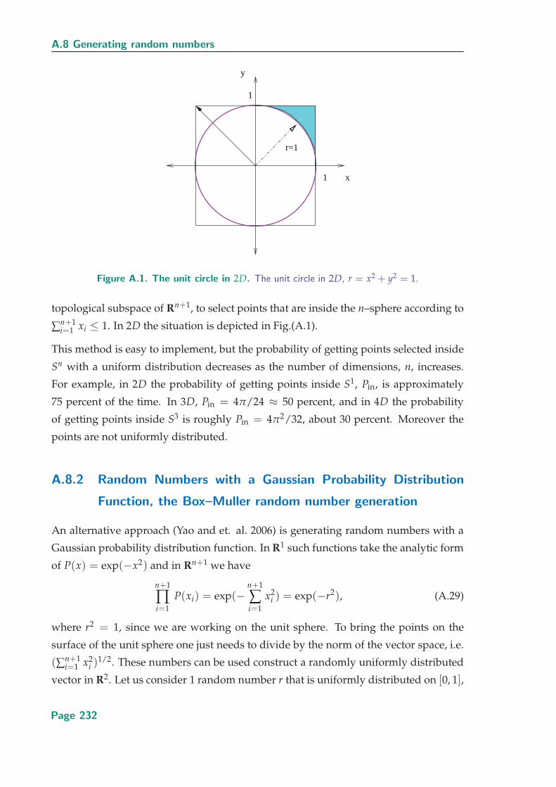
Figure A.1. The unit circle in 2D. The unit circle in 2D, r = x2 + y2 = 1.
topological subspace of Rn+1, to select points that are inside the n–sphere according to
∑n+1i=1 xi ≤ 1. In 2D the situation is depicted in Fig.(A.1).
This method is easy to implement, but the probability of getting points selected inside
Sn with a uniform distribution decreases as the number of dimensions, n, increases.
For example, in 2D the probability of getting points inside S1, Pin, is approximately
75 percent of the time. In 3D, Pin = 4π/24 ≈ 50 percent, and in 4D the probability
of getting points inside S3 is roughly Pin = 4π2/32, about 30 percent. Moreover the
points are not uniformly distributed.
A.8.2 Random Numbers with a Gaussian Probability Distribution
Function, the Box–Muller random number generation
An alternative approach (Yao and et. al. 2006) is generating random numbers with a
Gaussian probability distribution function. In R1 such functions take the analytic form
of P(x) = exp(−x2) and in Rn+1 we have
n+1
∏i=1
P(xi) = exp(−n+1
∑i=1
x2i ) = exp(−r2), (A.29)
where r2 = 1, since we are working on the unit sphere. To bring the points on the
surface of the unit sphere one just needs to divide by the norm of the vector space, i.e.
(∑n+1i=1 x2
i )1/2. These numbers can be used construct a randomly uniformly distributed
vector in R2. Let us consider 1 random number r that is uniformly distributed on [0, 1],
Page 232
Appendix A Mathematical concepts
and another uniformly distributed number θ ∈ [0, 2π]. To construct our uniformly
distributed vector of random numbers in R2 with Gaussian probability distribution,
one needs to consider
r ∈ [0, 1] =⇒ ln(r) ∈ (−∞, 0]=⇒√−2 ln(r) ∈ [0, ∞). (A.30)
To make it uniformly distributed onto the surface of the sphere set
a′0 =
√−2 ln(r) cos(θ) and a
′1 =
√−2 ln(r) sin(θ), (A.31)
and divide by its norm. One can now build a random vector in R4 by just considering
two sets of the 2 dimensional vectors with r1, r2 ∈ [0, 1] and θ1, θ2 ∈ [0, 2π] and combine
them together as such:
aμ =
[ln
1(r1r2)2
] 12
×(√−2 ln(r1) cos θ1,
√−2 ln(r1) sin θ1,√
−2 ln(r2) cos θ2,√−2 ln(r2) sin θ2
). (A.32)
In Rn+1, one just needs to consider n/2 sets, when n + 1 is odd just keep n/2 − 1 and
half of the next set.
Page 233

Page 234

Appendix B
Partial differentialequations
IN this appendix we give a few details on partial differentil equa-
tions in particular on how these are classified.
Page 235
B.1 Partial differential equations
B.1 Partial differential equations
In this appendix give some terminalogy on how the PDE are classified, this concepts
are used in main tex right through the thesis.
B.1.1 Classification partial differential equations
Ordinary differential equations can be classified according to their order and whether
they are linear or non–linear differential equations. Partial differential equations (PDE)
can also be classified but it us in general more difficult to do so.
There are several types of PDE which can take the form
Kt(x, t) − aKxx(x, t) = 0 (diffusion equation), (B.1)
Ktt(x, t) − b2Kxx(x, t) = 0 (wave equation), (B.2)
Kxx(x, y) + Kyy(x, y) = 0 (Laplace equation). (B.3)
Here a and b are just constants.
The first two, Eq. (B.1) and Eq. (B.2), are evolution equations that describe how the pro-
cess evolves in time. The third, Eq. (B.3).
In general, let us consider a second order differential PDE
AKxx(x, t) + BKxt(x, t) + CKtt(x, t) + F(x, t,K,Kx ,Kt) = 0, (B.4)
where A, B and C are constant. Note that the second–order derivatives are assumed to
appear linearly, or to the first degree; the expression LK ≡ AKxx(x, t) + BKxt(x, t) +
CKtt(x, t) is called the principal part of the equation. It is this part that is used for the
classification, which is based on the sign of
D ≡ B2 − 4AC, (B.5)
called the discriminant. Using the descriminant we classify the PDE into three different
classes, elliptic, parabolic and hyperbolic using the following selection criterion
PDE =
⎧⎪⎪⎨⎪⎪⎩elliptic if D < 0
parabolic if D = 0
hyperbolic if D > 0.
(B.6)
Page 236

Appendix C
Option pricing details
IN this appendix we summarize some of the mathematical details
used in the formulation of the exotic options.
Page 237

C.1 More Different Options
C.1 More Different Options
Here we list a more complete set of options available in our days, the list is based
on Option Style (6 January 2008)
C.1.1 Non-Vanilla Exercise Rights
There are other, more unusual exercise styles in which the pay-off value remains the
same as a standard option (as in the classic American and European options above)
but where early exercise occurs differently:
Bermudan option
Bermudan option is an option where the buyer has the right to exercise at a set (always
discretely spaced) number of times. This is intermediate between a European option–
which allows exercise at a single time, namely expiry–and an American option, which
allows exercise at any time (the name is a pun: Bermuda is between America and
Europe). For example a typical Bermudan swaption might confer the opportunity to
enter into an interest rate swap. The option holder might decide to enter into the swap
at the first exercise date (and so enter into, say, a ten-year swap) or defer and have the
opportunity to enter in six months time (and so enter a nine-year and six-month swap).
Most exotic interest rate options are of Bermudan style.
Canary option
Canary option is an option whose exercise style lies somewhere between European op-
tions and Bermudan options. (The name is a pun on the relative geography of the
Canary Islands.) Typically, the holder can exercise the option at quarterly dates, but
not before a set time period (typically one year) has elapsed. The term was coined by
Keith Kline, who at the time was an agency fixed income trader at the Bank of New
York.
Capped-style option
The Capped-style option is not an interest rate cap, but a conventional option with a
pre-defined profit cap written into the contract. A capped-style option is automatically
exercised when the underlying security closes at a price making the option’s mark to
market match the specified amount.
Page 238

Appendix C Option pricing details
Compound option
A compound option is an option on another option, and as such presents the holder
with two separate exercise dates and decisions. If the first exercise date arrives and
the ’inner’ option’s market price is below the agreed strike, the first option will be
exercised (European style), giving the holder a further option at final maturity.
Shout option
A shout option allows the holder effectively two exercise dates: during the life of the
option they can (at any time) ”shout” to the seller that they are locking-in the current
price, and if this gives them a better deal than the pay-off at maturity they will use the
underlying price on the shout date, rather than the price at maturity to calculate their
final pay-off.
Swing option
A swing option gives the purchaser the right to exercise one and only one call or put
on any one of a number of specified exercise dates (this latter aspect is Bermudan).
Penalties are imposed on the buyer if the net volume purchased exceeds or falls below
specified upper and lower limits. This option allows the buyer to ”swing” the price of
the underlying asset. Primarily used in energy trading.
C.1.2 ’Exotic’ Options with Standard Exercise Styles
These options can be exercised either European style or American style; they differ
from the plain vanilla option only in the calculation of their pay-off value:
Cross option (or composite option)
A cross option (or composite option) is an option on some underlying asset in one
currency with a strike denominated in another currency. For example a standard
call option on IBM, which is denominated in dollars pays max(S − K, 0), where S is
the stock price at maturity and K is the strike. A composite stock option might pay
max(S/Q − K, 0), where Q is the prevailing FX rate. The pricing of such options natu-
rally needs to take into account FX volatility and the correlation between the exchange
rate of the two currencies involved and the underlying stock price.
Page 239

C.1 More Different Options
Quanto option
The quanto option is a cross option in which the exchange rate is fixed at the outset
of the trade, typically at 1. The payoff of an IBM quanto call option would then be
max(S − K, 0).
n exchange option
The n exchange option is the right to exchange one asset for another (such as a sugar
future for a corporate bond).
Basket option
The basket option is an option on the weighted average of several underlying assets.
Rainbow option
A rainbow option is a basket option where the weightings depend on the final perfor-
mance of the components. A common special case is an option on the worst-performing
of several stocks.
C.1.3 Non-vanilla path dependent “exotic” options
The following ”exotic options” are still options, but have payoffs calculated quite dif-
ferently from those above. Although these instruments are far more unusual they can
also vary in exercise style (at least theoretically) between European and American:
Lookback option
The lookback option is a path dependent option where the owner has the right to buy
(sell) the underlying instrument at its lowest (highest) price over some preceding pe-
riod.
Asian option
The asian option is an option where the payoff is not determined by the underlying price
at maturity but by the average underlying price over some pre-set period of time. For
example an Asian call option might pay max(daily average over last three months(S) −K, 0). Asian options were originated in Asian markets to prevent option traders from
attempting to manipulate the price of the underlying on the exercise date.
Page 240
Appendix C Option pricing details
Russian option
The russian option is a lookback option, which runs for perpetuity. That is, there is no
end to the period into which the owner can look back.
Game option or Israeli option
The game option or Israeli option is where the writer has the opportunity to cancel the
option he has offered, but must pay the payoff at that point plus a penalty fee.
The payoff of a cumulative Parisian option
The payoff of a cumulative Parisian option is dependent on the total amount of time the
underlying asset value has spent above or below a strike price.
The payoff of a standard Parisian option
The payoff of a standard Parisian option is dependent on the maximum amount of time
the underlying asset value has spent consecutively above or below a strike price.
Barrier option
The barrier option involves a mechanism where if a ’limit price’ is crossed by the under-
lying price, the option either can be exercised or can no longer be exercised.
Double Barrier option
The double barrier option involves a mechanism where if either of two ’limit prices’ is
crossed by the underlying, the option either can be exercised or can no longer be exer-
cised.
Cumulative Parisian barrier option
The cumulative Parisian barrier option involves a mechanism where if the total amount
of time the underlying asset value has spent above or below a ’limit price’, the option
can be exercised or can no longer be exercised.
Page 241
C.2 Maximum of Brownian motion with drift
Standard Parisian barrier option
The standard Parisian barrier option involves a mechanism where if the maximum amount
of time the underlying asset value has spent consecutively above or below a ’limit
price’, the option can be exercised or can no longer be exercised.
Reoption
A reoption occurs when a contract has expired without having been exercised. The
owner of the underlying security may then reoption the security. The term and strike
price of the new option may be the same as or different from the original option.
Binary option (also known as a digital option)
A binary option (also known as a digital option) pays a fixed amount, or nothing at all,
depending on the price of the underlying instrument at maturity.
Chooser option
A chooser option gives the purchaser a fixed period of time to decide whether the deriva-
tive will be a vanilla call or put.
Forward starting option
The forward starting option is an option whose strike price is determined in the future.
Cliquet option
The cliquet option is a sequence of forward starting options.
C.2 Maximum of Brownian motion with drift
In this section the joint density for a Brownian motion with drift and its maximum to
date is derived. Let us start with Brownian motion W(t), 0 ≤ t ≤ T defined on a
probability space (Ω,Ft, P). Under P, the Brownian motion W(t) has zero drift (that
is, it is a martingale). Let α be a given number, and define
W(t) = αt + W(t) for 0 ≤ t ≤ T. (C.1)
Page 242
Appendix C Option pricing details
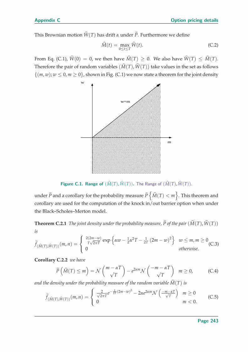
This Brownian motion W(T) has drift α under P. Furthermore we define
M(t) = max0≤t≤T
W(t). (C.2)
From Eq. (C.1), W(0) = 0, we then have M(T) ≥ 0. We also have W(T) ≤ M(T).
Therefore the pair of random variables (M(T), W(T)) take values in the set as follows
{(m, w); w ≤ 0, m ≥ 0}, shown in Fig. (C.1) we now state a theorem for the joint density
w=m
������������������������������������������������������������������������������������������������������������������������������������������������������������������������������������������������������������������������������������������������������������������������������������������������������������������������������������������������������������������������������������������������������������������������������������������������������������������������������������������������������������������������������������������������������������������������������������������������������������������������������������������������������������������������������������������������������������������������������������������������������������������������������������������������������������������������������������������������
������������������������������������������������������������������������������������������������������������������������������������������������������������������������������������������������������������������������������������������������������������������������������������������������������������������������������������������������������������������������������������������������������������������������������������������������������������������������������������������������������������������������������������������������������������������������������������������������������������������������������������������������������������������������������������������������������������������������������������������������������������������������������������������������������������������������������������������������
w
m
Figure C.1. Range of (M(T), W(T)). The Range of (M(T), W(T)).
under P and a corollary for the probability measure P{
M(T) < m}
. This theorem and
corollary are used for the computation of the knock in/out barrier option when under
the Black–Scholes–Merton model.
Theorem C.2.1 The joint density under the probability measure, P of the pair (M(T), W(T))
is
f(M(T),W(T))(m, n) =
⎧⎨⎩2(2m−w)
T√
2πTexp
{αw − 1
2α2T − 12T (2m − w)2
}w ≤ m, m ≥ 0
0 otherwise.(C.3)
Corollary C.2.2 we have
P(
M(T) ≤ m)
= N(
m − αT√T
)− e2αmN
(−m − αT√T
)m ≥ 0, (C.4)
and the density under the probability measure of the random variable M(T) is
f(M(T),W(T))(m, n) =
⎧⎨⎩ 2√2πT
e−1
2T (2m−w)2 − 2αe2αmN(−m−αT√
T
)m ≥ 0
0 m < 0.(C.5)
Page 243

C.2 Maximum of Brownian motion with drift
Where N (x) is the normal distribution, that is Eq. (A.15).
Page 244

Appendix D
The Fokker–PlanckEquation
IN this appendix we explicitly derive the Sturm–Liouville equation
and explain the connection betrween the classical Fokker–Planck
equation and the quantum version that is the Schrodinger equation.
Page 245
D.1 The Sturm–Liouville equation
D.1 The Sturm–Liouville equation
A general stochastic differential equation (SDE) can be written as
dX(u) = β(u, X(u)) du + γ(u, X(u)) dW(u). (D.1)
This equation represents a general stochastic differential equation with drift term β(u, X(u))
and diffusion term γ(u, X(u)). The transition probability density function can be ob-
tained using the Kolmogorov forward equation commonly known as the Fokker–Planck.
If we let P(t, T; x, y) denote the transition the probability then the Fokker-Planck equa-
tion is given by
∂
∂TK(y, T|x, t) =
[− ∂
∂yβ(T, y) +
12
∂2
∂y2 γ2(T, y)
]K(y, T|x, t)
= LFPK(y, T|x, t) = − ∂
∂yS(y, T), (D.2)
where LFP is the Fokker-Planck operator and S(y, T) is the probability current. A for-
mal solution with initial value K(y, T|x, t) = δ(y − x) can be derived using the Dyson
series (Dyson 1949, Risken 1984), i.e.
K(y, T|x, t) = exp [LFP(y)(T − t)] δ(y − x). (D.3)
Using a completeness relation for eigenfunction of Hermitian operators, which usually
form a complete set of eigenfunctions, i.e.,
δ(y − x) = ∑n
ψn(y)ψn(x). (D.4)
Eq. (D.3) may be written as
K(y, T|x, t) = ∑n
exp [LFP(y)(T − t)] ψn(y)ψn(x). (D.5)
If we set φ(x) and λ to be the eigenfunctions and eigenvalues of the Fokker-Planck
operator together with the transformation on the probability density
W(y, T) = φ(y)e−λT , (D.6)
then we see that when we apply the Fokker-Planck operator onto this transformation
∂
∂TW(y, T) = LFPW(y, T) (D.7)
it leads to an eigenvalue problem of the following form,
LFPφ(y) = −λφ(y). (D.8)
Page 246
Appendix D The Fokker–Planck Equation
In the case of stationary solution the probability current in Eq. (D.2) must vanish, we
must then have [∂
∂yβ(T, y) +
12
∂2
∂y2 γ2(T, y)
]K(y, T|x, t) = 0 (D.9)
so that
β(T, y)K(y, T; x, t) =12
∂
∂yγ2(T, y)K(y, T|x, t). (D.10)
If we let
β(T, y) = D(1)(y) (D.11)12
γ2(T, y) = D(2)(y) (D.12)
with
K(y, T|x, t) = Wst(y) (D.13)
then we have
D(1)(y)Wst(y) =∂
∂yD(2)(y)Wst(y) (D.14)
D(1)(y)
D(2)(y)D(2)(y)Wst(y) =
∂
∂yD(2)(y)Wst(y) (D.15)
D(1)(y)
D(2)(y)=
1D(2)(y)Wst(y)
∂
∂yD(2)(y)Wst(y), (D.16)
which gives after integration∫ ydy′
D(1)(y′)D(2)(y′)
= ln(D(2)(y)Wst(y)) + C. (D.17)
After taking the exponential we obtain
N0
D(2)(y)exp
[∫ ydy′
D(1)(y′)D(2)(y′)
]= Wst(y) = Ne−V(y), (D.18)
where N0 is just a constant of integration. Taking the natural log on both sides we get
V(y) = ln(D(2)(y)) −∫ y
dy′D(1)(y′)D(2)(y′)
. (D.19)
Using this potential the probability current may be written as
S(y, T) = −D(2)(y)e−V(y) ∂
∂yeV(y)W(y, T). (D.20)
Page 247
D.1 The Sturm–Liouville equation
As a result, using the probability current, Eq. (D.20), the Fokker-Planck operator in
Eq. (D.2), may be rewritten as
LFP =∂
∂yD(2)(y)e−V(y) ∂
∂yeV(y), (D.21)
which becomes an hermitian operator when it is transformed as
L = eV(y)
2 LFPe−V(y)
2 . (D.22)
Now using the eigenfunction and eigenvalue used earlier, that is if φn(y) and λn are
the eigenfunctions and eigenvalue of the Fokker-Planck operator respectively then the
eigenfunctions
ψn(y) = eV(y)
2 φn(y) (D.23)
are also eigenfunctions of the transformed Fokker-Planck operator, because
Lψn(y) = LeV(y)
2 φn(y) = eV(y)
2 LFPe−V(y)
2 eV(y)
2 φn(y)
= eV(y)
2 LFPφn(y)
= eV(y)
2 λnφn(y)
= λnψn(y). (D.24)
Hence even transformation of the Fokker-Planck operator we have the following eigen-
value problem
Lψn(y) = λnψn(y), (D.25)
just like the Schrodinger equation eigenvalue problem.
It can be shown that the set of eigenfunctions satisfies the completeness relation
δ(y − x) = ∑n
ψn(y)ψn(x) = eV(x)
2 eV(y)
2 ∑n
φn(y)φn(x)
= eV(x)
2 ∑n
φn(y)φn(x)
= eV(y)
2 ∑n
φn(y)φn(x). (D.26)
Page 248

Appendix D The Fokker–Planck Equation
Using this we can write down the expansion of the transition probability, in Eq. (D.3),
into eigenfunctions
K(y, T|x, t) = ∑n
exp [LFP(y)(T − t)] ψn(y)ψn(x)
= eV(y) ∑n
exp [LFP(y)(T − t)] φn(y)φn(x)
= eV(y) ∑n
exp [−λ(T − t)] φn(y)φn(x)
= eV(y)
2 e−V(x)
2 ∑n
exp [−λ(T − t)] ψn(y)ψn(x).
(D.27)
The Hermitian operator, Eq. (D.22), with Eq. (D.21) can be used to write down explicitly
the Fokker-Planck Hermitian operator. This operator can then be used to formulate an
arbitrary operator that would depend on the original stochastic differential equation,
Eq. (D.1). Here the potential, V(y) depends on the boundary conditions which can be
defined depending the problem taken into consideration.
Using Eq. (D.21) into Eq. (D.22), the operator can be rewritten as the product of two
hermitian operators, that is,
L = eV(y)
2∂
∂yD(2)(y)e−V(y) ∂
∂yeV(y)e−
V(y)2
= eV(y)
2∂
∂y
√D(2)(y)e−
V(y)2
√D(2)(y)e−
V(y)2
∂
∂ye
V(y)2 = −aa, (D.28)
where the operators a and a are defined as,
a =√
D(2)(y)e−V(y)
2∂
∂ye
V(y)2 , (D.29)
a = −eV(y)
2∂
∂y
√D(2)(y)e−
V(y)2 . (D.30)
We can now use Eq. (D.19) to rewrite those in terms of the functions D(1)(y) and
D(2)(y) and differential operators only. Since the L is an operator one must respect
the oder of the differential operators as well as how it operates on other functions. A
differential operator cannot just act on the function and disappear, it must act on it and
remain as a differential operator. This will soon become clear as we derive expressions
for a and a.
The differential of the potential, Eq. (D.19) is given by,
∂
∂yV(y)
2=
12
1D(2)(y)
[d
dyD(2)(y) − D(1)(y)
]. (D.31)
Page 249
D.1 The Sturm–Liouville equation
Hence for the a operator we obtain the following
a =√
D(2)(y)e−V(y)
2∂
∂ye
V(y)2
=√
D(2)(y)e−V(y)
2
[e
V(y)2
∂
∂yV(y)
2+ e
V(y)2
∂
∂y
]=
√D(2)(y)e−
V(y)2
[e
V(y)2
12
1D(2)(y)
[d
dyD(2)(y) − D(1)(y)
]+ e
V(y)2
∂
∂y
]=
√D(2)(y)
∂
∂y+
12
1√D(2)(y)
[d
dyD(2)(y) − D(1)(y)
]. (D.32)
Similarly for the a operator we obtain an equation which takes the form,
a = −eV(y)
2∂
∂y
√D(2)(y)e−
V(y)2
= −eV(y)
2
[e−
V(y)2
∂
∂y
√D(2)(y) +
√D(2)(y)
∂
∂ye−
V(y)2
]= − ∂
∂y
√D(2)(y) −
√D(2)(y)e
V(y)2 e−
V(y)2
−1
2√
D(2)(y)
[d
dyD(2)(y) − D(1)(y)
]
= − ∂
∂y
√D(2)(y) +
12
1√D(2)(y)
[d
dyD(2)(y) − D(1)(y)
]. (D.33)
Page 250
Appendix D The Fokker–Planck Equation
So that the transformed Fokker-Planck operator becomes
L = −aa =
⎡⎣ ∂
∂y
√D(2)(y) − 1
21√
D(2)(y)
[d
dyD(2)(y) − D(1)(y)
]⎤⎦⎡⎣√
D(2)(y)∂
∂y+
12
1√D(2)(y)
[d
dyD(2)(y) − D(1)(y)
]⎤⎦=
∂
∂y
√D(2)(y)
√D(2)(y)
∂
∂y+
∂
∂y
√D(2)(y)
12
1√D(2)(y)
[d
dyD(2)(y) − D(1)(y)
]
− 12
1√D(2)(y)
[d
dyD(2)(y) − D(1)(y)
] √D(2)(y)
∂
∂y
− 12
1√D(2)(y)
[d
dyD(2)(y) − D(1)(y)
]12
1√D(2)(y)
[d
dyD(2)(y) − D(1)(y)
]
=∂
∂yD(2)(y)
∂
∂y+
∂
∂y12
[d
dyD(2)(y) − D(1)(y)
]+
12
[d
dyD(2)(y) − D(1)(y)
]∂
∂y
− 12
[d
dyD(2)(y) − D(1)(y)
]∂
∂y
−
⎧⎨⎩12
1√D(2)(y)
[d
dyD(2)(y) − D(1)(y)
]⎫⎬⎭2
=∂
∂yD(2)(y)
∂
∂y+
12
[d2
dy2 D(2)(y) − ddy
D(1)(y)
]− 1
4D(2)(y)
[d
dyD(2)(y) − D(1)(y)
]2
=∂
∂yD(2)(y)
∂
∂y− Ω(y), (D.34)
so we have the following operator
L =∂
∂yD(2)(y)
∂
∂y− Ω(y), (D.35)
where the potential operator is given by
Ω(y) =1
4D(2)(y)
[d
dyD(2)(y) − D(1)(y)
]2
− 12
[d2
dy2 D(2)(y) − ddy
D(1)(y)
]. (D.36)
Here the L is the operator of the Sturm-Liouville equation.
Page 251

D.2 The connection between the Schroedinger equation and Fokker–Planckequation
D.2 The connection between the Schroedinger equation
and Fokker–Planck equation
Now if we consider the following potential
V(y)
2=
12
D−1 f (y) and D(2)(y) → D, (D.37)
where D is a constant. The operators a, Eq. (D.32), and a, Eq. (D.33), respectively can
then be rewritten as follows
a =√
De−f (y)2D
∂
∂ye
f (y)2D
=√
De−f (y)2D
(e
f (y)2D
f ′(y)
2D+ e
f (y)2D
√D
∂
∂y
)=
√D
f ′(y)
2D+√
D∂
∂y(D.38)
and
a = −ef (y)2D
∂
∂y
√D(2)(y)e−
f (y)2D
= −ef (y)2D
√D
∂
∂ye−
f (y)2D
= −ef (y)2D
√D
[e−
f (y)2D
f ′(y)√2D
+−e−f (y)2D
∂
∂y
]=
√D
f ′(y)
2D−√
D∂
∂y(D.39)
so that the operator L takes the form
LS = −aa =
[−√
Df ′(y)
2D+√
D∂
∂y
][√
Df ′(y)
2D+√
D∂
∂y
]= −
[f ′(y)
2√
D
]2
− f ′(y)
2∂
∂y+
f ′′(y)
2+
f ′(y)
2∂
∂y+ D
∂2
∂y2
= D∂2
∂y2 −[
14
[ f ′(y)]2
D− f ′′(y)
2
]. (D.40)
Hence we have
LS = D∂2
∂y2 − ΩS(y) (D.41)
Page 252

Appendix D The Fokker–Planck Equation
where the potential part of the Schrodinger operator takes the form of
ΩS(y) =
[14
[ f ′(y)]2
D− f ′′(y)
2
]. (D.42)
Now because we earlier showed that L satisfies the eigenvalue problem defined in,
Eq. (D.25), which is the same as the Schrodinger eigenvalue equation, i.e.,
LSψn(y) =
[D
∂2
∂y2 − ΩS(y)
]ψn(y) = λnψn(y) (D.43)
with D = h/2m and the time map to imaginary time25, t → iht. Hence we see that
by having applied a transformation ψn(y) = eV(y)
2 φn(y) to the probability density we
recover the Schrodinger equation.
D.3 The wave function and the probability density in
quantum mechanics
In quantum mechanics if we consider a particle of mass m moving along the y-axis in
a time–independent potential V(y), the corresponding time–dependent Schrodinger
equation corresponding to this one dimensional motion can be written as
ih∂
∂tψ(y, t) =
[− h2
2m∂2
∂y2 + V(y)
]ψ(y, t). (D.44)
Here ψ(y, t) is the wavefunction which describes everything that can be known about
the system and the particle moving under the influence of some external force. The
wavefunction may be defined as the projection of the vector |ψ(t)〉 onto the position
basis, i.e.,
ψ(y, t) = 〈y|ψ(t)〉. (D.45)
Since the position eigenstate from a basis for the state space the integral over all pro-
jections operator is the identity operator, i.e.,∫dy|y〉〈y| = 1. (D.46)
25A tranformation to imaginary time is known as a Wick rotation (Peskin and Schroeder 1995, Bjorken
and Drell. 1965), named after the Italian physicist Giancarlo Wick.
Page 253
D.3 The wave function and the probability density in quantum mechanics
Using this completeness relation we can then show that
〈ψ(t)|ψ(t)〉 = 〈ψ(t)|∫
dy|y〉〈y|ψ(t)〉
=∫
dy 〈ψ(t)|y〉〈y|ψ(t)〉
=∫
dy ψ�(y, t)ψ(y, t) = 1. (D.47)
Hence in this context
ψ�(y, t)ψ(y, t) = |ψ(y, t)|2, (D.48)
defines the probability of finding the particle at a given point in time t, i.e.,
P(y, t) dy = |ψ(y, t)|2 dy, (D.49)
so that
P(y, t) = |ψ(y, t)|2 (D.50)
is the position probability density. The wavefunction contains all of the information
about the system, it is in general a complex function that lies in Hilbert space, which
is |ψ(t)〉, y ∈ H. The time evolution of the probability density function of the po-
sition and velocity of a particle can also be described, in the classical world by the
Fokker-Planck equation. The Fokker-Planck equation can also be used for computing
the probability density of stochastic differential equation like the one represented in
Eq. (D.1).
Page 254
Appendix E
Source code
IN this appendix we give the program listing for the different chap-
ters in the main text. These codes include f90, HPF and some C++
code for the scientific programing aspect of the project. Also in this
appendix is the code used in packages such as R and Matlab.
Page 255
E.1 The R script nasdaq.r
E.1 The R script nasdaq.r
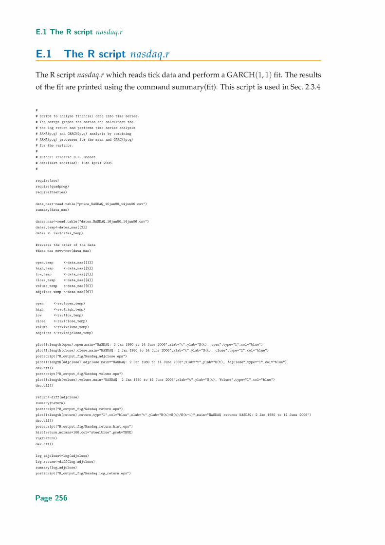
The R script nasdaq.r which reads tick data and perform a GARCH(1, 1) fit. The results
of the fit are printed using the command summary(fit). This script is used in Sec. 2.3.4
#
# Script to analyze financial data into time series.
# The script graphs the series and calcultest the
# the log return and performs time series analysis
# ARMA(p,q) and GARCH(p,q) analysis by combining
# ARMA(p,q) processes for the mean and GARCH(p,q)
# for the variance.
#
# author: Frederic D.R. Bonnet
# date(last modified): 16th April 2008.
#
require(zoo)
require(quadprog)
require(tseries)
data_nas<-read.table("price_NASDAQ_16jan80_14jun06.csv")
summary(data_nas)
dates_nas<-read.table("dates_NASDAQ_16jan80_14jun06.csv")
dates_temp<-dates_nas[[2]]
dates <- rev(dates_temp)
#reverse the order of the data
#data_nas_rev<-rev(data_nas)
open_temp <-data_nas[[1]]
high_temp <-data_nas[[2]]
low_temp <-data_nas[[3]]
close_temp <-data_nas[[4]]
volume_temp <-data_nas[[5]]
adjclose_temp <-data_nas[[6]]
open <-rev(open_temp)
high <-rev(high_temp)
low <-rev(low_temp)
close <-rev(close_temp)
volume <-rev(volume_temp)
adjclose <-rev(adjclose_temp)
plot(1:length(open),open,main="NASDAQ: 2 Jan 1980 to 14 June 2006",xlab="t",ylab="S(t), open",type="l",col="blue")
plot(1:length(close),close,main="NASDAQ: 2 Jan 1980 to 14 June 2006",xlab="t",ylab="S(t), close",type="l",col="blue")
postscript("R_output_fig/Nasdaq_adjclose.eps")
plot(1:length(adjclose),adjclose,main="NASDAQ: 2 Jan 1980 to 14 June 2006",xlab="t",ylab="S(t), AdjClose",type="l",col="blue")
dev.off()
postscript("R_output_fig/Nasdaq.volume.eps")
plot(1:length(volume),volume,main="NASDAQ: 2 Jan 1980 to 14 June 2006",xlab="t",ylab="S(t), Volume",type="l",col="blue")
dev.off()
return<-diff(adjclose)
summary(return)
postscript("R_output_fig/Nasdaq.return.eps")
plot(1:length(return),return,typ="l",col="blue",xlab="t",ylab="R(t)=S(t)/S(t-1)",main="NASDAQ returns NASDAQ: 2 Jan 1980 to 14 June 2006")
dev.off()
postscript("R_output_fig/Nasdaq_return_hist.eps")
hist(return,nclass=100,col="steelblue",prob=TRUE)
rug(return)
dev.off()
log_adjclose<-log(adjclose)
log_return<-diff(log_adjclose)
summary(log_adjclose)
postscript("R_output_fig/Nasdaq.log_return.eps")
Page 256
Appendix E Source code
plot(1:length(log_return),log_return,typ="l",col="blue",xlab="t",ylab="r(t)=log(S(t)/S(t-1))",main="NASDAQ returns: 2 Jan 1980 to 14 June 2006")
dev.off()
postscript("R_output_fig/Nasdaq.hist.log_return.eps")
hist(log_return,nclass=100,col="steelblue",prob=TRUE,main="NASDAQ: 2 Jan 1980 to 14 June 2006")
rug(log_return)
dev.off()
summary(log_return.arma <- arma(log_return, order = c(1, 0)))
summary(log_return.arma <- arma(log_return, order = c(2, 0)))
summary(log_return.arma <- arma(log_return, order = c(0, 1)))
summary(log_return.arma <- arma(log_return, order = c(0, 2)))
summary(log_return.arma <- arma(log_return, order = c(1, 1)))
sink("R_output_fig/Nasdaq.arma11_summaryfit.txt",append=TRUE)
summary(log_return.arma <- arma(log_return, order = c(1, 1)))
sink()
postscript("R_output_fig/Nasdaq.arma11.garch00.eps")
plot(log_return.arma)
dev.off()
require(fGarch)
spec=garchSpec()
spec
fit=garchFit(~garch(1,1),data=log_return)
print(fit)
postscript("R_output_fig/Nasdaq.arma00.garch11.eps")
plot(fit)
1
2
3
4
5
6
7
8
9
10
11
12
13
0
dev.off()
summary(fit)
sink("R_output_fig/Nasdaq.arma00.garch11_summaryfit.txt",append=TRUE)
summary(fit)
sink()
fit1=garchFit(~arma(0,1)+~garch(1,1),data=log_return)
print(fit1)
postscript("R_output_fig/Nasdaq.arma01.garch11.eps")
plot(fit1)
1
2
3
4
5
6
7
8
9
10
11
12
13
0
dev.off()
summary(fit1)
sink("R_output_fig/Nasdaq.arma01.garch11_summaryfit.txt",append=TRUE)
summary(fit1)
sink()
Page 257
E.1 The R script nasdaq.r
fit2=garchFit(~arma(1,1)+~garch(1,1),data=log_return)
print(fit2)
postscript("R_output_fig/Nasdaq.arma11.garch11.eps")
plot(fit2)
1
2
3
4
5
6
7
8
9
10
11
12
13
0
dev.off()
summary(fit2)
sink("R_output_fig/Nasdaq.arma11.garch11_summaryfit.txt",append=TRUE)
summary(fit2)
sink()
fit3=garchFit(~arma(2,2)+~garch(1,2),data=log_return)
print(fit3)
postscript("R_output_fig/Nasdaq.arma22.garch12.eps")
plot(fit3)
1
2
3
4
5
6
7
8
9
10
11
12
13
0
dev.off()
summary(fit3)
sink("R_output_fig/Nasdaq.arma22.garch12_summaryfit.txt",append=TRUE)
summary(fit3)
sink()
fit4=garchFit(~arma(1,2)+~garch(2,2),data=log_return)
print(fit4)
postscript("R_output_fig/Nasdaq.arma12.garch22.eps")
plot(fit4)
1
2
3
4
5
6
7
8
9
10
11
12
13
0
dev.off()
summary(fit4)
sink("R_output_fig/Nasdaq.arma12.garch22_summaryfit.txt",append=TRUE)
summary(fit4)
sink()
Page 258

Appendix E Source code
fit5=garchFit(~arma(2,2)+~garch(2,2),data=log_return)
print(fit5)
postscript("R_output_fig/Nasdaq.arma22.garch22.eps")
plot(fit5)
1
2
3
4
5
6
7
8
9
10
11
12
13
0
dev.off()
summary(fit5)
sink("R_output_fig/Nasdaq.arma22.garch22_summaryfit.txt",append=TRUE)
summary(fit5)
sink()
$ more Summary_garch11_fit.txt Print_garch_fit.txt
::::::::::::::
Summary_garch11_fit.txt
::::::::::::::
> summary(fit)
Title:
GARCH Modelling
Call:
garchFit(formula = ~garch(1, 1), data = log_return)
Mean and Variance Equation:
~arma(0, 0) + ~garch(1, 1)
Conditional Distribution:
dnorm
Coefficient(s):
mu omega alpha1 beta1
7.43221e-04 1.93125e-06 1.32214e-01 8.58471e-01
Error Analysis:
Estimate Std. Error t value Pr(>|t|)
mu 7.432e-04 1.006e-04 7.387 1.50e-13 ***
omega 1.931e-06 2.581e-07 7.483 7.26e-14 ***
alpha1 1.322e-01 9.571e-03 13.815 < 2e-16 ***
beta1 8.585e-01 9.353e-03 91.783 < 2e-16 ***
---
Signif. codes: 0 *** 0.001 ** 0.01 * 0.05 . 0.1 1
Log Likelihood:
-21444.01 normalized: -3.212105
Standadized Residuals Tests:
Statistic p-Value
Jarque-Bera Test R Chi^2 1400.505 0
Shapiro-Wilk Test R W NA NA
Ljung-Box Test R Q(10) 213.4334 0
Ljung-Box Test R Q(15) 240.7022 0
Ljung-Box Test R Q(20) 252.2096 0
Ljung-Box Test R^2 Q(10) 11.66196 0.3083168
Ljung-Box Test R^2 Q(15) 15.82622 0.3936941
Ljung-Box Test R^2 Q(20) 18.85845 0.5310435
LM Arch Test R TR^2 13.29254 0.3481412
Page 259
E.1 The R script nasdaq.r
Information Criterion Statistics:
AIC BIC SIC HQIC
6.425408 6.429486 6.425407 6.426816
Description:
Wed Jan 23 16:54:46 2008 by user: fbonnet
::::::::::::::
Nasdaq.arma01.garch11_summaryfit.txt
::::::::::::::
Title:
GARCH Modelling
Call:
garchFit(formula = ~arma(0, 1) + ~garch(1, 1), data = log_return)
Mean and Variance Equation:
~arma(0, 1) + ~garch(1, 1)
Conditional Distribution:
dnorm
Coefficient(s):
mu ma1 omega alpha1 beta1
7.08375e-04 1.80290e-01 1.77629e-06 1.28285e-01 8.62986e-01
Error Analysis:
Estimate Std. Error t value Pr(>|t|)
mu 7.084e-04 1.140e-04 6.215 5.12e-10 ***
ma1 1.803e-01 1.309e-02 13.772 < 2e-16 ***
omega 1.776e-06 2.347e-07 7.570 3.73e-14 ***
alpha1 1.283e-01 9.163e-03 14.001 < 2e-16 ***
beta1 8.630e-01 8.921e-03 96.737 < 2e-16 ***
---
Signif. codes: 0 *** 0.001 ** 0.01 * 0.05 . 0.1 1
Log Likelihood:
-21536.66 normalized: -3.225983
Standadized Residuals Tests:
Statistic p-Value
Jarque-Bera Test R Chi^2 1648.716 0
Shapiro-Wilk Test R W NA NA
Ljung-Box Test R Q(10) 20.98795 0.02117777
Ljung-Box Test R Q(15) 38.31875 0.0008093998
Ljung-Box Test R Q(20) 49.10475 0.0002971102
Ljung-Box Test R^2 Q(10) 10.49738 0.3979915
Ljung-Box Test R^2 Q(15) 15.11501 0.4431651
Ljung-Box Test R^2 Q(20) 18.52967 0.5525594
LM Arch Test R TR^2 13.14630 0.3584972
Information Criterion Statistics:
AIC BIC SIC HQIC
6.453464 6.458561 6.453462 6.455224
Description:
Wed Apr 16 13:31:44 2008 by user: fbonnet
::::::::::::::
Nasdaq.arma11.garch11_summaryfit.txt
::::::::::::::
Title:
GARCH Modelling
Call:
Page 260
Appendix E Source code
garchFit(formula = ~arma(1, 1) + ~garch(1, 1), data = log_return)
Mean and Variance Equation:
~arma(1, 1) + ~garch(1, 1)
Conditional Distribution:
dnorm
Coefficient(s):
mu ar1 ma1 omega alpha1 beta1
6.34014e-04 1.01793e-01 8.10861e-02 1.77735e-06 1.28346e-01 8.62887e-01
Error Analysis:
Estimate Std. Error t value Pr(>|t|)
mu 6.340e-04 1.212e-04 5.232 1.67e-07 ***
ar1 1.018e-01 8.523e-02 1.194 0.232
ma1 8.109e-02 8.544e-02 0.949 0.343
omega 1.777e-06 2.348e-07 7.571 3.71e-14 ***
alpha1 1.283e-01 9.170e-03 13.997 < 2e-16 ***
beta1 8.629e-01 8.934e-03 96.580 < 2e-16 ***
---
Signif. codes: 0 *** 0.001 ** 0.01 * 0.05 . 0.1 1
Log Likelihood:
-21537.36 normalized: -3.226087
Standadized Residuals Tests:
Statistic p-Value
Jarque-Bera Test R Chi^2 1640.465 0
Shapiro-Wilk Test R W NA NA
Ljung-Box Test R Q(10) 16.81144 0.0786419
Ljung-Box Test R Q(15) 33.36103 0.004182694
Ljung-Box Test R Q(20) 44.47849 0.001297920
Ljung-Box Test R^2 Q(10) 10.57112 0.3918924
Ljung-Box Test R^2 Q(15) 15.28725 0.4309308
Ljung-Box Test R^2 Q(20) 18.68275 0.5425253
LM Arch Test R TR^2 13.27991 0.3490285
Information Criterion Statistics:
AIC BIC SIC HQIC
6.453972 6.460090 6.453971 6.456085
Description:
Wed Apr 16 13:35:41 2008 by user: fbonnet
::::::::::::::
Nasdaq.arma22.garch12_summaryfit.txt
::::::::::::::
Title:
GARCH Modelling
Call:
garchFit(formula = ~arma(2, 2) + ~garch(1, 2), data = log_return)
Mean and Variance Equation:
~arma(2, 2) + ~garch(1, 2)
Conditional Distribution:
dnorm
Coefficient(s):
mu ar1 ar2 ma1 ma2 omega alpha1 beta1
3.17894e-04 4.14878e-01 1.29408e-01 -2.31151e-01 -1.87350e-01 1.87750e-06 1.38494e-01 7.39514e-01
beta2
1.12741e-01
Error Analysis:
Estimate Std. Error t value Pr(>|t|)
mu 3.179e-04 5.333e-04 0.596 0.5511
Page 261
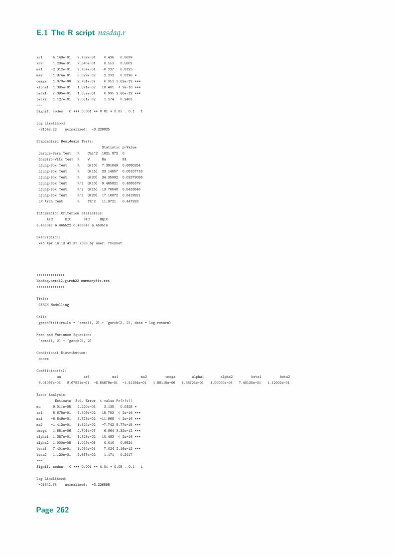
E.1 The R script nasdaq.r
ar1 4.149e-01 9.732e-01 0.426 0.6699
ar2 1.294e-01 2.340e-01 0.553 0.5802
ma1 -2.312e-01 9.737e-01 -0.237 0.8123
ma2 -1.874e-01 8.029e-02 -2.333 0.0196 *
omega 1.878e-06 2.701e-07 6.951 3.62e-12 ***
alpha1 1.385e-01 1.321e-02 10.481 < 2e-16 ***
beta1 7.395e-01 1.057e-01 6.995 2.66e-12 ***
beta2 1.127e-01 9.601e-02 1.174 0.2403
---
Signif. codes: 0 *** 0.001 ** 0.01 * 0.05 . 0.1 1
Log Likelihood:
-21542.28 normalized: -3.226825
Standadized Residuals Tests:
Statistic p-Value
Jarque-Bera Test R Chi^2 1621.872 0
Shapiro-Wilk Test R W NA NA
Ljung-Box Test R Q(10) 7.391649 0.6880254
Ljung-Box Test R Q(15) 23.14657 0.08107718
Ljung-Box Test R Q(20) 34.35992 0.02379058
Ljung-Box Test R^2 Q(10) 9.465821 0.4885379
Ljung-Box Test R^2 Q(15) 13.76548 0.5433846
Ljung-Box Test R^2 Q(20) 17.16872 0.6419921
LM Arch Test R TR^2 11.9721 0.447923
Information Criterion Statistics:
AIC BIC SIC HQIC
6.456346 6.465522 6.456343 6.459516
Description:
Wed Apr 16 13:42:31 2008 by user: fbonnet
::::::::::::::
Nasdaq.arma12.garch22_summaryfit.txt
::::::::::::::
Title:
GARCH Modelling
Call:
garchFit(formula = ~arma(1, 2) + ~garch(2, 2), data = log_return)
Mean and Variance Equation:
~arma(1, 2) + ~garch(2, 2)
Conditional Distribution:
dnorm
Coefficient(s):
mu ar1 ma1 ma2 omega alpha1 alpha2 beta1 beta2
9.01097e-05 8.67821e-01 -6.84879e-01 -1.41194e-01 1.88115e-06 1.38724e-01 1.00000e-08 7.40120e-01 1.12002e-01
Error Analysis:
Estimate Std. Error t value Pr(>|t|)
mu 9.011e-05 4.220e-05 2.135 0.0328 *
ar1 8.678e-01 5.509e-02 15.753 < 2e-16 ***
ma1 -6.849e-01 5.723e-02 -11.968 < 2e-16 ***
ma2 -1.412e-01 1.824e-02 -7.742 9.77e-15 ***
omega 1.881e-06 2.701e-07 6.964 3.32e-12 ***
alpha1 1.387e-01 1.323e-02 10.483 < 2e-16 ***
alpha2 1.000e-08 1.049e-06 0.010 0.9924
beta1 7.401e-01 1.054e-01 7.024 2.16e-12 ***
beta2 1.120e-01 9.567e-02 1.171 0.2417
---
Signif. codes: 0 *** 0.001 ** 0.01 * 0.05 . 0.1 1
Log Likelihood:
-21542.75 normalized: -3.226895
Page 262
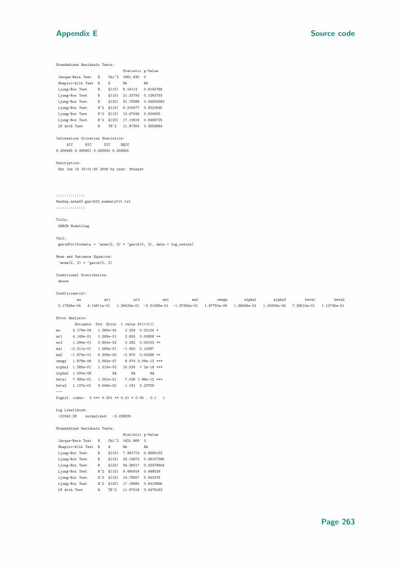
Appendix E Source code
Standadized Residuals Tests:
Statistic p-Value
Jarque-Bera Test R Chi^2 1661.630 0
Shapiro-Wilk Test R W NA NA
Ljung-Box Test R Q(10) 8.15112 0.6140786
Ljung-Box Test R Q(15) 21.33793 0.1263753
Ljung-Box Test R Q(20) 31.79398 0.04554363
Ljung-Box Test R^2 Q(10) 9.316377 0.5023645
Ljung-Box Test R^2 Q(15) 13.67046 0.550655
Ljung-Box Test R^2 Q(20) 17.10919 0.6458725
LM Arch Test R TR^2 11.87354 0.4558884
Information Criterion Statistics:
AIC BIC SIC HQIC
6.456485 6.465661 6.456482 6.459655
Description:
Sat Jun 14 19:01:40 2008 by user: fbonnet
::::::::::::::
Nasdaq.arma22.garch22_summaryfit.txt
::::::::::::::
Title:
GARCH Modelling
Call:
garchFit(formula = ~arma(2, 2) + ~garch(2, 2), data = log_return)
Mean and Variance Equation:
~arma(2, 2) + ~garch(2, 2)
Conditional Distribution:
dnorm
Coefficient(s):
mu ar1 ar2 ma1 ma2 omega alpha1 alpha2 beta1 beta2
3.17926e-04 4.14811e-01 1.29432e-01 -2.31085e-01 -1.87362e-01 1.87750e-06 1.38494e-01 1.00000e-08 7.39510e-01 1.12745e-01
Error Analysis:
Estimate Std. Error t value Pr(>|t|)
mu 3.179e-04 1.380e-04 2.304 0.02124 *
ar1 4.148e-01 1.566e-01 2.650 0.00806 **
ar2 1.294e-01 3.943e-02 3.282 0.00103 **
ma1 -2.311e-01 1.580e-01 -1.462 0.14367
ma2 -1.874e-01 6.308e-02 -2.970 0.00298 **
omega 1.878e-06 2.692e-07 6.974 3.09e-12 ***
alpha1 1.385e-01 1.315e-02 10.530 < 2e-16 ***
alpha2 1.000e-08 NA NA NA
beta1 7.395e-01 1.051e-01 7.036 1.98e-12 ***
beta2 1.127e-01 9.546e-02 1.181 0.23759
---
Signif. codes: 0 *** 0.001 ** 0.01 * 0.05 . 0.1 1
Log Likelihood:
-21542.28 normalized: -3.226825
Standadized Residuals Tests:
Statistic p-Value
Jarque-Bera Test R Chi^2 1621.869 0
Shapiro-Wilk Test R W NA NA
Ljung-Box Test R Q(10) 7.391774 0.6880133
Ljung-Box Test R Q(15) 23.14673 0.08107385
Ljung-Box Test R Q(20) 34.36017 0.02378904
Ljung-Box Test R^2 Q(10) 9.465918 0.488529
Ljung-Box Test R^2 Q(15) 13.76557 0.543378
Ljung-Box Test R^2 Q(20) 17.16884 0.6419846
LM Arch Test R TR^2 11.97218 0.4479163
Page 263
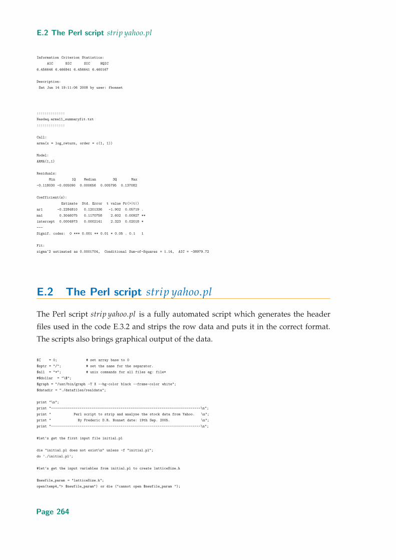
E.2 The Perl script strip yahoo.pl
Information Criterion Statistics:
AIC BIC SIC HQIC
6.456646 6.466841 6.456641 6.460167
Description:
Sat Jun 14 19:11:06 2008 by user: fbonnet
::::::::::::::
Nasdaq.arma11_summaryfit.txt
::::::::::::::
Call:
arma(x = log_return, order = c(1, 1))
Model:
ARMA(1,1)
Residuals:
Min 1Q Median 3Q Max
-0.118030 -0.005090 0.000656 0.005795 0.137082
Coefficient(s):
Estimate Std. Error t value Pr(>|t|)
ar1 -0.2284810 0.1201336 -1.902 0.05719 .
ma1 0.3046075 0.1170758 2.602 0.00927 **
intercept 0.0004973 0.0002141 2.323 0.02018 *
---
Signif. codes: 0 *** 0.001 ** 0.01 * 0.05 . 0.1 1
Fit:
sigma^2 estimated as 0.0001704, Conditional Sum-of-Squares = 1.14, AIC = -38979.72
E.2 The Perl script strip yahoo.pl
The Perl script strip yahoo.pl is a fully automated script which generates the header
files used in the code E.3.2 and strips the row data and puts it in the correct format.
The scripts also brings graphical output of the data.
$[ = 0; # set array base to 0
$sptr = "/"; # set the name for the separator.
$all = "*"; # unix commands for all files eg: file*
#$dollar = "\$";
$graph = "/usr/bin/graph -T X --bg-color black --frame-color white";
$datadir = "./datafiles/realdata";
print "\n";
print "-------------------------------------------------------------------------\n";
print " Perl script to strip and analyse the stock data from Yahoo. \n";
print " By Frederic D.R. Bonnet date: 19th Sep. 2005. \n";
print "-------------------------------------------------------------------------\n";
#let’s get the first input file initial.pl
die "initial.pl does not exist\n" unless -f "initial.pl";
do ’./initial.pl’;
#let’s get the input variables from initial.pl to create latticeSize.h
$newfile_param = "latticeSize.h";
open(temp4,"> $newfile_param") or die ("cannot open $newfile_param ");
Page 264
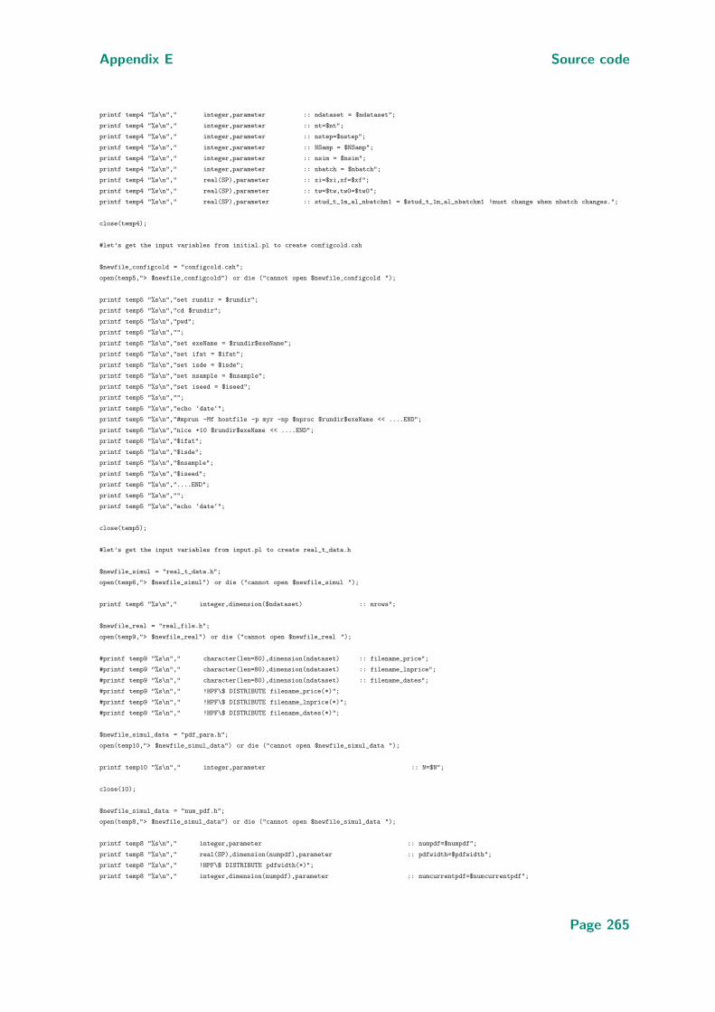
Appendix E Source code
printf temp4 "%s\n"," integer,parameter :: ndataset = $ndataset";
printf temp4 "%s\n"," integer,parameter :: nt=$nt";
printf temp4 "%s\n"," integer,parameter :: nstep=$nstep";
printf temp4 "%s\n"," integer,parameter :: NSamp = $NSamp";
printf temp4 "%s\n"," integer,parameter :: nsim = $nsim";
printf temp4 "%s\n"," integer,parameter :: nbatch = $nbatch";
printf temp4 "%s\n"," real(SP),parameter :: xi=$xi,xf=$xf";
printf temp4 "%s\n"," real(SP),parameter :: tw=$tw,tw0=$tw0";
printf temp4 "%s\n"," real(SP),parameter :: stud_t_1m_al_nbatchm1 = $stud_t_1m_al_nbatchm1 !must change when nbatch changes.";
close(temp4);
#let’s get the input variables from initial.pl to create configcold.csh
$newfile_configcold = "configcold.csh";
open(temp5,"> $newfile_configcold") or die ("cannot open $newfile_configcold ");
printf temp5 "%s\n","set rundir = $rundir";
printf temp5 "%s\n","cd $rundir";
printf temp5 "%s\n","pwd";
printf temp5 "%s\n","";
printf temp5 "%s\n","set exeName = $rundir$exeName";
printf temp5 "%s\n","set ifat = $ifat";
printf temp5 "%s\n","set isde = $isde";
printf temp5 "%s\n","set nsample = $nsample";
printf temp5 "%s\n","set iseed = $iseed";
printf temp5 "%s\n","";
printf temp5 "%s\n","echo ‘date‘";
printf temp5 "%s\n","#mprun -Mf hostfile -p myr -np $nproc $rundir$exeName << ....END";
printf temp5 "%s\n","nice +10 $rundir$exeName << ....END";
printf temp5 "%s\n","$ifat";
printf temp5 "%s\n","$isde";
printf temp5 "%s\n","$nsample";
printf temp5 "%s\n","$iseed";
printf temp5 "%s\n","....END";
printf temp5 "%s\n","";
printf temp5 "%s\n","echo ‘date‘";
close(temp5);
#let’s get the input variables from input.pl to create real_t_data.h
$newfile_simul = "real_t_data.h";
open(temp6,"> $newfile_simul") or die ("cannot open $newfile_simul ");
printf temp6 "%s\n"," integer,dimension($ndataset) :: nrows";
$newfile_real = "real_file.h";
open(temp9,"> $newfile_real") or die ("cannot open $newfile_real ");
#printf temp9 "%s\n"," character(len=80),dimension(ndataset) :: filename_price";
#printf temp9 "%s\n"," character(len=80),dimension(ndataset) :: filename_lnprice";
#printf temp9 "%s\n"," character(len=80),dimension(ndataset) :: filename_dates";
#printf temp9 "%s\n"," !HPF\$ DISTRIBUTE filename_price(*)";
#printf temp9 "%s\n"," !HPF\$ DISTRIBUTE filename_lnprice(*)";
#printf temp9 "%s\n"," !HPF\$ DISTRIBUTE filename_dates(*)";
$newfile_simul_data = "pdf_para.h";
open(temp10,"> $newfile_simul_data") or die ("cannot open $newfile_simul_data ");
printf temp10 "%s\n"," integer,parameter :: N=$N";
close(10);
$newfile_simul_data = "num_pdf.h";
open(temp8,"> $newfile_simul_data") or die ("cannot open $newfile_simul_data ");
printf temp8 "%s\n"," integer,parameter :: numpdf=$numpdf";
printf temp8 "%s\n"," real(SP),dimension(numpdf),parameter :: pdfwidth=$pdfwidth";
printf temp8 "%s\n"," !HPF\$ DISTRIBUTE pdfwidth(*)";
printf temp8 "%s\n"," integer,dimension(numpdf),parameter :: numcurrentpdf=$numcurrentpdf";
Page 265
E.2 The Perl script strip yahoo.pl
printf temp8 "%s\n"," !HPF\$ DISTRIBUTE numcurrentpdf(*)";
$newfile_simul_data = "ParamRealdata.asc";
open(temp7,"> $newfile_simul_data") or die ("cannot open $newfile_simul_data ");
printf temp7 "%i\n",$ndataset;
$idata = -1; #initializing the number of times get_yahoo_prices_tick routine is called
for ( $idataset = 0 ; $idataset <= $ndataset-1 ; $idataset++)
{
die "input.pl does not exist\n" unless -f "input.pl";
do ’./input.pl’;
for ( $istock = 0 ; $istock < $nstock ; $istock++)
{
for ( $iyears = 0 ; $iyears < $nyears ; $iyears++)
{
printf temp7 "%s\n",$stock[$istock];
$idata = $idata + 1; #the number of time the routine is called.
$tick_file = "$stock[$istock]$years[$iyears]$ext[0]";
print "the tick file taken into consideration: tick_file= $tick_file \n";
&get_yahoo_prices_tick($tick_file);
print "coming out from get_prices_old_tick: date= $date, Yop= $Yop, Ycl= $Ycl and volume= $volume\n";
print "\n";
print "coming out from get_prices_old_tick: date= $date, Yop= $Yop, Ycl= $Fld and volume= $volume\n";
print "coming out from reading routine nrows: $nrows \n";
#now start calculating some of the distribution.
$newfile_price[$idataset] = "price_$tick_file";
$newfile_dates[$idataset] = "dates_$tick_file";
&plot_rowdata ( $newfile_price[$idataset] , $data_set , $nrows , $nt , $Xwin_title[$idataset]);
if ( $nt <= $nrows )
{
print "nt=$nt <= nrows=$nrows so we cannot use the full data set";
print "coming out from plot_rowdata routine count_nrows=$count_nrows \n";
print "all the arrays are bounded to count_nrows=$count_nrows \n";
if ( $count_nrows != $nt ) {die;}
$nrows_arr[$idataset] = $nt;
}
elsif ( $nt => $nrows )
{
$nrows_arr[$idataset] = $nrows;
}
#$nrows_arr[$idataset] = $nrows;
printf temp7 "%s\n","$count_nrows";
printf temp7 "%s\n","Y_t_$newfile_price[$idataset]";
printf temp7 "%s\n","ln_Y_t_$newfile_price[$idataset]";
printf temp7 "%s\n","$newfile_dates[$idataset]";
}
}
}
$counter = 1;
#printf temp7 "%s\n","$counter";
for ( $ja = 1 ; $ja <= $nA ; $ja++)
{
if ( $counter < $nA )
{
$counter = $counter + $nAstep ;
# printf temp7 "%s\n","$counter";
}
Page 266
Appendix E Source code
elsif ( $counter > $nA )
{
exit;
}
}
#print "outside of the loop ja=$ja , counter = $counter \n";
#constructing the configuration number
$C = "c";
$zero = "0";
$twozero = "00";
$counter = 0;
for ( $isamp = 1 ; $isamp <= $NSamp ; $isamp++)
{
$counter = $counter + 1 ;
if ( $counter < 10 )
{
printf temp7 "%s\n","$C$twozero$counter";
}
elsif ( $counter >= 10 && $counter < 100 )
{
printf temp7 "%s\n","$C$zero$counter";
}
elsif ( $counter >= 100 )
{
printf temp7 "%s\n","$C$counter";
}
}
@maxnrows = sort @nrows_arr;
printf temp6 "%s\n"," integer,dimension($ndataset,$maxnrows[$idata]) :: rows";
printf temp6 "%s\n"," !HPF\$ DISTRIBUTE rows(*,*)";
printf temp6 "%s\n"," integer,dimension($ndataset,$maxnrows[$idata]) :: lnrows";
printf temp6 "%s\n"," !HPF\$ DISTRIBUTE lnrows(*,*)";
printf temp6 "%s\n"," real(SP),dimension($ndataset,$maxnrows[$idata]) :: price";
printf temp6 "%s\n"," !HPF\$ DISTRIBUTE price(*,*)";
printf temp6 "%s\n"," real(SP),dimension($ndataset,$maxnrows[$idata]) :: lnprice";
printf temp6 "%s\n"," !HPF\$ DISTRIBUTE lnprice(*,*)";
printf temp6 "%s\n"," real(SP),dimension($ndataset,$maxnrows[$idata]) :: r_of_t";
printf temp6 "%s\n"," !HPF\$ DISTRIBUTE r_of_t(*,*)";
close(temp6);
close(temp7);
printf temp8 "%s\n"," real(SP),dimension(numpdf,ndataset,$maxnrows[$idata]) :: returns";
printf temp8 "%s\n"," !HPF\$ DISTRIBUTE returns(*,*,*)";
printf temp9 "%s\n"," integer,dimension(ndataset,$maxnrows[$idata]) :: days,year";
printf temp9 "%s\n"," !HPF\$ DISTRIBUTE days(*,*)";
printf temp9 "%s\n"," !HPF\$ DISTRIBUTE year(*,*)";
printf temp9 "%s\n"," integer,dimension(ndataset,$maxnrows[$idata]) :: month_int";
printf temp9 "%s\n"," !HPF\$ DISTRIBUTE month_int(*,*)";
printf temp9 "%s\n"," character(len=10),dimension(ndataset,$maxnrows[$idata]):: month_char";
printf temp9 "%s\n"," !HPF\$ DISTRIBUTE month_char(*,*)";
printf temp9 "%s\n"," integer,dimension(ndataset,$maxnrows[$idata]) :: ais_mu_real";
printf temp9 "%s\n"," !HPF\$ DISTRIBUTE ais_mu_real(*,*,*)";
close(8);
close(9);
#Now starting the minority gamne
#system("make ; csh configcold.csh");
#
##############################################################
Page 267
E.2 The Perl script strip yahoo.pl
#subroutine to extract the successive difference of the natural logarithm
#of price
#Frederic D.R. Bonnet, Date: 20th of Sep. 2005.
#
sub plot_rowdata
{
local($f1,$which_set,$nrows,$nt,$title)=@_;
chop;
@Fld = split(’ ’, $_);
$Yop[0] = $Fld[0];
$Ymax[0] = $Fld[1];
$Ymin[0] = $Fld[2];
$Ycl[0] = $Fld[3];
$volume[0] = $Fld[4];
$Adj_close[0] = $Fld[5];
$newfile_price = "dln_S_$f1";
print "$Yop[0] $Ymax[0] $Ymin[0] $Ycl[0] $volume[0] $Adj_close[0]\n";
open(foo,"< $f1") or die ("cannot open $f1 ");
$newfile_ln_Y_t = "ln_Y_t_$f1";
open(temp2,"> $newfile_ln_Y_t") or die ("cannot open $newfile_ln_Y_t ");
$newfile_Y_t = "Y_t_$f1";
open(temp5,"> $newfile_Y_t") or die ("cannot open $newfile_Y_t ");
#first initialize the arrays.
for ( $irows = 1 ; $irows <= $nrows ; $irows++ )
{
$Yop [$irows] = 0.0;
$Ymax [$irows] = 0.0;
$Ymin [$irows] = 0.0;
$Ycl [$irows] = 0.0;
$volume [$irows] = 0.0;
$Adj_close[$irows] = 0.0;
$ln_Y_t[$irows] = 0.0;
}
for ( $irows = 1 ; $irows <= $nrows ; $irows++ )
{
$_= <foo>;
chop;
@Fld = split(’ ’, $_);
$Yop [$irows] = $Fld[0];
$Ymax [$irows] = $Fld[1];
$Ymin [$irows] = $Fld[2];
$Ycl [$irows] = $Fld[3];
$volume [$irows] = $Fld[4];
$Adj_close[$irows] = $Fld[5];
# printf "%f %f %f %f %f %f %f\n",$Yop[$irows],$Ymax[$irows],$Ymin[$irows],$Ycl[$irows],$volume[$irows],$Adj_close[$irows];
}
if ( $nt <= $nrows )
{
$which_nrows = $nt;
}
elsif ( $nt => $nrows )
{
$which_nrows = $nrows;
}
$count_nrows = 0;
for ( $irows = 1 ; $irows <= $which_nrows ; $irows++ )
{
$count_nrows = $count_nrows + 1;
$ln_Y_t[$which_nrows+1 - $irows] = log($Adj_close[$which_nrows+1 - $irows]);
Page 268
Appendix E Source code
printf temp2 "%6i %15.8f\n",$irows,$ln_Y_t [$which_nrows+1 - $irows];
printf temp5 "%6i %15.8f\n",$irows,$Adj_close[$which_nrows+1 - $irows];
}
$xaxis = ’t’;
$yaxis = ’ln[Y(t)]’;
$axes_lab = "--x-label \"$xaxis\" --y-label \"$yaxis\"";
$lines = "--line-mode 1";
system("$graph -L \"$title\" $axes_lab $lines < $newfile_ln_Y_t&");
$xaxis = ’t’;
$yaxis = ’Y(t)’;
$axes_lab = "--x-label \"$xaxis\" --y-label \"$yaxis\"";
$lines = "--line-mode 1";
system("$graph -L \"$title\" $axes_lab $lines < $newfile_Y_t&");
close(foo);
close(temp2);
close(temp5);
#delete some of the unecessary files.
# system("rm -f $newfile_ln_Y_t&");
return ( @Yop , @Ymax , @Ymin , @Ycl , @volume , @Adj_close , $count_nrows );
}
#
##############################################################
#subroutine to extract the prices from the old TickData files.
#Frederic D.R. Bonnet, Date: 21st of Sep. 2005.
#
sub get_yahoo_prices_tick
{
local($f1)=@_;
print "~~~~~~~~~~~~~~~~~~~~~~~~~~~~~~~~~~~~~~~~~~~~~~~~~~~~~~~~~~~\n";
print "getting the various entries from the file name. \n";
print "We are now printing out the details from the file: \n";
print "$f1\n";
print "~~~~~~~~~~~~~~~~~~~~~~~~~~~~~~~~~~~~~~~~~~~~~~~~~~~~~~~~~~~\n";
open(foo,"< $f1") or die ("cannot open $f1 ");
$_= <foo>;
chop;
@Fld = split(’,’, $_);
$date = $Fld[0];
$Yop = $Fld[1];
$Ymax = $Fld[2];
$Ymin = $Fld[3];
$Ycl = $Fld[4];
$volume = $Fld[5];
$Adj_close = $Fld[6];
$newfile_dates = "dates_$f1";
$newfile_price = "price_$f1";
print "$date $Yop $Ymax $Ymin $Ycl $volume $Adj_close\n";
open(boo,"> $newfile_dates") or die ("cannot open $newfile_dates ");
open(hoo,"> $newfile_price") or die ("cannot open $newfile_price ");
# printf boo "% ---dates of the stock---\n";
# printf hoo "% Yop Ymax Ymin Ycl info volume\n";
$end = 0;
$nrows = 0;
while ( $end == 0 )
{
$_= <foo>;
chop;
@Fld = split(’,’, $_);
# printf "%s %s %s %s %s %s %s %s %s \n",$Fld[0],$Fld[1],$Fld[2],$Fld[3],$Fld[4],$Fld[5],$Fld[6];
# printf boo "%s\n", $Fld[0];
Page 269

E.3 The discretization methods
printf boo "%s %s %s \n", split(’-’, $Fld[0]);
printf hoo "%s %s %s %s %s %s %s\n",$Fld[1],$Fld[2],$Fld[3],$Fld[4],$Fld[5],$Fld[6];
if ( $Fld[0] eq ’’ ){$end = 1 ;}
if ( $end == 0 ) {$nrows = $nrows + 1;}
}
close(boo);
close(hoo);
print "The number of lines in the file is nrows = $nrows\n";
close(foo);
print "~~~~~~~~~~~~~~~~~~~~~~~~~~~~~~~~~~~~~~~~~~~~~~~~~~~~~~~~~~~\n";
return($nrows,$date,$Yop,$Ymax,$Ymin,$Ycl,$volume,$Adj_close);
}
E.3 The discretization methods
E.3.1 The headers file for the discretization code
The latticesize.h file
integer,parameter :: ndataset = 2
integer,parameter :: nt=6678
integer,parameter :: nstep=512
integer,parameter :: NSamp = 25
integer,parameter :: nsim = 5
integer,parameter :: nbatch = 2
real(SP),parameter :: xi=-4.0,xf=4.0
real(SP),parameter :: tw=1.0,tw0=-0.5
real(SP),parameter :: stud_t_1m_al_nbatchm1 = 1.83 !must change when nbatch changes.
The real t data.h file generated by the perl script Code E.2
integer,dimension(2) :: nrows
integer,dimension(2,6677) :: rows
!HPF$ DISTRIBUTE rows(*,*)
integer,dimension(2,6677) :: lnrows
!HPF$ DISTRIBUTE lnrows(*,*)
real(SP),dimension(2,6677) :: price
!HPF$ DISTRIBUTE price(*,*)
real(SP),dimension(2,6677) :: lnprice
!HPF$ DISTRIBUTE lnprice(*,*)
real(SP),dimension(2,6677) :: r_of_t
!HPF$ DISTRIBUTE r_of_t(*,*)
The real file.h file generated by the perl script Code E.2
integer,dimension(ndataset,6677) :: days,year
!HPF$ DISTRIBUTE days(*,*)
!HPF$ DISTRIBUTE year(*,*)
integer,dimension(ndataset,6677) :: month_int
!HPF$ DISTRIBUTE month_int(*,*)
character(len=10),dimension(ndataset,6677):: month_char
!HPF$ DISTRIBUTE month_char(*,*)
integer,dimension(ndataset,6677) :: ais_mu_real
!HPF$ DISTRIBUTE ais_mu_real(*,*,*)
The num pdf.h file generated by the perl script Code E.2
integer,parameter :: numpdf=5
Page 270
Appendix E Source code
real(SP),dimension(numpdf),parameter :: pdfwidth=1.5*(/0.06,0.12,0.23,0.32,0.65/)
!HPF$ DISTRIBUTE pdfwidth(*)
integer,dimension(numpdf),parameter :: numcurrentpdf=(/1,5,20,40,250/)
!HPF$ DISTRIBUTE numcurrentpdf(*)
real(SP),dimension(numpdf,ndataset,6677) :: returns
!HPF$ DISTRIBUTE returns(*,*,*)
The pdf para.h file generated by the perl script Code E.2
integer,parameter :: N=60
E.3.2 The main code for the discretization code Sde main. f 90
!
! A program that implements an agent model.
! ---------------------------------------------------------------------------------------------------------------------
! Agent Model Minority Game
! ---------------------------------------------------------------------------------------------------------------------
! Author: F.D.R. Bonnet
! date: 17th of June 2005
! modifications: June-November 2005 Minority game agent model
! April 2006 euler
! milstein
! 1.5 strong approximation methods
! June 2006 inclusion of the fitting routine
! gamma, polygamma functions
! student distribtion.
!
! To compile
!
! use make file: /usr/local/bin/f95 -132 -colour=error:red,warn:blue,info:yellow Agentmodel_MG.f -o outputfile -agentMG
! ---------------------------------------------------------------------------------------------------------------------
! front end and subroutine and functions by Author: F.D.R. Bonnet.
!
!
PROGRAM agentmodel_MG
USE nrtype
IMPLICIT NONE
include ’latticeSize.h’
include ’real_t_data.h’
include ’real_file.h’
include ’num_pdf.h’
include ’pdf_para.h’
! global variables
integer :: nsample !The number of samples in statistics
! local variables
integer :: isde !the sde numerical approximation
integer :: ifat !the fattail empirical study
!variables used in the fat tail analysis
logical :: uexists=.true.
character(len=80) :: pdfprop
real(SP) :: x
real(SP) :: delta
real(SP) :: delta_diff_h
real(SP) :: delta_diff_gh
real(SP) :: delta_stu
real(SP) :: delta_student
Page 271

E.3 The discretization methods
real(SP) :: nu,h
!variables used in the real data import
character(len=80) :: lastconfig
character(len=4),dimension(NSamp) :: conf_num
!HPF$ DISTRIBUTE conf_num(*)
character(len=80),dimension(ndataset) :: file_price
character(len=80),dimension(ndataset) :: file_dates
character(len=80),dimension(ndataset) :: stock
!HPF$ DISTRIBUTE file_price(*)
!HPF$ DISTRIBUTE file_dates(*)
!HPF$ DISTRIBUTE stock(*)
!variables used in the integration routines
real(SP) :: integral_func
!variables used in the historical volatility routine.
real(SP),dimension(ndataset) :: sig,sig_std
!HPF$ DISTRIBUTE sig(*)
!HPF$ DISTRIBUTE sig_std(*)
! variables used in the fitting routine
integer, parameter :: nchi_test=1000 !the chi test array size
REAL(SP) :: alpha_h,beta_h,delta_h,mu_h
REAL(SP) :: alpha_gh,beta_gh,lamda_gh,delta_gh,mu_gh
REAL(SP), DIMENSION(2) :: a
REAL(SP), DIMENSION(3) :: a_stu
REAL(SP), DIMENSION(3) :: a_stu_fit
REAL(SP), DIMENSION(5) :: a_h,a_h_fit
REAL(SP), DIMENSION(6) :: a_gh,a_gh_fit
REAL(SP), DIMENSION(0:nchi_test) :: chi_test
REAL(SP), DIMENSION(2) :: chi_tol
!HPF$ DISTRIBUTE chi_tol(*)
REAL(SP), DIMENSION(size(a),size(a)) :: covar,alpha
REAL(SP), DIMENSION(size(a_stu),size(a_stu)) :: covar_stu,alpha_stu
REAL(SP), DIMENSION(size(a_h),size(a_h)) :: covar_h,alphamat_h
REAL(SP), DIMENSION(size(a_gh),size(a_gh)) :: covar_gh,alphamat_gh
REAL(SP) :: chisq
REAL(SP) :: alamda
LOGICAL(LGT), DIMENSION(size(a)) :: maska
LOGICAL(LGT), DIMENSION(size(a_h)) :: maska_h
LOGICAL(LGT), DIMENSION(size(a_gh)) :: maska_gh
LOGICAL(LGT), DIMENSION(size(a_stu)) :: maska_stu
!HPF$ DISTRIBUTE a(*)
!HPF$ DISTRIBUTE a_gh(*)
!HPF$ DISTRIBUTE a_stu(*)
!HPF$ DISTRIBUTE a_gh_fit(*)
!HPF$ DISTRIBUTE a_stu_fit(*)
!HPF$ DISTRIBUTE covar(*,*)
!HPF$ DISTRIBUTE covar_stu(*,*)
!HPF$ DISTRIBUTE covar_gh(*,*)
!HPF$ DISTRIBUTE alpha(*,*)
!HPF$ DISTRIBUTE alphamat_gh(*,*)
!HPF$ DISTRIBUTE alpha_stu(*,*)
!HPF$ DISTRIBUTE maska(*)
!HPF$ DISTRIBUTE maska_h(*)
!HPF$ DISTRIBUTE maska_gh(*)
!HPF$ DISTRIBUTE maska_stu(*)
!HPF$ DISTRIBUTE chi_test(*)
REAL(SP), DIMENSION(N) :: y_fitted
!HPF$ DISTRIBUTE y_fitted(*)
real(SP),dimension(size(a_stu),numpdf,ndataset) :: a_stu_pdf
Page 272
Appendix E Source code
!HPF$ DISTRIBUTE a_stu_pdf(*,*,*)
real(SP),dimension(N,numpdf,ndataset) :: midpoints,temp_sig
!HPF$ DISTRIBUTE midpoints(*,*,*)
!HPF$ DISTRIBUTE temp_sig(*,*,*)
real(SP),dimension(N,numpdf,ndataset) :: pdf
!HPF$ DISTRIBUTE pdf(*,*,*)
REAL(SP), DIMENSION(N,size(a_stu)) :: dyda_stu_pdf
!HPF$ DISTRIBUTE dyda(*,*)
real(SP),dimension(0:nstep) :: func_file,func_file_sig
!HPF$ DISTRIBUTE func_file(*)
!HPF$ DISTRIBUTE func_file_sig(*)
real(SP),dimension(0:nstep) :: stu_file,stu_file_sig
!HPF$ DISTRIBUTE stu_file(*)
!HPF$ DISTRIBUTE stu_file_sig(*)
real(SP),dimension(0:nstep) :: h_file,h_file_sig
!HPF$ DISTRIBUTE h_file(*)
!HPF$ DISTRIBUTE h_file_sig(*)
real(SP),dimension(0:nstep) :: gh_file,gh_file_sig
!HPF$ DISTRIBUTE gh_file(*)
!HPF$ DISTRIBUTE gh_file_sig(*)
REAL(SP), DIMENSION(0:nstep) :: y,xg,xg_stu,xg_h,xg_gh
!HPF$ DISTRIBUTE y(*)
!HPF$ DISTRIBUTE xg(*)
!HPF$ DISTRIBUTE xg_h(*)
!HPF$ DISTRIBUTE xg_gh(*)
!HPF$ DISTRIBUTE xg_stu(*)
! REAL(SP), DIMENSION(0:nstep,size(a)) :: dyda
!HPF$ DISTRIBUTE dyda(*,*)
REAL(SP), DIMENSION(0:nstep,size(a_h)) :: dyda_h
!HPF$ DISTRIBUTE dyda_h(*,*)
REAL(SP), DIMENSION(0:nstep,size(a_gh)) :: dyda_gh
!HPF$ DISTRIBUTE dyda_gh(*,*)
REAL(SP), DIMENSION(0:nstep,size(a_stu)) :: dyda_stu
!HPF$ DISTRIBUTE dyda_stu(*,*)
! variables used to generate the wiener process
real(SP),dimension(0:nstep+1) :: W_t
real(SP),dimension(0:nstep+1) :: B_t
!HPF$ DISTRIBUTE B_t(*)
!HPF$ DISTRIBUTE W_t(*)
integer,dimension(1) :: iseed !The seed for the random generator
!HPF$ DISTRIBUTE iseed(*)
! variables used for the stochastic calculus routines.
!variables used in the black and scholes example
integer :: put
integer :: iflag !error indecator
real(SP) :: S !the current price of the underlying asset
real(SP) :: E !the strike price
real(SP) :: sigma !The volatility
real(SP) :: t !The time to maturity
real(SP) :: r !The interest rate
real(SP) :: q !The continuous dividend yield
real(SP) :: opt_value !the value of the option
real(SP) :: delta_bs,gamma,rho,vega,theta
real(SP),dimension(0:4) :: greeks !The hedge statistics output as follows
! the counters
integer :: istep,idataset,irows
integer :: in,inumpdf
integer :: ichi
! Timer Support
Page 273
E.3 The discretization methods
INTEGER start_count, end_count, count_rate
REAL elapsed_time
interface
subroutine reala(ais_mu_real,file_price,file_dates,rows,lnrows,nrows,price,lnprice,r_of_t,&
days,month_char,month_int,year,conf_num,stock)
USE nrtype
implicit none
include ’latticeSize.h’
include ’real_t_data.h’
include ’real_file.h’
character(len=4),dimension(NSamp) :: conf_num
character(len=80),dimension(ndataset) :: file_price
character(len=80),dimension(ndataset) :: file_dates
character(len=80),dimension(ndataset) :: stock
!HPF$ DISTRIBUTE file_price(*)
!HPF$ DISTRIBUTE file_dates(*)
!HPF$ DISTRIBUTE stock(*)
end subroutine reala
subroutine wiener(W_t)
USE nrtype
implicit none
include ’latticeSize.h’
real(SP),dimension(0:nstep+1) :: W_t
!HPF$ DISTRIBUTE W_t(*)
end subroutine wiener
subroutine buble_bt(B_t,W_t)
USE nrtype
implicit none
include ’latticeSize.h’
real(SP),dimension(0:nstep+1) :: B_t
!HPF$ DISTRIBUTE B_t(*)
real(SP),dimension(0:nstep+1) :: W_t
!HPF$ DISTRIBUTE W_t(*)
end subroutine buble_bt
FUNCTION gammln_s(xx)
USE nrtype
!; USE nrutil, ONLY : arth,assert
IMPLICIT NONE
REAL(SP), INTENT(IN) :: xx
REAL(SP) :: gammln_s
end FUNCTION gammln_s
subroutine gauss(x,a,y,dyda,delta)
USE nrtype
IMPLICIT NONE
real(SP) :: delta
REAL(SP), DIMENSION(:), INTENT(IN) :: x,a
REAL(SP), DIMENSION(:), INTENT(OUT) :: y
REAL(SP), DIMENSION(:,:), INTENT(OUT) :: dyda
end subroutine gauss
subroutine student(x,a,y,dyda,delta)
USE nrtype
IMPLICIT NONE
real(SP) :: delta
REAL(SP), DIMENSION(:), INTENT(IN) :: x,a
REAL(SP), DIMENSION(:), INTENT(OUT) :: y
REAL(SP), DIMENSION(:,:), INTENT(OUT) :: dyda
end subroutine student
subroutine Gen_hyper_geo(x,a,y,dyda,delta)
USE nrtype
!; USE nrutil, ONLY : assert_eq
IMPLICIT NONE
real(SP) :: delta
REAL(SP), DIMENSION(:), INTENT(IN) :: x,a
REAL(SP), DIMENSION(:), INTENT(OUT) :: y
REAL(SP), DIMENSION(:,:), INTENT(OUT) :: dyda
!HPF$ DISTRIBUTE x(*)
!HPF$ DISTRIBUTE a(*)
!HPF$ DISTRIBUTE y(*)
!HPF$ DISTRIBUTE dyda(*,*)
end subroutine Gen_hyper_geo
subroutine hyper_geo(x,a,y,dyda,delta)
Page 274
Appendix E Source code
USE nrtype
! ; USE nrutil, ONLY : assert_eq
IMPLICIT NONE
real(SP) :: delta
REAL(SP), DIMENSION(:), INTENT(IN) :: x,a
REAL(SP), DIMENSION(:), INTENT(OUT) :: y
REAL(SP), DIMENSION(:,:), INTENT(OUT) :: dyda
!HPF$ DISTRIBUTE x(*)
!HPF$ DISTRIBUTE a(*)
!HPF$ DISTRIBUTE y(*)
!HPF$ DISTRIBUTE dyda(*,*)
end subroutine hyper_geo
SUBROUTINE mrqmin(x,y,sig,a,maska,covar,alpha,chisq,funcs,alamda,delta)
USE nrtype
!; USE nrutil, ONLY : assert_eq,diagmult
! USE nr, ONLY : covsrt,gaussj
IMPLICIT NONE
real(SP) :: delta
REAL(SP), DIMENSION(:), INTENT(IN) :: x,y,sig
REAL(SP), DIMENSION(:), INTENT(INOUT) :: a
REAL(SP), DIMENSION(:,:), INTENT(OUT) :: covar,alpha
REAL(SP), INTENT(OUT) :: chisq
REAL(SP), INTENT(INOUT) :: alamda
LOGICAL(LGT), DIMENSION(:), INTENT(IN) :: maska
INTERFACE
SUBROUTINE funcs(x,a,yfit,dyda,delta)
USE nrtype
real(SP) :: delta
REAL(SP), DIMENSION(:), INTENT(IN) :: x,a
REAL(SP), DIMENSION(:), INTENT(OUT) :: yfit
REAL(SP), DIMENSION(:,:), INTENT(OUT) :: dyda
END SUBROUTINE funcs
END INTERFACE
end SUBROUTINE mrqmin
subroutine black_scholes(value,greeks,s0,x,sigma,t,r,q,put,iflag)
use nrtype
implicit none
integer,intent(in) :: put
integer,intent(out) :: iflag !error indecator
real(SP),intent(in) :: s0 !the current price of the underlying asset
real(SP),intent(in) :: x !the strike price
real(SP),intent(in) :: sigma !The volatility
real(SP),intent(in) :: t !The time to maturity
real(SP),intent(in) :: r !The interest rate
real(SP),intent(in) :: q !The continuous dividend yield
real(SP),intent(out) :: value !the value of the option
real(SP),dimension(0:4),intent(out) :: greeks !The hedge statistics output as follows
end subroutine black_scholes
FUNCTION qromb(func,a,b)
USE nrtype
!; USE nrutil, ONLY : nrerror
! USE nr, ONLY : polint,trapzd
IMPLICIT NONE
REAL(SP), INTENT(IN) :: a,b
REAL(SP) :: qromb
INTERFACE
FUNCTION func(x)
USE nrtype
REAL(SP), DIMENSION(:), INTENT(IN) :: x
REAL(SP), DIMENSION(size(x)) :: func
END FUNCTION func
END INTERFACE
end FUNCTION qromb
FUNCTION qromo(func,a,b,midexp)
USE nrtype
!; USE nrutil, ONLY : nrerror
! USE nr, ONLY : polint
IMPLICIT NONE
REAL(SP), INTENT(IN) :: a,b
REAL(SP) :: qromo
INTERFACE
FUNCTION func(x)
Page 275

E.3 The discretization methods
USE nrtype
IMPLICIT NONE
REAL(SP), DIMENSION(:), INTENT(IN) :: x
REAL(SP), DIMENSION(size(x)) :: func
END FUNCTION func
SUBROUTINE midexp(funk,aa,bb,s,n)
USE nrtype
IMPLICIT NONE
REAL(SP), INTENT(IN) :: aa,bb
REAL(SP), INTENT(INOUT) :: s
INTEGER(I4B), INTENT(IN) :: n
INTERFACE
FUNCTION funk(x)
USE nrtype
IMPLICIT NONE
REAL(SP), DIMENSION(:), INTENT(IN) :: x
REAL(SP), DIMENSION(size(x)) :: funk
END FUNCTION funk
END INTERFACE
END SUBROUTINE midexp
END INTERFACE
end FUNCTION qromo
SUBROUTINE midexp(funk,aa,bb,s,n)
USE nrtype
!; USE nrutil, ONLY : arth
IMPLICIT NONE
REAL(SP), INTENT(IN) :: aa,bb
REAL(SP), INTENT(INOUT) :: s
INTEGER(I4B), INTENT(IN) :: n
INTERFACE
FUNCTION funk(x)
USE nrtype
REAL(SP), DIMENSION(:), INTENT(IN) :: x
REAL(SP), DIMENSION(size(x)) :: funk
END FUNCTION funk
END INTERFACE
end SUBROUTINE midexp
function func_test_v(x)
USE nrtype
IMPLICIT NONE
REAL(SP), DIMENSION(:), INTENT(IN) :: x
REAL(SP), DIMENSION(size(x)) :: func_test_v
end function func_test_v
function func_improper_v(x)
USE nrtype
IMPLICIT NONE
REAL(SP), DIMENSION(:), INTENT(IN) :: x
REAL(SP), DIMENSION(size(x)) :: func_improper_v
end function func_improper_v
function strlen(string)
implicit none
character*(*) string
integer :: strlen
end function strlen
subroutine fit_pdf(delta_student,midpoints,chi_tol,maska_stu,a_stu,distribution,conf_num,stock,inumpdf,idataset)
USE nrtype
implicit none
include ’latticeSize.h’
include ’pdf_para.h’
include ’num_pdf.h’
integer :: idataset
integer :: inumpdf
real(SP) :: delta_student
character(len=4),dimension(NSamp) :: conf_num
character(len=80),dimension(ndataset) :: stock
!HPF$ DISTRIBUTE stock(*)
!HPF$ DISTRIBUTE conf_num(*)
REAL(SP), DIMENSION(2), INTENT(IN) :: chi_tol
!HPF$ DISTRIBUTE chi_tol(*)
REAL(SP), DIMENSION(:), INTENT(INOUT) :: a_stu
!HPF$ DISTRIBUTE a_stu(*)
Page 276

Appendix E Source code
LOGICAL(LGT), DIMENSION(size(a_stu)) :: maska_stu
!HPF$ DISTRIBUTE maska_stu(*)
real(SP),dimension(N,numpdf,ndataset) :: midpoints
!HPF$ DISTRIBUTE midpoints(*,*,*)
interface
subroutine distribution(x,a,y,dyda,delta)
USE nrtype
IMPLICIT NONE
real(SP) :: delta
REAL(SP), DIMENSION(:), INTENT(IN) :: x,a
REAL(SP), DIMENSION(:), INTENT(OUT) :: y
REAL(SP), DIMENSION(:,:), INTENT(OUT) :: dyda
!HPF$ DISTRIBUTE x(*)
!HPF$ DISTRIBUTE a(*)
!HPF$ DISTRIBUTE y(*)
!HPF$ DISTRIBUTE dyda(*,*)
end subroutine distribution
end interface
end subroutine fit_pdf
end interface
! start of the execution commands.
CALL SYSTEM_CLOCK(start_count, count_rate)
write(*,*)
write(*,*)’Would you like to use the sde numerical approxiamtion?’
write(*,*)’ifat=0 : no , ifat=1 : yes’
read(*,’(i2)’) ifat
write(*,*)
write(*,*) ifat
write(*,*)
write(*,*)
write(*,*)’Would you like to use the sde numerical approxiamtion?’
write(*,*)’isde=0 : no , isde=1 : yes’
read(*,’(i2)’) isde
write(*,*)
write(*,*) isde
write(*,*)
write(*,*)
write(*,*)’How many samples would you like to consider in the simulation: ’
read(*,’(i4)’) nsample
write(*,*)
write(*,*) nsample
if (NSamp.ne.nsample) pause ’mismatch in the number of samples, NSamp /= nsample’
write(*,*)
write(*,*)’Enter a seed for the random generator iseed: ’
read(*,’(i8)’) iseed(1)
write(*,*)
write(*,*) iseed(1)
!first bring in the real data.
call reala(ais_mu_real,file_price,file_dates,rows,lnrows,nrows,price,lnprice,r_of_t, &
days,month_char,month_int,year,conf_num,stock)
call hist_vol(sig,sig_std,r_of_t,file_price,rows,lnrows,nrows,price,lnprice,1)
do idataset=1,ndataset
lastconfig = ’return_’
lastconfig = lastconfig(1:strlen(lastconfig))//stock(idataset)
lastconfig = lastconfig(1:strlen(lastconfig))//month_char(idataset,1)
lastconfig = lastconfig(1:strlen(lastconfig))//conf_num(1)
file_price(idataset) = lastconfig(1:strlen(lastconfig))//’.asc’
Page 277

E.3 The discretization methods
write(*,*)’=============’
write(*,*)file_price(idataset)
write(*,*)’=============’
open(15+idataset,file=file_price(idataset),status=’unknown’,action=’write’)
do irows=1,nrows(idataset)
write(15+idataset,’(i6,2x,f15.8)’)rows(idataset,irows),r_of_t(idataset,irows)
end do
close(15+idataset)
end do
call get_pdf(r_of_t,file_price,rows,lnrows,nrows,price,lnprice,stock,conf_num)
call wiener(W_t)
call buble_bt(B_t,W_t) !generating the buble B(t)
! empirical analysis for the fat-tail analysis.
if ( ifat == 1 ) then
do idataset=1,ndataset
do inumpdf=1,numpdf
nu = 2.001
h = 0.5
a_stu(1) = nu
a_stu(2) = h
a_stu(3) = 1.0
maska_stu(1) = .true.
maska_stu(2) = .true.
maska_stu(3) = .true.
chi_tol(1) = 0.005
chi_tol(2) = 10
call fit_pdf(delta_student,midpoints,chi_tol,maska_stu,a_stu,student,conf_num,stock,inumpdf,idataset)
a_stu_pdf(1,inumpdf,idataset) = a_stu(1)
a_stu_pdf(2,inumpdf,idataset) = a_stu(2)
a_stu_pdf(3,inumpdf,idataset) = a_stu(3)
!now graphing the student distibution with the fitted values.
call student(midpoints(:,inumpdf,idataset),a_stu_pdf(:,inumpdf,idataset),y_fitted(:),dyda_stu_pdf(:,:),delta_student)
lastconfig = ’fitted_stu_pdf_’
lastconfig = lastconfig(1:strlen(lastconfig))//stock(idataset)
lastconfig = lastconfig(1:strlen(lastconfig))//conf_num(inumpdf)
file_price(idataset) = lastconfig(1:strlen(lastconfig))//’.asc’
open(14+idataset+inumpdf,file=file_price(idataset),status=’unknown’,action=’write’)
do in=1,N
write(14+idataset+inumpdf,’(f15.8,2x,f15.8)’)midpoints(in,inumpdf,idataset),y_fitted(in)
end do
close(14+idataset+inumpdf)
!callin the fitting routine now with hyperbolic distribution
alpha_h = 100.0
beta_h = 0.001
delta_h = 0.005
mu_h = 0.0
a_h_fit(1) = alpha_h !alpha
Page 278
Appendix E Source code
a_h_fit(2) = beta_h !beta
a_h_fit(3) = delta_h !delta
a_h_fit(4) = mu_h !mu
a_h_fit(5) = 60.0 !the scaling in front of the function
maska_h(1:4) = .true.
maska_h(5) = .true.
chi_tol(1) = 0.0005
chi_tol(2) = 10
! call fit_pdf(delta_diff_h,midpoints,chi_tol,maska_h,a_h_fit,hyper_geo,conf_num,stock,inumpdf,idataset)
end do
end do
!performing the fiting for the gaussian
open(103,file=’gauss_dist.dat’,status=’unknown’,action=’read’)
delta = ( xf - xi ) / nstep
do istep=0,nstep
x = xi + istep * delta
xg(istep) = x
read(103,’(2x,f20.10,2x,f20.10,2x,f20.10)’) xg(istep),func_file(istep),func_file_sig(istep)
end do
close(103)
write(*,*)
write(*,*)’The results for the fitted values for gaussian model’
write(*,’(a17,2x,a20,2x,a20,2x,a21)’)’a(1)’,’a(2)’,’chisq’,’alamda’
a(1) = 2.5
a(2) = 1.0
alamda = -1.0
maska(1) = .true.
maska(2) = .true.
do
call mrqmin(xg,func_file,func_file_sig,a,maska,covar,alpha,chisq,gauss,alamda,delta)
write(*,’(f20.8,2x,f20.8,2x,f20.8,2x,f20.8)’)a(1),a(2),chisq,alamda
if ( chisq <= 0.00000001 ) then
alamda = 0.0
call mrqmin(xg,func_file,func_file_sig,a,maska,covar,alpha,chisq,gauss,alamda,delta)
exit
end if
end do
!now performing the fit for the student distribution
nu = 2.5
h = 1.0
write(*,*)
write(*,*)nu,(nu+1.0)/2.0,exp(gammln_s( (nu+1.0)/2.0 )),(nu)/2.0, exp(gammln_s( (nu)/2.0 ))
a_stu(1) = nu
a_stu(2) = h
a_stu(3) = 58.29378
delta = ( xf - xi ) / nstep
call student(xg,a_stu,y,dyda_stu,delta)
open(215,file=’student_dist.dat’,status=’unknown’,action=’write’)
do istep=0,nstep
write(215,’(2x,f20.10,2x,f20.10,2x,f20.10)’)xg(istep),y(istep),1.0
end do
close(215)
open(222,file=’dyda1_student.dat’,status=’unknown’,action=’write’)
Page 279
E.3 The discretization methods
open(223,file=’dyda2_student.dat’,status=’unknown’,action=’write’)
open(224,file=’dyda3_student.dat’,status=’unknown’,action=’write’)
do istep=0,nstep
write(222,’(2x,f20.10,2x,f20.10)’)xg(istep),dyda_stu(istep,1)
write(223,’(2x,f20.10,2x,f20.10)’)xg(istep),dyda_stu(istep,2)
write(224,’(2x,f20.10,2x,f20.10)’)xg(istep),dyda_stu(istep,3)
end do
close(222)
close(223)
close(224)
open(225,file=’student_dist.dat’,status=’unknown’,action=’read’)
delta_stu = ( xf - xi ) / nstep
do istep=0,nstep
x = xi + istep * delta_stu
xg_stu(istep) = x
read(225,’(2x,f20.10,2x,f20.10,2x,f20.10)’) xg_stu(istep),stu_file(istep),stu_file_sig(istep)
end do
close(225)
nu = 3.5
h = 1.0
a_stu_fit(1) = nu
a_stu_fit(2) = h
a_stu_fit(3) = 41.0
write(*,*)
write(*,*)nu,(nu+1.0)/2.0,exp(gammln_s( (nu+1.0)/2.0 )),(nu)/2.0, exp(gammln_s( (nu)/2.0 ))
write(*,*)
write(*,*)’The results for the fitted values for model student function ’
write(*,’(a17,2x,a20,2x,a20,2x,a21,2x,a20)’)’a(1)’,’a(2)’,’a(3)’,’chisq’,’alamda’
alamda = -1.0
maska_stu(1) = .true.
maska_stu(2) = .true.
maska_stu(3) = .true.
covar_stu = 0.0
alpha_stu = 0.0
do
call mrqmin(xg_stu, stu_file, stu_file_sig, a_stu_fit, &
maska_stu, covar_stu, alpha_stu, chisq, student, alamda, delta_stu)
write(*,’(f20.8,2x,f20.8,2x,f20.8,2x,f20.8,2x,f20.8)’)a_stu_fit(1),a_stu_fit(2),a_stu_fit(3),chisq,alamda
if ( chisq <= 0.00000001 ) then
alamda = 0.0
call mrqmin(xg_stu, stu_file, stu_file_sig, a_stu_fit, &
maska_stu, covar_stu, alpha_stu, chisq, student, alamda, delta_stu)
exit
end if
end do
!now performing the fit for the gh distribution
alpha_gh = 2.0
beta_gh = 1.0
lamda_gh = 3.5
delta_gh = 0.5
mu_gh = 1.0
a_gh(1) = alpha_gh !alpha
a_gh(2) = beta_gh !beta
a_gh(3) = lamda_gh !lamda
a_gh(4) = delta_gh !delta
a_gh(5) = mu_gh !mu
a_gh(6) = 32.215 !the scaling in front of the function
Page 280
Appendix E Source code
call Gen_hyper_geo(xg,a_gh,y,dyda_gh,delta)
open(216,file=’gh_dist.dat’,status=’unknown’,action=’write’)
open(217,file=’dyda1_gh.dat’,status=’unknown’,action=’write’)
open(218,file=’dyda2_gh.dat’,status=’unknown’,action=’write’)
open(219,file=’dyda3_gh.dat’,status=’unknown’,action=’write’)
open(220,file=’dyda4_gh.dat’,status=’unknown’,action=’write’)
open(221,file=’dyda5_gh.dat’,status=’unknown’,action=’write’)
open(222,file=’dyda6_gh.dat’,status=’unknown’,action=’write’)
do istep=0,nstep
write(216,’(2x,f20.10,2x,f20.10,2x,f20.10)’)xg(istep),y(istep),1.0
write(217,’(2x,f20.10,2x,f20.10)’)xg(istep),dyda_gh(istep,1)
write(218,’(2x,f20.10,2x,f20.10)’)xg(istep),dyda_gh(istep,2)
write(219,’(2x,f20.10,2x,f20.10)’)xg(istep),dyda_gh(istep,3)
write(220,’(2x,f20.10,2x,f20.10)’)xg(istep),dyda_gh(istep,4)
write(221,’(2x,f20.10,2x,f20.10)’)xg(istep),dyda_gh(istep,5)
write(222,’(2x,f20.10,2x,f20.10)’)xg(istep),dyda_gh(istep,6)
end do
close(216)
close(217)
close(218)
close(219)
close(220)
close(221)
close(222)
open(226,file=’gh_dist.dat’,status=’unknown’,action=’read’)
delta_diff_gh = ( xf - xi ) / nstep
do istep=0,nstep
x = xi + istep * delta_diff_gh
xg_gh(istep) = x
read(226,’(2x,f20.10,2x,f20.10,2x,f20.10)’) xg_gh(istep),gh_file(istep),gh_file_sig(istep)
end do
close(226)
a_gh_fit(1) = 2.0 !alpha
a_gh_fit(2) = 1.0 !beta
a_gh_fit(3) = 3.5 !lamda
a_gh_fit(4) = 0.5 !delta
a_gh_fit(5) = 1.0 !mu
a_gh_fit(6) = 32.0 !the scaling in front of the function
write(*,*)
write(*,*)’The results for the fitted values for model Generalized Hyper-Geometric function ’
write(*,’(a12,2x,a15,2x,a15,2x,a16,2x,a16,2x,a13,2x,a15,2x,a16)’)&
’a(1)’,’a(2)’,’a(3)’, &
’a(4)’,’a(5)’,’a(6)’,’chisq’,’alamda’
alamda = -1.0
maska_gh(1:6) = .true.
chi_test(:) = 0.0
ichi = 0
do
call mrqmin(xg_gh, gh_file, gh_file_sig, a_gh_fit, &
maska_gh, covar_gh, alphamat_gh, chisq, Gen_hyper_geo, alamda, delta_gh)
write(*,’(f15.8,2x,f15.8,2x,f15.8,2x,f15.8,2x,f15.8,2x,f15.8,2x,f15.8,2x,f20.8)’) &
a_gh_fit(1),a_gh_fit(2),a_gh_fit(3), &
a_gh_fit(4),a_gh_fit(5),a_gh_fit(6),chisq,alamda
ichi = ichi + 1
chi_test(ichi) = chisq
if ( abs(chi_test(ichi) - chi_test(ichi-1)) <= 0.0005 .and. ichi >= 20 ) then
alamda = 0.0
call mrqmin(xg_gh, gh_file, gh_file_sig, a_gh_fit, &
maska_gh, covar_gh, alphamat_gh, chisq, Gen_hyper_geo, alamda, delta_gh)
Page 281
E.3 The discretization methods
exit
end if
end do
!now testing the hyper_geometric distribution
alpha_h = 2.0
beta_h = 1.0
delta_h = 0.5
mu_h = 1.0
a_h(1) = alpha_gh !alpha
a_h(2) = beta_gh !beta
a_h(3) = delta_gh !delta
a_h(4) = mu_gh !mu
a_h(5) = 2.157698 !the scaling in front of the function
call hyper_geo(xg,a_h,y,dyda_h,delta)
open(227,file=’h_dist.dat’,status=’unknown’,action=’write’)
open(228,file=’dyda1_h.dat’,status=’unknown’,action=’write’)
open(229,file=’dyda2_h.dat’,status=’unknown’,action=’write’)
open(230,file=’dyda3_h.dat’,status=’unknown’,action=’write’)
open(231,file=’dyda4_h.dat’,status=’unknown’,action=’write’)
open(232,file=’dyda5_h.dat’,status=’unknown’,action=’write’)
do istep=0,nstep
write(227,’(2x,f20.10,2x,f20.10,2x,f20.10)’)xg(istep),y(istep),1.0
write(228,’(2x,f20.10,2x,f20.10)’)xg(istep),dyda_h(istep,1)
write(229,’(2x,f20.10,2x,f20.10)’)xg(istep),dyda_h(istep,2)
write(230,’(2x,f20.10,2x,f20.10)’)xg(istep),dyda_h(istep,3)
write(231,’(2x,f20.10,2x,f20.10)’)xg(istep),dyda_h(istep,4)
write(232,’(2x,f20.10,2x,f20.10)’)xg(istep),dyda_h(istep,5)
end do
close(227)
close(228)
close(229)
close(230)
close(231)
close(232)
open(226,file=’h_dist.dat’,status=’unknown’,action=’read’)
delta_diff_h = ( xf - xi ) / nstep
do istep=0,nstep
x = xi + istep * delta_diff_h
xg_h(istep) = x
read(226,’(2x,f20.10,2x,f20.10,2x,f20.10)’) xg_h(istep),h_file(istep),h_file_sig(istep)
end do
close(226)
a_h_fit(1) = 3.0 !alpha
a_h_fit(2) = 2.0 !beta
a_h_fit(3) = 1.5 !delta
a_h_fit(4) = 0.0 !mu
a_h_fit(5) = 1.0 !the scaling in front of the function
write(*,*)
write(*,*)’The results for the fitted values for model Hyper-Geometric function ’
write(*,’(a12,2x,a15,2x,a15,2x,a16,2x,a16,2x,a15,2x,a16)’)&
’a(1)’,’a(2)’,’a(3)’, &
’a(4)’,’a(5)’,’chisq’,’alamda’
alamda = -1.0
maska_h(1:5) = .true.
chi_test(:) = 0.0
ichi = 0
do
call mrqmin(xg_h, h_file, h_file_sig, a_h_fit, &
maska_h, covar_h, alphamat_h, chisq, hyper_geo, alamda, delta_h)
Page 282
Appendix E Source code
write(*,’(f15.8,2x,f15.8,2x,f15.8,2x,f15.8,2x,f15.8,2x,f15.8,2x,f20.8)’) &
a_h_fit(1),a_h_fit(2),a_h_fit(3), &
a_h_fit(4),a_h_fit(5),chisq,alamda
ichi = ichi + 1
chi_test(ichi) = chisq
if ( abs(chi_test(ichi) - chi_test(ichi-1)) <= 0.00005 .and. ichi >= 20 ) then
alamda = 0.0
call mrqmin(xg_h, h_file, h_file_sig, a_h_fit, &
maska_h, covar_h, alphamat_h, chisq, hyper_geo, alamda, delta_h)
exit
end if
end do
end if
!testing the integration routine.
write(*,*)
integral_func=qromb(func_test_v,xi,xf)
write(*,*)"the integral between",xi," and",xf," of func = sin(exp(x)) + cos(x):",integral_func
integral_func=qromo(func_improper_v,0.0,xf,midexp)
write(*,*)"the integral between",0.0," and inf of func_improper = (x(:)**4) * exp(-2.0*(x(:)**2)):",integral_func
write(*,*)
!black scholes routine test.
! double opt_value,S,E,sigma,t,r;
! double delta,q,theta,gamma,vega,rho;
! double greeks[5];
! long i,iflag,put;
write(*,*)
write(*,*)"Black Scholes example"
iflag = 0
put = 1
E = 100.0
S = 100.0
r = 0.10
sigma = 0.3
q = 0.06
write(*,*)"European Put Options"
write(*,*)"--------------------------------------------------------------------"
write(*,*)" Time Value Delta Gamma Theta Vega Rho"
write(*,*)" ==== ===== ===== ===== ===== ==== ==="
do istep = 1,10
t = dble(istep)*0.1
call black_scholes(opt_value,greeks,S,E,sigma,t,r,q,put,iflag)
gamma = greeks(0)
delta_bs = greeks(1)
theta = greeks(2)
rho = greeks(3)
vega = greeks(4)
write(*,’(2x,f8.3,2x,f8.3,2x,f8.3,2x,f8.3,2x,f8.3,2x,f8.3,2x,f8.3)’)t,opt_value,delta_bs,gamma,theta,vega,rho
end do
write(*,*)"European Call Options"
write(*,*)"--------------------------------------------------------------------"
write(*,*)" Time Value Delta Gamma Theta Vega Rho"
write(*,*)" ==== ===== ===== ===== ===== ==== ==="
put = 0
do istep = 1, 10
t = dble(istep)*0.1
call black_scholes(opt_value,greeks,S,E,sigma,t,r,q,put,iflag)
Page 283
E.3 The discretization methods
gamma = greeks(0)
delta_bs = greeks(1)
theta = greeks(2)
rho = greeks(3)
vega = greeks(4)
write(*,’(2x,f8.3,2x,f8.3,2x,f8.3,2x,f8.3,2x,f8.3,2x,f8.3,2x,f8.3)’)t,opt_value,delta_bs,gamma,theta,vega,rho
end do
! numerical aproximation methods for SDE.
if ( isde == 1 ) then
call sde_numApprox(W_t)
end if
CALL SYSTEM_CLOCK(end_count)
elapsed_time = REAL(end_count - start_count) / REAL(count_rate)
write(*,*)
write(*,’(a,2x,f15.2,a,i8,a)’)’The elapsed time is’,elapsed_time, &
’ seconds for nt ’,nt,’ with routine call’
write(*,*)
end program agentmodel_MG
!
! cccccccccccccccccccccccccccccccccccccccccccccccccccccccccccccccc
! the historical volatility routine
! written by Frederic D.R. Bonnet: 15th of June 2006
!
subroutine covariance(r_of_t,file_price,rows,lnrows,nrows,price,lnprice,stock,conf_num)
USE nrtype
implicit none
include ’latticeSize.h’
include ’real_t_data.h’
include ’num_pdf.h’
!global variables
character(len=80),dimension(ndataset) :: file_price
character(len=80),dimension(ndataset) :: stock
!HPF$ DISTRIBUTE file_price(*)
!HPF$ DISTRIBUTE stock(*)
character(len=4),dimension(NSamp) :: conf_num
!HPF$ DISTRIBUTE conf_num(*)
!local variables
! character(len=80) :: lastconfig
integer :: dt
real(SP),dimension(numpdf,ndataset) :: returns_bar
!HPF$ DISTRIBUTE returns_bar(*,*)
real(SP) :: r_of_t_2
real(SP),dimension(ndataset) :: r_of_t_bar
!HPF$ DISTRIBUTE r_of_t_bar(*)
!counters
integer :: irows,idataset,inumpdf
!start of the execution commands.
returns_bar(:,:) = 0.0
do inumpdf=1,numpdf
dt = numcurrentpdf(inumpdf)
Page 284
Appendix E Source code
do idataset=1,ndataset
do irows=1,nrows(idataset)
if ( rows(idataset,irows) .ne. lnrows(idataset,irows) ) then
write(*,*)’*********The rows and lnrows variable differ*********’
end if
if ( irows <= dt ) then
r_of_t(idataset,irows) = lnprice(idataset,irows) - lnprice(idataset,irows+dt)
r_of_t_2 = log( price(idataset,irows) / price(idataset,irows + dt) )
else if ( irows > dt ) then
r_of_t(idataset,irows) = lnprice(idataset,irows) - lnprice(idataset,irows-dt)
r_of_t_2 = log( price(idataset,irows) / price(idataset,irows - dt) )
end if
end do
r_of_t_bar(idataset) = sum( r_of_t(idataset,:) ) / nrows(idataset)
returns(inumpdf,:,:) = r_of_t(:,:)
returns_bar(inumpdf,:) = sum( returns(inumpdf,:,:),dim=2 ) / nrows(:)
!now define the threshold centered at the mean
end do
end do
! do idataset=1,ndataset
! do irows=1,nrows(idataset)
! write(1000+idataset,’(i6,2x,f15.8,2x,i6,2x,f15.8,2x,f15.8)’)&
! rows(idataset,irows),price(idataset,irows), &
! lnrows(idataset,irows),lnprice(idataset,irows), &
! r_of_t(idataset,irows)
! end do
! end do
return
end subroutine covariance
!
! cccccccccccccccccccccccccccccccccccccccccccccccccccccccccccccccccccc
! prints the significant length of a string.
! Every character is significant with the
! exception of:
! blank (32)
! null (0)
! reqd. routines - NONE
!
function strlen(string)
implicit none
!global variables
character*(*) string
integer strlen
!local variables
integer i, blank
blank = ichar(’ ’)
strlen = len(string)
i = ichar(string(strlen:strlen))
do while ((i.eq.blank .or. i.eq.0) .and. strlen.gt.0)
strlen = strlen - 1
i = ichar(string(strlen:strlen))
end do
return
Page 285
E.3 The discretization methods
end function strlen
E.3.3 The subroutine dri f t f unc. f 90
The subroutine dri f t f unc. f 90 calculates the drift function and it first derivative, otherderivatives are done numerically.
!
! cccccccccccccccccccccccccccccccccccccccccccccccccccccccccccccccccccccccc
! Author: Frederic D.R. Bonnet; date: August 2005.
! sets the drif terms of the SDE
!
function a_t(t,x)
USE nrtype
implicit none
! global variable
REAL(SP) :: a_t
REAL(SP), INTENT(IN) :: t
REAL(SP), INTENT(IN) :: x
! local variables
real(SP) :: tk
! counters
! start of the execution commnads
tk = t
a_t = (0.15**2) * x * ( 1.0 + x**2 )
end function a_t
!
! cccccccccccccccccccccccccccccccccccccccccccccccccccccccccccccccccccccccc
! Author: Frederic D.R. Bonnet; date: May 2006.
! sets the derivative of the drift terms wrt x of the SDE
!
function dadx(t,x)
USE nrtype
implicit none
! global variable
REAL(SP) :: dadx
REAL(SP), INTENT(IN) :: t
REAL(SP), INTENT(IN) :: x
! local variables
real(SP) :: tk
! counters
! start of the execution commnads
tk = t
dadx = (0.15**2) * ( 1.0 + 3.0 * (x**2) )
end function dadx
Page 286

Appendix E Source code
E.3.4 The subroutine di f f usion f unc. f 90
The subroutine di f f usion f unc. f 90 calculates the diffusion function and it first deriva-tive, other derivatives are done numerically.
!
! cccccccccccccccccccccccccccccccccccccccccccccccccccccccccccccccccccccccc
! Author: Frederic D.R. Bonnet; date: August 2005.
! sets the diffusion terms of the SDE
!
function b_t(t,x)
USE nrtype
implicit none
! global variable
REAL(SP) :: b_t
REAL(SP), INTENT(IN) :: t,x
! local variables
real(SP) :: tk
! counters
! start of the execution commnads
tk = t
b_t = 0.15 * ( 1.0 + x**2 )
end function b_t
!
! cccccccccccccccccccccccccccccccccccccccccccccccccccccccccccccccccccccccc
! Author: Frederic D.R. Bonnet; date: May 2006.
! sets the derivative of the diffusion terms wrt x of the SDE
!
function dbdx(t,x)
USE nrtype
implicit none
! global variable
REAL(SP) :: dbdx
REAL(SP), INTENT(IN) :: t,x
! local variables
real(SP) :: tk
! counters
! start of the execution commnads
tk = t
dbdx = 2.0 * 0.15 * x
end function dbdx
E.3.5 The subroutine wiener. f 90
The subroutine wiener. f 90 calculates the wiener process or Brownian motion the re-sults are shown in Fig. (3.2)
!
! cccccccccccccccccccccccccccccccccccccccccccccccccccccccccccccccccccccccc
Page 287
E.3 The discretization methods
! Author: Frederic D.R. Bonnet; date: August 2005.
! calculates the Wiener process W(t)
!
!
subroutine wiener(W_t)
USE nrtype
implicit none
include ’latticeSize.h’
! global variable
real(SP),dimension(0:nstep+1) :: W_t
!HPF$ DISTRIBUTE W_t(*)
! local variables
real(SP) :: delta
real(SP) :: tk
real(SP) :: harvestr
real(SP) :: G1,G2
real(SP) :: X_t
real(SP) :: mean_W_t
real(SP) :: var_W_t
real(SP), dimension(0:nstep+1) :: arr1,arr2,x
!HPF$ DISTRIBUTE x(*)
!HPF$ DISTRIBUTE arr1(*)
!HPF$ DISTRIBUTE arr2(*)
real(SP),dimension(0:nstep+1) :: harvest_r
real(SP),dimension(0:nstep+1) :: G_1,G_2
!HPF$ DISTRIBUTE harvest_r(*)
!HPF$ DISTRIBUTE G_1(*)
!HPF$ DISTRIBUTE G_2(*)
! counters
integer :: i,k,istep
interface
subroutine gauss_random_ser(harvestr,G1,G2,idistri)
USE nrtype
implicit none
include ’latticeSize.h’
integer :: idistri
real(SP) :: harvestr
real(SP) :: G1,G2
end subroutine gauss_random_ser
subroutine gauss_random_par(harvest_r,G_1,G_2)
USE nrtype
implicit none
include ’latticeSize.h’
real(SP),dimension(0:nstep+1) :: harvest_r
real(SP),dimension(0:nstep+1) :: G_1,G_2
end subroutine gauss_random_par
end interface
! start of the execution commnads
call gauss_random_ser(harvestr,G1,G2,1)
write(*,*)
write(*,*)’this is the start of the wiener process’
write(*,*)
open(101,file=’g1.dat’,status=’unknown’,action=’write’)
open(102,file=’g2.dat’,status=’unknown’,action=’write’)
do i=1,nstep
call gauss_random_ser(harvestr,G1,G2,0)
Page 288
Appendix E Source code
x(i) = harvestr
arr1(i) = G1
arr2(i) = G2
write(101,’(2x,f30.15,2x,f30.15)’)harvestr,G1
write(102,’(2x,f30.15,2x,f30.15)’)harvestr,G2
end do
close(101)
close(102)
! now constructing the Wiener process
! getting the array of gaussian random numbers
call gauss_random_par(harvest_r,G_1,G_2)
open(103,file=’wiener_proc.dat’,status=’unknown’,action=’write’,position=’append’)
delta = ( tw - tw0 ) / nstep
tk = tw0 - delta
k = 0
W_t(:) = 0.0
X_t = 0.0
mean_W_t = 0.0
do istep=1,nstep+1
k = k + 1
tk = tk + delta
X_t = X_t + G_1(k) * sqrt( delta )
W_t(k) = X_t
write(103,’(2x,f10.5,2x,f30.15)’)tk,W_t(k)
mean_W_t = mean_W_t + ( X_t / nstep )
end do
close(103)
k=0
var_W_t = 0.0
do istep=1,nstep
k = k + 1
var_W_t = var_W_t + ( W_t(k) - mean_W_t )**2
end do
var_W_t = var_W_t / (nstep-1)
write(*,’(2x,a,2x,f10.5)’)’the mean of W_t: ’,mean_W_t
write(*,’(2x,a,2x,f10.5)’)’the variance of W_t: ’,var_W_t
return
end subroutine wiener
E.3.6 The subroutine explicit sol. f 90
The subroutine euler. f 90 calculates the explicit solution for Eq. (4.108)
!
! cccccccccccccccccccccccccccccccccccccccccccccccccccccccccccccccccccccccc
! Author: Frederic D.R. Bonnet; date: August 2005.
! sets the diffusion terms of the SDE
!
!
Page 289
E.3 The discretization methods
subroutine Explecit_sol(X_t,W_t,X_0,isim)
USE nrtype
implicit none
include ’latticeSize.h’
! global variable
integer :: isim
real(SP) :: X_0
real(SP),dimension(0:nstep+1) :: X_t
!HPF$ DISTRIBUTE X_t(*)
real(SP),dimension(0:nstep+1) :: W_t
!HPF$ DISTRIBUTE W_t(*)
! local variables
real(SP) :: delta
real(SP) :: tk
! counters
integer :: k,istep
interface
function a_t(t,x)
USE nrtype
implicit none
include ’latticeSize.h’
REAL(SP) :: a_t
REAL(SP), INTENT(IN) :: t
REAL(SP), INTENT(IN) :: x
end function a_t
function b_t(t,x)
USE nrtype
implicit none
include ’latticeSize.h’
REAL(SP) :: b_t
REAL(SP), INTENT(IN) :: t,x
end function b_t
end interface
! start of the execution commnads
write(*,’(2x,a,2x,i5)’)’For simulation of X_t(:): ’,isim
open(107,file=’xt.dat’,status=’unknown’,action=’write’,position=’append’)
delta = ( tw - tw0 ) / nstep
tk = tw0 - delta
k = 0
X_t = 0.0
X_t(0) = X_0
do istep=1,nstep
k = k + 1
tk = tk + delta
X_t(k) = tan ( 0.15 * W_t(k) + atan(X_t(0)) )
write(107,’(2x,f10.5,2x,f30.15)’)tk,X_t(k)
end do
close(107)
return
end subroutine Explecit_sol
Page 290
Appendix E Source code
E.3.7 The subroutine euler. f 90
The subroutine euler. f 90 calculates the euler scheme Eq. (4.62)
!
! cccccccccccccccccccccccccccccccccccccccccccccccccccccccccccccccccccccccc
! Author: Frederic D.R. Bonnet; date: August 2005.
! calculates the Ito sums and compares it with the explicit solution
!
!
subroutine euler_aprox(Y_t,W_t,X_0,isim)
USE nrtype
implicit none
include ’latticeSize.h’
! global variable
integer :: isim
real(SP) :: X_0
real(SP),dimension(0:nstep+1) :: Y_t
!HPF$ DISTRIBUTE W_t(*)
real(SP),dimension(0:nstep+1) :: W_t
!HPF$ DISTRIBUTE W_t(*)
! local variables
real(SP) :: delta
real(SP) :: tk
real(SP) :: Y_t_old
! counters
integer :: k,istep
interface
function a_t(t,x)
USE nrtype
implicit none
include ’latticeSize.h’
REAL(SP) :: a_t
REAL(SP), INTENT(IN) :: t
REAL(SP), INTENT(IN) :: x
end function a_t
function b_t(t,x)
USE nrtype
implicit none
include ’latticeSize.h’
REAL(SP) :: b_t
REAL(SP), INTENT(IN) :: t,x
end function b_t
end interface
! start of the execution commnads
write(*,’(2x,a,2x,i5)’)’For simulation of Y_t_euler(:): ’,isim
open(108,file=’yt_euler.dat’,status=’unknown’,action=’write’,position=’append’)
delta = ( tw - tw0 ) / nstep
tk = tw0 - delta
k = 0
Y_t(:) = 0.0
Y_t(0) = X_0
do istep=1,nstep
k = k + 1
tk = tk + delta
Y_t_old = Y_t(k-1)
Page 291

E.3 The discretization methods
Y_t(k) = Y_t_old + a_t(tk,Y_t_old) * delta + b_t(tk,Y_t_old) * ( W_t(k+1) - W_t(k) )
write(108,’(2x,f10.5,2x,f30.15)’)tk,Y_t(k)
end do
close(108)
return
end subroutine euler_aprox
E.3.8 The subroutine milstein. f 90
The subroutine milstein. f 90 calculates the Milstein scheme Eq. (4.71)
!
! cccccccccccccccccccccccccccccccccccccccccccccccccccccccccccccccccccccccc
! Author: Frederic D.R. Bonnet; date: August 2005.
! calculates the ito sums and compares it with the explecit solution
!
!
subroutine milstein_aprox(Y_t,W_t,X_0,isim)
USE nrtype
implicit none
include ’latticeSize.h’
! global variable
integer :: isim
real(SP) :: X_0
real(SP),dimension(0:nstep+1) :: Y_t
!HPF$ DISTRIBUTE W_t(*)
real(SP),dimension(0:nstep+1) :: W_t
!HPF$ DISTRIBUTE W_t(*)
! local variables
integer(SP) :: whichdev
real(SP) :: h
real(SP) :: err
real(SP) :: b_of_t,db_of_tdx
real(SP) :: delta
real(SP) :: tk
real(SP) :: Y_t_old
! counters
integer :: k,istep
interface
function a_t(t,x)
USE nrtype
implicit none
include ’latticeSize.h’
REAL(SP) :: a_t
REAL(SP), INTENT(IN) :: t
REAL(SP), INTENT(IN) :: x
end function a_t
function b_t(t,x)
USE nrtype
implicit none
include ’latticeSize.h’
REAL(SP) :: b_t
REAL(SP), INTENT(IN) :: t,x
Page 292

Appendix E Source code
end function b_t
FUNCTION dfridr(func,t,x,h,err,idev)
USE nrtype
!; USE nrutil, ONLY : assert,geop,iminloc
IMPLICIT NONE
REAL(SP), INTENT(IN) :: t,x,h
REAL(SP), INTENT(OUT) :: err
REAL(SP) :: dfridr
integer(SP), INTENT(IN) :: idev
INTERFACE
FUNCTION func(t,x)
USE nrtype
IMPLICIT NONE
REAL(SP), INTENT(IN) :: t,x
REAL(SP) :: func
END FUNCTION func
END INTERFACE
END FUNCTION dfridr
end interface
! start of the execution commnads
write(*,’(2x,a,2x,i5)’)’For simulation of Y_t_milstein(:): ’,isim
open(109,file=’yt_milstein.dat’,status=’unknown’,action=’write’,position=’append’)
delta = ( tw - tw0 ) / nstep
tk = tw0 - delta
k = 0
Y_t(:) = 0.0
Y_t(0) = X_0
do istep=1,nstep
k = k + 1
tk = tk + delta
h = delta
b_of_t = b_t(tk,Y_t_old)
Y_t_old = Y_t(k-1)
whichdev = 1 !taking the derivative with respect to x
db_of_tdx = dfridr(b_t,tk,Y_t_old,h,err,whichdev)
Y_t(k) = Y_t_old + a_t(tk,Y_t_old) * delta + b_t(tk,Y_t_old) * ( W_t(k+1) - W_t(k) ) + & !The Euler term
(1.0 / 2.0 ) * b_t(tk,Y_t_old) * db_of_tdx * ( ( W_t(k+1) - W_t(k) )**2 - delta ) !The Milstein term
write(109,’(2x,f10.5,2x,f30.15)’)tk,Y_t(k)
end do
close(109)
return
end subroutine milstein_aprox
E.3.9 The subroutine d f ridr 1. f 90
The subroutine d f ridr 1. f 90 calculates the first numerical deriavative for a function inone dimension.
FUNCTION dfridr_1(func,x,h,err)
USE nrtype; USE nrutil, ONLY : assert,geop,iminloc
IMPLICIT NONE
REAL(SP), INTENT(IN) :: x,h
REAL(SP), INTENT(OUT) :: err
Page 293
E.3 The discretization methods
REAL(SP) :: dfridr_1
INTERFACE
FUNCTION func(x)
USE nrtype
IMPLICIT NONE
REAL(SP), INTENT(IN) :: x
REAL(SP) :: func
END FUNCTION func
END INTERFACE
INTEGER(I4B),PARAMETER :: NTAB=10
REAL(SP), PARAMETER :: CON=1.4_sp,CON2=CON*CON,BIG=huge(x),SAFE=2.0
INTEGER(I4B) :: ierrmin,i,j
REAL(SP) :: hh
REAL(SP), DIMENSION(NTAB-1) :: errt,fac
REAL(SP), DIMENSION(NTAB,NTAB) :: a
call assert(h /= 0.0, ’dfridr_1 arg’)
hh=h
a(1,1)=(func(x+hh)-func(x-hh))/(2.0_sp*hh)
err=BIG
fac(1:NTAB-1)=geop(CON2,CON2,NTAB-1)
do i=2,NTAB
hh=hh/CON
a(1,i)=(func(x+hh)-func(x-hh))/(2.0_sp*hh)
do j=2,i
a(j,i)=(a(j-1,i)*fac(j-1)-a(j-1,i-1))/(fac(j-1)-1.0_sp)
end do
errt(1:i-1)=max(abs(a(2:i,i)-a(1:i-1,i)),abs(a(2:i,i)-a(1:i-1,i-1)))
ierrmin=iminloc(errt(1:i-1))
if (errt(ierrmin) <= err) then
err=errt(ierrmin)
dfridr_1=a(1+ierrmin,i)
end if
if (abs(a(i,i)-a(i-1,i-1)) >= SAFE*err) RETURN
end do
END FUNCTION dfridr_1
E.3.10 The subroutine strg 15 taylor. f 90
The subroutine strg 15 taylor. f 90 calculates the order 1.5 strong Taylor scheme Eq. (4.88)
!
! cccccccccccccccccccccccccccccccccccccccccccccccccccccccccccccccccccccccc
! Author: Frederic D.R. Bonnet; date: August 2005.
! calculates the Ito sums and compares it with the explicit solution
!
!
subroutine strg_15_taylor_aprox(Y_t,W_t,X_0,isim)
USE nrtype
implicit none
include ’latticeSize.h’
! global variable
integer :: isim
real(SP) :: X_0
real(SP),dimension(0:nstep+1) :: Y_t
!HPF$ DISTRIBUTE W_t(*)
real(SP),dimension(0:nstep+1) :: W_t
!HPF$ DISTRIBUTE W_t(*)
! local variables
integer(SP) :: whichdev
Page 294
Appendix E Source code
real(SP) :: h
real(SP) :: err
real(SP) :: b_of_t
real(SP) :: db_of_tdx,da_of_tdx
real(SP) :: dda_of_t_dxdx,ddb_of_t_dxdx
real(SP) :: delta
real(SP) :: tk
real(SP) :: Y_t_old
real(SP),dimension(0:nstep+1) :: delta_z
real(SP),dimension(0:nstep+1) :: harvest_r
real(SP),dimension(0:nstep+1) :: G_1,G_2
!HPF$ DISTRIBUTE delta_z(*)
!HPF$ DISTRIBUTE harvest_r(*)
!HPF$ DISTRIBUTE G_1(*)
!HPF$ DISTRIBUTE G_2(*)
! counters
integer :: k,istep
interface
subroutine gauss_random_par(harvest_r,G_1,G_2)
USE nrtype
implicit none
include ’latticeSize.h’
real(SP),dimension(0:nstep+1) :: harvest_r
real(SP),dimension(0:nstep+1) :: G_1,G_2
end subroutine gauss_random_par
function a_t(t,x)
USE nrtype
implicit none
include ’latticeSize.h’
REAL(SP) :: a_t
REAL(SP), INTENT(IN) :: t
REAL(SP), INTENT(IN) :: x
end function a_t
function dadx(t,x)
USE nrtype
implicit none
include ’latticeSize.h’
REAL(SP) :: dadx
REAL(SP), INTENT(IN) :: t
REAL(SP), INTENT(IN) :: x
end function dadx
function b_t(t,x)
USE nrtype
implicit none
include ’latticeSize.h’
REAL(SP) :: b_t
REAL(SP), INTENT(IN) :: t,x
end function b_t
function dbdx(t,x)
USE nrtype
implicit none
include ’latticeSize.h’
REAL(SP) :: dbdx
REAL(SP), INTENT(IN) :: t,x
end function dbdx
FUNCTION dfridr(func,t,x,h,err,idev)
USE nrtype
!; USE nrutil, ONLY : assert,geop,iminloc
IMPLICIT NONE
REAL(SP), INTENT(IN) :: t,x,h
REAL(SP), INTENT(OUT) :: err
REAL(SP) :: dfridr
integer(SP), INTENT(IN) :: idev
INTERFACE
FUNCTION func(t,x)
USE nrtype
IMPLICIT NONE
Page 295
E.3 The discretization methods
REAL(SP), INTENT(IN) :: t,x
REAL(SP) :: func
END FUNCTION func
END INTERFACE
END FUNCTION dfridr
end interface
! start of the execution commnads
write(*,’(2x,a,2x,i5)’)’For simulation of Y_t_strg_15_taylor(:): ’,isim
!first call some random numbers.
call gauss_random_par(harvest_r,G_1,G_2)
open(109,file=’yt_strg1.5.dat’,status=’unknown’,action=’write’,position=’append’)
delta = ( tw - tw0 ) / nstep
delta_z(:) = (1.0/2.0) * ( delta**(3/2) ) * ( G_1(:) + ( G_2(:)/sqrt(3.0) ) )
tk = tw0 - delta
k = 0
Y_t(:) = 0.0
Y_t(0) = X_0
do istep=1,nstep
k = k + 1
tk = tk + delta
h = delta
b_of_t = b_t(tk,tk)
Y_t_old = Y_t(k-1)
whichdev = 1 !taking the derivative with respect to x
da_of_tdx = dfridr(a_t,tk,Y_t_old,h,err,whichdev)
db_of_tdx = dfridr(b_t,tk,Y_t_old,h,err,whichdev)
dda_of_t_dxdx = dfridr(dadx,tk,Y_t_old,h,err,whichdev)
ddb_of_t_dxdx = dfridr(dbdx,tk,Y_t_old,h,err,whichdev)
Y_t(k) = Y_t_old + a_t(tk,Y_t_old) * delta + b_t(tk,Y_t_old) * ( W_t(k+1) - W_t(k) ) + & !The Euler term
(1.0 / 2.0 ) * b_t(tk,Y_t_old) * db_of_tdx * ( ( W_t(k+1) - W_t(k) )**2 - delta ) + & !The milstein term
da_of_tdx * b_t(tk,Y_t_old) * delta_z(k) + & !Strg_15_taylor
0.5*( a_t(tk,Y_t_old)*da_of_tdx + 0.5*(b_t(tk,Y_t_old)**2)*dda_of_t_dxdx ) * (delta**2) + &
( a_t(tk,Y_t_old)*db_of_tdx + 0.5*(b_t(tk,Y_t_old)**2)*ddb_of_t_dxdx ) * &
( ( W_t(k+1) - W_t(k) ) * delta - delta_z(k) ) + &
0.5 * b_t(tk,Y_t_old) * ( b_t(tk,Y_t_old) * ddb_of_t_dxdx + (db_of_tdx)**2 ) * &
( (1.0/3.0) * ( W_t(k+1) - W_t(k) )**2 - delta ) * ( W_t(k+1) - W_t(k) )
write(109,’(2x,f10.5,2x,f30.15)’)tk,Y_t(k)
end do
close(109)
return
end subroutine strg_15_taylor_aprox
E.3.11 The subroutine d f ridr. f 90
The subroutine d f ridr. f 90 calculates the first numerical deriavative for a function intwo dimension. The routine is modified, here, such that it is possible to pass entirefunctions throught the argument list.
!
Page 296
Appendix E Source code
! cccccccccccccccccccccccccccccccccccccccccccccccccccccccccccccccc
! function to take the derivative of an arbitrary function
! written by Frederic D.R. Bonnet: 4th of Septembre 2005
!
FUNCTION dfridr(func,t,x,h,err,idev)
USE nrtype; USE nrutil, ONLY : assert,geop,iminloc
IMPLICIT NONE
REAL(SP), INTENT(IN) :: t,x,h
REAL(SP), INTENT(OUT) :: err
REAL(SP) :: dfridr
integer(SP), INTENT(IN) :: idev
INTERFACE
FUNCTION func(t,x)
USE nrtype
IMPLICIT NONE
REAL(SP), INTENT(IN) :: t,x
REAL(SP) :: func
END FUNCTION func
END INTERFACE
INTEGER(I4B),PARAMETER :: NTAB=10
REAL(SP), PARAMETER :: CON=1.4_sp,CON2=CON*CON,BIG=huge(x),SAFE=2.0
INTEGER(I4B) :: ierrmin,i,j
REAL(SP) :: hh
REAL(SP), DIMENSION(NTAB-1) :: errt,fac
REAL(SP), DIMENSION(NTAB,NTAB) :: a
call assert(h /= 0.0, ’dfridr arg’)
hh=h
selectcase(idev)
case(0)
a(1,1)=(func(t+hh,x)-func(t-hh,x))/(2.0_sp*hh)
case(1)
a(1,1)=(func(t,x+hh)-func(t,x-hh))/(2.0_sp*hh)
end select
err=BIG
fac(1:NTAB-1)=geop(CON2,CON2,NTAB-1)
do i=2,NTAB
hh=hh/CON
selectcase(idev)
case(0)
a(1,i)=(func(t+hh,x)-func(t-hh,x))/(2.0_sp*hh)
case(1)
a(1,i)=(func(t,x+hh)-func(t,x-hh))/(2.0_sp*hh)
end select
do j=2,i
a(j,i)=(a(j-1,i)*fac(j-1)-a(j-1,i-1))/(fac(j-1)-1.0_sp)
end do
errt(1:i-1)=max(abs(a(2:i,i)-a(1:i-1,i)),abs(a(2:i,i)-a(1:i-1,i-1)))
ierrmin=iminloc(errt(1:i-1))
if (errt(ierrmin) <= err) then
err=errt(ierrmin)
dfridr=a(1+ierrmin,i)
end if
if (abs(a(i,i)-a(i-1,i-1)) >= SAFE*err) RETURN
end do
END FUNCTION dfridr
E.3.12 The subroutine gaussian. f 90
The subroutine gaussian. f 90 calculates Gaussian random generated numbers that areused in the numerical schemes above. The routines returns scalar arrays and multi–dimensional arrays of Gaussian random numbers, where the Box–Muller method isused.
Page 297
E.3 The discretization methods
!
! cccccccccccccccccccccccccccccccccccccccccccccccccccccccccccccccccccc
! Author: Frederic D.R. Bonnet: August 2005.
! subroutine that calculates the randomly distributed Gaussian numbers
!
subroutine gauss_random_ser(harvestr,G1,G2,idistri)
USE nrtype
implicit none
include ’latticeSize.h’
! global variables
integer :: idistri
real(SP) :: harvestr
real(SP) :: G1,G2
! local variables
real(SP) :: x,func
real(SP) :: mu,sigma,arg,fac
real(SP) :: delta
real(SP) :: r,theta
! counters
integer :: istep
! start of the execution commnads.
! call one set of random numbers and put them in a big array called r,
! it can be splited into 2, accessing both sides of the array using parameter nr.
! the random number is in (0,1) taking the nat log maps it onto (-infty,0]
! multiplying it by -2 maps it to [0,infty)
CALL random_number( harvestr )
if ( harvestr==0.0 ) harvestr = 1.0
r = harvestr
r = sqrt( -2.0*log(r) )
CALL random_number( harvestr )
theta = harvestr
theta = 2.0 * pi * theta
! G1 and G2 are independent and gaussian distributed with
! mean 0 and standard deviation 1.
! It is the cos and sine that normally distributed.
G1 = r * cos( theta )
G2 = r * sin( theta )
! now checking if the numbers are gaussian distributed.
if ( idistri == 1 ) then
! checking if the points are gaussian distributed
! comparing with the know distribution F(x) = 1/sqrt(2 pi)* Exp(-x^2/2 )
open(103,file=’gauss_dist.dat’,status=’unknown’,action=’write’)
delta = ( xf - xi ) / nstep
mu = 0.0
sigma = 0.5
do istep=0,nstep
x = xi + istep * delta
arg = - (1.0/2.0)*( (x- mu) / sigma )**2
fac = ( 1.0 / ( sqrt( 2.0 * pi ) * sigma ) )
func = Exp( arg ) * fac
Page 298

Appendix E Source code
write(103,’(2x,f20.10,2x,f20.10,2x,f20.10)’) x,func,1.0
end do
close(103)
end if
return
end subroutine gauss_random_ser
!
! cccccccccccccccccccccccccccccccccccccccccccccccccccccccccccccccccccc
! Author: Frederic D.R. Bonnet: August 2005.
! subroutine that calculates the randomly distributed Gaussian numbers
!
subroutine gauss_random_par(harvest_r,G_1,G_2)
USE nrtype
implicit none
include ’latticeSize.h’
! global variables
real(SP),dimension(0:nstep+1) :: harvest_r
real(SP),dimension(0:nstep+1) :: G_1,G_2
! local variables
! real(SP) :: pi
real(SP),dimension(0:nstep+1) :: r,theta
! start of the execution commnads.
! call one set of random numbers and put them in a big array called r,
! it can be splited into 2, accessing both sides of the array using parameter nr.
! the random number is in (0,1) taking the nat log maps it onto (-infty,0]
! multiplying it by -2 maps it to [0,infty)
! pi = 4.0 * atan ( 1.0 )
CALL random_number( harvest_r )
where ( harvest_r==0.0 ) harvest_r = 1.0
r = harvest_r
r = sqrt( -2.0*log(r) )
CALL random_number( harvest_r )
theta = harvest_r
theta = 2.0 * pi * theta
! G_1 and G_2 are independent and gaussian distributed with
! mean 0 and standard deviation 1.
! It is the cos and sine that normally distributed.
G_1 = r * cos( theta )
G_2 = r * sin( theta )
return
end subroutine gauss_random_par
E.4 The routines used in the main for different distribu-
tions and PDF
Page 299
E.4 The routines used in the main for different distributions and PDF
E.4.1 The subroutine Gen hyper geo(x, a, y, dyda, delta), GH(x)
The subroutine hyper geo(x, a, y, dyda, delta) subroutine for that implements the distri-bution GH(x), Eq. (2.17) in text. The derivatives were evaluated using Mathematicaand tranfered into Fortran code using the Fortran package in Mathematica.
!
! cccccccccccccccccccccccccccccccccccccccccccccccccccccccccccccccc
! generalized hyperbolic fucntion for the fitting routine
! written by Frederic D.R. Bonnet: 4th of Septembre 2006
!
subroutine Gen_hyper_geo(x,a,y,dyda,delta)
USE nrtype ; USE nrutil, ONLY : assert_eq
IMPLICIT NONE
include ’latticeSize.h’
!global variables
real(SP) :: delta
REAL(SP), DIMENSION(:), INTENT(IN) :: x,a
REAL(SP), DIMENSION(:), INTENT(OUT) :: y
REAL(SP), DIMENSION(:,:), INTENT(OUT) :: dyda
!HPF$ DISTRIBUTE x(*)
!HPF$ DISTRIBUTE a(*)
!HPF$ DISTRIBUTE y(*)
!HPF$ DISTRIBUTE dyda(*,*)
!local variables
integer(I4B) :: na,nx
real(SP) :: term_1
real(SP) :: dev10_besselK_s
real(SP), DIMENSION(size(x)) :: dev10_besselK_v
!HPF$ DISTRIBUTE dev10_besselK_v(*)
REAL(SP), DIMENSION(size(x)) :: term_2
!HPF$ DISTRIBUTE term_2(*)
REAL(SP), DIMENSION(size(x)) :: fac,arg,gam,expo_arg
REAL(SP), DIMENSION(size(x)) :: num,denom
!HPF$ DISTRIBUTE fac(*)
!HPF$ DISTRIBUTE arg(*)
!HPF$ DISTRIBUTE gam(*)
!HPF$ DISTRIBUTE expo_arg(*)
!HPF$ DISTRIBUTE num(*)
!HPF$ DISTRIBUTE denom(*)
!counters
integer :: istep
interface
FUNCTION bessk_s(n,x)
USE nrtype
INTEGER(I4B), INTENT(IN) :: n
REAL(SP), INTENT(IN) :: x
REAL(SP) :: bessk_s
END FUNCTION bessk_s
FUNCTION bessk_v(n,x)
USE nrtype
INTEGER(I4B), INTENT(IN) :: n
REAL(SP), DIMENSION(:), INTENT(IN) :: x
REAL(SP), DIMENSION(size(x)) :: bessk_v
END FUNCTION bessk_v
FUNCTION qromo_md(func,a,b,midexp_md,nu,x_istep)
USE nrtype
!; USE nrutil, ONLY : nrerror
! USE nr, ONLY : polint
IMPLICIT NONE
Page 300

Appendix E Source code
REAL(SP), INTENT(IN) :: a,b
REAL(SP), INTENT(IN) :: nu,x_istep
REAL(SP) :: qromo_md
INTERFACE
FUNCTION func(nu,x_istep,x)
USE nrtype
IMPLICIT NONE
REAL(SP), INTENT(IN) :: nu,x_istep
REAL(SP), DIMENSION(:), INTENT(IN) :: x
REAL(SP), DIMENSION(size(x)) :: func
END FUNCTION func
SUBROUTINE midexp_md(funk,aa,bb,s,n,nu,x_istep)
USE nrtype
IMPLICIT NONE
REAL(SP), INTENT(IN) :: aa,bb
REAL(SP), INTENT(INOUT) :: s
INTEGER(I4B), INTENT(IN) :: n
REAL(SP), INTENT(IN) :: nu,x_istep
INTERFACE
FUNCTION funk(nu,x_istep,x)
USE nrtype
IMPLICIT NONE
REAL(SP), INTENT(IN) :: nu,x_istep
REAL(SP), DIMENSION(:), INTENT(IN) :: x
REAL(SP), DIMENSION(size(x)) :: funk
END FUNCTION funk
END INTERFACE
END SUBROUTINE midexp_md
END INTERFACE
end FUNCTION qromo_md
SUBROUTINE midexp_md(funk,aa,bb,s,n,nu,x_istep)
USE nrtype
!; USE nrutil, ONLY : arth
IMPLICIT NONE
REAL(SP), INTENT(IN) :: aa,bb
REAL(SP), INTENT(INOUT) :: s
INTEGER(I4B), INTENT(IN) :: n
REAL(SP), INTENT(IN) :: nu,x_istep
INTERFACE
FUNCTION funk(nu,x_istep,x)
USE nrtype
REAL(SP), INTENT(IN) :: nu,x_istep
REAL(SP), DIMENSION(:), INTENT(IN) :: x
REAL(SP), DIMENSION(size(x)) :: funk
END FUNCTION funk
END INTERFACE
end SUBROUTINE midexp_md
function dev10_besselK_integrand(nu,x_istep,z)
USE nrtype
IMPLICIT NONE
REAL(SP), INTENT(IN) :: nu,x_istep
REAL(SP), DIMENSION(:), INTENT(IN) :: z
REAL(SP), DIMENSION(size(z)) :: dev10_besselK_integrand
end function dev10_besselK_integrand
end interface
!start of the execution commands
nx = assert_eq(size(x),size(y),size(dyda,1),’gh: nx’)
na = assert_eq(size(a),size(dyda,2),’gh: na’)
!the factors a(1)=alpha, a(2)=beta, a(3)=lamda, a(4)=delta, a(5)=mu
if ( a(1) < 0.0 ) return
if ( a(2) < 0.0 ) return
if ( a(2) > a(1) ) return
if ( a(4) < 0.0 ) return
expo_arg(:) = a(2)*(x(:)-a(5))
gam(:) = a(4)**2 + ( x(:) - a(5) )**2
Page 301
E.4 The routines used in the main for different distributions and PDF
fac(:) = gam(:)**( (a(3)-0.5)/2.0 )
num(:) = ( a(1)**2 - a(2)**2 )**(a(3)/2.0)
denom(:) = sqrt(2.0*pi) &
* ( a(1)**(a(3)-0.5) ) &
* a(4)**(a(3)) &
* bessk_v( Int(a(3)) , a(4)*num(:)**(1.0/a(3)) )
arg(:) = num(:) / denom(:)
y(:) = a(6)*arg(:) * fac(:) * bessk_v( Int(a(3)-0.5) , a(1) * gam(:)**0.5 ) * exp ( expo_arg(:) )
dyda(:,1) = (Exp(a(2)*(x(:) - a(5)))*a(1)**(-0.5 - a(3))*(a(1)**2 - a(2)**2)**(a(3)/2.)*(0.5 - a(3))*(a(4)**2 + &
(x(:) - a(5))**2)**((-0.5 + a(3))/2.)*bessk_v(int(-0.5 + a(3)),a(1)*Sqrt(a(4)**2 + (x(:) - a(5))**2)))/ &
(Sqrt(2*Pi)*a(4)**a(3)*bessk_s(int(a(3)),Sqrt(a(1)**2 - a(2)**2)*a(4))) + (Exp(a(2)*(x(:) - &
a(5)))*a(1)**(1.5 - a(3))*(a(1)**2 - a(2)**2)**(-1 + a(3)/2.)*a(3)*(a(4)**2 + (x(:) - &
a(5))**2)**((-0.5 + a(3))/2.)* bessk_v(int(-0.5 + a(3)),a(1)*Sqrt(a(4)**2 + (x(:) - a(5))**2)))/ &
(Sqrt(2*Pi)*a(4)**a(3)*bessk_s(int(a(3)),Sqrt(a(1)**2 - a(2)**2)*a(4))) + (Exp(a(2)*(x(:) - &
a(5)))*a(1)**(0.5 - a(3))*(a(1)**2 - a(2)**2)**(a(3)/2.)*(a(4)**2 + (x(:) - a(5))**2)**(0.5 + &
(-0.5 + a(3))/2.)*(-bessk_v(int(-1.5 + a(3)),a(1)*Sqrt(a(4)**2 + (x(:) - a(5))**2)) - bessk_v(int(0.5 + &
a(3)),a(1)*Sqrt(a(4)**2 + (x(:) - a(5))**2))))/(2.*Sqrt(2*Pi)*a(4)**a(3)*bessk_s(int(a(3)),Sqrt(a(1)**2 - &
a(2)**2)*a(4))) - (Exp(a(2)*(x(:) - a(5)))*a(1)**(1.5 - a(3))*(a(1)**2 - a(2)**2)**(-0.5 + a(3)/2.)* &
a(4)**(1.0 - a(3))*(a(4)**2 + (x(:) - a(5))**2)**((-0.5 + a(3))/2.)*bessk_v(int(-0.5 + a(3)),a(1)*Sqrt(a(4)**2 + &
(x(:) - a(5))**2))*(-bessk_s(int(-1.0 + a(3)),Sqrt(a(1)**2 - a(2)**2)*a(4)) - bessk_s(int(1.0 + a(3)),Sqrt(a(1)**2 - &
a(2)**2)*a(4))))/(2.*Sqrt(2*Pi)*bessk_s(int(a(3)),Sqrt(a(1)**2 - a(2)**2)*a(4))**2)
dyda(:,2) = -((Exp(a(2)*(x(:) - a(5)))*a(1)**(0.5 - a(3))*a(2)*(a(1)**2 - a(2)**2)**(-1 + a(3)/2.)*a(3)*(a(4)**2 + (x(:)- &
a(5))**2)**((-0.5 + a(3))/2.)*bessk_v(int(-0.5 + a(3)),a(1)*Sqrt(a(4)**2 + (x(:) - a(5))**2)))/(Sqrt(2*Pi)*a(4)**a(3)&
*bessk_s(int(a(3)),Sqrt(a(1)**2 - a(2)**2)*a(4)))) + (Exp(a(2)*(x(:) - a(5)))*a(1)**(0.5 - a(3))*(a(1)**2 - &
a(2)**2)**(a(3)/2.)*(a(4)**2 + (x(:) - a(5))**2)**((-0.5 + a(3))/2.)*(x(:) - a(5))* &
bessk_v(int(-0.5 + a(3)),a(1)*Sqrt(a(4)**2 + (x(:) - a(5))**2)))/(Sqrt(2*Pi)*a(4)**a(3)* &
bessk_s(int(a(3)),Sqrt(a(1)**2 - a(2)**2)*a(4))) + (Exp(a(2)*(x(:) - a(5)))*a(1)**(0.5 - a(3))*a(2)*(a(1)**2 - &
a(2)**2)**(-0.5 + a(3)/2.)*a(4)**(1 - a(3))*(a(4)**2 + (x(:) - a(5))**2)**((-0.5 + a(3))/2.)* &
bessk_v(int(-0.5 + a(3)),a(1)*Sqrt(a(4)**2 + (x(:) - a(5))**2))*(-bessk_s(int(-1.0 + a(3)),Sqrt(a(1)**2 - &
a(2)**2)*a(4)) - bessk_s(int(1.0 + a(3)),Sqrt(a(1)**2 - a(2)**2)*a(4))))/(2.*Sqrt(2*Pi)* &
bessk_s(int(a(3)),Sqrt(a(1)**2 - a(2)**2)*a(4))**2)
!Derivative(1,0)(bessk_v)( -0.5 + a(3) , a(1)*Sqrt(a(4)**2 + (x(:) - a(5))**2) )
term_1 = -0.5 + a(3)
term_2(:) = a(1)*Sqrt(a(4)**2 + (x(:) - a(5))**2)
dev10_besselK_v(:) = 0.0
! do istep=1,nstep+1
! dev10_besselK_v(istep) = qromo_md(dev10_besselK_integrand,0.0,xf,midexp_md,term_1,term_2(istep))
! end do
!Derivative(1,0)(bessk_s)( a(3) , Sqrt(a(1)**2 - a(2)**2)*a(4) )
! dev10_besselK_s = qromo_md(dev10_besselK_integrand,0.0,xf,midexp_md,a(3),Sqrt(a(1)**2 - a(2)**2)*a(4) )
dev10_besselK_s = 0.0
dyda(:,3) = -((Exp(a(2)*(x(:) - a(5)))*a(1)**(0.5 - a(3))*(a(1)**2 - a(2)**2)**(a(3)/2.)*(a(4)**2 + (x(:) - &
a(5))**2)**((-0.5 + a(3))/2.)*bessk_v(int(-0.5 + a(3)),a(1)*Sqrt(a(4)**2 + (x(:) - a(5))**2))*Log(a(1)))/ &
(Sqrt(2*Pi)*a(4)**a(3)*bessk_s(int(a(3)),Sqrt(a(1)**2 - a(2)**2)*a(4)))) + (Exp(a(2)*(x(:) - a(5)))*a(1)**(0.5 - &
a(3))*(a(1)**2 - a(2)**2)**(a(3)/2.)*(a(4)**2 + (x(:) - a(5))**2)**((-0.5 + a(3))/2.)* &
bessk_v(int(-0.5 + a(3)),a(1)*Sqrt(a(4)**2 + (x(:) - a(5))**2))*Log(a(1)**2 - a(2)**2))/(2.*Sqrt(2*Pi)*a(4)**a(3)* &
bessk_s(int(a(3)),Sqrt(a(1)**2 - a(2)**2)*a(4))) - (Exp(a(2)*(x(:) - a(5)))*a(1)**(0.5 - a(3))*(a(1)**2 - &
a(2)**2)**(a(3)/2.)*(a(4)**2 + (x(:) - a(5))**2)**((-0.5 + a(3))/2.)* &
bessk_v(int(-0.5 + a(3)),a(1)*Sqrt(a(4)**2 + (x(:) - a(5))**2))*Log(a(4)))/(Sqrt(2*Pi)*a(4)**a(3)* &
bessk_s(int(a(3)),Sqrt(a(1)**2 - a(2)**2)*a(4))) + (Exp(a(2)*(x(:) - a(5)))*a(1)**(0.5 - a(3))*(a(1)**2 - &
a(2)**2)**(a(3)/2.)*(a(4)**2 + (x(:) - a(5))**2)**((-0.5 + a(3))/2.)* &
bessk_v(int(-0.5 + a(3)),a(1)*Sqrt(a(4)**2 + (x(:) - a(5))**2))*Log(a(4)**2 + (x(:) - a(5))**2))/(2.*Sqrt(2*Pi)* &
a(4)**a(3)*bessk_s(int(a(3)),Sqrt(a(1)**2 - a(2)**2)*a(4))) + (Exp(a(2)*(x(:) - a(5)))*a(1)**(0.5 - a(3))*(a(1)**2 - &
a(2)**2)**(a(3)/2.)*(a(4)**2 + (x(:) - a(5))**2)**((-0.5 + a(3))/2.)* &
dev10_besselK_v(:) )/ &
(Sqrt(2*Pi)*a(4)**a(3)*bessk_s(int(a(3)),Sqrt(a(1)**2 - a(2)**2)*a(4))) - (Exp(a(2)*(x(:) - a(5)))*a(1)**(0.5 - &
a(3))*(a(1)**2 - a(2)**2)**(a(3)/2.)*(a(4)**2 + (x(:) - a(5))**2)**((-0.5 + a(3))/2.)* &
bessk_v(int(-0.5 + a(3)),a(1)*Sqrt(a(4)**2 + (x(:) - a(5))**2))* &
dev10_besselK_s )/ &
(Sqrt(2*Pi)*a(4)**a(3)*bessk_s(int(a(3)),Sqrt(a(1)**2 - a(2)**2)*a(4))**2)
Page 302
Appendix E Source code
dyda(:,4) = (Exp(a(2)*(x(:) - a(5)))*a(1)**(0.5 - a(3))*(a(1)**2 - a(2)**2)**(a(3)/2.)*a(4)**(1 - a(3))*(-0.5 + &
a(3))*(a(4)**2 + (x(:) - a(5))**2)**(-1 + (-0.5 + a(3))/2.)* &
bessk_v(int(-0.5 + a(3)),a(1)*Sqrt(a(4)**2 + (x(:) - a(5))**2)))/(Sqrt(2*Pi)* &
bessk_s(int(a(3)),Sqrt(a(1)**2 - a(2)**2)*a(4)))-(Exp(a(2)*(x(:) - a(5)))*a(1)**(0.5 - a(3))*(a(1)**2 - &
a(2)**2)**(a(3)/2.)*a(4)**(-1 - a(3))*a(3)*(a(4)**2 + (x(:) - a(5))**2)**((-0.5 + a(3))/2.)* &
bessk_v(int(-0.5 + a(3)),a(1)*Sqrt(a(4)**2 + (x(:) - a(5))**2)))/(Sqrt(2*Pi)* &
bessk_s(int(a(3)),Sqrt(a(1)**2 - a(2)**2)*a(4))) + (Exp(a(2)*(x(:) - a(5)))*a(1)**(1.5 - a(3))*(a(1)**2 - &
a(2)**2)**(a(3)/2.)*a(4)**(1 - a(3))*(a(4)**2 + (x(:) - a(5))**2)**(-0.5 + (-0.5 + a(3))/2.)* &
(-bessk_v(int(-1.5 + a(3)),a(1)*Sqrt(a(4)**2 + (x(:) - a(5))**2)) - &
bessk_v(int(0.5 + a(3)),a(1)*Sqrt(a(4)**2 + (x(:) - a(5))**2))))/(2.*Sqrt(2*Pi)* &
bessk_s(int(a(3)),Sqrt(a(1)**2 - a(2)**2)*a(4))) - (Exp(a(2)*(x(:) - a(5)))*a(1)**(0.5 - a(3))*(a(1)**2 - &
a(2)**2)**(0.5 + a(3)/2.)*(a(4)**2 + (x(:) - a(5))**2)**((-0.5 + a(3))/2.)* &
bessk_v(int(-0.5 + a(3)),a(1)*Sqrt(a(4)**2 + (x(:) - a(5))**2))* &
(-bessk_s(int(-1.0 + a(3)),Sqrt(a(1)**2 - a(2)**2)*a(4)) - &
bessk_s(int(1.0 + a(3)),Sqrt(a(1)**2 - a(2)**2)*a(4))))/(2.*Sqrt(2*Pi)*a(4)**a(3)* &
bessk_s(int(a(3)),Sqrt(a(1)**2 - a(2)**2)*a(4))**2)
dyda(:,5) = -((Exp(a(2)*(x(:) - a(5)))*a(1)**(0.5 - a(3))*a(2)*(a(1)**2 - a(2)**2)**(a(3)/2.)*(a(4)**2 + (x(:) - &
a(5))**2)**((-0.5 + a(3))/2.)*bessk_v(int(-0.5 + a(3)),a(1)*Sqrt(a(4)**2 + (x(:) - a(5))**2)))/ &
(Sqrt(2*Pi)*a(4)**a(3)*bessk_s(int(a(3)),Sqrt(a(1)**2 - a(2)**2)*a(4)))) - (Exp(a(2)*(x(:) - a(5)))*a(1)**(0.5 - &
a(3))*(a(1)**2 - a(2)**2)**(a(3)/2.)*(-0.5 + a(3))*(a(4)**2 + (x(:) - a(5))**2)**(-1 + (-0.5 + a(3))/2.)*(x(:) - &
a(5))*bessk_v(int(-0.5 + a(3)),a(1)*Sqrt(a(4)**2 + (x(:) - a(5))**2)))/(Sqrt(2*Pi)*a(4)**a(3)* &
bessk_s(int(a(3)),Sqrt(a(1)**2 - a(2)**2)*a(4))) - (Exp(a(2)*(x(:) - a(5)))*a(1)**(1.5 - a(3))*(a(1)**2 - &
a(2)**2)**(a(3)/2.)*(a(4)**2 + (x(:) - a(5))**2)**(-0.5 + (-0.5 + a(3))/2.)*(x(:) - a(5))* &
(-bessk_v(int(-1.5 + a(3)),a(1)*Sqrt(a(4)**2 + (x(:) - a(5))**2)) - &
bessk_v(int(0.5 + a(3)),a(1)*Sqrt(a(4)**2 + (x(:) - a(5))**2))))/(2.*Sqrt(2*Pi)*a(4)**a(3)* &
bessk_s(int(a(3)),Sqrt(a(1)**2 - a(2)**2)*a(4)))
dyda(:,6) = arg(:) * fac(:) * bessk_v( Int(a(3)-0.5) , a(1) * gam(:)**0.5 ) * exp ( expo_arg(:) )
return
end subroutine Gen_hyper_geo
!
! ccccccccccccccccccccccccccccccccccccccccccccccccccccccccccccccc
! function to caculate the Bessel function in its integral form
! k(nu,x)=1/2 int^inf_0 y^(nu-1) exp(-1/2(y-1/y)) dy
! written by Frederic D.R. Bonnet: 15th of June 2006
!
function besselK_integrand(nu,x_istep,z)
USE nrtype
IMPLICIT NONE
REAL(SP), INTENT(IN) :: nu,x_istep
REAL(SP), DIMENSION(:), INTENT(IN) :: z
REAL(SP), DIMENSION(size(z)) :: besselK_integrand
besselK_integrand = (1.0/2.0) * &
( z(:)**(nu-1.0) ) * &
exp( -(1.0/2.0)*x_istep*( z(:) + (1.0/z(:)) ) )
end function besselK_integrand
! ccccccccccccccccccccccccccccccccccccccccccccccccccccccccccccccc
! function to caculate the bessel function in its integral form
! k(nu,x)=1/2 int^inf_0 log(y) y^(nu-1) exp(-1/2(y-1/y)) dy
! written by Frederic D.R. Bonnet: 15th of June 2006
!
function dev10_besselK_integrand(nu,x_istep,z)
USE nrtype
IMPLICIT NONE
REAL(SP), INTENT(IN) :: nu,x_istep
REAL(SP), DIMENSION(:), INTENT(IN) :: z
REAL(SP), DIMENSION(size(z)) :: dev10_besselK_integrand
dev10_besselK_integrand = (1.0/2.0) * &
log(z(:)) * &
( z(:)**(nu-1.0) ) * &
exp( -(1.0/2.0)*x_istep*( z(:) + (1.0/z(:)) ) )
end function dev10_besselK_integrand
Page 303
E.4 The routines used in the main for different distributions and PDF
E.4.2 The subroutine hyper geo(x, a, y, dyda, delta), H(x)
The subroutine hyper geo(x, a, y, dyda, delta) subroutine for that implements the distri-bution H(x), Eq. (2.24) in text. The derivatives were evaluated using Mathematica andtranfered into Fortran code using the Fortran package in Mathematica.
!
! cccccccccccccccccccccccccccccccccccccccccccccccccccccccccccccccc
! generalized hyperbolic fucntion when lamda=1.0for the fitting routine
! written by Frederic D.R. Bonnet: 4th of July 2006
!
subroutine hyper_geo(x,a,y,dyda,delta)
USE nrtype ; USE nrutil, ONLY : assert_eq
IMPLICIT NONE
!global variables
real(SP) :: delta
REAL(SP), DIMENSION(:), INTENT(IN) :: x,a
REAL(SP), DIMENSION(:), INTENT(OUT) :: y
REAL(SP), DIMENSION(:,:), INTENT(OUT) :: dyda
!HPF$ DISTRIBUTE x(*)
!HPF$ DISTRIBUTE a(*)
!HPF$ DISTRIBUTE y(*)
!HPF$ DISTRIBUTE dyda(*,*)
!local variables
integer(I4B) :: na,nx
!counters
interface
FUNCTION bessk_s(n,x)
USE nrtype
INTEGER(I4B), INTENT(IN) :: n
REAL(SP), INTENT(IN) :: x
REAL(SP) :: bessk_s
END FUNCTION bessk_s
end interface
!start of the execution commands
nx = assert_eq(size(x),size(y),size(dyda,1),’h: nx’)
na = assert_eq(size(a),size(dyda,2),’h: na’)
!the factors a(1)=alpha, a(2)=beta, a(3)=delta, a(4)=mu, a(5)= scaling factor in front of function
if ( a(1) < 0.0 ) return
if ( a(2) < 0.0 ) return
if ( a(2) > a(1) ) return
if ( a(3) < 0.0 ) return
y(:) = a(5)*( (exp(x(:)*a(2) - a(1)*Sqrt(a(3)**2 + (x(:) - a(4))**2) - a(2)*a(4))*Sqrt(a(1))*Sqrt(a(1)**2 - &
a(2)**2)*(a(3)**2 + (x(:) - a(4))**2)**0.75)/(2.*a(3)*(a(1)*Sqrt(a(3)**2 + (x(:) - &
a(4))**2))**1.5* bessk_s(1,Sqrt(a(1)**2 - a(2)**2)*a(3))) )
dyda(:,1) = (exp(x(:)*a(2) - a(1)*Sqrt(a(3)**2 + (x(:) - a(4))**2) - a(2)*a(4))*a(1)**1.5*(a(3)**2 + (x(:) - &
a(4))**2)**0.75)/(2.*Sqrt(a(1)**2 - a(2)**2)*a(3)*(a(1)*Sqrt(a(3)**2 + (x(:) - a(4))**2))**1.5* &
bessk_s(1,Sqrt(a(1)**2 - a(2)**2)*a(3))) + (exp(x(:)*a(2) - a(1)*Sqrt(a(3)**2 + (x(:) - a(4))**2) - &
a(2)*a(4))*Sqrt(a(1)**2 - a(2)**2)*(a(3)**2 + (x(:) - a(4))**2)**0.75)/(4.*Sqrt(a(1))*a(3)*(a(1)* &
Sqrt(a(3)**2 + (x(:) - a(4))**2))**1.5*bessk_s(1,Sqrt(a(1)**2 - a(2)**2)*a(3))) - (3*exp(x(:)*a(2) - &
a(1)*Sqrt(a(3)**2 + (x(:) - a(4))**2) - a(2)*a(4))*Sqrt(a(1))*Sqrt(a(1)**2 - a(2)**2)*(a(3)**2 + (x(:) - &
a(4))**2)**1.25)/(4.*a(3)*(a(1)*Sqrt(a(3)**2 + (x(:) - a(4))**2))**2.5* &
bessk_s(1,Sqrt(a(1)**2 - a(2)**2)*a(3))) - (exp(x(:)*a(2) - a(1)*Sqrt(a(3)**2 + (x(:) - a(4))**2) - &
a(2)*a(4))*Sqrt(a(1))*Sqrt(a(1)**2 - a(2)**2)*(a(3)**2 + (x(:) - a(4))**2)**1.25)/ &
(2.*a(3)*(a(1)*Sqrt(a(3)**2 + (x(:) - a(4))**2))**1.5*bessk_s(1,Sqrt(a(1)**2 - a(2)**2)*a(3))) - &
Page 304

Appendix E Source code
(exp(x(:)*a(2) - a(1)*Sqrt(a(3)**2 + (x(:) - a(4))**2) - a(2)*a(4))*a(1)**1.5*(a(3)**2 + (x(:) - &
a(4))**2)**0.75*(-bessk_s(0,Sqrt(a(1)**2 - a(2)**2)*a(3)) - bessk_s(2,Sqrt(a(1)**2 - a(2)**2)*a(3))))/ &
(4.*(a(1)*Sqrt(a(3)**2 + (x(:) - a(4))**2))**1.5*bessk_s(1,Sqrt(a(1)**2 - a(2)**2)*a(3))**2)
dyda(:,2) = -(exp(x(:)*a(2) - a(1)*Sqrt(a(3)**2 + (x(:) - a(4))**2) - a(2)*a(4))*Sqrt(a(1))*a(2)*(a(3)**2 + &
(x(:) - a(4))**2)**0.75)/(2.*Sqrt(a(1)**2 - a(2)**2)*a(3)*(a(1)*Sqrt(a(3)**2 + (x(:) - a(4))**2))**1.5* &
bessk_s(1,Sqrt(a(1)**2 - a(2)**2)*a(3))) + (exp(x(:)*a(2) - a(1)*Sqrt(a(3)**2 + (x(:) - a(4))**2) - &
a(2)*a(4))*Sqrt(a(1))*Sqrt(a(1)**2 - a(2)**2)*(a(3)**2 + (x(:) - a(4))**2)**0.75*(x(:) - a(4)))/ &
(2.*a(3)*(a(1)*Sqrt(a(3)**2 + (x(:) - a(4))**2))**1.5*bessk_s(1,Sqrt(a(1)**2 - a(2)**2)*a(3))) + &
(exp(x(:)*a(2) - a(1)*Sqrt(a(3)**2 + (x(:) - a(4))**2) - a(2)*a(4))*Sqrt(a(1))*a(2)*(a(3)**2 + (x(:) - &
a(4))**2)**0.75*(-bessk_s(0,Sqrt(a(1)**2 - a(2)**2)*a(3)) - bessk_s(2,Sqrt(a(1)**2 - a(2)**2)*a(3))))/ &
(4.*(a(1)*Sqrt(a(3)**2 + (x(:) - a(4))**2))**1.5*bessk_s(1,Sqrt(a(1)**2 - a(2)**2)*a(3))**2)
dyda(:,3) = (3*exp(x(:)*a(2) - a(1)*Sqrt(a(3)**2 + (x(:) - a(4))**2) - a(2)*a(4))*Sqrt(a(1))*Sqrt(a(1)**2 - &
a(2)**2))/(4.*(a(1)*Sqrt(a(3)**2 + (x(:) - a(4))**2))**1.5*(a(3)**2 + (x(:) - a(4))**2)**0.25* &
bessk_s(1,Sqrt(a(1)**2 - a(2)**2)*a(3))) - (3*exp(x(:)*a(2) - a(1)*Sqrt(a(3)**2 + (x(:) - a(4))**2) - &
a(2)*a(4))*a(1)**1.5*Sqrt(a(1)**2 - a(2)**2)*(a(3)**2 + (x(:) - a(4))**2)**0.25)/(4.*(a(1)*Sqrt(a(3)**2 + &
(x(:) - a(4))**2))**2.5*bessk_s(1,Sqrt(a(1)**2 - a(2)**2)*a(3))) - (exp(x(:)*a(2) - a(1)*Sqrt(a(3)**2 + &
(x(:) - a(4))**2) - a(2)*a(4))*a(1)**1.5*Sqrt(a(1)**2 - a(2)**2)*(a(3)**2 + (x(:) - a(4))**2)**0.25)/ &
(2.*(a(1)*Sqrt(a(3)**2 + (x(:) - a(4))**2))**1.5*bessk_s(1,Sqrt(a(1)**2 - a(2)**2)*a(3))) - &
(exp(x(:)*a(2) - a(1)*Sqrt(a(3)**2 + (x(:) - a(4))**2) - a(2)*a(4))*Sqrt(a(1))*Sqrt(a(1)**2 - &
a(2)**2)*(a(3)**2 + (x(:) - a(4))**2)**0.75)/(2.*a(3)**2*(a(1)*Sqrt(a(3)**2 + (x(:) - a(4))**2))**1.5* &
bessk_s(1,Sqrt(a(1)**2 - a(2)**2)*a(3))) - (exp(x(:)*a(2) - a(1)*Sqrt(a(3)**2 + (x(:) - a(4))**2) - &
a(2)*a(4))*Sqrt(a(1))*(a(1)**2 - a(2)**2)*(a(3)**2 + (x(:) - a(4))**2)**0.75* &
(-bessk_s(0,Sqrt(a(1)**2 - a(2)**2)*a(3)) - bessk_s(2,Sqrt(a(1)**2 - a(2)**2)*a(3))))/ &
(4.*a(3)*(a(1)*Sqrt(a(3)**2 + (x(:) - a(4))**2))**1.5*bessk_s(1,Sqrt(a(1)**2 - a(2)**2)*a(3))**2)
dyda(:,4) = (exp(x(:)*a(2) - a(1)*Sqrt(a(3)**2 + (x(:) - a(4))**2) - a(2)*a(4))*Sqrt(a(1))*Sqrt(a(1)**2 - &
a(2)**2)*(-a(2) + (a(1)*(x(:) - a(4)))/Sqrt(a(3)**2 + (x(:) - a(4))**2))*(a(3)**2 + (x(:) - &
a(4))**2)**0.75)/(2.*a(3)*(a(1)*Sqrt(a(3)**2 + (x(:) - a(4))**2))**1.5* &
bessk_s(1,Sqrt(a(1)**2 - a(2)**2)*a(3))) - (3*exp(x(:)*a(2) - a(1)*Sqrt(a(3)**2 + (x(:) - a(4))**2) - &
a(2)*a(4))*Sqrt(a(1))*Sqrt(a(1)**2 - a(2)**2)*(x(:) - a(4)))/(4.*a(3)*(a(1)*Sqrt(a(3)**2 + (x(:) - &
a(4))**2))**1.5*(a(3)**2 + (x(:) - a(4))**2)**0.25*bessk_s(1,Sqrt(a(1)**2 - a(2)**2)*a(3))) + &
(3*exp(x(:)*a(2) - a(1)*Sqrt(a(3)**2 + (x(:) - a(4))**2) - a(2)*a(4))*a(1)**1.5*Sqrt(a(1)**2 - &
a(2)**2)*(a(3)**2 + (x(:) - a(4))**2)**0.25*(x(:) - a(4)))/(4.*a(3)*(a(1)*Sqrt(a(3)**2 + (x(:) - &
a(4))**2))**2.5*bessk_s(1,Sqrt(a(1)**2 - a(2)**2)*a(3)))
dyda(:,5) = (exp(x(:)*a(2) - a(1)*Sqrt(a(3)**2 + (x(:) - a(4))**2) - a(2)*a(4))*Sqrt(a(1))*Sqrt(a(1)**2 - &
a(2)**2)*(a(3)**2 + (x(:) - a(4))**2)**0.75)/(2.*a(3)*(a(1)*Sqrt(a(3)**2 + (x(:) - &
a(4))**2))**1.5* bessk_s(1,Sqrt(a(1)**2 - a(2)**2)*a(3)))
return
end subroutine hyper_geo
E.4.3 The subroutine hist vol, the historical volatility
The subroutine hist vol get the historical volatility for the given data set.
!
! cccccccccccccccccccccccccccccccccccccccccccccccccccccccccccccccc
! the historical volatility routine
! written by Frederic D.R. Bonnet: 15th of June 2006
!
subroutine hist_vol(sig,sig_std,r_of_t,file_price,rows,lnrows,nrows,price,lnprice,dt)
USE nrtype
implicit none
include ’latticeSize.h’
include ’real_t_data.h’
!global variables
integer :: dt
character(len=80),dimension(ndataset) :: file_price
!HPF$ DISTRIBUTE file_price(*)
real(SP),dimension(ndataset) :: sig,sig_std
Page 305
E.4 The routines used in the main for different distributions and PDF
!HPF$ DISTRIBUTE sig(*)
!HPF$ DISTRIBUTE sig_std(*)
!local variables
real(SP) :: r_of_t_2
real(SP),dimension(ndataset) :: r_of_t_bar
!HPF$ DISTRIBUTE r_of_t_bar(*)
real(SP),dimension(ndataset) :: sigsum
!HPF$ DISTRIBUTE sigsum(*)
!counters
integer :: irows,idataset
!start of the execution commands.
! write(*,*)nrows
r_of_t = 0.0
write(*,*)
do idataset=1,ndataset
do irows=1,nrows(idataset)
if ( rows(idataset,irows) .ne. lnrows(idataset,irows) ) then
write(*,*)’*********The rows and lnrows variable differ*********’
end if
if ( irows <= dt ) then
r_of_t(idataset,irows) = lnprice(idataset,irows) - lnprice(idataset,irows+dt)
r_of_t_2 = log( price(idataset,irows) / price(idataset,irows + dt) )
else if ( irows > dt ) then
r_of_t(idataset,irows) = lnprice(idataset,irows) - lnprice(idataset,irows-dt)
r_of_t_2 = log( price(idataset,irows) / price(idataset,irows - dt) )
end if
end do
r_of_t_bar(idataset) = sum( r_of_t(idataset,:) ) / nrows(idataset)
sigsum(idataset)=0.0
do irows=1,nrows(idataset)
sigsum(idataset) = sigsum(idataset) + ( r_of_t(idataset,irows) - r_of_t_bar(idataset) )**2
end do
sig(idataset) = sqrt( sigsum(idataset) / ( ( nrows(idataset) - 1 )*dt ) )
sig_std(idataset) = sig(idataset) * sqrt( 1.0 / ( 2.0*(nrows(idataset) - 1 ) ) )
write(*,’(a,1x,a40,1x,a,1x,i4,1x,a,1x,f15.8,1x,a,1x,f15.8)’)&
’For’,file_price(idataset),’with dt=’,dt,’the historical volatilty is: ’,sig(idataset),’+-’,sig_std(idataset)
end do
! do idataset=1,ndataset
! do irows=1,nrows(idataset)
! write(1000+idataset,’(i6,2x,f15.8,2x,i6,2x,f15.8,2x,f15.8,2x,f15.8)’)&
! rows(idataset,irows),price(idataset,irows), &
! lnrows(idataset,irows),lnprice(idataset,irows), &
! r_of_t(idataset,irows),r_of_t_2(idataset,irows)
! end do
! end do
return
end subroutine hist_vol
Page 306

Appendix E Source code
E.4.4 The subroutine for the Bessel function
The follwing subroutines calculates the Bessel functions. These are used in the func-
tions defined above.
The Bessel of first kind
FUNCTION bessi0_s(x)
USE nrtype; USE nrutil, ONLY : poly
IMPLICIT NONE
REAL(SP), INTENT(IN) :: x
REAL(SP) :: bessi0_s
REAL(SP) :: ax
REAL(DP), DIMENSION(7) :: p = (/1.0_dp,3.5156229_dp,&
3.0899424_dp,1.2067492_dp,0.2659732_dp,0.360768e-1_dp,&
0.45813e-2_dp/)
REAL(DP), DIMENSION(9) :: q = (/0.39894228_dp,0.1328592e-1_dp,&
0.225319e-2_dp,-0.157565e-2_dp,0.916281e-2_dp,&
-0.2057706e-1_dp,0.2635537e-1_dp,-0.1647633e-1_dp,&
0.392377e-2_dp/)
ax=abs(x)
if (ax < 3.75) then
bessi0_s=poly(real((x/3.75_sp)**2,dp),p)
else
bessi0_s=(exp(ax)/sqrt(ax))*poly(real(3.75_sp/ax,dp),q)
end if
END FUNCTION bessi0_s
FUNCTION bessi0_v(x)
USE nrtype; USE nrutil, ONLY : poly
IMPLICIT NONE
REAL(SP), DIMENSION(:), INTENT(IN) :: x
REAL(SP), DIMENSION(size(x)) :: bessi0_v
REAL(SP), DIMENSION(size(x)) :: ax
REAL(DP), DIMENSION(size(x)) :: y
LOGICAL(LGT), DIMENSION(size(x)) :: mask
REAL(DP), DIMENSION(7) :: p = (/1.0_dp,3.5156229_dp,&
3.0899424_dp,1.2067492_dp,0.2659732_dp,0.360768e-1_dp,&
0.45813e-2_dp/)
REAL(DP), DIMENSION(9) :: q = (/0.39894228_dp,0.1328592e-1_dp,&
0.225319e-2_dp,-0.157565e-2_dp,0.916281e-2_dp,&
-0.2057706e-1_dp,0.2635537e-1_dp,-0.1647633e-1_dp,&
0.392377e-2_dp/)
ax=abs(x)
mask = (ax < 3.75)
where (mask)
bessi0_v=poly(real((x/3.75_sp)**2,dp),p,mask)
elsewhere
y=3.75_sp/ax
bessi0_v=(exp(ax)/sqrt(ax))*poly(real(y,dp),q,.not. mask)
end where
END FUNCTION bessi0_v
The Bessel of second kind
FUNCTION bessi1_s(x)
USE nrtype; USE nrutil, ONLY : poly
IMPLICIT NONE
REAL(SP), INTENT(IN) :: x
REAL(SP) :: bessi1_s
REAL(SP) :: ax
REAL(DP), DIMENSION(7) :: p = (/0.5_dp,0.87890594_dp,&
0.51498869_dp,0.15084934_dp,0.2658733e-1_dp,&
0.301532e-2_dp,0.32411e-3_dp/)
Page 307
E.4 The routines used in the main for different distributions and PDF
REAL(DP), DIMENSION(9) :: q = (/0.39894228_dp,-0.3988024e-1_dp,&
-0.362018e-2_dp,0.163801e-2_dp,-0.1031555e-1_dp,&
0.2282967e-1_dp,-0.2895312e-1_dp,0.1787654e-1_dp,&
-0.420059e-2_dp/)
ax=abs(x)
if (ax < 3.75) then
bessi1_s=ax*poly(real((x/3.75_sp)**2,dp),p)
else
bessi1_s=(exp(ax)/sqrt(ax))*poly(real(3.75_sp/ax,dp),q)
end if
if (x < 0.0) bessi1_s=-bessi1_s
END FUNCTION bessi1_s
FUNCTION bessi1_v(x)
USE nrtype; USE nrutil, ONLY : poly
IMPLICIT NONE
REAL(SP), DIMENSION(:), INTENT(IN) :: x
REAL(SP), DIMENSION(size(x)) :: bessi1_v
REAL(SP), DIMENSION(size(x)) :: ax
REAL(DP), DIMENSION(size(x)) :: y
LOGICAL(LGT), DIMENSION(size(x)) :: mask
REAL(DP), DIMENSION(7) :: p = (/0.5_dp,0.87890594_dp,&
0.51498869_dp,0.15084934_dp,0.2658733e-1_dp,&
0.301532e-2_dp,0.32411e-3_dp/)
REAL(DP), DIMENSION(9) :: q = (/0.39894228_dp,-0.3988024e-1_dp,&
-0.362018e-2_dp,0.163801e-2_dp,-0.1031555e-1_dp,&
0.2282967e-1_dp,-0.2895312e-1_dp,0.1787654e-1_dp,&
-0.420059e-2_dp/)
ax=abs(x)
mask = (ax < 3.75)
where (mask)
bessi1_v=ax*poly(real((x/3.75_sp)**2,dp),p,mask)
elsewhere
y=3.75_sp/ax
bessi1_v=(exp(ax)/sqrt(ax))*poly(real(y,dp),q,.not. mask)
end where
where (x < 0.0) bessi1_v=-bessi1_v
END FUNCTION bessi1_v
The Bessel of third kind
SUBROUTINE bessik(x,xnu,ri,rk,rip,rkp)
USE nrtype; USE nrutil, ONLY : assert,nrerror
USE nr, ONLY : beschb
IMPLICIT NONE
REAL(SP), INTENT(IN) :: x,xnu
REAL(SP), INTENT(OUT) :: ri,rk,rip,rkp
INTEGER(I4B), PARAMETER :: MAXIT=10000
REAL(SP), PARAMETER :: XMIN=2.0
REAL(DP), PARAMETER :: EPS=1.0e-10_dp,FPMIN=1.0e-30_dp
INTEGER(I4B) :: i,l,nl
REAL(DP) :: a,a1,b,c,d,del,del1,delh,dels,e,f,fact,fact2,ff,&
gam1,gam2,gammi,gampl,h,p,pimu,q,q1,q2,qnew,&
ril,ril1,rimu,rip1,ripl,ritemp,rk1,rkmu,rkmup,rktemp,&
s,sum,sum1,x2,xi,xi2,xmu,xmu2
call assert(x > 0.0, xnu >= 0.0, ’bessik args’)
nl=int(xnu+0.5_dp)
xmu=xnu-nl
xmu2=xmu*xmu
xi=1.0_dp/x
xi2=2.0_dp*xi
h=xnu*xi
if (h < FPMIN) h=FPMIN
b=xi2*xnu
d=0.0
c=h
do i=1,MAXIT
b=b+xi2
d=1.0_dp/(b+d)
Page 308
Appendix E Source code
c=b+1.0_dp/c
del=c*d
h=del*h
if (abs(del-1.0_dp) < EPS) exit
end do
if (i > MAXIT) call nrerror(’x too large in bessik; try asymptotic expansion’)
ril=FPMIN
ripl=h*ril
ril1=ril
rip1=ripl
fact=xnu*xi
do l=nl,1,-1
ritemp=fact*ril+ripl
fact=fact-xi
ripl=fact*ritemp+ril
ril=ritemp
end do
f=ripl/ril
if (x < XMIN) then
x2=0.5_dp*x
pimu=PI_D*xmu
if (abs(pimu) < EPS) then
fact=1.0
else
fact=pimu/sin(pimu)
end if
d=-log(x2)
e=xmu*d
if (abs(e) < EPS) then
fact2=1.0
else
fact2=sinh(e)/e
end if
call beschb(xmu,gam1,gam2,gampl,gammi)
ff=fact*(gam1*cosh(e)+gam2*fact2*d)
sum=ff
e=exp(e)
p=0.5_dp*e/gampl
q=0.5_dp/(e*gammi)
c=1.0
d=x2*x2
sum1=p
do i=1,MAXIT
ff=(i*ff+p+q)/(i*i-xmu2)
c=c*d/i
p=p/(i-xmu)
q=q/(i+xmu)
del=c*ff
sum=sum+del
del1=c*(p-i*ff)
sum1=sum1+del1
if (abs(del) < abs(sum)*EPS) exit
end do
if (i > MAXIT) call nrerror(’bessk series failed to converge’)
rkmu=sum
rk1=sum1*xi2
else
b=2.0_dp*(1.0_dp+x)
d=1.0_dp/b
delh=d
h=delh
q1=0.0
q2=1.0
a1=0.25_dp-xmu2
c=a1
q=c
a=-a1
s=1.0_dp+q*delh
do i=2,MAXIT
a=a-2*(i-1)
c=-a*c/i
qnew=(q1-b*q2)/a
Page 309

E.4 The routines used in the main for different distributions and PDF
q1=q2
q2=qnew
q=q+c*qnew
b=b+2.0_dp
d=1.0_dp/(b+a*d)
delh=(b*d-1.0_dp)*delh
h=h+delh
dels=q*delh
s=s+dels
if (abs(dels/s) < EPS) exit
end do
if (i > MAXIT) call nrerror(’bessik: failure to converge in cf2’)
h=a1*h
rkmu=sqrt(PI_D/(2.0_dp*x))*exp(-x)/s
rk1=rkmu*(xmu+x+0.5_dp-h)*xi
end if
rkmup=xmu*xi*rkmu-rk1
rimu=xi/(f*rkmu-rkmup)
ri=(rimu*ril1)/ril
rip=(rimu*rip1)/ril
do i=1,nl
rktemp=(xmu+i)*xi2*rk1+rkmu
rkmu=rk1
rk1=rktemp
end do
rk=rkmu
rkp=xnu*xi*rkmu-rk1
END SUBROUTINE bessik
The modified Bessel of third kind
FUNCTION bessk1_s(x)
USE nrtype; USE nrutil, ONLY : assert,poly
USE nr, ONLY : bessi1
IMPLICIT NONE
REAL(SP), INTENT(IN) :: x
REAL(SP) :: bessk1_s
REAL(DP) :: y
REAL(DP), DIMENSION(7) :: p = (/1.0_dp,0.15443144_dp,&
-0.67278579_dp,-0.18156897_dp,-0.1919402e-1_dp,&
-0.110404e-2_dp,-0.4686e-4_dp/)
REAL(DP), DIMENSION(7) :: q = (/1.25331414_dp,0.23498619_dp,&
-0.3655620e-1_dp,0.1504268e-1_dp,-0.780353e-2_dp,&
0.325614e-2_dp,-0.68245e-3_dp/)
call assert(x > 0.0, ’bessk1_s arg’)
if (x <= 2.0) then
y=x*x/4.0_sp
bessk1_s=(log(x/2.0_sp)*bessi1(x))+(1.0_sp/x)*poly(y,p)
else
y=2.0_sp/x
bessk1_s=(exp(-x)/sqrt(x))*poly(y,q)
end if
END FUNCTION bessk1_s
FUNCTION bessk1_v(x)
USE nrtype; USE nrutil, ONLY : assert,poly
USE nr, ONLY : bessi1
IMPLICIT NONE
REAL(SP), DIMENSION(:), INTENT(IN) :: x
REAL(SP), DIMENSION(size(x)) :: bessk1_v
REAL(DP), DIMENSION(size(x)) :: y
LOGICAL(LGT), DIMENSION(size(x)) :: mask
REAL(DP), DIMENSION(7) :: p = (/1.0_dp,0.15443144_dp,&
-0.67278579_dp,-0.18156897_dp,-0.1919402e-1_dp,&
-0.110404e-2_dp,-0.4686e-4_dp/)
REAL(DP), DIMENSION(7) :: q = (/1.25331414_dp,0.23498619_dp,&
-0.3655620e-1_dp,0.1504268e-1_dp,-0.780353e-2_dp,&
0.325614e-2_dp,-0.68245e-3_dp/)
call assert(all(x > 0.0), ’bessk1_v arg’)
Page 310
Appendix E Source code
mask = (x <= 2.0)
where (mask)
y=x*x/4.0_sp
bessk1_v=(log(x/2.0_sp)*bessi1(x))+(1.0_sp/x)*poly(y,p,mask)
elsewhere
y=2.0_sp/x
bessk1_v=(exp(-x)/sqrt(x))*poly(y,q,.not. mask)
end where
END FUNCTION bessk1_v
The first modified Bessel of third kind
FUNCTION bessk0_s(x)
USE nrtype; USE nrutil, ONLY : assert,poly
USE nr, ONLY : bessi0
IMPLICIT NONE
REAL(SP), INTENT(IN) :: x
REAL(SP) :: bessk0_s
REAL(DP) :: y
REAL(DP), DIMENSION(7) :: p = (/-0.57721566_dp,0.42278420_dp,&
0.23069756_dp,0.3488590e-1_dp,0.262698e-2_dp,0.10750e-3_dp,&
0.74e-5_dp/)
REAL(DP), DIMENSION(7) :: q = (/1.25331414_dp,-0.7832358e-1_dp,&
0.2189568e-1_dp,-0.1062446e-1_dp,0.587872e-2_dp,&
-0.251540e-2_dp,0.53208e-3_dp/)
call assert(x > 0.0, ’bessk0_s arg’)
if (x <= 2.0) then
y=x*x/4.0_sp
bessk0_s=(-log(x/2.0_sp)*bessi0(x))+poly(y,p)
else
y=(2.0_sp/x)
bessk0_s=(exp(-x)/sqrt(x))*poly(y,q)
end if
END FUNCTION bessk0_s
FUNCTION bessk0_v(x)
USE nrtype; USE nrutil, ONLY : assert,poly
USE nr, ONLY : bessi0
IMPLICIT NONE
REAL(SP), DIMENSION(:), INTENT(IN) :: x
REAL(SP), DIMENSION(size(x)) :: bessk0_v
REAL(DP), DIMENSION(size(x)) :: y
LOGICAL(LGT), DIMENSION(size(x)) :: mask
REAL(DP), DIMENSION(7) :: p = (/-0.57721566_dp,0.42278420_dp,&
0.23069756_dp,0.3488590e-1_dp,0.262698e-2_dp,0.10750e-3_dp,&
0.74e-5_dp/)
REAL(DP), DIMENSION(7) :: q = (/1.25331414_dp,-0.7832358e-1_dp,&
0.2189568e-1_dp,-0.1062446e-1_dp,0.587872e-2_dp,&
-0.251540e-2_dp,0.53208e-3_dp/)
call assert(all(x > 0.0), ’bessk0_v arg’)
mask = (x <= 2.0)
where (mask)
y=x*x/4.0_sp
bessk0_v=(-log(x/2.0_sp)*bessi0(x))+poly(y,p,mask)
elsewhere
y=(2.0_sp/x)
bessk0_v=(exp(-x)/sqrt(x))*poly(y,q,.not. mask)
end where
END FUNCTION bessk0_v
E.4.5 The subroutine student(x, a, y, dyda, delta), f (x)
The subroutine student(x, a, y, dyda, delta) subroutine for that implements the studentdistribution f (x), Eq. (2.8) in text. The derivatives were evaluated using Mathematicaand tranfered into Fortran code using the Fortran package in Mathematica.
Page 311
E.4 The routines used in the main for different distributions and PDF
!
! cccccccccccccccccccccccccccccccccccccccccccccccccccccccccccccccc
! student fucntion for the fitting routine
! written by Frederic D.R. Bonnet: 4th of Septembre 2006
!
subroutine student(x,a,y,dyda,delta)
USE nrtype ; USE nrutil, ONLY : assert_eq
IMPLICIT NONE
!global variables
real(SP) :: delta
REAL(SP), DIMENSION(:), INTENT(IN) :: x,a
REAL(SP), DIMENSION(:), INTENT(OUT) :: y
REAL(SP), DIMENSION(:,:), INTENT(OUT) :: dyda
!local variables
integer(I4B) :: na,nx
real(SP) :: term_1
real(SP) :: arg_1
real(SP) :: arg_2
REAL(SP), DIMENSION(size(x)) :: fac,arg,gam
REAL(SP), DIMENSION(size(x)) :: term_2,num,denom
interface
FUNCTION gammln_s(xx)
USE nrtype
!; USE nrutil, ONLY : arth,assert
IMPLICIT NONE
REAL(SP), INTENT(IN) :: xx
REAL(SP) :: gammln_s
end FUNCTION gammln_s
function polygam(n,x,delta)
USE nrtype
implicit none
include ’latticeSize.h’
REAL(SP) :: polygam
integer, INTENT(IN) :: n
REAL(SP), INTENT(IN) :: x
real(SP) :: delta
end function polygam
end interface
!start of the execution commands
nx = assert_eq(size(x),size(y),size(dyda,1),’student: nx’)
na = assert_eq(size(a),size(dyda,2),’student: na’)
if ( a(1) < 2.0 ) return
if ( a(1) > 20.0 ) return
if ( a(2) <= 0.0 ) return
gam(:) = exp(gammln_s( (a(1)+1.0)/2.0 )) / exp(gammln_s( a(1) / 2.0 ))
fac(:) = 1.0 / sqrt( pi * (a(1) - 2.0) * a(2) )
arg(:) = 1.0 + x(:)**2 / ( a(2) * (a(1)-2.0) )
y(:) = a(3)*gam(:) * fac(:) * arg(:)**(-(a(1)+1.0)/2.0)
term_1 = (1.0/2.0)*(1.0/(a(1)-2.0))
num(:) = (1.0+a(1)) * x(:)**2
denom(:) = 2.0*a(2)*arg(:)*((-2.0+a(1))**2)
term_2(:) = (num(:) / denom(:)) - (1.0/2.0)*log(arg(:))
arg_1 = a(1)/2.0
arg_2 = (a(1)+1.0)/2.0
dyda(:,1) = y(:)*( - term_1 + term_2(:) - (1.0/2.0) * polygam(0,arg_1,delta) + (1.0/2.0) * polygam(0,arg_2,delta) )
Page 312
Appendix E Source code
dyda(:,2) = y(:)*( ( arg(:)**(-1.0) * ( (a(1)+1.0)*x(:)**2) / ( 2.0 * (a(1)-2.0) * a(2)**2 ) ) - 1.0/(2.0*a(2)) )
dyda(:,3) = gam(:) * fac(:) * arg(:)**(-(a(1)+1.0)/2.0)
return
end subroutine student
!
! cccccccccccccccccccccccccccccccccccccccccccccccccccccccccccccccccccccccc
! The polygamma function.
! Author: Frederic D.R. Bonnet; date: June 2006.
!
function polygam(n,x,delta)
USE nrtype
implicit none
! global variable
REAL(SP) :: polygam
integer, INTENT(IN) :: n
REAL(SP), INTENT(IN) :: x
real(SP) :: delta
! local variables
integer :: dn
real(SP) :: h
real(SP) :: err
interface
FUNCTION gammln_s(xx)
USE nrtype
!; USE nrutil, ONLY : arth,assert
IMPLICIT NONE
REAL(SP), INTENT(IN) :: xx
REAL(SP) :: gammln_s
end FUNCTION gammln_s
FUNCTION dfridr_1(func,x,h,err)
USE nrtype
!; USE nrutil, ONLY : assert,geop,iminloc
IMPLICIT NONE
REAL(SP), INTENT(IN) :: x,h
REAL(SP), INTENT(OUT) :: err
REAL(SP) :: dfridr_1
INTERFACE
FUNCTION func(x)
USE nrtype
IMPLICIT NONE
REAL(SP), INTENT(IN) :: x
REAL(SP) :: func
END FUNCTION func
END INTERFACE
END FUNCTION dfridr_1
end interface
! start of the execution commnads
! write(*,*)delta,x,gammln_s(x),exp(gammln_s(x))
dn = n
h = delta
polygam = dfridr_1(gammln_s,x,h,err)
end function polygam
Page 313
E.4 The routines used in the main for different distributions and PDF
E.4.6 The subroutine gauss(x, a, y, dyda, delta), f (x)
The subroutine gauss(x, a, y, dyda, delta) subroutine for that implements the Gaussiandistribution f (x), Eq. (2.2) in text. The derivatives were evaluated using Mathematicaand tranfered into Fortran code using the Fortran package in Mathematica.
!
! cccccccccccccccccccccccccccccccccccccccccccccccccccccccccccccccc
! gaussian fucntion for the fitting routine
! written by Frederic D.R. Bonnet: 4th of Septembre 2006
!
subroutine gauss(x,a,y,dyda,delta)
USE nrtype ; USE nrutil, ONLY : assert_eq
IMPLICIT NONE
!global variables
real(SP) :: delta
REAL(SP), DIMENSION(:), INTENT(IN) :: x,a
REAL(SP), DIMENSION(:), INTENT(OUT) :: y
REAL(SP), DIMENSION(:,:), INTENT(OUT) :: dyda
!HPF$ DISTRIBUTE x(*)
!HPF$ DISTRIBUTE a(*)
!HPF$ DISTRIBUTE y(*)
!HPF$ DISTRIBUTE dyda(*,*)
!local variables
integer(I4B) :: na,nx
real(SP) :: temp
REAL(SP), DIMENSION(size(x)) :: fac,arg
!HPF$ DISTRIBUTE fac(*)
!HPF$ DISTRIBUTE arg(*)
!start of the execution commands
nx = assert_eq(size(x),size(y),size(dyda,1),’fgauss: nx’)
na = assert_eq(size(a),size(dyda,2),’fgauss: na’)
temp = delta
arg(:) = - (1.0/2.0)*( (x(:)- a(1)) / a(2) )**2
fac(:) = ( 1.0 / ( sqrt( 2.0 * pi ) * a(2) ) )
y(:) = Exp( arg(:) ) * fac(:)
dyda(:,1) = y(:) * ( ( (x(:) - a(1)) / a(2) ) * (1.0/a(2)) )
dyda(:,2) = y(:) * ( -1.0/a(2) + (1.0/a(2))* ( (x(:) - a(1)) / a(2) )**2 )
return
end subroutine gauss
E.4.7 The subroutine f unc, f unc test v and f unc improper v test func-
tions
The subroutine f unc, f unc test v and f unc improper v are test functions used to test thefitting routines and the integration routines.
!
! cccccccccccccccccccccccccccccccccccccccccccccccccccccccccccccccc
! test fucntion for the derivative function.
! written by Frederic D.R. Bonnet: 4th of Septembre 2005
!
Page 314
Appendix E Source code
function func(x)
USE nrtype
IMPLICIT NONE
REAL(SP), INTENT(IN) :: x
REAL(SP) :: func
func = sin ( exp(x) ) + cos(x)
end function func
function func_test_v(x)
USE nrtype
IMPLICIT NONE
REAL(SP), DIMENSION(:), INTENT(IN) :: x
REAL(SP), DIMENSION(size(x)) :: func_test_v
func_test_v(:) = sin ( exp(x(:)) ) + cos(x(:))
end function func_test_v
function func_improper_v(x)
USE nrtype
IMPLICIT NONE
REAL(SP), DIMENSION(:), INTENT(IN) :: x
REAL(SP), DIMENSION(size(x)) :: func_improper_v
func_improper_v(:) = (x(:)**4) * exp(-2.0*(x(:)**2))
end function func_improper_v
E.4.8 The subroutine get pd f ()
The subroutine get pd f () calculates the PDF for the given data set, it is essentially theroutine that produces the histograms of the data.
!
! cccccccccccccccccccccccccccccccccccccccccccccccccccccccccccccccc
! the historical volatility routine
! written by Frederic D.R. Bonnet: 15th of June 2006
!
subroutine get_pdf(r_of_t,file_price,rows,lnrows,nrows,price,lnprice,stock,conf_num)
USE nrtype
implicit none
include ’latticeSize.h’
include ’real_t_data.h’
include ’num_pdf.h’
include ’pdf_para.h’
!global variables
character(len=80),dimension(ndataset) :: file_price
character(len=80),dimension(ndataset) :: stock
!HPF$ DISTRIBUTE file_price(*)
!HPF$ DISTRIBUTE stock(*)
character(len=4),dimension(NSamp) :: conf_num
!HPF$ DISTRIBUTE conf_num(*)
!local variables
character(len=80) :: lastconfig
integer :: dt
real(SP),dimension(numpdf,ndataset) :: delta_pdf
real(SP),dimension(N-1,ndataset) :: threshold
real(SP),dimension(N,numpdf,ndataset) :: midpoints
!HPF$ DISTRIBUTE delta_pdf(*,*)
Page 315
E.4 The routines used in the main for different distributions and PDF
!HPF$ DISTRIBUTE threshold(*,*)
!HPF$ DISTRIBUTE midpoints(*,*,*)
real(SP),dimension(N,numpdf,ndataset) :: pdf
!HPF$ DISTRIBUTE pdf(*,*,*)
integer,dimension(N,numpdf,ndataset) :: HistDataAll
!HPF$ DISTRIBUTE HistDataAll(*,*,*)
! real(SP),dimension(numpdf,ndataset) :: counter
!!HPF$ DISTRIBUTE counter(*,*)
real(SP),dimension(numpdf,ndataset) :: returns_bar
!HPF$ DISTRIBUTE returns_bar(*,*)
real(SP),dimension(ndataset) :: sig,sig_std
!HPF$ DISTRIBUTE sig(*)
!HPF$ DISTRIBUTE sig_std(*)
!counters
integer :: irows,idataset,inumpdf
integer :: in,j
interface
subroutine hist_vol(sig,sig_std,r_of_t,file_price,rows,lnrows,nrows,price,lnprice,dt)
USE nrtype
implicit none
include ’latticeSize.h’
include ’real_t_data.h’
integer :: dt
character(len=80),dimension(ndataset) :: file_price
!HPF$ DISTRIBUTE file_price(*)
real(SP),dimension(ndataset) :: sig,sig_std
!HPF$ DISTRIBUTE sig(*)
!HPF$ DISTRIBUTE sig_std(*)
end subroutine hist_vol
function strlen(string)
implicit none
character*(*) string
integer :: strlen
end function strlen
end interface
!start of the execution commands.
returns_bar(:,:) = 0.0
do inumpdf=1,numpdf
dt = numcurrentpdf(inumpdf)
call hist_vol(sig,sig_std,r_of_t,file_price,rows,lnrows,nrows,price,lnprice,dt)
returns(inumpdf,:,:) = r_of_t(:,:)
returns_bar(inumpdf,:) = sum( returns(inumpdf,:,:),dim=2 ) / nrows(:)
!now define the threshold centered at the mean
Threshold(1,:) = - pdfwidth(inumpdf) / 2.0 + returns_bar(inumpdf,:)
delta_pdf(inumpdf,:) = pdfwidth(inumpdf) / (N-2)
do in=2,N-1
threshold(in,:) = threshold(in-1,:) + delta_pdf(inumpdf,:)
end do
! get the midpoint
do in=1,N-2
midpoints(in+1,inumpdf,:) = 0.5 * ( threshold(in,:) + threshold(in+1,:) )
end do
midpoints(1,inumpdf,:) = Threshold(1,:) - 0.5 * delta_pdf(inumpdf,:)
midpoints(N,inumpdf,:) = Threshold(N-1,:) + 0.5 * delta_pdf(inumpdf,:)
Page 316

Appendix E Source code
!get histograms
HistDataAll(:,inumpdf,:) = 0
do idataset=1,ndataset
do irows = 1,nrows(idataset)
if(returns(inumpdf,idataset,irows) < threshold(1,idataset)) then
HistDataAll(1,inumpdf,idataset) = HistDataAll(1,inumpdf,idataset) + 1
elseif(returns(inumpdf,idataset,irows) >= threshold(N-1,idataset)) THEN
HistDataAll(N,inumpdf,idataset) = HistDataAll(N,inumpdf,idataset) + 1
else
do j = 1,N-2
if( returns(inumpdf,idataset,irows) >= threshold(j,idataset) .AND. &
returns(inumpdf,idataset,irows) < threshold(j+1,idataset)) then
HistDataAll(j+1,inumpdf,idataset) = HistDataAll(j+1,inumpdf,idataset) + 1
exit
end if
end do
end if
end do
end do
end do
! do in=1,N-1
! write(*,*)threshold(in,1),midpoints(in,1,1)
! end do
do idataset=1,ndataset
do inumpdf=1,numpdf
pdf(:,inumpdf,idataset) = HistDataAll(:,inumpdf,idataset) / &
( delta_pdf(inumpdf,idataset) * nrows(idataset) )
end do
end do
!writing the pdfs onto file.
do idataset=1,ndataset
do inumpdf=1,numpdf
lastconfig = ’pdf_’
lastconfig = lastconfig(1:strlen(lastconfig))//stock(idataset)
lastconfig = lastconfig(1:strlen(lastconfig))//conf_num(inumpdf)
file_price(idataset) = lastconfig(1:strlen(lastconfig))//’.asc’
open(13+idataset+inumpdf,file=file_price(idataset),status=’unknown’,action=’write’)
do in=1,N
write(13+idataset+inumpdf,’(f15.8,2x,f15.8)’)&
midpoints(in,inumpdf,idataset),pdf(in,inumpdf,idataset)
end do
close(13+idataset+inumpdf)
end do
end do
! do idataset=1,ndataset
! do irows=1,nrows(idataset)
! write(1000+idataset,’(i6,2x,f15.8,2x,i6,2x,f15.8,2x,f15.8)’)&
! rows(idataset,irows),price(idataset,irows), &
! lnrows(idataset,irows),lnprice(idataset,irows), &
! r_of_t(idataset,irows)
! end do
! end do
return
end subroutine get_pdf
Page 317

E.4 The routines used in the main for different distributions and PDF
E.4.9 The subroutine f it pd f . f 90
The subroutine f it pd f . f 90 fits the data to a given function declared in the main above.
subroutine fit_pdf(delta_student,midpoints,chi_tol,maska_stu,a_stu,distribution,conf_num,stock,inumpdf,idataset)
USE nrtype
implicit none
include ’latticeSize.h’
include ’pdf_para.h’
include ’num_pdf.h’
!global variables.
integer :: idataset
integer :: inumpdf
real(SP) :: delta_student
character(len=4),dimension(NSamp) :: conf_num
character(len=80),dimension(ndataset) :: stock
!HPF$ DISTRIBUTE stock(*)
!HPF$ DISTRIBUTE conf_num(*)
REAL(SP), DIMENSION(2), INTENT(IN) :: chi_tol
!HPF$ DISTRIBUTE chi_tol(*)
REAL(SP), DIMENSION(:), INTENT(INOUT) :: a_stu
!HPF$ DISTRIBUTE a_stu(*)
LOGICAL(LGT), DIMENSION(size(a_stu)) :: maska_stu
!HPF$ DISTRIBUTE maska_stu(*)
real(SP),dimension(N,numpdf,ndataset) :: midpoints
!HPF$ DISTRIBUTE midpoints(*,*,*)
!local variables
integer, parameter :: nchi_test=1000 !the chi test array size
logical :: uexists=.true.
REAL(SP) :: alamda
REAL(SP) :: chisq
character(len=80) :: pdfprop
REAL(SP), DIMENSION(0:nchi_test) :: chi_test
!HPF$ DISTRIBUTE chi_test(*)
character(len=80) :: lastconfig
character(len=80),dimension(ndataset) :: file_price
!HPF$ DISTRIBUTE file_price(*)
real(SP),dimension(N,numpdf,ndataset) :: temp_sig
!HPF$ DISTRIBUTE temp_sig(*,*,*)
REAL(SP), DIMENSION(size(a_stu),size(a_stu)) :: covar_stu,alpha_stu
!HPF$ DISTRIBUTE covar_stu(*,*)
!HPF$ DISTRIBUTE alpha_stu(*,*)
real(SP),dimension(N,numpdf,ndataset) :: pdf
!HPF$ DISTRIBUTE pdf(*,*,*)
!counters
integer :: in,ichi
interface
subroutine distribution(x,a,y,dyda,delta)
USE nrtype
! ; USE nrutil, ONLY : assert_eq
IMPLICIT NONE
real(SP) :: delta
REAL(SP), DIMENSION(:), INTENT(IN) :: x,a
REAL(SP), DIMENSION(:), INTENT(OUT) :: y
Page 318
Appendix E Source code
REAL(SP), DIMENSION(:,:), INTENT(OUT) :: dyda
!HPF$ DISTRIBUTE x(*)
!HPF$ DISTRIBUTE a(*)
!HPF$ DISTRIBUTE y(*)
!HPF$ DISTRIBUTE dyda(*,*)
end subroutine distribution
SUBROUTINE mrqmin(x,y,sig,a,maska,covar,alpha,chisq,funcs,alamda,delta)
USE nrtype
!; USE nrutil, ONLY : assert_eq,diagmult
! USE nr, ONLY : covsrt,gaussj
IMPLICIT NONE
real(SP) :: delta
REAL(SP), DIMENSION(:), INTENT(IN) :: x,y,sig
REAL(SP), DIMENSION(:), INTENT(INOUT) :: a
REAL(SP), DIMENSION(:,:), INTENT(OUT) :: covar,alpha
REAL(SP), INTENT(OUT) :: chisq
REAL(SP), INTENT(INOUT) :: alamda
LOGICAL(LGT), DIMENSION(:), INTENT(IN) :: maska
INTERFACE
SUBROUTINE funcs(x,a,yfit,dyda,delta)
USE nrtype
real(SP) :: delta
REAL(SP), DIMENSION(:), INTENT(IN) :: x,a
REAL(SP), DIMENSION(:), INTENT(OUT) :: yfit
REAL(SP), DIMENSION(:,:), INTENT(OUT) :: dyda
END SUBROUTINE funcs
END INTERFACE
end SUBROUTINE mrqmin
function strlen(string)
implicit none
character*(*) string
integer :: strlen
end function strlen
end interface
!start of the execution commands
lastconfig = ’pdf_’
lastconfig = lastconfig(1:strlen(lastconfig))//stock(idataset)
lastconfig = lastconfig(1:strlen(lastconfig))//conf_num(inumpdf)
file_price(idataset) = lastconfig(1:strlen(lastconfig))//’.asc’
pdfprop = file_price(idataset)
inquire(file=pdfprop,exist=uexists)
write(*,*)
if(uexists) then
write(*,’(a,2x,a80,1x,a)’)’the real pdf distribution datafile:’,pdfprop,’exists’
write(*,’(a,2x,a80)’)’we are now proceeding with the reading of:’,pdfprop
elseif(.not. uexists ) then
write(*,’(a,2x,a80,1x,a)’)’the real pdf distribution datafile:’,pdfprop,’does not exists’
stop
end if
open(13+idataset+inumpdf,file=file_price(idataset),status=’unknown’,action=’read’)
do in=1,N
read(13+idataset+inumpdf,’(f15.8,2x,f15.8)’)&
midpoints(in,inumpdf,idataset),pdf(in,inumpdf,idataset)
end do
close(13+idataset+inumpdf)
a_stu(size(a_stu)) = pdf(N/2,inumpdf,idataset)
write(*,*)
write(*,*)’The results for the fitted values for the distribution function: ’, file_price(idataset)
if ( size(a_stu) == 3 ) then
write(*,’(a17,2x,a20,2x,a20,2x,a21,2x,a20)’)’a(1)’,’a(2)’,’a(3)’,’chisq’,’alamda’
else if ( size(a_stu) == 5 ) then
write(*,’(a12,2x,a15,2x,a15,2x,a16,2x,a16,2x,a15,2x,a16)’)&
’a(1)’,’a(2)’,’a(3)’, &
’a(4)’,’a(5)’,’chisq’,’alamda’
Page 319
E.4 The routines used in the main for different distributions and PDF
end if
temp_sig = 1.0
alamda = -1.0
delta_student = ( midpoints(N,inumpdf,idataset) - midpoints(1,inumpdf,idataset) ) / N
chi_test(:) = 0.0
ichi = 0
covar_stu = 1.0
alpha_stu = 1.0
do
call mrqmin(midpoints(:,inumpdf,idataset),pdf(:,inumpdf,idataset), &
temp_sig(:,inumpdf,idataset),a_stu,maska_stu,covar_stu,alpha_stu,&
chisq,distribution,alamda,delta_student)
ichi = ichi + 1
chi_test(ichi) = chisq
if ( size(a_stu) == 3 ) then
write(*,’(f20.8,2x,f20.8,2x,f20.8,2x,f20.8,2x,f20.8)’)a_stu(1),a_stu(2),a_stu(3),chisq,alamda
else if ( size(a_stu) == 5 ) then
write(*,’(f15.8,2x,f15.8,2x,f15.8,2x,f15.8,2x,f15.8,2x,f15.8,2x,f20.8)’) &
a_stu(1),a_stu(2),a_stu(3), &
a_stu(4),a_stu(5),chisq,alamda
end if
if ( abs(chi_test(ichi) - chi_test(ichi-1)) <= chi_tol(1) .and. ichi >= chi_tol(2) ) then
alamda = 0.0
call mrqmin(midpoints(:,inumpdf,idataset),pdf(:,inumpdf,idataset), &
temp_sig(:,inumpdf,idataset),a_stu,maska_stu,covar_stu,alpha_stu,&
chisq,distribution,alamda,delta_student)
exit
end if
end do
return
end subroutine fit_pdf
E.4.10 The subroutine mrqmin. f 90
The subroutine mrqmin. f 90 is the fitting routine adapted to fit the distributions de-clared in the main. declared in the main above.
SUBROUTINE mrqmin(x,y,sig,a,maska,covar,alpha,chisq,funcs,alamda,delta)
USE nrtype; USE nrutil, ONLY : assert_eq,diagmult
USE nr, ONLY : covsrt,gaussj
IMPLICIT NONE
real(SP) :: delta
REAL(SP), DIMENSION(:), INTENT(IN) :: x,y,sig
REAL(SP), DIMENSION(:), INTENT(INOUT) :: a
REAL(SP), DIMENSION(:,:), INTENT(OUT) :: covar,alpha
REAL(SP), INTENT(OUT) :: chisq
REAL(SP), INTENT(INOUT) :: alamda
LOGICAL(LGT), DIMENSION(:), INTENT(IN) :: maska
INTERFACE
SUBROUTINE funcs(x,a,yfit,dyda,delta)
USE nrtype
real(SP) :: delta
REAL(SP), DIMENSION(:), INTENT(IN) :: x,a
REAL(SP), DIMENSION(:), INTENT(OUT) :: yfit
REAL(SP), DIMENSION(:,:), INTENT(OUT) :: dyda
END SUBROUTINE funcs
END INTERFACE
INTEGER(I4B) :: ma,ndata
INTEGER(I4B), SAVE :: mfit
call mrqmin_private
CONTAINS
!BL
SUBROUTINE mrqmin_private
Page 320
Appendix E Source code
REAL(SP), SAVE :: ochisq
REAL(SP), DIMENSION(:), ALLOCATABLE, SAVE :: atry,beta
REAL(SP), DIMENSION(:,:), ALLOCATABLE, SAVE :: da
ndata=assert_eq(size(x),size(y),size(sig),’mrqmin: ndata’)
ma=assert_eq((/size(a),size(maska),size(covar,1),size(covar,2),&
size(alpha,1),size(alpha,2)/),’mrqmin: ma’)
mfit=count(maska)
if (alamda < 0.0) then
allocate(atry(ma),beta(ma),da(ma,1))
alamda=0.001_sp
call mrqcof(a,alpha,beta,delta)
ochisq=chisq
atry=a
end if
covar(1:mfit,1:mfit)=alpha(1:mfit,1:mfit)
call diagmult(covar(1:mfit,1:mfit),1.0_sp+alamda)
da(1:mfit,1)=beta(1:mfit)
call gaussj(covar(1:mfit,1:mfit),da(1:mfit,1:1))
if (alamda == 0.0) then
call covsrt(covar,maska)
call covsrt(alpha,maska)
deallocate(atry,beta,da)
RETURN
end if
atry=a+unpack(da(1:mfit,1),maska,0.0_sp)
call mrqcof(atry,covar,da(1:mfit,1),delta)
if (chisq < ochisq) then
alamda=0.1_sp*alamda
ochisq=chisq
alpha(1:mfit,1:mfit)=covar(1:mfit,1:mfit)
beta(1:mfit)=da(1:mfit,1)
a=atry
else
alamda=10.0_sp*alamda
chisq=ochisq
end if
END SUBROUTINE mrqmin_private
!BL
SUBROUTINE mrqcof(a,alpha,beta,delta)
real(SP) :: delta
REAL(SP), DIMENSION(:), INTENT(IN) :: a
REAL(SP), DIMENSION(:), INTENT(OUT) :: beta
REAL(SP), DIMENSION(:,:), INTENT(OUT) :: alpha
INTEGER(I4B) :: j,k,l,m
REAL(SP), DIMENSION(size(x),size(a)) :: dyda
REAL(SP), DIMENSION(size(x)) :: dy,sig2i,wt,ymod
call funcs(x,a,ymod,dyda,delta)
sig2i=1.0_sp/(sig**2)
dy=y-ymod
j=0
do l=1,ma
if (maska(l)) then
j=j+1
wt=dyda(:,l)*sig2i
k=0
do m=1,l
if (maska(m)) then
k=k+1
alpha(j,k)=dot_product(wt,dyda(:,m))
alpha(k,j)=alpha(j,k)
end if
end do
beta(j)=dot_product(dy,wt)
end if
end do
chisq=dot_product(dy**2,sig2i)
END SUBROUTINE mrqcof
END SUBROUTINE mrqmin
Page 321
E.4 The routines used in the main for different distributions and PDF
E.4.11 The subroutine qromo md. f 90
The subroutine qromo md. f 90 is the integration routine modified, here, to pass entiresubroutine and functions for multidimensional functions in the argument list.
FUNCTION qromo_md(func,a,b,midexp_md,nu,x_istep)
USE nrtype
!; USE nrutil, ONLY : nrerror
USE nr, ONLY : polint
IMPLICIT NONE
REAL(SP), INTENT(IN) :: a,b
REAL(SP), INTENT(IN) :: nu,x_istep
REAL(SP) :: qromo_md
INTERFACE
FUNCTION func(nu,x_istep,x)
USE nrtype
IMPLICIT NONE
REAL(SP), INTENT(IN) :: nu,x_istep
REAL(SP), DIMENSION(:), INTENT(IN) :: x
REAL(SP), DIMENSION(size(x)) :: func
END FUNCTION func
SUBROUTINE midexp_md(funk,aa,bb,s,n,nu,x_istep)
USE nrtype
IMPLICIT NONE
REAL(SP), INTENT(IN) :: aa,bb
REAL(SP), INTENT(INOUT) :: s
INTEGER(I4B), INTENT(IN) :: n
REAL(SP), INTENT(IN) :: nu,x_istep
INTERFACE
FUNCTION funk(nu,x_istep,x)
USE nrtype
IMPLICIT NONE
REAL(SP), INTENT(IN) :: nu,x_istep
REAL(SP), DIMENSION(:), INTENT(IN) :: x
REAL(SP), DIMENSION(size(x)) :: funk
END FUNCTION funk
END INTERFACE
END SUBROUTINE midexp_md
END INTERFACE
INTEGER(I4B), PARAMETER :: JMAX=14,JMAXP=JMAX+1,K=5,KM=K-1
REAL(SP), PARAMETER :: EPS=1.0e-6
REAL(SP), DIMENSION(JMAXP) :: h,s
REAL(SP) :: dqromo
INTEGER(I4B) :: j
h(1)=1.0
do j=1,JMAX
call midexp_md(func,a,b,s(j),j,nu,x_istep)
if (j >= K) then
call polint(h(j-KM:j),s(j-KM:j),0.0_sp,qromo_md,dqromo)
if (abs(dqromo) <= EPS*abs(qromo_md)) RETURN
end if
s(j+1)=s(j)
h(j+1)=h(j)/9.0_sp
end do
! call nrerror(’qromo_md: too many steps’)
END FUNCTION qromo_md
E.4.12 The subroutine midexp md. f 90
The subroutine midexp md. f 90 is the integration routine modified, here, to pass entiresubroutine and functions for multidimensional functions in the argument list.
SUBROUTINE midexp_md(funk,aa,bb,s,n,nu,x_istep)
USE nrtype; USE nrutil, ONLY : arth
Page 322

Appendix E Source code
IMPLICIT NONE
REAL(SP), INTENT(IN) :: aa,bb
REAL(SP), INTENT(INOUT) :: s
INTEGER(I4B), INTENT(IN) :: n
REAL(SP), INTENT(IN) :: nu,x_istep
INTERFACE
FUNCTION funk(nu,x_istep,x)
USE nrtype
REAL(SP), INTENT(IN) :: nu,x_istep
REAL(SP), DIMENSION(:), INTENT(IN) :: x
REAL(SP), DIMENSION(size(x)) :: funk
END FUNCTION funk
END INTERFACE
REAL(SP) :: a,b,del
INTEGER(I4B) :: it
REAL(SP), DIMENSION(2*3**(n-2)) :: x
b=exp(-aa)
a=0.0
if (n == 1) then
s=(b-a)*sum(func(nu,x_istep, (/0.5_sp*(a+b)/) ))
else
it=3**(n-2)
del=(b-a)/(3.0_sp*it)
x(1:2*it-1:2)=arth(a+0.5_sp*del,3.0_sp*del,it)
x(2:2*it:2)=x(1:2*it-1:2)+2.0_sp*del
s=s/3.0_sp+del*sum(func(nu,x_istep,x))
end if
CONTAINS
FUNCTION func(nu,x_istep,x)
REAL(SP), INTENT(IN) :: nu,x_istep
REAL(SP), DIMENSION(:), INTENT(IN) :: x
REAL(SP), DIMENSION(size(x)) :: func
func=funk(nu,x_istep,-log(x))/x
END FUNCTION func
END SUBROUTINE midexp_md
E.4.13 The subroutine trapzd. f 90
The subroutine trapzd. f 90 is the trapezoidal integration method.
SUBROUTINE trapzd(func,a,b,s,n)
USE nrtype; USE nrutil, ONLY : arth
IMPLICIT NONE
REAL(SP), INTENT(IN) :: a,b
REAL(SP), INTENT(INOUT) :: s
INTEGER(I4B), INTENT(IN) :: n
INTERFACE
FUNCTION func(x)
USE nrtype
REAL(SP), DIMENSION(:), INTENT(IN) :: x
REAL(SP), DIMENSION(size(x)) :: func
END FUNCTION func
END INTERFACE
REAL(SP) :: del,fsum
INTEGER(I4B) :: it
if (n == 1) then
s=0.5_sp*(b-a)*sum(func( (/ a,b /) ))
else
it=2**(n-2)
del=(b-a)/it
fsum=sum(func(arth(a+0.5_sp*del,del,it)))
s=0.5_sp*(s+del*fsum)
end if
END SUBROUTINE trapzd
Page 323
E.5 Some functions used in the evaluation of functions and options
E.5 Some functions used in the evaluation of functions
and options
E.5.1 The subroutine black scholes, the Black–Scholes model and the
Greeks
The subroutine black scholes calculates the Black–Scholes option price for a given set ofparameters. Also returns the Greeks.
!
! cccccccccccccccccccccccccccccccccccccccccccccccccccccccccccccccc
! the Black and Scholes routine
! written by Frederic D.R. Bonnet: 14th of June 2006
!
subroutine black_scholes(value,greeks,s0,x,sigma,t,r,q,put,iflag)
use nrtype
implicit none
!global variables
integer,intent(in) :: put
integer,intent(out) :: iflag !error indecator
real(SP),intent(in) :: s0 !the current price of the underlying asset
real(SP),intent(in) :: x !the strike price
real(SP),intent(in) :: sigma !The volatility
real(SP),intent(in) :: t !The time to maturity
real(SP),intent(in) :: r !The interest rate
real(SP),intent(in) :: q !The continuous dividend yield
real(SP),intent(out) :: value !the value of the option
real(SP),dimension(0:4),intent(out) :: greeks !The hedge statistics output as follows
!greeks(0)=gamma;greeks(1)=delta
!greeks(2)=theta;greeks(3)=rho;greeks(4)=vega
! local variables
real(SP) :: one=1.0,two=2.0
real(DP), PARAMETER :: eps= 1.110223024625156800e-16 !define eps a very small value
real(SP) :: temp,temp1,np
real(SP) :: d1,d2
interface
function cum_norm(x)
USE nrtype
! ; USE nr, ONLY : erf
IMPLICIT NONE
REAL(SP), INTENT(IN) :: x
REAL(SP) :: cum_norm
end function cum_norm
end interface
!start of the execution commands
if( x < eps) then !{ /* then strike price (X) is too small */
iflag = 2
return
end if
if (sigma < EPS) then !{ /* then volatility (sigma) is too small */
iflag = 3
return
end if
Page 324
Appendix E Source code
if (t < EPS) then !{ /* then time to expiry (t) is too small */
iflag = 3
return
end if
temp = log(s0/x)
d1 = temp+(r-q+(sigma*sigma/two))*t
d1 = d1/(sigma*sqrt(t))
d2 = d1-sigma*sqrt(t)
!/* evaluate the option price */
if (put==0) then
value = (s0*exp(-q*t)*cum_norm(d1)- x*exp(-r*t)*cum_norm(d2))
else
value = (-s0*exp(-q*t)*cum_norm(-d1) + x*exp(-r*t)*cum_norm(-d2))
end if
!{ /* then calculate the greeks */
temp1 = -d1*d1/two;
d2 = d1-sigma*sqrt(t);
np = (one/sqrt(two*PI)) * exp(temp1);
if (put==0) then !{ /* a call option */
greeks(1) = (cum_norm(d1))*exp(-q*t) !/* delta */
greeks(2) = -s0*exp(-q*t)*np*sigma/(two*sqrt(t)) &
+ q*s0*cum_norm(d1)*exp(-q*t) &
- r*x*exp(-r*t)*cum_norm(d2) !/* theta */
greeks(3) = x*t*exp(-r*t)*cum_norm(d2) !/* rho */
else !{ /* a put option */
greeks(1) = (cum_norm(d1) - one)*exp(-q*t) !/* delta */
greeks(2) = -s0*exp(-q*t)*np*sigma/(two*sqrt(t)) &
- q*s0*cum_norm(-d1)*exp(-q*t) &
+ r*x*exp(-r*t)*cum_norm(-d2) !/* theta */
greeks(3) = -x*t*exp(-r*t)*cum_norm(-d2) ! /* rho */
end if
greeks(0) = np*exp(-q*t)/(s0*sigma*sqrt(t)) !/* gamma */
greeks(4) = s0*sqrt(t)*np*exp(-q*t); ! /* vega */
return
end subroutine black_scholes
E.5.2 The cum norm(x) function
!
! cccccccccccccccccccccccccccccccccccccccccccccccccccccccccccccccccccccccccccc
! The cumnlative normal distribution function for the Black & Scholes routine
! written by Frederic D.R. Bonnet: 14th of June 2006
!
function cum_norm(x)
USE nrtype ; USE nr, ONLY : erfc
IMPLICIT NONE
REAL(SP), INTENT(IN) :: x
REAL(SP) :: cum_norm
cum_norm = 0.5e0*erfc(-x*7.071067811865475e-1)
end function cum_norm
E.5.3 The Er f (x) function
FUNCTION erf_s(x)
Page 325
E.5 Some functions used in the evaluation of functions and options
USE nrtype
USE nr, ONLY : gammp
IMPLICIT NONE
REAL(SP), INTENT(IN) :: x
REAL(SP) :: erf_s
erf_s=gammp(0.5_sp,x**2)
if (x < 0.0) erf_s=-erf_s
END FUNCTION erf_s
FUNCTION erf_v(x)
USE nrtype
USE nr, ONLY : gammp
IMPLICIT NONE
REAL(SP), DIMENSION(:), INTENT(IN) :: x
REAL(SP), DIMENSION(size(x)) :: erf_v
erf_v=gammp(spread(0.5_sp,1,size(x)),x**2)
where (x < 0.0) erf_v=-erf_v
END FUNCTION erf_v
E.5.4 The Er f c(x) function
FUNCTION erfc_s(x)
USE nrtype
USE nr, ONLY : gammp,gammq
IMPLICIT NONE
REAL(SP), INTENT(IN) :: x
REAL(SP) :: erfc_s
erfc_s=merge(1.0_sp+gammp(0.5_sp,x**2),gammq(0.5_sp,x**2), x < 0.0)
END FUNCTION erfc_s
FUNCTION erfc_v(x)
USE nrtype
USE nr, ONLY : gammp,gammq
IMPLICIT NONE
REAL(SP), DIMENSION(:), INTENT(IN) :: x
REAL(SP), DIMENSION(size(x)) :: erfc_v
LOGICAL(LGT), DIMENSION(size(x)) :: mask
mask = (x < 0.0)
erfc_v=merge(1.0_sp+gammp(spread(0.5_sp,1,size(x)), &
merge(x,0.0_sp,mask)**2),gammq(spread(0.5_sp,1,size(x)), &
merge(x,0.0_sp,.not. mask)**2),mask)
END FUNCTION erfc_v
E.5.5 The log(Γ(x)) function
FUNCTION gammln_s(xx)
USE nrtype; USE nrutil, ONLY : arth,assert
IMPLICIT NONE
REAL(SP), INTENT(IN) :: xx
REAL(SP) :: gammln_s
REAL(DP) :: tmp,x
REAL(DP) :: stp = 2.5066282746310005_dp
REAL(DP), DIMENSION(6) :: coef = (/76.18009172947146_dp,&
-86.50532032941677_dp,24.01409824083091_dp,&
-1.231739572450155_dp,0.1208650973866179e-2_dp,&
-0.5395239384953e-5_dp/)
call assert(xx > 0.0, ’gammln_s arg’)
x=xx
tmp=x+5.5_dp
tmp=(x+0.5_dp)*log(tmp)-tmp
gammln_s=tmp+log(stp*(1.000000000190015_dp+&
sum(coef(:)/arth(x+1.0_dp,1.0_dp,size(coef))))/x)
END FUNCTION gammln_s
Page 326
Appendix E Source code
FUNCTION gammln_v(xx)
USE nrtype; USE nrutil, ONLY: assert
IMPLICIT NONE
INTEGER(I4B) :: i
REAL(SP), DIMENSION(:), INTENT(IN) :: xx
REAL(SP), DIMENSION(size(xx)) :: gammln_v
REAL(DP), DIMENSION(size(xx)) :: ser,tmp,x,y
REAL(DP) :: stp = 2.5066282746310005_dp
REAL(DP), DIMENSION(6) :: coef = (/76.18009172947146_dp,&
-86.50532032941677_dp,24.01409824083091_dp,&
-1.231739572450155_dp,0.1208650973866179e-2_dp,&
-0.5395239384953e-5_dp/)
if (size(xx) == 0) RETURN
call assert(all(xx > 0.0), ’gammln_v arg’)
x=xx
tmp=x+5.5_dp
tmp=(x+0.5_dp)*log(tmp)-tmp
ser=1.000000000190015_dp
y=x
do i=1,size(coef)
y=y+1.0_dp
ser=ser+coef(i)/y
end do
gammln_v=tmp+log(stp*ser/x)
END FUNCTION gammln_v
The Γ(x) function
FUNCTION gammp_s(a,x)
USE nrtype; USE nrutil, ONLY : assert
USE nr, ONLY : gcf,gser
IMPLICIT NONE
REAL(SP), INTENT(IN) :: a,x
REAL(SP) :: gammp_s
call assert( x >= 0.0, a > 0.0, ’gammp_s args’)
if (x<a+1.0_sp) then
gammp_s=gser(a,x)
else
gammp_s=1.0_sp-gcf(a,x)
end if
END FUNCTION gammp_s
FUNCTION gammp_v(a,x)
USE nrtype; USE nrutil, ONLY : assert,assert_eq
USE nr, ONLY : gcf,gser
IMPLICIT NONE
REAL(SP), DIMENSION(:), INTENT(IN) :: a,x
REAL(SP), DIMENSION(size(x)) :: gammp_v
LOGICAL(LGT), DIMENSION(size(x)) :: mask
INTEGER(I4B) :: ndum
ndum=assert_eq(size(a),size(x),’gammp_v’)
call assert( all(x >= 0.0), all(a > 0.0), ’gammp_v args’)
mask = (x<a+1.0_sp)
gammp_v=merge(gser(a,merge(x,0.0_sp,mask)), &
1.0_sp-gcf(a,merge(x,0.0_sp,.not. mask)),mask)
END FUNCTION gammp_v
E.6 The minority game
E.6.1 The headers file for the minority game code
Page 327
E.6 The minority game
The latticesize.h file
integer,parameter :: nA=61, nS=4, mem=4, nt=4800
integer,parameter :: nstep=256
integer,parameter :: NSamp = 5
integer,parameter :: nsim = 2
integer,parameter :: nbatch = 2
real(SP) :: tw=1941.0,tw0=1.0
real(SP),parameter :: stud_t_1m_al_nbatchm1 = 1.83d0 !must change when nbatch changes.
The real t data.h file
integer,parameter :: ndataset = 2
integer,parameter :: nAstep=20
integer,dimension(ndataset) :: nrows
character(len=80),dimension(ndataset) :: filename_price
character(len=80),dimension(ndataset) :: filename_lnprice
character(len=80),dimension(ndataset) :: filename_dates
!HPF filename_price(*)
!HPF filename_lnprice(*)
!HPF filename_dates(*)
E.6.2 The minority source code
!
! A program that implements an agent model.
! ---------------------------------------------------------------------------------------------------------------------
! Agent Model Minority Game
! ---------------------------------------------------------------------------------------------------------------------
! Author: F.D.R. Bonnet
! date: 17th of Juune 2005
!
! To compile
!
! use make file: /usr/local/bin/f95 -132 -colour=error:red,warn:blue,info:yellow Agentmodel_MG.f -o outputfile -agentMG
! ---------------------------------------------------------------------------------------------------------------------
! front end by Author: F.D.R. Bonnet.
!
!
PROGRAM agentmodel_MG
USE nrtype
IMPLICIT NONE
include ’latticeSize.h’
include ’real_t_data.h’
! global variables
integer :: npred=(2)**(mem) !The total number of predictions
integer :: nagent, nstrat !number of agent, number of strategies
integer :: nsample !The number of samples in statistics
integer :: A_of_t !decision of all agents
integer,dimension(0:nt) :: mu_of_t !array mu(t)
!HPF$ DISTRIBUTE mu_of_t(*)
integer,dimension(nA,nS,((2**mem)+1)) :: ais_mu !The behavior rule, +1 or -1
!HPF$ DISTRIBUTE ais_mu(*,*,*)
integer,dimension(nA) :: si_of_t !The strategy used by agent i
!HPF$ DISTRIBUTE si_of_t(*)
real(SP),dimension(((2**mem)+1)) :: avgA !The average value of A
!HPF$ DISTRIBUTE avgA(*)
Page 328

Appendix E Source code
real(SP),dimension(((2**mem)+1)) :: T !The frequency of history T^\nu / T
!HPF$ DISTRIBUTE T(*)
real(SP),dimension(nA,nS) :: ur !The strategy score U_{i,s}(t)
!HPF$ DISTRIBUTE ur(*,*)
real(SP),dimension(nA,nS) :: del_ur !The strategy score del_U_{i,s}(t)
!HPF$ DISTRIBUTE del_ur(*,*)
! local variables
integer :: isde !the sde numerical approximation
integer :: ipayoff !the payoff switch
integer :: iwindow !the window switch
integer :: ireal !using real data or not
integer :: big_T !starting time in MG
integer :: mu
integer :: iwin !the wining side52
integer :: eqT !The equlibration time.
integer :: whichnt !nt depending on ireal=0 MG, ireal=1 real data
character(len=80) :: lastconfig
character(len=3) :: nS_file
character(len=3) :: mem_file
character(len=3) :: temp
character(len=10) :: temp2
character(len=3),dimension(nA) :: nA_file
character(len=4),dimension(NSamp) :: conf_num
!HPF$ DISTRIBUTE nA_file(*)
!HPF$ DISTRIBUTE conf_num(*)
character(len=80),dimension(ndataset) :: file_price
character(len=80),dimension(ndataset) :: file_dates
character(len=80),dimension(ndataset) :: file_Pt
character(len=80),dimension(ndataset) :: stock
!HPF$ DISTRIBUTE file_price(*)
!HPF$ DISTRIBUTE file_dates(*)
!HPF$ DISTRIBUTE file_Pt(*)
!HPF$ DISTRIBUTE stock(*)
real(SP) :: Theta !The predictibility
real(SP) :: sigmaSQ !The sigma**2
real(SP) :: alpha !The alpha value alpha = (2**mem) / nA
real(SP) :: mu_ran
real(SP) :: rnum !a random number for the selection process
real(SP),dimension(0:nstep+1) :: W_t
real(SP),dimension(0:nstep+1) :: B_t
!HPF$ DISTRIBUTE B_t(*)
!HPF$ DISTRIBUTE W_t(*)
real(SP),dimension(nA) :: sigmaSQ_AVE !The average sigmaSQ for the statistics
real(SP),dimension(nA) :: Theta_AVE !The average Theta for the statistics
real(SP),dimension(nA) :: sigmaSQ_SIG !The standard deviation sigmaSQ for the statistics
real(SP),dimension(nA) :: Theta_SIG !The standard deviation Theta for the statistics
real(SP),dimension(nA) :: sigmaSQ_DEL !The error sigmaSQ for the statistics
real(SP),dimension(nA) :: Theta_DEL !The error Theta for the statistics
!HPF$ DISTRIBUTE sigmaSQ_AVE(*)
!HPF$ DISTRIBUTE Theta_AVE(*)
!HPF$ DISTRIBUTE sigmaSQ_SIG(*)
!HPF$ DISTRIBUTE Theta_SIG(*)
!HPF$ DISTRIBUTE sigmaSQ_DEL(*)
!HPF$ DISTRIBUTE Theta_DEL(*)
real(SP),dimension(NSamp,nA) :: sigmaSQ_ARR !The array sigmaSQ for the statistics
real(SP),dimension(NSamp,nA) :: Theta_ARR !The array Theta for the statistics
!HPF$ DISTRIBUTE sigmaSQ_ARR(*,*)
!HPF$ DISTRIBUTE Theta_ARR(*,*)
real(SP),dimension(0:nt) :: At !array A_of_t
!HPF$ DISTRIBUTE At(*)
real(SP),dimension(0:nt) :: P_of_t !asset price P_of_t
!HPF$ DISTRIBUTE P_of_t(*)
Page 329
E.6 The minority game
integer,dimension(1) :: iseed !The seed for the random generator
!HPF$ DISTRIBUTE iseed(*)
! variables used for the stochastic calculus routines.
real(SP),dimension(0:nstep+1) :: I_t
!HPF$ DISTRIBUTE I_t(*)
real(SP),dimension(0:nstep+1) :: Ito_sol
!HPF$ DISTRIBUTE Ito_sol(*)
! the counters
integer :: ja,ia,is,it,imu,counter
integer :: isamp
integer :: idataset
integer :: ibig_T
integer,dimension(nA) :: count_iwindow_it
!HPF$ DISTRIBUTE count_iwindow_it(*)
integer :: samp_count
! Timer Support
INTEGER start_count, end_count, count_rate
REAL elapsed_time
interface
subroutine initiala(ais_mu)
USE nrtype
implicit none
include ’latticeSize.h’
integer,dimension(nA,nS,((2**mem)+1)) :: ais_mu
!HPF$ DISTRIBUTE ais_mu(*,*,*)
end subroutine initiala
subroutine wiener(W_t)
USE nrtype
implicit none
include ’latticeSize.h’
real(SP),dimension(0:nstep+1) :: W_t
!HPF$ DISTRIBUTE W_t(*)
end subroutine wiener
subroutine buble_bt(B_t,W_t)
USE nrtype
implicit none
include ’latticeSize.h’
real(SP),dimension(0:nstep+1) :: B_t
!HPF$ DISTRIBUTE B_t(*)
real(SP),dimension(0:nstep+1) :: W_t
!HPF$ DISTRIBUTE W_t(*)
end subroutine buble_bt
function strlen(string)
implicit none
character*(*) string
integer :: strlen
integer :: i, blank
end function strlen
end interface
! start of the execution commands.
CALL SYSTEM_CLOCK(start_count, count_rate)
write(*,*)
write(*,*)’Would you like to use the sde numerical approxiamtion?’
write(*,*)’isde=0 : no , isde=1 : yes’
read(*,’(i2)’) isde
write(*,*)
write(*,*) isde
write(*,*)
write(*,*)
Page 330
Appendix E Source code
write(*,*)’Would you like to use real data or not?’
write(*,*)’ireal=0 : no pur MG , ireal=1 : yes a window’
read(*,’(i2)’) ireal
write(*,*)
write(*,*) ireal
write(*,*)
write(*,*)
write(*,*)’Would you like to use a window for the score update?’
write(*,*)’iwindow=0 : no window full nt , iwindow=1 : yes a window’
write(*,*)’you must specify the start of the window’
read(*,’(i4)’) iwindow
write(*,*)
write(*,*) iwindow
write(*,*)
write(*,*)
write(*,*)’When would you like to start the window?’
write(*,*)’big_T= must >= 1’
read(*,’(i10)’) big_T
write(*,*)
write(*,*) big_T
write(*,*)
write(*,*)
write(*,*)’Which payoff are we going to use?’
write(*,*)’ipayoff=0 : the MG g_i(t)=-a_i,s^mu(t) A(t), ipayoff=1 : $game g_i(t)=a_i,s^mu(t-1) A(t)’
read(*,’(i4)’) ipayoff
write(*,*)
write(*,*) ipayoff
write(*,*)
write(*,*)’Enter the number of agent should be equal to nA: ’
read(*,’(i4)’) nagent
write(*,*)
write(*,*) nagent
write(*,*)
write(*,*)’Enter the number of strategies should be equal nS: ’
read(*,’(i4)’) nstrat
write(*,*)
write(*,*) nstrat
if (nA.ne.nagent) pause ’mismatch in nA’
if (nS.ne.nstrat) pause ’mismatch in nS’
write(*,*)
write(*,*)’How many samples would you like to consider in the simulation: ’
read(*,’(i4)’) nsample
write(*,*)
write(*,*) nsample
if (NSamp.ne.nsample) pause ’mismatch in the number of samples, NSamp /= nsample’
write(*,*)
write(*,*)’Enter a seed for the random generator iseed: ’
read(*,’(i8)’) iseed(1)
write(*,*)
write(*,*) iseed(1)
write(*,*)
write(*,*)’Enter the equilibration time eqT: ’
read(*,’(i4)’) eqT
write(*,*)
Page 331
E.6 The minority game
write(*,*) eqT
eqT = eqT * npred
write(*,*)
write(*,’(a,2x,i5)’)’The total number of predictions npred = 2**(mem)=’,npred
write(*,*)
write(*,’(5x,a,4x,a,14x,a,10x,a,22x,a,10x,a)’) ’ja’,’The alpha’,’Norm*sigmaSQ’,’sigmaSQ’,’norm*Theta’,’Theta’
! now general routines to be used later in stochastic calculus.
call ito_sums(I_t,Ito_sol)
! executing the bubble routine. first the wiener process:
call wiener(W_t)
call buble_bt(B_t,W_t) !generating the buble B(t)
! numerical aproximation methods for SDE.
if ( isde == 1 ) then
call sde_numApprox(W_t)
end if
! starting the minority game.
sigmaSQ_ARR(:,:) = 0.0d0
Theta_ARR(:,:) = 0.0d0
samp_count = 0
! if ( ireal == 1 ) then
idataset = 1
call reala(ais_mu_real,file_price,file_dates,nrows,price,lnprice,days,month_int,year,nA_file,nS_file,mem_file,conf_num,stock)
nS_file = nS_file(1:strlen(nS_file))
mem_file = mem_file(1:strlen(mem_file))
temp2 = stock(idataset)
temp2 = temp2(1:strlen(temp2))
stock(idataset) = temp2
do ja=1,nA,nAstep
temp = nA_file(ja)
temp = temp(1:strlen(temp))
nA_file(ja) = temp
end do
! end if
write(*,*)
do isamp=1,nsample
samp_count = samp_count + 1
open(11+isamp,file=’minorityG_sigma.dat’,status=’unknown’,position=’append’,action=’write’)
open(12+isamp,file=’minorityG_predi.dat’,status=’unknown’,position=’append’,action=’write’)
iseed(1) = iseed(1) + isamp
write(*,’(a,2x,i5,2x,a,i5)’)’The new seed for this simulation: ’,isamp,’is iseed(1) = iseed(1) + isamp = ’,iseed(1)
write(*,’(10x,a,6x,a,6x,a,20x,a,12x,a,23x,a,15x,a)’) &
’T’,’nA’,’alpha’, &
’sigmaSQ*((nt-eqT)*nA)’,’sigmaSQ’, &
’Theta*((nt-eqT)*nA )’,’Theta’
do ja=1,nA,nAstep
call random_seed(put=iseed) !initializing the random seed
Page 332

Appendix E Source code
20 call initiala(ais_mu)
ur = 0.0d0 !initialing the scores
si_of_t = 1 !initialing the strategies vector
avgA = 0.0d0 !initializing the average value for A.
T = 0.0d0 !initializing the T value.
call random_number( mu_ran )
mu = int(mu_ran*npred) !initializing a random value for mu = {1,..,2**mem=npred}
if ( ipayoff == 0 .or. ipayoff == 1 ) mu_of_t(1) = mu !initializing mu_of_t(1) for MG
if ( ipayoff == 0 .or. ipayoff == 1 ) mu_of_t(0) = mu !initializing mu_of_t(0) for dollar game
write(1000+isamp+ja+1000*ipayoff,’(2x,i5,2x,f15.10,2x,i5)’) npred,mu_ran,mu !writing out the values for the ran valu of mu
write(1000+isamp+ja+1000*ipayoff,*)mu_of_t(0),mu_of_t(1)
counter = 0
sigmaSQ = 0.0d0 !initializing the sigma**2 value
P_of_t(:) = 0.0
count_iwindow_it(ja) = 0
if ( ireal == 0 ) then
whichnt = nt
else if ( ireal == 1 ) then
whichnt = nrows(idataset)
end if
! write(*,*)whichnt
lastconfig = ’pt_’
lastconfig = lastconfig(1:strlen(lastconfig))//’S’//nS_file
lastconfig = lastconfig(1:strlen(lastconfig))//’M’//mem_file
lastconfig = lastconfig(1:strlen(lastconfig))//’nA’//nA_file(ja)
lastconfig = lastconfig(1:strlen(lastconfig))//stock(idataset)
lastconfig = lastconfig(1:strlen(lastconfig))//conf_num(isamp)
file_price(idataset) = lastconfig(1:strlen(lastconfig))//’.asc’
open(13+isamp+ja,file=file_price(idataset),status=’unknown’,position=’append’,action=’write’)
do it = 1,whichnt
if ( ireal == 0 ) then
if ( it == eqT ) then
sigmaSQ = 0.0d0
avgA (:) = 0.0d0
T(:) = 0.0d0
end if
end if
A_of_t = 0 !initializing the value of A(t)
P_of_t(0) = price(idataset,1)
At(it) = 0
do ia=1,ja
do is=1,nS
call random_number( rnum )
if ( ur(ia,si_of_t(ia)) == ur(ia,is) ) then
if ( rnum < 0.5d0 ) then
si_of_t(ia) = is
end if
else if ( ur(ia,si_of_t(ia)) < ur(ia,is) ) then
si_of_t(ia) = is
end if
end do
Page 333

E.6 The minority game
A_of_t = A_of_t + ais_mu(ia,si_of_t(ia),mu)
counter = counter + 1
if ( (A_of_t) > (nA*nS*(npred+1)) ) then
goto 20
end if
end do
if ( ireal == 0 ) then
At(it) = A_of_t
P_of_t(it) = P_of_t(it-1) * exp ( ( dble(At(it)) / (10.0*ja) ) )
! P_of_t(it) = P_of_t(it-1) * exp ( ( dble(At(it)) / (ja) ) )
! P_of_t(it) = P_of_t(it-1) * ( ja + dble(At(it)) ) / ( ja - dble(At(it)) )
write(13+isamp+ja,’(2x,i10,2x,f30.15,2x,i10,2x,f30.15,2x,f30.15,2x,f30.15)’) &
it,P_of_t(it),At(it),dble(At(it)),dble(At(it))/ja,exp(dble(At(it))/ja)
else if ( ireal == 1 ) then
if ( it == 1 ) then
At(it) = lnprice(idataset,it) - lnprice(idataset,it+1)
else if ( it > 1 ) then
At(it) = lnprice(idataset,it) - lnprice(idataset,it-1)
end if
P_of_t(it) = P_of_t(it-1) * exp ( ( dble(A_of_t) / (10.0*ja) ) )
! P_of_t(it) = P_of_t(it-1) * exp ( ( dble(A_of_t) / (ja) ) )
write(13+isamp+ja,’(2x,i10,2x,f30.15,2x,i10,2x,f30.15,2x,f30.15,2x,f30.15)’) &
it,P_of_t(it),A_of_t,dble(A_of_t),dble(A_of_t)/ja,exp(dble(A_of_t)/ja)
! write(2000+isamp+ja,’(2x,i10,2x,i10,2x,f30.15,2x,f30.15,2x,f30.15)’) &
! it,A_of_t,dble(A_of_t),dble(A_of_t)/ja,exp(dble(A_of_t)/ja)
end if
avgA(mu) = avgA(mu) + A_of_t !building the array avgA(mu)
T(mu) = T(mu) + 1 !number of times T(mu) appears
sigmaSQ = sigmaSQ + dble ( ( A_of_t )**2 )
if ( ireal == 0 ) then
if ( A_of_t > 0 ) then
iwin = 0
else
iwin = 1
end if
else if ( ireal == 1 ) then
if ( ais_mu_real(idataset,it) == -1 ) then
iwin = 0
else if ( ais_mu_real(idataset,it) == 1 ) then
iwin = 1
end if
end if
if ( iwindow == 0 ) then
!At should be the real return
if ( ipayoff == 0 ) then
ur(:,:) = ur(:,:) - ais_mu(:,:,mu) * At(it) !update of the scores in the Minority game
else if ( ipayoff == 1 ) then
ur(:,:) = ur(:,:) + ais_mu(:,:,mu_of_t(it-1) ) * At(it) !update of the scores in the $game
end if
else if ( iwindow == 1 ) then
if ( it - big_T + 1 > 0 ) then
count_iwindow_it(ja) = count_iwindow_it(ja) + 1 !counting the number of times in the sum
Page 334
Appendix E Source code
del_ur(:,:) = 0.0
if ( ipayoff == 0 ) then
! write(*,*)’line 470’
do ibig_T=it - big_T + 1,it
! write(*,*)ibig_T
write(1000+isamp+ja+1000*ipayoff,’(5x,i5,5x,i5,5x,i4,2x,i10,2x,f15.10)’) &
ibig_T,it,mu,mu_of_t(ibig_T),At(ibig_T)
del_ur(:,:) = del_ur(:,:) - ais_mu(:,:,mu_of_t(ibig_T) ) * At(ibig_T) !update of the scores in the Minority game
end do
ur(:,:) = del_ur(:,:)
else if ( ipayoff == 1 ) then
do ibig_T=it - big_T + 1,it
write(1000+isamp+ja+1000*ipayoff,’(5x,i5,5x,i5,5x,i4,2x,i10,2x,f15.10)’) &
ibig_T,it,mu,mu_of_t(ibig_T-1),At(ibig_T)
del_ur(:,:) = del_ur(:,:) + ais_mu(:,:,mu_of_t(ibig_T-1) ) * At(ibig_T) !update of the scores in the $game
end do
ur(:,:) = del_ur(:,:)
end if
else if ( it - big_T + 1 <= 0 ) then
count_iwindow_it(ja) = count_iwindow_it(ja) + 1 !counting the number of times in the sum
del_ur(:,:) = 0.0
if ( ipayoff == 0 ) then
! write(*,*)’line 489’
do ibig_T=1,it
write(1000+isamp+ja+1000*ipayoff,’(5x,i5,5x,i5,5x,i4,2x,i10,2x,f15.10)’) &
ibig_T,it,mu,mu_of_t(ibig_T),At(ibig_T)
del_ur(:,:) = del_ur(:,:) - ais_mu(:,:,mu_of_t(ibig_T)) * At(ibig_T) !update of the scores in the Minority game
end do
ur(:,:) = del_ur(:,:)
else if ( ipayoff == 1 ) then
do ibig_T=1,it
write(1000+isamp+ja+1000*ipayoff,’(5x,i5,5x,i5,5x,i4,2x,i10,2x,f15.10)’) &
ibig_T,it,mu,mu_of_t(ibig_T-1),At(ibig_T)
del_ur(:,:) = del_ur(:,:) + ais_mu(:,:,mu_of_t(ibig_T-1) ) * At(ibig_T) !update of the scores in the $game
end do
ur(:,:) = del_ur(:,:)
end if
end if
end if
mu = mod ( 2 * mu + iwin , npred )
if ( iwindow == 0 ) then
mu_of_t(it) = mu
if ( mu == (2**mem) - 1 ) mu = 1
if ( mu == 0 ) mu = (2**mem) + 1
if ( mu_of_t(it) == (2**mem) - 1 ) mu_of_t(it) = 1
if ( mu_of_t(it) == 0 ) mu_of_t(it) = (2**mem) + 1
elseif ( iwindow == 1 ) then
if ( it + 1 <= whichnt ) then
mu_of_t(it+1) = mu
if ( mu == (2**mem) - 1 ) mu = 1
if ( mu == 0 ) mu = (2**mem) + 1
if ( mu_of_t(it+1) == (2**mem) - 1 ) mu_of_t(it+1) = 1
if ( mu_of_t(it+1) == 0 ) mu_of_t(it+1) = (2**mem) + 1
elseif ( it + 1 > whichnt ) then
mu_of_t(it) = mu
if ( mu == (2**mem) - 1 ) mu = 1
if ( mu == 0 ) mu = (2**mem) + 1
if ( mu_of_t(it) == (2**mem) - 1 ) mu_of_t(it) = 1
Page 335
E.6 The minority game
if ( mu_of_t(it) == 0 ) mu_of_t(it) = (2**mem) + 1
end if
end if
end do
close(13+isamp+ja) !closing the P(t) files
! write(*,*) count_iwindow_it
Theta = 0.0d0
do imu=1,npred
if ( T(imu) > 0.0d0 ) then
Theta = Theta + ( avgA(imu)**2 ) / T(imu)
end if
end do
Theta = Theta / ( ( nt - eqT ) * ja )
sigmaSQ = sigmaSQ / ( ( nt - eqT ) * ja )
alpha = dble( npred ) / dble ( ja )
sigmaSQ_ARR(isamp,ja) = sigmaSQ
Theta_ARR(isamp,ja) = Theta
write(11+isamp,’(2x,f10.4,2x,f30.15)’) alpha , sigmaSQ
write(12+isamp,’(2x,f10.4,2x,f30.15)’) alpha , Theta
write(*,’(2x,i10,2x,i5,2x,f10.4,2x,f30.4,2x,f30.15,2x,f30.4,2x,f30.15)’) &
count_iwindow_it(ja),ja, alpha , &
sigmaSQ *( ( nt - eqT ) * jA ) , sigmaSQ , &
Theta*( ( nt - eqT) * jA ) , Theta
end do
close(11+isamp)
close(12+isamp)
end do
! now gathering the statistics for sigmaSQ and Theta
sigmaSQ_AVE(:) = 0.0
Theta_AVE(:) = 0.0
do isamp=1,nsample
do ja=1,nA,nAstep
sigmaSQ_AVE(ja) = sigmaSQ_AVE(ja) + sigmaSQ_ARR(isamp,ja)
Theta_AVE(ja) = Theta_AVE(ja) + Theta_ARR(isamp,ja)
end do
end do
sigmaSQ_AVE(:) = sigmaSQ_AVE(:) / nsample
Theta_AVE(:) = Theta_AVE(:) / nsample
sigmaSQ_SIG(:) = 0.0
Theta_SIG(:) = 0.0
do isamp=1,nsample
do ja=1,nA,nAstep
sigmaSQ_SIG(ja) = sigmaSQ_SIG(ja) + ( sigmaSQ_ARR(isamp,ja) - sigmaSQ_AVE(ja) )**2
Theta_SIG(ja) = Theta_SIG(ja) + ( Theta_ARR(isamp,ja) - Theta_AVE(ja) )**2
end do
end do
do ja=1,nA,nAstep
sigmaSQ_DEL(ja) = sqrt ( sigmaSQ_SIG(ja) / ( nsample * ( nsample - 1 ) ) )
Theta_DEL(ja) = sqrt ( Theta_SIG(ja) / ( nsample * ( nsample - 1 ) ) )
Page 336
Appendix E Source code
end do
! writing out the results for the averaged values.
write(*,*)’line 592 in Agentmodel_MG.f90’
open(119,file=’minorityG_sigma_ave.dat’,status=’unknown’,position=’append’,action=’write’)
open(120,file=’minorityG_predi_ave.dat’,status=’unknown’,position=’append’,action=’write’)
do ja=1,nA,nAstep
alpha = dble( npred ) / dble ( ja )
write(*,’(2x,f10.4,2x,f30.15,2x,f30.15,2x,f30.15)’) alpha , sigmaSQ_AVE(ja) , sigmaSQ_SIG(ja) , sigmaSQ_DEL(ja)
write(119,’(2x,f10.4,2x,f30.15,2x,f30.15)’) alpha , sigmaSQ_AVE(ja) , sigmaSQ_DEL(ja)
write(120,’(2x,f10.4,2x,f30.15,2x,f30.15)’) alpha , Theta_AVE(ja) , Theta_DEL(ja)
! write(*,’(2x,f10.4,2x,f30.15,2x,f30.15,2x,f30.15)’) alpha , Theta_AVE(ja) , Theta_SIG(ja) , Theta_DEL(ja)
end do
close(119)
close(120)
CALL SYSTEM_CLOCK(end_count)
elapsed_time = REAL(end_count - start_count) / REAL(count_rate)
write(*,’(a,2x,f15.2,a,i8,a)’)’The elapsed time is’,elapsed_time,’ seconds for nt ’,nt,’ with routine call’
write(*,*)
end program agentmodel_MG
!
! cccccccccccccccccccccccccccccccccccccccccccccccccccccccccccccccc
! test fucntion for the derivative function.
! written by Frederic D.R. Bonnet: 4th of Septembre 2005
!
function func(x)
USE nrtype
IMPLICIT NONE
REAL(SP), INTENT(IN) :: x
REAL(SP) :: func
func = sin ( exp(x) ) + cos(x)
end function func
!
! cccccccccccccccccccccccccccccccccccccccccccccccccccccccccccccccccccc
! Returns the significant length of a string.
! Every character is significant with the
! exception of:
! blank (32)
! null (0)
! reqd. routines - NONE
!
function strlen(string)
implicit none
character*(*) string
integer strlen
integer i, blank
blank = ichar(’ ’)
strlen = len(string)
i = ichar(string(strlen:strlen))
do while ((i.eq.blank .or. i.eq.0) .and. strlen.gt.0)
strlen = strlen - 1
i = ichar(string(strlen:strlen))
end do
return
end function strlen
Page 337
E.6 The minority game
E.6.3 The routine that initialises the real data
module nrtype
INTEGER, PARAMETER :: I4B = SELECTED_INT_KIND(9)
INTEGER, PARAMETER :: I2B = SELECTED_INT_KIND(4)
INTEGER, PARAMETER :: I1B = SELECTED_INT_KIND(2)
INTEGER, PARAMETER :: SP = KIND(1.0)
INTEGER, PARAMETER :: DP = KIND(1.0D0)
INTEGER, PARAMETER :: SPC = KIND((1.0,1.0))
INTEGER, PARAMETER :: DPC = KIND((1.0D0,1.0D0))
INTEGER, PARAMETER :: LGT = KIND(.true.)
REAL(SP), PARAMETER :: PI=3.141592653589793238462643383279502884197_sp
REAL(SP), PARAMETER :: PIO2=1.57079632679489661923132169163975144209858_sp
REAL(SP), PARAMETER :: TWOPI=6.283185307179586476925286766559005768394_sp
REAL(SP), PARAMETER :: SQRT2=1.41421356237309504880168872420969807856967_sp
REAL(SP), PARAMETER :: EULER=0.5772156649015328606065120900824024310422_sp
REAL(DP), PARAMETER :: PI_D=3.141592653589793238462643383279502884197_dp
REAL(DP), PARAMETER :: PIO2_D=1.57079632679489661923132169163975144209858_dp
REAL(DP), PARAMETER :: TWOPI_D=6.283185307179586476925286766559005768394_dp
end module nrtype
MODULE nrutil
USE nrtype
IMPLICIT NONE
INTEGER(I4B), PARAMETER :: NPAR_ARTH=16,NPAR2_ARTH=8
INTEGER(I4B), PARAMETER :: NPAR_GEOP=4,NPAR2_GEOP=2
INTEGER(I4B), PARAMETER :: NPAR_CUMSUM=16
INTEGER(I4B), PARAMETER :: NPAR_CUMPROD=8
INTEGER(I4B), PARAMETER :: NPAR_POLY=8
INTEGER(I4B), PARAMETER :: NPAR_POLYTERM=8
INTERFACE assert
MODULE PROCEDURE assert1,assert2,assert3,assert4,assert_v
END INTERFACE
INTERFACE geop
MODULE PROCEDURE geop_r, geop_d, geop_i, geop_c, geop_dv
END INTERFACE
CONTAINS
FUNCTION iminloc(arr)
REAL(SP), DIMENSION(:), INTENT(IN) :: arr
INTEGER(I4B), DIMENSION(1) :: imin
INTEGER(I4B) :: iminloc
imin=minloc(arr(:))
iminloc=imin(1)
END FUNCTION iminloc
!BL
SUBROUTINE assert1(n1,string)
CHARACTER(LEN=*), INTENT(IN) :: string
LOGICAL, INTENT(IN) :: n1
if (.not. n1) then
write (*,*) ’nrerror: an assertion failed with this tag:’, &
string
STOP ’program terminated by assert1’
end if
END SUBROUTINE assert1
!BL
SUBROUTINE assert2(n1,n2,string)
CHARACTER(LEN=*), INTENT(IN) :: string
LOGICAL, INTENT(IN) :: n1,n2
if (.not. (n1 .and. n2)) then
write (*,*) ’nrerror: an assertion failed with this tag:’, &
string
STOP ’program terminated by assert2’
end if
END SUBROUTINE assert2
!BL
SUBROUTINE assert3(n1,n2,n3,string)
CHARACTER(LEN=*), INTENT(IN) :: string
LOGICAL, INTENT(IN) :: n1,n2,n3
if (.not. (n1 .and. n2 .and. n3)) then
write (*,*) ’nrerror: an assertion failed with this tag:’, &
Page 338
Appendix E Source code
string
STOP ’program terminated by assert3’
end if
END SUBROUTINE assert3
!BL
SUBROUTINE assert4(n1,n2,n3,n4,string)
CHARACTER(LEN=*), INTENT(IN) :: string
LOGICAL, INTENT(IN) :: n1,n2,n3,n4
if (.not. (n1 .and. n2 .and. n3 .and. n4)) then
write (*,*) ’nrerror: an assertion failed with this tag:’, &
string
STOP ’program terminated by assert4’
end if
END SUBROUTINE assert4
!BL
SUBROUTINE assert_v(n,string)
CHARACTER(LEN=*), INTENT(IN) :: string
LOGICAL, DIMENSION(:), INTENT(IN) :: n
if (.not. all(n)) then
write (*,*) ’nrerror: an assertion failed with this tag:’, &
string
STOP ’program terminated by assert_v’
end if
END SUBROUTINE assert_v
!BL
!BL
FUNCTION geop_r(first,factor,n)
REAL(SP), INTENT(IN) :: first,factor
INTEGER(I4B), INTENT(IN) :: n
REAL(SP), DIMENSION(n) :: geop_r
INTEGER(I4B) :: k,k2
REAL(SP) :: temp
if (n > 0) geop_r(1)=first
if (n <= NPAR_GEOP) then
do k=2,n
geop_r(k)=geop_r(k-1)*factor
end do
else
do k=2,NPAR2_GEOP
geop_r(k)=geop_r(k-1)*factor
end do
temp=factor**NPAR2_GEOP
k=NPAR2_GEOP
do
if (k >= n) exit
k2=k+k
geop_r(k+1:min(k2,n))=temp*geop_r(1:min(k,n-k))
temp=temp*temp
k=k2
end do
end if
END FUNCTION geop_r
!BL
FUNCTION geop_d(first,factor,n)
REAL(DP), INTENT(IN) :: first,factor
INTEGER(I4B), INTENT(IN) :: n
REAL(DP), DIMENSION(n) :: geop_d
INTEGER(I4B) :: k,k2
REAL(DP) :: temp
if (n > 0) geop_d(1)=first
if (n <= NPAR_GEOP) then
do k=2,n
geop_d(k)=geop_d(k-1)*factor
end do
else
do k=2,NPAR2_GEOP
geop_d(k)=geop_d(k-1)*factor
end do
temp=factor**NPAR2_GEOP
k=NPAR2_GEOP
do
if (k >= n) exit
Page 339
E.6 The minority game
k2=k+k
geop_d(k+1:min(k2,n))=temp*geop_d(1:min(k,n-k))
temp=temp*temp
k=k2
end do
end if
END FUNCTION geop_d
!BL
FUNCTION geop_i(first,factor,n)
INTEGER(I4B), INTENT(IN) :: first,factor,n
INTEGER(I4B), DIMENSION(n) :: geop_i
INTEGER(I4B) :: k,k2,temp
if (n > 0) geop_i(1)=first
if (n <= NPAR_GEOP) then
do k=2,n
geop_i(k)=geop_i(k-1)*factor
end do
else
do k=2,NPAR2_GEOP
geop_i(k)=geop_i(k-1)*factor
end do
temp=factor**NPAR2_GEOP
k=NPAR2_GEOP
do
if (k >= n) exit
k2=k+k
geop_i(k+1:min(k2,n))=temp*geop_i(1:min(k,n-k))
temp=temp*temp
k=k2
end do
end if
END FUNCTION geop_i
!BL
FUNCTION geop_c(first,factor,n)
COMPLEX(SP), INTENT(IN) :: first,factor
INTEGER(I4B), INTENT(IN) :: n
COMPLEX(SP), DIMENSION(n) :: geop_c
INTEGER(I4B) :: k,k2
COMPLEX(SP) :: temp
if (n > 0) geop_c(1)=first
if (n <= NPAR_GEOP) then
do k=2,n
geop_c(k)=geop_c(k-1)*factor
end do
else
do k=2,NPAR2_GEOP
geop_c(k)=geop_c(k-1)*factor
end do
temp=factor**NPAR2_GEOP
k=NPAR2_GEOP
do
if (k >= n) exit
k2=k+k
geop_c(k+1:min(k2,n))=temp*geop_c(1:min(k,n-k))
temp=temp*temp
k=k2
end do
end if
END FUNCTION geop_c
!BL
FUNCTION geop_dv(first,factor,n)
REAL(DP), DIMENSION(:), INTENT(IN) :: first,factor
INTEGER(I4B), INTENT(IN) :: n
REAL(DP), DIMENSION(size(first),n) :: geop_dv
INTEGER(I4B) :: k,k2
REAL(DP), DIMENSION(size(first)) :: temp
if (n > 0) geop_dv(:,1)=first(:)
if (n <= NPAR_GEOP) then
do k=2,n
geop_dv(:,k)=geop_dv(:,k-1)*factor(:)
end do
else
Page 340
Appendix E Source code
do k=2,NPAR2_GEOP
geop_dv(:,k)=geop_dv(:,k-1)*factor(:)
end do
temp=factor**NPAR2_GEOP
k=NPAR2_GEOP
do
if (k >= n) exit
k2=k+k
geop_dv(:,k+1:min(k2,n))=geop_dv(:,1:min(k,n-k))*&
spread(temp,2,size(geop_dv(:,1:min(k,n-k)),2))
temp=temp*temp
k=k2
end do
end if
END FUNCTION geop_dv
end MODULE nrutil
!
! cccccccccccccccccccccccccccccccccccccccccccccccccccccccccccccccccccccccc
! Author: Frederic D.R. Bonnet; date: June 2005.
! initializes the possible actions to 1.
!
subroutine initiala(ais_mu)
USE nrtype
implicit none
include ’latticeSize.h’
! global variable
integer,dimension(nA,nS,((2**mem)+1)) :: ais_mu
!HPF$ DISTRIBUTE ais_mu(*,*,*)
! local variables
integer,dimension(3) :: shapea=(/nA,nS,((2**mem)+1)/)
!HPF$ DISTRIBUTE shapea(BLOCK)
integer,dimension(nA*nS*((2**mem)+1)) :: harvesta
!HPF$ DISTRIBUTE harvesta(BLOCK)
real(SP),dimension(nA*nS*((2**mem)+1)) :: harvests
!HPF$ DISTRIBUTE harvests(BLOCK)
real(SP),dimension(nA*nS*((2**mem)+1)) :: harvestr
!HPF$ DISTRIBUTE harvestr(BLOCK)
! start of the execution commnads
! generating the number numbers for the array a_{i,s}^{mu}
call random_number( harvests )
where( harvests==0.0 ) harvests = 1.0
! write(*,’(10f15.8)’) harvests
call random_number( harvestr )
where( harvestr==0.0 ) harvestr = 1.0
! write(*,*)
! write(*,’(10f15.8)’) harvestr
! write(*,*)
! write(*,’(10f15.8)’) harvests - harvestr
harvesta = int ( ( harvests - harvestr ) / Abs( harvests - harvestr ) )
! write(*,*)
! write(*,’(10f15.10)’) harvests
! write(*,*)
! write(*,’(10i5)’) int(harvests)
ais_mu = reshape( harvesta,shapea )
return
end subroutine initiala
Page 341

E.6 The minority game
E.6.4 The routine real. f 90
!
! cccccccccccccccccccccccccccccccccccccccccccccccccccccccccccccccccccccccc
! Author: Frederic D.R. Bonnet; date: June 2005.
! initializes the possibles actions to +1 and -1
! according to the real data.
!
subroutine reala(ais_mu_real,file_price,file_dates,nrows,price,lnprice,days,month_int,year,nA_file,nS_file,mem_file,conf_num,stock)
USE nrtype
implicit none
include ’latticeSize.h’
include ’real_t_data.h’
! global variable
character(len=3) :: nS_file
character(len=3) :: mem_file
character(len=3),dimension(nA) :: nA_file
character(len=4),dimension(NSamp) :: conf_num
character(len=80),dimension(ndataset) :: file_price
character(len=80),dimension(ndataset) :: file_lnprice
character(len=80),dimension(ndataset) :: file_dates
character(len=80),dimension(ndataset) :: stock
!HPF$ DISTRIBUTE file_price(*)
!HPF$ DISTRIBUTE file_dates(*)
!HPF$ DISTRIBUTE file_lnprice(*)
!HPF$ DISTRIBUTE stock(*)
! local variables
logical :: uexists=.true.
integer :: ndatasetQP
character(len=80) :: lastconfig
character(len=80) :: quarkprop
! counters
integer :: counter
integer :: idataset,irows
real(SP) :: rnum !random number for selecting when
!ais_mu_real(i+1)=ais_mu_real(i)
integer :: ja,isamp
interface
function strlen(string)
implicit none
character*(*) string
integer :: strlen
integer :: i, blank
end function strlen
end interface
! start of the execution commnads
open(20,file=’ParamRealdata.asc’,form=’formatted’,status=’old’,action=’read’)
read (20,*) ndatasetQP
if (ndatasetQP /= ndataset) pause ’mismatch in ndataset’
do idataset=1,ndataset
read (20,’(a80)’) stock(idataset)
read (20,*) nrows(idataset)
read (20,’(a80)’) filename_price(idataset)
read (20,’(a80)’) filename_lnprice(idataset)
Page 342
Appendix E Source code
read (20,’(a80)’) filename_dates(idataset)
end do
read (20,’(a3)’) nS_file
read (20,’(a3)’) mem_file
do ja=1,nA,nAstep
read (20,’(a3)’) nA_file(ja)
end do
do isamp=1,NSamp
read (20,’(a4)’) conf_num(isamp)
end do
close(20)
do idataset=1,ndataset
!checking the existence of the propagators.
!The price file
lastconfig = filename_price(idataset)
file_price(idataset) = lastconfig(1:strlen(filename_price(idataset)))
write(*,*)
write(*,’(a,3x,a100)’)’We are now reading from:’,file_price(idataset)
quarkprop = file_price(idataset)
inquire(file=quarkprop,exist=uexists)
if(uexists) then
write(*,’(a,2x,a80,1x,a)’)’the real price datafile:’,quarkprop,’exists’
write(*,’(a,2x,a80)’)’we are now proceeding with the reading of:’,quarkprop
elseif(.not. uexists ) then
write(*,’(a,2x,a80,1x,a)’)’the real price datafile:’,quarkprop,’does not exists’
stop
end if
! now proceeding with the data input into arrays
open(21,file=quarkprop,form=’formatted’,status=’old’,action=’read’)
do irows=1,nrows(idataset)
read(21,’(i6,2x,f15.8)’) rows(idataset,irows),price(idataset,irows)
end do
close(21)
!The ln price file
lastconfig = filename_lnprice(idataset)
file_lnprice(idataset) = lastconfig(1:strlen(filename_lnprice(idataset)))
write(*,*)
write(*,’(a,3x,a100)’)’We are now reading from:’,file_lnprice(idataset)
quarkprop = file_lnprice(idataset)
inquire(file=quarkprop,exist=uexists)
if(uexists) then
write(*,’(a,2x,a80,1x,a)’)’the real price datafile:’,quarkprop,’exists’
write(*,’(a,2x,a80)’)’we are now proceeding with the reading of:’,quarkprop
elseif(.not. uexists ) then
write(*,’(a,2x,a80,1x,a)’)’the real price datafile:’,quarkprop,’does not exists’
stop
end if
! now proceeding with the data input into arrays
open(23,file=quarkprop,form=’formatted’,status=’old’,action=’read’)
do irows=1,nrows(idataset)
read(23,’(i6,2x,f15.8)’) lnrows(idataset,irows),lnprice(idataset,irows)
end do
Page 343
E.6 The minority game
close(23)
!The dates file
lastconfig = filename_dates(idataset)
file_dates(idataset) = lastconfig(1:strlen(filename_dates(idataset)))
write(*,*)
write(*,’(a,3x,a100)’)’We are now reading from:’,file_dates(idataset)
quarkprop = file_dates(idataset)
inquire(file=quarkprop,exist=uexists)
if(uexists) then
write(*,’(a,2x,a80,1x,a)’)’the real dates datafile:’,quarkprop,’exists’
write(*,’(a,2x,a80)’)’we are now proceeding with the reading of:’,quarkprop
elseif(.not. uexists ) then
write(*,’(a,2x,a80,1x,a)’)’the real dates datafile:’,quarkprop,’does not exists’
stop
end if
! now proceeding with the data input into arrays
open(22,file=quarkprop,form=’formatted’,status=’old’,action=’read’)
do irows=1,nrows(idataset)
read(22,*) days(idataset,irows),month_char(idataset,irows),year(idataset,irows)
end do
close(22)
end do
!now converting the month character string into integer string.
where ( month_char(:,:) == "Jan" ) month_int(:,:) = 1
where ( month_char(:,:) == ’Feb’ ) month_int(:,:) = 2
where ( month_char(:,:) == ’Mar’ ) month_int(:,:) = 3
where ( month_char(:,:) == ’Apr’ ) month_int(:,:) = 4
where ( month_char(:,:) == ’May’ ) month_int(:,:) = 5
where ( month_char(:,:) == ’Jun’ ) month_int(:,:) = 6
where ( month_char(:,:) == ’Jul’ ) month_int(:,:) = 7
where ( month_char(:,:) == ’Aug’ ) month_int(:,:) = 8
where ( month_char(:,:) == ’Sep’ ) month_int(:,:) = 9
where ( month_char(:,:) == ’Oct’ ) month_int(:,:) = 10
where ( month_char(:,:) == ’Nov’ ) month_int(:,:) = 11
where ( month_char(:,:) == ’Dec’ ) month_int(:,:) = 12
!now converting the format 05 to 2005 and 88 into 1988
where ( year(:,:) <= 10 ) year(:,:) = year(:,:) + 2000
where ( year(:,:) >= 10 .and. year(:,:) < 2000 ) year(:,:) = year(:,:) + 1900
ais_mu_real(:,:) = 0 !initializing the array to 0
counter = 0
do idataset=1,ndataset
do irows=1,nrows(idataset) - 1
counter = counter + 1
if ( price(idataset,irows) < price(idataset,irows + 1) ) then
ais_mu_real(idataset,irows) = 1
else if ( price(idataset,irows) == price(idataset,irows + 1) ) then
call random_number( rnum )
if ( rnum < 0.5 ) then
ais_mu_real(idataset,irows) = 1
else if ( rnum > 0.5 ) then
ais_mu_real(idataset,irows) = -1
end if
Page 344
Appendix E Source code
else if ( price(idataset,irows) > price(idataset,irows + 1) ) then
ais_mu_real(idataset,irows) = -1
end if
end do
if ( price(idataset,nrows(idataset)-1) < price(idataset,nrows(idataset)) ) then
ais_mu_real(idataset,nrows(idataset)) = 1
else if ( price(idataset,nrows(idataset)-1) == price(idataset,nrows(idataset)) ) then
call random_number( rnum )
if ( rnum < 0.5 ) then
ais_mu_real(idataset,nrows(idataset)) = 1
else if ( rnum > 0.5 ) then
ais_mu_real(idataset,nrows(idataset)) = -1
end if
else if ( price(idataset,nrows(idataset)-1) > price(idataset,nrows(idataset)) ) then
ais_mu_real(idataset,nrows(idataset)) = -1
end if
!now calculating the return.
! r_of_t(idataset,1:nrows(idataset)) = log( price(idataset,1:nrows(idataset)) / price(idataset,1:nrows(idataset)-1) )
end do
! do idataset=1,ndataset
! do irows=1,nrows(idataset)
! write(6000+idataset,’(2i6,2x,f15.8,2x,i3)’)&
! nrows(idataset),rows(idataset,irows),price(idataset,irows),ais_mu_real(idataset,irows)
! end do
! end do
return
end subroutine reala
E.7 The code that calculates the Bubble in section 7.3
!
! cccccccccccccccccccccccccccccccccccccccccccccccccccccccccccccccccccccccc
! Author: Frederic D.R. Bonnet; date: Jully 2005.
! initializes the bubble function B(t).
!
!
subroutine buble_bt(B_t,W_t)
USE nrtype
implicit none
include ’latticeSize.h’
! global variable
real(SP),dimension(0:nstep+1) :: B_t
!HPF$ DISTRIBUTE B_t(*)
real(SP),dimension(0:nstep+1) :: W_t
!HPF$ DISTRIBUTE W_t(*)
! local variables
real(SP) :: m
real(SP) :: mu_0
real(SP) :: y0
real(SP) :: delta_t
real(SP) :: B_0
real(SP) :: sig0
Page 345

E.7 The code that calculates the Bubble in section 7.3
real(SP) :: t_c
real(SP) :: alpha
real(SP) :: delta
real(SP) :: tk
! counters
integer :: k,istep
! start of the execution commnads
m = 3.0
mu_0 = 0.01
y0 = 1.0
delta_t = 0.0003
B_0 = 1.0
B_t(0) = B_0
sig0 = sqrt( delta_t )
t_c = 1.0
alpha = 1.0 / ( m - 1.0 )
open(105,file=’Bt_proc.dat’,status=’unknown’,action=’write’)
delta = ( tw - tw0 ) / nstep
tk = tw0 - delta
k = 0
do istep=1,nstep
k = k + 1
tk = tk + delta
B_t(k) = ( alpha**alpha ) * ( 1.0 / ( abs( mu_0 - (sig0/( B_t(0)**m )) * W_t(k) ) )**alpha )
! write(*,’(2x,i5,2x,i5,2x,f10.5,2x,f30.15,2x,f30.15)’) istep , k , tk , W_t(k) , B_t(k)
write(105,’(2x,f10.5,2x,f30.15)’) tk , B_t(k)
end do
close(105)
return
end subroutine buble_bt
Page 346

Appendix F
Maple output for thenon–Gaussian model
IN this appendix we give the Maple output for the evaluation of
the Chapman–Kolmogorov for the non–Gaussian model discussed
in Chapter 6.3.3
Page 347
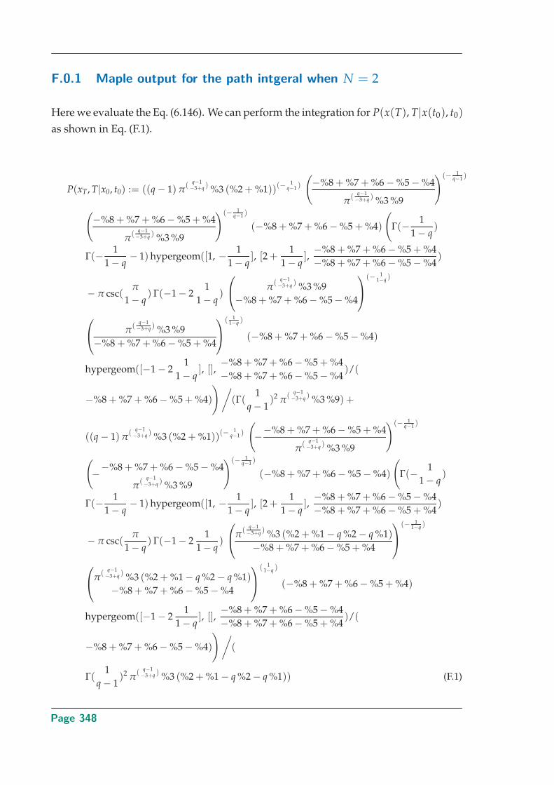
F.0.1 Maple output for the path intgeral when N = 2
Here we evaluate the Eq. (6.146). We can perform the integration for P(x(T), T|x(t0), t0)
as shown in Eq. (F.1).
P(xT, T|x0, t0) := ((q − 1) π( q−1−3+q ) %3 (%2 + %1))(− 1
q−1 )
(−%8 + %7 + %6 − %5 − %4
π(
q−1−3+q ) %3 %9
)(− 1q−1 )
(−%8 + %7 + %6 − %5 + %4
π( q−1−3+q ) %3 %9
)(− 1q−1 )
(−%8 + %7 + %6 − %5 + %4)
(Γ(− 1
1 − q)
Γ(− 11 − q
− 1) hypergeom([1, − 11 − q
], [2 +1
1 − q],−%8 + %7 + %6 − %5 + %4−%8 + %7 + %6 − %5 − %4
)
− π csc(π
1 − q) Γ(−1 − 2
11 − q
)
⎛⎝ π( q−1−3+q ) %3 %9
−%8 + %7 + %6 − %5 − %4
⎞⎠(− 11−q )
⎛⎝ π(
q−1−3+q ) %3 %9
−%8 + %7 + %6 − %5 + %4
⎞⎠( 11−q )
(−%8 + %7 + %6 − %5 − %4)
hypergeom([−1 − 21
1 − q], [],
−%8 + %7 + %6 − %5 + %4−%8 + %7 + %6 − %5 − %4
)/(
−%8 + %7 + %6 − %5 + %4)
)/(Γ(
1q − 1
)2 π(
q−1−3+q ) %3 %9) +
((q − 1) π( q−1−3+q ) %3 (%2 + %1))(− 1
q−1 )
(−−%8 + %7 + %6 − %5 + %4
π(
q−1−3+q ) %3 %9
)(− 1q−1 )
(−−%8 + %7 + %6 − %5 − %4
π(
q−1−3+q ) %3 %9
)(− 1q−1 )
(−%8 + %7 + %6 − %5 − %4)
(Γ(− 1
1 − q)
Γ(− 11 − q
− 1) hypergeom([1, − 11 − q
], [2 +1
1 − q],−%8 + %7 + %6 − %5 − %4−%8 + %7 + %6 − %5 + %4
)
− π csc(π
1 − q) Γ(−1 − 2
11 − q
)
⎛⎝π(
q−1−3+q ) %3 (%2 + %1 − q %2 − q %1)
−%8 + %7 + %6 − %5 + %4
⎞⎠(− 11−q )
⎛⎝π( q−1−3+q ) %3 (%2 + %1 − q %2 − q %1)
−%8 + %7 + %6 − %5 − %4
⎞⎠( 11−q )
(−%8 + %7 + %6 − %5 + %4)
hypergeom([−1 − 21
1 − q], [],
−%8 + %7 + %6 − %5 − %4−%8 + %7 + %6 − %5 + %4
)/(
−%8 + %7 + %6 − %5 − %4)
)/(
Γ(1
q − 1)2 π
( q−1−3+q ) %3 (%2 + %1 − q %2 − q %1)) (F.1)
Page 348
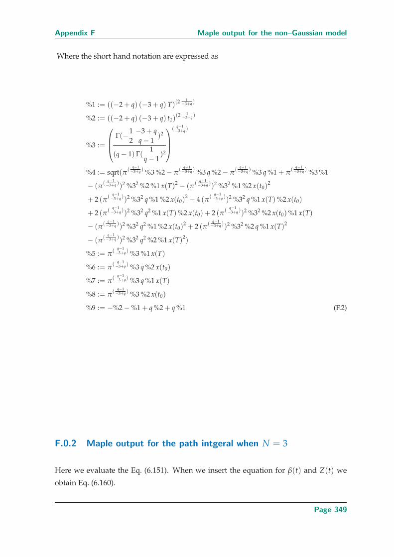
Appendix F Maple output for the non–Gaussian model
Where the short hand notation are expressed as
%1 := ((−2 + q) (−3 + q) T)(2 1−3+q )
%2 := ((−2 + q) (−3 + q) t1)(2 1
−3+q )
%3 :=
⎛⎜⎜⎝ Γ(−12−3 + qq − 1
)2
(q − 1) Γ(1
q − 1)2
⎞⎟⎟⎠( q−1−3+q )
%4 := sqrt(π( q−1−3+q ) %3 %2 − π
( q−1−3+q ) %3 q %2 − π
( q−1−3+q ) %3 q %1 + π
( q−1−3+q ) %3 %1
− (π(
q−1−3+q ))2 %32 %2 %1 x(T)2 − (π
(q−1−3+q ))2 %32 %1 %2 x(t0)
2
+ 2 (π( q−1−3+q ))2 %32 q %1 %2 x(t0)
2 − 4 (π( q−1−3+q ))2 %32 q %1 x(T) %2 x(t0)
+ 2 (π(
q−1−3+q ))2 %32 q2 %1 x(T) %2 x(t0) + 2 (π
(q−1−3+q ))2 %32 %2 x(t0) %1 x(T)
− (π( q−1−3+q ))2 %32 q2 %1 %2 x(t0)
2 + 2 (π( q−1−3+q ))2 %32 %2 q %1 x(T)2
− (π( q−1−3+q ))2 %32 q2 %2 %1 x(T)2)
%5 := π( q−1−3+q ) %3 %1 x(T)
%6 := π( q−1−3+q ) %3 q %2 x(t0)
%7 := π(
q−1−3+q ) %3 q %1 x(T)
%8 := π( q−1−3+q ) %3 %2 x(t0)
%9 := −%2 − %1 + q %2 + q %1 (F.2)
F.0.2 Maple output for the path intgeral when N = 3
Here we evaluate the Eq. (6.151). When we insert the equation for β(t) and Z(t) we
obtain Eq. (6.160).
Page 349
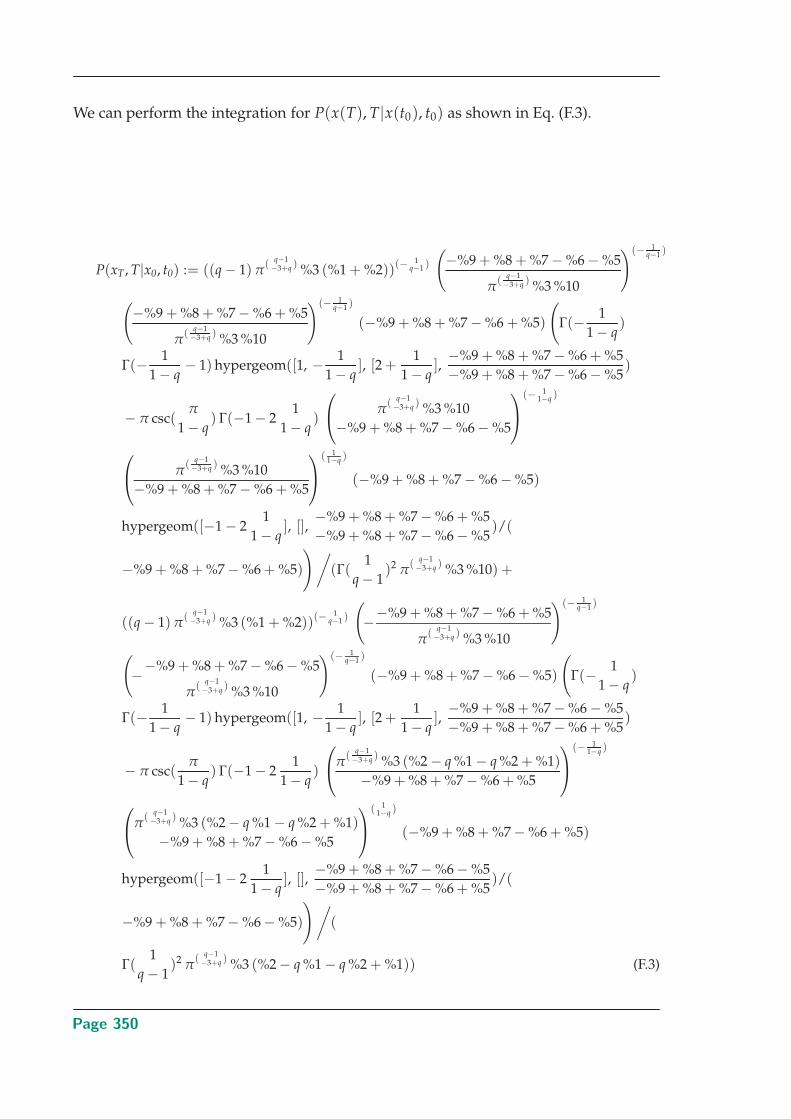
We can perform the integration for P(x(T), T|x(t0), t0) as shown in Eq. (F.3).
P(xT, T|x0, t0) := ((q − 1) π( q−1−3+q ) %3 (%1 + %2))(− 1
q−1 )
(−%9 + %8 + %7 − %6 − %5
π(
q−1−3+q ) %3 %10
)(− 1q−1 )
(−%9 + %8 + %7 − %6 + %5
π( q−1−3+q ) %3 %10
)(− 1q−1 )
(−%9 + %8 + %7 − %6 + %5)
(Γ(− 1
1 − q)
Γ(− 11 − q
− 1) hypergeom([1, − 11 − q
], [2 +1
1 − q],−%9 + %8 + %7 − %6 + %5−%9 + %8 + %7 − %6 − %5
)
− π csc(π
1 − q) Γ(−1 − 2
11 − q
)
⎛⎝ π( q−1−3+q ) %3 %10
−%9 + %8 + %7 − %6 − %5
⎞⎠(− 11−q )
⎛⎝ π(
q−1−3+q ) %3 %10
−%9 + %8 + %7 − %6 + %5
⎞⎠( 11−q )
(−%9 + %8 + %7 − %6 − %5)
hypergeom([−1 − 21
1 − q], [],
−%9 + %8 + %7 − %6 + %5−%9 + %8 + %7 − %6 − %5
)/(
−%9 + %8 + %7 − %6 + %5)
)/(Γ(
1q − 1
)2 π(
q−1−3+q ) %3 %10) +
((q − 1) π( q−1−3+q ) %3 (%1 + %2))(− 1
q−1 )
(−−%9 + %8 + %7 − %6 + %5
π(
q−1−3+q ) %3 %10
)(− 1q−1 )
(−−%9 + %8 + %7 − %6 − %5
π(
q−1−3+q ) %3 %10
)(− 1q−1 )
(−%9 + %8 + %7 − %6 − %5)
(Γ(− 1
1 − q)
Γ(− 11 − q
− 1) hypergeom([1, − 11 − q
], [2 +1
1 − q],−%9 + %8 + %7 − %6 − %5−%9 + %8 + %7 − %6 + %5
)
− π csc(π
1 − q) Γ(−1 − 2
11 − q
)
⎛⎝π(
q−1−3+q ) %3 (%2 − q %1 − q %2 + %1)
−%9 + %8 + %7 − %6 + %5
⎞⎠(− 11−q )
⎛⎝π( q−1−3+q ) %3 (%2 − q %1 − q %2 + %1)
−%9 + %8 + %7 − %6 − %5
⎞⎠( 11−q )
(−%9 + %8 + %7 − %6 + %5)
hypergeom([−1 − 21
1 − q], [],
−%9 + %8 + %7 − %6 − %5−%9 + %8 + %7 − %6 + %5
)/(
−%9 + %8 + %7 − %6 − %5)
)/(
Γ(1
q − 1)2 π
( q−1−3+q ) %3 (%2 − q %1 − q %2 + %1)) (F.3)
Page 350
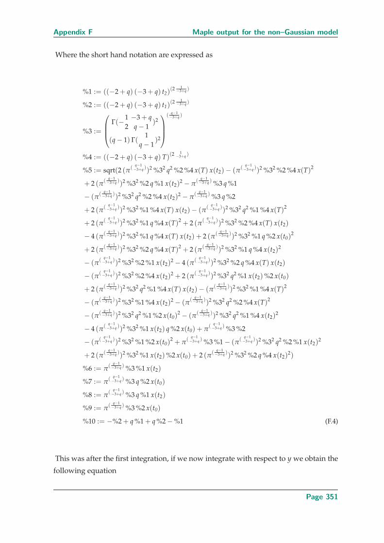
Appendix F Maple output for the non–Gaussian model
Where the short hand notation are expressed as
%1 := ((−2 + q) (−3 + q) t2)(2 1
−3+q )
%2 := ((−2 + q) (−3 + q) t1)(2 1
−3+q )
%3 :=
⎛⎜⎜⎝ Γ(−12−3 + qq − 1
)2
(q − 1) Γ(1
q − 1)2
⎞⎟⎟⎠( q−1−3+q )
%4 := ((−2 + q) (−3 + q) T)(2 1−3+q )
%5 := sqrt(2 (π(
q−1−3+q ))2 %32 q2 %2 %4 x(T) x(t2)− (π
(q−1−3+q ))2 %32 %2 %4 x(T)2
+ 2 (π( q−1−3+q ))2 %32 %2 q %1 x(t2)
2 − π( q−1−3+q ) %3 q %1
− (π(
q−1−3+q ))2 %32 q2 %2 %4 x(t2)
2 − π(
q−1−3+q ) %3 q %2
+ 2 (π( q−1−3+q ))2 %32 %1 %4 x(T) x(t2)− (π
( q−1−3+q ))2 %32 q2 %1 %4 x(T)2
+ 2 (π(
q−1−3+q ))2 %32 %1 q %4 x(T)2 + 2 (π
(q−1−3+q ))2 %32 %2 %4 x(T) x(t2)
− 4 (π( q−1−3+q ))2 %32 %1 q %4 x(T) x(t2) + 2 (π
( q−1−3+q ))2 %32 %1 q %2 x(t0)
2
+ 2 (π( q−1−3+q ))2 %32 %2 q %4 x(T)2 + 2 (π
( q−1−3+q ))2 %32 %1 q %4 x(t2)
2
− (π( q−1−3+q ))2 %32 %2 %1 x(t2)
2 − 4 (π( q−1−3+q ))2 %32 %2 q %4 x(T) x(t2)
− (π( q−1−3+q ))2 %32 %2 %4 x(t2)
2 + 2 (π( q−1−3+q ))2 %32 q2 %1 x(t2) %2 x(t0)
+ 2 (π(
q−1−3+q ))2 %32 q2 %1 %4 x(T) x(t2)− (π
(q−1−3+q ))2 %32 %1 %4 x(T)2
− (π( q−1−3+q ))2 %32 %1 %4 x(t2)
2 − (π( q−1−3+q ))2 %32 q2 %2 %4 x(T)2
− (π(
q−1−3+q ))2 %32 q2 %1 %2 x(t0)
2 − (π(
q−1−3+q ))2 %32 q2 %1 %4 x(t2)
2
− 4 (π( q−1−3+q ))2 %32 %1 x(t2) q %2 x(t0) + π
( q−1−3+q ) %3 %2
− (π(
q−1−3+q ))2 %32 %1 %2 x(t0)
2 + π(
q−1−3+q ) %3 %1 − (π
(q−1−3+q ))2 %32 q2 %2 %1 x(t2)
2
+ 2 (π( q−1−3+q ))2 %32 %1 x(t2) %2 x(t0) + 2 (π
( q−1−3+q ))2 %32 %2 q %4 x(t2)
2)
%6 := π(
q−1−3+q ) %3 %1 x(t2)
%7 := π( q−1−3+q ) %3 q %2 x(t0)
%8 := π( q−1−3+q ) %3 q %1 x(t2)
%9 := π( q−1−3+q ) %3 %2 x(t0)
%10 := −%2 + q %1 + q %2 − %1 (F.4)
This was after the first integration, if we now integrate with respect to y we obtain the
following equation
Page 351
∫ ∞
−∞((q − 1) π
( q−1−3+q ) %3 (%1 + %2))(− 1
q−1 )
(−%9 + %8 + %7 − %6 − %5
π(
q−1−3+q ) %3 %10
)(− 1q−1 )
(−%9 + %8 + %7 − %6 + %5
π( q−1−3+q ) %3 %10
)(− 1q−1 )
(−%9 + %8 + %7 − %6 + %5)
(Γ(− 1
1 − q)
Γ(− 11 − q
− 1) hypergeom([1, − 11 − q
], [2 +1
1 − q],−%9 + %8 + %7 − %6 + %5−%9 + %8 + %7 − %6 − %5
)
− π csc(π
1 − q) Γ(−1 − 2
11 − q
)
⎛⎝ π( q−1−3+q ) %3 %10
−%9 + %8 + %7 − %6 − %5
⎞⎠(− 11−q )
⎛⎝ π(
q−1−3+q ) %3 %10
−%9 + %8 + %7 − %6 + %5
⎞⎠( 11−q )
(−%9 + %8 + %7 − %6 − %5)
hypergeom([−1 − 21
1 − q], [],
−%9 + %8 + %7 − %6 + %5−%9 + %8 + %7 − %6 − %5
)/(
−%9 + %8 + %7 − %6 + %5)
)/(Γ(
1q − 1
)2 π(
q−1−3+q ) %3 %10) +
((q − 1) π( q−1−3+q ) %3 (%1 + %2))(− 1
q−1 )
(−−%9 + %8 + %7 − %6 + %5
π(
q−1−3+q ) %3 %10
)(− 1q−1 )
(−−%9 + %8 + %7 − %6 − %5
π(
q−1−3+q ) %3 %10
)(− 1q−1 )
(−%9 + %8 + %7 − %6 − %5)
(Γ(− 1
1 − q)
Γ(− 11 − q
− 1) hypergeom([1, − 11 − q
], [2 +1
1 − q],−%9 + %8 + %7 − %6 − %5−%9 + %8 + %7 − %6 + %5
)
− π csc(π
1 − q) Γ(−1 − 2
11 − q
)
⎛⎝π(
q−1−3+q ) %3 (%2 − q %1 − q %2 + %1)
−%9 + %8 + %7 − %6 + %5
⎞⎠(− 11−q )
⎛⎝π( q−1−3+q ) %3 (%2 − q %1 − q %2 + %1)
−%9 + %8 + %7 − %6 − %5
⎞⎠( 11−q )
(−%9 + %8 + %7 − %6 + %5)
hypergeom([−1 − 21
1 − q], [],
−%9 + %8 + %7 − %6 − %5−%9 + %8 + %7 − %6 + %5
)/(
−%9 + %8 + %7 − %6 − %5)
)/(
Γ(1
q − 1)2 π
( q−1−3+q ) %3 (%2 − q %1 − q %2 + %1))dy
Page 352
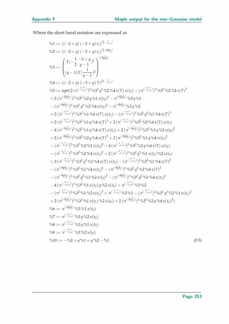
Appendix F Maple output for the non–Gaussian model
Where the short hand notation are expressed as
%1 := ((−2 + q) (−3 + q) t2)(2 1
−3+q )
%2 := ((−2 + q) (−3 + q) t1)(2 1
−3+q )
%3 :=
⎛⎜⎜⎝ Γ(−12−3 + qq − 1
)2
(q − 1) Γ(1
q − 1)2
⎞⎟⎟⎠( q−1−3+q )
%4 := ((−2 + q) (−3 + q) T)(2 1−3+q )
%5 := sqrt(2 (π( q−1−3+q ))2 %32 q2 %2 %4 x(T) x(t2)− (π
( q−1−3+q ))2 %32 %2 %4 x(T)2
+ 2 (π(
q−1−3+q ))2 %32 %2 q %1 x(t2)
2 − π(
q−1−3+q ) %3 q %1
− (π( q−1−3+q ))2 %32 q2 %2 %4 x(t2)
2 − π( q−1−3+q ) %3 q %2
+ 2 (π(
q−1−3+q ))2 %32 %1 %4 x(T) x(t2)− (π
(q−1−3+q ))2 %32 q2 %1 %4 x(T)2
+ 2 (π( q−1−3+q ))2 %32 %1 q %4 x(T)2 + 2 (π
( q−1−3+q ))2 %32 %2 %4 x(T) x(t2)
− 4 (π(
q−1−3+q ))2 %32 %1 q %4 x(T) x(t2) + 2 (π
(q−1−3+q ))2 %32 %1 q %2 x(t0)
2
+ 2 (π( q−1−3+q ))2 %32 %2 q %4 x(T)2 + 2 (π
( q−1−3+q ))2 %32 %1 q %4 x(t2)
2
− (π(
q−1−3+q ))2 %32 %2 %1 x(t2)
2 − 4 (π(
q−1−3+q ))2 %32 %2 q %4 x(T) x(t2)
− (π( q−1−3+q ))2 %32 %2 %4 x(t2)
2 + 2 (π( q−1−3+q ))2 %32 q2 %1 x(t2) %2 x(t0)
+ 2 (π( q−1−3+q ))2 %32 q2 %1 %4 x(T) x(t2)− (π
( q−1−3+q ))2 %32 %1 %4 x(T)2
− (π( q−1−3+q ))2 %32 %1 %4 x(t2)
2 − (π( q−1−3+q ))2 %32 q2 %2 %4 x(T)2
− (π( q−1−3+q ))2 %32 q2 %1 %2 x(t0)
2 − (π( q−1−3+q ))2 %32 q2 %1 %4 x(t2)
2
− 4 (π(
q−1−3+q ))2 %32 %1 x(t2) q %2 x(t0) + π
(q−1−3+q ) %3 %2
− (π( q−1−3+q ))2 %32 %1 %2 x(t0)
2 + π( q−1−3+q ) %3 %1 − (π
( q−1−3+q ))2 %32 q2 %2 %1 x(t2)
2
+ 2 (π(
q−1−3+q ))2 %32 %1 x(t2) %2 x(t0) + 2 (π
(q−1−3+q ))2 %32 %2 q %4 x(t2)
2)
%6 := π( q−1−3+q ) %3 %1 x(t2)
%7 := π(
q−1−3+q ) %3 q %2 x(t0)
%8 := π( q−1−3+q ) %3 q %1 x(t2)
%9 := π( q−1−3+q ) %3 %2 x(t0)
%10 := −%2 + q %1 + q %2 − %1 (F.5)
Page 353

Page 354
Bibliography
ADAM-M., AND SZAFARZ-A. (1992). Speculative bubbles and financial markets, Oxford Economic Pa-
pers, 44, pp. 626–640.
ALDRICH-J. (1997). R. A. Fisher and the making of maximum likelihood 1912-1922, Statistical Science,
12 (3), pp. 162–176.
ALLISON-A., AND ABBOTT-D. (2000). Stable processes in an econometric time series, American Inst.
Physics, Unsolved Problems of Noise and fluctuations (UPoN’99), Vol. 511, pp. 221–232.
ANDERSEN-J., AND SORNETTE-D. (2003). The $-game, Eur. Phys. J. B, 31, pp. 141–145.
ANDERSEN-J., AND SORNETTE-D. (2004). Fearless versus fearful speculative financial bubble, Physica
A, 337, p. 565.
ANDERSON-B., AND MOORE-J. (1979). Optimal Filtering, Prentice-Hall information and system sciences
series, Englewood Cliffs, N.J.
ANKERHOLD-J., GRABERT-H., AND PECHUKAS-P. (2005). Quantum Brownian motion with large fric-
tion, Chaos, 15, p. 026106.
ARTHUR-W. (1994). Inductive reasoning and bounded rationality: the El Farol bar problem, Am. Econo.
Rev., 84, pp. 406–411.
ARTHUR-W., DURLAUF-S., AND LANE-D. (1997a). The economy as an evolving complex system,
Addison-Wesley, Vol. XXVII of SFI Studies in the Sciences of Complexity.
ARTHUR-W., HOLLAND-J., BARON-B. L., PALMER-R., AND TAYLOR-P. (1997b). Asset pricing under en-
dogenous expectations in an artificial stock market, The Economy as an Evolving Complex System,
II, Vol. XXVII of SFI Studies in the Sciences of Complexity see Ref. (Arthur et al. 1997a).
BAAQUIE-B. E. (2004). Quantum Finance: Path Integrals and Hamiltonians for Options and Interest
Rates, Cambridge University Press, Cambridge.
BACHELIER-L. (1900). Theorie de la speculation, Annales de l’Ecole Normal Superieur, 17, pp. 21–86.
BACHELIER-L. (1964). Theorie de la speculation, L. Gobay, Sceaux, 1995 (reprinted in P. Cootner, Ed.,
The Random Character of Stock Market Prices, MIT Press, Cambridge, MA), pp. 17–78.
BACKUS-D., FORESI-S., LAI-K., AND WU-L. (1997). Accounting for biases in Black-Scholes, Working
paper of NYU Stern School of Business.
BACRY-E., DELOUR-J., AND MUZY-J.-F. (2001). Multifractal random walk, Phys. Rev. E, 64, p. 026103.
BADER-A., AND LOSCHMIDT-L. (2001). Josef Loschmidt, physicist and chemist, Phys. Today, 54, pp. 45–
50.
BARNDORFF-NIELSEN-O. (1977). Exponentially decreasing distributions for the logarithm of particle
size, Proceedings of the Royal Society of London A, 353, pp. 401–419.
Page 355
Bibliography
BARNDORFF-NIELSEN-O. (1998). Processes of normal inverse Gaussian type, Finance and Statistics, 2,
pp. 41–68.
BARNDORFF-NIELSEN-O., AND HALGREEN-O. (1977). Infinite divisibility of the hyperbolic and gen-
eralized inverse gaussian distribution, Zeitschrift fur Wahrscheinlichkeitstheorie und Verwandte
Gebiete, 38, pp. 309–312.
BERA-A., AND HIGGINS-M. (1993). ARCH models: properties estimation and testing, Journal of Eco-
nomics Surveys, 7, pp. 305–362.
BJORKEN-J., AND DRELL.-S. (1965). Relativistic Quantum Fields, McGraw-Hill, New York.
BLACK-F. (1976). Studies in stock price volatility changes, Proceeding of the 1976, Meeting of the Buisi-
ness and Economics Statistic Section, American Statistical Associates, pp. 177–181.
BLACK-F., AND SCHOLES-M. (1973). The pricing of options and corporate liabilities, Polit. Economy,
81, p. 637.
BOLLERSLEV-T. (1986). Generalized autoregressive conditional heteroskedasticity, Journal of Economics,
31, pp. 307–327.
BOLLERSLEV-T., CHOU-R., AND KRONER-K. (1992). ARCH modelling in finance: a review of the theory
and empirical evidence, Journal of Econometrics, 52, pp. 5–59.
BOLLERSLEV-T., ENGLE-R., AND NELSON-D. (1994). ARCH models in Handbook of Econometrics,
Elsevier Science, Amsterdam.
BONNET-F., BOWMAN-P. O., LEINWEBER-D. B., AND WILLIAMS-A. G. (2000a). Infrared behavior of
the gluon propagator on a large volume lattice, Phys. Rev., D62, p. 051501.
BONNET-F., BOWMAN-P. O., LEINWEBER-D. B., WILLIAMS-A. G., AND ZHANG-J. (2002a). Overlap
quark propagator in Landau gauge, Phys. Rev., D65, p. 114503.
BONNET-F. D., BOWMAN-P. O., LEINWEBER-D. B., WILLIAMS-A. G., AND ZANOTTI-J. M. (2001a).
Infinite volume and continuum limits of the Landau gauge gluon propagator, Phys. Rev., D64,
p. 034501.
BONNET-F. D., LEINWEBER-D. B., AND WILLIAMS-A. G. (2001b). General algorithm for improved
lattice actions on parallel computing architectures, J. Comput. Phys., 170, pp. 1–17.
BONNET-F., EDWARDS-R. G., FLEMING-G. T., LEWIS-R., AND RICHARDS-D. G. (2004). Mesonic form
factors, Nucl.Phys.Proc.Suppl., 128, pp. 59–65.
BONNET-F., FITZHENRY-P., LEINWEBER-D. B., STANFORD-M. R., AND WILLIAMS-A. G. (2000b). Cali-
bration of smearing and cooling algorithms in SU(3): color gauge theory, Phys. Rev., D62, p. 094509.
BONNET-F., LEINWEBER-D. B., WILLIAMS-A. G., AND ZANOTTI-J. M. (2002b). Improved smoothing
algorithms for lattice gauge theory, Phys. Rev., D65, p. 114510.
BONNET-F., LEINWEBER-D., WILLIAMS-A. G., ZANOTTI-J., AND ZHANG-J. (2002c). Quark propagator
in a covariant gauge, Nucl. Phys. Proc. Suppl., 109A, pp. 158–162.
BORLAND-L. (1998a). Microscopic dynamics of the nonlinear Fokker-Planck equation: A phenomeno-
logical model, Phys. Rev. E, 57, pp. 6634–.
Page 356

Bibliography
BORLAND-L. (1998b). Microscopic dynamics of the nonlinear Fokker-Planck equation: A phenomeno-
logical model, Phys. Rev. E, 57, pp. 6634–6642.
BORLAND-L. (2002a). Option pricing formulas based on a non–Gaussian stock price model, Phys. Rev.
Lett., 89, p. 098701.
BORLAND-L. (2002b). A theory of non–gaussian option pricing, Quantitative Finance, 2, pp. 415–431.
BORLAND-L. (2002c). A theory of non-Gaussian option pricing, Quantitative Finance, 2, pp. 415–431.
BORLAND-L., AND BOUCHAUD-J.-P. (2004). A non-Gaussian option pricing model with skew, cond
mat/0403022v2.
BOUCHAUD-J., AND POTTERS-M. (2000a). Theory of Financial Risks, From Statistical Physics to Risk
Management, Cambridge University Press., Cambridge.
BOUCHAUD-J.-P., AND CONT-R. (1998). A Langevin approach to stock market fluctuations and crashes,
Eur. Phys. J. B, 6, p. 543.
BOUCHAUD-J.-P., AND POTTERS-M. (2000b). Theory of Financial Risks, Cambridge University Press,
Cambridge.
BOUCHAUD-J.-P., AND POTTERS-M. (2004). Theory of Financial Risk and Derivative Pricing: From
Statistical Physics to Risk Management, Cambridge, Cambridge.
BOUCHAUD-J.-P., IORI-G., AND SORNETTE-D. (1996). Real world options: Smile and residual risk, Risk,
93, pp. 61–65.
BOUCHAUD-J.-P., MEZARD-M., AND POTTERS-M. (2002). Statistical properties of stock order books:
empirical results and models, Quant. Fin., 2, p. 251.
BOUGEROL-P., AND PICARD-N. (1992). Stationarity of GARCH process and of some non–negative time
series, Journal of Econometrics, 52, pp. 115–127.
BOX-G., AND JENKINS-G. (1976). Time Series Analysis: Forecasting and Control, Holden–Day, San
Francisco.
BROCKWELL-P., AND DAVIS-R. (2002). Introduction to Time Series and Forecasting, Springer.
BROCK-W., LAKONISKOK-J., AND LE BARON-B. (1992). Simple technical trading rules and the stochastic
properties of stock returns, J. of Finance, p. 30.
BROWN-R. (1828). A brief account of microscopical observations made in the months of June, July, and
August, 1827, on the particles contained in the pollen of plants; and on the general existence of
active molecules in organic and inorganic bodies, Philos. Mag., 4, pp. 161–173.
BUCHEN-P., AND KELLY-M. (1996). The maximum entropy distribution of an asset inferred from option
prices, The Journal of Finance and Quantitative Analysis, 31, pp. 143–159.
BURRAGE-K., BURRAGE-P., AND MITSUI-T. (2000). Numerical solutions of stochastic differential equa-
tions implementation and stability issues, Journal of Computational and Applied Mathematics
archive, 125, pp. 171–182.
Page 357
Bibliography
CAI-Y. (2003). Convergence theory of a numerical method for solving the Chapman–Kolmogorov equa-
tion, SIAM, 40, pp. 2337–2351.
CAI-Y. (2005). A forecasting procedure for nonlinear autoregressive time series models, J. Forecasting,
24, pp. 335–351.
CALDARELLI-G., MARSILI-M., AND ZHANG-Y.-C. (1997). A prototype model of stock exchange, Euro-
phys. Lett., 50, pp. 479–484.
CALLEN-H., AND WELTON-T. (1951). Irreversibility and generalised noise, Phys. Rev., 83, pp. 34–40.
CAMERER-C. (1989). Bubbles and fads in asset prices, J. of Economics Surveys, 3, p. 3.
CAMPBELL-J., LO-A., AND MACKINLAY-A. (1997). The Econometrics of Financial Markets, Princeton
University Press, Princeton NJ.
CAVAGNA-A. (1999). Irrelevance of memory in the minority game, Phys. Rev. E, 59, p. R3783.
CAVAGNA-A., GARRAHAN-J., GIARDINA-I., AND SHERRINGTON-D. (1999). Emergence of cooperation
and organization in an evolutionary game, Phys. Rev. Lett., 83, p. 4429.
CHALET-D., AND ZHANG-Y.-C. (1997). Emergence of cooperation and organization in an evolutionary
game, Physica A, 246, p. 407.
CHALET-D., CHESSA-A., MARSILI-M., AND ZHANG-Y.-C. (2001). From minority games to real mar-
kets, Quant. Fin., 212, p. 1.
CHIARELLA-C., AND EL-HASSAN-N. (1997). Evaluation of derivative security prices in the hjm frame-
work as path integrals using fast fourier transform techniques, Journal of Financial Engineering, 6,
pp. 121–147.
CHIARELLA-C., EL-HASSAN-N., AND KUCERA-A. (1999). Evaluation of american option prices in a
path integral framework using fourier-hermite series expansions, Journal of Economics Dynamics
& Control, 23, pp. 1387–1424.
COLEMAN-C. J. (2002). Huygen’s principle applied to radio wave propagation, Rad. Sci., 37, p. 1105.
COLEMAN-S. (1985). Aspects of Symmetry, Cambridge University Press, Cambridge.
CONT-R. (2001). Empirical properties of asset returns: stylized facts and statistical issues, quantitative
finance, 1, p. 223.
CONT-R., AND TANKOV-P. (2004). Financial Modelling with Jump Processes, Chapman and Hall/CRC
financial series, London.
COURTAULT-J., KABANOV-Y., BRU-B., CREPEL-P., LEBON-I., AND MARCHAND-A. L. (2000). A Louis
Bachelier on the centary of: Theorie de la speculation, Math. Finance, 10, pp. 341–353.
COX-J., ROSS-S., AND RUBINSTEIN-M. (1979). Option pricing: a simplified approach, J. Financial Eco-
nomics, 7, p. 229.
CURADO-E., AND TSALLIS-C. (1991a). Generalized statistical mechanics: connection with thermody-
namics, J. Phys. A, 24, p. L69.
Page 358
Bibliography
CURADO-E., AND TSALLIS-C. (1991b). Generalized statistical mechanics: connection with thermody-
namics, J. Phys. A: Math. Gen., 24, p. L69.
DASH-J. W. (2004). QUantitative Finance and Risk Management: a Physicist’s Approach, World Scien-
tific.
DELBRIDGE-A. (2001). The Macquarie Dictionary, 3rd edn, The Macquarie Library, North Ryde, NSW,
Australia.
DEMPSTER-A., LAIRD-N., AND RUBIN-D. (1977). Maximum likelihood from incomplete data using the
em algorithm, Journal of the Royal Statistical Society of London B, 39, pp. 1–38.
DING-Z., AND GRANGER-C. (1996). Modeling volatility persistence of speculative returns: a new ap-
proach, Journal of Econometrics, 73, pp. 185–215.
DING-Z., GRANGER-C., AND ENGLE-R. (1993). A long memory property of stock market returns and a
new model, J. Empirical Finance, 1, p. 83.
DYSON-F. (1949). The radiation theories of Tomonaga, Schwinger, and Feynman, Phys. Rev., 75, p. 486.
EBERLEIN-E. (2001). Applications of Generalized Hyperbolic Levy Motion to Finance, O.E. Barndorff-
Nielsen et.al. (eds), Birkhauser.
EBERLEIN-E., AND TAQQU-M. (1986). Dependence in Probability and Statistics: A Survey of Recent
Results, rogress in Probability and Statistics Series, Boston.
EINSTEIN-A. (1905a). This Einstein relation has been obtained independently in 1904 by William Suther-
land, Ann. Phys., 17, p. 549.
EINSTEIN-A. (1905b). Uber die von der molakular kinetisken theorie der warne geforderte bewegaung
von in ruhenden flussigkeiten suspendierten teilchen, Ann. Phys., 17, p. 549.
EINSTEIN-A. (1908). Elementare theorie der Brownschen bewegung, Z. Elektrochem. Angrew. Phys.
Chem., 14, pp. 235–239.
ENGLE-R. (1982). Auto–regressive conditional heteroskedasticity with estimates of variance of United
Kingdom inflation, Econometrica, 50, pp. 987–1007.
ENGLE-R. (1995). ARCH Selected Readings. Advanced Text in Econometrics, Oxford University press,
Oxford.
ENGLE-R., AND NG-V. (1993). Measuring and testing the impact of news on volatility, Journal of Fi-
nance, 48, pp. 1749–1777.
EVANS-G. (1991). Pitfalls in testing for explosive bubbles in asset prices, American Economics Rev., 81,
p. 922.
FALLER-D., AND PETRUCCIONE-F. (2003). A master equation approach to option pricing, Physica A,
319, pp. 519–534.
FAMA-D. (1965). The behavior of stock market prices, J. of Finance, 38, pp. 34–105.
FARMER-J. (1998). Market force, ecology and evolution, adap-org/9812005.
Page 359
Bibliography
FELLER-W. (1966). An Introduction to Probability Theory and its Applications, John Willey, Vol II, Lon-
don.
FEYNMAN-R., AND HIBBS-A. (1965). Quantum Mechanics and Path Integrals, McGraw-Hill, New York.
FEYNMAN-R. P. (1948). Space-time approach to non-relativistic quantum mechanics, Rev. Mod. Phys.,
20, p. 367.
FEYNMAN-R. P. (1972). Statistical Mechanics: a Set of Lectures, W.A. Benjamin Inc. Advanced book
program, Massachussetts.
FOMIN-V. (1999). Optimal Filtering, Kluwer Academic Publishers, Dordrecht.
FORSBERG-L., AND BOLLERSLEV-T. (2002). Bridging the gap between distribution of realized (ECU)
volatility and ARCH modelling (of the EURO): The GARCH-NIG model, Journal of Applied
Econometrics, 17, pp. 535–548.
FOUQUE-J., PAPANICOLAOU-G., AND SIRCAR-K. R. (2000). Derivatives in Financial Markets with
Stochastic Volatility, Cambridge University Press.
FRISH-U. (1995). Turbulence, Cambridge University Press., Cambridge.
GEMAN-H., MADAN-D., PLISKA-S., AND (EDS.)-T. V. (2000). Mathematical Finance–Bachelier
Congress, Springer Finance, New York.
GLASSERMAN-P. (2003). Monte Carlo Methods in Financial Engineering, Springer, New York.
GLIMM-J., AND JAFFE-A. (1981). Quantum Physics: A Functional Point of View, SpringerVerlag, Berlin.
GOLDSTEN-L., JAGANNATHAN-R., AND RUNKLE-D. (1993). Relationship between the expected value
and the volatility of nominal excess return on stocks, Journal of Finance, 48, pp. 1779–1801.
GOSSET-W. (1908). The probable error of a mean, Biometrika, 6 (1), pp. 1–25.
GRIFFITHS-D. J. (2004). Introduction to Quantum Mechanics (2nd ed.), Prentice Hall.
HAMILTON-J. (1994). Time series analysis, Princeton University press, Princeton.
HANGGI-P. (2005). Introduction: 100 years of Brownian motion, Chaos, 15, pp. 026101–5.
HANGI-P., AND INGOLD-G. (2005). Fundamental aspects of quantum Brownian motion, Chaos, 15,
p. 026105.
HAVEN-E. E. (2002). A discussion on embedding the Black and Scholes option pricing model in a
quantum physics setting, Physica A, 304, pp. 507–524.
HOMMES-C. (2001). Financial markets as nonlinear adaptive evolutionary systems, Quantitative Fi-
nance, 1, p. 149.
HULL-J. (2000a). Option, Futures, and Other Derivatives, 4th edn. Prentice Hall, Wiley, New Jersey.
HULL-J. (2000b). Techniques and Applications of Path Integrals, Prentice Hall, New Jersey.
ILINSKI-K. (1997). Physics of finance, hep-th/9710148.
INGBER-L. (2000). High-resolution path-integral development of financial options, Physica A, 283,
pp. 529–558.
Page 360
Bibliography
ITZYKSON-C., AND ZUBER-J. (1980). Quantum Field Theory, Mc Graw Hill, Singapore.
JACKWERTH-J. C., AND RUBINSTEIN-M. (1996). Recovering probability distribution from option prices,
The Journal of Finance, 51 No 5, pp. 1611–1631.
JOHANSEN-A., SORNETTE-D., AND LEDOIT-O. (1999). Predicting financial crashes using discrete scale
invariance, J. Risk, 1, p. 5.
JOHNSON-N., HART-M., HUI-P., AND ZHENG-D. (2000). Traders dynamics in a model market, Inter-
national Journal of Theoretical and Applied Finance, 3, pp. 443–450.
ITO -K. (1951). Multiple Wierner integrals, J. Math. Society of Japan, 3, pp. 157–169.
KAC-M. (1949). On distributions of certain Wiener functionals, Transactions of American Mathematical
Society, 65, p. 113.
KAC-M. (1959). Probability and Related Topics in Physical Science, Interscience, New York.
KAC-M. (1980). Integration in Function Spaces and Some of its Applications, Academia Nazionale Dei
Lincei, Pisa.
KARATZAS-I., AND SHREVE-S. (1988). Brownian Motion and Stochastic Calculus, Springer–Verlag, New
York.
KAY-S. (1993). Fundamentals of Statistical Signal Processing: Estimation Theory, Prentice Hall, N. J.
KERSEN-H. (1987). Statistical Mechanics, Wiley, New York.
KLEINERT-H. (2004). Path Integrals in Quantum Mechanics, Statistics, Polymer Physics, and Financial
Markets, World Scientific, Singapore.
KLOEDEN-P., AND PLATEN-E. (1992). Numerical Solution of Stochastic Differential Equations, Springer,
Application of Mathematics Vol. 23, New York.
KOLMOGOROV-A. N. (1992). On Analytic Methods in Probability Theory, Kluwer, Dordrecht.
KRAWIEECKI-A., AND HOLYST-J. (2003). Stochastic resonance as a model for financial market crashes
and bubbles, Physica A, 317, pp. 597–608.
KUBO-R. (1957). Statistical–mechanical theory of irreversible processes. 1. General theory and simple
applications to magnetic and conduction problems, J. Phys. Soc. Jpn., 12, pp. 570–586.
LARSSON-S., AND THOMEE-V. (2005). Partial Differential Equations with Numerical Methods,
Springer–Verlag, Berlin.
LE BARON-B. (2000). Agent-based computational finance: Suggested readings and early research, J. of
Economics Dyn. Control, 24, p. 679.
LE BARON-B., ARTHUR-W., AND PALMER-R. (1999). Time series properties of an artificial stock market,
J. of Economics Dyn. Control, 23, pp. 1487–1516.
LEHMANN-E. L., AND CASELLA-G. (1998). Theory of Point Estimation, Springer.
LEVY-G. (2004). Computational Finance, Numerical Methods for Pricing Financial Instruments, Elsevier,
Butterworth Heinemann, Oxford.
Page 361
Bibliography
LIU-Y., CIZEAU-P., MEYER-M., PENG-C. K., AND STANLEY-H.-E. (1997). Correlation in economic time
series, Physica A, 245, p. 437.
LI-W., LING-S., AND MCALEER-M. (2002). A survey of recent theoretical results for time series models
with garch errors, Journal of Economics Survey, 16, pp. 245–269.
LJUNG-G. M., AND BOX-G. E. P. (1978). On a measure of a lack of fit in time series models, Biometrika,
65, pp. 297–303.
LO-A. (1991). Long term memory in stock market prices, Econometrica, 59, p. 1279.
LOGAN-J. (2004). Applied Partial Differential Equations, Springer–Verlag, New York.
LUX-T., AND MARCHESI-M. (1999). Scaling and critically in a stochatic multiagent model of financial
market, Nature, 397, pp. 498–500.
MANDLEBROT-B. (1963). The variation of certain speculative prices, J. Business, 35, pp. 394–419.
MANDLEBROT-B. (1997). Fractals and Scaling in Finance: Discontinuity, Contraction, Risk, springer,
New York.
MANSUY-R. (2005). Histoire de martingale, Math. & Sci. hum / Mathematical Social Sciences, 169,
pp. 105–113.
MANTEGNA-R., AND STANLEY-E. (1995). Scaling behaviour in the dynamics of an economic index,
Nature, 376, p. 46.
MARSILI-M., CHALET-D., AND ZECCHINA-R. (2000). Exact solution of a modified El Farol’s bar prob-
lem: Efficiency and the role of market impact, Physica A cond mat/9908480, 280, p. 522.
MATACZ-A. (2000). Path dependent option pricing: the path integral partial averaging method, cond-
mat/0005319.
MCKENZIE-M., HEATHER-M., BROOKS-R., AND FAFF-R. (2001). Power ARCH modelling of commodi-
ties futures data on the London metal exchange, The European Journal of Finance, 7, pp. 22–28.
MERTON-R. (1973). Theory of rational option pricing, Bell J. Econom. Manag. Sci., 4, p. 141.
MERTON-R. (1976a). Option pricing using variance gamma Markov chains, J. Financial Economics, 3,
p. 125.
MERTON-R. (1990). Continuous Time Finance, Cambridge, Blackwell.
MERTON-R. C. (1976b). Option pricing when underlying stock returns are discontinuous, J. Fin. Econ.,
3, pp. 125–144.
MFREIDLIN. (1985). Functional Integration and Partial Differential Equations, Princeton University
Press, Princeton, New Jersey.
MICHAEL-F., AND JOHNSON-M. (2003). Financial market dynamics, Physica A, 320, pp. 525–534.
MISTRAL-F. (1979). Lou Tresor dou Felibrige ou Dictionnaire Provencal–Francais, Petit, Raphaele–les–
Arles.
Page 362
Bibliography
MONTAGNA-G., NICROSINI-O., AND MORENI-N. (2002). A path integral way to option pricing, Physica
A, 310, pp. 450–466.
MUZY-J.-F., AND BACRY-E. (2002). Multifractal stationary random measures and multifractal random
walks with log infinity divisible scaling laws, Phys. Rev. E, 66, p. 056121.
MUZY-J.-F., DELOUR-J., AND BACRY-E. (2000). Modelling fluctuations of financial time series: from
cascade process to stochastic volatility model, Eur. Phys. J. B Quantitative Finance, 17, p. 537.
MUZY-J.-F., SORNETTE-D., DELOUR-J., AND ARNCODO-A. (2001). Multifractal returns and hierarchical
portfolio theory, Quantitative Finance, 1, p. 131.
NELSON-D. (1990). Stationarity and persistence in the GARCH(1, 1) model, Econometrics Theory, 6,
pp. 318–334.
NELSON-D. (1991). Conditional heteroskedasticity in asset returns: a new approach, Econometrica, 59,
pp. 347–370.
OETIKER-T., PARTL-H., HYNA-I., AND SCHLEGL-E. (2000). The Not So Short Introduction to LATEX
2e, GNU General Public License, Cambridge.
ØKSENDAL-B. (2003). Stochastic Differential Equations, Springer–Verlag, Berlin.
ONSAGER-L., AND MACHLUP-S. (1953). Fluctuations and irreversible processes, Phys. Rev., 91,
pp. 1505–1512.
Option Style (6 January 2008). Web. http://en.wikipedia.org/wiki/Asian-option.
OTTO-M. (1998). Using path integrals to price interest rate derivatives, cond-mat/9812318.
OTTO-M. (1999). Stochastic relaxational dynamics applied to finance: towards non-equilibrium option
pricing theory, Eur. Phys. J., B 14, pp. 383–394.
PALM-F. (1996). GARCH models of volatility, Handbook of Statistic, Statistical Methods in Finance, 14,
pp. 209–240.
PAUL-W., AND BASCHNAGEL-J. (1999). Stochastic Processes: from Physics to Finance, Springer-Verlag,
Berlin Heidelberg.
PESKIN-M., AND SCHROEDER-D. (1995). An Introduction to Quantum Field Theory, Addison Wesley,
New York.
POCHART-B., AND BOUCHAUD-J.-P. (2002). The skew multifractal random walk with application to
option smiles, Quantitative Finance, 2, pp. 303–314.
POTTERS-M., CONT-R., AND BOUCHAUD-J.-P. (1998). Financial markets as adaptive systems, Euro-
physics letters, 41, p. (3).
PRAUSE-K. (1999). The Generalized Hyperbolic Model: Estimation, Financial Derivatives, and Risk
Measures, Dissertation zur Erlangung des doctorgrades, Albert-Ludwigs-Universitat Freiburg.
RACHLEVSKY-REICH-B., BEN-SHAUL-I., CHAN-N. T., LO-A., AND POGGIO-T. (1999). Gem: A global
electronic market system, Information Syst., 24, p. 495.
Page 363
Bibliography
RAIBLE-S. (2000). Levy Processes in Finance: Theory, Numerics and Empirical Facts, Dissertation zur
Erlangung des doctorgrades, Albert-Ludwigs-Universitat Freiburg.
REBBI-C. (1983). Lattice Gauge Theories and Monte Carlo Simulations / Claudio Rebbi (ed), World
scientific, Singapore.
RISKEN-H. (1984). The Fokker–Planck Equation, Methods of Solution and Applications, Springer–
Verlag, Berlin.
RIVERS-R. J. (1987). Path Integrals Methods in Quantum Field Theory, Cambridge, Cambridge.
ROEHNER-B., AND SORNETTE-D. (1998). The sharp peak-flat trough pattern and critical speculation,
Eur. Phys. J. B, 4, p. 387.
ROEPSTORFF-G. (1994). Path Integrals Approach to Quantum Physics, Springer–Verlag, Berlin.
RUBINSTEIN-M. (1994). Implied binomial trees, The Journal of Finance, 49, pp. 771–818.
SAKURAI-J. (1994). Modern Quantum Mechanics, Addison Wesley, New York.
SAVIT-R., MANUCA-R., AND RIOLO-R. (1999). Adaptive competition, market efficiency, and phase
transitions, Phys. Rev. Lett., 82, p. 2203.
SCHRODINGER-E. (1926a). Quantisierung als eigenwertproblem (zweite mitteilung), Annalen der
Physik, 79, pp. 489–527.
SCHRODINGER-E. (1926b). An undulatory theory of the mechanics of atoms and molecules, Phys. Rev.,
28, p. 1049.
SCHULMAN-L. S. (1981). Techniques and Applications of Path Integrals, Wiley New York.
SHIFMAN-M. (1994). Instantons in Gauge Theories, World scientific.
SHREVE-S. (2004). Stochastic Calculus for Finance II, Continuous Time Models, Springer finance, New
York.
SIMON-B. (1979). Functional Integration and Quantum Physics, Academic Press, New York.
SORENSON-H., AND ALSPACH-D. (1971). Recursive Bayesian estimation using Gaussian sums, Auto-
matica, 7, pp. 465–479.
SORNETTE-D., AND ANDERSEN-J. (2002). A non-linear super exponential rational model of speculative
financial bubble, Int. J. of Modern Physics C, 13, pp. 1–17.
STAMPFLI-J., AND GOODMAN-V. (2001). The Mathematics of Finance, The Brooks/Cole series in advan-
vced mathematics, Brooks/Cole, CA, USA.
STANISLAVSKY-A. A. (2003). Black-Scholes model under subordination, Physica A, 318, pp. 469–474.
SUTHERLAND-W. (1905). A dynamical theory of diffusion for non–electrolyte and molecular mass of
albumin, Philos. Mag., 9, pp. 781–785.
The Comprehensive R Archive Network (April 4, 2004, by Friedrich Leisch). Web. http://cran.r-
project.org/.
Tick Data Global Historical Data Solutions (2008). Web. http://www.tickdata.com/.
Page 364
Appendix F Bibliography
TSALLIS-C. (1988a). Possible generalization of boltzmann-gibbs statistics, J. Stat. Phys., 52, p. 479.
TSALLIS-C. (1988b). Possible generalization of Boltzmann-Gibbs statistics, J. Stat. Phys., 52, p. 479.
TSALLIS-C., ANTENEODO-C., BORLAND-L., AND OSORIO-R. (2003). Nonextensive statistical mechan-
ics and economics, Physica A, 324, p. 89.
TSVELIK-A. (1995). Quantum Field Theory in Condensed Matter Physics, Cambridge, New York.
VAN DER HOEK-J., AND ELLIOT-R. (2006). Binomial Models in Finance, Springer Finance, New York.
VRIES-C. (1994). The Handbook of International Macroeconomics, ed. F. van der Ploeg, Blackwell Ox-
ford.
WIENER-N. (1921a). The average of an analytic functional, Proc. Natl. Acad. Sci. (USA), 7, p. 294.
WIENER-N. (1921b). The average of an analytic functional and Brownian motion, Proc. Natl. Acad. Sci.
(USA), 7, p. 253.
WIENER-N. (1923). Differential-space, J. Math. Phys., 2, p. 131.
WOO-W. (1987). Some evidence of speculative bubbles in the foreign exchange markets, J. Money Credit
and Banking, 19, p. 499.
Yahoo Finance (2008). Web. http://finance.yahoo.com/.
YAO-W., AND ET. AL.. (2006). The review of particle physics, Journal of Physics, G33, p. 1.
ZHANG-J., BOWMAN-P. O., LEINWEBER-D. B., WILLIAMS-A. G., AND BONNET-F. (2004). Scaling be-
haviour of the overlap quark propagator in Landau gauge, Nucl. Phys. Proc. Suppl., 129, pp. 495–
497.
ZHANG-Y.-C. (1998). Evolving models of financial markets, Europhys. News, 29, p. 51.
ZHANG-Y.-C. (1999). Towards a theory of marginally efficient markets, Physica A, 269, p. 30.
ZINN-JUSTIN-J. (2002). Quantum Field Theory and Critical Phenomena (The International Series of
Monographs on Physics, 113), Oxford, New York.
ZINN-JUSTIN-J. (2005). Path Integrals in Quantum Mechanics, Oxford, New York.
Page 365

Page 366
Index
GARCH(p, q)
asymmetric II, 51
γ = 1.5 order Taylor scheme, 87
ARCH(p)
linear, 38
ARMA(p, q)
linear, 38
AR(p)
linear, 37
GARCH(p, q), 39
GJR − GARCH(p, q), 51
asymmetric I, 49
exponential, 52
linear, 45
Bachelier L., 6
binomial tree, 13
bubble, 201
change of numeraire, 129
clustering, 12
cumulative Parisian, 241
delta hedge, 119
Discriminant, 236
distribution
Generalized hyperbolic, 32
Dyson operator, 229
early exercise premium, 130
Euler–Marayama, 84
evolution equations, 236
excess demand, 196
fat–tailed, 29
fat-tails, 12
Feynman path integral, 136
Feynman–Kac formula, 105
forward contracts, 112
forward starting, 242
futures, 112
Gaussian distribution, 29
heteroskedasticity, 12
conditional, 12
interaction picture, 229
intrinsic value, 130
Ito–Doeblin, 75
kurtosis, 30
leptokurtic, 32
leverage, 49
Martingale, 58
Milstein, 85
minority, 187
minority game, 188
monofractal, 155
multifractal, 155
Neumann Series, 230
numeraire, 125
option
Asian, 125, 128
fixed strike call, 129
asian, 240
barrier, 125, 241
basket, 240
Bermudan, 238
binary, 242
call, 114
Canary, 238
Capped-style, 238
chooser, 242
cliquet, 242
Compound, 239
cross, 239
Page 367
Index
cumulative Parisian barrier, 241
digital, 242
double barrier, 241
down–and–in, 126
down–and–out, 125
European, 114
exchange, 240
exotic, 125
floating strike lookback, 128
game, 241
Israeli, 241
lookback, 125, 128, 240
path–dependent, 125
path–independent, 125
quanto, 240
reoption, 242
russian, 241
shout, 239
standard Parisian barrier, 242
swing, 239
up–and–in, 126
up–and–out, 125
pay–off, 114
PDE
elliptic, 236
hyperbolic, 236
parabolic, 236
perpetual American put, 130
platykurtic, 32
principle part, 236
random walk, 56
scaled symmetric, 58
standard Parisian, 241
stiff, 83
successive difference, 114
swaps, 112, 113
symmetric random walk
quadratic variation, 58
time ordering, 230
Tomonaga–Schwinger, 229
vanilla, 123
volatility, 17, 18
model, 18
stochastic model, 95
Wick rotation, 253
Page 368
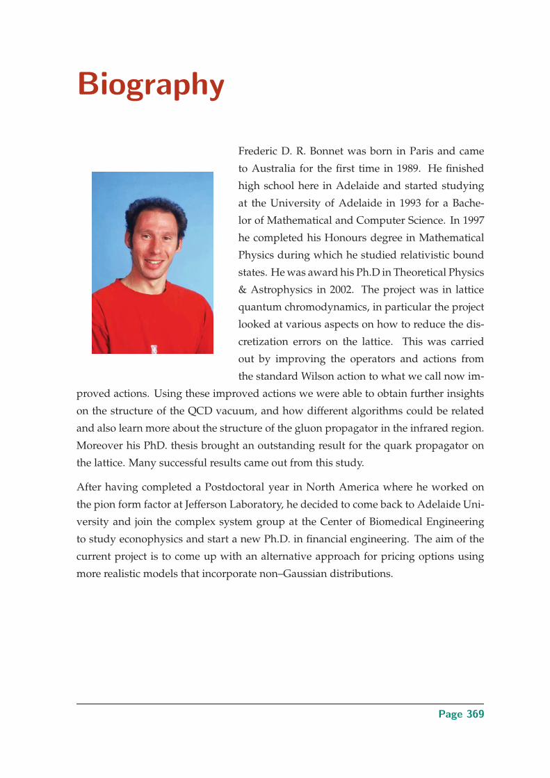
Biography
Frederic D. R. Bonnet was born in Paris and came
to Australia for the first time in 1989. He finished
high school here in Adelaide and started studying
at the University of Adelaide in 1993 for a Bache-
lor of Mathematical and Computer Science. In 1997
he completed his Honours degree in Mathematical
Physics during which he studied relativistic bound
states. He was award his Ph.D in Theoretical Physics
& Astrophysics in 2002. The project was in lattice
quantum chromodynamics, in particular the project
looked at various aspects on how to reduce the dis-
cretization errors on the lattice. This was carried
out by improving the operators and actions from
the standard Wilson action to what we call now im-
proved actions. Using these improved actions we were able to obtain further insights
on the structure of the QCD vacuum, and how different algorithms could be related
and also learn more about the structure of the gluon propagator in the infrared region.
Moreover his PhD. thesis brought an outstanding result for the quark propagator on
the lattice. Many successful results came out from this study.
After having completed a Postdoctoral year in North America where he worked on
the pion form factor at Jefferson Laboratory, he decided to come back to Adelaide Uni-
versity and join the complex system group at the Center of Biomedical Engineering
to study econophysics and start a new Ph.D. in financial engineering. The aim of the
current project is to come up with an alternative approach for pricing options using
more realistic models that incorporate non–Gaussian distributions.
Page 369

Page 370

Scientific genealogy
1774 MA University of Cambridge John Cranke
1782 MA University of Cambridge Thomas Jones
1811 MA University of Cambridge Adam Sedgwick
1830 MA University of Cambridge William Hopkins
1857 MA University of Cambridge Edward John Routh
1868 MA University of Cambridge John William Strutt (Lord Rayleigh)
1883 MA University of Cambridge Joseph John Thomson
1903 MA University of Cambridge John Sealy Townsend
1923 DPhil University of Oxford Victor Albert Bailey
1948 MSc University of Sydney Ronald Ernest Aitchison
1964 PhD University of Sydney Peter Harold Cole
1980 PhD University of Adelaide Kamran Eshraghian
1995 PhD University of Adelaide Derek Abbott
2008 PhD submitted University of Adelaide Frederic D. R. Bonnet
Page 371