Iterative Controller Tuning Using Bode’s Integrals ∗

A. Karimi, D. Garcia and R. LongchampLaboratoire d’automatique,

Ecole Polytechnique Federale de Lausanne (EPFL),1015 Lausanne, Switzerland. email: alireza.karimi@epfl.ch

Abstract

An iterative controller tuning based on a frequency criterion is proposed. The frequency criterionis defined as the weighted sum of squared errors between the desired and measured gain margin, phasemargin and crossover frequency. The method benefits from specific feedback relay tests to determinethe gain margin, the phase margin and the crossover frequency of the closed-loop system.The Bode’sintegrals are used to approximate the derivatives of amplitude and phase of the plant model withrespect to the frequency without any model of the plant. This additional information is employedto estimate the gradient and the Hessian of the frequency criterion in the iterative controller tuningmethod. Simulation examples and experimental results illustrate the effectiveness and the simplicityof the proposed method to design and tuning the controllers.

Keywords: Iterative method, relay feedback test, phase margin, gain margin, auto-tuning

1 Introduction

Recently, a great attention has been given to the data-driven controller design methods without or withlittle use of models. These methods use the experimental closed-loop data and do not suffer from unmodeleddynamics like the model-based approaches. They can generally be applied to the slowly time-varyingsystems as well. The Iterative controller tuning methods are usually based on the minimization of a timedomain criterion. The main drawback is the effect of the measurement noise and the disturbances. Thereal-time experiments are commonly time consuming and expensive. On the other hand, the robustnessspecifications cannot be explicitly included into the criterion. In this paper, a frequency criterion isproposed which will be minimized iteratively. The frequency criterion is defined as the weighted sum ofsquared errors between the desired and measured gain margin, phase margin and crossover frequency.Thus the robustness of the closed -loop system is directly taken into account in the criterion. The methodbenefits from specific feedback relay tests to determine the gain margin, the phase margin and the crossoverfrequency of the closed-loop system. In each experiments only the amplitude and the phase of the looptransfer function are measured. These experiments are shorter than the conventional experiments forcontroller tuning and are less sensitive to the measurement noise and disturbances.

The main contribution of this paper is the use of Bode’s integrals for the estimation of the gradientand the Hessian of the frequency criterion. The Bode’s integrals [1] show the relation between the phaseand the amplitude of minimum phase stable systems. It was shown in [5] how these integrals can be usedto approximate the derivatives of the amplitude and the phase of a system with respect to frequency at agiven frequency. It is interesting to notice that the approximation is made only with the knowledge of theamplitude and the phase of the system at the given frequency and the system static gain. In this paperthe results will be extended to the estimation of the derivatives of the amplitude and phase of the systemwith respect to the controller parameters. As a result, with a simple relay test, not only the phase marginand the crossover frequency are identified (criterion evaluation) but also the gradient and the Hessian of

∗This research work is financially supported by the Swiss National Science Foundation under grant No. 2100-064931.01

1

the frequency criterion are approximated with no parametric model of the plant. The simulations and theexperimental results show the fast convergence of the proposed iterative method.

An iterative procedure for gain and phase margin adjustment for a PI controller was presented in [2].The approach uses similar relay tests, but the gradient of the criterion is not calculated and an ad hocalgorithm is used instead. As a result the algorithm converges much slower than the proposed method.

The paper is organized as follows: In Section 2 several relay feedback tests will be presented formeasuring the gain margin, phase margin and the crossover frequency and an adaptive algorithm is usedto improve the precision of the measurements. Section 3 shows how the Bode’s integrals can be usedfor the estimation of the derivatives of amplitude and phase with respect to the frequency. The iterativetuning method for desired phase margin and crossover frequency is presented in Section 4 and is extendedto adjust the gain margin in Section 5. A simulation example is given in Section 6 and the experimentalresults for a three-tank system are presented in Section 7. Finally, Section 8 gives some concluding remarks.

2 Relay feedback test

The relay method is a well-known technique to identify useful points on the Nyquist curve by generatingan appropriate oscillation with a relay feedback. This section recalls some schemes to measure the criticalfrequency ( the frequency at which the phase of the loop is −π), gain margin, phase margin and crossoverfrequency.

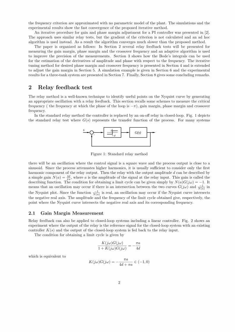
In the standard relay method the controller is replaced by an on-off relay in closed-loop. Fig. 1 depictsthe standard relay test where G(s) represents the transfer function of the process. For many systems

0G(s)

d

-d_

Figure 1: Standard relay method

there will be an oscillation where the control signal is a square wave and the process output is close to asinusoid. Since the process attenuates higher harmonics, it is usually sufficient to consider only the firstharmonic component of the relay output. Then the relay with the output amplitude d can be described bya simple gain N(a) = 4d

πa , where a is the amplitude of the signal at the relay input. This gain is called thedescribing function. The condition for obtaining a limit cycle can be given simply by N(a)G(jω) = −1. Itmeans that an oscillation may occur if there is an intersection between the two curves G(jω) and −1

N(a) inthe Nyquist plot. Since the function −1

N(a) is real, an oscillation may occur if the Nyquist curve intersectsthe negative real axis. The amplitude and the frequency of the limit cycle obtained give, respectively, thepoint where the Nyquist curve intersects the negative real axis and its corresponding frequency.

2.1 Gain Margin Measurement

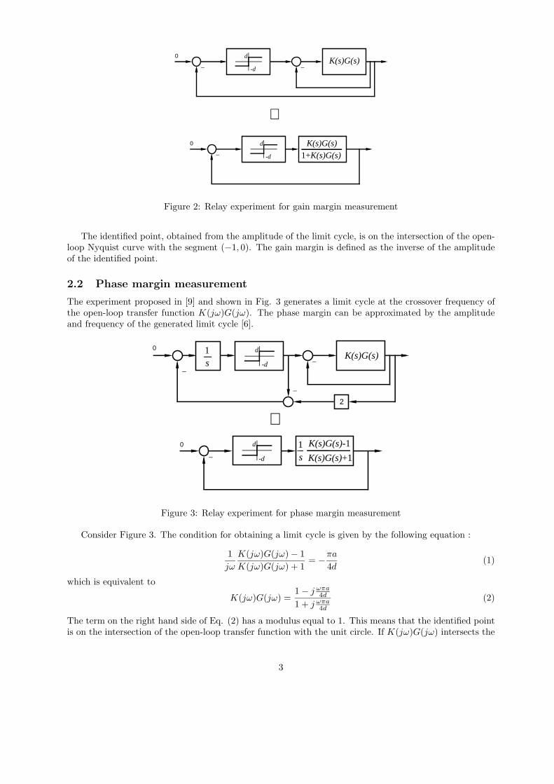
Relay feedback can also be applied to closed-loop systems including a linear controller. Fig. 2 shows anexperiment where the output of the relay is the reference signal for the closed-loop system with an existingcontroller K(s) and the output of the closed-loop system is fed back to the relay input.

The condition for obtaining a limit cycle is given by

K(jω)G(jω)1 + K(jω)G(jω)

= −πa

4d

which is equivalent toK(jω)G(jω) = − πa

4d + πa∈ (−1, 0)

2

0 d

-d_ _

0 d

-d_

⇔

K(s)G(s)

1+K(s)G(s)

K(s)G(s)

Figure 2: Relay experiment for gain margin measurement

The identified point, obtained from the amplitude of the limit cycle, is on the intersection of the open-loop Nyquist curve with the segment (−1, 0). The gain margin is defined as the inverse of the amplitudeof the identified point.

2.2 Phase margin measurement

The experiment proposed in [9] and shown in Fig. 3 generates a limit cycle at the crossover frequency ofthe open-loop transfer function K(jω)G(jω). The phase margin can be approximated by the amplitudeand frequency of the generated limit cycle [6].

0 d

_

_

_

2

K(s)G(s)1s

0 d

-d_

K(s)G(s)+1

K(s)G(s)-11s

⇔

-d

Figure 3: Relay experiment for phase margin measurement

Consider Figure 3. The condition for obtaining a limit cycle is given by the following equation :

1jω

K(jω)G(jω) − 1K(jω)G(jω) + 1

= −πa

4d(1)

which is equivalent to

K(jω)G(jω) =1 − j ωπa

4d

1 + j ωπa4d

(2)

The term on the right hand side of Eq. (2) has a modulus equal to 1. This means that the identified pointis on the intersection of the open-loop transfer function with the unit circle. If K(jω)G(jω) intersects the

3

unit circle several times, the phase margin is defined by the closest point to −1. This point correspondsto the limit cycle with the largest amplitude a which is stable.

Let ωc be the measured limit cycle frequency (equal to the crossover frequency) and ac the relay inputamplitude. Then the phase of the identified point can be computed as follows:

� K(jωc)G(jωc) = −2 arctan(πacωc

4d)

The phase margin Φm is then given by

Φm = π − 2 arctan(πacωc

4d)

2.3 Improving the approximation

The proposed methods for measuring the gain and phase margins by the relay method have the drawbackthat the method of the describing function must be used for the identification of the frequencies and thepoints on the Nyquist curve of interest. This approach is approximative. The assumption that the processattenuates higher harmonics is not always guaranteed especially for the phase margin measurement scheme,where the relative degree of the transfer function 1

sK(s)G(s)−1K(s)G(s)+1 is 1. Experiments have shown relative errors

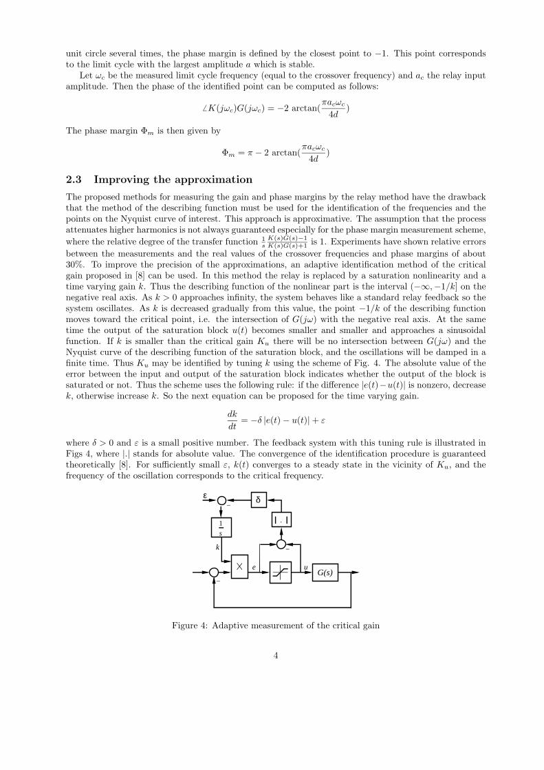
between the measurements and the real values of the crossover frequencies and phase margins of about30%. To improve the precision of the approximations, an adaptive identification method of the criticalgain proposed in [8] can be used. In this method the relay is replaced by a saturation nonlinearity and atime varying gain k. Thus the describing function of the nonlinear part is the interval (−∞,−1/k] on thenegative real axis. As k > 0 approaches infinity, the system behaves like a standard relay feedback so thesystem oscillates. As k is decreased gradually from this value, the point −1/k of the describing functionmoves toward the critical point, i.e. the intersection of G(jω) with the negative real axis. At the sametime the output of the saturation block u(t) becomes smaller and smaller and approaches a sinusoidalfunction. If k is smaller than the critical gain Ku there will be no intersection between G(jω) and theNyquist curve of the describing function of the saturation block, and the oscillations will be damped in afinite time. Thus Ku may be identified by tuning k using the scheme of Fig. 4. The absolute value of theerror between the input and output of the saturation block indicates whether the output of the block issaturated or not. Thus the scheme uses the following rule: if the difference |e(t)−u(t)| is nonzero, decreasek, otherwise increase k. So the next equation can be proposed for the time varying gain.

dk

dt= −δ |e(t) − u(t)| + ε

where δ > 0 and ε is a small positive number. The feedback system with this tuning rule is illustrated inFigs 4, where |.| stands for absolute value. The convergence of the identification procedure is guaranteedtheoretically [8]. For sufficiently small ε, k(t) converges to a steady state in the vicinity of Ku, and thefrequency of the oscillation corresponds to the critical frequency.

G(s)_

_

.

_

1

s

e u

k

ε δ

Figure 4: Adaptive measurement of the critical gain

4

This method can also be applied to closed-loop systems in order to determine the gain and phasemargins as well as the critical and crossover frequencies of the open-loop transfer function K(s)G(s) byreplacing the relay in Fig. 2 and 3 with the saturation and the time varying gain.

3 Bode’s integrals

The relations between the phase and the amplitude of a stable minimum-phase system have been inves-tigated for the first time by Bode [1]. The results are based on Cauchy’s residue theorem and have beenextensively used in network analysis. Two integrals are presented in this section. The first one, whichis well known in the control engineering field, shows the relation between the phase of the system ateach frequency as a function of the derivative of its amplitude. But the second integral has been used inthe control design for the first time in [5]. The integral shows how the amplitude of the system at eachfrequency is related to the derivative of the phase and the static gain of the system.

3.1 Derivative of amplitude

Bode has shown in [1] that for a stable minimum-phase transfer function G(jω), the phase of the systemat ω0 is given by:

� G(jω0) =1π

∫ +∞

−∞

d ln |G(jω)|dν

ln coth|ν|2dν (3)

where ν = ln ωω0

. Since ln coth |ν|2 decreases rapidly as ω deviates from ω0, the integral depends mostly on

d ln |G(jω)|dν (the slope of the Bode plot) near ω0. Therefore, assuming that the slope of the Bode plot is

almost constant in the neighborhood of ω0, � G(jω0) can be approximated by:

� G(jω0) ≈1π

d ln |G(jω)|dν

∣∣∣∣ω0

∫ +∞

−∞ln coth

|ν|2dν =

π

2d ln |G(jω)|

dν

∣∣∣∣ω0

(4)

This property is often used in loop shaping where the slope of the amplitude Bode plot at crossoverfrequency is limited to -20dB/decade in order to obtain approximately a phase margin of 90◦. Here themeasured phase of the system at ω0 is used to determine approximately the slope of the amplitude Bodeplot (sa):

sa(ω0) =d ln |G(jω)|

dν

∣∣∣∣ω0

= ω0d ln |G(jω)|

dω

∣∣∣∣ω0

≈ 2π

� G(jω0) (5)

3.2 Derivative of phase

The second Bode’s integral shows that the amplitude of a stable minimum-phase system can be determineduniquely from its phase and its static gain. More precisely, the logarithm of the system amplitude at ω0

is given by [1]:

ln |G(jω0)| = ln |Kg| −ω0

π

∫ +∞

−∞

d(� G(jω)/ω)dν

ln coth|ν|2dν (6)

where Kg is the static gain of the plant. In the same way, assuming that � G(jω)/ω is linear (in alogarithmic scale) in the neighborhood of ω0, one has:

ln |G(jω0)| ≈ ln |Kg| −ω0

π

d(� G(jω)/ω)dν

∣∣∣∣ω0

π2

2(7)

ln |G(jω0)| ≈ ln |Kg| −πω2

0

2

[1ω0

d � G(jω)dω

∣∣∣∣ω0

−� G(jω0)

ω20

](8)

which gives the slope of the Bode phase plot at ω0:

sp(ω0) =d � G(jω)

dν

∣∣∣∣ω0

= ω0d � G(jω)

dω

∣∣∣∣ω0

≈ � G(jω0) +2π

[ln |Kg| − ln |G(jω0)|] (9)

5

Note that for the systems containing an integrator, the static gain cannot be computed. For suchsystems, the static gain of the system without the integrator should be estimated and used in the aboveformula (note that the phase of the integrator is constant and its derivative is zero).

4 Iterative procedure for phase margin adjustment

First of all, a performance criterion in the frequency domain is defined as follows:

J(ρ) =12[λ1(ωc − ωd)2 + λ2(Φm − Φd)2] (10)

where ρ is the vector of the controller parameters, λ1 and λ2 are weighting factors, ωc and ωd are re-spectively the measured and desired crossover frequencies, and Φm and Φd are the measured and desiredphase margins. Then the controller parameters minimizing the criterion are obtained by the iterativeGauss-Newton formula:

ρi+1 = ρi − γiR−1J ′(ρi) (11)

where i is the iteration number, γi is a positive scalar representing the step size, R is a square positivedefinite matrix of dimension nρ and J ′(ρ) is the gradient of the criterion with respect to ρ. This algorithmconverges to the vector of parameters minimizing the criterion, provided that the step size is properlychosen. The matrix R can be chosen equal to the identity matrix or to the Hessian of the criterion toobtain faster convergence.

The gradient of the criterion is given by:

J ′(ρ) = λ1(ωc − ωd)∂ωc

∂ρ+ λ2(Φm − Φd)Φ′

m (12)

where Φ′m is the derivative of the phase margin with respect to ρ computed through the chain rule (note

that Φm is a function of ρ and ωc):

Φ′m =

∂Φm

∂ρ+

∂Φm

∂ω

∣∣∣∣ωc

∂ωc

∂ρ(13)

Now replacing Φm in the above equation by � L(jωc) + π gives (where L(jω) = K(jω)G(jω)):

Φ′m =

∂ � L(jωc)∂ρ

+∂ � L(jω)

∂ω

∣∣∣∣ωc

∂ωc

∂ρ(14)

The first term in the above equation is equal to ∂ � K(jωc)/∂ρ which is completely known at each iteration.Furthermore one has:

∂ � L(jω)∂ω

∣∣∣∣ωc

=∂ � K(jω)

∂ω

∣∣∣∣ωc

+∂ � G(jω)

∂ω

∣∣∣∣ωc

=∂ � K(jω)

∂ω

∣∣∣∣ωc

+sp(ωc)ωc

(15)

Again, the first term is completely known and sp(ωc) can be approximated using Eq. (9). Now, it onlyremains to compute ∂ωc/∂ρ. For this purpose, we use the fact that the loop gain at ωc in each iterationis equal to 1, therefore its derivative (or derivative of its logarithm) with respect to ρ will be zero. Thenone has:

∂ ln |L(jωc)|∂ρ

+∂ ln |L(jω)|

∂ω

∣∣∣∣ωc

∂ωc

∂ρ= 0 (16)

but from the Bode’s integral (see Eq. (5)) one has:

∂ ln |L(jω)|∂ω

∣∣∣∣ωc

≈ 2 � L(jωc)πωc

=2(Φm − π)

πωc(17)

6

Thus ∂ωc/∂ρ can be approximated as follows (note that ∂ ln |L(jω)|/∂ρ = ∂ ln |K(jω)|/∂ρ):

∂ωc

∂ρ≈ − πωc

2(Φm − π)∂ ln |K(jωc)|

∂ρ(18)

Notice that the gradient of the criterion is computed using only the measured crossover frequency ωc andthe measured amplitude and phase of the plant. In the same way, the Hessian of the criterion can beapproximated without any additional information as follows:

H = J ′′(ρ) = λ1∂ωc

∂ρ(∂ωc

∂ρ)T + λ2Φ′

m(Φ′m)T + λ1(ωc − ωd)

∂2ωc

∂ρ2+ λ2(Φm − Φd)Φ′′

m (19)

The last two terms can be neglected because they are small especially in the neighborhood of the finalsolution. In addition, this simplification makes the Hessian always positive which fixes the numericalproblems normally encountered in the iterative Newton algorithm. The use of the Hessian matrix in theiterative formula (Eq. 11) instead of R significantly improves the convergence speed.

R = H ≈ λ1∂ωc

∂ρ(∂ωc

∂ρ)T + λ2Φ′

m(Φ′m)T (20)

5 Iterative procedure for phase and gain margins adjustment

In the previous section, the controller is designed using only the information on one frequency point of theplant. Although this approach is very fast and simple and works well for the majority of the industrialprocesses, it may not work appropriately for some complex high-order systems. This means that thespecifications may be satisfied just locally at the crossover frequency and it is possible that the behaviorof the system changes drastically elsewhere, leading for example to a very small gain margin. For suchsystems, it may be preferable to tune the phase and gain margins at the same time. However, thisnecessitates two relay experiments in each iteration: one relay test to measure the gain margin and theother for the phase margin. A frequency criterion can be defined as follows:

J(ρ) =12[λ1(ωc − ωd)2 + λ2(Φm − Φd)2 + λ3(Ku −Kd)2] (21)

where Ku = |L(jωu)| is the amplitude of the loop transfer function where it intersects the negative realaxis (� L(jωu) = −π). ωu is the critical loop frequency, Kd is the inverse of the desired gain margin andλ1, λ2 and λ3 are weighting factors. The gradient of the criterion is given by:

J ′(ρ) = λ1(ωc − ωd)∂ωc

∂ρ+ λ2(Φm − Φd)Φ′

m + λ3(Ku −Kd)K ′u (22)

where K ′u is the derivative of the critical loop gain with respect to ρ computed as follows:

K ′u =

∂|L(jωu)|∂ρ

+∂|L(jω)|

∂ω

∣∣∣∣ωu

∂ωu

∂ρ(23)

The first term is equal to |G(jωu)| · ∂|K(jωu)|/∂ρ which can be easily computed at each iteration. Thesecond term can be approximated using the Bode’s integrals in a similar way as is done for the phasemargin. First the derivative of the amplitude of the loop gain is computed using Eq. (5) as follows:

∂|L(jω)|∂ω

∣∣∣∣ωu

= |L(jωu)| ∂ ln |L(jω)|∂ω

∣∣∣∣ωu

≈ Ku2� L(jωu)

πωu= −2Ku

ωu(24)

Then ∂ωu/∂ρ is computed using the fact that in each iteration � L(jωu) = −π and consequently itsderivative with respect to ρ will be zero, which gives:

∂ � L(jωu)∂ρ

+∂ � L(jω)

∂ω

∣∣∣∣ωu

∂ωu

∂ρ= 0 (25)

7

The first term in the above equation is equal to ∂ � K(jωu)/∂ρ which can be computed knowing thecontroller at each iteration. Furthermore one has:

∂ � L(jω)∂ω

∣∣∣∣ωu

=∂ � K(jω)

∂ω

∣∣∣∣ωu

+∂ � G(jω)

∂ω

∣∣∣∣ωu

(26)

Again, knowing the controller at each iteration, the first term in the right hand side can be computedwhile the second term is approximated using the Bode’s integral of Eq. (9). Therefore ∂ωu/∂ρ is given by:

∂ωu

∂ρ= −

(∂ � K(jω)

∂ω

∣∣∣∣ωu

+sp(ωu)ωu

)−1∂ � K(jωu)

∂ρ(27)

In a similar way an approximation of the Hessian can also be computed as follows:

R = H ≈ λ1∂ωc

∂ρ(∂ωc

∂ρ)T + λ2Φ′

m(Φ′m)T + λ3K

′u(K ′

u)T (28)

6 Simulation example

Now let us consider a complex plant model including a time delay as follows:

G(s) =e−0.3s

(s2 + 2s + 3)3(s + 3)(29)

This model was proposed in [7] and represents a difficult problem to be solved using a PID controller. Itshould be noted that neither the traditional Ziegler-Nichols method nor a more advanced method based ona first-order plant model [3] can give a stabilizing controller for this plant. In the following, it is shown thata PID controller which confers appropriate specifications on the closed-loop system can be tuned with theiterative phase and gain margins adjustment method. This method requires two experiments per iterationand is more convenient for high-order complex systems. However, one should note that the experimentaltime for the gain margin measurement can be chosen to be smaller than that of the phase margin, becausethe critical frequency is appreciably larger than the crossover frequency.

The specifications are set for this example at ωd = 0.2 rad/s for the crossover frequency, and Φd = 70◦

and Kd = 13 for the phase and for the inverse of the gain margin, respectively. The initial controller is

designed using the Kappa-Tau tuning rule proposed in [4] which gives the following stabilizing controller:

K(s) = 4.5 (1 +1

0.41s+ 0.033s) (30)

The performance criterion of Eq. (21) is used and the weighting factors are chosen such that almost thesame weighting be obtained for the three parts of the criterion:

λ1 =1ω2

d

λ2 =1

Φ2d

λ3 =1K2

d

Two closed-loop experiments are performed to measure a crossover frequency of 0.139 rad/s, a phasemargin of 78.5◦ and a gain margin of 4.39, which give a performance criterion of 0.104. With these values,the gradient and Hessian are calculated, and a new controller is obtained. After one other iteration thefollowing controller is obtained:

K(s) = 4.93 (1 +1

0.316s+ 0.125s) (31)

with a performance criterion of 0.0017. This controller gives 0.1997 rad/s for the crossover frequency, 66.0◦

for the phase margin and 2.97 for the gain margin. It should be noted that no significant improvementcan be achieved with further iterations. A comparison of the closed-loop performance between the initial

8

0 10 20 30 400

0.2

0.4

0.6

0.8

1

Time [s]

Step response

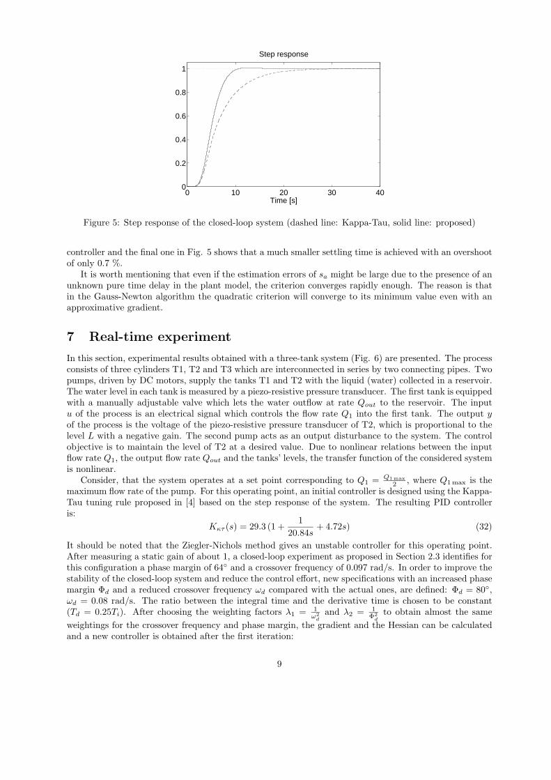
Figure 5: Step response of the closed-loop system (dashed line: Kappa-Tau, solid line: proposed)

controller and the final one in Fig. 5 shows that a much smaller settling time is achieved with an overshootof only 0.7 %.

It is worth mentioning that even if the estimation errors of sa might be large due to the presence of anunknown pure time delay in the plant model, the criterion converges rapidly enough. The reason is thatin the Gauss-Newton algorithm the quadratic criterion will converge to its minimum value even with anapproximative gradient.

7 Real-time experiment

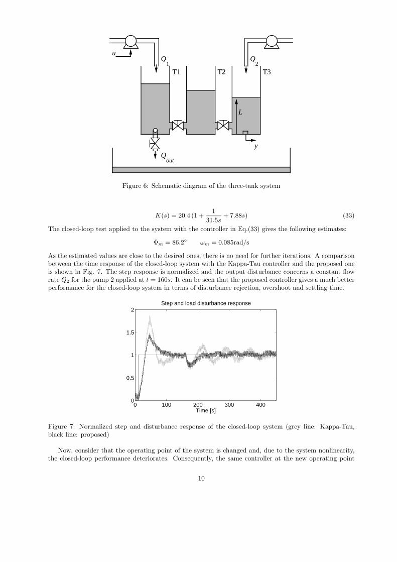
In this section, experimental results obtained with a three-tank system (Fig. 6) are presented. The processconsists of three cylinders T1, T2 and T3 which are interconnected in series by two connecting pipes. Twopumps, driven by DC motors, supply the tanks T1 and T2 with the liquid (water) collected in a reservoir.The water level in each tank is measured by a piezo-resistive pressure transducer. The first tank is equippedwith a manually adjustable valve which lets the water outflow at rate Qout to the reservoir. The inputu of the process is an electrical signal which controls the flow rate Q1 into the first tank. The output yof the process is the voltage of the piezo-resistive pressure transducer of T2, which is proportional to thelevel L with a negative gain. The second pump acts as an output disturbance to the system. The controlobjective is to maintain the level of T2 at a desired value. Due to nonlinear relations between the inputflow rate Q1, the output flow rate Qout and the tanks’ levels, the transfer function of the considered systemis nonlinear.

Consider, that the system operates at a set point corresponding to Q1 = Q1 max2 , where Q1 max is the

maximum flow rate of the pump. For this operating point, an initial controller is designed using the Kappa-Tau tuning rule proposed in [4] based on the step response of the system. The resulting PID controlleris:

Kκτ (s) = 29.3 (1 +1

20.84s+ 4.72s) (32)

It should be noted that the Ziegler-Nichols method gives an unstable controller for this operating point.After measuring a static gain of about 1, a closed-loop experiment as proposed in Section 2.3 identifies forthis configuration a phase margin of 64◦ and a crossover frequency of 0.097 rad/s. In order to improve thestability of the closed-loop system and reduce the control effort, new specifications with an increased phasemargin Φd and a reduced crossover frequency ωd compared with the actual ones, are defined: Φd = 80◦,ωd = 0.08 rad/s. The ratio between the integral time and the derivative time is chosen to be constant(Td = 0.25Ti). After choosing the weighting factors λ1 = 1

ω2d

and λ2 = 1Φ2

d

to obtain almost the sameweightings for the crossover frequency and phase margin, the gradient and the Hessian can be calculatedand a new controller is obtained after the first iteration:

9

Q1

Q2

Qout

T2 T3T1

u

y

L

Figure 6: Schematic diagram of the three-tank system

K(s) = 20.4 (1 +1

31.5s+ 7.88s) (33)

The closed-loop test applied to the system with the controller in Eq.(33) gives the following estimates:

Φm = 86.2◦ ωm = 0.085rad/s

As the estimated values are close to the desired ones, there is no need for further iterations. A comparisonbetween the time response of the closed-loop system with the Kappa-Tau controller and the proposed oneis shown in Fig. 7. The step response is normalized and the output disturbance concerns a constant flowrate Q2 for the pump 2 applied at t = 160s. It can be seen that the proposed controller gives a much betterperformance for the closed-loop system in terms of disturbance rejection, overshoot and settling time.

0 100 200 300 4000

0.5

1

1.5

2

Time [s]

Step and load disturbance response

Figure 7: Normalized step and disturbance response of the closed-loop system (grey line: Kappa-Tau,black line: proposed)

Now, consider that the operating point of the system is changed and, due to the system nonlinearity,the closed-loop performance deteriorates. Consequently, the same controller at the new operating point

10

does not meet the specification (a phase margin Φm = 55◦ and a crossover frequency ωm = 0.066 rad/s areobtained) and the controller should be retuned. After one iteration, using the proposed tuning method,the following controller is obtained:

K(s) = 23 (1 +1

42.3s+ 10.6s) (34)

The closed-loop system with this controller gives the following performances which are very close to thedesired ones:

Φm = 73.7◦ ωm = 0.0791rad/s

0 100 200 300 4000

0.5

1

1.5

2

Time [s]

Step and load disturbance response

0 100 200 300 4000

2

4

6

Time [s]

Control signal

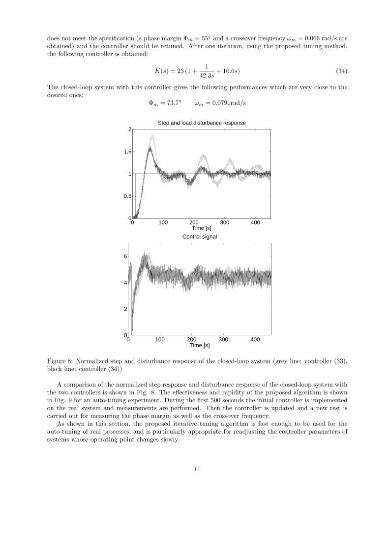
Figure 8: Normalized step and disturbance response of the closed-loop system (grey line: controller (33),black line: controller (34))

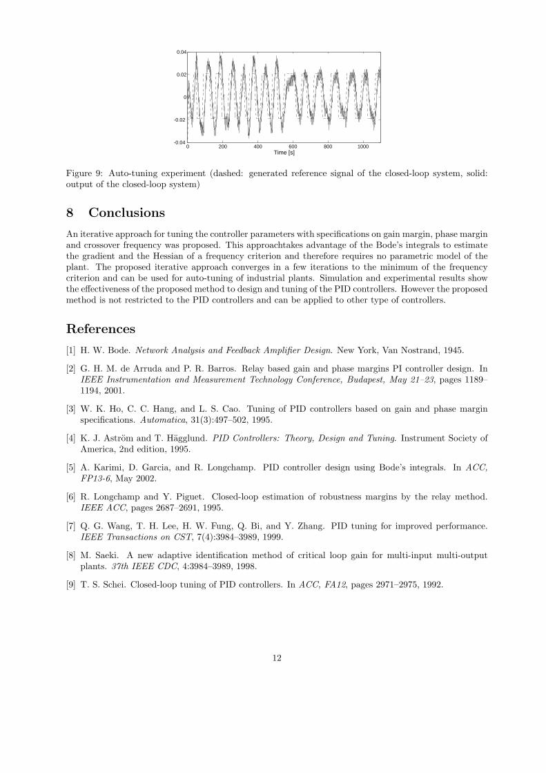
A comparison of the normalized step response and disturbance response of the closed-loop system withthe two controllers is shown in Fig. 8. The effectiveness and rapidity of the proposed algorithm is shownin Fig. 9 for an auto-tuning experiment. During the first 500 seconds the initial controller is implementedon the real system and measurements are performed. Then the controller is updated and a new test iscarried out for measuring the phase margin as well as the crossover frequency.

As shown in this section, the proposed iterative tuning algorithm is fast enough to be used for theauto-tuning of real processes, and is particularly appropriate for readjusting the controller parameters ofsystems whose operating point changes slowly.

11

0 200 400 600 800 1000-0.04

-0.02

0

0.02

0.04

Time [s]

Figure 9: Auto-tuning experiment (dashed: generated reference signal of the closed-loop system, solid:output of the closed-loop system)

8 Conclusions

An iterative approach for tuning the controller parameters with specifications on gain margin, phase marginand crossover frequency was proposed. This approachtakes advantage of the Bode’s integrals to estimatethe gradient and the Hessian of a frequency criterion and therefore requires no parametric model of theplant. The proposed iterative approach converges in a few iterations to the minimum of the frequencycriterion and can be used for auto-tuning of industrial plants. Simulation and experimental results showthe effectiveness of the proposed method to design and tuning of the PID controllers. However the proposedmethod is not restricted to the PID controllers and can be applied to other type of controllers.

References

[1] H. W. Bode. Network Analysis and Feedback Amplifier Design. New York, Van Nostrand, 1945.

[2] G. H. M. de Arruda and P. R. Barros. Relay based gain and phase margins PI controller design. InIEEE Instrumentation and Measurement Technology Conference, Budapest, May 21–23, pages 1189–1194, 2001.

[3] W. K. Ho, C. C. Hang, and L. S. Cao. Tuning of PID controllers based on gain and phase marginspecifications. Automatica, 31(3):497–502, 1995.

[4] K. J. Astrom and T. Hagglund. PID Controllers: Theory, Design and Tuning. Instrument Society ofAmerica, 2nd edition, 1995.

[5] A. Karimi, D. Garcia, and R. Longchamp. PID controller design using Bode’s integrals. In ACC,FP13-6, May 2002.

[6] R. Longchamp and Y. Piguet. Closed-loop estimation of robustness margins by the relay method.IEEE ACC, pages 2687–2691, 1995.

[7] Q. G. Wang, T. H. Lee, H. W. Fung, Q. Bi, and Y. Zhang. PID tuning for improved performance.IEEE Transactions on CST, 7(4):3984–3989, 1999.

[8] M. Saeki. A new adaptive identification method of critical loop gain for multi-input multi-outputplants. 37th IEEE CDC, 4:3984–3989, 1998.

[9] T. S. Schei. Closed-loop tuning of PID controllers. In ACC, FA12, pages 2971–2975, 1992.

12