Leading singularities and off-shell conformal integrals

arX

iv:1

303.

6909

v2 [

hep-

th]

4 J

un 2

013

HU-Mathematik: 2013-06 HU-EP-13/15IPPP/13/09 DCPT/13/18 SLAC-PUB-15409LAPTH-016/13 CERN-PH-TH/2013-058

Leading singularities and off-shell conformal integrals

James Drummonda,b, Claude Duhrc,d, Burkhard Edene, Paul Heslopf ,Jeffrey Penningtong, Vladimir A. Smirnove,h

a CERN, Geneva 23, Switzerland

b LAPTH, CNRS et Universite de Savoie, F-74941 Annecy-le-Vieux Cedex, France

c Institut fur Theoretische Physik, ETH Zurich, CH-8093, Switzerland

d Institute for Particle Physics Phenomenology,

University of Durham, Durham, DH1 3LE, U.K.

e Institut fur Mathematik, Humboldt-Universitat, Zum großen Windkanal 6, 12489 Berlin

f Mathematics department, Durham University, Durham DH1 3LE, United Kingdom

g SLAC National Accelerator Laboratory, Stanford University, Stanford, CA 94309, USA

h Nuclear Physics Institute of Moscow State University, Moscow 119992, Russia

Abstract

The three-loop four-point function of stress-tensor multiplets in N = 4 super Yang-Millstheory contains two so far unknown, off-shell, conformal integrals, in addition to the known,ladder-type integrals. In this paper we evaluate the unknown integrals, thus obtaining thethree-loop correlation function analytically. The integrals have the generic structure ofrational functions multiplied by (multiple) polylogarithms. We use the idea of leadingsingularities to obtain the rational coefficients, the symbol – with an appropriate ansatzfor its structure – as a means of characterising multiple polylogarithms, and the techniqueof asymptotic expansion of Feynman integrals to obtain the integrals in certain limits.The limiting behaviour uniquely fixes the symbols of the integrals, which we then liftto find the corresponding polylogarithmic functions. The final formulae are numericallyconfirmed. The techniques we develop can be applied more generally, and we illustrate thisby analytically evaluating one of the integrals contributing to the same four-point functionat four loops. This example shows a connection between the leading singularities and theentries of the symbol.

In memory of Francis Dolan.

http://arxiv.org/abs/1303.6909v2

Contents

1 Introduction 3

2 Conformal four-point integrals and single-valued polylogarithms 92.1 The symbol . . . . . . . . . . . . . . . . . . . . . . . . . . . . . . . . . . . 102.2 Single-Valued Harmonic Polylogarithms (SVHPLs) . . . . . . . . . . . . . 122.3 The x → 0 limit of SVHPLs . . . . . . . . . . . . . . . . . . . . . . . . . . 13

3 The short-distance limit 15

4 The Easy integral 184.1 Residues of the Easy integral . . . . . . . . . . . . . . . . . . . . . . . . . . 184.2 The symbol of E(x, x) . . . . . . . . . . . . . . . . . . . . . . . . . . . . . 214.3 The analytic result for E(x, x): uplifting from the symbol . . . . . . . . . . 224.4 The analytic result for E(x, x): the direct approach . . . . . . . . . . . . . 224.5 Numerical consistency tests for E . . . . . . . . . . . . . . . . . . . . . . . 23

5 The Hard integral 245.1 Residues of the Hard integral . . . . . . . . . . . . . . . . . . . . . . . . . 245.2 The symbols of H(a)(x, x) and H(b)(x, x) . . . . . . . . . . . . . . . . . . . 265.3 The analytic results for H(a)(x, x) and H(b)(x, x) . . . . . . . . . . . . . . . 275.4 Numerical consistency checks for H . . . . . . . . . . . . . . . . . . . . . . 32

6 The analytic result for the three-loop correlator 32

7 A four-loop example 337.1 Asymptotic expansions . . . . . . . . . . . . . . . . . . . . . . . . . . . . . 347.2 A differential equation . . . . . . . . . . . . . . . . . . . . . . . . . . . . . 367.3 An integral solution . . . . . . . . . . . . . . . . . . . . . . . . . . . . . . . 387.4 Expression in terms of multiple polylogarithms . . . . . . . . . . . . . . . . 427.5 Numerical consistency tests for I(4) . . . . . . . . . . . . . . . . . . . . . . 46

8 Conclusions 47

A Asymptotic expansions of the Easy and Hard integrals 48

B An integral formula for the Hard integral 50B.1 Limits . . . . . . . . . . . . . . . . . . . . . . . . . . . . . . . . . . . . . . 51B.2 First non-trivial example (weight three) . . . . . . . . . . . . . . . . . . . . 51B.3 Weight five example . . . . . . . . . . . . . . . . . . . . . . . . . . . . . . 52B.4 The function H(a) from the Hard integral . . . . . . . . . . . . . . . . . . . 52

C A symbol-level solution of the four-loop differential equation 53

2

1 Introduction

The work presented in this paper is motivated by recent progress in planar N = 4 superYang-Mills (SYM) theory in four dimensions, although the methods that we exploit andfurther develop should be of much wider applicability.

N = 4 SYM theory has many striking properties due to its high degree of symmetry;for instance it is conformally invariant, even as a quantum theory [1], and the spectrum ofanomalous dimensions of composite operators can be found from an integrable system [2].Most strikingly perhaps, it is related to IIB string theory on AdS5×S5 by the AdS/CFTcorrespondence [3]. This is a weak/strong coupling duality in which the same physicalsystem is conveniently described by the field theory picture at weak coupling, while thestring theory provides a way of capturing its strong coupling regime. The strong couplinglimit of scattering amplitudes in the model has been elaborated in ref. [4] from a stringperspective. The formulae take the form of vacuum expectation values of polygonal Wilsonloops with light-like edges.

This duality between amplitudes and Wilson loops remains true at weak coupling [5],extending to the finite terms in N = 4 SYM previously known relations between theinfrared divergences of scattering amplitudes and the ultra-violet divergences of (light-like) Wilson lines in QCD [6]. Furthermore, it was recently discovered that both sides ofthis correspondence can be generated from n-point correlation functions of stress-tensormultiplets by taking a certain light-cone limit [7].

The four-point function of stress-tensor multiplets was intensely studied in the earlydays of the AdS/CFT duality, in the supergravity approximation [8] as well as at weakcoupling. The one-loop [9] and two-loop [10] corrections are given by conformal ladderintegrals.

A Feynman-graph based three-loop result has never become available because of theformidable size and complexity of multi-leg multi-loop computations. Already the twoparallel two-loop calculations [10] drew heavily upon superconformal symmetry. However,a formulation on a maximal (‘analytic’) superspace [11,12] makes it apparent that the loopcorrections to the lowest x-space component are given by a product of a certain polynomialwith linear combinations of conformal integrals, cf. ref. [13–16]. Then in ref. [17,18], usinga hidden symmetry permuting integration variables and external variables, the problem offinding the three-loop integrand was reduced down to just four unfixed coefficients withoutany calculation and furhter down to only one overall coefficient after a little further analysis.This single overall coefficient can then easily be fixed e.g. by comparing to the MHV four-point three-loop amplitude [19] via the correlator/amplitude duality or by requiring theexponentiation of logarithms in a double OPE limit [17].

Beyond the known ladder and the ‘tennis court’, the off-shell three-loop four-pointcorrelator contains two unknown integrals termed ‘Easy’ and ‘Hard’ in ref. [17]. In thiswork we embark on an analytic evaluation of the Easy and Hard integrals postulating that

• the integrals are sums∑

i Ri Fi, where Ri are rational functions and Fi are pure

functions, i.e. Q-linear combinations of logarithms and multiple polylogarithms [20],

3

• the rational functions Ri are given by the so-called leading singularities (i.e. residuesof global poles) of the integrals [21],

• the symbol of each Fi can be pinned down by appropriate constraints and thenintegrated to a unique transcendental function.

The principle of uniform transcendentality, innate to the planarN = 4 SYM theory, impliesthat the symbols of all the pure functions are tensors of uniform rank six. Our strategy willbe to make an ansatz for the entries that can appear in the symbols of the pure functionsand to write down the most general tensor of uniform rank six of this form. We then imposea set of constraints on this general tensor to pin down the symbols of the pure functions.First of all, the tensor needs to satisfy the integrability condition, a criterion for a generaltensor to correspond to the symbol of a transcendental function. Next the symmetriesof the integrals induce additional constraints, and finally we equate with single variableexpansions corresponding to Euclidean coincidence limits. The latter were elaborated forthe Easy and Hard integrals in ref. [22, 23] using the method of asymptotic expansion

of Feynman integrals [24]. This expansion technique reduces the original higher-pointintegrals to two-point integrals, albeit with high exponents of the denominator factors andcomplicated numerators.

To be specific, up to three loops the off-shell four-point correlator is given by [9,10,17]

G4(1, 2, 3, 4) = G(0)4 +

2 (N2c − 1)

(4π2)4R(1, 2, 3, 4)

[aF (1) + a2F (2) + a3F (3) +O(a4)

], (1.1)

Here Nc denotes the number of colors and a is the ’t Hooft coupling. G(0)4 represents the

tree-level contribution and R(1, 2, 3, 4) is a universal prefactor, in particular taking intoaccount the different SU(4) flavours which can appear (see ref. [17, 18] for details). Ourfocus here is on the loop corrections. These can be written in the compact form (exposingthe hidden S4+ℓ symmetry) as

F (ℓ)(x1, x2, x3, x4) =x212x

213x

214x

223x

224x

234

ℓ! (π2)ℓ

∫

d4x5 . . . d4x4+ℓ f

(ℓ)(x1, . . . , x4+ℓ) , (1.2)

where

f (1)(x1, . . . , x5) =1

∏

1≤i<j≤5 x2ij

, (1.3)

f (2)(x1, . . . , x6) =148x212x

234x

256 + S6 permutations∏

1≤i<j≤6 x2ij

, (1.4)

f (3)(x1, . . . , x7) =120(x2

12)2(x2

34x245x

256x

267x

273) + S7 permutations

∏

1≤i<j≤7 x2ij

. (1.5)

4

Writing out the sum over permutations in the above expressions, these are written asfollows

F (1) = g1234 , (1.6)

F (2) = h12;34 + h34;12 + h23;14 + h14;23 (1.7)

+ h13;24 + h24;13 +1

2

(x212x

234 + x2

13x224 + x2

14x223

)[ g1234]

2 ,

F (3) = [L12;34 + 5 perms ] + [T12;34 + 11 perms ] (1.8)

+ [E12;34 + 11 perms ] + 12[ x2

14x223H12;34 + 11 perms ]

+ [ (g × h)12;34 + 5 perms ] ,

which involve the following integrals:

g1234 =1

π2

∫d4x5

x215x

225x

235x

245

, (1.9)

h12;34 =x234

π4

∫d4x5 d

4x6

(x215x

235x

245)x

256(x

226x

236x

246)

.

At three-loop order we encounter

(g × h)12;34 =x212x

434

π6

∫d4x5d

4x6d4x7

(x215x

225x

235x

245)(x

216x

236x

246)(x

227x

237x

247)x

267

,

L12;34 =x434

π6

∫d4x5 d

4x6 d4x7

(x215x

235x

245)x

256(x

236x

246)x

267(x

227x

237x

247)

,

T12;34 =x234

π6

∫d4x5d

4x6d4x7 x2

17

(x215x

235)(x

216x

246)(x

237x

227x

247)x

256x

257x

267

, (1.10)

E12;34 =x223x

224

π6

∫d4x5 d

4x6 d4x7 x2

16

(x215x

225x

235)x

256(x

226x

236x

246)x

267(x

217x

227x

247)

,

H12;34 =x234

π6

∫d4x5 d

4x6 d4x7 x2

57

(x215x

225x

235x

245)x

256(x

236x

246)x

267(x

217x

227x

237x

247)

.

Here g, h, L are recognised as the one-loop, two-loop and three-loop ladder integrals, respec-tively, the dual graphs of the off-shell box, double-box and triple-box integrals. Off-shell,the ‘tennis court’ integral T can be expressed as the three-loop ladder integral L by usingthe conformal flip properties1 of a two-loop ladder sub-integral [25]. The only new integralsare thus E and H (see fig. 1).

1Such identities rely on manifest conformal invariance and will be broken by the introduction of mostregulators. For instance, the equivalence of T and L is not true for the dimensionally regulated on-shellintegrals.

5

3

1

4

2

1

2

3

4

E12;34 H12;34

Figure 1: The Easy and Hard integrals contributing to the correlator of stress tensormultiplets at three loops.

Conformal four-point integrals are given by a factor carrying their conformal weight,say, (x2

13x224)

n times some function of the two cross ratios

u =x212x

234

x213x

224

= x x , v =x214x

223

x213x

224

= (1− x)(1 − x) . (1.11)

Ladder integrals are explicitly known for any number of loops, see ref. [26] where theyare very elegantly expressed as one-parameter integrals. Integration is simplified by thechange of variables from the cross-ratios (u, v) to (x, x) as defined in the last equation. Theunique rational prefactor, x2

13x224 (x − x), is common to all cases and can be computed by

the leading singularity method as we illustrate shortly. This is multiplied by pure polylog-arithm functions which fit with the classification of single-valued harmonic polylogarithms(SVHPLs) in ref. [27]. The associated symbols of the ladder integrals are then tensorscomposed of the four letters {x, x, 1− x, 1− x}.

On the other hand, for generic conformal four-point integrals (of which the Easy andHard integrals are the first examples) there are no explicit results. Fortunately, in recentyears a formalism has been developed in the context of scattering amplitudes to find at leastthe rational prefactors (i.e. the leading singularities), which are given by the residues of theintegrals [21]. There is one leading singularity for each global pole of the integrand and it isobtained by deforming the contour of integration to lie on a maximal torus surrounding thepole in question, i.e. by computing the residue at the global pole. As an illustration2, letus apply this technique to the massive one-loop box integral g1234 defined in eq. (1.9). Itsleading singularity is obtained by shifting the contour to encircle one of the global poles of

2The massless box-integral (i.e. the same integral in the limit x2i,i+1 → 0) is discussed in ref. [28] in

terms of twistor variables as the simplest example of a ‘Schubert problem’ in projective geometry. Theoff-shell case that we discuss here was also recently discussed by S. Caron-Huot (see [29]).

6

the integrand, where all four terms in the denominator vanish. To find this let us considera change of coordinates from xµ

5 to pi = x2i5. The Jacobian for this change of variables is

J = det

(∂pi∂xµ

5

)

= det (−2xµi5) , J2 = det (4xi5 · xj5) = 16 det

(x2ij − x2

i5 − x2j5

),

(1.12)where the second identity follows by observing that det(M) =

√

det(MMT ). Using thischange of variables the massive box becomes

g1234 =1

π2

∫d4pi

p1p2p3p4 J. (1.13)

To find its leading singularity we simply compute the residue around all four poles at pi = 0(divided by 2πi). We obtain

g1234 →1

4π2λ1234, λ1234 =

√

det(x2ij)i,j=1..4 = x2

13x224 (x− x) (1.14)

in full agreement with the analytic result [26].Note that we do not consider explicitly a contour around the branch cut associated

with the square root factor J in the denominator of (1.13). Because there is no pole atinfinity, the residue theorem guarantees that such a contour is equivalent to the one wealready considered. On the other hand, in higher-loop examples, Jacobians from previousintegrations cannot be discarded in this manner. In all the examples we consider, theseJacobians always collapse to become simple poles when evaluated on the zero loci of theother denominators and thereby contribute non-trivially to the leading singularity.

The main results of this paper are the analytic evaluations of the Easy and Hardintegrals. Due to Jacobian poles, the Easy integral has three distinct leading singularities,out of which only two are algebraically independent, though. The Hard integral has twodistinct leading singularities, too. Armed with this information we then attempt to findthe pure polylogarithmic functions multiplying these rational factors. Our main inputs forthis are analytic expressions for the integrals in the limit x → 0 obtained from the resultsin [23]. Matching these asymptotic expressions with an ansatz for the symbol of the purefunctions we obtain unique answers for the pure functions.

The pure functions contributing to the Easy integral are given by SVHPLs, correspond-ing to a symbol with entries drawn from the set {x, 1− x, x, 1− x}. In this case there is avery straightforward method for obtaining the corresponding function from its asymptotics,by essentially lifting HPLs to SVHPLs as we explain in the next section. However, theSVHPLs are not capable of meeting all constraints for the pure functions contributing tothe Hard integral, so that we need to enlarge the set of letters. A natural guess is to includex − x (cf. ref. [30]) since it also occurs in the rational factors, and indeed this turns outto be correct. Ultimately, one of the pure functions is found to have a four-letter symbolcorresponding to SVHPLs, but the symbol of the other function contains the new letter:the corresponding function cannot be expressed through SVHPLs alone, but it belongs toa more general class of multiple polylogarithms.

7

2

1

3

4

Figure 2: The four-loop integral I(4)14;23 defined in eq. (1.15).

Let us stress that the analytic evaluation of the Easy and Hard integrals completesthe derivation of the three-loop four-point correlator of stress-tensor multiplets in N = 4SYM. The multiple polylogarithms that we find can be numerically evaluated to very highprecision, which paves the way for tests of future integrable system predictions for thefour-point function, or for instance for further analyses of the operator product expansion.

Finally, since our set of methods has allowed to obtain the analytic result for the Easyand Hard integrals in a relatively straightforward way (despite the fact that these arenot at all simple to evaluate by conventional techniques) we wish to investigate whetherthis can be repeated to still higher orders. We examine a first relatively simple looking,but non-trivial, four-loop example from the list of integrals contributing to the four-pointcorrelator at that order [18]:

I(4)14;23 =

1

π8

∫d4x5d

4x6d4x7d

4x8 x214x

224x

234

x215x

218x

225x

226x

237x

238x

245x

246x

247x

248x

256x

267x

278

. (1.15)

The computation of its unique leading singularity follows the same lines as at three loops.However, just as for the Hard integral, the alphabet {x, 1−x, x, 1−x} and the correspondingfunction space are too restrictive. Interestingly, this integral is related to the Easy integralby a differential equation of Laplace type. Solving this equation promotes the denominatorfactor 1 − u of the leading singularities of the Easy integral to a new entry in the symbolof the four-loop integral. Note that it is at least conceivable that the letter x − x arrivesin the symbol of the Hard integral due to a similar mechanism, although admittedly notevery integral obeys a simple differential equation.

The paper is organised as follows:

• In Section 2, we give definitions of the concepts introduced here: symbols, harmonicpolylogarithms, SVHPLs, multiple polylogarithms and so on.

• In Section 3, we comment on the asymptotic expansion of Feynman integrals.

8

• In Sections 4 and 5 we derive the leading singularities, symbols and ultimately thepure functions corresponding to the Easy and Hard integrals. We also present nu-merical data indicating the correctness of our results.

• In Section 7, we perform a similar calculation for the four-loop integral, I(4).

• Finally we draw some conclusions. We include several appendices collecting someformulae for the asymptotic expansions of the integrals and alternative ways how toderive the analytic results.

2 Conformal four-point integrals and single-valued poly-

logarithms

The ladder-type integrals that contribute to the correlator are known. More precisely, ifwe write

g13;24 =1

x213x

224

Φ(1)(u, v) ,

h13;24 =1

x213x

224

Φ(2)(u, v) ,

l13;24 =1

x213x

224

Φ(3)(u, v) ,

(2.1)

then the functions Φ(L)(u, v) are given by the well-known result [26],

Φ(L)(u, v) = −1

L! (L− 1)!

∫ 1

0

dξ

v ξ2 + (1− u− v) ξ + ulogL−1 ξ

×(

logv

u+ log ξ

)L−1 (

logv

u+ 2 log ξ

)

= −1

x− xf (L)

(x

x− 1,

x

x− 1

)

,

(2.2)

where the conformal cross ratios are given by eq. (1.11) and where we defined the purefunction

f (L)(x, x) =

L∑

r=0

(−1)r(2L− r)!

r! (L− r)!L!logr(xx) (Li2L−r(x)− Li2L−r(x)) . (2.3)

At this stage, the variables (x, x) are simply a convenient parametrisation which rationalisesthe two roots of the quadratic polynomial in the denominator of eq. (2.2). We note thatx and x are complex conjugate to each other if we work in Euclidean space while they areboth real in Minkowski signature.

The particular combination of polylogarithms that appears in eq. (2.2) is not random,but it has a particular mathematical meaning: in Euclidean space, where x and x are

9

complex conjugate to each other, the functions Φ(L) are single-valued functions of thecomplex variable x. In other words, the combination of polylogarithms that appears in theladder integrals is such that they have no branch cuts in the complex x plane. In order tounderstand the reason for this, it is useful to look at the symbols of the ladder integrals.

2.1 The symbol

One possible way to define the symbol of a transcendental function is to consider its totaldifferential. More precisely, if F is a function whose differential satisfies

dF =∑

i

Fi d logRi , (2.4)

where the Ri are rational functions, then we can define the symbol of F recursively by [31]

S(F ) =∑

i

S(Fi)⊗ Ri . (2.5)

As an example, the symbols of the classical polylogarithms and the ordinary logarithmsare given by

S(Lin(z)) = −(1− z)⊗ z ⊗ . . .⊗ z︸︷︷︸

(n−1) times

and S

(1

n!lnn z

)

= z ⊗ . . .⊗ z︸︷︷︸

n times

. (2.6)

In addition the symbol satisfies the following identities,

. . .⊗ (a · b)⊗ . . . = . . .⊗ a⊗ . . .+ . . .⊗ b⊗ . . . ,

. . .⊗ (±1)⊗ . . . = 0 ,

S (F G) = S(F )∐∐S(G) ,

(2.7)

where ∐∐ denotes the shuffle product on tensors. Furthermore, all multiple zeta valuesare mapped to zero by the symbol map. Conversely, an arbitrary tensor

∑

i1,...,in

ci1...inωi1 ⊗ . . .⊗ ωin (2.8)

whose entries are rational functions is the symbol of a function only if the following inte-

grability condition is fulfilled,

∑

i1,...,in

ci1...in d logωik ∧ d logωik+1ωi1 ⊗ . . .⊗ ωik−1

⊗ ωik+2⊗ . . .⊗ ωin = 0 , (2.9)

for all consecutive pairs (ik, ik+1).The symbol of a function also encodes information about the discontinuities of the

function. More precisely, the singularities (i.e. the zeroes or infinities) of the first entries of a

10

symbol determine the branching points of the function, and the symbol of the discontinuityacross the branch cut is obtained by dropping this first entry from the symbol. As anexample, consider a function F (x) whose symbol has the form

S(F (x)) = (a1 − x)⊗ . . .⊗ (an − x) , (2.10)

where the ai are independent of x. Then F (x) has a branching point at x = a1, and thesymbol of the discontinuity across the branch cut is given by

S [disca1F (x)] = 2πi (a2 − x)⊗ . . .⊗ (an − x) . (2.11)

If F is a Feynman integral, then the branch cuts of F are dictated by Cutkosky’s rules. Inparticular, for Feynman integrals without internal masses the branch cuts extend betweenpoints where one of the Mandelstam invariants becomes zero or infinity. As a consequence,the first entries of the symbol of a Feynman integral must necessarily be Mandelstaminvariants [32]. In the case of the four-point position space integrals we are considering inthis paper, the first entries of the symbol must then be distances between two points, x2

ij

for i, j = 1 . . . 4. Combined with conformal invariance, this implies that the first entries ofthe symbols of conformally invariant four-point functions can only be cross ratios. As anexample, consider the symbol of the one-loop four-point function,

S[f (1)(x, x)

]= u⊗

1− x

1− x+ v ⊗

x

x. (2.12)

The first entry condition puts strong constraints on the transcendental functions thatcan contribute to a conformal four-point function. In order to understand this better letus consider a function whose symbol can be written in the form

S(F ) = u⊗ Su + v ⊗ Sv = (xx)⊗ Su + [(1− x)(1− x)]⊗ Sv , (2.13)

where Su and Sv are tensors of lower rank. Let us assume we work in Euclidean spacewhere x and x are complex conjugate to each other. It then follows from the previousdiscussion that F has potential branching points in the complex x plane at x ∈ {0, 1,∞}.Let us compute for example the discontinuity of F around x = 0. Only the first term ineq. (2.13) can give rise to a non-zero contribution, and x and x contribute with oppositesigns. So we find

S [disc0(F )] = 2πi Su − 2πi Su = 0 . (2.14)

The argument for the discontinuities around x = 1 and x = ∞ is similar. We thusconclude that F is single-valued in the whole complex x plane. This observation putsstrong constraints on the pure functions that might appear in the analytical result for aconformal four-point function. In particular, the ladder integrals Φ(L) are related to thesingle-valued analogues of the classical polylogarithms,

Dn(x) = Rn

n−1∑

k=0

Bk2k

k!logk|x|Lin−k(x) , (2.15)

11

where Rn denotes the real part for n odd and the imaginary part otherwise and Bk arethe Bernoulli numbers. For example, we have

f (1)(x, x) = 4iD2(x) . (2.16)

2.2 Single-Valued Harmonic Polylogarithms (SVHPLs)

For more general conformal four-point functions more general classes of polylogarithms mayappear. The simplest extension of the classical polylogarithms are the so-called harmonicpolylogarithms (HPLs), defined by the iterated integrals3 [33]

H(a1, . . . , an; x) =

∫ x

0

dt fa1(t)H(a2, . . . , an; t) , ai ∈ {0, 1} , (2.17)

with

f0(x) =1

xand f1(x) =

1

1− x. (2.18)

By definition, H(x) = 1 and in the case where all the ai are zero, we use the specialdefinition

H(~0n; x) =1

n!logn x . (2.19)

The number n of indices of a harmonic polylogarithm is called its weight. Note that theharmonic polylogarithms contain the classical polylogarithms as special cases,

H(~0n−1, 1; x) = Lin(x) . (2.20)

In ref. [35] it was shown that infinite classes of generalised ladder integrals can be ex-pressed in terms of single-valued combinations of HPLs. Single-valued analogues of HPLswere studied in detail in ref. [27], and an explicit construction valid for all weights was pre-sented. Here it suffices to say that for every harmonic polylogarithm of the form H(~a; x)there is a function L~a(x) with essentially the same properties as the ordinary harmonicpolylogarithms, but in addition it is single-valued in the whole complex x plane. We willrefer to these functions as single-valued harmonic polylogarithms (SVHPLs). Explicitly,the functions L~a(x) can be expressed as

L~a(x) =∑

i,j

cij H(~ai; x)H(~aj; x) , (2.21)

where the coefficients cij are polynomials of multiple ζ values such that all branch cutscancel.

There are two natural symmetry groups acting on the space of SVHPLs. The firstsymmetry group acts by complex conjugation, i.e., it exchanges x and x. The conformalfour-point functions we are considering are real, and thus eigenfunctions under complex

3In the following we use the word harmonic polylogarithm in a restricted sense, and only allow forsingularities at x ∈ {0, 1} inside the iterated integrals.

12

conjugation, while the SVHPLs defined in ref. [27] in general are not. It is thereforeconvenient to diagonalise the action of this symmetry by defining

L~a(x) =1

2

[L~a(x)− (−1)|~a|L~a(x)

],

L~a(x) =1

2

[L~a(x) + (−1)|~a|L~a(x)

],

(2.22)

where |~a| denotes the weight of L~a(x). Note that we have apparently doubled the numberof functions, so not all the functions L~a(x) and L~a(x) can be independent. Indeed, one canobserve that

L~a(x) = [product of lower weight SVHPLs of the form L~a(x) ] . (2.23)

The functions L~a(x) can thus always be rewritten as linear combinations of products ofSVHPLs of lower weights. In other words, the multiplicative span of the functions L~a(x)and multiple zeta values spans the whole algebra of SVHPLs. As an example, in this basisthe ladder integrals take the very compact form

f (L)(x, x) = (−1)L+1 2L0, . . . , 0︸︷︷︸

L−1

,0,1,0, . . . , 0︸︷︷︸

L−1

(x) . (2.24)

While we present most of our result in terms of the L~a(x), we occassionally find it convenientto employ the L~a(x) and the L~a(x) to obtain more compact expressions.

The second symmetry group is the group S3 which acts via the transformations of theargument

x → x , x → 1− x , x → 1/(1− x) , (2.25)

x → 1/x , x → 1− 1/x , x → x/(x− 1) .

This action of S3 permutes the three singularities {0, 1,∞} in the integral representationsof the harmonic polylogarithms. In addition, this action has also a physical interpretation.The different cross ratios one can form out of four points xi are parametrised by the groupS4/(Z2×Z2) ≃ S3. The action (2.25) is the representation of this group on the cross ratiosin the parametrisation (1.11).

2.3 The x → 0 limit of SVHPLs

We will be using knowledge of the asymptotic expansions of integrals in the limit x → 0in order to constrain, and even determine, the integrals themselves. If the function livesin the space of SVHPLs there is a very direct and simple way to obtain the full functionfrom its asymptotic expansion.

This direct procedure relies on the close relation between the series expansion of SVH-PLs around x = 0 and ordinary HPLs. In the case where SVHPLs are analytic at (x, x) = 0(i.e. when the corresponding word ends in a ‘1’) then

limx→0

Lw(x) = Hw(x) . (2.26)

13

Similar results exist in the case where Lw(x) is not analytic at the origin. In that casethe limit does strictly speaking not exist, but we can, nevertheless, represent the functionin a neighbourhood of the origin as a polynomial in log u, whose coefficients are analyticfunctions. More precisely, using the shuffle algebra properties of SVHPLs, we have a uniquedecomposition

Lw(x) =∑

p,w′

ap,w′ logp uLw′(x) , (2.27)

where ap,w′ are integer numbers and Lw′(x) are analytic at the origin (x, x) = 0.Conversely, if we are given a function f(x, x) that around x = 0 admits the asymptotic

expansion

f(x, x) =∑

p,w

ap,w logp uHw(x) +O(x) , (2.28)

where the ap,w are independent of (x, x) and w are words made out of the letters 0 and1 ending in a 1, there is a unique function fSVHPL(x, x) which is a linear combination ofproducts of SVHPLs that has the same asymptotic expansion around x = 0 as f(x, x).Moreover, this function is simply obtained by replacing the HPLs in eq. (2.28) by theirsingle-valued analogues,

fSVHPL(x, x) =∑

p,w

ap,w logp uLw(x) . (2.29)

In other words, f(x, x) and fSVHPL(x, x) agree in the limit x → 0 up to power-suppressedterms.

It is often the case that we find simpler expressions by expanding out all products, i.e.by not explicitly writing the powers of logarithms of u. More precisely, replacing log u bylog x+ log x in eq. (2.28) and using the shuffle product for HPLs, we can write eq. (2.28)in the form

f(x, x) =∑

w

aw Hw(x) + log x P (x, log x) +O(x) , (2.30)

where P (x, log x) is a polynomial in log x whose coefficients are HPLs in x. From theprevious discussion we know that there is a linear combination of SVHPLs that agreeswith f(x, x) up to power-suppressed terms. In fact, this function is independent of theactual form of the polynomial P , and is completely determined by the first term in theleft-hand side of eq. (2.30),

fSVHPL(x, x) =∑

w

aw Lw(x) . (2.31)

So far we have only described how we can always construct a linear combination ofSVHPLs that agrees with a given function in the limit x → 0 up to power-suppressedterms. The inverse is obviously not true, and we will encounter such a situation for theHard integral. In such a case we need to enlarge the space of functions to include moregeneral classes of multiple polylogarithms. Indeed, while SVHPLs have symbols whose

14

entries are all drawn from the set {x, x, 1 − x, 1 − x}, it was observed in ref. [30] thatthe symbols of three-mass three-point functions (which are related to conformal four-pointfunctions upon sending a point to infinity) in dimensional regularisation involve functionswhose symbols also contain the entry x − x. Function of this type cannot be expressedin terms of HPLs alone, but they require more general classes of multiple polylogarithms,defined recursively by G(x) = 1 and,

G(a1, . . . , an; x) =

∫ x

0

dt

t− a1G(a2, . . . , an; t) , G(~0p; x) =

logp(x)

p!, (2.32)

where ai ∈ C. We will encounter such functions in later sections when constructing theanalytic results for the Easy and Hard integrals.

3 The short-distance limit

In this section we sketch how the method of ‘asymptotic expansion of Feynman integrals’can deliver asymptotic series for the x → 0 limit of the Easy and the Hard integral. Theseexpansions contain enough information about the integrals to eventually fix ansatze for thefull expressions.

In ref. [22,23] asymptotic expansions were derived for both the Easy and Hard integralsin the limits where one of the cross ratios, say u, tends to zero. The limit u → 0, v → 1can be described as a short-distance limit, x2 → x1. Let us assume that we have got ridof the coordinate x4 by sending it to infinity and that we are dealing with a function ofthree coordinates, x1, x2, x3, one of which, say x1, can be set to zero. The short-distancelimit we are interested in then corresponds to x2 → 0, so that the coordinate x2 is small(soft) and the coordinate x3 is large (hard). This is understood in the Euclidean sense, i.e.x2 tends to zero precisely when each of its component tends to zero. One can formalisethis by multiplying x2 by a parameter ρ and then considering the limit ρ → 0 upon whichu ∼ ρ2, v − 1 ∼ ρ.

For a Euclidean limit in momentum space, one can apply the well-known formulaefor the corresponding asymptotic expansion written in graph-theoretical language (seeref. [24] for a review). One can also write down similar formulae in position space. Inpractice, it is often more efficient to apply the prescriptions of the strategy of expansionby regions [24,36] (see also Chapter 9 of ref. [37] for a recent review), which are equivalentto the graph-theoretical prescriptions in the case of Euclidean limits. The situation iseven simpler in position space where we work with propagators 1/x2

ij . It turns out thatin order to reveal all the regions contributing to the asymptotic expansion of a position-space Feynman integral it is sufficient to consider each of the integration coordinates xi

either soft (i.e. of order x2) or hard (i.e. of order x3). Ignoring vanishing contributions,which correspond to integrals without scale, one obtains a set of regions relevant to thegiven limit. One can reveal this set of regions automatically, using the code described inrefs. [38, 39].

15

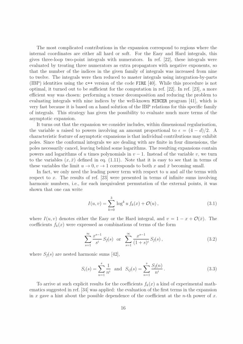
The most complicated contributions in the expansion correspond to regions where theinternal coordinates are either all hard or soft. For the Easy and Hard integrals, thisgives three-loop two-point integrals with numerators. In ref. [22], these integrals wereevaluated by treating three numerators as extra propagators with negative exponents, sothat the number of the indices in the given family of integrals was increased from nineto twelve. The integrals were then reduced to master integrals using integration-by-parts(IBP) identities using the c++ version of the code FIRE [40]. While this procedure is notoptimal, it turned out to be sufficient for the computation in ref. [22]. In ref. [23], a moreefficient way was chosen: performing a tensor decomposition and reducing the problem toevaluating integrals with nine indices by the well-known MINCER program [41], which isvery fast because it is based on a hand solution of the IBP relations for this specific familyof integrals. This strategy has given the possibility to evaluate much more terms of theasymptotic expansion.

It turns out that the expansion we consider includes, within dimensional regularisation,the variable u raised to powers involving an amount proportional to ǫ = (4 − d)/2. Acharacteristic feature of asymptotic expansions is that individual contributions may exhibitpoles. Since the conformal integrals we are dealing with are finite in four dimensions, thepoles necessarily cancel, leaving behind some logarithms. The resulting expansions containpowers and logarithms of u times polynomials in v − 1. Instead of the variable v, we turnto the variables (x, x) defined in eq. (1.11). Note that it is easy to see that in terms ofthese variables the limit u → 0, v → 1 corresponds to both x and x becoming small.

In fact, we only need the leading power term with respect to u and all the terms withrespect to x. The results of ref. [23] were presented in terms of infinite sums involvingharmonic numbers, i.e., for each inequivalent permutation of the external points, it wasshown that one can write

I(u, v) =3∑

k=0

logk u fk(x) +O(u) , (3.1)

where I(u, v) denotes either the Easy or the Hard integral, and v = 1 − x + O(x). Thecoefficients fk(x) were expressed as combinations of terms of the form

∞∑

s=1

xs−1

siS~(s) or

∞∑

s=1

xs−1

(1 + s)iS~(s) , (3.2)

where S~(s) are nested harmonic sums [42],

Si(s) =

s∑

n=1

1

niand Si~(s) =

s∑

n=1

S~(n)

ni. (3.3)

To arrive at such explicit results for the coefficients fk(x) a kind of experimental math-ematics suggested in ref. [34] was applied: the evaluation of the first terms in the expansionin x gave a hint about the possible dependence of the coefficient at the n-th power of x.

16

Then an ansatz in the form of a linear combination of nested sums was constructed andthe coefficients in this ansatz were fixed by the information about the first terms. Finally,the validity of the ansatz was confirmed using information about the next terms. Thecomplete x-expansion was thus inferred from the leading terms.

For the purpose of this paper, it is more convenient to work with polylogarithmicfunctions in x rather than harmonic sums. Indeed, sums of the type (3.2) can easily beperformed in terms of harmonic polylogarithms using the algorithms described in ref. [43].We note, however, that during the summation process, sums of the type (3.2) with i = 0are generated. Sums of this type are strictly speaking not covered by the algorithms ofref. [43], but we can easily reduce them to the case i 6= 0 using the following procedure,

∞∑

s=1

xs−1 Si~(s) =1

x

∞∑

s=1

xs

s∑

n=1

1

ni1

S~(n) =1

x

∞∑

s=0

xs

s∑

n=0

1

niS~(n) , (3.4)

where the last step follows from S~(0) = 0. Reshuffling the sum by letting s = n1 + n, weobtain the following relation which is a special case of eq. (96) in ref. [34]:

∞∑

s=1

xs−1 Si~(s) =1

x

∞∑

n1=0

xn1

∞∑

n=0

xn

niS~(n) =

1

1− x

∞∑

s=1

xs−1

siS~(s) . (3.5)

The last sum is now again of the type (3.2) and can be dealt with using the algorithms ofref. [43].

Performing all the sums that appear in the results of ref. [23], we find for example

x213 x

224E14;23 =

log u

x

(

H2,2,1 −H2,1,2 +H1,3,1 + 2H1,2,1,1 −H1,1,3 − 2H1,1,1,2 (3.6)

− 6ζ3H2 − 6ζ3H1,1

)

−2

x

(

2ζ3H2,1 − 4ζ3H1,2 + 4ζ3 H1,1,1 +H3,2,1

− H3,1,2 +H2,3,1 −H2,1,3 + 2H1,4,1 + 2 H1,3,1,1 + 2H1,2,2,1 − 2H1,1,4

− 2H1,1,2,2 − 2H1,1,1,3 − 6 ζ3H3

)

+O(u) ,

x413 x

424 H12;34 =

4 log u

x2

(

H1,1,2,1 −H1,1,1,2 − 6ζ3H1,1

)

−2

x2

(

4H2,1,2,1 − 4 H2,1,1,2 (3.7)

+ 4H1,1,3,1 −H1,1,2,1,1 − 4H1,1,1,3 +H1,1,1,2,1 − 24ζ3H2,1 + 6ζ3H1,1,1

)

+ O(u) ,

where we used the compressed notation, e.g., H2,1,1,2 ≡ H(0, 1, 1, 1, 0, 1; x). The resultsfor the other orientations are rather lengthy, so we do not show them here, but we collectthem in Appendix A. Let us however comment about the structure of the functions fk(x)that appear in the expansions. The functions fk(x) can always be written in the form

fk(x) =∑

l

Rk,l(x)× [HPLs in x] , (3.8)

17

where Rk,l(x) may represent any of the following rational functions

1

x2,

1

x,

1

x(1 − x). (3.9)

We note that the last rational function only enters the asymptotic expansion of H13;24.The aim of this paper is to compute the Easy and Hard integrals by writing for each

integral an ansatz of the form∑

i

Ri(x, x)Pi(x, x) , (3.10)

and to fix the coefficients that appear in the ansatz by matching the limit x → 0 tothe asymptotic expansions presented in this section. In the previous section we arguedthat a natural space of functions for the polylogarithmic part Pi(x, x) are functions thatare single-valued in the complex x plane in Euclidean space. We however still need todetermine the rational prefactors Ri(x, x), which are not constrained by single-valuedness.

A natural ansatz would consist in using the same rational prefactors as those appearingin the ladder type integrals. For ladder type integrals we have

Rladderi (x, x) =

1

(x− x)α, α ∈ N , (3.11)

plus all possible transformations of this function obtained from the action of the S3 sym-metry (2.25). Then in the limit u → 0 we obtain

limx→0

Rladderi (x, x) =

1

xα. (3.12)

We see that the rational prefactors that appear in the ladder-type integrals can only giverise to rational prefactors in the asymptotic expansions with are pure powers of x, and sothey can never account for the rational function 1/(x(1−x)) that appears in the asymptoticexpansion ofH13;24. We thus need to consider more general prefactors than those appearingin the ladder-type integrals. This issue will be addressed in the next sections.

4 The Easy integral

4.1 Residues of the Easy integral

The Easy integral is defined as

E12;34 =x223x

224

π6

∫d4x5 d

4x6 d4x7 x2

16

(x215x

225x

235)x

256(x

226x

236x

246)x

267(x

217x

227x

247)

. (4.1)

To find all its leading singularities we order the integrations as follows

E12;34 =x223x

224

π6

[∫d4x6 x2

16

x226x

236x

246

(∫d4x5

x215x

225x

235x

256

)(∫d4x7

x217x

227x

247x

267

)]

. (4.2)

18

First the x7 and x5 integrations: they are both the same as the massive box computedin the Introduction and thus give leading singularities (see eq. (1.14))

±1

4 λ1236±

1

4 λ1246, (4.3)

respectively. So we can move directly to the final x6 integration

1

16 π6

∫d4x6 x2

16

x226x

236x

246λ1236λ1246

. (4.4)

Here there are five factors in the denominator and we want to take the residues whenfour of them vanish to compute the leading singularity, so there are various choices toconsider. The simplest option is to cut the three propagators 1/x2

i6. Then on this cut wehave λ1236|cut = ±x2

16x223 and λ1246|cut = ±x2

16x224, where the vertical line indicates the value

on the cut, and the integral reduces to the massive box. This simplification of the λ factorsis similar to the phenomenon of composite leading singularities [44]. Thus cutting eitherof the two λs will result in4

leading singularity #1 of E12;34 = ±1

64 π6λ1234

. (4.5)

The only other possibility is cutting both λ’s. There are then three possibilities, firstlywe could cut x2

26 and x236 as well as the two λ′s. On this cut λ1236 reduces to ±x2

16x223 and

one obtains residue #1 again. Similarly in the second case where we cut x226, x

246 and the

two λs.So finally we consider the case where we cut x2

36, x246 and the two λ’s. In this case

λ1236|cut = ±(x216x

223 − x2

13x226) and λ1246|cut = ±(x2

16x224 − x2

14x226). Notice that setting

λ1236 = λ1246 = 0 means setting x216 = x2

26 = 0. We then need to compute the Jacobianassociated with cutting x2

36, x246, λ1236, λ1246

det

(∂(x2

36, x246, λ1236, λ1246)

∂xµ6

)∣∣∣∣cut

= ±16 det(

xµ36, xµ

46, xµ16x

223 − x2

13xµ26, xµ

16x224 − x2

14xµ26

)∣∣∣cut

= ±16 det (xµ36, x

µ46, x

µ16, x

µ26)(x

223x

214 − x2

24x213)

∣∣cut

= ±4λ1234(x223x

214 − x2

24x213) ,

(4.6)

The result of the x6 integral (4.4) is

1

64 π6

x216

x226λ1234(x

223x

214 − x2

24x213)

∣∣∣∣cut

(4.7)

4With a slight abuse of language, in the following we use the word ‘cut’ to designate that we look atthe zeroes of a certain denominator factor.

19

At this point there is a subtlety, since on the cut we have simultaneously x216x

223 −

x213x

226 = x2

16x224 − x2

14x226 = 0, i.e. x2

16 = x226 = 0 and so

x216

x226

is undefined. More specifically,

the integral depends on whether we take x216x

223−x2

13x226 = 0 first or x2

16x224−x2

14x226 = 0 first.

So we get two possibilities (after multiplying by the external factors x223x

224 in eq. (4.1)) :

leading singularity #2 of E12;34 = ±x213x

224

64 π6 λ1234(x223x

214 − x2

24x213)

(4.8)

leading singularity #3 of E12;34 = ±x214x

223

64 π6 λ1234(x223x

214 − x2

24x213)

. (4.9)

We conclude that the Easy integral takes the ‘leading singularity times pure function’form5

E12;34 =1

x213x

224

[E(a)(x, x)

x− x+

E(b)(x, x)

(x− x)(v − 1)+

v E(c)(x, x)

(x− x)(v − 1)

]

. (4.10)

We note that the x3 ↔ x4 symmetry relates E(b) and E(c). Furthermore, putting everythingover a common denominator it is easy to see that E(a) can be absorbed into the other twofunctions. We conclude that there is in fact only one independent function, and the Easyintegral can be written in terms of a single pure function E(x, x) as

E12;34 =1

x213x

224 (x− x)(v − 1)

[

E(x, x) + v E

(x

x− 1,

x

x− 1

)]

. (4.11)

The function E(x, x) is antisymmetric under the interchange of x, x

E(x, x) = −E(x, x) , (4.12)

to ensure that E12;34 is a symmetric function of x, x, but it possesses no other symmetry.The other two orientations of the Easy integral are then found by permuting various

points and are given by

E13;24 =1

x213x

224 (x− x)(u− v)

[

uE

(1

x,1

x

)

+ v E

(1

1− x,

1

1− x

)]

, (4.13)

E14;23 =1

x213x

224 (x− x)(1− u)

[

E(1− x, 1− x) + uE

(

1−1

x, 1−

1

x

)]

. (4.14)

It is thus enough to have an expression for E(x, x) to determine all possible orientationsof the Easy integral. The functional form of E(x, x) will be the purpose of the rest of thissection.

5A similar form of the Easy leading singularities, as well as those of the Hard integral discussed in thenext section, was independently obtained by S. Caron-Huot [45].

20

4.2 The symbol of E(x, x)

In this subsection we determine the symbol of E(x, x), and in the next section we de-scribe its uplift to a function. This strategy seems over-complicated in the case at hand,because E(x, x) can in fact directly be obtained in terms of SVHPLs of weight six fromits asymptotic expansion using the method described in Section 2.3. The two-step deriva-tion (symbol and subsequent uplift) is included mainly for pedagogical purposes becauseit equally applies to the Hard integral and our four-loop example, where the functions arenot writeable in terms of SVHPLs only so that a direct method yet has to be found.

Returning to the Easy integral, we start by writing down the most general tensor ofrank six that

• has all its entries drawn from the set {x, 1− x, x, 1− x},

• satisfies the first entry condition, i.e. the first factors in each tensor are either xx or(1− x)(1 − x),

• is odd under an exchange of x and x.

This results in a tensor that depends on 2 · 45/2 = 1024 free coefficients (which we assumeto be rational numbers). Imposing the integrability condition (2.9) reduces the number offree coefficients to 28, which is the number of SVHPLs of weight six that are odd under anexchange of x and x. The remaining free coefficients can be fixed by matching to the limitu → 0, v → 1, or equivalently x → 0.

In order to take the limit, we drop every term in the symbol containing an entry 1− xand we replace x → u/x, upon which the singularity is hidden in u. As a result, everypermutation of our ansatz yields a symbol composed of the three letters {u, x, 1−x}. Thistensor can immediately be matched to the symbol of the asymptotic expansion of the Easyintegral discussed in Section 3. Explicitly, the limits

x213x

224 E12;34 → −

1

x2

[

limx→0

E(x, x) + limx→0

E

(x

x− 1,

x

x− 1

)]

+1

xlimx→0

E

(x

x− 1,

x

x− 1

)

(4.15)

x213x

224 E13;24 → −

1

xlimx→0

E

(1

1− x,

1

1− x

)

(4.16)

x213x

224 E14;23 →

1

xlimx→0

E(1− x, 1− x) (4.17)

can be matched with the asymptotic expansions recast as HPLs. All three conditions areconsistent with our ansatz; each of them on its own suffices to determine all remainingconstants. The resulting symbol is a linear combination of 1024 tensors with entries drawnfrom the set {x, 1− x, x, 1− x} and with coefficients {±1, ±2}.

Note that the uniqueness of the uplift procedure for SVHPLs given in Section 2.3 impliesthat each asymptotic limit is sufficient to fix the symbol.

21

4.3 The analytic result for E(x, x): uplifting from the symbol

In this section we determine the function E(x, x) defined in eq. (4.11) starting from itssymbol. As the symbol has all its entries drawn from the set {x, 1 − x, x, 1 − x}, thefunction E(x, x) can be expressed in terms of the SVHPLs classified in [27]. Additionalsingle-valued terms6 proportional to zeta values can be fixed by again appealing to theasymptotic expansion of the integral.

We start by writing down an ansatz for E(x, x) as a linear combination of weight six ofSVHPLs that is odd under exchange of x and x. Note that we have some freedom w.r.t.the basis for our ansatz. In the following we choose basis elements containing a singlefactor of the form L~a(x). This ensures that all the terms are linearly independent.

Next we fix the free coefficients in our ansatz by requiring its symbol to agree with thatof E(x, x) determined in the previous section. As we had started from SVHPLs with thecorrect symmetries and weight, all coefficients are fixed in a unique way. We arrive at thefollowing expression for E(x, x):

E(x, x) = 4L2,4 − 4L4,2 − 2L1,3,2 + 2L2,1,3 − 2L3,1,2 + 4L3,2,0

− 2L2,2,1,0 + 8L3,1,0,0 + 2L3,1,1,0 − 2L2,1,1,1,0

(4.18)

For clarity, we suppressed the argument of the L functions and we employed the com-pressed notation for HPLs, e.g., L3,2,1 ≡ L0,0,1,0,1,1(x, x). The asymptotic limits of the lastexpression correctly reproduce the terms proportional to zeta values in eq. (3.7) and theformulae in Appendix A.

4.4 The analytic result for E(x, x): the direct approach

Here we quickly give the direct method for obtaining E(x, x) explicitly from its asymptoticsvia the method outlined in Section 2.3.

The asymptotic value of the Easy integral in the permutation E12;34 is given in Ap-pendix A. Comparing eq. (A.1) with eq. (4.15) and further writing log u = log x + log xand expanding out products of functions we find for the asymptotic value of E(x, x):

E(x, x) = 4ζ3H2,1 + 2H2,4 − 2H4,2 +H1,2,3 −H1,3,2 − 2H1,4,0 +H2,1,3 −H3,1,2

+ 2H3,2,0 −H1,3,1,0 +H2,1,2,0 − 2H2,2,0,0 −H2,2,1,0 +H3,1,1,0 + 2H1,2,0,0,0

+H1,2,1,0,0 −H2,1,1,0,0 − 20ζ5H1 + 8ζ3H3 + 2ζ3H1,2

+ log x P (x, log x) +O(x) ,

(4.19)

where P is a polynomial in log x with coefficients that are HPLs in x. From the discussionin Section 2.3 we know that there is a unique combination of SVHPLs with this precise

6In principle we cannot exclude at this stage more complicated functions of weight less than six multi-plied by zeta values.

22

asymptotic behavior, and so we find a natural ansatz for E(x, x),

E(x, x) = 4ζ3L2,1 + 2L2,4 − 2L4,2 + L1,2,3 − L1,3,2 − 2L1,4,0 + L2,1,3 − L3,1,2 + 2L3,2,0

− L1,3,1,0 + L2,1,2,0 − 2L2,2,0,0 − L2,2,1,0 + L3,1,1,0 + 2L1,2,0,0,0 + L1,2,1,0,0

− L2,1,1,0,0 − 20ζ5L1 + 8ζ3L3 + 2ζ3L1,2 . (4.20)

We have lifted this function from its asymptotics in just one limit x → 0 while we alsoknow two other limits of this function given in eq. (3.7) and Appendix A. Remarkably,eq. (4.20) is automatically consistent with these two limits, giving a strong indication thatit is indeed the right function. Furthermore, eq. (4.20) can then in turn be rewritten ina way that makes the antisymmetry under exchange of x and x manifest, and we recovereq. (4.20). Note also that antisymmetry in x ↔ x was not input anywhere, and the factthat the resulting function is indeed antisymmetric is a non-trivial consistency check.

As an aside we also note here that the form of E(x, x), expressed in the particular basisof SVHPLs we chose to work with, is very simple, having only coefficients ±1 or ±2 forthe polylogarithms of weight six. Indeed other orientations of E have even simpler forms,for instance

E(1/x, 1/x) = L2,4 − L3,3 − L1,2,3 + L1,3,2 − L1,4,0 −L2,1,3 + L3,1,2 − L4,0,0 + L4,1,0

+ L1,3,0,0 + L1,3,1,0 − L2,1,2,0 + L2,2,1,0 + L3,0,0,0 − L3,1,1,0 − L1,2,1,0,0

− L2,1,0,0,0 + L2,1,1,0,0 + 8ζ3L3 − 2ζ3L1,2 − 6ζ3L2,0 − 4ζ3L2,1 ,

(4.21)

with all coefficients of the weight six SVHPLs being ±1, or in the manifestly antisymmetricform with all weight six SVHPLs with coefficient +1

(4.22)E(1/x, 1/x) = L2,4 + L1,3,2 + L3,1,2 + L4,1,0 + L1,3,0,0

+ L1,3,1,0 + L2,2,1,0 + L3,0,0,0 + L2,1,1,0,0 + 6ζ3L3 − 2ζ3L2,1.

4.5 Numerical consistency tests for E

We have determined the analytic result for the Easy integral relying on the knowledge ofits residues, symbol and asymptotic expansions. In order to check the correctness of theresult, we evaluated E14;23 numerically7 and compared it to a direct numerical evaluationof the coordinate space integral using FIESTA [48, 49].

To be specific, we evaluate the conformally-invariant function x213x

224 E14;23. Applying

a conformal transformation to send x4 to infinity, the integral takes the simplified form,

limx4→∞

x213x

224E14;23 =

1

π6

∫d4x5d

4x6d4x7 x

213x

216

(x215x

225)x

256(x

226x

236)x

267(x

217x

237)

, (4.23)

with only 8 propagators. We use the remaining freedom to fix x213 = 1 so that u = x2

12

and v = x223. Other numerical values for x2

13 are possible, of course, but we found that thischoice yields relatively stable numerics.

7All polylogarithms appearing in this paper have been evaluated numerically using the GiNaC [46]and HPL [47] packages.

23

u v Analytic FIESTA δ0.1 0.2 82.3552 82.3553 6.6e-70.2 0.3 57.0467 57.0468 3.2e-80.3 0.1 90.3540 90.3539 5.9e-80.4 0.5 37.1108 37.1108 1.9e-80.5 0.6 31.9626 31.9626 1.9e-80.6 0.2 54.2881 54.2881 6.9e-80.7 0.3 42.6519 42.6519 4.4e-80.8 0.9 23.0199 23.0199 1.7e-80.9 0.5 30.8195 30.8195 2.4e-8

Table 1: Numerical comparison of the analytic result for x213x

224E14;23 against FIESTA for

several values of the conformal cross ratios.

After Feynman parameterisation, the integral is only seven-dimensional and can beevaluated with off-the-shelf software. We generate the integrand with FIESTA and performthe numerical integration with a stand-alone version of CIntegrate. Using the algorithmDivonne8, we obtain roughly five digits of precision after five million function evaluations.

In total, we checked 40 different pairs of values for the cross ratios and we found verygood agreement in all cases. A sample of the numerical checks is shown in Table 1. Notethat δ denotes the relative error between the analytic result and the number obtained byFIESTA,

δ =

∣∣∣∣

Nanalytic −NFIESTA

Nanalytic +NFIESTA

∣∣∣∣. (4.24)

5 The Hard integral

5.1 Residues of the Hard integral

To find all the leading singularities we consider each integration sequentially as follows

H12;34 =x234

π6

{∫d4x6

x216x

226x

236x

246

[∫d4x5 x2

56

x215x

225x

235x

245

(∫d4x7

x237x

247x

257x

267

)]}

. (5.1)

Let us start with the x7 integration,

∫d4x7

x237x

247x

257x

267

. (5.2)

8Experience shows that Divonne outperforms other algorithms of the Cuba library for problems roughlythis size.

24

This is simply the off-shell box considered in Section 1, and so its leading singularities are(see eq. (1.14))

±1

4 λ3456. (5.3)

Next we turn to the x5 integration, which now takes the form∫

d4x5 x256

x215x

225x

235x

245λ3456

. (5.4)

There are five factors in the denominator, and we want to cut four of them to computethe leading singularity. The simplest option is to cut the four propagators 1/x2

i5. Doingso would yield a new Jacobian factor 1/λ1234 (exactly as in the previous subsection) andfreeze λ3456|cut = ±x2

56x234. This latter factor simply cancels the numerator and we are left

with the final x6 integration being that of the box in the Introduction. Putting everythingtogether, the leading singularity for this choice is

leading singularity #1 of H12;34 = ±1

64π6 λ21234

. (5.5)

Returning to the x5 integration, eq. (5.4), we must consider the possibility of cuttingλ3456 and three other propagators. Cutting x2

35 and x245 immediately freezes λ3456|cut =

±x256x

234 which is canceled by the numerator. Thus it is not possible to cut these two

propagators and λ3456. However, cutting x215, x

225, x

235 and λ3456 is possible (the only other

possibility, i.e. cutting x215, x

225, x

245 and λ3456, gives the same result by by invariance of the

integral under exchange of x3 and x4). Indeed one finds that when x235 = 0,

λ3456 = ±(x245x

236 − x2

56x234) . (5.6)

To compute the leading singularity associated with this pole we need to compute theJacobian

J = det

(∂(x2

15, x225, x

235, λ3456)

∂xµ5

)

, (5.7)

As in the box case, it is useful to consider the square of J (on the cut),

J2 = 16 det

(x2ij −2xi · ∂λ3456/∂x5

−2xi · ∂λ3456/∂x5 (∂λ3456/∂x5)2

)

. (5.8)

The result of the x5 integration is then simply

x256

Jx245

∣∣∣∣cut

=x236

Jx234

∣∣∣∣cut

, (5.9)

where the second equality follows since x256 and x2

45 are to be evaluated on the cut (indicatedby the vertical line) for which x2

45x236−x2

56x234 = 0. Finally we need to turn to the remaining

x6 integral. We are simply left with

1

16π6

∫d4x6

x216x

226x

246J

∣∣∣∣cut

, (5.10)

25

where we note that the x236 propagator term has canceled with the numerator in eq. (5.9).

So we have no choice left for the quadruple cut as there are only four poles. In fact on theother cut of the three propagators we find J|cut = 4(x2

14x223 − x2

13x224)x

236, and so this brings

back the propagator x236.

Computing the Jacobian associated with this final integration thus yields the final resultfor the leading singularity,

leading singularity #2 of H12;34 = ±1

64π6 (x214x

223 − x2

13x224)λ1234

. (5.11)

We conclude that the Hard integral can be written as these leading singularities timespure functions, i.e. it has the form

H12;34 =1

x413x

424

[H(a)(x, x)

(x− x)2+

H(b)(x, x)

(v − 1)(x− x)

]

, (5.12)

where H(a),(b) are pure polylogarithmic functions. The pure functions must furthermoresatisfy the following properties

H(a)(x, x) = H(a)(x, x) , H(b)(x, x) = −H(b)(x, x) , (5.13)

H(a)(x, x) = H(a)(x/(x− 1), x/(x− 1)) , H(b)(x, x) = H(b)(x/(x− 1), x/(x− 1)) ,

in order that H12;34 be symmetric in x, x and under the permutation x1 ↔ x2. Furthermorewe would expect that H(a)(x, x) = 0 in order to cancel the pole at x − x. In fact it willturn out in this section that even without imposing this condition by hand we will arriveat a unique result which nevertheless has this particular property.

By swapping the points around we automatically get

H13;24 =1

x413x

424

[H(a)(1/x, 1/x)

(x− x)2+

H(b)(1/x, 1/x)

(u− v)(x− x)

]

, (5.14)

H14;23 =1

x413x

424

[H(a)(1− x, 1− x)

(x− x)2+

H(b)(1− x, 1− x)

(1− u)(x− x)

]

. (5.15)

5.2 The symbols of H(a)(x, x) and H(b)(x, x)

In order to determine the pure functions contributing to the Hard integral, we proceed justlike for the Easy integral and first determine the symbol. For the Hard integral we haveto start from two ansatze for the symbols S[H(a)(x, x)] and S[H(b)(x, x)]. While both purefunctions are invariant under the exchange x1 ↔ x2, S[H

(a)] must be symmetric under theexchange of x, x and S[H(b)] has to be antisymmetric, cf. eq. (5.13). Going through exactlythe same steps as for E we find that the single-variable limits of the symbols cannot bematched against the data from the asymptotic expansions using only entries from the set{x, 1− x, x, 1− x}. We thus need to enlarge the ansatz.

Previously, the letter x − x ∼ λ1234 has been encountered in ref. [30, 50] in a similarcontext. We therefore consider all possible integrable symbols made from the letters {x, 1−

26

x, x, 1 − x, x − x} which obey the initial entry condition (2.13). In the case of the Easyintegral, the integrability condition only implied that terms depending on both x and xcome from products of single-variable functions. Here, on the other hand, the condition ismore non-trivial since, for example,

d logx

x∧ d log(x− x) = d log x ∧ d log x ,

d log1− x

1− x∧ d log(x− x) = d log(1− x) ∧ d log(1− x) .

(5.16)

We summarise the dimensions of the spaces of such symbols, split according to parity underexchange of x and x, in Table 2.

Weight Even Odd1 2 02 3 13 6 34 12 95 28 246 69 65

Table 2: Dimensions of the spaces of integrable symbols with entries drawn from the set{x, 1− x, x, 1− x, x− x} and split according to the parity under exchange of x and x.

Given our ansatz for the symbols of the functions we are looking for, we then matchagainst the twist two asymptotics as described previously. We find a unique solution forthe symbols of both H(a) and H(b) compatible with all asymptotic limits. Interestingly,the limit of H13;24 leaves one undetermined parameter in S[H(a)], which we may fix byappealing to another limit. In the resulting symbols, the letter x − x occurs only in thelast two entries of S[H(a)] while it is absent from S[H(b)]. Although we did not imposethis as a constraint, S[H(a)] goes to zero when x → x, which is necessary since the integralcannot have a pole at x = x.

5.3 The analytic results for H(a)(x, x) and H(b)(x, x)

In this section we integrate the symbol of the Hard integral to a function, i.e. we determinethe full answers for the functions H(a)(x, x) and H(b)(x, x) that contribute to the Hardintegral H12;34.

In the previous section we already argued that the symbol ofH(b)(x, x) has all its entriesdrawn form the set {x, 1 − x, x, 1 − x}, and so it is reasonable to assume that H(b)(x, x)can be expressed in terms of SVHPLs only. We may therefore proceed by lifting directlyfrom the asymptotic form as we did in Section 4.4 for the Easy integral. By comparing theform of H13;24, eq. (5.14), with its asymptotic value (1.14) we can read off the asymptotic

27

form of H(1/x, 1/x). Writing log u as log x + log x, expanding out all the functions andneglecting log x terms, we can the lift directly to the full function by simply convertingHPLs to SVHPLs. In this way we arrive at

H(b)(1/x, 1/x) = 2L2,4 − 2L3,3 − 2L1,1,4 − 2L1,4,0 + 2L1,4,1 − 2L2,3,1 + 2L3,1,2

− 2L4,0,0 + 2L4,1,0 + 2L1,1,1,3 + 2L1,1,3,0 + 2L1,3,0,0 − 2L1,3,1,1

− 2L2,1,1,2 + 2L2,1,2,1 + 2L3,0,0,0 − 2L3,1,1,0 − 2L1,1,1,2,1 − 2L1,1,2,1,0

+ 2L1,1,2,1,1 − 2L1,2,1,0,0 + 2L1,2,1,1,0 − 2L2,1,0,0,0 + 2L2,1,1,0,0

+ 16ζ3L3 − 16ζ3L2,1 .

(5.17)

Other orientations although still quite simple do not all share the property that they onlyhave coefficients ±2. Using the basis of SVHPLs that makes the parity under exchange ofx and x explicit, we can write the last equation in the equivalent form

H(b)(x, x) = 16L2,4 − 16L4,2 − 8L1,3,2 − 8L1,4,1 + 8L2,1,3 − 8L2,2,2 + 8L2,3,1 − 8L3,1,2

+ 16L3,2,0 + 8L3,2,1 − 8L4,1,1 + 4L1,2,2,1 − 8L1,3,1,1 − 4L2,1,1,2 + 8L2,1,2,1

− 8L2,2,1,0 − 4L2,2,1,1 + 8L3,1,1,0 − 4L1,1,2,1,1 − 24L2,1,1,1,0 . (5.18)

Next, we turn to the function H(a)(x, x). As the symbol of H(a)(x, x) contains theentry x− x, it cannot be expressed through SVHPLs only. Single-valued functions whosesymbols have entries drawn form the set {x, 1 − x, x, 1 − x, x − x} have been studiedup to weight four in ref. [30], and a basis for the corresponding space of functions wasconstructed. The resulting single-valued functions are combinations of logarithms of x andx and multiple polylogarithms G(a1, . . . , an; 1), with ai ∈ {0, 1/x, 1/x}. Note that theharmonic polylogarithms form a subalgebra of this class of functions, because we have,e.g.,

G

(

0,1

x,1

x; 1

)

= H(0, 1, 1; x) . (5.19)

This class of single-valued functions thus provides a natural extension of the SVHPLs wehave encountered so far. In the following we show how we can integrate the symbol ofH(a)(x, x) in terms of these functions. The basic idea is the same as for the case of theSVHPLs: we would like to write down the most general linear combination of multiplepolylogarithms of this type and fix their coefficients by matching to the symbol and theasymptotic expansion of H(a)(x, x). Unlike the SVHPL case, however, some of the stepsare technically more involved, and we therefore discuss these points in detail.

Let us denote by G the algebra generated by log x and log x and by multiple polylog-arithms G(a1, . . . , an; 1), with ai ∈ {0, 1/x, 1/x}, with coefficients that are polynomials inmultiple zeta values. Note that without loss of generality we may assume that an 6= 0.In the following we denote by G± the linear subspaces of G of the functions that are re-spectively even and odd under an exchange of x and x. Our first goal will be to constructa basis for the algebra G, as well as for its even and odd subspaces. As we know thegenerators of the algebra G, we automatically know a basis for the underlying vector space

28

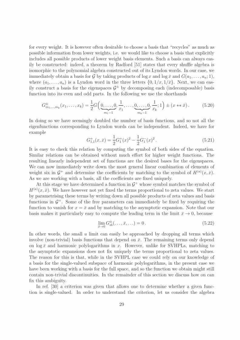
for every weight. It is however often desirable to choose a basis that “recycles” as much aspossible information from lower weights, i.e. we would like to choose a basis that explicitlyincludes all possible products of lower weight basis elements. Such a basis can always eas-ily be constructed: indeed, a theorem by Radford [51] states that every shuffle algebra isisomorphic to the polynomial algebra constructed out of its Lyndon words. In our case, weimmediately obtain a basis for G by taking products of log x and log x and G(a1, . . . , an; 1),where (a1, . . . , an) is a Lyndon word in the three letters {0, 1/x, 1/x}. Next, we can eas-ily construct a basis for the eigenspaces G± by decomposing each (indecomposable) basisfunction into its even and odd parts. In the following we use the shorthands

G±m1,...,mk

(x1, . . . , xk) =1

2G(

0, . . . , 0︸︷︷︸

m1−1

,1

x1, . . . , 0, . . . , 0

︸︷︷︸

mk−1

,1

xk; 1)

± (x ↔ x) . (5.20)

In doing so we have seemingly doubled the number of basis functions, and so not all theeigenfunctions corresponding to Lyndon words can be independent. Indeed, we have forexample

G+1,1(x, x) =

1

2G+

1 (x)2 −

1

2G−

1 (x)2 . (5.21)

It is easy to check this relation by computing the symbol of both sides of the equation.Similar relations can be obtained without much effort for higher weight functions. Theresulting linearly independent set of functions are the desired bases for the eigenspaces.We can now immediately write down the most general linear combination of elements ofweight six in G+ and determine the coefficients by matching to the symbol of H(a)(x, x).As we are working with a basis, all the coefficients are fixed uniquely.

At this stage we have determined a function in G+ whose symbol matches the symbol ofH(a)(x, x). We have however not yet fixed the terms proportional to zeta values. We startby parametrising these terms by writing down all possible products of zeta values and basisfunctions in G+. Some of the free parameters can immediately be fixed by requiring thefunction to vanish for x = x and by matching to the asymptotic expansion. Note that ourbasis makes it particularly easy to compute the leading term in the limit x → 0, because

limx→0

G±~m(. . . , x, . . .) = 0 . (5.22)

In other words, the small u limit can easily be approached by dropping all terms whichinvolve (non-trivial) basis functions that depend on x. The remaining terms only dependon log x and harmonic polylogarithms in x. However, unlike for SVHPLs, matching tothe asymptotic expansions does not fix uniquely the terms proportional to zeta values.The reason for this is that, while in the SVHPL case we could rely on our knowledge ofa basis for the single-valued subspace of harmonic polylogarithms, in the present case wehave been working with a basis for the full space, and so the function we obtain might stillcontain non-trivial discontinuities. In the remainder of this section we discuss how on canfix this ambiguity.

In ref. [30] a criterion was given that allows one to determine whether a given func-tion is single-valued. In order to understand the criterion, let us consider the algebra

29

G generated by multiple polylogarithms G(a1, . . . , an; an+1), with ai ∈ {0, 1/x, 1/x} andan+1 ∈ {0, 1, 1/x, 1/x}, with coefficients that are polynomials in multiple zeta values. Notethat G contains G as a subalgebra. The reason to consider the larger algebra G is that G car-ries a Hopf algebra structure9 [52], i.e. G can be equipped with a coproduct ∆ : G → G⊗G.Consider now the subspace GSV of G consisting of single-valued functions. It is easy to seethat GSV is a subalgebra of G. However, it is not a sub-Hopf algebra, but rather GSV is aG-comodule, i.e. ∆ : GSV → GSV ⊗ G. In other words, when acting with the coproduct ona single-valued function, the first factor in the coproduct must itself be single-valued. Asa simple example, we have

∆(L2) =1

2L0 ⊗ log

1− x

1− x+

1

2L1 ⊗ log

x

x. (5.23)

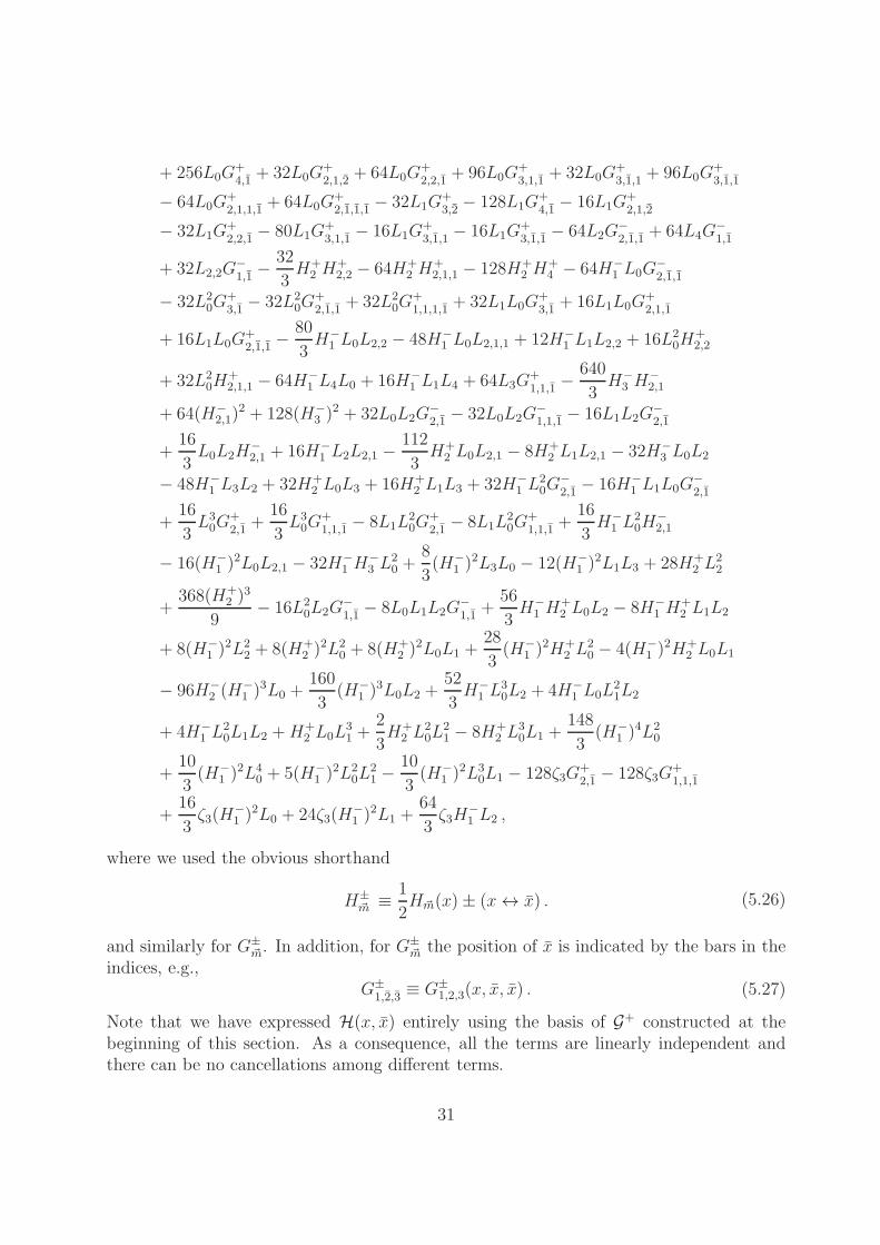
Note that this is a natural extension of the first entry condition discussed in Section 2.This criterion can now be used to recursively fix the remaining ambiguities to obtain asingle-valued function. In particular, in ref. [30] an explicit basis up to weight four wasconstructed for GSV . We extended this construction and obtained a complete basis atweight five, and we refer to ref. [30] about the construction of the basis. All the remainingambiguities can then easily be fixed by requiring that after acting with the coproduct, thefirst factor can be decomposed into the basis of GSV up to weight five. We then finallyarrive at

H(a)(x, x) = H(x, x)−28

3ζ3L1,2 + 164ζ3L2,0 +

136

3ζ3L2,1 −

160

3L3L2,1 − 66L0L1,4

−148

3L0L2,3 +

64

3L2L3,1 +

52

3L0L3,2 + 16L1L3,2 + 36L0L4,1 + 64L1L4,1

+70

3L0L1,2,2 + 24L0L1,3,1 +

26

3L1L1,3,1 − 8L2L2,1,1 + 64L0L2,1,2

−58

3L0L2,2,0 − 4L0L2,2,1 +

50

3L1L2,2,1 − 12L0L3,1,0 −

88

3L0L3,1,1

+ 18L1L3,1,1 −32

3L0L1,1,2,1 − 18L0L1,2,1,1 +

166

3L0L2,1,1,0 − 8L0L2,1,1,1

+ 328ζ3L3 + 32L32 − 64L2L4 .

(5.24)

The function H(x, x) is a single-valued combination of multiple polylogarithms that cannotbe expressed through SVHPLs alone,

H(x, x) = −128G+4,2

− 512G+5,1

− 64G+3,1,2

+ 64G+3,1,2

− 64G+3,1,2

− 128G+3,2,1

+ 64G+4,1,1

− 64G+4,1,1

− 448G+4,1,1

+ 64G+2,1,2,1

+ 64G+2,1,2,1

+ 64G+2,2,1,1

+ 64G+2,2,1,1

− 64G+2,2,1,1

+ 128G+2,2,1,1

+ 128G+2,2,1,1

+ 256G+3,1,1,1

+ 128G+3,1,1,1

− 128G+3,1,1,1

+ 192G+3,1,1,1

− 64G+3,1,1,1

− 64G+3,1,1,1

+ 192G+3,1,1,1

+ 128H+2,4 − 128H+

4,2

+640

3H+

2,1,3 −64

3H+

2,3,1 −256

3H+

3,1,2 + 64H+2,1,1,2 − 64H+

2,2,1,1 + 64L0G+3,2

(5.25)

9Note that we consider a slightly extended version of the Hopf algebra considered in ref. [52] that allowsus to include consistently multiple zeta values of even weight, see ref. [53, 54].

30

+ 256L0G+4,1

+ 32L0G+2,1,2

+ 64L0G+2,2,1

+ 96L0G+3,1,1

+ 32L0G+3,1,1

+ 96L0G+3,1,1

− 64L0G+2,1,1,1

+ 64L0G+2,1,1,1

− 32L1G+3,2

− 128L1G+4,1

− 16L1G+2,1,2

− 32L1G+2,2,1

− 80L1G+3,1,1

− 16L1G+3,1,1

− 16L1G+3,1,1

− 64L2G−2,1,1

+ 64L4G−1,1

+ 32L2,2G−1,1

−32

3H+

2 H+2,2 − 64H+

2 H+2,1,1 − 128H+

2 H+4 − 64H−

1 L0G−2,1,1

− 32L20G

+3,1

− 32L20G

+2,1,1

+ 32L20G

+1,1,1,1

+ 32L1L0G+3,1

+ 16L1L0G+2,1,1

+ 16L1L0G+2,1,1 −

80

3H−

1 L0L2,2 − 48H−1 L0L2,1,1 + 12H−

1 L1L2,2 + 16L20H

+2,2

+ 32L20H

+2,1,1 − 64H−

1 L4L0 + 16H−1 L1L4 + 64L3G

+1,1,1

−640

3H−

3 H−2,1

+ 64(H−2,1)

2 + 128(H−3 )

2 + 32L0L2G−2,1 − 32L0L2G

−1,1,1 − 16L1L2G

−2,1

+16

3L0L2H

−2,1 + 16H−

1 L2L2,1 −112

3H+

2 L0L2,1 − 8H+2 L1L2,1 − 32H−

3 L0L2

− 48H−1 L3L2 + 32H+

2 L0L3 + 16H+2 L1L3 + 32H−

1 L20G

−2,1

− 16H−1 L1L0G

−2,1

+16

3L30G

+2,1

+16

3L30G

+1,1,1

− 8L1L20G

+2,1

− 8L1L20G

+1,1,1

+16

3H−

1 L20H

−2,1

− 16(H−1 )

2L0L2,1 − 32H−1 H

−3 L

20 +

8

3(H−

1 )2L3L0 − 12(H−

1 )2L1L3 + 28H+

2 L22

+368(H+

2 )3

9− 16L2

0L2G−1,1

− 8L0L1L2G−1,1

+56

3H−

1 H+2 L0L2 − 8H−

1 H+2 L1L2

+ 8(H−1 )

2L22 + 8(H+

2 )2L2

0 + 8(H+2 )

2L0L1 +28

3(H−

1 )2H+

2 L20 − 4(H−

1 )2H+

2 L0L1

− 96H−2 (H

−1 )

3L0 +160

3(H−

1 )3L0L2 +

52

3H−

1 L30L2 + 4H−

1 L0L21L2

+ 4H−1 L

20L1L2 +H+

2 L0L31 +

2

3H+

2 L20L

21 − 8H+

2 L30L1 +

148

3(H−

1 )4L2

0

+10

3(H−

1 )2L4

0 + 5(H−1 )

2L20L

21 −

10

3(H−

1 )2L3

0L1 − 128ζ3G+2,1

− 128ζ3G+1,1,1

+16

3ζ3(H

−1 )

2L0 + 24ζ3(H−1 )

2L1 +64

3ζ3H

−1 L2 ,

where we used the obvious shorthand

H±~m ≡

1

2H~m(x)± (x ↔ x) . (5.26)

and similarly for G±~m. In addition, for G±

~m the position of x is indicated by the bars in theindices, e.g.,

G±1,2,3

≡ G±1,2,3(x, x, x) . (5.27)

Note that we have expressed H(x, x) entirely using the basis of G+ constructed at thebeginning of this section. As a consequence, all the terms are linearly independent andthere can be no cancellations among different terms.

31



424 H13;24 against FIESTA for

several values of the conformal cross ratios.

5.4 Numerical consistency checks for H

In the previous section we have determined the analytic result for the Hard integral. Inorder to check that our method indeed produced the correct result for the integral, wehave compared our expression numerically against FIESTA. Specifically, we evaluate theconformally-invariant function x4

13x424 H13;24. Applying a conformal transformation to send

x4 to infinity, the integral takes the simplified form,

limx4→∞

x413x

424 H13;24 =

1

π6

∫d4x5d

4x6d4x7 x

413x

257

(x215x

225x

235)x

256(x

236)x

267(x

217x

227x

237)

, (5.28)

with 9 propagators. As we did for E14;23, we use the remaining freedom to fix x213 = 1 so

that u = x212 and v = x2

23, and perform the numerical evaluation using the same setup. Wecompare at 40 different values, and find excellent agreement in all cases. A small sampleof the numerical checks is shown in Table 3.

6 The analytic result for the three-loop correlator

In the previous sections we computed the Easy and Hard integrals analytically. Usingeq. (1.8), we can therefore immediately write down the analytic answer for the three-loopcorrelator of four stress tensor multiplets. We find

x213 x

224 F3 =

6

x− x

[

f (3)(x) + f (3)

(

1−1

x

)

+ f (3)

(1

1− x

)]

+2

(x− x)2f (1)(x)

[

v f (2)(x) + f (2)

(

1−1

x

)

+ u f (2)

(1

1− x

)] (6.1)

32

+4

x− x

[1

v − 1E(x) +

v

v − 1E

(x

x− 1

)

+1

1− uE(1− x)

+u

1− uE

(

1−1

x

)

+u

u− vE

(1

x

)

+v

u− vE

(1

1− x

)]

+1

(x− x)2

[

(1 + v)H(a)(x) + (1 + u)H(a) (1− x) + (u+ v)H(a)

(1

x

)]

+1

x− x

[v + 1

v − 1H(b)(x) +

1 + u

1− uH(b) (1− x) +

u+ v

u− vH(b)

(1

x

)]

.

The pure functions appearing in the correlator are defined in eqs. (2.3), (4.20), (5.17)and (5.24). For clarity, we suppressed the dependence of the pure functions on x, i.e. wewrite f (L)(x) ≡ f (L)(x, x) and so on. All the pure functions can be expressed in termsof SVHPLs, except for H(a) which contains functions whose symbols involve x − x as anentry. We checked that these contributions do not cancel in the sum over all contributionsto the correlator.

7 A four-loop example

In this section we will discuss a four-loop integral to illustrate how our techniques can beapplied at higher loops. The example we consider contributes to the four-loop four-pointfunction of stress-tensor multiplets in N = 4 SYM. Specifically, we consider the Euclidean,conformal, four-loop integral,

I(4)14;23 =

1

π8

∫d4x5d

4x6d4x7d

4x8x214x

224x

234

x215x

218x

225x

226x

237x

238x

245x

246x

247x

248x

256x

267x

278

=1

x213x

224

f(u, v) , (7.1)

where the cross ratios u and v are defined by eq. (1.11). As we will demonstrate in thefollowing sections, this integral obeys a second-order differential equation whose solution isuniquely specified by imposing single-valued behaviour, similar to the generalised laddersconsidered in ref. [35].

The four-loop contribution to the stress-tensor four-point function in N = 4 SYMcontains some integrals that do not obviously obey any such differential equations, and withthe effort presented here we also wanted to learn to what extent the two-step procedure ofderiving symbols and subsequently uplifting them to functions can be repeated for thosecases. Our results are encouraging: the main technical obstable is obtaining sufficient datafrom the asymptotic expansions; we show that this step is indeed feasible, at least for I(4),and present the results in Section 7.1. Ultimately we find it simpler to evaluate I(4) bysolving a differential equation, and in this case the asymptotic expansions provide stringentconsistency checks.

33

7.1 Asymptotic expansions

Let us first consider the limits of the four-loop integral (7.1) and its point permutationsfor x12, x34 → 0. We derive expressions for its asymptotic expansion in the limit whereu → 0, v → 1 similar to those for the Easy and Hard integrals obtained in Section 3. Thelogarithmic terms can be fully determined, while the non-logarithmic part of the expansionrequires four-loop IBP techniques that allow us to reach spin 15. This contains enoughinformation to fix the ζn log

0(u) terms (important for beyond-the-symbol contributions)while the purely rational part of the asymptotic series remains partially undetermined.However, our experience with Easy and Hard has shown that each of the three coincidencelimits is (almost) sufficient to pin down the various symbols. Inverting the integrals fromone orientation to another ties non-logarithmic terms in one expansion to logarithmic onesin another, so that we do in fact command over much more data than it superficially seems.It is also conceivable to take into account more than the lowest order in u.

We start by investigating the asymptotic expansion of the integral I(4)14;23 whose coinci-

dence limit x12, x34 → 0 diverges as log2 u. There are three contributing regions: while inthe first two regions the original integral factors into a product of two two-loop integrals ora one-loop integral and a trivial three-loop integral, the third part corresponds to the four-loop ‘hard’ region in which the original integral is simply expanded in the small distances.The coefficients of the logarithmically divergent terms in the asymptotic expansion, i.e.the coefficients of log2 u and log u, can be worked out from the first two regions alone. Itis easy to reach high powers in x and we obtain a safe match onto harmonic series of thetype (3.2) with i > 1. Similar to the case of the Easy and Hard integrals discussed inSection 3, we can sum up the harmonic sums in terms of HPLs. Note that the absence ofharmonic sums with i = 1 implies the absence of HPLs of the form H1,...(x).

In the hard region, we have explicitly worked out the contribution from spin zerothrough eight, i.e., up to and including terms of O(x8). By what has been said above aboutthe form of the series, this amount of data is sufficient to pin down the terms involvingzeta values, while we cannot hope to fix the purely rational part where the dimension ofthe ansatz is larger than the number of constraints we can obtain. The linear combinationdisplayed below was found from the limit x → 0 of the symbol of the four-loop integralderived in subsequent sections. Its expansion around x = 0 reproduces the asymptoticexpansion of the integral up to O(x8). We find

x213 x

224 I

(4)14;23 = (7.2)

1

2 xlog2 u

[

H2,1,3 −H2,3,1 +H3,1,2 −H3,2,1 + 2H2,1,1,2 − 2H2,2,1,1 + ζ3(6H3 + 6H2,1)]

+

1

xlog u

[

−4H2,1,4 + 4H2,4,1 − 3H3,1,3 + 3H3,3,1 − 3H4,1,2 + 3H4,2,1 − 4H2,1,1,3 − 4H2,1,2,2

+ 4H2,2,2,1 + 4H2,3,1,1 − 2H3,1,1,2 + 2H3,2,1,1 + ζ3(−18H4 − 8H2,2 − 2H3,1 + 8H2,1,1)]

+

1

x

[

10H2,1,5 + 2H2,2,4 − 2H2,3,3 − 10H2,5,1 + 8H3,1,4 − 8H3,4,1 + 6H4,1,3 − 6H4,3,1

34

+ 6H5,1,2 − 6H5,2,1 + 8H2,1,1,4 + 6H2,1,2,3 + 8H2,1,3,2 − 2H2,1,4,1 + 2H2,2,2,2 − 4H2,2,3,1

− 4H2,3,1,2 − 10H2,3,2,1 − 4H2,4,1,1 + 4H3,1,1,3 + 6H3,1,2,2 − 6H3,2,2,1 − 4H3,3,1,1 + 4H2,1,1,2,2

− 4H2,1,2,2,1 − 4H2,2,1,1,2 + 4H2,2,2,1,1 + ζ3(36H5 + 8H2,3 + 12H3,2 − 12H4,1 − 4H2,1,2

− 16H2,2,1 − 8H3,1,1) + ζ5(10H3 + 10H2,1)]

+O(u) .

Next we turn to the asymptotic expansion of the orientation I(4)12;34. Here the Euclidean

coincidence limit x12, x34 → 0 is finite, and thus the only region we need to analyse is thefour-loop hard region, for which we have determined the asymptotic expansion up to andincluding terms of O(x15). Just like for the non-logarithmic part in the asymptotic expan-

sion of I(4)14;23, eq. (7.2), we have fixed the terms proportional to zeta values by matching

an ansatz in terms of HPLs onto this data, and once again, the terms not containing zetavalues are taken from the relevant limit of the symbol. We find

x213 x

224 I

(4)12;34 = (7.3)

1

x

[

4H1,3,4 − 4H1,5,2 + 2H1,1,2,4 − 2H1,1,4,2 + 2H1,2,1,4 − 2H1,2,3,2 + 2H1,3,1,3 + 2H1,3,3,1

− 2H1,4,1,2 − 2H1,5,1,1 +H1,1,2,1,3 +H1,1,2,3,1 −H1,1,3,1,2 −H1,1,3,2,1 +H1,2,1,1,3 +H1,2,1,3,1

−H1,2,2,1,2 +H1,2,2,2,1 − 2H1,2,3,1,1 +H1,3,1,2,1 −H1,3,2,1,1 +H1,2,1,1,2,1 −H1,2,1,2,1,1+

ζ3(8H1,1,3 − 8H1,2,2 + 4H1,1,2,1 − 4H1,2,1,1) + 70 ζ7H1

]

+O(u) .

The expansion around x = 0 of this expression reproduces the asymptotic expansion of theintegral up to O(x15).

The most complicated integrals appearing in the asymptotic expansion of I(4)14;23, I

(4)12;34

are four-loop two-point dimensionally regularised (in position space) integrals which belongto the family of integrals contributing to the evaluation of the five-loop contribution to theKonishi anomalous dimension [22],

G(a1, . . . , a14) =

∫ddx6d

dx7ddx8d

dx9

(x216)

a1(x217)

a2(x218)

a3(x219)

a4(x26)

a5(x27)

a6(x28)

a7

×1

(x29)

a8(x267)

a9(x268)

a10(x269)

a11(x278)

a12(x279)

a13(x289)

a14, (7.4)

with various integer indices a1, . . . , a14 and d = 4− 2ǫ.The complexity of the IBP reduction to master integrals is determined, in a first ap-

proximation, by the number of positive indices and the maximal deviation from the cornerpoint of a sector, which has indices equal to 0 or 1 for non-positive and positive indices, cor-respondingly. This deviation can be characterised by the number

∑

i∈ν+(ai−1)−

∑

i∈ν−ai

where ν± are sets of positive (negative) indices. So the most complicated (for an IBPreduction) integrals appearing in the contribution of spin s to the asymptotic expansion inthe short-distance limit have nine positive indices and the deviation from the corner pointis equal to 2s− 2. It was possible to get results up to spin 15.

35

As in ref. [22] the IBP reduction was performed by the c++ version of the code FIRE [40].The master integrals of this family either reduce, via a dual transformation, to the cor-responding momentum space master integrals [55, 56] or can be taken from ref. [22]. Toarrive at contributions corresponding to higher spin values, FIRE was combined with arecently developed alternative code to solve IBP relations LiteRed [57] based on the alge-braic properties of IBP relations revealed in ref. [58]. (See ref. [59] where this combinationwas presented within the Mathematica version of FIRE.)

7.2 A differential equation

We can use the magic identity [25] on the two-loop ladder subintegral

I(2)(x1, x2, x4, x7) = h14;27 =1

π4

∫d4x5d

4x6x224

x215x

225x

226x

245x

246x

267x

256

. (7.5)

The magic identity reads

I(2)(x1, x2, x4, x7) = I(2)(x2, x1, x7, x4) , (7.6)

and using it on the four-loop integral we find

I(4)14;23 =

1

π4

∫d4x7d

4x8

x218x

237x

238x

247x

248x

278

I(2)(x1, x2, x4, x7)

=1

π4

∫d4x7d

4x8

x218x

237x

238x

247x

248x

278

I(2)(x2, x1, x7, x4)

=1

π8

∫d4x5d

4x6d4x7d

4x8x217x

214x

234

x218x

237x

238x

247x

248x

278x

225x

215x

216x

275x

276x

264x

256

. (7.7)

The resulting integral (7.7) is ‘boxable’, i.e. we may apply the Laplace operator at thepoint x2. The only propagator which depends on x2 is the one connected to the point x5

and we have

✷21

x225

= −4π2δ4(x25) . (7.8)

The effect of the Laplace operator is therefore to reduce the loop order by one [25]. Thuson the full integral I(4) we have

✷2I(4)14;23 = −

4

π6

∫d4x6d

4x7d4x8x

217x

214x

234

x218x

237x

238x

247x

248x

278x

212x

216x

272x

276x

264x

226

= −4x214

x212x

224

E14;23 , (7.9)

where we have recognised the Easy integral,

E14;23 =1

π6

∫d4x6d

4x7d4x8x

234x

224x

217

x218x

237x

238x

247x

248x

278x

216x

272x

276x

264x

226

=1

x213x

224

fE(u, v) . (7.10)

36

The differential equation (7.9) becomes an equation for the function f ,

✷21

x213x

224

f(u, v) = −4x214

x212x

213x

424

fE(u, v) . (7.11)

Applying the chain rule we obtain the following equation in terms of u and v,

∆(2)f(u, v) = −4

ufE(u, v) , (7.12)

where∆(2) = 4[2(∂u + ∂v) + u∂2

u + v∂2v − (1− u− v)∂u∂v] . (7.13)

In terms of (x,x) we havexx∂x∂xf(x, x) = −fE(x, x) , (7.14)

wheref(x, x) = −(x− x)f(u, v) (7.15)

and similarly for fE . Note that f(x, x) = −f(x, x). Now we recall that the functionfE(u, v) defined by eq. (7.10) in the orientation E14;23 is of the form

fE(u, v) =1

(x− x)(1− xx)

[

E(1− x, 1− x) + xxE(

1−1

x, 1−

1

x

)]

. (7.16)

Hence we find the following equation for f ,

(1− xx)xx∂x∂xf(x, x) = −[

E(1− x, 1− x) + xxE(

1−1

x, 1−

1

x

)]

. (7.17)

Without examining the equation in great detail we can immediately make the followingobservations about f .

• The function f is a pure function of weight eight. From eq. (7.15) the only leadingsingularity of the four-loop integral I(4) is therefore of the 1/(x− x) type, just as forthe ladders.

• The final entries of the symbol of f(x, x) can be written as functions only of x or of x,but not both together. This follows because the right-hand side of eq. (7.17) containsonly functions of weight six, whereas there would be a contribution of weight sevenif the final entries could not be separated into functions of x or x separately.

• The factor (1− xx) on the left-hand side implies that the next-to-final entries in thesymbol of f(x, x) contain the letter (1− xx).

In ref. [35], slightly simpler, but very similar, equations were analysed for a class ofgeneralised ladder integrals. The analysis of ref. [35] can be adapted to the case of thefour-loop integral I(4) and, as in ref. [35], the solution to the equation (7.17) is uniquelydetermined by imposing single-valued behaviour on f .

37

First of all we note that any expression of the form h(x)−h(x) obeys the homogeneousequation and antisymmetry under the exchange of x and x and hence can be added to anysolution of eq. (7.17). However, the conditions of single-valuedness,

[discx − discx]f(x, x) = 0 , [disc1−x − disc1−x]f(x, x) = 0 , (7.18)

and that 0 and 1 are the only singular points, fix this ambiguity.Let us see how the ambiguity is fixed. Imagine that we have a single-valued solution

and we try to add h(x) − h(x) to it so that it remains a single-valued solution. Then theconditions (7.18) on the discontinuites tell us that h can have no branch cuts at x = 0 orx = 1. Since these are the only places that the integral has any singularities, we concludeit has no branch cuts at all. Since the only singularities of the integral are logarithmicbranch points, h has no singularities at all and the only allowed possibility is that h isconstant, which drops out of the combination h(x)− h(x). Thus there is indeed a uniquesingle-valued solution to eq. (7.17). The argument we have just outlined is identical to theone used in ref. [35] to solve for the generalised ladders.

A very direct way of obtaining the symbol of the single-valued solution to eq. (7.17) isto make an ansatz of weight eight from the five letters

{x, 1− x, x, 1− x, 1− xx} , (7.19)

and impose integrability and the initial entry condition. Then imposing that the differentialequation is satisfied directly at symbol level leads to a unique answer.

7.3 An integral solution

Now let us look at the differential equation (7.17) in detail and construct the single-valuedsolution. It will be convenient to organise the right-hand side of the differential equation(7.17) according to symmetry under x ↔ 1/x. We define

E+(x, x) =1

2

[

E(1− x, 1− x) + E(

1−1

x, 1−

1

x

)]

,

E−(x, x) =1

2

[

E(1− x, 1− x)− E(

1−1

x, 1−

1

x

)]

. (7.20)

Then the differential equation reads

(1− xx)xx∂x∂xf(x, x) = −(1 − xx)E−(x, x)− (1 + xx)E+(x, x) . (7.21)

We may now split the equation (7.21) into two parts

xx∂x∂xfa(x, x) = −E−(x, x) , (7.22)

(1− xx)xx∂x∂xfb(x, x) = −(1 + xx)E+(x, x) . (7.23)

Note that we may take both fa and fb to be antisymmetrc under x ↔ 1/x.

38

The equation (7.22) is of exactly the same form as the equations considered in ref. [35].Following the prescription given in ref. [35], Section 6.1, it is a simple matter to find asingle-valued solution to the equation (7.22) in terms of single-valued polylogs. We find

fa(x, x) =L3,4,0 − 2L4,3,0 + L5,2,0 + 2L3,2,2,0 − 2L4,1,2,0 − L4,2,0,0 − 2L4,2,1,0 + L5,0,0,0

+ 2L5,1,0,0 + 2L5,1,1,0 + 2L4,1,1,0,0 − 4ζ3(L5 − 2L3,2 + 2L4,0 + 3L4,1) (7.24)

We now treat the equation (7.23) for fb. Let us split it into two parts so that fb(x, x) =f1(x, x) + f2(x, x),

(1− xx)xx∂x∂xf1(x, x) = −E+(x, x) ,

(1− xx)∂x∂xf2(x, x) = −E+(x, x) . (7.25)

We may write integral solutions

f1(x, x) = −

∫ x

1

dt

t

∫ x

1

dt

t

E+(t, t)

1− tt(7.26)

and

f2(x, x) = −f1(1/x, 1/x) = −

∫ x

1

dt

∫ x

1

dtE+(t, t)

1− tt(7.27)

which obey the equations (7.25).It follows that the full function f is given by

f(x, x) = fa(x, x) + f1(x, x) + f2(x, x) + h(x)− h(x) (7.28)

for some holomorphic function h. We note that f(x, 1)− fa(x, 1) = h(x)− h(1).Now we examine the function f2 in more detail. Writing E+(t, t) =

∑

i Hwi(t)Hw′

i(t)

we find

f2(x, x) =∑

i

∫ x

1

dt

tHwi

(t)Iw′

i(t, x) (7.29)

where, for a word w made of the letters 0 and 1,

Iw(x, x) =

∫ x

1

dt

t− 1/xHw(t) = (−1)d(G( 1

x, w; x)−G( 1

x, w; 1)) . (7.30)

We may now calculate the symbol of f2. We note that

df2(x, x) = d logx∑

i

Hwi(x)Iw′

i(x, x)− (x ↔ x) . (7.31)

The symbol of Iw is obtained recursively using

S(Iw(x, x)) = S(Hw(x))⊗1− xx

1− xa0− (−1)a0S(Iw′(x, x))⊗

x

1− xa0, (7.32)

39

where w = a0w′. When w is the empty word I(x, x) is a logarithm,

I(x, x) = log1− xx

1− x. (7.33)

Using the relations (7.31,7.32,7.33) we obtain the symbol of f2(x, x). One finds that theresult does not obey the initial entry condition (i.e. the first letters in the symbol arenot only of the form u = xx or v = (1 − x)(1 − x)). However, the inital entry conditioncan be uniquely restored by adding the symbols of single-variable functions in the formS(h2(x))− S(h2(x)). Inverting x ↔ 1/x we may similarly treat f1(x, x) = −f2(1/x, 1/x).Combining everything we obtain the symbol

S(f(x, x)) = S(fa(x, x)+f2(x, x)+h2(x)−h2(x)−f2(1/x, 1/x)−h2(1/x)+h2(1/x)) . (7.34)

The symbol obtained this way agrees with that obtained by imposing the differential equa-tion on an ansatz as described around eq. (7.19).

Given that single-valuedness uniquely determines the solution of the differential equa-tion (7.17) one might suspect that we can use this property to give an explicit representationof the function h2(x). Indeed this is the case. The integral formula (7.29) can, in principle,have discontinuities around any of the five divisors obtained by setting a letter from theset (7.19) to zero.

Let us consider the discontinuity of f2(x, x) at x = 1/x,

discx=1/xf2(x, x) =

∫ x

1/x

dt disct=1/x

∫ x

1

dtE+(t, t)

1− tt

=

∫ x

1/x

dt discx=1/t

∫ x

1

dtE+(t, t)

1− tt

= −

∫ x

1/x

dt

t(2πi)E+(t, 1/t) . (7.35)

The above expression vanishes due to the symmetry of E+ under x ↔ 1/x and the anti-symmetry under x ↔ x. The absence of such discontinuities is the reason that we split theoriginal equation into two pieces, one for fa and one for fb.

Now let us consider the discontinuity around x = 1. We find

disc1−xf2(x, x) = −

∫ x

1

dt

tdisc1−t

∫ x

1

dt

t− 1/tE+(t, t)

= −(2πi)

∫ x

1

dt

tE+(t, 1/t) +

∫ x

1

dt

∫ x

1

dtdisc1−tE+(t, t)

1− tt. (7.36)

The first term above again vanishes due to the symmetries of E+. The second term willcancel against the corresponding term involving disc1−tE+(t, t) in the integrand when wetake the combination [disc1−x − disc1−x]f2(x, x). The discontinuities at x = 1 and x = 1 off2 therefore satisfy the single-valuedness conditions (7.18) since E+ does.

40

For the discontinuities at x = 0 we find

discxf2(x, x) =

∫ x

0

dt disct

∫ x

1

dtE+(t, t)

1− tt=

∫ x

0

dt

∫ x

1

dt

1− ttdisctE+(t, t) . (7.37)

Now writing the t integral above as∫ x

1=

∫ x

0−∫ 1

0and using [disct − disct]E+(t, t) = 0 we

find

[discx − discx]f2(x, x) =

[

−

∫ x

0

dt

∫ 1

0

dt

1− ttdisctE+(t, t)

]

+ (x ↔ x)

= discx

[

−

∫ x

0

dt

∫ 1

0

dt

1− ttE+(t, t)

]

+ (x ↔ x) (7.38)

Thus f2(x, x) is not single-valued by itself since the above combination of discontinuities(7.38) does not vanish. Note however that eq. (7.38) is of the form k(x)+k(x), as necessaryin order for it to be cancelled by adding a term of the form h2(x)− h2(x) to f2(x, x). Wenow construct such a function h2(x).

Let

h02(x) =

∫ x

0

dt

∫ 1

0

dt

1− ttE+(t, t) . (7.39)

Writing E+(t, t) =∑

i Hwi(t)Hw′

i(t) we find

h02(x) = −

∫ x

0

dt

t

∑

i

H(wi; t)

∫ 1

0

dt

t− 1/tH(w′

i; t) . (7.40)

We can write ∫ 1

0

dt

t− 1/tHw′

i(t) = (−1)dG(1/t, w′

i(0, 1); 1) , (7.41)

where we have made explicit that w′i is a word in the letters 0 and 1 and d is the number

of 1 letters. One can always rewrite this in terms of HPLs at argument t. Indeed we canrecursively apply the formula

G(1t, a2, a3 . . . , an; 1) =

∫ t

0

dr

r − 1G(a2

r, a3, . . . , an; 1)−

∫ t

0

dr

rG(1

r, a3, . . . , an; 1) . (7.42)

to achieve this. Note that ai ∈ {0, 1} in the above formula. We also need

G(1t, 0q; 1) = (−1)q+1Hq+1(t) . (7.43)

Once this has been done, one can use standard HPL relations to calculate the products

Hwi(t)G(1/t, w′

i; 1) (7.44)

and perform the remaining integral from 0 to x w.r.t. t. We thus obtain a function h02

whose discontinuity at x = 0 is minus that of the x-dependent contribution to [discx −discx]f2(x, x).

41

In ref. [35] an explicit projection operator F was introduced which removes the dis-continuity at x = 0 of a linear combination of HPLs while preserving the discontinuityat x = 1. The orthogonal projector (1 − F) removes the discontinuity at x = 1 whilepreserving that at x = 0. We define

h2(x) = (1− F)h02(x) . (7.45)

Explicitly we find

h2(x) =151

16ζ6H2 +

15

2ζ23H2 −

3

2ζ2ζ3H2,0 −

15

4ζ5H2,0 − ζ2ζ3H2,1 +

19

4ζ4H2,2 + 2ζ3H2,3

− ζ2H2,4 +21

8ζ4H2,0,0 +

19

4ζ4H2,1,0 +

17

2ζ4H2,1,1 + 5ζ3H2,1,2 − ζ2H2,1,3 −

3

2ζ3H2,2,0

+ ζ3H2,2,1 − ζ2H2,2,2 +1

2ζ2H2,3,0 − ζ2H2,3,1 −

3

2ζ3H2,0,0,0 − 3ζ3H2,1,0,0 − 3ζ3H2,1,1,0

+ 4ζ3H2,1,1,1 + ζ2H2,1,2,0 − 2ζ2H2,1,2,1 +1

2H2,1,4,0 + ζ2H2,2,1,0 +

1

2H2,3,2,0 −

1

2H2,4,0,0

−H2,4,1,0 +1

2ζ2H2,1,0,0,0 + ζ2H2,1,1,0,0 + 2ζ2H2,1,1,1,0 +H2,1,1,3,0 +H2,1,2,2,0 −H2,1,3,0,0

+ 2H2,1,1,1,2,0 −H2,1,3,1,0 +H2,2,1,2,0 −1

2H2,2,2,0,0 −H2,2,2,1,0 +

1

2H2,3,0,0,0 −H2,3,1,1,0

−H2,1,1,2,0,0 +1

2H2,1,2,0,0,0 −H2,1,2,1,0,0 − 2H2,1,2,1,1,0 +H2,2,1,0,0,0 +H2,2,1,1,0,0

+H2,1,1,1,0,0,0 . (7.46)

Here the H functions are all implicitly evaluated at argument x.The contribution from f1(x, x) = −f2(1/x, 1/x) is made single-valued by inversion on

x. So we defineh(x) = h2(x)− h2(1/x) . (7.47)

Finally we deduce that the combination

f(x, x) = fa(x, x) + f1(x, x) + f2(x, x) + h(x)− h(x) (7.48)

is single-valued and obeys the differential equation (7.17) and hence describes the four-loop integral I(4) defined in equation (7.1). The equations (7.29), (7.46), (7.47) and (7.48)therefore explicitly define the function f .

7.4 Expression in terms of multiple polylogarithms

Now let us rewrite the integral form (7.29), (7.30) for f2(x, x) in terms of multiple poly-logarithms. We use the following generalisation of relation (7.42),

G( 1y, a2, . . . , an; z) =(G(1

z; y)−G( 1

a2; y))G(a2, . . . , an; z)

+

∫ y

0

(dt

t− 1a2

−dt

t

)

G(1t, a3, . . . , an; z) (7.49)

42

to recursively rewrite the G(1t, . . .) appearing in the Iw′

i(t, x) in eq. (7.29) so that the t

appears as the final argument. Note that in eq. (7.49), the two terms involving an explicitappearance of 1/a2 vanish in the case a2 = 0. The recursion begins with

G( 1y; z) = log(1− yz) = G(1

z; y) . (7.50)

The recursion allows us to write the products Hwi(t)Iw′

i(t, x) as a sum of multiple polylog-

arithms of the form G(w; t) where the weight vectors depend on x. Then we can performthe final integration dt/t to obtain an expression for f2 in terms of multiple polylogs.

We may relate f1(x, x) directly to f2(x, x) since

f1(x, x) = −

∫ x

1

dt

t

∫ x

1

dt

t

E+(t, t)

1− tt=

∫ x

1

dt

t2

∫ x

1

dt

t(t− 1/t)E+(t, t)

=

∫ x

1

dt

t

[∫ x

1

dt

t− 1/tE+(t, t)−

∫ x

1

dt

tE+(t, t)

]

= f2(x, x)−∑

i

[H0wi(x)−H0wi

(1)][H0w′

i(x)−H0w′

i(1)] . (7.51)

For a practical scheme we express E+ as a sum over Hwi(t)Hw′

i(t) and do the t integration.

In any single term of the integrand of f2, the recursion (7.49) will lead to multiple poly-logarithms of the type G(. . . , 1/x; t). Next, we take the shuffle product with the secondpolylogarithm and integrate over t.

In this raw form our result is not manifestly antisymmetric under x ↔ x. Remarkably,in the sum over all terms only G(0, 1/x, . . . ; x) remain. Upon rewriting

G(0, 1

x, a1, . . . , an; x

)= G(0; x)G

(1x, a1, . . . , an; x

)−

∫ x

0

dt

t− 1x

G(0; t)G(a1, . . . , an; t)

(7.52)we can use (7.49) to swap G(1/x, . . . ; x) for (a sum over) G(. . . , 1/x; x). Replacing theoriginal two-variable polylogarithms by 1/2 themselves and 1/2 the x, x swapped version,we can obtain a manifestly antisymmetric form. The shuffle algebra is needed to removezeroes from the rightmost position of the weight vectors and to bring the letters 1/x, 1/xto the left of all entries 1. Finally we rescale to argument 1.

In analogy to the notation introduced for the Hard integral let us write

G3,2,1 = G(0, 0, 1

xx, 0, 1

x, 1x; 1)

(7.53)

etc. Collecting terms, we find

I(4)14;23(x, x) = (7.54)

− L2,2,4 + 2L2,3,3 − L2,4,2 − 2L2,1,1,4 + 2L2,1,2,3 − 2L2,1,3,2 + 2L2,1,4,1 + 2L2,2,1,3 − 2L2,2,2,2

− 2L2,2,3,1 + 2L2,3,1,2 + 2L2,3,2,0 + 2L2,3,2,1 − 2L2,4,1,0 − 2L2,4,1,1 − 2L3,1,3,0 + 2L3,3,1,0

− 4L2,1,1,2,2 + 4L2,1,2,2,1 + 4L2,2,1,1,2 − 4L2,2,2,1,0 − 4L2,2,2,1,1 − 4L3,1,1,2,0 + 2L3,2,1,0,0

43

+ 4L3,2,1,1,0 + L0 (−H−1,2,4 + 2H−

1,3,3 −H−1,4,2 − 2H−

1,1,1,4 + 2H−1,1,2,3 − 2H−

1,1,3,2 + 2H−1,1,4,1

+ 2H−1,2,1,3 − 2H−

1,2,2,2 − 2H−1,2,3,1 + 2H−

1,3,1,2 + 2H−1,3,2,1 − 2H−

1,4,1,1 − 4H−1,1,1,2,2 + 4H−

1,1,2,2,1

+ 4H−1,2,1,1,2 − 4H−

1,2,2,1,1) + 4H−1,2,5 − 4H−

1,3,4 − 4H−1,4,3 + 4H−

1,5,2 + 8H−1,1,1,5 − 4H−

1,1,2,4

+ 4H−1,1,4,2 − 8H−

1,1,5,1 − 4H−1,2,1,4 + 8H−

1,2,3,2 + 4H−1,2,4,1 − 8H−

1,3,1,3 − 4H−1,4,1,2 − 4H−

1,4,2,1

+ 8H−1,5,1,1 + 8H−

1,1,1,2,3 + 8H−1,1,1,3,2 − 8H−

1,1,2,3,1 − 8H−1,1,3,2,1 − 8H−

1,2,1,1,3 + 8H−1,2,3,1,1

− 8H−1,3,1,1,2 + 8H−

1,3,2,1,1 + ζ3 (8L2,3 − 12L3,2 − 12L2,1,2 + 12L2,2,1 − 12L3,1,0 − 16L3,1,1

− 12L0H−1,1,2 + 12L0H

−1,2,1 + 16H−

1,1,3 − 16H−1,3,1 − 16H−

1,1,1,2 + 16H−1,2,1,1) + 2L3ζ5

+ ζ23 (−24L2 − 72H−2 − 48H−

1,1)+

G+2(−L4,2 − L4,0,0 − 2L4,1,0 − 2L4,1,1 − 4L2,1ζ3 + 4L0ζ3H

−2 + 4L1ζ3H

−2

+ 3L2H−4 + 2L1,1H

−4 − 4L1H

−5 + 4ζ3H

−1,2 − 2L0,0H

−1,3 + 5L0H

−1,4 − 2L1H

−1,4 − 12H−

1,5

+ 12ζ3H−2,1 − L0,0H

−2,2 + 2L0H

−2,3 − 2L1H

−2,3 − 6H−

2,4 + L0H−3,2 − 2L1H

−3,2 − 4L0H

−4,1

− 2L1H−4,1 + 2H−

4,2 + 16H−5,1 + 16ζ3H

−1,1,1 − 2L0,0H

−1,1,2 + 6L0H

−1,1,3 − 12H−

1,1,4 − 2L0,0H−1,2,1

+ 6L0H−1,2,2 − 8H−

1,2,3 + 2L0H−1,3,1 − 8H−

1,3,2 + 4H−1,4,1 + 2L0,0H

−2,1,1 + 2L0H

−2,1,2 − 4H−

2,1,3

− 2L0H−2,2,1 − 4H−

2,2,2 + 4H−2,3,1 − 6L0H

−3,1,1 + 4H−

3,1,2 + 12H−3,2,1 + 12H−

4,1,1

+ 4L0H−1,1,1,2 − 8H−

1,1,1,3 − 8H−1,1,2,2 − 4L0H

−1,2,1,1 + 8H−

1,2,2,1 + 8H−1,3,1,1 − L2H

+4 )+

G+3(2L3,2 + 4L3,1,0 + 4L3,1,1 − 8ζ3H

−2 − 6L2H

−3 − 2L0,0H

−3 − 4L1,1H

−3 + 8L0H

−4

+ 6L1H−4 − 20H−

5 − 8ζ3H−1,1 + 8L0H

−1,3 + 4L1H

−1,3 − 20H−

1,4 + 6L0H−2,2 + 4L1H

−2,2

− 16H−2,3 + 4L0H

−3,1 + 4L1H

−3,1 − 16H−

3,2 − 8H−4,1 + 4L0H

−1,1,2 − 16H−

1,1,3 + 4L0H−1,2,1

− 16H−1,2,2 − 8H−

1,3,1 − 4L0H−2,1,1 − 8H−

2,1,2 + 8H−3,1,1 − 8H−

1,1,1,2 + 8H−1,2,1,1 + 2L2H

+3 )+

G+2,1

(2L3,2 − L4,0 − 2L4,1 + 2L3,1,0 − 12L2ζ3 + 16ζ3H−2 − 4L2H

−3

− 2L0,0H−3 + 8L0H

−4 + 8L1H

−4 − 20H−

5 + 16ζ3H−1,1 + 4L0H

−1,3 − 16H−

1,4 + 4L0H−2,2

− 12H−2,3 − 12H−

3,2 + 4L0H−1,1,2 − 8H−

1,1,3 − 8H−1,2,2 − 4L0H

−2,1,1 + 8H−

2,2,1 + 8H−3,1,1) +

G+4(3L0H

−3 − 12H−

4 + 3L0H−1,2 − 12H−

1,3 + 6L0H−2,1 − 12H−

2,2 − 12H−3,1 + 6L0H

−1,1,1

− 12H−1,1,2 − 12H−

1,2,1) +G+3,1

(2L3,0 + 4L3,1 − 8ζ3H−1 + 2L0H

−3 − 4L1H

−3 − 8H−

4

+ 4L0H−1,2 − 8H−

1,3 + 4L0H−2,1 − 8H−

2,2 − 8H−1,1,2 + 8H−

2,1,1) +G+

2,2(L4 + L3,0 + 4L3,1

− 16ζ3H−1 − 4L1H

−3 + 4H−

1,3 + 4H−2,2 + 8H−

3,1 − 4L0H−1,1,1 + 8H−

1,2,1 + 8H−2,1,1) +

G+2,1,1

(−2L4 + 2L3,0 + 16ζ3H−1 + 4L0H

−1,2 − 8H−

1,3 − 8H−2,2) +

G+5(−4H−

3 − 4H−1,2 − 8H−

2,1 − 8H−1,1,1) +G+

4,1(−6L2,1 + 3L0H

−2 + 6L1H

−2 − 12H−

3

− 12H−1,2 − 12H−

2,1) +G+3,2

(−2L3 − 8L2,1 + 2L0H−2 + 8L1H

−2 − 4H−

3 − 8H−1,2

− 8H−2,1 + 8H−

1,1,1) +G+

3,1,1(4L3 + 4L0H

−2 − 16H−

3 − 8H−1,2) +G+

2,3(−4L3 − 8L2,1

+ 2L0H−2 + 8L1H

−2 − 4H−

1,2 − 8H−2,1 + 8H−

1,1,1) +G+2,2,1

(4L3 − 8H−3 − 8H−

1,2)+

G+2,1,2

(4L3 + 4L2,1 − 4L1H−2 − 4H−

3 + 8H−2,1) +G+

2,1,1,1(4L0H

−2 − 8H−

3 )+

44

(10G+2,4

+ 8G+3,3

+ 3G+4,2

− 8G+2,1,3

− 8G+2,2,2

− 4G+2,3,1

− 8G+3,1,2

− 8G+3,2,1

− 6G+4,1,1

+ 4G+2,1,1,2

− 4G+2,2,1,1

)L2 + (−16G+2,4

− 12G+3,3

− 6G+4,2

− 4G+5,1

+ 12G+2,1,3

+ 12G+2,2,2

+ 8G+2,3,1

+ 8G+3,1,2

+ 8G+3,2,1

− 8G+2,1,1,2

− 8G+2,1,2,1

− 8G+3,1,1,1

)H−2 +

(−16G+2,4

− 16G+3,3

− 12G+4,2

− 8G+5,1

+ 8G+2,1,3

+ 8G+2,2,2

+ 8G+3,1,2

)H−1,1+

(20G+2,5

+ 20G+3,4

+ 12G+4,3

+ 4G+5,2

− 16G+2,1,4

− 12G+2,2,3

− 12G+2,3,2

− 16G+3,1,3

− 16G+3,2,2

− 8G+3,3,1

− 12G+4,1,2

− 12G+4,2,1

− 8G+5,1,1

+ 8G+2,1,1,3

+ 8G+2,1,2,2

− 8G+2,2,2,1

− 8G+2,3,1,1

+ 8G+3,1,1,2

− 8G+3,2,1,1

)H−1 +

G−2,1

(2L3,2 − L4,0 − 2L4,1 + L3,0,0 + 2L3,1,0 − 12L2ζ3 + 8ζ3H+2 − 4L2H

+3

+ 8L1H+4 − 16ζ3H

+1,1 − 4H+

2,3 + 4L0H+3,1 − 4H+

3,2 − 16H+4,1 − 4L0H

+1,1,2 + 8H+

1,1,3

+ 8H+1,2,2 + 4L0H

+2,1,1 − 8H+

2,2,1 − 8H+3,1,1)+

G−3,1

(2L3,0 + 4L3,1 + 4L1ζ3 − 6L0H+3 − 4L1H

+3 + 20H+

4 − 4L0H+1,2 + 16H+

1,3

− 4L0H+2,1 + 16H+

2,2 + 8H+3,1 + 8H+

1,1,2 − 8H+2,1,1) +G−

2,2(L4 + L3,0 + 4L3,1 + 8L1ζ3

− 2L0H+3 − 4L1H

+3 + 4H+

4 + 4H+1,3 + 4H+

2,2 + 4L0H+1,1,1 − 8H+

1,2,1 − 8H+2,1,1) +

G−2,1,1

(−2L4 + 2L3,0 − 8L1ζ3 − 4L0H+3 + 16H+

4 − 4L0H+1,2 + 8H+

1,3 + 8H+2,2) +

G−4,1

(−3L2,0 − 6L2,1 + 3L0H+2 + 6L1H

+2 ) +G−

3,2(−2L3 − 2L2,0 − 8L2,1+

2L0H+2 + 8L1H

+2 − 8H+

1,2 − 8H+2,1 − 8H+

1,1,1) +G−3,1,1

(4L3 − 2L2,0 + 8H+1,2) +

G−2,3

(−4L3 − 2L2,0 − 8L2,1 − L0,0,0 − 8ζ3 + 2L0H+2 + 8L1H

+2 − 12H+

1,2

− 8H+2,1 − 8H+

1,1,1) +G−2,2,1

(4L3 + 2L0,0,0 + 16ζ3 + 8H+1,2) +G−

2,1,2(4L3 + L2,0

+ 4L2,1 + L0,0,0 + 8ζ3 − 2L0H+2 − 4L1H

+2 + 8H+

1,2) +G−2,1,1,1

(−2L2,0 − 2L0,0,0 − 16ζ3)+

G−5,1

(4H+2 + 8H+

1,1) +G−4,2

(3L2 + 12H+1,1) +G−

4,1,1(−6L2 + 12H+

2 ) +G−3,3

(8L2 + 2L0,0

− 4H+2 + 16H+

1,1) +G−3,2,1

(−8L2 − 4L0,0 + 8H+2 ) +G−

3,1,2(−8L2 − 2L0,0 + 8H+

2

− 8H+1,1) +G−

3,1,1,1(4L0,0 + 8H+

2 ) +G−2,4

(10L2 + 4L0,0 − 4H+2 + 16H+

1,1) +

G−2,3,1

(−4L2 − 4L0,0) +G−2,2,2

(−8L2 − 4L0,0 + 4H+2 − 8H+

1,1) +G−2,2,1,1

(−4L2 + 8H+2 )+

G−2,1,3

(−8L2 − 4L0,0 + 4H+2 − 8H+

1,1) +G−2,1,2,1

(4L0,0 + 8H+2 ) +G−

2,1,1,2(4L2 + 4L0,0)+

(−10G−2,5

− 8G−3,4

− 3G−4,3

+ 10G−2,1,4

+ 8G−2,2,3

+ 8G−2,3,2

+ 4G−2,4,1

+ 8G−3,1,3

+ 8G−3,2,2

+ 8G−3,3,1

+ 3G−4,1,2

+ 6G−4,2,1

− 8G−2,1,1,3

− 8G−2,1,2,2

− 4G−2,1,3,1

− 4G−2,2,1,2

+ 4G−2,3,1,1

− 8G−3,1,1,2

− 8G−3,1,2,1

− 6G−4,1,1,1

+ 4G−2,1,1,1,2

− 4G−2,1,2,1,1

)L0+

(−10G−2,5

− 10G−3,4

− 6G−4,3

− 2G−5,2

+ 8G−2,1,4

+ 6G−2,2,3

+ 6G−2,3,2

+ 8G−3,1,3

+ 8G−3,2,2

+ 4G−3,3,1

+ 6G−4,1,2

+ 6G−4,2,1

+ 4G−5,1,1

− 4G−2,1,1,3

− 4G−2,1,2,2

+ 4G−2,2,2,1

+ 4G−2,3,1,1

− 4G−3,1,1,2

+ 4G−3,2,1,1

)L1+

45



224 I

(4)(x1, x2, x3, x4) againstFIESTA for several values of the conformal cross ratios.

20G−2,6

+ 20G−3,5

+ 12G−4,4

+ 4G−5,3

− 20G−2,1,5

− 16G−2,2,4

− 12G−2,3,3

− 12G−2,4,2

− 20G−3,1,4

− 16G−3,2,3

− 16G−3,3,2

− 8G−3,4,1

− 12G−4,1,3

− 12G−4,2,2

− 12G−4,3,1

− 4G−5,1,2

− 8G−5,2,1

+ 16G−2,1,1,4

+ 12G−2,1,2,3

+ 12G−2,1,3,2

+ 8G−2,2,1,3

+ 8G−2,2,2,2

− 8G−2,3,2,1

− 8G−2,4,1,1

+ 16G−3,1,1,3

+ 16G−3,1,2,2

+ 8G−3,1,3,1

+ 8G−3,2,1,2

− 8G−3,3,1,1

+ 12G−4,1,1,2

+ 12G−4,1,2,1

+ 8G−5,1,1,1

− 8G−2,1,1,1,3

− 8G−2,1,1,2,2

+ 8G−2,1,2,2,1

+ 8G−2,1,3,1,1

− 8G−3,1,1,1,2

+ 8G−3,1,2,1,1

7.5 Numerical consistency tests for I(4)

In order to check the correctness of the result from the previous section, we evaluatedI(4) numerically and compared it to a direct numerical evaluation of the coordinate spaceintegral using FIESTA. In detail, we evaluate the conformally-invariant function f(u, v) =x213x

224 I

(4)(x1, x2, x3, x4) by first applying a conformal transformation to send x4 to infinity,the integral takes the simplified form,

limx4→∞

x213x

224 I

(4)14;23 =

1

π8

∫d4x5d

4x6d4x7d

4x8 x213

x215x

218x

225x

226x

237x

238x

256x

267x

278

, (7.55)

and then using the remaining freedom to fix x213 = 1 so that u = x2

12 and v = x223. In com-

parison with the two 3-loop integrals, the extra loop in this case yields a moderately morecumbersome numerical evaluation. As such, we modify the setup for the 3-loop examplesslightly and only perform 5×105 integral evaluations. We nevertheless obtain about 5 dig-its of precision, and excellent agreement with the analytic function at 40 different points.See Table 4 for an illustrative sample of points.

46

8 Conclusions

Recent years have seen a lot of advances in the analytic computation of Feynman integralscontributing to the perturbative expansion of physical observables. In particular, a moresolid understanding of the mathematics underlying the leading singularities and the classesof functions that appear at low loop orders have opened up new ways of evaluating multi-scale multi-loop Feynman integrals analytically.

In this paper we applied some of these new mathematical techniques to the computationof the two so far unknown integrals appearing in the three-loop four-point stress-tensorcorrelator in N = 4 SYM, and even a first integral occurring in the planar four-loopcontribution to the same function. The computation was made possible by postulatingthat these integrals can be written as a sum over all the leading singularities (definedas the residues at the global poles of the loop integrand), each leading singularity beingmultiplied by a pure transcendental function that can be written as a Q-linear combinationof single-valued multiple polylogarithms in one complex variable. After a suitable choicewas made for the entries that can appear in the symbols of these functions, the coefficientscan easily be fixed by matching to some asymptotic expansions of the integrals in the limitwhere one of the cross ratios vanishes. In all cases we were able to integrate the symbolsobtained form this procedure to a unique polylogarithmic function, thus completing theanalytic computation of the the three-loop four-point stress-tensor correlator in N = 4SYM. While for the Easy integral the space of polylogarithmic function is completelyclassified in the mathematical literature, new classes of multiple polylogarithms appear inthe analytic results for the Hard integral and the four-loop integral we considered.

One might wonder, given that the Hard integral function H(a) involves genuine two-variable functions, whether there could have been a similar contribution to the Easy inte-gral, compatible with all asymptotic limits. Indeed there does exist a symbol of a single-valued function, not expressible in terms of SVHPLs alone, which evades all constraintsfrom the asymptotic limits. In other words the function is power suppressed in all limits,possibly up to terms proportional to zeta values. However, the evidence we have presented(in particular the numerical checks) strongly suggests that such a contribution is absentand therefore the Easy integral is expressible in terms of SVHPLs only.

We emphasise that the techniques we used for the computation are not limited tothe rather special setting of the N = 4 model. First, by sending a point to infinity aconformal four-point integral becomes a near generic three-point integral. Such integralsappear as master integrals for phenomenologically relevant processes, like for example thequantum corrections to the decay of a heavy particle into two massive particles. Second,the conformal integrals we calculated have the structure

∑Ri Fi (so residue times pure

function) that is also observed for integrals contributing to on-shell amplitudes. However,we believe that this is in fact a common feature of large classes of Feynman integrals (ifnot all) and one purpose of this work is to advocate our combination of techniques as ameans of solving many other diagrams.

Further increasing the loop-order or the number of points might eventually hamper ourprospects of success. Indeed, beyond problems of merely combinatorial nature there are also

47

more fundamental issues, for example to what extent multiple polylogarithms exhaust thefunction spaces. It is anticipated in ref. [60,61] that elliptic integrals will eventually appearin higher-point on-shell amplitudes. Via the correlator/amplitude duality this observationwill eventually carry over to our setting. Nevertheless, some papers [61, 62] also hint at amore direct albeit related way of evaluating loop-integrals by casting them into a ‘d log-form’, which should have a counterpart for off-shell correlators.

Acknowledgements

We acknowledge stimulating discussions with Simon Caron-Huot. We are grateful to Alexan-der Smirnov for the possibility to use his c++ version of FIRE. PH would also like to ac-knowledge many inspirational discussions with Hugh Osborn and Francis Dolan (to whomthis work is dedicated) from 2005-6 in which we were attempting to find the three-loop cor-relator from the corresponding twist two anomalous dimensions using many similar ideasto the current work. CD is supported by the ERC grant ‘IterQCD’. BE is supported bythe DFG ‘eigene Stelle’ 32302603. PH is supported by STFC through the ConsolidatedGrant number ST/J000426/1. JP is supported in part by the US Department of Energyunder contract DE–AC02–76SF00515. The work of VS was supported by the Alexandervon Humboldt Foundation (Humboldt Forschungspreis) and by the Russian Foundationfor Basic Research through grant 11-02-01196.

A Asymptotic expansions of the Easy and Hard inte-

grals

In this appendix we collect the asymptotic expansions of the different orientations of theEasy and Hard integrals in terms of harmonic polylogarithms. The results for E14;23 andH12;34 were already presented in Section 3. The results for the other orientations are givenbelow.

x213x

224 E12;34 = log3 u

[

−1

3x2

(

2H1,2 +H1,1,1

)

+1

3x

(

H1,2 +H1,1,1

)]

(A.1)

+ log2 u[ 2

x2

(

2H2,2 +H2,1,1 + 2H1,3 +H1,1,2

)

−1

2x

(

− 4H2,2 − 3H2,1,1 − 4H1,3 −H1,2,1 − 4H1,1,2

)]

+ log u[ 1

x2

(

− 16H3,2 − 8H3,1,1 − 16H2,3 − 8H2,1,2 − 8H1,4 + 4 H1,3,1

− 4H1,2,2 −H1,2,1,1 − 4H1,1,3 + 2 H1,1,2,1 −H1,1,1,2

+1

x

(

8H3,2 + 5H3,1,1 + 8H2,3 +H2,2,1 + 6H2,1,2 + 4 H1,4 −H1,3,1

+ 5H1,2,2 +H1,2,1,1 + 4H1,1,3 − 2 H1,1,2,1 +H1,1,1,2

)]

48

+1

x2

(

4ζ3H1,2 + 2ζ3H1,1,1 + 32H4,2 + 16H4,1,1 + 32 H3,3 + 16H3,1,2

+ 16H2,4 − 8H2,3,1 + 8H2,2,2 + 2 H2,2,1,1 + 8H2,1,3 − 4H2,1,2,1 + 2H2,1,1,2

− 8H1,4,1 + 4 H1,3,2 + 4H1,3,1,1 + 4H1,2,3 − 2H1,2,2,1 + 2H1,2,1,2 − 4 H1,1,3,1

+ H1,1,2,1,1 −H1,1,1,2,1

)

+1

x

(

− 4ζ3H2,1 − 6ζ3H1,2 − 2ζ3H1,1,1 − 16 H4,2

− 10H4,1,1 − 16H3,3 − 10H3,1,2 − 8H2,4 + 4H2,3,1 − 8 H2,2,2 − 2H2,2,1,1

− 6H2,1,3 + 4H2,1,2,1 − 2H2,1,1,2 + 2 H1,4,1 − 6H1,3,2 − 4H1,3,1,1 − 6H1,2,3

+ 2H1,2,2,1 − 2H1,2,1,2 + 4H1,1,3,1 −H1,1,2,1,1 +H1,1,1,2,1 − 8ζ3 H3

+ 20ζ5H1

)

+O(u) ,

x213x

224E13;24 =

log u

x

(

H2,2,1 −H2,1,2 +H1,3,1 −H1,2,1,1 −H1,1,3 +H1,1,2,1 − 6 ζ3H2

)

+1

x

(

4ζ3H2,1 − 2ζ3H1,2 − 2H3,2,1 + 2H3,1,2 − 2H2,3,1 +H2,2,1,1 + 2H2,1,3

− 2H2,1,2,1 +H2,1,1,2 − 4H1,4,1 + 3H1,3,1,1 +H1,2,1,2 + 4H1,1,4 − 2H1,1,3,1

− H1,1,2,2 −H1,1,2,1,1 −H1,1,1,3 +H1,1,1,2,1 + 12ζ3H3

)

+O(u) , (A.2)

x413x

424 H13;24 = log3 u

[ 1

3x2

(

2H2,1 −H1,2 −H1,1,1

)

+1

3(1− x)x

(

H2,1 −H3

)]

(A.3)

+ log2 u[ 1

x2

(

− 4H3,1 − 2H2,2 + 2H1,3 + 2H1,2,1 + 2H1,1,2

)

+1

(1− x)x

(

− 2H3,1 −H2,2 −H2,1,1 −H1,3 +H1,2,1 + 4H4

)]

+ log u[ 1

x2

(

16H3,2 + 8H3,1,1 + 8H2,3 − 8H2,2,1 − 4H1,4 − 12H1,3,1

− 4H1,2,2 + 2H1,2,1,1 − 4H1,1,3 − 2H1,1,1,2

)

+1

(1− x)x

(

4H4,1 + 4H3,2

+ 6H3,1,1 + 4H2,3 + 2H2,1,2 + 8H1,4 − 4H1,3,1 − 2H1,2,2 − 2H1,2,1,1

− 2H1,1,3 + 2H1,1,2,1 − 20H5

)]

+1

x2

(

32ζ3H2,1 − 16ζ3H1,2 − 16ζ3H1,1,1

+ 64H5,1 − 32H4,2 − 32H4,1,1 − 24H3,3 + 16H3,2,1 − 16H3,1,2 − 24H2,4

+ 40H2,3,1 − 4H2,2,1,1 − 8H2,1,3 + 4H2,1,1,2 + 40H1,4,1 + 4H1,3,2

− 8H1,3,1,1 − 4H1,2,3 + 4H1,2,2,1 − 4H1,2,1,2 + 8H1,1,1,3

)

+1

(1− x)x

(

16ζ3H2,1 − 4H4,2 − 12H4,1,1 − 4H3,3 − 12H3,2,1 − 8H3,1,2

− 12H2,4 + 4H2,3,1 + 2H2,2,1,1 − 4H2,1,2,1 + 2H2,1,1,2 − 20H1,5 + 4H1,4,1

+ 4H1,3,2 + 6H1,3,1,1 + 4H1,2,3 + 2H1,2,1,2 + 8H1,1,4 − 4H1,1,3,1 − 2H1,1,2,2

− 2H1,1,2,1,1 − 2H1,1,1,3 + 2H1,1,1,2,1 − 16ζ3H3 + 40H6

)

+O(u) ,

49

x413x

424 H14;23 =

log3 u

3x

[1

x

(

2H2,1 −H1,2 + 2H1,1,1

)

− 2H2,1 −H1,2 − 2H1,1,1 −H3

]

+ log2 u[

−2

x2

(

2H3,1 +H2,2 −H1,3 + 2H1,2,1 + 2H1,1,2

)

(A.4)

+4

x

(

H3,1 +H2,2 +H1,3 +H1,2,1 +H1,1,2 +H4

)]

+ log u[ 4

x2

(

4H3,2 − 4H3,1,1 + 2H2,3 + 4H2,1,2 −H1,4 + 2H1,3,1 + 4H1,2,2

− 2H1,2,1,1 + 4H1,1,3 + 2H1,1,1,2

)

+4

x

(

2H4,1 + 4H3,2 − 2H3,1,1 + 4H2,3

+ 2H2,1,2 + 5H1,4 + 2H1,3,1 + 4H1,2,2 − 2H1,2,1,1 + 4H1,1,3 + 2H1,1,1,2

+ 5H5

)]

+8

x2

(

4ζ3H2,1 − 2ζ3H1,2 + 4ζ3H1,1,1 + 8H5,1 − 4H4,2 + 8H4,1,1

− 6H3,3 + 4H3,2,1 − 4H3,1,2 − 3H2,4 + 2H2,3,1 − 4H2,2,2 + 2H2,2,1,1

− 6H2,1,3 − 2H2,1,1,2 + 2H1,4,1 − 3H1,3,2 + 4H1,3,1,1 − 5H1,2,3 + 2H1,2,2,1

− 2H1,2,1,2 − 4H1,1,4 − 2H1,1,2,2 − 2H1,1,1,3

)

+8

x

(

− 4ζ3H2,1 − 2ζ3H1,2

− 4ζ3H1,1,1 + 3H4,2 − 2H4,1,1 + 3H3,3 − 2H3,2,1 + 4H2,4 + 2H2,2,2

+ 2H2,1,3 + 5H1,5 + 3H1,3,2 − 2H1,3,1,1 + 3H1,2,3 − 2H1,2,2,1 + 4H1,1,4

+ 2H1,1,2,2 + 2H1,1,1,3 − 2ζ3H3 + 5H6

)

+O(u) ,

B An integral formula for the Hard integral

We want to find an integral formula for pure functions which involve x− x in the symbolas well as x, x, 1− x, 1− x. We are interested in single-valued functions, i.e. ones obeyingthe constraints on the discontinuities,

[discx − discx]f(x, x) = 0 , [disc1−x − disc1−x]f(x, x) = 0 . (B.1)

and with no other discontinuities.It will be sufficient for us to consider functions whose symbols have final letters drawn

from a restricted set of letters,

S(F ) = S(X)⊗x

x+ S(Y )⊗

1− x

1− x+ S(Z)⊗ (x− x) . (B.2)

where X, Y, Z are single-valued functions of x, x.We will suppose also that the function F obeys F (x, x) = 0, as required to remove the

poles at x = x present in the leading singularities of the conformal integrals. We thereforetake Z(x, x) = 0 also. If F has a definite parity under x ↔ x then X and Y have theopposite parity while Z has the same parity.

The functions X, Y and Z are not independent of each other. Integrability (i.e. d2F =0) imposes the following restrictions,

dX ∧ d logx

x+ dY ∧ d log

1− x

1− x+ dZ ∧ d log(x− x) = 0 . (B.3)

50

We may then define the derivative of F w.r.t x to be

∂xF (x, x) =X

x−

Y

1− x+

Z

x− x, (B.4)

so that

F (x, x) =

∫ x

x

dt

[X(t, x)

t−

Y (t, x)

1− t+

Z(t, x)

t− x

]

. (B.5)

A trivial example is the Bloch-Wigner dilogarithm function, defined via,

F2(x, x) = log xx (H1(x)−H1(x))− 2(H2(x)−H2(x)) . (B.6)

It has a symbol of the form (B.2) where

X1 = log(1− x)(1 − x), Y1 = − log xx Z1 = 0 . (B.7)

Thus we can write the integral formula (B.5) for F2.

B.1 Limits

We want to be able to calculate the limits of the functions to compare with the asymptoticexpressions obtained in Section 3. The formula (B.5) allows us to calculate the limit x → 0(which means dropping any power suppressed terms in this limit). We may commute thelimit and integration

limx→0

F (x, x) =

∫ x

x

dt limx→0

[X(t, x)

t−

Y (t, x)

1− t+

Z(t, x)

t

]

. (B.8)

In the second and third terms one may also set the lower limit of integration to zero.directly. In the first one should take care that contributions from X(t, x) which do notvanish as t → 0 produce extra logarithms of x, beyond those explicitly appearing in thelimit of X , as the lower limit approaches zero.

B.2 First non-trivial example (weight three)

The first example of a single-valued function whose symbol involves x − x is at weightthree [30]. There is exactly one such function at this weight, i.e. all single-valued functionscan be written in terms of this one and single-valued functions constructed from single-variable HPLs with arguments x and x only. It obeys F3(x, x) = −F3(x, x). The symboltakes the form (B.2) with

X2 = − log(xx)(H1(x) +H1(x)) +1

2(H1(x) +H1(x))

2 ,

Y2 = −1

2log2(xx) + log(xx)(H1(x) +H1(x)) ,

Z2 = 2 log xx (H1(x)−H1(x))− 4(H2(x)−H2(x)) . (B.9)

51

Note that X2, Y2 and Z2 are single-valued and that Z2 is proportional to the Bloch-Wignerdilogarithm (it is the only antisymmetric weight-two single-valued function so it had tobe). They obey the integrability condition (B.3) so we can write the integral formula (B.5)to define the function F3.

We have constructed a single-valued function with a given symbol, but in fact thisfunction is uniquely defined since there is no antisymmetric function of weight one whichis single-valued which could be multiplied by ζ2 and added to our result. Moreover, sinceit is antisymmetric in x and x, we cannot add a constant term proportional to ζ3.

Looking at the limit x → 0 we find, following the discussion above,

limx→0

F3(x, x) =1

2log2 xH1(x) + log x(H2(x) +H1,0(x)−H1,1(x))

− 3H3(x)−H1,2(x) +H2,0(x) +H2,1(x) +H1,0,0(x)−H1,1,0(x) (B.10)

Starting from the original symbol for F3 and taking the limit x → 0 we see that the aboveformula indeed correctly captures the limit.

B.3 Weight five example

We now give an example directly analogous to the weight-three example above but atweight five. The example we are interested in is symmetric F5(x, x) = F5(x, x). It has asymbol of the canonical form (B.2) with

X4(x, x) = (L0,0,1,1 − L1,1,0,0 −L0,1,1,1 + L1,1,1,0) ,

Y4(x, x) = (L0,0,0,1 − L1,0,0,0 −L0,0,1,1 + L1,1,0,0) ,

Z4(x, x) = (L0,0,1,1 + L1,1,0,0 − L0,1,1,0 −L1,0,0,1) . (B.11)

The above functions are single-valued and obey the integrability condition and thereforedefine a single-valued function of two variables of weight five via the integral formula.

Taking the limit x → 0 we find

limx→0

F5(x, x) =H1,1H0,0,0 + (H1,1,0 −H1,1,1)H0,0

+ (−H3,1 +H2,1,1 +H1,1,0,0 −H1,1,1,0)H0

−H1,4 −H2,3 + 2H4,1 +H1,3,1 −H3,1,0 −H3,1,1

+H2,1,1,0 +H1,1,0,0,0 −H1,1,1,0,0 + 2H1,1ζ3 . (B.12)

This formula correctly captures the limit taken directly on the symbol of F5. This weight-five function plays a role in the construction of the Hard integral.

B.4 The function H(a) from the Hard integral

The function H(a) from the Hard integral is a weight-six symmetric function obeying thecondition H(a)(x, x) = 0. The symbol of H(a) is known but is not of the form (B.2).

52

However, we can use shuffle relations to rewrite the symbol in terms of logarithms of u andv and functions which end with our preferred set of letters. We find the symbol can berepresented by a function of the form

H(a)(1− x, 1− x)

= (2H0,0(u) + 4H0(u)H0(v) + 8H0,0(v))(L0,0,1,1 + L1,1,0,0 −L0,1,1,0 − L1,0,0,1)

− 8F5(H0(u) + 2H0(v)) + F6 . (B.13)

Here F5 is the weight-five function defined in Section B.3. The function F6 is now onewhose symbol is of the form (B.2), where the functions X5, Y5 and Z5 take the form

X5 = 20L0,0,0,1,1 + 12L0,0,1,1,0 − 32L0,0,1,1,1 − 8L0,1,0,1,1 − 12L0,1,1,0,0 − 8L0,1,1,0,1

+ 16L0,1,1,1,1 − 8L1,0,0,1,1 + 8L1,0,1,1,0 − 20L1,1,0,0,0 + 8L1,1,0,0,1 + 8L1,1,0,1,0

+ 32L1,1,1,0,0 − 16L1,1,1,1,0 − 16L1,1ζ3 , (B.14)

Y5 = 20L0,0,0,0,1 − 32L0,0,0,1,1 − 8L0,0,1,1,0 + 16L0,0,1,1,1 − 8L0,1,0,0,1 + L0,1,1,0,0

− 20L1,0,0,0,0 + 8L1,0,0,1,0 + 16L1,0,0,1,1 + 8L1,0,1,0,0 + 32L1,1,0,0,0 − 16L1,1,0,0,1

− 16L1,1,1,0,0 − 16L1,0ζ3 + 64L1,1ζ3 . (B.15)

Z5 = 32F5 . (B.16)

Note that the ζ3 terms have been chosen in such a way the the functions X5, Y5 and Z5

obey the integrability condition (B.3). The integral formula for F6 based on the abovefunctions will give a single-valued function with the correct symbol, i.e. one such that H(a)

defined in eq. (B.13) has the correct symbol and is single-valued.We recall that the Hard integral takes the form

H14;23 =1

x413x

424

[H(a)(1− x, 1− x)

(x− x)2+

H(b)(1− x, 1− x)

(1− xx)(x− x)

]

. (B.17)

Calculating the limit x → 0 we find that H(a) reproduces the terms proportional to 1/x2

in the limit exactly, including the zeta terms. Note that in this limit the contributions ofH(a) and H(b) are distinguishable since the harmonic polylogarithms come with differentpowers of x. Since there are no functions of weight four or lower which are symmetric in xand x and which vanish at x = x and which vanish in the limit x → 0, we conclude thatH(a) defined in eq. (B.13) is indeed the function. Comparing numerically with the formulaobtained in Section 5 we indeed find agreement to at least five significant figures.

C A symbol-level solution of the four-loop differential

equation

In this appendix we sketch an alternative approach to the evaluation of the four-loop inte-gral. Mor precisely, we will show how the function I(4) can be determined using symbols and

53

the coproduct on multiple polylogarithms. We start from the differential equation (7.17),which we recall here for convenience,

∂x∂xf(x, x) = −1

(1− xx)xxE1(x, x)−

1

(1− xx)E2(x, x) , (C.1)

where we used the abbreviations E1(x, x) = E(1− x, 1− x) and E2(x, x) = E(1− 1/x, 1−1/x). We now act with the symbol map S on the differential equation, and we get

∂x∂xS[f (x, x)] = −1

(1− xx)xxS[E1(x, x)]−

1

(1− xx)S[E2(x, x)] , (C.2)

where the differential operators act on tensors only in the last entry, e.g.,

∂x[a1 ⊗ . . .⊗ an] = [∂x log an] a1 ⊗ . . .⊗ an−1 , (C.3)

and similarly for ∂x. It is easy to see that the tensor

S1 = S[E1(x, x)]⊗

(

1−1

xx

)

⊗ (xx) + S[E2(x, x)]⊗ (1− xx)⊗ (xx) (C.4)

solves the equation (C.2). However, S1 is not integrable in the pair of entries (6,7), andso S1 is not yet the symbol of a solution of the differential equation. In order to obtainan integrable solution, we need to add a solution to the homogeneous equation associatedto eq. (C.2). The homogeneous solution can easily be obtained by writing down the mostgeneral tensor S2 with entries drawn from the set {x, x, 1− x, 1− x, 1− xx} that has thecorrect symmetries and satisfies the first entry condition and

∂x∂xS2 = 0 . (C.5)

In addition, we may assume that S2 satisfies the integrability condition in all factors ofthe tensor product except for the pair of entries (6, 7), because S1 satisfies this conditionas well. The symbol of the solution of the differential equation is then given by S1 + S2,subject to the constraint that the sum is integrable. It turns out that there is a uniquesolution, which can be written in the schematic form

S[f(x, x)] = s−1 ⊗ u⊗ u+ s−2 ⊗ v ⊗ u+ s−3 ⊗1− x

1− x⊗

x

x+ s+4 ⊗

x

x⊗ u

+ s+5 ⊗ u⊗x

x+ s+6 ⊗

1− x

1− x⊗ u+ s+7 ⊗ v ⊗

x

x+ s−8 ⊗

x

x⊗

x

x

+ s−9 ⊗ (1− u)⊗ u ,

(C.6)

where s±i are (integrable) tensor that have all their entries drawn from the set {x, x, 1 −x, 1− x} and the superscript refers to the parity under an exchange of x and x.

The form (C.6) of the symbol of f(x, x) allows us to make the following more refinedansatz: as the s±i are symbols of SVHPLs, and using the fact that the symbol is the

54

maximal iteration of the coproduct, we conclude that there are linear combinations f±i (x, x)

of SVHPLs of weight six (including products of zeta values and SVHPLs of lower weight)such that S[f±

i (x, x)] = s±i and

∆6,1,1[f(x, x)] = f−1 (x, x)⊗ log u⊗ log u+ f−

2 (x, x)⊗ log v ⊗ log u

+ f−3 (x, x)⊗ log

1− x

1− x⊗ log

x

x+ f+

4 (x, x)⊗ logx

x⊗ log u

+ f+5 (x, x)⊗ log u⊗ log

x

x+ f+

6 (x, x)⊗ log1− x

1− x⊗ log u

+ f+7 (x, x)⊗ log v ⊗ log

x

x+ f−

8 (x, x)⊗ logx

x⊗ log

x

x+ f−

9 (x, x)⊗ log(1− u)⊗ u .

(C.7)

The coefficients of the terms proportional to zeta values and SVHPLs of lower weight(which were not captured by the symbol) can easy be fixed by appealing to the differentialequation, written in the form10

(id⊗∂x⊗∂x)∆6,1,1[f(x, x)] = −1

(1− xx)xxE1(x, x)⊗1⊗1−

1

(1 − xx)E2(x, x)⊗1⊗1 . (C.8)

The expression (C.7) has the advantage that it captures more information about the func-tion f(x, x) than the symbol alone. In particular, we can use eq. (C.7) to derive an iteratedintegral representation for f(x, x) with respect to x only. To see how this works, first notethat there must be functions A±(x, x), that are respectively even and odd under an ex-change of x and x, such that

∆7,1[f(x, x)] = A−(x, x)⊗ log u+ A+(x, x)⊗ logx

x. (C.9)

with

∆6,1[A−(x, x)] = f−

1 (x, x)⊗ log u+ f−2 (x, x)⊗ log v + f+

4 (x, x)⊗ logx

x

+ f+6 (x, x)⊗ log

1− x

1− x+ f−

9 (x, x)⊗ log(1− u) ,

∆6,1[A+(x, x)] = f−

3 (x, x)⊗ log1− x

1− x+ f+

5 (x, x)⊗ log u

+ f+7 (x, x)⊗ log v + f−

8 (x, x)⊗ logx

x.

(C.10)

The (6,1) component of the coproduct of A+(x, x) does not involve log(1 − u), and soit can entirely be expressed in terms of SVHPLs. We can thus easily obtain the result forA+(x, x) by writing down the most general linear combination of SVHPLs of weight seventhat are even under an exchange of x and x and fix the coefficients by requiring the (6,1)component of the coproduct of the linear combination to agree with eq. (C.10). In this

10We stress that differential operators act in the last factor of the coproduct, just like for the symbol.

55

way we can fix A+(x, x) up to zeta values of weight seven (which are integration constantsof the original differential equation).

The coproduct of A−(x, x), however, does involve log(1 − u), and so it cannot beexpressed in terms of SVHPLs alone. We can nevertheless derive a first-order differentialequation for A−(x, x). We find

∂xA−(x, x) =

1

x

[f−1 (x, x) + f+

4 (x, x)]−

1

1− x

[f−2 (x, x) + f+

6 (x, x)]

−x

1− xxf−9 (x, x)

≡ K(x, x) .

(C.11)

The solution to this equation is

A−(x, x) = h(x) +

∫ x

x

dtK(t, x) , (C.12)

where h(x) is an arbitrary function of x. The integral can easily be performed in terms ofmultiple polylogarithms. Antisymmetry of A−(x, x) under an exchange of x and x requiresh(x) to vanish identically, because

A−(x, x) = h(x)+

∫ x

x

dt ∂tA−(t, x) = h(x)+A−(x, x)−A−(x, x) = h(x)+A−(x, x) . (C.13)

We thus obtain a unique solution for A−(x, x).Having obtained the analytic expressions for A±(x, x) (up to the integration constants

in A+(x, x)), we can easily obtain a first-order differential equation for f(x, x),

∂xf(x, x) =1

x[A−(x, x) + A+(x, x)] . (C.14)

The solution reads

f(x, x) =

∫ x

x

dt

t[A−(t, x) + A+(t, x)] . (C.15)

The integral can again easily be performed in terms of multiple polylogarithms and theantisymmetry of f(x, x) under an exchange of x and x again excludes any arbitrary functionof x only. The solution to eq. (C.14) is however not yet unique, because of the integrationconstants in A+(x, x), and we are left with three free coefficients of the form,

(c1 ζ7 + c2 ζ5 ζ2 + c3 ζ4 ζ3) logx

x. (C.16)

The free coefficients can be fixed using the requirement that f(x, x) be single-valued (seethe discussion in Section 7). Alternatively, they can be fixed by requiring that f(x, x) beodd under inversion of (x, x) and vanish at x = x. We checked that the resulting functionagrees analytically with the result derived in Section 7.

56

References

[1] M. T. Grisaru, M. Rocek and W. Siegel, Phys. Rev. Lett. 45 (1980) 1063;W. E. Caswell and D. Zanon, Phys. Lett. B100 (1981) 152; P. S. Howe, K. S. Stelleand P. K. Townsend, Nucl. Phys. B214 (1983) 519; S. Mandelstam, Proc. 21st Int.Conf. on High Energy Physics, eds. P. Petiau and M. Proneuf, Journal de Physique43, colloque C-3, suppl. 12 (1982); Nucl. Phys. B213 (1983) 149; L. Brink, O. Lind-gren and B. E. W. Nilsson, Nucl. Phys. B212 (1983) 401; Phys. Lett. B123 (1983)323; P. S. Howe, K. S. Stelle and P. K. Townsend, Nucl. Phys. B236 (1984) 125.

[2] J. A. Minahan and K. Zarembo, JHEP 0303 (2003) 013 [hep-th/0212208]; N. Beisert,V. Dippel and M. Staudacher, JHEP 0407 (2004) 075 [hep-th/0405001]; N. Beisertand M. Staudacher, Nucl. Phys. B727 (2005) [hep-th/0504190].

[3] J. Maldacena, Adv. Theor. Math. Phys. 2 (1998) 231 [hep-th/9711200]; S. Gubser,I. Klebanov and A. Polyakov, Phys. Lett. B428 (1998) 105 [hep-th/9802109]; E. Wit-ten, Adv. Theor. Math. Phys. 2 (1998) 253 [hep-th/9802150].

[4] L. Alday and J. Maldacena, JHEP 0706 (2007) 064 [arXiv:0705.0303 [hep-th]].

[5] J. M. Drummond, G. P. Korchemsky and E. Sokatchev, Nucl. Phys. B795 (2008) 385[arXiv:0707.0243 [hep-th]]; A. Brandhuber, P. Heslop and G. Travaglini, Nucl. Phys.B794 (2008) 231 [arXiv:0707.1153 [hep-th]]; J. Drummond, J. Henn, G. Korchemskyand E. Sokatchev, Nucl. Phys. B815 (2009) 142 [arXiv:0803.1466 [hep-th]]; Z. Bern,L. Dixon, D. Kosower, R. Roiban, M. Spradlin, C. Vergu and A. Volovich, Phys. Rev.D78 (2008) 045007 [arXiv:0803.1465 [hep-th]].

[6] G. P. Korchemsky and A. V. Radyushkin, Phys. Lett. B171 (1986) 459; S. V. Ivanov,G. P. Korchemsky and A. V. Radyushkin, Yad. Fiz. 44 (1986) 230 [Sov. J. Nucl. Phys.44 (1986) 145]; G. P. Korchemsky and A. V.Radyushkin, Sov. J. Nucl. Phys. 45 (1987)127 [Yad. Fiz. 45 (1987) 198]; Sov. J. Nucl. Phys. 45 (1987) 910 [Yad. Fiz. 45 (1987)1466]; Nucl. Phys. B283 (1987) 342; G. P. Korchemsky and G. Marchesini, Nucl.Phys. B 406 (1993) 225 [hep-ph/9210281].

[7] L. F. Alday, B. Eden, G. P. Korchemsky, J. Maldacena and E. Sokatchev, JHEP1109 (2011) 123 [arXiv:1007.3243 [hep-th]]; B. Eden, G. P. Korchemsky andE. Sokatchev, JHEP 1112 (2011) 002 [arXiv:1007.3246 [hep-th]]; Phys. Lett. B709(2012) 247[arXiv:1009.2488 [hep-th]].

[8] E. D’Hoker, D. Z. Freedman, S. D. Mathur, A. Matusis and L. Rastelli, Nucl. Phys.B562 (1999) 353 [hep-th/9903196]; E. D’Hoker, S. D. Mathur, A. Matusis andL. Rastelli, Nucl. Phys. B589 (2000) 38 [hep-th/9911222]; G. Arutyunov and S. Frolov,Phys. Rev. D62 (2000) 064016 [hep-th/0002170]; G. Arutyunov, F. A. Dolan, H. Os-born and E. Sokatchev, Nucl. Phys. B665 (2003) 273 [hep-th/0212116].

57

[9] B. Eden, P. S. Howe, C. Schubert, E. Sokatchev and P. West, Nucl. Phys. B557 (1999)355 [hep-th/9811172]; Phys. Lett. B466 (1999) 20 [hep-th/9906051]; F. Gonzalez-Rey, I. Y. Park and K. Schalm, Phys. Lett. B448 (1999) 37 [hep-th/9811155].

[10] B. Eden, C. Schubert and E. Sokatchev, Phys. Lett. B482 (2000) 309 [hep-th/0003096]; M. Bianchi, S. Kovacs, G. Rossi and Y. Stanev, Nucl. Phys. B584 (2000)216 [hep-th/0003203].

[11] A. Galperin, E. Ivanov, S. Kalitsyn, V. Ogievetsky and E. Sokatchev, Class. Quant.Grav. 1 (1984) 469.

[12] G. G. Hartwell and P. S. Howe, Int. J. Mod. Phys. A 10 (1995) 3901 [hep-th/9412147].

[13] B. Eden, A. C. Petkou, C. Schubert and E. Sokatchev, Nucl. Phys. B607 (2001) 191[hep-th/0009106].

[14] B. U. Eden, P. S. Howe, A. Pickering, E. Sokatchev and P. C. West, Nucl. Phys. B581 (2000) 523 [hep-th/0001138].

[15] F. A. Dolan and H. Osborn, Nucl. Phys. B 629 (2002) 3 [hep-th/0112251].

[16] P. J. Heslop and P. S. Howe, JHEP 0301 (2003) 043 [hep-th/0211252].

[17] B. Eden, P. Heslop, G. P. Korchemsky and E. Sokatchev, Nucl. Phys. B862 (2012)193 [arXiv:1108.3557 [hep-th]].

[18] B. Eden, P. Heslop, G. P. Korchemsky and E. Sokatchev, Nucl. Phys. B862 (2012)450 [arXiv:1201.5329 [hep-th]].

[19] Z. Bern, L. J. Dixon and V. A. Smirnov, Phys. Rev. D72 (2005) 085001[hep-th/0505205].

[20] A. B. Goncharov, Math. Res. Lett. 5 (1998) 497.

[21] F. Cachazo, [arXiv:0803.1988 [hep-th]].

[22] B. Eden, P. Heslop, G. P. Korchemsky, V. A. Smirnov and E. Sokatchev, Nucl. Phys.B862 (2012) 123 [arXiv:1202.5733 [hep-th]].

[23] B. Eden, [arXiv:1207.3112 [hep-th]].

[24] V. A. Smirnov, Springer Tracts Mod. Phys. 177 (2002) 1.

[25] J. M. Drummond, J. Henn, V. A. Smirnov and E. Sokatchev, JHEP 0701 (2007) 064[hep-th/0607160].

[26] N. I. Usyukina and A. I. Davydychev, Phys. Lett. B298 (1993) 363; Phys. Lett. B305(1993) 136.

58

[27] F. C. S. Brown, C. R. Acad. Sci. Paris, Ser. I (2004) 338.

[28] N. Arkani-Hamed, J. L. Bourjaily, F. Cachazo and J. Trnka, JHEP 1206 (2012) 125[arXiv:1012.6032 [hep-th]].

[29] S. Caron-Huot, ECT*, Trento workshop “Scattering Amplitudes: from QCD to max-imally supersymmetric Yang-Mills theory and back”,http://sites.google.com/site/trentoworkshop/program/

[30] F. Chavez and C. Duhr, JHEP 1211 (2012) 114 [arXiv:1209.2722 [hep-ph]].

[31] A. B. Goncharov, M. Spradlin, C. Vergu and A. Volovich, Phys. Rev. Lett. 105 (2010)151605 [arXiv:1006.5703 [hep-th]].

[32] D. Gaiotto, J. Maldacena, A. Sever and P. Vieira, JHEP 1112 (2011) 011[arXiv:1102.0062 [hep-th]].

[33] E. Remiddi and J. A. M. Vermaseren, Int. J. Mod. Phys. A15 (2000) 725 [hep-ph/9905237].

[34] J. Fleischer, A. V. Kotikov, O. L. Veretin and , Nucl. Phys. B 547 (1999) 343 [hep-ph/9808242].

[35] J. M. Drummond, JHEP 1302 (2013) 092 [arXiv:1207.3824 [hep-th]].

[36] M. Beneke and V. A. Smirnov, Nucl. Phys. B 522 (1998) 321 [hep-ph/9711391].

[37] V. A. Smirnov, Springer Tracts Mod. Phys. 250 (2012) 1.

[38] A. Pak and A. Smirnov, Eur. Phys. J. C 71 (2011) 1626 [arXiv:1011.4863 [hep-ph]].

[39] B. Jantzen, A. V. Smirnov and V. A. Smirnov, Eur. Phys. J. C 72 (2012) 2139[arXiv:1206.0546 [hep-ph]].

[40] A. V. Smirnov, JHEP 0810 (2008) 107 [arXiv:0807.3243 [hep-ph]].

[41] S. G. Gorishnii, S. A. Larin, L. R. Surguladze and F. V. Tkachov, Comput. Phys.Commun. 55 (1989) 381.

[42] J. A. M. Vermaseren, Int. J. Mod. Phys. A14 (1999) 2037 [hep-ph/9806280].

[43] S. Moch, P. Uwer and S. Weinzierl, J. Math. Phys. 43 (2002) 3363 [hep-ph/0110083].

[44] E. I. Buchbinder and F. Cachazo, JHEP 0511 (2005) 036 [hep-th/0506126].

[45] S. Caron-Huot, unpublished.

[46] C. W. Bauer, A. Frink and R. Kreckel, cs/0004015 [cs-sc].

59

[47] D. Maitre, Comput. Phys. Commun. 174, 222 (2006); [hep-ph/0507152]. D. Maitre,Comput. Phys. Commun. 183 (2012) 846 [hep-ph/0703052].

[48] A. V. Smirnov and M. N. Tentyukov, Comput. Phys. Commun. 180 (2009) 735[arXiv:0807.4129 [hep-ph]].

[49] A. V. Smirnov, V. A. Smirnov and M. Tentyukov, Comput. Phys. Commun. 182(2011) 790 [arXiv:0912.0158 [hep-ph]].

[50] O. Schnetz, [arXiv:1302.6445 [math.NT]].

[51] D. E. Radford, J. Alg. 58 (1979), 432-454.

[52] A. B. Goncharov, (2001) [math/0103059v4].

[53] F. Brown, arXiv:1102.1310 [math.NT].

[54] C. Duhr, JHEP 1208 (2012) 043 [arXiv:1203.0454 [hep-ph]].

[55] P. A. Baikov and K. G. Chetyrkin, Nucl. Phys. B837 (2010) 186 [arXiv:1004.1153[hep-ph]].

[56] R. N. Lee, A. V. Smirnov and V. A. Smirnov, Nucl. Phys. B856 (2012) 95[arXiv:1108.0732 [hep-th]].

[57] R. N. Lee, [arXiv:1212.2685 [hep-ph]].

[58] R. N. Lee, JHEP 0807 (2008) 031 [arXiv:0804.3008 [hep-ph]].

[59] A. V. Smirnov and V. A. Smirnov, [arXiv:1302.5885 [hep-ph]].

[60] S. Caron-Huot and K. J. Larsen, JHEP 1210 (2012) 026 [arXiv:1205.0801 [hep-ph]].

[61] N. Arkani-Hamed, J. Bourjaily, F. Cachazo, A. Goncharov, A. Postnikov and J. Trnka,[arXiv:1212.5605 [hep-th]].

[62] A. E. Lipstein and L. Mason, [arXiv:1212.6228 [hep-th]].

60

Leading singularities and off-shell conformal integrals

Documents

Transcript of Leading singularities and off-shell conformal integrals