Preprint typeset in JHEP style - HYPER VERSION IFT-UAM/CSIC-12-116;FTUAM-12-117

No Conformal Anomaly in Unimodular

Gravity.

Enrique Alvarez ? • and Mario Herrero-Valea •

? Physics Department. Theory Unit CERN 1211 Geneve 23, Switzerland

• Instituto de Fısica Teorica UAM/CSIC and Departamento de Fısica Teorica

Universidad Autonoma de Madrid, E-28049–Madrid, Spain

E-mail: enrique.alvarez@uam.es mario.herrero@estudiante.uam.es

Abstract: The conformal invariance of unimodular gravity survives quantum cor-

rections, even in the presence of conformal matter. Unimodular gravity can actually

be understood as a certain truncation of the full Einstein-Hilbert theory, where in

the Einstein frame the metric tensor enjoys unit determinant. Our result is com-

patible with the idea that the corresponding restriction in the functional integral is

consistent as well.

arX

iv:1

301.

5130

v3 [

hep-

th]

21

Mar

201

3

Contents

1. Introduction. 1

2. A more general scalar-tensor theory 3

3. ’t Hooft’s approach: effective action after integrating the confor-

mal factor. 5

4. Conformal invariance 7

5. One-loop computation 9

6. Conclusions. 13

A. Weyl covariant curvature 14

B. Conformal anomaly 16

– 1 –

1. Introduction.

A radical approach towards explaining why (the zero mode of) the vacuum energy

seems to violate the equivalence principle (the active cosmological constant problem)

is just to eliminate the direct coupling in the action between the potential energy

and the gravitational field [1]. This leads to consider unimodular theories, where the

metric tensor is constrained to be unimodular

gE ≡∣∣detgEµν

∣∣ = 1 (1.1)

in the Einstein frame. This equality only stands in those reference frames obtained

from the Einstein one by an area preserving diffeomorphism. Those are by definition

the ones that enjoy unit jacobian, and g is a singlet under them.

We shall represent the absolute value of the determinant of the metric tensor in an

arbitrary frame as g instead of |g| in order to simplify the corresponding formu-

las. We work in arbitrary dimension n in order to be able to employ dimensional

regularization as needed. The simplest nontrivial such unimodular action [1] reads

SU ≡ −Mn−2

∫dnx RE + Smatt =

−Mn−2

∫dnx g

1n

(R +

(n− 1)(n− 2)

4n2

gµν∇µg ∇νg

g2

)+ Smatt (1.2)

where the n-dimensional Planck mass is related to the n-dimensional Newton constant

through

Mn−2 ≡ 1

16πG. (1.3)

and Smatt is the matter contribution to the action.

This theory is conformally (Weyl) invariant under

gµν = Ω2(x)gµν(x) (1.4)

(the Einstein metric is inert under those) as well as under area preserving (trans-

verse) diffeomorphisms, id est, those that enjoy unit jacobian, thereby preserving

the Lebesgue measure. We shall speak always of conformal invariance in the above

sense.

The aim of this paper is to explore whether this gauge symmetry is anomalous or

survives when one loop quantum corrections are taken into account. The result we

have found is that, given the fact that this theory can be thought as a partial gauge

– 1 –

fixed sector of a conformal upgrading of General Relativity, there is no conformal

anomaly for unimodular gravity, even when conformal matter is included.

Other interesting viewpoints on the cosmological constant from the point of view of

unimodular gravity are [11] [12]. In this last reference Smolin suggested the absence

of conformal anomaly for related theories.

We will proceed as follows. First, we will define a more general scalar-tensor theory

by introducing a spurion field σ. This theory is diffeomorphism as well as conformal

invariant and unimodular gravity is no more than a partial gauge fixed sector of

it. This happens to be, also, the same theory that t’Hooft proposed [10] in order to

solve some special issues of black hole complementarity. Consequently, in section 3 we

will explore t’Hooft’s approach in order to obtain the divergent part of the one-loop

effective action of such theory. In section 4, however, we will show how the scalar-

tensor action can be written in a more useful and manifestly conformal invariant

form and we will use it to easily compute the one-loop gravitational counterterm

in section 5. Our result is not only consistent with t’Hoofts computations but also

shows in a very clear way how the anomaly vanishes.

– 2 –

2. A more general scalar-tensor theory

It is technically quite complicated to gauge fixing a theory invariant under area pre-

serving (transverse) diffeomorphisms only, because the theory is reducible, id est, the

corresponding gauge parameters are not independent. This usually demands a huge

ghost sector [9]. In order to avoid these, presumably physically irrelevant intricacies

, it proves convenient to introduce a new theory which enjoys diffeomorphism invari-

ance and that is such that the unimodular theory is a partial gauge fixing of it. This

is easily achieved by introducing a compensating field, C(x), defined so that

g(x)C2 ≡ e2n√

(n−1)(n−2)σ(x)

(2.1)

transforms as a true scalar. This diffeomorphism invariant theory is still Weyl in-

variant provided that

e2n√

(n−1)(n−2)σ(x)

= Ω2n e2n√

(n−1)(n−2)σ(x)

. (2.2)

Id est, the composite exponential field has got conformal weight −2n. In general, a

conformal tensor of conformal weight −λ behaves under conformal transformations

as

δT = λ T (2.3)

At the linear level, Ω(x) ≡ 1 + ω(x), the spurion field σ transforms with the gauge

parameter like a true Goldstone boson does.

δσ =√

(n− 1)(n− 2) ω (2.4)

This result conveys the fact that the spurion is nothing else than the dilaton. The

unimodular theory of our interest is recovered when the partial unitary gauge

C = 1 (2.5)

is chosen. The residual gauge symmetries are then the area preserving diffeomor-

phisms as well as Weyl invariance.

Let us be quite explicit on this point. Under a diffeomorphism

δxµ = ξµ (2.6)

the compensating field behaves as

δC = ∂λξλC − ξλ∂λC (2.7)

– 3 –

whereas it is a singlet under conformal transformations. Under finite transformations

C ′(x′) = C(x).det∂x′

∂x. (2.8)

To reach the gauge C = 1 starting from a non-vanishing C 6= 0 it is then enough to

choose

det

(∂x′

∂x

)=

1

C(x)(2.9)

The gauge C = 1 means that

e2n√

(n−1)(n−2)σ(x)

= g(x). (2.10)

The new action is then written as

S ≡∫dnx√g

e−√n−2n−1

σ

[−Mn−2 ( R + gµν∇µσ ∇νσ) +

1

2gµν∇µΦ∇νΦ

]−e−

n√(n−1)(n−2)

σV (Φ)

. (2.11)

This action is conformal invariant as well as diffeomorphism invariant with all fields

transforming as indicated above.

The spurion σ(x) corresponds to a conformal rescaling of the metric, and behaves

as a ghost (its kinetic energy term has got the wrong sign). It is standard, since

the work [6] to perform its functional integral over imaginary values of the field. We

shall keep an open mind on this issue for the time being.

The canonically normalized field is

φg ≡ −2√

2Mn−22

√n− 1

n− 2e− 1

2

√n−2n−1

σ. (2.12)

The old gauge C = 1 now reads

φg + 232M

n−22

√n− 1

n− 2g−

n−24n = 0. (2.13)

In terms of φg the action is

SST =

∫dnx√g

− n− 2

8(n− 1)R φ2

g −1

2gµν∇µφg∇νφg +

n− 2

8(n− 1)Mn−2φ2g

1

2(∇Φ)2 − (−1)

2nn−2

(n− 2

8(n− 1)

) nn−2 1

Mnφ

2nn−2g V (Φ)

. (2.14)

– 4 –

It is instructive to study in detail how the equations of motion (EM) of the scalar-

tensor theory reduce to the unimodular ones in the unitary gauge. Indeed,

δSUδgµν

=δSSTδgµν

+δSSTδφg

δφgδgµν

∣∣∣∣φg=−2

32M

n−22

√n−1n−2

g−n−24n

. (2.15)

This conveys the fact that the scalar-tensor EM imply the unimodular EM, whereas

the converse assertion is untrue: the unimodular EM do not imply the scalar-tensor

ones. The unimodular theory is a subsector of the more general scalar tensor theory,

as stated in the title of the present section.

In this scalar-tensor theory it is possible to go to the Einstein frame through

gµν = 26

n−2M2

(n− 1

n− 2

) 2n−2

φ− 4n−2

g gEµν . (2.16)

This metric gEµν is a conformal singlet; that is, it remains invariant under Weyl

transformations. In the gauge C = 1 we go round the whole circle and the metric in

Einstein’s frame is unimodular,

C = 1 ⇒ gE = 1. (2.17)

It is also possible here to define, again following [6][10],

ilog φg ≡ η. (2.18)

In the following we will just work with the gravitational sector, since as we will show

later, inclussion of matter will not change any of our conclusions. Thus, in the rest

of this text we will forget about the scalar field.

3. ’t Hooft’s approach: effective action after integrating the

conformal factor.

The gravitational piece of the previous Lagrangian is identical to the one proposed

by ’t Hooft in [10] in order to solve conceptual problems of black holes. For this

purpose it is essential to integrate first over the scalar field in such a way as to

get a conformally invariant theory of gravity. The divergent part of the functional

– 5 –

integral over the scalar field can be easily computed after it is conveniently rotated

to imaginary values, as advertised earlier

e− 1

2

√n−2n−1

σ(x) ≡ 1 + iα(x) α ∈ R (3.1)

and the result of this integration over Dα can be expressed in terms of the Weyl

tensor. Let us remind its origin. The Schouten tensor is defined as

Aαβ ≡1

n− 2

(Rαβ −

1

2(n− 1)Rgαβ

)and the Weyl tensor reads

Wαβµν ≡ Rαβµν + (Aβµgαν + Aανgβµ − Aβνgαµ − Aαµgβν) .

Under conformal transformations, it transforms as a conformal tensor of weight λ =

−1:

Wαβµν ≡ e2σ Wαβµν . (3.2)

So its square has got weight λ = 2 in such a way that

|g|2/nW µνρσWµνρσ = |g|2/n(RµνρσR

µνρσ − 2RµνRµν +

1

3R2

)(3.3)

is pointwise invariant (but behaves as a true scalar in four dimensions only).

The Weyl tensor vanishes identically in low dimension n = 2 and n = 3 and a

space with n ≥ 4 is conformally flat iff W = 0. In that case, the claim is that the

counterterm reads

Ldiv = −√g

480π2 (n− 4)WµνρσW

µνρσ. (3.4)

This functional behavior (barring the coefficient) could have been predicted from the

fact that the result theory had to be pointwise conformal invariant. It can also be

written as

Ldiv =

√g

960π2 (n− 4)

(RµνR

µν − 1

3R2

). (3.5)

The second expression is easily obtained assuming that the Euler topological invariant

vanishes, id est ∫d4x√g(RµνρσR

µνρσ − 4RµνRµν −R2

)= 0. (3.6)

It is perhaps worth remarking that the quantity

δ(g

2nWµνρσ W

µνρσ)

= 0 (3.7)

– 6 –

which is invariant under area preserving diffeomorphisms only, enjoys pointwise con-

formal invariance in any dimension, when the power of the determinant is determined

in order to enhance area preserving diffeomorphisms to the full group of diffeomor-

phisms, the resulting expression is conformal invariant only in dimension n = 4

δ (√gWµνρσ W

µνρσ) = −4− n2n

2nω(x)√g Wµνρσ W

µνρσ . (3.8)

This fact, first noticed by Duff [4] leads to the understanding of the standard con-

formal anomaly in dimensional regularization through finite remainders coming from

the ε 1ε

cancellation.

4. Conformal invariance

Instead of working with the scalar-tensor theory in the form we just obtained, let us

clarify its physical content by defining the following vector field

Wµ ≡1

n− 2e−√n−2n−1

σ∇µe

√n−2n−1

σ=

1√(n− 2)(n− 1))

∇µσ (4.1)

which under conformal transformations behaves as an abelian gauge field

W′

µ = Ω−1∇µΩ +Wµ. (4.2)

This fact encodes a deep meaning, namely that in general we should be always able to

construct a pointwise invariant conformal theory from a non-invariant one by adding

interactions with this gauge field in a similar way as it is done in a Yang-Mills theory

to implement local invariance under SU(N) to the fermionic matter. This is precisely

the situation we have in the unimodular theory (which is more clear when described

through this more general scalar-tensor theory), which naively, and forgetting for

the moment the implications of the C = 1 partial gauge fixing, is no more than an

upgrading of Einstein-Hilbert theory into a conformal invariant one, so it has to be

possible to rewrite it just as General Relativity coupled to this Wµ field.

Thus, let us start as usual by defining a gauge covariant derivative by meanings of

the gauge connection, which upgrades the riemmanian connection to

Γ(W )µνρ = Γµνρ − δµνWρ − δµρWν + gνρWµ (4.3)

– 7 –

which allows us to define a conformal (as well as diffeomorphism) covariant derivative

by

DµT = ∇Γ(W )µ T + λWµT (4.4)

where −λ is the conformal weight of the tensor T and ∇Γ(W )µ states for the derivative

defined through the Weyl connection Γ(W ).

The important fact that arises here is that even if this Weyl connection is not a

metric one, all dynamical quantities can however be canonically constructed just by

defining a new metric in such a way that

Gαβ = e− 2σ√

(n−2)(n−1) gαβ −→ Γ(W )µνρ [gαβ] = Γµνρ [Gαβ] (4.5)

which enjoys all expected properties.

So at this point things are straightforward and we can compute naive Weyl invariant

(once proper integration measure is provided) geometrical quantities out of the Dµ

derivative, such as the Riemman tensor defined by its conmutator, which will be

related to the ones computed just with the usual metric gµν in a fancy way. We

consign details of those computations to the appendix but just let us recall the final

result for the Weyl curvature scalar in terms of the usual one together with the

spurion field, which is

R = R− 2

√n− 1

n− 2∇2σ − (∇σ)2. (4.6)

The success of this construct is that, via an integration by parts, it corresponds

exactly with the Lagrangian density of the scalar-tensor theory, so the full action

can be rewritten in a manifestly Weyl invariant way as

S =

∫dnx√G R =

∫dnx√g e−√n−2n−1

σ (R + (∇σ)2

)(4.7)

and this shows clearly how the Weyl invariant scalar-tensor theory is just a com-

pletion of the usual Einstein-Hilbert theory in order to have pointwise conformal

invariance through the gauge field Wµ.

It is also interesting to check what the partial gauge fixing C = 1 means with respect

to conformal invariance. From the equation[2.1], we can see that it reduces to just

G = 1, which is exactly the unimodularity condition that we also imposed in the

Einstein-Hilbert Lagrangian to define the Unimodular theory. This clearly shows

that this theory, at least at the classical level, is no more than a common partially

– 8 –

gauge fixed sector of both General Relativity and Conformal Gravity, corresponding

to those physical systems that, maintaining conformal invariance (which implies the

impossibility of adding a cosmological constant term to the Lagrangian) have general

coordinate transformations invariance reduced to area preserving diffeomorphisms

only.

This statement has also another useful implication, which is that when written

through the conformally invariant metric Gµν , the background field expansion of

the action is straightforward and identical to the expansion of the Einstein-Hilbert

Lagrangian with the added step of changing all geometrical quantities by the ones

constructed through Wµ. This is easily understood since the covariant structure is

the same in both cases and the only difference is the adding of conformal invariance.

5. One-loop computation

Our goal in this work was to determine whether the conformal invariance of unimod-

ular gravity was broken by quantum corrections in the form of a trace anomaly.

There is a general issue of consistency here.

When computing anomalies, the problem is usually reduced to a theory propagating

in a background (non-dynamical) gravitational field. This gives rise to the computa-

tion of determinants that depend upon the background metric. What we are doing

in this paper is slightly different, in the sense that we are considering the gravita-

tional field as a dynamical entity, and computing its one loop effects. It is a fact that

the Einstein-Hilbert Lagrangian is non renormalizable. This has been shown to be

the case also for the unimodular variants, as studied in [1]. The consistency of our

approach is then not guaranteed. The meaning of our result is then rather that no

obvious inconsistency appears when considering the theory to one loop order. This

fact alone is highly nontrivial.

As it is explained in Appendix B, the computation of the conformal anomaly can

be reduced to the calculation of the n = d Schwinger-de Witt coefficient in the

expansion of the heat kernel corresponding to the quadratic differential operator of

the effective action for quantum fluctuations. However, when the expression [4.7] is

taken into account, things are easier, since what the heat kernel expansion states is

that the conformal (or trace) anomaly is

−∫d(vol)T = λad (5.1)

– 9 –

where −λ is the conformal weight of the corresponding second order operator, T ≡Tµν g

µν is the trace of the one-loop energy momentum tensor, and ad is certain

coefficient in the expansion of the heat kernel of the operator of quadratic fluctuations

as given in the Appendix, formula (B.8).So if we are dealing with pointwise conformal

operators in our Lagrangian, this vanishes identically and computing the Schwinger-

de Witt coefficient is not necessary. And, recalling what we proved before, this is

exactly the situation we are dealing with ,so we should expect the conformal anomaly

to cancel in this theory. However, let allow us to be more explicit and compute the

counterterm exactly by recalling that the full action of the unimodular theory in the

scalar-tensor description was written in a manifestly conformally (Weyl) invariant

way, namely

S = −Mn−2

∫dnx√G R = −Mn−2

∫dnx√g e−√n−2n−1

σ (R + (∇σ)2

)(5.2)

Therefore, performing a background field expansion (which has been discussed in

some detail in the second reference of [1])

gµν ≡ gµν + hµν (5.3)

σ ≡ σ + σ

provided with the (often dubbed classical) conformal transformations

δC gµν = 2ω(x)gµν (5.4)

δChµν = 2ω(x)hµν

δC σ =√

(n− 1)(n− 2) ω

δCσ = 0

we can reconstruct again the conformal invariant structure, this time at the linear

level, by expanding all quantities in the same way as we did in section 4, but using this

time the background field, so we will denote everything computed this way by adding

a bar over it. The fact that the variation of the dinamical spurion σ vanishes means

that all the expressions of Weyl invariant geometrical quantities will be identical to

the ones at the non-linear level by just replacing the full field σ by the background2 one σ and since all these changes can be encoded, as we showed before, into a

conformal rescaling of the metric, this implies that the perturbative expansion of

this action will match the well-known one of Einstein-Hilbert Lagrangian with just

2It is worth remarking that doing this, the covariant derivative of the gravitational fluctuation

hµν , which is a tensor of conformal weight λ = −2, transforms as another conformal tensor of the

same weight.

– 10 –

the corresponding change of metric and operators done at every step. So doing it

and taking care of fixing the gauge in a conformally (Weyl) background invariant

way 3, we are done.

The background (zeroth order) term reads simply

S = −Mn−2

∫dnx√g e−√n−2n−1

σR. (5.5)

On the other hand, the linear terms that have to cancel in order to ensure absence

of tadpoles are

Sσ = −Mn−2

∫dnx√ge−√n−2n−1

σ

√n− 2

n− 1Rσ (5.6)

Sh = Mn−2

∫dnx√ge−√n−2n−1

σ

√n− 2

n− 1εµνh

µν (5.7)

where εµν is the background Einstein tensor and we have performed a convenient

partial integration in the gravitational fluctuation action. The linear equations of

motion for the background metric are then encoded into these linear terms and read

−Rαβ +1

2Rgαβ = ∇ασ∇βσ −

1

2

(∇σ)2gαβ. (5.8)

The trace of the above implies directly R = −(∇σ)2

and on the other hand, the

geometrical Bianchi identities demand that

0 = ∇α

(−Rαβ +

1

2Rgαβ

)= ∇2σ∇βσ =

1

2

√n− 2

n− 1∇βσ

((∇σ)2 − R

). (5.9)

Altogether they imply R =(∇σ)2

= ∇2σ = 0 = R, which, as with Einstein equa-

tions, is no more than a consequence of the background equations of motion once

we take account of the substitution of operators by conformal ones that we were

discussing.

Finally and as we argued, the second order term has to be the same as in the

expansion of the Einstein-Hilbert Lagrangian, where at each step the substitution

gµν → Gαβ = e− 2√

(n−2)(n−1)σgαβ (5.10)

3The best option, taking into account that our goal is to compute the gravitational one-loop

counterterm, is generalizing the harmonic gauge to Dµhµν = 0.

– 11 –

is made, which implies also subtituing all derivatives by the background Weyl invari-

ant one Dµ.

Thus

Sh2 = −Mn−2

∫dnx√G

[1

4DµHDµH −

1

2DµHD

ρHµρ +

1

2DµH

µρDνHνρ−

−1

4DµH

νρDµHνρ − RνβHβαH

να +1

2hRαβH

αβ − R2

(H2

4− 1

2HαβHαβ

)](5.11)

where Hµν is the graviton fluctuation of the rescaled metric Gµν , corresponding to

Hµν = e− 2√

(n−2)(n−1)σ

(hµν −

2σgµν√(n− 2)(n− 1)

). (5.12)

This in turn means that (provided that the corresponding conformal harmonic gauge

fixing is used) the counterterm is simply given in terms of the t’Hooft-Veltman [10]

counterterm by performing the same operator substitution we were doing formerly

Sc =1

8π2(n− 4)

203

80

∫dnx

√G R2 =

=1

8π2(n− 4)

203

80

∫dnx√g e−√n−2n−1

σ

(R− 2

√n− 1

n− 2∇2σ −

(∇σ)2

)2

(5.13)

which is manifestly pointwise conformally invariant and also it vanishes on-shell when

background equations of motion are taken into account. This is in accord with the

naive fact that the conformal anomaly should vanish owing to the manifest conformal

invariance of the action.

The inclusion of non-interacting conformal matter does not change the situation. For

example, a scalar field interacts with the gravitational field according to

Smatt ≡∫dnx

1

2gµνE ∇µΦ∇νΦ =

∫dnx g

1n

1

2gµν∇µΦ∇νΦ (5.14)

Once embedded in a diffeomorphism invariant theory, the action principle reads

S =

∫dnx√g e−√n−2n−1

σ 1

2gµν∇µΦ∇νΦ (5.15)

– 12 –

and given the transformation of σ, it is plain to check that the operator

∆f ≡ ∇µ

(√g e−√n−2n−1

σgµν∇µf

)(5.16)

is conformally invariant.

6. Conclusions.

It has been shown that the conformal invariance of unimodular gravity survives quan-

tum corrections, even in the presence of scalar conformal matter. This result is a

consequence of the fact that the corresponding operator governing quadratic fluctu-

ations around an arbitrary background is manifestly conformal invariant (vanishing

conformal weight).

Another way of looking at this result is through the computation of the counterterm,

which is quite simply determined from the standard ’t Hooft-Veltman counterterm.

This counterterm is Weyl invariant for any dimension, id est, its variation vanishes

as opposed to being proportional to n − 4. It actually vanishes on shell, once the

background equations of motion are used. The fact that the conformal anomaly

should vanish for unimodular gravity was already conjectured by Blas in his Ph.D.

thesis work [3].

The physical situation is not unlike the gauge current in a vectorlike gauge theory,

where it is also quite plain that no anomaly is present.

As a general remark, the unimodular theory can be understood as a certain trunca-

tion of the full Einstein-Hilbert theory, where in a certain frame (the Einstein frame)

the metric tensor is unimodular (with determinant equal to one). Our result is com-

patible with the idea that the corresponding restriction at the quantum level (i.e. in

the functional integral) is consistent as well.

– 13 –

A. Weyl covariant curvature

Once the Weyl covariant derivative defined through the gauge field Wµ is constructed,

geometrical quantities can be computed. To start with, the commutator of two of

such derivatives defines a curvature through Ricci’s identity (and is independent of

the conformal weight of the tensor acted upon, so the in appearance arbitrary term

λWµT does not cause any contradiction and indeed it is needed to ensure that the

derivative of the metric vanishes)

Rµνρσ = Rµνρσ − gµρ (∇νWσ +WνWσ)− gµσ (∇νWσ +WνWρ) (A.1)

+gνρ (∇µWσ +WµWσ) + gνσ (∇µWρ +WµWρ) +(∇λW

λ)2

(gµσgνρ − gµρgνσ) =

Rµνρσ + gµρ (∇ν∇σσ +∇νσ∇σσ)− gµσ (∇ν∇σσ +∇νσ∇ρσ)

−gνρ (∇µ∇σσ +∇µσ∇σσ) + gνσ (∇µ∇ρσ +∇µσ∇ρσ) + (∇σ)2 (gµσgνρ − gµρgνσ) .

It is easy to realize that, defining a new metric by a conformal rescaling Gαβ =

e− 2σ√

(n−2)(n−1) gαβ, what we have is

Rµνρσ = e2√

(n−1)(n−2)σRµνρσ

[gαβ e

− 2√(n−1)(n−2)

σ]

=

(G

g

)1/n

Rµνρσ [Gαβ] (A.2)

which corresponds to the usual Riemman tensor that we would compute using the

metric Gαβ with a prefactor (G/g)1/n whose origin is to ensure pointwise conformal

invariance. Accordingly

Rµν = Rµν + (n− 2) (∇µWν +WµWν) + gµν(∇λW

λ − (n− 2)WλWλ)

=

= Rµν −√n− 2

n− 1∇µ∇νσ +

1

n− 1∇µσ∇νσ −

−gµν

(1√

(n− 1)(n− 2)∇2σ +

1

n− 1∇λσ∇λσ

).

And this Ricci tensor has also got a quite simple interpretation

Rµν = e2√

(n−1)(n−2)σRµν

[gαβ e

− 2√(n−1)(n−2)

σ]

=

(G

g

)1/n

Rµν [Gαβ] (A.3)

manifestly conformal invariant under

gµν → Ω2gµν

e− 2√

(n−1)(n−2)σ → Ω−2e

− 2√(n−1)(n−2)

σ. (A.4)

– 14 –

From this, the curvature scalar is straightforward and inherits the same interpretation

R = R + 2 (n− 1)∇λWλ − (n− 2) (n− 1)WλW

λ =

= R− 2

√n− 1

n− 2∇2σ − (∇σ)2 =

(G

g

)1/n

R [Gαβ] . (A.5)

From all this, the Einstein tensor results to be

Eµν = Rµν −1

2Rgµν +

1

n− 1∇µσ∇νσ+

√(n− 1)(n− 2)∇2σgµν +

n− 3

2(n− 1)(∇σ)2gµν .

(A.6)

Finally, taking into account that the measure

√g e− n√

(n−1)(n−2)σdnx =

√G

(G

g

)−1/n

(A.7)

is conformal invariant, the only dimension two pointwise invariant operator is∫dnx√ge− n√

(n−1)(n−2)σR =

∫dnx√g e−√n−2n−1

σ (R + (∇σ)2) (A.8)

and after integration by parts, the full action can then be written as

S =

∫dnx√ge− n√

(n−1)(n−2)σR =

∫dnx√G R (A.9)

where the factors G/g cancel exactly and show how dynamics can be obtained from

the metric Gαβ even if it does not encode all information about the nature of the

Weyl covariant derivative (explicitely, it knows nothing about the λWµT term of the

derivative).

At the linear level, the conformal classical (or background) transformations are

δC gµν = 2ω(x)gµν

δChµν = 2ω(x)hµν

δC σ =√

(n− 1)(n− 2) ω

δCσ = 0 (A.10)

and since they vanish for the spurion field fluctuation, this means that all the ge-

ometrical construct we just did in this appendix can be redone on the background

field expansion as well just by replacing σ by σ.

– 15 –

B. Conformal anomaly

It is well known that one loop computations are equivalent to the calculation of

functional determinants. One of the simplest definitions of the determinant of an

operator is through the ζ-function technique [8]. We shall follow conventions as in

[2]. Given a differential operator of the general form

∆ ≡ −DµDµ + Y (B.1)

with Dµ ≡ ∂µ +Xµ, we assume that the elliptic operator ∆ enjoys eigenvalues λn

∆φn = λnφn (B.2)

normalized in such a way that ∫dnx√g φi φj = δij. (B.3)

Now the heat kernel is formally defined as

K(τ) ≡ e−τ∆ (B.4)

and its action on functions reads

(Kf)(x) =

∫d(vol)y K(x, y; τ) f(y). (B.5)

The ultraviolet (UV) behavior is controlled by the short time Schwinger-de Witt

expansion which reads

K(x, y; τ) = K0(x, y; τ)∑p=0

b2pτp (B.6)

where for instance the flat space kernel reads

K0(x, y; τ) =1

(4πτ)n2

e−(x−y)2

4τ . (B.7)

The integrated quantity Y (τ, f) ≡ tr (Kf) also enjoys a corresponding short time

expansion

Y (τ, f) =∑k=0

τk−n2 ak(f). (B.8)

The trace in the preceding formulas involves spacetime integration as well as sum

over all finite rank indices. Sometimes one simply writes Y (τ) ≡ Y (τ, 1).

– 16 –

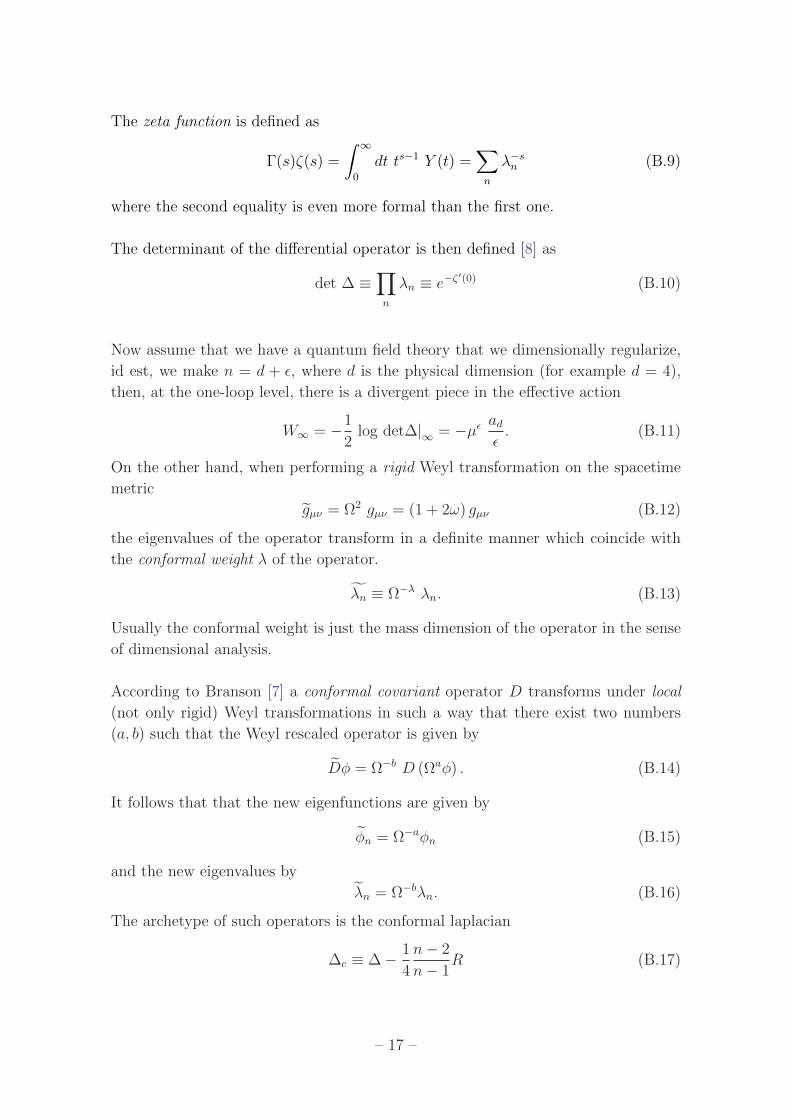
The zeta function is defined as

Γ(s)ζ(s) =

∫ ∞0

dt ts−1 Y (t) =∑n

λ−sn (B.9)

where the second equality is even more formal than the first one.

The determinant of the differential operator is then defined [8] as

det ∆ ≡∏n

λn ≡ e−ζ′(0) (B.10)

Now assume that we have a quantum field theory that we dimensionally regularize,

id est, we make n = d + ε, where d is the physical dimension (for example d = 4),

then, at the one-loop level, there is a divergent piece in the effective action

W∞ = −1

2log det∆|∞ = −µε ad

ε. (B.11)

On the other hand, when performing a rigid Weyl transformation on the spacetime

metric

gµν = Ω2 gµν = (1 + 2ω) gµν (B.12)

the eigenvalues of the operator transform in a definite manner which coincide with

the conformal weight λ of the operator.

λn ≡ Ω−λ λn. (B.13)

Usually the conformal weight is just the mass dimension of the operator in the sense

of dimensional analysis.

According to Branson [7] a conformal covariant operator D transforms under local

(not only rigid) Weyl transformations in such a way that there exist two numbers

(a, b) such that the Weyl rescaled operator is given by

Dφ = Ω−b D (Ωaφ) . (B.14)

It follows that that the new eigenfunctions are given by

φn = Ω−aφn (B.15)

and the new eigenvalues by

λn = Ω−bλn. (B.16)

The archetype of such operators is the conformal laplacian

∆c ≡ ∆− 1

4

n− 2

n− 1R (B.17)

– 17 –

which is such that

∆c

(Ω−

n−22 φ

)= Ω−

n+22 ∆φ. (B.18)

There are no known diffeomorphisms invariant operators built out of the metric alone

with b = 0.

In the case of the standard scalar laplacian,

∆ ≡ ∇2 ≡ 1√g∂µ (gµν

√g∂ν) (B.19)

the conformal weight coindices with its mass dimension, λ = 2.

The new zeta function after the Weyl transformation is given in general by

ζ(s) = ΩDs ζ(s) (B.20)

so that the determinant defined through the ζ-function scales as

det ∆ = Ω−λζ(0) det ∆ (B.21)

and this modifies correspondingly the effective action

W = W + λ ω ζ(0). (B.22)

The energy-momentum tensor is defined in such a way that under a general variation

of the metric the variation of the effective action reads

δW ≡ 1

2

∫d(vol)xTµνδg

µν (B.23)

which in the particular case that this variation is proportional to the metric tensor

itself (like in a conformal transformation at the lineal level), δgµν = −2ωgµν yields

the integrated trece of the energy-momentum tensor

δW = −∫d(vol)ωT. (B.24)

Conformal invariance in the above sense then means that the energy-momentum

tensor must be traceless. When quantum corrections are taken into account, it

follows that

−∫d(vol)T = λ ζ(0). (B.25)

It is not difficult to show that

ζ(0) ≡ lims→0

s

∫ ∞0

dt ts−1Y (t) = lims→0

s

∫ 1

0

dt ts−1Y (t) = ad (B.26)

– 18 –

where n = d is the specific value of the spacetime dimension. The conformal anomaly

is usually then written as

−∫d(vol)T = λad. (B.27)

The Schwinger-de Witt coefficient corresponding to the physical dimension, n = d

precisely coincides with the divergent part of the effective action when computed

in dimensional regularization as indicated above. This means that in order to com-

pute the one loop conformal anomaly in many cases it is enough to compute the

corresponding counterterm.

This argument shows clearly that when the conformal weight of the operator of

interest vanishes, λ = 0 all eigenvalues remain invariant and there is no conformal

anomaly for determinants defined through the zeta function. In our case this will

follow from the manifest Weyl invariance of the construction of the operator at all

steps. This conformal invariance in turn in inherited from the mother theory which

enjoys invariance under area preserving diffeomorphisms only. This is the origin of

the background dilaton σ of gravitational origin, essential in our approach.

– 19 –

Acknowledgments

We have enjoyed many discussions with Luis Alvarez-Gaume. This work has been

partially supported by the European Union FP7 ITN INVISIBLES (Marie Curie Ac-

tions, PITN- GA-2011- 289442)and (HPRN-CT-200-00148) as well as by FPA2009-

09017 (DGI del MCyT, Spain) and S2009ESP-1473 (CA Madrid). M.H. acknowl-

edges a ”Campus de Excelencia” grant from the Departamento de Fısica Teorica of

the UAM. The authors acknowledge the support of the Spanish MINECOs Centro

de Excelencia Severo Ochoa Programme under grant SEV-2012-0249.

References

[1] E. Alvarez and A. F. Faedo, “Unimodular cosmology and the weight of energy,”

Phys. Rev. D 76, 064013 (2007) [hep-th/0702184].

E. Alvarez and M. Herrero-Valea, “Unimodular gravity with external sources,”

arXiv:1209.6223 [hep-th].

[2] E. Alvarez and A. F. Faedo, “Renormalized Kaluza-Klein theories,” JHEP 0605, 046

(2006) [hep-th/0602150].

E. Alvarez, A. F. Faedo and J. J. Lopez-Villarejo, “Ultraviolet behavior of transverse

gravity,” JHEP 0810, 023 (2008) [arXiv:0807.1293 [hep-th]].

[3] D. Blas, ‘Aspects of Infrared Modifications of Gravity,” arXiv:0809.3744 [hep-th].

[4] M. J. Duff, “Twenty years of the Weyl anomaly,” Class. Quant. Grav. 11, 1387

(1994) [hep-th/9308075].

[5] L. P. Eisenhart, ”Non-Riemannian Geometry” (Dover,NY,2005)

[6] G. W. Gibbons, S. W. Hawking and M. J. Perry, “Path Integrals and the

Indefiniteness of the Gravitational Action,” Nucl. Phys. B 138, 141 (1978).

[7] J. Erdmenger, “Conformally covariant differential operators: Properties and

applications,” Class. Quant. Grav. 14, 2061 (1997) [hep-th/9704108].

[8] S. W. Hawking, “Zeta Function Regularization of Path Integrals in Curved

Space-Time,” Commun. Math. Phys. 55, 133 (1977).

[9] M. Henneaux and C. Teitelboim, “Quantization of gauge systems,” Princeton, USA:

Univ. Pr. (1992) 520 p

[10] G. ’t Hooft, “Probing the small distance structure of canonical quantum gravity

using the conformal group,” arXiv:1009.0669 [gr-qc].

M. J. G. Veltman, “Quantum Theory of Gravitation,” Conf. Proc. C 7507281, 265

(1975).

– 20 –

[11] Y. J. Ng and H. van Dam, “Unimodular Theory Of Gravity And The Cosmological

Constant,” J. Math. Phys. 32, 1337 (1991).

[12] L. Smolin, “The Quantization of unimodular gravity and the cosmological constant

problems,” Phys. Rev. D 80, 084003 (2009) [arXiv:0904.4841 [hep-th]].

HEP :: Search :: Help Powered by Invenio v1.0.0-rc0+ Problems/Questions to

feedback@inspirehep.net

– 21 –