MIT-CTP/4298

Exactly Stable Collective Oscillations inConformal Field Theory

Ben Freivogel, John McGreevy and S. Josephine Suh

Center for Theoretical Physics, MIT, Cambridge, Massachusetts 02139, USA

Abstract

Any conformal field theory (CFT) on a sphere supports completely undamped collective

oscillations. We discuss the implications of this fact for studies of thermalization using

AdS/CFT. Analogous oscillations occur in Galilean CFT, and they could be observed in

experiments on ultracold fermions.

September 2011; revised December 2011

1

arX

iv:1

109.

6013

v2 [

hep-

th]

28

Dec

201

1

I. INTRODUCTION

Conformal field theories (CFTs) are interesting for many reasons: they arise in the study

of critical phenomena, on the worldsheet of fundamental strings, and in the holographic dual

of anti-de Sitter spacetimes [1–3]. It is plausible that all quantum field theories are relevant

deformations of conformally invariant ultraviolet fixed points.

Here we describe an exotic property of any CFT in any number of dimensions. Any

relativistic CFT whose spatial domain is a sphere contains a large class of non-stationary

states whose time evolution is periodic, with frequencies that are integer multiples of the

inverse radius of the sphere.

Nonrelativistic CFTs that realize the Schrodinger algebra also support undamped oscil-

lations in the presence of a spherically symmetric harmonic potential. Cold fermionic atoms

with tuned two-body interactions can provide an experimental realization of such a system,

and the modes we discuss (which, in this context, have been discussed previously in [4])

could be (but have not yet been) observed.

The existence of these permanently oscillating many-body states is guaranteed by sl(2,R)

subalgebras of the conformal algebra, formed from the Hamiltonian and combinations of

operators which act as ladder operators for energy eigenstates. It is striking that any CFT

in any dimension, regardless of the strength or complication of its interactions, has states

that undergo undamped oscillation.

We emphasize the distinction between these oscillating states and an energy eigenstate

of an arbitrary Hamiltonian. Time evolution of an energy eigenstate is just multiplication

of the wavefunction by a phase – nothing happens. Given knowledge of the exact energy

eigenstates of any system, one may construct special operators whose correlations oscillate

in time in certain states. In contrast, we show below that in the states described here,

accessible physical quantities such as the energy density vary in time (at leading order in N2

in holographic examples). Further, the oscillations arise and survive at late times starting

from generic initial conditions1.

The persistence of these oscillations conflicts with conventional expectations for thermal-

ization of an interacting theory. The conventional wisdom is that an arbitrary initial state

will settle down to an equilibrium stationary configuration characterized by its energy and

angular momenta (for a recent discussion of this expectation, see [5]). This is not the case

1 We explain the precise sense in which they are generic in III.

2

for CFT’s due to the presence of these undamped oscillations.

The existence of these modes is due to the existence of extra conserved charges in CFT

generated by conformal Killing vectors. Any conserved charge will partition the Hilbert space

of a system into sectors which do not mix under time evolution. However, in the conventional

situation there will be be a stationary state for each value of the charges which represents

equilibrium in that sector. The states we describe do not approach a stationary state; rather,

the amplitude of the oscillations is a conserved quantity, as we explain in Section III.

Any system with a finite number of degrees of freedom will exhibit quasiperiodic evolution:

the time dependence of e.g. a correlation function in such a system is inevitably a sum of a

finite number of Fourier modes. The class of oscillations we describe can be distinguished

from such generic behavior in two respects: First, for each oscillating state the period is fixed

to be an integer multiple of the circumference of the sphere. Second, and more importantly,

the oscillations persist and remain undamped in a particular thermodynamic limit – namely,

a large-N limit where the number of degrees of freedom per site diverges. Many such CFTs

are described by classical gravity theories in asymptotically anti-de Sitter spacetime (AdS).

The latter fact points to a possible obstacle in studying thermalization of CFTs on a

sphere using holography: when subjecting the CFT to a far-from-equilibrium process, if one

excites such a mode of oscillation, this excitation will not go away, even at infinite N . (The

simplest way to circumvent this obstable is to study CFT on the plane. Then this issue does

not arise, as the frequency of the modes in question goes to zero.)

In holographic theories, certain oscillating states with period equal to the circumference of

the sphere have an especially simple bulk description. Begin with a Schwarzschild-AdS black

hole in the bulk. This is dual to a CFT at finite temperature on the boundary. Now boost

the black hole. This boost symmetry is an exact symmetry of AdS, and it creates a black

hole that “sloshes” back and forth forever2. The dual CFT therefore has periodic correlators.

The boosted black hole is related to the original black hole by a large diffeomorphism that

acts nontrivially on the boundary. The boundary description of the boosting procedure is to

act with a conformal Killing vector on the thermal state. The relevant CKV’s are periodic

in time, and they act nontrivially on the thermal state, so they produce oscillations.

This document is organized as follows: In section II we construct the oscillating states

explicitly. In section III we describe conserved charges associated with conformal symmetry

2 Such oscillations are known to S. Shenker and L. Susskind as “sloshers”. The action of conformal boosts

on AdS black holes has been studied previously in [6].

3

whose nonzero expectation value diagnoses oscillations in a given state. We also derive

operator equations which demonstrate that certain ` = 1 moments of the stress-energy

tensor in CFT on a sphere behave like harmonic oscillators. In section IV we specialize to

holographic CFTs and discuss the gravitational description of a specific class of oscillations

around thermal equilibrium. In section V, we discuss the effect of the existence of oscillating

states on correlation functions of local operators. We end with some explanation of our initial

motivation for this work and some comments and open questions. Appendix A summarizes

the conformal algebra. Appendix B gives some details on the normalization of the oscillating

states. Appendix C extends Goldstone’s theorem to explain the linearized oscillations of

smallest frequency. Appendix D constructs one of the consequent linearized modes of the

large AdS black hole, following a useful analogy with the translation mode of the Schwarzchild

black hole in flat space. Appendix E constructs finite oscillations of an AdS black hole and

calculates observables in the dual CFT. In the final Appendix F, we explain that an avatar of

these modes has already been studied in experiments on cold atoms, and that it is in principle

possible to demonstrate experimentally the precise analog of these oscillating states.

II. STABLE OSCILLATIONS IN RELATIVISTIC CFT ON A SPHERE

Consider a relativistic CFT on a d-sphere cross time. We set c = 1 and measure energies

in units of the inverse radius of the sphere, R−1. The conformal algebra acting on the Hilbert

space of the CFT contains d (non-independent) copies of the sl(2,R) algebra,

[H,Li+] = Li+, [H,Li−] = −Li−, [Li+, Li−] = 2H (II.1)

(with no sum on i in the last equation) as reviewed in Appendix A. Here i = 1...d is an index

labeling directions in the Rd in which Sd−1 is embedded as the unit sphere.

We construct the oscillating states in question using the sl(2,R) algebras as follows. Let

|ε〉 be an eigenstate of H, H|ε〉 = ε|ε〉. Consider a state of the form

|Ψ(t = 0)〉 = N eαL++βL−|ε〉, (II.2)

where L+ = Li+ and L− = Lj− for some i, j ∈ 1, ..., d, N is a normalization constant given

in Appendix B, and α and β are complex numbers. If α, β are chosen so that the operator

in (II.2) is unitary, there is no constraint on α, β from normalizability; more generally, finite

4

N constrains α, β as described in Appendix B. It evolves in time as3

|Ψ(t)〉 = N e−iHteαL++βL−|ε〉 = N eαe−itL++βeitL−e−iHt|ε〉 = N e−iεteα(t)L++β(t)L− |ε〉, (II.3)

where α(t) = αe−it and β(t) = βeit. |Ψ〉 has been constructed in analogy with coherent

or squeezed states in a harmonic oscillator, where one also has ladder operators for the

Hamiltonian. Restoring units, |Ψ〉 is seen to oscillate with frequency 1/R.

More generally, the time evolution of a state

|Ψ(t = 0)〉 = g(L1+, ..., L

d+, L

1−, ..., L

d−)|ε〉 (II.4)

where g is any regular function of the 2d variables Li+, Lj−, 1 ≤ i, j ≤ d, is given by replacing

Li± with Li±e±it ∀ i. For example, oscillating state with frequency 2/R is given by (II.4)

with g =∑∞

m=01

(m!)2

(αL2

+ + βL2−)m

, where L+ can be any of Li+, 1 ≤ i ≤ d, and similarly

for L−.4 Note, however, that not every such function g produces an oscillating state - a

state in which physical quantities such as energy density display oscillation - as opposed to

a state whose time evolution is given by a trivial but nonetheless periodic factor, as with

an energy eigenstate. Take for example g = L+, which merely produces another eigenstate.

The criterion for oscillation which we establish in section III below (〈Q±,i〉 6= 0 for some i)

can be applied to an initial state |Ψ(t = 0)〉 = g|ε〉 to determine whether |Ψ〉 is indeed an

oscillating state. In addition, normalizability of |Ψ〉 will constrain the function g in a manner

which we have not determined.

To retain the simple time evolution in the above construction, the stationary state |ε〉cannot be replaced by a nonstationary state

∑i

ci|εi〉, with terms that evolve in time with

distinct phases. However, it can be replaced by a stationary density matrix ρ, which evolves

in time with a phase A (possibly zero),

[H, ρ] = Aρ. (II.5)

Examples include an energy eigenstate ρ = |ε〉〈ε|, and thermal density matrices ρ =

e−βHZ−1β . Given such a ρ, an initial ensemble

ρ(t = 0) = N eαL++βL−ρeβ∗L++α∗L− (II.6)

3 This can be checked using the Baker-Campbell-Hausdorff formula eBAe−B =∞∑n=0

1n! (adB)nA.

4 The coefficient (m!)2

is designed to give the state a finite norm. We note that a state of the form (II.4)

with g = eαLn++βLn

− is only normalizable for n = 0, 1; in particular, the direct analog of a squeezed state

does not seem to exist.

5

evolves in time as

ρ(t) = N e−iAteα(t)L++β(t)L−ρeβ(t)∗L++α(t)∗L− . (II.7)

We refer to the collective oscillation ρ as having been “built on” ρ, in the same way |Ψ〉was built on |ε〉, by acting with a sufficiently constrained function of ladder operators g at

t = 0. In section IV, we give a holographic description of the subset of oscillations built on

a thermal density matrix for which g = eαL++βL− and αL+ + βL− is anti-Hermitian.

III. DIAGNOSING THE AMPLITUDE OF OSCILLATIONS

It may be useful to be able to diagnose the presence of the above oscillations in a generic

state of a CFT. Here we identify conserved charges associated with conformal Killing vectors,

which correspond to the conserved amplitudes of possible oscillations.

Consider CFT on a spacetime M . Given a conformal Killing vector field (CKV) ξµ on

M , there is an associated current and charge acting in the Hilbert space of the CFT

jµξ = T µνξν , Qξ =

∫Σ

dd−1x√g jµξ nµ, (III.1)

where Σ is a spatial hypersurface and nµ is a normal vector. ∇µjµξ is given by a state-

independent but ξ-dependent constant

∇µjµξ = ∇µT

µν + T µν(∇µξν +∇νξµ) = αξTµµ , (III.2)

where αξ = 2d∇µξ

µ is a c-number which vanishes when ξµ is an exact Killing vector field

(KV)5. Then ddtQξ =

∫Σdd−1x

√g αξT

µµ nt, which vanishes for CFT on R × Sd−1 as follows.

The trace anomaly has angular momentum ` = 0. The proper CKVs have ` = 1 and hence

the associated αξ have ` = 1. The integral over the sphere vanishes and Qξ is exactly

conserved.

ξµ’s can be obtained explicitly by projecting Jab = i(Xa∂b −Xb∂a), a, b = −1, 0, 1, ..., d

in R(2,d) to the r → ∞ boundary of AdSd+1, the hypersurfaced∑i=1

Ωi 2 = 1 in coordinates

(r, t,Ω1, ...,Ωd) with r ≥ 0, −∞ < t <∞, defined by

X−1 = R√

1 + r2 cos t, (III.3)

X0 = R√

1 + r2 sin t, (III.4)

Xi = RrΩi. (III.5)

5 Note that in (III.2) we have assumed Tµν is both symmetric and traceless, up to a trace anomaly.

6

In particular, CKVs which are not KVs, corresponding to boosts J±,i ≡ J−1,i ± iJ0,i in

R(2,d), are

ξ±,i = ∓ie±it Ωi∂t − e±it[(1− Ωi2)∂Ωi − Ωi

∑j 6=i

Ωj∂Ωj

]∣∣∣∣∑k

Ωk 2=1

. (III.6)

Letting

[(1 − Ωi2)∂Ωi − Ωi

∑j 6=i

Ωj∂Ωj

]∣∣∣∣∑k

Ωk 2=1

≡ f iα(θ)∂θα where θα, α = 1, ..., d − 1 are

coordinates on Sd−1, the associated charges are

Q±,i = ∓ie±it∫Sd−1

dd−1θ√g TttΩ

i − e±it∫

Sd−1

dd−1θ√g Ttαf

iα(θ). (III.7)

Now consider the quantities

X i ≡∫Sd−1

dd−1θ√g TttΩ

i, P i ≡ −∫Sd−1

dd−1θ√g Ttαf

iα(Ω) . (III.8)

These are the ith coordinate of the center of mass of the CFT state in the embedding space

of Sd−1, and its momentum, respectively. From conservation of the charges Q±,i, they satisfy

the operator equations

X i − P i = 0 P i + X i = 0 (III.9)

– they undergo simple harmonic oscillation. From (III.7), the initial conditions for these

oscillations are determined by the conformal charges.

It follows that given an arbitrary state, if any of the 2d expectation values 〈Q±,i〉 are non-

zero at t = 0, some of the non-complex, physical quantities 〈X i〉 and 〈P i〉 will oscillate with

undying amplitude. The fact that 〈Q±,i〉 6= 0 for some i is an open condition justifies our use

of the word ‘generic’ in the Introduction. As a check that the condition is a good criterion

for physical oscillation, note that if |Ψ〉 is an energy eigenstate, 〈Ψ|Q±,i|Ψ〉 = 0. This follows

from 〈Ψ|[H,Q±,i]|Ψ〉 = 〈Ψ| ± Q±,i|Ψ〉 = 0 6 using H|Ψ〉 = E|Ψ〉. On the other hand,

〈Ψ|Q±,i|Ψ〉 = 0 ∀ i does not imply that |Ψ〉 is an energy eigenstate, indicating that there are

non-oscillating states which are not energy eigenstates. Take for example a superposition of

energy eigenstates |Ψ〉 = |Ψ1〉+ |Ψ2〉, where |Ψ1〉 and |Ψ2〉 belong to different towers in the

CFT spectrum, where each tower is built on ladder operators acting on a primary energy

eigenstate. Then clearly 〈Ψ|Q±,i|Ψ〉 = 0 ∀ i, although |Ψ〉 is not an eigenstate.

6 Q±,i = e±itLi±, as explained in following paragraph.

7

Finally, we clarify a potentially confusing point. By construction, all of the (d+2)(d+1)2

charges QAB are time-independent. There is one associated with each generator of the

conformal group in d dimensions; on general grounds of Noether’s theorem, they satisfy the

commutation relations of so(2, d). Since the Hamiltonian for the CFT on the sphere H is

one of these generators, and H is not central (e.g. [H,Li±] = ±Li±), there may appear to

be a tension between the two preceding sentences. Happily, there is no contradiction: the

time evolution of the conformal charges Q±,i arising from their failure to commute with the

time-evolution operator is precisely cancelled by the explicit time dependence of the CKVs

ξ±,i:d

dtQ±,i = ∂tQ

±,i − i[H,Q±,i] = 0. (III.10)

Thus Q±,i = e±itLi±.

IV. HOLOGRAPHIC REALIZATION OF OSCILLATIONS

The discussion in the previous sections applies to any relativistic CFT on the sphere. We

now turn to the case of holographic CFTs and the dual gravitational description of a special

class of collective oscillations built on thermal equilibrium, for which g = eαL++βL− and is

anti-Hermitian.

A. Bouncing Black Hole

Consider a relativistic CFTd with a gravity dual, on Sd−1. We focus on collective oscilla-

tions of the form in (II.7), built on the thermal density matrix ρ = Z−1β

∑ε e−βε|ε〉〈ε|, with

the parameter αL+ + βL− restricted to be anti-Hermitian. With this restriction, eαL++βL−

is a finite transformation in SO(2, d).

The gravity dual of such a state can be constructed by a ‘conformal boost’ of a black

hole, as follows. Begin with the static global AdS black hole dual to ρ [3, 7]. Now consider

a non-normalizable bulk coordinate transformation, which reduces to the finite conformal

transformation eαL++βL− at the UV boundary of AdS. Such a transformation falls off too

slowly to be gauge identification, but too fast to change the couplings of the dual CFT; it

changes the state of the CFT.

For example, a coordinate transformation that corresponds to the boost J01 in the em-

bedding coordinates (X−1, X0, X1, ..., Xd) of AdSd+1, maps empty AdSd+1 to itself, but will

8

produce a collective oscillation when acting on a global AdS black hole7. The CFT state at

some fixed time is of the form

N eα(L1+−L1

−)

(∑ε

e−βε|ε〉〈ε|

)eα∗(L1−−L1

+) (IV.1)

where α is the boost parameter and real, and evolves as in (II.7) with phase A = 0. In

Appendix E, we discuss the bouncing black hole obtained from such a boost of the BTZ

black hole. We exhibit oscillations of the stress-energy tensor expectation value and of

entanglement entropy of a subregion in the corresponding mixed state.

B. Bulk Modes

In the CFT, excitations corresponding to oscillations of the form in (IV.1) are created

by modes of the stress-energy tensor – linear combinations of L+ and L− – acting on the

thermal ensemble. They can be interpreted as Goldstone excitations resulting from the

breaking of conformal symmetry by the thermal state of the CFT. We elaborate on this

point in Appendix C.

For simple large-N gauge theories, these L± are single-trace operators. The above excita-

tions then translate holographically to single-particle modes in the form of solutions to the

linearized equation of motion for the metric in the bulk. They have ` = 1 on Sd−1, as all

conformal generators including L± have ` = 1. Their frequency is ω = ±1/R – oscillations

of higher frequency are built with exponentials of higher powers of the stress-energy tensor,

and correspond to multi-particle states.

In Appendix D, we construct one such ` = 1 mode in the global AdS4-Schwarzschild

background, from which the others can be obtained by transformations in SO(2) × SO(3).

In general d, the d·2 bulk modes in question will be related by symmetries in SO(2)×SO(d).8

Note that in empty global AdS, there are no analogous ` = 1 modes, as all global conformal

generators annihilate the vacuum in CFT. However, there are single-particle modes which are

7 The reader may be worried about ambiguities in the procedure of translating a KV on AdSd+1 into a

vector field on the AdS black hole. The UV boundary condition and choice of gauge grµ = 0 appears to

make this procedure unique; this is demonstrated explicitly for the linearized modes in appendix D.8 These modes are not compatible with the Regge-Wheeler gauge for the metric [8] common in the literature

on quasinormal modes. They are perturbations of the metric due to coordinate transformations that

asymptote to conformal transformations on the boundary; these coordinate transformations do not preserve

the Regge-Wheeler gauge. As such, they were not identified in the spectrum of quasinormal modes of the

metric in AdS black holes studied in the Regge-Wheeler gauge [9–13].

9

dual in the CFT to states created by single-trace primary operators acting on the vacuum,

and descendant states obtained by acting with Ln+ for some integer n ≥ 1 on such primary

states. The latter correspond to linearized oscillations built on energy eigenstates. Together

these single-particle modes are a subset of normal modes found in AdS (see e.g. [13], [14]).

V. CONSEQUENCE FOR CORRELATION FUNCTIONS

What does the existence of these modes imply for thermalization as measured by corre-

lation functions of local operators?

A generic correlation function G(t) in a thermal state will decay exponentially in time

to a mean value associated with Poincare recurrences which is of order e−S. In a large-N

CFT, S ∼ T d−1V N2. This Poincare-recurrence behavior of G is therefore of order e−N2, and

does not arise at any order in perturbation theory. We expect the contributions to generic

correlators at any finite order in the 1/N expansion to decay exponentially in time like e−aT t

where a is some order-one numerical number. From the point of view of a bulk holographic

description, this is because waves propagating in a black hole background fall into the black

hole; the amplitude for a particle not to have fallen into the black hole after time t should

decay exponentially, like e−aT t. At leading order in N2, i.e. in the classical limit in the bulk,

G(t) decays exponentially in time at a rate determined by the least-imaginary quasinormal

mode of the associated field. A process whereby the final state at a late time t 1/T is

correlated with the initial state is one by which the black hole retains information about

its early-time state, and hence one which resolves the black hole information problem; this

happens via contributions of order e−N2

[15].

The preceding discussion of Poincare recurrences is not special to CFT. In CFT, there are

special correlators which are exceptions to these expectations. A strong precedent for this

arises in hydrodynamics, where correlators of operators which excite hydrodynamic modes

enjoy power-law tails Gspecial(t) ∼ 1st−b, where s is the entropy density and b is another

number. In deconfined phases of large-N theories, s ∝ N2 and the long-time tails arise as

loop effects in the bulk [16]. For the high-temperature phase of of large-N CFTs with gravity

duals, the necessary one-loop computation was performed by [17].

A similar situation obtains for large-N CFTs on the sphere. While correlation functions

for generic operators have perturbative expansions in N which decay exponentially in time

10

and (non-perturbatively) reach the Poincare limit e−N2

at late times,

Ggeneric(t) ∼∞∑g=0

cge−agTtN2−2g + c∞e

−N2

, (V.1)

special correlation functions are larger at late times.

One very special example is given by

Gvery special(t) ≡ 〈L−(t)L+(0)〉T .

Using [H,L−] = − 1RL− we have

Gvery special(t) = e−it/R〈L−(0)L+(0)〉T

and hence ∣∣∣∣Gvery special(t)

Gvery special(0)

∣∣∣∣ = 1 ;

the amplitude of this correlation does not decay at all. This is analogous in hydrodynamics

to correlations of the conserved quantities themselves, such as P i(k = 0), which are time

independent.

There are other operators, in particular certain modes of the stress-energy tensor, which

can excite and destroy the oscillations we have described, and therefore have non-decaying

contributions to their autocorrelation functions. These receive oscillating contributions at

one loop, in close analogy with the calculation of [17], which finds

〈T xy(t, k = 0)T xy(0, k = 0)〉T = T 2

∫k

(Gxtxt(t, k)Gytyt(t, k) +Gxtyt(t, k)Gxtyt(t, k)

)(V.2)

where Gabcd(t, k) ≡ 〈T ab(t, k)T cd(0,−k)〉T . This is most easily understood (when a gravity

dual is available) via the bulk one-loop Feynman diagram: The con-

tribution from k = 0 in the momentum integral dominates at late times and produces the

power-law tail in t.

The analog in CFT on Sd−1 is given by the lowest angular-momentum mode of stress-

energy tensor Oπ =∫Sd−1 Tijπ

ij where π is a transverse traceless J = 2 ( ~J = ~L + ~S) tensor

spherical harmonic. The leading contribution to 〈Oπ(t)Oπ(0)〉T at late times can again be

described by the one-loop diagram above. The intermediate state now involves a sum over

angular momenta rather than momenta; the term where both of the intermediate gravitons

11

sit in the oscillating mode gives a contribution proportional to eit/R which does not decay;

all other contributions decay exponentially in time.

Similarly, if we have additional conserved global charges in our CFT, we can construct

non-decaying contributions where the graviton is in the oscillating mode and the bulk photon

line carries the conserved charge, as follows: This is analogous to the

long-time tails in current-current correlators in hydrodynamics.

This paper [18] observes oscillations in real-time correlation functions in finite-volume

CFT in 1+1 dimensions. Some of the explicit formulae are special to 1+1 dimensions. Also,

[15] presents some such correlators.

VI. DISCUSSION

We provide some context for our thinking about these oscillating states, which could have

been studied long ago9, and in particular for thinking about collective oscillations dual to

bouncing black holes.

Our initial motivation was to consider whether it is always the case that the entanglement

entropy of subregions in QFT grows monotonically in time. If an entire system thermalizes,

a subsystem should only thermalize faster, since the rest of the system can behave as a

thermal bath.

However, it is well-known that a massive particle in global AdS oscillates about ρ = 0 in

coordinates where

ds2 = R2(− cosh ρ2dt2 + dρ2 + sinh ρ2dΩ2), (VI.1)

with a period of oscillation 2πR. This is because the geometry is a gravitational potential

well. Massive geodesics of different amplitudes of oscillation about ρ = 0 are mapped to each

other by isometries of AdS. Specifically, the static geodesic ρ = 0 for all t can be mapped to

a geodesic oscillating about ρ = 0 by a special conformal transformation.

9 We are aware of the following related literature: Recently, very similar states were used as ground-like

states for an implementation of an AdS2/CFT1 correspondence [19]. Coherent states for SL(2,R) were

constructed in [20]. The states we study are not eigenstates of the lowering operator L−, but rather

of linear combinations of powers of L+ and L−, and H. [19] builds pseudocoherent states which are

annihilated by a linear combination of L− and H. Other early work which emphasizes the role of SL(2,R)

representation theory in conformal quantum mechanics is [21].

12

The effect of a massive object in the bulk on the entanglement entropy of a subregion in

the dual CFT is proportional to its mass in Planck units (see section 6 of [22]). Only a very

heavy object, whose mass is of order N2, will affect the entanglement entropy at leading

order in the 1/N2 expansion (which is the only bit of the entanglement entropy that we

understand holographically so far). A localized object in AdS whose mass is of order N2 is

a large black hole. Therefore, by acting with an AdS isometry on a global AdS black hole,

one can obtain a state in the CFT in which the entanglement entropy oscillates in time.

But this bouncing black hole is none other than the dual description of a collective oscil-

lation built on thermal equilibrium, as introduced near (IV.1). (Recall that in systems with

a classical gravity dual, the thermal ensemble at temperature of order N0 is dominated by

energy eigenstates with energy of order N2. ) The existence of this phenomenon is not a

consequence of holography, but rather merely of conformal invariance.

An important general goal is to clarify in which ways holographic CFTs are weird because

of holography and in which ways they are weird just because they are CFTs. Our analysis

demonstrates that these oscillations are an example of the latter. The effect we have de-

scribed arises because of the organization of the CFT spectrum into towers of equally-spaced

states.

In holographic calculations, there is a strong temptation to study the global AdS extension

because it is geodesically complete. This means compactifying the space on which the CFT

lives by adding the ‘point at infinity’. We have shown here that this seemingly-innocuous

addition can make a big difference for the late-time behavior!

We close with some comments and open questions.

1. How are these oscillations deformed as we move away from the conformal fixed point?

What does adding a relevant operator do to the oscillations? Such a relevant deforma-

tion should produce a finite damping rate for the mode. This damping rate provides

a new scaling function – it has dimensions of energy and can depend only on R and

the coupling of the relevant perturbation g, and must vanish as g → 0. If the scaling

dimension of g is ν, the damping rate is Γ(g,R) = g1/νΦ(gRν) where Φ(x) is finite as

x→ 0. It may be possible to determine this function Φ holographically.

2. If we consider the special case of a CFT which is also a superconformal field theory,

there are other stable oscillations that we can make by exponentiating the action of the

fermionic symmetry generators Sα±. Since [H,Sα±] = ±Sα±, these modes have frequency

13

12R

. Fermionic exponentials are simple, and these states take the form

|a(t)〉 = eaα(t)Sα+|∆〉 =(1 + aα(t)Sα+

)|∆〉 (VI.2)

with a(t) = eit/2Ra(0).

3. We can define an analog for the bouncing black hole of the Aichelberg-Sexl shockwave

[23] that results from a lightlike boost a Schwarzchild black hole in flat space. Here

one takes the limit of lightlike boost β →∞, while simultaneously reducing the mass

to keep the energy fixed. In this limit of the bouncing black hole, which merits further

study, the profile of the boundary energy density is localized on the wavefront.

4. For which background geometries M can such states of CFT be constructed? A suf-

ficient condition is the existence of a CKV ξ on M whose Lie bracket with the time-

translation generator ∂t is of the form [∂t, ξ] = cξ for some constant c. It would be

interesting to decide whether there exist spacetimes M with such CKVs where the

constant c remains finite as the volume of M is taken to infinity (unlike Sd−1 × Rwhere c = R−1 → 0). This would be interesting because in finite volume theories do

not thermalize anyway (at finite N) because they are not in a thermodynamic limit.

5. It would be interesting to generalize these oscillations to CFTs on spacetimes with

boundary, with conformal boundary conditions.

6. The recent paper [24] also identifies undamped oscillating states in holographic CFTs

on S2 using AdS gravity. These ‘geons’ are normalizible of classical AdS gravity with

frequency of oscillation n/R. They clearly differ from the states constructed above

in that they are excitations above the AdS vacuum, whereas our construction relies

on broken conformal invariance. There has been also some interesting recent work on

damped oscillations in the approach to equilibrium in scalar collapse in AdS [25].

14

Acknowledgements

We thank Ethan Dyer, Gary Horowitz, Roman Jackiw, Matthew Kleban, Lauren Mc-

Gough, Mike Mulligan, Massimo Porrati, Steve Shenker, Lenny Susskind, Brian Swingle,

Erik Tonni and Martin Zwierlein for discussions, comments and encouragement. This work

was supported in part by funds provided by the U.S. Department of Energy (D.O.E.) under

cooperative research agreement DE-FG0205ER41360, and in part by the Alfred P. Sloan

Foundation.

Appendix A: Conformal Algebra

Take the coordinates of the flat spacetime on which the global conformal group SO(2, d)

acts linearly to be (X−1, X0, X1, ..., Xd), with signature (−,−,+, ...,+). This is the embed-

ding space of AdSd+1 with boundary R×Sd−1. The compact subgroups SO(2) and SO(d) of

SO(2, d) correspond to time translation and spatial rotations in R×Sd−1, and are generated

by rotations J−10 and Jij, i, j = 1, ..., d. In order to identify ladder operators acting on

eigenstates of the Hamiltonian on Sd−1, H = −J−10, we will situate Jµν in an so(1, d+ 1)

algebra [26] with generators adapted to the global conformal symmetry of Rd.1011

D′ = −iJ−10 = iH, M ′ij = Jij, P ′i = Ji,−1 + iJi0 ≡ Li+, K ′i = Ji,−1 − iJi0 ≡ Li− . (A.1)

Note it was necessary to Euclideanize flat spacetime from R(1,d−1) to Rd in order to

identify the Hamiltonian in radially quantized R × Sd−1 with the dilation operator in flat

spacetime. Now, from the familiar relations [D′, P′i ] = iP

′i , [D

′, K

′i ] = −iK ′i , and [P

′i , K

′j] =

−2i(gijD′ −M ′

ij) in Rd, one can easily identify d copies of the SL(2,R) algebra with H as

the central operator,

[H,Li+] = Li+, [H,Li−] = −Li−,[Li+, L

j−] = 2Hδij + 2iM ′ij, [Li±, L

j±] = 0. (A.2)

10 Our conventions are Jab = i(Xa∂b − Xb∂a), [Jab, Jcd] = i(gadJbc + gbcJad − gacJbd − gbdJac) for a, b =

−1, 0, 1, ..., d. The so(1, d + 1) algebra is manifest in the basis J′

−10 = D′, J′

ij = Jij , J′

−1i = (P′

i −K′

i)/2, J′

0i = (P′

i +K′

i)/2 with signature (−,+,+, ...,+).11 Generators of so(1, d+1) adapted to the conformal symmetry of Rd, which we denote using primed letters

D′,M ′ij , P′i ,K

′i, can be related to generators of so(2, d) adapted to the conformal symmetry of R1,d−1,

D,Mij , Pi,Ki, by expressing the latter generators in terms of rotations J−10 and Jij in AdSd+1. In

particular, in the isomorphism between D,Mij , Pi,Ki and J−10, Jij, J0−1 = 12 (P0 +K0), from which

we see D′ = iH = iJ0−1 = i 12 (P0 +K0).

15

Note the raising (lowering) operators commute with raising (lowering) operators, but raising

operators do not commute with lowering operators.

Appendix B: Norms of coherent states

Using formulas found in [27], we can determine the norm of a general coherent state of the

form (II.2). For definiteness, will consider here coherent states built on energy eigenstates

of the form |m, ε0〉 ∝ Lm+ |ε0〉 with |ε0〉 a primary state. The norm-squared |N |−2 of the state

eαL++βL− |m, ε0〉 is

|N |−2 =

(∣∣∣cosh√αβ∣∣∣2 +

∣∣∣∣βα∣∣∣∣ ∣∣∣sinh

√αβ∣∣∣2)2(ε+m) ∞∑

n=0

1

n!2Cn (n+m)!

m!

Γ(2ε0 + n+m)

Γ(2ε0 +m)

(B.1)

where

C = cosh2(√

αβ)(∣∣∣∣∣β tanh2

(√αβ)

α

∣∣∣∣∣+ 1

)2

√

βα

tanh(√

αβ)∣∣∣∣β tanh2(

√αβ)

α

∣∣∣∣+ 1

+1

2

√α

β

∗

sinh(

2√αβ∗)

√

βα

∗sech2

(√αβ)

tanh(√

αβ∗)∣∣∣∣β tanh2(

√αβ)

α

∣∣∣∣+ 1

+

√α

βtanh

(√αβ) .

Using the ratio test for convergence,∑∞

n=0 an converges if limn→∞

∣∣∣an+1

an

∣∣∣ < 1, we get the

condition for convergence that |C| < 1. In the special case that β = −α∗, i.e. αL+ + βL− is

anti-Hermitian or eαL++βL− is unitary, C = 0, so the norm squared is exactly 1 as it should

be. When β = α∗, i.e. αL+ + βL− is Hermitian, the condition becomes sinh2 (2|α|) < 1.

When β = 0, we find C = |α|2, and the condition for convergence is |α|2 < 1.

Appendix C: Goldstone States

It is useful to interpret some of the states we have described by adapting Goldstone’s

theorem [28]. The remarks in the following two paragraphs are useful in developing intuition

for this adaptation, but a reader impatient with discussion of holography can skip to the

holography-independent argument which follows.

In the Schwarzchild black hole in flat space, there is a static ` = 1 mode [8] which has a

very simple interpretation. The black hole in flat space breaks translation invariance: the

` = 1 mode is the Goldstone mode. It just shifts the center of mass of the BH.

16

There is a strong analogy between the breaking of translation invariance by the

Schwarzchild black hole in flat space and the breaking of conformal invariance by the

Schwarzchild black hole in AdS. But there is an important difference between momentum in

flat space and the conformal charges in AdS: unlike [~p,Hflat] = 0, the conformal charges do

not commute with the Hamiltonian. So there is a small modification of Goldstone’s theorem

which takes this into account and leads to definite time dependence e−it/R, rather than no

time dependence.

More generally, the oscillations we construct in (II.2) and (IV.1) can be viewed as Gold-

stone states arising from the breaking of conformal symmetry by the state on which the

oscillation is built, the “base state”. In fact there is such a mode for each of the 2d charges

Q±,i in (III.10) which does not annihilate the base state.

The following algebraic argument shows that the state arising from spontaneous breaking

of conformal symmetry associated with any of the charges Q±,i has frequency ±1/R, in

agreement with the evolution found in (II.3) for n = 1.

To make the logic explicit, recall the usual Goldstone argument for a charge which com-

mutes with H in a relativistic QFT. Proceed by noting that the broken current is an inter-

polating field for the Goldstone mode:

〈π(kµ)|jµ(x)|symmetry-broken groundstate〉 = ifπkµe−ikx . (C.1)

Then current conservation gives 0 = ∂µjµ ∝ kµk

µ, and hence the long-wavelength ~k = 0

Goldstone mode |π〉 has ω = 0.

Here is the adaptation. Let Q be any of the charges Q±,i. Significantly, Q = Q(t) has

explicit time-dependence. Let |∆〉 be a state of the CFT that breaks the conformal symmetry

associated with Q(t) but which is still stationary (the generalization to mixed states will be

clear). Let |∆, π(ω)〉 be the Goldstone state expected from spontaneous symmetry breaking.

Then we can parametrize the matrix element

〈∆, π(ω)|Q(t)|∆〉 = fπe−iωt, (C.2)

where fπ is a constant that depends on the normalization of Q(t), and ω the frequency of the

Goldstone excitation, which is to be determined. Taking the partial derivative with respect

17

to time on both sides,

−iωfπe−iωt = 〈∆, π(ω)|∂tQ(t)|∆〉 (C.3)

= 〈∆, π(ω)|i[H,Q(t)]|∆〉

= ± i

R〈∆, π(ω)|Q(t)|∆〉 = ± i

Rfπe−iωt,

where in the second line we have used ddtQ = 0. This shows ω = ±1/R for Q±, as claimed.

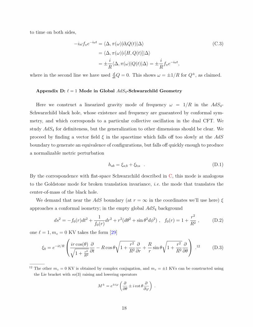
Appendix D: ` = 1 Mode in Global AdS4-Schwarzchild Geometry

Here we construct a linearized gravity mode of frequency ω = 1/R in the AdS4-

Schwarzchild black hole, whose existence and frequency are guaranteed by conformal sym-

metry, and which corresponds to a particular collective oscillation in the dual CFT. We

study AdS4 for definiteness, but the generalization to other dimensions should be clear. We

proceed by finding a vector field ξ in the spacetime which falls off too slowly at the AdS

boundary to generate an equivalence of configurations, but falls off quickly enough to produce

a normalizable metric perturbation

hab = ξa;b + ξb;a . (D.1)

By the correspondence with flat-space Schwarzchild described in C, this mode is analogous

to the Goldstone mode for broken translation invariance, i.e. the mode that translates the

center-of-mass of the black hole.

We demand that near the AdS boundary (at r = ∞ in the coordinates we’ll use here) ξ

approaches a conformal isometry; in the empty global AdS4 background

ds2 = −f0(r)dt2 +1

f0(r)dr2 + r2(dθ2 + sin θ2dφ2) , f0(r) = 1 +

r2

R2, (D.2)

one ` = 1,mz = 0 KV takes the form [29]

ξ0 = e−it/R

ir cos(θ)√1 + r2

R2

∂

∂t−R cos θ

√1 +

r2

R2

∂

∂r+R

rsin θ

√1 +

r2

R2

∂

∂θ

.12 (D.3)

12 The other mz = 0 KV is obtained by complex conjugation, and mz = ±1 KVs can be constructed using

the Lie bracket with so(3) raising and lowering operators

M± = e±iϕ(∂

∂θ± i cot θ

∂

∂ϕ

).

18

The AdS4-Schwarschild metric is

ds2 = −f(r)dt2 +dr2

f(r)+ r2

(dθ2 + sin2 θdϕ2

), f(r) = 1 +

r2

R2− r+

r. (D.4)

We make the ansatz

ξ = e−iωt(ig(r) cos θ

∂

∂t+R h(r) cos θ

∂

∂r+R j(r) sin θ

∂

∂θ

). (D.5)

We demand that the resulting metric perturbation hab

• is in the ‘gaussian normal’ gauge hra = 0 customary for holography,

• is normalizable, corresponding to a state in the dual CFT,

• satisfies the b.c. ξa → ξa0 as r →∞.

Our boundary condition ξr→∞→ ξ0 determines ω = 1, but leaving ω arbitrary provides a

check.

Imposing the gaussian normal gauge hra = 0, we find

h(r) = c1

√f(r) , (D.6)

g(r) = c1

∫ ∞r

dr′

f(r′)3/2+ c2 ,

j(r) = −c1

∫ ∞r

dr′

r′2f(r′)1/2+ c3 .

Normalizability determines ω2 = 1. Demanding ξ → ξ0 as r →∞ gives

c1 = −1 , c2 = R , c3 = 1/R , (D.7)

after which one can check that the normalizability conditions htt, htθ, hθθ, hφφr→∞∼ O(1

r)

are satisfied.

The resulting metric perturbation hab is

habdxadxb = e−

itR

[− cos θ

(2fg + h

(2r +

R2r+

r2

))dt2 + i sin θ

(fg − r2j

)dtdθ

+2rR(h+ rj) cos θ(dθ2 + sin2 θdϕ2

)]. (D.8)

19

Appendix E: Oscillating Observables for a Bouncing Black Hole

For simplicity, we work with the non-rotating 2 + 1-dimensional BTZ black hole, using

coordinates in which its metric is

ds2 = −(r2

R2−r2

+

R2)dt2 +

dr2

r2

R2 −r2+R2

+r2

R2dx2. (E.1)

Here R is the AdS radius, r+ the radius of the black hole, and xR∼ x

R+ 2π.

The stress-energy tensor in the finite-temperature CFT corresponding to this large global

AdS black hole can be obtained by varying the bulk Einstein action with respect to the

boundary metric and using local counterterms [30]. With light-like coordinates x± = t± x,

T++ = T−− =r2

+

32πR3(E.2)

and T µµ ∝ R = 0, where R is the scalar curvature of the boundary metric.

The stress-energy tensor for a BTZ black hole, after a coordinate transformation corre-

sponding to a boost in SO(2, 2), is then obtained most easily by transforming T++ and T−−

under the conformal transformation induced on the boundary by the SO(2, 2) boost. Note

T µµ remains zero. For the boost eiβJ01

, v = tanh β, acting on embedding coordinates of AdS3,

the corresponding coordinate transformation on coordinates (t, x, r) in (E.1) is given by

tant′

R=

√1− v2

√1 + ( r

R)2 sin t

R√1 + ( r

R)2 cos t

R+ v r

Rcos x

R

, (E.3)

tanx′

R=

√1− v2 r

Rsin x

R

v√

1 + ( rR

)2 cos tR

+ rR

cos xR

,

r′

R=

√√√√( v√1− v2

√1 +

( rR

)2

cost

R+

1√1− v2

r

Rcos

x

R

)2

+( rR

sinx

R

)2

,

from which follows

Tt′t′ = Tx′x′ =

(1−v2)(R2+r2+)

(v cos( t′−x′R )−1)

2 +(1−v2)(R2+r2+)

(v cos( t′+x′R )−1)

2 − 2R2

32πGR3, (E.4)

Tt′x′ =v (1− v2)

(R2 + r2

+

)sin(t′

R

)sin(x′

R

) (v cos

(t′

R

)cos(x′

R

)− 1)

8πGR3(v cos

(t′−x′R

)− 1)2 (

v cos(t′+x′

R

)− 1)2 . (E.5)

Note J01 = (L1+−L1

−)/(2i), so that the stress-energy tensor above is that of the collective

oscillation in (IV.1) with α = β. It indeed manifestly oscillates in time. Its two nonzero

components are plotted in Fig. 1.

20

FIG. 1: Energy and momentum density as a function of position x′ and time t′ with R = r+ =

G = 1, v = 0.5.

2 4 6 8 10 12 t¢

2.050

2.055

2.060

2.065

2.070

2.075

2.080

S

2 4 6 8 10 12 t¢

0.53040

0.53045

0.53050

S

FIG. 2: Entanglement entropy of the interval 0 ≤ x′ ≤ π, left, and 0 ≤ x′ ≤ π/64 with R = r+ =

G = c = 1, v = 0.5, and cutoff ε = 0.01.

We can also confirm that in the same state, the entanglement entropy calculated by the

covariant holographic method in [22], of a spatial subregion with respect to the rest of S1,

oscillates.

Given the endpoints x′1, x′2 of such a spatial subregion, its entanglement entropy as a

function of t′ is given by

S(x′1, x′2, t′) =

c

6logL(x′1, x

′2, t′), (E.6)

where L(x′1, x′2, t′) is the length of the space-like geodesic ending at points p′1 =

(t′, x′1, r′c), p

′2 = (t′, x′2, r

′c), with r′c = 1

εan infrared cutoff in the SO(2, 2)-boosted BTZ black

hole.

The desired space-like geodesic may be obtained by first mapping p′i to pi = (ti, xi, ri),

i = 1, 2, where (t, x, r) are non-boosted coordinates given by the inverse coordinates trans-

formation of (E.3), and again mapping pi to qi = (w+ i, w− i, zi), i = 1, 2, where (w+, w−, z)

21

are coordinates in which the BTZ black hole has the manifestly AdS metric

ds2 = R2

(dw+dw− + dz2

z2

). (E.7)

The coordinate transformation from (t, x, r) to (w+, w−, r) is given by

w± ≡ X ± T =

√r2 − r2

+

re

(x±t)r+R2 , z =

r+

rexr+

R2 . (E.8)

In the newest coordinates, the space-like geodesic with endpoints qi = (w+ i, w− i, zi),

i = 1, 2 can be boosted by the mapping w′± = γ±1w±, γ =√

1−β1+β

, with β the usual Lorentz

boost parameter in coordinates (T,X), to lie on a constant T hypersurface. The resulting

geodesic is a circular arc satisfying

(γw+ + γ−1w−

2− A)2 + z2 = B2,

γw+ − γ−1w−2

= C, (E.9)

where constants γ,A,B,C can be determined by the two endpoints qi, i = 1, 2, and which

has length

L = R log(w+ 2 − w+ 1)2(w− 2 − w− 1)2 + 2(w+ 2 − w+ 1)(w− 2 − w− 1)(z2

1 + z22) + (z2 − z1)2

(w+ 2 − w+ 1)(w− 2 − w− 1)z1z2

.

(E.10)

Translating back to original coordinates (t′, x′, r′), L = L(x′1, x′2, t′), one has the holo-

graphic entanglement entropy (E.6) in a bouncing black hole geometry. The smoothly oscil-

lating entanglement entropy is plotted for two different intervals in the spatial domain S1 of

the CFT in Fig. 2.

Appendix F: Oscillations in Galilean Conformal Field Theory

We point out that these oscillations can be observed in experiments on ultracold fermionic

atoms at unitarity, and that related modes have already been studied in detail [31–34]

(for reviews of the subject see [35–38]). The specific mode we discuss has been predicted

previously by very different means in [4].

In the experiments, lithium atoms are cooled in an optical trap and their short-ranged

two-body interactions are tuned to a Feshbach resonance via an external magnetic field.

Above the superfluid transition temperature, this physical system is described by a Galilean-

invariant CFT [39, 40]. The symmetries of such a system comprise a Schrodinger algebra,

which importantly for our purposes contains a special conformal generator C. (This symme-

try algebra has been realized holographically by isometries in [41, 42] (see also [43]) and more

22

generally in [44].) The Hamiltonian for such a system in a spherically-symmetric harmonic

trap Hosc is related to the free-space Hamiltonian H by [39, 40]

Hosc = H + ω20C. (F.1)

This Hosc is analogous to the Hamiltonian of relativistic CFT on the sphere in that its

spectrum is determined by the spectrum of scaling dimensions of operators.

In the experiments of [31, 32], “breathing modes” of the fluid were excited by varying the

frequency of the trap. One goal was to measure the shear viscosity of the strongly-coupled

fluid (for a useful discussion, see §5.2 of [45]). Energy is dissipated via shear viscosity in

these experiments because the trapping potential is not isotropic. The anisotropy of the trap

breaks the special conformal generator. If the trap were spherical, our analysis would apply,

and we predict that the mode with frequency 2ω0 would not be damped, to the extent that

our description is applicable (e.g. the trap is harmonic and spherical and the coupling to the

environment can be ignored)13.

This prediction is consistent with the linearized hydro analysis of [46, 47], and one can

check that the sources of dissipation included in [34, 45] all vanish for the lowest spherical

breathing mode. The mode we predict is adiabatically connected to the breathing mode

studied in [31–34]. Note that an infinite-lifetime mode of frequency 2ω0 is also a prediction

for a free non-relativistic gas. Indeed, this is also a Galilean CFT, though a much more

trivial one.

There is a large (theoretical and experimental) literature on the collective modes of

trapped quantum gases, e.g. [46–49]. Much of the analysis of these collective modes in

the literature relies on a hydrodynamic approximation. In this specific context of unitary

fermions in 2+1 dimensions, linearized modes of this nature were described in a full quantum

mechanical treatment at zero temperature by Pitaevskii and Rosch [50] and further studied

in 3+1 dimensions by Werner and Castin [39]. Further, their existence was attributed to

a hidden so(2, 1) symmetry of the problem, which is the relevant part of the Schrodinger

symmetry. The undamped nonlinear mode at 2ω0 was described in [4]. Here we make several

additional points:

• There are such stable modes at any even multiple of the frequency of the harmonic

potential.

13 Note that this is not the lowest-frequency mode of the spherical trap; linearized hydrodynamic analysis

predicts a linear mode with frequency√

2ω0.

23

• The fully-nonlinear modes of finite amplitude can be explicitly constructed, and remain

undamped.

• These modes are superuniversal – they can be generalized to oscillations in any con-

formal field theory.

In a Galilean CFT with a harmonic potential, the oscillations can be constructed as

follows. Consider an eigenstate of Hosc = H + ω20C constructed from a primary operator O

with dimension ∆O [40],

|∆O〉 = e−HO†|0〉, Hosc|∆O〉 = ∆O|∆O〉. (F.2)

Defining ladder operators L± ≡ H − ω20C ± iω0D, the states

exp (α0L+ + β0L−)|∆O〉 (F.3)

with α0, β0 c-numbers, evolve under Hosc as

e−it∆O exp(e−2iω0tα0L+ + e2iω0tβ0L−

)|∆O〉. (F.4)

The algebraic manipulations which demonstrate this time evolution are identical to those

for coherent states of a simple harmonic oscillator.

The Galilean generalization of (II.4) should be clear. The crucial property of the CFT

spectrum is again the existence of equally-spaced levels connected to |∆O〉 by the ladder

operators L+, L−.

Any real trap will be slightly anisotropic. Following [34, 45], estimates can be made using

linearized hydrodynamics for the damping rate arising from the resulting shear of the fluid, in

terms of the measured shear viscosity (see eqn. (159) of [45]). We are not prepared to estimate

other sources of dissipation. It would be interesting to use softly-broken conformal invariance

to predict the frequencies and damping rates of collective modes in slightly anisotropic traps

in the nonlinear regime.

[1] J. M. Maldacena, Adv.Theor.Math.Phys. 2, 231 (1998), hep-th/9711200.

[2] S. Gubser, I. R. Klebanov, and A. M. Polyakov, Phys.Lett. B428, 105 (1998), hep-th/9802109.

[3] E. Witten, Adv.Theor.Math.Phys. 2, 253 (1998), hep-th/9802150.

[4] Y. Castin, Comptes Rendus Physique 5, 407 (2004), ISSN 1631-0705, URL http://www.

sciencedirect.com/science/article/pii/S1631070504000866.

24

[5] V. E. Hubeny, S. Minwalla, and M. Rangamani (2011), 1107.5780.

[6] G. T. Horowitz and N. Itzhaki, JHEP 9902, 010 (1999), hep-th/9901012.

[7] E. Witten, Adv.Theor.Math.Phys. 2, 505 (1998), hep-th/9803131.

[8] T. Regge and J. A. Wheeler, Phys.Rev. 108, 1063 (1957).

[9] D. Birmingham, I. Sachs, and S. N. Solodukhin, Phys.Rev.Lett. 88, 151301 (2002), hep-

th/0112055.

[10] V. Cardoso and J. P. Lemos, Phys.Rev. D64, 084017 (2001), gr-qc/0105103.

[11] A. S. Miranda and V. T. Zanchin, Phys.Rev. D73, 064034 (2006), gr-qc/0510066.

[12] A. O. Starinets, Phys.Lett. B670, 442 (2009), 0806.3797.

[13] E. Berti, V. Cardoso, and A. O. Starinets, Class.Quant.Grav. 26, 163001 (2009), 0905.2975.

[14] J. Natario and R. Schiappa, Adv. Theor. Math. Phys. 8, 1001 (2004), hep-th/0411267.

[15] J. M. Maldacena, JHEP 0304, 021 (2003), hep-th/0106112.

[16] P. Kovtun and L. G. Yaffe, Phys.Rev. D68, 025007 (2003), hep-th/0303010.

[17] S. Caron-Huot and O. Saremi, JHEP 1011, 013 (2010), 0909.4525.

[18] D. Birmingham, I. Sachs, and S. N. Solodukhin, Phys.Rev. D67, 104026 (2003), hep-

th/0212308.

[19] C. Chamon, R. Jackiw, S.-Y. Pi, and L. Santos, Phys.Lett.B (2011), 1106.0726.

[20] A. Barut and L. Girardello, Commun.Math.Phys. 21, 41 (1971).

[21] V. de Alfaro, S. Fubini, and G. Furlan, Nuovo Cim. A34, 569 (1976).

[22] V. E. Hubeny, M. Rangamani, and T. Takayanagi, JHEP 0707, 062 (2007), 0705.0016.

[23] P. Aichelburg and R. Sexl, Gen.Rel.Grav. 2, 303 (1971).

[24] O. J. Dias, G. T. Horowitz, and J. E. Santos (2011), 1109.1825.

[25] D. Garfinkle and L. A. Zayas (2011), 1106.2339.

[26] S. Minwalla, Adv.Theor.Math.Phys. 2, 781 (1998), hep-th/9712074.

[27] M. Ban, J. Opt. Soc. Am. B 10, 1347 (1993).

[28] J. Goldstone, Il Nuovo Cimento (1955-1965) 19, 154 (1961), URL http://dx.doi.org/10.

1007/BF02812722.

[29] M. Henneaux and C. Teitelboim, Commun.Math.Phys. 98, 391 (1985).

[30] V. Balasubramanian and P. Kraus, Commun.Math.Phys. 208, 413 (1999), hep-th/9902121.

[31] J. Kinast, A. Turlapov, and J. E. Thomas, Phys. Rev. Lett. 94, 170404 (2005).

[32] J. E. Thomas, J. Kinast, and A. Turlapov, Phys. Rev. Lett. 95, 120402 (2005).

[33] S. Riedl, E. R. Sanchez Guajardo, C. Kohstall, A. Altmeyer, M. J. Wright, J. H. Denschlag,

R. Grimm, G. M. Bruun, and H. Smith, Phys. Rev. A 78, 053609 (2008), 0809.1814, URL

http://link.aps.org/doi/10.1103/PhysRevA.78.053609.

[34] C. Cao, E. Elliott, J. Joseph, H. Wu, J. Petricka, T. Schfer, and J. E. Thomas, Science 331,

58 (2011), 1007.2625, URL http://www.sciencemag.org/content/331/6013/58.abstract.

[35] W. Ketterle and M. W. Zwierlein, Rivista del Nuovo Cimento 031, 247 (2008), 0801.2500.

[36] I. Bloch, J. Dalibard, and W. Zwerger, Rev. Mod. Phys. 80, 885 (2008), 0704.3011.

[37] S. Giorgini, L. P. Pitaevskii, and S. Stringari, Rev. Mod. Phys. 80, 1215 (2008), URL http:

//link.aps.org/doi/10.1103/RevModPhys.80.1215.

[38] Y. Castin and F. Werner, ArXiv e-prints (2011), 1103.2851.

25

[39] F. Werner and Y. Castin, Phys. Rev. A 74, 053604 (2006).

[40] Y. Nishida and D. T. Son, Phys.Rev. D76, 086004 (2007), 0706.3746.

[41] D. Son, Phys.Rev. D78, 046003 (2008), 0804.3972.

[42] K. Balasubramanian and J. McGreevy, Phys.Rev.Lett. 101, 061601 (2008), 0804.4053.

[43] C. Duval, G. W. Gibbons, and P. Horvathy, Phys.Rev. D43, 3907 (1991), hep-th/0512188.

[44] K. Balasubramanian and J. McGreevy, JHEP 1101, 137 (2011), 1007.2184.

[45] T. Schafer and D. Teaney, Rept.Prog.Phys. 72, 126001 (2009), 0904.3107.

[46] H. Heiselberg, Phys. Rev. Lett. 93, 040402 (2004), URL http://link.aps.org/doi/10.1103/

PhysRevLett.93.040402.

[47] S. Stringari, EPL (Europhysics Letters) 65, 749 (2004), URL http://stacks.iop.org/

0295-5075/65/i=6/a=749.

[48] G. E. Astrakharchik, R. Combescot, X. Leyronas, and S. Stringari, Phys. Rev. Lett. 95, 030404

(2005), URL http://link.aps.org/doi/10.1103/PhysRevLett.95.030404.

[49] S. Stringari (2007), cond-mat/0702526.

[50] L. P. Pitaevskii and A. Rosch, Phys. Rev. A 55, R853 (1997).

26