
Hydrodynamics of electromagnetically controlled jet oscillations
156
Delft University of Technology Hydrodynamics of electromagnetically controlled jet oscillations Righolt, Bernhard DOI 10.4233/uuid:3c676ede-2ddb-41f7-ad29-eec9eab29526 Publication date 2016 Document Version Final published version Citation (APA) Righolt, B. (2016). Hydrodynamics of electromagnetically controlled jet oscillations. https://doi.org/10.4233/uuid:3c676ede-2ddb-41f7-ad29-eec9eab29526 Important note To cite this publication, please use the final published version (if applicable). Please check the document version above. Copyright Other than for strictly personal use, it is not permitted to download, forward or distribute the text or part of it, without the consent of the author(s) and/or copyright holder(s), unless the work is under an open content license such as Creative Commons. Takedown policy Please contact us and provide details if you believe this document breaches copyrights. We will remove access to the work immediately and investigate your claim. This work is downloaded from Delft University of Technology. For technical reasons the number of authors shown on this cover page is limited to a maximum of 10.
-
Upload
khangminh22 -
Category
Documents
-
view
0 -
download
0
Transcript of Hydrodynamics of electromagnetically controlled jet oscillations

Delft University of Technology
Hydrodynamics of electromagnetically controlled jet oscillations
Righolt, Bernhard
DOI10.4233/uuid:3c676ede-2ddb-41f7-ad29-eec9eab29526Publication date2016Document VersionFinal published versionCitation (APA)Righolt, B. (2016). Hydrodynamics of electromagnetically controlled jet oscillations.https://doi.org/10.4233/uuid:3c676ede-2ddb-41f7-ad29-eec9eab29526
Important noteTo cite this publication, please use the final published version (if applicable).Please check the document version above.
CopyrightOther than for strictly personal use, it is not permitted to download, forward or distribute the text or part of it, without the consentof the author(s) and/or copyright holder(s), unless the work is under an open content license such as Creative Commons.
Takedown policyPlease contact us and provide details if you believe this document breaches copyrights.We will remove access to the work immediately and investigate your claim.
This work is downloaded from Delft University of Technology.For technical reasons the number of authors shown on this cover page is limited to a maximum of 10.

Hydrodynamics of electromagnetically
controlled jet oscillations
PROEFSCHRIFT
ter verkrijging van de graad van doctor
aan de Technische Universiteit Delft,
op gezag van de Rector Magnificus prof. ir. K.C.A.M. Luyben,
voorzitter van het College van Promoties,
in het openbaar te verdedigen op donderdag 7 juli 2016 om 10:00 uur
door
Bernhard Willem RIGHOLT
natuurkundig ingenieur
geboren te Leidschendam

Dit proefschrift is goedgekeurd door depromotor: Prof. dr. ir. C.R. Kleijncopromotor: Dr. S. Kenjereš Dipl.-Ing.
Samenstelling van de promotiecommissie:Rector Magnificus voorzitterProf. dr. ir. C.R. Kleijn Technische Universiteit Delft, promotorDr. S. Kenjereš Dipl.-Ing. Technische Universiteit Delft, copromotor
Onafhankelijke leden:Prof. dr. ir. C. Vuik Technische Universiteit DelftProf. dr. D. J. E. M. Roekaerts Technische Universiteit DelftProf. dr. ir. B. J. Geurts Universiteit TwenteProf. dr. K. Pericleous University of GreenwichIr. D. van der Plas Tata Steel EuropeProf. dr. R.F. Mudde Technische Universiteit Delft, reservelid
This work was supported by the Dutch Technology Foundation STW, Tata Steel and ABB.
Copyright © 2016 by B. W. Righolt
All rights reserved. No part of the material protected by this copyright notice may bereproduced or utilized in any form or by any means, electronic or mechanical, includingphotocopying, recording, or by any information storage and retrieval system, without writtenpermission from the author.
ISBN: 978-94-6186-664-6


Contents
Summary xi
Samenvatting xv
1 Introduction 1
1.1 Background . . . . . . . . . . . . . . . . . . . . . . . . . . . . . . . . . . . 1
1.2 Physical phenomena in steel casting . . . . . . . . . . . . . . . . . . . . . . 2
1.3 Research objectives . . . . . . . . . . . . . . . . . . . . . . . . . . . . . . . 3
1.3.1 Mechanism for self-sustained flow oscillations in a thin cavity . . . . 4
1.3.2 Prediction of large scale jet oscillations in a thin cavity . . . . . . . . 4
1.3.3 Electromagnetic flow control of jet oscillations in a thin cavity . . . . 4
1.3.4 Magnetohydrodynamic free surface flow in a shallow cavity . . . . . 5
1.4 Funding of this PhD thesis . . . . . . . . . . . . . . . . . . . . . . . . . . . 5
1.5 Outline . . . . . . . . . . . . . . . . . . . . . . . . . . . . . . . . . . . . . 5
Bibliography . . . . . . . . . . . . . . . . . . . . . . . . . . . . . . . . . . . . . 7
2 Methods 9
2.1 Introduction . . . . . . . . . . . . . . . . . . . . . . . . . . . . . . . . . . . 9
2.2 One-way coupled magnetohydrodynamics . . . . . . . . . . . . . . . . . . . 9
2.3 One-way coupled magnetohydrodynamics solver . . . . . . . . . . . . . . . 10
2.4 Volume of fluid and magnetohydrodynamics . . . . . . . . . . . . . . . . . . 11
2.5 MMIT Magnetohydrodynamics . . . . . . . . . . . . . . . . . . . . . . . . . 12
v

vi Contents
2.6 Dynamic Smagorinsky model . . . . . . . . . . . . . . . . . . . . . . . . . . 14
2.7 Spalding’s Law . . . . . . . . . . . . . . . . . . . . . . . . . . . . . . . . . 16
Bibliography . . . . . . . . . . . . . . . . . . . . . . . . . . . . . . . . . . . . . 19
3 Analytical solutions of one-way coupled magnetohydrodynamic free surface flow 21
3.1 Introduction . . . . . . . . . . . . . . . . . . . . . . . . . . . . . . . . . . . 22
3.2 Analytical derivation . . . . . . . . . . . . . . . . . . . . . . . . . . . . . . 23
3.2.1 Conservation equations . . . . . . . . . . . . . . . . . . . . . . . . . 24
3.2.2 Boundary conditions . . . . . . . . . . . . . . . . . . . . . . . . . . 24
3.2.3 Lubrication theory . . . . . . . . . . . . . . . . . . . . . . . . . . . 27
3.2.4 Core flow . . . . . . . . . . . . . . . . . . . . . . . . . . . . . . . . 28
3.2.5 End wall flow . . . . . . . . . . . . . . . . . . . . . . . . . . . . . . 31
3.2.6 Analytic solution for the end wall flow . . . . . . . . . . . . . . . . . 33
3.2.7 Increased magnetic interaction . . . . . . . . . . . . . . . . . . . . . 39
3.3 Numerical modeling . . . . . . . . . . . . . . . . . . . . . . . . . . . . . . 40
3.3.1 Moving mesh interface tracking method . . . . . . . . . . . . . . . . 40
3.3.2 Volume of fluid method . . . . . . . . . . . . . . . . . . . . . . . . 41
3.4 Numerical results . . . . . . . . . . . . . . . . . . . . . . . . . . . . . . . . 43
3.4.1 Base case . . . . . . . . . . . . . . . . . . . . . . . . . . . . . . . . 43
3.4.2 Three-dimensionality of the flow . . . . . . . . . . . . . . . . . . . . 45
3.4.3 Increased deformation . . . . . . . . . . . . . . . . . . . . . . . . . 45
3.4.4 Error . . . . . . . . . . . . . . . . . . . . . . . . . . . . . . . . . . 49
3.5 Conclusions . . . . . . . . . . . . . . . . . . . . . . . . . . . . . . . . . . . 49
Bibliography . . . . . . . . . . . . . . . . . . . . . . . . . . . . . . . . . . . . . 53
4 Dynamics of a single, oscillating turbulent jet in a confined cavity 55
4.1 Introduction . . . . . . . . . . . . . . . . . . . . . . . . . . . . . . . . . . . 55
4.2 Methods . . . . . . . . . . . . . . . . . . . . . . . . . . . . . . . . . . . . . 56
4.2.1 Description of setup . . . . . . . . . . . . . . . . . . . . . . . . . . 56
4.2.2 Numerical fluid flow models . . . . . . . . . . . . . . . . . . . . . . 58

Contents vii
4.3 Validation of the numerical method . . . . . . . . . . . . . . . . . . . . . . . 59
4.4 Model for self-sustained oscillations of a jet in a confined cavity . . . . . . . 62
4.4.1 Physical mechanisms . . . . . . . . . . . . . . . . . . . . . . . . . . 62
4.4.2 Model description . . . . . . . . . . . . . . . . . . . . . . . . . . . 65
4.5 Determination of model parameters and its implications . . . . . . . . . . . . 66
4.5.1 Reduced parameters . . . . . . . . . . . . . . . . . . . . . . . . . . 67
4.5.2 Parameter estimation . . . . . . . . . . . . . . . . . . . . . . . . . . 69
4.5.3 Model application . . . . . . . . . . . . . . . . . . . . . . . . . . . 70
4.6 Conclusion . . . . . . . . . . . . . . . . . . . . . . . . . . . . . . . . . . . 73
Bibliography . . . . . . . . . . . . . . . . . . . . . . . . . . . . . . . . . . . . . 76
4.A A posteriori determination of the model parameters . . . . . . . . . . . . . . 76
4.A.1 Phase average . . . . . . . . . . . . . . . . . . . . . . . . . . . . . . 76
4.A.2 Cost function . . . . . . . . . . . . . . . . . . . . . . . . . . . . . . 77
4.A.3 Error estimation . . . . . . . . . . . . . . . . . . . . . . . . . . . . 77
4.B Derivation of the maximum jet angle . . . . . . . . . . . . . . . . . . . . . . 77
5 Electromagnetic control of an oscillating turbulent jet in a confined cavity 81
5.1 Introduction . . . . . . . . . . . . . . . . . . . . . . . . . . . . . . . . . . . 82
5.2 Problem definition and methods . . . . . . . . . . . . . . . . . . . . . . . . 83
5.2.1 Description of the set-up . . . . . . . . . . . . . . . . . . . . . . . . 83
5.2.2 Dimensionless numbers . . . . . . . . . . . . . . . . . . . . . . . . 83
5.2.3 Magnetic field calculation . . . . . . . . . . . . . . . . . . . . . . . 84
5.2.4 Flow simulations . . . . . . . . . . . . . . . . . . . . . . . . . . . . 85
5.2.5 Validation . . . . . . . . . . . . . . . . . . . . . . . . . . . . . . . . 87
5.3 Influence of electromagnetic forcing on self-sustained oscillations . . . . . . 87
5.3.1 Mean velocity . . . . . . . . . . . . . . . . . . . . . . . . . . . . . . 87
5.3.2 Oscillation frequency . . . . . . . . . . . . . . . . . . . . . . . . . . 92
5.3.3 Pressure oscillations . . . . . . . . . . . . . . . . . . . . . . . . . . 93
5.3.4 Jet angle amplitude . . . . . . . . . . . . . . . . . . . . . . . . . . . 93
5.3.5 Flow regimes . . . . . . . . . . . . . . . . . . . . . . . . . . . . . . 95

viii Contents
5.4 Zero-dimensional model of the jet oscillation . . . . . . . . . . . . . . . . . 95
5.4.1 Unforced flow (N = 0) . . . . . . . . . . . . . . . . . . . . . . . . . 95
5.4.2 Electromagnetically forced flow (N 6= 0) . . . . . . . . . . . . . . . 96
5.5 Determination of the model parameters and its implications . . . . . . . . . . 97
5.5.1 Non-dimensional model . . . . . . . . . . . . . . . . . . . . . . . . 97
5.5.2 Parameter fitting . . . . . . . . . . . . . . . . . . . . . . . . . . . . 98
5.5.3 Parameter estimation . . . . . . . . . . . . . . . . . . . . . . . . . . 99
5.5.4 Model application . . . . . . . . . . . . . . . . . . . . . . . . . . . 100
5.6 Conclusion . . . . . . . . . . . . . . . . . . . . . . . . . . . . . . . . . . . 101
Bibliography . . . . . . . . . . . . . . . . . . . . . . . . . . . . . . . . . . . . . 106
5.A Electromagnetic field . . . . . . . . . . . . . . . . . . . . . . . . . . . . . . 106
6 Dynamics of a bifurcated jet in a confined cavity with a free surface 109
6.1 Introduction . . . . . . . . . . . . . . . . . . . . . . . . . . . . . . . . . . . 109
6.2 Numerical method and validation . . . . . . . . . . . . . . . . . . . . . . . . 110
6.2.1 Description of the set-up . . . . . . . . . . . . . . . . . . . . . . . . 110
6.3 Oscillation mechanism free surface . . . . . . . . . . . . . . . . . . . . . . . 113
6.3.1 Jet splitting . . . . . . . . . . . . . . . . . . . . . . . . . . . . . . . 113
6.3.2 Pressure deficit growth . . . . . . . . . . . . . . . . . . . . . . . . . 114
6.3.3 Maximum pressure deficit and fluid overshoot . . . . . . . . . . . . . 117
6.3.4 Pressure deficit decrease . . . . . . . . . . . . . . . . . . . . . . . . 119
6.4 Influence of a wall . . . . . . . . . . . . . . . . . . . . . . . . . . . . . . . 119
6.5 Conclusion . . . . . . . . . . . . . . . . . . . . . . . . . . . . . . . . . . . 121
Bibliography . . . . . . . . . . . . . . . . . . . . . . . . . . . . . . . . . . . . . 122
7 Conclusions and outlook 125
7.1 General conclusions . . . . . . . . . . . . . . . . . . . . . . . . . . . . . . . 125
7.1.1 Benchmark MHD free surface flow problem . . . . . . . . . . . . . . 125
7.1.2 Mechanism for self-sustained jet oscillations . . . . . . . . . . . . . 125
7.1.3 Model description of self-sustained jet oscillations . . . . . . . . . . 126

Contents ix
7.1.4 Electromagnetic forcing of single jet oscillations . . . . . . . . . . . 126
7.2 Research opportunities . . . . . . . . . . . . . . . . . . . . . . . . . . . . . 127
7.2.1 Zero-dimensional models . . . . . . . . . . . . . . . . . . . . . . . . 127
7.2.2 Damping of oscillations . . . . . . . . . . . . . . . . . . . . . . . . 127
7.2.3 Towards improved continuous steel casting . . . . . . . . . . . . . . 128
Bibliography . . . . . . . . . . . . . . . . . . . . . . . . . . . . . . . . . . . . . 130
List of Publications 133
Acknowledgements 135
Curriculum Vitae 137


Summary
Continuous steel casting is an industrial process where turbulent liquid steel jets enter a thinmould through a submerged nozzle. In the mould the steel is cooled, such that it solidifies.The submerged jets can show self-sustained oscillatory behaviour, which has an impact onthe distribution of heat, the solidification of the steel and therefore the overall quality of thesteel. Oscillations of the liquid steel jets also influence the free surface in the mould, leadingto the unwanted inclusion of slag particles and again degraded quality of the steel. By theapplication of an electromagnetic brake, the liquid steel flow can be controlled, jet oscillationscan be suppressed, and hence the quality of the steel product improved.
In this thesis we use numerical and analytical methods to study the flow dynamics of self-sustained single and bifurcated submerged liquid jet oscillations in a liquid filled thin cavitywith and without a free surface. Furthermore we study the influence of electromagnetic forceson single jets and free surface flows.
Firstly, we developed three-dimensional, time dependent flow simulation methods that com-bine large eddy turbulence modelling with electromagnetic body forces and two differentapproaches to free surface modelling, viz. Volume of Fluid (VOF) and Moving Mesh In-terface Tracking (MMIT). Various aspects of these simulation codes were validated againstexperimental flow and free surface data by Kalter (2015), obtained in a parallel PhD projectthrough Particle Image Velocimetry in a water model.
Secondly, to further validate the numerical simulation codes, we derived an analytical solu-tion for a two-dimensional benchmark problem, consisting of a shallow cavity with a freesurface, where the flow is driven by an electromagnetic force and the free surface deforma-tion is restored by both gravity and surface tension. Under specific constraints for the Reyn-olds number, Hartmann number, capillary number, Bond number and cavity aspect ratio, weanalytically solve the details of the flow dynamics and the free surface deformation usinglubrication theory and matching of asymptotic expansions. With these solutions we demon-strate the validity of both numerical models. Consecutively we use the numerical solutions toevaluate the validity of the analytical solution when the constraints for which it was derivedare relaxed. In future research, the presented analytical solution and the information aboutthe range of the dimensionless numbers for which it is valid, can serve as a benchmark prob-
xi

xii Summary
lem for newly developed numerical simulation codes for free surface magnetohydrodynamicflows.
Thirdly, using the results of our three-dimensional computational simulations, we developeda zero-dimensional, delay differential equation type model which quantitatively describesthe self-sustained oscillation of a jet in a thin cavity. Three terms in the zero-dimensionalmodel equation represent the three physical mechanisms that contribute to the self-sustainedoscillation, viz. (i) pressure driven oscillation growth, (ii) amplitude limitation by geometryand (iii) delayed destruction of the recirculation zone. The zero-dimensional model equationcontains four model parameters, and we show that these parameters can be a priori calculatedfrom the Reynolds number (Re), the cavity width to nozzle diameter ratio (W/d), the inletvelocity and the nozzle diameter. By comparing predictions from the zero-dimensional modelto data from our three-dimensional computational simulations as well as experimental databy Kalter (2015), we show that the zero-dimensional model with a priori calculated modelparameters correctly predicts the frequency and waveform of the jet oscillation for a widerange of Reynolds numbers and cavity width to nozzle diameter aspect ratios. In agreementwith our three-dimensional simulations, the zero-dimensional model predicts that for givenaspect ratio there is a critical Reynolds number below which the self-sustained oscillationsvanish.
Fourthly, we extended our zero-dimensional model to include the effect of a body force onthe self-sustained oscillations. In particular, the body force studied is an electromagneticforce, originating from an externally applied magnetic field and an imposed electrical currentacross the domain. Again, results from the zero-dimensional model are being compared toexperimental data by Kalter (2015) and data from our own three-dimensional computationalsimulations. We show that the three physical mechanisms that contribute to the self-sustainedoscillation, and thus the form of the model equation, remain the same as in the absence ofelectromagnetic body forces. The value of the four model parameters, however, now alsodepends on an additional dimensionless number, viz. the (signed) Stuart number, representingthe ratio of electromagnetic body forces and inertial forces. We present closed relations to apriori predict the value of the four model parameters as a function of the Reynolds number,the Stuart number, the cavity width to nozzle diameter aspect ratio, the inlet velocity, andthe nozzle diameter. From both zero-dimensional model predictions and three-dimensionalcomputational simulations, we demonstrate that three flow regimes can be distinguished,separated by the positive critical Stuart number and the negative critical Stuart number. Inbetween these two values, inertial forces are dominant. Outside this range, electromagneticforces are dominant, and either enhance or suppress oscillations.
Finally, using detailed spatio-temporally resolved flow and pressure data from our three-dimensional model simulations, we demonstrate the validity of the pressure-based mechan-ism for self-sustained jet oscillations in a thin cavity, as suggested earlier in literature (Hon-eyands, Kalter). For both single and bifurcated jet arrangements, the jets deflect towardsthe jet-induced bounded recirculation zones. The pressure deficit in the recirculation zonedeflects the jet further, leading to an increasing pressure deficit. This continues until the re-circulation zone cannot grow any further due to geometrical restrictions and the jet reaches

Summary xiii
an extreme position. The liquid flow then escapes the recirculation zone, feeding a differ-ent recirculation zone. For the single jet configuration this leads to the jet being deflectedto the opposite side. For the bifurcated jet configuration this leads to the opposite jet beingdeflected.
We conclude this thesis with the main findings, and we describe how these main findings canlead to the further understanding of self-sustained oscillations in a continuous steel castingmould.


Samenvatting
Tijdens het continu gieten van staal wordt vloeibaar staal via een dompelpijp in een gietvormgegoten. De gietvorm wordt actief gekoeld, waardoor het staal langzaam stolt. De turbulentejets die uit de dompelpijp stromen, kunnen zichzelf in stand houdend, oscillerend gedragvertonen. Dit gedrag heeft invloed op zowel de warmteverspreiding in de gietvorm als op hetstaaloppervlak aan de bovenzijde van de gietvorm. Beide kunnen een negatief effect hebbenop de kwaliteit van het geproduceerde staal. De oscillaties van de jets kunnen beïnvloedworden met behulp van een zogenaamde elektromagnetische rem, waardoor de kwaliteit vanhet staal verbetert.
In dit proefschrift gebruiken we numerieke simulaties en wiskundige modellen om de vloei-stofdynamische mechanismen achter de oscillaties van jets in gietvormen te ontrafelen. Webestuderen zowel rechte als gesplitste dompelpijpen in een gietvorm met of zonder een vrijoppervlak. Daarnaast bestuderen wij de invloed van elektromagnetische krachten hierop.
Ten eerste hebben wij simulatieprogramma’s ontwikkeld waarmee de driedimensionale, tijds-afhankelijke, turbulente stroming in de gietvorm, onder invloed van elektromagnetischekrachten, gesimuleerd kan worden. We hebben daarin twee methodes geïmplementeerd voorhet numeriek simuleren van het vrije oppervlak: de Volume of Fluid (VOF) methode en deMoving Mesh Interface Tracking (MMIT) methode. De simulatieprogramma’s zijn gevali-deerd aan de hand van experimentele data over de vloeistofstroming en het gedrag van hetvrije oppervlak, zoals verkregen in een parallel promotieproject van Kalter (2015) met behulpvan Particale Image Velocimetry.
Ten tweede hebben wij om onze computersimulatieprogramma’s verder te kunnen validereneen relevant tweedimensionaal magnetohydrodynamisch stromingsprobleem gedefinieerd datwij analytisch konden oplossen zodat we de oplossingen konden vergelijken met de resultatenvan de numerieke simulaties. Dit validatieprobleem bestaat uit de stroming in een ondiepelaag vloeistof met een vrij oppervlak, welke vervormt ten gevolge van een opgelegde elektro-magnetische kracht, de zwaartekracht en de oppervlaktespanning. Met behulp van lubricationtheory en matching of asymptotic expansions hebben wij de stroming in de vloeistoflaag ende vervorming van het vrije oppervlak mathematisch bepaald voor kleine waardes van hetReynolds getal, het Hartmann getal, het capillair getal, het Bond getal en de breedte-diepte
xv

xvi Samenvatting
verhouding van de vloeistoflaag. Met deze mathematische oplossing hebben we de geldigheidvan de numerieke simulatiemethodes aangetoond. Omgekeerd hebben we daarna de nume-rieke simulaties gebruikt om te onderzoeken in hoeverre de analytische oplossing ook voorgrotere waardes van de genoemde kentallen geldig blijft. Met deze kennis kan onze mathe-matische oplossing in toekomstig onderzoek gebruikt worden voor de validatie van nieuwenumerieke simulatiecodes magnetohydrodynamische vrije oppervlakte stromingen.
Ten derde hebben wij een nuldimensionaal model ontwikkeld dat zowel het optreden als defrequenties en de golfvorm van de zichzelf in stand houdende jetoscillaties in een dunnegietvorm kwantitatief voorspelt. Dit nuldimensionale model is geïnspireerd door de me-chanismen die we hebben waargenomen in onze driedimensionale numerieke simulaties enis mathematisch gebaseerd op een tijdsafhankelijke differentiaalvergelijking met een vertra-gingsterm. De modelvergelijking bevat drie termen, die de drie stadia van de oscillatie be-schrijven, namelijk (i) groei van de oscillatie ten gevolge van drukminima in de geïnduceerdestromingsrecirculaties, (ii) demping en beperkte amplitude door de geometrische begrenzingen (iii) vertraagde vernietiging van de recirculatiezone. Het model bevat vier modelconstan-ten. Wij tonen aan dat deze vier constanten a priori kwantitatief kunnen worden bepaald uithet Reynolds getal, de breedte van de gietvorm, de diameter van de gietpijp en de instroom-snelheid van de jet. Op basis van vergelijkingen met experimentele data van Kalter (2015)en resultaten van onze drie-dimensionale numerieke simulaties tonen wij aan dat het ontwik-kelde nuldimensionale model de frequentie en golfvorm van de jetoscillatie correct voorspelt.Bovendien voorspelt het nuldimensionale model correct dat er voor elke verhouding tussende breedte van de gietvorm en de diameter van de gietpijp een kritisch Reynolds getal bestaat,waaronder de zichzelf in stand houdende oscillaties verdwijnen.
Ten vierde hebben wij het nuldimensionale model voor de jetoscillaties in een dunne gietvormuitgebreid naar de situatie waarin een elektromagnetische volumekracht, opgewekt door eenextern opgelegd magneetveld en een extern opgelegde elektrische stroom, werkzaam is op devloeistof. Weer vergelijken we de resultaten van het nuldimensionale model met experimen-tele resultaten van Kalter (2015) en met de resultaten van onze driedimensionale simulaties.We laten zien dat ook in aanwezigheid van elektromagnetische krachten dezelfde drie fysi-sche mechanismen ten grondslag liggen aan de oscillaties. Echter, de vier model parameterszijn nu afhankelijk van een extra dimensieloos kental, namelijk het Stuart getal. Het Stuartgetal is de verhouding tussen de elektromagnetische en de traagheidskrachten. Uit zowel deresultaten van het nuldimensionale model, als de driedimensionale simulaties blijkt dat erdrie regimes in het stromingsgedrag optreden, gescheiden door een positief en een negatiefkritisch Stuart getal. Tussen beide waardes zijn de traagheidskrachten dominant. Voor grotereabsolute waardes van het Stuart getal hebben de elektromagnetische krachten de overhand,waarbij de oscillaties respectievelijk onderdrukt of versterkt worden.
Ten slotte hebben wij de juistheid van het op druk gebaseerde mechanisme voor de zich-zelf in stand houdende jet oscillatie in een dunne gietvorm, zoals eerder voorgesteld in deliteratuur (Honeyands, Kalter), aangetoond met behulp van de stroomsnelheid en druk uitonze tijdsafhankelijke, driedimensionale simulaties. Zowel enkele als gesplitste jets buigenaf in de richting van de door de jet veroorzaakte recirculatiezone. Ten gevolge van het lo-

Samenvatting xvii
kale drukminimum in het midden van deze recirculatie buigt de jet steeds verder af, leidendtot een versterkt drukminimum. Dit zet zich voort totdat de recirculatiezone niet verder kangroeien ten gevolge van de geometrische begrenzing, waardoor de jet een extremum bereikt.De vloeistof stroomt dan weg uit de recirculatiezone, waarop een andere recirculatie in detegenoverliggende zijde van de holte wordt gevoed. Voor een enkele jet zal deze jet afbuigennaar de andere zijde van de gietvorm, en voor een gesplitste jet zal de jet aan de andere zijdeafbuigen.
We sluiten dit proefschrift af met een beschouwing over hoe de belangrijkste bevindingengebruikt kunnen worden om te komen tot een beter begrip en een betere beheersing vanvloeistofoscillaties in gietvormen bij continu staalgieten.

1. Introduction
1.1 Background
In the current century, the world steel production was nearly doubled from 0.85× 10⁹ metrictons in 2001 to 1.5 × 10⁹ metric tons in 2012. While the Dutch steel production, solely dueto the Tata Steel (formerly Corus) plant in IJmuiden, has increased by 14% in this period,the production rate in China exploded with a 370% growth.21,22 The European steel marketis still recovering from the economic crisis in 2008 and not yet back to the production rate of2007.
The casting of metal in the beginning of the twentieth century was a batch process, casting theliquid metals in blocks. Already in 1887, the first idea for a continuous caster was patented.1
The basic concept never changed and is schematically depicted in Figure 1.1. The vertical,water cooled mould is filled with metal and the solidified metal is extracted and cut at thebottom. By the middle of the twentieth century this method was used and further developed,mostly for copper and aluminium casting.
Steel casting was more difficult since the melting temperature is relatively high (∼ 1500C)and the solidification is slow, because of the relatively low thermal conductivity. Innovations,such as1
• the oscillating mould (1949) with negative strip time (1954),• the bending of the steel strip with a liquid core into a horizontal position (1963),• the submerged pipe to prevent nitrogen pick-up and re-oxidation (1965),• the tundish and rotating tower (1968) (solving the problem of the liquid steel arriving
at the caster in batches) and• the electromagnetic brake (EMBr) (Kawasaki in the early 80s), to reduce oscillations
and damp turbulence
were techniques that helped to improve the efficiency and quality of the produced steel. AnEMBr helps increasing the production rate and quality of steel.
1

2 Chapter 1
Submerged entry
nozzle (SEN)Free surface
with slag layer
Liquid steel
Figure 1.1 Schematic representation of the continuous casting process (left 19), with the complete sys-tem from ladle to solid strip. The liquid steel arrives at the system in batches, flows into the tundishto make it a batch process, after which it is poured into the mould. (right, zoom-in) Mould of thecontinuous casting process. The liquid steel enters the mould via the submerged entry nozzle (SEN).
1.2 Physical phenomena in steel casting
Continuous steel casting is a complex industrial process. Many different physical phenomenaare taking place in the steel casting process.1
1. Fluid mechanics is an important phenomenon in the steel casting process. The flowis highly turbulent in the top of the caster near the jets emerging from the submergedentry nozzle (SEN), and the fluid might relaminarize further down the mould. The flowmay induce large scale oscillations in the mould.5,7
2. A slag layer is present on top of the liquid. This slag layer prevents oxidation of theliquid steel when in direct contact with air. Due to large velocities in the top of themould, the steel-slag interface can move violently, possibly leading to the inclusion ofthe slag and other pollutants into the steel.4 Gravitational forces, and to a lesser degreesurface tension forces, play a key role in the behavior of this interface.
3. An electromagnetic break (EMBr) is an external magnetic field that is often applied tothe steel flow.3 The EMBr is installed in order to damp the flow and free surface os-cillations. The magnetic field induces an electrical current and subsequently a Lorentz

Introduction 3
force, which may not only affect the large scale motions and free surface oscillations,but also the turbulence and its isotropy.10
4. The solidification of the liquid steel starts at the boundaries to form a solid shell. Thissolidified shell is lubricated by the slag layer to protect it from contact with the coppermould. Flow oscillations and inclusions in the liquid steel largely determine the qualityof the solid steel product.1
5. The heat transfer from the liquid steel to the surroundings plays an important role inthe solidification process. The rate and uniformity of the heat transfer determine theoptimal thickness and uniformity of the solidified shell respectively, and thus ensure ahigh quality of the solid steel.1
6. The thermomechanical behavior of the solidifying shell becomes relevant further downthe mould. As the steel cools down, it shrinks. This may create an isolating air gapbetween the solid steel and the mould, highly reducing the heat transfer from the steelto the surroundings.
7. The tapering of the mould, in order to compensate for thermomechanical shrinkage.1
8. The copper mould oscillates significantly in order to reduce the risk of the solidifyingshell to stick to the mould, despite the lubricating behaviour of the slag layer in betweensteel and mould.1
9. The liquid core reduction, where the solidified shells on opposite sides of the caster arepressed together, reduces the size of the liquid core and speeds up the solidification.1
10. Argon is injected into the mould, to prevent clogging of the small nozzle and to blowout any pollutants residing in the caster.20
1.3 Research objectives
In this thesis we address, from a fundamental point of view, the first three of the physicalphenomena mentioned in section 1.2, namely (i) fluid flow and turbulence, (ii) the free surfacemovement, and (iii) the influence of electromagnetic forcing on both. We will not addressthe remainder of the aforementioned phenomena that play a role in practical continuous steelcasting.
In this thesis we use analytical methods and two- and three-dimensional Computational FluidDynamics (CFD) simulations. Complementary, an experimental study is carried out.6 By an-swering the research questions detailed in this section, we will unravel fundamental physicalaspects of the flow oscillations, free surface behavior and electromagnetic control that aredifficult to assess experimentally. Furthermore, we will work towards the development of anLarge Eddy Simulation (LES) based, Volume Of Fluid (VOF) free surface numerical simula-tion code for magnetohydrodynamic (MHD) flows in the OpenFOAM framework, validated

4 Chapter 1
against water model experiments and applicable to the optimization of MHD flows in steelcasting.
1.3.1 Mechanism for self-sustained flow oscillations in a thin cavity
In thin slab continuous steel casting, the liquid steel is fed into a thin mould through a so-called bifurcated (two-port) nozzle, as illustrated in Figure 1.1. The two jets may inducelarge scale flow oscillations. It is known,7 that under certain conditions, the oscillations ofboth jets in a bifurcated configuration align in anti-phase, in other words, both oscillatorsare coupled. Honeyands and Herbertson 5 and Kalter et al. 7 hypothesized a mechanism forthese anti-symmetric oscillations. This mechanism is based on the pressure deficit in therecirculation zones that form due to the confinement and both jets.
Large scale self-sustained oscillations are also found in more fundamental flow configura-tions, such as a single jet in a confined cavity. Similar to the bifurcated jet, the proposedphysical mechanism behind these oscillations is based on the pressure deficit in the recircu-lation zones that form due to the confinement.
The observation of these pressure deficits in oscillating recirculation zones is difficult to real-ize experimentally, which makes the proof for these hypotheses difficult. Numerical simula-tions on the other hand, can provide full space and time resolved fields of the velocity andpressure throughout the domain. This leads us to the first research question
Can we prove the pressure based mechanism for self-sustained single and bifurcated jet os-cillations in a thin cavity?
1.3.2 Prediction of large scale jet oscillations in a thin cavity
The occurence and frequency of the large scale self-sustained flow oscillations depend on thegeometry of the cavity and the flow properties. To obtain this dependence, parameter studiescan be carried out both numerically and experimentally, but in both approaches this willrequire extensive effort. The ability for a priori prediction of the occurence and frequencyof these large scale oscillations would therefore be of great practical value. Simple, zero-dimensional models can be found in literature, that describe various types of oscillations innature and technology.
This motivated us to address the question
How can jet oscillations in a confined cavity be represented by a simple, predictive model?
1.3.3 Electromagnetic flow control of jet oscillations in a thin cavity
Body forces can be used to enhance or suppress flow oscillations. In steel casting, for ex-ample, electromagnetic forcing is widely used to suppress flow oscillations. The applicabil-

Introduction 5
ity of the developed predictive model becomes more apparent when this model additionallyincorporates body forces, such as the electromagnetic force. These electromagnetic bodyforces can have a significant influence on fluid flows.8–11
This leads us to the research question
How can body forces, such as the electromagnetic force, be incorporated into a simple, pre-dictive model for self-sustained flow oscillation in a confined cavity?
1.3.4 Magnetohydrodynamic free surface flow in a shallow cavity
The electromagnetic control of large scale oscillations also influences the behavior of the freesurface. This may, in principle, again be studied by numerical flow simulations. Even thoughseveral authors have combined the physics of free surface flows and MHD in numerical sim-ulations,12,14–18,23 their validation has been very limited. Also, for MHD free surface flows,simple test problems, preferably with analytical solutions, are not encountered in literature.Experiments2,13 are not generally suitable for verification, due to the difficulty of the properdefinition of boundary conditions. This leads us to the following research question
Can we devise a simple, analytically tractable benchmark problem for magnetohydrodynamicfree surface flow, including the relevant electromagnetic, surface tension and gravity forces?
From a numerical perspective, such a benchmark problem is a powerful tool for thoroughvalidation of computational methods. Algorithms that do not pass these tests, should not beapplied on more complicated configurations.
1.4 Funding of this PhD thesis
This thesis presents research that has been part of project 10488 funded by the Dutch Techno-glogy Foundation (STW). Partners in this project were Tata Steel Europe, ABB and VorTech.Furthermore, support was received from SURFsara for using the Lisa Compute Cluster, pro-ject MP-235-12.
1.5 Outline
The outline of the thesis is as follows. In chapter 2 we present relevant details of the numericalmethods, as far as those are not addressed in the other chapters. The first research questionwill be addressed in chapters 4 and 6. The second and third research question are addressedin chapters 4 and 5 respectively. The fourth research question will be the subject of chapter3. In chapter 7 we will discuss our main findings and discuss opportunities in potential futureresearch.

6 Chapter 1
Bibliography
[1] Abbel, G. Continugieten van plakken bij Corus IJmuiden: Achtergronden en Geschiedenis. Technical report,Corus IJmuiden, IJmuiden (2000).
[2] Alpher, R. A., Hurwitz, H., Johnson, R. H., and White, D. R. Some Studies of Free-Surface Mercury Mag-netohydrodynamics. Reviews of Modern Physics, volume 32(4):pp. 758–769 (1960).
[3] Cukierski, K. and Thomas, B. G. Flow Control with Local Electromagnetic Braking in Continuous Castingof Steel Slabs. Metallurgical and Materials Transactions B, volume 39(1):pp. 94–107 (2007).
[4] Hibbeler, L. and Thomas, B. Mold slag entrainment mechanisms in continuous casting molds. Iron and SteelTechnology, volume 10(10):pp. 121–136 (2013).
[5] Honeyands, T. and Herbertson, J. Flow dynamics in thin slab caster moulds. Steel Research International,volume 66(7):pp. 287–293 (1995).
[6] Kalter, R. Electromagnatic control of oscillating flows in a cavity. Ph.D. thesis, Delft, University of Techno-logy (2014).
[7] Kalter, R., Tummers, M. J., Kenjereš, S., Righolt, B. W., and Kleijn, C. R. Oscillations of the fluid flow andthe free surface in a cavity with a submerged bifurcated nozzle. International Journal of Heat and Fluid Flow(2013).
[8] Kenjereš, S. Electromagnetic enhancement of turbulent heat transfer. Physical Review E, volume 78(6):p.066309 (2008).
[9] Kenjereš, S. Large eddy simulations of targeted electromagnetic control of buoyancy-driven turbulent flow ina slender enclosure. Theoretical and Computational Fluid Dynamics, volume 23(6):pp. 471–489 (2009).
[10] Kenjereš, S. and Hanjalic, K. On the implementation of effects of Lorentz force in turbulence closure models.International Journal of Heat and Fluid Flow, volume 21(3):pp. 329–337 (2000).
[11] Kenjereš, S. and Hanjalic, K. Numerical simulation of magnetic control of heat transfer in thermal convection.International Journal of Heat and Fluid Flow, volume 25(3):pp. 559–568 (2004).
[12] Miao, X., Lucas, D., Ren, Z., Eckert, S., and Gerbeth, G. Numerical modeling of bubble-driven liquid metalflows with external static magnetic field. International Journal of Multiphase Flow, volume 48:pp. 32–45(2013).
[13] Morley, N. B., Gaizer, A. A., Tillack, M. S., and Abdou, M. A. Initial liquid metal magnetohydrodynamic thinfilm flow experiments in the McGA-loop facility at UCLA. Fusion Engineering and Design, volume 27(0):pp.725–730 (1995).
[14] Samulyak, Bo, Li, Kirk, and McDonald. Computational algorithms for multiphase magnetohydrodynamicsand applications to accelerator targets. Condensed Matter Physics, volume 13:p. 43402 (2010).
[15] Samulyak, R., Du, J., Glimm, J., and Xu, Z. A numerical algorithm for MHD of free surface flows at lowmagnetic Reynolds numbers. Journal of Computational Physics, volume 226(2):pp. 1532–1549 (2007).
[16] Tagawa, T. Numerical Simulation of a Falling Droplet of Liquid Metal into a Liquid Layer in the Presence ofa Uniform Vertical Magnetic Field. ISIJ International, volume 45(7):pp. 954–961 (2005).
[17] Tagawa, T. Numerical Simulation of Liquid Metal Free-surface Flows in the Presence of a Uniform StaticMagnetic Field. ISIJ International, volume 47(4):pp. 574–581 (2007).
[18] Tagawa, T. and Ozoe, H. Effect of external magnetic fields on various free-surface flows. Progress in Com-putational Fluid Dynamics, An International Journal, volume 8(7):p. 461 (2008).
[19] van Vliet, E. Numerical simulations of the electromagnetic controlled solidifying mould flow in a steel casterusing OpenFOAM. Workshop on Numerical Simulations of MHD Flow (2010).
[20] Wang, J., Zhu, M., Zhou, H., and Wang, Y. Fluid Flow and Interfacial Phenomenon of Slag and Metalin Continuous Casting Tundish With Argon Blowing. Journal of Iron and Steel Research, International,

Introduction 7
volume 15(4):pp. 26–31 (2008).
[21] World Steel Association. Steel Statistical Yearbook 2011. World Steel Association (2011).
[22] World Steel Association. Steel Statistical Yearbook 2013. World Steel Association (2013).
[23] Zhang, C., Eckert, S., and Gerbeth, G. The Flow Structure of a Bubble-Driven Liquid-Metal Jet in a HorizontalMagnetic Field. Journal of Fluid Mechanics, volume 575:pp. 57–82 (2007).


2. Methods
2.1 Introduction
The numerical simulations performed in this thesis have been performed within the Open-FOAM 18 framework. Several extensions have been implemented during the course of theproject. In this chapter we will more extensively describe parts of the numerical methods,as far as they have not been addressed in the consecutive chapters. In section 2.2 we de-scribe one-way coupled magnetohydrodynamics (MHD) and in section 2.3 we describe thesingle phase one-way coupled MHD solver. In sections 2.4 and 2.5 implementation detailsof the MHD free surface solvers are described, combining MHD with the Volume Of Fluid(VOF) and Moving Mesh Interface Tracking (MMIT) method respectively. In section 2.6 adescription of the LES model is given and in section 2.7 relevant information on the boundarycondition in the LES model is presented.
2.2 One-way coupled magnetohydrodynamics
Magnetohydrodynamics describes the interaction between electromagnetic fields and fluidflow and exists in different flavours. In liquid metal MHD, the induced magnetic field issmall in comparison to the imposed magnetic field. This one-way coupled MHD in whichthe imposed magnetic field influences the flow, but the magnetic field is not influenced by theflow, is described by conservation of mass, momentum and charge, which respectively reduceto4
∇ ·u = 0, (2.1)∂u
∂t+ (u ·∇)u =
1
ρ∇p+∇ · (ν∇u) +
1
ρfL, (2.2)
∇ · j = 0. (2.3)
9

10 Chapter 2
Here, u is the fluid velocity, ρ the fluid density, p the pressure, ν the kinematic viscosity of thefluid, fL the Lorentz force and j the electrical current density. The Lorentz force is expressedas
fL = j× b, (2.4)
where b is the externally imposed magnetic field. The electical current densiy is expressedusing Ohm’s law for a moving conducting fluid, as
j = σ (−∇φ+ u× b) , (2.5)
where σ is the electrical conductivity of the fluid and φ the electric potential.
The one-way coupled MHD approximation is valid when the magnetic Reynolds numberRem = µσu0l 1, where µ is the magnetic permability, u0 a characteristic velocity scaleand l a characteristic length scale.
2.3 One-way coupled magnetohydrodynamics solver
The numerical solver for one-way coupled MHD simulations used in this thesis (chapter 5),which is also a basis for the free surface solvers as discussed below, is built on the pimpleFoamsolver and pre-dominantly based on Van Vliet 24 . The main addition to the native PISOalgorithm8,9 in OpenFOAM is the step where the equation for the electric potential, φ, issolved.11 Combining conservation of charge and Ohm’s law (equations 2.3 and 2.5) leads,for constant electrical conductivity, to the Poisson equation:
∇2φ = ∇ · (u× b) . (2.6)
In pimpleFoam, this Poisson equation is implemented within the OpenFOAM 2.1 frameworkusing the object oriented basis of the software. This results in equation 2.6 being solved ineach time-step. From φ, the current j is calculated (equation 2.5), and then the Lorentz forcefL (equation 2.4) is determined.
Furthermore, Van Vliet 24 implemented the four step projection method after Ni et al. 17 inthis numerical solver. This means that the terms u×b in equations 2.5 and 2.6 are evaluatedat grid cell face centers rather than grid cell centers. This is a conservative scheme, whichbecomes especially important in higher Hartmann number (see equation 2.7) flows, as itguarantees the balance between pressure and Lorentz force at the cell center.
We demonstrate validation of the numerical solver with laminar Hartmann flow.4 Hartmannflow is the flow of a fluid with viscosity ν and electrical conductivity σ between two isolatingflat plates separated by a distance 2w, driven by a pressure gradient ∂p∂x , under the influenceof a transversal magnetic field b = by, and optionally a spanwise electric field e = e0z. Withu = u(y)x the solution to this problem is
u(y)
u0=
(1− cosh
(Ha yw
)
coshHa
), σb2u0 = −∂p
∂x− σe0b, Ha = bw
√σ
ρν. (2.7)

Methods 11
0
0.5
1
-1 -0.5 0 0.5 1
u/u 0
[-]
y/w [-]
Ha = 0
Ha = 10Ha = 100
Figure 2.1 Analytical (solid lines) and numerical (symbols) solution for Poisseuile flow (Ha = 0) andHartmann flow (Ha = 10 and Ha = 100) at Re = 10.
For Re = 10, Figure 2.1 shows the numerical and analytical solutions for Ha = 0, Ha = 10and Ha = 100.
2.4 Volume of fluid and magnetohydrodynamics
The Volume of Fluid (VOF) method for simulating two immiscible fluids is based on solving atransport equation for an indicator function, which determines the separation between the twofluids.7,20 The Continuum Surface Force (CSF) approach is used for implementation of theinterfacial tension force2 and an artificial compression velocity is introduced for maintaininga sharp interface.26
The describing equations for two-phase VOF flows are the continuity equation (see equation2.1) and the Navier-Stokes equations,2,7
∂ρui∂t
+ uj∂ρui∂xj
= − ∂p
∂xi+
∂
∂xj
[µ
(∂ui∂xj
+∂uj∂xi
)]+ fi + γκ
∂α
∂xi, (2.8)
where α is the indicator function, fi the body force, ρ and µ the phase averaged density andviscosity (i.e. ρ = αρ1+(1−α)ρ2) and κ the curvature of the interface in the CSF approach,2
determined by
κ =∂
∂xk
1∣∣∣∣∂α
∂xj
∣∣∣∣
∂α
∂xk
. (2.9)
and the transport equation for the indicator function α20
∂α
∂t+
∂
∂xj(αuj) +
∂
∂xj(ur,iα (1− α)) = 0. (2.10)

12 Chapter 2
The indicator function equals 1 for the first fluid and 0 for the second fluid and is in the range(0, 1) around the interface, as indicated in Figure 2.2. The third term includes the artificialcompression velocity, ur,i and is zero outside the interface region. This term can be derivedfrom the continuity equations for the fluid fractions in the two-fluid Euler approach, leadingto the relative velocity ur,i = u1,i − u2,i between both fluids.1 The term compressibilitydoes not refer to compression of the distinct fluids, but compression of the interface itself,which can be seen as additional convection of the fluid fraction due to ur,i. For the theoret-ical infinitesimally thin interface, the third term in equation 2.10 will vanish, leading to theconventional VOF equation.
In the one-way coupled MHD-VOF solver, the body force fi is the Lorentz force (see equation2.4), which is responsible for the interaction with the magnetic field. From conservationof charge (equation 2.3) and the definition of the current density (equation 2.5), a Poissonequation for the electric potential is derived:
∂
∂xi
(σ∂φ
∂xi
)=
∂
∂xi(σεijkujbk) . (2.11)
This equation differs from single phase MHD equations, as the electrical conductivty σ isgenerally different across the fluids. σ is linearly interpolated between both fluids, whichmeans harmonic interpolation on the resistivity, i.e.
σ = ασ1 + (1− α)σ2 or1
ρe=
α
ρe,1+
1− αρe,2
, with ρe =1
σ. (2.12)
We will use the VOF method for free surface flows, i.e., fluid 1 is the liquid, which is water,salty water or another electrically conductive fluid, and fluid 2 is air.
2.5 MMIT Magnetohydrodynamics
The moving mesh interface tracking (MMIT) method is based on aligning a boundary ofthe numerical mesh with the interface between two phases, as is shown in Figure 2.2. Thisresults in a sharp interface by definition and allows for the implementation of exact bound-ary conditions at the interface. The approach as proposed by Muzaferija and Peric 16 andthe implementation by Tukovic and Jasak 23 was used. A separate mesh is constructed foreach fluid phase. When the flow field changes in time, first the mesh on this boundary is up-dated accordingly and second the interior mesh points are adjusted based on the free surfacemovement.
The moving mesh interface tracking method introduces in addition to continuity and mo-mentum equations the so called space conservation law, i.e.
d
dt
∫
V
dV −∫
S
nius,idS = 0, (2.13)

Methods 13
VOF MMIT
Figure 2.2 Schematical representation of the VOF (left) and MMIT (right) methods. The blue controlvolumes indicate the liquid phase, and the white control volumes the gas phase.
where us,i is the velocity of the face S and ni the outward face normal. This velocity ofeach face of every control volume V has to be accounted for in the integrated momentumequations.16,23 in terms of an additional flux −ρus,jui.For the interface, the boundary condition can be exactly imposed at the mesh boundary, e.g.no mass should cross the boundary and the stresses at opposite sides of the interface shouldmatch. Non-zero mass fluxes through the interface are corrected by moving the boundary.This correction is used as a boundary condition in the Poisson equation for moving the interiorpoints in the domain by an amount di:
∂
∂xj
(Γ∂di∂xj
)= 0, (2.14)
where Γ is a diffusion parameter that is inversely proportional to the square of the distance tothe free surface.
For the implementation of the magnetohydrodynamic force, the Poisson equation for theelectric potential is solved (as described in section 2.4), and the Lorentz force calculatedand applied between mesh updates, which hence does not need further treatment. When thesecond fluid is non-conducting, the boundary condition for the electric potential φ needs toaccount for a non-zero Lorentz force, as the velocity is non-zero, hence
dφ
dn= niεijkujbk, (2.15)
where ni is the surface normal vector of the interface, as defined by the mesh. This boundarycondition is schematically shown in Figure 2.3.
We will use the MMIT method for water-air free surface flows. Air, being the top-layer, hasa negligible influence on the free surface behavior. Therefore, the secondary mesh can beomitted from the simulation domain.

14 Chapter 2
Figure 2.3 Control volume in the MMIT method, indicating the interface condition, as the flow normalto the interface is zero. The definition of the current at boundaries of the control volume (gray arrows,j), the face normal (n), the face normal component of the current (black arrows, jinin) and the resultingLorentz force (thick arrow, f ).
2.6 Dynamic Smagorinsky model
To account for the turbulence in the liquid flow, we apply the Large Eddy Simulation (LES)approach. In LES, one decomposes the instantaneous velocity into a filtered velocity and aresidual velocity: Ui = ui + u′i. The filtered velocity, ui is the part of the velocity that canbe respresented by the mesh and can be solved for. The residual velocity u′i represents thecontribution of the smallest, subgrid-sized eddies which cannot be solved.19 We denote theimplicit filtering operation by (.).
After applying the filter on the Navier-Stokes equations (equation 2.2):
∂ui∂t
+ uj∂ui∂xj
= −1
ρ
∂p
∂xi+
∂
∂xj
(ν∂ui∂xj− τRij
), (2.16)
where τRij is the residual stress, defined as
τRij = UiUj − uiuj . (2.17)
Furthermore, the anisotropic residual-stress tensor τ rij = τRij − 23k
rδij is used instead of theresidual-stress tensor, where kr = 1
2τRii is the residual kinetic energy. Now the isotropic part
is incorporated in the filtered pressure p = p+ 23k
r. The anisotropic residual-stress tensor isthe component of the filtered Navier-Stokes equations that needs to be modelled.

Methods 15
The dynamic Smagorinsky model6,13 is an improved version of the standard Smagorinskymodel.21 In the standard Smagorinsky model, the residual stress is modelled as:
τ rij = −2νrSij , νr = (CS∆)2 S, S =
(2SijSij
)1/2, Sij =
1
2
(∂ui∂xj
+∂uj∂xi
).
(2.18)where νr is the eddy viscosity of the residual motions, S the characteristic rate of strain, Sijthe filtered rate of strain and CS is the Smagorinsky coefficient, a model parameter, typicallytaking a value between 0.05 and 0.2.
In the dynamic Smagorinsky model, the Smagorinsky coefficient is not constant and based onthe local flow conditions. It has the advantage that it correctly handles differences in turbu-lence intensities throughout the domain and intrinsically handles the damping of turbulencetowards the walls. Furthermore, it was shown to be effective in modelling the subgrid scalesin low magnetic Reynolds number MHD flows.12
The dynamic Smagorinsky model applies another filter, the test-filter. This filter is wider thanthe original filter (often twice as wide) and denoted by (.). When the test filter of width ∆is applied a smaller part of the turbulent spectrum is resolved, as compared to the originallyapplied filter with width ∆. In the overlapping part of the spectrum, that is, the part smallerthan the double filter width, but larger than the original filter width, two different expressionsfor the subgrid scale stress will provide a local, dynamic Smagorinsky coefficient.
The subgrid scale stress, τ rij follows from equations 2.18 and the subtest scale stress Tij iscalculated in a similar way on the wider test filter19
τ rij = −2cS∆2S Sij , Tij = −2cS∆2S Sij , (2.19)
where cS = C2S .
The contribution to the resolved stress tensor by the scales of motion in between the two filterwidths, Lij , can be shown to be
Lij = Tij − τ rij = uiuj − uiuj (2.20)
and alsoLij = −2cSMij , (2.21)
withMij = ∆2S Sij − ∆2S Sij . (2.22)
The difference between the two expressions is minimalized with a least squares method,which will result in
cS =1
2
LijMij
M2ij
. (2.23)
A problem is that cS may become too large locally.13 Two possible solutions are (i) to applysome (local) averaging or (ii) to truncate isolated large values of cS . We follow the approach

16 Chapter 2
for local averaging as outlined by,Zang et al. 27 which is the area weighted average of theface-interpolated values of LijMij and M2
ij , which, on hexahedral cells for arbitrary variablef becomes
〈f〉 =1
2f +
1
12
6∑
nb=1
fnb, (2.24)
with 〈.〉 denoting the averaging procedure, such that the local coefficient becomes
cS =1
2
〈LijMij〉〈M2
ij〉. (2.25)
For the test-filter operation (.), we use the following filter, universally applicable for all kindsof meshes
ui =
∑f Afuf,i∑f Af
(2.26)
where uf,i is the face-interpolated value and Af is the face surface area. Please note that inthe remainder of this thesis we will omit in our notation the overline of the implicit filteringoperation, and denote ui by ui.
This dynamic Smagorinsky model is also applied in our free surface (VOF) simulations. Thisis valid, because the Reynolds stresses are effectively weighted by the volume fraction α.14
2.7 Spalding’s Law
In wall-bounded Large Eddy Simulations, where, depending on the grid size and flow con-ditions at the boundary, the boundary layer may or may not be fully resolved, a universalvelocity profile should be imposed as boundary condition in near-wall cells in terms of wall-units y+ = yuτ/ν and u+ = u/uτ when y+ > 1. uτ is the friction velocity,
uτ =
√(ν + νSGS)
∂u
∂n, (2.27)
An example of such a universal wall function is Spalding’s law,5,15,22,25 which implicitly givesu+ as a function of y+:
y+ = u+ +1
E
[eκu
+ −(
1 + κu+ +1
2(κu+)2 +
1
6(κu+)3
)], (2.28)
where E = 9.8 and κ = 0.41, which is a unification of the log law u+ = 1κ ln (y+) +B and
the viscous profile u+ = y+.19 The shape of the universal Spalding’s law, the log law andthe viscous profile are shown in Figure 2.4.
A common approach for the implementation of wall functions is to calculate the friction velo-city uτ (equation 2.27), calculate y+ from the wall-distance y, find u+ from the wall-function

Methods 17
0
5
10
15
20
25
0.1 1 10 100 1000
u+
y+
Spalding lawu+ = y+
u+ = 1κ lny++B
Figure 2.4 Spaldings law in wall-units (solid line), compared to the log law (long dash, with B = 5.2and κ = 0.41) and the viscous layer (short dash).
(equation 2.28), calculate the wall-parallel velocity component u and impose that value at thefirst grid cell near the wall,3 which in principle turns it into a slip velocity condition.
The implementation in OpenFOAM differs from the above, as the wall function is imposedas a momentum source at the boundary.10 This is realized via the value of the sub-grid-scale viscosity, νSGS at the wall. Physically, νSGS,w = 0, however, here a non-zero valueintroduces a momentum flux in the discretized form of the Navier-Stokes equations. In thecontext of the computational algoritm, it can be summarized as follows, with the superscriptn denoting the time step index:
1. The PISO algorithm is used to calculate uni , pn.
2. The LES model is applied to compute νnSGS .
3. For each boundary grid cell, uτ is calculated from uni and νnSGS,w.
4. An updated νSGS,w is determined
• For very small uτ , νSGS,w = 0, the wall region is fully resolved, and no furthersteps are necessary.
• For larger uτ , equation 2.28, which is implicit in uτ via y+ and u+ is iterativelysolved for uτ .
5. νn+1SGS,w is calculated from uτ via equation 2.27 and hence acts as a momentum source
in the next time-step, which repeats at step 1.

18 Chapter 2
Bibliography
[1] Berberovic, E., van Hinsberg, N. P., Jakirlic, S., Roisman, I. V., and Tropea, C. Drop impact onto a liquid layerof finite thickness: Dynamics of the cavity evolution. Physical Review E, volume 79(3):p. 036306 (2009).
[2] Brackbill, J. U., Kothe, D. B., and Zemach, C. A continuum method for modeling surface tension. Journal ofComputational Physics, volume 100(2):pp. 335–354 (1992).
[3] Chung, T. J. Computational Fluid Dynamics. Cambridge University Press, 1 edition (2002).
[4] Davidson, P. A. An Introduction to Magnetohydrodynamics. Cambridge University Press, 1 edition (2001).
[5] Duprat, C., Balarac, G., Métais, O., Congedo, P. M., and BrugiÃlre, O. A wall-layer model for large-eddysimulations of turbulent flows with/out pressure gradient. Physics of Fluids, volume 23(1):p. 015101 (2011).
[6] Germano, M., Piomelli, U., Moin, P., and Cabot, W. H. A dynamic subgrid-scale eddy viscosity model.Physics of Fluids A: Fluid Dynamics, volume 3(7):p. 1760 (1991).
[7] Hirt, C. and Nichols, B. Volume of fluid (VOF) method for the dynamics of free boundaries. Journal ofComputational Physics, volume 39(1):pp. 201–225 (1981).
[8] Issa, R. I. Solution of the implicitly discretised fluid flow equations by operator-splitting. Journal of Compu-tational Physics, volume 62(1):pp. 40–65 (1986).
[9] Jasak, H. Error Analysis and Estimation for the Finite Volume Method with Applications to Fluid Flows.Ph.D. thesis, Imperial College, London (1996).
[10] Jones, W. P. Turbulence modelling and numerical solution methods for variable desnity and combusting. InLibby, P. A. and Williams, F. A., editors, Turbulent Reacting Flows, pp. 309–374. Academic Press Inc. (1994).
[11] Kenjereš, S. and Hanjalic, K. On the implementation of effects of Lorentz force in turbulence closure models.International Journal of Heat and Fluid Flow, volume 21(3):pp. 329–337 (2000).
[12] Knaepen, B. and Moin, P. Large-eddy simulation of conductive flows at low magnetic Reynolds number.Physics of Fluids, volume 16(5):p. 1255 (2004).
[13] Lilly, D. K. A proposed modification of the Germano subgrid-scale closure method. Physics of Fluids A:Fluid Dynamics, volume 4(3):p. 633 (1992).
[14] Liovic, P. and Lakehal, D. Interface-turbulence interactions in large-scale bubbling processes. InternationalJournal of Heat and Fluid Flow, volume 28(1):pp. 127–144 (2007).
[15] Martín-Alcántara, A., Sanmiguel-Rojas, E., Gutiérrez-Montes, C., and Martínez-Bazán, C. Drag reductioninduced by the addition of a multi-cavity at the base of a bluff body. Journal of Fluids and Structures,volume 48:pp. 347–361 (2014).
[16] Muzaferija, S. and Peric, M. Computation of Free-Surface Flows using the Finite-Volume Method and Mov-ing Grids. Numerical Heat Transfer, Part B: Fundamentals, volume 32(4):pp. 369–384 (1997).
[17] Ni, M.-J., Munipalli, R., Morley, N., Huang, P., and Abdou, M. A current density conservative scheme forincompressible MHD flows at a low magnetic Reynolds number. Part I: On a rectangular collocated gridsystem. Journal of Computational Physics, volume 227(1):pp. 174–204 (2007).
[18] OpenCFD Ltd. The Open Source Computational Fluid Dynamics (CFD) Toolbox (12/2011).
[19] Pope, S. B. Turbulent Flows. Cambridge University Press, Cambridge, 1 edition (2000).
[20] Rusche, H. Computational Fluid Dynamics of Dispersed Two-Phase Flows at High Phase Fractions. PhDthesis, Imperial College (2002).
[21] Smagorinsky, J. General circulation experiments with the primitive equations I. The basic experiment.Monthly Weather Review, volume 91(3):pp. 99–164 (1963).
[22] Spalding, D. B. A single formula for the law of the wall. Journal of Applied Mechanics, volume 28:pp.455–458 (1961).

Methods 19
[23] Tukovic, Ž. and Jasak, H. A moving mesh finite volume interface tracking method for surface tension dom-inated interfacial fluid flow. Computers and Fluids, volume 55:pp. 70–84 (2012).
[24] Van Vliet, E. Personal communication (2010-2014).
[25] de Villiers, E. The Potential of Large Eddy Simulation for the Modeling of Wall Bounded Flows. PhD thesis,Imperial College, London (2006).
[26] Weller, H. G. A New Approach to VOF-based Interface Capturing Methods for Incompressible and Com-pressible Flow. Technical report, OpenCFD (2008).
[27] Zang, Y., Street, R. L., and Koseff, J. R. A dynamic mixed subgridâARscale model and its application toturbulent recirculating flows. Physics of Fluids A: Fluid Dynamics, volume 5(12):pp. 3186–3196 (1993).


3. Analytical solutions of one-waycoupled magnetohydrodynamicfree surface flow§
We study the flow in a two-dimensional layer of conductive liquid under the influence ofsurface tension, gravity, and Lorentz forces due to imposed potential differences and trans-verse magnetic fields, as a function of the Hartmann number, the Bond number, the Reynoldsnumber, the capillary number and the height-to-width ratio A. For aspect ratios A 1and Reynolds numbers Re ≤ A, lubrication theory is applied to determine the steady stateshape of the liquid surface to lowest order. Assuming low Hartmann (Ha ≤ O(1)), capillary(Ca ≤ O(A4)), Bond (Bo ≤ O(A2)) numbers and contact angles close to 90, the flow de-tails below the surface and the free surface elevation for the complete domain are determinedanalytically using the method of matched asymptotic expansions. The amplitude of the freesurface deformation scales linearly with the capillary number and decreases with increasingBond number, while the shape of the free surface depends on the Bond number and the con-tact angle condition. The strength of the flow scales linearly with the magnetic field gradientand applied potential difference and vanishes for high aspect ratio layers (A → 0). The ana-lytical model results are compared to numerical simulations using a finite volume movingmesh interface tracking (MMIT) method and a volume of fluid (VOF) method, where theLorentz force is calculated from the equation for the electric potential. It is shown that theanalytical result for the free surface elevation is accurate within 0.4% for MMIT and 1.2%for VOF when Ha2 ≤ 1, Ca ≤ A4, Bo ≤ A2, Re ≤ A and A ≤ 0.1. For A = 0.1, theanalytical solution remains accurate within 1% of the MMIT solution when either Ha2 isincreased to 400, Ca to 200A4 or Bo to 100A2.
§Parts of this chapter have been published as: Righolt, B. W., Kenjereš, S., Kalter, R., Tummers, M. J., and Kleijn, C.R. Analytical solutions of one-way coupled magnetohydrodynamic free surface flow Applied Mathematical Model-ling, 2015
21

22 Chapter 3
3.1 Introduction
Magnetohydrodynamic (MHD) free surface flow of a conductive liquid in a spatially non-uniform magnetic field is relevant to various applications in e.g. metallurgy11,14,18,28 andcrystal growth processes, such as Czochralski and Bridgman growth.12,14,30
Wall-bounded single phase MHD flow of a conducting liquid in a magnetic field has beenthe subject of many theoretical studies, e.g. pipe32 and duct17 flow in a uniform magneticfield, convection in a non-uniform magnetic field1, buoyancy driven Darcy flow in a uniformmagnetic field5,9,26, and lubrication flow with injected currents.16 Free surface MHD flowhas been studied both theoretically and experimentally, e.g. driven by an imposed magneticfield,21 by injected currents,19,25 or due to buoyancy.33
In this chapter we will study the one-way coupled magnetohydrodynamic (MHD) free surfaceflow of a conductive fluid in a shallow, two-dimensional cavity subject to a differentiallyapplied electric potential in a spatially non-uniform magnetic field. The Lorentz force willbe the only driving force for the flow, while gravity and surface tension act as the restoringforces for the free surface deformation. We will use the analytical methods of lubricationtheory and matched asymptotic expansions to determine the free surface elevation and flowinside the cavity. This combination of methods has been used previously to study flows inshallow cavities, for example in buoyancy driven single phase flow,7 and later for free surfaceflow driven by a Marangoni force.29 It has also been used for single phase MHD flow13 andfree surface MHD flow in a uniform magnetic field2. The combination of a free surface anda non-uniform magnetic field distinguishes our work from previous studies.
Our analytical solutions will subsequently be compared with numerical results from two finitevolume based free surface, one-way coupled Navier-Stokes MHD flow solvers. The freesurface is modelled using a moving mesh interface tracking (MMIT) method35 and a volumeof fluid (VOF) method. The electric potential in the one-way coupled MHD problem iscalculated from a Poisson equation.
The goal of this chapter is to (i) find asymptotic analytical solutions for the flow in a conduct-ive layer of fluid influenced by Lorentz, gravity and surface tension forces, (ii) validate theanalytical solution and two different free surface MHD flow solvers against each other and(iii) use the numerical solvers to explore the parameter space, in terms of Hartmann number,capillary number, Bond number, Reynolds number and aspect ratio, for which the analyt-ical solution is accurate. With the obtained knowledge about its accuracy and limitations,the presented asymptotic analytical solutions may subsequently serve as a benchmark for thevalidation of other numerical solvers for combined free surface and MHD flows.
This chapter is outlined as follows. The mathematical framework is presented in Section3.2, this includes the derivation of the flow in the core, the free surface elevation and theturning flow near the side walls. Section 3.3 introduces both numerical MHD free surfaceflow solvers. In Section 3.3 we validate the numerical models and the analytical solution interms of the various dimensionless numbers.

Analytical solutions of one-way coupled magnetohydrodynamic free surface flow 23
Figure 3.1 Schematic representation of the two-dimensional liquid layer, with a potential difference ∆φacross the domain and an insulated bottom. The dash-dotted line is the undisturbed interface and thesolid line h(x) is the equilibrium surface position after application of a magnetic field in the directionperpendicular to the xy-plane, where the relative field strength is indicated in the top.
3.2 Analytical derivation
We consider a two-dimensional, finite-size liquid layer of width l and initial height d, asdepicted in Figure 3.1. The aspect ratio A of the cavity is defined as A = d/l. The liquid hasan electrical conductivity σ, density ρ and kinematic viscosity ν. The fluid above the liquidlayer is assumed to have negligible electrical conductivity, density and viscosity. The surfacetension between the two phases is denoted by γ and the downward directed gravitational forceby g.
The left wall of the system is kept at a fixed electrical potential − 12∆φ, the right wall at 1
2∆φand the bottom wall is electrically insulated. A magnetic field b′/b0 = −(αz′/l)x − (1 +αx′/l)z is imposed, which in the plane of interest, the z = 0 plane, gives a linearly increasingmagnetic field b′ = −b0 (1 + αx′/l) z. The Lorentz force associated with this magnetic fieldhas a zero z-component in the z = 0 plane.
In equilibrium, a net current flows from the right to the left wall, which due to its interactionwith the magnetic field leads to a Lorentz force f ′ = j′ × b′. This causes a net downwardforce on the conducting liquid, which is stronger at the right side than at the left side. Thiswill initiate a circulating flow inside the fluid that via pressure build-up deforms the interface.Viscous, gravitational and surface tension forces act to oppose the Lorentz force.
24 Chapter 3
3.2.1 Conservation equations
The problem will be studied from the conservation equations for mass, momentum and cur-rent, which, for an incompressible, non-Newtonian fluid, read
∇′ ·u′ = 0, (3.1)∂u′
∂t′+ (u′ ·∇′)u′ = −1
ρ∇′p′ + ν∇′2u′ + 1
ρj′ × b′ + g′, (3.2)
∇′ · j′ = 0. (3.3)
In this set of equations, u′ is defined as the velocity u′ = u′x + v′y and g′ is defined as thegravitational force g′ = −gy. The flow is not influencing the magnetic field, as the magneticReynolds number Rem = σµu∗l 1, with µ the magnetic permeability and u∗ the charac-teristic velocity scale. Under these conditions, the current j′ can be deduced from Ohm’s lawfor moving media via the electric potential φ and is defined as j′ = σ (−∇′φ′ + u′ × b′).8
3.2.2 Boundary conditions
The liquid layer is bounded by four boundaries.
Walls
The walls are located at x′ = − 12 l, x
′ = 12 l and y′ = 0, namely the left side wall, the right
side wall and the bottom wall. The boundary conditions here are straightforward
1. x′ = − 12 l: u
′ = v′ = 0 and φ′ = 12∆φ
2. x′ = 12 l: u
′ = v′ = 0 and φ′ = − 12∆φ
3. y′ = 0: u′ = v′ = 0 and φ′y′ = 0
Thus, the side walls are kept at a fixed potential, while the bottom wall is insulated. All wallsimpose no-slip conditions for the fluid velocity.
Free surface
The free surface is located at y′ = h′(x′) and at this interface the kinematic condition holds.Surface tension acts against surface deformation and no current will flow across the interface.

Analytical solutions of one-way coupled magnetohydrodynamic free surface flow 25
Figure 3.2 The kinematic boundary condition can be derived from this figure.
Kinematic condition The kinematic boundary condition can be derived from the fact thatno fluid moves from the interface into the second fluid, in other words (or see Figure 3.2).
lim∆x′→0
h′(x′ + ∆x′)− h′(x′)∆x′
= h′x′ =v′
u′(3.4)
u′h′x′ = v′ (3.5)
Surface tension To describe the surface tension, the normal and tangential vectors at theinterface are defined (see Figure 3.3)
t =1
N(1, h′x′) (3.6)
n =1
N(−h′x′ , 1) (3.7)
N =√
1 + h′2x′ . (3.8)
Furthermore, the stress tensor is defined as
S′ij = −p′δij + µ(u′i,j + u′j,i). (3.9)
Such that at the interface for constant surface tension γ
S′ijnjti = 0 (3.10)S′ijnjni = γK. (3.11)
Figure 3.3 The normal and tangential vectors at the interface.

26 Chapter 3
The curvature K can be derived from K = ∇ ·n = n1x + n2y =h′x′x′
N3.
Evaluating the tangential component of Eq. 3.10 using the stress definition 3.9 gives
2h′x′(v′y′ − u′x′) + (1− h′2x′)(v′x′ + u′y′) = 0. (3.12)
And for the normal component (Eq. 3.11):
γh′x′x′
N3=
1
N2
[(−p′ + 2µu′x′)h
′2x′ + (−p′ + 2µv′y′)− 2µ(u′y′ + v′x′)h
′x′
](3.13)
Current boundary condition No current will flow across the interface, which results inthe last boundary condition, which includes the electric potential:
j′ini = 0, (3.14)
With ~j′ = (−φ′x′ + v′b′,−φ′y′ − u′b′) this gives:
φ′x′h′x′ − φ′y′ = b′(u′ + v′h′x′). (3.15)
Other constraints
Some other constraints can be derived for this system in steady state
• There is no net mass flow in the horizontal direction, thus
∫ h′(x′)
0
u′(x′, y′)dy′ = 0. (3.16)
• The total volume in the cavity is conserved, thus
∫ 12 l
− 12 l
h′(x′)dx′ = V = ld. (3.17)
• Finally the contact point behaviour at the three-phase point has to be described, which,for a certain contact angle θ, reads
h′x′
(±1
2
)= ∓A−1 tan
(θ − π
2
). (3.18)

Analytical solutions of one-way coupled magnetohydrodynamic free surface flow 27
3.2.3 Lubrication theory
The mathematical formulation of the problem, does not have a simple, closed form solutionof the differential equations. The lubrication theory will be applied to the problem, such thata solution can be derived for the centre of the domain, in the lowest order of the asymptoticlimit (infinitely thin layer). This solution will then be matched with the outer flow near thewalls.36
We will solve this problem in dimensionless, lubrication type variables,
x′ = lx, y′ = dy, h′ = dh, u′ = u∗u,
v′ = Au∗v, p′ =µu∗l
d2p, b′ = b0b, φ′ = (∆φ)φ. (3.19)
Here the non-primed variables are the lubrication type variables. x and y are the horizontaland vertical coordinates respectively, h is the free surface elevation, u and v are the horizontaland vertical velocity components, b is the perpendicular component of the magnetic field andφ the electric potential. b0 is the magnetic field strength in the centre of the cavity (x = 0)and the characteristic velocity u∗ is defined as
u∗ =σ∆φb0αd
ρνA, (3.20)
which follows from the balance between viscous and Lorentz forces.
The system is in a steady, two-dimensional motion. In lubrication variables the conservationequations reduce to:
ux + vy = 0, (3.21)ReA2 (uux + vuy) = −Apx +A3uxx +Auyy
− 1
α
(φy +Ha2Aub
)b, (3.22)
ReA3 (uvx + vvy) = −py +A4vxx +A2vyy
+A1
α
(φx −Ha2Avb
)b−ABo
Ca, (3.23)
A2φxx + φyy = Ha2[A3(vb)x −A(ub)y
]. (3.24)
The subscripts denote derivatives with respect to the coordinate in the subscript.
In this context, the Reynolds number, Re, the Hartmann number, Ha, the Bond number, Boand the capillary number Ca, are defined as
Re =u∗d
ν, Ha2 =
σb20d2α
ρν, Bo =
ρgd2
γ, Ca =
ρνu∗
γ. (3.25)
In order to eliminate the pressure from the conservation equations, we introduce the streamfunction ψ, which obeys the continuity equation (Equation 3.21)
u = ψy, v = −ψx, (3.26)

28 Chapter 3
such that a single equation in ψ remains instead of equations for the horizontal and verticalmomentum (Equations 3.22 and 3.23):
ReA2[ψyψxyy − ψxψyyy −A2 (ψxψxxy − ψyψxxx)
]
= Aψyyyy + 2A3ψxxyy +A5ψxxxx
− 1
α
[φyyb+A2 (φxxb+ φxbx) +Ha2A
(ψyyb
2 +A2ψxxb2 + 2A2ψxbbx
)],
(3.27)
and for the charge conservation equation
A2φxx + φyy = −Ha2(A3ψxxb+A3ψxbx +Aψyyb
). (3.28)
The boundary conditions at the wall are straightforwardly transformed, while the free surfaceboundary conditions are respectively transformed to
u′h′x′ = v′, (3.29)
2A2h′x′(v′y′ − u′x′) + (1−A2h
′2x′)(u
′y′ +A2v′x′) = 0, (3.30)
Ca−1A3h′x′x′(1 +A2h′2x′)−3/2 = −p+ 2A2(1 +A2h
′2x′)−1 (3.31)[
v′y′ − h′x′u′y′ +A2h′x′(−v′x′ + h′x′u′x′],
A2φ′x′h′x′ − φ′y′ = (Au′ +A3h′x′v
′)b′, (3.32)
where a third dimensionless group, Ca, the capillary number, is introduced
Ca =µu∗
γ. (3.33)
The modified pressure pm is introduced to eliminate the hydrostatic pressure from the Navier-Stokes equation (Equation 3.23), such that
pm = p+ABo
Ca(y − 1), (3.34)
and the boundary condition from Equation 3.31, results in
A3hxx(1 +A2h2x)−3/2 = −Capm +ABo(h− 1) + 2A2(1 +A2h2
x)−1
[−ψxy − hxψyy +A2hx(ψxx + hxψxy)
],
(3.35)
3.2.4 Core flow
The system of four equations is now reduced to a set of two equations with the stream functionψ and the electric potential φ as unknowns. We will be looking for a solution where the flow

Analytical solutions of one-way coupled magnetohydrodynamic free surface flow 29
is in the x-direction only in the lowest order near x = 0. To obtain the expression that is validin the region far away from the wall, the stream function will be expanded as
ψ =
∞∑
n=0
Anψn(x, y), (3.36)
where a similar expansion can be used for the pressure p, the electric potential φ and theinterface deformation h(x) =
∑∞n=0A
nhn(x), where h0 = 1 is the undisturbed interface.
For the dimensionless parameters we will use the following asymptotic limits
Re = ReA, Ha2 = Ha2, (3.37)
where Re and Ha2 are both of order O(1). The presented solution strategies will be valid forRe ≤ O(A) and Ha2 ≤ O(1).
To obtain the equation for the lowest order stream function ψ0, the assumptions in Equations3.36 and 3.37 are substituted in Equations 3.32 and 3.27. By collecting all the terms in thesame n-th order in A, the equations for ψn and φn can be obtained to arbitrarily order. Thiswill give us
ψ0yyyy =1
α
(φ1yyb+Ha2ψ0yyb
2), φ1yy +Ha2ψ0yyb = 0. (3.38)
It should be noted that the lowest order equation for the stream function contains higherorder terms of the electric potential, which can be eliminated by means of the higher orderequations of the electric potential, thus:
ψ0yyyy = 0, φ0yy = 0. (3.39)
The boundary conditions
ψ0 = ψ0y = φ0y = 0 on y = 0,ψ0 = ψ0yy = φ0y = 0h1xx = −Capm0 +Boh1 on y = 1 +Ah1,
(3.40)
are obtained from no-slip and electrically insulating conditions, Equation 3.16 and by substi-tuting the asymptotic expansions for the free surface, where the following asymptotic limit isused (with Ca = O(1)):
Ca = CaA4, Bo = BoA2, (3.41)
thus Ca = O(A4) and Bo = O(A2). However, the derivation is also valid for Ca ≤ A4.Bo can appear in the equations to any order, as it is competing with surface tension as therestoring force. Using these assumptions, the surface tension and gravity force will turn out tofirst act at the same order of magnitude of the asymptotic expansions. For smallerBo, surfacetension dominates the restoring force, while for larger Bond number gravity will dominate asa restoring force.

30 Chapter 3
For ψ0 we will get ψ0 = 0, while for the solution of the lowest order electric potential, itcan be seen that the solution φ0 = x satisfies the Poisson equation for the electric potentialas well as the boundary conditions at the outer walls, the bottom wall and the free surface. Itfollows that p0 = 0 and thus h1 = 0
This result has implications for the limiting case A = 0. In the case of an infinitely wideor very thin layer, the zeroth order solution will be the only term remaining, as all terms ofO(A) and higher vanish. Thus, in this case, the electromagnetic forces will not cause flowin the domain. In this paper we study bounded domains with 0 < A 1, such that higherorder terms should be included. Progressing to the first order solution, we obtain
ψ1yyyy =1
α
(φ2yyb+Ha2ψ1yyb
2 + φ0xxb+ φ0xbx
), (3.42)
φ0xx + φ2yy = −Ha2ψ1yyb, (3.43)
which, with known b and φ0, simplifies to
ψ1yyyy =1
αφ0xbx = −1. (3.44)
Subject to the boundary conditions at the bottom wall and top free surface (Equations 3.29-3.32)
ψ1 = ψ1y = 0 on y = 0,ψ1 = ψ1yy = 0 on y = 1 +Ah1 +A2h2,
(3.45)
this gives
ψ1(x, y) = − 1
48y2(2y2 − 5y + 3
). (3.46)
Reintroducing the pressure by means of Equations 3.22 and 3.23 allows to solve for thepressure, which reads
pm1 = −1 + αx
α
(y − 5
8
)+ pref , (3.47)
where pref is the reference pressure.
The boundary condition at y = 1 +Ah1(x) +A2h2(x), based on the modified pressure pm1
reads, where pref is eliminated in favor of a different integration constant,
h2xxx = −Capm1x +Boh2x, (3.48)
h2xxx =3
8Ca+Boh2x. (3.49)
This third order differential equation in h2, gives the general solution
h2(x) =1√Bo
(λ1e√Box + λ2e
−√Box
)− 3Ca
8Box+ λ3, (3.50)
with λ1, λ2 and λ3 constants that will follow from the matching condition with the boundarylayer flow and the other constraints.
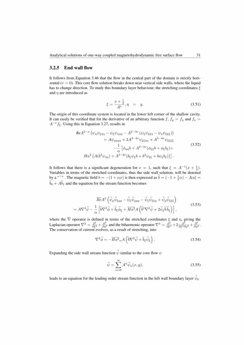
Analytical solutions of one-way coupled magnetohydrodynamic free surface flow 31
3.2.5 End wall flow
It follows from Equation 3.46 that the flow in the central part of the domain is strictly hori-zontal (v = 0). This core flow solution breaks down near vertical side walls, where the liquidhas to change direction. To study this boundary layer behaviour, the stretching coordinates ξand η are introduced as
ξ =x+ 1
2
Aν, η = y. (3.51)
The origin of this coordinate system is located in the lower left corner of the shallow cavity.It can easily be verified that for the derivative of an arbitrary function f , fy = fη and fx =A−νfξ. Using this in Equation 3.27, results in
ReA2−ν (ψηψξηη − ψξψηηη −A2−3ν (ψξψξξη − ψηψξξξ))
= Aψηηηη + 2A3−2νψξξηη +A5−4νψξξξξ
− 1
α
[φηηb+A2−2ν(φξξb+ φξbξ)+
Ha2(A(b2ψηη) +A3−2ν(bξψξb+ b2ψξξ + bψξbξ)
)].
(3.52)
It follows that there is a significant degeneration for ν = 1, such that ξ = A−1(x + 12 ).
Variables in terms of the stretched coordinates, thus the side wall solution, will be denotedby a "˜" . The magnetic field b = −(1 + αx) is then expressed as b = (−1 + 1
2α)−Aαξ =
b0 +Ab1 and the equation for the stream function becomes
ReA2(ψyψξyy − ψξψyyy − ψξψξξy + ψyψξξξ
)
= A∇4ψ − 1
α
[b∇2φ+ bξφξ +Ha2A
(b2∇2ψ + 2ψξ b bξ
)],
(3.53)
where the ∇ operator is defined in terms of the stretched coordinates ξ and η, giving theLaplacian operator∇2 = ∂2
∂ξ2 + ∂2
∂η2 and the biharmonic operator∇4 = ∂2
∂ξ4 +2 ∂2
∂ξ2∂η2 + ∂2
∂η4 .The conservation of current evolves, as a result of stretching, into
∇2φ = −Ha2αA(b∇2ψ + bξψξ
). (3.54)
Expanding the side wall stream function ψ similar to the core flow ψ
ψ =
∞∑
n=0
Anψn(x, y), (3.55)
leads to an equation for the leading order stream function in the left wall boundary layer ψ0

32 Chapter 3
∇4ψ0 =1
α
[b0∇2φ1 + b1∇2φ0 + b1ξφ0ξ + b0ξφ1ξ +Ha2
(b20∇2ψ0 + 2b0b0ξψ0ξ
)].
(3.56)Simultaneously we obtain from the charge conservation equation
∇2φ0 = 0, (3.57)
∇2φ1 = −Ha2(b0∇2ψ0 + b0ξψ0ξ
), (3.58)
which, together with b0ξ = 0, reduces Equation 3.56 to
∇4ψ0 = 0. (3.59)
This has the solution ψ0 = 0, which agrees with the observation for the core flow. When thecontact angle boundary condition is limited to
tan(θ − 12π) = mA2, (3.60)
where m ≤ O(1) is a measure for the contact angle. The boundary condition for the freesurface gives h1ξξ = 0 and h1ξ(0) = 0. Thus, for the free surface deformation it is obtainedthat h1 = 0.
It is observed that φ = x relates to φ0 = − 12 and φ1 = ξ, which is satisfying the above
problem. Using ψ0 = 0, the first order stream function ψ1 obeys
∇4ψ1 =1
α
[b0∇2φ2 + b1∇2φ1 + b1ξφ1ξ + b0ξφ2ξ
+ Ha2(
2b0b1∇2ψ0 + b20∇2ψ1
)]. (3.61)
Reducing this with relation ∇2φ2 = −Ha2(b1∇2ψ0 + b0∇2ψ1
)from charge conservation
results in∇4ψ1 =
1
αb1ξφ1ξ = −1, (3.62)
which ultimately describes the change of flow direction in the boundary layer flow near theleft wall.
The walls at the side and bottom are no-slip, meaning ψ1 = ψ1y = 0 at the bottom andψ1 = ψ1ξ = 0 at the left wall. For the free surface ψ1 = 0 (from Equation 3.16), ψ1ξ = 0
(from Equation 3.5) and ψ1yy − ψ1ξξ = 0 (from Equations 3.12, 3.13 and 3.15), effectivelyreducing at this order to ψ1 = ψ1yy = 0. The solution for ξ → ∞ should match with thecore flow solution (Equation 3.46).

Analytical solutions of one-way coupled magnetohydrodynamic free surface flow 33
The derivation for the right wall flow can be obtained following the exact same arguments,but with the stretching coordinate ζ = A−1( 1
2 − x), and leads to the same results as the leftwall. This will not be repeated here.
A final boundary condition for the top surface is obtained from Equation 3.31
h2ξξ = 0, (3.63)
Combining this with the contact angle boundary condition 3.18, h2ξ = m (and similarly forthe right wall) and the volume conserving property (Equation 3.17), this leads to a closedexpression for the free surface elevation that is valid over the full width of the liquid layer:
h2(x) =1√Bo
3Ca
8Bo
sinh(√
Box)
cosh(
12
√Bo) −m
cosh(√
Box)
sinh(
12
√Bo)
− 3Ca
8Box+
2m
Bo, (3.64)
From Equation 3.46 we see that the flow strength scales with a single dimensionless para-meter, α, while the free surface elevation depends on Ca and Bo as well. This has as aninteresting consequence that, for example, the velocities in the liquid layer can be increasedat fixed free surface elevation, or vice versa.
In the absence of gravity, e.g. Bo = 0, Equation 3.49 would simplify to h2xxx = 3/8Ca,with solution
h2 =1
16Ca
(x3 − 3
4x
)−m
(x2 − 1
12
), (3.65)
which is consistent with Equation 3.64, in the limit for Bo → 0. For decreasing influenceof surface tension, in other words, for increasing Ca, the linear term in Equation 3.64 willbecome dominant. However, the limit Ca → ∞ does not exist, as close enough to the sidewalls, surface tension is always significant.
Reducing Equation 3.65 to units carrying a dimension, gives
∆h′ = A2dh2 =Cadα
16A2
(x′3
l3− 3
4
x′
l
)=σ∆φb0dlα
γ
(x′3
l3− 3
4
x′
l
), (3.66)
The horizontal velocity profile in dimensioned variables, follows from the stream functionfor the core flow (Equation 3.46):
u′(y′) = − 1
48Au∗
(8y′3
d3− 15
y′2
d2+ 6
y′
d
). (3.67)
3.2.6 Analytic solution for the end wall flow
The flow in the side wall is described by the biharmonic Equation 3.62
∇4ψ1 = −1. (3.68)

34 Chapter 3
With boundary conditions
ψ1 = 0, ψ1η = 0 on η = 0
ψ1 = 0, ψ1ηη − ψ1ξξ = 0, ψξ = 0 on η = 1
ψ1 = 0, ψ1ξ = 0 on ξ = 0
ψ1 = ψ1(η), ψ1ξ = 0 for ξ →∞.
(3.69)
We will now apply the transformation
χ(x, y) = ψ1 − ψ1(y). (3.70)
For clarity and staying in line with literature notation, we will now use x, y instead of ξ, ηand reduce the boundary conditions to:
χ = 0, χy = 0 on y = 0χ = 0, χyy = 0 on y = 1χ = f(y) = −ψ1(y), χx = 0 on x = 0χ = 0, χx = 0 for x→∞.
(3.71)
The solution to Equation 3.70 can be found using the Laplace transform:
f(p, y) = L[χ(x, y)] =
∫ ∞
0
χ(x, y)e−pxdx, (3.72)
As a first step, Equation 3.70 is Laplace transformed
L[∇4χ] =∂4f
∂y4+ 2p2 ∂
2f
∂y2+ p4f = p3χ(0, y)
+:
0p2χx(0, y) + pχxx(0, y) + χxxx(0, y) + 2
p∂
2χ
∂y2(0, y) +
*0
∂2χx∂y2
(0, y)
.
(3.73)
This reduces the differential equation in coordinates x and y to a differential equation in yonly. At x = 0 additional boundary conditions on χxx and χxxx are required by the aboveformula. χ(0, y) is expanded in a sine series as follows
χ(0, y) =
∞∑
n=1
bn sin(nπy) with bn = 2
∫ 1
0
χ(0, y) sin(nπy)dy (3.74)
The unknown functions χxx and χxxx are expanded by the same means, thus
∂2χ
∂x2(0, y) =
∞∑
n=1
cn sin(nπy)∂3χ
∂x3(0, y) =
∞∑
n=1
dn sin(nπy), (3.75)

Analytical solutions of one-way coupled magnetohydrodynamic free surface flow 35
however, the coefficients cn and dn can not be determined at this point.
The ordinary differential equation for the function f(p, y) now becomes
∂4f
∂y4+ 2p2 ∂
2f
∂y2+ p4f =
∞∑
n=1
βn(p) sin(nπy) (3.76)
βn(p) =
(p3 − 2pn2π2
)bn + pcn + dn
(p2 − n2π2)2 . (3.77)
The general solution of this differential equation is
f(p, y) = K1 sin(py) +K2 cos(py) +K3y sin(py) +K4y cos(py) +∑
βn(p) sin(nπy).
(3.78)
The four boundary conditions on the two boundaries for y provide the integration constantsKi
K1 =∑
n
−βn(p)nπ
p− cos p sin p(3.79)
K2 = 0 (3.80)
K3 =∑
n
βn(p) sin2 pnπ
p− cos p sin p(3.81)
K4 =∑
n
βn(p) sin p cos pnπ
p− cos p sin p(3.82)
(3.83)
And thus
f(p, y) =∑
n
βn(p)[
sin(nπy)+
nπ
p− cos p sin p
(− sin(py) + sin2 p sin(py)y + sin p cos p cos(py)y
) ] (3.84)
The inverse Laplace transform will in principle provide the stream function χ. It shouldhowever be noted that the coefficient βn still contains unknowns cn and dn. The inverseLaplace transform and the unknown coefficients can be found in the same solution step,using complex analysis. The steps follow the procedure by Benthem 3 and is schematicallysummarized in figure 3.4.
The inverse Laplace transformation is given by the Bromwich integral (see Kwok 20 andDuffy 10 p61):
χ(x, y) =1
2πilimR→∞
∫ a+iR
a−iRf(p, y)epxdp (3.85)

36 Chapter 3
Re
Im
Figure 3.4 The inverse Laplace transform is provided by the integral along the solid line. The pathintegral is closed by adding the dashed, semi-circle, which integral is zero by Jordan’s lemma. Theresidue theorem gives the integral for the poles (dark crosses) inside the closed path.
where a > 0. The contour integral can be closed with the left semi-circle, and by applicationof Jordan’s lemma, this gives:
χ(x, y) =1
2πi
∮
C
f(p, y)epxdp (3.86)
The integral can be evaluated by applying the Cauchy residue theorem
χ(x, y) =∑
k
Res(f(pk, y)), (3.87)
where the summation is over the poles of f(p, y) inside the closed contour. It is observedthat the first pole is p = 0 and the subsequent poles are solutions of p − cos p sin p = 0 (or2p− sin 2p = 0).
2p − sin(2p) = 0 has infinitely many complex solutions, which we will find numerically.Therefor we will truncate the above infinite sums after the first P terms. There, we need tofind the poles inside the closed loop and thus the poles closest to the origin. To find the polesof 2p − sin(2p) = 0 we will combine the search algorithm outlined by Meylan and Gross 22
with knowledge about the equation.
The algorithm is based on the fact that the anti-clockwise integral of the variation of theargument along a closed loop is a measure for the amount of poles inside this closed loop. Thebrute force algorithm is based on performing the closed loop integral on boxes and refiningthe boxes until only one pole is counted inside. Newton’s method will then be used to finda pole. If the starting point is outside the basin of attraction of the pole, another refinementstep will be performed. Applying the brute force method on the current problem is ratherexpensive. The brute force method will be applied on a significantly reduced subset of thecomplex numbers

Analytical solutions of one-way coupled magnetohydrodynamic free surface flow 37
• If p is a pole, then are p∗, −p and −p∗ also poles of the equation. In other words,finding the poles in the first quadrant is sufficient.
• Writing p = x+ ıy, we obtain
x = sinx cosh y, (3.88)y = cosx sinh y. (3.89)
Which can be reduced to x2 = cosh2 y − y2 coth2 y, which is a monotonically in-creasing function. In other words, if we find the pole in the first quadrant closest to theorigin, we know that each subsequent pole in the first quadrant has a larger real andimaginary part than the current pole.
Using this algorithm, as many poles as desired can be found, while the found poles are alsothe ones closest to the origin, which is necessary for the intended inverse Laplace transform.In order to find the Laplace transform, we apply the residue theorem. The residue at p = 0 is0, which follows from
Res(f(0, y)) = limp→0
pf(p, y) = 0. (3.90)
The residues at the other poles are depending on the unknown coefficients cn and dn. Tocalculate the unknown quantity, we make us of
Res
(g(p)
h(p)
)=
g(p)
h′(p). (3.91)
For this problem, h(p) = p − sin p cos p and h′(p) = 2 sin2 p can be used. With the numer-ically obtained poles and the above method for calculating the residue at pole pk, we find,when including all prefactors
Res(f(pk, y)) = F (pk, y)
∞∑
n=1
nπβn(p) (3.92)
with
F (pk, y) =− sin(pky) + sin2 pk sin(pky)y + sin pk cos pk cos(pky)y
2 sin2 pk. (3.93)
The coefficient cn and dn are still undetermined, but we will choose them such, that theresidues for the poles with Re(pk) > 0 vanish for arbitrary y, in other words, for the specificpole pk, this requires
P∑
n=1
nπ
(p3k − pkn2π2
)bn + pkcn + dn
(p2k − n2π2)
2 = 0, (3.94)
where the infinite sum is truncated after the first P terms. Considering the first P poles inthe first quadrant and obtaining the P in the fourth quadrant for free, this gives a set of 2P

38 Chapter 3
0
0.2
0.4
0.6
0.8
1
0 0.2 0.4 0.6 0.8 1
y
ξ
0
0.01
0.02
0.03
0.04
0 0.01 0.02 0.03 0.04y
ξ
Figure 3.5 The velocity vector plot (left) in the left side wall region is depicted, which is derived fromthe side wall stream function (Equation 3.95) for P = 2048. The flow is turning clockwise, while thevelocity at the left and bottom boundary is zero and the top boundary is a free surface. The streamlineplot (right) is determined for P = 8192 shows isocontours of the stream function in the region of thelower left corner of the domain, demonstrating the existence of a counter-rotating eddy in the corner.
equations in 2P unknowns. In matrix notation this results in a full matrix of (2P )2 complexcomponents, which can be solved for cn and dn by Gauss elimination.
When the poles pk and coefficients cn and dn are known, Equation 3.87 provides the solutionto the problem.
χ(x, y) =
2P∑
k=1
P∑
n=1
nπβn(−pk)F (−pk, y)e−pkx, (3.95)
which can straightforwardly be transformed back to the streamfunction ψ1. It should benoted that, the Gauss elimination is an O(P 3) algorithm, while the calculation of ψ1 is inprinciple O(P 2), the prefactor for the latter calculation is rather large, based on the amountof operations and the fact that is operated on a grid looping over x and y.
Figure 3.5 shows the currently obtained velocity field for P = 2048 and streamlines in theregion close to the corner for P = 8192. A counter-rotating eddy was found close to thecorner, as was predicted by Moffatt 23 . Such a counter-rotating eddy was not found in thecorner near the free surface.
Figure 3.6 shows the velocity magnitude along the line ξ = y, where a different number ofpoles are included to calculate the stream function. It shows the convergence of the velocitymagnitude with an increasing number of poles. It can be seen that increasing the amount ofpoles above 4 does not change the velocity profile beyond a distance of 0.1 from the corner,while P = 1024 and P = 8192 are enough for an accurate velocity profile beyond a distanceof 0.01 and 0.002 respectively.
The minimum in this velocity profile is related to the centre of the eddy. Increasing the

Analytical solutions of one-way coupled magnetohydrodynamic free surface flow 39
10−10
10−8
10−6
10−4
10−2
10−3 10−2 10−1
√u2
+v2
√ξ2 + y2
P = 16384P = 8192P = 1024P = 4
Figure 3.6 The velocity magnitude along the line ξ = y in Figure 3.5, which shows the effect ofincreasing the amount of poles (see Equation 3.95) on the velocity magnitude for P = 4, P = 1024,P = 8192 and P = 16384.
number of poles reveals a secondary minimum, which is an indication for the second eddy ofthe infinite series of eddies in the corner, as predicted by Moffatt 23 .
3.2.7 Increased magnetic interaction
In the derivation of the free surface elevation (Equation 3.64), it was found that for the Hart-mann number Ha = O(1), only O(A) flow is present. Suppose the square of the Hartmannnumber increases by an order inA, thusHa2 = Ha2A−1. For this higher Hartmann number,it can be shown that, again, ψ0 = 0 and the core flow ψ1, can be solved by
ψ1yyyy = −1, ψ1 = − 1
48y2(2y2 − 5y + 3
), (3.96)
which would result in the general solution for h2 as given by Equation 3.50.
For the side wall solution, again ψ0 = 0 is found, however, at higher order
∇4ψ1 =1
α
(φ1ξ b1ξ +Ha2
αψ1ξ b0b1ξ
)= −1−
(1
2α− 1
)Ha2
αψ1ξ. (3.97)
which means that the analytical side wall solution from Section 3.2.5 is no longer valid forHa2 = O(A−1).
For Ha2 = O(A−2), the primary flow in the core region will no longer be one-dimensional,as the equation for the core flow would read
ψ0yyyy =1
αHa2ψ0xbbx = Ha2 (1 + αx)ψ0x. (3.98)

40 Chapter 3
3.3 Numerical modeling
The analytic solution to the liquid layer problem with a Lorentz force will be compared withnumerical solutions obtained from two different methods for evaluating free surface flows.The first method is the moving mesh interface tracking (MMIT) method, where the meshaligns with the free surface. The second method is the volume of fluid (VOF) method, wherethe free surface is tracked with a transport equation for the liquid fraction.
The numerical simulations are performed using the standard31 and extended34 OpenFOAMsoftware. Available solvers were extended with the one-way coupled MHD equations for bothmethods, respectively interTrackFoam of distribution 1.6 extend and interFoam of distribution2.1.
3.3.1 Moving mesh interface tracking method
The moving mesh interface tracking method is based on aligning a boundary of the numericalmesh with the free surface. This results in a sharp interface by definition and allows for theimplementation of exact boundary conditions at the interface. The approach as proposed byMuzaferija and Peric 24 and the implementation by Tukovic and Jasak 35 was used.
The moving mesh interface tracking method introduces, in addition to continuity and mo-mentum equations, the so called space conservation law, i.e.
d
dt′
∫
V ′dV ′ −
∫
S′n ·vs
′dS′ = 0 (3.99)
where vs′ is the velocity of the surface. This velocity of the surface of an arbitrary con-
trol volume V ′ has to be accounted for in the integrated mass and momentum conservationequations.24,35
The boundary conditions from Section 3.2.2 do also apply for the numerical simulations,e.g. no mass should cross the boundary and the stresses at opposite sides of the interfaceshould match. Non-zero mass fluxes through the free surface are corrected by moving theboundary. This correction is used as a boundary condition in the Laplace equation for movingthe interior points in the domain by an amount d′:
∇′Γ ·∇′d′ = 0 (3.100)
where Γ is a diffusion parameter that is inversely proportional to the square of the distance tothe free surface.
Details of the numerical simulation
The simulations were performed on an initially square cell grid containing 20N × N cells,representing the bottom layer only, with A = 0.05 and Re = A, Ha = 1, Ca = A4

Analytical solutions of one-way coupled magnetohydrodynamic free surface flow 41
and Bo = A2. Figure 3.7(top) shows the vertical velocity component along a horizontalline y = 0.5 for various N . The difference in maximum velocity obtained on a mesh withN = 20, compared to N = 10 and N = 30 meshes was 0.5% and −0.05% respectively.The convective term is discretized with a second order central differencing scheme, the timederivative with a second order implicit method and the least squares method was used forgradient calculation.
The numerical values for the material properties of the top phase are defined to be σ2/σ = 0,ρ2/ρ = 0 and ν2/ν = 0, and are necessary for the boundary conditions, for example thepressure in the gas phase is assumed to be constant. The zero conductivity constraint forthe top phase was implemented via the boundary condition for the electric potential at theinterface.
3.3.2 Volume of fluid method
The VOF method is based on solving a transport equation for an indicator function, whichdetermines the spatial distribution of the fractions of two immiscible fluids and consequentlythe density of the liquid in the Navier-Stokes equations.15,27 The Continuum Surface Force(CSF) approach is used for implementation of the interfacial tension force between the twofluids6 and an artificial compression velocity is introduced for sharpening the resulting diffuseinterface between the two fluids.37
The describing equations for two-phase VOF flows are the continuity equation
∂vj∂xj
= 0, (3.101)
where vi is the velocity vector, the Navier-Stokes equations,6,15
∂ρvi∂t
+ vj∂ρvi∂xj
= − ∂p
∂xi+
∂
∂xj
[µ
(∂vi∂xj
+∂vj∂xi
)]+ fi + γκ
∂α
∂xi, (3.102)
where α is the indicator function, fi the body force, ρ and µ the phase averaged density andviscosity and κ the curvature of the interface in the CSF approach,6 determined by
κ =∂
∂xk
1∣∣∣∣∂α
∂xj
∣∣∣∣
∂α
∂xk
. (3.103)
and the transport equation for the indicator function α27
∂α
∂t+
∂
∂xj(αvj) +
∂
∂xj(vr,iα (1− α)) = 0. (3.104)
For the studied liquid-air flow, the indicator function equals 1 for the liquid phase and 0 forthe air phase and is in the range (0, 1) around the interface. The third term includes the

42 Chapter 3
artificial compression velocity, vr,i and is zero outside the interface region. This term can bederived from the continuity equations for the phase fractions in the two-fluid Euler approach,leading to the relative velocity vr,i = vl,i − vg,i between the liquid and the gas phase.4 Theterm compressibility does not refer to compression of the distinct phases, but compression ofthe interface itself, which can be seen as additional convection of the phase fraction due tovr,i.
The body force fi is the Lorentz force,
fi = εijkjjbk. (3.105)
The magnetic field bi is externally applied and constant in time, whereas the current densityji is calculated from the electric potential φ. From conservation of current
∂jj∂xj
= 0 (3.106)
and the definition of the current density
ji = σ
(− ∂φ∂xi
+ εijkujbk
), (3.107)
an additional Poisson’s equation for the electric potential is introduced
∂
∂xi
(σ∂φ
∂xi
)=
∂
∂xi(σεijkujbk) , (3.108)
where the electrical conductivity σ is linearly interpolated between both phases, which meansharmonic interpolation on the resistivity.
Details of the numerical simulation
The simulations were performed on a square cell grid containing 20N × 3N cells, wherethe bottom 20N × N cells were initially filled with the conductive fluid, and the remainingpart was filled with gas. For these simulations hence A = 0.05 and furthermore Re = A,Ha = 1, Ca = A4 and Bo = A2. Figure 3.7(bottom) shows the vertical velocity componentalong a horizontal line y = 0.5 for various N . The difference in maximum velocity obtainedon a mesh with N = 20, compared to N = 10 and N = 30 meshes was 6.6% and 0.2%respectively. The time derivative is discretized using a second order implicit method, whereasthe convective and diffusive terms are discretized using a second order central differencingscheme.
The values for σ2, ρ2 and ν2 are explicitly used during the simulation, and are non-zero toavoid singularities in the problem. For the present simulations σ2/σ = 10−18, ρ2/ρ = 10−3
and ν2/ν = 10.

Analytical solutions of one-way coupled magnetohydrodynamic free surface flow 43
0
2 ·10−4
4 ·10−4
6 ·10−4
8 ·10−4
1 ·10−3
-0.5 -0.48 -0.46 -0.44 -0.42 -0.4
v[-
]
x [-]
N = 10N = 20N = 30
0
2 ·10−4
4 ·10−4
6 ·10−4
8 ·10−4
1 ·10−3
-0.5 -0.48 -0.46 -0.44 -0.42 -0.4
v[-
]
x [-]
N = 10N = 20N = 30
Figure 3.7 The vertical velocity v along the horizontal line y = 0.5 for respectively N = 10, N = 20and N = 30. (top) For the MMIT simulations, where the grid consists of 20N × N control volumes.(bottom) For the VOF simulations where the grid consist of 20N × 3N control volumes, with thebottom 20N ×N control volumes initially liquid filled.
3.4 Numerical results
3.4.1 Base case
For A = 0.1, Figure 3.8 compares the free surface elevation of the analytical results for thefirst order deformation with the numerical results from both the MMIT and VOF method. ForRe = A, Ha = 1, Bo = A2 and Ca = A4, it can be seen that the analytical solution is ingood agreement with the numerically determined free surface elevations.
Figure 3.9 shows the pressure and horizontal velocity (from Equation 3.46 and 3.26) for thevertical line x = 0. Again a good agreement is obtained between analytical results andnumerical simulations.
In Figure 3.10, both velocity components along the line y = 0.5 in the region close to thewall are depicted. The analytic solution is obtained from Equation 3.95, with P = 1024. Forboth velocity components and both simulation methods, it is seen that the velocity profilesobtained from the numerical simulations accurately match the analytical expression for thesecomponents.

44 Chapter 3
-0.02
-0.01
0
0.01
0.02
-0.4 -0.2 0 0.2 0.4
h[-
]
x [-]
Figure 3.8 Elevation h of the free surface over the width of the domain for A = 0.1, Re = A,Ha2 = 1, Bo = A2 and Ca = A4. The MMIT simulation (circles), the VOF simulation (squares) andthe first order analytic approximation (solid line) of Equation 3.64 are shown.
0
0.2
0.4
0.6
0.8
1
0 0.02 0.04 0.06 0.08 0.1
y[-
]
p [-]
0
0.2
0.4
0.6
0.8
1
-0.001 0 0.001 0.002u [-]
Figure 3.9 Pressure p (left) and horizontal velocity u (right) for the line x = 0 for A = 0.1, Re = A,Ha2 = 1, Bo = A2 and Ca = A4. The MMIT simulation (circles), the VOF simulation (squares) andthe first order analytic approximation (solid line) are shown.
0
2 ·10−4
4 ·10−4
6 ·10−4
8 ·10−4
1 ·10−3
-0.5 -0.45 -0.4
v[-
]
x [-]
0
−6 ·10−4
−5 ·10−4
−4 ·10−4
−3 ·10−4
−2 ·10−4
−1 ·10−4
-0.5 -0.45 -0.4
u[-
]
x [-]
Figure 3.10 The horizontal (left) and vertical (right) velocity component along the line y = 0.5 forA = 0.1, Re = A, Ha2 = 1, Bo = A2 and Ca = A4. The MMIT simulation (circles), the VOFsimulation (squares) and the first order analytic approximation of Equation 3.95 using P = 1024 (solidline) are shown.

Analytical solutions of one-way coupled magnetohydrodynamic free surface flow 45
0
2 ·10−4
4 ·10−4
6 ·10−4
8 ·10−4
1 ·10−3
-0.5 -0.45 -0.4
v[-
]
x [-]
0
−6 ·10−4
−5 ·10−4
−4 ·10−4
−3 ·10−4
−2 ·10−4
−1 ·10−4
-0.5 -0.45 -0.4
u[-
]
x [-]
0
−1 ·10−4
−5 ·10−5
5 ·10−5
1 ·10−4
-0.5 -0.45 -0.4
w[-
]
x [-]
Figure 3.11 Horizontal (left) and vertical (middle) velocity components (as Figure 3.10) and spanwisevelocity component (right), along the line y = 0.5 for A = 0.1, Re = A, Ha2 = 1, Bo = A2, Ca =A4 and θ = 90, for the analytical solution (solid line), the two-dimensional numerical simulation (©),and the numerical simulation for a cavity with z-dimension 100d (4), 10d (5) and d (♦).
3.4.2 Three-dimensionality of the flow
In this section we will numerically evaluate, using the MMIT method, the effect of bound-ing walls in the third dimension on the two-dimensional flow in the z = 0-plane. In thez = 0-plane, the Lorentz force has a zero component in the z-direction, therefore the three-dimensionality of the magnetic field does not influence the equations for u and v in that plane(Equations 3.22 and 3.23). By introducing walls to bound the domain in the z direction,however, additional viscous shear from these walls can be expected. Figure 3.11 comparesthe velocity components for increasing size w of the domain in the z-direction. This size wasconsecutively increased from w = d, to w = d/A and to w = d/A2. For w = d, the ve-locities in the xy-plane are significantly smaller than analytically derived, whereas the shapeof these velocity profiles has not changed. This is caused by the viscous shear from the wallsthat bound the domain in the z-direction. When the extend of the domain in the z directionincreases, Figure 3.11 shows that the velocity profiles converge to the velocity profile fromthe two-dimensional numerical simulation and the analytical solution, without generating asignificant velocity component in the spanwise direction. Therefore, for large enough domainsizes in the third dimension, the presented two-dimensional analytical solution is valid for theflow in the z = 0-plane of the formulated three-dimensional problem.
3.4.3 Increased deformation
Section 3.2.7 showed the difficulties in deriving the final solution for increasing Hartmannnumber. In this section we will obtain numerical results for the surface elevation under higherHartmann number, as well as higher capillary number, Bond number, Reynolds number andaspect ratio, in order to determine to what degree the analytic solution of Equation 3.64 holds.

46 Chapter 3
MMIT
Figure 3.12 shows the free surface elevation for a set of cases in which, starting fromA = 0.1,θ = 90, Re = A, Ha2 = 1, Ca = A4, Bo = A2, either of the parameters Ha, Ca, Bo orA is increased to large values for which the analytic solution is not expected to hold.
From Figure 3.12(a) it can be seen, that, even though the derivation for the free surfaceelevation is valid for Ha2 ≤ O(1), the analytical solution using Ha2 = 1000 still closelyagrees with the numerical solution.
Also for capillary number increasing up to Ca = 1000A4, the numerical solution remainsclose to the analytical expression, as can be seen from Figure 3.12(b), where both numericaland analytical free surface elevations are scaled with the capillary number. We obtain thisresults, even though from a comparison between the boundary condition used with the presentassumptions onCa (Equation 3.41) and the full boundary condition (Equation 3.13), it followthat for increasing values of Ca the boundary condition gets increasingly complex. Figure3.12(c) shows that for increasing Bo numbers, the free surface elevation quickly decreases,as does the surface curvature in the core, in line with Equation 3.64. The analytical model fitsthe numerical data well for increasing Bo. Finally, Figure 3.12(d) shows that for an aspectratio as large as A = 0.5, the analytically determined free surface elevation is still matchingthe numerical result of the MMIT method very well.
VOF
Figure 3.13 shows what happens to the free surface elevation when increasing either Ha,Ca, Bo and A using the VOF method. As for the MMIT method, it is seen that the analyticalexpression for the free surface elevation is relatively accurate even for larger values of thedimensionless parameters than assumed in deriving the analytical model. This is especiallyso for Ha and Bo.
For large Ca = 1000A4, the free surface elevation starts to deviate visibly, whereas forA ≥ 0.5, the simulations did not result in a converged steady state solution, which we havealso seen for Ha2 > 4000. As various of the properties are varied over many orders ofmagnitude, challenges with numerical stability are not surprising. Further addressing theseissues is outside the scope of this chapter. We can however conclude that the MMIT methodis more robust in handling these parameter variations.

Analytical solutions of one-way coupled magnetohydrodynamic free surface flow 47
-0.02
-0.01
0
0.01
0.02
-0.4 -0.2 0 0.2 0.4
h[-
]
x [-]
(a)
-0.02
-0.01
0
0.01
0.02
-0.4 -0.2 0 0.2 0.4
h/C
a[-
]
x [-]
(b)
-0.02
-0.01
0
0.01
0.02
-0.4 -0.2 0 0.2 0.4
h[-
]
x [-]
(c)
-0.02
-0.01
0
0.01
0.02
-0.4 -0.2 0 0.2 0.4
h[-
]
x [-]
(d)
Ha2 = 1Ha2 = 100Ha2 = 1000
Ca = A4
Ca = 100A4
Ca = 1000A4
Bo = A2
Bo = 10A2
Bo = 100A2
A = 0.05A = 0.5A = 1
Figure 3.12 The surface elevation h from the MMIT simulations (symbols), horizontally rescaled to[−0.5, 0.5], where from A = 0.1, Ha2 = 1, Ca = A4, Bo = A2, either of the parameters Ha2 (a),Ca (b) , Bo (c) and A (d) is varied. The solid line indicates the analytic solution (Equation 3.64)

48 Chapter 3
-0.02
-0.01
0
0.01
0.02
-0.4 -0.2 0 0.2 0.4
y[-
]
x [-]
(a)
-0.02
-0.01
0
0.01
0.02
-0.4 -0.2 0 0.2 0.4
h/C
a[-
]
x [-]
(b)
-0.02
-0.01
0
0.01
0.02
-0.4 -0.2 0 0.2 0.4
h[-
]
x [-]
(c)
-0.02
-0.01
0
0.01
0.02
-0.4 -0.2 0 0.2 0.4
h[-
]
x [-]
(d)
Ha2 = 1Ha2 = 100Ha2 = 1000
Ca = A4
Ca = 100A4
Ca = 1000A4
Bo = A2
Bo = 10A2
Bo = 100A2
A = 0.05A = 0.2
Figure 3.13 The surface elevation h from the VOF simulations (symbols), horizontally rescaled to[−0.5, 0.5], where from A = 0.1, Ha2 = 1, Ca = A4, Bo = A2, either of the parameters Ha2 (a),Ca (b) , Bo (c) and A (d) is varied. The solid line indicates the analytic solution (Equation 3.64)

Analytical solutions of one-way coupled magnetohydrodynamic free surface flow 49
3.4.4 Error
The normalized root mean square distance between the derived analytical elevation (Equation3.64) and the calculated profile is defined as
e[xi] =
∑i
(A2h(xiA)− yi
)2∑i (A2h(xiA))
2 with h(x) =3
8
Ca
Bo
sinh(√
Box)
cosh(
12
√Bo) 1√
Bo− x
(3.109)
Figure 3.14 shows this normalized root mean square distance for either increasing Ha2, Ca,Bo, A or Re and for both numerical approaches. This distance is a measure for the deviationof the analytical result from the numerical simulation. It shows that the analytical solutionstarts to deviate more than 1% from the numerical solution for Ha2 > 1000. For Ca >1000A4 the analytical solution deviates more than 1% from the MMIT solution.
For the aspect ratio it is also concluded from Figure 3.14, that the analytical solution is within1% from the free surface elevation obtained from the MMIT model for values of the aspectratioA up to 0.5. For Reynolds numbers increasing toRe = 1000A, the free surface elevationobtained from the analytic model is within 1% from the free surface elevation obtained fromthe MMIT method.
In general, it can be seen from Figure 3.14 that the VOF solution for the free surface elevationalways deviates more from the analytical solution than the MMIT solutions. In addition tothe numerical challenges mentioned above, it should be noted that the properties of the topphase are non-zero in the VOF simulation, in contrast to the MMIT simulations and analyticalderivation.
3.5 Conclusions
In this chapter we have studied the flow and free surface elevation of a layer of conductiveliquid with height-to-width ratio A 1, that is subject to a potential difference horizontallyacross the domain and a traverse x-dependent magnetic field. It was shown that the surfacetension and gravity forces in combination with the unevenly distributed Lorentz forces onthe fluid induce a steady state flow, which scales linearly with conductivity, magnetic fieldgradient and applied potential difference and which vanishes for infinitely long layers (A →0), whereas the free surface deformation depends on the capillary number, the Bond numberand the contact angle condition.
Increasing pressure within the layer will cause the interface to deform. The profile of thisinterface was derived analytically for Hartmann numbers up to O(1), capillary numbers upto O(A4), Bond numbers up to O(A2) and Reynolds numbers up to O(A), while A 1.It was proven that to lowest order approximation, the surface elevation profile is a functionof the capillary number, the Bond number and the contact angle condition. The magnitude

50 Chapter 3
0.1%
1%
10%
10−2 10−1 100 101 102 103 104
erro
r
Ha2
(a)A = 0.1, Ca = A4, Bo = A2, Re = A
0.1%
1%
10%
10−2 10−1 100 101 102 103 104
erro
r
Ca/A4
(b)A = 0.1, Ha2 = 1, Bo = A2, Re = A
0.1%
1%
10%
10−2 10−1 100 101 102 103 104
erro
r
Bo/A2
(c)A = 0.1, Ha2 = 1, Ca = A4, Re = A
0.1%
1%
10%
10−2 10−1 100 101 102 103 104
erro
r
Re/A
(d)A = 0.1, Ha2 = 1, Ca = A4, Bo = A2
0.1%
1%
10%
10−1 100
erro
r
A
(e)Ha2 = 1, Ca = A4, Bo = A2, Re = A
Figure 3.14 The normalized root mean square distance between the rescaled elevation from the numer-ical simulation, either MMIT (solid line) or VOF (dashed line) and the analytical free surface elevation,where from the case A = 0.1, Re = A, Ha2 = 1, Ca = A4 and Bo = A2 either (from top to bottom)Ha2, Ca, Bo, A or Re is varied. The root mean square distance is normalized with
∫h2(x)dx.

Analytical solutions of one-way coupled magnetohydrodynamic free surface flow 51
of the free surface displacement scales linearly with the capillary number and decreases withincreasing Bond number. The shape of the free surface is determined by both the Bondnumber and the contact angle boundary condition.
Furthermore, the biharmonic equation for the stream function in the side wall region wassolved analytically, showing the turning of the flow and the presence of small eddies in thecorner regions.
The first order approximation of the analytic solution was compared to finite volume compu-tational models for free surface flow simulation using either a moving mesh interface trackingtechnique or a volume of fluid method to track the interface, in combination with a one-waycoupled MHD solver via the equation for the electric potential. The analytically derivedelevation and subsurface flow properties match the numerical simulations well.
The analytical solution presented in this paper is derived up to O(A). This means that thelowest order neglected terms are of order O(A2). For small enough aspect ratio (A = 0.1)these terms quickly reduce to values smaller than 1%. Indeed, the difference with the nu-merically found solution is only 0.4% (MMIT) and 1.2% (VOF) for A = 0.1. We thereforeconclude that the contribution of the neglected higher order terms in the analytical solution,for an aspect ratio of 0.1, is smaller than 1%.
From our numerical simulations we have observed that the MMIT method is more robust thanthe VOF method. Using the MMIT simulations, it is observed, that for larger values of theHartmann number, capillary number, Bond number, Reynolds number and aspect ratio, wherethe underlying assumptions of the analytic solution are no longer satisfied, the analyticalsolution and numerical results match within 1%, for A = 0.1 and either Ha2 up to 400, Caup to 200A4 or Bo up to 100A2 and within 2% for A = 0.5.
Bibliography
[1] Alboussière, T., Garandet, J. P., and Moreau, R. Asymptotic analysis and symmetry in MHD convection.Physics of Fluids, volume 8(8):pp. 2215–2226 (1996).
[2] Ben Hadid, H. and Henry, D. Numerical study of convection in the horizontal Bridgman configuration underthe action of a constant magnetic field. Part 2. Three-dimensional flow. Journal of Fluid Mechanics, volume333:pp. 57–83 (1997).
[3] Benthem, J. A Laplace transfor method for the solution of semi-infinte and finite strip problems in stressanalysis. Quarterly Journal of Mechanics and Applied Mathemathics, volume 16(4):pp. 413–429 (1963).
[4] Berberovic, E., van Hinsberg, N. P., Jakirlic, S., Roisman, I. V., and Tropea, C. Drop impact onto a liquid layerof finite thickness: Dynamics of the cavity evolution. Physical Review E, volume 79(3):p. 036306 (2009).
[5] Bian, W., Vasseur, P., and Bilgen, E. Effect Of An External Magnetic Field On Buoyancy-driven Flow In aShallow Porous Cavity. Numerical Heat Transfer, Part A: Applications, volume 29(6):pp. 625–638 (1996).
[6] Brackbill, J. U., Kothe, D. B., and Zemach, C. A continuum method for modeling surface tension. Journal ofComputational Physics, volume 100(2):pp. 335–354 (1992).
[7] Cormack, D., Stone, G., and Leal, L. The effect of upper surface conditions on convection in a shallow cavity
52 Chapter 3
with differentially heated end-walls. International Journal of Heat and Mass Transfer, volume 18(5):pp.635–648 (1975).
[8] Davidson, P. A. An Introduction to Magnetohydrodynamics. Cambridge University Press, 1 edition (2001).
[9] Davoust, L., Cowley, M. D., Moreau, R., and Bolcato, R. Buoyancy-driven convection with a uniform mag-netic field. Part 2. Experimental investigation. Journal of Fluid Mechanics, volume 400:pp. 59–90 (1999).
[10] Duffy, D. G. Transform methods for solving partial differential equations. CRC Press (1994).
[11] Fautrelle, Y. and Sneyd, A. D. Instability of a plane conducting free surface submitted to an alternatingmagnetic field. Journal of Fluid Mechanics, volume 375:pp. 65–83 (1998).
[12] Garandet, J. and Alboussière, T. Bridgman growth: Modelling and experiments. Progress in Crystal Growthand Characterization of Materials, volume 38(1):pp. 73–132 (1999).
[13] Garandet, J., Alboussiere, T., and Moreau, R. Buoyancy driven convection in a rectangular enclosure witha transverse magnetic field. International Journal of Heat and Mass Transfer, volume 35(4):pp. 741–748(1992).
[14] Gillon, P. Materials processing with high direct-current magnetic fields. JOM, volume 47(5):pp. 34–37(1995).
[15] Hirt, C. and Nichols, B. Volume of fluid (VOF) method for the dynamics of free boundaries. Journal ofComputational Physics, volume 39(1):pp. 201–225 (1981).
[16] Hughes, W. F. and Elco, R. A. Magnetohydrodynamic lubrication flow between parallel rotating disks.Journal of Fluid Mechanics, volume 13(01):pp. 21–32 (1962).
[17] Hunt, J. C. R. Magnetohydrodynamic Flow in Rectangular Ducts. Journal of Fluid Mechanics,volume 21(04):pp. 577–590 (1965).
[18] Juel, A., Mullin, T., Ben Hadid, H., and Henry, D. Magnetohydrodynamic convection in molten gallium.Journal of Fluid Mechanics, volume 378:pp. 97–118 (1999).
[19] Kharicha, A., Teplyakov, I., Ivochkin, Y., Wu, M., Ludwig, A., and Guseva, A. Experimental and numericalanalysis of free surface deformation in an electrically driven flow. Experimental Thermal and Fluid Science,volume 62:pp. 192–201 (2015).
[20] Kwok, Y. K. Applied Complex Variables. Cambridge University Press, New York, 1 edition (2002).
[21] Lehnert, B. An Instability of Laminar Flow of Mercury Caused by an External Magnetic Field. Proceedings ofthe Royal Society of London. Series A, Mathematical and Physical Sciences, volume 233(1194):pp. 299–302(1955).
[22] Meylan, M. H. and Gross, L. A parallel algorithm to find the zeros of a complex analytic function. ANZIAMJournal, volume 44(0):pp. E236—E254 (2003).
[23] Moffatt, H. K. Viscous and resistive eddies near a sharp corner. Journal of Fluid Mechanics,volume 18(01):pp. 1–18 (1964).
[24] Muzaferija, S. and Peric, M. Computation of Free-Surface Flows using the Finite-Volume Method and Mov-ing Grids. Numerical Heat Transfer, Part B: Fundamentals, volume 32(4):pp. 369–384 (1997).
[25] Northrup, E. F. Some Newly Observed Manifestations of Forces in the Interior of an Electric Conductor.Physical Review (Series I), volume 24(6):pp. 474–497 (1907).
[26] Ozoe, H. and Okada, K. The effect of the direction of the external magnetic field on the three-dimensionalnatural convection in a cubical enclosure. International Journal of Heat and Mass Transfer, volume 32(10):pp.1939–1954 (1989).
[27] Rusche, H. Computational Fluid Dynamics of Dispersed Two-Phase Flows at High Phase Fractions. PhDthesis, Imperial College (2002).
[28] S. Oshima and R. Yamane. Shape-control of Liquid Metal Free Surfaces by Means of a Static MagneticField. In J. Szekely, J. W. Evans, K. Blazek, and N. El-Kaddah, editors, Magnetohydrodynamics in ProcessMetallurgy, pp. 251–259. The Minerals, Metals and Materials Society (1991).

Analytical solutions of one-way coupled magnetohydrodynamic free surface flow 53
[29] Sen, A. K. and Davis, S. H. Steady thermocapillary flows in two-dimensional slots. Journal of Fluid Mech-anics, volume 121:p. 163 (1982).
[30] Series, R. W. and Hurle, D. T. J. The use of magnetic fields in semiconductor crystal growth. Journal ofCrystal Growth, volume 113(1-2):pp. 305–328 (1991).
[31] SGI Corp. OpenFOAM (2012).
[32] Shercliff, J. A. The Flow of Conducting Fluids in Circular Pipes Under Transverse Magnetic Fields. Journalof Fluid Mechanics, volume 1(06):pp. 644–666 (1956).
[33] Sundaravadivelu, K., Kandaswamy, P., and Kumar, K. Effect of magnetic field on the liquid-gas interfacialdeformation in thermocapillary convection problem. Zeitschrift für angewandte Mathematik und Physik,volume 51(3):p. 491 (2000).
[34] The OpenFOAM extend project. OpenFOAM-extend (2012).
[35] Tukovic, Z. and Jasak, H. A moving mesh finite volume interface tracking method for surface tension dom-inated interfacial fluid flow. Computers and Fluids, volume 55:pp. 70–84 (2012).
[36] Verhulst, F. Methods and Applications of Singular Perturbations. Springer Science+Business Media, Inc., 1edition (2005).
[37] Weller, H. G. A New Approach to VOF-based Interface Capturing Methods for Incompressible and Com-pressible Flow. Technical report, OpenCFD (2008).


4. Dynamics of a single, oscillatingturbulent jet in a confined cav-ity§
We demonstrate how the self-sustained oscillation of a confined jet in a thin cavity can bequantitatively described by a zero-dimensional model of the delay differential equation typewith two a priori predicted model constants. This model describes the three phases in self-sustained oscillations, viz.: (i) pressure driven growth of the oscillation, (ii) amplitude limit-ation by geometry and (iii) delayed destruction of the recirculation zone. The two parametersof the model are the growth rate of the jet angle by a pressure imbalance, and the delay timefor the destruction of this pressure imbalance. We present closed relations for both model con-stants as a function of the jet Reynolds number Re, the inlet velocity vin, the cavity width Wand the cavity width over inlet diameter W/d and we demonstrate that these model constantsdo not depend on other geometric ratios. The model and the obtained model constants havebeen successfully validated against three dimensional Large Eddy Simulations, and planarParticle Image Velocimetry measurements, for 1600 < Re ≤ 7100 and 20 ≤ W/d < 50.The presented model inherently contains the transition to a non-oscillating mode for decreas-ing Reynolds numbers or increasing W/d-ratios and allows for the quantitative prediction ofthe corresponding critical Reynolds number and critical W/d.
4.1 Introduction
A fluid jet may demonstrate self-sustained oscillations when it is confined in both directionsperpendicular to its flow direction. This phenomenon has been observed for jet Reynoldsnumbers ranging from Re = 1002,11,19,31 up to Re = 170, 000.20 The physical mechanismfor this oscillation is well understood for both laminar31 and turbulent10 jets. The dimen-
§Published as: Righolt, B. W., Kenjereš, S., Kalter, R., Tummers, M. J., and Kleijn, C. R., Dynamics of an oscillatingturbulent jet in a confined cavity. Physics of Fluids, 27:095107, 2015
55

56 Chapter 4
sions of the confining cavity are known to have an important influence on the presence andfrequencies of these oscillations. For very wide cavities, the domain becomes unboundedin one direction, and the self-sustained oscillation disappears.18 A jet in such a wide cav-ity shows meandering, self-similar behavior.13 For decreasing cavity width, the oscillationfrequency increases,14,18 until the cavity geometry approaches that of a sudden expansion,where strong asymmetries and oscillations are present as well.4,6,7 A vast amount of fluidicoscillators exist,10,19,23,25 which are for example found in backward facing steps, flows overcavities24 and jets through orifices.22 The systems have in common that either implicitly orexplicitly a delayed feedback loop is present that triggers the oscillatory behavior.
Delayed feedback mechanisms are very common in nature and technology and can result inoscillations of any type. Some of these mechanisms can be described by a delay differentialequation (DDE) with a single delay constant. The delay time between the uptake of oxygen inthe lungs and the reception in the brain stem plays a role in the arterialCO2 control system.16
In economics, the interplay between income and capital stock can be explained with a timedelay in investments.29. Another example is the large time-scale temperature oscillation onthe southern hemisphere, often referred to as El Nino, with a delay time that is associatedwith the transit time of Rossby and Kelvin waves across the Pacific ocean.3,28 DDE modelshave also been proposed for the oscillation of the reattachment length in a confined jet flow31
or for convective rolls in a closed box.30 Although the physical mechanism active in eachof the above examples may be very different, they have all been successfully described withDDE-type models.
The objective of the present study is (i) to develop a DDE-type model for the oscillations ofa turbulent jet in a confined cavity, which represents the physical phases of the oscillatingmotion and (ii) to use this model to predict necessary conditions for the existence of self-sustained oscillations depending on the jet Reynolds number Re, and cavity width to nozzlediameter ratio W/d. We use both Large Eddy Simulations and experimental data to validateour DDE model and its predictions.
The paper is outlined as follows. The confined jet configuration and numerical methods for3D LES turbulent flow simulations are given in section 4.2, the experimental validation ofthe numerical flow simulations is presented in section 4.3. In section 4.4 we present a zero-dimensional DDE-type model for single jet oscillations in a confined cavity and in section4.5 we discuss how the model parameters in the DDE model can be obtained from given flowproperties.
4.2 Methods
4.2.1 Description of setup
In this paper we study the flow in a cavity as depicted in Figure 4.1. This cavity has dimen-sions height × width × thickness (H ×W × T ). A downward oriented square tube of inner

Dynamics of a single, oscillating turbulent jet in a confined cavity 57
S
y
x
vin
inflow
outflow
free surface
H =
0.7
m
W = 0.3 m
p1
p2
dn d
Figure 4.1 Studied configuration of a single jet in a confined geometry. The cavity has dimensionsH ×W × T = 0.7× 0.3× 0.035 m3. The nozzle inner width is d = 0.01 m and is submerged by adistance dn = 0.1 m. The definition of the instantaneous jet angle θ, which is calculated between thenozzle exit and a line at a distance S downstream from the nozzle exit, and monitoring locations p1 andp2 are indicated.
dimensions d is inserted centrally to a depth dn, which injects the fluid into the cavity with avelocity vin. For H ×W × T = 0.7× 0.3× 0.035 m3, d = 0.01 m and dn = 0.1 m, theflow of salt water in this configuration is essentially two-dimensional, as will be demonstratedfurther in this paper by showing its insensitivity to the precise value of T , and to friction at thefront and back walls. The flow in this configuration was previously investigated experiment-ally using planar particle imaging velocimetry by Kalter et al. 10 . The outflow was placed offcenter, in order to allow for optical access. In the present study we use the same dimensionsH , T , d, dn, whereas the width W is varied between W/d = 10 and W/d = 100. Forthe cases W/d ≥ 50 the height H was increased to H/W = 2.5. The top of the cavityis a free surface and the working fluid has a density ρ = 1.1× 10³ kgm−3 and viscosityν = 1.27× 10⁻⁶ m2s−1.
In Figure 4.1 the instantaneous jet angle θ is defined. The jet angle was determined by a leastsquares fit of a straight line through the points xi = maxx(|v(yi)|), in other words, throughthe x-coordinates of the locations of maximum velocity magnitude for every line y = yi inthe range (−dn − S) < yi < (−dn), where we set S equal to W . Figure 4.2 shows thecollections (xi, yi) and the resulting linear fit for three time instances in half a period of the

58 Chapter 4
-0.7
-0.6
-0.5
-0.4
-0.3
-0.2
-0.1
-0.1 0 0.1
y[m
]
x [m]-0.1 0 0.1
x [m]-0.1 0 0.1
x [m]
Figure 4.2 The instantaneous jet angle is calculated from a least squares fit (blue line) through the pointsof maximum velocity (red dots) per y-coordinate in the instantaneous velocity field obtained from thenumerical simulation (black vectors). Here shown for Re = 4700 and W/d = 30 at t = 64 s (left), aquarter period later at t = 74 s and half a period later at t = 84 s.
oscillation.
4.2.2 Numerical fluid flow models
We consider the LES filtered, single phase, incompressible Navier-Stokes equations
∂vi∂t
+ vj∂vi∂xj
=∂
∂xj
[(ν + νSGS)
(∂vi∂xj
+∂vj∂xi
)]− 1
ρ
∂p
∂xi, (4.1)
where vi is the velocity, ρ the fluid density, ν the laminar viscosity, νSGS the sub-grid-scale viscosity from the LES model and p the pressure. We use the finite-volume based toolOpenFOAM 2.134 to solve the discretized equations using the PISO scheme.8
The dynamic Smagorinsky model15 has been employed to calculate the sub-grid-scale vis-cosity as νSGS = (C∆)
2 S, where ∆ is the local grid size, defined as ∆ = (∆x∆y∆z)1/3
and S the characteristic rate of strain, S = (2SijSij)1/2 and Sij = (∂vi/∂xj + ∂vj/∂xi) /2.
The Smagorinsky constant C is defined as C = 〈LijMij〉 /2⟨M2ij
⟩, with the resolved stress
tensor Lij = vivj − vivj and Mij = 2∆2SSij − 2 (2∆)2 SSij , where · indicates the fil-

Dynamics of a single, oscillating turbulent jet in a confined cavity 59
tering operation. An important advantage of the dynamic Smagorinsky model for the studiedapplication is that it automatically handles the damping of turbulence towards the walls.
As recommended by Lilly 15 we use local averaging (indicated by < . >) of the Smagorinskycoefficient in order to reduce computational instabilities, due to local small values ofM2
ij . Wefollow the approach of Zang et al. 35 and apply averaging over three control volumes in everydirection, as well as clipping of the total viscosity ν + νSGS at 0, in order to partially allowfor backscatter, i.e. the transfer of energy to larger scales.15 For the studied applications, theregion where νSGS/ν < −0.5 occupies less than 1% of the total domain.
The equations are discretized on an orthogonal, rectangular mesh, consisting of 128× 275×34 ≈ 1.1 × 10⁶ grid cells. This being a sufficient grid resolution is demonstrated in Fig-ure 4.3(bottom), which shows contours of the instantaneous νSGS/ν. The maximum valueνSGS/ν ≤ 10, and the domain averaged νSGS/ν = 0.1.
Temporal discretization is done using a second order fully implicit scheme,34 with a time stepcorresponding to max(Co = u∆t/∆x) = 1. Within the distributed version of OpenFoam,higher order explicit temporal discretization schemes are not available. Moreover, Vuorinenet al. have shown that their implementation and application of a third and fourth Runge-Kuttaexplicit temporal discretization within OpenFOAM led to a small efficiency gain only. Theconvective and diffusive terms are spatially discretized using a second order central differen-cing scheme.
The instantaneous value of y+ at the walls locally reaches values as low as y+ = 0.1 andas high as y+ = 15. We therefore apply, at all solid wall boundaries, a universal velocityprofile called Spalding’s law,27 viz. y+ = u+ +1/E
[exp(κu+)−
(1+κu+ +1/2(κu+)2 +
1/6(κu+)3)]
, with y+ = yuτ/ν, u+ = v/uτ , the friction velocity u2τ = (ν + νSGS) dv/dn,
κ = 0.41 and E = 9.8.5,9,17,32 This law is valid for 0 ≤ y+ ≤ 300 and we thereforegenerally apply it to all walls of the domain. For y+ < 10, which is the case for most partsof the walls, Spalding’s law reduces to the laminar flow no-slip boundary condition. Indeed,using a laminar flow boundary condition instead of Spalding’s law led to minor changes inthe flow behaviour only. This also indicates that our simulations are relatively insensitive tothe near-wall grid size.
For the inflow via the nozzle, a periodic inlet domain, of length 10d, was applied to guaranteefully developed inflow conditions. The free liquid surface at y = 0 was modeled using a freeslip boundary condition.
4.3 Validation of the numerical method
We validate the numerical model for a jet of Re = vind/ν = 4700 in a confined cavity asdefined in Figure 4.1 using data from our previous experiments.10 In Figure 4.3 vectors of themean velocity and contours of the horizontal and vertical components of the mean velocityare depicted, both for the present numerical simulation and for the experiment. In Figure

60 Chapter 4
-0.4
-0.3
-0.2
-0.1
y[m
]
Simulation Experiment
u=
0.1
m/s
Experiment
-0.4
-0.3
-0.2
-0.1
y[m
]
Experiment
-0.02
0
0.02
u[m
/s]
Experiment
-0.4
-0.3
-0.2
-0.1
y[m
]
Experiment
-0.1 0 0.1x [m]
-0.4
-0.3
-0.2
-0.1
0
0.1
v[m
/s]
Experiment
-0.1 0 0.1x [m]
-1
0
1
2
3
4
ν SG
S/ν
[-]
Experiment
Figure 4.3 For Re = 4700 and W/d = 30 in the z = 0-plane, simulation (left) and experiment(right), from top to bottom: Vector fields of the mean velocity, contours of the horizontal mean velocity,contours of the vertical mean velocity and contours of the scaled instantaneous sub-grid-scale viscosityνSGS/ν.

Dynamics of a single, oscillating turbulent jet in a confined cavity 61
-0.3
-0.2
-0.1
0
0.1
v y[m
/s]
y =−0.18 m
-0.3
-0.2
-0.1
0
0.1
v y[m
/s]
y =−0.28 m
-0.3
-0.2
-0.1
0
0.1
-0.15 -0.1 -0.05 0 0.05 0.1 0.15
v y[m
/s]
x [m]
y =−0.38 m
0
0.005
0.01
0.015
0.02
k[m
2 /s2 ]
y =−0.18 m
0
0.005
0.01
0.015
0.02
k[m
2 /s2 ]
y =−0.28 m
0
0.005
0.01
0.015
0.02-0.15 -0.1 -0.05 0 0.05 0.1 0.15
k[m
2 /s2 ]
x [m]
y =−0.38 m
Figure 4.4 (left) The vertical component of the mean velocity for Re = 4700 and W/d = 30 for thelines y = −0.18 m, y = −0.28 m and y = −0.38 m, which is respectively 0.08 m, 0.18 m and0.28 m below the nozzle exit for both the numerical simulation (solid red) and the experiments (dashedblue and circles, Kalter et al. 10 ) (right) The turbulent kinetic energy obtained from the numerical sim-ulations is shown for the same lines (red).
4.4 the vertical component of the mean velocity on three horizontal lines downstream fromthe nozzle is depicted. These comparisons show a good agreement between numerical andexperimental mean velocities.
Figure 4.4 furthermore shows profiles of the turbulent kinetic energy obtained from the nu-merical simulations, where at each distance a double peak is observed, which is related to thelong term oscillations of the jet in the cavity.
Figure 4.5 shows a time series of the jet angle for both the numerical simulations and the ex-periments. The dominant frequency of oscillation was determined at f = 0.022± 0.001 Hzfor the simulations and f = 0.023± 0.002 Hz for the experiments. This leads to a Strouhalnumber St = fW/vin of St = 0.011, which is in accordance with findings from literature.10
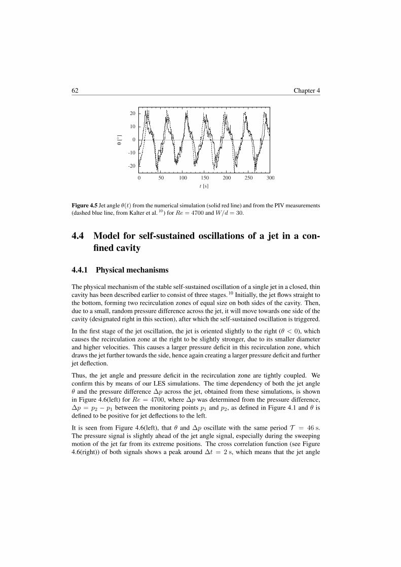
62 Chapter 4
-20
-10
0
10
20
0 50 100 150 200 250 300
θ[
]
t [s]
Figure 4.5 Jet angle θ(t) from the numerical simulation (solid red line) and from the PIV measurements(dashed blue line, from Kalter et al. 10 ) for Re = 4700 and W/d = 30.
4.4 Model for self-sustained oscillations of a jet in a con-fined cavity
4.4.1 Physical mechanisms
The physical mechanism of the stable self-sustained oscillation of a single jet in a closed, thincavity has been described earlier to consist of three stages.10 Initially, the jet flows straight tothe bottom, forming two recirculation zones of equal size on both sides of the cavity. Then,due to a small, random pressure difference across the jet, it will move towards one side of thecavity (designated right in this section), after which the self-sustained oscillation is triggered.
In the first stage of the jet oscillation, the jet is oriented slightly to the right (θ < 0), whichcauses the recirculation zone at the right to be slightly stronger, due to its smaller diameterand higher velocities. This causes a larger pressure deficit in this recirculation zone, whichdraws the jet further towards the side, hence again creating a larger pressure deficit and furtherjet deflection.
Thus, the jet angle and pressure deficit in the recirculation zone are tightly coupled. Weconfirm this by means of our LES simulations. The time dependency of both the jet angleθ and the pressure difference ∆p across the jet, obtained from these simulations, is shownin Figure 4.6(left) for Re = 4700, where ∆p was determined from the pressure difference,∆p = p2 − p1 between the monitoring points p1 and p2, as defined in Figure 4.1 and θ isdefined to be positive for jet deflections to the left.
It is seen from Figure 4.6(left), that θ and ∆p oscillate with the same period T = 46 s.The pressure signal is slightly ahead of the jet angle signal, especially during the sweepingmotion of the jet far from its extreme positions. The cross correlation function (see Figure4.6(right)) of both signals shows a peak around ∆t = 2 s, which means that the jet angle

Dynamics of a single, oscillating turbulent jet in a confined cavity 63
-10
-5
0
5
10
0 30 60 90 120 150
-20
-10
0
10
20
∆p
[Pa]−−
θ[
]—
t [s]
-1
-0.5
0
0.5
1
0 10 20 30 40 50
c[-
]
∆t [s]
Figure 4.6 (left) Time series of the pressure difference between monitoring point p1 and p2 (as definedin Figure 4.1) (dashed blue) and a time series of the jet angle θ (solid red) for Re = 4700. The verticallines indicate the time instances for the snap shots in Figure 4.2. (right) Cross correlation functionbetween ∆p and θ.
follows the pressure difference with a small time delay of 2 s. At the extreme positions, othereffects take over, and the phase difference is not clearly visible anymore. These observationsand the found time delay were found to be rather insensitive to the choice of the location ofprobe-points p1 and p2.
Next, in the second stage of the jet oscillation, the jet approaches the side wall and the recir-culation zone can not shrink any further, because this would lead to a strongly non-circular re-circulation zone with relatively high velocities, which becomes unphysical. At that moment,the maximum jet deflection θmax is reached. Now the driving mechanism in the increasingpressure deficit in the upper recirculation zone vanishes, and the driving motion for the jetdeflection therefore also vanishes.
With reference to Figure 4.2(right) we can estimate θmax. In the extreme right position of thejet (θ = −θmax), a recirculation zone of diameter W/2 is present in the upper right corner,and a second adjacent recirculation zone of diameter W lower in the cavity. Now, for theangle θ between the vertical and the line connecting the nozzle exit with the tangent pointof the two recirculation zones, we find from simple geometrical considerations1 tan (θ) =(
32 +√
2)−1
, or θ ≈ 19.
Indeed, in our simulations, we find a constant θmax = 18 independent of Re for a widerange of W/d. In Figure 4.7 both a time series and a phase averaged jet angle are shownfor Reynolds numbers between Re = 3150 and Re = 7100. The jet angle amplitude isalmost independent of Re. The oscillation frequency, however, differs significantly, withperiods increasing roughly inversely proportional with Re, from T = 31 s to T = 59 supon decreasing Re from 7100 to 3150. This is in accordance with the constant Strouhalnumber behavior as determined by Kalter et al. 10 . In Figure 4.8, W/d is varied between 10and 50. The frequency of oscillation increases with decreasing W/d, in correspondence withfindings of Lawson and Davidson 14 . It should be noted that W/d = 10 is the geometry ratiopreviously studied by Villermaux and Hopfinger 31 . The amplitude θmax of the oscillation isonly weakly dependent on W/d for W/d ≥ 20.

64 Chapter 4
-20
-10
0
10
20
0 50 100 150 200
θ[
]
t [s]0 0.2 0.4 0.6 0.8 1
t/T [−]
Re = 3150Re = 4700Re = 7100
Figure 4.7 (left) Time series of the jet angle θ and (right) phase average jet angle profile normalizedby the period T , for Re = 3150 (dashed red), Re = 4700 (solid blue) and Re = 7100 (long-dashedgreen) with period T = 59 s, T = 46 s and T = 31 s respectively.
Finally, the third and final stage starts when the jet oscillation has reached its maximum de-flection angle and the jet impinges on the side wall. This causes a division of flow betweenan upper, strong recirculation zone and a downward directed flow along the wall. The down-ward flow along the right wall starts to feed a recirculation zone in the lower left part of thecavity. This new recirculation zone is visible in Figure 4.2(right). The diminishing flow ratein the upper recirculation zone results in a smaller pressure deficit in the centre of the upperrecirculation zone. Simultaneously, the secondary recirculation zone lower in the cavity startsto grow in strength. Less fluid is fed to the recirculation zone in the upper right part of thecavity, which causes the pressure deficit inside the upper right recirculation zone to quicklydecrease. The jet will not remain in its extreme position, -θmax, but will move downward andsubsequently towards the left, with θ returning to 0, as follows from Figure 4.6. The decayof the strong recirculation zone is associated with a delay time scale τ , which plays a crucial
-20
-10
0
10
20
100 150 200
θ[
]
t [s]0 0.2 0.4 0.6 0.8 1
t/T [−]
W/d = 10W/d = 20W/d = 30W/d = 50
Figure 4.8 (left) Time series of the jet angle θ(t) and (right) phase average jet angle profile, with thetime-axis scaled by the period T , forRe = 4700 andW/d = 10 (dashed red),W/d = 20 (long-dashedgreen), W/d = 30 (solid blue) and W/d = 50 (short-dashed turquoise), and T = 7.5 s, T = 22 s,T = 43 s and T = 1.8× 10² s respectively.

Dynamics of a single, oscillating turbulent jet in a confined cavity 65
role in the self-sustained nature of the oscillation. As the jet crosses the vertical at θ = 0, thefirst stage re-starts. This self-sustained oscillation repeats itself indefinitely.
4.4.2 Model description
In this section, we propose a zero-dimensional model for the self-sustained jet oscillation ina confined cavity based on the relevant physical mechanisms. We start from the horizontalcomponent of the Navier-Stokes equations,
∂vx∂t
+ vx∂vx∂x
+ vy∂vx∂y
= −1
ρ
∂p
∂x+ ν
∂2ux∂x2
+ ν∂2ux∂y2
. (4.2)
Neglecting the viscous terms in this equation due to the high Reynolds number of the flow,we show that on the left hand side of this equation, the third term is dominant. Firstly, vxis estimated from the jet oscillation, i.e. vx ∼ −S ∂θ∂t ∼ −SθmaxT , and vy is estimated fromvy ∼ vin. An order of magnitude analysis leads to
∂vx∂t
vy∂vx∂y
∼SθmaxT 2
vinSθmaxT S
∼ S
vinT,
vx∂vx∂x
vy∂vx∂y
∼S2θ2maxT 2W
vinSθmaxT S
∼ S2θmaxvinTW
. (4.3)
Observing from Figure 4.2 that S ∼W and using the observation that St = W/(vinT ) 1,we now find that
∂vx∂t
vy∂vx∂y
∼ St 1,vx
∂vx∂x
vy∂vx∂y
∼ St θmax 1. (4.4)
From Equation 4.2 two leading terms remain:
vy∂vx∂y∼ −1
ρ
dp
dx, (4.5)
which can be rewritten using the above expressions for vx and vy , and recalling ∆p = p2−p1,to
dθ
dt∝ 1
ρvinW∆p. (4.6)
From Figure 4.6 we observed that θ and ∆p are tightly coupled. Hence we may pose
∆p ∝ θ. (4.7)
Now, combining equations 4.6 and 4.7, we find that, during the growing stage of the jetoscillation,
dθ
dt= rθ, (4.8)
where r is the growth rate of the jet oscillation. This expression is not a sufficient descriptionfor the time evolution of the jet behaviour, as it does not incorporate the maximum achievablejet angle and consecutive decay of the upper recirculation zone.

66 Chapter 4
The maximum achievable jet angle acts as a damping mechanism on the self-excited jet os-cillation, as it prevents unlimited growth of the jet angle. Hence, we introduce an obstructionparameter, µ, and introduce a damping term in Equation 4.8,
d
dtθ = (r − µθ2)θ. (4.9)
The third order of the damping term in θ is chosen as the lowest possible order which is (i)higher than the order of the leading forcing term, and (ii) able to maintain symmetry of themodel equation. The equation now has three equilibrium points, namely θ = 0, which isunstable, and θ = ±
√r/µ, which are stable equilibria. Thus, the value of the obstruction
parameter µ is related to the growth rate parameter r and to the maximum deflection angleθmax as µ = r/θ2
max. Later we show that the inclusion of the feedback term in the model, asdiscussed below, leads to a small correction in µ.
As described above, the delay time τ is associated with the decay time of the strong recircu-lation zone, eventually restoring the jet angle θ. This is represented in the model Equation4.10 by the negative feedback term, with a feedback strength k, and k < r. The delay time τis of the order of the turnover time of the recirculation zone, which scales with W/vin. Laterwe will show that it is also weakly dependent on Re.
This leads to the full model equation
d
dtθ(t) = rθ(t)− µθ3(t)− kθ(t− τ), (4.10)
where r, µ, k and τ are the model parameters described above. This is an example of aretarded delay differential equation12 and is also referred to as delayed-action oscillator. Inthis form it is used for example in the description of the El Nino oscillation.3,28 The threeterms on the right hand side of the equation can be associated with the three stages in theoscillating motion as described above.
4.5 Determination of model parameters and its implica-tions
We now discuss how the four model parameters r, µ, k and τ in Equation 4.10 can be pre-dicted a priori, as a function of Re and W/d. From LES simulations at given W/d andRe, we computationally determine the best fitting parameter set r, µ, k, τ, by applying theNelder-Mead simplex method21 on the phase-averaged jet angle. This procedure is furtheroutlined in appendix 4.A.
Figure 4.9 shows the phase-averaged jet angle from LES, for different Re and W/d, in con-junction with the DDE model predictions, using the values of r, µ, k and τ as optimized andindicated for each separate case. The thus obtained solutions of the model equation are ingood agreement with the jet angle from the LES simulation, except for the inflexion points

Dynamics of a single, oscillating turbulent jet in a confined cavity 67
-20
-10
0
10
20
θ[
]
Re = 3150W/d = 30
r = 0.184 s−1
µ = 8.63×10⁻⁴ s−1
k = 0.138 s−1
τ = 9.53 s
-20
-10
0
10
20
0 10 20 30 40 50
θ[
]
t [s]
Re = 7100W/d = 30
r = 0.319 s−1
µ = 11.8×10⁻⁴ s−1
k = 0.228 s−1
τ = 6.61 s
Re = 4700W/d = 20
r = 0.497 s−1
µ = 18.1×10⁻⁴ s−1
k = 0.356 s−1
τ = 3.94 s
0 10 20 30 40 50t [s]
Re = 4700W/d = 35
r = 0.226 s−1
µ = 4.65×10⁻⁴ s−1
k = 0.198 s−1
τ = 5.63 s
Figure 4.9 Phase averaged jet angle profile from the LES simulations (solid red) and from the DDEmodel (dashed blue), for four cases with different Reynolds numbers and cavity widths. The modelparameters r, µ, k and τ obtained from the fitting procedure are shown per figure.
observed in the LES simulation that are not reproduced by the DDE model and which areprobably due to higher order non-linear effects not taken into account in the model.
4.5.1 Reduced parameters
The non-linear delay model for a single jet in a confined cavity (Equation 4.10) contains fourconstants, viz. r, µ, k and τ . In terms of a dimensionless time t′ = rt and a scaled jet angleθ′ =
√µ/rθ, the behavior of the model, however, is determined by only two independent
parameters, α = k/r and δ = rτ :
dθ′
dt′= θ′ − θ′3 − αθ′(t′ − δ). (4.11)
Here α denotes the relative strength of the feedback mechanism compared to the growth rate,and δ denotes the dimensionless delay time. Thus, as an alternative to r, µ, k, τ , the modelEquation 4.10 can also be defined in terms of α, δ, µ, τ . From a linear stability analysis ofEquation 4.11, its neutral curve δn can be derived,28
δn(α) = arccos
(3α− 2
α
)(α2 − (3α− 2)2
)− 12 . (4.12)
For δ < δn(α), the oscillations vanish. The behavior of Equation 4.11 for α < 1 is describedby Suarez and Schopf 28 . They showed that the shape of the oscillation is sinusoidal close to

68 Chapter 4
α
δ
Unstable
δ
Unstable
Re = 3150Re = 4700 Re = 7100
0.5
0.6
0.7
0.8
0.9
1
0 0.5 1 1.5 2 2.5 3
Stable
W/d = 30
W/d = 20W/d = 25
W/d = 30W/d = 35
0 0.5 1 1.5 2 2.5 3
Stable
Re = 4,700
Figure 4.10 The neutral curve (Equation 4.12) of the reduced model (Equation 4.11), where the shadedregion depicts the region of stability, while the white region depicts the unstable modes. The parametervalues for Re = 3150 up to Re = 7100 and W/d = 30 (left) and for W/d = 20 up to W/d = 50 andRe = 4700 (right) are depicted in this diagram. The error bars in these graphs indicate the accuracy inthe fit, see appendix 4.A for details.
the neutral curve δ = δn(α), while for δ ≥ 10, the oscillation reaches a block wave with aperiod of oscillation of twice the delay time.
The jet oscillations studied in this paper, see Figures 4.7(right) and 4.8(right), are of a sinus-oidal nature, leading to the expectation that apparently the parameters α and δ in Equation4.11 should be close to the neutral curve. This is indeed the case. Combinations of α and δfar above the critical curve were not observed for any studied combination of W/d and Reand seem to be unphysical for the studied flows.
Figure 4.10 shows the neutral curve, Equation 4.12, in conjunction with the found optimalvalues for α and δ for different sets of Re and W/d. Indeed, the best fit parameters all resideon, or very close to, the neutral curve. In other words, the number of parameters in the modelcan be reduced by one, to δ, µ, τ , by application of Equation 4.12 which relates δ to α. FromFigure 4.10, it is also observed that α, i.e. the relative strength of the feedback compared tothe initial growth rate, decreases for increasing Re, whereas α increases for increasing W/d.
The parameter set can be further reduced by using a relation between µ and θmax. Without thefeedback term it was derived that θmax =
√r/µ. By including the feedback term however,
the maximum jet angle should be slightly corrected, as for α and δ close to the neutral curve,it was found that θ′max =
√2(1− α2), and thus
µ =2r(1− α2
)
θ2max
. (4.13)
Herewith it is demonstrated that the parameter set r, µ, k, τ can be reduced to r, τ bymaking use of relations 4.12 and 4.13 with α = k/r and δ = rτ .

Dynamics of a single, oscillating turbulent jet in a confined cavity 69
0
0.2
0.4
0.6
0 0.2 0.4 0.6
r mod
el[ s−
1]
r f it[s−1]
0
5
10
0 5 10τ m
odel[s]
τ f it [s]
Figure 4.11 Parity plot for r (left) and τ (right) following from the fit (horizontal axis) and the model(vertical axis, equations 4.15), for different Re (red circles for W/d = 30 and green squares forW/d = 20) and W/d (blue triangles for Re = 4700).
4.5.2 Parameter estimation
From dimensional arguments r and τ are expected to scale as
r = κ1vinW
f
(Re,
W
d,H
d,dnd,T
d
), τ = κ2
W
ving
(Re,
W
d,H
d,dnd,T
d
). (4.14)
From our LES simulations for varying Re (1600 < Re < 7100), W/d (20 ≤ W/d < 50),T/d (3 ≤ T/d < 6), H/d (70 ≤ H/d ≤ 100) and dn/d (10 ≤ dn/d ≤ 25), we find thatf = f(Re,W/d) and g = g(Re,W/d), both being independent of T/d, H/d and dn/d forthe studied range.
From a consecutive fitting procedure of the parameters, we determined r and τ as a functionof vin, W , Re and W/d, as
r = κ1vinW
Re−14
(W
d
)− 12
, τ = κ2W
vinRe
59 , (4.15)
with κ1 = 5.9± 0.2 and κ2 = 0.13± 0.01.
Figure 4.11 compares the results of the fit with the model estimation for the parameters rand τ (Equation 4.15), showing a good agreement of our model with the parameters obtainedfrom the LES simulations.

70 Chapter 4
-20
-10
0
10
20
0 20 40 60 80 100
θ[
]
(a)
0 10 20 30 40
(b)
-20
-10
0
10
20
0 10 20 30 40 50
θ[
]
(c)
0 10 20 30 40 50 60 70
(d)
-20
-10
0
10
20
0 20 40 60 80
θ[
]
t [s]
(e)
0 20 40 60 80t [s]
(f)
Figure 4.12 Example model solutions (solid lines) and θ obtained from the numerical simulations(symbols and dashed lines). Unless stated otherwise, T/d = 3.5, dn/d = 10, H/d = 70 (for W/d <50) and H/d = 2.5W/d (for W/d ≥ 50) and ν = 1.0× 10⁻⁶ m2/s (a) Re = 4700 and W/d = 30,(b) Re = 7100 and W/d = 20, (c) Re = 4700, W/d = 30, ν = 2.0× 10⁻⁶ m2/s and vinchanged accordingly to satisfy Re = 4700, (d) Re = 4700, W/d = 30, T/d = 5.0, (e) Re = 4700,W/d = 30, H/d = 100, (f) Re = 4700, W/d = 30, dn/d = 25.
4.5.3 Model application
Validations of the presented model (Equation 4.10 with r, τ , µ, k obtained from equations4.12, 4.13 and 4.15), are shown in Figure 4.12 for Re = 4700 and W/d = 30, and Re =7100 and W/d = 20. The figure demonstrates the applicability of the present model for theprediction of the jet angle oscillation in a confined cavity for liquids of different viscosity andthe independence of the model constants on T/d, H/d and dn/d for the studied ranges.
Of course, the frequency of an oscillating jet in a confined cavity for all Re and W/d maysimply be calculated from the observed constant Strouhal number, St = 0.011. However, for

Dynamics of a single, oscillating turbulent jet in a confined cavity 71
-20
-10
0
10
20
0 50 100 150 200
θ[
]
t [s]0 50 100 150 200
t [s]
Figure 4.13 The jet angle θ(t) for (left) Re = 900 and W/d = 30, initialized with the oscillating flowfield for Re = 1600 and (right) Re = 4700 and W/d = 100, initialized with zero velocity in thedomain.
sufficiently wide cavities, these oscillations are not present.13,18 From Figure 4.10 it followsthat the system is stable for δ < 1. As δ = rτ , an approximate relation between the criticalReynolds number and the width to nozzle diameter ratio can be found:
Recrit = κ3
(W
d
) 1811
, (4.16)
with κ3 = (κ1κ2)−36/11
= 2.4± 0.7. This implies that
1. for certain W/d there is a Recrit, below which oscillations cease and2. for certain Re, there is a (W/d)crit, above which oscillations cease.
The ceasing of the oscillations is demonstrated in Figure 4.13, which shows the jet angle forRe = 900 and W/d = 30 and for Re = 4700 and W/d = 100. According to the aboveRecrit, the oscillations of the jet angle should vanish for these conditions, and indeed, noperiodic jet oscillations are observed.
In table 4.1, we summarize, for the cases in Figures 4.12 and 4.13, r, τ , Recrit, (W/d)critas well as frequencies following from St = 0.011, the LES simulation, the experiments byKalter et al. and the DDE model. From this table, it also follows why the oscillations vanish.The growth rate of the supposed jet angle oscillation becomes very weak, such that a possibledeflection of the jet does not get amplified significantly.
The stable and oscillating modes listed in table 4.1 are summarized in a flow stability diagramin Figure 4.14 in conjunction with the critical curve (Equation 4.16).

72C
hapter4Table 4.1 For givenRe andW/d, r and τ (eq. 4.15) are calculated. Furthermore, using Equation 4.16,Recrit is calculated based onW/d. The lastfour columns indicate the oscillation frequency, based on St = 0.011, the LES model, the experiments by Kalter et al. 10 and the zero-dimensionalmodel respectively. Unless stated otherwise, H/d = 70 (for W/d < 50) and H/d = 2.5W/d (for W/d ≥ 50), dn/d = 10, T/d = 3.5 andν = 1.27× 10⁻⁶ m2/s.
Re W/d r [s−1] τ [s] Recrit fSt [Hz] fLES [Hz] fexp [Hz] fmodel [Hz]500 30 0.05 19.2 ∼ 900 0.0023 no oscillations Re ≤ Recrit900 30 0.06 14.9 ∼ 900 0.0042 no oscillations Re ≤ Recrit
1600 30 0.11 11.6 ∼ 900 0.0073 0.0098± 0.004 0.00951600 50 0.09 11.8 ∼ 2000 0.0044 no oscillations Re ≤ Recrit3150 20 0.35 5.71 ∼ 400 0.022 0.034± 0.003 0.0323150 30 0.19 8.56 ∼ 900 0.015 0.017± 0.001 0.014 0.0184700 20 0.48 4.75 ∼ 400 0.033 0.045± 0.002 0.0424700 25 0.34 5.94 ∼ 600 0.026 0.032± 0.002 0.0314700 30 0.26 7.11 ∼ 900 0.022 0.022± 0.001 0.022 0.0244700 35 0.21 8.32 ∼ 1100 0.019 0.015± 0.002 0.0194700 50 0.12 11.9 ∼ 2000 0.013 0.006± 0.002 0.0114700 100 0.04 23.8 ∼ 6000 0.0066 no oscillations Re ≤ Recrit7100 20 0.65 3.98 ∼ 400 0.050 0.059± 0.005 0.0547100 30 0.35 5.98 ∼ 900 0.033 0.031± 0.002 0.035 0.031
10000 30 0.46 5.12 ∼ 900 0.047 0.042 0.0394700 30 0.41 4.55 ∼ 900 0.034 0.035± 0.002 0.037 1
4700 30 0.26 7.11 ∼ 900 0.022 0.020± 0.003 0.024 2
4700 30 0.26 7.11 ∼ 900 0.022 0.021± 0.003 0.024 3
4700 30 0.26 7.11 ∼ 900 0.022 0.024± 0.004 0.024 4
1 ν = 2.0× 10⁻⁶ m2/s; 2 T/d = 5.0; 3H/d = 100; 4 dn/d = 25

Dynamics of a single, oscillating turbulent jet in a confined cavity 73
0
2000
4000
6000
8000
10000
20 30 40 50 60 70 80 90 100
Re
W/d
Figure 4.14 Flow stability as a function of Re and W/d for simulations (squares) and experiments(circles). Oscillatory flows are indicated by open symbols, non-oscillating flow by closed symbols. Thecritical Reynolds number predicted by the DDE model, with its uncertainty, is depicted by the solidline and grey area respectively. Oscillatory flows are expected for Re > Recrit. For all symbolsT/d = 3.5, dn/d = 10 and ν = 1.27× 10⁻⁶ m2/s.
4.6 Conclusion
We studied the dynamics of the self-sustained oscillation of a turbulent jet in a confinedcavity. We presented a zero-dimensional DDE-type model that describes the oscillation ofthe jet angle in such a system. The model includes the three consecutive phases of the jetoscillation, which are the pressure driven growth of the oscillation, the limited amplitude dueto the confinement, and the delayed destruction of the pressure deficit in the recirculationzone by a feedback loop. These phases are described by their respective terms in a delaydifferential equation with four parameters. We showed that the dimensionless behavior ofthe model can be properly represented by just two parameters, which are the growth rate ofthe oscillation, r, and the delay time, τ , for the destruction of the strong recirculation zoneadjacent to the oscillating jet. Closed relations have been proposed for both parameters asa function of the jet Reynolds number Re, the inlet velocity vin, the cavity width W andthe cavity width to nozzle diameter ratio W/d. For the studied ranges (3 < T/d < 6),70 < H/d < 100, 10 < dn/d < 25) both model parameters are independent of thesegeometry ratios.

74 Chapter 4
The model displays the correct oscillation behavior of the jet across the domain for rangesof at least 1600 < Re < 7100 and 20 ≤ W/d < 50 when these are compared with threedimensional Large Eddy Simulations. The model also describes that jet oscillations vanishfor Reynolds numbers below a critical value, and W/d above a critical value, which bothcan be predicted a priori. As this model includes the prediction of stable modes, it can be ofinterest for all kinds of industrial applications where the stabilization of oscillating flows isrelevant. This model also offers perspective for pressure dominated oscillations in multi-jetconfigurations and more irregular oscillations, by additionally introducing two oscillators andmultiple delay terms, respectively.
Acknowledgement
This work was supported by the Dutch Technology Foundation STW, Tata Steel, and ABB.We thank SURFsara for the support in using the Lisa Compute Cluster, project code MP-235-12. We thank Jasper Hollander for his assistance in the initial set-up of the numericalsimulations.
Bibliography
[1] supplemental material at [...] for the geometrical derivation of the maximum jet angle, S. ().
[2] Bouchet, G. and Climent, E. Unsteady behavior of a confined jet in a cavity at moderate Reynolds numbers.Fluid Dynamics Research, volume 44(2):p. 025505 (2012).
[3] Boutle, I., Taylor, R. H. S., and Römer, R. A. El Niño and the delayed action oscillator. American Journal ofPhysics, volume 75(1):pp. 15–24 (2007).
[4] Drikakis, D. Bifurcation phenomena in incompressible sudden expansion flows. Physics of Fluids,volume 9(1):pp. 76–87 (1997).
[5] Duprat, C., Balarac, G., Métais, O., Congedo, P. M., and Brugière, O. A wall-layer model for large-eddysimulations of turbulent flows with/out pressure gradient. Physics of Fluids, volume 23(1):p. 015101 (2011).
[6] Escudier, M. P., Oliveira, P. J., and Poole, R. J. Turbulent flow through a plane sudden expansion of modestaspect ratio. Physics of Fluids, volume 14(10):pp. 3641–3654 (2002).
[7] Fearn, R. M., Mullin, T., and Cliffe, K. A. Nonlinear flow phenomena in a symmetric sudden expansion.Journal of Fluid Mechanics, volume 211:pp. 595–608 (1990).
[8] Issa, R. I. Solution of the implicitly discretised fluid flow equations by operator-splitting. Journal of Compu-tational Physics, volume 62(1):pp. 40–65 (1986).
[9] Jones, W. P. Turbulence modelling and numerical solution methods for variable desnity and combusting. InLibby, P. A. and Williams, F. A., editors, Turbulent Reacting Flows, pp. 309–374. Academic Press Inc. (1994).
[10] Kalter, R., Tummers, M. J., Kenjereš, S., Righolt, B. W., and Kleijn, C. R. Effects of electromagnetic forcingon self-sustained jet oscillations. Physics of Fluids, volume 26(6):p. 065101 (2014).
[11] Kolšek, T., Jelic, N., and Duhovnik, J. Numerical study of flow asymmetry and self-sustained jet oscillationsin geometrically symmetric cavities. Applied Mathematical Modelling, volume 31(10):pp. 2355–2373 (2007).

Dynamics of a single, oscillating turbulent jet in a confined cavity 75
[12] Lakshmanan, M. and Senthilkumar, D. V. Dynamics of Nonlinear Time-Delay Systems. Springer, Berlin,Heidelberg (2010).
[13] Landel, J. R., Caulfield, C. P., and Woods, A. W. Meandering due to large eddies and the statisticallyself-similar dynamics of quasi-two-dimensional jets. Journal of Fluid Mechanics, volume 692:pp. 347–368(2012).
[14] Lawson, N. and Davidson, M. Self-Sustained Oscillation of a Submerged Jet in a Thin Rectangular Cavity.Journal of Fluids and Structures, volume 15(1):pp. 59–81 (2001).
[15] Lilly, D. K. A proposed modification of the Germano subgrid-scale closure method. Physics of Fluids A:Fluid Dynamics, volume 4(3):p. 633 (1992).
[16] Mackey, M. C. and Glass, L. Oscillation and chaos in physiological control systems. Science, volume197(4300):pp. 287–289 (1977).
[17] Martín-Alcántara, A., Sanmiguel-Rojas, E., Gutiérrez-Montes, C., and Martínez-Bazán, C. Drag reductioninduced by the addition of a multi-cavity at the base of a bluff body. Journal of Fluids and Structures,volume 48:pp. 347–361 (2014).
[18] Mataoui, A. and Schiestel, R. Unsteady phenomena of an oscillating turbulent jet flow inside a cavity: Effectof aspect ratio. Journal of Fluids and Structures, volume 25(1):pp. 60–79 (2009).
[19] Maurel, A., Ern, P., Zielinska, B. J. A., and Wesfreid, J. E. Experimental study of self-sustained oscillationsin a confined jet. Physical Review E, volume 54(4):pp. 3643–3651 (1996).
[20] Molloy, N. A. and Taylor, P. L. Oscillatory Flow of a Jet into a Blind Cavity. Nature, volume 224(5225):pp.1192–1194 (1969).
[21] Nelder, J. A. and Mead, R. A Simplex Method for Function Minimization. The Computer Journal,volume 7(4):pp. 308–313 (1965).
[22] Powell, A. On the Edgetone. The Journal of the Acoustical Society of America, volume 33(4):pp. 395–409(1961).
[23] Rockwell, D. and Naudascher, E. Self-Sustained Oscillations of Impinging Free Shear Layers. Annual Reviewof Fluid Mechanics, volume 11(1):pp. 67–94 (1979).
[24] Rowley, C. W., Colonius, T., and Basu, A. J. On self-sustained oscillations in two-dimensional compressibleflow over rectangular cavities. Journal of Fluid Mechanics, volume 455:pp. 315–346 (2002).
[25] Shakouchi, T. New fluidic oscillator, flowmeter, without control port and feedback loop. Journal of DynamicSystems, Measurement and Control, Transactions of the ASME, volume 111(3):pp. 535–539 (1989).
[26] Shampine, L. F. and Thompson, S. Solving DDEs in Matlab. Applied Numerical Mathematics,volume 37(4):pp. 441–458 (2001).
[27] Spalding, D. B. A single formula for the law of the wall. Journal of Applied Mechanics, volume 28:pp.455–458 (1961).
[28] Suarez, M. and Schopf, P. A delayed action oscillator for ENSO. Journal of the Atmospheric Sciences,volume 45(21):pp. 3283–3287 (1988).
[29] Szydlowski, M., Krawiec, A., and Tobola, J. Nonlinear oscillations in business cycle model with time lags.Chaos, solitons and fractals, volume 12(3):pp. 505–517 (2001).
[30] Villermaux, E. Memory-Induced Low Frequency Oscillations in Closed Convection Boxes. Physical ReviewLetters, volume 75(25):pp. 4618–4621 (1995).
[31] Villermaux, E. and Hopfinger, E. Self-sustained oscillations of a confined jet: a case study for the non-lineardelayed saturation model. Physica D: Nonlinear Phenomena, volume 72(3):pp. 230–243 (1994).
[32] de Villiers, E. The Potential of Large Eddy Simulation for the Modeling of Wall Bounded Flows. PhD thesis,Imperial College, London (2006).
[33] Vuorinen, V., Keskinen, J. P., Duwig, C., and Boersma, B. J. On the implementation of low-dissipativeRungeâASKutta projection methods for time dependent flows using OpenFOAMÂo. Computers & Fluids,

76 Chapter 4
volume 93:pp. 153–163 (2014).
[34] Weller, H. G., Tabor, G., Jasak, H., and Fureby, C. A tensorial approach to computational continuum mech-anics using object-oriented techniques. Computers in Physics, volume 12(6):pp. 620–631 (1998).
[35] Zang, Y., Street, R. L., and Koseff, J. R. A dynamic mixed subgridâARscale model and its application toturbulent recirculating flows. Physics of Fluids A: Fluid Dynamics, volume 5(12):pp. 3186–3196 (1993).
4.A A posteriori determination of the model parameters
The proposed model (Equation 4.10) for the jet oscillation comprises four unknowns, thegrowth factor r, the obstruction factor µ, the delay time τ and the delay strength k. Theseparameters can be obtained from fitting the solution of Equation 4.10 with a realization of thejet angle as a function of time. The fitting procedure for obtaining r, µ, k and τ is as followsand is calculated using MATLAB-R2013b.
1. Calculation of the phase average of θ(t).
2. Loop over different sets r, µ, k, τ of initial conditions.
(a) Calculate phase of periodic solution by solving Equation 4.10 for one or moresets of r, µ, k, τ using Matlab’s dde23 routine.26 This routine is able tosolve (systems of) non-linear differential delay equations of the form y′(t) =f(t, y(t), y(t− τ)).
(b) Calculate the value of the cost function (Equation 4.17) for the solution.
(c) Apply the Nelder-Mead Simplex Method21 on the parameters and repeat fromstep (a) until convergence is reached.
The determination of the parameters includes a loop over several sets of initial conditions,since the minimum found by the Nelder-Mead method is not necessarily a global minimum.From 10 different initial values, we select the solution with the lowest value of the costfunction.
4.A.1 Phase average
The phase average θ(t) is calculated from the time signal θ(t) by rescaling each period,defined from positive zero-crossing to the next positive zero-crossing, to the dominant period,and subsequent averaging of the phases, finally the phase average is rescaled to the mean peakvalue. Thus
1. Determine ti, the i-th zero-crossing (where θ(t = ti) = 0).
2. Define the i-th phase, θi(t) from θ(t) between ti−1 < t < ti.

Dynamics of a single, oscillating turbulent jet in a confined cavity 77
3. Define the stretched phase θ∗i (t′) = θi
(t−ti−1
Ti
)with Ti = ti − ti−1.
4. Calculate the phase average θ∗(t′) = 1N
∑Ni=1 θ
∗i (t∗) and the mean amplitude θ∗ =
1N
∑Ni=1 max θ∗i .
5. Rescale the phase average θ(t) = θ∗(t/T )θ∗
max θ∗.
4.A.2 Cost function
The cost function that is minimized in the Nelder-Mead method is defined as
f(θ, θ) = m1m2m3
∫ Tθ0
(θ − θ
)2
dt∫ Tθ
0θ2dt
, (4.17)
which is the normalized root-mean-square distance between the phase-averaged θ and thecalculated θ, multiplied by additional multipliers, m1, m2 and m3 in order to improve theconvergence rate of the algorithm, i.e.
• if the oscillation period Tθ is different from intended period: Tθ. m1 = 1 +
10(
max(TθTθ,TθTθ
)− 1)
• if any of r, µ, k, δ − 1 or δ − δn(α) is negative: m2 =∏
q∈r,k,µ,δ,δ−δn(α)1− 100 min(0, q)
• if α > 1: m3 = 1 + 100(max(α, 1)− 1).
4.A.3 Error estimation
In order to quantify the error in our fitting procedure, we use a bootstrapping of resamplingresiduals. If we denote the original phase-averaged signal by θi and the fit by θ∗i , then theresidual is defined as εi = θi − θ∗i . Now, the fitting procedure is repeatedly executed onθi = θ∗i + εj . The error in r, µ, k and τ is obtained as the standard deviation of the resultingsets of parameter values. The error in α and δ is then straightforwardly obtained.
4.B Derivation of the maximum jet angle
In this appendix, we derive the maximum jet angle for an oscillating jet in a confined cavity.When the jet is in an extreme right position, figure 4.15 is a schematic representation of the

78 Chapter 4
two recirculation zones: a recirculation zone with diameter W/2 in the upper right and asecond adjacent reicrculation zone of diameter W lower in the cavity.
The maximum jet angle is indicated with α, and can be calculated from (x1, y1), which is thetangent point of both circles, i.e.
tanα =|x1||y1|
(4.18)
Based on similar triangles (identified by the angle γ), it is found that
sin γ =x1
W/2=
W/4
3W/4→ x1 =
W
6. (4.19)
Now, the circle in the upper left has center ( 14 ,− 1
4 ) and radius W/4, hence
(x− W
4
)2
+
(y +
W
4
)2
=
(W
4
)2
(4.20)
As (x1, y1) resides on this circle, and x1 is known, we find
y1 = −W4± W
6
√2, (4.21)
and thus
tanα =16
14 + 1
6
√2
=1
32 +√
2, (4.22)
which has been used in the paper.

Dynamics of a single, oscillating turbulent jet in a confined cavity 79
Figure 4.15 Schematic representation of two recirculation zones of diameter W and W/2. The originis located at the nozzle exit, and the maximum jet angle, α is observed as the angle between the verticaland the line connecting the nozzle exit with the tangent point of the two circles.


5. Electromagnetic control of anoscillating turbulent jet in a con-fined cavity§
Control of self-sustained jet oscillations in confined cavities is of importance for many indus-trial applications. It has been shown that the mechanism underlying these oscillations con-sists of three stages: (i) growth of the oscillation, (ii) amplitude limitation and (iii) delayeddestruction of the recirculation zone bounding the jet. It has also been shown that oscillationsmay be enhanced or suppressed by applying (e.g. electromagnetic) body forces.
In the current paper we study the influence of electromagnetic forces oriented aligned with oropposite to the direction of the jet on the oscillation mechanism. The influence of the forcingis found to depend on the Stuart number N in relation to a critical Stuart number Ncrit. Wedemonstrate that for |N | < Ncrit, the oscillation mechanism is essentially unaltered, withmoderate modifications in the jet oscillation amplitude and frequency compared to N = 0.For N > Ncrit, electromagnetic forcing leads to total suppression of the self-sustained os-cillations. For N < Ncrit, electromagnetic forces dominate over inertia and lead to stronglyenhanced oscillations, which for N −Ncrit become irregular.
As was earlier demonstrated for N = 0, the present paper shows that for −6Ncrit < N <Ncrit the oscillatory behaviour, i.e. frequencies, oscillation amplitudes and wave shapes, canbe described quantitatively with a zero-dimensional model of the delay differential equation(DDE) type, with model constants that can be a priori determined from the Reynolds andStuart number and geometric ratios.
§Submitted as: Righolt, B. W., Kenjereš, S., Kalter, R., Tummers, M. J., and Kleijn, C. R., Electromagnetic controlof an oscillating turbulent jet in a confined cavity.
81

82 Chapter 5
5.1 Introduction
In continuous steel casting, in which liquid steel from a tundish is injected into a thin mouldthrough an injection tube with tailored nozzle configuration,1,5 an even distribution of heat isimportant in order to achieve uniform solidification and high quality steel.27,41 Flow turbu-lence and large scale self-sustained flow oscillations12,13 may have a large detrimental impacton the temperature distribution and steel quality.11 Both can be well controlled by means ofan electromagnetic brake (EMBr).6,7,14
Electromagnetic forcing of conductive fluids is achieved by the simultaneous application of(induced or externally supplied) electric currents and external magnetic fields. This for-cing can enhance or suppress self-sustained jet oscillations,13 enhance wall-heat transferby increased turbulent mixing,15,16 control flows near boundaries,3,29 in order to reducedrag,26,30,31 or to control the boundary layer thickness,8,21 which influences flow separa-tion.4,37
Although in many industrial applications complicated nozzle configurations with multiple in-jected jets are commonly used,1,5 most of the relevant mechanisms determining flow stabilityare also present, and can be studied more generically, in a single jet configuration.13,33 Asingle jet injected into a thin confined cavity exhibits self-sustained oscillations above a crit-ical Reynolds number, depending on the width to nozzle diameter ratio.28 These oscillationsare found in a large range of jet Reynolds numbers, i.e. 100 < Re < 170, 000.2,13,19,23,24,34
For given jet Reynolds number, increasing the cavity width leads to a decreasing oscillationfrequency,20 until the oscillation vanishes.22
In this paper we study the influence of electromagnetic body forces on single jet oscillationsin a confined cavity. We impose the Lorentz force as a body force to enhance and suppressthese oscillations. The objective of this paper is to (i) study the fundamental flow regimesintroduced by imposing an EMBr on a single jet oscillation, (ii) investigate the similarit-ies between the self-sustained jet oscillation mechanism with and without application of anEMBr, (iii) demonstrate that flow oscillations in thin cavities in the presence of EMBr for-cing can be described by a zero-dimensional model of the Delay Differential Equation (DDE)type.
The paper is outlined as follows. The electromagnetically controlled jet configuration, a de-scription of the electromagnetic forcing and the numerical methods used to simulate these aregiven in section 5.2, the physical mechanisms underneath the self-sustained oscillation in thepresence of an EMBr are discussed in section 5.3. Section 5.4 describes a zero-dimensionalmodel for electromagnetically controlled single jet oscillations in a confined cavity, and sec-tion 5.5 discusses the details of the model parameters and demonstrates the applicability ofthe model.

Electromagnetic control of an oscillating turbulent jet in a confined cavity 83
5.2 Problem definition and methods
5.2.1 Description of the set-up
Figure 5.1 depicts the configuration of a thin liquid filled cavity that we study in this paper.The cavity has dimensions H ×W × T = 0.7× 0.3× 0.035 m3 and was previously stud-ied experimentally using planar particle imaging velocimetry (PIV)13, as well as numericallyfor varying width W using Large Eddy Simulations (LES). In28 we also proposed a zero-dimensional model that predicts the amplitude and frequency of self-sustained jet oscillationsin thin liquid filled cavities as a function of the jet Reynolds number and geometric ratios. Asquare nozzle of size d = 0.01 m is submerged to a depth dn = 0.1 m underneath the freeliquid surface and injects the fluid with a velocity vin into the cavity. The electrically conduct-ing fluid in the domain has density ρ = 1.1× 10³ kgm−3, viscosity ν = 1.27× 10⁻⁶ m2s−1
and conductivity σ = 7.1 Sm−1. These properties correspond to the working fluid used inthe experiments of the previous studies.13
In the present work, we apply electromagnetic forcing as a body force for the control of thejet motion. We follow the design by Kalter et al. 13 and place two electrodes on opposite sidesof the cavity, at a distance L below the nozzle exit with a potential difference ∆φ = φ1−φ2.These electrodes are centered in the z-direction and have an area of A = 0.03× 0.03 m2.A direct current I flows either from left to right (I > 0) or from right to left (I < 0)between both electrodes. Furthermore, we place three magnets in the top of the domain, justunderneath the nozzle exit against the outside of the back wall. The magnets are aligned withtheir centers at y = −0.15 m and z = −0.045 m and separated by a distance D = 0.08 m.The poles of the magnets are facing in alternating direction. The directions of the resultingLorentz forces are also depicted in Figure 5.1 and can be flipped by changing the direction ofthe electrical current. Later we will show that this leads to an enhancement or suppression ofthe oscillations.
In Figure 5.1(left) we indicate the jet angle θ, which is defined from a least squares fit of a linethrough the points (xi, yi) defined by xi = maxx (|v(yi)|) and (−dn − S) < yi < (−dn),where we choose S = W . Furthermore, the two monitoring points, p1 and p2 are defined onopposite sides of the jet.28
5.2.2 Dimensionless numbers
In this work we define the Reynolds number, Re, the Stuart number, N , and the Strouhalnumber, St, as
Re =vind
ν, N =
BrefdI
ρAv2in
, St =fW
vin, (5.1)
here, Bref is a reference magnetic field strength, that we will define later. f is the frequencyof the long term self-sustained oscillations. Note that N takes the sign of I , thus N > 0 for
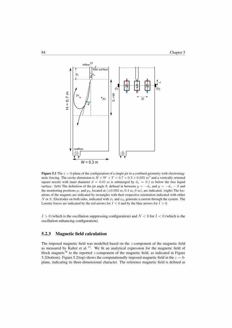
84 Chapter 5
S =
W
S NN
L
D
y
x
vin
inflow
outflow
free surfaceH
= 0
.7 m
W = 0.3 m
n dd
Figure 5.1 The z = 0-plane of the configuration of a single jet in a confined geometry with electromag-netic forcing. The cavity dimension is H ×W × T = 0.7× 0.3× 0.035 m3 and a vertically orientedsquare nozzle with inner diameter d = 0.01 m is submerged by dn = 0.1 m below the free liquidsurface. (left) The definition of the jet angle θ, defined in between y = −dn and y = −dn − S andthe monitoring positions p1 and p2, located at (±0.092 m, 0.4 m, 0 m), are indicated. (right) The loc-ations of the magnets are indicated by rectangles with their respective orientation indicated with eitherN or S. Electrodes on both sides, indicated with φ1 and φ2, generate a current through the system. TheLorentz forces are indicated by the red arrows for I < 0 and by the blue arrows for I > 0.
I > 0 (which is the oscillation suppressing configuration) and N < 0 for I < 0 (which is theoscillation enhancing configuration).
5.2.3 Magnetic field calculation
The imposed magnetic field was modelled based on the z-component of the magnetic fieldas measured by Kalter et al. 13. We fit an analytical expression for the magnetic field ofblock magnets36 to the reported z-component of the magnetic field, as indicated in Figure5.2(bottom). Figure 5.2(top) shows the computationally imposed magnetic field in the z = 0-plane, indicating its three-dimensional character. The reference magnetic field is defined as

Electromagnetic control of an oscillating turbulent jet in a confined cavity 85
0.1 T
-0.1 0 0.1x [m]
-0.4
-0.2
0
0.2
0.4
Bz
[T]
-0.1 0 0.1x [m]
-0.2
-0.1
y[m
]
-0.2
-0.1
0
0.1
0.2
Figure 5.2 (top) Contours of the z-component of the imposed magnetic field and arrows of x and ycomponents of the magnetic field in the z = 0-plane, white rectangles indicate the positions of thethree magnets. (bottom) The z-component of the magnetic field for the numerical simulations (solidline) and experiments 13 (symbols) at y = −0.15 m for three z-positions in the cavity: close to the backwall (z/T = −1/2, blue, circles), in the center of the domain (z/T = 0, green, squares) and close tothe front wall (z/T = 1/2, red, triangles).
the magnetic field strength in this plane in the center of the central magnet, thus Bref =0.15 T. The magnitude of the x and y components of the magnetic field in the z = 0-planeis of the same order of magnitude as the z component of the magnetic field. The imposedelectric current leads to an electric potential as shown in Figure 5.3(top) and Lorentz forces asshown in Figure 5.3(bottom) for I > 0. For I < 0, the electrical potential and consequentlythe Lorentz force are reversed.
5.2.4 Flow simulations
The LES filtered, single phase, incompressible Navier-Stokes equations are solved in thisstudy:
∂vi∂t
+ vj∂vi∂xj
(5.2)
= −1
ρ
∂p
∂xi+
∂
∂xj
[(ν + νSGS)
(∂vi∂xj
+∂vj∂xi
)]+ fi.
Here vi is the velocity, ρ the material density, ν the laminar viscosity, νSGS the sub-grid-scaleviscosity from the LES model, p the pressure and fi the Lorentz force. The Lorentz force iscalculated from the current ji and magnetic field bi as17
fi = εijkjjbk with ji =σ
ρ
(− ∂φ∂xi
+ εijkujbk
), (5.3)

86 Chapter 5
30 N/m3
-0.3
-0.2
-0.1
0
y[m
]
-10
-5
0
5
10
φ[V
]
-0.1 0 0.1x [m]
-0.3
-0.2
-0.1
0
y[m
]
-30
-20
-10
0
10
20
30
F l,z
[N/m
3 ]
Figure 5.3 (top) Contours of the electric potential, when a current I = 4 A is directed from left to right.(bottom) Contours of the z-component of the corresponding Lorentz force and vectors of the x and ycomponents in the z = 0-plane. The position of the magnets is indicated by white rectangles, and theposition of the nozzle with black rectangles.

Electromagnetic control of an oscillating turbulent jet in a confined cavity 87
where σ is the electrical conductivity of the fluid and φ is the electric potential, which isobtained from solving the Poisson equation
∂2φ
∂x2i
=∂
∂xi(εijkujbk) , (5.4)
We use the open source code OpenFOAM 2.138 based on the finite volume method to solvethe discretized equations using the PISO scheme.9 As a sub-grid-scale LES model we usethe dynamic Smagorinsky model, which is effective in modelling the subgrid scales in theseone-way coupled MHD flows.18 The discretization of the equations and the wall treatmentare in line with our previous publication.28
5.2.5 Validation
The numerical model is validated against experiments13 for a jet of Re = 4, 700 and elec-tromagnetic forcing with N = 0.017 (I = 4 A) in the oscillation suppressing configuration.Figures 5.4 and 5.5 show computed time averaged velocities compared to experimental data.The comparisons show a good agreement in the mean velocity between the numerical andexperimental results. It is noted that the simulated and measured flow field are not fully sym-metric due to the asymmetry in the outflow in the bottom of the domain (see Figure 5.1).The numerical simulations also show a good agreement in the oscillation frequency for vari-ous N , as we show in Figure 5.9, which also shows the N − St relation obtained from theexperiments.
5.3 Influence of electromagnetic forcing on self-sustainedoscillations
This section described the influence of the electromagnetic force on the mean velocity, oscil-lation frequency, the pressure difference across the jet, the amplitude of the jet angle oscilla-tion, and the flow regimes.
5.3.1 Mean velocity
For Re = 4, 700, we performed numerical simulations for various −0.075 < N < 0.015.Figure 5.6 shows the corresponding mean velocity vector fields, which demonstrates thatthe velocity field is strongly dependent on N , with the jet and recirculation zone strengthincreasing for negative N and decreasing for positive N .
The scaling of the jet velocity with N can be determined from a vertical momentum balancewhen considering a control volume of width ∆X centered around the magnet below the jet

88 Chapter 5
-0.4
-0.3
-0.2
-0.1
y[m
]Simulation Experiment
u=
0.1
m/s
Experiment
-0.4
-0.3
-0.2
-0.1
y[m
]Experiment
-0.02
0
0.02
u[m
/s]
Experiment
-0.4
-0.3
-0.2
-0.1
y[m
]Experiment
-0.1 0 0.1x [m]
-0.4
-0.3
-0.2
-0.1
0
0.1
v[m
/s]
Experiment
-0.1 0 0.1x [m]
-0.4
-0.3
-0.2
-0.1
y[m
]
-1
0
1
2
3
4
ν SG
S/ν
[-]
Experiment
Figure 5.4 For Re = 4, 700 and N = 0.017 in the z = 0-plane, simulation (left) and experiment(right), from top to bottom: Vector fields of the mean velocity, contours of the horizontal mean velocity,contours of the vertical mean velocity and contours of the scaled instantaneous sub-grid-scale viscosityνSGS/ν. The black rectangles indicate the position of the magnets.
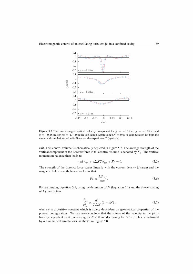
Electromagnetic control of an oscillating turbulent jet in a confined cavity 89
-0.3
-0.2
-0.1
0
0.1
y =−0.18 m
-0.3
-0.2
-0.1
0
0.1
v y[m
/s]
y =−0.28 m
-0.3
-0.2
-0.1
0
0.1
-0.15 -0.1 -0.05 0 0.05 0.1 0.15x [m]
y =−0.38 m
Figure 5.5 The time averaged vertical velocity component for y = −0.18 m, y = −0.28 m andy = −0.38 m, for Re = 4, 700 in the oscillation suppressing (N = 0.017) configuration for both thenumerical simulation (red solid line) and the experiment 13 (symbols).
exit. This control volume is schematically depicted in Figure 5.7. The average strength of thevertical component of the Lorentz force in this control volume is denoted by FL. The verticalmomentum balance then leads to
− ρd2v2in + ρ∆XTv2
jet + FL = 0. (5.5)
The strength of the Lorentz force scales linearly with the current density (I/area) and themagnetic field strength, hence we know that
FL ∝IBrefarea
. (5.6)
By rearranging Equation 5.5, using the definition of N (Equation 5.1) and the above scalingof FL, we obtain
v2jet
v2in
∝ d2
T∆X(1− cN) , (5.7)
where c is a positive constant which is solely dependent on geometrical properties of thepresent configuration. We can now conclude that the square of the velocity in the jet islinearly dependent on N , increasing for N < 0 and decreasing for N > 0. This is confirmedby our numerical simulations, as shown in Figure 5.8.

90 Chapter 5
-1
-0.8
-0.6
-0.4
-0.2
0
(y+
d n)/
W[−
]
-1
-0.8
-0.6
-0.4
-0.2
0
(y+
d n)/
W[−
]
-1
-0.8
-0.6
-0.4
-0.2
0
(y+
d n)/
W[−
]
-1
-0.8
-0.6
-0.4
-0.2
0
-0.5 -0.25 0 0.25 0.5
(y+
d n)/
W[−
]
x/W [−]
0.3vin
-0.5 -0.25 0 0.25 0.5x/W [−]
N = 0
N =−0.008
N =−0.025
N =−0.05
N = 0.008
N = 0.025
Figure 5.6 Vector field of the mean velocity for Re = 4, 700 and Stuart numbers in the range−0.05 ≤N ≤ 0.025. The positions of the magnets are indicated by gray rectangles.

Electromagnetic control of an oscillating turbulent jet in a confined cavity 91
ΔXI
vin
vjet
FL
Figure 5.7 The Lorentz force FL is active in a control volume of width ∆X , thickness T and certainheight. The control volume is used for deriving the scaling relation of vjet/vin as a function of N .
0
0.01
0.02
0.03
0.04
0.05
0.06
0.07
-0.08 -0.06 -0.04 -0.02 0 0.02 0.04
v2 jet/
v2 in[-
]
N [-]
Re = 3,150Re = 4,700Re = 7,100
Figure 5.8 The square of the mean jet velocity (calculated through an area of size D × T located aty = −0.19 m), normalized by the inlet velocity vin as a function of N . The vertical dashed linesindicate N = ±Ncrit.

92 Chapter 5
0
0.01
0.02
0.03
0.04
0.05
0.06
-0.3 -0.2 -0.1 0 0.1 0.2
St
sign(N)√|N|
St = 0.011
St =0.18 √
−N
Re = 3,150Re = 4,700Re = 7,100
Figure 5.9 St as a function of N for the oscillation suppressing (N > 0) and enhancing (N < 0)configuration for Re = 3, 150 (blue circles), Re = 4, 700 (green squares) and Re = 7, 100 (redtriangles). The dashed lines indicate the lines St = 0.011 and St = 0.18
√−N and the vertical lines
indicate N = ±Ncrit.
5.3.2 Oscillation frequency
Without electromagnetic forcing (N = 0), it is shown in13,28 that the jet oscillates with aconstant Strouhal number St = 0.011, and thus that f ∼ vin ∼ vjet‘ for fixed W .
For N > 0, the Lorentz force in the jet opposes the inflowing jet, leading to a lower jetvelocity. For small, but positive N , the electromagnetic braking is weak, and we confirm thatremains St = 0.011, as shown in Figure 5.9. The oscillation frequency does not change untilN > Ncrit, when the electromagnetic force becomes dominant over the inertial force and theoscillations are completely suppressed.
For N < 0, the Lorentz force is directed in the same direction as the inflowing jet, leading toincreased vjet at fixed in. From Equation 5.7 and f ∼ vjet it may be expected that for largenegative N , St ∝
√−N . This is indeed observed in the present numerical simulations (see
Figure 5.9) irrespective of Re in the range 3, 150 ≤ Re ≤ 7, 100, showing good agreementwith the experimentally observed proportionality of St with
√−N .*
*Please note that in Kalter et al., the definition of the Stuart number and the calculation, are incorrect by a constantfactor 3.15. Here, we use the correct values.

Electromagnetic control of an oscillating turbulent jet in a confined cavity 93
-1.5-1
-0.5
00.5
1
1.5
5 6 7 8
−−
∆p/〈∆
p〉[-
]
t/T [-]
N = 0.025
5 6 7 8
—θ/
〈θ〉[
-]
t/T [-]
N = 0.008
Figure 5.10 The pressure difference ∆p normalized by 〈∆p〉 and the jet angle θ normalized with 〈θ〉, asa function of the time normalized with the period T for N = −0.025 (top, T = 17 s, 〈∆p〉 = 33 Pa,〈θ〉 = 26) and N = 0.008 (bottom, T = 52 s, 〈∆p〉 = 10 Pa, 〈θ〉 = 30) and Re = 4, 700.
5.3.3 Pressure oscillations
We define the pressure difference across the jet as ∆p = p2 − p1 (see Figure 5.1). In ourearlier paper28 we have shown that the proportionality of ∆p and θ is a key property of theself-sustained jet oscillation.28 We confirm with Figure 5.10 that this proportionality remainspresent forN 6= 0. The pressure difference between the center and the edge of a recirculationzone is proportional to the square of the tangential velocity near its edge.12 As the square ofthe jet velocity is linearly dependent on N (see Equation 5.7) we also expect the amplitudeof the pressure oscillation, 〈∆p〉, to be linearly dependent on N . This is confirmed by ournumerical simulations, as shown Figure 5.11. This observation is independent of Re.
5.3.4 Jet angle amplitude
The amplitude of the jet angle oscillation, 〈θ〉, is also dependent on N , as we show in Figure5.12. For N = 0, 〈θ〉 is the largest (〈θ〉 = 18), and can be obtained from geometricalconsiderations.28
In the oscillation suppressing configuration (N > 0), the oscillations vanish for N > Ncrit,whereas in the oscillation enhancing configuration (N < 0), 〈θ〉 reaches a constant value, i.e,〈θ〉 = 12.5
for N < −Ncrit. For |N | < Ncrit, 〈θ〉 roughly diminishes quadratically with
N , i.e.:
〈θ〉 = θmax − β(
N
Ncrit
)2
, (5.8)
with θmax = 18 and β = 5.5. We determined Ncrit = 0.013. Both functions for 〈θ〉 areindicated in Figure 5.12.
The physical reasoning behind this behavior of 〈θ〉 becomes apparent from Figure 5.6. Inthe oscillation suppressing configuration (N > 0), the flow is pushed downward by themagnets in the corners. This prevents the growth of the recirculation zones and hence limits

94 Chapter 5
0
0.02
0.04
0.06
0.08
-0.08 -0.06 -0.04 -0.02 0 0.02 0.04
〈∆p〉
ρv2 in
[-]
N [-]
-20
0
20
100 150 200
∆p
[Pa]
t [s]
-20
0
20100 150 200
∆p
[Pa]
t [s]
Re = 3,150Re = 4,700Re = 7,100
fLine(x)
Figure 5.11 The amplitude 〈∆p〉 of the pressure oscillations, normalized by the energy ρv2in as afunction of N for Re = 3, 150 (blue circles), Re = 4, 700 (green squares) and Re = 7, 100 (redtriangles). The insets show the instantaneous ∆p for N = −0.025, N = 0 and N = 0.025. Thevertical dashed lines indicate ±Ncrit. The error bars indicate the standard deviation of the calculated〈∆p〉.
0
5
10
15
20
-0.08 -0.06 -0.04 -0.02 0 0.02
〈θ〉[
]
N
Re = 3,150Re = 4,700Re = 7,100
Figure 5.12 The amplitude 〈θ〉 of the jet angle oscillation as a function of N , with 〈θ〉 = θmax −β(N/Ncrit)
2 with θmax = 18 and β = 5.5, for |N | < Ncrit = 0.013. 〈θ〉 = 12.5 for N <−Ncrit, and 〈θ〉 = 0 for N > Ncrit.

Electromagnetic control of an oscillating turbulent jet in a confined cavity 95
〈θ〉. Conversely, in the oscillation enhancing configuration (N < 0), the recirculation zonegets elongated (see Figure 5.6 for N = −0.008), which also leads to a reduced jet angle.Increasing the current further (N < −Ncrit), leads to the flow mainly being driven by theelectromagnetic forcing, a approximately constant flow profile and hence constant 〈θ〉.
5.3.5 Flow regimes
We can now conclude that for varying N , three regimes can be distinguished, independent ofRe and separated by Ncrit = 0.013:
• For N > Ncrit, oscillations are suppressed.• For −Ncrit < N < Ncrit, self-sustained oscillations by the jet are dominant. St
remains constant and has the same value as for N = 0. However, the jet amplitudedecreases quadratically with |N |.
• For N < −Ncrit, the Lorentz forces are dominant and control the oscillations in thedomain.
5.4 Zero-dimensional model of the jet oscillation
In this section, we describe a zero-dimensional DDE-type model, which quantitatively de-scribes single jet oscillations, then we show how it can be applied to electromagneticallyforced single jet oscillations. Such a quantitative description can be used to predict the fre-quency and waveform of jet oscillations, and is an alternative for experiments of full three-dimensional numerical simulations.
5.4.1 Unforced flow (N = 0)
As we have shown earlier, the self-sustained oscillation of the jet, in the absence of electro-magnetic forcing, can be explained from the transient behaviour of ∆p and θ.28 When thejet is slightly oriented to one side (say, the right, θ < 0), the recirculation zone on the rightwill be stronger, i.e., it has a smaller diameter and higher velocities. This leads to a largerpressure deficit in the recirculation zone, deflecting the jet even further. The jet angle willsubsequently reach an extreme, as the jet impinges on the side wall and the recirculation zonecan not shrink any further. Subsequently, the fluid escapes the strong recirculation zone onthe right and feeds the recirculation zone on the left. The pressure deficit in the recirculationzone on the right diminishes, and the jet angle will deflect to the left.
In28 we showed, from a horizontal momentum balance, that the growth of the jet angle duringthe initial stage of the oscillation is proportional to the horizontal pressure difference over the

96 Chapter 5
jetdθ
dt∝ ∆p (5.9)
Furthermore, we have shown that ∆p ∼ θ, and hence
dθ
dt= rθ, (5.10)
where r is the growth rate of the oscillation.
The maximum jet angle, 〈θ〉, that can be reached is constrained by the geometry. This acts asa damping term on the oscillation, hence
dθ
dt=(r − µθ2
)θ, (5.11)
where µ is the obstruction parameter, related to 〈θ〉.In the last stage of the oscillation, the strong recirculation quickly decays in a timescale τ ,which is of the order of the turnover time of the recirculation zone. This leads to the fullmodel equation28
d
dtθ(t) = rθ(t)− µθ3(t)− kθ(t− τ), (5.12)
where k is the decay rate for the destruction of the strong recirculation zone. Equation 4.10is a zero-dimensional model, which is of the Delay Differential Equation (DDE) type. Itsmodel constants can be determined a priori as a function of inflow parameters and geometryonly.28
5.4.2 Electromagnetically forced flow (N 6= 0)
Here we argue that the general shape of model equation 5.12 remains valid for N 6= 0,but with modified model parameters that will now also depend on N . We will discuss theinfluence ofN 6= 0 on each of the three right-hand terms in Equation 5.12, viz. (i) the growthterm, (ii) the damping term, and (iii) the delayed decay term.
(i) Equation 5.9 remains true for N 6= 0 as the imposed Lorentz force in the present configur-ation is dominantly vertical (see Figure 5.3). Furthermore, from Figure 5.10 we conclude that∆p and θ remain proportional. Therefore, Equation 5.10 remains valid as well for N 6= 0.Thus, the form of the growth term in Equation 5.12 remains unchanged. The constant of pro-portionality, the growth rate r, is however influenced by the Lorentz force, as ∆p is highlydependent on the electromagnetic forcing. We have shown in Figure 5.11 that 〈∆p〉 dependslinearly on N . Due to this dependence, we also expect r to be linearly dependent on N .
(ii) For each value of N , we find a specific value for the maximum jet deflection angle 〈θ〉.For N = 0, only the geometry obstructs the motion of the jet angle, leading to 〈θ〉 = 18.28
In Figure 5.12 above, we have shown that the maximum jet angle depends quadratically on
Electromagnetic control of an oscillating turbulent jet in a confined cavity 97
N for |N | < Ncrit. For N > Ncrit the oscillations vanish, and thus 〈θ〉 = 0, whereas forN < −Ncrit, we have shown that the oscillation is enhanced mainly by the electromagneticforcing and the maximum jet angle is constant, 〈θ〉 = 12.5
. For each N , the maximum jet
deflection can be accounted for through a damping term of the form of the second right-handterm in Equation 4.10, with the model constant µ now being a function of N .
(iii) Since, for |N | < Ncrit the flow is dominated by inertial forces, the description of the os-cillation by means of the delayed feedback mechanism28 still holds, with the model constantbeing slightly dependent on N .
For N < −Ncrit, the electromagnetic forcing has a larger influence on the delay time. Thevelocities in the domain quickly increase with decreasing N , leading to a shorter delay timeτ and larger influence of the feedback induced destruction of the recirculation zone pressureminimum. We therefore expect both model constants k and τ in the delayed decay term tostrongly depend on N for N < −Ncrit.
5.5 Determination of the model parameters and its implic-ations
For N = 0, the self-sustained jet oscillations in a thin, confined cavity can be described byEquation 5.12, which contains four model parameters, r, µ, k and τ . These parameters canbe determined a priori based on Re, W/d, vin and W .28 In this section we will demonstratethat the electromagnetic forcing can be incorporated with one additional parameter, viz. N .
5.5.1 Non-dimensional model
Model Equation 5.12 can be written in terms of the dimensionless time t′ = rt and jet angleθ′ =
√µ/rθ:28
dθ′
dt′= θ′ − θ′3 − αθ′ (t′ − δ) . (5.13)
The variables α = k/r and δ = rτ denote the relative strength of the feedback mechanismcompared to the growth rate and the dimensionless delay time respectively. The neutral curve,obtained from a linear stability analysis, is28,32
δn(α) = arccos
(3α− 2
α
)(α2 − (3α− 2)2
)− 12 . (5.14)
This critical curve separates the stable and oscillatory regimes of the model Equation 5.13.For δ < δn(α), all modes are stable and no oscillations will be present. For δ > δn(α),oscillatory modes will be sinusoidal of shape close to the neutral curve and approach block-waves for δ ≥ 10.

98 Chapter 5
-20
-10
0
10
20
0 10 20 30 40 50
θ[
]
t [s]
N =−0.025
r = 0.504 s−1
µ = 14.9×10⁻⁴ s−1
k = 0.496 s−1
τ = 2.34 s
0 10 20 30 40 50t [s]
N = 0.008
r = 0.2 s−1
µ = 10.3×10⁻⁴ s−1
k = 0.145 s−1
τ = 9.52 s
Figure 5.13 The phase averaged jet angle amplitude (solid red line) in conjunction with the model fit(dashed blue line), for Re = 4, 700 and for N = −0.025 (top) and N = 0.008 (bottom).
5.5.2 Parameter fitting
From our numerical simulations for varying N , we calculate θ(t) and the phase average jetangle amplitude. From a fitting procedure we determine the best fitting parameter set r, µ, k, τfollowing the method outlined in.28
In Figure 5.13 we show the phase averaged jet angle amplitude together with the solutionof the DDE model for the fitted parameter set, for both N = −0.025 and N = 0.008. Thisfigure shows the good agreement between the zero-dimensional model solution and the actualjet angle profile obtained from the LES simulations.
For N > Ncrit no oscillations are present, hence we cannot calculate a phase average, nordetermine α and δ from the numerical simulations. However, for N < Ncrit = 0.013 wedetermine the parameters α and δ for −5Ncrit ≤ N ≤ Ncrit, 3, 150 ≤ Re ≤ 7, 100 andW/d = 30.
We show the fitted parameters α and δ for this parameter set and the neutral curve δn (Equa-tion 5.14) in Figure 5.14. From this stability diagram a clear distinction between the inertialdominated and electromagnetically dominated regimes becomes apparent. For |N | < Ncritthe jet oscillation itself is dominant, and we showed in our previous publication28, that theparameters describing these oscillation are close to the neutral curve. And indeed, thisis observed in Figure 5.14. For N < −Ncrit, the parameters cluster together close to(δ, α) = (1, 1). In other words, for N < −Ncrit the normalized behavior of the systemdoes not change. Although the parameters α and δ sparsely change over a variation in N , theunderlying variables r, µ, k and τ , will change significantly as we will later show.

Electromagnetic control of an oscillating turbulent jet in a confined cavity 99
0.5
0.6
0.7
0.8
0.9
1
-0.08 -0.06 -0.04 -0.02 0 0.02
α
N δ
Unstable
Re = 3150Re = 4700Re = 7100
0 0.5 1 1.5 2 2.5 3-10
-1
0
1
N/N
crit
Stable
Figure 5.14 For−0.08 ≤ N ≤ 0.02 (color of symbols) and 3, 150 ≤ Re ≤ 7, 100 (symbol type) (left)α as a function of N and (right) the neutral curve (Equation 5.14, solid line), with the shaded and non-shaded area denoting the regions of stable and oscillatory modes, respectively. The parameter values(δ, α) are indicated in the diagram, where the colors indicate |N | < Ncrit (grey-red) and N < −Ncrit
(blue) as well.
5.5.3 Parameter estimation
Without forcing the model parameters r and τ were found to be given by28
r = κ1vinW
Re−14
(W
d
)− 12
, τ = κ2W
vinRe
59 , (5.15)
with κ1 = 5.9 and κ2 = 0.13.
In Section 5.4.2 we anticipated that r decreases linearly with N . For N = 0, the presentmodel should reduce to the unforced model, hence we may pose
κ1(N) = κ1
(1− λ1
N
Ncrit
), (5.16)
which thus consists of a contribution by the inertial force and a contribution by the magneticforce. From our numerical simulations and fitted model parameters, we determine that λ1 =0.49± 0.02.
For the delay time τ such a unified approach across both the inertially dominated and electro-magnetically dominated regimes is not possible. For −Ncrit < N < 0 we expect a smallerdelay time, since fluid is accelerated in the recirculation zone, and for 0 < N < Ncrit thefluid is decelerated and we expect the delay time to increase. Hence, for |N | < Ncrit
κ2(N) = κ2
(1 + λ2
N
Ncrit
). (5.17)
From our numerical simulations and fitted parameters we find that λ2 = 0.58± 0.09.
For N < −Ncrit we use the above observation that δ remains close to constant, and hence

100 Chapter 5
we defineτ =
δminr
, (5.18)
with δmin = 1.13 the average value for δ observed in our simulations. Hence, with r fromEquations 5.15 and 5.16, τ can be determined.
For given N we now determine k from r, τ and δ. For |N | < Ncrit, the pair (α, δ) residesclose to the neutral curve δn(α) (Equation 5.14), which thus determines α. For N < −Ncrit,we use the above observation from Figure 5.14 that α ≈ 0.99. From α we determine k = αr.
µ follows from the amplitude 〈θ′〉 of the dimensionless form of the DDE model equation(Equation 5.13)28 and the behavior of 〈θ〉. For N = 0 we found 〈θ′〉 =
√2 (1− α2). This
also holds for |N | < Ncrit. For N < −Ncrit, the parameters are no longer distributed alongthe neutral curve, but given by α ≈ 0.99 and δ = 1.13 above. For this regime we find〈θ′〉 = γ = 0.61.
µ =
2r(1− α2
)
〈θ〉2 if |N | < Ncrit
γ2r
〈θ〉2 if N < −Ncrit, (5.19)
Now, for given N , the model parameters r, µ, k and τ can be determined from Equations5.15 and 5.16, Equation 5.19, k = αr and Equations 5.15, 5.17 and 5.18, respectively
5.5.4 Model application
Figure 5.15 compares the parameters obtained from the model presented in Equations 5.15-5.19 with the parameters obtained from the fit of the phased-average jet oscillation profilesfrom the numerical simulations. With this figure we confirm that the present model gives thecorrect model parameters to determine the jet oscillation properties.
In table 5.1 we compare the frequencies obtained from the LES simulations and the presentedzero-dimensional model. The table demonstrates that our model correctly predicts the singlejet oscillation frequency along the range −6Ncrit ≤ N ≤ Ncrit, as is also indicated withFigure 5.16. The deviation is only larger than 10% for the most extreme cases (N = Ncritand N = −6Ncrit), where the first is close to being damped and the latter enhanced, to suchan extend that the oscillations become irregular.
In Figure 4.12 we show the numerically obtained jet angle profile and the jet angle profileobtained from the model for several combinations ofRe andN . The figure demonstrates thatthe zero-dimensional DDE-type model can successfully be applied on the electromagneticforcing of a self-sustained oscillating jet, both in the inertia, as in the electromagnetic forcedominant regimes. For larger negative N (N = −0.075, bottom right in figure 4.12), theforced flow shows irregular behavior, which is observed from the significant variation inperiod and amplitude during the oscillation. This phenomenon due to the strong amplification

Electromagnetic control of an oscillating turbulent jet in a confined cavity 101
0
0.2
0.4
0.6
0.8
0 0.2 0.4 0.6 0.8
r mod
el[ s−
1]
r f it[s−1]
0
5
10
0 5 10
τ mod
el[s]
τ f it [s]
0
0.2
0.4
0.6
0.8
0 0.2 0.4 0.6 0.8
k mod
el[ s−
1]
k f it[s−1]
0
0.001
0.002
0.003
0 0.001 0.002 0.003
µ mod
el[s]
µ f it [s]
Re = 3,150Re = 4,700Re = 7,100
Re = 3,150Re = 4,700Re = 7,100
Figure 5.15 Parity plot for r (top left), τ (top right), k (bottom left) and µ (bottom right) showingthe fitted parameter value (horizontal axis) compared to the parameter value obtained from the model(Equations 5.15-5.19).
of the oscillation for large negative N is not described by the present model. For the other Nhowever, the presented model shows a good agreement in profile shape and frequency.
5.6 Conclusion
We studied the effect of an electromagnetic body force on self-sustained jet oscillations ina confined cavity. Three flow regimes can be distinguished, that are separated by the crit-ical Stuart number Ncrit: 1) for N > Ncrit, all inertia induced large scale oscillations aresuppressed by electromagnetic body forces, 2) for |N | < Ncrit, the jet inertia is dominantcompared to the electromagnetic force, but the latter influences the jet oscillation in amplitudeand frequency, 3) for N < −Ncrit, the electromagnetic forces dominate the flow and controlthe flow oscillations. For the configuration studied in this paper we found Ncrit = 0.013.
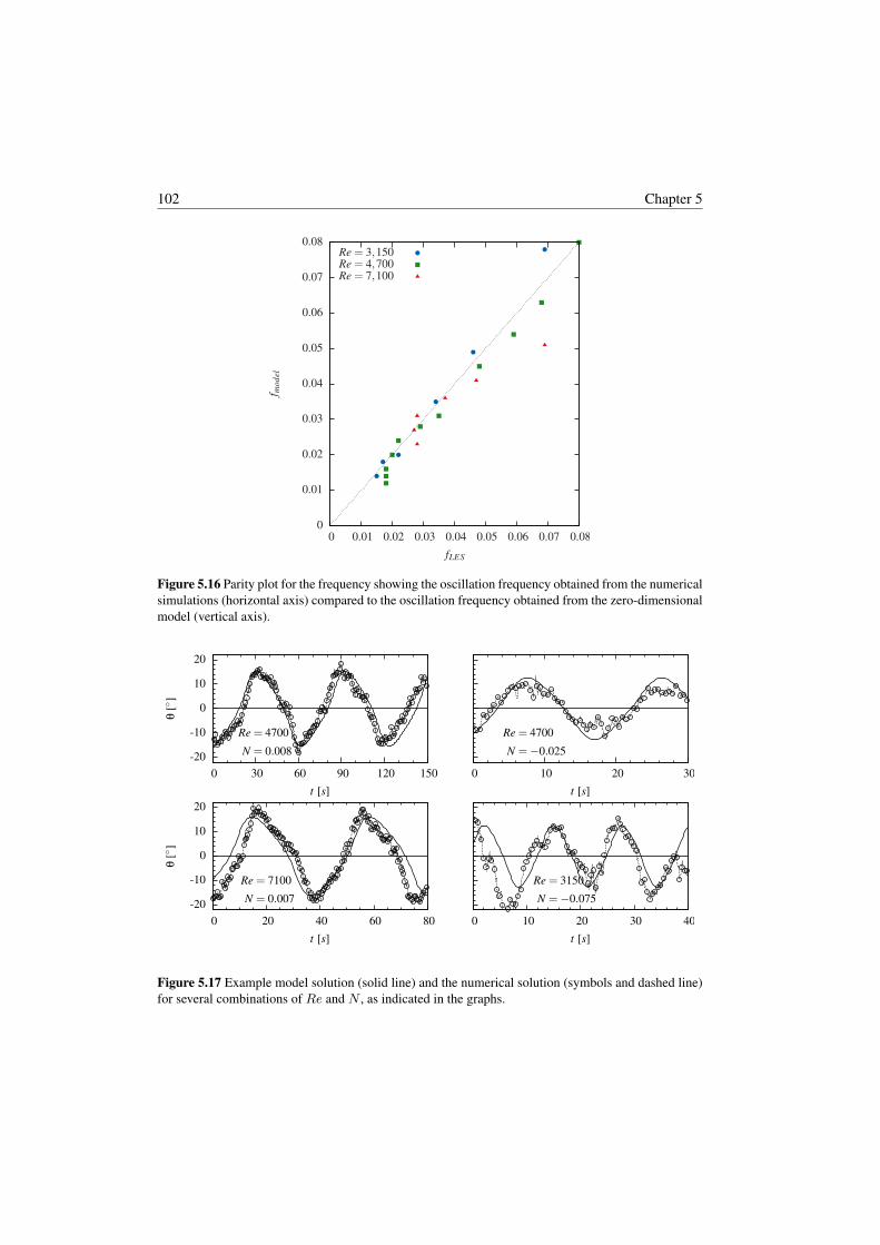
102 Chapter 5
0
0.01
0.02
0.03
0.04
0.05
0.06
0.07
0.08
0 0.01 0.02 0.03 0.04 0.05 0.06 0.07 0.08
f mod
el
fLES
Re = 3,150Re = 4,700Re = 7,100
Figure 5.16 Parity plot for the frequency showing the oscillation frequency obtained from the numericalsimulations (horizontal axis) compared to the oscillation frequency obtained from the zero-dimensionalmodel (vertical axis).
-20
-10
0
10
20
0 30 60 90 120 150
θ[
]
t [s]
Re = 4700
N = 0.008
0 10 20 30t [s]
Re = 4700
N =−0.025
-20
-10
0
10
20
0 20 40 60 80
θ[
]
t [s]
Re = 7100
N = 0.007
0 10 20 30 40t [s]
Re = 3150
N =−0.075
Figure 5.17 Example model solution (solid line) and the numerical solution (symbols and dashed line)for several combinations of Re and N , as indicated in the graphs.

Electromagnetic control of an oscillating turbulent jet in a confined cavity 103
Table 5.1 This table compares the oscillation frequency obtained from the LES simulations and thezero-dimensional model equation as a function of Re and N .
Re N fLES [Hz] fmodel [Hz]3150 −0.075 0.069 0.0783150 −0.038 0.046 0.0493150 −0.019 0.034 0.0353150 −0.005 0.022 0.0203150 0 0.017 0.0183150 0.005 0.015 0.0143150 0.014 − −4700 −0.051 0.080 0.0804700 −0.034 0.068 0.0634700 −0.026 0.059 0.0544700 −0.017 0.048 0.0454700 −0.009 0.035 0.0314700 −0.004 0.029 0.0284700 0 0.022 0.0244700 0.004 0.020 0.0204700 0.009 0.018 0.0164700 0.011 0.018 0.0144700 0.013 0.018 0.0124700 0.015 − −7100 −0.015 0.069 0.0517100 −0.007 0.047 0.0417100 −0.004 0.037 0.0367100 0.0 0.028 0.0317100 0.004 0.027 0.0277100 0.007 0.028 0.023
We incorporated the effect of the electromagnetic forcing in a zero-dimensional DDE-typemodel that describes the jet oscillation. The additional Lorentz force is included in the modelby the additional dependence on N . We have shown that this newly defined model correctlyrepresents the jet oscillation for the Reynolds number 3150 ≤ Re ≤ 7100 and −6Ncrit ≤N ≤ Ncrit.Although this paper only addresses a specific configuration of electromagnetic forcing, webelieve that the method can also be applied on different EMBr configurations and even dif-ferent types of body forces. This means that one can expect to find three regimes, a jet inertiadominated regime, an oscillation enhancing regime and an oscillation suppressing regime.The effect of these forces on the zero-dimensional model for the jet oscillation will be de-pendent on a dimensionless number describing the ratio of the imposed force and the inertialforce.

104 Chapter 5
For large negative N the oscillations are more irregular with respect to the deviation in theamplitude between periods. The currently presented model does not include this irregularityin the oscillation.
The forced single jet oscillation model also has potential for other types of forced single jetflows, such as jets with a different density, or by application of acoustic forcing.10,25,35,39,40
Bibliography
[1] Arcos-Gutierrez, H., Barrera-Cardiel, G., Barreto, J. d. J., and Garcia-Hernandez, S. Numerical Studyof Internal SEN Design Effects on Jet Oscillations in a Funnel Thin Slab Caster. ISIJ International,volume 54(6):pp. 1304–1313 (2014).
[2] Bouchet, G. and Climent, E. Unsteady behavior of a confined jet in a cavity at moderate Reynolds numbers.Fluid Dynamics Research, volume 44(2):p. 025505 (2012).
[3] Breuer, K., Park, J., and Henoch, C. Actuation and control of a turbulent channel flow using Lorentz forces.Physics of Fluids, volume 16(4):pp. 897–907 (2004).
[4] Dattarajan, S. and Johari, H. Control of a separating boundary layer with Lorentz force actuators. Physics ofFluids, volume 20(4) (2008).
[5] Garcia-Hernandez, S., Morales, R., De JesÞs Barreto, J., and Morales-Higa, K. Numerical optimization ofnozzle ports to improve the fluidynamics by controlling backflow in a continuous casting slab mold. ISIJInternational, volume 53(10):pp. 1794–1802 (2013).
[6] Ha, M. Y., Lee, H. G., and Seong, S. H. Numerical simulation of three-dimensional flow, heat transfer, andsolidification of steel in continuous casting mold with electromagnetic brake. Journal of Materials ProcessingTechnology, volume 133(3):pp. 322–339 (2003).
[7] Haiqi, Y., Baofeng, W., Huiqin, L., and Jianchao, L. Influence of electromagnetic brake on flow field of liquidsteel in the slab continuous casting mold. Journal of Materials Processing Technology, volume 202(1-3):pp.179–187 (2008).
[8] Henoch, C. and Stace, J. Experimental investigation of a salt water turbulent boundary layer modified by anapplied streamwise magnetohydrodynamic body force. Physics of Fluids, volume 7(6):pp. 1371–1383 (1995).
[9] Issa, R. I. Solution of the implicitly discretised fluid flow equations by operator-splitting. Journal of Compu-tational Physics, volume 62(1):pp. 40–65 (1986).
[10] Juniper, M., Li, L., and Nichols, J. Forcing of self-excited round jet diffusion flames. Proceedings of theCombustion Institute, volume 32 I:pp. 1191–1198 (2009).
[11] Kalter, R., Righolt, B. W., Kenjereš, S., Kleijn, C. R., and Tummers, M. J. Experimental Modeling of HeatTransfer in a Continuous Casting Mould Model. p. V01CT16A005. ASME (2014).
[12] Kalter, R., Tummers, M., Kenjereš, S., Righolt, B., and Kleijn, C. Oscillations of the fluid flow and thefree surface in a cavity with a submerged bifurcated nozzle. International Journal of Heat and Fluid Flow,volume 44:pp. 365–374 (2013).
[13] Kalter, R., Tummers, M. J., Kenjereš, S., Righolt, B. W., and Kleijn, C. R. Effects of electromagnetic forcingon self-sustained jet oscillations. Physics of Fluids, volume 26(6):p. 065101 (2014).
[14] Kalter, R., Tummers, M. J., Kenjereš, S., Righolt, B. W., and Kleijn, C. R. Electromagnetic flow control of abifurcated jet in a rectangular cavity. International Journal of Heat and Fluid Flow, volume 47:pp. 113–122(2014).
[15] Kenjereš, S. Electromagnetic enhancement of turbulent heat transfer. Physical Review E, volume 78(6):p.066309 (2008).

Electromagnetic control of an oscillating turbulent jet in a confined cavity 105
[16] Kenjereš, S. Large eddy simulations of targeted electromagnetic control of buoyancy-driven turbulent flow ina slender enclosure. Theor. Comput. Fluid Dyn., volume 23(6):pp. 471–489 (2009).
[17] Kenjereš, S. and Hanjalic, K. On the implementation of effects of Lorentz force in turbulence closure models.International Journal of Heat and Fluid Flow, volume 21(3):pp. 329–337 (2000).
[18] Knaepen, B. and Moin, P. Large-eddy simulation of conductive flows at low magnetic Reynolds number.Physics of Fluids, volume 16(5):p. 1255 (2004).
[19] Kolšek, T., Jelic, N., and Duhovnik, J. Numerical study of flow asymmetry and self-sustained jet oscillationsin geometrically symmetric cavities. Applied Mathematical Modelling, volume 31(10):pp. 2355–2373 (2007).
[20] Lawson, N. and Davidson, M. Self-Sustained Oscillation of a Submerged Jet in a Thin Rectangular Cavity.Journal of Fluids and Structures, volume 15(1):pp. 59–81 (2001).
[21] Lee, C. and Kim, J. Control of the viscous sublayer for drag reduction. Physics of Fluids, volume 14(7):pp.2523–2529 (2002).
[22] Mataoui, A. and Schiestel, R. Unsteady phenomena of an oscillating turbulent jet flow inside a cavity: Effectof aspect ratio. Journal of Fluids and Structures, volume 25(1):pp. 60–79 (2009).
[23] Maurel, A., Ern, P., Zielinska, B. J. A., and Wesfreid, J. E. Experimental study of self-sustained oscillationsin a confined jet. Physical Review E, volume 54(4):pp. 3643–3651 (1996).
[24] Molloy, N. A. and Taylor, P. L. Oscillatory Flow of a Jet into a Blind Cavity. Nature, volume 224(5225):pp.1192–1194 (1969).
[25] Monkewitz, P. A., Bechert, D. W., Barsikow, B., and Lehmann, B. Self-excited oscillations and mixing in aheated round jet. Journal of Fluid Mechanics, volume 213:pp. 611–639 (1990).
[26] Pang, J. and Choi, K.-S. Turbulent drag reduction by Lorentz force oscillation. Physics of Fluids,volume 16(5):pp. L35–L38 (2004).
[27] Peng, X., Zhou, J., and Qin, Y. Improvement of the temperature distribution in continuous casting mouldsthrough the rearrangement of the cooling water slots. Journal of Materials Processing Technology, volume167(2-3):pp. 508–514 (2005).
[28] Righolt, B. W., Kenjereš, S., Kalter, R., Tummers, M. J., and Kleijn, C. R. Dynamics of an oscillatingturbulent jet in a confined cavity. Physics of Fluids, volume 27:p. 095107 (2015).
[29] Rossi, L. and Thibault, J.-P. Investigation of wall normal electromagnetic actuator for seawater flow control.Journal of Turbulence, volume 3:p. N5 (2002).
[30] Shatrov, V. and Gerbeth, G. Electromagnetic flow control leading to a strong drag reduction of a sphere. FluidDynamics Research, volume 36(3):p. 153 (2005).
[31] Shatrov, V. and Gerbeth, G. Magnetohydrodynamic drag reduction and its efficiency. Physics of Fluids,volume 19(3) (2007).
[32] Suarez, M. and Schopf, P. A delayed action oscillator for ENSO. Journal of the Atmospheric Sciences,volume 45(21):pp. 3283–3287 (1988).
[33] Thomas Honeyands and Joe Herbertson. Flow dynamics in thin slab caster moulds. Steel Research Interna-tional, volume 66(7):pp. 287–293 (1995).
[34] Villermaux, E. and Hopfinger, E. Self-sustained oscillations of a confined jet: a case study for the non-lineardelayed saturation model. Physica D: Nonlinear Phenomena, volume 72(3):pp. 230–243 (1994).
[35] Voropayev, S., Nath, C., and Fernando, H. Mixing by turbulent buoyant jets in slender containers. PhysicsLetters, Section A: General, Atomic and Solid State Physics, volume 376(45):pp. 3213–3218 (2012).
[36] Votyakov, E. V., Zienicke, E., and Kolesnikov, Y. B. Constrained Flow Around a Magnetic Obstacle. Journalof Fluid Mechanics, volume 610:pp. 131–156 (2008).
[37] Weier, T., Gerbeth, G., Mutschke, G., Lielausis, O., and Lammers, G. Control of Flow Separation UsingElectromagnetic Forces. Flow, Turbulence and Combustion, volume 71(1):pp. 5–17 (2003).

106 Chapter 5
Table 5.2 The properties of the three magnets contributing to the magnetic field imposed in the numer-ical simulations.
Magnet 1 Magnet 2 Magnet 3(Mx,My, h) (0.04, 0.084, 0.04) m (0.042, 0.08, 0.04) m (0.04, 0.084, 0.04) m(xc, yc, zc) (−0.078,−0.15, 0.01) m (0.0,−0.15, 0.01) m (0.078,−0.15, 0.01) mBface −0.55 T 0.65 T −0.55 T
[38] Weller, H. G., Tabor, G., Jasak, H., and Fureby, C. A tensorial approach to computational continuum mech-anics using object-oriented techniques. Computers in Physics, volume 12(6):pp. 620–631 (1998).
[39] Yu, M., Lin, T., and Hsieh, Y. Influence of acoustic forcing on the near field development of a heated planejet. Experimental Thermal and Fluid Science, volume 25(1-2):pp. 13–22 (2001).
[40] Zhang, C., Eckert, S., and Gerbeth, G. The Flow Structure of a Bubble-Driven Liquid-Metal Jet in a HorizontalMagnetic Field. Journal of Fluid Mechanics, volume 575:pp. 57–82 (2007).
[41] Zhang, L., Rong, Y.-M., Shen, H.-F., and Huang, T.-Y. Solidification modeling in continuous casting by finitepoint method. Journal of Materials Processing Technology, volume 192-193:pp. 511–517 (2007).
5.A Electromagnetic field
The analytical expression for the imposed magnetic field, is based on the algebraic calcula-tions by Votyakov et al.:
Bx(x, y, z) =1
B0
∑
k=±1
∑
j=±1
∑
i=±1
(ijk) arctanh
[y − jMy
r(i, j, k)
], (5.20)
By(x, y, z) =1
B0
∑
k=±1
∑
j=±1
∑
i=±1
(ijk) arctanh
[x− iMx
r(i, j, k)
], (5.21)
Bz(x, y, z) = − 1
B0
∑
k=±1
∑
j=±1
∑
i=±1
(ijk) arctan
[(x− iMx) (y − jMy)
(z − kh) r(i, j, k)
].(5.22)
Here r(i, j, k) =[(x− iMx)2 + (y − jMy)2 + (z − kh)2
]1/2and B0 is such that
Bz(0, 0, 0) = 1. This follows from an integral over the region Ω =|x| ≤Mx, |y| ≤My, h ≤ |z| ≤ ∞ of magnetic dipoles, i.e., two magnets of dimensions2Mx × 2My separated by 2h, connected by a soft core.
In the present work, three magnets are positioned on one side of the cavity. Therefore, thesummation over k = +1 can be omitted from above summation, wheres the summation iscarried out over three separate magnets, with their origin in (xc, yc, zc) and certain magnitude.The resulting properties for the magnets are summarized in table 5.2. As the magnets arepositioned on one side, the normalization of the magnetic field was handled with respect tothe face of the magnet, rather than the origin.


6. Dynamics of a bifurcated jet ina confined cavity with a free sur-face§
6.1 Introduction
A single fluid jet that is confined in the two directions perpendicular to the flow, may exhibitself-sustained oscillations under specific conditions.10,15 Those jet oscillations are observedfor jet Reynolds numbers ranging from Re = 10013 up to Re = 170, 000.14 For one of thespanwise directions sufficiently wide, as compared to the nozzle diameter (i.e. W/d ≥ 20),the jet oscillation can be described by three stages, where the formation of recirculation zonesat both sides of the jet plays a major role. First, the jet is slightly deflected to, say, the right.This feeds more flow to the recirculation zone on the right, which now becomes stronger,with an increasing pressure deficit in the center of the recirculation. This causes a further jetdeflection to the right as it is limited by the geometry. Second the jet deflection reaches amaximum amplitude and the pressure deficit does not decrease any further, which means thatthe driving force of the jet deflection vanishes. Third, at the right wall, the downward flowwill increase, causing the growth of a recirculation zone at the left of the jet and a diminishingpressure deficit at its right. This results in the jet moving towards the left. The process thenrepeats.15
Self-sustained oscillations are also observed for situations in which a bifurcated jet is confinedin a thin cavity. A bifurcated jet originates from a nozzle with two ports (as schematicallydepicted in Figure 6.1), hence resulting in two jets discharging into the cavity in more or lessopposite directions.
Such a confined bifurcated jet configuration is relevant in, for example, continuous steel
§Parts of this chapter published as: Righolt, B. W., Kenjereš, S., Kalter, R., Tummers, M. J., and Kleijn, C. R.Numerical study of turbulent submerged bifurcated jets impingement and interactions with a free surface. In: 8thInternational Symposium on Turbulence and Shear Flow Phenomena, TSFP Proceedings. 2013.
109

110 Chapter 6
casting. Two- or four-port nozzles are commonly used for the injection of hot, liquid steelinto the casting mould in order to obtain an optimal distribution of the fluid with respect to thequality of the resulting solidified steel slab. Oscillations as described above are an unwantedside-effect of the fluidic system under consideration.
Numerical simulations, sometimes coupled with water model experiments, are commonlyused to study the continuous steel casting process. Simulation studies generally apply varioussimplifications, focussing on either cooling or solidification of the steel,11 the movement ofthe free surface17,18,23 or the electromagnetic brake.4,5,19,21 Sometimes the focus is on thepure flow mechanics only.3 As direct Numerical Simulations (DNS) are not computationallyfeasible due to the high (> 10000) jet Reynolds numbers, such studies rely on RANS, T-RANS and LES for the modelling of turbulence.
From water model experiments, Torres-Alonso et al. 17,18 report dynamic free surface dis-tortions with a duration of 10 s and a frequency of 0.01 Hz. They numerically predict thisdistortion using a Reynolds Stress Model. The origin of the distortion is found in the interac-tion between both jets below the nozzle tips. The origin of the large period of the distortion isthe high Reynolds stresses at the boundary of the jet and the upper recirculation zones. Thefrequency of the jet oscillations matches the frequency of the free surface oscillations.
Honeyands and Herbertson 9 and Kalter et al. 10 propose a mechanism for the self-sustainedoscillation of bifurcated jets in a thin cavity. Similar to the self-sustained oscillations of asingle jet in a cavity, the confinement of the liquid jets in both directions perpendicular to theflow is an essential prerequisite for the oscillation to exist, leading to the necessary formationof recirculation zones in the domain. The pressures in the recirculation zones play a role in theproposed mechanism. Furthermore, the oscillations of the two jets will align in anti-phase,due to the interaction between both sides of the domain.
The goal of the present work is to provide thorough proof for the mechanism of the self-sustained oscillation in a bifurcated jet configuration in a thin cavity, as proposed by Honey-ands and Herbertson 9 and Kalter et al. 10 by means of numerical simulations. These simula-tions can provide detailed pressure fields, which are difficult to obtain experimentally.
6.2 Numerical method and validation
6.2.1 Description of the set-up
The model geometry, shown in Figure 6.1, consists of a thin cavity, with dimensions0.65× 0.8× 0.035 m3 (= W × H × T = width×height×thickness). The cavity is filledup to a height h = 0.7 m with water, with ρ = 1.0× 10³ kg/m3 and kinematic viscosityν = 1.0× 10⁻⁶ m2/s. The water-air interfacial tension is σ = 0.07 N/m. The fluid emergesfrom the nozzle through two vertical openings of inner dimensions d2 = 0.01× 0.01 m2
on opposite sides of the nozzle (see Figure 6.1). The nozzle submergence depth, which is

Dynamics of a bifurcated jet in a confined cavity with a free surface 111
x
y
h =
0.7
m
W = 0.65m
H =
0.8
m
n
p1
p2
d
d
d
x
z
T=
0.0
35
m
Figure 6.1 The schematics of the setup considered in this paper is depicted. A top view (top) and sideview (bottom) of the cavity of dimensionW ×H×T = 0.8× 0.65× 0.035 m3 is shown. The nozzleis submerged by dn = 0.125 m and has inner diameter 0.01 m and a wall thickness of 0.005 m. Thefluid depth h = 0.7 m. Furthermore, p1 and p2 indicate two monitoring points at x = ±0.175 m andthe gray angle indicates the jet angle.
the distance between the equilibrium water-air surface and inner bottom of the nozzle, isdn = 0.125 m.
The Reynolds number is based on the average velocity, vin of each of the jets emerging fromthe nozzle and the nozzle diameter as Rejet = vind/ν = 12, 500. The average velocity inthe inlet pipe is thus 2vin. A Cartesian coordinate system is defined as depicted in Figure 6.1,where the origin is located in the center of the inlet pipe at the position of the equilibriumfree surface, where the x coordinate is along the width, the y coordinate along the height andthe z coordinate along the depth of the cavity.

112 Chapter 6
In this work, we solve the incompressible, two-phase (Volume Of Fluid), LES filtered Navier-Stokes equations and the transport equation for the indicator function α,7,16,20
∂ρvi∂t
+ vj∂ρvi∂xj
=∂
∂xj
[(µ+ µt)
(∂vi∂xj
+∂vj∂xi
)]− ∂p
∂xi+ fi + γκ
∂α
∂xi, (6.1)
∂α
∂t+
∂
∂xj(αvj) +
∂
∂xj(vr,jα (1− α)) = 0. (6.2)
In these equations, α has value 1 in cells containing the liquid phase only and 0 for the gasphase, whereas intermediate values ofα indicate the position of the free surface. Furthermore,ρ = αρ1 + (1−α)ρ2 is the phase averaged density, µ the phase averaged dynamic viscosity,µt the turbulent viscosity, vi the velocity, p the pressure, fi the gravitational force, σ thesurface tension between both phases and κ the curvature of the interface, which is calculatedas κ = ∇α/ |∇α|.2 The third term in the transport equation for α represents an interfacecompression, which is intended to maintain the interface as sharp as possible.1,8
The turbulent viscosity µt is obtained from the dynamic Smagorinsky model, a Large EddySimulation (LES) model.
µtρ
= νSGS = (C∆)2 S, (6.3)
where ∆ is the local grid size, defined as ∆ = (∆x∆y∆z)1/3. S is the characteristic rate
of strain S = (2SijSij)1/2 with Sij = (∂vi/∂xj + ∂vj/∂xi) /2. C is the Smagorinsky
constant, C = 〈LijMij〉 /2⟨M2ij
⟩, with the resolved stress tensor Lij = vivj − vivj and
Mij = 2∆2SSij − 2 (2∆)2 SSij , where · indicates the filtering operation.
To reduce computational instabilities due to local small values of M2ij , we follow the recom-
mendation by Lilly 12 , and apply local averaging (〈.〉), using the approach by Zang et al. 22 ,which means averaging over three control volumes in every direction, whereas the total vis-cosity is clipped at ν + νSGS = 0.
The orthogonal, rectangular, uniform grid consists of 520 × 640 × 28 ≈ 9.4 × 10⁶ con-trol volumes. For time integration, a second order implicit scheme is used, with a time-step obtained from the lowest of the Courant criterion max(Co = u∆t/∆x) = 0.6 ormax(Coα = u∆t/∆x) = 0.2 for regions where 0.01 < α < 0.99. The convective anddiffusive terms are discretized using a second order central differencing scheme.
As y+ at the walls might reach local peak values as high as y+ ≈ 40 and local mininum valuesas low as y+ ≈ 0.01, we imposed the universal Spalding’s law as a boundary condition (seesection 2.7 for details). Furthermore, the inflow for the nozzle is a periodic domain of length10d, which guarantees fully developed inflow conditions. The volumetric flow rate at theoutlet was fixed at a value equal to the volumetric flow rate at the inlet in order to maintainthe correct liquid level in the domain throughout the simulation.
The frequency of the self-sustained oscillations for the numerical simulation is fsim =0.14 Hz, which is invariant under refining the mesh in the high-velocity regions by a factor
Dynamics of a bifurcated jet in a confined cavity with a free surface 113
2 in each direction, resulting in 13.6 × 10⁶ control volumes. The numerically obtained fre-quency is insensitive to ±10% changes in viscosity and changes only by about 0.01 Hz for0.01 m changes in the nozzle depth. The frequency obtained from the experiment differsabout 35% from the numerically obtained frequency, fexp = 0.09 Hz.10 Despite this differ-ence, we believe that our numerical simulation reflects the correct physics behind the oscilla-tion mechanism. This believe stems from the good agreement with experiments when lookingat the time averaged and instantaneous flow patterns in Figures 6.2 and 6.3. Figure 6.2 showsvectors of the time-averaged velocity in the upper right corner of the domain and contoursof the z-component of the vorticity, demonstrating a reasonable agreement between our ex-periments and simulations. Furthermore, Figure 6.3 shows snapshots of the instanteneousvelocity distributions for both the numerical simulations and the experiments. When the timeaxis is non-dimensionalized with the oscillation period, this figure shows a good agreementbetween experiment and simulation during the different stages of the oscillation.
6.3 Oscillation mechanism free surface
Hypotheses for the mechanism behind self-sustained oscillations of a bifurcated jet flow ina confined cavity have been proposed by Honeyands and Herbertson 9 and Kalter et al. 10 .They describe the oscillation in four consecutive stages. These stages are depicted in Figure6.3. In the next sections, we will describe these four stages, and provide detailed proof forthe mechanism based on numerical simulations.
6.3.1 Jet splitting
In the first stage (t/T = 0), the jet is oriented towards the right side, as can be seen fromFigure 6.3 (top). The jet impinges on the right wall, and splits into an upward flow, feedinga recirculation zone at the upper right, and a downward directed flow. As can be seen fromthis figure, the upper right recirculation zone is large, and at this point in time, also its centeris at its furthest right position. This can also be seen from Figure 6.4, where the x-coordinateof the center of the recirculation zone is shown as a function of time, for both the numericalsimulation and the experiment. This center of the recirculation zone is determined from thelocal maximum of the function Γ1(~x) proposed by Graftieaux et al. 6:
Γ1(~x) =1
N
N∑
i=1
|(~x− ~xi)× ~u(~xi)||(~x− ~xi)||~u(~xi)|
, (6.4)
where the summation runs over N points ~xi within 4 mm of the point ~x.
The upper left Figure 6.3 also shows the pressure deficit in the recirculation zone, whichpulls the jet further upward. The minimum pressure in each of the four recirculation zonesis shown as a function of time in Figure 6.5. From this figure we observe that the pressuredeficit at the upper right is in a minimum in this stage of the oscillation around t/T = 0.

114 Chapter 6
u=
1m
/s
-0.3
-0.2
-0.1
y[m
]
Simulation Experiment
0 0.1 0.2 0.3x [m]
-0.3
-0.2
-0.1
y[m
]
Simulation ExperimentSimulation Experiment
0 0.1 0.2 0.3x [m]
-15
-10
-5
0
5
10
15
ωz
[m/s
]
Figure 6.2 Comparison between the mean velocity from the simulation (left) and the experiment (right)in the z = 0-plane. (top) vectors of the mean velocity, (bottom) contours of the z-component of thevorticity, ωz = ∂u
∂y− ∂v
∂x.
6.3.2 Pressure deficit growth
In the second stage (t/T = 0.2), the jet moves further upward, reducing the space availablefor the recirculation zone. As a result the velocities and pressure deficit in the recirculationzone further increase. Also, the center of the recirculation zone moves to the left, i.e. towardsthe nozzle. This horizontal movement of the recirculation zone centre is also shown in Figure6.4. The development of the pressure deficit as a function of time is shown in Figure 6.5.

Dynamics of a bifurcated jet in a confined cavity with a free surface 115
-0.2
-0.1
0
y[m
]
-120 -60 0 60 120p [Pa]
t/T
=0
-0.2
-0.1
0
y[m
]
t/T
=0.
2
-0.2
-0.1
0
y[m
]
t/T
=0.
5
0 0.1 0.2 0.3
x [m]
-0.2
-0.1
0
y[m
]
t/T
=0.
8
0 0.1 0.2 0.3
x [m]
Figure 6.3 Vector fields of the instantaneous velocity in the z = 0-plane during the four phases (topto bottom) of the self-sustained oscillation, for the numerical simulation result in conjunction withcontours of the pressure (left) and for the experiment, obtained from PIV (right).

116 Chapter 6
0.1
0.2
0 0.5 1 1.5 2 2.5 3 3.5 4
|x|[m
]
t/T [-]
Figure 6.4 The distance between the nozzle centerline and the center of the recirculation zone in thez = 0-plane, for the numerical simulation (upper right recirculation zone (solid black), upper leftrecirculation zone (dashed black)), for the experiment (upper right recirculation zone, symbols) and forthe numerical simulation with a fixed top wall (upper right (solid red), upper left (dashed red)).
0
40
80
120
p 0−
p[P
a]
0
40
80
120
0 1 2 3 4 5
p 0−
p[P
a]
t/T [-]
Upper leftLower left
Upper rightLower right
Figure 6.5 The difference between the ambient pressure p0 and the minimum pressure in each of thefour recirculation zones as a function of time for the free surface (top) and solid wall (bottom). Thetime axis is in correspondence with the previous figures.

Dynamics of a bifurcated jet in a confined cavity with a free surface 117
Figure 6.6 Contours of the pressure p during four stages of the bifurcated jet oscillation for the fullwidth of the domain. The free surface position is indicated by a solid black line. In the figure, weindicated the iso-contours for p = −80 Pa and p = −10 Pa.
6.3.3 Maximum pressure deficit and fluid overshoot
In the third stage (t/T = 0.5), the upper right recirculation zone reaches an extreme positionclosest to the nozzle (see Figures 6.3 (third row) and 6.4), with the pressure deficit reachinga maximum (Figure 6.5).
The pressure deficit in the center of the recirculation zone also affects the free surface. Thiscan be seen from Figure 6.6, which shows the pressure in the z = 0-plane in conjunction withthe position of the free surface. From Figure 6.6 (bottom left), it follows that the pressuredeficit in the recirculation zone causes a local minimum of the free surface elevation. Inprobe location p1, the elevation shows a maximum in this stage as follows from Figure 6.7.
Simultaneously, a minimum pressure deficit is reached in the recirculation zone in the upperleft (see Figure 6.5 and 6.6), which is in the same state as the upper right recirculation zone

118 Chapter 6
-0.005
0
0.005
0.01η
[m]
-0.005
0
0.005
0.01
0 0.5 1 1.5 2
η[m
]
t/T [-]
Figure 6.7 The free surface elevation at the monitoring locations p1 (top) and p2 (bottom), as indicatedin Figure 6.1 as a function of time for the numerical simulation (lines) and the experiment (symbols).The free surface elevation for the numerical simulation is obtained by averaging the free surface eleva-tion in the z-direction.
during stage 1. From Figure 6.4, it follows that the system is in an anti-symmetric oscillation,i.e. when the upper left recirculation zone moves towards the nozzle, the upper right recircu-lation zone moves away from the nozzle and vice versa. This means that both recirculationzones move towards the right (or left) simultaneously. Figure 6.7 demonstrates that the sameanti-symmetric oscillation is also visible in the elevation of the free surface on opposite sidesof the domain.
It was observed by Kalter et al. 10 , that the overshoot of fluid, from the left side of the cavityto the right, or vice versa, through the gaps between the nozzle and the front and back wall,plays an elementary role in this stage. We identify the mass flow through the gaps betweenfront and back wall in Figure 6.8. The mass flow is defined through the plane x = 0 andy ≥ −0.15 m. It follows from this figure that, approximately halfway the period, the signof the mass flow changes direction when the recirculation zones are in extreme positions. Inother words, the cross flow through the gap between nozzle and front and back wall is inthe same direction as the movement of the recirculation zones, indicating the strong couplingbetween both.

Dynamics of a bifurcated jet in a confined cavity with a free surface 119
0.05
0.1
0.15
0.2
0.25
0 0.2 0.4 0.6 0.8 1-0.2
-0.1
0
0.1
0.2|x|
[m]
φ m[k
g/s]
t/T [-]
Figure 6.8 The distance between the nozzle centerline and the center of the recirculation zone in thez = 0-plane for a single period for the numerical simulation for the upper right recirculation zone (solidblack line), the upper left recirculation zone (dashed black line). The red line indicates the mass flowrate (positive from left to right) through the gaps between the nozzle pipe and the front and back wall(x = 0, y ≥ −0.13 m).
6.3.4 Pressure deficit decrease
In the fourth stage, the upper right recirculation zone collapses rapidly, aided by the liquidovershoot from the left to the right which pushes the recirculation zone away from the nozzle.As a result the pressure deficit in the upper right recirculation zone quickly decreases (seeFigure 6.5). The pressure deficit at the upper left as well as at the lower right increases (seeFigures 6.5 and 6.6). The jet now moves downwards and the recirculation zone moves awayfrom the nozzle, until it reaches the first stage and the process repeats.
6.4 Influence of a wall
It might be questioned whether the free surface is essential in maintaining the self-sustainedoscillation of the bifurcated jet flow. In this section we will show that the anti-symmetricoscillation of the bifurcated jet configuration in a thin cavity is also present when a solid wallis placed on top of the domain, thus suppressing the free surface oscillations. Therefore, thefree surface is not a requisite for the self-sustained oscillations to exist.
The occurrence of the self-sustained, anti-symmetric oscillation in the presence of a top wallis readily confirmed from Figures 6.4 and 6.9, which show the distance between the nozzleand the centres of the recirculation zones at the upper left and upper right of the domain, andthe pressure fields in the full domain respectively. From Figure 6.9 we can see the same fourstages as discussed for the case with a free surface. So, in general, the mechanism for theself-sustained oscillation is the same with and without the presence of a free surface.

120 Chapter 6
Figure 6.9 Contours of the pressure p during the four stages of the bifurcated jet oscillation for a domainwithout a free surface, but a fixed wall covering the top part of the domain. The iso-contours indicatep = −70 Pa (solid) and p = −10 Pa (dashed).
However, comparing the self-sustained oscillations for the free surface cavity and the fixedwall cavity, differences can be observed. The first difference can be observed from the com-parison of Figures 6.6 and 6.9. We observe that, apart from the pressure deficits in the centerof the recirculation zone, there are local peaks in the pressure in the upper left and upper rightcorner of the domain. For the fixed wall case, these peak pressures are higher than for thefree surface case, which can be explained by the fact the high pressure elevates the free sur-face, therefore relieving the pressure a bit. This can be confirmed from Figure 6.6, where thehighest elevation is reached near both side walls, especially so when the pressure underneaththe free surface is relatively high. At the same time, the pressure minimum in the center ofthe recirculation zone causes the free surface to lower, accelerate the fluid a bit more, thuscausing an even lower pressure minimum. This can be seen from Figure 6.6 (stage 1, left sideand stage 3 right side), where the minimum free surface elevation is located directly abovethe center of the recirculation zone, where the pressure is lowest.
Dynamics of a bifurcated jet in a confined cavity with a free surface 121
A second difference can be related to the larger pressure gradients in the domain for the fixedwall case and is observed from Figure 6.4, which shows the distances between the nozzleand the center of each recirculation zone. It follows from this figure that the recirculationzone moves significantly closer to the nozzle when a fixed wall is present at the top. Thelarger pressure gradients in the top of the domain, eventually represented as a force on therecirculation zone, explains this larger amplitude oscillation of the recirculation zone center.
6.5 Conclusion
In this chapter we have studied the oscillation mechanism of a bifurcated jet configurationin a confined cavity by means of numerical simulations. The sideways oriented jets formtwo strong recirculation zones in the upper left and upper right of the domain. The positionsand strengths of these recirculation zones oscillate in anti-phase causing an oscillation inthe free surface. In this chapter we have shown proof for a mechanism that explains thepresence of these self-sustained oscillations from the growing and shrinking pressure deficitsin these two recirculation zones. As the jet on one side of the cavity moves upwards, therecirculation zone will move towards the nozzle, which simultaneously causes the pressuredeficit inside this recirculation zone to increase, until a maximum pressure deficit is reachedand the recirculation zone collapses.
The free surface elevation profiles follow the trend of the pressure differences across thedomain, which, for an unbound top of the domain, lowers the overall pressure gradient acrossthe domain, and therefore reduces the amplitude of the oscillation of the recirculation zone.
Although the overall characteristics of the oscillation do not differ much between free surfaceor fixed wall, one should not conclude that the free surface can be omitted in numericalsimulations. Especially when the Reynolds number is increased, severe bubble entrainmentwill start to occur above the recirculation zone center and free surface oscillation magnitudeswill increase.
Bibliography
[1] Berberovic, E., van Hinsberg, N. P., Jakirlic, S., Roisman, I. V., and Tropea, C. Drop impact onto a liquid layerof finite thickness: Dynamics of the cavity evolution. Physical Review E, volume 79(3):p. 036306 (2009).
[2] Brackbill, J. U., Kothe, D. B., and Zemach, C. A continuum method for modeling surface tension. Journal ofComputational Physics, volume 100(2):pp. 335–354 (1992).
[3] Chaudhary, R., Ji, C., Thomas, B. G., and Vanka, S. P. Transient Turbulent Flow in a Liquid-Metal Model ofContinuous Casting, Including Comparison of Six Different Methods. Metallurgical and Materials Transac-tions B (2011).
[4] Cukierski, K. and Thomas, B. G. Flow Control with Local Electromagnetic Braking in Continuous Castingof Steel Slabs. Metallurgical and Materials Transactions B, volume 39(1):pp. 94–107 (2007).
[5] Garcia-Hernandez, S., Morales, R., and Torres-Alonso, E. Effects of EMBr position, mould curvature and

122 Chapter 6
slide gate on fluid flow of steel in slab mould. Ironmaking and Steelmaking, volume 37(5):pp. 360–368(2010).
[6] Graftieaux, L., Michard, M., and Grosjean, N. Combining PIV, POD and vortex identification algorithms forthe study of unsteady turbulent swirling flows. Measurement Science and Technology, volume 12(9):p. 1422(2001).
[7] Hirt, C. and Nichols, B. Volume of fluid (VOF) method for the dynamics of free boundaries. Journal ofComputational Physics, volume 39(1):pp. 201–225 (1981).
[8] Hoang, D. A., van Steijn, V., Portela, L. M., Kreutzer, M. T., and Kleijn, C. R. Benchmark numericalsimulations of segmented two-phase flows in microchannels using the Volume of Fluid method. Computers& Fluids, volume 86:pp. 28–36 (2013).
[9] Honeyands, T. and Herbertson, J. Flow dynamics in thin slab caster moulds. Steel Research International,volume 66(7):pp. 287–293 (1995).
[10] Kalter, R., Tummers, M., Kenjereš, S., Righolt, B., and Kleijn, C. Oscillations of the fluid flow and the freesurface in a cavity with a submerged bifurcated nozzle. International Journal of Heat and Fluid Flow (2013).
[11] Kang, K., Ryou, H., and Hur, N. Coupled Turbulent Flow, Heat, and Solute Transport in Continuous CastingProcesses with an Electromagnetic Brake. Numerical Heat Transfer, Part A: Applications: An InternationalJournal of Computation and Methodology, volume 48(5):p. 461 (2005).
[12] Lilly, D. K. A proposed modification of the Germano subgrid-scale closure method. Physics of Fluids A:Fluid Dynamics, volume 4(3):p. 633 (1992).
[13] Maurel, A., Ern, P., Zielinska, B. J. A., and Wesfreid, J. E. Experimental study of self-sustained oscillationsin a confined jet. Physical Review E, volume 54(4):pp. 3643–3651 (1996).
[14] Molloy, N. A. and Taylor, P. L. Oscillatory Flow of a Jet into a Blind Cavity. Nature, volume 224(5225):pp.1192–1194 (1969).
[15] Righolt, B. W., Kenjereš, S., Kalter, R., Tummers, M. J., and Kleijn, C. R. Dynamics of an oscillatingturbulent jet in a confined cavity. Physics of Fluids, volume 27:p. 095107 (2015).
[16] Rusche, H. Computational Fluid Dynamics of Dispersed Two-Phase Flows at High Phase Fractions. PhDthesis, Imperial College (2002).
[17] Torres-Alonso, E., Morales, R., and García-Hernández, S. Cyclic turbulent instabilities in a thin slab mold.Part II: Mathematical model. Metallurgical and Materials Transactions B: Process Metallurgy and MaterialsProcessing Science, volume 41(3):pp. 675–690 (2010).
[18] Torres-Alonso, E., Morales, R. D., Demedices, L. G., Nájera, A., Palafox-Ramos, J., and Ramirez-Lopez,P. Flow dynamics in thin slab molds driven by sustainable oscillating jets from the feeding SEN. ISIJInternational, volume 47(5):pp. 679–688 (2007).
[19] Wang, Y. and Zhang, L. Fluid Flow-Related Transport Phenomena in Steel Slab Continuous Casting Strandsunder Electromagnetic Brake. Metallurgical and Materials Transactions B (2011).
[20] Weller, H. G. A New Approach to VOF-based Interface Capturing Methods for Incompressible and Com-pressible Flow. Technical report, OpenCFD (2008).
[21] Yu, H. and Zhu, M. Numerical simulation of the effects of electromagnetic brake and argon gas injection onthe three-dimensional multiphase flow and heat transfer in slab continuous casting mold. ISIJ International,volume 48(5):pp. 584–591 (2008).
[22] Zang, Y., Street, R. L., and Koseff, J. R. A dynamic mixed subgridâARscale model and its application toturbulent recirculating flows. Physics of Fluids A: Fluid Dynamics, volume 5(12):pp. 3186–3196 (1993).
[23] Zhang, H., Shen, H., and Liu, B. Computational modeling of macroscopic transportation in continuouscastings. Materials Science Forum, volume 508:pp. 543–548 (2006).


7. Conclusions and outlook
In this chapter, we discuss the answers to the research questions formulated in chapter 1 andwe discuss our main findings in a broader perspective, suggesting further research opportun-ities.
7.1 General conclusions
7.1.1 Benchmark MHD free surface flow problem
In chapter 3 we have introduced a benchmark problem, which describes the free surfaceelevation of a shallow layer of conductive fluid. For low height-to-width aspect ratios, wehave analytically derived the shape of the free surface under the influence of electromagnetic,gravitational and surface tension forces. The analytical solution is given in terms of theReynolds number, the Hartmann number, the Bond number, the capillary number and thecavity aspect ratio. By means of two different numerical free surface modelling techniqueswe have demonstrated the range of applicability of the analytical solution in terms of therelevant dimensionless parameters. This tractable benchmark problem can be considered asa valuable tool for validating numerical methods for modelling magnetohydrodynamic freesurface flows.
7.1.2 Mechanism for self-sustained jet oscillations
Our numerical LES simulations described in chapters 4 and 6 have provided more detailedinsight in the role of the pressure in the large scale self-sustained oscillations found in thincavities for several jet configurations. For both single jet and bifurcated jet arrangements,recirculation zones will form next to the turbulent jet. We have shown that deviations in thejet angle can be attributed to the pressure deficit in the center of such a recirculation zone.This pressure deficit induces jet deflection and at the same time increases with increasingjet angle. This is a strong feedback loop, causing the jet to deflect to an extreme position
125

126 Chapter 7
with maximum pressure deficit in the recirculation zone. In the extreme position of the jet,fluid escapes from the recirculation zone. The fluid escapes to the bottom of the domainfor single jet configurations and in a cross flow in bifurcated jet configurations. This leadsto a decreasing pressure deficit in the recirculation zone. As the driving force for the jetdeflection vanishes, it returns to the central state. In the single jet configuration the jet willdeflect towards the opposite side, whereas in the bifurcated jet configuration, the jet on theopposite side will deflect. The process repeats indefinitely.
7.1.3 Model description of self-sustained jet oscillations
In chapter 4 we have described the self-sustained oscillation of a single jet in a confinedcavity by means of a Delay Differential Equation (DDE)-type model, which contains a termfor each of the three consecutive stages of the jet oscillation: (i) pressure deficit driven growthof the oscillation, (ii) amplitude limitation by geometry and (iii) delayed destruction of therecirculation zone:
∂θ
∂t= rθ − µθ3 − kθ(t− τ). (7.1)
We have shown that with a proper parametrization for the model parameters r, µ, k and τ ,this model predicts the jet oscillation characteristics as a function of the Reynolds number andcavity width to nozzle diameter ratio (W/d). The model also determines a critical Reynoldsnumber for given W/d, below which self-sustained oscillations can not exist.
7.1.4 Electromagnetic forcing of single jet oscillations
We have demonstrated in chapter 5 that the zero-dimensional model for self-sustained singlejet oscillations in a confined cavity (Equation 7.1) does also predict the oscillations in elec-tromagnetically forced flow oscillations, when the effect of the force is incorporated in themodel parameters. The effect of an electromagnetic body force on the self-sustained oscilla-tions distinguishes three regimes: an oscillation enhancing regime, an oscillation suppressingregime and a regime where the body force is of minor influence. The regimes are separatedby a critical Stuart number, Ncrit, that describes the ratio of the electromagnetic force andthe inertial terms. For the studied configuration, Ncrit = 0.013. When the oscillations areenhanced, the body force causes an increase in pressure difference, and therefore also in thegrowth rate r. Furthermore, due to the higher velocities, the delay time τ decreases.

Conclusions and outlook 127
7.2 Research opportunities
7.2.1 Zero-dimensional models
The DDE model that was shown to represent the physics behind self-sustained oscillations ofa single jet in a confined cavity, both with and without electromagnetic forcing, offers manyfurther research possibilities.
Single jet
The zero dimensional model derived in this thesis for single jet oscillations, can for a specificchoice of the parameters r, µ, k and τ result in a constant non-zero solution (this can happenfor example when k is small). For the single jet oscillation, this means that the jet deflectstowards one side of the cavity, and then stays in this position. We have observed this innumerical simulations for some cavity thicknesses outside the range of cavity thicknessesstudied in chapter 4. This suggests that except for the self-sustained oscillation regimes,there may be two stationary regimes, a symmetric and a non-symmetric one.
Alternative body forces
In the present work we have focussed on a specific configuration of the Lorentz forcedue to imposed magnetic fields and injected currents. We believe that the presented zero-dimensional model will generally be useful when an imposed body force (not necessarilyelectromagnetic) is in the same direction as the fluid jet. For these situations, namely, themotivation behind the growing term in the model equation remains valid. When the workingfluid in the thin cavity is a liquid metal, an external magnetic field only, which leads to in-duced currents, will be sufficient to suppress jet oscillations. As the electromagnetic force insuch a situation would also mainly be in the direction of the main jet, the model is expectedto remain useful.
7.2.2 Damping of oscillations
In this thesis we have outlined a method for benchmarking any free surface MHD flow solver.The analytically solved benchmark problem can be extended with, for example, temperature1
or a Marangoni force.7 For larger deformations, it may be possible to obtain at least a partialsolution for the free surface deformation.6
In the benchmark problem, we have looked at steady state solutions of the deformed free sur-face state of a shallow layer of conductive liquid. In the two-dimensional numerical simula-tions, we have observed interesting phenomena during the transient phase towards the steadystate solution. For some conditions, the free surface monotonously moves to this state, while

128 Chapter 7
under other conditions the steady state is reached in a damped oscillating manner. The dis-tinction between various damping modes can most likely be attributed to the balance betweenviscous and magnetic forces, which is the Hartmann number. For the damping of jet oscil-lations, we have only distinguished between oscillating and non-oscillating flows, however,investigation of the transient phase towards the damping may give more insight in optimizingthe damping configurations.
7.2.3 Towards improved continuous steel casting
In this section we describe how the main findings and methodologies discussed in this thesiscan be applied for improving the continuous steel casting process.
Critical damping
Above, we observed that at a specific Hartmann number, critical damping of free surfaceoscillation in the shallow cavity may occur. This is a situation with injected electrical currentsand an imposed magnetic field. This has a relevance in electromagnetic braking in liquids,as it suggests that critical damping of an oscillation can occur. In other words, there is anoptimal magnetic field strength for damping of the oscillations. Increasing the magnetic fieldstrength above this optimum may therefore be less effective as an electromagnetic brake.
This insight may also be applied to the damping of the jet oscillations in single and bifurcatedjet geometries. In this thesis we did not distinguish between the several damped modes. Itis worth to investigate if the observation of critical damping also exists in terms of the Stuartnumber (ratio of magnetic and inertial forces) for oscillating jets in thin cavities.
Zero-dimensional modelling
The zero-dimensional model describes the time evaluation of the single variable, θ, repres-enting the angle of a single jet in a thin cavity. Realistic steel casting applications, however,are multi-jet configurations. It is possible to devise a coupled system with two oscillators,representing both jets in a bifurcated jet configuration. Such a system may look like
∂θ1
∂t= rθ1 − µθ3
1 − k (θ1(t− δ)− θ2(t− δ)) , (7.2)
∂θ2
∂t= rθ2 − µθ3
2 − k (θ2(t− δ)− θ1(t− δ)) . (7.3)
Here, θ1 and θ2 can represent the angles of both jets with respect to an axis. The first andsecond term on the right side of the equation have a similar representation as for the single jet,i.e. pressure driven oscillation growth and amplitude limitation by the geometry. The finalterm represents the coupling of both jets with a delay time, which represents the pressure dropby the overflow between both sides of the mould. Among the possible solutions of this set

Conclusions and outlook 129
of model equations, one solution is the anti-symmetric oscillation of θ1 and θ2. This is whatwe observed in the bifurcated jet geometries studied in this thesis. We may anticipate that asimilar stability criterion as for the single jet model exists. For the steel casting application,however, lowering the fluid velocity or increasing the width of the mould are not the mostviable options for the suppression of large scale self-sustained oscillations.
Besides introducing electromagnetic forces, there is an additional route that is worth to invest-igate with respect to suppressing of oscillations in a dual-jet model. These coupled oscillatorsare a well-studied phenomenon,3–5 and popular in, for example, electrical systems. Interest-ing phenomena in these coupled oscillators are amplitude death (AD)4,5 and oscillation death(OD).2 For both AD and OD the oscillations cease, for AD to the same ground state (typ-ically zero), and for OD to dissimilar states (typically non-zero). Delayed feedback maybe one reason for AD, but in typical steel casting applications, this does not seem to occur.From these extensive studies on coupled oscillators, other routes that may lead to the ceasingof oscillations are worth to investigate. One relevant opportunity is to investigate whetherasymmetries in a continuous caster design may influence the (ceasing of the) oscillation in abeneficial way. Such a simplified model may provide substantial additional insight into theself-sustained oscillation of bifurcated jets.
Three-dimensional simulations
In this thesis we have developed two numerical methods for three-dimensional free surfaceflows subject to electromagnetic forcing. These numerical models have been demonstratedonly with imposed electrical currents, via the boundary conditions for the electric potential.The methods, however, can also be applied for pure one-way coupled magnetohydrodynam-ics, where only currents induced by the external magnetic field occur. These same numericalmethods can therefore be used for investigations of electromagnetic braking configurationsin continuous steel casting.
Bibliography
[1] Cormack, D. E., Leal, L. G., and Imberger, J. Natural Convection in a Shallow Cavity with Differentially HeatedEnd Walls. Part 1. Asymptotic Theory. Journal of Fluid Mechanics, volume 65(02):pp. 209–229 (1974).
[2] Koseska, A., Volkov, E., and Kurths, J. Transition from Amplitude to Oscillation Death via Turing Bifurcation.Physical Review Letters, volume 111(2):p. 024103 (2013).
[3] Lakshmanan, M. and Senthilkumar, D. V. Dynamics of Nonlinear Time-Delay Systems. Springer, Berlin,Heidelberg (2010).
[4] Ramana Reddy, D. V., Sen, A., and Johnston, G. L. Time Delay Induced Death in Coupled Limit CycleOscillators. Physical Review Letters, volume 80(23):pp. 5109–5112 (1998).
[5] Ramana Reddy, D. V., Sen, A., and Johnston, G. L. Experimental Evidence of Time-Delay-Induced Death inCoupled Limit-Cycle Oscillators. Physical Review Letters, volume 85(16):pp. 3381–3384 (2000).

130 Chapter 7
[6] Sen, A. K. Thermocapillary convection in a rectangular cavity with a deformable interface. Physics of Fluids,volume 29(11):pp. 3881–3883 (1986).
[7] Sen, A. K. and Davis, S. H. Steady thermocapillary flows in two-dimensional slots. Journal of Fluid Mechanics,volume 121:p. 163 (1982).


List of Publications
[1] Righolt, B. W., Kenjereš, S., Kalter, R., Tummers, M. J., and Kleijn, C. R. Analytical solutions of one-waycoupled magnetohydrodynamic free surface flow. Applied Mathematical Modelling, 40:2577–2592, 2015.
[2] Righolt, B. W., Kenjereš, S., Kalter, R., Tummers, M. J., and Kleijn, C. R. Dynamics of an oscillatingturbulent jet in a confined cavity. Physics of Fluids, 27:095107, 2015. doi: 10.1063/1.4930926.
[3] Righolt, B. W., Kenjereš, S., Kalter, R., Tummers, M. J., and Kleijn, C. R. Electromagnetic control of anoscillating turbulent jet in a confined cavity. submitted, 2016.
[4] Righolt, B. W., Kenjereš, S., Kalter, R., Tummers, M. J., and Kleijn, C. R. Numerical study of turbulentsubmerged bifurcated jets impingement and interactions with a free surface. In: 8th International Symposiumon Turbulence and Shear Flow Phenomena, TSFP Proceedings. 2013.
[5] Kalter, R., Tummers, M. J., Kenjereš, S., Righolt, B. W., and Kleijn, C. R. Oscillations of the fluid flow andthe free surface in a cavity with a submerged bifurcated nozzle. International Journal of Heat and Fluid Flow,2013. ISSN 0142-727X. doi: 10.1016/j.ijheatfluidflow.2013.07.007.
[6] Kalter, R., Tummers, M. J., Kenjereš, S., Righolt, B. W., and Kleijn, C. R. Electromagnetic flow controlof a bifurcated jet in a rectangular cavity. International Journal of Heat and Fluid Flow, 47, 2014. ISSN0142-727X. doi: 10.1016/j.ijheatfluidflow.2014.03.006.
[7] Kalter, R., Tummers, M. J., Kenjereš, S., Righolt, B. W., and Kleijn, C. R. Effects of electromagnetic forcingon self-sustained jet oscillations. Physics of Fluids, 26(6):065101, 2014. ISSN 1070-6631, 1089-7666. doi:10.1063/1.4880897.
[8] Kalter, R., Tummers, M. J., Wefers Bettink, J. B., Righolt, B. W., Kenjereš, S., and Kleijn, C. R. Aspect RatioEffects on Fluid Flow Fluctuations in Rectangular Cavities. Metall and Materi Trans B, pages 1–8, 2014.ISSN 1073-5615, 1543-1916. doi: 10.1007/s11663-014-0119-7.
[9] Kidess, A., Kenjereš, S., Righolt, B., and Kleijn, C. Marangoni driven turbulence in high energy surfacemelting processes. International Journal of Thermal Sciences, 104:412–422, 2016.
[10] Kenjereš, S. and Righolt, B. Simulations of magnetic capturing of drug carriers in the brain vas-cular system. International Journal of Heat and Fluid Flow, 2012. ISSN 0142-727X. doi:10.1016/j.ijheatfluidflow.2012.03.008.
[11] Kenjereš, S., Righolt, B. W., Mulder, A. d., and Janssen, J. Simulations of Magnetic Drug Capturing inthe Patient Specific Brain Vascular System under Pulsating Flow Conditions. In: Long, M., editor, WorldCongress on Medical Physics and Biomedical Engineering May 26-31, 2012, Beijing, China, number 39 inIFMBE Proceedings, pages 2154–2157. Springer Berlin Heidelberg, 2013. ISBN 978-3-642-29304-7, 978-3-642-29305-4.
133

134 List of Publications
[12] Kenjereš, S. and Righolt, B. W. Simulation of Magnetic Capturing Efficiency of Drug Carriers in the BrainVascular System. In: 7th International Symposium on Turbulence and Shear Flow Phenomena, volume 2.2011.
[13] Kenjereš, S., Righolt, B., de Mulder, A., and Janssen, J. Simulations of Magnetic Drug Capturing in thePatient Specific Brain Vascular System under Pulsating Flow Conditions. In: World Congress on MedicalPhysics and Biomedical Engineering May 26-31, 2012, Beijing, China, pages 2154–2157. Springer BerlinHeidelberg, 2013.

Acknowledgements
The completion of this thesis has occupied me for a significant part in the last few years. Thisjourney will be a chapter of my life that I will never forget. Many people have accompaniedme on this journey, which made travelling lot easier. I would like to thank everybody whocontributed to this thesis in some way.
First, I want to thank my promoter and supervisor. Chris, you have put great trust in me, byasking me for this position in an early stage of my masters thesis. Your valuable insights,remarks and input that lead to this thesis are highly appreciated. You gave me the opportunityto pursue some interesting ideas, which lead to a thesis that looks completely different fromwhat I expected in the start. Your valuable lessons will help me in the next chapters of mylife.
Saša, your enthusiasm as co-promotor and my daily supervisor is contagious. You encour-aged me when I needed it the most and your constructive comments gave me some very usefulpushes ahead. I profited a lot from your knowledge on multiple numerical techniques.
Rudi, as a colleague on the same project, you never refused to perform additional measure-ments when I thought I needed them. Our many hours of discussing the fundamentals of steelcasting taught me to properly separate numerics from physics. Also, I enjoyed our joint tripsto Sweden and Germany a lot. Mark, after being the supervisor of my bachelor thesis, youalso took part in this project as supervisor for Rudi. Your critical contributions to our regularprogress meetings helped me on many occasions.
Supervising students is part of the job of a PhD candidate. I enjoyed this part of the work, andwant to thank both students for their contribution. Ivar, your work gave much more insight inthe MMIT method. Jasper, you started with the numerically study on single jets oscillations.From both of your contributions I later profited in my further research.
During the intensive period of a PhD project, colleagues become good friends. They contrib-ute both scientifically and socially. Anton, at the very beginning of my journey to becomingan OpenFOAM expert, until the end, you were always happy to answer my OpenFOAM orprogramming related questions. I am also thankful that we shared the experience in strugglingthrough the finalization of our theses. Michiel, I will never forget our endless discussions in
135

136 Acknowledgements
front of the whiteboard, from which we mutually benefited in advancing our modelling skills.Laurens, you can be annoying at times, but I enjoyed to have you as a roommate. Dries, Koen,we already met during the first year of our studies in 2005. Thank you for all the fun momentsin the past few years. I would also like to thank my other roommates: Davide, Farzad, Mi-loš, Vincent, Patrick, Hrushikesh, Duong, Wenjie, Cees and Ozgur, thanks for many fruitfuldiscussions and enjoyable moments.
I would like to thank the support staff at our university and elsewhere, as their work is essen-tial for performing research. First of all the support from our secretaries: Anita and Fiona,and earlier Amanda and Angela. I would also like to thank the support staff of the univer-sity and at SurfSARA for their solutions to all my technical questions. Furthermore, I wouldlike to thank the people in the OpenFOAM community, as their sharing of knowledge andcontributions helped me in many ways
Furthermore many thanks to all colleagues and students for making my time at the Multi-Scale Physics department, and later Transport Phenomena, such a good time. Naming themall would lead to a long list, where I inevitably will forget some of you. If you read this, youbelong to this list. I would, however, like to address some of you: Annekatrien, I appreciatethe results of your baking skills over the years, and I am glad I could resist the peer pressureof you (and Dries) to bake something myself. Anand, you only joined the department rightbefore I left, but I enjoyed our visits to De Kuip and Augsburg.
I want to thank my friends outside of the university for their patience with my stories aboutthe project, which they may or may not have appreciated. The moments we spend togetherhelped me to clear my mind from the research and regain some energy.
Finally, I would like to thank my family. Christiaan, as my older brother, who recently ob-tained his PhD, your independent advise is highly appreciated, and I have good memories onour shared rides when you still spent time in the Netherlands. My parents, your unconditionallove and support for my choices, during this chapter, all earlier chapters, and many more tocome, is very valuable to me.

Curriculum Vitae
Bernhard Righolt was born on May 31st 1987 in Leidschendam. He went to CSG JohannesCalvijn in 1999, to obtain is Gymnasium diploma in 2005. He then went to Delft, to obtainhis BSc degree in Applied Physics in 2008 and his MSc degree in Applied Physics in 2010. Inthe same year he started working as a PhD student in the Department of Multi-Scale Physics,later Chemical Engineering. In 2014 he started working as a technological consultant withALTEN Technology.
137