Bistable Oscillations Arising from Synaptic Depression

BISTABLE OSCILLATIONS ARISING FROM SYNAPTICDEPRESSION∗

AMITABHA BOSE† , YAIR MANOR‡ , AND FARZAN NADIM§

SIAM J. APPL. MATH. c© 2001 Society for Industrial and Applied MathematicsVol. 62, No. 2, pp. 706–727

Abstract. Synaptic depression is a common form of short-term plasticity in the central andperipheral nervous systems. We show that in a network of two reciprocally connected neurons a singledepressing synapse can produce two distinct oscillatory regimes. These distinct periodic behaviorscan be studied by varying the maximal conductance, ginh, of the depressing synapse. For small ginh,the network has a short-period solution controlled by intrinsic cellular properties. For large ginh, thesolution has a much longer period and is controlled by properties of the synapse. We show that inan intermediate range of ginh values both stable periodic solutions exist simultaneously. Thus thenetwork can switch oscillatory modes either by changing ginh or, for fixed ginh, by changing initialconditions.

Key words. synaptic plasticity, inhibition, excitation, neuromodulation, bistability

AMS subject classifications. 92C20, 34C15, 34C26

PII. S0036139900378050

1. Introduction. Although synapses are commonly modeled to be linear trans-fer functions between two neurons, it is now widely recognized that synapses arenonlinear dynamic devices. Chemical synapses express various forms of short-termdynamics such as use-dependent facilitation and depression (reviewed in [39]). Use-dependent synaptic depression is ubiquitous in all nervous systems. This form ofsynaptic plasticity is usually defined as a reduction in the amplitude of the synapticconductance in response to the firing of action potentials (spikes) in the presynapticneuron: the synaptic current in response to each spike within a burst is smaller thanthe previous one. Although the mechanisms underlying synaptic depression have beenstudied extensively, its functional significance is mostly unknown. Several computa-tional and theoretical studies have proposed that synaptic depression can be usedin various tasks, such as dynamic gain control [1, 34], burst detection [21], sequencedetermination [7], and rhythmogenesis [32].

The dynamics of synaptic depression were recently characterized in an exper-imental study of the rhythmically active pyloric network of the spiny lobster [22].This study showed that, because of depression, synaptic efficacy in a rhythmic net-work depends nonlinearly on the frequency of the network and the duty cycles of theneurons involved. Using these results, Nadim et al. [27] demonstrated that synap-tic depression can be used as a switch mechanism between two modes of oscillation

∗Received by the editors September 13, 2000; accepted for publication (in revised form) April 10,2001; published electronically December 4, 2001.

http://www.siam.org/journals/siap/62-2/37805.html†Department of Mathematical Sciences, Center for Applied Mathematics and Statistics, New

Jersey Institute of Technology, Newark, NJ 07102 ([email protected]). The research of this authorwas supported in part by NSF grant DMS-9973230 and NJIT grant 421540.

‡Life Sciences Department, Ben-Gurion University of the Negev and Zlotowski Center for Neu-roscience, Beer-Sheva, Israel 84105 ([email protected]). The research of this author wassupported in part by the Israel Science Foundation grant 314/99-1 and the Zlotowski Center forNeuroscience.

§Department of Mathematical Sciences, Center for Applied Mathematics and Statistics, NewJersey Institute of Technology, Newark, NJ 07102 and Department of Biological Sciences, RutgersUniversity, Newark, NJ 07102 ([email protected]). The research of this author was supported in partby the Alfred P. Sloan Foundation and NJIT grant 421140.

706

BISTABILITY THROUGH SYNAPTIC DEPRESSION 707

in reciprocally inhibitory rhythmic networks: a high-frequency oscillation controlledby intrinsic neuronal properties (cell-dominated) and a low-frequency oscillation con-trolled by the dynamics of depression (synapse-dominated).

Nadim et al. [27] provide a heuristic explanation for the mechanism that enablesor disables the depressing synapse to control the network oscillations and producebistability. There are, however, several questions that remain unanswered, the mostimportant of which are as follows: What switches the network from one mode to theother? What parameters are important in each of the two modes? What mechanismgives rise to the bistability of periodic orbits? What values of parameters supportbistability? Is the switch mechanism specific to inhibitory-inhibitory circuits, or canit be extended to other circuits as well? In this manuscript, we address these questionsdirectly by using analytical tools.

Excitatory-inhibitory (EI) pairs of neurons are common elementary circuits in themammalian brain. Such circuits are found in the sensory-motor cortex [16], the visualcortex [2], the hippocampus [3], the olivo-cerebellar system [36], the nucleus reticularisthalami [30], and so on. Often these circuits show rhythmic activity generated byintrinsic properties or emerging from network interactions. Due to the ubiquity ofEI circuits, it is important to obtain a good understanding of the processes thatcontrol their output. This, together with the proposed role of synaptic depression ininhibitory-inhibitory loops [27], led us to address the existence of a switch mechanismand bistability of rhythmic activity in EI circuits that involve synaptic depression.

Our model consists of a reciprocally coupled pair of neurons: an oscillatory exci-tatory neuron E and a nonoscillatory inhibitory neuron I. We address the situationwhere the synapse from I to E is depressing and the synapse from E to I is strong andfast. We show that, depending on the maximal conductance, ginh, of the depressingsynapse, two distinct oscillation modes emerge. When ginh is small, the depressingsynapse remains weak, the rhythm is fast, and its frequency is controlled by the in-trinsic properties of the E neuron. Alternatively, when ginh is large, the synapseis strong, the rhythm is slow, and its frequency is controlled by ginh and the timecourses of the depressing synapse. Our analysis shows that the two modes coexist foran intermediate range of values of ginh if the intrinsic time constants of the neuronsare much smaller than the decay and depression time courses of the synapse. Thusthe network exhibits bistability of periodic orbits. The results of this work apply tomore general EI networks, such as the case where the E to I synapse is depressingor when E is not an intrinsic oscillator.

The paper is organized as follows. In section 2, we describe the model of thedepressing synapse and give the equations for the E and I cells. Here the geometrictechniques that are used throughout the paper are described. In section 3, we provethat the EI network is bistable. We show that if the maximal conductance of thedepressing synapse is too large or too small, then only a single stable solution persists.We also elaborate on how depression can be useful in other network architectures. Insection 4, we compare our model of synaptic depression to previously proposed models.We then discuss implications of bistability and how the mechanism described in thiswork may be exploited by modulators of the activity of neuronal networks.

2. The model. The cells are modeled using standard biophysical current-balanceequations. The rate of change of the membrane potential v is proportional to the sumof ionic currents flowing through the cell. Each ionic current is given as a product ofa conductance and a driving force, the difference between v and a fixed equilibriumpotential being associated with that current. Each cell in our model has a single non-

708 AMITABHA BOSE, YAIR MANOR, AND FARZAN NADIM

I

τα

τκ

τβvi

ginh E

Fig. 1. Schematic diagram showing the definition and time courses of synaptic depression.Time traces of the membrane potential of the I cell and the synaptic conductance ginh are shown.The time constants are, respectively, τβ for depression, τα for recovery from depression, and τκ forthe decay of the synapse when the I cell is not active.

linear intrinsic current in which the conductance is gated by the membrane potentialof the cell. The “gating variable” w follows a simple differential equation given below.The biophysical equations and parameter values used for simulations are providedin the appendix. For the analysis below, we focus on the qualitative form of theseequations. The qualitative behavior is extracted from the shape and position of thenullclines in the phase space of each cell.

The basic properties of our model of synaptic depression are shown schematicallyin Figure 1. Traces shown are the membrane potential vi of the I neuron and thesynaptic conductance of the depressing synapse (from I to E). When vi crosses thethreshold for synaptic release vthresh, the conductance ginh rapidly rises to a peak andthen decays with a time course given by τβ . The value of the peak is dependent notonly on the maximum synaptic conductance ginh but also on the intrinsic and synaptictime constants. When vi falls below the threshold for transmission, ginh decays withtime constant τκ. For the duration that vi remains below the threshold, ginh recoversfrom depression with time constant τα. The time constant τα is long compared to theintrinsic time constants of the I neuron. Therefore, if vi is below the transmissionthreshold for a short duration, ginh does not fully recover from depression, and thesubsequent peak of ginh will be smaller.

2.1. The neurons. Both the excitatory and the inhibitory neurons are modeledas two-dimensional singularly perturbed systems and have an active (high voltage)and a silent or inactive state. In dimensionless form, the neuron E is described usingthe equations

εv′e = fe(ve, we),w′

e = [w∞(ve)− we]/τe(ve),(2.1)

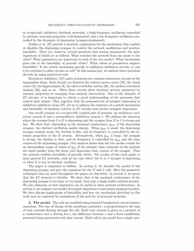
where ve denotes the voltage and we is the gating variable for the cell. The nonlinearityfe consists of the sum of currents which are intrinsic to the cell. The parameter ε � 1is the singular perturbation parameter and the derivative is with respect to t. Theve-nullcline, given by Ce = {(ve, we) : fe(ve, we) = 0}, is cubic shaped, whereas thewe-nullcline, given by Se = {(ve, we) : w∞(ve) − we = 0}, is sigmoidal. We assumethat these two curves intersect along the middle branch of the cubic Ce, thus ensuringthat an isolated E cell is oscillatory [29] (Figure 2). We denote the local minimumpoint, or left knee, of Ce by (vLK , wLK) and the local maximum point, or right knee,of Ce by (vRK , wRK). The time constant τe is given by

τe(ve) =

{τR if ve > vθ,τL if ve < vθ,

(2.2)

where vθ ∈ (vLK , vRK) is the threshold for entering the active phase and τR and τLare the time constants during the active and silent phase, respectively. We assume


ve

we

CeSe

(vL, wRK)

(vLK, wLK)

(vRK, wRK)

(vR, wLK)

Fig. 2. Phase-plane diagram of the activity of the isolated E cell. Ce is the ve-nullcline, and Se

is the we-nullcline. The solid trajectory is the singular periodic orbit consisting of slow movementof the solution along Ce and fast jumps from the left (vLK , wLK) and right (vRK , wRK) knees of Ceto the opposite branch.

that fe > 0 (< 0) below (above) the cubic and w∞(ve)−we > 0 (< 0) below (above)the sigmoid Se.

We shall study the network dynamics in the phase space by exploiting the factthat the parameter ε is small, allowing us to use techniques of geometric singularperturbation theory. We first construct singular solutions by analyzing the reducedequations which are appropriately scaled versions of (2.1) when ε = 0. Solutions ofthe reduced equations are pieced together to obtain a singular periodic orbit. Eachpiece of this orbit is a valid trajectory when ε = 0. It is then necessary to show thatfor ε small and positive there is a periodic solution of (2.1) near the singular solution.

The reduced equations and singular periodic orbit for the isolated E cell areconstructed as follows. The slow reduced equations are obtained by setting ε = 0 in(2.1) to obtain

0 = fe(ve, we),w′

e = [w∞(ve)− we]/τe(ve).(2.3)

These equations govern the evolution of E during its active or silent state. The firstequation is algebraic and constrains E to lie on the cubic Ce. The second equationgives the direction and speed of the flow on the cubic.

The fast reduced equations are obtained by rescaling time in (2.1) by lettingξ = t/ε and then setting ε = 0. This yields

ve = fe(ve, we),we = 0.

(2.4)

Here the derivative is with respect to ξ. These equations govern the fast jumpsbetween the active and silent states of the cell. Because of the second equation, we

acts as a parameter in the first equation. Note that both the slow and the fast reducedequations are scalar differential equations. For the fast equations (2.4), the left andright branches of Ce are attracting, and the middle branch is repelling. The left kneeis attracting from the left and repelling from the right; the opposite is true for theright knee.


intrinsic

inhibited

excited

intrinsic

IE

v

w

vthreshvthresh

E neuron I neuronfast excitation

slow inhibition(depressing)

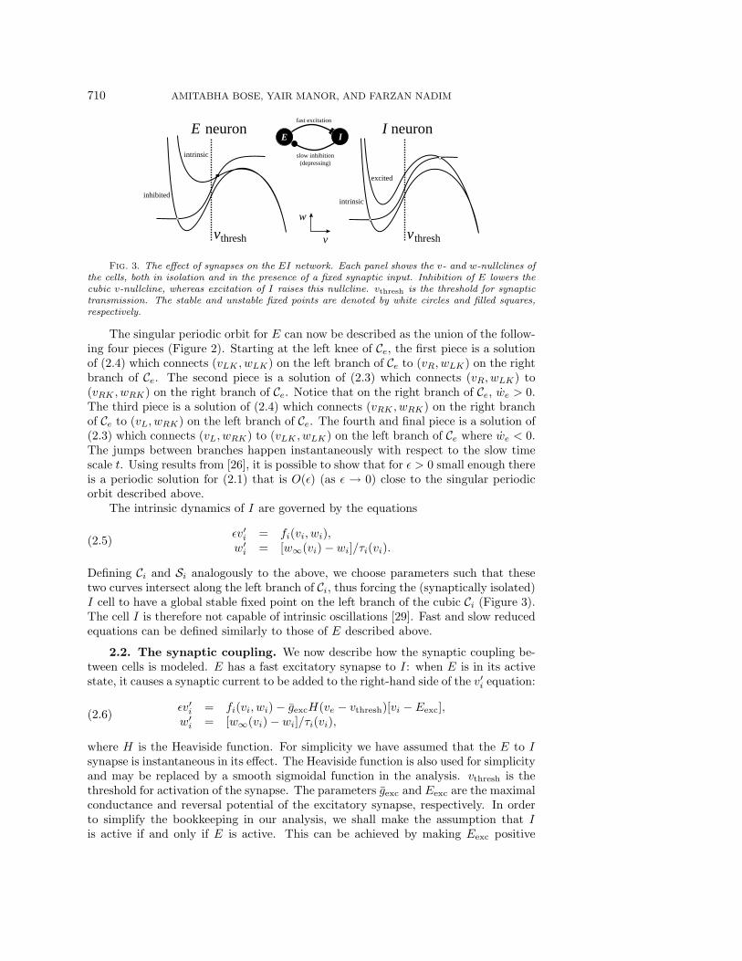
Fig. 3. The effect of synapses on the EI network. Each panel shows the v- and w-nullclines ofthe cells, both in isolation and in the presence of a fixed synaptic input. Inhibition of E lowers thecubic v-nullcline, whereas excitation of I raises this nullcline. vthresh is the threshold for synaptictransmission. The stable and unstable fixed points are denoted by white circles and filled squares,respectively.

The singular periodic orbit for E can now be described as the union of the follow-ing four pieces (Figure 2). Starting at the left knee of Ce, the first piece is a solutionof (2.4) which connects (vLK , wLK) on the left branch of Ce to (vR, wLK) on the rightbranch of Ce. The second piece is a solution of (2.3) which connects (vR, wLK) to(vRK , wRK) on the right branch of Ce. Notice that on the right branch of Ce, we > 0.The third piece is a solution of (2.4) which connects (vRK , wRK) on the right branchof Ce to (vL, wRK) on the left branch of Ce. The fourth and final piece is a solution of(2.3) which connects (vL, wRK) to (vLK , wLK) on the left branch of Ce where we < 0.The jumps between branches happen instantaneously with respect to the slow timescale t. Using results from [26], it is possible to show that for ε > 0 small enough thereis a periodic solution for (2.1) that is O(ε) (as ε → 0) close to the singular periodicorbit described above.

The intrinsic dynamics of I are governed by the equations

εv′i = fi(vi, wi),w′

i = [w∞(vi)− wi]/τi(vi).(2.5)

Defining Ci and Si analogously to the above, we choose parameters such that thesetwo curves intersect along the left branch of Ci, thus forcing the (synaptically isolated)I cell to have a global stable fixed point on the left branch of the cubic Ci (Figure 3).The cell I is therefore not capable of intrinsic oscillations [29]. Fast and slow reducedequations can be defined similarly to those of E described above.

2.2. The synaptic coupling. We now describe how the synaptic coupling be-tween cells is modeled. E has a fast excitatory synapse to I: when E is in its activestate, it causes a synaptic current to be added to the right-hand side of the v′i equation:

εv′i = fi(vi, wi)− gexcH(ve − vthresh)[vi − Eexc],w′

i = [w∞(vi)− wi]/τi(vi),(2.6)

where H is the Heaviside function. For simplicity we have assumed that the E to Isynapse is instantaneous in its effect. The Heaviside function is also used for simplicityand may be replaced by a smooth sigmoidal function in the analysis. vthresh is thethreshold for activation of the synapse. The parameters gexc and Eexc are the maximalconductance and reversal potential of the excitatory synapse, respectively. In orderto simplify the bookkeeping in our analysis, we shall make the assumption that Iis active if and only if E is active. This can be achieved by making Eexc positive


enough so that the excitatory synapse raises the cubic Ci in the phase plane, gexc

large enough so that this raised cubic intersects Si along its right branch somewhereabove the right knee of Ci (Figure 3), and τi(vi) small enough for vi > vthresh. Thisensures that excitation from E to I forces the I trajectory to jump to the right branchof the cubic Ci and that the I cell stays in the active state as long as E does.

The coupling from I to E is a depressing, slowly decaying inhibitory synapse.The reversal potential Einh is negative enough so that inhibition lowers the cubic Cein the phase plane. This synaptic current is described using two variables s and d;the former models the effect of the inhibitory current on E; the latter models thedynamics of depression. The equations which govern E become

εv′e = fe(ve, we)− ginhs[ve − Einh],w′

e = [w∞(ve)− we]/τe(ve),d′ = H(vthresh − vi)[1− d]/τα −H(vi − vthresh)d/τβ ,εs′ = H(vi − vthresh)[d− s]/τγ − εH(vthresh − vi)s/τκ.

(2.7)

Note that d recovers towards 1 whenever I is silent and decays towards 0 wheneverI is active. s decays towards 0 whenever I is silent and is reset (in the fast time scale)to the current value of d whenever I becomes active (Figure 4). Only the variable s(and not d) directly affects the behavior of E. However, since s = d in the singularlimit when I is active, d influences the behavior of E during the active phase. Notethat, except in the transition to the active state, the inhibition to E is always decaying.On the right branch the decay is controlled by τβ , and on the left branch the decayis controlled by τκ. Note also that the extent of recovery of d depends on the ratio ofτL and τR (see (2.3)) and on the time constants τα and τβ .

2.3. The coupled singular equations. We now define the singular equationswhich will be the focus of the analysis for the rest of this paper. These are equationsobtained from (2.7) as above but in which we shall make a few simplifications. First,since we assume that I is active if and only if E is active, we will not explicitly trackthe I trajectory. We are concerned only with whether or not vi is above or below thethreshold vthresh. Further, to ease the analysis, we assume that w∞(ve) = 0 when Eis in the silent state (ve < vLK) and w∞(ve) = 1 when E is active (ve > vRK). Thuswhen E is in the silent state it obeys the following set of slow equations:

0 = fe(ve, we)− sginh[ve − Einh],w′

e = −we/τL,d′ = [1− d]/τα,s′ = −s/τκ.

(2.8)

Alternatively, when E is in the active state it obeys the following set of slow equations:

0 = fe(ve, we)− sginh[ve − Einh],w′

e = [1− we]/τR,d′ = −d/τβ ,0 = d− s.

(2.9)

The fast equations that govern the transition from the silent to the active state are

ve = fe(ve, we)− sginh[ve − Einh],we = 0,

d = 0,s = H(vi − vthresh)[d− s]/τγ ,

(2.10)


vi

time

d

s

(a)

vi

wi

vthresh

dd

s s = d

with timeconstant τβ

with timeconstant τα

with timeconstant τκ

(b)

Fig. 4. Dynamics of the synaptic variables d and s. (a) Time traces of d and s depend onthe oscillations of the presynaptic voltage vi. (b) On the two branches of the v-nullcline in the Iphase plane, d, and s increase or decrease with fixed time constants. vthresh denotes the thresholdfor synaptic transmission.

and the fast equations that govern the transition from the active to the silent state are

ve = fe(ve, we)− sginh[ve − Einh],we = 0,

d = 0,s = H(vi − vthresh)(d− s).

(2.11)

The fourth equation in (2.10) shows that s is reset to d (on the fast time scale) onthe transition to the active state. The fourth equation in (2.9) shows that s remainsequal to d in the active phase and both decay with a time constant τβ (Figure 4).


Our main focus will be on how the network output changes with changes of themaximal conductance ginh of the depressing synapse. We shall choose and fix theother parameters in section 3.

3. Results. We will prove the existence of two distinct oscillatory regimes for themodel (2.6)–(2.7) with ε small and positive. The analyses of this section, however, willbe performed on the reduced (ε = 0) equations (2.8)–(2.11). Using the results of [26]on singular perturbations for the types of solutions discussed in this section, it followsthat (2.6)–(2.7) have solutions that are O(ε)-close to their singular counterparts.

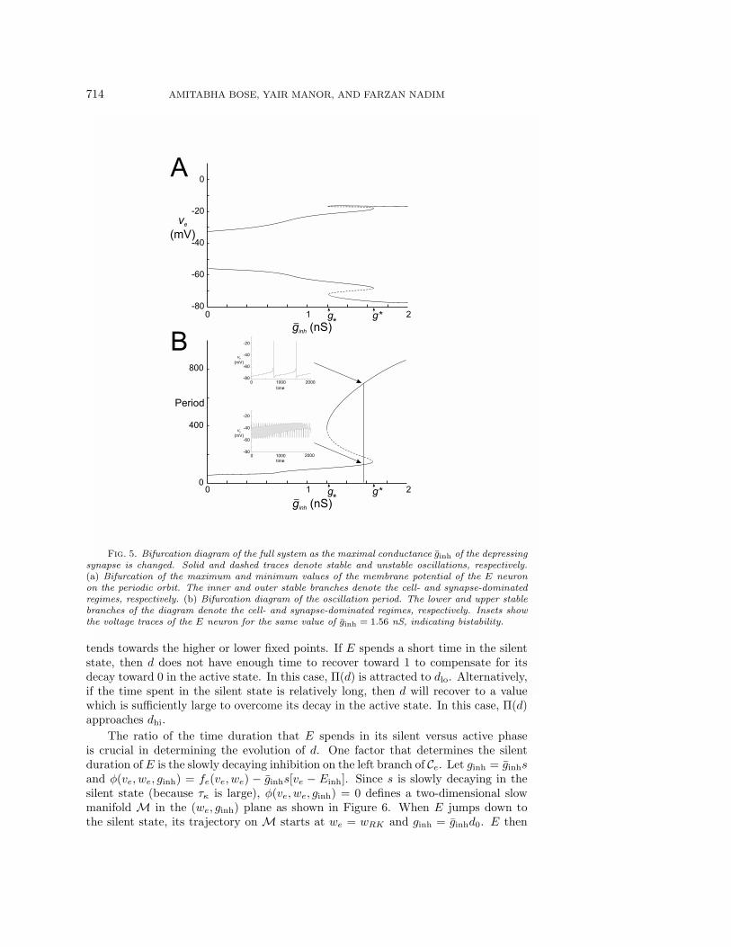
The main results of this paper are shown in Figure 5. This figure shows thebifurcation diagram of the periodic solutions of (2.6)–(2.7), where the maximum con-ductance ginh of the depressing synapse is varied. The solid curves correspond tostable periodic solutions. In the region of bistability, these curves are separated by anunstable periodic orbit denoted by the dashed curves. Figure 5(a) shows the minimumand maximum of ve on the periodic orbits.

The upper branch in Figure 5(b) corresponds to stable long-period solutions, whilethe lower branch corresponds to stable short-period solutions. The period on theupper branch is determined by the properties of the depressing synapse, whereas onthe lower branch it is largely determined by the intrinsic properties of E. We will showthat for fixed τR, τL, τβ and for τα and τκ sufficiently large there exist two maximalconductances of the depressing synapse g∗ and g∗, such that if g∗ < ginh < g∗, (2.8)–(2.11) has two stable and one unstable periodic solutions. One of the stable solutionshas a period O(τL + τR). The other has much longer period of O(τκ). Alternatively,if ginh < g∗, there is a unique, stable periodic solution of (2.8)–(2.11) whose period isO(τL + τR), and if g∗ < ginh, there is a unique stable periodic solution of (2.8)–(2.11)whose period is O(τκ).

3.1. Bistability of solutions. To construct the periodic orbits, we will definea one-dimensional Poincare map and show that its fixed points correspond to theperiodic orbits. First, we will prove that for some value of ginh the system is bistable.We will then show that for ginh small enough, or large enough, only one stable solutionpersists.

We stated earlier that inhibition lowers the cubic Ce in the E-phase plane. Forthe sake of simplicity, let us assume that inhibition from I lowers only the left branchof Ce (Figure 3). This assumption affects the results only minimally as we discussbelow. Thus, no matter what the level of inhibition, when E is in its active state, itlies on Ce and makes the transition to the silent state from (vRK , wRK), the right kneeof Ce. Therefore, at the moment E makes the transition to the silent state, ve = vRK ,we = wRK , but the values of s and d, while equal, are unknown. This simplifyingassumption enables us to define a one-dimensional Poincare map Π at the right knee.The map Π records the value of d each time E jumps down to the silent state.

The map Π is defined by following the trajectory from the right knee back to theright knee. Start at the right knee of Ce with d(0) = d0. From this point, E jumpsdown to the silent state. Let t = T1 be the time at which E jumps back up to theactive state, and let t = T2 be the time at which E returns to the right knee of Ce.The map Π : [0, 1] → (0, 1) is defined by Π(d0) = d(T2). If d(T2) = d(0) = d, then dis a fixed point of Π, corresponding to a singular periodic solution of (2.8)–(2.11). Insections 3.2 and 3.3 we will show that for an appropriate choice of ginh, there are twovalues of d, dlo < dhi such that Π(dlo) = dlo and Π(dhi) = dhi. The fixed point dlo (dhi)corresponds to the periodic orbit on the lower (upper) branch of Figure 5. The timethat E spends in the silent phase is the primary determinant of whether the solution


-80

-60

-40

-20

0 1000 2000

ve

(mV)

time

-80

-60

-40

-20

0 1000 2000

ve

(mV)

time

-80

0

-60

-40

-20ve

(mV)

ginh (nS)_

ginh (nS)_

0

400

800

Period

B

A

g*g*

g*g*

Fig. 5. Bifurcation diagram of the full system as the maximal conductance ginh of the depressingsynapse is changed. Solid and dashed traces denote stable and unstable oscillations, respectively.(a) Bifurcation of the maximum and minimum values of the membrane potential of the E neuronon the periodic orbit. The inner and outer stable branches denote the cell- and synapse-dominatedregimes, respectively. (b) Bifurcation diagram of the oscillation period. The lower and upper stablebranches of the diagram denote the cell- and synapse-dominated regimes, respectively. Insets showthe voltage traces of the E neuron for the same value of ginh = 1.56 nS, indicating bistability.

tends towards the higher or lower fixed points. If E spends a short time in the silentstate, then d does not have enough time to recover toward 1 to compensate for itsdecay toward 0 in the active state. In this case, Π(d) is attracted to dlo. Alternatively,if the time spent in the silent state is relatively long, then d will recover to a valuewhich is sufficiently large to overcome its decay in the active state. In this case, Π(d)approaches dhi.

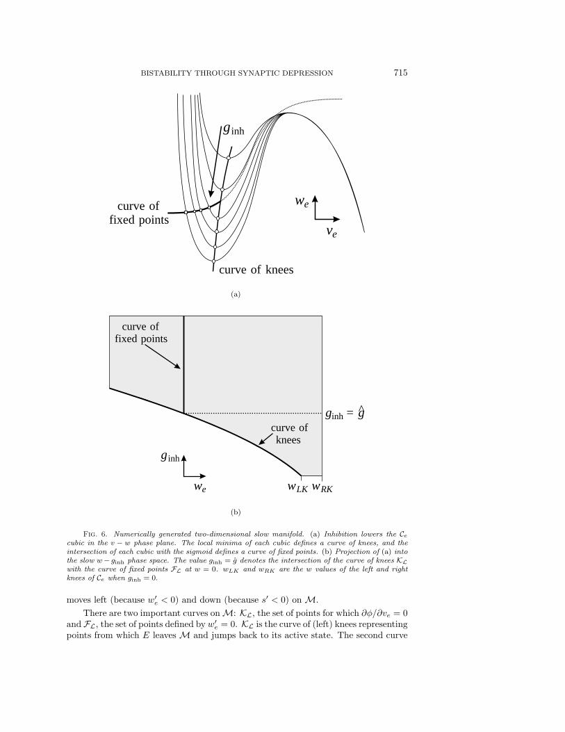
The ratio of the time duration that E spends in its silent versus active phaseis crucial in determining the evolution of d. One factor that determines the silentduration of E is the slowly decaying inhibition on the left branch of Ce. Let ginh = ginhsand φ(ve, we, ginh) = fe(ve, we) − ginhs[ve − Einh]. Since s is slowly decaying in thesilent state (because τκ is large), φ(ve, we, ginh) = 0 defines a two-dimensional slowmanifold M in the (we, ginh) plane as shown in Figure 6. When E jumps down tothe silent state, its trajectory on M starts at we = wRK and ginh = ginhd0. E then


ve

we

curve of knees

curve offixed points

ginh

(a)

curve ofknees

curve offixed points

we wLK wRK

ginh

= gginh^

(b)

Fig. 6. Numerically generated two-dimensional slow manifold. (a) Inhibition lowers the Cecubic in the v − w phase plane. The local minima of each cubic defines a curve of knees, and theintersection of each cubic with the sigmoid defines a curve of fixed points. (b) Projection of (a) intothe slow w− ginh phase space. The value ginh = g denotes the intersection of the curve of knees KLwith the curve of fixed points FL at w = 0. wLK and wRK are the w values of the left and rightknees of Ce when ginh = 0.

moves left (because w′e < 0) and down (because s′ < 0) on M.

There are two important curves onM: KL, the set of points for which ∂φ/∂ve = 0and FL, the set of points defined by w′

e = 0. KL is the curve of (left) knees representingpoints from which E leaves M and jumps back to its active state. The second curve


FL represents a curve of stable fixed points of the reduced system (2.8) for the we

variable. These points are not actual fixed points on M because on FL, dginh/dt < 0.For small values of ginh, E is oscillatory, and hence, for these values, we does not havea fixed point on M. Therefore, FL exists only for ginh sufficiently large. Because ginh

is always decreasing on M, E will always reach the curve of knees KL and jump backup to the active state.

Without the above assumption concerning the effect of inhibition on the rightbranch of Ce, we would still be able to define a one-dimensional Poincare map. How-ever, the right branches of the E cubic would now also define a two-dimensional slowmanifold, U . We would need to track the position of E as it evolves along U . Asbefore, we could define a one-dimensional Poincare map at we = wRK on U . Now wewould also need to measure the time it takes for the cell to evolve from we = wRK

on U to the curve of knees on U from which it could jump down to the silent state.This time is an increasing function of d. However, for the long-period orbit, it issmall compared to the time spent in the silent state, and thus the added time forwhich the synapse would depress would be negligible compared to the long time spentrecovering. For the short-period orbit, the time is small since the time goes to zero asd → 0. Thus the above assumption about the effect of inhibition on the right branchof Ce does not affect the qualitative results.

3.2. The short-period orbit. Assume τR, τL, and τβ are chosen and fixed.We will show that if τα is sufficiently large, there exists an interval [0, d∗] which mapsinto itself under Π. From (3.2) it is clear that Π is continuous with respect to d. Thisimplies the existence of a fixed point in [0, d∗] which we will call dlo.

Solving for d in (2.8)–(2.9), when E is silent we obtain

d(T1) = 1− (1− d0)e−T1/τα ,(3.1)

and, when E is active, we obtain

d(T2) = d(T1)e−(T2−T1)/τβ ,

d(T2) = (1− (1− d0)e−T1/τα)e−(T2−T1)/τβ .(3.2)

Suppose d0 = 0. Then it is clear that d(T2) > 0, implying that Π(0) > 0. To findan appropriate d∗ we need a bit more notation. Let g be the intersection point ofKL and FL (Figure 6), satisfying φ(ve, 0, g) = 0 and (∂φ/∂v)(ve, 0, g) = 0. Thusg = ginh implies that s = g/ginh. We choose d∗ to be strictly less than g/ginh, say,d∗ = g/(2ginh). The choice of d∗ appears to be arbitrary, but later we will discusshow various parameters depend on d∗.

We need to show that Π(d∗) < d∗. The time T2 − T1 is bounded from belowby TA, the active time duration of the isolated E cell. Note that TA = τR log[(1 −wLK)/(1− wRK)], which is O(τR). Therefore,

d(T2) < (1− (1− d∗)e−T1/τα)e−TA/τβ .(3.3)

If the right-hand side of (3.3) is less than d∗, then so is d(T2). After rearrangingterms, this condition can be written as

1− d∗eTA/τβ

1− d∗< e−T1/τα .(3.4)

Evaluating (3.4) at d∗ = g/(2ginh) yields

2ginh − geTA/τβ

2ginh − g< e−T1/τα .(3.5)


w

ginh

= ginh inh hi

= g

d

d

g

ginh inh lo

synapsecontrolled

cellcontrolledKL

FL

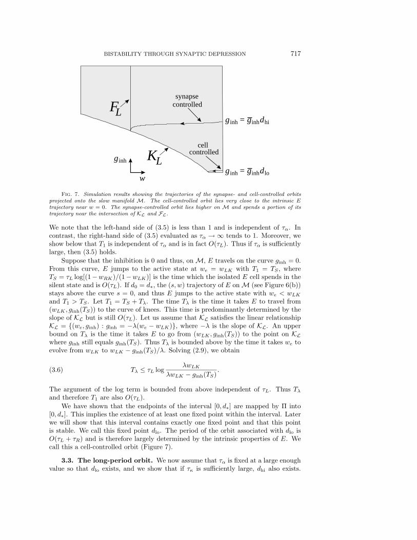
Fig. 7. Simulation results showing the trajectories of the synapse- and cell-controlled orbitsprojected onto the slow manifold M. The cell-controlled orbit lies very close to the intrinsic Etrajectory near w = 0. The synapse-controlled orbit lies higher on M and spends a portion of itstrajectory near the intersection of KL and FL.

We note that the left-hand side of (3.5) is less than 1 and is independent of τα. Incontrast, the right-hand side of (3.5) evaluated as τα → ∞ tends to 1. Moreover, weshow below that T1 is independent of τα and is in fact O(τL). Thus if τα is sufficientlylarge, then (3.5) holds.

Suppose that the inhibition is 0 and thus, on M, E travels on the curve ginh = 0.From this curve, E jumps to the active state at we = wLK with T1 = TS , whereTS = τL log[(1−wRK)/(1−wLK)] is the time which the isolated E cell spends in thesilent state and is O(τL). If d0 = d∗, the (s, w) trajectory of E on M (see Figure 6(b))stays above the curve s = 0, and thus E jumps to the active state with we < wLK

and T1 > TS . Let T1 = TS + Tλ. The time Tλ is the time it takes E to travel from(wLK , ginh(TS)) to the curve of knees. This time is predominantly determined by theslope of KL but is still O(τL). Let us assume that KL satisfies the linear relationshipKL = {(we, ginh) : ginh = −λ(we − wLK)}, where −λ is the slope of KL. An upperbound on Tλ is the time it takes E to go from (wLK , ginh(TS)) to the point on KLwhere ginh still equals ginh(TS). Thus Tλ is bounded above by the time it takes we toevolve from wLK to wLK − ginh(TS)/λ. Solving (2.9), we obtain

Tλ ≤ τL logλwLK

λwLK − ginh(TS).(3.6)

The argument of the log term is bounded from above independent of τL. Thus Tλ

and therefore T1 are also O(τL).

We have shown that the endpoints of the interval [0, d∗] are mapped by Π into[0, d∗]. This implies the existence of at least one fixed point within the interval. Laterwe will show that this interval contains exactly one fixed point and that this pointis stable. We call this fixed point dlo. The period of the orbit associated with dlo isO(τL + τR) and is therefore largely determined by the intrinsic properties of E. Wecall this a cell-controlled orbit (Figure 7).

3.3. The long-period orbit. We now assume that τα is fixed at a large enoughvalue so that dlo exists, and we show that if τκ is sufficiently large, dhi also exists.


Recall that none of the analysis of the previous section involved τκ; therefore, fixingτκ does not affect the existence of dlo.

As before, we will show that a certain interval, in this case [d∗, 1], is mappedinto itself by Π. Suppose first that d0 = 1. Then using (3.2), d(T2) = e−TA/τβ < 1.Therefore, Π(1) < 1. Assume that d∗ > g/ginh. As with d∗, we will later showhow d∗ depends on parameters. To show that Π(d∗) > d∗, we need an analogueof (3.5). As seen from the slow phase space M, we = 0 is the lowest value of wfrom which E can jump to the active state. Therefore, T2 − T1 is bounded above byTmax = τR log[1/(1−wRK)], which is the time from we = 0 to we = wRK on the rightbranch of Ce. A calculation similar to that of (3.3)–(3.4) shows that Π(d∗) > d∗ if

1− d∗eTmax/τβ

1− d∗> e−T1/τα .(3.7)

We now choose d∗ = 2g/ginh, where we assume that 2g < ginh. Evaluating (3.7) atd∗ = 2g/ginh, we find

ginh − 2geTmax/τβ

ginh − 2g> e−T1/τα .(3.8)

Note that the left-hand side of (3.8) is again a quantity that is less than one butbounded away from zero, and is independent of T1. The right-hand side of (3.8) canbe made arbitrarily small by making T1 large. It is easy to make T1 large by makingτκ large. Suppose for the sake of argument that τκ → ∞. In this case, ginh does notdecay and E is attracted to FL and must remain in the silent state. In this case,T1 → ∞ as τκ → ∞. Clearly then, if τκ is sufficiently large, then T1 will also be. Forthis case, (3.8) will then hold, and Π(d∗) > d∗.

As before, these two results imply that there exists dhi ∈ [d∗, 1], which is a fixedpoint of Π. The period of the solution associated with dhi is O(τκ) and is determinedby the time constant of the inhibitory decay. We call this orbit synapse-controlled(Figure 7).

3.4. Stability of orbits. We have shown that Π(d∗) > d∗ and Π(d∗) < d∗.Since Π is a continuous mapping, this implies the presence of dmed ∈ [d∗, d∗] suchthat Π(dmed) = dmed. We now show that dlo, dmed, and dhi are the only fixed pointsof Π and that dlo and dhi are stable, while dmed is unstable.

A fixed point d of the map Π is stable if |Π′(d)| < 1 and unstable if |Π′(d)| > 1.This gives a local result, valid in a neighborhood of the fixed point. We will showthe stronger result that |Π′(d0)| < 1 for any d0 ∈ [0, d∗] or d0 ∈ [d∗, 1]. This gives auniform result which also implies uniqueness of the fixed points.

Using (3.2), we find that Π(d0) = d(T1)e−(T2−T1)/τβ , where T1 and T2 both depend

on d0. In the following argument, let ′ denote the derivative with respect to d0. Astraightforward calculation using (3.1)–(3.2) and the chain rule shows that

Π′(d0) =[e−T1/τα [1 + [1− d0]T

′1/τα]− d(T1)[T2 − T1]

′]e−[T2−T1]/τβ .(3.9)

Note that d(T1) < 1, τα is fixed, and e−[T2−T1]/τβ < 1. Therefore, by showing thate−T1/ταT ′

1 and [T2−T1]′ are small on the intervals of interest, we will have shown that

the |Π′| < 1 on these intervals.Consider first [d∗, 1]. If τκ is sufficiently large, then E jumps up from a neighbor-

hood of s = g/ginh and we = 0. Assuming that E actually jumps up when s = g/ginh


and we = 0, the time T2 − T1 is the time on the right branch that E takes to go fromwe = 0 to we = wRK . This time is independent of d0, which implies that [T2−T1]

′ = 0.We next estimate e−T1/ταT ′

1. For the interval [d∗, 1], the time T1 is the timeit takes s to decay from d0 to g/ginh. Therefore, g/ginh = d0e

−T1/τκ . Taking thederivative with respect to d0 and using the chain rule, we find

0 = e−T1/τκ − d0T′1e

−T1/τκ/τκ

or

T ′1 = τκ/d0.(3.10)

Thus on [d∗, 1], T ′1 is O(τκ). The time T1 is bounded from above by the time it takes

s to decay from 1 to g/ginh, which is τκ log(ginh/g). Therefore,

e−T1/τα >

[g

ginh

]τκ/τα.(3.11)

Thus e−T1/τα is O(aτκ) for some a < 1. This shows that e−T1/ταT ′1 is O(τκa

τκ),which can be made small by making τκ large, independent of d0. As a result, if τκ issufficiently large, then uniformly for all d0 ∈ [d∗, 1], |Π′(d0)| < 1. This implies thatdhi is the unique stable fixed point on this interval.

Now consider d0 ∈ [0, d∗]. We showed earlier that T1 = TS + Tλ, where TS isthe time it takes E to evolve in the silent state along ginh = 0 and Tλ is the extratime E evolves due to the slope of the curve of knees. Clearly, T ′

1 = T ′λ since TS is

independent of d0. There are several ways to show that T ′λ can be made small. One

way is to use the slope of the curve of knees −λ. If λ → ∞, then the curve of kneesKL becomes vertical, and Tλ → 0. In this case, clearly, T ′

1 = T ′λ → 0 since T1 will

equal TS which is independent of d0. This also implies that [T2−T1]′ = 0 in this limit

as T2 − T1 will equal TA, which is also independent of d0. Therefore, if we make thecurve of knees more vertical, we can make |Π′| < 1.

Recall that the curve of knees is given by φ = 0 and φv = 0, where φ(ve, we, ginh) =fe(ve, we)− ginh[ve−Einh]. Let (vK(ginh), wK(ginh)) denote the curve of knees. Plug-ging this into φ = 0 and differentiating with respect to ginh, we find

0 = φve

∂vK∂ginh

+ φwe

∂wK

∂ginh+ φginh

.

Using φve = 0 and rearranging terms, we find that the slope of the curve of kneessatisfies

∂ginh

∂wK=

−φwe

φginh

=∂fe/∂we

vK − Einh.(3.12)

The slope is negative since ∂fe/∂we < 0 and vK − Einh > 0 since the synapse isinhibitory. The slope can be made large in magnitude by making |∂fe/∂we| large.This quantity is solely determined by the intrinsic properties of the cell. In our case,||∂fe/∂we|| is proportional to |gCa[ve − ECa]|, where gCa and ECa are the maximalconductance and reversal potential of calcium. See the appendix for the equations.The calcium reversal potential is very high, and, in particular, lies far to the rightof the left branch of Ce. Assuming that gCa is sufficiently large, for our equations,


||∂fe/∂we|| is large. Therefore, we conclude that |Π′| < 1 for do ∈ [0, d∗]. This showsthat dlo is the unique stable fixed point in this interval.

The stability of the fixed points dlo and dhi, together with the continuity of Π,immediately implies that there exists an unstable fixed point on the interval [d∗, d∗].Call this fixed point dmed. Note that, since it is unstable and Π is differentiable,Π′(dmed) > 1. To prove that it is the unique fixed point on this interval, we firstnote that T ′

1 > 0 on this interval. This follows since the curve of knees is negativelysloped and the evolution in the w direction is independent of d0. The time T1 changesfrom O(τL) to O(τκ) as d0 increases and is sigmoidal shaped. Thus T ′

1 has one localmaximum and is relatively large at d. In contrast, as before [T2 − T1]

′ is small. Infact, if the curve of knees is made more vertical, as above, then [T2 − T1]

′ → 0.Thus using (3.9) Π′(d) > 0. For simplicity, assume (T2 − T1)

′ = 0. Then using (3.9)the magnitude of Π′(d0) is controlled by the term e−T1/ταT ′

1/τα. This term has asingle local maximum, which must be large since Π′(dmed) > 1. Since Π′ > 0 andΠ′(dhi) ≤ 1, it follows that if there is an additional fixed point between dmed and dhi,

say, d, then Π(d) ≤ 1. But this implies that Π′ > 1 on some subinterval of (d, dhi).This, however, contradicts the fact that e−T1/ταT ′

1/τα has a single local maximum.Therefore, dmed is unique.

3.5. Existence of an interval of bistability. To complete the bifurcationdiagram, we show that if ginh is too small, the system has only a single short-periodorbit. Alternatively, if ginh is too large, the system has only a single large-periodorbit.

Recall that g is defined by φ(ve, 0, g) = 0, φve(ve, 0, g) = 0. Thus if ginh < g, the

curve of fixed points FL will not exist on the manifold M. This implies that the timeT1 is largely determined by the intrinsic dynamics of the isolated E cell and there isno chance that (3.7)–(3.8) can be satisfied. Thus dhi cannot exist. Moreover, if dhi

does not exist, dmed cannot exist either. Suppose to the contrary that dmed continuesto exist. Since Π(dmed) = dmed, Π

′(dmed) > 1, and Π(1) < 1, it must follow that thereexists at least one fixed point in (dmed, 1). This contradicts the lack of existence ofdhi. This finally implies that there exists a g∗ such that if ginh < g∗, then a singlesmall period orbit exists.

Similarly, if ginh is too large, then dlo cannot exist. Suppose that ginh → ∞.Then the left-hand side of (3.5) tends to 1, while the right-hand side remains lessthan 1. Clearly, if ginh is sufficiently large, (3.5) fails to hold. For the same reason asabove, once dlo disappears, dmed must also. Therefore, there exists a g∗ such that ifginh > g∗, then there exists a single long-period orbit.

The analysis above provides sufficient but not necessary conditions on the timeconstants and conductances for the existence of an interval of bistability of solutions.In particular, the methods that we have employed show the existence of g∗ and g∗

but do not provide lower and upper bounds for these values.

3.6. Dependence on parameters and simulations. The existence and sta-bility of solutions depends on the relative values of several of the time constantspresent in the equations. As we showed above, the short-period orbit is controlled byintrinsic parameters, while the long-period orbit is controlled by synaptic parameters.In particular, for the short-period orbit, in which the synapse remains depressed, it isimportant that τL is small relative to τα. Alternatively, for the long-period solution,it is important that τL is small relative to τκ. Thus the range of bistability can beexpanded by varying τα and τκ. Specifically, increasing τα increases g∗ so that the


cell-controlled range is larger. Increasing τκ has the effect of decreasing g∗. A slowerdecay of inhibition gives the synapse more time to recover in the silent state, thusallowing smaller values of the maximal conductance ginh to produce a long-period so-lution. By decreasing τα the short-period solution can be destroyed, while decreasingτκ destroys the long-period solution. Similar results can be obtained by fixing τα andvarying τL.

In section 3, we chose d∗ and d∗ in a seemingly ad hoc fashion. These values alsodepend on the parameters in much the same way as g∗ and g∗. Namely, for fixed ginh,increasing τα implies that d∗ also increases, while increasing τκ decreases d∗. Thesechanges will affect the values of the fixed points dhi and dlo but will not change whichparameters control the existence of these fixed points.

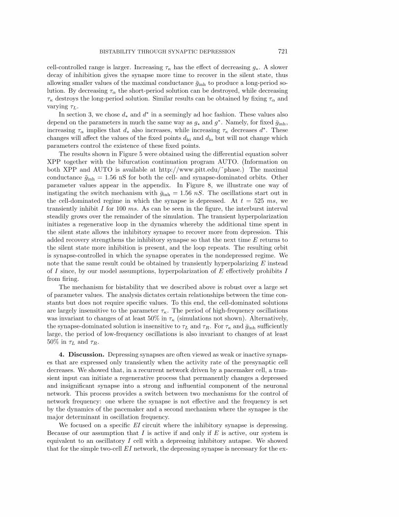
The results shown in Figure 5 were obtained using the differential equation solverXPP together with the bifurcation continuation program AUTO. (Information onboth XPP and AUTO is available at http://www.pitt.edu/˜phase.) The maximalconductance ginh = 1.56 nS for both the cell- and synapse-dominated orbits. Otherparameter values appear in the appendix. In Figure 8, we illustrate one way ofinstigating the switch mechanism with ginh = 1.56 nS. The oscillations start out inthe cell-dominated regime in which the synapse is depressed. At t = 525 ms, wetransiently inhibit I for 100 ms. As can be seen in the figure, the interburst intervalsteadily grows over the remainder of the simulation. The transient hyperpolarizationinitiates a regenerative loop in the dynamics whereby the additional time spent inthe silent state allows the inhibitory synapse to recover more from depression. Thisadded recovery strengthens the inhibitory synapse so that the next time E returns tothe silent state more inhibition is present, and the loop repeats. The resulting orbitis synapse-controlled in which the synapse operates in the nondepressed regime. Wenote that the same result could be obtained by transiently hyperpolarizing E insteadof I since, by our model assumptions, hyperpolarization of E effectively prohibits Ifrom firing.

The mechanism for bistability that we described above is robust over a large setof parameter values. The analysis dictates certain relationships between the time con-stants but does not require specific values. To this end, the cell-dominated solutionsare largely insensitive to the parameter τκ. The period of high-frequency oscillationswas invariant to changes of at least 50% in τκ (simulations not shown). Alternatively,the synapse-dominated solution is insensitive to τL and τR. For τκ and ginh sufficientlylarge, the period of low-frequency oscillations is also invariant to changes of at least50% in τL and τR.

4. Discussion. Depressing synapses are often viewed as weak or inactive synaps-es that are expressed only transiently when the activity rate of the presynaptic celldecreases. We showed that, in a recurrent network driven by a pacemaker cell, a tran-sient input can initiate a regenerative process that permanently changes a depressedand insignificant synapse into a strong and influential component of the neuronalnetwork. This process provides a switch between two mechanisms for the control ofnetwork frequency: one where the synapse is not effective and the frequency is setby the dynamics of the pacemaker and a second mechanism where the synapse is themajor determinant in oscillation frequency.

We focused on a specific EI circuit where the inhibitory synapse is depressing.Because of our assumption that I is active if and only if E is active, our system isequivalent to an oscillatory I cell with a depressing inhibitory autapse. We showedthat for the simple two-cell EI network, the depressing synapse is necessary for the ex-


time

vI

(mV)

vE

(mV)

d0 1000 2000 3000 4000 5000

0.0

0.5

–70

–50

–30

–10

–70

–50

–30

–10

Fig. 8. Simulation results demonstrating the bistability of solutions and a mechanism forswitching between cell- and synapse-dominated orbits. The neurons begin in the cell-dominatedmode, where d is small. At t = 500 ms we transiently hyperpolarized I for 100 ms. The lower traceshows that during the hyperpolarization d has an opportunity to grow. This resulted in a switch tothe much slower synapse-dominated mode of oscillation. The black bar denotes the hyperpolarizinginterval. Note that during this interval I is still excited by E.

istence of bistability. Indeed, if synapses are nondepressing, whenever I is in its activephase, E receives the same synaptic inhibition, independent of the initial conditionsor previous perturbations, and therefore remains in the same functional state.

In our analysis, we have assumed that the participating neurons make fast transi-tions between low (hyperpolarized) and high (depolarized) potentials. This assump-tion facilitated the use of geometric singular perturbation techniques that readilyallowed us to dissect the model into slow and fast subsystems of lower dimension.Each of these reduced systems is controlled by a subset of the parameters of the orig-inal model. The analysis of the reduced systems, therefore, enabled us to determinewhich parameters control what aspects of the network output (e.g., period).

4.1. Models of synaptic depression. In the past few years, several mod-els of synaptic depression have been proposed. Noteworthy are the models of Ab-bott et al. [1] and Tsodyks and Markram [34]. In both studies, the cells were modeledas integrate-and-fire neurons. Abbott et al. model synaptic depression as follows:when the presynaptic neuron produces a spike, the synaptic conductance rises instan-taneously to a value gα, and it decays to zero with a preset time constant. g is themaximal synaptic conductance, and α describes depression. The variable α recoversbetween presynaptic spikes and is instantaneously scaled down (depresses) by a fixedratio whenever a spike occurs. The model of Tsodyks and Markram is based on theidea that synaptic resources are partitioned into 3 states: active, inactive, and recov-ered. A presynaptic spike instantaneously transfers a fixed fraction of the resourcesfrom the recovered to the active state. The active resources quickly decay to theinactive state. The inactivate resources, in turn, change to recovered resources witha slower time constant.

In both models, synaptic strength is a function of interspike interval only andis totally independent of the presynaptic voltage during these intervals. However, insome neuronal systems the extent of synaptic recovery is a function of the presynaptic


voltage [22]. Moreover, the models of Abbott et al. and Markram and Tsodyks assumethat the synaptic transmission terminates almost immediately after the presynapticspike. When the sole activity of neurons is spiking, this assumption is reasonable.However, in many cases the electrical activity of neurons is more complex. For ex-ample, spiking activity may be modulated by subthreshold activity or ride on top ofslow waves. In some cases, synaptic transmission can even occur in the absence ofspikes but just as a result of slow variations in membrane potentials [5, 11, 22].

As in the models of Abbott et al. and Tsodyks and Markram, we view the dynam-ics of the synapse and the effect on the postsynaptic neuron as related but separateprocesses. In our model, these two processes are identical when the presynaptic cell isactive but behave differently when the presynaptic cell is silent. We therefore definetwo variables d and s, respectively, describing the depression dynamics and the effecton the postsynaptic cell. d and s evolve with different kinetics during the silent phase:d increases (the synapse recovers), whereas s decreases (the effect on the postsynapticcell decays). In the active phase, however, d and s are nearly identical and followthe same dynamics. Our model of synaptic depression thus lies between the model ofAbbott et al., which consists of a single dynamic variable, and the model of Tsodyksand Markram, which uses two variables. Our model is, in fact, more general thanthese models since it takes into account factors other than the interspike interval.In particular, synaptic transmission is not dependent just on the length of the silentphase, but also on the duration of the active phase. Moreover, in our model, recoveryfrom depression can also be dependent on the presynaptic voltage. In this work, wemade the simplifying assumption that the synaptic threshold Vthresh is all or none.However, in the more general case, the synaptic transfer function may be smooth,and therefore the extent of d recovery could be voltage-dependent.

4.2. Bistability in neuronal systems. Both experimental and theoreticalwork have shown that brief perturbations (such as a short current pulse, short synap-tic input, or brief exposure to a neuromodulator) can induce long-lasting changes inneuronal networks. These changes may be in the membrane potential of neurons [14],patterns of activity [8, 20], responses to input signals [15], phasing [37], coupling versusdecoupling [12], firing frequency [10], or period of network oscillation [27]. Bistabilityin neuronal systems has been associated with a variety of functions, such as motorcontrol [10, 18, 20], visual perception [9, 35], memory [4, 17], and representation oftemporal durations [28]. In view of the wide range of behaviors attributed to neuronalbistability in its different forms, it is important to understand how bistability arises.

Bistability can be created by intrinsic neuronal properties such as voltage-gatedionic currents. For example, voltage-gated calcium currents have been associated withbistability of membrane potential in several experimental [15, 38] and theoretical [6]studies. Bistability in firing patterns can also be generated by time delays in feedbackloops [19]. In rhythmic networks, bistability may be inherent to the network architec-ture [31, 33]. In our model, bistability of the oscillation period arises from synapticdepression. This form of bistability differs from those described in other rhythmicnetworks in that it involves a switch in the controlling mechanism of the periodicorbits. For example, Somers and Kopell [31] obtain bistability between synchronousand antiphase solutions in mutually coupled excitatory networks. However, in theirmodel the periods of both solutions are completely determined by the intrinsic prop-erties of the cells. In our model, the bistability of periodic orbits does not merelyimply that the network can be switched from one periodic solution to the other bya transient input. The interesting and perhaps more profound result of the switch is


that a component of the network that was previously ineffective is now in control ofthe network frequency. This may have important implications for neuromodulation,as discussed below.

4.3. The role of network parameters. The cell-dominated regime, or short-period orbit, is controlled by the intrinsic neuronal properties, such as the time con-stants τL and τR that govern the time intervals spent on the left and right branchesin the absence of synaptic input. This mode of oscillation persists as long as thedepressing synapse is prevented from recovering. For example, if the time constantof synaptic recovery τα is much larger than τL (or the time constant of depression τβis much smaller than τR), the oscillation will be cell-dominated, unless the maximalsynaptic conductance ginh is unrealistically large. Because the depressing synapseis weak in this regime, the oscillation period is mostly insensitive to changes in thesynaptic time constants τκ, τα, or τβ . However, sufficient decrease of τα relative toτL (or increase of τβ relative to τR) will switch the system to the synapse-dominatedregime, where these synaptic parameters are the most important factors in determin-ing the oscillation period. In the synapse-dominated regime, τL and τR do not affectthe oscillation period.

The range of the bistable regime is determined by the synaptic time constantsτκ, τβ , and τα. An increase in τα will weaken the synapse by slowing down recoveryfrom depression and hence push g∗ (the turning point of the cell-dominated branch)to the right. A similar effect is obtained by decreasing τβ and hence speeding updepression. Alternatively, increasing τκ enables the synapse to remain effective for alonger time when the cells are in their inactive state. Thus increasing τκ will pushg∗ (the turning point of the synapse-dominated branch) to the left. Decreasing τκor τα (or increasing τβ) sufficiently could cause the two turning points g∗ and g∗ tocoalesce, thereby destroying the bistable regime.

The mechanism for bistability that we described applies quite generally to a va-riety of network architectures. For example, if the excitatory synapse is the one thatshows depression, or if both synapses are depressing, the two modes of oscillationmay still be present and overlap to produce bistability. In fact, a network with twodepressing synapses with distinct time scales may have a separate switch mechanismfor each synapse, potentially providing multiple oscillatory regimes (dominated by theintrinsic properties of the cells, by one synapse, or by both synapses).

4.4. Significance for modulation of rhythmic networks. The rhythmicnetwork that we have analyzed has the capability to regulate its frequency upon ar-rival of the appropriate signal. Long-lasting changes in oscillation period can be trig-gered by an appropriately timed, brief synaptic, or modulatory input. For instance, ifthe system is operating in the cell-dominated regime, an inhibitory input that occursduring and prolongs the silent phase can have a large impact on the system because itwill allow recovery from depression and switch the system to the synapse-dominatedregime. However, the same input during the active phase of the cell-dominated os-cillation will be mostly ignored because the depressed synapse cannot recover duringthis phase. In this case, the perturbation will merely generate a time shift of theoscillation.

Our work also demonstrates that some parameters affect the oscillation periodorbit only in the synapse-dominated regime and not in the cell-dominated regime. Forexample, in the cell-dominated regime the network is largely insensitive to changes inthe decay time constant of synaptic inhibition. In contrast, in the synapse-dominatedregime this parameter is important and determines the duration of the interburst


phase. This allows the neuronal circuit to be primed (for example, by a modulatoryeffect that prolongs the decay time constant) for the change in control, without anyapparent change in output, prior to the occurrence of a triggering event. Hence aneuronal circuit in the cell-dominated regime would switch to the synapse-dominatedregime in two steps. A similar mechanism has been described in the endogenousburster R15 in Aplysia, where electrical activity changes from bursting to beatingfollowing a brief perturbation but only in the presence of serotonin [20]. This pro-cedure could be used as a safety mechanism to prevent the system from accidentallyswitching from one activity mode to another, for example, as a result of synapticnoise.

Neural networks are largely controlled by neuromodulation. Often, neuromod-ulation is used for fine tuning of functional circuits [23]. However, in many casesneuromodulation can produce far more extensive changes. For instance, neuromodu-lation can switch neurons to participate at different times in distinct functional circuits[13, 25]. Also, neuromodulation can reconfigure neuronal circuits [24] so that the samehardware can be used to produce different outputs, thereby adding to the flexibilityof neural networks. Despite the wide impact of neuromodulation on neural activity,many aspects of neuromodulatory action are not well understood. For example, inmost cases it is not known whether modulators affect neural networks by targetingcellular and/or synaptic components directly or whether they modify the networks bychanging one component of the network, thereby triggering a cascade of events thatleads to a new network output. We propose that in a neuronal network that includesdepressing synapses, modulatory effects that change the dynamics of these synapsesare sufficient to reconfigure the entire network. Such a mechanism could allow thenetwork to utilize components that were previously functionally insignificant or toremove components that were previously important.

Appendix. The equations that we used for the simulations in Figures 5–8 areas follows:

Cv′ = Iext − ICa − Ileak − Isyn,(A.1)

w′ = [w∞(v)− w]/τ(v),(A.2)

where ICa = gCam∞(v)[1−w][v−ECa], Ileak = gleak[v−Eleak], and Iext is an externaltonic current. All voltages are in mV , time constants are in msec, and conductancesare in nSs. The functions m∞ and w∞ have the form 1/(1 + exp(−(v − x1)/x2)).The function τ = τL + [τR − τL]h∞(v). Common parameter values for both cells areECa = 0, Eleak = −65, gCa = 1.6, gleak = 0.3, C = 1, τL = 50, τR = 50, and, for m∞,x1 = −50, x2 = 4. For the E cell we used Iext = 0 and for w∞, x1 = −53 and x2 = 1;for the I cell we used Iext = −1.5 and x1 = −64 and x2 = 6.

The excitatory synaptic current from E to I is given by gexcse(vi −Eexc), wherege = 0.1 and Eexc = 0. The variable se = 1/(1 + exp(−(ve − x1)/x2)) with x1 = −53and x2 = 1. The inhibitory current from I to E is of the form ginhsi(ve − Einh) withEinh = −80. The synaptic variable si and the depression variable di obey

s′i = [dis∞(vi)− si]/τsi(vi),(A.3)

d′i = [d∞(vi)− di]/τdi(vi),(A.4)

where s∞(vi) = 1/(1 + exp(−(vi − vthresh)/x2)) with vthresh = −64 and x2 = 6,τsi(vi) = τκ + [τγ − τκ]s∞(vi) with τγ = 1, τκ = 500, d∞(vi) = 1/[1 + exp(vi − vrec)]with vrec = −55, and τdi(vi) = τβ + [τα − τβ ]d∞(vi) with τα = 600 and τβ = 100.


REFERENCES

[1] L. F. Abbott, J. A. Varela, K. Sen, and S. B. Nelson, Synaptic depression and corticalgain control, Science, 275 (1997), pp. 220–224.

[2] Y. Adini, D. Sagi, and M. Tsodyks, Excitatory-inhibitory network in the visual cortex: Psy-chophysical evidence, Proc. Natl. Acad. Sci. USA, 94 (1997), pp. 10426–10431.

[3] D. G. Amaral and M. P. Witter, Hippocampal formation, in The Rat Nervous System, G.Paxinos, ed., Academic Press, San Diego, pp. 443–493.

[4] C. A. Barnes, M. S. Suster, J. Shen, and B. L. McNaughton, Multistability of cognitivemaps in the hippocampus of old rats, Nature, 388 (1997), pp. 272–275.

[5] M. Burrows and M. V. S. Siegler, Graded synaptic transmission between local interneuronsand motoneurons in the metathoracic ganglion of the locust, J. Physiol. (Lond.), 285 (1978),pp. 231–255.

[6] V. Booth and J. Rinzel, A minimal, compartmental model for a dendritic origin of bistabilityof motoneuron firing patterns, J. Comput. Neurosci., 2 (1995), pp. 299–312.

[7] D. Buonomano, Decoding temporal information: A model based on short-term synaptic plas-ticity, J. Neurosci., 20 (2000), pp. 1129–1141.

[8] K. P. Carlin, K. E. Jones, Z. Jiang, L. M. Jordan, and R. M. Brownstone, Dendritic L-type calcium currents in mouse spinal motoneurons: Implications for bistability, EuropeanJ. Neurosci., 12 (2000), pp. 1635–1646.

[9] K. E. Eastman and H. S. Hock, Bistability in the perception of motion and stationarity:Effects of temporal asymmetry, Percept. Psychophys., 61 (1999), pp. 1055–1065.

[10] T. Eken, H. Hultborn, and O. Kiehn, Possible functions of transmitter-controlled plateaupotentials in alpha motoneurons, Prog. Brain Res., 80 (1989), pp. 257–267.

[11] K. Graubard, Synaptic transmission without action potentials: Input-output properties of anonspiking presynaptic neuron, J. Neurophysiol., 41 (1978), pp. 1014–1025.

[12] A. L. Harris, D. C. Spray, and M. V. Bennett, Control of intercellular communication byvoltage dependence of gap junctional conductance, J. Neurosci., 3 (1983), pp. 79–100.

[13] S. L. Hooper and M. Moulins, Switching of a neuron from one network to another by sensory-induced changes in membrane properties, Science, 244 (1989), pp. 1587–1589.

[14] J. Hounsgaard, H. Hultborn, B. Jespersen, and O. Kiehn, Bistability of alpha-motoneurons in the decerebrate cat and in the acute spinal cat after intravenous 5-hydroxytryptophan, J. Physiol. (Lond.), 405, (1988), pp. 345–67.

[15] S. W. Hughes, D. W. Cope, T. I. Toth, S. R. Williams, and V. Crunelli, All thalamo-cortical neurons possess a T-type Ca2+ “window” current that enables the expression ofbistability-mediates activities, J. Physiol. (Lond.), 517 (1999), pp. 805–815.

[16] E. G. Jones, Connectivity of the primate sensory-motor cortex, in Cerebral Cortex, Vol. 5, E.G. Jones and A. Peter, eds., Plenum Press, New York, 1986, pp. 113–183.

[17] A. B. Kirillov, C. D. Myre, and D. J. Woodward, Bistability, switches and working memoryin a two-neuron inhibitory-feedback model, Biol. Cybernet., 68 (1993), pp. 441–449.

[18] D. Kleinfeld, F. Raccuia-Behling, and H. J. Chiel, Circuits constructed from identifiedAplysia neurons exhibit multiple patterns of persistent activity, Biophys. J., 57 (1990), pp.697–715.

[19] S. Kunec and A. Bose, Role of axonal delays in organizing the behavior of self-inhibitingneurons, Phys. Rev. E, 63 (2001), 0219081-13.

[20] H. A. Lechner, D. A. Baxter, J. W. Clark, and J. H. Byrne, Bistability and its regulationby serotonin in the endogenously bursting neuron R15 in Aplysia, J. Neurophysiol., 75(1996), pp. 957–962.

[21] J. Lisman, Bursts as a unit of neuronal information: Making unreliable synapses reliable,Trends Neurosci., 20 (1997), pp. 38–43.

[22] Y. Manor, F. Nadim, L. F. Abbott, and E. Marder, Temporal dynamics of graded synaptictransmission in the lobster stomatogastric ganglion, J. Neurosci., 17 (1997), pp. 5610–5621.

[23] E. Marder and J. M. Weimann, Modulatory control of multiple task processing in the stom-atogastric nervous system, in Neurobiology of Motor Program Selection, J. Kien, C. Mc-Crohan, and B. Winlow, eds., Pergamon Press, New York, 1992, pp. 3–19.

[24] E. Marder, J. C. Jorge-Rivera, V. Kilman, and J. M. Weimann, Peptidergic modulationof synaptic transmission in a rhythmic motor system, in The Synapse: In Development,Health, and Disease, B. W. Festoff, D. Hanta, and B. A. Ctron, eds., JAI Press, Greenwich,CT, 1997, pp. 213–233.

[25] P. Meyrand, J. Simmers, and M. Moulins, Construction of a pattern-generating circuit withneurons of different networks, Nature, 351 (1991), pp. 60–63.


[26] E. F. Mishchenko, Y. S. Koselev, A. Y. Koselev, and N. K. Rozov, Asymptotic Meth-ods in Singularly Perturbed Systems, Monogr. Contemp. Math., Revaz Gamkrelidze, ed.,Consultants Bureau, New York, London, 1994.

[27] F. Nadim, Y. Manor, N. Kopell, and E. Marder, Synaptic depression creates a switch thatcontrols the frequency of an oscillatory circuit, Proc. Natl. Acad. Sci. USA, 96 (1999), pp.8206–8211.

[28] H. Okamoto and T. Fukai, A model for neural representation of temporal duration, Biosys-tems, 55 (2000), pp. 59–64.

[29] J. Rinzel and G. B. Ermentrout, Analysis of neural excitability and oscillations, in Methodsin Neuronal Modeling: From Ions to Networks, C. Koch and I. Segev, eds., MIT Press,Cambridge, MA, 1998, pp. 251–291.

[30] M. E. Scheibel and A. B. Scheibel, Structural organization of nonspecific thalamic nucleiand their projection toward cortex, Brain Res., 6 (1967), pp. 60–94.

[31] D. Somers and N. Kopell, Rapid synchronization through fast threshold modulation, Biol.Cybernet., 68 (1993), pp. 393–407.

[32] J. W. S. Tabak, M. O’Donnovan, and J. Rinzel, Modeling of spontaneous activity in develop-ing spinal cord using activity-dependent depression in an excitatory network, J. Neurosci.,20 (2000), pp. 3041–3056.

[33] D. Terman, N. Kopell, and A. Bose, Dynamics of two mutually coupled slow inhibitoryneurons, Phys. D, 117 (1998), pp. 241–275.

[34] M. V. Tsodyks and H. Markram, The neural code between neocortical pyramidal neuronsdepends on neurotransmitter release probability, Proc. Natl. Acad. Sci. USA, 94 (1997),pp. 719–723.

[35] G. Vetter, J. D. Haynes, and S. Pfaff, Evidence for multistability in the visual perceptionof pigeons, Vision Res., 40 (2000), pp. 2177–2186.

[36] J. Voogd and M. Glickstein, The anatomy of the cerebellum, Trends Neurosci., 21 (1998),pp. 370–375.

[37] J. L. Wilkens and R. E. Young, Patterns and bilateral coordination of scaphognathite rhythmsin the lobster Homarus americanus, J. Exp. Biol., 63 (1975), pp. 219–235.

[38] S. R. Williams, T. I. Toth, J. P. Turner, S. W. Hughes, and V. Crunelli, The “window”component of the low threshold Ca2+current produces input signal amplification and bista-bility in cat and rat thalamocortical neurons, J. Physiol. (Lond.), 505 (1997), pp. 689–705.

[39] E. Zucker, Calcium- and activity-dependent synaptic plasticity, Curr. Opin. Neurobiol., 9(1999), pp. 305–313.

Bistable Oscillations Arising from Synaptic Depression

Documents

Transcript of Bistable Oscillations Arising from Synaptic Depression