Lecture Notes onStellar OscillationsJ�rgen Christensen-DalsgaardInstitut for Fysik og Astronomi, Aarhus Universitet

Fourth EditionOctober 1997

ii

PrefaceThe purpose of the present set of notes is to provide the technical background for the studyof stellar pulsation, particularly as far as the oscillation frequencies are concerned. Thusthe notes are heavily biased towards the use of oscillation data to study the interior of stars;also, given the importance of the study of solar oscillations, a great deal of emphasis is givento the understanding of their properties. In order to provide this background, the notes gointo considerably more detail on derivations and properties of equations than is common,e.g., in review papers on this topic. However, in a course on stellar pulsations they mustbe supplemented with other texts that consider the application of these techniques to, forexample, helioseismology. More general background information about stellar pulsation canbe found in the books by Unno et al. (1989) and Cox (1980). An excellent description ofthe theory of stellar pulsation, which in many ways has yet to be superseded, was given byLedoux & Walraven (1958). Cox (1967) (reprinted in Cox & Giuli 1968) gave a very clearphysical description of the instability of Cepheids, and the reason for the location of theinstability strip.The notes were originally written for a course in helioseismology given in 1985, and theywere substantially revised in the Spring of 1989 in connection with a course on pulsatingstars.I am grateful to the students who attended these courses for their comments. This hasled to the elimination of some, although surely not all, errors in the text. Further commentsand corrections are most welcome.Preface to 3rd editionThe notes have been very substantially revised and extended in this edition, relative tothe previous two editions. Thus Chapters 6 and 9 are essentially new, as are sections 2.4,the present section 5.1, section 5.3.2, section 5.5 and section 7.6. Some of this materialhas been adopted from various reviews, particularly Christensen-Dalsgaard & Berthomieu(1991). Also, the equation numbering has been revised. It is quite plausible that additionalerrors have crept in during this revision; as always, I should be most grateful to be toldabout them. Preface to 4th editionIn this edition three appendices have been added, including a fairly extensive set of studentproblems in Appendix C. Furthermore, Chapter 10, on the excitation of oscillations, is new.The remaining revisions are relatively minor, although new material and updated resultshave been added throughout.The present edition will be made available on the World Wide Web, at URLhttp://www.obs.aau.dk/�jcd/oscilnotes/. Aarhus, October 24, 1997J�rgen Christensen-Dalsgaardiii

iv

ContentsPreface . . . . . . . . . . . . . . iii1. Introduction . . . . . . . . . . . . 12. Analysis of oscillation data . . . . . . . . 52.1 Spatial �ltering . . . . . . . . . . . . 52.2 Fourier analysis of time strings . . . . . . . . 112.2.1 Analysis of a single oscillation . . . . . . . . 112.2.2 Several simultaneous oscillations . . . . . . . 132.2.3 Data with gaps . . . . . . . . . . . 172.2.4 Further complications . . . . . . . . . . 192.2.5 Large-amplitude oscillations . . . . . . . . 202.3 Results on solar oscillations . . . . . . . . . 222.4 Other types of multi-periodic stars . . . . . . . 262.4.1 Observations of � Scuti oscillations . . . . . . . 282.4.2 Pulsating white dwarfs . . . . . . . . . . 283. A little hydrodynamics . . . . . . . . . 313.1 Basic equations of hydrodynamics . . . . . . . 313.1.1 The equation of continuity . . . . . . . . . 323.1.2 Equations of motion . . . . . . . . . . 323.1.3 Energy equation . . . . . . . . . . . 333.1.4 The adiabatic approximation . . . . . . . . 353.2 Equilibrium states and perturbation analysis . . . . 363.2.1 The equilibrium structure . . . . . . . . . 363.2.2 Perturbation analysis . . . . . . . . . . 373.3 Simple waves . . . . . . . . . . . . 393.3.1 Acoustic waves . . . . . . . . . . . 393.3.2 Internal gravity waves . . . . . . . . . . 403.3.3 Surface gravity waves . . . . . . . . . . 434. Equations of linear stellar oscillations . . . . . 454.1 Mathematical preliminaries . . . . . . . . . 454.2 The oscillation equations . . . . . . . . . 474.2.1 Separation of variables . . . . . . . . . . 47v

4.2.2 Radial oscillations . . . . . . . . . . . 524.3 Linear, adiabatic oscillations . . . . . . . . 534.3.1 Equations . . . . . . . . . . . . 534.3.2 Boundary conditions . . . . . . . . . . 555. Properties of solar and stellar oscillations . . . 575.1 The dependence of the frequencies on the equilibrium model 575.1.1 What do frequencies of adiabatic oscillations depend on? . . 575.1.2 The dependence of solar oscillation frequencies on the physics ofthe solar interior . . . . . . . . . . 585.1.3 The scaling with mass and radius . . . . . . . 605.2 The physical nature of the modes of oscillation . . . . 625.2.1 The Cowling approximation . . . . . . . . 625.2.2 Trapping of the modes . . . . . . . . . . 635.2.3 p modes . . . . . . . . . . . . . 675.2.4 g modes . . . . . . . . . . . . . 695.3 Some numerical results . . . . . . . . . . 715.3.1 Results for the present Sun . . . . . . . . . 715.3.2 Results for the models with convective cores . . . . . 805.4 Oscillations in stellar atmospheres . . . . . . . 835.5 The functional analysis of adiabatic oscillations . . . . 885.5.1 The oscillation equations as linear eigenvalue problems in a Hilbertspace . . . . . . . . . . . . . 885.5.2 The variational principle . . . . . . . . . 915.5.3 E�ects on frequencies of a change in the model . . . . 925.5.4 E�ects of near-surface changes . . . . . . . . 946. Numerical techniques . . . . . . . . . 996.1 Di�erence equations . . . . . . . . . . 996.2 Shooting techniques . . . . . . . . . . 1006.3 Relaxation techniques . . . . . . . . . 1016.4 Formulation as a matrix eigenvalue problem . . . 1016.5 Richardson extrapolation . . . . . . . . 1026.6 Variational frequencies . . . . . . . . . 1036.7 The determination of the mesh . . . . . . . 1037. Asymptotic theory of stellar oscillations . . . 105vi

7.1 A second-order di�erential equation for �r . . . . 1057.2 The JWKB analysis . . . . . . . . . . 1077.3 Asymptotic theory for p modes . . . . . . . 1107.4 Asymptotic theory for g modes . . . . . . . 1177.5 A general asymptotic expression . . . . . . 1217.5.1 Derivation of the asymptotic expression . . . . . 1217.5.2 The Duvall law for p-mode frequencies . . . . . 1257.5.3 Asymptotic properties of the p-mode eigenfunctions . . 1287.6 Analysis of the Duvall law . . . . . . . . 1287.6.1 The di�erential form of the Duvall law . . . . . 1297.6.2 Inversion of the Duvall law . . . . . . . . 1387.6.3 The phase-function di�erence H2(!) . . . . . . 1418. Rotation and stellar oscillations . . . . . 1478.1 The e�ect of large-scale velocities on the oscillation frequencies 1478.2 The e�ect of pure rotation . . . . . . . . 1498.3 Splitting for spherically symmetric rotation . . . . 1528.4 General rotation laws . . . . . . . . . 1549. Helioseismic inversion . . . . . . . . 1599.1 Inversion of the rotational splitting . . . . . . 1599.1.1 One-dimensional rotational inversion . . . . . 1599.1.2 Two-dimensional rotational inversion . . . . . 1679.2 Inversion for solar structure . . . . . . . 1709.3 Some results of helioseismic inversion . . . . . 17210. Excitation and damping of the oscillations . . 17710.1 A perturbation expression for the damping rate . . 17710.2 The quasi-adiabatic approximation . . . . . . 17810.3 A simple example: perturbations in the energy generation rate 17910.4 Radiative damping of acoustic modes . . . . . 18010.5 The condition for instability . . . . . . . 182References . . . . . . . . . . . . 187Appendix A. Useful properties of Legendre functions 199Appendix B. E�ects of a perturbation on acoustic-modefrequencies . . . . . . . . . . . 201Appendix C. Problems . . . . . . . . . 203vii

viii

1. IntroductionThere are two reasons for studying stellar pulsations: to understand why, and how, certaintypes of stars pulsate; and to use the pulsations to learn about the more general propertiesof these, and hence perhaps other, types of stars.Stars whose luminosity varies periodically have been known for centuries. However,only within the last hundred years has it been de�nitely established that in many casesthese variations are due to intrinsic pulsations of the stars themselves. For obvious reasonsstudies of pulsating stars initially concentrated on stars with large amplitudes, such as theCepheids and the long period variables. The variations of these stars could be understood interms of pulsations in the fundamental radial mode, where the star expands and contracts,while preserving spherical symmetry. It was realized very early (Shapley 1914) that theperiod of such motion is approximately given by the dynamical time scale of the star:tdyn ' � R3GM �1=2 ' (G��)�1=2 ; (1:1)where R is the radius of the star, M is its mass, �� is its mean density, and G is thegravitational constant. Thus observation of the period immediately gives an estimate ofone intrinsic property of the star, viz: its mean density.It is a characteristic property of the Cepheids that they lie in a narrow, almost verticalstrip in the HR diagram, the so-called instability strip. As a result, there is a direct relationbetween the luminosities of these stars and their radii; assuming also a mass-luminosityrelation one obtains a relation between the luminosities and the periods, provided that thelatter scale as tdyn. This argument motivates the existence of a period-luminosity relationfor the Cepheids: thus the periods, which are easy to determine observationally, may beused to infer the intrinsic luminosities; since the apparent luminosities can be measured, onecan determine the distance to the stars. This provides one of the most important distanceindicators in astrophysics.The main emphasis in the early studies was on understanding the causes of the pulsa-tions, particularly the concentration of pulsating stars in the instability strip. As in manyother branches of astrophysics major contributions to the understanding of stellar pulsa-tion was made by Eddington (e.g. Eddington 1926). However, the identi�cation of theactual cause of the pulsations, and of the reason for the instability strip, was �rst arrivedat independently by Zhevakin (1953) and by Cox & Whitney (1958).In parallel with these developments, it has come to be realized that some, and prob-ably very many, stars pulsate in more complicated manners than the Cepheids. In manyinstances more than one mode of oscillation is excited simultaneously in a star; these modesmay include both radial overtones, in addition to the fundamental, and nonradial modes,where the motion does not preserve spherical symmetry. (It is interesting that Emden[1907], who laid the foundation for the study of polytropic stellar models, also considered arudimentary description of such nonradial oscillations.) This development is extremely im-portant for attempts to use pulsations to learn about the properties of stars: each observedperiod is in principle (and often in practice) an independent measure of the structure of thestar, and hence the amount of information about the star grows with the number of modesthat can be detected. A very simple example are the double mode Cepheids, which havebeen studied extensively by, among others, J. Otzen Petersen, Copenhagen (e.g. Petersen1973, 1974, 1978). These are apparently normal Cepheids which pulsate simultaneously1

in two modes, in most cases identi�ed as the fundamental and the �rst overtone of radialpulsation. While measurement of a single mode, as discussed above, provides a measureof the mean density of the star, two periods roughly speaking allow determination of itsmass and radius. It is striking that, as discussed by Petersen, even this limited informationabout the stars led to a con ict with the results of stellar evolution theory which has onlybeen resolved very recently with the computation of new, improved opacity tables.In other stars, the number of modes is larger. An extreme case is the Sun, where cur-rently several thousand individual modes have been identi�ed. It is expected that with morecareful observation, frequencies for as many as 106 modes can be determined accurately.Even given likely advances in observations of other pulsating stars, this would mean thatmore than half the total number of known oscillation frequencies for all stars would belongto the Sun. This vast amount of information about the solar interior forms the basis forhelioseismology, the science of learning about the Sun from the observed frequencies. Thishas already lead to a considerable amount of information about the structure and rotationof the solar interior; much more is expected from observations, including some from space,now being prepared.The observed solar oscillations mostly have periods in the vicinity of �ve minutes,considerably shorter than the fundamental radial period for the Sun, which is approximately1 hour. Both the solar �ve-minute oscillations and the fundamental radial oscillation areacoustic modes, or p modes, driven predominantly by pressure uctuations; but whereasthe fundamental radial mode has no nodes, the �ve-minute modes are of high radial order,with 20 { 30 nodes in the radial direction.The observational basis for helioseismology, and the applications of the theory devel-oped in these notes, are described in a number of reviews. General background informa-tion was provided by, for example, Deubner & Gough (1984), Leibacher et al. (1985),Christensen-Dalsgaard, Gough & Toomre (1985), Libbrecht (1988), Gough & Toomre(1991) and Christensen-Dalsgaard & Berthomieu (1991). Examples of more specializedapplications of helioseismology to the study of the solar interior were given by Christensen-Dalsgaard (1988a, 1996a).Since we believe the Sun to be a normal star, similarly rich spectra of oscillations wouldbe expected in other similar stars. An immediate problem in observations of stars, however,is that they have no, or very limited, spatial resolution. Most of the observed solar modeshave relatively short horizontal wavelength on the solar surface, and hence would not bedetected in stellar observations. A second problem in trying to detect the expected solar-like oscillations in other stars is their very small amplitudes. On the Sun the maximumvelocity amplitude in a single mode is about 15 cms�1, whereas the luminosity amplitudesare of the order of 1 micromagnitude or less. Clearly extreme care is required in observingsuch oscillations in other stars, where the total light-level is low. In fact, despite severalattempts and some tentative results, no de�nite detection of oscillations in a solar-like starhas been made. Nevertheless, to obtain information, although less detailed than availablefor the Sun, for other stars would be extremely valuable; hence a great deal of e�ort isbeing spent on developing new instrumentation with the required sensitivity.Although oscillations in solar-like stars have not been de�nitely detected, other typesof stars display rich spectra of oscillations. A particularly interesting case are the whitedwarfs; pulsations are observed in several groups of white dwarfs, at di�erent e�ectivetemperatures. Here the periods are considerably longer than the period of the fundamentalradial oscillation, indicating that a radically di�erent type of pulsation is responsible forthe variations. In fact it now seems certain that the oscillations are driven by buoyancy,as are internal gravity waves; such modes are called g modes. An excellent review of the2

properties of pulsating white dwarfs was given by Winget (1988). Another group of stars ofconsiderable interest are the � Scuti stars, which fall in the instability strip near the mainsequence.The present notes are mainly concerned with the basic theory of stellar pulsation,particularly with regards to the oscillation periods and their use to probe stellar interiors.However, as a background to the theoretical developments, Chapter 2 gives a brief intro-duction to the problems encountered in analyses of observations of pulsating stars, andsummarizes the existing data on the Sun, as well as on � Scuti stars and white dwarfs. Amain theme in the the theoretical analysis is the interplay between numerical calculationsand simpler analytical considerations. It is a characteristic feature of many of the observedmodes of oscillation that their overall properties can be understood quite simply in termsof asymptotic theory, which therefore gives an excellent insight into the relation betweenthe structure of a star, say, and its oscillation frequencies. Asymptotic results also formthe basis for some of the techniques for inverse analysis used to infer properties of the solarinterior from observed oscillation frequencies. However, to make full use of the observationsaccurate numerical techniques are evidently required. This demand for accuracy motivatesincluding a short chapter on some of the numerical techniques that are used to computedfrequencies of stellar models. Departures from spherical symmetry, in particular rotation,induces �ne structure in the frequencies. This provides a way of probing the internal ro-tation of stars, including the Sun, in substantial detail. A chapter on inverse analysesdiscusses the techniques that are used to analyse the observed solar frequencies and givesbrief summaries of some of the results. The notes end with an outline of some aspects ofthe theory of the excitation of stellar pulsations, and how they may be used to understandthe location of the Cepheid instability strip.

3

4

2. Analysis of oscillation data.Observation of a variable star results in a determination of the variation of the propertiesof the star, such as the luminosity or the radial velocity, with time. To interpret the data,we need to isolate the properties of the underlying oscillations. When only a single modeis present, its period can normally be determined simply, and often very accurately. Theanalysis is much more complicated in the case of several modes, particularly when theiramplitudes are small or their frequencies closely spaced. Here one has to use some form ofFourier analysis in time to isolate the frequencies that are present in the data.For lack of better information, it is often assumed that stellar oscillations have thesimplest possible geometry, namely radial symmetry. This assumption is successful in manycases; however, radial oscillations are only a few among the many possible oscillationsof a star. Hence the possible presence of nonradial modes must be kept in mind. Theobservational evidence for such modes in stars other than the Sun was summarized by Unnoet al. (1989). In the case of the Sun the oscillations can be observed directly as functionsof position on the solar disk as well as time. Thus here it is possible to analyze theirspatial properties. This is done by means of a generalized 2-dimensional Fourier transformin position on the solar surface, to isolate particular types of modes. This is followed bya Fourier transform in time which isolates the frequencies of the modes of that type. Infact, the average over the stellar surface implicit in observations of stellar oscillations canbe thought of as one example of such a spatial Fourier transform.In this chapter I give a brief description of how the observable properties of the oscilla-tions may be analyzed. The problems discussed here were treated in considerable detail byChristensen-Dalsgaard & Gough (1982). There are several books speci�cally on time-seriesanalysis (e.g. Blackman & Tukey 1959; Bracewell 1978); an essentially \nuts-and-bolts"description, with computer algorithms and examples, was given by Press et al. (1986).2.1 Spatial �ltering.As shown in Chapter 4, small-amplitude oscillations of a spherical object like a star can bedescribed in terms of spherical harmonics Y ml (�; �) of co-latitude � (i.e., angular distancefrom the polar axis) and longitude �. HereY ml (�; �) = (�1)mclm Pml (cos �) exp(im�) ; (2:1)where Pml is a Legendre function, and the normalization constant clm is determined byc2lm = (2l+ 1)(l�m)!4�(l+m)! ; (2:2)such that the integral of jY ml j2 over the unit sphere is 1. The degree l measures the totalhorizontal wave number kh on the surface bykh = LR ; (2:3)5

Figure 2.1. Contour plots of the real part of spherical harmonics Y ml [cf.equation (2.1); for simplicity the phase factor (�1)m has been suppressed].Positive contours are indicated by continuous lines and negative contours bydashed lines. The � = 0 axis has been inclined by 45� towards the viewer, andis indicated by the star. The equator is shown by \++++". The followingcases are illustrated: a) l = 1, m = 0; b) l = 1, m = 1; c) l = 2, m = 0; d) l= 2, m = 1; e) l = 2, m = 2; f) l = 3, m = 0; g) l = 3, m = 1; h) l = 3, m= 2; i) l = 3, m = 3; j) l = 5, m = 5; k) l = 10, m = 5; l) l = 10, m = 10.6

where L =pl(l+ 1), and R is the radius of the Sun. Equivalently the wavelength is� = 2�kh = 2�RL : (2:4)Thus L is, roughly speaking, the number of wavelengths along the solar circumference.The azimuthal order m measures the number of nodes (i.e., zeros) along the equator. Theappearance of a few spherical harmonics is illustrated in Figure 2.1. Explicit expressions forselected Legendre functions, and a large number of useful results on their general properties,are given in Abramowitz & Stegun (1964). A summary is provided in Appendix A.In writing down the spherical harmonics, I have left open the choice of polar axis. Infact, it is intuitively obvious that for a spherically symmetric star the choice of orientationof the coordinate system is irrelevant. If, on the other hand, the star is not sphericallysymmetric but possesses an axis of symmetry, this should be chosen as polar axis. Themost important example of this is rotation, which is discussed in Chapter 8. In the presentsection I neglect departures from symmetry, and hence I am free to choose any direction ofthe polar axis.Observations show that the solar oscillations consist of a superposition of a large num-ber of modes, with degrees ranging from 0 to more than 1500. Thus here the observationsand the data analysis must be organized so as to be sensitive to only a few degrees, toget time strings with contributions from su�ciently few individual oscillations that theirfrequencies can subsequently be resolved by Fourier analysis in time. The simplest form ofmode isolation is obtained in whole-disk (or integrated-light) observations, where the inten-sity variations or velocity in light from the entire solar disk are observed. This correspondsto observing the Sun as a star, and, roughly speaking, averages out modes of high degree,where regions of positive and negative uctuations approximately cancel.To get a quantitative measure of the sensitivity of such observations to various modes,we consider �rst observations of intensity oscillations. The analysis in Chapter 4 showsthat the oscillation in any scalar quantity, in particular the intensity, may be written onthe form I(�; � ; t) =p4�<fI0 Y ml (�; �) exp[�i(!0t � �0)]g=I0p4�(�1)mclmPml (cos �) cos(m�� !0t+ �0) ; (2:5)where <(z) is he real part of a complex quantity z. With the normalization chosen for thespherical harmonic, the rms of the intensity perturbation over the solar surface and timeis I0=p2. The response in whole-disk observations is obtained as the average over the diskof the Sun. Neglecting limb darkening, the result isI(t) = 1A ZA I(�; �; t)dA ; (2:6)where A is area on the disk. To evaluate the integral, a de�nite choice of coordinate systemis needed. As mentioned above, we are free to choose the computationally most convenientorientation, which is to have the polar axis point towards the observer. Then the integralis zero unless m = 0, and for m = 0I(t) = S(I)l I0 cos(!0t � �0) ; (2:7)7

where the spatial response function S(I)l isS(I)l = 1� Z 2�0 d� Z �=20 p2l + 1Pl(cos �) cos � sin �d�= 2p2l+ 1Z �=20 Pl(cos �) cos � sin � d� : (2:8)This may be calculated directly for low l, or by recursion. Some results are shown inFigure 2.2.Observations of the velocity oscillations are carried out by measuring the Doppler shiftof spectral lines; hence such observations are only sensitive to the line-of-sight componentof velocity. For low-degree modes with periods shorter than about an hour, the velocity�eld is predominantly in the radial direction [cf. equation (4.59)], and may be written asV (�; �; t) = p4�<fV0 Y ml (�; �) exp[�i(!0t � �0)]arg ; (2:9)where ar is the unit vector in the radial direction. Here the rms over the solar surfaceand time of the radial component of velocity is V0=p2. The result of whole-disk Dopplervelocity observations may consequently be written, choosing again the polar axis to pointtowards the observer, as v(t) = S(V)l V0 cos(!0t � �0) ; (2:10)where S(V)l = 2p2l+ 1Z �=20 Pl(cos �) cos2 � sin �d� (2:11)is the velocity response function. This di�ers from S(I)l only by the factor cos � in theintegrand, which is due to the projection of the velocity onto the line of sight. As a resultthe response is slightly larger at l = 3 than for intensity observations (see Figure 2.2).Figure 2.2. Spatial response functions S(I)l and S(V)l for observations of in-tensity and line-of-sight velocity, respectively, in light integrated over a stellardisk. 8

The response corresponding to a di�erent choice of polar axis can be obtained bydirect integration of the spherical harmonics, with a di�erent orientation, over the stellardisk. A simpler approach, however, is to note that there are transformation formulaeconnecting spherical harmonics corresponding to di�erent orientations of the coordinatesystem (Edmonds 1960). An important special case is when the polar axis is in the planeof the sky; this is approximately satis�ed for the Sun, where the inclination of the rotationaxis, relative to the sky, is at most about 7�. One then obtains the response asS0lm = �lmSl ; (2:12)where Sl is the response as determined in equation (2.8) or (2.11), and the coe�cients �lmcan be evaluated as described by Christensen-Dalsgaard & Gough (1982). In particular itis easy to see that �lm is zero when l �m is odd, for in this case the Legendre functionPml (cos �) is antisymmetric around the equator. Also �l�m = �lm . The non-trivial valuesof �lm for the lowest degrees are:�00 = 1 �11 = 1p2�20 = 12 �22 = p64�31 = p34 �33 = p54 (2:13)To isolate modes of higher degrees, one must analyse observations made as functionsof � and �. Had data been available that covered the entire Sun, modes corresponding toa single pair (l0; m0) could in principle have been isolated by multiplying the data, aftersuitable scaling, with a spherical harmonic Y m0l0 (�; �) and integrating over the solar surface;it follows from the orthogonality of the spherical harmonics that the result would containonly oscillations corresponding to the degree and azimuthal order selected. In practice theobservations are restricted to the visible disk of the Sun, and the sensitivity to velocityoscillations is further limited close to the limb due to the projection onto the line of sight.To illustrate the principles in the mode separation in a little more detail, I note that,according to equations (2.1) and (2.9), the combined observed Doppler velocity on the solarsurface is of the formVD(�; �; t) = sin � cos� Xn;l;mAnlm(t)clmPml (cos �) cos[m�� !nlmt� �nlm(t)] : (2:14)Now the axis of the coordinate system has been taken to be in the plane of the sky;longitude � is measured from the central meridian. [Also, to simplify the notation the factor(�1)mp4� has been included in Anlm .] For simplicity, I still assume that the velocity ispredominantly in the radial direction, as is the case for �ve-minute oscillations of low ormoderate degree; the factor sin � cos� results from the projection of the velocity vector ontothe line of sight. The amplitudes Anlm and phases �nlm may vary with time, as a result ofthe excitation and damping of the modes. 9

As discussed above, it may be assumed that VD has been observed as a functionof position (�; �) on the solar surface. The spatial transform may be thought of as anintegration of the observations multiplied by a weight function Wl0m0(�; �) designed to givegreatest response to modes in the vicinity of l = l0; m = m0. The result is the �ltered timestring Vl0m0(t) = ZA VD(�; �; t)Wl0m0(�; �)dA= Xn;l;mSl0m0lmAnlm cos[!nlmt + �nlm;l0m0 ] : (2:15)Here, the integral is over area on the solar disk, and dA = sin2 � cos� d�d�; also, I intro-duced the spatial response function Sl0m0lm, de�ned by(Sl0m0lm)2 = �S(+)l0m0lm�2 + �S(�)l0m0lm�2 ; (2:16)where S(+)l0m0lm = clm ZAWl0m0 (�; �)Pml (cos �) cos(m�) sin � cos� dA ; (2:17)and S(�)l0m0lm = clm ZAWl0m0(�; �)Pml (cos �) sin(m�) sin � cos� dA : (2:18)The new phases �nlm;l0m0 in equation (2.15) depend on the original phases �nlm and onS(+)l0m0lm and S(�)l0m0lm.It is evident that to simplify the subsequent analysis of the time string Vl0m0(t), it isdesirable that it contain contributions from a limited number of spherical harmonics (l;m).This is to be accomplished through a suitable choice of the weight functionWl0m0 (�; �) suchthat Sl0m0lm is large for l = l0, m = m0 and \small" otherwise. Indeed, it follows from theorthogonality of the spherical harmonics that, ifWl0m0 is taken to be the spherical harmonicY m0l0 , if the integrals in equations (2.17) and (2.18) are extended to the full sphere, and if, inthe integrals, sin � cos� dA is replaced by sin � d�d�, then essentially Sl0m0lm / �l0 l�m0m.It is obvious that, with realistic observations restricted to one hemisphere of the Sun,this optimal level of concentration cannot be achieved. However, the result suggests thatsuitable weights can be obtained from spherical harmonics. Weights of this nature arealmost always used in the analysis. The resulting response functions are typically of orderunity for jl�l0j <� 2, jm�m0j <� 2 and relatively small elsewhere (e.g. Duvall & Harvey 1983;Christensen-Dalsgaard 1984a); this is roughly comparable to the mode isolation achieved inwhole disk observations. That the response extends over a range in l and m is analogous tothe quantum-mechanical uncertainty principle between localization in space and momentum(here represented by wavenumber). If the area being analyzed is reduced, the spread in land m is increased; conversely, intensity observations, which do not include the projectionfactor sin � cos�, e�ectively sample a larger area of the Sun and therefore, in general, leadto somewhat greater concentration in l and m (see also Fig. 2.2).10

2.2 Fourier analysis of time strings.The preceding section considered the spatial analysis of oscillation observations, eitherimplicitly through observation in integrated light or explicitly through a spatial transform.Following this analysis we are left with timestrings containing a relatively limited number ofmodes. These modes may then be separated through Fourier analysis in time. Here I mainlyconsider simple harmonic oscillations. These are typical of small-amplitude pulsating stars,such as the Sun. Some remarks on periodic oscillations with more complex behaviour aregiven in section 2.2.5.A simple harmonic oscillating signal can be written asv(t) = a0 cos(!0t� �0) : (2:19)Here !0 is the angular frequency, and the period of oscillation is � = 2�=!0. Oscillations areoften also discussed in terms of their cyclic frequency � = 1=� = !=2�, measured in mHzor �Hz. A period of 5 minutes (typical of the most important class of solar oscillations)corresponds to � = 3.3 mHz = 3300 �Hz, and ! = 0:021 s�1. In studies of classicalpulsating stars it is common to measure the period in units of the dynamical time scaletdyn [cf. equation (1.1)] by representing it in terms of the pulsation constantQ = �� MM��1=2� RR���3=2 : (2:20)ThusQ provides information about the more intricate properties of stellar interior structure,beyond the simple scaling of the period with the dynamical time scale.2.2.1 Analysis of a single oscillation.The signal in equation (2.19) is assumed to be observed from t = 0 to t = T . Then theFourier transform is~v(!) = Z T0 v(t)ei!tdt = 12a0 Z T0 hei(!0t��0) + e�i(!0t��0)i ei!tdt (2:21)= 12a0� e�i�0i(! + !0) [ei(!+!0)T � 1] + ei�0i(! � !0) [ei(!�!0)T � 1]�= a0�ei[T=2(!+!0)��0] sin[T=2(!+ !0)]! + !0 + ei[T=2(!�!0)+�0] sin[T=2(!� !0)]! � !0 �= T2 a0�ei[T=2(!+!0)��0]sinc [T2 (! + !0)] + ei[T=2(!�!0)+�0]sinc [T2 (! � !0)]� ;where sinc (x) = sin xx : (2:22)Plots of sinc (x) and sinc 2(x) are shown in Figure 2.3. The power spectrum isP (!) = j~v(!)j2 (2:23)11

Figure 2.3. The sinc function (a) and sinc 2 function (b) [cf. equation(2.22)].and has the appearance shown schematically in Figure 2.4.If T!0 � 1 the two components of the spectrum at ! = �!0 and ! = !0 are wellseparated, and we need only consider, say, the positive !-axis; then, approximatelyP (!) ' 1=4T 2a20sinc 2 �T2 (! � !0)� : (2:24)I use this approximation in the following. Then both the maximum and the centre ofgravity of P is at ! = !0. Thus in principle both quantities can be used to determinethe frequencies from observations of oscillation. In practice the observed peak often hasa more complex structure, due to observational noise and uctuations in the oscillationamplitude. In such cases the centre of gravity is often better de�ned than the location ofthe maximum of the peak. As a measure of the accuracy of the frequency determination,and of the ability to separate closely spaced peaks, we may use the width �! of the peak,which may be estimated by, sayT2 �!2 ' �2 ; �! ' 2�T ; �� ' 1T : (2:25)(More precisely, the half width at half maximum of sinc 2(x) is 0:443�.) Hence to determinethe frequency accurately, we need extended observations (T must be large.) In fact, therelative resolution �!!0 ' 2�!0T = �T (2:26)12

Figure 2.4. Schematic appearance of the power spectrum of a single har-monic oscillation. Note that the oscillation gives rise to a peak on both thepositive and the negative !-axis.Figure 2.5. Schematic representation of spectrum containing 3 well-separated modes.is 1 divided by the number of oscillation periods during the observing time T . Note alsothat for 8 hours of observations (a typical value for observations from a single site) thewidth in cyclic frequency is �� = 34�Hz.2.2.2 Several simultaneous oscillations.Here the time string isv(t) = a1 cos(!1t � �1) + a2 cos(!2t � �2) + a3 cos(!3t � �3) + � � � : (2:27)The spectrum might be expected to be, roughly, the sum of the spectra of the individualoscillations, as shown schematically in Figure 2.5. This would allow the individual frequen-cies to be determined. This is the case if the modes are well separated, with j!i�!j jT � 1for all pairs i 6= j. However, in the Sun and other types of pulsating stars the oscillationfrequencies are densely packed, and the situation may be a great deal more complicated. Iconsider the case of just two oscillations in more detail:v(t) = a1 cos(!1t� �1) + a2 cos(!2t� �2) : (2:28)Then on the positive !-axis we get the Fourier transform~v(!) 'T2 �a1ei[T=2(!�!1)+�1]sinc �T2 (! � !1)�+ a2ei[T=2(!�!2)+�2]sinc �T2 (! � !2)�� ; (2:29)13

and the powerP (!) = T 24 �a21sinc 2 �T2 (! � !1)�+ a22sinc 2 �T2 (! � !2)� (2:30)+2a1a2sinc �T2 (! � !1)� sinc �T2 (! � !2)� cos �T2 (!2 � !1)� (�2 � �1)�� :Note that a naive summation of the two individual spectra would result in the �rst twoterms; the last term is caused by interference between the modes, which is very importantfor closely spaced frequencies. The outcome depends critically on the relative phases, andto some extent the relative amplitudes, of the oscillations.In Figure 2.6 are shown some examples of spectra containing two oscillations. Here,to limit the parameter space, a1 = a2. �! = !2 � !1 is the frequency di�erence (which isnon-negative in all cases), and �� = �2 � �1 is the phase di�erence at t = 0. The verticallines the locations of the frequencies !1 and !2. Note in particular that when �� = 3�=2,the splitting is arti�cially exaggerated when �! is small; the peaks in power are shifted byconsiderable amounts relative to the actual frequencies. This might easily cause confusion inthe interpretation of observed spectra. These e�ects were discussed by Loumos & Deeming(1978) and analyzed in more detail by Christensen-Dalsgaard & Gough (1982). From theresults in Figure 2.6 we obtain the rough estimate of the frequency separation that can beresolved in observations of duration T regardless of the relative phase:�! ' 12T : (2:31)Note that this is about twice as large as the width of the individual peaks estimated inequation (2.25).To demonstrate in more detail the e�ect on the observed spectrum of the duration ofthe time series, I consider the analysis of an arti�cial data set with varying resolution, forthe important case of low-degree, high-order p modes of a rotating star. I use a simpli�edapproximation to the asymptotic theory presented in Chapter 7 [cf. equations (7.44) and(7.46)], and the discussion of the e�ects of rotation in Chapter 8 [cf. equation (8.41)], andhence approximate the frequencies of such modes as�nlm ' ��0(n+ l2 + �0)� l(l+ 1)D0 +m��rot ; (2:32)where n is the radial order (i.e., the number of nodes in the radial direction), and l andm were de�ned in section 2.1. Here the last term is caused by rotation, with ��rot =1=�rot, where �rot is an average over the star of the rotation period. The remainingterms approximate the frequencies of the nonrotating star. The dominant term is the �rst,according to which the frequencies depend predominantly on n and l in the combinationn+ l=2. Thus to this level of precision the modes are organized in groups according to theparity of l. The term in l(l + 1) causes a separation of the frequencies according to l, and�nally the last term causes a separation, which is normally considerably smaller, accordingto m. There is an evident interest in being able to resolve these frequency separationsobservationally. 14

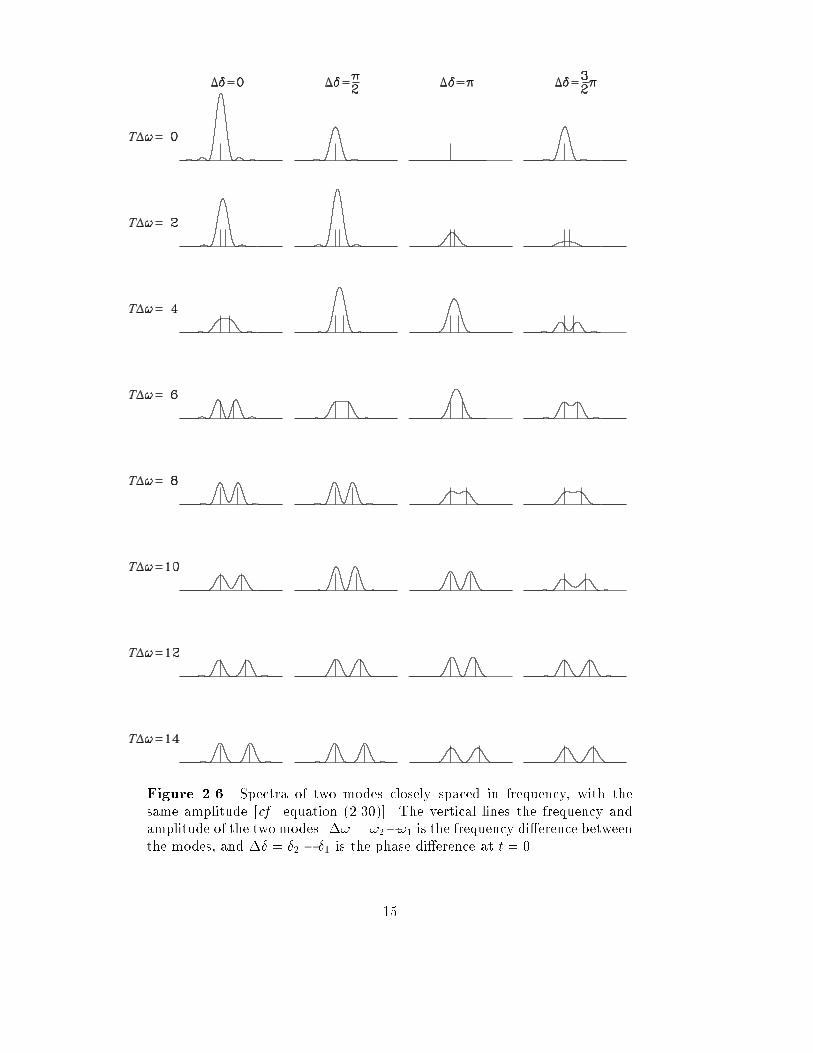
Figure 2.6. Spectra of two modes closely spaced in frequency, with thesame amplitude [cf. equation (2.30)]. The vertical lines the frequency andamplitude of the two modes. �! = !2�!1 is the frequency di�erence betweenthe modes, and �� = �2 � �1 is the phase di�erence at t = 0.15

Figure 2.7. Power spectra of simulated time series of duration 600 h( ), 60 h ( ), 10 h ( ) and 3 h ( ).The power is on an arbitrary scale and has been normalized to a maximumvalue of 1. The location of the central frequency for each group of rotationallysplit modes, as well as the value of the degree, are indicated on the top of thediagram. (From Christensen-Dalsgaard 1984b.)The frequencies were calculated from equation (2.32), with ��0 = 120�Hz, �0 = 1:2,D0 = 1:5�Hz and a rotational splitting ��rot = 1�Hz (corresponding to about twice thesolar surface rotation rate). These values are fairly typical for solar-like stars. The responseof the observations to the modes was calculated as described in section 2.1; for simplicitythe rotation axis was assumed to be in the plane of the sky, so that only modes with evenl �m can be observed. For clarity the responses for l = 3 were increased by a factor 2.5.The amplitudes and phases of the modes were chosen randomly, but were the same for alltime strings. The data were assumed to be noise-free.Short segments of the resulting power spectra, for T = 3h; 10 h; 60h and 600 h, areshown in Figure 2.7. The power is on an arbitrary scale, normalized so that the maximumis unity in each case. For T = 600 h the modes are completely resolved. At T = 60 hthe rotational splitting is unresolved, but the modes at individual n and l can to a largeextent be distinguished; however, a spurious peak appears next to the dominant peak withl = 1 at 2960�Hz. For T = 10 h modes having degrees of the same parity merge; herethe odd-l group at � ' 2960�Hz gives rise to two clearly resolved, but �ctitious, peaks ofwhich one is displaced by about 20�Hz relative to the centre of the group. These e�ectsare qualitatively similar to those seen in Figure 2.6. Finally, the spectrum for T = 3h isdominated by interference and bears little immediate relation to the underlying frequencies.16

Figure 2.8. Sketch of interrupted time series. This corresponds to two 8hour data segments, separated by a 16 hour gap.The case shown in Figure 2.7 was chosen as typical among a fairly large sample withdi�erent random phases and amplitudes. The results clearly emphasize the care that isrequired when interpreting inadequately resolved data. Furthermore, in general all valuesof m are expected to be observed for stellar oscillations, adding to the complexity.2.2.3 Data with gaps.From a single site (except very near one of the poles) the Sun or a star can typically beobserved for no more than 10{12 hours out of each 24 hours. As discussed in connectionwith Figure 2.7, this is far from enough to give the required frequency resolution. Thusone is faced with combining data from several days. This adds confusion to the spectra.I consider again the signal in equation (2.19), but now observe it for t = 0 to T and � to� + T . The signal is unknown between T and � , and it is common to set it to zero here,as sketched in Figure 2.8. Then the Fourier transform is, on the positive !-axis,~v(!) = Z T0 v (t) ei!tdt + Z �+T� v(t)ei!tdt' T2 a0 nei[ T2 (!�!0)+�0] + ei[(�+T2 )(!�!0)+�0]o sinc [T2 (! � !0)]= Ta0ei[1=2(�+T )(!�!0)+�0] cos[�2 (! � !0)]sinc [T2 (! � !0)] ; (2:33)and the power is P (!) = T 2a20 cos2[�2 (! � !0)]sinc 2[T2 (! � !0)] : (2:34)Thus one gets the spectrum from the single-day case, modulated by the cos2[12�(! � !0)]factor. As � > T this introduces apparent �ne structure in the spectrum. An example with� = 3T is shown in Figure 2.9.When more days are combined this so-called side-band structure can be somewhatsuppressed, but never entirely removed. In particular, there generally remain two additionalpeaks separated from the main peak by �! = 2�=� or �� = 1=� . For � = 24 hours, �� =11.57 �Hz.Exercise 2.1:Evaluate the power spectrum for the signal in equation (2.19), observed between 0 andT , � and � + T , ::: N� , N� + T , and verify the statement made above.17

Figure 2.9. Power spectrum of the time series shown in Figure 2.8 [cf.equation (2.34)].If several closely spaced modes are present as well, the resulting interference may getquite complicated, and the interpretation correspondingly di�cult. An example of this isshown in Figure 2.10, together with the corresponding spectrum resulting from a singleday's observations.Figure 2.10. In (a) is shown the spectrum for two closely spaced modes withT�! = 10, �� = 3�=2, observed during a single day, from Figure 2.6. In(b) is shown the corresponding case, but observed for two 8 hour segmentsseparated by 24 hours.The e�ects of gaps can conveniently be represented in terms of the so-called windowfunction w(t), de�ned such that w(t) = 1 during the periods with data and w(t) = 0 duringthe gaps. Thus the observed data can be written asv(t) = w(t)v0(t) ; (2:35)18

where v0(t) is the underlying signal (which, we assume, is there whether it is observed ornot). It follows from the convolution theorem of Fourier analysis that the Fourier transformof v(t) is the convolution of the transforms of v0(t) and w(t):~v(!) = ( ~w � ~v0)(!) = Z ~w(! � !0)~v0(!0)d!0 ; (2:36)here `�' denotes convolution, and ~w(!) is the transform of a timestring consisting of 0 and1, which is centred at zero frequency. It follows from equation (2.36) that if the peaks inthe original power spectrum P0(!) = j~v0(!)j2 are well separated compared with the spreadof the window function transform Pw(!) = j ~w(!)j2, the observed spectrum P (!) = j~v(!)j2consists of copies of Pw(!), shifted to be centred on the `true' frequencies. Needless tosay, the situation becomes far more complex when the window function transforms overlap,resulting in interference.There are techniques that to some extent may compensate for the e�ects of gaps inthe data, even in the presence of noise (e.g. Brown & Christensen-Dalsgaard 1990). How-ever, these are relatively ine�cient when the data segments are shorter than the gaps. Toovercome these problems, several independent projects are under way to construct net-works of observatories with a suitable distribution of sites around the Earth, to study solaroscillations with minimal interruptions. Campaigns to coordinate observations of stellaroscillations from di�erent observatories have also been organized. Furthermore, the satel-lite SOHO has carried helioseismic instruments to the L1 point between the Earth and theSun, where the observations can be carried out without interruptions. This has the addedadvantage of avoiding the e�ects of the Earth's atmosphere.2.2.4 Further complications.The analysis in the preceding sections is somewhat unrealistic, in that it is assumed that theoscillation amplitudes are strictly constant. If the oscillation is damped, one has, insteadof equation (2.19) v(t) = a0 cos(!0t� �0)e��t ; (2:37)where � is the damping rate. If this signal is observed for an in�nitely long time, one obtainsthe power spectrum P (!) = 14 a20(! � !0)2 + �2 : (2:38)A peak of this form is called a Lorentzian pro�le. It has a half width at half maximum of�.Exercise 2.2:Verify equation (2.38). 19

Figure 2.11. Power spectrum for the damped oscillator in equation (2.37),observed for a �nite time T . The abscissa is frequency separation, in unitsof T�1. The ordinate has been normalized to have maximum value 1. Thecurves are labelled by the value of �T , where � is the damping rate.If the signal in equation (2.37) is observed for a �nite time T , the resulting peak isintermediate between the sinc 2 function and the Lorentzian, tending to the former for�T � 1, and towards the latter for �T � 1. This transition is illustrated in Figure 2.11.Equation (2.37) is evidently also an idealization, in that it (implicitly) assumes a suddenexcitation of the mode, followed by an exponential decay. In the Sun, at least, it appearsthat the oscillations are excited stochastically, by essentially random uctuations due tothe turbulent motion in the outer parts of the solar convection zone. It may be shown thatthis process, combined with exponential decay, gives rise to a spectrum that on average hasa Lorentzian pro�le. The statistics of the determination of frequencies, amplitudes and linewidths from such a spectrum was studied by S�rensen (1988), Kumar, Franklin & Goldreich(1988) and Schou (1993).So far I have considered only noise-free data. Actual observations of oscillations containnoise from the observing process, from the Earth's atmosphere and from the random velocity(or intensity) �elds in the solar or stellar atmosphere. At each frequency in the powerspectrum the noise may be considered as an oscillation with a random amplitude andphase; this interferes with the actual, regular oscillations, and may suppress or arti�ciallyenhance some of the oscillations. However, because the noise is random, it may be shownto decrease in importance with increasingly long time series.2.2.5 Large-amplitude oscillations.For large-amplitude pulsating stars, such as Cepheids, the oscillation typically no longerbehaves like the simple sine function in equation (2.19). Very often the oscillation is stillstrictly periodic, however, with a well-de�ned frequency !0. Also the light curve, for exam-ple, in many cases has a shape similar to the one shown in Figure 2.12, with a rapid riseand a more gradual decrease. 20

Figure 2.12. Example of non-sinuosoidal oscillation. This is roughly similarto observed light curves of large-amplitude Cepheids.Figure 2.13. The �rst 3 Fourier components of the oscillation shown inFigure 2.12. The remaining components have so small amplitudes that theydo not contribute signi�cantly to the total signal.It is still possible to carry out a Fourier analysis of the oscillation. Now, however,peaks appear at the harmonics k!0 of the basic oscillation frequency, where k = 1; 2; : : : .This corresponds to representing the observed signal as a Fourier seriesv(t) =Xk ak sin(k !0t � �k) : (2:39)21

Figure 2.13 shows the �rst few Fourier components of the oscillation in Figure 2.12. Moregenerally the shape of the oscillation is determined, say, by the amplitude ratios ak=a1and the phase di�erences �k � k �1. These quantities have proved very convenient for thecharacterization of observed light curves (e.g. Andreasen & Petersen 1987), as well as forthe analysis of numerical results. One may hope that further work in this direction willallow an understanding of the physical reasons underlying the observed behaviour.In a double-mode, large-amplitude pulsating star, with basic frequencies !1 and !2,Fourier analysis in general produces peaks at the combination frequencies k!1 + j!2, forintegral k and j. Thus the spectrum may become quite complex. In particular, the detectionof additional basic frequencies is di�cult, since these might easily be confused with thecombination frequencies, given the �nite observational resolution.2.3 Results on solar oscillationsBy far the richest spectrum of oscillations has been observed for the Sun; this allows detailedinvestigations of the properties of the solar interior. Thus it is reasonable to summarize theobservational situation and prospects for the Sun. The observed, and possibly observed,modes are shown schematically in Figure 2.14. Only the modes in the �ve-minute regionhave de�nitely been observed and identi�ed. As mentioned in Chapter 1, they are standingacoustic waves, generally of high radial order. It is interesting that they are observed at allvalues of the degree, from purely radial modes at l = 0 to modes of very short horizontalwavelength at l = 1500. Furthermore, there is little change in the amplitude per modebetween these two extremes. There is still considerable doubt about the observationalreality of the long-period oscillations; if real, they can be identi�ed as standing gravitywaves, or g modes.Figure 2.15 shows an example of an observed power spectrum of solar oscillations. Thiswas obtained by means of Doppler velocity measurements in light integrated over the solardisk, and hence, according to the analysis in section 2.1, is dominated by modes of degrees0 { 3. The data were obtained from the BiSON network of six stations globally distributedin longitude, to suppress the daily side-bands, and span roughly four months. Thus theintrinsic frequency resolution, as determined by equation (2.25), is smaller than the thick-ness of the lines. It might be noticed that the peaks occur in groups, corresponding tothe expression for the frequencies given in equation (2.32). Also there is a visible increasein the line-width when going from low to high frequency. The broadening of the peaks athigh frequency is probably caused by the damping and excitation processes, as discussedin section 2.2.4; thus the observations indicate that the damping rate increases with in-creasing frequency. Finally, there is clearly a well-de�ned distribution of amplitudes, witha maximum around 3000 �Hz and very small values below 2000, and above 4500, �Hz.This distribution is essentially the same at all degrees where the �ve-minute oscillationsare observed. An interesting analysis of the observed dependence of mode amplitudes ondegree, azimuthal order and frequency was presented by Libbrecht et al. (1986).Several extensive tables of �ve-minute oscillation frequencies have been published inrecent years. An example, compiled from several sources, was given by Libbrecht, Woodard& Kaufman (1990). To illustrate the quality of current frequency determinations, Figure2.16 shows observed frequencies at low and moderate degree from one year's observationswith the High Altitude Observatory's LOWL instrument (see Tomczyk et al. 1995). Theerror bars have been magni�ed by a factor 1000 over the usual 1� error bars. For the most22

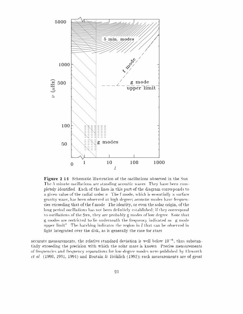
Figure 2.14. Schematic illustration of the oscillations observed in the Sun.The 5 minute oscillations are standing acoustic waves. They have been com-pletely identi�ed. Each of the lines in this part of the diagram corresponds toa given value of the radial order n. The f mode, which is essentially a surfacegravity wave, has been observed at high degree; acoustic modes have frequen-cies exceeding that of the f mode. The identity, or even the solar origin, of thelong period oscillations has not been de�nitely established; if they correspondto oscillations of the Sun, they are probably g modes of low degree. Note thatg modes are restricted to lie underneath the frequency indicated as \g modeupper limit". The hatching indicates the region in l that can be observed inlight integrated over the disk, as is generally the case for stars.accurate measurements, the relative standard deviation is well below 10�5, thus substan-tially exceeding the precision with which the solar mass is known. Precise measurementsof frequencies and frequency separations for low-degree modes were published by Elsworthet al. (1990, 1991, 1994) and Toutain & Fr�ohlich (1992); such measurements are of great23

Figure 2.15. Power spectrum of solar oscillations, obtained from Dopplerobservations in light integrated over the disk of the Sun. The ordinate isnormalized to show velocity power per frequency bin. The data were ob-tained from six observing stations and span approximately four months. (SeeElsworth et al. 1995.)diagnostic importance for the properties of the solar core (cf. section 7.3). An extensiveset of high-degree frequencies was obtained by Bachmann et al. (1995).From spatially resolved observations, individual frequencies !nlm can in principle bedetermined. Because of observational errors and the large amount of data resulting fromsuch determination, it has been common to present the results in terms of coe�cients in�ts to the m-dependence of the frequencies, either averaged over n at given l (Brown &Morrow 1987) or for individual n and l (e.g., Libbrecht 1989). A common form of the �t isin terms of Legendre polynomials,!nlm = !nl0 + 2�LXj=1 aj(n; l)Pj �mL � : (2:40)As discussed below, in Chapter 8 [cf. equation (8.32)] the coe�cients aj with odd j arisefrom rotational splitting; the coe�cients with even j are caused by departures from sphericalsymmetry in solar structure, or from e�ects of magnetic �elds.It is probably a fair assessment that the major developments in helioseismology in thecoming years will result from improvements in the observations. The principal problems incurrent data are the presence of gaps, leading to sidebands in the power spectra, and thee�ects of atmospheric noise. The problem with gaps will be overcome through observationsfrom global networks; nearly continuous observations, which are furthermore free of e�ectsof the Earth's atmosphere, will be obtained from space. The result, �ve years from now,should be greatly improved sets of frequencies, extending to high degree, from which onemay expect a vast improvement in our knowledge about the solar interior.24

Figure 2.16. Plot of observed solar p-mode oscillation frequencies, as afunction of the degree l, from one year of observations. The vertical lines showthe 1000� error bars. Each ridge corresponds to a given value of the radialorder n, the lowest ridge having n = 1. (See Tomczyk, Schou & Thompson1996).As shown in Figure 2.9, gaps in the timeseries introduce sidebands in the spectrum;these add confusion to the mode identi�cation and contribute to the background of noisein the spectra. Largely uninterrupted timeseries of several days', and up to a few weeks',duration have been obtained from the South Pole (e.g. Grec et al. 1980 and Duvall et al.1991); however, to utilize fully the phase stability of the modes at relatively low frequencyrequires continuous observations over far longer periods, and these cannot be obtained froma single terrestrial site.Nearly continuous observations can be achieved from a network of observing stations,suitably placed around the Earth (e.g. Hill & Newkirk 1985). An overview of networkprojects was given by Hill (1990). A group from the University of Birmingham has operatedthe BiSON(2:1) network for several years, to perform whole-disk observations using theresonant scattering technique (e.g. Aindow et al. 1988). A similar network (the IRIS(2:2)network) has been set up by a group at the University of Nice (Fossat 1991).An even more ambitious network has been established in the GONG(2:3) project, or-ganized by the National Solar Observatory of the United States (for an introduction to theproject, see Harvey, Kennedy & Leibacher 1987). This project involves the setting up atcarefully selected locations of six identical observing stations. They use an interferometrictechnique to observe solar oscillations of degrees up to around 250. In addition to the design(2:1) Birmingham Solar Oscillation Network(2:2) International Research on the Interior of the Sun(2:3) Global Oscillation Network Group 25

and construction of the observing equipment, a great deal of e�ort is going into preparingfor the merging and analysis of the very large amounts of data expected, and into estab-lishing the necessary theoretical tools. The network became operational in October 1995when the last station, in Udaipur (India) started observingMajor e�orts have gone into the development of helioseismic instruments for theSOHO(2:4) satellite, which was launched in December 1995. SOHO is located near theL1 point between the Earth and the Sun, and hence is in continuous sunlight. This permitsnearly unbroken observations of solar oscillations. A further advantage is the absence ofe�ects from the Earth's atmosphere. These are particularly troublesome for observationsof high-degree modes, where seeing is a serious limitation (e.g. Hill et al. 1991), and forintensity observations of low-degree modes, which su�er from transparency uctuations.SOHO carries three instrument packages for helioseismic observations:{ The GOLF instrument (for Global Oscillations at Low Frequency; see Gabriel et al.1991). This uses the resonant scattering technique in integrated light. Because of thegreat stability of this technique, it is hoped to measure oscillations at comparatively lowfrequency, possibly even g modes. Unlike the p modes, which have formed the basisfor helioseismology so far, the g modes have their largest amplitude near the solarcentre; hence, detection of these modes would greatly aid the study of the structureand rotation of the core. Also, since the lifetime of p modes increases rapidly withdecreasing frequency, very great precision is possible for low-frequency p modes.{ The SOI-MDI experiment (for Solar Oscillations Investigation { Michelson DopplerImager; see Scherrer, Hoeksema & Bush 1991) will use the Michelson interferometertechnique. By observing the entire solar disk with a resolution of 4 arcseconds, andparts of the disk with a resolution of 1.2 arcseconds, it will be possible to measureoscillations of degree as high as a few thousand; furthermore, very precise data shouldbe obtained on modes of degree up to about 1000, including those modes for whichground-based observation is severely limited by seeing. As a result, it will be possibleto study the structure and dynamics of the solar convection zone, and of the radiativeinterior, in great detail.{ The VIRGO experiment (forVariability of solar IRradiance and Gravity Oscillations;see Andersen 1991). This contains radiometers and Sun photometers to measure oscil-lations in solar irradiance and broad-band intensity. It is hoped that this will allow thedetection of g modes; furthermore, the observations will supplement those obtained inDoppler velocity, particularly with regards to investigating the phase relations for theoscillations in the solar atmosphere.2.4 Other types of multi-periodic starsAs mentioned in Chapter 1, the information content in stellar pulsations increases with thenumber of observable modes. Here I consider two classes of stars with complex pulsationspectra: the � Scuti stars and the pulsating white dwarfs.(2:4) SOlar and Heliospheric Observatory 26

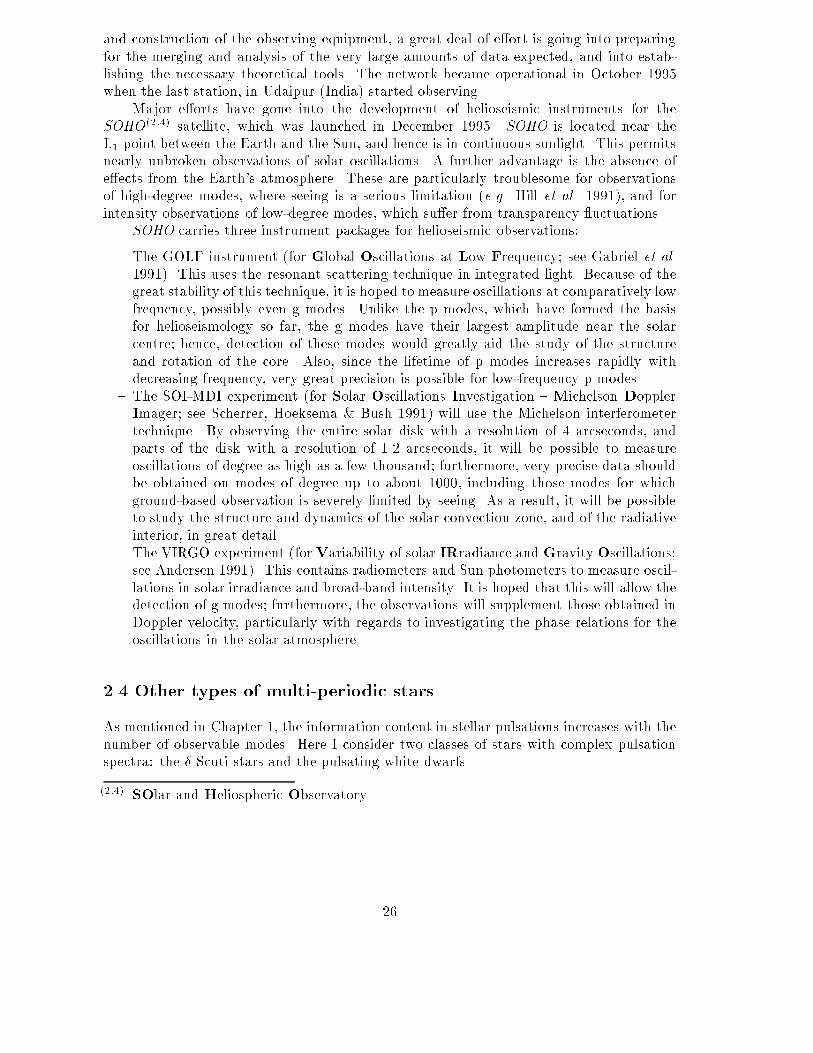
Figure 2.17. Schematic oscillation spectra of a number of � Scuti stars.27

2.4.1 Observations of � Scuti oscillationsThe � Scuti stars fall in an extension of the Cepheid instability strip, close to the mainsequence. They typically have masses around 2� 2:5M� and are either near or just afterthe end of core hydrogen burning. Although they have been recognized as a separate classof pulsating stars since the work of Eggen (1957ab), only within the last decade have thedetails of their spectra of pulsations become clear. The fact that these stars typicallyhave periods of the order of one hour presents a considerable di�culty: observations froma single site will lead to a great deal of confusion from the side-bands (cf. section 2.2.3),complicating the determination of the oscillation frequencies. However, thanks to a numberof observing campaigns involving two or more observatories extensive data for a numberof stars have become available (e.g. Michel & Baglin 1991; Michel et al. 1992; for recentreviews, see Breger 1995ab).The most extensive observations of � Scuti stars have been photometric, althoughthe oscillations have also been observed spectroscopically. Schematic spectra of severalstars are shown in Figure 2.17. The observed frequency range corresponds to low-orderacoustic modes. However, the distributions of modes excited to observable frequencies areevidently strikingly di�erent: in some cases only modes in a narrow frequency band arefound, whereas in other cases the observed modes extend quite widely in frequency. So far,no obvious correlation between the frequency distribution and other parameters of the starshas been found.From a comparison with computed oscillation spectra (see section 5.3.2) it is clear thatonly a subset of the possible modes of oscillation are excited to observable amplitudes inthese stars. However, the reasons for the mode selection is currently unclear. This greatlycomplicates the mode identi�cation. A further complication comes from the fact that thebasic parameters of these stars, such as their mass and radius, are in most cases known withpoor accuracy. On the other hand, the � Scuti stars have the potential for providing veryvaluable information about stellar evolution: unlike the Sun, these stars have convectivecores, and hence the frequency observations may give information about the properties ofsuch cores, including the otherwise highly uncertain degree of overshoot from the cores.Therefore, a great deal of e�ort is going into further observations of � Scuti stars as wellas in calculations to elucidate the diagnostic potential of the observations and analyze theexisting data. Particularly promising are observations of � Scuti stars in open clusters.With CCD photometry it is possible to study several variable stars in such a cluster atonce, and furthermore \classical" observations of the cluster can be used to constrain theparameters of the stars, such as their distance, age and chemical composition (e.g. Bregeret al. 1993ab).2.4.2 Pulsating white dwarfsThe �rst observations of oscillations in white dwarfs were made in 1970 { 1975 (McGraw& Robinson 1976). The initial results were obtained for so-called DA white dwarfs, char-acterized by the presence of hydrogen in their spectra, with e�ective temperatures around10 000K. Since then, additional groups of pulsating white dwarfs have been detected, eachcharacterized by a fairly sharply de�ned instability region. These regions are indicatedschematically in the HR diagram in Figure 2.18.28

Figure 2.18. Compact pulsators in the HR diagram. The PPNV are theplanetary nebula nuclei variables. The thin line shows the location of the Zero-Age Main Sequence, while the heavy line indicates the white-dwarf coolingsequence. The DOV are variables at the transition between the planetarynebula nuclei and the proper white dwarfs, the DBV are variable white dwarfswith helium atmospheres and the the DAV are variable white dwarfs withhydrogen in their atmospheres. (Adapted from Winget 1988.)The typical periods of pulsating white dwarfs are in the range 3 { 10 mins. This is farlonger than the dynamical timescales tdyn for these stars [cf. equation (1.1)] which are ofthe order of seconds. In fact, the observed modes are identi�ed with the so-called g modes,i.e., standing gravity waves. As discussed in Chapter 5, such modes may have periods ofarbitrary length. As for the � Scuti stars, it is characteristic that not all the possible modesin a given frequency range are observed; the mode selection is apparently related to thepossibility of trapping of modes in regions of chemical inhomogeneity, although the precisemechanism is so far not understood. 29

The oscillations have been observed photometrically. As in other cases the complica-tions associated with gaps in the data from a single site have led to collaborative e�ortsto obtain continuous data through the combined e�orts of several observatories. This hasbeen organized in the very ambitious Whole Earth Telescope (WET) project, where morethan ten observatories have been involved in campaigns to observe a single star over 1 { 2weeks (for overviews, see Winget 1993; Kawaler 1995). This has led to the most detailedpulsation spectra for any star other than the Sun. As an example, Figure 2.19 shows thespectrum obtained for a DB variable; the window function for the observations is shown inthe insert and demonstrates the remarkable degree to which the sidebands are suppressed.

Figure 2.19. Power spectrum of the DB variable GD358, obtained with theWhole Earth Telescope. Numbers with arrows represent multiplet identi�ca-tions. (From Winget et al. 1994.)The analysis of the observed frequencies is providing a great deal of information aboutthe white dwarfs. As examples might be mentioned accurate determination of white-dwarfmasses and rotation rates. Perhaps the most interesting result is the measurement of periodchanges in white dwarfs, caused by the evolution of the stars along the white-dwarf coolingsequence (e.g. Winget et al. 1985; Kepler et al. 1991).30

3. A little hydrodynamics.To provide a background for the presentation of the theory of stellar oscillations, thischapter brie y discusses some basic principles of hydrodynamics. A slightly more detaileddescription, but still essentially without derivations, was given by Cox (1980). In addition,any of the many detailed books on hydrodynamics (e.g. Batchelor 1967; Landau & Lifshitz1959) can be consulted. Ledoux & Walraven (1958) give a very comprehensive introductionto hydrodynamics, with special emphasis on the application to stellar oscillations.3.1 Basic equations of hydrodynamics.It is assumed that the gas can be treated as a continuum, so that its properties can bespeci�ed as functions of position r and time t. These properties include the local density�(r; t), the local pressure p(r; t) (and any other thermodynamic quantities that may beneeded), as well as the local instantaneous velocity v(r; t). Here r denotes the positionvector to a given point in space, and the description therefore corresponds to what is seenby a stationary observer. This is known as the Eulerian description. In addition, it is oftenconvenient to use the Lagrangian description, which is that of an observer who follows themotion of the gas. Here a given element of gas can be labelled, e.g. by its initial position r0,and its motion is speci�ed by giving its position r(t; r0) as a function of time. Its velocityv(r; t) = drdt at �xed r0is equivalent to the Eulerian velocity mentioned above.The time derivative of a quantity �, observed when following the motion isd�dt = �@�@t �r +r� � drdt = @�@t + v � r� : (3:1)The time derivative d=dt following the motion is also known as the material time derivative;in contrast @=@t is the local time derivative (i.e., the time derivative at a �xed point).The properties of the gas are expressed as scalar and vector �elds. Thus we need a littlevector algebra; convenient summaries can be found, e.g. in books on electromagnetism (suchas Jackson 1975; Reitz, Milford & Christy 1979). I shall assume the rules for manipulatinggradients and divergences to be known. In addition, we need Gauss's theorem:Z@V a � n dA = ZV div a dV ; (3:2)where V is a volume, with surface @V , n is the outward directed normal to @V , and a isany vector �eld. From this one also obtainsZ@V �n dA = ZV r� dV (3:3)for any scalar �eld �. 31

3.1.1 The equation of continuity.The fact that mass is conserved can be expressed as@�@t + div (�v) = 0 ; (3:4)where � is density. This is a typical conservation equation, balancing the rate of change ofa quantity in a volume with the ux of the quantity into the volume. Had there been anysources of mass, they would have appeared on the right-hand side. By using the relation(3.1), equation (3.4) may also be writtend�dt + � divv = 0 ; (3:5)giving the rate of change of density following the motion. Note that � = 1=V , where V isthe volume of unit mass; thus an alternative formulation is1V dVdt = div v : (3:6)Hence div v is the rate of expansion of a given volume of gas, when following the motion.3.1.2 Equations of motion.Under solar or stellar conditions one can generally ignore the internal friction (or viscosity)in the gas. The forces on a volume of gas therefore consist ofi) Surface forces, i.e., the pressure on the surface of the volumeii) Body forces.Thus the equations of motion can be written� dvdt = �rp+ � f ; (3:7)where f is the body force per unit mass which has yet to be speci�ed. The pressure p isde�ned such that the force on a surface element dA with outward normal n is �pn dA.This may be identi�ed with the ordinary thermodynamic pressure.By using equation (3.1), we may also write equation (3.7) as� @ v@t + �v � rv = �rp+ � f : (3:8)Among the possible body forces I consider only gravity. Thus in particular I neglecte�ects of magnetic �elds, which might otherwise provide a body force on the gas. The forceper unit mass from gravity is the gravitational acceleration g, which can be written as thegradient of the gravitational potential �:g = r� ; (3:9)where � satis�es Poisson's equation r2� = �4�G� : (3:10)32

It is often convenient to use also the integral solution to Poisson's equation� (r; t) = G ZV �(r0; t)dVjr� r0j : (3:11)3.1.3 Energy equation.To complete the equations we need a relation between p and �. This must take the form ofa thermodynamic relation. Speci�cally the �rst law of thermodynamics,dqdt = dEdt + p dVdt ; (3:12)must be satis�ed; here dq=dt is the rate of heat loss or gain, and E the internal energy, perunit mass. As before V = 1=� is speci�c volume. Thus equation (3.12) expresses the factthat the heat gain goes partly to change the internal energy, partly into work expandingor compressing the gas. Alternative formulations of equation (3.12), using the equation ofcontinuity, are dqdt = dEdt � p�2 d�dt = dEdt + p� div v : (3:13)By using thermodynamic identities the energy equation can be expressed in terms of other,and more convenient, variables.dqdt = 1�(�3 � 1) �dpdt � �1p� d�dt� (3:14a)= cp�dTdt � �2 � 1�2 Tp dpdt � (3:14b)= cV �dTdt � (�3 � 1) T� d�dt � : (3:14c)Here cp and cV are the speci�c heat per unit mass at constant pressure and volume, andthe adiabatic exponents are de�ned by�1 = �@ ln p@ ln ��ad ; �2 � 1�2 = �@ lnT@ ln p �ad ; �3 � 1 = �@ lnT@ ln ��ad : (3:15)These relations are discussed in more detail in, e.g., Cox & Giuli (1968).It is evident that the relation between p, � and T , as well as the �i's, depend onthe thermodynamic state and composition of the gas. Indeed, as will be discussed below,the dependence of �1 on the properties of the gas forms the basis for using observed solaroscillation frequencies to probe the details of the statistical mechanics of partially ionizedgases and the infer the helium abundance of the solar convective envelope. However, inmany cases one may as a �rst approximation regard the gas as fully ionized and neglecte�ects of degeneracy and radiation pressure. Then the equation of state is simplyp = kB�T�mu ; (3:16)33

where kB is Boltzmann's constant, mu is the atomic mass unit and � is the mean molecularweight. Also �1 = �2 = �3 = 5=3 : (3:17)I note that radiation pressure decreases �1 below this value; this e�ect becomes noticeablein stars whose mass exceeds a few solar masses. Thus Otzen Petersen (1975) showed thatradiation pressure caused a systematic increase of the pulsation constant (cf. equation[2.20]) with increasing luminosity along the Cepheid instability strip.We need to consider the heat gain in more detail. Speci�cally, it can be written as�dqdt = � �� divF ; (3:18)here � is the rate of energy generation per unit mass (e.g. from nuclear reactions), and Fis the ux of energy. In general radiation is the only signi�cant contributor to the energy ux; in particular molecular conduction is almost always negligible.In convection zones turbulent gas motion provides a very e�cient transport of energy.Ideally the entire hydrodynamical system, including convection, must be described as awhole. In this case only the radiative ux would be included in equation (3.18). However,under most circumstances the resulting equations are too complex to be handled analyticallyor numerically. Thus it is customary to separate out the convective motion, by performingaverages of the equations over length scales that are large compared with the convectivemotion, but small compared with other scales of interest. In this case the convective uxappears as an additional contribution in equation (3.18). The convective ux must thenbe determined, from the other quantities characterizing the system, by considering theequations for the turbulent motion. A familiar example of this (which is also characteristicof the lack of sophistication in current treatments of convection) is the mixing-length theory.The incorporation of convection in the hydrodynamical equations was discussed insome detail by Unno et al. (1989). However, it is fair to say that this is currently one ofthe principal uncertainties in stellar hydrodynamics.The general calculation of the radiative ux is also non-trivial. In stellar atmospheresthe full radiative transfer problem, as known from the theory of the structure of stellaratmospheres, must be solved in combination with the hydrodynamic equations. This isanother active area of research, and the subject of a major monograph (Mihalas & Mihalas1984). In stellar interiors the di�usion approximation is adequate, and the radiative ux isgiven by F = � 4�3�� rB = � 4a~cT 33�� rT ; (3:19)where B = (a~c=4�)T 4 is the integrated Planck function, � is the opacity, ~c is the speed oflight and a is the radiation density constant; this provides a relation between the state ofthe gas and the radiative ux, which is analogous to a simple conduction equation.When the mean free path of a photon is very large, one can neglect the contributionfrom absorption to the heating of the gas. Then we have thatdivF = 4���aB ; (3:20)where �a is the opacity arising from absorption; this is the so-called Newton's law of cooling.Finally, one can generalize the Eddington approximation, which may be known from thetheory of static stellar atmospheres, to the three-dimensional case (see Unno & Spiegel1966), to obtain divF = �4���a(J �B) ; (3:21)34

F = � 4�3(�a + �s)�rJ ; (3:22)where �s is the scattering opacity and J is the mean intensity. As shown by Unno &Spiegel the Eddington approximation tends to the di�usion approximation when �a�!1.Furthermore, it has the correct limit in the optically thin case.Here I have implicitly assumed that the scattering and absorption coe�cients are in-dependent of the frequency of radiation. In the di�usion approximation, the generalizationto frequency-dependence leads to the introduction of the Rosseland mean opacity. In theoptically thin case, one must in general take into account the details of the distribution ofintensity with frequency; thus, in equations (3.20) { (3.22) the absorption and scattering co-e�cients must be thought of as suitable averages, whereas F and J are frequency-integratedquantities.3.1.4 The adiabatic approximation.For the purpose of calculating stellar oscillation frequencies, the complications of the energyequation can be avoided to a high degree of precision, by neglecting the heating term inthe energy equation. To see that this is justi�ed, consider the energy equation on the form,using equation (3.19)dTdt � �2 � 1�2 Tp dpdt = 1cp �� + 1�div �4a~cT 33�� rT�� : (3:23)Here the term in the temperature gradient can be estimated as1�cp div �4a~cT 33�� rT� � 4a~cT 43��2cpL2 = T�F ; (3:24)where L is a characteristic length scale, and �F is a characteristic time scale for radiation,�F = 3��2cpL24a~cT 3 ' 1012 ��2L2T 3 ; in cgs units : (3:25)Typical values for the entire Sun are � = 1, � = 1, T = 106, L = 1010, and hence �F � 107years. This corresponds to the Kelvin-Helmholtz time for the star. For the solar convectionzone the corresponding values are � = 100, � = 10�5, T = 104, L = 109, and hence�F � 103 years. In the outer parts of the star the term in � vanishes, whereas in thecore it corresponds to a characteristic time �� � cpT=� which is again of the order of theKelvin-Helmholtz time. T=�F or T=�� must be compared with the time derivative of T inequation (3.23), which can be estimated as T/(period of oscillation). Typical periods areof the order of minutes to hours, and hence the heating term in equation (3.23) is generallyvery small compared with the time derivative terms. Near the surface, on the other hand,the density, and hence the radiative time scale, is low, and the full energy equation mustbe taken into account.Where the heating can be neglected, the motion occurs adiabatically. Then p and �are related by dpdt = �1p� d�dt : (3:26)35

This equation, together with the continuity equation (3.4), the equations of motion (3.8)and Poisson's equation (3.10), form the complete set of equations for adiabatic motion.Most of our subsequent work is based on these equations.3.2 Equilibrium states and perturbation analysis.A general hydrodynamical description of a star, using the equations presented in the preced-ing section, is far too complex to handle, even numerically on the largest existing computers.To put this in perspective, it may be mentioned that �A. Nordlund and R. Stein (e.g. Nord-lund & Stein 1989; Stein, Nordlund & Kuhn 1989), by stretching the capabilities of existingcomputers to the limits, have been able to follow numerically the development of a verysmall region near the solar surface for a few hours. Even though this is a tremendousachievement, which will be of great value to our understanding of solar convection andsolar oscillations, it clearly demonstrates the impracticality of a direct numerical solutionfor, say, general oscillations involving the entire Sun. Furthermore, even to the extent thatsuch a solution were possible, the results would in general be so complicated that a simpli-�ed analysis is needed to understand them. Fortunately, in the case of stellar oscillations,considerable simpli�cations are possible. The observed solar oscillations have very smallamplitudes compared with the characteristic scales of the Sun, and so it can be treatedas a small perturbation around a static equilibrium state. Even in \classical" pulsatingstars, where the surface amplitudes are large, most of the energy in the motion is in regionswhere the amplitudes are relatively small; thus many of the properties of these oscillations,including their periods, can be understood in terms of small-perturbation theory. In thissection I discuss the general equations for such small perturbations.3.2.1 The equilibrium structure.The equilibrium structure is assumed to be static, so that all time derivatives can be ne-glected. In addition, I assume that there are no velocities. Then the continuity equation,(3.4), is trivially satis�ed. The equations of motion (3.8) reduce to the equation of hydro-static support, r p0 = �0g0 = �0r�0 ; (3:27)where I have denoted equilibrium quantities with the subscript \0". Poisson's equation(3.10) is unchanged, r2�0 = �4�G�0 : (3:28)Finally the energy equation (3.18) is0 = dqdt = �0 � 1�0 divF0 : (3:29)It might be noted that one often considers equilibrium structures that change on longtime scales. Here hydrostatic equilibrium is enforced (departures from hydrostatic equi-librium result in motion on essentially the free-fall time scale for the star, of the order ofhours). However, it is not assumed that there is no heating, so that the general energyequation (3.18) is used. Such a star is said to be in hydrostatic, but not in thermal, equilib-rium. Typical examples are stars where nuclear burning does not supply the main sourceof energy, as during the pre-main-sequence contraction, or after hydrogen exhaustion inthe core. Even during normal main sequence evolution the heating term provides a smallcontribution to the energy, which is normally taken into account in calculations of stellarevolution. However, we need not consider this further here.36

For the present purpose the most important example of equilibrium is clearly a spher-ically symmetric state, where the structure depends only on the distance r to the centre.Here g0 = �g0ar , where ar is a unit vector directed radially outward, and equation (3.27)becomes dp0dr = �g0�0 : (3:30)Also Poisson's equation may be integrated once, to yieldg0 = Gr2 Z r0 4��0r02 dr0 = Gm0r2 ; (3:31)where m0(r) is the mass in the sphere interior to r. The ux is directed radially outward,F = Fr;0ar , so that the energy equation gives�0�0 = 1r2 ddr �r2 Fr;0� = 14�r2 dL0dr ;where L0 = 4�r2 Fr;0 is the total ow of energy through the sphere with radius r; hencedL0dr = 4�r2�0�0 : (3:32)Finally the di�usion expression (3.19) for the ux may be writtendT0dr = � 3�0�016�r2a~cT 30 L0 : (3:33)Equations (3.30) { (3.33) are clearly the familiar equations for stellar structure.3.2.2 Perturbation analysis.We consider small perturbations around the equilibrium state. Thus, e.g., the pressure iswritten as p(r; t) = p0(r) + p0(r; t) ; (3:34)where p0 is a small perturbation; this is the so-called Eulerian perturbation, i.e., the per-turbation in a given point. The equations are then linearized in the perturbations, byexpanding them in the perturbations retaining only terms that do not contain products ofthe perturbations.Just as in the general case it is convenient to use also a description involving a refer-ence frame following the motion; the perturbation in this frame is called the Lagrangianperturbation. If an element of gas is moved from r0 to r0+ ���r due to the perturbation, theLagrangian perturbation in pressure may be calculated as�p(r) = p(r0 + ���r)� p0(r0) = p(r0) + ���r � rp0 � p0(r0)= p0(r0) + ���r � rp0 : (3:35)Equation (3.35) is of course completely equivalent to the relation (3.1) between the localand the material time derivative. Note also that the velocity is given by the time derivativeof the displacement ���r, v = @���r@t : (3:36)37

Equations for the perturbations are obtained by inserting expressions like (3.34) in thefull equations, subtracting equilibrium equations and neglecting quantities of order higherthan one in p0, �0, v, etc. For the continuity equation the result is@�0@t + div (�0v) = 0 ; (3:37)or, by using equation (3.36) and integrating with respect to time�0 + div (�0���r) = 0 : (3:38)Note that this equation may also, by using the analogue to equation (3.35), be written as��+ �0div (���r) = 0 ; (3:39)which corresponds to equation (3.5).The equations of motion become�0@2���r@t2 = �0@v@t = �rp0 + �0g0 + �0g0 ; (3:40)where, obviously, g0 = r�0. Also the perturbation �0 in the gravitational potential satis�esthe perturbed Poisson's equation r2�0 = �4�G�0 ; (3:41)with the solution, equivalent to equation (3.11)�0 = G ZV �0(r0; t)jr� r0j dV : (3:42)The energy equation requires a little thought. We need to calculate, e.g.,dpdt = @p@t + v � rp = @p0@t + v � rp0 = @p0@t + @���r@t � rp0 = @@t(�p) ; (3:43)to �rst order in the perturbations. Note that to this order there is no di�erence betweenthe local and the material time derivative of the perturbations. Thus we have for the energyequation, from e.g. equation (3.14a),@�q@t = 1�0(�3;0 � 1) �@�p@t � �1;0p0�0 @��@t � : (3:44)This equation is most simply expressed in Lagrangian perturbations, but it may be trans-formed into Eulerian perturbations by using equation (3.35). From equation (3.18) theperturbation in the heating rate is given by�0 @�q@t = �(��� divF) = (��� div F)0 ; (3:45)if equation (3.29) is used. Finally it is straightforward to obtain the perturbation in theradiative ux, in the di�usion approximation, from equation (3.19).38

For adiabatic motion we neglect the heating term and obtain@�p@t � �1;0p0�0 @��@t = 0 ;or, by integrating over time �p = �1;0p0�0 �� ; (3:46)or, on Eulerian form p0 + ���r � rp0 = �1;0p0�0 (�0 + ���r � r�0) : (3:47)3.3 Simple wavesIt is instructive to consider simple examples of wave motion. This provides an introductionto the techniques needed to handle the perturbations. In addition, general stellar oscillationscan in many cases be approximated by simple waves, which therefore give physical insightinto the behaviour of the oscillations.3.3.1 Acoustic waves.As the simplest possible equilibrium situation, we may consider the spatially homogeneouscase. Here all derivatives of equilibrium quantities vanish. According to equation (3.27)gravity must then be negligible. Such a situation clearly cannot be realized exactly. How-ever, if the equilibrium structure varies slowly compared with the oscillations, this maybe a reasonable approximation. I also neglect the perturbation in the gravitational poten-tial; for rapidly varying perturbations regions with positive and negative �0 nearly cancelin equation (3.42), and hence �0 is small. Finally, I assume the adiabatic approximation(3.46).The equations of motion (3.40) give�0 @2���r@t2 = �rp0 ;or, by taking the divergence �0 @2@t2 (div ���r) = �r2p0 :However, div ���r can be eliminated by using the continuity equation (3.38), and p0 can beexpressed in terms of �0 from the adiabatic relation. The result is@2�0@t2 = �1;0p0�0 r2�0 = c20r2�0 ; (3:48)where c20 � �1;0p0�0 (3:49)39

has the dimension of a squared velocity. This equation has the form of the wave equation.Thus it has solutions in the form of plane waves�0 = a exp[i(k � r� ! t)] : (3:50)(As discussed in more detail in Chapter 4 it is convenient to write the solution in complexform; the physically realistic solution is obtained by taking the real part of the complexsolution). By substituting equation (3.50) into (3.48) we obtain�!2�0 = c20 div (ik�0) = �c20jkj2�0 :Thus this is a solution, provided ! satis�es the dispersion relation!2 = c20 jkj2 : (3:51)The waves are plane sound waves, and equation (3.51) is the dispersion relation for suchwaves. The adiabatic sound speed c0 is the speed of propagation of the waves. I note thatwhen the ideal gas law, equation (3.16), is satis�ed, the sound speed is given byc20 = �1;0kBT0�mu ; (3:52)Thus c0 is essentially determined by T0=�.With a suitable choice of phases the real solution can be written as�0 = a cos(k � r� !t) ; (3:53)p0 = c20a cos(k � r� !t) ; (3:54)���r = c20�0!2a cos(k � r� !t+ �2 )k : (3:55)Thus the displacement ���r, and hence the velocity v, is in the direction of the wave vectork.3.3.2 Internal gravity waves.As a slightly more complicated case, we consider a layer of gas strati�ed under gravity. Thushere there is a pressure gradient, determined by equation (3.30). However, I assume thatthe equilibrium quantities vary so slowly that their gradients can be neglected comparedwith gradients of perturbations. Also, as before, I neglect the perturbation in the gravita-tional potential. Clearly one solution must be the adiabatic sound waves considered above.However, here we seek other solutions in the form of waves with much lower frequencies.It is possible to derive an approximate wave equation under these circumstances (cf:section 6.5). However, to simplify the analysis I assume a solution in the form of a planewave from the outset. Thus I take all perturbation variables to vary asexp[i(k � r� !t)] :Because of the presence of gravity there is a preferred direction in the problem. I choose avertical coordinate r directed upward, so that g0 = �g0ar , andrp0 = dp0dr ar ; r�0 = d�0dr ar : (3:56)40

Also I separate the displacement ���r and the wave vector k into radial and horizontalcomponents, ���r = �rar + ���h ; (3:57)k = krar + kh : (3:58)The radial and horizontal components of the equations (3.40) are��0!2�r = �ikrp0 � �0g0 ; (3:59)��0!2���h = �ikhp0 ; (3:60)and the continuity equation, (3.38), can be written�0 + �0ikr�r + �0ikh � ���h = 0 : (3:61)From equations (3.60) and (3.61) we �nd the pressure perturbationp0 = !2k2h (�0 + ikr�0�r) : (3:62)This may be used in equation (3.59), to obtain��0!2�r = �i krk2h!2�0 + !2�0k2rk2h �r � �0g0 : (3:63)For very small frequency the �rst term in �0 can be neglected compared with the second,yielding �0!2 �1 + k2rk2h� �r = �0g0 : (3:64)Notice that this equation has a fairly simple physical meaning. Buoyancy acting on the den-sity perturbation provides a vertical force �0g0 per unit volume that drives the motion. Theleft-hand side gives the vertical acceleration times the mass �0 per unit volume; however,it is modi�ed by the term in the wave numbers. This arises from the pressure perturba-tion; in order to move vertically a blob of gas must displace matter horizontally, and thisincreases its e�ective inertia. This e�ect is stronger the longer the horizontal wavelength ofthe perturbation, and hence the smaller its horizontal wave number.The adiabatic relation (3.47) gives�0 = c�20 p0 + �0���r � � 1p0�1;0rp0 � 1�0r�0� : (3:65)However, we may estimate the importance of the term in p0 by noting that, according toequation (3.62), c�20 p0�0 ' !2c20k2h :41

Here the denominator on the right-hand side is the sound-wave frequency corresponding tothe horizontal wave number kh (cf: equation [3.51]); since we are speci�cally interested inoscillations with frequencies far smaller than the frequencies of sound waves, this term canbe neglected. Physically, the neglect of the pressure perturbation essentially corresponds toassuming that the perturbation is always in hydrostatic equilibrium; this might be comparedwith the conventional discussion of convective stability in terms of displaced blobs of uid,where pressure balance is also assumed. Inserting the expression for �0 resulting fromequation (3.65), when p0 is neglected in equation (3.64) �nally yields!2�1 + k2rk2h� �r = N2�r ; (3:66)where N2 = g0 � 1�1;0 d ln p0dr � d ln �0dr � (3:67)is the square of the buoyancy or Brunt-V�ais�al�a frequency N .The physical signi�cance of N follows from the `blob' argument for convective stability(e.g. Christensen-Dalsgaard 1993a; see also Cox 1980, section 17.2): if a uid elementis displaced upwards adiabatically, its behaviour depends on whether the density of theelement is higher or smaller than its new surroundings. When N2 > 0 the element isheavier than the displaced uid, and buoyancy forces it back towards the original position;thus in this case the element executes an oscillation around the equilibrium position. Onthe other hand, if N2 < 0 the element is lighter than the displaced uid and buoyancyacts to enhance the motion, forcing the element away from equilibrium; this correspondsto convective instability.From equation (3.66) we obtain the dispersion relation!2 = N21 + k2r=k2h : (3:68)When N2 > 0 the motion is oscillatory. Then N is the frequency in the limit of in�nitekh, i.e., for in�nitely small horizontal wave length. This corresponds to oscillations of uidelements in the form of slender \needles". For greater horizontal wavelength the horizontalmotion increases the inertia, as discussed above, and hence decreases the frequency. Thesewaves are known as internal gravity waves (not to be confused with the gravitational wavesin general relativity).The condition that N2 > 0 can also be written asd ln �0d ln p0 > 1�1;0 ; (3:69)when it is not satis�ed, ! is imaginary, and the motion grows exponentially with time. Thisis the linear case of convective instability. In general the motion grows until it breaks downinto turbulence due to nonlinear e�ects. Thus gravity waves cannot propagate in convectiveregions. I return to this when discussing the asymptotic theory of stellar oscillations.The condition (3.69) is the proper criterion for convective stability; it is normallyknown as the Ledoux condition. The more usual condition, in terms of p and T , vizd lnT0d ln �0 < rad = �2;0 � 1�2;0 ; (3:70)42

can be obtained from equation (3.68) by using thermodynamic identities, when the chemi-cal composition is homogeneous. Equation (3.70) is known as the Schwarzschild criterion.When there are gradients in the chemical composition, the two conditions are not equiva-lent. Nonetheless, the Schwarzschild criterion is most often used in calculations of stellarevolution, due to computational convenience.3.3.3 Surface gravity waves.In addition to the internal gravity waves described above, there is a distinct, and morefamiliar, type of gravity waves, known, e.g. from the Bay of Aarhus. These are waves at adiscontinuity in density.We consider a liquid at constant density �0, with a free surface. Thus the pressure onthe surface is assumed to be constant. The layer is in�nitely deep. I assume that the liquidis incompressible, so that �0 is constant and the density perturbation �0 = 0. From theequation of continuity we therefore get div v = 0 : (3:71)Gravity g is assumed to be uniform, and directed vertically downwards. I ignore theperturbation in the gravitational potential.In the interior of the liquid the equations of motion reduce to�0@v@t = �rp0 : (3:72)The divergence of this equation gives r2p0 = 0 : (3:73)We introduce a horizontal coordinate x, and a vertical coordinate z increasing downward,with z = 0 at the free surface. We now seek a solution in the form of a wave propagatingalong the surface, in the x-direction. Here p0 has the formp0(x; z; t) = f(z) cos(khx� !t) ; (3:74)where f is a function yet to be determined. By substituting equation (3.74) into equation(3.73) we obtain d2fdz2 = k2hf ;or f(z) = a exp(�khz) + b exp(khz) : (3:75)As the layer is assumed to be in�nitely deep, b must be zero.We must now consider the boundary condition at the free surface. Here the pressureis constant, and therefore the Lagrangian pressure perturbation vanishes (the pressure isconstant on the perturbed surface), i.e.,0 = �p = p0 + ���r � rp0 = p0 + �z�0g0 at z = 0 ; (3:76)43

where �z is the z-component of the displacement. This is obtained from the vertical com-ponent of equation (3.72), for the solution in equation (3.75) with b = 0, as�z = � kh�0!2 p0 : (3:77)Thus equation (3.76) reduces to 0 = �1� g0kh!2 � p0 ;and hence the dispersion relation for the surface waves is!2 = g0kh : (3:78)The frequencies of the surface gravity waves depend only on their wave length and ongravity, but not on the internal structure of the layer, in particular the density. In this theyresemble a pendulum, whose frequency is also independent of its constitution. Indeed thefrequency of a wave with wave number kh, and wave length �, is the same as the frequencyof a mathematical pendulum with lengthL = 1kh = �2� :

44

4. Equations of linear stellar oscillationsIn the present chapter the equations governing small oscillations around a spherical equilib-rium state are derived. The general equations were presented in section 3.2. However, herewe make explicitly use of the spherical symmetry. These equations describe the general,so-called nonradial oscillations, where spherical symmetry of the perturbations is not as-sumed. The more familiar case of radial, or spherically symmetric, oscillations, is containedas a special case.4.1 Mathematical preliminariesIt is convenient to write the solution to the perturbation equations on complex form, withthe physically realistic solution being obtained as the real part of the complex solution. Tosee that this is possible, notice that the general equations can be written asA@y@t = B(y) ; (4:1)where the vector y consists of the perturbation variables (���r; p0; �0; � � �), A is a matrix withreal coe�cients, and B is a linear matrix operator involving spatial gradients, etc:, withreal coe�cients. Neither A nor B depend on time. If y is a complex solution to equation(4.1) then the complex conjugate y� is also a solution, sinceA@y�@t = �A@y@t �� = [B(y)]� = B(y�) ;and hence, as the system is linear and homogeneous, the real part <(y) = 1=2(y+ y�) is asolution.Because of the independence of time of the coe�cients in equation (4.1), solutions canbe found on the form y(r; t) = y(r) exp(� i ! t) : (4:2)This is a solution if the amplitude function y satis�es the eigenvalue equation�i!A � y = B(y) : (4:3)Equations of this form were also considered in section 3.3 for simple waves. Note that inequations (4.2) and (4.3) the frequency ! must in general be assumed to be complex.Equation (4.2) is an example of the separability of the solution to a system of linearpartial di�erential equations, when the equations do not depend of one of the coordinates.As the equilibrium state is spherically symmetric, we may expect a similar separability inspatial coordinates. Speci�cally I use spherical polar coordinates (r; �; �) (cf. Figure 4.1),where r is the distance to the centre, � is colatitude (i.e., the angle from the polar axis),and � is longitude. Here the equilibrium is independent of � and �, and the solution mustbe separable. However, the form of the separated solution depends on the physical natureof the problem, and so must be discussed in the context of the reduction of the equations.This is done in the next section. 45

Figure 4.1. The spherical polar coordinate system.Here I present some relations in spherical polar coordinates that will be needed in thefollowing [see also Appendix 2 of Batchelor (1967)]. Let ar, a� and a� be unit vectors inthe r, � and � directions, let V be a general scalar �eld, and letF = Frar + F�a� + F�a� (4:4)be a vector �eld. Then the gradient of V isrV = @V@r ar + 1r @V@� a� + 1r sin � @V@� a� ; (4:5)the divergence of F isdivF = 1r2 @@r (r2Fr) + 1r sin � @@� (sin �F�) + 1r sin � @F�@� ; (4:6)and consequently the Laplacian of V isr2V = div (rV )= 1r2 @@r �r2 @V@r � + 1r2 sin � @@� �sin � @V@� � + 1r2 sin2 � @2V@�2 : (4:7)46

Finally, we need the directional derivatives, in the direction, say, of the vectorn = nrar + n�a� + n�a�:The directional derivative n � rV of a scalar is obtained, as would be naively expected, asthe scalar product of n with the gradient in equation (4.5). However, in the directionalderivatives n � rF of a vector �eld, the change in the unit vectors ar, a� and a� must betaken into account. The result isn � rF =�n � rFr � n�F�r � n�F�r � ar + �n � rF� � n�F�r cot � + n�Frr � a�+ (n � rF� + n�Frr + n�F�r cot �)a� ; (4:8)where the directional derivatives of Fr , F� and F� are the same as for a scalar �eld.As the radial direction has a special status, it is convenient to introduce the horizontal(or, properly speaking, tangential) component of the vector F:Fh = F�a� + F�a� ; (4:9)and similarly the horizontal components of the gradient, divergence and Laplacian asrhV = 1r @V@� a� + 1r sin � @V@� a� ; (4:10)rh �F = 1r sin � @@� (sin �F�) + 1r sin � @F�@� ; (4:11)and r2hV = 1r2 sin � @@� (sin � @V@� ) + 1r2 sin2 � @2V@�2 : (4:12)4.2 The Oscillation Equations4.2.1 Separation of variablesThe displacement ���r is separated into radial and horizontal components as���r = �rar + ���h : (4:13)The horizontal component of the equations of motion, (3.40), is�0@2���h@t2 = �rhp0 + �0rh�0 : (4:14)As the horizontal gradient of equilibrium quantities is zero, the horizontal divergence ofequation (4.14) gives �0 @2@t2rh � ���h = �r2hp0 + �0r2h�0 : (4:15)47

The equation of continuity, (3.38), can be written as�0 = � 1r2 @@r (�0r2�r)� �0rh � ���h : (4:16)This can be used to eliminate rh � ���h from equation (4.15), which becomes� @2@t2 ��0 + 1r2 @@r (r2�0�r)� = �r2hp0 + �0r2h�0 : (4:17)The radial component of equation (3.40) is�0@2�r@t2 = �@p0@r � �0g0 + �0 @�0@r : (4:18)Finally, Poisson's equation (3.41) may be written as1r2 @@r �r2 @�0@r � +r2h�0 = �4�G�0 : (4:19)It should be noticed that in equations (4.17) { (4.19) derivatives with respect to theangular variables � and � only appear in the combination r2h.We now have to consider the energy equation (3.44), together with equation (3.45) forthe heat gain. The result clearly depends on the form assumed for the ux F. However, ifthe ux can be expressed in terms of a gradient of a scalar, as in the di�usion approximation[equation (3.19)], the energy equation also only contains derivatives with respect to � and� in r2h.Exercise 4.1:Show this.We may now address the separation of the angular variables. The object is to factorout the variation of the perturbations with � and � as a function f(�; �). From the formof the equations this is clearly possible, if f is an eigenfunction of the horizontal Laplaceoperator, r2hf = � 1r2�f ; (4:20)where � is a constant. That 1=r2 has to appear is obvious from equation (4.12); the choiceof sign is motivated later. Writing it out in full, equation (4.20) becomes1sin � @@� �sin � @f@�� + 1sin2 � @2f@�2 = �� f : (4:21)As the coe�cients in this equation are independent of �, the solution can be furtherseparated, as f(�; �) = f1(�)f2(�) : (4:22)48

It follows from equation (4.21) that f2 satis�es an equation of the formd2f2d�2 = �f2 ;where � is another constant; this has the solution f2 = exp(��1=2�). However, the solutionhas to be continuous and hence periodic, i.e., f2(0) = f2(2�). Consequently we mustdemand that �1=2 = im, where m is an integer.When used in equation (4.21), this gives the following di�erential equation for f1:ddx �(1� x2)df1dx �+ ��� m21� x2� f1 = 0 ; (4:23)where x = cos �. It can be shown that this equation has a regular solution only when� = l(l+ 1) ; (4:24)where l is a non-negative integer and jmj � l : (4:25)The regular solution is f1(�) = Pml (cos �) ;where Pml is the Legendre function. By including an appropriate scaling factor we may�nally write f(�; �) = (�1)mclmPml (cos �) exp(im�) � Y ml (�; �) ; (4:26)where Y ml is a spherical harmonic; here clm is a normalization constant given by equation(2.2), such that the integral of jY ml j2 over the unit sphere is 1. Y ml is characterized by itsdegree l and its azimuthal order m; the properties of spherical harmonics were discussed inmore detail in section 2.1 (see also Appendix A). From equations (4.20) and (4.24) we alsohave that r2hf = � l(l+ 1)r2 f : (4:27)The dependent variables in equations (4.17) { (4.19) can now be written as�r(r; �; �; t) = p4� ~�r(r)Y ml (�; �) exp(�i!t) ; (4:28a)p0(r; �; �; t) = p4� ~p0(r)Yml (�; �) exp(�i!t) ; (4:28b)etc: Also it follows from equation (3.35) that if the Eulerian perturbations are on theform given in these equations, so are the Lagrangian perturbations. Then the equationscontain Y ml (�; �) exp(�i!t) as a common factor. After dividing by it, the following ordinarydi�erential equations for the amplitude functions ~�r; ~p0; � � �, result:!2 �~�0 + 1r2 ddr (r2�0 ~�r)� = l(l+ 1)r2 (~p0 � �0 ~�0) ; (4:29)�!2�0~�r = � d~p0dr � ~�0g0 + �0d~�0dr ; (4:30)49

1r2 ddr r2d~�0dr ! � l(l+ 1)r2 ~�0 = �4�G~�0 ; (4:31)together with the energy equation��~p� �1;0p0�0 �~�� = �0(�3;0 � 1)�~q : (4:32)It should be noted that equations (4.29) { (4.32) do not depend on the azimuthal orderm. This is a consequence of the assumed spherical symmetry of the equilibrium state,which demands that the results should be independent of the choice of polar axis for thecoordinate system. Changing the polar axis would change the spherical harmonics, in sucha way that a new spherical harmonic, with given l and m, would be a linear combinationover m of the old spherical harmonics with the given value of l (Edmonds 1960). As thischange of axis can have no e�ect on the dynamics of the oscillations, the equations mustbe independent of m, as found here.From equation (4.14) the horizontal component of the displacement is given by���h = p4� ~�h(r)�@Y ml@� a� + 1sin � @Y ml@� a�� exp(�i!t) ; (4:33)where ~�h(r) = 1r!2 ( 1�0 ~p0 � ~�0) : (4:34)Thus the (physical) displacement vector can be written as���r = p4�<��~�r(r)Y ml (�; �)ar + ~�h(r)�@Y ml@� a� + 1sin � @Y ml@� a��� exp(�i!t)� : (4:35)As noted in section 4.1 the frequency ! is in general complex. That this is so may beseen from the energy equation (4.32), if the expression (3.45) for the heating rate pertur-bation is used. Assuming the time dependence given in equations (4.28) for the perturbedquantities equation (3.45) can be written as�q = i�0!�(��� div F) : (4:36)Here the perturbations on the right-hand side can be expressed in terms of the perturbationsin, say, density and temperature. For instance, since � is a function �(�; T ) of density andtemperature, we obtain�(��) = ��(�1 + � @ ln �@ ln ��T� ��� + � @ ln �@ lnT �� �TT ) : (4:37)50

The expression for �(divF) depends on the treatment of the energy transport, discussedin section 3.1.3. Often the di�usion approximation is adequate; then �(divF) may beobtained in a fashion similar to the derivation of equation (4.37) by perturbing equation(3.19), although with considerable e�ort. Note that this gives rise to a term in the secondderivative of �T with respect to r; the same is true if the Eddington approximation [equation(3.21)] is used, whereas the use of Newton's law of cooling [equation (3.20)] gives a directrelation between the heat loss and the local thermodynamic variables, and hence doesnot increase the order of the equations. However, regardless of the approximation used,substitution of the relevant relations into the energy equation, written in terms of � and T ,results in an equation which, because of the factor i=! in the expression for �q, has complexcoe�cients. Hence the oscillation equations cannot in general have a real solution.The complex frequency can be expressed as ! = !r + i�, where !r and � are real;consequently the dependence of the perturbations on � and t is of the formcos(m�� !rt + �0)e�t ; (4:38)where �0 is the initial phase. For m 6= 0 this describes a wave traveling around the equatorwith angular phase speed !r=m, whereas for m = 0 the perturbation is a standing wave.The period of the perturbation is � = 2�=!r. Its amplitude grows or decays exponentiallywith time, depending on whether the growth rate � is positive or negative.Neglecting �, we may obtain the mean square components of the displacement, whenaveraged over a spherical surface and time, from equation (4.35). For the radial componentthe result is�r2rms = hj�r � ar j2i= 1� Z �0 dt I n< h~�r(r)Y ml (�; �) exp(�i!t)io2 d = 12 j~�r(r)j2 ; (4:39)where is solid angle. Similarly, the mean square length of the horizontal component of���r is �h2rms = hj���hj2i = 1=2 l(l+ 1)j~�h(r)j2 ; (4:40)where ~�h is the amplitude function introduced in equation (4.34).Exercise 4.2:Verify equations (4.39) and (4.40). Note that the latter is a little tricky: this requiresintegration by parts and use of the fact that Pml satis�es equation (4.21).The kinetic energy of pulsation isEkin = 12 ZV jvj2�0dV :As in equations (4.39) and (4.40) it follows from equation (4.35) that the time-averagedenergy is 1=4!2E , whereE = 4� Z R0 [j~�r(r)j2 + l(l+ 1)j~�h(r)j2] �0r2dr : (4:41)51

For m 6= 0 Ekin is independent of t, in accordance with the running-wave nature of theoscillation in this case, whereas for m = 0 we have Ekin = 12!2E cos2(!t � �0). It isconvenient to introduce the dimensionless measure E of E , byE = 4� R R0 [j~�r(r)j2 + l(l+ 1)j~�h(r)j2]�0r2drM [j~�r(R)j2 + l(l+ 1)j~�h(R)j2] = MmodeM ; (4:42)where M is the total mass of the star, and Mmode is the so-called modal mass; thus Eprovides a measure of the normalized inertia of the mode. These quantities are de�nedsuch that the time-averaged kinetic energy in the oscillation is1=2MmodeV 2rms = 1=2EMV 2rms ; (4:43)where V 2rms is the mean, over the stellar surface and time, of the squared total velocity ofthe mode.From equation (4.27) it follows that for any perturbation quantity 0,r2h 0 = � l(l+ 1)r2 0 : (4:44)Thus if the oscillations are regarded locally as plane waves, as in equation (3.50), we maymake the identi�cation l(l+ 1)r2 = k2h ; (4:45)where kh is length of the horizontal component of the wave vector, as in equation (3.58);note in particular that kh depends on r.For completeness, I note that the modes discussed so far (which are the only modesconsidered in the following), are known as spheroidal modes. In addition there is a secondclass of modes, the toroidal modes, which are brie y discussed in Cox (1980), section 17.3.In a spherically symmetric (and hence nonrotating) star, they have zero frequency andcorrespond to in�nitely slow, purely horizontal motion. In a rotating star they give rise tooscillations whose frequencies are of the order of the rotation frequency.4.2.2 Radial oscillationsFor radial oscillations, with l = 0, the perturbation in the gravitational �eld may be elim-inated analytically. From Poisson's equation in the form (4.31) we have, by using theequation of continuity (4.16) with zero horizontal part, that1r2 ddr r2d~�0dr ! = 4�Gr2 ddr (r2�0~�r) ;or, as the gravitational force must be �nite at r = 0,d~�0dr = 4�G�0~�r : (4:46)Furthermore, the term containing ~�0 drops out in equation (4.29).52

With these eliminations, the oscillation equations can be reduced to a relatively simpleform. We write the energy equation (4.32) as~�0 = �0�1;0p0 ~p0 + �0 ~�r � 1�1;0p0 dp0dr � 1�0 d�0dr �� �20�1;0p0 (�3;0 � 1)�~q : (4:47)Then equation (4.29) may be written asd~�rdr = �2r ~�r � 1�1;0p0 dp0dr ~�r � 1�1;0p0 ~p0 + �0�1;0p0 (�3;0 � 1)�~q ; (4:48)or, introducing � � ~�r=r,~p0 = ��1;0p0r�d�dr + 3r � + 1�1;0p0 dp0dr �� + �0(�3;0 � 1)�~q : (4:49)By substituting equations (4.46), (4.47) and (4.49) into equation (4.30) we obtain, after alittle manipulation,1r3 ddr �r4�1;0p0 d�dr�+ ddr [(3�1;0 � 4)p0]� + �0!2r� = ddr [�0(�3;0 � 1)�~q] : (4:50)Exercise 4.3:Fill in the missing steps in the derivation of equation (4.50).It is important to note that the apparent simplicity of equation (4.50) hides a greatdeal of complexity in the heating term on the right-hand side. Nevertheless, this equationis convenient for discussions of the properties of radial oscillations. In these notes, however,I shall mostly consider the general equations for nonradial oscillations, where l can takeany value.4.3 Linear, adiabatic oscillationsTo simplify the notation, from now on I drop the tilde on the amplitude functions, and the\0" on equilibrium quantities. This should not cause any confusion.4.3.1 EquationsFor adiabatic oscillations, �q = 0 and equation (4.32) can be written�0 = ��1pp0 + ��r � 1�1p dpdr � 1� d�dr� : (4:51)53

This may be used to eliminate �0 from equations (4.29) { (4.31). From equation (4.29) weobtain d�rdr = ��2r + 1�1p dpdr� �r + 1� � l(l+ 1)!2r2 � 1c2 � p0 � l(l+ 1)!2r2 �0 ; (4:52)where we used that c2 = �1p=� is the square of the adiabatic sound speed [cf. equation(3.49)]. It is convenient to introduce the characteristic acoustic frequency Sl byS2l = l(l+ 1)c2r2 = k2hc2 : (4:53)Then equation (4.52) can be written asd�rdr = ��2r + 1�1p dpdr� �r + 1�c2 �S2l!2 � 1� p0 � l(l+ 1)!2r2 �0 : (4:54)Equation (4.30) givesdp0dr = �(!2 �N2)�r + 1�1p dpdr p0 + �d�0dr ; (4:55)where, as in equation (3.67), N is the buoyancy frequency, given byN2 = g� 1�1p dpdr � 1� d�dr� : (4:56)Finally, equation (4.31) becomes1r2 ddr �r2 d�0dr � = �4�G� p0c2 + ��rg N2� + l(l+ 1)r2 �0 : (4:57)Equations (4.54), (4.55) and (4.57) constitute a fourth-order system of ordinary dif-ferential equations for the four dependent variables �r, p0, �0 and d�0=dr. Thus it is acomplete set of di�erential equations.For radial oscillations equations (4.54) and (4.55), after elimination of the terms in�0 by means of equation (4.46), reduce to a second-order system in �r and p0; an alterna-tive formulation of this set of equations is obtained from equation (4.50), by setting theright-hand side to zero. The reduction to second order is a useful simpli�cation from acomputational point of view, and it may be exploited in asymptotic analyses. However,here I shall always treat radial oscillations in the same way as the nonradial case.It should be noticed that all coe�cients in equations (4.54), (4.55) and (4.57) are real.Also, as discussed below, the same is true of the boundary conditions. Since the frequencyonly appears in the form !2, we may expect that the solution is such that !2 is real, inwhich case the eigenfunctions may also be chosen to be real. This may be proved to betrue in general. Thus the frequency is either purely real, in which case the motion is anundamped oscillator, or purely imaginary, so that the motion grows or decays exponentially.From a physical point of view this results from the adiabatic approximation, which ensuresthat energy cannot be fed into the motion, except from the gravitational �eld; thus theonly possible type of instability is a dynamical instability. I shall almost always considerthe oscillatory case, with !2 > 0; note, however, that the convective instability discussedbrie y in section 3.3.2 is an example of a dynamical instability.54

4.3.2 Boundary conditionsTo supplement the four equations in the general case, we need four boundary conditions.These are discussed in considerable detail in Unno et al. (1989), section 18.1, and in Cox(1980), section 17.6. Here I give only a brief summary.The centre, r = 0 is a regular singular point of the equations. Thus, as is usual in thetheory of di�erential equations, the equations admit both regular and singular solutions atthis point. Two of the conditions serve to select the regular solutions. By expanding theequations, it may be shown that near r = 0, �r behaves like rl�1, whereas p0 and �0 behaveas rl. In the special case of radial oscillations, however, the coe�cient to the leading-orderterm in �r vanishes, and �r goes as r. Indeed it is obvious from geometrical considerationsthat for spherically symmetric oscillations, the displacement must vanish at the centre.From the expansions, two relations between the solution near r = 0 may be obtained. Inparticular, it may be shown that for l > 0,�r ' l�h ; for r ! 0 : (4:58)In the radial case, one of the conditions was implicitly used to obtain equation (4.46),and only one central condition remains.One surface condition is obtained by demanding continuity of �0 and its derivative atthe surface radius r = R. Outside the star the density perturbation vanishes, and Poisson'sequation may be solved analytically. The solution vanishing at in�nity is�0 = Ar�l�1 ;where A is a constant. Consequently �0 must satisfyd�0dr + l+ 1r �0 = 0 at r = R : (4:59)The second condition depends on the treatment of the stellar atmosphere, and mayconsequently be quite complicated. These complications are discussed further in Chapter 5.For the moment, I note that if the star is assigned a de�nite boundary at r = R, it isphysically reasonable to assume that the boundary is free, so that no forces act on it. Inthis way the star can be considered as an isolated system. This is equivalent to requiringthe pressure to be constant at the perturbed surface. Thus as the second surface boundarycondition I take that the Lagrangian pressure perturbation vanish, i.e.,�p = p0 + �r dpdr = 0 at r = R : (4:60)As shown later, a more detailed analysis of the atmospheric behaviour of the oscillationsgives a very similar result, except at high frequencies.From equation (4.60) one can estimate the ratio between the radial and horizontal com-ponents of the displacement on the surface. The amplitude of the horizontal displacementis given by equation (4.34). In most cases, however, the perturbation in the gravitationalpotential is small. Thus we have approximately, from equation (4.60), that�h(R)�r(R) = gsR!2 � ��2 ; (4:61)55

where gs is the surface gravity, and � is a dimensionless frequency, de�ned by�2 = R3GM !2 : (4:62)Thus the surface value of �h=�r, to this approximation, depends only on frequency. Theratio of the rms horizontal to vertical displacement [cf. equations (4.39) and (4.40)] is�hrms�rrms = pl(l+ 1)�2 at r = R : (4:63)For the important case of the solar �ve-minute oscillations, �2 � 1000, and so the motionis predominantly vertical, except at large l.

56

5. Properties of solar and stellar oscillations.It is straightforward to solve numerically the equations and boundary conditions derived inthe previous chapter. Reference may be made to Chapter 6 or, for example, to Unno et al.(1989) section 18.2. However, some care is required to achieve the accuracy needed in theinterpretation of the observed frequencies. The numerical techniques are discussed in somedetail in Chapter 6.The equations and boundary conditions have non-trivial solutions only for speci�cvalues of the frequency !, which is therefore an eigenvalue of the problem. Each eigenfre-quency corresponds to a mode of oscillation; from the computation one obtains also theeigenfunction, i.e., the variation of the perturbations �r, p0, etc: with r. As the equationsare homogeneous, the solution is determined only to within a constant factor. Thus theequations do not determine the amplitude of the motion. This is �xed by non-linear e�ects,or by a possible external forcing that may be responsible for the oscillations. However, theeigenfunctions resulting from the calculation give the distribution of the amplitude withposition in the star; thus they may be used, e.g., to relate the observable surface amplitudeto the amplitude in the interior, or to the total energy in the oscillation.This chapter �rst considers the general dependence of oscillation frequencies on theproperties of stars, including their mass and radius. Then the properties of stellar oscilla-tions are discussed in terms of a highly simpli�ed, largely physical, asymptotic description,valid in the limit where the radial order of the mode (which is roughly given by the numberof nodes in the eigenfunction in the radial direction) is large. The asymptotic descriptionis made mathematically more rigorous and extended in Chapter 7; however, the resultsobtained here are at least qualitatively valid. Furthermore numerical examples, based onresults of oscillation calculations, are given for a model of the present Sun and for mod-els representing � Scuti stars. They are to a large extent representative for other starsas well. Further results for other types of stars were given by, for example, Unno et al.(1989) and Christensen-Dalsgaard (1986). Section 5.4 discusses the behaviour of adiabaticoscillations in an isothermal atmosphere, which is often an adequate approximation to realstellar atmospheres. Finally, section 5.5 presents some general properties of the solutionsto the oscillation equations, including an analysis of the e�ects on the frequencies of a smallperturbation to the equilibrium model or the physics of the oscillations.5.1 The dependence of the frequencies on the equilibrium model.5.1.1 What do frequencies of adiabatic oscillations depend on?The coe�cients in the adiabatic oscillation equations (4.54), (4.55) and (4.57) obviouslydepend on the structure of the equilibrium model. Indeed, this is the whole basis for usingobserved frequencies to probe the structure of, say, the Sun. A closer inspection revealsthat the coe�cients are determined solely by the set of equilibrium variables�; p; �1; g ; (5:1)as functions of r. However, the equilibrium model satis�es the stellar structure equations(3.30) and (3.31); in addition it may be assumed to have a given mass and radius, whichat least in the case of the Sun are known with high precision.57

If �(r) is given, g(r) is determined by equation (3.31); and, given g, the equation(3.30) of hydrostatic support may be integrated from the surface to provide p(r) (thesurface pressure is known from theoretical or empirical atmospheric models). Thus of theset (5.1) only the two functions �(r) and �1(r) are independent, and the adiabatic oscillationfrequencies are determined solely by these two functions. Conversely, if no other constraintsare imposed, the observed frequencies give direct information only about � and �1.One might imagine that �1 could be determined from the equation of state if p and� were known. However, to determine the thermodynamic state the chemical compositionmust be known, and this cannot be assumed, in particular as it varies through the star. Inaddition, the equation of state under stellar conditions is not known with su�cient accuracy.On the other hand �1 cannot be completely unconstrained, as it must be close to 5/3 inthe interior of the star where the gas is almost fully ionized.To a fair degree of approximation the chemical composition can be speci�ed by asingle parameter, such as the abundance Y by mass of helium. In this approximation justthree quantities should su�ce to specify fully the thermodynamic state. In principle thesethree quantities could be �, p and �1 which, as argued above, should be obtainable fromthe oscillation observations. If the equation of state were known one should be able todetermine any other thermodynamic variable, including Y , from these observed quantities.Outside the ionization zones, being very nearly constant, �1 gives a poor determination ofthe thermodynamic state; however, it varies su�ciently in the ionization zones to allow adetermination of Y , provided that the properties of the equation of state are known withsu�cient accuracy. Indeed, procedures for such a determination of the helium abundanceof the Sun have been proposed (e.g. D�appen & Gough 1984, 1986; Kosovichev et al. 1992).As discussed in section 7.6.3 an apparently quite e�cient technique can be obtained on thebasis of the asymptotic behaviour of the oscillations in the helium ionization zone.The preceding discussion was made in terms of the pair (�;�1). However, any otherindependent pair of model variables, related directly to � and �1, may be used instead.As will be discussed extensively below, observed oscillations have in many cases (includingthe Sun) essentially the nature of standing acoustic waves. Their frequencies are largelydetermined by the behaviour of sound speed c, and hence it would be natural to use c asone of the variables, combined with, e.g., � or �1. Also, it is evident that analysis of suchoscillations may be used to determine properties of the sound speed; as discussed in section7.6.2 below, the observations for the Sun are su�ciently rich that the observed frequenciesmay be inverted to obtain an estimate of the sound speed in most of the Sun. It followsfrom equation (3.52) that this provides a measure of T=�. However, it is important tonote that measurements of adiabatic oscillation frequencies do not by themselves allow adetermination of the temperature in a star. Only if the mean molecular weight can beotherwise constrained (e.g. by demanding that its variation in the stellar interior resultsfrom normal stellar evolution) is it possible to estimate the stellar interior temperature.This limitation is of obvious importance for the use of observed solar oscillation frequenciesto throw a light on the apparent de�cit of observed solar neutrinos (e.g. Christensen-Dalsgaard 1991a).5.1.2 The dependence of oscillation frequencies on the physics of the stellar interiorsAs discussed in texts on stellar evolution (e.g. Christensen-Dalsgaard 1993a; Kippenhahn &Weigert 1990) the computation of stellar models depends on assumptions about the physicalproperties of matter in the stars, in particular the equation of state, the opacity and therates of nuclear reactions; these aspects of the calculation might be called the microphysics.58

Furthermore, the computations involve a number of simplifying assumptions, often coveringmuch complex physics which might be called the macrophysics:{ The treatment of convection is generally approximated through a parametrization ofthe properties of the uppermost layers of the convection zone. A typical (and commonlyused) example is mixing-length theory which depends on the mixing-length parameter�c; the value of �c �xes the value s of the speci�c entropy in the bulk of the convec-tion zone, where the temperature strati�cation is essentially adiabatic and where s istherefore nearly constant.{ The dynamical e�ects of convection (the so-called turbulent pressure) is ignored.{ It is assumed that there is no mixing outside convectively unstable regions; also elementsettling and di�usion is usually ignored.{ E�ects of magnetic �elds are ignored.Similarly, the calculations of oscillation frequencies are often done in the adiabatic ap-proximation. Even when nonadiabatic e�ects are taken into account, their treatment isuncertain, since there is no de�nite theory for the perturbation in the convective ux, in-duced by the oscillations. Also, the perturbations in the turbulent pressure are usuallyneglected.The goals of the analysis of observed frequencies are evidently to test both the micro-physics and the simplifying assumptions. This must be done in such a way that the resultsare not compromised by the uncertainties mentioned above. A further complication is thata given region of the model in general is a�ected by several aspects of the microphysics,e.g. both the opacity and the equation of state; under these circumstances it may evidentlybe di�cult or impossible to isolate the cause of discrepancies between observations andmodels.In the analysis of solar data a very considerable simpli�cation results from the presenceof the convection zone, despite the uncertainties in the detailed description of convection.The reason is that, regardless of these uncertainties, there is no doubt that convection inalmost the entire convection zone is a very e�cient means of energy transport, requiringonly a minute superadiabatic gradient. Thus to a very good approximation the relationbetween pressure and density is determined byd ln �d ln p ' 1�1 ; (5:2)such that, as mentioned above, the speci�c entropy s is virtually constant; also, sinceradiation plays no role for the energy transport, the structure is independent of opacity.The value of s is determined by the structure of the thin region just beneath the surfacewhere the gradient is signi�cantly superadiabatic. It follows that the structure of the bulkof the convection zone is determined just by the value of s, by the composition (which,because of the very e�cient mixing can be assumed to be uniform), and by the equationof state. Consequently modes of oscillation that are sensitive just to the structure of theconvection zone are ideally suited to test the properties of the equation of state and todetermine the solar composition (see also Christensen-Dalsgaard & D�appen 1992). It willbe shown in section 5.2.3 that solar �ve-minute oscillations of degree higher than about 40have this property. 59

It should also be noted that much of the uncertain macrophysics is concentrated verynear the surface. This is true of the dynamical e�ects of convection, since convectivevelocities are likely to be very small elsewhere, of the details of convective energy transport,and of the e�ects of the visible magnetic �eld. Apart from convective overshoot and ahypothetical strong internal magnetic �eld, the remaining di�culties listed are concernedwith the composition pro�le in the radiative interior of the model. Although the list ofproblems is not exhaustive, this argument gives some support to the simpli�ed view ofsolar structure shown in Figure 5.1.Figure 5.1. Schematic representation of solar structure. The thin hashedarea near the surface indicates the region where the physics is uncertain, be-cause of e�ects of convection, nonadiabaticity, etc. At the base of the convec-tion zone, convective overshoot and di�usion introduce additional uncertainty.The structure of the adiabatic part of the convection zone is determined bythe equation of state (EOS), and the constant values of speci�c entropy s,and composition (given by the abundances X and Z of hydrogen and heavyelements). Beneath the convection zone the structure also depends on opacity� and the energy generation rate �.5.1.3 The scaling with mass and radiusIt is evident that the oscillation frequencies depend on the total mass and radius of thestar. Indeed, it was noted in Chapter 1 that the dynamical time scale tdyn can be regardedas a characteristic period of radial oscillation. It is interesting that a similar estimate canbe obtained by regarding the oscillations as standing acoustic waves. Here we expect thatthe period is approximately given by the sound travel time across the star, i.e.,� � R�c ; (5:3)60

where �c is a suitable average of the sound speed. Approximating the density by the meandensity and using the equation of hydrostatic support we furthermore have the estimates� � MR3 ; p � GM2R4 (5:4)(e.g. Christensen-Dalsgaard 1993a). Using these to estimate �c in equation (5.3) yields� � � R3GM �1=2 = tdyn ; (5:5)where I neglected �1.This scaling can be brought on a �rmer footing. Motivated by the estimates in equation(5.4) I express p and � in terms ofp = R4GM2 p ; � = R3M � : (5:6)Also, I measure distance to the centre in terms of x = r=R, and the mass inside r in termsof q = m=M . Then gravity, sound speed, characteristic acoustic frequency Sl and buoyancyfrequency N may be written asg = GMR2 g ; c = �GMR �1=2 c ; Sl = �GMR3 �1=2 Sl ; N = �GMR3 �1=2 N ; (5:7)where g = qx2 ; c2 = �1p� ; S2l = l(l+ 1)c2x2 ;N2 = g� 1�1p dpdx � 1� d�dx� : (5:8)Finally, I introduce scaled perturbations �r, p0 and �0 by�r = R�r ; p0 = GM2R4 p0 ; �0 = GMR �0 : (5:9)Then the adiabatic oscillation equations (4.54), (4.55) and (4.57), written in terms of �r, p0and �0 as functions of x, can be expressed solely in terms of p, �, �1, g, c, Sl and N , if !is replaced by the dimensionless frequency �, de�ned by�2 = R3GM !2 : (5:10)This evidently corresponds to measuring the period in units of the dynamical time scale.Exercise 5.1:Verify the scalings given in equations (5.7) and (5.8) and write down the oscillationequations in the indicated (so-called dimensionless) form.61

For models that constitute a so-called homologous series (e.g. Kippenhahn & Weigert1990), the functions q(x), p(x) and �(x) are uniquely determined. Thus the dimensionlessfrequencies � or, equivalently, the pulsation constants Q de�ned in equation (2.20), are thesame for all models in such a series: in this case the periods scale precisely as tdyn. Aparticular example is the case of polytropic models: for each polytropic index there is aunique set of dimensionless adiabatic oscillation frequencies �. For more realistic stellarmodels the scalings are not exactly satis�ed and hence � (or Q) shows some dependence onstellar parameters; however, it is still often the case that the scaling with t�1dyn dominatesthe variation of the oscillation frequencies. Examples of this are shown below.5.2 The physical nature of the modes of oscillation.The general oscillation equations appear quite complicated. In particular, analytical solu-tions can only be obtained in certain, very restricted cases (cf. Cox 1980, section 17.7).While such results o�er some insight into the behaviour of the modes, a more fruitful ap-proach is in general to approximate the equations to a point where they can be discussedanalytically. This is facilitated by the fact that the observed modes of solar oscillations,both in the �ve-minute region and in the long period region, generally are of high radialorder; thus asymptotic theory is applicable to an, actually surprisingly high, degree ofaccuracy.5.2.1 The Cowling approximation.The general equations are of fourth order. This is a di�culty in asymptotic studies whichgenerally deal with second-order systems. Fortunately the perturbation in the gravitationalpotential can often be neglected. To see this we may consider the integral solution inequation (3.42) to Poisson's equation. This can be written in separated form as�0(r) = 4�G2l+ 1 " 1rl+1 Z r0 �0(r0)r0l+2 dr0 + rl Z Rr �0(r0)r0l�1 dr0# ; (5:11)this is most easily seen by verifying that this solution satis�es the separated Poisson'sequation (4.31). From equation (5.11) it follows that j�0j is small compared with �0 underthe following two circumstances:i) When l is large.ii) When the radial order jnj is large.In the former case (r0=r)l+2 (which appears in the �rst integral) is small when r0 < r, and(r=r0)l�1 (which appears in the second integral) is small when r0 > r; in addition �0 isreduced by the factor (2l + 1)�1. In the second case �0 contains integrals over rapidlyvarying functions of r and is therefore reduced relative to the size of the integrand.Under these circumstances it appears reasonable to neglect �0. This approximationwas �rst studied carefully by Cowling (1942), and is therefore known as the Cowling ap-proximation. It reduces the order of the system of equations to two, with a correspondingreduction in the number of boundary conditions.62

It must be pointed out that the neglect of �0 is not quite as obvious as may seemfrom this discussion. In fact its mathematical justi�cation has not been fully analyzed. Asdiscussed in 5.3.1 the properties of the so-called f mode, with no radial zeros, with l = 1 aredrastically di�erent in the Cowling approximation and for the full equations. Nonetheless,for high-order or high-degree modes the validity of the approximation has been con�rmedcomputationally (e.g. Robe 1968; Christensen-Dalsgaard 1991a).5.2.2 Trapping of the modes.The equations in the Cowling approximation can be written asd�rdr = ��2r � 1�1H�1p � �r + 1�c2 �S2l!2 � 1� p0 ; (5:12)dp0dr = �(!2 �N2)�r � 1�1H�1p p0 ; (5:13)where H�1p = �d ln pdr ; (5:14)hence Hp is the pressure scale height, i.e., the distance, roughly, over which the pressurechanges by a factor e. For oscillations of high radial order, the eigenfunctions vary muchmore rapidly than the equilibrium quantities; thus, e.g., the left hand side of equation(5.12) is much larger than the �rst term on the right hand side which contains derivativesof equilibrium quantities. As a �rst, very rough approximation, I simply neglect theseterms, reducing the equations to d�rdr = 1�c2 �S2l!2 � 1� p0 ; (5:15)dp0dr = �(!2 �N2)�r : (5:16)These two equations can be combined into a single second-order di�erential equation for�r; neglecting again derivatives of equilibrium quantities, the result isd2�rdr2 = !2c2 �1� N2!2 ��S2l!2 � 1� �r : (5:17)This equation represents the crudest possible approximation to the equations of non-radial oscillations. In fact the assumptions going into the derivations are questionable. Inparticular, the pressure scale height becomes small near the stellar surface (notice thatHp = p=(�g) is proportional to temperature), and so derivatives of pressure and densitycannot be neglected. I return to this question in Chapter 7. Similarly, the term in 2=rneglected in equation (5.12) is large very near the centre. Nevertheless, the equation isadequate to describe the overall properties of the modes of oscillation, and in fact gives areasonably accurate determination of their frequencies.63

Figure 5.2. Buoyancy frequency N (cf. equation [4.56]; continuous line) andcharacteristic acoustic frequency Sl (cf. equation [4.53]; dashed lines, labelledby the values of l), shown in terms of the corresponding cyclic frequencies,against fractional radius r=R for a model of the present Sun. The heavyhorizontal lines indicate the trapping regions for a g mode with frequency� = 100�Hz, and for a p mode with degree 20 and � = 2000�Hz.From equation (5.17) it is evident that the characteristic frequencies Sl and N , de�nedin equations (4.53) and (4.56), play a very important role in determining the behaviourof the oscillations. They are illustrated in Figure 5.2 for the \standard" solar model. Sltends to in�nity as r tends to zero and decreases monotonically towards the surface, dueto the decrease in c and the increase in r. As discussed in section 3.3, N2 is negative inconvection zones (although generally of small absolute value), and positive in convectivelystable regions. All normal solar models have a convection zone in the outer about 30 percent of the radius, whereas the entire interior is stable. The sharp maximum in N verynear the centre is associated with the increase towards the centre in the helium abundancein the region where nuclear burning has taken place. Here, e�ectively, lighter material ison top of heavier material, which adds to the convective stability and hence increases N .This is most easily seen by using the ideal gas law for a fully ionized gas, equation (3.16)which is approximately valid in the interior of the stars, to rewrite N2 asN2 ' g2�p (rad �r+r�) ; (5:18)where, following the usual convention,r = d lnTd ln p ; rad = �@ lnT@ ln p �ad ; r� = d ln�d ln p : (5:19)In the region of nuclear burning, � increases with increasing depth and hence increasingpressure, and therefore the term in r� makes a positive contribution to N2.64

Figure 5.3. (a) Hydrogen content X against mass fraction m=M for threemodels in a 2:2M� evolution sequence. The solid line is for age 0, the dottedline for age 0.47 Gyr and the dashed line for age 0.71 Gyr. Only the inner 40per cent of the models is shown. (b) Scaled buoyancy frequency, expressedin terms of cyclic frequency, against m=M for the same three models. In thescaling factor, R and R0 are the radii of the actual and the zero-age mainsequence model, respectively. For the model of age 0.71 Gyr, the maximumvalue of (R=R0)3=2N=2� is 2400�Hz. (c) Scaled buoyancy frequencyN (heavylines) and characteristic acoustic frequency Sl for l = 2 (thin lines), for thesame three models, plotted against fractional radius r=R.65

The behaviour of N is rather more extreme in stars with convective cores; this isillustrated in Figure 5.3 for the case of a 2:2M� evolution sequence. The convective coreis fully mixed and here, therefore, the composition is uniform, with r� = 0. However, instars of this and higher masses the convective core generally shrinks during the evolution,leaving behind a steep gradient in the hydrogen abundance X , as shown in Figure 5.3a.This causes a sharp peak in r� and hence in N . When plotted as a function of massfraction m=M , as in panel (b) of Figure 5.3, the location of this peak is essentially �xedalthough its width increases with the shrinking of the core(5:1). However, as illustrated inFigure 5.3c, the location shifts towards smaller radius: this is a consequence of the increasewith evolution of the central density and hence the decrease in the radial extent of a regionof given mass. This also causes an increase gravity g in this region and hence in N , visiblein the �gure. In accordance with equation (5.7), the characteristic frequencies have beenscaled by R3=2 in Figure 5.3: it is evident that Sl, and N in the outer parts of the model,are then largely independent of evolution. Thus the stellar envelope essentially changeshomologously, while this is far from the case for the core; it follows that stellar oscillationssensitive to the structure of the core might be expected to show considerable variation withevolution of the dimensionless frequency � introduced in equation (5.10). This is con�rmedby the numerical results shown in section 5.3.2.To analyze the behaviour of the oscillations I write equation (5.17) asd2�rdr2 = �K(r)�r ; (5:20)where K(r) = !2c2 �N2!2 � 1��S2l!2 � 1� : (5:21)The local behaviour of �r depends on the sign of K. Where K is positive, �r is locally anoscillating function of r, and where K(r) is negative the solution is locally an exponentiallyincreasing or decreasing function of r. Indeed, as will be shown in more detail in Chapter 7,in the former case the solution may be written approximately as�r � cos�Z K1=2dr + �� ; K > 0 ; (5:22)(� being a phase determined by the boundary conditions) while in the latter case�r � exp�� Z jKj1=2dr� ; K < 0 : (5:23)Thus according to this description the solution oscillates wheno1) j!j > jN j and j!j > Sl ;or o2) j!j < jN j and j!j < Sl ;(5:1) The erratic variation in N in the chemically inhomogeneous region is caused by small uctuations, introduced by numerical errors, in X(m).66

and it is exponential when e1) jN j < j!j < Sl ;or e2) Sl < j!j < jN j :These possibilities are discussed graphically in Unno et al. (1989), section 16.For a given mode of oscillation there may be several regions where the solution oscil-lates, according to criterion o1) or o2), with intervening regions where it is exponential.However, in general one of these oscillating regions is dominant, with the solution decay-ing exponentially away from it. The solution is then said to be trapped in this region;its frequency is predominantly determined by the structure of the model in the region oftrapping. The boundaries of the trapping region are generally at points where K(r) = 0;such points are known as turning points. From equation (5.22) it follows that within thetrapping region the mode oscillates the more rapidly as a function of r, the higher the valueof K. Thus, if the order of the mode is roughly characterized by the number of zeros in�r(5:2) the order generally increases with increasing K.From the behaviour of Sl and N shown in Figure 5.2, and the conditions for an oscil-lating solution, we may expect two classes of modes:i) Modes with high frequencies satisfying o1), labelled p modes.ii) Modes with low frequencies satisfying o2), labelled g modes.These are discussed separately below.Typical trapping regions, for a p and a g mode in a model of the present Sun, areshown in Figure 5.2. I note also that in evolved stars with convective cores the large valuesof N at the edge of the core may lead to the condition o2) being satis�ed even at quite highfrequency. Thus here one might expect that the distinction in frequency between p and gmodes becomes less clear. Some consequences of that are illustrated in section 5.3.2.5.2.3 p modes.These are trapped between an inner turning point r = rt and the surface; the trapping atthe surface is in fact not contained in the analysis presented so far, but will be discussed insection 5.4 and in Chapter 7. The inner turning point is located where Sl(rt) = !, orc2(rt)r2t = !2l(l+ 1) : (5:24)This condition determines rt as a function of l and !.For p modes, in particular the observed solar modes in the �ve-minute region, wetypically have that ! � N . Then K can be approximated byK(r) ' 1c2 (!2 � S2l ) : (5:25)(5:2) The concept of order is de�ned more precisely in section 5.3.1.67

In this approximation, therefore, the dynamics of the p modes is solely determined by thevariation of the sound speed with r. These modes are standing acoustic waves, with therestoring force being dominated by pressure, and this motivates denoting them p modes.Indeed, equation (5.25) determining the radial behaviour of the modes can be obtainedvery simply from the dispersion relation (3.51) for a plane sound wave. I write the squaredlength jkj2 of the wave vector as the sum of a radial and a horizontal component, i.e.,jkj2 = k2r + k2h :Here kh is determined from l by equation (4.45); thus equation (3.51) becomes!2c2 = k2r + l(l+ 1)r2 ;or k2r = 1c2 (!2 � S2l ) : (5:26)Here, by equation (5.20), k2r must be identi�ed with K, and equation (5.26) is thereforeidentical to equation (5.25).The sequence of approximations used to derive equation (5.25) corresponds closely tothe approximations made in the analysis of simple sound waves. Thus it is not surprisingthat the same dispersion relation is recovered. Nevertheless, it is gratifying to see that thefull oscillation equations reduce to the correct behaviour in this limit.Figure 5.4. Propagation of acoustic waves, corresponding to modes with l =30, � = 3mHz (deeply penetrating rays) and l = 100, � = 3mHz (shallowlypenetrating rays). The lines orthogonal to the former path of propagationillustrate the wave fronts. 68

The interior re ection of the p modes can be understood very simply in terms of raytheory. A mode can be regarded as a superposition of propagating sound waves. Two suchwaves are illustrated in Figure 5.4. As they propagate into the Sun, the deeper parts ofthe wave fronts experience a higher sound speed and therefore travel faster. Consequently,the direction of propagation is bent away from the radial direction. This is completelyanalogous to the refraction experienced by light rays when traveling into a medium with ahigher speed of light; mathematically it is expressed by the decrease in the radial componentof the wave vector with increasing sound speed shown in equation (5.26). At the re ectionpoint the wave travels horizontally; the condition (5.24) then follows directly from thedispersion relation for sound waves. A complete analysis of p modes in terms of ray theoryhas been given by Gough (1984, 1986a).The dependence of the turning point position rt on mode degree and frequency is ofgreat importance for the interpretation of the observations of the 5 minute oscillations. Itis illustrated in Figure 5.5, for a normal model of the present Sun. Curves are shown forthree di�erent frequencies, spanning the range of the observations. For small l, rt is veryclose to the centre, whereas for higher degrees the turning point moves closer to the surface.In particular, I note that for l >� 40 the modes are essentially trapped in convection zone,which has a depth of about 0:28R. As discussed in section 5.1.2, such modes are very wellsuited for investigations of the properties of the equation of state of stellar matter.From equation (5.25) it follows that K increases with the frequency. This increasesthe number of zeros in the eigenfunction, i.e., the mode order. This means, equivalently,that the frequency increases with mode order.5.2.4 g modes.Here the turning point positions are determined by the condition N = !. As seen in Figure5.2, at low frequencies (where claims have been made for the detection of modes in theSun; cf. section 2.3) this gives rise to one turning point very near the centre of the Sun,and a second just below the base of the convection zone. At higher frequencies the upperturning point is deeper in the model, and for frequencies close to the maximum in N , themodes are trapped in the deep interior. However, to this approximation the position of theturning points is independent of l.For high-order g modes typically !2 � S2l , and we may approximate K byK(r) ' 1!2 (N2 � !2) l(l+ 1)r2 ; (5:27)thus in this case the dynamics is dominated by the variation of the buoyancy frequency Nwith r. Gravity, acting on the density perturbation, provides the dominant restoring force,and this is the reason that the modes are called g modes. The modes are trapped gravitywaves. In fact, by arguments similar to those used above for the p modes, one obtainsfrom the dispersion relation (3.68) for gravity waves that the radial component of the wavenumber is given by k2r = l(l+ 1)r2 �N2!2 � 1� ; (5:28)this is in accordance with the relation for K given in equation (5.27).69

Figure 5.5. The location rt (a) of the inner turning point, and the depthof penetration R � rt (b), in units of the solar radius R, for p modes in astandard solar model. The results are shown as functions of degree l, forthree typical frequencies.From equation (5.27) it follows that K increases with decreasing !. Thus the order ofthe mode increases with decreasing !, or, equivalently, ! decreases with increasing order.It may also be noticed that the frequencies of g modes cannot exceed the maximum Nmaxin the buoyancy frequency in the stellar interior. As shown below (cf. Fig. 5.6) one doesindeed �nd an upper limit on numerically computed g-mode frequencies. The approach tothis limit as l gets large was analyzed by Christensen-Dalsgaard (1980).70

5.3 Some numerical results.To get a feeling for the basic properties of the oscillations, it is useful to consider resultsof calculations of eigenfrequencies and eigenfunctions. The results presented in this sectionare largely based on models computed with the code described by Christensen-Dalsgaard(1982). This is similar to other calculations making the traditional assumptions of stellarevolution theory (leading to what is often somewhat misleadingly termed \standard models"in the solar case): the physics of the model (equation of state, energy reactions and opacity)are treated in reasonable, although not full, detail, convection is handled with mixing lengththeory, and it is assumed that convectively stable regions of the model are not mixedduring the evolution. Needless to say the predicted ux of neutrinos for the solar model issubstantially higher than the observed value.5.3.1 Results for the present SunFor the model of the present Sun, the hydrogen abundance and mixing length were adjustedto obtain a model with the observed solar luminosity and radius at solar age. Figure 5.6and 5.7 show computed eigenfrequencies for this model, as functions of the degree l. It isconvenient to regard l as a continuously varying, real parameter; this is mathematicallycompletely permissible in the separated oscillation equations, although clearly only integrall have physical meaning. Consequently, the curves are shown as continuous, which helpsidentifying the modes. The curves are labelled by the radial order which is essentially givenby the number of zeros in the radial direction in the eigenfunctions.It is evident that there are two distinct, but slightly overlapping, groups of modes, withvery di�erent behaviour of the frequency as a function of l. The upper set of modes corre-spond to the p modes discussed in section 5.2.3, whose dominant restoring force is pressure.The radial order has been indicated on some of curves; it is evident that the frequencies ofthese modes increase with order, as mentioned in section 5.2.3. The modes labelled withorder 0, although similar in behaviour to the p modes, are in fact physically distinct; forl greater than about 20 their frequencies are approximately given by the expression (3.78)for a surface gravity wave. They are known as f modes. Finally, the lower group of modescorresponds to the g modes, discussed in section 5.2.4, where the dominant restoring forceis buoyancy. For these modes the frequencies decrease with increasing number of nodes (cf.section 5.2.4). It is evident that buoyancy demands variation over horizontal surfaces; thusthere are no g modes for spherically symmetrical oscillations, i.e., for l = 0. Only the gmodes of order less than 50 have been shown; in fact, the g-mode spectrum extends to zerofrequency at all degrees, although the modes obviously become increasingly crowded withincreasing degree. On the other hand the gap between the g and the f modes is real.It might be noticed that there are apparent crossings of the frequencies, as functions ofl, between the f mode and some of the g modes. A closer examination shows that insteadthe modes make so-called avoided crossings where they approach very closely without actu-ally crossing. This phenomenon is well-known from atomic physics; a very clear discussionof the behaviour in the vicinity of an avoided crossing was given by von Neuman & Wigner(1929). Indeed, there is a deep mathematical similarity between the equations of nonra-dial oscillations and the Schr�odinger equation (see Christensen-Dalsgaard 1980, 1981; also,Section 5.5 below). 71

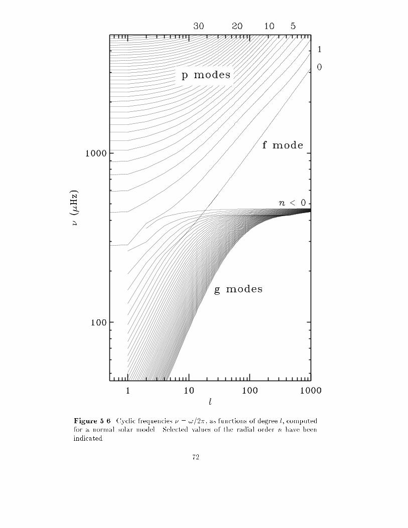
Figure 5.6. Cyclic frequencies � = !=2�, as functions of degree l, computedfor a normal solar model. Selected values of the radial order n have beenindicated. 72

The precise classi�cation of the modes, i.e., the assignment of radial orders to them,presents some interesting and so far unsolved problems. It appears that at each l it ispossible to assign to each mode an integral order n, which ranges from minus to plusin�nity, such that, at least for reasonably simple stellar models(5:3) jnj gives the number ofzeros in �r; the possible zero at r = 0 is only counted in the radial case, where l = 0. Ashinted above, this is arranged such that in simple models n > 0 for p modes, n = 0 for the fmode and n < 0 for g modes. Also, with a single exception discussed below, the frequency isan increasing function of n; this rule is evidently consistent with the fact, mentioned above,that the frequency increases with the number of radial nodes for p modes and decreaseswith the number of radial nodes for g modes. It is conventional to denote p, f and g modesof a given degree l0 as pn(l = l0), f(l = l0) and gjnj(l = l0).Eckart (1960) proposed a general, and mathematically precise, scheme for the classi�-cation of waves in a strati�ed medium. It was applied by Scu aire (1974) and Osaki (1975)to the de�nition of the radial order n for a nonradially pulsating star, on the basis of thebehaviour with varying r of the point (�r(r); p0(r)) in the so-called phase diagram. It maybe shown (Gabriel & Scu aire 1979; Christensen-Dalsgaard 1980) that in the Cowling ap-proximation this de�nition has the desirable property of being invariant under a continuousmodi�cation of the equilibrium model or a continuous change of l. Also, for simple modelsor in the limit of high-order modes this de�nition reduces to the simple counting of radialnodes in the eigenfunction, described above. The Eckart scheme is not generally applicable,however, when solutions of the full equations are considered. One �nds, for example, thatin models of the present Sun application of this classi�cation procedure to the lowest-orderp modes with l = 1, computed from the full equations, results in a misidenti�cation of themodes with n = 1 and 2; for more evolved models the problem extends to modes of higherorder. Guenther (1991) considered an evolution sequence of 1M� models extending to thebase of the giant branch. In the �nal model he found it di�cult to determine the orderof a number of l = 1 modes; from his plots of the eigenfunctions it is evident that theorigin of the problem is the presence in the solution of a signi�cant slowly varying trendwhich shifts the radial displacement su�ciently to eliminate several nodes. Problems werealso encountered by Lee (1985) for l = 1 modes in evolved models of � Scuti stars, and byChristensen-Dalsgaard & Mullan (1994) for polytropic models of index exceeding 3.3. Itis interesting that these di�culties appear to be restricted to l = 1, at least for realisticstellar models.The problem of mode classi�cation may appear somewhat academic, of little interestin analysis of observed frequencies. In fact, it is a severe nuisance when computing modesfor a given model, making it very di�cult to ensure that all modes have been computed, orto relate the modes to those of another, slightly di�erent model. Thus there is still a needfor a reliable classi�cation scheme, valid for a wide range of models. More details on theseproblems were given by Christensen-Dalsgaard (1991a).There are a few special cases. For l = 0 only modes with n > 0 are found; this is inaccordance with the fact, mentioned above, that buoyancy can only act in the presence ofhorizontal variation. Also, for l = 1 the mode with n = 0 is peculiar in that its frequencyis zero; indeed a mode with l = 1 and no zero in the radial direction may seem somewhatunphysical, as it displaces the centre of mass of the star. However, the mode correspondsto an in�nitely slow, uniform motion of the entire star, without deformation; this must be(5:3) The de�nition of a `simple' model in this context is not straightforward; examplesmight be zero-age main sequence models or, e.g., polytropes of index between 1.5 and 3.73

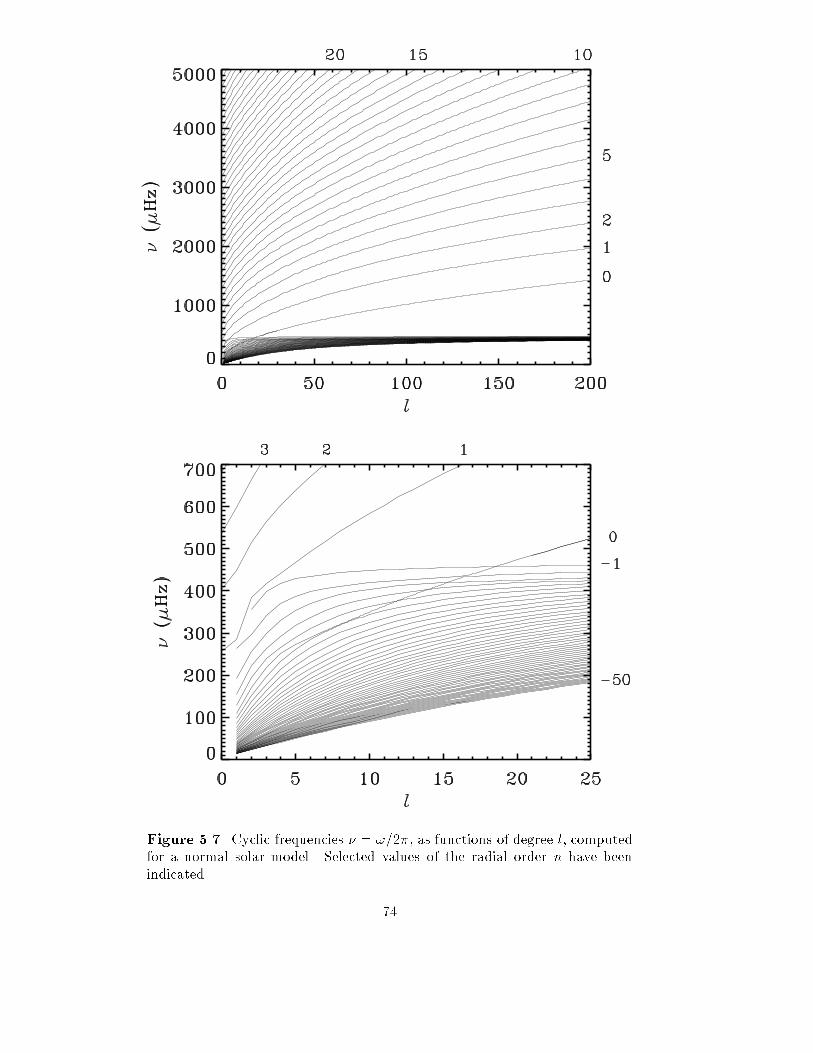
Figure 5.7. Cyclic frequencies � = !=2�, as functions of degree l, computedfor a normal solar model. Selected values of the radial order n have beenindicated. 74

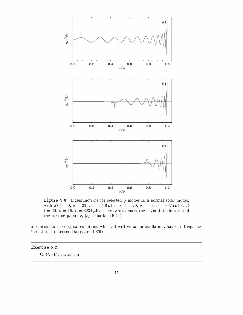
Figure 5.8. Eigenfunctions for selected p modes in a normal solar model,with a) l = 0, n = 23, � = 3310�Hz; b) l = 20, n = 17, � = 3375�Hz; c)l = 60, n = 10, � = 3234�Hz. The arrows mark the asymptotic location ofthe turning points rt [cf. equation (5.24)].a solution to the original equations which, if written as an oscillation, has zero frequency(see also Christensen-Dalsgaard 1976).Exercise 5.2:Verify this statement. 75

It is interesting that this f mode with l = 1 behaves very di�erently in the Cowlingapproximation and for the full set of equations. In the Cowling approximation there is amode with l = 1 having no nodes in the radial displacement, intermediate in frequencybetween the p and the g modes, which must be identi�ed with the f mode. From a physicalpoint of view it can be thought of roughly as an oscillation of the whole star in the grav-itational potential de�ned by the equilibrium model. The connection between this modeand the zero-frequency mode for the full problem can be investigated by making a contin-uous transition from the Cowling approximation to the full set of equations; this can beaccomplished formally by introducing a factor � on the right-hand side of equation (4.19),such that � = 0 corresponds to the Cowling approximation and � = 1 to the full equations(Christensen-Dalsgaard 1978). When � is increased from 0 to 1, the transition from thel = 1 f mode in the Cowling approximation to the zero-frequency \mode" in the full casetakes place through a sequence of avoided crossings with the g modes, where the frequenciesapproach very closely without actually crossing. A similar transition occurs for solutionsof the full equations, between the f mode with l = 2 and the zero-frequency mode withl = 1, as l is decreased continuously from 2 to 1 (Aizenman, Smeyers & Weigert 1977;Christensen-Dalsgaard 1978).Figure 5.9. Eigenfunctions of p modes with l = 1, plotted against fractionalradius r=R in the outermost parts of a normal solar model. The cases shownare: � = 1612�Hz ( ); � = 2293�Hz ( ); � = 3650�Hz( ).Figures 5.8 and 5.9 illustrate typical eigenfunctions for p modes. According to equation(4.41) the quantity plotted, viz. r �1=2�r, is related to the contribution to the energy densityfrom the radial component of velocity. For the p modes this shows that the energy, at leastat low degrees, is distributed throughout most of the Sun. In particular, the radial modespenetrate essentially to the centre. At higher degree the modes are trapped in the outerpart of the model. This is in accordance with the predictions of section 5.2.3; indeed,the arrows for the modes with l = 20 and 60 show the locations of the turning pointspredicted by equation (5.24). Intuitively, one might expect the sensitivity of the frequencyof a mode to the structure of the Sun to be given roughly by the energy density; thus thefrequencies of low-degree p modes should give averages of solar structure over the entire76

Sun. In contrast to the energy, the displacement is strongly peaked towards the surface;this is obvious from Figure 5.8 if it is recalled that the density decreases by about 9 ordersof magnitude from the centre to the surface of the Sun. With increasing degree the p modesbecome con�ned closer and closer to the surface; however, the behaviour near the surface,at a given frequency, changes little with l.Figure 5.9 shows the eigenfunctions in the outer few per cent of the solar radius ofmodes of degree l = 1 with di�erent frequencies. It is evident that the mode energydecreases in the atmosphere; this can be understood from the discussion in section 5.4,which shows that for an isothermal atmosphere the energy decreases exponentially withheight for frequencies below the so-called acoustical cut-o� frequency which in the solarcase corresponds to a cyclic frequency of about 5000�Hz. However, it should be noticedthat at frequencies below about 2000�Hz even the photospheric amplitude is substantiallysmaller than the amplitudes at greater depth. This is related to the re ection of the modesnear the surface which is not contained in the simpli�ed discussion in section 5.2.3; anasymptotic description that includes the surface re ection will be given in section 7.5.Figure 5.10 shows eigenfunctions for g modes. These are con�ned to the deep interiorof the Sun, with maximum energy very near the centre. At a given frequency the numberof radial zeros increases rapidly with l; on the other hand there is little change in theoverall distribution of the energy. That the modes extend over essentially the same regionof the star is consistent with the fact, mentioned in section 5.2.4, that for these modes thelocations of the turning points depend on frequency but not on degree.We may also consider global properties of the eigenfunctions. Of considerable interestis the inertia parameter E de�ned in equation (4.42). It is shown for p modes and low-degree g modes in Figure 5.11, as a function of the cyclic frequency � = !=2�. Each curvecorresponds to a given value of l, with the points for the individual modes being connectedby continuous lines. This format for displaying results on the oscillations clearly makes littlephysical sense, in that non-integer mode orders do not have any meaning; nevertheless itprovides a convenient illustration of the dependence of oscillation quantities on frequencyand degree. The p-mode results in panel (a) show an obvious marked decrease of theinertia, at �xed surface amplitude, with increasing frequency, as well as a weaker but stillsubstantial decrease with increasing degree. The dependence on degree is a direct result ofthe variation of the depth of penetration: with increasing degree the lower turning pointmoves closer to the surface and hence the oscillation involves a smaller part of the star, thusdecreasing the inertia. Similarly, the increase with decreasing frequency can be understoodfrom the re ection properties near the surface and is consistent with the eigenfunctionsshown in Figure 5.9: since the inertia measure in equation (4.42) is normalized with thesurface displacement, the decrease in the value of the eigenfunction at the surface, relativeto the interior, leads to an increase in E at low frequency.The results for low-degree modes, in panel (b) show that at the lowest degrees there isessentially a continuous transition between the p and the g modes, the inertia continuingto rise rapidly with decreasing frequency. At slightly higher degree (l = 3 � 5) there isa beginning tendency towards stronger g-mode trapping as the frequency approaches themaximum in N in the deep interior of the model. This trend is strongly accentuated athigher degree, as shown in Figure 5.12. Here the variation is extremely strong, with verylarge values being reached for high frequencies or high degrees. For such modes a surfaceamplitude large enough to be observed would correspond to totally unrealistic amplitudesin the interior. This is emphasized also by Figure 5.13 which shows the ratio between themaximum interior, and the surface, radial displacement. The reason for this is the trappingof the modes at high degrees and frequencies near the maximum in the buoyancy frequency77

Figure 5.10. Eigenfunctions for selected g modes in a normal solar model,with a) l = 1, n = �5, � = 110�Hz; b) l = 2, n = �10, � = 104�Hz; c)l = 4, n = �18, � = 106�Hz.N . It is particularly pronounced for modes whose frequencies exceed the secondary maxi-mum in N at 400 �Hz. The very low values of E found at selected frequencies for highervalues of l occur where the g modes pass through avoided crossings and take on the char-acter of surface gravity waves; this happens when their frequencies are near the extensionsof the f-mode frequencies shown in Figure 5.6. It is interesting that this phenomenon canbe traced in inertia to a degree as low as 3. However, in general it is evident that the pos-sibilities for observing g modes, regardless of the excitation mechanisms, must be limitedto fairly low values of the degree. 78

Figure 5.11. The dimensionless inertia E [cf. equation (4.42)] for computedmodes of oscillation in a normal solar model, plotted against frequency �for �xed values of the degree l. The inertia has been normalized by thenorm of the total displacement at the photospheric level. (a) results for pmodes; selected values of l have been indicated. (b) results for low-degreeg and p modes, using the following line styles: l = 0 ( ), l = 1( ), l = 2 ( ), l = 3 ( ), l = 4 ( ),and l = 5 ( ). 79

Figure 5.12. The dimensionless inertia E [cf. equation (4.42)] for computedf and g modes of oscillation in a normal solar model, plotted against frequency� for �xed values of the degree l. For clarity, modes of degree 5, 10, 15, 20and 25 have been shown with dotted lines; in addition, selected values of lare indicated in the �gure.From the preceding discussion, there is obviously a high degree of regularity in thecomputational results. Also, it is clear that at least some of these properties can be un-derstood in simple terms by considering the asymptotic behaviour of the oscillations; thisunderstanding is of great assistance in the interpretation of the observed modes. This isemphasized by more detailed study of the asymptotic behaviour of the oscillations, whichforms an important part of the remainder of these notes.5.3.2 Results for the models with convective coresTo illustrate the e�ect of a convective core, particularly the maximum in the buoyancyfrequency at the edge of the core, Figure 5.14 shows the behaviour of the oscillation fre-quencies, as functions of stellar age, for a 2:2M� evolution sequence. These models mayrepresent � Scuti stars; characteristic frequencies at a few ages in the sequence were illus-trated in Figure 5.3. As in that �gure I have applied the scaling according to t�1dyn. As aresult, the frequencies of largely acoustic modes, including the radial modes, change verylittle with age. It should be noticed also that except at low order, the acoustic modes ex-hibit a distinct pattern, with a close pairing of the radial and l = 2 modes. Such a patternof closely-spaced peaks is familiar in solar data (cf. Fig. 2.15) and may also have been80

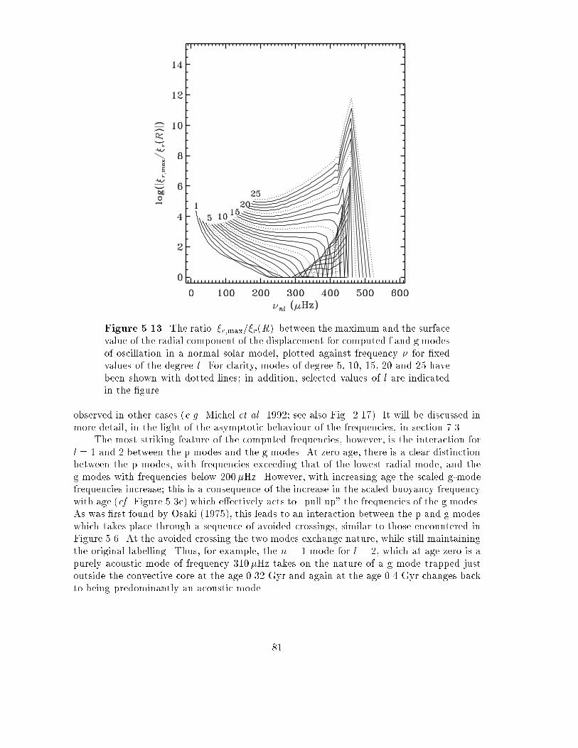
Figure 5.13. The ratio j�r;max=�r(R)j between the maximum and the surfacevalue of the radial component of the displacement for computed f and g modesof oscillation in a normal solar model, plotted against frequency � for �xedvalues of the degree l. For clarity, modes of degree 5, 10, 15, 20 and 25 havebeen shown with dotted lines; in addition, selected values of l are indicatedin the �gure.observed in other cases (e.g. Michel et al. 1992; see also Fig. 2.17). It will be discussed inmore detail, in the light of the asymptotic behaviour of the frequencies, in section 7.3.The most striking feature of the computed frequencies, however, is the interaction forl = 1 and 2 between the p modes and the g modes. At zero age, there is a clear distinctionbetween the p modes, with frequencies exceeding that of the lowest radial mode, and theg modes with frequencies below 200�Hz. However, with increasing age the scaled g-modefrequencies increase; this is a consequence of the increase in the scaled buoyancy frequencywith age (cf. Figure 5.3c) which e�ectively acts to \pull up" the frequencies of the g modes.As was �rst found by Osaki (1975), this leads to an interaction between the p and g modeswhich takes place through a sequence of avoided crossings, similar to those encountered inFigure 5.6. At the avoided crossing the two modes exchange nature, while still maintainingthe original labelling. Thus, for example, the n = 1 mode for l = 2, which at age zero is apurely acoustic mode of frequency 310�Hz takes on the nature of a g mode trapped justoutside the convective core at the age 0.32 Gyr and again at the age 0.4 Gyr changes backto being predominantly an acoustic mode. 81

Figure 5.14. Scaled oscillation frequencies, as functions of age, in a 2:2M�evolution sequence. Modes of the same radial order have been connected.The solid lines are for radial modes, of degree l = 0, the dotted lines are forl = 1 and the dashed lines for l = 2.This behaviour is further emphasized by considering the eigenfunctions of these modes;examples of eigenfunctions near the p1 � p2(l = 2) avoided crossing at age 0.4 Gyr areshown in Figure 5.15. Before the avoided crossing, the p1 mode has a substantial amplitudenear the edge of the convective core, and hence to a large extent behaves like a g mode,whereas the p2 mode is predominantly a p mode, with largest amplitude in the outer parts.At the point of closest approach of the frequencies, at an age of 0.39 Gyr, both modeshave a mixed character, with substantial amplitudes in the deep interior and near thesurface, whereas after the avoided crossing the p2 mode looks like a g mode, whereas thep1 mode largely behaves like a p mode. It should be noted that this behaviour introduces apotential di�erence between the mathematical classi�cation of the modes and their physicalnature: modes with order n > 0, which in simple models would be p modes, may take onthe character of g modes. Also, it is evident that the presence of the g-like modes inthe p-mode spectrum, particularly at late evolutionary stages, complicates the analysis ofobserved frequencies. Dziembowski & Kr�olikowska (1990) pointed out that mode selectionmight be a�ected by the larger energy of the modes that behave like g modes, therebyrestricting the choice of modes in the identi�cation. However, such arguments depend onthe mechanisms responsible for exciting the modes and limiting their amplitudes, whichare so far incompletely understood. It should also be noted that if g-mode like pulsationscould in fact be identi�ed, their frequencies would give strong constraints on conditionsin the region just outside the stellar core. In fact, Dziembowski & Pamyatnykh (1991)82

Figure 5.15. Scaled eigenfunctions for the p1(l = 2) mode (continuous line)and the p2(l = 2) mode (dashed line) in the vicinity of the avoided crossingnear age 0.4 Gyr, (R=R0)3=2� = 400�Hz in Figure 5.14. (a) Age 0.36 Gyr.(b) Age 0.39 Gyr. (c) Age 0.44 Gyr.pointed out that measurement of g-mode frequencies might provide a measure of the extentof convective overshoot from the core.5.4 Oscillations in stellar atmospheres.In the preceding section I neglected terms of the order of the inverse scale heights in equi-librium quantities. As pointed out, this is invalid near the stellar surface, where the scale83

heights become small compared with the wavelength of the oscillations. In the present sec-tion I discuss these e�ects in the particularly simple case of an isothermal atmosphere. Thishas the signi�cant advantage of allowing an analytical solution of the oscillation equations.Furthermore, it is a reasonable approximation to a realistic stellar atmosphere where thetemperature variation is substantially slower than the variations in pressure and density.In particular, in the solar case the temperature has a minimum at an optical depth ofabout 10�4, corresponding to an altitude of about 500 km above the visible surface. Anearly treatment of this problem was given by Biermann (1947); for a somewhat more recentreview, see Schatzman & Sou�rin (1967). The extension of the results obtained here to amore general model is discussed in Chapter 7.I neglect e�ects of ionization and treat the gas in the atmosphere as ideal, so that theequation of state is given by equation (3.16), where the mean molecular weight � is takento be constant. Then equation (3.30) of hydrostatic support givesdpdr = �g� = � pHp ; (5:29)where the pressure and density scale heights Hp and H (which are evidently the same inthis case) are given by Hp = H = kBTg�mu : (5:30)As the extent of the atmosphere of at least main-sequence stars is much smaller than thestellar radius, g can be taken to be constant. Then H is constant, and the solution toequation (5.29) is p = ps exp�� hH � : (5:31)Thus, from equation (3.16), � = �s exp�� hH � : (5:32)Here I have introduced the altitude h = r � R, where R is the photospheric radius (corre-sponding to the visible surface of the Sun, e.g. de�ned as the point where the temperatureequals the e�ective temperature), and ps and �s are the values of p and � at h = 0.We now consider the oscillations. As argued in section 3.1.4, the motion becomesstrongly nonadiabatic in the stellar atmosphere. Nonetheless, for simplicity, I shall hereuse the adiabatic approximation in the atmosphere. This preserves the most importantfeatures of the atmospheric behaviour of the oscillations, at least qualitatively. The studyof atmospheric waves and oscillations, with full consideration of e�ects of radiative transfer,is a very complex and still incompletely developed area (e.g. Christensen-Dalsgaard &Frandsen 1983). It might be noticed that the waves are in fact approximately adiabaticin the upper part of the atmosphere. Here the di�usion approximation (upon which theargument in section 3.1.4 was based) is totally inadequate, as the gas is optically thin; indeedthe density is so low that the gas radiates, and hence looses energy, very ine�ciently, andthe motion is nearly adiabatic. 84

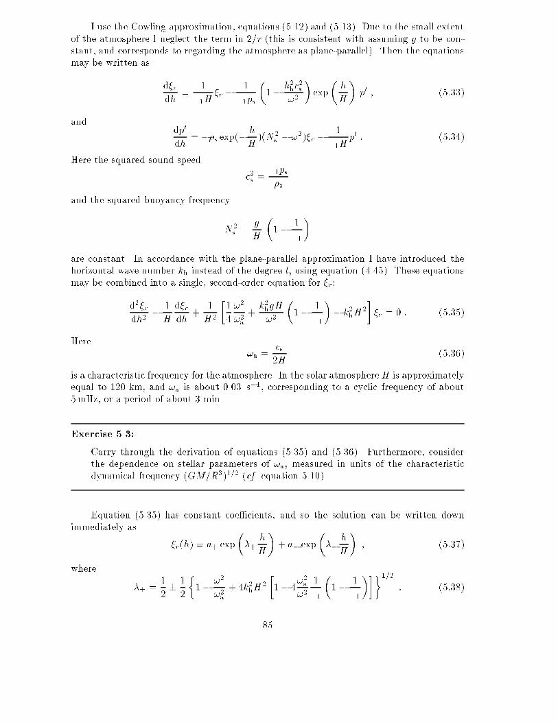
I use the Cowling approximation, equations (5.12) and (5.13). Due to the small extentof the atmosphere I neglect the term in 2=r (this is consistent with assuming g to be con-stant, and corresponds to regarding the atmosphere as plane-parallel). Then the equationsmay be written as d�rdh = 1�1H �r � 1�1ps �1� k2hc2s!2 � exp� hH� p0 ; (5:33)and dp0dh = ��s exp(� hH )(N2s � !2)�r � 1�1Hp0 : (5:34)Here the squared sound speed c2s = �1ps�sand the squared buoyancy frequencyN2s = gH �1� 1�1�are constant. In accordance with the plane-parallel approximation I have introduced thehorizontal wave number kh instead of the degree l, using equation (4.45). These equationsmay be combined into a single, second-order equation for �r:d2�rdh2 � 1H d�rdh + 1H2 �14 !2!2a + k2hgH!2 �1� 1�1�� k2hH2� �r = 0 : (5:35)Here !a = cs2H (5:36)is a characteristic frequency for the atmosphere. In the solar atmosphereH is approximatelyequal to 120 km, and !a is about 0.03 s�1, corresponding to a cyclic frequency of about5mHz, or a period of about 3 min.Exercise 5.3:Carry through the derivation of equations (5.35) and (5.36). Furthermore, considerthe dependence on stellar parameters of !a, measured in units of the characteristicdynamical frequency (GM=R3)1=2 (cf. equation 5.10).Equation (5.35) has constant coe�cients, and so the solution can be written downimmediately as �r(h) = a+ exp��+ hH� + a� exp��� hH� ; (5:37)where �� = 12 � 12 �1� !2!2a + 4k2hH2 �1� 4!2a!2 1�1 �1� 1�1���1=2 : (5:38)85

These equations have been the subject of extensive studies in connection with early attemptsto interpret observations of 5 minute oscillations of high degree (see e.g. Stein & Leibacher1974). From the expression for �� one may qualitatively expect two regimes: one where thefrequency is relatively large, kh is relatively small and the �rst two terms in f� � �g dominate;the second where the frequency is small, kh is large and the last term in f� � �g dominates.These correspond to atmospheric acoustic waves and gravity waves, respectively. From thepoint of view of global stellar oscillations interest centres on waves with a wavelength muchlarger than the scale height of the atmosphere. Thus I neglect the last term, reducingequation (5.38) to �� = 12 � 12 �1� !2!2a �1=2 : (5:39)This is clearly the relation for purely vertical waves.Equation (5.39) shows the physical meaning of !a. When ! < !a, �� are real, andthe motion behaves exponentially in the atmosphere. When ! > !a, �� are complex, andthe motion corresponds to a wave propagating through the atmosphere. Thus !a is theminimum frequency of a propagating wave, and is consequently known as the acousticalcut-o� frequency (Lamb 1909). The exponential behaviour in the former case providesthe upper re ection of p modes, which was absent in the simpli�ed asymptotic analysisof section 5.3. To study this in more detail, I consider the boundary conditions for anatmosphere of in�nite extent. Here the energy density in the motion must be bounded ash tends to in�nity. The energy density is proportional to ��2r , which for the two solutionsbehaves as ��2r � exp(� hH ) exp(2�� hH ) = exp"��1� !2!2a �1=2 hH # : (5:40)Therefore only the �� solution is acceptable, and here the energy density decreases expo-nentially. This gives rise to the atmospheric re ection. Thus only modes with frequenciesbelow !a are trapped in the stellar interior. At higher frequencies the waves propagatethrough the atmosphere; oscillations at such frequencies would therefore rapidly loose en-ergy (such waves, generated in the convection zone, may contribute to the heating of thesolar chromosphere). In fact, the observed spectrum of oscillations stops at frequencies ofabout 5mHz. It should be noticed that �� > 0, so that the displacement increases with al-titude. This increase can in fact be observed by comparing oscillation amplitudes obtainedin spectral lines formed at di�erent levels in the atmosphere.From this solution we may obtain a more realistic boundary condition, to replace thecondition (4.60) discussed earlier. The condition of adiabaticity (4.51) and the continuityequation (3.38) give �pp = �1 ��� = ��1div ���r ' ��1 d�rdh = ��1��H �r ; (5:41)or p0 = �p� �r dpdh = 1Hp(1� �1��)�r ; (5:42)where, for simplicity, I neglected the horizontal part of the divergence of ���r (this could, quitesimply, be included). This provides a boundary condition that may be used in numericalcomputations, in place of equation (4.60). Typically it is applied at a suitable point, suchas the temperature minimum, in the atmosphere of the stellar model.86

When ! is small compared with !a, we can approximate �� by�� ' 12 �1� �1� 12 !2!2a �� = 14 !2!2a : (5:43)Then �1�� can be neglected in equation (5.42), compared with 1, and we recover theboundary condition in equation (4.60). In this limit the displacement is almost constantthroughout the atmosphere. Also, it follows from equation (5.41) that the Lagrangianperturbations of pressure and density, and consequently also of temperature, are small.Physically, this means that the atmosphere is just lifted passively up and down by theoscillation, without changing its structure. Only when the frequency is quite close to theacoustical cut-o� frequency does the oscillation have a dynamical e�ect on the atmosphere.In reality the Sun is surrounded by a corona with a temperature exceeding 106 K. Herethe scale heights are large, and the acoustical cut-o� frequency correspondingly small. Atypical temperature is 1:6� 106K, corresponding to !a ' 0:001 s�1. This is below the fre-quencies of the modes observed in the 5 minute region, and these are therefore propagatingin the corona. This atmospheric structure may be approximated by representing it by twoisothermal layers, corresponding to the inner atmosphere and the corona, respectively. Inthe corona the two solutions obtained from equation (5.39) are waves propagating outwardsinto, and inwards from, the corona. Of these only the former solution is physically realistic(unless one assumes that there is a source of waves in the outer corona!). It may be written,as a function of altitude and time, as�r(h; t) = A��1=2 exp[i(krh� !t)] ; (5:44)where the radial wave number iskr = H�1 �!2!2a � 1�1=2 : (5:45)This solution may also be used to obtain a boundary condition on numerical solutions ofthe oscillation equations in the inner atmosphere, by requiring that the displacement andthe pressure perturbation be continuous at the interface between the atmosphere and thecorona. I shall not write down this condition in detail. Note, however, that as the solution(5.44) is complex, the relation obtained between �r and p0 has complex coe�cients. Thusthe solution and the eigenfrequency are no longer purely real. Physically, the propagatingwave in the corona carries away energy from the oscillation, which is therefore damped,even in the adiabatic approximation. This damping gives rise to an imaginary part in theeigenfrequency, which corresponds to an exponential decay of the solution with time.To estimate the importance of these e�ects we return to the solution (5.37), in theinner atmosphere. Because of the e�ect of the corona both terms must now be included.By matching to equation (5.44) it may be shown that the two terms are roughly of thesame order of magnitude at the interface, where h = hc, say. At the altitude h the ratiobetween the terms is therefore, roughly,����a+ exp(�+h=H)a� exp(��h=H) ���� � ����exp[�+(h� hc)=H ]exp[��(h� hc)=H ]���� = exp"�hc � hH �1� !2!2a �1=2# : (5:46)87

The base of the corona is approximately at hc = 2000 km. Thus hc=H � 16, and the ratioin equation (5.46) is very small in the lower part of the atmosphere, unless ! is close to!a. Therefore in general it is an excellent approximation to neglect the term in a+. Bythe same argument, perturbations in the structure of the atmosphere, or the physics of theoscillations, at the temperature minimum, say, or higher, have little e�ect on the solution inthe deep atmosphere; hence they barely perturb the solution in the interior of the Sun or theeigenfrequencies. This is fortunate; for the upper solar atmosphere is highly inhomogeneous,and contains magnetic �elds of strength su�cient to modify the properties of the oscillations.In addition, the modes may get non-linear at su�cient altitudes, which also a�ects theirpropagation. Even so, the assumption of a pure exponentially decaying solution is probablyadequate in the inner atmosphere. This has been con�rmed by numerical calculations.The large decrease in the oscillation energy from the lower atmosphere to the base ofthe corona also limits the importance of the loss of energy in the form of propagating wavesin the corona. Detailed, nonadiabatic calculations generally show that this only makesa small contribution to the damping of the modes, except at very high frequencies. Thedominant source of damping is heat loss due to the radiative or convective ux in the upperconvection zone and the lower atmosphere.5.5 The functional analysis of adiabatic oscillations.A great deal of insight into the properties of adiabatic oscillations can be obtained byregarding the equations as an eigenvalue problem in a Hilbert space (Eisenfeld 1969; Dyson& Schutz 1979; Christensen-Dalsgaard 1981). Here I consider two di�erent, but very closelyrelated, formulations: one based on the unseparated oscillation equations, valid for generalperturbations and a second obtained after separation of the oscillation equations in termsof spherical harmonics.5.5.1 The oscillation equations as linear eigenvalue problems in a Hilbert spaceTo obtain the general form, I go back to the perturbed equations of motion, equation (3.40).After separation of the time dependence on the form (4.2) this can be written as!2���r = F(���r) ; (5:47)where F(���r) = 1�0rp0 � g0 � �0�0g0 : (5:48)Here the perturbation quantities denote the amplitudes, after the separation of the timedependence. As indicated, F is a linear functional of ���r. To see this, note that from thecontinuity equation (3.38) �0 is a linear functional of ���r; so, therefore, is the gravitationalpotential perturbation �0 as given by equation (3.42). In the adiabatic case p0 is obtainedfrom �0 and ���r as in equation (3.47); this de�nes the adiabatic operator Fa. The nonadia-batic case is more complicated, but here also it is possible to obtain p0 as a linear functionalof ���r (see Christensen-Dalsgaard 1981).To cast the problems in terms of functional analysis, I introduce a space H of vectorfunctions of position in the star, with suitable regularity properties, and de�ne an innerproduct on H by < ���; ��� >= ZV �0���� � ��� dV ; (5:49)88

for ���; ��� in H; here \*" denotes the complex conjugate. I also introduce the domain D(F) ofthe operator F as those vectors in H such that the boundary condition (4.60) is satis�ed.The central result of this section is now that, as shown by Lynden-Bell & Ostriker (1967),the operator Fa corresponding to equation (5.48) for adiabatic oscillations is symmetric, inthe sense that < ���;Fa(���) >=< Fa(���); ��� > ; for ���; ��� 2 D(F) : (5:50)The formulation in terms of the spatially separated variables proceeds in a very similarmanner. The separated oscillation equations (4.18) and (4.17) may be written1� dp0dr + �0� g � d�0dr = !2�r ; (5:51)1r �p0� � �0� = !2�h : (5:52)As before, the quantities on the left-hand side can be obtained in terms of �r and �h; inparticular, �0 is found from �0 from the separated integral solution to Poisson's equationgiven in equation (5.11). I introduce the subspace Hl of the space of pairs of quadraticallyintegrable functions on the interval [0; R], with vectors� � (�r; �h) 2 Hl : (5:53)Then equations (5.51) and (5.52) can be written asFl(�) = !2� ; (5:54)de�ning the operator Fl corresponding to the separated oscillation equations. Assumingagain the adiabatic relation for p0 one obtains the linear operator Fa;l for adiabatic oscilla-tions in Hl. The boundary conditions on �r and �h can be imposed by restricting the partof Hl where Fa;l is de�ned. Thus I de�ne the domain of Fa;l byD(Fa;l) = f(�r; �h)j�r � l�h ! 0 for r ! 0 ^ �p(R) = 0g ; (5:55)the boundary conditions on �0 are satis�ed automatically by the integral expression (5.11).The inner product on Hl is de�ned by< �; � >l� 4� Z R0 [��r(r)�r(r) + L2��h(r)�h(r)]r2�dr ; (5:56)for two vectors � = (�r; �h) and � = (�r; �h) in Hl. Again one may show, using the explicitexpression, that the operator Fa;l is symmetric, i.e.,< Fa;l(�); � >l=< �;Fa;l(�) >l for all �; � 2 D(Fa;l) : (5:57)From equations (5.50) and (5.57) follow immediately a number of useful properties ofFa and Fa;l. For simplicity I generally present them in terms of Fa; precisely analogousrelations are obviously valid for Fa;l. The simplest result is that the squared eigenfrequenciesare real. This may be demonstrated by introducing the functional � on D(F) by�(���) = < ���;Fa(���) >< ���; ��� > ; (5:58)89

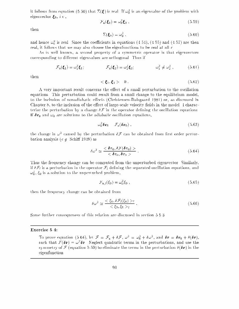
it follows from equation (5.50) that �(���) is real. If !20 is an eigenvalue of the problem witheigenvector ���0, i.e., Fa(���0) = !20���0 ; (5:59)then �(���0) = !20 ; (5:60)and hence !20 is real. Since the coe�cients in equations (4.54), (4.55) and (4.57) are thenreal, it follows that we may also choose the eigenfunctions to be real at all r.As is well known, a second property of a symmetric operator is that eigenvectorscorresponding to di�erent eigenvalues are orthogonal. Thus ifFa(���1) = !21���1; Fa(���2) = !22���2; !21 6= !22 ; (5:61)then < ���1; ���2 >= 0 : (5:62)A very important result concerns the e�ect of a small perturbation to the oscillationequations. This perturbation could result from a small change to the equilibrium model,to the inclusion of nonadiabatic e�ects (Christensen-Dalsgaard 1981) or, as discussed inChapter 8, to the inclusion of the e�ect of large-scale velocity �elds in the model. I charac-terize the perturbation by a change �F in the operator de�ning the oscillation equations.If ���r0 and !0 are solutions to the adiabatic oscillation equations,!20���r0 = Fa(���r0) ; (5:63)the change in !2 caused by the perturbation �F can be obtained from �rst order pertur-bation analysis (e.g. Schi� 1949) as�!2 ' < ���r0; �F(���r0) >< ���r0; ���r0 > : (5:64)Thus the frequency change can be computed from the unperturbed eigenvector. Similarly,if �Fl is a perturbation in the operator Fl de�ning the separated oscillation equations, and!20 , �0 is a solution to the unperturbed problem,Fa;l(�0) = !20�0 ; (5:65)then the frequency change can be obtained from�!2 ' < �0; �Fl(�0) >l< �0; �0 >l : (5:66)Some further consequences of this relation are discussed in section 5.5.3.Exercise 5.4:To prove equation (5.64), let F = Fa + �F , !2 = !20 + �!2, and ���r = ���r0 + �(���r),such that F(���r) = !2���r. Neglect quadratic terms in the perturbations, and use thesymmetry of F (equation 5.50) to eliminate the terms in the perturbation �(���r) in theeigenfunction. 90

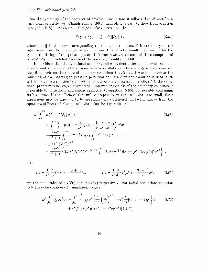
5.5.2 The variational principleFrom the symmetry of the operator of adiabatic oscillations it follows that !2 satis�es avariational principle (cf. Chandrasekhar 1964). Indeed, it is easy to show from equation(5.50) that if ���� 2 H is a small change to the eigenvector, then�(���0 + ����) = !20 +O(k����k2) ; (5:67)where k � � �k is the norm corresponding to < � � � ; � � � >. Thus � is stationary at theeigenfrequencies. From a physical point of view this re ects Hamilton's principle for thesystem consisting of the pulsating star. It is conservative, because of the assumption ofadiabaticity, and isolated because of the boundary condition (4.60).It is evident that the variational property, and equivalently the symmetry of the oper-ators F and Fl, are not valid for nonadiabatic oscillations, where energy is not conserved.Also it depends on the choice of boundary conditions that isolate the system, such as thevanishing of the Lagrangian pressure perturbation. If a di�erent condition is used, suchas the match to a solution in an isothermal atmosphere discussed in section 5.4, the varia-tional property is no longer guaranteed. However, regardless of the boundary condition itis possible to write down expressions analogous to equation (5.60), but possibly containingsurface terms; if the e�ects of the surface properties on the oscillations are small, theseexpressions may be expected to be approximately variational. In fact it follows from theequations of linear adiabatic oscillations that for any radius r�!2 Z r�0 � ��2r + L2�2h� r2dr (5:68)= Z r�0 ��1pD21 + 2dpdr �rD1 + 1� d�dr dpdr �2r� r2dr� 8�G2l + 1 Z r�0 r�(l�1)D2(r) Z r0 r0l+2D2(r0)dr0dr+ p0(r�)�r(r�)r�2+ 4�G2l + 1 �2�(r�)�r(r�)r��(l�1) Z r�0 D2(r)rl+2 dr � [�(r�)�r(r�)]2 r�3� ;here D1 = 1r2 ddr (r2�r)� l(l+ 1)r �h; D2 = 1r2 ddr (r2��r)� l(l+ 1)r ��h (5:69)are the amplitudes of div(���r) and div(����r) respectively. For radial oscillations equation(5.68) may be considerably simpli�ed, to give!2 Z r�0 �2r�r2dr = Z r�0 (�1p r4 � ddr � �rr ��2 � r�2r ddr [(3�1 � 4)p])dr (5:70)+ r� [3�1p(r�)�r(r�) + r��p(r�)] �r(r�) :91

These equations are valid at any r�. If the surface radius is chosen for r�, and the surfaceterms are neglected, they reduce to the expression de�ned symbolically in equation (5.60).In fact, the surface terms are in general relatively small, and even the complete expressionsare approximately variational. As discussed by Christensen-Dalsgaard, Gough & Morgan(1979) and J. Christensen-Dalsgaard (1982), they may be utilized in the computation ofaccurate oscillation frequencies (see also section 6.6).5.5.3 E�ects on frequencies of a change in the model.As an example of the use of equation (5.66), I discuss in more detail the interpretation ofchanges in the frequencies caused by changes in the equilibrium model. Consider a mode(n; l), with eigenvector �nl = (�r;nl; �;nl) 2 Hl; without loss of generality I may assume that�r;nl(r) and �;nl(r) are real. The relative frequency change caused by the perturbation �Flis then, according to equation (5.66)�!nl!nl = 12 �!2nl!2nl = < �nl ; �Fl(�nl) >l2!2nl < �nl ; �nl >l : (5:71)Here the denominator is proportional !2nlEnl, where Enl was de�ned in equation (4.42).Also, I represent �Fl on component form as�Fl(�nl) = (�r[�nl]; �h[�nl]) ; (5:72)where �r[�nl](r) and �h[�nl](r) are functions of r. Then we can write equation (5.71) asEnl �!nl!nl = Inl ; (5:73)where Inl = 2� R R0 ��r;nl(r)�r[�nl](r) + L2�h;nl(r)�h[�nl](r)��r2drM!2nl [�2r(R) + l(l+ 1)�2h(R)] : (5:74)Thus Inl gives the integrated e�ect of the perturbation, normalized to the total surfacedisplacement.Equations (5.73) and (5.74) provide a linear relation between the change in the modeland the change in the frequency. These expressions are somewhat formal. However, itfollows from the discussion in section 5.1 that the changes in the coe�cients of the oscillationequations, and hence the changes �r[�nl](r) and �h[�nl](r) in the components of �Fl, can beexpressed in terms of changes in two suitably chosen model variables, for example densityand sound speed. For simplicity, I assume that the change in the model occurs without achange in its radius (this would in general be the case for models of the Sun, where theradius is known with high accuracy) and let �r� and �rc2 denote the changes, between theequilibrium models, in � and c2 at �xed r(5:4). Then, after some manipulation, equation(5.73) can be written as�!nl!nl = Z R0 �Knlc2;�(r)�rc2c2 (r) +Knl�;c2(r)�r�� (r)�dr (5:75)(5:4) These model changes should not be confused with the Lagrangian perturbations asso-ciated with the oscillations, introduced in Chapters 3 and 4.92

Figure 5.16. Kernels for an l = 0, n = 21 mode (with frequency � =3:04mHz) of a model of the present Sun. Panels (a) and (b) show RKnlc2;�and RKnl�;c2 . The Knlc2;� is positive everywhere, while the kernel Knl�;c2 takeson both positive and negative values. Panels (c) and (d) similarly show thekernels RKnl�;Y and RKnlY;� for the same mode; the insert in panel (d) showsthe detailed behaviour of RKnlY;� in the hydrogen and helium ionization zones.93

(e.g. Gough & Thompson 1991), where the kernels Knlc2;� and Knl�;c2 are computed from theeigenfunctions. Examples of such kernels are shown in Figure 5.16.As discussed in section 5.1.1, other pairs of \mechanical" variables may be used insteadof (c2; �); the transformation between these pairs can be accomplished by means of the equa-tion of hydrostatic support and mass, expressed in terms of the model changes, and suitableintegrations by part. If it is also assumed that the equation of state is known, further trans-formation is possible. An important example is provided by the relation c2 = �1p=�, where�1 can be obtained as a function �1(p; �; Y; Z) of pressure, density and chemical composi-tion as speci�ed by the abundances Y and Z by mass of helium and heavy elements. Thisyields �rc2c2 ="�@ ln �1@ ln p ��;Y;Z + 1# �rpp + "�@ ln �1@ ln � �p;Y;Z � 1# �r��+ �@ ln �1@Y �p;�;Z �rY + �@ ln �1@Z �p;�;Y �rZ : (5:76)By substituting this into equation (5.75), and eliminating �rp by means of the perturbedequation of hydrostatic support, �!nl=!nl can be expressed in terms of �r�=�, �rY and �rZ.Since the surface heavy-element abundance may be obtained from spectroscopic observa-tions it is reasonable to assume Z to be known; neglecting therefore the term in �rZ, we�nally obtain �!nl!nl = Z R0 �Knl�;Y (r)�r�� (r) +KnlY;�(r)�rY (r)�dr : (5:77)Examples of these kernels are shown in Figure 5.16, panels (c) and (d). In particular,it should be noticed that KnlY;� is signi�cantly di�erent from zero only in the hydrogenand helium ionization zones. As discussed in section 9.2 this substantially facilitates thedetermination of �r�=� through inverse analysis.5.5.4 E�ects of near-surface changesI now assume that �Fl in equation (5.72) is localized near the stellar surface, in the sensethat �r[�](r) ' 0 ; �h[�](r) ' 0 for R� r > � ; (5:78)for some small �. For modes extending substantially more deeply than the region of theperturbation, i.e., with R� rt � �, the eigenfunctions are nearly independent of l at �xedfrequency in that region (see also Figure 5.8 and the associated discussion). Hence Inldepends little on l at �xed !. To get a more convenient representation of this property, Iintroduce Qnl = EnlE0(!nl) ; (5:79)where El(!) is obtained by interpolating to ! in Enl at �xed l. ThenQnl�!nl (5:80)94

Figure 5.17. The inertia ratio Qnl, de�ned in equation (5.79), against fre-quency �, for f and p modes in a normal solar model. Each curve correspondsto a given degree l, selected values of which are indicated.is independent of l, at �xed !, for modes such that R � rt � �. Conversely, if Qnl�!nl isindependent of l at �xed ! for a given set of modes, then �Fl is probably largely localizedoutside r = max(rt) over the set of modes considered.An important example concerns the uncertainties in the physics of the model and theoscillations in the near-surface region, discussed in section 5.1.2 and indicated schematicallyin Figure 5.1. These are con�ned to a very thin region, and hence we may expect that theire�ects on the frequencies, when scaled with Qnl , are largely independent of degree at agiven frequency. As discussed below, and in more detail in sections 7.6 and 9.2, this can beused to eliminate the e�ects of the uncertainties in the analysis of observed frequencies.Qnl has been plotted in Figure 5.17, for selected values of l. Its variation with l islargely determined by the change in the penetration depth. Modes with higher degreepenetrate less deeply and hence have a smaller inertia at given surface displacement. As aconsequence of this their frequencies are more susceptible to changes in the model.It should be noticed that, as discussed above, much of the uncertainty in the propertiesof the stellar models and the physics of the oscillations is concentrated in a region very nearthe surface of the star. Thus, according to the discussion following equation (5.80), we mayexpect that these uncertainties lead to frequency changes such that Qnl�!nl is a functionof frequency alone. This allows the e�ects to be eliminated in analysis of solar oscillationfrequencies. 95

Figure 5.18. Relative sound-speed di�erence �rc2=c2 between a model withmodi�ed surface opacity and a normal model, in the sense (modi�ed model){ (normal model).To illustrate this behaviour, we may analyze model changes localized very near thesolar surface. Speci�cally, I consider a solar model where the opacity has been arti�ciallyincreased by a factor of 2 at temperatures below about 105K; this is compared with a normalmodel of the present Sun. In both models the mixing-length parameter and compositionhave been adjusted so as to obtain a model with solar radius and luminosity; the e�ect ofthis is that the interior of the model is virtually the same. The opacity has no e�ect inthe bulk of the convection zone where energy transport is totally dominated by convection;hence the change in the model is largely con�ned to the atmosphere and the uppermostparts of the convection zone. Figure 5.18 shows the sound-speed di�erence �rc2 betweenthe modi�ed and the normal model.The unscaled di�erences between frequencies of the two models are shown in Figure5.19a. It is evident that the di�erences show a very systematic increase in magnitudewith increasing degree. As shown by Figure 5.19b this is entirely suppressed by scalingthe di�erences by Qnl. Indeed, the di�erences now seem to decrease with increasing l.This is predominantly due to the fact that at the largest values of l the modes can nolonger be assumed to be independent, near the surface, of degree at �xed frequency (foran asymptotic description of this behaviour, see for example Gough & Vorontsov 1995). Asmall additional contribution comes from the fact that the modes only penetrate partly, toa degree-dependent extent, into the region where the sound speed has been modi�ed.It might also be noted that the frequency di�erences are very small at low frequency.This is related to the fact that low-frequency modes have very small amplitudes in thesurface region (cf. Figure 5.9). However, a proper understanding of this feature requires amore careful analysis (see Christensen-Dalsgaard & Thompson 1997).96

Figure 5.19. Frequency di�erences between a model with modi�ed sur-face opacity and a normal model, in the sense (modi�ed model) { (nor-mal model). Panel (a) shows the raw di�erences. In panel (b) the dif-ferences have been scaled by Qnl, in accordance with equation (5.80).Points corresponding to a given degree have been connected, accordingto the following line styles: l = 0; 1; 2; 3; 4; 5; 10; 20; 30 ( );l = 40; 50; 70; 100 ( ); l = 150; 200; 300; 400 ( ); l =600; 700; 800; 900; 1000; 1100 ( ).A rather similar behaviour is obtained for the observed frequencies, as shown in Figure5.20. The unscaled di�erences (panel a) shows a strong dependence on l, which is largely(but not completely) suppressed by scaling. This strongly suggests that most of the errorsin the model are located very near the surface. I note that this is precisely the region where,according to the arguments in section 5.1.2, many of the uncertainties in the physics of themodel and the oscillations are located. Thus it is not surprising that we obtain an e�ecton the frequencies of this nature. As discussed in section 9.2 it is possible to suppress thee�ect, precisely because of its systematic dependence on frequency. However, I note also inFigure 5.20b that there is a signi�cant dependence of the di�erences on degree; this mustbe associated with errors in the model in deeper layers. I return to the origin of thesedi�erences in section 7.6.2.The probable presence of near-surface errors in the model must be taken into accountwhen relating di�erences between observed and computed frequencies to the correspondingdi�erences between the structure of the Sun and the model. Speci�cally, consider thedetermination of corrections �rc2 and �r� to a solar model, from the di�erences �!nl =!(obs)nl �!nl between observed frequencies !(obs)nl and model frequencies !nl : here we expectdi�erences between the Sun and the model both in the internal structure, characterized by(c2; �), and in the near-surface layers. In addition, the observed frequencies are unavoidablya�ected by errors. From the analysis above we therefore expect that equation (5.75) mustbe replaced by�!nl!nl = Z R0 �Knlc2;�(r)�rc2c2 (r) +Knl�;c2(r)�r�� (r)�dr +Q�1nl G(!nl) + �nl ; (5:81)97

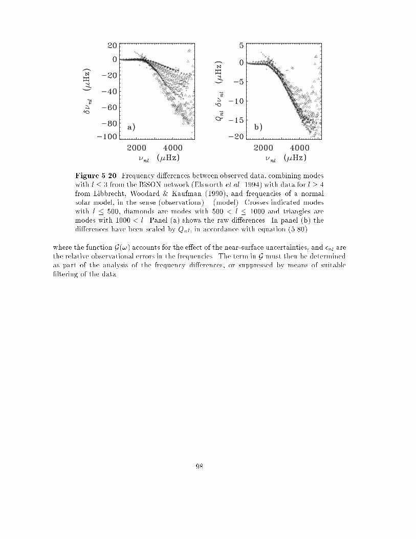
Figure 5.20. Frequency di�erences between observed data, combining modeswith l � 3 from the BiSON network (Elsworth et al. 1994) with data for l � 4from Libbrecht, Woodard & Kaufman (1990), and frequencies of a normalsolar model, in the sense (observations) { (model). Crosses indicated modeswith l � 500, diamonds are modes with 500 < l � 1000 and triangles aremodes with 1000 < l. Panel (a) shows the raw di�erences. In panel (b) thedi�erences have been scaled by Qnl, in accordance with equation (5.80).where the function G(!) accounts for the e�ect of the near-surface uncertainties, and �nl arethe relative observational errors in the frequencies. The term in G must then be determinedas part of the analysis of the frequency di�erences, or suppressed by means of suitable�ltering of the data.98

6. Numerical techniquesThe di�erential equations (4.54), (4.55) and (4.57), in combination with boundary con-ditions such as equations (4.58) { (4.60), constitute a two point boundary value problem.Non-trivial solutions to the problem can be obtained only at selected values of the frequency!, which is therefore an eigenvalue of the problem. Problems of this nature are extremelycommon in theoretical physics, and hence there exists a variety of techniques for solvingthem. Nevertheless, the computation of solar adiabatic oscillations possesses special fea-tures, which merit discussion. In particular, we typically need to determine a large numberof frequencies very accurately, to match the volume and precision of the observed data.Speci�c numerical techniques are discussed in considerable detail by, for example, Unnoet al. (1989) and Cox (1980). Here I concentrate more on general properties of the solutionmethod. The choice of techniques and examples is unavoidably biased by my personalexperience, but should at least give an impression of what can be achieved, and how toachieve it.I note that a self-contained package for computing stellar adiabatic oscillations, withdocumentation and further notes on the numerical techniques, is available on the WWWat http://www.obs.aau.dk/�jcd/adipack.n/.6.1 Di�erence equations.The numerical problem can be formulated generally as that of solvingdyidx = IXj=1 aij(x)yj(x) ; for i = 1; : : : ; I ; (6:1)with suitable boundary conditions at x = x1 and x2, say. Here the order I of the systemis four for the full nonradial case, and two for radial oscillations or nonradial oscillations inthe Cowling approximation.To handle these equations numerically, I introduce a mesh x1 = x(1) < x(2) < : : : <x(Nme) = x2 in x, where Nme is the total number of mesh points. Similarly I introducey(n)i � yi(x(n)), and a(n)ij � aij(x(n)). A commonly used, very simple representation of thedi�erential equations is in terms of second-order centred di�erences, where the di�erentialequations are replaced by the di�erence equationsy(n+1)i � y(n)ix(n+1) � x(n) = 12 IXj=1 ha(n)ij y(n)j + a(n+1)ij y(n+1)j i ; i = 1; : : : ; I : (6:2)These equations allow the solution at x = x(n+1) to be determined from the solution atx = x(n).More elaborate and accurate di�erence schemes (e.g. Press et al. 1986; Cash & Moore1980), can be set up which allow the rapid variation in high-order eigenfunctions to berepresented with adequate accuracy on a relatively modest number of meshpoints. Alter-natively one may approximate the di�erential equations on each mesh interval (x(n); x(n+1))by a set of equations with constant coe�cients, given byd�(n)idx = IXj=1 a(n)ij �(n)j (x); for i = 1; : : : ; I ; (6:3)99

where a(n)ij � 12 (a(n)ij + a(n+1)ij ) (Gabriel & Noels 1976). These equations may be solvedanalytically on the mesh intervals, and the complete solution is obtained by continuousmatching at the mesh points. This technique clearly permits the computation of modesof arbitrarily high order. I have considered its use only for systems of order two, i.e., forradial oscillations or non-radial oscillations in the Cowling approximation.6.2 Shooting techniques.Perhaps the conceptually simplest technique for handling a boundary value problem is theshooting technique. For simplicity, I consider �rst the case of a second-order system, suchas results from making the Cowling approximation. Then there is one boundary condition,namely equation (4.58), at the centre, and one condition, equation (4.60), at the surface. Forany value of ! the equations may be integrated numerically, imposing the central boundarycondition on �r and �h, and the quantity�(!) � �p0 + dpdr �r�����r=R (6:4)may be evaluated. The eigenfrequencies are obviously the zeros of �(!). A convenientmethod of locating them is to evaluate �(!) at a sequence of points !1; !2; : : :; once aninterval has been found where � changes sign the zero can be found, for instance, byapplying the secant method. An attractive feature of the method is precisely this abilityto search automatically for all modes in a given frequency range, particularly when it iscombined with a method for determining the order of a given mode, so that a check can bemade that no modes have been skipped.A slight elaboration of this basic technique is required to make it computationallye�cient. Due to the rapid decrease of temperature near the solar surface, the equationsare almost singular here. Far from the eigenfrequencies the solution therefore generallyincreases rapidly towards the surface; this translates into a dramatic variation of � with !,which complicates the determination of the zeros. To avoid this problem, one may computesolutions (�(i)r ; �(i)h ) and (�(s)r ; �(s)h ) satisfying the inner and the surface boundary conditions,respectively. A continuous match of the interior and exterior solutions requires the existenceof non-zero constants C(i) and C(s) such thatC(i)�(i)r (rf) = C(s)�(s)r (rf)C(i)�(i)h (rf) = C(s)�(s)h (rf) ; (6:5)where rf is an appropriately chosen �tting point. This set of equations has a solution onlyif the determinant �f(!) = �(i)r (rf)�(s)h (rf)� �(i)h (rf)�(s)r (rf) (6:6)vanishes. Hence the eigenfrequencies are determined as the zeros of �f , as before.The choice of �tting point should be guided by the expected behaviour of the eigen-function, in such a way that the integration of the di�erential equations proceeds in a stablefashion. Thus, for instance, when solving for a strongly trapped g mode of high degree,rf should be near the maximum in the buoyancy frequency where the mode is trapped; inthis way the integration from both the centre and the surface is in the direction where thesolution increases. Similarly, when integrating for a p mode of high degree, rf should be inthe oscillatory region near the surface. 100

The solution of the full fourth-order problem proceeds in a very similar fashion. Herethere are two linearly independent solutions that satisfy the boundary conditions at thecentre, and two linearly independent solutions that satisfy the conditions at the surface.The condition that these two sets of solutions match continuously at a point rf leads to aset of equations whose solution requires the vanishing of a 4� 4 determinant. It should benoted, however, that problems arise when the e�ect of the perturbation in the gravitationalpotential is small. In this case, although the two separate solutions from e.g. the centre areformally linearly independent, they are in practice very close to being linearly dependent,and the zeros of �f are therefore ill-determined. This is no major concern in practice, sinceunder these circumstances the Cowling approximation is in general adequate. However,as discussed below the problem may be avoided through the use of some variant of therelaxation technique.6.3 Relaxation techniques.The relaxation technique considers the set of di�erence equations, such as equations (6.2),together with the homogeneous boundary conditions and a normalization condition, as aset of equations for the unknown quantities fy(n)i ; i = 1; : : : ; I ; n = 1; : : : ; Nme;!g. Dueto the appearance of the eigenfrequency, the equations are non-linear in the unknowns.They are solved by linearizing around an assumed initial trial solution, and the solutionis obtained by iteration. This technique is equivalent to what is commonly known as theHenyey technique in computations of stellar evolution (Henyey, Forbes & Gould 1964; seealso Baker, Moore & Spiegel 1971; Kippenhahn & Weigert 1990).A disadvantage of this technique is that it requires a reasonably accurate trial solution,both for the eigenfrequency and the eigenfunction, if the iteration is to converge to thedesired mode. Also it is not immediately possible to search a given part of the spectrum.These problems may be avoided by dropping one of the boundary conditions, and regarding! as given (e.g. Castor 1971; Osaki & Hansen 1973). The di�erence equations are thena linear set of equations for the fy(n)i g which may be solved directly. Given the solution,the remaining boundary condition, now regarded as a function of !, is solved to obtain theeigenfrequencies. Thus in this form the relaxation technique retains the advantages of theshooting method, in that a region of the spectrum can be scanned. Once a su�ciently closeapproximation to the solution has been found, the rate of convergence can be increased byswitching to simultaneous iteration for the eigenfrequency and eigenfunction.As for the shooting technique, the straight determination of the eigenfrequency throughroot-seeking on one of the boundary conditions is rather ill-behaved. This problem may beavoided by imposing all boundary conditions, but permitting for general ! a discontinuityin one component of the eigenfunction at a suitable interior �tting point rf . The eigenfre-quencies are then determined by requiring that the discontinuity vanish. I have found thatthis technique allows stable solution of the full set of equations for all relevant degrees andfrequencies.6.4 Formulation as a matrix eigenvalue problem.As discussed in section 5.5 the equations of adiabatic oscillation, written as in equations(5.51) and (5.52), constitute a linear eigenvalue problem in function space. If the operatoron the right hand side is discretized, the result is a linear discrete eigenvalue problem.101

By solving this, one obtains (approximations to) the eigenvalues and eigenfunctions of thecontinuous problem.A method of this nature (but generalized to the non-adiabatic case) was used byKeeley (1977) for radial oscillations. Kn�olker & Stix (1983) used it for adiabatic non-radial oscillations in the Cowling approximation. In these cases, the operator describingthe left hand side of the oscillation equations is a pure di�erential operator; hence itsdiscrete representation only couples the solution at a few neighbouring meshpoints andresults in an eigenvalue problem where the matrix is banded, with only a few o�-diagonalelements. Consequently, e�cient techniques exist for the determination of the eigenvalues.In contrast, in the full non-radial problem the terms in �0 couple all parts of the model[see also equation (5.11)]; then the corresponding matrix is full, although for large l it isdiagonally dominated, due to the factors (r0=r)l+1 and (r=r0)l occurring respectively in the�rst and second term on the right hand side of equation (5.11). In this case it is not evidentthat su�ciently fast algorithms exist for the determination of the matrix eigenvalues tomake the technique competitive with the shooting or relaxation techniques. No attempthas apparently been made to apply it to this problem.The matrix eigenvalue problem can also be derived directly from the variational prin-ciple as expressed in equation (5.68), by means of the so-called Rayleigh-Ritz method (e.g.Strang & Fix 1973). To do so the eigenfunction is expanded on a set of suitable basisfunctions, and the expansion coe�cients are determined by imposing the condition thatthe expression (5.68) be stationary. Although this method has proven useful in atomicphysics (e.g. B. L. Christensen-Dalsgaard 1982), the e�ects of the gravitational potentialonce again lead to a full matrix in the resulting eigenvalue problem.I �nally note that Pesnell (1990) has developed an e�cient algorithm, based on themethod of Castor (1971), for computing nonradial oscillations both in the adiabatic andthe nonadiabatic case. This involves formulating the oscillation equations as a generalizedlinear algebraic eigenvalue problem; in contrast to the techniques discussed above, Poisson'sequation is left on di�erential form, and hence the resulting matrices are sparse. Cox et al.(1989) applied this method to the computation of solar oscillations.6.5 Richardson extrapolation.The di�erence scheme (6.2), which is used by at least some versions of the shooting, relax-ation and matrix eigenvalue techniques, is of second order. Consequently the truncationerrors in the eigenfrequency and eigenfunction scale as N�2me . If !(12Nme) and !(Nme) arethe eigenfrequencies obtained from solutions with 12Nme and Nme meshpoints, the leadingorder error term therefore cancels in!(Ri) � 1=3[4!(Nme)� !(1=2Nme)] : (6:7)The evaluation of !(Ri), known as Richardson extrapolation, was used by Shibahashi &Osaki (1981) to compute frequencies of solar oscillation. This provides an estimate of theeigenfrequency that is substantially more accurate than !(Nme), although of course at someadded computational expense. 102

6.6 Variational frequencies.The variational property discussed in section 5.5.2 can be used to obtain an estimate of theoscillation frequency which is at least formally more accurate than the frequency obtainedas eigenvalue of the solution of the oscillation equations (Christensen-Dalsgaard, Gough &Morgan 1979; J. Christensen-Dalsgaard 1982). It follows from equation (5.67) that if thecomputed eigenfunction is substituted into the functional �(�), the result agrees with thesquared eigenfrequency to within an error that is quadratic in the error in the eigenfunction.If the latter error goes as N�2me , the error in �(�) would be expected to vary as N�4me ; thisassumes that the evaluation of �(�), for given �, is su�ciently accurate.For realistic solar models the complete expressions (5.68) or (5.70) must be used,including the surface terms. However, since these terms are in general relatively small, thevariational property is still approximately satis�ed. Hence the expressions may be usedto provide estimates of the frequency which are less sensitive to numerical error than theeigenfrequency. On the other hand, it should be noted that the variational property, andthe analysis leading to equations (5.68) and (5.70), assume that the solar model satis�esthe equations of hydrostatic equilibrium and the mass equation exactly. When the model isitself the result of a numerical solution of the equations of stellar structure this is evidentlynot the case; then, even if they were to be evaluated with in�nitely high precision forthe given model, the variational frequency and the eigenfrequency would not agree. Thediscrepancy provides an estimate of the e�ect on the frequencies of the inconsistencies in themodel. Examples of this were discussed by Christensen-Dalsgaard & Berthomieu (1991).6.7 The determination of the mesh.Computational e�ciency demands that the distribution of mesh points be chosen appro-priately. It is immediately obvious from the eigenfunctions (cf. Figures 5.8 and 5.10) thata mesh uniform in r is far from optimal; also the distribution of points should clearly bedi�erent for p and for g modes.Procedures exist that determine the optimal mesh as part of the numerical solution of aset of di�erential equations (Gough, Spiegel & Toomre 1975). In the present case, however,the requirements on the mesh are essentially driven by the behaviour of the modes of highradial order, whose eigenfunctions are given, with considerable precision, by the asymptoticexpression (5.22). Thus to have a roughly constant number of meshpoints between the nodesin the eigenfunction, the mesh should be approximately uniformly spaced in terms of theintegral in this equation.To de�ne a exible method for setting up the mesh I have adopted a simpli�ed versionof the procedure developed by Gough et al. (1975). Thus I introduce a variable z, with arange from 0 to 1, such that the mesh is uniform in z, and determined bydzdr = �H(r) ; (6:8)here � is a normalization constant, relating the ranges of z and r, and the function Hdetermines the properties of the mesh. Given H , z is obtained asz(r) = � Z r0 H(r0)dr0 ; (6:9)103

with � = Z R0 H(r)dr!�1 : (6:10)The mesh fr(n); n = 1; : : : ; Nmeg is �nally determined by solving the equationsz(r(n)) = n� 1Nme � 1 ; (6:11)by interpolating in the computed z(r).The choice of the function H must be guided by the asymptotic behaviour of themodes, as described by the function K in equation (5.22). Speci�cally, I have usedH(r)2 = R�2 + c1!2gc2 + c2 jN j2!2gr2 + c3�d ln pdr �2 ; (6:12)where !2g � GM=R3 = t�2dyn is a characteristic squared frequency. Here the term in c1results from noting that in the limit of an extreme p mode K / c�2 [cf. equation (5.25)],whereas the term in c2 similarly corresponds to the extreme g-mode case, where K / N2=r2[cf. equation (5.27)]. The term in c3 provides extra meshpoints near the surface, wherethe re ection of the p modes takes place. Finally the constant term ensures a reasonableresolution of regions where the other terms are small.The parameters in this expression can be determined by testing the numerical accuracyof the computed frequencies (e.g. Christensen-Dalsgaard & Berthomieu 1991). For nor-mal solar models reasonable choices, based on a fairly extensive (but far from exhaustive)set of calculations, are given in Table 6.1. In the p-mode case the mesh is predominantlydetermined by the variation of sound speed, with the term in N giving a signi�cant contri-bution near the centre and the term in d ln p=dr contributing very near the surface. Theg-mode mesh is dominated by the term in N in most of the radiative interior, whereas inthe convection zone, where jN j is generally small, the constant term dominates; the termin d ln p=dr is again important in the surface layers.Table 6.1c1 c2 c3p-mode mesh 10. 0.01 0.015g-mode mesh 0.025 0.1 0.0001Parameters in equation (6.12) for determination of meshes suitable for com-puting p and g modes in a model of the present Sun.104

7. Asymptotic theory of stellar oscillationsIn Chapter 5 I discussed in a qualitative way how di�erent modes of oscillation are trappedin di�erent regions of the Sun. However, the simpli�ed analysis presented there can, witha little additional e�ort, be made more precise and does in fact provide quite accuratequantitative information about the oscillations.The second-order di�erential equation (5.17) derived in the previous chapter cannotbe used to discuss the eigenfunctions. Thus in section 7.1 I derive a more accurate second-order di�erential equation for �r. In section 7.2 the asymptotic solution of such equationsby means of the JWKB method is brie y discussed, with little emphasis on mathematicalrigour; the results are used to obtain asymptotic expressions for the eigenfrequencies andeigenfunctions. They are used in sections 7.3 and 7.4 to discuss p and g modes. Thisapproximation, however, is invalid near the surface, and furthermore su�ers from criticalpoints in the stellar interior where it formally breaks down. In section 7.5 I discuss anasymptotic formulation derived by D. O. Gough (cf. Deubner & Gough 1984) that doesnot su�er from these problems; in particular, it incorporates the atmospheric behaviour ofthe oscillations analyzed in section 5.4. On the other hand, it uses a dependent variablewith a less obvious physical meaning. This method gives a uni�ed asymptotic treatment ofthe oscillations throughout the Sun.One of the most important results of the asymptotic analysis is the so-called Duvallrelation, which was �rst discovered by Duvall (1982) from analysis of observed frequenciesof solar oscillation. A rough justi�cation for the relation is given in section 7.3, and a morerigorous derivation is presented in section 7.5. It is shown that frequencies of p modesapproximately satisfy Z Rrt �1� L2c2!2r2�1=2 drc = [n+ �(!)]�! : (7:1)This is evidently a very special dependence of the frequencies on n and l. As discussed insection 7.6, this relation gives considerable insight into the dependence of the frequencieson the sound speed, and it provides the basis for approximate, but quite accurate, methodsfor inferring the solar internal sound speed on the basis of observed frequencies.7.1 A second-order di�erential equation for �rTo obtain this equation I go back to the two equations (5.12) and (5.13) in the Cowlingapproximation. By di�erentiating equation (5.12) and eliminating dp0=dr using equation(5.13) we obtaind2�rdr2 = � �2r � 1�1H�1p � d�rdr � �� 2r2 � ddr � 1�1H�1p �� �r+ 1�c2 �S2l!2 � 1���(!2 �N2)�r � 1�1H�1p p0 + � ddr ln ���� 1�c2 �S2l!2 � 1������ p0� :(7:2)105

Here p0 may be expressed in terms of �r and its derivative by means of equation (5.12).The result isd2�rdr2 = ��2r � 1�1H�1p � d�rdr+ �� 1�1H�1p + ddr ln ���� 1�c2 �S2l!2 � 1������ d�rdr + [�K(r) + ~h(r)]�r ; (7:3)where K is still given by equation (5.21). All other terms in �r are lumped together in ~h;these contain derivatives of equilibrium quantities, and so may be assumed to be negligiblecompared with K (except, as usual, near the surface). Equation (7.3) may also be writtenas d2�rdr2 � d ln fdr d�rdr + [K(r)� ~h(r)]�r = 0 ; (7:4)where f(r) = 1�r2c2 ����S2l!2 � 1���� : (7:5)It should be noticed that the principal di�erence between equation (7.4) and equation(5.20) derived previously is the presence of a term in d�r=dr. This occurs because I have nownot neglected the term in �r on the right-hand side of equation (5.12), and the correspondingterm in p0 in equation (5.13). These terms cannot be neglected if �r is rapidly varying, asassumed.It is convenient to work with an equation without a �rst derivative, on the form ofequation (5.20). I introduce �r by �r(r) = f(r)1=2�r(r) ; (7:6)�r satis�es d2�rdr2 + [K(r)� h(r)]�r = 0 ; (7:7)where h(r) = ~h(r)� 12 d2 ln fdr2 + 14 �d ln fdr �2 : (7:8)Here h, like ~h, is generally small compared with K. When it is neglected asymptotically,equation (7.7) is identical to equation (5.20), apart from the change of the dependentvariable. In particular, the trapping properties of the modes, as inferred from this analysis,are the same as obtained previously.It is obvious that the derivation of equation (7.7) fails near points where !2 = S2l , andwhere consequently f has a singular logarithmic derivative. These are the turning pointsof p modes. This problem can be avoided by deriving instead a second-order di�erentialequation for p0 (see Unno et al. 1989, Chapter 16); but, hardly surprisingly, this equationhas problems at the turning points for the g modes. It is possible to develop a coherentasymptotic theory by suitably combined use of these two equations; a more convenientapproach, however, is to use a second-order equation that is valid throughout the model.I return to this in section 7.5, but base the initial asymptotic analysis on the somewhatsimpler equation (7.7). 106

7.2 The JWKB analysisTo analyze equation (7.7) asymptotically I use the JWKB method (for Je�reys, Wentzel,Kramers and Brillouin; in fact the method seems to have been �rst used by Liouville). It iswidely used in quantum mechanics (see e.g. Schi� 1949, section 34), and is also describedin Unno et al. (1989), Chapter 16. It is possible to provide a �rm mathematical foundationfor the method; knowing that this is so, it is enough here to sketch how it works, withoutworrying too much about its convergence properties.The assumption is that the solution varies rapidly compared with equilibrium quanti-ties, i.e., compared with K(r). Thus I write it as�r(r) = a(r) exp[i(r)] ; (7:9)where is rapidly varying, so that the local radial wave numberkr = ddr (7:10)is large; a(r) is a slowly varying amplitude function. Formally, it is always possible to writethe solution in this form. If equation (7.9) is substituted into equation (7.7), neglecting h,one obtains �d2adr2 + 2ikr dadr + iadkrdr � k2ra� exp(i) = �K(r)a(r) exp(i) : (7:11)On the left-hand side the dominant term is the one containing k2r ; to ensure that this termcancels with the right-hand side, kr must be chosen askr(r) = K(r)1=2 : (7:12)The next-order terms are those in kr which must cancel. Thus1a dadr = �12 1kr dkrdr ;or, apart from a constant factor,a(r) = jkrj�1=2 = jK(r)j�1=4 : (7:13)This leaves in equation (7.11) only term in the second derivative of a. The asymptoticapproximation consists of neglecting this term, which by the assumption is small comparedwith k2ra. Then the approximate solution is completely speci�ed by equations (7.12) and(7.13). Since the solution may be chosen to be real, it can be written as�r(r) = A jK(r)j�1=4 cos�Z rr0 K(r0)1=2dr0 + �� ; for K(r) > 0 ; (7:14a)or �r(r) = jK(r)j�1=4 �A+ exp�Z rr0 jK(r0)j1=2dr0� +A� exp�� Z rr0 jK(r0)j1=2dr0��for K(r) < 0 ; (7:14b)107

for some suitable r0. Here A and �, or A+ and A�, are real constants which must bedetermined from the boundary conditions.Notice that this solution has the property of being locally exponential where K < 0.Thus it is in accordance with the discussion in section 5.2. On the other hand, it breaksdown at the zeros of K; formally this may be seen from the fact that there a, as obtainedin equation (7.12), is singular, and its second derivative cannot be neglected in equation(7.11). Thus we need to make a special analysis of the points where K = 0. In particular,this is required to connect the solution in the exponential and oscillatory regions, and henceapply the boundary conditions.I consider a turning point r1 such that K(r) < 0 for r < r1 and K(r) > 0 for r > r1.If r1 is a simple zero for K, close to r1 we have approximately thatK(r) ' K1(r � r1) ; (7:15)where K1 > 0 is a constant. I introduce the new independent variable x byx = K1=31 (r� r1) ; (7:16)then the equation for �r can be approximated byd2�rdx2 = �x�r ;with the solution �r(r) = C1Ai (�x) + C2Bi (�x) ; (7:17)where C1 and C2 are constants, and Ai and Bi are the Airy functions (e.g. Abramowitz &Stegun 1964).To be de�nite, I consider a solution that is trapped in the oscillatory region outside r1,and hence we need to choose the constants C1 and C2 such as to select the solution thatdecreases exponentially as r decreases beneath r1. When x < 0, and jxj is large, Ai (�x)and Bi (�x) have the following asymptotic behaviour:Ai (�x) ' 12p� jxj�1=4 exp��23 jxj3=2� ;Bi (�x) ' 1p� jxj�1=4 exp�23 jxj3=2� : (7:18)Thus we must require that C2 = 0, and the solution satisfying the boundary condition forr < r1 is therefore �r(r) = C1Ai (�x) : (7:19)We can use this solution to determine the phase � in equation (7.14a). For largepositive x the asymptotic expansion of Ai (�x) isAi (�x) ' 1p� jxj�1=4 cos�23x3=2 � �4� : (7:20)108

This must agree with what is obtained from equation (7.14), assuming that there is a regionwhere both this equation and the approximation in equation (7.19) are valid. From theexpansion of K in equation (7.15) we obtain = Z rr1 K(r0)1=2dr0 + � = 23x3=2 + � ;so that equation (7.14a) gives�r ' AK�1=61 x�1=4 cos�23x3=2 + �� : (7:21)This agrees with equation (7.20) if � = ��4 : (7:22)Su�ciently far from the turning point r1 the JWKB solution satisfying the boundary con-ditions at r = r1 is thus�r(r) = A1jK(r)j�1=4 cos�Z rr1 K(r0)1=2dr0 � �4� : (7:23)Similarly, if there is an outer turning point at r = r2, so that K(r) > 0 for r < r2 andK(r) < 0 for r > r2, one �nds that the asymptotic solution that is exponentially decayingfor r > r2 is �r(r) = A2jK(r)j�1=4 cos�Z r2r K(r0)1=2dr0 � �4� : (7:24)Exercise 7.1:Verify this.To obtain the full solution we must match the two separate solutions smoothly at asuitable point between r1 and r2, r = rf , say. I de�ne1 � 1(rf) = Z rfr1 K(r)1=2dr � �4 ;2 � 2(rf) = Z r2rf K(r)1=2dr � �4 :Then the conditions that both �r and its �rst derivative be continuous at r = rf giveA1K(rf)�1=4 cos1 = A2K(rf)�1=4 cos2 ;�A1K(rf)�1=4 sin1 = A2K(rf)�1=4 sin2 :109

Notice that in the derivative I have neglected terms coming from the di�erentiation of K;these are small compared with the term included. These linear equations for A1, A2 onlyhave a non-trivial solution if their determinant vanishes. This leads tosin1 cos2 + cos1 sin2 = sin(1 + 2) = 0 ;or 1 + 2 = (n� 1)� ;where n is an integer. ThusZ r2r1 K(r)1=2dr = (n� 12)�; n = 1; 2; : : : : (7:25)Here K depends on the frequency !; thus equation (7.25) implicitly determines the fre-quencies of the modes trapped between r1 and r2. In addition, we �nd that A1 = A2.We can also �nd the asymptotic behaviour of the eigenfunctions. From the de�nitionof �r, equations (7.5) and (7.6), it follows from equation (7.23) that for r1 < r < r2�r(r) = ~A��1=2r�1c�1 ����S2l!2 � 1����1=2 jK(r)j�1=4 cos�Z rr1 K(r0)1=2dr0 � �4�= A��1=2r�1c�1=2 ���� S2l =!2 � 1N2=!2 � 1 ����1=4 cos�Z rr1 K(r0)1=2dr0 � �4� ; (7:26)where A = ~A!�1=2. This expression is clearly valid only at some distance from the turningpoints, where the asymptotic approximation (7.20) can be used. Thus the apparentlysingular behaviour in j � � � j causes no problems.Notice that in equation (7.26) c�1=2 (which is proportional to T�1=4) and j � � � j1=4vary relatively little through the region where the modes are trapped. Thus the variationof �r through the Sun is dominated by ��1=2r�1. This is the reason why I plotted theeigenfunction in terms of �1=2r�r(r) in Figures 5.8 and 5.10.We can also �nd the solution in the exponential regions, by using the asymptoticexpansion for Ai in equation (7.18). The results are, for the solution corresponding toequation (7.26) in the trapping region�r(r) ' 12A��1=2r�1c�1=2 ���� S2l =!2 � 1N2=!2 � 1 ����1=4 exp�� Z r1r jK(r0)j1=2 dr0� for r < r1 ;(7:27a)and�r(r) ' 12A��1=2r�1c�1=2 ���� S2l =!2 � 1N2=!2 � 1 ����1=4 exp�� Z rr2 jK(r0)j1=2 dr0� for r > r2 :(7:27b)7.3 Asymptotic theory for p modesFor high frequencies we may, as in section 5.2, approximate K byK(r) ' 1c2 (!2 � S2l ) : (7:28)110

As discussed previously the theory, as formulated so far, does not provide re ection atthe surface. Mathematically, this is expressed by the lack of a turning point near thesurface. Thus equation (7.25) for the eigenfrequencies cannot immediately be used. It isshown in section 7.5 below that a proper treatment of the surface leads to an asymptoticbehaviour similar to that discussed above; however, the e�ective phase shift in the equationcorresponding to (7.25) is di�erent. Thus the frequencies for the p modes approximatelysatisfy Z Rrt (!2 � S2l )1=2 drc = (n+ �)� ; (7:29)where � is a new phase constant, which contains the contribution 1=4 from the innerturning point, and an, as yet unidenti�ed, contribution from the outer turning point. It isconvenient to write this equation asZ Rrt �1� L2!2 c2r2�1=2 drc = (n + �)�! ; (7:30)where L2 = l(l+1). Notice that the left-hand side of this equation is a function of w = !=L(it follows from equation [5.24] that rt is determined by !=L); thus equation (7.30) can bewritten as �(n+ �)! = F �!L� ; (7:31)where F (w) = Z Rrt �1� c2r2w2�1=2 drc : (7:32)The observed and computed frequencies in fact satisfy relations like equation (7.31) quiteclosely; this was �rst noticed by Duvall (1982) for the observed frequencies. An example isillustrated in Figure 7.1.When the function F (w) is known from observations, equation (7.32) can be invertedto determine c(r). I return to this in section 7.6.It is instructive to consider a special case of this equation, which is furthermore a rea-sonable approximation to the Sun. The solar convection zone is approximately adiabaticallystrati�ed, so that d ln pdr = �1 d ln �dr ; (7:33)here I assume �1 to be constant (this is evidently not true in the ionization zones of Hend He, but they only occupy the outer few per cent of the Sun). We may also assumethat g is constant. Finally I take as boundary conditions on the equilibrium structure thatp = � = 0 at r = R. With these assumptions the sound speed is given byc2 = g�p (R� r) ; (7:34)where �p = 1=(�1� 1) is an e�ective polytropic index of the region considered. I also treatthe layer as plane parallel, so that r can be replaced by R in the integral in equation (7.32).Then the integral may easily be evaluated, to yieldF (w) = �2 w �pRg : (7:35)111

Figure 7.1. Observed frequencies of solar oscillation, plotted according toequation (7.31). Note that L has been replaced by the surface tangential wavenumber (here denoted kh), according to equation (4.45). The constant valueof �, 1.45, was determined such as to minimize the spread in the relation(7.31). (Adapted from Christensen-Dalsgaard et al. 1985.)Exercise 7.2:Derive equations (7.34) and (7.35).Thus the dispersion relation (7.31) gives!2 = 2�p gR(n+ �)L : (7:36)In particular, ! is proportional to L1=2. This property is approximately satis�ed by thecomputed (and observed) frequencies at high degree (cf. Figure 5.6). Indeed, equation(7.36) might be expected to be approximately valid for modes whose degree is so high thatthey are entirely trapped within the convection zone.112

For modes of low degree, rt is very close to the centre (see Figure 5.5). In equation(7.30), therefore, the second term in the bracket on the left-hand side is much smaller thanunity over most of the range of integration. To exploit this, I consider the di�erenceI = Z R0 drc � Z Rrt �1� c2w2r2�1=2 drc = Z rt0 drc + Z Rrt "1� �1� c2w2r2�1=2# drc� I1 + I2 ; (7:37)where w = !=L. Notice that c is almost constant near the centre (it may be shown thatthe �rst derivative of c is zero at r = 0). Thus I take c to be constant in the �rst integral,and obtain I1 = rtc(0) ' L! = 1w ; (7:38)by using equation (5.24). In the second integral the integrand is only substantially di�erentfrom zero for r close to rt, which was assumed to be small. Thus here I also approximate cby its value at r = 0. Furthermore, the upper limit of integration may be replaced by 1.Then we obtain I2 = 1w Z 10 h1� �1� u2�1=2i duu2 = 1w ��2 � 1� : (7:39)Thus, �nally, I = 1w �2 ;and equation (7.30) may be approximated byZ R0 drc � L! �2 = (n+ �)�! ;or ! = (n+ L=2 + �)�Z R0 drc : (7:40)The derivation of equation (7.40) clearly lacks rigour. However, it may be shown froma more careful asymptotic analysis of the central region (e.g. Vandakurov 1967; Tassoul1980) that the result is correct to leading order, except that L should be replaced by l+1=2.Equation (7.40) may also be written as�nl = !nl2� ' (n+ l2 + 14 + �)�� ; (7:41)where �� = "2 Z R0 drc #�1 (7:42)is the inverse of twice the sound travel time between the centre and the surface. Thisequation predicts a uniform spacing �� in n of the frequencies of low-degree modes. Also,modes with the same value of n+ l=2 should be almost degenerate,�nl ' �n�1;l+2 : (7:43)113

This frequency pattern has been observed for the solar �ve-minute modes of low degree(cf. Chapter 2), and may be used in the search for stellar oscillations of solar type. Infact, as shown in Figure 5.14 it is visible even down to very low radial order for computedfrequencies of models near the zero-age main sequence.The deviations from the simple relation (7.41) have considerable diagnostic potential.The expansion of equation (7.30), leading to equation (7.40), can be extended to take intoaccount the variation of c in the core (Gough 1986a); alternatively it is possible to take theJWKB analysis of the oscillation equations to higher order (Tassoul 1980). The result maybe written as �nl ' (n+ l2 + 14 + �)�� � (AL2 � �)��2�nl ; (7:44)where A = 14�2�� "c(R)R � Z R0 dcdr drr # :Hence ��nl � �nl � �n�1;l+2 ' �(4l+ 6) ��4�2�nl Z R0 dcdr drr ; (7:45)where I neglected the term in the surface sound speed c(R). It is often convenient to rep-resent observed or computed frequencies in terms of a limited set of parameters associatedwith the asymptotic description of the modes. This may be accomplished by �tting theasymptotic expression to the frequencies. By carrying out a polynomial �t in the quan-tity x � x0, where x = n + l=2 and x0 is a suitable reference value (Scherrer et al. 1983,Christensen-Dalsgaard 1988b) one obtains the average over n of ��nl ash��nlin ' (4l+ 6)D0 ; (7:46)where D0 ' � 14�2x0 Z R0 dcdr drr : (7:47)Thus ��nl is predominantly determined by conditions in the stellar core. Physically, thismay be understood from the fact that only near the centre is kh comparable with kr. Else-where the wave vector is almost vertical, and the dynamics of the oscillations is largelyindependent of their horizontal structure, i.e., of l; therefore at given frequency the contri-butions of these layers to the frequency are nearly the same, and hence almost cancel inthe di�erence in equation (7.45).It should be noted that the accuracy of expressions (7.46) and (7.47) is questionable;they appear to agree fortuitously with frequencies computed for models of the presentSun, whereas they are less successful for models of di�erent ages or masses (Christensen-Dalsgaard 1991a). However, the form of the dependence of h��nlin on l shown in equation(7.46), as well as the argument that this quantity is most sensitive to conditions in stellarcores, probably have a broader range of validity. As a star evolves, the hydrogen abundancein the core decreases and hence the mean molecular weight increases. For an approximatelyideal gas, the sound speed may be obtained fromc2 ' kBT�mu ; (7:48)114

since the central temperature varies little during hydrogen burning, due to the strong tem-perature sensitivity of the nuclear reaction rates, the main e�ect on the sound speed in thecore comes from the change in the mean molecular weight �. Consequently c decreases asthe star evolves, the decrease being most rapid at the centre where hydrogen burning isfastest. As a result, c develops a local minimum at the centre, and dc=dr is positive inthe core. This region gives a negative contribution to D0 [cf. equation (7.45)], of increas-ing magnitude with increasing age, and hence D0 decreases with increasing age (see alsoChristensen-Dalsgaard 1991a). Hence D0, which can in principle be observed, is a measureof the evolutionary state of the star. On the other hand, the overall frequency separation��, de�ned in equation (7.42), approximately scales as the inverse of the dynamical timescale which, for main-sequence stars, is largely determined by the mass.These considerations motivate presenting the average frequency separations in a(��0; D0) diagram, as illustrated in Figure 7.2; this is analogous to the ordinaryHertzsprung-Russell diagram. As shown in panel (b) (note the di�erent scales) most ofthe variation in ��0 is in fact related to tdyn, such that ��0 scales as M1=2=R3=2. It isevident from Figure 7.2 that on the assumption that the other parameters of the star (suchas composition) are known, a measurement of �� and D0 may allow determination of themass and evolutionary state of the star (Christensen-Dalsgaard 1984b; Ulrich 1986, 1988;Christensen-Dalsgaard 1988b). On the other hand, Gough (1987) analyzed the sensitivity ofthis result to the other stellar parameters, and found that the uncertainty in the knowledgeof the heavy element abundance, in particular, had a severe e�ect on the determination ofthe mass and age. As an example of such sensitivity, Figure 7.2(c) shows the consequences ofa increase of the hydrogen abundance by 0.03. A careful analysis of the information contentin measured frequency separations, when combined with more traditional measurements ofstellar properties, was given by Brown et al. (1994).The eigenfunctions of p modes can be found from equation (7.26). It is convenient touse equation (7.29) to getZ rrt K(r0)1=2dr0 = � Z Rr K(r0)1=2dr0 + (n+ �)� ;so that we obtain�r(r) ' A��1=2c�1=2r�1 ����1� S2l!2 ����1=4 cos"! Z Rr �1� S2l!2�1=2 dr0c � (�1=4+ �)�# ; (7:49)where I have again neglected N2=!2. This derivation neglects the fact that the presentsimple asymptotic description breaks down near the surface and the lower turning point.As shown in section 7.5, a more appropriate treatment gives essentially the same result,except that the term �1=4 in equation (7.49) must be replaced by 1=4. Also, to simplify thisexpression further I note that S2l decreases quite rapidly with increasing r. Near r = rt, !2and S2l are comparable, but at some distance from the turning point we can assume thatS2l =!2 � 1. Here, therefore�r(r) ' A��1=2c�1=2r�1 cos"! Z Rr dr0c � (1=4+ �)�# : (7:50)115

Figure 7.2 Evolution tracks ( ) and curves of constant centralhydrogen abundance ( ) in (��0; D0) diagrams. Here ��0 is theaverage separation between modes of the same degree and adjacent radialorder, and D0 is related to the small separation between �nl and �n�1;l+2[cf. equation (7.46)]. The stellar masses, in solar units, and the values ofthe central hydrogen abundance, are indicated. In panel (b), the frequencyseparations have been scaled by (�)�1=2 (� /M=R3 being the mean density),to take out the variation with t�1dyn. Panel (c) shows the e�ect of increasing thehydrogen abundance by 0.03 (heavy lines), relative to the case presented inpanel (a) (shown here with thin lines). (From Christensen-Dalsgaard 1993b.)116

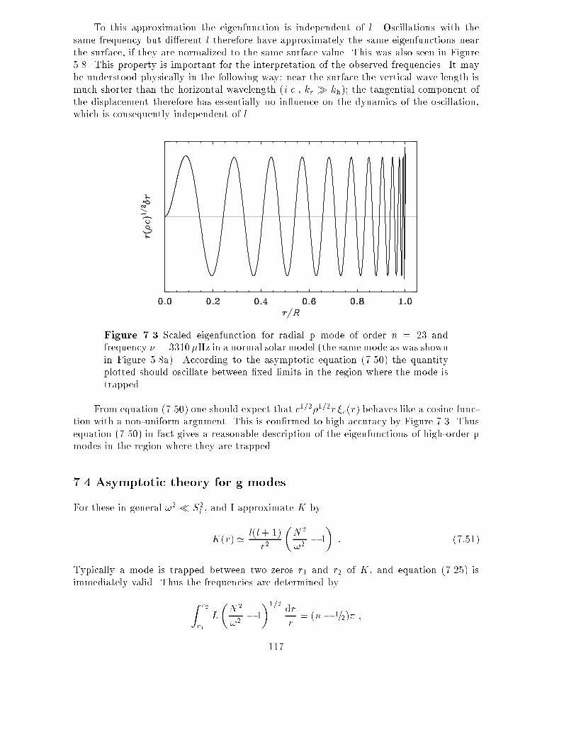
To this approximation the eigenfunction is independent of l. Oscillations with thesame frequency but di�erent l therefore have approximately the same eigenfunctions nearthe surface, if they are normalized to the same surface value. This was also seen in Figure5.8. This property is important for the interpretation of the observed frequencies. It maybe understood physically in the following way: near the surface the vertical wave length ismuch shorter than the horizontal wavelength (i.e., kr � kh); the tangential component ofthe displacement therefore has essentially no in uence on the dynamics of the oscillation,which is consequently independent of l.Figure 7.3 Scaled eigenfunction for radial p mode of order n = 23 andfrequency � = 3310�Hz in a normal solar model (the same mode as was shownin Figure 5.8a). According to the asymptotic equation (7.50) the quantityplotted should oscillate between �xed limits in the region where the mode istrapped.From equation (7.50) one should expect that c1=2�1=2r �r(r) behaves like a cosine func-tion with a non-uniform argument. This is con�rmed to high accuracy by Figure 7.3. Thusequation (7.50) in fact gives a reasonable description of the eigenfunctions of high-order pmodes in the region where they are trapped.7.4 Asymptotic theory for g modesFor these in general !2 � S2l , and I approximate K byK(r) ' l(l+ 1)r2 �N2!2 � 1� : (7:51)Typically a mode is trapped between two zeros r1 and r2 of K, and equation (7.25) isimmediately valid. Thus the frequencies are determined byZ r2r1 L�N2!2 � 1�1=2 drr = (n� 1=2)� ;117

or Z r2r1 �N2!2 � 1�1=2 drr = (n� 1=2)�L : (7:52)Here the left-hand side is solely a function of !, so that equation (7.52) can be written, inanalogy with equation (7.31), as n � 1=2L = G(!) ; (7:53)where G(!) = 1� Z r2r1 �N2!2 � 1�1=2 drr : (7:54)I have here implicitly assumed that N has a single maximum, so that there is a single,well-de�ned trapping region at each frequency. In many stellar models, including somemodels of the Sun, there may be several maxima in N , and this may give rise to, atleast mathematically, interesting phenomena. Roughly speaking, to each maximum therecorresponds asymptotically a separate spectrum of g modes; where modes correspondingto di�erent regions happen to have nearly the same frequencies, the modes may interact in\avoided crossings" (e.g. Christensen-Dalsgaard, Dziembowski & Gough 1980).In the model illustrated in Figure 5.2 N has a weak secondary maximum near r=R =0:35, and at a frequency of about 410�Hz; this is in fact faintly re ected in the behaviourof the frequencies shown in Figure 5.6, where there is an accumulation of modes at thisfrequency, for l > 15. I neglect this local maximum and assume that N has a singlemaximum, Nmax, in the interior of the Sun; from equation (7.54) it then follows thatG(!)! 0 for ! ! Nmax :Consequently ! ! Nmax for L!1 :This behaviour is clearly visible in Figures 5.6 and 5.7.For high-order, low-degree g modes ! is much smaller than N over most of the interval[r1; r2]. This suggests that a similar approximation to the one leading to equation (7.40)should be possible. In fact, the integral may be expanded near the centre, in much the sameway as the integral in equation (7.30), by using the fact that N � r near r = 0. However,the expansion near the upper turning point can apparently not be done in a similarlysimple fashion, and in any case the result does not quite have the correct dependence onl. A proper asymptotic analysis (Tassoul 1980) shows that the frequencies of low-degree,high-order g modes are given by ! = L Z r2r1 N drr�(n+ l=2 + �g) ; (7:55)where �g is a phase constant. Thus in this case the periods are asymptotically equallyspaced in the order of the mode. The spacing decreases with increasing l, as is also obviousfrom Figure 5.6. 118

The analysis was carried to the next asymptotic order by Tassoul (1980). Ellis (1988),Provost & Berthomieu (1986) and Gabriel (1986) compared the resulting expressions withnumerically computed frequencies for polytropic or solar models.In the trapping region the eigenfunction is given by equation (7.26). We may assumethat !2 � S2l , and so obtain�r(r) ' A��1=2r�1c�1=2 �Sl! �1=2 ����N2!2 � 1�����1=4 cos"L Z rr1 �N2!2 � 1�1=2 dr0r0 � �4#= A�L!�1=2 ��1=2r�3=2 ����N2!2 � 1�����1=4 cos"L Z rr1 �N2!2 � 1�1=2 dr0r0 � �4# : (7:56)Except close to the turning points r1, r2 we may assume thatN2=!2 � 1 (note, from Figure5.2, that N increases very rapidly from 0 at the centre and at the base of the convectionzone). Here, therefore,�r(r) ' AL1=2��1=2r�3=2N�1=2 cos"L Z rr1 �N2!2 � 1�1=2 dr0r0 � �4# : (7:57)Hence we expect that �1=2r3=2N1=2�r behaves like a distorted cosine function. This iscon�rmed by Figure 7.4. Thus equation (7.57), as the corresponding equation for the pmodes, gives a fairly accurate description of the eigenfunction in the trapping region.Figure 7.4 Scaled eigenfunction for high-order g mode of degree 2, radialorder n = �10 and frequency � = 104�Hz in a normal solar model (the samemode as was shown in Figure 5.10b). According to the asymptotic equation(7.57) the quantity plotted should oscillate between �xed limits in the regionwhere the mode is trapped. 119

Outside the trapping region the eigenfunction locally decays exponentially; this isalso described by saying that the mode is evanescent. In particular, g modes are alwaysevanescent in convection zones. From Figure 5.2 it follows that this evanescent region isessentially restricted to the convection zone for � < 200�Hz. At higher frequencies theevanescent region extends more deeply, and for frequencies near the maximum in N themode is oscillatory only in a narrow region around x = 0:1. Thus one would expect suchmodes to be very e�ciently trapped. To study the trapping I use the asymptotic expression(7.27b). In the convection zone we can assume that N = 0; and for low-frequency (andhigh-degree) modes I neglect !2=S2l compared with 1. Then K ' �L2=r2, and the variationin �r through the convection zone may be approximated by�r(r) ' 12 �L!�1=2 ��1=2r�3=2 exp��L Z rr2 dr0r0 � = 12 �L!�1=2 r2L��1=2r�(3=2+L) : (7:58)Thus the density decrease with increasing radius causes an increase in the amplitude, butthis is compensated for by the power law decrease represented by r�L (note that this isthe global manifestation of the locally exponential behaviour in the evanescent region). Toget an idea about the relative importance of these two e�ects I note that the radius rb atthe base of the solar convection zone is about 0.7 R, whereas the ratio between the surfacedensity and the density at the base of the convection zone is about 10�6. Thus we obtain�r(rb)=�r(R) � 10�3(0:7)�(3=2+L) � 10�2:8+0:15L : (7:59)This approximation, however, assumed the validity of the asymptotic expression (7.27b)right up to the surface. This is not true, as the assumptions underlying the analysis breakdown close to the surface where the pressure scale height becomes small. From the morecomplete asymptotic theory, to be described in the following section, it may be shown thatas a result there is an additional factor of L3=2 in equation (7.59). Thus the trapping, athigh l, is in fact substantially stronger than indicated by that equation.This analysis roughly describes the trapping of low-frequency modes. At higher fre-quencies the deepening of the evanescent region must also be taken into account, and theasymptotic analysis becomes rather complicated. Reference may be made, however, to thenumerical results presented in Figures 5.12 and 5.13. At low frequencies the increase in theinterior amplitude with degree, at �xed frequency, is roughly in accordance with the asymp-totic discussion given above. The steep increase with increasing frequency at � > 400�Hzis related to the faint local maximum in N at that frequency, which was discussed above(cf. Figure 5.2); modes with higher frequency suddenly get trapped much deeper in theSun, and their maximum amplitudes consequently rise very rapidly. For comparison onemight note that a mode with a velocity amplitude of 1m sec�1 and a period of 1 hour hasa relative surface displacement amplitude of about 10�6. Thus modes with an amplituderatio of more than 106 are not likely to be seen. Clearly there is little hope of observing gmodes of degree greater than 20.A more careful analysis than presented here would probably allow an understandingof many of the features shown in Figures 5.12 and 5.13. This would be interesting but has,as far as I know, not been undertaken so far.120

7.5 A general asymptotic expressionAn approximate asymptotic description of the oscillations has been derived by Gough (seeDeubner & Gough 1984), on the basis of earlier work by Lamb (1932). This does notassume that the pressure and density scale heights are much larger than the wavelength;but it assumes that the oscillations vary much more rapidly than r and g, so that theproblem is locally one of oscillations of a plane-parallel layer under constant gravity. Also,as usual, the perturbation in the gravitational potential is neglected. Then the governingequations are equations (5.12) and (5.13), but without the term in 2=r in the former. Whenmanipulating the equations, I neglect derivatives of r and g, but keep derivatives of thethermodynamic quantities.7.5.1 Derivation of the asymptotic expressionThe trick of the analysis is to write the equations in terms of� = div ���r : (7:60)By using the equation of continuity and the condition of adiabaticity we may also write �as � = � 1�1 �p0p � �gp �r� : (7:61)The oscillation equations can be written asd�rdr = � + 1� k2h!2 p0 ; (7:62)and dp0dr = ��!2 + gd ln �dr � �r + g�� : (7:63)In keeping with the plane-parallel approximation I have expressed l by kh, given by equation(4.45), and I assume kh to be constant.By multiplying equation (7.61) by �1p and di�erentiating we obtain, on using equations(7.62) and (7.63) d�1dr p� � �1g��+ �1pd�dr = ��!2�r + gk2h!2 p0 : (7:64)This equation, together with equation (7.61), can be used to express �r in terms of � andits �rst derivative. The result is��g � !4gk2h� �r = �1 �p� + !2gk2h �pd�dr � g��+ pd ln �1dr ��� : (7:65)Finally, by di�erentiating equation (7.64) and using equations (7.62), (7.63) and (7.65)to eliminate �r, p0 and their derivatives, we obtain the following second-order di�erentialequation for �:d2�dr2 + � 2c2 dc2dr + 1� d�dr� d�dr+ � 1�1 d2�1dr2 � 2�1 d�1dr g�p + k2h�N2!2 � 1� � 1� d�dr 1�1 d�1dr + �!2�1p�� = 0 : (7:66)121

Here I have introduced the adiabatic sound speed c from equation (3.49) and the buoyancyfrequency N from equation (3.67).The di�erential equation for � contains no interior singular points. However, it is clearfrom equation (7.65) that the case where the coe�cient to �r vanishes is in some sensesingular. This occurs when !2 = gkh : (7:67)It is easy to show that then the solution for � to equation (7.65) grows exponentially towardsthe interior; as this is clearly unacceptable, � must be zero. Then equation (7.61) givesp0 = g��r ; (7:68)and equation (7.62) has the solution �r = a exp(khr) ; (7:69)where a is an arbitrary constant. It is easy to show that the resulting p0 satis�es equation(7.63). Thus this is one possible solution to the plane-parallel oscillation equations. Itshould be noticed that equation (7.67) agrees with equation (3.78) for the frequency of asurface gravity wave. Thus the mode we have found must be identi�ed with a surface gravitywave; and we have shown that its frequency is independent of the structure of the modelbelow the surface, if sphericity is neglected. This result was �rst obtained by Gough. It isobvious from Figure 5.6 that the mode can be followed to degrees well below 10, althoughhere the correction to the frequency given by equation (7.67) becomes signi�cant.To analyze equation (7.66) it is convenient to eliminate the term in d�=dr. Thus Iintroduce X by X = c2�1=2� : (7:70)After considerable manipulation one then �nds that X satis�es the di�erential equationd2Xdr2 + �k2h �N2!2 � 1� + !2c2 � 12 ddr (H�1)� 14H�2�X = 0 ; (7:71)where I have introduced the density scale height H byH�1 = �d ln �dr : (7:72)Finally, I de�ne a characteristic frequency !c by!2c = c24H2 �1� 2dHdr � ; (7:73)and use equation (4.53) for the acoustic frequency Sl, to obtaind2Xdr2 + 1c2 �S2l �N2!2 � 1�+ !2 � !2c�X = 0 : (7:74)122

Figure 7.5. The acoustical cut-o� frequency !c de�ned in equation (7.73)(solid line), and the approximation !a appropriate to an isothermal region[cf. equation (5.36); dashed line] in the outermost parts of a normal model ofthe present Sun.This is the �nal second-order di�erential equation. Considering that the only approxima-tions made in deriving it are the constancy of g and the neglect of the derivatives of r, it isremarkably simple.It might be noticed that equation (7.74) can also be derived from a careful analysis ofthe propagation of waves in stellar interiors. This has been carried out by Gough (1986a).Notice that if H is constant (as was assumed in section 5.4), equation (7.73) for !creduces to the frequency !a de�ned in equation (5.36). Thus !c, as introduced here, gen-eralizes the acoustical cut-o� frequency de�ned for the isothermal atmosphere. Figure 7.5shows !c and !a in the outer parts of a normal solar model; they are in fact quite similar,except in a thin region very near the top of the convection zone, where the rapid variationin the superadiabatic gradient causes large excursions in !c.Near the surface S2l is small, and the coe�cient to X in equation (7.74) is dominatedby the last two terms; hence X is exponential when !2 < !2c . This provides the trappingof the modes at the surface. In the interior !2c (which roughly varies as g2=T ) is generallysmall, below about 600�Hz in models of the present Sun.We may write equation (7.74) asd2Xdr2 +K(r)X = 0 ; (7:75)where K(r) = !2c2 �1� !2c!2 � S2l!2 �1� N2!2 �� � !2c2 1� !2l;+!2 ! 1� !2l;�!2 ! ; (7:76)123

de�ning the characteristic frequencies !l;+ and !l;�. They are plotted in Figure 7.6, ina model of the present Sun. Equation (7.76) shows that the trapping of the modes isdetermined by the value of the frequency, relative to behaviour of !l;+ and !l;�. In theinterior of the Sun, particularly for large l,!l;+ ' Sl ; !l;� ' N : (7:77)Thus here we recover the conditions for trapping discussed in section 5.2.2. This wasindeed to be expected, as the assumptions entering the present formulation provide a naturaltransition from the previously discussed simpli�ed asymptotic treatment to the atmosphericbehaviour of the oscillations. On the other hand, near the surface where Sl=! � 1!l;+ ' !c ; (7:78)while !l;� is small. Thus the trapping near the surface is controlled by the behaviour of !l;+.As shown in Figure 7.6 trapping extends in frequency up to about 5:3mHz, although thespike in !l;+ just beneath the photosphere provides some partial re ection at even higherfrequency. Also, modes with frequency � >� 2mHz propagate essentially to the photosphere,while modes of lower frequency are re ected at some depth in the convection zone. Thisbehaviour is visible in the eigenfuctions shown in Figure 5.9; also it is largely responsiblefor the transition of the mode energy normalized with the surface displacement, shown inFigure 5.11, from steep decrease to near constancy with increasing frequency.Figure 7.6. Characteristic frequencies !l;+=(2�) (continuous curves) and!l;�=(2�) (dashed curves) for a model of the present Sun [cf. equation (7.76)].The curves are labelled with the degree l. The right-hand panel shows theoutermost parts of the model on an expanded horizontal scale. The �guremay be compared with the simple characteristic frequencies plotted in Figure5.2. 124

7.5.2 The Duvall law for p-mode frequenciesWe may apply the JWBK analysis discussed in section 7.1 to equation (7.74). Thus theasymptotic expression (7.25) for the frequency gives! Z r2r1 �1� !2c!2 � S2l!2 �1� N2!2 ��1=2 drc ' �(n� 1=2) ; (7:79)where r1 and r2 are adjacent zeros of K such that K > 0 between them.This expression is now also formally valid for p modes. Given the rapid variation of !l;+near the surface its practical validity might be questioned. Christensen-Dalsgaard (1984c)evaluated the left-hand side of equation (7.79), substituting computed eigenfrequenciesfor !, and found that the deviations from the asymptotic relation were relatively modest;however, substantially better agreement is obtained if !c is replaced by the simple expressionfor an isothermal atmosphere, given in equation (5.36).Equation (7.79) may be used to justify the approximate relation (7.29) for the fre-quencies of acoustic modes, with � = �(!) being a function of frequency (see also Deubner& Gough 1984). Here I present an argument derived by Christensen-Dalsgaard & P�erezHern�andez (1992). Assuming that the term in N2 can be neglected, I write equation (7.79)as �(n� 1=2)! 'F �!L�� 1! (I1 + I2 + I3) ; (7:80)where F (w) = Z Rrt �1� c2w2r2�1=2 drc ; (7:81)and the dimensionless integrals I1 � I3 are de�ned byI1 =! Z Rr2 �1� S2l!2�1=2 drc ; (7:82)I2 =! Z r2r1 "�1� S2l!2�1=2 � �1� !2c!2 � S2l!2�1=2# drc ; (7:83)I3 =! Z r1rt �1� S2l!2�1=2 drc : (7:84)I assume that !2c > 0 in the vicinity of the lower turning point, so that rt < r1 [where rt isgiven by equation (5.24)]; also I have assumed that R > r2 for all modes of interest.To show that equation (7.30) is approximately valid, with � being a function of !, wemust show that I1 + I2 + I3 is predominantly a function of frequency. In so doing I makethe assumptions:� S2l =!2 � 1 at the upper turning point.� !2c=!2 � 1 at the lower turning point. 125

Near the upper turning point we may then neglect the term in S2l =!2, and hence the positionof the turning point is approximately given by r2 ' Rt, where Rt is de�ned by ! = !c(Rt).Thus r2 is a function of frequency alone; the same is therefore obviously true for I1. I3 issmall; in fact, by expanding S2l in the vicinity of rt, neglecting the variation in !c and c, itis straightforward to show thatI3 ' 13 �!c;t! �3 !Hc;tct � �!c;t! �2 ; (7:85)where !c;t, ct and Hc;t are the values of !c, c and the sound-speed scale height at rt. Thus,although I3 depends on rt and hence on !=L, the term is O((!c=!)2) and hence negligible.This leaves I2 to be dealt with. To investigate its dependence on l and ! I rewrite itasI2 =! Z r2r1 "�1� S2l!2�1=2 � �1� !2c!2 � S2l!2�1=2#"�1� S2l!2�1=2 + �1� !2c!2 � S2l!2�1=2#�1� S2l!2�1=2 + �1� !2c!2 � S2l!2�1=2 drc= 1! Z r2r1 !2c�1� S2l!2�1=2 + �1� !2c!2 � S2l!2�1=2 drc : (7:86)Since !2c=c decreases quite rapidly with increasing depth (cf. Figure 7.5), this integral isdominated by the region near the upper turning point r2. It is true that the integrand isnearly singular, with an integrable singularity, at r = r1; but the contribution from thatis essentially O(!2c;t=!2) and is therefore small. Near r2, S2l =!2 is negligible; thus we canapproximate I2 as I2 ' 1! Z r2r1 !2c1 + �1� !2c!2�1=2 drc ; (7:87)which is obviously a function of frequency alone.It follows that equation (7.80) may �nally be written asZ Rrt �1� L2c2!2r2�1=2 drc = [n+ �(!)]�! ; (7:88)with � ' �(!) = 1� (I1 + I2)� 1=2 : (7:89)This argument is evidently valid in general for stellar models where !2c=c decreases su�-ciently rapidly with increasing depth.It is instructive consider the analysis for the special case where the outer layers of thestar can be approximated by an adiabatically strati�ed, plane-parallel layer; also I neglectthe variation of �1. Then we obtain equation (7.34) for c, and furthermore!2c = g�p4(R� r) �1 + 2�p� ; (7:90)126

where �p = 1=(�1 � 1) is the e�ective polytropic index of the layer. Finally N is zero.From equation (7.90) !c is small except near the surface, and so it is reasonable to neglectit in most of the region where the p mode is trapped (notice, however, that this becomesquestionable for high l, where the trapping region is con�ned very close to the surface).To approximate equation (7.79) I use a trick similar to that employed to derive equation(7.40). Thus I write equation (7.79) as�(n� 1=2)! = Z Rr1 �1� S2l!2�1=2 drc � Z Rr2 �1� S2l!2�1=2 drc� Z r2r1 "�1� S2l!2�1=2 � �1� !2c!2 � S2l!2�1=2# drc : (7:91)Here, approximately, r2 is given by !c(r2) = !, and is therefore close to the surface.Furthermore, the dominant contribution to the third integral in question (7.91) comes fromthe region near r2. In the last two integrals I therefore use the approximations (7.34) and(7.90) for c and !c; furthermore I neglect the variation of r in Sl. These integrals may then,with a little e�ort, be evaluated analytically. The result is�(n� 12 )! = Z Rr1 �1� S2l!2�1=2 drc � 12[�p(�p + 2)]1=2 �! : (7:92)This may also be written as equation (7.30), with� = 1=2[�p(�p + 2)]1=2 � 1=2 : (7:93)Thus in this case � is a constant which is related to the e�ective polytropic index of thesurface layers.Exercise 7.3:Derive equation (7.92).If the entire layer is polytropic, with equation (7.30) and (7.90) everywhere valid, equa-tion (7.74) may be solved analytically (e.g. Christensen-Dalsgaard 1980). The conditionthat the solution decreases exponentially at great depths determines the eigenfrequenciesas !2 = 2�p �n + �p2 �L gR : (7:94)This is in accordance with equation (7.36) obtained asymptotically, but with a di�erent �,� = �p2 : (7:95)It is easy to show that the di�erence between this exact � and the asymptotic approximationin equation (7.93) is small; it tends to zero for large �p.127

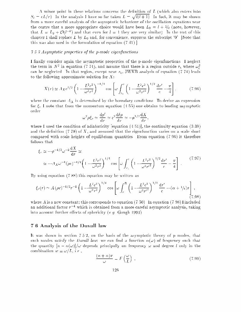
A minor point in these relations concerns the de�nition of L (which also enters intoSl = cL=r). In the analysis I have so far taken L = pl(l+ 1). In fact, it may be shownfrom a more careful analysis of the asymptotic behaviour of the oscillation equations nearthe centre that a more appropriate choice would have been L0 = l + 1=2 (note, however,that L = L0 + O(l�1) and that even for l = 1 they are very similar). In the rest of thischapter I shall replace L by L0 and, for convenience, suppress the subscript `0'. [Note thatthis was also used in the formulation of equation (7.41).]7.5.3 Asymptotic properties of the p-mode eigenfunctionsI �nally consider again the asymptotic properties of the p-mode eigenfunctions. I neglectthe term in N2 in equation (7.74), and assume that there is a region outside rt where !2ccan be neglected. In that region, except near rt, JWKB analysis of equation (7.74) leadsto the following approximate solution for X :X(r) ' AXc1=2 �1� L2c2!2r2��1=4 cos"! Z rrt �1� L2c2!2r02�1=2 dr0c � �4# ; (7:96)where the constant AX is determined by the boundary conditions. To derive an expressionfor �r I note that from the momentum equation (4.55) one obtains to leading asymptoticorder !2��r ' dp0dr ' c2d��dr ' ��1=2dXdr ;where I used the condition of adiabaticity [equation (4.51)], the continuity equation (3.39)and the de�nition (7.70) of X , and assumed that the eigenfunction varies on a scale shortcompared with scale heights of equilibrium quantities. From equation (7.96) it thereforefollows that�r '� ��1=2!�2 dXdr ''� AX!�1(�c)�1=2�1� L2c2!2r2�1=4 cos"! Z rrt �1� L2c2!2r02�1=2 dr0c + �4# : (7:97)By using equation (7.88) this equation may be written as�r(r) ' A (�c)�1=2r�1 �1� L2c2!2r2�1=4 cos"! Z Rr �1� L2c2!2r02�1=2 dr0c � (�+ 1=4)�# ;(7:98)where A is a new constant; this corresponds to equation (7.50). In equation (7.98) I includedan additional factor r�1 which is obtained from a more careful asymptotic analysis, takinginto account further e�ects of sphericity (e.g. Gough 1993).7.6 Analysis of the Duvall lawIt was shown in section 7.5.2, on the basis of the asymptotic theory of p modes, thatsuch modes satisfy the Duvall law: we can �nd a function �(!) of frequency such thatthe quantity [n + �(!)]=! depends principally on frequency ! and degree l only in thecombination w � !=L, i.e., (n+ �)�! = F �!L� ; (7:99)128

where L = pl(l+ 1). Here the function F (!=L) is related to the adiabatic sound speedc(r) by F (w) = Z lnRln rt(w) �1� a2w2�1=2 a�1d ln r ; (7:100)where a = c=r. Also, the function �(!) is primarily determined by conditions near thestellar surface. As illustrated in Figure 7.1 the observed frequencies of solar oscillationsatisfy a relation of the form given in equation (7.99) quite accurately. This suggests thatthese relations are useful tools for analysing solar oscillation frequencies. It should benoted, however, that they are only approximately valid. In fact, a much more precise �tto the observed frequencies can be obtained by including additional terms (e.g. Gough &Vorontsov 1995) which take into account the e�ect of the perturbation in the gravitationalpotential (signi�cant at low degree) and the dependence of the modes on degree near theupper turning point (important at high degree).In this section I illustrate some properties of the Duvall law by applying it to frequen-cies computed for solar models, as well as to observed frequencies. The results are basedon computations by Christensen-Dalsgaard, Pro�tt & Thompson (1993) who consideredboth normal solar models and models which included e�ects of di�usion and gravitationalsettling of helium; recent opacity tables (Iglesias, Rogers & Wilson 1992) and a reasonableapproximation to the equation of state were used. Thus the results illustrate both howwell modern solar models �t the observed frequencies and the sensitivity of such analysesto relatively subtle features of the model calculations, such as gravitational settling.7.6.1 The di�erential form of the Duvall lawA very powerful relation can be obtained by considering the e�ect on equation (7.88) ofsmall changes to the equilibrium structure. I consider two cases (two solar models or a solarmodel and the Sun) with the same surface radius, labelled with the superscripts (1) and(2), and introduce the di�erences �!nl = !(2)nl � !(1)nl , �rc(r) = c(2)(r)� c(1)(r) and ��(!) =�(2)(!)� �(1)(!). By substituting c(2)(r) = c(1)(r) + �rc(r) and �(2)(!) = �(1)(!) + ��(!)into equation (7.88), retaining only terms linear in �rc, �� and �!, one obtainsSnl �!nl!nl ' Z Rrt �1� c2L2!2nlr2��1=2 �rcc drc + � ��(!nl)!nl ; (7:101)where Snl = Z Rrt �1� L2c2r2!2nl��1=2 drc � �d�d! ; (7:102)and I have suppressed the superscript (1). This relation was �rst obtained by Christensen-Dalsgaard, Gough & P�erez Hern�andez (1988).Exercise 7.4:Derive equation (7.101). If initially you obtain a di�erent result, you may be in goodcompany: so did the referee of Christensen-Dalsgaard et al. (1988).129

Figure 7.7. The solid lines show the inertia ratio Qnl, de�ned in equation(5.79), against �=(l+ 1=2) in a normal solar model, each curve correspondingto a given degree l. The upper abscissa shows the turning-point radius rt,related to �=(l+ 1=2) through equation (5.24). The heavy dashed curve showsthe asymptotic scaling ~Snl=�0, where ~Snl is de�ned as in equation (7.102) butneglecting the term in d�=d!.Equation (7.101) may be written asSnl �!nl!nl ' H1 �!nlL �+H2(!nl) ; (7:103)where H1(w) = Z Rrt �1� c2r2w2��1=2 �rcc drc ; (7:104)and H2(!) = �!��(!) : (7:105)Some properties of this equation were discussed by Christensen-Dalsgaard, Gough & P�erezHern�andez (1988) and by Christensen-Dalsgaard et al. (1989). As pointed out in the latterpaper, H1(!=L) and H2(!) can be obtained separately, to within a constant, by means of adouble-spline �t of the expression (7.103) to p-mode frequency di�erences. The dependenceof H1 on !=L is determined by the sound-speed di�erence throughout the star, whereasH2(!) depends on di�erences in the upper layers of the models.There is a close analogy between equation (7.103) and the `exact' equation (5.81).Indeed, one �nds that the scaling Qnl in that equation is asymptotically equal to Snl=S0,where S0 = limw!0 S(w) (Christensen-Dalsgaard 1991b); one may show that S0 = �0 where�0 = Z R0 drc (7:106)130

is the acoustical radius of the star. The close correspondence between Qnl and Snl=�0 isillustrated in Figure 7.7. Furthermore, the term G(!) in equation (5.81) to some extentcorresponds to the termH2(!) in equation (7.103), in that both terms contain contributionsfrom the uncertain regions very near the stellar surface. However, as discussed in section7.6.3 below H2 may also be used to gain information about somewhat deeper regions.Since c=r decreases quite rapidly with increasing r, (Lc=r!)2 � 1 except near theturning point rt; hence as a rough approximation 1 � L2c2=r2!2 may be replaced by 1 inthe integrals in equations (7.101) and (7.102). If furthermore the terms in �� and d�=d!can be neglected, the result is the very simple relation between the changes in sound speedand frequency: �!! ' Z Rrt �rcc drcZ Rrt drc : (7:107)This shows that the change in sound speed in a region of the Sun a�ects the frequencywith a weight determined by the time spent by the mode, regarded as a superposition oftraveling waves, in that region. Thus changes near the surface, where the sound speed islow, have relatively large e�ects on the frequencies. Although this expression is only a roughapproximation, it is a useful guide in attempts to interpret frequency di�erences betweenmodels, or between observed and computed frequencies.Figure 7.8. Fractional di�erence in sound speed between a model of thepresent Sun with di�usion and a normal model, without di�usion. FromChristensen-Dalsgaard, Pro�tt & Thompson (1993).To illustrate the behaviour of the separation in equation (7.103) I consider di�erencesbetween two models of Christensen-Dalsgaard et al. (1993): a model with di�usion andsettling and a normal solar model. Figure 7.8 shows the sound-speed di�erence betweenthese models. It is dominated by the fact that the convection zone is slightly deeper in themodel with di�usion: since the temperature and sound-speed gradients are steeper in theconvection zone than in the radiative region below, there is a region where the sound speedincreases more rapidly with depth in the di�usive model, and this leads to the behaviourseen in the �gure. Furthermore, due to settling of helium out of the convection zone the131

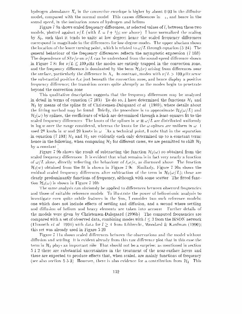
hydrogen abundance Xe in the convective envelope is higher by about 0.03 in the di�usivemodel, compared with the normal model. This causes di�erences in �1, and hence in thesound speed, in the ionization zones of hydrogen and helium.Figure 7.9a shows scaled frequency di�erences, at selected values of l, between these twomodels, plotted against �=L (with L = l + 1=2; see above). I have normalized the scalingby S0, such that it tends to unity at low degree; hence the scaled frequency di�erencescorrespond in magnitude to the di�erences for low-degree modes. The upper abscissa showsthe location of the lower turning point, which is related to !=L through equation (5.24). Thegeneral behaviour of the frequency di�erences re ects the asymptotic expression (7.103).The dependence of S��=� on �=L can be understood from the sound-speed di�erence shownin Figure 7.8: for �=L <� 100�Hz the modes are entirely trapped in the convection zone,and the frequency di�erence is dominated by the term H2(�) arising from di�erences nearthe surface, particularly the di�erence in Xe. In contrast, modes with �=L > 100�Hz sensethe substantial positive �rc just beneath the convection zone, and hence display a positivefrequency di�erence; the transition occurs quite abruptly as the modes begin to penetratebeyond the convection zone.This qualitative description suggests that the frequency di�erences may be analyzedin detail in terms of equation (7.103). To do so, I have determined the functions H1 andH2 by means of the spline �t of Christensen-Dalsgaard et al. (1989), where details aboutthe �tting method may be found. Brie y, the procedure is to approximate H1(!=L) andH2(!) by splines, the coe�cients of which are determined through a least-squares �t to thescaled frequency di�erences. The knots of the splines in w � !=L are distributed uniformlyin logw over the range considered, whereas the knots for the !-splines are uniform in !. Iused 28 knots in w and 20 knots in !. [As a technical point, I note that in the separationin equation (7.103) H1 and H2 are evidently each only determined up to a constant term;hence in the following, when comparing H2 for di�erent cases, we are permitted to shift H2by a constant.]Figure 7.9b shows the result of subtracting the function H2(!) so obtained from thescaled frequency di�erences. It is evident that what remains is in fact very nearly a functionof !=L alone, directly re ecting the behaviour of �rc=c, as discussed above. The functionH1(w) obtained from the �t is shown in Figure 7.9c. Similarly, Figure 7.10a shows theresidual scaled frequency di�erences after subtraction of the term in H1(!=L); these areclearly predominantly functions of frequency, although with some scatter. The �tted func-tion H2(!) is shown in Figure 7.10b.The same analysis can obviously be applied to di�erences between observed frequenciesand those of suitable reference models. To illustrate the power of helioseismic analysis toinvestigate even quite subtle features in the Sun, I consider two such reference models:one which does not include e�ects of settling and di�usion, and a second where settlingand di�usion of helium and heavy elements are taken into account. Further details ofthe models were given by Christensen-Dalsgaard (1996b). The computed frequencies arecompared with a set of observed data, combining modes with l � 3 from the BiSON network(Elsworth et al. 1994) with data for l � 4 from Libbrecht, Woodard & Kaufman (1990);this set was already used in Figure 5.20.Figure 7.11a shows scaled di�erences between the observations and the model withoutdi�usion and settling. It is evident already from this raw di�erence plot that in this case theterm in H2 plays an important role. That should not be a surprise: as mentioned in section5.1.2 there are substantial uncertainties in the treatment of the near-surface layers andthese are expected to produce e�ects that, when scaled, are mainly functions of frequency(see also section 5.5.3). However, there is also evidence for a contribution from H1. This132

Figure 7.9. Scaled frequency di�erences corresponding to the model di�er-ences shown in Figure 7.8, plotted against �=(l + 1=2). The upper abscissashows the location of the lower turning point, which is related to �=(l + 1=2)through equation (5.24). In panels (a) and (b) points corresponding to �xedl have been connected. (a) Original scaled frequency di�erences. (b) Scaleddi�erences, after subtraction of the function H2(!) obtained from the spline�t. (c) The �tted function H1(!=L).133

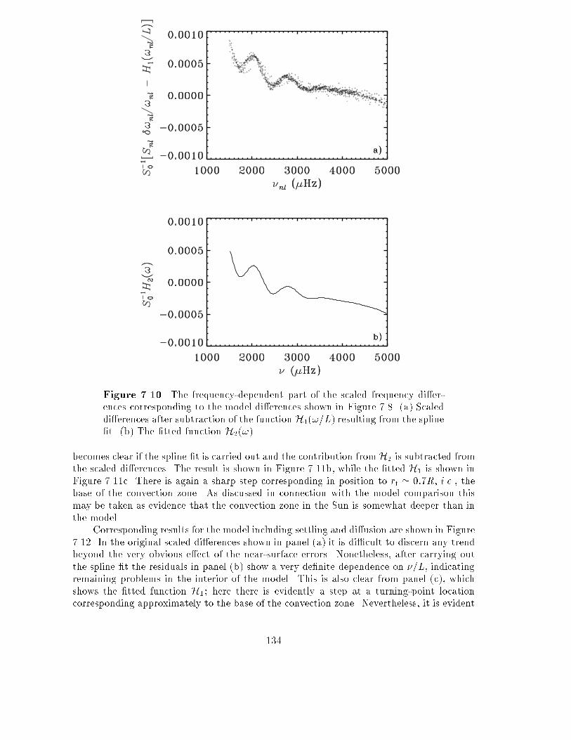
Figure 7.10. The frequency-dependent part of the scaled frequency di�er-ences corresponding to the model di�erences shown in Figure 7.8. (a) Scaleddi�erences after subtraction of the function H1(!=L) resulting from the spline�t. (b) The �tted function H2(!).becomes clear if the spline �t is carried out and the contribution fromH2 is subtracted fromthe scaled di�erences. The result is shown in Figure 7.11b, while the �tted H1 is shown inFigure 7.11c. There is again a sharp step corresponding in position to rt ' 0:7R, i.e., thebase of the convection zone. As discussed in connection with the model comparison thismay be taken as evidence that the convection zone in the Sun is somewhat deeper than inthe model.Corresponding results for the model including settling and di�usion are shown in Figure7.12. In the original scaled di�erences shown in panel (a) it is di�cult to discern any trendbeyond the very obvious e�ect of the near-surface errors. Nonetheless, after carrying outthe spline �t the residuals in panel (b) show a very de�nite dependence on �=L, indicatingremaining problems in the interior of the model. This is also clear from panel (c), whichshows the �tted function H1; here there is evidently a step at a turning-point locationcorresponding approximately to the base of the convection zone. Nevertheless, it is evident134

Figure 7.11. Scaled frequency di�erences between observed frequencies (seetext) and a solar model neglecting settling and di�usion, in the sense (obser-vations) { (model), plotted against �=(l+ 1=2). The upper abscissa shows thelocation of the lower turning point, which is related to �=(l + 1=2) throughequation (5.24). In panels (a) and (b) points corresponding to �xed l havebeen connected. (a) Original asymptotically scaled frequency di�erences. (b)Scaled di�erences, after subtraction of the function H2(!) obtained from thespline �t. (c) The �tted function H1(!=L).135

Figure 7.12. Scaled frequency di�erences between observed frequencies (seetext) and a solar model including settling and di�usion, in the sense (obser-vations) { (model), plotted against �=(l+ 1=2). See caption to Figure 7.11.136

Figure 7.13. The frequency-dependent part of the scaled frequency dif-ferences between observations and models. (a) Scaled di�erences, shown inFigure 7.11a, after subtraction of the function H1(!=L) resulting from thespline �t. (b) The solid line shows the �tted function H2(!) for this data set,while the dashed line shows the corresponding �tted function obtained fromthe di�erences in Figure 7.12a.even from this simple analysis that the inclusion of di�usion and settling very substantiallyimproves the agreement between the model and the Sun.It is evident that there is considerably more scatter in Figure 7.11b than in the cor-responding Figure 7.9b. This is due to observational errors, both random and systematic.In particular, it may be noticed that there is an apparent break at around �=L ' 15�Hz.In fact, the observed frequencies were obtained from two separate sets of observations, themerge taking place at l = 400; it has later been found that there were slight systematicerrors in the high-degree set. This di�culty is clearly re ected in the �tted H1(!=L) inFigure 7.11c. Furthermore, there appears to be problems at low degree, corresponding tothe highest values of �=L. 137

The residual after subtraction of the �tted H1 from the scaled di�erences, and the�tted H2, are shown in Figure 7.13. In panel (a) are shown the residuals for the modelneglecting di�usion and settling. As before, these are indeed predominantly a function offrequency. They are dominated by a slowly varying trend which, as argued in section 7.6.3below re ects errors in the near-surface region of the model. However, there is also a weakbut clearly noticeable oscillatory signal. As discussed in section 7.6.3 this probably re ectsa di�erence between the Sun and the model in the hydrogen abundance in the convectiveenvelope. This oscillatory behaviour is also very evident in the �tted H2(!), shown as asolid line in panel (b). In contrast, H2(!) for the model with settling and di�usion, shownas a dashed line, gives very little evidence for such oscillations, indicating that the envelopehydrogen abundance for this model is quite similar to that of the Sun.7.6.2 Inversion of the Duvall lawThe function F (w) in equation (7.99) can be determined from the observations (cf. Figure7.1). Given F , equation (7.100) is an integral equation of the Abel type, and can be invertedanalytically to obtain the sound speed implicitly, thus:r = R exp �� 2� Z aas �w�2 � a�2��1=2 dFdw dw� (7:108)(Gough 1984). This relation was used by Christensen-Dalsgaard et al. (1985) to infer thesound speed in the solar interior. The properties of this inversion technique were discussedin considerable detail by Gough (1986b).Exercise 7.5:Con�rm that equation (7.108) is a solution to equation (7.100). This is most simplydone by substituting equation (7.100) into equation (7.108).The asymptotic description leading to equation (7.108) clearly su�ers from systematicerrors. It has been found, for example, that for the most deeply penetrating modes of lowdegree the perturbation to the gravitational potential has a substantial e�ect on the func-tions F (!=L) obtained by �tting the relation (7.99) to computed or observed frequencies;this may cause problems for the inversion in the solar core. Also, for modes trapped near thesurface the behaviour near the upper turning point depends on the degree; this introduceswhat is e�ectively an l-dependent term in �. It is possible to generalize equation (7.99) totake such e�ects into account and hence obtain a substantially more precise inversion (e.g.Vorontsov & Shibahashi 1991).Alternatively, it appears that the systematic errors cancel to some extent when di�er-ences are taken between inversions of di�erent sets of frequencies. Christensen-Dalsgaardet al. (1985) made use of this by considering di�erences between inversions done for thesolar data and for frequencies for a reference model. A more systematic approach followsfrom the separation of scaled frequency di�erences in equation (7.103). Here the functionH1(!=L) is related to the sound-speed di�erence between the models, or between the Sunand the model, through equation (7.104). As shown by Christensen-Dalsgaard, Gough &138

Thompson (1989), given a determination of H1, that equation is an integral equation for�rc=c, with the solution�rcc = �2a� dd ln r Z aas (a2 � w2)�1=2H1(w)dw ; (7:109)where as = a(R). [It should be noticed that the right-hand side of equation (7.104) isthe same functional of w as that which arises in the asymptotic expression for the linearfrequency splitting due to latitudinally-independent rotation at a rate (r), with �rc=cinstead of (Gough 1984). Thus it can be inverted in the same way.]Figure 7.14. The solid line shows the di�erence in squared sound speed�rc2=c2 inferred by applying equation (7.109) to the function H1(!=L) shownin Figure 7.9c. For comparison, the dashed line shows the true di�erencebetween the two models. Adapted from Christensen-Dalsgaard, Pro�tt &Thompson (1993).Christensen-Dalsgaard et al. (1989) carried out a careful test of the di�erential method,as applied to several di�erent pairs of models. Also, Christensen-Dalsgaard, Gough &Thompson (1988) used the method to invert di�erences between observed frequencies andfrequencies computed for a solar model. Here I illustrate its properties by applying it to themodel pair shown in Figure 7.8 and to di�erences between solar and computed frequenciessuch as those shown in Figures 7.11 and 7.12.Figure 7.14 shows the �rc2=c2 inferred from the scaled frequency di�erences in Figure7.9 between the di�usive and the normal solar model, by applying equation (7.109) tothe �tted function H1(!=L) shown in Figure 7.9c. For comparison, the �gure also showsthe true sound-speed di�erence, previously plotted in Figure 7.8. It is evident that theinversion reproduces the main features of the true �rc2=c2 which considerable precision.One noticeable di�erence is that the transition at the base of the convection zone is lesssharp: as discussed in section 9.1 it is a general property of inverse analyses that they smooththe properties of the true structure. However, otherwise the inferred and the true �rc2=c2are quite close over the entire range, 0:2R < r < 0:95R, where the solution is plotted. Atsmaller and larger radii the systematic errors associated with the asymptotic representationincreasingly a�ects the results; hence here the solution has not been obtained.139

Figure 7.15. The dotted line shows the di�erence in squared sound speed�rc2=c2 between the Sun and a solar model without di�usion and settling, in-ferred by applying equation (7.109) to the function H1(!=L) shown in Figure7.11c, corresponding to di�erences between observed and model frequencies.The solid line shows the corresponding �rc2=c2 between the Sun and a modelincluding di�usion and gravitational settling, obtained from H1(!=L) in Fig-ure 7.12c.From the frequency di�erences illustrated in Figures 7.11 and 7.12 we may now inferthe error in the sound speed in the solar models. Figure 7.15 shows the results of evaluating�rc=c by applying equation (7.109) to the H1(!=L) shown in Figures 7.11c and 7.12c. Thesound-speed di�erences are small, corresponding to errors in T=� in the models of generallyless than 2 per cent. Nonetheless, the di�erences are clearly highly systematic. It is inter-esting that the relatively subtle, and often neglected, e�ect of gravitational settling leadsto a substantial improvement in the agreement between the model and the observations,largely by increasing the depth of the convection zone in the model. This is a strikingillustration of the power of helioseismology to probe the details of the solar interior. How-ever, it should also be pointed out that modest modi�cations in the opacity, well within theprecision of current opacity tables, might introduce changes in the sound speed of similarmagnitude. The separation of opacity uncertainties from e�ects of di�usion and settlingis a major challenge, which will undoubtedly require better physical understanding of theprocesses involved.The cause of the dominant di�erence between the Sun and the nondi�usive model isprobably that the depth of the convection zone in the model is too small. In fact, themodel with di�usion has a slightly deeper convection zone. From a more careful analysisof such results of inversions it is possible to obtain an estimate of the convection-zonedepth db which is largely independent of other uncertainties in the model. In this wayChristensen-Dalsgaard, Gough & Thompson (1991) found that db = (0:713� 0:003)R.It should �nally be mentioned that several other techniques have been developed to in-vert the Duvall law (7.99) (Brodsky & Vorontsov 1987, 1988a; Shibahashi 1988; Shibahashi& Sekii 1989). Gough & Thompson (1991) have made a comparison of these di�erent tech-niques. The results suggest that, at least for the cases considered, the di�erential techniquedescribed here is superior. Nonasymptotic inversion of similar data sets will be discussedin Section 9.2. 140

7.6.3 The phase-function di�erence H2(!)The function H2(!) is predominantly determined by the region near the stellar surface.Christensen-Dalsgaard & P�erez Hern�andez (1992) analyzed the relation of H2(!) to thedi�erences in sound speed and �1 in the outer parts of the Sun: di�erences localized verynear the surface give rise to a component ofH2 that varies slowly with !, whereas di�erencesat somewhat greater depth introduce an oscillatory variation with ! in H2, the \frequency"of which increases with the depth of the di�erence. This is in fact a general property offrequency di�erences caused by sharply localized modi�cations to stellar structure (e.g.Thompson 1988; Vorontsov 1988; Gough 1990), and re ects the variation with frequencyin the phase of the eigenfunction at the location of the modi�cation. At the surface thebehaviour of the eigenfunction changes slowly with frequency, whereas at greater deptha change in frequency causes the eigenfunction to \sweep through" the point where themodel was changed, causing a rapid variation in the frequency change. In the case of thevariation of H2 with !, Christensen-Dalsgaard & P�erez Hern�andez (1991) found severalcases where the relatively sharp change in �1 in the second helium ionization zone causedan oscillatory behaviour of H2(!). Similar variations in the basic phase function �(!) wereanalyzed, for example, by Brodsky & Vorontsov (1988b, 1989) and Baturin & Mironova(1990). Vorontsov, Baturin & Pamyatnykh (1992) showed how the phase could be separatedin a quantitative fashion into components varying slowly and rapidly with frequency. Thistype of analysis provides a powerful diagnostic of the properties of the ionization zones ofhydrogen and helium, of great interest both for the analysis of the equation of state andfor attempts to determine the helium abundance of the solar convection zone.It is very convenient to express H2(!) in terms of di�erences between two models, orthe Sun and a model, in a form analogous to equation (5.81). Christensen-Dalsgaard &P�erez Hern�andez (1992) showed that �(!), and hence H2(!), can be determined directlyfrom the model structure, without computing full modes of oscillation. In this way theywere able to �nd kernels relating H2 to the model changes. The kernels turn out to beparticularly simple if the model changes are expressed in terms of c and the (isothermal)acoustical cut-o� frequency !a = c2Hp = �1g2c (7:110)[cf. equation (5.36)]. Thus I express H2 asH2(!) = Z Rr0 �Kc(r;!)�rcc +K!a(r;!)�r!a!a �dr + G2(!) ; (7:111)where r0 is a point suitably deep in the convection zone. Here, as in equation (5.81), theterm G2(!) contains the contributions from the di�erences (or errors) in the physics of theoscillations: as argued in section 5.5.3 such errors are likely to be con�ned very close to thestellar surface and hence probably depend on frequency alone, when properly scaled.The kernel Kc varies slowly with position and frequency, and hence give little interest-ing contribution to H2. On the other hand, the kernels K!a have a very distinct behaviour.This is illustrated in Figure 7.16, both as a function of r (at �xed frequency) and as a func-tion of frequency (at �xed r). The r-dependence is qualitatively similar to the behaviourof the scaled eigenfunctions shown in Figure 5.8: the kernels oscillate within an envelopewhich varies as c(r)�1. The frequency dependence clearly illustrates the behaviour dis-cussed above in a qualitative manner: at the surface the kernels vary slowly with frequency141

Figure 7.16. The kernels K!a(r;!) relating changes in !a to H2(!) [cf.equation (7.111)]. The left-hand column shows the kernels as functions of rat the frequencies indicated, whereas the right-hand column shows the kernelsagainst frequency, at the radii indicated.142

(the erratic variations at the lowest frequencies are due to numerical errors), and the vari-ation with frequency becomes increasingly rapid with increasing depth. In fact, as shownby Christensen-Dalsgaard & P�erez Hern�andez (1992) the kernels may be approximated byK!a(r;!) ' � 1c(r) cos[2!(�(r)� � 0)] ; (7:112)where �(r) = Z Rr drc (7:113)is the acoustical depth, i.e., the sound travel time between the point considered and thesurface; also, � 0 is roughly a constant. It is evident that according to equation (7.112) K!ais an oscillatory function of !, oscillating increasingly rapidly with increasing � and henceincreasing depth.Figure 7.17. The adiabatic exponent �1 in a normal solar model (solidcurve) and in a model with helium di�usion and settling (dashed curve).According to equation (7.111) the variation of K!a with ! at a certain r correspondsto the H2(!) arising from a localized change in !a at that position. Hence a sharp featurein �r!a at some point r = r� will give rise to an oscillatory contribution to H2(!) with a`frequency' which, from equation (7.112), is approximately 2�(r�). Such contributions arein fact clearly visible both in Figure 7.10b, corresponding to the di�erence between twomodels di�ering in the envelope helium abundance, and in Figure 7.13b for the di�erencesbetween the Sun and a model. The `frequency' of the variation corresponds to a depth ofroughly 0:02R, i.e., the region of the second ionization of helium.To understand the origin of this feature I �rst consider the behaviour of �1. In regionsof no or full ionization it is very close to 5=3. However, ionization causes a decrease of �1below this value; as illustrated in Figure 7.17, there is a major dip in �1 in the overlappingregions of hydrogen and �rst helium ionization and a smaller, secondary dip in the region ofsecond helium ionization. It is evident that the depth of the second dip must depend on thehelium abundance. The e�ect is clearly visible by comparing the solid curve in Figure 7.17,for the normal nondi�usive model with an envelope helium abundance Ye = 0:28, with thedashed curve for the model with di�usion and settling, where Ye has been reduced to 0.25.143

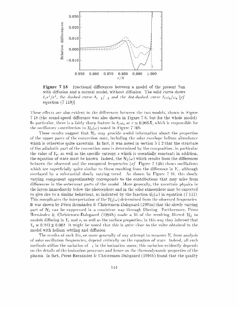
Figure 7.18. Fractional di�erences between a model of the present Sunwith di�usion and a normal model, without di�usion. The solid curve shows�rc2=c2, the dashed curve �r�1=�1 and the dot-dashed curve �r!a=!a [cf.equation (7.110)].These e�ects are also evident in the di�erences between the two models, shown in Figure7.18 (the sound-speed di�erence was also shown in Figure 7.8, but for the whole model).In particular, there is a fairly sharp feature in �r!a at r ' 0:985R, which is responsible forthe oscillatory contribution to H2(!) noted in Figure 7.10b.These results suggest that H2 may provide useful information about the propertiesof the upper parts of the convection zone, including the solar envelope helium abundancewhich is otherwise quite uncertain. In fact, it was noted in section 5.1.2 that the structureof the adiabatic part of the convection zone is determined by the composition, in particularthe value of Ye, as well as the speci�c entropy s which is essentially constant; in addition,the equation of state must be known. Indeed, the H2(!) which results from the di�erencesbetween the observed and the computed frequencies (cf. Figure 7.13b) shows oscillationswhich are super�cially quite similar to those resulting from the di�erence in Ye, althoughoverlayed by a substantial slowly varying trend. As shown by Figure 7.16, this slowlyvarying component approximately corresponds to the contributions that may arise fromdi�erences in the outermost parts of the model. More generally, the uncertain physics inthe layers immediately below the photosphere and in the solar atmosphere may be expectedto give rise to a similar behaviour, as indicated by the function G2(!) in equation (7.111).This complicates the interpretation of the H2(!) determined from the observed frequencies.It was shown by P�erez Hern�andez & Christensen-Dalsgaard (1994a) that the slowly varyingpart of H2 can be suppressed in a consistent way through �ltering. Furthermore, P�erezHern�andez & Christensen-Dalsgaard (1994b) made a �t of the resulting �ltered H2 tomodels di�ering in Ye and s, as well as the surface properties; in this way they inferred thatYe = 0:243� 0:002. It might be noted that this is quite close to the value obtained in themodel with helium settling and di�usion.The results of such �ts, or more generally of any attempt to measure Ye from analysisof solar oscillation frequencies, depend critically on the equation of state. Indeed, all suchmethods utilize the variation of �1 in the ionization zones; this variation evidently dependson the details of the ionization processes and hence on the thermodynamic properties of theplasma. In fact, P�erez Hern�andez & Christensen-Dalsgaard (1994b) found that the quality144

of the �t depended quite sensitively on the assumed equation of state, giving strong prefer-ence for one formulation over another, even though both were comparatively sophisticated.This indicates that it may be possible to get some separate information about the compo-sition and the thermodynamic properties of matter in the solar convection zone. However,it is evident that one might conceive of errors in the equation of state whose e�ect weresimilar to that corresponding to a change in the helium abundance. Such e�ects evidentlycannot be separated on the basis of an analysis of the oscillation frequencies.I �nally note that the function �(!) also enters into the asymptotic behaviour oflow-degree modes [cf. equation (7.44)]. This suggests that it may be possible to obtaininformation about the near-surface regions, similar to what can be determined from H2(!),by analyzing observations of stellar oscillations where only modes of degree less than threeare generally visible. Brodsky & Vorontsov (1988a) presented a method to determine afunction closely related to �(!) on the basis of low-degree data alone. This was appliedto models of main-sequence stars by P�erez Hern�andez & Christensen-Dalsgaard (1993),who found a characteristic dependence on the stellar parameters. A demonstration ofthe practical utility of this type of analysis, given realistic observational errors and otheruncertainties, requires further investigations, however.

145

146

8. Rotation and stellar oscillationsI have so far assumed that there are no velocity �elds in the equilibrium model. This ismanifestly false for an object like the Sun which is rotating; in particular, the observedsurface rotation depends on latitude, thus implying the presence of velocity �elds. Inaddition, other large-scale velocity �elds, such as those caused by convection, could havean e�ect on the modes. Hence we must investigate such e�ects. Apart from their intrinsicinterest, the principal purpose of such studies is obviously to be able to probe the velocity�elds from the observed properties of the oscillations.It is straightforward to see, from a purely geometrical argument, that rotation mighta�ect the observed frequencies. Assume the angular velocity to be uniform, and consideran oscillation with a frequency !0, independent of m, in the frame rotating with the star. Iintroduce a coordinate system in this frame, with coordinates (r0; �0; �0) which are relatedto the coordinates (r; �; �) in an inertial frame through(r0; �0; �0) = (r; �; �� t) : (8:1)It follows from equation (4.35) that, in the rotating frame, the perturbations depend on�0 and t as cos(m�0 � !0t); hence, the dependence in the inertial frame is cos(m�� !mt),where !m = !0 +m : (8:2)Thus an observer in the inertial frame �nds that the frequency is split uniformly accordingto m.This description is obviously incomplete. Even in the case of uniform rotation, thee�ects of the Coriolis force must be taken into account in the rotating frame, causing acontribution to the frequency splitting (Cowling and Newing 1949; Ledoux 1949). Fur-thermore, in general the angular velocity is a function (r; �) of position. Nevertheless, asshown below, the e�ect of the Coriolis force is often small and equation (8.2) is approx-imately correct if is replaced by a suitable average of the position-dependent angularvelocity.To arrive at an expression valid for any rotation law it is convenient to consider �rstthe even more general case of an arbitrary stationary velocity �eld in the star.8.1 The e�ect of large-scale velocities on the oscillation frequenciesWe need to reconsider the derivation of the perturbation equations, including the e�ects ofa velocity �eld. I shall assume that the equilibrium structure is stationary, so that all localtime derivatives vanish. Even with this assumption the determination of the equilibriumstructure is a non-trivial problem, due to the distortion caused by the velocity �elds (e.g.due to centrifugal e�ects in a rotating star). However, here I assume that the velocity v0 inthe equilibrium state is su�ciently slow that terms quadratic in v0 can be neglected. Theequation of continuity (3.5) gives, because of the assumed stationaritydiv (�0v0) = 0 : (8:3)Also, because of the neglect of terms of order jvj2, the equations of motion (3.8) reduce to0 = �rp0 + �0g0 : (8:4)147

As usual I have replaced the body force per unit mass f by the gravitational accelerationg. Thus equation (3.27) of hydrostatic support is unchanged. In the solar case, the ratiobetween the neglected centrifugal force and surface gravity is of order 2� 10�5 and so theerror in equation (8.4) is in fact small.The perturbation analysis also requires some care. It was treated in considerable detailby Lynden-Bell & Ostriker (1967), and is discussed in Cox (1980), Chapter 5. Here I justpresent a few of the main features.The velocity at a given point in space can be written asv = v0 + v0 ; (8:5)where v0 is the Eulerian velocity perturbation. The displacement ���r must be determinedrelative to the moving equilibrium uid; it is related to the velocity perturbation byd���rdt = ���v = v0 + (���r � r)v0 : (8:6)Here ���v is the Lagrangian velocity perturbation and, as in section 3.1, d=dt is the materialtime derivative, d���rdt = @���r@t + (v0 � r)���r ; (8:7)in contrast to the zero-velocity case, the local and the material time derivatives of pertur-bations are now di�erent.The perturbed continuity equation may be written as0 = @�0@t + div (�0v0 + �0v0)= @@t [�0 + div (�0���r)] + div f�0v0 + �0[(v0 � r)���r� (���r � r)v0]g ; (8:8)on using equations (8.6) and (8.7). After some manipulation, using equation (8.3), this maybe reduced to @A@t + div (Av0) = 0 ; (8:9)where A = �0 + div (�0���r) : (8:10)This may also, by using again equation (8.3), be written as�0 ddt � A�0� = 0 ; (8:11)from which we conclude that A = 0, i.e., that equation (3.38) is valid in this case also.To obtain the perturbed momentum equation I use equation (3.7); from the fact thatLagrangian perturbation and material time derivative commute,ddt (� ) = � �d dt � (8:12)148

for any quantity , we then obtain�0d���vdt = �(�rp+ �g) = �rp0 + �0g0 + �0g0 ; (8:13)by using equation (8.4). Alternatively this may be written, from equation (8.6), as�0d2���rdt2 = �rp0 + �0g0 + �0g0 ;or, by using equation (8.7) and neglecting the term quadratic in v0,�0@2���r@t2 + 2�0(v0 � r)�@���r@t � = �rp0 + �0g0 + �0g0 ; (8:14)which replaces equation (3.40). Finally, from the commutativity in equation (8.12), one�nds that the perturbed energy equation (3.43) is still valid. Thus to this level of accuracy,the only change in the perturbation equations is the inclusion of the term in the �rst timederivative of ���r in equation (8.14)As the equilibrium structure is independent of time, we may still separate the time de-pendence as exp(�i!t). Using, for simplicity, the same symbols for the amplitude functionsin this separation, we obtain from the equations of motion�!2�0���r� 2i!�0(v0 � r)���r = �r p0 + �0g0 + �0g0 : (8:15)Here the term in v0 is a small perturbation. Thus we can investigate its e�ect by means ofperturbation analysis, as discussed in section 5.5. Following equations (5.47) and (5.48) Iwrite equation (8.15) as !2���r = F(���r) + �F(���r) ; (8:16)where �F(���r) = �2i!(v0 � r)���r : (8:17)It now follows from equation (5.64) and the de�nition of the inner product that the changein ! caused by the velocity �eld is, to �rst order,�! = �iRV �0���r� � (v0 � r)���r dVRV �0j���rj2 dV : (8:18)8.2 The e�ect of pure rotationNow v0 is taken to correspond to a pure rotation, with angular velocity = (r; �) thatmay depend on r and �. I assume that the entire star is rotating around a common axisand choose this as the axis of the spherical polar coordinate system. Thenv0 = r sin � a� = � r ; (8:19)where I have introduced the rotation vector = (cos� ar � sin � a�) :149

We must now evaluate equation (8.18) for a normal mode of oscillation, and hence we haveto consider the derivative in the direction of v0. From equation (4.26) the perturbationsdepend on � as exp(im�); thus for a scalar quantity a(v0 � r)a = r sin � 1r sin � @a@� = im a : (8:20)For a vector F I use equation (4.8), and note that the directional derivatives of the coordi-nates of F can be found by using equation (8.20). The result is(v0 � r)F = imF+[�F� sin � ar � F� cos � a� + (Fr sin � + F� cos �) a�] : (8:21)This can also be written as (v0 � r)F = imF+� F : (8:22)Thus equation (8.15) becomes�!2�0���r+ 2m!�0���r � 2i!�0� ���r = �rp0 + �0g0 + �0g0 : (8:23)In the case of a uniform rotation rate this equation may be obtained much moresimply. Here we may transform to a coordinate system rotating with the star, with coordi-nates (r0; �0; �0) = (r; �; � � t). In this system the dependence of the perturbations on �0and t is as cos(m�0 +mt� !t) = cos(m�0 � !0t) ; (8:24)where !0 � ! �m (see also the simple analysis in the introduction to this chapter). Towrite down the equations of motion in the rotating system I note that here there is no termin the equilibrium velocity; however, we must add the term �2�0� ���v from the Coriolisforce on the right-hand side. Using that to the required order of precision the velocityperturbation is ���v = �i!���r, the result is�!02�0���r = �rp0 + �0g0 + �0g0 + 2i!�0� ���r : (8:25)But this agrees with equation (8.23), if a term in 2 is neglected.In the general case of non-uniform rotation it might be argued that this relation wouldhold locally at any given point in the uid, thus resulting again in equation (8.23). However,it is not clear (to me, at least) whether this is a consistent derivation of that relation, orwhether it results from fortuitous cancellation of terms coming from the variation of . Inany case it allows a simple interpretation of the two terms in in equation (8.23): the�rst term comes from the coordinate rotation, or equivalently from the advection of therotating star relative to an observer in an inertial frame, and the second term comes fromthe Coriolis force.We must now calculate the integral. By substituting ���r, given by the complex form ofequation (4.35), for F in equation (8.21) we obtain(v0 � r)���r = im ���r+p4� ���h @Y ml@� ar � �h cos �sin � @Y ml@� a� + ��r sin � Y ml + �h cos � @Y ml@� � a�� :(8:26)150

Thus ~R � ZV �0���r� � (v0 � r)���r dV = im ZV �0j���rj2 dV+ 4� ZV �0 ���r�(Y ml )��h@Y ml@� � j�hj2�@Y ml@� �� @Y ml@� cos �sin �+ ��h�r �@Y ml@� �� Y ml + j�hj2�@Y ml@� �� @Y ml@� cos �sin � � dV : (8:27)Here Y ml is always multiplied by its complex conjugate, so that the �-dependence cancels.Hence the integration over � is trivial. It should be noticed also that all terms in the secondintegral in equation (8.27) contain the �-derivative of Y ml or its complex conjugate, whichis proportional to im. Thus ~R contains im as a factor, and can be written, using equation(4.26), as ~R = im 8�2c2lmRnlm ; (8:28)whereRnlm = Z �0 sin �d� Z R0 (j�r(r)j2Pml (cos �)2 + j�h(r)j2 "�dPmld� �2 + m2sin2 �Pml (cos �)2#� Pml (cos �)2 [�r�(r)�h(r) + �r(r)��h(r)]�2Pml (cos �)dPmld� cos �sin � j�h(r)j2�(r; �)�0(r)r2dr : (8:29)Similarly, the denominator in equation (8.18) can be written as~I � ZV �0j���rj2dV = 8�2c2lmInlm ; (8:30)where Inlm = Z �0 sin �d� Z R0 �j�r(r)j2Pml (cos �)2+j�h(r)j2 "�dPmld� �2 + m2sin2 �Pml (cos �)2#)�0(r)r2dr= 22l + 1 (l+ jmj)!(l� jmj)! Z R0 �j�rj2 + l(l+ 1)j�hj2� �0(r)r2dr (8:31)[compare with equation (4.41)]. From equations (8.18), (8.28) and (8.30) we �nally obtainthe rotational splitting, i.e., the perturbation in the frequencies caused by rotation, as�!nlm = mRnlmInlm : (8:32)This may obviously be written on the form�!nlm = Z R0 Z �0 Knlm(r; �)(r; �)rdrd� ; (8:33)where the kernel Knlm is de�ned by equations (8.29) and (8.31).151

The rotational splitting for a uniformly rotating star was �rst obtained by Cowling &Newing (1949) and Ledoux (1949). The general case was considered by Hansen, Cox & vanHorn (1977) and Gough (1981).8.3 Splitting for spherically symmetric rotationTo proceed we must make an explicit assumption about the variation of with �. Forsimplicity I shall assume �rst that is independent of �. In fact, as mentioned earlier,the solar surface rotation depends on �; however, the assumption of �-independent rotationcan be regarded as the �rst term in an expansion of , say, in terms of powers of cos �. Inthis case the integrals over � in equation (8.29) only involve Legendre functions and maybe evaluated analytically. Two of the terms require a little care. One containsZ �0 Pml (cos �)dPmld� cos �sin � sin �d� = � Z 1�1 Pml (x)dPmldx xdx= � 12xPml (x)2����1�1 + 12 Z 1�1 Pml (x)2dx ; (8:34)and here the integrated term vanishes, as Pml (x) is either symmetrical or anti-symmetricalin x = cos �. The other non-trivial integral, which was already encountered in the evaluationof Inlm , isZ �0 "�dPmld� �2 + m2sin2 �Pml (cos �)2# sin �d�= � Z �0 Pml (cos �) � dd� �sin �dPmld� � � m2sin �Pml (cos �)� d� = L2 Z 1�1 Pml (x)2dx ; (8:35)by using that Pml satis�es equation (4.23). As usual, I have introduced L2 � l(l+ 1). Foradiabatic oscillations we can take �r and �h to be real. Thus, from equation (8.29), (8.31)and (8.32), we �nally obtain for the rotational splitting�!nlm = mR R0 (r) ��r2 + L2�2h � 2�r�h � �2h� r2�drR R0 ��r2 + L2�2h� r2�dr ; (8:36)where I have dropped the subscript \0" on �. It should be noticed that the integrands inequation (8.36) are given solely in terms of �r, �h and l, and therefore are independent ofm.Hence in the case of spherically symmetric rotation the rotational splitting is proportionalto m.It is convenient to write equation (8.36) as�!nlm = m�nl Z R0 Knl(r)(r)dr ; (8:37)where Knl = ��r2 + L2�2h � 2�r�h � �2h� r2�R R0 ��r2 + L2�2h � 2�r�h � �2h� r2�dr ; (8:38)152

Figure 8.1. Coe�cients �nl for acoustic modes in a normal solar model.Points corresponding to �xed l have been connected, according to the follow-ing line styles: l = 1: ; l = 2: ; l = 3: ;l = 4: ; l = 5: ; l = 10; 15; : : : ; 50: (with�nl increasing with l).and �nl = R R0 ��r2 + L2�2h � 2�r�h � �2h� r2�drR R0 ��r2 + L2�2h� r2�dr : (8:39)By using this de�nition we ensure that the rotational kernel Knl is unimodular, i.e.,Z R0 Knl(r)dr = 1 : (8:40)Hence for uniform rotation, where = s is constant,�!nlm = m�nls : (8:41)In this case the e�ect of rotation is completely given by the constant �nl . For high-orderor high-degree p modes the terms in �r2 and L2�2h dominate; as shown in Figure 8.1, �nlis then close to one. Thus the rotational splitting between adjacent m-values is givenapproximately by the rotation rate. Physically, the neglected terms in equation (8.39) arisefrom the Coriolis force; thus rotational splitting for p modes is dominated by advection.For high-order g modes, on the other hand, we can neglect the terms containing �r, so that�nl ' 1� 1L2 : (8:42)In particular, the splitting of high-order g modes of degree 1 is only half the rotation rate.153

Returning to the case where depends on r, it should be noted that the integral inequation (8.37) provides a weighted average of (r). For high-order p modes we can usethe asymptotic behaviour of the eigenfunctions to obtain�!nlm ' mZ Rrt �1� L2c2r2!2nl��1=2 (r) drcZ Rrt �1� L2c2r2!2nl ��1=2 drc ' m Z Rrt (r) drcZ Rrt drc ; (8:43)where in the last equality I crudely approximated (1 � L2c2=r2!2) by 1. Note that thelast equality corresponds to neglecting the terms in �h in equation (8.38) and using that,according to equation (7.26), �r � (�c)�1=2r�1 outside the turning point; in this approxi-mation we obtain the intuitively appealing result that the rotational splitting is an averageof the rotation rate, weighted by the sound travel time in the radial direction. The �rst,more accurate expression can also be obtained from ray theory (Gough 1984). In fact, itis straightforward to show that the weight given to (r) is simply the sound-travel time,corresponding to the radial distance dr, along a ray; this evidently becomes in�nite at thelower turning point. It should be noted that the �rst part of equation (8.43) may also bewritten as Snl�!nlm ' m Z Rrt �1� c2L2!2nlr2��1=2 (r)drc ; (8:44)in complete analogy with equation (7.101) for the frequency change resulting from a changein the sound speed; here I neglected the term �d�=d! in equation (7.102) which in generalis small.Figure 8.2 shows a few kernels for the case of spherically symmetric rotation, for high-order p modes. The strong increase towards the solar surface, which is also implicit inequation (8.43), is evident. Also, the kernels clearly get very small beneath the turningpoint, but are locally enhanced just above it. This e�ect arises from the term in �h inequation (8.38); physically it corresponds to the fact that the waves travel approximatelyhorizontally in this region, and hence spend a relatively long time there, as also indicatedby the integrable singularity at r = rt in equation (8.43).8.4 General rotation lawsIn the general case, where depends on both r and �, the rotational splitting may becomputed from equations (8.29), (8.31) and (8.32), by evaluating the two-dimensional inte-gral in equation (8.29). This integral is in general m-dependent, and so the splitting is nolonger a linear function of m. To illustrate the properties of the splitting, it is instructiveto rewrite equation (8.29) for Rnlm, using integration by parts:Rnlm = Z �0 d� Z R0 Pml (cos �)2���r2 + (L2 � 1)�2h � 2�r�h� sin �(r; �)+ �2h �32 cos � @@� + 12 sin � @2@�2 ��r2� dr (8:45)154

Figure 8.2 . Kernels Knl for the frequency splitting caused by sphericallysymmetric rotation (cf. equation [8.38]). In a) is plotted RKnl(r) for a modewith l = 1, n = 22 and � = 3239�Hz. The maximum value of RKnl(r) is 62.In b) is shown the same mode, on an expanded vertical scale, ( )together with the modes l = 20, n = 17, � = 3375�Hz ( ), andl = 60, n = 10, � = 3234�Hz ( ). Notice that the kernels almostvanish inside the turning-point radius rt, and that there is an accumulationjust outside the turning point.(Cuypers 1980). I consider again the case of high-order p-modes; here the terms in �r2 andL2�2h dominate, and consequently�!nlm ' m R �0 sin � [Pml (cos �)]2 R R0 (r; �)[�r(r)2 + L2�h(r)2]r2� drd�R �0 sin � [Pml (cos �)]2 d� R R0 [�r(r)2 + L2�h(r)2]r2� dr : (8:46)Hence, the splitting is simply an average of the angular velocity (r; �), weighted byr2�[�r(r)2 + L2�h(r)2]Pml (cos �)2. Approximating the eigenfunction as in the derivation ofequation (8.43) and using, furthermore, an asymptotic approximation to Pml , this may bewritten as�!nlm ' m Z cos�� cos � �cos2� � cos2 ���1=2 Z Rrt �1� L2c2r2!2��1=2 (r; �) drc d(cos �)1� Z Rrt �1� L2c2r2!2��1=2 drc ; (8:47)155

where � = sin�1(m=L) (Gough and Thompson 1990, 1991; Gough 1991). The asymptoticapproximation to Pml shows that a given spherical harmonic is con�ned essentially to thelatitude band between ��; within this region Pml oscillates as a function of �, whereas athigher latitudes it decreases exponentially. The variation of the extent of the Pml with m=Lallows resolution of the latitudinal variation of the angular velocity, in much the same wayas the variation of the depth of penetration with !=L allows resolution of the variation withradius. In particular, with increasing l the sectoral modes (with l = jmj) get increasinglycon�ned towards the equator (see also Figure 2.1). Thus, the rotational splitting of sectoralmodes provides a measure of the solar equatorial angular velocity.Exercise 8.1:Con�rm the statements about the oscillatory properties of the spherical harmonics, byanalyzing equation (4.23) satis�ed by the Legendre function.To study the splitting without making the asymptotic approximation, it is convenientto consider a parameterized representation of (r; �). Here I use an expansion of the form(r; �) = smaxXs=0 s(r) cos2s � : (8:48)Then the integrals over � can be evaluated analytically, in much the same way as thederivation of equation (8.36), and the rotational splitting becomes (see also Cuypers 1980)�!nlm = m smaxXs=0 Z R0 Knlms(r)s(r)dr : (8:49)HereKnlms(r) = �r2I�1nl ��(�r � �h)2 + (L2 � 2s2 � 3s� 2)�2h�Qlms + s(2s� 1)�2hQlms�1 ;(8:50)where Inl = Z R0 �r2 ��r2 + L2�2h�dr ; (8:51)and Qlms = 2l + 12 (l� jmj)!(l+ jmj)! Z 1�1 x2s[Pml (x)]2dx : (8:52)For spherically symmetric rotation, s = 0 for s > 0. Since Qlm0 = 1, the kernelKnlm0(r) = �nlKnl(r) is independent of m, and the splitting is uniform in m. Thus werecover the results of section 8.3.The factor Qlms is a polynomial in m2 of degree s. Up to s = 2 explicit expression areQlm1 = 2L2 � 2m2 � 14L2 � 3 ; (8:53)and Qlm2 = Rml+1 �Rml+2 + Rml+1 + Rml �+Rml �Rml+1 +Rml +Rml�1� ; (8:54)156

where Rml = l2 �m24l2 � 1 : (8:55)Hence equation (8.49) leads to an expansion of the rotational splitting in odd powers ofm. This corresponds to the odd terms in the expansion (2.40) of the m-dependence of thefrequencies in terms of Legendre polynomials. By carrying out a similar expansion of them-dependence of the kernels Knlms(r) in equation (8.49) one can relate each of the odd-jexpansion coe�cients aj of the frequencies to the expansion coe�cients s of the rotationrate: 2�a2j+1(n; l) = smaxXs=0 Kjnls(r)s(r)dr : (8:56)As discussed by Brown et al. (1989), this forms the basis for an expansion to determinethe s, and hence to estimate the rotation rate as a function of r and �.The choice of expansion polynomials for �!nlm and (r; �) is clearly not unique. Inparticular, it was pointed out by Ritzwoller and Lavely (1991) that a more suitable expan-sion of the rotational splitting could be obtained in terms of Clebsch-Gordon coe�cients;with a proper choice of expansion functions for the rotation rate (r; �) the relations corre-sponding to equation (8.56) decouple such that each expansion coe�cient for the splittingis related to a single expansion function for the angular velocity.It should be noted that, in general, averaging or expansion of the observed frequenciesmay involve loss of information; for the purpose of inversion it is, in principle, preferableto work directly in terms of the observed frequencies. In fact, as mentioned below a di-rect inversion of the frequency splittings �!nlm for individual m, in terms of a discretizedrepresentation of (r; �) on a grid in r and �, is now computationally feasible (see alsoSchou, Christensen-Dalsgaard & Thompson 1994). On the other hand, by suitably com-bining the frequencies before inversion, the computational e�ort required may be greatlyreduced. Furthermore, it is often the case that the quality of the observations does notallow a complete determination of the individual frequencies; in that case inversion has tobe based on expansions such as the one given in equation (2.40).157

158

9. Helioseismic inversionThe expression (8.37) for the splitting caused by spherically symmetric rotation is a par-ticularly simple example of the relation between the observable properties of the oscillationfrequencies, and the properties of the solar interior which we wish to determine. The de-termination of (r) from the �!nlm constitute the simplest example of an inverse problem.In particular, there is a linear relation between the observables and the property of thesolar interior. In contrast, the oscillation frequencies depend in a non-linear fashion on thestructure of the Sun, as speci�ed by for example �(r) and c(r) (cf. section 5.1). However,by assuming that the real solar structure can be obtained from the structure of a givenreference model by applying small corrections, the di�erences in frequency between theobservations and the reference model can be obtained from a linear perturbation analysisof the oscillation equations, resulting, once more, in a linear relation between the frequencydi�erences and the corrections to the model; this was discussed in some detail in section5.5.3 [see equation (5.75)]. Thus the linear inverse problem forms the basis for much of theinverse theory for solar oscillations.Inverse problems have a vast literature, covering their application in, for example,geophysics and radiation theory (e.g. Parker 1977; Craig & Brown 1986; Deepak 1977;Tarantola 1987). The application to the solar inverse problem was discussed by Gough(1985), and Christensen-Dalsgaard, Schou & Thompson (1990) made a systematic compar-ison of di�erent inversion techniques, as applied to the problem of spherically symmetricrotation. The following discussion is to a large extent based on their results.9.1 Inversion of the rotational splittingGiven the simplicity of the rotational-splitting inverse problem, it serves as a very usefulprototype of more general inversions. Furthermore, a determination of the solar internalrotation is of great intrinsic interest. For these reasons, in this section I consider rotationalinversion in some detail.9.1.1 One-dimensional rotational inversionI �rst consider the inversion for a spherically symmetric rotation rate (r). Thus the dataare �i = Z R0 Ki(r)(r)dr+ �i ; i = 1; : : : ;M ; (9:1)where, for notational simplicity, I represent the pair (n; l) by the single index i; M isthe number of modes in the data set considered. �i is the scaled rotational splittingm�1��1nl �!nlm , the kernels Ki having been normalized as in equation (8.40), and �i is theobservational error in �i. The goal of the inversion is to determine an approximation �(r0)to the true angular velocity, as a function of position r0 in the Sun; obviously this is onlypossible for those parts of the Sun about which the oscillations provide data. In most casesconsidered so far, the inversion is carried out through linear operations on the data. Hence� is linearly related to the data: for each r0 there exists a set of inversion coe�cients ci(r0)such that �(r0) =Xi ci(r0)�i : (9:2)159

It follows from equation (9.1) that this may be written as�(r0) = Z R0 K(r0; r)(r)dr ; (9:3)where the averaging kernel K(r0; r) is given byK(r0; r) =Xi ci(r0)Ki(r) : (9:4)The inversion coe�cients and averaging kernels clearly depend on the choice of inver-sion method, and of possible parameters that enter into the method; indeed, the inversionmay be thought of as a way to determine coe�cients and averaging kernels such as to ob-tain as much information about the angular velocity as possible. On the other hand, oncethe method and parameters have been chosen, the coe�cients and averaging kernels areindependent of the data. Hence they can be used to make a data-independent comparisonof di�erent inversion methods; this was the approach taken by Christensen-Dalsgaard et al.(1990).The averaging kernels provide an indication of the resolution of the inversion; it isclearly desirable to achieve averaging kernels that are sharply peaked around r = r0, andwith small amplitude far away from that point. As a quantitative measure of resolution itis common to use a width of K(r0; r) obtained as the distance between the quartile points,de�ned such that one quarter of the area of K(r0; r), regarded as function of r, lies belowthe lower, and one quarter of the area above the upper, quartile point. The inversioncoe�cients give information about the propagation of errors from the data to the solution�(r0). In particular, if the standard error �(�i) is the same for all the observed modesthen the standard error in the result of the inversion is�[�(r0)] = �(r0)�(�i) ; (9:5)where I introduced the error magni�cation�(r0) = "Xi ci(r0)2#1=2 : (9:6)The optimization of the inversion techniques is often based on a trade-o� between width ofthe averaging kernels and error magni�cation (cf. Figure 9.2 below).A procedure which is based explicitly on the determination of the inversion coe�cientsis the technique of optimally localized averages, developed by Backus and Gilbert (1970);this has been used extensively for helioseismic inversion. The goal is to choose the co-e�cients ci(r0) such as to make K(r0; r) approximate as far as possible a delta function�(r � r0) centred on r0; then �(r0) provides an approximation to (r0). This is achievedby determining the coe�cients c(r0) such as to minimizeZ R0 (r � r0)2K(r0; r)2dr + �Xij Eijcicj ; (9:7)subject to the constraint Z R0 K(r0; r)dr = 1 ; (9:8)160

here Eij is the covariance matrix of the data. This is equivalent to solving the set of linearequations Xj Wijcj = b ; (9:9)and Xj cj = 1 ; (9:10)where b is a Lagrangian multiplier. HereWij = Sij + �Eij ; (9:11)where Sij = Z R0 (r � r0)2Ki(r)Kj(r)dr : (9:12)Furthermore, � is a parameter which, as discussed below, must be adjusted to optimize theresult.The e�ect of the minimization is most easily understood for � = 0. Minimizing equation(9.7) subject to equation (9.8) ensures that K(r0; r) is large close to r0, where the weightfunction (r� r0)2 is small, and small elsewhere. This is precisely the required \delta-ness"of the combined kernel. However, with no further constraints, the optimization of thecombined kernel may result in numerically large coe�cients of opposite sign. Hence, thevariance in �, which can be estimated as�2(�) =Xij Eijcicj ; (9:13)would be large. The e�ect of the second term in equation (9.7), when � > 0, is to restrict�2(�). The size of � determines the relative importance of the localization and the size ofthe variance in the result. Hence, � must be determined to ensure a trade-o� between thelocalization and the error, measured by the width of K(r0; r) and �(r0), respectively; � isgenerally known as the trade-o� parameter.The principal di�culty of this method is computational expense: at each target radiusr0 it involves the solution of a set of linear equations whose order is the number of datapoints. Je�rey (1988) proposed an alternative version where the coe�cients were deter-mined by minimizing the di�erence between K(r0; r) and the delta function �(r� r0). Thisis computationally more e�cient, in that only one matrix inversion is required, but resultsin averaging kernels with somewhat undesirable properties.More recently Pijpers & Thompson (1992, 1994) have developed this method further,by matching K(r0; r) instead to a prescribed target function T (r0; r) which more closelymatches the behaviour that can be achieved with the given mode set. They dubbed thisthe SOLA technique (for Subtractive Optimally Localized Averaging), to distinguish it fromthe MOLA technique (for Multiplicative Optimally Localized Averaging) discussed above.Speci�cally, the coe�cients ci(r0) are determined by minimizingZ R0 [K(r0; r)� T (r0; r)]2 dr + �Xij Eijcicj ; (9:14)161

where again � is a tradeo� parameter. In addition, the width of T (r0; r) functions as aparameter, in most cases depending on r0, of the method. As before, the inclusion of thelast term in equation (9.14) serves to limit the error in the solution. The minimizationleads to the following system of linear equations for the ci(r0):Xj (Kij + �Eij)cj(r0) = Ti(r0) ; (9:15)here Kij = Z R0 Ki(r)Kj(r)dr ; (9:16)and Ti(r0) = Z R0 T (r0; r)Ki(r)dr : (9:17)In equation (9.15) the coe�cient matrix on the left-hand side is independent of r0. Thusit can be inverted or, more e�ciently, suitably factored, once and for all; after this thedetermination of the coe�cients at each target point r0 is virtually free. Compared withthe MOLA technique the computational e�ort is therefore reduced by roughly a factorgiven by the number of target locations. An additional advantage of the technique is theability to choose the target function such as to tailor the averaging kernels to have speci�cproperties. This method seems likely to become the procedure of choice to obtain optimallylocalized averaging kernels.A second commonly used technique is the regularized least-squares, or Tikhonov,method (see, for example, Craig and Brown 1986). Here the solution �(r) is parameterized,often as a piecewise constant function on a grid r0 < r1 < : : : < rN , with �(r) = j on theinterval [rj�1; rj]; the parameters j are determined through a least-squares �t to the data.In general, this least-squares procedure needs to be regularized to obtain a smooth solution.This is achieved by including in the minimization a term which restricts the square of �,or the square of its �rst or second derivative. Thus, for example one may minimizeXi "Z R0 Ki(r)�(r)dr ��i#2 + �2 Z R0 �d2 �dr2 �2 dr ; (9:18)where in the last term a suitable discretized approximation to d2 �=dr2, in terms of the j ,is used. The minimization of equation (9.18) clearly leads to a set of linear equations for �j ,de�ning the solution; however, it is still the case that the procedure can be formulated as inequation (9.2) and hence leads to the determination of inversion coe�cients and averagingkernels. By restricting the second derivative the last term in equation (9.18) suppressesrapid oscillations in the solution, and hence ensures that it is smooth; the weight �2 givento this term serves as a trade-o� parameter, determining the balance between resolutionand error for this method.The asymptotic expression (8.44) for the frequency splitting provides the basis fora �nal example of an inversion method in widespread use. The right-hand side of thatequation is a function H(!=L) which is in principle determined by the observed splittingsafter scaling with S. Given H(w), the angular velocity can be obtained from(r) = �2a� dd ln r Z aas (a2 � w2)�1=2H(w)dw ; (9:19)162

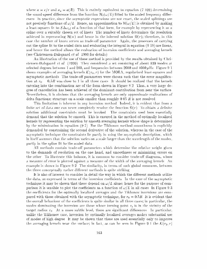
where a = c=r and as = a(R). This is entirely equivalent to equation (7.109) determiningthe sound-speed di�erence from the function H1(!=L) �tted to the scaled frequency di�er-ences. In practice, since the asymptotic expressions are not exact, the scaled splittings arenot precisely functions of !=L. Hence, an approximation to H(!=L) is obtained by makinga least-squares �t to S�!nl of a function of that form, for example by representing it as aspline over a suitably chosen set of knots. The number of knots determines the resolutionachieved in representing H(w) and hence in the inferred solution �(r); therefore, in thiscase the number of knots serves as trade-o� parameter. Again, the processes of carryingout the spline �t to the scaled data and evaluating the integral in equation (9.19) are linear,and hence the method allows the evaluation of inversion coe�cients and averaging kernels(see Christensen-Dalsgaard et al. 1990 for details).An illustration of the use of these method is provided by the results obtained by Chri-stensen-Dalsgaard et al. (1990). They considered a set consisting of about 830 modes atselected degrees between 1 and 200, and frequencies between 2000 and 4000�Hz. Figure 9.1shows examples of averaging kernels K(r0; r) for the MOLA, regularized least-squares andasymptotic methods. The trade-o� parameters were chosen such that the error magni�ca-tion at r0 = 0:5R was close to 1 in all three cases. It should be realized that the kernelsentering into the combination are of the form shown in Figure 8.2. Thus, a very large de-gree of cancellation has been achieved of the dominant contribution from near the surface.Nevertheless, it is obvious that the averaging kernels are only approximate realizations ofdelta functions; structure on a scale smaller than roughly 0.05 R is not resolved.This limitation is inherent in any inversion method. Indeed, it is evident that from a�nite set of data one can never completely resolve the function (r). To obtain a de�nitesolution additional constraints must be invoked. The constraints used here essentiallydemand that the solution be smooth. This is ensured in the method of optimally localizedkernels by representing the solution by smooth averaging kernels whose shape is determinedby the minimization in equation (9.7). For the Tikhonov method smoothness is explicitlydemanded by constraining the second derivative of the solution, whereas in the case of theasymptotic technique the constraints lie partly in using the asymptotic description, whichin itself assumes that the solution varies on a scale larger than the wavelength of the modes,partly in the spline �t to the scaled data.All methods contain trade-o� parameters which determine the relative weight givento the demands of resolution on the one hand, and smoothness or minimizing errors onthe other. To illustrate this balance, it is common to consider trade-o� diagrams, wherea measure of error is plotted against a measure of the width of the averaging kernels. Anexample is shown in Figure 9.2. The similarity, in terms of such global measures, betweenthe three conceptually rather di�erent methods is quite striking.It is also of interest to consider in detail the way in which the di�erent methods utilizethe data, as expressed in terms of the inversion coe�cients. In the case of the asymptotictechnique it may be shown that these depend on !=L alone; hence for the purpose of com-parison it is sensible to plot the coe�cients as a function of !=L in all cases. In Figure 9.3the coe�cients for the optimally localized averages and the Tikhonov inversions are com-pared with those obtained with the asymptotic technique, for r0 = 0:5R. It is evident thatthe overall behaviour of the coe�cients is quite similar in all three cases; in particular, themodes dominating the inversion are those whose turning point rt is in the vicinity of thetarget radius r0. At a more subtle level, there are signi�cant di�erences. In particular,unlike the Tikhonov case, inversion by optimally localized averages makes substantial useof modes of high degree. It may be shown that these are used essentially only to improvethe averaging kernels near the surface; in fact, as can be seen in Figure 9.1 the K(r0; r)163

Figure 9.1. Averaging kernels K(r0; r) at selected radii (r0=R =0:1; 0:2;: : : ; 1:0) for inversion by means of the MOLA technique (panel a), theTikhonov inversion with second-derivative smoothing (panel b) and asymp-totic inversion (panel c). The parameters in each inversion method have beenchosen to obtain approximately the same error magni�cation for r0 = 0:5R.In each case, the kernel at r0 = 0:5R is shown as a bolder curve. FromChristensen-Dalsgaard et al. (1990).164

Figure 9.2. The trade-o� between error magni�cation �(r0) [cf. equation(9.6)] and width (de�ned as distance between quartile points), for inversionat r0 = 0:5R. Results are shown for the MOLA technique ( ), Tikhonovinversion (�) and asymptotic inversion (4), in each case varying the relevanttrade-o� parameter over a wide range. From Christensen-Dalsgaard et al.(1990).for Tikhonov inversion have quite substantial amplitude at very short wavelength near thesurface, whereas such structure is entirely suppressed by the minimization in equation (9.7)for the optimally localized averages. Christensen-Dalsgaard, Hansen & Thompson (1993)found that considerable insight into such details of the behaviour of the inversion methodscan be obtained by analyzing the Tikhonov case by means of the so-called Generalized Sin-gular Value Decomposition; this provides a natural basis for expressing the inverse problemwhich can then be used to study the properties of other inversion methods.Graphs such as Figure 9.2 are very useful for the choice of the trade-o� parameter; how-ever, it is evident that this choice depends critically on the particular application, includingthe errors in the data. The question of how to �x the trade-o� parameter, or indeed evenhow to choose the inversion method, has given rise to a great deal of debate, occasionallyof an almost philosophical (or, dare one say, religious) nature. It has been suggested thatinversion methods should be chosen which aim at �tting the data; this makes the methodof optimally localized averages, whose goal is instead to design the averaging kernels, lessattractive. Also, a great deal of emphasis has been placed on techniques for objectivelydetermining the trade-o� parameters, based on the errors in the data and possibly theproperties of the solution. In contrast, the approach taken in helioseismology has to a largeextent been pragmatic: in fact, it can be argued that since no method, or choice of trade-o�,165

Figure 9.3. Inversion coe�cients ci(r0) for the inversions illustrated in Fig-ure 9.1, at r0 = 0:5R; they have been plotted against �=(l+ 1=2) which, accord-ing to equation (5.24), measures the depth of penetration of the modes. Thecontinuous line in both panels shows coe�cients for the asymptotic methodwhich are functions of �=(l + 1=2). Panel (a) gives the coe�cients obtainedwith the MOLA technique, whereas panel (b) shows coe�cients for Tikhonovinversion. From Christensen-Dalsgaard et al. (1990).can provide the exact solution given the necessarily incomplete data, the most importantaspect of the inversion is to be able to interpret the result and its signi�cance. In thisrespect, the averaging kernels which graphically illustrate the resolution, and the inversioncoe�cients which allow evaluation of e�ects of errors in the data, are clearly very useful.By choosing di�erent inversion methods, and di�erent values of the trade-o� parameters,considering in each case the properties of the resulting inversion, one can hope to obtaina more complete impression of the underlying solution. In this process prior knowledge,166

or prejudices, about the solution clearly play a signi�cant role; these should ideally beformulated in a well-de�ned statistical sense, but probably often are not.9.1.2 Two-dimensional rotational inversionSo far, I have considered inversion for a function that depends on r alone. It is evidentlydesirable, however, to carry out inversion for more general properties, for example, theangular velocity (r; �), which are functions both of r and �.I concentrate on the case of rotation; it should be noticed, however, that anotherinteresting inverse problem concerns the departure of the structure from spherical symmetrycaused, for example, by a latitude dependence of the energy transport in the convectionzone. The form of the inverse problem evidently depends on the representation of the data.It is often the case that the data do not allow determination of indiviual frequencies !nlm .In that case, it is customary to make �ts of the general form shown in equation (2.35), i.e.,!nlm = !nl0 + 2� jmaxXj=1 aj(n; l)P(l)j (m) ; (9:20)where P(l)j is a polynomial of degree j. In many published observations the polynomials P(l)jhave been chosen to be Legendre polynomials P(l)j (m) = lPj(m=l) or P(l)j (m) = LPj(m=L)[as in equation (2.35)]; however, other choices are more convenient for subsequent inversionof the data (Ritzwoller & Lavely 1991; Schou, Christensen-Dalsgaard & Thompson 1994).Di�erent forms for the representation of (r; �) may also be chosen. The odd expansioncoe�cients a2j+1 are related to the angular velocity by an expression equivalent to equation(8.33). However, given the expansion of the splittings in polynomials, it is natural to expandalso the rotation rate in polynomials in cos2 � [see also equation (8.48)]:(r; �) = smaxXs=0 s(r) (1)2s (cos �) ; (9:21)where (1)2s (x) is a polynomial in x2 of degree s (see, for example, Korzennik et al. 1988;Brown et al. 1989; Thompson 1990). It may be shown that only s with s � j contributeto a2j+1. From the fact that the a2j+1 depend linearly on the splittings which in turn arelinear functions of the expansion functions s(r) for , it follows that kernels Kjnls existsuch that 2�a2j+1(n; l) = smaxXs=j Z R0 Kjnls(r)s(r)dr : (9:22)These relations can be reduced to a set of 1-dimensional inverse problems for the expansioncoe�cients s(r) which may be solved by the methods discussed in section 9.1.1. Theinversion is greatly simpli�ed if one makes a judicious choice of polynomials in the expansion(9.21): it is possible to choose polynomials such that all terms with s 6= j in equation (9.22)vanish identically [Ritzwoller & Lavely (1991); for details see Schou et al. (1994)]. Thenequation (9.22) simpli�es to2�a2s+1(n; l) = Z R0 Ksnls(r)s(r)dr ; (9:23)167

so that the separate 1-dimensional inversions can be carried out independently. Inversionmethods of this form, using polynomial expansions of in cos �, are often referred to as1.5D inversion.The expansion of evidently imposes a rather special structure on the solution, unlessa large number of terms is included. An alternative is to perform a direct two-dimensionalinversion by means of a regularized least-squares technique (e.g. Sekii 1991; Schou 1991;Schou, Christensen-Dalsgaard & Thompson 1992, 1994). Here the inferred �(r; �) is rep-resented on a suitable grid (rp; �q) in r and �, p = 1; : : : ; nr, q = 1; : : : ; n�, by expansioncoe�cients pq. These expansion coe�cients can be determined through a regularized least-squares �tting technique, analogous to the one described in equation (9.18). Assuming thatsplittings �!nlm for individual models are available, related to (r; �) by equation (8.33),the solution is determined by minimizingXnlm Rr;�Knlm �rdrd� � �!nlm�nlm !2+ �r Zr;� fr(r; �)�@2 �@r2 �2 d�dr + �� Zr;� f�(r; �)�@2 �@�2 �2 d�dr ; (9:24)here �nlm is the standard deviation for the observed splitting �!nlm . The last two termsserve to regularize the solution, as before, and depend on the weight functions fr and f�and the trade-o� parameters �r and �� . Instead of �!nlm , expansion coe�cients a2j+1 withthe corresponding kernels may evidently also be used. As in the 1-dimensional case, thetrade-o� parameters must be determined such as to ensure a balance between resolutionand error. However, here one must also balance the resolution in the radial and latitudedirections (e.g. Schou et al. 1994).To illustrate the resolution in both r and �, Schou et al. (1992) introduced generalizedaveraging kernels K(r0; �0; r; �) de�ned such that the inferred angular velocity �(r0; �0) isrelated to the true angular velocity (r; �) through�(r0; �0) = Z �0 Z R0 K(r0; �0; r; �)(r; �) rdrd� : (9:25)Such averaging kernels can be obtained for any linear inversion techniques, i.e., techniqueswhere the inferred solution is related linearly to the data. This is true both for inversionsassuming an expansion of in powers of cos � and for the full 2-dimensional techniquesdiscussed above. Examples of such kernels are shown in Figure 9.4, both for inversion usingexpansion of the splittings in a coe�cients and for a full, two-dimensional inversion. In theformer case, only a1, a3 and a5 were included and the latitude information is consequentlyrelatively limited; hence the kernels have a substantial extent in latitude. A particularlystriking feature is the fact that the attempt to determine the angular velocity close to thepole results in what contains aspects of extrapolation from lower latitudes: indeed, it isobvious that the rotation of the region very near the pole has little e�ect on the frequencysplittings and hence cannot be determined from the inversion. The inversion based onindividual splittings provides substantially better resolution in latitude, as might have beenanticipated. Within the convection zone it is possible to determine the rotation over aregion extending only a few per cent of the solar radius in both directions, for realistic setsof observed frequency splittings. 168

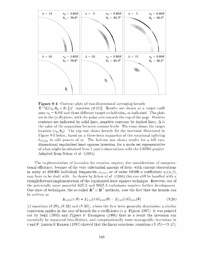
Figure 9.4. Contour plots of two-dimensional averaging kernelsR�2K(r0; �0; r; �) [cf. equation (9.25)]. Results are shown at a target radiinear r0 = 0:8R and three di�erent target co-latitudes, as indicated. The plotsare in the (r; �) plane, with the polar axis towards the top of the page. Positivecontours are indicated by solid lines, negative contours by dashed lines; � isthe value of the separation between contour levels. The cross shows the targetlocation (r0; �0). The top row shows kernels for the inversion illustrated inFigure 9.6 below, based on a three-term expansion of the rotational splitting�!nlm in odd powers of m. The bottom row shows results for a full two-dimensional regularized least-squares inversion, for a mode set representativeof what might be obtained from 1 year's observations with the GONG project.Adapted from Schou et al. (1994).The implementation of inversion for rotation requires due consideration of computa-tional e�ciency, because of the very substantial amount of data: with current observationsas many as 200 000 individual frequencies !nlm , or of order 50 000 a coe�cients aj(n; l),may have to be dealt with. As shown by Schou et al. (1994) this can still be handled with astraightforward implementation of the regularized least-squares technique. However, use ofthe potentially more powerful SOLA and MOLA techniques requires further development.One class of techniques, the so-called IR1 IR1 methods, uses the fact that the kernels canbe written as Knlm(r; �) = F1nl(r)G1 lm(�) + F2nl(r)G2 lm(�) (9:26)[cf equations (8.29), (8.32) and (8.33)], where the �rst term generally dominates; a similarexpression applies in the case of kernels for a coe�cients (e.g. Pijpers 1997). It was pointedout by Sekii (1993) and Pijpers & Thompson (1996) that as a result the inversion canessentially be separated into distinct, and computationally more manageable, inversions inr and �. Larsen & Hansen (1997) showed that the linear equations [equations (9.15) { (9.17)]169

arising in the SOLA technique can be solved e�ciently by using explicitly the discretizedrepresentation of the kernels. By using also the structure given by equation (9.26), Larsen(in preparation) has developed an iterative technique which allows two-dimensional SOLAinversion to be carried out with fairly modest means. These e�cient techniques are nowbeing applied to the very extensive and accurate data obtained with the GONG and SOHOprojects.9.2 Inversion for solar structureIn its most general form, the dependence of the oscillation frequencies on solar structuremay be expressed as !nl = Fnl [�(r); c2(r); : : :] ; (9:27)where, as indicated, other properties beyond the \mechanical" structure as characterizedby � and c2 may a�ect the frequencies. This equation is often approximated by the corre-sponding equation for the adiabatic frequencies, i.e.,!adnl = Fadnl [�(r); c(r)] ; (9:28)where the functional Fadnl is determined through the solution of the equations of adiabaticoscillation. The inverse problem for solar structure then consists of inferring properties ofthe structure by \solving" equation (9.27) or (9.28), given a set of observed frequenciesf!(obs)nl g.A di�culty in this process is that the frequencies depend on solar structure in a compli-cated, nonlinear way. As is common for nonlinear equations, the analysis proceeds throughlinearisation around an initial reference model. Let (�0(r); c0(r)) correspond to the referencemodel, which has adiabatic oscillation frequencies !(0)nl . We seek to determine corrections�r�(r) = �(r)� �0(r) and �rc2(r) = c2(r)� c20(r) to match the di�erences !(obs)nl � !(0)nl be-tween the observed frequencies and those of the reference model. As discussed in sections5.5.3 and 5.5.4, linearization of equation (9.27), assuming �r� and �rc2 to be small, leadsto �!nl!nl = Z R0 �Knlc2;�(r)�rc2c2 (r) +Knl�;c2(r)�r�� (r)�dr +Q�1nl G(!nl) + �nl ; (9:29)where the kernels Knlc2;� and Knl�;c2 are determined from the eigenfunctions in the referencemodel (see also section 5.5.3). In equation (9.29) I included a contribution from the un-certainties in the near-surface region, expressed by the term in G; this may be assumed tocontain the di�erence between the \true" function Fnl in equation (9.27) and the adiabaticapproximation Fadnl in equation (9.28). Furthermore, I explicitly included the observationalerrors �nl . An additional constraint on �r� is that the mass of the Sun and the referencemodel be the same, i.e., 4� Z R0 �r�(r)�(r) �(r)r2dr = 0 : (9:30)In this way the original nonlinear inverse problem is reduced to a linear problem, whichmay be analyzed by means of techniques similar to those discussed in section 9.1.1.170

Unlike the rotational case, the linearized inverse problem given by equation (9.29)involves three unknown functions: �r�(r), �rc2(r) and G(!). These may, after suitableparametrization, be determined through least-squares �tting with appropriate regulariza-tion (e.g. Dziembowski, Pamyatnykh, & Sienkiewicz 1990). Alternatively, some form ofoptimally localized averages may be used, by forming a linear combination of equations(9.29),Xi ci(r0)�!i!i =Xi ci(r0) Z R0 Kic2;�(r)�rc2c2 (r)dr+Xi ci(r0) Z R0 Ki�;c2(r)�r�� (r)dr+Xi ci(r0)Q�1i G(!i) +Xi ci(r0)�i ; (9:31)where, as in section 9.1.1, i labels the modes. If the goal is to determine the correction toc2(r0), the coe�cients ci(r0) must be chosen such that the �rst term on the right-hand sideof equation (9.31) provides an average of �rc2=c2 localized near r = r0, while minimizingthe e�ect of the remaining terms.A natural generalization of the SOLA technique is to obtain the coe�cients ci(r0)through minimization ofZ R0 �Kc2;�(r0; r)� T (r0; r)�2 dr + � Z R0 C�;c2(r0; r)2dr + �Xij Eijci(r0)cj(r0) ; (9:32)where Kc2;�(r0; r) =Xi ci(r0)Kic2;�(r) (9:33)is the averaging kernel; the cross termC�;c2(r0; r) =Xi ci(r0)Ki�;c2(r) (9:34)measures the in uence of the contribution from �r� on the inferred �rc2, and Eij is thecovariance matrix, as before. The constraint (9.30) is incorporated by adding a �ctitiousdata point, with zero data and zero error, and with zero sound-speed kernel and a densitykernel given by �r2. The term in G(!), where G is assumed to be a slowly varying functionof frequency, may be suppressed by restricting the combinations of the data to such thatare insensitive to a contribution of this form (D�appen et al. 1991; Kosovichev et al. 1992).Speci�cally, the coe�cients may be constrained to satisfyXi ci(r0)Q�1i �(!i) = 0 ; � = 0; : : : ;� ; (9:35)for a suitably chosen set of functions �. It was shown by Basu et al. (1996a) that anequivalent, but potentially more exible, suppression of the near-surface terms may bebased on the �ltering technique considered by P�erez Hern�andez & Christensen-Dalsgaard(1994a). 171

Although the inversion has been discussed in terms of the pair (c2; �), other sets ofvariables characterizing the equilibrium structure of the Sun may be used (see also section5.1.1). In particular, as discussed in section 5.5.3, the frequency changes can be expressedin terms of changes �r� and �rY in density and helium abundance, if the equation of state(and the heavy-element abundance) are assumed to be known. Another equivalent, andcommonly used, pair is (u; Y ), where u = p=� is the squared isothermal sound speed. Fromthe point of view of inversion, these pairs have the substantial advantage that the kernelscorresponding to �rY are relatively small and essentially con�ned to the ionization zonesof hydrogen and helium. Thus in the minimization corresponding to equation (9.32), it iscomparatively easy to suppress the cross term C�;Y (r0; r). Furthermore, inversion can becarried out to determine the di�erence �rY between the solar and model helium abundance(e.g. Kosovichev et al. 1992). It should be noted, however, that di�erences between thesolar and model equations of state may introduce systematic errors in the results of suchinversions. Basu & Christensen-Dalsgaard (1997) showed how the di�erences in equationof state might be taken explicitly into account in the inversion, albeit at the expense ofan increase in the error in the solution; they also pointed out that the inversion might becarried out to determine the intrinsic di�erence in �1 between the solar and model equationsof state, i.e., the di�erence at �xed p, � and composition.I �nally note that asymptotic inversion techniques to determine the solar internalsound speed were discussed in section 7.6.2; in particular, it is possible to estimate thesound speed directly from the data, without the use of linearization. Such techniqueswere originally developed in geophysics (see Brodsky & Levshin 1979); their application tothe helioseismic problem was �rst considered by Gough (1984). In these techniques, theuncertainties associated with the near-surface region are contained in the function �(!) or,for the di�erential technique, in the function H2(!) (cf. section 7.6.3).9.3 Some results of helioseismic inversionTo illustrate the power of current helioseismic analysis, it is instructive to present a fewselected results of the application of helioseismic inversion; results of the use of the di�er-ential asymptotic technique were already shown in Figure 7.13. I �rst consider inversionto determine solar structure. As discussed in section 5.1, this is carried out to determinecorrections to an assumed initial reference model. An example is provided by the resultsof Basu et al. (1996b), based on observations by the LOWL instrument, developed at theHigh Altitude Observatory (Tomczyk et al. 1995). The inversions were carried out in termsof corrections �rc2 and �r�. In the former case the variable pair (c2; �) was used, while thedensity inversion used the pair (�; Y ); as discussed in section 5.5.3 it is therefore sensitiveto possible errors in the equation of state. As reference was used a model typical of re-cent normal solar models, computed with little a priori attempt to match the observations.The model included settling of helium and heavy elements, and used equation of state andopacity tables from Livermore. The inversion for the corrections was performed by meansof the SOLA method discussed in section 9.2 The results are shown in Figure 9.5; thereare evidently systematic di�erences between the Sun and the model but these are generallyfairly small. It is probable that the sharp bump in �rc2=c2 at r=R ' 0:65 is a result of weakmixing just beneath the convection zone, which partly o�sets the sharp gradient in thehydrogen abundance established by helium settling in this region. Similarly, the negative�rc2=c2 at the edge of the core could result from partial mixing of the central region. One172

Figure 9.5. Corrections to a reference solar model, obtained by invertingdi�erences between the observed frequencies and the frequencies of the model.Panel a) shows corrections to the squared sound speed c2, and panel b) showscorrections to �. The vertical bars indicate the errors in the results, based onthe errors in the observed frequencies, whereas the horizontal bars provide ameasure of the resolution in the inversion (from Basu et al. 1996b).173

cannot exclude, however, that errors in the opacity may play a signi�cant role. Nonethe-less, it is remarkable that models computed without direct reference to the observations,but based solely on our knowledge of the physics of the solar interior, are so successful inreproducing the structure as inferred from the helioseismic analysis.Figure 9.6. The inferred solar angular velocity obtained from inversion ofrotational splitting observations, given in terms of an expansion in powers ofm. Results are displayed at three target co-latitudes: �0 = 0� (the pole),�0 = 45�, and �0 = 90� (the equator). Dashed lines indicate 1-� error barsbased on the observers' error estimates. (From Tomczyk et al. 1996).To illustrate the determination of the solar internal angular velocity, I present resultsobtained by Tomczyk, Schou & Thompson (1996), for LOWL splitting measurements. Theobservations were given in terms of expansions of the frequency splittings in polynomialsof order up to m5. The inversion was carried out as a least-squares �t to determine thetwo-dimensional function �(r0; �0). The results are presented in Figure 9.6, in the formof inferred angular velocities at the equator, latitude 45�, and the pole. It is striking thatin an outer region the angular velocity is quite similar to the behaviour at the surface; itshould be noted that the inversion does not impose continuity with the surface angularvelocity. This region corresponds roughly to the convection zone, which covers the outerabout 28 per cent of the solar radius (as inferred helioseismically; cf. Christensen-Dalsgaard,Gough & Thompson 1991). In the lower part of the convection zone there appears to bea transition such that the angular velocity in the radiative interior is roughly independentof latitude, at a value intermediate between the surface equatorial and polar values, butsubstantially closer to the former. Also there is a possibly not statistically signi�cant, butstill tantalizing, hint of a reduction of the rotation rate very near the centre. Similar resultshave been obtained from analysis of a set of low-degree splittings from the BiSON network(Elsworth et al. 1995). 174

In interpreting results such as these, it is important to keep in mind the limited reso-lution of the inversion. Thus, with the data that were used, it is not possible to distinguishbetween the gradual transition to latitude-independent rotation in Figure 9.6 and a dis-continuous transition at, for example, the base of the convection zone. Because of thesmall number of terms used to describe the m-dependence of the splittings, the resolutionin latitude is even poorer, as illustrated by the averaging kernels which were shown inFigure 9.4.

175

176

10. Excitation and damping of the oscillationsSo far I have almost exclusively considered adiabatic oscillations, and therefore have beenunable to investigate the stability or instability of the modes. Such questions are of obviousinterest, however. Here I consider some simple properties of the nonadiabatic problem. Amajor goal is to get a feel for the conditions under which a mode may be self-excited, i.e.,with a positive growth rate.10.1 A perturbation expression for the damping rateIn the present section I derive an expression which allows an estimate of the growth ordamping rate on the basis of the adiabatic eigenfunction. The procedure is to use the per-turbation expression in equation (5.64) which was derived from the oscillation equationswritten as a linear eigenvalue problem in equation (5.47). Now, however, I take the per-turbation �F to be the departure from adiabatic oscillations in the momentum equation.From the perturbed energy equation, equations (3.44) and (3.45) it follows thatp0p =�1 �0� + �r �d ln pdr � �1 d ln �dr � + i! �3 � 1p (��� divF)0=p0adp + i! �3 � 1p (��� divF)0 ; (10:1)where I dropped the subscript \0" on equilibrium quantities, and assumed a time depen-dence as exp(�i!t). Herep0ad = p�1 �0� + �rp�d ln pdr � �1 d ln �dr � (10:2)is the pressure perturbation corresponding to adiabatic oscillations. It follows that the per-turbed momentum equation (3.40) can be written, after separation of the time dependence,as ��!2���r = �rp0ad + � g0 + �0g � i!r[(�3 � 1)(��� divF)0] : (10:3)This is of the form considered in equation (5.47):!2���r = Fad(���r) + �F(���r) ; (10:4)with Fad(���r) = 1�rp0ad � g0 � �0� g ; (10:5)and �F(���r) = i!�r[(�3 � 1)(��� divF)0] : (10:6)As argued in section 5.5, Fad is in fact a linear operator on ���r. It may be shown that sameis true for �F . 177

The e�ects on the frequency of departures from adiabaticity can now immediately beobtained from the perturbation expression (5.64) as�!2 = i! ZV ���r� � r[(�3 � 1)(��� divF)0]dVRV �j���rj2dV : (10:7)The integral in the numerator can be rewritten asZV div [���r�(�3 � 1)(��� divF)0]dV � ZV div (���r�)(�3 � 1)(��� divF)0dV ; (10:8)the �rst integral can be transformed, by using Gauss's theorem (3.2), into an integralover the stellar surface which can be neglected, whereas in the second integral we use thecontinuity equation (3.39). The result is, �nally, that the frequency change caused bynon-adiabaticity is �! = i2!2 ZV ���� (�3 � 1)(��� divF)0dVRV �j���rj2dV : (10:9)This is the desired expression. It should be noted that this expression is valid also in thefull nonadiabatic case, if the nonadiabatic eigenfunctions are used.10.2 The quasi-adiabatic approximationTo evaluate the integral in the numerator in equation (10.9) we need an expression for(�� � divF)0. Using that � = �(�; T ) (I neglect a possible Eulerian perturbation in thecomposition) it is easy to see that(��)0 = �� ��T T 0T + (�� + 1)�0� � ; (10:10)where �T = � @ ln �@ ln T �� ; �� = � @ ln �@ ln ��T : (10:11)Similarly, the perturbation in the ux can be evaluated from the di�usion approxi-mation, equation (3.19), and in particular assuming that there are no other contributions(such as convection) to the heat transport. The result isF0 = �(3� �T )T 0T � (1 + ��)�0� �Frar � 4a~cT 33�� rT 0 ; (10:12)where �T = � @ ln �@ ln T �� ; �� = �@ ln �@ ln ��T ; (10:13)178

and Fr is the equilibrium radiative ux (which is of course in the radial direction). Theunderlying assumption in the perturbation treatment leading to equation (5.64) and hence(10.9) is that �F should be evaluated for the adiabatic eigenfunction. Regardless of theassumption of adiabaticity we may obtain �0 from the equation of continuity as��� = �div (���r); �0 = ��� �r d�dr : (10:14)From adiabaticity it follows that the temperature perturbation can be computed from�TT = (�3 � 1)��� ; T 0 = �T � �r dTdr : (10:15)Hence, given ���r, �0 and T 0 can be computed, and then (�� � divF)0 can be obtainedfrom equations (10.10) and (10.12). Since this approximation to the damping rate can beobtained from the adiabatic eigenfunction, it is known as the quasi-adiabatic approximation.As the adiabatic eigenfunctions may be chosen to be real, the integrals in equation (10.9)are real, and hence �! is purely imaginary. Thus it represents a pure damping or excitation,with no e�ect on the (real) oscillation frequency.It should be noted that the approximation is not without problems. The perturbationapproach is based on the assumption that the perturbation is small. This is true in mostof the star, but not very near the surface where nonadiabatic e�ects become strong. Herenonadiabaticity has a substantial e�ect on the eigenfunction, and hence an evaluation of theintegral in equation (10.9) based on the adiabatic eigenfunctions is questionable. Nonethe-less, we may hope that the quasi-adiabatic approximation at least gives an indication ofthe stability properties of the mode. A separate problem, which would equally a�ect a fullnonadiabatic treatment, is the neglect of convective contributions to the heat ux. Thisintroduces a major uncertainty in the calculation of the stability of modes in cool starswith extensive outer convection zones. Indeed, it was shown by Baker & Gough (1979) thatthe transition to stability at the cool side of the Cepheid instability strip most likely is theresult of the increased importance of convection.10.3 A simple example: perturbations in the energy generation rateTo illustrate some simple properties of equation (10.9) I consider the case where the nona-diabaticity is dominated by the energy generation. Here is convenient to work purely interms of Lagrangian perturbations, by noting that(��� divF)0 = �(��� div F) ; (10:16)since the equilibrium model is assumed to be in thermal equilibrium. Also, it is obviousthat �(��) can be obtained from an expression analogous to equation (10.10). Neglectingthe term in F and using equation (10.15) we �nd�! = i2!2 ZV ������� ����2 (�3 � 1)[�� + 1 + (�3 � 1)�T ]��dVRV �j���rj2dV : (10:17)179

Since �T and �� are positive, and �3 ' 5=3, it is obvious that the integrals in equation(10.17) are positive. With the assumed time dependence as exp(�i!t) this corresponds toa growth in the oscillation amplitude, i.e., to instability of the mode.The physical nature of this instability is very simple and closely related to the operationof a normal heat energy: at compression the gas is hotter than normal and this, togetherwith the increased density, causes an increase in the release of energy; this increases thetendency of the gas to expand back towards equilibrium; at expansion the gas is cooler andless dense and hence the energy production is low; this similarly increases the tendencyof collapse towards the equilibrium; both e�ects increase the oscillation amplitude. Thismechanism is closely analogous to the operation of a normal car engine where energy is alsoreleased (through the ignition of the air{fuel mixture) at the point of maximum compression.For acoustic modes, which have large amplitudes in the outer part of the star, thedamping and excitation is normally dominated by the e�ects of the ux. This is morecomplicated and will be discussed in section 10.5. However, the destabilization throughnuclear reactions may play an important role for g modes in several cases; this includes theSun which becomes unstable towards a few low-order g modes in relatively early phases ofits evolution (see, for example, Christensen-Dalsgaard, Dilke & Gough 1974).10.4 Radiative damping of acoustic modesI now consider the e�ects on high-order or high-degree acoustic modes and hence neglectthe e�ect of nuclear reactions. As in Problem 2.2(vi) (cf. Appendix C) I assume that the ux perturbation is dominated by the term in rT 0 in equation (10.12), to obtain(divF)0 = 4a~cT 43�� jkj2T 0T = !2 4a~cT 43��c2 T 0T ; (10:18)where in the last equality I used the dispersion relation for plane sound waves. Here T 0=Tcan be obtained from the adiabatic relation (10.15) where, in accordance with the treatmentof plane sound waves, I neglect derivatives of equilibrium quantities. HenceT 0T = �TT = (�3 � 1)��� ; (10:19)As a result equation (10.9) for the damping rate becomes�! = � i2 ZV (�3 � 1)2 ������� ����2 4a~cT 43��c2 dVRV �j���rj2dV : (10:20)It is evident from equation (10.20) that �! is negative, i.e., the mode is damped. Thisis again obvious from physical considerations: the e�ect of the term in the temperaturegradient is to increase the heat ux from regions that are compressed and heated, and todecrease it from regions that are expanded; hence e�ectively there is heat loss at compressionand heat gain at expansion, and this works to dampen the oscillation. It should be pointedout here that the opacity uctuations, acting through the �rst term in equation (10.12),may counteract that: if opacity is increased at compression the ux of radiation goingout through the star is preferentially absorbed at compression, hence heating the gas andcontributing to the excitation of the oscillation. This mechanism, the so-called Eddingtonvalve, is responsible for the pulsations of the stars in the instability strip.180

To compare with the asymptotic expression derived below it is instructive to writeequation (10.20) in terms of ���r; from the continuity equation we have, still assuming aplane sound wave and using the dispersion relation, that���� ��� ���� = jdiv ���rj = jkjj���rj = !c j���rj : (10:21)Hence we obtain �!! = � i!2 ZV ( � 1)2 2 4a~cT 43�p2 j���rj2�dVRV �j���rj2dV ; (10:22)by using c2 = p=�; for simplicity I assume that �3 = �1 = .It is of some interest to consider also the damping from the asymptotic point of view.I start from the modi�ed dispersion relation derived in Problem 2.2!2 = c2jkj2�F ; (10:23)where �F = 1 + i! �F1 + i!�F ; �F = 3��p4a~c( � 1)T 4jkj2 = 3� p24a~c( � 1)T 4!2 : (10:24)If nonadiabatic e�ects are weak, i.e., !�F � 1, we can write equation (10.23) as!2 = c2jkj2 � c2jkj2(1� �F) ' c2jkj2 � i!ad � 1 �F ; (10:25)where !ad is the frequency in the adiabatic case. Equation (10.25) is a perturbed version ofthe sound-wave dispersion relation, of the form considered in Appendix B. Hence the e�ectof the damping on the frequencies can be obtained from equations (B.6) and (B.7) asS �!! ' � i2! Z Rrt �1� L2c2!2r2��1=2 � 1 �F drc ; (10:26)where S = Z Rrt �1� L2c2!2r2��1=2 drc � �d�d! : (10:27)By substituting the expression for �F we �nally obtainS �!! ' � i!2 Z Rrt ( � 1)2 2 4a~cT 43�p2 �1� L2c2!2r2��1=2 drc : (10:28)This equation essentially corresponds to equation (10.22) if we note that asymptotically�j���rj2dV can be identi�ed with c�1(1� L2c2=!2r2)�1=2dr, to within a constant factor.181

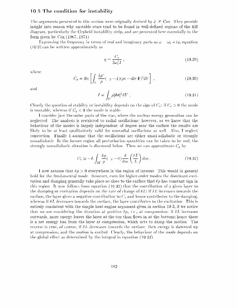
10.5 The condition for instabilityThe arguments presented in this section were originally derived by J. P. Cox. They provideinsight into reason why unstable stars tend to be found in well-de�ned regions of the HRdiagram, particularly the Cepheid instability strip, and are presented here essentially in theform given by Cox (1967, 1974).Expressing the frequency in terms of real and imaginary parts as ! = !r+ i�, equation(10.9) can be written approximately as � ' Cr2!2r I ; (10:29)where Cr = Re �ZV ���� (�3 � 1)(��� divF)0dV � ; (10:30)and I = ZV �j���rj2dV : (10:31)Clearly the question of stability or instability depends on the sign of Cr: if Cr > 0 the modeis unstable, whereas if Cr < 0 the mode is stable.I consider just the outer parts of the star, where the nuclear energy generation can beneglected. The analysis is restricted to radial oscillations; however, as we know that thebehaviour of the modes is largely independent of degree near the surface the results arelikely to be at least qualitatively valid for nonradial oscillations as well. Also, I neglectconvection. Finally I assume that the oscillations are either quasi-adiabatic or stronglynonadiabatic. In the former region all perturbation quantities can be taken to be real; thestrongly nonadiabatic situation is discussed below. Then we can approximate Cr byCr ' �L ZM ��� (�3 � 1) ddm ��LL � dm : (10:32)I now assume that �� > 0 everywhere in the region of interest. This would in generalhold for the fundamental mode. However, even for higher-order modes the dominant exci-tation and damping generally take place so close to the surface that �� has constant sign inthis region. It now follows from equation (10.32) that the contribution of a given layer tothe damping or excitation depends on the rate of change of �L: if �L increases towards thesurface, the layer gives a negative contribution to Cr and hence contributes to the damping,whereas if �L decreases towards the surface, the layer contributes to the excitation. This isentirely consistent with the simple heat-engine argument given in section 10.3, if we noticethat we are considering the situation at positive ��, i.e., at compression: if �L increasesoutwards, more energy leaves the layer at the top than ows in at the bottom; hence thereis a net energy loss from the layer at compression, which acts to damp the motion. Thereverse is true, of course, if �L decreases towards the surface: then energy is dammed upat compression, and the motion is excited. Clearly, the behaviour of the mode depends onthe global e�ect as determined by the integral in equation (10.32).182

We now need to consider the behaviour of the luminosity perturbation in more detail.It is given by an expression corresponding to equation (10.12) for the perturbation in the ux. For low-order modes one can probably neglect the term in the derivative of �T=T ,as well as a term in the displacement. Expressing the equation in terms of the Lagrangianluminosity perturbation, we obtain�LL = (4� �T )�TT � �� ��� : (10:33)In the region where the oscillations are nearly adiabatic, �T=T ' (�3 � 1)��=�, and hence�LL ' ��LL �a = [(4� �T )(�3 � 1)� ��] ��� : (10:34)In most of the star, �� is close to unity, �T is negative (as, for example, for Kramersopacity) and �3 ' 5=3. Also, ��=� generally increases outwards. Hence it follows fromequation (10.34) that in most cases �L increases towards the surface, so that the tendencyis towards stability. This is quite reassuring: after all most stars do not show obviousvariability, suggesting that special circumstances are required to excite modes to largeamplitudes.Figure 10.1 �3 � 1 against temperature in the region of He+ ionization inan equilibrium model of a stellar envelope.

183

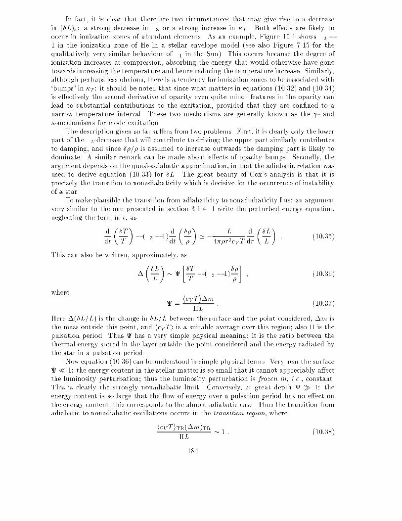
In fact, it is clear that there are two circumstances that may give rise to a decreasein (�L)a: a strong decrease in �3 or a strong increase in �T . Both e�ects are likely tooccur in ionization zones of abundant elements. As an example, Figure 10.1 shows �3 �1 in the ionization zone of He in a stellar envelope model (see also Figure 7.15 for thequalitatively very similar behaviour of �1 in the Sun). This occurs because the degree ofionization increases at compression, absorbing the energy that would otherwise have gonetowards increasing the temperature and hence reducing the temperature increase. Similarly,although perhaps less obvious, there is a tendency for ionization zones to be associated with`bumps' in �T : it should be noted that since what matters in equations (10.32) and (10.34)is e�ectively the second derivative of opacity even quite minor features in the opacity canlead to substantial contributions to the excitation, provided that they are con�ned to anarrow temperature interval. These two mechanisms are generally known as the - and�-mechanisms for mode excitation.The description given so far su�ers from two problems. First, it is clearly only the lowerpart of the �3-decrease that will contribute to driving; the upper part similarly contributesto damping, and since ��=� is assumed to increase outwards the damping part is likely todominate. A similar remark can be made about e�ects of opacity bumps. Secondly, theargument depends on the quasi-adiabatic approximation, in that the adiabatic relation wasused to derive equation (10.33) for �L. The great beauty of Cox's analysis is that it isprecisely the transition to nonadiabaticity which is decisive for the occurrence of instabilityof a star.To make plausible the transition from adiabaticity to nonadiabaticity I use an argumentvery similar to the one presented in section 3.1.4. I write the perturbed energy equation,neglecting the term in �, asddt ��TT �� (�3 � 1) ddt � ��� � ' � L4��r2cV T ddr ��LL � : (10:35)This can also be written, approximately, as���LL � � ��TT � (�3 � 1)��� � ; (10:36)where = hcV T i�m�L : (10:37)Here �(�L=L) is the change in �L=L between the surface and the point considered, �m isthe mass outside this point, and hcV T i is a suitable average over this region; also � is thepulsation period. Thus has a very simple physical meaning: it is the ratio between thethermal energy stored in the layer outside the point considered and the energy radiated bythe star in a pulsation period.Now equation (10.36) can be understood in simple physical terms. Very near the surface� 1: the energy content in the stellar matter is so small that it cannot appreciably a�ectthe luminosity perturbation; thus the luminosity perturbation is frozen in, i.e., constant.This is clearly the strongly nonadiabatic limit. Conversely, at great depth � 1: theenergy content is so large that the ow of energy over a pulsation period has no e�ect onthe energy content; this corresponds to the almost adiabatic case. Thus the transition fromadiabatic to nonadiabatic oscillations occurs in the transition region, wherehcV T iTR(�m)TR�L � 1 : (10:38)184

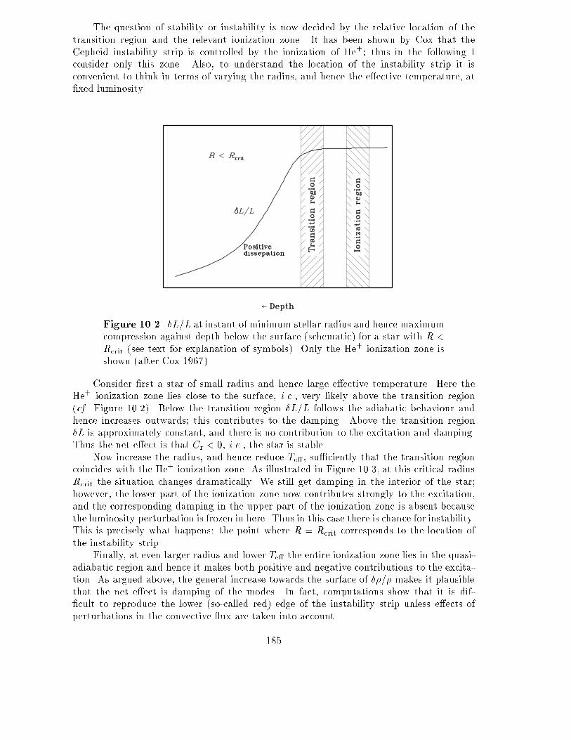
The question of stability or instability is now decided by the relative location of thetransition region and the relevant ionization zone. It has been shown by Cox that theCepheid instability strip is controlled by the ionization of He+; thus in the following Iconsider only this zone. Also, to understand the location of the instability strip it isconvenient to think in terms of varying the radius, and hence the e�ective temperature, at�xed luminosity.Figure 10.2. �L=L at instant of minimum stellar radius and hence maximumcompression against depth below the surface (schematic) for a star with R <Rcrit (see text for explanation of symbols). Only the He+ ionization zone isshown (after Cox 1967).Consider �rst a star of small radius and hence large e�ective temperature. Here theHe+ ionization zone lies close to the surface, i.e., very likely above the transition region(cf. Figure 10.2). Below the transition region �L=L follows the adiabatic behaviour andhence increases outwards; this contributes to the damping. Above the transition region�L is approximately constant, and there is no contribution to the excitation and damping.Thus the net e�ect is that Cr < 0, i.e., the star is stable.Now increase the radius, and hence reduce Te� , su�ciently that the transition regioncoincides with the He+ ionization zone. As illustrated in Figure 10.3, at this critical radiusRcrit the situation changes dramatically. We still get damping in the interior of the star;however, the lower part of the ionization zone now contributes strongly to the excitation,and the corresponding damping in the upper part of the ionization zone is absent becausethe luminosity perturbation is frozen in here. Thus in this case there is chance for instability.This is precisely what happens: the point where R = Rcrit corresponds to the location ofthe instability strip.Finally, at even larger radius and lower Te� the entire ionization zone lies in the quasi-adiabatic region and hence it makes both positive and negative contributions to the excita-tion. As argued above, the general increase towards the surface of ��=� makes it plausiblethat the net e�ect is damping of the modes. In fact, computations show that it is dif-�cult to reproduce the lower (so-called red) edge of the instability strip unless e�ects ofperturbations in the convective ux are taken into account.185

Figure 10.3. �L=L at instant of minimum stellar radius and hence maximumcompression against depth below the surface (schematic) for a star with R =Rcrit (see text for explanation of symbols). Only the He+ ionization zone isshown (after Cox 1967).This argument may be more quantitative, to determine the approximate location ofthe instability strip. In fact, it is not di�cult to obtain a relation that determine the slopeof the strip (see exercise 10.1). It was arguments of this kind which �rst led Cox to identifythe He+ ionization as being mainly responsible for the Cepheid instability.The location of the transition region, as given in equation (10.38), depends on theperiod of oscillation. I have so far argued for the behaviour of a single mode (although thechanging radius would also tend to increase the period and hence push the transition regiondeeper). However, it should be noted that higher-order modes would tend to have transitionregions closer to the surface. It follows that they should become unstable at higher e�ectivetemperatures. This is indeed con�rmed by more detailed stability calculations.The arguments as given here refer speci�cally to the Cepheid instability strip. However,very similar arguments can be applied to other driving mechanisms, at least in fairly hotstars where convection can be neglected. Thus any suitable feature that may cause asubstantial dip in (�L=L)a might be expected to give rise to an instability region. It hasbeen found recently, through improvements in the treatment of iron line contributions, thatthere is a bump in the opacities near temperatures of 2� 105K which can account for the� Cephei and other B star pulsations in this way (e.g. Moskalik & Dziembowski 1992). Asimilar mechanism is responsible for the excitation of g modes in pulsating white dwarfs(e.g. Winget et al. 1982).186

ReferencesAbramowitz, M. & Stegun, I. A., 1964. Handbook of Mathematical Functions, NBS AppliedMathematics Series No. 55, NBS, Washington, D.C.Aindow, A., Elsworth, Y. P., Isaak, G. R., McLeod, C. P., New, R. & van der Raay, H. B.,1988. [The current status of the Birmingham solar seismology network]. Seismology ofthe Sun & Sun-like Stars, p. 157 { 160, eds Domingo, V. & Rolfe, E. J., ESA SP-286.Aizenman, M., Smeyers, P. & Weigert, A., 1977. [Avoided crossing of modes of non-radialstellar oscillations]. Astron. Astrophys., 58, 41 { 46.Andersen, B. N., 1991. [VIRGO | solar irradiance and radiance monitoring on SOHO].Adv. Space Res., vol. 11, No. 4, 93 { 102.Andreasen, G. K. & Petersen, J. O., 1987. [Cepheids in the Magellanic Clouds. I. Fourierdecomposition of LMC Cepheid light curves]. Astron. Astrophys., 180, 129 { 144.Bachmann, K. T., Duvall, T. L., Harvey, J. W. & Hill, F., 1995. [Measurement of high-degree solar oscillation frequencies]. Astrophys. J., 443, 837 { 842.Backus, G. & Gilbert, F., 1970. [Uniqueness in the inversion of inaccurate gross Earthdata]. Phil. Trans. R. Soc. London, Ser. A, 266, 123 { 192.Baker, N. H. & Gough. D. O., 1979. [Pulsations of model RR Lyrae stars]. Astrophys. J.,234, 232 { 244.Baker, N. H., Moore, D. W. & Spiegel, E. A., 1971. [Aperiodic behaviour of a non-linearoscillator]. Q. Jl. Mech. appl. Math., 24, 391 { 422.Basu, S. & Christensen-Dalsgaard, J., 1997. [Equation of state and helioseismic inversions].Astron. Astrophys., 322, L5 { L8.Basu, S., Christensen-Dalsgaard, J., Schou, J., Thompson, M. J. & Tomczyk, S., 1996b.[Solar structure as revealed by LOWL data]. Proc. Conf. on \Windows on the Sun'sinterior", Bombay, Oct. 1995; Bull. Astron. Soc. India, 24, 147 { 150.Basu, S., Thompson, M. J., Christensen-Dalsgaard, J. & P�erez Hern�andez, F. 1996a. [Fil-tering out near-surface uncertainties from helioseismic inversion]. Mon. Not. R. astr.Soc., 280, 651 { 660.Batchelor, G. K., 1967. An Introduction to Fluid Mechanics, Cambridge University Press.Baturin, V. A. & Mironova, I. V., 1990. [On the possibility of determining helium abun-dance from helioseismological data]. Pis'ma Astron. Zh., 16, 253 { 259 (Englishtranslation: Sov. Astron. Lett., 16, 108 { 111).Biermann, L., 1947. [ �Uber die Ursache der chromosph�arischen Turbulenz und des UV-Exzesses der Sonnenstrahlung]. Z. Astrophys., 25, 161 { 177.Blackman, R. B. & Tukey, J. W., 1959. The Measurement of Power Spectra, Dover, NewYork.Bracewell, R. N., 1978. The Fourier Transform and its Applications, 2. ed., McGraw-Hill,New York.Breger, M., 1995a. [Asteroseismology of delta Scuti stars: review]. In Proc. GONG'94:Helio- and Astero-seismology from Earth and Space, eds Ulrich, R. K., Rhodes Jr, E. J.& D�appen, W., Astronomical Society of the Paci�c Conference Series, San Francisco,76, 596 { 605.Breger, M., 1995b. [Astrophysical applications of delta Scuti stars]. In Proc. IAU Colloq.155: Astrophysical Applications of Stellar Pulsation, eds Stobie, R. S. & Whitelock, P.A., ASP Conf. Ser., 83, 70 { 79. 187

Breger, M., Martin, B., Garrido, R., Shi-yang, Jiang, Zhi-ping, Li, Hube, D. P., Stich,J.,Ostermann, W., Paparo, M., 1993b. [EP Cancri: a nonradially pulsating � Scutistar in the Praesepe cluster]. Astron. Astrophys., 281, 90 { 94.Breger, M., Stich, J., Garrido, R., Martin, B., Shi-yang, Jiang, Zhi-ping, Li, Hube, D. P.,Ostermann, W., Paparo, M., Schreck, M., 1993a. [Nonradial pulsation of the � Scutistar BU Cancri in the Praesepe cluster]. Astron. Astrophys., 271, 482 { 486.Brodsky, M. A. & Levshin, A., 1979. [An asymptotic approach to the inversion of freeoscillation data]. Geophys. J. R. astr. Soc., 58, 631 { 654.Brodsky, M. A. & Vorontsov, S. V., 1987. [An asymptotic technique for solving the inverseproblem of helioseismology]. Pis'ma Astron. Zh., 13, 438 { 443 (English translation:Sov. Astron. Lett., 13, 179 { 181).Brodsky, M. A. & Vorontsov, S. V., 1988a. [On the technique of the inversion of helioseismo-logical data]. Proc. IAU Symposium No 123, Advances in helio- and asteroseismology,p. 137 { 140, eds Christensen-Dalsgaard, J. & Frandsen, S., Reidel, Dordrecht.Brodsky, M. A. & Vorontsov, S. V., 1988b. [Helioseismological inverse problem: diagnosticsof the structure of the lower solar atmosphere]. Seismology of the Sun & Sun-like Stars,p. 487 { 491, eds Domingo, V. & Rolfe, E. J., ESA SP-286.Brodsky, M. A. & Vorontsov, S. V., 1989. [The inverse problem of helioseismology: probingthe structure of the lower solar atmosphere]. Pis'ma Astron. Zh., 15, 61 { 69 (Englishtranslation: Sov. Astron. Lett., 15, 27 { 30).Brown, T. M. & Christensen-Dalsgaard, J., 1990. [A technique for estimating complicatedpower spectra from time series with gaps]. Astrophys. J., 349, 667 { 674.Brown, T. M. & Morrow, C. A. 1987. [Depth and latitude dependence of solar rotation].Astrophys. J., 314, L21 - L26.Brown, T. M., Christensen-Dalsgaard, J., Dziembowski, W. A., Goode, P., Gough, D. O.& Morrow, C. A., 1989. [Inferring the Sun's internal angular velocity from observedp-mode frequency splittings]. Astrophys. J., 343, 526 { 546.Brown, T. M., Christensen-Dalsgaard, J., Mihalas, B. & Gilliland, R. L., 1994. [The e�ec-tiveness of oscillation frequencies in constraining stellar model parameters]. Astrophys.J., 427, 1013 { 1034.Cash, J. R. & Moore, D. R., 1980. [A high order method for the numerical solution oftwo-point boundary value problems]. BIT, 20, 44 { 52.Castor, J. I., 1971. [On the Calculation of Linear, Nonadiabatic Pulsations of StellarModels]. Astrophys. J., 166, 109 { 129.Chandrasekhar, S., 1964. [A general Variational Principle Governing the Radial and theNon-radial Oscillations of Gaseous Masses]. Astrophys. J., 139, 664 { 674.Christensen-Dalsgaard, B. L., 1982. [On the use of the �nite-element method with Lagrangemultipliers in scattering theory]. J. Phys. A, 15, 2711 { 2722.Christensen-Dalsgaard, J., 1976. [On isolated stars in non-radial oscillation]. Mon. Not.R. astr. Soc., 174, 87 { 89.Christensen-Dalsgaard, J., 1978. [Solar oscillations]. PhD Dissertation, University of Cam-bridge.Christensen-Dalsgaard, J., 1980. [On adiabatic non-radial oscillations with moderate orlarge l]. Mon. Not. R. astr. Soc., 190, 765 { 791.Christensen-Dalsgaard, J., 1981. [The e�ect of non-adiabaticity on avoided crossings ofnon-radial stellar oscillations]. Mon. Not. R. astr. Soc., 194, 229 { 250.Christensen-Dalsgaard, J., 1982. [On solar models and their periods of oscillation]. Mon.Not. R. astr. Soc., 199, 735 { 761. 188

Christensen-Dalsgaard, J., 1984a. [Optimized response functions for two-dimensional ob-servations of solar oscillations]. Proceedings of Conference on Solar Seismology fromSpace, p. 219, eds Ulrich, R. K., Harvey, J., Rhodes, E. J. & Toomre, J., NASA, JPLPubl. 84-84.Christensen-Dalsgaard, J., 1984b. [What will asteroseismology teach us?]. Space ResearchProspects in Stellar Activity and Variability, p. 11 { 45, ed. Praderie, F., Paris Obser-vatory Press.Christensen-Dalsgaard, J., 1984c. [Solar oscillations]. Theoretical Problems in Stellar Sta-bility and Oscillations, p. 155 { 207, Institut d'Astrophysique, Li�ege.Christensen-Dalsgaard, J., 1986. [Theoretical aspects of helio- and asteroseismology]. Seis-mology of the Sun and the distant Stars, p. 23 { 53, ed. Gough, D. O., Reidel,Dordrecht.Christensen-Dalsgaard, J., 1987. [Helio- and asteroseismology: Basic techniques and inverseproblems]. Methodes mathematiques pour l'astrophysique, p. 479 { 524, eds Auvergne,M. & Baglin, A., (Soci�et�e Fran�caise des Sp�ecialiste d'Astronomie, Paris).Christensen-Dalsgaard, J., 1988a. [Study of solar structure based on p-mode helioseismol-ogy]. Seismology of the Sun & Sun-like Stars, p. 431 { 450, eds Domingo, V. & Rolfe,E. J., ESA SP-286.Christensen-Dalsgaard, J., 1988b. [A Hertzsprung-Russell diagram for stellar oscillations].Proc. IAU Symposium No 123, Advances in helio- and asteroseismology, p. 295 { 298,eds Christensen-Dalsgaard, J. & Frandsen, S., Reidel, Dordrecht.Christensen-Dalsgaard, J., 1991a. [Some aspects of the theory of solar oscillations]. Geo-phys. Astrophys. Fluid Dynamics, 62, 123 { 152.Christensen-Dalsgaard, J., 1991b. [Solar oscillations and the physics of the solar interior].In Challenges to theories of the structure of moderate-mass stars, Lecture Notes inPhysics, vol. 388, p. 11 { 36, eds Gough, D. O. & Toomre, J., Springer, Heidelberg.Christensen-Dalsgaard, J., 1993a. Lecture Notes on Stellar Structure and Evolution (3. ed),D.f.I. Print, Aarhus.Christensen-Dalsgaard, J., 1993b. [On the asteroseismic HR diagram]. In Proc. GONG1992: Seismic investigation of the Sun and stars, ed. Brown, T. M., AstronomicalSociety of the Paci�c Conference Series, San Francisco, 42, 347 { 350Christensen-Dalsgaard, J., 1996a. [Testing a solar model: the forward problem]. In Proc.VI IAC Winter School "The structure of the Sun", ed. T. Roca Cortes, CambridgeUniversity Press, 47 { 139.Christensen-Dalsgaard, J., 1996b. [Helioseismology, solar models and solar neutrinos]. InProc. Workshop on Theoretical and Phenomenological Aspects of Underground Physics(TAUP'95), ed. Fatas, M., Nucl. Phys. B, Suppl., 48, 325 { 334.Christensen-Dalsgaard, J. & Berthomieu, G., 1991. [Theory of solar oscillations]. In Solarinterior and atmosphere, p. 401 { 478, eds Cox, A. N., Livingston, W. C. & Matthews,M., Space Science Series, University of Arizona Press.Christensen-Dalsgaard, J. & D�appen, W., 1992. [Solar oscillations and the equation ofstate]. Astron. Astrophys. Rev., 4, 267 { 361.Christensen-Dalsgaard, J. & Frandsen, S., 1983. [Radiative transfer and solar oscillations].Solar Phys., 82, 165 { 204.Christensen-Dalsgaard, J. & Gough, D. O., 1982. [On the interpretation of �ve-minuteoscillations in solar spectrum line shifts]. Mon. Not. R. astr. Soc., 198, 141 { 171.Christensen-Dalsgaard, J. & Mullan, D. J., 1994. [Accurate frequencies of polytropic mod-els]. Mon. Not. R. astr. Soc., 270, 921 { 935.189

Christensen-Dalsgaard, J. & P�erez Hern�andez, F., 1992. [Phase-function di�erences forstellar acoustic oscillations { I. Theory]. Mon. Not. R. astr. Soc., 257, 62 { 88.Christensen-Dalsgaard, J. & Schou, J., 1988. [Di�erential rotation in the solar interior].Seismology of the Sun & Sun-like Stars, p. 149 { 153, eds Domingo, V. & Rolfe, E. J.,ESA SP-286.Christensen-Dalsgaard, J. & Thompson, M. J., 1997. [On solar p-mode frequency shiftscaused by near-surface model changes]. Mon. Not. R. astr. Soc., 284, 527 { 540.Christensen-Dalsgaard, J., Duvall, T. L., Gough, D. O., Harvey, J. W. & Rhodes, E. J.,1985. [Speed of sound in the solar interior]. Nature, 315, 378 { 382.Christensen-Dalsgaard, J., Dziembowski, W. & Gough, D. O., 1980. [How deep is the solarconvection zone?]. Lecture Notes in Physics, 125, p. 313 { 341 eds Dziembowski, W.& Hill, H. A., Springer, Heidelberg.Christensen-Dalsgaard, J., Gough, D. O. & Morgan, J. G., 1979. [Dirty solar models].Astron. Astrophys., 73, 121 { 128.Christensen-Dalsgaard, J., Gough, D. O. & Thompson, M. J., 1988. [Determination of thesolar internal sound speed by means of a di�erential asymptotic inversion]. Seismologyof the Sun & Sun-like Stars, p. 493 { 497, eds V. Domingo & E. J. Rolfe, ESA SP-286,Noordwijk, Holland.Christensen-Dalsgaard, J., Gough, D. O. & Thompson, M. J., 1989. [Di�erential asymptoticsound-speed inversions]. Mon. Not. R. astr. Soc., 238, 481 { 502.Christensen-Dalsgaard, J., Gough, D. O. & Thompson, M. J., 1991. [The depth of the solarconvection zone]. Astrophys. J., 378, 413 { 437.Christensen-Dalsgaard, J., Gough, D. O. & Toomre, J., 1985. [Seismology of the Sun].Science, 229, 923 { 931.Christensen-Dalsgaard, J., Gough, D. O. & P�erez Hern�andez, F., 1988. [Stellar dishar-mony]. Mon. Not. R. astr. Soc., 235, 875 { 880.Christensen-Dalsgaard, J., Hansen, P. C. & Thompson, M. J., 1993. [Generalized singularvalue decomposition analysis of helioseismic inversions]. Mon. Not. R. astr. Soc., 264,541 { 564.Christensen-Dalsgaard, J., Pro�tt, C. R. & Thompson, M. J., 1993. [E�ects of di�usionon solar models and their oscillation frequencies]. Astrophys. J., 403, L75 { L78.Christensen-Dalsgaard, J., Schou, J. & Thompson, M. J., 1990. [A comparison of methodsfor inverting helioseismic data]. Mon. Not. R. astr. Soc., 242, 353 { 369.Claverie, A., Isaak, G. R., McLeod, C. P., van der Raay, H. B., Pall�e, P. L. & Roca Cortes,T., 1984. [Continuous observation of solar oscillations from two suitably spaced groundstations]. Mem. Soc. Astron. Ital., 55, 63 { 66.Cowling, T. G., 1941. [The non-radial oscillations of polytropic stars]. Mon. Not. R. astr.Soc., 101, 367 { 375.Cowling, T. G. & Newing, R. A., 1949. [The oscillations of a rotating star]. Astrophys. J.,109, 149 { 158.Cox, A. N., Guzik, J. A. & Kidman, R. B., 1989. [Oscillations of solar models with internalelement di�usion]. Astrophys. J., 342, 1187 { 1206.Cox, J. P., 1967. In Aerodynamic Phenomena in Stellar Atmospheres, IAU Symp. No 28,p. 3, Academic Press, London.Cox, J. P., 1974. [Pulsating stars]. Rep. Prog. Phys., 37, 563 { 698.Cox, J. P., 1980. Theory of Stellar Pulsation, Princeton University Press.Cox, J. P. & Giuli, R. T., 1968. Principles of Stellar Structure, Gordon & Breach, NewYork. 190

Cox, J. P. & Whitney, C., 1958. [Stellar pulsation. IV. A semitheoretical period-luminosityrelation for classical Cepheids]. Astrophys. J., 127, 561 { 572.Craig, I. J. D. & Brown, J. C., 1986. Inverse problems in astronomy: a guide to inversionstrategies for remotely sensed data, Adam Hilger, Bristol.Cuypers, J. 1980. [On the calculation of the frequency splitting of adiabatic nonradialstellar oscillations by slow di�erential rotation]. Astron. Astrophys., 89, 207 { 208.D�appen, W. & Gough, D. O., 1984. [On the determination of the helium abundance ofthe solar convection zone]. Theoretical Problems in Stellar Stability and Oscillations,p. 264 { 269 (Institut d'Astrophysique, Li�ege).D�appen, W. & Gough, D. O., 1986. [Progress report on helium abundance determination].Seismology of the Sun and the distant Stars, p. 275 { 280, ed. Gough, D. O., Reidel,Dordrecht.D�appen, W., Gough, D. O., Kosovichev, A. G. & Thompson, M. J., 1991. [A new inversionfor the hydrostatic strati�cation of the Sun]. In Challenges to theories of the structureof moderate-mass stars, Lecture Notes in Physics, vol. 388, p. 111 { 120, eds Gough,D. O. & Toomre, J., Springer, Heidelberg.Deepak, A., 1977. Inversion Methods in Atmospheric Remote Sounding, Academic, NewYork.Deubner, F.-L. & Gough, D. O., 1984. [Helioseismology: Oscillations as a diagnostic of thesolar interior]. Ann. Rev. Astron. Astrophys. 22, 593 { 619.Duvall, T. L., 1982. [A dispersion law for solar oscillations]. Nature, 300, 242 { 243.Duvall, T. L. & Harvey, J. W., 1983. [Observations of solar oscillations of low and inter-mediate degree]. Nature, 302, 24 { 27.Duvall, T. L., Dziembowski, W. A., Goode, P. R., Gough, D. O., Harvey, J. W. & Leibacher,J. W., 1984. [The internal rotation of the Sun]. Nature, 310, 22 { 25.Duvall, T. L., Harvey, J. W., Je�eries, S. M. & Pomerantz, M. A., 1991. [Measurements ofhigh-frequency solar oscillation modes]. Astrophys. J., 373, 308 { 316.Dyson, J. & Schutz, B. F., 1979. [Perturbations and stability of rotating stars. I. Com-pleteness of normal modes]. Proc. Roy. Soc. London, A368, 389 { 410.Dziembowski, W. A. & Pamyatnykh, A. A., 1991. [A potential asteroseismological test forconvective overshooting theories]. Astron. Astrophys., 248, L11 { L14.Dziembowski, W. A., Pamyatnykh, A. A. & Sienkiewicz, R., 1990. [Solar model from thehelioseismology and the neutrino ux problem]. Mon. Not. R. astr. Soc., 244, 542 {550.Dziembowski, W. & Kr�olikowska, M., 1990. [On the mechanism of mode selection in �Scuti stars]. Acta Astron., 40, 19 { 26.Eckart, C., 1960. Hydrodynamics of Oceans and Atmospheres, Pergamon Press.Eddington, A. S., 1926. The Internal Constitution of the Stars, Cambridge UniversityPress.Edmonds, A. R., 1960. Angular Momentum in Quantum Mechanics, 2. Edition, PrincetonUniversity Press, Princeton, N. J.Eggen, O. J., 1957a. [Population type I, short-period variable stars in the Hertzsprunggap]. Astron. J., 62, 14 (Abstract).Eggen, O. J., 1957b. [Distribution of the nearer bright stars in the color-luminosity array].Astron. J., 62, 45 { 55.Eisenfeld, J., 1969. [A completeness theorem for an integro-di�erential operator]. J. Math.Anal. Applic., 26, 357 { 375. 191

Ellis, A. N., 1988. [Inversion of asymptotic gravity-mode frequencies and its application tothe Sun]. Proc. IAU Symposium No 123, Advances in helio- and asteroseismology, p.147 { 150, eds Christensen-Dalsgaard, J. & Frandsen, S., Reidel, Dordrecht.Elsworth, Y., Howe, R., Isaak, G. R., McLeod, C. P. & New, R., 1990. [Evidence from solarseismology against non-standard solar-core models]. Nature, 347, 536 { 539.Elsworth, Y., Howe, R., Isaak, G. R., McLeod, C. P. & New, R., 1991. [Low-l p-mode solareigenfrequency measurements from the Birmingham Network]. Mon. Not. R. astr.Soc., 251, 7p { 9p.Elsworth, Y., Howe, R., Isaak, G. R., McLeod, C. P., Miller, B. A., New, R., Speake, C.C. & Wheeler, S. J., 1994. [Solar p-mode frequencies and their dependence on solaractivity: recent results from the BISON network]. Astrophys. J., 434, 801 { 806.Elsworth, Y., Howe, R., Isaak, G. R., McLeod, C. P., Miller, B. A., New, R., Wheeler, S.J. & Gough, D. O., 1995. [Slow rotation of the Sun's interior]. Nature, 376, 669 { 672.Elsworth, Y., Howe, R., Isaak, G. R., McLeod, C. P., Miller, B. A., Wheeler, S. J. &New, R., 1995. [Fine spacing of the l = 0, l = 2 acoustic eigenmodes and the solarneutrino problem: particle physics and cosmological implications]. In Proc. GONG'94:Helio- and Astero-seismology from Earth and Space, eds Ulrich, R. K., Rhodes Jr, E.J. & D�appen, W., Astronomical Society of the Paci�c Conference Series, vol. 76, SanFrancisco, 76, 51 { 54.Emden, R., 1907. Gaskugelen (Teubner, Leibzig und Berlin).Fossat, E., 1991. [The IRIS network for full disk helioseismology: Present status of theprogramme]. Solar Phys., 133, 1 { 12.Gabriel, A. H. and the GOLF team, 1991. [Global oscillations at low frequency from theSOHO mission (GOLF)]. Adv. Space Res., vol. 11, No. 4, 103 { 112.Gabriel, M., 1986. [Solar g modes: a method to �nd the depth of the convection zone].Seismology of the Sun and the distant Stars, p. 177 { 186, ed. Gough, D. O., Reidel,Dordrecht.Gabriel, M. & Noels, A., 1976. [Stability of a 30M� star towards g+ modes of high sphericalharmonic values]. Astron. Astrophys., 53, 149 { 157.Gabriel, M. & Scu aire, R., 1979. [Properties of non-radial stellar oscillations]. ActaAstron., 29, 135 { 149.Gough, D. O., 1981. [A new measure of the solar rotation]. Mon. Not. R. astr. Soc., 196,731 { 745.Gough, D. O., 1984. [On the rotation of the Sun]. Phil. Trans. R. Soc. London, Ser. A,313, 27 { 38.Gough, D. O., 1985. [Inverting helioseismic data]. Solar Phys., 100, 65 { 99.Gough, D. O., 1986a. [EBK quantization of stellar waves]. Hydrodynamic and magnetohy-drodynamic problems in the Sun and stars, ed. Osaki, Y., University of Tokyo Press,p. 117 { 143.Gough, D. O., 1986b. [Asymptotic sound-speed inversions]. Seismology of the Sun and thedistant Stars, p. 125 { 140, ed. Gough, D. O., Reidel, Dordrecht.Gough, D. O., 1987. [Seismological measurement of stellar ages]. Nature, 326, 257 { 259.Gough, D. O., 1990. [Comments on helioseismic inference]. Progress of seismology ofthe sun and stars, Lecture Notes in Physics, vol. 367, 283 { 318, eds Osaki, Y. &Shibahashi, H., Springer, Berlin.Gough, D. O., 1993. [Course 7. Linear adiabatic stellar pulsation]. In Astrophysical uiddynamics, Les Houches Session XLVII, eds Zahn, J.-P. & Zinn-Justin, J., Elsevier,Amsterdam, 399 { 560 192

Gough, D. O. & Thompson, M. J., 1990. [The e�ect of rotation and a buried magnetic �eldon stellar oscillations]. Mon. Not. R. astr. Soc., 242, 25 { 55.Gough, D. O. & Thompson, M. J., 1991. [The inversion problem]. In Solar interior andatmosphere, eds Cox, A. N., Livingston, W. C. & Matthews, M., p. 519 { 561, SpaceScience Series, University of Arizona Press.Gough, D. O. & Toomre, J., 1991. [Seismic observations of the solar interior]. Ann. Rev.Astron. Astrophys., 29, 627 { 685.Gough, D. O. & Vorontsov, S. V., 1995. [Seismology of the solar envelope: measuring theacoustic phase shift generated in the outer layers]. Mon. Not. R. astr. Soc., 273, 573{ 582.Gough, D. O., Spiegel, E. A. & Toomre, J., 1975. [Highly stretched meshes as functionalsof solutions]. Lecture Notes in Physics, 35, 191 { 196, ed. Richtmyer, R. D., Springer,Heidelberg.Grec, G., Fossat, E. & Pomerantz, M., 1980. [Solar oscillations: full disk observations fromthe geographic South Pole]. Nature, 288, 541 { 544.Guenther, D. B., 1991. [The p-mode oscillation spectra of an evolving 1M� sun-like star].Astrophys. J., 375, 352 { 365.Hansen, C. J., Cox, J. P. & van Horn, H. M., 1977. [The e�ects of di�erential rotation onthe splitting of nonradial modes of stellar oscillation]. Astrophys. J., 217, 151 { 159.Harvey, J. W., Kennedy, J. R. & Leibacher, J. W., 1987. [GONG: to see inside our Sun].Sky and Telescope, 74, 470 { 476.Henyey, L. G., Forbes, J. E. & Gould, N. L., 1964. [A new method of automatic computationof stellar evolution]. Astrophys. J., 139, 306 { 317.Hill, F., 1990. [Networks for helioseismic observation]. Proc. IAU Colloquium No 121,Inside the Sun, p. 265 { 278, eds Berthomieu G. & Cribier M., Kluwer, Dordrecht.Hill, F. & Newkirk, G., 1985. [On the expected performance of a solar oscillation network].Solar Phys., 95, 201 { 219.Hill, F., Gough, D. O., Merry�eld, W. J. & Toomre, J., 1991. [Simulation of e�ects ofatmospheric seeing on the observation of high-degree solar oscillations]. Astrophys. J.,369, 237 { 246.Jackson, J. D., 1975. Classical Electrodynamics, 2. ed., Wiley, New York.Je�rey, W., 1988. [Inversion of helioseismic data]. Astrophys. J., 327, 987 { 992.Kawaler, S. D., 1995. [Probing the extraordinary ends of ordinary stars: white dwarfseismology with the Whole Earth Telescope]. In Proc. IAU Colloq. 155: AstrophysicalApplications of Stellar Pulsation, eds Stobie, R. S. & Whitelock, P. A., ASP Conf. Ser.,83, 81 { 90.Keeley, D. A., 1977. [Linear stability analysis of stellar models by the inverse iterationmethod]. Astrophys. J., 211, 926 { 933.Kepler, S. O., Winget, D. E., Nather, R. E., Bradley, P. A., Grauer, A. D., Fontaine, G.,Bergeron, P., Vauclair, G., Claver, C. F., Marar, T. M. K., Seetha, S., Ashoka, B. N.,Mazeh, T., Leibowitz, E., Dolez, N., Chevreton, M., Barstow, M. A., Clemens, J. C.,Kleinman, S. J., Sansom, A. E., Tweedy, R. W., Kanaan, A., Hine, B. P., Provencal,J. L., Wesemael, F., Wood, M. A., Brassard, P., Solheim, J. E. & Emanuelsen, P.-I.,1991. [A detection of the evolutionary time scale of the DA white dwarf G117{B15Awith the Whole Earth Telescope]. Astrophys. J., 378, L45 { L48.Kippenhahn, R. & Weigert, A., 1990. Stellar structure and evolution, Springer-Verlag,Berlin.Kn�olker, M. & Stix, M., 1983. [A convenient method to obtain stellar eigenfrequencies].Solar Phys., 82, 331 { 341. 193

Korzennik, S. G., Cacciani, A., Rhodes, E. J., Tomczyk, S. & Ulrich, R. K., 1988. [Inversionof the solar rotation rate versus depth and latitude]. Seismology of the Sun & Sun-likeStars, p. 117 { 124, eds Domingo, V. & Rolfe, E. J., ESA SP-286.Kosovichev, A. G., Christensen-Dalsgaard, J., D�appen, W., Dziembowski, W. A., Gough,D. O. & Thompson, M. J., 1992. [Sources of uncertainty in direct seismological mea-surements of the solar helium abundance]. Mon. Not. R. astr. Soc., 259, 536 {558.Kumar, P., Franklin, J. & Goldreich, P., 1988. [Distribution function for the time-averagedenergies of stochastically excited solar p-modes]. Astrophys. J., 328, 879 { 887.Lamb, H., 1909. [On the theory of waves propagated vertically in the atmosphere]. Proc.London Math. Soc., 7, 122 { 141.Lamb, H., 1932. Hydrodynamics, 6th ed., Cambridge University Press.Landau, L. D. & Lifshitz, E. M., 1959. Fluid Mechanics, Pergamon, Oxford.Larsen, R. M. & Hansen, P. C., 1997. [E�cient implementation of the SOLA molli�ermethod]. Astron. Astrophys. Suppl., 121, 587 { 598.Ledoux, P., 1949. [Contributions �a l'�Etude de la Structure Interne des �Etoiles et de leurStabilit�e]. Mem. Soc. R. Sci. Li�ege, 4th ser., 9, 3 { 294. ([Chapitre V: Stabilit�edynamique et pulsations d'�etoiles gazeuses anim�ees d'un mouvement de rotation uni-forme]. p. 263 { 294).Ledoux, P. & Walraven, T., 1958. [Variable stars]. Handbuch der Physik, vol. 51, chapterIV p. 353 { 604 (Springer-Verlag).Lee, U., 1985. [Stability of the Delta Scuti stars against nonradial oscillations with lowdegree l]. Publ. Astron. Soc. Japan, 37, 279 { 291.Leibacher, J. W., Noyes, R. W., Toomre, J. & Ulrich, R. K., 1985. [Helioseismology].Scienti�c American, 253, (September) p. 34 { 43 (US p. 48 { 57).Libbrecht, K. G., 1988. [Solar and stellar seismology]. Space Sci. Rev., 47, 275 { 301.Libbrecht, K. G., 1989. [Solar p-mode frequency splittings]. Astrophys. J., 336, 1092 {1097.Libbrecht, K. G. & Woodard, M. F., 1990. [Solar-cycle e�ects on solar oscillation frequen-cies]. Nature, 345, 779 { 782.Libbrecht, K. G., Popp, B. D., Kaufman, J. M. & Penn, M. J., 1986. [The excitation anddamping of solar oscillations]. Nature, 323, 235 { 238.Libbrecht, K. G., Woodard, M. F. & Kaufman, J. M., 1990. [Frequencies of solar oscillation].Astrophys. J. Suppl., 74, 1129 { 1149.Loumos, G. L. & Deeming, T. J., 1978. [Spurious results from Fourier analysis of data withclosely spaced frequencies]. Astrophys. Space Sci.,Lynden-Bell, D. & Ostriker, j. P., 1967. [On the stability of di�erentially rotating bodies].Mon. Not. R. astr. Soc., 136, 293 { 310.McGraw, J. T. & Robinson, E. L., 1976. [High-speed photometry of luminosity-variableDA dwarfs: R808, GD99, and G117-B15a]. Astrophys. J., 205, L155 { L158.Michel, E. & Baglin, A., 1991. [STEPHI { seismology of � Scuti stars from multi-sitephotometry campaigns]. Adv. Space Res., vol. 11, No. 4, 167 { 170.Michel, E., Belmonte, J. A., Alvarez, M., Jiang, S. Y., Chevreton, M., Auvergne, M., Goupil,M. J., Baglin, A., Mangeney, A., Roca Cort�es, T., Liu, Y. Y., Fu, J. N., Dolez, N.,1992. [Multi-periodicity of the � Scuti star GX Pegasi. Second photometry campaignof the STEPHI network]. Astron. Astrophys., 255, 139 { 148.Mihalas, D. & Mihalas, B. W., 1984. Foundations of Radiation Hydrodynamics, OxfordUniversity Press. 194

Monteiro, M. J. P. F. G., Christensen-Dalsgaard, J. & Thompson, M. J., 1994. [Seismicstudy of overshoot at the base of the solar convective envelope]. Astron. Astrophys.,283, 247 { 262.Moskalik, P. & Dziembowski, W. A., 1992. [New opacities and the origin of the � Cepheipulsation]. Astron. Astrophys., 256, L5 { L8.Nordlund, �A. & Stein, R. F., 1989. [Simulating magnetoconvection]. Solar and stellargranulation, Proc. NATO ARW, Capri, June 21 { 25, p. 453 { 470, eds Rutten, R. J.& Severino, G., Kluwer, Dordrecht.Osaki, Y., 1975. [Nonradial oscillations of a 10 solar mass star in the main-sequence stage].Publ. Astron. Soc. Japan, 27, 237 { 258.Osaki, Y. & Hansen, C. J., 1973. [Nonradial oscillations of cooling white dwarfs]. Astrophys.J., 185, 277 { 292.P�erez Hern�andez, F. & Christensen-Dalsgaard, J., 1993. [The phase function for solar-likestars]. In Proc. GONG 1992: Seismic investigation of the Sun and stars, ed. Brown,T. M., Astronomical Society of the Paci�c Conference Series, San Francisco, 42, 343 {346P�erez Hern�andez, F. & Christensen-Dalsgaard, J., 1994a. [The phase function for stellaracoustic oscillations. II. E�ects of �ltering]. Mon. Not. R. astr. Soc., 267, 111 { 124.P�erez Hern�andez, F. & Christensen-Dalsgaard, J., 1994b. [The phase function for stellaracoustic oscillations. III. The solar case]. Mon. Not. R. astr. Soc., 269, 475 { 492.Parker, R. L., 1977. [Understanding inverse theory]. Ann. Rev. Earth Planet. Sci., 5, 35{ 64.Pesnell, W. D., 1990. [Nonradial, nonadiabatic stellar pulsations]. Astrophys. J., 363, 227{ 233.Petersen, J. O., 1973. [Masses of double mode Cepheid variables determined by analysis ofperiod ratios]. Astron. Astrophys., 27, 89 { 93.Petersen, J. O., 1974. [E�ects upon period ratios of Cepheid models from arti�cial changesin opacity and mean molecular weight]. Astron. Astrophys., 34, 309 { 311.Petersen, J. O., 1975. [On Epstein's weighting function and pulsation constants of Cepheidmodels]. M�em. Soc. R. Sci. Li�ege, 6th ser., 8, 299 { 305.Petersen, J. O., 1978. [Masses of double mode Cepheid variables based on observed periods].Astron. Astrophys., 62, 205 { 215.Pijpers, F.P., 1997. [Solar rotation inversions and the relationship between a-coe�cientsand mode splittings]. Astron. Astrophys., 326, 1235 { 1240.Pijpers, F. P. & Thompson, M. J., 1992. [Faster formulations of the optimally localizedaverages method for helioseismic inversion]. Astron. Astrophys., 262, L33 { L36.Pijpers, F. P. & Thompson, M. J., 1994. [The SOLA method for helioseismic inversion].Astron. Astrophys., 281, 231 { 240.Pijpers, F. P. & Thompson, M. J., 1996. [A modi�ed IR1 IR1 method for helioseismicinversions]. Mon. Not. R. astr. Soc., 279, 498 { 510.Press, W. H., Flannery, B. P., Teukolsky, S. A. & Vetterling, W. T., 1986. NumericalRecipes, Cambridge University Press.Provost, J. & Berthomieu, G., 1986. [Asymptotic properties of low degree solar gravitymodes]. Astron. Astrophys., 165, 218 { 226.Reitz, J. R., Milford, F. J., & Christy, R. W. 1979. Foundations of Electromagnetic Theory,3. ed., Addison-Wesley, Reading, Massachusetts.Ritzwoller, M. H. & Lavely, E. M., 1991. [A uni�ed approach to the helioseismic forwardand inverse problems of di�erential rotation]. Astrophys. J., 369, 557 { 566.195

Robe, H., 1968. [Les oscillations non radiales des polytropes]. Ann. d'Astrophys., 31, 475{ 482.Schatzman, E. & Sou�rin, P., 1967. [Waves in the solar atmosphere]. Ann. Rev. Astron.Astrophys., 5, 67 { 84.Scherrer, P. H., Hoeksema, J. T. & Bush, R. I., 1991. [The Solar Oscillations Investigation| Michelson Doppler Imager for SOHO]. Adv. Space Res., vol. 11, No. 4, 113 { 122.Scherrer, P. H., Wilcox, J. M., Christensen-Dalsgaard, J. & Gough, D. O., 1983. [Detectionof solar �ve-minute oscillations of low degree]. Solar Phys., 82, 75 { 87.Schi�, L. I., 1949. Quantum Mechanics, McGraw Hill, New York.Schou, 1992. On the analysis of helioseismic data, PhD Dissertation, Aarhus University.Schou, J., 1991. [On the 2-dimensional rotational inversion problem]. In Challenges totheories of the structure of moderate-mass stars, Lecture Notes in Physics, vol. 388, p.93 { 100, eds Gough, D. O. & Toomre, J., Springer, Heidelberg.Schou, J., Christensen-Dalsgaard, J. & Thompson, M. J., 1992. [The resolving power ofcurrent helioseismic inversions for the Sun's internal rotation]. Astrophys. J., 385, L59{ L62.Schou, J., Christensen-Dalsgaard, J. & Thompson, M. J., 1994. [On comparing helioseismictwo-dimensional inversion methods]. Astrophys. J., 433, 389 { 416.Scu aire, R., 1974. [The non radial oscillations of condensed polytropes]. Astron. Astro-phys., 36, 107 { 111.Sekii, T., 1991. [Two-dimensional inversion for solar internal rotation]. Publ. Astron. Soc.Japan, 43, 381 { 411.Sekii, T., 1993. [A new strategy for 2D inversion for solar rotation]. Mon. Not. R. astr.Soc., 264, 1018 { 1024.Shapley, H., 1914. [On the nature and cause of Cepheid variation]. Astrophys. J., 40, 448{ 465.Shibahashi H., 1988. [Inverse problem: acoustical potential vs acoustic length]. Proc.IAU Symposium No 123, Advances in helio- and asteroseismology, p. 133 { 136, edsChristensen-Dalsgaard, J. & Frandsen, S., Reidel, Dordrecht.Shibahashi, H. & Osaki, Y., 1981. [Theoretical eigenfrequencies of solar oscillations of lowharmonic degree l in �ve-minute range]. Publ. Astron. Soc. Japan, 33, 713 { 719.Shibahashi, H. & Sekii, T., 1988. [Sound velocity distribution in the Sun inferred fromasymptotic inversion of p-mode spectra]. Seismology of the Sun & Sun-like Stars, p.471 { 480, eds Domingo, V. & Rolfe, E. J., ESA SP-286.Stein, R. F. & Leibacher, J., 1974. [Waves in the solar atmosphere]. Ann. Rev. Astron.Astrophys., 12, 407 { 435.Stein, R. F., Nordlund, �A. & Kuhn, J. R., 1989. [Convection and waves]. Solar and stellargranulation, Proc. NATO ARW, Capri, June 21 { 25, p. 381 { 399, eds Rutten, R. J.& Severino, G., Kluwer, Dordrecht, Holland.Strang, G. & Fix, G. J., 1973. An analysis of the �nite element method, Prentice-Hall.S�rensen, J. M., 1988. [Measurements of oscillation parameters from synthetic time series].Seismology of the Sun & Sun-like Stars, p. 41 { 45, eds Domingo, V. & Rolfe, E. J.,ESA SP-286.Tarantola, A., 1987. Inverse Problem Theory, Elsevier, Amsterdam.Tassoul, M., 1980. [Asymptotic approximations for stellar nonradial pulsations]. Astrophys.J. Suppl., 43, 469 { 490.Thompson, M. J., 1988. [Evidence for a thin perturbative layer near the base of the solarconvection zone]. Seismology of the Sun & Sun-like Stars, p. 321 { 324, eds Domingo,V. & Rolfe, E. J., ESA SP-286. 196

Thompson, M. J., 1990. [A new inversion of solar rotational splitting data]. Solar Phys.,125, 1 { 12.Tomczyk, S., Schou, J. & Thompson, M. J., 1996. [Low-degree frequency splitting mea-surements and the rotation of the solar core]. Proc. Conf. on \Windows on the Sun'sinterior", Bombay, Oct. 1995; Bull. Astron. Soc. India, 24, 245 { 250.Tomczyk, S., Streander, K., Card, G., Elmore, D., Hull, H. & Caccani, A., 1995. [Aninstrument to observe low-degree solar oscillations]. Solar Phys., 159, 1 { 21.Toutain, T. & Fr�ohlich, C., 1992. [Characteristics of solar p-modes: Results from the IPHIRexperiment]. Astron. Astrophys., 257, 287 { 297.Ulrich, R. K., 1986. [Determination of stellar ages from asteroseismology]. Astrophys. J.,306, L37 - L40.Ulrich, R. K., 1988. [Can stellar mass be measured by asteroseismology?]. Proc. IAU Sym-posium No 123, Advances in helio- and asteroseismology, p. 299 { 302, eds Christensen-Dalsgaard, J. & Frandsen, S., Reidel, Dordrecht.Unno, W. & Spiegel, E. A., 1966. [The Eddington approximation in the radiative heatequation]. Publ. Astron. Soc. Japan, 18, 85 { 95.Unno, W., Osaki, Y., Ando, H. & Shibahashi, H., 1989. Nonradial Oscillations of Stars(2nd edition) (University of Tokyo Press).Vandakurov, Yu. V., 1967. [On the frequency distribution of stellar oscillations]. Astron.Zh., 44, 786 { 797 (English translation: Soviet Astronomy AJ, 11, 630 { 638).von Neuman, J. & Wigner, E., 1929. [ �Uber merkw�urdige diskrete Eigenwerte. �Uber dasVerhalten von Eigenwerten bei adiabatischen Prozessen]. Phys. Z., 30, 467 { 470.Vorontsov, S. V., 1988. [A search of the e�ects of magnetic �eld in the solar �ve-minuteoscillations]. Proc. IAU Symposium No 123, Advances in helio- and asteroseismology,p. 151 { 154, eds Christensen-Dalsgaard, J. & Frandsen, S., Reidel, Dordrecht.Vorontsov, S. V. & Shibahashi, H., 1990. [Second-order asymptotic inversions of the soundspeed inside the Sun]. Progress of seismology of the sun and stars, Lecture Notes inPhysics, vol. 367, 326 { 328, eds Osaki, Y. & Shibahashi, H., Springer, Berlin.Vorontsov, S. V., Baturin, V. A. & Pamyatnykh, A. A., 1992. [Seismology of the solarenvelope: towards the calibration of the equation of state]. Mon. Not. R. astr. Soc.,257, 32 { 46.Whittaker, E. T. & Watson, G. N., 1927. A course of modern analysis, Cambridge Univer-sity Press.Winget, D. E., 1988. [Seismological investigations of compact stars]. Proc. IAU Sympo-sium No 123, Advances in helio- and asteroseismology, p. 305 { 324, eds Christensen-Dalsgaard, J. & Frandsen, S., Reidel, Dordrecht.Winget, D. E., 1993. [The Whole Earth Telescope]. In Proc. GONG 1992: Seismicinvestigation of the Sun and stars, ed. Brown, T. M., Astronomical Society of thePaci�c Conference Series, San Francisco, 42, 331 { 342.Winget, D. E., Kepler, S. O., Robinson, E. L., Nather, R. E., O'Donoghue, D., 1985. [Ameasurement of secular evolution in the pre-white dwarf star PG 1159-035]. Astrophys.J., 292, 606 { 613.Winget, D. E., Nather, R. E., Clemens, J. C., Provencal, J. L., Kleinman, S. J., Bradley,P. A., Claver, C. F., Dixson, J. S., Montgomery, M. H., Hansen, C. J., Hine, B. P.,Birch, P., Candy, M., Marar, T. M. K., Seetha, S., Ashoka, B. N., Leibowitz, E.M., O'Donoghue, D., Warner, B., Buckley, D. A. H., Tripe, P., Vauclair, G., Dolez,N., Chevreton, M., Serre, T., Garrido, R., Kepler, S. O., Kanaan, A., Augusteijn, T.,Wood, M. A., Bergeron, P. & Grauer, A. D., 1994. [Whole Earth telescope observationsof the DBV white dwarf GD 358]. Astrophys. J., 430, 839 { 849.197

Winget, D. E., Van Horn, H. M., Tassoul, M., Hansen, C. J., Fontaine, G. & Carroll, B.W., 1982. [Hydrogen-driving and the blue edge of compositionally strati�ed ZZ Cetistar models]. Astrophys. J., 252, L65 { L68.Zhevakin, S. A., 1953. Astron. Zhurn., 30, 161.

198

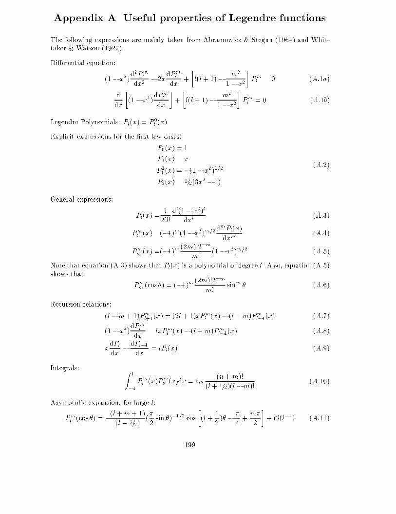
Appendix A. Useful properties of Legendre functionsThe following expressions are mainly taken from Abramowicz & Stegun (1964) and Whit-taker & Watson (1927).Di�erential equation:(1� x2)d2Pmldx2 � 2xdPmldx + �l(l+ 1)� m21� x2 �Pml = 0 (A:1a)ddx �(1� x2)dPmldx �+ �l(l+ 1)� m21� x2�Pml = 0 (A:1b)Legendre Polynomials: Pl(x) = P 0l (x).Explicit expressions for the �rst few cases:P0(x) = 1P1(x) = xP 11 (x) = �(1� x2)1=2P2(x) = 1=2(3x2 � 1) (A:2)General expressions: Pl(x) = 12ll! dl(1� x2)ldxl (A:3)Pml (x) =(�1)m(1� x2)m=2dmPl(x)dxm (A:4)Pmm (x) =(�1)m (2m)!2�mm! (1� x2)m=2 (A:5)Note that equation (A.3) shows that Pl(x) is a polynomial of degree l. Also, equation (A.5)shows that Pmm (cos �) = (�1)m (2m)!2�mm! sinm � (A:6)Recursion relations:(l�m+ 1)Pml+1(x) = (2l+ 1)xPml (x)� (l +m)Pml�1(x) (A:7)(1� x2)dPmldx = lxPml (x)� (l+m)Pml�1(x) (A:8)xdPldx � dPl�1dx = lPl(x) (A:9)Integrals: Z 1�1 Pml (x)Pml0 (x)dx = �ll0 (n+m)!(l+ 1=2)(l�m)! (A:10)Asymptotic expansion, for large l:Pml (cos �) = �(l +m+ 1)�(l + 3=2) (�2 sin �)�1=2 cos�(l + 12)� � �4 + m�2 �+O(l�1) (A:11)199

200

Appendix B. E�ects of a perturbationon acoustic-mode frequenciesIn several of the Problems we consider the e�ect on the frequencies of acoustic modes, asdescribed by the asymptotics leading to the Duvall law, of various modi�cations (such asthe perturbation in the gravitational potential, changes in the sound speed and rotation).These results all re ect a more general expression, which is derived here.I start from the dispersion relation for a plane sound wave, with the addition of aperturbation �rg(r) which, as indicated, is assumed to be a function of r alone:!2 = c2jkj2 + �rg(r) (B:1)(cf. equation (3.51)), where for simplicity I dropped \0" on equilibrium quantities. I nowuse that jkj2 = k2r + k2h, where k2h is given by equation (4.45). Therefore, kr is given bykr =�!2c2 � L2r2 � 1c2 �rg�1=2'!c "�1� L2c2!2r2�1=2 � 12!2 �1� L2c2!2r2��1=2 �rg# ; (B:2)where in the last equality I assumed that �rg was small. The condition that we have astanding wave can be expressed asZ Rrt krdr = (n+ �)� ; (B:3)where, as usual, � takes into account the phase change at the surface. By substitutingequation (B.2) we obtain(n + �)�! ' Z Rrt �1� L2c2!2r2�1=2 drc � 12!2 Z Rrt �1� L2c2!2r2��1=2 �rgdrc : (B:4)If we neglect the term in �rg we obviously obtain the usual Duvall law, equation (7.1).Hence equation (B.4) shows the e�ect of the perturbation on the Duvall law.We can now �nd the e�ect on the oscillation frequencies of the perturbation. I assumethat the result is to change the frequency from ! to !+ �!. Also it should be recalled that� = �(!) in general depends on !. By multiplying equation (B.4) by ! and perturbing itwe obtain�d�d! �! = �! Z Rrt �1� L2c2!2r2�1=2 drc + ! Z Rrt �1� L2c2!2r2��1=2 L2c2!2r2 �!! drc� 12! Z Rrt �1� L2c2!2r2��1=2 �rgdrc : (B:5)From this we �nally obtainS �!! ' 12!2 Z Rrt �1� L2c2!2r2��1=2 �rgdrc ; (B:6)201

where S = Z Rrt �1� L2c2!2r2��1=2 drc � �d�d! : (B:7)This is the desired general expression.It should be noticed that equation (B.6) has a very simple physical interpretation:Apart from the (generally small) term in d�=d! in S, the equation shows that the changein !2 is just a weighted average of �rg, with the weight functionW(r) = 1c �1� L2c2!2r2��1=2 :However, it is easily seen that W(r)dr is just the sound travel time, corresponding to theradial distance dr, along the ray describing the mode. Hence the weight in the averagesimply gives the time that the mode, regarded as a superposition of plane waves, spends ina given region of the star.Example I. E�ect of a change in sound speed: If the sound speed is changed from c toc+ �rc, the dispersion relation for sound waves can be written!2 = c2jkj2 + 2c�rcjkj2 = c2jkj2 + 2!2 �rcc : (B:8)Hence here �rg = 2!2�rc=c. Consequently, the frequency change is given byS �!! ' Z Rrt �1� L2c2!2r2��1=2 �rcc drc : (B:9)It should be noted that in general a change to the model would result also in an intrinsicchange �� in �. As a result, the general asymptotic expression for the frequency change(which can be obtained by including explicitly a term in the change in � when derivingequation (B.5) from equation (B.4)) isS �!! ' Z Rrt �1� L2c2!2r2��1=2 �rcc drc + � ��! : (B:10)Thus we recover equation (7.101).Example II. E�ect of rotation: As discussed in Chapter 8 the dominant e�ect of rotation ispurely geometrical and results in the dispersion relation for sound waves being modi�ed to!2 = c2jkj2 + 2m! ; (B:11)where I assume that the rotation rate depends on r alone. Hence here �rg(r) = 2m!(r),and we obtain the perturbation in the frequency caused by rotation asS�! ' m Z Rrt �1� L2c2!2r2��1=2 (r)drc : (B:12)202

Appendix C. ProblemsThe following problems have been used in courses on stellar pulsations in Aarhus. Theyoriginally appeared on the weekly problem sheets (Ugesedler), but are collected here forconvenience and more general use. In a few cases reference is made to programming andplotting with IDL. Obviously any other convenient graphics package may be used instead.The problems are collected in sections corresponding approximately to the sections ofthe main text, although the numbering has not been maintained.C.1 Analysis of oscillation dataProblem 1.1:Discrete Fourier transform. Observationally, the data are typically given at discretetimes tn. Hence the continuous Fourier transform considered in Section 2.2 is notimmediately relevant. Here we consider the simple case where the data are uniformlyspaced in time, tn = n�t ; n = 0; : : : ; N � 1 (C:1)(this can in fact often be arranged). Then we de�ne the discrete Fourier transform asv(!j) = 1N N�1Xn=0 v(tn) exp(i!jtn) ; (C:2)given at the discrete frequencies !j . For the moment we do not specify !j .i) Find the discrete transform of the simple harmonic oscillator given in equation(2.19). Sketch the power jv(!j)j2. Compare with the continuous transform.A very e�cient procedure for computing the discrete transform is the Fast FourierTransform (FFT). This requires that the number of data points is a power 2� of 2, andprovides the transform only at the frequencies!j = 2�N�tj = 2�T j ; j = 0; : : : ; N ; (C:3)where T = N�t is the total duration of the observing run. For more details about theFFT, see also Numerical Recipes (Press et al. 1986).ii) Sketch the power resulting from a FFT of the time string given by the harmonicoscillator in equation (2.19); for simplicity take the frequency !0 of the oscillatorto be 2�j0=(N�t) for some integer j0. Note that very little of the sinc functionstructure in the continuous transform is preserved.Normally, the number of data points will evidently not be an integral power of 2.In that case, the data are extended by zeros up to a total number N1 = 2� > N .203

iii) Consider the e�ect on the FFT of the simple harmonic oscillator of extending thedata by zeros in this way. Show how this can be used to resolve the structure ofthe peak of the power spectrum (note that we do not need to take the smallestpossible power of 2).Note: In manipulating the Fourier transforms, it is useful to recall thatcos x = 1=2(eix + e�ix) ;NXn=0 xn = 1� xN+11� x : (C:4)Problem 1.2:Multiperiodic harmonic oscillations. (This requires access to a computer withgraphics facilities. Here reference is made to the graphics and data analysis packageIDL, which is a very convenient tool for this type of exercise).Consider a timestring consisting of a sum of harmonic oscillators,v(t) = KXk=0 ak cos(!kt� �k) : (C:5)Take the amplitudes ak and the phases �k to be uniformly distributed random numbers,between 0 and 1, and 0 and 2�, respectively. Also choose suitably \random" frequencies!k.i) Plot v(t) for a total time T that is substantially larger than the longest period2�=!k, for several di�erent numbers K of individual oscillations. Note how theappearance of the time string becomes increasingly \chaotic" as K is increased.ii) Plot the power spectra of the time strings found under i), using IDL's FFT routine.Consider the extent to which the individual frequencies can be separated. Howdoes this depend on the number of modes or the total duration of the time string?A typical observed time string of solar oscillations (corresponding, for example, toobservations made in light integrated over the solar surface) contains of order 50 modes.Clearly, separating them is no trivial task.Problem 1.3:A non-harmonic oscillator. A simple model of a large-amplitude pulsating star(e.g. a Cepheid) is provided by the following functionv(t) = a0 sin[!t+ � sin(!t)] : (C:6)204

i) Show that v(t) is periodic, with the period � = 2�=!.ii) Sketch (or get IDL to plot) v(t) for ! = 1, a0 = 1, � = 0:5.iii) For small �, �nd a simple expression for v(t) by expanding it in powers of �,including the term of order �2. (If this is too hard, consider just the term oforder �). Try to guess what the expansion to higher orders in � will look like,qualitatively.iv) Use IDL to �nd the Fourier transform and power spectrum of v(t) for some typicalcases. Compare with the expansion obtained in iii).Problem 1.4:A double-mode non-harmonic oscillator. In Problem 1.3 we considered asimple model of a large-amplitude pulsating star. Here the signal was given byv(t) = a0 sin[!t + � sin(!t)]; the e�ect of the term in � is roughly to give a distor-tion to the phase which depends on the instantaneous amplitude of the oscillation.This distortion may result from non-linear e�ects near the surface of the star a�ectingwhat is essentially a harmonic oscillation in the stellar interior.We can generalize this concept to multiperiodic oscillators. For simplicity, weconsider a double-mode star, and assume that the signal can be written asv(t) =a1 sin[!1t + �a1 sin(!1t) + �a2 sin(!2t)]+a2 sin[!2t + �a1 sin(!1t) + �a2 sin(!2t)] : (C:7)i) For small � and �, expand v(t) in terms of harmonic functions. Include enoughterms to get a feel for what the form of a general term might be.ii) Use IDL to plot the time series and the power spectrum for typical cases. (It maybe a good idea to use a logarithmic scale for the power, suitably truncated, toshow the presence of weak peaks.) Compare with the expansion in i).iii) What would happen if the star were pulsating in several modes?Problem 1.5:Spatial analysis of oscillation observations. As mentioned brie y in Section 2.1,the analysis of observations of solar oscillations essentially proceeds by multiplying theobserved Doppler velocity �eld v(�; �; t) by di�erent spherical harmonics Y m0l0 (�; �)and integrating over the area A of the solar disk that is observed. The result is afunction vl0m0(t) of time that predominantly contains contributions from modes withl = l0, m = m0. Had the integration been over the entire Sun, the orthogonality ofthe spherical harmonics would have given complete isolation of these modes. However,since we can only see part of the Sun other modes leak in and complicate the analysis.205

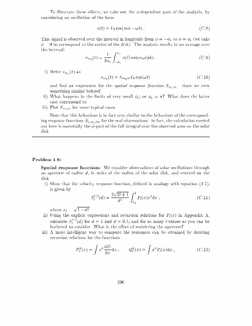
To illustrate these e�ects, we take out the �-dependent part of the analysis, byconsidering an oscillation of the formv(t) = V0 cos(m�� !t) : (C:8)This signal is observed over the interval in longitude from � = ��c to � = �c (we take� = 0 to correspond to the centre of the disk). The analysis results in an average overthe interval: vm0(t) = 12�c Z �c��c v(t) cos(m0�)d� : (C:9)i) Write vm0(t) as vm0(t) = Sm0mV0 cos(!t) (C:10)and �nd an expression for the spatial response function Sm0m. Have we seensomething similar before?ii) What happens in the limits of very small �c; or �c = �? What does the lattercase correspond to.iii) Plot Sm0m for some typical cases.Note that this behaviour is in fact very similar to the behaviour of the correspond-ing response functions Sl0m0lm for the real observations. In fact, the calculation carriedout here is essentially the �-part of the full integral over the observed area on the solardisk.Problem 1.6:Spatial response functions. We consider observations of solar oscillations throughan aperture of radius d, in units of the radius of the solar disk, and centred on thedisk.i) Show that the velocity response function, de�ned in analogy with equation (2.7),is given by S(v)l (d) = 2p2l+ 1d2 Z 1x1 Pl(x)x2dx ; (C:11)where x1 = p1� d2.ii) Using the explicit expressions and recursion relations for Pl(x) in Appendix A,calculate S(v)l (d) for d = 1 and d = 0:5, and for as many l-values as you can bebothered to consider. What is the e�ect of restricting the aperture?iii) A more intelligent way to compute the responses can be obtained by derivingrecursion relations for the functionsPkl (x) = Z xk dPldx dx ; Qkl (x) = Z xkPl(x)dx ; (C:12)206

based on the recursion relations for Pl and its derivative, as well as a little inte-gration by parts. Try to see whether you can �nd a way of doing that, and makea more extensive computation for the cases considered in ii). It may help to lookin Christensen-Dalsgaard & Gough (1982).C.2 A little hydrodynamicsProblem 2.1:Waves at a density discontinuity. In section 3.3.3 a relation is derived for gravitywaves on a free surface. It is interesting also to consider gravity waves at an interfacewhere the density jumps discontinuously. Examples are waves in a glass with oil ontop of water, or waves at the interface between a helium-rich core and a hydrogen-richenvelope.{ Consider a system consisting of an in�nite layer of density �1 on top of an in�nitelayer of density �2, with �1 < �2. The assumptions are otherwise as in section3.3.3. By requiring that the vertical displacement and the pressure are continuousat the perturbed interface between the layers, show that the oscillation frequenciesare given by !2 = �2 � �1�2 + �1 g0k : (C:13)Does this make sense in the limits �1 ! 0 and �1 ! �2?Problem 2.2:Damping of simple sound waves. To illustrate the e�ects of non-adiabaticity, weconsider the radiative damping of the simple sound waves discussed in section 3.3.1.Except where otherwise noted, the assumptions are the same as in that section.At low density, we use Newton's law of cooling, equation (3.20), for the radiativecooling. Also, we assume the ideal gas law, so that in particular �1 = �2 = �3 = =5=3, and that there is no nuclear energy generation. Finally, we consider a perturbationin the form of a plane wave, as in equation (3.50).i) Assume that the opacity � is constant (i.e., independent of � and T ). Show thatthe relation between p0 and �0, on complex form, can be writtenp0p0 = N �0�0 ; (C:14)207

where N = �N ; �N = 1+ 3i4 !�N1 + i!�N ; (C:15)and �N = p04a~c�0�0( � 1)T 40 (C:16)is a characteristic time scale for cooling by Newton's law.ii) Show that the dispersion relation for a plane sound wave is!2 = c20jkj2�N ; (C:17)where c0 = ( p0=�0)1=2 is the adiabatic sound speed.iii) Consider a wave where the wave number k is real. Show that the imaginary partof ! is negative and that therefore the wave is damped, i.e., that the amplitudedecreases with time. What is the physical explanation for the damping? (Youmay assume that the damping is weak, so that Re(!)� Im(!).)iv) As a more realistic case, assume that the opacity depends on � and T , suchthat � / �aT b where a and b are positive (this corresponds to conditions instellar atmospheres where the opacity is dominated by H� absorption). Find theexpression for N in this case, and verify that the wave is damped in this case also.What is the e�ect of the opacity variation on the magnitude of the damping rate?v) Discuss the behaviour of the dispersion relation in the limits �N !1 and �N ! 0.Consider also the behaviour corresponding to �! 0 at �xed T (corresponding toconditions high in a stellar atmosphere).We now consider the limit of high density, where the di�usion approximation,equation (3.19), can be used for the radiative ux. We still assume that equilibriumquantities are constant and consider a plane wave.vi) Show that the perturbation in the radiative cooling rate is given by(divF)0 = 4a~cT 403�0�0 jkj2T 0T0 (C:18)(remember that we assume that rT0 = 0).vii) Hence show that equations (C.14) and (C.17) are still valid, if N and �N arereplaced by F and �F, where F = �F ; �F = 1+ i !�F1 + i!�F ; �F = 3�0�0p04a~c( � 1)T 40 jkj2 : (C:19)Compare this expression for the time scale �F for radiative di�usion with theestimate given in section 3.1.4. 208

viii) Show that this also results in damping of a sound wave. Discuss the physics ofthe damping.Finally, we consider the e�ects of nuclear energy generation on the waves. Weassume that the energy generation rate � / �Tn, and that radiative e�ects can beneglected.ix) Show that in this case the relation between p0 and �0 can be writtenp0p0 = � �0�0 ; (C:20)where � = �� ; �� = 1� i(n� 1)n !��1� i!�� ; (C:21)and �� = p0n�0�0( � 1) (C:22)is a characteristic time scale for nuclear heating.x) Show that this leads to excitation of the sound wave, such that its amplitude growswith time. Discuss the physics of the excitation.xi) Discuss qualitatively the case where both nuclear energy generation and radiativedamping, in the di�usion approximation, are taken into account. For which wavesmight the overall e�ect be an excitation?Problem 2.3:Dispersion relation for sound waves in a gravitating uid. We consider acousticwaves in a homogeneous system, as in section 3.3.1, but include the e�ect of self-gravityon the wave. Hence in the equation of motion, the term �0r�0 should be included onthe right-hand side, but we continue to neglect the equilibrium gravitational accelera-tion.i) Show that equation (3.48) should be replaced by@2�0@t2 = c20r2�0 + 4�G�0�0 : (C:23)ii) We assume a plane-wave solution, on the form given in equation (3.50). Show thatthe dispersion relation is !2 = c20 jkj2 � 4�G�0 : (C:24)209

iii) When the frequency ! obtained from equation (C.24) is imaginary, the perturba-tion either grows or decays exponentially with time. Show that this occurs whenthe wavelength � of the wave satis�es � > �crit and �nd �crit. Compare withequation (10.4) of Lecture Notes on Stellar Structure and Evolution.C.3 Properties of solar and stellar oscillationsProblem 3.1:Rays of sound waves. Ray theory is a very powerful tool for understanding thepropagation of waves in a medium where conditions vary slowly. It is entirely analogousto the study of the propagation of light rays. An important example is its use todescribe the properties of acoustic oscillations in the Sun. We consider an acousticwave that propagates in the (x� z) plane where the sound speed c depends on z butnot x. The wave is described by a wave vector k = (kx; kz) and has a given frequency!; one may think of it as being excited with a �xed frequency at some point in theregion. Clearly, ! and k satisfy the dispersion relation (3.51). The x�component kxof k is �xed, whereas the z�component kz depends on z.i) Show from equation (3.51) thatkz = � !2k2xc2 � 1�1=2 kx : (C:25)The propagation of the ray is parallel to the wave vector. Hence we can describe theposition (x; z) of a point on the ray by the equationsdxds = kxdzds = kz ; (C:26)where s is a suitably chosen measure of position along the ray. From these equationswe obtain dxdz = kxkz ; (C:27)which determines the shape of the ray.ii) Let z measure depth beneath some surface, and assume that c(z)2 increases lin-early with z, c(z)2 = c20 + Az ; (C:28)where c0 and A are constants (this corresponds approximately to conditions neara stellar surface). Try to sketch, qualitatively, the behaviour of the ray.iii) Find the solution to the equation for the ray.210

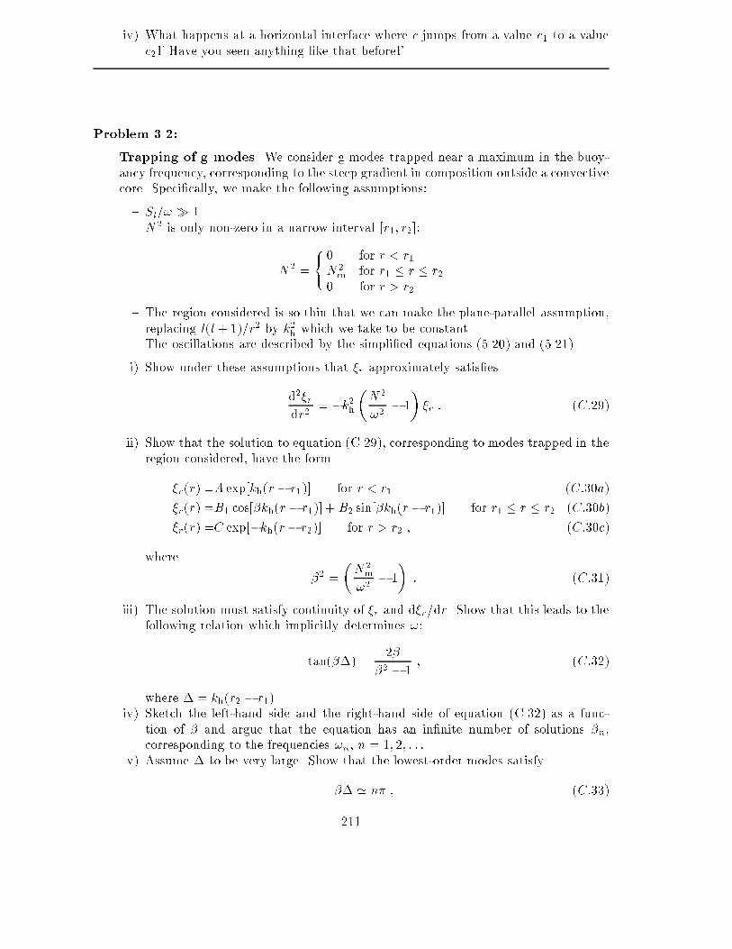
iv) What happens at a horizontal interface where c jumps from a value c1 to a valuec2? Have you seen anything like that before?Problem 3.2:Trapping of g modes. We consider g modes trapped near a maximum in the buoy-ancy frequency, corresponding to the steep gradient in composition outside a convectivecore. Speci�cally, we make the following assumptions:{ Sl=! � 1.{ N2 is only non-zero in a narrow interval [r1; r2]:N2 = ( 0 for r < r1N2m for r1 � r � r20 for r > r2{ The region considered is so thin that we can make the plane-parallel assumption,replacing l(l+ 1)=r2 by k2h which we take to be constant.{ The oscillations are described by the simpli�ed equations (5.20) and (5.21).i) Show under these assumptions that �r approximately satis�esd2�rdr2 = �k2h �N2!2 � 1� �r : (C:29)ii) Show that the solution to equation (C.29), corresponding to modes trapped in theregion considered, have the form�r(r) =A exp[kh(r� r1)] for r < r1 (C:30a)�r(r) =B1 cos[�kh(r � r1)] + B2 sin[�kh(r� r1)] for r1 � r � r2 (C:30b)�r(r) =C exp[�kh(r� r2)] for r > r2 ; (C:30c)where �2 = �N2m!2 � 1� : (C:31)iii) The solution must satisfy continuity of �r and d�r=dr. Show that this leads to thefollowing relation which implicitly determines !:tan(��) = 2��2 � 1 ; (C:32)where � = kh(r2 � r1).iv) Sketch the left-hand side and the right-hand side of equation (C.32) as a func-tion of � and argue that the equation has an in�nite number of solutions �n,corresponding to the frequencies !n, n = 1; 2; : : :.v) Assume � to be very large. Show that the lowest-order modes satisfy�� ' n� ; (C:33)211

and hence !2 ' N2m1 + (n�=�)2 : (C:34)vi) Sketch (or plot) the solution �r(r) in this approximation for the �rst few values ofn.vii) Does equation (C.34) look familiar? (Hint: Relate r2 � r1 to the vertical wave-length, and hence the vertical wavenumber kr, of the mode.)viii) Consider the opposite extreme of very high-order modes. Show that !n ! 0 forn !1, and that consequently the frequencies are still given by equation (C.34).Show also that the periods �n of pulsation may be approximated by�n ' �0n ; �0 = 2�2Nm� : (C:35)Thus the periods increase linearly with n.ix) Try to solve the dispersion relation (C.32) numerically, to obtain !n=Nm as afunction of �, and make plots of the corresponding eigenfunctions.Problem 3.3:A simple example of avoided crossings. Avoided crossings play a major role inunderstanding the properties of spectra of stellar oscillations. Here we analyze a verysimple physical system that exhibit this behaviour.Consider two coupled oscillators, with a time dependence described by y1(t) andy2(t), and satisfying the di�erential equationsd2y1dt2 = � !1(�)2y1 + �y2d2y2dt2 = � !2(�)2y2 + �y1 (C:36)Here � is a coupling parameter, which we assume to be constant. In the absence ofcoupling (i.e., for � = 0) the oscillators have frequencies !1 and !2 which, as indicated,depend on a parameter �. We assume that at � = �0 the two uncoupled oscillatorscross, i.e., !1(�0) = !2(�0)i) Show that the system in equation (C.36) has solutions of the form� y1(t)y2(t)� = � c1c2� exp(�i!t) ; (C:37)where the frequencies are given by!2� = 12(!21 + !22)� 12 �(!21 � !22)2 + 4�2�1=2 : (C:38)ii) Discuss the behaviour of !�, as functions of �, far from �0 (in the sense thatj!21(�)� !22(�)j � �) and at � = �0.212

To analyze the behaviour of the system in more detail and �nd the coe�cients,we simplify the expressions by assuming that !21 = 1, !22 = �.iii) Make a plot of !�(�) and show that the two solutions are the two branches of ahyperbola.iv) Find the coe�cients fc(�)1 (�); c(�)2 (�)g, normalized such that (c(�)1 )2+(c(�)2 )2 = 1.What is their behaviour far from the avoided crossing? And at the point of closestapproach of the frequencies? Make a plot of the coe�cients.Problem 3.4:A perturbation treatment of avoided crossings. As shown by von Neuman &Wigner (1929) it is possible to describe the behaviour of the eigenfrequencies near anavoided crossing by a simple extension of the usual �rst-order perturbation analysis.This Problem reproduces von Neuman & Wigner's analysis.We consider the eigenvalue problemF� = �� : (C:39)Here we express the operator F asF = F0 + � �F ; (C:40)where � �F is a small perturbation. (We use the real parameter � to vary the per-turbation; �F is a �xed operator.) We assume that both F0 and �F are symmetricoperators. The eigenvalues and eigenvectors for the unperturbed operator F0 are givenby F0�(0)i = �(0)i �(0)i ; i = 1; 2; : : : : (C:41)Here the �(i)i are taken to be normalized, k�(i)i k2 =< �(i)i ; �(i)i >= 1. We assumethat �(0)1 and �(0)2 are very close together and neglect the remaining eigenvalues andeigenvectors in the following.We let �(�) be the eigenvalue of the perturbed operator, and assume that thecorresponding eigenvector �(�) can be expressed as�(�) = c1(�)�(0)1 + c2(�)�(0)2 : (C:42)i) By substituting equation (C.42) into equation (C.39), and taking the scalar prod-uct of the resulting equation with �(0)1 and �(0)2 , show that the eigenvalues are��(�) =12 h�(0)1 + �(0)2 + �(< �F >11 + < �F >22)i� 12 �h�(0)1 � �(0)2 + �(< �F >11 � < �F >22)i2 + 4�2j < �F >12 j2�1=2 ;(C:43)213

where < �F >ij=< �(0)i ; �F�(0)j > ; i; j = 1; 2 : (C:44)ii) Sketch the behaviour of the eigenvalues. Show that the minimum separation be-tween �+(�) and ��(�) is��min = ��0 2j < �F >12 j[(< �F >11 � < �F >22)2 + 4j < �F >12 j2]1=2 ; (C:45)where ��0 = �(0)2 � �(0)1 , and occurs at� = �min = ��0(< �F >11 � < �F >22)(< �F >11 � < �F >22)2 + 4j < �F >12 j2 : (C:46)iii) Compare this solution with the eigenfrequencies obtained in Problem 3.3.iv) Show that if the coupling term < �F >12 is zero, equation (C.43) reduces tothe usual expression for the change in the eigenvalue induced by a perturbation,equation (5.64).v) Discuss the behaviour of the coe�cients c(�)1;2 (�) associated with the eigenvalues��(�) in the limit where j��min=��0j � 1.Note that if the coupling term < �F >12 vanishes, the avoided crossing is replacedby a true crossing of the eigenvalues. It may be shown that this is the case for theeigenvalue problem in equation (5.47) if we consider two eigenfunctions ���(0)1 and ���(0)2with di�erent values of the degree l. This is the reason why the curves for l = 0 andl = 1, for instance, cross in Figure 5.14.Problem 3.5:The perturbation of the stellar surface. The displacement given in equation(4.35) shows how each part of the star is moved by the oscillation. We take t = 0.i) Consider the behaviour in the equatorial plane. Sketch or plot the perturbedsurface for (l;m) = (0; 0); (1; 1); (2; 2) using the expressions in the notes on theLegendre functions. Consider di�erent values of the ratio �t=�r.ii) Repeat i), but in the plane passing through the pole, at � = 0.C.4 Asymptotic theory of stellar oscillationsProblem 4.1:A simple derivation of the Duvall law. Equation (7.30) can be justi�ed rathermore simply than by going through the full JWKB analysis (even though the argumentsare essentially equivalent). We start from the dispersion relation for a plane soundwave, neglecting self-gravity (equation 3.51):!2 = c20jkj2 ; (C:47)214

and write jkj2 = k2r+k2h. For a wave corresponding to a mode of oscillation, kh is givenby equation (4.45).i) Dropping subscripts \0" on equilibrium quantities, show thatk2r = !2c2 � L2r2 ; (C:48)where L2 = l(l+ 1).ii) Argue that the condition for a standing wave (i.e., a mode of oscillation) is roughlythat Z Rrt krdr = n� : (C:49)A more careful analysis shows that n in equation (C.48) should be replaced byn + �, where � takes care of the behaviour near the lower turning point rt and thesurface.iii) Use equation (C.49), modi�ed in this way, and equation (C.48) to derive equation(7.30).Problem 4.2:The e�ect of the gravitational potential perturbation on p-mode frequen-cies. By combining the results of Problems 2.3 and 4.1, we can estimate the errormade in the Cowling approximation.i) Repeat the analysis in Problem 4.1, but using the dispersion relation (C.24) (cf.Problem 2.3) for a gravitating uid, to obtain the following modi�ed form ofequation (7.30):! Z Rr0t �1� L2c2!2r2 + 4�G�!2 �1=2 drc ' �(n+ �) : (C:50)ii) The last term in the bracket in equation (C.50) arises from the e�ect of the per-turbation in the gravitational potential. Since this term is generally small, we canexpand the bracket. Show that the result may be written as�(n+ �)! ' Z Rrt �1� L2c2!2r2�1=2 drc + 2�G!2 Z Rrt ��1� L2c2!2r2��1=2 drc ; (C:51)with the usual de�nition of rt.We note that, as rt is a function of !=L, equation (C.51) may be written as�(n+ �)! = F �!L�+ 1!2F� �!L� ; (C:52)215

where the functions F (w) and F�(w) are de�ned by equation (C.51). This is a gener-alization of equation (7.31).From equation (C.51) we can derive an approximate expression for the di�erence�!(�) = !(F ) � !(C) between the frequency !(F ) obtained taking the perturbationin the gravitational potential into account, and the frequency !(C) obtained in theCowling approximation.iii) Show by expanding equation (C.51) in �!(�), including only the linear term, andneglecting a small term arising from the frequency-dependence of �, that�!(�) ' � 1! 2�G Z Rrt ��1� L2c2!2r2��1=2 drcZ Rrt �1� L2c2!2r2��1=2 drc : (C:53)Thus the frequency change induced by the gravitational potential perturbationdepends on an average of the density structure of the equilibrium model, over theregion where the mode is trapped.Problem 4.3:E�ects of a change to the model. We assume that the oscillation frequencies aregiven by the Duvall law, equation (7.88), where � = �(!) is a function of frequency.Consider the case where the structure of the equilibrium model is changed (keeping thesurface radius R �xed) such that c(r) is replaced by c(r) + �c(r), and �(!) is replacedby �(!) + ��(!) (note that � as used here should not be confused with the use of �elsewhere to denote the Lagrangian perturbation). As a result of these changes, theeigenfrequency !nl is changed to !nl + �!nl .i) Show that �!nl is given bySnl �!nl!nl ' Z Rrt �1� L2c2r2!2nl��1=2 �cc drc + � ��!nl ; (C:54)where Snl = Z Rrt �1� L2c2r2!2nl��1=2 drc � �d�d! : (C:55)ii) Sketch the behaviour of the weight function1c �1� L2c2r2!2nl ��1=2 (C:56)for a typical increase of the sound speed with depth (you may, for example, assumethat c2 increases roughly linearly with depth). What is the e�ect of the singularityat r = rt? 216

iii) Discuss the physical interpretation of the weight given to �c=c in equation (C.54)(try to think in terms of travel time for sound waves).iv) Having made it through this derivation, go back and reconsider Problem 4.2 onthe e�ect of the perturbation in the gravitational potential on the oscillation fre-quencies.Problem 4.4:The e�ect of discontinuities on oscillation frequencies. Sharp features in thestellar model introduce characteristic oscillations in the frequencies as a function ofmode order. An example was encountered in section 7.6.3 where we discussed the e�ecton the phase function H2(!) of the rapid variation in �1 in the second helium ionizationzone. Another important example is the e�ect of the boundaries of convective regions.Here we discuss the e�ects of such features in a very simple way. The analysis is basedon Appendix B of Monteiro, Christensen-Dalsgaard & Thompson (1994). We assumethat the oscillations are described by equation (7.74).i) At the base of a convective envelope the temperature gradient r � d lnT=d ln pgoes from being adiabatic in the convection zone to being radiative below it. Thetransition occurs very abruptly, in such a way thatr is continuous but its gradientdr=dr is essentially discontinuous (see also Lecture Notes on Stellar Structure andEvolution, Fig. 6.3a). Argue that as a result !2c in equation (7.74) is discontinuous,whereas the other terms are continuous.ii) Certain simpli�ed models of convective overshoot predict that r is discontinuousat the edge of the convective region. Argue that in this case !2c has a �-functionsingularity at the convection-zone boundary.The results of i) and ii) suggests that we consider an equation of the formd2Ydx2 + [!2 � V 2(x)]Y (x) = 0 ; (C:57)on the interval [0; xt], where the \potential" V (x) has either a discontinuity or a �-function behaviour at some location in [0; xt]. The eigenfrequencies ! are determinedby imposing the boundary conditionsY (0) = Y (xt) = 0 : (C:58)iii) As a reference case we consider the potential being constant everywhere, V = Va,say. Show that the corresponding eigenfrequencies satisfy the following dispersionrelation !20 � V 2a = �n�xt �2 ; (C:59)n being an integer corresponding to the (number of zeros+1) of the eigenfunction.217

iv) To illustrate the e�ects of a discontinuity we consider the following modi�ed po-tential: V1(x) = �Vb for 0 � x < �1xtVa for �1xt � x < xt . (C:60)Show that Y and dY=dx are everywhere continuous. Hence, imposing the sameboundary conditions as before, show that ! satis�es the dispersion relationtan(�b�1xt) = ��b�a tan[�a(1� �1)xt] ; (C:61)where �a = �!2 � V 2a �1=2 ; �b = �!2 � V 2b �1=2 : (C:62)v) To study the e�ect of a �-function singularity, consider the following modi�edpotential: V 22 (x) = V 2a +A��(x� �2xt) : (C:63)Show that Y (x) is still everywhere continuous, whereas dY=dx satis�es the follow-ing jump condition at x = �2xt:dYdx �����2xt+ � dYdx �����2xt� = A�Y (�2xt) : (C:64)(Hint: integrate the di�erential equation (C.57) across the x = �2xt.) Hencederive the following dispersion relation for !:tan(�a�2xt) = � tan[�a(1� �2)xt]1 �A���1a tan[�a(1� �2)xt] : (C:65)We now consider the discontinuity or the singularity as small perturbations on ahigh-order mode. Speci�cally, we assume that !0 � Va; also, writing ! = !0 + �!,and �V 2 = V 2a � V 2b , we assume that j�!j � !0, j�V 2j � V 2a , and that jA�j � Va.vi) Show, by expanding equation (C.61) in terms of the small quantities, that in thecase of a discontinuity the frequency change has a periodic component which isapproximately given by�!p1 � �V 24xt!20 sin(2�a�1xt) : (C:66)vii) Show, by expanding equation (C.65) in terms of the small quantities, that in thecase of a �-function singularity the frequency change has a periodic componentwhich is approximately given by�!p2 � A�2xt!0 cos(2�a�2xt) : (C:67)218

Note that in both cases the analysis predicts a frequency perturbation which os-cillates as a function of the unperturbed frequency !0. With the assumption that!0 � Va the \frequency" of this oscillation is approximately 2!0�ixt; hence it measuresthe location of the discontinuity or singularity. The two cases di�er in the frequencydependence of the amplitude of the oscillation (!�20 for a discontinuity, !�10 for a sin-gularity) and in the phase of the oscillation. This in principle allows a determinationof the nature of the sharp feature. As discussed by Monteiro et al. an analysis of thisnature allows testing for the presence of overshoot below the solar convection zone.viii) (Optional) Some stars have growing convective cores during parts of the corehydrogen burning phase. Argue that this leads to a discontinuity in density. Tryto carry out a similar analysis for this case.C.5 Rotation and stellar oscillationsProblem 5.1:Asymptotic description of rotational splitting. We can derive the asymptoticexpression for the rotational splitting of p-mode frequencies very simply from the plane-wave treatment in section 3.3.1. We neglect the Coriolis force, so that the only changein the equation of motion is the addition of the term �2m!�0���r on the right-handside (cf. equation (8.23)). This is treated in much the same way as the analysis of thee�ect of the perturbation in the gravitational potential in Problem 4.2.i) Show that the dispersion relation for plane sound waves is changed to!2 = c2jkj2 + 2m! : (C:68)ii) We assume that the rotation rate = (r) is a function of r alone, and that it issmall. Show that the modi�ed Duvall relation can be written�n+ �! = Z Rrt �1� L2c2!2r2�1=2 drc � m! Z Rrt �1� L2c2!2r2��1=2 (r)drc : (C:69)iii) Hence show that the e�ect of rotation is to produce a frequency shift �! given byS �! ' m Z Rrt �1� L2c2r2!2��1=2 (r)drc ; (C:70)where S = Z Rrt �1� L2c2r2!2��1=2 drc � �d�d! : (C:71)Does this look familiar? 219

Problem 5.2:Asymptotic inversion of rotational splitting. Given the result of Problem 5.1,and the treatment of the asymptotic sound-speed inversion in section 7.6.2, �nd amethod for inverting observed rotational splittings to determine the rotation rate (r),assuming it to be a function of r alone.C.6 Excitation and damping of stellar oscillationsProblem 6.1:Stochastic excitation of oscillations. It is generally believed that the observedmodes of solar oscillation are damped. This has been indicated by a number of calcu-lations, although there have been reports to the contrary also. If the modes are in factstable, their most likely cause is the turbulent convection near the solar surface. Inthe uppermost part of the convection zone the velocity of the convective elements getsclose to the sound speed. Such elements are quite e�cient at emitting acoustic noise,and the noise excites the normal modes of the system. Essentially similar processes areresponsible for the generation of the notes of wind instruments, including the organ.In this Problem we do not go into the physical details of this excitation process, butinstead concentrate on one aspect: its stochastic nature. The excitation of each modeis caused by the e�ect of a very large number of essentially uncorrelated convectiveelements. Consequently, the e�ective excitation force is a random function of time.Here we model the process through the behaviour of a damped harmonic oscillatorthat is excited by a random forcing. It may in fact be shown that this is a reasonablemodel for the nonlinear interaction between convection and the mode. We do not aimat a mathematically rigorous treatment of stochastic di�erential equations, but ratherat getting a feel for the properties of the solution.As a preparation, we �rst consider a simple damped oscillator, with no forcing.i) Consider an oscillator with amplitude A(t) which satis�es the di�erential equationd2Adt2 + 2�dAdt + !20A = 0 ; (C:72)with initial condition A(0) = A0 and dA=dt = 0 at t = 0. Find the solution fort > 0 and show that for � > 0 it corresponds to a damped oscillation. You mayassume that j�j � !0.ii) Find the Fourier transform of the solution from i), observed from t = 0 to t!1,and the corresponding power spectrum [see also equation (2.38)]. This spectrumis known as a Lorentz pro�le.We now consider an oscillator forced by a random function f(t) and hence satisfyingthe equation d2Adt2 + 2�dAdt + !20A = f(t) : (C:73)220

This equation is most easily dealt with in terms of its Fourier transform. We introducethe Fourier transforms ~A(!) and ~f(!) by~A(!) = Z A(t)ei!tdt ; ~f (!) = Z f(t)ei!tdt ; (C:74)where we do not attempt to specify the limits of integration precisely.iii) Show, by suitable use of integration by parts and neglecting the resulting boundaryterms, that ~A satis�es �!2 ~A� 2i�! ~A+ !20 ~A = ~f : (C:75)iv) Show from equation (C.75) that the power spectrum of the oscillator is given byP (!) = j ~A(!)j2 = j ~f(!)j2(!20 � !2)2 + 4�2!2 : (C:76)Equation (C.76) describes the solution resulting from a particular realization of theforcing. It is more interesting to consider an average over several such realizations(obtained either by repeated observation of the same mode or by averaging data forseveral similar modes). Furthermore, since the damping rate is generally very smallcompared with the oscillation frequency, we are mainly interested in the behaviourclose to ! = !0.v) Show that for j! � !0j � !0 the average power of the oscillation, as a function offrequency, is given by hP (!)i ' 14!20 hPf(!)i(! � !0)2 + �2 ; (C:77)where hPf(!)i is the average power of the forcing function.Since hPf(!)i is often a slowly varying function of frequency, the frequency-dependence of hP (!)i is dominated by the denominator in equation (C.77). Thisbehaviour is exactly the same as the pro�le for the unforced damped oscillator in ii).Hence we obtain the remarkable result that the spectrum of a stochastically forceddamped oscillator is Lorentzian, with a width determined by the linear damping rate�. Consequently, under the assumption of stochastic excitation one can make a mean-ingful comparison between computed damping rates and observed line widths. In thesolar case rather detailed calculations by Balmforth, including a relatively sophisti-cated treatment of convection and radiation, have in fact resulted in good agreementwith the observations. However, a more careful analysis of the statistical properties ofthe observed oscillations is required to con�rm that this is indeed the correct modelfor the excitation of the solar modes. If this is found to be the case, one might be ableto predict amplitudes of similar oscillations in other stars, which would be of obvioussigni�cance for attempts to detect such oscillations. In the longer run, we may hopeto be able to probe properties of convection in di�erent stars through observations oftheir oscillation amplitudes. 221

Finally it should be remarked that numerical simulations of such stochasticallyexcited oscillators are both relatively straightforward and very instructive.Problem 6.2:The location of the instability strip in the HR diagram. We have found thatinstability requires coincidence of the He+ ionization zone and the transition fromadiabatic to nonadiabatic oscillations. Here we analyse this condition in more detail.We consider the outer layers of a star. The mass of the layer is �m, and itsthickness is �r; we assume that �m�M and �r� R, whereM and R are the massand radius of the star. The pressure on the stellar surface is assumed to be zero.i) Show from the equation of hydrostatic support that the pressure at the base ofthe layer is p1 = GM�m4�R4 ; (C:78)where G is the gravitational constant.We assume that energy transport is through radiation, and that the opacity isgiven by the Kramers expression, which we write on the form� = ~�0pT�4:5 ; (C:79)where ~�0 is a constant, and T is temperature.ii) Show from the equations of hydrostatic support and radiative energy transportthat the temperature T1 at the base of the layer satis�esp1 ' K �ML �1=2 T 4:251 ; (C:80)where L is the luminosity of the star and K is a constant.In equation (10.38), it was argued that the transition from adiabaticity to nona-diabaticity occurs at a depth (�r)TR such thathcV T iTR(�m)TRL� � 1 ; (C:81)where hcV T iTR is an average of cV T over the region outside the transition point,(�m)TR is the mass of that region and � is the pulsation period. The condition forinstability is that (T1)TR ' Ti, where (T1)TR is the temperature at the transition pointand Ti ' 4� 104K is the temperature where He+ ionizes.We write the pulsation period as� = �0 R3=2M1=2 ; (C:82)222

where �0 is a constant, and approximate hcV T iTR by cV (T1)TR, where cV is assumedto be constant.iii) Show, using equations (C.78) and (C.80) { (C.82), that the instability conditionleads to to the following relation between L and R:L / R5=3 : (C:83)iv) Show that equation (C.83) can be expressed asL / T��e� ; (C:84)and �nd the exponent �.

223

224