arX

iv:q

-bio

/070

3047

v1 [

q-bi

o.M

N]

22

Mar

200

7 Oscillations and temporal signalling in cells

G. Tiana1, S. Krishna2, S. Pigolotti3, M. H. Jensen2 and K. Sneppen2

1Department of Physics, University of Milano and INFNvia Celoria 16, 20133 Milano, Italy.

2The Niels Bohr Institute, Bledgamsvej 16, 2100 Copenhagen, Denmark.3IMEDEA, C/ Miquel Marques, 21, 07190 Esporles, Mallorca, Spain.

February 9, 2008

Abstract

The development of new techniques to quantitatively measure geneexpression in cells has shed light on a number of systems that displayoscillations in protein concentration. Here we review the different mech-anisms which can produce oscillations in gene expression or protein con-centration, using a framework of simple mathematical models. We focuson three eukaryotic genetic regulatory networks which show “ultradian”oscillations, with time period of the order of hours, and involve, respec-tively, proteins important for development (Hes1), apoptosis (p53) andimmune response (NF-κB). We argue that underlying all three is a com-mon design consisting of a negative feedback loop with time delay whichis responsible for the oscillatory behaviour.

1 Introduction

Biological systems display fascinating spatial and temporal patterns, which hintthat the underlying cellular processes are highly dynamic and operate on awide range of time and length-scales. This is indeed confirmed by measure-ments of the temporal dynamics of protein concentrations and gene expressionlevels for various signalling and response systems, made using pulse-labelling[1], β-galactosidase measurements and immunoblotting [2], electromobility shiftassays [3], real time PCR [4], fluorescence techniques [5, 6, 7, 8], chromatinimmunoprecipitation assays [9] and microarrays [10]. Overall, it is now evidentthat regulatory and signal transduction networks do not depend merely on shift-ing the relevant protein concentrations from one steady state level to another.Rather, the signals often have a significant temporal variation that carries muchmore information and propogates through the regulatory networks in a complexmanner. With time-resolved data now available for a number of response andsignalling systems, it is perhaps the appropriate time to explore whether thereare any commonalities, or “design principles”, in the underlying mechanisms. In

1

this review we will show that a prominent subclass of such systems does indeedhave a common underlying design structure which combines a negative feedbackloop with a time delay.

This subclass consists of systems that display oscillatory behaviour undersome conditions. The most obvious examples are circadian rhythms and celldivision. Oscillations are also seen in the levels of cellular calcium [11]. andin embryo development. Somite segmentation, for instance, exhibits clearly pe-riodic spatial patterns which are produced by periodic temporal variation ofproteins like Hes1, Axin, Notch and Wnt [12, 13, 14, 15]. We also include inthis class, systems which display damped oscillations or semi-periodic behaviour.One example is oscillations, triggered by DNA damage, in p53, a key protein in-volved in cell death and apoptosis pathways [16, 5, 17, 6]. Hormones, such as theHuman Growth Factor, also show such intermittently periodic behaviour andpulsatile secretion [18]. For these systems the recurrent behaviour probably hasa direct physiological role. In cyanobacteria, for example, various physiologicalprocesses, like respiration and carbohydrate synthesis, are directly influencedby the circadian clock to be in sync with the day-night cycle [19]. For other sys-tems, however, clear oscillatory behaviour is not observed in the wild-type, butonly in certain mutants. For instance, the NF-κB signalling system, involvedin immune response in mammalian cells, shows oscillations in nuclear NF-κBconcentration only in a mutant which contains just one isoform of the NF-κBinhibitor, IκBα, and not the other isoforms [3]. Fluorescence measurements ofthe NF-κB system modified so that IκBα was overexpressed also showed sus-tained oscillations over several hours [7]. However, wild-type cells show at bestdamped oscillations [3]. Here it is not clear if the oscillations themselves havea significant physiological consequence or are merely a by-product of other re-quirements for the wild-type behaviour. Nevertheless, the sub-parts of thesesystems which are potentially oscillatory are important, often essential, compo-nents which influence the complex temporally varying wild-type response.

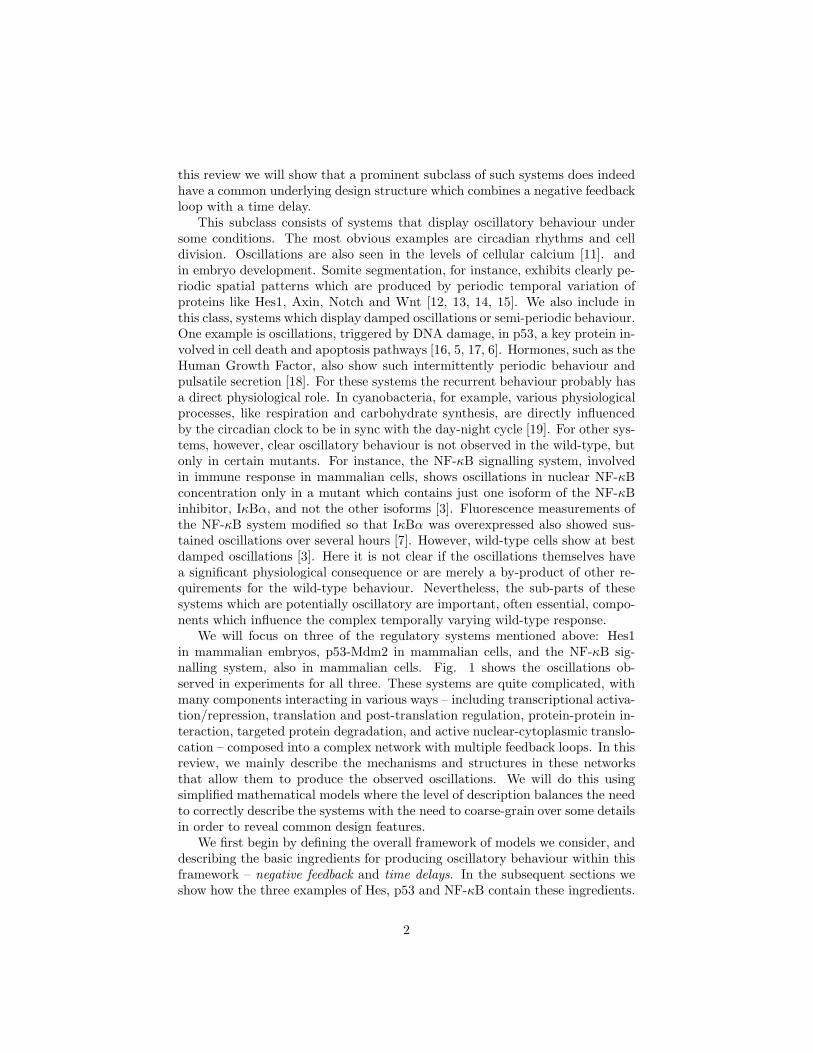
We will focus on three of the regulatory systems mentioned above: Hes1in mammalian embryos, p53-Mdm2 in mammalian cells, and the NF-κB sig-nalling system, also in mammalian cells. Fig. 1 shows the oscillations ob-served in experiments for all three. These systems are quite complicated, withmany components interacting in various ways – including transcriptional activa-tion/repression, translation and post-translation regulation, protein-protein in-teraction, targeted protein degradation, and active nuclear-cytoplasmic translo-cation – composed into a complex network with multiple feedback loops. In thisreview, we mainly describe the mechanisms and structures in these networksthat allow them to produce the observed oscillations. We will do this usingsimplified mathematical models where the level of description balances the needto correctly describe the systems with the need to coarse-grain over some detailsin order to reveal common design features.

We first begin by defining the overall framework of models we consider, anddescribing the basic ingredients for producing oscillatory behaviour within thisframework – negative feedback and time delays. In the subsequent sections weshow how the three examples of Hes, p53 and NF-κB contain these ingredients.

2

0 200 400 600 8000

0.2

0.4

0.6

0.8

1

[Hes

1]

0 200 400 600 800 10000

0.5

1

1.5

[p53

]

0 1000 2000 3000 40000

0.2

0.4

0.6

0.8

[NFk

B]

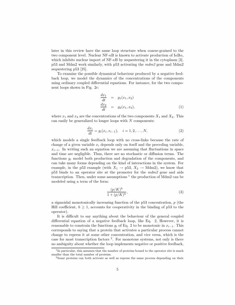
Figure 1: Experimentally observed “ultradian” oscillations in (a) Hes1, datataken from ref. [12], (b) p53, data taken from ref. [5] and (c) NF-κB, datataken from ref. [3].

3

1

4

2

3

5

6

Mdm2

p53 NF−kB

IkB

Hes1(c)(b)(a)

Hes1

Hes1 mRNA

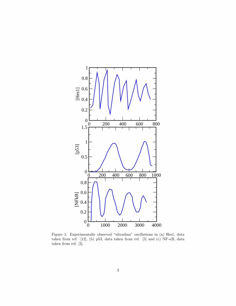
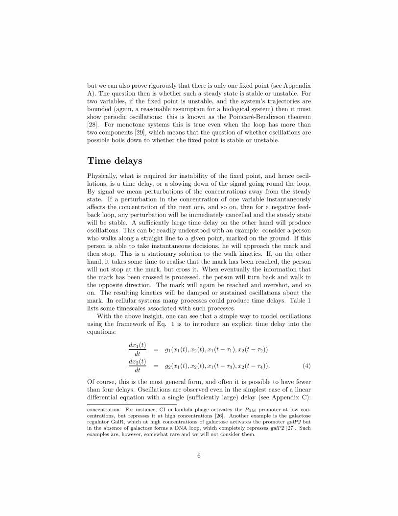
Figure 2: Negative feedback loops. (a) A generic multi-species negative feed-back loop, (b) the simplest negative feedback loop – a self-repressor, (c) twocomponent negative feedback loops for the three examples we examine. In allfigures a normal arrow represents an activating interaction, and a barred arrowrepresents a repressing interaction.

Therein we also elaborate, using stability analyses, the requirements for pro-ducing oscillations in these systems. Finally, we briefly discuss how to extractinformation about underlying structures from oscillatory time series data.

Negative feedback

Fig. 2a shows a schematic negative feedback loop. The individual nodes in thisloop are the relevant dynamical variables: they could be protein concentrations,gene expression levels, etc. Each variable either activates or represses the nextone in the loop. By an activator, we mean that if the concentration of protein 1goes up it tends to increase the concentration of protein 2 (either by increasingits production rate or decreasing its degradation rate). A repressor has theopposite effect. Then, a negative feedback loop is simply defined as a loopwith an odd number of repressors, so that the effect of a perturbation in theconcentration of any species in the loop eventually feeds back to itself witha negative sign. Feedback loops are, in general, the most common networkmotifs in cellular organization, especially when one considers the regulation ofsmall molecules [20]. We concentrate on negative feedback here because it washypothesized by Thomas [21], and rigorously proven for a wide class of systems[22, 23], that the presence of at least one negative feedback loop is a necessarycondition for oscillations.

The simplest negative feedback loop is of course a protein which repressesitself. There are many examples of such proteins: the main repressor of the SOSregulon in E. coli, LexA, also represses its own production [24]; Hes1, mentionedabove, also represses transcription of its own gene [12], shown schematically inFig. 2b. However, Hes1 looks like a one-component loop only if we coarse-grainover the intermediate steps in protein production. If we count the Hes1 mRNAalso then it becomes the two component negative feedback loop of Fig. 2c: onecomponent, Hes protein, represses the production of the second, Hes1 mRNA,while the second component activates the first. The other two systems we discuss

4

later in this review have the same loop structure when coarse-grained to thetwo component level. Nuclear NF-κB is known to activate production of IκBα,which inhibits nuclear import of NF-κB by sequestering it in the cytoplasm [3].p53 and Mdm2 work similarly, with p53 activating the mdm2 gene and Mdm2sequestering p53 [25].

To examine the possible dynamical behaviour produced by a negative feed-back loop, we model the dynamics of the concentrations of the componentsusing ordinary coupled differential equations. For instance, for the two compo-nent loops shown in Fig. 2c:

dx1

dt= g1(x1, x2)

dx2

dt= g2(x1, x2), (1)

where x1 and x2 are the concentrations of the two components X1 and X2. Thiscan easily be generalized to longer loops with N components:

dxi

dt= gi(xi, xi−1), i = 1, 2, . . . , N, (2)

which models a single feedback loop with no cross-links because the rate ofchange of a given variable xi depends only on itself and the preceding variable,xi−1. In writing such an equation we are assuming that fluctuations in spaceand time are negligible. Thus, there are no stochastic or diffusion terms. Thefunctions gi model both production and degradation of the components, andcan take many forms depending on the kind of interactions in the system. Forexample, in the p53 example (with X1 → p53, X2 → Mdm2), we know thatp53 binds to an operator site at the promoter for the mdm2 gene and aidstranscription. Then, under some assumptions 1 the production of Mdm2 can bemodeled using a term of the form:

(p/K)h

1 + (p/K)h, (3)

a sigmoidal monotonically increasing function of the p53 concentration, p (theHill coefficient, h ≥ 1, accounts for cooperativity in the binding of p53 to theoperator).

It is difficult to say anything about the behaviour of the general coupleddifferential equation of a negative feedback loop, like Eq. 2, However, it isreasonable to constrain the functions gi of Eq. 2 to be monotonic in xi−1. Thiscorresponds to saying that a protein that activates a particular process cannotchange to repress it at some other concentration, and vice versa, which is thecase for most transcription factors 2. For monotone systems, not only is thereno ambiguity about whether the loop implements negative or positive feedback,

1In particular, this assumes that the number of proteins bound to the operator site is muchsmaller than the total number of proteins.

2Some proteins can both activate as well as repress the same process depending on their

5

but we can also prove rigorously that there is only one fixed point (see AppendixA). The question then is whether such a steady state is stable or unstable. Fortwo variables, if the fixed point is unstable, and the system’s trajectories arebounded (again, a reasonable assumption for a biological system) then it mustshow periodic oscillations: this is known as the Poincare-Bendixson theorem[28]. For monotone systems this is true even when the loop has more thantwo components [29], which means that the question of whether oscillations arepossible boils down to whether the fixed point is stable or unstable.

Time delays

Physically, what is required for instability of the fixed point, and hence oscil-lations, is a time delay, or a slowing down of the signal going round the loop.By signal we mean perturbations of the concentrations away from the steadystate. If a perturbation in the concentration of one variable instantaneouslyaffects the concentration of the next one, and so on, then for a negative feed-back loop, any perturbation will be immediately cancelled and the steady statewill be stable. A sufficiently large time delay on the other hand will produceoscillations. This can be readily understood with an example: consider a personwho walks along a straight line to a given point, marked on the ground. If thisperson is able to take instantaneous decisions, he will approach the mark andthen stop. This is a stationary solution to the walk kinetics. If, on the otherhand, it takes some time to realise that the mark has been reached, the personwill not stop at the mark, but cross it. When eventually the information thatthe mark has been crossed is processed, the person will turn back and walk inthe opposite direction. The mark will again be reached and overshot, and soon. The resulting kinetics will be damped or sustained oscillations about themark. In cellular systems many processes could produce time delays. Table 1lists some timescales associated with such processes.

With the above insight, one can see that a simple way to model oscillationsusing the framework of Eq. 1 is to introduce an explicit time delay into theequations:

dx1(t)

dt= g1(x1(t), x2(t), x1(t − τ1), x2(t − τ2))

dx2(t)

dt= g2(x1(t), x2(t), x1(t − τ3), x2(t − τ4)), (4)

Of course, this is the most general form, and often it is possible to have fewerthan four delays. Oscillations are observed even in the simplest case of a lineardifferential equation with a single (sufficiently large) delay (see Appendix C):

concentration. For instance, CI in lambda phage activates the PRM promoter at low con-centrations, but represses it at high concentrations [26]. Another example is the galactoseregulator GalR, which at high concentrations of galactose activates the promoter galP2 butin the absence of galactose forms a DNA loop, which completely represses galP2 [27]. Suchexamples are, however, somewhat rare and we will not consider them.

6

dx/dt = −x(t − τ), which models the 1-component Hes loop of Fig. 2b whereHes1 represses itself after a time delay τ . Although a linear delay rate equationis an oversimplification of Hes1 production, the physics which lies behind moregeneral delay differential equations like Eq. (4) is the same. The added compli-cation is that the functions g1 and g2 are in general highly nonlinear, resultingin an amplification of the effect of the delay.

Putting an explicit time delay like this, of course, does not really shed lighton the mechanism producing the time delay. There are several possibilitieswhich can be used to produce oscillations in a negative feedback loop:

1. a process that takes a finite minimum time

2. many intermediate steps

3. a sharp response by some of the variables

4. saturated degradation

5. autocatalysis

To elaborate:

1. Rate equations, like Eq. 2, typically model processes which occur with agiven average rate, such as the binding of a protein to an operator site. Ahidden assumption is that the time interval between two binding eventsis Poisson distributed, which means that often there is a reasonable prob-ability for two events to be separated by a very short time interval (say,much shorter than the average time between events). Sometimes, how-ever, molecular processes take a certain minimum time. For instance, iftranscription and translation take a time τ after a polymerase binds to thepromoter, then the rate of production of the protein is more appropriatelymodeled as dx/dt ∝ P (t − τ), where P (t) is 1 if the polymerase is boundto the promoter at time t, and zero otherwise. Such logic has been usedto justify time-delay models in a variety of systems [31, 30, 32]. This isthe approach we will take to model the p53 and Hes systems, discussed inthe subsequent sections.

2. Processes like transcription and translation have this character becausethey are in fact composed of a large number of intermediate processes:the polymerase binds, first forming a closed complex, which then makesa transition to an open complex, and then to an elongating complex, fol-lowed by many “steps” along the DNA until the polymerase reaches theend of the gene. Even if each of these individual steps is a Poisson process,the net effect adds up to a time delay. Thus, instead of putting in an ex-plicit time delay as in Eq. 4, one could work with a negative feedback loop

7

with many components. One simple example of such an oscillator is therepressilator [33], which is a negative feedback loop with six components.

3. The repressilator also has another necessary ingredient – a nonlinearity inthe gi functions which allows some of the variables to respond to changesin the preceding variable in a faster-than-linear fashion. More precisely,the repressilator uses sigmoidal functions, like the function 3, to describetranscriptional repression, and needs Hill coefficients of at least 2 in orderto achieve oscillations. The earliest example of a negative feedback oscil-lator which uses a nonlinearity like this to produce a sharp response is amodel by Goodwin [34] where the Hill coefficient needs to be more than8.

4. Such high Hill coefficients are unlikely for biological systems, however. Inorder to get around this “problem”, Bliss, Painter and Marr [35] intro-duced another way of producing an effective time delay. They used thesaturated degradation of one of the concentrations. Saturated degradationmeans that there is an upper limit to the degradation rate of one species,thereby allowing it to remain abundant for a longer time, thus effectivelyslowing down the signal travelling around the loop. Such saturated degra-dation is quite common in biological systems, especially when proteins aretagged for targeted degradation by another protein, as we will show in theNF-κB case discussed below.

5. Finally, autocatalysis, where a molecule activates its own production canbe used to produce oscillations in systems like Eq. 1 [36]. In fact for twovariable systems where there is no explicit time-delay this is a necessarycondition for oscillations [37]. Note that this modification typically makesthe system non-monotonic.

This survey of the theoretical requirements for producing oscillations in neg-ative feedback loops already allows us to make an interesting observation: Mono-tone 2-component loops without an explicit time-delay cannot oscillate, what-ever the nonlinearity in the gi functions. We prove this explicitly in AppendixA. Thus, if one insists on modelling an oscillating system using two variables,one must choose between introducing a time delay, and sacrificing monotonicity.

2 Ultradian oscillations in biological systems

We now turn to three biological systems to illustrate these ideas in action. Inthe following, we will briefly give a description of the systems, p53-Mdm2, Hes1and NF-κB, in which “ultradian” oscillations have been observed, which havetime periods of the order of hours, as opposed to “circadian” 24 hour rhythms.We will discuss specific details of each system, at the same time emphasisingthat the basic physical mechanism which produces oscillations in all three is thesame – negative feedback along with time delays.

8

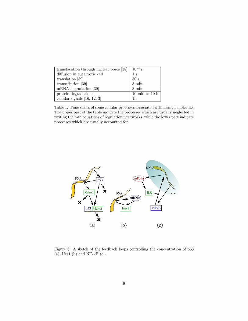
translocation through nuclear pores [38] 10−4sdiffusion in eucaryotic cell 1 stranslation [39] 30 stranscription [39] 3 minmRNA degradation [39] 3 minprotein degradation 10 min to 10 hcellular signals [16, 12, 3] 1h

Table 1: Time scales of some cellular processes associated with a single molecule.The upper part of the table indicate the processes which are usually neglected inwriting the rate equations of regulation newtworks, while the lower part indicateproceeses which are usually accounted for.

Figure 3: A sketch of the feedback loops controlling the concentration of p53(a), Hes1 (b) and NF-κB (c).

9

2.1 p53-Mdm2

The protein p53 is responsible for inducing apoptosis in cells with damagedDNA [40]. The concentration of p53 is usually kept low by a feedback mech-anism involving another protein, Mdm2, which binds to p53 and promotes itsdegradation. When the DNA is damaged, the cell expresses a number of kinaseswhich phosphorylate SER20 in p53, changing its affinity to Mdm2. This resultsin oscillations in the concentration of p53, observed both in western blot analy-sis [16, 41] (cf. Fig. 1(a)) and in single cell fluorescence experiments [5, 6]. Thestandard explanation for the overall increase in the concentration of p53 is thatits phoshoprylation decreases its affinity to Mdm2, shifting the thermodynamicequilibrium towards higher concentrations.

Apart from not explaining the oscillations, this argument does not agreewith other experimental evidence. Equilibrium isothermal titration calorime-try experiments have shown [42] that phosphorylation at SER20 decreases,not increases, the dissociation constant between p53 and Mdm2 from kD =575 ± 19 nM to kD = 360 ± 3 nM . The same effect is observed in vivo [43],where p53ASP20 (a mutated form which mimics phosphorylated p53) bindsMdm2 more tightly than p53ALA20 (which mimics unphosphorylated p53).Moreover, single cell experiments [5] show a slight decrease in the concentrationof p53 after DNA damage, which cannot be explained by the standard argument.

We showed that a simple model of the p53-Mdm2 system that incorporatesthe time delay associated with some relatively slow processes within the cell canaccount for the experimental facts in a simple way [30]. The feedback mechanismis sketched in Fig. 3(a) and the associated time-delayed rate equations are

∂p

∂t= S − a · pm − b · p (5)

∂m

∂t= c

p(t − τ) − pm(t − τ)

kg + p(t − τ) − pm(t − τ)− d · m

pm =1

2

(

(p + m + k) −√

(p + m + k)2 − 4p · m)

,

where the delay τ takes into account the half-life of mRNA, the diffusion time,the time needed to cross the nuclear membrane and the transcription/translationtime. One can solve Eqs. (5) numerically, simulating the damage to DNAby a sudden change in the dissociation constant k. Fig. 4 shows the onsetof oscillations in this model in response to a sudden decrease in k at timet = 2000 s.

Several observations emerge from the simulation results in Fig. 4. Mostinterestingly, what triggers oscillations is a decrease in the dissociation constantk, while any increase in its value just shifts the equilibrium towards higher valuesof p (cf. inset of Fig. 4). Moreover, just after t = 2000 s the concentration ofp53 decreases, as observed in the experiments. Finally, the concentration, pm,of the complex p53-Mdm2 is, at any time, essentially identical to the minimumof p and m (gray curve in Fig. 4), indicating that the complex is saturated.

10

10000 20000 30000 40000time [s]

0

100

200

300

400

conc

entr

atio

n

10000 20000 30000 40000

Figure 4: Oscillations displayed by the numerical solution of the dynamic equa-tions of p53. The numerical values of the rates are a = 3·10−2 s−1, b = 10−4 s−1,c = 1 s−1, d = 1 s−2, S = 1 s−1, k = 180, kg = 28 and τ = 1200 s. At timet = 20000 s the value of k is decreased of a factor 10. In the inset, the solution ofthe same equations, where the value of k is increased of a factor 10 at t = 20000s. The equations are solved with the Adams algorithm.

11

10−4

10−2

100

102

multiplier of k

0

101

∆p/p

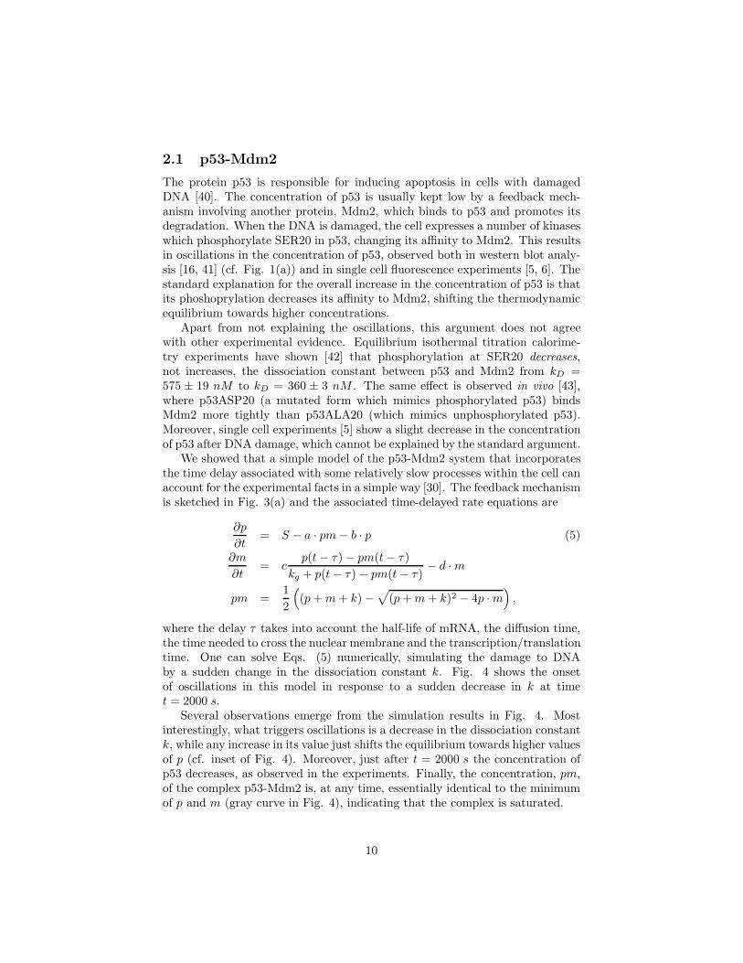
Figure 5: The height of the response peak ∆p with respect to the quantity thatmultiplies k, mimicking the stress. The dotted line indicates that the systemdoes not display oscillatory behaviour.

The relative change, ∆p, in the maximum concentration of p53 reached afterthe simulated stress event is displayed in Fig. 5 as a function of the change in k.The value of ∆p displays a sigmoidal behaviour if the stress decreases the valueof k. In contrast, in the absence of a time delay, this curve is linear with respectto k [30]. Thus, the time delay and the oscillations are crucial for producing asensitive system that can respond to stress in a sharp, faster-than-linear manner.

We also undertook a detailed analysis of the response of the oscillations tochanges in the parameters [30]. It turns out that the oscillations do not changequalitatively when parameters a, b and c are varied (by upto five orders of magni-tude), whereas a decrease in d or kg suppresses the oscillating behaviour. Theseparameters are associated with, respectively, the the degradation of Mdm2 andthe binding of p53 to the DNA. One could speculate therefore that these pro-cesses play an important role in the production of tumors that arise when thep53 response mechanism fails. This speculation is, in fact, consistent with theobservation that around the 45% of all tumors display mutations in the p53region which binds to DNA [44].

2.2 Stability analysis of the p53-Mdm2 model

The overall behaviour of the proteins with respect to time evidently depends onthe parameters of the dynamic equations, that is the production and degradation

12

rates and the delay. Over long timescales, the protein concentrations can eitherconverge to a steady state or a limit cycle (i.e., sustained oscillations). Chaoticbehaviour is never observed within this model.

A careful analysis of how the dynamics of the protein concentration dependson the parameters of the rate equations has been done by Neamtu and coworkersin ref. [45]. The main conclusion of this work is that under the condition that thedissociation constant k between p53 and Mdm2 is small, there exists a criticaldelay, τ0, above which the system shows oscillations (see details in AppendixC).

In the language of dynamical systems, the transition when the delay, τ ,crosses τ0 is a Hopf bifurcation. A Hopf bifurcation is the generic type ofbifurcation that occurs when a stable fixed point of the system becomes unstableand turns into a limit cycle, a dynamically oscillating state, as consequence ofa change in some parameter of the system (see Appendix B for more details).

2.3 Hes1 and its mRNA

The transcription factor Hes1 controls the differentiation of neurons in mam-malian embryos [46]. Its concentration is controlled by a feedback loop builtout of Hes1 and its own mRNA (see Fig. 3). Like p53, its concentrations dis-plays oscillations when the cells are stimulated with serum [12]. The period issimilar to that of p53, approximately two hours, and the oscillations last for≈ 12 hours. Hes1 is known to repress another protein called Mash1. Both theknocking out of Mash1 and its continuous expression by means of retroviral in-troduction results in a lack of cell differentiation. Only when there are periodicoscillations in the concentration of Hes1 (and thus of Mash1) is there properdifferentiation of neuronal cells [46], showing that the temporal variation of theprotein concentrations are critical for the developement of the nervous system.

The relation of Hes1 oscillations to segmentation and spatial patterns hasbeen studied by several authors. It is well known that oscillations in Hes1 ispart of Notch signalling and Hirata et al Ref. [12] studied the coordinatedsomite segmentation in the presomitic mesoderm of mice embryos and founda correlation between the oscillations of Hes1 and initiation of somites. Thegeneral issue of segmentation in vertebrates has been further studied in Ref.[13, 14, 15] indicating that the oscillations in the Notch pathway signaling areintimately related to the Wnt signaling. At the caudal end of the embryo Notchand Wnt oscillates out of phase when the gradient in the Wnt level is over agiven threshold [14, 15]. New cells are provided and move away from the caudalend each setting a boundary for a somite segmentation. This continues untilall somites are produced which subsequently gives rise to the spinal cord [13].Ultradian oscillations of signaling pathways are thus extremely important forsegmentation.

The control mechanism of Hes1 oscillations again involves a negative feed-back loop with one activation and one repression: the transcription of the mRNAof Hes1 activates the production (translation) of the protein, and Hes1 repressesthe transcription of its own mRNA. The main difference compared to p53 is that

13

here one of the nodes represents an mRNA, not a protein. However, this differ-ence is merely semantic: the control network still has two nodes, of which oneis activating and one is repressing. The molecular species of these nodes areimmaterial to the description of the oscillations 3.

We model the system using the following equations (cf. [31])

∂r

∂t=

αkh

kh + [s(t − τ)]h− krr(t) (6)

∂s

∂t= βr(t) − kss(t), (7)

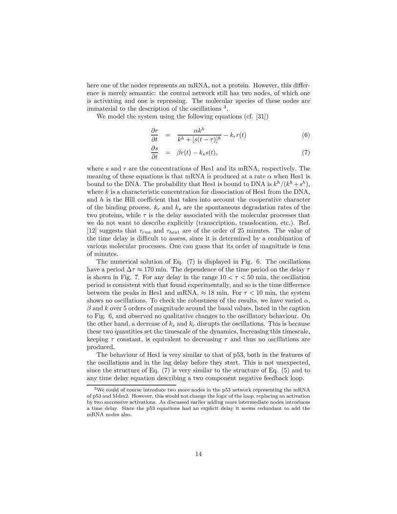
where s and r are the concentrations of Hes1 and its mRNA, respectively. Themeaning of these equations is that mRNA is produced at a rate α when Hes1 isbound to the DNA. The probability that Hes1 is bound to DNA is kh/(kh +sh),where k is a characteristic concentration for dissociation of Hes1 from the DNA,and h is the Hill coefficient that takes into account the cooperative characterof the binding process. kr and ks are the spontaneous degradation rates of thetwo proteins, while τ is the delay associated with the molecular processes thatwe do not want to describe explicitly (transcription, translocation, etc.). Ref.[12] suggests that τrna and τhes1 are of the order of 25 minutes. The value ofthe time delay is difficult to assess, since it is determined by a combination ofvarious molecular processes. One can guess that its order of magnitude is tensof minutes.

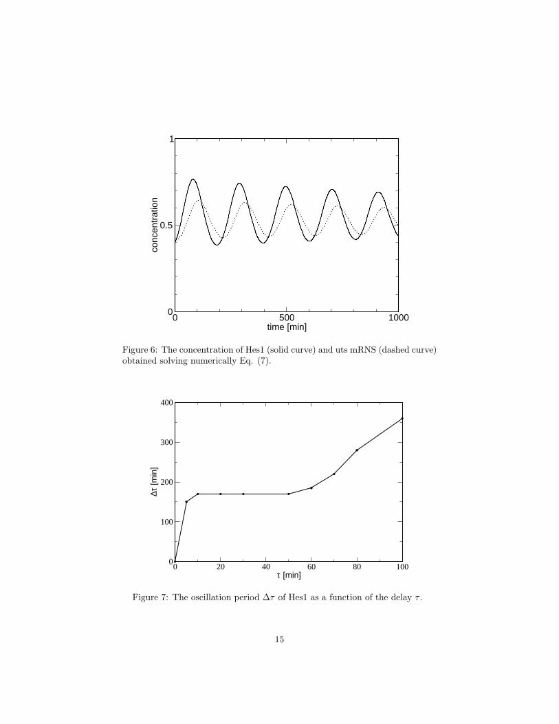
The numerical solution of Eq. (7) is displayed in Fig. 6. The oscillationshave a period ∆τ ≈ 170 min. The dependence of the time period on the delay τis shown in Fig. 7. For any delay in the range 10 < τ < 50 min, the oscillationperiod is consistent with that found experimentally, and so is the time differencebetween the peaks in Hes1 and mRNA, ≈ 18 min. For τ < 10 min, the systemshows no oscillations. To check the robustness of the results, we have varied α,β and k over 5 orders of magnitude around the basal values, listed in the captionto Fig. 6, and observed no qualitative changes to the oscillatory behaviour. Onthe other hand, a decrease of ks and kr disrupts the oscillations. This is becausethese two quantities set the timescale of the dynamics, Increasing this timescale,keeping τ constant, is equivalent to decreasing τ and thus no oscillations areproduced.

The behaviour of Hes1 is very similar to that of p53, both in the features ofthe oscillations and in the lag delay before they start. This is not unexpected,since the structure of Eq. (7) is very similar to the structure of Eq. (5) and toany time delay equation describing a two component negative feedback loop.

3We could of course introduce two more nodes in the p53 network representing the mRNAof p53 and Mdm2. However, this would not change the logic of the loop, replacing an activationby two successive activations. As discussed earlier adding more intermediate nodes introducesa time delay. Since the p53 equations had an explicit delay it seems redundant to add themRNA nodes also.

14

0 500 1000time [min]

0

0.5

1

conc

entr

atio

n

Figure 6: The concentration of Hes1 (solid curve) and uts mRNS (dashed curve)obtained solving numerically Eq. (7).

0 20 40 60 80 100τ [min]

0

100

200

300

400

∆τ [m

in]

Figure 7: The oscillation period ∆τ of Hes1 as a function of the delay τ .

15

2.4 NF-κB and IκB

The NF-κB family of proteins is one of the most studied in the last ten years,being involved in a variety of cellular processes including immune response, in-flammation, and development [3, 47]. NF-κB can be activated by a number ofexternal stimuli [48] including bacteria, viruses and various stresses and pro-teins (for instance, refs. [3, 7] used the tumor necrosis factor-α, TNF-α). Inresponse to these signals it targets over 150 genes including many chemokines,immunoreceptors, stress reponse genes, as well as acute phase inflammation re-sponse proteins [48]. Each NF-κB has a partner inhibitor called IκB, whichinactivates NF-κB by sequestering it both in the nucleus as well as in the cy-toplasm. In fact, the IκB proteins come in several isoforms α, β, ǫ [3, 49], andperhaps others [47]. Some of these isoforms are, in turn, transcriptionally ac-tivated by NF-κB, thus forming a negative feedback loop which is essentiallyidentical in structure to the other two discussed above.

The potential for this negative feedback loop to produce oscillations inthe nuclear-cytoplasmic translocation of NF-κB was initially shown by elec-trophoretic mobility shift assay experiments [3]. They found that wild-type cellsand mutants containing only the IκBα isoform showed damped oscillations. Incontrast, cells with only the IκBβ or ǫ isoforms do not show oscillations. Thisconclusion was bolstered by single-cell flourescence imaging experiments whichshow sustained oscillations of nuclear NF-κB in mammalian cells [7], with atime period of the order of hours. In these experiments IκBα was overexpressedhence the system behaves like the mutant which has only the IκBα isoform.

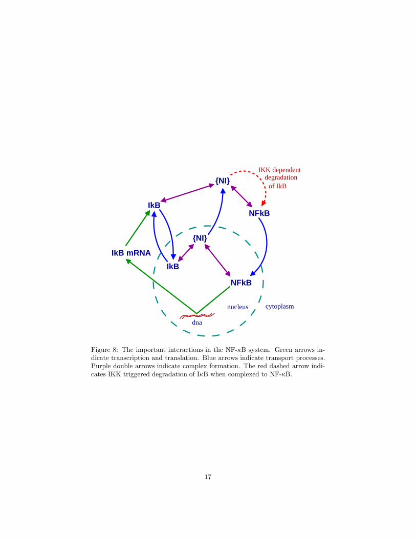
As sustained oscillations are clearest here, we will focus our modelling on thismutant. The following cellular processes, summarized in Fig. 8, are importantfor this system on the timescales we are interested in (i.e., we ignore processeswhich are very slow):

• NF-κB, when in the nucleus, activates transcription of the IκBα gene(henceforth we will drop α unless we are explicitly talking about morethan one isoform), producing IκB mRNA in the cytoplasm.

• The IκB mRNA is translated to form IκB protein.

• The IκB protein can be transported in and out of the nucleus.

• In both compartments, IκB forms a complex with NF-κB.

• The NF-κB-IκB complex (henceforth referred to as {NI}) cannot be im-ported into the nucleus. However, if it forms within the nucleus it can beexported out.

• Free NF-κB behaves in exactly the opposite way. Free NF-κB is activelytransported into the nucleus but not from the nucleus to the cytoplasm.

• The cytoplasmic {NI} complex is tagged by another protein, the IκB ki-nase (IKK), for proteolytic degradation. This results in degradation of

16

IkB

IkB

NFkB

IkB mRNA

NFkB

IKK dependentdegradation

of IkB

nucleus

dna

{NI}

{NI}

cytoplasm

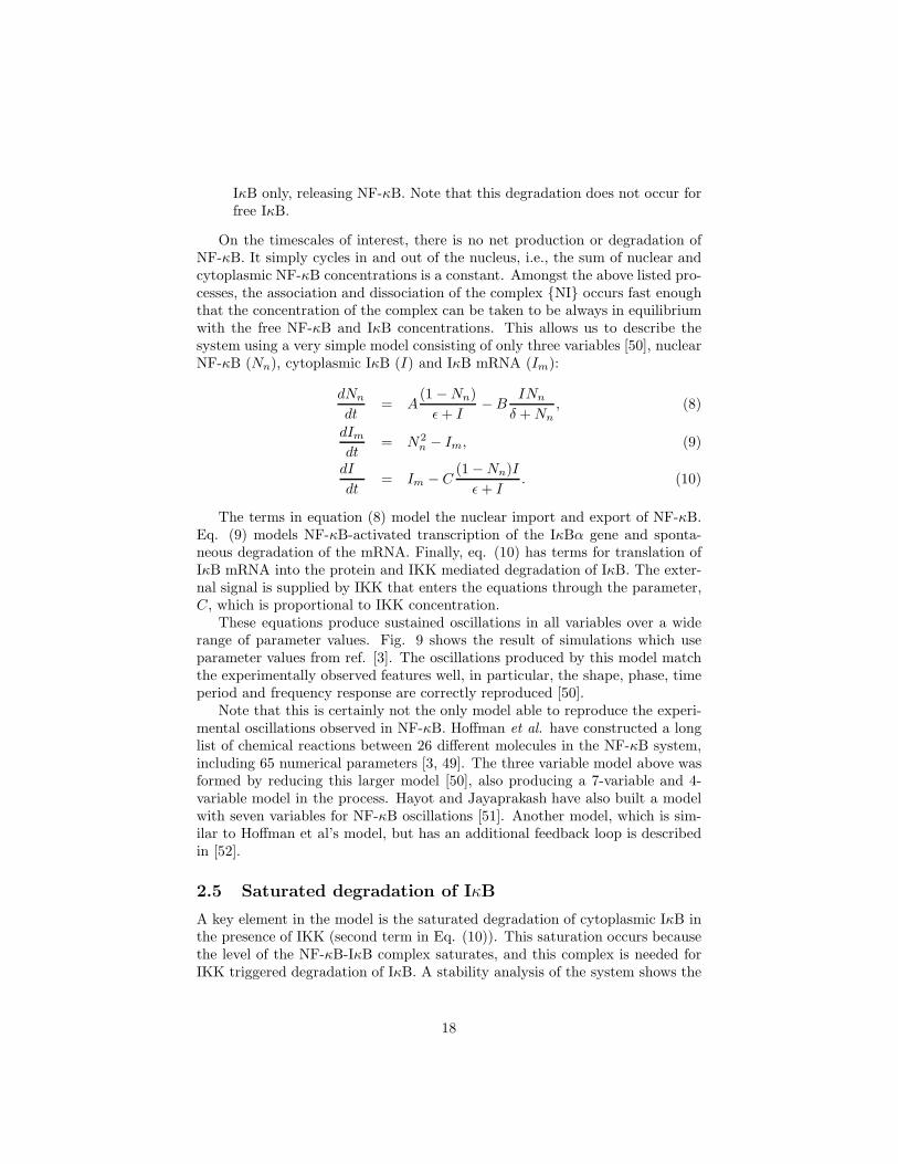
Figure 8: The important interactions in the NF-κB system. Green arrows in-dicate transcription and translation. Blue arrows indicate transport processes.Purple double arrows indicate complex formation. The red dashed arrow indi-cates IKK triggered degradation of IκB when complexed to NF-κB.

17

IκB only, releasing NF-κB. Note that this degradation does not occur forfree IκB.

On the timescales of interest, there is no net production or degradation ofNF-κB. It simply cycles in and out of the nucleus, i.e., the sum of nuclear andcytoplasmic NF-κB concentrations is a constant. Amongst the above listed pro-cesses, the association and dissociation of the complex {NI} occurs fast enoughthat the concentration of the complex can be taken to be always in equilibriumwith the free NF-κB and IκB concentrations. This allows us to describe thesystem using a very simple model consisting of only three variables [50], nuclearNF-κB (Nn), cytoplasmic IκB (I) and IκB mRNA (Im):

dNn

dt= A

(1 − Nn)

ǫ + I− B

INn

δ + Nn, (8)

dIm

dt= N2

n − Im, (9)

dI

dt= Im − C

(1 − Nn)I

ǫ + I. (10)

The terms in equation (8) model the nuclear import and export of NF-κB.Eq. (9) models NF-κB-activated transcription of the IκBα gene and sponta-neous degradation of the mRNA. Finally, eq. (10) has terms for translation ofIκB mRNA into the protein and IKK mediated degradation of IκB. The exter-nal signal is supplied by IKK that enters the equations through the parameter,C, which is proportional to IKK concentration.

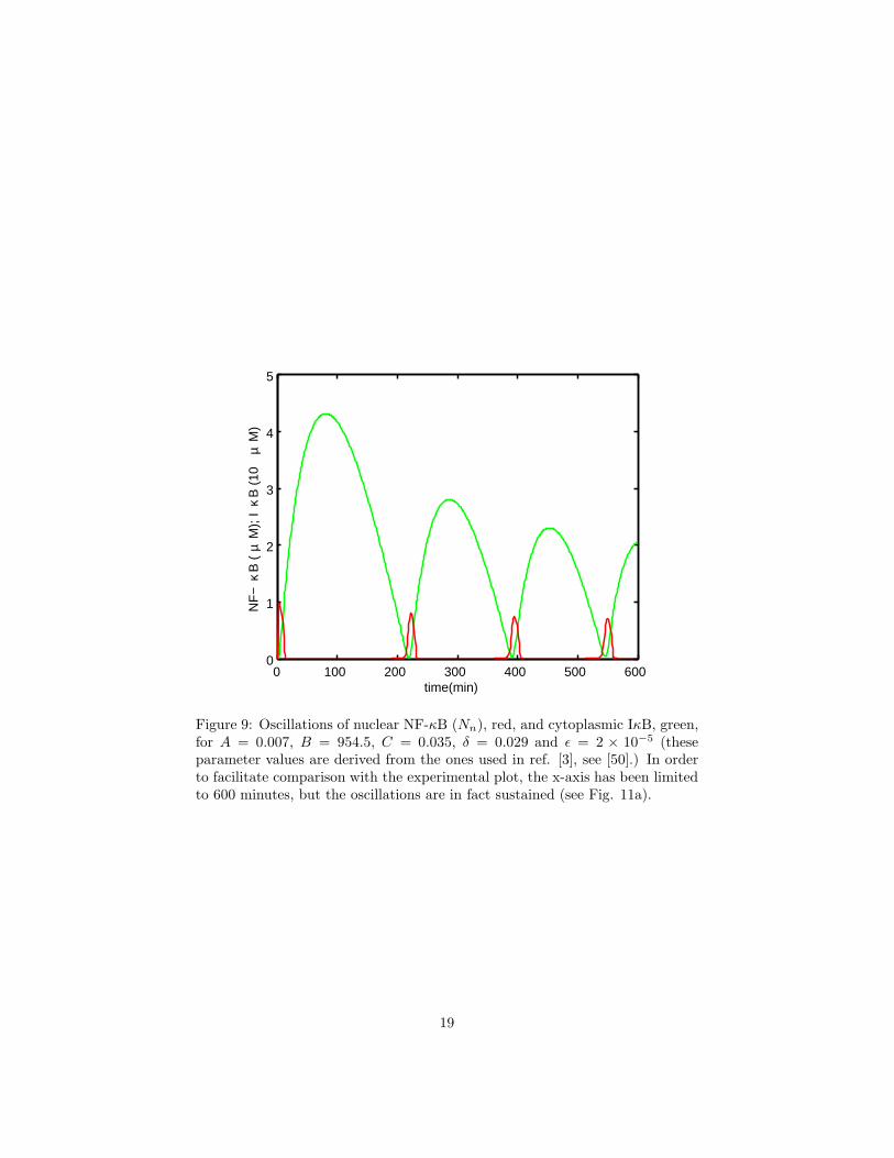
These equations produce sustained oscillations in all variables over a widerange of parameter values. Fig. 9 shows the result of simulations which useparameter values from ref. [3]. The oscillations produced by this model matchthe experimentally observed features well, in particular, the shape, phase, timeperiod and frequency response are correctly reproduced [50].

Note that this is certainly not the only model able to reproduce the experi-mental oscillations observed in NF-κB. Hoffman et al. have constructed a longlist of chemical reactions between 26 different molecules in the NF-κB system,including 65 numerical parameters [3, 49]. The three variable model above wasformed by reducing this larger model [50], also producing a 7-variable and 4-variable model in the process. Hayot and Jayaprakash have also built a modelwith seven variables for NF-κB oscillations [51]. Another model, which is sim-ilar to Hoffman et al’s model, but has an additional feedback loop is describedin [52].

2.5 Saturated degradation of IκB

A key element in the model is the saturated degradation of cytoplasmic IκB inthe presence of IKK (second term in Eq. (10)). This saturation occurs becausethe level of the NF-κB-IκB complex saturates, and this complex is needed forIKK triggered degradation of IκB. A stability analysis of the system shows the

18

0 100 200 300 400 500 6000

1

2

3

4

5

time(min)

NF

−κ

B (

µ M

); I

κB

(10

µ

M)

Figure 9: Oscillations of nuclear NF-κB (Nn), red, and cytoplasmic IκB, green,for A = 0.007, B = 954.5, C = 0.035, δ = 0.029 and ǫ = 2 × 10−5 (theseparameter values are derived from the ones used in ref. [3], see [50].) In orderto facilitate comparison with the experimental plot, the x-axis has been limitedto 600 minutes, but the oscillations are in fact sustained (see Fig. 11a).

19

importance of the saturated degradation for oscillations. We begin by examiningthe fixed points of the system.

The fixed point values of Nn, Im and I are solutions to

A(1 − Nn)

ǫ + I− B

INn

δ + Nn= 0,

N2n − Im = 0,

Im − C(1 − Nn)I

ǫ + I= 0.

Im and I can be eliminated using Im = N2n, giving I = (N2

nǫ)/(C − CNn −N2

n). From this we find that the fixed point value of Nn is a solution of theequation (C − CNn − N2

n)2 = (BCǫ2N3n)/[A(δ + Nn)], or equivalently,

N5n+(δ+2C)N4

n+C

[

2(δ − 1) + C − B

Aǫ2]

N3n+C[(C−2)δ−2C]N2

n+C2(1−2δ)Nn+C2δ = 0.

In general, this has two real solutions, one with C −CNn −N2n > 0 and the

other with C − CNn − N2n < 0. The latter results in a negative value for I and

therefore is not an acceptable solution. Thus we are left with only one fixedpoint.

Next, we linearize the equations around the fixed point, which gives theJacobian (see also Appendix B)

J =

− Aǫ+I − δBI

(δ+Nn)2 0 −A(1−Nn)(ǫ+I)2 − BNn

δ+Nn

2Nn −1 0CIǫ+I 1 −Cǫ(1−Nn)

(ǫ+I)2

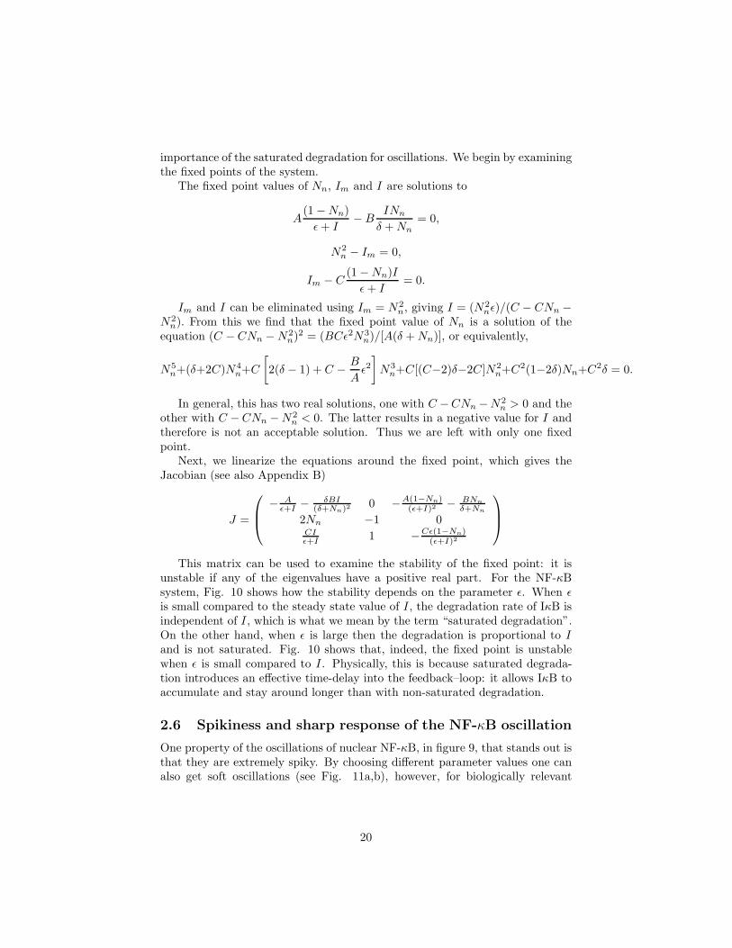
This matrix can be used to examine the stability of the fixed point: it isunstable if any of the eigenvalues have a positive real part. For the NF-κBsystem, Fig. 10 shows how the stability depends on the parameter ǫ. When ǫis small compared to the steady state value of I, the degradation rate of IκB isindependent of I, which is what we mean by the term “saturated degradation”.On the other hand, when ǫ is large then the degradation is proportional to Iand is not saturated. Fig. 10 shows that, indeed, the fixed point is unstablewhen ǫ is small compared to I. Physically, this is because saturated degrada-tion introduces an effective time-delay into the feedback–loop: it allows IκB toaccumulate and stay around longer than with non-saturated degradation.

2.6 Spikiness and sharp response of the NF-κB oscillation

One property of the oscillations of nuclear NF-κB, in figure 9, that stands out isthat they are extremely spiky. By choosing different parameter values one canalso get soft oscillations (see Fig. 11a,b), however, for biologically relevant

20

0 0.2 0.4 0.6 0.8 1 1.2 1.4 1.6 1.8 2

x 10−3

1.5

2

2.5

3x 10

−3

ε

I (di

men

sion

less

)

0 0.1 0.2 0.3 0.40

1

2

3

4

5x 10

−3ε = 5 × 10−4

Nn (dimensionless)

I (di

men

sion

less

)

0 0.1 0.2 0.3 0.40

1

2

3

4

5x 10

−3 ε = 1.5 × 10−3

Nn (dimensionless)

I (di

men

sion

less

)

ε = 5 × 10 −4

ε = 1.5 × 10 −3

A

B C

unstable

stable

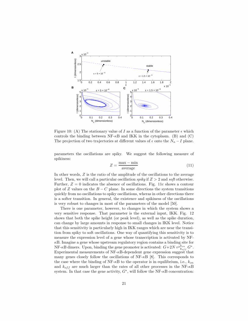
Figure 10: (A) The stationary value of I as a function of the parameter ǫ whichcontrols the binding between NF-κB and IKK in the cytoplasm. (B) and (C)The projection of two trajectories at different values of ǫ onto the Nn − I plane.

parameters the oscillations are spiky. We suggest the following measure ofspikiness:

Z =max − min

average(11)

In other words, Z is the ratio of the amplitude of the oscillations to the averagelevel. Then, we will call a particular oscillation spiky if Z > 2 and soft otherwise.Further, Z = 0 indicates the absence of oscillations. Fig. 11c shows a contourplot of Z values on the B − C plane. In some directions the system transitionsquickly from no oscillations to spiky oscillations, wheras in other directions thereis a softer transition. In general, the existence and spikiness of the oscillationsis very robust to changes in most of the parameters of the model [50].

There is one parameter, however, to changes in which the system shows avery sensitive response. That parameter is the external input, IKK. Fig. 12shows that both the spike height (or peak level), as well as the spike duration,can change by large amounts in response to small changes in IKK level. Noticethat this sensitivity is particularly high in IKK ranges which are near the transi-tion from spiky to soft oscillations. One way of quantifying this sensitivity is tomeasure the expression level of a gene whose transcription is activated by NF-κB. Imagine a gene whose upstream regulatory region contains a binding site forNF-κB dimers. Upon, binding the gene promoter is activated: G+2N ⇀↽kon

koffG∗.

Experimental measurements of NF-κB-dependent gene expression suggest thatmany genes closely follow the oscillations of NF-κB [8]. This corresponds tothe case where the binding of NF-κB to the operator is in equilibrium, i.e., kon

and koff are much larger than the rates of all other processes in the NF-κBsystem. In that case the gene activity, G∗, will follow the NF-κB concentration:

21

0 200 400 600 800 1000 1200 1400 16000

0.5

1

time (min)

Nn (

µ M

)

0 100 200 300 400 500 600 700 8000

0.2

0.4

0.6

0.8

time (min)

Nn (

µ M

) ε = 5 × 10 −4ε = 5 × 10 −4

ε = 2 × 10 −5

A

B

log 10

(C)

log10

(B)−6 −4 −2 0 2 4

−2.5

−2

−1.5

−1

−0.5

0Z=0.01

Z=2

Z=5

Z=10

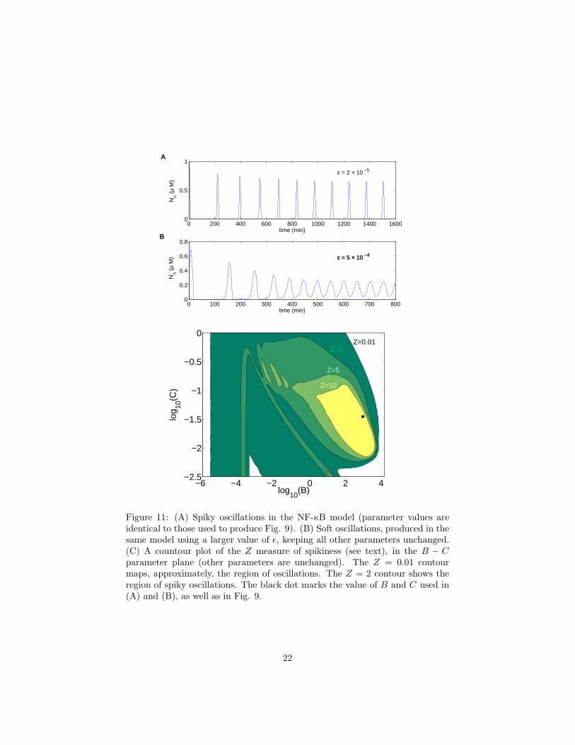
Figure 11: (A) Spiky oscillations in the NF-κB model (parameter values areidentical to those used to produce Fig. 9). (B) Soft oscillations, produced in thesame model using a larger value of ǫ, keeping all other parameters unchanged.(C) A countour plot of the Z measure of spikiness (see text), in the B − Cparameter plane (other parameters are unchanged). The Z = 0.01 contourmaps, approximately, the region of oscillations. The Z = 2 contour shows theregion of spiky oscillations. The black dot marks the value of B and C used in(A) and (B), as well as in Fig. 9.

22

A B

0 0.2 0.4 0.6 0.8 1 1.20

0.1

0.2

0.3

0.4

0.5

IKK (µ M)

spik

e du

ratio

n

Soft Osc., Z<2

Spiky Osc., Z>2

IKK=0.5 µ M

0 0.2 0.4 0.6 0.8 1 1.20

0.1

0.2

0.3

0.4

0.5

0.6

0.7

IKK (µ M)

peak

NF

−κ

B (

µ M

)

Soft Osc., Z<2

Spiky Osc., Z>2

IKK=0.5 µ M

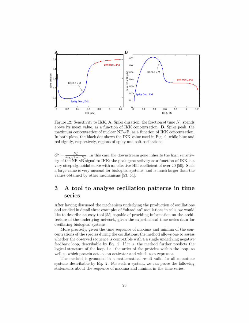
Figure 12: Sensitivity to IKK. A. Spike duration, the fraction of time Nn spendsabove its mean value, as a function of IKK concentration. B. Spike peak, themaximum concentration of nuclear NF-κB, as a function of IKK concentration.In both plots, the black dot shows the IKK value used in Fig. 9, while blue andred signify, respectively, regions of spiky and soft oscillations.

G∗ =N2

n

koff /kon+N2n. In this case the downstream gene inherits the high sensitiv-

ity of the NF-κB signal to IKK: the peak gene activity as a function of IKK is avery steep sigmoidal curve with an effective Hill coefficient of over 20 [50]. Sucha large value is very unusual for biological systems, and is much larger than thevalues obtained by other mechanisms [53, 54].

3 A tool to analyse oscillation patterns in time

series

After having discussed the mechanism underlying the production of oscillationsand studied in detail three examples of “ultradian” oscillations in cells, we wouldlike to describe an easy tool [55] capable of providing information on the archi-tecture of the underlying network, given the experimental time series data foroscillating biological systems.

More precisely, given the time sequence of maxima and minima of the con-centrations of the species during the oscillations, the method allows one to assesswhether the observed sequence is compatible with a a single underlying negativefeedback loop, describable by Eq. 2. If it is, the method further predicts thelogical structure of the loop, i.e. the order of the proteins within the loop, aswell as which protein acts as an activator and which as a repressor.

The method is grounded in a mathematical result valid for all monotonesystems describable by Eq. 2. For such a system, we can prove the followingstatements about the sequence of maxima and minima in the time series:

23

0 12 24time (hours)

0

0.2

0.4

0.6

0.8

1

conc

entr

atio

n

p53Mdm2

P M M P P M P

{ { { {

Pmax Mmax Pmin Mmin Pmax

M

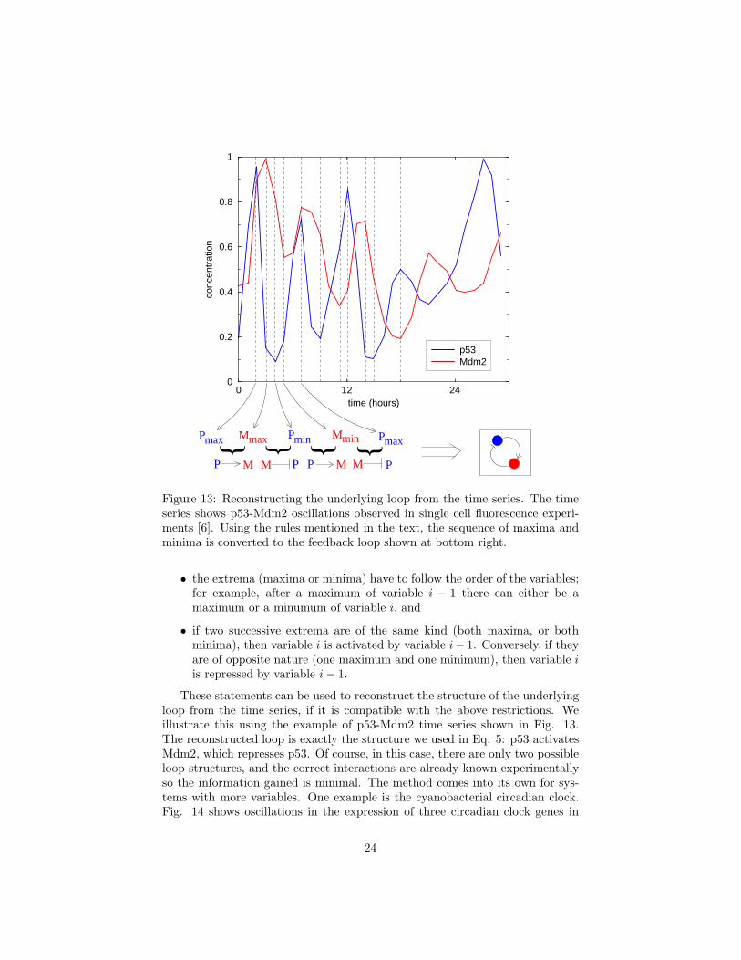
Figure 13: Reconstructing the underlying loop from the time series. The timeseries shows p53-Mdm2 oscillations observed in single cell fluorescence experi-ments [6]. Using the rules mentioned in the text, the sequence of maxima andminima is converted to the feedback loop shown at bottom right.

• the extrema (maxima or minima) have to follow the order of the variables;for example, after a maximum of variable i − 1 there can either be amaximum or a minumum of variable i, and

• if two successive extrema are of the same kind (both maxima, or bothminima), then variable i is activated by variable i− 1. Conversely, if theyare of opposite nature (one maximum and one minimum), then variable iis repressed by variable i − 1.

These statements can be used to reconstruct the structure of the underlyingloop from the time series, if it is compatible with the above restrictions. Weillustrate this using the example of p53-Mdm2 time series shown in Fig. 13.The reconstructed loop is exactly the structure we used in Eq. 5: p53 activatesMdm2, which represses p53. Of course, in this case, there are only two possibleloop structures, and the correct interactions are already known experimentallyso the information gained is minimal. The method comes into its own for sys-tems with more variables. One example is the cyanobacterial circadian clock.Fig. 14 shows oscillations in the expression of three circadian clock genes in

24

0 12 24 36 48Time (hrs)

0.6

0.8

1

1.2

1.4

1.6

Rel

ativ

e ex

pres

sion

leve

l

kaiB3kaiAkaiC1

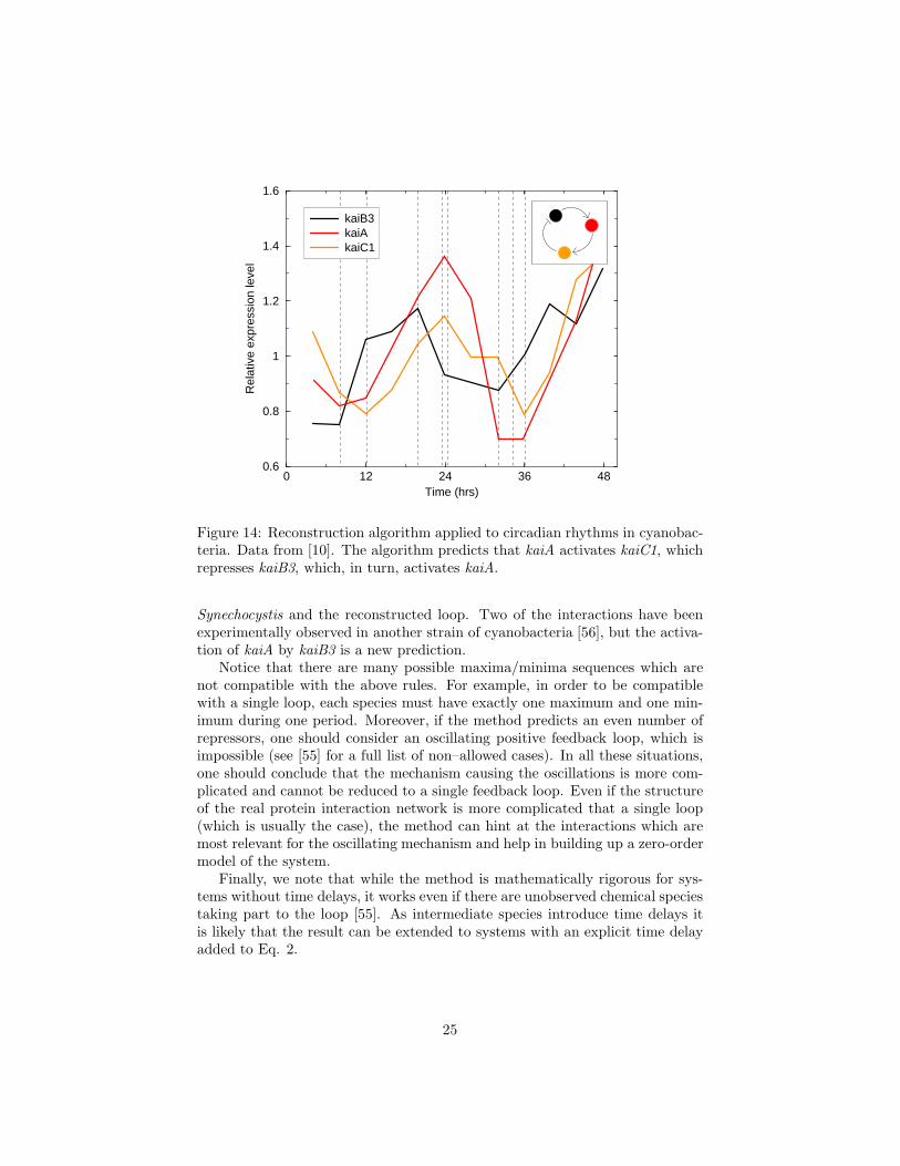
Figure 14: Reconstruction algorithm applied to circadian rhythms in cyanobac-teria. Data from [10]. The algorithm predicts that kaiA activates kaiC1, whichrepresses kaiB3, which, in turn, activates kaiA.

Synechocystis and the reconstructed loop. Two of the interactions have beenexperimentally observed in another strain of cyanobacteria [56], but the activa-tion of kaiA by kaiB3 is a new prediction.

Notice that there are many possible maxima/minima sequences which arenot compatible with the above rules. For example, in order to be compatiblewith a single loop, each species must have exactly one maximum and one min-imum during one period. Moreover, if the method predicts an even number ofrepressors, one should consider an oscillating positive feedback loop, which isimpossible (see [55] for a full list of non–allowed cases). In all these situations,one should conclude that the mechanism causing the oscillations is more com-plicated and cannot be reduced to a single feedback loop. Even if the structureof the real protein interaction network is more complicated that a single loop(which is usually the case), the method can hint at the interactions which aremost relevant for the oscillating mechanism and help in building up a zero-ordermodel of the system.

Finally, we note that while the method is mathematically rigorous for sys-tems without time delays, it works even if there are unobserved chemical speciestaking part to the loop [55]. As intermediate species introduce time delays itis likely that the result can be extended to systems with an explicit time delayadded to Eq. 2.

25

4 Summary and Outlook

Questions about cellular processes that use complex, temporally varying signalscan be crudely classified into the ‘How’ and ‘Why’ groups. ’How’ questionsdeal with the structure of the regulatory network and the range of dynamicalbehaviour it can produce: how does the network produce oscillations? whatare the necessary and sufficient mechanisms? how are they implemented inreal cellular systems? ‘Why’ questions deal with the physiological role of theparticular dynamical behaviour produced by the network: why does p53 startoscillating in response to DNA damage? do oscillations carry some informationthat can be decoded by downstream genes? could a non-oscillating system haveworked equally well for the cell?

In this review we have mainly investigated the ‘How’ questions for one sub-set of cellular response systems that use temporally varying signals: eukaryoticsystems exhibiting “ultradian” oscillations. The three systems we have mod-elled – p53, which is important for apoptosis, Hes1, which is part of the Notchcycle responsible for somite segmentation, and NF-κB, a key protein in immuneresponse – all turn out to have the same basic design that produces oscillations.The two key aspects of this design are the presence of negative feedback and timedelays. There are many ways of producing an effective time delay in cellularprocesses. In particular, we emphasised, using the example of NF-κB, saturateddegradation as one such mechanism.

Saturated degradation plays a role in many models of oscillatory negativefeedback–loops. The earliest use of this mechanism is in the model of Bliss,Painter and Marr [35], which is similar to our NF-κB model. Saturated degra-dation has also been used by Goldbeter in various models of cellular oscillations,e.g., the cell cycle [57], development in myxobacteria [58], yeast stress response[59] and the mammalian circadian clock [60]. It is also found in models of cal-cium oscillations in cells [61, 62]. In the p53-Mdm2 system too, as describedearlier, there is a similar saturated complex formation, where one componentof the complex is subsequently degraded. This is so similar to the NF-κB casethat it should be possible to construct a model for p53 oscillations which hasordinary differential equations without an explicit time delay (see for instance[6]). Because saturated degradation is easily implemented by complex formationwe conclude that it would be a very useful general mechanism for producing aneffective time delay in cellular systems.

Although we have focussed more on how the oscillations are produced, the‘Why’ question of whether the oscillations have a direct physiological role inthese systems is of course an important one. In NF-κB, oscillations are observed,not in wild-type cells, but rather in mutants or cells which overexpress certainproteins. Therefore, it is quite possible that oscillations themselves play nodirect role in the wild-type response [63]. However, wild-type cells do show acomplex temporal variation of NF-κB of which the spiky response of the IκBαmodule is an extremely important component (IκBalpha is the only isoformwhose knockout mutants are not viable [3]). Hes1 oscillations, even thoughdamped, might have a direct relevance for spatial pattern formation in embryos.

26

Hes1 is a key element in the Notch oscillating cycle, which, in mouse and chickenembryos, is coupled, out of phase, with the Wnt cycle. In each period of thesecycles, a somite is formed, thus leading to vertebrate segmentation. Furtherwork should clarify whether the Hes1 oscillations drives these cycles, or is slavedto them, or has a different role entirely. In the case of p53, the oscillationsappear to be sustained, therefore it is likely they are directly important for theapoptosis pathway, but again it is not clear precisely how.

Even in the absence of unambiguous evidence that oscillations have a directfunctional importance, investigations into the mechanisms underlying the oscil-lations have implications for some of the ‘Why’ questions. For instance, notingthat an oscillating signal carries much more information than a steady signal,[17, 64] suggested that differential regulation of downstream gene circuits couldbe achieved if they were sensitive to the frequency of the oscillation. Indeed, aswe have shown [50], it is easy for a single downstream gene to act as a ‘low-passfilter’. Regulatory circuits with multiple genes could be constructed to haveparticular frequency responses. However, it is perhaps more fruitful to look fora physiological role in other properties of the dynamics, rather than the peri-odicity. One such property, especially prominent in NF-κB oscillations, is thespikiness. A spiky signal of this kind carries even more information than a softoscillation or a steady state level. Spiky pulses, whether periodic or randomor isolated, are in a sense less “expensive”: If a downstream gene is expressedwhen p53 crosses some threshold it is energetically and metabolically cheaperto have a spike whose peak crosses the threshold for long enough to trigger thegene, than to produce and maintain the protein above that level for a long time.

In this context it is noteworthy that several of the most ubiquitous signallingmolecules in eukaryotes, hormones, exhibit recurrent spikes. The spikes some-time come in a nearly periodic fashion but may also appear more randomly.Why hormones appear in spikes is also not known. Again, we speculate thatspikes are an efficient way to trigger other regulatory mechanisms in the bodyas compared to a steady level which do not deliver ‘kicks’ to stimulate othercompartments. An added benefit is that the time between spikes allows an extralevel of regulation. In addition, it might not be good for a biological organismto be subjected to a constant level of hormones all around the clock.

A related issue where spikiness has implications is that of cross-talk betweensignals. Thus, a high constant level of a protein may potentially interfere withother signals being sent, for instance by saturating common receptors. In con-trast, a ‘quantization’ of the signal into spikes allows different signals to usecommon receptors without fear of interference. An analogy to cars is perhapsuseful to visualize this difference: If there were no traffic lights, it would still beeasy to drive a car to your destination provided the traffic was not too heavy.However, if all cars were made 10 times longer it would become much harder todrive at the same density of traffic. Indeed, railway tracks have less intersectionsbecause trains are, in effect, very long cars.

On a more concrete level, our analysis of the NF-κB network suggests thatthe spikiness of the oscillations was correlated to a sharp, threshold-like responseof the system. The output (nuclear NF-κB concentration), we found, could be

27

extremely sensitive to changes in the input (IKK) while remaining relativelyinsensitive to other parameters; a clear prediction that awaits experimentalverification. Such a threshold-like response is likely to be very important forthe differential regulation of downstream genes. It would be very interesting toknow if there is a causal connection between spikiness and sharp responses inthis system, as well as other regulatory systems.

Overall, we conclude that oscillations, especially spiky ones, have many use-ful properties that could be exploited to improve the speed and efficiency ofsignalling and response systems.

We are grateful to Alexander Hoffmann, Terry Hwa, Arnie Levine, EricSiggia, Galit Lahav and Ian Dodd for interesting discussions on oscillating ge-netics. S. K., M. H. J and K. S. acknowledge support from The Danish NationalResearch Foundation and Villum Kann Rasmussen Foundation. G. T. acknowl-edge support from the FIRB 2003 program of the Italian Ministry for Universityand Scientific Research.

A Properties of monotone systems

In this section we study the fixed point properties of a feedback loop composedof an arbitrary number, N , of nodes whose dynamics is given by Eq. (2) in themain text, which we repeat here:

dxi

dt= g

(A,R)i (xi, xi−1) i = 1 . . . N. (12)

Our analysis proceeds by noting that, using the monotonicity condition,we can write explicit functional relations between neighboring variables in thesteady state (when dxi/dt = 0):

g(A,R)i (x∗

i , x∗

i−1) = 0 ⇒ x∗

i = f(A,R)i (x∗

i−1) (13)

Notice that the functions fi have the same monotonicity properties as the giswith respect to the second argument (for this it is necessary that gi(x, y) be amonotonically decreasing function of x). By iterative substitution, we obtain:

x∗

i = fi(x∗

i−1) = fi(fi−1(x∗

i−2)) = . . . =

= fi ◦ fi−1 ◦ fi−2 ◦ . . . ◦ fi+1(x∗

i ) ≡ Fi(x∗

i ) (14)

where ◦ denotes convolution of functions. Here, we introduced the functionFi(x), which quantifies how the species i interacts with itself by transmittingsignals along the loop. Notice also that if Eq.(14) holds for one value of i, thenit holds for any i, since it is sufficient to apply fi+1() on both sides to obtainthe equation for x∗

i+1 and so on. For feedback loops, much useful informationcan be obtained from the properties of Fi(x). Firstly, by applying the chainrule, we obtain the slope of Fi(x) at x: F ′

i (x) =∏

j f ′

j(xj)|xi=x. The r.h.s isalways greater (less) than zero if the number of repressors present in the loop is

28

even (odd). In the former case, there can be multiple fixed points, i.e., this isa necessary condition for multistability. On the other hand, when there are anodd number of repressors, then Fi(x) is positive and monotonically decreasing,meaning that there is one and only one solution to the fixed point equationx∗

i = Fi(x∗

i ).To perform the stability analysis, we write the characteristic polynomial

evaluated at the fixed point:∏

i

[λ − ∂xgi(x, y)|x=x∗ ] =∏

i

∂ygi(x, y)|x=x∗ . (15)

The above equation can be greatly simplified using the relation F ′(x) =∏

i ∂ygi(x, y)/∂xgi(x, y), which is a consequence of the implicit function theoremand the chain rule. One then obtains the following equation:

N∏

i=1

(

λ

hi+ 1

)

= F ′(x∗) (16)

where the hi = −∂xgi(xi, xi=1)|x∗ are the degradation rates at the fixed point.Notice that, because F ′(x) is always negative in a negative feedback loop, all co-efficients of the characteristic polynomial are non-negative, hence it can not havereal positive roots. This means that the destabilization of the fixed point canonly occur via a Hopf bifurcation, i.e. with two complex conjugate eigenvaluescrossing into the positive real half-plane.

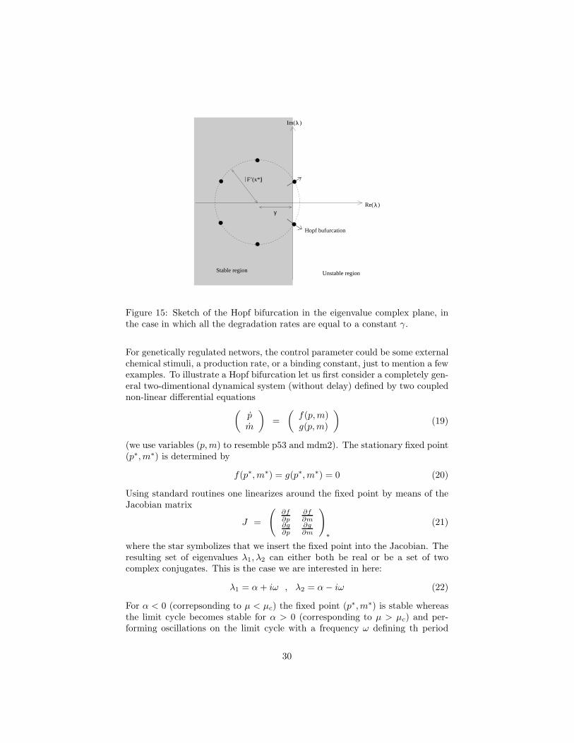
In the simple case in which all the degradation rates are equal and unchang-ing (i.e, hi = γ, a constant) the roots of the polynomial (16) in the complexplane are the vertices of a polygon centered on −γ with a radius |F ′| as sketchedin Fig. 15. Therefore, the fixed point will remain stable as long as

|F ′(x∗)| cos(π/N) < γ. (17)

In this case, Hopf’s theorem (see Appendix B) ensures the existence of a periodicorbit close to the transition value, whose period is:

T = 2π/Im(λ) (18)

which, in the simple case of equal degradation timescales, becomes T = 2π/[|F ′(x∗)|·sin(π/N)]. Notice that the Hopf theorem does not ensure that the orbit is sta-ble; however, since the system is bounded and there are no other fixed points,we expect the orbit to be attracting, at least close to the transition point.

Notice that condition (17) is always satisfied when N = 2. This result alsoextends to the more general case where degradation rates are unequal. Thus, wehave proven that a two-component monotone negative feedback loop withoutan explicit time delay can never show oscillations.

B Hopf bifurcations

Usually, the bifurcation takes place under the variation of some external ’control’parameter µ and the new state appears at a critical value µc of this parameter.

29

F’(x*)

Im( )

Re( )

λ

λγ

Stable region Unstable region

Hopf bufurcation

Figure 15: Sketch of the Hopf bifurcation in the eigenvalue complex plane, inthe case in which all the degradation rates are equal to a constant γ.

For genetically regulated networs, the control parameter could be some externalchemical stimuli, a production rate, or a binding constant, just to mention a fewexamples. To illustrate a Hopf bifurcation let us first consider a completely gen-eral two-dimentional dynamical system (without delay) defined by two couplednon-linear differential equations

(

pm

)

=

(

f(p, m)g(p, m)

)

(19)

(we use variables (p, m) to resemble p53 and mdm2). The stationary fixed point(p∗, m∗) is determined by

f(p∗, m∗) = g(p∗, m∗) = 0 (20)

Using standard routines one linearizes around the fixed point by means of theJacobian matrix

J =

(

∂f∂p

∂f∂m

∂g∂p

∂g∂m

)

∗

(21)

where the star symbolizes that we insert the fixed point into the Jacobian. Theresulting set of eigenvalues λ1, λ2 can either both be real or be a set of twocomplex conjugates. This is the case we are interested in here:

λ1 = α + iω , λ2 = α − iω (22)

For α < 0 (correpsonding to µ < µc) the fixed point (p∗, m∗) is stable whereasthe limit cycle becomes stable for α > 0 (corresponding to µ > µc) and per-forming oscillations on the limit cycle with a frequency ω defining th period

30

of the oscillation. For a genetic system this period could for instance be cir-cadian, ultradiand or related to cell cycles. Just above the bifurcation, thelimit cycle can be well approximated by a circle whoes radius for super-criticalHopf bifurcations generally grows continuosly as

√µ − µc (as in contrast to a

sub-critical Hopf bifurcation where the radius will jump and exhibit hysteresiseffects). When the control parameter µ is much larger than µc the limit cyclemay easily be deformed in various ways ’away’ from the circle.

When we introduce a time delay in the equations, as discussed above, wecan formally write it by introducing the delayed variable pτ into the equations:

(

pm

)

=

(

f(p, m)g(p, m, pτ )

)

(23)

We find numerically that the system still exhibits Hopf bifurcations when cross-ing critical lines in the parameter space. In fact, we find that one can drive thesystem through Hopf bifurcations by increasing the value of the time delay τthrough specific values.

The fixed point of p is of course equal to the fixed point of pτ , i..e.: f(p∗, m∗) =g(p∗, m∗, p∗) = 0. Now we use the same approach as above and linearize aroundthe fixed point:

q = p − p∗, r = m − m∗, qτ = pτ − p∗ (24)

which leads to the following dynamical equations for the increments:

q = f(p∗ + q, m∗ + r) = f(p∗, m∗) +∂f

∂p· q +

∂f

∂m· r =

= 0 + α · q + β · r (25)

r = g(p∗ + q, m∗ + r, p∗ + qτ ) =

= g(p∗, m∗, p∗) +∂g

∂p· q +

∂g

∂m· r +

∂g

∂pτ· qτ =

= 0 + γ · q + δ · r + ǫ · qτ (26)

We can now assume solutions on the form:

q(t) = q1eλ1t + q2e

λ2t, r(t) = r1eλ1t + r2e

λ2t (27)

and find after some lengthy algebra the eigenvalues:

λ1 =1

2

[

α + δ ± ((α − δ)2 + 4β(ǫe−λ1τ + γ))1

2

]

(28)

λ2 =1

2

[

α + δ ± ((α − δ)2 + 4β(ǫe−λ2τ + γ))1

2

]

(29)

We note that these are transcendal equations in the eigenvalues λ1, λ2 but thatthe time delay τ specifically appears into the relations (for a further discussion,see previous Appendix).

31

In many biological systems with genetic feed back regulations, there areoften more than two dynamical variables. We shall in the following sectionsdiscuss oscillatory states of the transcription factor NF-κB. As we show, thatsystem can favourably be reduced to a three dimensional dynamical system inthe variables NF-κB, its inhibitor IκB and the associated mRNA, IκBm. Letus for simplicity write these variables as N, I, Im thus formally obtaining thefollowing three dimensional dynamical system:

N

Im

I

=

f(N, Im, I)g(N, Im, I)h(N, Im, I)

(30)

The procedure to study this type of quations is exactly the same as for the two-dimensional system. From the stationary point N∗, I∗m, I∗ we linearize aroundit using the Jacobian matrix.

J =

∂f∂N

∂f∂Im

∂f∂I

∂g∂N

∂g∂Im

∂g∂I

∂h∂N

∂h∂Im

∂h∂I

∗

(31)

In this case one obtains three eigenvalues λ1, λ2, λ3 which are either all threereal, or one is real and the two others complex conjugates. Again, in the lastcase one may encounter a Hopf bifurcation where the fixed point N∗, I∗m, I∗

bifurcates into a limit cycle in the three-dimensional N, Im, I space, causingoscillations in these variables. Notice, that there topologically is a big differencebetween oscillatory limit cycles in two and three dimensions. In two dimensionsa limit cycle can ’enclose’ trajectories, which is not the case in three dimensionswhere tracjectories may ’escape around’ the limit cycles. An important theoremfor this type of behavior is called the Poincare-Bendixson theorem, which statesthat if a trajectory is confined to a closed, bounded region and there are nofixed points in that region, then the trajectory eventually approaches a closedorbit (see e.g. [28]).

C Stability analysis of delay systems

C.1 Linear delay systems

Consider the simplest delayed system of the form

dx

dt= ax(t) + bx(t − τ). (32)

A complete description of the solution is given in an appendix of ref. [65],while we will just investigate the conditions where the system display sustainedoscillations. The general solution of Eq. (32) is x = exp(λt) which, inserted in tinvestigate the conditions where the system display sustained oscillations. Thegeneral solution of Eq. (32) gives

λ = a + be−λτ . (33)

32

Defining λ = µ + iω, the oscillatory case takes place when µ = 0. The solutionis then

iω = a + b cosωτ − ib sinωτ (34)

which gives

ω = (b2 − a2)1/2 (35)

τ =arccos(−a/b)

(b2 − a2)1/2. (36)

A more general treatment [66] gives the conditions under which the systemconverges to a stationary solution, that is |a| > |b| for any τ or if |a| < |b| forτ < arccos(−a/b)/((b2 − a2)1/2). Roughly speaking, the system can oscillateif the dominant part of the kernel is the delayed one and if the delay is largeenough.

C.2 Absence of closed orbits

If we label the vector forming the left–hand of Eq. (1) as x and that formingthe side right–hand side as F, its divergence of F is

∇ · F =∂f

∂x− kx +

∂g

∂y− ky. (37)

Since we exclude that each of the two molecules can activate itself, the partialderivatives ∂f/∂x and ∂g/∂y are non–positive, and consequently ∇·F ≤ 0. Byvirtue of Green’s theorem, if the trajectory C were closed,

0 >

∫

∇ · xdA =

∮

C

x · n dl, (38)

where n is the normal to the trajectory, and consequently x · n = 0 everywhere.Since the circulation of a null vector is zero, this leads to a contradiction, andthe trajectory cannot be closed.

C.3 Stability analysis of the p53-mdm2 system

Neaumtu and coworkers develop in ref. [45] the complete stability analysis ofthe p53-mdm2 system with delay. First they show that for any choice of theparameters there is a unique stationary point for the rate equations. Considerthe system obtained by linearization of Eq. (5) aroud such point

∂p

∂t= (aρ10 − b)p(t) − aρ01m(t)

∂m

∂t= −dm(t) + cγ10p(t − τ) + cγ01p(t − τ), (39)

where ρ10 and ρ01 are the derivatives of pm(t) with respect to p and m inthe stationary point, while γ10 and γ10 are the derivatives of the function p −

33

pm/(kg + p − pm). Define p1 = b + d + aρ10, p0 = db + adρ10, q1 = cγ01 andq0 = cγ01(b+aρ10)−acρ01γ10. Let λ be the eigenvalues of the linearized system.It is possible to prove that if τ > 0 and p2

1q20 − q2

1p20 − 2p0q

20 > 0 then there is a

delay τ0 such that

Re

(

dλ

dτ

)

λ=iω0, tau=τ0

> 0 (40)

and consequently a Hopf bifurcation occurs at the stationary point.In the limit of large dissociation constant k, ρ10 = ρ01 = 0. Consequently

the condition for a Hopf bifurcation begins b2 > 0, which is always satisfied(except for the trivial case b = 0).

The critical delay τ0 is given by

τ0 =1

ω0

(

arcsinp1ω0

√

(p0 − ω20)

2 + ω20p

21

+ arcsinq1ω0

√

(p0 − ω20)

2 + ω20p

21

)

, (41)

where ω0 is the solution of the equation

ω4 + (−p21 − 2p0 + q2

1)ω2 + p20 − q2

0 = 0. (42)

34

References

[1] Little J W 1983 The SOS regulatory system: control of its state by thelevel of RecA protease, J. Mol. Biol. 167 791–808.

[2] Sassanfar M and Roberts J W 1990 Nature of the SOS-inducing signal inEscherichia coli: the involvement of DNA replication, J. Mol. Biol. 212

79–96

[3] Hoffmann A, Levchenko A, Scott M L, Baltimore D 2002, The IkappaB-NF-kappaB signaling module: temporal control and selective gene activation,Science 298 1241–1245

[4] Yamamoto T, Nakahata Y, Soma H, Akashi M, Mamine T, Takumi T2004 Transcriptional oscillation of canonical clock genes in mouse peripheraltissues. BMC Mol. Biol. 5 18

[5] Lahav G, Rosenfeld N, Sigal A, Geva–Zatorosky N, Levine A J, Elowitz MB and Alon U 2004 Dynamics of the p53–Mdm2 feedback loop in individualcells Nature Genetics 36 147–150

[6] Geva-Zatorsky N, Rosenfeld N, Itzkovitz S, Milo R, Sigal A, Dekel E,Yarnitzky T, Polak P, Liron Y, Kam Z, Lahav G, Alon U 2006 Oscilla-tions and variability in the p53 system Mol. Syst. Biol. 2 0033

[7] Nelson D E, Ihekwaba A E C, Elliott M, Johnson J R, Gibney C A, ForemanB E, Nelson G, See V, Horton C A, Spiller D G et al. 2004 Oscillations inNF-kB Signaling Control the Dynamics of Gene Expression Science 306,704–708

[8] Bosisio D, Marazzi I, Agresti A, Shimizu N, Bianchi M E and Natoli G 2006A hyper-dynamic equilibrium between promoter-bound and nucleoplasmicdimers controls NF-kappaB-dependent gene activity EMBO J. 25, 798–810.

[9] Metivier R, Penot G, Hubner M R, Reid G, Brand H, Kos M and GannonF 2003 Estrogen Receptor-alpha Directs Ordered, Cyclical, and Combina-torial Recruitment of Cofactors on a Natural Target Promoter Cell 115

751–763.

[10] Kucho K, Okamoto K, Tsuchiya Y, Nomura S, Nango M, Kanehisa M andIshiura M 2005 Global analysis of Circadian expression in the cyanobac-terium Synechoscystis sp. Strain PCC 6803, J Bacteriol 187 2190-2199.

[11] Berridge M J, Bootman M D, Roderick H L 2003 Calcium signalling: dy-namics, homeostasis and remodelling Nat. Rev. Mol. Cell Biol. 4 517–529

[12] Hirata H, Yoshiura S, Ohtsuka T, Bessho Y, Harada T, Yoshikawa K andKageyama R 2002 Oscillatory Expression of the bHLH Factor Hes1 Regu-lated by a Negative Feedback Loop, Science 298 840–843

35

[13] Pourquie O 2003 The Segmentation Clock: Converting Embryonic Timeinto Spatial Pattern Science 301, 328-330

[14] Aulehla A and Herrmann B G 2004 Segmentation in vertebrates: clock andgradient finally joined Genes & Development 18, 2060-2067

[15] Dequeant ML, Glynn E, Gaudenz K, Wahl M, Chen J, Mushegian A,Pourquie O 2006 A complex oscillating network of signaling genes underliesthe mouse segmentation clock Science 314 1595-1598

[16] Haupt Y, Maya R, Kazaz A and Oren M 1997 Mdm2 promotes the rapiddegradation of p53, Nature 387 296–299

[17] Lahav G 2004 The Strength of Indecisiveness: Oscillatory Behavior forBetter Cell Fate Determination Science’s STKE pe55.

[18] Editor(s): Derek J. Chadwick, Jamie A. Goode (2003) Mechanisms and Bi-ological Significance of Pulsatile Hormone Secretion Series: Novartis Foun-dation Symposia Wiley.

[19] Golden S S, Ishiura M, Johnson C H, Kondo T 1997 Annu Rev Plant PhysiolPlant Mol Biol 48 327–354

[20] Krishna S, Andersson A M C, Semsey S and Sneppen K 2006 Structure andfunction of negative feedback loops at the interface of genetic and metabolicnetworks. Nucl. Acids Res. 34, 2455–2462

[21] Thomas R 1981 in Quantum noise, Springer Series in Synergetics 9, Ed.Gardiner, Speinger, Berlin, pp. 180–193

[22] Snoussi E H 1998 Necessary conditions for multistationarity and stableperiodicity J Biol Sys 6 3–9

[23] Gouze J L 1998 Positive and negative circuits in dynamical systems, J.Biol. Syst. 6, 11–15

[24] Schnarr M et al. 1991 DNA Binding Properties of the LexA RepressorBiochimie 73 423-431

[25] Wu X, Bayle J H, Olson D, Levine A J 1993 The p53-mdm-2 autoregulatoryfeedback loop Genes Dev 7 1126–1132

[26] Dodd I B, Perkins A J, Tsemitsidis D, Egan J B (2001) Octamerization oflambda CI repressor is needed for effective repression of PRM and efficientswitching from lysogeny Genes Dev 15 3013–3022

[27] Semsey S, Virnik K, Adhya S (2006) Three-stage Regulation of the Amphi-bolic gal Operon: From Repressosome to GalR-free DNA J Mol Biol 358

355–363

36

[28] Strogatz S. 1994 Nonlinear Dynamics and Chaos (Addison-Wesley, ReadingMA)

[29] Mallet-Paret J and Smith H L 1990 The Poincare-Bendixson theorem formonotone cyclic feedback systems J. Dyn. Diff. Eq. 2 367–421.

[30] Tiana G, Jensen M H and Sneppen K 2002 Time delay as a key to apoptosisinduction in the p53 network, Eur. Phys. J. B 29 135–139

[31] Jensen M H, Sneppen K and Tiana G 2003 Sustained oscillations and timedelays in gene expression of protein Hes1 FEBS Lett. 541 176–177.

[32] Lewis J 2003 Autoinhibition with transcriptional delay: a simple mecha-nism for the zebrafish somitogenesis oscillator Curr Biol 13 1398-408

[33] Elowitz M B, Leibler S 2000 A synthetic oscillatory network of transcrip-tional regulators Nature 403 335–338

[34] Goodwin B C 1965 in Adv. Enzyme Regulation, ed. Weber, G. (PergamonPress, Oxford) Vol. 3, pp. 425–438.

[35] Bliss R D, Painter P R and Marr A G 1982 Role of feedback inhibition instabilizing the classical operon J. Theor. Biol. 97 177–193

[36] Guantes R, Poyatos J F 2006 Dynamical Principles of Two-ComponentGenetic Oscillators PLoS Comput Biol 2, e30

[37] Emery D. Conrad, ”Mathematical Models of Biochemical Oscillation,” May1999, Master’s Thesis

[38] Ribbeck K and Gorlich D 2001 Kinetic analysis of translocation throughnuclear pore complexes EMBO J. 20 1320–1330

[39] Alberts B, Bray D, Lewis J, Raff M, Roberts K, Watson J, MolecularBiology of the Cell, Garland (1994)

[40] Picksley S M and Lane D P 1993 The p53–Mdm2 autoregulatory feedbackloop: a paradigm for the regulation of growth control by p53? Bioessays15, 689–690

[41] Bar–Or R L, Maya R, Segel L A, Levine A J, Oren M 2000 Generation of os-cillations by the p53–Mdm2 feedback loop: a theoretical and experimentalstudy, Proc. Natl. Acad. Sci. USA 97, 11250–11256

[42] Schon O, Friedler A, Bycroft M, Freund S M V and Fersht A R 2002Molecular mechanism of the interaction between MDM2 and p53 J. Mol.Biol. 323 491

[43] Gottlieb T, Oren M 1996 p53 in growth control and neoplasia Biochim.Biophys. Acta 1287, 77–102

37

[44] Greenblatt M S, Bennett W P, Hollstein M, Harris C C 1994 Mutationsin the p53 tumor suppressor gene: clues to cancer etiology and molecularpathogenesis, Cancer res. 54 4855–4878

[45] Neamtu M, Horhat R F and Opris D 2006 A dynamic p53-mdm2 modelwith delay kernel arXiv preprint arXiv.math.DS/0601481

[46] Kageyama R, Ishibashi M, Takebayashi K and Tomita K, 1997 bHLH tran-scription factors and mammalian deuronal differentiation, Int. J. Biochem.Cell Biol. 29, 1389

[47] Basak S, Kim H, Kearns JD, Tergaonkar V, O’Dea E, Werner S L, BenedictC A, Ware CF, Ghosh G, Verma I M, Hoffmann A 2007 A fourth IkappaBprotein within the NF-kappaB signaling module. Cell. 128 369–381

[48] Pahl H L (1999) Activators and target genes of Rel/NF-kappaB transcrip-tion factors. Oncogene 18, 6853–6866.

[49] Kearns J D, Basak S, Werner S L, Huang C S, Hoffmann A 2006 IkBe pro-vides negative feedback to control NF-κB oscillations, signaling dynamics,and inflammatory gene expression J. Cell Biol. 173 659-664

[50] Krishna S, Jensen MH and Sneppen K 2006, Minimal model of spiky oscil-lations in NF-κB signaling, Proc. Natl. Acad. Sci. USA 103, 10840–10845

[51] Hayot F and Jayaprakash C 2005 NF-kB oscillations and cell-to-cell vari-ability J. Theor. Biol. 240 583-591

[52] Lipniacki T, Paszek P, Brasier A R, Luxon B and Kimmel M 2004 Mathe-matical model of NF-kB regulatory module J. Theor. Biol. 228, 195–215.

[53] Huang C–Y and Ferrel Jr J E 1996 Ultrasensitivity in the mitogen-activatedprotein kinase cascade Proc. Natl. Acad. Sci. USA 93 10078–10083

[54] Goldbeter A and Koshland D E 1981 An Amplified Sensitivity Arising fromCovalent Modification in Biological Systems Proc. Natl. Acad. Sci. USA 78

6840–6844

[55] Pigolotti S, Krishna S and Jensen M H 2007 Oscillation patternsin negativefeedback loops Proc. Natl. Acad. Sci. USA in press.

[56] Ishiura M, Kutsuna S, Aoki S, Iwasaki H, Andersson CR, Tanabe A, GoldenSS, Johnson CH, Kondo T 1998 Expression of a Gene Cluster kaiABC asa Circadian Feedback Process in Cyanobacteria Science 281 1519–1523

[57] Goldbeter A 1991 A Minimal Cascade Model for the Mitotic OscillatorInvolving Cyclin and cdc2 Kinase Proc. Natl. Acad. Sci. (USA) 88 9107–9111

38

[58] Igoshin O A, Goldbeter A, Kaiser D and Oster G 2004 A biochemicaloscillator explains several aspects of Myxococcus xanthus behavior duringdevelopment Proc. Natl. Acad. Sci. USA 101 15760–15765

[59] Jacquet H, Renault G, Lallet S, Mey J D and Goldbeter A 2003 Oscillatorynucleocytoplasmic shuttling of the general stress response transcriptionalactivators Msn2 and Msn4 in Saccharomyces cerevisiae J. Cell Biol. 161

497–505

[60] Leloup J C and Goldbeter A 2003 Toward a detailed computational modelfor the mammalian circadian clock Proc. Natl. Acad. Sci. USA 100 7051–7056

[61] Reidl J, Borowski P, Sensse A, Starke J, Zapotocky M Eiswirth M2005Model of Calcium Oscillations Due to Negative Feedback in OlfactoryCilia Biophys. J. 90 1147–1155

[62] Goldbeter A, Dupont G and Berridge M 1990 Minimal Model for Signal-Induced Ca2+ Oscillations and for Their Frequency Encoding ThroughProtein Phosphorylation Proc. Natl. Acad. Sci. USA 87 1461–1465

[63] Barken D, Wang C J, Kearns J, Cheong R, Hoffmann A and Levchenko A2005 Comment on ”Oscillations in NF-κB Signaling Control the Dynamicsof Gene Expression” Science 308, 52a–52a.

[64] Ting A Y and Endy D 2002 Decoding NF-κB Signaling Science 298 1189–1190

[65] Glass L and McKey M C 1988 From clocks to chaos, Princeton UniversityPress

[66] Hayes N D 1950 Roots of trascendental equations associated with certaindifference–differential equations, J. Lond. Math. Soc. 25 226–232

39

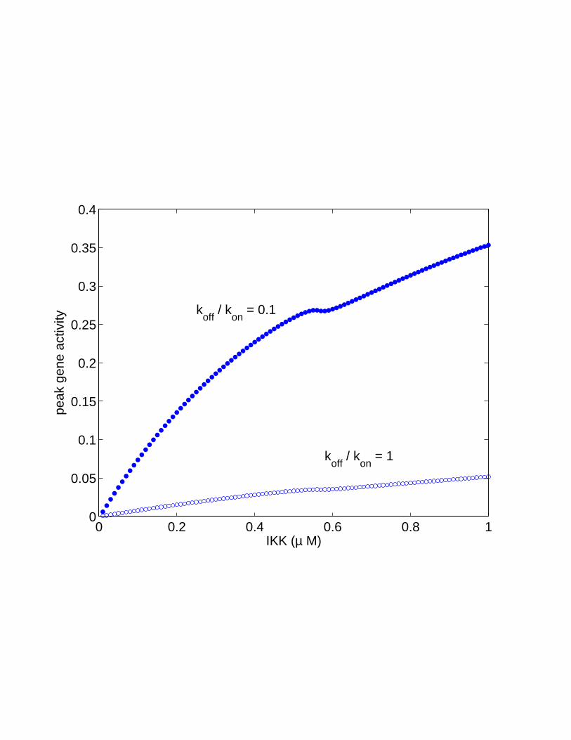
0 0.2 0.4 0.6 0.8 10

0.05

0.1

0.15

0.2

0.25

0.3

0.35

0.4

IKK (µ M)

peak

gen

e ac

tivity

koff

/ kon

= 0.1

koff

/ kon

= 1

0 500 1000 1500 20000

0.1

0.2

0.3

0.4

0.5

0.6

0.7

0.8

0.9

1

time (min)

gene

act

ivity

; N

n (µ

M)

G*G

2*

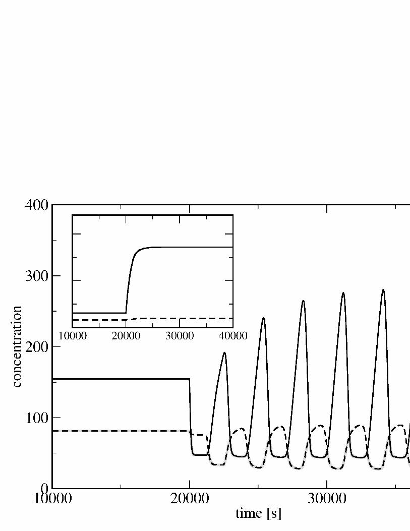
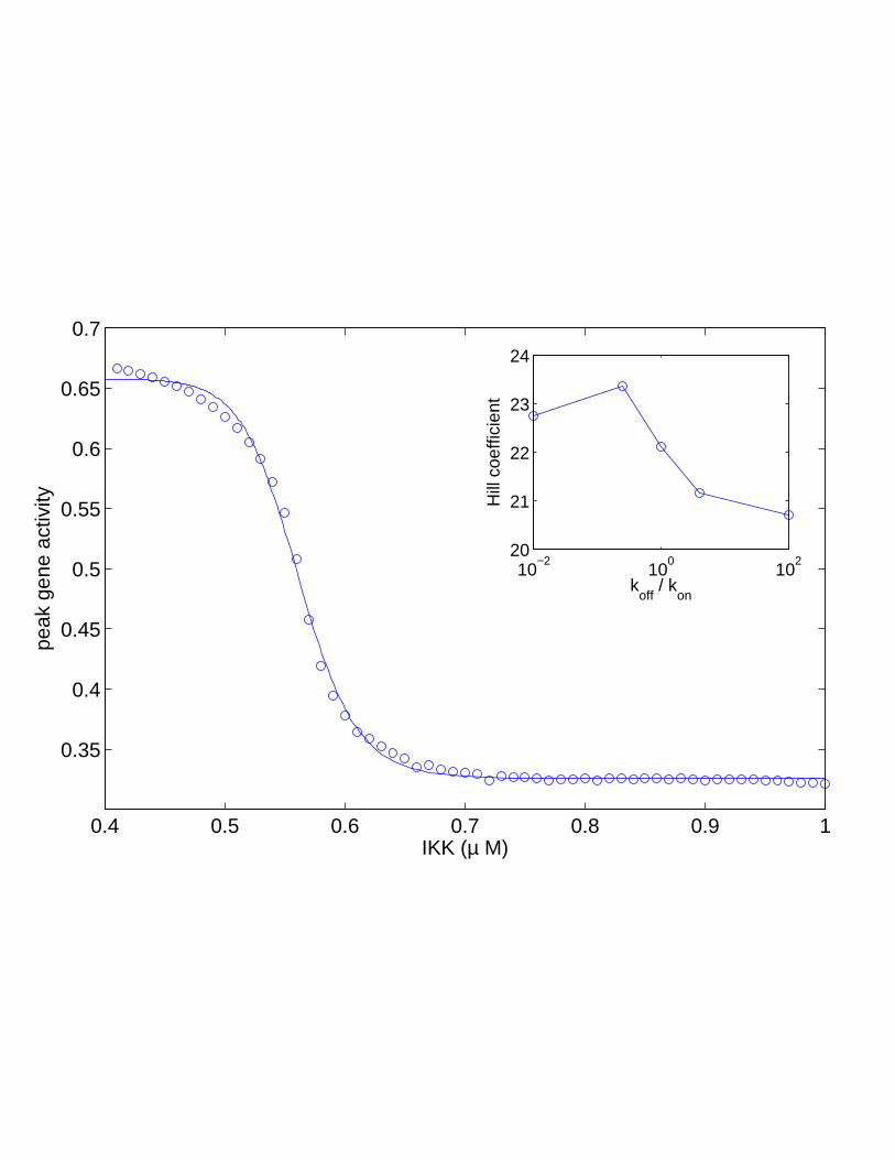
0.4 0.5 0.6 0.7 0.8 0.9 1

0.35

0.4

0.45

0.5

0.55

0.6

0.65

0.7

IKK (µ M)

peak

gen

e ac

tivity

10−2

100

102

20

21

22

23

24

koff

/ kon

Hill

coe

ffici

ent