Electro-osmotic oscillations

ELSEVIER Physica D 110 (1997) 154-168

PHYSICA

Electro-osmotic oscillations

Konstantin Gedalin Department of Physics, Ben-Gurion University, POB 653, Beer-Sheva 84105, Israel

Received 18 December 1996; received in revised form 7 April 1997; accepted 25 April 1997 Communicated by Y. Kuramoto

Abstract

In this paper we reproduce the continuum model of electro-osmotic oscillations at a non-charged porous membrane and study their onset with a focus on the singular nature of this transmission (singular Hopf bifurcation), resulting in a rapid transformation of the oscillations, harmonic at the onset, into the jerky ones of relaxation type.

PACS: 66.10. Cb; 82.40 Bj; 82.65 Fr; 87.22 Fg

1. Introduct ion

Electro-osmotic oscillations have been the object of interest by physicists, chemists and mathematicians ever

since Teorell [24-27] observed this phenomenon in a laboratory set-up devised to the mimic nerve excitation and

comprising as a basic element a porous, electrolyte solution saturated glass filter. Electro-osmotic oscillations may likely represent a common source of oscillations in biological and synthetic membranes in set-up largely different from that of Teorell. Before going into a detailed discussion of these oscillations, we wish to point out that they represent by no means the only type of oscillations encountered in purely diffusional (inertia-and source-less) ionic systems. Thus, to mention but a few examples, Forgacs [6] observed oscillations of membrane potential

upon passing a current through a cation exchange electrodialysis membrane separating two identical solutions of silver nitrate. The characteristic frequency of these oscillations was much higher than that typically recorded for electro-osmotic oscillations in Teorell's set-up. This pioneering work by Forgacs, followed by that of Seno and Yamabe [22] who observed what would be nova-days called an autosoliton train in an experimental set-up similar to that of Forgacs, triggered an extensive amount of research on electric oscillations and low frequency noise at electrodialysis membranes [9,10,16,23]. The physical mechanism behind these phenomena remains largely unclear, although recently some evidence appeared [17] that they might have to do with electroconvection [4,8,21], a mechanism closely related to electro-osmosis.

In order to outline the essence of the phenomenon of electro-osmotic oscillations, let us consider the following imaginary experiment, reproducing in general lines the classical one by Teorell.

Let two vessels, 1 and 2, contain an electrolyte solution (e.g., KC1) at two different concentrations C1 < C2 and be connected by a porous filter (capillary), filled by the same solution. Let the vessel 1 (with concentration C]) be

0167-2789/97/$17.00 Copyright © 1997 Elsevier Science B.V. All rights reserved PII S0167-2789(97)00075-4

K. Gedalin/Physica D 110 (1997) 154-168 155

wide open to the air and so, vessel 2 (C2) although this time through a thin manometer tube (with cross-section area Sin), so that the liquid elevation in it measures the hydrostatic pressure difference between the vessels. Let both vessels contain large working electrodes, allowing for a prolonged galvanostatic passage of a DC current I through the system in one direction, namely, from the vessel with lower concentration C1 to the one with higher concentration C2. Let both vessels be supplied with small test electrodes to measure the voltage drop on the filter. Concentrations in both vessels are viewed constant in the course of experiment and the osmotic pressure drop on the filter is negligible, so that, assuming equal ionic diffusivities, as for KC1, at zero current the pressure drop on the filter is zero, and the voltage drop is also negligible.

Changes of electric potential and pressure drop on the filter are recorded in response to increasing the electric current from zero by small increments.

It is observed tha t for the values of current between zero and some lowest threshold value, the system approaches the new steady state monotonically. For currents in the interval between this lower threshold and another critical value the system still comes to the steady state, but this time through small decaying oscillations. For currents above this critical value, the system changes its behavior and enters the state of non-decaying harmonic oscillations with amplitude and frequency dependent on the current. Upon a further current increase above the aforementioned critical value, the oscillations quickly attain the jerky shape typical of the relaxation oscillations.

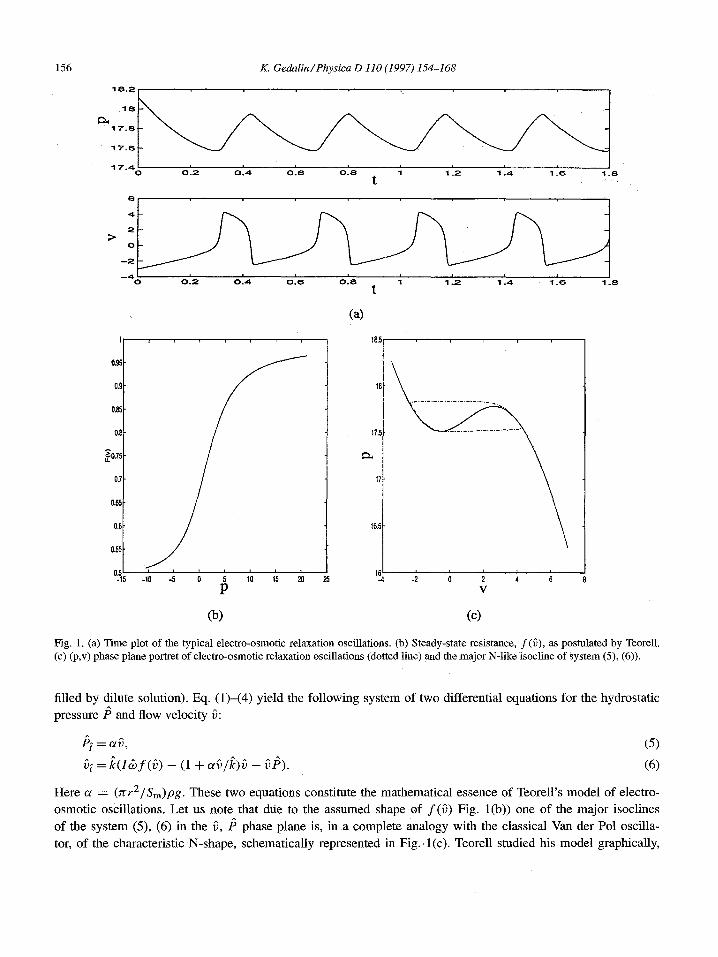
The oscillations which Teorell [24,25] observed were all of relaxation type, schematically depicted in Fig. l(a). To interpre t his observations, Teorell proposed a simple mathematical model in terms of a system of ODEs for the drops of hydrodynamic pressure and electric potential across the tilter, along with the electric resistance of the latter. The voltage on the filter has been assumed related to the resistance by Ohm's law

~(t3 = /~(~) . (1)

Furthermore, mass conservation law was used to relate the pressure drop on the tilter to the flow rate

d/3(~) zrr 2 - - - - p g O ( Z ) , (2)

d£ Sm

where p is the liquid density,/3 the pressure drop on the filter, r the membrane radius and Sm is the cross-section area of monometer tube. For the liquid flow rate in the filter Teorell proposed a generalized D'Arsy 's law type of dependence on the pressure and potential drop

~(~) = -~/3(~) + g,,}(F). (3)

Here the constants v and 09 are hydrostatic and electro-osmotic permeabilities, respectively, dependent on the parameters of the filter and the fluid (pore radius, viscosity, etc.).

To complete his system, Teorell proposed that the necessary nonlinearity in the system is provided by the dependence of the steady resistance of the capillary on the flow velocity and assumed a linear relaxation kinetics of hte instantaneous resistance in the system to the above-mentioned steady-state value f(O) according to the equation

dR(t') _ ~( f (~) _ k0")). (4) di

Here Ic is the constant relaxation coefficient and ~ is the liquid flow rate. For the steady-state resistance f (~) , Teorell postulated a shape of the type presented in Fig. 1 (b), with a negative flow velocity corresponding to a low resistance (capillary filled by concentrated solution) and vice versa, with a positive velocity yielding a high resistance (capillary

>

K. Gedalin/Physica D 110 (1997) 154-168

l e 2 L . . . . . ' ' ' / i ' % /

1 7 . 6

17.4 0 0 . 2 0 . 4 0 . 6 0 . 8 1 1 . 2 1 . 4 1 . 6 1 . 8

t ,

1

0,.~

0.9

6

~, o'.~ 0'.4 o'.~ o:~ -i , ~ ~ '.4 • '.6 , .8 t

(a)

0.85

O.8

~0.75

0.7

0.55

0.6

0.55

-10 -5 0 5 10 15 20 p

156

18'5 t

i i t i i

-4 -2 0 2 4 6 v

(b) (c)

Fig. 1. (a) Time plot of the typical electro-osmotic relaxation oscillations. (b) Steady-state resistance, f(~), as postulated by Teorell. (c) (p,v) phase plane portret of electro-osmotic relaxation oscillations (dotted line) and the major N-like isocline of System (5), (6)).

filled by dilute solution). Eq. (1)-(4) yield the following system of two differential equations for the hydrostatic pressure/3 and flow velocity 3:

/ 3 ~ = ~ , (5)

~ = lc(ICof(~) - (1 + ~fi/k)~ - 3/3). (6)

Here a = QrrZ/Sm)pg . These two equations constitute the mathematical essence of Teorell's model of electro- osmotic oscillations. Let us note that due to the assumed shape of f03) Fig. l(b)) one of the major isoclines of the system (5), (6) in the 0, /3 phase plane is, in a complete analogy with the classical Van der Pol oscilla- tor, of the characteristic N-shape, schematically represented in Fig. 1(c). Teorell studied his model graphically,


by the isocline method, and also numerically, showing the occurrence of electro-osmotic oscillations in it above a certain current threshold. Later on, Aranow [15] elaborated on the physical basis of Teorell's proposed mechanism. This author derived the equations of Teorell's model, except for the relaxation equation (4), from the first principles, a procedure that lifted the ad hoc assumption regarding the source of nonlinearity. The impor- tant feature which thus became apparent with this approach was the notion that the oscillations in the Teorell system were really hydrodynamic in origin and a consequence of the effect of the boundary conditions on the hydrodynamic stability. Kobatake and Fujita [12-14] criticized the arbitrary, in their opinion, relaxation h3}- pothesis (4) of Teorell's model, proposing instead identity of R and f ( v ) , and introducing into consideration the inertia of the liquid in the capillary. These authors also observed oscillations in their model and traced the connection between oscillations of the potential and equilibrium phase transition in the Van der Waals gas. A careful experimental study of the phenomenon of electro-osmotic oscillations has been carried out by Meats and Page [18,19]. They used a membrane (Nucleopore) with well-defined pore structure. The theoretical back- ground of their consideration was essentially identical to that of Kobatake and Fujita. A three-dimensional gen- eralization of the Teorell's model, taking into account both the relaxation of the instantaneous resistance and fluid inertia, has been considered by us in [7]. A continuum model of electro-osmotic oscillations was proposed by Rubinstein [20]. He formulated his model in terms of the Nemst-Planck electro-diffusion Of ions in the capillary combined with a generalized D'Arsy equation. In the limit of local electro=neutrality and for equal ionic diffusivities, he studied, by means of a weakly nonlinear perturbation analysis, the onset of oscillations through Hopf's bifurcation of the steady state. Rubinstein explained the appearance of relaxation oscillations in terms of his model, as a result of rapid diffusional relaxation o f the concentrations profiles in the capillary to the quasi-steady state ones, corresponding to the respective instantaneous value of the flow velocity. Recently, Larter [15] reviewed the studies on the Teorell oscillations in a more general context of membrane oscillations.

In the present paper we study the continuum model of electro-osmotic oscillations by Rubinstein [20] numerically. The organization of this paper is as follows. In Section 2 we reproduce the continuum model of electro-osmotic oscillations to be studied in due course. Section 3 is devoted to the singular Hopf bifurcation and the transition from the small-amplitude harmonic oscillations to the relaxation oscillations. In Section 4 we present the numerical algorithm and the results of the respective solution, including the numerically obtained extended bifurcation diagrams.

2. Continuum model of electro-osmosis, Hopf bifurcation

The local model of Teorell oscillations [25] consists of two Nemst-Planck equations for locally electro-neutral convective electro-diffusion of ions along a capillary (membrane or filter), combined With generalized D'Arsy law for the electro-osmotic flow rate. Let us direct the J-axis along the capillary and let the latter occupy the segment 0 < ~ < L. Assuming for simplicity equal ionic diffusivities (e.g., KC1), Nernst-Planck equations for the electrolyte concentration C(~, ~, electro field potential +(~, ~ and velocity 17 in the filter read

c + = d + + R r

R T 2

with the local electro-neutrality condition in the form C+ ---- 6"- = C. After adding and subtracting of (7) and (8) we obtain

158 K. Gedalin/Physica D 110 (1997) 154-168

D F 2 ^ ^ i ^ ^ ^ ^ ^

C~ = D C ~ - V C ~ , R~T - C c b 2 = - 2 = const. (9)

Here i is the electric current density in the capillary, the time independent control parameter in the galvanostafic regime. The coefficients F, R, T are the Faraday number, ideal gas constant and absolute temperature, respectively. The flow velocity in the filter V relates to the pressure and the electric potential gradients through the generalized D 'Arsy law

---- 9/3~ (2~, t') - & ~ (2~, t'). (10)

Here the constant coefficients of hydrostatic and dectro-osmofic permeability, v and co, respectively, are related to the characteristics of the fluid and the capillary through the relations

r 2 d~ ~ 3 = - - , ( 5 - . (11)

8/, 4zr/z

The parameters r a n d / z are the capillary radius and the dynamic viscosity of the liquid, respectively, while ~ is the wall potential of the capillary and d is the dielectric constant of the liquid. Furthermore, we take into account the incompressibility of the liquid, which yields

~'~ = 0. (12)

The set (7)-(12) is completed by the following boundary conditions:

C(0, t) = C1, C(Z, t) = C2, (13) c~(0, 2) = 0, /3(0, 2) = 0, (14)

^ j rr 2 /3~ = V@)~m pg. (15)

Conditions (13) merely state that at the outer edges of the filter the electrolyte concentrations are fixed at the bulk concentrations in the respective compartments. Conditions (14) fix the electric potential and the pressure at the left side of the filter at zero reference level. Condition (15) is the mass conservation law for the manometer tube, with p - fluid density in the right compartment, S m - manometer cross-section and g - gravity acceleration.

To simplify the mathematical formulation, it is convenient to introduce the following dimensionless variables:

~ F V /3 .~ = - - q b = V = - - , P - - , x = = , i = H o , t = - - .

C C1 R T ' vo PO L to

The normalization factors are determined from (9)-(15) by balancing the appropriate terms

8SmZ/~ /~) L C I ~ ) F ^ R T 1 to - - y r r 4 p g , vo = ~-,L Po = vo-~,v Io - - - - L ' o9 = co----.F v o L (16)

This yields, after elimination of +~ from (9) and (10), the dimensionless version of Eqs. (9) and (10)

e C t = Cxx - v C x , (17) I

v = - P x + -~o9, (18)

Vx = 0, (19)

where ~ = L Z / D t o .


For a membrane with r ~ 10-Sm, /3 = 1.6 x 10-9mZ/s, L ~ 1.2 x 10-4m, /z ~ 10-4kg/ms , ~

10 -2 V, C1 = 0.05, and Sm ~ 10 -6 m 2 [18], (16) and (17) yield to = 2 x 102 s, ~ = 0.05, I0 ~ 50 and co = O(1). The boundary conditions (13) and (15) are rewritten in the form

c ( 0 , t ) = 1, c ( 1 , t ) = A + 1,

q~(0, t) = 0, p(0, t) = 0,

p t = v .

(20)

(21)

(22)

This completes the mathematical formulation of the continuum model. We shall not satisfy here the initial conditions C(x, t) since in what follows we shall only be preoccupied with the limit state resulting from a Hopf bifurcation

from the following steady state solution of the above system:

I Co(x) = 1 + Ax, ~b0 = - - - - ln(1 + Ax), P0 = --wqb0. (23)

21

This solution is parametrized by I and A. Let us begin by analyzing the stability of solution (23). Let us look for a perturbed solution of the form (Y = Uo + U(x)e ~t. Here U is the solution vector (1?, C, •/3), U0 is the stationary

solution (23), and U(x) is the spatial part of the perturbation. After substitution and linearization with respect to

the perturbation, we have for the latter

0"~C + VCo = Cxx, (24)

Coqbx + C~ox = 0, (25)

V = -Px -- W~x, (26)

O-P(1) = V (27)

with boundary conditions for the perturbations in the form

P(O) = ~(0) = C(O) = C(1) = O. (28)

Integration of (24) yields for the concentration

C = V A [ c ° sh ( s /2 (2x~ 1)) _ 1 ] . (29) 0"~ [ cosh(s/2)

Here s = ~ . The integration of Eq. (26) over the segment 0 < x < 1 yields, taking into account (28),

(0" + 1 ) - - v = - a , ~ ( 1 ) . ( 3 0 )

o-

On the other hand, from (25) we obtain

1

~(1)=-I f C dx. (31) Co

0

Finally, comparison of (30) with (31) yields, trough expansion of the 1.h.s of the resulting transcendental equation

in powers of s and keeping the first two terms

1 + 0 - I + I w A Q 1 8 +0"26 Ic°4~-~-~ + O ( e 2 ) = 0 " (32)


Here Q = Q2 - 5Q1 + 4Qo,

1

Qi : f ( ( 2 x - 1) 2i - 1)

cg 0

d x < 0 , Q > 0 .

On the one hand, a simple analysis of solutions Eq. (32) yields that steady state U0 is unstable when 1 iw.4 Q 1 < - 1 and stable otherwise (½Io).4Ql > - 1 ) , i.e.,

Icr : - - 8 / 0 9 . 4 Q 1 . ( 3 3 )

On the other hand, for this critical value of the current, the conditions for a Hopf bifurcation hold, namely

i ffcr "~ -b- .~. (34)

This implies that the imaginary increment cr depends on ~ so that Crcr -+ ~ as ~ ~ 0 in a manner typical of a singular Hopf bifurcation. Thus, summarizing, in the vicinity of the bifurcation I = O(1) and, from (29) C = O(V), while P = O(~1/2V) and qb = O(V), while IVI << 1. In Section 3 we study this singular Hopf bifurcation, beginning with determination of its type.

3. Singular Hopf bifurcation

In this section we study the singular Hopf bifurcation of Section 2 following directly the methodology proposed by Baer and Erneux [1] for the Fi tzHugh-Nagumo system.

First, let us rewrite our model in a more convenient form

Ef t -]- VCx = Cxx, (35) 1

V = - P ( 1 ) + Io) C ' (36)

0

Pt(1) = V. (37)

Eq. (36) is the result of integration of D 'Arsy equation over the segment 0 < x < 1 and use of (28). To obtain the time-periodic solutions valid asymptotically for e --+ 0, we introduce a new fast time variable, defined as ~ = e-1/2t and seek the time-dependent variables and bifurcation parameter in the form of expansions:

k = 0 k = l cx~ oo

P = Po + ~ ~+1~/2p~(~, x), I = ~ ~/2j~, (38) k = l k = 0

where Co, P0 are the corresponding steady state solutions (23) and J0 is the critical value of the current at the

bifurcation point (33): Boundary conditions (28) yield Ck (t, O) = Ck (t, 1) = 0 for K > 0. Linearization of (35) with substitution of

the asymptotic expansions (38) into (35) yields:

E(k+l)/2Cr(k+l) + ~kvk+ 1 A + ek/2C(k+l)xek/2Vk+l = ek/2C(k+l)xx. (39)


Comparison of the corresponding orders of • in (39) yields C 1_3 in the form

C1 = V17t'l, C2 ~--- g27rl -t- V?Tt2 q- VirTr3,

2 V3 ~7. C3 = V37rl q- 2VI V27r2 -I- V2rn'3 V t~r~4 -t- (VI)2rr5 + l(V1)rrr6 -k- (4o)

Here

,4 ~! = "~xtx -- 1],

A I x 6 ~4 = -~ 360

A I x 5 ~6 = -~- 60

A I x 6 zr8 = ~ 360

~10 ~

:"1"12 ~ 7 ~

~ 2 = ? - x - ~ + , ~ 3 = 7 - - ~ - + '

X 5 X 3 X ] A IX5 X 4 X 3 .X 1 12---6 +72 l~-o ' ~5=-5-x N - - - + + 24 3-6 3--6--0 '

X 4 X 3 X I A [ x4 X 3 x 4 ] - - - - - 2 4 + 2-4 - 6---0 ' ~7 = ~- ~ - --6 + ~ '

12--0 + 96 120 + ~ ' ~9 = ~- 120 + i - ~ + '

x6 x6 1 6 + ~ - 2 - + 28.]' ~tl=72-0t_ -2-+--~- +2-8a'

2 2 6 +4-2 ' ~ ' 3 = } - ~ 5 6 - . I . - - 4 + 4 - - 1 5 + c u / "

Substitution of expressions (40) into (36) and (37) yields equations for Vk, Pk in the form

]. Oo (E(k-l-l)/2fk+l)n E(k+l)/2V(k+l) = --Po + •(k-l-2~/2pk + Jk• k/2~o ~--~(-- 1)" / C~+l dx, (41)

n=O 0 1/

P(n+J)r = 17,+1. (42)

By equating to zero the resulting coefficients of each power of • 1/2), V1 V2, Pl P2 are shown to satisfy, respectively, the equations

Vlr = -b.IP1 - lalV2 + Cl J2, P l r = V1 (43)

and

z G ,,3 P2r = V2. V2r-k-a lVIV2+P2=VILI+V1PIRI+" 6 I v 1, • (44)

Here

1 2(q2 -- q l l ) ln(l -k- z~) bl -- al -- , Cl ----= bl ,

Joq3 ' q3 A

Ll=q4bl+(q-~33 a l c l q 3 2 q l b l - 2q5+q6--2q13cl) J 2 A , q 3

q4 q]b] bt Rf (2q5 -5 q6 - 2q13),

q3 2 q3

-- -- 2q12 -- q7 -- ql l l q4 a2"~ G1 = - 6 (2ql3 2q5q3 q6)al + q3 + ~ _ 1 ] ,

162

and

1

J o - ql


1 1 1

qi = ~ dx, qij = C0--~g dx, q111 = C0--~x) 4 dx. o o o

Problems (43) and (44) can be simplified by introducing new dependent variables U1, U2, defined as

Vlr = U1, g2r = U2, (45)

Problems (43) and (44) with (45) obtain the form

Vlr = U1, UI~ = - V l ( b l + a l U 1 ) (46)

and

V2r + V2(alU1 + bl) + a l V l U 2

2R1 V?R1 V?Vl ( G 1 = U I ( L I W J 2 c l R 1 / b l ) - U I - ~ I + + 2

Let Ui = uifl and Vi = riot and v = T~, where

1 bl cr : (bl) -1/2 (bl > 0 ) , oe-- 1 5 = - - .

alo- ' al

With these notations, Eq. (46) and (47) obtain the form

aiR1 "~ V2r = U2. (47) 2bl ] '

V l T = - - U l , b i lT=Vl(1-1-Ul) (48)

and

u2T - v2(ul + 1) - vlu2 = bilL -- u2R -]- v2S -}- V2UlG, V2T = --bi2. (49)

Here L = (L1 + J 2 c l R 1 / b l ) / ~ / ~ , R = R1/~v/-~al, R = R 1 / ( ~ ' ~ a l ) , while the coefficient G is defined as G = (G1/2 - a l R 1 / 2 b l ) / b ~ - ~ . Systems (48) and (49) are suitable for study of the periodic solutions. For the system (49) to possess a periodic solution, the following solvability condition must hold:

Tp

f dZu l bi2R v2S -}- v2bilG) 0 (50) u - 7 ~ ( u l L -- + =

0

or

Tp

f dTu l , . u 2 R + v 2 S v21 G) O, (51) - - i . t t l l~ - - _ __= u l + l

o

where Tp is the period of oscillations. This equation yields the amplitude of Oscillations together with the correction to the bifurcation parameter. For small amplitudes, a periodic solution of (48) [1,2] is given by

Vl = r/COS(O)T) + lr]2 sin(2wT) + O(~3). (52)


Here co = 1 ~ t/2 + O0/3) and ~ is the amplitude of oscillation to be found from the solvability condition (51). Thus,

after substitution of (52) into (51), taking into account that u 1 = -Vl r with Tp = 7f/co we obtain the solvability condition in the form

L + ¼~2(C + R S) = 0. ~53)

Eq. (53) provides a relation between the amplitude 17 and the bifurcation parameter J2. Here parameter L represents the full deviation of the current from its critical value (Hopf bifurcation point). From the linear stability analysis of the steady state solution, we know that it is unstable (stable) for

L > 0 (L < 0). (54)

Thus, condition (53) implies that the periodic solutions and stable (unstable) steady state coexist for the same values of parameters if the coefficient of 72 is positive or negative, i.e. if

M = (G q- R S) > 0, (55)

M = ( G W R - - S ) < 0 . (56)

Thus, conditions (55) and (56) define the type of bifurcation: the bifurcation is subcritical if (55) holds, and is

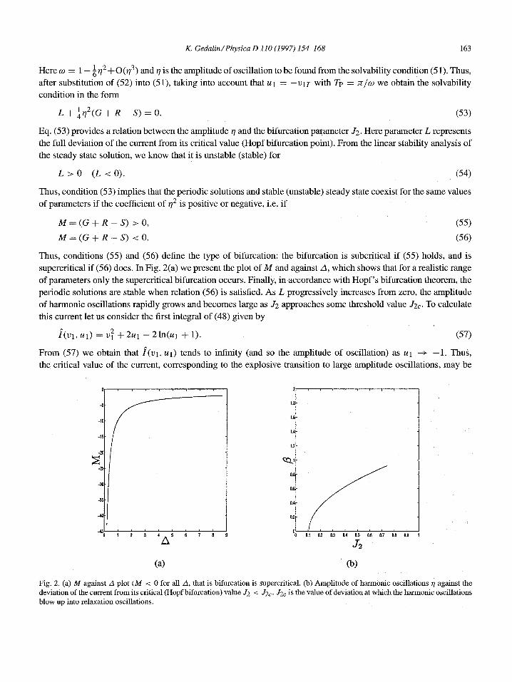
supercritical if (56) does. In Fig. 2(a) we present the plot of M and against A, which shows that for a realistic range of parameters only the supercritical bifurcation occurs. Finally, in accordance with Hopf 's bifurcation theorem, the

periodic solutions are stable when relation (56) is satisfied. As L progressively increases from zero, the amplitude of harmonic oscillations rapidly grows and becomes large as J2 approaches some threshold value J2c. To calculate

this current let us consider the first integral of (48) given by

l (v l , Ul) = vl 2 + 2Ul -- 21n(ul + 1). (57)

From (57) we obtain that [ (v] , u]) tends to infinity (and so the amplitude of oscillation) as Ul --+ 1. Thus, the critical value of the current, corresponding to the explosive transition to large amplitude oscillations, may be

-10

-15

-25

-30

-4O

i J i i r ~ , I

1 2 3 4 ~ 5 6 7 8

2

1.6

1.4

0.$

O.6

ol

J f /

/ /

/ /

o.~ o~ o~ o14 o:s 0.~ 0'.7 or,.

o'.e 0.9

(a) (b)

Fig. 2. (a) M against A plot (M < 0 for all A, that is bifurcation is supercritical. (b) Amplitude of harmonic oscillations ~ agnanst the deviation of the current from its critical (Hopf bifurcation) value -/2 < J2c. J2c is the value of deviation at which the harmonic oscillations blow up into relaxation oscillations.


obtained as a result of integration (51) in the vicinity of u 1 = - - 1 . Thus, the critical value satisfies the following condition:

L0 + (G + R -- S) = 0, (58)

which yields J2c = 0.78. The thus calculated bifurcation diagram is presented in Fig. 2(b) (the end point corresponds to the aforementioned blowup at J2c). We plot here the amplitude as a function of J2 for the general case which we study later numerically (A = 1.1).

4. Numerical results

The system (17)-(19), (20)-(22) was solved numerically by finite differences using an implicit (Cranck-Nicholson) method on a grid with a constant spatial step size h = 10 -2 and time step ts ~ 10 -4 for different values of the

current I. At each time step the diffusion equation was solved first with the velocity replaced by its value on the previous time layer. The updated concentration profile was substituted into the momentum equation, integrated over the segment by Simpson's method, with the updated pressure being determined from the boundary condition.

The thus updated velocity was then returned to the diffusion equation and the iteration process was continued until convergence. The relative accuracy of the computations was 10 -5, current I has been varied in the range between zero and I = 28 (which corresponds to the physical range between zero and 1.4 x 103A/m3), with 6 in the range

10-1-10 -3. The constant concentrations drop A was taken A = 1.1 and co = 1. The algorithm was tested upon the explicit steady state solution for low values of current between 1 and 10 (for these values, it is known that the time-dependent solution tends safely to the steady state) and large values of current in the range between 30 and 40 (for these values, it is known that the time-dependent solution tends to the full size relazation oscillations). The algorithm has also been tested by variation of the time steps (no sensitivity of the results to the magnitude of the

time steps has been observed for ts in the range 10-5-10-3). Below, we present some typical results obtained for different values of current, using the above scheme for A = 1.1. For low values of current between 0 and 24.0 the time-dependent solution tends monotonically to a steady state.

For the current in the range 24.0 < I < 24.2, upon a small perturbation of the steady state (of the order 10 -3 for

the flow rate), the system returns to the latter through a decaying oscillation, Fig. 3. The next stage in the behavior of the time-dependent solution sets in when the electric current just goes over

the value Icr = 24.2. This time, the system does not anymore approach a steady state, but rather tends to that of

harmonic oscillations (Fig. 4), with an amplitude increasing with the current deviation above the threshold value. Fig. 4(a) represents the time dependence of v and p, with the respective phase plane trajectory (Fig. 4(b)) reflecting

the occurrence of a plane periodic attractor of the form of elliptic limit cycle, corresponding to harmonic oscillations. The next stage in the behavior of the time dependent solution sets in near another threshold, Itr = 24.2011.

Thus, with the applied current changed from I = 24.2009 to I = 24.2011 during a small interval of time, we

observed a short-living large pulsations of the amplitude of small size stationary harmonic oscillations. When the current crossed the threshold Itr = 24.2011 the harmonic oscillations blew up into nonlinear oscillations of large amplitude. Note that a similar abruPt transition from harmonic to nonlinear oscillations was observed in [1] for relaxation oscillations in the FitzHugh-Nagumo system. There too, the blow up of harmonic oscillations into the full scale nonlinear ones had to do with presence of a small parameter and occurred through a sequence of nonlinear oscillations of a simpler nature, the so-called "french ducks". Similarly, we observe a somewhat different sequence of the "french duck" oscillations, depending on the current for its values aboves above the threshold Itr = 24.2011. We recognize here the following two different types of "french ducks", by classification of [3,5]: (a) the "french duck without head" (Fig. 5) and (b) "french duck with head" (Fig. 6).

K. Gedalin/Physica D 110(1997) 154--168 165

02 . . . . . . . .

-40.1

0 0.1 0.2 03 0.4 03 6.G 0.7 08 0.9 1

a.lfd04

164~

16.4 O 0.1 0,2 02 OA 0.5 0,6 0.? 0.8 09

1

16At]~

1 ~

16.401

I I I I I I I I r

-0.2 -035 ,.,~I -CLOG 0 0.~ 0:1 035 0.2 v

(a) (b)

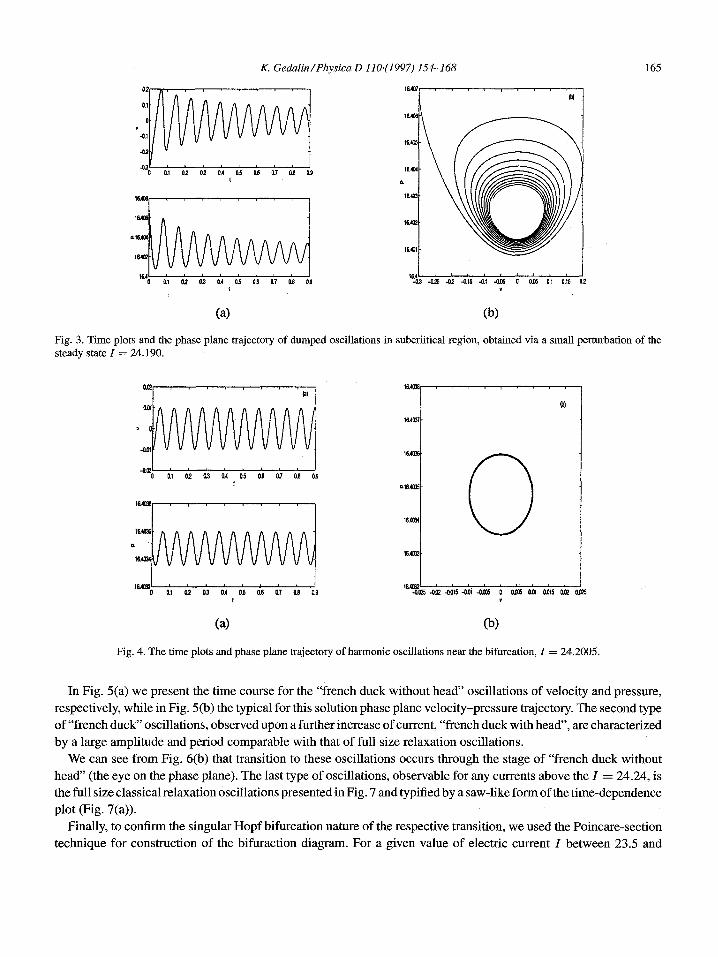
Fig. 3. Time plots and the phase plane trajectory of dumped oscillations in subcriitical region, obtained via a small perturbation of the steady state I = 24.190.

0.to . . . . . . . . l f ~

r J O I } ~ 1K4~]

I

t L t i i [

t o.16.4fl~

| r A ~ I i i i i i f r 1 r 0 0.1 0 2 0 3 0.4 0.5 0 5 02 0 3 ~.9

t

16.4~

, ] . . . .

v

(a) (b)

Fig. 4. The time plots and phase plane trajectory of harmonic oscillations near the bifurcation, I = 24.2005.

In Fig. 5(a) we present the time course for the "french duck without head" oscillations of velocity and pressure, respectively, while in Fig. 5(b) the typical for this solution phase plane velocity-pressure trajectory. The second type of"french duck" oscillations, observed upon a further increase of current, "french duck with head", are characterized by a large amplitude and period comparable with that of full size relaxation oscillations.

We can see from Fig. 6(b) that transition to these oscillations occurs through the stage of "french duck without head" (the eye on the phase plane). The last type of oscillations, observable for any currents above the I = 24.24, is the full size classical relaxation oscillations presentedin Fig. 7 and typified by a saw-like form of the time-dependence plot (Fig. 7(a)).

Finally, to confirm the singular Hopf bifurcation nature of the respective transition, we used the Poincare-section technique for construction of the bifuraction diagram. For a given value of electric current I between 23.5 and

O.


t

16.4~ , ,

16,41~' . . . . . . . . . . 0 O2 0.4 O~ O~ I

t

166

-0,5 -0.4 -0.3 -0~ -.0.I 0 Oh O~ 0.3 0,4 0.5 V

(a) (b)

Fig. 5. French duck without head, I = 24.2015.

3 . • ,, , .

. , , , , t i - 0 0.1 0 .2 0 .3 0 .4 0.5 0 ,6 0,?

I

16,..~ . . . . . . .

1 6 1

I

16A4 t i6.42

1~4[

16.38 '

, , , , , , , ,'

k~4~4

*'1 -~5 0 0,5 1 15 2 5 v

(a) (b)

Fig. 6. French duck with a head.

26.5, the b.v.p (17)-(22) was solved. A solution represents a trajectory in the phase space v, p(1, t), ~b(1, t). Such a trajectory tends to an attractor which can be characterized by its intersection with the plane p = 0, where P0 is the steady state value. The bifurcation diagram is now obtained by plotting the maximum and minimum velocity at the intersection points as a function of electric current I (Fig. 8). The plot in Fig. 8, obtained for A = 1.1, is typical of a singular supercritical Hopf bifurcation in accordance with the calculations of Section 3. The sharp growth of the amplitude is the reflection of the aforementioned singularity of bifurcation.

The parameter ranges obtained from analytical and numerical studies are in good agreement. Thus the analytical estimate predicts the critical point of the Hopf biffurcation at Icr = 24.196 (for A = 1.1), whereas the numerically

10.66

16£4

o.

4 , , , , , , , ,

-2 0 0.1 02 03 0.4 0.5 0.6 0.7 0,8 03

!

a, 1 6 ~ 5 5 1 6 ' 6 ~

16 r 0 0.1 0.2 0.3 0.4 0'5 0'5 0,7 03 0.9

t

16.,54

1652 -1.5

' ~ ; . . . . . .

-1 -9 0,5 ! 13 2 2'5 3 V


(a) ( b )

3,5

167

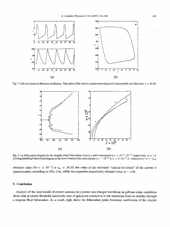
Fig. 7. Full size classical relaxation oscillations. Time plots of the velocity and pressure drop are of characteristic saw-like form, I ---- 24.26.

0~ 1A . . . . . . . . . 0fi

1.2 b 0.4

nr3 1 e , / a 02 ~ 0.8

> 0.1 b a -X-

o.6

0.4

" ~ 0.2 /i s

1 i i i i 0

' j * 1 0 a

(a) (b)

Fig. 8. (a) Bifurcation diagram for the singular Hopf bifurcation. Curves a and b correspond to • = 10 -3, 10 -4, respectively, A = 1,1. (b) Magnified Hopf bifurcation diagram in the close vicinity of the critical point, a: • = 10 -2, b: • = 3 x 10 -3, e - analytical (J = I - Icr).

obta ined va lue (for ~ = 10 -3 ) is /cr = 24.20; the value o f the es t imated "cr i t ical devia t ion" o f the current is

approximately , according to (58), 0.8E, whi le the respect ive numer ica l ly obtained value is ~ 1.0E.

5. Conclusion

Analys is o f the local mode l o f e lec t ro-osmosis in a porous non-charged m e m b r a n e in galvano-sta t ic condi t ions

shows that at certain threshold current the state o f quiescent conduct ion in the m e m b r a n e loses its stability through

a s ingular H o p f bifurcation. As a result, r ight above the bifurcat ion point, ha rmonic osci l lat ions o f the electr ic


potential, hydrostatic pressure and liquid velocity arise in the system upon a small perturbation of the steady state.

Due to the singular nature of the relevant Hopf bifurcation, these small-size harmonic oscillations grow to full

size relaxation oscillations in an exponentially small neighborhood of the critical point. This transition is realized

via the "french duck" scenario. Our weakly nonlinear bifurcation analysis of the aforementioned transition yields

explicit expressions for the threshold values of the bifurcation parameter which are in good agreement with the

results of numerical solution. These results thus complete those of [20], where the supercritical character of the

Hopf bifurcation was shown (without addressing its singular aspects) and the existence of electro-osmotic relaxation

oscillations was predicted.

Finally, let us point out that coexistence of stable quiescent conduction steady state and periodic oscillations

(subcritical Hopf bifurcation) is observable upon the inclusion into the local model of liquid inertia [7].

Acknowledgements

The author is very greatful to I. Rubinstein for the help in the preparation of the paper.

References

[1] S.M. Baer and T. Erneux, SIAM J. Appl. Math. 46 (1986). [2] S.M. Baer and T. Erneux, SIAM J. Appl. Math. 52 (1992). [3] E. Benoit, J.-L. Callot, E Dienfer and M. Diener, Coll. Math. 31 (1981) 37. [4] R. Bruinsma and S. Alexander, J. Chem. Phys. 92 (1990) 3074. 15] W. Eckhaus, Lecture Notes in Math. 985 (1983). [6] Ch. Forgacs, Nature 190 (1961) 339. [7] K. Gedalin, Local inertial model of electroosmotic oscillations, J. Chem. Phys., submitted. [8] A.P. Girin, Electrochimia 21 (1985) 52 (in Russian). [9] M.E. Green, J. Mem. Biol. 28 (1976) 181.

[10] M.E. Green and M. Yafusso, J. Phys. Chem. 72 (1968) 4072 (including erratum, J. Phys. Chem. 73 (1969)) 1626. [11] J. Kevorkian and J.D. Cole, Perturbation Methods in Appied Mathematics (Springer, Berlin, 1985). [12] Y. Kobatake, Physics 48 (1970) 301. [13] Y. Kobatake and H. Fujita, J. Chem. Phys. 40 (1964) 2212. [14] Y. Kobatake and H. Fujita, J. Chem. Phys. 40 (1964) 2219. [15] R. Latter, Chem. Rev. 90 (1990) 355. [16] S. Lifson, B. Gavish and S. Reich, Biophys. Struct. Mech. 4 (1978) 53. [17] E Maletzki, H.-I. R~Ssler and E. Staude, I. Membrance Sci. 71 (1992) 105. [18] P. Meares and K.R. Page, Proc. R. Soc. London A 339 (1974). [19] P. Meares and K.R. Page, Faraday Syrup. Chem. Soc. 9 (1974). [20] I. Rubinstein, Electrodiffusion of ions, SIAM (1990). [21] I. Rubinstein, Phys. Fluids A 3 (1991) 2301. [22] M. Seno and T. Yamabe, Bull. Chem. Soc. Japan 36 (1963) 877. [23] S.H. Stern and M.E. Green, J. Phys. Chem. 77 (1973) 1567. [24] T. Teorell, Exp. Cel. Res. 5 (1958) 83. [25] T. Teorell, J. Gen. Phys. 42 (1959) 831. [26] T. Teorell, J. Gen. Phys. 42 (1959) 847. [27] T. Teorell, Ark. Kemi. 18 (1961) 401.

Electro-osmotic oscillations

Documents

Transcript of Electro-osmotic oscillations