369

Chapter 22

Computational Modelling of Kinase Signalling Cascades

David Gilbert, Monika Heiner, Rainer Breitling, and Richard Orton

Abstract

In this chapter, we describe general methods used to create dynamic computational models of kinase signalling cascades, and tools to support this activity. We focus on the ordinary differential equation models, and show how these fit into a general framework of qualitative and quantitative (stochastic and continuous) models. The modelling we describe is part of the activity of BioModel engineering which provides a systematic approach for designing, constructing, and analyzing computational models of biological systems.

Key words: Computational modelling, Ordinary differential equations, Continuous Petri nets

Computational modelling of intracellular biochemical networks has become a growth topic in recent years, due to advances both in the power and availability of software systems for the simula-tion and analysis of such networks, as well as an increase in the quality and amount of experimentally determined parameter data available for modelling.

Modelling biochemical systems is the core part of the process of BioModel Engineering (1) which is at the interface of computing science, mathematics, engineering, and biology, and provides a systematic approach for designing, constructing, and analyzing computational models of biological systems. BioModel Engineering does not aim at engineering biological systems per se (in contrast to synthetic biology), but rather aims at describing their structure and behaviour, in particular at the level of intracellular molecular processes, using computational tools and techniques.

1. Introduction

Rony Seger (ed.), MAP Kinase Signaling Protocols: Second Edition, Methods in Molecular Biology, vol. 661,DOI 10.1007/978-1-60761-795-2_22, © Springer Science+Business Media, LLC 2010

370 Gilbert et al.

The most useful kinds of models for signalling pathways are dynamic models that describe the time course behaviour of molec-ular concentrations or even individual molecules. This contrasts with static models which merely describe the topology of the system, i.e. the molecular species involved and their relationships or wiring diagram. In addition to simulation, dynamic models permit a range of analytical techniques that give insight about system-level features that emerge from the elementary interactions of the components. Emergent properties such as bifurcations, robustness to interference, or oscillations are not obvious from the network topology and their discovery requires computational methodologies. Dynamic models provide a powerful framework for hypothesis generation and testing and the identification of inconsistencies between a model and experimental data. They are often used by life scientists as a means to explore their ideas about the organisation and control of a biological system.

The “correctness” of a model can be established in several ways. Biological model validation establishes whether a model contradicts our knowledge of a biological system and hence requires experimental data about the behaviour of the system. A special technique contributing to model validation is model checking, which establishes whether a set of formal properties hold for a model, and is often automated using computer programs. A biologically valid model can be incomplete and hence may not describe all the observations we can potentially make of a system, but should not incorrectly describe those behaviours of the system for which it allows predictions.

As the EGFR-activated ERK (EGFR/ERK) pathway is such an important signalling pathway, the deregulation of which has long been implicated in various forms of cancer, it has become a popular target for computational modelling strategies (2–4). Currently, there are a wide variety of models of the EGFR/ERK pathway available which have led to novel insights and interesting predictions as to how this system functions (5). A large number of the models of this pathway are based on the ordinary differential equation (ODE) approach (6). Examples of popular models of the EGFR/ERK pathway include the models described by Brightman et al. (7), Schoeberl et al. (8), and Brown et al. (9), all of which use an ODE-based approach. In general, models have been developed to illustrate particular aspects of pathway behaviour, and may not be consistent between each other. For instance, the Brightman and Brown models predict that the negative feedback loop from ERK to SOS is essential for a transient activation of ERK to be achieved, whereas the Schoeberl model predicts that the negative feedback loop is not required for the transient activation of ERK. Orton et al. (10) have developed a model which over-comes these inconsistencies and suggest some corrections to the Schoeberl model on which their work is based.

371Computational Modelling of Kinase Signalling Cascades

Aspects of behaviour of the MAPK pathway which have been investigated using computational models include:

Ultrasensitivity of the ERK cascade as a result of a two-step –distributive activation mechanisms (11–13).Oscillatory behaviour of the ERK cascade due to embedded –negative feedback loops (14).The effects of receptor location, trafficking, and degradation –on downstream ERK signalling (8, 15).The dynamic differences between the transient and sustained –activation of ERK by different growth factors (7, 16).The influence of Raf kinase inhibitor protein (RKIP) on the –ERK pathway (17).

In general, biochemical networks can always be modelled using qualitative information, describing the molecular species and their interconnections; if information about the reaction kinetics is known, quantitative models can also be employed. Modelling approaches based on ordinary differential equations (ODEs) have been described in detail before (e.g. (45)). Here we focus on approaches inspired by computing science concepts, which have recently gained popularity in systems biology (18, 19).

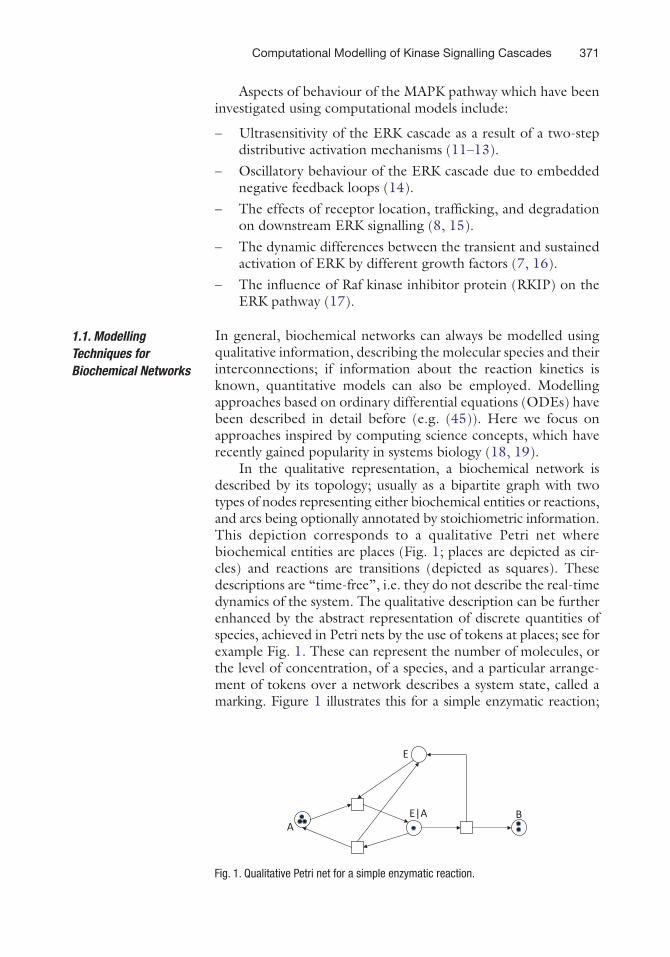
In the qualitative representation, a biochemical network is described by its topology; usually as a bipartite graph with two types of nodes representing either biochemical entities or reactions, and arcs being optionally annotated by stoichiometric information. This depiction corresponds to a qualitative Petri net where biochemical entities are places (Fig. 1; places are depicted as cir-cles) and reactions are transitions (depicted as squares). These descriptions are “time-free”, i.e. they do not describe the real-time dynamics of the system. The qualitative description can be further enhanced by the abstract representation of discrete quantities of species, achieved in Petri nets by the use of tokens at places; see for example Fig. 1. These can represent the number of molecules, or the level of concentration, of a species, and a particular arrange-ment of tokens over a network describes a system state, called a marking. Figure 1 illustrates this for a simple enzymatic reaction;

1.1. Modelling Techniques for Biochemical Networks

Fig. 1. Qualitative Petri net for a simple enzymatic reaction.

372 Gilbert et al.

note that the default stoichiometric weights have been omitted. The current state (marking) of the system, indicated by the black tokens in each place (circle), is as follows: there are no free molecules of enzyme E, three molecules of substrate A, one molecule of the enzyme–substrate complex E|A, and two molecules of the product B. Equally, we could say that there are three units of concentration of A, one unit of E|A, and two of B. Clearly, due to the lack of free enzyme, the enzyme–substrate complex will have to be broken up by decomplexation to release one molecule of E and B (forward reaction) or one molecule of E and A (reverse reaction) in order for any further complexation of A with E to take place. From a computing science perspective, the behaviour of such a net forms a discrete state space, which can be analysed in the bounded case, for example, by a branching time temporal logic, one instance of which is computational tree logic (CTL) (20).

Timed information can be added to the qualitative description in two ways – stochastic and continuous. The stochastic description preserves the discrete description of the values of biochemical entities, but in addition associates an exponentially distributed rate with each reaction. Thus stochastic approaches represent the individual behaviour of molecules and hence variability in the over-all (averaged) behaviour of a system. Special behavioural properties can be expressed using, e.g. continuous stochastic logic (CSL), see (21), a probabilistic counterpart of CTL.

In the continuous approach, discrete values of species are replaced with continuous values, and hence only overall (averaged) behaviour can be described by concentrations. A particular deterministic rate information is associated with each reaction, and thus the concen-tration of a particular species in such a model will have the same value at each point of time for repeated simulations. This approach permits the continuous model to be represented as a set of ODEs. The state space of such models can be analysed by, for example, linear temporal logic with constraints (LTLc) in the manner of (22).

Priami et al. showed how the stochastic p-calculus could be used to model biomolecular processes (23) and Regev et al. showed in more detail how the p-calculus can be used to model and simulate the MAPK pathway (24) using a continuous approach; subsequently, Phillips and Cardelli (25) used the stochastic p-calcu-lus to model the MAPK pathway by simulating the behaviour of individual molecules using the Gillespie algorithm (26). A related approach, the stochastic process algebra PEPA (27), was used by Calder et al. to model the influence of RKIP on the ERK signalling pathway (28), and permits different alternative formulations of a model to be formally compared. PEPA models can be simulated using the Gillespie algorithm or ODE solvers: Calder et al. have shown how to automatically derive ODEs from process algebra models (29).

373Computational Modelling of Kinase Signalling Cascades

The stochastic and continuous models are mutually related by approximation, and the qualitative model can be regarded as an abstraction of both quantitative descriptions. For more details of a formal framework that explains these relationships within the context of Petri nets, see (30). The advantages of using Petri nets as a kind of umbrella formalism include (31):

An intuitive and executable modelling style –A true concurrency (partial order) semantics, which may be –weakened to inter-leaving semantics to simplify analysesMathematically founded analysis techniques based on formal –semanticsCoverage of structural and behavioural properties as well as –their relationsIntegration of qualitative and quantitative analysis techniques –Reliable tool support –

Several tools are available which permit the construction of quantitative biochemical pathway models using kinetic descrip-tions and their simulation and analysis; these often read and write in SBML (32) format which is one de-facto standard for the description of quantitative models of biochemical pathways. Such tools include BioNessie (33), and Copasi (34). There are also databases of biochemical models, often with descriptions in SBML format, for example Biomodels (http://www.bio-models.org) (35), and more specialized databases such as the MAPK database at Brunel (mapk.brunel.ac.uk), which was developed as part of the SIMAP project (http://www.eurtd.org/simap).

MATLAB (36) is a high-level language and interactive environment that contains a large number of ODE solvers which can be used to numerically solve and analyse ODEs. The SimBiology toolbox extends MATLAB with tools for model-ling, simulating, and analyzing biochemical pathways, and has graphical interface as well as a facility to read and write SBML. The systems biology workbench (SBW) (37), is a software framework that includes Jarnac, a fast simulator of reaction networks, permitting time course simulation (ODE or stochas-tic), steady-state analysis, basic structural properties of networks, dynamic properties like the Jacobian, elasticities, sensitivities, and eigenvalues, and JDesigner, a friendly GUI front end to an SBW compatible simulator. Bifurcation analysis can be performed

2. Tools

374 Gilbert et al.

conveniently using Xppaut (38). CellDesigner (39) has a graph-ical interface using SBGN (Systems Biology Graphical Notation), is SBML compliant, and SBW-enabled so that it can integrate with other SBW-enabled simulation/analysis software packages. CellDesigner also supports simulation and parameter search, using the SBML ODE solver.

Petri net models can be designed using several software tools. Snoopy (40) supports qualitative as well as quantitative Petri nets, among them both continuous and stochastic Petri nets, and has an SBML interface. There are several analytical tools for Petri nets which can be accessed by the export feature of Snoopy, including Charlie (41), as well as a variety of model checkers, e.g. the IDD-MC (42) and DSSZ-MC (43) tools.

For more discussion of types of software to support model-ling (see Note 1).

In the following, we describe a method for building a model of an MAPK pathway, given some knowledge about the topology of the pathway, and basic assumptions about the kinetics involved. This is part of a larger process of BioModel Engineering – see (1) and Note 2.

ODE descriptions are so far the most widely used approach when modelling signalling pathways formally, and we now focus on this methodology. First we briefly recall the use of ODEs to model basic biochemical reactions; for more details refer to a standard text on biochemistry, e.g. (44).

Given a reaction A→B which occurs at a rate k, we can com-pute the time course of the concentrations of A and B by the fol-lowing equation, where [A] stands for the concentration of A etc:

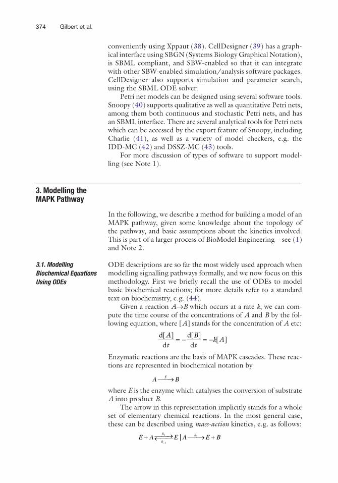
Enzymatic reactions are the basis of MAPK cascades. These reac-tions are represented in biochemical notation by

where E is the enzyme which catalyses the conversion of substrate A into product B.

The arrow in this representation implicitly stands for a whole set of elementary chemical reactions. In the most general case, these can be described using mass-action kinetics, e.g. as follows:

3. Modelling the MAPK Pathway

3.1. Modelling Biochemical Equations Using ODEs

d[ ] d[ ][ ]

d dA B

k At t

= - = -

¾¾®FA B

-

¾¾®¬¾¾+ ¾¾® +1

1

2|k

k

kE A E A E B

375Computational Modelling of Kinase Signalling Cascades

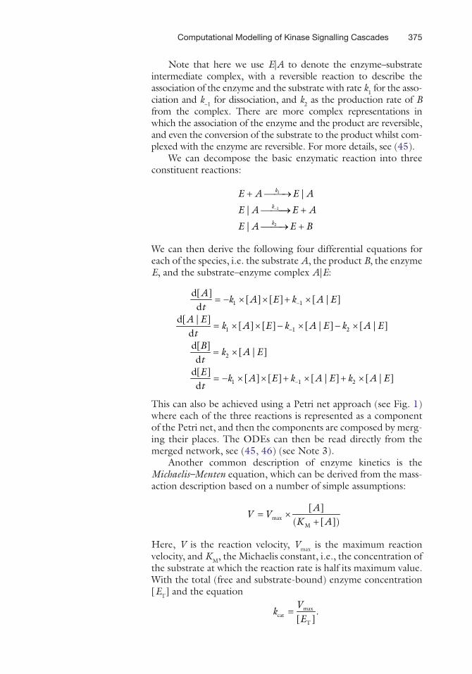
Note that here we use E|A to denote the enzyme–substrate intermediate complex, with a reversible reaction to describe the association of the enzyme and the substrate with rate k1 for the asso-ciation and k−1 for dissociation, and k2 as the production rate of B from the complex. There are more complex representations in which the association of the enzyme and the product are reversible, and even the conversion of the substrate to the product whilst com-plexed with the enzyme are reversible. For more details, see (45).

We can decompose the basic enzymatic reaction into three constituent reactions:

We can then derive the following four differential equations for each of the species, i.e. the substrate A, the product B, the enzyme E, and the substrate–enzyme complex A|E:

This can also be achieved using a Petri net approach (see Fig. 1) where each of the three reactions is represented as a component of the Petri net, and then the components are composed by merg-ing their places. The ODEs can then be read directly from the merged network, see (45, 46) (see Note 3).

Another common description of enzyme kinetics is the Michaelis–Menten equation, which can be derived from the mass-action description based on a number of simple assumptions:

Here, V is the reaction velocity, Vmax is the maximum reaction velocity, and KM, the Michaelis constant, i.e., the concentration of the substrate at which the reaction rate is half its maximum value. With the total (free and substrate-bound) enzyme concentration [ET] and the equation

1

1

2

|

|

|

k

k

k

E A E A

E A E A

E A E B

-

+ ¾¾®

¾¾¾® +

¾¾® +

1 1

1 1 2

2

1 1 2

d[ ][ ] [ ] [ | ]

dd[ | ]

[ ] [ ] [ | ] [ | ]dd[ ]

[ | ]d

d[ ][ ] [ ] [ | ] [ | ]

d

Ak A E k A E

tA E

k A E k A E k A Et

Bk A E

tE

k A E k A E k A Et

-

-

-

= - ´ ´ + ´

= ´ ´ - ´ - ´

= ´

= - ´ ´ + ´ + ´

maxM

[ ]( [ ])

AV V

K A= ´

+

maxcat

T

.[ ]V

kE

=

376 Gilbert et al.

We can write the differential equations describing the con-sumption of the substrate and the production of the product as follows:

This form has the advantage that [ET] might be dynamic, for example for an activated form of a kinase from the prevous stage in a cascade, while kcat and KM are constants. However, the assump-tions underlying the Michaelis–Menten equation have been derived for in vitro conditions and strictly apply at the initial stage of an enzyme assay, but are often inappropriate for the in vivo situation of a kinase signalling cascade. In particular, the assump-tions that the concentration of the product is close to zero, no product reverts to the substrate, and the concentration of the enzyme is much less than that of the substrate, are violated in the in vivo context (47) (see Note 3).

The mass-action equation for an enzymatic reaction is related to the Michaelis–Menten description by the following:

For a more detailed discussion of the use of mass-action vs. Michaelis–Menten kinetics in modelling signalling pathways see (45).

In the course of signal transduction, extracellular signalling mol-ecules bind to specific trans-membrane proteins (receptors) such as G-protein-coupled receptors (GPCRs) and receptor tyrosine kinases (RTKs), changing their conformation. This conformation change leads to a change in enzymatic activity of the receptor, which in turn affects the concentration of downstream com-pounds which are the substrates and products of the reaction catalysed by the receptor. In most cell types, MAPK cascades are activated through RTK and/or GPCR activation, which appear to function as central integration modules in signal processing. MAPK modules are evolutionarily conserved in cells from yeast to mammals. They typically consist of three kinases, which are acti-vated sequentially by phosphorylating each other in response to stimuli, forming a three-tiered cascade, (48). The kinase in the first tier of the cascade is typically activated at the plasma mem-brane, whereas the third kinase is typically translocated from the cytoplasm to the nucleus upon activation, where it can regulate gene transcription through affecting chromatin structure and modifying the activity of transcription factors. The downstream

cat TM

d[ ] d[ ] [ ][ ]

d d ( [ ])A B A

k Et t K A

= - = - ´ ´+

( ) ( )1

cot cot1 2

[ ][ ][ ]

[ ] [ ]

[ ][ ]

F

M M F

F

MKMKV k s k

K MK K MK

d MKd MKV

dt dt

= ´ ´ - ´+ +

= - = -

3.2. Modelling Signal Transduction Cascades

377Computational Modelling of Kinase Signalling Cascades

compounds may themselves be enzymes that in a cascade of enzy-matic reactions ultimately lead to a change in gene expression or some other major adjustment of cellular physiology.

From the modelling point of view, the main characteristic feature of the core of signal transduction pathways is that the prod-uct of one reaction becomes the enzyme for the next, and in gen-eral it is the dynamic behaviour, which is of interest in a signalling pathway, as opposed to the steady-state in a metabolic network.

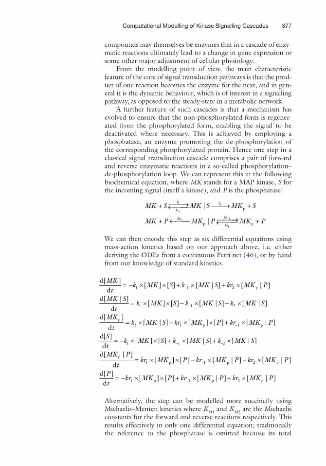
A further feature of such cascades is that a mechanism has evolved to ensure that the non-phosphorylated form is regener-ated from the phosphorylated form, enabling the signal to be deactivated where necessary. This is achieved by employing a phosphatase, an enzyme promoting the de-phosphorylation of the corresponding phosphorylated protein. Hence one step in a classical signal transduction cascade comprises a pair of forward and reverse enzymatic reactions in a so-called phosphorylation–de-phosphorylation loop. We can represent this in the following biochemical equation, where MK stands for a MAP kinase, S for the incoming signal (itself a kinase), and P is the phosphatase:

We can then encode this step as six differential equations using mass-action kinetics based on our approach above, i.e. either deriving the ODEs from a continuous Petri net (46), or by hand from our knowledge of standard kinetics.

1 1 2 p

1 1 2

p2 1 p 1 p

1 1 2

p1 p 1

d[ ][ ] [ ] [ | ] [ | ]

dd[ | ]

[ ] [ ] [ | ] [ | ]d

d[ ][ | ] [ ] [ ] [ | ]

dd[ ]

[ ] [ ] [ | ] [ | ]d

d[ | ][ ] [ ]

d

MKk MK S k MK S kr MK P

tMK S

k MK S k MK S k MK St

MKk MK S kr MK P kr MK P

tS

k MK S k MK S k MK StMK P

kr MK P krt

-

-

-

- -

-

= - ´ ´ + ´ + ´

= ´ ´ - ´ - ´

= ´ - ´ ´ + ´

= - ´ ´ + ´ + ´

= ´ ´ - p 2 p

1 p 1 p 2 p

[ | ] [ | ]

d[ ][ ] [ ] [ | ] [ | ]

d

MK P kr MK P

Pkr MK P kr MK P kr MK P

t -

´ - ´

= - ´ ´ + ´ + ´

Alternatively, the step can be modelled more succinctly using Michaelis–Menten kinetics where KM1 and KM2 are the Michaelis constants for the forward and reverse reactions respectively. This results effectively in only one differential equation; traditionally the reference to the phosphatase is omitted because its total

1 2

1

12

1

p

p p

|

|

k k

k

krkr

kr

MK S MK S MK S

MK P MK P MK P

-

-

¾¾¾®+ ¾¾® +¬¾¾¾

¾¾¾®+ ¬¾¾¾ +¬¾¾¾

378 Gilbert et al.

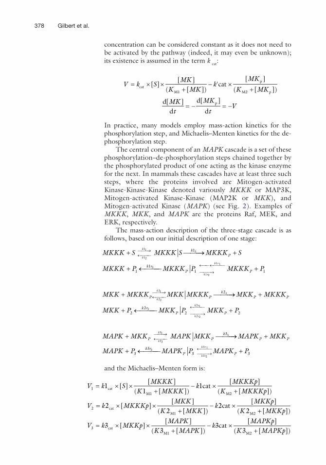
concentration can be considered constant as it does not need to be activated by the pathway (indeed, it may even be unknown); its existence is assumed in the term k¢cat:

In practice, many models employ mass-action kinetics for the phosphorylation step, and Michaelis–Menten kinetics for the de-phosphorylation step.

The central component of an MAPK cascade is a set of these phosphorylation–de-phosphorylation steps chained together by the phosphorylated product of one acting as the kinase enzyme for the next. In mammals these cascades have at least three such steps, where the proteins involved are Mitogen-activated Kinase-Kinase-Kinase denoted variously MKKK or MAP3K, Mitogen-activated Kinase-Kinase (MAP2K or MKK), and Mitogen-activated Kinase (MAPK) (see Fig. 2). Examples of MKKK, MKK, and MAPK are the proteins Raf, MEK, and ERK, respectively.

The mass-action description of the three-stage cascade is as follows, based on our initial description of one stage:

and the Michaelis–Menten form is:

pcat

M1 M2 p

p

[ ][ ][ ] cat

( [ ]) ( [ ])

d[ ]d[

'

]

d d

MKMKV k S k

K MK K MK

MKMKV

t t

= ´ ´ - ´+ +

= - = -

113

12

1 13

1 2

213

22

2 13

2 2

31

32

1

11 1 1

2

22 2 2

k

k

k r

k r

k

k

k r

k r

k

k

kP

k rP P

kP P P P

k rP P

P

MKKK S MKKK S MKKK S

MKKK P MKKK P MKKK P

MKK MKKK MKK MKKK MKK MKKK

MKK P MKK P MKK P

MAPK MKK

¾¾¾®¬¾¾¾

¬¾¾¬¾¾¾

¾¾¾®

¾¾¾®¬¾¾¾

¬¾¾¾

¾¾¾®

¾ ®¬¾¾¾

+ ¾¾¾® +

+ ¬¾¾¾ +

+ ¾¾¾® +

+ ¬¾¾¾ +

+ 3

3 13

3 2

3

33 3 3

k r

k r

kP P P

k rP P

MAPK MKK MAPK MKK

MAPK P MAPK P MAPK P

¾¾

¬¾¾¾¾¾¾®

¾¾¾® +

+ ¬¾¾¾ +

= ´ ´ - ´+ +

= ´ ´ - ´+ +

= ´ ´ - ´+ +

1 catM1 M2

2 catM1 M2

3 catM1 M2

[ ] [ ]1 [ ] 1cat

( 1 [ ]) ( [ ])[ ] [ ]

2 [ ] 2cat( 2 [ ]) ( 2 [ ])

[ ] [ ]3 [ ] 3cat

( 3 [ ]) ( 3 [ ])

MKKK MKKKpV k S k

K MKKK K MKKKpMKK MKKp

V k MKKKp kK MKK K MKKp

MAPK MAPKpV k MKKp k

K MAPK K MAPKp

379Computational Modelling of Kinase Signalling Cascades

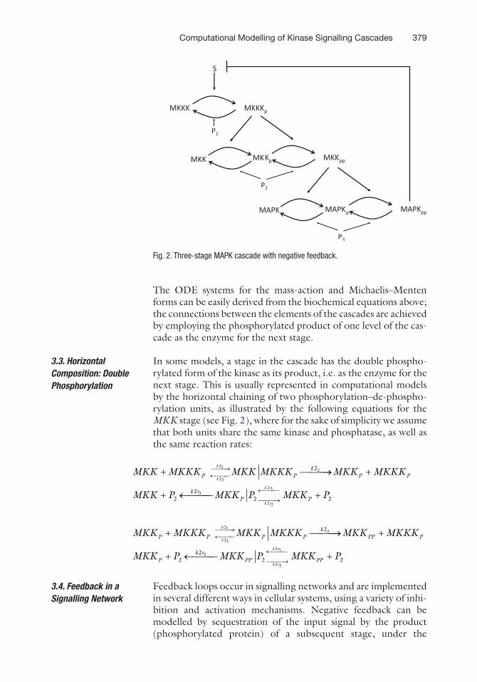
The ODE systems for the mass-action and Michaelis–Menten forms can be easily derived from the biochemical equations above; the connections between the elements of the cascades are achieved by employing the phosphorylated product of one level of the cas-cade as the enzyme for the next stage.

In some models, a stage in the cascade has the double phospho-rylated form of the kinase as its product, i.e. as the enzyme for the next stage. This is usually represented in computational models by the horizontal chaining of two phosphorylation–de-phospho-rylation units, as illustrated by the following equations for the MKK stage (see Fig. 2), where for the sake of simplicity we assume that both units share the same kinase and phosphatase, as well as the same reaction rates:

Feedback loops occur in signalling networks and are implemented in several different ways in cellular systems, using a variety of inhi-bition and activation mechanisms. Negative feedback can be modelled by sequestration of the input signal by the product (phosphorylated protein) of a subsequent stage, under the

3.3. Horizontal Composition: Double Phosphorylation

¾¾¾®¬¾¾¾

¬¾¾¾

¾¾¾®

¾¾¾®¬¾¾¾

¬¾¾¾

¾¾¾®

+ ¾¾¾® +

+ ¬¾¾¾ +

+ ¾¾¾® +

+ ¬¾¾¾ +

21

22

2 1

2 2

2

3

3

3

21

22

2 1

2 2

2

22 2 2

2

22 2 2

k

k

k r

k r

k

k

k r

k r

kP P P P

k rP P

kP P P P PP P

k rP PP PP

MKK MKKK MKK MKKK MKK MKKK

MKK P MKK P MKK P

MKK MKKK MKK MKKK MKK MKKK

MKK P MKK P MKK P

3.4. Feedback in a Signalling Network

Fig. 2. Three-stage MAPK cascade with negative feedback.

380 Gilbert et al.

assumption that the complex formed will not catalyse the phos-phorylation (49, 50). This will normally be a reversible reaction, with the rates ki1 and ki2 for the complexation and decomplexation respectively determining the strength of the inhibition. Thus, for example we can add the following equation to the mass-action description of the three-stage cascade above, and illustrated in Fig. 2.

Similarly, positive feedback can also be achieved by the sequestra-tion of the input signal by the product of a subsequent stage, under the additional condition that the resulting complex cataly-ses phosphorylation more actively than does the input signal alone with rates kp1, kp2, and kp3 . In this case, we can further add the following equation to the cascade in addition to the sequestration equation:

Many other molecular mechanisms achieving feedback can be envisaged. Each of these requires small modifications of the basic formalism and can be used to model the diversity of feed-back mechanisms observed in MAPK kinases, such as deactiva-tion of the active upstream component by the active downstream one, or desensitization by an additional change of state of the protein (such as phosphorylation at a second site); see e.g. (51).

There are many other components that need to be described in a model that attempts to capture more than the main signaling cas-cade in a MAPK pathway. For example, there are receptors and the signaling molecules that bind to them, as well as dimerisation of the receptors. These can simply be modeled using mass-action kinetics, in the manner of (8) and (52), where (EGFR|EGF)2 stands for a dimer.

Similarly, the complexation and decomplexation of other species such as Shc, Grb2, Sos, GAP, Ras-GTP, and various scaffolding proteins can be modelled using mass-action kinetics. Incorporating additional details, such as protein trafficking and subcellular localization requires specialized methods not discussed in this review (3).

1

1p p|

ki

kiS MAPK S MAPK

-

¾¾¾®+ ¬¾¾¾

1 2

1

p pp p p pp

| | | |k k

kMKKK S MAPK MKKK S MAPK MKKK S MAPK

-

¾¾¾®+ ¾¾¾® +¬¾¾¾

3.5. Receptors and Other Complexes

1

1

EGFR EGF EGFR | EGFk

k¾¾®+ ¬¾¾

2

2

EGFR | EGF EGFR | EGF (EGFR | EG_ F)2k

k¾¾®+ ¬¾¾

381Computational Modelling of Kinase Signalling Cascades

A model of a signalling pathway is of no use unless it both describes accurately the current data available and correctly predicts the behav-iour when the system is perturbed. Thus, the model should be fitted to the available data. This can be sometimes achieved by modifying kinetic parameters by hand and possibly aided by automated scanning through parameter ranges. However, this can be a time consuming process, and scanning multiple parameters can be both computation-ally expensive as well as producing a very large amount of data for interpretation by the modeler. There is now more use of automated techniques for parameter fitting, employing various optimization strategies, which attempt to find some best values of parameters which cause the model to acceptably fit to the data, for example (53). Of particular interest are those techniques which fit models to overall descriptions of the time-series behaviour of species, rather than to exact values which may vary between laboratories and experiments (54, 55).These techniques not only provide a useful “sanity check” of model behaviour, but can also produce quantitative results.

1. There are several different kinds of software which can be used to construct models of biochemical systems. One type has a graphical interface which permits users to construct models starting with the network wiring diagram (topology), and then to add the equations and kinetic parameters to the model under construction; such software can directly gener-ate a set of ODEs which can be solved using an ODE solver. Alternatively, the graphic-based software can be based on the Petri net formalism, so that users create a Petri net represen-tation of the model, initially qualitative (i.e. the wiring dia-gram, stoichiometry, and initial marking), and then to add kinetic information in terms of the rates, so that an ODE-based or stochastic model can be generated and simulated. Another class of approach permits users to describe the model using biochemical equations (e.g. mass-action, Michaelis–Menten), and the ODEs are generated automatically from these, for subsequent simulation. Finally, some modellers pre-fer to directly describe models in terms of ODEs, and then to solve these using an ODE solver.

2. A major activity in BioModel Engineering is that of identify-ing a (quantitative) model by means of (1) finding the struc-ture, (2) obtaining an initial state, and (3) parameter fitting. An important part of this will be detailed studies of the litera-ture and public databases, as well as intense interactions between computational modellers and experimentalists.

3.6. Tuning the Model

4. Notes

382 Gilbert et al.

Attempts at automating the first step are underway and con-sequently, the field of text mining of biomedical information is a very active one (56). Automated systems for extracting useful information from journals and patents will become more widely used as online full-text versions of experimental papers become more widely available.

3. While Michaelis–Menten kinetics are suitable for modelling biochemical systems which predominantly exhibit steady-state kinetics, such as metabolic pathways, there are problems in applying such an approach uncritically to systems which are characterised by dynamic behaviour, such as signalling path-ways (47). Thus many modellers use mass-action kinetics to describe such systems. Michaelis–Menten kinetics should not simply be used because of the smaller number of parameters in the model; instead it can be useful to implement a suitably relaxed version of the assumptions of Michaelis–Menten kinetics in the parameters of the mass-action equations, thus avoiding unrealistic model behaviour.

References

1. Gilbert, D.R., Breitling, R., Heiner, M., and Donaldson, R. (2009) An introduction to BioModel Engineering, illustrated for signal transduction pathways, in membrane comput-ing. Springer LNCS, Springer, New York 5391 13–28.

2. Kolch, W., Calder, M., and Gilbert, D.R. (2005) When kinases meet mathematics: the systems biology of MAPK signalling. FEBS Lett 579(8), 1891–1895.

3. Breitling, R., and Hoeller, D. (2005) Current challenges in quantitative modeling of epider-mal growth factor signaling. FEBS Lett 579(28), 6289–6294. Wiley.

4. Wiley, H.S., Shvartsman, S.Y., and Lauffenburger, D.A. (2003) Computational modeling of the EGF-receptor system: a para-digm for systems biology. Trends Cell Biol 13(1), 43–50.

5. Orton, R.J., Sturm, O., Gormand, A.M., Kolch, W., and Gilbert, D.R. (2005) Computational modelling of the receptor-tyrosine-kinase-activated MAPK pathway. Biochem J 392(Pt 2), 249–261.

6. Butcher, J.C. (2003) Numerical methods for ordinary differential equations. Wiley, Philadelphia

7. Brightman, F.A., and Fell, D.A. (2000) Differential feedback regulation of the MAPK cascade underlies the quantitative differences in EGF and NGF signalling in PC12 cells. FEBS Lett 482(3), 169–174.

8. Schoeberl, B., Eichler-Jonsson, C., Gilles, E.D. et al. (2002) Computational modeling of the dynamics of the MAP kinase cascade activated by surface and internalized EGF receptors. Nat Biotechnol 20(4), 370–375.

9. Brown, K.S., Hill, C.C., Calero, G.A., Myers, C.R., Lee, K.H., Sethna, J.P., and Cerione, R.A. (2004) The statistical mechanics of complex signaling networks: nerve growth factor signaling. Phys Biol 1(3–4), 184–195.

10. Orton, R.J., Sturm, O., Gormand, A., Kolch, W., and Gilbert, D.R. (2008) Computational modelling reveals feedback redundancy within the EGFR/ERK signalling pathway. IET Syst Biol 2(4), 173–183.

11. Huang, C.Y., and Ferrell, J.E. Jr. (1996) Ultrasensitivity in the mitogen-activated pro-tein kinase cascade. Proc Natl Acad Sci U S A 93, 10078–10083.

12. Burack, W.R., and Sturgill, T.W. (1997) The activating dual phosphorylation of MAPK by MEK is nonprocessive. Biochemistry 36, 5929–5933.

13. Ferrell, J.E. Jr., and Bhatt, R.R. (1997) Mechanistic studies of the dual phosphoryla-tion of mitogen-activated protein kinase. J Biol Chem 272, 19008–19016.

14. Kholodenko, B.N. (2000) Negative feedback and ultrasensitivity can bring about oscilla-tions in the mitogen-activated protein kinase cascades. Eur J Biochem 267, 1583–1588.

383Computational Modelling of Kinase Signalling Cascades

15. Resat, H., Ewald, J.A., Dixon, D.A., and Wiley, H.S. (2003) An integrated model of epidermal growth factor receptor trafficking and signal transduction. Biophys J 85, 730–743.

16. Sasagawa, S., Ozaki, Y., Fujita, K., and Kuroda, S. (2005) Prediction and validation of the distinct dynamics of transient and sustained ERK activation. Nat Cell Biol 7, 365–373.

17. Cho, K.H., Shin, S.Y., Kim, H.W., Wolkenhauer, O., McFerran, B., and Kolch, W. (2003) Mathematical modeling of the influence of RKIP on the ERK signaling path-way. LNCS 2602, 127–141.

18. Heiner, M., Uhrmacher, and Adelinde M. (Eds.) (2008).In: Proc. computational meth-ods in systems biology. LNCS, Springer, New York 5307.

19. Breitling, R., Gilbert, D., Heiner, M., and Priami, C. (2009) Formal methods in molec-ular biology, Dagstuhl Seminar 09091 Proceedings.

20. Clarke, E.M., Grumberg, O., and Peled, D.A. (1999) Model checking. MIT Press, Cambridge.

21. Parker, D., Norman, G., and Kwiatkowska, M. (2006) PRISM 3.0.beta1 users’ guide, Cambridge University Press, Cambridge.

22. Calzone, L., Chabrier-Rivier, N., Fages, F., and Soliman, S. (2006) Machine learning bio-chemical networks from temporal logic prop-erties. Trans on Computat Syst Biol VI, LNBI 4220, 68–94.

23. Priami, C., Regev, A., Shapiro, E., and Silverman, W. (2001) Application of a sto-chastic name-passing calculus to representa-tion and simulation of molecular processes. Inform Process Lett 80(1), 25–31.

24. Regev, A., Silverman, W., and Shapiro, E. (2001) Representation and simulation of biochemical processes using the p-calculus process algebra. Pac Symp Biocomput 6, 459–470.

25. Phillips A., and Cardelli L.A. (2005) Graphical representation for the stochastic pi-calculus. Trans on Computat Syst Biol VII, 4230, 123–152.

26. Gillespie, D.T. (1977) Exact stochastic simu-lation of coupled chemical reactions. J Phys Chem, 81(25), 2340–2361.

27. Gilmore S, Hillston J. (1994) The PEPA workbench: a tool to support a process alge-bra-based approach to performance model-ling. LNCS 794, 353–368.

28. Calder, M., Gilmore, S., and Hillston, J. (2006) Modelling the influence of RKIP on the ERK signalling pathway using the stochas-tic process algebra PEPA. Transactions on

computational systems biology. Springer, New York 4230, 1–23.

29. Calder, M., Gilmore, S., and Hillston, J. (2005) Automatically deriving ODEs from process algebra models of signalling pathways. In: Proc. computational methods in systems biology 2005. 204–215.

30. Gilbert, D.R., Heiner, M., and Lehrack, S. (2007) A unifying framework for modelling and analysing biochemical pathways using Petri nets. In: Proc. computational methods in systems biology 2007. Springer LNCS/LNBI, Springer, New York 4695, 200–216.

31. Heiner, M., Gilbert, D.R., and Donaldson, R. (2008) Petri nets for systems and synthetic biology in formal methods for systems biol-ogy. Springer LNCS, Springer, New York 5016, 215–264.

32. Hucka, M., Finney, A., Sauro, H.M. et. al. (2003) The system biology markup language (SBML): a medium for representation and exchange of biochemical network models’. Bioinformatics 19(4), 524–531.

33. BioNessie. A biochemical pathway simulation and analysis tool. University of Glasgow, http://www.bionessie.org

34. Hoops, S., Sahle, S., Gauges, R., Lee, C., Pahle, J., Simus, N., Singhal, M., Xu, L., Mendes, P., and Kummer, U. (2006) COPASI – a complex pathway simulator. Bioinformatics, 22, 3067–3074.

35. Le Noviere, N. et al. (2006) Biomodels data-base: a free, centralized database of curated, published, quantitative kinetic models of bio-chemical and cellular systems. Nucleic Acids Res 34(Database Issue), D689–D691.

36. Shampine, L.F., and Reichelt, M.W. (1997) The matlab ode suite. SIAM J Sci Comput, 18, 1–22.

37. Bergmann, F.T., and Sauro, H.M. (2006) SBW – a modular framework for systems biol-ogy. In Perrone, L. F., Lawson, B., Liu, J., and Wieland, F. P. (eds.).In: Proc. Winter Simulation Conference 2006, 1637–1645.

38. Ermentrout, B. Simulating, analyzing, and animating dynamical systems: a guide to XPPAUT for researchers and students, (Software, Environments, and Tools 14). SIAM publishers, 2002 ISBN-13: 978-0-898715-06-4.

39. Funakashi, A., Matsuoka, Y., Jouraku, A., Kitano, H., and Kikuchi, N. (2006) Cell designer: a mod-elling too for biochemical networks, Proc Winter Simulation Conference 2006. 1707–1712.

40. Snoopy. A tool to design and animate hierar-chical graphs. BTU Cottbus, CS Dep., http://www-dssz.informatik.tu-cottbus.de.

384 Gilbert et al.

41. Charlie Website. A tool for the analysis of place/transition nets. BTU Cottbus, http://www-dssz.informatik.tu-cottbus.de/soft-ware/charlie/charlie.html.

42. Schwarick, M., and Heiner, M. (2009) CSL model checking of biochemical networks with interval decision diagrams. In: Proc. compu-tational methods in systems biology 2009. Springer LNCS/LNBI, Springer, New York 5688, 296–312.

43. Heiner, M., Schwarick, M., and Tovchigrechko, A. (2009) DSSZ-MC – a tool for symbolic analysis of extended Petri nets. In: Proc. Petri nets 2009. Springer LNCS, Springer, New York 5606, 323–332.

44. Berg, J.M., Tymoczko, J.L., and Stryer, L. (2009) Biochemistry. W H Freeman, New York.

45. Breitling, R., Gilbert, D.R., Heiner, M., and Orton, R. (2008) A structured approach for the engineering of biochemical network mod-els, illustrated for signalling pathways. Brief Bioinform 9(5), 404–442.

46. Gilbert, D.R., and Heiner, M. (2006) From Petri nets to differential equations – an inte-grative approach for biochemical network analysis. Springer LNCS, Springer, New York 4024, 181–200.

47. Klipp, E., and Liebermeister, W. (2006) Mathematical modeling of intracellular signal-ing pathways. BMC Neurosci 7(Suppl 1), S10.

48. Orton, R.J., Sturm, O.E., Vyshemirsky, V., Calder, M., Gilbert, D.R., and Kolch, W. (2005) Computational modelling of the receptor-tyrosine-kinase-activated MAPK pathway. Biochem J 392, 249–261.

49. Blüthgen, N., Bruggeman, F.J., Legewie, S., Herzel, H., Westerhoff, H.V., and

Kholodenko, B.N. (2006) Effects of seques-tration on signal transduction cascades. FEBS J 273(5), 895–906.

50. Legewie, S., Schoeberl, B., Blüthgen, N., and Herzel, H. (2007) Competing docking inter-actions can bring about bistability in the MAPK cascade. Biophys J 93(7), 2279–2288.

51. Orton, R., Sturm, O., Gormand, A., Kolch, W., and Gilbert, D.R. (2008) Computational modelling reveals feedback redundancy within the EGFR/ERK signalling pathway. IET Syst Biol 1(4), 173–183.

52. Hornberg, J.J., Binder, B., Bruggeman, F.J., Schoeberl, B., Heinrich, R., and Hans, V.W. (2005) Control of MAPK signalling: from complexity to what really matters. Oncogene 24, 5533–5542.

53. Moles, C.G., M., Mendes, P., and Bang, J.R. (2003) Parameter estimation in bio-chemical pathways: a comparison of global optimization methods. Genome Res 13, 2467–2474.

54. Donaldson, R., and Gilbert, D.R. (2008) A model checking approach to the parameter estimation of biochemical pathways. In Proc. computational methods in systems biology. Springer LNCS, Springer, New York 5307, 269–287.

55. Rizk, A., Batt, G., Fages, F., and Soliman, S. (2008) On a continuous degree of satisfac-tion of temporal logic formulae with applica-tions to systems biology. In Proc. computational methods in systems biology. Springer LNCS, Springer, New York 5307, 251–268.

56. Cohen, A.M., and Hersh, R.W. (2005) A sur-vey of current work in biomedical text min-ing. Brief Bioinform 6(1), 57–71.