MANCaLog: A Logic for Multi-Attribute Network Cascades(Technical Report)

Paulo ShakarianNetwork Science Center and

Dept. of Electrical Engineeringand Computer ScienceU.S. Military AcademyWest Point, NY 10996

paulo@shakarian.net

Gerardo I. SimariDept. of Computer Science

University of OxfordWolfson Building, Parks Road

Oxford OX1 3QD, UKgerardo.simari@cs.ox.ac.uk

Robert SchroederCORE Lab

Defense Analysis Dept.Naval Postgraduate School

Monterey, CA 93943rcschroe@nps.edu

ABSTRACTThe modeling of cascade processes in multi-agent systemsin the form of complex networks has in recent years becomean important topic of study due to its many applications:the adoption of commercial products, spread of disease, thediffusion of an idea, etc. In this paper, we begin by identi-fying a desiderata of seven properties that a framework formodeling such processes should satisfy: the ability to rep-resent attributes of both nodes and edges, an explicit rep-resentation of time, the ability to represent non-Markoviantemporal relationships, representation of uncertain informa-tion, the ability to represent competing cascades, allowanceof non-monotonic diffusion, and computational tractability.We then present the MANCaLog language, a formalism basedon logic programming that satisfies all these desiderata, andfocus on algorithms for finding minimal models (from whichthe outcome of cascades can be obtained) as well as howthis formalism can be applied in real world scenarios. Weare not aware of any other formalism in the literature thatmeets all of the above requirements.

Categories and Subject DescriptorsI.2.4 [Artificial Intelligence]: Knowledge RepresentationFormalisms and Methods—Representation Languages

General TermsLanguages, Algorithms

KeywordsComplex Networks, Cascades, Logic Programming

1. INTRODUCTION AND RELATED WORKAn epidemic working through a population, cascading elec-

trical power failures, product adoption, and the spread ofa mutant gene are all examples of diffusion processes thatcan happen in multi-agent systems structured as complexnetworks. These network processes have been studied in a

This is an extended version of MANCaLog: A Logicfor Multi-Attribute Network Cascades, which ap-pears in: Proceedings of the 12th International Conferenceon Autonomous Agents and Multiagent Systems (AAMAS2013), Ito, Jonker, Gini, and Shehory (eds.), May 6–10,2013, Saint Paul, Minnesota, USA.

variety of disciplines, including computer science [10], bi-ology [11], sociology [8], economics [12], and physics [15].Much existing work in this area is based on pre-existingmodels in sociology and economics – in particular the workof [8, 12]. However, recent examinations of social networks– both analysis of large data sets and experimental – haveindicated that there may be additional factors to considerthat are not taken into account by these models. Theseinclude the attributes of nodes and edges, competing diffu-sion processes, and time. In this paper, we outline sevendesign criteria (Section 1.1) for such a framework and in-troduce MANCaLog (Section 2), which is to the best of ourknowledge the first logical language for modeling diffusionin complex networks that meets these criteria. MANCaLogis a rule-based framework (inspired by logic programming)that can richly express how agents adopt or fail to adoptcertain behaviors, and how these behaviors cascade througha network. We also introduce fixed-point based algorithmsthat allow for the calculation of the result of the diffusionprocess in Section 3. Note that these algorithms are provennot only to be correct, but also to run in polynomial time.Hence, our approach can not only better express many as-pects of cascades in complex networks, but it can do so ina reasonable amount of time. We conclude by discussingapplications of MANCaLog in Section 4.

Proofs of all results stated in this paper can be found in theappendix.

1.1 Desiderata of PropertiesWe begin by identifying a set of criteria that we believe a

framework for reasoning about cascades in complex networksshould satisfy.

1. Multiply labeled and weighted nodes and edges.Many existing frameworks for studying diffusion in complexnetworks assume that there is only one type of vertex thatmay become “active” [10] or may “mutate” [11, 15] and onlyone possible relationship between nodes. In reality, nodesand edges often have different properties. For instance, la-bels on edges can be used to differentiate between strongand weak ties (edge types) – a concept that is well stud-ied [7]. Recently, such attributes of nodes have been shownto impact influence in a network [1].

2. Explicit Representation of Time. Most work inthe literature assumes static models, with the exceptionof the recent developments in [4, 5, 6], which assume theexistence of a timestamped log referring to actions taken

arX

iv:1

301.

0302

v2 [

cs.A

I] 1

9 Ja

n 20

13

in the network in order to learn how nodes influence eachother. Though [4] tackles the problem of predicting thetime at which a certain node will take an action, the au-thors make several simplifying assumptions such as mono-tonicity of probability functions, probabilistic independence,sub-modularity and, most importantly for this criterion, amodeling of time solely based on temporal decay of influ-ence. We seek a richer model of temporal relationships be-tween conditions in the network structure, the current stateof the cascades in process, and how influence propagates.

3. Non-Markovian Temporal Relationships. Apartfrom time being explicitly represented, the temporal depen-dencies should be able to span multiple units of time. Hence,the“memoryless”mode of a standard Markov process, whereonly the information of the current state is required, is insuf-ficient. Here, we strive to create a framework where depen-dencies can be from other earlier time steps. This issue hasbeen previously studied with respect to more general logicprogramming frameworks such as [13], but to our knowledgehas not been applied to social networks.

4. Representation of Uncertainty. As in practice it isnot always possible to judge the attributes of all individualsin a network, an element of uncertainty must be included.However, in connection with point 7, this should not be atthe expense of tractability. For instance, the probabilisticmodels of [10] are normally addressed with simulation (andhence do not scale well) as the computation of the expectednumber of activated nodes is a #P -hard problem [3].

5. Competing Cascades. Often, in real-world situationsthere will be competing cascading processes. For example,in evolutionary graph theory [11], “mutants” and “residents”compete for nodes in the network – the success of one hingeson the failure of the other.

6. Non-Monotonic Cascades. In much existing work oncascades in complex networks, the number of nodes attain-ing a certain property at each time step can only increase.However, if we allow for competing cascades in the samemodel, we cannot have such a strong restriction as the suc-cess of one cascade may come at the expense of another.

7. Tractability. The social networks of interest in today’sdata mining problems often have millions of nodes. It isreasonable to expect that soon billion-node networks will becommonplace. Any framework for dealing with these prob-lems must be solvable in a reasonable amount of time andoffer areas for practical improvement for further scalability.

1.2 Related WorkThe above criteria can be summarized as the desire to

design the most expressive language for network cascadespossible while still allowing computation of the outcome ofa diffusion process to be completed in a tractable amountof time. As a comparison, let us briefly describe some rel-evant related work. Perhaps the best known general modelfor representing diffusion in complex networks is the in-dependent cascade/linear threshold (IC/LT) model of [10].However, although this framework was shown to be capa-ble of expressing a wide variety of sociological models, itassumes the Markov property and does not allow for therepresentation of multiple attributes on vertices and edges.A more recent framework, social network optimization prob-lems (SNOPs) [14] uses logic programming to allow for therepresentation of attributes, but this framework does not al-

 

 1

 2

 7

 9

 3

 4  10

 6

 8  5

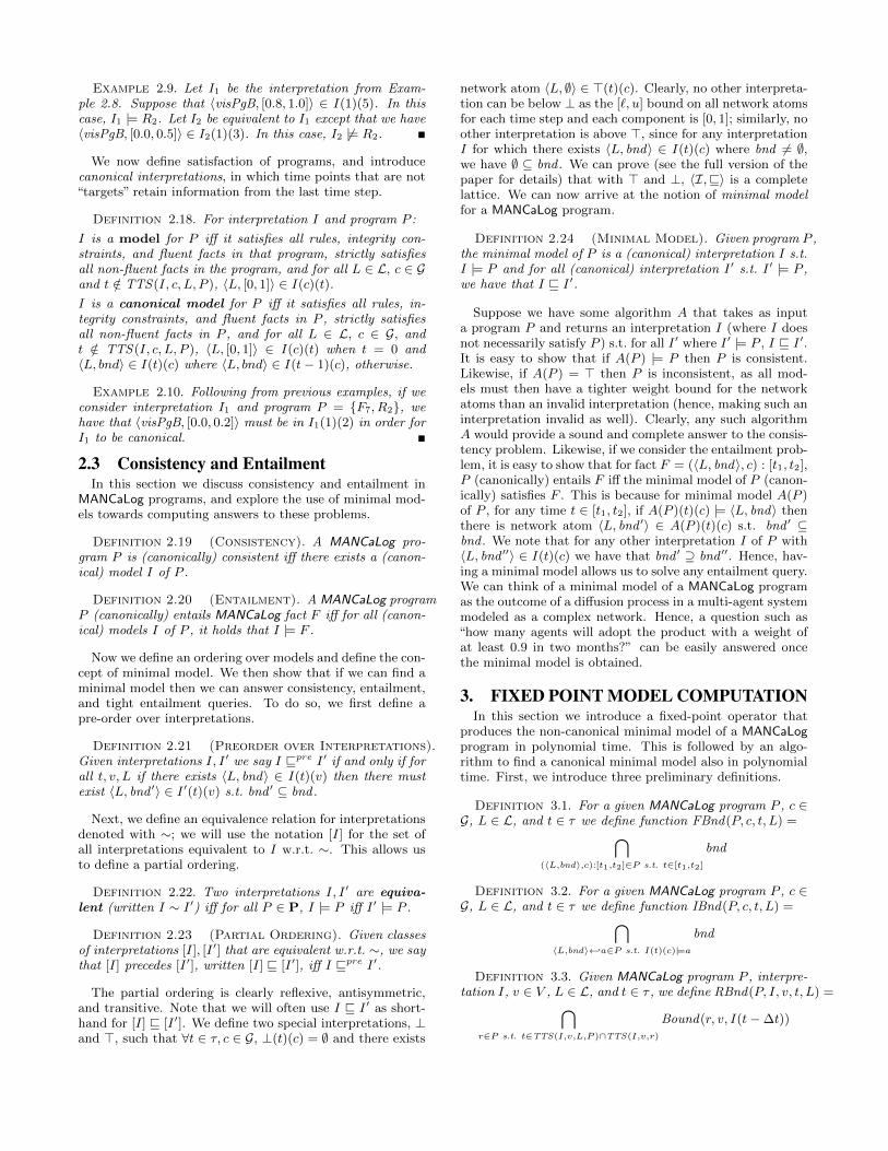
Figure 1: Simple online social network Gsoc. Solidedges are labeled with strTie, while dashed edges arelabeled with wkTie. White nodes are labeled withmale, while gray nodes are labeled with fem. Arrowsrepresent the direction of the edge; double-headededges represent two edges with the same label.

low for competing processes or non-monotonic cascades. Arelated logic programming framework, competitive diffusion(CD) [2] allows for competitive diffusion and non-monotonicprocesses but does not explicitly represent time and alsomakes Markovian assumptions. Further, we also note thatthe semantics of CD yields a “most probable interpretation”that is not a unique solution. Hence, a given model inthat framework can lead to multiple and possibly contra-dictory, outcomes to a cascade (this problem is avoided inMANCaLog). Another popular class of models is Evolution-ary Graph Theory (EGT) [11], which is highly related tothe voter model (VM) [15]. Although this framework al-lows for competing processes and non-monotonic diffusion,it also makes Markovian assumptions while not explicitlyrepresenting time. Further, determining the outcome of acascade in those models is NP-hard, while determining theoutcome in MANCaLog can be accomplished in polynomialtime. Table 1 lists how these models compare to MANCaLogwhen considering our design criteria.

2. FRAMEWORK

2.1 Syntax and SemanticsIn this paper we assume that agents are arranged in a

directed graph (or network) G = (V,E), where the set ofnodes corresponds to the agents, and the edges model therelationships between them. We also assume a set of labelsL, which is partitioned into two sets: fluent labels Lf (labelsthat can change over time) and non-fluent labels Lnf (labelsthat do not); labels can be applied to both the nodes andedges of the network. We will use the notation G = V ∪ Eto be the set of all components (nodes and edges) in thenetwork. Thus, c ∈ G could be either a node or an edge.

Example 2.1. We will use the sample online social net-work Gsoc shown in Figure 1 as the running example; Gsoc isused to denote the set of components of Gsoc. Here we haveLnf = {male, fem, strTie,wkTie} representing male, female,strong ties and weak ties, respectively. Additionally, we haveLf = {visPgA, visPgB} representing visiting webpage A andvisiting webpage B, respectively. �

In this paper, we present a logical language where we useatoms, referring to labels and weights, to describe propertiesof the nodes and edges. Though labels themselves couldbe modeled as atoms instead of predicates (to model non-ground labelings that allow for greater expressibility), forsimplicity of presentation we leave this to future work. Thefirst piece of the syntax is the network atom.

Table 1: Comparison with other modelsCriterion MANCaLog IC/LT [10] SNOP [14] CD [2] EGT/VM [11]

1. Labels Yes No Yes Yes No2. Explicit Representation of Time Yes No Yes No Yes3. Non-Markovian Temporal Relationships Yes No No No No4. Uncertainty Yes Yes Yes Yes Yes5. Competing Cascades Yes No No Yes Yes6. Non-monotonic Cascades Yes No No Yes Yes7. Tractablity PTIME #P-hard PTIME PTIME NP-hard

Definition 2.1 (Network Atom). Given label L ∈ Land weight interval bnd ⊆ [0, 1], then 〈L, bnd〉 is a net-work atom. A network atom is fluent (resp., non-fluent) ifL ∈ Lf (resp., L ∈ Lnf ). We use NA to denote the set ofall possible network atoms.

Network atoms describe properties of nodes and edges.The definition is intuitive: L represents a property of thevertex or edge, and associated with this property is someweight that may have associated uncertainty – hence repre-sented as an interval bnd , which can be open or closed. Aninvalid bound is represented by ∅, which is equivalent to allother invalid bounds.

Definition 2.2 (World). A world W is a set of net-work atoms such that for each L ∈ L there is no more thanone network atom of the form 〈L, bnd〉 in W .

A network formula over NA is defined using conjunc-tion, disjunction, and negation in the usual way. If a for-mula contains only non-fluent (resp., fluent) atoms, it is anon-fluent (resp., fluent) formula.

Definition 2.3 (Satisfaction of Worlds). Given aworld W and network formula f , satisfaction of W by f(denoted W |= f) is defined:

• If f = 〈L, [0, 1]〉 then W |= f .

• If f = 〈L, ∅〉 then W 6|= f .

• If f = 〈L, bnd〉, with bnd 6= ∅ and bnd 6= [0, 1], thenW |= f iff there exists 〈L, bnd ′〉 ∈W s.t. bnd ′ ⊆ bnd.

• If f = ¬f ′ then W |= f iff W 6|= f ′.

• If f = f1 ∧ f2 then W |= f iff W |= f1 and W |= f2.

• If f = f1 ∨ f2 then W |= f iff W |= f1 or W |= f2.

For some arbitrary label L ∈ L, we will use the nota-tion Tr = 〈L, [0, 1]〉 and F = 〈L, ∅〉 to represent a tautologyand contradiction, respectively. For ease of notation (andwithout loss of generality), we say that if there does notexist some bnd s.t. 〈L, bnd〉 ∈ W , then this implies that〈L, [0, 1]〉 ∈W .

Example 2.2. Following from Example 2.1, the networkatom 〈female, [1, 1]〉 can be used to identify a node as awoman. Likewise, the world W ={〈fem, [1, 1]〉, 〈male, [0, 0]〉, 〈visPgA, [1, 1]〉, 〈visPgB, [0, 0]〉

}

might be used to identify a woman who visits webpage A.Clearly, we have that W |=

〈fem, [1, 1]〉 ∧ ¬〈visPgA, [0.5, 0.9]〉 ∧ ¬〈visPgB, [0.1, 0.7]〉

Note that the network atoms formed with strTie and wkTieare not present; this could be due to the fact that such aworld is used to describe a node and not an edge, and hencethere is no information about those two labels. As such isthe case, W |= 〈strTie, [0, 1]〉 ∧ 〈wkTie, [0, 1]〉. �

The idea is to use MANCaLog to describe how properties(specified by labels) of the nodes in the network change overtime. We assume that there is some natural number tmax

that specifies the total amount of time we are considering,and we use τ = {t | t ∈ [0, tmax ]} to denote the set of alltime points. How well a certain property can be attributedto a node is based on a weight (to which the bnd bound inthe network atom refers). As time progresses, a weight caneither increase/decrease and/or become more/less certain.We now introduce the MANCaLog fact, which states thatsome network atom is true for a node or edge during certaintimes.

Definition 2.4 (MANCaLog Fact). If [t1, t2] ⊆ [0, tmax ],c ∈ G, and a ∈ NA, then (a, c) : [t1, t2] is a MANCaLogfact. A fact is fluent (resp., non-fluent) if atom a is fluent(resp., non-fluent). All non-fluent facts must be of the form(a, c) : [0, tmax ]. Let F be the set of all facts and Fnf ,Ff bethe set of all non-fluent and fluent facts, respectively.

Example 2.3. Following from Example 2.2, the followingfacts are based on Figure 1:

F1 = (〈male, [1, 1]〉, 1) : [0, tmax ]

F2 = (〈fem, [1, 1]〉, 1) : [0, tmax ]

F3 = (〈male, [1, 1]〉, 3) : [0, tmax ]

F4 = (〈strTie, [1, 1]〉, (1, 2)) : [0, tmax ]

F5 = (〈strTie, [1, 1]〉, (2, 1)) : [0, tmax ]

F6 = (〈wkTie, [1, 1]〉, (2, 3)) : [0, tmax ]

F7 = (〈visPgA, [0.8, 1.0]〉, 1) : [0, tmax ]

F8 = (〈visPgA, [0.5, 1.0]〉, 2) : [0, tmax ]

For instance, agent 1 is male, and has a strong tie to agent 2,who is female. �

Next, we introduce integrity constraints (ICs).

Definition 2.5. Given fluent network atom a and con-junction of network atoms b, an integrity constraint is of theform a←↩ b.

Intuitively, integrity constraint 〈L, bnd〉 ←↩ b means thatif at a certain time point a component (vertex or edge) ofthe network has a set of properties specified by conjunctionb, then at that same time the component’s weight for labelL must be in interval bnd .

Example 2.4. Following from the previous examples, theintegrity constraint 〈male, [0, 0]〉 ←↩ 〈fem, [1, 1]〉 would re-quire any node designated as a female to not be male. �

We now define MANCaLog rules. The idea behind rules issimple: an agent that meets some criteria is influenced bythe set of its neighbors who possess certain properties. Theamount of influence exerted on an agent by its neighbors isspecified by an influence function, whose precise effects willbe described later on when we discuss the semantics. As aresult, a rule consists of four major parts: (i) an influencefunction, (ii) neighbor criteria, (iii) target criteria, and (iv) atarget. Intuitively, (i) specifies how the neighbors influencethe agent in question, (ii) specifies which of the neighborscan influence the agent, (iii) specifies the criteria that causethe agent to be influenced, and (iv) is the property of theagent that changes as a result of the influence.

We will discuss each of these parts in turn, and then definerules in terms of these elements. First, we define influencefunctions and neighbor criteria.

Definition 2.6 (Influence Function). An influencefunction is a function ifl : N×N→ [0, 1]× [0, 1] that sat-isfies the following two axioms:

1. ifl can be computed in constant (O(1)) time.

2. For x′ > x we have ifl(x′, y) ⊆ ifl(x, y).

We use IFL to denote the set of all influence functions.

Intuitively, an influence function takes the number of qual-ifying influencers and the number of eligible influencers andreturns a bound on the new value for the weight of the prop-erty of the target node that changes. In practice, we expectthe time complexity of such a function to be a polynomialin terms of the two arguments. However, as both argumentsare naturals bounded by the maximum degree of a node inthe network, this value will be much smaller than the sizeof the network – we thus treat it as a constant here.

Example 2.5. The well-known “tipping model” originallyintroduced in [8, 12] states that an agent adopts a behaviorwhen a certain fraction of his incoming neighbors do so. Acommon tipping function is the majority threshold whereat least half of the agent’s neighbors must previously adoptthe behavior. We can represent this using the following in-fluence function:

tip(x, y) =

{[1.0, 1.0] if x/y ≥ 0.5

[0.0, 1.0] otherwise

This function says that an agent adopts a certain behaviorif at least half of his incoming neighbors have some property(strong ties, weak ties, meet some requirement of gender,income, etc.) and that we have no information otherwise.In our framework, we can leverage the bounds associated withthe influence function to create a “soft” tipping function:

sftTp(x, y) =

{[0.7, 1.0] if x/y ≥ 0.5

[0.0, 1.0] otherwise

Intuitively, the above function says that an agent adopts abehavior with a weight of at least 0.7 if half of the incomingneighbors that have some attribute and meet some criteria,and we have no information otherwise. Another possibilityis to have an influence function that may reduce the weightthat an agent adopts a certain behavior:

ngTp(x, y) =

{[0.0, 0.2] if x = y

[0.0, 1.0] otherwise

The ngTp function says that an agent will adopt a behav-ior with a weight no greater than 0.2 if all of the incomingneighbors possessing some property meet some criteria, andthat we have no information otherwise. �

Definition 2.7 (Neighbor Criterion). If gedge, gnode

are non-fluent network formulas (formed over edges and nodes,respectively), h is a conjunction of network atoms, and ifl isan influence function, then (gedge, gnode, h)ifl is a neighborcriterion.

Formulas gnode and h in a neighbor criterion specify the(non-fluent and fluent, respectively) criteria on a given neigh-bor, while formula gedge specifies the non-fluent criteria onthe directed edge from that neighbor to the node in question.

The next component is the “target criteria”, which are thecriteria that an agent must satisfy in order to be influencedby its neighbors. Ideas such as “susceptibility” [1] can beintegrated into our framework via this component. We rep-resent these criteria with a formula of non-fluent networkatoms. The final component, the “target”, is simply the la-bel of the target agent that is influenced by its neighbors.Hence, we now have all the pieces to define a rule.

Definition 2.8 (Rule). Given fluent label L, naturalnumber ∆t, target criteria f and neighbor criteria(gedge, gnode, h)ifl , a MANCaLog Rule is of the form:

r = L∆t← f, (gedge, gnode, h)ifl

We will use the notation head(r) to denote L.

Note that the target (also referred to as the head) of the ruleis a single label; essentially, the body of the rule characterizesa set of nodes, and this label is the one that is modified foreach node in this set. More specifically, the rule is essentiallysaying that when certain conditions for an agent and itsneighbors are met, the bnd bound for the network atomformed with label L on that agent changes. Later, in thesemantics, we introduce network interpretations, which mapcomponents (nodes and edges) of the network to worlds ata given point in time. The rule dictates how this mappingchanges in the next time step.

Definition 2.9 (MANCaLog Program). A program Pis a set of rules, facts, and integrity constraints s.t. eachnon-fluent fact F ∈ Fnf appears no more than once in theprogram. Let P be the set of all programs.

Example 2.6. Following from the previous examples, wecan have a MANCaLog program that leverage the sftTp andngTp influence functions in rules that are more expressive

Table 2: Example network interpretation, NI1.Comp. male fem strTie wkTie visPgA visPgB

1 [1, 1] [0, 0] - - [0.9, 1.0] [0.8, 1.0]2 [0, 0] [1, 1] - - [0.0, 0.3] [0.0, 0.2]3 [1, 1] [0, 0] - - [0.6, 1.0] [0.0, 0.2]4 [0, 0] [1, 1] - - [0.0, 0.2] [0.9, 1.0]5 [1, 1] [0, 0] - - [0.0, 0.2] [0.7, 1.0](1,2) - - [1, 1] [0, 0] - -(2,1) - - [1, 1] [0, 0] - -(1,3) - - [0, 0] [1, 1] - -(2,3) - - [0, 0] [1, 1] - -(3,4) - - [1, 1] [0, 0] - -(4,3) - - [1, 1] [0, 0] - -(4,5) - - [1, 1] [0, 0] - -

than previous models. Consider the following rules:

R1 = visPgA2←

〈fem, [1, 1]〉, (〈strTie, [0.9, 1]〉,Tr, 〈visPgA, [0.9, 1.0]〉)sftTp

R2 = visPgB1←

〈male, [1, 1]〉, (Tr,Tr, 〈visPgB, [0.8, 1.0]〉)sftTp

R3 = visPgA3←

〈male, [1, 1]〉, (Tr, 〈fem, [1, 1]〉,¬〈visPgA, [0.7, 1.0]〉)ngTp

Rule R1 says that a female agent in the network visits pageA with a weight of at least 0.7 (this is specified in the sftTpinfluence function) if at least half of her strong ties (withweight of at least 0.9) visited the page (with a weight of atleast 0.9) two days ago. The rest of the rules can be readanalogously. �

We now introduce our first semantic structure: the net-work interpretation.

Definition 2.10 (Network Interpretation). A net-work interpretation is a mapping of network components tosets of network atoms, NI : G → 2NA. We will use NI todenote the set of all network interpretations.

We note that not all labels will necessarily apply to allnodes and edges in the network. For instance, certain labelsmay describe a relationship while others may only describea property of an individual in the network. If a given label Ldoes not describe a certain component c of the network, thenin a valid network interpretation NI, 〈L, [0, 1]〉 ∈ NI(c).

Example 2.7. Consider G′soc, the induced subgraph of Gsoc

that has only nodes {1, 2, 3, 4, 5}. Table 2 shows the contentsof NI1, an example network interpretation. �

We define a MANCaLog interpretation as follows.

Definition 2.11 (Interpretation). A MANCaLog in-terpretation I is a mapping of natural numbers in the inter-val [0, tmax ] to network interpretations, i.e., I : N → NI.Let I be the set of all possible interpretations.

2.2 SatisfactionFirst, we define what it means for an interpretation to

satisfy a fact and a rule.

Definition 2.12 (Fact Satisfaction). An interpreta-tion I satisfies MANCaLog fact (a, c) : [t1, t2], written I |=(a, c) : [t1, t2], iff ∀t ∈ [t1, t2], I(t)(c) |= a.

Example 2.8. Consider interpretation I1, where I1(0) =NI1 (from Example 2.7), and MANCaLog facts F7 and F8

from Example 2.3. In this case, I1 |= F7 and I1 6|= F8. �

For non-fluent facts, we introduce the notion of strict sat-isfaction, which enforces the bound in the interpretation tobe set to exactly what the fact dictates.

Definition 2.13 (Strict Fact Satisfaction). Inter-pretation I strictly satisfies MANCaLog fact (c, a) : [t1, t2]iff ∀t ∈ [t1, t2], a ∈ I(t)(c).

Next, we define what it means for an interpretation tosatisfy an integrity constraint.

Definition 2.14 (IC Satisfaction). An interpretationI satisfies integrity constraint a ←↩ b iff for all t ∈ τ andc ∈ G, I(t)(c) |= ¬b ∨ a.

Before we define what it means for an interpretation tosatisfy a rule, we require two auxiliary definitions that areused to define the bound enforced on a label by a given rule,and the set of time points that are affected by a rule.

Definition 2.15 (Bound function). For a given rule

r = L∆t← f, (gedge, gnode, h)ifl , node v, and network interpre-

tation NI, Bound(r, v,NI) =

ifl(∣∣∣Qual

(v, gedge, gnode, h,NI

)∣∣∣, ∣∣∣Elig(v, gedge, gnode, NI

)∣∣∣),where Elig(v, gedge, gnode, NI) ={v′ ∈ V | NI(v′) |= gnode∧(v′, v) ∈ E∧NI

((v′, v)

)|= gedge

}and Qual(v, gedge, gnode, h,NI) ={

v′ ∈ Elig(v, gedge, gnode, NI) | NI(v′) |= h}

Intuitively, the bound returned by the function depends onthe influence function and the number of qualifying and el-igible nodes that influence it.

Definition 2.16 (Target Time Set). For interpreta-

tion I, node v, and rule r = L∆t← f, (gedge, gnode, h)ifl , the

target time set of I, v, r is defined as follows:

TTS(I, v, r) ={t ∈ [0, tmax ] | I(t−∆t)(v) |= f

}We also extend this definition to a program P , for a givenc ∈ G and L ∈ L, as follows; TTS(I, c, L, P ) =⋃r∈P,head(r)=L

TTS(I, c, r)∪{t ∈ [t1, t2] | (〈L, bnd〉, c) : [t1, t2] ∈ P

}

∪{t | 〈L, bnd〉 ←↩ b ∈ P ∧ I(t)(c) |= b

}We can now define satisfaction of a rule by an interpretation.

Definition 2.17. An interpretation I satisfies a rule r =

L∆t← f, (gedge, gnode, h)ifl iff for all v ∈ V and t ∈ TTS(I, v, r)

it holds that

I(t)(v) |=⟨L,Bound

(r, v, I(t−∆t)

)⟩.

Example 2.9. Let I1 be the interpretation from Exam-ple 2.8. Suppose that 〈visPgB, [0.8, 1.0]〉 ∈ I(1)(5). In thiscase, I1 |= R2. Let I2 be equivalent to I1 except that we have〈visPgB, [0.0, 0.5]〉 ∈ I2(1)(3). In this case, I2 6|= R2. �

We now define satisfaction of programs, and introducecanonical interpretations, in which time points that are not“targets” retain information from the last time step.

Definition 2.18. For interpretation I and program P :

I is a model for P iff it satisfies all rules, integrity con-straints, and fluent facts in that program, strictly satisfiesall non-fluent facts in the program, and for all L ∈ L, c ∈ Gand t /∈ TTS(I, c, L, P ), 〈L, [0, 1]〉 ∈ I(c)(t).

I is a canonical model for P iff it satisfies all rules, in-tegrity constraints, and fluent facts in P , strictly satisfiesall non-fluent facts in P , and for all L ∈ L, c ∈ G, andt /∈ TTS(I, c, L, P ), 〈L, [0, 1]〉 ∈ I(c)(t) when t = 0 and〈L, bnd〉 ∈ I(t)(c) where 〈L, bnd〉 ∈ I(t− 1)(c), otherwise.

Example 2.10. Following from previous examples, if weconsider interpretation I1 and program P = {F7, R2}, wehave that 〈visPgB, [0.0, 0.2]〉 must be in I1(1)(2) in order forI1 to be canonical. �

2.3 Consistency and EntailmentIn this section we discuss consistency and entailment in

MANCaLog programs, and explore the use of minimal mod-els towards computing answers to these problems.

Definition 2.19 (Consistency). A MANCaLog pro-gram P is (canonically) consistent iff there exists a (canon-ical) model I of P .

Definition 2.20 (Entailment). A MANCaLog programP (canonically) entails MANCaLog fact F iff for all (canon-ical) models I of P , it holds that I |= F .

Now we define an ordering over models and define the con-cept of minimal model. We then show that if we can find aminimal model then we can answer consistency, entailment,and tight entailment queries. To do so, we first define apre-order over interpretations.

Definition 2.21 (Preorder over Interpretations).Given interpretations I, I ′ we say I vpre I ′ if and only if forall t, v, L if there exists 〈L, bnd〉 ∈ I(t)(v) then there mustexist 〈L, bnd ′〉 ∈ I ′(t)(v) s.t. bnd ′ ⊆ bnd.

Next, we define an equivalence relation for interpretationsdenoted with ∼; we will use the notation [I] for the set ofall interpretations equivalent to I w.r.t. ∼. This allows usto define a partial ordering.

Definition 2.22. Two interpretations I, I ′ are equiva-lent (written I ∼ I ′) iff for all P ∈ P, I |= P iff I ′ |= P .

Definition 2.23 (Partial Ordering). Given classesof interpretations [I], [I ′] that are equivalent w.r.t. ∼, we saythat [I] precedes [I ′], written [I] v [I ′], iff I vpre I ′.

The partial ordering is clearly reflexive, antisymmetric,and transitive. Note that we will often use I v I ′ as short-hand for [I] v [I ′]. We define two special interpretations, ⊥and >, such that ∀t ∈ τ, c ∈ G, ⊥(t)(c) = ∅ and there exists

network atom 〈L, ∅〉 ∈ >(t)(c). Clearly, no other interpreta-tion can be below ⊥ as the [`, u] bound on all network atomsfor each time step and each component is [0, 1]; similarly, noother interpretation is above >, since for any interpretationI for which there exists 〈L, bnd〉 ∈ I(t)(c) where bnd 6= ∅,we have ∅ ⊆ bnd . We can prove (see the full version of thepaper for details) that with > and ⊥, 〈I,v〉 is a completelattice. We can now arrive at the notion of minimal modelfor a MANCaLog program.

Definition 2.24 (Minimal Model). Given program P ,the minimal model of P is a (canonical) interpretation I s.t.I |= P and for all (canonical) interpretation I ′ s.t. I ′ |= P ,we have that I v I ′.

Suppose we have some algorithm A that takes as inputa program P and returns an interpretation I (where I doesnot necessarily satisfy P ) s.t. for all I ′ where I ′ |= P , I v I ′.It is easy to show that if A(P ) |= P then P is consistent.Likewise, if A(P ) = > then P is inconsistent, as all mod-els must then have a tighter weight bound for the networkatoms than an invalid interpretation (hence, making such aninterpretation invalid as well). Clearly, any such algorithmA would provide a sound and complete answer to the consis-tency problem. Likewise, if we consider the entailment prob-lem, it is easy to show that for fact F = (〈L, bnd〉, c) : [t1, t2],P (canonically) entails F iff the minimal model of P (canon-ically) satisfies F . This is because for minimal model A(P )of P , for any time t ∈ [t1, t2], if A(P )(t)(c) |= 〈L, bnd〉 thenthere is network atom 〈L, bnd ′〉 ∈ A(P )(t)(c) s.t. bnd ′ ⊆bnd . We note that for any other interpretation I of P with〈L, bnd ′′〉 ∈ I(t)(c) we have that bnd ′ ⊇ bnd ′′. Hence, hav-ing a minimal model allows us to solve any entailment query.We can think of a minimal model of a MANCaLog programas the outcome of a diffusion process in a multi-agent systemmodeled as a complex network. Hence, a question such as“how many agents will adopt the product with a weight ofat least 0.9 in two months?” can be easily answered oncethe minimal model is obtained.

3. FIXED POINT MODEL COMPUTATIONIn this section we introduce a fixed-point operator that

produces the non-canonical minimal model of a MANCaLogprogram in polynomial time. This is followed by an algo-rithm to find a canonical minimal model also in polynomialtime. First, we introduce three preliminary definitions.

Definition 3.1. For a given MANCaLog program P , c ∈G, L ∈ L, and t ∈ τ we define function FBnd(P, c, t, L) =⋂

(〈L,bnd〉,c):[t1,t2]∈P s.t. t∈[t1,t2]

bnd

Definition 3.2. For a given MANCaLog program P , c ∈G, L ∈ L, and t ∈ τ we define function IBnd(P, c, t, L) =⋂

〈L,bnd〉←↩a∈P s.t. I(t)(c)|=a

bnd

Definition 3.3. Given MANCaLog program P , interpre-tation I, v ∈ V , L ∈ L, and t ∈ τ , we define RBnd(P, I, v, t, L) =⋂

r∈P s.t. t∈TTS(I,v,L,P )∩TTS(I,v,r)

Bound(r, v, I(t−∆t))

We can now introduce the operator.

Definition 3.4 (Γ Operator). For a given MANCaLogprogram P , we define the operator ΓP : I → I as follows:For a given I, for each t ∈ τ , c ∈ G, and L ∈ L, add 〈L, bnd〉to ΓP (I)(t)(c) where bnd is defined as:

bnd = bndprv ∩ FBnd(P, c, t, L) ∩IBnd(P, I, c, t, L) ∩ RBnd(P, I, c, t, L)

where 〈L, bndprv〉 ∈ I(t)(c).

It is easy to show that Γ can be computed in polynomialtime (the proof is in the full version). Next, we introducenotation for repeated applications of Γ.

Definition 3.5 (Iterated Applications of Γ). Givennatural number i > 0, interpretation I, and program P , wedefine Γi

P (I), the multiple applications of Γ, as follows:

ΓiP (I) =

{ΓP (I) if i = 1

ΓP (Γi−1P (I)) otherwise

We can prove that the iterated Γ operator converges after apolynomial number of applications:

Theorem 3.1. Given interpretation I and program P ,there exists a natural number k s.t. Γk

P (I) = Γk+1P (I), and

k ∈ O(|P | · din∗ · tmax · |E|

)where din∗ is the maximum in-degree in the network.

Proof (sketch). For a given vertex i ∈ V , we will usethe notation dini to denote the number of incoming neighbors(of any edge type). First note that for a given t ∈ τ, i ∈ V,and L ∈ L, a given rule r can tighten the bound on a networkatom formed with L no more than (dini +1) · (din∗ +1) times.At each application of Γ, at least one network atom must

tighten. Hence, as there are only O(|P | · din∗ · tmax · |E|

)tightenings possible, this is also the bound on the numberof applications of Γ.

In the following, we will use the notation Γ∗P to denote theiterated application of Γ after a number of steps sufficientfor convergence; Theorem 3.1 means that we can efficientlycompute Γ∗P . We also note that as a single application of Γcan be computed in polynomial time, this implies that wecan find a minimal model of a MANCaLog program in poly-nomial time. We now prove the correctness of the operator.We do this first by proving a key lemma that, when com-bined with a claim showing that for consistent program P ,Γ∗P is a model of P , tells us that Γ∗P is a minimal model for P .Following directly from this, we have that P is inconsistentiff Γ∗P = >.

Lemma 3.2. If I |= P and I ′ v I then Γ(I ′) v I.

Theorem 3.3. If program P is consistent then Γ∗P is aminimal model for P .

These results, when taken together, prove that tight entail-ment and consistency problems for MANCaLog can be solvedin polynomial time, which is precisely what we set out to ac-complish as part of our desiderata described in Section 1.1.Next, we develop an algorithm for the canonical versions

Algorithm 1 CANON PROC

Require: Program PEnsure: Interpretation I

1: cur interp = Γ∗P (⊥);2: Initialize matrix array cur free[·][·] where for v ∈ V, and

L ∈ L, cur free[v][L] = τ −TTS(cur interp, v, L, P )−{0};3: Initialize array vl pr[·] where for each t ∈ [1, tmax ], vl pr[t] ={(v, L) | t ∈ cur free[v][L]};

4: for t = 1, . . . , tmax do5: if vl pr[t] 6= ∅ then6: for (v, L) ∈ vl pr[t] do7: Remove 〈L, bnd〉 from I(t)(v);8: Let a be the atom in I(t−1)(v) of the form 〈L, bnd′〉;

9: Add a to I(t)(v);10: end for11: Set cur interp = Γ∗P (cur interp);12: end if13: For v ∈ V , and L ∈ L, cur free[v][L] = τ −

TTS(cur interp, v, L, P )− {0, . . . , t}14: For each t ∈ [t + 1, tmax ], vl pr[t] = {(v, L) | t ∈

cur free[v][L]}15: end for16: return I

of consistency and tight entailment, and show that we canbound the running time of the algorithm with a polynomial.We also note that subsequent runs of the convergence of Γwill likely complete quicker in practice, as the initial inter-pretation is the last interpretation calculated (cf. line 11).We also show that the interpretation produced by the algo-rithm is a canonical minimal model. Following from that, aprogram is inconsistent iff the algorithm returns >.

Proposition 3.1. Algorithm CANON PROC performs nomore than 1+tmax ·min(|L|, |P |) · |V | calculations of the con-vergence of Γ.

Theorem 3.4. If P is consistent, then CANON PROC(P )is the minimal canonical model of P .

4. APPLICATIONSIn this section, we will briefly discuss work in progress on

how MANCaLog can be applied in real world settings.It is widely acknowledged that modeling influence in multi-

agent systems (most usefully modeled as complex networks)is highly desirable for many practical problems as variedas viral marketing, prevention of drug use, vaccination, andpower plant failure. Though MANCaLog programs are a richmodel to work with, the acquisition of rules is the principalhurdle to overcome; this is mainly due to this richness ofrepresentation, since for each rule we must provide a setof conditions on the agents being influenced, conditions ontheir neighbors and their ties to their neighbors, and howcapable these neighbors are of influencing them. A domainexpert is likely able to provide important insights into thesecomponents, but the best way to obtain these rules is un-doubtedly to leverage the presence of large amounts of datain domains like Twitter (with about 340M messages sent perday, available through public APIs), Facebook (over 950Musers with more complex information; not publicly available,but data can be requested through apps), and blogging andphoto hosting sites such as Blogger and Flickr (which havemillions of users as well).

…

Data Sources

Clustering

Influence &

Susceptibility

Rule

Generation

Expert

Knowledge

MANCaLog

Program

Figure 2: An architecture for obtaining MANCaLogprograms from available data sources.

Concretely, we have begun working towards this goal byextracting several time-series, multi-attribute network datasets on which to apply MANCaLog. For instance, to studythe proliferation of research on different topics, we lookedat research on “niacin” indexed by Thomson Reuters Webof Knowledge (http://wokinfo.com). This topic was cho-sen due to its interest to a variety of disciplines, such asmedicine, biology, and chemistry; this gives the data morevariety compared with more discipline-specific topics. Weextracted an author-paper bipartite network consisting of3, 790 papers with 10, 465 authors and 16, 722 edges (cf. Fig-ure 3); from this data we can easily focus on various kinds ofnetworks (co-author, citation, etc.). We have also collectedattribute and time-series data for this network, as well asthe subjects of the papers; the propagation of these subjectsis a good starting point to test methods for the acquisitionof MANCaLog rules. We are harvesting larger datasets fromvarious online social networks. Further details can be foundin the full version of the paper.

A proposed learning architecture. We are currentlydeveloping a MANCaLog learning architecture (depicted inFig. 2) based on the use of state-of-the-art data analysis,clustering, and influence learning techniques as building blocksfor the acquisition of MANCaLog rules from data sets. Thekey question is not just the identification of the best tech-niques to adopt, but how to adapt them and combine themin such a way as to produce meaningful and useful outputs.

Consider the diagram in Fig. 2: the data first flows fromraw data sources to the cluster identification component,which has the goal of identifying sets of agents behavingas groups (for instance, teens influencing other teens of thesame sex in the consumption of music, or scientists of a cer-tain field influencing the research topics of others in a relatedfield) [16, 9]; the main output here is a set of conditions onnodes and edges that characterize groups of nodes. Onceclusters are identified, the influence recognition componentwill make use of both the clusters and the data sources torecognize what kind of influence is present in the system [1,5, 6]; the main output of this component is the influencefunction to be used in the MANCaLog rules. The rule gen-eration component then takes the output of the cluster iden-tification and influence recognition components, along withthe raw data (e.g., to analyze time stamps) and producesMANCaLog rules; the output of this component is involvedin a refinement cycle with experts who can provide feedbackon the rules being produced (such as possible combinationsof rules, identification of cases of overfitting, etc.).

Figure 3: (Left) Visualization of a multi-attributetime-series author-paper network from 1952 to 2012.(Top-Right) Close-up of the data inside the small boxin the main figure. (Bottom-Right) Close-up showingnode attributes. In all cases, authors are coloredgreen and papers are colored red. Data extractedfrom Thomson Reuters Web of Knowledge.

5. CONCLUSIONIn this paper, we presented the MANCaLog language for

modeling cascades in multi-agent systems organized in theform of complex networks. We started by establishing sevencriteria in the form of desiderata for such a formalism, andproved that MANCaLog meets all of them; to the best of ourknowledge, this has not been accomplished by any previousmodel in the literature. We also note that MANCaLog is thefirst language of its kind to consider network structure inthe semantics, potentially opening the door for algorithmsthat leverage features of network topology in more efficientlyanswering queries. Our current work involves implementingthe algorithms described in this paper, as well as the real-world applications described in Section 4; though our al-gorithms have polynomial time complexity, it is likely thatfurther optimizations will be needed in practice to ensurescalability for very large data sets.

In the near future, we shall also explore various typesof queries that have been studied in the literature, suchas finding agents of maximum influence, identifying agentsthat cause a cascade to spread more quickly, and identifyingagents that can be influenced in order to halt a cascade.

6. ACKNOWLEDGMENTSP.S. is supported by the Army Research Office (project

2GDATXR042). G.I.S. is supported under (UK) EPSRCgrant EP/J008346/1 – PrOQAW. The opinions in this paperare those of the authors and do not necessarily reflect theopinions of the funders, the U.S. Military Academy, or theU.S. Army.

7. REFERENCES[1] S. Aral and D. Walker. Identifying Influential and

Susceptible Members of Social Networks. Science,337(6092):337–341, 2012.

[2] M. Broecheler, P. Shakarian, and V. Subrahmanian. Ascalable framework for modeling competitive diffusionin social networks. In Proc. of SocialCom. IEEE, 2010.

[3] W. Chen, C. Wang, and Y. Wang. Scalable influencemaximization for prevalent viral marketing inlarge-scale social networks. In Proc. of KDD ’10,pages 1029–1038. ACM, 2010.

[4] A. Goyal, F. Bonchi, and L. Lakshmanan. Discoveringleaders from community actions. In Proc. of CIKM,pages 499–508. ACM, 2008.

[5] A. Goyal, F. Bonchi, and L. Lakshmanan. Learninginfluence probabilities in social networks. In Proc. ofWSDM, pages 241–250. ACM, 2010.

[6] A. Goyal, F. Bonchi, and L. Lakshmanan. Adata-based approach to social influence maximization.Proc. of VLDB, 5(1):73–84, 2011.

[7] M. Granovetter. The Strength of Weak Ties. TheAmerican Journal of Sociology, 78(6):1360–1380, 1973.

[8] M. Granovetter. Threshold models of collectivebehavior. The American Journal of Sociology,83(6):1420–1443, 1978.

[9] A. Jain. Data clustering: 50 years beyond K-means.Pattern Recognition Letters, 31(8):651–666, 2010.

[10] D. Kempe, J. Kleinberg, and E. Tardos. Maximizingthe spread of influence through a social network. InProc. of KDD ’03, pages 137–146. ACM, 2003.

[11] E. Lieberman, C. Hauert, and M. A. Nowak.Evolutionary dynamics on graphs. Nature,433(7023):312–316, 2005.

[12] T. C. Schelling. Micromotives and Macrobehavior.W.W. Norton and Co., 1978.

[13] P. Shakarian, A. Parker, G. I. Simari, and V. S.Subrahmanian. Annotated probabilstic temporal logic.ACM Trans. on Comp. Logic, 12(2), 2011.

[14] P. Shakarian, V. Subrahmanian, and M. L. Sapino.Using Generalized Annotated Programs to SolveSocial Network Optimization Problems. In Proc. ofICLP (tech. comm.), 2010.

[15] V. Sood, T. Antal, and S. Redner. Voter models onheterogeneous networks. Physical Review E,77(4):041121, 2008.

[16] T. Warren Liao. Clustering of time series data–asurvey. Pattern Recognition, 38(11):1857–1874, 2005.

8. APPENDIX

8.1 Set of interpretations form a complete lat-tice

With top interpretation > and bottom interpretation ⊥,〈I,v〉 is a complete lattice.

Proof. Let I′ be a subset of I. We can create inf (I′)as follows. We build interpretation I ′. For each t ∈ τ, c ∈G, L ∈ L, let `1 be the least of the set ∪I∈I′{`|〈L, [`, u]〉 ∈I(t)(c), 〈L, [`, u)〉 ∈ I(t)(c)} and `2 be the least of the set∪I∈I′{`|〈L, (`, u]〉 ∈ I(t)(c), 〈L, (`, u)〉 ∈ I(t)(c)}. Then, foreach t ∈ τ, c ∈ G, L ∈ L let u1 be the greatest element of theset ∪I∈I′{u|〈L, [`, u]〉 ∈ I(t)(c), 〈L, (`, u]〉 ∈ I(t)(c)}and u2 be the greatest of the set∪I∈I′{u|〈L, [`, u)〉 ∈ I(t)(c), 〈L, (`, u)〉 ∈ I(t)(c)}. If there isany interpretation I in I where there is not some bnd s.t.〈L, bnd〉 ∈ I(t)(c) then add 〈L, [0, 1]〉 to I ′(t)(c). If `2 ≤ `1and u1 ≥ u2 then add 〈L, (`2, u1]〉 to I ′(t)(c). If `2 ≤ `1 andu2 > u1 then add 〈L, (`2, u2)〉 to I ′(t)(c). If `2 > `1 andu2 > u1 then add 〈L, [`1, u2)〉 to I ′(t)(c). Finally, if `2 > `1and u1 ≥ u2 then add 〈L, [`1, u1]〉 to I ′(t)(c). Clearly, I ′ =inf (I′).

In the next part of the proof, we show we can createsup(I′) as follows. We build interpretation I ′. For eacht ∈ τ, c ∈ G, L ∈ L let `1 be the greatest of the set∪I∈I′{`|〈L, [`, u]〉 ∈ I(t)(c), 〈L, [`, u)〉 ∈ I(t)(c)} and `2 bethe greatest of the set∪I∈I′{`|〈L, (`, u]〉 ∈ I(t)(c), 〈L, (`, u)〉 ∈ I(t)(c)}. Then, foreach t ∈ τ, c ∈ G, L ∈ L let u1 be the least element of the set∪I∈I′{u|〈L, [`, u]〉 ∈ I(t)(c), 〈L, (`, u]〉 ∈ I(t)(c)} and u2 bethe least of the set ∪I∈I′{u|〈L, [`, u)〉 ∈ I(t)(c), 〈L, (`, u)〉 ∈I(t)(c)}. If max(`1, `2) > min(u1, u2) or (`2 > `1) ∧ (u2 <u1) ∧ (`2 = u2) then add 〈L, ∅〉 to I ′(t)(c). If `2 > `1 andu1 ≤ u2 then add 〈L, (`2, u1]〉 to I ′(t)(c). If `2 > `1 andu2 < u1 then add 〈L, (`2, u2)〉 to I ′(t)(c). If `2 ≤ `1 andu2 < u1 then add 〈L, [`1, u2)〉 to I ′(t)(c). Finally, if `2 ≤ `1and u1 ≤ u2 then add 〈L, [`1, u1]〉 to I ′(t)(c). Clearly,I ′ = sup(I′).

As both inf (I′) and sup(I′) exist and are clearly in I thenthe statement follows.

8.2 A single application of Γ can be computedin polynomial time

For interpretation I, Γ(I) can be computed by conductingO(|P |·|V |·tmax ·din∗ ) satisfaction checks where din∗ is the max-imum in-degree of a node in the network. (This combinedwith the assumption that the influence function is computedin constant time results in polynomial time computation fora single application of Γ.)

Proof. We note that a given rule will require the mostsatisfaction checks, as a rule will potentially affect a networkatom of a certain label for each vertex-time point pair. Bythe definition of RBnd , a given rule clearly causes no morethan O(din∗ ) satisfaction checks. As the number of rules isno more than |P |, the statement follows.

8.3 Proof of Theorem 3.1Given interpretation I and program P , there exists a nat-

ural number k s.t. ΓkP (I) = Γk+1

P (I), and

k ∈ O(|P | · din∗ · tmax · |E|

)where din∗ is the maximum in-degree in the network.

Proof. For a given vertex i ∈ V , we will use the notationdini to denote the number of incoming neighbors (of anyedge type) and din∗ = maxi d

ini . First we show that for a

given t ∈ τ, i ∈ V, and L ∈ L, a given rule r can tightenthe bound on a network atom formed with L no more than(dini + 1) · (din∗ + 1) times. This is because a given ruleadjusts the bound on a network atom based on the numberof eligible and qualifying neighbors, which are bounded bydini , d

in∗ respectively. At each application of Γ, at least one

network atom must tighten. Hence, as there are only O(|P |·

din∗ · tmax ·∑

i dini

)=O(|P | · din∗ · tmax · |E|

)tightenings

possible, this is also the bound on the number of applicationsof Γ.

8.4 Proof of Lemma 3.2If I |= P and I ′ v I then Γ(I ′) v I.

Proof. Suppose, BWOC, that Γ(I ′) = I. Then, thereexists some L ∈ L, t ∈ τ and c ∈ G s.t. 〈L, bnd〉 ∈ I(t)(c),〈L, bnd ′〉 ∈ I ′(t)(c), and 〈L, bnd ′′〉 ∈ Γ(I ′)(t)(c) s.t. bnd ⊃bnd ′′ and bnd ′ ⊇ bnd ′′. There are four things that affectbnd ′′: facts, rules, integrity constraints and bnd ′. Clearly,we need not consider the effect that either facts or bnd ′

have on bnd ′′, as I satisfies all facts and I ′ v I. We alsonote that a given integrity constraint imposed by Defini-tion 3.2 can tighten bnd ′′ no more than the associated bound

in any model. Hence, there must be some rule r = L∆t←

f, (gedge, gnode, h)ifl that causes bnd ′′ to become less thanbnd . As bnd ′′ 6= bnd ′, we know that t ∈ TTS(Γ(I ′), c, r) ∩TTS(I ′, c, r). As a result, we have Γ(I ′)(t−∆t)(c) |= f andI ′(t − ∆t)(c) |= f . Further, as I |= P, I ′ v I, and no rulecan modify a non-fluent atom, we have

|Elig(v, gedge, gnode,Γ(I ′)(t−∆t)| =

|Elig(v, gedge, gnode, I′(t−∆t)| =

|Elig(v, gedge, gnode,Γ(I ′)(t−∆t)|.

Further, we know that as I ′ v I, it must be the case that

|Qual(v, gedge, gnode, h, I(t−∆t))| ≥

|Qual(v, gedge, gnode, h, I′(t−∆t))|.

This implies, by Axiom 2 that, Bound(r, v, I(t − ∆t)) ⊆Bound(r, v, I ′(t−∆t)). This then implies that bnd ⊆ bnd ′′,which is a contradiction.

8.5 Proof of Theorem 3.3Γ∗P is a minimal model for P .

Proof. Claim: If program P is consistent then Γ∗P is amodel of P .Suppose, BWOC, that there is a fact in P that Γ∗P does notsatisfy. However, by the definition of Γ and the definition ofa fact, Γ∗P must satisfy all facts as the bound on the weightassociated with each fact is included in the intersection. Fur-ther, we can also see by the definition of Γ that Γ∗P strictly

satisfies all non-fluent facts in P . We also note that the fi-nal application of the Γ operator ensures that all integrityconstraints are satisfied by Γ∗P . Now, Suppose, BWOC, thatthere is a rule in P that Γ∗P does not satisfy. However, witheach application of Γ, for each rule, we include the boundon the weight returned by the Bound function for each timestep in the target time step associated with that rule. As Γis applied to convergence, and new bounds are intersectedwith each application, then we know that all time points inany associated target time set are considered in the inter-section.Proof of Theorem: The above claim tells us that Γ∗P |= P .Now consider interpretation I s.t. I |= P . As ⊥ v I, multi-ple applications of Lemma 3.2 tell us that Γ∗P v I. Hence,the statement follows.

8.6 Proof of Theorem 3.4If P is consistent, then CANON PROC(P ) is the minimal

canonical model of P .

Proof. CLAIM 1: If P is consistent, then CANON PROC(P )is a canonical model of P .Clearly, I = CANON PROC(P ) satisfies all facts and in-tegrity constraints in P . Hence, we shall consider programsthat only consist of rules in this proof. We say I L-canonicallysatisfies P iff I canonically satisfies {r ∈ P | head(r) = L}.Clearly, I canonically satisfies P if for all L ∈ L, P L-canonically satisfies by I. We say that I is an (L, c, q)-canonically consistent interpretation if for c ∈ G, for thefirst t ∈ τ −TTS(I, c, L, P )− {0}, I(t)(c) |= 〈L, bnd〉 where〈L, bnd〉 ∈ I(t − 1)(c). Consider some L ∈ L and c ∈ G.Clearly, I is an (L, c, 0)-model for P . Let us assume, forsome value q, that I is an (L, c, q−1) model for P . Let timepoint t be the q-th element of τ − TTS(I, c, L, P ) − {0}.Consider the time step before time t is considered in the for-loop at line 4 of CANON PROC, which causes the conditionat line 5 to be true. By line 13, τ −TTS(I, c, L, P )−{0} ⊆cur free[c][L]. This means that t is a member of both.Hence, when t is considered at line 4, the condition at line 5is true, causing 〈L, bnd〉 ∈ I(t)(c) ∩ I(t − 1)(c) and as theelement 〈L, bnd〉 ∈ I(t− 1)(c) is not changed here, we haveshown the I is an (L, c, q)-model for P . By the for-loop atline 6, for all L ∈ L and c ∈ G, I is an (L, c, q)-model for P .Hence, at the for-loop at line 4, we can be assured that forL ∈ L and c ∈ G that I (L, c, |τ − TTS(I, c, L, P ) − {0}|)satisfies P – which means that I canonically satisfies PCLAIM 2: If I is a canonical model for P ,cur interp v I is an interpretation that also strictly satisfiesall non-fluent facts in P , and cur interp′ is cur interp af-ter being manipulated in lines 6-10 of CANON PROC, thencur interp′ v I.

We note that by the definition of satisfaction of a non-fluent fact, and the fact that both cur interp and I muststrictly satisfy all non-fluent facts in P , we know that for allc ∈ G and L ∈ L that:

TTS(I, c, L, P ) = TTS(cur interp, c, L, P )

= TTS(cur interp′, c, L, P )

Let us assume that lines 6-10 of the algorithm are changingcur interp when the outer loop is considering time t andthat the condition at line 5 is true. Clearly,

t ∈ τ − TTS(I, v′, L′, P )− {0}

As a result, for any (v, L) pair considered at this pointby the algorithm, if 〈L, bnd〉 ∈ I(t)(v) and 〈L, bnd ′〉 ∈I(t − 1)(v) then we have bnd = bnd ′. By the algorithm,if we have 〈L, bnd∗〉 ∈ cur interp′(t)(v) and 〈L, bnd∗∗〉 ∈cur interp′(t− 1)(v) we have that bnd∗ = bnd∗∗. As〈L, bnd∗∗〉 ∈ cur interp(t − 1)(v), we know that bnd ′ ⊆bnd∗∗. As a result, we have cur interp′ v I, completing theclaim.Proof of theorem: As initially cur interp = Γ∗P and Γ∗P v Iby Theorem 3.3, we note that the algorithm changescur interp either by applying Γ or manipulating it in lines 6-10, which tells us (by claim 2) that for all models I of P thatCANON PROC(P ) v I. Since by claim 1 we know thatCANON PROC(P ) |= P , the statement of the theorem fol-lows.

8.7 Details on the Extracted DatasetOne way in which MANCaLog can be used is looking at

proliferation of research on different topics. We look atresearch conducted on niacin, an organic compound com-monly used for increasing levels of high density lipopro-teins (HDL). Using Thomson Reuters Web of Knowledge(http://wokinfo.com) we were able to extract informationon 4, 202 articles about niacin. This information was thenprocessed using the Science of Science (Sci2) Tool (http://sci2.cns.iu.edu) to extract numerous different networkssuch as author by paper networks, citation networks, and pa-per by subject networks. Each paper has attributes aboutwhen it was published, what journal it was published in, andwhat subjects the paper was about. During the first timeperiod there is a total of 508 papers with 856 different au-thors and 1, 231 connections based on an author being citedas an author of a given paper. During the second time pe-riod, there is a total of 3, 790 papers with 10, 465 differentauthors and 16, 772 connections.