Computational Optimization and Applications manuscript No.(will be inserted by the editor)

Flexbile-Attribute Problems

Jurij Mihelic, Borut Robic

Faculty of Computer and Information Science, University of Ljubljana, Sloveniae-mail: jurij.mihelic@fri.uni-lj.si,e-mail: borut.robic@fri.uni-lj.si

Received: date / Revised version: date

Abstract Problems with significant input-data uncertainty are very com-mon in practical situations. One approach to dealing with this uncertaintyis called scenario planning, where the data uncertainty is represented withscenarios. A scenario represents a potential realization of the importantparameters of the problem.

In this paper we present a new approach to coping with data uncertainty,called the flexibility approach. Here a problem is described as a set of inter-connected simple scenarios. The idea is to find a solution for each scenariosuch that, after a change in scenario, transforming from one solution to theother one is not expensive.

We define two versions of flexibility and hence two versions of the prob-lem, which are called the sum-flexible-attribute problem and the max-flexible-attribute problem. For both problems we prove the NP-hardness as well asthe non-approximability. We present polynomial time algorithms for solv-ing the two problems to optimality on trees. Finally, we discuss the possibleapplications and generalizations of the new approach.

Key words Uncertainty – flexibility – NP-hard – approximability – al-gorithms

1 Introduction

In reality we often run into problems that have significant input-data uncer-

tainty. For example, the uncertainty can be in price, demand, productioncosts, growth of the market as well as potential future changes in consumertastes, competitors reactions, the emergence of new technologies, etc. Thereare several well-known ways to represent data uncertainty [10]. In this pa-per we use the scenario-based representation of data uncertainty. Here, a

2 Jurij Mihelic, Borut Robic

scenario represents a potential realization of the parameters of the problem.Due to the unpredictability of the future, easy transitions among scenarios(as well as their solutions) are desired. The area of research dealing withscenarios is called scenario optimization.

In the simplest approach to scenario optimization, each scenario can betreated as an independent optimization problem. However, the solutionsfound may be so dissimilar that the transformation from one solution toanother (i.e., adapting to scenarios) becomes prohibitively expensive.

Another approach, called the robustness approach, is to find only onesolution that is suitable for each and every (possible) scenario. This ap-proach has already received considerable attention [1,2,5,9,10,13,14]. Un-fortunately, however, the solution might not be achievable due to scenariodiversity, or it might be suitable for some scenarios but very unsuitable forothers.

Yet another recent approach, called the flexibility approach, is to findmany solutions, one for each scenario, while ensuring that these solutionsare “similar” [11,12]. Such solutions are flexible in the sense that they allowa cheap transformation from one to another as a response to the change ofthe actual scenario.

Let us now present an application of the flexibility approach. (For broaderdiscussion on the applicability see below.) Consider the following problem ofsupply-chain management type. An organization or a company is consider-ing the possibility of starting the distribution of goods, e.g., food or medicinesupplies, in several different regions worldwide. However, the changing oflocal and non-local conditions, e.g., poverty level, natural disasters, wars,political decisions, may influence the decision whether goods are to be sup-plied in a region. In order to support the potentially changing distributionthe organization intends to set up several new facilities, i.e., distributioncenters, in different regions. In each region there are several candidate lo-cations (constituting the scenario) for setting up a facility, but only one ofthem is to be chosen. Additionally, there are known transportation routesbetween the regions. Clearly, the transportation cost between two regionsdepends on the locations that were chosen in the two regions. Thus, findinga good location in every region can greatly reduce the distribution costs.The aim of the organization is, therefore, to determine the set of locations,one in each region, that will minimize the distribution costs.

In this paper we present the flexibility approach with many intercon-nected and simple scenarios. In Section 2, we formalize two versions ofthe flexibility and hence introduce two important types of flexibility prob-lem, i.e., the sum-flexible-attribute problem and the max-flexible-attribute

problem. In Section 3, we describe a numerical example of the flexibilityproblems. In Section 4, we discuss the computational complexity of the twoproblems. In particular, we prove the NP-hardness of both problems as wellas presenting several approximability results. In Section 5, assuming sim-plified input data, we present polynomial time algorithms for solving theproblems to optimality. Finally, in Section 6 we discuss the generalizations

Flexbile-Attribute Problems 3

and the applicability of the flexibility approach. Section 7 concludes thepaper.

2 Flexbile-attribute problems (FAPs)

In flexible-attribute problems we deal with interconnected and simple sce-narios. Each scenario is described with a set of elements, called attributes.The possible transitions among scenarios are represented by an undirectedgraph whose vertices represent scenarios. Our aim is to choose one attributefor each vertex (scenario) in such a way that the total cost of transformingthe chosen attributes is optimized.

Let G = (V, E) be a graph where V = {1, 2, . . . , n} is a set of verticesand E is a set of edges (i, j) ∈ V × V . To each vertex i ∈ V is assigned aset of attributes Ai = {ai1, ai2, . . . , ai|Ai|}. Notice that Ai describes the i-thscenario si.

Let i and j be two connected vertices, i.e., (i, j) ∈ E. The cost of trans-forming attribute aik ∈ Ai to ajl ∈ Aj is denoted by cij(aik, ajl). Thesolution of a flexible-attribute problem will be a list (a1, a2, . . . , an), whereai ∈ Ai is an attribute chosen for scenario si. Thus, the cost of the transi-tion between si and sj , where (i, j) ∈ E, is simply the cost of transformingthe attribute ai ∈ Ai to aj ∈ Aj , i.e., cij(ai, aj)

There are several ways to define the total cost of transforming the at-tributes. We are interested in two of them and thus define two differentoptimization problems. The first problem is to minimize the function fsum,where

fsum =∑

(i,j)∈E

cij(ai, aj).

We call this problem the minimum sum-flexible-attribute problem (denotedby SumFAP). The approach of calculating such a total cost will be termedthe sum-flexibility.

The second problem is to minimize the objective function fmax, where

fmax = max(i,j)∈E

cij(ai, aj).

This problem is called the minimum max-flexible-attribute problem (denotedby MaxFAP) and the corresponding approach, the max-flexibility.

Notice that in the former approach the optimization is focused on theaverage case (the equality of all transitions) and in the latter on the worstcase. We discuss several generalizations of these problems in Section 6.

3 Example

Let us now give a small numerical example. Consider also the applicationof the supply-chain management type mentioned in Section 1. Let there

4 Jurij Mihelic, Borut Robic

be four regions represented by scenarios s1, s2, s3, and s4. Candidate loca-tions for placing a facility in the region si are represented by attributes.Let there be four candidate locations in the first and the third region andthree locations in the second and the fourth region. Thus, the correspond-ing sets of attributes are A1 = {a11, a12, a13, a14}, A2 = {a21, a22, a23}, A3 ={a31, a32, a33, a34}, and A4 = {a41, a42, a43}. Let there also be distributionroutes between all regions except between the second and the third one.The scenario graph representing distribution routes and attributes is shownin Figure 1.

Fig. 1 Scenario graph and optimal solution

For each pair of locations (represented by attributes aik and ajl) in twoconnected regions (represented by scenarios si and sj) the transportationcost cij(aik, ajl) is also known. For simplicity of our example, let this costbe cij(aik, ajl) = 1 + |i + k − j − l|. For both problems, i.e. SumFAP

and MaxFAP, the optimal solution is (a14, a23, a32, a41) with cost 4 and 1,respectively.

4 Time complexity of the FAP

4.1 Size of the solution space

Let us first discuss the size of the solution space. For both flexible-attributeproblems the feasible solutions are sequences (a1, a2, . . . , an) of attributeswhere ai ∈ Ai is the attribute chosen for scenario si. The number of feasiblesolutions equals the number of such possible sequences. For each si we canchoose one of |Ai| possible attributes. Thus, the size of the solution spaceis

∏

i∈V |Ai|, which is exponential in n when the input is non-trivial.

Thus, for a fixed n it is, in principle, possible to solve both problems tooptimality in polynomial time by a simple, exhaustive search of the solutionspace. In practice, however, even when n is a small constant the size of thesolution space is often too large for an efficient, exhaustive search. Addition-ally, in the following we also show that both problems are NP-hard whenn is variable.

Flexbile-Attribute Problems 5

4.2 NP-hardness

Our first result relating to the complexity of solving the flexible-attributeproblems is that SumFAP and MaxFAP are both NP-hard optimizationproblems. To prove this we show that decision versions of both these prob-lems are NP-complete. To show the latter we use the technique of reduction[3].

Theorem 1 Decision version of SumFAP is NP-complete.

Proof Reduction of the traveling salesperson problem (TSP), a well-knownNP-complete problem [8]. Given a set {c1, c2, . . . , cn} of cities and a matrixD = (dij)n×n, where dij ∈ N represents the distance between ci and cj , anda constant B > 0, the TSP problem asks whether there is a permutationT = (ci1 , ci2 , . . . , cin

) of cities such that the length m(T ) of the tour T is at

most B, i.e., if m(T ) =∑n−1

k=1 dik,ik+1+ din,i1 ≤ B.

Let P be the decision version of SumFAP. We can quickly show that Pbelongs to NP . For a given instance of P guess the attributes (a1, . . . , an)and check if fsum ≤ B.

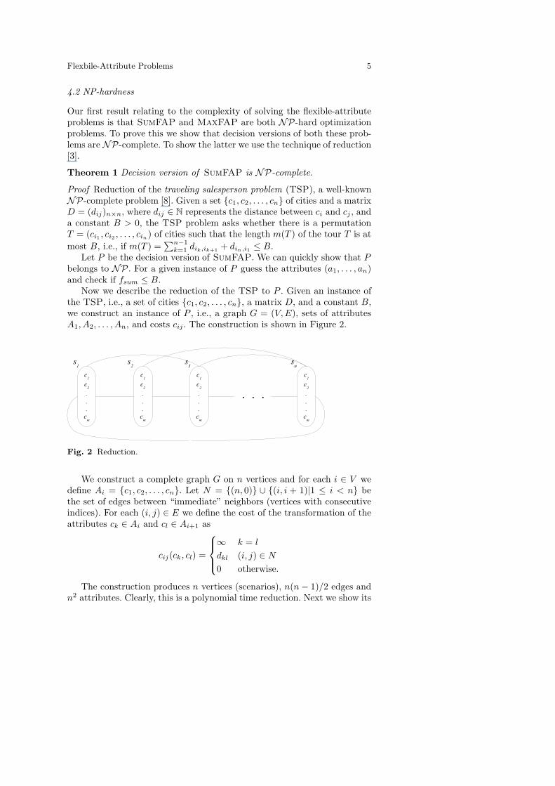
Now we describe the reduction of the TSP to P . Given an instance ofthe TSP, i.e., a set of cities {c1, c2, . . . , cn}, a matrix D, and a constant B,we construct an instance of P , i.e., a graph G = (V, E), sets of attributesA1, A2, . . . , An, and costs cij . The construction is shown in Figure 2.

Fig. 2 Reduction.

We construct a complete graph G on n vertices and for each i ∈ V wedefine Ai = {c1, c2, . . . , cn}. Let N = {(n, 0)} ∪ {(i, i + 1)|1 ≤ i < n} bethe set of edges between “immediate” neighbors (vertices with consecutiveindices). For each (i, j) ∈ E we define the cost of the transformation of theattributes ck ∈ Ai and cl ∈ Ai+1 as

cij(ck, cl) =

∞ k = l

dkl (i, j) ∈ N

0 otherwise.

The construction produces n vertices (scenarios), n(n − 1)/2 edges andn2 attributes. Clearly, this is a polynomial time reduction. Next we show its

6 Jurij Mihelic, Borut Robic

correctness by proving that for each instance of the TSP there is a solutionT = (cl1 , cl2 , . . . , cln) with cost z if and only if T is the solution with thecost z for the corresponding instance of P .

(⇒) Let T = (cl1 , cl2 , . . . , cln) be a solution of an instance of the TSP

with the cost z. Since T is a permutation, we have li 6= lj for all 1 ≤ i, j ≤ n.Thus,

∑

(i,j)∈E/N cij(cli,lj ) = 0 and hence

fsum(T ) =∑

(i,j)∈E

cij(cli , clj ) =

=∑

(i,j)∈N

cij(cli , clj ) =

=∑

(i,j)∈N

dli,lj =

=

n−1∑

k=1

dlk,lk+1+ dln,l1 =

= m(T ).

(⇐) Let T = (cl1 , cl2 , . . . , cln) be a solution for P with the cost z 6= ∞.Because z 6= ∞ we have cij(cli , clj ) 6= ∞ for all (i, j) ∈ E, and consequentlyli 6= lj . Thus, T is a permutation. We deduce that fsum(T ) = m(T ) in asimilar fashion as in the (⇒) part.

Recall that the optimization problem is NP-hard if its decision versionis NP-complete [3]. Thus, we have the following corollary.

Corollary 2 SumFAP is an NP-hard optimization problem.

Let us now turn to the MaxFAP problem and prove the following the-orem.

Theorem 3 Decision version of MaxFAP is NP-complete.

Proof Reduction of the Hamiltonian cycle problem (HCP). Given a graphH = (U, F ), is there a cycle T = (ui1 , ui2 , . . . , uin

) of vertices such that eachvertex is in T exactly once? Let P denote the decision version of MaxFAP.It is clear that P ∈ NP , so we describe the reduction of the HCP to P .

Given an instance H = (U, F ) of the HCP, we construct a completegraph G = (V, E) with |V | = |U | = n vertices and define sets of attributesA1, A2, . . . , An as Ai = {u1, u2, . . . , un} for each i ∈ V . In addition, wedefine, for each (i, j) ∈ E, the cost of the transformation of the attributesuk ∈ Ai and ul ∈ Ai+1 as

cij(uk, ul) =

0 (i, j) ∈ N, (uk, ul) ∈ F

∞ (i, j) ∈ N, (uk, ul) /∈ F

∞ (i, j) /∈ N, k = l

0 (i, j) /∈ N, k 6= l

Flexbile-Attribute Problems 7

where N = {(n, 0)} ∪ {(i, i + 1)|1 ≤ i < n}. This is clearly a polynomialreduction.

Now we show that for each instance of the HCP there is a solutionT = (ul1 , cu2

, . . . , cun) if and only if T is the solution with cost 0 of the

corresponding instance of P .(⇒) Let T = (ul1 , ul2 , . . . , uln) be a solution of the HCP. We compute

fmax on T , i.e.,

fmax(T ) = max(i.j)∈E

cij(uli , ulj ) =

= max[ max(i,j)∈E/N

cij(uli , ulj ), max(i,j)∈N

cij(uli , ulj )].

Since T is a permutation, we have li 6= lj for all (i, j) ∈ E/N . Thus, the firstmax(i,j)∈E/N cij(uli , ulj ) = 0. Since T is a cycle, we have (uli , ulj) ∈ F forall (i, j) ∈ N . Consequently, the second term is zero, too. Hence, fmax = 0.

(⇐) Let T = (ul1 , ul2 , . . . , uln) be a solution of P with cost 0. Sincefmax = 0, for all (i, j) ∈ E and for all uli and ulj holds, either (i, j) ∈ Nand (uli , ulj) ∈ F (meaning that T is a cycle), or either (i, j) /∈ N and li 6= lj(meaning that T visits every vertex in U exactly once). Consequently, T isa Hamiltonian cycle in H .

Corollary 4 MaxFAP is an NP-hard optimization problem.

4.3 Approximability

We have just shown that both SumFAP and MaxFAP are NP-hard op-timization problems. Searching for approximation algorithms is, therefore,a reasonable approach [3]. The following theorem is not surprising, and weomit the proof because of its simplicity (by contradiction).

Theorem 5 There are no polynomial absolute approximation algorithms for

SumFAP and MaxFAP, unless P=NP.

A more interesting fact is that both problems are non-approximable, i.e.,using the gap-technique [3] we prove the following theorem, which statesthat there are no polynomial approximation algorithms having a constantapproximation factor for SumFAP and MaxFAP.

Theorem 6 SumFAP/∈ APX and MaxFAP/∈ APX.

Proof By contradiction. In the proof of Theorem 3 replace the function ofthe attribute transformation cost with the following

cij(uk, ul) =

1 (i, j) ∈ N, (uk, ul) ∈ F

M (i, j) ∈ N, (uk, ul) /∈ F

M (i, j) /∈ N, k = l

1 (i, j) /∈ N, k 6= l

8 Jurij Mihelic, Borut Robic

Let x be an instance of HCP and x′ the corresponding instance of Max-

FAP. Let A be the (M − ǫ)-approximation algorithm for MaxFAP, whereǫ > 0. If x has a Hamiltonian cycle then the algorithm A must return theoptimal solution with the cost 1 on x′. Otherwise, if x has no Hamiltoniancycle then the optimal solution on x′ has the cost M . Thus, it is possible tosolve HCP to optimality with A. This is not possible unless P=NP.

The proof for SumFAP is similar and is, therefore, omitted.

4.4 Some additional properties

In this subsection we state a few additional properties of the two FAP prob-lems. Let S be a solution of an instance of SumFAP respectively MaxFAP.It is easy to prove the following theorem.

Theorem 7 fmax(S) ≤ fsum(S) ≤ |E|fmax(S).

Let S∗sum be an optimal solution for an instance of SumFAP and S∗

max

be an optimal solution for the same instance of MaxFAP.

Corollary 8 fmax(S∗max) ≤ fmax(S∗

sum) ≤ fsum(S∗sum) ≤ fsum(S∗

max) ≤|E|fmax(S∗

max).

Corollary 9 If A is an r-approximation algorithm for SumFAP, then Ais an r|E|-approximation algorithm for MaxFAP.

Proof Denote with x an instance of SumFAP resp. MaxFAP. Let A(x)be a solution returned by A on x. As by assumption A is an r-approxi-mation algorithm, we have fsum(S∗

sum) ≤ fsum(A(x)) ≤ rfsum(S∗sum), and

consequently fmax(S∗max) ≤ fmax(A(x)) ≤ fsum(A(x)) ≤ rfsum(S∗

sum) ≤r|E|fmax(S∗

max).

5 Algorithms on trees

Since both SumFAP and MaxFAP are NP-hard, it is very unlikely thatthey can be solved to optimality in polynomial time, unless P=NP . Inaddition, we have just presented some negative results relating to theirapproximability. In this situation it is, therefore, reasonable to search forsimplifications of the two problems that enable the construction of efficientalgorithms. In the following we describe algorithms for solving SumFAP

and MaxFAP to optimality where the input graph G is a tree. For thesimplicity of the description of the algorithms let s1 be a root in G and letus increasingly number the remaining scenarios with breadth-first search,as shown in Figure 3.

Both algorithms are based on dynamic programming [6]. The heart of thealgorithms is the assignment of the appropriate weights to the attributes.The algorithms consist of two parts. The first part is the initialization, where

Flexbile-Attribute Problems 9

Fig. 3 Example of a tree for flexible-attribute problems.

the weights of all the attributes belonging to leaf scenarios (vertices) are setto zero. The second part is the iterative processing of all the remainingscenarios. During each step of the processing the weights of the attributesbelonging to one scenario are computed. The difference between the algo-rithms SumFAP and MaxFAP is in the way the weights are calculated.

Denote with w(aik) the weight of the attribute aik ∈ Ai. Let A ={(i, j) ∈ E ∧ i < j}. Imagine A being arcs in the direction from the roots1 to the leaves of G. Denote with AlgSumFAP the polynomial algorithm forsolving SumFAP to optimality on a tree. The weight w(aik) of the attributeaik ∈ Ai is, in AlgSumFAP, calculated according to the following formula

w(aik) =∑

(i,j)∈A

minajl∈Aj

[cij(aik, ajl) + w(ajl)]. (1)

Denote by AlgMaxFAP polynomial algorithm for solving MaxFAP tooptimality on a tree. The calculation of weight w(aik) of the attribute aik ∈Ai is in AlgMaxFAP done according to the formula

w(aik) = max(i,j)∈A

minajl∈Aj

max[cij(aik, ajl), w(ajl)]. (2)

The algorithms AlgSumFAP and AlgMaxFAP are shown in Figure 4.

The initialization is from line 1 to line 5. First (line 1), the variable L isassigned to the set of leaf vertices. Then (lines 2 to 4), the weight of eachattribute of any leaf scenario is set to 0. The processed scenarios are storedin the variable W . Since all the leaf scenarios are already processed, W isinitialized to L (line 5).

The main loop of the algorithm is from line 6 to line 11. The loop isexecuted until all the scenarios are processed (line 6). In line 7, a scenarioi is selected such that it is not yet processed and that all its output arcslead to already-processed scenarios. In lines 8 and 9, the weights of the at-tributes aik ∈ Ai belonging to the selected scenario i are calculated. Theweight w(aik) of the attribute aik is calculated (line 9) according to formula1 or 2 for the algorithms AlgSumFAP or AlgMaxFAP, respectively. After the

10 Jurij Mihelic, Borut Robic

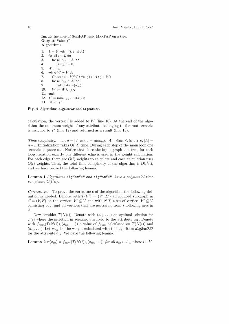
Input: Instance of SumFAP resp. MaxFAP on a tree.Output: Value f∗.Algorithm:

1. L = {i|¬∃j : (i, j) ∈ A};2. for all i ∈ L do

3. for all aik ∈ Ai do

4. w(aik) := 0;5. W := L;

6. while W 6= V do

7. Choose i ∈ V/W : ∀(i, j) ∈ A : j ∈ W ;

8. for all aik ∈ Ai do

9. Calculate w(aik);10. W := W ∪ {i};11. end;

12. f∗ = mina1k∈Aiw(a1k);

13. return f∗.

Fig. 4 Algorithms AlgSumFAP and AlgMaxFAP.

calculation, the vertex i is added to W (line 10). At the end of the algo-rithm the minimum weight of any attribute belonging to the root scenariois assigned to f∗ (line 12) and returned as a result (line 13).

Time complexity. Let n = |V | and l = maxi∈V |Ai|. Since G is a tree, |E| =n−1. Initialization takes O(nl) time. During each step of the main loop onescenario is processed. Notice that since the input graph is a tree, for eachloop iteration exactly one different edge is used in the weight calculation.For each edge there are O(l) weights to calculate and each calculation usesO(l) weights. Thus, the total time complexity of the algorithm is O(l2n),and we have proved the following lemma.

Lemma 1 Algorithms AlgSumFAP and AlgMaxFAP have a polynomial time

complexity O(l2n).

Correctness. To prove the correctness of the algorithm the following def-inition is needed. Denote with T (V ′) = (V ′, E′) an induced subgraph inG = (V, E) on the vertices V ′ ⊆ V and with N(i) a set of vertices V ′ ⊆ Vconsisting of i, and all vertices that are accessible from i following arcs inA.

Now consider T (N(i)). Denote with (aik, . . . ) an optimal solution forT (i) where the selection in scenario i is fixed to the attribute aik. Denotewith fsum(T (N(i)), (aik, . . . )) a value of fsum calculated on T (N(i)) and(aik, . . . ). Let waik

be the weight calculated with the algorithm AlgSumFAP

for the attribute aik. We have the following lemma.

Lemma 2 w(aik) = fsum(T (N(i)), (aik, . . . )) for all aik ∈ Ai, where i ∈ V .

Flexbile-Attribute Problems 11

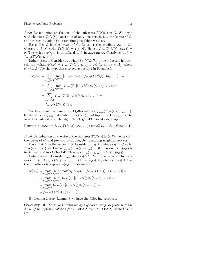
Proof By induction on the size of the sub-trees T (N(i)) in G. We beginwith the trees T (N(i)) consisting of only one vertex, i.e., the leaves of G,and proceed by adding the remaining neighbor vertices.

Basis. Let L be the leaves of G. Consider the attribute aik ∈ Ai,where i ∈ L. Clearly, T (N(i)) = ({i}, ∅). Hence, fsum(T (N(i)), (aik)) =0. The weight w(aik) is initialized to 0 in AlgSumFAP. Clearly, w(aik) =fsum(T (N(i)), (aik)).

Inductive step. Consider aik, where i ∈ V/L. With the induction hypoth-esis the weight w(ajl) = fsum(T (N(j)), (ajl, . . . )) for all ajl ∈ Aj , where(i, j) ∈ A. Use the hypothesis to replace w(ajl) in Formula 1.

w(aik) =∑

(i,j)∈A

minajl∈Aj

[cij(aik, ajl) + fsum(T (N(j)), (ajl, . . . ))] =

=∑

(i,j)∈A

minajl∈Aj

fsum(T ({i} ∪ N(j)), (aik, ajl, . . . )) =

=∑

(i,j)∈A

fsum(T ({i} ∪ N(j)), (aik, . . . )) =

= fsum(T (N(i)), (aik, . . . ))

We have a similar lemma for AlgMaxFAP. Let fmax(T (N(i)), (aik, . . . ))be the value of fmax calculated for T (N(i)) and (aik, . . . ). Let waik

be theweight calculated with the algorithm AlgMaxFAP for attribute aik.

Lemma 3 w(aik) = fmax(T (N(i)), (aik, . . . )) for all aik ∈ Ai, where i ∈ V .

Proof By induction on the size of the sub-trees T (N(i)) in G. We begin withthe leaves of G, and proceed by adding the remaining neighbor vertices.

Basis. Let L be the leaves of G. Consider aik ∈ Ai, where i ∈ L. Clearly,T (N(i)) = ({i}, ∅). Hence, fsum(T (N(i)), (aik)) = 0. The weight w(aik) isinitialized to 0 in AlgSumFAP. Clearly, w(aik) = fsum(T (N(i)), (aik)).

Inductive step. Consider aik, where i ∈ V/L. With the induction hypoth-esis w(ajl) = fsum(T (N(j)), (ajl, . . . )) for all ajl ∈ Aj , where (i, j) ∈ A. Usethe hypothesis to replace w(ajl) in Formula 2.

w(aik) = max(i,j)∈A

minajl∈Aj

max[cij(aik, ajl), fmax(T (N(j)), (ajl, . . . ))] =

= max(i,j)∈A

minajl∈Aj

fmax(T ({i} ∪ N(j)), (aik, ajl, . . . )) =

= max(i,j)∈A

fmax(T ({i} ∪ N(j)), (aik, . . . )) =

= fmax(T (N(i)), (aik, . . . ))

By Lemma 2 resp. Lemma 3 we have the following corollary.

Corollary 10 The value f∗ returned by AlgSumFAP resp. AlgMaxFAP is the

value of the optimal solution for SumFAP resp. MaxFAP, where G is a

tree.

12 Jurij Mihelic, Borut Robic

Proof For all a1k ∈ A1, where i ∈ V is the root vertex in G, the weightw(a1k) is the value of the optimal solution if the selection in s1 is fixed toa1k. Since f∗ = mina1k∈Ai

w(a1k), f∗ is optimal.

From Lemma 1 and Corollary 10 we have the following theorem.

Theorem 11 AlgSumFAP resp. AlgMaxFAP is a polynomial time algorithm

for optimally solving SumFAP resp. MaxFAP on a tree.

6 Applicability and generalizations

In previous sections we considered scenarios that are simple, i.e., each sce-nario is a set of attributes. There are many practical cases where such adescription is appropriate. Such situations often arise when the attributesrepresent real-world objects that are, in a way, independent. For example, ineconomics or game theory, where one models strategic interactions amongeconomic agents, attributes may represent actions that could be taken bya decision maker in an economic situation (scenario). The number of suchactions, which are considered in practical situations, must be manageable.Therefore, the set describing the scenario consists of a moderate number ofattributes.

Another example where a flexible-attribute framework can be straight-forwardly applied is when resolving lexical ambiguities in natural-languagetranslation [4,7]. For each word in the sentence a set of its alternative trans-lations is found. However, not all combinations of translations form a properinterpretation. To select the preferred interpretation a statistical model ofthe target language is used. To do this one might represent words with sce-narios, translations with attributes, and the cost of transforming attributeswith the statistical matching of the two translations. Additionally, a scenariograph might depend on the syntactic structure of the original sentence.

There are, however, practical cases where scenarios are more appropri-ately described by complex structures, such as graphs, matrices etc., de-pending on the optimization problem with input uncertainty.

One approach to dealing with such cases is that attributes representpossibly complex solutions of the instance of the optimization problem (sce-nario). For example, when solving the flexible 1-center problem one mustenumerate, for each scenario, all the optimal solutions of the 1-center prob-lem. The number of these is polynomial in the size of the problem instance.However, there are problems where enumerating all the solutions leads to anexponential explosion in the number of attributes. This can be mitigated bygenerating a subset of feasible solutions whose size depends on the availabletime for computation. If possible, the solutions should be generated in orderof decreasing quality.

Another approach is to consider a generalization of the two FAPs whenseveral attributes have to be selected in each scenario. Although the total

Flexbile-Attribute Problems 13

cost of transforming the solutions may seem to be difficult to calculate, itis tractable by solving the minimum assignment problem [11].

Yet another approach in cases where scenarios are described by com-plex structures is that each attribute is only a component of a solutionof the problem instance. Hence, the attributes must be selected in such away that they together represent the solution. For example, for the flexible

minimum spanning tree problem, each attribute is an edge of the network.Thus, when selecting attributes (edges) one must be careful (1) to selectthose that constitute a minimum spanning tree, while (2) minimizing thecost of transforming the tree to another one. Hence, in this approach anexponential explosion in the number of attributes is avoided at the cost ofa more complex attribute selection.

A similar example is to introduce flexibility to the k-center problem,which is known to be NP-hard. Each attribute is a vertex of a network.Given a network instance, a feasible solution is any selection of k attributes.Clearly, one might consider such selections that form good (possibly 2-approximate) solutions.

In many cases it is easy to show the NP-hardness of flexible versionsof optimization problems. For example, one can straightforwardly reducethe flexible minimum spanning tree or the flexible 1-center problem to cor-responding FAP. Notice that the original, i.e., non-flexible, problems arenot NP-hard. We have observed, however, that many other optimizationproblems, though polynomially solvable, become NP-hard when a flexibilityrequirement is added. An interesting problem would be to find out whetherthis holds for every problem in P , i.e., if the flexibility requirement is hardper se.

7 Conclusions

In this article we proposed a new approach, called the flexibility approach,for dealing with uncertainty in optimization problems. To demonstrate theusefulness of the approach we presented a few applications and defined twooptimization problems, SumFAP and MaxFAP. We proved that both theseproblems are NP-hard. Additionally, we showed the non-approximability ofthe two problems. Since it is very unlikely that any exact polynomial timealgorithm for the problems will be found, we considered a simplification ofthe two problems where the input graph is a tree. For this case we describeda polynomial time algorithm for solving the problems to optimality.

Some questions about the problems SumFAP and MaxFAP are stillopen, such as (i) the solvability of the generalized problems where morethan one attribute must be selected in each scenario, (ii) the exploitation ofthe other models for the transformation cost, and (iii) the solvability of theproblems on various other input graphs, such as cycles, circulant graphs,grids, etc.

14 Jurij Mihelic, Borut Robic

Acknowledgements

The authors wish to thank the anonymous referees for their thorough re-views and feedback on an earlier version of this paper.

References

1. Igor Averbakh and Oded Berman. Algorithms for Robust 1-Center Problemon a Tree. European J. of Operational Research, 123:292-302, 2000.

2. Igor Averbakh and Oded Berman. Minimax Regret p-Center Location on aNetwork with Demand Uncertainty. Location Science, 5:247-254, 1997.

3. G. Ausiello and P. Crescenzi and G. Gambosi and V. Kann and A. Marchetti-Spaccamela and M. Protasi. Complexity and Approximation: Combinatorial

Optimization Problems and their Approximability Properties, Springer Verlag,1999.

4. Kathryn L. Baker and Alexander M. Franz and Pamela W. Jordan. Copingwith Ambiguity in Knowledge-Based Natural Language Analysis. Proceedings

of FLAIRS-94, 1994.5. Randeep Bhatia and Sudipto Guha and Samir Khuller and Yoram J. Suss-

mann. Facility Location with Dynamic Distance Functions. J. of Combinatorial

Optimization, 2:199-217, 1998.6. Thomas H. Cormen and Charles E. Leiserson and Ronald L. Rivest and Clifford

Stein. Introduction to Algorithms, MIT Press, 2nd ed., 2001.7. Ido Dagan and Alon Itai. Word Sense Disambiguation Using a Second Lan-

guage Monolingual Corpus. Computational Linguistics, 20 (4):563-596, 1994.8. Michael. R. Garey and David. S. Johnson. Computers and Intractability: A

Guide to the Theory of NP-Completeness, W. H. Freeman and Co., San Fran-cisco, 1979.

9. Dorit S. Hochbaum and Anu Pathria. Locating Centers in a DynamicallyChanging Network, and Related Problems. Location Science, 6:243-256, 1998.

10. P. Kouvelis and G. Yu. Robust Discrete Optimization and its Applications.

Kluwer Academic Publishers, Boston, 1997.11. Amine Mahjoub and Jurij Mihelic and Christophe Rapine and Borut Robic. k-

Center Problem with Uncertainty: Flexible Approach. International Workshop

on Discrete Optimization Methods in Production and Logistics, Omsk-Irkutsk,Russia, 2004.

12. Jurij Mihelic and Amine Mahjoub and Christophe Rapine and Borut Robic.Two-stage investment problems under uncertainty. (submitted).

13. Daniel Serra and Vladimir Marianov. The Location of Emergency Services inChanging Network: The Case of Barcelona. Seventh International Symposium

on Locational Decisions, Edmonton, Canada, 1996.14. Lawrence V. Snyder. Facility Location Under Uncertainty: A Review. Dept.

of Industrial and Systems Engineering, Lehigh University, 04T-015, 2004