arX

iv:c

s/07

0214

3v1

[cs.

DB

] 24

Feb

200

7

Attribute Value Reordering For Efficient HybridOLAP

Owen Kasera,∗

a Dept. of Computer Science and Applied StatisticsU. of New Brunswick, Saint John, NB Canada

Daniel Lemireb

bUniversité du Québec à MontréalMontréal, QC Canada

Abstract

The normalization of a data cube is the ordering of the attribute values. For large multi-dimensional arrays where dense and sparse chunks are storeddifferently, proper normal-ization can lead to improved storage efficiency. We show thatit is NP-hard to compute anoptimal normalization even for 1×3 chunks, although we find an exact algorithm for 1×2chunks. When dimensions are nearly statistically independent, we show that dimension-wise attribute frequency sorting is an optimal normalization and takes timeO(dnlog(n))for data cubes of sizend. When dimensions are not independent, we propose and evaluatea several heuristics. The hybrid OLAP (HOLAP) storage mechanism is already 19%–30%more efficient than ROLAP, but normalization can improve it further by 9%–13% for a totalgain of 29%–44% over ROLAP.

Key words: Data Cubes, Multidimensional Binary Arrays, MOLAP, Normalization,Chunking

1 Introduction

On-line Analytical Processing (OLAP) is a database acceleration technique usedfor deductive analysis [2]. The main objective of OLAP is to have constant-time ornear constant-time answers for many typical queries. For example, in a database

∗ Corresponding author.This is an expanded version of our earlier paper [1].

Preprint submitted to Elsevier Science 1 February 2008

Table 1Two tables representing the volume of sales for a given day bythe experience level of thesalesmen. Given that three cities only have experienced salesmen, some orderings (left)will lend themselves better to efficient storage (HOLAP) than others (right).

<1 yrs 1–2 yrs >2 yrs

Ottawa $732

Toronto $643

Montreal $450

Halifax $43 $54

Vancouver $76 $12

<1 yrs 1–2 yrs >2 yrs

Halifax $43 $54

Montreal $450

Ottawa $732

Vancouver $76 $12

Toronto $643

containing salesmen’s performance data, one may want to compute on-line theamount of sales done in Ontario for the last 10 days, including only salesmen whohave 2 or more years of experience. Using a relational database containing salesinformation, such a computation may be expensive. Using OLAP, however, thecomputation is typically done on-line. To achieve such acceleration one can createa cubeof data, a map from all attribute values to a given measure. Inthe exam-ple above, one could map tuples containing days, experienceof the salesmen, andlocations to the corresponding amount of sales.

We distinguish two types of OLAP engines: Relational OLAP (ROLAP) and Mul-tidimensional OLAP (MOLAP). In ROLAP, the data is itself stored in a relationaldatabase whereas with MOLAP, a large multidimensional array is built with thedata. In MOLAP, an important step in building a data cube is choosing anormal-ization, which is a mapping from attribute values to the integers used to index thearray. One difficulty with MOLAP is that the array is often sparse. For example,not all tuples (day, experience, location) would match sales. Because of this sparse-ness, ROLAP uses far less storage. Additionally, there are compression algorithmsto further decrease ROLAP storage requirements [3,4,5]. Onthe other hand, MO-LAP can be much faster, especially if subsets of the data cubeare dense [6]. Manyvendors such as Speedware, Hyperion, IBM, and Microsoft arethus using HybridOLAP (HOLAP), storing dense regions of the cube using MOLAP and storing therest using a ROLAP approach.

While various efficient heuristics exist to find dense sub-cubes in data cubes [7,8,9],the dense sub-cubes are normalization-dependent. A related problem with MOLAPor HOLAP is that the attribute values may not have a canonicalordering, so thatthe exact representation chosen for the cube is arbitrary. In the salesmen example,imagine that “location” can have the values “Ottawa,” “Toronto,” “Montreal,” “Hal-ifax,” and “Vancouver.” How do we order these cities: by population, by latitude, bylongitude, or alphabetically? Consider the example given in Table 1: it is obviousthat HOLAP performance will depend on the normalization of the data cube. Astorage-efficient normalization may lead to better query performance.

2

One may object that normalization only applies when attribute values are not regu-larly sampled numbers. One argument against normalizationof numerical attributevalues is that storing an index map from these values to the actual index in the cubeamounts to extra storage. This extra storage is not important. Indeed, consider a datacube withn attribute values per dimension andd dimensions: we say such a cube isregular or n-regular. The most naive way to store such a map is for each possibleattribute value to store a new index as an integer from 1 ton. Assuming that indicesare stored using logn bits, this means thatnlogn bits are required. However, array-based storage of a regular data cube usesΘ(nd) bits. In other words, unlessd = 1,normalization is not a noticeable burden and all dimensionscan be normalized.

Normalization may degrade performance if attribute valuesoften used together arestored in physically different areas thus requiring extra IO operations. When at-tribute values have hierarchies, it might even be desirableto restrict the possiblereorderings. However, in itself, changing the normalization does not degrade theperformance of a data cube, unlike many compression algorithms. While automati-cally finding the optimal normalization may be difficult whenfirst building the datacube, the system can run an optimization routine after the data cube has been built,possibly as a background task.

1.1 Contributions and Organization

The contributions of this paper include a detailed look at the mathematical founda-tions of normalization, including notation for the remainder of the paper and futurework on normalization of block-coded data cubes (Sections 2and 3). In particu-lar, Section 3 includes a theorem showing that determining whether two data cubesare equivalent for the normalization problem is GRAPH ISOMORPHISM-complete.Section 4 considers the computational complexity of normalization. If data cubesare stored in tiny (size-2) blocks, an exact algorithm can compute the best normal-ization, whereas for larger blocks, it is conjectured that the problem is NP-hard.As evidence, we show that the case of size-3 blocks is NP-hard. Establishing thateven trivial cases are NP-hard helps justify use of heuristics. Moreover, the optimalalgorithm used for tiny blocks leads us to the Iterated Matching (IM) heuristic pre-sented later. An important class of “slice-sorting” normalizations is investigated inSection 5. Using a notion of statistical independence, a major contribution (The-orem 18) is an easily computed approximation bound for a heuristic called “Fre-quency Sort,” which we show to be the best choice among our heuristics when thecube dimensions are nearly statistically independent. Section 6 discusses additionalheuristics that could be used when the dimensions of the cubeare not sufficientlyindependent. In Section 7, experimental results compare the performance of heuris-tics on a variety of synthetic and “real-world” data sets. The paper concludes withSection 8. A glossary is provided at the end of the paper.

3

2 Block-Coded Data Cubes

In what follows,d is the number of dimensions (or attributes) of the data cubeCandni , for 1≤ i ≤ d, is the number of attribute values for dimensioni. Thus,C hassizen1× . . .×nd. To be precise, we distinguish between thecellsand theindicesof a data cube. “Cell” is a logical concept and each cell corresponds uniquely to acombination of values(v1,v2, . . . ,vd), with one valuevi for each attributei. In Ta-ble 1, one of the 15 cells corresponds to (Montreal, 1–2 yrs).Allocatedcells, such as(Vancouver, 1–2 yrs), store measure values, in contrast to unallocated cells such as(Montreal, 1–2 yrs). From now on, we shall assume that some initial normalizationhas been applied to the cube and that attributei’s values are{1,2, . . .ni}. “Index”is a physical concept and eachd-tuple of indices specifies a storage location withina cube. At this location there is a cell, allocated or otherwise.(Re-) normalizationchanges neither the cells nor the indices of the cube; (Re-)normalization changesthe assignment of cells to indices.

We use #C to denote the number of allocated cells in cubeC. Furthermore, we saythatC hasdensityρ = #C

n1×...×nd. While we can optimize storage requirements and

speed up queries by providing approximate answers [10,11,12], we focus on exactmethods in this paper, and so we seek an efficient storage mechanism to store all#C allocated cells.

There are many ways to store data cubes using different coding for dense regionsthan for sparse ones. For example, in one paper [9] a single dense sub-cube (chunk)with d dimensions is found and the remainder is considered sparse.

We follow earlier work [2,13] and store the data cube inblocks1 , which are disjointd-dimensional sub-cubes covering the entire data cube. We consider blocks of con-stant sizem1× . . .×md; thus, there are⌈ n1

m1⌉× . . .×⌈ nd

md⌉ blocks. For simplicity,

we usually assume thatmk dividesnk for all k ∈ {1, . . . ,d}. Each block can thenbe stored in an optimized way depending, for example, on its density. We consideronly two widely used coding schemes for data cubes, corresponding respectivelyto simple ROLAP and simple MOLAP. That is, either we represent the block as alist of tuples, one for each allocated cell in the block, or else we code the block asan array. For both extreme cases, a very dense or a very sparseblock, MOLAP andROLAP are respectivelyefficient. More aggressive compression is possible [14],but as long as we use block-based storage, normalization is afactor.

Assuming that a data cube is stored using block encoding, we need to estimate thestorage cost. A simplistic model is given as follows. The cost of storing a single cellsparsely, as a tuple containing the position of the value in the block asd attributevalues (cost proportional tod) and the measure value itself (cost of 1), is assumedto be 1+ αd, where parameterα can be adjusted to account for size differences

1 Many authors use the term “chunks” with different meanings.

4

between measure values and attribute values. Settingα small would favor sparseencoding (ROLAP) whereas settingα large would favor dense encoding (MOLAP).For example, while we might store 32-bit measure values, thenumber of valuesper attribute in a given block is likely less than 216. This motivates settingα =1/2 in later experiments and the remainder of the section. Thus, densely storing ablock with D allocated cells costsM = m1× . . .×md, but storing it sparsely costs(d/2+1)D.

It is more economical to store a block densely if(d/2+ 1)D > M, that is, ifD

m1×...×md> 1

d/2+1. This block coding is least efficient when a data cube has uni-form densityρ over all blocks. In such cases, it has a sparse storage cost ofd/2+1per allocated cell ifρ ≤ 1

d/2+1 or a dense storage cost of 1/ρ per allocated cell

if ρ > 1d/2+1. Given a data cubeC, H(C) denotes its storage cost. We have #C≤

H(C) ≤ n1× . . .×nd. Thus, we measure the cost per allocated cellE(C) as H(C)#C

with the convention that if #C = 0, thenE(C) = 1. The cost per allocated cellis bounded by 1 andd/2+ 1: 1≤ E(C) ≤ d/2+ 1. A weakness of the model isthat it ignores obvious storage overheads proportional to the number of blocks,n1m1× . . .× nd

md. However, as long as the number of blocks remains constant, it is rea-

sonable to assume that the overhead is constant. Such is the case when we considerthe same data cube under different normalizations using fixed block dimensions.

3 Mathematical Preliminaries

Now that we have defined a simple HOLAP model, we review two of the most im-portant concepts in this paper: slices and normalizations.Whereas a slice amountsto fixing one of the attributes, a normalization can be viewedas a tuple of permu-tations.

3.1 Slices

Consider ann-regulard-dimensional cubeC and letCi1,...,id denote the cell storedat indices(i1, . . . , id)∈ {1, . . . ,n}d. Thus,C has sizend. Theslice Cj

v of C, for indexv of dimensionj (1≤ j ≤ d and 1≤ v≤ n) is ad−1 - dimensional cube formed asC j

vi1,...,i j−1,i j+1,...,id = Ci1,...,i j−1,v,i j+1,...,id (See Figure 1).

For the normalization task, we simply need know which indices contain allocatedcells. Hence we often view a slice as ad− 1 - dimensional Boolean arrayC j

v.For example, in Figure 1, we might write (linearly)C1

3 = [0,1,0,5,9,2,4,0,0] and

C13 = [0,1,0,1,1,1,1,0,0], if we represent non-allocated cells by zeros. Let #C j

v

denote the number of allocated cells in sliceC jv.

5

1

2

dimension 1di

men

sion

21 2 3 1

2

31

5

6

2

3 3 1 4

2 7

1

9

dimensio

n 3

Fig. 1. A 3×3×3 cubeC with the sliceC13 shaded.

3.2 Normalizations and Permutations

Given a list ofn items, there aren! distinct possible permutations notedΓn (theSymmetry Group). If γ ∈ Γn permutesi to j, we writeγ(i) = j. The identity per-mutation is denotedι. In contrast to previous work on database compression (e.g.,[4]), with our HOLAP model there is no performance advantagefrom permutingthe order of the dimensions themselves. (Blocking treats all dimensions symmet-rically.) Instead, we focus on normalizations, which affect the order of each at-tribute’s values. A normalizationπ of a data cubeC is a d-tuple (γ1, . . . ,γd) ofpermutations whereγi ∈ Γn for i = 1, . . . ,d, and the normalized data cubeπ(C)

is π(C)i1,...,id = Cγ1(i1),...,γd(id) for all (i1, . . . , id) ∈ {1, . . . ,n}d. Recall that permuta-tions, and thus normalizations, are not commutative. However, normalizations arealways invertible, and there are(n!)d normalizations for ann-regular data cube.The identity normalization is denotedI = (ι, . . . , ι); whetherI denotes the identitynormalization or the identity matrix will be clear from the context. Similarly 0 maydenote the zero matrix.

Given a data cubeC, we define its correspondingallocation cube Aas a cube withthe same dimensions, containing 0’s and 1’s depending on whether or not the cellis allocated. Two data cubesC andC′, and their corresponding allocation cubesAandA′, are equivalent (C∼C′) if there is a normalizationπ such thatπ(A) = A′.

The cardinality of an equivalence class is the number of distinct data cubesC in thisclass. The maximum cardinality is(n!)d and there are such equivalence classes:consider the equivalence class generated by a “triangular”data cubeCi1,...,id = 1 ifi1≤ i2≤ . . .≤ id and 0 otherwise. Indeed, suppose thatCγ1(i1),...,γd(id) =Cγ′1(i1),...,γ

′d(id)

for all i1, . . . , id, thenγ1(i1)≤ γ2(i2)≤ . . .≤ γd(id) if and only if γ′1(i1)≤ γ′2(i2)≤. . . ≤ γ′d(id) which implies thatγi = γ′i for i ∈ {1, . . . ,d}. To see this, consider the2-d case whereγ1(i1) ≤ γ2(i2) if and only if γ′1(i1) ≤ γ′2(i2). In this case the resultfollows from the following technical proposition. For morethan two dimensions,the proposition can be applied to anypair of dimensions.

6

Proposition 1 Consider anyγ1,γ2,γ′1,γ′2 ∈ Γn satisfyingγ1(i) ≤ γ2( j)⇔ γ′1(i) ≤

γ′2( j) for all 1≤ i, j ≤ n. Thenγ1 = γ′1 andγ2 = γ′2.

PROOF. Fix i, then letk be the number ofj values such thatγ2( j)≥ γ1(i). We havethatγ1(i) = n−k+1 because it is the only element of{1, . . . ,n} having exactlykvalues larger or equal to it. Becauseγ1(i)≤ γ2( j)⇔ γ′1(i)≤ γ′2( j), γ′1(i) = n−k+1and henceγ′1 = γ1. Similarly, fix j and counti values to prove thatγ′2 = γ2. 2

However, there are singleton equivalence classes, since some cubes are invariantunder normalization: consider a null data cubeCi1,...,id = 0 for all (i1, . . . , id) ∈{1, . . . ,n}d.

To count the cardinality of a class of data cubes, it suffices to know how manyslicesC j

v of data cubeC are identical, so that we can take into account the invari-ance under permutations. Considering alln slices in dimensionr, we can count thenumber of distinct slicesdr and number of copiesnr,1, . . . ,nr,dr of each. Then, thenumber of distinct permutations in dimensionr is n!

nr,1!×...,×nr,dr ! and the cardinality

of a given equivalence class is∏dr=1

(n!

nr,1!×...,×nr,dr !

). For example, the equivalence

class generated byC =

0 1

0 1

has a cardinality of 2, despite having 4 possible

normalizations.

To study the computational complexity of determining cube similarity, we definetwo decision problems. The problem CUBE SIMILARITY hasC andC′ as inputand asks whetherC ∼ C′. Problem CUBE SIMILARITY (2-D) restrictsC andC′

to two-dimensional cubes. Intuitively, CUBE SIMILARITY asks whether two datacubes offer the same problem from a normalization-efficiency viewpoint. The nexttheorem concerns the computational complexity of CUBE SIMILARITY (2-D), butwe need the following lemma first. Recall that(γ1,γ2) is the normalization with thepermutationγ1 along dimension 1 andγ2 along dimension 2 whereas(γ1,γ2)(I) isthe renormalized cube.

Lemma 2 Consider the n×n matrix I′ = (γ1,γ2)(I). Then I′ = I ⇐⇒ γ1 = γ2.

We can now state Theorem 3, which shows that determining cubesimilarity isGRAPH ISOMORPHISM-complete [15]. A problemΠ belongs to this complexityclass when both

• Π has a polynomial-time reduction to GRAPH ISOMORPHISM, and• GRAPH ISOMORPHISMhas a polynomial-time reduction toΠ.

GRAPH ISOMORPHISM-complete problems are unlikely to be NP-complete [16],

7

yet there is no known polynomial-time algorithm for any problem in the class. Thiscomplexity class has been extensively studied.

Theorem 3 CUBE SIMILARITY (2-D) is GRAPH ISOMORPHISM-complete.

PROOF. It is enough to consider two-dimensional allocation cubes as 0-1 matri-ces. The connection to graphs comes via adjacency matrices.

To show that CUBE SIMILARITY (2-D) is GRAPH ISOMORPHISM-complete, weshow two polynomial-time many-to-one reductions: the firsttransforms an instanceof GRAPH ISOMORPHISMto an instance of CUBE SIMILARITY (2-D).

The second reduction transforms an instance of CUBE SIMILARITY (2-D) to aninstance of GRAPH ISOMORPHISM.

The graph-isomorphism problem is equivalent to are-normalizationproblem ofthe adjacency matrices. Indeed, consider two graphsG1 andG2 and their adjacencymatricesM1 andM2. The two graphs are isomorphic if and only if there is a permu-tationγ so that(γ,γ)(M1) = M2. We can assume without loss of generality that allrows and columns of the adjacency matrices have at least one non-zero value, sincewe can count and remove disconnected vertices in time proportional to the size ofthe graph.

We have to show that the problem of deciding whetherγ satisfies(γ,γ)(M1) = M2

can be rewritten as a data cube equivalence problem. It turnsout to be possible byextending the matricesM1 andM2. Let I be the identity matrix, and consider two

allocation cubes (matrices)A1 andA2 and their extensionsA1 =

A1 I I

I I 0

I 0 0

and

A2 =

A2 I I

I I 0

I 0 0

.

Consider a normalizationπ satisfyingπ(A1) = A2 for matricesA1,A2 having at leastone non-zero value for each column and each row. We claim thatsuch aπ must beof the formπ = (γ1,γ2) whereγ1 = γ2. By the number of non-zero values in eachrow and column, we see that rows cannot be permuted across thethree blocks ofrows because the first one has at least 3 allocated values, thesecond one exactly 2and the last one exactly 1. The same reasoning applies to columns. In other words,if x∈ [ j, jn], thenγi(x) ∈ [ j, jn] for j = 1,2,3 andi = 1,2.

Let γi | j denote the permutationγ restricted to blockj where j = 1,2,3. Define

8

γ ji = γi | j− jn for j = 1,2,3 andi = 1,2. By Lemma 2, each sub-block consisting

of an identity leads to an equality between two permutations. From the two identitymatrices in the top sub-blocks, for example, we have thatγ1

1 = γ22 andγ1

1 = γ32. From

the middle sub-blocks, we haveγ21 = γ1

2 and γ21 = γ2

2, and from the bottom sub-blocks, we haveγ3

1 = γ12. From this, we can deduce thatγ1

1 = γ22 = γ2

1 = γ12 so that

γ11 = γ1

2 and similarly,γ21 = γ2

2 andγ31 = γ3

2 so thatγ1 = γ2.

So, if we setA1 = M1 andA2 = M2, we have thatG1 andG2 are isomorphic if andonly if A1 is similar toA2. This completes the proof that if the extended adjacencymatrices are seen to be equivalent as allocation cubes, thenthe graphs are isomor-phic. Therefore, we have shown a polynomial-time transformation from GRAPH

ISOMORPHISMto CUBE SIMILARITY (2-D).

Next, we show a polynomial-time transformation from CUBE SIMILARITY (2-D)to GRAPH ISOMORPHISM. We reduce CUBE SIMILARITY (2-D) to DIRECTED

GRAPH ISOMORPHISM, which is in turn reducible to GRAPH ISOMORPHISM[17,18].

Given two 0-1 matricesM1 andM2, we want to decide whether we can find(γ1,γ2)such that(γ1,γ2)(M1) = M2. We can assume thatM1 andM2 are square matricesand if not, pad with as many rows or columns filled with zeros asneeded. Wewant a reduction from this problem to DIRECTED GRAPH ISOMORPHISM. Con-

sider the following matrices:M1 =

0 M1

0 0

and M2 =

0 M2

0 0

. BothM1 andM2

can be considered as the adjacency matrices of directed graphsG1 andG2. Supposethat the graphs are found to be isomorphic, then there is a permutationγ such that(γ,γ)(M1) = M2. We can assume without loss of generality thatγ does not permuterows or columns having only zeros across halves of the adjacency matrices. Onthe other hand, rows containing non-zero components cannotbe permuted acrosshalves. Thus, we can decomposeγ into two disjoint permutationsγ1 and γ2 andhence(γ1,γ2)(M1) = M2, which impliesM1∼M2. On the other hand, ifM1∼M2,then there is(γ1,γ2) such that(γ1,γ2)(M1) = M2 and we can chooseγ as the directsum ofγ1 andγ2. Therefore, we have found a reduction from CUBE SIMILARITY

(2-D) to DIRECTED GRAPH ISOMORPHISM and, by transitivity, to GRAPH ISO-MORPHISM.

Thus, GRAPH ISOMORPHISMand CUBE SIMILARITY (2-D) are mutually reducibleand hence CUBE SIMILARITY (2-D) is GRAPH ISOMORPHISM-complete. 2

Remark 4 If similarity between two n× n cubes can be decided in time cnk forsome positive integers c and k≥ 2, then graph isomorphism can be decided inO(nk) time.

Since GRAPH ISOMORPHISM has been reduced to a special case of CUBE SIMI -LARITY , then the general problem is at least as difficult as GRAPH ISOMORPHISM.

Yet we have seen no reason to believe the general problem is harder (for instance,NP-complete). We suspect that a stronger result may be possible; establishing (ordisproving) the following conjecture is left as an open problem.

Conjecture 5 The generalCUBE SIMILARITY problem is alsoGRAPH ISOMOR-PHISM-complete.

4 Computational Complexity of Optimal Normalization

It appears that it is computationally intractable to find a “best” normalizationπ (i.e.,π minimizes cost per allocated cellE(π(C))) given a cubeC and given the blocks’dimensions. Yet, when suitable restrictions are imposed, abest normalization canbe computed (or approximated) in polynomial time. This section focuses on theeffect of block size on intractability.

4.1 Tractable Special Cases

Our problem can be solved in polynomial time, if severe restrictions are placedon the number of dimensions or on block size. For instance, itis trivial to find abest normalization in 1-d. Another trivial case arises whenblocks are of size 1,since then normalization does not affect storage cost. Thus, any normalization isa “best normalization.” The situation is more interesting for blocks of size 2; i.e.,which havemi = 2 for some 1≤ i ≤ d andmj = 1 for 1≤ j ≤ d with i 6= j. A bestnormalization can be found in polynomial time, based on weighted-matching [19]techniques described next.

4.1.1 Using Weighted Matching

Given a weighted undirected graph, theweighted matching problemasks for anedge subset of maximum or minimum total weight, such that no two edges sharean endpoint. If the graph is complete, has an even number of vertices, and has onlypositive edge weights, then the maximum matching effectively pairs up vertices.

For our problem, normalization’s effect on dimensionk, for some 1≤ k≤ d, corre-sponds to rearranging the order of thenk slicesCk

v, where 1≤ v≤ nk. In our case,we are using a block size of 2 for dimensionk. Therefore, once we have chosen twoslicesCk

v andCkv′ to be the first pair of slices, we will have formed the first layer of

blocks and have stored all allocated cells belonging to these two slices. The totalstorage cost of the cube is thus a sum, over all pairs of slices, of the pairing-costof the two slices composing the pair. The order in which pairsare chosen is ir-relevant: only the actual matching of slices into pairs matters. Consider Boolean

10

vectorsb = Ckv andb′ = Ck

v′. If both bi andb′i are true, then theith block in the pairis completely full and costs 2 to store. Similarly, if exactly one ofbi andb′i is true,then the block is half-full. Under our model, a half-full block also costs 2, but anempty block costs 0. Thus, given any two slices, we can compute the cost of pairingthem by summing the storage costs of all these blocks. If we identify each slice witha vertex of a complete weighted graph, it is easy to form an instance of weightedmatching. (See Figure 2 for an example.) Fortunately, cubic-time algorithms existfor weighted matching [20], andnk is often small enough that cubic running timeis not excessive. Unfortunately, calculating thenk(nk− 1)/2 edge weights is ex-pensive; each involves two large Boolean vectors with1

nk∏d

i=1ni elements, for a

total edge-calculation time ofΘ(nk ∏d

i=1ni). Fortunately, this can be improved for

sparse cubes.

In the 2-d case, given any two rows, for exampler1 =[0 0 1 1

]andr2 =

[0 1 0 1

],

then we can compute the total allocation cost of grouping thetwo together as2(#r1+#r2−benefit) wherebenefitis the number of positions (in this case 1) whereboth r1 andr2 have allocated cells. (Thisbenefitrecords that one of the two allo-cated values could be stored “for free,” were slicesr1 andr2 paired.)

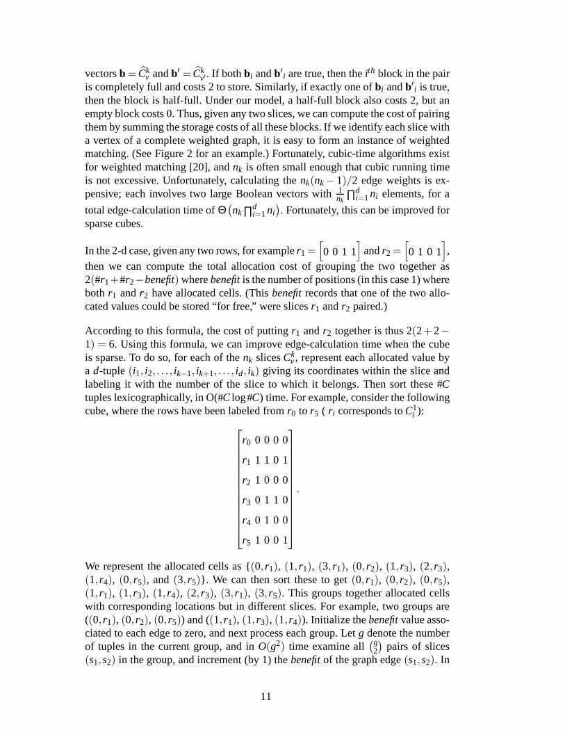
According to this formula, the cost of puttingr1 andr2 together is thus 2(2+2−1) = 6. Using this formula, we can improve edge-calculation timewhen the cubeis sparse. To do so, for each of thenk slicesCk

v, represent each allocated value bya d-tuple (i1, i2, . . . , ik−1, ik+1, . . . , id, ik) giving its coordinates within the slice andlabeling it with the number of the slice to which it belongs. Then sort these #Ctuples lexicographically, in O(#C log#C) time. For example, consider the followingcube, where the rows have been labeled fromr0 to r5 ( r i corresponds toC1

i ):

r0 0 0 0 0

r1 1 1 0 1

r2 1 0 0 0

r3 0 1 1 0

r4 0 1 0 0

r5 1 0 0 1

.

We represent the allocated cells as {(0, r1), (1, r1), (3, r1), (0, r2), (1, r3), (2, r3),(1, r4), (0, r5), and (3, r5)}. We can then sort these to get(0, r1), (0, r2), (0, r5),(1, r1), (1, r3), (1, r4), (2, r3), (3, r1), (3, r5). This groups together allocated cellswith corresponding locations but in different slices. For example, two groups are((0, r1), (0, r2), (0, r5)) and ((1, r1), (1, r3), (1, r4)). Initialize thebenefitvalue asso-ciated to each edge to zero, and next process each group. Letg denote the numberof tuples in the current group, and inO(g2) time examine all

(g2

)pairs of slices

(s1,s2) in the group, and increment (by 1) thebenefitof the graph edge(s1,s2). In

11

0

1

1

0

010

1

0

10

1A

B

C

D

A B

C D

4

4

6

6

6

4

Fig. 2. Mapping a normalization problem to a weighted matching problem on graphs. Rowsare labeled and we try to reorder them, given block dimensions 2×1 (where 2 is the verticaldimension). In this example, optimal solutions includer0, r1, r2, r3 andr2, r3, r1, r0.

our example, we would process the group ((0, r1), (0, r2), (0, r5)) and incrementthebenefits of edges (r1, r2), (r2, r5), and (r1, r5). For group ((1, r1), (1, r3), (1, r4)),we would increase thebenefits of edges (r1, r3), (r1, r4), and (r3, r4). Once all #Csorted tuples have been processed, the eventual weight assigned to edge(v,w) is2(#Ck

v +#Ckw−benefit(v,w)). In our example, we have that edge(r1, r2) has a ben-

efit of 1, and so a weight of 2(#r1+#r2−benefit) = 2(3+1−1) = 6.

A crude estimate of the running time to process the groups would be that eachgroup is O(nk) in size, and there are O(#C) groups, for a time of O(#Cn2

k). It canbe shown that time is maximized when the #C values are distributed into #C/nk

groups of sizenk, leading to a time bound ofΘ(#Cnk) for group processing, and anoverall edge-calculation time of #C(nk + log#C).

Theorem 6 The best normalization for blocks of size

i︷ ︸︸ ︷1× . . .×1×2×

k−1−i︷ ︸︸ ︷1. . .×1 can

be computed in O(nk× (n1×n2× . . .×nd)+n3k) time.

The improved edge-weight calculation (for sparse cubes) leads to the following.

Corollary 7 The best normalization for blocks of size

i︷ ︸︸ ︷1× . . .×1×2×

k−1−i︷ ︸︸ ︷1. . .×1 can

be computed in O(#C(nk + log#C)+n3k) time.

For more general block shapes, this algorithm is no longer optimal but neverthelessprovides a basis for sensible heuristics.

4.2 An NP-hard Case

In contrast to the 1× 2-block situation, we next show that it is NP-hard to findthe best normalization for 1× 3 blocks. The associated decision problem askswhether any normalization can store a given cube within a given storage bound,assuming 1×3 blocks. We return to the general cost model from Section 2 but

12

chooseα = 1/4, as this results in an especially simple situation where a block withthree allocated cells (D = 3) stores each of them at a cost of 1, whereas a blockwith fewer than three allocated cells stores each allocatedcell at a cost of 3/2.

The proof involves a reduction from the NP-complete problemExact 3-Cover (X3C),a problem which gives a setSand a setT of three-element subsets ofS. The ques-tion, for X3C, is whether there is aT ′ ⊆ T such that eachs∈ Soccurs in exactlyone member ofT ′ [17].

We sketch the reduction next. Given an instance of X3C, form an instance of ourproblem by making a|T |×|S| cube. Fors∈SandT ∈ T , the cube has an allocatedcell corresponding to(T,s) if and only if s∈ T. Thus, the cube has 3|T | cells that

need to be stored. The storage cost cannot be lower than9|T |−|S|2 and this bound

can be met if and only if the answer to the instance of X3C is “yes.” Indeed, anormalization for 1×3 blocks can be viewed as simply grouping the values of anattribute into triples. Suppose the storage bound is achieved, then at least|S| cellswould have to be stored in full blocks. Consider some full block and note there areonly 3 allocated cells in each row, so all 3 of them must be chosen (because blocksare 1×3). But the three allocated cells in a row can be mapped to aT ∈ T . Chooseit for T ′. None of these 3 cells’ columns intersect any other full blocks, becausethat would imply some other row had exactly the same allocation pattern and hencerepresents the sameT, which it cannot. So we see that eachs∈ S (column) mustintersect exactly one full block, showing thatT ′ is the cover we seek.

Conversely, supposeT ′ is a cover for X3C. Order the elements inT ′ arbitrarilyasT0,T1, . . . ,T|S|/3 and use any normalization that puts first (in arbitrary order) thethrees∈ T0, then next puts the threes∈ T1, and so forth. The three allocated cellsfor eachTi will be together in a (full) block, giving us at least the required “spacesavings” of3

2|T′|= |S|.

Theorem 8 It is NP-hard to find the best normalization when1×3 blocks are used.

We conjecture that it is NP-hard to find the best normalization whenever the blocksize is fixed at any size larger than 2. A related 2-d problem that is NP-hard wasdiscussed by Kaser [21]. Rather than specify the block dimensions, this problemallows the solution to specify how to divide each dimension into two ranges, thusmaking four blocks in total (of possibly different shape) .

5 Slice-Sorting Normalization for Quasi-Independent Attributes

In practice, whether or not a given cell is allocated may depend on the correspond-ing attribute values independently of each other. For example, if a store is closedon Saturdays almost all year, a slice corresponding to “weekday=Saturday” will be

13

sparse irrespective of the other attributes. In such cases,it is sufficient to normalizethe data cube using only an attribute-wise approach. Moreover, as we shall see, onecan easily compute the degree of independence of the attributes and thus decidewhether or not potentially more expensive algorithms need to be used.

We begin by examining one of the simplest classes of normalization algorithms,and we will assumen-regular data cubes forn ≥ 3. We say that a sequence ofvaluesx1, . . . ,xn is sorted in increasing (respectively, decreasing) order if xi ≤ xi+1

(respectively,xi ≥ xi+1) for i ∈ {1, . . . ,n−1}.

Recall thatC jv is the Boolean array indicating whether a cell is allocated or not in

sliceC jv.

Algorithm 1 (Slice-Sorting Normalization) Given an n-regular data cube C, thenslices have nd−1 cells. Given a fixed function g: {true, false}n

d−1→R, then for each

attribute j, we compute the sequence fjv = g(C j

v) for all attribute values v= 1, . . . ,n.Letγ j be a permutation such thatγ j( f j) is sorted either in increasing or decreasingorder, then a slice-sorting normalization is(γ1, . . . ,γd).

Algorithm 1 has time complexityO(dnd +dnlogn). We can precompute the aggre-gated valuesf j

v and speed up normalization toO(dnlog(n)). It does not produce aunique solution given a functiong because there could be many different valid waysto sort. A normalizationϖ = (γ1, . . . ,γd) is asolution to the slice-sorting problemifit provides a valid sort for the slice-sorting problem stated by Algorithm 1 . Givena data cubeC, denote the set of all solutions to the slice-sorting problem by SC,g.Two functionsg1 andg2 areequivalentwith respect to the slice-sorting problem ifSC,g1 = SC,g2 for all cubesC and we writeg1≃ g2 . We can characterize such equiv-alence classes using monotone functions. Recall that a function h : R→R is strictlymonotone nondecreasing (respectively, nonincreasing) ifx < y impliesh(x) < h(y)(respectively,h(x) > h(y)).

An alternative definition is thath is monotone if, wheneverx1, . . . ,xn is a sorted list,then so ish(x1), . . . ,h(xn). This second definition can be used to prove the existenceof a monotone function as the next proposition shows.

Proposition 9 For a fixed integer n≥ 3 and two functionsω1,ω2 : D→R whereDis a set with an order relation, if for all sequences x1, . . . ,xn∈D , ω1(x1), . . . ,ω1(xn)is sorted if and only ifω2(x1), . . . ,ω2(xn) is sorted, then there is a monotone func-tion h : R→ R such thatω1 = h◦ω2.

PROOF. The proof is constructive. Defineh over the image ofω2 by the formula

h(ω2(x)) = ω1(x).

To prove thath is well defined, we have to show that wheneverω2(x1) = ω2(x2)

14

thenω1(x1) = ω1(x2). Suppose that this is not the case, and without loss of general-ity, let ω1(x1) < ω1(x2). Then there isx3 ∈ D such thatω1(x1)≤ ω1(x3)≤ ω1(x2)or ω1(x3) ≤ ω1(x1) or ω1(x2) ≤ ω1(x3). In all three cases, because of the equal-ity betweenω2(x1) and ω2(x2), any ordering ofω2(x1),ω2(x2),ω2(x3) is sortedwhereas there is always one non-sorted sequence usingω1. There is a contradic-tion, proving thath is well defined.

For any sequencex1,x2,x3 such thatω2(x1) < ω2(x2) < ω2(x3), then we must eitherhaveω1(x1)≤ ω1(x2)≤ ω1(x3) or ω1(x1)≥ ω1(x2)≥ ω1(x3) by the conditions ofthe proposition. In other words, forx < y < z, we either haveh(x)≤ h(y)≤ h(z) orh(x)≥ h(y)≥ h(z) thus showing thath must be monotone.2

Proposition 10 Given two functions g1,g2 : {true, false}S→ R, we have that

SC,g1 = SC,g2

for all data cubes C if and only if there exist a monotone function h : R → R suchthat g1 = h◦g2.

PROOF. Assume there ish such thatg1 = h◦g2, and considerϖ = (γ1, . . . ,γd) ∈

SC,g1 for any data cubeC, thenγ j(g1(Cjv)) is sorted over indexv ∈ {1, . . . ,n} for

all attributes j = 1, . . . ,n by definition ofSC,g1. Thenγ j(h(g1(Cjv))) must also be

sorted overv for all j, since monotone functions preserve sorting. Thusϖ ∈ SC,g2.

One the other hand, ifSC,g1 = SC,g2 for all data cubesC, thenh exists by Proposi-tion 9. 2

A slice-sorting algorithm isstableif the normalization of a normalized cube can bechosen to be the identity, that is ifϖ ∈ SC,g thenI ∈ Sϖ(C),g for all C. The algorithmis strongly stableif for any normalizationϖ, Sϖ(C),g ◦ϖ = SC,g for all C. Strongstability means that the resulting normalization does not depend on the initial nor-malization. This is a desirable property because data cubesare often normalizedarbitrarily at construction time. Notice that strong stability implies stability: chooseϖ ∈ SC,g. Then there must existζ ∈ Sϖ(C),g such thatζ◦ϖ = ϖ which implies thatζ is the identity.

Proposition 11 Stability implies strong stability for slice-sorting algorithms andso, strong stability⇔ stability.

PROOF. Consider a slice-sorting algorithm, based ong, that is stable. Then bydefinition

ϖ ∈ SC,g⇒ I ∈ Sϖ(C),g (1)

15

for all C. Observe that the converse is true as well, that is,

I ∈ Sϖ(C),g⇒ ϖ ∈ SC,g. (2)

Hence we have thatϖ1 ◦ϖ ∈ SC,g implies thatI ∈ Sϖ1(ϖ(C)),g by Equation 1 andso, by Equation 2,ϖ1 ∈ Sϖ(C),g. Note that given anyϖ, all elements ofSC,g can bewritten asϖ1◦ϖ because permutations are invertible. Hence, givenϖ1 ◦ϖ ∈ SC,g

we haveϖ1 ∈ Sϖ(C),g and soSC,g⊂ Sϖ(C),g◦ϖ.

On the other hand, givenϖ1◦ϖ ∈ Sϖ(C),g◦ϖ, we have thatϖ1 ∈ Sϖ(C),g by cancel-lation, henceI ∈ Sϖ1(ϖ(C)),g by Equation 1, and thenϖ1◦ϖ ∈ SC,g by Equation 2.Therefore,Sϖ(C),g◦ϖ⊂ SC,g. 2

Defineτ : {true, false}S→R as the number oftruevalues in the argument. In effect,τ counts the number of allocated cells:τ(C j

v) = #C jv for any sliceC j

v. If the sliceC jv

is normalized,τ remains constant:τ(C jv) = τ

(ϖ

(C j

v

))for all normalizationsϖ.

Thereforeτ leads to a strongly stable slice-sorting algorithm. The converse is alsotrue if d = 2 , that is, if the slice is one-dimensional, then if

h(C jv) = h

(ϖ

(C j

v

))

for all normalizationsϖ thenh can only depend on the number of allocated (true)values in the slice since it fully characterizes the slice upto normalization. For thegeneral case (d > 2), the converse is not true since the number of allocated valuesis not enough to characterize the slices up to normalization. For example, one couldcount how many sub-slices along a chosen second attribute have no allocated value.

A function g is symmetricif g◦ϖ ≃ g for all normalizationsϖ. The followingproposition shows that up to a monotone function, strongly stable slice-sorting al-gorithms are characterized bysymmetric functions.

Proposition 12 A slice-sorting algorithm based on a function g is strongly stableif and only if for any normalizationϖ, there is a monotone function h: R→ R suchthat

g(

ϖ(C j

v

))= h

(g(C j

v))

(3)

for all attribute values v= 1, . . . ,n of all attributes j= 1, . . . ,d. In other words, itis strongly stable if and only if g is symmetric.

PROOF. By Proposition 10, Equation 3 is sufficient for strong stability. On theother hand, suppose that the slice-sorting algorithm is strongly stable and thatthere does not exist a strictly monotone functionh satisfying Equation 3, thenby Proposition 9, there must be a sorted sequenceg(C j

v1),g(C jv2),g(C j

v3) such that

16

Table 2Examples of 2-d data cubes and their probability distributions.

Data Cube Joint Prob. Dist. Joint Independent Prob. Dist.

1 0 1 0

0 1 0 1

1 0 1 0

0 1 0 1

18 0 1

8 0

0 18 0 1

8

18 0 1

8 0

0 18 0 1

8

116

116

116

116

116

116

116

116

116

116

116

116

116

116

116

116

1 0 0 0

0 1 0 0

0 1 1 0

0 0 0 0

14 0 0 0

0 14 0 0

0 14

14 0

0 0 0 0

116

18

116 0

116

18

116 0

18

14

18 0

0 0 0 0

g(

ϖ(C j

v1

)),g

(ϖ

(C j

v2

)),g

(ϖ

(C j

v3

))is not sorted. Because this last statement

contradicts strong stability, we have that Equation 3 is necessary. 2

Lemma 13 A slice-sorting algorithm based on a function g is strongly stable ifg = h◦ τ for some function h. For 2-d cubes, the condition is necessary.

In the above lemma, wheneverh is strictly monotone, theng≃ τ and we call thisclass of slice-sorting algorithmsFrequency Sort[9]. We will show that we canestimatea priori the efficiency of this class (see Theorem 18).

It is useful to consider a data cube as a probability distribution in the followingsense: given a data cubeC, let thejoint probability distributionΨ over the samend

set of indices be

Ψi1,...,in =

1/#C if Ci1,...,in 6= 0

0 otherwise.

The underlying probabilistic model is that allocated cellsare uniformly likely to bepicked whereas unallocated cells are never picked. Given anattributej ∈{1, . . . ,d},consider the number of allocated slices in sliceC j

v, #C jv, for v∈ {1, . . . ,n}: we can

define aprobability distributionϕ j along attributej asϕ jv = #C j

v#C . From theseϕ j for

all j ∈ {1, . . . ,d}, we can define thejoint independent probability distributionΦ asΦi1,...,id = ∏d

j=1 ϕ ji j, or in other wordsΦ = ϕ0⊗ . . .⊗ϕd−1. Examples are given in

Table 2.

Given a joint probability distributionΨ and the number of allocated cells #C, wecan build anallocation cube Aby computingΨ×#C. Unlike a data cube, an allo-cation cube stores values between 0 and 1 indicating how likely it is that the cell

17

be allocated. If we start from a data cubeC and compute its joint probability dis-tribution and from it, its allocation cube, we get a cube containing only 0’s and 1’sdepending on whether or not the given cell is allocated (1 if allocated, 0 otherwise)and we say we have thestrict allocation cubeof the data cubeC. For an alloca-tion cubeA, we define #A as the sum of all cells. We define the normalization ofan allocation cube in the obvious way. The more interesting case arises when weconsider the joint independent probability distribution:its allocation cube contains0’s and 1’s but also intermediate values. Given an arbitraryallocation cubeA andanother allocation cubeB, A is compatiblewith B if any non-zero cell inB hasa value greater than the corresponding cell inA and if all non-zero cells inB arenon-zero inA. We say thatA is strongly compatiblewith B if, in addition to beingcompatible withB, all non-zero cells inA are non-zero inB Given an allocationcubeA compatible withB, we can define the strongly compatible allocation cubeAB as

ABi1,...,id =

Ai1,...,id if Bi1,...,id 6= 0

0 otherwise

and we denote the remainder byABc = A−AB. The following result is immediatefrom the definitions.

Lemma 14 Given a data cube C and its joint independent probability distributionΦ, let A be the allocation cube ofΦ, then we have A is compatible with C. UnlessA is also the strict allocation cube of C, A is not strongly compatible with C.

We can computeH(A), the HOLAP cost of an allocation cubeA, by looking at eachblock. The cost of storing a block densely is stillM = m1× . . .×md whereas the costof storing it sparsely is(d/2+1)D whereD is the sum of the 0-to-1 values storedin the corresponding block. As before, a block is stored densely whenD≥ M

(d/2+1) .WhenB is the strict allocation cube of a cubeC, thenH(C) = H(B) immediately. If#A = #B andA is compatible withB, thenH(A)≥H(B) since the number of denseblocks can only be less. Similarly, sinceA is strongly compatible withB, A has theset of allocated cells asB but with lesser values. HenceH(A)≤H(B).

Lemma 15 Given a data cube C and its strict allocation cube B, for all allocationcubes A compatible with B such that#A = #B, we have H(A) ≥ H(B). On theother hand, if A is strongly compatible with B but not necessarily #A = #B, thenH(A)≤ H(B).

A corollary of Lemma 15 is that the joint independent probability distribution givesa bound on the HOLAP cost of a data cube.

Corollary 16 The allocation cube A of the joint independent probability distribu-tion Φ of a data cube C satisfies H(A)≥ H(C).

Given a data cubeC, consider a normalizationϖ such thatH(ϖ(C)) is minimal and

18

fs∈ SC,τ. SinceH(fs(C)) ≤ H(fs(A)) by Corollary 16 andH(ϖ(C)) ≥ #C by ourcost model, then

H(fs(C))−H(ϖ(C))≤ H(fs(A))−#C.

In turn,H(fs(A)) may be estimated using only the attribute-wise frequency distribu-tions and thus we may have a fast estimate ofH(fs(C))−H(ϖ(C)). Also, becausejoint independent probability distributions are separable, Frequency Sort is optimalover them.

Proposition 17 Consider a data cube C and the allocation cube A of its joint in-dependent probability distribution. A Frequency Sort normalization fs∈ SC,τ is op-timal over joint independent probability distributions ( H(fs(A)) is minimal ).

PROOF. In what follows, we consider only allocation cubes from independentprobability distributions and proceed by induction. LetD be the sum of cells ina block and letFA(x) = #(D > x) and fA(x) = #(D = x) denote, respectively, thenumber of blocks where the count is greater than (or equal to)x for allocation cubeA.

Frequency Sort is clearly optimal over any one-dimensionalcubeA in the sense thatin minimizes the HOLAP cost. In fact, Frequency Sort maximizesFA(x), which isa stronger condition (Ff s(A)(x)≥ FA(x)).

Consider two allocation cubesA1 andA2 and their productA1⊗A2. Suppose thatFrequency Sort is an optimal normalization for bothA1 andA2. Then the followingargument shows that it must be so forA1⊗A2. Block-wise, the sum of the cells inA1⊗A2, is given byD = D1× D2 whereD1 and D2 are respectively the sum ofcells inA1 andA2 for the corresponding blocks.

We have that

FA1⊗A2(x) = ∑y

fA1(y)FA2(x/y) = ∑y

FA1(x/y) fA2(y)

andfs(A1⊗A2) = fs(A1)⊗ fs(A2). By the induction hypothesis,Ffs(A1)(x)≥ FA1(x)and so∑yFA1(x/y) fA2(y)≤ ∑yFfs(A1)(x/y) fA2(y). But we can also repeat the argu-ment by symmetry

∑y

F(fs(A1))(x/y) fA2(y) = ∑y

ffs(A1)(y)FA2(x/y)≤∑y

ffs(A1)(y)Ffs(A2)(x/y)

and soFA1⊗A2(x)≤ Ffs(A1⊗A2)(x). The result then follows by induction.2

There is an even simpler way to estimateH(fs(C))−H(ϖ(C)) and thus decidewhether Frequency Sorting is sufficient as Theorem 18 shows (see Table 3 for ex-

19

amples). It should be noted that we give an estimate valid independently of thedimensions of the blocks; thus, it is necessarily suboptimal.

Theorem 18 Given a data cube C, letϖ be an optimal normalization and fs be aFrequency Sort normalization, then

H( f s(C))−H(ϖ(C))≤

(d2

+1

)(1−Φ ·B)#C

where B is the strict allocation cube of C andΦ is the joint independent probabilitydistribution. The symbol· denotes the scalar product defined in the usual way.

PROOF. Let A be the allocation cube of the joint independent probabilitydistri-bution. We use the fact that

H(fs(C))−H(ϖ(C))≤H(fs(A))−H(ϖ(C)).

We have thatfs is an optimal normalization over joint independent probability dis-tribution by Proposition 17 so thatH(fs(A))≤H(ϖ(A)). AlsoH(ϖ(C))= H(ϖ(B))by definition so that

H(fs(C))−H(ϖ(C))≤H(ϖ(A))−H(ϖ(B))

≤H(ϖ(AB))+H(ϖ(ABc))−H(ϖ(B))

≤H(ϖ(ABc))

sinceH(ϖ(AB))−H(ϖ(B))≤ 0 by Lemma 15.

Finally, we have that

H(ϖ(ABc))≤

(d2

+1

)#ABc

and #ABc = (1−Φ ·B)#C. 2

This theorem says thatΦ ·B gives a rough measure of how well we can expectFrequency Sort to perform over all block dimensions: whenΦ ·B is very closeto 1, we need not use anything but Frequency Sort whereas whenit gets close to0, we can expect Frequency Sort to be less efficient. We call this coefficient theIndependence Sum.

Hence, if the ROLAP storage cost is denoted byrolap, the optimally normalizedblock-coded cost byoptimal, and the Independence Sum byIS, we have the rela-tionship

rolap≥ optimal+(1− IS)rolap≥ fs≥ optimal

wherefs is the block-coded cost using Frequency Sort as a normalization algorithm.

20

Table 3Given data cubes, we give lowest possible HOLAP costH(ϖ(C)) using 2×2 blocks, andan example of a Frequency Sort HOLAP costH(fs(C)) plus the independence productΦ ·Band the bound from theorem 18 for the lack of optimality of Frequency Sort.

data cubeC H(ϖ(C)) H(fs(C)) Φ ·B(

d2 +1

)(1−Φ ·B)#C

1 0 1 0

0 1 0 1

1 0 1 0

0 1 0 1

8 16 12 8

1 0 0 0

0 1 0 0

0 1 1 0

0 0 0 0

6 6 916

72

1 0 1 0

0 1 1 1

1 1 1 0

0 1 0 1

12 16 1725

325

1 0 0 0

0 1 0 0

0 0 1 0

0 0 0 1

8 8 14 6

6 Heuristics

Since many practical cases appear intractable, we must resort to heuristics when theIndependence Sum is small. We have experimented with several different heuris-tics, and we can categorize possible heuristics as block-oblivious versus block-aware, dimension-at-a-time or holistic, orthogonal or not.

Block-awareheuristics use information about the shape and positioningof blocks.In contrast, Frequency Sort (FS) is an example of ablock-obliviousheuristic: itmakes no use of block information (see Fig. 3). Overall, block-aware heuristicsshould be able to obtain better performance when the block size is known, butmay obtain poor performance when the block size used does notmatch the blocksize assumed during normalization. The block-oblivious heuristics should be morerobust.

All our heuristics reorder one dimension at a time, as opposed to a “holistic” ap-

21

input a cubeCfor all dimensionsi do

for all attribute valuesv doCount the number of allocated cells in corresponding slice (value of #Ci

v)end forsort the attribute valuesv according to #Ci

vend for

Fig. 3. Frequency Sort (FS) Normalization Algorithm

proach when several dimensions are simultaneously reordered. In some heuristics,the permutation chosen for one dimension does not affect which permutation ischosen for another dimension. Such heuristics areorthogonal, and all the stronglystable slice-sorting algorithms in Section 5 are examples.Orthogonal heuristicscan safely process dimensions one at a time, and in any order.With non-orthogonalheuristics that process one dimension at a time, we typically process all dimensionsonce, and repeat until some stopping condition is met.

6.1 Iterated Matching heuristic

We have already shown that the weighted-matching algorithmcan produce an op-timal normalization for blocks of size 2 (see Section 4.1.1). The Iterated Matching(IM) heuristic processes each dimension independently, behaving each time as ifthe blocks consisted of two cells aligned with the current dimension (see Fig. 4).Since it tries to match slices two-by-two so as to align many allocated cells inblocks of size 2, it should perform well over 2-regular blocks. It processes eachdimension exactly once because it is orthogonal.

This algorithm is better explained using an example. Applying this algorithm alongthe rows of the cube in Fig. 2 (see page 12) amounts to buildingthe graph in thesame figure and solving the weighted-matching problem over this graph. The cubewould then be normalized to

1 1 −

− 1 −

− − 1

1 − 1

.

We would then repeat on the columns (over all dimensions). A small example,

1 − 1 1

1 − − −

, demonstrates this approach is suboptimal, since the normalization

shown is optimal for 2×1 and 1×2 blocks but not optimal for 2×2 blocks.

22

input a cubeCfor all dimensionsi do

for all attribute valuesv1 dofor all attribute valuesv2 do

wv1,v2 ← storage cost of slicesCiv1

andCiv2

using

blocks of shape 1× . . .×1︸ ︷︷ ︸i−1

×2×1× . . .×1︸ ︷︷ ︸d−i

end forend forform graphG with attribute valuesv as nodes and edge weightswsolve the weighted-matching problem overGorder the attribute values so that matched values are listedconsecutively

end for

Fig. 4. Iterated Matching (IM) Normalization Algorithm

6.2 One-Dense-Chunk Heuristic: iterated Greedy Sort (GS)

Earlier work [9] discusses data-cube normalization under adifferent HOLAP model,where only one block may be stored densely, but the block’s size is chosen adap-tively. Despite model differences, normalizations that cluster data into a single largechunk intuitively should be useful with our current model. We adapted the mostsuccessful heuristic identified in the earlier work and called the result GS for iter-ated Greedy Sort (see Fig. 5). It can be viewed as a variant of Frequency Sort thatignores portions of the cube that appear too sparse.

This algorithm’s details are shown in Fig. 5 and sketched briefly next. Parameterρbreak-evencan be set to the break-even density for HOLAP storage (ρbreak-even=

1αd+1 = 1

d/2+1) (see section 2). The algorithm partitions every dimension’s valuesinto “dense” and “sparse” values, based on the current partitioning of all otherdimensions’ values. It proceeds in several phases, where each phase cycles oncethrough the dimensions, improving the partitioning choices for that dimension. Thechoices are made greedily within a given phase, although they may be revised in alater phase. The algorithm often converges well before 20 phases.

Figure 6 shows GS working over a two-dimensional example with ρbreak-even=1

d/2+1 = 12. The goal of GS is to mark a certain number of rows and columns as

dense: we would then group these cells together in the hope ofincreasing the num-ber of dense blocks. Set∆i contains all “dense” attribute values for dimensioni.Initially, ∆i contains all attribute values for all dimensionsi. The initial figure is notshown but would be similar to the upper left figure, except that all allocated cellswould be marked as dense (dark square). In the upper-left figure, we present theresult after the rows (dimensioni = 1) have been processed for the first time. Rowsother than 1, 7 and 8 were insufficiently dense and hence removed from∆1: all al-

23

input a cubeC, break-even densityρbreak-even=1

d/2+1for all dimensionsi do

{ ∆i records attribute values classified as dense (initially, all)}initialize ∆i to contain each attribute valuev

end forfor 20 repetitionsdo

for all dimensionsi dofor all attribute valuesv do

{current∆ values mark off a subset of the slice as "dense"}ρv← density ofCi

v within ∆1×∆2× . . .×∆i−1×∆i+1× . . .if ρv < ρbreak-evenandv∈ ∆i then

removev from ∆i

else ifρv≥ ρbreak-evenandv 6∈ ∆i thenaddv to ∆i

end ifend forif ∆i is emptythen

addv to ∆i , for an attributev maximizingρv

end ifend for

end forRe-normalizeC so that each dimension is sorted by its finalρ values

Fig. 5. Greedy Sort (GS) Normalization Algorithm

located cells outside these rows have been marked “sparse” (light square). Then thecolumns (dimensioni = 2) are processed for the first time, considering only cellson rows 1, 7 and 8, and the result is shown in the upper right. Columns 0, 1, 3, 5 and6 are insufficiently dense and removed from∆2, so a few more allocated cells weremarked as sparse (light square). For instance, the density for column 0 is1

3 becausewe are considering only rows 1, 7 and 8. GS then re-examines the rows (using thenew ∆2 = {2,4,7,8,9}) and reclassifies rows 4 and 5 as dense, thereby updating∆1 = {1,4,5,7,8}. Then, when the columns are re-examined, we find that the den-sity of column 0 has become35 and reclassify it as dense (∆2 = {0,2,4,7,8,9}).A few more iterations would be required before this example converges. Then wewould sort rows and columns by decreasing density in the hopethat allocated cellswould be clustered near cell(0,0). (If rows 4, 5 and 8 continue to be 100% dense,the normalization would put them first.)

6.3 Summary of heuristics

Recall that all our heuristics are of the type “1-dimension-at-a-time”, in that theynormalize one dimension at a time. Greedy Sort (GS) is not orthogonal whereasIterated Matching (IM) and Frequency Sort (FS) are: indeed GS revisits the dimen-

24

0

2

4

6

8

10

0 2 4 6 8 10

densesparse

0

2

4

6

8

10

0 2 4 6 8 10

densesparse

0

2

4

6

8

10

0 2 4 6 8 10

densesparse

Fig. 6. GS Example. Top left: after rows processed once. Top right: after columns processedonce. Bottom left: after rows processed again. Bottom right: after columns processed again.

sions several times for different results. FS and GS are block-oblivious whereas IMassumes 2-regular blocks. The following table is a summary:

Heuristic block-oblivious/block-aware orthogonal

FS block-oblivious true

GS block-oblivious false

IM block-aware true

25

7 Experimental Results

In describing the experiments, we discuss the data sets used, the heuristics tested,and the results observed.

7.1 Data Sets

Recalling thatE(C) measures the cost per allocated cell, we define thekernelκm1,...,md as the set of all data cubesC of given dimensions such thatE(C) is min-imal (E(C) = 1) for some fixed block dimensionsm1, . . . ,md. In other words, it isthe set of all data cubesC where all blocks have density 1 or 0.

Heuristics were tested on a variety of data cubes. Several synthetic 12×12×12×12 data sets were used, and 100 random data cubes of each variety were taken.

• κbase2,2,2,2 refers to choosing a cubeC uniformly from κ2,2,2,2 and choosingπ uni-

formly from the set of all normalizations. Cubeπ(C) provides the test data; abest-possible normalization will compressπ(C) by a ratio of max(ρ, 1

3), whereρis the density ofπ(C). (The expected value ofρ is 50%.)

• κsp2,2,2,2 is similar, except that the random selection fromκ2,2,2,2 is biased towards

sparse cubes. (Each of the 256 blocks is independently chosen to be full withprobability 10% and empty with probability 90%.) The expected density of suchcubes is 10%, and thus the entire cube will likely be stored sparsely. The bestcompression for such a cube is to1

3 of its original cost.

• κsp2,2,2,2+N adds noise. For every index, there is a 3% chance that its status (al-

located or not) will be inverted. Due to the noise, the cube usually cannot benormalized to a kernel cube, and hence the best possible compression is proba-bly closer to1

3 +3%.

• κsp4,4,4,4+N is similar, except we choose fromκ4,4,4,4, notκ2,2,2,2.

Besides synthetic data sets, we have experimented with several data sets used pre-viously [21]: CENSUS (50 6-d projections of an 18-d data set) and FOREST (503-d projections of an 11-d data set) from the KDD repository [22], and WEATHER

(50 5-d projections of an 18-d data set) [23]2 . These data sets were obtained inrelational form, as a sequence〈t〉 of tuples and their initial normalizations can besummarized as “first seen, first when normalized,” which is arguably the normal-ization that minimizes data-cube implementation effort. More precisely, letπ bethe normal relational projection operator; e.g.,

π2(〈(a,b),(c,d),(e, f )〉) = 〈b,d, f 〉.

2 Projections were selected at random but, to keep test runs from taking too long, cubeswere required to be smaller than about 100MB.

26

Table 4Performance of heuristics. Compression ratios are in percent and are averages. Each num-ber represents 100 test runs for the synthetic data sets and 50 test runs for the others. Eachexperiment’s outcome was the ratio of the heuristic storagecost to the default normaliza-tion’s storage cost. Smaller is better.

Heuristic Synthetic Kernel-Based Data Sets “Real-World” Data Sets

κbase2,2,2,2 κsp

2,2,2,2 κsp2,2,2,2+N κsp

4,4,4,4+N CENSUS FOREST WEATHER

FS 61.2 56.1 85.9 70.2 78.8 94.5 88.6

GS 61.2 87.4 86.8 72.1 79.3 94.2 89.5

IM 51.5 33.7 49.4 97.5 78.2 86.2 85.4

Best result (estimated) 40 33 36 36 – – –

Also let therank r(v,〈t〉) of a valuev in a sequence〈t〉 be the number of distinctvalues that precede thefirst occurrence ofv in 〈t〉. The initial normalization for adata set〈t〉 permutes dimensioni by γi , whereγ−1

i (v) = r(πi(〈t〉)). If the tuples wereoriginally presented in a random order, commonly occurringvalues can be expectedto be mapped to small indices: in that sense, the initial normalization resembles animperfect Frequency Sort. This initial normalization has been called “OrderI ” inearlier work [9].

7.2 Results

The heuristics selected for testing were Frequency Sort (FS), Iterated Greedy Sort(GS), and Iterated Matching (IM). Except for the “κsp

4,4,4,4+N” data sets, where 4-regular blocks were used, blocks were 2-regular. IM implicitly assumes 2-regularblocks. Results are shown in Table 4.

Looking at the results in Table 4 for synthetic data sets, we see that GS was neverbetter than FS; this is perhaps not surprising, because the main difference betweenFS and GS is that the latter does additional work to ensure allocated cells are withina single hyperrectangle and that cells outside this hyperrectangle are discounted.

Comparing theκsp2,2,2,2 and κsp

2,2,2,2+N columns, it is apparent that noise hurt allheuristics, particularly the slice-sorting ones (FS and GS). However, FS and GSperformed better on larger blocks (κsp

4,4,4,4+N) than on smaller ones (κsp2,2,2,2+N)

whereas IM did worse on larger blocks. We explain this improved performance forslice-sorting normalizations (FS and GS) as follows: #Ci

v is a multiple of 43 underκ4,4,4,4 but a multiple of 23 underκ2,2,2,2. Thus,κ2,2,2,2 is more susceptible to noisethanκ4,4,4,4 under FS because the values #Ci

v are less separated. IM did worse onlarger blocks because it was designed for 2-regular blocks.

Table 4 also contains results for “real-world” data, and therelative performanceof the various heuristics depended heavily on the nature of the data set used. Forinstance, FORESTcontains many measurements of physical characteristics ofgeo-

27

0.85

0.9

0.95

1

1.05

1.1

1.15

1.2

1.25

1.3

0.1 0.2 0.3 0.4 0.5 0.6 0.7 0.8 0.9

FS=IM

0.59 0.72

Rat

io F

S/I

M

Independence Sum

ForestCensus

Weather

Fig. 7. Solution-size ratios of FS and IM as a function of Independence Sum. When theratio is above 1.0, FS is suboptimal; when it is less than 1.0,IM is suboptimal. We see thatas the Independence Sum approached 1.0, FS matched IM’s performance.

graphic areas, and significant correlation between characteristics penalized FS.

7.2.1 Utility of the Independence Sum

Despite the differences between data sets, the Independence Sum (from Section 5)

seems to be useful. In Figure 7 we plot the ratiosize using FSsize using IMagainst the Indepen-

dence Sum. When the Independence Sum exceeded 0.72, the ratio was always near1 (within 5%); thus, there is no need to use the more computationally expensiveIM heuristic. WEATHER had few cubes with Independence Sum over 0.6, but thesehad ratios near 1.0. For CENSUS, having an Independence Sum over 0.6 seemedto guarantee good relative performance for FS. On FOREST, however, FS showedpoorer performance until the Independence Sum became larger (≈ 0.72).

7.2.2 Density and Compressibility

The results of Table 4 are averages over cubes of different densities. Intuitively, forvery sparse cubes (density near 0) or for very dense cubes (density near 100%), wewould expect attribute-value reordering to have a small effect on compressibility:if all blocks are either all dense or all sparse, then attribute reordering does notaffect storage efficiency. We take the source data from Table4 regarding IteratedMatching (IM) and we plot the compression ratios versus the density of the cubes(see Fig. 8). Two of three data sets showed some compression-ratio improvementswhen the density is increased, but the results are not conclusive. An extensive study

28

Fig. 8. Compression ratios achieved with IM versus density for 50 test runs on three datasets. The bottom plot shows linear regression on a logarithmic scale: both CENSUS andWEATHER showed a tendency to better compression with higher density.

of a related problem is described elsewhere [9].

7.2.3 Comparison with Pure ROLAP Coding

To place the efficiency gains from normalization into context, we calculated (foreach of the 50 CENSUS cubes)cdefault, the HOLAP storage cost using 2-regular

29

blocks and the default normalization. We also calculatedcROLAP, the ROLAP cost,for each cube. The average of the 50 ratioscdefault

cROLAPwas 0.69 with a standard devi-

ation of 0.14. In other words, block-coding was 31% more efficient than ROLAP.On the other hand, we have shown that normalization brought gains of about 19%over the default normalization and the storage ratio itselfwas brought from 0.69 to0.56 in going from simple block coding to block coding together with optimizednormalization. FOREST and WEATHER were similar, and their respective averageratios cdefault

cROLAPwere 0.69 and 0.81. Their respective normalization gains were about

14% and 12%, resulting in overall storage ratios of about 0.60 and 0.71, respec-tively.

8 Conclusion

In this paper, we have given several theoretical results relating to cube normaliza-tion. Because even simple special cases of the problem are NP-hard, heuristics areneeded. However, an optimal normalization can be computed when 1×2 blocks areused, and this forms the basis of the IM heuristic, which seemed most efficient inexperiments. Nevertheless, a Frequency Sort algorithm is much faster, and anotherof the paper’s theoretical conclusions was that this algorithm becomes increasinglyoptimal as the Independence Sum of the cube increases: if dimensions are nearlystatistically independent, it is sufficient to sort the attribute values for each dimen-sion separately. Unfortunately, our theorem did not provide a very tight bound onsuboptimality. Nevertheless, we determined experimentally that an IndependenceSum greater than 0.72 always meant that Frequency Sort produced good results.

As future work, we will seek tighter theoretical bounds and more effective heuris-tics for the cases when the Independence Sum is small. We are implementing theproposed architecture by combining an embedded relationaldatabase with a C++layer. We will verify our claim that a more efficient normalization leads to fasterqueries.

Acknowledgements

The first author was supported in part by NSERC grant 155967 and the secondauthor was supported in part by NSERC grant 261437. The second author was atthe National Research Council of Canada when he began this work.

30

References

[1] O. Kaser, D. Lemire, Attribute-value reordering for efficient hybrid OLAP, in:DOLAP, 2003, pp. 1–8.

[2] S. Goil, High performance on-line analytical processing and data mining on parallelcomputers, Ph.D. thesis, Dept. ECE, Northwestern University (1999).

[3] F. Dehne, T. Eavis, A. Rau-Chaplin, Coarse grained parallel on-line analyticalprocessing (OLAP) for data mining, in: ICCS, 2001, pp. 589–598.

[4] W. Ng, C. V. Ravishankar, Block-oriented compression techniques for large statisticaldatabases, IEEE Knowledge and Data Engineering 9 (2) (1997)314–328.

[5] Y. Sismanis, A. Deligiannakis, N. Roussopoulus, Y. Kotidis, Dwarf: Shrinking thepetacube, in: SIGMOD, 2002, pp. 464–475.

[6] Y. Zhao, P. M. Deshpande, J. F. Naughton, An array-based algorithm for simultaneousmultidimensional aggregates, in: SIGMOD, ACM Press, 1997,pp. 159–170.

[7] D. W.-L. Cheung, B. Zhou, B. Kao, K. Hu, S. D. Lee, DROLAP - adense-region basedapproach to on-line analytical processing, in: DEXA, 1999,pp. 761–770.

[8] D. W.-L. Cheung, B. Zhou, B. Kao, H. Kan, S. D. Lee, Towardsthe building of adense-region-based OLAP system, Data and Knowledge Engineering 36 (1) (2001)1–27.

[9] O. Kaser, Compressing MOLAP arrays by attribute-value reordering: An experimentalanalysis, Tech. Rep. TR-02-001, Dept. of CS and Appl. Stats,U. of New Brunswick,Saint John, Canada (Aug. 2002).

[10] D. Barbará, X. Wu, Using loglinear models to compress datacube, in: Web-AgeInformation Management, 2000, pp. 311–322.

[11] J. S. Vitter, M. Wang, Approximate computation of multidimensional aggregates ofsparse data using wavelets, in: SIGMOD, 1999, pp. 193–204.

[12] M. Riedewald, D. Agrawal, A. El Abbadi, pCube: Update-efficient online aggregationwith progressive feedback and error bounds, in: SSDBM, 2000, pp. 95–108.

[13] S. Sarawagi, M. Stonebraker, Efficient organization oflarge multidimensional arrays,in: ICDE, 1994, pp. 328–336.

[14] J. Li, J. Srivastava, Efficient aggregation algorithmsfor compressed data warehouses,IEEE Knowledge and Data Engineering 14 (3).

[15] D. S. Johnson, A catalog of complexity classes, in: van Leeuwen [24], pp. 67–161.

[16] J. van Leeuwen, Graph algorithms, in: Handbook of Theoretical Computer Science[24], pp. 525–631.

[17] M. R. Garey, D. S. Johnson, Computers and Intractability: A Guide to the Theory ofNP-Completeness, W. H. Freeman, New York, 1979.

31

[18] H. B. Hunt, III, D. J. Rosenkrantz, Complexity of grammatical similarity relations:Preliminary report, in: Conference on Theoretical Computer Science, Dept. ofComputer Science, U. of Waterloo, 1977, pp. 139–148, cited in Garey and Johnson.

[19] H. Gabow, An efficient implementation of Edmond’s algorithm for maximummatching on graphs, J. ACM 23 (1976) 221–234.

[20] R. K. Ahuja, T. L. Magnanti, J. B. Orlin, Network Flows: Theory, Algorithms, andApplications, Prentice Hall, 1993.

[21] O. Kaser, Compressing arrays by ordering attribute values, Information ProcessingLetters 92 (2004) 253–256.

[22] S. Hettich, S. D. Bay, The UCI KDD archive,http://kdd.ics.uci.edu, lastchecked on 26/8/2005 (2000).

[23] C. Hahn, S. Warren, J. London, Edited synoptic cloud reports from ships and landstations over the globe (1982-1991),http://cdiac.esd.ornl.gov/epubs/ndp/ndp026b/ndp026b.htm, last checkedon 26/8/2005 (2001).

[24] J. van Leeuwen (Ed.), Handbook of Theoretical ComputerScience, Vol. A, Elsevier/MIT Press, 1990.

32