Physical and Structural Improvements in theStellar Evolutionary Code ATON2.3

Natalia Rezende Landin

September 2006

NATALIA REZENDE LANDIN

Physical and Structural Improvements in theStellar Evolutionary Code ATON2.3

Thesis submitted to UNIVERSIDADE FEDERAL DE MI-NAS GERAIS as a partial requirement for obtaining thePh.D. degree in Physics

Concentration Area: ASTROPHYSICS

Advisor: Dr. Luiz Paulo Ribeiro Vaz (UFMG)

Co-Advisor: Dr. Luiz Themystokliz Sanctos Mendes (UFMG)

International Collaboration: Drs. Francesca D’Antona and

Paolo Ventura (Osservatorio Astronomico di Roma, Italy)

Departamento de Fısica - ICEx - UFMG

2006

Agradecimentos

Agradeco sinceramente as seguintes pessoas e instituicoes que contribuiram para a reali-zacao deste trabalho:

- a Deus pela oportunidade de trabalhar fazendo o que gosto;

- aos meus pais, Eustaquio e Lia, pelo amor, carinho, dedicacao e por desempenharemtao bem o difıcil papel de pais;

- aos meus irmaos Rodrigo, Randal e Nardelle pelo apoio, companheirismo e amizade;

- as minhas sobrinhas Isabela e Ana Flavia por preencherem nossa casa e nossas vidascom suas alegrias;

- ao Dr. Luiz Paulo (UFMG) pela orientacao, incentivo e amizade durante todo ocurso;

- ao Dr. Luiz Themystokliz (CPDEE) pela co-orientacao e colaboracao ao longo detodo o trabalho;

- aos meus co-orientadores italianos, Dra. Francesca D’Antona e Dr. Paolo VenturaOsservatorio Astronomico di Roma), nao somente pela enorme contribuicao ao tra-balho, mas tambem pela hospitalidade durante minha estadia na Italia;

- aos professores e amigos do Laboratorio de Astrofısica;

- a todos os meus amigos;

- aos membros da banca examinadora pelas crıticas construtivas feitas a este trabalho.

- aos funcionarios do Departamento de Fısica da UFMG, pela contribuicao anonima;

- a CAPES, pelo apoio financeiro dado atraves de bolsas de estudos tanto no Brasilquanto no exterior;

- a FAPEMIG e ao CNPq (Instituto do Milenio e adicional de bolsa de pesquisa) pelosuporte financeiro dado para aquisicao de computadores.

i

Acknowledgements

I thank sincerely the following persons and institutions that contributed to the accom-plishment of this work:

- God for the opportunity to work doing what I like to do;

- my parents, Eustaquio e Lia, for their love, care, dedication and for performing sowell the hard role of being parents;

- my brothers Rodrigo, Randal and my sister Nardelle for their constant support,company and friendship;

- my nieces, Isabela and Ana Flavia, for filling our home and lives with their joy;

- Dr. Luiz Paulo (UFMG) for the orientation, support and friendship during all thecourse;

- Dr. Luiz Themystokliz Sanctos Mendes (CPDEE) for the co-orientation and collab-oration during all these years;

- my italian co-advisors, Dr. Francesca D’Antona and Dr. Paolo Ventura (Osservatorio

Astronomico di Roma) not only for the enourmous contribution to the work, butalso for their hospitality during my stay in Italy;

- my friends and teachers of the Astrophysics Lab;

- all my friends;

- the judging committee for the constructive critic given to this work;

- the staff of Physics Department - UFMG - for their anonymous contributions;

- CAPES for the financial support through scholarships during the whole course,including my stage in Italy;

- FAPEMIG and CNPq (Instituto do Milenio and research grants) for financial sup-port given to acquisition of computers.

ii

Contents

1 Introduction 1

2 Structural Changes in the Stellar Evolutionary Code ATON 2.3 92.1 Implementation of the structural changes . . . . . . . . . . . . . . . . . . . 92.2 The importance of the checkpoint mechanism . . . . . . . . . . . . . . . . 11

3 Internal Structure Constants 123.1 Apsidal motion . . . . . . . . . . . . . . . . . . . . . . . . . . . . . . . . . 13

3.1.1 Relativistic Effects . . . . . . . . . . . . . . . . . . . . . . . . . . . 153.1.2 Effects of a third body . . . . . . . . . . . . . . . . . . . . . . . . . 153.1.3 Effects of interstellar medium . . . . . . . . . . . . . . . . . . . . . 16

3.2 Equilibrium configuration of stars . . . . . . . . . . . . . . . . . . . . . . . 163.3 Internal structure constants for spherically symmetric configurations . . . . 183.4 The Kippenhahn & Thomas’s formulation . . . . . . . . . . . . . . . . . . 193.5 Tidal and/or rotational distortions on the equilibrium structure of stars . . 21

3.5.1 Rotational distortion . . . . . . . . . . . . . . . . . . . . . . . . . . 223.5.2 Tidal distortion . . . . . . . . . . . . . . . . . . . . . . . . . . . . . 253.5.3 Interaction between rotation and tides . . . . . . . . . . . . . . . . 293.5.4 Rotational inertia . . . . . . . . . . . . . . . . . . . . . . . . . . . . 32

3.6 Results . . . . . . . . . . . . . . . . . . . . . . . . . . . . . . . . . . . . . . 363.6.1 Internal structure constant for single non-rotating stars . . . . . . . 363.6.2 Internal structure constants for non-rotating stars in binary systems 373.6.3 Internal structure constants for single rotating stars . . . . . . . . . 383.6.4 Internal structure constants for rotating stars in binary systems . . 38

3.7 Discussion . . . . . . . . . . . . . . . . . . . . . . . . . . . . . . . . . . . . 393.7.1 Comparison with other works . . . . . . . . . . . . . . . . . . . . . 42

3.8 Comparison between theory and observations . . . . . . . . . . . . . . . . 443.9 Conclusions . . . . . . . . . . . . . . . . . . . . . . . . . . . . . . . . . . . 50

4 Theoretical Values of the Rossby Number 524.1 Introduction . . . . . . . . . . . . . . . . . . . . . . . . . . . . . . . . . . . 524.2 The solar dynamo . . . . . . . . . . . . . . . . . . . . . . . . . . . . . . . . 544.3 Input physics . . . . . . . . . . . . . . . . . . . . . . . . . . . . . . . . . . 554.4 Rossby number calculations . . . . . . . . . . . . . . . . . . . . . . . . . . 564.5 Conclusions . . . . . . . . . . . . . . . . . . . . . . . . . . . . . . . . . . . 60

iii

5 Non-Gray Atmospheres 635.1 Convection treatment in the atmosphere . . . . . . . . . . . . . . . . . . . 655.2 Non-gray boundary conditions in the ATON code . . . . . . . . . . . . . . . 675.3 Applications of the new rotating non-gray version of ATON2.4 code . . . . . 68

5.3.1 An overview of theoretical pre-main sequence models . . . . . . . . 685.3.2 An overview on the observational data of ONC . . . . . . . . . . . 695.3.3 Physical input of the models used to analyze the ONC stars . . . . 70

5.3.3.1 Boundary conditions . . . . . . . . . . . . . . . . . . . . . 705.3.3.2 Convective treatment . . . . . . . . . . . . . . . . . . . . . 715.3.3.3 The role of convection coupled with the non-gray atmo-

spheres . . . . . . . . . . . . . . . . . . . . . . . . . . . . 725.3.3.4 Rotation and initial angular momentum . . . . . . . . . . 735.3.3.5 The lithium depletion . . . . . . . . . . . . . . . . . . . . 75

5.3.4 Data from the literature - ONC . . . . . . . . . . . . . . . . . . . . 775.3.5 Derivation of masses and ages . . . . . . . . . . . . . . . . . . . . . 775.3.6 Comparison with gray models . . . . . . . . . . . . . . . . . . . . . 795.3.7 Stellar rotation in the ONC . . . . . . . . . . . . . . . . . . . . . . 80

5.3.7.1 The dichotomy in period distribution for different massranges . . . . . . . . . . . . . . . . . . . . . . . . . . . . 80

5.3.8 Disk locking and the disk lifetime . . . . . . . . . . . . . . . . . . . 815.3.9 An alternative view: the role of the magnetic field . . . . . . . . . . 845.3.10 A constant angular momentum evolution? . . . . . . . . . . . . . . 855.3.11 The X-ray emission of the ONC stars . . . . . . . . . . . . . . . . . 865.3.12 Conclusions . . . . . . . . . . . . . . . . . . . . . . . . . . . . . . . 87

6 Final Remarks 896.1 General conclusions . . . . . . . . . . . . . . . . . . . . . . . . . . . . . . . 896.2 Future works . . . . . . . . . . . . . . . . . . . . . . . . . . . . . . . . . . 92

6.2.1 Approximations to the meridional circulation velocity . . . . . . . . 926.2.2 Rotation-induced diffusion of chemicals . . . . . . . . . . . . . . . . 926.2.3 Effects of a µ-gradient . . . . . . . . . . . . . . . . . . . . . . . . . 936.2.4 Interaction between rotation and magnetic fields . . . . . . . . . . . 94

7 Sıntese do trabalho em lıngua portuguesa 967.1 Introducao . . . . . . . . . . . . . . . . . . . . . . . . . . . . . . . . . . . . 96

7.1.1 Tema de pesquisa . . . . . . . . . . . . . . . . . . . . . . . . . . . . 967.1.2 Relevancia e justificativa do tema de pesquisa . . . . . . . . . . . . 97

7.2 Mudancas estruturais no codigo ATON2.3 . . . . . . . . . . . . . . . . . . . 997.2.1 Implementacao das mudancas estruturais . . . . . . . . . . . . . . . 997.2.2 Importancia do “checkpoint”, ou ponto de controle . . . . . . . . . 99

7.3 Distorcoes na estrutura de equilıbrio devido as forcas rotacionais e de mare 1007.4 Calculo teorico do Numero de Rossby . . . . . . . . . . . . . . . . . . . . . 1027.5 Inclusao de atmosferas nao-cinza . . . . . . . . . . . . . . . . . . . . . . . 1047.6 Conclusoes . . . . . . . . . . . . . . . . . . . . . . . . . . . . . . . . . . . . 1067.7 Trabalhos futuros . . . . . . . . . . . . . . . . . . . . . . . . . . . . . . . . 108

References 108

iv

A Pre-main sequence stellar evolutionary models including internal struc-ture constants 114A.1 Standard models: single non-rotating stars . . . . . . . . . . . . . . . . . . 114A.2 Binary models: non-rotating stars in binary systems . . . . . . . . . . . . . 122A.3 Rotating models: single rotating stars . . . . . . . . . . . . . . . . . . . . . 130A.4 Rotating binary models: rotating stars in binary systems . . . . . . . . . . 138

B Published Papers 147B.1 Theoretical values of the Rossby Number for low-mass, rotating pre-main

sequence stars . . . . . . . . . . . . . . . . . . . . . . . . . . . . . . . . . . 147B.2 Non-gray rotating stellar models and the evolutionary history of the Orion

Nebular Cluster . . . . . . . . . . . . . . . . . . . . . . . . . . . . . . . . . 154

v

List of Figures

1.1 H-R diagram. . . . . . . . . . . . . . . . . . . . . . . . . . . . . . . . . . . 2

2.1 The functioning of the checkpoint mechanism . . . . . . . . . . . . . . . . 10

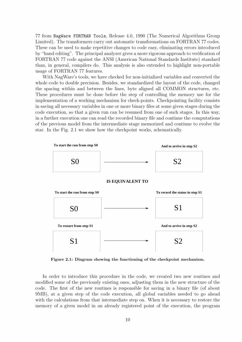
3.1 Rotational and tidal distortion . . . . . . . . . . . . . . . . . . . . . . . . . 173.2 Geometric configuration for the Roche potential. . . . . . . . . . . . . . . . 193.3 Evolutionary tracks for standard and distorted models. . . . . . . . . . . . 403.4 log(k2) vs. age for standard and distorted models. . . . . . . . . . . . . . . 413.5 log(k2) vs. age for different (X,Z) and log(kj) x log (M) for ZAMS models . 423.6 log(β) x log (M) and log(kj) x log(β) for ZAMS models . . . . . . . . . . . 423.7 Temporal evolution of stellar radius for different models. . . . . . . . . . . 433.8 Stellar radii and TR vs. age for EK Cep components. . . . . . . . . . . . . 453.9 EK Cep components and corresponding mass tracks in the HR diagram. . . 473.10 EK Cep components and corresponding mass tracks in the log(g) vs. log

(Teff) plane. . . . . . . . . . . . . . . . . . . . . . . . . . . . . . . . . . . . 483.11 Temporal evolution of Li content and log(k2) for EK Cep components. . . . 49

4.1 Chromospheric Ca II flux vs. Ro. . . . . . . . . . . . . . . . . . . . . . . . 534.2 Azimuthal and meridional fields. . . . . . . . . . . . . . . . . . . . . . . . . 554.3 The ω-effect. . . . . . . . . . . . . . . . . . . . . . . . . . . . . . . . . . . . 554.4 Prot vs. age. . . . . . . . . . . . . . . . . . . . . . . . . . . . . . . . . . . . 564.5 Local τc vs. age. . . . . . . . . . . . . . . . . . . . . . . . . . . . . . . . . . 574.6 Global convective turnover time vs. age. . . . . . . . . . . . . . . . . . . . 584.7 Dynamo number vs. age. . . . . . . . . . . . . . . . . . . . . . . . . . . . . 584.8 τc (global) vs. Teff and τc vs. Prot for some isochrones. . . . . . . . . . . . 594.9 Prot vs. Teff and R−2

o vs. Prot for some isochrones. . . . . . . . . . . . . . . 604.10 Ro−2 vs. Teff for some isochrones. . . . . . . . . . . . . . . . . . . . . . . . 61

5.1 Non-gray evolutionary tracks and isochrones for α=1.0, 2.0 and 2.2. . . . . 705.2 Overadiabaticity and mass fraction where (∇−∇ad) > 10−4 vs. luminosity. 735.3 Comparison between convection and non-grayness effects on the tracks. . . 745.4 The temporal evolution of lithium depletion. . . . . . . . . . . . . . . . . . 755.5 Lithium depletion vs. Teff . . . . . . . . . . . . . . . . . . . . . . . . . . . . 765.6 Mass and age histograms for the ONC stars. . . . . . . . . . . . . . . . . . 785.7 Age distributions for masses lower and higher than Mtr. . . . . . . . . . . . 795.8 The period histogram of all observed ONC objects. . . . . . . . . . . . . . 805.9 Period histograms as function of mass. . . . . . . . . . . . . . . . . . . . . 805.10 Period histograms as function of mass (Herbst et al. (2002). . . . . . . . . 82

vi

5.11 The mass distribution of the early fast rotators and slow rotators. . . . . . 835.12 The observed infrared excess as function of mass. . . . . . . . . . . . . . . 835.13 Fig. 1 from Barnes 2003 . . . . . . . . . . . . . . . . . . . . . . . . . . . . 855.14 Temporal evolution of periods for α=1.0, 2.0 and 2.2. . . . . . . . . . . . . 865.15 LX luminosity (ergs/s) plotted against mass. . . . . . . . . . . . . . . . . . 875.16 The fractional X-ray luminosity as a function of mass. . . . . . . . . . . . . 87

vii

List of Tables

3.1 ISC and gyration radii for ZAMS standard models. . . . . . . . . . . . . . 373.2 ISC and gyration radii for ZAMS tidal distorted models. . . . . . . . . . . 373.3 ISC and gyration radii for ZAMS rotating models. . . . . . . . . . . . . . . 383.4 ISC and β for ZAMS rotationally and tidally distorted models. . . . . . . . 383.5 The comparison between the available log (k2). . . . . . . . . . . . . . . . . 443.6 Absolute dimensions of EK Cep. . . . . . . . . . . . . . . . . . . . . . . . . 453.7 Summary of the apsidal motion related quantities. . . . . . . . . . . . . . . 50

4.1 Isochrones for all models. . . . . . . . . . . . . . . . . . . . . . . . . . . . . 62

5.1 Li abundances at 108yr for some models. . . . . . . . . . . . . . . . . . . . 755.2 Comparison between gray and non-gray models. . . . . . . . . . . . . . . . 81

A.1 ISC and gyration radii for 0.09 M⊙ pre-MS standard models. . . . . . . . . 114A.2 ISC and gyration radii for 0.10 M⊙ pre-MS standard models. . . . . . . . . 115A.3 ISC and gyration radii for 0.20 M⊙ pre-MS standard models. . . . . . . . . 115A.4 ISC and gyration radii for 0.30 M⊙ pre-MS standard models. . . . . . . . . 115A.5 ISC and gyration radii for 0.40 M⊙ pre-MS standard models. . . . . . . . . 116A.6 ISC and gyration radii for 0.50 M⊙ pre-MS standard models. . . . . . . . . 116A.7 ISC and gyration radii for 0.60 M⊙ pre-MS standard models. . . . . . . . . 116A.8 ISC and gyration radii for 0.70 M⊙ pre-MS standard models. . . . . . . . . 117A.9 ISC and gyration radii for 0.80 M⊙ pre-MS standard models. . . . . . . . . 117A.10 ISC and gyration radii for 0.90 M⊙ pre-MS standard models. . . . . . . . . 117A.11 ISC and gyration radii for 1.00 M⊙ pre-MS standard models. . . . . . . . . 118A.12 ISC and gyration radii for 1.20 M⊙ pre-MS standard models. . . . . . . . . 118A.13 ISC and gyration radii for 1.40 M⊙ pre-MS standard models. . . . . . . . . 118A.14 ISC and gyration radii for 1.60 M⊙ pre-MS standard models. . . . . . . . . 119A.15 ISC and gyration radii for 1.80 M⊙ pre-MS standard models. . . . . . . . . 119A.16 ISC and gyration radii for 2.00 M⊙ pre-MS standard models. . . . . . . . . 119A.17 ISC and gyration radii for 2.30 M⊙ pre-MS standard models. . . . . . . . . 120A.18 ISC and gyration radii for 2.50 M⊙ pre-MS standard models. . . . . . . . . 120A.19 ISC and gyration radii for 2.80 M⊙ pre-MS standard models. . . . . . . . . 120A.20 ISC and gyration radii for 3.00 M⊙ pre-MS standard models. . . . . . . . . 121A.21 ISC and gyration radii for 3.30 M⊙ pre-MS standard models. . . . . . . . . 121A.22 ISC and gyration radii for 3.50 M⊙ pre-MS standard models. . . . . . . . . 121A.23 ISC and gyration radii for 3.80 M⊙ pre-MS standard models. . . . . . . . . 122A.24 ISC and gyration radii for 0.09 M⊙ pre-MS tidal distorted models. . . . . . 122

viii

A.25 ISC and gyration radii for 0.10 M⊙ pre-MS tidal distorted models. . . . . . 123A.26 ISC and gyration radii for 0.20 M⊙ pre-MS tidal distorted models. . . . . . 123A.27 ISC and gyration radii for 0.30 M⊙ pre-MS tidal distorted models. . . . . . 123A.28 ISC and gyration radii for 0.40 M⊙ pre-MS tidal distorted models. . . . . . 124A.29 ISC and gyration radii for 0.50 M⊙ pre-MS tidal distorted models. . . . . . 124A.30 ISC and gyration radii for 0.60 M⊙ pre-MS tidal distorted models. . . . . . 124A.31 ISC and gyration radii for 0.70 M⊙ pre-MS tidal distorted models. . . . . . 125A.32 ISC and gyration radii for 0.80 M⊙ pre-MS tidal distorted models. . . . . . 125A.33 ISC and gyration radii for 0.90 M⊙ pre-MS tidal distorted models. . . . . . 125A.34 ISC and gyration radii for 1.00 M⊙ pre-MS tidal distorted models. . . . . . 126A.35 ISC and gyration radii for 1.20 M⊙ pre-MS tidal distorted models. . . . . . 126A.36 ISC and gyration radii for 1.40 M⊙ pre-MS tidal distorted models. . . . . . 126A.37 ISC and gyration radii for 1.60 M⊙ pre-MS tidal distorted models. . . . . . 127A.38 ISC and gyration radii for 1.80 M⊙ pre-MS tidal distorted models. . . . . . 127A.39 ISC and gyration radii for 2.00 M⊙ pre-MS tidal distorted models. . . . . . 127A.40 ISC and gyration radii for 2.30 M⊙ pre-MS tidal distorted models. . . . . . 128A.41 ISC and gyration radii for 2.50 M⊙ pre-MS tidal distorted models. . . . . . 128A.42 ISC and gyration radii for 2.80 M⊙ pre-MS tidal distorted models. . . . . . 128A.43 ISC and gyration radii for 3.00 M⊙ pre-MS tidal distorted models. . . . . . 129A.44 ISC and gyration radii for 3.30 M⊙ pre-MS tidal distorted models. . . . . . 129A.45 ISC and gyration radii for 3.50 M⊙ pre-MS tidal distorted models. . . . . . 129A.46 ISC and gyration radii for 3.80 M⊙ pre-MS tidal distorted models. . . . . . 130A.47 ISC and gyration radii for 0.09 M⊙ pre-MS rotating models. . . . . . . . . 130A.48 ISC and gyration radii for 0.10 M⊙ pre-MS rotating models. . . . . . . . . 131A.49 ISC and gyration radii for 0.20 M⊙ pre-MS rotating models. . . . . . . . . 131A.50 ISC and gyration radii for 0.30 M⊙ pre-MS rotating models. . . . . . . . . 131A.51 ISC and gyration radii for 0.40 M⊙ pre-MS rotating models. . . . . . . . . 132A.52 ISC and gyration radii for 0.50 M⊙ pre-MS rotating models. . . . . . . . . 132A.53 ISC and gyration radii for 0.60 M⊙ pre-MS rotating models. . . . . . . . . 132A.54 ISC and gyration radii for 0.70 M⊙ pre-MS rotating models. . . . . . . . . 133A.55 ISC and gyration radii for 0.80 M⊙ pre-MS rotating models. . . . . . . . . 133A.56 ISC and gyration radii for 0.90 M⊙ pre-MS rotating models. . . . . . . . . 133A.57 ISC and gyration radii for 1.00 M⊙ pre-MS rotating models. . . . . . . . . 134A.58 ISC and gyration radii for 1.20 M⊙ pre-MS rotating models. . . . . . . . . 134A.59 ISC and gyration radii for 1.40 M⊙ pre-MS rotating models. . . . . . . . . 134A.60 ISC and gyration radii for 1.60 M⊙ pre-MS rotating models. . . . . . . . . 135A.61 ISC and gyration radii for 1.80 M⊙ pre-MS rotating models. . . . . . . . . 135A.62 ISC and gyration radii for 2.00 M⊙ pre-MS rotating models. . . . . . . . . 135A.63 ISC and gyration radii for 2.30 M⊙ pre-MS rotating models. . . . . . . . . 136A.64 ISC and gyration radii for 2.50 M⊙ pre-MS rotating models. . . . . . . . . 136A.65 ISC and gyration radii for 2.80 M⊙ pre-MS rotating models. . . . . . . . . 136A.66 ISC and gyration radii for 3.00 M⊙ pre-MS rotating models. . . . . . . . . 137A.67 ISC and gyration radii for 3.30 M⊙ pre-MS rotating models. . . . . . . . . 137A.68 ISC and gyration radii for 3.50 M⊙ pre-MS rotating models. . . . . . . . . 137A.69 ISC and gyration radii for 3.80 M⊙ pre-MS rotating models. . . . . . . . . 138A.70 ISC and β for 0.09 M⊙ pre-MS rotationally and tidally distorted models. . 138A.71 ISC and β for 0.10 M⊙ pre-MS rotationally and tidally distorted models. . 139

ix

A.72 ISC and β for 0.20 M⊙ pre-MS rotationally and tidally distorted models. . 139A.73 ISC and β for 0.30 M⊙ pre-MS rotationally and tidally distorted models. . 139A.74 ISC and β for 0.40 M⊙ pre-MS rotationally and tidally distorted models. . 140A.75 ISC and β for 0.50 M⊙ pre-MS rotationally and tidally distorted models. . 140A.76 ISC and β for 0.60 M⊙ pre-MS rotationally and tidally distorted models. . 140A.77 ISC and β for 0.70 M⊙ pre-MS rotationally and tidally distorted models. . 141A.78 ISC and β for 0.80 M⊙ pre-MS rotationally and tidally distorted models. . 141A.79 ISC and β for 0.90 M⊙ pre-MS rotationally and tidally distorted models. . 141A.80 ISC and β for 1.00 M⊙ pre-MS rotationally and tidally distorted models. . 142A.81 ISC and β for 1.20 M⊙ pre-MS rotationally and tidally distorted models. . 142A.82 ISC and β for 1.40 M⊙ pre-MS rotationally and tidally distorted models. . 142A.83 ISC and β for 1.60 M⊙ pre-MS rotationally and tidally distorted models. . 143A.84 ISC and β for 1.80 M⊙ pre-MS rotationally and tidally distorted models. . 143A.85 ISC and β for 2.00 M⊙ pre-MS rotationally and tidally distorted models. . 143A.86 ISC and β for 2.30 M⊙ pre-MS rotationally and tidally distorted models. . 144A.87 ISC and β for 2.50 M⊙ pre-MS rotationally and tidally distorted models. . 144A.88 ISC and β for 2.80 M⊙ pre-MS rotationally and tidally distorted models. . 144A.89 ISC and β for 3.00 M⊙ pre-MS rotationally and tidally distorted models. . 145A.90 ISC and β for 3.30 M⊙ pre-MS rotationally and tidally distorted models. . 145A.91 ISC and β for 3.50 M⊙ pre-MS rotationally and tidally distorted models. . 145A.92 ISC and β for 3.80 M⊙ pre-MS rotationally and tidally distorted models. . 146

x

Resumo

No presente trabalho investigamos alguns efeitos fısicos que acontecem na estrutura eevolucao estelar. Focalizamos nossa atencao em estrelas de baixa massa na pre-sequenciaprincipal. Incluimos alguns efeitos fısicos no codigo de estrutura e evolucao estelarATON2.3, escrito pelo Dr. Italo Mazzitelli (1989) e posteriormente modificado pelo Dr.Luiz Themystokliz Sanctos Mendes (1999b) para adicionar os efeitos de rotacao e redis-tribuicao interna de momentum angular. Com o objetivo de economizar tempo computa-cional, introduzimos o mecanismo de parada de controle (checkpoint), que permite iniciaruma dada execucao em um estagio de evolucao intermediario, desde que os passos ini-ciais tenham sido devidamente registrados. Essas modificacoes foram feitas juntamentecom um controle completo de variaveis nao inicializadas, precisao e reestruturacao doprograma, visando futuramente paralelizar o codigo. Introduzimos efeitos combinados derotacao e forcas de mare na configuracao de equilıbrio das estrelas. Esses efeitos pertur-badores, contidos na funcao potencial total, desviam a forma da estrela da aproximacaoesfericamente simetrica. Usamos o metodo de Kippenhahn & Thomas (1970), poste-riormente aperfeicoado por Endal & Sofia (1976). A funcao potencial obtida por essesautores, adicionamos termos relacionados a forcas de mare e outros relacionados a partenao simetrica do potencial gravitacional devido a distorcao que tais forcas causam nafigura da estrela. Seguindo essa aproximacao, corrigimos as equacoes constitutivas a fimde obter uma configuracao estrutural de uma estrela distorcida. Derivamos uma nova ex-pressao para a inercia rotacional de estrelas sob a acao de potenciais perturbativos devidoa rotacao e forcas de mare. Calculos de constantes de estrutura interna e raios de giracaoforam incluıdos no codigo tanto para para o caso os modelos sem distorcao quanto paraos distorcidos. Apresentamos, pela primeira vez na literatura, calculos de constantes deestrutura interna que se extendam ate a pre-sequencia principal. Varias trilhas evolutivasforam geradas com os novos modelos, incluindo as grandezas mencionadas acima. Osnovos modelos foram testados atraves de dados observacionais das dimensoes absolutas,taxa de movimento apsidal e abundancia de lıtio das componentes do sistema binarioeclipsante EK Cephei. No presente trabalho, tambem apresentamos estimativas teoricasdo “convective turnover time”, τc, e Numeros de Rossby, Ro, para estrelas com massassemelhantes a massa solar, com rotacao e na pre-sequencia principal. Ro esta relacionadocom a forca magnetica na teoria do dınamo estelar e, pelo menos para estrelas na sequenciaprincipal, observa-se uma correlacao entre rotacao e atividade estelar. Incluimos tambema possibilidade de utilizar modelos de atmosferas nao cinza, com o objetivo de seguir aevolucao estelar de estrelas de baixa massa desde estagios bem iniciais, caracterizadospor baixa gravidade. Adotamos os modelos NextGen e ATLAS9 de atmosferas estelares.Usando os nossos novos modelos nao-cinza, geramos varios conjuntos de trilhas evolutivas,partindo da pre-sequencia principal. Tais trilhas foram usadas para investigar algumaspropriedades fısicas e rotacionais de estrelas jovens na Nebulosa de Orion. Comparacoesentre resultados teoricos e dados observacionais, permitiram-nos obter informacoes sobreesta classe de objetos, principalmente no que diz respeito a distribuicao inicial de mo-mentum angular. A interpretacao dos dados depende fortemente das consideracoes fısicasfeitas no modelos, sendo a eficiencia da conveccao a mais importante. Nossa analise in-dica que um segundo parametro e necessario para descrever a conveccao na pre-sequenciaprincipal. Tal parametro esta possivelmente relacionado ao efeito estrutural de um campomagnetico gerado por efeito dınamo.

xi

Abstract

We have investigated some physical phenomena that take place in the stellar structureand evolution. Special attention was given to low-mass pre-main sequence stars. We haveincluded the possibility of using non-gray atmosphere models in the boundary conditions,as well as the possibility of extracting information of some physical effects (like the internalstructure constant and the Rossby number) in the stellar evolutionary code ATON2.3. Thecode was originally written by Dr. Italo Mazzitelli (1989) and further improved by Dr.Luiz Themyztokliz Sanctos Mendes (1999b) to take into account the effects of rotationand redistribution of angular momentum. In order to save computing time, we haveintroduced a checkpoint mechanism that allow starting the run in any step of evolutionsince previous computations had been registered. This modification was done togetherwith a complete control for non-initialized variables, machine precision and restructuring,aiming a later implementation of parallel computation. We have introduced the effectsof tidal forces combined with the rotational ones on the equilibrium configuration of thestars. These disturbing effects, all included in the total potential function, deviate thestellar configuration from sphericity. We have used the Kippenhahn & Thomas (1970)approximation, which was further improved by Endal & Sofia (1976). To the potentialfunction obtained by the latter authors, we added both the terms related to the tidalpotentials and those related to the non-symmetrical part of the gravitational potentialdue to the distortion of the star figure due to tidal forces. Following this approach, wecorrect the constitutive equations in order to obtain a stellar structure configuration ofa distorted star. We dereived a new expression for the rotational inertia of tidally androtationally distorted star. We included also calculations of internal structure constantsand gyration radii, tabulating them for a serie of models. We presented, for the first timein the literature, calculations of the internal structure constant extended to the pre-mainsequence. Our new models were tested against observations through the analysis of theevolutionary status of EK Cephei. We also present theoretical estimates of the convectiveturnover time, τc, and Rossby numbers, Ro, for rotating pre-main sequence solar-typestars. Ro is related to the magnetic strength in dynamo theories and, at least for mainsequence stars, shows an observational correlation with stellar activity. We have includedthe possibility of using non-gray atmosphere models in order to follow the evolution oflow mass stars starting from early, low-gravity stages. NextGen and ATLAS9 atmospheremodels were adopted. By using our new non-gray models we generated sets of pre-mainsequence evolutionary tracks that were used to investigate some physical and rotationalproperties of young stars in the Orion Nebular Cluster (ONC). The comparison betweentheoretical results and observational data allows us to otain some information about thisclass of objects, mainly those related to the initial distribution of angular momentum.The data interpretation was found to depend strongly on the physical inputs, being theconvection efficiency the most significant one. The comparisons made indicate that asecond parameter is needed to describe convection in the pre-main sequence, possiblyrelated to the structural effect of a dynamo-generated magnetic field.

xii

Chapter 1

Introduction

The physical processes occuring in the stellar interiors cannot be directly observed,except, perhaps, through the elusive neutrinos. The vast majority of the informationwe have about the conditions existing inside a star, comes from the light emitted by itsatmosphere, what indirectly reflects the internal environment.

The stellar interior properties must be deduced from the observed features and fromthe laws that govern the stellar structure and evolution. Through a suitable combinationof these laws in theoretical models, one can have an insight of the equilibrium configurationand of the temporal evolution of the stars.

There exist only few stellar features that can be directly observed. For a large numberof stars, we have measurements of magnitudes (apparent and absolute) and color indexes.For the Sun and a relatively small number of components of binary systems, we havegood determination of masses, radii and luminosities. Additional verifications in theoriesare provided by data obtained from asteroseismology, the study of the internal structureof stars through the interpretation of their pulsation periods, and from binary systemsin which the line of apsides (the major axis of the orbit) presents a small rotation veloc-ity. This phenomenon depends on the stellar internal conditions and, therefore, providesinformation that can be used to control the stellar interior theories. Information aboutthe chemical composition of the stellar surface can be achieved spectroscopically, and onecan assume that the composition of the major part of the stellar interior is similar tothat of the outer layers, at least for main sequence (MS) stars. On the other hand, giantstars have already processed part of the elements originally present in their interior, andthe spectroscopic data can only provide reliable information about the surface chemicalcomposition.

When we try to understand the life of a star, we face a hard problem: stars last muchmore than a human life. A human could never watch a star go through its complete lifecycle. We need a special approach. We use the laws of physics and a few observablequantities to understand the lives of stars. In order to learn about the life cycles of a star,we look at a large number of stars. We can see them in various stages of development. Ifwe look at enough stars of various ages, we can put together a complete picture of stellarevolution. The tool we use to study stars is called the Hertzsprung-Russell diagram

1

(usually referred to by the abbreviation H-R diagram or HRD; another form of it isalso known as a Colour-Magnitude diagram, or CMD). It shows the relationship betweenabsolute magnitude, luminosity, spectral classification, and surface temperature of stars.The diagram was developed independently by Ejnar Hertzsprung in 1911 and Henry NorrisRussell in 1913 and represented a huge leap forward in understanding stellar evolution, orthe “lives of stars”. From it, most of the peculiarities of stellar behavior can be studied.One of these, in particular, is that the stars are sitting along a well-defined band called MS,where the majority of stars are clustered in a region from the bottom right to the top left(see Fig. 1.1). The H-R diagram is the fundamental tool astronomers use to explore thebirth and the death of stars. Although it began as a way to group information concerningthe intrinsic characteristics of stars, it quickily became a tool to explore changes in stars asthey age. It is used to define different types of stars and to match theoretical predictionsof stellar evolution using computer models with observations of actual stars. It is thennecessary to convert either the calculated quantities to observables, or the other wayaround, thus introducing an extra uncertainty.

Figure 1.1: Hertzsprung-Russell diagram with 22,000 stars plotted from the Hipparcos catalog and 1000from the Gliese catalog of nearby stars.

2

The theoretical studies about the stellar interior are based in a set of equations thatmust be solved simultaneously, aiming to reproduce the observed stellar properties andto explain the internal structure of the stars. Such models treat the physical phenomenataking place inside a star by describing them through basic equations that govern theinternal physical properties. The basis of the stellar structure theory was developed inthe first part of the past century, when several important works were published, amongwhich those of Chandrasekhar (1939) and Schwarzschild (1958) can be considered thefundamental ones.

The structure of a star can be described by a set of differential equations contain-ing variables like pressure, density, temperature, luminosity, etc. They are the so-called“constitutive equations”:

dP

dM= −

GM

4πr4(1.1a)

dr

dM=

1

4πr2ρ(1.1b)

dL

dM= ǫ− T

∂S

∂t(1.1c)

dT

dM= −

GMT

4πr4P∇, ∇ = ∇rad,∇conv . (1.1d)

This equations are respectively named equation of hydrostatic equilibrium, equationof continuity of mass, equation of conservation of energy and equation of transport ofenergy. Besides the set of Eqs. (1.1), it is also necessary to assume an equation of state ofthe material that form the star, an opacity law and an equation of energy generation todescribe the stellar structure. Furthermore, some boundary conditions must be definedin order to match interior and atmosphere integrations. The theoretical models are builtaiming the self consistent solution of these equations throughout the stellar radius, havingthe stellar mass and the initial chemical composition (and, eventually, some amount ofrotation) as input parameters. A sequence of models of stellar structure in successive timeintervals define a stellar “evolutionary track” in the HRD.

In the 1960’s, the construction of evolutionary models was stimulated by the introduc-tion of the relaxation method for the numerical solution of the differential equations thatdescribe the stellar structure (Henyey, Forbes & Gould 1964). This method replaces thedifferential equations with a set of finite difference equations whose solution is carried outglobaly and enables one to include time-dependent phenomena in a natural way. Also,the appearing of faster computers speeded up the improvement process of the models.Besides that, the knowledge of several other aspects of the stellar interiors, such as nu-cleosynthesis of elements (Clayton 1968) and more realistic opacity tables calculations(Cox & Stewart 1970), were important in bringing the models to a very well succeededinterpretation of a large part of intermediate mass stars in the MS phase.

The physical processes happening inside a star are rather complex to be completelyreproduced by the models. The models are necessarily an idealized scenario of this com-plicated environment and, consequently, cannot reproduce, with the desirable accuracy,the large quantity of observational data obtained from real stars. Since the first modelsbecame available, researchers have made efforts to improve the quality of the achievedresults by developing new numerical tools and/or by introducing in the codes improved

3

approximations for the underlying physical phenomena. It is important to emphasizethat, although some of the physical processes involved in the stellar theories have solidtheoretical basis, the corresponding implementation in the models is, most of the times, ahard task. This is due to a series of problems, such as numerical accuracy and instability,mathematical complexity, computational time, and so on. A significant number of im-portant questions related to stellar structure and evolution is still under debate. A goodexample is turbulence, that is not well understood, yet. Many of these several open issuesare discussed in some reference works. For example, the problem of the chemical mix-ing of elements was addressed by Goulpil & Zahn (1989); D’Antona & Mazzitelli (1984)discuss the lithium and berilium burning, Mihalas et al. (1988) treat the stellar equationof state; Canuto & Mazzitelli (1991) give some insight on the turbulent convection, andKippenhahn & Thomas (1970) investigated the influence of rotation in the stellar evolu-tion. Some of these subjects, like rotation and turbulent convection, have already beenimplemented in the evolutionary models and presented promising results.

Regarding the star formation process, one believes that the stars are formed fromclouds made up by the interstellar material. The chemical composition of a newborn staris similar to that of the cloud from which the star in question was formed. The totalstellar mass is primarily determined in the formation process, although it can undergosome changes due to the residual accretion after the protostellar phase (Basri & Bertout1989) and to outflows, which are mass loss processes due to magneto-rotationally drivenwinds (Hartmann & MacGregor 1982).

Star formation occurs as a result of the action of gravity on a wide range of scales,and different mechanisms may be important on different scales, depending on the forcesopposing gravity. On galactic scales, the tendency of interstellar matter to condenseunder gravity into star-forming clouds is counteracted by galatic tidal forces, and starformation can occur only where the gas becomes dense enough for its self-gravity toovercome these tidal forces, for example in spiral arms (Larson 2003). On intermediatescales, turbulence and magnetic fields may be the most important effects opposing gravity,while on the small scales of individual prestellar cloud cores, thermal pressure becomesthe most important force resisting gravitation. When the cloud core begins contracting,the centrifugal force associated with its angular momentum may eventually interrupt thecollapse, leading to the formation of a binary or multiple star system. When a very smallcentral region attains stellar density, the contraction is halted by the thermal pressureand a protostar forms and continues growing in mass by accretion. In this final stage ofstar formation, magnetic fields can become important by controlling gas accretion andoutflows. These events characterize the pre-main sequence (pre-MS) evolutionary phase.As the thermodynamic conditions within a star become close to those suitable for thenuclear reactions ignition, these phenomena finish and the star approaches a far morestable configuration, called MS.

After deutherium, lithium and berilium burning phases, which take place in earlyphases of evolution, the first element to be processed within the star is the Hydrogen.When the star has hydrogen burning as its main energy source, the latter can be consideredin the MS. Iben (1965) defines the Zero-Age Main Sequence (ZAMS) the time at which90% of the total stellar energy comes from the Hydrogen burning. The stars spend themajor part of their lives burning Hydrogen. This is a long, quiet and stable phase oftheir evolution. During the MS, the changes in radius, luminosity, temperature, density,and other quantities, are negligible. It will last until the available supply of Hydrogen for

4

“burning” is almost completely consumed. As the more massive stars have higher centraltemperature, pressure and density, they process their nuclear Hydrogen faster than thelower mass stars, remaining less time in the MS. Therefore, the time spent by a given starin the MS phase, and, in general, in its evolution after that, is determined by its initialmass.

Depending on the stellar mass, other chemical elements can be processed in the stel-lar nucleus. The production of new elements, other than Helium (from H-burning), bynuclear reactions is called “nucleosynthesis”. Again, the stellar mass will determine whatkind of reactions will take place in the central core of a star. Objects with less than0.08M⊙, the so-called brown dwarfs, are not real stars because they never develop a cen-tral temperature which is high enough to ignite Hydrogen burning. Instead, they releaseenergy by gravitational contraction. The very low mass stars (between about 0.25 and0.08 M⊙) are real fully convective stars that burn Hydrogen in their cores, via p-p chain,so slowly that they will stay on the MS for a very long time (about 1012 years). OnceHydrogen is burned out, the core collapes, but never reaches temperatures high enoughto ignite Helium-burning. Such stars evolve directly to white dwarfs. One believes thatthe universe is so young that no very low-mass stars has had time to evolve off the MS, sothis prediction is not really testable. Low mass stars (0.25<M/M⊙<1.2) have radiativecores, so that the surrounding Hydrogen cannot be transported into the core where itcan be burned. Instead, only the Hydrogen inilially present in the inner core, where thetemperature is high enough, will be processed via p-p chain. When the Hydrogen is usedup, the central core contracts gravitationally until the degeneracy halts the contraction.Eventually, the core will heat up until Helium can be ignited and, when this occurs, thestar is in a giant phase. He-burning in degenerate core takes place explosively, in a pro-cess called “Helium Flash”. The changes produced by this process are very rapid andthe physics involved becomes very difficult to be described approximately. Despite thedifficulties involved in calculations of the He flash, the star certainly ends up in a stableconfiguration, where it burns Helium in the core and Hydrogen in a shell around it. Thisphase is called the “Horizontal Branch”. After Helium is used up in the core, He-burningshell takes place, but the star will not be able to burn any further element because itcannot get hot enough in the core, and it will move to the white dwarf region.

High mass stars (M>1.2M⊙) have convective cores and, for this reason, a large amountof Hydrogen can be transported to the central regions, where it can be burned into He bythe CNO cycle. In this way, a considerable fraction of the Hydrogen is processed and thefollowing gravitational collapse phase may be relatively short. In the Hertzprung-Russeldiagram, the stars in this phase are supposed to be in a region called “Hertzsprung gap”,that lies between the MS and the giant branch. In fact, only a few stars observed in openclusters are found in this region. After Hydrogen is consumed in the core, the centralregions of the star begin collapsing, and the Hydrogen burning can continue in a shelloutside the core. When the temperature becomes high enough, Helium begins burningin the core, building Carbon. Even when the Helium in the core is finished, Helium cancontinue being processed into Carbon in a shell outside the core, while still further out theHydrogen burning shell continues producing Helium. The core contracts again, the outerlayers expand, and the star increases in luminosity. Then, the ignition of Carbon takesplace in the core building other elements like Mg, Ne and Na. After Carbon burning, anddepending on the mass of the star, further elements can be processed all the way to Fe,beyond which no further energy can be extracted by fusion because the production of any

5

heavier nucleus by direct fusion is endothermic. Massive stars can reach a stage wherethey consist of shells of nuclear burning, with Fe production in the core, surrounded byshells of Si, C and O, He and H. Eventually, the fuel sources will finish and the star (ifthe mass is high enough) will undergo a core collapse, resulting in a supernova. In thisprocess, a small amount of elements beyond Fe can be produced. The result of such acollapse can be a neutron star or a black Hole (for very high mass stars).

The main goal in building evolutionary tracks is to explain the processes describedabove, following the structural changes that a given star undergoes throughout its evolu-tion. Most of the current evolutionary models start the stellar evolution from the ZAMSand follow the evolution of the stars until their post-main sequence (post-MS) phase,without considering the processes that can take place on the pre-MS evolution that, con-sequently, affect the MS configuration. Since the works by Henyey et al. (1955) andHayashi (1961), it is commonly accepted that pre-MS stars derive their energy by gravi-tational contraction, with exception of a short D-burning phase. In general, the definitionof the zero point of ages for pre-MS evolution is connected to the location in luminosityof the starting model, i.e., the internal thermodynamic conditions within the star, forwhich, the stellar structure equations can be numerically solved. An extensivelly usedapproximation when modeling pre-mais sequence evolution, is to consider that the massaccretion proccess does not continue further the zero age point.

The first models, the so-called “standard models”, considered the star as an homo-geneous gas sphere, in complete hydrostatic equilibrium (balance between pressure andgravity). Besides, they did not include more complicated effects such as rotation, mag-netic fields, etc. These models were capable to reproduce the basic global characteristicsof the stars available by that time, but as the quantity and accuracy of observational dataincreased, the standard models showed to be inefficient and with many limitations. Theyfailed in reproducing the abundances of light elements like Lithium and Berilium in lowmass stars and in fitting the position in the HR diagram of some pre-MS componentsof binary systems. Another inconsistency between observations and standard models isthe anomalous surface abundances in evolved stars, suggesting that the elements maybe mixed in deeper layers (Langer et al. 1993). Rotation is a feature found in all starsand, even if its intensity is low, it is nowadays considered an important causing agent ofmixture.

In order to explain the new and more accurate observational stellar data, the modelistsimproved the evolutionary models with some non-standard effects. The first attempts toinclude rotation effects in the evolutionary codes date from the 1960’s and are in usestill today (Faulkner et al. 1968, Sackmann & Anand 1969, Kippenhahn & Thomas 1970,Papaloizou & Thomas 1972).

As already mentioned, magnetic fields can play an important role in the last stages ofpre-MS evolution. However, the existing evolutionary models do not take their effects intoaccount, although the subject is treated in some exploratory ways. According to D’Antonaet al. (2000), the inclusion of magnetic fields in the models, considering the hypothesisthat they are produced by rotation, changes the Schwarzschild’s stability criterion, sothat the convection is established for a temperature gradient higher than in non-magneticcases. This gradient is inversely proportional to the effective temperature, so the magneticfields seems to have a thermal effect in the pre-MS stars, leading to cooler models. Ina series of works, Maeder & Meynet (2003, 2004, 2005) and Eggenberger et al. (2005)studied the relative importance of rotational and magnetic effects in high mass stars, by

6

calculating the magnetic instabilities that may rise in differentially rotating stars andcreate magnetic fields.

While models with magnetic fields are not available, one can have some insight aboutthe stellar magnetic fields through the stellar magnetic activity, that can be observed ina broad range of phenomena (sunspots, flares, chromospheric emission lines). In solar-type stars, the driving mechanism for stellar magnetic activity is the magnetic field thatis presumably generated by a dynamo in the deep layers of the convection zone andin the overshoot region just below the convection zone itself (Montesinos et al. 2001).For fully convective stars the driving mechanism for stellar magnetic activity is thoughtto be a distributed dynamo, which depends on the turbulent velocity field. It is alsopossible that the dominant source of magnetic flux in the TTauri stars are “fossil fields”inherited from the star formation process (Mestel 1999). From the theoretical point ofview, researchers try to understand the observed correlations between activity-relatedparameters and stellar parameters such as mass, temperature, gravity, rotation velocity,and quantities related to the internal structure of the star. Semi-empirical calculationsof an activity indicator, such as the Rossby number, have been a way for this kind ofinvestigation (see Feigelson 2003). More recently, self-consistent values of th Rossbynumber, calculated theoretically by rotating models, became available (Kim & Demarque1996 and Landin et al. 2005).

As it is emphasized by Mihalas (2001), the atmosphere of a star is what we can see,measure and diagnose. So, the treatment given to the stellar atmosphere directly influ-ences the results obtained by the evolutionary models. Chabrier & Baraffe (1997) pointedout that the use of T(τ) relations or the gray atmosphere (widely used in the first models)is invalid when molecules form near the photosphere. For stars with effective temperaturebelow about 4000 K, the atmosphere must be modeled by using more realistic treatments,such as the non-gray approximation. Non-gray atmosphere boundary conditions can beobtained from the atmospheric models for a wide range of metallicities, effective temper-atures and gravities. As good examples, we can cite the NextGen (Allard et al. 1997)and ATLAS9 (Heiter et al. 2002) atmosphere models.

Because of the fact that binary stars are the most reliable source of accurate infor-mation about the most basic stellar parameters, they are largely used to compare theoryand observations. They provide also important information about stellar phenomena liketidal and rotational distortions, limb darkening, mutual irradiation, etc., which, althoughsometimes neglected, may be the responsible for some differences between stellar evolu-tion in binary and single stars (Claret 1993). It is well known that tidal and rotationaldistortions of the stellar configuration are related to the internal structure constants ofthe component stars (Kopal 1978). An important consequence of such distortions in ec-centric binary systems is the secular change in the position of the periastron, that can beaccurately measured by monitoring times of minimum light in eclipsing binaries. Fromthis kind of data, we can derive empirical values of the internal structure constants inorder to compare them with theoretical predictions.

All the effects cited above are important in the stellar structure and evolution. Theinclusion of new physical phenomena in stellar evolution models greatly improves thecomparisons with observations. This is the reason why modelists concentrate efforts incontinuously introducing new and more realistic physical inputs in the evolutionary codes.

The evolutionary code used in this study is the ATON2.3, originally writen by Dr.Italo Mazzitelli (Mazzitelli 1989, Mazzitelli et al. 1995 and D’Antona & Mazzitelli 1997)

7

and further updated by Dr. Luiz Themystokliz Sanctos Mendes (Electronic EngineeringDepartment of Universidade Federal de Minas Gerais), my co-advisor, in his Ph.D thesis,for including rotation and angular momentum redistribution (Mendes 1999b). This workwas coordinated by Dr. Luiz Paulo Ribeiro Vaz (Physics Department of UniversidadeFederal de Minas Gerais), also my Ph.D advisor, who started a scientific collaborationwith Dr. Francesca D’Antona (Osservatorio Astronomico di Roma, Italy) and Dr. ItaloMazzitelli allowing our access to their evolutionary code. The present Ph.D work wascarried through the international collaboration with the italian researchers, including ayear of activities in Italy, having Dr. D’Antona as foreign co-advisor. During this time,Dr. Paolo Ventura (Osservatorio Astronomico di Roma) participated of the collaborationwork, also.

In this work, we investigate some physical phenomena that take place in the stellarstructure and evolution, like stellar activity, rotation, tidal interaction and non-gray effectsof radiative process. Special attention is given to low mass pre-MS stars.

In general, inclusion of new physical processes in evolutionary codes is a work thatdemands a long time to be completed, mainly due to the many debuging steps in testingthe changes. Aiming to save computing time, we decided to change the computationalstructure of the ATON2.3 code, introducing a mechanism that allows starting the runin an intermediate step of the evolution, since the initial steps have been registered ina previous run. This mechanism is known as checkpoint. After that, we introduced inthe code some important modifications to test theoretical predictions. The first one wasthe theoretical computations of convective turnover times and Rossby numbers. Further,we implemented the computation of the internal structure constants, in the ATON2.3,fundamental in apsidal motion tests. Finally, we included in the code more realisticboundary conditions by using the NextGen and ATLAS9 atmosphere models.

In Chap. 2 we present the changes we made in the computational structure of the codeconcerning the checkpoint. The changes to consider the stellar equilibrium configurationmodifications due to tidal and rotational distortions, and the internal structure constantcalculations, are shown in Chap. 3. Chap. 4 presents the theoretical estimates of theRossby number with our modified model. In Chap. 5 we describe the implementationof non-gray boundary conditions. Chap. 6 gives the general conclutions and suggestssome future improvements of the work already done. And, finally, in Chap. 7 we bring asynopsis of the work in Portuguese.

8

Chapter 2

Structural Changes in the StellarEvolutionary Code ATON 2.3

The modeling of physical processes describing both the structure and the evolutionof stars is usually very complex. Some processes have well founded theoretical basis, butare implemented in stellar models with several degrees of simplifications. Often, thesedifficulties of implementation are due to mathematical complexity, numerical accuracy,long computing time, etc. On the other hand, there are some physical processes thatremain still very poorly understood and, for this reason, they are completely ignored inthe stellar models or taken into account in a very idealized approach.

In general, implementation of physical improvements in stellar evolutionary codes isa work that demands a long time to be completed, mainly when we are testing them,because the same calculation steps must be repeated several times. However, test phasesare a fundamental part of the model development and very efficient at locating certaintypes of faults in the program.

Aiming to save computing time, we changed the computational structure of the ATON

2.3 code, in order to introduce a mechanism that allow starting the run in an intermediatestep of the evolution, once the initial steps have been registered in a previous run. Thisis the mechanism of checkpoint. In this chapter we will explain how we have introducedit in the code and how it works.

2.1 Implementation of the structural changes

In order to improve the performance and to make easier the testing and debuggingof the physical changes introduced in the ATON2.3 code, it became evident, after anaccurate analysis, that its structure should undergo some changes. Since the code has beenevolving through the contribution of many different authors, it is written in many different“dialects” of FORTRAN, making necessary an uniformization of the code in numericalprecision, “common blocks” alignment, declaration of variables, etc. These structuralimprovements were made by using some analyzing and transforming tools for FORTRAN

9

77 from NagWare FORTRAN Tools, Release 4.0, 1990 (The Numerical Algorithms GroupLimited). The transformers carry out automatic transformations on FORTRAN 77 codes.These can be used to make repetitive changes to code easy, eliminating errors introducedby “hand editing”. The principal analyzer gives a more rigorous approach to verification ofFORTRAN 77 code against the ANSI (American National Standards Institute) standardthan, in general, compilers do. This analysis is also extended to highlight non-portableusage of FORTRAN 77 features.

With NagWare’s tools, we have checked for non-initialized variables and converted thewhole code to double precision. Besides, we standardized the layout of the code, changedthe spacing within and between the lines, byte aligned all COMMON structures, etc.These procedures must be done before the step of controlling the memory use for theimplementation of a working mechanism for check-points. Checkpointing facility consistsin saving all necessary variables in one or more binary files at some given stages during thecode execution, so that a given run can be resumed from one of such stages. In this way,in a further execution one can read the recorded binary file and continue the computationsof the previous model from the intermediate stage memorized and continue to evolve thestar. In the Fig. 2.1 we show how the checkpoint works, schematically.

IS EQUIVALENT TO

S1

S2 S1

S0

S2 S0

To start the run from step S0

To start the run from step S0

To restart from step S1

To record the status in step S1

And to arrive in step S2

And to arrive in step S2

Figure 2.1: Diagram showing the functioning of the checkpoint mechanism.

In order to introduce this procedure in the code, we created two new routines andmodified some of the previously existing ones, adjusting them in the new structure of thecode. The first of the new routines is responsible for saving in a binary file (of about9MB), at a given step of the code execution, all global variables needed to go aheadwith the calculations from that intermediate step on. When it is necessary to restore thememory of a given model in an already registered point of the execution, the program

10

makes use of the second new routine, especially designed for reading all this set of datafrom the corresponding binary file. With these variables restored in its memory, the codecan continue to run and produce, upon its termination, the same results generated if ithad started from the initial point, with an evident gain in computing time and. equallyimportant, without any loss of numerical accuracy.

2.2 The importance of the checkpoint mechanism

The checkpoint mechanism is a fundamental tool when modifying computational mod-els, mainly in cases where the program in question is complex and takes a long time tobe executed. In order to illustrate how the computing time varies with the complexityof the program, let us consider the execution time spent by earlier versions of the ATON

code for reproducing some characteristics of a star with the same mass and metallicity asthe sun, running in a XEON 1.8 GHz processor. The 2.0 version of the code is relativelysimple and spends 3 (three) minutes to perform the calculations for such a star withoutconsidering rotation, starting from the pre-MS and arriving in the MS configuration, whatis equivalent to an age of 9.6 billion years. But this computing time increases by a factorof 7 (seven) if we let this star evolve until 13 billion years, when it will be a red giant. Inthe post-MS phase, the time scale of the processes are much shorter than in MS, so anevolution of an interval of ∆t requires more computing time in the evolved phases thanin the previous MS ones.

The ATON2.3 code is a more realistic version of the stellar evolutionary model inquestion, in the sense that it takes into account the non-standard effects of rotation,ignored by the previous versions. We can choose among three different schemes of rotation:rigid body rotation or differential rotation over the whole star, or rigid body rotation inthe convective zones plus differential rotation in radiative regions. In the first two cases,the code spends about 13 (thirteen) minutes to evolve the star from the pre-MS to the MSconfiguration. In the third case, the same evolution is done in 25 (twenty five) minutes.The computing time for evolving a solar-like rotating stars from the pre-MS to the post-MSwill certainly increase considerably, but we do not quantify it, yet, because the rotatingversion of the code is not suitably tested beyond the MS phase.

The higher the consistency in the physical processes inserted in the evolutionary code,the greater will be the computing time needed to accomplish the computational task. So,the importance of a checkpoint mechanism is clear, not only during implementation andtest phases of aimed improvements, but also in the studies of the model properties, afterthe implementations have been tested. When some aimed improvement is activated ina more evolved phase of the stellar evolution, such as mass transfer in binary systems,mass loss in evolved phases, etc., the checkpoint mechanism is even more efficient. Itallows to evolve a model until a given stage, before the physical process in question isactivated, and store all necessary variables to continue the evolution. After that, we canstudy our modifications regarding this process, just by restarting the computation fromthe relevant point. In this mode of execution, all computing time spent to run the initialpart of calculations will be saved, without loss of information, accuracy or precision.

This mechanism was already successfully used in the present work to implement theself-consistent calculation of both local and global “convective turn over time”, and in thestudies about the internal redistribution of angular momentum.

11

Chapter 3

Internal Structure Constants

The internal structure constants, namely, k2, k3 and k4, also known as apsidal motionconstants, are important parameters in stellar astrophysics. They are mass concentrationparameters and depend on the mass distribution throughout the star. There is, also, adirect relation between the gravitational field of a non-spherical body and the internaldensity concentration in that body (Sahade & Wood 1978).

From the theoretical point of view, the values of kj (j=2, 3, 4) depend on the modelused. For the Roche model, in which the whole stellar mass is concentrated in its center,the kj ’s values are all equal to zero, while for a homogeneous model k2=3/4, k3=3/8 andk4=1/4. The values of the internal structure constants are essential to compute the the-oretical apsidal motion rates in close binaries, and the comparison with the observationsconstitutes an important test for evolutionary models. The most centrally concentratedstars have the lowest values of kj and the longest values of apsidal periods (Eq. 3.6).

From the observational point of view, it can be shown that the apsidal rate ω, inradians per cycle, in terms of the internal structure constants is given by (Martynov 1973,Hejlesen 1987):

ω

2π=

2∑

i=1

4∑

j=2

cjikji, (3.1)

where the index i denotes the component star (1=primary, 2=secondary) and j the har-monic order. Generally, the terms of orders higher than j=2 are very small and theequation above gives the empirical weighted mean k2 values for comparison with theo-retical coefficients (Eq. 3.18). Although not directly comparable with observational data,the apsidal motion constant, k2, is important in other astrophysics aspects, since synchro-nization and circularization time scales in close binaries are functions of k2 (Zahn 1977).Other applications of the internal structure constants are the computation of rotationalangular momenta (as can be seen in the Sect. 3.5.4), where gyration radii (defined in theEq. 3.83) can be expressed as a linear function of the apsidal motion constants (Ureche1976), and the determination of the effect of binarity in the geometry of the stellar surfacesdue to rotation and tides (Rucinski 1969, Kopal 1978).

Russell (1928) was the first one to find an analytical expression for the apsidal motion

12

period in close binaries (later improved by Cowling 1938), in terms of the stellar masses,relative radii and internal structure constants of the component stars. Meanwhile, Chan-drasekhar (1933) used polytropic models to predict internal structure constants for mainsequence stars. At that time the large uncertainties involved, in obtaining observationaldata as well as the use of polytropic models with an arbitrary index n, were responsible forthe apparently good agreement obtained between observed and predicted values of log k2.By using more realistic stellar models, a more elaborated expression for the apsidal motionperiod, separating rotational and tidal contributions to the total apsidal motion rate, wasderived by different authors. Apsidal motion test was also applied to polytropic stellarmodels by Sterne (1939), Brooker & Olle (1955) and later to early theoretical stellar mod-els at the ZAMS by Schwarzschild (1958) and Kushawa (1957), both using the old Keller& Meyerott (1955) opacities. Since then, comparisons between theory and observationshave systematically shown that real stars are more centrally condensed than predicted bytheoretical models. After that, Jeffery (1984) and Hejlesen (1987) computed more recentinternal structure constants for stars within the main sequence. The former author usedCarson (1976) opacities while Hejlesen used opacity tables by Cox & Stewart (1969). Themost recent internal structure constants for main sequence stars are those by Claret &Gimenez (1989a, 1991, 1992).

In this work, we present new calculations of internal structure constants extended,for the first time, to the pre-main sequence phase. We calculated internal structureconstants for spherically symmetric stars by using a standard version of the ATON code(without a disturbing potential). By using our new version of the ATON code, described inthe Sec. (3.5), we calculated new internal structure constants for rotating stars, stars inbinary systems, and rotating stars in binary systems. As a by-product of our calculations,we also derived a new expression for the rotational inertia of a star distorted by rotationand tidal forces (see Sec. 3.5.4). The results are presented in the Sec. (3.6). Discussionand comparisons with observed apsidal motion rates are given in Sect. (3.7).

3.1 Apsidal motion

The longitude of periastron of a binary orbit, denoted by ω, defines the direction ofthe line of apsides in the orbital plane. It is an element of the orbit, which is constant ifall the following conditions, in a system consisting of two gravitating bodies, are valid:

• the bodies can be regarded as point masses,

• they move in accordance with Newton’s law of gravitation (r−2), and

• the two bodies form a gravitationally isolated system.

However, if any of these assumptions are not satisfied, the size, the form, and the spatialposition of the orbit will vary. The most readily detected departure of the observed motionfrom the prediction of the simple theory is a variation in the value of ω with time, whatis referred to as rotation (advance or recession) of the line of apsides. For a more detaileddiscussion on this subject, the reader is addressed, for instance, to the works of Batten(1973) or Claret & Gimenez (2001).

There exist several types of perturbations that can lead to rotation of apsides, namelymutual tidal distortion of the components, distortion of the components due to axial

13

rotation, relativistic effects, presence of a third body, and recession due to a resistingcircumstellar medium.

In close binary systems, the axial rotation and the mutual tidal forces of the compo-nent stars will deform each other and destroy their spherical symmetry, by means of therespective disturbing potentials. Besides the changes in the stellar structure describedin Sect. 3.5, these disturbing potentials produce an observed variation in ω which is thesum of the variations produced by each component (Batten 1973). The final resultantvariation of ω produced by the disturbing potentials, Eq. (3.72), i.e., the rate of apsidaladvance, ω per orbital revolution, is given by

ω

2π=P

U= k21c21 + k22c22, (3.2)

where P is the anomalistic orbital period and U is the apsidal motion period, and

c2i =

[

(

Ωi

ωK

)2(

1 +M3−i

Mi

)

f(e) +15M3−i

Mi

g(e)

]

(

Ri

A

)5

. (3.3)

In Eq. (3.3), the subscript i=1,2 stands for star 1 and star 2 respectively, Mi and Ri

are stellar mass and radius of component i, A is the semi-major axis, e is the orbitaleccentricity, and functions f(e) and g(e) are defined as

f(e) = (1 − e2)−2 and (3.4)

g(e) =(8 + 12e2 + e4)f(e)2.5

8, (3.5)

(Ωi/ωK) being the ratio between the actual angular rotational velocity of the stars and thatcorresponding to synchronization with the average orbital velocity. Note that Eq. (3.2)is a special case of Eq. (3.1), in which only the second order harmonics are taken intoaccount. The first term in Eq. (3.3) represents the contribution to the total apsidal motiongiven by rotational distortions and the second term corresponds to the tidal contributions.

With the exception of the k2i’s, all parameters in the above equation can be indepen-dently measured and thus the weighted average of the internal structure constants can beempirically derived for individual systems. The observational average value of the apsidalmotion constant of the component stars is moreover given by

k2obs =1

c21 + c22

P

U=

1

c21 + c22

ω

2π. (3.6)

From Eqs. (3.3) and (3.6), we can see that the derived average values of log k2 dependon our knowledge of the rotation velocities of the component stars. In most binarieswith good absolute dimensions, the rotation velocities of the individual components areknown through spectroscopic analysis. Since the average orbital rotation, or Keplerianvelocity, is a function of the orbital period, the ratio of rotational velocities in Eq. (3.3),namely, Ωi/ωK , is well determined in these binaries (Claret & Gimenez 1993). For somesystems the observational values are not available. In these cases, the best approximationis given by assuming that the component stars are synchronized with the orbital velocityat periastron, where the tidal forces are at maximum. In this case, the mentioned rotationvelocities ratio is given by (Kopal 1978)

ω2P =

(1 + e)

(1 − e)3ω2K , (3.7)

14

where ωP is the angular velocity at periastron, e, as in Eq. (3.3), denotes the orbitaleccentricity, and ωK is the Keplerian angular velocity, given in Eq. (3.15). Claret &Gimenez (1993) have checked the validity of this approximation and they achieved agood agreement between the observed and the predicted rotational velocities assumingsynchronization at periastron (see their Fig. 6).

The mean values of k2i, calculated by Eq. (3.6), can be compared with those derivedfrom theoretical models, Eq. (3.18). However, the observed mean value of k2obs should becorrected first from non-distortional effects, like relativistic, third body, and interstellarmedium contributions.

3.1.1 Relativistic Effects

In cases where Newton’s law of Gravitation is not valid, where the relativistic effectsare important, the observed apsidal motion rate has to be corrected from the relativisticcontribution (Levi-Civita 1937; Kopal 1978; Gimenez 1985). Einstein’s theory of relativitypredicts an advance of the line of apsides, even if the two stars can be considered as pointmasses, due to the different time metrics in different points of the eccentric orbit. In thiscase, the displacement does not depend on rotational and tidal distortions and should beadded to the classical Newtonian term. In fact, it is found that the change in position ofthe periastron per orbit is given by (Levi-Civita 1937)

δω =6πGM

Ac2(1 − e2), (3.8)

where M denotes the total mass of the system and, if U ′ denotes the period of revolutionof the line of the apsides, we have

P

U ′= 6.35 × 10−6 M1 +M2

A(1 − e2), (3.9)

provided that the semi-major axis and the masses are given in solar units.

3.1.2 Effects of a third body

Other possible correction comes from the fact that the binary system may not becompletely isolated. The presence of a third component with period P ′ perturbs the orbitof a close binary system with period P , and one of the affected orbital elements is thelongitude of the periastron. The induced apsidal motion, U ′′, for coplanar orbits andsmall eccentricities can be approximated by (Martynov 1948)

P

U ′′=

3

8

M3

M1 +M2 +M3

(

P

P ′

)2

+225

32

M23

(M1 +M2 +M3)2

(

P

P ′

)3

. (3.10)

In general, if we consider that the two orbits are eccentric and not coplanar, we have

P

U ′′= 2a

(

1 −e2

2+

3

2e′

2 − 2 tan2 I

)

+ 50a2 (3.11)

where

a =3

8

M3

M1 +M2 +M3

(

P

P ′

)2

(1 − e2)−3/2, (3.12)

15

in which e is the eccentricity of the orbit of the close pair, e′ is the eccentricity of the orbitof the wide system, and I is the inclination angle between the close and the wide orbits.

Besides that, the line of the nodes also precesses with a period U ′′

P

U ′′= 2a

(

1 + 2e2 +3

2e′

2−

1

2tan2 I

)

− 2a2. (3.13)

3.1.3 Effects of interstellar medium

Another effect that may change the rate of advance of periastron is that of a viscousmedium. The resistance itself has no influence on that rate but the mutual attraction ischanged. Indeed, there appears a recession of the apsidal motion given by (Hadjidemetriou1967)

P

U ′′′= −

GP 2σ

2π(3.14)

where U ′′′ is the period of revolution of the line of the apsides due to this effect and σstands for the density of the medium. Average interstellar densities, though, imply thatthis effect should be in general a negligible contribution.

3.2 Equilibrium configuration of stars

A binary system consists of two stars that rotate around their own axis and, at thesame time, revolve around the center of mass of the system. Sometimes, the intrinsicrotation axis and the orbital one are aligned since the beginning of the formation process.Usually, the orbit begins with a considerable eccentricity and the component stars are notsynchronized with the orbital velocity. However, due to the inertial forces that take place,the system tends to align its axes, to synchronize rotational velocity of the componentswith the orbital speed by occasion of the periastron passage and, finally, to circularizethe orbit. When both the rotation and the orbital periods are equal, the system iscalled a synchronized binary system. Extensive spectroscopic evidence reveals that thecomponents of close binary systems do rotate with an angular velocity Ω which is generallyequal to the Keplerian angular velocity, ωK , of the orbital motion around a common centerof mass, so that

Ω ∼= ωK =

√

GM1 +M2

R3. (3.15)

However, occasionally Ω is much larger the ωK – the sense of rotation being direct inevery known case. In systems exhibiting circular orbits, synchronism between rotationand revolution may usually (though not always) be expected to exist, while componentsdescribing eccentric orbits rotate, as a rule, faster than their mean orbital angular velocity.

Generally, one of these stars, called primary, is larger (in size and mass) and hotterthan its companion (called secondary). It is a common situation, in certain evolutionarystages of the components, that the more massive star of the system is not the larger one orthe one of higher effective temperature. In these cases, it is necessary to specify what is tobe understood by “primary component”. When we are dealing with spectroscopic binarysystems, the primary is usually the more massive one, but in eclipsing binary systems thestar that has the higher effective temperature is normally designed as the primary one.

16

One important aspect of the evolution of close binaries is the dynamical evolution dueto tidal interaction, which is reflected in the rotation of the stars and in the eccentricityof their orbits.

Tidal deformation due to the companion would be symmetric about the line joiningtheir centers, if there were no dissipation of kinetic energy into heat. It is this dissipationthat induces a phase shift in the tidal bulge, and the tilted mass distribution, then, exertsa torque on the star, leading to an exchange of angular momentum between its spin andthe orbital motion. Theory distinguishes two components in the tide, namely, equilibriumtide and dynamical tide (Zahn 1989):

• Equilibrium tide is the hydrostatic adjustment of the structure of the star to theperturbing force exerted by the companion. The dissipation mechanism acting onthis tide is the interaction between the convective motions and the tidal flow (Zahn1966).

• Dynamical tide is the dynamical response to the tidal force exerted by the com-panion; it takes into account the elastic properties of the star, and the possibilitiesof resonances with its free modes of oscillation. The dissipation mechanism actingon this tide is the departure from adiabaticity of the forced oscillation, due to theradiative damping (Zahn 1975).

In standard models, the stars are assumed to be spherically symmetric. However,we know that the spherically symmetric configuration can be destroyed if a disturbingpotential exists. For example, rotating stars and stars in binary systems do not havespherical symmetries. Their equilibrium structures are distorted by rotational and tidalforces. While rotational forces distort the spherically symmetric configuration of a rotatingstar, relative to the original spherically symmetric shape of a non-rotating star, tidal forces(caused by the gravitational pull of the companion star) distort the spherically symmetricconfiguration of a star in a binary system (see Fig. 3.1).

Spherically

Tidallysymmetric

distorted

Rotationallydistorted

MstarM Mcompstar

Ω

Figure 3.1: Distortions in the figure of the star relative to a spherically symmetric shape, shownschematically. On the left are shown the distortions due to rotation. On the right are shown thedistortions due to tidal forces caused by a companion (in this case, the distortions effects are amplifiedto better understanding).

17

In the case of a rotating star in a binary system, both rotational and tidal forcesdistort its shape from the spherical symmetry. In cases in which tidal and/or rotationalforces are present, the analytic determination of these combined effects is quite complexand some approximative methods have been used in the literature. In such methods oneof these distortional forces (generally rotation) is analyzed in approximate ways (Mohanet al. 1990). Chandrasekhar (1933) developed the theory of distorted polytropes andKopal (1972, 1974) developed the concept of Roche equipotentials and Roche coordinatesto study the combined effects of a tidally and rotationally distorted star. Kippenhahn& Thomas (1970) proposed a method for determining the equilibrium structures of rota-tionally and tidally distorted stellar models. This method has an advantage that the non-spherical stellar equations can be easily obtained from the spherical ones. In Sect. (3.4),we will describe the method of Kippenhahn & Thomas (1970).

3.3 Internal structure constants for spherically sym-

metric configurations

Here we show how we computed the internal structure constants (kjs) based on thesimple (and unrealistic) assumption that stars can be described by spherically symmetricmodels. The kjs have been computed to permit the comparison with observed rates ofapsidal motion.

The Radau’s differential equation (Kopal, 1959) is numerically integrated throughoutall the structure through a 4th-order Runge Kutta method (Press et al. 1992):

rdηjdr

+ 6ρ(r)

ρ(r)(ηj + 1) + ηj(ηj − 1) = j(j + 1), (3.16)

where ηj(0) = j − 2 (j=2, 3, 4), ρ(r) is the local density at a distance r from the center,and ρ(r) is the mean density within the inner sphere of radius r. The resulting valueof the function ηj(R), which satisfies Radau’s equation with R being the radius of theconfiguration, is used to obtain the internal structure constants kjs:

kj =j + 1 − ηj(R)

2(j + ηj(R)), (3.17)

Because the observed motion of apsides is the sum of the motion produced by bothstars, the quantities k2i (where i=1,2 for the primary and the secondary star, respectively)cannot be determined separately. Only a weighted mean value of the apsidal motionconstant can be computed using

k2theo =c21k21theo + c22k22theo

c21 + c22, (3.18)

where c21 and c22 are given by Eq. (3.3), k21theo and k22theo are the theoretical apsidalmotion constants for the primary and the secondary, respectively, computed from themodels, Eq. (3.17), for the corresponding mass and radius of each individual componentstar. Such values are inferred from a previous comparison with the absolute dimensions.Before performing the apsidal motion comparison, one has to check if the models are ableto reproduce some basic stellar parameters, such as effective temperatures, and to predicta common age for the two components. A good discussion in this subject is given by

18

Claret & Gimenez (1993). The apsidal motion constant can be directly compared withobservational values as we will show in Sect. (3.1).

3.4 The Kippenhahn & Thomas’s formulation

The Kippenhahn & Thomas (1970) method (from now on simply KT70) is a strategyfor introducing disturbing potentials in evolutionary stellar models, in which the distortionproduced by a given disturbing potential is entirely included in the total potential function.In order to describe the distortions yielded by the combination of rotation and tidal forceseffects, KT70 used a Roche-like potential function ψR of the form

ψR = GM1

R1+G

M2

R2+

1

2Ω2

[

(

x−M1R

M1 +M2

)2

+ y2

]

. (3.19)

This is the total potential of the gravitational, rotational and tidal disturbing forcesacting at point P , which is outside of the two gaseous sphere stars. M1 and M2 are,respectively, the primary and secondary stellar masses, R1 e R2 are the distances of Pfrom their centers. R is the mutual separation between the centers of their masses, Gis the constant of gravitation and Ω is the angular velocity about a fixed axis which isperpendicular to the orbital x-y plane (as can be seen in the Fig. 3.2).

P

M2CM

R1

R2

z

y

x

R

y

MΨ x

Ω

Figure 3.2: Geometric configuration for the Roche potential of Eq. (3.19), which calculates the gravita-tional pseudo-potential of a point P in a binary system in which the primary is a rotating star.

In order to clarify how these disturbing effects were taken into account in the KT70method, the equations are re-derived here. In this formulation, the spherically symmetricsurfaces, normally used in standard stellar models, are replaced by suitable non-sphericalequipotential surfaces characterized by the total potential ψ, the mass Mψ enclosed bythe corresponding equipotential surface whose surface area is Sψ and encloses a volume

19

Vψ, and rψ, the radius of the topologically equivalent sphere with the same volume Vψ,enclosed by the equipotential surface.

For any quantity f that varies over an equipotential surface, we can define its meanvalue as

〈f〉 =1

Sψ

∫

ψ=const.fdσ, (3.20)

where Sψ is the surface area of the equipotential surface, defined as

Sψ =∫

ψ=const.dσ, (3.21)

and dσ is the surface element.The local effective gravity, given by

g =dψ

dn, (3.22)

where dn is the (non-constant) separation between two successive equipotential ψ andψ + dψ, so that we have

〈g〉 =1

Sψ

∫

ψ=const.

dψ

dndσ, (3.23)

〈g−1〉 =1

Sψ

∫

ψ=const.

(

dψ

dn

)−1

dσ. (3.24)

The volume between the surfaces ψ and ψ + dψ is given by

dVψ =∫

ψ=constdndσ

= dψ∫

ψ=const

(

dn

dψ

)

dσ

= dψSψ〈g−1〉, (3.25)

from which we obtain

dψ =1

Sψ〈g−1〉dVψ

=1

Sψ〈g−1〉

dMψ

ρ(ψ). (3.26)

and the volume of the topologically equivalent sphere is given by

Vψ =4π

3r3ψ. (3.27)

Eq. (3.26) can be combined with the general form of the hydrostatic equilibriumequation,

dP

dψ= −ρ, (3.28)

to givedP

dMψ= −

GMψ

4πr4ψ

fp, (3.29)

20

where fp is given by

fp =4πr4

ψ

GMψ

1

Sψ〈g−1〉. (3.30)

With these corrections, the four stellar structure equations become, with Mψ as theindependent variable,

dP

dMψ= −

GMψ

4πr4ψ

fp (3.31a)

drψdMψ

=1

4πr2ψρfp (3.31b)

dLψdMψ

= ǫ− T∂S

∂t(3.31c)

dTψdMψ

= −GMψT

4πr4ψP

∇, ∇ =

∇rad,ft

fp∇conv

. (3.31d)

where fp is given by Eq. (3.30) and

ft =

(

4πr2ψ

Sψ

)21

〈g〉〈g−1〉. (3.32)

In the case of isolated and non-rotating stars, fp = ft = 1, and the original stellarstructure equations are recovered. In order to obtain the internal structure of a distortedgas sphere, the set of Eqs. (3.31) must be numerically integrated under the suitableboundary conditions (see Chap. 5 for a discussion on non-gray boundary conditions).

This formulation was largely used in the literature mainly due to the easiness ofits implementation in existing evolutionary codes (e.g. Endal & Sofia 1976, Law 1980,Pinsonneault 1988, Martın & Claret 1996).

3.5 Tidal and/or rotational distortions on the equi-

librium structure of stars

The treatment we used to implement the tidal and rotational effects in stellar modelshas been derived by Kippenhahn & Thomas (1970) and modified by Endal & Sofia (1976).Instead of using a Roche potential, we use a more refined function to take into accountthe terms related to the distortion of the figure of the star. In order to accomplish thisgoal, we used the Clairaut-Legendre expansion for the gravitational potential of a self-gravitating body (Kopal 1959). This implementation was introduced in the ATON stellarevolutionary code, first for including effects of rotation (Mendes 1999b). The effects oftidal forces, as well as the combined effects of tidal forces and rotation on the structureof the star, are introduced in the present work.

The calculations presented here are derived within the framework of static tides. Inthe case of dynamic tides, a more refined treatment is required (see Claret & Willems2002, and Willems & Claret 2003).

In our model, tides and axial rotation are the two physical causes of the stellar config-uration departuring from a spherical form. We treat three different situations: 1) rotation

21

acting alone, 2) tidal forces acting alone and 3) a combination of both effects distortingthe star. We consider the special case in which we follow the evolution of only one ofthe binary system’s component, assuming that it rotates about a fixed axis perpendicularto the orbital plane. The disturbing star is considered to be a mass point located at asufficiently large distance from its companion in comparison to the radius of the distortedstar in question. Particularly, at this work, the ratio between the mutual separation andthe radius of the evolving (distorted) star is supposed to be constant, which imply in acircular orbit. The value of this ratio is established as an input parameter which dependson the system to be reproduced. In close binary systems, the separation of the stars isoften less than 10 times their radii. The assumptions made about the stellar separationdo not describe a real situation. They were used as an attempt to introduce the structuraleffects of tidal distortions in the ATON2.3 code, preserving its numerical convergence. Wehave also tried to use a fixed separation between the stars, but for typical separationsof close binary systems the stars evolve to a non physical configuration, in which theequipotential surfaces cross each other making the derivatives undefined in the crossingpoints.

Following Kopal (1959), we assume that the equipotential surfaces can be written asan expansion of the tesseral harmonics, Yj, of the form

r = r0

[

1 +∑

j

Yj(r0, θ, φ)

]

. (3.33)

where r0 is the mean radius of the corresponding equipotential. In this work, we assumethat the distortions of our configurations is so small that quantities of the order of squaresand higher powers of the individual harmonics Yj may be negleted. The tesseral harmonicsYj(r0, θ, φ) can be fatorized in the form

Yj(r0, θ, φ) = K(r0)Pj(θ, φ), (3.34)

where K(r0) is the radial part of the tesseral harmonics and Pj’s are the Legendre poly-nomials.

3.5.1 Rotational distortion

Rotation alone would render the star a rotational spheroid flattened at the poles (seeleft panel of Fig. 3.1). The total potential is divided in three parts according to Eq. (3.35).ψs is the spherically symmetric part of the gravitational potential, ψr is the cylindricallysymmetric potential due to rotation and ψd is the cilindrically symmetric part of thegravitational potential due to distortion of the figure of the star caused by rotation. Ifthe coordinates of the point P are the radius r and the polar angle θ the components ofthe potential at P can be written as (Kopal 1959):

ψ = ψs + ψr + ψd

ψs =GMψ

r

ψr =1

2Ω2 sin2 θ

ψd = −4π

3r3P2(cos θ)

∫ r0

0ρr′70Mψ

Ω2 5 + η2

2 + η2dr′0 (3.35)

22

In Eq. (3.35), Ω is the rotation angular velocity of the distorted star, r0 is the radius of theequipotential surface at θ0, which is defined such that P2(cos θ0) = 0, P2 is the 2nd orderLegendre polynomial. Here, the shape of rotating configurations is described by followingthe expansion given in Eq. (3.33). We note that terms further than the second-harmonic(Y2) have amplitudes as small as (Y2)

2. By limiting ourselves to consider terms in Y of nohigher than the second order, we can simplify our notation replacing Y2 due to rotationby Yrot. In this way, the equipotential surface is given by

r(r0, θ) = r0

[

1 + Yrot

]

. (3.36)

In their turn, the Yrot’s are given by:

Yrot = −Ω2r3

0

3GMψ

5

2 + η2(r0)P2(cos θ). (3.37)

The quantity η2 is of particular interest to our study, because we can derive from it thetheoretical apsidal motion constants (see Sect. 3.1). The evaluation of η2 can be done bynumerically integrating the Radau’s equation:

r0dη2

dr0+ 6

ρ(r0)

ρ(r0)(η2 + 1) + η2(η2 − 1) = 6. (3.38)

This equation is slightly different form Eq. (3.16). Here, we use j=2 and the sphericalradius, r, which appears in Eq. (3.16), was replaced by r0, the mean radius of the distortedconfiguration. η2 can also be associated to the logarithmic derivative of the tesseralharmonic, Yrot, with respect to r0:

η2 =r0Yrot

∂Yrot

∂r0. (3.39)

Yrot is a measure of the deviation from the sphericity caused by rotation.If we define the radial part of the axisymmetric tesseral harmonic, A(r0), as

A(r0) =Ω2r3

0

3GMψ

5

2 + η2, (3.40)

the equipotential surface, Eq. (3.36), can be rewritten as

r(r0, θ) = r0[

1 −A(r0)P2(cos θ)]

. (3.41)

In order to relate r0 to rψ, we evaluate the volume integral from r = 0 to r given by Eq.(3.41) and the resulting expression is

Vψ =4πr3

0

3

[

1 +3

5A2 −

2

35A3

]

. (3.42)

For simplicity, the arguments of the constant A(r0) were suppressed. From the equationabove, rψ is given by

rψ = r0

[

1 +3

5A2 −

2

35A3

]1/3

. (3.43)

23

Usually, one has that rψ and r0 can be calculated through Eq. (3.43) by means of aniterative procedure.

Since the local effective gravity is given by

g =∂ψ

∂n=

(

∂ψ

∂r

)2

+

(

1

r

∂ψ

∂θ

)2

1/2

, (3.44)

g can be found by differentiation of Eq. (3.35). The integrals in Eq. (3.35) and its deriva-tives must be evaluated numerically. Once the values of 〈g〉 and 〈g−1〉 are known for aset of points on an equipotential surfaces, Sψ〈g〉 and Sψ〈g−1〉 can be found, respectively,from Eqs. (3.23) and (3.24) by numerically integrating over θ, as follows:

Sψ〈g〉 =∫ 2π

0

∫ π

0

[(

−GMψ

r′2+

4π

r′4P2(cos θ)

∫ r0

0ρr′70Mψ

Ω25 + η2

2 + η2dr′0 + Ω2r′ sin θ

−4π

3r′3P2(cos θ)ρ

r70

MψΩ2 5 + η2

2 + η2

∂r0∂r′

+ Ωr′2sin2 θ

∂Ω

∂r′

)

r′=r

]2

1/2

dσ (3.45)

where r0 is given by Eq. (3.41) and dσ, the surface element of a rotationally distorted gassphere, is given by

dσ = r′ sin θ

r′2+ r2

0A2

(

∂P2(cos (θ)

∂θ

)2

1/2

dθdφ. (3.46)

Sψ〈g−1〉 is obtained by exchanging the expression for ∂ψ∂n

in Eq. (3.45) by that for(

∂ψ∂n

)−1.

In the equations above, P2(cos θ) are the Legendre polynomial of order 2, given by

P2(cos θ) =1

2(3 cos2 θ − 1) (3.47)

and its derivative with respect to θ, ∂P2(cos θ)/∂θ, is given by

∂P2(cos θ)

∂θ= −3 sin θ cos θ, (3.49)

The expressions for ∂r0/∂r and ∂r0/∂θ are:

∂r0∂r

=r0

r + r20

[

− P2(cos θ) ∂A∂r0

] (3.50)

∂r0∂θ

=

r20

[

−A∂P2(cos θ)∂θ

]

r + r20

[

− P2(cos θ) ∂A∂r0

] (3.51)

where∂A

∂r0=A

r0

(

3(2 + η2) − r0∂η2/∂r02 + η2

)

, (3.52)

and the derivatives of η2 with respect to r0 are obtained from Eq. (3.38).

24

3.5.2 Tidal distortion

Tidal distortion acting alone would tend to elongate the star in the direction of theother component (see right panel of Fig. 3.1). The total potential is divided in three partsaccording to Eq. (3.53). ψs is the spherically symmetric part of the gravitational potential,ψt is the non-symmetric potential due to tidal forces, and ψd is the non-symmetric partof the gravitational potential due to distortion of the figure of the star caused by thepresence of the companion star. If the coordinates of the point P are the radius r, thepolar angle θ and the azimuthal angle φ, the components of the potential at P can bewritten as (Kopal 1959):

ψ = ψs + ψt + ψd

ψs =GMψ

r

ψt =GM2

R

(

r′0R

)2

P2(λ) +GM2

R

(

r′0R

)3

P3(λ) +GM2

R

(

r′0R

)4

P4(λ)

ψd =4πGM2

r3R3P2(λ)

∫ r0

0ρr′70Mψ

5 + η2

2 + η2

dr′0 +4πGM2

r4R4P3(λ)

∫ r0

0ρr′90Mψ

6 + η3

3 + η3

dr′0

+4πGM2

r5R5P4(λ)

∫ r0

0ρr′110Mψ

7 + η4

4 + η4dr′0 (3.53)

In Eq. (3.53), M2 is the mass of the disturbing companion star, R is the mutual separationbetween the centers of mass of the two stars, λ = cosφ sin θ, r0 is the radius of theequipotential surface at θ0, and φ0 is defined such that BP2(λ0)+CP3(λ0)+DP4(λ0) = 0,where λ0 = cosφ0 sin θ0. Pj (j=2, 3, 4) is the jth order Legendre polynomial, and Yj isthe tesseral harmonic relating r to r0 on a given equipotential surface:

r(r0, θ, φ) = r0

[

1 +4∑

2

Yj

]

. (3.54)

We do not consider terms further than the fourth-harmonic because the fifith harmonicY5 is found to be as small as (Y2)

2, and this we agreed to ignore. So, Yj ’s are given by:

Yj =M2

Mψ

4∑

j=2

2j + 1

j + ηj(r0)

(

r0R

)j+1

Pj(λ), (3.55)

The quantity ηj is of particular interest to our study, because we can derive fromit the apsidal motion constants by using our theoretical stellar models (see Sect. 3.1).The evaluation of the quantity above can be done by numerically integrating the Radau’sequation:

r0dηjdr0

+ 6ρ(r0)

ρ(r0)(ηj + 1) + ηj(ηj − 1) = j(j + 1). (3.56)

This equation is slightly different form Eq. (3.16). The spherical radius, r, whichappears in Eq. (3.16) was replaced by r0, the mean radius of the distorted configuration.

Here, ηj can also be associated to the logarithmic derivative of tesseral harmonics, Yj,with respect to r0,

25

ηj =r0Yj

∂Yj∂r0

. (3.57)

Yjs are a measure of the deviation from the sphericity caused by tidal forces.If we define the radial parts of the non-symmetric tesseral harmonics, namely the

constants B(r0), C(r0) and D(r0), as

B(r0) =M2

Mψ

(

r0R

)3 5

2 + η2

,

C(r0) =M2

Mψ

(

r0R

)4 7

3 + η3and

D(r0) =M2

Mψ

(

r0R

)5 9

4 + η4, (3.58)

the equipotential surface, Eq. (3.54), can be rewritten as

r(r0, θ, φ) = r0[

1 +B(r0)P2(λ) + C(r0)P3(λ) +D(r0)P4(λ)]

, (3.59)

In order to relate r0 to rψ, we evaluate the volume integral from r = 0 to r given byEq. (3.75) and the resulting expression is

Vψ =4πr3

0

3

[

1 +3

5B2 +

3

7C2 +

2

35B3 +

6

35B2D +

4

35BC2

+20

231BD2 +

6

77C2D +

18

1001D3 +

1

3D2

]

. (3.60)

For simplicity, the arguments of constants B(r0), C(r0) and D(r0) were suppressed.From the equation above, rψ is given by

rψ = r0

[

1 +3

5B2 +

3

7C2 +

2

35B3 +

6

35B2D +

6

35B2D

+4

35BC2 +

20

231BD2 +

6

77C2D +

18

1001D3 +

1

3D2

]1/3

. (3.61)

By means of an iterative procedure, rψ and r0 can be calculated through Eq. (3.61).Since the local effective gravity is given by

g =∂ψ

∂n=

(

∂ψ

∂r

)2

+

(

1

r

∂ψ

∂θ

)2

+

(

1

r sin θ

∂ψ

∂φ

)2

1/2

, (3.62)

g can be found by differentiation of Eq. (3.53).The integrals in Eq. (3.53) and its derivatives must be evaluated numerically. Once

the values of 〈g〉 and 〈g−1〉 are known for a set of points on an equipotential surfaces,

26

Sψ〈g〉 and Sψ〈g−1〉 can be found, respectively, from Eqs. (3.23) and (3.24) by numerically

integrating over θ and φ, as follows:

Sψ〈g〉 =∫ 2π

0

∫ π

0

[(

−GMψ

r′2−

12πGM2

r′4R3P2(λ)

∫ r0

0ρr′70Mψ

5 + η2

2 + η2

dr′0

+4πGM2

r′3R3P2(λ)ρ

r70

Mψ

5 + η2

2 + η2

∂r0∂r′

−16πGM2

r′5R4P3(λ)

∫ r0

0ρr′90Mψ

6 + η3

3 + η3dr′0

+4πGM2

r′4R4P3(λ)ρ

r90

Mψ

6 + η3

3 + η3

∂r0∂r′

−20πGM2

r′6R5P4(λ)

∫ r0

0ρr′110Mψ

7 + η4

4 + η4

dr′0

+4πGM2

r′5R5P4(λ)ρ

r110

Mψ

7 + η4

4 + η4

∂r0∂r′

+2GM2r0R3

P2(λ)∂r0∂r′

+3GM2r

20

R4P3(λ)

∂r0∂r′

+4GM2r

30

R5P4(λ)

∂r0∂r′

)

r′=r

]2

+

[(

4πGM2

r′4R3

∂P2(λ)

∂θ

∫ r0

0ρr′70Mψ

5 + η2

2 + η2

dr′0 +4πGM2

r′4R3P2(λ)ρ

r70

Mψ

5 + η2

2 + η2

∂r0∂θ

+4πGM2

r′5R4

∂P3(λ)

∂θ

∫ r0

0ρr′90Mψ

6 + η3

3 + η3

dr′0 +4πGM2

r′5R4P3(λ)ρ

r90

Mψ

6 + η3

3 + η3

∂r0∂θ

+4πGM2

r′6R5

∂P4(λ)

∂θ

∫ r0

0ρr′110Mψ

7 + η4

4 + η4dr′0 +

4πGM2

r′6R5P4(λ)ρ

r110

Mψ

7 + η4

4 + η4

∂r0∂θ

+2GM2r0r′R3

P2(λ)∂r0∂θ

+GM2

r′R

(

r0R

)2 ∂P2(λ)

∂θ+

3GM2r20

r′R4P3(λ)

∂r0∂θ

+GM2

r′R

(

r0R

)3 ∂P3(λ)

∂θ+

4GM2r30

r′R5P4(λ)

∂r0∂θ

+GM2

r′R

(

r0R

)4 ∂P4(λ)

∂θ

)

r′=r

]2

+

[(

4πGM2

r′4R3 sin θ

∂P2(λ)

∂φ

∫ r0

0ρr′70Mψ

5 + η2

2 + η2

dr′0 +4πGM2

r′4R3 sin θP2(λ)ρ

r70

Mψ

5 + η2

2 + η2

∂r0∂φ

+4πGM2

r′5R4 sin θ

∂P3(λ)

∂φ

∫ r0

0ρr′90Mψ

6 + η3

3 + η3dr′0 +

4πGM2

r′5R4 sin θP3(λ)ρ

r90

Mψ

6 + η3

3 + η3

∂r0∂φ

+4πGM2

r′6R5 sin θ

∂P4(λ)

∂φ

∫ r0

0ρr′110Mψ

7 + η4

4 + η4

dr′0 +4πGM2

r′6R5 sin θP4(λ)ρ

r110

Mψ

7 + η4

4 + η4

∂r0∂φ

+2GM2r0r′R3 sin θ

P2(λ)∂r0∂φ

+GM2

r′R sin θ

(

r0R

)2 ∂P2(λ)

∂φ+

3GM2r20

r′R4 sin θP3(λ)

∂r0∂φ

+GM2

r′R sin θ

(

r0R

)3 ∂P3(λ)

∂φ+

4GM2r0r′R5 sin θ

P4(λ)∂r0∂φ

+GM2

r′R sin θ

(

r0R

)4 ∂P4(λ)

∂φ

)

r′=r

]2

1/2

dσ, (3.63)

where r0 is given by Eq. (3.59).Sψ〈g

−1〉 is obtained by exchanging the expression for ∂ψ∂n

in Eq. (3.63) by that for(

∂ψ∂n

)−1.

27

The surface element, dσ, of a rotationally and tidally distorted gas sphere, is given by

dσ =

r′2+ r2

0

(

B∂P2(λ)

∂θ+ C

∂P3(λ)

∂θ+D

∂P4(λ)

∂θ

)2

×

r′2sin2 θ + r2

0

(

B∂P2(λ)

∂φ+ C

∂P3(λ)

∂φ+D

∂P4(λ)

∂φ

)2

− r20

(

B∂P2(λ)

∂θ+ C

∂P3(λ)

∂θ+D

∂P4(λ)

∂θ

)2

×

(

B∂P2(λ)

∂φ+ C

∂P3(λ)

∂φ+D

∂P4(λ)

∂φ

)2

1/2

dθdφ. (3.64)

In the equations above, Pj(λ) are the Legendre polynomials, given by

P2(λ) = P2(cosφ sin θ) =1

2(3 cos2 φ sin2 θ − 1), (3.65a)

P3(λ) = P3(cosφ sin θ) =1

2(5 cos3 φ sin3 θ − 3 cosφ sin θ) and (3.65b)

P4(λ) = P4(cosφ sin θ) =1

8(35 cos4 φ sin4 θ − 30 cos2 φ sin2 θ + 3) (3.65c)

and their derivatives with respect to θ, ∂Pj(λ)/∂θ, are given by

∂P2(λ)

∂θ= 3 cos2 φ sin θ cos θ, (3.66a)

∂P3(λ)

∂θ=

15

2cos3 φ sin2 θ cos θ −

3

2cosφ cos θ and (3.66b)

∂P4(λ)

∂θ=

35

2cos4 φ sin3 θ cos θ −

15

2cos2 φ sin θ cos θ. (3.66c)

The partial derivatives with respect to φ, ∂Pj(λ)/∂φ, are

∂P2(λ)

∂φ= −3 sin2 θ cosφ sinφ, (3.67a)

∂P3(λ)

∂φ= −

15

2sin3 θ cos2 φ sinφ+

3

2sinφ cos θ and (3.67b)

∂P4(λ)

∂φ= −

35

2sin4 θ cos3 φ sinφ+

15

2sin2 θ sinφ cosφ. (3.67c)

The expressions for ∂r0/∂r, ∂r0/∂θ and ∂r0/∂φ are:

∂r0∂r

=r0

r + r20

[

P2(λ) ∂B∂r0

+ P3(λ) ∂C∂r0

+ P4(λ) ∂D∂r0

] , (3.68)

∂r0∂θ

=

r20

[

B ∂P2(λ)∂θ

+ C ∂P3(λ)∂θ

+D ∂P4(λ)∂θ

]

r + r20

[

P2(λ) ∂B∂r0

+ P3(λ) ∂C∂r0

+ P4(λ) ∂D∂r0

] and (3.69)

28

∂r0∂φ

=

r20

[

B ∂P2(λ)∂φ

+ C ∂P3(λ)∂φ

+D ∂P4(λ)∂φ

]

r + r20

[

P2(λ) ∂B∂r0

+ P3(λ) ∂C∂r0

+ P4(λ) ∂D∂r0

] , (3.70)

where ∂B∂r0

, ∂C∂r0

and ∂D∂r0

are:

∂B

∂r0=

B

r0

(

3(2 + η2) − r0∂η2/∂r02 + η2

)

, (3.71a)

∂C

∂r0=

C

r0

(

4(3 + η3) − r0∂η3/∂r03 + η3

)

and (3.71b)

∂D

∂r0=

D

r0

(

5(4 + η4) − r0∂η4/∂r04 + η4

)

. (3.71c)

3.5.3 Interaction between rotation and tides

Rotation alone would render the component a rotational spheroid flattened at thepoles, while tidal distortion will tend to elongate it in the direction of the other component(see Fig. 3.1).

The total potential is divided in four parts according to Eq. (3.72). ψs is the sphericallysymmetric part of the gravitational potential, ψr is the cylindrically symmetric potentialdue to rotation, ψt is the non-symmetric potential due to tidal forces, and ψd is the non-symmetric part of the gravitational potential due to distortion of the figure of the star.Note that ψr and the 1st terms of ψd (Eq. 3.72), related to rotation, will invoke a singlesecond harmonic distortion, given by Eq. (3.37). If the coordinates of the point P are theradius r, the polar angle θ and the azimuthal angle φ, the components of the potential atP can be written as (Kopal 1959):

ψ = ψs + ψr + ψt + ψd (3.72)

ψs =GMψ

r

ψr =1

2Ω2 sin2 θ

ψt =GM2

R

(

r′0R

)2

P2(λ) +GM2

R

(

r′0R

)3

P3(λ) +GM2

R

(

r′0R

)4

P4(λ)

ψd = −4π

3r3P2(cos θ)

∫ r0

0ρr′70Mψ

Ω2 5 + η2

2 + η2

dr′0 +4πGM2

r3R3P2(λ)

∫ r0

0ρr′70Mψ

5 + η2

2 + η2

dr′0

+4πGM2

r4R4P3(λ)

∫ r0

0ρr′90Mψ

6 + η3

3 + η3dr′0 +

4πGM2

r5R5P4(λ)

∫ r0

0ρr′110Mψ

7 + η4

4 + η4dr′0

In Eq. (3.72), M2 is the mass of the disturbing companion star, Ω is the rotation angularvelocity of the distorted star, R is the mutual separation between the centers of massof the two stars, λ = cosφ sin θ, r0 is the mean radius of the equipotential surface at θ0and φ0, which are defined such that −AP2(cos θ0) + BP2(λ0) + CP3(λ0) +DP4(λ0) = 0,where λ0 = cosφ0 sin θ0. Pj is the jth order Legendre polynomial, and Yj is the tesseralharmonic relating r to r0 on a given equipotential surface. To the order of accuracy we

29

have been working, both distortions are simply additive, so that the external surface ofthe primary should be given by

r(r0, θ, φ) = r0

[

1 + Yrot +4∑

2

Yj

]

. (3.73)

In their turn, the Yj ’s are given by Eq. (3.55) and the Yrot is given by Eq. (3.37). Thequantity ηj is of particular interest to our study, because we can derive from it the apsidalmotion constants from the theoretical stellar models (see Sect. 3.1). The evaluation ofthe quantity above can be done by numerically integrating the Radau’s equation:

r0dηjdr0

+ 6ρ(r0)

ρ(r0)(ηj + 1) + ηj(ηj − 1) = j(j + 1). (3.74)

This equation is slightly different form Eq. (3.16). The spherical radius, r, which appearsin Eq. (3.16) was replaced by r0, the mean radius of the distorted configuration andηj can also be associated to the logarithmic derivative of tesseral harmonics, Yj, withrespect to r0. The Y2 term includes the second order effects of rotation and tides. Theremaining Yj are affected only by tidal distortions. This assumption is valid only in thisapproximation. If second order terms in Yj were taken into account, as discussed in Kopal(1989), Eq. (3.74) will contain quantities of the order of the squares of the individual ηj’sand cross-terms of both second order η2’s, η2,tid and η2,rot.

If we define the radial parts of the tesseral harmonics, namely the constants A(r0) (ac-cording to Eq. 3.40) and B(r0), C(r0) and D(r0) (according to Eq. 3.58), the equipotentialsurface, Eq. (3.73), can be rewritten as

r(r0, θ, φ) = r0[

1 − A(r0)P2(cos θ) +B(r0)P2(λ) + C(r0)P3(λ) +D(r0)P4(λ)]

, (3.75)

In order to relate r0 to rψ, we evaluate the volume integral from r = 0 to r given by Eq.(3.75) and the resulting expression is

Vψ =4πr3

0

3

[

1 + 35A2 + 3

5AB + 3

5B2 + 3

7C2 − 2

35A3 − 3

35A2B + 9

140A2D + 3

35AB2 + 2

35AC2

+ 635ABD + 10

231AD2 + 2

35B3 + 6

35B2D + 4

35BC2 + 20

231BD2 + 6

77C2D + 18

1001D3 + 1

3D2

]

. (3.76)

For simplicity, the arguments of constants A(r0), B(r0), C(r0) and D(r0) were suppressed.From the equation above, rψ is given by

rψ = r0

[

1 +3

5A2 +

3

5AB +

3

5B2 +

3

7C2 −

2

35A3 −

3

35A2B +

9

140A2D +

9

140A2D +

3

35AB2 +

1

3D2

+2

35AC2 +

6

35ABD +

10

231AD2 +

2

35B3 +

6

35B2D +

4

35BC2 +

20

231BD2 +

6

77C2D +

18

1001D3

]1/3

. (3.77)

Usually, one has that rψ and r0 can be calculated through Eq. (3.77) by means of aniterative procedure.

Since the local effective gravity is given by Eq. (3.62), g can be found by differentiationof Eq. (3.72). The integrals in Eq. (3.72) and its derivatives must be evaluated numerically.Once the values of 〈g〉 and 〈g−1〉 are known for a set of points on an equipotential surfaces,

30

Sψ〈g〉 and Sψ〈g−1〉 can be found, respectively, from Eqs. (3.23) and (3.24) by numerically

integrating over θ and φ, as follows:

Sψ〈g〉 =∫ 2π

0

∫ π

0

[(

−GMψ

r′2+

4π

r′4P2(cos θ)

∫ r0

0ρr′70Mψ

Ω2 5 + η2

2 + η2

dr′0

−12πGM2

r′4R3P2(λ)

∫ r0

0ρr′70Mψ

5 + η2

2 + η2dr′0 −

4π

3r′3P2(cos θ)ρ

r70

MψΩ2 5 + η2

2 + η2

∂r0∂r′

+4πGM2

r′3R3P2(λ)ρ

r70

Mψ

5 + η2

2 + η2

∂r0∂r′

−16πGM2

r′5R4P3(λ)

∫ r0

0ρr′90Mψ

6 + η3

3 + η3

dr′0

+4πGM2

r′4R4P3(λ)ρ

r90

Mψ

6 + η3

3 + η3

∂r0∂r′

−20πGM2

r′6R5P4(λ)

∫ r0

0ρr′110Mψ

7 + η4

4 + η4dr′0

+4πGM2

r′5R5P4(λ)ρ

r110

Mψ

7 + η4

4 + η4

∂r0∂r′

+ Ω2r′ sin θ + Ωr′2sin2 θ

∂Ω

∂r′

+2GM2r0R3

P2(λ)∂r0∂r′

+3GM2r

20

R4P3(λ)

∂r0∂r′

+4GM2r

30

R5P4(λ)

∂r0∂r′

)

r′=r

]2

+

[(

−4π

3r′4∂P2(cos θ)

∂θ

∫ r0

0ρr′70Mψ

Ω25 + η2

2 + η2dr′0 −

4π

3r′4P2(cos θ)ρ

r70

MψΩ2 5 + η2

2 + η2

∂r0∂θ

+4πGM2

r′4R3

∂P2(λ)

∂θ

∫ r0

0ρr′70Mψ

5 + η2

2 + η2dr′0 +

4πGM2

r′4R3P2(λ)ρ

r70

Mψ

5 + η2

2 + η2

∂r0∂θ

+4πGM2

r′5R4

∂P3(λ)

∂θ

∫ r0

0ρr′90Mψ

6 + η3

3 + η3dr′0 +

4πGM2

r′5R4P3(λ)ρ

r90

Mψ

6 + η3

3 + η3

∂r0∂θ

+4πGM2

r′6R5

∂P4(λ)

∂θ

∫ r0

0ρr′110Mψ

7 + η4

4 + η4

dr′0 +4πGM2

r′6R5P4(λ)ρ

r110

Mψ

7 + η4

4 + η4

∂r0∂θ

+Ω2r′ sin θ cos θ + Ωr′ sin2 θ∂Ω

∂θ+

2GM2r0r′R3

P2(λ)∂r0∂θ

+GM2

r′R

(

r0R

)2 ∂P2(λ)

∂θ+

3GM2r20

r′R4P3(λ)

∂r0∂θ

+GM2

r′R

(

r0R

)3 ∂P3(λ)

∂θ

+4GM2r

30

r′R5P4(λ)

∂r0∂θ

+GM2

r′R

(

r0R

)4 ∂P4(λ)

∂θ

)

r′=r

]2

+

[(

−4π

r′4 sin θP2(cos θ)ρ

r70

MψΩ2 5 + η2

2 + η2

∂r0∂φ

+4πGM2

r′4R3 sin θ

∂P2(λ)

∂φ

∫ r0

0ρr′70Mψ

5 + η2

2 + η2dr′0

+4πGM2

r′4R3 sin θP2(λ)ρ

r70

Mψ

5 + η2

2 + η2

∂r0∂φ

+4πGM2

r′5R4 sin θ

∂P3(λ)

∂φ

∫ r0

0ρr′90Mψ

6 + η3

3 + η3dr′0

+4πGM2

r′5R4 sin θP3(λ)ρ

r90

Mψ

6 + η3

3 + η3

∂r0∂φ

+4πGM2

r′6R5 sin θ

∂P4(λ)

∂φ

∫ r0

0ρr′110Mψ

7 + η4

4 + η4

dr′0

+4πGM2

r′6R5 sin θP4(λ)ρ

r110

Mψ

7 + η4

4 + η4

∂r0∂φ

+ Ωr′ sin θ∂Ω

∂φ+

2GM2r0r′R3 sin θ

P2(λ)∂r0∂φ

+GM2

r′R sin θ

(

r0R

)2 ∂P2(λ)

∂φ+

3GM2r20

r′R4 sin θP3(λ)

∂r0∂φ

+GM2

r′R sin θ

(

r0R

)3 ∂P3(λ)

∂φ

+4GM2r0r′R5 sin θ

P4(λ)∂r0∂φ

+GM2

r′R sin θ

(

r0R

)4 ∂P4(λ)

∂φ

)

r′=r

]2

1/2

dσ (3.78)

31

where r0 is given by Eq. (3.75) and dσ, the surface element of a rotationally and tidallydistorted gas sphere, is given by

dσ =

r′2+ r2

0

(

−A∂P2(cos (θ)

∂θ+B

∂P2(λ)

∂θ+ C

∂P3(λ)

∂θ+D

∂P4(λ)

∂θ

)2

×

r′2sin2 θ + r2

0

(

B∂P2(λ)

∂φ+ C

∂P3(λ)

∂φ+D

∂P4(λ)

∂φ

)2

− r20

(

−A∂P2(cos θ)

∂θ+B

∂P2(λ)

∂θ+ C

∂P3(λ)

∂θ+D

∂P4(λ)

∂θ

)2

×

(

B∂P2(λ)

∂φ+ C

∂P3(λ)

∂φ+D

∂P4(λ)

∂φ

)2

1/2

dθdφ. (3.79)

Sψ〈g−1〉 is obtained by exchanging the expression for ∂ψ∂n

in Eq. (3.78) by that for(

∂ψ∂n

)−1.

In the equations above, the 2nd order Legendre polynomial, P2(cos θ), is given by Eq. (3.47)and its jth order counterparts, Pj(λ), are given by Eq. (3.65). Their derivatives with re-spect to θ, ∂P2(cos θ)/∂θ and ∂Pj(λ)/∂θ, are given by Eq. (3.48) and (3.66), respectively.The partial derivatives with respect to φ, ∂Pj(λ)/∂φ, are given in Eq. (3.67). The expres-sions for ∂r0/∂r, ∂r0/∂θ and ∂r0/∂φ are:

∂r0∂r

=r0

r + r20

[

− P2(cos θ) ∂A∂r0

+ P2(λ) ∂B∂r0

+ P3(λ) ∂C∂r0

+ P4(λ) ∂D∂r0

] , (3.80)

∂r0∂θ

=

r20

[

− A∂P2(cos θ)∂θ

+B ∂P2(λ)∂θ

+ C ∂P3(λ)∂θ

+D ∂P4(λ)∂θ

]

r + r20

[

− P2(cos θ) ∂A∂r0

+ P2(λ) ∂B∂r0

+ P3(λ) ∂C∂r0

+ P4(λ) ∂D∂r0

] and (3.81)

∂r0∂φ

=

r20

[

B ∂P2(λ)∂φ

+ C ∂P3(λ)∂φ

+D ∂P4(λ)∂φ

]

r + r20

[

− P2(cos θ) ∂A∂r0

+ P2(λ) ∂B∂r0

+ P3(λ) ∂C∂r0

+ P4(λ) ∂D∂r0

] , (3.82)

where ∂A∂r0

is given by Eq. (3.52) and ∂B∂r0

, ∂C∂r0

and ∂D∂r0

are given by Eq. (3.71).

3.5.4 Rotational inertia

Rotational inertia (or momentum of inertia) is an important tool for studying tidalevolution theories. A good knowledge of stellar rotational inertia is required to predictthe circularization and synchronization time scales (Zahn 1977).

Unfortunately, it is difficult to find tabulated values of momenta of inertia for reliablestellar configurations. Motz (1952) computed values of rotational inertia by using theexisting (and unrealistic) models at that time. Rucinski (1988) obtained values of theradii of gyration for low-mass zero-age main sequence stars. The radius of gyration of a

32

body is the distance between a given axis of this body 1 and its center of gyration2. It isgiven by

β =

√

I

MR2, (3.83)

where I is the rotational inertia of the star, and M and R are the stellar mass and radius,respectively. Claret & Gimenez (1989b) presented radii of gyration calculations for themore massive stars during the hydrogen burning phases. They used standard models, inwhich the stars are described by spherically symmetric configurations.

As a consequence of considering in the total potential its tidal and rotational disturbingcontributions, the rotational inertia of the star is changed. Law (1980) has derived therotational inertia of the rotationally distorted mass shell related to the given mesh point

∆I =2

3dmψr

2ψ

(

r0rψ

)4 [

1 +3

20

5∑

i=1

αiAi(iη2 + 5)

]

, (3.84)

where

αi =5

i!(5 − i)!

∫ π

0P i

2(cos θ) sin3 θdθ. (3.85)

Here, we describe how we derived a new expression for the rotational inertia by takinginto account both rotational and tidal distortions. The rotational inertia of a sphericalshell (where the angular velocity is kept constant) can be written as

∆I = R2dm, (3.86)

where R = r sin θ, and dm = ρr2 sin θdrdθdφ. Then,

∆I = ρ∫ 2π

0

∫ π

0

∫ r2

r1r4 sin3 θdrdθdφ =

ρ

5

∫ 2π

0

∫ π

0(r5

2 − r51) sin3 θdθdφ, (3.87)

where r1 and r2 are the suitable equipotential surfaces of the distorted configuration

r1 = r01[1 − A(r01)P2(cos θ) +B(r01)P2(λ) + C(r01)P3(λ) +D(r01)P4(λ)]

r2 = r02[1 − A(r02)P2(cos θ) +B(r02)P2(λ) + C(r02)P3(λ) +D(r02)P4(λ)].

The Pj’s are the non-radial parts of the axisymmetric tesseral harmonics (Y ′

j s) andthey are a measure of the deviation from the sphericity. The deviations associated withthese harmonics, Pj, with the order j higher than 2 do not contribute significantly to thetotal departure from the spherical symmetry (Claret & Willems 2002). Besides, if weconsider all the terms in the r1 and r2 expressions, the number of terms in the Eq. (3.87)will increase from 42 (forty two) to 252 (two hundred fifty two). So, we derived a newexpression for the rotational inertia of a tidally and rotationally distorted mass shell

1In a rotating body, the rotation axis is considered. If no axis is specified, the centroidal axis, whichis the line joining the centroid of each cross section along the length of an axial member such as trussdiagonal, is assumed.

2The center of gyration of a body is defined as that point at which the whole mass might be concen-trated (theoretically) without altering the body’s rotational inertia. In other words, this is the centerabout which the body can rotate without moving linearly or vibrating.

33

related to a given mesh point by considering only the deviations of order less than 2. Inthis way, ∆I becomes

∆I =ρ

5

∫ 2π

0

∫ π

0

r502[1 −A(r02)P2(cos θ) +B(r02)P2(λ)]5

− r501[1 − A(r01)P2(cos θ) +B(r01)P2(λ)]5

sin θ3dθdφ. (3.88)

The powers of 5 (five) of the terms inside brackets can be expanded by using the “multi-nomial theorem”, given by

(x1 + x2 + ... + xp)n =

∑

0≤a1,a2,...,ap≤n

a1+a2+...+ap=n

(

n

a1, a2, ..., ap

)

xa11 xa22 ...x

ap

p , (3.89)

where n and p are integers and non-negative numbers. The numbers

(

n

a1, a2, ..., ap

)

=n!

a1!a2!...ap!(3.90)

are the “multinomial coefficients”. The summation is taken over all combinations of theindices a1 through ap such that a1 + a2 + ... + ap = n; a1, a2, ..., ap, must be integers andnon-negative numbers. Here we are interested in the special case where n = 5 and p = 3.

By applying this theorem to Eq. (3.88), we have

∆I =ρ

5

r502

∫ 2π

0dφ∫ π

0sin3 θdθ

∑

0≤a1,a2,a3≤5

a1+a2+a3=5

(

5!a1!a2!a3!

)

[

−A(r02)P2(cos θ)

]a2[

B(r02)P2(λ)

]a3

− r501

∫ 2π

0dφ∫ π

0sin3 θdθ

∑

0≤a1,a2,a3≤5

a1+a2+a3=5

(

5!

a1!a2!a3!

)

[

−A(r01)P2(cos θ)

]a2[

B(r01)P2(λ)

]a3

(3.91)

We can make use of the relation∫

x

∑

i f(xi)dxi =∑

i

∫

x f(xi)dxi, and rewrite the Eq. (3.91),as

∆I =ρ

5

∑

0≤a1,a2,a3≤5

a1+a2+a3=5

ka

[

−r502A

a2(r02)Ba3(r02) + r5

01Aa2(r01)B

a3(r01)]

, (3.92)

where

ka =

(

5!

a1!a2!a3!

)

∫ 2π

0

∫ π

0P a2

2 (cos θ)P a32 (λ) sin3 θdθdφ. (3.93)

By considering

r01 = r0,

r02 = r01 + dr01 = r0 + dr0,

A(r01) = A,

B(r01) = B,

A(r02) = A(r01) + dA(r01) = A+ dA and

B(r02) = B(r01) + dB(r01) = B + dB,

34

the expression in brackets in the Eq. (3.92) can be written as

[

−r502A

a2(r02)Ba3(r02) + r5

01Aa2(r01)B

a3(r01)]

= (3.94)[

−(r0 + dr0)5(A+ dA)a2(B + dB)a3 + r5

0Aa2Ba3

]

.

The first three powers in Eq. (3.94) can be expanded by using the “binomial theorem”,which is actually a particular case of the “multinomial theorem”, Eq. (3.89), for p = 2. Inthis case, as the increment terms are small if compared with the correspondent variables,the terms of order higher than 2 can be ignored. Then, Eq. (3.94) becomes

[

−r50A

a2a3Ba3−1dB − r5

0a2Aa2−1Ba3dA− 5r4

0Aa2Ba3dr0

]

= (3.95a)

−r40dr0

[

r0a3Aa2Ba3−1 dB

dr0+ r0a2B

a3Aa2−1 dA

dr0+ 5Aa2Ba3

]

= (3.95b)

−r40dr0A

a2Ba3

[

a3r0B

dB

dr0+ a2

r0A

dA

dr0+ 5

]

= (3.95c)

−r40dr0A

a2Ba3

[

a3 η2 + a2 η2 + 5]

, (3.95d)

where η2 is the internal structure constant of order 2. The derivatives of the constantsA and B with respect to r0 are given by Eqs. (3.52) and (3.71). So, r0

AdAdr0

and r0BdBdr0

inEqs. (3.95), are equal to η2.

Now we can rewrite the Eq. (3.92), as

∆I = −ρ

5r40dr0

∑

0≤a1,a2,a3≤5

a1+a2+a3=5

kaAa2Ba3

(

a2 η2 + a3 η2 + 5)

. (3.96)

Since dmψ = 4πρr2ψdrψ,

∆I = −1

20πdmψr

2ψ

(

r40

rψ

)5dr0drψ

∑

0≤a1,a2,a3≤5

a1+a2+a3=5

kaAa2Ba3

[

η2 (a2 + a3) + 5]

, (3.97)

where ka is given by the Eq. (3.93).In the special situation in which only tidal forces distorte the star, the rotational

inertia of a given mass shell is

∆I =4

3dmψr

2ψ

(

r0rψ

)4dr0drψ

[

1 +3

80π

5∑

p=1

kpBp(pη2 + 5)

]

, (3.98)

where kp is given by

kp =5

p!(5 − p)!

∫ 2π

0

∫ π

0P p

2 (λ) sin3 θdθdφ. (3.99)

35

3.6 Results

We computed theoretical values of internal structure constants by using our new ver-sion of the ATON evolutionary code, which is able to reproduce stars with sphericallysymmetric configurations, as well as tidally and rotationally distorted stars (as describedin Sect. 3.5). The grids cover a mass range from 0.09 to 3.8 M⊙ and were computed fromearly stages of pre-main sequence phase up to main sequence phase. The radiative opac-ities are taken from Iglesias & Rogers (1993), extended by Alexander & Ferguson (1994)tables in the low-temperature regime. The OPAL equation of state (Rogers et al. 1996) isused in the range 3.7<logT<8.7, while in the low-T high density regime we use the Miha-las et al. (1988) EOS (Equation Of State). The nuclear network includes 14 elements and22 reactions; the relevant cross-sections are taken from Caughlan & Fowler (1988). Weadopted the solar metallicity with Z=0.0175 and Y=0.27. The classical Mixing LengthTheory (MLT – Bohm-Vitense 1958) was used to treat the convective transport of energy.The mixing length parameter has been fixed to α=Λ/Hp=1.5. This is the α value which,according to our calibration, best reproduces the solar radius at the solar age by usinggray models. For the sake of simplicity, only 20 models are presented for each evolutionarytrack.

We present four sets of evolutionary models, namely: single non-rotating stars (whichwe also called standard set of models), non-rotating stars in binary systems (modelsdistorted only by tidal forces), single rotating stars (models distorted only by rotation)and rotating stars in binary systems (which we also called rotating binary models). Incases in which rotation is present, we assumed diferential rotation in radiative regions andrigid body rotation in convective zones. For the range 0.6− 1.25M⊙, the initial angularmomentum-mass relation can be easily obtained from the respective mass-radius andmass-moment of inertia relations from Kawaler (1987):

Jkaw = 1.566 × 1050

(

M

M⊙

)0.985

cgs. (3.100)

For stars in binary systems we suppose separations typical for close binaries (7 times theradius of the star whose evolution is followed) and the disturbing star is supposed to bea mass point of the same mass as its primary.

Here, we present the values of internal structure constants and momentum of inertiaat the ZAMS. We also followed the evolution of these quantities in the pre-main sequencephase. In Sect. (3.6.1) and Appendix (A.1) we present the results for standard models.In this case, the star is supposed to be spherically symmetric. More realistic models,which consider departure from the sphericity due to rotation and/or tidal forces, areused to derive internal structure constants and momenta of inertia. In Sect. (3.6.2) andAppendix (A.2) the case of non-rotating stars in binary systems is studied. Rotatingsingle stars are considered in Sect. (3.6.3) and Appendix (A.3). And, finally, the moreinteresting case, that of rotating stars in binary systems, is investigated in Sect. (3.6.4)and Appendix (A.4).

3.6.1 Internal structure constant for single non-rotating stars

In Table (3.1) we show the values of the internal structure constants (ISC) and theradius of gyration (β), Eq. (3.83), for standard stellar models at the ZAMS. In column 1

36

we have the stellar mass (in M⊙); in column 2 the logarithm of the stellar luminosity insolar units; in column 3, the logarithm of the effective temperature (K), in column 4, thelogarithm of the surface gravity (cgs); in columns 5, 6 and 7 we have the logarithm of theinternal structure constants, k2, k3, k4, respectively, and in column 8, we have the radiusof gyration (cgs). The corresponding evolutionary tracks are given in Appendix (A.1).

Table 3.1: Internal structure constants and gyration radii for ZAMS standard models.

Mass (M⊙) log(L/L⊙) log(Teff ) log (g) log(k2) log(k3) log(k4) β0.09 −3.32122 3.43644 5.41172 −0.69496 −1.11389 −1.39363 0.46000.10 −3.01021 3.48389 5.33626 −0.71575 −1.14173 −1.42713 0.45540.20 −2.25402 3.52547 5.04742 −0.76992 −1.21732 −1.52124 0.44530.30 −1.93350 3.54445 4.97890 −0.74917 −1.19129 −1.49182 0.44890.40 −1.67671 3.56238 4.91879 −0.79248 −1.24582 −1.55598 0.44020.50 −1.38393 3.58846 4.82724 −0.91330 −1.36425 −1.67253 0.41190.60 −1.06429 3.62533 4.73427 −1.11292 −1.57029 −1.87884 0.38080.70 −0.75942 3.66437 4.65250 −1.31993 −1.79363 −2.10753 0.35340.80 −0.48087 3.70271 4.58530 −1.49580 −1.98579 −2.30509 0.33140.90 −0.34985 3.72749 4.60457 −1.54909 −2.07193 −2.40448 0.32161.00 −0.12828 3.75378 4.53390 −1.74765 −2.30769 −2.65626 0.29571.20 0.31812 3.79345 4.32538 −2.30285 −2.99721 −3.42458 0.23611.40 0.67844 3.82184 4.14554 −2.72355 −3.54841 −4.09312 0.19621.60 0.95354 3.85948 4.07901 −2.84017 −3.70612 −4.29543 0.18611.80 1.18080 3.90054 4.06713 −2.82775 −3.69157 −4.28060 0.18692.00 1.37506 3.93673 4.06339 −2.80522 −3.66847 −4.25781 0.18872.30 1.63358 3.98137 4.04412 −2.77735 −3.63472 −4.22174 0.19132.50 1.78019 4.00838 4.04178 −2.74705 −3.60224 −4.18952 0.19302.80 1.97646 4.04428 4.03833 −2.70151 −3.55389 −4.13989 0.19673.00 2.09462 4.06563 4.03554 −2.67646 −3.52419 −4.10809 0.19843.30 2.25818 4.09403 4.02697 −2.64965 −3.49390 −4.07665 0.20143.50 2.34971 4.11292 4.03653 −2.61088 −3.45267 −4.03391 0.20373.80 2.48235 4.13750 4.03795 −2.57366 −3.41645 −3.99784 0.2069

3.6.2 Internal structure constants for non-rotating stars in bi-

nary systems

In table (3.2), we show the values of the internal structure constants and the radiusof gyration (Eq. 3.83) for tidally distorted stellar models at the ZAMS. Same header asin Table (3.1). The corresponding evolutionary tracks are given in Appendix (A.2).

Table 3.2: Internal structure constants and gyration radii for ZAMS tidal distorted models.

Mass (M⊙) log(L/L⊙) log(Teff ) log (g) log(k2) log(k3) log(k4) β0.09 −3.31963 3.43675 5.41136 −0.69967 −1.11929 −1.39941 0.46000.10 −3.00981 3.48392 5.33598 −0.72007 −1.14675 −1.43254 0.45540.20 −2.25284 3.52548 5.04626 −0.77561 −1.22466 −1.52986 0.44530.30 −1.93338 3.54445 4.97878 −0.75514 −1.19888 −1.50066 0.44890.40 −1.67236 3.56259 4.91529 −0.79768 −1.25338 −1.56514 0.44020.50 −1.38201 3.58849 4.82543 −0.91924 −1.37245 −1.68227 0.41190.60 −1.06324 3.62516 4.73253 −1.11493 −1.57412 −1.88415 0.38080.70 −0.75837 3.66389 4.64955 −1.31969 −1.79456 −2.10965 0.35340.80 −0.48079 3.70262 4.58486 −1.50335 −1.99536 −2.31605 0.33140.90 −0.34498 3.72806 4.60197 −1.56734 −2.09529 −2.43091 0.32151.00 −0.12680 3.75389 4.53287 −1.75686 −2.31906 −2.66879 0.29601.20 0.31835 3.79345 4.32515 −2.31252 −3.00854 −3.43639 0.23611.40 0.68113 3.82160 4.14192 −2.73507 −3.56066 −4.10512 0.19641.60 0.95602 3.85901 4.07464 −2.85298 −3.71984 −4.30878 0.18611.80 1.18516 3.89952 4.05872 −2.84769 −3.71186 −4.30078 0.18672.00 1.37887 3.93588 4.05619 −2.81576 −3.67905 −4.26808 0.18892.30 1.63454 3.98107 4.04196 −2.78843 −3.64696 −4.23410 0.19132.50 1.78425 4.00726 4.03322 −2.76594 −3.62160 −4.20898 0.19292.80 1.97827 4.04383 4.03469 −2.71545 −3.56899 −4.15503 0.19673.00 2.09799 4.06479 4.02877 −2.69436 −3.54300 −4.12708 0.19843.30 2.25808 4.09406 4.02716 −2.65939 −3.50647 −4.09001 0.20153.50 2.35323 4.11228 4.03044 −2.62556 −3.46863 −4.04986 0.20393.80 2.48704 4.13681 4.03047 −2.59603 −3.44068 −4.02359 0.2069

37

3.6.3 Internal structure constants for single rotating stars

In Table (3.3) we show the values of the internal structure constants and the radiusof gyration, Eq. (3.83), for rotating stellar models at the ZAMS. Same header as inTable (3.1). The corresponding evolutionary tracks are given in Appendix (A.3).

Table 3.3: Internal structure constants and gyration radii for ZAMS rotating models.

M (M⊙) log(L/L⊙) log(Teff ) log (g) log(k2) log(k3) log(k4) β P(d)0.09 −3.5403 3.3831 5.4499 −0.7119 −1.1329 −1.4134 0.4657 0.03240.10 −3.2990 3.4267 5.4643 −0.7421 −1.1704 −1.4558 0.4666 0.02370.20 −2.3161 3.5086 5.1436 −0.8662 −1.3370 −1.6571 0.4452 0.04310.30 −1.9701 3.5350 5.0252 −0.7934 −1.2461 −1.5542 0.4520 0.07770.40 −1.7070 3.5552 4.9498 −0.8075 −1.2697 −1.5854 0.4465 0.11660.50 −1.4201 3.5812 4.8572 −0.9087 −1.3659 −1.6790 0.4185 0.16350.60 −1.1007 3.6174 4.7578 −1.0979 −1.5585 −1.8707 0.3857 0.22270.70 −0.7912 3.6567 4.6694 −1.3053 −1.7787 −2.0941 0.3573 0.29190.80 −0.5084 3.6964 4.5998 −1.4872 −1.9784 −2.3000 0.3346 0.38250.90 −0.2677 3.7282 4.5334 −1.6967 −2.2194 −2.5524 0.3101 0.52661.00 −0.1446 3.7498 4.5403 −1.7516 −2.3102 −2.6583 0.2984 0.60731.20 0.2747 3.7896 4.3563 −2.2449 −2.9259 −3.3422 0.2431 1.21611.40 0.6715 3.8174 4.1449 −2.7466 −3.5686 −4.1078 0.1961 1.09181.60 0.9423 3.8548 4.0797 −2.8700 −3.7417 −4.3329 0.1852 1.38891.80 1.1764 3.8958 4.0588 −2.8640 −3.7321 −4.3239 0.1856 1.68182.00 1.3736 3.9324 4.0530 −2.8320 −3.6974 −4.2884 0.1877 1.94572.30 1.6306 3.9784 4.0388 −2.7973 −3.6567 −4.2460 0.1903 2.39682.50 1.7790 4.0055 4.0347 −2.7714 −3.6281 −4.2160 0.1925 2.69022.80 1.9759 4.0420 4.0321 −2.7280 −3.5831 −4.1701 0.1960 3.12463.00 2.0949 4.0634 4.0285 −2.7018 −3.5521 −4.1369 0.1980 3.43923.30 2.2537 4.0933 4.0303 −2.6550 −3.5018 −4.0853 0.2015 3.85683.50 2.3535 4.1107 4.0255 −2.6394 −3.4831 −4.0653 0.2031 4.18523.80 2.4867 4.1356 4.0273 −2.6014 −3.4427 −4.0230 0.2063 4.5782

3.6.4 Internal structure constants for rotating stars in binarysystems

In Table (3.4) we show the values of the internal structure constants and the radiusof gyration, Eq. (3.83), for rotationally and tidally distorted stellar models at the ZAMS.Same header as in Table (3.1) The corresponding evolutionary tracks are given in Ap-pendix (A.4).

Table 3.4: Internal structure constants and gyration radii for ZAMS rotationally and tidally distortedmodels.

Mass (M⊙) log(L/L⊙) log(Teff ) log (g) log(k2) log(k3) log(k4) β P(d)0.09 −3.5403 3.3831 5.4499 −0.7119 −1.1329 −1.4134 0.4657 0.03240.10 −3.2987 3.4267 5.4642 −0.7429 −1.1717 −1.4576 0.4666 0.02370.20 −2.3161 3.5086 5.1436 −0.8662 −1.3370 −1.6571 0.4452 0.04310.30 −1.9701 3.5350 5.0251 −0.7929 −1.2456 −1.5537 0.4520 0.07780.40 −1.7068 3.5552 4.9497 −0.8073 −1.2691 −1.5844 0.4465 0.11660.50 −1.4201 3.5812 4.8572 −0.9087 −1.3659 −1.6790 0.4185 0.16350.60 −1.1006 3.6174 4.7578 −1.0992 −1.5601 −1.8723 0.3857 0.22270.70 −0.7909 3.6566 4.6688 −1.3036 −1.7757 −2.0906 0.3574 0.29240.80 −0.5084 3.6964 4.5998 −1.4872 −1.9784 −2.3000 0.3346 0.38250.90 −0.2676 3.7282 4.5332 −1.6967 −2.2194 −2.5523 0.3101 0.52691.00 −0.1446 3.7498 4.5403 −1.7516 −2.3102 −2.6583 0.2984 0.60731.20 0.2747 3.7896 4.3563 −2.2449 −2.9259 −3.3422 0.2431 1.21601.40 0.6715 3.8174 4.1449 −2.7466 −3.5686 −4.1078 0.1961 1.09181.60 0.9434 3.8546 4.0779 −2.8740 −3.7455 −4.3370 0.1851 1.39541.80 1.1742 3.8963 4.0632 −2.8585 −3.7304 −4.3239 0.1860 1.66502.00 1.3736 3.9324 4.0527 −2.8327 −3.6990 −4.2903 0.1876 1.94622.30 1.6308 3.9783 4.0384 −2.7987 −3.6581 −4.2473 0.1903 2.39892.50 1.7790 4.0055 4.0347 −2.7714 −3.6281 −4.2160 0.1925 2.70322.80 1.9758 4.0420 4.0324 −2.7272 −3.5836 −4.1721 0.1960 3.13173.00 2.0949 4.0634 4.0285 −2.7018 −3.5521 −4.1369 0.1980 3.43783.30 2.2564 4.0926 4.0248 −2.6627 −3.5090 −4.0926 0.2010 3.90513.50 2.3531 4.1108 4.0264 −2.6401 −3.4846 −4.0669 0.2032 4.17483.80 2.4845 4.1360 4.0312 −2.5960 −3.4371 −4.0170 0.2067 4.5384

38

3.7 Discussion

In this section, we discuss the results presented in Sect. (3.6) and the differencesobtained with each model. As already expected, the effects of rotational distortions aregreater than those of tidal distortions. We investigate the ZAMS models in order toquantify such differences. We calculate how different the non-standard values of thesecond order internal structure constant are as compared with the standard ones for eachstellar mass at the ZAMS. The binary models produced values of log k2 lower than thestandard models, on average, by a factor of about 0.0076, with a maximum difference of0.0132 being found for the 1.8M⊙ model. For the rotating models and for the rotatingbinary models this average factor is 0.0276 and 0.0277, respectively, while the maximumdifference was the same for both models, 0.1401, for the 0.9M⊙ model.

For the gyration radii, we found, for a given mass at the ZAMS, values slightly higherfor the binary rotating models than for those calculated with the standard models. Thisis due to the combined differences between the radius and the rotational inertia of eachmodel at the ZAMS.

In general, the models distorted only by tidal forces are similar to the standard onesand the models distorted only by rotation are similar to the rotating binary models. Thisis a consequence of the fact that the rotation effects are more important than the tidalones. Here, we will concentrate in investigating the differences between the standardmodels and the rotating binary models, because rotating stars in binary systems is thecase of scientific interest for studying apsidal motion.

In Fig. (3.3) we show the path followed by our standard models (solid lines) and ourrotationally and tidally distorted models (dashed lines) fora the following masses: 0.09,0.2, 0.3, 0.4, 0.6, 0.8, 1.0, 1.2, 1.8, 2.0 and 3.8M⊙. We can see that the rotationally andtidally distorted pre-MS evolutionary tracks have lower effective temperature than theirstandard counterparts. The low mass tracks are more sensitive to distortion effects.

In Fig. (3.4) we plotted the log(k2) as a function of the logarithm of the stellar age(years). This figure illustrates the significant change in mass concentration during thepre-main sequence evolution, especially for higher masses. For clarity we report onlysome selected masses, which are the same as in Fig. (3.3). For ages less than 1Myr thelog k2 do not vary significantly, neither with time nor with mass (see Fig. 3.4). For modelswith mass lower than 0.3M⊙, log k2 remains roughly constant during the evolution. Formasses greater than 0.4M⊙ the values of log k2 are constant until a given age, after whichthey start to drop. As the mass increases the decreasing of log k2 starts earlier. It seemsthat log k2 remains constant until the star develops a radiative core.

The right panel of Fig. (3.5) shows the values of log kj plotted as function of logM forZAMS standard models (solid lines) and for ZAMS rotating binary models (dashed lines).The curves corresponding to the distorted models remain below to those correspondingto the standard models. For the same reason as in Fig. (3.3), we report only the standardand rotating binary models. The three consecutive harmonics remain roughly constant inthe mass range 0.09-0.4M⊙. As the mass increases from 0.4M⊙ to 1.5M⊙, the values ofkj drop significantly (2-3 orders of magnitude) and reach their minimum value at 1.5M⊙.For masses greater than 1.5M⊙ we note a parallel behaviour of the kjs. The temporalevolution of log(β) presents the same behaviour as the temporal evolution of log(k2),shown in the left panel of Fig. (3.5). Also log(β) behaves roughly in the same way aslog(kj) as function of log(M) (open circles curve in the left panel of Fig. 3.6), showing

39

Figure 3.3: The evolutionary tracks for the standard (solid lines) and the rotating binary models (dashedlines). For clarity, we report only models with masses 0.09, 0.2 0.3, 0.4, 0.6, 0.8, 1.0, 1.2, 1.8, 2.0, and3.8M⊙ from top to bottom).

a minimum at 1.5M⊙, corresponding to the change in the dominant energy source fromthe proton-proton chain to the CNO cycle as pointed out by Claret & Gimenez (1989b).This similar behaviour is due to the already known linear relationship between log(kj)and log(β), as can be seen in the right panel of Fig. (3.6) and also in Fig. (1) by Motz(1952). In the left panel of Fig. (3.6), we plotted the log(β) as a function of log(M), atthe ZAMS, for our standard and non-standard models and also for those by Claret &Gimenez (1989b). For masses above 1.4M⊙ our models predict a lower value of log(β)than the Claret & Gimenez (1989b) ones. Although these models have slightly differentchemical compositions, the comparison is still valid. A control made with a one solar massmodel with the same initial chemical composition as those by Claret & Gimenez (1989b)shows that the gyration radius at the ZAMS did not vary significantly.

Hejlesen (1987) pointed out that, for a given mass, there is a significant decrease inkj for increasing j, and the relevance of including the higher order terms, when compar-ing with observations, can be judged from Eq. (3.1). log(k3) and log(k4) are really lessimportant than log(k2) in the mass range that he analysed (0.5-32M⊙), but the samestatement cannot be extended to less massive stars (M≤0.5M⊙). As can be seen from theright panel of Fig. (3.5), in the mass range 1.5-3.8M⊙, the decrease of log kj for increasing

40

Figure 3.4: The temporal evolution of the log(k2) for the standard (solid lines) and the rotating binarymodels (dashed lines). As in Fig. (3.3), we report only models with masses 0.09, 0.2 0.3, 0.4, 0.6, 0.8,1.0, 1.2, 1.8, 2.0, and 3.8M⊙ (from bottom to top).

j is two times the same dropping observed for stars less massive than 0.5M⊙. In thelow-mass range, the assumption that the harmonics of order greater than j=2 can beneglected, widely used when analysing the apsidal motion of binary systems, seems notto be justified.

From Fig. (3.7), we can compare the differences of the stellar radii as a function ofstellar age and mass, produced by the standard (solid lines) and distorted (dotted lines)models. From this figure we can see that, for a 0.5M⊙ star, the stellar radius at the ZAMSobtained by the rotating binary models are slightly smaller than that produced by thestandard models. For the one solar mass model, this difference, although less important,is still observed. On the other hand, for the 2M⊙ model the situation is the opposite: thedistorted models predict a larger stellar radius at the ZAMS than the standard models.The threshold mass for this transition is at about 1.3-1.5M⊙. According to Sackmann(1970), this behavior in the effects of rotation shows up in all physical quantities of astar. In this work, we verify that tidal effects act in the same way as rotational onesbut on a smaller scale. Such a behavior is primarily explained by the cross-over fromthe proton-proton chain to the CNO cycle, that occurs around 1.5M⊙, depending on theinitial chemical composition.

41

Figure 3.5: Left: we have log(k2) as a function of the logarithm of stellar age for 1M⊙ standardmodels and for the following initial chemical compositions: (X,Z)= (0.7,0.02), (0.07,0.04), (0.7,0.004)and (0.8,0.02). Right: we plotted log(kj) as function of log (M) for ZAMS models. The curves in solidlines represent the standard models and the dashed lines refers to the rotating binary models.

Figure 3.6: Left: With open circles, we plotted our standard models and with crosses we show ourrotating binary models in the log(β) - log (M) plane. The full triangles correspond to the results byClaret & Gimenez (1989b). Right: log(kj) (j =2 3, 4) as a function of log(β) for ZAMS models. Solidlines correspond to standard models and dashed lines refer to rotating binary models.

3.7.1 Comparison with other works

In this section, we compare the results obtained by our standard models with thoseproduced by other standard models available in the literature.

Our standard values of internal structure constants at the ZAMS are in qualitativeagreement with those obtained by Hejlesen (1987), Claret & Gimenez (1989a) and Claret

42

Figure 3.7: The comparison between the predicted stellar radii by our standard models and rotationallyand tidally distorted ones. We report only the 0.5, 1.0 and 2.0 M⊙. Solid curves denote standard modelsand dotted ones stand for rotating binary models.

& Gimenez (1992).Here, it is important to remember that the observed apsidal motion rates indicate

that real stars are more centrally condensed than predicted by theoretical models, andthis means that the lower the value of k2 the closer to real (observed) stellar configurationswe are. In this way, we say the lower k2 the “better”. In this section, we present theoreticalindividual stellar values of log (k2). They cannot be directly compared with observed onesbecause the latter depends on the properties of the two binary system’s components.

In order to do a better comparison between our results and the previous ones, wecomputed additional grids of 1M⊙ standard models, with different values of the mixinglength parameter (α=2.0 and α=1.5), and with four different initial chemical compo-sitions, (X,Z)=(0.7,0.02), (0.7,0.04), (0.7,0.004) and (0.8,0.02). From the left panel ofFig. (3.5), where we plotted the temporal evolution of log (k2) for α=1.5 and the initialchemical compositions mentioned above, one can have an insight on how the metallicityaffects the value of the second order internal structure constant. During the first 1Myrthe chemical composition does not alter log (k2), but it becomes important from this ageon. The metal poorer stars evolve to more centrally condensed configurations (lower val-ues of log k2) than their metal richer counterparts. As can be seen from the left panelof Fig. (3.5), using the initial chemical composition (X,Z)=(0.7,0.04) (dotted lines) pro-duces roughly the same effect on the evolution of log(k2) as using the initial chemistry(X,Z)=(0.8,0.02) (long-dashed lines).

For the initial chemical composition (X,Z)=(0.7,0.02), we could compare the valueof log (k2) computed by our 1M⊙ model with three values available in the literature.From Table (3.5), we can see that, for this chemical composition and α=1.5, our 1M⊙

model produces log (k2) lower than that obtained by Claret & Gimenez (1992). For themetallicity in question and α=2.0, our 1M⊙ model produces log (k2) value greater thanthat obtained by Claret & Gimenez (1989a), which, by its turn, is greater than log (k2)value of Hejlesen (1987). Now, let us consider the α which fits the sun for each model,namely, α=1.5 (for this work and Claret & Gimenez 1992) and α=2.0 (for Claret &Gimenez 1989a and Hejlesen 1987). Still remaining on the same metallicity, the bestvalue of log (k2) is obtained by Hejlesen (1987), followed by ours, Claret & Gimenez(1989a) and Claret & Gimenez (1992), in this order. Although Claret & Gimenez (1992)set of models use updated opacities, for (X,Z)=(0.7,0.02) they obtained a value of k2 for

43

Table 3.5: The comparison between our results (obtained with standard models) on internal structureconstant and those previously existing in the literature. We are comparing log (k2) values for a 1M⊙

model at the ZAMS.

Reference αMLT (X,Z) log(k2)Hejlesen (1987) 2.0 (0.7,0.02) −1.768Claret & Gimenez (1989a) 2.0 (0.7,0.02) −1.747Claret & Gimenez (1992) 1.5 (0.7,0.02) −1.619this work 1.5 (0.7,0.02) −1.763this work 2.0 (0.7,0.02) −1.669Hejlesen (1987) 2.0 (0.7,0.04) −1.614this work 1.5 (0.7,0.04) −1.479this work 2.0 (0.7,0.04) −1.400Hejlesen (1987) 2.0 (0.7,0.004) −2.035this work 1.5 (0.7,0.004) −2.128this work 2.0 (0.7,0.004) −2.027Hejlesen (1987) 2.0 (0.8,0.02) −1.578this work 1.5 (0.8,0.02) −1.626this work 2.0 (0.8,0.02) −1.538

1M⊙ model at the ZAMS, which is 1.34 times greater than that obtained by Claret &Gimenez (1989a). On the other hand, the former models produce log (k2) lower than thelatter ones for masses greater than 1.1M⊙.

For the remaining initial chemical compositions, we could compare our 1M⊙ model’sresults only with those by Hejlesen (1987). By comparing this two models for α=2.0, werealize that Hejlesen (1987) found a “better” value of k2 than us. This can be due to thefact that our best fit to the sun is obtained with α=1.5. When we turn our attentionto the models with α which reproduces the solar radius at the solar age (α=1.5 for thiswork and α=2.0 for Hejlesen 1987 models) we see: 1) for (X,Z)=(0.7,0.04), Hejlesen’s(1987) models produce log (k2) lower than our models; 2) for the two other metallicities,(X,Z)=(0.7,0.004) and (X,Z)=(0.8,0.02), our models reproduce more realistic internalstructure constants. The log (k2) values obtained by each author, at the ZAMS, arelisted in Table (3.5). Although Hejlesen (1987) obtained the lowest values of k2 for somemetallicities, he used older opacities (Cox & Stewart 1969). The ATON2.3 code has manyupdate and modern features regarding the physics of stellar interiors, such as most up todate OPAL Rogers & Iglesias (1993) opaicties and OPAL Rogers et al. (1996) equationof state.

3.8 Comparison between theory and observations

In order to test our new models, we chose the very interesting double-lined eclipsingbinary system EK Cep (P=4d.42). Double-lined eclipsing binary systems are often goodcandidates to test evolutionary models, but very few systems have as high number ofconstraints as in the case of EK Cep. The mass and radius of the primary component ofthis system are M1 = 2.029±0.023M⊙ and R1 = 1.579±0.007R⊙, while for the secondary,this values are M2 = 1.124 ± 0.012M⊙ and R2 = 1.315 ± 0.006R⊙ (Claret 2006). Asdescribed in this paper, EK Cep has accurate determination of absolute parameters (at

44

Table 3.6: Absolute dimensions of EK Cep. masses, radii and luminosities are given in solar units,effective gravities in cgs units and effective temperatures in K. Data obtained from Claret (2006).

Primary SecondaryMass (M⊙) 2.029 ± 0.023 1.124 ± 0.012Radius (R⊙) 1.579 ± 0.007 1.315 ± 0.006log(g) (cgs) 4.349 ± 0.010 4.251 ± 0.006log (L/L⊙) 1.17 ± 0.04 0.19 ± 0.07log (Teff)(K) 3.954 ± 0.010 3.756 ± 0.015

least concerning masses and radii), its secondary component is a pre-main sequence star,the apsidal motion presented by the system has a high relativistic contribution, the lessmassive component has its Lithium abundance measured and, also, the metallicity of thebinary is evaluated. Among these characteristics, the most important one for our analysisis the fact that EK Cep B is the only known pre-main sequence system with apsidalmotion measured.

EK Cep was discovered as an eclipsing binary system by Strohmeier (1959) from pho-tographic observations. The photometric elements and the spectroscopic orbit of thesystem were first presented by Ebbighausen (1966a, 1966b), and further revised by otherauthors. The apsidal motion of EK Cep was first reported in Khaliullin (1983a). Tomkin(1983) determined the masses and the radii for the primary and secondary componentsof the system. He also noted that the secondary is oversized in comparison with a mainsequence star with the same mass and supposed that it might still be contracting towards

Figure 3.8: Radii (left) and effective temperature ratios (right) predicted by our binary rotating modelsfor EK Cep components determined mass. The additional tracks refer to the maximum and minimummass of each component star, according to the errors in their determination. Full lines denote theprimary while dotted ones denote the secondary. Note that there is an acceptable agreement betweenradii and TR for a same isochron (vertical line). Horizontal lines represent the error bars in radii andTR determinations.

45

the main sequence. A study of the evolutionary status of both components made by Hill& Ebbighausen (1984) revealed that both the brighter and the fainter component arezero-age main sequence objects, despite Tomkin’s (1983) suggestion about the secondary.Gimenez & Margrave (1985) obtained a good agreement between theoretical apsidal mo-tion rates (calculated with their models) and observationally determined rates. Popper(1987) reported some anomalies in the secondary of EK Cep, such as low effective gravityand temperature and the excess radiation in the blue band, that appears to be consistentwith the hypothesis of the pre-main sequence nature of this star. From high-resolutionspectroscopy in the LiIλ6708 A region of the EK Cep binary system, Martın & Rebolo(1993) determined the lithium abundance of EK Cep B and provided new evidence that ithas not settled onto the ZAMS. Claret et al. (1995) compared the observed parameters ofEK Cep with theoretically predicted values. They derived a common age for the systemaround 2×107 years and confirmed the fainter component as a pre-main sequence star,while the more massive companion is in the beginning of the Hydrogen-burning phase. Forthe evolutionary age, they estimated the newtonian apsidal motion rate that is in agree-ment with the observations, considering the predicted relativistic contribution of about40%. These authors also followed the lithium depletion during the computation of theirmodels, which is consistent with the abundances determined by Martın & Rebolo (1993).The evolutionary status of EK Cep was studied by other authors in order to explain itsseveral observed properties. Yildiz (2003) modeled the component stars by invoking arapidly rotating core for the primary. Marques et al. (2004) investigated the role of over-shooting in the modeling of pre-MS evolution of the secondary. The more recent analysismade about EK Cep was that by Claret (2006). Due to problems with the empirical de-termination of the effective temperatures of the component stars, he adopted the effectivetemperature ratio, which is better determined from the light curve analysis than theirabsolute values. Inconsistency found in the photometric distances for both componentssupports this approach. The other constraints Claret (2006) used in his analysis are radii,apsidal motion and lithium depletion, besides the effective temperature ratio. By using arotating model (assuming local conservation of the angular momentum), with α=1.4 and(X,Z)=(0.7075,0.0175), he fitted the radii and the effective temperature ratio in the sameisochrone (24.2×106 years).

In order to analyze the evolutionary status of EK Cep with the absolute dimensionsgiven in Table (3.6), we followed the same approach as Claret (2006). As emphasized bythis author, before computing stellar models for a given star it is fundamental to defineclearly which observational parameters will be used as constraints. Here we will also adoptthe masses, radii and effective temperature ratio. Apsidal motion and lithium depletionare used as additional constraints after obtaining an acceptable solution. By using ourrotating binary models, we fitted the physical properties of the two component stars ofEK Cep simultaneously at the same isochron. We used a mixing length parameter α=1.5and an initial chemical composition of (X,Z)=(0.67,0.012). We tried to remain as closeas possible to the solar composition based on the suggestion by Martın & Rebolo (1993)about the metallicity of the system, which corresponds to a metal content typical of ayoung disk solar-type star. From Fig. (3.8), we can see that, with these specific modelswe were able to reproduce radii and the effective temperature ratio for EK Cep systemwithin the uncertainties. The age derived is around (17.2 ± 0.4)×106 years.

In Fig. (3.9), we place with crosses the stellar components of EK Cep system in theclassical HR diagram. In Fig. (3.10), we place EK Cep stars in the log(g) versus log (Teff)

46

plane. The squares represent the errors in their positions. We also report the evolutionarytracks corresponding to the dynamically determined masses for both components of thesystem. We plotted, also, the tracks for the minimum and maximum masses for eachcomponent according to the errors in mass determinations. Evolutionary tracks wereobtained with our new binary rotating models. The primary is represented by continuouslines while the secondary is represented by dotted lines.

We can see from these figures, that our tracks reproduce very well the position of thesecondary both in the HR diagram and in the log(g) versus log (Teff) plane. Its positionin both planes is consistent with its pre-main sequence nature. On the other hand, evenif we consider the errors involved, the primary position cannot be fitted by a model withthe same input parameters, such as αMLT, initial composition, rotation law, etc., as thesecondary. This is because we decided to use radius and effective temperature ratio asconstraints for our models, instead of using effective temperatures only. The opposite isalso true: the model which best fits the components positions in the HR diagram doesnot reproduce the observed stellar radii and effective temperature ratio. For example,with the initial chemical composition (X,Z)=(0.7125,0.019) we obtain a good fit in theHR diagram and in the log(g) vs. log (Teff) but we cannot fit the stellar radii.

The lithium depletion for both components was followed by our computations whose

Figure 3.9: EK Cep components and corresponding mass tracks in the classical HR diagram (log (L/L⊙)vs. log (Teff)). We show evolutionary tracks for the dynamically determined masses (with their errors).The crosses inside the squares are the components’ loci in the HR diagram with respective errors. Sameremarks as Fig. (3.8).

47

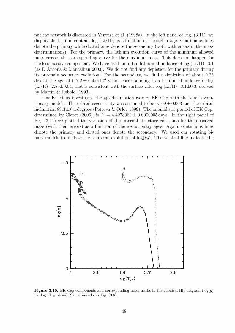
nuclear network is discussed in Ventura et al. (1998a). In the left panel of Fig. (3.11), wedisplay the lithium content, log (Li/H), as a function of the stellar age. Continuous linesdenote the primary while dotted ones denote the secondary (both with errors in the massdeterminations). For the primary, the lithium evolution curve of the minimum allowedmass crosses the corresponding curve for the maximum mass. This does not happen forthe less massive component. We have used an initial lithium abundance of log (Li/H)=3.1(as D’Antona & Montalban 2003). We do not find any depletion for the primary duringits pre-main sequence evolution. For the secondary, we find a depletion of about 0.25dex at the age of (17.2 ± 0.4)×106 years, corresponding to a lithium abundance of log(Li/H)=2.85±0.04, that is consistent with the surface value log (Li/H)=3.1±0.3, derivedby Martın & Rebolo (1993).

Finally, let us investigate the apsidal motion rate of EK Cep with the same evolu-tionary models. The orbital eccentricity was assumed to be 0.109± 0.003 and the orbitalinclination 89.3±0.1 degrees (Petrova & Orlov 1999). The anomalistic period of EK Cep,determined by Claret (2006), is P = 4.4278062 ± 0.0000005 days. In the right panel ofFig. (3.11) we plotted the variation of the internal structure constants for the observedmass (with their errors) as a function of the evolutionary ages. Again, continuous linesdenote the primary and dotted ones denote the secondary. We used our rotating bi-nary models to analyze the temporal evolution of log(k2). The vertical line indicate the

Figure 3.10: EK Cep components and corresponding mass tracks in the classical HR diagram (log(g)vs. log (Teff plane). Same remarks as Fig. (3.8).

48

Figure 3.11: Left: Temporal evolution of Lithium abundances for EK Cep range of masses (2.006-2.052M⊙ for the primary and 1.112-1.136M⊙ for the secondary). Right: The second order apsidalmotion constant as a function of the stellar age for EK Cep. In both panels we present the theoreticalpredictions of our binary rotating models. Same remarks as in Fig. (3.8).

age at which we took the internal structure constants to derive the apsidal motion rate.From the models for the observed masses and radii of the binary system, we derived theinternal structure constants for both stars at the age of (17.2 ± 0.4)×106 yr. The mod-els predict that values of k2 are 0.0035 ± 0.0007 and 0.0086 ± 0.0009, for the primaryand the secondary components, respectively. By using Eq. (3.18) we obtained the pre-dicted apsidal motion constant for the system log (k2 theo)=−2.21±0.05. From Eq. (3.2)and this theoretical value, we obtained the newtonian contribution of the apsidal motionrate (ωN=0.00040±0.00005 deg/cycle). We also calculated the relativistic contributionof the advance of periastron (ωR=0.000439±0.000003 deg/cycle), which corresponds toabout 52% of the total rate. In this way, our models predict an apsidal motion rate ofω=0.00084±0.00005 deg/cycle and, consequently, an apsidal period of Utheo=5200±300years. These values can be compared with the observed ones. Claret (2006) used a seriesof works (Khaliullin 1983b, Gimenez & Margrave 1985, Hill & Ebbighausen 1984, Claret etal. 1995, and others) to derive the observed apsidal motion rate of this system. He reportedthe observed mean value of the internal structure constant, as log(k2)=−2.09±0.09, whichis equivalent to an observed apsidal motion of about ωobs=0.00097±0.00015 deg/cycle, af-ter the relativistic correction. This apsidal motion rate produces an apsidal period ofUobs=4500±700 years. From Table (3.7), where our results are summarized, it can beseen that our predicted values are in good agreement with the observed ones and thedifferences lie within the errors. The results obtained by Claret (2006) are also reported.

49

Table 3.7: Summary of the apsidal motion related quantities.

Quantity Predicted Observational Claret 2006log(k2) −2.21±0.05 −2.09±0.09 −2.11±0.06U (years) 5200±300 4500±700 4600±400ω (deg/cycle) 0.00084±0.00005 0.00097±0.00015 0.00095±0.00008

3.9 Conclusions

For the first time, we computed values of internal structure constants for for low-masspre-main sequence stars and developed an evolutionary model that takes into accountthe combined effect of rotation and tidal forces due to a companion stars. For all sets ofmodels, namely, standard, rotating and rotating binary models, we tabulated the internalstructure constants (k2, k3 and k4) and the gyration radii (defined in Eq. 3.83) for ZAMSmodels and their temporal evolution. Our standard values were compared with thoseavailable in literature and are found to be in agreement with them. Our values for k2,obtained with our standard models, are smaller than the last published values by Claret& Gimenez (1992). Our rotating binary models produce internal structure constants evensmaller than our standard ones. We remember the reader that the observations indicatethat the values of k2 should be smaller in real stellar configurations.

In the low-mass range, the assumption that the harmonics of order greater than j=2can be neglected, widely used when analysing the apsidal motion of binary systems, seemsnot to be justified. We verify that tidal effects acts in the same way as rotational onesbut in a smaller scale. Besides, the rotationally and tidally distorted models produceopposite effects in the physical quantities of a star for masses below 1.3-1.5M⊙ and formasses above this threshold (Fig. 3.7). This behavior in distortion effects is caused bythe transition from the p-p chain and CNO cycle. The non-standard evolutionary tracksare cooler than standard ones, mainly for low mass stars (Fig. 3.3). As can be seen fromFig. (3.5), distorted models predict more concentrated stars at the ZAMS than standardmodels. Due to the combined differences between the radius and the rotational inertiaobtained with standard models and distorted ones, the gyration radii produced by thelatter models are slightly larger, for a given mass at the ZAMS, than those yielded by theformer ones.

Using our new set of evolutionary tracks computed with rotating binary models weinvestigated the evolutionary status of the interesting double-lined eclipsing binary sys-tem EK Cep. Its primary, a 2.029 M⊙ star, seems to be in the Hydrogen-burning phase,and its secondary, a solar-like star (1.124 M⊙), is confirmed as a pre-main sequence star.We followed the same approach as Claret (2006), in our analysis. Instead of using theabsolute values of the effective temperature of each component, we decide to use thestellar radii and the temperature ratio, to avoid the uncertainties involved in individualtemperatures determinations. These values were reproduced by using a model with aninitial chemical composition of (X,Z)=(0.67,0.012) and an α mixing length parameter ofα=1.5. We also followed the lithium content during the pre-main sequence evolution ofboth components. As expected, we do not find any significant depletion for the primary,while the Li depletion for the secondary agrees with the observed values within the un-certainties. The quantities related to the apsidal motion of the system were also derivedin this work (see Table 3.7). The predicted values for the apsidal motion rate and period

50

are, respectively, ωtheo=0.00084±0.00005 deg/cycle and Utheo=5200±300 years, while theobserved values are ωobs=0.0097±0.00015 deg/cycle and Uobs=4500±700. Again, differ-ences remains within the errors. As mentioned above, we were able to model EK Cepwith our rotating binary models (and with the standard ones, also). Nevertheless, someuncertainties still remain. So, our model, as well as the models proposed by other au-thors, cannot be considered as definitive. From both the theoretical and the observationalpoint of view, there are improvements that could be done in order to reduce uncertaintiesand discrepancies. On the theoretical side, we can use a better approximation for thecompanion star, by considering the simultaneous evolution of the two components of abinary system. From the observational point of view, one can reduce the uncertainties onthe absolute dimensions, specially on the effective temperatures.

51

Chapter 4

Theoretical Values of the Rossby Number

4.1 Introduction

Magnetic activity in solar-type stars encompasses a variety of phenomena, such asstarspots, activity cycles, heated outer atmospheres, X-ray emission, and many others.The driving mechanism for this activity is generally attributed to a dynamo that resultsfrom the interaction between rotation and convective motions in the star’s outer envelope(Sect. 4.2). Theoretical work by a number of researchers indicates that for main-sequence,solar-type stars the field is generated and amplified at the tachocline, the thin layer ofdifferential rotation between the convection zone and the nearly rigidly rotating radiativeinterior. For stars of spectral type ranging from mid-F to early-M dwarfs, rotation andactivity are thought to be controlled by this process, also called an α−Ω dynamo (Mohanty& Basri 2003). Its efficiency is strongly dependent on the rotation rate and convectivetimescales. Young and rapidly rotating stars are, in general, very active. Specific modelsof dynamo theory, such as the α−Ω type, have been successful in explaining the qualitativefeatures of solar activity (Weiss & Tobias 2000).

Activity is strongly correlated with rotation velocity in the mid-F to mid-M dwarfs; itincreases rapidly with the projected velocity, v sin i, then saturates above some thresholdvelocity (∼ 10 km/s). This relationship is evident only down to K types. As we go from Mto M6 types the rotation activity connection becomes less clear. Mohanty & Basri (2003)analyzed rotation velocities and chromospheric Hα activity, derived from high-resolutionspectra, in a sample of mid-M to L field dwarfs. They found that, in the spectral typerange M4-M8.5, the saturation-type rotation-activity relation is similar to that in earliertypes, but the activity saturates at a significantly higher velocity in the M5.5-M8.5 dwarfsthan in the M4-M5 ones. This may result from a change in the dynamo behaviour in laterspectral types.

For fully convective stars, such as pre-MS late type stars, this theory cannot be readilyapplied, as they miss the tachocline. However, since magnetic indicators, such as activeregions and strong flaring, have also been reported for those stars, dynamo mechanismsoperating on the full convection region have also been proposed (e.g. Durney et al. 1993).

52

On the other hand, as shown in Fig. (4.1), observations of stellar activity in solar-type stars have shown a very tight relationship between chromospheric Ca II flux andthe Rossby number Ro (Noyes et al. 1984), defined as the ratio of the rotation period,Prot, to the convective turnover time, τc. The Rossby number plays an important role indynamo models, being related to the growth rate of the field. It is an indicator of rotationwhich, by its turn, indicates magnetic activity. For solar-type stars, since τc cannot bedirectly measured, Ro is generally computed through a polynomial fit of τc to the B-Vcolor index. τc(B − V ) is a theoretically-derived convective overturn time, calculatedassuming a mixing length to scale height ratio α ∼ 2 (Noyes et al. 1984).

Figure 4.1: Chromospheric Ca II flux vs. Rossby number for main sequence stars. Closed and opencircles represent “young” and “old” stars (Noyes et al. 1984).

For pre-main sequence stars, Rossby numbers have been used to study the relationshipbetween X-ray emission and magnetic fields (e.g. Flaccomio et al. 2003c, Feigelson et al.2003). In this case, however, a clear relationship between activity and rotation is not seenas in the case of main-sequence stars, and one has to resort to evolutionary models forestimating Rossby numbers.

Though current stellar evolutionary codes are not yet able to deal with magnetic fields,a first step towards that direction is the introduction of rotation on those models, as itis a key component of stellar dynamos. This is the case of the ATON 2.3 evolutionarycode, in which both rotation and internal angular momentum redistribution have beenintroduced. Such capabilities allow us to make some exploratory work towards a futureversion that can handle magnetic field generation from first principles.

We computed convective turnover times and Rossby numbers for a range of rotatinglow-mass stellar models, and discuss their behavior with time from the pre-MS to thezero-age main sequence. Some comparisons with previous work in the literature are also

53

made. A substantial part of this chapter was published in Landin et al. (2005).

4.2 The solar dynamo

In this section, we give a short description of the solar magnetic field. For a com-prehensive overview of solar dynamo theory as a whole an excellent place to start is therecent article by Ossendrijver (2003)

The stellar convective zone consists of a plasma, i.e. a gas that contains electricallycharged particles, which is continuously moving around. Since the plasma is moving,the charged particles are moving and we obtain electrical currents. However, electricalcurrents generate magnetic fields (Ampere’s law). These magnetic fields in turn generateelectric currents (Faraday’s law) and therefore we obtain the following loop: electriccurrent - magnetic field - electric current - magnetic field - electric current - magnetic fieldetc, etc. As long as this loop is not interrupted the Sun will always produce magneticfields.

However, this is a very simplified picture of the solar dynamo and does not tell usanything about the properties of the motions of the plasma. The flow of the plasma hasto fulfill certain properties for the dynamo to work. These properties are:

1. The flow has to be turbulent. A laminar flow does not work.

2. The flow has to be fully three-dimensional.

3. The flow has to be helical.

Thus we need very complicated flows in order to generate any magnetic fields whatso-ever. Another important ingredient for dynamo action is differential rotation, i.e. the factthat the Sun rotates faster at the equator than at the poles. In other words the rotationrate of the Sun varies with latitudes (but also with radius).

The lines of magnetic field of the star is stretched, twisted an folded by the motionsof the plasma within the solar convection zone. In order to increase the magnetic fieldstrength, the motions of the plasma have to continuously transform a meridional magneticfield into an azimuthal magnetic field and vice versa. A meridional magnetic field isbasically a field that points from the north to south or south to north, while an azimuthalmagnetic field points from east to west or west to east (left panel of Fig. 4.2). So, we getanother loop: meridional magnetic field - azimuthal magnetic field - meridional magneticfield - azimuthal magnetic field etc. Again the Sun will produce magnetic field as long asthis cycle is not interrupted.

Let us now describe how the flow of the plasma achieves this loop. Firstly, the so-lar differential rotation stretches the magnetic field and winds it around the Sun. Thisstretching takes a meridional magnetic field and stretches it into a azimuthal magneticfield (see Figs. 4.2 and 4.3). This only happens because the Sun rotates faster at theequator than at the pole. If the Sun would rotate at the same rate everywhere (as a solidbody) nothing would happen to the magnetic field and the dynamo would not work. Theeffect of stretching the magnetic field by differential rotation is often referred to as theomega-effect (see Fig. 4.3). Now that we stretched the meridional magnetic field into aazimuthal magnetic field we need to do the opposite. This is done by the alpha-effect

54

Figure 4.2: Azimuthal and meridional fields in the dynamo theory.

Figure 4.3: The ω-effect in the dynamo theory.

which is due to the interaction of convection and rotation. The alpha-effect basicallytakes the azimuthal magnetic field generated by the omega-effect and transforms it backinto meridional flow. Exactly how this works is at present not well understood.

4.3 Input physics

The ATON 2.3 code has many updated and modern features regarding the physics ofstellar interiors, of which a full account can be found in Ventura et al. (1998a). Someof its most important features are: most up to date OPAL (Rogers & Iglesias 1993)opacities, supplemented by those of Alexander & Ferguson (1994) for lower (T< 6000K)temperatures; diffusive mixing and overshooting; convection is treated under both themixing length theory (MLT) or the Full Spectrum of Turbulence (FST) from Canuto &Mazzitelli (1991,1992) and Canuto et al. (1996).

The approach for including structural effects of rotation and internal angular momen-tum redistribution in the ATON 2.3 code is described elsewhere (Mendes et al. 1999a,2003). Angular momentum losses in the star’s external layers due to magnetized stellarwinds are also taken into account, in the form of a boundary condition at the surface.We adopted the prescription used in Chaboyer et al. (1995) with a “wind index” n = 1.5,

55

which reproduces well the Skumanich (1972) law v ∝ t−1/2:

∂J

∂t= K

(

R

R⊙

)2−n (M

M⊙

)−n/3

ω1+4n/3, ω < ωcrit, (4.1)

∂J

∂t= K

(

R

R⊙

)2−n (M

M⊙

)−n/3

ωω4n/3crit , ω ≥ ωcrit, (4.2)

where ωcrit introduces a critical rotation level at which the angular momentum loss satu-rates. The constant K in our models was calibrated by adjusting a 1M⊙ model so thatits surface velocity matches the current solar rotation rate at the equator.

4.4 Rossby number calculations

Convective turnover times and Rossby numbers were computed for models rangingfrom 0.6 to 1.2M⊙ (in 0.1M⊙ increments) with solar chemical composition. For ease ofcomparison with a previous work by Kim & Demarque (1996), that provided the firsttheoretical calculations of Rossby number, convection was treated according to the MLT,with the free parameter α set to 1.5 (which fits the solar radius at the solar age for a graynon-rotating model). Rotation was modeled according to rigid body law in convectivezones and local conservation of angular momentum in radiative regions (Mendes et al.1999a). The initial rotation for all models was taken from the Kawaler (1987) relationsbetween mass and angular momentum for low-mass stars (see Eq. 3.100).

Fig. (4.4) depicts the rotation period as a function of age for all models, and shows thetypical spin-up during contraction followed by the longer phase of continuous spin-down.

Figure 4.4: Rotation period plotted against age, for each model mass.

56

For the 1M⊙ model, this results in an initial velocity of nearly 3 km s−1 at the beginningof the Hayashi phase. This is about one order of magnitude below the value used by Kim& Demarque (1996), but we decided to adopt a lower initial rotational velocity because,in this way, our models are able to reproduce the observed angular velocity of TTauristars at the corresponding age. The local convective turnover time, τc, was calculated ata distance of one-half the mixing length, αHP/2, above the base of the convection zone.Its value is computed through the equation τc = αHP/v.

Fig. (4.5) shows the temporal evolution of the local convective turnover time (in sec-onds). For a given mass, it decreases during the Hayashi contraction and reaches itsminimum when the contraction stops. After that, τc remains constant until the starsreach a main sequence configuration.

Figure 4.5: “Local” convective turnover times as a function of age for all models.

However, most relevant for our purposes are Figs. (4.6) and (4.7), which show theprofiles of the “global” convective turnover time, defined as

τc =∫ R⋆

Rb

dr

v, (4.3)

and the “dynamo number” Ro−2, respectively, as functions of age. These figures show thatτc also decreases substantially during contraction to the ZAMS, but after that remainsnearly constant and depends only on the mass. With regard to Ro, it is seen that it followsτc during contraction but, after that, increases as expected since the rotation period alsoincreases.

By using the evolutionary tracks, we constructed a set of isochrones for the ages of0.2, 0.5, 0.7, 1.0, 2.0, 4.55 (solar age), 10 and 15 Gyr. In Table (4.1), we list theircharacteristics, such as stellar mass (column 1), logarithm of the effective temperature

57

Figure 4.6: “Global” convective turnover time as a function of age for each model mass.

Figure 4.7: The dynamo number as a function of age for each model mass.

(column 2), logarithm of the stellar luminosity (column 3), global convective turnover time(column 4), dynamo number (column 5) and the rotation period, in days, (column 6). Inthe left panel of Fig. (4.8), we show a plot of the global convective turnover time versusTeff for each mass model. The local convective turnover time gives the same result asthe global τc except for a scaling factor (Kim & Demarque 1996), because the convectiveturnover timescale is weighted towards the deepest part of the convection zone, where the

58

shortcomings of the mixing length approximation are least important. Isochrones for theglobal convective turnover time versus period are shown in the right panel of Fig. (4.8).

Figure 4.8: The global convective turnover time as a function of effective temperature and age (left)and the same quantity as a function of rotation period and age (right).

In the left panel of Fig. (4.9), we show the rotation period versus the logarithm of theeffective temperature. The rightmost points (those with the lowest temperatures) corre-spond to the lowest mass considered, namely, 0.6M⊙. In our models, we treat rotation,in convective zones, according to the rigid body law and, in radiative regions, rotationwas modeled by assuming local conservation of angular momentum. To the best of ourknowledge, this is the best way to mimic stellar rotation. If we assume that it is a correcttreatment for stellar rotation, Fig. (4.9) can be used to uniquely determine the mass andthe age of a star by observing its effective temperature and the rotation period. In theright panel of the same figure, we plotted the inverse square of the Rossby number versusthe rotation period. Once more, the rightmost point of each line represents the lowestmass. Also this figure can be used to infer an stellar mass and age from observationalquantities. In this case, measurements of rotation period and an activity index (relatedto the Rossby number) are useful to estimate stellar mass and age. Of course, thesedeterminations are model dependent and are subjected to the assumptions made in eachmodel. Our predictions for the dynamo number differ quantitatively from that of Kim &Demarque (1996) by two orders of magnitude. This difference is addressed to a differentinput value used in both works for the angular velocity.

Fig. (4.10) shows the dynamo number Ro−2 as a function of effective temperatureand age. After establishing an empirical relation between Ro−2 and magnetic activityindices, one can use Fig. (4.10) to determine the stellar mass and age from the effectivetemperature and an activity index.

We believe that this set of results can be useful to support observational studies ofactive pre-main sequence stars, as well as for testing stellar models against observations.

59

Figure 4.9: Left: Rotation period as a function of effective temperature and age. Right: The dynamonumber as a function of rotation period and age. For clarity, we do not report the 15 Gyr isochron.

4.5 Conclusions

To the best of our knowledge, the only work that reports Ro calculations for rotatingpre-main sequence stars is the one by Kim & Demarque (1996). Our results show thesame trends for Ro and τc found in that work, such as, for example, the decrease of τcduring the pre-main sequence phase and its nearly constant value from that point on.The main difference occurs in the values of Ro: in certain cases, our values are lower bytwo orders of magnitude. Though a full analysis of these discrepancies are still going on,they can be traced at least to differences in the initial rotation rates and internal angularmomentum mechanism adopted in both cases.

60

Figure 4.10: Dynamo number as a function of temperature and age (days) for isochrones of 0.2, 0.5,0.7, 1.0, 2.0, 4.55 (solar age), 10 and 15 Gyr.

61

Table 4.1: Isochrones for all models.

Mass τc Rotation(M⊙) log (Teff) log (L/L⊙) (days ) Ro−2 Period (d)

0.2Gyr0.60 3.6149 −1.13415 120.2859 4863.1904 0.75370.70 3.6508 −0.85839 93.5565 4295.6924 0.61560.80 3.6880 −0.60034 78.0725 3979.4875 0.51090.90 3.7221 −0.36201 57.8066 1798.2704 0.57931.00 3.7489 −0.14360 43.3016 1312.1923 0.51071.10 3.7698 0.05327 30.7249 840.2523 0.42901.20 3.7908 0.23910 14.7793 135.7796 0.5523

0.5Gyr0.60 3.6147 −1.12873 122.2169 63.0188 6.58570.70 3.6511 −0.85175 94.6016 226.0953 2.67790.80 3.6900 −0.58831 73.6797 292.8649 1.89390.90 3.7244 −0.34844 58.0709 278.6011 1.48711.00 3.7514 −0.12971 42.1280 280.3475 1.03781.10 3.7738 0.07390 27.3749 228.5956 0.79491.20 3.7940 0.26196 13.0489 41.0794 0.8864

0.7Gyr0.60 3.6145 −1.12643 123.7466 16.8957 13.16070.70 3.6512 −0.84898 93.7444 34.1065 6.88750.80 3.6903 −0.58609 73.9136 120.0507 2.95800.90 3.7249 −0.34448 57.0625 88.3630 2.43771.00 3.7522 −0.12387 42.2890 109.0130 1.67351.10 3.7750 0.08300 26.4771 78.0264 1.26221.20 3.7950 0.27319 12.7794 23.3266 1.0950

1Gyr0.60 3.6146 −1.12405 125.1279 9.9933 17.08560.70 3.6516 −0.84516 93.3750 11.2314 11.98790.80 3.6909 −0.58074 74.3170 15.2874 8.28200.90 3.7257 −0.33755 56.8681 13.2240 6.31011.00 3.7530 −0.11541 41.5055 20.7376 3.86141.10 3.7761 0.09587 26.5180 12.8111 3.17731.20 3.7962 0.29010 11.7439 9.1811 1.6389

2Gyr0.60 3.6150 −1.11848 124.0540 4.7964 24.61710.70 3.6524 −0.83706 93.7042 4.3440 19.25090.80 3.6927 −0.56723 75.4010 4.0526 16.06030.90 3.7277 −0.31785 56.6820 2.6826 14.06121.00 3.7553 −0.08623 41.0925 1.5957 13.01181.10 3.7784 0.13731 24.3629 0.5856 12.90891.20 3.7979 0.34697 10.1410 0.2333 9.1969

4.55 Gyr0.60 3.6164 −1.10583 123.8610 2.0500 37.59700.70 3.6550 −0.81612 93.5239 1.6472 31.20730.80 3.6971 −0.53350 71.1808 1.3054 27.28480.90 3.7328 −0.26479 53.8329 0.8621 25.14101.00 3.7605 −0.00313 38.5843 0.3882 25.47021.10 3.7807 0.25745 21.7490 0.1025 28.0496

10 Gyr0.60 3.6197 −1.07964 121.5720 0.8441 56.42120.70 3.6611 −0.77012 91.0848 0.6311 47.93520.80 3.7071 −0.45204 70.1379 0.4487 43.88890.90 3.7429 −0.12265 51.3548 0.2098 44.9542

15 Gyr0.60 3.6229 −1.05529 119.5294 0.5580 69.38820.70 3.6677 −0.72121 90.7505 0.3918 60.48670.80 3.7164 −0.35712 66.5298 0.2118 59.0670

62

Chapter 5

Non-Gray Atmospheres

At any point inside a star, photons of different energies may be found traveling invarious directions. These photons constitute the radiation field at a particular point andtime. Photons passing through matter may be scattered or absorbed by atoms, ionsand molecules. They may also be emitted as a result of charged particle motions, orfrom excited atomic and molecular states. These processes, taken collectively, result inmodifications of the radiation field passing through matter. When this happens the matterand the radiation are coupled.

The energy flows through the star, from the interior to the atmosphere, and thisflux can be transported by three mechanisms: radiative transfer, convective transportand conduction. The efficiency of these process is mainly determined by the quantityof energy to be transported by the particles of the medium, by the number of existingparticles and by their velocities. Besides, the opacity of the material to the motion of theparticles that carry the energy plays an important role in the process of energy flow. Theenergy transport in atmospheres of most stars is radiative. In this case, the opacity ischaracterized by the cross section of the particles and by their numerical density.

In order to understand the processes that take place when the light is radiated to space,we use an equation that describes the energy transport through the stars, the Radiative

Transfer Equation (RTE). One of the great problems in stellar atmospheres is to findout a solution to this equation, because in the outermost regions of a star the mean freepath of the particles is large and the diffusion approximation is not valid. The nature ofthe transfer equation depends on the geometry of the medium through which the energyflows. The source function, which is the local contribution given to the radiation field, isinfluenced by the nature of the physical medium. Sometimes the source function dependson the radiation field itself. So, for each different condition existing in atmosphere, wewill have a different solution of the RTE.

As getting formal solutions of the RTE is not a simple task, theoretical astrophysicistshave been seeking solutions to an idealized radiative transfer problem known as the gray

atmosphere. In the gray atmosphere approximation the increase of the temperature Tfrom the surface moving inwards is described via a relationship between T and the op-tical depth (τ), and the pressure is calculated by integrating the hydrostatic equilibrium

63

equation. The matching between the interior and the external layers is made at τ=2/3.Substantially, any link between pressure and temperature, fixed by the either convectiveor radiative gradient, is ignored. This approximation has the advantage that a completesolution can be obtained for the radiation field irrespective of the physical details of theatmosphere. In the gray atmosphere approach, the opacity is independent of frequency.Thus, all frequencies can be treated equally, as far as the radiative transfer is concerned.The independence of the radiative transfer from frequency has the interesting consequencethat all aspects of the mathematical description are independent of frequency. But, onthe other hand, we know that the physical processes of interaction between radiation andmatter are not frequency independent. Certainly, bound-bound transitions cannot beconsidered as gray processes. However, there are some bound-free transitions that exhibitonly weak frequency dependence over substantial regions of the spectrum. If those regionsare responsible for the part of the spectrum containing most of the radiant flux, then theatmosphere will be very similar to a gray atmosphere. Absorption due to the H− ion isrelatively frequency-independent along the visible part of the spectrum, and in some starsit is the dominant source of opacity. However, the main source of a gray opacity is theelectron scattering. Thompson scattering by free electrons is frequency-independent bydefinition, and for stars hotter than about 25,000 K, it is the dominant source of opacityalong the range of wavelengths encompassing the maximum flow of energy. Thus, the Oand B stars have atmospheres that, to a very high degree, may be regarded as gray ones.

Very low mass stars are characterized by effective temperatures in the range of 2000K≤Teff≤5000K, whereas brown dwarfs and extra-solar giant planets can cover a much coolertemperature regime, down to 100K. Such low effective temperatures allow the presence ofstable molecules, whose bands constitute the main source of absorption along the charac-teristic frequency domain. Such particular conditions are responsible for strong non-grayeffects and significant departure of the spectral energy distribution from a black bodyemission (Baraffe & Allard 1997). Observations of cooler stellar and sub-stellar objectshave revealed the presence of a wide variety of molecular absorbers and numerous con-densates that complicate accurate modeling of these cool stellar atmospheres (Allard etal. 1997). In the non-gray treatment, a self-consistent integration is performed down toan optical depth at which the diffusion approximation is valid (Morel et al. 1994), andincludes the treatment of atmospheric convection, which cannot be neglected at low Teff ’s.The use of frequency-dependent opacities may also modify the onset of convection withinthe atmosphere, and both the Teff and the colors of the tracks can be strongly affected.The necessity of adopting outer boundary conditions based on realistic non-gray atmo-sphere models for the pre-MS and low mass MS was pointed out by Chabrier & Baraffe(1997) and references therein, who have shown that the use of radiative T(τ) relations orgray atmosphere models is invalid when molecules form near the photosphere, at Teff be-low 4000K. Outer boundary conditions based on the gray assumptions yield hotter modelsfor a given mass. According to Baraffe et al. (1998) the use of an inappropriate outerboundary condition, such as the Eddington approximation, yields an overestimation ofTeff for a given mass up to 300 K.

64

5.1 Convection treatment in the atmosphere

The analysis made by Heiter et al. (2002) revealed that spectroscopic and photometricobservations are best reproduced by the models when using an inefficient convectiontreatment in atmospheres. Convective transport of energy in stellar atmospheres is one ofthe most complex astrophysical problems. Many of the approximations usually admittedfor the stellar interior, such as diffusive radiative transfer, are no longer valid. Moreover,through most of a convective stellar atmosphere, radiative losses are large enough to makeconvection less efficient in transporting energy than radiation. Only stars which have asurface convection zone extending deep into the stellar envelope can maintain efficientconvective energy transfer near the bottom of their atmosphere.

One strong motivation to apply a more complete description of stellar turbulent con-vection stems from the result that low values of the scale length parameter α, e.g., 0.5, arerequired to fit Balmer line profiles for the sun and other cool dwarfs (Fuhrmann 1993),while much larger values (between 1 and 2) are necessary to reproduce their observedradii (Morel 1994). Likewise, α has to be varied over an even larger domain (1<α<3) toreproduce the red giant branch in HR diagrams of galactic open clusters and associationsfor stars with masses ranging from 1M⊙ to 20M⊙ (Stothers 1997, 1995).

D’Antona & Montalban (2003) have shown that a stellar model is fully describedonly when we specify not only the atmospheric model used as boundary conditions tothe interior, but also the convection parameters used for the atmospheric grid, includingthe value of the optical depth at which the boundary conditions are taken, that is, thephotospheric matching point, τph. In fact, until now, the expensive model atmospherecomputations have been generally performed only for one specific convection model, e.g., agiven ratio of mixing length to pressure scale height, in the Mixing Length Theory (MLT),α=αatm. The value of α can be changed only in the computation in the interior (α=αin),e.g. to fit the solar radius in the solar model. However, if a large value of τph is chosen asmatching point between the atmosphere and the interior, the most superadiabatic part ofthe convection zone is all included in the atmosphere. Consequently, the changing of αin

does not affect the model in the same way as a full change the convection parameter inthe whole model, including the atmosphere.

There is broad consensus in the literature that the treatment of superadiabatic con-vection in the pre-MS affects the tracks location to a great extent. In a series of worksfocusing on understanding the role played by different physical inputs on the pre-MS evo-lution, D’Antona & Mazzitelli (1997), D’Antona & Montalban (2003), and Montalban etal. (2004) outlined the major impact of convection modeling on the location of the stellartracks in the HR diagram. Convection was found to be by far the most relevant ingredientinfluencing the determination of the mass and age of observed stars.

When modeling convection, it is essential to specify the mixing scale Λ, i.e. the typicaldistance that convective eddies travel before dissolving and delivering their excess gravo-thermal heat to the environment. The role played by Λ is relevant for the determinationof the temperature gradient, as the conservation of flux implies that a larger Λ mustbe compensated by a lower degree of overadiabaticity. The convective flux behaves asFC∼Λ2 in zones where most of the energy is carried by convection. Conversely, withinlow efficiency convective regions, FC∼Λ8. The impact of the choice of Λ is therefore moreevident where convection is not efficient. The pre-MS tracks result to be particularlysensitive to convective modeling, because the surface convection extends to most of the

65

(if not the whole) star, and the low densities involved (particularly in the early phases ofgravitational contraction) make the convective process highly inefficient.

Presently, the main ways of computing convection in stellar envelopes, for wide gridsof stellar models, are:

1. The traditional mixing length theory — MLT (Bohm-Vitense 1958, and subsequentvariations of this same model) — assumes that both the dimension of the convectiveeddies and the mixing length are proportional to the local value of the pressure scaleheight, i.e. Λ = αHp, where α is a free parameter that is usually calibrated in orderto reproduce the solar radius.

2. In the Full Spectrum of Turbulence model — FST (Canuto et al. 1996) — the wholespectrum of eddies’ dimensions is considered, and the mixing length is taken as thedistance of the nearest convective border.

3. MLT, in which the α value for each gravity and Teff is calibrated upon 2D or 3Dhydrodynamical simulations.

Ludwig et al. (1999), using their 2D radiation hydrodynamic models, have provided acalibration of the parameter α in a wide region of Teff ’s and gravities1 to be used inthe computation of gray stellar models. These 2D models indicate that convection inthe pre-MS is on average more ‘efficient’ than in the MS, corresponding to a larger α.The idea of calibrating the average α using numerical simulations has been extendedby now to a few 3D computations: Ludwig et al. (AHS, 2002), for an M dwarf at Teff

= 2800 K and log(g)=5, find α ≃2.1; and Trampedach et al. (1999), for the range ofmain sequence gravities and log Teff=3.68–3.83, find α ≃1.6–1.8 in the whole range.Asplund et al. (2000) have compared 2D and 3D atmosphere models of the Sun, andfound that the 2D solar model has marginally larger gradients than the 3D one. Althoughan extrapolation to regions not explicitly computed is not allowed, these few 3D models,also indicate efficient convection in the overadiabatic envelope. Montalban & D’Antona(2006) have computed gray models by using this calibration: the tracks they obtain arevery similar to the FST tracks2. Unfortunately, a very efficient convection in pre-MS isnot consistent with the lithium depletion patterns of young open clusters (D’Antona &Montalban 2003). Any attempt to calibrate convection efficiency in pre-MS by meansof comparisons between binary masses dynamically determined and those assigned fromdifferent sets of evolutionary tracks, seems to be ambiguous (Landin et al. 2007).

1α is mapped in the domain Teff=4300−7100 K, log(g)=2.54−4.742The FST convection model corresponds to very efficient convection, as shown by the quasi-coincidence

of the resulting tracks with the tracks employing the MLT α calibrated on the 2D hydrodynamic models.We find confusing and misleading the statement by Baraffe et al. (2002), who point out that the FSTmodel is very inefficient in the upper solar layers, where it provides results that are not consistent with thehydrodynamic simulations of convection for the solar model (nevertheless, remember that the FST modelprovides a better fit than MLT for the spectrum of solar oscillations, see e.g. Canuto & Christensen-Dalsgaard, 1998). What matters in the description of the pre-MS is the average efficiency of convectionin the whole superadiabatic envelope, and this is very large for the FST, roughly corresponding to an αvalue in the MLT description somewhat larger than 2.

66

5.2 Non-gray boundary conditions in the ATON code

The outward integration of the structural equations of stellar interior must match theinward integration of the equations of its atmosphere at a given point. This point is thevalue of optical depth at which the boundary conditions are taken or, in other words,the photospheric “matching point” τph. This matching point can vary according to theapproximation used to obtain the atmospheric parameters.

In previous versions of the ATON code (including that by Mendes et al. 1999a, withrotation) a gray model provides the atmospheric parameters used as external boundaryconditions to the interior. The internal structure is matched at τph=2/3 with the valuesof P and T found via a Krishna-Swamy (1966) T (τ) relation.

Recently, the ATON2.0 code, without the modifications including rotation by Mendeset al. (1999a), was updated with non-gray boundary conditions, by using the NextGen(Allard & Hauschildt 1997, hereafter AH) and the ATLAS9 (Heiter et al. 2002) atmospheremodels.

In the non-gray tracks presented by Montalban et al. (2000), the NextGen atmospheremodels were used as boundary conditions. The AH grid is available for the followingranges: 3.5≤log(g)≤6.0 in gravity, −2.0≤[M/H]≤0.0 in metallicity and 1500 K≤Teff≤10,000 K in temperature. The AH models adopt classical Mixing Length Theory (MLT)with α=1.0.

After that, the ATLAS9 atmosphere models were included in the ATON2.0 code, pro-viding another alternative to establish the atmospheric parameters (Montalban et al.2001). In these models convection is treated either in the Mixing Length Theory (MLT)or in the Full Spectrum of Turbulence (FST) formulation. Both ATLAS9 grids, the MLT(with α=1.25) and the FST formulations are used to treat the convection in the atmo-sphere. They are available for metallities ranging from [M/H]=−2.0 to +1.0 dex, but onlythe tables with solar metallicity was incorporated in the ATON2.0 code. These grids rangefrom 2.0 to 5.0 in log(g) and from 4,000 K to 10,000 K in effective temperatures.

In order to follow the evolution of very low mass stars starting from early, low-gravitystages, we implemented in the code the PMS tables with the more recent low-gravitymodels by Allard et al. (2000), hereafter AHS. These PMS models can be understoodas an extension, towards low gravities and low temperatures, of the the already referredNextGen models. The AHS grid is available for the solar metallicity, for gravities in therange of 2.0≤log(g)≤3.5 and temperatures in the interval of 2,000 K≤Teff≤6,800 K.

The NextGen and PMS original tables, besides a lot of other information, give us thetemperature, pressure, physical depth, extension of the convective zone and density valuesfor several optical depths ranging from 0.0 to 100 for a given combination of effectivetemperature and gravity. By using linear interpolation, we created a simplified tablecontaining the physical quantities cited above for each of the following typical values ofoptical depth: τ=1, 3, 10 and 100.

Instead of using two different NextGen derived models, we merged the original NextGentables with their PMS counterparts. Eventually, we obtained rectangular tables in therange 2≤log(g)≤6 and 2000 K≤Teff≤6800 K.

After the present work, the ATON2.4 code can now, besides the inclusion of the effectsof rotation (Mendes et al. 1999a), determine the boundary conditions to the interior byusing not only the classical gray models, but also the MLT and FST grids of the ATLAS9,the NextGen and the PMS non-gray models. For all these non-gray models, the match

67

with the interior can be done at four different optical depth, τ=1, 3, 10 and 100. Oncethe optical depth is chosen, P (τ), T (τ) and ρ(τ) are obtained by third order interpolatingtheir values in the Teff vs. log(g) plane.

5.3 Applications of the new rotating non-gray ver-

sion of ATON2.4 code

This new version of the code was used to generate new sets of rotating non-gray pre-MStracks, in order to analyse the rotational properties and evolution of a sample of young pre-MS stars in the Orion Nebular Cluster (ONC, Landin et al. 2006). In order to analyzethe importance of convection in the pre-MS and in the ONC rotational properties, wecomputed three different sets of models by varying the mixing lenth parameter: α=1.0,α=2.0 and α=2.2. Our main goal is to improve our understanding of the appropriatephysical constraints to be used for a general description of the evolution of stellar structureand its angular momentum with time. We are particularly interested in the choice of thestellar initial angular momentum and its variation with time and, also, in the importanceof convection efficiency during the pre-MS. To do this, we check our models with respectto sets of relevant observations. A substantial part of this chapter was published in Landinet al. (2006).

5.3.1 An overview of theoretical pre-main sequence models

Since the pioneering works by Henyey et al. (1955) and Hayashi (1961), it is commonlyaccepted that pre-MS stars derive their luminosity by gravitational contraction, with theonly exception of the short deuterium burning phase. Derivation of masses of youngstellar associations has, then, generally been made by standard hydrostatic stellar modelsincluding deuterium burning, an approach that we will use in this work. This procedurerests on the assumption that neither the residual accretion after the protostellar phasenor the uncertainty in the zero point of ages affect the results in a strong way.

Nevertheless, the theoretical description of moderately low and low mass objects isaffected by the first principle uncertainties in the description of some physical inputs,in particular opacities, convection, equation of state (D’Antona 1993) and treatmentof boundary conditions (BCs, Chabrier & Baraffe 1997). Since the low mass stars inthe pre-MS are fully convective and over-adiabatic, any change in the convective modelsubstantially alters the location of the track in the theoretical HR plane. The use of a lessefficient treatment of convection leads to larger temperature gradients, so that, for a givenluminosity, the structure readjusts on a more expanded configuration, with a consequentshift of the track to lower effective temperatures (Teff) (e.g. D’Antona & Mazzitelli 1994,1997; D’Antona & Montalban 2003). The path followed by the theoretical pre-MS trackson the HR diagram is also dependent on the boundary conditions used to fit the numericalintegration of the structural equations of the interior with the atmosphere. The use ofa non-gray atmospheric treatment shifts the tracks to cooler Teffs within an extendedinterval of masses and ages (Montalban et al. 2004). The effect due to the non-graynessof the atmosphere is, in many cases, overwhelmed by the uncertainties related to thetreatment of convection, that has a similar, but even stronger effect on the tracks, with

68

only a few exceptions that are relevant for this work, as will be discussed in Sects. (5.3.6)and (5.3.3).

5.3.2 An overview on the observational data of ONC

Young stellar clusters provide a unique opportunity to test stellar pre-MS models.Many studies in the past have been focused on the Orion Nebula Cluster (ONC), becauseit contains thousands of pre-MS objects. Hillenbrand (1997) measured the V and I mag-nitudes (and colors) of ∼900 stars and located them in the theoretical HR diagram byusing bolometric corrections and taking into account the interstellar extinction for thedetermination of colors and bolometric magnitudes. In spite of the non-negligible uncer-tainties weighting on the derivation of these stellar parameters (Hillenbrand et al. 1997),such a work has been widely used, in connection with theoretical pre-MS tracks, to inferimportant information concerning the cluster itself. The mass and age distributions andthe slope of the mass function can all be estimated by inferring the appropriate mass andage for each observed star. It is clear that the results obtained with this approach willdepend to a certain extent on the set of tracks used to perform the analysis, and on thephysical inputs adopted to calculate the evolution. This is confirmed by the fact that,specifically for the ONC, studies that used different sets of evolutionary tracks reachedsignificantly different conclusions, particularly with respect to the mass and age distri-bution, and, more important, to the age spread and, consequently, to the evolutionaryhistory of the star formation process within the cluster (Palla & Stahler 1999).

In the past few years, new detailed observational studies of the ONC have been under-taken, focused on the rotational properties of the stars. Stassun et al. (1999) and Herbstet al. (2002) measured the rotational periods of ∼400 stars belonging to the ONC. All ofthem are in the Hillenbrand (1997) sample, so they can be located on the HR diagram.More recently, Stassun et al. (2004) and Flaccomio et al. (2003a, 2003b) reanalyzed allthe archival Chandra observations of the ONC studying in great detail the X-ray prop-erties of the observed objects, in an attempt to elucidate the origin of X-ray emission inpre-MS stars. All this available information renders the ONC an excellent laboratory totest stellar evolution theories of the pre-MS phase.

None of the previous analyses of the ONC rotational database has been done using non-gray models, and the effect of using different convection efficiencies has not been exten-sively tested. We therefore decided to use this database to test and calibrate our new setsof non-gray tracks for rotating stellar models, with masses in the range 0.085≤M/M⊙≤3.8.As a byproduct, we will have insight on how much the rotational properties of this popu-lation depend on the choice of the evolutionary tracks. At present, there is no definitiveobservational constraint that can be used to choose among the tracks obtained by usingdifferent convection inputs. In this work we derive masses and ages with different sets, inorder to appreciate how much the results we are presently interested in, namely those onthe angular momentum evolution, depend on the choice. In particular, we will test therole of (a) boundary conditions (gray and non-gray), (b) different convection efficienciesin the framework of the MLT, and (c) rotating and non-rotating models.

As indicated by the non-negligible differences among the set of tracks adopted, weshow that the detailed period distribution as a function of mass and age is dependent onthe physical inputs. However, the qualitative information on the rotational distribution ofstars of different mass in the ONC remains similar, and we confirm that the distribution

69

of periods is bimodal only for masses larger than a “transition” mass depending on theconvection model.

5.3.3 Physical input of the models used to analyze the ONCstars

Figure 5.1: Paths followed by the theoretical tracks (left) and isochrones (right) of the rotating modelscalculated with three different values of the free parameter α determining the mixing length. For clarity,we report only the following masses calculated with our three sets of tracks (α1.0, α2.0, α2.2): 0.09, 0.1,0.2, 0.3, 0.35, 0.5, 0.7, 1.0, 1.4, 2.0, 2.5, 3.0, 3.3 and 3.8 M⊙ from bottom to top. The observational datafrom Hillenbrand (1997) are represented by • symbols.

We computed pre-MS stellar evolutionary tracks in the mass range 0.085≤M/M⊙≤3.8.We adopted the solar chemistry with Z=0.0175 and Y=0.27, while the starting deuteriumabundance in mass fraction, following Linsky (1998), was set to X(D)=2×10−5. Theevolution starts from a fully convective configuration with central temperatures in therange 5.3<log (Tc)<5.8, follows deuterium and lithium burning and end at the mainsequence configuration. The micro-physics inputs (opacities, equation of state, nuclearnetwork) were the same used in the distorted models presented in Sect. (3.6).

5.3.3.1 Boundary conditions

The boundary conditions were obtained with our new rectangular table (NextGen +PMS models) at τ=10. The ATLAS9 tables were not used because, since they are availableonly for temperatures above Teff=4000 K, they cannot be used to compute models below∼ 0.7M⊙. Consequently, the FST formulation was not used to treat convection in ouranalysis. Gray models were computed for comparison with previous results.

70

The gray tracks of models with α=1.0 are systematically hotter than their non-graycounterparts, although the difference in Teff varies with the mass. For the lowest massesof our sample, i.e. M≤0.2M⊙, the high gravities allow the differences to remain within∆Teff∼100 K. This difference increases to ∼250 K at 0.6M⊙ and reaches a maximum of∼400 K in 1M⊙ models, the largest differences happening at the end of the Hayashi track,as can be seen in Fig. (5.3). The stars for which the pre-MS tracks are most sensitiveto the boundary conditions are those with masses in the range 0.4M⊙≤M≤1M⊙: thedifference in Teff slightly increases along each track, and reaches a maximum of ∆Teff∼400 K, when the radiative core is formed.

The Teff of more massive stars are less influenced by the atmospheric treatment. Thesedifferences in Teff lead to the assignment of a different mass to a given observed star. Weverify that, consistent with the above discussion, this effect is negligible for the lowestmasses, while it leads to differences of the order of ∼0.1M⊙ for M∼0.3−0.5M⊙, where, aswe shall see, the bulk of the ONC population is found. For larger masses the differencesare larger because the tracks for different masses are closer to each other.

5.3.3.2 Convective treatment

Apart from the quoted cases, in which α can be calibrated on hydrodynamic models,the necessity to simplify the numerical treatment of convection leads stellar modelists touse a single α for the convection zone and for all the evolutionary phases. This choiceis equivalent to adopting an average efficiency of the convective transport on the wholeextension of the convective region, and on all the evolutionary phases. There is no goodreason to assume that the α that, e.g., fits the solar radius should be used for othermasses and for different evolutionary phases. Further, the efficiency of convection mightchange considerably within a convective zone, thus requiring the use of a variable α. Thusa preliminary investigation of the effects of changing this parameter is mandatory. Wecomputed sets of models with three different values of the α parameter: the models withαin=2.0 (α2.0 set) allow a fit of the solar radius for non-rotating models3; the models withαin=2.2 (α2.2 set) are chosen to provide a “very efficient convection” set. Both these setsare termed HCE (high convection efficiency) sets. We further provide tracks with αin=1.0(α1.0 set), which define our LCE (low convection efficiency) models . This latter choice,according to D’Antona & Montalban (2003), confirmed in Sect. (5.3.3.5), leads to a betteragreement with the lithium vs. Teff relation observed in young open clusters stars. Re-member, however, that the adopted BCs come from model atmospheres computed, downto τph=10, with αatm=1.0 (see the discussion in Sect. 5.2 and in Montalban et al. 2004).We show in Fig. (5.1) the comparison between tracks (left panel) and isochrones (rightpanel) of these three sets, showing the well known fact that both masses and ages areaffected by the choice of the convection model. The observed stellar loci are also reported.In the early phases, with the exception of the D-burning phase, gravitational contractionis the only source of energy. The densities and temperatures increase until the centralregions become radiatively stable; shortly after, H-burning takes over as the main energysource. We see from the left panel of Fig. (5.1) that the α2.0 and α2.2 tracks are system-atically hotter, the differences being larger for higher masses and smaller for older ages.This behavior can be understood on the basis of the different degree of overadiabaticity

3Also Baraffe et al. (1998) and Montalban et al. (2004) find a similar αin (=1.9) to reproduce the solarradius.

71

present in the various masses at different ages. The exact temperature profile depends onthe overadiabaticity (∇−∇ad), which is defined as the excess of the effective temperaturegradient in comparison with the adiabatic temperature gradient, and it is only noticeablydifferent from zero at the border of the convective zone, where convection becomes inef-ficient. We investigated the evolution of the degree of overadiabaticity at τ=10 for somemass tracks and for the three values of the mixing length parameter (α) used in this work.We found that the lower the α parameter, the higher the overadiabaticity at τ=10.

The two panels of Fig. (5.2) show, respectively, the evolution of the overadiabaticityat τ=10 and of the width (in solar masses) of the external region of the star where(∇−∇ad)>10−4. For clarity we report only the α1.0 and α2.0 models. The luminosity ison the abscissa as a time indicator. A detailed inspection of Fig. (5.2) shows:

1. the overadiabaticity at τ=10 of the α1.0 models is systematically higher than theirα2.0 counterparts. This can be understood on the basis of the intrinsic lower effi-ciency of the convective model adopted, due to a lower mixing length;

2. due to the higher internal densities of the less massive models (hence, greater con-vective efficiencies), the overadiabaticity differences increase with the mass;

3. in the less massive models the differences above tend to narrow with age;

4. the extension in mass of the overadiabatic region is also systematically higher in theα1.0 models, and tends to shrink with age.

We verified that models of the same mass belonging to the two sets of tracks follow thesame L(t) relation. The differences in the location of the tracks are, therefore, to be totallyascribed to differences in the effective temperatures. Since the interior of these structuresis practically adiabatic (in the center, (∇−∇ad)<10−7 in all cases), the radius is mainlydetermined by the degree of the overadiabaticity. This explains why larger differences arefound for higher masses. In the lowest masses the efficiency of convection increases atolder ages, so that the sensitivity to the adopted model for convection is strongly reduced.The low mass tracks approach each other at low luminosities (see Fig. 5.1).

5.3.3.3 The role of convection coupled with the non-gray atmospheres

We note a point that is generally overlooked, but that is crucial in order to understandthe relevant parameters in track building: Montalban et al. (2004) have shown that theproblem of convection is intertwined in a subtle way with the problem of non-gray bound-ary conditions. For example, in the MLT framework, convection in the pre-MS should bedescribed not only by the ratio α = l/Hp in the interior of the star (αin), below the non-gray atmosphere, but also by the value that this parameter has in the atmosphere itself(αatm), and by the matching point between atmosphere and interior (τph). In particular,the two widely used sets of model atmosphere by Baraffe et al. (1998) are referred to asthe set built with α=1.9 and the set having α=1.0. Thus, they are supposed to providea clue to how the tracks vary by changing from a moderately high convective efficiency,represented by the set α=1.9, to a low convection efficiency represented by the set α=1.However, in Baraffe et al. (1998), the parameter α refers only to the value of αin, and ismisleading for two reasons: (1) the set αin=1.9 stops at masses M≥0.6M⊙, and only theset αin=1.0 is available for masses M<0.6M⊙; (2) for both sets, the atmospheric model

72

Figure 5.2: Left: Variation with luminosity of the overadiabaticity of the stellar layer at τ=10 of somepre-MS models calculated with different values of the parameter α entering the mixing length expression.Right: The variation with luminosity of the fraction of the mass of the star where (∇ − ∇ad) > 10−4,for the same masses shown in the left panel. For clarity we show only models α1.0 and α2.0.

grid adopted is the same, and computed with αatm=1.0. Montalban et al. (2004) haveshown that the fact that most of the superadiabatic part of the envelope is computed witha very inefficient convection (αatm=1.0) shifts the Teff by ∼150K for the solar pre-MS.Thus, one may be led to attribute the smaller Teff of the Baraffe et al. (1998) tracks tothe use of the non-gray atmospheres, whereas they are due in part to the fact that thesenon-gray atmospheres are computed with LCE.

In Fig. (5.3) we show the evolutionary tracks for 0.3, 0.4, 0.7 and 1.0M⊙, respectivelyin blue, red, magenta and black curves. Continuous lines stand for non-gray tracks withα=1.0, dotted lines refers to non-gray α=2.2 tracks and dashed lines correspond to grayα=1.0 tracks. In this figure we used non-rotating models. For the 0.3 and 0.4 M⊙ (blueand red tracks in Fig. 5.3), the mass range of interest in our analysis, we can notice thatthe role of convection is more important than that of (non-)grayness, but only in earlierphases of pre-MS. As tracks evolve in their Hayashi phases, the differences between trackswith the same boundary conditions and different convection efficiency decreases. Thedifferences between tracks with different boundary conditions and with α=1.0 remainsroughly constant during the evolution (mainly for the 0.4 M⊙), but in the bottom of theHayashi track these mass tracks are more influenced by the boundary conditions.

5.3.3.4 Rotation and initial angular momentum

Rotation was modeled according to the rigid body law. This choice is motivated bythe fact that most of the low mass stars are still fully convective in the evolutionary stagesof interest for this study. As a first attempt, the initial angular momentum Jin for allmodels was estimated according to the prescriptions by Kawaler (1987). In that work, arelationship between angular momentum and stellar mass for stars earlier than F0 was

73

Figure 5.3: Paths followed by theoretical evolutionary tracks of the non-rotating models for 0.3, 0.4,0.7, 1.0 M⊙, respectively in blue, red, magenta and black. The non-gray α=1.0 models are reported withcontinuous lines, with dotted lines we plotted the non-gray α=2.2 models and the gray α=1.0 models areshowed with dashed lines.

derived using main-sequence (MS) stellar models, and an estimate of the mean initialangular momentum-mass relation was made for stars of later spectral type. As masseslarger than about 1.5M⊙ do not lose much angular momentum during their early evolu-tionary phases, it can be assumed that these stars reach the MS with the same angularmomentum that they had at the beginning of their evolution. Kawaler (1987) was ableto reproduce the observational relation at M>1.5M⊙ using his own models for radiativestars and, then, he extended the models to lower mass stars. For these, however, theobservations do not provide a direct comparison with the initial angular momentum, astheir rotation has been slowed down during the main sequence lifetime (but not signifi-cantly during the pre-MS, if we adopt the hypothesis of pre-MS disk locking in the sameway as Bouvier et al. 1997). For the range 0.6− 1.25M⊙, the initial angular momentum-mass relation can be easily obtained from Kawaler’s (1987) work (see Eq. 3.100). Oncestarted with this initial angular momentum, we keep it constant in our models duringthe pre-MS according to the above mentioned hypothesis, whose validity will be checkedlater. This expression will then be extended to smaller masses as a result of the presentstudy. The comparisons made in this work will help us to calibrate different models ofangular momentum evolution.

Before proceeding with the analysis of the observational data of ONC, we would liketo perform another comparison between the theoretical models in order to investigate theconvection efficiency in the pre-MS on the light of lithium depletion.

74

5.3.3.5 The lithium depletion

In Fig. (5.4) we plotted, on the left panel, the temporal evolution of lithium depletionof our rotating models for 0.6, 0.7, 0.8, 0.9 and 1.0M⊙ and, on the right panel, its non-rotating counterpart. Solid curves represent the LCE models, while dotted and dashedlines refers to the HCE models. From this two panel figure, we can see that HCE modelsdeplete more lithium than LCE models. If rotation is not considered, the two HCE modelspredict roughly the same Li depletion for a given value of α. When rotation is taken intoaccount, the models, however, became much more sensitive to the convection efficiency.This result can also be seen from Table (5.1).

Figure 5.4: The temporal evolution of lithium depletion for our rotating (left) and non-rotating (right)models. The continuous lines, the dotted lines and the dashed lines stand for α=1.0, α=2.0 and α=2.2models, respectively. We report the following masses: 0.6, 0.7, 0.8, 0.9 and 1.0M⊙. We have used aninitial Li abundance of log (Li/H)=3.1.

Table (5.1) shows the lithium concentrations for our three sets of tracks and their non-rotating counterparts. We report the values for 0.7, 0.8, 0.9, 1.0 and 1.2 M⊙ at 108yr. A

Table 5.1: Lithium abundances at the age of 108yr for 0.7, 0.8, 0.9, 1.0 and 1.2 M⊙. We report thevalues obtained with different sets of our non-gray models, with (“rot”) and without (“non-rot”) rotation.The initial lithium concentration is log (Li/H)=3.1.

Models 0.7M⊙ 0.8M⊙ 0.9M⊙ 1.0M⊙ 1.2M⊙

rot α=1.0 0.540 2.397 2.877 3.016 3.081rot α=2.0 −0.991 1.459 2.057 2.510 2.939rot α=2.2 −1.171 1.256 1.899 2.382 2.884non-rot α=1.0 0.740 2.440 2.887 3.018 3.081non-rot α=2.0 −0.734 1.505 2.085 2.523 2.933non-rot α=2.2 −0.731 1.502 2.087 2.523 2.933

75

comparison between log (Li/H) found with rotating and non-rotating models, keeping αfixed, is qualitatively in agreement with the abundances found by Mendes et al. (1999a),i.e., rotating models provide greater lithium depletion especially for low-mass stars at theage in question. Another comparison between the abundances found with different valuesof α, keeping the rotation status fixed, confirms the results by D’Antona & Montalban(2003): the lithium depletion of the HCE models is too large to be consistent with thelithium depletion observed by Soderblom et al. (1993) and Garcia Lopez et al. (1994) inyoung open clusters, which can be reproduced only by the LCE α1.0 models. In Fig. (5.5),we compare the lithium depletion predicted by our three sets of models (rotating and non-rotation) with the observational data cited above. The comparison was made at 108 yr,the age of Pleiades, the young open cluster analyzed in this figure. We have normalizedthe lithium abundances in the models to an initial abundance log(Li/H)=3.1 (as D’Antona& Montalban 2003). As we can see, only circles (α=1.0) can fit the open cluster lithiumdata and the presence of rotation makes the models cooler and more lithium depleted.

On the contrary, the solar radius is reproduced only by the α2.0 model, and 2Dhydrodynamic computations indicate HCE in the pre-MS. We regard this result as anindication that the efficiency of convection in the pre-MS might be affected by otherparameter(s). The “second parameter” affecting lithium depletion is identified as thestellar rotation rate by Siess & Livio (1997) and in the papers by Ventura et al. (1998b)and D’Antona et al. (2000). The first authors propose that α is smaller in fast rotatingpre-MS stars due to the twisting of convective cells, the others show that the action of thedynamo-induced magnetic field due to the interaction of rotation and convection modifiesthe structure of the convective layers and reduces lithium depletion.

Figure 5.5: Lithium depletion vs. Teff for observational data of Pleiades from Soderblom et al. (1993)and Garcia Lopez et al. (1994) in young open clusters (crosses) compared to lithium depletion predictedby our rotating (full symbols) and non-rotating models (open symbols) at 108 yr for the three sets of αmodels. We have used an initial Li abundance of log (Li/H)=3.1.

76

5.3.4 Data from the literature - ONC

In order to study angular momentum evolution in the pre-MS phase, we compare oursets of evolutionary tracks with observational data of the ONC stars. To accomplish thisgoal we need some key parameters, such as effective temperatures and luminosities (toinfer masses and ages of the stars) and also the rotation period and an index that allowsus to distinguish between different kinds of angular momentum evolutions.

The ONC data we used have been kindly provided by Dr. Keivan Stassun, who haswidely worked on the rotational properties of ONC (Stassun et al. 1999, 2004). Our finalstudy sample is composed of a combination of data from the following sources:

1. Rotation periods: Stassun et al. (1999), Herbst et al. (2002);

2. Effective temperatures and luminosities: Hillenbrand (1997);

3. Infrared continuum excess, ∆[I−K]: Hillenbrand et al. (1998);

4. Ca II equivalent width, EW(Ca II): Hillenbrand (1997), Hillenbrand et al. (1998);

5. X-ray luminosities: Stassun et al. (2004).

The rotation period diagnostic was obtained by photometry, interpreting the periodicphotometric variability as caused by rotation, probably due to the presence of stellarspots.

The IR excess (∆[I−K]) was obtained from combined optical and infrared photometricdata. Extinction and spectral typing uncertainties are the main sources of errors in∆[I−K] estimates. For earlier spectral type stars ( <

∼ K2) the errors are negligible (<0.05mag), for spectral types in the range K2−M3, typical errors are between 0.1−0.3 mag,and it is largest for the latest spectral types, where mis-classification causes relativelylarger errors.

The EW(Ca II) was obtained from the optical spectroscopic study by Hillenbrand(1997) and analyzed by Hillenbrand et al. (1998). Their measurements uncertainty isestimated at 0.5A, based on measurements of multiple spectra of the same star.

In order to obtain more reliable values for LX of ONC stars, Stassun (2004) reanalyzedall archival Chandra/ACIS observations of these objects using updated calibrations andincluding time-filtering of flares.

The effective temperatures and luminosities were obtained from optical spectroscopyand photometry.

5.3.5 Derivation of masses and ages

For each of the three sets of tracks previously discussed, we assigned to each observedpoint a mass and an age by linearly interpolating between the two nearest tracks. Aninspection of Fig. (5.1) can help us understand, at least qualitatively, the differencesthat we should find by varying α. For each observed star in the α2.0 and α2.2 sets,we assign a systematically smaller mass than in the α1.0 models, hence a younger age(we recall that this evolutionary phase is governed by gravitational contraction, thatproceeds on a Kelvin-Helmoltz time scale τKH∝

M2

RL). If the α2.0 or α2.2 sets are used, we

therefore expect a mass distribution shifted to lower masses and, on the average, a youngerpopulation. Typical internal errors are <

∼ 0.2 dex in log(L/L⊙) for all spectral types andare <

∼ 0.02 dex in log(Teff) for late-type (K−M) stars, but increase towards earlier spectral

77

Figure 5.6: Mass (left) and age (right) histograms based, respectively, on masses and ages assigned tothe observed stars in the ONC using three different sets of tracks, calculated with three prescriptions forconvection, α=1.0, 2.0 and 2.2.

types. This leads to an uncertainty in the determination of mass that is <∼ 0.1M⊙ for

M<0.5M⊙, and gradually increases to ∼0.2M⊙ for M∼1M⊙. The attribution of age ismainly influenced by the uncertainty on the luminosity, that makes the age uncertain by∼1 Myr at the age of 1 Myr. This poses the problem of whether the age distribution wefind should be considered either as the result of a burst of star formation or as a realindication of age differences from star to star. In the course of the investigation we favoura statistical interpretation of data as an indication of some age evolution, based on theevolution of rotational periods.

The left panel of the Fig. (5.6) shows the mass distribution of the observed stars, ob-tained by using the three sets. Only masses M<1.6M⊙ are plotted because they representmost of the stars in the sample. The mass function for the α1.0 set peaks in the massinterval 0.3−0.4M⊙, but we also note the presence of a significant group of stars withmasses in the range 0.2−0.3M⊙ and another group in the interval of 0.6−0.9M⊙. Forthe HCE models, this latter group of objects becomes less relevant and the mass functionpeaks in the mass interval 0.2−0.4M⊙. The right panel of Fig. (5.6) confirms that theage distribution depends on the choice of α. We note that a slightly younger populationis obtained as the value of α increases, and, in α2.0 and α2.2 cases, a very young groupof stars appears at ages ∼1−2×105yr, but is not present for LCE (α1.0) models. Thiscan be understood by considering, in the right panel of Fig. (5.1), the relative location ofobserved points and theoretical isochrones. Age differences are also due to the differentslope of the isochrones corresponding to the two sets of tracks, which, in turn, are relatedto the differential variation of temperature with mass. In HCE models there is a groupof objects with ages clustering around 100, 000 yr. For the α2.0 case this young group ismade up of ∼40 stars and for the α2.2 set its presence is still more evident, exhibiting∼70 objects.

After analysing the rotation period of ONC stars as a function of the inferred mass,

78

Figure 5.7: The comparison between age distributions of the observed stars with assigned mass lowerand higher than Mtr. The Mtr value is 0.5M⊙ for LCE models and 0.35M⊙ for HCE models.

we define a transition mass, Mtr, for HCE and LCE models, on the basis of the rotationperiods distribution. Here we compare, in Fig. (5.7), the age distribution for two differentranges of mass, M>Mtr and M<Mtr (see the definition of Mtr in Sect. 5.3.7.1). Wesee from the left panel of Fig. (5.7) that in the α1.0 set the two populations show asimilar distribution. On the contrary, the age distribution of the two groups for HCEmodels is very different. Thus, while the existence of a group of younger stars wouldbe possible in the formation history of the ONC, it should be present for any mass. Thediscrepancy in the age distribution may be again an indication that the α1.0 set provides abetter description of the ONC stellar population, in agreement with the lithium depletiondiscussed in Sect. (5.3.3.5) and with the previous analysis made by D’Antona & Montalban(2003). In any case, this certainly is not final and we proceed with the analysis by usingthe three sets of tracks.

5.3.6 Comparison with gray models

We compare now the effects introduced by the two major factors, i.e. convection andboundary conditions. Although for masses M>1M⊙ the treatment of convection is morerelevant than the boundary conditions adopted in determining the effective temperature oftracks (Montalban et al. 2004), for the interesting range of mass for the ONC comparison,namely 0.2−0.4M⊙, and the non-gray models, convection is important mainly in the earlyevolutionary phases. At later phases (ages >1Myr), convection becomes more adiabaticand the non-grayness becomes the main factor affecting the track location.

For gray atmospheric treatment, keeping α fixed to 1.0 would concentrate the samemass distribution at M∼0.2−0.3M⊙. There would also be a considerable reduction of thepopulation with masses in the range 0.6<M/M⊙<1. A larger effect would be obtained ifwe had used gray models with α=2.0. In this case, the mass function would be peakedin the range 0.1<M/M⊙<0.3, and the average age of the observed stars would be slightlyyounger than ∼1Myr. This latter result was obtained by Herbst et al. (2002) during theiranalysis of the ONC population using the tracks by D’Antona & Mazzitelli (1994) thatuse gray approximation and the very efficient FST model for convection.

79

Figure 5.8: The period histogram of all observed ONC objects. The total distribution of periods hasa bimodal character, showing a primary peak of fast rotators (P∼2 days) and a secondary peak of slowrotators (P∼8 days).

Figure 5.9: Period histograms showing the dependence on mass of the period distribution of the ONCobjects. Stars more massive than Mtr have a bimodal period distribution and their less massive counter-parts rotate faster and exhibit a unimodal distribution. This behavior can be seen independently of thechoice of α. The Mtr values are as in Fig. (5.7).

5.3.7 Stellar rotation in the ONC

5.3.7.1 The dichotomy in period distribution for different mass ranges

We examine in Fig. (5.8) the distribution of the observed rotational periods. Wenote the presence of a primary peak corresponding to fast rotators with 1 <

∼ P(d) <∼ 3,

and a secondary peak at P∼8d. The former can be associated with spin up due tothe conservation of the total angular momentum. The latter indicates the presence of amechanism acting to prevent stellar spinning up, at least in the early evolutionary phases.Attridge & Herbst (1992), Choi & Herbst (1996) suggested that this can be due to a “disk

80

Table 5.2: Main physical parameters of the present gray (G) and non-gray (NG) models. N< (N>) isthe percentage of the Nt stars that have mass less (greater) than Mtr for different rotation periods (P ).See text for details.

Models Massrange

Agerange Mtr N< N< N>

(M⊙) (Myr) (M⊙) P<4d P>6d P>6dG α=1.0 0.2−0.3 0.6−2.5 0.35 65% 19% 53%G α=1.5 0.1−0.3 0.3−1.3 0.25 65% 19% 54%NG α=1.0 0.2−0.4 1−2 0.5 63% 18% 53%NG α=2.0 0.2−0.4 0.6−2.5 0.35 67% 18% 55%NG α=2.2 0.2−0.4 0.4−1.6 0.35 67% 23% 54%

locking” mechanism, caused by magnetic coupling between the star and the disk (Konigl1991). Following Herbst et al. (2002) we investigate in detail the rotational status ofthe various masses involved. The rotational properties of the stars vary considerablywith mass: stars with masses larger than a threshold value, Mtr, have a clearly bimodaldistribution, while the less massive sample (M≤Mtr) contains only a tail of slow rotators.This behavior was first observed by Attridge & Herbst (1992) and discussed by Herbst etal. (2002). We define the “transition mass”, Mtr, which depends on the track set chosenfor the analysis, in order to maximize the effect of bimodality. Although the dichotomydoes not depend on the chosen set, the transition mass varies according to it. For LCEmodels it is 0.5M⊙, while a reasonable value is 0.35M⊙ for HCE models. If we had usedour gray models with α=1.5, Mtr would have been even smaller, namely, 0.25M⊙, inagreement with the findings by Herbst et al. (2002), who used the HCE FST models byD’Antona & Mazzitelli (1994). In Fig. (5.9) we show period histograms for stars less andmore massive than Mtr, respectively. The secondary peak at P∼ 8d, already seen in theFig. (5.8), is present only in the population at M>Mtr, while the low mass objects showa clear trend towards short periods. Table (5.2) shows the percentages of slow and fastrotators (here defined by the limitations P>6d and P<4d, respectively). Fast rotatorscontain more than 60% of stars with M<Mtr. On average, only 20% of stars with M<Mtr

and ∼54% of those with M>Mtr have P>6d.This dichotomy indicates that either (i) disk locking is responsible for the presence

of the secondary peak, and stars with M>Mtr tend to be embedded in their disks longerthan their low mass counterparts, (ii) the locking time is similar, but masses >Mtr evolvefaster and a larger fraction of their pre-MS lifetime is locked, or (iii) the “locking period”of the group with M<Mtr is significantly lower than ∼8d. Our analysis confirms possibleinterpretations of the observed distribution of periods given by Herbst et al. (2002) (seetheir Fig. 15, here reproduced in our Fig. 5.10). The uncertainty on the convection modelsimply alters the transition mass from ∼0.25M⊙ to a maximum of 0.5M⊙ for LCE models.

5.3.8 Disk locking and the disk lifetime

Following the suggestion by Herbst et al. (2002), that the longer period peak in thedistribution indicates that some stars are locked in their disks with a period near 8 days,we simply considered the stars with periods larger than a threshold period (Pthresh), whichwe put at 8d, as locked. For stars at P<Pthresh, unlocked stars according to our criterion,

81

Figure 5.10: Histograms showing the period distribution for ONC stars with masses exceeding 0.25 M⊙

(top panel) and with masses less than 0.25 M⊙ (bottom panel). Mass estimate based on the models ofD’Antona & Mazzitelli (1994). This figure corresponds to Fig. 15, from Herbst et al. (2002).

we determine the epoch at which their period was equal to 8 days. This would be the timeat which the stars would have lost their disks, and began a constant angular momentumevolution. Here we consider that angular momentum losses by magnetic braking are neg-ligible at the pre-MS, since its timescale is much longer than the evolutionary timescaleduring pre-MS evolution. The temporal variations of radius and angular velocity weredetermined on the basis of our tracks once the mass was assigned. Following this hy-pothesis, we found some stars which had P=Pthresh at an age younger than 105yr. In ourinterpretation, these stars have lost their disks very early and can be considered to haveevolved without a disk. In this way, we identify three distinct populations:

1. early fast rotators – stars locked only for ages < 105yr,

2. slow rotators – stars probably still disk embedded,

3. moderate rotators.

Stars in the last group may have lost their disks at ages greater than 105yr. Theyrepresent, on average, ∼45% of the stars of the whole sample and this percentage do notchange significantly with the choice of α. As long as the assumption that the lockingperiod is independent of mass is valid, the disks seem to survive longer for higher masses.For all sets of tracks, the percentage of early fast rotators is ∼40% for M<0.4M⊙, andgradually drops below ∼12% for M>0.6M⊙.

The mass distribution of the slow and early fast rotators is shown in Fig. (5.11). Wenote, in particular, the maximum at 0.6−0.8M⊙ (for LCE models) and 0.3−0.5M⊙ (forHCE models) characterizing the slow rotator population (dotted line). We can comparethe fraction of early fast rotators identified in the ONC with the non-accreting fractionof TT and Brown Dwarfs in star forming regions of similar ages (ρ Oph and Taurus,

82

Figure 5.11: The mass distribution of the sources which according to our analysis rotate fast since earlyevolutionary phases (solid lines) compared to those that are slow rotators in the current epoch (dottedlines). This comparison is shown for the three sets of models (α1.0, α2.0 and α2.2).

Mohanty et al. 2005). The lower limit to this non-accreting fraction is ∼35%, not verydifferent from our result.

Figure 5.12: The observed infrared excess of our sample stars plotted against their inferred massaccording to the three sets of models used in this work.

In our analysis we use the rotation period as an indicator of the presence of a disksurrounding these stars. In order to test the reliability of this hypothesis, we should useseveral observational indicators of the presence of disk and accretion, like the infraredexcess ∆[I−K], the equivalent width of Ca II line, the excess in the L-band and Hα, Ca,O emission lines. Near IR excess as disk indicators and EW Ca II as accretion diagnosticmust be used with caution (Hillenbrand 1997). But, as this is mainly a theoretical work,we will check what is already in the literature for ONC stars, namely IR excess ∆[I−K]and EW Ca II, mainly as additional arguments.

It is expected that still locked stars have ∆[I−K]>0.3, and those that evolved withoutdisk, should have infrared excess significantly lower than this threshold value (Herbst etal. 2002). We report in Fig. (5.12) the observed stars on the plane ∆[I−K] vs. mass. Wecan see that sources that we identified as still locked (slow rotators - crosses) are mainlyconcentrated above the ∆[I−K]=0.3 line, while those that evolved without a disk (early

83

fast rotators - open squares) lie mainly below it, for the three sets of models. This straightcorrelation between the infrared excess and our derivation of the presence of a disk agreeswith our theoretical considerations.

The equivalent width of Ca II lines is commonly used as an indicator of an activeaccretion process. For accreting stars we expect emission lines and EW(Ca II)<−1, whilefor non-accreting objects we have EW(Ca II)>1 (Flaccomio et al. 2003b). We cannotexpect a direct correlation between ∆[I−K] and EW(Ca II), because some stars mightstill have a disk, although no longer accreting. Yet, we expect that the observed starswith EW(Ca II)<−1 and ∆[I−K]>0.3 should have a disk surrounding them, and the disklocking mechanism should be active. We could identify ∼40 stars with known rotationperiods that satisfy both requirements, about 30% of which are actually identified as stilldisk embedded according to our criterion (P>Pthresh=8d). Part of the remaining havelong rotation periods, very close to Pthresh, which suggest the presence of a disk.

5.3.9 An alternative view: the role of the magnetic field

The idea that disk-locking is responsible for the dichotomy observed, which eventuallyleads to the presence of two peaks in the distribution of periods of the ONC stars, wasrecently criticized by Barnes (2003), who argued that the possible role of disks can beonly to set an initial distribution of periods, since disk-locking should affect all the starsequally.

Based on the observed color-period diagrams of several open clusters (e.g. IC 2391,α Per, Pleiades, M34, etc.), Barnes (2003) found that a double population with distinctrotational properties characterizes any stellar association. Further, he found that a sys-tematic trend with age is apparent, namely, that older clusters have a smaller number ofrapid rotators, that eventually disappear at ages ∼800 Myr.

Barnes (2003) interpreted these observations as a result of a different morphology of themagnetic field configuration. According to his suggestion, rapid rotators have small scalemagnetic fields associated with their convective region, which cannot be anchored eitherto the inner radiative core or to the star’s external layers. All the fully convective starsshould belong to this group. Conversely, the slowly rotating stars are characterized bylarge scale magnetic fields, probably associated with the presence of an interface dynamobetween the external convective region and the internal radiative zone. In this case, theprocess of spinning down the star is much more efficient. The dynamo, that is probablycreated by the decoupling between the convective and radiative zones, anchors the spun-down convective envelope to the rapidly rotating core, thus favouring a constant migrationof the stars belonging to the rapidly rotating group to the slowly rotating sample. Thisshould explain the complete absence of the fast rotator sequence at old ages (see Barnes2003, Fig. 1, reproduced here in our Fig. 5.13). Due to the young age of the ONC, bothpopulations should be present there, as we found above.

This interpretation is not correct if we take our results at face value: if we rely onour attribution of masses and ages, the great majority of the stars observed are indeedfully convective, i.e. should all belong to the rapidly rotating sequence. We suggest thatthe magnetic field itself plays a role in inhibiting convection (Gough & Tayler 1966; Moss1968; Ventura et al. 1998b) and favours an earlier appearance of a radiative core in thestars having M>Mtr. Consequently, we do not reject the idea that the presence of adouble population is indeed due to the magnetic field configuration, rather than to the

84

Figure 5.13: Color-period diagrams (on a linear scale) for a series of open clusters and for the youngand old Mount Wilson stars. Note the change in scale for the old Mount Wilson stars. Two sequencesof slow and fast rotators, called I and C, respectively, are visible, as is a cuneiform gap between them(Fig. 1 from Barnes 2003).

effects of a disk-locking mechanism.

5.3.10 A constant angular momentum evolution?

For those stars that we identified to have lost their disks in early evolutionary phases,i.e., the early fast rotators, we may test the hypothesis that they evolved at constantangular momentum from the beginning. The distribution of these objects in the P vs.inferred age plane is shown in Fig. (5.14) for α=1.0, α=2.0 and α=2.2 models. We useddifferent symbols as mass identifiers. We can see a clear trend towards shorter periodsfor older ages, especially for the α1.0 models, possibly indicating angular momentumconservation. We checked the possibility of reproducing the observed rotational patternwith age by means of our rotating models. This approach allows us to find out the rangeof initial angular momenta that, for each mass, must be used to calculate the models. Welimit this analysis to the subsample of mass range given in Table (5.2). We divided theobserved sources into three classes of mass, indicated in Fig. (5.14) with open circles ()masses in the interval 0.2<M/M⊙<0.3, with full squares ( ) 0.3<M/M⊙<0.4 and withcrosses (×) M>0.4M⊙. Solid lines indicate the temporal variation of rotation periods,according to the evolution of our three sets of models with masses M=0.2, 0.3 and 0.4M⊙,calculated by assuming an initial angular momentum following the prescriptions given inEq. (3.100). We note that the temporal evolution of the periods vary with the parameterα, as it affects the radius of the stars. These curves can only reproduce the upper envelopeof the observed loci, but, particularly at the ages shared by the bulk of the ONC stellar

85

Figure 5.14: The temporal evolution of the periods of our three sets of models with masses in the range0.2M⊙≤M≤0.4M⊙ evolved starting with an initial angular momentum calculated on the basis of theKawaler (1987) prescription (solid lines), and with the same values multiplied by a factor of 3 (dashedlines). The stars that we suppose evolve with a constant angular momentum, i.e., without a disk, arealso shown. The symbols identify the mass range 0.2<M/M⊙<0.3, is used for 0.3<M/M⊙<0.4, and× for stars with M>0.4M⊙.

population, they lead to rotation velocities too slow with respect to most of the observedvalues.

To reproduce the rotation period of the fastest stars, we need to use an initial angularmomentum at least three times larger than that prescribed by Kawaler (1987), if we useLCE models, and even larger for HCE models. To fully bracket the observed periods it isnecessary to assume a distribution of initial angular momenta Jin, at least, in the rangeJkaw<Jin<3Jkaw. This result can be used to extend the Kawaler (1987) prescription tothe very low mass stars.

5.3.11 The X-ray emission of the ONC stars

Flaccomio et al. (2003a, 2003b) and Stassun et al. (2004) performed deep analyses ofthe archival Chandra data and derived the LX luminosity of all the sources included inthe Hillenbrand (1997) sample. Their goal was to correlate LX of pre-MS stars with thefactors most likely driving the X-ray emission itself, i.e., accretion and rotation. Theirmain finding was the lack of a clear correlation between LX and rotation period. Theyinterpreted this result as evidence that the ONC pre-MS stars are indeed in the “super-saturated” regime of the rotation-activity relationship. This seems to be confirmed bythe average value of the fractional X-ray luminosity log(LX/Lbol)∼−3.6, that is slightlysmaller than the main sequence saturation value of log(LX/Lbol)∼−3.

Concerning the relationship between accretion and X-ray emission, Stassun et al.(2004) found that accreting stars have X-ray luminosities on average lower than theirnon-accreting counterparts, as a possible result of X-ray extinction by circumstellar gasin magnetospheric accretion columns. We could not find any clear correlation betweenEW(Ca II) and LX, although this might be a consequence of the smaller sample of starswith evidence of accretion (i.e. EW(Ca II)<−1) used in the present work, compared tothe complete sample by Hillenbrand (1997) and Hillenbrand et al. (1998) analyzed byStassun et al. (2004).

We used our mass determinations to look for any relationship between stellar massand X-ray luminosity. In agreement with Flaccomio et al. (2003a), we find that LX is

86

Figure 5.15: Top: LX luminosity (ergs/s) plotted against mass (obtained with our three sets of models)for the ONC observed sources with known rotation periods. Bottom: The same as top, with bolometricluminosity on the vertical axis.

correlated with mass (upper panels of Fig. 5.15). This trend is not due to a qualitativedifference in the X-ray emissions, but rather to a general correlation between mass andbolometric luminosity (lower panels of Fig. 5.15). This is confirmed in Fig. (5.16), wherewe see that the LX/Lbol ratio is practically independent of mass for the three α models wehave used. We note the high dispersion around the average value of log(LX/Lbol)∼−3.6,present at lowest masses, that is probably connected to the lower luminosities of theseobjects.

Figure 5.16: The fractional X-ray luminosity as a function of mass for the same stars and models shownin Fig. (5.15).

5.3.12 Conclusions

We use the observed stellar population of the ONC to test our pre-MS evolutionarytracks, to better understand the main physical properties characterizing the evolution ofyoung stars. By comparing the location of the tracks in the HR diagram with the positionof the observed objects, we assign to any single star a mass and an age, for three differentconvection efficiency models.

87

We confirm the well known result, that the treatment of convection is generally themost relevant physical input in determining Teffs of pre-MS tracks in the HR diagram.The boundary conditions adopted also play a non-negligible role in determining the pathfollowed by the evolutionary sequences on the HR plane. Gray models are systematicallyhotter than their non-gray counterparts. This effect, for the range of masses and ages atwhich most of the ONC population is found, has a similar quantitative effect as a changeof the convective model. The use of non-gray models is recommended to describe theseearly evolutionary phases.

On the observational side, we find that the bulk of the observed stars in the ONC havemasses in the range 0.2M⊙≤M≤0.4M⊙, for all non-gray models. The age distributionsare more affected by the choice of the MLT parameter α. Ages are 1−2 Myr from theα1.0 set, 0.6−2.5Myr for α2.0 set and 0.4−1.6Myr for α2.2 models. This study confirmsthe presence of a dichotomy in the rotational properties between the objects with M<Mtr,whose period distribution peaks at short values, and stars with M>Mtr, that present asecondary peak at P∼8d. The transition value of mass between the two populations isat M∼0.5M⊙ for LCE and at M∼0.35M⊙ for HCE models. If disk-locking is responsiblefor the secondary peak observed in the overall period distribution, these results can beinterpreted by assuming either that stars with M<Mtr lose their disk earlier, or that theirlocking period is shorter. The X-ray emission shows no correlation with period, supportingthe suggestion that these stars are indeed in the super-saturated regime of the rotation-Xray luminosity relationship. The correlation of the X-ray flux with mass appears to bethe consequence of the increased average luminosity of more massive objects.

For the low-mass stars that presumably evolved without a disk, we find that our resultsare consistent with an evolution-conserving angular momentum. The comparison betweenthe model period evolution and the observed values suggests that initial angular momentaat least 3 times larger than those found by means of the Kawaler (1987) law are neededfor stars with mass in the range 0.2M⊙≤M≤0.4M⊙. This analysis was not possible forthe higher masses sample, due to the lack of a statistically meaningful sample of rapidlyrotating stars.

The idea that the double population of the ONC can be explained on the basis of adifferent morphology of the stellar magnetic fields seems to be ruled out by the fact thatalmost all the observed sources are fully convective, according to our interpretation, butnot all fast rotators. However, a mechanism (e.g. the magnetic field itself) inhibitingconvection might favour an earlier appearance of the radiative core, at least in some ofthe stars. In our analysis we found other indications that convection in the pre-MS maybe affected by other parameter(s): although 2D hydrodynamic simulations predict HCEin the pre-MS, we find two results in favour of LCE: (1) the lithium depletion in HCEmodels is too large to be consistent with the pre-MS depletion shown in young openclusters; (2) the age distribution derived from HCE models for two groups of smaller andhigher masses is very different. It may be that the lower convection efficiency neededin the pre-MS is due to the structural effect of the dynamo-induced magnetic field, assuggested by Ventura et al. (1998b) and D’Antona et al. (2000). This possibility leads usnot to dismiss the idea of an earlier appearance of a radiative core in the M>Mtr group.

The evolutionary tracks (for masses ranging from 0.085 to 1.6M⊙) and isochrones(from 2×105 to 1×107Myr) are available from the web site: www.mporzio.astro.it/∼tsa

88

Chapter 6

Final Remarks

In this chapter, we present a general conclusion of our work. A more specific conclusionof each topic has already been given in the respective chapters, along the work. Ourwork contributed to improve the capability of the ATON code in reproducing observations,but some discrepances between theory and observations still remain. Questions such asturbulence, magnetic fields and others, must be adressed in order to improve agreementbetween theory an observation and to solve some shortcomings of stellar modeling. Somedirections for future work will be also presented.

6.1 General conclusions

In this work, we introduced some physical and structural improvements in the stellarevolutionary code ATON2.3 (Mendes 1999b, 1999a) in order to save computing time and toinvestigate the evolution of low mass stars. In Chap. (2), we describe how we changed thecomputational structure of the code, by means of a mechanism that allows starting the runat an intermediate step of evolution, since the initial steps have already been registeredin a previous execution. This is the mechanism of checkpointing. The version of the ATON

code with checkpointing was used throughout this work in order to introduce furtherimprovements. The internal structure of a star and its equilibrium configuration werediscussed in Chap. (3). Internal structure constants are important parameters in stellarastrophysics, used to predict the apsidal motion rate in eccentric binary systems. Theygive us information about the degree of mass concentration of a star. By numericallyintegrating the Radau’s equation (Eq. 3.16) we obtained the quantities ηj (j=2, 3, 4)needed to calculate the apsidal motion constants (or also, the internal structure constants)by means of Eq. (3.17). Considering stars as gas spheres is an unreliable approximation,since there exists some effects such as rotation and tidal forces, that deviate the stellarconfiguration from the sphericity. We took these effects into account in the ATON code byreplacing the spherically symmetric surfaces by suitable non-symmetrical equipotentialsurfaces characterized by the total potential ψ given in Eq. (3.72). We used the KT70method for introducing tidal disturbing potentials and coupling them to the rotational

89

potential, but instead of using a Roche potential, we use a more refined potential functionin order to take into account the terms related to the tidal forces and to the distortionthat affect the figure of the star. Following this approach, we obtained the correctionfactors fp (Eq. 3.30) and f t (Eq. 3.32) to be applied in the four stellar structure equations(Eqs. 3.31) in order to obtain stellar models of a rotationally and tidally distorted star.We also derived a new expression for the rotational inertia of a star distorted by thedisturbing effects cited above, and used it to obtain the gyration radius, β, (Eq. 3.83),an important parameter used to predict circularization and synchronization timescales.By using standard and distorted models, we computed evolutionary models for massesvarying from 0.09M⊙ to 3.8M⊙. The values of apsidal motion constants for low-mass starsas well as those of the gyration radii at the ZAMS are tabulated in Tables (3.1), (3.2), (3.3)and (3.4), for standard, non-rotating binary, single rotating and rotating binary models,respectively. The corresponding pre-main sequence values are presented in Appendix (A).Rotational effects affects the stars in the same way, being the influence of rotation themost important, comparatively. Distorted models produce internal structure constantsthat are smaller and, consequently, closer to those of real stars (according to the presentobservations of apsidal motion periods) than standard models, keeping constant otherinputs parameters. Our kj and β values are also smaller than those tabulated by Claret& Gimenez (1989a, 1992) for the same initial chemical composition and mixing lengthwhich each model must use to fits the sun. Besides, we verify that the effects of tidaland rotational distortions affect the stellar physical quantities in opposite ways for massesbelow and above ∼1.3−1.5M⊙. In order to test our new set of rotating binary models,we used it to investigate the evolutionary status of the peculiar double-lined eclipsingbinary system EK Cep. It has accurate determination of absolute dimensions and wellknown properties, as apsidal motion, lithium contents for the secondary and a publishedevaluation of its metallicity. Moreover, the secondary is a pre-main sequence star. Thissystem was analyzed following the same approach as Claret (2006). Stellar radii andthe effective temperature ratio were reproduced on the same isochrone for the observedmasses by models with α=1.5 and (X,Z)=(0.67,0.012). By using our models, we werenot able to reproduce, simultaneously, the individual values of the effective temperaturesof the component stars of EK Cep. The derived age is 17.2 ± 0.4 × 106 years. Thelithium depletion for the secondary and the apsidal motion rate predicted by our modelsare in qualitative agreement with the observed values. The differences remain within thetheoretical and observational errors.

In order to study the magnetic activity of solar-like pre-main sequence stars, we intro-duced in the ATON2.3 code calculations of both the theoretical convective turnover time,τc, and of the Rossby Number, Ro (see Chap. 4). These quantities were computed for arange of rotating low-mass stellar models. We discussed their behavior as a function oftime and mass and compared our results with those obtained by previous works. For agiven age, τc decreases substantially during the contraction to the ZAMS, but, after that,it remains nearly constant. During the contraction on the Hayashi track, the Ro followsthe same behavior as τc, but, after reaching a main sequence configuration, it increases asexpected, since the rotation period also increases in this phase. We calculate theoreticalisochrones that can be used to infer stellar mass and age from observational quantities,such as effective temperature, rotation period and an activity index. Our theoretical re-sults are in agreement with those by Kim & Demarque (1996), which, to the best of ourknowledge, is the only work that reports such calculations for rotating stars.

90

Aiming at investigating stellar evolution of low-mass stars starting from early, low-gravity stages, we updated the ATON2.3 code with non-gray boundary conditions, by usingthe NextGen (Allard & Hauschildt 1997), ATLAS9 (Heiter et al. 2002) and NextGenPMS (Allard et al. 2000) atmosphere models (details in Chap. 5). This new version ofthe code was used to generate new sets of rotating non-gray tracks that were used toanalyze the rotational properties of a sample of young pre-main sequence stars in theOrion Nebula Cluster (ONC) (Landin et al. 2006) and to understand the main physicalproperties characterizing the evolution of young stars. By comparing the location of thetracks in the HR diagram with the position of the observed objects, we assign to any singlestar a mass and an age, for three different convection efficiency degrees, α=1.0, α=2.0and α=2.2. We confirm that the convection treatment is generally the most importantphysical input in determining effective temperatures of pre-main sequence evolutionarytracks. The path followed by the evolutionary sequences on the HR diagram is alsoaffected by the boundary conditions, being the gray models hotter than their non-graycounterparts. For the particular range of masses and ages at which most of the ONCpopulation is found, non-gray effects are more important than the convection efficiency.The bulk of the observed stars in the ONC have masses in the range 0.2M⊙≤M≤0.4M⊙,independent of the α value. On the other hand, age distributions are strongly affectedby the choice of the MLT parameter. Our work confirms the dichotomy present in therotational properties of the ONC objects (Herbst et al. 2002). For masses below a giventhreshold value, defined as transition mass (Mtr), the period distribution has a singlepeak at short period values, while for masses above Mtr the distribution has a secondarypeak at about 8 days. By assuming that disk-locking is the mechanism responsible forthe secondary peak in the overall distribution, two interpretations are possible: either1) stars with M<Mtr lose their disks earlier or, 2) their locking period is shorter. TheX-ray emissions of ONC stars were also analyzed but no correlation with period wasfound, supporting the suggestion that these stars are indeed in the super-saturation regimeof the rotation-X-ray luminosity relationship. For the stars that presumably evolvedwithout a disk, we found that our results are consistent with an evolution-conservingangular momentum. The comparison between the model predicted rotation periods andthe observed values suggests that initial angular momenta at least 3 times larger thanthose prescribed by Kawaler’s (1987) prescription are needed for stars with mass in therange 0.2M⊙≤M≤0.4M⊙. The idea that the double population of the ONC can beexplained by means of a different morphology of the stellar magnetic fields seems to beruled out by the fact that almost all the observed sources are fully convective, accordingto our interpretation and have a range of periods. We found indications that convectionin pre-main sequence can be affected by other parameters. Although 2D hydrodynamicsimulations predict high convection efficiency (HCE) in the pre-main sequence, we foundtwo results in favour of low convection efficiency (LCE): 1) the lithium depletion predictedby HCE models is too large to be consistent with the values observed in young openclusters; 2) the age distribution derived from HCE models for two groups of smaller andhigher masses is very different.

All these changes introduced in the ATON code helped us to better understand stellarstructure and evolution and study the input parameters that influence the path followedby tracks. It is important to concentrate efforts in including new physical effects in stellarevolutionary codes, always aiming to better reproduce observations.

91

6.2 Future works

In this section, we briefly present some improvements that should be done in theATON code. The first one concerns the equations currently used in the code to obtain themeridional circulation velocity, U(r). The second one refers to the the inclusion of therotation-induced diffusion of chemicals in the microscopic diffusion process. The inclusionof the effects of a gradient in the chemical composition in the code is also aimed. Finally,we discuss the importance of treating the interaction between magnetic fields and rotationin a consistent way.

6.2.1 Approximations to the meridional circulation velocity

It is well know that stellar rotation causes a thermal imbalance that, by its turn,produces meridional circulation currents. Even if the star initially rotates as a rigid body,the circulation currents change the internal angular velocity profile, leading to differentialrotation, which in turn can trigger a number of hydrodynamical instabilities in the non-viscous stellar plasma, resulting in turbulent motions. In order to readjust the stellarangular velocity profile, the angular momentum must be internally redistributed.

These two physical effects, rotation and internal angular momentum redistribution,were introduced in the ATON code by Mendes (1999b). The first effect is implementedaccording to the Kippenhahn & Thomas (1970) work while the second one follows theframework established by Chaboyer & Zahn (1992). The original expressions for the U(r)(Zahn 1992) were derived for massive main sequence stars with radiative envelopes, beingnot suitable to describe the circulation process in the low mass, pre-main sequence stars.Some approximations in this theory must be revised in order to treat the instabilitiesdriven by rotation in such young stars. Particularly, the gravitational contribution tothe total energy, which is not negligible in early evolutionary phases, must be consideredaccording to Maeder & Zahn (1998) approximation. Mendes (1999b) used their approachfor the U(r), but tests with a 1M⊙ pre-main sequence models yield negative values forthis quantity in a considerable fraction of the radiative region. This means that thecirculation currents sink in the poles and rises in the equator, which increases the thermalimbalance instead of acting against it. In order to get a more suitable expression for theU(r) arising in solar-like pre-MS stars, we intend to use the revised U(r) expression givenby Zahn (private communication). This is a fundamental change that must be done inthe code, since the next aimed improvements depends strongly on the U(r).

6.2.2 Rotation-induced diffusion of chemicals

Chaboyer & Zahn (1992) and Zahn (1992) presented a treatment to the meridionalcirculation and turbulence in rotating stars by assuming that turbulence is anisotropic inradiative regions and that horizontal motions are stronger than the vertical ones. Theyconsidered the effects of the meridional circulation in the internal transport of both chem-icals and angular momentum, which are still described by a diffusion equation, but theinternal angular momentum obeys an advection-diffusion equation. Although Chaboyer& Zahn (1992) and Zahn (1992) give a suitable treatment to the effects of the meridionalcirculation, they consider only one of the many instabilities resulting the anisotropic tur-bulence. This approach was adopted by Mendes (1999b), but, in addition, he considered

92

most of hydrodynamic instabilities related to rotation. However, this approach is usedonly when the chemical elements are instantaneously mixed. A more realistic approxima-tion to the mixing of chemicals would be the rotation-induced diffusion, which we aim tointroduce in the code in the near future.

The rotation-induced diffusion of chemicals is very important for stellar evolution, sinceit could explain the anomalous abundances in high-mass stars and the lithium depletion inless massive ones. In order to take this effect into account, we need, first, to compute theeffective diffusion coefficient, which depends on the stellar radius, meridional circulationvelocity and both the vertical an the horizontal diffusivities (see Eq. 5.2 by Mendes 1999b).This improvement is relatively easy to implement, since the code already calculates allnecessary variables to compute such coefficient. The next step, in order to introducethe rotation-induced diffusion of chemicals, is to use the microscopic diffusion process,already implemented a previous version of ATON code. This consists basically in addingthe value of the effective diffusion coefficient computed at each diffusion time step to themicroscopic diffusion coefficient.

6.2.3 Effects of a µ-gradient

The nuclear reactions build up a gradient of molecular weight, ∇µ, throughout thestar. These chemical inhomogeneities, by its turn, are advected by the meridian flow,until the “µ-currents” are strong enough to cancel the meridian velocity U(r) at somedepth. Thereafter, the star is divided in two homogeneous regions, separated by a “µ-barrier” of increasing strength, which can only be prevented if the rotation approachesthe break-up speed, i.e. if the centrifugal force is close to the local gravity (Zahn 1993).In this approach, the situation is quite different because the chemical inhomogeneities areeroded by the anisotropic turbulence.

According to Mestel (1953), who investigated the effects of a gradient in the chemicalcomposition in the mixing caused by meridional circulation in rotating stars, wheneversuch gradient exists, the meridional circulation creates a non-spherical distribution ofchemical composition which tends to prevent the circulation itself. In this way, the pres-ence of a µ-gradient has an inhibiting effect on the rotation-induced mixing. However,the extention of such inhibition is not yet well understood and the available results arestill controversial.

In order to take the µ-gradient effect into account in the ATON code, we intend tofollow the suggestion by Maeder & Zahn (1998), in which the dependence of the resultingmeridional circulation velocity on the ∇µ is not only considered through the contributiondue to the horizontal variations but also by including it in the expression for the supera-diabatic gradient. In semiconvection regions, they found that the usual expression forU(r), without ∇µ, would predict an inverted circulation (which is equivalent to obtain anegative value for U(r)). With the inclusion of a ∇µ in the U(r) expression, as describedby their Eq. (4.38), this and other unphysical situations do not occur. Maybe, the missingeffect of a ∇µ in our calculations of the meridional circulation velocity is the cause of ourresulting negative velocity.

93

6.2.4 Interaction between rotation and magnetic fields

It is well know that magnetic fields play an important role in a number of astrophysicalprocesses. In the final stages of star formation, when the protostar is still growing inmass due to residual accretion, the magnetic interactions may mediate gas accretionand launch the bipolar jets that typically announce the birth of a new star (Larson2003). Approaching the main-sequence, magnetic braking slows down rotation, and thethermal effect of the magnetic field is expected to vanish for solar-type stars (D’Antonaet al. 2000). Besides, magnetic fields play an essential role in stellar angular momentumevolution because the only way to extract angular momentum from a single star seemsto be the magnetic coupling to the surrounding gas. In order to model this process inClassical TTauri stars, a dipolar magnetic field has been assumed with the axis of thedipole aligned with the axis of rotation (Bouvier et al. 1993). However, observationaltests do not support the assumption of an aligned dipole (Kuker & Rudiger 1999). So, insuch a modeling, it is very important to know the true field geometry, which may varyfrom star to star.

The geometry of stellar magnetic fields is, in general, a complicating factor consideringits modeling in the existing evolutionary models, which are essentially one-dimensional,but some efforts have been done to accomplish this goal. Lydon & Sofia (1995) devel-oped a strategy to modify the equations of stellar structure and evolution (includingmixing length theory) for the effects of a large scale magnetic field confined within astar. D’Antona et al. (2000) presented evolutionary models for the pre-main sequence,including zero-order thermal modifications that are due to a parametric inclusion of mag-netic field effects. Their main result is that, whichever is the convection treatment, theinclusion of magnetic fields leads to cooler models and to lower lithium depletions in thepre-main sequence. By using a more realistic approximation, Li et al. (2006) developed atwo-dimensional stellar evolutionary code for studying solar variability due to structuralchanges produced by varying internal magnetic fields of arbitrary configurations.

As discussed by Spruit (1999, 2002), the magnetic field can be created in radiativelayers of stars with differential rotation. Even a small toroidal field is subject to an in-stability (called “Tayler instability” by Spruit), which creates a vertical field component.Differential rotation winds up this vertical component, so that many new horizontal fieldlines are produced. These horizontal field lines become progressively closer and denserin a star presenting differential rotation, and, therefore, a much stronger horizontal fieldis built. This is the dynamo process described by Spruit. The Tayler instability is char-acterized by a short timescale. The magnetic shear instability may be present, but it isof much less importance. In a series of works, Maeder & Meynet (2003, 2004, 2005) andEggenberger (2005) studied the relative importance of rotational and magnetic effects inhigh mass stars, by calculating the magnetic instabilities that may rise in differentiallyrotating stars and create magnetic fields. They conclude that the Tayler instability andthe Tayler-Spruit dynamo are of major importance for stellar evolution, both for thetransport of angular momentum and for the transport of chemical elements.

The development of a stellar evolutionary code that treats simultaneously rotationand magnetic fields is of high importance for studying the results on tracks, surface com-position, rotation, and for analyzing the coupling between magnetic fields and differentialrotation. In the near future, with a forthcoming version of the ATON code which will treatproperly the instabilities driven by rotation, we will focus our efforts on the rotational

94

evolution in order to understand how magnetic fields interact with differential rotation.At another parallel task, the ATON 2.0 code is undergoing significant enhancements

concerning the nuclear evolution, with a wider nuclear network that includes 30 nuclearspecies, and some small physical changes in the equation of state, also. With the aimof transforming the ATON code in a more powerful tool for understand observed stellarproperties, we intend to include all these features in the rotating version and create aunified version of the ATON code.

95

Chapter 7

Sıntese do trabalho em lıngua portuguesa

Uma versao resumida do trabalho realizado durante o curso de doutorado e apresen-tada neste capıtulo. Maiores detalhes podem ser obtidos nos demais capıtulos.

7.1 Introducao

7.1.1 Tema de pesquisa

O tema deste trabalho esta relacionado com estudos teoricos computacionais de de-terminados efeitos fısicos na evolucao estelar, como atmosferas nao-cinza, distorcoes demare na estrutura de equilıbrio devido a presenca de uma outra componente em sistemasbinarios, calculos de constantes de estrutura interna, importantes nos estudos de movi-mentos apsidais, e do Numero de Rossby, relacionado com atividade magnetica (atravesde estimativas de ındices de atividade e de escalas de tempos convectivos).

Para realizarmos este trabalho, utilizamos o codigo de estrutura e evolucao estelarATON2.3 (Mendes et al. 1999b), ao qual tivemos acesso por meio de uma colaboracao cien-tifıca internacional entre meu orientador, Dr. Luiz Paulo Ribeiro Vaz, e os pesquisadoresitalianos, Dra. Francesca D’Antona e Dr. Italo Mazzitelli, autores do codigo no qualintroduzimos os efeitos fısicos citados acima. O primeiro resultado desta colaboracaofoi a tese de doutorado do Dr. Luiz Themystokliz Sanctos Mendes, que introduziu osefeitos de rotacao e redistribuicao de momentum angular no referido codigo e que e meuco-orientador no presente trabalho. Parte do meu curso de doutorado, assim como o deLuiz T.S. Mendes, foi realizado no Osservatorio Astronomico di Roma, Italia, sob a co-orientacao da Dra. D’Antona. Desta vez, contamos tambem com a valiosa colaboracaodo Dr. Paolo Ventura.

Este trabalho foi realizado basicamente em tres etapas:

1. Introducao de melhorias na estrutura do codigo, como a possibilidade de se fazeruma parada de controle (“check point”), visando facilitar a verificacao e correcaodas implementacoes e modificacoes fısicas no modelo, realizadas na etapa 2;

96

2. Aperfeicoamento do modelo computacional, atraves da inclusao dos efeitos fısicoscitados acima (atmosferas nao-cinza, distorcoes de mare, etc.);

3. Utilizacao do modelo, com suas novas caracterısticas, como ferramenta na analisede dados observacionais de estrelas.

Como as implementacoes da etapa 2 sao independentes, a medida que foram inseridasno modelo, o mesmo ja pode ser usado na analise de dados observacionais, como, porexemplo, na localizacao de estrelas pre-sequencia principal no diagrama de Hertzprung-Russel (diagrama HR).

7.1.2 Relevancia e justificativa do tema de pesquisa

Os modelos de estrutura e evolucao estelar tradicionais, isto e, sem rotacao, camposmagneticos, etc., sao capazes de explicar as caracterısticas globais das estrelas. Porem,nas ultimas decadas, a quantidade e a precisao dos dados observacionais apresentaram umcrescimento significativo, evidenciando, assim, as limitacoes desses modelos mais simples.

A inclusao de novos efeitos fısicos nos modelos de evolucao estelar melhoram significa-tivamente as comparacoes entre os mesmos e os dados observacionais. Ha aproximada-mente vinte anos, descobriu-se que a perda de massa por ventos estelares causava grandeimpacto na evolucao estelar. Entretanto, algumas discrepancias significativas permanece-ram e a inclusao de rotacao possibilitou um progresso substancial na comparacao com asabundancias quımicas observadas. Segundo Maeder & Meynet (2003), a introducao deaproximacoes que considerem o campo magnetico e a proxima, mas nao a ultima, nessaserie de modificacoes, cujos efeitos devem influenciar todos os resultados dos modelos deevolucao estelar.

O grande interesse dos estudiosos da evolucao estelar e reproduzir, satisfatoriamente,as propriedades e condicoes estruturais dos interiores das estrelas, conciliando assim, osresultados teoricos alcancados com os modelos e dados obtidos com as observacoes. Poressa razao, muito se esforca para considerar, da forma mais realista possıvel, os processosfısicos que afetam as propriedades fundamentais das estrelas.

O codigo ATON2.3 (Mendes et al. 1999b), que esta sendo adotado como ponto departida neste trabalho, ja leva em conta a rotacao estelar, redistribuicao de momen-tum angular e possui uma caracterıstica peculiar, que e o tratamento da turbulencia notransporte de energia por conveccao, fenomenos que, comprovadamente por dados obser-vacionais, fazem parte do cenario de evolucao estelar. No entanto, sabe-se que, em regioesdo interior estelar, os campos magneticos podem ser gerados por efeitos de dınamo, ouseja, interacao entre rotacao e conveccao (Spruit 2002). Alem de incorporar no modeloo tratamento de campos magneticos e seu efeito combinado com rotacao, outras apro-ximacoes fısicas, mais facilmente implementaveis nos codigos existentes, tem se mostradonecessarias para explicar as observacoes. Algumas dessas modificacoes ja estao sendoincorporadas por outros autores em seus modelos, a saber:

• distorcoes de mare na estrutura de equilıbrio, devidas a presenca de uma ou maiscomponentes em sistema multiplos;

• calculo das constantes de movimentos apsidais;

• uso de atmosferas estelares nao cinza;

• estudos sobre correlacao entre rotacao e atividade estelar atraves de estimativas deescalas de tempos convectivos.

97

De modo geral, pode-se dizer que a estrutura de equilıbrio de uma estrela e, basi-camente, esfericamente simetrica. No entanto, essa estrutura pode sofrer algumas de-formacoes causadas por forcas rotacionais e/ou por forcas de mare, devido a acao dagravidade exercida por estrelas companheiras, em sistemas binarios ou multiplos. As dis-torcoes no potencial devido a rotacao ja sao consideradas na versao 2.3 do codigo ATON,porem as distorcoes devido as forcas de mare ainda nao foram incorporadas e estas saomenos significativas que aquelas. No entando, quando ha a presenca simultanea de rotacaoe mare, os efeitos das distorcoes nos parametros fısicos sao apreciaveis. Estes efeitos setornam ainda mais realcados no caso de sistemas binarios sincronizados. Maiores detalhessobre estes efeitos de distorcoes podem ser encontrados em Mohan et al. (1990).

Uma outra modificacao que precisa ser incorporada no codigo ATON2.3, e melhorar otratamento usado na modelagem da atmosfera estelar. A aproximacao cinza (isto e, suporque o coeficiente de absorcao seja independente da frequencia) fornece, em geral, um valormaior para a massa mınima para a queima do hidrogenio e modelos mais quentes e maisdensos para uma mesma massa, se comparados a modelos nao-cinza, superestimandoTeff (Montalban et al. 2000). Atmosferas nao-cinza, assim como presenca de camposmagneticos, exercem influencia direta na localizacao, no diagrama HR, de estrelas pre-sequencia principal. A utilizacao deste tipo de atmosfera, faz com que os interiores setornem sistematicamente mais frios (e com massa mınima para a queima do hidrogeniomenor), se comparados aqueles gerados com modelos de atmosfera cinza (ou sem camposmagneticos), para um determinado valor de massa (Burrows et al. 1993). Como, pelosmodelos atuais, aceita-se que a energia e transportada por conveccao dentro de estrelasna fase de pre-sequencia principal, parece plausıvel que, rotacao ou campos magneticos(ou o efeito de ambos), possam inibir a eficiencia do transporte convectivo de energia,seja por diminuir a quantidade de energia levada por conveccao ou por fazer com que ogradiente de temperatura crıtico para a instabilidade convectiva seja maior.

Como tem-se descoberto objetos estelares e subestelares cada vez mais frios, a pre-senca de moleculas e partıculas condensadas tem complicado enormemente o entendi-mento de suas propriedades fısicas. Modelos precisos de atmosferas estelares que incluamestes processos, sao a chave para estabelecer os parametros atmosfericos destes objetos.Esses modelos possuem um papel crucial em determinar caracterısticas estruturais ajus-tando as condicoes superficiais de interiores dos modelos e fornecendo transformacoes aosvarios planos observacionais. Eles tambem podem revelar caracterısticas espectroscopicasde anas marrons (estrelas cuja massa total nao e suficiente para disparar a queima dohidrogenio) e ajudar a estabelecer sua detectabilidade (Allard et al. 1997).

Como a principal aplicacao dos modelos evolutivos estelares tem sido a investigacaodas etapas que acontecem ao longo da evolucao estelar, os modelos computacionais temsido constantemente melhorados com o intuito de minimizarem as discrepancias existentesentre suas previsoes e os dados observacionais disponıveis na literatura. Sendo assim, enecessario inserir no codigo o calculo de constantes de movimentos apsidais, a partir dasconstantes de estrutura interna, para permitir a interpretacao das taxas de movimentosapsidais obtidas observacionalmente. Um dos objetivos de incluir no modelo as distorcoesde mare na estrutura de equilıbrio da estrela e obter valores mais realistas das constantesde estrutura interna, uma vez que elas sofrem influencia direta de tais distorcoes.

98

7.2 Mudancas estruturais no codigo ATON2.3

Todos os modelos de estrutura e evolucao estelar apresentam limitacoes diversas, umavez que muitos processos fısicos relevantes sao complexos e ou sao considerados de formaaproximada ou sao integralmente ignorados, seja pelas dificuldades matematicas associa-das, seja pela falta de compreensao dos mesmos. Mesmo os processos fısicos mais simples,sobre os quais hoje se tem domınio, sao incorporados nos modelos, em sua maioria, deforma simplificada, devido, em parte, aos excessivos tempos de calculo que estes requerem.Este fato torna a introducao de melhorias, fısicas ou numericas, nos codigos, tarefas arduase demoradas, principalmente nas fases iniciais e de testes.

7.2.1 Implementacao das mudancas estruturais

Para melhorar a performance do programa e facilitar o teste e controle das modificacoessao necessarias algumas mudancas em sua estrutura. Apos analise do codigo disponıvel,decidimos que algumas melhorias de ordem estrutural deveriam ser introduzidas no codigoATON2.3. Com o uso da ferramenta NagWare Fortran Tools, Release 4.0, 1990 (The Nu-merical Algoritms Group Limited), para a analise, depuracao e transformacao de codigosescritos em FORTRAN 77, fizemos o controle da existencia de variaveis nao inicializadas econvertemos todo o codigo para precisao dupla. Alem disso, padronizamos a disposicao docodigo, mudando o espacamento entre as linhas, alinhando todas as estruturas de COM-

MON, etc. Esses procedimentos devem preceder uma modificacao ha muito desejada, quee o controle do uso de memoria para implementar um mecanismo de “checkpoint”, ouseja, de poder interromper o programa em determinado estagio do calculo e ser capaz dereassumir, posteriormente, o calculo sem qualquer perda de precisao numerica. O “check-

point” consiste em executar o codigo evolutivo ate um dado estagio arbitrario, gravar,em um arquivo binario, todas as variaveis necessarias para continuar os calculos a partirdaquele ponto, sem a necessidade dos calculos anteriores.

Para implementar este procedimento, duas rotinas foram agregadas ao codigo e outrasforam modificadas para se adequarem a sua nova estrutura. Uma das novas rotinas, em umdeterminado ponto de execucao do codigo, grava em arquivo binario (de aproximadamente9MB), todas as variaveis globais indispensaveis a retomada dos calculos a partir de umponto intermediario. Quando se faz necessario restaurar a memoria de um determinadomodelo em um dado ponto de execucao, o programa utiliza uma outra rotina especialmentecriada para ler todo esse conjunto de dados do arquivo binario correspondente. Comessas variaveis armazenadas em sua memoria, o codigo pode retomar os calculos e geraros mesmos resultados que uma execucao semelhante que tivesse partido do ponto inicial,com um evidente ganho de tempo de calculo.

7.2.2 Importancia do “checkpoint”, ou ponto de controle

O mecanismo de “checkpoint” e fundamental quando se trabalha na modificacao demodelos computacionais, principalmente nos casos em que o programa utilizado e com-plexo e gasta muito tempo para ser executado. Para termos uma ideia de como o tempocomputacional varia com a complexidade do programa, vamos considerar o tempo deexecucao gasto por algumas versoes do codigo ATON para reproduzir as caracterısticas deuma estrela de mesma massa e metalicidade que o Sol, rodando em um processador xeon

99

de 1,8 GHz. A versao 2.0 e relativamente simples e gasta 3 minutos para reproduzir ascaracterısticas dessa estrela sem considerar rotacao, partindo da pre-sequencia principal(PSP) e chegando ate o final da sequencia principal (SP), o que equivale para o codigouma idade de 7,6 bilhoes de anos. Mas este tempo torna-se quatro vezes maior se dei-xamos essa mesma estrela evoluir ate 10 bilhoes de anos, ja em sua fase pos-sequenciaprincipal. O codigo ATON2.3, e uma versao mais realista do modelo evolutivo em questao.Ele pode tratar a estrela girando de uma das seguintes formas: como um corpo rıgido oucom rotacao diferencial ao longo de toda a estrela, ou, ainda, apresentando rotacao mista,de corpo rıgido em regioes convectivas e com rotacao diferencial em zonas radiativas. Noprimeiro e no segundo casos, o codigo gasta aproximadamente treze minutos e no terceiro,vinte e cinco minutos para gerar o modelo estelar desde a PSP ate o final da SP. Os dadossobre a pos-sequencia principal nao foram apresentados porque a versao 2.3 do codigoainda nao foi devidamente testada nesta fase.

Tendo em vista que, a medida que mais fenomenos fısicos sao inseridos no codigoevolutivo, maior se torna o tempo de execucao necessario, percebemos que uma paradade controle foi uma ferramenta extremamente util durante a implementacao de atmos-feras nao cinza e, provavelmente o sera em implementacoes futuras de fenomenos maiscomplexos como campos magneticos. Este mecanismo torna-se mais importante aindaquando se esta na fase de testes, pois o mesmo permite que todas as variaveis essenciaisdo modelo, ate um determinado passo, sejam armazenadas em um arquivo e lidas poste-riormente para dar continuacao a execucao. Uma vez que os passos iniciais do programasejam os mesmos, nao e necessario refazer os calculos desde o inıcio. Sendo assim, aimplementacao do “checkpoint” tem como objetivo principal, reduzir o tempo que deveraser gasto para inserir no codigo as melhorias fısicas desejadas. Entretanto, podemos uti-lizar a opcao para estudos de efeitos de diferentes aproximacoes que sao ativadas aposdeterminadas fases, como, por exemplo, transferencia de massa em sistemas binarios e/ouperda de massa em determinadas fases evolutivas da estrela.

7.3 Distorcoes na estrutura de equilıbrio devido as

forcas rotacionais e de mare

Um sistema binario de estrelas consiste de um par de estrelas que giram em torno deseus proprios eixos, ao mesmo tempo que orbitam em torno do centro de massa do sistema.Nem sempre os eixos de rotacao intrınseca e o orbital estao alinhados desde o inıcio doprocesso de formacao, assim como a orbita comeca, em geral, com uma excentricidadesignificativa e com as estrelas componentes nao sincronizadas com a velocidade orbital.Entretanto, devido as forcas de deformacao que aparecem, o sistema tende a alinharos eixos, sincronizar as componentes na velocidade de rotacao orbital por ocasiao dapassagem pelo periastro e, finalmente, a circularizar a orbita. Quando os perıodos derotacao e de revolucao sao iguais, dizemos que se trata de um sistema binario sincronizado.Dessas duas estrelas, geralmente, uma delas, chamada de primaria, e maior e mais quenteque a outra (chamada de secundaria), tanto em tamanho quanto em massa. Dependendodo estagio evolutivo das componentes, muitas vezes a de maior massa nao e a estrelamaior ou a de temperatura efetiva mais alta. Nesses casos, e sempre necessario especificaro que se entende por componente “primaria”, se a de maior massa (o que e o mais comumquando se trata de sistemas binarios espectroscopicos) ou se a de Teff mais alta (o que

100

e o mais comum quando se trata de sistemas eclipsantes). Devido aos efeitos de rotacaoe de mare causados pela presenca da companheira, as componentes do sistema binariotornam-se distorcidas rotacionalmente e por forcas de mare.

A estrutura de equilıbrio de estrelas com rotacao e estrelas em sistemas binarios naoapresenta simetria esferica. Enquanto as forcas rotacionais distorcem a configuracao daestrela que roda, em relacao a forma originalmente esfericamente simetrica de uma estrelaparada (Fig. 3.1), as forcas de mare, causadas pela atracao gravitacional de uma com-panheira, distorcem a configuracao de uma estrela em um sistema binario (Fig. 3.1). Nocaso de estrelas com rotacao em um sistema binario tanto as forcas rotacionais quanto asde mare distorcem sua forma.

O estudo analıtico do problema de determinar os efeitos combinados das forcas derotacao e mare nas estruturas de equilıbrio de estrelas e bastante complexo. Metodosalternativos tem sido geralmente usados na literatura para estudar estes efeitos.

Kopal (1972, 1974) desenvolveu em detalhes o conceito de equipotenciais de Roche ecoordenadas de Roche para estudar os problemas de estrelas distorcidas rotacionalmentee por efeitos de mare em sistemas binarios. Kippenhahn & Thomas (1970), daqui prafrente KT70, propuseram um metodo para determinar a estrutura de equilıbrio de modelosestelares em que rotacao e distorcoes por efeitos de mare estao presentes. Este metodotem a vantagem de possibilitar, a partir de um codigo de estrutura estelar esferica, obter-se facilmente um modelo de estrutura nao esferica. Uma descricao detalhada do metodopode ser vista na Secao (3.4).

Para se obter a estrutura interna de uma esfera gasosa distorcida por forcas rotacionaise de mare, o sistema de Eqs. (3.31) tem que ser numericamente integrado, sujeito acondicoes de contorno adequadas. Neste caso, o calculo da superfıcie equipotencial reale um problema complicado. KT70 propuseram que as superfıcies equipotenciais reaisda estrela distorcida poderiam ser substituıdas pelas superfıcies equipotenciais de Rocheapropriadas (ver Eq. 3.19).

Ao inves de usar o potencial de Roche, preferimos seguir o tratamento mais refinadodado por Endal & Sofia (1976) para a funcao potencial, acrescido de um potencial pertur-bativo devido as forcas de mare. Usando a expansao de Clairaut-Legendre para o potencialgravitacional de um corpo auto-gravitante (Kopal 1959), introduzimos termos adicionaisao potencial total referentes as partes cilindricamente simetrica e assimetrica do potencialgravitacional devido as distorcoes rotacionais e de mare, respectivamente. A Eq. (3.72)representa o potencial total usado neste trabalho. Uma descricao detalhada (a) da im-plementacao dos efeitos de distorcao por rotacao e forcas de mare e (b) do calculo teoricodas constantes de movimento apsidais pode ser vista na Secao (3.5). Como consequenciada presenca destes potenciais perturbativos, a inercia rotacional da estrela muda. Sendoassim, uma nova expressao para esta grandeza foi derivada na Secao (3.5.4).

Estas implementacoes foram introduzidas no codigo ATON2.3, com a finalidade deobter estimativas mais realistas para as constantes de movimentos apsidais (kj, j=2, 3e 4) e compara-las com os valores obtidos a partir de dados observacionais. Na Secao(3.1) nos apresentamos as expressoes usadas nos calculos observacionais destas constan-tes. Na Secao (3.6) apresentamos novos modelos evolutivos incluindo valores teoricos dasconstantes de estrutura interna e raio de giracao (Eq. 3.83) para quatro conjuntos demodelos: padrao, distorcido por rotacao, distorcido por forcas de mare e distorcido porambos efeitos. Os modelos cobrem o intervalo de massas que vai de 0,09 a 3,8 M⊙. Oraio de giracao de um corpo e a distancia entre um dado eixo deste corpo (por exemplo,

101

o eixo de rotacao) e seu centro de giracao1.Os modelos distorcidos apresentam valores de k2 menores que os modelos padrao,

ou seja, valores mais proximos aos obtidos observacionalmente. Como os valores de k2

disponıveis na literatura foram obtidos com modelos padrao fizemos uma comparacaoentre estes e as nossas estimativas para esta grandeza para o caso padrao. Comparamosmodelos de mesma composicao quımica inicial e αMLT que cada modelo precisa usar parareproduzir o raio solar na idade atual e percebemos que nossos valores concordam comos anteriomente publicados (Hejlesen 1987, Claret & Gimenez 1989a, Claret & Gimenez1992), sendo que os nossos valores estao mais de acordo com os observados que os modelosacima.

Usamos os modelos distorcidos por forcas de mare e rotacao para analisar um in-teressante sistema binario eclipsante de linha dupla, EK Cep, com o objetivo de testarnossas modificacoes. Para a investigacao do estado evolutivo da estrela, usamos a mesmaaproximacao que Claret (2006). Adotamos como vinculo para nossos modelos a razao dastemperaturas efetivas, ao inves de usar seus valores individuais. Usando trilhas correspon-dentes as massas determinadas dinamicamente, conseguimos reproduzir os raios das estre-las e a razao das temperaturas efetivas (nao seus valores individuais) na mesma isocrona(17, 2 ± 0.4 Manos), com (X,Z)=(0,67, 0,012) e α=1,5. A fracao de lıtio, log(Li/H),prevista pelos modelos de 1,124 M⊙, referentes a secundaria, na idade de 17, 2± 0.4× 106

anos, concorda com o valor medido por Martın & Rebolo (1993). A partir dos valores in-dividuais de k2 estimados pelos modelos referentes a cada uma das massas determinadas,obtivemos o valor medio teorico desta grandeza e calculamos o valor previsto para a taxade movimento apsidal do sistema (ω). Uma comparacao entre ωteorico e ωobservado (Claret2006), mostra que nossas previsoes concordam com as observacoes e as diferencas estaodentro dos erros.

7.4 Calculo teorico do Numero de Rossby

Atividade magnetica em estrelas como o Sol abrange um grande numero de fenomenos,tais como manchas estelares, ciclos de atividade, aquecimento de camadas atmosfericasexternas, emissao em raios-X e muitos outros. Geralmente, estes fenomenos sao atribuıdosao dınamo estelar, que e um mecanismo que resulta da interacao entre rotacao diferenciale os movimentos convectivos no envelope externo das estrelas. Do ponto de vista teorico,existem indicacoes de que o campo magnetico de estrelas parecidas com o Sol, na sequenciaprincipal, e gerado e amplificado na tachocline, uma fina camada que roda diferencialmenteentre a zona convectiva e o interior radiativo. Para estrelas de tipo espectral entre F e M,acredita-se que a rotacao e a atividade sao controladas por um mecanismo do tipo α-Ω(Mohanty & Basri 2003). Ja para o caso de estrelas completamente convectivas, comoestrelas de baixa massa na pre-sequencia principal, esta teoria nao pode ser aplicada, umavez que elas nao possuem a tachocline. No entanto, elas apresentam fenomenos tıpicos deatividade magnetica e espera-se que outro tipo de dınamo, como o dınamo tipo α2 quedepende de movimentos turbulentos, opere neste tipo de estrela e gere o campo magneticoresponsavel pela atividade estelar observada (Kuker & Rudiger 1999). Uma quantidademuito importante no estudo de atividade magnetica estelar e o Numero de Rossby, Ro.

1O centro de giracao de um corpo e definido como o ponto no qual toda a massa do corpo poderiaestar concentrada (teoricamente) sem alterar seu momentum de inercia.

102

Ro e definido como sendo a razao entre o perıodo de rotacao e a escala de tempo demovimentos convectivos, τc. Na teoria de dınamo, o Numero de Rossby esta relacionadocom a taxa de crescimento do campo magnetico. Para estrelas na sequencia principal,Ro tem sido usado para estudar a relacao entre emissao em raio-X e campos magneticos(Flaccomio et al. 2003c, Feigelson et al. 2003).

Neste trabalho apresentamos calculos auto-consistentes de Numeros de Rossby e tem-pos de escala convectico (do ingles, convective turnover time) para uma serie de modelosde estrelas de baixa massa e que levam em conta a rotacao estelar. O comportamentodestas grandezas durante a pre-sequencia principal foi analizado, discutido e comparadocom os resultados de trabalhos anteriores.

O “convective turnover time” local foi calculado a uma distancia de metade do com-primento de mistura, αHp/2, acima da base convectiva. O Numero de Rossby e calculadoatraves da relacao Ro = Prot/τc. O “convective turnover time” global e definido como aintegral do inverso da velocidade convectiva local ao longo de toda a regiao convectiva.

Geramos trilhas evolutivas que vao de 0,6 M⊙ a 1,2 M⊙, com composicao quımicainicial solar e αMLT=1,5. Em zonas convectivas usamos rotacao de corpo rıgido e emregioes radiativas a rotacao e diferencial.

Como pode ser visto na Fig. (4.6), para um dado valor de massa o “convective turnovertime” global diminui durante a contracao de Hayashi e atinge seu valor mınimo quando acontracao termina. Permanece, entao, constante ate que a estrela atinge uma configuracaode estrela na sequencia principal. Ro segue o mesmo comportamento de τc durante a con-tracao de Hayashi, mas, depois disso, aumenta, como ja era de se esperar, uma vez que operıodo de rotacao tambem aumenta. Usando as trilhas evolutivas, construimos tambem,isocronas para as idades de 0,2, 0,5, 0,7, 1,0, 2,0, 4,55 (idade do Sol), 10 e 15 bilhoes deanos. No lado esquerdo da Fig. (4.8), mostramos a variacao do “convective turnover time”global com a temperatura efetiva e a idade. Como as curvas sao isocronas, um aumentode temperatura pode ser entendido como um aumento na massa. No lado direito destamesma figura, temos o τc global em funcao do perıodo de rotacao. A variacao do perıodode rotacao com a temperatura efetiva e mostrada na Fig. (4.9). Se supusermos que osefeitos da rotacao sao tratados corretamente, podemos usar esta figura para determinarunicamente a massa e a idade de uma estrela atraves de dados observados de sua tem-peratura efetiva e perıodo de rotacao. Na Fig. (4.10) mostramos o Numero de Dınamo,Ro−2, em funcao da temperatura efetiva e a idade. Depois de estabelecer uma relacaoempırica entre Ro−2 e os ındices de atividade magnetica, pode-se usar a Fig. (4.10) paradeterminar a massa e a idade da estrela a partir da temperatura efetiva e um ındice deatividade.

Pelo que sabemos, o presente trabalho e o segundo na literatura a apresentar calculosteoricos de tempos de escala convectivos e Numeros de Rossby para estrelas com rotacaona sequencia principal. Os primeiros a realizarem tais calculos foram Kim & Demarque(1996). Nossos resultados estao de acordo com os obtidos por estes autores principal-mente no que se refere ao comportamento geral de τc e Ro (Figs. 4.4, 4.5, 4.6, 4.7, 4.8,4.9, 4.10). A principal diferenca se refere aos valores de Ro: em alguns casos, nossosvalores sao ate duas ordens de magnitude menores que os de Kim & Demarque (1996).A principal causa desta diferenca esta possivelmente relacionada com a taxa de rotacaoinicial usada nos modelos. Acreditamos que esse conjunto de resultados possam dar umacontrapartida teorica util a estudos observacionais de atividade estelar na pre-sequenciaprincipal, podendo tambem ser usados para testar os modelos com as observacoes.

103

7.5 Inclusao de atmosferas nao-cinza

No interior estelar, encontram-se fotons de varias frequencias, viajando em todas asdirecoes atraves do material da estrela. Estes fotons constituem o campo de radiacao emum dado ponto e instante. A medida que a radiacao flui ao longo da estrela, os fotons docampo de radiacao irao, fatalmente, interagir com o material estelar, ora sendo absorvidospor algum atomo, ora sendo espalhados para uma outra direcao. Pode ocorrer tambemque fotons sejam adicionados ao campo de radiacao atraves de emissao.

A energia flui atraves da estrela, do interior para a atmosfera, e esse fluxo pode ocorrerpor meio de tres mecanismos: transferencia radiativa, transporte convectivo e conducao.A eficiencia desses processos e determinada, principalmente, pela quantidade de energiaa ser carregada pelas partıculas do meio, pelo numero de partıculas existentes e porsuas velocidades. Alem disso, a opacidade do material ao movimento das partıculasque carregam a energia, tambem afeta a eficiencia. No caso de radiacao, a opacidade ecaracterizada pela secao de choque e pela densidade.

Na atmosfera estelar, contudo, a energia e transportada, principalmente, atraves deradiacao. Para entender os processos que afetam a luz radiada para o espaco, usamosuma equacao de transferencia radiativa, que descreve o transporte de energia ao longo dasestrelas. Encontrar uma solucao para esta equacao constitui um dos grandes problemasem atmosferas estelares, pois nestas regioes o livre caminho medio das partıculas e grandee a aproximacao de difusao nao e valida. A natureza da equacao de transferencia dependeda geometria e do meio atraves do qual a energia flui. A natureza do meio fısico exerceinfluencia sobre detalhes da funcao fonte, que e a contribuicao local dada ao campo deradiacao. Em determinados casos, a funcao fonte pode depender do proprio campo deradiacao. Entao, a forma da solucao deve ser diferente para diferentes condicoes quepossam existir.

Uma aproximacao que foi bastante usada no seculo passado para resolver uma equacaode transferencia, foi a “atmosfera cinza”. Embora esta seja uma situacao idealizada, essetratamento tem a vantagem de se poder obter uma solucao completa para o campo deradiacao sem recorrer aos detalhes fısicos da atmosfera. Nesse modelo, a opacidade eindependente da frequencia, de modo que a equacao de transferencia pode ser tratada damesma forma, qualquer que seja o valor da frequencia.

Como esse modelo e uma aproximacao de atmosfera cinza e uma representacao inexatado que ocorre numa atmosfera estelar, principalmente em estrelas de baixa temperaturaefetiva, sua aplicabilidade e limitada. Dentre as transicoes atomicas que ocorrem nasatmosferas, algumas dependem fortemente da frequencia, outras apresentam uma fracadependencia na frequencia em uma grande regiao do espectro. Se estas regioes espectraiscorrespondem aquelas que contem a maior parte do fluxo radiativo, a atmosfera seramuito parecida com uma atmosfera cinza. Um exemplo classico de fonte de opacidadecinza e o espalhamento de eletrons. O espalhamento Thomson por eletrons livres e, pordefinicao, independente da frequencia e, para estrelas cuja temperatura superficial e maiorque 25 000K, esta e a fonte dominante de opacidade ao longo do intervalo de comprimentosde onda que abrange o fluxo maximo de energia.

Porem, na maioria dos casos, o modelo de atmosferas nao-cinza nao se aplica e devemosconsiderar a dependencia com a frequencia de todos os processos fısicos importantes nestecenario. Para reproduzir corretamente dados observacionais de estrelas mais frias, taiscomo anas marrons e estrelas de baixa massa, e compreender melhor a estrutura e evolucao

104

das mesmas, alem do uso de modelos de atmosferas nao-cinza, sao necessarias outrasconsideracoes, tais como ETNL (Equilıbrio Termodinamico Nao Local), e utilizacao detabelas de opacidade mais completas (Kurucz 1992, 1993).

Em um codigo de evolucao estelar, parametros fısicos atmosfericos servem de condicoesde contorno externa para os calculos do interior. No codigo ATON2.3 estes parametros saocalculados com um modelo de atmosfera cinza. Uma das melhorias apresentadas nestetrabalho, e a implementacao do calculo destes parametros usando um modelo mais realistade atmosfera nao-cinza. Utilizamos os modelos de atmosfera nao-cinza desenvolvidos pordois grupos distintos:

1. Grupo Nextgen (NextGen - Allard & Hauschildt 1997 e PMS - Allard et al. 2000). Oprimeiro abrange os intervalos 3,5<log g<6,0 e 4000K <Teff<10 000K, enquanto osegundo abrange os intervalos 2,0<log g<3,5 e 2000K<Teff<6800K. Atraves de umajuncao das duas tabelas no intervalo comum de temperaturas, obtivemos uma tabelaretangular nos intervalos 2,0<log g<6,0 e 2000K<Teff<6800K para metalicidade 0,0e profundidades oticas τ= 1, 3, 10 e 100.

2. Grupo de Kupka (ATLAS9 - Heiter et al. 2002). Neste caso a conveccao e tratadaou com a formulacao MLT (Mixing Length Theory) ou com a formulacao FST (FullSpectrum of Turbulence) para os mesmo valores de metalicidade e profundidadeotica que o Nextgen porem no intervalo de temperatura de 4000K<Teff<10 000K eno intervalo de gravidade de 2,0<log g<5,0.

Com esta nova versao do codigo, foi possıvel calcular varias trilhas evolutivas de es-trelas de baixa massa partindo da pre-sequencia principal. Esse conjunto de trilhas foiutilizado para estudar algumas propriedades fısicas e rotacionais das estrelas jovens daNebulosa de Orion (ou Orion Nebula Cluster - ONC) que tem perıodo de rotacao, tem-peratura efetiva e luminosidade determinados. A comparacao entre os resultados teoricose os dados experimentais nos permitiram extrair algumas informacoes relativas a essaclasse de objetos, principalmente no que diz respeito a distribuicao de momentum an-gular inicial. A interpretacao dos dados depende das consideracoes iniciais feitas nosmodelos, sendo a eficiencia da conveccao um dos principais fatores, seguida das condicoesde contorno utilizadas. Geramos tres conjuntos de modelos com diferentes valores de α,parametro que determina a eficiencia do transporte convectivo na aproximacao da teo-ria do comprimento de mistura. Analisamos as propriedades rotacionais das estrelas daNebulosa de Orion com esses tres conjuntos de modelos e investigamos as diferencas obti-das. As estimativas de massa nao variam muito com a escolha de α, sendo que intervalode massas tıpico e 0,2-0,4 M⊙. A determinacao de idades, por sua vez, e mais influen-ciada pela eficiencia da conveccao. A analise das propriedades rotacionais das estrelas deONC comecam pela observacao de uma bimodalidade da distribuicao geral dos perıodoscom um pico em perıodos curtos e um segundo pico em perıodos mais longos (Fig. 5.8).Nossa analise confirma que as propriedades rotacionais dessas estrelas estao estreitamenterelacionadas com a massa. Verificamos a presenca de uma dicotomia nas propriedadesrotacionais dos objetos em ONC. Para estrelas com massa abaixo de um certo valor,definido como massa de transicao (Mtr), a distribuicao de perıodos possui um unico picoem torno de 2 dias, enquanto para estrelas cujas massas sao maiores que Mtr a distribuicaoapresenta tambem um pico secundario em torno de 8 dias (ver Fig. 5.9 que mostra a di-cotomia na distribuicao de perıodos para os tres conjuntos de modelos). Supondo queum mecanismo de “disk-locking” e o responsavel pelo segundo pico na distribuicao geral,

105

podemos dar tres interpretacoes ao fenomeno: 1) estrelas com M<Mtr perderam o discomais jovens, 2) seu “locking-period” e menor, ou 3) o perıodo no qual elas permanecemligadas ao disco e o mesmo, independentemente da massa, mas estrelas com massa >Mtr

evoluem mais rapido e passam a maior parte de suas fases pre-sequencia principal lig-adas aos seus discos. A massa de transicao depende fortemente das consideracoes fısicasfeitas nos modelos. Para os modelos com atmosferas cinza Mtr∼0,25M⊙. Para modeloscom alta eficiencia convectiva Mtr∼0,35M⊙ e para aqueles com baixa eficiencia convectivaMtr∼0,5M⊙ (estes valores estao listados na Tabela 5.2). Partindo da hipotese de que asestrelas perdem o disco quando os seus perıodos de rotacao sao 8 dias, definimos tresclasses de estrelas em ONC: 1) estrelas que evoluiram praticamente sem disco; 2) estrelasque ainda estao circundadas pelos seus discos e 3) estrelas que rodam moderadamente. Aevolucao das estrelas que, segundo nosso criterio, evoluiram sem disco, e consistente coma aproximacao de evolucao com momentum angular constante. Uma comparacao entre operıodo de rotacao previsto pelos modelos e os valores observados sugere que o momen-tum angular inicial seja pelo menos tres vezes o valor estimado por Kawaler (1987) paraestrelas no intervalo 0,2M⊙≤M≤0,4M⊙. Encontramos indicacoes de que a conveccao napre-sequencia principal pode ser afetada por outros parametros. Embora simulacoes 2Dprevem conveccao eficiente (HCE) nesta fase evolutiva, encontramos dois resultados emfavor da conveccao pouco eficiente (LCE): a exaustao de lıtio prevista por modelos HCE emuito alta e nao esta de acordo com os valores observados em aglomerados abertos jovens;2) a distribuicao de idades produzida por modelos HCE para dois grupos de objetos (demassas maiores e menores que Mtr) e muito diferente.

Nao encontramos nenhuma correlacao entre as emissoes de raios-X e os perıodos dasestrelas em ONC, sugerindo que estas estrelas ainda estao no regime de super-saturacao darelacao entre rotacao e luminosidade em raios-X. A ideia de que a dicotomia na distribuicaode perıodos possa ser explicada por diferentes morfologias dos campos magneticos este-lares, sugerida por Barnes (2003), aparentemente nao deve ser aplicada as estrelas ONC,uma vez que quase todos os objetos sao completamente convectivos, de acordo com nossaanalise evolutiva e, no entanto, possuem perıodos diversos. Contudo, tal hipotese nao deveser totalmente descartada, pois ha mecanismos como, por exemplo, a presenca de cam-pos magneticos, que podem modificar os criterios de estabilidade, inibindo a conveccao,e assim favorecer o aparecimento de um caroco radiativo precocemente.

7.6 Conclusoes

Os resultados do presente trabalho contribuiram para aumentar a capacidade do codigode estrutura e evolucao estelar ATON em reproduzir dados observacionais. Mas apesar dosesforcos que vem sendo feitos neste sentido, algumas discrepancias ainda permanecem emaberto e serao tratadas em um futuro proximo.

A primeira modificacao que fizemos no codigo ATON foi a implementacao de um me-canismo que nos permite comecar a execucao de um determinado modelo em um pontointermediario da evolucao, desde que os passos iniciais tenham sido devidamente registra-dos em execucoes anteriores (Capıtulo 2). Este mecanismo e chamado de checkpoint e suaprincipal utilidade e economizar tempo computacional durante a fase de implementacaoe teste de futuras modificacoes no programa. As vantagens da nova versao do codigo como checkpoint foram utilizadas nas demais implementacoes descritas neste trabalho.

106

A estrutura interna de uma estrela e sua configuracao de equilıbrio foram discuti-das no Capıtulo (3). As constantes de estrutura interna sao parametros importantes emastrofısica estelar e sao usados para prever a taxa de movimento apsidal em sistemasbinarios. Elas nos dao informacoes sobre o grau de concentracao de materia de uma es-trela. Seus calculos foram introduzidos no codigo ATON atraves da Eq. (3.17), sendo queos valores de ηj (j=2, 3, 4) foram previamente obtidos integrando-se numericamente aequacao de Radau (Eq. 3.16). Apesar dos primeiros modelos (modelos padrao) conside-rarem que as estrelas fossem esferas gasosas, sabe-se que efeitos como rotacao e forcasde mare distorcem estas estruturas, afastando-as das formas esfericamente simetricas.Neste trabalho, introduzimos estes efeitos no codigo ATON e investigamos suas influenciasna estrutura interna da estrela. Para tal, utilizamos o metodo de KT70 no qual assuperfıcies esfericamente simetricas sao substituıdas por superfıcies equipotenciais nao-simetricas adequadas, caracterizadas pelo potencial total ψ (Eq. 3.72). Ao inves de usarum potencial de Roche, como no metodo de KT70, preferimos utilizar uma expressaomais refinada para a funcao potencial no qual incluimos os termos relativos aos potenciaisperturbativos e as componentes nao-simetricas do potencial gravitacional devido as dis-torcoes da figura da estrela. Seguindo esta aproximacao obtivemos os fatores de correcaopara as equacoes constitutivas (Eqs. 3.31) para obter a configuracao estrutural de umaestrela distorcida por rotacao e por forcas de mare. Uma vez que a forma da estrela ealterada por estes potenciais perturbativos, o momentum de inercia de uma estrela dis-torcida tambem muda, deduzimos, entao, uma nova expressao para esta grandeza levandoem conta estes efeitos.

Usando modelos padrao e distorcidos, obtivemos quatro conjuntos de trilhas evolutivasque vao de 0,09M⊙ a 3,8M⊙. Os efeitos devido a rotacao sao quantitativamente maisimportantes que os devido as forcas de mare. Para cada trilha calculamos os valores dasconstantes de estrutura interna (k2, k3 e k4) e dos raios de giracao ao longo da evolucaona pre-sequencia principal. Nossos valores de kj foram comparados com os calculadospor outros autores. Nossos valores obtidos com modelos padrao sao menores que aquelesobtidos por Claret & Gimenez (1992), sendo que os valores obtidos com nossos modelosdistorcidos sao ainda menores. Gostarıamos de ressaltar que os valores teoricos de kjpublicados ate entao apresentam-se acima dos valores observados.

Para testar nossos modelos distorcidos, utilizamos o sistema binario eclipsante EK Cepcuja secundaria e um estrela na pre-sequencia principal. Usando trilhas evolutivas paraas massas determinadas dinamicamente, com (X, Z)=(0,67, 0,012) e α=1,5, conseguimosreproduzir as dimensoes absolutas do sistema (exceto os valores individuais das Teff ) emuma mesma isocrona (17, 2 ± 0.4 milhoes de anos), assim como a taxa de movimentoapsidal e a abundancia de lıtio.

Como era de nosso interesse investigar a evolucao de estrelas de baixa massa na pre-sequencia principal, foi fundamental modificar as condicoes de contorno do codigo ATON

de atmosferas cinza para nao-cinza. Para tal, utilizamos dois modelos de atmosferas nao-cinza: o do grupo NextGen (Allard & Hauschildt 1997, Allard et al. 2000) e o do grupoATLAS9 (Heiter et al. 2002). O primeiro trata a conveccao com a teoria do comprimentode mistura (do ingles, Mixing Length Theory - MLT) e usam α=1,0. Utilizamos os mo-delos chamados NextGen; que cobre o intervalo de 4000K a 10 000K, gravidade; e o PMSque vai de 2000 k a 6800 k e em temperatura, e 3,5≤log g≤6,0 em logarıtmo da gravidade;e o PMS que vai de 2000K a 6800K e 2,0≤log g≤3,5. Ambos para a metalicidade solare profundidades oticas τ=1, 3, 10, 100. O segundo grupo trata a conveccao tanto com o

107

MLT quanto com a teoria do espectro completo de turbulencia (do ingles, Full Spectrumof Turbulence - FST) para os mesmos valores de metalicidades e profundidades oticas queo NextGen, porem no intervalo de temperatura de 4000K≤Teff≤10 000K e no intervalode gravidade de 2,0≤log g≤5,0.

Com a nova versao do codigo, foi possıvel calcular varias trilhas evolutivas de estrelasde baixa massa partindo da pre-sequencia principal. Este conjunto de trilhas foi utilizadopara estudar algumas propriedades fısicas e rotacionais das estrelas jovens da nebulosa deOrion que tem perıodo de rotacao, temperatura efetiva e luminosidade determinados. Acomparacao entre os resultados teoricos e os dados experimentais nos permitiram extrairalgumas informacoes relativas a esta classe de objetos, principalmente no que diz respeitoa distribuicao de momentum angular inicial.

A interpretacao dos dados depende das consideracoes iniciais feitas nos modelos, sendoa eficiencia da conveccao um dos principais fatores.

7.7 Trabalhos futuros

As melhorias fısicas que ainda nao estao devidamente implementadas no codigo deestrutura e evolucao estelar ATON e que sao de nosso imediato interesse, estao estreitamenterelacionadas com a rotacao e redistribuicao de momentum angular.

O tratamento padrao de redistribuicao de momentum angular (Zahn 1992) nao e ad-equado para descrever fases evolutivas nas quais a principal contribuicao energetica naoseja a energia nuclear, como e o caso da fase pre-sequencia principal. Tratamentos alter-nativos foram analisados e, em breve, serao implementados no codigo com o objetivo de seobter uma expressao mais adequada para a corrente de circulacao meridiana. Uma outramelhoria importante e a inclusao do coeficiente de difusao dos componentes quımicos,devido a rotacao, no processo de difusao microscopica. Pretendemos tambem incluir umtratamento dos efeitos de um gradiente de peso molecular nas correntes circulatorias inter-nas. Ao contrario da inclusao de campos magneticos, os aperfeicoamentos citados acimanao apresentam grandes dificuldades. Acredita-se que considerar de maneira adequada ainteracao entre rotacao e campos magneticos nos modelos de estrutura e evolucao estelarrepresentara um grande progresso para melhorar comparacoes entre teoria e observacoes.

108

References

Alexander, D.R., Ferguson, J.W., 1994, ApJ 437, 879.Allard, F., & Hauschildt, P.H., 1997, Nextgen, see http://dilbert.physat.uga.edu/∼yeti/

mdwarfs.html (AH).Allard, F., Hauschildt, P.H., Alexander, D.R., Starrfield, S., 1997, ARA&A 35, 137.Allard, F., Hauschildt, P.H., Schweitzer, A., 2000, ApJ 539, 366 (AHS).Asplund, M., Ludwig, H.-G., Nordlund, A., Stein, R.F., 2000, A&A 359, 669.Attridge, J.M., Herbst, W., 1992, ApJ 398, 61.Baraffe, I., Chabrier, G., Allard, F., Hauschildt, P.H., 1998, A&A 337, 403.Baraffe, I., Allard, F., 1997, arXiv:astro-ph/9705077 v1.Baraffe, I., Chabrier, G., Allard, F., Hauschildt, P.H., 2002, A&A 382, 563.Barnes, S.A., 2003, ApJ 586, 464.Basri, G., Bertout, C., 1989, ApJ 341, 340.Batten, A.H., 1973, in Binary and Multiple Systems of Stars, Pergamon Press, Oxford.Bodenheimer, P., 1965, ApJ 144, 709.Bohm-Vitense, E., 1958, Z. Astroph. 46, 108.Bouvier, J., Cabrit, S., Fernandez, M., Martın, E.L., Matthews, J.M., 1993, A&A 272,

176.Bouvier, J., Forestini, M., Allain, S., 1997, A&A 326, 1023.Brooker, R.A., Olle, T.W., 1955, MNRAS,115, 101.Burrows A., Hubbard W.B., Saumon W., Lunine J.I., 1993, ApJ 406, 158.Canuto, V.M., Mazzitelli, I., 1991, ApJ 370, 295.Canuto, V.M., Mazzitelli, I., 1992, ApJ 389, 724.Canuto, V.M., Goldman, I., Mazzitelli, I., 1996, ApJ 473, 550.Canuto, V.M., Christensen-Dalsgaard, J., 1998, Ann. Rev. Fluid Mech. 30, 167.Carson, T.R., 1976, ARA&A 14, 95.Caughlan, G.R. Fowler, W.A., 1988, Atomic Data Nucl. Tab. 40, 283.Chabrier, G., Baraffe, I., 1997, A&A 327, 1039.Chandrasekhar, S., 1933, MNRAS 93, 390.Chandrasekhar, S., 1939, in An introduction to the study of stellar structure, University

of Chicao Press.Chaboyer, B., Zahn, J.-P., 1992, A&A 253, 173.Chaboyer, B., Demarque, P., Pinsonneault, M.H., 1995, ApJ 441, 865.Choi, P.I., Herbst, W., 1996, AJ 111, 283.Claret, A., Gimenez, A., 1989a, A&AS 81, 1.Claret, A., Gimenez, A., 1989b, A&AS 81, 37.Claret, A., Gimenez, A., 1991, A&AS 87, 507.Claret, A., Gimenez, A., 1992, A&AS 96, 255.Claret, A., Gimenez, A., 1993, A&A 277, 487.Claret, A., Gimenez, A., Martın, E. L., 1995, A&A 302, 741.

109

Claret, A., Gimenez, A., 2001, LNP 563, 1.Claret, A., Willems, B., 2002, A&A 388, 518.Claret, A., 2006, A&A 445, 1061.Clayton, D.B., 1968, in Principles of stellar evolution and nucleosynthesis, McGraw-Hill,

New York.Cox, A.N., Stewart, J.N., 1969, Nautshnij Informatsij 15, 1.Cox, A.N., Stewart, J.N., 1970, ApJS 19, 243.Cowling, T.G., 1938, MNRAS 98, 734.D’Antona, F., Mazzitelli, I., 1984, A&A 138, 431.D’Antona, F., 1993, Inside the stars, Proceedings of the 137th IAU Colloquium, eds. A.

Baglin & W. Weiss, ASP Conf. Ser. 40, 395, San Francisco.D’Antona, F., 2000, Star formation from the small to the large scale, ESLAB Symp. (33:

1999: Noordwijk, The Netherlands), eds. F. Favata, A. Kaas & A. Wilson, ESA SP445, 161.

D’Antona, F.,Ventura, P., Mazzitelli, I., 2000, ApJ 543, 77.D’Antona, F., Mazzitelli, I., 1994, ApJS 90, 467.D’Antona, F., Mazzitelli, I., 1997, MmSAI 68, 807.D’Antona, F., Montalban, J., 2003, A&A 412, 213.Durney, B.R., De Young, D.S., Roxburgh, I.W., 1993, Sol. Phys. 145, 207.Ebbighausen, E.G., 1966a, AJ 71, 642.Ebbighausen, E.G., 1966b, AJ 71, 730.Eggenberger, P., Maeder, A., Meynet, G., 2005, A&A 440, 9.Endal, A. S., Sofia, S., 1976, ApJ 210, 184.Faulkner, J., Roxburgh, I.W., Strittmatter, P.A., 1968, ApJ 151, 203.Feigelson, E.D., Gaffney, J.A., Garmire, G., Hillenbrand, L.A., Townsley, L., 2003, ApJ

584, 911.Flaccomio, E., Damiani, F., Micela, G., Sciortino, S., Harnden, JR., F.R., Murray, S.S.,

Wolk, S.J., 2003a, ApJ 582, 382.Flaccomio, E., Damiani, F., Micela, G., Sciortino, S., Harnden, JR., F.R., Murray, S.S.,

Wolk, S.J., 2003b, ApJ 582, 398.Flaccomio, E., Micela, G., Sciortino, S., 2003c, A&A 402, 277.Fuhrmann, K., Axer, M., Gehren, T., 1993, A&A 271, 451.Garcia Lopez, R.J., Rebolo, R., Martın, E.,L., 1994, A&A 282, 518.Gimenez, A., 1985, ApJ 297, 405.Gimenez, A., Margrave, T.E., 1985, AJ 90, 358.Goulpil, M.J., Schatzman, E.L., Zahn, J.-P. (eds.), 1989, Proceedings of Rotation and

Mixing in Stellar Interior Conference, Spring-Verlag.Gough, D.O., Tayler, R.J., 1966, MNRAS 133, 85.Hadjidemetriou, J., 1967, Adv. Astr. Astrophys. 5, 131.Hartmann, L., MacGregor, K.B., 1982, AJ 259, 180.Hartmann, L., Cassen, P., & Kenyon, S.J., 1997, ApJ 475, 770.Hauschildt, P.H., Allard, F., Baron, E., 1999, ApJ 512, 377.Hayashi, C., 1961, PASJ 13, 450.Heiter, U., Kupka, F., van’t Veer-Menneret, C., Barban, C., Weiss, W.W., Goupil, M.-J.,

Schmidt, W., Katz, D., Garrido, R., 2002, A&A 392, 619.Hejlesen, P.M., 1987, A&AS 69, 251.Henyey, L.G., Lelevier, R., Levee, R.D., 1955, PASP 67, 154.Henyey, L.C., Forbes, J.E., Gould, N.L., 1964, ApJ 139, 306.

110

Herbst, W., Bailer-Jones, C.A.L., Mundt, R., Meisenheimer, K., Wackermann, R., 2002,A&A 396, 513.

Hill, G., Ebbighausen, E.G., 1984, AJ 89, 1256.Hillenbrand, L.A., 1997, AJ 113, 1733.Hillenbrand, L.A., Strom, S.E., Calvet, N., Merril, K.M., Gatley, I., Makidon, R.B.,

Meyer, M.R., Skrutskie, M.F., 1998, AJ 116, 1816.Iben, I., 1965, ApJ 141, 993.Iglesias, C.A., Rogers, F.J., 1993, ApJ 412, 752.Jeffery, C.M., 1984, MNRAS 207, 323.Kawaler, S.D., 1987, PASP 99, 1322.Keller, G., Meyerott, R.E., 1955, ApJ 122, 32.Khaliullin, Kh.F., 1983a, AZh. 60, 72.Khaliullin, Kh.F., 1983b, Sov. Astron. 27, 43.Kim, Y.C., Demarque, P.S., 1996, ApJ 457, 340.Kippenhahn, R., Thomas, H.C., 1970, in Stellar Rotation, Sletteback, A. & Reidel, D.,

eds.Konigl, A., 1991, ApJ 370, L39.Kopal, Z., 1959, in Close Binary Systems, (New York: Wiley).Kopal, Z., 1972, Adv. Astron. Astrophys. 9, 1.Kopal, Z., 1974, Astrophys. Space Sci. 27, 389.Kopal, Z., 1978, in Dynamics of Close Binary Systems, Reidel, Dordreccht.Kopal, Z., 1989, in The Roche Problem, Kluwer Academic Publishers, Dordrecht.Krishna Swamy, K.S., 1966, ApJ 145, 174.Kuker, M., Rudiger, G., 1999, A&A 346, 922.Kurucz, R.L., 1992, RMxAA 23, 181.Kurucz, R.L., 1993, ASP Conf. Ser. 44, 87.Kushawa, R.S., 1957, ApJ 125, 242.Landin, N.R., Mendes, L.T.S., Vaz, L.P.R., 2005, AIPC 784, 607.Landin, N.R., Ventura, P., D’Antona, F., Mendes, L.T.S., Vaz, L.P.R., 2006, A&A 456,

269.Landin, N.R., Ventura, P., D’Antona, F., Mendes, L.T.S., Vaz, L.P.R., 2007, in prepara-

tion.Langer, G.E., Hoffman, R., Sneden, C., 1993, PASP 105, 301.Larson, R.B., 2003, Rep. Prog. Phys. 66, 1651.Law W.-Y., 1980, Ph.D. Thesis, Yale Universty.Levi-Civita, T., 1937, Amer. J Math. 59, 225.Li, L.H., Ventura, P., Basu, S., Sofia, S., Demarque, P., 2006, ApJS 164, 215.Linsky, J.L., 1998, Space Sci. Rev. 84, 285.Ludwig, H., Freytag, B., Steffen, M., 1999, A&A 346, 111.Ludwig, H.-G., Allard, F., Hauschildt, P.-H., 2002, A&A 395, 99.Lydon, T.J. Sofia, S., 1995, ApJSS 101, 357.Maeder, A., Meynet, G., 2003, A&A 411, 543.Maeder, A., Meynet, G., 2004, A&A 422, 225.Maeder, A., Meynet, G., 2005, A&A 440, 1041.Maeder, A., Zahn, J.-P., 1998, A&A 334, 1000.Marques, J.P., Fernandes, J., Monteiro, M.J.P.F.G., 2004, A&A 422, 239.Martın, E.L., Claret, A., 1996, A&A 306, 408.Martın, E.L., Rebolo, R., 1993, A&A 274, 274.Martynov, D.YA., 1948, Izv. Engelhardt Obs. No. 25

111

Martynov, D.Ya., 1973, in Eclipsing Variable Stars, V.P. Tsesevich (ed.), IPST Astrophys.Library, Jerusalem, p. 291

Mazzitelli, I., 1989, ApJ 340, 249.Mazzitelli, I., D’Antona, F., Caloi, V., 1995, A&A 302, 382.Mendes, L.T.S., D’Antona, F., Mazzitelli, I., 1999a, A&A 341, 174.Mendes, L.T.S., 1999b, Ph.D. Thesis, Federal University of Minas Gerais.Mendes, L.T.S., Vaz, L.P.R., D’Antona, F., Mazzitelli, I., 2003, Open Issues in Local Star

Formation and Early Stellar Evolution, edited by J. Lepine, and J. Gregorio-Hetem,Astrophysics and Space Science Library 299, Kluwer Academic Publishers, Dordrecht,The Netherlands.

Mestel, L., 1953, MNRAS 113, 716.Mestel, L., 1999, Stellar Magnetism, Oxford, Claredndon.Mihalas, D., Dappen, W., Hummer, D.G., 1988, ApJ 331, 815.Mihalas, D., 2001, Publ. Astron. Soc. Aust. 18, 311.Mohan, C., Saxena, R. M., Agarwal, S. R., 1990, Ap&SS 163, 23.Mohanty, S., Basri, G., 2003, AJ 583, 451.Mohanty, S., Jayawardhana, R., Basri, G., 2005, ApJ 626, 498.Montalban, J., D’Antona, F., Mazzitelli, I., 2000, A&A 360, 935.Montalban, J., Kupka, F., D’Antona, F., Schmidt, W., 2001, A&A 370, 982.Montalban, J., D’Antona, F., 2006, MNRAS in press.Montalban, J., D’Antona, F., Kupka, F., Heiter, U., 2004, A&A 416, 1081.Montesinos, B., Thomas, J.H., Ventura, P., Mazzitelli, I., 2001, MNRAS 326, 877.Morel, P., van’t Veer-Menneret, C., Provost, J., Berthomieu, G., Castelli, F., Cayrel, R.,

Goupil, M.J., Lebreton, Y., 1994, A&A 286, 91.Moss, D.L., 1968, MNRAS 141, 165.Motz, L., 1952, AJ 115, 562.Noyes, R.W., Hartmann, S.,W., Baliunas, S., Duncan, D.K., Vaughan A., 1984, ApJ 279,

763.Ossendrijver, M., 2003, A&A 11, 287.Palla, F., Stahler, W.S., 1990, ApJ 360, L47.Palla, F., Stahler, W.S., 1993, ApJ 418, 414.Palla, F., Stahler, W.S., 1999, ApJ 525, 772.Papaloizou, J.C.B., Wheelan, J.A.J., 1972, MNRAS 164, 1.Petrova, A.V., Orlov, V.V., 1999, AJ 117, 587.Pinsonneault, M.H., 1988, Ph.D. Thesis, Yale University.Popper, D.M., 1987, ApJ 313, 81.Press, W.H., Teukolsky, S.A., Vetterling, W.T., Flannery, B.P., 1992, Numerical Recipes

in Fortran 77: The art of Scientific Computing, Cambridge University Press.Rogers, F.J., Iglesias, C.A., 1993, ApJ 412, 572.Rogers, F.J., Swenson, F.J., Iglesias, C.A. , 1996, ApJ 456, 902.Rucinski, S.M., 1969, Acta Astron. 19, 125.Rucinski, S.M., 1988, AJ 95, 1895.Russell, H.N., 1928, MNRAS 88, 642.Sahade, J., Wood, F.B., 1978, in Interacting Binary Stars, Pergamom Press, Oxford.Sackmann, I.J., Anand, S.P.S., 1969, ApJ 155, 257.Sackmann, I.J., 1970, A&A 8, 76.Schwarzschild, M., 1958, in Structure and Evolution of the Stars, Princeton Univ. Press.Siess, L., Livio, M., 1997, ApJ 490, 785.Skumanich, A., 1972, ApJ 171, 565.

112

Soderblom, D.R., Jones, B.F., Balachandran, S., Stauffer, J.R., Duncan, D.K., Fedele,S.B., Hudon, J.D., 1993, AJ 106, 1059.

Spruit, H.C., 1999, A&A 349, 189.Spruit, H.C., 2002, A&A 381, 923.Stahler, S.W. 1988, ApJ 332, 804.Stassun, K.G., Mathieu, R.D., Mazeh, T., Vrba, F.J., 1999, AJ 117, 2941.Stassun, K.G., Ardila, D.R., Basri, G., Mathieu, R.D., 2004, AJ 127, 3537.Sterne, T.E., 1939, MNRAS 99, 662.Stothers, R.B., Chin, C., 1995, ApJ 440, 297.Stothers, R.B., Chin, C., 1997, ApJ 478, L103.Strohmeier, W., 1959, kleine Veroff. Bamberg , No. 27.Strom, K.M., Strom, S.E., Edwards, S., Cabrit, S., Skrutskie, M.F., 1989, AJ 97, 1451.Swenson, F.J., Faulkner, J., Rogers, F.J., Iglesias, C.A., 1994, ApJ 425, 286.Tomkin, J., 1983, ApJ 271, 717.Tout, C.A., Livio, M., Bonnell, I.A., 1999, MNRAS 310, 360.Trampedach, R., Stein, R.F., Christensen-Dalsgaard, J., Nordlund, A. 1999, Theory and

tests of convection in stellar structure, ASP Conf. Ser. 173, 233.Ureche, V., 1976, IAU Symp. No. 73, P. Eggleton ed., Reidel, Dordrecht.Ventura, P., Zeppieri, A., Mazzitelli, I., D’Antona, F., 1998, A&A 334, 953.Ventura, P., Zeppieri, A., Mazzitelli, I., D’Antona, F., 1998, A&A 331, 1011.Yildiz, M., 2003, A&A 409, 689.Walter, F.M., 1987, PASP 99, 31.Weiss, N.O., Tobias, S.M., 2000, Sp. Sci. Rev. 94, 99.Willems, B., Claret, A., 2003, A&A 410, 289.Zahn, J.-P., 1966, AnAp. 29, 489.Zahn, J.-P., 1975, A&A 41, 329.Zahn, J.-P., 1977, A&A 57, 383.Zahn, J.-P., 1989, A&A 220, 112.Zahn, J.-P., 1992, A&A 265, 115.Zahn, J.-P., 1993, SSRv. 66, 285.

113

Appendix A

Pre-main sequence stellar evolutionarymodels including internal structureconstants

A.1 Standard models: single non-rotating stars

Pre-main sequence evolutionary tracks for standard stellar models are given in Ta-bles (A.1) to (A.23). In the first column we have the logarithm of the stellar age (years);in the second column, the logarithm of the stellar luminosity in solar units; in column 3,the logarithm of the effective temperature (K), in column 4, the logarithm of the surfacegravity (cgs); in columns 5, 6 and 7 we have the logarithm of the internal structure con-stants, k2, k3, k4, respectively, and in column 8, we have the radius of gyration (in cgsunits).

Table A.1: Evolutionary tracks including internal structure constants and gyration radii for 0.09 M⊙

pre-MS standard models.

log(age) log(L/L⊙) log(Teff ) log(g) log(k2) log(k3) log(k4) β3.8975 −0.72054 3.43826 2.81834 −1.05419 −1.57227 −1.93262 0.39185.2168 −0.94463 3.45269 3.10013 −0.96727 −1.47484 −1.82306 0.40515.7548 −1.15876 3.46350 3.35752 −0.91599 −1.40712 −1.74467 0.41466.3383 −1.31886 3.47042 3.54529 −0.89493 −1.37683 −1.70722 0.41916.4894 −1.49207 3.47693 3.74455 −0.87044 −1.34557 −1.67017 0.42386.7322 −1.71254 3.48382 3.99255 −0.83501 −1.30164 −1.61990 0.43057.0035 −1.93346 3.48925 4.23521 −0.82363 −1.28082 −1.59190 0.43327.3027 −2.15378 3.49265 4.46910 −0.81148 −1.26373 −1.56957 0.43597.6111 −2.37449 3.49454 4.69739 −0.80184 −1.24923 −1.55098 0.43797.9326 −2.59468 3.49471 4.91826 −0.78227 −1.22461 −1.52208 0.44198.2629 −2.81499 3.49055 5.12193 −0.74665 −1.18100 −1.47263 0.44908.5898 −3.03567 3.47696 5.28825 −0.71316 −1.13843 −1.42332 0.45608.9385 −3.25318 3.44844 5.39168 −0.69740 −1.11728 −1.39782 0.4594

11.2704 −3.21730 3.45865 5.39666 −0.69960 −1.12021 −1.40137 0.458911.7531 −2.98374 3.48821 5.28134 −0.72865 −1.15847 −1.44660 0.452712.1085 −2.81560 3.49265 5.13093 −0.76687 −1.20652 −1.50128 0.445012.3390 −2.79858 3.48892 5.09899 −0.77489 −1.21847 −1.51656 0.443212.4711 −2.76350 3.49578 5.09136 −0.77239 −1.21820 −1.51927 0.443312.5568 −2.75716 3.50634 5.12725 −0.75746 −1.20018 −1.50002 0.446312.5829 −2.69789 3.53991 5.20229 −0.87381 −1.32860 −1.64038 0.4209

114

Table A.2: Evolutionary tracks including internal structure constants and gyration radii for 0.10 M⊙

pre-MS standard models.

log(age) log(L/L⊙) log(Teff ) log(g) log(k2) log(k3) log(k4) β3.8575 −0.62893 3.44022 2.78030 −1.05154 −1.57208 −1.93555 0.39205.1759 −0.85335 3.45476 3.06288 −0.97001 −1.47972 −1.83044 0.40455.7077 −1.06871 3.46592 3.32289 −0.91370 −1.40668 −1.74608 0.41486.3023 −1.23048 3.47267 3.51166 −0.89094 −1.37356 −1.70506 0.41966.4509 −1.40085 3.47888 3.70686 −0.86860 −1.34397 −1.66916 0.42416.6946 −1.62125 3.48578 3.95485 −0.83541 −1.30278 −1.62165 0.43046.9700 −1.84191 3.49162 4.19889 −0.82129 −1.27936 −1.59133 0.43357.2707 −2.06234 3.49563 4.43535 −0.81130 −1.26410 −1.57061 0.43597.5804 −2.28302 3.49795 4.66532 −0.80333 −1.25179 −1.55439 0.43767.9011 −2.50325 3.49884 4.88909 −0.79011 −1.23458 −1.53357 0.44048.2439 −2.72267 3.49704 5.10133 −0.76132 −1.19940 −1.49362 0.44618.6710 −2.93809 3.48887 5.28407 −0.72497 −1.15385 −1.44144 0.4535

11.2833 −2.91551 3.49267 5.27671 −0.73326 −1.16452 −1.45378 0.451811.8838 −2.73697 3.49633 5.11278 −0.77078 −1.21171 −1.50754 0.444212.1732 −2.71669 3.49373 5.08210 −0.77451 −1.21751 −1.51509 0.443312.3297 −2.69845 3.49466 5.06759 −0.77258 −1.21746 −1.51748 0.443412.4313 −2.65587 3.50867 5.08105 −0.76527 −1.21008 −1.51123 0.444712.4937 −2.59476 3.54102 5.14934 −0.80038 −1.25804 −1.56999 0.439412.5060 −2.49315 3.57848 5.19758 −0.94586 −1.39598 −1.70564 0.406512.5159 −2.33028 3.62634 5.22612 −1.33562 −1.78816 −2.09397 0.3522

Table A.3: Evolutionary tracks including internal structure constants and gyration radii for 0.20 M⊙

pre-MS standard models.

log(age) log(L/L⊙) log(Teff ) log(g) log(k2) log(k3) log(k4) β2.9189 0.40800 3.51232 2.33279 −0.99952 −1.52206 −1.89451 0.40014.2656 0.18688 3.51468 2.56336 −0.95963 −1.47976 −1.84761 0.40714.7416 −0.03374 3.51546 2.78709 −0.92959 −1.43963 −1.79843 0.41275.1196 −0.25419 3.51484 3.00507 −0.90267 −1.40416 −1.75567 0.41785.5936 −0.46423 3.51332 3.20903 −0.87653 −1.36953 −1.71426 0.42286.0245 −0.64031 3.51191 3.37946 −0.85513 −1.34036 −1.67885 0.42716.1864 −0.82576 3.51153 3.56340 −0.83436 −1.31128 −1.64277 0.43146.4321 −1.04619 3.51230 3.78693 −0.81464 −1.28297 −1.60669 0.43566.7176 −1.26653 3.51301 4.01010 −0.79848 −1.26022 −1.57801 0.43897.0334 −1.48652 3.51533 4.23939 −0.78727 −1.24362 −1.55663 0.44157.3642 −1.70697 3.51891 4.47416 −0.78015 −1.23251 −1.54160 0.44317.6995 −1.92728 3.52257 4.70909 −0.77516 −1.22491 −1.53123 0.44428.0548 −2.14553 3.52497 4.93695 −0.77213 −1.22019 −1.52478 0.4449

10.6049 −2.20964 3.52381 4.99639 −0.76952 −1.21682 −1.52076 0.445411.2889 −2.19614 3.52114 4.97225 −0.76638 −1.21293 −1.51643 0.446011.5373 −2.19642 3.51948 4.96586 −0.76329 −1.20909 −1.51212 0.446711.6901 −2.19517 3.51849 4.96068 −0.76032 −1.20539 −1.50798 0.447311.7997 −2.19209 3.51826 4.95667 −0.75750 −1.20185 −1.50401 0.447811.8843 −2.18481 3.51951 4.95438 −0.75513 −1.19889 −1.50073 0.448311.9526 −2.16195 3.52577 4.95657 −0.75394 −1.19753 −1.49945 0.4485

Table A.4: Evolutionary tracks including internal structure constants and gyration radii for 0.30 M⊙

pre-MS standard models.

log(age) log(L/L⊙) log(Teff ) log(g) log(k2) log(k3) log(k4) β2.9991 0.69806 3.55037 2.37105 −0.92937 −1.43049 −1.78528 0.41324.2756 0.47190 3.55457 2.61402 −0.88880 −1.38685 −1.73730 0.42044.7492 0.25146 3.55701 2.84419 −0.86353 −1.35199 −1.69397 0.42555.1481 0.03284 3.55806 3.06701 −0.84502 −1.32647 −1.66235 0.42925.7330 −0.14681 3.55802 3.24650 −0.83137 −1.30774 −1.63930 0.43205.8791 −0.31062 3.55696 3.40608 −0.81858 −1.29039 −1.61809 0.43466.0987 −0.53153 3.55397 3.61503 −0.80269 −1.26801 −1.59021 0.43806.3586 −0.75208 3.55010 3.82012 −0.78882 −1.24805 −1.56472 0.44096.6461 −0.97263 3.54588 4.02377 −0.77757 −1.23171 −1.54361 0.44346.9519 −1.19317 3.54162 4.22725 −0.76801 −1.21817 −1.52639 0.44547.2770 −1.41329 3.53958 4.43922 −0.76122 −1.20808 −1.51324 0.44707.6188 −1.63322 3.54062 4.66331 −0.76389 −1.20787 −1.51045 0.44808.0003 −1.85032 3.54347 4.89182 −0.78378 −1.22948 −1.53191 0.4485

10.3679 −1.88151 3.54326 4.92219 −0.74905 −1.19119 −1.49183 0.448910.9213 −1.87781 3.54255 4.91562 −0.74788 −1.18965 −1.49000 0.449211.1540 −1.87596 3.54233 4.91291 −0.74677 −1.18815 −1.48823 0.449411.3025 −1.87290 3.54253 4.91066 −0.74571 −1.18673 −1.48654 0.449611.4112 −1.86848 3.54320 4.90892 −0.74471 −1.18536 −1.48491 0.449811.4867 −1.85531 3.54623 4.90785 −0.79020 −1.24571 −1.55522 0.445011.5271 −1.82566 3.55019 4.89405 −0.81608 −1.27188 −1.58272 0.4374

115

Table A.5: Evolutionary tracks including internal structure constants and gyration radii for 0.40 M⊙

pre-MS standard models.

log(age) log(L/L⊙) log(Teff ) log(g) log(k2) log(k3) log(k4) β2.7435 1.04905 3.56580 2.20670 −0.93246 −1.43378 −1.78820 0.41264.0392 0.82515 3.57384 2.46278 −0.88178 −1.37749 −1.72626 0.42184.5169 0.60466 3.57905 2.70410 −0.84858 −1.33171 −1.66959 0.42844.9045 0.38472 3.58224 2.93679 −0.82677 −1.30120 −1.63137 0.43295.5165 0.18301 3.58367 3.14425 −0.81329 −1.28210 −1.60729 0.43585.6822 0.04483 3.58398 3.28367 −0.80539 −1.27111 −1.59355 0.43745.8955 −0.17588 3.58326 3.50149 −0.79329 −1.25436 −1.57278 0.43996.1490 −0.39671 3.58054 3.71145 −0.78192 −1.23827 −1.55256 0.44246.4273 −0.61763 3.57603 3.91433 −0.77209 −1.22392 −1.53407 0.44456.7230 −0.83817 3.57077 4.11382 −0.76323 −1.21124 −1.51778 0.44647.0299 −1.05884 3.56516 4.31205 −0.75575 −1.20059 −1.50418 0.44817.3483 −1.27899 3.56039 4.51313 −0.77469 −1.21767 −1.51920 0.44927.7022 −1.49614 3.55958 4.72703 −0.78890 −1.24128 −1.54789 0.44688.3032 −1.68069 3.56200 4.92123 −0.79142 −1.24487 −1.55527 0.4421

10.2805 −1.63368 3.56161 4.87269 −0.79156 −1.24853 −1.56015 0.442010.6349 −1.60685 3.56409 4.85578 −0.82120 −1.27579 −1.58632 0.434610.8450 −1.57273 3.56743 4.83502 −0.86520 −1.31734 −1.62725 0.424910.9901 −1.52879 3.57177 4.80841 −0.92641 −1.37515 −1.68464 0.413111.0931 −1.47422 3.57723 4.77572 −1.01356 −1.45662 −1.76459 0.399411.1710 −1.40436 3.58435 4.73431 −1.13510 −1.57024 −1.87619 0.3837

Table A.6: Evolutionary tracks including internal structure constants and gyration radii for 0.50 M⊙

pre-MS standard models.

log(age) log(L/L⊙) log(Teff ) log(g) log(k2) log(k3) log(k4) β2.8043 1.14203 3.58159 2.27379 −0.90012 −1.38962 −1.73383 0.41894.1221 0.91933 3.59014 2.53072 −0.85519 −1.34052 −1.68026 0.42714.6027 0.69894 3.59611 2.77497 −0.82555 −1.29929 −1.62897 0.43325.0383 0.48366 3.59981 3.00505 −0.80646 −1.27229 −1.59491 0.43725.5295 0.31235 3.60147 3.18302 −0.79624 −1.25768 −1.57634 0.43945.6887 0.14147 3.60204 3.35614 −0.78819 −1.24629 −1.56193 0.44115.9326 −0.07908 3.60137 3.57403 −0.77896 −1.23335 −1.54572 0.44316.2069 −0.29992 3.59876 3.78442 −0.77035 −1.22110 −1.53022 0.44496.4956 −0.52076 3.59398 3.98613 −0.76260 −1.20987 −1.51577 0.44666.7949 −0.74147 3.58805 4.18316 −0.75558 −1.19979 −1.50281 0.44827.1033 −0.96201 3.58183 4.37882 −0.77446 −1.21699 −1.51800 0.44947.4378 −1.18013 3.57746 4.57943 −0.78912 −1.24142 −1.54792 0.44667.7805 −1.33434 3.58144 4.74959 −0.83493 −1.28918 −1.60011 0.42899.1395 −1.40731 3.58238 4.82631 −0.85507 −1.30391 −1.61207 0.4249

10.2295 −1.36382 3.58614 4.79785 −0.87938 −1.32992 −1.63890 0.416910.5219 −1.32096 3.59104 4.77461 −0.93718 −1.38672 −1.69518 0.407110.6988 −1.26934 3.59707 4.74708 −1.01078 −1.45845 −1.76624 0.395510.8182 −1.20854 3.60429 4.71516 −1.10026 −1.54470 −1.85160 0.382810.9060 −1.13573 3.61290 4.67678 −1.21199 −1.65177 −1.95778 0.368710.9735 −1.04710 3.62295 4.62836 −1.36590 −1.79996 −2.10496 0.3531

Table A.7: Evolutionary tracks including internal structure constants and gyration radii for 0.60 M⊙

pre-MS standard models.

log(age) log(L/L⊙) log(Teff ) log(g) log(k2) log(k3) log(k4) β2.8468 1.24114 3.59193 2.29521 −0.88286 −1.36576 −1.70416 0.42244.1585 1.01803 3.60131 2.55586 −0.84167 −1.32123 −1.65585 0.43004.6410 0.79776 3.60815 2.80349 −0.81364 −1.28209 −1.60704 0.43585.2474 0.58927 3.61256 3.02962 −0.79588 −1.25681 −1.57504 0.43965.4796 0.44964 3.61451 3.17707 −0.78759 −1.24492 −1.55986 0.44135.6831 0.24568 3.61590 3.38656 −0.77871 −1.23220 −1.54361 0.44335.9430 0.02498 3.61555 3.60587 −0.77103 −1.22134 −1.52989 0.44496.2272 −0.19560 3.61329 3.81741 −0.76410 −1.21146 −1.51737 0.44646.5220 −0.41654 3.60883 4.02053 −0.75777 −1.20231 −1.50562 0.44786.8218 −0.63732 3.60260 4.21636 −0.76658 −1.20816 −1.50894 0.44917.1379 −0.85715 3.59651 4.41184 −0.78460 −1.23298 −1.53656 0.44837.4677 −1.03600 3.59657 4.59093 −0.81570 −1.27045 −1.58080 0.43527.7611 −1.07545 3.61355 4.69829 −0.98629 −1.43771 −1.74587 0.39829.0095 −1.12782 3.61414 4.75303 −0.99859 −1.45142 −1.75827 0.3969

10.0268 −1.07990 3.61952 4.72662 −1.04279 −1.49612 −1.80338 0.388710.3127 −1.02908 3.62611 4.70217 −1.10898 −1.56155 −1.86879 0.378810.4881 −0.96764 3.63396 4.67213 −1.19706 −1.64870 −1.95602 0.367210.6082 −0.89556 3.64280 4.63543 −1.30535 −1.75449 −2.06162 0.354110.6955 −0.81113 3.65252 4.58985 −1.44264 −1.88807 −2.19502 0.339810.7617 −0.70893 3.66335 4.53097 −1.61573 −2.05368 −2.35985 0.3246

116

Table A.8: Evolutionary tracks including internal structure constants and gyration radii for 0.70 M⊙

pre-MS standard models.

log(age) log(L/L⊙) log(Teff ) log(g) log(k2) log(k3) log(k4) β2.7548 1.39043 3.59616 2.22982 −0.88228 −1.36437 −1.70179 0.42254.0828 1.16859 3.60694 2.49478 −0.84125 −1.32044 −1.65450 0.43004.5680 0.94813 3.61527 2.74855 −0.81207 −1.27980 −1.60402 0.43615.1410 0.73800 3.62106 2.98185 −0.79246 −1.25193 −1.56879 0.44025.4143 0.59499 3.62394 3.13636 −0.78306 −1.23843 −1.55155 0.44225.6105 0.40073 3.62642 3.34055 −0.77403 −1.22539 −1.53481 0.44425.8720 0.18007 3.62727 3.56459 −0.76672 −1.21495 −1.52148 0.44586.1580 −0.04059 3.62600 3.78017 −0.76070 −1.20637 −1.51060 0.44716.4553 −0.26149 3.62261 3.98753 −0.75522 −1.19849 −1.50052 0.44836.7563 −0.48229 3.61709 4.18624 −0.77795 −1.22017 −1.52063 0.44937.0792 −0.70035 3.61185 4.38335 −0.79051 −1.24276 −1.54905 0.44607.3858 −0.83837 3.61633 4.53929 −0.84990 −1.30376 −1.61408 0.42627.6341 −0.81286 3.64195 4.61625 −1.09247 −1.54595 −1.85403 0.38097.9002 −0.84594 3.65532 4.70283 −1.24444 −1.72117 −2.03579 0.36509.6762 −0.81823 3.65451 4.67186 −1.21069 −1.67983 −1.99166 0.3647

10.0327 −0.76687 3.66130 4.64766 −1.28122 −1.75075 −2.06301 0.355610.2288 −0.70618 3.66942 4.61948 −1.36169 −1.82931 −2.14135 0.345310.3673 −0.62993 3.67943 4.58324 −1.46966 −1.93488 −2.24695 0.333210.4678 −0.53869 3.68991 4.53395 −1.61656 −2.07815 −2.38997 0.319210.5419 −0.42984 3.69937 4.46291 −1.81131 −2.26395 −2.57446 0.3034

Table A.9: Evolutionary tracks including internal structure constants and gyration radii for 0.80 M⊙

pre-MS standard models.

log(age) log(L/L⊙) log(Teff ) log(g) log(k2) log(k3) log(k4) β2.6879 1.51621 3.59896 2.17321 −0.88074 −1.36190 −1.69833 0.42294.0217 1.29516 3.61087 2.44190 −0.84047 −1.31925 −1.65277 0.43014.5086 1.07479 3.62039 2.70037 −0.81128 −1.27868 −1.60249 0.43615.0432 0.86448 3.62736 2.93853 −0.79073 −1.24951 −1.56567 0.44055.3615 0.71696 3.63110 3.10104 −0.78021 −1.23442 −1.54643 0.44285.5555 0.52736 3.63457 3.30451 −0.77065 −1.22059 −1.52865 0.44495.8199 0.30682 3.63667 3.53345 −0.76321 −1.20986 −1.51486 0.44656.1084 0.08587 3.63639 3.75329 −0.75764 −1.20190 −1.50471 0.44776.4072 −0.13491 3.63382 3.96376 −0.75281 −1.19498 −1.49588 0.44886.7121 −0.35542 3.62931 4.16625 −0.78203 −1.22604 −1.52694 0.44927.0371 −0.56130 3.62648 4.36080 −0.79957 −1.25406 −1.56247 0.44227.3180 −0.65229 3.63660 4.49228 −0.90127 −1.35365 −1.66326 0.41517.5295 −0.56658 3.67097 4.54405 −1.22292 −1.68265 −1.99188 0.36367.7280 −0.54435 3.69965 4.63652 −1.44707 −1.94720 −2.27030 0.33859.3577 −0.56736 3.69244 4.63073 −1.36271 −1.85253 −2.17153 0.34429.7841 −0.51590 3.69920 4.60630 −1.43026 −1.91893 −2.23760 0.33549.9949 −0.45795 3.70618 4.57628 −1.51679 −2.00534 −2.32430 0.3253

10.1368 −0.38982 3.71328 4.53654 −1.62820 −2.11576 −2.43476 0.313310.2463 −0.30479 3.72020 4.47917 −1.78053 −2.26489 −2.58352 0.298810.3324 −0.19595 3.72563 4.39207 −1.99738 −2.47265 −2.78956 0.2819

Table A.10: Evolutionary tracks including internal structure constants and gyration radii for 0.90 M⊙

pre-MS standard models.

log(age) log(L/L⊙) log(Teff ) log(g) log(k2) log(k3) log(k4) β2.6419 1.62387 3.60094 2.12465 −0.87836 −1.35845 −1.69384 0.42343.9728 1.40321 3.61379 2.39670 −0.84024 −1.31841 −1.65128 0.43034.4605 1.18293 3.62425 2.65881 −0.81166 −1.27872 −1.60214 0.43624.9689 0.97185 3.63223 2.90183 −0.79076 −1.24908 −1.56478 0.44075.3170 0.82236 3.63672 3.06926 −0.77960 −1.23309 −1.54440 0.44315.5087 0.63697 3.64096 3.27162 −0.76958 −1.21860 −1.52578 0.44535.7754 0.41650 3.64415 3.50485 −0.76169 −1.20717 −1.51104 0.44706.0670 0.19580 3.64511 3.72938 −0.75626 −1.19937 −1.50105 0.44826.3678 −0.02496 3.64347 3.94358 −0.75751 −1.19834 −1.49817 0.44916.6775 −0.24522 3.63990 4.14957 −0.78196 −1.22785 −1.52955 0.44866.9943 −0.42894 3.64014 4.33423 −0.81292 −1.26758 −1.57689 0.43737.2523 −0.47334 3.65635 4.44349 −0.96439 −1.41549 −1.72400 0.40337.4339 −0.34438 3.69759 4.47946 −1.33906 −1.80629 −2.11774 0.34847.5892 −0.26417 3.73362 4.54338 −1.68128 −2.20916 −2.54307 0.30909.0155 −0.34087 3.72511 4.58603 −1.52479 −2.04248 −2.37278 0.32289.5483 −0.29107 3.73014 4.55637 −1.60541 −2.12380 −2.45405 0.31319.7769 −0.23684 3.73503 4.52171 −1.70179 −2.22224 −2.55332 0.30259.9226 −0.17630 3.73954 4.47921 −1.81532 −2.33683 −2.66851 0.2908

10.0306 −0.10630 3.74332 4.42434 −1.95273 −2.47226 −2.80335 0.278010.1246 −0.01294 3.74559 4.34005 −2.14654 −2.65678 −2.98480 0.2629

117

Table A.11: Evolutionary tracks including internal structure constants and gyration radii for 1.00 M⊙

pre-MS standard models.

log(age) log(L/L⊙) log(Teff ) log(g) log(k2) log(k3) log(k4) β2.2954 1.89085 3.59019 1.86040 −0.90746 −1.39647 −1.73867 0.41773.6550 1.67269 3.60567 2.14051 −0.86541 −1.35255 −1.69267 0.42534.1464 1.45262 3.61851 2.41190 −0.83246 −1.30761 −1.63785 0.43194.5435 1.23223 3.62932 2.67554 −0.80600 −1.27069 −1.59197 0.43745.1029 1.02512 3.63764 2.91592 −0.78678 −1.24336 −1.55743 0.44155.3018 0.89817 3.64183 3.05965 −0.77754 −1.23010 −1.54052 0.44355.5216 0.69054 3.64722 3.28885 −0.76636 −1.21393 −1.51973 0.44595.7953 0.46991 3.65099 3.52453 −0.75866 −1.20277 −1.50532 0.44766.0918 0.24932 3.65262 3.75165 −0.75352 −1.19536 −1.49580 0.44886.3961 0.02857 3.65157 3.96819 −0.77685 −1.21804 −1.51739 0.44956.7156 −0.18661 3.64965 4.17573 −0.79040 −1.24198 −1.54752 0.44587.0039 −0.31571 3.65598 4.33014 −0.84918 −1.30257 −1.61255 0.42607.2246 −0.27725 3.68400 4.40376 −1.09444 −1.54584 −1.85315 0.38117.3696 −0.11545 3.72546 4.40779 −1.55903 −2.04707 −2.36546 0.32027.4906 −0.03885 3.75730 4.45853 −1.89608 −2.45991 −2.80859 0.28128.7585 −0.13013 3.75158 4.52696 −1.71051 −2.26307 −2.60773 0.29749.3538 −0.08153 3.75533 4.49334 −1.80109 −2.35701 −2.70269 0.28729.5876 −0.03068 3.75866 4.45582 −1.90172 −2.46198 −2.80963 0.27679.6979 0.00841 3.76078 4.42520 −1.98100 −2.54323 −2.89155 0.26899.8058 0.06194 3.76269 4.37932 −2.09337 −2.65791 −3.00779 0.2588

Table A.12: Evolutionary tracks including internal structure constants and gyration radii for 1.20 M⊙

pre-MS standard models.

log(age) log(L/L⊙) log(Teff ) log(g) log(k2) log(k3) log(k4) β2.2057 2.04983 3.59157 1.78614 −0.89867 −1.38437 −1.72352 0.41943.5814 1.83255 3.60787 2.06862 −0.85997 −1.34491 −1.68302 0.42644.0773 1.61213 3.62191 2.34518 −0.82927 −1.30298 −1.63187 0.43264.4758 1.39195 3.63386 2.61320 −0.80462 −1.26852 −1.58900 0.43775.0180 1.18283 3.64370 2.86163 −0.78594 −1.24196 −1.55544 0.44175.2406 1.05353 3.64883 3.01145 −0.77656 −1.22849 −1.53827 0.44375.4589 0.85106 3.65554 3.24076 −0.76506 −1.21188 −1.51693 0.44625.7366 0.63068 3.66100 3.48300 −0.75654 −1.19952 −1.50098 0.44816.0380 0.41004 3.66444 3.71742 −0.75105 −1.19159 −1.49075 0.44936.3520 0.18984 3.66588 3.94337 −0.78310 −1.22731 −1.52760 0.44926.6604 0.00563 3.66886 4.13949 −0.80490 −1.25912 −1.56751 0.44016.9142 −0.05901 3.68338 4.26222 −0.92344 −1.37378 −1.68200 0.41067.0947 0.03668 3.71492 4.29268 −1.28431 −1.74347 −2.05206 0.35517.2054 0.23034 3.75110 4.24376 −1.85830 −2.38368 −2.71621 0.28557.2767 0.37729 3.78156 4.21865 −2.32734 −2.96962 −3.35982 0.23337.3557 0.25077 3.79134 4.38429 −2.16954 −2.84929 −3.26808 0.24878.5441 0.25361 3.79453 4.39419 −2.15625 −2.84148 −3.26661 0.24519.0480 0.29444 3.79635 4.36064 −2.24430 −2.93926 −3.37166 0.23689.2511 0.33117 3.79736 4.32797 −2.32411 −3.02555 −3.46296 0.22979.3704 0.36278 3.79747 4.29680 −2.39260 −3.09605 −3.53466 0.2240

Table A.13: Evolutionary tracks including internal structure constants and gyration radii for 1.40 M⊙

pre-MS standard models.

log(age) log(L/L⊙) log(Teff ) log(g) log(k2) log(k3) log(k4) β2.1323 2.18049 3.59216 1.72479 −0.89016 −1.37268 −1.70898 0.42113.5221 1.96407 3.60908 2.00889 −0.85430 −1.33700 −1.67310 0.42754.0207 1.74393 3.62398 2.28861 −0.82569 −1.29789 −1.62542 0.43334.4213 1.52400 3.63698 2.56055 −0.80266 −1.26563 −1.58521 0.43814.9454 1.31312 3.64788 2.81504 −0.78496 −1.24041 −1.55333 0.44195.1915 1.18200 3.65386 2.97006 −0.77573 −1.22717 −1.53644 0.44395.4078 0.98460 3.66166 3.19866 −0.76449 −1.21093 −1.51559 0.44645.6887 0.76414 3.66848 3.44641 −0.75542 −1.19778 −1.49864 0.44845.9937 0.54377 3.67341 3.68651 −0.76586 −1.20528 −1.50355 0.44966.3119 0.33006 3.67720 3.91536 −0.78542 −1.23353 −1.53613 0.44786.5960 0.18427 3.68437 4.08983 −0.82541 −1.27891 −1.58768 0.43326.8236 0.16766 3.70343 4.18269 −1.01424 −1.46394 −1.77091 0.39456.9735 0.30602 3.73433 4.16792 −1.49229 −1.96938 −2.28357 0.32957.0597 0.51773 3.76609 4.08325 −2.12054 −2.69314 −3.04648 0.25667.1104 0.65840 3.79256 4.04846 −2.56650 −3.27652 −3.71954 0.21067.1476 0.70581 3.81502 4.09091 −2.75949 −3.56567 −4.09442 0.19367.2039 0.52735 3.81818 4.28200 −2.40991 −3.20164 −3.71989 0.22207.7861 0.55540 3.83256 4.31146 −2.46469 −3.28530 −3.83730 0.21368.8074 0.60023 3.83315 4.26898 −2.56487 −3.39099 −3.94801 0.20629.0764 0.63924 3.82963 4.21592 −2.65906 −3.48146 −4.03511 0.2001

118

Table A.14: Evolutionary tracks including internal structure constants and gyration radii for 1.60 M⊙

pre-MS standard models.

log(age) log(L/L⊙) log(Teff ) log(g) log(k2) log(k3) log(k4) β2.1002 2.29213 3.59233 1.67179 −0.88236 −1.36194 −1.69563 0.42273.4764 2.07560 3.60991 1.95865 −0.84837 −1.32887 −1.66302 0.42863.9754 1.85540 3.62542 2.24090 −0.82165 −1.29234 −1.61850 0.43414.3782 1.63511 3.63926 2.51655 −0.80004 −1.26200 −1.58065 0.43864.8837 1.42401 3.65103 2.77473 −0.78337 −1.23820 −1.55051 0.44225.1507 1.29138 3.65768 2.93397 −0.77454 −1.22551 −1.53431 0.44415.3643 1.09885 3.66624 3.16071 −0.76381 −1.21003 −1.51444 0.44645.6480 0.87851 3.67431 3.41334 −0.75451 −1.19656 −1.49708 0.44855.9567 0.65822 3.68055 3.65859 −0.77877 −1.21980 −1.51848 0.44966.2652 0.46112 3.68626 3.87853 −0.79168 −1.24293 −1.54797 0.44536.5301 0.34706 3.69645 4.03337 −0.85318 −1.30502 −1.61368 0.42526.7351 0.37081 3.71778 4.09492 −1.11558 −1.56543 −1.87139 0.37786.8608 0.54683 3.74745 4.03757 −1.69129 −2.19385 −2.51829 0.30476.9287 0.74905 3.77527 3.94666 −2.30101 −2.93007 −3.31989 0.23686.9693 0.87245 3.79937 3.91964 −2.68760 −3.45021 −3.94550 0.19907.0136 0.96901 3.84551 4.00765 −2.87604 −3.73386 −4.31765 0.18187.0651 0.78883 3.85111 4.21022 −2.55346 −3.41109 −3.99648 0.20757.2950 0.81074 3.88100 4.30786 −2.50825 −3.36271 −3.95193 0.20908.6320 0.84922 3.87872 4.26028 −2.59998 −3.45528 −4.04441 0.20298.9121 0.88201 3.86740 4.18221 −2.70926 −3.56190 −4.14912 0.1958

Table A.15: Evolutionary tracks including internal structure constants and gyration radii for 1.80 M⊙

pre-MS standard models.

log(age) log(L/L⊙) log(Teff ) log(g) log(k2) log(k3) log(k4) β2.0317 2.38992 3.59232 1.62513 −0.87512 −1.35198 −1.68326 0.42413.4301 2.17466 3.61021 1.91198 −0.84437 −1.32288 −1.65526 0.42963.9317 1.95455 3.62623 2.19614 −0.81930 −1.28860 −1.61350 0.43474.3363 1.73424 3.64070 2.47434 −0.79891 −1.25995 −1.57776 0.43904.8193 1.52275 3.65330 2.73623 −0.78313 −1.23737 −1.54911 0.44245.1153 1.38708 3.66065 2.90130 −0.77457 −1.22506 −1.53338 0.44425.3261 1.19907 3.66981 3.12596 −0.76448 −1.21050 −1.51470 0.44655.6123 0.97865 3.67896 3.38296 −0.75516 −1.19704 −1.49736 0.44855.9228 0.76033 3.68634 3.63082 −0.78048 −1.22374 −1.52343 0.44926.2166 0.58320 3.69365 3.83718 −0.79890 −1.25243 −1.55975 0.44206.4657 0.49659 3.70598 3.97310 −0.89324 −1.34381 −1.65192 0.41636.6500 0.55826 3.72858 4.00184 −1.24220 −1.69918 −2.00692 0.36046.7542 0.76246 3.75649 3.90926 −1.88258 −2.42035 −2.76021 0.28206.8101 0.93735 3.78136 3.83385 −2.42165 −3.10031 −3.52996 0.22406.8446 1.04735 3.80539 3.81997 −2.74179 −3.53455 −4.06431 0.19396.9003 1.19452 3.88788 4.00276 −2.86498 −3.72261 −4.30858 0.18296.9454 1.00864 3.89058 4.19944 −2.53979 −3.39977 −3.98869 0.20847.0765 1.04550 3.92805 4.31248 −2.49235 −3.34508 −3.93371 0.21058.4305 1.05566 3.92144 4.27587 −2.54586 −3.39824 −3.98634 0.20718.7419 1.08668 3.90690 4.18668 −2.66309 −3.51272 −4.09906 0.1995

Table A.16: Evolutionary tracks including internal structure constants and gyration radii for 2.00 M⊙

pre-MS standard models.

log(age) log(L/L⊙) log(Teff ) log(g) log(k2) log(k3) log(k4) β2.0185 2.47689 3.59235 1.58403 −0.86848 −1.34279 −1.67183 0.42553.3982 2.25961 3.61047 1.87381 −0.83935 −1.31588 −1.64651 0.43063.8988 2.03970 3.62691 2.15946 −0.81581 −1.28366 −1.60727 0.43544.3040 1.81951 3.64191 2.43964 −0.79662 −1.25667 −1.57357 0.43954.7741 1.60770 3.65518 2.70457 −0.78166 −1.23524 −1.54634 0.44275.0848 1.47116 3.66299 2.87233 −0.77353 −1.22352 −1.53135 0.44445.2916 1.28862 3.67264 3.09347 −0.76414 −1.20996 −1.51394 0.44655.5798 1.06807 3.68266 3.35408 −0.76412 −1.20537 −1.50539 0.44855.8862 0.85685 3.69108 3.59900 −0.78293 −1.22889 −1.53018 0.44836.1670 0.69770 3.69968 3.79254 −0.80985 −1.26404 −1.57251 0.43816.4024 0.63666 3.71369 3.90961 −0.94593 −1.39674 −1.70480 0.40656.5668 0.73453 3.73674 3.90397 −1.38307 −1.85415 −2.16672 0.34266.6529 0.94691 3.76272 3.79549 −2.03583 −2.61827 −2.98385 0.26456.7015 1.09612 3.78584 3.73875 −2.50402 −3.22594 −3.69486 0.21596.7415 1.22930 3.82349 3.75620 −2.81294 −3.64321 −4.21196 0.18786.7974 1.39042 3.92443 3.99881 −2.84589 −3.70292 −4.28940 0.18496.8387 1.20157 3.92582 4.19325 −2.51610 −3.37531 −3.96459 0.21066.9458 1.24969 3.96758 4.31218 −2.48354 −3.33710 −3.92675 0.21208.2613 1.23763 3.95736 4.28335 −2.50654 −3.35836 −3.94699 0.21098.5965 1.26899 3.94108 4.18688 −2.61933 −3.46771 −4.05409 0.2028

119

Table A.17: Evolutionary tracks including internal structure constants and gyration radii for 2.30 M⊙

pre-MS standard models.

log(age) log(L/L⊙) log(Teff ) log(g) log(k2) log(k3) log(k4) β1.9530 2.58945 3.59198 1.53068 −0.85929 −1.33007 −1.65601 0.42733.3488 2.37345 3.61053 1.82092 −0.83313 −1.30702 −1.63529 0.43193.8515 2.15340 3.62742 2.10851 −0.81159 −1.27752 −1.59938 0.43634.2584 1.93333 3.64309 2.39125 −0.79391 −1.25260 −1.56826 0.44004.7100 1.72057 3.65721 2.66050 −0.78003 −1.23268 −1.54291 0.44305.0455 1.58156 3.66579 2.83381 −0.77234 −1.22157 −1.52867 0.44475.2501 1.40298 3.67599 3.05319 −0.76378 −1.20922 −1.51279 0.44665.5399 1.18391 3.68715 3.31690 −0.78252 −1.22538 −1.52594 0.44845.8327 0.98960 3.69667 3.54930 −0.79381 −1.24597 −1.55156 0.44606.0966 0.85574 3.70689 3.72406 −0.83354 −1.28713 −1.59636 0.43086.3122 0.83489 3.72288 3.80888 −1.04295 −1.49264 −1.79921 0.38926.4453 0.98710 3.74592 3.74880 −1.60626 −2.11022 −2.43596 0.31406.5125 1.17456 3.76912 3.65416 −2.18994 −2.83316 −3.24391 0.24666.5539 1.29797 3.79234 3.62362 −2.55834 −3.32062 −3.83392 0.20976.6080 1.48923 3.86823 3.73591 −2.79588 −3.62959 −4.20513 0.18866.6581 1.64346 3.97002 3.98885 −2.80416 −3.65662 −4.24140 0.18776.6963 1.45492 3.97153 4.18341 −2.47882 −3.33360 −3.92062 0.21366.7867 1.50803 4.01626 4.30923 −2.45291 −3.30326 −3.89091 0.21508.0528 1.47660 4.00263 4.28615 −2.45152 −3.29878 −3.88503 0.21578.4193 1.51092 3.98511 4.18175 −2.57321 −3.41683 −4.00078 0.2068

Table A.18: Evolutionary tracks including internal structure constants and gyration radii for 2.50 M⊙

pre-MS standard models.

log(age) log(L/L⊙) log(Teff ) log(g) log(k2) log(k3) log(k4) β1.9521 2.65651 3.59171 1.49878 −0.85392 −1.32258 −1.64665 0.42843.3255 2.43953 3.61061 1.79134 −0.82960 −1.30180 −1.62859 0.43273.8272 2.21927 3.62773 2.08011 −0.80933 −1.27402 −1.59476 0.43694.2342 1.99923 3.64372 2.36409 −0.79253 −1.25033 −1.56516 0.44044.6793 1.78580 3.65830 2.63583 −0.77930 −1.23131 −1.54094 0.44335.0223 1.64688 3.66720 2.81034 −0.77197 −1.22072 −1.52736 0.44495.2222 1.47342 3.67757 3.02529 −0.76401 −1.20921 −1.51256 0.44665.5086 1.25863 3.68930 3.28702 −0.78861 −1.23384 −1.53553 0.44805.7924 1.07496 3.69939 3.51102 −0.79560 −1.24980 −1.55736 0.44406.0470 0.95597 3.71050 3.67449 −0.84948 −1.30252 −1.61226 0.42546.2496 0.96148 3.72736 3.73640 −1.11620 −1.56875 −1.87560 0.37726.3643 1.13820 3.75002 3.65031 −1.72764 −2.26350 −2.60621 0.29796.4248 1.30085 3.77196 3.57544 −2.24429 −2.91983 −3.35932 0.23936.4636 1.41458 3.79648 3.55977 −2.56117 −3.34001 −3.87376 0.20826.5253 1.63807 3.89327 3.72346 −2.76742 −3.59988 −4.17660 0.19036.5729 1.79043 3.99483 3.97734 −2.77010 −3.62034 −4.20523 0.18956.6099 1.60829 3.99886 4.17560 −2.46384 −3.31746 −3.90488 0.21516.6939 1.65845 4.04386 4.30543 −2.43285 −3.28105 −3.86851 0.21697.9352 1.61809 4.02882 4.28562 −2.42164 −3.26661 −3.85270 0.21858.3175 1.65448 4.01092 4.17764 −2.54644 −3.38728 −3.97102 0.2093

Table A.19: Evolutionary tracks including internal structure constants and gyration radii for 2.80 M⊙

pre-MS standard models.

log(age) log(L/L⊙) log(Teff ) log(g) log(k2) log(k3) log(k4) β1.9056 2.74616 3.59122 1.45636 −0.84659 −1.31231 −1.63380 0.43003.2871 2.53012 3.61041 1.74918 −0.82442 −1.29434 −1.61910 0.43383.7905 2.30988 3.62791 2.03942 −0.80587 −1.26890 −1.58813 0.43764.1986 2.08988 3.64433 2.32510 −0.79028 −1.24689 −1.56062 0.44094.6329 1.87546 3.65948 2.60013 −0.77789 −1.22905 −1.53787 0.44364.9913 1.73479 3.66894 2.77862 −0.77096 −1.21904 −1.52502 0.44515.1865 1.56695 3.67954 2.98885 −0.78011 −1.22459 −1.52746 0.44675.4626 1.36302 3.69169 3.24138 −0.78963 −1.23865 −1.54256 0.44705.7344 1.19487 3.70258 3.45311 −0.80059 −1.25580 −1.56522 0.44015.9761 1.09915 3.71493 3.59823 −0.88912 −1.34064 −1.65001 0.41546.1558 1.14957 3.73276 3.61913 −1.26144 −1.72895 −2.04070 0.35646.2477 1.33464 3.75443 3.52072 −1.87369 −2.46135 −2.83723 0.27916.3017 1.46748 3.77604 3.47434 −2.29962 −3.01623 −3.49520 0.23226.3507 1.61376 3.81992 3.50359 −2.59952 −3.40639 −3.96982 0.20396.4106 1.84013 3.92778 3.70864 −2.73209 −3.56368 −4.14057 0.19276.4554 1.98696 4.02850 3.96471 −2.72728 −3.57514 −4.15888 0.19236.4913 1.81140 4.03502 4.16633 −2.43464 −3.28616 −3.87268 0.21776.5712 1.85280 4.07972 4.30374 −2.39276 −3.23850 −3.82479 0.22057.7968 1.80956 4.06320 4.28092 −2.37872 −3.22064 −3.80530 0.22238.1872 1.84889 4.04518 4.16948 −2.50495 −3.34305 −3.92540 0.2125

120

Table A.20: Evolutionary tracks including internal structure constants and gyration radii for 3.00 M⊙

pre-MS standard models.

log(age) log(L/L⊙) log(Teff ) log(g) log(k2) log(k3) log(k4) β1.9034 2.78869 3.59222 1.44782 −0.84187 −1.30558 −1.62534 0.43103.2856 2.57172 3.61129 1.74106 −0.81970 −1.28785 −1.61106 0.43463.7896 2.35174 3.62898 2.03179 −0.80238 −1.26403 −1.58202 0.43824.1984 2.13165 3.64557 2.31826 −0.78771 −1.24327 −1.55602 0.44144.6471 1.91827 3.66094 2.59309 −0.77606 −1.22646 −1.53457 0.44394.9803 1.78093 3.67033 2.76800 −0.76958 −1.21709 −1.52253 0.44535.1829 1.60958 3.68152 2.98414 −0.79293 −1.23926 −1.54267 0.44675.4529 1.41533 3.69376 3.22734 −0.79370 −1.24729 −1.55438 0.44555.7158 1.26184 3.70520 3.42657 −0.81139 −1.26647 −1.57691 0.43525.9460 1.19214 3.71863 3.55001 −0.94475 −1.39402 −1.70178 0.40336.1001 1.28886 3.73736 3.52819 −1.42400 −1.91885 −2.24270 0.33486.1780 1.45825 3.75820 3.44218 −1.98018 −2.60690 −3.01162 0.26576.2274 1.57536 3.78086 3.41568 −2.34132 −3.08305 −3.58852 0.22726.2862 1.75763 3.84808 3.50233 −2.59882 −3.40681 −3.97277 0.20356.3430 1.97834 3.95765 3.71988 −2.71249 −3.54228 −4.11863 0.19386.3857 2.10762 4.05503 3.98013 −2.70313 −3.54623 −4.12824 0.19506.4209 1.91551 4.05463 4.17062 −2.39392 −3.23929 −3.82315 0.22126.5034 1.94915 4.09915 4.31507 −2.33837 −3.17845 −3.76220 0.22527.7748 1.92888 4.08203 4.26684 −2.36237 −3.19909 −3.78102 0.22368.1295 1.96992 4.06428 4.15484 −2.49618 −3.32903 −3.90894 0.2137

Table A.21: Evolutionary tracks including internal structure constants and gyration radii for 3.30 M⊙

pre-MS standard models.

log(age) log(L/L⊙) log(Teff ) log(g) log(k2) log(k3) log(k4) β1.8938 2.85544 3.59217 1.42225 −0.83489 −1.29592 −1.61339 0.43243.2678 2.63964 3.61168 1.71611 −0.81578 −1.28183 −1.60319 0.43563.7716 2.41969 3.62955 2.00752 −0.79987 −1.25990 −1.57643 0.43894.1815 2.19947 3.64648 2.29546 −0.78630 −1.24067 −1.55231 0.44184.6325 1.98626 3.66217 2.57143 −0.77548 −1.22504 −1.53233 0.44424.9584 1.85099 3.67177 2.74510 −0.76950 −1.21640 −1.52123 0.44555.1842 1.66504 3.68443 2.98170 −0.79723 −1.24852 −1.55443 0.44605.4450 1.48797 3.69691 3.20869 −0.79758 −1.25423 −1.56476 0.44145.6938 1.36114 3.70919 3.38462 −0.84703 −1.29977 −1.61025 0.42405.8985 1.34749 3.72451 3.45955 −1.10960 −1.56677 −1.87502 0.37756.0126 1.49488 3.74382 3.38942 −1.67139 −2.22568 −2.58174 0.30216.0783 1.62470 3.76433 3.34163 −2.11621 −2.80271 −3.25958 0.24996.1264 1.73794 3.79378 3.34618 −2.40923 −3.18719 −3.73106 0.22006.1967 1.96943 3.89454 3.51775 −2.60685 −3.41841 −3.98770 0.20326.2487 2.17443 4.00403 3.75071 −2.69187 −3.52325 −4.10070 0.19546.2893 2.26222 4.09273 4.01771 −2.65523 −3.49857 −4.08093 0.20066.3258 2.04798 4.08058 4.18335 −2.32771 −3.16428 −3.74478 0.22726.4165 2.06959 4.12233 4.32874 −2.26192 −3.09534 −3.67667 0.23247.7733 2.09625 4.10631 4.23801 −2.35641 −3.18962 −3.76986 0.22478.0640 2.13926 4.08916 4.12638 −2.49293 −3.32212 −3.90054 0.2147

Table A.22: Evolutionary tracks including internal structure constants and gyration radii for 3.50 M⊙

pre-MS standard models.

log(age) log(L/L⊙) log(Teff ) log(g) log(k2) log(k3) log(k4) β1.8942 2.88844 3.59309 1.41848 −0.83058 −1.28987 −1.60588 0.43333.2702 2.67278 3.61261 1.71223 −0.81239 −1.27694 −1.59700 0.43633.7746 2.45275 3.63055 2.00404 −0.79743 −1.25626 −1.57170 0.43944.1847 2.23279 3.64762 2.29224 −0.78466 −1.23813 −1.54892 0.44224.6551 2.02023 3.66347 2.56821 −0.77438 −1.22326 −1.52990 0.44444.9484 1.89076 3.67277 2.73491 −0.78509 −1.23114 −1.53541 0.44565.1846 1.70156 3.68623 2.97792 −0.79881 −1.25377 −1.56218 0.44475.4389 1.53716 3.69886 3.19287 −0.80616 −1.26298 −1.57482 0.43705.6777 1.43274 3.71191 3.34949 −0.89757 −1.34786 −1.65644 0.41315.8579 1.46450 3.72821 3.38291 −1.26162 −1.73720 −2.05210 0.35625.9532 1.61286 3.74743 3.31142 −1.80505 −2.40256 −2.78854 0.28546.0133 1.72422 3.76898 3.28626 −2.17916 −2.89431 −3.37981 0.24286.0738 1.87337 3.81987 3.34069 −2.45239 −3.24354 −3.80151 0.21606.1401 2.10425 3.92608 3.53465 −2.61118 −3.42300 −3.99277 0.20286.1890 2.29437 4.03382 3.77548 −2.67379 −3.50375 −4.08026 0.19676.2291 2.34325 4.11363 4.04582 −2.59935 −3.44225 −4.02388 0.20566.2775 2.15924 4.10594 4.19908 −2.31752 −3.14710 −3.72443 0.22856.4047 2.15960 4.13822 4.32784 −2.24210 −3.07096 −3.65003 0.23507.7662 2.19984 4.12104 4.21890 −2.36175 −3.19097 −3.76917 0.22528.0239 2.24381 4.10420 4.10754 −2.49570 −3.32024 −3.89648 0.2152

121

Table A.23: Evolutionary tracks including internal structure constants and gyration radii for 3.80 M⊙

pre-MS standard models.

log(age) log(L/L⊙) log(Teff ) log(g) log(k2) log(k3) log(k4) β1.9054 2.93274 3.59450 1.41554 −0.82480 −1.28167 −1.59564 0.43453.2773 2.71698 3.61403 1.70942 −0.80799 −1.27047 −1.58872 0.43733.7821 2.49683 3.63206 2.00170 −0.79431 −1.25149 −1.56542 0.44014.1930 2.27702 3.64934 2.29063 −0.78258 −1.23478 −1.54438 0.44274.6971 2.06491 3.66542 2.56705 −0.77308 −1.22103 −1.52676 0.44474.9570 1.92718 3.67558 2.74544 −0.80027 −1.25112 −1.55728 0.44545.1896 1.75314 3.68897 2.97304 −0.80338 −1.26232 −1.57455 0.44115.4329 1.61273 3.70204 3.16572 −0.83692 −1.29212 −1.60437 0.42675.6503 1.55659 3.71650 3.27970 −1.03252 −1.48831 −1.79712 0.38915.7869 1.65134 3.73368 3.25368 −1.51972 −2.05477 −2.40005 0.32135.8660 1.76940 3.75303 3.21301 −1.96460 −2.62782 −3.06483 0.26595.9196 1.86434 3.77739 3.21550 −2.25071 −3.00608 −3.52994 0.23485.9979 2.07034 3.86434 3.35728 −2.47909 −3.27868 −3.84251 0.21426.0587 2.29483 3.97314 3.56801 −2.61278 −3.43178 −4.00457 0.20256.1041 2.45966 4.07728 3.81973 −2.63994 −3.47430 −4.05173 0.19916.1438 2.43554 4.13783 4.08607 −2.49036 −3.33765 −3.92093 0.21466.1998 2.34761 4.14846 4.21653 −2.31952 −3.14718 −3.72408 0.22767.0050 2.29859 4.15990 4.31130 −2.22433 −3.05453 −3.63415 0.23677.7570 2.34591 4.14098 4.18830 −2.35985 −3.18816 −3.76573 0.22557.9710 2.39056 4.12441 4.07738 −2.49935 −3.32339 −3.89939 0.2155

A.2 Binary models: non-rotating stars in binary sys-

tems

Pre-main sequence evolutionary tracks for tidally distorted stellar models are given inTables (A.24) to (A.46). Same header as in tables of Appendix (A.1).

Table A.24: Evolutionary tracks including internal structure constants and gyration radii for 0.09 M⊙

pre-MS tidal distorted models.

log(age) log(L/L⊙) log(Teff ) log(g) log(k2) log(k3) log(k4) β2.8237 −0.12680 3.39446 2.05084 −1.25868 −1.83666 −2.25359 0.35964.1959 −0.35189 3.40695 2.32498 −1.16469 −1.72113 −2.11106 0.37234.7072 −0.57144 3.42613 2.62092 −1.10049 −1.63466 −2.00488 0.38335.1343 −0.79102 3.44314 2.90841 −1.02791 −1.54602 −1.90190 0.39565.5237 −1.01140 3.45624 3.18113 −0.95034 −1.45303 −1.79777 0.40896.1624 −1.21357 3.46594 3.42209 −0.91351 −1.40106 −1.73584 0.41616.3816 −1.35003 3.47162 3.58125 −0.89503 −1.37576 −1.70491 0.42006.5681 −1.55808 3.47920 3.81961 −0.86416 −1.33703 −1.65966 0.42596.8177 −1.77891 3.48566 4.06629 −0.83291 −1.29667 −1.61272 0.43177.0941 −1.99941 3.49054 4.30629 −0.82562 −1.28107 −1.59021 0.43397.3965 −2.22013 3.49333 4.53818 −0.81200 −1.26302 −1.56755 0.43667.7065 −2.44047 3.49487 4.76468 −0.80275 −1.24876 −1.54914 0.43878.0314 −2.66068 3.49413 4.98193 −0.77701 −1.21750 −1.51335 0.44388.3621 −2.88121 3.48775 5.17697 −0.74007 −1.17222 −1.46213 0.45148.6871 −3.10177 3.47010 5.32692 −0.71135 −1.13521 −1.41883 0.45749.1294 −3.31143 3.43825 5.40916 −0.69993 −1.11966 −1.39986 0.4599

11.4796 −3.14966 3.47063 5.37697 −0.70935 −1.13236 −1.41530 0.457811.8349 −2.91777 3.49120 5.22739 −0.74762 −1.18190 −1.47301 0.449912.1941 −2.80660 3.49198 5.11927 −0.77514 −1.21654 −1.51242 0.444312.3851 −2.79130 3.48924 5.09299 −0.78038 −1.22564 −1.52515 0.4430

122

Table A.25: Evolutionary tracks including internal structure constants and gyration radii for 0.10 M⊙

pre-MS tidal distorted models.

log(age) log(L/L⊙) log(Teff ) log(g) log(k2) log(k3) log(k4) β3.8575 −0.62897 3.44022 2.78201 −1.05854 −1.58093 −1.94604 0.39215.1760 −0.85338 3.45476 3.06355 −0.97544 −1.48601 −1.83718 0.40455.7078 −1.06874 3.46592 3.32318 −0.91887 −1.41273 −1.75263 0.41486.3023 −1.23049 3.47267 3.51181 −0.89597 −1.37944 −1.71144 0.41966.4509 −1.40085 3.47888 3.70693 −0.87355 −1.34972 −1.67538 0.42416.6946 −1.62126 3.48578 3.95489 −0.84025 −1.30841 −1.62773 0.43046.9700 −1.84192 3.49162 4.19891 −0.82600 −1.28483 −1.59723 0.43357.2707 −2.06234 3.49563 4.43536 −0.81600 −1.26951 −1.57641 0.43597.5804 −2.28303 3.49795 4.66533 −0.80801 −1.25716 −1.56013 0.43767.9011 −2.50325 3.49884 4.88910 −0.79475 −1.23991 −1.53926 0.44048.2439 −2.72267 3.49704 5.10134 −0.76582 −1.20459 −1.49918 0.44618.6710 −2.93810 3.48887 5.28407 −0.72929 −1.15887 −1.44683 0.4535

11.2846 −2.91518 3.49269 5.27645 −0.73770 −1.16968 −1.45932 0.451711.8845 −2.73689 3.49632 5.11269 −0.77538 −1.21701 −1.51320 0.444212.1736 −2.71668 3.49372 5.08207 −0.77911 −1.22283 −1.52078 0.443312.3299 −2.69840 3.49467 5.06759 −0.77715 −1.22277 −1.52318 0.443412.4314 −2.65579 3.50870 5.08110 −0.76976 −1.21532 −1.51687 0.444712.4938 −2.59448 3.54115 5.14958 −0.80564 −1.26380 −1.57603 0.439312.5061 −2.49186 3.57887 5.19784 −0.95206 −1.40236 −1.71214 0.406112.5160 −2.32875 3.62679 5.22640 −1.34572 −1.79860 −2.10445 0.3518

Table A.26: Evolutionary tracks including internal structure constants and gyration radii for 0.20 M⊙

pre-MS tidal distorted models.

log(age) log(L/L⊙) log(Teff ) log(g) log(k2) log(k3) log(k4) β2.9189 0.40798 3.51232 2.33437 −1.00607 −1.53048 −1.90463 0.40014.2657 0.18685 3.51468 2.56409 −0.96612 −1.48824 −1.85774 0.40714.7416 −0.03377 3.51546 2.78745 −0.93590 −1.44788 −1.80826 0.41275.1196 −0.25422 3.51484 3.00525 −0.90895 −1.41238 −1.76547 0.41785.5937 −0.46425 3.51332 3.20913 −0.88270 −1.37764 −1.72395 0.42286.0245 −0.64032 3.51191 3.37951 −0.86119 −1.34832 −1.68838 0.42716.1864 −0.82576 3.51153 3.56342 −0.84028 −1.31903 −1.65202 0.43146.4321 −1.04619 3.51230 3.78694 −0.82054 −1.29068 −1.61586 0.43566.7176 −1.26654 3.51301 4.01011 −0.80424 −1.26770 −1.58688 0.43897.0334 −1.48652 3.51533 4.23939 −0.79296 −1.25100 −1.56537 0.44157.3642 −1.70697 3.51891 4.47416 −0.78583 −1.23985 −1.55026 0.44317.6995 −1.92729 3.52257 4.70909 −0.78085 −1.23225 −1.53986 0.44428.0548 −2.14553 3.52497 4.93695 −0.77777 −1.22748 −1.53335 0.4449

10.6112 −2.20936 3.52379 4.99604 −0.77516 −1.22409 −1.52931 0.445411.2902 −2.19614 3.52114 4.97222 −0.77199 −1.22018 −1.52496 0.446011.5380 −2.19642 3.51947 4.96584 −0.76888 −1.21631 −1.52062 0.446711.6906 −2.19515 3.51849 4.96065 −0.76589 −1.21259 −1.51646 0.447311.8000 −2.19208 3.51826 4.95666 −0.76305 −1.20902 −1.51246 0.447811.8846 −2.18474 3.51953 4.95438 −0.76066 −1.20603 −1.50915 0.448311.9528 −2.16183 3.52581 4.95657 −0.75945 −1.20464 −1.50783 0.4485

Table A.27: Evolutionary tracks including internal structure constants and gyration radii for 0.30 M⊙

pre-MS tidal distorted models.

log(age) log(L/L⊙) log(Teff ) log(g) log(k2) log(k3) log(k4) β2.9991 0.69804 3.55038 2.37284 −0.93554 −1.43838 −1.79473 0.41324.2757 0.47189 3.55458 2.61479 −0.89482 −1.39469 −1.74663 0.42054.7492 0.25144 3.55701 2.84455 −0.86949 −1.35976 −1.70321 0.42555.1481 0.03282 3.55806 3.06719 −0.85092 −1.33415 −1.67147 0.42925.7330 −0.14682 3.55802 3.24660 −0.83726 −1.31543 −1.64845 0.43205.8791 −0.31062 3.55696 3.40613 −0.82437 −1.29794 −1.62708 0.43466.0987 −0.53153 3.55397 3.61506 −0.80840 −1.27545 −1.59905 0.43806.3586 −0.75208 3.55010 3.82013 −0.79449 −1.25542 −1.57346 0.44096.6461 −0.97263 3.54588 4.02378 −0.78315 −1.23893 −1.55216 0.44346.9519 −1.19317 3.54162 4.22726 −0.77355 −1.22533 −1.53484 0.44547.2770 −1.41330 3.53958 4.43922 −0.76676 −1.21522 −1.52166 0.44707.6188 −1.63322 3.54062 4.66332 −0.76943 −1.21501 −1.51885 0.44808.0003 −1.85032 3.54347 4.89183 −0.78937 −1.23664 −1.54032 0.4485

10.3665 −1.88156 3.54327 4.92224 −0.75501 −1.19877 −1.50065 0.448910.9210 −1.87780 3.54255 4.91562 −0.75384 −1.19721 −1.49882 0.449111.1538 −1.87597 3.54233 4.91291 −0.75271 −1.19570 −1.49703 0.449411.3024 −1.87291 3.54253 4.91066 −0.75165 −1.19427 −1.49532 0.449611.4111 −1.86849 3.54320 4.90892 −0.75064 −1.19289 −1.49368 0.449811.4865 −1.85539 3.54622 4.90789 −0.79548 −1.25288 −1.56383 0.445011.5269 −1.82574 3.55018 4.89407 −0.82121 −1.27869 −1.59078 0.4375

123

Table A.28: Evolutionary tracks including internal structure constants and gyration radii for 0.40 M⊙

pre-MS tidal distorted models.

log(age) log(L/L⊙) log(Teff ) log(g) log(k2) log(k3) log(k4) β2.7435 1.04902 3.56581 2.20852 −0.93863 −1.44166 −1.79763 0.41264.0392 0.82513 3.57384 2.46354 −0.88779 −1.38533 −1.73561 0.42184.5170 0.60464 3.57905 2.70445 −0.85444 −1.33933 −1.67865 0.42844.9046 0.38470 3.58224 2.93697 −0.83255 −1.30869 −1.64026 0.43295.5165 0.18299 3.58367 3.14434 −0.81904 −1.28957 −1.61615 0.43585.6822 0.04482 3.58398 3.28371 −0.81111 −1.27855 −1.60238 0.43745.8955 −0.17588 3.58326 3.50152 −0.79892 −1.26167 −1.58145 0.43996.1490 −0.39672 3.58054 3.71146 −0.78753 −1.24555 −1.56118 0.44246.4273 −0.61764 3.57603 3.91434 −0.77763 −1.23108 −1.54253 0.44456.7230 −0.83818 3.57077 4.11383 −0.76873 −1.21834 −1.52615 0.44647.0299 −1.05885 3.56516 4.31205 −0.76122 −1.20763 −1.51248 0.44817.3483 −1.27900 3.56039 4.51314 −0.78022 −1.22478 −1.52756 0.44927.7022 −1.49615 3.55958 4.72704 −0.79462 −1.24856 −1.55640 0.44688.3031 −1.68069 3.56200 4.92124 −0.79742 −1.25249 −1.56413 0.4421

10.2803 −1.63369 3.56161 4.87270 −0.79740 −1.25580 −1.56849 0.442010.6348 −1.60686 3.56409 4.85578 −0.82739 −1.28383 −1.59577 0.434510.8450 −1.57274 3.56743 4.83503 −0.87240 −1.32624 −1.63738 0.424910.9901 −1.52881 3.57176 4.80843 −0.93358 −1.38434 −1.69530 0.413111.0930 −1.47425 3.57723 4.77574 −1.01952 −1.46456 −1.77407 0.399411.1710 −1.40440 3.58434 4.73433 −1.14109 −1.57833 −1.88587 0.3837

Table A.29: Evolutionary tracks including internal structure constants and gyration radii for 0.50 M⊙

pre-MS tidal distorted models.

log(age) log(L/L⊙) log(Teff ) log(g) log(k2) log(k3) log(k4) β2.8043 1.14200 3.58159 2.27563 −0.90613 −1.39727 −1.74296 0.41894.1221 0.91931 3.59015 2.53148 −0.86107 −1.34817 −1.68936 0.42714.6028 0.69892 3.59611 2.77532 −0.83133 −1.30679 −1.63787 0.43325.0383 0.48364 3.59981 3.00521 −0.81212 −1.27961 −1.60358 0.43725.5295 0.31234 3.60148 3.18311 −0.80190 −1.26501 −1.58501 0.43945.6887 0.14147 3.60204 3.35619 −0.79380 −1.25356 −1.57052 0.44115.9326 −0.07908 3.60137 3.57405 −0.78453 −1.24056 −1.55423 0.44316.2069 −0.29992 3.59876 3.78443 −0.77588 −1.22824 −1.53866 0.44496.4956 −0.52076 3.59398 3.98614 −0.76809 −1.21694 −1.52412 0.44666.7949 −0.74147 3.58805 4.18316 −0.76103 −1.20681 −1.51107 0.44827.1033 −0.96201 3.58183 4.37882 −0.77997 −1.22404 −1.52628 0.44947.4378 −1.18013 3.57746 4.57943 −0.79486 −1.24872 −1.55642 0.44667.7805 −1.33434 3.58144 4.74959 −0.84118 −1.29708 −1.60926 0.42899.1401 −1.40730 3.58238 4.82630 −0.86106 −1.31168 −1.62122 0.4249

10.2295 −1.36381 3.58614 4.79785 −0.88560 −1.33792 −1.64828 0.416910.5219 −1.32095 3.59105 4.77460 −0.94372 −1.39503 −1.70484 0.407110.6988 −1.26933 3.59707 4.74708 −1.01767 −1.46709 −1.77622 0.395510.8182 −1.20853 3.60429 4.71516 −1.10889 −1.55521 −1.86343 0.382810.9060 −1.13572 3.61290 4.67678 −1.21943 −1.66097 −1.96835 0.368710.9735 −1.04709 3.62295 4.62836 −1.37366 −1.80950 −2.11588 0.3531

Table A.30: Evolutionary tracks including internal structure constants and gyration radii for 0.60 M⊙

pre-MS tidal distorted models.

log(age) log(L/L⊙) log(Teff ) log(g) log(k2) log(k3) log(k4) β2.8468 1.24110 3.59193 2.29706 −0.88882 −1.37332 −1.71316 0.42244.1586 1.01801 3.60131 2.55663 −0.84750 −1.32881 −1.66485 0.43004.6410 0.79774 3.60815 2.80383 −0.81936 −1.28950 −1.61583 0.43585.2475 0.58925 3.61256 3.02979 −0.80150 −1.26407 −1.58362 0.43965.4796 0.44963 3.61451 3.17716 −0.79320 −1.25216 −1.56841 0.44135.6831 0.24568 3.61590 3.38660 −0.78427 −1.23936 −1.55207 0.44335.9430 0.02498 3.61555 3.60590 −0.77657 −1.22848 −1.53831 0.44496.2272 −0.19561 3.61329 3.81742 −0.76959 −1.21852 −1.52569 0.44646.5220 −0.41655 3.60883 4.02053 −0.76325 −1.20936 −1.51391 0.44786.8218 −0.63733 3.60260 4.21636 −0.77204 −1.21516 −1.51716 0.44917.1379 −0.85716 3.59651 4.41185 −0.79026 −1.24015 −1.54494 0.44837.4677 −1.03601 3.59657 4.59094 −0.82184 −1.27816 −1.58972 0.43527.7611 −1.07545 3.61355 4.69828 −0.99285 −1.44611 −1.75569 0.39829.0094 −1.12782 3.61414 4.75304 −1.00478 −1.45956 −1.76794 0.3969

10.0268 −1.07991 3.61952 4.72662 −1.04927 −1.50455 −1.81333 0.388710.3127 −1.02908 3.62611 4.70217 −1.11573 −1.57027 −1.87903 0.378810.4881 −0.96764 3.63396 4.67213 −1.20412 −1.65773 −1.96657 0.367210.6082 −0.89556 3.64280 4.63543 −1.31280 −1.76391 −2.07255 0.354110.6955 −0.81113 3.65252 4.58985 −1.45054 −1.89793 −2.20637 0.339810.7617 −0.70894 3.66335 4.53097 −1.62407 −2.06398 −2.37162 0.3246

124

Table A.31: Evolutionary tracks including internal structure constants and gyration radii for 0.70 M⊙

pre-MS tidal distorted models.

log(age) log(L/L⊙) log(Teff ) log(g) log(k2) log(k3) log(k4) β2.7548 1.39039 3.59617 2.23166 −0.88824 −1.37195 −1.71081 0.42254.0829 1.16857 3.60695 2.49553 −0.84710 −1.32804 −1.66353 0.43004.5680 0.94810 3.61527 2.74888 −0.81780 −1.28723 −1.61281 0.43615.1412 0.73798 3.62107 2.98202 −0.79806 −1.25917 −1.57732 0.44025.4144 0.59498 3.62394 3.13644 −0.78864 −1.24563 −1.56004 0.44225.6105 0.40073 3.62642 3.34059 −0.77956 −1.23252 −1.54320 0.44425.8720 0.18007 3.62727 3.56461 −0.77224 −1.22205 −1.52983 0.44586.1580 −0.04059 3.62600 3.78018 −0.76618 −1.21342 −1.51888 0.44716.4553 −0.26150 3.62261 3.98753 −0.76069 −1.20552 −1.50878 0.44836.7563 −0.48230 3.61709 4.18624 −0.78345 −1.22719 −1.52886 0.44937.0792 −0.70035 3.61185 4.38335 −0.79627 −1.25006 −1.55754 0.44607.3858 −0.83837 3.61633 4.53929 −0.85624 −1.31204 −1.62381 0.42627.6341 −0.81285 3.64195 4.61625 −1.10372 −1.56045 −1.87042 0.38107.9000 −0.84584 3.65534 4.70279 −1.25380 −1.73328 −2.04977 0.36509.6759 −0.81825 3.65450 4.67187 −1.21455 −1.68679 −2.00074 0.3647

10.0325 −0.76691 3.66129 4.64767 −1.28342 −1.75562 −2.06974 0.355610.2286 −0.70622 3.66942 4.61949 −1.36645 −1.83787 −2.15215 0.345310.3672 −0.62998 3.67942 4.58327 −1.47400 −1.94308 −2.25722 0.333210.4678 −0.53876 3.68990 4.53397 −1.61248 −2.07591 −2.38911 0.319210.5419 −0.42991 3.69936 4.46295 −1.81135 −2.26806 −2.58066 0.3034

Table A.32: Evolutionary tracks including internal structure constants and gyration radii for 0.80 M⊙

pre-MS tidal distorted models.

log(age) log(L/L⊙) log(Teff ) log(g) log(k2) log(k3) log(k4) β2.6879 1.51617 3.59896 2.17506 −0.88672 −1.36950 −1.70737 0.42294.0218 1.29513 3.61087 2.44265 −0.84634 −1.32688 −1.66184 0.43014.5086 1.07476 3.62039 2.70069 −0.81702 −1.28611 −1.61130 0.43615.0433 0.86445 3.62736 2.93869 −0.79633 −1.25674 −1.57421 0.44055.3615 0.71695 3.63110 3.10112 −0.78578 −1.24160 −1.55490 0.44285.5555 0.52736 3.63457 3.30455 −0.77617 −1.22770 −1.53702 0.44495.8199 0.30682 3.63667 3.53347 −0.76872 −1.21694 −1.52319 0.44656.1084 0.08587 3.63639 3.75330 −0.76312 −1.20894 −1.51298 0.44776.4072 −0.13491 3.63381 3.96377 −0.75828 −1.20200 −1.50413 0.44886.7121 −0.35542 3.62931 4.16625 −0.78759 −1.23311 −1.53520 0.44927.0371 −0.56130 3.62648 4.36081 −0.80549 −1.26153 −1.57113 0.44227.3180 −0.65229 3.63660 4.49228 −0.90779 −1.36185 −1.67273 0.41517.5295 −0.56658 3.67097 4.54405 −1.23006 −1.69182 −2.00261 0.36367.7281 −0.54436 3.69964 4.63653 −1.45534 −1.95776 −2.28236 0.33859.3577 −0.56736 3.69244 4.63073 −1.37074 −1.86276 −2.18328 0.34429.7841 −0.51590 3.69920 4.60630 −1.43858 −1.92946 −2.24962 0.33549.9949 −0.45795 3.70618 4.57628 −1.52547 −2.01623 −2.33665 0.3253

10.1368 −0.38982 3.71328 4.53654 −1.63734 −2.12709 −2.44750 0.313310.2463 −0.30479 3.72020 4.47917 −1.79022 −2.27671 −2.59668 0.298810.3324 −0.19595 3.72563 4.39207 −2.00774 −2.48504 −2.80322 0.2819

Table A.33: Evolutionary tracks including internal structure constants and gyration radii for 0.90 M⊙

pre-MS tidal distorted models.

log(age) log(L/L⊙) log(Teff ) log(g) log(k2) log(k3) log(k4) β2.6419 1.62383 3.60095 2.12649 −0.88434 −1.36606 −1.70288 0.42343.9729 1.40318 3.61379 2.39744 −0.84612 −1.32605 −1.66036 0.43034.4607 1.18291 3.62427 2.65919 −0.81739 −1.28616 −1.61096 0.43624.9690 0.97182 3.63223 2.90198 −0.79637 −1.25632 −1.57333 0.44075.3170 0.82235 3.63672 3.06933 −0.78517 −1.24027 −1.55285 0.44315.5087 0.63697 3.64096 3.27166 −0.77510 −1.22570 −1.53413 0.44535.7754 0.41649 3.64415 3.50486 −0.76719 −1.21423 −1.51934 0.44706.0670 0.19580 3.64511 3.72939 −0.76173 −1.20640 −1.50930 0.44826.3678 −0.02497 3.64347 3.94359 −0.76298 −1.20536 −1.50641 0.44916.6775 −0.24522 3.63990 4.14958 −0.78686 −1.23421 −1.53708 0.44866.9943 −0.42894 3.64014 4.33423 −0.81795 −1.27429 −1.58486 0.43737.2523 −0.47333 3.65635 4.44349 −0.96719 −1.42022 −1.73034 0.40337.4339 −0.34441 3.69758 4.47946 −1.33970 −1.80787 −2.12053 0.34847.5893 −0.26420 3.73362 4.54342 −1.68928 −2.21993 −2.55562 0.30909.0160 −0.34084 3.72511 4.58601 −1.52914 −2.04744 −2.37818 0.32289.5485 −0.29105 3.73014 4.55635 −1.61387 −2.13597 −2.46840 0.31319.7769 −0.23682 3.73503 4.52170 −1.70891 −2.23221 −2.56503 0.30249.9226 −0.17628 3.73954 4.47919 −1.82172 −2.34532 −2.67816 0.2908

10.0307 −0.10628 3.74332 4.42432 −1.95899 −2.48053 −2.81273 0.278010.1246 −0.01291 3.74559 4.34002 −2.15204 −2.66405 −2.99316 0.2629

125

Table A.34: Evolutionary tracks including internal structure constants and gyration radii for 1.00 M⊙

pre-MS tidal distorted models.

log(age) log(L/L⊙) log(Teff ) log(g) log(k2) log(k3) log(k4) β2.2954 1.89081 3.59019 1.86221 −0.91363 −1.40433 −1.74804 0.41773.6551 1.67266 3.60568 2.14122 −0.87144 −1.36043 −1.70207 0.42534.1465 1.45259 3.61851 2.41220 −0.83832 −1.31523 −1.64691 0.43194.5436 1.23220 3.62932 2.67568 −0.81173 −1.27812 −1.60077 0.43745.1030 1.02510 3.63764 2.91599 −0.79238 −1.25059 −1.56597 0.44155.3018 0.89817 3.64183 3.05969 −0.78311 −1.23728 −1.54898 0.44355.5216 0.69054 3.64722 3.28887 −0.77188 −1.22101 −1.52806 0.44595.7953 0.46991 3.65099 3.52454 −0.76416 −1.20982 −1.51362 0.44766.0918 0.24932 3.65262 3.75165 −0.75899 −1.20238 −1.50405 0.44886.3961 0.02856 3.65157 3.96820 −0.78237 −1.22509 −1.52565 0.44956.7156 −0.18661 3.64965 4.17573 −0.79617 −1.24928 −1.55602 0.44587.0039 −0.31572 3.65598 4.33014 −0.85553 −1.31054 −1.62175 0.42607.2246 −0.27724 3.68400 4.40376 −1.10123 −1.55456 −1.86337 0.38117.3696 −0.11545 3.72546 4.40779 −1.56793 −2.05820 −2.37807 0.32027.4907 −0.03901 3.75728 4.45864 −1.90728 −2.47332 −2.82331 0.28128.7579 −0.13023 3.75157 4.52702 −1.71889 −2.27289 −2.61835 0.29749.3537 −0.08155 3.75533 4.49336 −1.81065 −2.36871 −2.71568 0.28729.5876 −0.03069 3.75866 4.45583 −1.91175 −2.47417 −2.82308 0.27679.6979 0.00841 3.76078 4.42520 −1.99125 −2.55553 −2.90505 0.26899.8059 0.06194 3.76269 4.37931 −2.10411 −2.67069 −3.02173 0.2588

Table A.35: Evolutionary tracks including internal structure constants and gyration radii for 1.20 M⊙

pre-MS tidal distorted models.

log(age) log(L/L⊙) log(Teff ) log(g) log(k2) log(k3) log(k4) β2.2057 2.04980 3.59158 1.78796 −0.90482 −1.39220 −1.73287 0.41943.5814 1.83252 3.60787 2.06933 −0.86599 −1.35278 −1.69242 0.42644.0773 1.61210 3.62191 2.34548 −0.83513 −1.31061 −1.64095 0.43264.4759 1.39190 3.63386 2.61333 −0.81035 −1.27595 −1.59780 0.43775.0181 1.18281 3.64370 2.86171 −0.79156 −1.24920 −1.56400 0.44175.2406 1.05353 3.64883 3.01149 −0.78213 −1.23568 −1.54674 0.44375.4589 0.85106 3.65554 3.24078 −0.77057 −1.21896 −1.52526 0.44625.7366 0.63067 3.66100 3.48301 −0.76203 −1.20657 −1.50925 0.44816.0380 0.41004 3.66444 3.71742 −0.75652 −1.19861 −1.49898 0.44936.3521 0.18984 3.66588 3.94338 −0.78870 −1.23442 −1.53592 0.44926.6604 0.00563 3.66886 4.13950 −0.81093 −1.26670 −1.57628 0.44016.9142 −0.05901 3.68338 4.26222 −0.93004 −1.38209 −1.69161 0.41067.0947 0.03669 3.71492 4.29268 −1.29185 −1.75308 −2.06321 0.35517.2054 0.23034 3.75111 4.24376 −1.86825 −2.39590 −2.72973 0.28557.2767 0.37730 3.78157 4.21864 −2.33727 −2.98117 −3.37206 0.23337.3557 0.25077 3.79134 4.38430 −2.17845 −2.85979 −3.27903 0.24878.5440 0.25361 3.79453 4.39419 −2.16526 −2.85218 −3.27787 0.24519.0480 0.29443 3.79635 4.36065 −2.25356 −2.95021 −3.38317 0.23689.2511 0.33117 3.79736 4.32797 −2.33358 −3.03666 −3.47458 0.22979.3704 0.36278 3.79747 4.29680 −2.40224 −3.10723 −3.54627 0.2240

Table A.36: Evolutionary tracks including internal structure constants and gyration radii for 1.40 M⊙

pre-MS tidal distorted models.

log(age) log(L/L⊙) log(Teff ) log(g) log(k2) log(k3) log(k4) β2.1323 2.18047 3.59217 1.72662 −0.89628 −1.38048 −1.71829 0.42113.5222 1.96403 3.60908 2.00960 −0.86031 −1.34485 −1.68247 0.42754.0208 1.74390 3.62398 2.28890 −0.83154 −1.30551 −1.63448 0.43334.4214 1.52396 3.63698 2.56069 −0.80838 −1.27305 −1.59401 0.43814.9455 1.31309 3.64788 2.81511 −0.79058 −1.24766 −1.56189 0.44195.1915 1.18199 3.65386 2.97010 −0.78131 −1.23435 −1.54491 0.44395.4078 0.98460 3.66166 3.19868 −0.77000 −1.21802 −1.52394 0.44645.6887 0.76414 3.66848 3.44642 −0.76091 −1.20483 −1.50691 0.44845.9937 0.54377 3.67341 3.68651 −0.77136 −1.21231 −1.51179 0.44966.3119 0.33006 3.67720 3.91537 −0.79112 −1.24076 −1.54456 0.44786.5960 0.18427 3.68437 4.08983 −0.83161 −1.28669 −1.59668 0.43326.8236 0.16766 3.70343 4.18269 −1.02104 −1.47256 −1.78093 0.39456.9735 0.30603 3.73433 4.16792 −1.50086 −1.98010 −2.29579 0.32957.0597 0.51773 3.76609 4.08324 −2.13025 −2.70462 −3.05904 0.25667.1104 0.65840 3.79256 4.04845 −2.57625 −3.28745 −3.73083 0.21067.1476 0.70582 3.81502 4.09090 −2.76910 −3.57650 −4.10534 0.19367.2039 0.52742 3.81818 4.28195 −2.42272 −3.21634 −3.73514 0.22207.7908 0.55546 3.83256 4.31141 −2.47020 −3.29249 −3.84498 0.21368.8074 0.60023 3.83313 4.26893 −2.57143 −3.39909 −3.95655 0.20629.0640 0.63737 3.82985 4.21864 −2.65846 −3.48263 −4.03688 0.2004

126

Table A.37: Evolutionary tracks including internal structure constants and gyration radii for 1.60 M⊙

pre-MS tidal distorted models.

log(age) log(L/L⊙) log(Teff ) log(g) log(k2) log(k3) log(k4) β2.1002 2.29210 3.59233 1.67362 −0.88845 −1.36971 −1.70490 0.42273.4765 2.07557 3.60991 1.95934 −0.85436 −1.33671 −1.67237 0.42863.9755 1.85538 3.62542 2.24119 −0.82750 −1.29995 −1.62755 0.43414.3782 1.63508 3.63926 2.51668 −0.80575 −1.26941 −1.58944 0.43864.8838 1.42398 3.65103 2.77481 −0.78899 −1.24546 −1.55907 0.44225.1507 1.29137 3.65768 2.93400 −0.78012 −1.23270 −1.54278 0.44415.3643 1.09885 3.66624 3.16072 −0.76933 −1.21713 −1.52279 0.44645.6480 0.87851 3.67431 3.41335 −0.75999 −1.20361 −1.50536 0.44855.9567 0.65822 3.68055 3.65859 −0.78431 −1.22687 −1.52675 0.44966.2652 0.46111 3.68626 3.87854 −0.79750 −1.25029 −1.55653 0.44536.5301 0.34706 3.69645 4.03337 −0.85963 −1.31306 −1.62295 0.42526.7351 0.37082 3.71778 4.09492 −1.11824 −1.56952 −1.87701 0.37786.8608 0.54679 3.74744 4.03759 −1.70198 −2.20814 −2.53469 0.30476.9287 0.74905 3.77527 3.94665 −2.30942 −2.93899 −3.32848 0.23686.9693 0.87243 3.79936 3.91964 −2.69685 −3.46072 −3.95596 0.19907.0137 0.96910 3.84571 4.00838 −2.88549 −3.74474 −4.32847 0.18187.0652 0.78810 3.85102 4.21061 −2.55982 −3.41911 −4.00466 0.20757.3069 0.81071 3.88109 4.30827 −2.51172 −3.36759 −3.95688 0.20908.6333 0.84966 3.87864 4.25953 −2.60637 −3.46308 −4.05223 0.20288.9121 0.88261 3.86725 4.18101 −2.71278 −3.56645 −4.15342 0.1957

Table A.38: Evolutionary tracks including internal structure constants and gyration radii for 1.80 M⊙

pre-MS tidal distorted models.

log(age) log(L/L⊙) log(Teff ) log(g) log(k2) log(k3) log(k4) β2.0317 2.38990 3.59233 1.62696 −0.88120 −1.35972 −1.69249 0.42413.4302 2.17462 3.61022 1.91269 −0.85034 −1.33070 −1.66458 0.42963.9318 1.95452 3.62623 2.19643 −0.82513 −1.29620 −1.62254 0.43474.3363 1.73421 3.64070 2.47447 −0.80462 −1.26736 −1.58654 0.43904.8195 1.52272 3.65330 2.73630 −0.78874 −1.24462 −1.55768 0.44245.1153 1.38707 3.66065 2.90133 −0.78015 −1.23225 −1.54185 0.44425.3261 1.19907 3.66981 3.12597 −0.77001 −1.21761 −1.52306 0.44655.6123 0.97864 3.67896 3.38297 −0.76066 −1.20409 −1.50564 0.44855.9228 0.76032 3.68634 3.63083 −0.78607 −1.23085 −1.53174 0.44926.2166 0.58319 3.69365 3.83719 −0.80487 −1.25995 −1.56847 0.44206.4657 0.49659 3.70598 3.97310 −0.89978 −1.35203 −1.66142 0.41636.6500 0.55826 3.72858 4.00184 −1.24944 −1.70847 −2.01781 0.36046.7542 0.76247 3.75649 3.90925 −1.89185 −2.43161 −2.77273 0.28206.8101 0.93735 3.78136 3.83384 −2.43114 −3.11110 −3.54125 0.22406.8446 1.04735 3.80539 3.81997 −2.75148 −3.54546 −4.07544 0.19396.9003 1.19452 3.88787 4.00275 −2.87467 −3.73366 −4.31990 0.18296.9454 1.00859 3.89057 4.19946 −2.54961 −3.41146 −4.00111 0.20857.0768 1.04525 3.92804 4.31270 −2.50326 −3.35823 −3.94776 0.21058.4297 1.05565 3.92142 4.27582 −2.55638 −3.41083 −3.99974 0.20718.7435 1.08808 3.90705 4.18588 −2.66911 −3.52033 −4.10711 0.1993

Table A.39: Evolutionary tracks including internal structure constants and gyration radii for 2.00 M⊙

pre-MS tidal distorted models.

log(age) log(L/L⊙) log(Teff ) log(g) log(k2) log(k3) log(k4) β2.0185 2.47686 3.59235 1.58587 −0.87453 −1.35051 −1.68104 0.42553.3983 2.25960 3.61048 1.87451 −0.84531 −1.32368 −1.65581 0.43063.8989 2.03968 3.62691 2.15974 −0.82163 −1.29125 −1.61628 0.43544.3041 1.81967 3.64196 2.43978 −0.80233 −1.26407 −1.58234 0.43954.7742 1.60767 3.65519 2.70464 −0.78728 −1.24248 −1.55490 0.44275.0848 1.47116 3.66299 2.87236 −0.77911 −1.23071 −1.53982 0.44445.2916 1.28861 3.67264 3.09349 −0.76967 −1.21707 −1.52231 0.44655.5798 1.06807 3.68266 3.35409 −0.76962 −1.21243 −1.51368 0.44855.8862 0.85684 3.69108 3.59901 −0.78860 −1.23607 −1.53856 0.44836.1670 0.69769 3.69968 3.79254 −0.81532 −1.27081 −1.58033 0.43816.4024 0.63666 3.71369 3.90961 −0.95143 −1.40367 −1.71292 0.40656.5668 0.73453 3.73674 3.90397 −1.38942 −1.86216 −2.17607 0.34266.6529 0.94692 3.76272 3.79547 −2.04255 −2.62522 −2.99068 0.26456.7015 1.09615 3.78584 3.73875 −2.51189 −3.23497 −3.70464 0.21596.7414 1.22905 3.82339 3.75603 −2.82061 −3.65169 −4.22061 0.18786.7974 1.39040 3.92434 3.99851 −2.85303 −3.71104 −4.29769 0.18496.8387 1.20178 3.92584 4.19313 −2.52604 −3.38681 −3.97642 0.21066.9453 1.25063 3.96762 4.31140 −2.49140 −3.34624 −3.93609 0.21198.2619 1.23784 3.95739 4.28326 −2.51461 −3.36744 −3.95622 0.21098.5966 1.26924 3.94111 4.18672 −2.62792 −3.47730 −4.06378 0.2027

127

Table A.40: Evolutionary tracks including internal structure constants and gyration radii for 2.30 M⊙

pre-MS tidal distorted models.

log(age) log(L/L⊙) log(Teff ) log(g) log(k2) log(k3) log(k4) β1.9530 2.58943 3.59198 1.53252 −0.86531 −1.33775 −1.66517 0.42743.3489 2.37341 3.61053 1.82161 −0.83907 −1.31479 −1.64456 0.43193.8516 2.15337 3.62742 2.10880 −0.81740 −1.28508 −1.60837 0.43634.2585 1.93330 3.64309 2.39138 −0.79960 −1.25999 −1.57700 0.44004.7101 1.72054 3.65721 2.66058 −0.78564 −1.23992 −1.55146 0.44305.0455 1.58156 3.66579 2.83384 −0.77791 −1.22875 −1.53714 0.44475.2501 1.40298 3.67599 3.05321 −0.76932 −1.21633 −1.52116 0.44665.5399 1.18391 3.68715 3.31691 −0.78808 −1.23249 −1.53427 0.44845.8327 0.98959 3.69667 3.54931 −0.79960 −1.25330 −1.56009 0.44606.0966 0.85574 3.70689 3.72407 −0.83982 −1.29501 −1.60546 0.43086.3122 0.83489 3.72288 3.80888 −1.04954 −1.50114 −1.80923 0.38926.4453 0.98711 3.74592 3.74879 −1.61486 −2.12096 −2.44815 0.31406.5125 1.17456 3.76912 3.65416 −2.19885 −2.84355 −3.25504 0.24656.5539 1.29798 3.79234 3.62362 −2.56753 −3.33110 −3.84471 0.20976.6080 1.48925 3.86824 3.73593 −2.80539 −3.64033 −4.21609 0.18866.6581 1.64346 3.97002 3.98886 −2.81363 −3.66744 −4.25241 0.18776.6963 1.45491 3.97152 4.18342 −2.48731 −3.34379 −3.93129 0.21366.7867 1.50802 4.01626 4.30924 −2.46131 −3.31338 −3.90154 0.21508.0527 1.47658 4.00263 4.28617 −2.45992 −3.30897 −3.89575 0.21578.4192 1.51090 3.98511 4.18177 −2.58190 −3.42713 −4.01148 0.2068

Table A.41: Evolutionary tracks including internal structure constants and gyration radii for 2.50 M⊙

pre-MS tidal distorted models.

log(age) log(L/L⊙) log(Teff ) log(g) log(k2) log(k3) log(k4) β1.9521 2.65647 3.59172 1.50062 −0.85993 −1.33024 −1.65577 0.42853.3255 2.43950 3.61061 1.79203 −0.83554 −1.30956 −1.63784 0.43273.8273 2.21924 3.62774 2.08039 −0.81513 −1.28157 −1.60374 0.43694.2343 1.99921 3.64372 2.36421 −0.79822 −1.25770 −1.57389 0.44044.6794 1.78577 3.65830 2.63590 −0.78491 −1.23854 −1.54948 0.44335.0223 1.64687 3.66720 2.81037 −0.77755 −1.22790 −1.53582 0.44495.2222 1.47341 3.67757 3.02530 −0.76955 −1.21633 −1.52093 0.44665.5086 1.25863 3.68930 3.28702 −0.79422 −1.24099 −1.54389 0.44805.7924 1.07496 3.69939 3.51103 −0.80148 −1.25723 −1.56600 0.44406.0470 0.95597 3.71050 3.67449 −0.85584 −1.31053 −1.62153 0.42546.2496 0.96148 3.72736 3.73640 −1.12302 −1.57757 −1.88599 0.37726.3643 1.13820 3.75002 3.65030 −1.73618 −2.27408 −2.61814 0.29796.4248 1.30085 3.77196 3.57544 −2.25307 −2.93013 −3.37037 0.23936.4636 1.41455 3.79647 3.55977 −2.57013 −3.35040 −3.88474 0.20826.5254 1.63845 3.89347 3.72389 −2.77696 −3.61085 −4.18805 0.19036.5729 1.79051 3.99497 3.97783 −2.78048 −3.63212 −4.21745 0.18956.6099 1.60783 3.99877 4.17567 −2.47000 −3.32504 −3.91293 0.21516.6939 1.65864 4.04388 4.30531 −2.43967 −3.28964 −3.87774 0.21697.9351 1.61801 4.02884 4.28580 −2.42926 −3.27589 −3.86263 0.21868.3174 1.65438 4.01094 4.17783 −2.55215 −3.39478 −3.97909 0.2093

Table A.42: Evolutionary tracks including internal structure constants and gyration radii for 2.80 M⊙

pre-MS tidal distorted models.

log(age) log(L/L⊙) log(Teff ) log(g) log(k2) log(k3) log(k4) β1.9056 2.74612 3.59122 1.45821 −0.85257 −1.31994 −1.64288 0.43003.2872 2.53009 3.61041 1.74988 −0.83033 −1.30207 −1.62832 0.43383.7905 2.30985 3.62791 2.03971 −0.81166 −1.27642 −1.59708 0.43764.1986 2.08984 3.64433 2.32524 −0.79597 −1.25425 −1.56933 0.44094.6331 1.87543 3.65948 2.60020 −0.78349 −1.23627 −1.54640 0.44364.9913 1.73478 3.66894 2.77864 −0.77654 −1.22621 −1.53347 0.44515.1865 1.56695 3.67954 2.98887 −0.78567 −1.23172 −1.53584 0.44675.4626 1.36302 3.69169 3.24139 −0.79533 −1.24587 −1.55100 0.44705.7344 1.19487 3.70258 3.45311 −0.80661 −1.26339 −1.57402 0.44015.9761 1.09915 3.71493 3.59823 −0.89561 −1.34886 −1.65955 0.41546.1558 1.14957 3.73276 3.61913 −1.26888 −1.73857 −2.05192 0.35646.2477 1.33465 3.75443 3.52072 −1.88217 −2.47164 −2.84863 0.27916.3017 1.46756 3.77606 3.47434 −2.30866 −3.02705 −3.50702 0.23226.3507 1.61386 3.81996 3.50365 −2.60865 −3.41685 −3.98056 0.20396.4106 1.84022 3.92782 3.70873 −2.74153 −3.57437 −4.15136 0.19276.4554 1.98701 4.02859 3.96501 −2.73669 −3.58588 −4.16969 0.19236.4913 1.81118 4.03499 4.16643 −2.44404 −3.29766 −3.88475 0.21776.5713 1.85257 4.07972 4.30395 −2.40162 −3.24926 −3.83607 0.22067.7977 1.80960 4.06319 4.28081 −2.38954 −3.23362 −3.81896 0.22228.1877 1.84893 4.04516 4.16938 −2.51645 −3.35652 −3.93939 0.2125

128

Table A.43: Evolutionary tracks including internal structure constants and gyration radii for 3.00 M⊙

pre-MS tidal distorted models.

log(age) log(L/L⊙) log(Teff ) log(g) log(k2) log(k3) log(k4) β1.9034 2.78865 3.59222 1.44950 −0.84784 −1.31320 −1.63441 0.43103.2857 2.57170 3.61129 1.74168 −0.82560 −1.29555 −1.62025 0.43473.7896 2.35171 3.62898 2.03204 −0.80816 −1.27154 −1.59094 0.43824.1985 2.13162 3.64557 2.31837 −0.79338 −1.25061 −1.56471 0.44144.6472 1.91825 3.66094 2.59315 −0.78165 −1.23368 −1.54308 0.44394.9803 1.78092 3.67033 2.76802 −0.77514 −1.22426 −1.53097 0.44535.1829 1.60957 3.68152 2.98415 −0.79854 −1.24643 −1.55107 0.44675.4529 1.41532 3.69376 3.22734 −0.79948 −1.25462 −1.56293 0.44555.7158 1.26184 3.70520 3.42657 −0.81756 −1.27423 −1.58589 0.43525.9460 1.19214 3.71863 3.55001 −0.95117 −1.40230 −1.71152 0.40336.1001 1.28886 3.73736 3.52818 −1.43235 −1.92955 −2.25499 0.33486.1780 1.45825 3.75820 3.44218 −1.98857 −2.61689 −3.02246 0.26576.2274 1.57537 3.78086 3.41569 −2.35000 −3.09319 −3.59917 0.22726.2862 1.75764 3.84809 3.50233 −2.60788 −3.41724 −3.98364 0.20356.3430 1.97834 3.95765 3.71990 −2.72191 −3.55303 −4.12970 0.19386.3857 2.10762 4.05503 3.98014 −2.71254 −3.55712 −4.13946 0.19506.4209 1.91550 4.05463 4.17062 −2.40084 −3.24774 −3.83202 0.22126.5034 1.94913 4.09915 4.31510 −2.34746 −3.18943 −3.77388 0.22527.7747 1.92889 4.08203 4.26684 −2.37142 −3.21004 −3.79264 0.22368.1295 1.96995 4.06428 4.15481 −2.50231 −3.33672 −3.91705 0.2137

Table A.44: Evolutionary tracks including internal structure constants and gyration radii for 3.30 M⊙

pre-MS tidal distorted models.

log(age) log(L/L⊙) log(Teff ) log(g) log(k2) log(k3) log(k4) β1.8938 2.85541 3.59218 1.42411 −0.84082 −1.30349 −1.62240 0.43243.2679 2.63961 3.61169 1.71680 −0.82166 −1.28951 −1.61235 0.43563.7717 2.41966 3.62955 2.00781 −0.80563 −1.26739 −1.58531 0.43894.1816 2.19944 3.64648 2.29559 −0.79197 −1.24800 −1.56098 0.44184.6326 1.98623 3.66217 2.57150 −0.78108 −1.23225 −1.54084 0.44424.9584 1.85098 3.67177 2.74513 −0.77507 −1.22356 −1.52966 0.44555.1842 1.66503 3.68443 2.98171 −0.80295 −1.25578 −1.56292 0.44605.4450 1.48797 3.69691 3.20870 −0.80354 −1.26177 −1.57352 0.44145.6939 1.36113 3.70918 3.38463 −0.85180 −1.30654 −1.61870 0.42405.8985 1.34749 3.72451 3.45955 −1.11830 −1.57876 −1.88919 0.37746.0126 1.49490 3.74382 3.38941 −1.68026 −2.23779 −2.59581 0.30216.0783 1.62470 3.76433 3.34164 −2.12519 −2.81467 −3.27319 0.24996.1264 1.73796 3.79378 3.34619 −2.41836 −3.19891 −3.74371 0.22006.1967 1.96945 3.89455 3.51777 −2.61651 −3.43060 −4.00072 0.20326.2487 2.17445 4.00404 3.75074 −2.70191 −3.53581 −4.11393 0.19546.2893 2.26221 4.09273 4.01773 −2.66708 −3.51314 −4.09629 0.20066.3259 2.04804 4.08063 4.18351 −2.33724 −3.17696 −3.75868 0.22726.4166 2.06938 4.12230 4.32885 −2.27236 −3.10876 −3.69138 0.23247.7737 2.09631 4.10630 4.23791 −2.36954 −3.20586 −3.78738 0.22478.0641 2.13932 4.08914 4.12624 −2.50280 −3.33485 −3.91427 0.2147

Table A.45: Evolutionary tracks including internal structure constants and gyration radii for 3.50 M⊙

pre-MS tidal distorted models.

log(age) log(L/L⊙) log(Teff ) log(g) log(k2) log(k3) log(k4) β1.8942 2.88840 3.59309 1.42034 −0.83650 −1.29742 −1.61485 0.43333.2703 2.67275 3.61261 1.71292 −0.81826 −1.28460 −1.60612 0.43633.7747 2.45271 3.63056 2.00432 −0.80318 −1.26373 −1.58056 0.43944.1848 2.23276 3.64762 2.29237 −0.79032 −1.24544 −1.55757 0.44224.6552 2.02020 3.66347 2.56829 −0.77997 −1.23046 −1.53839 0.44444.9484 1.89076 3.67278 2.73493 −0.79068 −1.23831 −1.54385 0.44565.1846 1.70155 3.68623 2.97793 −0.80459 −1.26111 −1.57075 0.44475.4389 1.53715 3.69886 3.19288 −0.81240 −1.27057 −1.58344 0.43705.6777 1.43273 3.71191 3.34950 −0.89999 −1.35185 −1.66203 0.41315.8579 1.46451 3.72821 3.38291 −1.26842 −1.74650 −2.06319 0.35625.9532 1.61287 3.74743 3.31142 −1.81210 −2.41201 −2.79958 0.28546.0133 1.72421 3.76898 3.28627 −2.18583 −2.90218 −3.38752 0.24286.0739 1.87360 3.81997 3.34085 −2.45958 −3.25199 −3.80989 0.21606.1401 2.10447 3.92619 3.53486 −2.61938 −3.43310 −4.00320 0.20286.1891 2.29451 4.03392 3.77574 −2.68216 −3.51402 −4.09070 0.19676.2291 2.34308 4.11364 4.04604 −2.60668 −3.45164 −4.03354 0.20576.2775 2.15856 4.10571 4.19886 −2.32158 −3.15277 −3.73043 0.22856.4017 2.15950 4.13819 4.32781 −2.24333 −3.07361 −3.65293 0.23507.7650 2.19970 4.12107 4.21916 −2.36054 −3.19109 −3.76935 0.22528.0232 2.24364 4.10423 4.10785 −2.49637 −3.32266 −3.89908 0.2152

129

Table A.46: Evolutionary tracks including internal structure constants and gyration radii for 3.80 M⊙

pre-MS tidal distorted models.

log(age) log(L/L⊙) log(Teff ) log(g) log(k2) log(k3) log(k4) β1.9054 2.93271 3.59451 1.41741 −0.83070 −1.28918 −1.60456 0.43453.2775 2.71692 3.61403 1.71016 −0.81383 −1.27809 −1.59779 0.43733.7822 2.49677 3.63207 2.00202 −0.80005 −1.25893 −1.57424 0.44014.1931 2.27697 3.64935 2.29078 −0.78823 −1.24207 −1.55300 0.44274.6972 2.06485 3.66542 2.56713 −0.77867 −1.22822 −1.53523 0.44474.9571 1.92717 3.67558 2.74547 −0.80596 −1.25838 −1.56578 0.44545.1897 1.75313 3.68897 2.97306 −0.80935 −1.26988 −1.58334 0.44115.4329 1.61272 3.70204 3.16573 −0.84316 −1.30007 −1.61363 0.42675.6503 1.55659 3.71650 3.27970 −1.04040 −1.49819 −1.80838 0.38915.7869 1.65140 3.73369 3.25365 −1.52606 −2.06172 −2.40743 0.32135.8660 1.76942 3.75304 3.21302 −1.97299 −2.63861 −3.07762 0.26595.9196 1.86431 3.77738 3.21550 −2.25905 −3.01643 −3.54167 0.23485.9980 2.07069 3.86449 3.35758 −2.48351 −3.28554 −3.85111 0.21416.0588 2.29513 3.97330 3.56836 −2.62229 −3.44351 −4.01799 0.20256.1041 2.45984 4.07742 3.82013 −2.64941 −3.48609 −4.06515 0.19916.1438 2.43517 4.13781 4.08636 −2.49603 −3.34566 −3.93049 0.21466.1998 2.34738 4.14837 4.21639 −2.33161 −3.16243 −3.74145 0.22777.0015 2.29851 4.15993 4.31149 −2.23612 −3.06931 −3.65104 0.23677.7563 2.34577 4.14101 4.18855 −2.37227 −3.20349 −3.78309 0.22567.9708 2.39048 4.12444 4.07755 −2.50738 −3.33379 −3.91146 0.2155

A.3 Rotating models: single rotating stars

Pre-main sequence evolutionary tracks for rotating stellar models are given in Ta-bles (A.47) to (A.69). Same header as in tables of Appendix (A.1).

Table A.47: Evolutionary tracks including internal structure constants and gyration radii for 0.09 M⊙

pre-MS rotating models.

log(age) log(L/L⊙) log(Teff ) log(g) log(k2) log(k3) log(k4) β P(d)2.8237 −0.1259 3.3938 2.0479 −1.2622 −1.8412 −2.2590 0.3592 45.15714.1938 −0.3507 3.4064 2.3233 −1.1683 −1.7257 −2.1163 0.3720 25.73554.7042 −0.5700 3.4255 2.6196 −1.1046 −1.6397 −2.0106 0.3830 13.80795.1313 −0.7898 3.4424 2.9076 −1.0325 −1.5516 −1.9082 0.3953 7.59105.5207 −1.0100 3.4554 3.1808 −0.9552 −1.4590 −1.8045 0.4087 4.33206.1512 −1.2132 3.4651 3.4235 −0.9185 −1.4073 −1.7429 0.4161 2.57366.3844 −1.3524 3.4708 3.5864 −0.9004 −1.3823 −1.7124 0.4201 1.80656.5657 −1.5553 3.4781 3.8198 −0.8711 −1.3456 −1.6694 0.4260 1.08836.8140 −1.7761 3.4844 4.0676 −0.8403 −1.3061 −1.6235 0.4322 0.63587.0892 −1.9967 3.4890 4.3092 −0.8347 −1.2923 −1.6031 0.4346 0.37097.3908 −2.2172 3.4914 4.5427 −0.8228 −1.2764 −1.5828 0.4377 0.22137.7000 −2.4377 3.4925 4.7715 −0.8156 −1.2645 −1.5670 0.4402 0.13348.0223 −2.6581 3.4911 4.9904 −0.7912 −1.2347 −1.5328 0.4461 0.08358.3414 −2.8792 3.4836 5.1848 −0.7540 −1.1888 −1.4805 0.4546 0.05598.6259 −3.1017 3.4636 5.3305 −0.7267 −1.1536 −1.4390 0.4614 0.04158.8533 −3.3250 3.4269 5.4088 −0.7162 −1.1391 −1.4212 0.4643 0.03529.2264 −3.5330 3.3846 5.4487 −0.7120 −1.1331 −1.4136 0.4656 0.0324

11.5704 −3.3642 3.4259 5.4455 −0.7160 −1.1386 −1.4204 0.4647 0.032511.8679 −3.1334 3.4709 5.3941 −0.7295 −1.1568 −1.4425 0.4615 0.036112.0443 −2.9072 3.4879 5.2337 −0.7694 −1.2080 −1.5019 0.4522 0.0498

130

Table A.48: Evolutionary tracks including internal structure constants and gyration radii for 0.10 M⊙

pre-MS rotating models.

log(age) log(L/L⊙) log(Teff ) log(g) log(k2) log(k3) log(k4) β P(d)2.7698 0.0317 3.4117 2.0098 −1.2534 −1.8377 −2.2609 0.3601 34.69604.0376 −0.2006 3.4130 2.2480 −1.1753 −1.7393 −2.1376 0.3707 21.31064.5462 −0.4199 3.4233 2.5094 −1.1163 −1.6602 −2.0399 0.3808 12.34154.9825 −0.6395 3.4393 2.7942 −1.0537 −1.5805 −1.9446 0.3918 6.80265.3798 −0.8594 3.4535 3.0725 −0.9818 −1.4934 −1.8452 0.4045 3.83275.7826 −1.0748 3.4643 3.3329 −0.9271 −1.4224 −1.7633 0.4148 2.22216.3274 −1.2370 3.4709 3.5234 −0.9059 −1.3913 −1.7246 0.4198 1.47446.4715 −1.4075 3.4769 3.7203 −0.8849 −1.3634 −1.6906 0.4244 0.96286.7099 −1.6279 3.4836 3.9706 −0.8536 −1.3247 −1.6460 0.4311 0.56266.9813 −1.8487 3.4888 4.2174 −0.8429 −1.3053 −1.6203 0.4346 0.32777.2788 −2.0691 3.4919 4.4566 −0.8374 −1.2954 −1.6054 0.4374 0.19417.5865 −2.2898 3.4932 4.6903 −0.8343 −1.2890 −1.5957 0.4397 0.11667.9042 −2.5101 3.4928 4.9180 −0.8259 −1.2772 −1.5808 0.4434 0.07178.2330 −2.7304 3.4889 5.1309 −0.7980 −1.2433 −1.5422 0.4508 0.04638.5628 −2.9510 3.4767 5.3091 −0.7635 −1.1997 −1.4917 0.4599 0.03248.8868 −3.1710 3.4497 5.4262 −0.7459 −1.1760 −1.4630 0.4652 0.0256

10.8963 −3.2659 3.4345 5.4630 −0.7438 −1.1726 −1.4585 0.4663 0.023811.6527 −3.0342 3.4751 5.3929 −0.7630 −1.1984 −1.4897 0.4614 0.027311.9322 −2.8119 3.4879 5.2174 −0.8062 −1.2535 −1.5531 0.4506 0.038712.2107 −2.7561 3.4876 5.1567 −0.8187 −1.2696 −1.5716 0.4473 0.0435

Table A.49: Evolutionary tracks including internal structure constants and gyration radii for 0.20 M⊙

pre-MS rotating models.

log(age) log(L/L⊙) log(Teff ) log(g) log(k2) log(k3) log(k4) β P(d)2.9189 0.4129 3.5112 2.3309 −1.0163 −1.5438 −1.9206 0.3994 18.12654.2593 0.1903 3.5131 2.5622 −0.9768 −1.5020 −1.8741 0.4065 11.05404.7340 −0.0305 3.5134 2.7859 −0.9479 −1.4634 −1.8266 0.4122 6.81835.1111 −0.2514 3.5122 3.0042 −0.9229 −1.4303 −1.7866 0.4174 4.25085.5372 −0.4638 3.5098 3.2097 −0.8982 −1.3977 −1.7475 0.4226 2.73076.0300 −0.6445 3.5076 3.3842 −0.8781 −1.3702 −1.7141 0.4271 1.87796.1812 −0.8206 3.5067 3.5592 −0.8598 −1.3443 −1.6818 0.4315 1.28896.4222 −1.0410 3.5068 3.7846 −0.8433 −1.3199 −1.6500 0.4361 0.79216.7061 −1.2614 3.5070 4.0118 −0.8306 −1.3015 −1.6263 0.4400 0.48457.0202 −1.4814 3.5085 4.2460 −0.8254 −1.2921 −1.6129 0.4429 0.29187.3488 −1.7017 3.5106 4.4858 −0.8270 −1.2915 −1.6096 0.4449 0.17387.6802 −1.9222 3.5120 4.7261 −0.8352 −1.2998 −1.6169 0.4460 0.10378.0171 −2.1424 3.5101 4.9636 −0.8571 −1.3259 −1.6451 0.4453 0.06348.2896 −2.2767 3.5077 5.1045 −0.8725 −1.3449 −1.6663 0.4443 0.0474

10.8892 −2.2628 3.5074 5.0814 −0.8610 −1.3305 −1.6498 0.4458 0.049411.3759 −2.2495 3.5061 5.0590 −0.8537 −1.3215 −1.6398 0.4468 0.051811.5951 −2.2484 3.5049 5.0519 −0.8489 −1.3157 −1.6333 0.4476 0.052611.7365 −2.2471 3.5041 5.0461 −0.8443 −1.3101 −1.6271 0.4484 0.053411.8400 −2.2450 3.5037 5.0412 −0.8399 −1.3047 −1.6212 0.4492 0.054011.9212 −2.2419 3.5038 5.0373 −0.8357 −1.2997 −1.6156 0.4499 0.0546

Table A.50: Evolutionary tracks including internal structure constants and gyration radii for 0.30 M⊙

pre-MS rotating models.

log(age) log(L/L⊙) log(Teff ) log(g) log(k2) log(k3) log(k4) β P(d)2.9991 0.7007 3.5499 2.3701 −0.9399 −1.4441 −1.8016 0.4130 26.47724.2730 0.4734 3.5538 2.6136 −0.8993 −1.4005 −1.7536 0.4203 15.69314.7454 0.2530 3.5560 2.8437 −0.8747 −1.3666 −1.7113 0.4255 9.48785.1409 0.0340 3.5566 3.0666 −0.8570 −1.3421 −1.6809 0.4293 5.79765.7344 −0.1495 3.5562 3.2497 −0.8441 −1.3244 −1.6591 0.4322 3.86785.8795 −0.3113 3.5547 3.4066 −0.8322 −1.3081 −1.6391 0.4349 2.73576.0964 −0.5321 3.5511 3.6148 −0.8176 −1.2874 −1.6132 0.4384 1.72926.3540 −0.7527 3.5465 3.8197 −0.8052 −1.2693 −1.5899 0.4417 1.10116.6404 −0.9735 3.5416 4.0240 −0.7958 −1.2552 −1.5713 0.4444 0.70146.9447 −1.1938 3.5366 4.2282 −0.7886 −1.2446 −1.5574 0.4469 0.44707.2691 −1.4140 3.5339 4.4422 −0.7852 −1.2386 −1.5488 0.4489 0.27877.6091 −1.6340 3.5339 4.6688 −0.7852 −1.2373 −1.5458 0.4504 0.16917.9742 −1.8525 3.5350 4.9005 −0.8065 −1.2583 −1.5661 0.4515 0.1017

10.1769 −1.9260 3.5342 4.9768 −0.7922 −1.2447 −1.5527 0.4520 0.086710.8840 −1.9132 3.5335 4.9595 −0.7899 −1.2416 −1.5492 0.4523 0.089911.1376 −1.9125 3.5330 4.9563 −0.7884 −1.2397 −1.5469 0.4525 0.090611.2946 −1.9109 3.5327 4.9536 −0.7870 −1.2379 −1.5448 0.4528 0.091311.4080 −1.9085 3.5328 4.9513 −0.7857 −1.2362 −1.5428 0.4530 0.091811.4964 −1.9050 3.5333 4.9494 −0.7844 −1.2345 −1.5409 0.4533 0.092311.5687 −1.9002 3.5341 4.9480 −0.7833 −1.2330 −1.5390 0.4535 0.0926

131

Table A.51: Evolutionary tracks including internal structure constants and gyration radii for 0.40 M⊙

pre-MS rotating models.

log(age) log(L/L⊙) log(Teff ) log(g) log(k2) log(k3) log(k4) β P(d)2.7435 1.0500 3.5654 2.2062 −0.9410 −1.4448 −1.8014 0.4125 51.39014.0372 0.8262 3.5735 2.4624 −0.8901 −1.3884 −1.7393 0.4217 29.82964.5151 0.6054 3.5785 2.7041 −0.8570 −1.3427 −1.6827 0.4285 17.67084.9019 0.3855 3.5816 2.9367 −0.8356 −1.3127 −1.6450 0.4330 10.58085.5124 0.1826 3.5828 3.1453 −0.8226 −1.2943 −1.6217 0.4360 6.64585.6805 0.0473 3.5829 3.2817 −0.8153 −1.2841 −1.6089 0.4376 4.89975.8918 −0.1736 3.5818 3.4994 −0.8039 −1.2682 −1.5892 0.4403 3.01226.1435 −0.3944 3.5787 3.7093 −0.7934 −1.2532 −1.5702 0.4429 1.88606.4205 −0.6153 3.5738 3.9123 −0.7846 −1.2401 −1.5532 0.4452 1.19926.7153 −0.8359 3.5681 4.1123 −0.7769 −1.2289 −1.5385 0.4474 0.76787.0205 −1.0565 3.5619 4.3107 −0.7710 −1.2202 −1.5271 0.4494 0.49357.3374 −1.2769 3.5564 4.5123 −0.7872 −1.2342 −1.5391 0.4509 0.31467.6850 −1.4961 3.5543 4.7274 −0.8064 −1.2623 −1.5715 0.4501 0.19348.1891 −1.6996 3.5555 4.9433 −0.8078 −1.2703 −1.5860 0.4457 0.1180

10.2528 −1.6659 3.5546 4.9048 −0.8141 −1.2761 −1.5901 0.4478 0.129710.6338 −1.6425 3.5566 4.8903 −0.8372 −1.2988 −1.6135 0.4410 0.131410.8530 −1.6130 3.5593 4.8728 −0.8732 −1.3331 −1.6480 0.4322 0.133510.9986 −1.5763 3.5627 4.8512 −0.9251 −1.3824 −1.6972 0.4215 0.136311.1025 −1.5315 3.5669 4.8248 −0.9944 −1.4477 −1.7622 0.4094 0.140211.1818 −1.4758 3.5722 4.7918 −1.0903 −1.5375 −1.8509 0.3954 0.1457

Table A.52: Evolutionary tracks including internal structure constants and gyration radii for 0.50 M⊙

pre-MS rotating models.

log(age) log(L/L⊙) log(Teff ) log(g) log(k2) log(k3) log(k4) β P(d)2.8043 1.1429 3.5814 2.2734 −0.9077 −1.3994 −1.7455 0.4189 56.86734.1207 0.9200 3.5899 2.5305 −0.8627 −1.3503 −1.6919 0.4271 32.76354.6012 0.6996 3.5958 2.7749 −0.8331 −1.3091 −1.6407 0.4333 19.21975.0336 0.4840 3.5993 3.0054 −0.8142 −1.2823 −1.6068 0.4373 11.53175.5287 0.3132 3.6008 3.1827 −0.8043 −1.2682 −1.5888 0.4396 7.75365.6844 0.1457 3.6013 3.3527 −0.7968 −1.2574 −1.5751 0.4413 5.29095.9266 −0.0751 3.6004 3.5706 −0.7881 −1.2452 −1.5597 0.4434 3.24076.1995 −0.2958 3.5975 3.7810 −0.7801 −1.2338 −1.5452 0.4454 2.01966.4874 −0.5167 3.5925 3.9831 −0.7731 −1.2234 −1.5318 0.4472 1.28286.7859 −0.7374 3.5862 4.1805 −0.7670 −1.2145 −1.5201 0.4490 0.82377.0934 −0.9581 3.5797 4.3767 −0.7849 −1.2303 −1.5338 0.4505 0.53017.4232 −1.1774 3.5744 4.5775 −0.8024 −1.2575 −1.5660 0.4489 0.33447.7716 −1.3490 3.5760 4.7607 −0.8403 −1.2993 −1.6132 0.4344 0.21228.8745 −1.4442 3.5760 4.8599 −0.8596 −1.3147 −1.6276 0.4306 0.1680

10.2363 −1.3985 3.5792 4.8269 −0.8771 −1.3338 −1.6476 0.4233 0.177910.5400 −1.3582 3.5836 4.8046 −0.9309 −1.3864 −1.6997 0.4136 0.182910.7142 −1.3122 3.5888 4.7798 −0.9982 −1.4520 −1.7647 0.4028 0.188510.8325 −1.2591 3.5948 4.7515 −1.0788 −1.5298 −1.8416 0.3910 0.195510.9204 −1.1964 3.6019 4.7180 −1.1747 −1.6215 −1.9326 0.3779 0.204510.9886 −1.1209 3.6104 4.6772 −1.3009 −1.7423 −2.0525 0.3635 0.2168

Table A.53: Evolutionary tracks including internal structure constants and gyration radii for 0.60 M⊙

pre-MS rotating models.

log(age) log(L/L⊙) log(Teff ) log(g) log(k2) log(k3) log(k4) β P(d)2.8468 1.2415 3.5917 2.2949 −0.8900 −1.3749 −1.7150 0.4224 66.15364.1572 1.0187 3.6011 2.5555 −0.8486 −1.3303 −1.6666 0.4300 37.68114.6398 0.7983 3.6079 2.8035 −0.8207 −1.2912 −1.6178 0.4359 21.88995.2427 0.5895 3.6122 3.0300 −0.8030 −1.2660 −1.5859 0.4397 13.23315.4810 0.4483 3.6141 3.1791 −0.7949 −1.2543 −1.5709 0.4415 9.47475.6841 0.2446 3.6154 3.3885 −0.7863 −1.2419 −1.5551 0.4435 5.90985.9435 0.0239 3.6149 3.6077 −0.7790 −1.2317 −1.5421 0.4452 3.60186.2272 −0.1969 3.6123 3.8192 −0.7726 −1.2224 −1.5302 0.4468 2.23396.5211 −0.4178 3.6075 4.0221 −0.7669 −1.2140 −1.5193 0.4484 1.41326.8205 −0.6386 3.6010 4.2181 −0.7740 −1.2182 −1.5211 0.4498 0.90837.1350 −0.8586 3.5946 4.4138 −0.7968 −1.2476 −1.5531 0.4495 0.58077.4682 −1.0453 3.5934 4.5987 −0.8274 −1.2857 −1.5984 0.4379 0.36817.7702 −1.1039 3.6072 4.7177 −0.9832 −1.4392 −1.7513 0.4031 0.25609.0489 −1.1611 3.6069 4.7759 −0.9843 −1.4411 −1.7520 0.4020 0.2228

10.0570 −1.1134 3.6122 4.7492 −1.0310 −1.4881 −1.7994 0.3937 0.232510.3437 −1.0636 3.6185 4.7250 −1.0989 −1.5555 −1.8668 0.3837 0.240410.5146 −1.0055 3.6259 4.6966 −1.1837 −1.6398 −1.9512 0.3724 0.250110.6305 −0.9393 3.6341 4.6634 −1.2841 −1.7385 −2.0499 0.3601 0.262610.7159 −0.8626 3.6430 4.6228 −1.4025 −1.8527 −2.1637 0.3467 0.279710.7815 −0.7718 3.6529 4.5716 −1.5588 −2.0040 −2.3147 0.3323 0.3045

132

Table A.54: Evolutionary tracks including internal structure constants and gyration radii for 0.70 M⊙

pre-MS rotating models.

log(age) log(L/L⊙) log(Teff ) log(g) log(k2) log(k3) log(k4) β P(d)2.7548 1.3909 3.5960 2.2296 −0.8891 −1.3731 −1.7122 0.4225 89.92624.0822 1.1689 3.6068 2.4947 −0.8479 −1.3291 −1.6648 0.4300 50.65564.5670 0.9486 3.6151 2.7485 −0.8188 −1.2885 −1.6143 0.4361 29.05775.1357 0.7384 3.6208 2.9820 −0.7992 −1.2606 −1.5790 0.4403 17.31525.4153 0.5942 3.6237 3.1379 −0.7898 −1.2472 −1.5618 0.4424 12.21455.6114 0.3997 3.6261 3.3422 −0.7810 −1.2343 −1.5453 0.4444 7.70545.8726 0.1791 3.6268 3.5663 −0.7740 −1.2243 −1.5325 0.4460 4.64026.1582 −0.0416 3.6253 3.7818 −0.7684 −1.2163 −1.5222 0.4474 2.84746.4548 −0.2625 3.6217 3.9890 −0.7634 −1.2090 −1.5128 0.4488 1.78096.7552 −0.4832 3.6159 4.1877 −0.7850 −1.2294 −1.5316 0.4499 1.13537.0766 −0.7023 3.6101 4.3850 −0.7995 −1.2536 −1.5613 0.4471 0.71657.3873 −0.8488 3.6133 4.5467 −0.8567 −1.3138 −1.6265 0.4287 0.46927.6430 −0.8380 3.6365 4.6324 −1.0936 −1.5509 −1.8622 0.3848 0.34327.9230 −0.8783 3.6480 4.7225 −1.2347 −1.7111 −2.0272 0.3691 0.26439.7062 −0.8482 3.6477 4.6902 −1.2052 −1.6763 −1.9908 0.3688 0.2888

10.0617 −0.7975 3.6543 4.6659 −1.2702 −1.7397 −2.0537 0.3595 0.299610.2581 −0.7375 3.6622 4.6376 −1.3588 −1.8289 −2.1436 0.3490 0.312910.3943 −0.6635 3.6719 4.6025 −1.4628 −1.9302 −2.2449 0.3370 0.330910.4910 −0.5777 3.6822 4.5588 −1.5942 −2.0575 −2.3718 0.3239 0.351110.5632 −0.4767 3.6919 4.4958 −1.7731 −2.2303 −2.5441 0.3092 0.4010

Table A.55: Evolutionary tracks including internal structure constants and gyration radii for 0.80 M⊙

pre-MS rotating models.

log(age) log(L/L⊙) log(Teff ) log(g) log(k2) log(k3) log(k4) β P(d)2.6879 1.5166 3.5989 2.1731 −0.8874 −1.3704 −1.7084 0.4229 117.43684.0213 1.2954 3.6108 2.4419 −0.8470 −1.3277 −1.6628 0.4301 65.50314.5081 1.0750 3.6202 2.7005 −0.8177 −1.2870 −1.6124 0.4362 37.15745.0395 0.8647 3.6272 2.9388 −0.7972 −1.2578 −1.5755 0.4406 21.91125.3622 0.7163 3.6309 3.1023 −0.7867 −1.2428 −1.5562 0.4429 15.20395.5562 0.5266 3.6343 3.3059 −0.7773 −1.2291 −1.5386 0.4450 9.61085.8204 0.3061 3.6363 3.5348 −0.7701 −1.2187 −1.5252 0.4467 5.72206.1086 0.0852 3.6359 3.7547 −0.7648 −1.2111 −1.5155 0.4480 3.47336.4069 −0.1356 3.6332 3.9651 −0.7604 −1.2047 −1.5073 0.4491 2.15406.7110 −0.3562 3.6284 4.1674 −0.7896 −1.2355 −1.5380 0.4497 1.35817.0362 −0.5643 3.6250 4.3633 −0.8081 −1.2648 −1.5748 0.4433 0.84937.3205 −0.6633 3.6338 4.4996 −0.9064 −1.3623 −1.6744 0.4173 0.57707.5379 −0.5894 3.6660 4.5578 −1.2196 −1.6823 −1.9945 0.3665 0.44087.7441 −0.5743 3.6927 4.6517 −1.4390 −1.9393 −2.2640 0.3417 0.34239.3869 −0.5946 3.6858 4.6456 −1.3555 −1.8453 −2.1660 0.3473 0.33669.8110 −0.5433 3.6926 4.6213 −1.4249 −1.9147 −2.2356 0.3386 0.3544

10.0218 −0.4852 3.6998 4.5917 −1.5086 −1.9974 −2.3181 0.3286 0.377410.1643 −0.4165 3.7073 4.5524 −1.6202 −2.1084 −2.4295 0.3167 0.410410.2736 −0.3309 3.7147 4.4958 −1.7694 −2.2536 −2.5740 0.3022 0.463110.3560 −0.2264 3.7207 4.4142 −1.9770 −2.4536 −2.7728 0.2859 0.5520

Table A.56: Evolutionary tracks including internal structure constants and gyration radii for 0.90 M⊙

pre-MS rotating models.

log(age) log(L/L⊙) log(Teff ) log(g) log(k2) log(k3) log(k4) β P(d)2.6419 1.6242 3.6009 2.1245 −0.8849 −1.3668 −1.7037 0.4233 148.30153.9726 1.4034 3.6137 2.3967 −0.8466 −1.3267 −1.6611 0.4303 81.97024.4602 1.1832 3.6242 2.6589 −0.8180 −1.2869 −1.6118 0.4363 46.07704.9661 0.9720 3.6321 2.9020 −0.7970 −1.2572 −1.5743 0.4407 26.87895.3175 0.8219 3.6366 3.0702 −0.7859 −1.2412 −1.5539 0.4432 18.45805.5093 0.6363 3.6408 3.2728 −0.7760 −1.2268 −1.5354 0.4454 11.69865.7760 0.4159 3.6439 3.5061 −0.7683 −1.2156 −1.5209 0.4472 6.89706.0673 0.1952 3.6448 3.7306 −0.7631 −1.2081 −1.5113 0.4484 4.14046.3678 −0.0256 3.6429 3.9449 −0.7638 −1.2066 −1.5080 0.4494 2.54326.6767 −0.2460 3.6392 4.1507 −0.7913 −1.2393 −1.5426 0.4491 1.58436.9948 −0.4327 3.6389 4.3374 −0.8206 −1.2783 −1.5898 0.4384 0.99807.2556 −0.4841 3.6539 4.4508 −0.9632 −1.4173 −1.7285 0.4051 0.70097.4417 −0.3624 3.6939 4.4909 −1.3316 −1.7998 −2.1132 0.3508 0.57877.6043 −0.2931 3.7284 4.5597 −1.6701 −2.1998 −2.5358 0.3129 0.49709.0539 −0.3642 3.7196 4.5964 −1.5183 −2.0357 −2.3668 0.3258 0.45949.5757 −0.3144 3.7248 4.5672 −1.5980 −2.1165 −2.4478 0.3162 0.48969.8030 −0.2600 3.7300 4.5330 −1.6913 −2.2106 −2.5421 0.3057 0.52769.9488 −0.1987 3.7348 4.4906 −1.8055 −2.3263 −2.6586 0.2940 0.5789

10.0574 −0.1270 3.7389 4.4352 −1.9437 −2.4622 −2.7938 0.2810 0.653710.1523 −0.0295 3.7418 4.3487 −2.1427 −2.6516 −2.9802 0.2655 0.7909

133

Table A.57: Evolutionary tracks including internal structure constants and gyration radii for 1.00 M⊙

pre-MS rotating models.

log(age) log(L/L⊙) log(Teff ) log(g) log(k2) log(k3) log(k4) β P(d)2.2954 1.8910 3.5901 1.8603 −0.9140 −1.4049 −1.7487 0.4177 295.09263.6547 1.6729 3.6056 2.1405 −0.8718 −1.3609 −1.7027 0.4253 160.64004.1462 1.4528 3.6185 2.4120 −0.8387 −1.3158 −1.6475 0.4319 88.71074.5432 1.2324 3.6292 2.6757 −0.8122 −1.2787 −1.6015 0.4374 49.59195.1020 1.0252 3.6375 2.9163 −0.7929 −1.2513 −1.5668 0.4416 29.04995.3023 0.8978 3.6417 3.0605 −0.7837 −1.2380 −1.5499 0.4436 21.03685.5221 0.6901 3.6471 3.2898 −0.7726 −1.2219 −1.5291 0.4461 12.55215.7957 0.4695 3.6508 3.5256 −0.7651 −1.2110 −1.5150 0.4478 7.35646.0919 0.2488 3.6523 3.7527 −0.7602 −1.2039 −1.5058 0.4490 4.38756.3960 0.0280 3.6511 3.9693 −0.7823 −1.2252 −1.5260 0.4498 2.67706.7152 −0.1878 3.6490 4.1772 −0.8000 −1.2537 −1.5609 0.4463 1.64167.0052 −0.3205 3.6547 4.3341 −0.8588 −1.3138 −1.6249 0.4270 1.08057.2287 −0.2881 3.6818 4.4115 −1.0999 −1.5535 −1.8627 0.3828 0.80947.3772 −0.1313 3.7227 4.4182 −1.5574 −2.0444 −2.3632 0.3225 0.79697.5055 −0.0681 3.7533 4.4776 −1.8772 −2.4389 −2.7869 0.2856 0.69768.8246 −0.1500 3.7471 4.5354 −1.7118 −2.2616 −2.6053 0.3004 0.61449.3863 −0.1013 3.7510 4.5019 −1.8034 −2.3575 −2.7029 0.2903 0.66169.6158 −0.0501 3.7545 4.4644 −1.9036 −2.4607 −2.8071 0.2798 0.71899.7582 0.0042 3.7574 4.4215 −2.0124 −2.5704 −2.9168 0.2691 0.79099.8616 0.0631 3.7593 4.3702 −2.1373 −2.6966 −3.0441 0.2583 0.8864

Table A.58: Evolutionary tracks including internal structure constants and gyration radii for 1.20 M⊙

pre-MS rotating models.

log(age) log(L/L⊙) log(Teff ) log(g) log(k2) log(k3) log(k4) β P(d)2.2057 2.0500 3.5915 1.7861 −0.9051 −1.3926 −1.7333 0.4194 424.68153.5812 1.8326 3.6078 2.0686 −0.8663 −1.3531 −1.6928 0.4264 229.20394.0771 1.6122 3.6219 2.3452 −0.8354 −1.3110 −1.6414 0.4326 124.81864.4756 1.3922 3.6338 2.6133 −0.8107 −1.2764 −1.5983 0.4377 68.96215.0170 1.1828 3.6436 2.8618 −0.7919 −1.2497 −1.5646 0.4417 39.63305.2409 1.0534 3.6488 3.0121 −0.7826 −1.2362 −1.5474 0.4438 28.31025.4593 0.8507 3.6555 3.2415 −0.7711 −1.2196 −1.5260 0.4463 17.86885.7370 0.6303 3.6609 3.4829 −0.7627 −1.2074 −1.5102 0.4482 143.59636.0381 0.4097 3.6642 3.7182 −0.7574 −1.1997 −1.5002 0.4495 5.72186.3520 0.1893 3.6656 3.9443 −0.7887 −1.2344 −1.5359 0.4495 3.40406.6610 0.0039 3.6683 4.1414 −0.8106 −1.2668 −1.5767 0.4406 2.10216.9160 −0.0635 3.6824 4.2659 −0.9267 −1.3800 −1.6904 0.4115 1.49297.0985 0.0288 3.7136 4.2982 −1.2884 −1.7511 −2.0622 0.3564 1.38727.2113 0.2190 3.7495 4.2516 −1.8553 −2.3809 −2.7140 0.2872 1.54097.2855 0.3622 3.7797 4.2291 −2.3236 −2.9605 −3.3458 0.2350 1.62117.3695 0.2210 3.7872 4.4005 −2.1380 −2.8050 −3.2134 0.2534 1.10068.6320 0.2392 3.7907 4.3966 −2.1607 −2.8371 −3.2535 0.2469 1.11099.0903 0.2804 3.7925 4.3625 −2.2443 −2.9306 −3.3535 0.2384 1.19969.2849 0.3179 3.7936 4.3291 −2.3245 −3.0162 −3.4426 0.2312 1.29349.4012 0.3502 3.7938 4.2975 −2.3999 −3.0936 −3.5220 0.2253 1.3892

Table A.59: Evolutionary tracks including internal structure constants and gyration radii for 1.40 M⊙

pre-MS rotating models.

log(age) log(L/L⊙) log(Teff ) log(g) log(k2) log(k3) log(k4) β P(d)2.1323 2.1806 3.5921 1.7248 −0.8965 −1.3808 −1.7186 0.4211 576.46823.5220 1.9642 3.6091 2.0089 −0.8605 −1.3451 −1.6828 0.4275 309.12534.0205 1.7440 3.6239 2.2886 −0.8318 −1.3058 −1.6348 0.4333 166.80864.4214 1.5239 3.6370 2.5608 −0.8086 −1.2733 −1.5944 0.4381 91.12954.9443 1.3132 3.6478 2.8150 −0.7909 −1.2480 −1.5623 0.4419 54.95535.1904 1.1831 3.6538 2.9689 −0.7817 −1.2349 −1.5455 0.4439 38.60015.4006 0.9906 3.6613 3.1919 −0.7707 −1.2190 −1.5251 0.4464 23.13805.6805 0.7702 3.6682 3.4399 −0.7616 −1.2058 −1.5080 0.4484 13.10165.9848 0.5497 3.6731 3.6803 −0.7703 −1.2114 −1.5110 0.4497 7.55716.3031 0.3352 3.6769 3.9101 −0.7915 −1.2408 −1.5443 0.4481 4.46886.5892 0.1854 3.6837 4.0872 −0.8295 −1.2843 −1.5941 0.4343 2.98286.8197 0.1621 3.7020 4.1840 −1.0086 −1.4598 −1.7683 0.3967 2.39256.9734 0.2938 3.7325 4.1740 −1.4736 −1.9496 −2.2645 0.3327 2.44697.0625 0.5040 3.7643 4.0910 −2.1031 −2.6698 −3.0205 0.2596 2.95707.1153 0.6474 3.7907 4.0535 −2.5659 −3.2715 −3.7095 0.2119 3.22137.1547 0.6918 3.8123 4.1037 −2.7712 −3.5774 −4.1033 0.1940 1.21187.2101 0.5148 3.8146 4.2911 −2.4228 −3.2123 −3.7252 0.2224 0.82617.6373 0.5395 3.8272 4.3181 −2.4716 −3.2913 −3.8389 0.2137 0.75138.7997 0.5847 3.8282 4.2767 −2.5756 −3.4018 −3.9555 0.2061 0.81749.0831 0.6249 3.8253 4.2244 −2.6721 −3.4946 −4.0454 0.1999 0.9199

134

Table A.60: Evolutionary tracks including internal structure constants and gyration radii for 1.60 M⊙

pre-MS rotating models.

log(age) log(L/L⊙) log(Teff ) log(g) log(k2) log(k3) log(k4) β P(d)2.1002 2.2922 3.5923 1.6718 −0.8886 −1.3700 −1.7052 0.4227 751.31503.4763 2.0756 3.6099 1.9587 −0.8545 −1.3369 −1.6726 0.4286 399.45093.9753 1.8555 3.6254 2.2409 −0.8277 −1.3002 −1.6278 0.4341 213.89154.3781 1.6352 3.6392 2.5166 −0.8059 −1.2697 −1.5897 0.4386 115.77314.8830 1.4240 3.6510 2.7749 −0.7892 −1.2457 −1.5594 0.4422 66.15595.1509 1.2912 3.6576 2.9343 −0.7804 −1.2330 −1.5431 0.4441 45.86365.3645 1.0987 3.6662 3.1611 −0.7696 −1.2175 −1.5232 0.4465 27.24555.6481 0.8783 3.6742 3.4138 −0.7604 −1.2041 −1.5059 0.4485 15.26105.9567 0.6580 3.6804 3.6590 −0.7833 −1.2259 −1.5259 0.4497 8.69976.2655 0.4605 3.6861 3.8794 −0.7997 −1.2530 −1.5596 0.4455 5.25486.5309 0.3455 3.6961 4.0348 −0.8614 −1.3159 −1.6266 0.4255 3.68406.7367 0.3676 3.7173 4.0974 −1.1258 −1.5787 −1.8868 0.3784 3.19316.8635 0.5413 3.7468 4.0415 −1.7012 −2.2049 −2.5301 0.3056 3.62726.9325 0.7436 3.7746 3.9504 −2.3140 −2.9402 −3.3269 0.2373 4.46756.9739 0.8672 3.7985 3.9223 −2.7081 −3.4693 −3.9607 0.1989 4.76337.0174 0.9592 3.8409 4.0066 −2.9108 −3.7724 −4.3565 0.1807 1.64757.0698 0.7790 3.8465 4.2112 −2.5849 −3.4476 −4.0341 0.2059 1.05087.3246 0.7998 3.8752 4.3062 −2.5483 −3.4106 −4.0034 0.2068 0.84508.6418 0.8390 3.8730 4.2578 −2.6420 −3.5048 −4.0973 0.2007 0.94438.9205 0.8723 3.8622 4.1808 −2.7430 −3.6021 −4.1920 0.1939 1.1237

Table A.61: Evolutionary tracks including internal structure constants and gyration radii for 1.80 M⊙

pre-MS rotating models.

log(age) log(L/L⊙) log(Teff ) log(g) log(k2) log(k3) log(k4) β P(d)2.0317 2.3900 3.5923 1.6251 −0.8814 −1.3599 −1.6927 0.4241 949.20043.4300 2.1747 3.6102 1.9120 −0.8505 −1.3309 −1.6648 0.4296 503.53503.9316 1.9546 3.6262 2.1962 −0.8253 −1.2964 −1.6227 0.4347 268.02854.3362 1.7343 3.6407 2.4744 −0.8048 −1.2676 −1.5868 0.4390 147.72014.8189 1.5228 3.6533 2.7364 −0.7889 −1.2448 −1.5579 0.4424 80.87775.1154 1.3870 3.6606 2.9016 −0.7803 −1.2325 −1.5421 0.4443 55.32295.3261 1.1992 3.6698 3.1261 −0.7703 −1.2179 −1.5234 0.4465 33.02635.6121 0.9787 3.6789 3.3831 −0.7610 −1.2045 −1.5061 0.4486 18.31035.9226 0.7604 3.6862 3.6311 −0.7888 −1.2339 −1.5349 0.4493 10.36856.2167 0.5827 3.6935 3.8378 −0.8056 −1.2604 −1.5688 0.4422 6.45766.4661 0.4952 3.7057 3.9743 −0.9005 −1.3529 −1.6623 0.4167 4.72466.6513 0.5552 3.7282 4.0042 −1.2460 −1.7042 −2.0133 0.3611 4.41226.7565 0.7579 3.7560 3.9126 −1.8855 −2.4222 −2.7619 0.2827 5.44016.8131 0.9334 3.7808 3.8363 −2.4318 −3.1094 −3.5378 0.2242 6.47956.8481 1.0436 3.8044 3.8243 −2.7590 −3.5523 −4.0812 0.1935 3.05416.9033 1.1866 3.8838 4.0004 −2.8906 −3.7532 −4.3419 0.1818 1.92166.9491 1.0012 3.8867 4.1988 −2.5687 −3.4343 −4.0268 0.2068 1.22627.0841 1.0342 3.9232 4.3128 −2.5230 −3.3817 −3.9742 0.2089 0.94908.4410 1.0475 3.9168 4.2741 −2.5811 −3.4396 −4.0317 0.2053 1.03768.7523 1.0797 3.9027 4.1844 −2.6910 −3.5450 −4.1344 0.1977 1.2712

Table A.62: Evolutionary tracks including internal structure constants and gyration radii for 2.00 M⊙

pre-MS rotating models.

log(age) log(L/L⊙) log(Teff ) log(g) log(k2) log(k3) log(k4) β P(d)2.0185 2.4769 3.5923 1.5840 −0.8747 −1.3507 −1.6813 0.4255 1168.48833.3981 2.2597 3.6105 1.8738 −0.8454 −1.3238 −1.6560 0.4306 614.66323.8988 2.0397 3.6269 2.1595 −0.8217 −1.2914 −1.6164 0.4354 325.56184.3040 1.8196 3.6419 2.4397 −0.8024 −1.2642 −1.5825 0.4395 176.20274.7736 1.6077 3.6552 2.7046 −0.7874 −1.2427 −1.5551 0.4427 95.80405.0849 1.4711 3.6630 2.8726 −0.7793 −1.2309 −1.5401 0.4445 65.12185.2918 1.2885 3.6726 3.0937 −0.7699 −1.2173 −1.5226 0.4465 39.17135.5798 1.0679 3.6826 3.3544 −0.7695 −1.2124 −1.5137 0.4485 21.52695.8864 0.8566 3.6910 3.5995 −0.7917 −1.2397 −1.5426 0.4484 12.26726.1673 0.6970 3.6995 3.7933 −0.8134 −1.2682 −1.5774 0.4383 7.86646.4031 0.6354 3.7135 3.9108 −0.9436 −1.3946 −1.7036 0.4068 6.00916.5681 0.7320 3.7365 3.9061 −1.3766 −1.8468 −2.1600 0.3431 6.07376.6549 0.9438 3.7624 3.7979 −2.0332 −2.6138 −2.9784 0.2650 7.78306.7040 1.0935 3.7854 3.7403 −2.5060 −3.2267 −3.6942 0.2159 8.88036.7433 1.2232 3.8211 3.7562 −2.8186 −3.6488 −4.2169 0.1876 3.89516.7999 1.3839 3.9211 3.9969 −2.8615 −3.7217 −4.3100 0.1839 2.21086.8417 1.1955 3.9226 4.1926 −2.5382 −3.4019 −3.9937 0.2093 1.41636.9501 1.2416 3.9637 4.3117 −2.5057 −3.3644 −3.9570 0.2107 1.07958.2686 1.2306 3.9537 4.2826 −2.5309 −3.3880 −3.9796 0.2094 1.15518.6019 1.2619 3.9377 4.1869 −2.6413 −3.4941 −4.0831 0.2015 1.4361

135

Table A.63: Evolutionary tracks including internal structure constants and gyration radii for 2.30 M⊙

pre-MS rotating models.

log(age) log(L/L⊙) log(Teff ) log(g) log(k2) log(k3) log(k4) β P(d)1.9530 2.5895 3.5920 1.5307 −0.8654 −1.3379 −1.6654 0.4273 1535.93763.3487 2.3735 3.6105 1.8209 −0.8391 −1.3149 −1.6447 0.4319 804.85693.8515 2.1534 3.6274 2.1086 −0.8175 −1.2852 −1.6085 0.4363 423.58574.2584 1.9334 3.6431 2.3912 −0.7997 −1.2601 −1.5771 0.4401 245.93604.7098 1.7206 3.6572 2.6606 −0.7858 −1.2401 −1.5516 0.4431 132.35215.0456 1.5813 3.6657 2.8340 −0.7780 −1.2289 −1.5373 0.4447 88.81825.2497 1.4034 3.6759 3.0528 −0.7695 −1.2165 −1.5214 0.4466 53.69055.5396 1.1841 3.6871 3.3168 −0.7888 −1.2333 −1.5351 0.4484 29.26475.8327 0.9894 3.6966 3.5495 −0.7983 −1.2516 −1.5582 0.4461 17.14596.0968 0.8553 3.7068 3.7245 −0.8358 −1.2904 −1.6007 0.4309 11.47146.3127 0.8337 3.7227 3.8099 −1.0430 −1.4933 −1.8011 0.3895 9.43106.4465 0.9849 3.7457 3.7506 −1.6049 −2.1093 −2.4364 0.3145 10.80416.5140 1.1726 3.7689 3.6556 −2.1891 −2.8304 −3.2403 0.2468 13.43936.5557 1.2961 3.7920 3.6243 −2.5609 −3.3224 −3.8355 0.2096 14.44066.6097 1.4856 3.8666 3.7359 −2.8053 −3.6408 −4.2184 0.1881 4.81526.6602 1.6386 3.9679 3.9887 −2.8199 −3.6747 −4.2620 0.1871 2.68826.6986 1.4493 3.9690 4.1835 −2.4971 −3.3556 −3.9456 0.2127 1.72336.7910 1.4991 4.0132 4.3111 −2.4715 −3.3260 −3.9170 0.2143 1.28668.0666 1.4717 3.9997 4.2844 −2.4749 −3.3265 −3.9162 0.2144 1.37148.4264 1.5060 3.9824 4.1803 −2.5972 −3.4446 −4.0317 0.2058 1.7382

Table A.64: Evolutionary tracks including internal structure constants and gyration radii for 2.50 M⊙

pre-MS rotating models.

log(age) log(L/L⊙) log(Teff ) log(g) log(k2) log(k3) log(k4) β P(d)1.9521 2.6566 3.5917 1.4988 −0.8600 −1.3304 −1.6559 0.4285 1808.24123.3254 2.4396 3.6106 1.7913 −0.8356 −1.3096 −1.6379 0.4327 941.14193.8272 2.2193 3.6277 2.0801 −0.8152 −1.2816 −1.6038 0.4369 493.44894.2342 1.9992 3.6437 2.3641 −0.7983 −1.2578 −1.5740 0.4404 282.26774.6792 1.7858 3.6583 2.6359 −0.7850 −1.2387 −1.5496 0.4433 151.02665.0223 1.6468 3.6672 2.8105 −0.7777 −1.2280 −1.5360 0.4449 101.07265.2223 1.4734 3.6776 3.0254 −0.7697 −1.2165 −1.5211 0.4466 61.64945.5088 1.2585 3.6893 3.2873 −0.7928 −1.2394 −1.5423 0.4481 33.76475.7927 1.0747 3.6993 3.5114 −0.7996 −1.2541 −1.5619 0.4441 20.16946.0474 0.9555 3.7104 3.6751 −0.8546 −1.3093 −1.6205 0.4255 13.85086.2503 0.9605 3.7273 3.7374 −1.1244 −1.5792 −1.8876 0.3774 12.00366.3654 1.1365 3.7499 3.6518 −1.7346 −2.2717 −2.6154 0.2982 14.61156.4261 1.2994 3.7718 3.5765 −2.2534 −2.9295 −3.3686 0.2393 17.37066.4650 1.4128 3.7960 3.5613 −2.5717 −3.3506 −3.8833 0.2081 8.35566.5268 1.6354 3.8922 3.7239 −2.7823 −3.6163 −4.1935 0.1899 5.50436.5747 1.7864 3.9932 3.9777 −2.7878 −3.6402 −4.2258 0.1889 3.06566.6119 1.6030 3.9966 4.1757 −2.4794 −3.3358 −3.9245 0.2144 1.95996.6966 1.6529 4.0414 4.3055 −2.4515 −3.3034 −3.8926 0.2161 1.45607.9400 1.6134 4.0264 4.2852 −2.4383 −3.2866 −3.8743 0.2176 1.52768.3206 1.6498 4.0088 4.1775 −2.5638 −3.4082 −3.9936 0.2085 1.9531

Table A.65: Evolutionary tracks including internal structure constants and gyration radii for 2.80 M⊙

pre-MS rotating models.

log(age) log(L/L⊙) log(Teff ) log(g) log(k2) log(k3) log(k4) β P(d)1.9056 2.7462 3.5912 1.4564 −0.8527 −1.3201 −1.6430 0.4300 2252.57213.2870 2.5301 3.6104 1.7492 −0.8304 −1.3021 −1.6284 0.4338 1169.25863.7904 2.3099 3.6279 2.0394 −0.8117 −1.2765 −1.5972 0.4376 610.03304.1987 2.0899 3.6443 2.3252 −0.7960 −1.2543 −1.5694 0.4409 325.47004.6323 1.8757 3.6595 2.6000 −0.7836 −1.2364 −1.5465 0.4436 172.94144.9913 1.7348 3.6689 2.7787 −0.7766 −1.2263 −1.5336 0.4451 114.64015.1865 1.5669 3.6795 2.9890 −0.7856 −1.2317 −1.5358 0.4467 70.67735.4628 1.3629 3.6917 3.2416 −0.7941 −1.2444 −1.5494 0.4470 39.53345.7347 1.1946 3.7026 3.4535 −0.8073 −1.2639 −1.5744 0.4401 24.29125.9764 1.0987 3.7149 3.5988 −0.8957 −1.3487 −1.6593 0.4155 17.39766.1564 1.1486 3.7327 3.6201 −1.2699 −1.7393 −2.0525 0.3566 16.56586.2486 1.3335 3.7543 3.5217 −1.8838 −2.4722 −2.8481 0.2793 20.76536.3028 1.4665 3.7759 3.4750 −2.3124 −3.0306 −3.5096 0.2322 23.12236.3517 1.6119 3.8192 3.5039 −2.6144 −3.4234 −3.9872 0.2037 10.64036.4118 1.8380 3.9269 3.7090 −2.7493 −3.5834 −4.1610 0.1924 6.57446.4569 1.9838 4.0273 3.9652 −2.7464 −3.5973 −4.1820 0.1919 3.64276.4929 1.8070 4.0333 4.1666 −2.4494 −3.3046 −3.8925 0.2171 2.29826.5740 1.8462 4.0777 4.3055 −2.4121 −3.2623 −3.8507 0.2201 1.67497.8072 1.8062 4.0611 4.2795 −2.4022 −3.2486 −3.8353 0.2214 1.77958.1921 1.8455 4.0433 4.1683 −2.5287 −3.3706 −3.9546 0.2118 2.2916

136

Table A.66: Evolutionary tracks including internal structure constants and gyration radii for 3.00 M⊙

pre-MS rotating models.

log(age) log(L/L⊙) log(Teff ) log(g) log(k2) log(k3) log(k4) β P(d)1.9034 2.7887 3.5922 1.4478 −0.8479 −1.3133 −1.6345 0.4310 2475.30683.2856 2.5717 3.6113 1.7411 −0.8256 −1.2956 −1.6203 0.4347 1282.93763.7896 2.3518 3.6290 2.0318 −0.8082 −1.2716 −1.5910 0.4382 667.75054.1984 2.1317 3.6456 2.3182 −0.7934 −1.2507 −1.5648 0.4414 696.76484.6462 1.9185 3.6609 2.5928 −0.7817 −1.2338 −1.5432 0.4439 370.29404.9804 1.7809 3.6703 2.7680 −0.7752 −1.2244 −1.5311 0.4453 247.38255.1829 1.6096 3.6815 2.9841 −0.7991 −1.2471 −1.5518 0.4467 150.41655.4530 1.4153 3.6938 3.2273 −0.8002 −1.2554 −1.5637 0.4456 85.92705.7160 1.2617 3.7052 3.4266 −0.8164 −1.2734 −1.5854 0.4353 54.31205.9463 1.1917 3.7186 3.5503 −0.9531 −1.4043 −1.7134 0.4035 40.85926.1007 1.2878 3.7373 3.5289 −1.4341 −1.9316 −2.2570 0.3351 42.91836.1788 1.4573 3.7581 3.4428 −1.9899 −2.6178 −3.0229 0.2658 52.33486.2283 1.5745 3.7807 3.4159 −2.3527 −3.0955 −3.6008 0.2272 55.66786.2870 1.7556 3.8472 3.5022 −2.6141 −3.4244 −3.9910 0.2034 11.59126.3440 1.9760 3.9566 3.7197 −2.7296 −3.5620 −4.1391 0.1935 6.99586.3869 2.1047 4.0538 3.9800 −2.7206 −3.5669 −4.1499 0.1946 3.84326.4223 1.9122 4.0531 4.1706 −2.4073 −3.2559 −3.8410 0.2207 2.48646.5050 1.9455 4.0975 4.3149 −2.3618 −3.2065 −3.7925 0.2246 1.79207.7772 1.9254 4.0804 4.2667 −2.3861 −3.2277 −3.8118 0.2230 1.99928.1315 1.9665 4.0628 4.1549 −2.5145 −3.3516 −3.9332 0.2132 2.5780

Table A.67: Evolutionary tracks including internal structure constants and gyration radii for 3.30 M⊙

pre-MS rotating models.

log(age) log(L/L⊙) log(Teff ) log(g) log(k2) log(k3) log(k4) β P(d)1.8938 2.8555 3.5922 1.4222 −0.8409 −1.3036 −1.6225 0.4324 2911.44363.2678 2.6397 3.6117 1.7161 −0.8217 −1.2896 −1.6124 0.4356 1503.51553.7716 2.4197 3.6295 2.0075 −0.8057 −1.2674 −1.5854 0.4389 780.31294.1815 2.1995 3.6465 2.2955 −0.7920 −1.2481 −1.5610 0.4418 414.84574.6323 1.9863 3.6622 2.5714 −0.7811 −1.2323 −1.5409 0.4442 219.81564.9584 1.8510 3.6718 2.7452 −0.7751 −1.2236 −1.5298 0.4455 147.37055.1843 1.6650 3.6844 2.9818 −0.8031 −1.2558 −1.5629 0.4460 85.49535.4451 1.4878 3.6969 3.2089 −0.8029 −1.2611 −1.5729 0.4414 50.71255.6940 1.3609 3.7092 3.3849 −0.8506 −1.3046 −1.6163 0.4240 33.82905.8988 1.3469 3.7245 3.4601 −1.1143 −1.5739 −1.8842 0.3776 28.45816.0132 1.4941 3.7438 3.3902 −1.6766 −2.2333 −2.5913 0.3022 33.42416.0790 1.6240 3.7642 3.3421 −2.1215 −2.8089 −3.2661 0.2499 37.32726.1270 1.7368 3.7934 3.3466 −2.4152 −3.1941 −3.7379 0.2200 19.05056.1975 1.9683 3.8941 3.5181 −2.6150 −3.4280 −3.9976 0.2030 12.53516.2496 2.1727 4.0034 3.7510 −2.7013 −3.5343 −4.1121 0.1952 7.31106.2904 2.2594 4.0917 4.0182 −2.6665 −3.5118 −4.0947 0.2003 3.96426.3272 2.0450 4.0794 4.1836 −2.3423 −3.1819 −3.7637 0.2268 2.72106.4179 2.0667 4.1209 4.3286 −2.2766 −3.1130 −3.6957 0.2318 1.95797.7750 2.0934 4.1050 4.2380 −2.3714 −3.2074 −3.7889 0.2242 2.40558.0655 2.1364 4.0880 4.1265 −2.5037 −3.3353 −3.9146 0.2143 3.0991

Table A.68: Evolutionary tracks including internal structure constants and gyration radii for 3.50 M⊙

pre-MS rotating models.

log(age) log(L/L⊙) log(Teff ) log(g) log(k2) log(k3) log(k4) β P(d)1.8942 2.8885 3.5931 1.4185 −0.8366 −1.2975 −1.6150 0.4333 3130.65723.2701 2.6728 3.6126 1.7122 −0.8183 −1.2846 −1.6062 0.4363 1615.54273.7746 2.4528 3.6305 2.0040 −0.8032 −1.2638 −1.5806 0.4394 855.55344.1847 2.2328 3.6476 2.2923 −0.7904 −1.2455 −1.5576 0.4422 443.19734.6550 2.0202 3.6635 2.5683 −0.7800 −1.2305 −1.5385 0.4444 234.80544.9485 1.8908 3.6728 2.7350 −0.7907 −1.2384 −1.5439 0.4456 159.98025.1847 1.7015 3.6862 2.9781 −0.8045 −1.2611 −1.5708 0.4447 91.44795.4390 1.5371 3.6989 3.1931 −0.8111 −1.2697 −1.5831 0.4371 55.76375.6778 1.4326 3.7119 3.3498 −0.9010 −1.3531 −1.6633 0.4132 38.88345.8583 1.4639 3.7282 3.3835 −1.2703 −1.7493 −2.0664 0.3563 35.98415.9537 1.6122 3.7474 3.3120 −1.8123 −2.4122 −2.7997 0.2856 42.41466.0140 1.7236 3.7689 3.2867 −2.1871 −2.9042 −3.3901 0.2428 44.95846.0744 1.8725 3.8195 3.3409 −2.4621 −3.2558 −3.8148 0.2159 20.35356.1409 2.1033 3.9257 3.5351 −2.6223 −3.4367 −4.0074 0.2027 12.92096.1899 2.2928 4.0332 3.7759 −2.6859 −3.5187 −4.0961 0.1965 7.40776.2301 2.3403 4.1126 4.0464 −2.6139 −3.4604 −4.0435 0.2054 3.99066.2790 2.1580 4.1052 4.1994 −2.3305 −3.1631 −3.7420 0.2280 2.81616.4094 2.1572 4.1370 4.3277 −2.2531 −3.0855 −3.6663 0.2345 2.10407.7687 2.1974 4.1198 4.2187 −2.3720 −3.2044 −3.7841 0.2247 2.69628.0256 2.2413 4.1031 4.1075 −2.5060 −3.3337 −3.9114 0.2148 3.4725

137

Table A.69: Evolutionary tracks including internal structure constants and gyration radii for 3.80 M⊙

pre-MS rotating models.

log(age) log(L/L⊙) log(Teff ) log(g) log(k2) log(k3) log(k4) β P(d)1.9054 2.9327 3.5945 1.4155 −0.8308 −1.2893 −1.6047 0.4345 3445.72553.2773 2.7170 3.6140 1.7094 −0.8139 −1.2781 −1.5978 0.4373 1775.22373.7821 2.4968 3.6321 2.0017 −0.8001 −1.2590 −1.5743 0.4401 925.98254.1930 2.2770 3.6493 2.2906 −0.7883 −1.2421 −1.5531 0.4427 476.16024.6969 2.0649 3.6654 2.5671 −0.7787 −1.2283 −1.5353 0.4447 252.01624.9571 1.9271 3.6756 2.7455 −0.8060 −1.2584 −1.5659 0.4454 167.13605.1897 1.7531 3.6890 2.9732 −0.8082 −1.2688 −1.5825 0.4411 98.98365.4330 1.6126 3.7020 3.1659 −0.8409 −1.2978 −1.6114 0.4268 63.52885.6506 1.5563 3.7165 3.2801 −1.0388 −1.4964 −1.8065 0.3892 48.85345.7873 1.6508 3.7336 3.2542 −1.5250 −2.0606 −2.4064 0.3214 51.84915.8664 1.7689 3.7530 3.2134 −1.9685 −2.6302 −3.0654 0.2659 56.95265.9202 1.8639 3.7773 3.2157 −2.2556 −3.0099 −3.5324 0.2347 56.65135.9984 2.0695 3.8640 3.3574 −2.4850 −3.2836 −3.8463 0.2140 21.41466.0594 2.2938 3.9727 3.5682 −2.6195 −3.4373 −4.0090 0.2023 13.12396.1048 2.4582 4.0767 3.8199 −2.6476 −3.4808 −4.0571 0.1989 7.35576.1446 2.4330 4.1369 4.0862 −2.4957 −3.3423 −3.9244 0.2143 4.00246.2009 2.3463 4.1477 4.2167 −2.3331 −3.1613 −3.7378 0.2272 2.97287.0148 2.2965 4.1588 4.3108 −2.2356 −3.0664 −3.6456 0.2362 2.39997.7592 2.3438 4.1400 4.1880 −2.3730 −3.2017 −3.7788 0.2251 3.17417.9728 2.3885 4.1235 4.0772 −2.5085 −3.3323 −3.9075 0.2151 4.0869

A.4 Rotating binary models: rotating stars in binary

systems

Pre-main sequence evolutionary tracks for rotationally and tidally distorted stellarmodels are given in Tables (A.70) to (A.92). Same header as in tables of Appendix (A.1).

Table A.70: Evolutionary tracks including internal structure constants and gyration radii for 0.09 M⊙

pre-MS rotationally and tidally distorted models.

log(age) log(L/L⊙) log(Teff ) log(g) log(k2) log(k3) log(k4) β P(d)2.8237 −0.1259 3.3938 2.0492 −1.2621 −1.8411 −2.2588 0.3593 45.15514.1938 −0.3507 3.4064 2.3239 −1.1683 −1.7256 −2.1163 0.3720 25.73354.7042 −0.5700 3.4255 2.6198 −1.1046 −1.6397 −2.0106 0.3830 13.80685.1314 −0.7898 3.4424 2.9077 −1.0325 −1.5516 −1.9082 0.3953 7.59055.5208 −1.0101 3.4554 3.1808 −0.9551 −1.4590 −1.8045 0.4087 4.33176.1513 −1.2132 3.4651 3.4235 −0.9185 −1.4073 −1.7429 0.4161 2.57356.3844 −1.3524 3.4708 3.5864 −0.9004 −1.3823 −1.7124 0.4201 1.80656.5657 −1.5553 3.4781 3.8198 −0.8711 −1.3456 −1.6694 0.4260 1.08836.8140 −1.7761 3.4844 4.0676 −0.8403 −1.3061 −1.6235 0.4322 0.63587.0892 −1.9967 3.4890 4.3092 −0.8347 −1.2923 −1.6031 0.4346 0.37097.3908 −2.2172 3.4914 4.5427 −0.8228 −1.2764 −1.5828 0.4377 0.22137.7000 −2.4377 3.4925 4.7715 −0.8156 −1.2645 −1.5670 0.4402 0.13348.0223 −2.6581 3.4911 4.9904 −0.7912 −1.2347 −1.5328 0.4461 0.08358.3414 −2.8792 3.4836 5.1848 −0.7540 −1.1888 −1.4805 0.4546 0.05598.6259 −3.1017 3.4636 5.3305 −0.7267 −1.1536 −1.4390 0.4614 0.04158.8533 −3.3250 3.4269 5.4088 −0.7162 −1.1391 −1.4212 0.4643 0.03529.2264 −3.5330 3.3846 5.4487 −0.7120 −1.1331 −1.4136 0.4656 0.0324

11.5704 −3.3642 3.4259 5.4455 −0.7160 −1.1386 −1.4204 0.4647 0.032511.8711 −3.1295 3.4714 5.3924 −0.7300 −1.1575 −1.4434 0.4614 0.036212.0479 −2.9040 3.4880 5.2309 −0.7701 −1.2089 −1.5030 0.4520 0.0501

138

Table A.71: Evolutionary tracks including internal structure constants and gyration radii for 0.10 M⊙

pre-MS rotationally and tidally distorted models.

log(age) log(L/L⊙) log(Teff ) log(g) log(k2) log(k3) log(k4) β P(d)3.8575 −0.6246 3.4386 2.7779 −1.0687 −1.5934 −1.9603 0.3913 7.05895.1685 −0.8496 3.4530 3.0610 −0.9862 −1.4993 −1.8522 0.4039 3.92815.6886 −1.0661 3.4640 3.3229 −0.9293 −1.4260 −1.7678 0.4145 2.27106.3043 −1.2310 3.4707 3.5165 −0.9075 −1.3937 −1.7277 0.4196 1.49686.4465 −1.3944 3.4765 3.7053 −0.8874 −1.3670 −1.6952 0.4241 0.99446.6870 −1.6149 3.4831 3.9557 −0.8562 −1.3284 −1.6506 0.4307 0.58096.9605 −1.8357 3.4885 4.2028 −0.8438 −1.3073 −1.6231 0.4345 0.33837.2588 −2.0562 3.4918 4.4426 −0.8388 −1.2976 −1.6083 0.4373 0.20017.5672 −2.2767 3.4932 4.6765 −0.8352 −1.2907 −1.5981 0.4396 0.12017.8848 −2.4971 3.4929 4.9047 −0.8280 −1.2802 −1.5845 0.4430 0.07378.2133 −2.7175 3.4893 5.1190 −0.8010 −1.2474 −1.5471 0.4503 0.04748.5435 −2.9381 3.4777 5.2999 −0.7660 −1.2033 −1.4962 0.4594 0.03308.8665 −3.1583 3.4517 5.4212 −0.7474 −1.1782 −1.4659 0.4650 0.0259

10.7498 −3.2794 3.4314 5.4643 −0.7441 −1.1733 −1.4594 0.4664 0.023711.6318 −3.0482 3.4735 5.4005 −0.7616 −1.1969 −1.4881 0.4619 0.026911.9080 −2.8234 3.4877 5.2285 −0.8046 −1.2518 −1.5515 0.4513 0.037812.1991 −2.7565 3.4878 5.1583 −0.8192 −1.2704 −1.5728 0.4474 0.043312.3579 −2.7468 3.4846 5.1349 −0.8230 −1.2776 −1.5831 0.4461 0.045412.4620 −2.7177 3.4908 5.1300 −0.8194 −1.2758 −1.5839 0.4464 0.045912.5354 −2.6781 3.5079 5.1591 −0.8113 −1.2673 −1.5764 0.4481 0.0433

Table A.72: Evolutionary tracks including internal structure constants and gyration radii for 0.20 M⊙

pre-MS rotationally and tidally distorted models.

log(age) log(L/L⊙) log(Teff ) log(g) log(k2) log(k3) log(k4) β P(d)2.9189 0.4129 3.5112 2.3322 −1.0162 −1.5437 −1.9205 0.3994 18.12584.2594 0.1903 3.5131 2.5628 −0.9768 −1.5020 −1.8741 0.4065 11.05364.7341 −0.0306 3.5134 2.7862 −0.9479 −1.4634 −1.8266 0.4122 6.81825.1111 −0.2514 3.5122 3.0044 −0.9229 −1.4303 −1.7866 0.4174 4.25085.5372 −0.4638 3.5098 3.2098 −0.8982 −1.3977 −1.7475 0.4226 2.73076.0300 −0.6445 3.5076 3.3843 −0.8781 −1.3702 −1.7141 0.4271 1.87796.1812 −0.8206 3.5067 3.5593 −0.8598 −1.3443 −1.6818 0.4315 1.28896.4222 −1.0410 3.5068 3.7846 −0.8433 −1.3199 −1.6500 0.4361 0.79216.7061 −1.2614 3.5070 4.0118 −0.8306 −1.3015 −1.6263 0.4400 0.48457.0202 −1.4814 3.5085 4.2460 −0.8254 −1.2921 −1.6129 0.4429 0.29187.3488 −1.7017 3.5106 4.4858 −0.8270 −1.2915 −1.6096 0.4449 0.17387.6802 −1.9222 3.5120 4.7261 −0.8352 −1.2998 −1.6169 0.4460 0.10378.0170 −2.1423 3.5101 4.9635 −0.8571 −1.3259 −1.6451 0.4453 0.06348.2895 −2.2766 3.5077 5.1045 −0.8725 −1.3449 −1.6663 0.4443 0.0474

10.8892 −2.2628 3.5074 5.0814 −0.8610 −1.3305 −1.6498 0.4458 0.049411.3759 −2.2495 3.5061 5.0590 −0.8537 −1.3215 −1.6398 0.4468 0.051811.5951 −2.2484 3.5049 5.0519 −0.8489 −1.3157 −1.6333 0.4476 0.052611.7365 −2.2471 3.5041 5.0461 −0.8443 −1.3101 −1.6271 0.4484 0.053411.8400 −2.2450 3.5037 5.0412 −0.8399 −1.3047 −1.6212 0.4492 0.054011.9212 −2.2419 3.5038 5.0373 −0.8357 −1.2997 −1.6156 0.4499 0.0546

Table A.73: Evolutionary tracks including internal structure constants and gyration radii for 0.30 M⊙

pre-MS rotationally and tidally distorted models.

log(age) log(L/L⊙) log(Teff ) log(g) log(k2) log(k3) log(k4) β P(d)2.9991 0.7007 3.5499 2.3715 −0.9398 −1.4440 −1.8014 0.4130 26.47594.2725 0.4736 3.5538 2.6140 −0.8993 −1.4005 −1.7536 0.4203 15.69934.7451 0.2532 3.5560 2.8437 −0.8747 −1.3666 −1.7113 0.4255 9.491365.1406 0.0342 3.5566 3.0666 −0.8570 −1.3421 −1.6809 0.4293 5.79975.7343 −0.1494 3.5562 3.2496 −0.8441 −1.3244 −1.6591 0.4322 3.86875.8795 −0.3113 3.5547 3.4066 −0.8322 −1.3081 −1.6391 0.4349 2.73596.0964 −0.5321 3.5511 3.6148 −0.8176 −1.2874 −1.6132 0.4384 1.72936.3540 −0.7527 3.5465 3.8197 −0.8052 −1.2693 −1.5899 0.4417 1.10126.6404 −0.9735 3.5416 4.0240 −0.7958 −1.2552 −1.5713 0.4444 0.70146.9446 −1.1938 3.5366 4.2281 −0.7886 −1.2446 −1.5574 0.4469 0.44717.2691 −1.4139 3.5339 4.4422 −0.7852 −1.2386 −1.5488 0.4489 0.27877.6090 −1.6340 3.5339 4.6688 −0.7852 −1.2373 −1.5458 0.4504 0.16917.9741 −1.8525 3.5349 4.9004 −0.8068 −1.2586 −1.5664 0.4515 0.1017

10.1773 −1.9260 3.5342 4.9768 −0.7917 −1.2442 −1.5522 0.4520 0.086710.8841 −1.9132 3.5335 4.9595 −0.7893 −1.2411 −1.5487 0.4523 0.089911.1377 −1.9125 3.5330 4.9563 −0.7879 −1.2392 −1.5464 0.4525 0.090611.2946 −1.9109 3.5327 4.9536 −0.7865 −1.2374 −1.5443 0.4528 0.091311.4080 −1.9085 3.5328 4.9513 −0.7851 −1.2357 −1.5423 0.4530 0.091811.4964 −1.9050 3.5332 4.9494 −0.7839 −1.2340 −1.5404 0.4533 0.092311.5687 −1.9002 3.5341 4.9480 −0.7827 −1.2325 −1.5385 0.4535 0.0926

139

Table A.74: Evolutionary tracks including internal structure constants and gyration radii for 0.40 M⊙

pre-MS rotationally and tidally distorted models.

log(age) log(L/L⊙) log(Teff ) log(g) log(k2) log(k3) log(k4) β P(d)2.7435 1.0500 3.5654 2.2076 −0.9409 −1.4447 −1.8012 0.4125 51.38764.0373 0.8262 3.5735 2.4630 −0.8901 −1.3884 −1.7392 0.4217 29.82874.5151 0.6054 3.5785 2.7043 −0.8570 −1.3427 −1.6827 0.4285 17.67044.9019 0.3855 3.5816 2.9368 −0.8356 −1.3127 −1.6450 0.4330 10.58055.5125 0.1825 3.5828 3.1454 −0.8226 −1.2943 −1.6217 0.4360 6.64565.6805 0.0473 3.5829 3.2817 −0.8153 −1.2841 −1.6089 0.4376 4.89975.8918 −0.1736 3.5818 3.4994 −0.8039 −1.2682 −1.5892 0.4403 3.01216.1435 −0.3944 3.5787 3.7093 −0.7934 −1.2532 −1.5702 0.4429 1.88606.4205 −0.6153 3.5738 3.9123 −0.7846 −1.2401 −1.5532 0.4452 1.19926.7153 −0.8359 3.5681 4.1123 −0.7769 −1.2289 −1.5385 0.4474 0.76787.0205 −1.0565 3.5619 4.3107 −0.7710 −1.2202 −1.5271 0.4494 0.49357.3374 −1.2769 3.5564 4.5123 −0.7872 −1.2342 −1.5391 0.4509 0.31467.6850 −1.4961 3.5543 4.7274 −0.8064 −1.2623 −1.5715 0.4501 0.19348.1892 −1.6996 3.5555 4.9433 −0.8078 −1.2703 −1.5859 0.4457 0.1180

10.2530 −1.6659 3.5546 4.9048 −0.8128 −1.2743 −1.5880 0.4478 0.129710.6338 −1.6425 3.5566 4.8903 −0.8365 −1.2984 −1.6133 0.4410 0.131410.8530 −1.6130 3.5593 4.8728 −0.8722 −1.3322 −1.6472 0.4322 0.133510.9986 −1.5763 3.5627 4.8512 −0.9238 −1.3809 −1.6956 0.4216 0.136311.1025 −1.5315 3.5669 4.8248 −0.9924 −1.4456 −1.7599 0.4094 0.140211.1818 −1.4758 3.5722 4.7918 −1.0878 −1.5347 −1.8480 0.3954 0.1457

Table A.75: Evolutionary tracks including internal structure constants and gyration radii for 0.50 M⊙

pre-MS rotationally and tidally distorted models.

log(age) log(L/L⊙) log(Teff ) log(g) log(k2) log(k3) log(k4) β P(d)2.8043 1.1429 3.5814 2.2749 −0.9077 −1.3993 −1.7454 0.4189 56.86424.1207 0.9200 3.5899 2.5311 −0.8627 −1.3503 −1.6919 0.4271 32.76234.6013 0.6996 3.5958 2.7752 −0.8331 −1.3091 −1.6406 0.4333 19.21895.0336 0.4840 3.5993 3.0055 −0.8142 −1.2823 −1.6068 0.4373 11.53135.5287 0.3132 3.6008 3.1828 −0.8043 −1.2682 −1.5888 0.4396 7.75355.6844 0.1457 3.6013 3.3527 −0.7968 −1.2574 −1.5751 0.4413 5.29095.9266 −0.0751 3.6004 3.5706 −0.7881 −1.2452 −1.5597 0.4434 3.24076.1995 −0.2958 3.5975 3.7810 −0.7801 −1.2338 −1.5452 0.4454 2.01966.4874 −0.5167 3.5925 3.9831 −0.7731 −1.2234 −1.5318 0.4472 1.28286.7859 −0.7374 3.5862 4.1805 −0.7670 −1.2145 −1.5201 0.4490 0.82377.0934 −0.9581 3.5797 4.3767 −0.7849 −1.2303 −1.5338 0.4505 0.53017.4232 −1.1774 3.5744 4.5775 −0.8024 −1.2575 −1.5660 0.4489 0.33447.7716 −1.3490 3.5760 4.7607 −0.8403 −1.2993 −1.6132 0.4344 0.21228.8744 −1.4442 3.5760 4.8599 −0.8596 −1.3147 −1.6276 0.4306 0.1680

10.2363 −1.3985 3.5792 4.8269 −0.8771 −1.3338 −1.6476 0.4233 0.177910.5400 −1.3582 3.5836 4.8046 −0.9309 −1.3864 −1.6997 0.4136 0.182910.7142 −1.3122 3.5888 4.7798 −0.9982 −1.4520 −1.7647 0.4028 0.188510.8325 −1.2591 3.5948 4.7515 −1.0788 −1.5298 −1.8416 0.3910 0.195510.9204 −1.1964 3.6019 4.7180 −1.1747 −1.6215 −1.9326 0.3779 0.204510.9886 −1.1209 3.6104 4.6772 −1.3009 −1.7423 −2.0525 0.3635 0.2168

Table A.76: Evolutionary tracks including internal structure constants and gyration radii for 0.60 M⊙

pre-MS rotationally and tidally distorted models.

log(age) log(L/L⊙) log(Teff ) log(g) log(k2) log(k3) log(k4) β P(d)2.8468 1.2415 3.5917 2.2964 −0.8899 −1.3748 −1.7149 0.4224 66.15004.1572 1.0187 3.6011 2.5561 −0.8486 −1.3303 −1.6666 0.4300 37.67994.6398 0.7983 3.6079 2.8037 −0.8207 −1.2912 −1.6178 0.4359 21.88935.2428 0.5895 3.6122 3.0302 −0.8030 −1.2660 −1.5859 0.4397 13.23285.4810 0.4483 3.6141 3.1792 −0.7948 −1.2543 −1.5709 0.4415 9.47475.6841 0.2446 3.6154 3.3885 −0.7863 −1.2419 −1.5551 0.4435 5.90975.9435 0.0239 3.6149 3.6077 −0.7790 −1.2317 −1.5421 0.4452 3.60186.2272 −0.1969 3.6123 3.8192 −0.7726 −1.2224 −1.5302 0.4468 2.23396.5211 −0.4178 3.6075 4.0221 −0.7669 −1.2140 −1.5193 0.4484 1.41326.8205 −0.6386 3.6010 4.2181 −0.7740 −1.2182 −1.5211 0.4498 0.90837.1350 −0.8586 3.5946 4.4138 −0.7968 −1.2476 −1.5531 0.4495 0.58067.4682 −1.0453 3.5934 4.5987 −0.8274 −1.2857 −1.5984 0.4379 0.36817.7702 −1.1039 3.6072 4.7177 −0.9832 −1.4392 −1.7513 0.4031 0.25609.0494 −1.1610 3.6069 4.7759 −0.9867 −1.4438 −1.7547 0.4020 0.2228

10.0570 −1.1134 3.6122 4.7491 −1.0337 −1.4909 −1.8021 0.3937 0.232510.3437 −1.0635 3.6186 4.7249 −1.1017 −1.5588 −1.8702 0.3837 0.240410.5146 −1.0054 3.6259 4.6966 −1.1807 −1.6361 −1.9473 0.3724 0.250110.6305 −0.9393 3.6341 4.6634 −1.2795 −1.7325 −2.0435 0.3601 0.262710.7160 −0.8626 3.6430 4.6228 −1.4025 −1.8525 −2.1635 0.3467 0.279710.7815 −0.7718 3.6529 4.5716 −1.5589 −2.0039 −2.3144 0.3323 0.3045

140

Table A.77: Evolutionary tracks including internal structure constants and gyration radii for 0.70 M⊙

pre-MS rotationally and tidally distorted models.

log(age) log(L/L⊙) log(Teff ) log(g) log(k2) log(k3) log(k4) β P(d)2.7548 1.3909 3.5961 2.2311 −0.8890 −1.3730 −1.7120 0.4225 89.92124.0822 1.1689 3.6068 2.4953 −0.8479 −1.3291 −1.6648 0.4300 50.65394.5671 0.9486 3.6151 2.7488 −0.8188 −1.2885 −1.6143 0.4361 29.05685.1358 0.7384 3.6208 2.9821 −0.7992 −1.2606 −1.5790 0.4403 17.31465.4153 0.5942 3.6237 3.1379 −0.7898 −1.2472 −1.5618 0.4424 12.21455.6114 0.3997 3.6261 3.3423 −0.7810 −1.2343 −1.5453 0.4444 7.70535.8726 0.1791 3.6268 3.5663 −0.7740 −1.2243 −1.5325 0.4460 4.64026.1582 −0.0416 3.6253 3.7818 −0.7684 −1.2163 −1.5222 0.4474 2.84746.4548 −0.2625 3.6217 3.9890 −0.7634 −1.2090 −1.5128 0.4488 1.78096.7552 −0.4832 3.6159 4.1877 −0.7850 −1.2294 −1.5316 0.4499 1.13537.0766 −0.7023 3.6101 4.3850 −0.7995 −1.2536 −1.5613 0.4471 0.71657.3873 −0.8488 3.6133 4.5467 −0.8577 −1.3149 −1.6274 0.4287 0.46927.6430 −0.8380 3.6365 4.6324 −1.0946 −1.5516 −1.8626 0.3849 0.34327.9230 −0.8784 3.6480 4.7225 −1.2337 −1.7086 −2.0239 0.3691 0.26439.7060 −0.8484 3.6477 4.6904 −1.1980 −1.6669 −1.9804 0.3687 0.2864

10.0616 −0.7977 3.6542 4.6661 −1.2679 −1.7372 −2.0512 0.3595 0.297110.2580 −0.7376 3.6621 4.6378 −1.3519 −1.8202 −2.1341 0.3490 0.310310.3943 −0.6636 3.6718 4.6027 −1.4538 −1.9189 −2.2323 0.3370 0.328210.4910 −0.5779 3.6821 4.5585 −1.5838 −2.0447 −2.3578 0.3240 0.353210.5632 −0.4769 3.6918 4.4955 −1.7622 −2.2176 −2.5305 0.3092 0.4033

Table A.78: Evolutionary tracks including internal structure constants and gyration radii for 0.80 M⊙

pre-MS rotationally and tidally distorted models.

log(age) log(L/L⊙) log(Teff ) log(g) log(k2) log(k3) log(k4) β P(d)2.6879 1.5166 3.5989 2.1745 −0.8873 −1.3703 −1.7083 0.4229 117.43044.0214 1.2954 3.6108 2.4425 −0.8470 −1.3277 −1.6628 0.4301 65.50054.5081 1.0750 3.6203 2.7007 −0.8177 −1.2870 −1.6124 0.4362 37.15615.0396 0.8646 3.6272 2.9389 −0.7972 −1.2578 −1.5755 0.4406 21.91075.3622 0.7163 3.6309 3.1023 −0.7867 −1.2428 −1.5562 0.4429 15.20395.5562 0.5266 3.6343 3.3059 −0.7773 −1.2291 −1.5386 0.4450 9.61085.8204 0.3061 3.6363 3.5348 −0.7701 −1.2187 −1.5252 0.4467 5.72206.1087 0.0852 3.6359 3.7547 −0.7648 −1.2111 −1.5155 0.4480 3.47336.4070 −0.1356 3.6332 3.9651 −0.7604 −1.2047 −1.5073 0.4491 2.15406.7111 −0.3562 3.6284 4.1674 −0.7896 −1.2355 −1.5380 0.4497 1.35817.0362 −0.5643 3.6250 4.3633 −0.8081 −1.2648 −1.5748 0.4433 0.84937.3205 −0.6633 3.6338 4.4996 −0.9065 −1.3623 −1.6744 0.4173 0.57707.5379 −0.5894 3.6660 4.5578 −1.2196 −1.6823 −1.9945 0.3665 0.44087.7440 −0.5743 3.6928 4.6517 −1.4391 −1.9393 −2.2640 0.3417 0.34239.3869 −0.5946 3.6858 4.6456 −1.3554 −1.8452 −2.1660 0.3473 0.33669.8110 −0.5433 3.6926 4.6213 −1.4249 −1.9147 −2.2356 0.3386 0.3544

10.0218 −0.4852 3.6998 4.5917 −1.5086 −1.9974 −2.3181 0.3286 0.377410.1643 −0.4165 3.7073 4.5524 −1.6202 −2.1084 −2.4294 0.3167 0.410410.2736 −0.3309 3.7147 4.4959 −1.7694 −2.2536 −2.5740 0.3022 0.463110.3560 −0.2264 3.7206 4.4142 −1.9770 −2.4536 −2.7728 0.2859 0.5520

Table A.79: Evolutionary tracks including internal structure constants and gyration radii for 0.90 M⊙

pre-MS rotationally and tidally distorted models.

log(age) log(L/L⊙) log(Teff ) log(g) log(k2) log(k3) log(k4) β P(d)2.6419 1.6241 3.6009 2.1260 −0.8848 −1.3667 −1.7036 0.4234 148.29343.9726 1.4034 3.6137 2.3973 −0.8466 −1.3267 −1.6611 0.4303 81.96694.4602 1.1831 3.6242 2.6592 −0.8180 −1.2869 −1.6118 0.4363 46.07514.9662 0.9720 3.6321 2.9021 −0.7970 −1.2572 −1.5743 0.4407 26.87795.3175 0.8219 3.6366 3.0703 −0.7859 −1.2412 −1.5539 0.4432 18.45795.5093 0.6363 3.6408 3.2729 −0.7760 −1.2268 −1.5354 0.4454 11.69865.7760 0.4159 3.6439 3.5062 −0.7683 −1.2156 −1.5209 0.4472 6.89706.0673 0.1952 3.6448 3.7307 −0.7631 −1.2081 −1.5113 0.4484 4.14036.3678 −0.0256 3.6429 3.9449 −0.7638 −1.2066 −1.5080 0.4494 2.54326.6767 −0.2460 3.6392 4.1507 −0.7913 −1.2393 −1.5426 0.4491 1.58436.9948 −0.4327 3.6389 4.3374 −0.8206 −1.2783 −1.5898 0.4384 0.99807.2556 −0.4841 3.6539 4.4508 −0.9632 −1.4173 −1.7285 0.4051 0.70097.4417 −0.3624 3.6939 4.4909 −1.3316 −1.7998 −2.1132 0.3508 0.57877.6043 −0.2931 3.7284 4.5598 −1.6701 −2.1998 −2.5358 0.3129 0.49709.0539 −0.3642 3.7196 4.5964 −1.5183 −2.0357 −2.3668 0.3258 0.45949.5757 −0.3144 3.7248 4.5672 −1.5980 −2.1165 −2.4478 0.3162 0.48969.8030 −0.2599 3.7300 4.5330 −1.6913 −2.2106 −2.5421 0.3057 0.52769.9488 −0.1987 3.7348 4.4906 −1.8055 −2.3263 −2.6586 0.2940 0.5789

10.0574 −0.1270 3.7389 4.4352 −1.9437 −2.4622 −2.7938 0.2810 0.653710.1523 −0.0295 3.7418 4.3487 −2.1427 −2.6516 −2.9802 0.2655 0.7909

141

Table A.80: Evolutionary tracks including internal structure constants and gyration radii for 1.00 M⊙

pre-MS rotationally and tidally distorted models.

log(age) log(L/L⊙) log(Teff ) log(g) log(k2) log(k3) log(k4) β P(d)2.2954 1.8910 3.5901 1.8618 −0.9140 −1.4048 −1.7486 0.4177 295.07593.6548 1.6729 3.6056 2.1410 −0.8718 −1.3609 −1.7026 0.4253 160.63254.1462 1.4528 3.6185 2.4122 −0.8387 −1.3158 −1.6475 0.4319 88.70674.5433 1.2324 3.6292 2.6758 −0.8122 −1.2787 −1.6015 0.4374 49.58975.1020 1.0252 3.6375 2.9163 −0.7929 −1.2513 −1.5668 0.4416 29.04895.3023 0.8978 3.6417 3.0605 −0.7837 −1.2380 −1.5499 0.4436 21.03675.5221 0.6901 3.6471 3.2898 −0.7726 −1.2219 −1.5291 0.4461 12.55205.7957 0.4695 3.6508 3.5256 −0.7651 −1.2110 −1.5150 0.4478 7.35646.0919 0.2488 3.6523 3.7527 −0.7602 −1.2039 −1.5058 0.4490 4.38746.3960 0.0280 3.6511 3.9694 −0.7823 −1.2252 −1.5260 0.4498 2.67706.7152 −0.1878 3.6490 4.1772 −0.8000 −1.2537 −1.5609 0.4463 1.64167.0052 −0.3205 3.6547 4.3341 −0.8588 −1.3138 −1.6249 0.4270 1.08057.2287 −0.2881 3.6818 4.4115 −1.0999 −1.5535 −1.8627 0.3828 0.80947.3772 −0.1313 3.7227 4.4182 −1.5574 −2.0444 −2.3632 0.3225 0.79697.5055 −0.0681 3.7533 4.4776 −1.8772 −2.4389 −2.7869 0.2856 0.69768.8246 −0.1500 3.7471 4.5354 −1.7118 −2.2616 −2.6053 0.3004 0.61449.3863 −0.1013 3.7510 4.5019 −1.8034 −2.3575 −2.7029 0.2903 0.66169.6158 −0.0501 3.7545 4.4644 −1.9036 −2.4607 −2.8071 0.2798 0.71899.7582 0.0042 3.7574 4.4215 −2.0124 −2.5704 −2.9168 0.2691 0.79099.8616 0.0631 3.7593 4.3702 −2.1373 −2.6966 −3.0441 0.2583 0.8864

Table A.81: Evolutionary tracks including internal structure constants and gyration radii for 1.20 M⊙

pre-MS rotationally and tidally distorted models.

log(age) log(L/L⊙) log(Teff ) log(g) log(k2) log(k3) log(k4) β P(d)2.2057 2.0500 3.5915 1.7875 −0.9050 −1.3925 −1.7332 0.4194 424.65923.5812 1.8326 3.6078 2.0692 −0.8662 −1.3531 −1.6928 0.4264 229.19304.0771 1.6122 3.6219 2.3454 −0.8354 −1.3110 −1.6414 0.4326 124.81344.4756 1.3922 3.6338 2.6134 −0.8107 −1.2764 −1.5983 0.4377 68.95935.0170 1.1828 3.6436 2.8619 −0.7919 −1.2497 −1.5646 0.4417 39.63175.2409 1.0534 3.6488 3.0121 −0.7826 −1.2362 −1.5474 0.4438 28.31005.4593 0.8507 3.6555 3.2415 −0.7711 −1.2196 −1.5260 0.4463 17.86875.7370 0.6303 3.6609 3.4829 −0.7627 −1.2074 −1.5102 0.4482 143.59036.0381 0.4097 3.6642 3.7182 −0.7574 −1.1997 −1.5002 0.4495 5.72176.3520 0.1893 3.6656 3.9443 −0.7887 −1.2344 −1.5359 0.4495 3.40406.6610 0.0039 3.6683 4.1414 −0.8106 −1.2668 −1.5767 0.4406 2.10216.9160 −0.0635 3.6824 4.2659 −0.9267 −1.3800 −1.6904 0.4115 1.49297.0985 0.0288 3.7136 4.2982 −1.2884 −1.7512 −2.0622 0.3564 1.38727.2113 0.2190 3.7495 4.2516 −1.8554 −2.3809 −2.7140 0.2871 1.54097.2855 0.3622 3.7797 4.2291 −2.3236 −2.9605 −3.3458 0.2350 1.62117.3695 0.2210 3.7872 4.4005 −2.1380 −2.8050 −3.2134 0.2534 1.10068.6320 0.2392 3.7907 4.3966 −2.1607 −2.8371 −3.2535 0.2469 1.11099.0903 0.2804 3.7925 4.3625 −2.2443 −2.9306 −3.3535 0.2384 1.19969.2849 0.3179 3.7936 4.3291 −2.3245 −3.0162 −3.4426 0.2312 1.29349.4012 0.3502 3.7938 4.2975 −2.3999 −3.0936 −3.5220 0.2253 1.3892

Table A.82: Evolutionary tracks including internal structure constants and gyration radii for 1.40 M⊙

pre-MS rotaionally and tidally distorted models.

log(age) log(L/L⊙) log(Teff ) log(g) log(k2) log(k3) log(k4) β P(d)2.1323 2.1806 3.5921 1.7262 −0.8964 −1.3807 −1.7185 0.4211 576.43163.5220 1.9642 3.6091 2.0094 −0.8605 −1.3451 −1.6827 0.4275 309.11224.0205 1.7440 3.6239 2.2888 −0.8318 −1.3058 −1.6348 0.4333 166.80134.4215 1.5239 3.6370 2.5609 −0.8086 −1.2733 −1.5944 0.4381 91.12554.9443 1.3132 3.6478 2.8151 −0.7909 −1.2480 −1.5623 0.4419 54.95325.1904 1.1831 3.6538 2.9689 −0.7817 −1.2349 −1.5455 0.4439 38.59985.4006 0.9906 3.6613 3.1919 −0.7707 −1.2190 −1.5251 0.4464 23.13795.6805 0.7702 3.6682 3.4399 −0.7616 −1.2058 −1.5080 0.4484 13.10165.9848 0.5497 3.6731 3.6803 −0.7703 −1.2114 −1.5110 0.4497 7.55716.3031 0.3352 3.6769 3.9101 −0.7915 −1.2408 −1.5443 0.4481 4.46886.5892 0.1854 3.6837 4.0872 −0.8295 −1.2843 −1.5941 0.4343 2.98286.8197 0.1621 3.7020 4.1840 −1.0086 −1.4598 −1.7684 0.3967 2.39256.9734 0.2938 3.7325 4.1740 −1.4736 −1.9496 −2.2645 0.3327 2.44697.0625 0.5040 3.7643 4.0910 −2.1031 −2.6698 −3.0206 0.2596 2.95707.1153 0.6474 3.7907 4.0535 −2.5659 −3.2715 −3.7095 0.2119 3.22137.1547 0.6918 3.8123 4.1037 −2.7712 −3.5774 −4.1033 0.1940 1.21187.2101 0.5148 3.8146 4.2911 −2.4228 −3.2122 −3.7252 0.2224 0.82607.6305 0.5394 3.8272 4.3181 −2.4714 −3.2911 −3.8387 0.2137 0.75148.7990 0.5845 3.8282 4.2768 −2.5745 −3.4007 −3.9545 0.2061 0.81739.0670 0.6225 3.8256 4.2280 −2.6682 −3.4914 −4.0427 0.2003 0.9120

142

Table A.83: Evolutionary tracks including internal structure constants and gyration radii for 1.60 M⊙

pre-MS rotationally and tidally distorted models.

log(age) log(L/L⊙) log(Teff ) log(g) log(k2) log(k3) log(k4) β P(d)2.1002 2.2922 3.5923 1.6732 −0.8886 −1.3699 −1.7051 0.4227 751.27623.4764 2.0756 3.6099 1.9592 −0.8545 −1.3369 −1.6726 0.4286 399.43343.9753 1.8554 3.6254 2.2411 −0.8277 −1.3001 −1.6278 0.4341 213.88144.3781 1.6352 3.6392 2.5167 −0.8059 −1.2697 −1.5897 0.4386 115.76794.8831 1.4240 3.6510 2.7749 −0.7892 −1.2457 −1.5594 0.4422 66.15315.1509 1.2912 3.6576 2.9344 −0.7804 −1.2330 −1.5431 0.4441 45.86335.3645 1.0987 3.6662 3.1611 −0.7696 −1.2175 −1.5232 0.4465 27.24545.6481 0.8783 3.6742 3.4138 −0.7604 −1.2041 −1.5059 0.4485 15.26105.9567 0.6580 3.6804 3.6590 −0.7833 −1.2259 −1.5259 0.4497 8.69976.2655 0.4605 3.6861 3.8794 −0.7997 −1.2530 −1.5596 0.4455 5.25486.5309 0.3455 3.6961 4.0348 −0.8614 −1.3159 −1.6266 0.4255 3.68406.7367 0.3676 3.7173 4.0974 −1.1258 −1.5787 −1.8868 0.3784 3.19316.8635 0.5413 3.7468 4.0415 −1.7012 −2.2048 −2.5300 0.3056 3.62726.9325 0.7436 3.7746 3.9504 −2.3143 −2.9413 −3.3290 0.2373 4.46756.9739 0.8672 3.7985 3.9223 −2.7079 −3.4691 −3.9606 0.1989 4.76337.0172 0.9591 3.8407 4.0060 −2.9094 −3.7709 −4.3553 0.1807 1.65127.0697 0.7797 3.8466 4.2109 −2.5831 −3.4458 −4.0325 0.2059 1.05207.3239 0.7997 3.8752 4.3062 −2.5460 −3.4081 −4.0011 0.2068 0.84558.6388 0.8388 3.8730 4.2582 −2.6355 −3.4981 −4.0907 0.2007 0.94378.9114 0.8709 3.8624 4.1829 −2.7349 −3.5947 −4.1849 0.1941 1.1190

Table A.84: Evolutionary tracks including internal structure constants and gyration radii for 1.80 M⊙

pre-MS rotationally and tidally distorted models.

log(age) log(L/L⊙) log(Teff ) log(g) log(k2) log(k3) log(k4) β P(d)2.0317 2.3899 3.5923 1.6265 −0.8813 −1.3598 −1.6926 0.4241 949.15083.4301 2.1747 3.6102 1.9125 −0.8504 −1.3308 −1.6647 0.4296 503.51063.9317 1.9546 3.6262 2.1964 −0.8253 −1.2964 −1.6227 0.4347 268.01574.3362 1.7343 3.6407 2.4745 −0.8048 −1.2675 −1.5868 0.4390 146.57984.8188 1.5228 3.6533 2.7363 −0.7889 −1.2449 −1.5579 0.4424 80.265005.1154 1.3870 3.6606 2.9016 −0.7804 −1.2325 −1.5421 0.4443 54.899375.3262 1.1990 3.6698 3.1263 −0.7702 −1.2179 −1.5234 0.4465 32.76355.6124 0.9786 3.6789 3.3833 −0.7610 −1.2045 −1.5061 0.4486 18.16145.9229 0.7602 3.6862 3.6313 −0.7879 −1.2329 −1.5339 0.4493 10.28536.2169 0.5826 3.6935 3.8379 −0.8052 −1.2593 −1.5670 0.4422 6.40666.4663 0.4952 3.7057 3.9744 −0.8987 −1.3512 −1.6610 0.4166 4.68816.6514 0.5554 3.7282 4.0042 −1.2479 −1.7080 −2.0182 0.3610 4.37906.7565 0.7582 3.7560 3.9126 −1.8867 −2.4254 −2.7658 0.2827 5.39976.8131 0.9335 3.7808 3.8363 −2.4339 −3.1143 −3.5434 0.2242 6.43066.8481 1.0436 3.8044 3.8243 −2.7612 −3.5580 −4.0886 0.1935 3.05426.9035 1.1867 3.8841 4.0016 −2.8935 −3.7596 −4.3500 0.1819 1.91666.9493 1.0004 3.8866 4.1993 −2.5705 −3.4400 −4.0345 0.2070 1.22497.0877 1.0317 3.9230 4.3147 −2.5227 −3.3860 −3.9811 0.2092 0.94468.4517 1.0483 3.9166 4.2724 −2.5853 −3.4483 −4.0427 0.2051 1.04158.7550 1.0799 3.9025 4.1836 −2.6946 −3.5531 −4.1446 0.1977 1.2734

Table A.85: Evolutionary tracks including internal structure constants and gyration radii for 2.00 M⊙

pre-MS rotationally and tidally distorted models.

log(age) log(L/L⊙) log(Teff ) log(g) log(k2) log(k3) log(k4) β P(d)2.0185 2.4769 3.5923 1.5854 −0.8746 −1.3506 −1.6811 0.4255 1168.41323.3982 2.2597 3.6105 1.8743 −0.8454 −1.3238 −1.6559 0.4306 614.64253.8988 2.0397 3.6269 2.1597 −0.8217 −1.2914 −1.6164 0.4354 325.54434.3040 1.8195 3.6419 2.4398 −0.8024 −1.2642 −1.5825 0.4395 176.19424.7737 1.6077 3.6552 2.7047 −0.7874 −1.2427 −1.5551 0.4427 95.80005.0850 1.4711 3.6630 2.8726 −0.7793 −1.2309 −1.5401 0.4445 65.12145.2918 1.2885 3.6726 3.0938 −0.7699 −1.2173 −1.5226 0.4465 39.17105.5798 1.0679 3.6826 3.3544 −0.7695 −1.2124 −1.5137 0.4485 21.52685.8864 0.8566 3.6910 3.5995 −0.7917 −1.2397 −1.5426 0.4484 12.26726.1673 0.6970 3.6995 3.7933 −0.8134 −1.2682 −1.5774 0.4383 7.86646.4031 0.6354 3.7135 3.9108 −0.9436 −1.3946 −1.7037 0.4068 6.00916.5681 0.7320 3.7365 3.9061 −1.3766 −1.8468 −2.1600 0.3431 6.07376.6549 0.9438 3.7624 3.7979 −2.0329 −2.6130 −2.9772 0.2650 7.78306.7040 1.0934 3.7854 3.7404 −2.5067 −3.2285 −3.6972 0.2159 8.88006.7433 1.2232 3.8211 3.7562 −2.8191 −3.6500 −4.2184 0.1876 3.89556.7999 1.3839 3.9211 3.9969 −2.8620 −3.7231 −4.3119 0.1839 2.21106.8417 1.1955 3.9226 4.1926 −2.5386 −3.4031 −3.9954 0.2093 1.41646.9500 1.2416 3.9637 4.3117 −2.5062 −3.3655 −3.9585 0.2107 1.07968.2686 1.2306 3.9537 4.2826 −2.5314 −3.3890 −3.9811 0.2094 1.15528.6019 1.2619 3.9377 4.1869 −2.6434 −3.4973 −4.0868 0.2015 1.4362

143

Table A.86: Evolutionary tracks including internal structure constants and gyration radii for 2.30 M⊙

pre-MS rotationally and tidally distorted models.

log(age) log(L/L⊙) log(Teff ) log(g) log(k2) log(k3) log(k4) β P(d)1.9530 2.5895 3.5920 1.5321 −0.8654 −1.3378 −1.6652 0.4274 1535.84033.3488 2.3735 3.6105 1.8214 −0.8391 −1.3149 −1.6447 0.4319 804.81233.8516 2.1534 3.6274 2.1088 −0.8175 −1.2852 −1.6085 0.4363 423.56594.2584 1.9333 3.6431 2.3913 −0.7997 −1.2601 −1.5771 0.4401 245.92354.7098 1.7206 3.6572 2.6606 −0.7858 −1.2401 −1.5516 0.4431 132.34655.0456 1.5813 3.6657 2.8340 −0.7780 −1.2289 −1.5373 0.4447 88.81745.2497 1.4034 3.6759 3.0528 −0.7695 −1.2165 −1.5214 0.4466 53.69025.5396 1.1841 3.6871 3.3168 −0.7888 −1.2333 −1.5351 0.4484 29.26465.8327 0.9894 3.6966 3.5495 −0.7983 −1.2516 −1.5582 0.4461 17.14586.0968 0.8553 3.7068 3.7245 −0.8358 −1.2904 −1.6007 0.4309 11.47146.3127 0.8337 3.7227 3.8099 −1.0430 −1.4934 −1.8011 0.3895 9.43106.4465 0.9849 3.7457 3.7506 −1.6049 −2.1093 −2.4364 0.3145 10.80426.5140 1.1726 3.7689 3.6556 −2.1891 −2.8304 −3.2404 0.2468 13.43946.5557 1.2962 3.7920 3.6243 −2.5610 −3.3225 −3.8357 0.2096 14.44066.6097 1.4856 3.8667 3.7359 −2.8054 −3.6408 −4.2183 0.1881 4.81486.6602 1.6386 3.9679 3.9887 −2.8188 −3.6737 −4.2608 0.1871 2.68806.6986 1.4493 3.9690 4.1835 −2.4970 −3.3554 −3.9454 0.2127 1.72326.7908 1.4996 4.0132 4.3108 −2.4714 −3.3259 −3.9170 0.2142 1.28748.0638 1.4714 3.9997 4.2848 −2.4746 −3.3264 −3.9160 0.2145 1.37128.4255 1.5057 3.9824 4.1808 −2.5935 −3.4407 −4.0276 0.2058 1.7372

Table A.87: Evolutionary tracks including internal structure constants and gyration radii for 2.50 M⊙

pre-MS rotationally and tidally distorted models.

log(age) log(L/L⊙) log(Teff ) log(g) log(k2) log(k3) log(k4) β P(d)1.9521 2.6565 3.5917 1.5002 −0.8600 −1.3303 −1.6558 0.4285 1808.15133.3255 2.4395 3.6106 1.7919 −0.8356 −1.3096 −1.6379 0.4327 941.10543.8272 2.2193 3.6277 2.0803 −0.8152 −1.2816 −1.6038 0.4369 493.42224.2343 1.9992 3.6437 2.3642 −0.7983 −1.2578 −1.5740 0.4404 282.25354.6792 1.7858 3.6583 2.6359 −0.7850 −1.2387 −1.5496 0.4433 151.02035.0223 1.6468 3.6672 2.8105 −0.7777 −1.2280 −1.5360 0.4449 101.07195.2223 1.4734 3.6776 3.0254 −0.7697 −1.2165 −1.5211 0.4466 61.64925.5088 1.2585 3.6893 3.2873 −0.7928 −1.2394 −1.5423 0.4481 33.76465.7927 1.0747 3.6993 3.5115 −0.7996 −1.2541 −1.5619 0.4441 20.16946.0474 0.9555 3.7104 3.6751 −0.8546 −1.3093 −1.6205 0.4255 13.85086.2503 0.9605 3.7273 3.7374 −1.1244 −1.5792 −1.8876 0.3774 12.00366.3654 1.1365 3.7499 3.6518 −1.7346 −2.2717 −2.6154 0.2982 14.61166.4261 1.2994 3.7718 3.5765 −2.2535 −2.9295 −3.3686 0.2393 17.37076.4650 1.4128 3.7960 3.5613 −2.5717 −3.3506 −3.8833 0.2081 8.35546.5268 1.6354 3.8922 3.7238 −2.7823 −3.6163 −4.1935 0.1899 5.53096.5747 1.7864 3.9932 3.9777 −2.7878 −3.6401 −4.2258 0.1889 3.08046.6119 1.6030 3.9966 4.1757 −2.4836 −3.3406 −3.9297 0.2144 1.96926.6965 1.6529 4.0414 4.3054 −2.4519 −3.3037 −3.8929 0.2161 1.46307.9402 1.6134 4.0264 4.2851 −2.4406 −3.2892 −3.8771 0.2176 1.53448.3207 1.6498 4.0088 4.1775 −2.5651 −3.4093 −3.9946 0.2085 1.9621

Table A.88: Evolutionary tracks including internal structure constants and gyration radii for 2.80 M⊙

pre-MS rotationally and tidally distorted models.

log(age) log(L/L⊙) log(Teff ) log(g) log(k2) log(k3) log(k4) β P(d)1.9056 2.7462 3.5912 1.4578 −0.8526 −1.3200 −1.6429 0.4300 2252.43253.2871 2.5301 3.6104 1.7497 −0.8304 −1.3021 −1.6284 0.4338 1169.20223.7904 2.3099 3.6279 2.0396 −0.8117 −1.2765 −1.5972 0.4376 609.99724.1987 2.0898 3.6443 2.3253 −0.7960 −1.2543 −1.5694 0.4409 325.45104.6324 1.8757 3.6595 2.6000 −0.7836 −1.2364 −1.5465 0.4436 172.93324.9913 1.7348 3.6689 2.7787 −0.7766 −1.2263 −1.5336 0.4451 114.63905.1865 1.5669 3.6795 2.9890 −0.7856 −1.2317 −1.5358 0.4467 70.67715.4628 1.3629 3.6917 3.2416 −0.7941 −1.2444 −1.5494 0.4470 39.53335.7347 1.1946 3.7026 3.4535 −0.8073 −1.2639 −1.5744 0.4401 24.29125.9765 1.0987 3.7149 3.5988 −0.8957 −1.3487 −1.6593 0.4155 17.39766.1564 1.1486 3.7327 3.6201 −1.2699 −1.7393 −2.0525 0.3566 16.56596.2486 1.3335 3.7543 3.5217 −1.8840 −2.4728 −2.8491 0.2793 20.76556.3028 1.4665 3.7759 3.4750 −2.3128 −3.0318 −3.5119 0.2322 23.12196.3517 1.6118 3.8192 3.5039 −2.6149 −3.4249 −3.9903 0.2037 10.64226.4118 1.8379 3.9269 3.7089 −2.7498 −3.5852 −4.1645 0.1924 6.59396.4569 1.9838 4.0273 3.9652 −2.7464 −3.5986 −4.1850 0.1919 3.65326.4929 1.8071 4.0333 4.1667 −2.4496 −3.3057 −3.8951 0.2171 2.30426.5740 1.8461 4.0776 4.3055 −2.4111 −3.2622 −3.8520 0.2201 1.67927.8086 1.8063 4.0611 4.2793 −2.3986 −3.2455 −3.8334 0.2214 1.78528.1925 1.8456 4.0433 4.1681 −2.5288 −3.3720 −3.9575 0.2118 2.2991

144

Table A.89: Evolutionary tracks including internal structure constants and gyration radii for 3.00 M⊙

pre-MS rotationally and tidally distorted models.

log(age) log(L/L⊙) log(Teff ) log(g) log(k2) log(k3) log(k4) β P(d)1.9034 2.7887 3.5922 1.4491 −0.8479 −1.3132 −1.6345 0.4310 2475.22253.2857 2.5717 3.6113 1.7415 −0.8256 −1.2956 −1.6203 0.4347 1282.86973.7896 2.3517 3.6290 2.0320 −0.8082 −1.2716 −1.5910 0.4382 667.74444.1984 2.1317 3.6456 2.3183 −0.7934 −1.2507 −1.5648 0.4414 696.73144.6463 1.9185 3.6609 2.5928 −0.7817 −1.2338 −1.5432 0.4439 370.28084.9804 1.7809 3.6703 2.7680 −0.7752 −1.2244 −1.5311 0.4453 247.38085.1829 1.6096 3.6815 2.9841 −0.7991 −1.2471 −1.5518 0.4467 150.41595.4530 1.4153 3.6938 3.2273 −0.8002 −1.2554 −1.5637 0.4456 85.92675.7160 1.2617 3.7052 3.4266 −0.8164 −1.2734 −1.5854 0.4353 54.31185.9463 1.1917 3.7186 3.5503 −0.9531 −1.4043 −1.7134 0.4035 40.85926.1007 1.2878 3.7373 3.5289 −1.4341 −1.9316 −2.2570 0.3351 42.91846.1788 1.4573 3.7581 3.4428 −1.9899 −2.6178 −3.0229 0.2658 52.33506.2283 1.5745 3.7807 3.4159 −2.3527 −3.0955 −3.6008 0.2272 55.66786.2870 1.7556 3.8473 3.5022 −2.6141 −3.4244 −3.9910 0.2034 11.58616.3440 1.9760 3.9567 3.7197 −2.7296 −3.5620 −4.1391 0.1935 6.99286.3869 2.1047 4.0538 3.9800 −2.7206 −3.5669 −4.1499 0.1946 3.84156.4223 1.9122 4.0531 4.1706 −2.4060 −3.2544 −3.8394 0.2207 2.48506.5050 1.9456 4.0975 4.3149 −2.3609 −3.2055 −3.7914 0.2246 1.79127.7778 1.9255 4.0804 4.2666 −2.3824 −3.2234 −3.8072 0.2230 1.99868.1317 1.9666 4.0628 4.1548 −2.5133 −3.3503 −3.9318 0.2132 2.5770

Table A.90: Evolutionary tracks including internal structure constants and gyration radii for 3.30 M⊙

pre-MS rotationally and tidally distorted models.

log(age) log(L/L⊙) log(Teff ) log(g) log(k2) log(k3) log(k4) β P(d)1.8938 2.8554 3.5922 1.4237 −0.8408 −1.3035 −1.6224 0.4324 2911.32703.2679 2.6396 3.6117 1.7166 −0.8217 −1.2895 −1.6124 0.4356 1503.42223.7716 2.4197 3.6296 2.0077 −0.8057 −1.2674 −1.5854 0.4389 780.27104.1815 2.1995 3.6465 2.2956 −0.7920 −1.2481 −1.5610 0.4418 414.82444.6324 1.9863 3.6622 2.5715 −0.7811 −1.2323 −1.5409 0.4442 219.79704.9584 1.8509 3.6718 2.7452 −0.7751 −1.2236 −1.5298 0.4455 147.36935.1843 1.6650 3.6844 2.9818 −0.8031 −1.2558 −1.5629 0.4460 85.49495.4451 1.4878 3.6969 3.2089 −0.8029 −1.2611 −1.5729 0.4414 50.71245.6940 1.3609 3.7092 3.3849 −0.8506 −1.3046 −1.6163 0.4240 33.82905.8988 1.3469 3.7245 3.4601 −1.1143 −1.5739 −1.8843 0.3776 28.45826.0132 1.4941 3.7438 3.3902 −1.6770 −2.2342 −2.5926 0.3022 33.42396.0790 1.6240 3.7642 3.3421 −2.1215 −2.8093 −3.2669 0.2499 37.32726.1270 1.7368 3.7934 3.3466 −2.4152 −3.1943 −3.7386 0.2200 19.05076.1975 1.9683 3.8941 3.5181 −2.6150 −3.4282 −3.9984 0.2030 12.53556.2496 2.1727 4.0034 3.7510 −2.7013 −3.5346 −4.1129 0.1952 7.31136.2904 2.2594 4.0917 4.0182 −2.6653 −3.5108 −4.0941 0.2003 3.96426.3271 2.0449 4.0793 4.1836 −2.3402 −3.1797 −3.7618 0.2268 2.72156.4178 2.0668 4.1210 4.3286 −2.2770 −3.1138 −3.6970 0.2318 1.95807.7741 2.0933 4.1050 4.2381 −2.3713 −3.2076 −3.7896 0.2242 2.40488.0652 2.1363 4.0880 4.1266 −2.5072 −3.3392 −3.9191 0.2143 3.0983

Table A.91: Evolutionary tracks including internal structure constants and gyration radii for 3.50 M⊙

pre-MS rotationally and tidally distorted models.

log(age) log(L/L⊙) log(Teff ) log(g) log(k2) log(k3) log(k4) β P(d)1.8942 2.8884 3.5931 1.4199 −0.8365 −1.2974 −1.6149 0.4333 3130.52253.2702 2.6728 3.6126 1.7127 −0.8183 −1.2846 −1.6062 0.4363 1615.47093.7746 2.4527 3.6305 2.0042 −0.8032 −1.2638 −1.5806 0.4394 855.51314.1848 2.2328 3.6476 2.2923 −0.7904 −1.2455 −1.5576 0.4422 443.17574.6551 2.0202 3.6635 2.5683 −0.7800 −1.2305 −1.5385 0.4444 234.79474.9485 1.8908 3.6728 2.7350 −0.7907 −1.2384 −1.5439 0.4456 159.97915.1847 1.7015 3.6862 2.9781 −0.8045 −1.2611 −1.5708 0.4447 91.44755.4390 1.5371 3.6989 3.1931 −0.8111 −1.2697 −1.5831 0.4371 55.76355.6778 1.4326 3.7119 3.3498 −0.9010 −1.3531 −1.6633 0.4132 38.88335.8583 1.4639 3.7282 3.3835 −1.2717 −1.7510 −2.0681 0.3564 35.98375.9537 1.6122 3.7474 3.3120 −1.8132 −2.4125 −2.7989 0.2856 42.41476.0140 1.7237 3.7689 3.2867 −2.1890 −2.9064 −3.3925 0.2428 44.95766.0744 1.8722 3.8194 3.3408 −2.4637 −3.2576 −3.8164 0.2159 20.35216.1408 2.1031 3.9256 3.5349 −2.6240 −3.4389 −4.0098 0.2027 12.92096.1899 2.2927 4.0331 3.7756 −2.6878 −3.5210 −4.0987 0.1965 7.40846.2301 2.3406 4.1126 4.0461 −2.6123 −3.4589 −4.0420 0.2054 3.99146.2791 2.1594 4.1057 4.1999 −2.3354 −3.1690 −3.7483 0.2279 2.81186.4137 2.1573 4.1371 4.3278 −2.2564 −3.0896 −3.6708 0.2345 2.10277.7701 2.1976 4.1198 4.2183 −2.3735 −3.2064 −3.7863 0.2247 2.69768.0262 2.2415 4.1030 4.1071 −2.5108 −3.3393 −3.9174 0.2148 3.4743

145

Table A.92: Evolutionary tracks including internal structure constants and gyration radii for 3.80 M⊙

pre-MS rotationally and tidally distorted models.

log(age) log(L/L⊙) log(Teff ) log(g) log(k2) log(k3) log(k4) β P(d)1.9054 2.9327 3.5945 1.4169 −0.8307 −1.2892 −1.6046 0.4345 3445.39903.2773 2.7170 3.6140 1.7099 −0.8139 −1.2781 −1.5978 0.4373 1775.18033.7821 2.4968 3.6321 2.0019 −0.8001 −1.2590 −1.5743 0.4401 925.94714.1930 2.2770 3.6493 2.2907 −0.7883 −1.2421 −1.5531 0.4427 476.14154.6970 2.0649 3.6654 2.5671 −0.7787 −1.2283 −1.5353 0.4447 252.00664.9571 1.9271 3.6756 2.7455 −0.8060 −1.2584 −1.5659 0.4454 167.13485.1897 1.7531 3.6890 2.9732 −0.8094 −1.2697 −1.5829 0.4411 98.98295.4330 1.6126 3.7020 3.1659 −0.8415 −1.2981 −1.6116 0.4268 63.52865.6506 1.5563 3.7165 3.2801 −1.0419 −1.4992 −1.8092 0.3892 48.85475.7873 1.6508 3.7336 3.2542 −1.5291 −2.0640 −2.4094 0.3214 51.84945.8664 1.7689 3.7530 3.2134 −1.9729 −2.6339 −3.0686 0.2659 56.95255.9202 1.8639 3.7773 3.2157 −2.2602 −3.0137 −3.5356 0.2347 56.65175.9985 2.0697 3.8641 3.3576 −2.4899 −3.2878 −3.8502 0.2140 21.40716.0594 2.2939 3.9728 3.5684 −2.6243 −3.4415 −4.0128 0.2023 13.11836.1048 2.4583 4.0767 3.8201 −2.6522 −3.4848 −4.0607 0.1989 7.35236.1446 2.4329 4.1369 4.0863 −2.5032 −3.3499 −3.9321 0.2143 4.00146.2010 2.3471 4.1481 4.2172 −2.3351 −3.1628 −3.7389 0.2271 2.96927.0301 2.2968 4.1586 4.3098 −2.2395 −3.0700 −3.6489 0.2361 2.40517.7615 2.3442 4.1398 4.1872 −2.3741 −3.2022 −3.7789 0.2251 3.17997.9739 2.3888 4.1233 4.0763 −2.5095 −3.3328 −3.9076 0.2151 4.0947

146

Appendix B

Published Papers

B.1 Theoretical values of the Rossby Number for

low-mass, rotating pre-main sequence stars

N.R. Landin, L.T.S. Mendes and L.P.R. Vaz

published in the Proceedings of Magnetic Fields in the

Universe: From Laboratory and Stars to Primordial Structures. AIPConference Proceedings, Volume 784, p. 607-612 (2005).

My specific contribution to this paper:

1. By using the version of the ATON code described in Chap. (4), I generated stellarevolutionary models and obtained self consistent theoretical estimates for globalconvective turnover time τc and Rossby Number Ro for rotating pre-main sequencestars.

2. I created and analyzed the figures presented in the paper.

3. I also made a comparison between our results and the only work we found out inliterature that reports these quantities for young rotating stars.

147

B.2 Non-gray rotating stellar models and the evolu-

tionary history of the Orion Nebular Cluster

N.R. Landin, P. Ventura, F. D’Antona, L.T.S. Mendes and L.P.R. Vaz

published at the Astronomy and Astrophysics main journal vol. 456,pages 269-282.

My specific contribution to this paper:

1. By using the version of the ATON code described in Chap. (5), I computed new setsof pre-main sequence stellar evolutionary tracks.

2. For each star of our ONC sample, provided by Dr. K. Stassun, I estimate a massand an age, for each of our sets of models by linearly interpolating between thetwo nearest tracks and studied how these estimatives varies with the mixing lengthparameter.

3. I analyzed the rotational properties of the ONC stars, studied the observationalevidences of disk locking and looked for its trends with mass.

4. I made the comparison between the lithium abundances found with the modelsand those observed in young open clusters (Soderblom et al. 1993 and GarciaLopez et al. 1994).

5. I created and analyzed the figures and tables presented in the paper.

154