STELLAR ATMOSPHERES

Jeremy TatumUniversity of Victoria

University of Victoria

Stellar Atmospheres

Jeremy Tatum

This text is disseminated via the Open Education Resource (OER) LibreTexts Project (https://LibreTexts.org) and like the hundredsof other texts available within this powerful platform, it is freely available for reading, printing and "consuming." Most, but not all,pages in the library have licenses that may allow individuals to make changes, save, and print this book. Carefullyconsult the applicable license(s) before pursuing such effects.

Instructors can adopt existing LibreTexts texts or Remix them to quickly build course-specific resources to meet the needs of theirstudents. Unlike traditional textbooks, LibreTexts’ web based origins allow powerful integration of advanced features and newtechnologies to support learning.

The LibreTexts mission is to unite students, faculty and scholars in a cooperative effort to develop an easy-to-use online platformfor the construction, customization, and dissemination of OER content to reduce the burdens of unreasonable textbook costs to ourstudents and society. The LibreTexts project is a multi-institutional collaborative venture to develop the next generation of open-access texts to improve postsecondary education at all levels of higher learning by developing an Open Access Resourceenvironment. The project currently consists of 14 independently operating and interconnected libraries that are constantly beingoptimized by students, faculty, and outside experts to supplant conventional paper-based books. These free textbook alternatives areorganized within a central environment that is both vertically (from advance to basic level) and horizontally (across different fields)integrated.

The LibreTexts libraries are Powered by MindTouch and are supported by the Department of Education Open Textbook PilotProject, the UC Davis Office of the Provost, the UC Davis Library, the California State University Affordable Learning SolutionsProgram, and Merlot. This material is based upon work supported by the National Science Foundation under Grant No. 1246120,1525057, and 1413739. Unless otherwise noted, LibreTexts content is licensed by CC BY-NC-SA 3.0.

Any opinions, findings, and conclusions or recommendations expressed in this material are those of the author(s) and do notnecessarily reflect the views of the National Science Foundation nor the US Department of Education.

Have questions or comments? For information about adoptions or adaptions contact info@LibreTexts.org. More information on ouractivities can be found via Facebook (https://facebook.com/Libretexts), Twitter (https://twitter.com/libretexts), or our blog(http://Blog.Libretexts.org).

This text was compiled on 07/11/2022

®

1

TABLE OF CONTENTS

1: Definitions of and Relations between Quantities used in Radiation Theory

1.1: Introduction to Radiation Theory1.2: Radiant Flux or Radiant Power, \(\phi\) or P1.3: Variation with Frequency or Wavelength1.4: Radiant Intensity, I1.5: "Per unit"1.6: Relation between Flux and Intensity1.7: Absolute Magnitude1.8: Normal Flux Density F1.9: Apparent Magnitude1.10: Irradiance E1.11: Exitance M1.12: Radiance L1.13: Lambertian Surface1.14: Relations between Flux, Intensity, Exitance, Irradiance1.15: A= \(\pi\) B1.16: Radiation Density (u)1.17: Radiation Density and Irradiance1.18: Radiation Pressure (P)

2: Blackbody Radiation

2.1: Absorptance, and the Definition of a Black Body2.2: Radiation within a cavity enclosure2.3: Kirchhoff's Law2.4: An aperture as a black body2.5: Planck's Equation2.6: Wien's Law2.7: Stefan's Law (The Stefan-Boltzmann Law)2.8: A Thermodynamical Argument2.9: Dimensionless forms of Planck's equation2.10: Derivation of Wien's and Stefan's Laws

3: The Exponential Integral Function

3.1: Section 1-3.2: Section 2-3.3: Section 3-3.4: Section 4-3.5: Section 5-3.6: Section 6-

4: Flux, Specific Intensity and other Astrophysical Terms

4.1: Introduction4.2: Luminosity

2

4.3: Specific Intensity4.4: Flux4.5: Mean Specific Intensity4.6: Radiation Pressure4.7: Other Integrals4.8: Emission Coefficient

5: Absorption, Scattering, Extinction and the Equation of Transfer

5.1: Introduction5.2: Absorption5.3: Scattering, Extinction and Opacity5.4: Optical Depth5.5: The Equation of Transfer5.6: The Source Function (Die Ergiebigkeit)5.7: A Series of Problems5.8: Source function in scattering and absorbing atmospheres5.9: More on the Equation of Transfer

6: Limb Darkening

6.1: Introduction. The Empirical Limb-darkening6.2: Simple Models of the Atmosphere to Explain Limb Darkening

7: Atomic Spectroscopy

7.1: Introduction7.2: A Very Brief History of Spectroscopy7.3: The Hydrogen Spectrum7.4: The Bohr Model of Hydrogen-like Atoms7.5: One-dimensional Waves in a Stretched String7.6: Vibrations of a Uniform Sphere7.7: The Wave Nature of the Electron7.8: Schrödinger's Equation7.9: Solution of Schrödinger's Time-independent Equation for the Hydrogen Atom7.10: Operators, Eigenfunctions and Eigenvalues7.11: Spin7.12: Electron Configurations7.13: LS-coupling7.14: States, Levels, Terms, Polyads, etc.7.15: Components, Lines, Multiplets, etc.7.16: Return to the Hydrogen Atom7.17: How to recognize LS-coupling7.18: Hyperfine Structure7.19: Isotope effects7.20: Orbiting and Spinning Charges7.21: Zeeman effect7.22: Paschen-Back Effect7.23: Zeeman effect with nuclear spin7.24: Selection rules

3

7.25: Some forbidden lines worth knowing7.26: Stark Effect

8: Boltzmann's and Saha's Equations

8.1: Introduction8.2: Stirling's Approximation. Lagrangian Multipliers.8.3: Some Thermodynamics and Statistical Mechanics8.4: Boltzmann's Equation8.5: Some Comments on Partition Functions8.6: Saha's Equation8.7: The Negative Hydrogen Ion8.8: Autoionization and Dielectronic Recombination8.9: Molecular Equilibrium8.10: Thermodynamic Equilibrium

9: Oscillator Strengths and Related Topics

9.1: Introduction, Radiance, and Equivalent Width9.2: Oscillator Strength. (die Oszillatorenstärke)9.3: Einstein A Coefficient9.4: Einstein B Coefficient9.5: Line Strength9.6: LS-coupling9.7: Atomic hydrogen9.8: Zeeman Components9.9: Summary of Relations Between f, A and S

10: Line Profiles

10.1: Natural Broadening (Radiation Damping)10.2: Thermal Broadening10.3: Microturbulence10.4: Combination of Profiles10.5: Pressure Broadening10.6: Rotational Broadening10.7: Instrumental Broadening10.8: Other Line-Broadening Mechanisms10.9: Appendix A- Convolution of Gaussian and Lorentzian Functions10.10: APPENDIX B- Radiation Damping as Functions of Angular Frequency, Frequency and Wavelength10.11: APPENDIX C- Optical Thinness, Homogeneity and Thermodynamic Equilibrium

11: Curve of Growth

11.1: Introduction to Curve of Growth11.2: A Review of Some Terms11.3: Theory of the Curve of Growth11.4: Curve of Growth for Gaussian Profiles11.5: Curve of Growth for Lorentzian Profiles11.6: Curve of Growth for Voigt Profiles

4

11.7: Observational Curve of Growth11.8: Interpreting an Optically Thick Profile11.9: APPENDIX A- Evaluation of the Voigt Curve of Growth Integral

Index

Index

Glossary

Thumbnail: Note the two smaller eruptions before the big one. The Sun’s upper atmosphere (corona) is shown here. (CC BY-SA 3.0Unported; Patrick McCauley/From Quarks to Quasars/SDO via Wikipedia).

Stellar Atmospheres (Tatum) is shared under a CC BY-NC 4.0 license and was authored, remixed, and/or curated by Jeremy Tatum via sourcecontent that was edited to conform to the style and standards of the LibreTexts platform; a detailed edit history is available upon request.

1

CHAPTER OVERVIEW

1: Definitions of and Relations between Quantities used in Radiation Theory

1: Definitions of and Relations between Quantities used in Radiation Theory is shared under a CC BY-NC 4.0 license and was authored, remixed,and/or curated by Jeremy Tatum via source content that was edited to conform to the style and standards of the LibreTexts platform; a detailededit history is available upon request.

1.1: Introduction to Radiation Theory1.2: Radiant Flux or Radiant Power, \(\phi\) or P1.3: Variation with Frequency or Wavelength1.4: Radiant Intensity, I1.5: "Per unit"1.6: Relation between Flux and Intensity1.7: Absolute Magnitude1.8: Normal Flux Density F1.9: Apparent Magnitude1.10: Irradiance E1.11: Exitance M1.12: Radiance L1.13: Lambertian Surface1.14: Relations between Flux, Intensity, Exitance, Irradiance1.15: A= \(\pi\) B1.16: Radiation Density (u)1.17: Radiation Density and Irradiance1.18: Radiation Pressure (P)

Topic hierarchy

Tag directory

1.1.1 https://phys.libretexts.org/@go/page/6643

1.1: Introduction to Radiation TheoryAn understanding of any discipline must include a familiarity with and understanding of the words used within that discipline, andthe theory of radiation is no exception. The theory of radiation includes such words as radiant flux, intensity, irradiance, radiance,exitance, source function and several others, and it is necessary to understand the meanings of these quantities and the relationsbetween them. The meanings of most of the more commonly encountered quantities and the symbols recommended to representthem have been agreed upon and standardized by a number of bodies, including the International Union of Pure and AppliedPhysics, the International Commission on Radiation Units and Measurement, the American Illuminating Engineering Society, theRoyal Society of London and the International Standards Organization. It is rather unfortunate that many astronomers appear not tofollow these conventions, and frequent usages of words such as "flux" and "intensity", and the symbols and units used for them, arefound in astronomical literature that differ substantially from usage that is standard in most other disciplines within the physicalsciences.

In this chapter I use the standard terms, but I point out when necessary where astronomical usage sometimes differs. In particular Ishall discuss the astronomical usage of the words "intensity" and "flux" (which differs from standard usage) in sections 1.12 and1.14 . Standard usage also calls for SI units, although the older CGS units are still to be found in astronomical writings. Exceptwhen dealing with electrical units, this usually gives rise to little difficulty to anyone who is aware that .Where electrical units are concerned, the situation is much less simple.

1.1: Introduction to Radiation Theory is shared under a CC BY-NC 4.0 license and was authored, remixed, and/or curated by Jeremy Tatum viasource content that was edited to conform to the style and standards of the LibreTexts platform; a detailed edit history is available upon request.

1 watt = 107erg s−1

1.2.1 https://phys.libretexts.org/@go/page/6644

1.2: Radiant Flux or Radiant Power, ϕ ϕ or PThis is simply the rate at which energy is radiated from a source, in watts.

It is particularly unfortunate that, even with this most fundamental of concepts, astronomical usage is often different. Whendescribing the radiant power of stars, it is customary for astronomers to use the word luminosity, and the symbol In standardusage, the symbol is generally used for the quantity known as radiance, while in astronomical custom, the word "flux" has yet adifferent meaning. Particle physicists use the word “luminosity” in yet another quite different sense.

The radiant power ("luminosity") of the Sun is .

1.2: Radiant Flux or Radiant Power, or P is shared under a CC BY-NC 4.0 license and was authored, remixed, and/or curated by Jeremy Tatumvia source content that was edited to conform to the style and standards of the LibreTexts platform; a detailed edit history is available uponrequest.

L.

L

3.85 × W1026

ϕ

1.3.1 https://phys.libretexts.org/@go/page/6645

1.3: Variation with Frequency or WavelengthThe radiant flux per unit frequency interval can be denoted by , or per unit wavelength interval by . Therelations between them are

It is useful to use a subscript or to denote "per unit frequency or wavelength interval", but parentheses, for example or , to denote the value of a quantity at a given frequency or wavelength. In some contexts, where great clarity and precision of

meaning are needed, it may not be overkill to use both, the symbol , for example, for the radiant intensity per unit frequencyinterval at frequency .

We shall be defining a number of quantities such as flux, intensity, radiance, etc., and establishing relations between them. In manycases, we shall omit any subscripts, and assume that we are discussing the relevant quantities integrated over all wavelengths.Nevertheless, very often the several relations between the various quantities will be equally valid if the quantities are subscriptedwith or .

The same applies to quantities that are weighted according to wavelength-dependent instrumental sensitivities and filters to define aluminous flux, which is weighted according to the photopic wavelength sensitivity of a defined standard human eye. The unit ofluminous flux is the lumen. The number of lumens in a watt of monochromatic radiation depends on the wavelength (it is zerooutside the range of sensitivity of the eye!), and for heterochromatic radiation the conversion between lumens and watts requiressome careful computation. The number of lumens generated by a lightbulb per watt of power input is called the luminousefficiency of the lightbulb. This may seem at first to be a topic of very remote interest, if any, to astronomers, but those who wouldobserve the faintest and most distant galaxies may well at some time in their careers have occasion to discuss the luminousefficiencies of lighting fixtures in the constant struggle against light pollution of the skies.

The topic of lumens versus watts is a complex and specialist one, and we do not discuss it further here, except for one brief remark.When dealing with visible radiation weighted according to the wavelength sensitivity of the eye, instead of the terms radiant flux,radiant intensity, irradiance and radiance, the corresponding terms that are used become luminous flux (expressed in lumens ratherthan watts), luminous intensity, illuminance and luminance. Further discussion of these topics can be found in section 1.10 and1.12.

1.3: Variation with Frequency or Wavelength is shared under a CC BY-NC 4.0 license and was authored, remixed, and/or curated by JeremyTatum via source content that was edited to conform to the style and standards of the LibreTexts platform; a detailed edit history is available uponrequest.

 Φν W Hz−1  Φλ W m−1

= ; =Φλ

ν2

cλν Φν

λ2

cΦλ (1.3.1)

ν λ α(ν)

α(λ)

(ν)Iν

ν

ν λ

1.4.1 https://phys.libretexts.org/@go/page/6646

1.4: Radiant Intensity, INot all bodies radiate isotropically, and a word is needed to describe how much energy is radiated in different directions. One canimagine, for example, that a rapidly-rotating star might be nonspherical in shape, and will not radiate isotropically. The intensity ofa source towards a particular direction specified by spherical coordinates ( , ) is the radiant flux radiated per unit solid angle inthat direction. It is expressed in , and the standard symbol is . In astronomical custom, the word "intensity" and thesymbol are commonly used to describe a very different concept, to which we shall return later.

When dealing with visible radiation, we use the phrase luminous intensity rather than radiant intensity, and the unit is a lumen persteradian, or a candela. At one time, the standard of luminous intensity was taken to be that of a candle of defined design, thoughthe present-day candela (which is one of the fundamental units of the SI system of units) has a different and more precisedefinition, to be described in section 1.12. The candela and the old standard candle are of roughly the same luminous intensity.

1.4: Radiant Intensity, I is shared under a CC BY-NC 4.0 license and was authored, remixed, and/or curated by Jeremy Tatum via source contentthat was edited to conform to the style and standards of the LibreTexts platform; a detailed edit history is available upon request.

θ ϕ

W sr−1 I

I

1.5.1 https://phys.libretexts.org/@go/page/6647

1.5: "Per unit"We have so far on three occasions used the phrase "per unit", as in flux per unit frequency interval, per unit wavelength interval,and per unit solid angle. It may not be out of place to reflect briefly on the meaning of "per unit".

The word density in physics is usually defined as "mass per unit volume" and is expressed in kilograms per cubic metre. But do wereally mean the mass contained within a volume of a cubic metre? A cubic metre is, after all, a rather large volume, and the densityof a substance may well vary greatly from point to point within that volume. Density, in the language of thermodynamics, is anintensive quantity, and it is defined at a point. What we really mean is the following. If the mass within a volume is , theaverage density in that volume is . The density at a point is

Perhaps the short phrase "per unit mass" does not describe this concept with precision, but it is difficult to find an equally shortphrase that does so, and the somewhat loose usage does not usually lead to serious misunderstanding.

Likewise, is described as the flux "per unit wavelength interval", expressed in . But does it really mean the flux radiatedin the absurdly large wavelength interval of a metre? Let be the flux radiated in a wavelength interval . Then

Intensity is flux "per unit solid solid angle", expressed in watts per steradian. Again a steradian is a very large angle. What isactually meant is the following. If is the flux radiated into an elemental solid angle (which, in spherical coordinates, is

) then the average intensity over the solid angle is . The intensity in a particular direction ( , ) is

That is,

1.5: "Per unit" is shared under a CC BY-NC 4.0 license and was authored, remixed, and/or curated by Jeremy Tatum via source content that wasedited to conform to the style and standards of the LibreTexts platform; a detailed edit history is available upon request.

δV δm

δm/δV

, i.e. .limδV→ 0

δm

δV

dm

dV(1.5.1)

Φλ W m−1

δΦ δλ

= ; i.e. .Φλ limδλ→ 0

δΦ

δλ

dΦ

dλ(1.5.2)

δΦ δω

sinθ δθ δϕ δω δΦ/δω θ Φ

.limδω→ 0

δΦ

δω(1.5.3)

I = .dΦ

dω(1.5.4)

1.6.1 https://phys.libretexts.org/@go/page/6648

1.6: Relation between Flux and IntensityFor an isotropic radiator,

For an anisotropic radiator

the integral to be taken over an entire sphere. Expressed in spherical coordinates, this is

If the intensity is axially symmetric (i.e. does not depend on the azimuthal coordinate ) equation becomes

These relations apply equally to subscripted flux and intensity and to luminous flux and luminous intensity.

Example:

Suppose that the intensity of a light bulb varies with direction as

(Note the use of parentheses to mean "at angle ".)

Draw this (preferably accurately by computer - it is a cardioid), and see whether it is reasonable for a light bulb. Note also that, ifyou put in equation , you get .

Show that the total radiant flux is related to the forward intensity by

and also that the flux radiated between and is

1.6: Relation between Flux and Intensity is shared under a CC BY-NC 4.0 license and was authored, remixed, and/or curated by Jeremy Tatum viasource content that was edited to conform to the style and standards of the LibreTexts platform; a detailed edit history is available upon request.

Φ = 4πI. (1.6.1)

Φ = ∫ Idω, (1.6.2)

Φ = I(θ,ϕ) sinθdθdϕ.∫2π

0

∫π

0

(1.6.3)

ϕ 1.6.3

Φ = 2π I(θ) sinθdθ.∫π

0(1.6.4)

I(θ) = 0.5I(0)(1 +cosθ) (1.6.5)

θ

θ = 0 1.6.5 I(θ) = I(0)

Φ = 2πI(0) (1.6.6)

θ = 0 θ = π/2

Φ = πI(0).3

2(1.6.7)

1.7.1 https://phys.libretexts.org/@go/page/7968

1.7: Absolute MagnitudeThe subject of magnitude scales in astronomy is an extensive one, which is not pursued at length here. It may be useful, however,to see how magnitude is related to flux and intensity. In the standard usage of the word flux, in the sense that we have used ithitherto in this chapter, flux is related to absolute magnitude or to intensity, according to

or

That is, the difference in magnitudes of two stars is related to the logarithm of the ratio of their radiant fluxes or intensities.

If we elect to define the zero point of the magnitude scale by assigning the magnitude zero to a star of a specified value of itsradiant flux in watts or intensity in watts per steradian, equations and can be written

or to its intensity by

If by and we are referring to flux and intensity integrated over all wavelengths, the absolute magnitudes in equations to are referred to as absolute bolometric magnitudes. Practical difficulties dictate that the setting of the zero points of the various

magnitude scales are not quite as straightforward as arbitrarily assigning numerical values to the constants and and I donot pursue the subject further here, other than to point out that and must be related by

1.7: Absolute Magnitude is shared under a CC BY-NC 4.0 license and was authored, remixed, and/or curated by Jeremy Tatum via source contentthat was edited to conform to the style and standards of the LibreTexts platform; a detailed edit history is available upon request.

− = 2.5 log( / )M2 M1 Φ1 Φ2 (1.7.1)

− = 2.5 log( / )M2 M1 I1 I2 (1.7.2)

1.7.1 1.7.2

M = −2.5 log ΦM0 (1.7.3)

M = −2.5 log IM0′ (1.7.4)

Φ I 1.7.1

1.7.4

M0 M0′

M0 M0′

= −2.5 log 4π = −2.748.M0′

M0 M0 (1.7.5)

1.8.1 https://phys.libretexts.org/@go/page/7969

1.8: Normal Flux Density FThe rate of passage of energy per unit area normal to the direction of energy flow is the normal flux density, expressed in .

If a point source of radiation is radiating isotropically, the radiant flux being , the normal flux density at a distance will be divided by the area of a sphere of radius . That is

If the source of radiation is not isotropic (or even if it is) we can express the normal flux density in some direction at distance interms of the intensity in that direction:

That is, the normal flux density from a point source falls off inversely with the square of the distance.

1.8: Normal Flux Density F is shared under a CC BY-NC 4.0 license and was authored, remixed, and/or curated by Jeremy Tatum via sourcecontent that was edited to conform to the style and standards of the LibreTexts platform; a detailed edit history is available upon request.

W m−2

Φ r Φ

r

F = Φ/(4π )r2 (1.8.1)

r

F = I/r2 (1.8.2)

1.9.1 https://phys.libretexts.org/@go/page/7970

1.9: Apparent MagnitudeAlthough it is not the purpose of this chapter to discuss astronomical magnitude scales in detail, it should be evident that, just asintensity is related to absolute magnitude (both being intrinsic properties of a star, independent of the distance of an observer), sonormal flux density is related to apparent magnitude, and they both depend on the distance of observer from star. The relationshipis

We could in principle set the zero point of the scale by writing

and assigning a numerical value to , so that there would then be a one-to-one correspondence between normal flux density in and apparent magnitude. If we are dealing with normal flux density integrated over all wavelengths, the corresponding

magnitude is called the apparent bolometric magnitude.

1.9: Apparent Magnitude is shared under a CC BY-NC 4.0 license and was authored, remixed, and/or curated by Jeremy Tatum via source contentthat was edited to conform to the style and standards of the LibreTexts platform; a detailed edit history is available upon request.

− = 2.5 log( / )m2 m1 F1 F2 (1.9.1)

m = −2.5 log Fm0 (1.9.2)

m0

W m−2

1.10.1 https://phys.libretexts.org/@go/page/7971

1.10: Irradiance ESuppose that some surface is being irradiated from a point source of radiation of intensity at a distance . The normalflux density ("normal" meaning normal to the direction of propagation), as we have seen, is . If the surface being irradiated isinclined so that its normal is inclined at an angle to the line joining it to the point source of radiation, the rate at which radiantenergy is falling on unit area of the surface will be .

In any case, the rate at which radiant energy is falling upon unit area of a surface is called the irradiance of that surface. It isdenoted by the symbol , and the units are . In the simple geometry that we have described, the relation between theintensity of the source and the irradiance of the surface is

If we are dealing with visible radiation, the number of lumens falling per unit area on a plane surface is called the illuminance, andis expressed in lumens per square metre, or lux. Recall that a lumen is the SI unit of luminous flux, and the candela is the unit ofluminous intensity, and that an isotropic point source of light radiating with a luminous intensity of cd (that is, ) emits atotal luminous flux of . The relation between the illuminance of a surface and the luminous intensity of a source of light isthe same as the relation between irradiance and radiant intensity, namely, equation , or, if the surface is being illuminatednormally, equation 1.8.2. If the luminous intensity of a source of light in some direction is one candela, the irradiance of a point ona surface that is closest to the source is if the distance is one metre, if the distance is one cm, and ifthe distance is one foot. A lumen per square metre is a lux, and a lumen per square cm is a phot. A lumen per square foot is often(usually!) given the extraordinary name of a "foot-candle". This is a most illogical misuse of language, and is mentioned here onlybecause the term is still in frequent use in non-scientific circles. Lumen, candela and lux are, respectively, the SI units of luminousflux, luminous intensity and illuminance. Phot and "foot-candle" are non-SI units of illuminance. The exact definition of thecandela will be given in section 1.12; the lumen and lux are derived from the candela. Those who are curious about other strange-sounding units encountered in the quantitative measurement of the visible portion of radiation will also find the definition of "stilb"in section 1.12.

Problem

A table is being illuminated by a light bulb fixed at a distance vertically above the table. The fixture is such that the socket isabove the bulb, and the luminous intensity of the bulb varies as

where is the angle from the downward vertical from the bulb. Show that the illuminance at a point on the table at a distance from the sub-bulb point is

where , and draw a graph of this for to . For what value of does the irradiance fall to half of the sub-bulbirradiance?

Problem

If the table in the above problem is a circular table of radius a, show that the flux that it intercepts is

What is this if and if ? Is this what you would expect? (Compare equation 1.6.7.)

1.10: Irradiance E is shared under a CC BY-NC 4.0 license and was authored, remixed, and/or curated by Jeremy Tatum via source content thatwas edited to conform to the style and standards of the LibreTexts platform; a detailed edit history is available upon request.

I W sr−1 r

I/r2

θ

I cos θ/r2

E W m−2

E = (I cos θ)/r2 (1.10.1)

I I lm sr−1

4π lm

1.10.1

1lm m−2 1lm cm−2 1lm ft−2

h

I(θ) = I(0)(1 +cos θ)1

2(1.10.2)

θ r

E(r) = [ ]I(0)

2h2

(1 + +1r′2)1

2

(1 +r′2)2(1.10.3)

= r/hr′ = 0r′ = 2r′ r′

ϕ = πI(0)[ ]3 +2 −2h( +a2 h2 a2 h2)

12

2( + )a2 h2(1.10.4)

a = 0 a → ∞

1.11.1 https://phys.libretexts.org/@go/page/7994

1.11: Exitance MThe exitance of an extended surface is the rate at which it is radiating energy (in all directions) per unit area. The usual symbol is

and the units are . It is an intrinsic property of the radiating surface and is not dependent on the position of an observer.

Most readers will be aware that some property of a black body is equal to . Technically it is the exitance (integrated over allwavelengths, with no subscript on the ) that is equal to , so that, in our notation, the Stefan-Boltzmann law would be written

where has the value .

Likewise the familiar Planck equation for a black body:

gives the exitance per unit wavelength interval.

The word "emittance" is an older word for what is now called exitance.

The emissivity of a radiating surface is the ratio of its exitance at a given wavelength and temperature to the exitance of a blackbody at that wavelength and temperature.

1.11: Exitance M is shared under a CC BY-NC 4.0 license and was authored, remixed, and/or curated by Jeremy Tatum via source content thatwas edited to conform to the style and standards of the LibreTexts platform; a detailed edit history is available upon request.

M W m−2

σT 4

M σT 4

M = σ ,T4 (1.11.1)

σ 5.7 ×10−8W m−2K−4

=Mλ

2πhc2

( −1)λ5 ehc/kT(1.11.2)

1.12.1 https://phys.libretexts.org/@go/page/7995

1.12: Radiance LThe concept of exitance does nothing to describe a situation in which the brightness of an extended radiating (or reflecting) surfaceappears to vary with the direction from which it is viewed. For example, the centre of the solar disc is brighter than the limb (whichis viewed at an oblique angle), particularly at shorter wavelengths, and the Moon is much brighter at full phase than at first or lastquarter.

There are two concepts we can use to describe the directional properties of an extended radiating surface. I shall call them radiance, and "surface brightness" . I first define them, and then I determine the relationship between them. Please keep in mind the

meaning of "per unit", or, as it is written in the next sentence, "from unit".

The radiance of an extended source is the irradiance of an observer from unit solid angle of the extended source. It is an intrinsicproperty of the source and is independent of the distance of any observer. This is because, while irradiance of an observer falls offinversely as the square of the distance, the area included in unit solid angle increases as the square of the distance of the observer.While the radiance does not depend on the distance of the observer, it may well depend on the direction ( , ) from which theobserver views the surface.

The surface brightness of an extended source is the intensity (i.e. flux emitted into unit solid angle) from unit projected area ofthe source. "Projected" here means projected on a plane that is normal to the line joining the observer to a point on the surface. Thesolid angle referred to here is subtended at a point on the surface. Like radiance, surface brightness is a property intrinsic to thesource and is independent of the distance (but not the direction) to the observer.

These concepts may become clearer as I try to explain the relationship between them. This I shall do by supposing that the surfacebrightness of a point on the surface is in some direction; and I shall calculate the irradiance of an observer in that direction fromunit solid angle around the point.

In figure I.1 I draw an elemental area and the vector representing that area. In some direction making an angle with the normalto , the area projected on a plane at right angles to that direction is . We suppose the surface brightness to be , and,since surface brightness is defined to be intensity per unit projected area, the intensity in the direction of interest is . Theirradiance of an observer at a distance from the elemental area is . But is the solidangle subtended by the elemental area at the observer. Therefore, by definition, is , the radiance. Thus . We see,then, that radiance and surface brightness are one and the same thing. Henceforth we can use the one term radiance and theone symbol for either, and either definition will suffice to define radiance.

In the figure the surface brightness at some point on a surface in a direction that makes an angle with the normal is . Theintensity radiated in that direction by an element of area is . The irradiance of a surface at a distance away is

. But , the solid angle subtended by . But the radiance of a point on the righthand surface is the irradiance of the point in the left hand surface from unit solid angle of the former. Thus , and we see that

the two definitions, namely surface brightness and radiance, are equivalent, and will henceforth be called just radiance.

Radio astronomers usually use the term "surface brightness". In the literature of stellar atmospheres, however, the term used forradiance is often "specific intensity" or even just "intensity" and the symbol used is . This is clearly a quite different usage of theword intensity and the symbol that we have used hitherto. The use of the adjective "specific" does little to help, since in mostcontexts in physics, the adjective "specific" is understood to mean "per unit mass". It is obviously of great importance, in bothreading and writing on the subject of stellar atmospheres, to be very clear as to the meaning intended by such terms as "intensity".

The radiance per unit frequency interval of a black body is often given the symbol , and the radiance per unit wavelengthinterval is given the symbol . We shall see later that these are related to the blackbody exitance functions (see equation 1.11.2

L B

L

θ ϕ

B

B

δA

δA δA  cosθ B

BδA  cosθ

r δE = δI/ = BδA  cosθ/r2 r2 δA  cosθ/r2

δω δE/δω L L = B

L B

L

FIGURE I.1

θ B

dA dI = BdA cosθ r

dE = dI/ = BdA cosθ/r2 r2 dA cosθ/ = dωr2 dA L

L = B

I

I

Bν

Bλ

1.12.2 https://phys.libretexts.org/@go/page/7995

for ) by and . Likewise the integrated (over all wavelengths) radiance of a black body is sometimeswritten in the form . Here , being the Stefan-Boltzmann constant used in equation 1.11.1. (But see also section1.17.)

Summary so far: The concepts "radiance" and "surface brightness", for which we started by using separate symbols, and , areidentical, and the single name radiance and the single symbol suffice, as also will either definition. The symbol can now bereserved specifically for the radiance of a black body.

Although perhaps not of immediate interest to astronomers other than those concerned with light pollution, I now discuss thecorresponding terms used when dealing with visible light. Instead of the terms radiant flux, radiant intensity, irradiance andradiance, the terms used are luminous flux, luminous intensity, illuminance and luminance. (This is the origin of the symbol usedfor luminance and for radiance.) Luminous flux is expressed in lumens. Luminous intensity is expressed in lumens per steradian orcandela. Illuminance is expressed in lumens per square metre, or lux. Luminance is expressed in , or , or

or nit. The standard of luminous intensity was at one time the intensity of light from a candle of specified design burningat a specified rate. It has long been replaced by the candela, whose intensity is indeed roughly that of the former standard candle.The candela, when first introduced, was intended to be a unit of luminous intensity, equal approximately in magnitude to that of theformer "standard candle", but making no reference to an actual real candle; it was defined such that the luminance of a black bodyat the temperature of melting platinum ( ) was exactly . Since 1979 we have gone one step further,recognizing that obtaining and measuring the radiation from a black body at the temperature of melting platinum is a matter ofsome practical difficulty, and the current definition of the candela makes no mention of platinum or of a black body, and thecandela is defined in such a manner that if a source of monochromatic radiation of frequency has a radiant intensityof in that direction, then the luminous intensity is one candela. The reader may well ask what if the source in notmonochromatic, or what if it is monochromatic but of a different frequency? Although it is not the intention here to treat this topicthoroughly, the answer, roughly, is that scientists involved in the field have prepared a table of a standard "photopic" relativesensitivity of a "standard" photopic human eye, normalized to unity at its maximum sensitivity at (about ).For the conversion between watts and lumens for monochromatic light of wavelength other than , one must multiply theconversion at by the tabular value of the sensitivity at the wavelength in question. To calculate the luminance of aheterochromatic source, it is necessary to integrate over all wavelengths the product of the radiance per unit wavelength intervaltimes the tabular value of the photopic sensitivity curve.

We have mentioned the word "photopic". The retina of the eye has two types of receptor cells, known, presumably from theirshape, as "rods" and "cones". At high levels of illuminance, the cones predominate, but at low levels, the cones are quiteinsensitive, and the rods predominate. The sensitivity curve of the cones is called the "photopic" sensitivity, and that of the rods(which peaks at a shorter wavelengths than the cones) is the "scotopic" sensitivity. It is the standard photopic curve that defines theconversion between radiance and luminance.

I make one last remark on this topic. Namely , together with the metre, kilogram, second, kelvin, ampère and mole, the candela isone of the fundamental base units of the Système International des Unités. The lumen, lux and nit are also SI units, but the phot isnot. The SI unit of luminance is the nit, although in practice this word is rarely heard ( or serve). The non-SI unitknown as the stilb is a luminance of one candela per square centimetre.

1.12: Radiance L is shared under a CC BY-NC 4.0 license and was authored, remixed, and/or curated by Jeremy Tatum via source content thatwas edited to conform to the style and standards of the LibreTexts platform; a detailed edit history is available upon request.

Mλ = πMν Bν = πMλ Bλ

B = aT 4 a = σ/π σ

L B

L B

L

lm m−2sr−1 lux sr−1

cd m−2

2042 K 600, 000 cd m−2

5.4 × Hz1014

1/683 W sr−1

5.4 × Hz1014 555 nm

555 nm

555 nm

lux sr−1 cd m−2

1.13.1 https://phys.libretexts.org/@go/page/7997

1.13: Lambertian SurfaceA lambertian radiating surface [Johann Heinrich Lambert 1728 - 1777] is one whose intensity varies with angle according toLambert's Law;

Consider a small element of a lambertian radiating surface, such that the intensity radiated by this element in the normaldirection is , and the normal radiance is therefore . The radiance at angle is the intensity divided by the projectedarea:

Thus the radiance of a lambertian radiating surface is independent of the angle from which it is viewed. Lambertian surfaces radiateisotropically. The radiance of a black body is lambertian. Since the Sun exhibits limb-darkening; the Sun is not a black body, nor isit lambertian.

For a reflecting surface to be lambertian, it is required that the radiance be independent not only of the angle from which it isviewed, but also of the angle from which it is irradiated (or illuminated). In discussing the properties of reflecting surfaces, oneoften distinguishes between two extreme cases. At the one hand is the perfectly diffusing lambertian surface; blotting paper issometimes cited as a near lambertian example. The other extreme is the perfectly reflecting surface, or specular reflection (Latinspeculum, a mirror), in which the angle of reflection equals the angle of incidence. It might be noted that expensive textbooks areoften printed on specularly reflecting paper and are difficult to read, whereas inexpensive textbooks are often printed on paper thatis approximately lambertian and are consequently easy to read.

The full description of the reflecting properties of a surface requires a bidirectional reflectance distribution function, which is afunction of the direction ( , ) of the incident light and the direction of the reflected (scattered) ( , ) light. Also included inthe theory are the several albedoes (normal, geometric and Bond). These concepts are of great importance in the study of planetaryphysics, but are not pursued further here. Some further details may be found, for example, in Lester, P. L., McCall, M. L. andTatum, J. B., J. Roy. Astron. Soc. Can ., 73, 233 (1979).

1.13: Lambertian Surface is shared under a CC BY-NC 4.0 license and was authored, remixed, and/or curated by Jeremy Tatum via source contentthat was edited to conform to the style and standards of the LibreTexts platform; a detailed edit history is available upon request.

I(θ) = I(0) cos θ. (1.13.1)

FIGURE I.2

δA

I(0) I(θ)/δA θ

=I(0) cos θ

δA cos θ

I(0)

δA(1.13.2)

θi ϕi θr ϕr

1.14.1 https://phys.libretexts.org/@go/page/8000

1.14: Relations between Flux, Intensity, Exitance, IrradianceIn this section I am going to ask, and answer, three questions.

i. (See figure I.3 )

A point source of light has an intensity that varies with direction as ). What is the radiant flux radiated into the hemisphere ? This is easy; we already answered it for a complete sphere in equation 1.6.3. For a hemisphere, the answer is

ii. At a certain point on an extended plane radiating surface, the radiance is ). What is the emergent exitance at that point?

Consider an elemental area (see figure I.4). The intensity ) radiated in the direction is the radiance times theprojected area . Therefore the radiant power or flux radiated by the element into the hemisphere is

and therefore the exitance is

iii. A point is at the centre of the base of a hollow radiating hemisphere whose radiance in the direction is . What isthe irradiance at that point ? (See figure I.5.)

Consider an elemental area on the inside of the hemisphere at a point where the radiance is (figure I.5). Theintensity radiated towards is the radiance times the area:

FIGURE I.3

I(θ,ϕ

θ < π/2

ϕ = I(θ,ϕ) sinθdθdϕ.∫2π

0∫

π/2

0(1.14.1)

L(θ,ϕ M

FIGURE I.4

δA I(θ,ϕ (θ,ϕ)

cosθ δA

δϕ = L(θ,ϕ) cosθ sinθdθdϕδA,∫2π

0

∫π/2

0

(1.14.2)

M = L(θ,ϕ) cosθ sinθdθdϕ∫2π

0

∫π/2

0

(1.14.3)

O (θ,ϕ) L(θ,ϕ)

O

FIGURE I.5

  sinθ δθ δϕa2 L(θ,ϕ)

O

1.14.2 https://phys.libretexts.org/@go/page/8000

The irradiance at from this elemental area is (see equation (1.10.1)

and so the irradiance at O from the entire hemisphere is

The same would apply for any shape of inverted bowl - or even an infinite plane radiating surface (see figure I.6.)

1.14: Relations between Flux, Intensity, Exitance, Irradiance is shared under a CC BY-NC 4.0 license and was authored, remixed, and/or curatedby Jeremy Tatum via source content that was edited to conform to the style and standards of the LibreTexts platform; a detailed edit history isavailable upon request.

δI(θ,ϕ) = L(θ,ϕ) sinθδθδϕa2 (1.14.4)

O

δE = = L(θ,ϕ) cosθ sinθδθδϕ,δI(θ,ϕ) cosθ

a2(1.14.5)

E = L(θ,ϕ) cosθ sinθδθδϕ.∫2π

0

∫π/2

0

(1.14.6)

FIGURE I.6

1.15.1 https://phys.libretexts.org/@go/page/8001

1.15: A= π π BThere are several occasions in radiation theory in which one quantity is equal to times another, the two quantities being related byan equation of the form . I can think of three, and they are all related to the three questions asked and answered in section1.14.

If the source in question i of Section 1.14 is an element of a lambertian surface, then is given by Equation 1.13.1, and inthat case Equation 1.14.1 becomes

If the element in question ii is lambertian, is independent of and f , and equation 1.14.3 becomes

This, then is the very important relation between the exitance and the radiance of a lambertian surface. It is easy to rememberwhich way round it is if you think of the units in which and are expressed and think of as a solid angle.

If the hemisphere of question iii is uniformly lambertian (for example, if the sky is uniformly dull and cloudy) then is the sameeverywhere in the sky, and the irradiance is

1.15: A= B is shared under a CC BY-NC 4.0 license and was authored, remixed, and/or curated by Jeremy Tatum via source content that wasedited to conform to the style and standards of the LibreTexts platform; a detailed edit history is available upon request.

π

A = πB

I(θ, ϕ)

ϕ = πI(0) (1.15.1)

δ A L θ

M = πL (1.15.2)

M L π

L

E = πL (1.15.3)

π

1.16.1 https://phys.libretexts.org/@go/page/8004

1.16: Radiation Density (u)This is merely the radiation energy density per unit volume, expressed in , and usually given the symbol .

1.16: Radiation Density (u) is shared under a CC BY-NC 4.0 license and was authored, remixed, and/or curated by Jeremy Tatum via sourcecontent that was edited to conform to the style and standards of the LibreTexts platform; a detailed edit history is available upon request.

J m−3

u

1.17.1 https://phys.libretexts.org/@go/page/8006

1.17: Radiation Density and Irradiance

Figure I.7 shows a hemisphere filled with radiation, the energy density being J m . The motion of the photons is presumed to beisotropic, and all are moving at speed . The centre of the base of the hemisphere, O, is being irradiated - i.e. bombarded withphotons coming from all directions. How is the irradiance at O related to the energy density? How much energy per unit area isarriving at O per unit time? I shall show that the answer is

Photons are arriving at O from all directions, but only a fraction

are coming from directions within the elemental solid angle between and and and .

If there are photons per unit volume, the rate at which photons (moving at speed ) are passing through an elemental area at from directions within the elemental solid angle is

(This is because the elemental area presents a projected area to the photons arriving from that particular direction.)

The rate at which photons arrive per unit area (divide by ) from the entire hemisphere above (integrate) is

The rate at which energy arrives per unit area from the hemisphere above is

which was to be demonstrated (Quod Erat Demonstrandum)

A more careful argument should convince the reader that it does not matter if all the photons do not carry the same energy. Justdivide the population of photons into groups having different energies. The total energy is the sum of the energies of all thephotons, whether these are equal or not.

I mentioned in section 1.12 that Stefan's law is sometimes written , where is Stefan's constant divided by . It is alsosometimes written , and in this case .

1.17: Radiation Density and Irradiance is shared under a CC BY-NC 4.0 license and was authored, remixed, and/or curated by Jeremy Tatum viasource content that was edited to conform to the style and standards of the LibreTexts platform; a detailed edit history is available upon request.

FIGURE I.7

u −3

c

E

E = uc/4. (1.17.1)

sinθδθδϕ

4π(1.17.2)

θ θ+δθ ϕ ϕ+δϕ

n c A O

sinθδθδϕ

×ncδA cosθ.sinθδθδϕ

4π(1.17.3)

δA  cosθ

δA

∫2π

0

∫π/2

0

nc sinθcosθdθdϕ

4π(1.17.4)

= uc/4,∫2π

0

∫π/2

0

uc sinθcosθdθdϕ

4π(1.17.5)

L = aT 4 a π

u = a T 4 a = 4σ/c

1.18.1 https://phys.libretexts.org/@go/page/8007

1.18: Radiation Pressure (P)Photons carry momentum and hence exert pressure. Pressure is rate of change of momentum (i.e. force) per unit area.

The pressure exerted by radiation (in , or ) is related to the energy density of radiation (in ) by

or

depending on the circumstances!

First, we may imagine a parallel beam of photons that have come a long way from their original source. For example, they might bephotons that have arrived at a comet from the Sun, and they are about to push material out from the comet to form the tail of thecomet. Each of them is travelling with speed . We suppose that there are of them per unit volume, and therefore the number ofthem per unit area arriving per unit time is . Each of them carries momentum . [As in section 1.17 they need not all carry thesame momentum. The total momentum is the sum of each.] The rate of arrival of momentum per unit area is . But

is the energy of each photon, so the rate of arrival of momentum per unit area is equal to the energy density. (Verify that theseare dimensionally similar.) If all the photons stick (i.e. if they are absorbed), the rate of change of momentum per unit area (i.e. thepressure) is just equal to the energy density (Equation ); but if they are reflected elastically, the rate of change of momentumper unit area is twice the energy density (Equation ).

If the radiation is isotropic, the situation is different. The radiation may be approximately isotropic deep in the atmosphere of a star,though I fancy not completely isotropic, because there is sure to be a temperature gradient in the atmosphere. I suppose for theradiation to be truly isotropic, you'd have to go to the very center of the star.

We'll start from Equation 1.17.4, which gives the rate at which photons arrive at a point per unit area. ("at a point per unit area"?This makes sense only if you bear in mind the meaning of "per unit"!) If the energy of each photon is , the momentum of each is

. (This is the relation, from special relativity, between the energy and momentum of a particle of zero rest mass.) However, it isthe normal component of the momentum which contributes to the pressure, and the normal component of each photon is

. The rate at which this normal component of momentum arrives per unit area is found by multiplying the integrand inEquation 1.17.4 by this. Bearing in mind that is the energy density , we obtain

The pressure on the surface is the rate at which the normal component of this momentum is changing. If the photons stick, this is

But if they bounce, it is twice this, or .

1.18: Radiation Pressure (P) is shared under a CC BY-NC 4.0 license and was authored, remixed, and/or curated by Jeremy Tatum via sourcecontent that was edited to conform to the style and standards of the LibreTexts platform; a detailed edit history is available upon request.

h/λ

P N m−2 Pa u J m−3

P = 2u (1.18.1)

P = u (1.18.2)

P = u/3 (1.18.3)

P = u/6 (1.18.4)

c n

nc h/λ

nhc/λ = nhν

hν

1.18.2

1.18.1

E

E/c

(E cosθ)/c

nE u

sinθ θ dθdϕ.u

4π∫

2π

0∫

π/2

0cos2 (1.18.5)

sinθ θ dθdϕ = u/6.u

4π∫

2π

0

∫π/2

0

cos2 (1.18.6)

u/3

1

CHAPTER OVERVIEW

2: Blackbody RadiationThis chapter briefly summarizes some of the formulas and theorems associated with blackbody radiation. A small point of style isthat when the word "blackbody" is used as an adjective, it is usually written as a single unhyphenated word, as in "blackbodyradiation"; whereas when "body" is used as a noun and "black" as an adjective, two separate words are used. Thus a black bodyemits blackbody radiation. The Sun radiates energy only very approximately like a black body. The radiation from the Sun is onlyvery approximately blackbody radiation.

2.1: Absorptance, and the Definition of a Black Body2.2: Radiation within a cavity enclosure2.3: Kirchhoff's Law2.4: An aperture as a black body2.5: Planck's Equation2.6: Wien's Law2.7: Stefan's Law (The Stefan-Boltzmann Law)2.8: A Thermodynamical Argument2.9: Dimensionless forms of Planck's equation2.10: Derivation of Wien's and Stefan's Laws

2: Blackbody Radiation is shared under a CC BY-NC 4.0 license and was authored, remixed, and/or curated by Jeremy Tatum via source contentthat was edited to conform to the style and standards of the LibreTexts platform; a detailed edit history is available upon request.

2.1.1 https://phys.libretexts.org/@go/page/6651

2.1: Absorptance, and the Definition of a Black BodyIf a body is irradiated with radiation of wavelength , and a fraction of that radiation is absorbed, the remainder being eitherreflected or transmitted, is called the absorptance at wavelength . Note that is written in parentheses, to mean "atwavelength ", not as a subscript, which would mean "per unit wavelength interval". The fractions of the radiation reflected andtransmitted are, respectively, the reflectance and the transmittance. The sum of the absorptance, reflectance and transmittance isunity, unless you can think of anything else that might happen to the radiation.

A body for which for all wavelengths is a black body.

A body for which a has the same value for all wavelengths, but less than unity, is a grey body.

(Caution: We may meet the word "absorbance" later. It is not the same as absorptance.)

2.1: Absorptance, and the Definition of a Black Body is shared under a CC BY-NC 4.0 license and was authored, remixed, and/or curated byJeremy Tatum via source content that was edited to conform to the style and standards of the LibreTexts platform; a detailed edit history isavailable upon request.

λ a(λ)

a(λ) λ λ

λ

a(λ) = 1

2.2.1 https://phys.libretexts.org/@go/page/6652

2.2: Radiation within a cavity enclosureConsider two cavities at the same temperature. We'll suppose that the two cavities can be connected by a "door" that can be openedor closed to allow or to deny the passage of radiation between the cavities. We'll suppose that the walls of one cavity are bright andshiny with an absorptance close to zero, and the walls of the other cavity are dull and black with an absorptance close to unity.We'll also suppose that, because of the difference in nature of the walls of the two cavities, the radiation density in one is greaterthan in the other. Let us open the door for a moment. Radiation will flow in both directions, but there will be a net flow of radiationfrom the high-radiation-density cavity to the low-radiation-density cavity. As a consequence, the temperature of one cavity will riseand the temperature of the other will fall. The (now) hotter cavity can then be used as a source and the (now) colder cavity can beused as a sink in order to operate a heat engine which can then do external work, such work, for example, to be used for repeatedlyopening and closing the door separating the two cavities. We have thus constructed a perpetual motion machine that can continue todo work without the expenditure of energy.

From this absurdity, we can conclude that, despite the difference in nature of the walls of the two cavities (which were initially atthe same temperature), the radiation densities within the two cavities must be equal. We deduce the important principle that theradiation density inside an enclosure is determined solely by the temperature and is independent of the nature of the walls of theenclosure.

2.2: Radiation within a cavity enclosure is shared under a CC BY-NC 4.0 license and was authored, remixed, and/or curated by Jeremy Tatum viasource content that was edited to conform to the style and standards of the LibreTexts platform; a detailed edit history is available upon request.

2.3.1 https://phys.libretexts.org/@go/page/6653

2.3: Kirchhoff's LawKirchhoff's law, as well as his studies with Bunsen (who invented the Bunsen burner for the purpose) showing that every elementhas its characteristic spectrum, represents one of the most important achievements of mid-nineteenth century physics andchemistry. The principal results were published in 1859, the same year as Darwin's The Origin of Species, and it has been claimedthat the publication of Kirchhoff's law was at least as influential in the advance of science as the Darwinian theory of evolution. Itis therefore distressing that so few people can achieve the triple task of spelling his name, pronouncing it correctly, and properlystating his law. Kirchhoff and Bunsen laid the foundations of quantitative and qualitative spectroscopy.

Imagine an enclosure filled with radiation at some temperature such that the energy density per unit wavelength interval atwavelength is . Here I have used a subscript and parentheses, according to the convention described in Section 1.3, but, toavoid excessive pedantry, I shall henceforth omit the parentheses and write just . Imagine that there is some object, a football,perhaps, levitating in the middle of the enclosure and consequently being irradiated from all sides. The irradiance, in fact, per unitwavelength interval, is given by Equation 1.17.1

If the absorptance at wavelength is , the body will absorb energy per unit area per unit wavelength interval at a rate .

The body will become warm, and it will radiate energy. Let the rate at which it radiates energy per unit area per unit wavelengthinterval (i.e. the exitance) be . When the body and the enclosure have reached an equilibrium state, the rates of absorption andemission of radiant energy will be equal:

But and are related through Equation , and is independent of the nature of the surface (of the walls of the enclosure orof any body within it), and so we see that the ratio of the exitance to the absorptance of any surface is independent of the nature ofthe surface. This is Kirchhoff's Law. (In popular parlance, "good emitters are good absorbers".) The ratio is a function only oftemperature and wavelength. For a black body, the absorptance is unity, and the exitance is then the Planck function.

2.3: Kirchhoff's Law is shared under a CC BY-NC 4.0 license and was authored, remixed, and/or curated by Jeremy Tatum via source content thatwas edited to conform to the style and standards of the LibreTexts platform; a detailed edit history is available upon request.

λ (λ)uλ

uλ

= c/4Eλ uλ (2.4.1)

λ a(λ) a(λ)Eλ

Mλ

= a(λ) .Mλ Eλ (2.4.2)

E u 2.4.1 uλ

2.4.1 https://phys.libretexts.org/@go/page/6654

2.4: An aperture as a black bodyWe consider an enclosure at some temperature and consequently filled with radiation of density per unit wavelength interval.The inside walls of the enclosure are being irradiated at a rate given by Equation 2.4.1. Now pierce a small hole in the side of theenclosure. Radiation will now pour out of the enclosure at a rate per unit area that is equal to the rate at which the walls are beingradiated from within. In other words the exitance of the radiation emanating from the hole is the same as the irradiance within. Nowirradiate the hole from outside. The radiation will enter the hole, and very little of it will get out again; the smaller the hole, themore nearly will all of the energy directed at the hole fail to get out again. The hole therefore absorbs like a black body, andtherefore, by Kirchhoff's law, it also radiates like a black body. Put another way, a black body will radiate in the same way as will asmall hole pierced in the side of an enclosure. Sometimes, indeed, a warm box with a small hole in it is used to emulate blackbodyradiation and thus to calibrate the sensitivity of a radio telescope.

2.4: An aperture as a black body is shared under a CC BY-NC 4.0 license and was authored, remixed, and/or curated by Jeremy Tatum via sourcecontent that was edited to conform to the style and standards of the LibreTexts platform; a detailed edit history is available upon request.

uλ

2.5.1 https://phys.libretexts.org/@go/page/6655

2.5: Planck's EquationThe importance of Planck's equation in the early birth of quantum theory is well known. Its theoretical derivation is dealt with incourses on statistical mechanics. In this section I merely give the relevant equations for reference.

Planck's equation can be given in various ways, and here I present four. All will be given in terms of exitance. The radiance is theexitance divided by .(Equation 1.15.2.). The four forms are as follows, in which I have made use of equations 1.3.1 and theexpression for the energy of a single photon.

The rate of emission of energy per unit area per unit time (i.e. the exitance) per unit wavelength interval:

The rate of emission of photons per unit area per unit time per unit wavelength interval:

The rate of emission of energy per unit area per unit time (i.e. the exitance) per unit frequency interval:

The rate of emission of photons per unit area per unit time per unit frequency interval:

The constants are:

Symbols:

2.5: Planck's Equation is shared under a CC BY-NC 4.0 license and was authored, remixed, and/or curated by Jeremy Tatum via source contentthat was edited to conform to the style and standards of the LibreTexts platform; a detailed edit history is available upon request.

π

hν = hc/λ

=Mλ

C1

( −1)λ5 e /λTK1

(2.6.1)

=Nλ

C2

( −1)λ4 e /λTK1

(2.6.2)

=Mν

C3ν3

−1e ν/TK2(2.6.3)

=Nν

C4ν2

−1e ν/TK2(2.6.4)

C1

C2

C3

C4

K1

K2

=

=

=

=

=

=

2πhc2

2πc

2πh/c2

2π/c2

hc/k

h/k

=

=

=

=

=

=

3.7418 ×10−16W m2

1.8837 ×109m s−1

4.6323 × kg s10−50

6.9910 ×10−17m−2s2

1.4388 × m K10−2

4.7992 × s K10−11

(2.6.5)

(2.6.6)

(2.6.7)

(2.6.8)

(2.6.9)

(2.6.10)

(2.5.1)

h = Planck's constant

k = Boltzmann's constant

c = speed of light

T = temperature

λ = wavelength

ν = frequency

(2.5.2)

2.6.1 https://phys.libretexts.org/@go/page/8014

2.6: Wien's LawThe wavelengths or frequencies at which these functions reach a maximum, and what these maximum values are, can be found bydifferentiation of these functions. They do not all come to a maximum at the same wavelength. For the four Planck functionsdiscussed in Section 2.6 (Equations 2.6.1- 2.6.4), the wavelengths or frequencies at which the maxima occur are given by:

For Equation 2.6.1:

For Equation 2.6.2:

For Equation 2.6.3:

For Equation 2.6.4:

Any of these equations (but more usually the first one) may be referred to as Wien's law.

The constants are

where the are the solutions of

and have the values

The Wien constants then have the values

The maximum ordinates of the functions are given by

The constants are given by

λ = /TW1 (2.6.1)

λ = /TW2 (2.6.2)

ν = TW3 (2.6.3)

ν = TW4 (2.6.4)

= ,Wnhc

kxn(n = 1, 2) (2.6.5)

= ,Wnkxn

h(n = 3, 4) (2.6.6)

xn

= (6 −n)(1 − )xn e−xn (2.6.7)

= 4.965114x1 (2.6.8)

= 3.920690x2 (2.6.9)

= 2.821439x3 (2.6.10)

= 1.593624x4 (2.6.11)

= 2.8978 ×  m KW1 10−3 (2.6.12)

= 3.6697 ×  m KW2 10−3 (2.6.13)

= 5.8790 ×  W3 1010 Hz K−1 (2.6.14)

= 3.3206 ×  W4 1010 Hz K−1 (2.6.15)

(max) =Mλ A1T 5 (2.6.16)

(max) =Nλ A2T 4 (2.6.17)

(max) =Mν A3T 3 (2.6.18)

(max) =Nν A4T 2 (2.6.19)

An

= ,An2πk6−n yn

h4c3(n = 1, 2) (2.6.20)

2.6.2 https://phys.libretexts.org/@go/page/8014

where the are dimensionless numbers defined by

That is,

The constants therefore have the values

2.6: Wien's Law is shared under a CC BY-NC 4.0 license and was authored, remixed, and/or curated by Jeremy Tatum via source content that wasedited to conform to the style and standards of the LibreTexts platform; a detailed edit history is available upon request.

= ,An2πk6−n yn

h2c2(n = 3, 4) (2.6.21)

yn

=yn

x6−nn

−1exn(2.6.22)

= 21.20144y1 (2.6.23)

= 4.779841y2 (2.6.24)

= 1.421435y3 (2.6.25)

= 0.6476102y4 (2.6.26)

An

= 1.2867 ×A1 10−5 W m−2K−5m−1 (2.6.27)

= 2.1011 ×A2 1017 ph s−1m−2K−4m−1 (2.6.28)

= 5.9568 ×A3 10−19 W m−2K−3Hz−1 (2.6.29)

= 1.9657 ×A4 104 ph s−1m−2K−2Hz−1 (2.6.30)

2.7.1 https://phys.libretexts.org/@go/page/8015

2.7: Stefan's Law (The Stefan-Boltzmann Law)The total exitance integrated over all wavelengths or frequencies can be found by integrating Equations 2.6.1 - 2.6.4. Integration of2.6.1 over wavelengths or of 2.6.3 over frequencies each, of course, gives the same result:

where

Equation is Stefan's Law, or the Stefan-Boltzmann law, and is Stefan's constant.

Integration of Equation 2.6.2 over wavelengths or of 2.6.4 over frequencies each, of course, gives the same result:

where

Here is the Riemann zeta-function:

2.7: Stefan's Law (The Stefan-Boltzmann Law) is shared under a CC BY-NC 4.0 license and was authored, remixed, and/or curated by JeremyTatum via source content that was edited to conform to the style and standards of the LibreTexts platform; a detailed edit history is available uponrequest.

M = σT 4 (2.7.1)

σ = = 5.6705 ×  2π5k4

15h3c210−8 W m−2K4 (2.7.2)

2.7.1 σ

N = ρT 3 (2.7.3)

ρ = = 1.5205 ×  4πζ(3)k3

h3c210−8 ph s−1m−2K−3 (2.7.4)

ζ(3)

ζ(3) = 1 + + + +. . . = 1.202057( )1

2

3

( )1

3

3

( )1

4

3

(2.7.5)

2.8.1 https://phys.libretexts.org/@go/page/8016

2.8: A Thermodynamical ArgumentI have pointed out that Wien's and Stefan's laws can be derived by differentiation and integration respectively of Planck's equation.Readers should try that for themselves if only to convince themselves that neither is particularly easy, nor indeed is the derivationof Planck's equation to begin with. Those who succeed may justifiably congratulate themselves. Those who fail may consolethemselves with the thought that Stefan's law was derived from a simple thermodynamical argument long before the derivation ofPlanck's equation, and it is not necessary to know Planck's equation, let alone how to differentiate it or integrate it, in order toarrive at Stefan's law. You do, however, have to know a little thermodynamics.

Among the plethora of thermodynamical relations is to be found one that reads:

The derivation is usually started by writing entropy as a function of volume and temperature, and the derivation is commonly foundas a preliminary to the derivation of the Joule effect for a nonideal gas. When Equation is applied to the equation of state of anon-ideal gas (for example a van der Waals gas), it can be used to calculate the drop in temperature during a Joule expansion. Wewish to apply it, however, to radiation in an enclosure.

We assume that the radiation is isotropic and in a steady state. Under such conditions, photons will presumably bounce rather thanstick at the walls, otherwise they would rapidly become depleted - or, if they are absorbed, others are being emitted at the samerate. Either way, the radiation pressure is given by Equation 1.18.3, i.e. . The energy density depends only on thetemperature and not on the volume; therefore the term on the left hand side of equation 2.9.1 is just the energy density

. And since the pressure is , the term is .

Equation therefore becomes

or

which yields Stefan's law upon integration.

2.8: A Thermodynamical Argument is shared under a CC BY-NC 4.0 license and was authored, remixed, and/or curated by Jeremy Tatum viasource content that was edited to conform to the style and standards of the LibreTexts platform; a detailed edit history is available upon request.

= T −P( )∂U

∂VT

( )∂P

∂TV

(2.8.1)

2.8.1

P = u/3

(∂U/∂V )Tu u/3 (∂P/∂T )V (du/dT1

3)V

2.8.1

u = ( )−T

3

du

dT

u

3(2.8.2)

4u = T ,du

dT(2.8.3)

2.9.1 https://phys.libretexts.org/@go/page/8020

2.9: Dimensionless forms of Planck's equationThe Planck functions (of wavelength or frequency and temperature) can be collapsed on to dimensionless functions of a singlevariable if we express the exitance in units of the maximum exitance, and the wavelength or frequency in units of the wavelengthor frequency at which the maximum occurs. Equations 2.7.1-4 and 16-20 will be needed to achieve this, and the reader might enjoydoing it as a challenge. (I said "might".) The results are

where

The numerical values of are given in equations 2.7.8-11, and the values of are

The numbers are independent of the values of any physical constants such as , or , and will not change as ourknowledge of these values improves. These functions, which are independent of temperature, are drawn in figures II.1,2,3,4 shownat the end of this chapter.

Example

Here is an example to show the use of the dimensionless functions to calculate the blackbody radiance quickly. What is theradiance per unit wavelength of a black body at ? You may prefer to calculate this directly from equation 2.6.1, butlet's try it using the dimensionless form. From equation 2.7.1 we find that the wavelength at which maximum exitance per unitwavelength occurs is , and therefore our dimensionless wavelength to be inserted into equation 2.10.1 is 0.6902. Thisgives a radiance per unit wavelength interval (in units of the maximum) of 0.6832. But equation 2.7.16 gives the maximumradiance per unit wavelength interval as and therefore the radiance at is

.

I don't think there is much point in integrating the dimensionless functions 2.10.1-4 over all wavelengths and frequencies, but, forthe record:

=Mλ

b1

( −1)λ5 e /λx1(2.10.1)

=Nλ

b2

( −1)λ4 e /λx2

(2.10.2)

=Mν

b3ν3

−1e νx3(2.10.3)

=Nν

b4ν2

−1e νx4(2.10.4)

= −1 (n = 1, 2, 3, 4)bn exn (2.10.5)

xn bn

= 142.32492b1 (2.10.6)

= 49.435253b2 (2.10.7)

= 15.801016b3 (2.10.8)

= 3.9215536b4 (2.10.9)

  ,  xn yn bn h c k

5000 K 400 nm

579.56 nm

4.0178 ×  1013 W m−2m−1 400 nm

2.745 ×  1013 W m−2m−1

dλ = = 1.52080∫∞

0

Mλ

π4x1

15y1(2.10.10)

dλ = = 1.97199∫∞

0

Nλ

2ζ(3)x2

y2

(2.10.11)

dν = = 1.61924∫∞

0

Mν

π4

15x3y3(2.10.12)

dν = = 2.32946∫∞

0

Nν

2ζ(3)

x4y4(2.10.13)

2.9.2 https://phys.libretexts.org/@go/page/8020

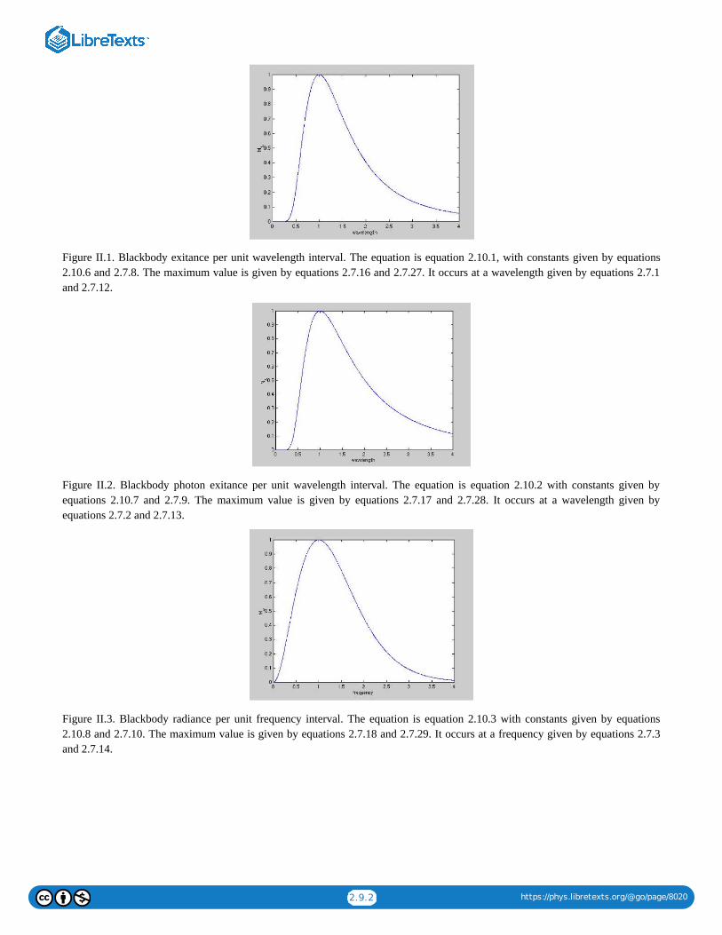
Figure II.1. Blackbody exitance per unit wavelength interval. The equation is equation 2.10.1, with constants given by equations2.10.6 and 2.7.8. The maximum value is given by equations 2.7.16 and 2.7.27. It occurs at a wavelength given by equations 2.7.1and 2.7.12.

Figure II.2. Blackbody photon exitance per unit wavelength interval. The equation is equation 2.10.2 with constants given byequations 2.10.7 and 2.7.9. The maximum value is given by equations 2.7.17 and 2.7.28. It occurs at a wavelength given byequations 2.7.2 and 2.7.13.

Figure II.3. Blackbody radiance per unit frequency interval. The equation is equation 2.10.3 with constants given by equations2.10.8 and 2.7.10. The maximum value is given by equations 2.7.18 and 2.7.29. It occurs at a frequency given by equations 2.7.3and 2.7.14.

2.9.3 https://phys.libretexts.org/@go/page/8020

Figure II.4. Blackbody photon radiance per unit frequency interval. The equation is equation 2.10.4 with constants given byequations 2.10.9 and 2.7.11. The maximum value is given by equations 2.7.19 and 2.7 30. It occurs at a frequency given byequations 2.7.4 and 2.7.15.

2.9: Dimensionless forms of Planck's equation is shared under a CC BY-NC 4.0 license and was authored, remixed, and/or curated by JeremyTatum via source content that was edited to conform to the style and standards of the LibreTexts platform; a detailed edit history is available uponrequest.

2.10.1 https://phys.libretexts.org/@go/page/8021

2.10: Derivation of Wien's and Stefan's LawsWien's and Stefan's Laws are found, respectively, by differentiation and integration of Planck's equation. Neither of these isparticularly easy, and they are not found in every textbook. Therefore, I derive them here.

Wien's LawPlanck's equation for the exitance per unit wavelength interval (equation 2.6.1) is

in which I have omitted some subscripts. Differentiation gives

is greatest when this is zero; that is, when

where

Hence, with equation 2.6.9, the wavelength at which M is a maximum, is given by

The maximum value of is found be substituting this vale of back into Planck's equation, to arrive at equation 2.7.16. Thecorresponding versions of Wien's Law appropriate to the other version's of Planck's equation are found similarly.

Stefan's LawIntegration of Planck's equation to arrive at Stefan's law is a bit more tricky.

It should be clear that , and therefore I choose to integrate the easier of the functions, namely . Tointegrate , the first thing we would do anyway would be to make the substitution .

Planck's equation for the blackbody exitance per unit frequency interval is

Let ; then

And, except for the numerical value of the integral, we already have Stefan's law. The integral can be evaluated numerically, butnot without difficulty, and there is an analytical solution for it.

Consider the indefinite integral and integrate it by parts:

Now put the limits in:

= ,M

C

1

( −1)λ5 eK/λT(2.11.1)

= − ⋅ [5 ⋅( −1)+ ⋅(− ) ] .1

C

dM

dλ

1

( −1)eK/λT 2λ4 eK/λT λ5 K

Tλ2eK/λT (2.11.2)

M

x = 5 (1 − ) ,e−x (2.11.3)

x = .K

λT(2.11.4)

λ = .hc

kxT(2.11.5)

M λ

dλ = dν∫ ∞

0Mλ ∫ ∞

0Mν Mν

Mλ ν = c/λ

= .Mν C3 ∫∞

0

dνν3

−1e ν/TK2(2.11.6)

x = ν/TK2

= ,Mν

2πk4T 4

c2h3∫

∞

0

dxx3

−1ex(2.11.7)

∫ = ln(1 − )−3 ∫ ln(1 − )dx+const.dxx3

−1exx3 e−x x2 e−x (2.10.1)

= −3 ln(1 − )dx.∫∞

0

dxx3

−1ex∫

∞

0

x2 e−x (2.10.2)

2.10.2 https://phys.libretexts.org/@go/page/8021

Write down the Maclaurin expansion of the integrand:

and integrate term by term to obtain

We must now evaluate

The series is the Riemann -function. For , it diverges. For etc., it has to be evaluated numerically. For

etc., the sums can be written explicitly in terms of . For example:

One of the stages necessary in evaluating the -function is to derive the infinite product

If we can do that, we are more than halfway there.

Let's start by considering the Fourier expansion of :

In Equation is an integer, not necessarily so; we shall suppose that is some number between 0 and 1. There is noneed to consider any sine terms, because is an even function of . We work out what the Fourier coefficients are in the usualway, to get

As usual, and for the usual reason, is an exception:

We have therefore arrived at the Fourier expansion of :

Put and rearrange slightly:

Since we are assuming that is some number between 0 and 1, we shall re-write this so that the denominators are all positive:

= 3 ( + + +. . .) dx∫∞

0

dxx3

−1ex∫

∞

0

x2 e−x 1

2e−2x 1

3e−3x (2.10.3)

= 6(1 + + +. . .) .∫∞

0

dxx3

−1ex1

24

1

34(2.11.8)

1 + + +. . .1

24

1

34

∑1

∞ 1

nmζ m = 1 m = 3, 5, 7,

m = 2, 4, 6, π

ζ(2) = ,π2

6(2.10.4)

ζ(4) = ,π4

90(2.10.5)

ζ(6) = .π6

945(2.10.6)

ζ

= [1 − ] [1 − ][1 − ] . . .sinαπ

απα2 ( α)

1

2

2

( α)1

3

2

(2.11.9)

cosθx

cosθx = cosnx∑0

∞

an (2.11.10)

2.11.10n θ θ

cosθx x

= (−1 , n = 1, 2, 3, . . .an )n2θ sinθπ

−θ2 n2(2.11.11)

a0

= .a0sinθπ

θπ(2.11.12)

cosθx

cosθx = ( − + − +. . .) .2θ sinθπ

π

1

2θ2

cosx

−θ2 12

cos 2x

−θ2 22

cos 3x

−θ2 32(2.11.13)

x = π

π cotθπ− = 2θ( + +. . .) .1

θ

1

−θ2 12

1

−θ2 22(2.11.14)

θ

π cotθπ− = − − −. . .1

θ

2θ

−12 θ2

2θ

−22 θ2(2.11.15)

2.10.3 https://phys.libretexts.org/@go/page/8021

Now multiply both sides by and integrate from to . The integration must be done with care. The indefinite integral

of the left hand side is , i.e. . The definite integral between and is

.

The limit of the second term is , so the definite integral is . Integrating the right hand side is a bit easier, so we

arrive at

On taking the antilogarithm, we arrive at the required infinite product:

Now expand this as a power series in :

The first one is easy, but subsequent ones rapidly get more difficult, but you do have to get at least as far as .

Now compare this expansion with the ordinary Maclaurin expansion:

and we arrive at the correct expressions for the Riemann -functions. We then get for Stefan's law:

where

QuestionsFinally, now that you have struggled through Riemann’s zeta-function, let’s just make sure that you have understood the reallysimple stuff, so here are a couple of easy questions – and you won’t have to bother with zeta-functions.

1. By what factor should the temperature of a black body be increased so that

a) The integrated radiance (over all frequencies) is doubled?

b) The frequency at which its radiance is greatest is doubled?

c) The spectral radiance per unit wavelength interval at its wavelength of maximum spectral radiance is doubled?

2. A block of shiny silver (absorptance = 0.23) has a bubble inside it of radius , and it is held at a temperature of .

A block of dull black carbon (absorptance = 0.86) has a bubble inside it of radius , and it is held at a temperature of ,

Calculate the ratio

Answers. 1. a) 1.189 b) 2.000 c) 1.149

2. 13.5

2.10: Derivation of Wien's and Stefan's Laws is shared under a CC BY-NC 4.0 license and was authored, remixed, and/or curated by JeremyTatum via source content that was edited to conform to the style and standards of the LibreTexts platform; a detailed edit history is available uponrequest.

dθ θ = 0 θ = α

lnsinθπ−lnθ+constant ln( )+constantsinθπ

θ0 α

ln( )− ln( )sinαπ

αlimθ→ 0

sinθπ

θ

lnπ ln( )sinαπ

απ

ln( ) = ln( )+ln( )+. . .sinαπ

απ

−12 α2

12

−22 α2

22(2.11.16)

= [1 − ] [1 − ][1 − ] . . .sinαπ

απα2 ( α)

1

2

2

( α)1

3

2

(2.11.17)

α2

= 1 +() +() +() +. . .sinαπ

απα2 α4 α6 (2.11.18)

α4

= 1 − + −. . .sinαπ

απ

π2

3!α2 π4

5!α4 (2.11.19)

ζ

M = = σ ,2π5k4

15h3c2T 4 T 4 (2.11.20)

σ = 5.6705 ×   .10−8 W m−2K−4

2.2cm 1200K

4.3cm 2300K

.Integrated radiation energy density inside the carbon bubble

Integrated radiation energy density insdie the silver bubble(2.10.7)

1

3: The Exponential Integral FunctionSooner or later (in particular in the next chapter) in the study of stellar atmospheres, we have need of the exponential integralfunction. This brief chapter contains nothing about stellar atmospheres or even astronomy, but it describes just as much as we needto know about the exponential integral function. It is not intended as a thorough exposition of everything that could be writtenabout the function.

The exponential integral function of order , written as a function of a variable , is defined as

I shall restrict myself to cases where is a non-negative integer and is a non-negative real variable. For stellar atmosphere theoryin the next chapter we shall have need of up to and including 3.

Let us start by seeing what the values of the functions are when . We have

and this is infinite for and for . For larger it is .

Thus , , , , , etc.

Thereafter the functions (of whatever order) decrease monotonically as increases, approaching zero asymptotically for large .

The function is easy to evaluate. It is

The evaluation of the exponential integral function for is less easy but it can be done by numerical (e.g. Simpson)integration. The upper limit of the integral in equation 3.1 is infinite, but this difficulty can be overcome by means of thesubstitution , from which the equation becomes

Since both limits are finite, this can now in principle be integrated numerically in a straightforward way, for example by Simpson'srule or similar algorithm, except that, at the lower limit, is infinite and it is necessary first to determine the limit of theintegrand as , which is zero.

There is, however, a way of evaluating the exponential integral function for without the necessity of numerical integration.Consider, for example,

If this is integrated (very carefully!) by parts, we arrive at

Thus from this recurrence relation, once we have evaluated , we can evaluate and hence and so on.

The recurrence relation , however, holds only for (as will become apparent during the careful partial integration), so thereis no getting around the numerical integration for . Furthermore, for small values of the functions for or becomevery large, becoming infinite as , which makes them very sensitive when trying to compute the next function up. Thus forsmall or for constructing a table it may in the end be less trouble to take the bull by the horns and integrate them all numerically.

It will afford good programming practice to prepare a table of for to , in steps of , for . The tableshould ideally have five columns, the first being the values of , and the remaining four being , to . A graph ofthese functions is shown in figure .

n a

(a) = dx.En ∫∞

1

x−ne−ax (3.1)

n a

n

a = 0

(0) = dxEn ∫∞

1

x−n (3.2)

n = 0 n = 1 n 1/(n−1)

(0) = ∞E0 (0) = ∞E1 (0) = 1E2 (0) =E312

(0) =E413

a a

(a)E0

(a) = dx = .E0 ∫∞

1

e−ax e−a

a(3.3)

n > 0

y = 1/x

(0) = dy.En ∫1

0

yn−2e−a/y (3.4)

a/y

y → 0

n ≥ 2

(a) = dx.En+1 ∫∞

1

x−(n+1)e−ax (3.5)

(a) = [ −a (a)] .En+1

1

ne

−aEn (3.6)

(a)E1 (a)E2 (a)E3

3.6 n ≥ 1

n = 1 a n = 0 1

a → 0

a

(a)En a = 0 2 0.01 n = 0, 1, 2, 3

201 a (a)En n = 1 4

III.1

2

In practice, in performing the calculations for figure , this is what I found. The function for was easy; it is given simplyby equation . For , I integrated by Simpson's rule; intervals in was adequate to compute the function to nine decimalplaces. The function for was unexpectedly difficult. The recurrence relation was not useful at small , as discussedabove. I therefore attempted to integrate it using Simpson's rule, yet, although the function is, on the face of it, very simple:

Simpson's rule seemed inadequate to compute the function precisely even with as many as intervals in . Neither therecurrence relation nor numerical integration was without problems! I had no difficulty, however, with integrating the function with

, and so I then used the recurrence relation backwards to calculate the function for and all was well.

The exponential integral function

3: The Exponential Integral Function is shared under a CC BY-NC 4.0 license and was authored, remixed, and/or curated by Jeremy Tatum viasource content that was edited to conform to the style and standards of the LibreTexts platform; a detailed edit history is available upon request.

III.1 n = 0

3.3 n = 1 100 y

n = 2 3.6 a

(a) = dy,E2 ∫1

0

e−a/y (3.7)

1000 y

n = 3 n = 2

FIGURE III.1

1 https://phys.libretexts.org/@go/page/6657

Welcome to the Physics Library. This Living Library is a principal hub of the LibreTexts project, which is a multi-institutionalcollaborative venture to develop the next generation of open-access texts to improve postsecondary education at all levels of higherlearning. The LibreTexts approach is highly collaborative where an Open Access textbook environment is under constant revisionby students, faculty, and outside experts to supplant conventional paper-based books.

Home is shared under a not declared license and was authored, remixed, and/or curated by LibreTexts.

1 https://phys.libretexts.org/@go/page/6658

Welcome to the Physics Library. This Living Library is a principal hub of the LibreTexts project, which is a multi-institutionalcollaborative venture to develop the next generation of open-access texts to improve postsecondary education at all levels of higherlearning. The LibreTexts approach is highly collaborative where an Open Access textbook environment is under constant revisionby students, faculty, and outside experts to supplant conventional paper-based books.

Home is shared under a not declared license and was authored, remixed, and/or curated by LibreTexts.

1 https://phys.libretexts.org/@go/page/6659

Welcome to the Physics Library. This Living Library is a principal hub of the LibreTexts project, which is a multi-institutionalcollaborative venture to develop the next generation of open-access texts to improve postsecondary education at all levels of higherlearning. The LibreTexts approach is highly collaborative where an Open Access textbook environment is under constant revisionby students, faculty, and outside experts to supplant conventional paper-based books.

Home is shared under a not declared license and was authored, remixed, and/or curated by LibreTexts.

1 https://phys.libretexts.org/@go/page/6660

Welcome to the Physics Library. This Living Library is a principal hub of the LibreTexts project, which is a multi-institutionalcollaborative venture to develop the next generation of open-access texts to improve postsecondary education at all levels of higherlearning. The LibreTexts approach is highly collaborative where an Open Access textbook environment is under constant revisionby students, faculty, and outside experts to supplant conventional paper-based books.

Home is shared under a not declared license and was authored, remixed, and/or curated by LibreTexts.

1 https://phys.libretexts.org/@go/page/6661

Welcome to the Physics Library. This Living Library is a principal hub of the LibreTexts project, which is a multi-institutionalcollaborative venture to develop the next generation of open-access texts to improve postsecondary education at all levels of higherlearning. The LibreTexts approach is highly collaborative where an Open Access textbook environment is under constant revisionby students, faculty, and outside experts to supplant conventional paper-based books.

Home is shared under a not declared license and was authored, remixed, and/or curated by LibreTexts.

1 https://phys.libretexts.org/@go/page/6662

Welcome to the Physics Library. This Living Library is a principal hub of the LibreTexts project, which is a multi-institutionalcollaborative venture to develop the next generation of open-access texts to improve postsecondary education at all levels of higherlearning. The LibreTexts approach is highly collaborative where an Open Access textbook environment is under constant revisionby students, faculty, and outside experts to supplant conventional paper-based books.

Home is shared under a not declared license and was authored, remixed, and/or curated by LibreTexts.

1

CHAPTER OVERVIEW

4: Flux, Specific Intensity and other Astrophysical Terms

4: Flux, Specific Intensity and other Astrophysical Terms is shared under a CC BY-NC 4.0 license and was authored, remixed, and/or curated byJeremy Tatum via source content that was edited to conform to the style and standards of the LibreTexts platform; a detailed edit history isavailable upon request.

4.1: Introduction4.2: Luminosity4.3: Specific Intensity4.4: Flux4.5: Mean Specific Intensity4.6: Radiation Pressure4.7: Other Integrals4.8: Emission Coefficient

Topic hierarchy

4.1.1 https://phys.libretexts.org/@go/page/6664

4.1: IntroductionIn previous chapters we have used the definitions and symbols of the quantities in radiation theory as recommended by variousbodies. We mentioned that, in the context of the special needs of stellar atmosphere theory, usage sometimes differs from thestandard. In this chapter we introduce the definitions and symbols that are commonly used in stellar atmosphere theory, and wecontinue to use the astronomical usage henceforth.

In a later paragraph you will be asked to imagine a "horizontal" surface in the atmosphere of a star. Lest you are thinking of a staras a large, ball-shaped thing, and the word "horizontal" is puzzling, let me say that, at least for the time being, I am considering a"shallow" atmosphere; that is, an atmosphere whose depth is very small compared with the radius of the star. To that extent, theatmosphere can be considered as a plane parallel atmosphere. This will not do for a greatly extended atmosphere, such as that of anM supergiant; as to whether it is an appropriate model for a star like the Sun, remind yourself how sharply-defined the limb of theSun is, and hence how rapidly the atmosphere becomes opaque.

4.1: Introduction is shared under a CC BY-NC 4.0 license and was authored, remixed, and/or curated by Jeremy Tatum via source content that wasedited to conform to the style and standards of the LibreTexts platform; a detailed edit history is available upon request.

4.2.1 https://phys.libretexts.org/@go/page/6665

4.2: LuminosityThe most important differences between "standard" and "astrophysical" usages are in the meanings of flux and intensity. What wehave hitherto called the "radiant flux" of a source of radiation, expressed in watts, is generally called by astronomers, whendescribing the radiant flux from an entire star, the luminosity of the star, and the symbol used is . While this can be expressed inwatts, it is commonly expressed in units of the luminosity of the Sun, which is .

4.2: Luminosity is shared under a CC BY-NC 4.0 license and was authored, remixed, and/or curated by Jeremy Tatum via source content that wasedited to conform to the style and standards of the LibreTexts platform; a detailed edit history is available upon request.

Φ

L

3.85 × watts1026

4.3.1 https://phys.libretexts.org/@go/page/6666

4.3: Specific IntensityInstead of the word "radiance", for which we have hitherto used the symbol , the name commonly used in the context of stellaratmosphere theory is specific intensity and the symbol used is . In most branches of physics, the word "specific" is used to mean"per unit mass", but that meaning is not intended in the present context. It might be noted that the word "specific" is often omitted,so that what we have hitherto called "radiance" is now "intensity" . Note also that this in not the same as what is meant in"standard" usage by "intensity", for which the symbol, in standard usage, is also . In this and subsequent chapters, I shall alwaysinclude the word "specific".

The quantity we have in earlier chapters called "radiance" was used to describe the brightness of an extended radiating surface, andthe new term "specific intensity" can equally be used in a similar context. More often, however, you may need to imagine yourselfembedded somewhere within a stellar atmosphere and you are looking around to see the watts per square metre per steradianarriving at you from various directions.

4.3: Specific Intensity is shared under a CC BY-NC 4.0 license and was authored, remixed, and/or curated by Jeremy Tatum via source contentthat was edited to conform to the style and standards of the LibreTexts platform; a detailed edit history is available upon request.

L

I

L I

I

4.4.1 https://phys.libretexts.org/@go/page/6667

4.4: FluxThe word "flux" in the context of stellar atmosphere theory differs from the "flux" of standard terminology. The symbol used is ,occasionally but not always printed in a special font. Let us imagine a horizontal surface embedded somewhere in a stellaratmosphere. It is being irradiated from below and above, but rather more from below than from above. Let us concentrate ourattention for the time being on the radiation that is coming up from below. The rate of arrival of radiant energy per unit area frombelow from all directions would, in "standard" nomenclature, have been called the irradiance. After passage through the surface, itwould be called the exitance. Now, using the nomenclature of stellar atmosphere theory, we call the rate of upward passage ofradiant energy per unit area through a horizontal surface within the atmosphere the upward or the outward flux. The symbol is (sometimes printed in a special font), and the SI units would be . Likewise, the rate of passage of radiant energy per unitarea from above to below is the downward or inward flux, . The net upward flux is

If you are standing upright, is the irradiance of the soles of your feet, while is the irradiance of the top of your head. If wemeasure the spherical angle from a downwardly-directed -axis, then, following equation 1.14.5, we have

which is sometimes written for short

or just

At the surface of the star (if there is such a thing!) , so that . This is the same as equation 1.15.2. At thecentre of the star, is isotropic and .

4.4: Flux is shared under a CC BY-NC 4.0 license and was authored, remixed, and/or curated by Jeremy Tatum via source content that was editedto conform to the style and standards of the LibreTexts platform; a detailed edit history is available upon request.

F

F+

W m−2

F−

F = − .F+ F− (4.4.1)

F+ F−

θ z

= I(θ,ϕ) cosθ sinθ dθdϕF+ ∫2π

0

∫π/2

0

(4.4.2)

= I(θ,ϕ) cosθ sinθ dθdϕF− ∫2π

0

∫π/2

π

(4.4.3)

F = − = I(θ,ϕ) cosθ sinθ dθdϕ,F+ F− ∫2π

0

∫π

0

(4.4.4)

F = I cosθ dω∫4π

(4.4.5)

∫ I cosθ dω (4.4.6)

= 0F− F = = πIF+

I F = 0

4.5.1 https://phys.libretexts.org/@go/page/6668

4.5: Mean Specific IntensityLook around you again from your position somewhere in the middle of a stellar atmosphere. The specific intensity around you isnot isotropic. It is quite large in the sky above you, but is much greater if you look towards the hell at your feet. The mean specificintensity around the complete steradians around you is

or, for short

At the centre of the star, where the specific intensity is isotropic, .

4.5: Mean Specific Intensity is shared under a CC BY-NC 4.0 license and was authored, remixed, and/or curated by Jeremy Tatum via sourcecontent that was edited to conform to the style and standards of the LibreTexts platform; a detailed edit history is available upon request.

J 4π

J = I(θ) sinθ dθdϕ1

4π∫

2π

0

∫π

0

(4.5.1)

J = ∫ Idω.1

4π(4.5.2)

J = I

4.6.1 https://phys.libretexts.org/@go/page/6669

4.6: Radiation PressureRecall equation 1.18.5 and the conditions for which it is valid. It was derived for isotropic radiation. In the atmosphere, radiation isnot isotropic; there is a net flux of radiation outwards. Therefore the radiation density must go inside the integral sign. We can alsowrite the equation in terms of specific intensity, making use of equations 1.15.3 and 1.17.1. The equation for the radiation pressurethen becomes

where by now we are used to the abbreviated notation.

If the radiation is isotropic, this is not zero; it is . In the expressions for and for , the power of is even (0 and 2respectively) and one can see both physically and mathematically that neither of them is zero for isotropic radiation. One the otherhand, the expression for has an odd power of , and it is therefore zero for isotropic radiation, as expected.

4.6: Radiation Pressure is shared under a CC BY-NC 4.0 license and was authored, remixed, and/or curated by Jeremy Tatum via source contentthat was edited to conform to the style and standards of the LibreTexts platform; a detailed edit history is available upon request.

P = I θ dω,1

c∫

4π

cos2 (4.6.1)

4π/(3c) J P cosθ

F cosθ

4.7.1 https://phys.libretexts.org/@go/page/8686

4.7: Other IntegralsOther integrals occurring in the theory of stellar atmospheres are (using the abbreviated notation)

The SI units for are . For , , , they are . For they are .

4.7: Other Integrals is shared under a CC BY-NC 4.0 license and was authored, remixed, and/or curated by Jeremy Tatum via source content thatwas edited to conform to the style and standards of the LibreTexts platform; a detailed edit history is available upon request.

H = ∫ I cosθdω = F/(4π)1

4π(4.7.1)

= 0 if isotropic (4.7.2)

K = ∫ I θdω = cP/(4π)1

4πcos2 (4.7.3)

= J/3 if isotropic. (4.7.4)

F W m−2I J H K  W m−2 sr−1

P Pa

4.8.1 https://phys.libretexts.org/@go/page/8687

4.8: Emission CoefficientThis is the intensity emitted per unit volume of a gas. In this definition, the word “intensity” (without being preceded by the word“specific”) is intended to mean what is meant in section 1.4. The symbol used for emission coefficient is , and the SI units are

.

The mass emission coefficient is the intensity per unit mass, and is related to the volume emission coefficient by . Notall authors are equally clear as to whether they are referring to a volume or a mass emission coefficient.

4.8: Emission Coefficient is shared under a CC BY-NC 4.0 license and was authored, remixed, and/or curated by Jeremy Tatum via source contentthat was edited to conform to the style and standards of the LibreTexts platform; a detailed edit history is available upon request.

j

 W sr−1

m−3

jm j = ρjm

1

CHAPTER OVERVIEW

5: Absorption, Scattering, Extinction and the Equation of Transfer5.1: Introduction5.2: Absorption5.3: Scattering, Extinction and Opacity5.4: Optical Depth5.5: The Equation of Transfer5.6: The Source Function (Die Ergiebigkeit)5.7: A Series of Problems5.8: Source function in scattering and absorbing atmospheres5.9: More on the Equation of Transfer

5: Absorption, Scattering, Extinction and the Equation of Transfer is shared under a CC BY-NC 4.0 license and was authored, remixed, and/orcurated by Jeremy Tatum via source content that was edited to conform to the style and standards of the LibreTexts platform; a detailed edithistory is available upon request.

5.1.1 https://phys.libretexts.org/@go/page/6671

5.1: IntroductionAs radiation struggles to make its way upwards through a stellar atmosphere, it may be weakened by absorption and scattering.The combined effect of absorption and scattering is called extinction. Scattering may simply be by reflection from dust particles. Ifthe radiation interacts with an atom, the atom may be excited to a higher energy level and almost immediately (typically on a time-scale of nanoseconds) the atom drops down to its original level and emits a photon of the same frequency as the one it absorbed.Such a process - temporary absorption followed almost immediately by re-emission without change in wavelength - is probablybest described in the present context as scattering. Individual atoms in a stellar atmosphere generally radiate dipole radiation;however, since many randomly oriented atoms take place in the process, the scattering can be regarded as isotropic. If, however, theexcited atom collides with another atom before re-emission, the collision may be super-elastic; as the atom falls to a lower state, theenergy it gives up, instead of being radiated as a photon, goes to kinetic energy of the colliding atoms. The radiation has beenconverted to kinetic energy. This process is absorption.

5.1: Introduction is shared under a CC BY-NC 4.0 license and was authored, remixed, and/or curated by Jeremy Tatum via source content that wasedited to conform to the style and standards of the LibreTexts platform; a detailed edit history is available upon request.

5.2.1 https://phys.libretexts.org/@go/page/6672

5.2: AbsorptionTo start with, let us suppose that the predominating mechanism is absorption with no scattering. We can define a linear absorptioncoefficient as follows. Let the specific intensity at some level in an atmosphere be . At a level in the atmosphere higher by adistance , the specific intensity has dropped, as a result of absorption, to . (Here , by the convention of differentialcalculus, means the increase in , and it is in this case negative. The quantity , which is positive, is the decrease in .) Thelinear absorption coefficient is defined such that the fractional decrease in the specific intensity over a distance is given by

The coefficient is of dimension and the SI unit is . In general, will depend on frequency or wavelength, and, at aparticular wavelength, the Equation would be written

If Equation is integrated over a finite distance, for a slab of atmosphere, say, between , where the specific intensity is , and , where the specific intensity is , it becomes

And if is uniform and not a function of , this becomes

Now let , so that Equation becomes

and Equation becomes , where is the number of atoms per unit volume. Then is the atomicabsorption coefficient, or atomic absorption cross-section. It is of dimension and the SI unit is .

In a similar manner, we can define , where is the mass density, as the mass absorption coefficient, with correspondingmodifications in all the other equations. It is of dimension and the SI unit is .

We might also mention here that in laboratory chemistry, one comes across the word absorbance of a solution. This is the linearabsorption coefficient divided by the concentration of the solute. While this word in not usually encountered in stellar atmospheretheory, it is mentioned here partly because it is very similar in concept to the several concepts discussed in this section, and alsobecause of the similarity of the word to the rather different absorptance defined in Chapter 2. In chemical texts, the exponentialdecrease of intensity with distance is often referred to as the Lambert-Beer Law, or simply as Lambert's Law. This is mentionedhere merely to point out that this is not at all related to the Lambert's Law discussed in Chapter 1.

5.2: Absorption is shared under a CC BY-NC 4.0 license and was authored, remixed, and/or curated by Jeremy Tatum via source content that wasedited to conform to the style and standards of the LibreTexts platform; a detailed edit history is available upon request.

α I

dx I +dI dI

I −dx I

α dx

− = αdxdI

I(5.2.1)

L−1 m−1 α

− = α(ν)dxdIν

Iν(5.2.2)

5.2.1 x = 0

I 0 x = X I

I = exp[− α(x)dx]I 0 ∫X

0

(5.2.3)

α x

I = exp(−αX)I 0 (5.2.4)

= α/nαa 5.2.1

−dI/I = ndxαa (5.2.5)

5.2.4 I = exp(− nX)I 0 αa n αa

L2 m2

= α/ραm ρ

L2M−1 m2kg−1

5.3.1 https://phys.libretexts.org/@go/page/6673

5.3: Scattering, Extinction and OpacityIf the predominating mechanism is scattering with no absorption, we can define in a similar manner linear, atomic and massscattering coefficients, using the symbol rather than . For the physical distinction between absorption and scattering, seeSection 5.1. And if both absorption and scattering are important, we can define linear, atomic and mass extinction coefficients,using the symbol , where

All the foregoing equations are valid, whether we use linear, atomic or mass absorption, scattering or extinction coefficients, andwhether we refer to radiation integrated over all frequencies or whether at a particular wavelength or within a specified wavelengthrange.

The mass extinction coefficient is generally referred to as the opacity.

5.3: Scattering, Extinction and Opacity is shared under a CC BY-NC 4.0 license and was authored, remixed, and/or curated by Jeremy Tatum viasource content that was edited to conform to the style and standards of the LibreTexts platform; a detailed edit history is available upon request.

σ α

κ

κ = α +σ. (5.3.1)

5.4.1 https://phys.libretexts.org/@go/page/6674

5.4: Optical DepthThe product of linear extinction coefficient and distance, or, more properly, if the extinction coefficient varies with distance, theintegral of the extinction coefficient with respect to distance,

is the optical depth, or optical thickness, . It is dimensionless. Specific intensity falls off with optical depth as

Thus optical depth can also be defined by . While the optical depth is generally used to describe how opaque astellar atmosphere or an interstellar cloud is, when describing how opaque a filter is, one generally uses , which iscalled the density of the filter. Density is times optical depth. If a star is hidden behind a cloud of optical depth it will bedimmed by magnitudes. If it is hidden behind a filter of density it will be dimmed by magnitudes. The reader isencouraged to verify these assertions.

5.4: Optical Depth is shared under a CC BY-NC 4.0 license and was authored, remixed, and/or curated by Jeremy Tatum via source content thatwas edited to conform to the style and standards of the LibreTexts platform; a detailed edit history is available upon request.

τ = ∫ κ(x)dx (5.4.1)

τ

I = .I0e

−τ (5.4.2)

ln( /I)I 0 ln( /I)I 0

( /I)log10 I 0

d 0.4343 τ

1.086τ d 2.5d

5.5.1 https://phys.libretexts.org/@go/page/6675

5.5: The Equation of TransferThe equation of transfer deals with the transfer of radiation through an atmosphere that is simultaneously absorbing, scattering andemitting.

Suppose that, between and the absorption coefficient and the scattering coefficient at frequency are and , andthe emission coefficient per unit frequency interval is . In this interval, suppose that the specific intensity per unit frequencyinterval increases from to ( might be positive or negative). The specific intensity will be reduced by absorption andscattering and increased by emission. Thus:

This is one form - the most basic form - of the equation of transfer. Notice that and do not have a subscript.

5.5: The Equation of Transfer is shared under a CC BY-NC 4.0 license and was authored, remixed, and/or curated by Jeremy Tatum via sourcecontent that was edited to conform to the style and standards of the LibreTexts platform; a detailed edit history is available upon request.

FIGURE V.1

x x+dx ν α(ν) σ(ν)

dνjν

Iν +dIν Iν dIν

d = −[ α(ν) + σ(ν) − (ν)]dx.Iν Iν Iν jν (5.5.1)

α σ

5.6.1 https://phys.libretexts.org/@go/page/6676

5.6: The Source Function (Die Ergiebigkeit)This is the ratio of the emission coefficient to the extinction coefficient. A review of the dimensions of these will show that thedimensions of source function are the same as that of specific intensity, namely (perhaps per unit wavelength orfrequency interval). The usual symbol is . Thus

Imagine a slice of gas of thickness . Multiply the numerator and denominator of the right hind side of equation 5.6.1 by .Observe that the numerator is now the specific intensity (radiance) of the slice, while the denominator is its optical thickness. Thusan alternative definition of source function is specific intensity per unit optical thickness. Later, we shall evaluate the sourcefunction in an atmosphere in which the extinction is pure absorption, in which it is purely scattering, and in which it is a bit of each.

5.6: The Source Function (Die Ergiebigkeit) is shared under a CC BY-NC 4.0 license and was authored, remixed, and/or curated by Jeremy Tatumvia source content that was edited to conform to the style and standards of the LibreTexts platform; a detailed edit history is available uponrequest.

 W m−2 sr−1

S

= =Sν

jν

α(ν) +σ(ν)

jν

κ(ν)(5.6.1)

dx dx

5.7.1 https://phys.libretexts.org/@go/page/8694

5.7: A Series of ProblemsI am now going to embark upon a series of problems that at first sight may appear to be not very relevant to stellar atmospheres, butthe reader is urged to be patient and look at them, partly because they make use of many of the ideas encountered up to this point,and also because they culminate in determining how the flux and the mean specific intensity in an atmosphere increase with opticaldepth in terms of the source function.

Problem 1

An infinite plane radiating surface has a uniform specific intensity (radiance) . What is the flux (irradiance) at a point , situatedat a height above the surface?

We have already answered that question in equation 1.15.3, and the answer, which, unsurprisingly since the plane is infinite inextent, is independent of , is , so let's get on with

Problem 2

Same as Problem 1, except that this time the space between the radiating plane and the point is filled with a uniform gas ofabsorption coefficient . The specific intensity (radiance) of the surface, we are told, is, following astrophysical custom, .Unfortunately I shall also be compelled to make use of "intensity" in the "standard" sense of Chapter 1, and for that I shall use thesymbol .

The elemental area is , or, since , it is . The intensity of the elemental area towards is thespecific intensity (radiance) times the projected area:

If there were no absorption, the irradiance of by the elemental area would be

which becomes

But it is reduced by absorption by a factor , where . Therefore the irradiance of by the elemental area is

For the irradiance at (or "flux" in the astrophysics sense) by the entire infinite plane we integrate from to and to , to obtain

If we now write , this becomes

I P

h

h πI

P

α I

I

FIGURE V.2

r dr dϕ r = h tanθ tanθ θdθdϕh2 sec2 P

dI = I tanθ θ dϕ  cosθh2 sec2 (5.7.1)

P

dIcosθ/( θ),h2 sec2 (5.7.2)

I sinθcosθ dθ dϕ. (5.7.3)

e−τ sec θ τ = αh P

I sinθcosθ dθ dϕ.e−τ sec θ (5.7.4)

P ϕ = 0 2π θ = 0

π/2

2πI sinθcosθdθ∫π/2

0

e−τ sec θ (5.7.5)

x = sec θ

Irradiance at P = 2πI (τ),E3 (5.7.6)

5.7.2 https://phys.libretexts.org/@go/page/8694

and we hope that the reader has not forgotten the meaning of - if you have, as the game of snakes and ladders would say, Goback to Chapter 3. Note that, at , this becomes , as expected.

A point is situated at a height above an infinite plane slice of gas of optical thickness and source function . There isnothing between and the slice of gas. What is the flux (irradiance) at ?

At first glance this appears to be identical to Problem 1, except that the specific intensity of the slice is . However, a morecareful look at the diagram will reveal that the specific intensity of the slice is by no means uniform. It is darkest directly below ,and, when looks farther from his nadir, the slice gets brighter and brighter, being at an angle . The upwards flux("irradiance") at is therefore

Same as Problem 3, except that this time we'll place an absorbing gas of optical thickness between and the slice .

In that case the flux (irradiance) at from an element at an angle is reduced by and consequently the flux at from theentire slice is

If we write , we very soon see that this is

Problem 5 (an important result in atmosphere theory)

Now consider a point at an optical depth in a stellar atmosphere. (The use of the word "depth" will imply that is measureddownwards from the surface towards the centre of the star.) We shall assume a plane parallel atmosphere i.e. a shallow atmosphere,or one than is shallow compared with the radius of the star, or we are not going to go very deep into the atmosphere. The point isembedded in an absorbing, scattering, emitting gas. The flux coming up from below is equal to contributions from all the slicesbeneath , from to :

The flux pouring down from above is the contribution from all the slices above, from to :

E3

τ = 0 πI

FIGURE V.3

P h δτ S

P P

Sδt

P

P S  sec θ δt θ

P

= 2πSδt sec θcosθ sinθ dθ = 2πSδtF+ ∫π/2

0

(5.7.7)

t P δt

FIGURE V.4

P θ e−t sec θ P

= 2πSδt sec θcosθ sinθ dθ = 2πSδt.F+ ∫π/2

0

(5.7.8)

x = sec θ

Flux (irradiance) at P = 2πSδt (t)E2 (5.7.9)

P τ τ

P

P t = τ t = ∞

= 2π S(t) (t−τ)dtF+ ∫∞

τ

E2 (5.7.10)

t = 0 t = τ

= 2π S(t) (τ − t)dtF− ∫τ

0

E2 (5.7.11)

5.7.3 https://phys.libretexts.org/@go/page/8694

The net upward flux at a point at an optical depth in an absorbing, scattering, emitting atmosphere is

The integral is just times this.

The reader is now asked to find the integrals and . These should be given in the form of integrals that include a sourcefunction and an exponential integral function or . It is important to get the argument the right way round.One way is right; the other is wrong.

Problem 6

This is an easier problem, though the result is nevertheless important.

Figure V.5 shows a slab of gas of optical thickness . The observer is supposed to be to the right of the slab, and optical depth ismeasured from the right hand face of the slab towards the left. At an optical depth within the slab is a slice of optical thickness

. The slab is supposed to have a uniform source function throughout. Source function is specific intensity per unit opticalthickness, so the specific intensity of the slice is . The emergent intensity from this slice, by the time that it reaches the righthand surface of the slab, is . The emergent specific intensity of the entire slab is the sum of the contributions of all suchslices throughout the slab; that is . If the source function is uniform throughout the slab, so that is not a function of ,we find that the emergent specific intensity of the slab is

Problem. A quantity of hot gas is held in a box 50 cm long. The emission coefficient of the gas is and theextinction coefficient is . What is the emergent specific intensity (radiance)? (I make it .)

5.7: A Series of Problems is shared under a CC BY-NC 4.0 license and was authored, remixed, and/or curated by Jeremy Tatum via sourcecontent that was edited to conform to the style and standards of the LibreTexts platform; a detailed edit history is available upon request.

P τ

F (τ) = 2π [ S(t) (t−τ)dt− S(t) (τ − t)dt]∫∞

τ

E2 ∫τ

0

E2 (5.7.1)

H 1/(4π)

J(τ) Kτ)

S(t) E(t−τ) E(τ − t)

FIGURE V.5

τ

t

dt S

Sdt

S dte−t

S dt∫ τ

0e−t S t

I = S (1 − )e−t (5.7.2)

0.06 W sr−1m−3

0.025 cm−1 1.71 ×10−2W m−2sr−1

5.8.1 https://phys.libretexts.org/@go/page/8695

5.8: Source function in scattering and absorbing atmospheresSuppose that at some point in a stellar atmosphere the mean specific intensity per unit frequency interval surrounding it is . If allof the radiation arriving at that point is isotropically scattered, the emission coefficient will simply be . But from equation5.6.1 we see that in a purely scattering atmosphere, the ratio of to is the source function. Thus we see that, for anatmosphere in which the extinction is due solely to scattering, the source function is just

If on the other hand the extinction is all due to absorption, we have . If we multiply top and bottom by , thenumerator will be , the increase in the specific intensity in a distance , while the denominator is the absorptance in a layer ofthickness . Thus the source function in a purely absorbing atmosphere is the ratio of the specific intensity to the absorptance. Butthis ratio is the same for all surfaces, including that of a black body, for which the absorptance is unity. Thus in an atmosphere inwhich the extinction is due solely to absorption, the source function is equal to the specific intensity (radiance) of a black body, forwhich we shall use the symbol . For a purely absorbing atmosphere, we have

In an atmosphere in which extinction is by both scattering and absorption the source function is a linear combination of equations and , in proportion to the relative importance of the two processes:

5.8: Source function in scattering and absorbing atmospheres is shared under a CC BY-NC 4.0 license and was authored, remixed, and/or curatedby Jeremy Tatum via source content that was edited to conform to the style and standards of the LibreTexts platform; a detailed edit history isavailable upon request.

Jνjν σ(ν)Jν

jν σ(ν)

= .Sν Jν (5.8.1)

= /α(ν)Sν jν dx

dIν dx

dx

B

= .Sν Bν (5.8.2)

5.8.1 5.8.2

= +Sν

α(ν)

α(ν)+σ(ν)Bv

σ(ν)

α(ν)+σ(ν)Jν (5.8.3)

5.9.1 https://phys.libretexts.org/@go/page/8696

5.9: More on the Equation of TransferRefer to equation 5.5.1. We see from what had been subsequently discussed that and that

. Therefore

and this is another form of the equation of transfer.

Now consider a spherical star with a shallow atmosphere ("plane parallel atmosphere"). In figure , radial distance is measuredradially outwards from the centre of the star. Optical depth is measured from outside towards the centre of the star. The thickness ofthe layer is . The coordinate is measured from the centre of the star towards the observer, and the path length through theatmosphere in that direction at angle is . The equation of transfer can be written

Now and . Therefore

This is yet another form of the equation of transfer. The quantity is often written , so that equation is often written

Let us do to each term in equation . By I mean integrate over steradians. In spherical coordinates . We obtain

The left hand side is and the first term on the right hand side is . (See the definitions - equations 4.5.2 and 4.7.1.) Inthe case of isotropic scattering, the source function is isotropic so that, in this case

and this is another form of the equation of transfer.

On the other hand, if we do to each term in equation 5.15, we obtain

[α(ν) +σ(ν)]dx = dτ(ν)

dx = dτ(ν)jν

= − ,dIv

dτ(ν)Sν Iν (5.9.1)

V.6 r

dr z

θ dz = dr sec θ

d (θ) = −[κ(ν) (θ) − ]dz.Iν Iν jν (5.9.2)

κ(ν)dz = −sec θdτ(ν) = κ(ν)jν Sν

cosθ = (θ) −d (θ)Iν

dτ(ν)Iν Sν (5.9.3)

cosθ μ 5.9.3

μ = (θ) −d (θ)Iv

dτ(ν)Iν Sν (5.9.4)

FIGURE V.6

∮ dω14π

5.9.4 ∮ 4π

dω = sinθdθdϕ

∮ cosθdω = ∮ dω− ∮ dω1

4π

d (θ)Iν

dτ(ν)

1

4πIν

1

4πSν (5.9.5)

d /dτ(ν)Hν Jν

= − ,dHν

dτ(ν)Jν Sν (5.9.6)

∮ cosθdω14π

5.9.2 https://phys.libretexts.org/@go/page/8696

In the case of isotropic scattering the last integral is zero, so that

and this is yet another form of the equation of transfer.

Now is independent of optical depth (why? - in a plane parallel atmosphere, this just expresses the fact that the flux (watts persquare metre) is conserved), so we can integrate equation to obtain

Note also that , and, if the radiation is isotropic, so that,

where is the mean specific intensity (radiance) at the surface, which is half the specific intensity at the surface (since theradiance of the sky above the surface is zero). Thus

Therefore

This shows, to this degree of approximation (which includes the approximation that the radiation in the atmosphere is isotropic -which can be the case exactly only at the centre of the star) how the mean specific intensity increases with optical depth.

Let be the temperature at optical depth .

Let be the surface temperature.

Let be the effective temperature, defined by ,

We also have and .

From these we find the following relations between these temperatures:

Note also that at , and at .

5.9: More on the Equation of Transfer is shared under a CC BY-NC 4.0 license and was authored, remixed, and/or curated by Jeremy Tatum viasource content that was edited to conform to the style and standards of the LibreTexts platform; a detailed edit history is available upon request.

∮ θdω = ∮ cosθdω− ∮ cosθdω1

4π

d (θ)Iν

dτ(ν)cos2 1

4πIν

1

4πSν (5.9.7)

= ,dKν

dτ(ν)Hν (5.9.8)

Hν

5.9.8

= τ(ν) +constantKν Hν (5.9.9)

= /(4π)Hν Fν = /3Kν Jν

= + (0)Jν3 τ(ν)Fν

4πJν (5.9.10)

(0)Jν

(0) = (0) = /(2π)Jν1

2Iν Fν (5.9.11)

= (1 + τ(ν))JνFν

2π

3

2(5.9.12)

T τ

T0

Teff F (0) = σT 4eff

πJ = σT 4 πJ(0) = σ = FT 40

12

=(1 + τ) = (1 + τ)T 4 3

2T 4

0

1

2

3

2T 4

eff (5.9.13)

= =T 40

2

2 +3πT 4 1

2T 4

eff(5.9.14)

= = 2T 4eff

4

2 +3τT 4 T 4

0 (5.9.15)

T = Teff τ = 2/3 T = T0 τ = 0

1

CHAPTER OVERVIEW

6: Limb DarkeningLimb darkening is an optical effect seen in stars (including the Sun), where the center part of the disk appears brighter than theedge or limb of the image.

Thumbnail: A filtered image of the Sun in visible light, showing the limb-darkening effect as a dimmer luminosity towards theedge or limb of the solar disk. The image was taken during the 2012 transit of Venus (seen here as the dark spot at the upper right).(CC BY 2.5; Brocken Inaglory).

6: Limb Darkening is shared under a CC BY-NC 4.0 license and was authored, remixed, and/or curated by Jeremy Tatum via source content thatwas edited to conform to the style and standards of the LibreTexts platform; a detailed edit history is available upon request.

6.1: Introduction. The Empirical Limb-darkening6.2: Simple Models of the Atmosphere to Explain Limb Darkening

Topic hierarchy

6.1.1 https://phys.libretexts.org/@go/page/6678

6.1: Introduction. The Empirical Limb-darkeningThe Sun is not equally bright all over, but it is darkened towards the limb. The effect is more pronounced at the blue end of thespectrum and less pronounced at the red. A reasonably good empirical representation of the form of the limb darkening is given byan equation for the specific intensity of the form

Here, is the radius of the solar disc, is radial distance from the center of the disc and is the limb darkening coefficient. This isoften written in terms of (see Figure ) or of :

Whether written in the form of Equation or , is the specific intensity at the center of the disc. The specific intensityat the limb (where or ) is . The limb darkening coefficient can be written as

Equation is shown in graphical form in figure for different values of the limb darkening coefficient.

. Equation for six limb darkening coefficients, from the lowest curve upwards,

. The "curve" for the last of these (no limb darkening) is formed from three of the boundary lines.The curve for is a circle. The radius of the disc is taken to be , is the center of the disc and is the limb.

Limb-darkening is much greater in the violet and near ultraviolet than in the red. For example, at a wavelength of , , whereas at .

A slightly better empirical representation of the limb darkening can be obtained with two parameters, and :

I(r) = I(0)[1 −u(1 − )]−a2 r2

a2

− −−−−−−

√ (6.1.1)

a r u

θ VI.1 μ = cos θ

I(θ) = I(0) [1 −u(1 −cos θ)]

= I(0)[1 −u(1 −μ)]

(6.1.2)

(6.1.3)

FIGURE VI.1

6.1.1 6.1.3 I(0)

r = a θ = 90∘ I(0)(1 −u)

u = .I(center) −I(limb)

I(center)(6.1.4)

6.1.1 VI.2

FIGURE VI.2 6.1.1

u = 1.0, 0.8, 0.6, 0.4, 0.2 and 0.0

u = 1 1 r = 0 r = ±1

600 nm

u = 0.56 320 nm u = 0.95

u′ ν ′

I(θ) = I(0) [1 − (1 −cos θ) − θ]u′ ν ′ sin2 (6.1.5)

6.1.2 https://phys.libretexts.org/@go/page/6678

Why is the Sun darkened towards the limb?

We may perhaps imagine that the surface of the Sun radiates like a black body with uniform lambertian radiance, but it issurrounded by an absorbing atmosphere. Light from near the limb has to traverse a greater length of atmosphere than light fromnear the center of the disk and this accounts for the limb darkening. If that is the explanation, we should be able to calculate whatform of limb darkening to expect, and see how well it agrees with what is observed. If the agreement is only moderately good,perhaps we could assume that the atmosphere is not only an absorbing atmosphere, but it also emits radiation of its own, and wecould see if we could adjust the ratio of emission to extinction (the source function) to obtain good agreement with the model andthe observations. Or perhaps, rather than thinking of a uniform radiating surface sharply separated from a surrounding atmosphere,we may imagine that there is no such sharp boundary, but, rather, the density and temperature of the solar gases increasecontinuously with depth. In that case, suppose that we can see everywhere to a given optical depth, say to . Near the limb, anoptical depth of unity does not take us very deep (in terms of kilometers) into the atmosphere, because we are looking almosttangentially at the surface of the Sun, so we reach only relatively high levels in the atmosphere where the temperature is relativelycool. Near the center, on the other hand, where we are peering down perpendicularly into the Sun, an optical depth of one reachesdeep down (in terms of kilometers) to places where the atmosphere is very hot. Thus the center appears brighter than the limb.

At any rate, the point is that, by making precise measurements of the form of the limb darkening and comparing thesemeasurements with the predictions of different models, we should in principle be able to deduce something about the run of densityand temperature with optical depth in the atmosphere.

One practical difficulty of doing this is that it turns out that it is necessary to make quite precise measurements of the exact form ofthe limb darkening very close to the limb to be able to distinguish convincingly between different models.

Are there any prospects of being able to measure the limb darkening of stars other than the Sun? The future will tell whetheradvances in technology, such as adaptive optics, may enable us to observe the limb darkening of other stars directly. Other methodsare possible. For example, the detailed light curve of an eclipsing binary star undoubtedly gives us information on the limbdarkening of the star that is being eclipsed. There are many factors that affect the form of the light curve of an eclipsing binary star,and the detailed interpretation of light curves is not at all easy - but no one ever claimed that astronomy was easy. In principle lunaror asteroidal occultations of stars might enable us to determine the limb darkening of a star. Another possible method is from acareful examination of the line profiles in the spectrum of a rotating star. If a star is of uniform brightness and is rotating rapidly,the intensity profiles of its spectrum lines are broadened and have a semi-elliptical profile. However, if the star is darkened towardsthe limb, the line profile is affected. If the star's disk is completely limb darkened ( , so that the specific intensity at the limb iszero), it is an interesting exercise to show that the line profile is parabolic. For intermediate limb darkening, the profile is neitherelliptical nor parabolic; an exact analysis of its shape could in principle tell us the limb darkening coefficient.

6.1: Introduction. The Empirical Limb-darkening is shared under a CC BY-NC 4.0 license and was authored, remixed, and/or curated by JeremyTatum via source content that was edited to conform to the style and standards of the LibreTexts platform; a detailed edit history is available uponrequest.

τ = 1

u = 1

6.2.1 https://phys.libretexts.org/@go/page/6679

6.2: Simple Models of the Atmosphere to Explain Limb Darkening1. The Sun consists of a spherical body emitting continuous blackbody radiation of radiance (specific intensity) surrounded by ashallow ("plane parallel") atmosphere which absorbs light and is of optical thickness but does not emit. See figure .

The emergent specific intensity at the centre of the disc is

and at a position on the disc given by is

so that the limb darkening is given by

If the limb darkening is indeed like this, then a graph of versus will be a straight line whose slope will bethe optical thickness of the atmosphere. However, in practice such a graph does not yield a straight line, and a comparison ofEquation , which is shown in figure , with the observed limb darkening shown in figure , suggests that this is not atall a promising model.

Equation for four values of the optical thickness of the atmosphere. The curves are drawn for and . Thecurves do not greatly resemble the empirical, observed curves of figure , suggesting that this is not a very good atmosphericmodel.

2. This second model is similar to the first model, except that the atmosphere emits radiation as well as absorbing it. We supposethat the surface of the Sun is a black body of specific intensity . The subscript refers to the surface of the Sun. I have omitted asubscript . The argument is the same whether we are dealing with the specific intensity per unit frequency interval (Planckfunction) or the integrated specific intensity (Stefan's law). Suppose that the atmosphere, of optical thickness , is an emitting,absorbing atmosphere, of source function , being a Planck function corresponding to a cooler temperature than the surface. The

Bν

τ(ν) VI.3

FIGURE VI.3

(0) =Iν Bνe−τ(ν) (6.2.1)

θ

(θ) =Iν Bνe−τ(ν) sec θ (6.2.2)

(θ) = (0)Iν Iv e−τ(ν)(sec θ−1) (6.2.3)

ln[ (θ)/ (θ)]Iν Iν 1 −sec θ

6.2.3 VI.4 VI.2

FIGURE VI.4

6.2.3 τ τ = 0.2, 0.4, 0.6 0.8

VI.2

B1 1

ν

τ

B2

6.2.2 https://phys.libretexts.org/@go/page/6679

emergent specific intensity will be the sum of the emergent intensity of the atmosphere (see Equation 5.7.2) and the specificintensity of the surface reduced by its passage through the atmosphere. At the centre of the disc, this will be

and at a position on the disc it will be

and so the limb darkening will be given by

In attempting to find a good fit between Equation and the observed limb darkening, we now have two adjustable parameters, and the ratio . In figure we show the limb darkening for and for a representative ratio

. If we are dealing with radiation integrated over all wavelengths, this would imply an atmospheric temperature equalto times the surface temperature. There is no combination of the two parameters that gives a limb darkening verysimilar to the observed limb darkening, so this model is not a specially good one.

Equation for , and and .

3. In this model we do not assume a hard and fast photosphere surrounded by an atmosphere of uniform source function; rather, wesuppose that the source function varies continuously with depth. In figure we draw two levels in the atmosphere, at opticaldepths and . The reader should recall that we are dealing only with a "plane parallel" atmosphere - i.e. one that is shallowcompared with the radius of the star. The geometric distance between the two levels is therefore much exaggerated in the figure.

The source function of the shell between optical depths and is . In the direction the radiance (specific intensity) ofan elemental shell of optical thickness is .. (I have not explicitly indicated in this expression the dependence onfrequency or wavelength of the source function or optical depth.) By the time the radiation from this shell reaches the outermostpart of the atmosphere (i.e. where ), it has been reduced by a factor . The specific intensity resulting from the additionof all such elemental shells is

This important Equation, attributed to Karl Schwarzschild, gives the limb darkening as a function of the way in which the sourcefunction varies with optical depth. The usual situation is that it is the limb darkening that is known and it is required to find ,

I(0) = + (1 − )B1e−τ B2 e−τ (6.2.4)

θ

I(θ) = + (1 − )B1e−τ sec θ B2 e−τ sec θ (6.2.5)

=I(θ)

I(0)

( − ) +B1 B2 e−τ sec θ B2

( − ) +B1 B2 e−τ B2(6.2.6)

6.2.6

τ /B2 B1 VI.5 τ = 0.5, 1.0,  1.5 2.0

/ = 0.5B2 B1

(0.5 = 0.84)1/4

FIGURE VI.5

6.2.6 / = 0.5B2 B1 τ = 0.5,  1.0,  1.5 2.0

VI.6

τ τ +dτ

FIGURE VI.6

τ τ +dτ S(τ) θ

dτ S(τ) sec θdτ

τ = 0 e−τ sec θ

I(θ) = sec θ S(τ) dτ∫∞

0

e−τ sec θ (6.2.7)

S(τ)

6.2.3 https://phys.libretexts.org/@go/page/6679

so that Equation has to be solved as an integral Equation. This, however, is not as difficult as it may first appear because itwill be noticed that if we write , the Equation is merely a Laplace Transform:

so that the source function is the inverse Laplace transform of the limb darkening.

If we assume that the source function can be expressed as a polynomial in the optical depth:

we find for the limb darkening (remembering that )

If we compare this with the empirical limb darkening Equation 6.3 we find the coefficients in terms of the limb darkeningcoefficients, as follows:

If we extend this analysis a little further, we find that if the source function is given by

the limb darkening is

where and it is left to the reader to determine a general relation between the and the .

If the limb darkening is given by Equation , calculate the mean specific intensity (radiance) over the solar disc in termsof and . If the limb darkening is given by Equation , what is the mean specific intensity in terms of and ?This is an important calculation because if, for example, you need to calculate the irradiance of a planet or a comet by the Sun,the intensity of the Sun is the mean radiance times the projected area of the solar disc

6.2: Simple Models of the Atmosphere to Explain Limb Darkening is shared under a CC BY-NC 4.0 license and was authored, remixed, and/orcurated by Jeremy Tatum via source content that was edited to conform to the style and standards of the LibreTexts platform; a detailed edithistory is available upon request.

6.2.7

s = sec θ

I(s) = sL[S(τ)] (6.2.8)

S(τ) = I(0)( + τ + . . . )a0 a1 a2τ2 (6.2.9)

1/s = cosθ

I(θ) = I(0)( + cosθ+2 θ. . . )a0 a1 a2 cos2 (6.2.10)

a

= 1 − −a0 u′ ν ′ (6.2.11)

=a1 u′ (6.2.12)

=a21

2ν ′ (6.2.13)

S(τ) = I(0)∑0

N

anτn (6.2.14)

I(θ) = I(0)∑0

N

unμn (6.2.15)

μ = cosθ an un

Exercise 6.2.1

??? I

I(0) u ??? I(0),  u′ ν ′

1

CHAPTER OVERVIEW

7: Atomic Spectroscopy

7: Atomic Spectroscopy is shared under a CC BY-NC 4.0 license and was authored, remixed, and/or curated by Jeremy Tatum via source contentthat was edited to conform to the style and standards of the LibreTexts platform; a detailed edit history is available upon request.

7.1: Introduction7.2: A Very Brief History of Spectroscopy7.3: The Hydrogen Spectrum7.4: The Bohr Model of Hydrogen-like Atoms7.5: One-dimensional Waves in a Stretched String7.6: Vibrations of a Uniform Sphere7.7: The Wave Nature of the Electron7.8: Schrödinger's Equation7.9: Solution of Schrödinger's Time-independent Equation for the Hydrogen Atom7.10: Operators, Eigenfunctions and Eigenvalues7.11: Spin7.12: Electron Configurations7.13: LS-coupling7.14: States, Levels, Terms, Polyads, etc.7.15: Components, Lines, Multiplets, etc.7.16: Return to the Hydrogen Atom7.17: How to recognize LS-coupling7.18: Hyperfine Structure7.19: Isotope effects7.20: Orbiting and Spinning Charges7.21: Zeeman effect7.22: Paschen-Back Effect7.23: Zeeman effect with nuclear spin7.24: Selection rules7.25: Some forbidden lines worth knowing7.26: Stark Effect

Topic hierarchy

7.1.1 https://phys.libretexts.org/@go/page/6685

7.1: IntroductionAtomic spectroscopy is, of course, a vast subject, and there is no intention in this brief chapter of attempting to cover such a hugefield with any degree of completeness, and it is not intended to serve as a formal course in spectroscopy. For such a task a thousandpages would make a good start. The aim, rather, is to summarize some of the words and ideas sufficiently for the occasional needsof the student of stellar atmospheres. For that reason this short chapter has a mere 26 sections.

Wavelengths of spectrum lines in the visible region of the spectrum were traditionally expressed in angstrom units (Å) after thenineteenth century Swedish spectroscopist Anders Ångström, one Å being . Today, it is recommended to use nanometres (

) for visible light or micrometres ( ) for infrared. Å . The older word micron issynonymous with micrometre, and should be avoided, as should the isolated abbreviation . The usual symbol for wavelength is .

Wavenumber is the reciprocal of wavelength; that is, it is the number of waves per metre. The usual symbol is , although issometimes seen. In SI units, wavenumber would be expressed in , although is often used. The extraordinary illiteracy "aline of 15376 wavenumbers" is heard regrettably often. What is intended is presumably "a line of wavenumber 15376 ." Thekayser was an unofficial unit formerly seen for wavenumber, equal to . As some wag once remarked: "The Kaiser (kayser)is dead!"

It is customary to quote wavelengths below as wavelengths in vacuo, but wavelengths above in "standard air".Wavenumbers are usually quoted as wavenumbers in vacuo, whether the wavelength is longer or shorter than . Suggestionsare made from time to time to abandon this confusing convention; in any case it is incumbent upon any writer who quotes awavelength or wavenumber to state explicitly whether s/he is referring to a vacuum or to standard air, and not to assume that thiswill be obvious to the reader. Note that, in using the formula used for overlapping orders, the wavelengthconcerned is neither the vacuum nor the standard air wavelength; rather it is the wavelength in the actual air inside thespectrograph.

If I use the symbols and for vacuum wavelength and wavenumber and and for wavelength and wavenumber in standardair, the relation between and is

"Standard air" is a mythical substance whose refractive index is given by

where is in . This corresponds closely to that of dry air at a pressure of and temperature C containing % by volume of carbon dioxide.

To calculate given is straightforward. To calculate given requires iteration. Thus the reader, as an exercise, should try tocalculate the vacuum wavenumber of a line of standard air wavelength . In any case, the reader who expects to be dealingwith wavelengths and wavenumbers fairly often should write a small computer or calculator program that allows the calculation togo either way.

Frequency is the number of waves per second, and is expressed in hertz ( ) or or , as appropriate. The usual symbol is , although is also seen. Although wavelength and wavenumber change as light moves from one medium to another, frequency

does not. The relation between frequency, speed and wavelength is

where is the speed in vacuo, which has the defined value .

A spectrum line results from a transition between two energy levels of an atom The frequency of the radiation involved is related tothe difference in energy levels by the familiar relation

where is Planck's constant, . If the energy levels are expressed in joules, this will give the frequency in .This is not how it is usually done, however. What is usually tabulated in energy level tables is , in units of . Thisquantity is known as the term value of the level. Equation then becomes

m10−10

nm μm 1 nm = 10 = μm = m10−3 10−9

μ λ

σ ν~

m−1 cm−1

cm−1

1 cm−1

200 nm 200 nm

200 nm

= =n1λ1 n2λ2 n3λ3

λ0 σ0 λ σ

λ σ0

λ =1

nσ0(7.1.1)

n

(n −1) = 834.213 + + ,.107 240603.0

130 −σ20

1599.7

38.9 −σ20

(7.1.2)

σ0 μm−1 760 mm Hg 15∘

0.03

λ σ0 σ0 λ

555.5 nm

Hz MHz GHz

ν f

c = νλ0 (7.1.3)

c 2.997 924 58 ×108m s−1

hν = ΔE, (7.1.4)

h 6.626075 ×  J s10−34 Hz

E/(hc) cm−1

T 7.1.4

7.1.2 https://phys.libretexts.org/@go/page/6685

Thus the vacuum wavenumber is simply the difference between the two tabulated term values.

In some contexts it may also be convenient to express energy levels in electron volts, being . Energylevels of neutral atoms are typically of the order of a few eV. The energy required to ionize an atom from its ground level is calledthe ionization energy, and its SI unit would be the joule. However, one usually quotes the ionization energy in , or the ionizationpotential in volts.

It may be remarked that sometimes one hears the process of formation of a spectrum line as one in which an "electron" jumps fromone energy level to another. This is quite wrong. It is true that there is an adjustment of the way in which the electrons aredistributed around the atomic nucleus, but what is tabulated in tables of atomic energy levels or drawn in energy level diagrams isthe energy of the atom, and in equation is the change in energy of the atom. This includes the kinetic energy of all theparticles in the atom as well as the mutual potential energy between the particles.

We have seen that the wavenumber of a line is equal to the difference between the term values of the two levels involved in itsformation. Thus, if we know the term values of two levels, it is a trivial matter to calculate the wavenumber of the line connectingthem. In spectroscopic analysis the problem is very often the converse - you have measured the wavenumbers of several spectrumlines; can you from these calculate the term values of the levels involved? For example, here are four (entirely hypothetical andartificially concocted for this problem) vacuum wavenumbers, in :

The reader who is interested on spectroscopy, or in crossword puzzles or jigsaw puzzles, is very strongly urged to calculate the termvalues of the four levels involved with these lines, and to see whether this can or cannot be done without ambiguity from these dataalone. Of course, you may object that there are six ways in which four levels can be joined in pairs, and therefore I should havegiven you the wavenumbers of six lines. Well, sorry to be unsympathetic, but perhaps two of the lines are two faint to be seen, orthey may be forbidden by selection rules, or their wavelengths might be out of the range covered by your instrument. In any case, Ihave told you that four levels are involved, which is more information that you would have if you had just measured thewavenumbers of these lines from a spectrum that you had obtained in the laboratory. And at least I have helped by convertingstandard air wavelengths to vacuum wavenumbers. The exercise will give some appreciation of some of the difficulties inspectroscopic analysis.

In the early days of spectroscopy, in addition to flames and discharge tubes, common spectroscopic sources included arcs andsparks. In an arc, two electrodes with a hundred or so volts across them are touched, and then drawn apart, and an arc forms. In aspark, the potential difference across the electrodes is some thousands of volts, and it is not necessary to touch the electrodestogether; rather, the electrical insulation of the air breaks down and a spark flies from one electrode to the other. It was noticed thatthe arc spectrum was usually very different from the spark spectrum, the former often being referred to as the "first" spectrum andthe latter as the "second" spectrum. If the electrodes were, for example, of carbon, the arc or first spectrum would be denoted by C Iand the spark or second spectrum by C II. It has long been known now that the "first" spectrum is mostly that of the neutral atom,and the "second" spectrum mostly that of the singly-charged ion. Since the atom and the ion have different electronic structures, thetwo spectra are very different. Today, we use the symbols C I, or Fe I, or Zr I, etc., to denote the spectrum of the neutral atom,regardless of the source, and C II , C III, C IV, etc., to denote the spectra of the singly-, doubly- triply-ionized atoms, C , C ,C , etc. There are 4278 possible spectra of the first 92 elements to investigate, and many more if one adds the transuranicelements, so there is no want of spectra to study.

Hydrogen, of course, has only one spectrum, denoted by H I, since ionized hydrogen is merely a proton. The regions in spacewhere hydrogen is mostly ionized are known to astronomers as "H II regions". Strictly, this is a misnomer, for there is no "secondspectrum" of hydrogen, and a better term would be "H regions", but the term "H II regions" is by now so firmly entrenched that itis unlikely to change. It is particularly ironic that the spectrum exhibited by an "H II region" is that of neutral hydrogen (e.g. thewell-known Balmer series), as electrons and protons recombine and drop down the energy level ladder. On the other hand, apartfrom the 21 cm line in the radio region, the excitation temperature in regions where hydrogen is mostly neutral (and hence called,equally wrongly, "H I regions") is far too low to show the typical spectrum of neutral hydrogen, such as the Balmer series. Thus itcan be accurately said that "H II regions" show the spectrum of H I, and "H I regions" do not. Lest it be thought that this is

= ΔTσ0 (7.1.5)

1 eV 1.60217733 ×  J10−19

eV

7.1.4 ΔE

μm−1

1.96643

2.11741

2.28629

2.43727

+ ++

+++

+

7.1.3 https://phys.libretexts.org/@go/page/6685

unnecessary pedantry, it should be made clear at the outset that the science of spectroscopy, like those of celestial mechanics orquantum mechanics, is one in which meticulous accuracy and precision of ideas is an absolute necessity, and there is no room forvagueness, imprecision, or improper usage of terms. Those who would venture into spectroscopy would do well to note this fromthe beginning.

7.1: Introduction is shared under a CC BY-NC 4.0 license and was authored, remixed, and/or curated by Jeremy Tatum via source content that wasedited to conform to the style and standards of the LibreTexts platform; a detailed edit history is available upon request.

7.2.1 https://phys.libretexts.org/@go/page/6686

7.2: A Very Brief History of SpectroscopyPerhaps the first quantitative investigation that can be said to have a direct bearing on the science of spectroscopy would be thediscovery of Snel's law of refraction in about 1621. I am not certain, but I believe the original spelling of the Dutch mathematicianwho discovered the law was Willebrod Snel or Willebrord Snel, whose name was latinized in accordance with the custom oflearned scholars of the day to Snellius, and later anglicized to the more familiar spelling Snell.

Sir Isaac Newton's experiments were described in his Opticks of 1704. A most attractive illustration of the experiment, described ina work by Voltaire, is reproduced in Condon and Shortly's famous Theory of Atomic Spectra (1935). Newton showed that sunlightis dispersed by a prism into a band of colours, and the colours are recombined into white light when passed through an oppositely-oriented second prism. The infrared spectrum was discovered by Sir William Herschel in 1800 by placing thermometers beyond thered end of the visible spectrum. Johann Ritter the following year (and independently Wollaston) discovered the ultravioletspectrum. In the period 1800-1803 Thomas Young demonstrated the wave nature of light with his famous double slit experiment,and he correctly explained the colours of thin films using the undulatory theory. Using Newton's measurements of thisphenomenon, Young computed the wavelengths of Newton's seven colours and obtained the range to . In 1802 WilliamWollaston discovered dark lines in the solar spectrum, but attached little significance to them.

In 1814 Joseph Fraunhofer, a superb instrument maker, made a detailed examination of the solar spectrum; he made a map of 700of the lines we now refer to as "Fraunhofer lines". (Spectrum lines in general are sometimes described as "Fraunhofer lines", butthe term should correctly be restricted to the dark lines in the solar spectrum.) In 1817 he observed the first stellar spectra with anobjective prism. He noted that planetary spectra resembled the solar spectrum, while many stellar spectra differed. Although thephenomenon of diffraction had been described as early as 1665 by Grimaldi, and Young had explained double-slit diffraction,Fraunhofer constructed the first diffraction grating by winding wires on two finely-cut parallel screws. With these gratings hemeasured the first wavelengths of spectrum lines, obtaining 588.7 for the line he had labelled D. We now know that this line is aclose pair of lines of Na I, whose modern wavelengths are 589.0 and 589.6 nm. That different chemical elements produce their owncharacteristic spectra was noted by several investigators, including Sir John Herschel, (son of Sir William), Fox Talbot (pioneer inphotography), Sir Charles Wheatstone (of Wheatstone Bridge fame), Anders Ångström (after whom the now obsolete unit theangstrom, Å, was named), and Jean Bernard Foucault (famous for his pendulum but also for many important studies in physicaloptics, including the speed of light) and especially by Kirchhoff and Bunsen. The fundamental quantitative law known asKirchhoff's Law (see Chapter 2, section 2.4) was announced in 1859, and Kirchhoff and Bunsen conducted their extensiveexamination of the spectra of several elements. They correctly explained the origin of the solar Fraunhofer lines, investigated thechemical composition of the solar atmosphere, and laid the basic foundations of spectrochemical analysis. In 1868 Ångströmpublished wavelengths of about 1000 solar Fraunhofer lines. In the 1870s, Rowland started to produce diffraction gratings ofunparalleled quality and published extensive lists of solar wavelengths. New elements were being discovered spectroscopically:

Cs, Rb, Tl (1860-61); In (1863); He (1868 - in the chromosphere of the solar spectrum at the instants of second and third contact ofa solar eclipse, by Lockyer); Ga (1875); Tm (1870); Nd, Pr (1885); Sm, Ho (1886); Lu, Yb (1907).

Michelson measured the wavelength of three Cd I lines with great precision in 1893, and Fabry and Pérot measured thewavelengths of other lines in terms of the Cd I standards. For many years the wavelength of a cadmium lines was used as a basisfor the definition of the metre.

Although the existence of ultraviolet radiation had been detected by Richter, the first person actually to see an ultraviolet (UV)spectrum was Sir George Stokes (of viscosity and fluorescence fame), using a quartz prism (ordinary glass absorbs UV) and afluorescent uranium phosphate screen. In 1906 Lyman made extensive investigations into ultraviolet spectra, including thehydrogen series now known as the Lyman series. Langley invented the bolometer in 1881, paving the way to the investigation ofinfrared spectra by Paschen. Balmer published his well-known formula for the wavelengths of the hydrogen Balmer series in 1885.Zeeman discovered magnetic splitting in 1896. Bohr's theory of the hydrogen atom appeared in 1913, and the wave mechanics ofSchrödinger was developed in the mid 1920s.

7.2: A Very Brief History of Spectroscopy is shared under a CC BY-NC 4.0 license and was authored, remixed, and/or curated by Jeremy Tatumvia source content that was edited to conform to the style and standards of the LibreTexts platform; a detailed edit history is available uponrequest.

424 675 nm

7.3.1 https://phys.libretexts.org/@go/page/6687

7.3: The Hydrogen SpectrumIn 1885, J. J. Balmer, a lecturer in a ladies' college in Switzerland, devised a simple formula relating the wavelengths of the lines inthe visible region of the atomic hydrogen spectrum to the natural numbers, and these lines have since been referred to as theBalmer series and have been denoted by H , H , H ,...,starting at the long wavelength end. The standard air wavelengths in nmand the vacuum wavenumbers in μm are as follows:

The series eventually converges to a series limit, the Balmer limit, at a standard air wavelength of or a vacuumwavenumber of . In the way in which Balmer's formula is usually written today, the vacuum wavenumbers of thelines in the Balmer series are given by

being 3, 4, 5, etc., for , etc. The number is called the Rydberg constant for hydrogen, and has the value .

Later, a similar series, to be named the Lyman series, was discovered in the ultraviolet, and several similar series were found in theinfrared, named after Paschen, Brackett, Pfund, Humphreys, Hansen and Strong, and successively less famous people. Indeed in theradio region of the spectrum there are series named just for numbers; thus we may talk about the line.

A single formula can be used to generate the wavenumbers of the lines in each of these series:

Here for the Lyman, Balmer, Paschen, Brackett, Pfund, Humphreys... series.

Similar (not identical) spectra are observed for other hydrogen-like atoms, such as , etc., the Rydbergconstants for these atoms being different from the Rydberg constant for hydrogen. Deuterium and tritium have very similar spectraand their Rydberg constants are very close to that of the atom.

Each "line" of the hydrogen spectrum, in fact, has fine structure, which is not easily seen and usually needs carefully designedexperiments to observe it. This fine structure need not trouble us at present, but we shall later be obliged to consider it. Aninteresting historical story connected with the fine structure of hydrogen is that the quantity plays a prominent role inthe theory that describes it. This quantity, which is a dimensionless pure number, is called the fine structure constant , and thereciprocal of its value is close to the prime number 137. Sir Arthur Eddington, one of the greatest figures in astrophysics in theearly twentieth century, had an interest in possible connections between the fundamental constants of physics and the naturalnumbers, and became almost obsessed with the notion that the reciprocal of the fine structure constant should be exactly 137, eveninsisting on hanging his hat on a conference hall coatpeg number 137.

7.3: The Hydrogen Spectrum is shared under a CC BY-NC 4.0 license and was authored, remixed, and/or curated by Jeremy Tatum via sourcecontent that was edited to conform to the style and standards of the LibreTexts platform; a detailed edit history is available upon request.

α β γ-1

Hα

Hβ

Hγ

Hδ

Hϵ

λ

nm

656.28

486.13

434.05

410.17

397.01

σ0

μm−1

1.5233

2.0565

2.3032

2.4373

2.5181

(7.3.1)

364.60 nm

2.7420 μm−1

= R( − ) ,  n = 3, 4, 5. . .σ01

4

1

n2(7.3.2)

n Hα,  Hβ,  Hγ R

10.9679 μm−1

109α

= R( − ) ,   = +1, +2, . . .σ01

n21

1

n22

n2 n1 n1 (7.3.3)

= 1, 2, 3, 4, 5, 6...n1

,   ,  He+ Li++ Be+++

H1

/(4π ℏc)e2 ϵ0

α

7.4.1 https://phys.libretexts.org/@go/page/6688

7.4: The Bohr Model of Hydrogen-like AtomsThe model proposed in 1913 by the Danish physicist Niels Bohr (and later further developed by Arnold Sommerfeld) to describethe hydrogen spectrum was of great importance in the historical development of atomic theory. Even though it is very differentfrom the modern description of an atom, it is difficult to avoid a summary of it in any introductory description of spectroscopy. Inthe simplest form, we could describe a model of an electron moving around a proton in a circular orbit. Here, however, we shallinclude in the theory such hydrogenlike atoms as , etc. Furthermore, we shall not suppose that the electronmoves around the nucleus; rather we assume that the nucleus has a charge ( = atomic number) and mass , and the electronhas a mass , and the electron and nucleus move around their common centre of mass.

In Bohr's original model it was assumed that the electron could move round only in certain circular orbits (he and Sommerfeld laterincluded the possibility of elliptic orbits in order to explain fine structure) such that the angular momentum is an integral multipleof Planck's constant divided by . [The symbol is short for and is a quantum unit of angular momentum.] This was anempirical assumption made only because it correctly predicted the appearance of the hydrogen spectrum.

Let us suppose that the hydrogen-like atom has a nucleus of charge and mass , and the electron has charge and mass , and that the distance between them is . The distance of the nucleus from the centre of mass is and the distance

of the electron from the centre of mass is . We'll suppose that the speed of the electron in its orbit around the centreof mass is . It may not be immediately obvious, and the reader should take the trouble to derive it, that the angular momentum ofthe system is . Bohr's first assumption, then is that

where is an integer.

The Coulomb force on the electron is equal to its mass times its centripetal acceleration:

If you eliminate from these, you obtain an expression for the radius of the th orbit:

where

The quantity represented by the symbol is called the reduced mass of the electron. It is slightly less than the actual mass of theelectron. In the hydrogen atom, in which the nucleus is just a proton, the ratio is about 1836, so that . Forheavier hydrogen-like atoms it is closer to .

Notice that the radius depends on , so that, for example, the radius of the orbit is four times that of the orbit. Thereader should now calculate the radius of the first Bohr orbit for hydrogen. It should come to about , so that the diameterof the hydrogen atom in its ground state is a little over one angstrom. Logically, I suppose, the symbol should be used for thefirst Bohr orbit, but in practice the usual symbol used is . If you wish to calculate the radius of the first Bohr orbit for some otherhydrogen-like atom, such as , or , or muonic hydrogen, note that for such atoms the only things that are different are themasses or charges or both, so there is no need to repeat the tedious calculations that you have already done for hydrogen. It wouldalso be of interest to calculate the radius of the orbit with , in view of the observation of the radio line mentioned insection 7.3.

By eliminating rather than from equations and you could get an explicit expression for the speed of the electron inits orbit. Alternatively you can simply calculate from equation now that you know . You should, for interest, calculate ,the speed of the electron in the first Bohr orbit, and see how large a fraction it is of the speed of light and hence to what extent ournonrelativistic analysis so far has been. You should also calculate the frequency of the orbital electron - i.e. how many times persecond it orbits the nucleus. The explicit expression for is

,   ,  He+ Li++ Be+++

Ze Z M

m

2π ℏ h/(2π)

+Ze M −e

m a ma/(M +m)

Ma/(M +m)

v

mva

mva = nℏ, (7.4.1)

n

= .Ze2

4πϵ0a2

mv2

Ma/(M +m)(7.4.2)

v n

a = ,4πϵ0ℏ2n2

Z μe2(7.4.3)

μ = .mM

m +M(7.4.4)

μ

M/m μ = 0.99946m

m

n2 n = 2 n = 1

0.053 nm

a1

a0

D He+

n = 109 109α

a v 7.4.1 7.4.2

v 7.4.2 a v

v

7.4.2 https://phys.libretexts.org/@go/page/6688

The energy of the atom is the sum of the mutual potential energy between nucleus and electron and the orbital kinetic energies ofthe two particles. That is:

If we make use of equation this becomes

Then, making use of equation , we obtain for the energy

In deriving this expression for the energy, we had taken the potential energy to be zero at infinite separation of proton and nucleus,which is a frequent convention in electrostatics. That is, the energy level we have calculated for a bound orbit is expressed relativeto the energy of ionized hydrogen. Hence the energy of all bound orbits is negative. In tables of atomic energy levels, however, it ismore usual to take the energy of the ground state ( ) to be zero. In that case the energy levels are given by

Further, as explained in section 7.1, it is customary to tabulate term values rather than energy levels, and this is achieved bydividing by . Thus

The expression before the large parentheses is called the Rydberg constant for the atom in question. For hydrogen ( ),it has the value .

If we put and the resulting expression is called the Rydberg constant for a hydrogen nucleus of infinite mass; it is theexpression one would arrive at if one neglected the motion of the nucleus. It is one of the physical constants whose value is knownwith greatest precision, its value being

(The gravitational constant is probably the least precisely known.)

The term value equal to , or the corresponding energy, which is or , iscalled a rydberg.

We can use equation now to calculate the term values for the hydrogen atom. We use, of course, the Rydberg constant for thereal hydrogen atom, not for infinite mass. We obtain:

v = .MZe2

4π (M +m)ℏnϵ0(7.4.5)

E = − + m + M .Ze2

4π aϵ0

1

2v2 1

2( )

mv

M

2

(7.4.6)

7.4.2

E = − + m +m(M +m)v2

M

1

2v2 1

2

m2

Mv2

= − m( ) .1

2

M +m

Mv2

7.4.5

E = − ⋅ .μZ2e4

2(4πϵ0)2ℏ2

1

n2(7.4.7)

n = 1

E = ⋅(1 − ) .μZ2e4

2(4πϵ0)2ℏ2

1

n2(7.4.8)

T

hc

T = ⋅(1 − ) .μZ2e4

2(4π hcϵ0)2ℏ2

1

n2(7.4.9)

H  :  Z = 11

1.09679 ×107m−1

Z = 1 μ = m

= 1.097 373 153 4 × .R∞ 107m−1

G

1.097 373 153 4 ×107m−1 2.1799 × J10−18 13.61 eV

7.4.9

7.4.3 https://phys.libretexts.org/@go/page/6688

Notice the large gap between and , which corresponds to the line Lyman- 75% of the way from the ground level () to the ionization limit ( ). The level is 89% of the way, and is 94% of the way.

You can now calculate the vacuum wavenumbers (and standard air or vacuum wavelengths) for all the series. The lower level forthe Lyman series is , so the wavenumbers of the lines are just equal to the term values of the higher levels. The vacuumwavelengths of the Lyman lines, as well as the series limit, are therefore:

The Lyman series limit corresponds to an ionization potential of 13.59 .

The lower level of the Balmer series is , so you can now verify the wavelengths and wavenumbers given in section 7.2. In asimilar manner, you can calculate the wavelengths of the several infrared series.

Should you wish to calculate the wavelengths of corresponding lines in the spectra of other hydrogenlike atoms, such as , or or muonic hydrogen, all you need do is to put the appropriate values of and in the expression for the Rydberg constant (seeequation ). The wavelengths of corresponding lines in the spectrum of deuterium are close to, but not exactly equal to, thoseof . The reader is strongly urged to calculate the term values for He . Then draw two energy level diagrams, to scale, side-by-side, for and , positioning them so that for is at the same horizontal level as for . Please do this - it willtake only a few minutes with pencil and paper, but it would take me all day to try and do it on this computer. In any case, you willunderstand it far better if you do it yourself. You will find that, for He , lies a long, long way below . The wavelengthof the line, which corresponds to , is . You will find that the ionization potential for is . You will findthat the levels of nearly coincide with the levels of , but that the odd-numbered levels of fall inbetween. The series whose lower level is is called the Fowler series, and the wavelength of its first member is

. (The reference in which I looked this up did not say whether this was the vacuum or the standard air wavelength.Please, always, when you are writing your scientific material, be absolutely explicit about this; you cannot expect the reader toguess. For the time being, however, you have enough information to calculate the term values for and hence to calculate thevacuum wavenumber and the standard air wavelength yourself.) The series for which the lower level is is called thePickering series. You should be able to calculate the following standard air wavelengths:

You will notice that half of these coincide closely with lines in the Balmer series of . These lines are important in the spectra of stars.

The Bohr theory has been remarkably successful in enabling you to calculate the energy levels, wavelengths and series limits forhydrogenlike atoms, and consequently no apology need be offered for discussing it in such detail. Yet it has its limitations. It doesnot explain the fine structure (which we have yet to describe) that can be observed in hydrogenlike spectra, and is inadequate todeal with the spectra of more complex atoms, in which the "fine structure" is by no means as "fine" as it is in hydrogen. True, Bohrand Sommerfeld managed to refine the theory with some success by including the possibility of elliptical orbits. Yet a moreunsatisfying aspect of Bohr theory is not so much its weakness in dealing with fine structure, but is the somewhat arbitrary and adhoc nature of its assumptions. In classical electromagnetic theory, an electron in orbit around a proton will radiate away energy andwill rapidly spiral in towards the nucleus. And the assumption that the only orbits possible are those in which the angularmomentum of the system is an integral number of times , while it successfully predicts the spectrum, hardly explains it.

n = 1 n = 2 α

n = 1 n = ∞ n = 3 n = 4

n = 1

volts

n = 2

D He+

Z μ

7.4.9

H1 +

H He+ n = 1 H n = 2 He+

+ n = 1 n = 2

Ly α 30.38nm He+ 54.4 volts

n = 2, 4, 6 He+ n = 1, 2, 3 H He+

He II n = 3

468.6 nm

He+

n = 4

656.02 nm

541.16

485.94

454.17

433.87

419.99

410.01

H I

O

h/(2π)

7.4.4 https://phys.libretexts.org/@go/page/6688

The development of wave mechanics not only copes better with fine structure, but the quantization of energy levels appearsnaturally and without the need for ad hoc assumptions.

7.4: The Bohr Model of Hydrogen-like Atoms is shared under a CC BY-NC 4.0 license and was authored, remixed, and/or curated by JeremyTatum via source content that was edited to conform to the style and standards of the LibreTexts platform; a detailed edit history is available uponrequest.

7.5.1 https://phys.libretexts.org/@go/page/6689

7.5: One-dimensional Waves in a Stretched StringThe last sentence in the previous section may strike you as rather odd, because one sometimes has the impression that quantummechanics is replete with ad hoc assumptions, peppered as it is with various quantum numbers which can assume only integralvalues for some mysterious reason that no one can understand. Therefore, before moving on to wave mechanics as applied toatomic spectra, it will be useful to remind ourselves of some aspects of the behaviour of waves in a taut, stretched string. By doingthis, we may be able to take some of the "mystery" out of quantum mechanics, and to see that many of its assumptions are my nomeans ad hoc, and arise rather naturally from the elementary theory of waves.

We'll start by imagining a long, taut string, which is constrained so that it can vibrate only in a single plane. Let us suppose that itsuffers a brief disturbance, such as by being struck or plucked. In that case a wave (not necessarily periodic) of the form

will travel down the string to the right (positive -direction) with speed (this is not intended to mean the speed of light - just thespeed at which waves are propagated in the string, which depends on its mass per unit length and its tension), and another wave

will move to the left. The symbol is just the transverse displacement of the string. It can easily be verified by direct substitutionthat either of these satisfies a differential Equation of the form

Indeed it is also easy to verify that any linear combination such as

also satisfies the differential Equation. Since Equation is a second-order differential equation, there are just two arbitraryconstants of integration, and, since there are two arbitrary constants in Equation ., the latter is the most general solution of thedifferent Equation. The differential Equation is the general differential Equation for a wave in one dimension. Two points are worthnoting. One, there is no minus sign in it. Two, if your memory fails you, you can easily determine which side of the Equation the is on by considering the dimensions.

If the function is periodic, it can be represented as the sum of a number (perhaps an infinite number) of sine and cosine terms withfrequencies related to each other by rational fractions. Even if the function is not periodic, it can still be represented by sine andcosine functions, except that in this case there is a continuous distribution of component frequencies. The distribution of componentfrequencies is then the Fourier transform of the wave profile. (If you are shaky with Fourier transforms, do not worry - I promisenot to mention them again in this chapter.) Because of this, I shall assume all waves to be sinusoidal functions.

Let us now assume that the string is fixed at both ends. (Until this point I had not mentioned whether the ends of the string werefixed or not, although I had said that the string was taut. I suppose it would be possible for those of mathematical bent to imagine ataut string of infinite length, though my imagination begins to falter after the first few parsecs.) If a sine wave travels down thestring, when it reaches the end it reverses its direction, and it does so again at the other end. What happens is that you end up withtwo waves travelling in opposite directions:

Here is the propagation constant and is the angular frequency .

By a trigonometric identity this can be written:

This is a stationary sin wave ( ) whose amplitude ( ) varies periodically with time. In other words, it is a stationary orstanding wave system. Notice particularly that a stationary or standing wave system is represented by the product of a function ofspace and a function of time:

= (x −ct)Ψ1 f1 (7.5.1)

x c

= (x +ct)Ψ2 f2 (7.5.2)

Ψ

= .c2 Ψ∂2

∂x2

Ψ∂2

∂t2(7.5.3)

Ψ = A  (x −ct) +B  (x +ct)f1 f2 (7.5.4)

7.5.3

7.5.4

c2

Ψ =

=

a sink(x −ct) +a sink(x +ct)

a sin(kx −ωt) +a sin(kx +ωt).(7.5.5)

k 2π/λ ω 2πν

Ψ = 2a cos ωt sinkx. (7.5.6)

sinkx 2a cos ωt

Ψ(x, t) = Ψ(x). χ(t). (7.5.7)

7.5.2 https://phys.libretexts.org/@go/page/6689

Because the string is fixed at both ends (these are fixed boundary conditions) the only possible wavelengths are such that there is anode at each fixed end, and consequently there can only be an integral number of antinodes or half wavelengths along the length ofthe string. If the length of the string is , the fundamental mode of vibration has a wavelength and a fundamental frequency of

. Other modes (the higher harmonics) are equal to an integral number of times this fundamental frequency; that is ,where is an integer. Note that the introduction of this number , which is restricted to integral values (a "quantum number", ifyou will) is a consequence of the fixed boundary conditions.

Which modes are excited and with what relative amplitudes depends upon the initial conditions − that is, on whether the string isplucked (initially , ) or struck (initially , ), and where it was plucked or struck. It would require someskill and practice (ask any musician) to excite only one vibrational mode, unless you managed to get the initial conditions exactlyright, and the general motion is a linear superposition of the normal modes.

I'll mention just one more thing here, which you should recall if you have studied waves at all, namely that the energy of a wave ofa given frequency is proportional to the square of its amplitude.

Volumes could be written about the vibrations of a stretched string. I would ask the reader to take notice especially of these fourpoints.

1. A stationary solution is the product of a function of space and a function of time.2. Restriction to a discrete set of frequencies involving an integral number is a consequence of fixed boundary conditions.3. The general motion is a linear combination of the normal modes.4. The energy of a wave is proportional to the square of its amplitude.

7.5: One-dimensional Waves in a Stretched String is shared under a CC BY-NC 4.0 license and was authored, remixed, and/or curated by JeremyTatum via source content that was edited to conform to the style and standards of the LibreTexts platform; a detailed edit history is available uponrequest.

l 2l

c/(2l) nc/(2l)

n n

Ψ ≠ 0 = 0Ψ Ψ = 0 ≠ 0Ψ

7.6.1 https://phys.libretexts.org/@go/page/6690

7.6: Vibrations of a Uniform SphereThis is a three-dimensional problem and the wave equation is

The wave-function here, , which is a function of the coordinates and the time, can be thought of as the density of the sphere; itdescribes how the density of the sphere is varying in space and with time.

In problems of spherical symmetry it is convenient to write this in spherical coordinates. The expression for in sphericalcoordinates is fairly lengthy. You have probably not memorized it, but you will have seen it or know where to look it up. Stationarysolutions are of the form

Is it necessary to know the mathematical details of these functions? Probably not if it is not your intention to have a career intheoretical spectroscopy. If you are going to have a career in theoretical spectroscopy, it probably wouldn't hurt to do the detailedcalculation - but in practice a great deal of calculation can be and is done without reference to the detailed algebra; all that isnecessary to know and become familiar with are the properties of the functions and how they react to the several operatorsencountered in quantum mechanics. At this stage, we are just looking at some general principles, and need not worry about thedetails of the algebra, which can be fairly involved.

The spherical coordinates , , are independent variables, and consequently the timeindependent part of the wave function can bewritten as the product of three functions:

Again, it is not immediately necessary to know the detailed forms of these functions - you will find them in various books onphysics or chemistry or spectroscopy. The simplest is − it is a simple sinusoidal function, usually written as . The function

is a bit more complicated and it involves things called Legendre polynomials. The function involves somewhat less-familiarpolynomials called Laguerre polynomials. But there are boundary conditions. Thus goes only from to , and in that intervalthere can only be an integral number of half waves. Likewise, goes only from to , and goes only from to , where is theradius of the sphere. All three of these functions have integral "quantum numbers" associated with them. There is nothingmysterious about this, nor is it necessary to see the detailed algebra to see why this must be so; it is one of the inevitable constraintsof fixed boundary conditions. The function , the radial part of the wavefunction, has associated with it an integer , which cantake only integral values . The function , the meridional wavefunction, has associated with it an integer , which, for agiven radial function (i.e. a given value of ) can have only the n different integral values . Finally, thefunction , the azimuthal wavefunction, has associated with it an integer m, which, for a given meridional function (i.e. a givenvalue of ) can have only the different integral values . Thus for a given , the number ofpossible wavefunctions is

You will have to remember how to sum arithmetic series in order to evaluate this, so please do so. The answer is .

When I first came across these quantum numbers, it was in connection with the wave mechanics of the hydrogen atom, and Ithought there was something very mysterious about atomic physics. I was reassured only rather later - as I hope you will bereassured now - that the introduction of these quantum numbers is nothing to do with some special mysterious properties of atoms,but comes quite naturally out of the classical theory of vibrating spheres. Indeed, if you come to think about it, it would be verydifficult indeed to believe that the wavefunctions of vibrating spheres did not involve numbers that had to be integers withrestrictions on them.

The time-independent part of the wavefunction can be written:

Often the angular parts of the wavefunction are combined into a single function:

Ψ = .c2∇2 Ψ (7.6.1)

Ψ

∇2

Ψ(r, θ, ϕ; t) = ψ(r, θ, ϕ). χ(t). (7.6.2)

r θ ϕ

ψ(r, θ, ϕ) = R(r). Θ(θ). Φ(ϕ). (7.6.3)

Φ e−imϕ

Θ R

ϕ 0 2π

θ 0 π r 0 a a

R n

1,  2. 3, … Θ l

n 0,  1,  2,   …   … n −1

Φ

l 2l +1 −l,   − l +1,   …  0,   … l −1,  l n

2l +1.∑0

n−1

n2

(r, θ, ϕ) = (r). (θ). (ϕ).ψlmn Rnl Θlm Φm (7.6.4)

(θ, ϕ) = (θ). (ϕ).Ylm Θlm Φm (7.6.5)

7.6.2 https://phys.libretexts.org/@go/page/6690

The functions are known as spherical harmonics.

When performing various manipulations on the wavefunctions, very often all that happens is that you end up with a similarfunction but with different values of the integers ("quantum numbers"). Anyone who does a lot of such calculations soon gets usedto this, and consequently, rather than write out the rather lengthy functions in full, what is done is merely to list the quantumnumber of a function between two special symbols known as a "ket". (That's one half of a bracket.) Thus a wavefunction may bewritten merely as . This is done frequently in the quantum mechanics of atoms. I have never seen it done in other, more"classical" branches of physics, but I see no reason why it should not be done, and I dare say that it is in some circles.

The problem of a vibrating sphere of uniform density is fairly straightforward. Similar problems face geophysicists or planetaryscientists when discussing the interiors of the Earth or the Moon or other planets, or astrophysicists studying "helioseismology" or"asteroseismology" - except that you have to remember there that you are not dealing with uniform spheres.

7.6: Vibrations of a Uniform Sphere is shared under a CC BY-NC 4.0 license and was authored, remixed, and/or curated by Jeremy Tatum viasource content that was edited to conform to the style and standards of the LibreTexts platform; a detailed edit history is available upon request.

Ylm

|lmn⟩

7.7.1 https://phys.libretexts.org/@go/page/8909

7.7: The Wave Nature of the ElectronIn 1906 Barkla had shown that when "soft" (relatively long wavelength, low-energy) x-rays were scattered by carbon, theyexhibited polarization phenomena in just the way one would expect if they were transverse waves. In 1913 the father-and-son teamof W.H and W.L. Bragg had performed their experiments on the diffraction and interference of x-rays by crystals, and they showedthat x-rays behaved just as one would expect for short wavelength electromagnetic waves. In 1919, Compton carried out hisfamous experiments on the scattering of x-rays by light atoms, including carbon, though he used higher energy ("harder") x-raysthan in Barkla's experiments. Some of the x-rays were scattered without change of wavelength, as expected from classicalThomson scattering theory, and the wave nature of x-rays appeared to be very firmly established. Yet not all of the x-rays werescattered thus. Indeed when the scattering was from a light element such as carbon most of the scattered x-rays were found to havea longer wavelength than the incident x-rays. Most readers will be familiar with at least the broad outline of these experiments, andhow Compton showed that the phenomenon could most easily be explained if, instead of being treated as waves of wavelength ,they were treated as though they were particles of momentum . Thus x-rays appeared to have a "wave-particle duality", theirbehaviour in some circumstances being better treated as a wave phenomenon, and in others as though they were particles.

In 1924 de Broglie speculated that perhaps the electron, hitherto regarded, following the initial experiments in 1897 of J. J.Thomson, as a particle, might also exhibit "wave-particle duality" and in some circumstances, rather than be treated as a particle ofmomentum p might better be described as a wave of wavelength . During the 1920s Davisson and Germer indeed did scatteringexperiments, in which electrons were scattered from a nickel crystal, and they found that electrons were selectively scattered in aparticular direction just as they would if they were waves, and in a rather similar manner to the Bragg scattering of x-rays. Thusindeed it seemed that electrons, while in some circumstances behaving like particles, in others behaved like waves.

De Broglie went further and suggested that, if electrons could be described as waves, then perhaps in a Bohr circular orbit, theelectron waves formed a standing wave system with an integral number of waves around the orbit:

Then, if , we have

thus neatly "explaining" Bohr's otherwise ad hoc assumption, described by equation 7.4.1. From a modern point of view this"explanation" may look somewhat quaint, and little less "ad hoc" than Bohr's original assumption. One might also think thatperhaps there should have been an integral number of half-wavelengths in a Bohr orbit. Yet it portended more interesting things tocome. For example, one is reminded of the spherical harmonics in the solution to the vibrating sphere described in section 7.6, inwhich there is an integral number of antinodes between and .

For those who appreciate the difference between the phase velocity and the group velocity of a wave, we mention here that anelectron moves with the group velocity of the wave that describes its behaviour.

We should also mention that the wave description of a particle is not, of course, restricted to an electron, but it can be used todescribe the behaviour of any particle.

Finally, the equation can also conveniently be written

where and is the propagation constant The propagation constant can also be written in the form ,since .

7.7: The Wave Nature of the Electron is shared under a CC BY-NC 4.0 license and was authored, remixed, and/or curated by Jeremy Tatum viasource content that was edited to conform to the style and standards of the LibreTexts platform; a detailed edit history is available upon request.

λ

h/λ

h/p

nλ = 2πr. (7.7.1)

λ = h/(mv)

mvr = nh/(2π), (7.7.2)

ϕ = 0 ϕ = 2π

p = h/λ

p = ℏk, (7.7.3)

ℏ = h/(2π) k 2π/λ k = ω/v

ω = 2πν = 2πv/λ = kv

7.8.1 https://phys.libretexts.org/@go/page/8875

7.8: Schrödinger's EquationIf the behaviour of an electron can be described as if it were a wave, then it can presumably be described by the wave Equation:

Here is the speed of the electron, or, rather, the group velocity of its wave manifestation.

Periodic solutions for are given by , and, since , Equation can be written in the form

The total energy is the sum of the kinetic and potential energies , and the kinetic energy is . This, of course, isthe nonrelativistic form for the kinetic energy, and you can judge for yourself from the calculation you did just before we arrived atEquation 7.4.5 to what extent this is or is not justified. If, instead of you substitute the de Broglie expression in the form ofEquation 7.7.3, you arrive at Schrödinger's Equation:

To describe the behaviour of a particle in any particular situation in which it finds itself -.e.g. if it found itself confined to theinterior of a box, or attached to the end of a spring, or circling around a proton - we have to put in the Equation how depends onthe coordinates. The stationary states of an atom, i.e. its energy levels, are described by standing, rather than progressive, waves,and we have seen that standing waves are described as a product of a function of space and a function of time:

If you put this into Equation (all you have to do is to note that and that ), you find that the time-independent part of Schrödinger's Equation satisfies

When we are dealing with time-varying situations - for example, when an atom is interacting with an electromagnetic wave (light),we must use the full Schrödinger Equation . When dealing with stationary states (i.e. energy levels), we deal with the time-independent Equation .

Let's suppose for a moment that we are discussing not something complicated like a hydrogen atom, but just a particle movingsteadily along the -axis with momentum . We'll try and describe it as a progressive wave function of the form

(That's just a compressed way of writing .) This means that

Now let us use , and as well as the (nonrelativistic, note) relation between kinetic energy andmomentum , and we arrive at

In three dimensions (i.e. if the particle were not restricted to the axis but were moving in some arbitrary direction in space), thisappears as:

This is referred to as Schrödinger's Time-dependent Equation.

7.8: Schrödinger's Equation is shared under a CC BY-NC 4.0 license and was authored, remixed, and/or curated by Jeremy Tatum via sourcecontent that was edited to conform to the style and standards of the LibreTexts platform; a detailed edit history is available upon request.

Ψ = .v2∇2 Ψ (7.8.1)

v

Ψ = − ΨΨ ω2 ω = kv 7.8.1

Ψ+ Ψ = 0.∇2k

2 (7.8.2)

E T +V /(2m)p2

p

Ψ+ (E −V )Ψ = 0∇2 2m

ℏ2(7.8.3)

V

Ψ(x, y, z; t) = ψ(x, y, z). χ(t). (7.8.4)

7.8.3 Ψ = χ ψ∇2 ∇2 Ψ = ψχ

ψ + (E −V )ψ = 0.∇2 2m

ℏ2(7.8.5)

7.8.3

7.8.5

x px

Ψ = constant × .ei(kx−ωt) (7.8.6)

a cos(kx −ωt) +b sin(kx −ωt)

= −iωΨ and = − .∂Ψ

∂t

Ψ∂2

∂x2k

2 (7.8.7)

E = hν = ℏω p = h/λ = ℏk

E = /(2m)p2

iℏ = − +V (x, t)Ψ.∂ψ

∂t

ℏ2

2m

Ψ∂2

∂t2(7.8.8)

x

iℏ = − Ψ+V (x, y, z; t)Ψ.Ψℏ2

2m∇2 (7.8.9)

7.9.1 https://phys.libretexts.org/@go/page/8877

7.9: Solution of Schrödinger's Time-independent Equation for the Hydrogen AtomThe Schrödinger equation is best written and solved for atoms in spherical coordinates. The expression for is sphericalcoordinates is lengthy and can be found mathematical and many physics or chemistry texts. I am not going to reproduce it here.The expression for the potential energy of a hydrogen-like atom to be substituted for in Schrödinger's equation is

The full solution of the equation, written out in all its glory, is impressive to behold, and it can be seen in several texts - but I amnot going to write it out just yet. This is not because it is not important, nor to discourage those who would like actually to workthrough the algebra and the calculus in detail to arrive at the result. Indeed I would encourage those who are interested to do so.Rather, however, I want to make some points about the solution that could be overlooked if one gets too heavily bogged down inthe details of the algebra. The solution is, unsurprisingly, quite similar to the solution for a vibrating solid discussed in Section 7.6,to which you will probably want to refer from time to time.

Since the spherical coordinates are independent variables, physically meaningful solutions are those in which isa product of separate functions of and . Upon integration of the equation, constants of integration appear, and, as in thesolution for the vibrations of a sphere, these constants are restricted to integral values and for the same reasons described in section7.6. Thus the wavefunctions can be written as

The quantum numbers are subject to the same restrictions as in section 7.6. That is, is a positive integer; is a nonnegativeinteger that can have any of the integral values from to ; is an integer that can have any of the integral valuesfrom to . For a given there are possible combinations of and , a result that you found shortly before you reachedequation 7.6.4.

The only function that I shall write out explicitly is the function . It is periodic with an integral number of antinodes between and and is usually written as a complex number:

(You will recall that , and the ease with which this relation allows us to deal with trigonometric functions.)Because is usually written as a complex number, is also necessarily complex.

Now in section 7.5 we discussed waves in a stretched string, and in that section the function was merely the transversedisplacement of the string. It will be convenient to recall that, for a given frequency, the energy of the wave is proportional to thesquare of its amplitude. In section 7.6 we discussed the vibrations of a sphere, and in that case is the density, and howit varies in space and time. For a standing wave, is the time-averaged mean density and how it varies with position. Whatmeaning can be given to or to when we are discussing the wave mechanics of a particle, or, in particular, the wavefunction thatdescribes an electron in orbit around a proton? The interpretation that was given by Max Born is as follows. We'll start with thetime-independent stationary solution and we'll recall that we are writing it as a complex number. Born gives no immediatephysical interpretation of ; rather, he suggests the following physical interpretation of the real quantity , where the asteriskdenotes the complex conjugate. Let denote an element of volume. (In rectangular coordinates, would be merely ; inspherical coordinates, which we are using in our description of the hydrogen atom, .) Then is theprobability that the electron is in that volume element . Thus is the probability density function that describes the positionof the electron, and itself is the probability amplitude. Likewise, in a time-varying situation, is the probability that, in atime interval , the electron is in the volume element .

Since is a probability − i.e. a dimensionless number − it follows that is a dimensioned quantity, having dimensions , and therefore when its numerical value is to be given it is essential that the units (in SI, ) be explicitly stated.

Likewise the dimensions of are and the SI units are .

If is a solution of Schrödinger's time-independent equation, that any constant multiple of is also a solution. However, in viewof the interpretation of as a probability, the constant multiplier that is chosen, the so-called normalization constant, is chosensuch as to satisfy

∇2

V

V = − .Ze2

4π rϵ0(7.9.1)

r,  θ,  ϕ ψ(r,  θ,ϕ)r,  θ ϕ

(r, θ,ϕ) = (r). (θ). (ϕ).ψnlm Rnl Θlm Φm (7.9.2)

n l

n 0 n−1 m 2l+1−l +l n n2 l m

(ϕ)Φm

0 2π

Φ = .eimϕ (7.9.3)

= cosx+ i sinxeix

Φ ψ

Ψ(x, t)

Ψ(x, y, z; t)ψ(x, y, z)

Ψ ψ

ψ

ψ ψψ∗

dτ dτ dxdydz

dτ = sinθdrdθdϕr2 ψ dτψ∗

dτ ψψ∗

ψ ψ dτdtψ∗

dt dτ

ψ dτψ∗ ψ

L−3/2 m−3/2

Ψ L−3/2T−1/2 m−3/2s−1/2

ψ ψ

ψψ∗

7.9.2 https://phys.libretexts.org/@go/page/8877

This just means that the probability that the electron is somewhere is unity. The function is a complicated function of thecoordinates and the quantum numbers, and the normalization constant is also a complicated function of the quantum numbers. Formany purposes it is not necessary to know the exact form of the function, and I am tempted not to show the function at all. I shallnow, however, write out in full the normalized wavefunction for hydrogen, though I do so for just two reasons. One is to givemyself some practice with the equation editor of the computer program that I am using to prepare this document. The other is justto reassure the reader that there does indeed exist an actual mathematical expression for the function, even if we shall rarely, if everin this chapter, have occasion to use it. The function, then, is

Here and are the associated Legendre and Laguerre polynomials respectively, and is given by equation 7.4.3 with and ; that is, . You might at least like to check that the dimensions of are correct. Obviously I

have not shown how to derive this solution of the Schrödinger equation; mathematicians are paid good money to do things likethat. I just wanted to show that a solution really does exist, and what it means.

The specific equations for , , and their squares, and graphical drawings of them, for particular values of thequantum numbers, are given in many books. I do not do so here. I do make some remarks concerning them. For example some ofthe drawings of the function have various pleasing shapes, such as, for example, something that resembles a figure 8. Itmust not be thought, however, that such a figure represents the orbit that the electron pursues around the nucleus. Nor must it bethought that the drawing represents a volume of space within which an electron is confined. It represents a polar diagram showingthe angular dependence of the probability density. Thus the probability that the electron is within angular distances and ofthe -axis is equal to times the solid angle subtended (at the nucleus) by the zone between and , which is

. Likewise the probability that the distance of the electron from the nucleus is between and and is times the volume of the shell of radii and , which is . It might be noted that the radial function for goesthrough a maximum at a distance from the nucleus of , the radius of the first Bohr orbit.

Although I have not reproduced the individual radial, meridional and azimuthal functions for particular values of the quantumnumbers, this is not because they are not important, and those who have books that list those functions and show graphs of themwill probably like to pore over them - but I hope they will do so with a greater understanding and appreciation of them followingmy brief remarks above.

Exercise: What are the dimensions and SI units of the functions , , and ?

The wavefunction is a complicated one. However, it is found by experience that many of the mathematical operations that areperformed on it during the course of quantum mechanical calculations result in a very similar function, of the same form but withperhaps different values of the quantum numbers. Sometimes all that results is the very same function, with the same quantumnumbers, except that the operation results merely in multiplying the function by a constant. In the latter case, the wavefunction iscalled an eigenfunction of the operator concerned, and the multiplier is the corresponding eigenvalue. We shall meet someexamples of each. Because of this circumstance, it is often convenient, instead of writing out equation in full every time,merely to list the quantum numbers of the function inside a "ket". Thus the right hand side of equation may be written insteadmerely as . With practice (and usually with only a little practice) it becomes possible to manipulate these kets very quicklyindeed. (It might be remarked that, if the practice is allowed to lapse, the skills also lapse!)

7.9: Solution of Schrödinger's Time-independent Equation for the Hydrogen Atom is shared under a CC BY-NC 4.0 license and was authored,remixed, and/or curated by Jeremy Tatum via source content that was edited to conform to the style and standards of the LibreTexts platform; adetailed edit history is available upon request.

ψ sinθdrdθdϕ = 1.∫2π

0∫

π

0∫

∞

0ψ∗r2 (7.9.4)

ψ

(r, θ,ϕ) = ⋅ θ ⋅ (cosθ) ⋅ ⋅ ⋅ψlmn

eimϕ

2π−−

√

(2l+1)(l−|m|)!

2(l+|m|)!

− −−−−−−−−−−−−−

√ sin|m| P|m|l

4(n− l−1)!Z3

[(n+1)!]3n4a30

− −−−−−−−−−−−−

√ ( )2Zr

na0

l

e−

Zr

na0

⋅ ( ) .L2l+1n+1

2Zr

na0

(7.9.5)

P L a0

n = 1,  Z = 1 μ = m 0.0529 nm ψ

(ϕ)Φm (θ)Θlm (r)Rnl

[Θ(θ)]2

θ θ+dθ

z [Θ(θ)]2 θ θ+dθ

2π sinθ dθ r r r+dr [R(r)]2

r r+dr 4π drr2 n = 1r = a0

Exercise 7.9.1

R Θ Φ

7.9.5

7.9.57.9.5

|lmn⟩

7.10.1 https://phys.libretexts.org/@go/page/8879

7.10: Operators, Eigenfunctions and EigenvaluesSooner or later any books on quantum mechanics will bring in these words. There will also be discussions about whether certainpairs of operators do or do not commute. What is this all about?

Recall that Schrödinger's Equation is equation 7.8.5, and, for hydrogenlike atoms we use the Equation 7.9.1 for the potentialenergy. We might like to solve Equation 7.8.5 to find the wavefunctions. In fact mathematically-minded people have already donethat for us, and I have reproduced the result as Equation 7.9.5. We might well also be interested to know the value of the totalenergy for a given eigenfunction. Equation 7.8.5 can be rearranged to read:

This tells us that, if we operate on the wavefunction with the expression in parentheses, the result of the operation is that you endup merely with the same function, multiplied by . Seen thus, we have an eigenvalue problem. The solution of the Schrödingerequation is tantamount to seeking a function that is an eigenfunction of the operator in parentheses. The operator in parentheses, forreasons that are as obvious to me as they doubtless would have been to the nineteenth century Scottish-Irish mathematician SirWilliam Hamilton, is called the hamiltonian operator . Thus Equation can be written as

If we choose, instead of writing out the wavefunction in full, merely to list its quantum number inside a ket, Schrödinger's equation,written in operator-ket form becomes

And what do we get for the eigenvalue of the hamiltonian operator operating on the hydrogenlike eigenfunction? We'll leave it tothe mathematically inclined to work through the algebraic details, but what we get is the very same expression, Equation 7.4.7, thatwe got for the energy levels in Section 7.4 when we were dealing with the Bohr model - but this time without the arbitrary Bohrassumptions. This is exciting stuff! (Before we get too carried away, however, we'll note that, like the original Bohr model withcircular orbits, this model predicts that the energy levels depend solely upon the one quantum number n. Fine structure of the lines,however, visible only with difficulty in hydrogenlike atoms, but much more obvious in more complex spectra, suggests that thisisn't quite good enough yet. But we still don't deny that it is exciting so far.)

I hope this may have taken some of the mystery out of it - though there is a little more to come.

I used to love attending graduate oral examinations. After the candidate had presented his research with great confidence, one ofmy favorite questions would be: "What is the significance of pairs of operators that commute?" In case you ever find yourself in thesame predicament, I shall try to explain here. Everyone knows what commuting operators are. If two operators and commute,then it doesn't matter in which order they are performed - you get the same result either way. That is, . That is, thecommutator of the two operators, , or, as it is often written, , is zero. So much anyone knows. But that is not thequestion. The question is: What is the significance of two operators that commute? Why are commutating pairs of operators ofspecial interest? The significance is as follows:

If two operators commute, then there exists a function that is simultaneously aneigenfunction of each; conversely if a function is simultaneously an eigenfunction of twooperators, then these two operators necessarily commute.

This is so easy to see that it is almost a truism. For example, let be a function that is simultaneously an eigenfunction of twooperators and , so that and . Then

and

It therefore immediately becomes of interest to know whether there are any operators that commute with the hamiltonian operator,because then the wavefunction 7.9.5 will be an eigenfunction of these operators, too, and we'll want to know the correspondingeigenvalues. And any operators that commute with the hamiltonian operator will also commute with each other, and all will have

E

(V − )ψ = Eψ.ℏ2

2m∇2 (7.10.1)

E

H 7.10.1

Hψ = Eψ. (7.10.2)

H|lmn⟩ = E|lmn⟩. (7.10.3)

A B

ABψ =BAψ

AB−BA [A, B]

ψ

A B Aψ = aψ Bψ = bψ

ABψ =Abψ = bAψ = baψ = abψ (7.10.1)

BAψ =Baψ = aBψ = abψ. (Q.E.D.)

7.10.2 https://phys.libretexts.org/@go/page/8879

equation 7.9.5 as an eigenfunction. (I interject the remark here that the word "hamiltonian" is an adjective, and like similaradjectives named after scientists, such as "newtonian", "gaussian", etc., is best written with a small initial letter. Some speakers alsotreat the word as if it were a noun, talking about "the hamiltonian". This is an illiteracy similar to talking about "a spiral" or "anelliptical" or "a binary", or, as is heard in bird-watching circles, "an Orange-crowned". I hope the reader will not perpetuate such adegradation of the English language, and will always refer to "the hamiltonian operator".)

Let us return briefly to the wavefunction that describes a moving particle discussed at the end of section 7.8, and specifically to thetime-dependent equation 7.8.9. The total energy of such a particle is the sum of its kinetic and potential energies, which, innonrelativistic terms, is given by

If we compare this with equation 7.8.9 we see that we can write this in operator form if we replace by the operator and by the operator (or, in one dimension, by ).

(The minus sign for is chosen to ensure that is a periodic rather than an exponentially expanding function of .)

Now let us return to the hydrogen atom and ask ourselves what is the orbital angular momentum of the electron. The angularmomentum of a particle with respect to an origin (i.e. the nucleus) is defined by , where is the linear momentum and is the position vector with respect to the origin. In rectangular coordinates it is easy to write down the components of this vectorproduct:

Writing these equations in operator form, we have:

and similar expressions for the operators l and l . Do any two of these commute? Try l and l . You'll find very soon that they donot commute, and in fact you should get

and two similar relations obtained by cyclic permutation of the subscripts. Indeed in the context of quantum mechanics anyoperator satisfying a relation like is defined as being an angular momentum operator.

We have been using spherical coordinates to study the hydrogen atom, so the next thing we shall want to do will be to express theoperators l , l and l in spherical coordinates. This will take a little time, but if you do this, you will obtain two rather complicatedexpressions for the first two, but the third one turns out to be very simple:

Now look at the wavefunction 7.9.5. Is this by any chance an eigenfunction for the operator ? By golly − it is, too! Justcarry out that simple operation, and you will immediately find that

In writing this equation, we are expressing angular momentum in units of . Since is an eigenfunction of the hamiltonianoperator as well as of the -component of the angular momentum operator, l and must commute.

We have just found that the function is an eigenfunction of the operator l and that the operator has the eigenvalue , anumber that, for a given can have any of the integral values from to .

If you are still holding on to the idea of a hydrogen atom being a proton surrounded by an electron moving in circular or ellipticalorbits around it, you will conclude that the only orbits possible are those that are oriented in such a manner that the -component ofthe angular momentum must be an integral number of times , and you will be entirely mystified by this magical picture. Seen

E = +V .p2

2m(7.10.4)

E iℏ ∂∂t

p

−iℏ∇ px −iℏ ∂

∂x

p ψ x

l

l = r ×p p r

= y −z ,lx pz py (7.10.5)

= z −x ,ly px pz (7.10.6)

= x −y .lz py px (7.10.7)

≡ −iℏ(y −z )lx∂

∂z

∂

∂y(7.10.8)

y z x y

[ , ] ≡ iℏlx ly lz (7.10.9)

7.10.9

x y z

≡ −iℏ .lz∂

∂ϕ(7.10.10)

7.10.10

|lmn⟩ = m|lmn⟩.lz (7.10.11)

ℏ |lmn⟩

z z H

|lmn⟩ z m

l 2l +1 −l +l

z

ℏ

7.10.3 https://phys.libretexts.org/@go/page/8879

from the point of view of wave mechanics, however, there is nothing at all mysterious about it, and indeed it is precisely what onewould expect. All we are saying is that the distribution of electrons around the nucleus is described by a probability amplitudefunction that must have an integral number of antinodes in the interval to , in exactly the same way that we describe thevibrations of a sphere. It is all very natural and just to be expected.

I shall not go further into the algebra, which you can either do yourself (it is very straightforward) or refer to books on quantummechanics, but if you write out in full the operator l (and you can work in either rectangular or spherical coordinates) you willsoon find that it commutes with l and hence also with , and hence is an eigenfunction of it, too. The correspondingeigenvalue takes a bit more algebra, but the result, after a bit of work, is

As before, we are expressing angular momentum in units of .

There is much, much more of this fascinating stuff, but I'll just pause here to summarize the results.

The energy levels are given by equation 7.4.7, just as predicted from the Bohr model. They involve only the one quantum number(often called the "principal" quantum number) , which can have any nonnegative integral value. Orbital angular momentum cantake the values , where, for a given , can have the integral values from to . The -component of angularmomentum can have, for a given value of , the integral values from to . For a given value of there is a total of possible combinations of and .

7.10: Operators, Eigenfunctions and Eigenvalues is shared under a CC BY-NC 4.0 license and was authored, remixed, and/or curated by JeremyTatum via source content that was edited to conform to the style and standards of the LibreTexts platform; a detailed edit history is available uponrequest.

ϕ = 0 2π

2

z H |lmn⟩

|lmn⟩ = l(l +1)|lmn⟩.l2 (7.10.12)

ℏ

n

ℏl(l +1)− −−−−−

√ n l n 0 n −1 z

l 2l +1 −l +l n n2

l m

7.11.1 https://phys.libretexts.org/@go/page/8880

7.11: SpinThe model described in section 7.10 describes the hydrogen spectrum quite well, and, though it is much heavier mathematicallythan the Bohr model, it is much more satisfying because it does not have the ad hoc assumptions of the Bohr model. It is still notgood enough, though. It predicts that all of the wavefunctions with a given value of have the same energy, because theexpression for the energy included only the single quantum number . Careful measurements show, however, that the Balmer lineshave fine structure, and consequently the energy levels have some fine structure and hence the energy is not a function of alone.The fine structure is much more obvious in more complex atoms, so the form of the Schrödinger equation we have seen so far isinadequate to explain this structure. At the theoretical level, we obviously used the nonrelativistic expression for thekinetic energy. This is good enough except for precise measurements, when it is necessary to use the correct relativistic expression.

This short chapter is not a textbook or formal course in quantum mechanics, and its intention is little more than to introduce thevarious words and ideas that are used in spectroscopy. At this stage, then, although there is a strong temptation to delve deeper intoquantum mechanics and pursue further the ideas that we have started, I am merely going to summarize some of the results and theways in which spectra are described. Anyone who wants to pursue the quantum theory of spectra further and in detail will sooner orlater come across some quite forbidding terms, such as Clebsch-Gordan coefficients, Racah algebra, - and - symbols, andtensorial harmonics. What these are concerned with is the algebra of combining the wavefunctions of two or more electrons andcalculating the resulting angular momenta. The - and - symbols are parentheses or braces in which various quantum numbersare displayed, and they are manipulated according to certain rules as two or more wavefunctions are combined. It is in fact greatfun to use them, and you can do stupendous calculations at enormous speed and with very little thought - but only after you haveovercome the initial steep learning process and only if you keep in constant practice. If you programme the manipulations for acomputer to deal with, not only are the calculations done even faster, but it doesn't matter if you are out of practice - the computer'smemory will not lapse!

It is found that the complete wavefunction that describes an electron bound in an atom requires not just three, but four quantumnumbers. There are the three quantum numbers that we are already familiar with - , and , except that the third of these nowbears a subscript and is written . The energy of a wavefunction depends mostly on n, but there is a small dependence also on .Orbital angular momentum, in units of , is and its -component is . The additional quantum number necessary todescribe an electron bound to an atom is denoted by the symbol ms, and it can take either of two values, and . For agiven value of , therefore, there are now combinations of the quantum numbers - i.e. wavefunctions. (Recall that, beforewe introduced the concept of electron spin, we had predicted just wavefunctions for a given . See the discussion immediatelyfollowing equation 7.9.2.)

In terms of a mechanical model of the electron, it is convenient to associate the extra quantum number with a spin angularmomentum of the electron. The spin angular momentum of an electron, in units of , is , where has the only value

. In other words, the spin angular momentum of an electron, in units of , is . Its -component is ; that is, or .

The concept that an electron has an intrinsic spin and that its -component is or arose not only from a study of spectra(including especially the splitting of lines when the source is placed in a magnetic field, known as the Zeeman effect) but also fromthe famous experiment of Stern and Gerlach in 1922. The totality of evidence from spectroscopy plus the Stern-Gerlach experimentled Goudsmit and Uhlenbeck in 1925 to propose formally that an electron has an intrinsic magnetic moment, and certainly if wethink of an electron as a spinning electric charge we would indeed expect it to have a magnetic moment. A magnetic dipole mayexperience a torque if it is placed in a uniform magnetic field, but it will experience no net force. However, if a magnetic dipole isplaced in a nonuniform magnetic field - i.e. a field with a pronounced spatial gradient in its strength, then it will indeed experiencea force, and this is important in understanding the Stern-Gerlach experiment. Stern and Gerlach directed a beam of "electrons" (I'llexplain the quote marks shortly) between the poles of a strong magnet in which one of the pole pieces was specially shaped so thatthe "electrons" passed through a region in which there was not only a strong transverse magnetic field but also a large transversemagnetic field gradient. One might have expected the beam to become broadened as the many electrons were attracted one way oranother and to varying degrees, depending on the orientation of their magnetic moments to the field gradient. In fact the beam wassplit into two, with one half being pulled in the direction of the field gradient, and the other half being pushed in the oppositedirection. This is because there were only two possible directions of the magnetic moment vector. (As a matter of experimentaldetail it was not actually a beam of electrons that Stern and Gerlach used. This would have completely spoiled the experiment,because an electron is electrically charged and an electron beam would have been deflected by the Lorentz force far more than bythe effect of the field gradient on the dipole moment. As far as I recall they actually used a beam of silver atoms. These were not

n2 n

n

n

/(2m)p2

3 j 6 j

3 j 6 j

n l m

ml l

ℏ l(l +1)− −−−−−

√ z ml

+1/2 −1/2

n 2n2 2n2

n2 n

ℏ s(s +1)− −−−−−−√ s

1/2 ℏ 3/2 z ms +1/2

−1/2

z +1/2 −1/2

7.11.2 https://phys.libretexts.org/@go/page/8880

accelerated in a particle accelerator of any sort (after all, they are neutral) but were just vaporized in an oven, and a beam wasselected by means of two small apertures between the oven and the magnet. The silver atom has a number of paired electrons (withno resultant magnetic moment) plus a lone, unpaired electron in the outer shell, and this was the electron that supplied the magneticmoment.)

In some atoms the orbital angular momentum and the spin angular momentum are more strongly coupled to each other thanthey are to the -axis. In that case and are no longer "good quantum numbers". The total angular momentum of the electron(orbit and spin combined) is given the symbol . Its magnitude, in units of , is and its -component is called . In thatcase the four "good quantum numbers" that describe the electron are , , and rather than , , , . Intermediate cases arepossible, but we'll worry about that later. In any case the wavefunction that describes an electron is described by four quantumnumbers, and of course no two wavefunctions (and hence no two electrons bound in an atom) have the same set of four quantumnumbers. (If we return briefly to the vibrating sphere, each mode of vibration is described by three quantum numbers. It makes nosense to talk about two different modes having the same set of three quantum numbers.) The truism that no two electrons bound inan atom have the same set of four quantum numbers is called Pauli's Exclusion Principle.

7.11: Spin is shared under a CC BY-NC 4.0 license and was authored, remixed, and/or curated by Jeremy Tatum via source content that wasedited to conform to the style and standards of the LibreTexts platform; a detailed edit history is available upon request.

l s

z ml mm

j ℏ j(j+1)− −−−−−

√ z m

n l j m n l ml ms

7.12.1 https://phys.libretexts.org/@go/page/8881

7.12: Electron ConfigurationsThe several electrons that surround an atomic nucleus will have various orbital angular momenta - that is, each electron will have acertain value of the orbital angular momentum quantum number .

An electron with is called an electron. An electron with is called a electron. An electron with is called a electron. An electron with is called an electron.

This curious and admittedly illogical notation derives from the early study of the spectra of the alkali (e.g. ) and alkali earth(e.g. ) elements in which four series of lines were noted, which, at the time, were called the "Sharp", "Principal", "Diffuse"and "Fundamental" series. Only later, when atomic structure was better understood, were these series associated with what we nowknow to be electrons with . (San Francisco Police Department, SFPD, is NOT a good mnemonic to use in trying theremember them.) After , the letters go , , , … etc., being omitted.

An electron with, for example, , is often described as being "in a p-orbital". Bear in mind, however, the meaning of the shapesdescribed by the wavefunctions as discussed in section 9.

Electrons with , etc., are said to be in the " , etc. " shells. This almost as curious and not very logicalnotation derives from the early study of x-ray spectra, in which various observed absorption edges or groups of emission lines werelabelled , etc., and, with subsequent knowledge, these have since been associated with electrons with the principalquantum number being 1, 2, 3, 4. Presumably, since it wasn't initially known which xray absorption edge would ultimately prove tobe the "first" one, it made good sense to start the notation somewhere near the middle of the alphabet.

The restrictions on the values of the quantum numbers together with the Pauli exclusion principle enable us to understand theelectron configurations of the atoms. For example the electron configuration of copper, , in its ground state is

This is usually pronounced, including by myself, "one-s-squared, two-s-squared, two-p-to-thesixth…" etc, but we shall soon seethat this is certainly not how it ought to be pronounced, and I shall not discourage the reader who wants to do it properly, while Icontinue with my slovenly ways.

What it means is as follows:

The refers to electrons with ; that is to -shell electrons. The notation that follows indicates that there are two -electrons; that is, two electrons with zero orbital angular momentum. (In a Bohr-Sommerfeld model presumably they'd either haveto be motionless, or else move two and fro in a straight line through the nucleus! We don't have that difficulty in a wave-mechanical model.) Now recall than can have integral values only up to , so that the only electrons possible in the -shellare -electrons with . Consequently the only possible value of is zero. There are the two possible values for , however,namely and so two -electrons (but no more than two) are possible in the -shell. Thus the -shell is full, and thequantum numbers for the two -shell electrons are:

Next we come to . This indicates that there are two -electrons in the -shell and six -electrons in the L-shell. Let's look attheir quantum numbers:

l

l = 0 s

l = 1 p

l = 2 d

l = 3 f

Na, K

Mg, Ca

l = 0, 1, 2, 3

l = 2 g h i k j

l = 1

n = 1,  2,  3,  4 K,  L,  M ,  N

K,  L,  M ,  N

Cu

1 2 2 3 3 3 04ss2 s2 p6 s2 p6 d1 (7.12.1)

1 n = 1 K s2 s

l n−1 K

s l = 0 ml ms

+1/2 −1/2 s K K

K

n

1

1

l

0

0

ml

0

0

ms

+1/2

−1/2

(7.12.2)

2 2s2 p6 s L p

7.12.2 https://phys.libretexts.org/@go/page/8881

And so on, and so on and so on… Many physics and chemistry books give the configurations of the ground states of all the atomsin the periodic table, and such tables are well worth careful study. Recall that, for a given , can take values only up to , sothat, for example, the -shell ( ) can have only , , and electrons. Within a given shell, there can be only two -electrons,six -electrons, ten -electrons, electrons with orbital angular momentum quantum number . A given shell can hold only

electrons each having its unique set of four quantum numbers. You will observe that copper, in its ground configuration, hasfull , , and shells, plus one outer electron in its shell.

As said at the beginning of this chapter, we expect only to introduce some of the words and ideas encountered in spectroscopy.Careful study of more detailed textbooks will be necessary, and I strongly recommend trying yourself to build up the groundconfigurations of at least the first 30 elements, up to zinc. Compare your efforts with tables in the books, and you will find that theground configurations of a very few of the first thirty elements may not be exactly what you predicted.

7.12: Electron Configurations is shared under a CC BY-NC 4.0 license and was authored, remixed, and/or curated by Jeremy Tatum via sourcecontent that was edited to conform to the style and standards of the LibreTexts platform; a detailed edit history is available upon request.

n

2

2

2

2

2

2

2

2

l

0

0

1

1

1

1

1

1

ml

0

0

−1

−1

0

0

1

1

ms

+1/2

−1/2

+1/2

−1/2

+1/2

−1/2

+1/2

−1/2

(7.12.3)

n l n−1

N n = 3 s p d s

p d 2(2l+1) l

2n2

K L M N

7.13.1 https://phys.libretexts.org/@go/page/8882

7.13: LS-couplingEach of the several electrons in an atom has an orbital angular momentum and a spin angular momentum , and there arenumerous conceivable ways in which the various angular momenta can be coupled together to result in the total electronic angularmomentum of the atom. (The total angular momentum of the atom may also include a small contribution from the nucleus. Thiscontribution is usually quite tiny, but measurable. We'll ignore it for the time being; in any case, many nuclides (including most ofthose that have even numbers of protons and neutrons) have zero nuclear spin.

One of the simplest coupling schemes is called LS-coupling (or sometimes Russell-Saunders coupling). In this scheme (which maybe regarded as one extreme of a host of conceivable coupling schemes), all the orbital angular momenta of the several electronsare strongly coupled together to form the total electronic orbital angular momentum of the atom, which is denoted by . This canbe represented symbolically by

The summation indicated is a vector summation. The magnitude of is , and can have nonnegative integral values, 0, 1, 2, 3, etc.

Similarly, all the spin angular momenta of the several electrons are strongly coupled together to form the total electronic spinangular momentum of the atom, which is denoted by . This can be represented symbolically by

The magnitude of is . If there is an even number of electrons in the atom, can have nonnegative integral values.If there is an odd number of electrons in the atoms, the value of S is a positive odd integral number times , such as

,… etc.

The total electronic orbital angular momentum of the atom, , then couples weakly to the total electronic spin angular momentumof the atom, , to form the total (orbital plus spin) electronic angular momentum of the atom, denoted by . This is denotedsymbolically by

The magnitude of is . If there is an even number of electrons, can take any of the nonnegativeintegral values from to . If there is an odd number of electrons, can have any of the odd-half-integral values from to . The -component of is . If is integral (i.e. if there is an even number of electrons),

can have any of the integral values from to . If is odd-half-integral, can have any of the odd-half-integral values from to .

In many of the lighter elements near the beginning of the periodic table, the coupling of the angular momenta is close to that ofideal -coupling. There are appreciable departures from this simple scheme higher up in the periodic table. We shall discuss othercoupling schemes a little later.

7.13: LS-coupling is shared under a CC BY-NC 4.0 license and was authored, remixed, and/or curated by Jeremy Tatum via source content thatwas edited to conform to the style and standards of the LibreTexts platform; a detailed edit history is available upon request.

l s

l

L

∑ I = L. (7.13.1)

L ℏL(L +1)− −−−−−−

√ L

s

S

∑s = S (7.13.2)

S ℏS(S +1)− −−−−−−

√ S

1/2

1/2,  3/2,  5/2

L

S J

L +S = J (7.13.3)

J ℏJ(J +1)− −−−−−−

√ J 2 min{L, S} +1

|L −S| L +S J 2 min{L, S} +1

|L −S| L +S z J Mℏ J

M 2J +1 −J +J J M 2J +1

−J +J

LS

7.14.1 https://phys.libretexts.org/@go/page/8915

7.14: States, Levels, Terms, Polyads, etc.An electron configuration is a listing of the number of electrons in each shell and the orbital angular momentum of each. We gavean example of the lowest electron configuration of in section 7.12.

For a given electron configuration it is possible to predict the several (many) eigenfunctions that can exist. I shall not show how todo this, but I shall list, by way of example, the quantum numbers of the eigenfunctions that can arise from two electrons in thesame shell (i.e. having the same principal quantum number .) If two electrons are in the same shell, they are referred to as"equivalent" -electrons, and the electron configuration is written . If they are in different shells (have different ) they are"nonequivalent" electrons, and the configuration is written . We are going to deal, then with two equivalent -electrons, .Without proof, I now list the 15 possible combinations of quantum numbers of the 15 states that arise from thisconfiguration.

L S J M Term Level

1 0 0 0 0

2 1 1 0 0

3 1 1 1 -1

4 1 1 1 0

5 1 1 1 1

6 1 1 2 -2

7 1 1 2 -1

8 1 1 2 0

9 1 1 2 1

10 1 1 2 2

11 2 0 2 -2

12 2 0 2 -1

13 2 0 2 0

14 2 0 2 1

15 2 0 2 2

In principle we could write out in full the complete wavefunction for each of these states, though it is simpler to write thewavefunction in the form of a , in which we merely list the quantum numbers - because most of the operatorsencountered in quantum mechanics when acting upon the spherical harmonics result in similar functions with at most a change inthe quantum numbers. Thus the wavefunction for the first state in the list above would be written merely as , and thewavefunction for the last one would be written .

Cu I

p

n p

p p2 n

p. p p p2

LSJM

S1 1S0

3P0

3P1

P3

3P2

D1 1D2

ket|LSJM⟩

|0000⟩

|2022⟩

7.14.2 https://phys.libretexts.org/@go/page/8915

The totality of states with the same values of and is called a term. Thus the nine states 2 to 10 all have the same values of and and they comprise a term. The five states 11 to 15 also have the same values of and , and they also comprise a term.There is only one state with and . This is a term that contains only one state.

A term is denoted by the letter ,… according to whether its -value is ,…. The value of is written as an upper left superscript. Thus the three terms are as follows:

These terms are generally pronounced "singlet-S, triplet-P , singlet-D".

The totality of states with the same values of , , and is called a level. Thus the term has three levels, denoted by , and , in which the value of is written as a bottom right subscript.

Except in the presence of an external magnetic or electric field, all states belonging to a given level have the same energy, and onan energy level diagram they would appear as a single horizontal line. The number of states in a given level is and this iscalled the degeneracy of the level.

The number of levels in a term (see discussion following equation 7.13.3) is . This is called the multiplicity ofthe term. In all of the terms discussed above arising from the configuration , is less than or equal to , and therefore themultiplicity of these terms is , which is equal to the upper left superscript. Consider, however, the terms and , whichoccur in some other configurations. In these two cases, , so the multiplicity is . For we have and ; themultiplicity is and the only level in the term has . For , we have and ; the multiplicity is and the threelevels are . Nevertheless it is customary to pronounce these terms "triplet-S, quintet-P".

The statistical weight of a level or a term is the number of states in it. The statistical weight of a level is the same as itsdegeneracy, and is . The statistical weight of a term is the sum of the degeneracies of its constituent levels, and is

, regardless of the relative sizes of and . You should verify this for each of the levels and terms in theconfiguration . The symbol , by the way, is a form of the Greek letter pi, and resembles the way in which pi is written inhandwriting.

Exercise. Show that regardless of the relative sizes of and .

The reader might note that not all authors retain the distinction between degeneracy, multiplicity and statistical weight, or thesymbols I am using to represent them. In particular, the symbol is (regrettably) often used for the statistical weight or degeneracyof a level. It is not always clear what concept is being represented by a given symbol, and it is important in your own writingalways to make it clear yourself and never to assume that your readers will understand what you intend if you not make it clear.Please also do not refer to the upper left superscript of a term as its "multiplicity". The multiplicity is ; the upperleft superscript is .

Parentage. We'll try to understand this word by means of an example, and we'll consider the neutral vanadium atom. The spectrumof vanadium is quite complex, and there are many lowlying terms. For example, among the many terms whose term values arewithin of the ground level are four terms. These are terms with , The multiplicity of such a term is , the

-values being . The ground configuration of is . Here I have abbreviated the first ten electronsin the configuration with the letters , to indicate full and shells. In fact in the present discussion, I am not going to bespecially interested in the first electrons, and I am going to indicate the ground configuration merely by . In fact, none ofthe four terms under discussion comes from this configuration. They all come from excited configurations. Specifically, inorder of increasing energy, the configurations of these four terms are:

You will notice that two of them (the second and fourth) arise from the same configuration.

L S L

S L S

L = 0 S = 0

S, P, D, F, G, H, I, K L 0, 1, 2, 3, 4, 5, 6, 7

2S+1

State 1:

States 2 - 10:

States 11 - 15:

S1

P3

D1

(7.14.1)

L S J P3 3P03P1

3P2 J

2J +1

d

2min{L,S} +1 g

p2 S L

2S+1 S3 P5

L < S 2L+1 S3 S = 1 L = 0

1 J = 1 P5 S = 2 L = 1 35P1,2,3

ϖ

2J +1

(2L+1)(2S+1) L S

p2 ϖ

(2J +1) = (2L+1)(2S+1)∑|L−S|

L+S

L S

g

2min{L,S} +1

2S+1

3 μm−1 D6 S = 52

L = 2 5

J , , , ,12

32

52

72

92

VI KL3 3 3 4s2 p6 d3 s2

KL K L

18 3 4d3 s2

D6

D6

3 4sd4

3 4s4pd3

3 4pd4

3 4s4pd3

(7.14.2)

7.14.3 https://phys.libretexts.org/@go/page/8915

Let us consider how the several terms arise. Consider the first of them. The configuration of (titanium is the elementjust before vanadium in the periodic table) gives rise to a great many terms (I believe it gives rise to terms). In particular there isa term. If you now add a electron (to turn titanium into vanadium) to the term of , this gives rise to two terms,one of which is the first of our terms of interest. The term of the configuration is called the parent of this term, and,to make this clear, the configuration of the first term is written

In a similar manner, the configurations of the other three terms of with their parents indicated are

Many terms of have the same parent. Thus is parent to eight terms in the lowest of term value. The totalityof terms having the same parent is called a polyad.

Parity. The wavefunction that describes a particular term has the property that if it is inverted through the origin (this means, inspherical coordinates, that and are replaced by and respectively) the wavefunction is either unchanged or justchanges in sign. In the former case the term is said to be of even parity; in the latter case it is of odd parity. This may sound like arather obscure wavemechanical nicety, bit it is of sufficient importance to a working spectroscopist that he or she needs to know theparity of each term. Because of this it is usual (in fact essential) to indicate a term of odd parity by means of the upper rightsuperscript . Terms of odd parity, for example, might be written , , etc. It is easy to know (if not to understand why) agiven term has odd or even parity. If the (scalar) sum of the -values of the configuration from which a term arises is even, theparity is even; if it is odd, the parity is odd. When we earlier considered the terms arising from , all the terms had even parity,because the sum of the -values of the two electrons is .

The reason why a working spectroscopist needs to know the parity of a term will become evident later in section 7.24 on selectionrules.

7.14: States, Levels, Terms, Polyads, etc. is shared under a CC BY-NC 4.0 license and was authored, remixed, and/or curated by Jeremy Tatumvia source content that was edited to conform to the style and standards of the LibreTexts platform; a detailed edit history is available uponrequest.

D6 3d4 Ti I16

D5 4s D5 Ti I V ID6 D5 Ti I 3d4

V I D6

3 ( D)4sd4 5 (7.14.3)

D6 V I

3 4s( F)4pd3 5

3 ( D)4pd4 5

3 4s( P)4pd3 5

(7.14.4)

V I 3 ( D)d4 5 3 μm−1

θ ϕ π−θ π+ϕ

o 3Po 4So

l

p2

l p 2

7.15.1 https://phys.libretexts.org/@go/page/8916

7.15: Components, Lines, Multiplets, etc.An atom can make a transition from one level to another. This may be as a result of a collision with another atom. If one (or both)of the colliding atoms moves to a higher energy level, there will be a loss of kinetic energy; the collision is inelastic. If one (orboth) moves to a lower level, there will be a gain in kinetic energy; the collision is superelastic. We are concerned here, however,with transitions from one level to another involving absorption or emission of radiation (or of a photon, depending on whether youprefer to think of light as waves or as particles). If a photon is absorbed and the atom moves up to a higher energy level, the processis called photoexcitation and an absorption line is formed. If an atom falls down to a lower level it may emit a photon ofappropriate frequency or wavenumber ( or ); this is radiative de-excitation. It is possible for a photon of theright frequency ( ) actually to stimulate a downward transition, thus amplifying the intensity of the original photon. Thisprocess is called light amplification by stimulated emission of radiation, generally abbreviated to laser. In any case, although thetransition from one level to another may well result in a change of electron configuration, the energy levels concerned are those ofthe atom, and it is the atom, not "the electron" that makes a transition between energy levels. This point was discussed in section7.1.

However, we have seen that a level (defined by ) in fact consists of several ( ) states, all of which in the absence of anexternal magnetic or electric field, have the same energy. Evidently a line must be the totality of several transitions connecting theseveral states of which the two levels are composed. In the presence of a magnetic field (for example, in a sunspot) the variousstates within a level become separated in energy, and consequently the several components of a line become separated inwavelength. This is the Zeeman effect. These is a somewhat similar effect in the presence of an electric field, known as the Starkeffect. However, stellar atmospheres are typically highly ionized plasmas and hence good electrical conductors that cannot sustainhigh electric potential differences, thus the Stark effect is not often met with in stellar atmosphere except on a microscopic scalewhen atom-atom interactions may give rise to Stark broadening of spectrum lines.

Before we proceed, just a reminder. A term is defined by . A term comprises levels, each defined by . Alevel comprises states, each defined by .

Now for some more definitions. A (Zeeman) component is a transition between two states. (In most contexts, the two states willbelong to different levels.)

A line is the totality of components connecting two levels. (In many, but not all, contexts, the two levels will belong to differentterms.) Imagine two levels, one with (and hence five states) and the other with ( and hence seven states). In principlethere are ways of connecting one of the five states in one level with one of the seven states in the other. In practice, the actualnumber of transitions possible is rather less than this, since some of the transitions have zero probability. This will be discussedlater in section 7.24 on selection rules.

A multiplet is the totality of lines connecting two terms. Imagine two terms, for example a term and a term. The former hasthree levels, the latter five. (Exercise: What are the -values for each?) In principle there are 15 ways of connecting one of the threelevels of the former with one of the five of the latter. In practice, the selection rules (see later) preclude several of these.

In atomic spectroscopy, it is customary to indicate a line by writing the two levels with a dash between them, and the lower level iswritten first, whether the line is in emission of absorption. For example, a line might be . If you want to specify anabsorption line, you could use rather than a dash, or if you want to specify an emission line. In molecular spectroscopy it iscustomary to write the upper state first. A multiplet in atomic spectroscopy would be written .

The totality of terms connecting two polyads is a supermultiplet.

The totality of terms connecting two configurations is a transition array.

7.15: Components, Lines, Multiplets, etc. is shared under a CC BY-NC 4.0 license and was authored, remixed, and/or curated by Jeremy Tatumvia source content that was edited to conform to the style and standards of the LibreTexts platform; a detailed edit history is available uponrequest.

hν = ΔE σ = ΔT

hν = ΔT

LSJ 2J +1

LS 2 min{L, S} +1 LSJ

2J +1 LSJM

J = 2 J = 3

35

P5 D5

J

5P2−5D3

→ ←

P5 − D5

7.16.1 https://phys.libretexts.org/@go/page/8917

7.16: Return to the Hydrogen AtomWe have until now talked about the "levels" … of hydrogen, and the Lyman and Balmer "lines" connecting them. Thisnomenclature is now suspect.

In its lowest configuration the sole electron in hydrogen is in the -shell and has . The only possible -value is zero, andhence the lowest configuration in hydrogen is . This single electron has and , and hence for the atom and

. Thus the only term in the -shell is , and this has but a single level, . (We are not considering here the verysmall contribution made by the spin of the nucleus; this is unimportant for most contexts in optical spectroscopy, but is important -VERY important - in the microwave region.)

In the -shell, , and hence the electron can be in an -orbital or a -orbital. (See section 7.12 to recall the phrase "theelectron is in a -orbital".) That is, the configuration can be or . In either case, of course, , so that the two possibleterms in the -shell are (with one level, ) and (with two levels, and ).

I leave it up to the honour and integrity of the reader to convince him/herself that the possible configurations for are , or . There are three terms: , and , levels (write down the -levels of each) and states.

In brief, although we have hitherto talked about the levels, this is all right for , but is three levels in twoterms, and is five levels in three terms.

The term values of the nine levels included in and are as follows, in . I have also written out the statistical weight of each level.

Notice that the statistical weights of the , and shells ( ) are, respectively, , and - i.e , as explained insection 7.11. In section 7.9 (see especially immediately following equation 7.9.2), before the introduction of electron spin, we haddeduced that the statistical weight of each shell was just ; the introduction of electron spin has doubled that.

So just how many transitions are there in the "line" ? We cannot answer that until we have familiarized ourselves with theselection rules, but I make it that comprises three transition arrays, three multiplets, seven lines, and I'm not sure just howmany components! We'll come back to this in section 7.24..

7.16: Return to the Hydrogen Atom is shared under a CC BY-NC 4.0 license and was authored, remixed, and/or curated by Jeremy Tatum viasource content that was edited to conform to the style and standards of the LibreTexts platform; a detailed edit history is available upon request.

n = 1, 2, 3

K n = 1 l

1s l = 0 s = 1/2 L = 0

S = 1/2 K S2 2S1/2

L n = 2 s p

p 2s 2p s = 1/2

L S2 2S1/2 P2 2P1/22P3/2

n = 3 3s 3p

3d S2 P2 D2 5 J 18

n = 1,  2,  3 n = 1 n = 2

n = 3

n = 1, 2 3 μm−1

2J +1

3d 2D 5

2

3d 2D 3

2

3p 2Po3

2

3s 2S 1

2

3p 2Po1

2

2p 2Po3

2

2s 2S 1

2

2p 2Po1

2

1s 2S 1

2

9.7492342

9.7492306

9.7492306

9.7492208

9.7492198

8.2259272

8.2258942

8.2258907

0.0000000

6

4

4

2

2

4

2

2

2

(7.16.1)

K L M n = 1, 2, 3 2 8 18 2n2

n2

Hα

Hα

7.17.1 https://phys.libretexts.org/@go/page/8918

7.17: How to recognize LS-coupling-coupling is in practice a good approximation in light atoms, but there are appreciable departures from -coupling in the

heavier atoms. Generally the several lines in a multiplet in -coupling are fairly close together in wavelength for -coupling,but, as departures from -coupling become more pronounced, the lines in a multiplet may become more widely separated andmay appear in quite different parts of the spectrum.

In -coupling, multiplets always connect terms with the same value of . Thus, while would be "allowed" for -coupling, would not. is a necessary condition for -coupling, but is not a sufficient condition. Thus while amultiplet with certainly indicates departure from -coupling, by no means guarantees that you have -coupling. In spectroscopy, the term "forbidden" generally refers to transitions that are forbidden to electric dipole radiation.Transitions that are forbidden merely to -coupling are usually referred to as "semi-forbidden", or as "intersystem" or"intercombination" transitions. We shall have more on selection rules in section 7.24.

The energies, or term values, of the levels (each defined by ) within a term are given, for -coupling, by a simple formula:

Here is the spin-orbit coupling coefficient, whose value depends on the electron configuration. What is the separation in termvalues between two adjacent levels, say between level and ? Evidently (if you apply equation ) it is just . HenceLandé's Interval Rule, which is a good test for -coupling: The separation between two adjacent levels within a term isproportional to the larger of the two J-values involved. For example, in the term of (the first excited termabove the ground term), the separation between the and levels is , while the separation between and is . Landé's rule is approximately satisfied, showing that the term conforms closely, but not exactly, to -coupling. It is true that for doublet terms (and all the terms in and for example, are doublets) this is not of much help,since there is only one interval. There are, however, other indications. For example, the value of the spin-orbit coupling coefficientcan be calculated from -theory, though I do not do that here. Further, the relative intensities of the several lines within amultiplet (or indeed of multiplets within a polyad) can be predicted from -theory and compared with what is actually observed.We discuss intensities in a later chapter.

The spin-orbit coupling coefficient a can be positive or negative. If it is positive, the level within a term with the largest lieshighest; such a term is called a normal term, though terms with negative are in fact just as common as "normal" terms. If isnegative, the level with largest lies lowest, and the term is called an inverted term. Within a shell (such as the -shell) all the electrons may be referred to as a subshell, and all the electrons are another subshell. The subshell of electrons can hold at mosttwo electrons; the subshell of electrons can hold at most six electrons. If the outermost subshell (i.e. the electrons responsible forthe optical spectrum) is less than half full, is positive and the terms are normal. If it is more than half full, is negative and theterms are inverted. If the subshell is exactly half full, is small, the term is compact and may be either normal or inverted. Forexample in , the term (which has three levels - write down their -values) is normal. There are only two electrons outof six allowed in that subshell, so the subshell is less than half full. The term of has four electrons, so the subshellis more than half full, and the term is inverted. The term of the same atom has a subshell that is exactly half full. Theterm happens to be normal, but the two levels are separated by only , which is relatively quite tiny.

7.17: How to recognize LS-coupling is shared under a CC BY-NC 4.0 license and was authored, remixed, and/or curated by Jeremy Tatum viasource content that was edited to conform to the style and standards of the LibreTexts platform; a detailed edit history is available upon request.

LS LS

LS LS

LS

LS S D − P3  3 LS

D − P3  1 ΔS = 0 LS

ΔS ≠ 0 LS ΔS = 0 LS

LS

LSJ LS

T = a[J(J +1) −L(L +1) −S(S +1)].1

2(7.17.1)

a

J J −1 7.17.1 aJ

LS

KL3s S)3(2 p3P o Mg IJ = 2 J = 1 4.07 mm−1 J = 1

J = 0 2.01 mm−1 LS

Na I K I

LS

LS

J

a a

J L s

p s

p

a a

a

Al I 3 Pp2  4 J p

2s2 Pp4  4 O II p

2 2s2 p3  2Po

0.15 mm−1

7.18.1 https://phys.libretexts.org/@go/page/8919

7.18: Hyperfine StructureThe levels and lines of many atoms have a hyperfine structure that is detectable only with high resolution, which may require notonly interferometry but also a low temperature and low pressure source so that the intrinsic line width is small. Part of this very finestructure is due to the existence of several isotopes, and is not technically what is ordinarily meant by hyperfine structure, but isbetter referred to as isotope effects, which are dealt with in section 7.19. Hyperfine structure proper arises from the existence ofnuclear spin, and it is this aspect that is dealt with in this section.

Protons and neutrons, the constituents of an atomic nucleus, collectively known as "nucleons", have, like the electron, a spin of . That is to say, they possess an angular momentum

oriented such that the component in some direction can have only one of the two values . Consequently a nucleus with aneven number of nucleons must have an integral spin (which might be zero) while a nucleus with an odd number of nucleons musthave an integral-plus-half spin, which cannot be zero. The spin quantum number of a nucleus is denoted by the symbol . Themagnitude of the nuclear angular momentum is . It should be noted that different isotopes of a given element ingeneral have different nuclear spins and consequently different hyperfine structure.

Whether the electrons in an atom are coupled by or or intermediate coupling, the coupling between the electrons is muchstronger than the weak coupling between electrons and nucleus. Thus, in considering the coupling between the electrons and thenucleus, can usually be regarded as a "good quantum number". To determine the total angular momentum of an atom, we have toadd (vectorially, and by the rules of quantum mechanics) the nuclear angular momentum to the electronic angular momentum .This forms the total angular momentum of the atom, including nuclear spin, denoted by the symbol :

This equation is very similar to equation 7.13.3, except that, in equation 7.13.3, although can be either integral or integral-plus-one-half, is integral; whereas, in equation 7.18.1 both and have the possibility of being either integral or integral-plus-one-half. In any case, there are values of , going from to . If is integral, all values of areintegral; and if is integral-plus-one-half, so are all values of . The magnitude of is .

The nature of the interaction between and is the same as that between and in -coupling, and consequently the spacingof the term values of the hyperfine levels is similar to that described by equation 7.17.1 for the spacing of the levels within a termfor -coupling namely:

except that . Landé's interval rule is obeyed; that is to say, the separation of two hyperfine levels within a level isproportional to the larger of the two -values involved.. There are similar selection rules for transitions between the hyperfinelevels of one level and those of another, namely and , forbidden , and (naturally!) . Calculatingthe spacings and intensities in the hyperfine structure of a line is precisely like calculating the spacings and intensities of the lineswithin a multiplet in -coupling.

For nuclei with zero spin, the quantum number was associated with the vector , which was oriented such that its -componentwas , where could have any of the values from to . (We are here describing the situation in the quasi-mechanical descriptive vector model, rather than in terms of the possible eigenvalues of the quantum-mechanical operators, whichsupplies the real reason for the restricted values of the quantum numbers.) With nuclear spin, however, the quantum number isassociated with the vector , which is oriented such that its -component is , where can have any of the valuesfrom to , these values being integral or integral-plus-one-half according to whether is integral or integral-plus-onehalf.Thus each level is split into hyperfine levels, and each hyperfine level is -fold degenerate. Thus thestatistical weight of a level is . (For a derivation of this, recall the Exercise in Section 7.14 concerning thestatistical weight of a term in -coupling.)

If the nuclear spin is zero, the statistical weight of a level is the same as its degeneracy, namely just . For nonzero nuclearspin, the correct expression for the statistical weight is . Nevertheless, the statistical weight is often treated as

1/2

ℏ = ℏ( +1)1

2

1

2

− −−−−−−−√

1

23–

√ (7.18.1)

± ℏ12

I

ℏI(I +1)− −−−−−−√

LS jj

J

I J

F

F = J +I. (7.18.1)

S

L J I

2min  {I, J} +1 F |J −I| J +1 J +I F

J +I F F ℏF (F +1)− −−−−−−−

√

J I L S LS

LS

T = b[F (F +1) −J(J +1) −I(I +1)],1

2(7.18.2)

b << a

F

ΔF ΔJ = 0 ±1 (0 ↔ 0) ΔI = 0

LS

M J z

Mℏ M 2J +1 −J +J

M

F z Mℏ M 2F +1−F +F F

2min{J, I} +1 (2F +1)(2I +1)(2J +1)

LS

2J +1(2I +1)(2J +1)

7.18.2 https://phys.libretexts.org/@go/page/8919

though it were merely , and indeed there are many contexts in which this can be safely done. We shall return to this inChapter 9 when discussing the Boltzmann and Saha equations.

Hyperfine structure of spectrum lines is not often evident in the visible spectrum of stars. Generally the resolution is too poor andthe lines are so broadened by high temperature as to mask any hyperfine structure. However, the nuclear spin of, for example, the

(vanadium) atom is , and the hyperfine structure of the lines, even if not fully resolved, is sufficient to make the linesnoticeably broad. In the radio region, the most famous line of all is the -cm line of atomic hydrogen, and this involves hyperfinestructure. The ground term of is , which consists of the single level . This level has . The nuclear spin (spinof a proton) is , so the level is split into two hyperfine levels with and . The -cm line is the transition betweenthese two hyperfine levels. The transition is forbidden to electric dipole radiation (there is no parity change) and so it involvesmagnetic dipole radiation. It is therefore intrinsically a very weak line, but there is an awful lot of space out there with an awful lotof hydrogen in it.

7.18: Hyperfine Structure is shared under a CC BY-NC 4.0 license and was authored, remixed, and/or curated by Jeremy Tatum via source contentthat was edited to conform to the style and standards of the LibreTexts platform; a detailed edit history is available upon request.

2J +1

1V5 I = 7/221

H I 1s S 2 2S1/2 J = 12

I = 12

F = 0 1 21

7.19.1 https://phys.libretexts.org/@go/page/8920

7.19: Isotope effectsThe existence of different isotopes of an element gives rise to what could be called hyperfine structure, except that we arerestricting the use of the term hyperfine structure to the splitting caused by nuclear spin. There are two quite different isotopeeffects, which I refer to as the mass effect and the volume effect.

The effect of different isotopic masses is to displace the centre of mass between nucleus and electrons a small amount. In thehydrogen atom, for example, the term values (neglecting fine structure and referring to the Bohr model) are given by equation7.4.9, in which the expression for the Rydberg constant includes the reduced mass of the electron. It becomes a simplematter to calculate the energy levels and Balmer wavelengths of , etc., merely by exchanging the reduced mass in by the reduced mass in the other species. I commend this exercise to the reader. For example, by how much does the wavelength ofHα differ in the spectra of ordinary hydrogen and deuterium? For more complex atoms, the calculation of the isotope shift is moredifficult, but the basic reason for the shift is the same.

It might well be thought that isotope shifts would be greatest for very light atoms, but would be negligible for heavier atoms,because the displacement of the position of the centres of mass in different isotopes of a heavy atoms such as, for example, iron,would be negligible. This is indeed the case for the mass isotope effect. It comes as something of a surprise, therefore, to learn thatthere are significant isotope shifts between isotopes of quite massive isotopes, such as lead, cadmium, gold, mercury, promethiumand osmium, and that such shifts have even been observed in stellar spectra. The shift is a result of the relatively large volumes ofthese nuclei. There is no need to go into the detailed theory of the volume effect here, though it is at least useful to know of itsexistence and, to some extent, its cause. An allowed electric dipole line always involves a transition between two levels belongingto different configurations, and the volume effect is most marked for those transitions in which the two configurations havedifferent numbers of -electrons. These are electrons with zero orbital spin angular momentum, and, in the Bohr-Sommerfeldatomic model (mentioned briefly in section 7.4), these orbits would be ellipses that have degenerated into straight lines through thenucleus. In other words, we can understand that the volume effect is related to the penetration of the nuclei by -electrons, and wecan see why the effect is most marked in the largest nuclei.

7.19: Isotope effects is shared under a CC BY-NC 4.0 license and was authored, remixed, and/or curated by Jeremy Tatum via source content thatwas edited to conform to the style and standards of the LibreTexts platform; a detailed edit history is available upon request.

μ =Mm

M+m

D,   ,  He+ Li++ H

s

s

7.20.1 https://phys.libretexts.org/@go/page/8921

7.20: Orbiting and Spinning ChargesIn the next section, section 7.21, we are going to look at the Zeeman effect, which is the symmetric splitting of spectrum lines in amagnetic field. Before we get to that, however, it will be useful to review some elementary principles of classical mechanics andelectromagnetism in relation to orbiting and spinning electric charges. In particular, an orbiting or a spinning electric charge hasangular momentum and also a magnetic moment. In this section we shall calculate both of these quantities for an orbiting chargeand for a spinning charge. In particular we shall calculate for each the ratio of the magnetic moment to the angular momentum foreach. This quantity should be called the magnetogyric ratio, though for some reason some people refer to it, entirely illogically, asthe “gyromagnetic” ratio.

We shall start by considering a point electric charge of mass and charge moving with speed in a circle of radius . It iselementary classical mechanics that its angular momentum is . This may be seen either by thinking of angular momentum assynonymous with moment of momentum (in which case the moment of momentum is times ) or thinking of angularmomentum as (in which case it is times ). The dimensions of angular momentum are , and the SI units areconveniently expressed as (joule seconds). You should check that the dimensions of are correct.

Before calculating the magnetic moment, it is worth while to consider what is meant by magnetic moment. This is because thereare several different ways in which magnetic moment could be defined (I can think of twelve plausible definitions!) and it by nomeans clear what different authors think that they mean by the term. I shall use the following concept (which is standard SI). If amagnet is placed in an external magnetic field (of which the SI unit is tesla), the magnet will in general experience a torque. (Isay "in general" because if the magnetic moment is parallel or antiparallel to the field, there will be no torque.) The magnitude ofthe torque depends on the orientation of the magnet with respect to the torque. There are two particular directions (opposite to eachother - i.e. differing by ) in which the torque is a maximum. Definition: The magnetic dipole moment is the maximum torqueexperienced in unit magnetic field . It is a vector quantity, and I propose to use the symbol for it, or for its magnitude, unlesscontexts arise in which µ might be confused with something else (such as permeability, for example). I shall warn if I need to usean alternative symbol. With that definition, the expression for the torque on a magnet of moment in a external field is

This equation alone will not define uniquely, for (if you have experienced solutions of vector equations before) the equationcannot be solved uniquely for . However, in concert with the definition given in the italicized sentence above, the magneticmoment is defined uniquely and without ambiguity. The SI unit is . ( would also do in principle, except that jouledoes not suggest the concept of torque as well as does.) An example is usually given in introductory electricity courses for thetorque on a plane, current-carrying coil, in which it is shown that the magnetic moment in that case is equal to the current times thearea of the coil (times the number of turns if there are more than one). Thus equivalent and fully acceptable SI units are . Thedimensions of magnetic moment are . (It will be noted that magnetic moment is often quoted in other units such as or

. If not actually wrong, these must describe dimensionally different definitions of what is meant by magnetic moment. , for example, is not dimensionally the same as . I do not pursue this aspect here; I have given the standard SI

treatment.)

With that introduction, we can now move to calculate the magnetic moment of a point electric charge moving with speed in acircle of radius . The effective current is the charge divided by the period of the orbit, which is . Thearea of the circle is , so the magnetic moment is .

The ratio of the magnetic moment to the angular momentum, i.e. the magnetogyric ratio, is . The SI unit is . For anelectron moving in a circle (of whatever radius and at whatever speed) its magnitude is .

What about a spinning sphere of finite radius? Well, if the charge and the mass are both uniformly distributed throughout thesphere, or if they are not uniformly distributed but charge and mass are equally distributed throughout the sphere, then themagnetogyric ratio is again just , because every little element of the spinning sphere can be considered to be a point chargemoving in a circle.

But what if the charge and mass densities are distributed differently? For example, if the sphere were a charged metal sphere, inwhich the mass is distributed uniformly through the sphere, but the charge is confined to the surface? In this case you would expectthe magnetogyric ratio to be a good deal greater than . You will probably find it easy to calculate the angular momentum of auniform sphere of mass and radius spinning at angular speed . It will be slightly more difficult, but a very good exercise, to

m e v a

mva

mv a

Iω ma2 v/a ML2T−1

J s J s

B

180∘

B μ μ

τ μ B

τ = μ×B (7.20.1)

μ

μ

N m T−1 J T−1

N m

A m2

IL2 T m3

G cm3

T m3 N m T−1

e v

a e÷(2πa/v) = ev/(2πa)

πa2 eav/2

e2m

C kg−1

8.794 ×1010C kg−1

e2m

⋅12

em

m a ω

7.20.2 https://phys.libretexts.org/@go/page/8921

work out the magnetic moment, assuming that all the charge is on the surface. You should find that the magnetogyric ratio is ,which, as expected, is a good deal larger than . From this it might be anticipated that, if we could somehow measure (perhapsfrom the Zeeman effect) the magnetogyric ratio of an electron (which, indeed, we can, and with quite extraordinary precision) wecan get some information about how mass and charge are distributed throughout the electron. In fact it turns out that themagnetogyric ratio of a spinning electron is very close to . This suggests not only that the charge is distributed near to thesurface but that the mass is concentrated near to the centre. Is this true? It is true that we can measure the magnetogyric ratiospectroscopically, and it is true that it turns out to be very close to . Whether deducing from this that an electron is a sphere inwhich the charge is held near the surface and the mass is centrally concentrated is a bit more problematical. It is not necessarily"wrong", but it may not be a very useful model to describe other properties of the electron beyond its magnetogyric ratio. Particlephysicists generally regard an electron as a "lepton" without any discernible internal structure. Perhaps physics cannot say what anelectron (or anything else) really "is"; we can describe its observable properties and use whatever models appear best to describethese and to predict its behaviour.

I move now to the question of what is the potential energy of a magnet of moment when it is situated in a magnetic field .When the angle between and is , there is a torque on the magnet of magnitude (see equation )). The workneeded to increase by is , and the work needed to go from to is therefore , which is thedifference in potential energy between the two positions. We may choose the zero level for potential energy where we will. If, forexample, we choose the potential energy to be zero when and are parallel, the potential energy at angle is . If,on the other hand, we choose the potential energy to be zero when and are at right angles to each other (as is very often done),the potential energy at angle is , or . With this convention, the potential energy is , or for and

parallel, perpendicular or antiparallel.

One last topic before proceeding to the Zeeman effect. Those who have studied classical mechanics will appreciate that if aspinning body, of angular momentum is subjected to an external torque , it will precess with an angular speed , and the threevectors are related by

Again, those familiar with vector equations will note that this equation cannot be solved uniquely for , because we don't know theangle between and . If, however, we are dealing with a nonvertical top spinning on a table, the torque is at right angles to theangular momentum vector and the rate of precession is , where is the distance between the bottom of the top (sorry for thechoice of words) and the centre of mass. (Those who are very familiar with the theory of the top, will recognize that we are herereferring to the rate of true or pseudo regular precession, after nutational motion has been damped out - but there is no need forsuch niceties here.)

Now consider a spinning magnet whose magnetic moment is and whose angular momentum is . Suppose it is placed in amagnetic field . It now experiences a torque . The result of this is that, regardless of the angle between and , will precess around at an angular speed . That is to say, at an angular speed equal to times the magnetogyric ratio. In thecase of a particle of charge and mass moving in a circle the angular speed of precession is . This is called the Larmorangular speed, and is the Larmor frequency. If , and are expressed in , and respectively, the Larmor frequencywill be in .

7.20: Orbiting and Spinning Charges is shared under a CC BY-NC 4.0 license and was authored, remixed, and/or curated by Jeremy Tatum viasource content that was edited to conform to the style and standards of the LibreTexts platform; a detailed edit history is available upon request.

⋅56

em

⋅12

em

e/m

e/m

μ B

μ B θ μB sinθ 7.20.1

θ dθ μB sinθdθ θ1 θ2 μB(cos −cos )θ1 θ2

μ B θ μB(1 −cosθ)

μ B

θ −μB cosθ −μ ⋅ B −μB 0 +μB μ

B

L τ Ω

τ = Ω ×L. (7.20.2)

Ω

τ L

mgl/L l

μ L

B τ = μ×B L B L

B μB/L B

e m eB

2meB

4πme B m C T kg

Hz

7.21.1 https://phys.libretexts.org/@go/page/8922

7.21: Zeeman effectWhen a hot gas which is emitting or absorbing spectrum lines is placed in a magnetic field, the lines become split into severalcomponents. This is known as the Zeeman effect, discovered in 1896 by the Dutch spectroscopist P. Zeeman.

If we start by thinking of an atom with zero nuclear spin, it will be recalled that every energy level except those with isdegenerate. That is, there are wavefunctions, or eigenstates, or just states, each described by a quantum number , whichgoes from to , and each of these states has exactly the same energy. When the atom is placed in an external magnetic field,this degeneracy is removed, and each state has a slightly different energy. This happens to both levels involved in the formation ofa line (unless one of the levels has ), with the result that the line that joins the two levels is split up into a number ofcomponents. It will be recalled that a line joins two levels. In a similar manner a (Zeeman) component joins two states. Just as amultiplet is the totality of lines joining two terms, so a line is the totality of components joining two levels. In the absence of amagnetic field, all the states within a level have the same energy, and all the components that make up a line have the samewavelength. A term is described by . Its multiplicity is and its statistical weight is . A levelis described by . Its degeneracy and statistical weight are . A state is described by . It is not degenerate; itsstatistical weight is .

In sections 9 ,10, and 11 of this chapter, I went to some trouble to persuade you that an electron is not a hard, spinning sphere thatmoves in a circular orbit around a nucleus. Rather I described electrons in terms of wavefunctions that describe the probabilityamplitude, and quantum numbers were eigenvalues of certain operators and were restricted to certain values as a result of boundaryconditions. What model we use to describe the behaviour of atoms depends on our purpose, and, if our purpose was to obtainexpertise in the intricacies of quantum mechanical calculations, we would have to become heavily involved in the algebra of kets,operators and eigenfunctions. Our present purpose, however, is to become acquainted in a rather descriptive way with spectroscopy,and in describing Zeeman phenomena without the intention of performing quantum mechanical calculations. It will be convenientto revert to a model of an electron, if not as a hard, spinning, orbiting particle, at least as an entity that possesses the attributes oforbital and spin angular momentum and consequently also of magnetic moment.

In particular, we recall that an orbiting electron has an orbital angular momentum , where has the value . Now, if we take the magnetogyric ratio of an orbiting electron to be , the magnetic moment of an

orbiting electron is . (Those who object to this simple treatment - and there are some rather obvious objections -

will have no alternative but to do a proper quantum mechanical derivation, though the result is the same.) In any case, the quantity

, a unit of magnetic moment, is called the Bohr magneton, and its value is or . I shall use the

symbol to indicate the Bohr magneton. Thus the orbital angular momentum of an electron is and its magneticmoment is The magnetogyric ratio of an orbiting electron (not taking into account the contribution to angularmomentum and magnetic moment from its spin) is , or, if we agree to express angularmomentum in units of and magnetic moment in units of Bohr magnetons, the magnetogyric ratio of an orbiting electron (stilltaking no account of the contributions of spin) is . The spin angular momentum of an electron is , where ,and its magnetic moment is (very close to) , so that its magnetogyric ratio is just , or, in units of and , it is .(The exact value of the magnetogyric ratio, in units of , is a little more than , and is one of the most precisely-known of thefundamental physical constants. Its value in the year 2000 is given as 2.002 319 304 374.)

In discussion of the Zeeman effect, we shall need to know the magnetogyric ratio of the atom in a given level, since this determinesthe way in which the levels are split in a magnetic field. The ratio of the magnetic moment in units of to the angular momentumin units of is known as the Landé splitting factor, and is generally denoted by the symbol . It is the magnetogyric ratio in unitsof , or . The magnetogyric ratio, or Landé splitting factor, of an atom in a given level depends on theangle between the vectors and and hence on their resultant , and , though I do not do it here, it is not difficult to show that, inthe case of -coupling, the Landé splitting factor has the value

(This formula is calculated using the approximate value for the magnetogyric ratio of the electron rather than the more accurate . More accurately, it should be written

J = 0

2J +1 M

−J +J

J = 0

LS 2min{L, S} +1 (2L +1)(2S +1)

LSJ 2J +1 LSJM

1

ℏl(l +1)− −−−−−

√ ℏ = h/(2π)

1.055 × J s10−34 e/(2m)

⋅l(l +1)− −−−−−√

eℏ

2m

eℏ

2m9.274 ×  10−24 N m T−1 A m2

μB ℏl(l +1)− −−−−−

√l(l +1)− −−−−−√ μB

/ℏ = e/(2m) = 8.794 ×  μB 1010 C kg−1

ℏ

1 ℏs(s +1)− −−−−−−

√ s = 1/2

2 ℏs(s +1)− −−−−−−

√ e/m μ ℏ 2

/ℏμB 2

μB

ℏ g

e/(2m) 8.794 ×  1010 C kg−1

L S J

LS

g = 1 + .J(J +1) +S(S +1) −L(L +1)

2J(J +1)(7.21.1)

2

2.00232

7.21.2 https://phys.libretexts.org/@go/page/8922

Formulas for the -factor for other coupling schemes are available, but I do not give them here, since in practice the couplingbetween electron angular momenta in complex atoms is usually intermediate between idealized extremes, and the calculation has tobe done numerically. In many of the lightest atoms, however, pure -coupling is a good approximation. The -value can be foundexperimentally from observations of the Zeeman effect, and, in addition to Landé's interval rule mentioned earlier, this affordsanother good indication of how close a level is to -coupling.

Problem. The line of at is often used to investigate magnetic fields in sunspots. The strongest line ofthe multiplet that includes this line is . Calculate the -factor for each of the four levels mentioned.

A small point to be made is as follows. From what we have said, the magnetic moment of an atom (excluding nuclear spin, if any)is of magnitude . (This follows from the definition of , which is the ratio of the magnetic moment in units ofthe Bohr magneton - i.e. - to the angular momentum in units of .) In vector form this must be written , where

is a dimensionless vector of magnitude and the minus sign arises because of the negative electron charge, themagnetic moment and angular momentum vectors being oppositely directed.

When the Zeeman effect was first investigated, lines were observed to be split into just three components, and this was referred toas the normal Zeeman effect. Later, more complex patterns were observed, and this was referred to as the anomalous Zeemaneffect. As we now understand it, the so-called "normal" Zeeman effect is merely the Zeeman effect observed on lines joining levelswith spin , which have a simpler Zeeman pattern than other lines. In addition to the Stern-Gerlach experiment, it was thestudy of "anomalous" Zeeman splitting that gave rise to the discovery of electron spin.

We are now in a position to start looking at how energy levels are split in the presence of a magnetic field. Let us consider, forexample, a level ( ). The Landé factor is . (Note that for any level in which S = 0 and therefore in which and are necessarily equal, Equation (or ) shows that .)

The magnetic moment is . The energy of a magnet is a magnetic field is , so in this case it is . But is equal to times the component of in the direction of , which is . Thus the energy of the state in

the magnetic field is . There are three values of . The splitting of the level into its three states is linearlyproportional to the magnetic field , and the separation between adjacent states is .

If we consider a level, again , and the states have just the same spacing, except that this time there are five states, with to .

Now consider the line . This is the totality of all transitions connecting the three states in the one to the five states in theother. Not all transitions are possible, however, so there are not fifteen components to the line. Selection rules (to be dealt with inSection 7.24) limit the only possible transitions to those for which or . Figure VII.1 shows the energy levels of theeight states and the nine possible transitions that connect them.

It will be seen that the nine components are in three groups of three, and that, because the spacings in the two levels are the same(which in turn is a result of ), all three lines in a given group have exactly the same wavelength (although I have drawn themslightly separated). Consequently, you will see in the spectrum apparently only three Zeeman components, the full

g = 1 +1.00232 .J(J +1) +S(S +1) −L(L +1)

2J(J +1)(7.21.2)

g

LS g

LS

−5P1  5Do0 Fe I 617.33 nm

−5P3  5Do4 g

μ = gμB J(J +1)− −−−−−−√ g

μ/μB ℏ μ = −g JμB

J J(J +1)− −−−−−−

√

S = 0

1P1 L,  S,  J = 1, 0, 1 1 J

L 7.21.1 7.21.2 g = 1

μ = −g J = − JμB μB −μ ⋅ B

J ⋅ BμB J ⋅ B B J B M M

MBμB M  (−1,  0,  1)

B BμB

1D2 g = 1

M = −2 +2

−1P1  1D2

ΔM = 0 ±1

S = 0

FIGURE VII.1

7.21.3 https://phys.libretexts.org/@go/page/8922

nine not being completely separated. This is what was called the "normal" Zeeman effect. However, as soon as , the -valuesof the two levels will be different, spacings of the states in the two levels will be different, all the components will be fullyseparated, and we see the "anomalous" Zeeman effect, although there is nothing really at all anomalous about it. In a sense, the"normal" Zeeman effect is exceptional. In figure I have drawn, schematically (with wavelength increasing linearly to theright), the Zeeman pattern for . The splitting factors for the and levels are, respectively, and . It happens

that in this case all six Zeeman components are equally spaced, though this is not always the case; the exact pattern of Zeemancomponents varies from line to line

7.21: Zeeman effect is shared under a CC BY-NC 4.0 license and was authored, remixed, and/or curated by Jeremy Tatum via source content thatwas edited to conform to the style and standards of the LibreTexts platform; a detailed edit history is available upon request.

S ≠ 0 g

VII.2

−2S 1

2

 2P 3

2

P S 2 4/3

FIGURE VII.2

7.22.1 https://phys.libretexts.org/@go/page/8923

7.22: Paschen-Back EffectThe description I have given so far of the way in which a level is split up and the states are separated in a magnetic field is good forrelatively weak magnetic fields, but begins to break down for strong fields. What do I mean by "weak" and "strong"? The type ofsplitting I have described starts to break down when the energy separation of the states of a level becomes comparable to theseparation of the levels within a multiplet. Stated otherwise, it breaks down when the strength of the coupling between and becomes comparable to the strength of the coupling between and . At that stage, the coupling between and breaks down,and ceases to be a "good quantum number". and become separately coupled to, and precess separately around, . Thecomponents of and in the direction of , in units of , are and , with possible values from to and to .respectively. The interaction energies between and and between and , are, respectively, and , andthere will also be a relatively small remanent spin-orbit interaction between and , represented by , so the totalinteraction energy, which determines the splitting of the level into separate states, is . This givesrise to a quite different pattern of splitting of the levels into their constituent states, and consequently a quite different pattern of thesplitting of a line into its components. This is the Paschen-Back effect. The Landé splitting factor can then no longer be defined asthe ratio of the magnetic moment in Bohr magnetons to the angular momentum in units of . and are no longer coupled toeach other, and is no longer a good quantum number. Rather, the -factor is the ratio of the sum of the components of the orbitaland spin magnetic moments in the direction of to the sum of the components of the orbital and spin angular momenta in thatdirection. That is

The first excited term of is a term. The separation in term values between the levels and is and between and is , so that the multiplet evidently conforms to Landé's interval rule and hence to

-coupling. How large a magnetic field, in tesla, would be necessary so that splitting of the states within the level is ?

(I make it about 29 T, which is a very strong field.)

Problem. On a sheet of graph paper, draw the three levels of a multiplet. Choose a scale so that the spin-orbit couplingcoefficient (equation 7.17.1) = one inch, so that the energy levels of the three levels of the term are at , and inches.The level has only one state, and the -values for the other two levels are each . Now apply a weak magnetic field, thusseparating the states, and to the right of your zero-field energy level diagram of the three levels draw the energy levels for the ninestates, such that the separation between adjacent states is one tenth of an inch. The level, of course, is not split. The othertwo levels are split into three and five states. Mark the value of against each state. (We have previously used the symbol ,but in the present context, let's call it so as to be able to distinguish it from and .) You now have the Zeeman effect.Now apply a strong field. Since and are each , the projections of each can be , so there are nine combinations of

and . For each of these, calculate supposing that (on the scale of your graph) inches and inches. Here, I'll do it:

These are the energies of the states in the Paschen-Back effect, so you can now draw them on your graph paper. Leave a gap of acouple of inches between the Zeeman energies and the Paschen-Back energies. You may be interested to know how the Zeemanstates correlate with the Paschen-Back states. Well, a given value of correlates with the same value of , and that

J B

L S L S

J L S B

L S B ℏ ML MS −L +L −S +S

L B S B BμBML 2 BμBMS

L S AMLMS

( +2 ) B +AML MS μB MLMS

ℏ L S

J g

B

g = .+2ML MS

+ML MS

(7.22.1)

Exercise 7.22.1

Mg I3Po J = 0 J = 1 20 cm−1

J = 1 J = 2 40 cm−1

LS 3Po1

20 cm−1

P3

a −2 −1 +1

J = 0 g 1.5

J = 0

MJ M

MJ ML MS

S L 1 −1,  0,   +1

ML MS ( +2 ) B +AML MS μB MLMS B = 4μB

A = 0.2

MJ +MS ML

7.22.2 https://phys.libretexts.org/@go/page/8923

gives you two of the correlations without ambiguity. For the rest, I have tabulated, in the last column above, the and valuesof the Zeeman state that correlates with each Paschen-Back state. You can now join each Zeeman state to its correspondingPaschen-Back state with a straight line. You can think of the horizontal scale as being increasing magnetic field. In reality, althoughthe Zeeman splitting starts out by increasing linearly with magnetic field, it is not linear all the way to the corresponding Paschen-Back states; the detailed calculation has to be done numerically.

Of course, in very strong magnetic fields, even the coupling between the several to form and the several to form breaksdown, and the individual and couple strongly with . You then have to be careful to be sure that no two electrons have thesame set of values of , , , .. This complete breakdown of the coupling of the several angular momenta to each other infavour of coupling to the magnetic field is called the complete Paschen-Back effect - but that's another story, which I don't deal withhere.

7.22: Paschen-Back Effect is shared under a CC BY-NC 4.0 license and was authored, remixed, and/or curated by Jeremy Tatum via sourcecontent that was edited to conform to the style and standards of the LibreTexts platform; a detailed edit history is available upon request.

J MJ

ls L ss S

ls ss B

n l ml ms

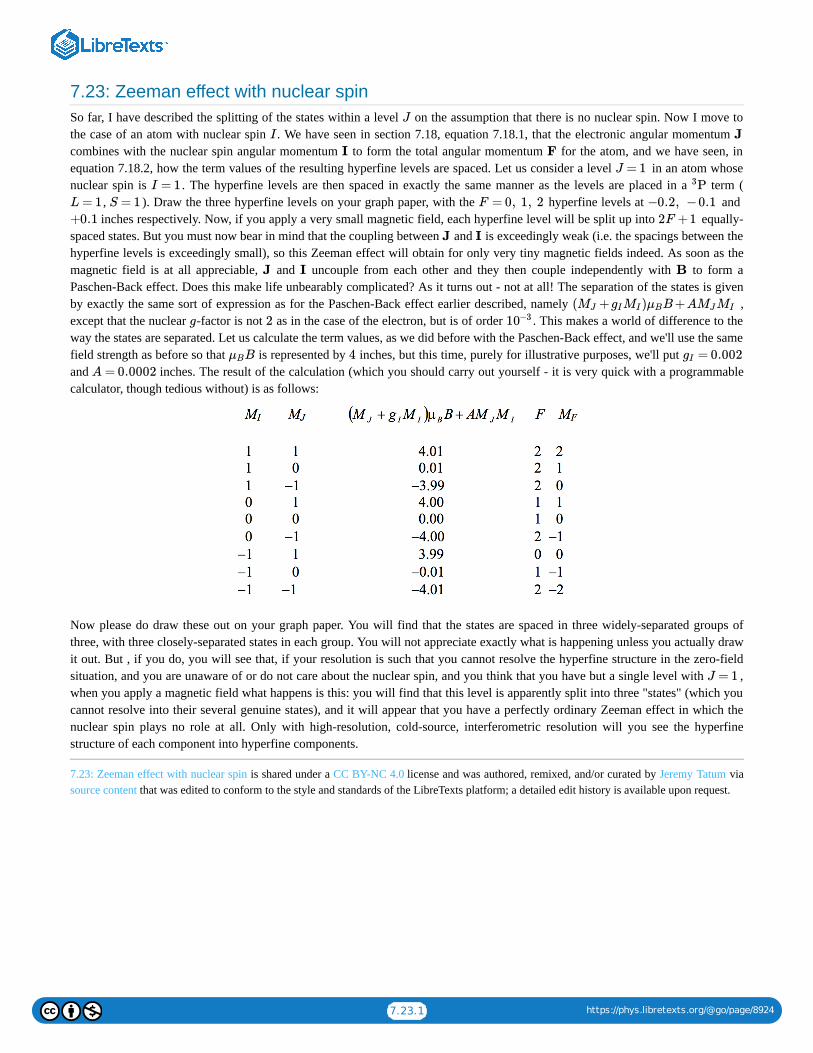
7.23.1 https://phys.libretexts.org/@go/page/8924

7.23: Zeeman effect with nuclear spinSo far, I have described the splitting of the states within a level on the assumption that there is no nuclear spin. Now I move tothe case of an atom with nuclear spin . We have seen in section 7.18, equation 7.18.1, that the electronic angular momentum combines with the nuclear spin angular momentum to form the total angular momentum for the atom, and we have seen, inequation 7.18.2, how the term values of the resulting hyperfine levels are spaced. Let us consider a level in an atom whosenuclear spin is . The hyperfine levels are then spaced in exactly the same manner as the levels are placed in a term (

, ). Draw the three hyperfine levels on your graph paper, with the hyperfine levels at and inches respectively. Now, if you apply a very small magnetic field, each hyperfine level will be split up into equally-

spaced states. But you must now bear in mind that the coupling between and is exceedingly weak (i.e. the spacings between thehyperfine levels is exceedingly small), so this Zeeman effect will obtain for only very tiny magnetic fields indeed. As soon as themagnetic field is at all appreciable, and uncouple from each other and they then couple independently with to form aPaschen-Back effect. Does this make life unbearably complicated? As it turns out - not at all! The separation of the states is givenby exactly the same sort of expression as for the Paschen-Back effect earlier described, namely ,except that the nuclear -factor is not as in the case of the electron, but is of order . This makes a world of difference to theway the states are separated. Let us calculate the term values, as we did before with the Paschen-Back effect, and we'll use the samefield strength as before so that is represented by inches, but this time, purely for illustrative purposes, we'll put and inches. The result of the calculation (which you should carry out yourself - it is very quick with a programmablecalculator, though tedious without) is as follows:

Now please do draw these out on your graph paper. You will find that the states are spaced in three widely-separated groups ofthree, with three closely-separated states in each group. You will not appreciate exactly what is happening unless you actually drawit out. But , if you do, you will see that, if your resolution is such that you cannot resolve the hyperfine structure in the zero-fieldsituation, and you are unaware of or do not care about the nuclear spin, and you think that you have but a single level with ,when you apply a magnetic field what happens is this: you will find that this level is apparently split into three "states" (which youcannot resolve into their several genuine states), and it will appear that you have a perfectly ordinary Zeeman effect in which thenuclear spin plays no role at all. Only with high-resolution, cold-source, interferometric resolution will you see the hyperfinestructure of each component into hyperfine components.

7.23: Zeeman effect with nuclear spin is shared under a CC BY-NC 4.0 license and was authored, remixed, and/or curated by Jeremy Tatum viasource content that was edited to conform to the style and standards of the LibreTexts platform; a detailed edit history is available upon request.

J

I J

I F

J = 1

I = 1 P3

L = 1 S = 1 F = 0,  1,  2 −0.2,   −0.1

+0.1 2F +1

J I

J I B

( + ) B +AMJ gI MI μB MJ MI

g 2 10−3

BμB 4 = 0.002gI

A = 0.0002

J = 1

7.24.1 https://phys.libretexts.org/@go/page/8925

7.24: Selection rulesIt will be recalled that a multiplet is the totality of transitions between two terms. For example, is the multipletconnecting the two terms and . Each term has three levels, and therefore there are nine ways of connecting the levels of oneterm with the other, each transition resulting in a line. But in fact only six of these transitions are "allowed" or "permitted", theremaining three being "forbidden". This is because of certain "selection rules", or restrictions in the way some of the quantumnumber can change. Likewise there are restrictions on the number of multiplets that can connect the terms of two polyads, or on thenumber of Zeeman components that can connect the states of two levels. In all of these situations there are selection rules thatrestrict certain quantum numbers from changing by other than certain amounts. In this section we shall try to understand in aqualitative way how such selection rules arise. We shall list the various selection rules, and see how this will affect the number oflines in a multiplet, or the number of components in a line.

Everyone knows that when an electric dipole oscillates it radiates an electromagnetic wave. Likewise, if a dipole, rather thanperiodically oscillating, suddenly undergoes a change in its electric dipole moment − for example, if the distance between twoopposite electric charges suddenly changes − a pulse of electromagnetic radiation will be radiated. While the radiation from asingle atom will be radiated like that of a dipole, in a gas with enormous numbers of atoms oriented in completely randomdirections, the radiation will appear isotropic.

One reasonable way of explaining how an atom radiates a pulse (a quantum) of electromagnetic radiation when it changes from onestate to another is that its dipole moment changes, and the energy radiated is related to the change in its dipole moment. Indeed inquantum mechanics, the amount of energy radiated when an atom changes from one state to another is determined by the square ofa quantity known as the transition moment:

Here is the usual volume element, and is the wavefunction of the initial state. is the dipole moment operator, whichdepends on the positions of all the electrons in the atom. is the conjugate of the wavefunction of the final state. Those who havelots of practice in performing such calculations are experienced enough to know that the effect of the dipole moment operator ismerely to produce a similar wavefunction with perhaps some changes in the quantum numbers. Therefore, in order to save writingout the complete expression for the wavefunction in full, they merely list the quantum numbers of the initial wavefunction in a ket,and of the conjugate of the final function in a bra, thus:

Again, those who do such calculations daily for a living soon recognize, from the very symmetries of the wavefunctions (grouptheory) and without having to worry greatly about the details of the functions, that this transition moment is zero unless there arecertain relations between the initial and final quantum numbers. It is those transitions that result in a nonzero transition momentthat are "allowed". If the transition moment is zero, which it is except for certain combinations of initial and final quantumnumbers, the transition is "forbidden".

For example, if we are discussing the possible Zeeman components of a line, the only "allowed" transitions - i.e. the only nonzerotransition moments - are those in which the initial and final values of are either equal or differ by . We say that the "selectionrule" for the Zeeman effect is . We already took account of this restriction in drawing figures VII.1 and VII.2. Inthe former, instead of 15 possible components, there are only nine with nonzero transition moments and which satisfy the selectionrule, and in figure VII.2 there are only six rather than eight.

Actually, when observing the Zeeman effect, if we view the light from a direction perpendicular to the magnetic field, we see thatthe components with are plane polarized parallel to the magnetic field, and are called the -components, and the oneswith are plane polarized perpendicular to the magnetic field, and are called the -components (German senkrecht -perpendicular). (It may appear that the symbols and , especially the former, are by now doing more than their fair share ofwork.) If the spectrum is viewed from a direction along the magnetic field, the -components will be found to be circularlypolarized in opposite senses, while the -components are not visible at all.

Just as the number of Zeeman components of a line is limited by the selection rule in a similar manner the number ofpossible lines in a multiplet is limited by a selection rule ( forbidden). I already mentioned that a multiplet has just six lines rather than nine. Figure VII.3 shows the possible transitions. (Unlike figures VII.1 and VII.2, in which

P −3  3Do

P3 3Do

∫ μ dτ .ψ∗f

ψi (7.24.1)

dτ ψI μ

ψ∗f

⟨ |μ|LSJM⟩.L′S ′J ′M ′ (7.24.2)

M ±1

ΔM = 0,   ±1

ΔM = 0 p

ΔM = ±1 s

s p

s

p

ΔM = 0, ±1

ΔJ = 0, ±1 0 ↔ 0 P −3  3Do

7.24.2 https://phys.libretexts.org/@go/page/8925

the horizontal scale was linear in wavelength with wavelength increasing to the right, the horizontal scale in figure VII.3 has nosignificance.)

It may be that a line, or a component, is forbidden to dipole radiation and that, if µ is the electric dipole moment operator, thetransition moment is zero. However, if we substitute for the dipole moment operator the operator for electric quadrupole ormagnetic dipole moment, the transition moment is not zero. In that case a transition that is forbidden to electric dipole ( )radiation may be permitted to electric quadrupole ( ) or magnetic dipole ( ) radiation. and transitions are very weakand are rarely observed under laboratory conditions (though they occur in astronomical sources for reasons that will be explainedlater). Therefore lines that are forbidden to electric dipole radiation are generally referred to merely as "forbidden" lines - eventhough they are not actually forbidden to or radiation. The carrier (atom) for a forbidden line is often written in brackets.For example, there is an line in the spectrum of the aurora at arising from the neutral oxygen atom, so the line is saidto be a line of .

Some multiplets are forbidden to electric dipole radiation only if the terms concerned conform strictly to -coupling, but may beallowed for electric dipole radiation if there are departures from -coupling. Such transitions are "semi-forbidden", and thecarrier is sometimes written between a bracket and a parenthesis. Thus there is a semi-forbidden line at due to . For

-coupling, electric dipole radiation is allowed only if . That is to say, transitions are allowed between two triplet terms,or between two singlet terms, but not between a triplet or a singlet. (In this connection I am referring to a term as a "triplet"term, even though it has just one level.) Not everyone uses this bracket-parenthesis convention.

In the neutral helium atom, there are singlet terms and triplet terms. -coupling is the norm, and, because of this, there are notransitions between any of the singlet terms and a triplet term. Indeed, it is as if there are two entirely independent sets of terms andtwo spectra, and indeed the singlet terms and the triplet terms are sometimes referred to as "para-helium" and "ortho-helium"respectively. Under such circumstances it is difficult (or impossible in the absence of additional independent evidence) to know therelative energies of the triplet and singlet terms, or to know which is the ground term of the atom − although we do now know thatthe ground term of helium is a term.

Neutral calcium also has a set of singlet terms and a set of triplet terms, but there are departures from -coupling, and there aremultiplets that connect singlet with triplet terms and vice versa. Such multiplets are called "intercombination" or "intersystem"multiplets. For example the line at is a member of a multiplet of .

Here is a list of the various selection rules I can think of. I haven’t included nuclear spin, but you may deduce what the rules are,given that the coupling between electron angular momentum and nuclear spin is generally pure -coupling (analogous to -coupling).

For Electric Dipole Transitions. Transitions take place between terms of different configurations, such that the -value of oneelectron must change by . It follows that allowed transitions are between terms of opposite parity. Lines within a multiplet aresubject to the selection rule , except that to is forbidden. (These rules break down for electric dipole radiation inthe presence of a strong external electric field, which need not concern us here, but needs to be considered with respect to the Starkeffect.) Zeeman components of a line are subject to the selection rule .

For -coupling, there are the following additional constraints. ; that is to say, intersystem transitions are forbiddento electric dipole radiation. They are "semi-forbidden". , except that to is forbidden. Thus ,

FIGURE VII.3

E1

E2 M1 E2 M1

E2 M1

E2 557.7 nm

[ ]O I

LS

LS

345.3 nm [ )Al ILS ΔS = 0

S3

LS

S3

LS

657.3 nm S−1  3Po [ )Ca I

JI LS

l

±1

ΔJ = 0,   ±1 0 0

δM = 0, ±1

LS ΔS = 0

ΔL = 0,   ±1 0 0 S− So

7.24.3 https://phys.libretexts.org/@go/page/8925

, multiplets would all be indicative of departures from -coupling. Transitions must also take placebetween terms of common parentage.

For Magnetic Dipole Transitions. Transitions take place between terms of a single configuration, and hence between terms of thesame parity. Lines within a multiplet are subject to the selection rule , except that to is forbidden. Zeemancomponents of a line are subject to the selection rule , except that and cannot both be zero.

For -coupling there are the additional constraints and .

For Electric Quadrupole Transitions. Transitions take place either between terms of the same configuration or betweenconfigurations in which the -value of one electron changes by . In either case this implies that transitions take place betweenterms of the same parity. Lines within a multiplet are subject to the selection rule , except that

and are forbidden. This implies that must be at least . Zeeman components of a line aresubject to the selection rule .

For -coupling there are the additional constraints and , except that are forbidden. Transitions must also take place between terms of common parentage.

Exercise. In section 7.16 I listed the first ten levels for the hydrogen atom - i.e. the levels in the first three shells. I also asserted thatHα comprises three transition arrays, three multiplets, seven lines and an unspecified number of Zeeman components. Now thatyou are familiar with selection rules, you are in a position to verify this. Therefore, as an exercise, list all of the arrays, multipletsand lines comprising . (You should assume -coupling; obviously with just one electron there is no distinction between -and -coupling.) For example, is one array. is a multiplet. is a line. In the table in

section 7.16, I have listed the statistical weight of each level. For each level, list the possible values, and then, using the Zeemanselection rules, determine how many Zeeman components there are for each level, and therefore for as a whole. How many ofthe Zeeman components have distinct wavelengths?

In the above exercise, perhaps you ignored the effect of nuclear spin. Now include nuclear spin ( ). You will see now thateach of the eight levels involved in the formation of is split into two hyperfine levels with different values of . Now, howmany hyperfine and Zeeman are there?

Now answer the same questions with deuterium. One might hope that the deuterium nucleus (the "deuteron") has zero nuclear spin- but no such luck, for the spin of the deuteron is . Thus most of the levels are composed of three hyperfine levels. (Why did Isay "most"? Some of the levels have just two hyperfine levels, don't they? Do you see why?) How many hyperfine and Zeemancomponents are allowed by the selection rules?

Of course, natural hydrogen includes both and a very small amount of , and the spectra of both will be exhibited. Truly is a much more complicated "line" than we envisaged in section 7.3! To add to the complication, we must not forget that underterrestrial conditions, hydrogen is molecular, and there are three possible isotopomers - and - and those familiar withmolecular spectra will recall that there are obvious differences between the spectra of homonuclear and heteronuclear molecules.One could clearly spend a lifetime studying the spectrum of hydrogen!

7.24: Selection rules is shared under a CC BY-NC 4.0 license and was authored, remixed, and/or curated by Jeremy Tatum via source content thatwas edited to conform to the style and standards of the LibreTexts platform; a detailed edit history is available upon request.

S− Do P − Fo LS

ΔJ = 0,   ±1 0 0

ΔM = 0,   ±1 ΔJ ΔM

LS ΔS = 0 ΔL = 0

l ±2

ΔJ = 0,   ±1,   ±2

0 −0,   − ,  0 −112

12

1 −0 +J ′ J ′′ 2

ΔM = 0,   ±1,   ±2

LS ΔS = 0 ΔL = 0,   ±1,   ±2

ΔL = 0 −0,  0 −1,  1 −0

Hα LS LS

jj 2p−3d 2p −3d D 2Po  2 2p −3d 2Po3

2

 2D 5

2

M

Hα

I = 1/2

Hα F

I = 1

H1 H2 Hα

,  HDH2 D2

7.25.1 https://phys.libretexts.org/@go/page/8948

7.25: Some forbidden lines worth knowingThe states in the ground level of an atom are the only stable states. Atoms may be raised to higher levels by collisions, but theseexcited states are not very stable, and an atom in an excited state will very soon de-excite by radiative emission of a photon.Lifetimes in the excited states are typically of the order of nanoseconds. However, the probability of de-excitation by emission ofmagnetic dipole or electric quadrupole radiation is much smaller than that for electric dipole radiation, and the lifetimes of excitedstates for or radiation may be seconds or even minutes. Such states are called metastable states. In normal laboratoryconditions the interval between interatomic collisions (or collisions with the wall of the containing vessel) is very much shorterthan the mean lifetime of a metastable level. (You can work out the inter-collision time from kinetic theory of gases.) Thus an atomwill be knocked out of a metastable level by collision long before it has had a chance to emit or radiation. This is not so invery thin gases in some astronomical sources, such as the aurora or in emission nebulae. In such milieus collisions are few and farbetween, giving ample time for or radiative de-excitation.

It is worth noting, however, that the condition for the successful emission of or radiation is not quite as simple as supposingthat the mean lifetime of a metastable level must be less than the intercollision interval. A collision may be inelastic, in which casesome of the kinetic energy is absorbed and the metastable atom makes an upward transition; or it may be superelastic, in whichcase the metastable atoms undergoes a radiationless downward transition, the excess energy going to increase the kinetic energy ofthe colliding particle; or the collision may be elastic, in which case there is no change in kinetic energy and the metastable atomremains in its metastable state. In order to determine the condition for emission or non-emission of "forbidden" radiation, it isnecessary to take account of the probability of these several processes. In practice the probability that a collision will be inelastic orsuperelastic may be quite small, so that very few collisions result in removing an atom from its metastable state. Thus it is quitepossible for or lines to be observed even if the mean time between collisions is appreciably less than the mean lifetime of ametastable state − though under laboratory conditions, the collision frequency is altogether far too high. In astronomical sourceswhere "forbidden" lines can be emitted, they are still very weak − but we have the advantage of being able to look through sourcesof vast extent.

Now that we understand how forbidden lines can be observed in astronomical sources, I give some examples of a few forbiddenlines worth knowing.

The first three terms of are indicated schematically in figure VIII.4. They arise from the same configuration, so the termis an inverted term and none of the transitions are . The transitions I have drawn are all "forbidden". I have drawn transitionsas continuous lines and transitions as dashed lines. You should verify this by reference to the selection rules.

Starting from the left, the first two lines are at and . The mean lifetime of the level is of order about a second.The branching ratio is such that the ultraviolet (dashed) transition is very much less likely than the green transition at

. This green transition is usually the strongest auroral line, and you can even see that it is greenish in colour. The nexttime you look at an aurora you can reflect that electric quadrupole radiation is entering your eye! What a thrill! The linealso occurs in the short-lived trains left by meteors. The two dashed (magnetic dipole) lines at the right are at and ,and are red. The mean lifetime of the level is more than a minute, and they also appear in the auroral spectrum, but muchhigher in the atmosphere, where the inter-collision time is longer. When you look at an aurora you can usually see a red glowhigher than the green glow. You are seeing magnetic dipole as well as electric quadrupole radiation!

There are several somewhat similar magnetic dipole and electric quadrupole lines involving the first three terms of the spectra of , , , , , which occur in the spectra of emission nebulae, including planetary nebulae. In figure VII.5 I

M1 E2

M1 E2

M1 E2

M1 E2

M1 E2

O I p4 P3

E1 E2

M1

FIGURE VII.4

297.2 557.7 nm 1S0

M1 E2

557.5 nm

557.7 nm

636.3 630.0 nm1D2

[ ]O II [ ]O III [ ]N I [ ]N II [ ]N III

7.25.2 https://phys.libretexts.org/@go/page/8948

illustrate just three lines of . The configuration of all terms is and so the term is not inverted. The transitions and (notice - no parity change) are at and and are among the strongest observed in

nebulae, and are often denoted by and , although they have nothing whatever to do with nitrogen, the letter presumablysignifying "nebular". I would strongly discourage such notation. The transition is at . Before these lines wereunderstood, they were referred to as "nebulium".

Before the spectrum of the solar corona was understood, the emission lines from the corona were ascribed to "coronium", but it isnow known that they are "forbidden" lines from highly-ionized metals. The separation between levels within a single term is verylarge for highly-ionized atoms, and many of the observed lines in the coronal spectrum are magnetic dipole lines connecting twolevels within the same term. For example, one of the strongest of the coronal lines, the green line at , arises from the ion

− that is to say the spectrum . This is isoelectronic with the neutral aluminium atom, and the ground term of the configuration is a normal term with two levels − and . In the separation in term value of these

levels is only , but they are much more widely spaced in so that, in this spectrum, the wavelength of

is .

The last example is the famous - transition of neutral hydrogen, . Here, the lowest level is , which is the one and only

level is the ground term, . The level is split into two hyperfine levels as a result of the interaction between the total electronicangular momentum and the nuclear spin ), the -values of the two hyperfine levels being and . The - lineis a magnetic dipole transition between these two hyperfine levels. The nuclear spin of deuterium is , and consequently theground level of deuterium is split into hyperfine levels with and . A transition between these two is predicted at ,but apparently there is as yet no unambiguous detection of it from an astronomical source.

7.25: Some forbidden lines worth knowing is shared under a CC BY-NC 4.0 license and was authored, remixed, and/or curated by Jeremy Tatumvia source content that was edited to conform to the style and standards of the LibreTexts platform; a detailed edit history is available uponrequest.

[ ]O III p2 P3

−3P2  1D2 −3P2  1D2 500.7 495.9 nm

N1 N2 N

−1D2  1S0 436.3 nm

FIGURE VII.5

530.3 nm

Fe13+ [ ]Fe XIV

KL3 S)3ps2(1 2PoJ = 1

232

Al I112 cm−1 Fe XIV −2Po

1

2

 2Po3

2

530.3 nm

21 cm H I2S 1

2

S2

(J = )12

(I = 12

F 0 1 21 cm

I = 1

F = 12

32

92 cm

7.26.1 https://phys.libretexts.org/@go/page/8950

7.26: Stark EffectThe Stark effect concerns the separation of the states within a level as the result of the application of an external electric field, andthe consequent splitting of lines into Stark components. The atmosphere of a star, being hot and highly ionized, is an electricalconductor and consequently cannot sustain electric potential gradients (fields). Thus the splitting of a line into its Stark componentsis not normally observed in stellar atmospheres, and for that reason I am not going into a detailed description of it or the theory ofthe effect here. There are just two small points that are probably worth mentioning.

The first point concerns the Balmer series of . The details of the Stark pattern vary from line to line in the series, but it happensthat in every even member of the series, that is to say , , etc., there is no central, undisplaced Stark component. Under somecircumstances, even if the hydrogen lines are broad and the Stark components are unresolved, this may result in a small dip at thetop of an emission line, or a small bump at the bottom of an emission line. There are other effects (see the chapter on line profiles)that can result in a dip at the top of an emission line or a bump at the bottom of an absorption line, but if the cause is Stark splitting,this may be recognized in that it affects only the even members of the Balmer series, and not the odd members ( , , etc.).

The second point is that, although a stellar atmosphere cannot sustain a large macroscopic electric field, when two atoms approacheach other in a near-collision, each induces a temporary electric dipole on the other. (This is the origin of the van der Waals forces,which fall off inversely as the sixth power of the interatomic distance.) The resulting electric field of one atom on the other, and theother on the one, results in a general broadening of the lines, often asymmetrically, as a result of Stark effect, and this effectobviously increases with pressure and is one of the components of the phenomenon of pressure broadening, to be discussed in alater chapter.

7.26: Stark Effect is shared under a CC BY-NC 4.0 license and was authored, remixed, and/or curated by Jeremy Tatum via source content thatwas edited to conform to the style and standards of the LibreTexts platform; a detailed edit history is available upon request.

H I

Hβ Hδ

Hα Hγ

1

CHAPTER OVERVIEW

8: Boltzmann's and Saha's Equations

8: Boltzmann's and Saha's Equations is shared under a CC BY-NC 4.0 license and was authored, remixed, and/or curated by Jeremy Tatum viasource content that was edited to conform to the style and standards of the LibreTexts platform; a detailed edit history is available upon request.

8.1: Introduction8.2: Stirling's Approximation. Lagrangian Multipliers.8.3: Some Thermodynamics and Statistical Mechanics8.4: Boltzmann's Equation8.5: Some Comments on Partition Functions8.6: Saha's Equation8.7: The Negative Hydrogen Ion8.8: Autoionization and Dielectronic Recombination8.9: Molecular Equilibrium8.10: Thermodynamic Equilibrium

Topic hierarchy

8.1.1 https://phys.libretexts.org/@go/page/6692

8.1: IntroductionA measurement of the strength of a spectrum line can in principle enable us to determine the number of atoms in the initial level ofthe transition that produces it. For an emission line, that initial level is the upper level of the transition; for an absorption line it isthe lower level. In order to determine the total number of atoms (in all energy levels) in the source, it is necessary to know, inaddition to the number of atoms in a particular level, how the atoms are distributed, or partitioned, among their numerous energylevels. This is what Boltzmann's equation is concerned with. But even this will tell us only how many atoms there are in aparticular ionization stage. If we are to determine the total abundance of a given element, we must also know how the atoms aredistributed among their several ionization stages. This is what Saha's equation is concerned with.

8.1: Introduction is shared under a CC BY-NC 4.0 license and was authored, remixed, and/or curated by Jeremy Tatum via source content that wasedited to conform to the style and standards of the LibreTexts platform; a detailed edit history is available upon request.

8.2.1 https://phys.libretexts.org/@go/page/6693

8.2: Stirling's Approximation. Lagrangian Multipliers.In the derivation of Boltzmann's equation, we shall have occasion to make use of a result in mathematics known as Stirling'sapproximation for the factorial of a very large number, and we shall also need to make use of a mathematical device known asLagrangian multipliers. These two mathematical topics are described in this section.

8.2i Stirling's Approximation

Stirling's approximation is

Its derivation is not always given in discussions of Boltzmann's equation, and I therefore offer one here.

The gamma function is defined as

or, what amounts to the same thing,

In either case it is easy to derive, by integration by parts, the recursion formula

If is a positive integer, , this amounts to

I shall start from equation . It is easy to show, by differentiation with respect to , that the integrand has a maximumvalue of where . I am therefore going to divide both sides of the equation by this maximum value, so that the newintegrand is a function that has a maximum value of where :

Now make a small change of variable. Let , so that

Bearing in mind that we aim to obtain an approximation for large values of , let us try to obtain an expansion of as a series in. A convenient way of obtaining this is to take the logarithm of the integrand:

and. provided that , the Maclaurin expansion is

If is sufficiently large, this becomes

so that

lnN ! ≅N lnN −N . (8.2.1)

Γ(x+1) = dt∫∞

0txe−t (8.2.2)

Γ(x) = dt.∫∞

0tx−1e−t (8.2.3)

Γ(x+1) = xΓ(x). (8.2.4)

x N

Γ(N +1) = N !. (8.2.5)

8.2.2 t txe−t

(x/e)x t = x

1 t = x

Γ(x+1) = dt.( )e

x

x

∫∞

0( )t

x

x

e−(t−x) (8.2.6)

s = t−x

Γ(x+1) = ds = f(s)ds.( )e

x

x

∫∞

−x

(1 + )s

x

x

e−s ∫∞

−x

(8.2.7)

x f(s)s/x

lnf(s) = x ln(1 + )−s,s

x(8.2.8)

|s| < x

lnf(s) = x( − ⋅ +. . .)−s.s

x

1

2( )s

x

2(8.2.9)

x

lnf(s) = − ,s2

2x(8.2.10)

Γ(x+1) = exp(− )ds.( )e

x

x

∫∞

−∞

s2

2x(8.2.11)

8.2.2 https://phys.libretexts.org/@go/page/6693

While this integral is not particularly easy, it is at least well known (it occurs in the theory of the gaussian distribution, forexample), and its value is . Thus we have, for large ,

or, if is an integer,

On taking logarithms of both sides, we obtain

or, since is large:

For very large (i.e. if ), we can make the further approximation

or

Any of equations 8.2.12 - 17 may be referred to as Stirling's approximation.

The largest value of for which my hand calculator will return is . For this, it gives

For very large numbers, the approximation will be much better. The extreme approximation represented by equations or , however, becomes reasonable only for unreasonably large numbers, such as the number of protons in the Universe. We

shall be making use of the much better approximation equation , which does not require such unimaginably huge numbers.

For smaller numbers that we commonly deal with in spectroscopy (where we are typically dealing with the number of atoms in asample of gas) the following approximation is remarkably good:

This almost the same as equation , except that, in deriving it, I have taken to expansion of equation to one more term.Thus, to eight significant figures, , while equation results in .

8.2ii Lagrangian Multipliers

This topic concerns the problem of determining where a function of several variables is a maximum (or a minimum) where thevariables are not independent but are connected by one or more functional relations.

Let be some function of , and . Then, if , and are independent variables, one would ordinarily understandthat, where is a maximum, the derivatives are zero:

However, if , and are not completely independent, but are related by some constraining equation such as , thesituation is slightly less simple. An example from thermodynamics comes to mind. Entropy, , is a function of state:

. However, for a particular substance, , and are related by an equation of state. In effect, we cannotdetermine for the system at any point in , , space, but we are restricted to explore only on the two-dimensional surfacerepresented by the equation of state.

2πx− −−

√ x

Γ(x+1) = ( )x

e

x

2πx− −−

√ (8.2.12)

x

N ! =( )N

e

N

2πN− −−−

√ (8.2.13)

lnN ! =(N + ) lnN −N +ln ,1

22π−−

√ (8.2.14)

N

lnN ! ≅N lnN −N . (8.2.15)

N lnN >> 1

lnN ! = N lnN (8.2.16)

logN ! = N logN . (8.2.17)

N N ! 69

lnN ! = 226.2, N lnN −N = 223.2. (8.2.1)

8.2.168.2.17

8.2.15

lnN ! =(N + ) lnN −N + +ln1

2

1

12N2π−−

√ (8.2.18)

8.2.14 8.2.920! = 2.4329020 ×1018 8.2.18 2.432 902 9 ×1018

ψ = ψ(x, y, z) x y z x y z

ψ

= = = 0.∂ψ

∂x

∂ψ

∂y

∂ψ

∂z(8.2.19)

x y z f(x, y, z) = 0S

S = S(P ,V ,T ) P V T

S P V T

8.2.3 https://phys.libretexts.org/@go/page/6693

We return now to our function . If we move by infinitesimal displacements , , from a point where is a maximum, thecorresponding changes in both and will be zero, and therefore both of the following equations must be satisfied:

Consequently any linear combination of and , such as , where is an arbitrary constant, also satisfies a similarequation. The constant is sometimes called an "undetermined multiplier" or a "Lagrangian multiplier", although often someadditional information in an actual problem enables the constant to be identified - and we shall see an example of this in thederivation of Boltzmann's equation.

In summary, the conditions that is a maximum if , and are related by a functional constraint are

where .

Of course, if is a function of many variables , , not just three, and the variables are subject to several constraints, such as , etc., where , , , etc., are functions connecting all or some of the variables, the conditions for to be

a maximum (or minimum) are

8.2: Stirling's Approximation. Lagrangian Multipliers. is shared under a CC BY-NC 4.0 license and was authored, remixed, and/or curated byJeremy Tatum via source content that was edited to conform to the style and standards of the LibreTexts platform; a detailed edit history isavailable upon request.

ψ dx dy dz ψ

ψ f

dψ = dx+ dy+ dz = 0,∂ψ

∂x

∂ψ

∂y

∂ψ

∂z(8.2.20)

df = dx+ dy+ dz = 0.∂f

∂x

∂f

∂y

∂f

∂z(8.2.21)

ψ f ϕ = ψ+λf λ

λ

ψ x y z f(x, y, z) = 0

= 0,   = 0,   = 0,∂ϕ

∂x

∂ϕ

∂y

∂ϕ

∂z(8.2.22)

ϕ = ψ+λf

ψ x1 …x2

f = 0,  g = 0,  h = 0 … f g h ψ

+λ +μ +ν +. . . = 0, i = 1, 2, 3, . . .∂ψ

∂xi

∂f

∂xi

∂g

∂xi

∂h

∂xi(8.2.23)

8.3.1 https://phys.libretexts.org/@go/page/6694

8.3: Some Thermodynamics and Statistical MechanicsBesides needing to know Stirling's approximation and the method of Lagrangian multipliers, before we can embark uponBoltzmann's equation we also need to remind ourselves of two small results from thermodynamics and statistical mechanics. Imention these only briefly here, with barely adequate explanations. Fuller treatments are given in courses or books onthermodynamics and statistical mechanics. If you are rusty on these topics, or perhaps have never studied them thoroughly, the onlyconsequence is that you may not be able fully to understand the derivation of Boltzmann's equation. This will not matter a greatdeal and should not deter you from reading subsequent sections. It is more important to understand what Boltzmann's equationmeans and how to apply it, and this can be done even if you have missed some of the details of its derivation.

Most readers will either understand this section very well and will not need prolonged explanation, or will not understand it at all,and will be happy to skip over it. Therefore, for brevity's sake, I do little more than quote the results, and I do not even explainwhat many of the symbols mean.

Those who are familiar with thermodynamics will have no difficulty in recalling

The result that we shall be needing in Section 8.4 is , or more likely its reciprocal:

The relation we need from statistical mechanics is Boltzmann's relation between entropy and thermodynamic probability. Supposewe have an assembly of particles that can be distributed or "partitioned" among distinct states. If is the number of ways inwhich this partition can be achieved, Boltzmann's equation for the entropy (indeed, his conception of entropy) is

Here, is Boltzmann's constant, . Those who remember having seen this before might just like to be remindedof the gist of the argument leading to it. It presupposes some functional relation between and , and it notes that, if you haveseveral assemblies, the total " " for the ensemble as a whole is the product of the 's of the individual assemblies, whereas thetotal entropy is the sum of the individual entropies, and therefore the entropy must be proportional to the logarithm of the numberof possible configurations.

That was very brief, but it will do for the purposes of Section 8.4.

8.3: Some Thermodynamics and Statistical Mechanics is shared under a CC BY-NC 4.0 license and was authored, remixed, and/or curated byJeremy Tatum via source content that was edited to conform to the style and standards of the LibreTexts platform; a detailed edit history isavailable upon request.

dU = TdS−PdV . (8.3.1)

= T(∂U/∂S)V

= .( )∂S

∂UV

1

T(8.3.2)

N m X

S = k lnX. (8.3.3)

k 1.38 ×  10−23 J K−1

S X

X X

8.4.1 https://phys.libretexts.org/@go/page/6695

8.4: Boltzmann's EquationIf we have a large number of atoms in a hot, dense gas, the atoms will constantly be experiencing collisions with each other,leading to excitation to the various possible energy levels. Collisional excitation will be followed, typically on timescales of theorder of nanoseconds, by radiative deexcitation. If the temperature and pressure remain constant, there will exist a sort of dynamicequilibrium between collisional excitations and radiative de-excitations, leading to a certain distribution of the atoms among theirvarious energy levels. Most of the atoms will be in low-lying levels; the number of atoms in higher levels will decreaseexponentially with energy level. The lower the temperature, the faster will be the population drop at the higher levels. Only at veryhigh temperatures will high-lying energy levels be occupied by an appreciable number of atoms. Boltzmann's Equation shows justwhat the distribution of the atoms will be among the various energy levels as a function of energy and temperature.

Let's imagine a box (constant volume) holding atoms, each of which has possible energy levels. Suppose that there are atoms in energy level . The total number of atoms is given by

Here, is a running integer going from to , including as one of them.

The total internal energy of the system is

We now need to establish how many ways there are of arranging atoms such that there are in the first energy level, in thesecond, and so on. We shall denote this number by . To some, it will be intuitive that

That is,

I don't find it immediately obvious myself, and I am happier with at least a minimal proof. Thus, the number of ways in which

atoms can be chosen from to occupy the first level is , where the parentheses denote the usual binomial coefficient. For

each of these ways, we need to know the number of ways in which atoms can be chosen from the remaining . This is, of

course, . Thus the number of ways of populating the first two levels is . On continuing with this

argument, we eventually arrive at

If the binomial coefficients are written out in full (do it - don't just take my word for it), there will be lots of cancellations and youalmost immediately arrive at Equation .

We now need to know the most probable partition - i.e. the most probable numbers , , etc. The most probable partition is theone that maximizes with respect to each of the - subject to the constraints represented by Equations and .

Mathematically it is easier to maximize , which amounts to the same thing. Taking the logarithm of Equation , we obtain

Apply Stirling's approximation to the factorials of all the variables. (You'll see in a moment that it won't matter whether or not youalso apply it to the constant term ) We obtain

N m Nj

Ej N

N = .∑i=1

m

Ni (8.4.1)

i 1 m j

U

U = .∑i=1

m

NiEi (8.4.2)

N N1 N2

X

X = .N !

! !. . . . . . !. . . . . . !N1 N2 Nj Nm

(8.4.3)

X = .N !

!∏mi=1 Ni

(8.4.4)

N1

N ( )N

N1

N2 N −1

( )N −1

N2

( )N

N1

( )N −1

N2

X =( )( ) . . . . . .( ) .N

N1

N −1

N2

N −m+1

Nm

(8.4.5)

8.4.3

N1 N2

X Nj 8.4.1 8.4.2

lnX 8.4.3

lnX = lnN ! − ln ! −ln !−. . .N1 N2 (8.4.6)

lnN !

lnX ≅lnN ! −( ln − ) −( ln − )−. . .N1 N1 N1 N2 N2 N2 (8.4.7)

8.4.2 https://phys.libretexts.org/@go/page/6695

Let us now maximize with respect to one of the variables, for example , in a manner that is consistent with the constraintsof Equations and . Using the method of Lagrangian multipliers, we obtain, for the most probable occupation number ofthe th level, the condition

Upon carrying out the differentiations, we obtain

That is to say:

What now remains is to identify the Lagrangian multipliers (or ) and . Multiply both sides of Equation by .Recall that is a running subscript going from to , and that is one particular value of . Therefore now change the subscriptfrom to , and sum from to , and Equation now becomes

where we have made use of Equations and . From Equation , we see that

so that

Now apply Equation 8.3.3, followed by Equation 8.3.2, and we immediately make the identification

Thus Equation becomes

We still have to determine . If we change the subscript in Equation from to and sum from to , we immediately findthat

Thus

where I have omitted the summation limits ( and ) as understood..

However, there is one factor we have not yet considered. Most energy levels in an atom are degenerate; that is to say there areseveral states with the same energy. Therefore, to find the population of a level, we have to add together the populations of theconstituent states. Thus each term in Equation must be multiplied by the statistical weight of the level. (This isunfortunately often given the symbol . See section 7.14 for the distinction between , and . The symbol is a form of theGreek letter pi.) Thus we arrive at Boltzmann's Equation:

The denominator of the expression is called the partition function (die Zustandsumme). It is often given the symbol or or .

lnX Nj

8.4.1 8.4.2

j

+λ +μ = 0.∂ lnX

∂Nj

∂N

∂Nj

∂U

∂Nj

(8.4.8)

−ln +λ+μ = 0.Nj Ej (8.4.9)

= = C .Nj eλ+μEj eμEj (8.4.10)

λ C = eλ μ 8.4.9 Nj

i 1 m j i

j i i = 1 m 8.4.9

− ln +λN +μU = 0,∑i=1

m

Ni Ni (8.4.11)

8.4.1 8.4.2 8.4.7

− ln = lnX−lnN ! −N ,∑i=1

m

Ni Ni (8.4.12)

lnX = lnN ! −(λ+1)N −μU. (8.4.13)

μ = − .1

kT(8.4.14)

8.4.10

= C .Nj e− /(kT )Ej (8.4.15)

C 8.4.15 j i 1 m

C = .N

∑mi=1 e

− /(kT )Ej

(8.4.16)

=Nj

N

e− /(kT )Ej

∑ e− /(kT )Ej

(8.4.17)

1 m

8.4.17 ϖ

g d g ϖ ϖ

=Nj

N

ϖje− /(kT )Ej

∑ϖie− /(kT )Ei

(8.4.18)

u Q Z

8.4.3 https://phys.libretexts.org/@go/page/6695

The statistical weight of a level of an atom with zero nuclear spin is . If the nuclear spin is , the statistical weight of a levelis . However, the same factor occurs in the numerator and in every term of the denominator of equation

, and it therefore cancels out from top and bottom. Consequently, in working with Boltzmann's equation, under mostcircumstances it is not necessary to be concerned about whether the atom has any nuclear spin, and the statistical weight of eachlevel in equation can usually be safely taken to be .

In equation we have compared the number of atoms in level with the number of atoms in all level. We can also comparethe number of atoms in level with the number in the ground level 0:

Or we could compare the number in level to the number in level 1, where “2” represent any two level, 2 lying higher than 1:

8.4: Boltzmann's Equation is shared under a CC BY-NC 4.0 license and was authored, remixed, and/or curated by Jeremy Tatum via sourcecontent that was edited to conform to the style and standards of the LibreTexts platform; a detailed edit history is available upon request.

2J +1 I

(2I +1)(2J +1) 2I +1

8.4.18

8.4.18 (2J +1)

8.4.18 j

j

=Nj

N0

ϖje− /(kT )Ej

ϖ0(8.4.19)

2

= = .N2

N1

ϖ2

ϖ1e−( − )/(kT )E2 E1

ϖ2

ϖ1e−hν/(kT ) (8.4.20)

8.5.1 https://phys.libretexts.org/@go/page/6696

8.5: Some Comments on Partition FunctionsThe topics we discuss in this section are

i. Divergence of partition functions.ii. Metals and nonmetals.

iii. Product of partition functions.iv. Particles in a box.

i. Divergence of Partition FunctionsWe can perhaps start by computing the partition function of atomic hydrogen. We have seen that each "level" (technically eachshell) of hydrogen is actually a group of several terms, and that the total number of states in the shell - i.e. its statistical weight - is

. See section 7.16. If we include nuclear spin, the statistical weight of each shell is actually for ordinary hydrogen and for deuterium. However, as agreed in section 8.4, we need not be concerned with nuclear spin, and we can take the statisticalweight of each shell to be . The energy levels are given by equation 7.4.8:

but how many "levels" are there? That is, what is the upper limit of the sum in the partition function? Our first response is thatthere are an infinite number of energy levels converging towards the ionization limit at . The same is true of other atoms;they, too, have infinite series of Rydberg levels. Evidently to calculate the partition function, we have to sum an infinite series, inthis case, the series being

We can take anything that does not contain outside the summation symbol and absorb it in the constant, and so we have toevaluate the sum

Now we all remember that there are several tests to determine whether or not a series converges, and that, during an exam, all thetests that we remember fail, and the one test that we need is the one and only test that we cannot remember or never understood.Here is our chance now - Determine whether the above series converges or diverges!

I'll let you pause for a while you do that.

Darn it! The series diverges! The partition function is infinite! Although the uppermost "levels" have a high excitation potential andtherefore cannot individually have high occupation numbers, there is an infinite number of them. The atoms are partitioned amongan infinite number of levels, and the probability of any individual level being occupied approaches zero! Disaster!

This is a difficult subject, and not one in which I can claim much expertise, but a qualitative explanation goes something like this.The Coulomb potential of an isolated electric charge (in the present case we are thinking of the hydrogen nucleus; for heavieratoms we are thinking of the atom less the outermost, optical electron) is hyperbolic, approaching the ionization limitasymptotically, becoming horizontal as if you draw a graph of the potential. In a partially ionized gas (which includes allstellar atmospheres) there are numerous charged particles - electrons and ions, and they all interact with one another. If two chargedparticles approach each other, the electric potential in the space between them becomes slightly lowered beneath the theoreticalzero potential for an isolated charge. This is all one needs to resolve the difficulty. The ionization potential is lowered just a little(the exact amount will depend on the density of charged particles) and this eliminates the infinite number of Rydberg levels justbeneath the ionization limit. There remains then a finite number of levels, and a finite number of terms in the partition function.

We do not, for our present purpose, necessarily need to know the exact amount of the lowering of the ionization potential, or howmany "levels" remain, because we soon find that after the first few levels, the occupation numbers rapidly decrease and do notcontribute much to the partition function. Where we choose to terminate the summation depends on the temperature and theprecision we hope to achieve. Try calculating, for example, for and . This should giveyou some idea.

2n2 4n2 6n2

2n2

E = const. ×(1 − ) ,1

n2(8.5.1)

m

13.6 eV

2 exp[−(1 − ) /(kT )].∑n=1

∞

n2 1

n2(8.5.2)

n

exp( ).∑1

∞

n2 1

kTn2(8.5.3)

r → ∞

exp(−E/(kT )) E = 10 eV T = 20, 000 K

8.5.2 https://phys.libretexts.org/@go/page/6696

Here is another insightful semiclassical guide. Consider the electron orbits in a Bohr model of the hydrogen atom. The radii of theorbits increase as . There comes a time when this radius becomes comparable to the average nearest-neighbour distance betweenatoms. If we assume an ideal gas equation of state, , where is the number of atoms per unit volume, we might take thenearest-neighbour distance to be , and we could equate this to the radius of the largest existing Bohr orbit. Presumably thiswill limit the number of Balmer lines we could see in a stellar atmosphere, and it will also tell us where to cut off the summation incalculating the partition function. Radio astronomers observe transitions involving very large quantum numbers - e.g. .Presumably these come from hydrogen atoms in a region of space where the nearest neighbour distance is large enough the permitthe existence of Bohr orbits of high quantum number.

ii. Metals and NonmetalsThere is a difference between calculating the partition functions of metals and of nonmetals - but first it is necessary to say what Imean by a "metal". It would be difficult to find two chemists or two physicists or two engineers who would agree on the exactdefinition of a metal. Among astronomers, however, there is near unanimity: the periodic table comprises hydrogen, helium, and allthe remaining elements are "metals". This is a distressing misuse of the English language, and I strongly discourage it. I shouldmake it plain that in this section - indeed in this chapter or book - this is not what I mean when I write the word "metal". Although,as I say, few scientists would agree on the precise definition, if I say "a metal is an element which, in the solid state, is hard, shiny,and conducts electricity", I should not be far off the mark. Almost everyone will find some immediate objection to that definition -but it is still not far off the mark, and certainly much better than the astronomers' "any element other than hydrogen and helium". Inbrief, elements that we think of in everyday life as being metals - such as iron, zinc, titanium, copper, lead, vanadium, tin, and so on- are metals. Neon, argon, chlorine, carbon, germanium, are not. From the spectroscopic point of view, a metal is characterized byhaving many, many energy levels, including many not far above the ground level. The calculation of the partition function is longand tedious, because so many levels, especially low-lying levels, must be taken into account. In the old days when thesecalculations were done by hand calculator, the levels were taken term by term, the statistical weight of each term being

. The partition functions are fairly sensitive to temperature. Nonmetals, on the other hand, are characterized bytypically having a large gap between the ground term and the first excited term. Consequently, the Boltzmann factors for termsother than the ground term are small, and, as a result, the partition function of a nonmetal is, to a good approximation, merely equalto the statistical weight of the ground term - and it hardly changes with temperature.

Now here is a question I used to enjoy asking students, both graduate and undergraduate. I would take particular pleasure in askinggraduate students during a thesis defence. Think of a fairly hot star, such as Vega - say its temperature is something like .You will recall having seen the spectrum if Vega - it shows a beautiful development of the Balmer series of hydrogen. Obviouslymany of the higher "levels" are excited in the hot atmosphere; not all of neutral hydrogen atoms are still in the ground "level". Thequestion is: At , what fraction of the neutral hydrogen atoms in the atmosphere remain in the ground "level"? And, just tomake it clear that I was not expecting detailed precise calculations, I would give the question as a "multiple-choice" question, withjust three alternatives:

(a) Nearly all of them? (b) About half of them? (c) Hardly any of them?

Usually answers would be pretty evenly divided among the three. Have a go at it yourself. All the information you need is to befound in this chapter and chapter 7. It is important that you should have some feeling for the answer.

You will probably also be asking yourself how many of the hydrogen atoms are neutral, and how many are ionized. We shall comeback to that when we have discussed Saha's equation. The answer will depend not only on the temperature but also on the pressure.

iii. Product of Partition FunctionsIn some systems, the total energy may be made up of several different sources of energy. Consider, for example, a simple diatomicmolecule. Its energy may be the sum of the electronic excitation energy, energy of vibration, and kinetic energy of rotation. If theseseveral sources of energy are independent of each other, the total energy will be merely the sum of the separate contributions:

In practice, for real molecules, this is just a first approximation - in reality, there is some interaction between the severalcontributions to the energy, but the intention here is not to get bogged down in the finer details of molecular structure but merely tomake a small point concerning partition functions, as follows. Provided that the several energy contributions are independent and

n2

P = NkT N

N−1/3

H 109α

(2S+1)(2L+1)

20, 000 K

20, 000 K

= + + .Etot. Eel. Evib. Erot. (8.5.4)

8.5.3 https://phys.libretexts.org/@go/page/6696

do not interact significantly and the energies are consequently additive, the total wavefunction is the product of the threewavefunctions:

Here and are the wavefunctions and energy levels for a simple harmonic oscillator and and are thewavefunctions and energy levels of a rigid rotator. It will be easily understood that a molecule cannot simultaneously be a rigidrotator and a harmonic oscillator, which is why equations and are just first approximations. However, the vibrations of amolecule are generally far faster than the relatively slow and ponderous rotations, and electron motions are faster still, so the firstapproximation is not too bad. More to the point for our present purpose is that every term of the partition function is of the form

, and consequently, if the total energy is the sum of the individual contributions, as in equation , the total partitionfunction is the product of the partition functions of the individual contributions:

The extent to which this approximation is valid in real molecules is not the main subject of discussion here. I merely wished toestablish that, provided equation holds, then equation follows.

iv. Particles in a Box

The reader may vaguely remember studying, in an introductory quantum mechanics course, perhaps without quite knowing why,something called "particle in a box". This was actually useful, and we shall need it before proceeding to the next section. Perhapsthe topic would better have been called "waves in a box", because it was the wavefunctions that describe the wave aspect of aparticle that were under discussion. If the particle (and its associated wave) is confined in a box, the wavefunctions are restricted tofunctions that have an integral number of antinodes between opposite walls, and consequently the energy levels can have onlydiscrete values - another example of the inevitability of discrete energy levels resulting from boundary constraints. If the box is acube of side , the energy levels are given by

Problem: Verify that the above expression has the dimensions of energy.

If we have many particles in a box, we may be interested to know how the numerous particles are distributed or partitioned amongthe energy levels. In other words, we need to know the partition function, which is just

If the box is very large, the energy levels are very close together and almost continuous. (If the box is infinitely large, there are noboundary constraints and hence there is a continuum of possible energies). If the levels are almost continuous, we can replace thesummations with integrals:

where is the volume of the box. We shall need this result in section 8.6.

Problem: What are the dimensions of the expression 8.5.9?

8.5: Some Comments on Partition Functions is shared under a CC BY-NC 4.0 license and was authored, remixed, and/or curated by Jeremy Tatumvia source content that was edited to conform to the style and standards of the LibreTexts platform; a detailed edit history is available uponrequest.

ψ = ψel.ψvib.ψrot. (8.5.5)

ψvib. Evib. ψrot. Erot.

8.5.4 8.5.5

e−E/(kT ) 8.5.4

u = uel.uvib.urot. (8.5.6)

8.5.4 8.5.6

a

= ( + + ) .Enxnynz

h2

8ma2n2x n2

y n2z (8.5.7)

exp[− ].∑=0nx

∞

∑=0ny

∞

∑=0nz

∞ ( + + )h2 n2x n2

y n2z

8m kTa2(8.5.8)

Partition function = exp[− ]d d d∫∞

0

∫∞

0

∫∞

0

( + + )h2 n2x n2

y n2z

8m kTa2nx ny nz

= [ exp(− )dn]∫∞

0

h2n2

8m kTa2

3

= V ,( )2πmkT

h2

3

2

(8.5.9)

V = a3

8.6.1 https://phys.libretexts.org/@go/page/6697

8.6: Saha's EquationConsider the reversible reaction

where is a neutral atom and its first ion. Let , , be the numbers of neutral atoms, ions and electrons respectively,held in a box of volume . Then

is the Saha function. It is a function of temperature and pressure, high temperature favouring ionization and high pressure favouringrecombination. (Students of chemistry will recognize this as an application of Le Chatelier's principle.) The equation tells us therelative numbers of the three types of particle (i.e. the degree of ionization) in an equilibrium situation when the number ofionizations per second is equal to the number of recombinations per second.

Now the number of particles in a given energy level is proportional to the Boltzmann factor for that level, and the total number ofparticles is proportional to the sum of the Boltzmann factors for all the levels - i.e. to the partition function. Thus, using the symbol

to denote partition functions, we have, for Saha's equation:

The partition function is the sum of the Boltzmann factors over all the states, translational and internal (electronic). The totalenergy of a particle is the sum of its translational and internal energies, so that total partition function is the product of itstranslational and internal partition functions, for which we shall use the symbol . Therefore

Here , which is very little different from .

The internal partition function of the electron is merely its statistical weight . In calculating the internal partitionfunctions of the atom and ion, it is, of course, essential to measure all energies from the same level - the ground level of the neutralatom, for example. You would not be so foolish, of course, as to calculate the partition function of the atom by using, in theBoltzmann sum, the energies of each level above the ground level of the atom, and then calculate the partition function of the ionby using the energies above some quite different level, such as the energy of the ground stage of the ion, would you? Most of usprobably would be so foolish; we should, of course, add (the ionization energy) to each level of the ion. If we do calculate thepartition function of the ion using energies above the ground level of the ion, we must then multiply the result, , by .Being even more careful, we should remember, from section 8.5, that the ionization energy is in practice lowered by a smallamount . Finally, let us now use the symbol to denote number of particles per unit volume (so that , and on noaccount to be confused with the quantum numbers used in section 8.5) and we arrive at the usual form for Saha's equation:

It might be noted that is a function of , which leads to a slight complication in the computation of Saha's equation, whichwe shall encounter in one of the problems that follow.

It should be remarked that Saha's equation played an extremely important role in the understanding of the stellar spectral sequence.As is well known, the sequence of spectral types OBAFG… is a result of the degree of ionization and excitation of the elements asa function of temperature, and the difference in the degree of ionization between main sequence stars and giants of a giventemperature is the result of the higher degree of ionization in the relatively low pressure atmospheres of the giant stars. This couldnot be understood at a quantitative level until the development of Saha's equation and its application to stellar atmospheres by Saha,Fowler, Milne and Payne (later Payne-Gaposhkin) in the 1920s.

Problems.

Problem 1. Verify that equation balances dimensionally.

A ⇋ + ,A+ e− (8.6.1)

A A+ N0 Ni Ne

V

= S(T , P )NeNi

N0(8.6.2)

Q

= .NeNi

N0

QeQi

Q0(8.6.3)

u

= V .NeNi

N0( )

2πmkT

h2

3

2 ueui

u0(8.6.4)

m =memi

m0me

2s +1 = 2

χi

ui e− /kTχi

Δχi n n = N/V

n

= exp(− ).neni

n0( )

2πmkT

h2

3

2 2ui

u0

( −Δ )χi χi

kT(8.6.5)

Δχi ne

8.6.5

8.6.2 https://phys.libretexts.org/@go/page/6697

Problem 2. In the bad old days, we did calculations using logarithm tables! You probably will never have to do that, but thisexercise will nevertheless turn out to be useful. Show that Saha's equation can be written as

and determine the numerical value of the constants and if is expressed in , is in , is the ionization potential involts, and logarithms are common logarithms (i.e. to the base 10). I make them and . It is common also towrite equation in the form

in which .

Problem 3. You are going to calculate the Saha function for hydrogen, and so you need the partition functions for the electron, theneutral hydrogen atom and the hydrogen ion. The electron is easy. Its spin is , so its partition function is , as already discussedand indeed already incorporated into Saha's equation. The partition function for neutral hydrogen can be taken to be the statisticalweight of its shell, which is . Now what about the statistical weight of the hydrogen ion? The hydrogen ion is aproton, which has spin . Therefore, as for the electron, should the partition function be ? The answer is no! Whencalculating the Saha equation for hydrogen, you should take the partition function of the proton to be . This probably seemsentirely illogical and you are probably quite sure that I am wrong. But before coming to this conclusion, read again the lastparagraph of section 8.4 and the first paragraph of section 8.5i. You can include the effect of the proton spin provided that you takeit into account for both and . If you insist that the statistical weight of the proton is , you must also insist that the statisticalweight of the shell of is . As with the Boltzmann equation, you usually need not be concerned with nuclear spin -it cancels out in . There is nothing, however, to cancel out the factor for the electron partition function.

Problem 4. A kilogram of water is contained is a box of volume one cubic metre. The box is made of material that won't melt orvaporize. (!) Draw a graph showing, as a function of temperature, from to , the logarithm of the numbers perunit volume of each of the species , , , , . (Assume there are no higher ionization stages, and no molecules.)

This is going to be difficult, and will involve some computation. The first thing you are going to need to do is to calculate the Sahafunctions of the species involved as a function of temperature., and for this, you will need the partition functions . For the electron,the partition function is and is already incorporated in the Saha equation. As discussed in Problem 3, the partition function of should be taken to be , and, as for the electron, it is mercifully independent of temperature. For neutral , the statistical weight ofthe ground shell is , and, as you will already have discovered if you carried out the little calculation in section 8.5ii, you canprobably take this to be the partition function at all temperatures between and . The ground term of neutraloxygen is , and the first excited term is at a term value of . Probably only the ground term contributesappreciably to the partition function, but you might want to check that. The ground term of is and the first excited term isa long way up. Thus, for all species, you can probably take the partition function to be the statistical weight of the ground term andindependent of temperature. You are very lucky that I did not throw a metal into the mix!

The ionization limits of and are at and respectively. We don't yet know by how much, theionization energy is lowered, so we'll ignore to begin with. You now have enough information to calculate the Saha functionsfor hydrogen and for oxygen as a function of temperature.

We have been asked to calculate the numbers of five species and we are therefore going to need four equations. We started with onekilogram of water. We know that grams of water contain molecules, where is Avogadro's number. (You may want to lookup the exact molar mass of .) Thus, we started with molecules. Let's call that number .

Now see if you agree with the following five equations.

log = A + log T +log −B( )neni

n0

3

2

ui

u0

−ΔVi Vi

T(8.6.6)

A B n m−3 T K Vi

A = 21.68 B = 5039.7

8.6.6

log = 27.24 − log θ +log −θ( −Δ ),neni

n0

3

2

ui

u0

Vi Vi (8.6.7)

θ = 5039.7/T

1/2 2

n = 1 2 = 2n2

= 1/2 2

1

H H+ 2

n = 1 H 4 = 4n2

/ui u0 2

10, 000 K 20, 000 K

e H H+ O O+

2 H+

1 H

2

10, 000 20, 000 K

P3 D1 15868 cm−1

O II 4So

H O 101678 109837 cm−1 Δχi

Δχi

18 A A

OH2 1000A/18 N

+ = 2NNH NH+ (8.6.8)

+ = NNO NO+ (8.6.9)

+ =NH+ NO+ Ne (8.6.10)

= VNeNH+ SHNH (8.6.11)

= VNeNO+ SONO (8.6.12)

8.6.3 https://phys.libretexts.org/@go/page/6697

We do indeed have five equations in the five unknowns, and all other quantities in the equations are known. The first two expressthe stoichiometry of the water molecule. The third expresses electrical neutrality. The last two are Saha's equations for hydrogenand oxygen. They five equations are not very difficult equations, although the last two are nonlinear, which makes them slightlyawkward. We can make them a little easier. I am going to re-write them:

If we now, just for the moment, suppose that is a quantity whose value is known. In that case, equations to wouldcomprise five linear equations in just four unknowns. The condition for these equations to be consistent is that the determinant ofthe coefficients and the constant terms be zero:

If I have done my algebra right (you might like to check this), this is a cubic equation in :

You can now solve this for . Remember, however, that, in calculating the Saha functions, you ignored the lowering of theionization potential , so what you have found is but a first approximation for . This is a function of the electron density. Onerather old formula, due to Unsöld, is

where is in volts and is in m (indicating that the lowering of the potential is proportional to the distance betweenthe charged particles.). If you can find a more recent and perhaps better formula, by all means use it. You can use your firstapproximation for to calculate the Saha functions, and then repeat the entire calculation and continue to iterate until you obtainan acceptably small change in . It is probable that only one iteration will be necessary. Having found (and ) it is thenstraightforward to find the remaining unknowns from equation to . Just make sure that you make use of all fiveequations as a check for arithmetic mistakes.

Problem 5. A bottle of methyl cyanate is held in a cylinder with a movable piston such that the pressure remainsconstant at one pascal. Heat it up to some temperature at which you can assume that the only species present are electrons and theneutral atoms and singly ionized stages of , , and - i.e. no higher ionization stages and no molecules. The cylinder andpiston are not allowed to melt - they are required only to provide constant pressure conditions, in contrast to the previous problemin which you had a constant volume. You have nine unknowns, and you will need nine equations. In this problem you are askedmerely to write down the nine required equations, not necessarily to solve them unless you particularly want to. There will be Sahaequations for each element, an equation expressing electrical neutrality, and four equations reflecting the stoichiometry. You mayassume the ideal gas equation .

8.6: Saha's Equation is shared under a CC BY-NC 4.0 license and was authored, remixed, and/or curated by Jeremy Tatum via source content thatwas edited to conform to the style and standards of the LibreTexts platform; a detailed edit history is available upon request.

+ −2N = 0NH NH+ (8.6.13)

+ −N = 0NO NO+ (8.6.14)

+ − = 0NH+ NO+ Ne (8.6.15)

V − = 0SHNH NeNH+ (8.6.16)

V − = 0SONO NeNO+ (8.6.17)

Ne 8.6.13 8.6.17

1

0

0

V SH

0

1

0

1

−Ne

0

0

1

0

0

V SO

0

1

1

0

−Ne

−2N

−N

−Ne

0

0

= 0 (8.6.18)

Ne

+V ( + ) +V [V −(2 + )N ] −3 N = 0.N 3e SO SH N 2

e SHSO SH SO Ne V 2SHSO (8.6.19)

Ne

ΔVi Ne

Δ = 7 × ,Vi 10−5n1/3e (8.6.20)

Vi (= /V )ne Ne-3

ne

ne ne Ne

8.6.13 8.6.17

CNOCH3

C H O N

P = nkT

8.7.1 https://phys.libretexts.org/@go/page/9027

8.7: The Negative Hydrogen IonThe word "ion" in the gas phase is often thought of as the positively charged remnant of an atom that has lost one or moreelectrons. However, any electrically charged atom (or molecule or radical), whether positively charged (as a result of loss of anelectron) or negatively charged (having an additional electron) can correctly be called an "ion". In this section, we are interested inthe negative hydrogen ion, , a bound system consisting of a proton and two electrons.

The formation of such an ion can be qualitatively described, in classical terms, as follows. A hydrogen atom, consisting of a protonand an electron, is approached by a second electron. The electric field of the second electron (which falls off with distance as )induces a dipole moment in the neutral hydrogen atom, with the two electrons then being at opposite sides of the proton. Theinduced dipole moment is proportional to the electric field of the polarizing electron, and hence to . The second electron nowfinds itself immersed in the electric field of the dipole that it has itself induced in the neutral atom, and can be captured by it. Thefield of the dipole falls is proportional to , where , the induced dipole moment, is already proportional to . Thus the forcebetween the neutral (but dipolar) hydrogen atom and the intruding second electron falls off as , and the second electron movesin a potential varying as . Because of this, the energy level structure of is very different from that of . In , the potentialfalls off as , which results in the familiar infinite Rydberg series of levels. For a potential of the form , if theSchrödinger equation predicts a finite number of bound levels below the ionization limit, and, in the case of , there is just onebound level, and it is a mere below the ionization limit. The can be called the ionization potential of the ion orthe electron affinity of the atom. Perhaps the latter term is preferable, because it is a little odd to refer to removing an electronfrom the ion (so that it is then no longer an ion) as "ionization"! As Professor Joad might have said: "It all depends what youmean by 'ionization'". In any case, an electron can easily be removed from either by a mild collision or by any photon of(vacuum) wavelength shorter than about .

In the solar atmosphere, most hydrogen atoms are neutral and have the electron in the shell ( shell). Only a few are in theform of or . (I am not sure offhand which is more numerous, or − that would make a good lunchtime discussion.)But because is so readily stripped of an electron by almost any old photon, makes an appreciable contribution to thecontinuous opacity of the solar atmosphere. The continuous absorption can be either by "bf" (bound-free) transitions or so-called"ff" (free-free) transitions. In the latter case the second electron is unbound, but it swerves in the field of the dipole that it has itselfinduced in the neutral atom.

8.7: The Negative Hydrogen Ion is shared under a CC BY-NC 4.0 license and was authored, remixed, and/or curated by Jeremy Tatum via sourcecontent that was edited to conform to the style and standards of the LibreTexts platform; a detailed edit history is available upon request.

H−

r−2

r−2

H

p/r3 p r−2

r−5

r−4 H− H H

r−1 r−n n > 1

H−

0.7 eV 0.7 eV H−

H

H−

H−

1771 nm

n = 1 K

H+ H− H+ H−

H− H−

H

8.8.1 https://phys.libretexts.org/@go/page/9028

8.8: Autoionization and Dielectronic RecombinationThe ionization energy as discussed until this point has meant the energy required to remove an electron from an atom, initially in itsground level, leaving the removed electron with no kinetic energy. The neutral atom has a number of discrete energy levels belowthe ionization limit; above that limit, there is a continuum of energy states - which merely means that the electron is unbound andthere are no restrictions on its kinetic energy.

However, it is possible for more than one electron in an atom to be excited, and in that case it is quite possible for an atom to existin a discrete bound level whose energy is above the ionization limit as described in the previous paragraph. Although this is quitepossible, an atom generally does not stay long in one of these highly excited levels. One of the electrons can easily slip away fromthe atom without the absorption of any additional energy, thereby leaving behind an ion in an excited state. Such a process is calledautoionization, and the levels or states concerned are autoionization levels or states.

The converse process is quite possible. An ion in an excited state can capture a hitherto free electron, thus forming the neutral atomwith two excited electrons. The process is dielectronic recombination. Downward transitions from these autoionization levels tolower discrete level can occur.

As mentioned above, the mean lifetime of the atom in one of these autoionization levels is rather short. As a consequence ofHeisenberg's uncertainty principle, there is a corresponding uncertainty in the energy level that is inversely proportional to thelifetime. Stated otherwise, the autoionization energy levels are relatively broad. Consequently lines resulting from downwardtransitions originating from these autoionization levels are relatively broad, and indeed such lines are often recognized or at leastsuspected from their relatively diffuse appearance. Such lines are readily observed, for example, in the spectra of copper, zinc andcadmium among others.

8.8: Autoionization and Dielectronic Recombination is shared under a CC BY-NC 4.0 license and was authored, remixed, and/or curated byJeremy Tatum via source content that was edited to conform to the style and standards of the LibreTexts platform; a detailed edit history isavailable upon request.

8.9.1 https://phys.libretexts.org/@go/page/9029

8.9: Molecular EquilibriumThe dissociation of diatomic molecules can be treated in a way that is very similar to Saha's equation for ionization. Consider, forexample, the following reversible reaction

The equilibrium is governed by an equation that is essentially identical to the Saha equation:

Here is the equilibrium constant, is , and is the dissociation energy. To a first approximation thepartition function of the molecule is the product of the electronic, vibrational and rotational partition functions, althoughusually today more precise calculations are made. The equation is often written in terms of partial pressures:

in which where the gases may be considered to be ideal.

Let us consider again Problem 5 of section 8.6, in which we have methyl cyanate held at some pressure , but this timewe'll work at some temperature where we shall suppose that the only species to be expected would be neutral atoms and neutraldiatomic molecules. The species concerned are . We shall evidentlyneed 14 equations. They are:

The first of these equations is the ideal gas equation. The next three express the stoichiometry of methyl cyanate. The remainingten, which are nonlinear, are the equilibrium equations. Some skill and experience in the solution of multiple nonlinearsimultaneous equations is necessary actually to solve these equations.

8.9: Molecular Equilibrium is shared under a CC BY-NC 4.0 license and was authored, remixed, and/or curated by Jeremy Tatum via sourcecontent that was edited to conform to the style and standards of the LibreTexts platform; a detailed edit history is available upon request.

AB ↔ A +B (8.9.1)

= = .nAnB

nABKAB ( )

2πmkT

h2

3

2 uAuB

uABe− /(kT )D0

0 (8.9.2)

KAB m /( )mAmB mAmB D00

uAB

=pApB

pABK ′

AB(8.9.3)

= kTK ′AB

KAB

CNOCH3 P

C, H, O, N, C2, CN, CO, CN, H2, OH, NH, O2, NO, N2

+ + + + + + + + + + + + + = P /(kT ),nC nH nO nN nC2nCH nCO nCN nH2

nOH nNH nO2nNO nN2

(8.9.4)

+2 + + + = 2( + + + +2 ),nC nC2nCH nCO nCN nN nCN nNH nNO nN2

(8.9.5)

+ +2 + + = 3( + + + +2 ),nH nCH nH2nOH nNH nN nCN nNH nNO nN2

(8.9.6)

+ + +2 + = + + + +2 ,nO nCO nOH nO2nNO nN nCN nNH nNO nN2

(8.9.7)

= , = , = , = , = ,n2C

KC2nC2

nCnH KCHnCH nCnO KCOnCO nCnN KCNnCN n2H

KH2nH2

(8.9.7-11)

= , = , = , = , = .nOnH KOHnOH nNnH KNHnNH n2O

KO2nO2

nNnO KNOnNO n2N KN2

nN2(8.9.12-16)

8.10.1 https://phys.libretexts.org/@go/page/9030

8.10: Thermodynamic EquilibriumThose who have studied thermodynamics will be familiar with such elementary and easy concepts as entropy, enthalpy, Gibbs freeenergy, chemical potential, activity and fugacity, and will have no difficulty in grasping their meaning. Much more difficult tograsp, however, is the very difficult concept of temperature. I have vague memories of something called the Zeroth Law ofThermodynamics which, I seem to recall, went something like this: "If two bodies are in thermodynamic equilibrium with eachother, and each is in thermodynamic equilibrium with a third, then all three bodies are at the same temperature." I understood thatthis was a law of great profundity, though I was never quite sure whether any part of the Universe could ever truly be inthermodynamic equilibrium and that the Universe would be a pretty dull place if it were. This section may or may not (more likelythe latter) make the concept of temperature any easier.

Let us try to imagine a system consisting of a hot gas with a solid body suspended in it.

Let us imagine that we are somehow able to measure the distribution of the translational speeds of the molecules in the case, andthe distribution is found to conform to a Maxwell-Boltzmann distribution with a root-mean-square speed . We could thencalculate the quantity and call this quantity . We could call this quantity the kinetic temperature of the gas. We might,for example, say that the kinetic temperature of the gas is . Some may think that it would be simpler merely to say how fastthe molecules are moving. In any case, the kinetic temperature of the gas is merely a way of expressing what the root-mean-squarespeed of the molecules is.

Let us also imagine that we are able to determine how the molecules are partitioned among their numerous discrete energy levels.We may find that they are distributed according to the Boltzmann distribution with parameter , and we could call that parameterthe excitation temperature, which would then merely be a way of saying how fast or how slowly the occupation numbers of thelevels fall off with energy.

We might also be able to determine the extent to which the atoms are ionized, and we could apply Saha's equation and hence definean ionization temperature.

Unless the molecules are single atoms, we might also be able to determine how the molecules are partitioned among their variousvibrational levels or among their numerous rotational levels, and we could assign to these distributions a vibrational temperatureand a rotational temperature respectfully.

If we look at the solid, it may be glowing with heat, and we may be able to determine how its exitance per unit wavelength intervalvaries with temperature, and we might observe that it conforms to Planck's radiation formula. We might be able to measure its totalexitance, . We could then pretend that it is a black body, and we could define , where is the StefanBoltzmannconstant, as the effective temperature. Or we could note the wavelength at which the exitance per unit wavelength interval isgreatest, and we could define as the colour temperature where is Wien's constant..

Small wonder that "temperature" and "thermodynamic equilibrium" are such difficult concepts to grasp! However, I think it is fairto make the following statements: If the system is in thermodynamic equilibrium, then all of these various possible measures of"temperature" (kinetic, excitation, ionization, vibrational, rotational, effective, colour) are equal. If they are not equal, the system isnot in thermodynamic equilibrium.

8.10: Thermodynamic Equilibrium is shared under a CC BY-NC 4.0 license and was authored, remixed, and/or curated by Jeremy Tatum viasource content that was edited to conform to the style and standards of the LibreTexts platform; a detailed edit history is available upon request.

V

m /(3k)V 2 T

300 K

T

M (M/σ)1/4σ

W /λmax W

1

CHAPTER OVERVIEW

9: Oscillator Strengths and Related Topics

9: Oscillator Strengths and Related Topics is shared under a CC BY-NC 4.0 license and was authored, remixed, and/or curated by Jeremy Tatumvia source content that was edited to conform to the style and standards of the LibreTexts platform; a detailed edit history is available uponrequest.

9.1: Introduction, Radiance, and Equivalent Width9.2: Oscillator Strength. (die Oszillatorenstärke)9.3: Einstein A Coefficient9.4: Einstein B Coefficient9.5: Line Strength9.6: LS-coupling9.7: Atomic hydrogen9.8: Zeeman Components9.9: Summary of Relations Between f, A and S

Topic hierarchy

9.1.1 https://phys.libretexts.org/@go/page/6699

9.1: Introduction, Radiance, and Equivalent WidthIf we look at a hot, glowing gas, we can imagine that we could measure its radiance in . If we disperse the light with aspectrograph, we may see that it is made up of numerous discrete emission lines. These lines are not infinitesimally narrow, buthave a finite width and a measurable profile. At any particular wavelength within the wavelength interval covered by the line, let ussuppose that the radiance per unit wavelength interval is . Here, we are using the symbol for radiance,which is customary in astronomy, rather than the symbol , which we used in chapter 1. We insist, however, on the correct use ofthe word "radiance", rather than the often too-loosely used "intensity". We might imagine that we could measure by comparingthe radiance per unit wavelength interval in the spectrum of the gas with the radiance per unit wavelength interval of a black bodyat a known temperature (or of any other body whose emissivity is known), observed under the same conditions with the samespectrograph.

The radiance of the whole line is given by In principle, the integration limits are and , although in practicefor most lines the integration need be performed only within a few tenths of a nanometer from the line center.

The radiance of an emission line depends, among other things, upon the number of atoms per unit area in the line of sight (the"column density") in the initial (i.e. upper) level of the line.

You will have noticed that I wrote "depends upon", rather than "is proportional to". We may imagine that the number of atoms perunit area in the line of sight could be doubled either by doubling the density (number of atoms per unit volume), or by doubling thedepth of the layer of gas. If doubling the column density results in a doubling of the radiance of the line, or, expressed otherwise, ifthe radiance of a line is linearly proportional to the column density, the line is said to be optically thin. Very often a line is notoptically thin, and the radiance is not proportional to the number of atoms per unit area in the upper level. We shall return to thistopic in the chapter on the curve of growth. In the meantime, in this chapter, unless stated otherwise, we shall be concerned entirelywith optically thin sources, in which case , where is the column density and the subscript denotes the upper level. Weshall also suppose that the gas is homogenous and of a single, uniform temperature and pressure throughout.

In the matter of notation, I am using:

Thus in a volume , and in a layer of thickness .

Most lines in stellar spectra are absorption lines seen against a brighter continuum. In an analogous laboratory situation, we mayimagine a uniform layer of gas seen against a continuum. We'll suppose that the radiance per unit wavelength interval of thebackground continuum source is . We shall establish further notation by referring to figure , which represents anabsorption line against a continuum. The radiance per unit wavelength interval is plotted against wavelength horizontally.

is the radiance per unit wavelength interval at some wavelength within the line profile, and is the radiance per unitwavelength interval at the line center.

W m−2  sr−1

Iλ  W m−2  sr−1  m−1 I

L

Iλ

I I = dλ.∫ ∞0 Iλ 0 ∞

I ∝ N2 N

n

N

N

= number of atoms per unit volume

= column density

= number of atoms

V , N = nV t, N = nt

(c)Iλ IX.1

FIGURE IX.1

(λ)Iλ ( )Iλ λ0

9.1.2 https://phys.libretexts.org/@go/page/6699

The equivalent width ( ) of an absorption line is the width of the adjacent continuum that has the same areaas is taken up by the absorption line. Expressed as a defining equation, this means:

Again in principle the integration limits are to , although in practice a few tenths of a nanometre will suffice. Equivalent widthis expressed in nm (or in Å). It must be stressed that equivalent width is a measure of the strength of an absorption line, and is in noway related to the actual width (or full width at half minimum) of the line. In figure , the width of the continuum has thesame area as the absorption line.

In principle, the equivalent width could also be expressed in frequency units (Hz), via a defining equation:

This is sometimes seen in theoretical discussions, but in practice equivalent width is usually expressed in wavelength units. Thetwo are related by

Unless otherwise specified, I shall omit the superscript , and will normally mean equivalent width expressed in wavelengthunits, as in Equation .

A layer of cool gas lies above an extended source of continuous radiation, and an absorption line formed in the gas layer has anequivalent width . If the temperature of the extended continuous source is now increased so that its spectral radiance at thewavelength of the line is doubled, what will now be the equivalent width of the line?

The equivalent width of an absorption line depends, among other things, upon the number of atoms per unit area in the line of sight(the "column density") in the initial (i.e. lower) level of the line. If the gas is optically thin, , where the subscript indicatesthe lower level of the line.

If the absorption coefficient at wavelength and has the same value throughout the gas, and it the thickness of the gaslayer is are related by

Thus Equation can be written

and this equation is sometimes cited as the definition of the equivalent width. The definition, however, is Equation . Equation can be used to calculate it, but only if is uniform throughout the gas. In the optically thin limit, the first term in the

Maclaurin expansion of , so that, for an optically thin homogeneous gas,

The reader should verify, as ever, the dimensional correctness of all of the foregoing equations.

We have seen that the radiance of an emission line or the equivalent width of an absorption line depends, among other things, onthe column density of atoms in the initial state. In fact, in a homogeneous optically thin gas, the radiance or equivalent width islinearly proportional to the product of two things. One is the column density of atoms in the initial state. The other is an intrinsicproperty of the atom, or rather of the two atomic levels involved in the formation of the line, which determines how much energy asingle atom emits or absorbs. There are three quantities commonly used to describe this property, namely oscillator strength,Einstein coefficient and line strength.

W die Aequivalentbreite

W (c) = ∫ [ (c) − (λ)] dλ.Iλ Iλ Iλ (9.1.1)

0 ∞

IX.1 W

(c) = ∫ [ (c) − (ν)] dν.W(ν)Iν Iν Iν (9.1.2)

= , = .W(ν) c

λ2W

(λ)W

(λ) c

ν2W

(ν) (9.1.3)

(λ) W

9.1.1

Exercise 9.1.1

W

W ∝ N1

λ is α(λ)

t, (λ) and  (c)Iλ Iλ

(λ) = (c)exp [−α(λ)t] .Iλ Iλ (9.1.4)

9.1.1

W = ∫ [1 −exp(−α(λ)t)] dλ, (9.1.5)

9.1.1

9.1.4 α(λ)

1 −exp(−α(λ)t)  is α(λ)t

W = t∫ α(λ)dλ. (9.1.6)

9.1.3 https://phys.libretexts.org/@go/page/6699

All three of these quantities are related by simple equations, but oscillator strength is particularly appropriate when discussingabsorption lines, Einstein coefficient is particularly appropriate when discussing emission lines, while line strength is a quantummechanical quantity particularly useful in theoretical work. Because of this very technical usage of the term line strength, the termshould not be used merely to describe how "intense" a particular line appears to be.

9.1: Introduction, Radiance, and Equivalent Width is shared under a CC BY-NC 4.0 license and was authored, remixed, and/or curated by JeremyTatum via source content that was edited to conform to the style and standards of the LibreTexts platform; a detailed edit history is available uponrequest.

9.2.1 https://phys.libretexts.org/@go/page/6700

9.2: Oscillator Strength. (die Oszillatorenstärke)The concept of oscillator strength arises from a classical electromagnetic model of the absorption of radiation by an atom. While adetailed understanding of each step in the derivation requires an understanding and recall of some results from classical mechanicsand electromagnetic theory, it is not at all difficult to understand qualitatively the meaning of oscillator strength and at least thegeneral gist of the argument that follows.

An atom consists of a nucleus surrounded by electrons - but not all of the electrons are equally strongly bound. We are going tothink of an atom as having, for the purposes of this model, just two parts of interest, namely an outer loosely bound electron, andthe rest of the atom. If this system is set into vibration, we'll suppose that it has a natural frequency , but that the oscillations aredamped. An oscillating dipole does, of course, radiate electromagnetic waves. That is to say, it loses energy. That is to say, theoscillations are damped. If the atom is placed in an oscillating electric field (i.e. if you shine a light on the atom) given by

the electron will experience a force per unit mass . The Equation of motion is

This is the differential Equation that describes forced, damped oscillations. The solutions to this Equation are well known, but Ishall defer detailed consideration of it until the chapter on line profiles. Suffice it to say, for our present purposes, that it is possibleto determine, from analysis of this Equation, how much energy is absorbed.

If a periodic force is applied to a mass attached to a fixed point by a spring, and the motion is damped, either by viscous forces (forexample, if the mass were immersed in a fluid) or by internal stresses in the spring, not all of the work done by the periodic forcegoes into setting the mass in motion; some of it is dissipated as heat. In a way, we are imagining the atom to consist of an electronattached by some sort of force to the rest of the atom; not all of the work done by the forcing electromagnetic wave goes intosetting the electron in motion. Some of the work is absorbed or degraded into a non-mechanical form. Perhaps the energy is lostbecause the accelerating electron radiates away energy into space. Or perhaps, if you believe in discrete energy levels, the atom israised to a higher energy level. It does not matter a great deal what you believe happens to the energy that is "lost" or "absorbed";the essential point for the present is that Equation allows us to calculate (and I do promise to do this in the chapter on lineprofiles) just how much energy is lost or absorbed, and hence, if the atom is irradiated by a continuum of wavelengths, it enables usto calculate the equivalent width of the resulting spectrum line. The result obtained is

The reader should, as ever, check that the above expression has the dimensions of length. If every quantity on the right hand side isexpressed in SI units, the calculated equivalent width will be in meters.

The reader may well object that s/he is not at all satisfied with the above argument. An atom is not at all like that, it will be said.Besides, Equation says that the equivalent width depends only on the wavelength, and that all lines of the same wavelengthhave the same equivalent width. This is clearly nonsense. Let us deal with these two objections in turn.

First: Atoms are not at all like that. For a start, an atom is an entity that can exist only in certain discrete energy levels, and the onlyatoms that will absorb radiation of a given frequency are those that are in the lower level of the two levels that are involved in aline. Thus in Equation must be replaced by , the column density (number per unit area in the line of sight) of just thoseatoms that are in the lower level of the line involved. Thus Equation should be replaced by

ω0

cos ωtE

cos ωteEm

+γ + x = cos ωt.x x ω20

eE

m(9.2.1)

9.2.1

W = .N e2λ2

4 mε0 c2(9.2.2)

W

N

λ

ε0

e, m

c

= equivalent width in wavelength units.

= column density (number per unit area in the line of sight) of absorbing atoms.

= wavelength of the line.

= permittivity of free space.

= charge and mass of the electron.

= speed of light.

9.2.2

N 9.2.2 N1

9.2.2

W = .N1e2λ2

4 mε0 c2(9.2.3)

9.2.2 https://phys.libretexts.org/@go/page/6700

Second: The equivalent width of a line obviously does not depend only on its wavelength. Many lines of very nearly the samewavelength can have almost any equivalent width, and the equivalent width can vary greatly from line to line. We therefore nowcome to the definition of oscillator strength:

The absorption oscillator strength of a line is the ratio of its observed equivalent width to the equivalent width (wrongly)predicted on the basis of the classical oscillator model and given by Equation .

Thus the expression for the equivalent width becomes

The oscillator strength for a given line must be determined either experimentally or theoretically before the column density of aparticular atom in, for example, a stellar spectrum can be determined from the observed equivalent width of a line. In principle, theoscillator strength of a line could be measured in the laboratory if one were able, for example, to measure the equivalent width of aline produced in an absorbing gas in front of a continuum source, and if one were able independently to determine . Otherexperimental methods can be devised (see section 9.3 on Einstein coefficients), and theoretical methods are also available (seesection 9.5 on line strengths).

It should be emphasized that Equation applies only to an optically thin layer of gas. As far as I can see, there is no reasonwhy Equation is restricted either to a homogeneous layer of gas of uniform temperature and pressure, or to a gas inthermodynamic equilibrium - but it does require the layer to be optically thin.

We shall now restrict ourselves to an optically thin layer that is in thermodynamic equilibrium and of uniform temperaturethroughout. In that case, is given by Boltzmann's Equation (see Equation 8.4.18):

Here is the total number of atoms per unit area in all levels, is the statistical weight of the lower level, and is thepartition function. Thus Equations and combined become

In the above Equations I have used slightly different fonts for , the electronic charge, and , the base of natural logarithms.

The quantity is called the absorption oscillator strength. An emission oscillator strength can be defined by

and either side of this Equation is usually given the symbol . Indeed, it is more usual to tabulate the quantity than or alone. I should also point out that the notation seen in the literature is very often rather than . However, in chapter 7 I went toconsiderable trouble to distinguish between statistical weight, degeneracy and multiplicity, and I do not wish to change the notationhere. In any case, the value of (a form of the Greek letter pi) for an atomic energy level is . (We pointed out in chapter 7why it is not usually necessary to include the further factor for an atom with nonzero nuclear spin.) Equation isusually written

If we take the common logarithm of Equation , we obtain

If everything is in SI units, this is

Definition

f12

9.2.3

W = .N1f12e2λ2

4 mε0 c2(9.2.4)

N1

9.2.4

9.2.4

N1

= .N1

N

ϖ1e− /(kT )E1

u(9.2.5)

N ϖ1 2J +1 u

9.2.4 9.2.5

W = .N e2λ2ϖ1f12e

− /(kT )E1

4 m uε0 c2(9.2.6)

e e

f12 f21

= ,ϖ1f12 ϖ2f21 (9.2.7)

ϖf ϖf f12 f21

gf ϖf

ϖ 2J +1

2I +1 9.2.6

W = .N ϖfe2λ2

e− /(kT )E1

4 m uε0 c2(9.2.8)

9.2.8

log = log +logN −log u − log e.W

ϖfλ2

e2

4 mε0 c2

eV1

kT(9.2.9)

9.2.3 https://phys.libretexts.org/@go/page/6700

I'd be happy for the reader to check my arithmetic here, and let me know (jtatum at uvic dot ca) if it's not right. Here W and λ are tobe expressed in meters and N in atoms per square meter. V1 is the excitation potential of the lower level of the line in volts, and θ is5039.7/T, where T is the excitation temperature in kelvin. Thus, if we measure the equivalent widths of several lines from an

optically thin gas, and plot versus the excitation potential of the lower level of each line, we should get a straight line

whose slope will give us the excitation temperature, and, provided that we know the partition function, the intercept will give us thecolumn density of the neutral atoms (in all levels) or of a particular ionization state.

Often it will happen that some points on the graph fall nowhere near the regression line. This could be because of a wildly-erroneous oscillator strength, or because of a line misidentification. Sometimes, especially for the resonance lines (the strongestlines arising from the lowest level or term) a line lies well below the regression line; this may be because these lines are notoptically thin. Indeed, Equation applies only for optically thin lines.

Equation shows how we can make use of Boltzmann’s Equation and plot a straight-line graph whose slope and intercept willgive us the excitation temperature and the column density of the atoms. We can go further and make use of Saha’s Equation. If we

plot versus the lower excitation potential for atomic lines and do the same thing separately for ionic lines, we should

obtain two straight lines of the same slope (provided that the gas is in thermodynamic equilibrium so that the excitationtemperatures of atom and ion are the same). From the difference between the intercepts of the two lines we can get the electrondensity. Here’s how it works.

If we set up Equation or Equation for the atomic lines and for the ionic lines, we see that the difference between the

intercepts will be equal to , and, if the gas is optically thin, this is also equal to . Here the subscripts denote

atom and ion, is column density and is particles per unit volume. Then from Equation 8.6.7 we see that

Here , where is the ionization temperature and, in assuming that this is the same as the excitation temperaturesobtained from the slopes of the lines, we are assuming thermodynamic equilibrium. is the ionization potential of the atom. Thuswe can obtain the electron density – except for one small detail. is the lowering of the excitation potential, which itselfdepends on . We can first assume it is zero and hence get a first approximation for ; then iterate to get a better in the samemanner that we did in solving Problem 4 of section 8.6.

So far we have discussed the equivalent width of a line. A line, however, is the sum of several Zeeman components, with (in theabsence of an external magnetic field) identical wavelengths. It is possible to define an oscillator strength of a Zeeman component.Is the oscillator strength of a line equal to the sum of the oscillator strengths of its components? The answer is no. Provided the lineand all of its components are optically thin, the equivalent width of a line is equal to the sum of the equivalent widths of itscomponents. Thus Equation shows that the value of a line is equal to the sum of the values of its components. Afurther point to make is that, for a component, the statistical weight of each state of the component is unity. (A review from chapter7 of the meanings of line, level, component, state, etc., might be in order here.) Thus, for a component there is no distinctionbetween absorption and emission oscillator strength, and one can use the isolated symbol with no subscripts, and the unqualifiedphrase "oscillator strength" (without a "absorption" or "emission" prefix) when discussing a component. One can accurately saythat the value of a line is equal to the sum of the values of its components. In other words, , sothat one could say that the oscillator strength of a line is the average of the oscillator strength of its components. Of course, thisdoesn't tell you, given the value of a line, what the -values of the individual components are. We defer discussion of that to alater section of this chapter.

The phrase " -value" is often used instead of "oscillator strength". I was rather forced into that in the previous paragraph, when Ineeded to talk about values versus f-values. However, in general, I would discourage the use of the phrase " -value" and wouldencourage instead the phrase "oscillator strength". After all, we never talk about the "evalue" of the electron or the " -value" ofthe Sun. I suppose "weighted oscillator strength" could be used for .

9.2: Oscillator Strength. (die Oszillatorenstärke) is shared under a CC BY-NC 4.0 license and was authored, remixed, and/or curated by JeremyTatum via source content that was edited to conform to the style and standards of the LibreTexts platform; a detailed edit history is available upon

log = −14.053 +logN −log u −θ .W

ϖfλ2V1 (9.2.10)

log( )W

ϖfλ2

9.2.10

9.2.10

log( )W

ϖfλ2

9.2.9 9.2.10

log( )Naui

Niualog( )naui

niua

N n

log( ) = difference between intercepts  = 27.24 − log θ −θ(V −ΔV ) −lognaui

niua

3

2ne (9.2.11)

θ is 5039.7/T T

V

ne ΔV

ne ne V

9.2.8 ϖf ϖf

f

ϖf f ϖf(line) = Σf(components)

ϖf f

f

ϖf f

M

ϖf

9.2.4 https://phys.libretexts.org/@go/page/6700

request.

9.3.1 https://phys.libretexts.org/@go/page/6701

9.3: Einstein A CoefficientAlthough either oscillator strength or Einstein coefficient could be used to describe either an emission line or an absorption line,oscillator strength is more appropriate when talking about absorption lines, and Einstein coefficient is more appropriate whentalking about emission lines.

We think of an atom as an entity that can exist in any of a number of discrete energy levels. Only the lowest of these is stable; thehigher levels are unstable with lifetimes of the order of nanoseconds. When an atom falls from an excited level to a lower level, itemits a quantum of electromagnetic radiation of frequency given by

where respectively being the energies of the upper (initial ) and lower (final) levels. The number ofdownward transitions per unit time is supposed to be merely proportional to the number of atoms, , at a given time in the upperlevel. The number of downward transitions per unit time is since in calculus means the rate at which is increasing.Thus

The proportionality constant is the Einstein coefficient for spontaneous emission for the transition from . It isequivalent to what, in the study of radioactivity, would be called the decay constant, usually given the symbol . It has dimensions

. Typically for electric dipole transitions, it is of order . As in radioactivity, integration of the aboveEquation shows that if, at time zero, the number of atoms in the upper level is , the number remaining after time will be

Likewise, as will be familiar from the study of radioactivity (or of first-order chemical reactions, if you are a chemist), the meanlifetime in the upper level is and the halflife in the upper level is . This does presume, however, that there is onlyone lower level below . We return to this point in a moment, when we consider the situation when there is a choice of more thanone lower level to which to decay from .

Since there are downward transitions per units time from , and each transition is followed by emission of anenergy quantum , the rate of emission of energy from these atoms, i.e. the radiant power or radiant flux (see chapter 1) is

(For absolute clarity, we could append the subscript 21 to the frequency in order to make clear that the frequency is the frequencyappropriate to the transition between the two energy levels; but a surfeit of subscripts might be too distracting to the point ofactually making it less clear.) Provided the radiation is emitted isotropically, the intensity is

The emission coefficient (intensity per unit volume) is

If we are looking at a layer, or slice, or slab, of gas, the radiance is

Here, I have been obliged to use correctly for intensity and radiance, rather than follow the unorthodox astronomicalcustom of using for radiance and calling it "intensity". I hope that, by giving the SI units, I have made it clear, though the readermay want to refer again to the definitions of the various quantities described in chapter 1. I am using the symbols described insection 9.1 of the present chapter for . I should also point out that Equations 9.3.4-7 require the gas to be opticallythin.

Equation and assume that the atom, starting from level 2, can decay to only one lower level. This may sometimes be thecase, or, even if it is not, transitions to one particular lower level are far more likely than decay to any or all of the others. But ingeneral, there will be a choice (with different branching ratios) of several lower levels. The correct form for the decay constant

A

A

ν

hν = ΔE, (9.3.1)

ΔE = − ,  and E2 E1 E2 E1

N2

− ,N2 N2 N2

− = .N2 A21N2 (9.3.2)

A21  to E2 E1

λ

T−1  and SI units s −1 108s−1

(0)N2 t

(t) = (0) .N2 N2 e− tA21 (9.3.3)

1/A21 (ln2)/A21

E2

E2

A21N2  to E2 E1

hν N2

Φ = hν watts.N2A21 (9.3.4)

ν

I = .hνN2A21

4πW sr−1 (9.3.5)

j = .hνn2A21

4πW m−3sr−1 (9.3.6)

L = . .hνN2A21

4πW m−2sr−1 (9.3.7)

I and L

I

N , n and N

9.3.2 9.3.3

9.3.2 https://phys.libretexts.org/@go/page/6701

under those circumstances is , the sum to be taken over all the levels below to which the atom can decay, and themean lifetime in level 2 is . Nowadays it is possible to excite a particular energy level selectively and followelectronically on a nanosecond timescale the rate at which the light intensity falls off with time. This tells us the lifetime (and hencethe sum of the relevant Einstein coefficients) in a given level, with great precision without having to measure absolute intensities orthe number of emitting atoms. This is a great advantage, because the measurement of absolute intensities and determination of thenumber of emitting atoms are both matters of great experimental difficulty, and are among the greatest sources of error inlaboratory determinations of oscillator strengths. The method does not by itself, however, give the Einstein coefficients ofindividual lines, but only the sum of the Einstein coefficients of several possible downward transitions. Measurements of (ortheoretical calculations of) relative oscillator strengths or branching ratios (which do not require absolute intensity measurementsor determinations of the number of emitting or absorbing atoms), combined with lifetime measurements, however, can result inrelatively reliable absolute oscillator strengths or Einstein coefficients.

We shall deal in section 9.4 with the relation between oscillator strength and Einstein coefficient.

If the optically thin layer of gas described by Equation is in thermodynamic equilibrium, then is given by Boltzmann'sEquation, so that Equation becomes

The common logarithm of this is

If everything is in SI units, this becomes

Thus a graph of versus the upper excitation potential will yield (for optically thin lines) the temperature and the

column density of atoms from the slope and intercept. I leave it to the reader to work out the procedure for determining the electrondensity in a manner similar to how we did this for absorption lines in developing Equation 9.2.11.

The radiance of a line is, of course, the sum of the radiances of its Zeeman components, and, since the radiance is proportional to , one can say, following a similar argument to that given in the penultimate paragraph of section 9.2, that the Einstein

coefficient of a line is equal to the average of the Einstein coefficients of its components.

At this stage, you may be asking yourself if there is a relation between oscillator strength and Einstein coefficient. There is indeed,but I crave your patience a little longer, and I promise to address this in Section 9.4.

“Transition Probability” ( .) The expression “transition probability” is often used for the Einstein coefficient, and it is even sometimes defined as “the probability per second that an atom will make a spontaneous downward

transition from level 2 to level 1”. Both are clearly wrong.

In probability theory (especially in the theory of Markov chains) one sometimes has to consider a system that can exist in any ofseveral states (as indeed an atom can) and the system, starting from one state, can make a transition to any of a number of otherpossible states. The probability of making a particular transition is called, not unnaturally, the transition probability. The transitionprobability so defined is a dimensionless number in the range zero to one inclusive. The sum of the transition probabilities to allpossible final states is, of course unity. “Branching ratio” is another term often used to describe this concept, although perhaps“branching fraction” might be better. In any case, the reader must be aware that in many papers on spectroscopy, the phrase“transition probability” is used when what is intended is the Einstein coefficient.

The reader will have no difficulty in showing (from Equation ) that the probability that an atom, initially in level 2, will makea spontaneous downward transition to level 1 in time , and that the probability that it will have made this transition ina second is . With being typically of order , this probability is, unsurprisingly, rather close to one!

9.3: Einstein A Coefficient is shared under a CC BY-NC 4.0 license and was authored, remixed, and/or curated by Jeremy Tatum via sourcecontent that was edited to conform to the style and standards of the LibreTexts platform; a detailed edit history is available upon request.

λ =∑A21 E2

1/∑A21

9.3.7 N2

9.3.7

L = .Nhcϖ2A21e

− /(kT )E2

4πλu(9.3.8)

log( ) = log +logN −log u − log e.Lλ

ϖ2A21

hc

4π

eV2

kT(9.3.9)

log( ) = −25.801 +logN −log u −θ .Lλ

ϖ2A21V2 (9.3.10)

log( )Lλ

ϖ2A21V2

ϖ2A21

dieÜbergangswahrscheinlichkeit

A

A

9.3.3

t,  is 1 −e tA21

1 −e−A21 A21 108  s−1

9.4.1 https://phys.libretexts.org/@go/page/6702

9.4: Einstein B CoefficientIn section 9.2 on oscillator strengths, we first defined what we meant by absorption oscillator strength . We then showed that theequivalent width of a line is proportional to . We followed this by defining an emission oscillator strength by theequation . Thereafter we defined a weighted oscillator strength to be used more or less as a single symbolequal to either . Can we do a similar sort of thing with Einstein coefficient? That is, we have defined , theEinstein coefficient for spontaneous emission (i.e. downward transition) without any difficulty, and we have shown that theintensity or radiance of an emission line is proportional to . Can we somehow define an Einstein absorption coefficient ?But this would hardly make any sense, because atoms do not make spontaneous upward transitions! An upward transition requireseither absorption of a photon or collision with another atom.

For absorption lines (upwards transitions) we can define an Einstein coefficient such that the rate of upward transitions fromlevel 1 to level 2 is proportional to the product of two things, namely the number of atoms currently in the initial (lower) leveland the amount of radiation that is available to excite these upward transitions. The proportionality constant is the Einsteincoefficient for the transition, . There is a real difficulty in that by “amount of radiation” different authors mean different things.It could mean, for example, any of the four things:

the energy density per unit wavelength interval at the wavelength of the line, expressed in ; the energy density per unit frequency interval at the frequency of the line, expressed in ;

radiance (unorthodoxly called “specific intensity” or even merely “intensity” and given the symbol by many astronomers) perunit wavelength interval at the wavelength of the line, expressed in ;

radiance per unit frequency interval at the frequency of the line, expressed in .

Thus there are at least four possible definitions of the Einstein coefficient and it is rarely clear which definition is intended by agiven author. It is essential in all one’s writings to make this clear and always, in numerical work, to state the units. If we use thesymbols for these four possible definitions of the Einstein coefficient, the SI units and dimensions for eachare

You can, of course, find equivalent ways of expressing these units (for example, you could express in metres per kilogram ifyou thought that that was helpful!), but the ones given make crystal clear the meanings of the coefficients.

The relations between them are (omitting the subscripts 12):

For the derivation of these, you will need to refer to equations 1.3.1, 1.15.3 and 1.17.12,

From this point henceforth, unless stated otherwise, I shall use the first definition without a superscript, so that the Einsteincoefficient, when written , will be understood to mean . Thus the rate of radiation-induced upward transitions from level 1to level 2 will be taken to be times times .

Induced downward transitions.

f12

ϖ1f12 f21

=ϖ2f21 ϖ1f12 ϖf

 or ϖ2f21 ϖ1f12 A21

ϖ2A21 A12

B

N1

B12

uλ  J m−3 m−1

uν  J m−3 Hz−1

Lλ I

   W m−2 sr−1 m−1

Lν    W m−2 sr−1 Hz−1

B

,   ,   ,  Ba12 Bb

12 Bc12 Bd

12 B

:Ba12

:Bb12

:Bc12

:Bd12

(s−1 J m−3  m−1)−1

(s−1 J m−3  Hz−1)−1

(s−1 W m−2  sr−1  m−1)−1

(s−1 W m−2  sr−1  Hz−1)−1

TM−1L2

LM−1

LM−1 T2

LM−1

Bb12

= = = ;Ba λ2

cBb c

4πBc λ2

4πBd (9.4.1)

= = = ;Bb ν2

4πBc c

4πBd ν2

cBa (9.4.2)

= = = ;Bc λ2

cBd 4π

cBa 4πλ2

c2Bb (9.4.3)

= = = ;Bd 4πν2

c2Ba 4π

cBb ν2

cBc (9.4.4)

B12 Ba12

2B1 N1 uλ

9.4.2 https://phys.libretexts.org/@go/page/6702

The Einstein coefficient and the oscillator strength (which are closely related to each other in a manner that will be shownlater this section) are concerned with the forced upward transition of an atom from a level 1 to a higher level 2 by radiation of awavelength that corresponds to the energy difference between the two levels. The Einstein coefficient is concerned with thespontaneous downward decay of an atom from a level 2 to a lower level 1.

There is another process. Light of the wavelength that corresponds to the energy difference between levels 2 and 1 may induce adownward transition from an atom, initially in level 2, to the lower level 1. When it does so, the light is not absorbed; rather, theatom emits another photon of that wavelength. Of course the light that is irradiating the atoms induces upward transitions fromlevel 1 to level 2, as well as inducing downward transitions from level 2 to level 1, and since, for any finite positive temperature,there are more atoms in level 1 than in level 2, there is a net absorption of light. (The astute leader will note that there may be moreatoms in level 2 than in level 1 if it has a larger statistical weight, and that the previous statement should refer to states rather thanlevels.) If, however, the atoms are not in thermodynamic equilibrium and there are more atoms in the higher levels than in thelower (the atom is “top heavy”, corresponding to a negative excitation temperature), there will be Light Amplification by StimulatedEmission of Radiation (LASER). In this section, however, we shall assume a Boltzmann distribution of atoms among their energylevels and a finite positive excitation temperature. The number of induced downward transitions per unit time from level 2 to level1 is given by . Here is the Einstein coefficient for induced downward transition.

Let denote a particular atomic level. Let denote any level lower than and let denote any level higher than . Let bethe number of atoms in level at some time. The rate at which decreases with time as a result of these processes is

This equation describes only the rate at which is depleted by the three radiative processes. It does not describe the rate ofreplenishment of level by transitions from other levels, nor with its depletion or replenishment by collisional processes. Equation

when integrated results in

Here

(Compare equation 9.3.3, which dealt with a two-level atom in the absence of stimulating radiation.)

The reciprocal of is the mean lifetime of the atom in level .

Consider now just two levels – a level 2 and a level below it, 1. The rate of spontaneous and induced downward transitions from to is equal to the rate of forced upward transitions from to :

I have omitted the subscripts 21 to , since there in only one wavelength involved, namely the wavelength corresponding to theenergy difference between the levels 2 and1. Let us assume that the gas and the radiation field are in thermodynamic equilibrium.In that case the level populations are governed by Boltzmann’s equation (equation 8.4.19), so that equation becomes

from which

where I have made use of

Now, still assuming that the gas and photons are in thermodynamic equilibrium, the radiation distribution is governed by Planck’sequation (equations 2.6.4, 2.6.5, 2.6.9; see also equation 2.4.1):

B12 f12

A21

B21N2uλ B21

m n m n′ m Nm

m Nm

− = + + .Nm Nm∑n

Amn Nm∑n

BmnuλmnNm∑

n′

Bmnuλmn(9.4.5)

Nm

m

9.4.5

(t) = (0) .Nm Nm e− tΓm (9.4.6)

= + +Γm ∑n

Amn ∑n

Bmnuλmn ∑n′

Bmn′uλmn′ (9.4.7)

Γm m

m

n n m

+ = .A21N2 B21N2uλ B12N1uλ (9.4.8)

λ

9.4.8

( + ) = ,A21 B21uλ N0ϖ2

ϖ0e− /(kT )E2 B12uλN0

ϖ1

ϖ0e− /(kT )E1 (9.4.9)

= ,uλA21ϖ2

−B12ϖ1ehc/(λkT ) B21ϖ2

(9.4.10)

− = hc/λ.E2 E1 (9.4.11)

9.4.3 https://phys.libretexts.org/@go/page/6702

On comparing equations and , we obtain

A reminder here may be appropriate that the here is as defined near the beginning of this section. Also, in principle therewould be no objection to defining an such that , just as was done for oscillator strength, although Ihave never seen this done.

Einstein coefficient and Equivalent width.

Imagine a continuous radiant source of radiance per unit wavelength interval , and in front of it an optically thin layer of gascontaining atoms per unit area in the line of sight in level 1. The number of upward transitions per unit area per unit time tolevel 2 is , and each of these absorbs an amount of energy. The rate of absorption of energy per unit area perunit solid angle is therefore This, by definition of equivalent width (in wavelength units), is equal to

.

Therefore

If we compare this with equation 9.2.4 we obtain the following relation between a and :

It also follows from equations and that

I shall summarize the various relations between oscillator strength, Einstein coefficient and line strength in section 9.9.

9.4: Einstein B Coefficient is shared under a CC BY-NC 4.0 license and was authored, remixed, and/or curated by Jeremy Tatum via sourcecontent that was edited to conform to the style and standards of the LibreTexts platform; a detailed edit history is available upon request.

= .uλ8πhc

( −1)λ5 ehc/(λkT )(9.4.12)

9.4.10 9.4.12

= = .ϖ1B12 ϖ2B21λ5

8πhcϖ2A21 (9.4.13)

B Ba

ϖB ϖB = =ϖ1B12 ϖ2B21

B12

Lλ

N1

Bc12N1Lλ12 hc/λ12

× × .14π

Bc12N1Lλ12

hc

λ12

WLλ12

W = = .hcBc

12N1

4πλ12

h

λ12N1B

a12 (9.4.14)

B12 f12

= .Ba12

e2λ3

4 hmε0 c2f12 (9.4.15)

9.4.13 9.4.15

= .ϖ2A212πe2

mcε0 λ2ϖ1f12 (9.4.16)

9.5.1 https://phys.libretexts.org/@go/page/6703

9.5: Line StrengthThe term line strength, although often loosely used to indicate how prominent or otherwise a spectrum line is, has acquired intheoretical spectroscopy a rather definite specialist meaning, which is discussed in this section.

In discussing the intensities of emission lines, the Einstein is an appropriate parameter to use, whereas in discussing theequivalent widths of absorption lines the appropriate parameter is oscillator strength . Either of these can be determinedexperimentally in the laboratory. The Einstein coefficient and the oscillator strength are related (I summarize the relations in section9.9) and either could in principle be used whether discussing an emission or an absorption line.

In theoretical studies one generally uses yet another parameter, called the line strength.

The theoretical calculation of line strengths is a specialized study requiring considerable experience in quantum mechanics, and isnot treated in any detail here. Instead I give just a short qualitative description, which I hope will be sufficient for the reader tounderstand the meaning of the term line strength without actually being able to calculate it. Absolute line strengths can becalculated in terms of explicit algebraic formulas (albeit rather long ones) for hydrogen-like atoms. For all others, approximatenumerical methods are used, and it is often a matter of debate whether theoretically calculated line strengths are more or lesspreferable to experimentally determined oscillator strengths, Einstein coefficients or lifetimes. As a general rule, the more complexthe atom, unsurprisingly the more difficult (and less reliable?) are the theoretical calculations, whereas for light atoms theoreticalline strengths may be preferable to experimental oscillator strengths.

Energy levels of atoms are found from the eigenvalues of the time-independent wave equation. For the interaction ofelectromagnetic radiation with an atom, however, solutions of the time-dependent equation are required. The effect of theelectromagnetic radiation is to impose a time-dependent perturbation on the wavefunctions. In the formation of permitted lines, theelectromagnetic wave interacts with the electric dipole moment of the atom. This is a vector quantity given by , where isthe position vector of the th electron in the atom. The expectation value of this quantity over the initial ( )and final ( ) states of atransition is

or, as it is usually written

Here, for permitted lines, is the electric dipole moment operator. For forbidden lines it is replaced with either the magneticdipole moment operator or the electric quadrupole moment operator, or, in principle, moments of even higher order. In any case,the above quantity is called the transition moment. In the case of electric dipole (permitted) lines, its SI unit is , although it ismore commonly expressed in units of (“atomic unit”) or, in older literature, cgs esu, or, in some chemical literature, debye.

1 debye = cgs esu = 0.3935 atomic units =

1 atomic unit = .

The square of the transition moment is called the line strength. Oscillator strengths and Einstein coefficients of Zeemancomponents (i.e. of transitions between states) are proportional to their line strengths, or to the squares of their transition moments.The symbol generally used for line strength is . Line strengths are additive. That is to say the strength of a line is equal to the sumof the strengths of its Zeeman components. In this respect it differs from oscillator strength or Einstein coefficient, in which theoscillator strength or Einstein coefficient of a line is equal to the average oscillator strength of Einstein coefficient of itscomponents. Furthermore, line strength is symmetric with respect to emission and absorption, and there is no need for distinctionbetween and . Intensities of emission lines are proportional to their line strengths or to their weighted Einsteincoefficients . Equivalent widths of absorption lines are proportional to their line strengths or to their weighted oscillatorstrengths .

I dwell no more on this subject in this section other than to state, without derivation, the relations between Einstein coefficient andline strength. The formulas below, in which and are the “rationalized” permittivity and permeability of free space, are validfor any coherent set of units; in particular they are suitable for SI units.

For electric dipole radiation:

A

f

∑ eiri ri

i i f

∫ μ dτ ,ψ∗f ψi (9.5.1)

⟨ |μ|nLSJM⟩.n′L′S ′J ′M ′ (9.5.2)

μ

C m

ea0

10−18 3.336 ×  C m10−30

8.478 ×  C m10−30

S

S12 S21 S

ϖ2A21

ϖ1f12

ε0 μ0

9.5.2 https://phys.libretexts.org/@go/page/6703

For electric quadrupole radiation:

For magnetic dipole radiation:

The subscripts to the symbol indicate whether the line strength is for electric dipole, electric quadrupole ormagnetic dipole radiation. Although I have not derived these equations, you should check to see that they are dimensionallycorrect. The dimensional analysis will have to use the four dimensions of electromagnetic theory, and you must note that the SIunits for line strength are and for electric dipole, electric quadrupole and magnetic dipole radiationrespectively. Please let me know (jtatum@uvic.ca) if you find any discrepancies. In equation , is the permeability of freespace.

By making use of equation 9.4.16, we also find, for electric dipole radiation, that

9.5: Line Strength is shared under a CC BY-NC 4.0 license and was authored, remixed, and/or curated by Jeremy Tatum via source content thatwas edited to conform to the style and standards of the LibreTexts platform; a detailed edit history is available upon request.

= .ϖ2A2116π3

3hε0λ3SE1 (9.5.3)

= .ϖ2A218π5

5 hε0 λ5SE2 (9.5.4)

= .ϖ2A2116π3μ0

3hλ3SM1 (9.5.5)

E1,  E2,  M1 S

  ,    C2 m2 C2 m4  A2 m4

9.5.5 μ0

= ϖf = .ϖ1f128 mcπ2

3h λe2SE1 (9.5.6)

9.6.1 https://phys.libretexts.org/@go/page/6704

9.6: LS-couplingThe expression 9.5.2 gives the transition moment for a component, and its square is the strength of the component. For the strengthof a line, one merely adds the strengths of the components. In general it is very hard to calculate the transition moment accuratelyin absolute units.

In LS-coupling, the strength of a line can be written as the product of three factors:

Here is the strength of the transition array, and is given by

Here is the larger of the two azimuthal quantum numbers involved in the transition. and are the radial parts of the initialand final wavefunctions (each of which has dimension ). The reader should verify that the expression has dimensions ofthe square of electric dipole moment. In general (which is the only dimensioned term on the right hand side of Equation )is difficult to calculate, and it determines the absolute scale of the line strengths. Unless the strength of the transition array can bedetermined (in or equivalently in atomic units of ), absolute values of line strengths will remain unknown. However,for -coupling, there exist explicit algebraic expressions for , the relative strengths of the multiplets within the array, andfor , the relative strengths of the lines within a multiplet. In this section I give the explicit formulas for the relative strengths ofthe lines within a multiplet.

In -coupling there are two types of multiplet – those in which changes by 1, and those in which does not change. I deal firstwith multiplets in which changes by 1. In the following formulas, is the larger of the two orbital angular momentum quantumnumbers involved. For multiplets connecting two -coupled terms, is the same in each term. The selection rule for is

. The lines in which changes in the same way as (i.e. if increases by 1, also increases by 1) are the strongestlines in the multiplet, and are called the main lines or the principal lines. The lines in which does not change are weaker(“satellite” lines), and the lines in which the change in is in the opposite sense to the change in are the weakest (“secondsatellites”). Some of the following formulas include the factor . This is included so that the transition moment (the squareroot of the line strength) can be recovered if need be.

Main lines, to :

First satellites (weaker lines), no change in :

Second satellites (weakest lines), to :

The multiplet . Here, we have , and .

There are six lines. In what follows I list them, together with the value to be substituted in the formulas, and the value of .

S = S(M)S(L) .σ2 (9.6.1)

σ2

= .σ2 e2

4 −1l2( dr)∫

∞

0

r3RiRf

2

(9.6.2)

l Ri Rf

L−3/2 9.6.2

σ2 9.6.1

C2 m2 a20e

2

LS S(M)

S(L)

LS L L

L L

LS S J

ΔJ = 0, ±1 J L L J

J

J L

(−1)2

.Multiplet L to L−1– –––––––––––––––––––

J J −1

S(L) =(J +L−S−1)(J +L−S)(J +L+S+1)(J +L+S)

4JL(4 −1)(2S+1)L2(9.6.3)

J

S(L) =(2J +1)(J +L−S)(J −L+S+1)(J +L+S+1)(−J +L+S)

4J(J +1)L(4 −1)(2S+1)L2(9.6.4)

J J +1

S(L) =(−1 (J −L+S+1)(−J +L+S)(J −L+S+2)(−J +L+S−1))2

4(J +1)L(4 −1)(2S+1)L2(9.6.5)

Example 9.6.1

P − D3  3 S = 1 L = 2

J

S(L)

9.6.2 https://phys.libretexts.org/@go/page/6704

The transitions and the positions and intensities of the lines are illustrated in figure IX.2.

It was mentioned in Chapter 7 that one of the tests for -coupling was Hund’s interval rule, which governs the spacings of thelevels within a term, and hence the wavelength spacings of the lines within a multiplet. Another test is that the relative intensities ofthe lines within a multiplet follow the line strength formulas for -coupling. The characteristic spacings and intensities form a“fingerprint” by which -coupling can be recognized. It is seen in the present case that there are three main lines, thestrongest of which has two satellites, and the second strongest has one satellite.

The second type of multiplet is the symmetric multiplet, in which there is no change in − for example, . The strongestlines (main lines) are those in which there is no change in .

The formulas for the relative line strengths within a symmetric multiplet are:

Main lines, no change in J:

Satellite lines, changes by ; in the following formula, is the larger of the two -values:

−3P0  3D1

−3P1  3D2

−3P1  3D1

−3P2  3D3

−3P2  3D2

−3P2  3D1

Main

Main

First satellite

Main

First satellite

Second satellite

J = 1

J = 2

J = 1

J = 3

J = 2

J = 1

S(L)

S(L)

S(L)

S(L)

S(L)

S(L)

=

=

=

=

=

=

1/9

1/4

1/12

7/15

1/12

1/180

=

=

=

=

=

=

0.11111

0.25000

0.08333

0.46667

0.08333

0.00556

LS

LS

LS P − D)(3  3

FIGURE IX.2

L P − P3  3

J

S(L) =(2J +1)[J(J +1) +L(L+1) −S(S+1)]2

4J(J +1)L(L+1)(2L+1)(2S+1)(9.6.6)

J ±1 J J

S(L) =(−1 (J +L−S)(J −L+S)(J +L+S+1)(−J +L+S+1))2

4JL(L+1)(2L+1)(2S+1)(9.6.7)

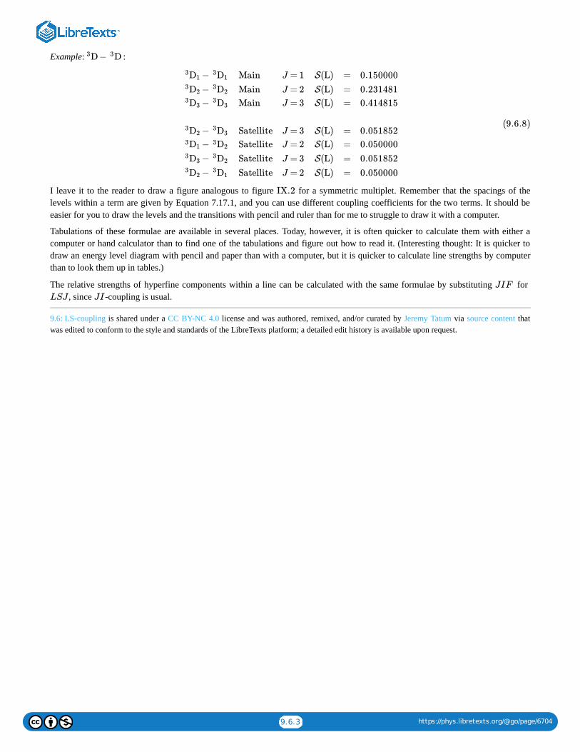
9.6.3 https://phys.libretexts.org/@go/page/6704

Example: :

I leave it to the reader to draw a figure analogous to figure for a symmetric multiplet. Remember that the spacings of thelevels within a term are given by Equation 7.17.1, and you can use different coupling coefficients for the two terms. It should beeasier for you to draw the levels and the transitions with pencil and ruler than for me to struggle to draw it with a computer.

Tabulations of these formulae are available in several places. Today, however, it is often quicker to calculate them with either acomputer or hand calculator than to find one of the tabulations and figure out how to read it. (Interesting thought: It is quicker todraw an energy level diagram with pencil and paper than with a computer, but it is quicker to calculate line strengths by computerthan to look them up in tables.)

The relative strengths of hyperfine components within a line can be calculated with the same formulae by substituting for , since -coupling is usual.

9.6: LS-coupling is shared under a CC BY-NC 4.0 license and was authored, remixed, and/or curated by Jeremy Tatum via source content thatwas edited to conform to the style and standards of the LibreTexts platform; a detailed edit history is available upon request.

D − D3  3

−3D1  3D1

−3D2  3D2

−3D3  3D3

−3D2  3D3

−3D1  3D2

−3D3  3D2

−3D2  3D1

Main

Main

Main

Satellite

Satellite

Satellite

Satellite

J = 1

J = 2

J = 3

J = 3

J = 2

J = 3

J = 2

S(L)

S(L)

S(L)

S(L)

S(L)

S(L)

S(L)

=

=

=

=

=

=

=

0.150000

0.231481

0.414815

0.051852

0.050000

0.051852

0.050000

(9.6.8)

IX.2

JIF

LSJ JI

9.7.1 https://phys.libretexts.org/@go/page/9048

9.7: Atomic hydrogenWhat is meant by the oscillator strength of ? This question may well be asked, recalling that technically is not a single line,but consists of three transition arrays, three multiplets, seven lines, and I don’t think we ever worked out quite how many Zeemanand hyperfine components.

The hydrogen atom is a two-body system, and for such a system the wavefunction and its eigenvalues (energy levels) can beworked out explicitly in algebraic terms. The same is true of the transition moments and hence the strengths of each Zeeman andhyperfine component. The strength of the entire “line” of is then merely the sum of the strengths of all the Zeeman andhyperfine components of which it is composed. Then the weighted oscillator strength of is merely calculated from equation9.5.6. As for the question: What is ? – the question need not arise, since all one is likely to need is the product . However ifthis has been worked out by adding the strengths of all the Zeeman and hyperfine components, it would be , which, for thelower level of , is .

For the record, here are the weighted oscillator strengths, , for the first four “lines” of the Lyman and Balmer series for .

9.7: Atomic hydrogen is shared under a CC BY-NC 4.0 license and was authored, remixed, and/or curated by Jeremy Tatum via source contentthat was edited to conform to the style and standards of the LibreTexts platform; a detailed edit history is available upon request.

Hα Hα

Hα

Hα

ϖ ϖf

4n2

Hα 8

ϖf H

α

β

γ

δ

Lyman

0.555

0.105

0.0387

0.0186

Balmer

3.139

0.588

0.220

0.103

(9.7.1)

9.8.1 https://phys.libretexts.org/@go/page/9049

9.8: Zeeman ComponentsIn this section I give , the relative strengths of Zeeman components within a line.

I consider first lines for which changes by , and then lines for which does not change.

Components connecting to :

Components connecting to :

Components in which does not change:

In these equations is the larger of the two -values involved in the line; and are, respectively, the larger and the smallerof the two -values involved in the component. Note that these formulas are not normalized to a sum of unity. In order to do so,the strength of each component should be divided by the sum of the strengths of all the components – i.e. by the strength of theline.

Consider the Zeeman pattern of figure . The strength factors for each of the nine components, reading from left to right inthe figure, will be found to be

0 2 6 12 16 12 6 2 0

Normalized to unity, these are

0.0000 0.0357 0.1071 0.2143 0.2857 0.2143 0.1071 0.0357 0.0000

As described in section 7.27 in connection with figure , the components within each group of three are unresolved, so therelative strengths of the three groups are .

Consider also the Zeeman pattern of figure . The strength factors for each of the six components, reading from left toright in the figure, will be found to be

2 6 8 8 6 2

or, normalized to unity,

.

Components for which changes by

Components for which does not change:

For a line , the relative strengths of the components are

S(C)

J 1 J

Lines connecting J to J−1.– ––––––––––––––––––––––––––

M M −1

S(C) = (J+ )(J+ )M> M< (9.8.1)

M M +1

S(C) = (J− )(J− ).M< M> (9.8.2)

M

S(C) = 4(J+M)(J−M). (9.8.3)

J J M> M<

M

Example 9.8.1

VII.1

VII.117

57

17

VII.2

116

316

416

416

316

116

Lines for which J does not change.– ––––––––––––––––––––––––––––––––

M ±1

S(C) = (J+ )(J− ).M< M> (9.8.4)

M

S(C) = 4 .M2 (9.8.5)

Example 9.8.2

J−J = 2 −2

9.8.2 https://phys.libretexts.org/@go/page/9049

9.8: Zeeman Components is shared under a CC BY-NC 4.0 license and was authored, remixed, and/or curated by Jeremy Tatum via sourcecontent that was edited to conform to the style and standards of the LibreTexts platform; a detailed edit history is available upon request.

M ′

−2

−2

−1

−1

−1

0

0

0

1

1

1

2

2

M ′′

−2

−1

−2

−1

0

−1

0

1

0

1

2

1

2

S(C)

16

4

4

4

6

6

0

6

6

4

4

4

16

(9.8.6)

9.9.1 https://phys.libretexts.org/@go/page/9050

9.9: Summary of Relations Between f, A and SIn this section I use to mean either or , since these are equal; likewise I use to mean either or .The Einstein coefficient is used exclusively in connection with emission spectroscopy. The coefficient is defined here in termsof radiation energy density per unit wavelength interval; that is, it is the of section 9.4. The relations between the possibledefinitions of are given in equations 9.4.1-4.

The following relations for electric dipole radiation may be useful. In these, is the “rationalized” definition of free spacepermittivity, and the formulas are suitable for use with SI units.

For electric quadrupole radiation:

For magnetic dipole radiation:

in which is the free space permeability.

9.9: Summary of Relations Between f, A and S is shared under a CC BY-NC 4.0 license and was authored, remixed, and/or curated by JeremyTatum via source content that was edited to conform to the style and standards of the LibreTexts platform; a detailed edit history is available uponrequest.

ϖf ϖ1f12 ϖ2f21 ϖB ϖ1B12 ϖ2B21

A B

Ba

B

ε0

= ϖB = ϖf = S;ϖ2A218πhc

λ5

2πe2

mcε0 λ2

16π3

3hε0λ3(9.9.1)

ϖB = ϖf = S = ;e2λ3

4h mε0 c22π2λ2

3 ch2ε0

λ5

8πhcϖ2A21 (9.9.2)

ϖf = S = = ϖB;8 mcπ2

3h λe2

mcε0 λ2

2πe2ϖ2A21

4h mε0 c2

e2λ3(9.9.3)

S = = ϖB = ϖf .3hε0λ3

16π3ϖ2A21

3 ch2ε0

2π2λ2

3h λe2

8 mcπ2(9.9.4)

= S.ϖ2A218π5

5 hε0 λ5(9.9.5)

= S,ϖ2A21

16π3μ0

3hλ3(9.9.6)

μ0

1

CHAPTER OVERVIEW

10: Line ProfilesSpectrum lines are not infinitesimally narrow; they have a finite width. A graph of radiance or intensity per unit wavelength (orfrequency) versus wavelength (or frequency) is the line profile. There are several causes of line broadening, some internal to theatom, others external, and each produces its characteristic profile. Some types of profile, for example, have a broad core and smallwings; others have a narrow core and extensive, broad wings. Analysis of the exact shape of a line profile may give us informationabout the physical conditions, such as temperature and pressure, in a stellar atmosphere.

10.1: Natural Broadening (Radiation Damping)10.2: Thermal Broadening10.3: Microturbulence10.4: Combination of Profiles10.5: Pressure Broadening10.6: Rotational Broadening10.7: Instrumental Broadening10.8: Other Line-Broadening Mechanisms10.9: Appendix A- Convolution of Gaussian and Lorentzian Functions10.10: APPENDIX B- Radiation Damping as Functions of Angular Frequency, Frequency and Wavelength10.11: APPENDIX C- Optical Thinness, Homogeneity and Thermodynamic Equilibrium

10: Line Profiles is shared under a CC BY-NC 4.0 license and was authored, remixed, and/or curated by Jeremy Tatum via source content that wasedited to conform to the style and standards of the LibreTexts platform; a detailed edit history is available upon request.

10.1.1 https://phys.libretexts.org/@go/page/6707

10.1: Natural Broadening (Radiation Damping)The classical oscillator model of the atom was described in Section 9.2. In this model, the motion of the optical electron, whensubject to the varying electromagnetic field of a light wave, obeys the differential equation for forced, damped, oscillatory motion:

Because the oscillating (hence accelerating) electron itself radiates, the system loses energy, which is equivalent to saying that themotion is damped, and is the damping constant. Electromagnetic theory tell us that the rate of radiation of energy from anaccelerating electron is

(The reader, as always, should check the dimensions of this and all subsequent expressions.)

For an electron that is oscillating, the average rate of loss of energy per cycle is

Here the bar denotes the average value over a cycle.

If the amplitude and angular frequency of the oscillation are and , the maximum acceleration is and the mean squareacceleration is . The energy (kinetic plus potential) of the oscillating electron is

Thus we can write for the average rate of loss per cycle of energy from the system by electromagnetic radiation:

The energy therefore falls off according to

The radiated wavelength is given by , so that Equation becomes

It will be recalled from the theory of lightly damped oscillations that the solution to Equation shows that the amplitude fallsoff with time as , and that the energy falls off as . Thus we identify the coefficient of on the right handside of Equation as the classical radiation damping constant :

Numerically, if is in and is in ,

We are now going to calculate the rate at which energy is transported per unit area by an electromagnetic wave, and also tocalculate the rate at which an optically thin slab of a gas of classical oscillators absorbs energy, and hence we are going to calculatethe classical absorption coefficient. We start by recalling, from elementary electromagnetism, that the energy held per unit volumein an electric field is and the energy held per unit volume in a magnetic field is . In an isotropic medium, thesebecome and , and, in vacuo, they become .

+γ + x = cosωt.x x ω20

eE

m(10.1.1)

γ

⋅ .2

3

e2x2

4πε0c3(10.1.2)

⋅ .2

3

e2x2¯ ¯¯¯

4πε0c3(10.1.3)

a ω0 aω20

12a2ω4

0

W = m .1

2a2ω2

0 (10.1.4)

⋅ ⋅W2

3

e2ω20

4π mε0 c3(10.1.5)

= − ⋅ ⋅W .W1

3

e2ω20

4π mε0 c3(10.1.6)

λ = 2πc/ω0 10.1.6

= − ⋅W .W2πe2

3 mcε0 λ2(10.1.7)

10.1.1

exp(− γt)12

exp(−γt) W

10.1.7 γ

γ = .2πe2

3 mcε0 λ2(10.1.8)

γ s−1 λ m

γ = .2.223 ×10−5

λ2(10.1.9)

D ⋅ E12

B ⋅ H12

ε12E2 μ1

2H 2  and 1

2ε0E

2 12μ0H

2

10.1.2 https://phys.libretexts.org/@go/page/6707

For an oscillating electric field of the form , the average energy per unit volume per cycle is .

Similarly for an oscillating magnetic field, the average energy per unit volume per cycle is . An electromagnetic waveconsists of an electric and a magnetic wave moving at speed , so the rate at which energy is transmitted across unit area is

, and the two parts are equal, so that the rate at which energy is transmitted per unit area by a plane

electromagnetic wave is .

Now we are modelling the classical oscillator as an electron bound to an atom, and being subject to a periodic force froman electromagnetic wave. The rate of absorption of energy by such an oscillator (see, for example, Chapter 12 of ClassicalMechanics is

We imagine a plane electromagnetic wave arriving at (irradiating) a slab of gas containing classical oscillators per unit area, or

per unit volume. The rate of arrival of energy per unit area, we have seen, is . The rate of absorption of energy per unitarea is

The absorptance (see Chapter 2, section 2.2) is therefore

and the linear absorption coefficient is

A reminder here might be in order. Absorptance is defined in section 2.2, and in the notation of figure IX.1, the absorptanceat wavelength would be . Absorption coefficient is defined by equation 5.2.1: . Fora thick slice of gas, of thickness , this integrates, in the notation of figure IX.1, to . But for anoptically thin gas, which is what we are considering, unless stated otherwise, in this chapter, this becomes

. Thus, for an optically thin gas, absorptance is just absorption coefficient times thickness of thegas. And the relation between particle density and column density .

We can write . Let us also write as . Also, in the near vicinity of the line, let us make theapproximation . We then obtain for the absorption coefficient, in the vicinity of the line,

Make sure that I have made no mistakes in deriving equations ,11 and 12, and check the dimensions of each expressionas you go. Let me know if you find anything wrong.

Now the equivalent width in frequency units of an absorption line in an optically thin layer of gas of geometric thickness is(see equation 9.1.6)

E = cosωtE =12ε0E2¯ ¯¯¯ 1

4ε0E

2

14μ0H

2

c

( + ) c14ε0E

2 14μ0H

2

c12ε0E

2

cosωteEm

.γe2E

2ω2

2m[( − + ]ω20 ω2)2 γ2ω2

N

n c12ε0E

2

.N γe2E

2ω2

2m[( − + ]ω20 ω2)2 γ2ω2

a = .N γe2ω2

m c[( − + ]ε0 ω20 ω2)2 γ2ω2

(10.1.10)

α = .nγe2ω2

m c[( − + ]ε0 ω20 ω2)2 γ2ω2

(10.1.11)

a

λ ( (c) − (λ)) / (c)Iλ Iλ Iλ α −dI/I = α dx

t (λ) = (c)exp(−αt)Iλ Iλ

( (c) − (λ)) / (c) = αtIλ Iλ Iλn N  is N = nt

−ω = ( −ω) ( +ω)ω20 ω0 ω0 ω 2πν

+ω = 2ωω0

α = .γne2

16 mc [(ν − + ]π2 ε0 ν0)2 ( )γ

4π

2(10.1.12)

Exercise 10.1.1

10.1.10

t

= t αd(ν − ).W (ν) ∫∞

−∞

ν0 (10.1.13)

10.1.3 https://phys.libretexts.org/@go/page/6707

(a) For those readers who (understandably) object that expression is valid only in the immediate vicinity of the line,and therefore that we cannot integrate from , integrate expression from .

(b) For the rest of us, integrate Equation from . A substitution willprobably be a good start.

We obtain

where is in and is in . Thus the classical oscillator model predicts that the equivalent width in frequency units isindependent of the frequency (and hence wavelength) of the line, and also independent of the damping constant. If we express theequivalent width in wavelength units (see equation 9.1.3), we obtain:

This is the same as equation 9.2.2.

When we discussed this equation in Chapter 9, we pointed out that the equivalent widths of real lines differ from this prediction bya factor , the absorption oscillator strength, and we also pointed out that has to be replaced by , the column density ofatoms in the initial (lower) level. Thus, from this point, I shall replace with . However, in this chapter we are not so muchconcerned with the equivalent width, but with the line profile and the actual width. The width of an emission line in this context iscommonly expressed as the full width at half maximum (FWHM) and the width of an absorption line as the full width at halfminimum (FWHm). (These are on no account to be confused with the equivalent width, which is discussed in section 9.1.) Notethat some writers use the term “half-width”. It is generally not possible to know what a writer means by this.

In terms of the notation of figure IX.1 (in which “ ” denotes “continuum”), but using a frequency rather than a wavelength scale,the absorptance at frequency is

The profile of an absorption line is thus given by

For radiation damping we have

The maximum value of the absorptance (at the line centre) is

This quantity is also and it is also known as the central depth of the line. (Be sure to refer to figure IX.1 to understand

its meaning.) I shall use the symbol interchangeably, according to context.

It is easy to see that the value of at which the absorptance is half its maximum value is . That is to say, the full widthat half maximum (FWHM) of the absorptance, which I denote as , is, in frequency units:

(In wavelength units, it is times this.) This is also the FWHm of the absorption profile.

Equation can be written

Exercise 10.1.2

10.1.12

−∞ to  +∞ 10.1.11 0 to ∞

10.1.11 ν− = −∞ to  +∞ν0 4π(ν− ) = γ tanθν0

= = 2.654 × N ,W (ν) N e2

4mcε010−6 (10.1.14)

W (ν) Hz N m−2

W = .N e2λ2

4mc2ε0

(10.1.15)

f12 N N1

N N1f12

c

ν

a(ν) = .(c) − (ν)Iν Iν

(c)Iν(10.1.16)

(ν) = (c) (1 −a(ν)) .Iν Iν (10.1.17)

a(ν) = .γN1f12e

2

16 mc [(ν − + ]π2 ε0 ν0)2 ( )γ

4π

2(10.1.18)

a( ) = .ν0N1f12e

2

mc γε0(10.1.19)

(c)− ( )Iν Iν ν0

(c)Iνd

d or a( )ν0

ν −ν0 γ/(4π)

w

w = .γ

2π(10.1.20)

/cλ2

10.1.18

10.1.4 https://phys.libretexts.org/@go/page/6707

The absorption line profile (see Equation ) can be written

Notice that at the line centre, minus the central depth; and a long way from the line centre, , asexpected. This type of profile is called a Lorentz profile.

From equations (but with substituted for ), and , we find that

This is true whether equivalent width and FWHm are measured in frequency or in wavelength units. (It is a pity that, for theoreticalwork, frequency is more convenient than wavelength, since frequency is proportional to energy, but experimentalists often (notinvariably!) work with gratings, which disperse light linearly with respect to wavelength!)

Indeed the equivalent width of any type of profile can be written in the form

the value of the constant depending upon the type of profile.

In photographic days, the measurement of equivalent widths was a very laborious procedure, and, if one had good reason to believethat the line profiles in a spectrum were all lorentzian, the equivalent with would be found by measuring just the FWHm and thecentral depth. Even today, when equivalent widths can often be determined by computer from digitally-recorded spectra almostinstantaneously, there may be occasions where low-resolution spectra do not allow this, and all that can be honestly measured arethe central depths and equivalent widths. The type of profile, and hence the value to be used for the constant in Equation ,requires a leap of faith.

It is worth noting (consult equations , and ) that the equivalent width is determined by the column density ofthe absorbing atoms (or, rather, on ), the FWHm is determined by the damping constant, but the central depth depends onboth. You can determine the damping constant by measuring the FWHm.

The form of the Lorentz profile is shown in figure X.1 for two lines, one with a central depth of 0.8 and the other with a centraldepth of 0.4. Both lines have the same equivalent width, the product being the same for each. Note that this type of profile hasa narrow core, skirted by extensive wings.

= .a(ν)

a( )ν0

1

4 +1( )ν−ν0

w

2(10.1.21)

10.1.1

= 1 − .(ν)Iν

(c)Iν

d

4 +1( )ν−ν0

w

2(10.1.22)

( )/ (c) = 1Iν ν0 Iν (ν) = (c)Iν Iν

10.1.14 N1f12 N 10.1.19 10.1.20

Equivalent width = × central depth  × FWHmπ

21.571 × central depth  × FWHm. (10.1.23)

Equivalent width  =  constant  ×  central depth  × FWHm , (10.1.24)

10.1.14

10.1.410.1.19 10.1.20

N1f12

wd

FIGURE X.1

10.1.5 https://phys.libretexts.org/@go/page/6707

Of course a visual inspection of a profile showing a narrow core and extensive wings, while suggestive, doesn’t prove that theprofile is strictly lorentzian. However, Equation can be rearranged to read

This shows that if you make a series of measurements of and plot a graph of the left hand side versus , you shouldobtain a straight line if the profile is lorentzian, and you will obtain the central depth and equivalent width (hence also the dampingconstant and the column density) from the intercept and slope as a bonus. And if you don’t get a straight line, you don’t have aLorentz profile.

It will be recalled that the purely classical oscillator theory predicted that the equivalent widths of all lines (in frequency units) of agiven element is the same, namely that given by Equation . The obvious observation that this is not so led us to introducethe emission oscillator strength, and also to replace . Likewise, Equation predicts that the FWHm (in wavelengthunits) is the same for all lines. (Equation 10.2.20 gives the FWHm in frequency units. To understand my caveat “in wavelengthunits”, refer also to equations and . You will see that the predicted FWHm in wavelength units is

, which is exceedingly small, and the core, at least, is beyond the resolution of most spectrographs.)

Obviously the damping constants for real lines are much larger than this. For real lines, the classical damping constant has to bereplaced with the quantum mechanical damping constant .

At present I am describing in only a very qualitative way the quantum mechanical treatment of the damping constant. Quantummechanically, an electromagnetic wave is treated as a perturbation to the hamiltonian operator. We have seen in section 9.4 thateach level has a finite lifetime – see especially equation 9.4.7. The mean lifetime for a level . Each level is notinfinitesimally narrow. That is to say, one cannot say with infinitesimal precision what the energy of a given level (or state) is. Theuncertainty of the energy and the mean lifetime are related through Heisenberg’s uncertainty principle. The longer the lifetime, thebroader the level. The energy probability of a level is given by a Lorentz function with parameter , given by equation 9.4.7and equal to the reciprocal of the mean lifetime. Likewise a level has an energy probability distribution given by a Lorentzfunction with parameter . When an atom makes a transition between , naturally, there is an energy uncertainty in theemitted or absorbed photon, and so there is a distribution of photons (i.e. a line profile) that is a Lorentz function with parameter

. This parameter must replace the classical damping constant . The FWHm of a line, in frequency units, is now , which varies from line to line.

Unfortunately it is observed, at least in the spectrum of main sequence stars, if not in that of giants and supergiants, that theFWHms of most lines are about the same! How frustrating! Classical theory predicts that all lines have the same FWHm. We knowclassical theory is wrong, so we go to the trouble of doing quantum mechanical theory, which predicts different FWHms from lineto line. And then we go and observe main sequence stars and we find that the lines all have the same FWHm (admittedly muchbroader than predicted by classical theory.)

The explanation is that, in main sequence atmospheres, lines are additionally broadened by pressure broadening, which also gives aLorentz profile, which is generally broader than, and overmasks, radiation damping. (The pressures in the extended atmospheres ofgiants and supergiants are generally much less than in main sequence stars, and consequently lines are narrower.) We return topressure broadening in a later section.

10.1: Natural Broadening (Radiation Damping) is shared under a CC BY-NC 4.0 license and was authored, remixed, and/or curated by JeremyTatum via source content that was edited to conform to the style and standards of the LibreTexts platform; a detailed edit history is available uponrequest.

10.1.22

= + .(c)Iν

(c) − (ν)Iν Iν

4

dw2(ν − )ν0

2 1

d2(10.1.25)

(ν)Iν (ν−ν0)2

10.1.14

N  by N1 10.1.20

10.1.8 10.1.9

= 1.18 × me2

3 mϵ0 c210−14

γ

Γ

m is 1/Γm

m Γm

n

Γn m and n

Γ = +Γm Γn Γ γ

Γ/(2π)

10.2.1 https://phys.libretexts.org/@go/page/6708

10.2: Thermal BroadeningLet us start with an assumption that the radiation damping broadening is negligible, so that, for all practical purposes the spread ofthe frequencies emitted by a collection of atoms in a gas is infinitesimally narrow. The observer, however, will not see aninfinitesimally thin line. This is because of the motion of the atoms in a hot gas. Some atoms are moving hither, and the wavelengthwill be blue-shifted; others are moving yon, and the wavelength will be red-shifted. The result will be a broadening of the lines,known as thermal broadening. The hotter the gas, the faster the atoms will be moving, and the broader the lines will be. We shall beable to measure the kinetic temperature of the gas from the width of the lines.

First, a brief reminder of the relevant results from the kinetic theory of gases, and to establish our notation.

The Maxwell distribution gives the distribution of speeds. Consider a gas of atoms, and let be the number of them thathave speeds between . Then

More relevant to our present topic is the distribution of a velocity component. We’ll choose the -component, and suppose that the -direction is the line of sight of the observer as he or she peers through a stellar atmosphere. Let be the number of atoms

with velocity components between . Then the gaussian distribution is

which, of course, is symmetric about .

Now an atom with a line-of-sight velocity component gives rise to a Doppler shift , where (provided that ) . If we are looking at an emission line, the left hand side of Equation gives us the line profile

(provided the line is optically thin, as is always assumed in this chapter unless specified otherwise). Thus the line profile of anemission line is

This is a gaussian, or Doppler, profile.

It is easy to show that the full width at half maximum (FWHM) is

This is also the full width at half minimum (FWHm) of an absorption line, in frequency units. This is also the FWHM or FWHm inwavelength units, provided that be substituted for .

The profile of an absorption line of central depth is

Notation: c =  speed of light 

V =  velocity of a particular atom  = u +v +wx y z

V =  speed of that atom  = ( + + )u2

v2

w2

1

2

=  modal speed of all the atoms  = = 1.414Vm2kT

m

− −−−√

kT

m

− −−√

= mean speed of all the atoms  = = 1.596 = 1.128V¯ ¯¯ 8kT

πm

− −−−√

kT

m

− −−√ Vm

=  root mean square speed of all the atoms  = = 1.732 = 1.225VRMS3kT

m

− −−−√

kT

m

− −−√ Vm

N dVNV

V  and V +dV

= exp(− ) dV .dVNV

N

4

π−−

√ V3

m

V2 u

2

V2

m

(10.2.1)

x

x duNu

u and du

= exp(− ) du,duNu

N

1

π−−

√ Vm

u2

V2

m

(10.2.2)

u = 0

u ν −ν0 <<u2

c2

=ν−ν0

ν0

u

c10.2.2 (ν)/ ( )Iν Iν ν0

= exp[− ] .(ν)Iν

( )Iν ν0

c2

V 2m

(ν −ν0)2

vν20

(10.2.3)

w = = 1.6651 .Vmν0

cln16− −−−

√Vmν0

c(10.2.4)

λ0 ν0

d(= )(c)− ( )Iν Iν ν0

(c)Iν

= 1 −d exp[− ] ,(ν)Iν

(c)Iv

c2

V 2m

(ν −ν0)2

ν20

(10.2.5)

10.2.2 https://phys.libretexts.org/@go/page/6708

which can also be written

(Verify that when , the right hand side is . Do the same for equation 10.2.22.)

In figure X.2, I draw two gaussian profiles, each of the same equivalent width as the lorentzian profiles of figure X.1, and of thesame two central depths, namely 0.4 and 0.8. We see that a gaussian profile is “all core and no wings”. A visual inspection of aprofile may lead one to believe that it is probably gaussian, but, to be sure, one could write Equation in the form

and plot a graph of the left hand side versus . If the profile is truly gaussian, this will result in a straight line, from which and can be found from the slope and intercept.

Integrating the Doppler profile to find the equivalent width is slightly less easy than integrating the Lorentz profile, but it is left asan exercise to show that

Compare this with equation 10.2.23 for a Lorentz profile.

Figure X.3 shows a lorentzian profile (continuous) and a gaussian profile (dashed), each having the same central depth and thesame FWHm. The ratio of the lorenzian equivalent width to the gaussian equivalent width is

= 1 −dexp[− ] .(ν)Iν

(c)Iν

(ν − ln16ν0)2

w2(10.2.6)

ν − = wν012

1 − d12

10.2.6

ln[ ] = lnd−(c) − (ν)Iν Iν

(c)Iν

(ν − ln16ν0)2

w2(10.2.7)

(ν −ν0)2

w d

Equivalent width  = × central depth  ×FWHmπ

ln16

− −−−−√

= 1.064 × central depth  ×FWHm. (10.2.8)

FIGURE X.2

÷ = = 1.476.π

2π

ln 16

− −−−√ π ln2

− −−−√

10.2.3 https://phys.libretexts.org/@go/page/6708

10.2: Thermal Broadening is shared under a CC BY-NC 4.0 license and was authored, remixed, and/or curated by Jeremy Tatum via sourcecontent that was edited to conform to the style and standards of the LibreTexts platform; a detailed edit history is available upon request.

FIGURE X.3

10.3.1 https://phys.libretexts.org/@go/page/6709

10.3: MicroturbulenceIn the treatment of microturbulence in a stellar atmosphere, we can suppose that there are many small cells of gas moving inrandom directions with a maxwellian distribution of speeds. The distinction between microturbulence and macroturbulence is thatin microturbulence the size of the turbulent cells is very small compared with the optical depth, so that, in looking down through astellar atmosphere we are seeing many cells of gas whose distribution of velocity components is gaussian. In macroturbulence thesize of the cells is not very small compared with the optical depth, so that , in peering through the haze of an atmosphere, we cansee at most only a very few cells.

If the distribution of velocity components of the microturbulent cells is supposed gaussian, then the line profiles will be just likethat for thermal broadening, except that, instead of the modal speed of the atoms we substitute the modal speed

of the microturbulent cells. Thus the line profile resulting from microturbulence is

The FWHM in frequency units is

or, in wavelength units,

If the thermal and microturbulent broadening are comparable in size, we still get a gaussian profile, except that for wemust substitute

This actually requires formal proof, and this will be given as an exercise in Section 5.

Since either thermal broadening or microturbulence will result in a gaussian profile, one might think that it would not be possible totell, from a spectrum exhibiting gaussian line profiles, whether the broadening was caused primarily by high temperature or bymicroturbulence. But a little more thought will show that in principle it is possible to distinguish, and to determine separately thekinetic temperature and the modal microturbulent speed. Think about it, and see if you can devise a way.

THINKINGThe key is, in purely thermal broadening, the light atoms (such as lithium) move faster than the heavier atoms (such as cadmium),the speeds being inversely proportional to the square roots of their atomic masses. Thus the lines of the light atoms will be broaderthan the lines of the heavy atoms. In microturbulence all atoms move en masse at the same speed and are therefore equally broad.We have seen, beneath Equation 10.3.7, that the FWHM, in frequency units, is

If we form the quantity

for a lithium line and for a cadmium line, we will obtain

from which are immediately obtained.

=Vm 2kT/m− −−−−−

√ξm

= 1 −d exp[− ] .(ν)Iν

( )Iν ν0

c2

ξ2m

(ν −ν0)2

ν20

(10.3.1)

ξmν0 ln16− −−−

√

c(10.3.2)

.ξmλ0 ln16

− −−−√

c(10.3.3)

 or Vm ξm

= .+V 2m ξ2

m

− −−−−−−√ 2kT/m+ξ2

m

− −−−−−−−−−√ (10.3.4)

w = .ν0

c(2kT/m+ ) ln16ξ2

m

− −−−−−−−−−−−−−−−√ (10.3.5)

X =w2c2

ln16ν20

(10.3.6)

= +  and  = + ,XLi2kT

mLiξ2

m XCd2kT

mCdξ2

m (10.3.7)

T  and ξm

10.3.2 https://phys.libretexts.org/@go/page/6709

A Li line at 670.79 nm has a gaussian FWHM = 9 pm (picometres) and a Cd line at 508.58 nm has a gaussian FWHm = 3 pm.Calculate the kinetic temperature and the modal microturbulent speed.

10.3: Microturbulence is shared under a CC BY-NC 4.0 license and was authored, remixed, and/or curated by Jeremy Tatum via source contentthat was edited to conform to the style and standards of the LibreTexts platform; a detailed edit history is available upon request.

Exercise 10.3.1

10.4.1 https://phys.libretexts.org/@go/page/6710

10.4: Combination of ProfilesSeveral broadening factors may be simultaneously present in a line. Two mechanisms may have similar profiles (e.g. thermalbroadening and microturbulence) or they may have quite different profiles (e.g. thermal broadening and radiation damping). Weneed to know the resulting profile when more than one broadening agent is present. Let us consider an emission line, and let

. Let us suppose that the lines are broadened, for example, by thermal broadening, the thermal broadening functionbeing . Suppose, however, that, in addition, the lines are also broadened by radiation damping, the radiation damping profilebeing . At a distance from the line centre, the contribution to the line profile is the height of the function weighted bythe function . That is to say the resulting profile is given by

The reader should convince him- or herself that this is exactly the same as

This profile is called the convolution of the two constituent profiles, and is often written symbolically

Convolving Two Gaussian Functions

Let us consider, for example, the convolution of two Gaussian functions, for example the convolution of thermal andmicroturbulent broadening.

Suppose one of the Gaussian functions is

Here . The area under the curve is unity, the HWHM is and the peak is . (Verify these.) Suppose that the

second Gaussian function is

It can now be shown, using Equation or , that the convolution of is

where

We used this result already in Section 10.4 when, in adding microturbulent to thermal broadening, we substituted for . In case you find the integration to be troublesome, I have done it in an Appendix to this Chapter.

Convolving Two Lorentzian FunctionsNow let’s consider the combination of two lorentzian functions. Radiation damping gives rise to a lorentzian profile, and we shallsee later that pressure broadening can also give rise to a lorentzian profile. Let us suppose that the two lorentzian profiles are

and

x = λ−λ0

f(x)g(x) ξ f(ξ)

g(x−ξ) h(x)

h(x) = f(ξ)g(x−ξ)dξ.∫∞

−∞(10.4.1)

h(x) = f(x−ξ)g(ξ)dξ.∫∞

−∞(10.4.2)

h = f ∗ g. (10.4.3)

(x) = ⋅ exp(− ) = exp(− ) .G11

g1

ln2

π

− −−−√

ln2x2

g21

0.46972

g1

0.69315x2

g21

(10.4.4)

x = λ−λ0 g11g1

ln 2π

−−−√

(x) = ⋅ exp(− ) .G21

g2

ln2

π

− −−−√

ln2x2

g22

(10.4.5)

10.4.1 10.4.2  and G1 G2

G(x) = (x) ∗ (x) = ⋅ exp(− ) ,G1 G21

g

ln2

π

− −−−√

ln2x2

g2(10.4.6)

= + .g2 g21 g2

2 (10.4.7)

+V 2m ξ2

m

− −−−−−−√

Vm

(x) = ⋅L1l1

π

1

+x2 l21(10.4.8)

10.4.2 https://phys.libretexts.org/@go/page/6710

Here . The area under the curve is unity, the HWHM is and the peak is . (Verify these.) It can be shown that

where

Details of the integration are in the Appendix to this Chapter.

Convolving a Lorentzian Function with a Gaussian FunctionLet us now look at the convolution of a Gaussian profile with a lorentzian profile; that is, the convolution of

with

We can find the convolution from either Equation or from Equation , and we obtain either

or

The expression or , which is a convolution of a Gaussian and a lorentzian profile, is called a Voigt profile. (A roughattempt at pronunciation would be something like Focht.)

A useful parameter to describe the “gaussness” or “lorentzness” of a Voigt profile might be

which is 0 for a pure lorentz profile and 1 for a pure Gaussian profile. In figure X.4 I have drawn Voigt profiles for (continuous, dashed and dotted, respectively). The profiles are normalized so that all have the same area.

A nice exercise for those who are more patient and competent with computers than I am would be to draw 1001 Voigt profiles, with going from 0 to 1 in steps of 0.001, perhaps normalized all to the same height rather than the same area, and make a movie of a

Gaussian profile gradually morphing to a lorentzian profile. Let me know if you succeed!

(x) = ⋅ .L2l2

π

1

+x2 l22(10.4.9)

x = λ−λ0 l1 1/(πl)

L(x) = L(x) ∗ (x) = ⋅ ,L21

π

1

+x2 l2(10.4.10)

l = + .l1 l2 (10.4.11)

G(x) = ⋅ exp(− )1

g

ln2

π

− −−−√

ln2x2

g(10.4.12)

L(x) = ⋅ .1

π

1

+x2 l2(10.4.13)

10.4.1 10.4.2

V (x) = dξ1

g

ln2

π3

− −−−√ ∫

∞

−∞

exp(−[(ξ−x ln2]/ ))2 g2

+ξ2 l2(10.4.14)

V (x) = dξ.1

g

ln2

π3

− −−−√ ∫

∞

−∞

exp[−( ln2)/ ]ξ2 g2

(ξ−x +)2 l2(10.4.15)

10.4.14 10.4.15

= ,kGg

g+ l(10.4.16)

= 0.25, 0.5 and 0.75kG

kG

10.4.3 https://phys.libretexts.org/@go/page/6710

As for the gauss-gauss and lorentz-lorentz profiles, I have appended some details of the integration of the gauss-lorentz profile inthe Appendix to this Chapter.

The FWHM or FWHm in wavelength units of a Gaussian profile (i.e. ) is

The FWHM or FWHm in frequency units of a lorentzian profile is

Here is the sum of the radiation damping constant (see section 2) and the contribution from pressure broadening (see section6). For the FWHM or FWHm in wavelength units (i.e. ), we have to multiply by .

Integrating a Voigt ProfileThe area under Voigt profile is , where is given by Equation , which itself had to be evaluated with anumerical integration. Since the profile is symmetric about , we can integrate from and multiply by 2. Even so, thedouble integral might seem like a formidable task. Particularly troublesome would be to integrate a nearly lorentzian profile withextensive wings, because there would then be the problem of how far to go for an upper limit. However, it is not at all a formidabletask. The area under the curve given by Equation is unity! This is easily seen from a physical example. The profile givenby Equation is the convolution of the lorentzian profile of Equation with the Gaussian profile of Equation ,both of which were normalized to unit area. Let us imagine that an emission line is broadened by radiation damping, so that itsprofile is lorentzian. Now suppose that it is further broadened by thermal broadening (Gaussian profile) to finish as a Voigt profile.(Alternatively, suppose that the line is scanned by a spectrophotometer with a Gaussian sensitivity function.) Clearly, as long as theline is always optically thin, the additional broadening does not affect the integrated intensity.

Now we mentioned in sections 2 and 3 of this chapter that the equivalent width of an absorption line can be calculated from FWHm, and likewise the area of an emission line is FWHM, where

for a Gaussian profile and for a lorentzian profile. We know that the integral of isunity, and it is a fairly straightforward matter to calculate both the height and the FWHM of . From this, it becomes possibleto calculate the constant as a function of the Gaussian fraction . The result of doing this is shown in figure X.4A.

FIGURE X.4

2g

= = .wG

(2kT/m+ )ξ2m

12 λ0 ln16

− −−−√

c

1.665(2kT/m+ )ξ2m

12 λ0

c(10.4.17)

= Γ/(2π) = 0.1592Γ,wL (10.4.18)

Γ 2/t¯

2l /cλ20

2 V (x)dx∫ ∞0

V (x) 10.4.14

x = 0 0 to ∞

10.4.1410.4.14 10.4.13 10.4.12

c× central depth × c× height ×c is 1.064(= )π/ ln16

− −−−−−√ 1.571(= π/2) V (x)

V (x)c kG

10.4.4 https://phys.libretexts.org/@go/page/6710

This curve can be fitted with the empirical Equation

where . The error incurred in using this formula nowhere exceeds0.5%; the mean error is 0.25%.

The Voigt Profile in Terms of the Optical Thickness at the Line Center.Another way to write the Voigt profile that might be useful is

Here and is a dummy variable, which disappears when the definite integral is performed. The Gaussian HWHM is , and the lorentzian HWHM is . The optical thickness at is , and the optical

thickness at the line centre is . is a dimensionless coefficient, whose value depends on the Gaussian fraction . is clearly given by

If we now let and , and also make use of the symmetry of the integrand about , thisbecomes

On substitution of (in order to make the limits finite), we obtain

which can readily be numerically integrated for a given value of . Recall that and hence that . The results of the integration are as follows. The column is explained following figure X.4B.

FIGURE X.4A

c = + + + ,a0 a1kG a2k2G a3k

3G (10.4.19)

= 1.572, = 0.05288, = −1.323 and  = 0.7658a0 a1 a2 a3

τ(x) = Clτ(0) dξ.∫∞

−∞

exp[−(ξ−x ln2/ ])2 g2

+ξ2 l2(10.4.20)

x = λ−λ0 ξ

g = /cλ0Vm ln2−−−

√ l = Γ/(4πc)λ20 λ− = xλ0 τ(x)

τ(0) C

= g/(g+ l)kG C

Cl dξ = 1.∫∞

−∞

exp[− ln2/ ]ξ2 g2

+ξ2 l2(10.4.21)

l = g/l′ ln2−−−

√ ξ = g/ξ′ ln2−−−

√ ξ = = 0ξ′

2C d = 1.l′ ∫∞

0

exp(− )ξ′2

+ξ′2 l′2ξ′ (10.4.22)

=ξ′ 2 tl′

1−t2

4C dt = 1,∫1

0

exp[−{2 t/(1 − ) ]l′ t2 }2

1 + t2(10.4.23)

l′ l/g = 1/ −1kG= (1/ −1)l′ kG ln2

−−−√ Capprox

10.4.5 https://phys.libretexts.org/@go/page/6710

The last entry, the value of for , a pure Gaussian profile, is . These data are graphed in figure X.4B.

The empirical formula

where

fits the curve tolerably well within (but not outside) the range .

10.4: Combination of Profiles is shared under a CC BY-NC 4.0 license and was authored, remixed, and/or curated by Jeremy Tatum via sourcecontent that was edited to conform to the style and standards of the LibreTexts platform; a detailed edit history is available upon request.

C = 1kG 1/π

FIGURE X.4B

= a + + + + ,Capprox k−bG c0 c1kG c2k

2G c3k

3G (10.4.24)

a = +0.309031

= −0.82999c1

b = +1.132747

= +1.21782c2

= +0.16510c0

= −0.54665c3

= 0.15 to 1.00kG

10.5.1 https://phys.libretexts.org/@go/page/6711

10.5: Pressure BroadeningThis is a fairly difficult subject, and I am no expert in it. The reader will forgive me if I accordingly treat it rather briefly anddescriptively.

The phenomena of pressure broadening (also known as collisional broadening) are often divided into effects resulting from theshort time interval between atomic collisions, and effects resulting at the moment of collision. I shall begin by describing the firstof these phenomena.

The only possible absolutely monochromatic unbroadened infinitesimally narrow line with a single, uniquely defined frequency isa sine wave of infinite extent. A sine wave of finite length is not a true sine wave of a single frequency, but it has a spread ofcomponent frequencies, which can be determined by Fourier analysis. This, by the way, is the reason behind Heisenberg’suncertainty principle (Unsicherheitsprinzip). If the wavefunction that describes a particle is very limited in extent, then the positionof the particle is relatively well determined. On the other hand, the limited extent of the wavefunction means that it has acorrespondingly broad Fourier spread of constituent wavelengths, and hence the momentum is correspondingly uncertain.

The atmospheres of giant and supergiant stars are relatively thin; pressure broadening is slight and lines tend to be narrow. In theatmospheres of main sequence stars, however, collisions between atoms are frequent. The frequent occurrence of collisionsinterrupts the wave trains and divides them into short wave-packets, with a corresponding spread of component frequencies. Thusthe spectrum lines are broadened.

The Fourier distribution of amplitudes of component frequencies of a sine wave that is truncated by a box function is the same asthe Fourier distribution of amplitudes of a light wave that is diffracted by a single slit. That is to say it is a sinc function of the form

and the intensity distribution is the square of this. The shorter the intercollision time, the wider the spread ofconstituent frequencies, just as a narrow slit produces a wide diffraction pattern. Thus one might expect the profile of a pressurebroadened line to resemble a single slit diffraction pattern, which, it will be recalled, looks like figure X.5.

The profile would indeed look like that if all intercollision times were exactly equal and all wave-train fragments were of exactlythe same length. There is, however, a Poisson distribution of intercollision times, and so the above profile has to be convolved withthis Poisson distribution. While I don’t do the calculation here, the resulting profile is a Lorentz profile except that the dampingconstant is replaced by , where is the mean time between collisions. The mean time between collisions is given, fromkinetic theory of gases, by

Here are, respectively, the masses, diameters and number density of the atoms. Hence, if the kinetic temperature isindependently known, the number density of the particles can be determined from the FWHm of a pressure-broadened line.

It will be recalled that classical radiation damping theory predicts the same FWHm for all lines, with a classical damping constant . Quantum mechanical theory predicts a damping constant and hence FWHm that differs from line to line. Yet in the spectrum

(sinΔν)/Δν

FIGURE X.5

Γ 2/t¯ t¯

= .t¯1

nd2

m

16πkT

− −−−−−√ (10.5.1)

m, d and n

γ Γ

10.5.2 https://phys.libretexts.org/@go/page/6711

of a main sequence star, one quite often finds that all lines of a given element have the same FWHm and hence the same effectivedamping constant. This is because the width of a Lorentz profile is determined more by pressure broadening than by radiationdamping.

There are further broadening effects caused by interactions that take place at the moment of collision. If an atom is approached byan electron or an ion, it will temporarily be in an electric field, and consequently the lines will be broadened by Stark effect, whichmay be either linear (proportional to the electric field ) or quadratic ( ), or neutral-neutral reactions give rise to interactionsbetween temporarily induced dipole moments (van der Waals forces), and these all have different dependences on interatomicdistance. Neutral magnesium is very sensitive to quadratic Stark effect, and hydrogen is sensitive to linear Stark effect. The entiresubject is quite difficult, and I leave it here except to point out two small details. Very often the broadening is not symmetric, linestypically having wider wings to the long wavelength side than on the short wavelength side. This is because the effect of theinteractions is to lower and broaden the energy levels of a transition, the lower energy level generally being lowered more than theupper. A second point is that the hydrogen Balmer lines are often much broadened by linear Stark effect, and this can be recognizedbecause the Stark pattern for the Balmer series is such that there are no undisplaced Stark components for even members of theseries – etc. Thus results in a central dip to these lines in an emission spectrum or a central bump in an absorptionline.

10.5: Pressure Broadening is shared under a CC BY-NC 4.0 license and was authored, remixed, and/or curated by Jeremy Tatum via sourcecontent that was edited to conform to the style and standards of the LibreTexts platform; a detailed edit history is available upon request.

E ∝ E2

Hβ, Hδ, Hζ,

10.6.1 https://phys.libretexts.org/@go/page/8823

10.6: Rotational BroadeningThe lines in the spectrum of a rotating star are broadened because light from the receding limb is redshifted and light from theapproaching limb is blueshifted. It may be remarked that early-type stars (type F and earlier) tend to be much faster rotators thanlater-type stars, and consequently early-type stars show more rotational broadening. It should also be remarked that pole-on rotatorsdo not, of course, show rotational broadening (even early-type fast rotators).

I shall stick to astronomical custom and refer to a “redshift” as a shift towards a longer wavelength, even though for an infraredline a “redshift” in this sense would be a shift away from the red! A “longward” shift doesn’t quite solve the problem either, forthe following reason. While it is true that relativity makes no distinction between a moving source and a moving observer, inthe case of the Doppler effect in the context of sound in air, if the observer is moving, there may be a change in the pitch of theperceived sound, but there is no change in wavelength!

We shall start by considering a star whose axis of rotation is in the plane of the sky, and which is of uniform radiance across itssurface. We shall then move on to oblique rotators, and then to limb-darkened stars. A further complication that could beconsidered would be non-uniform rotation. Thus, the Sun does not rotate as a solid body, but the angular speed at low latitudes isfaster than at higher latitudes – the so-called “equatorial acceleration”.

In figure X.6, on the left hand we see the disc of a star as seen on the sky by an observer. PQ is the axis of rotation, supposed to bein the plane of the sky, and AB is the equator. X is a point on the surface of the star at coordinates , latitude . The star issupposed to be rotating with an equatorial speed . What we are going to show is that all points on the chord LMN have the sameradial velocity away from or towards the observer, and consequently all light from points on this chord has the same Doppler shift.

The right hand part of the figure shows the star seen from above the pole P. The small circle is the parallel of latitude CD shown onthe left hand part of the figure.

M is a point on the equator and also on the chord LMN. Its speed is and the radial component of its velocity is . Thespeed of the point M is , and its radial velocity is . But

. Therefore . Therefore the radialvelocity of X is , which is the same as that of M, and therefore all points on the chord LMN have radial velocity

.

Therefore all points on the chord constant are subject to the same Doppler shift

The ordinate of an emission line profile at Doppler shift compared with its ordinate at the line center is equal to the ratio of thelength of the chord constant to the diameter of the stellar disk:

(x, y) θ

ve

ve sinαvecosθve cosθ sinOPXve

x = PM sinα = a sinα and x = PX sinOPX = a cosθ sinOPX cosθ sinOPX = sinαsinαve

sinα = x/ave ve

x =

= .Δλ

λ

xve

ac(10.6.1)

Δλ

x = 2a

10.6.2 https://phys.libretexts.org/@go/page/8823

In the above, we have assumed that the axis of rotation is in the plane of the sky, or that the inclination of the equator to the planeof the sky is . If the inclination is not , the only effect is that all radial velocities are reduced by a factor of , so thatEquation becomes

and this is the line profile. It is an ellipse, and if we write Equation can be written

The basal width of the line (which has no asymptotic wings) is and the FWHM is . The profile of an absorptionline of central depth is

It is left as an exercise to show that

From the width of a rotationally broadened line we can determine , but we cannot determine separately withoutadditional information. Likewise, we cannot determine the angular speed of rotation unless we know the radius independently.

It might be noted that, for a rotating planet, visible only by reflected light, the Doppler effect is doubled by reflection, so the basalwidth of a rotationally broadened line is

Now let us examine the effect of limb darkening. I am going to use the words intensity and radiance in their strictly correct sensesas described in Chapter 1, and the symbols respectively. That is, radiance = intensity per unit projected area. For spectralintensity and spectral radiance – i.e. intensity and radiance per unit wavelength interval, I shall use a subscript .

We suppose that the spectral radiance at a distance from the center of the disc is . The intensity from an elemental area on the disc is . The area between the vertical strip and the annulus in figure X.7 is a little parallelogram of length

and width , so that . Here , so that

= = .(Δλ)Iλ

(0)Iλ(1 − )

x2

a2

1

2

(1 − )c2(Δλ)

2

v2eλ2

1

2

(10.6.2)

i

90∘ 90∘ sin i10.6.2

= ,(Δλ)Iλ

(0)Iλ(1 − )

c2(Δλ)2

iv2e sin2 λ2

1

2

(10.6.3)

= X and  = Y(Δλ)Iλ

(0)Iλ

Δλ

λ10.6.3

+ = 1.x2

( )sin ive

c

2

y2

12(10.6.4)

2 sin ive

c

sin i3√ ve

c

d

= 1 −d ,(Δλ)Iλ

(0)Iλ(1 − )

c2(Δλ)2

iv2e sin2 λ2

12

(10.6.5)

Equivalent width = ×central depth×FWHm = 0.9069dw.π

12−−

√(10.6.6)

sin ive  and ive

.4 sin ive

c

I and Lλ

FIGURE X.7

r (r)Lλ dA

d = (r)dAIλ Lλ

dy dx dA = dxdy = −y2 r2 x2

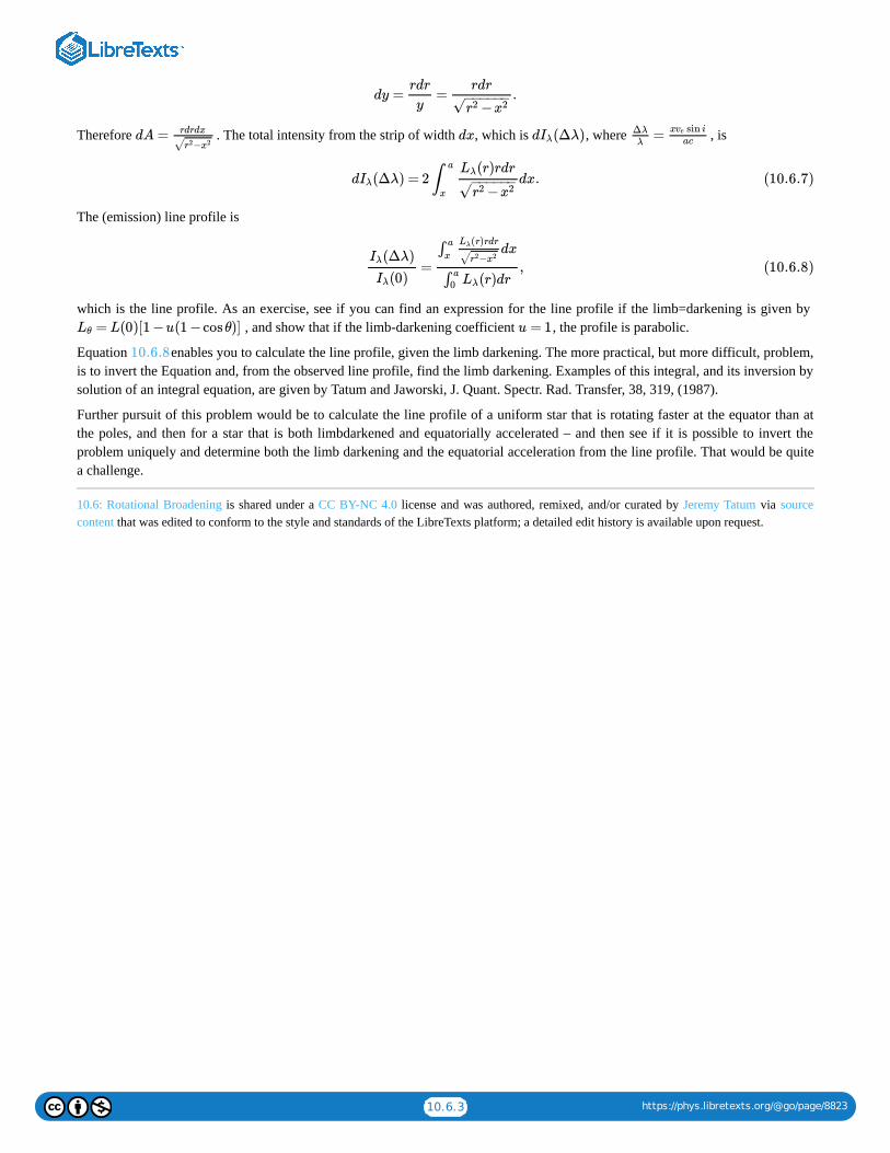
10.6.3 https://phys.libretexts.org/@go/page/8823

Therefore . The total intensity from the strip of width , which is , where , is

The (emission) line profile is

which is the line profile. As an exercise, see if you can find an expression for the line profile if the limb=darkening is given by , and show that if the limb-darkening coefficient , the profile is parabolic.

Equation enables you to calculate the line profile, given the limb darkening. The more practical, but more difficult, problem,is to invert the Equation and, from the observed line profile, find the limb darkening. Examples of this integral, and its inversion bysolution of an integral equation, are given by Tatum and Jaworski, J. Quant. Spectr. Rad. Transfer, 38, 319, (1987).

Further pursuit of this problem would be to calculate the line profile of a uniform star that is rotating faster at the equator than atthe poles, and then for a star that is both limbdarkened and equatorially accelerated – and then see if it is possible to invert theproblem uniquely and determine both the limb darkening and the equatorial acceleration from the line profile. That would be quitea challenge.

10.6: Rotational Broadening is shared under a CC BY-NC 4.0 license and was authored, remixed, and/or curated by Jeremy Tatum via sourcecontent that was edited to conform to the style and standards of the LibreTexts platform; a detailed edit history is available upon request.

dy = = .rdr

y

rdr

−r2 x2− −−−−−

√

dA = rdrdx

−r2 x2√dx d (Δλ)Iλ =Δλ

λ

x sin iveac

d (Δλ) = 2 dx.Iλ ∫a

x

(r)rdrLλ

−r2 x2− −−−−−

√(10.6.7)

= ,(Δλ)Iλ

(0)Iλ

dx∫ a

x

(r)rdrLλ

−r2 x2√

(r)dr∫ a

0 Lλ

(10.6.8)

= L(0)[1 −u(1 −cosθ)]Lθ u = 1

10.6.8

10.7.1 https://phys.libretexts.org/@go/page/8857

10.7: Instrumental BroadeningEven if the radiation damping profile of a line is negligible and if it is subject to negligible thermal, pressure and rotationalbroadening, it still has to suffer the indignity of instrumental broadening. Almost any type of spectrograph will broaden a line. Thebroadening produced by a prism is inversely proportional to the size of the prism, and the broadening produced by a grating isinversely proportional to the number of grooves in the grating. After a spectrum is produced (and broadened) by a spectrograph, itmay be scanned by a further instrument such as a microphotometer, or even if it is recorded digitally, it is still further broadened bythe point spread function. The instrumental broadening can in principle be determined experimentally by measuring theinstrumentally-produced profile of an intrinsically very narrow line. Then, when the instrument is used to examine a broad line, theobserved profile is the convolution of the true profile and the instrumental profile. We can write this symbolically as

Here are respectively the observed, true and instrumental profiles, and the asterisk denotes the convolution. Themathematical problem is to deconvolve this equation so that, given the instrumental profile and the observed profile it is possible torecover the true profile. This is done by making use of a mathematical theorem known as Borel’s theorem, which is that theFourier transform of the convolution of two functions is equal to the product of the Fourier transforms of each. That is

where the bar denotes the Fourier transform. Numerical fast Fourier transform computer programs are now readily available, so theprocedure is to calculate the Fourier transforms of the observed and instrumental profile, divide the former by the latter to obtain ,and then calculate the inverse Fourier transform to obtain the true profile. This procedure is well known in radio astronomy, inwhich the observed map of a sky region is the convolution of the true map with the beam of the radio telescope, though, unlike theone-dimensional spectroscopic problem the corresponding radio astronomy problem is two-dimensional.

10.7: Instrumental Broadening is shared under a CC BY-NC 4.0 license and was authored, remixed, and/or curated by Jeremy Tatum via sourcecontent that was edited to conform to the style and standards of the LibreTexts platform; a detailed edit history is available upon request.

O = T ∗ I. (10.7.1)

O,  T and I

= × ,O¯ ¯¯

T¯ ¯

I¯

(10.7.2)

T¯ ¯

10.8.1 https://phys.libretexts.org/@go/page/8858

10.8: Other Line-Broadening MechanismsI just briefly mention here one or two additional sources of line-broadening.

Lines may be broadened by unresolved or smeared Zeeman splitting, particularly for lines involving levels with large Landé g-factors. By “smeared” I mean the situation that arises if there is a large range of magnetic field strength through the line of sight orbecause (as is always the case with stars other than the Sun) you are looking at a wholedisc spectrum. Since the splitting dependson the field strength, the lines will obviously be smeared rather than cleanly divided into a number of discrete Zeeman components.Zeeman smearing is often large in the spectrum of white dwarf stars, where magnetic fields can be large and the observer looksthrough a large range of magnetic field strength.

Different Zeeman components are plane or circularly polarized according to the direction of the magnetic field. Thus in principleone should be able to recognize Zeeman effect, even if smeared or not fully resolved, by its changing appearance in differentpolarization directions. However, this will be true only if the magnetic field is uniform in direction, as it may mostly be in, forexample, a sunspot. For a whole-disc spectrum there will be a variety of different directions of the magnetic field, and so thepolarization information will be lost.

Broad lines are sometimes the result of unresolved hyperfine structure in elements with a large nuclear spin such as vanadium, orunresolved isotopic lines in elements with several isotopes of comparable abundance such as tin, copper or chlorine.

Another source of line broadening is autoionization (in absorption spectra) or dielectronic recombination (in emission spectra) inelements such as copper. These mechanisms were described in section 8.8.

One last remark might be made, namely that line broadening, whether instrumental, thermal, rotational, etc., does not change theequivalent width of a line, provided that the line is everywhere optically thin. This does not apply, however, if the line is noteverywhere optically thin.

10.8: Other Line-Broadening Mechanisms is shared under a CC BY-NC 4.0 license and was authored, remixed, and/or curated by Jeremy Tatumvia source content that was edited to conform to the style and standards of the LibreTexts platform; a detailed edit history is available uponrequest.

10.9.1 https://phys.libretexts.org/@go/page/8859

10.9: Appendix A- Convolution of Gaussian and Lorentzian FunctionsEquation 10.5.6 is

The integration is straightforward, if taken slowly and carefully, provided you know the integral . It

goes thus:

where

where

where

We have now completed the integration, except that we now have to remember what a, C and B were. When we do this, after a bitmore careful algebra we arrive at the result

In a similar manner, equation 10.5.10 is

Resolve the integrand into partial fractions:

Evaluation of the constants is straightforward, if slightly tedious, by the usual method of partial fractions:

Now

G(x) = (x) ∗ (x) = exp(− ) exp(− ) dξ.G1 G21

g1g2

ln2

π∫

∞

−∞

ln2ξ2

g21

(ξ−x ln2)2

g22

(10.A.1)

exp(−k )dx =∫∞

−∞ x2 π

k

−−√

G(x) = exp[−(a +bξ+c)]dξ,1

g1g2

ln2

π∫

∞

−∞ξ2 (10.A.2)

a = , b = − , c = .( + ) ln2g2

1 g22

g21g2

2

x ln4

g22

ln2x2

g22

G(x) = exp[−a( +2Bξ+C)]dξ,1

g1g2

ln2

π∫

∞

−∞ξ2 (10.A.3)

B = b/(2a), C = c/a. (10.9.1)

G(x) = exp[−a{(ξ+B +C − }]dξ1

g1g2

ln2

π∫

∞

−∞)2 B2

= exp[−a( +C − )]dζ1

g1g2

ln2

π∫

∞

−∞ζ2 B2

= exp(−a )dζ = ,K ln2

πg1g2∫

∞

−∞ζ2 K ln2

g1g2 πa−−

√

(10.A.4)

(10.A.5)

(10.A.6)

K = exp[−a(C − )].B2 (10.9.2)

G(x) = (x) ∗ (x) = ⋅ exp(− ) .G1 G21

g

ln2

π

− −−−√

ln2x2

g2(10.A.7)

L(x) = (x) ∗ (x) = dξ.L1 L2l1l2

π2∫

∞

−∞

1

+ξ2 l21

1

(ξ−x +)2 l22(10.A.8)

= + + + .1

+ξ2 l21

1

(ξ−x +)2 l22

Aξ

+ξ2 l21

B

+ξ2 l21

C(ξ−x)

(ξ−x +)2 l22

D

(ξ−x +)2 l22(10.A.9)

A = −C = 2xα,

B = ( + − )α,x2 l22 l21

D = ( − + )α,x2 l22 l21

where α = 1/[( + + −4 ].x2 l22 l21)2 l21l22

(10.A.10)

(10.9.3)

(10.9.4)

(10.9.5)

10.9.2 https://phys.libretexts.org/@go/page/8859

From symmetry considerations, this is:

We have now completed the integration, except that we now have to remember what and were. When we do this, after a bitmore careful algebra we arrive at the result

where

The Voigt profile is given by equation 10.5.14:

For short, I am going to write the ratio as . The relation between this ratio and the gaussian fraction . In the above equation, , and I am going to choose a wavelength scale such

that ; in other words wavelength interval is to be expressed in units of . Thus I shall write the equation as

The integration has to be done numerically, and there is a problem in that the limits are infinite. We can deal with this with thechange of variable , when the integral becomes

The limits are now finite, and the integrand is zero at each limit. Computing time will be much diminished by the furthersubstitution , when the expression becomes

This is faster than the previous expression because one avoids having to compute the trigonometric function tan. It could also havebeen arrived at in one step by means of the substitution , though such a substitution may not have been immediatelyobvious. Like the previous expression, the limits are finite, and the integrand is zero at each end. Numerical integration would nowseem to be straightforward, although there may yet be some difficulty. Suppose one is integrating, for example, by Simpson’smethod. A question might arise as to how many intervals should be used. Simpson’s method is often very effective with aremarkably small number of intervals, but, for high precision, one may nevertheless wish to use a fine interval. If one uses a fineinterval, however, as one approaches either limit, the expression becomes very large, and, even though the integrandthen becomes small, a computer may be reluctant to return a value for the exp function, and it may deliver an error message. Thebest way to deal with that difficulty is to set the integrand equal to zero whenever the absolute value of the argument of the expfunction exceeds some value below which the computer is happy.

One might be tempted to reduce the amount of computation by saying that , but this is not correct, for, while the Voigtprofile is symmetric about , the integrand is not symmetric about . However, if

L(x) = (A +B +C +D ) .l1l2

π2∫

∞

−∞

ξdξ

+ξ2 l21

∫∞

−∞

dξ

+ξ2 l21

∫∞

−∞

(ξ−x)dξ

(ξ−x +)2 l22∫

∞

−∞

dξ

(ξ−x +)2 l22(10.A.11)

L(x) = (B +D ) .2l1l2π2

∫∞

0

dξ

+ξ2 l21

∫∞

0

dξ

+ξ2 l22

(10.A.12)

L(x) = ( + ) = ( B+ D)/π.2l1l2π2

πB

2l1

πD

2l2l2 l1 (10.A.13)

B D

L(x) = ⋅ ,l

π

1

+x2 l2(10.A.14)

l = + .l1 l2 (10.9.6)

V (x) = dξ.l

g

ln2

π2

− −−−√ ∫

∞

−∞

exp(−[(ξ−x ln2]/ ))2 g2

+ξ2 l2(10.A.15)

l/g a

 is a = (1 − )/ , = 1/(1 +a)kG kG kG kG x = λ−λ0

g = 1 g

V (x) = a dξ.ln2

π3

− −−−√ ∫

∞

−∞

exp(−(ξ−x ln2))2

+ξ2 a2(10.A.16)

ξ = a tanθ

V (x) = exp[−(a tanθ−x ln2]dθ.ln2

π3

− −−−√ ∫

π/2

−π/2)2 (10.A.17)

t = tan θ12

V (x) = dtln16

π3

− −−−−√ ∫

1

−1

exp[−{2at/(1 − ) −x ln2]t2 }2

1 + t2(10.A.18)

ξ = 2at1−t2

t/(1 − )t2

= 2∫ 1−1

∫ 10

x = 1 t = 0

10.9.3 https://phys.libretexts.org/@go/page/8859

it is true that and , and hence that and this can be used toeconomise to a small extent. It is still necessary to calculate for all values of , both positive and negative, but the number ofintegration steps for each point can be halved.

10.9: Appendix A- Convolution of Gaussian and Lorentzian Functions is shared under a CC BY-NC 4.0 license and was authored, remixed,and/or curated by Jeremy Tatum via source content that was edited to conform to the style and standards of the LibreTexts platform; a detailededit history is available upon request.

V (x) = ,  and  (x) = ,  and  (x) = ,∫1

−1V1 ∫

0

−1V2 ∫

1

0(10.9.7)

V (x) = (x) + (x)V1 V2 (x) = (−x)V1 V2 V (x) = (x) + (−x)V1 V1

(x)V1 x

10.10.1 https://phys.libretexts.org/@go/page/8884

10.10: APPENDIX B- Radiation Damping as Functions of Angular Frequency,Frequency and WavelengthIt occurred to me while preparing this Chapter as well as the preceding and following ones, that sometimes I have been usingangular frequency as argument, sometimes frequency, and sometimes wavelength. In this Appendix, I bring together the salientformulas for radiation damping in terms of . I reproduce equation 10.2.11 for theabsorption coefficient for a set of forced, damped oscillators, except that I replace , the number per unit volume of oscillators with

, the effective number of atoms per unit volume in the lower level of a line, and I replace the classical damping constant with , which may include a pressure broadening component.

You should check that the dimensions of this expression are , which is appropriate for linear absorption coefficient. You maynote that . Indeed check the dimensions of all expressions that follow, at each stage.

We can write , and the equation becomes

Now I think it will be owned that the width of a spectrum line is very, very much smaller than its actual wavelength, except perhapsfor extremely Stark-broadened hydrogen lines, so that, in the immediate vicinity of a line, can be neglected compared with ;and a very long way from the line, where this might not be so, the expression is close to zero anyway. (Note that you can neglect

only with respect to ; you cannot just put where it lies alone in the denominator!) In any case, I have no compunctionat all in making the approximation

The maximum of the curve is

The optical thickness at the line centre (whether or not the line is optically thin) is

is the number of atoms in level 1 per unit area in the line of sight, whereas is the number per unit volume.

The HWHM of curve is

The area under the curve is

As expected, the area does not depend upon .

To express the absorption coefficient as a function of frequency, we note that , and we obtain

The maximum of this is (of course) the same as equation 10.B.4.

The HWHM of the curve is

Δω = ω − , Δν = ν −  and  Δ λ = λ −ω0 ν0 λ0

n

n1f12 γ

Γ

α = .Γn1f12 e2ω2

m c[( − + ]ε0 ω2 ω20)2 Γ2ω2

m−1 (10.B.1)

L−1

[ / ] ≡  and [Γ] ≡e2 ε0 ML3T−2 T−1

− = (ω − )(ω + ) = Δω(2 +Δω)ω2 ω20 ω0 ω0 ω0

α = .Γ ( +Δωn1f12 e2 ω0 )2

m c[(Δω (2 +Δω + ( +Δω ]ε0 )2 ω0 )2 Γ2 ω0 )2m−1 (10.B.2)

Δω ω0

Δω ω Δω = 0

α(Δω) = .Γn1f12 e2

4m c[(Δω +( Γ ]ε0 )2 12

)2m−1 (10.B.3)

α(Δω)

α(0) = .e2n1f12

m cΓε0m−1 (10.B.4)

τ(0) = .e2N1f12

m cΓε0(10.B.5)

N1 n1

α(Δω)

HWHM = Γ .1

2rad s−1 (10.B.6)

α(Δω)

Area = .πe2n1f12

2m cε0m−1rad s−1 (10.B.7)

Γ

ω = 2πν

α(Δν) = .Γn1f12 e2

16 m c[(Δν + ]π2 ε0 )2 ( )Γ4π

2m−1 (10.B.8)

α(Δν)

10.10.2 https://phys.libretexts.org/@go/page/8884

The area under the curve is

In a manner similar to our procedure following equation 10.B.12, we write , and , ,and neglect with respect to , and we obtain:

The maximum of this is (of course) the same as equation 10.B.4. (Verifying this will serve as a check on the algebra.)

The HWHM of the curve is

The area under the curve is

Did I forget to write down the units after this equation?

These results for might be useful in tabular form. For , replace .

It is to be noted that if the radiation damping profile is thermally broadened, the height of the absorption coefficient curvediminishes, while the area is unaltered provided that the line is optically thin. The optically thick situation is dealt with in thefollowing chapter. It might also be useful to note that a gaussian profile of the form

has an area of if

10.10: APPENDIX B- Radiation Damping as Functions of Angular Frequency, Frequency and Wavelength is shared under a CC BY-NC 4.0license and was authored, remixed, and/or curated by Jeremy Tatum via source content that was edited to conform to the style and standards of theLibreTexts platform; a detailed edit history is available upon request.

HWHM = Γ/(4π) .s−1 (10.B.9)

α(Δν)

Area = .e2n1f12

4m cε0m−1s−1 (10.B.10)

α = ⋅ .Γn1f12 e2

m cε0

⎛

⎝

λ2λ40

4 +π2c2 ( − )λ20 λ2 2

λ2λ40Γ2

⎞

⎠m−1 (10.B.11)

− = ( −λ)( +λ)λ20 λ2 λ0 λ0 λ = +Δλλ0

Δλ λ0

α(Δλ) = ⋅ .Γn1f12 e2

16 mπ2 ε0c3

⎛

⎝⎜

λ40

(Δλ +)2 λ40Γ2

16π2c2

⎞

⎠⎟ m−1 (10.B.12)

α(Δλ)

HWHM = m.Γλ2

0

4πc(10.B.13)

α(Δλ)

Area = .λ2

0e2n1f12

4mε0c2(10.B.14)

α τ  by n1 N1

Height

Area

HWMH

Δω

Γe2n1f12

4m c[(Δω +( Γ ]ε0 )2 1

2)2

e2n1f12

m cΓε0

πe2n1f12

2m cε0

Γ12

Δν

Γe2n1f12

16 m c[(Δν + ]π2 ε0 )2 ( )Γ

4π

2

e2n1f12

m cΓε0

e2n1f12

4m cε0

Γ/(4π)

Δλ

Γe2λ40n1f12

16 m [(Δλ + ]π2 ε0c3 )2λ4

0Γ2

16π2c2

e2n1f12

m cΓε0

λ20e2n1f12

4mε0c2

Γλ20

4πc

(10.10.1)

α(Δλ) = α(0)exp(− )(Δλ)c2

V 2m λ2

0

(10.B.15)

λ20e2n1f12

4mε0c2

α(0) = .λ0e2n1f12

4 m cπ−−√ ε0 Vm(10.B.16)

10.11.1 https://phys.libretexts.org/@go/page/8904

10.11: APPENDIX C- Optical Thinness, Homogeneity and ThermodynamicEquilibriumIt has also occurred to me while preparing these chapters that some of the equations are valid only under certain conditions, such asthat the gas is optically thin, or is homogeneous or is in thermodynamic equilibrium, or some combination of these, or none ofthem. It would be tedious to spell out all of the conditions after each equation. Yet it is important to know under what conditionseach is valid. In this Appendix I try to give some guidance. For example, most of the equations in this Chapter deal with lineprofiles in an optically thin gas, whereas in the next Chapter the gas is no longer optically thin. In the end, however, the only wayof being sure of what conditions apply to each equation is to understand the basic physics behind each rather than attempting tomemorize which conditions apply to which equations.

The linear absorption coefficient at a point within a gas is proportional to the local number density of absorbers. (Thesubscript 1 refers to “atoms in the lower level of the line concerned”.)The optical thickness of a slab of gas of thickness isrelated to the absorption coefficient (which may or may not vary throughout the slab) by . This is so whether or notthe gas is optically thin or whether it is homogeneous. Likewise, the column density of absorbers is related to the numberdensity by . If the gas is homogeneous in the sense that is not a function of , and consequently is not afunction of either, then these equations become simply , and this is so whether or not the gas is opticallythin.

Whether optically thin or thick, and whether homogeneous or not, the optical thickness is proportional to the column density ,just as the absorption coefficient is proportional to .

If a layer of gas of thickness is not homogeneous, the optical thickness is related to the absorption coefficient and the thicknessof the gas by . If the gas is homogeneous so that is independent of , then the relation is merely .Neither of these equations requires the gas to be optically thin. That is, they are valid whether the gas is optically thin or thick. Theabsorption coefficient at a point within the gas is proportional to the local density (number of absorbers per unit volume there.) Theoptical thickness is proportional to the column density of absorbers along the line of sight, whether or not the gas is optically thinand whether or not it is homogeneous.

However, the equivalent width and central depth of an absorption line, or the intensity or radiance, or central intensity or radianceper unit wavelength interval of an emission line, are proportional to the column density of atoms only if the gas is optically thin.Indeed this simple proportionality can serve as a good definition of what is meant by being optically thin.

The equivalent width of an absorption line is given by . If the gas is homogeneous, this becomes . If, in addition, the gas is optically thin at all wavelengths within the line, this becomes (by

Maclaurin expansion), merely . Note that, if are expressed in m and if is expressed in , theequivalent width will be in m. If, however, you choose to express wavelengths in angstroms and the thickness of a cloud in parsecs,that is your problem, and you are on your own.

Any equations in which we have gone from , the total number of atoms per unit volume in all levels to via Boltzmann’sequation, implies an assumption of thermodynamic equilibrium. An example would be going from equation 9.2.4 (which does notimply thermodynamic equilibrium) to equations 9.2.6-10 (which do imply thermodynamic equilibrium). If a gas is truly inthermodynamic equilibrium, this implies that the gas will be at a single, homogenous temperature – otherwise there will be heatflow and no equilibrium. It is doubtful if anything in the Universe is truly in thermodynamical equilibrium in the very strictest useof the term. However, even in an atmosphere in which the temperature is different from point to point, we may still have localthermodynamic equilibrium (LTE), in the sense that, at any point, it is all right to calculate the distribution of atoms among theirenergy levels by Boltzmann’s equation, or the degree of ionization by Saha’s equation, or the atomic speeds by theMaxwellBoltzmann equation, or the radiation energy density by Planck’s equation – and you may even be able to use the sametemperature for each. This may be all right within a small volume of an atmosphere; only when considered over large ranges ofspace and time will it be evident that the atmosphere is not in true thermodynamic equilibrium.

10.11: APPENDIX C- Optical Thinness, Homogeneity and Thermodynamic Equilibrium is shared under a CC BY-NC 4.0 license and wasauthored, remixed, and/or curated by Jeremy Tatum via source content that was edited to conform to the style and standards of the LibreTextsplatform; a detailed edit history is available upon request.

α n1

D

τ = α(x)dx∫ D

0

N1

= (x)dxN1 ∫ D

0 n1 n1 x α

x τ = αD and  = DN1 n1

N

n1

D

τ = α(x)dx∫ D

0α x τ = αD

W = ∫ [1 −exp{−τ(λ)}] dλ

W = ∫ [1 −exp{−Dα(λ)}] dλ

W = D ∫ α(λ)dλ λ and D α m−1

n n1

1

CHAPTER OVERVIEW

11: Curve of GrowthIt will be part of the aim of this chapter to predict the curve of growth for gaussian and lorentzian profiles, and also for Voigt profilefor different Gauss/Lorentz ratios. The curve of growth (die Wachstumskurve) is a graph showing how the equivalent width of anabsorption line, or the radiance of an emission line, increases with the number of atoms producing the line.

11.1: Introduction to Curve of Growth11.2: A Review of Some Terms11.3: Theory of the Curve of Growth11.4: Curve of Growth for Gaussian Profiles11.5: Curve of Growth for Lorentzian Profiles11.6: Curve of Growth for Voigt Profiles11.7: Observational Curve of Growth11.8: Interpreting an Optically Thick Profile11.9: APPENDIX A- Evaluation of the Voigt Curve of Growth Integral

11: Curve of Growth is shared under a CC BY-NC 4.0 license and was authored, remixed, and/or curated by Jeremy Tatum via source content thatwas edited to conform to the style and standards of the LibreTexts platform; a detailed edit history is available upon request.

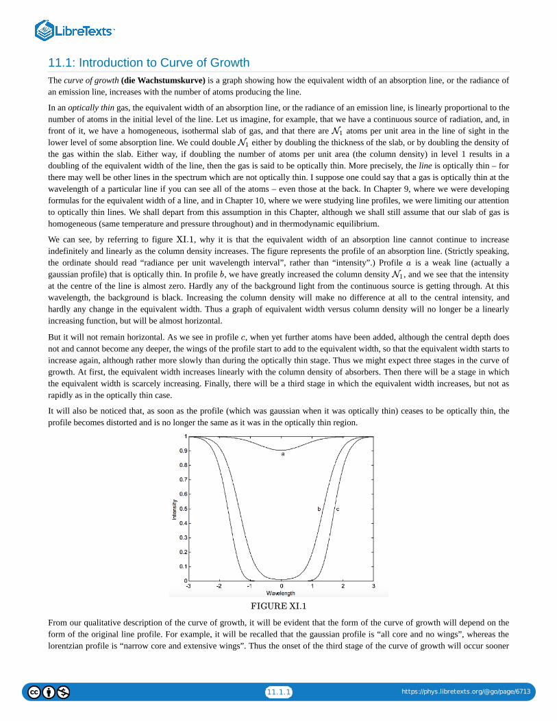
11.1.1 https://phys.libretexts.org/@go/page/6713

11.1: Introduction to Curve of GrowthThe curve of growth (die Wachstumskurve) is a graph showing how the equivalent width of an absorption line, or the radiance ofan emission line, increases with the number of atoms producing the line.

In an optically thin gas, the equivalent width of an absorption line, or the radiance of an emission line, is linearly proportional to thenumber of atoms in the initial level of the line. Let us imagine, for example, that we have a continuous source of radiation, and, infront of it, we have a homogeneous, isothermal slab of gas, and that there are atoms per unit area in the line of sight in thelower level of some absorption line. We could double either by doubling the thickness of the slab, or by doubling the density ofthe gas within the slab. Either way, if doubling the number of atoms per unit area (the column density) in level 1 results in adoubling of the equivalent width of the line, then the gas is said to be optically thin. More precisely, the line is optically thin – forthere may well be other lines in the spectrum which are not optically thin. I suppose one could say that a gas is optically thin at thewavelength of a particular line if you can see all of the atoms – even those at the back. In Chapter 9, where we were developingformulas for the equivalent width of a line, and in Chapter 10, where we were studying line profiles, we were limiting our attentionto optically thin lines. We shall depart from this assumption in this Chapter, although we shall still assume that our slab of gas ishomogeneous (same temperature and pressure throughout) and in thermodynamic equilibrium.

We can see, by referring to figure , why it is that the equivalent width of an absorption line cannot continue to increaseindefinitely and linearly as the column density increases. The figure represents the profile of an absorption line. (Strictly speaking,the ordinate should read “radiance per unit wavelength interval”, rather than “intensity”.) Profile is a weak line (actually agaussian profile) that is optically thin. In profile , we have greatly increased the column density , and we see that the intensityat the centre of the line is almost zero. Hardly any of the background light from the continuous source is getting through. At thiswavelength, the background is black. Increasing the column density will make no difference at all to the central intensity, andhardly any change in the equivalent width. Thus a graph of equivalent width versus column density will no longer be a linearlyincreasing function, but will be almost horizontal.

But it will not remain horizontal. As we see in profile , when yet further atoms have been added, although the central depth doesnot and cannot become any deeper, the wings of the profile start to add to the equivalent width, so that the equivalent width starts toincrease again, although rather more slowly than during the optically thin stage. Thus we might expect three stages in the curve ofgrowth. At first, the equivalent width increases linearly with the column density of absorbers. Then there will be a stage in whichthe equivalent width is scarcely increasing. Finally, there will be a third stage in which the equivalent width increases, but not asrapidly as in the optically thin case.

It will also be noticed that, as soon as the profile (which was gaussian when it was optically thin) ceases to be optically thin, theprofile becomes distorted and is no longer the same as it was in the optically thin region.

From our qualitative description of the curve of growth, it will be evident that the form of the curve of growth will depend on theform of the original line profile. For example, it will be recalled that the gaussian profile is “all core and no wings”, whereas thelorentzian profile is “narrow core and extensive wings”. Thus the onset of the third stage of the curve of growth will occur sooner

N1

N1

XI.1

a

b N1

c

FIGURE XI.1

11.1.2 https://phys.libretexts.org/@go/page/6713

for a lorentzian profile than for a gaussian profile. We shall find, as we proceed, that for a pure gaussian profile, the third stage ofthe classic curve of growth is scarcely evident, whereas for a pure lorentzian profile, the second stage is scarcely evident. Theclassic three-stage curve of growth is exhibited for a Voigt profile in which the gaussian and lorentzian contributions arecomparable.

It will be part of the aim of this chapter to predict the curve of growth for gaussian and lorentzian profiles, and also for Voigt profilefor different Gauss/Lorentz ratios.

This by itself will be an interesting intellectual exercise – but can it be taken further? Yes it can. Imagine a situation is which wehave a spectrum in which the resolution is not sufficient to measure the profiles of individual lines with any great precision. Nogreat imagination is in fact needed, for this will usually be the case with a stellar spectrum. If we can somehow construct a curve ofgrowth, we might be able to deduce the line profiles, or at least the FWHm (full width at half minimum) of the gaussian component(which will tell us the kinetic temperature) and of the lorentzian component (which will tell us the mean time between collisionsand hence the pressure). We cannot, of course, change the column density of a stellar atmosphere. However, some lines of a givenelement will be weak (because they have a high excitation potential, or a small oscillator strength, or both) and others will be strong(because they have a low excitation potential, or a large oscillator strength, or both), and perhaps a curve of growth can beconstructed from many lines of a given atom, and so we will be able to deduce the temperature and the pressure, even though wecannot resolve the details of individual line profiles.

So far, I have discussed the curve of growth for an absorption line. What about an emission line? We understand that the intensityof the centre of an absorption line cannot drop below the “floor” corresponding to zero intensity. But is there a “ceiling” that willstop the growth of the centre of an emission line, or can we go on increasing the intensity of an emission line indefinitely? Theanswer is that, for a gas in thermodynamic equilibrium, there is indeed a “ceiling”, and that occurs when the radiance per unitwavelength interval of the centre of the emission line reaches the ordinate of the Planck blackbody curve having a blackbodytemperature equal to the kinetic and excitation temperature of the gas. When the line centre is completely optically thick, it radiateslike a black body at that wavelength. Adding more atoms to the column density will not increase the central intensity. Whathappens is that photons emitted by atoms near the back of the slab of gas are re-absorbed as they struggle forward towards thefront.

11.1: Introduction to Curve of Growth is shared under a CC BY-NC 4.0 license and was authored, remixed, and/or curated by Jeremy Tatum viasource content that was edited to conform to the style and standards of the LibreTexts platform; a detailed edit history is available upon request.

11.2.1 https://phys.libretexts.org/@go/page/6714

11.2: A Review of Some TermsBefore continuing, a review of some terms such as absorption coefficient, absorptance, central depth and optical thickness may beof some use.

Imagine a thin slice of absorbing gas of thickness . At one side of the slice, suppose that the specific intensity (radiance) per unitwavelength interval wavelength is and that, after passage of the radiation through the slice, the specific intensity is nowonly . ( is negative.) The fractional decrease in the specific intensity is proportional to :

is the linear absorption coefficient, and is of dimension . Now let imagine that, rather than an infinitesimally thin slice ofgas, we have a slab of gas of finite thickness and that it is sitting in front of a continuum source of specific intensity (radiance)per unit wavelength interval , where “ ” indicates “continuum”. The radiance after passage through the slice is given byintegrating Equation :

The quantity

is the optical thickness of the slab. It is dimensionless. If the slab of gas is homogeneous, in the sense that is the samethroughout the slab and is not a function of , this becomes simply

Let us suppose that, after passage through the slab of gas, the specific intensity (radiance) of the gas at wavelength , which wasinitially , is now , The fraction of the radiance that has been absorbed is the absorptance at wavelength :

It is dimensionless. The relation between absorptance and optical thickness is evidently

For a gas of very small optical thickness, in which only a tiny fraction of the radiation has been absorbed (which will not in generalbe the case in this chapter), Maclaurin expansion of either of these Equations will show that

If, in addition, the slab of gas is homogeneous,

The absorptance at the line centre is

and we have also called this, in Chapter 10, the central depth .

The absorption coefficient of a gas at the wavelength of an absorption line is proportional to , the number of atoms per unitvolume in the initial (lower) level of the transition. This is so whether the slab of gas is optically thin or not; we are concerned herewith the absorption coefficient and the number density at a point within the gas, not with the slab as a whole. The optical thicknessof a slab of gas is proportional to , the number of atoms per unit area in the line of sight (column density) in the initial level.This is so whether or not the slab is homogeneous. In the sense in which the words intensive and extensive are used inthermodynamics, it could be said that absorption coefficient is an intensive quantity and optical thickness and absorptance are

δx

λ (λ)Iλ

+δIλ Iλ δIλ δx

− = α(λ)δx.δ (λ)Iλ

(λ)Iλ(11.2.1)

α(λ) L−1

D

(c)Iλ c

11.2.1

(λ) = (c)exp[− α(λ)dx] ,Iλ Iλ ∫D

0

(11.2.2)

τ(λ) = α(λ)dx∫D

0

(11.2.3)

α(λ)

x

τ(λ) = Dα(λ). (11.2.4)

λ

(c)Iλ (λ)Iλ λ, a(λ)

a(λ) =(c) − (λ)Iλ Iλ

(c)Iλ(11.2.5)

a(λ) = 1 − , τ(λ) = −ln(1 −a(λ)).e−τ(λ) (11.2.6 a,b)

a(λ) ≈ τ(λ). (11.2.7)

a(λ) ≈ Dα(λ). (11.2.8)

a( ) = ,λ0

(c) − ( )Iλ Iλ λ0

(c)Iλ(11.2.9)

d

n1

N1

11.2.2 https://phys.libretexts.org/@go/page/6714

extensive quantities. While the optical thickness is proportional to , the radiance per unit wavelength interval and the equivalentwidth are not linearly proportional to unless the gas is optically thin.

For the terms such as atomic and mass absorption coefficient, opacity, and the distinction between absorption, scattering andextinction, see Chapter 5.

11.2: A Review of Some Terms is shared under a CC BY-NC 4.0 license and was authored, remixed, and/or curated by Jeremy Tatum via sourcecontent that was edited to conform to the style and standards of the LibreTexts platform; a detailed edit history is available upon request.

N1

N1

11.3.1 https://phys.libretexts.org/@go/page/6715

11.3: Theory of the Curve of GrowthLet us think again of our homogeneous slab of gas in front of a continuum source. Let be the radiance per unit wavelengthinterval of the continuum at wavelength . Let be the optical thickness in the vicinity of a line and . If the slab isof thickness , the emergent radiance per unit wavelength as a function of wavelength will be

The equivalent width is given by

or, by making use of Equation ,

If the line is symmetric, this may be evaluated as

In former days, gallant efforts were made to find, using various approximations in the different regimes of the curve of growth,algebraic expressions for evaluating this integral. The availability of modern computers enables us to carry out the integrationnumerically.

11.3: Theory of the Curve of Growth is shared under a CC BY-NC 4.0 license and was authored, remixed, and/or curated by Jeremy Tatum viasource content that was edited to conform to the style and standards of the LibreTexts platform; a detailed edit history is available upon request.

(c)Iλ

λ τ(x) x = λ−λ0

D

(x) = (c)exp[−τ(x)].Iλ Iλ (11.3.1)

W

W (c) = ( (c) − (x)) dx,Iλ ∫∞

−∞

Iλ Iλ (11.3.2)

11.3.1

W = [1 −exp{−τ(x)}] dx.∫∞

−∞

(11.3.3)

W = 2 [1 −exp{−τ(x)}] dx.∫∞

0

(11.3.4)

11.4.1 https://phys.libretexts.org/@go/page/6716

11.4: Curve of Growth for Gaussian ProfilesBy “gaussian profile” in the title of this section, I mean profiles that are gaussian in the optically-thin case; as soon as there aredepartures from optical thinness, there are also departures from the gaussian profile. Alternatively, the absorption coefficient andthe optical depth are gaussian; the absorptance is not.

For an optically-thin thermally-broadened line, the optical thickness as a function of wavelength is given by

where the HWHM is

Here is the modal speed. (See Chapter 10 for details.) The line profiles, as calculated from equations 11.3.4 and , areshown in figure XI.2 for the following values of the optical thickness at the line centre:

On combining equations 11.3.4 and and , we obtain the following expression for the equivalent width:

or

where

The half-width at half maximum (HWHM) of the expression for the optical thickness corresponds to .For the purposes of practical numerical integration of Equation , I shall integrate from that is to say from

times the HWHm. One can appreciate from figure XI.2 that going outside these limits will not contribute significantly to theequivalent width. I shall calculate the equivalent width for central optical depths ranging from

.

What we have in figure XI.3 is a curve of growth for thermally broadened lines (or lines that, in the optically thin limit, have agaussian profile, which could include a thermal and a microturbulent component). I have plotted this from

; that is .

τ(x) = τ(0)exp(− ) ,ln2x2

g2(11.4.1)

g = .Vmλ0 ln2

−−−√

c(11.4.2)

Vm 11.4.1τ(0) = , , , , 1, 2, 4, 8.1

1618

14

12

11.4.1 11.4.2

W = 2 (1 −exp{−τ(0) }) dx,∫∞

0e− ln 2/x2 g2

(11.4.3)

W = (1 −exp{−τ(0) }) dΔ,2Vmλ0

c∫

∞

0e

−Δ2

(11.4.4)

Δ = = .x ln2

−−−√

g

cx

Vmλ0(11.4.5)

11.4.1 Δ = = 0.8326ln2−−−

√

11.4.4 Δ = −5 to  +5±6

1/20(log τ(0) = −1.3) to  (log τ(0) = 5.0)105

log τ(0) = −1.3 to  +5.0 τ(0) = 0.05 to 105

11.4.2 https://phys.libretexts.org/@go/page/6716

11.4: Curve of Growth for Gaussian Profiles is shared under a CC BY-NC 4.0 license and was authored, remixed, and/or curated by Jeremy Tatumvia source content that was edited to conform to the style and standards of the LibreTexts platform; a detailed edit history is available uponrequest.

FIGURE XI.2

FIGURE XI.3

11.5.1 https://phys.libretexts.org/@go/page/6717

11.5: Curve of Growth for Lorentzian ProfilesThe optical depth of a line broadened by radiation damping is given, as a function of wavelength, by

where the HWHM is

and the optical thickness at the line center is

Here , and the damping constant may include a contribution from pressure broadening. As in Section 11.4, in figureXI.4 I draw line profiles for optical thicknesses at the line center .

We see that the wings continue to add to the equivalent width as soon as, and indeed before, the central depth has reached unity. Oncombining equations 11.3.4, ,2 and 3, we obtain the following expression for the equivalent width:

in which - i.e. distance from the line center in units of the HWHM.

If we now substitute , the expression for the equivalent width becomes

Now that we have a finite upper limit, the expression can be integrated numerically without artificial and unjustified truncation. Asdescribed in the Appendix to Chapter 10, calculation of the trigonometric function cos can be avoided, and hence the integrationmuch speeded up, by the substitution of . Although the denominator of the integrand is obviously zero at the upperlimit, so is the numerator, and the value of the integrand at the upper limit is finite and equal to . Figure XI.5 shows the

equivalent width, in units of as a function of .

11.5: Curve of Growth for Lorentzian Profiles is shared under a CC BY-NC 4.0 license and was authored, remixed, and/or curated by JeremyTatum via source content that was edited to conform to the style and standards of the LibreTexts platform; a detailed edit history is available uponrequest.

τ(x) = τ(0) ,l2

+x2 l2(11.5.1)

l =Γλ2

0

4πc(11.5.2)

τ(0) = .e2N1f12

m cΓϵ0(11.5.3)

x = λ−λ0 Γ

τ(0) = , , , , 1, 2, 4, 8116

18

14

12

11.5.1

W = (1 −exp{− }) dy,Γλ2

0

2πc∫

∞

0

τ(0)

+1y2(11.5.4)

y = x/l

y = tanθ

W = dθ.Γλ2

0

2πc∫

π/2

0

1 −exp[−τ(0) θ]cos2

θcos2(11.5.5)

t = tan( θ)12

τ(0)Γλ2

0

2πcτ(0)

FIGURE XI.4 FIGURE XI.5

11.6.1 https://phys.libretexts.org/@go/page/6718

11.6: Curve of Growth for Voigt ProfilesOur next task is to construct curves of growth for Voigt profiles for different values of the ratio of the lorentzian and gaussianHWHMs, , which is

or, better, for different values of the gaussian ratio . These should look intermediate in appearance between figures XI.3and 5.

The expression for the equivalent width in wavelength units is given by Equation 11.3.4:

combined with Equation 10.5.20

That is:

Here

, is the Lorentzian (where may include a pressure-broadening contribution), is the gaussian (where may include a microturbulence contribution), and

is the equivalent width, all of dimension .

The symbol , also of dimension L, is a dummy variable, which disappears after the definite integration. is the opticalthickness at the line centre. is a dimensionless number given by Equation 10.5.23 and tabulated as a function of gaussian fractionin Chapter 10. The reader is urged to check the dimensions of Equation carefully. The integration of Equation isdiscussed in Appendix A.

Our aim is to calculate the equivalent width as a function of for different values of the gaussian fraction .What we find is as follows. Let ; that is, is the equivalent width expressed in units of . For lessthan about 5, where the wings contribute relatively little to the equivalent width, we find that is almost independent of thegaussian fraction. The difference in behaviour of the curve of growth for different profiles appears only for large values of ,when the wings assume a larger role. However, for any profile which is less gaussian than about equal to about 0.9, thebehaviour of the curve of growth (for ) mimics that for a lorentzian profile. For that reason I have drawn curves of growthin figure XI.6 only for . This corresponds to , or to

respectively.

l/g

= = = ,l

g

Γλ0

4πVm ln2−−−

√

Γλ0

πVm ln65536− −−−−−−

√

Γλ0

34.841Vm(11.6.1)

=kGg

l+g

W = 2 [1 −exp{−τ(x)}] dx.∫∞

0(11.3.4)

τ(x) = Clτ(0) dξ.∫∞

−∞

exp[−(ξ−x ln2/ ])2 g2

+ξ2 l2(10.5.20)

W = 2 (1 −exp{−Clτ(0) dξ}) dx.∫∞

0∫

∞

−∞

exp[−(ξ−x ln2/ ])2 g2

+ξ2 l2(11.6.2)

x = λ−λ0 l HWHM = Γ/(4πc)λ20 Γ

g HWHM = /cVmλ0 ln2−−−

√ Vm

W L

ξ τ(0)C

11.6.2 11.6.2

τ(0) = g/(l+g)kG

= W /gW ′ ln2−−−

√ W ′ g/ ln2−−−

√ τ(0)W ′

τ(0)kG

τ(0) > 5= 0.9, 0.99, 0.999 and 1kG l/g = 0.1111, 0.0101, 0.0010 and 0

Γ / = 1.162, 0.1057, 0.0105 and 0λ0 Vm

11.6.2 https://phys.libretexts.org/@go/page/6718

11.6: Curve of Growth for Voigt Profiles is shared under a CC BY-NC 4.0 license and was authored, remixed, and/or curated by Jeremy Tatum viasource content that was edited to conform to the style and standards of the LibreTexts platform; a detailed edit history is available upon request.

FIGURE XI.6

11.7.1 https://phys.libretexts.org/@go/page/8032

11.7: Observational Curve of GrowthEquation 11.6.2 and figure XI.6 show how the equivalent width of a line will grow as the optical thickness is increased, which canbe achieved either by increasing the geometrical thickness of the gas under study or by increasing the number density of theabsorbers (atoms). Of course, if you are looking at the spectrum of a stellar atmosphere, you cannot do either of these things, butyou might be able to construct a curve of growth by looking at many lines from the same element (such as an element from the irongroup, which has lots of lines of a wide range of equivalent widths.) Then, by comparing the form of the observed curve of growthwith one of the theoretical curves, you could deduce the gaussian and lorentzian HWHm, , of your lines (and hence possiblythe temperature and pressure) even if your resolution were not sufficient to determine the individual line profiles with anyprecision. You will notice the word “possibly” – because it has to be remembered that includes both a thermal and amicroturbulent component, and includes both a radiation damping and pressure broadening component. Provided that the gasunder study is homogeneous and of a uniform temperature throughout (I suppose this rules out a stellar atmosphere!) should bethe same for all lines of a given element. (The microturbulent component of should be the same for all elements.) The radiationdamping component of will vary from line to line, but in practice, at least in the atmosphere of a main sequence star (but notnecessarily of a giant, where the atmospheric pressure is much lower), the pressure broadening component of will be much greaterthan the radiation damping component, and hence will be the same for all lines of a given element. The theories of thermal,microturbulent, radiation damping and pressure broadening are all covered in Chapter 10.

It is all very well to say plot log versus log for many lines of an iron-group element, but we immediately discover that wedon’t know either. The dimensionless quantity is given by

and we don’t know – indeed one of our aims is to find it. The optical depth at the line centre is given by

and we don’t know − again, one of our aims is to find it. However, these equations can be written in the form

and

Also, from Boltzmann’s equation (where applicable!), we have

from which

where the “constant” is a function of , the excitation energy of the lower level of the line. From this, we obtain

Thus, provided we take a set of lines all having the same lower excitation level (or at least the same lower term, provided thatdepartures from -coupling are not so severe as to scatter the levels widely), we can construct a partial curve of growth byplotting versus for these lines. These will be displaced both vertically and horizontally from the theoretical curves offigure XI.6 by arbitrary amounts, which will not affect the shape of the curve.

We can then take another set of lines, having a different common lower excitation level (or term), and plot another partial curve ofgrowth. It will be displaced horizontally (but not vertically) from the first fragment, and it must be slid horizontally until it meshesin with the first fragment. And so we continue, building up partial curves of growth from sets of lines with a common lower term,sliding them horizontally until they all mesh with each other in a single continuous curve, which we can then compare with theshapes of the theoretical curves to obtain and and hence the temperature and pressure.

11.7: Observational Curve of Growth is shared under a CC BY-NC 4.0 license and was authored, remixed, and/or curated by Jeremy Tatum viasource content that was edited to conform to the style and standards of the LibreTexts platform; a detailed edit history is available upon request.

g and l

g

l

g

g

l

l

l

W ′ τ(0)W ′

= W /g,W ′ ln2−−−

√ (11.7.1)

g

τ(0) = ,N1f12e2

mc Γϵ0(11.7.2)

Γ

log = log W + constantW ′ (11.7.3)

log τ(0) = log + constant.N1f12 (11.7.4)

ln = ln(N /u) − /(kT ) +ln ,N1 E1 ϖ1 (11.7.5)

log = log +C( )N1 ϖ1 E1 (11.7.6)

E1

log τ(0) = log ϖf +C( ).E1 (11.7.7)

LS

log W log ϖf

g l

11.8.1 https://phys.libretexts.org/@go/page/8036

11.8: Interpreting an Optically Thick ProfileThis chapter has been concerned with optically thick lines and with the curve of growth – and how one might recover theparameters and from the curve of growth even if the profiles of individual lines are not resolved. This section is written rather asan afterthought, albeit an important one, and it does not concern the curve of growth. It discusses how one might analyse the profileof a line that is well resolved, but is not optically thin. I use as an example a line that is thermally broadened and which, if opticallythin, would have a gaussian profile. The optically thick line is no longer gaussian, but can one recover (and hence ) from it?Just for a change, and because it is a while since we used the term “source function”, I’ll deal with an emission line.

As discussed in Section 5.7, the radiance of a slab of gas of source function is given by

Here, . For a thermally-broadened line, this becomes

where

In figure XI.7, I draw two such profiles, in which the line strength of one is times the line strength of the other. The lines,perhaps, belong to the same multiplet and the ratio of the line strengths is known. (I am here using the term line strength in thetechnical sense of Chapter 7.) Figure XI.7 was drawn with , but since the lines are not optically thin, neither the ratio of theirareas nor the ratio of their heights is two.

We can measure the half widths of the two profiles at the same height.

Then:

after which

and hence

The same technique can be used for lorentzian profiles.

g l

g T

S

(x) = S dτ = S(1 − ).Iλ ∫τ(x)

0e−τ e−τ(x) (11.8.1)

x = λ−λ0

(x) = S [1 −exp{−τ(0)exp(− ln2/ )}] ,Iλ x2 g2 (11.8.2)

g = / .Vmλ0 ln2−−−

√

A

A = 2

FIGURE XI.7

Δ  and Δx1 x2

S[1 −exp{−τ(0)exp(−(Δ ln2/ )}] = S[1 −exp{−Aτ(0)exp(−(Δ ln2/ )}],x1)2 g2 x2)2 g2 (11.8.3)

= −lnA,(Δ ) ln2x1

g2

(Δ ) ln2x2

g2(11.8.4)

= .g2 [(Δ −(Δ ]x1)2 x2)2

lnA(11.8.5)

11.8.2 https://phys.libretexts.org/@go/page/8036

11.8: Interpreting an Optically Thick Profile is shared under a CC BY-NC 4.0 license and was authored, remixed, and/or curated by Jeremy Tatumvia source content that was edited to conform to the style and standards of the LibreTexts platform; a detailed edit history is available uponrequest.

11.9.1 https://phys.libretexts.org/@go/page/8047

11.9: APPENDIX A- Evaluation of the Voigt Curve of Growth IntegralWe wish to evaluate the equivalent width as given by equation 11.6.2:

We slightly simplify it by introducing dimensionless variables defined by , where is anyof . That is, we are expressing lengths in units of . Then:

We shall eventually want to evaluate the integral as a function of the gaussian ratio , and we note that .

Since is a dummy variable, we could in principle dispense with the prime as superfluous, but it is probably helpful to retain theprime. The limits of the inner integral can be made finite by means of a change of variable. The substitution willachieve this, but the introduction of a trigonometric function will increase the computing time. An alternative is , whichlooks clumsier but is rather faster. The equation becomes

This integral is not particularly easy, and I do not advise merely putting it into a prepackaged integration program without criticalexamination. (Indeed I never advocate that!) One is faced with the usual problems of numerical integration: What should be thestep size and number of steps? And, in the case of the outer integral, how far should we take the upper limit? One way to determinethe necessary number of intervals (and step size) is to try, say 100 intervals, and then try 1000, and see if it makes any difference.Similarly with determining the upper limit to the outer integration, try integrating to , and then to 10, and see if it makes anydifference. But this integral has some problems of its own.

Some insight into the problems can be obtained by looking at the behaviour of the inner integrand. This function, ,

is shown as a function of for four different values of in figure XI.A1 The value of for the figure is , which has noparticular significance, since the figure is intended solely for illustrative purposes.

For , the function is symmetric about , but not for other values of . For small values of x', there is no particulardifficulty with the integration, either by Simpson’s rule or by seven-point integration (see my Web notes on Celestial Mechanics,Chapter 1).

W = 2 (1 −exp{−Clτ(0) dξ}) dx.∫∞

0∫

∞

−∞

exp[−(ξ−x ln2/ ])2 g2

+ξ2 l2(11.A.1)

, ,  and W ′ x′ ξ′ l′ = =X ′ Xc

λ0Vm

X ln 2√g

X

W , x, ξ or l g/ ln2−−−

√

= 2 (1 −exp{−C τ(0) d }) d .W ′ ∫∞

0l′ ∫

∞

−∞

exp[−( − ]ξ′ x′)2

+ξ′2 l′2ξ′ x′ (11.A.2)

kG = ( −1)l′ 1kG

ln2−−−

√

ξ′

= tanθξ′ l′

=ξ′ 2 tl′

1−t2

= 2 1 −exp −2Cτ(0) dt d .W ′ ∫∞

0

⎛

⎝

⎧

⎩⎨ ∫

1

−1

exp[−( − ]2 tl′

1−t2x′)2

1 + t2

⎫

⎭⎬⎞

⎠x′ (11.A.3)

= 5x′

exp[−( − ]2 tl′

1−t2x′)2

1+t2

t x′ l′ 1/(4π)

= 0x′ t = 0 x′

FIGURE XI.A1

11.9.2 https://phys.libretexts.org/@go/page/8047

However, for large , the integrand is close to zero for most of the range between , but, close to , theintegrand exhibits a sharp spike, becoming almost a delta-function for larger . A coarse interval for integration may miss thespike altogether, while a very fine interval will use massive amounts of computer time to no good purpose over most of the rangeof . Fortunately, the area under the spike is progressively smaller and smaller for larger and larger but the nagging question stillremains, when may one stop integrating? One useful, efficient and effective technique is to adjust the size of the interval forintegration according to the slope of the function. A coarse interval is quite adequate while the graph is near-horizontal, but a muchfiner integration step kicks in as soon as the slope becomes large. This requires a certain amount of programming legerdemain, butis frequently resorted to in such situations.

The part of equation 11.A 2:

represents the optically thick Voigt profile. This is shown for for several in figure XI.A.2. The value has no particular significance; figure XI.A.2 was drawn solely for illustrative purposes.

The equivalent width (equation 11.A.1) is the area above these curves, and it can be seen again that determining the upper limit for is a problem.

We can, however, remember that the profile that we are integrating is the convolution of a gaussian and a lorentzian, and that in units of . The gaussian component has very small wings, whereas the lorentzian profile has extensive

wings. The ratio of the gaussian component to the ordinate to the lorentzian component is , where

. The value of at which this ratio drops to 0.0001 is shown as a function of in figure XI.A.1a. Beyondthis point one can treat the wings of the profile as lorentzian.

Thus equation 11.A.2 can be integrated by treating the optically thin profile as a Voigt function up to some and as alorentzian function thereafter. That is, I have written equation 11.A.2 as

x′ t = −1.0 and 0.0 t = 1.0x′

t x′

exp{−Clτ(0) dξ}∫∞

−∞

exp[−(ξ−x ln2/ ])2 g2

+ξ2 l2(11.A.4)

= 1/(4π)l′ τ(0) = 1/(4π)l′

FIGURE XI.A2

x′

 is λ−x′ λ0 2g/ ln2−−−

√

( ) exp(− )+l′2 x′2

l′2x′2

= (1/ −1)l′ kG ln2−−−

√ x′ kG

= ax′

11.9.3 https://phys.libretexts.org/@go/page/8047

On substitution of in the first integral and in the second, this becomes

where . The dreaded symbol has now gone and, further, there is no problem at the upper limit of the secondintegral, for the value of the integrand when is unity.

11.9: APPENDIX A- Evaluation of the Voigt Curve of Growth Integral is shared under a CC BY-NC 4.0 license and was authored, remixed,and/or curated by Jeremy Tatum via source content that was edited to conform to the style and standards of the LibreTexts platform; a detailededit history is available upon request.

FIGURE XI.A.1A

= 2W ′ (1 −exp{−C τ(0) d }) d∫a

0l′ ∫

∞

−∞

exp[−( − ]ξ′ x′)2

+ξ′2 l′2ξ′ x′

+2 (1 −exp{− }) d .∫∞

a

τ(0)

+x′2 l′2x′

(11.9.1)

(11.9.2)

(11.A.5)

=ξ′ 2 tl′

1−t2 = tanθx′ l′

= 2W ′ 1 −exp −2Cτ(0) dt d∫a

0

⎛

⎝

⎧

⎩⎨ ∫

1

−1

exp[−( − ]2 tl′

1−t2 x′)2

1 + t2

⎫

⎭⎬⎞

⎠x′

+2 dθ,l′ ∫π/2

α

(1 −exp{−τ(0) θ})cos2

θcos2

(11.9.3)

(11.9.4)

(11.A.6)

tanα = /al′ ∞θ = π/2

1 https://phys.libretexts.org/@go/page/23097

IndexAalbedoes

1.13: Lambertian Surface anomalous Zeeman effect

7.21: Zeeman effect apparent bolometric magnitude

1.9: Apparent Magnitude atomic absorption coefficient

5.2: Absorption atomic spectra

7: Atomic Spectroscopy

Bblack body

2.1: Absorptance, and the Definition of a BlackBody Bohr Model

7.4: The Bohr Model of Hydrogen-like Atoms boltzmann's Equation

8: Boltzmann's and Saha's Equations

Cconvolution

10.4: Combination of Profiles curve of growth

11.1: Introduction to Curve of Growth

EEmission Coefficient

4.8: Emission Coefficient exitance

1.11: Exitance M

GGaussian Profile

10.1: Natural Broadening (Radiation Damping) grey body

2.1: Absorptance, and the Definition of a BlackBody

Hhyperfine structure

7.18: Hyperfine Structure

Iindex of refraction

7.1: Introduction

LLambert's Law

1.13: Lambertian Surface Lambertian Surface

1.13: Lambertian Surface Landé splitting factor

7.21: Zeeman effect limb darkening coefficient

6.1: Introduction. The Empirical Limb-darkening line profiles

10: Line Profiles line strength

9.5: Line Strength Lorentz profile

10.1: Natural Broadening (Radiation Damping) luminosity

4.2: Luminosity

Mmass extinction coefficient

5.3: Scattering, Extinction and Opacity Microturbulence

10.3: Microturbulence

Oopacity

5.3: Scattering, Extinction and Opacity Optical Depth

5.4: Optical Depth oscillator strength

9: Oscillator Strengths and Related Topics

PPlanck distribution

2.5: Planck's Equation pressure broadening

10.1: Natural Broadening (Radiation Damping) 10.5: Pressure Broadening

RRadiance

9.1: Introduction, Radiance, and Equivalent Width radiation damping constant

10.1: Natural Broadening (Radiation Damping) Radiation Density

1.16: Radiation Density (u) radiation pressure

1.18: Radiation Pressure (P) 4.6: Radiation Pressure

SSaha's Equation

8: Boltzmann's and Saha's Equations 8.6: Saha's Equation

Schrodinger's Equation7.8: Schrödinger's Equation

Specific Intensity4.3: Specific Intensity

specular reflection1.13: Lambertian Surface

Stefan's constant2.7: Stefan's Law (The Stefan-Boltzmann Law)

Stefan's Laws2.10: Derivation of Wien's and Stefan's Laws

VVoigt profile

10.4: Combination of Profiles Voigt Profiles

11.6: Curve of Growth for Voigt Profiles

WWien's

2.10: Derivation of Wien's and Stefan's Laws Wien's law

2.6: Wien's Law

ZZeeman effect

7.21: Zeeman effect

1 https://phys.libretexts.org/@go/page/26557

IndexAalbedoes

1.13: Lambertian Surface anomalous Zeeman effect

7.21: Zeeman effect apparent bolometric magnitude

1.9: Apparent Magnitude atomic absorption coefficient

5.2: Absorption atomic spectra

7: Atomic Spectroscopy

Bblack body

2.1: Absorptance, and the Definition of a BlackBody Bohr Model

7.4: The Bohr Model of Hydrogen-like Atoms boltzmann's Equation

8: Boltzmann's and Saha's Equations

Cconvolution

10.4: Combination of Profiles curve of growth

11.1: Introduction to Curve of Growth

EEmission Coefficient

4.8: Emission Coefficient exitance

1.11: Exitance M

GGaussian Profile

10.1: Natural Broadening (Radiation Damping) grey body

2.1: Absorptance, and the Definition of a BlackBody

Hhyperfine structure

7.18: Hyperfine Structure

Iindex of refraction

7.1: Introduction

LLambert's Law

1.13: Lambertian Surface Lambertian Surface

1.13: Lambertian Surface Landé splitting factor

7.21: Zeeman effect limb darkening coefficient

6.1: Introduction. The Empirical Limb-darkening line profiles

10: Line Profiles line strength

9.5: Line Strength Lorentz profile

10.1: Natural Broadening (Radiation Damping) luminosity

4.2: Luminosity

Mmass extinction coefficient

5.3: Scattering, Extinction and Opacity Microturbulence

10.3: Microturbulence

Oopacity

5.3: Scattering, Extinction and Opacity Optical Depth

5.4: Optical Depth oscillator strength

9: Oscillator Strengths and Related Topics

PPlanck distribution

2.5: Planck's Equation pressure broadening

10.1: Natural Broadening (Radiation Damping) 10.5: Pressure Broadening

RRadiance

9.1: Introduction, Radiance, and Equivalent Width radiation damping constant

10.1: Natural Broadening (Radiation Damping) Radiation Density

1.16: Radiation Density (u) radiation pressure

1.18: Radiation Pressure (P) 4.6: Radiation Pressure

SSaha's Equation

8: Boltzmann's and Saha's Equations 8.6: Saha's Equation

Schrodinger's Equation7.8: Schrödinger's Equation

Specific Intensity4.3: Specific Intensity

specular reflection1.13: Lambertian Surface

Stefan's constant2.7: Stefan's Law (The Stefan-Boltzmann Law)

Stefan's Laws2.10: Derivation of Wien's and Stefan's Laws

VVoigt profile

10.4: Combination of Profiles Voigt Profiles

11.6: Curve of Growth for Voigt Profiles

WWien's

2.10: Derivation of Wien's and Stefan's Laws Wien's law

2.6: Wien's Law

ZZeeman effect

7.21: Zeeman effect

1 https://phys.libretexts.org/@go/page/29416

GlossarySample Word 1 | Sample Definition 1