A&A 422, 193–203 (2004)DOI: 10.1051/0004-6361:20040151c© ESO 2004

Astronomy&

Astrophysics

Stellar activity and magnetism studied by optical interferometry

K. Rousselet-Perraut1, C. Stehle2, T. Lanz2,3,4, J. B. Le Bouquin1, T. Boudoyen1,M. Kilbinger5, O. Kochukhov6, and S. Jankov7

1 Laboratoire d’Astrophysique de l’Observatoire de Grenoble, BP 53, 38041 Grenoble Cedex 9, France2 Laboratoire de l’Univers et de ses THeories, UMR 8102, Observatoire de Paris, 5 place Jules Janssen, 92195 Meudon, France3 Department of Astronomy, University of Maryland, College Park, MD 20742, USA4 NASA Goddard Space Flight Center, Code 681, Greenbelt, MD 20771, USA5 Institut fur Astrophysik und Extraterrestrische Forschung, Universitat Bonn, Auf dem Hugel 71, 53121 Bonn, Germany6 Uppsala Astronomical Observatory, Box 515, 751 20, Uppsala, Sweden7 Observatoire de la Cote d’Azur, Departement Fresnel, CNRS UMR 6528, 06460 Saint Vallier de Thiey, France

Received 31 March 2003 / Accepted 23 March 2004

Abstract. By means of numerical simulations, we investigate the ability of optical interferometry, via the fringe phase observ-able, to address stellar activity and magnetism. To derive abundance maps and stellar rotation axes, we use color differentialinterferometry which couples high angular resolution to high spectral resolution. To constrain magnetic field topologies, we addto this spectro-interferometer a polarimetric mode. Two cases of well-known Chemically Peculiar (CP) stars (βCrB and α2CVn)are simulated to derive instrumental requirements to obtain 2D-maps of abundance inhomogeneities and magnetic fields. Weconclude that the near-infrared instrument AMBER of the VLTI will allow us to locate abundance inhomogeneities of CP starslarger than a fraction of milliarcsecond whereas the polarimetric mode of the French GI2T/REGAIN interferometer wouldpermit one to disentangle various magnetic field topologies on CP stars. We emphasize the crucial need for developing andvalidating inversion algorithms so that future instruments on optical aperture synthesis arrays can be optimally used.

Key words. techniques: interferometric – techniques: polarimetric – stars: chemically peculiar – stars: magnetic fields –stars: activity

1. Introduction

Stellar magnetism and activity have been most often studiedwith various spectro-polarimetric techniques, such as the anal-ysis of the shape of line profiles in different Stokes parameters(the moment technique proposed by Mathys (1988)), the BroadBand Linear Polarization technique (Leroy et al. 1993), theZeeman-Doppler (Semel 1989; Donati 1996) or the Magnetic-Doppler (Piskunov & Kochukhov 2002) Imaging techniques(so-called ZDI and MDI techniques respectively). Generally,however, the poor angular resolution drastically limits detec-tion and/or diagnosis since the polarized signals are averagedover the stellar surface and thus cancel because of symmetry.This is why optical interferometry appears to be very attractiveto address stellar activity by providing an high angular resolu-tion (Wittkowski et al. (2002) and references herein). In this as-trophysical context, spectrometric information is also of stronginterest: the spectrograph of the GI2T/REGAIN Interferometer(Mourard et al. 2002) has allowed one to constrain the radiativewind of hot stars (Vakili et al. 1997; Berio et al. 1999) or os-cillations in Be stars (Vakili et al. 1998), and the high spectral

Send offprint requests to: K. Rousselet-Perraut,e-mail: karine.perraut@obs.ujf-grenoble.fr

mode of AMBER (Petrov et al. 2000) is required to constraincomplex patchy stellar surfaces and/or environments. Finallypolarimetric interferometry allows one to resolve local polar-ized stellar features and is thus a powerful tool for studyingscattering phenomena, magnetism, etc.: the first attempts ofinterfero-polarimetric observations have been reported essen-tially for studies of scattering and mass-loss phenomena insidehot and extended environments (Hanbury Brown et al. 1974;Vakili 1981; Rousselet-Perraut et al. 1997).

Depending on the angular resolution achieved, optical in-terferometry can be a tool for studying various classes of ob-jects. As an example, the 1 milli-arcsec (1 mas) obtained withthe European VLTI array (Glindemann et al. 2003) is of stronginterest within the context of stellar physics, e.g. to partiallyresolve Young Stellar Objects and thus provide new insightsinto stellar formation and star forming regions. Further in thefuture, the fiber network OHANA linking the Hawaiian tele-scopes on Mauna Kea (Perrin et al. 2003) will provide angu-lar resolutions of a fraction of a mas in the near-infrared range,which will be of benefit to many fields of investigation of stellarphysics (e.g. star forming regions, giant stars, main sequencestars, etc.).

Article published by EDP Sciences and available at http://www.aanda.org or http://dx.doi.org/10.1051/0004-6361:20040151

194 K. Rousselet-Perraut et al.: Stellar activity and magnetism studied by optical interferometry

In Chesneau et al. (2000) we proposed to investigate theability of spectro-(polari)metric interferometry to constrain:

– abundance inhomogeneities and stellar rotation axes byspectro-interferometry (also called color differential inter-ferometry);

– scattering and mass-loss phenomena by polarimetric inter-ferometry;

– magnetism by spectro-polarimetric interferometry (alsocalled SPIN).

The first step of our investigation is reported byRousselet-Perraut et al. (2000) and consists of a numer-ical experiment for studying magnetic field topology ofAp stars by neglecting the effects of radiative transfer, stellarrotation, etc. We concluded from this crude approach thatSPIN could be a powerful tool for studying stellar activity andmagnetism and that a more robust and detailed modelling wasrequired in order to reliably prepare, and later interpret, futureobservations made with optical aperture synthesis arrays. Thepresent paper deals with this detailed modelling and simulatestwo cases on two existing interferometers. We first describe thefringe phase observable (Sect. 2) and illustrate its usefulnessto determine stellar rotation axes, to detect stellar spots orto study magnetic field topologies (Sect. 3). Spot detectionand magnetic topology study applications are illustrated indetail for two well-known Chemically Peculiar (CP) stars,βCrB and α2CVn, assumed to be observed either with theGI2T/REGAIN interferometer or with AMBER on the VLTI(Sect. 4). The signal amplitudes and accuracies are discussedwithin the context of current and planned instruments.

2. The differential fringe phase

2.1. Observable

A two-telescope interferometer can sample the Fourier trans-form |O|eiψ of a stellar brightness distribution O(α) at spatialfrequency B/λ where B stands for the interferometric baselinevector projected on the sky and λ is the mean wavelength atwhich the interferometer operates.

Fringe phase information is provided by the position of thebrightest fringe of the interferogram but, in practice, is cor-rupted by the Earth atmosphere. Several techniques such asphase referencing (Colavita 1992) or closure phase (Jennison1958) allow one to retrieve phase information. It has been alsodemonstrated (Petrov 1988) that differential phases betweentwo wavelengths, λ1 and λ2, can be measured by color differen-tial interferometry, provided that the object is partially resolvedand a spectrometer is coupled to the interferometer. In thiscase, we record phase measurements for each spectral channel.The differential fringe phase between two spectral channels re-mains mostly unbiased by atmospheric contributions. Such atechnique can be generalized to polarimetric measurements:differential phases between different spectral channels can bemeasured for the four Stokes parameters, provided that aspectro-polarimeter is coupled to the interferometer (Fig. 1).

2.2. Link to the stellar parameters

From the Van-Cittert Zernike theorem, the fringe phase isgiven by:

ψ ∼∫

sin (2παB/λ).O(α) d2α∫cos (2παB/λ).O(α) d2α

(1)

with O(α), the object intensity distribution.If the object is unresolved or marginally resolved, then

2παB/λ� 1 and the fringe phase expression becomes:

ψ ∼ 2π

∫α.O(α) d2α∫O(α) d2α

· Bλ∼ p.2π

Bλ

(2)

with p, the stellar photocenter:

p =

∫α.O(α) d2α∫O(α) d2α

· (3)

The fringe phase is thus proportional to the photocenter of theintensity distribution and is equivalent to the first moment ofthe intensity distribution (see Jankov et al. (2001) for the wholeformalism).

2.3. Calibration

In practice, interferometric signals are affected by instrumen-tal polarization due to the interferometer itself. The optics ofone interferometric arm can introduce (Rousselet-Perraut et al.1996):

– an intensity attenuation which can differ for each polar-ization component (i.e. natural, s and p linearly polar-ized components, and left and right circularly polarizedcomponents);

– a phase shift between the reference polarization directions:a cross-talk effect appears between the different polarizedcomponents;

– a rotation of the reference system of the polarizationdirections.

All these effects are well known in (spectro-)polarimetry andspectro-polarimeters are designed to minimize them. In opti-cal interferometry, the fringe phase is only affected by the dif-ferential phase shift, which introduces an offset in the fringeposition. Such an instrumental effect can be easily substracted,either by observing a calibrator of the same spectral type (sucha calibrator can be an unpolarized as well as unresolved star), orby computing differential fringe phases between close spectralchannels. For instance, if we measure phase signals in emissionor absorption lines, the instrumental effect can be consideredas achromatic in such a narrow spectral range. The differentialfringe phase throughout the line profile is without bias. Withinthe context of polarimetric measurements, another calibrationtechnique consists of intercorrelating the two polarized inter-ferograms, right and left ones or s and p ones (Chesneau et al.2001).

K. Rousselet-Perraut et al.: Stellar activity and magnetism studied by optical interferometry 195

V(polar, )λSPIN

λ(polar, )ψ

Wav

efro

ntC

orre

ctio

n

Ligh

tC

olle

ctin

gB

eam

Tran

spor

tatio

n

Frin

geTr

acki

ng

Pola

rizat

ion

Con

trol

Bea

mC

ombi

natio

n Spec

tral

Dis

pers

ion

Pola

rizat

ion

Ana

lysi

s

Beam Quality ControlO

ptic

al P

ath

Del

ay

2.1 2.2 2.3 2.4 2.4 2.4 2.5

DeformableMirror

λ

V

V

ψ(Β/λ1)

(Β/λ1)

ψ(Β/λ2)

(Β/λ2)

λ1

λ2

Sensor

WFS

WFS

WFS

V

V

s

s

p

p (Β/λ)

ψ (Β/λ)

(Β/λ)

ψ (Β/λ)

Fig. 1. An interferometer (left) combines two or more beams (a third beam is displayed at the bottom with dashed lines) and produces inter-ference fringes whose visibility V and fringe phase ψ (i.e. position of the brightest fringe) are recorded. In “classical” interferometry, visibilityand phase are recorded across a spectral band. If the interferometer is complemented with a spectrograph (top), one can record visibilities andfringe phases in various spectral channels. Similarly, if the interferometer is equipped with a polarimeter (bottom), one records visibilities andfringe phases in various polarization directions (as an example, we display the recording of visibility and phase for both linearly polarizeddirections s and p). The Spectro-Polarimetric INterferometry technique (SPIN) couples an interferometer with a spectro-polarimeter (middle)and allows one to record visibilities and fringe phases in various polarization directions for each spectral channel.

3. Stellar activity and magnetism studiedby optical interferometry

In the following, we consider two kinds of fringe phasemeasurements in the partially resolved range:

– the fringe phase ψI in the I-Stokes parameter (i.e. in naturallight) obtained with a spectro-interferometer. The differen-tial phases are computed between the continuum and thespectral line under study;

– the fringe phase ψV in the V-Stokes parameter (i.e. in circu-larly polarized light) obtained with a spectro-polarimetricinterferometer (which measures the fringe positions inthe right and left polarization directions). The differentialphases are computed between the continuum and the spec-tral line under study. These measurements concern the mag-netism study via the Zeeman effect analysis.

In this section we only illustrate the fringe phase usefulnessto probe stellar activity and magnetism. Detailed science casesand instrumental requirements are given in the following sec-tions within the context of existing or planned interferometers.

– Rotation axis determination: during the stellar rotation,the interferometer “sees” across spectral Doppler profileiso-velocity strips of the star. The photocenter moves across

the spectral line. This displacement obviously varies withthe rotational velocity and also depends on the interfero-metric baseline orientation with respect to the stellar ro-tation axis. Measuring fringe phases ψI across a Dopplerprofile during Earth-rotation synthesis is a means for deter-mining the stellar rotator orientation on the sky (Lagardeet al. 1995). This orientation will significantly help existing(Zeeman-)Doppler Imaging inversion methods.

– Spot detection: differential fringe phase ψI can used to lo-cate spots on stellar surfaces (Jankov et al. 2003). Since it isequivalent to the first moment of the intensity distribution,this observable has a large sensitivity in the limb regions(Fig. 2): a spot at the stellar limb (which is the case of theSouthern spot) has a weak spectral signature, even for a fa-vorable line of sight inclined by 50◦ (a). On the other hand,such a spot generates a large photocenter (i.e. phase) signa-ture during the stellar rotation, as illustrated by the photo-center signature in the Y direction (c) when the spot is at thetop, or by the photocenter signature in the X direction (b)when the spot is on the right or on the left.A further interesting property of the fringe phase is to pro-vide access to absolute orientations via the phase sign,even for edge-on or pole-on geometries. While such stel-lar geometries cannot be reconstructed from spectral signa-tures due to the “mirror-effect” (Fig. 3a), the photocenter

196 K. Rousselet-Perraut et al.: Stellar activity and magnetism studied by optical interferometry

−0.5 0.0 0.50.0

0.5

1.0

−0.1

−0.053

−0.0017

0.05

wavelenght [A]

p

Phase of fringes (0o base)

−0.5 0.0 0.50.0

0.5

1.0

0.81

0.87

0.92

0.98

wavelenght [A]

p

Normalized spectrum

−0.5 0.0 0.50.0

0.5

1.0

−0.14

−0.048

0.046

0.14

wavelenght [A]

p

Phase of fringes (90o base)

i = 50

Star geometry

λ 0 λ 0 λ 0(a) (b) (c)

Photocenters

x y

∆λ ∆λ ∆λ

Spectrumϕ

x

y

North hemisphere

Spot in theSouth hemisphere

Spot in the

Fig. 2. Simulation of a patchy surface seen with a line of sight inclined by 50◦ (left). Two chromium spots, one in each hemisphere, lead to adynamical spectrum a) and to photocenter (i.e. fringe phase) signatures (b), c)) throughout the stellar rotation. The scale to the right of eachgraph corresponds either to the intensity in the line a), or to the fringe phase in radians (b), c)). The two spots have the same characteristics:the radius equals 18◦; the abundance variation between the stellar surface and the spot equals 3 dex. The stellar diameter equals 0.88 mas, therotational speed is v sin i = 15 km s−1, the effective temperature is Teff = 11 500 K, and log g = 4. λ0 = 4824.12 Å and the spectra extend over±0.47 Å from the line center. The interferometric baseline equals 50 m.

−0.5 0.0 0.50.0

0.5

1.0

0.8

0.86

0.92

0.98

wavelenght [A]

p

Normalized spectrum

−0.5 0.0 0.50.0

0.5

1.0

−0.21

−0.073

0.067

0.21

wavelenght [A]

p

Phase of fringes (0o base)

−0.5 0.0 0.50.0

0.5

1.0

−0.22

−0.076

0.07

0.22

wavelenght [A]

p

−0.5 0.0 0.50.0

0.5

1.0

0.91

0.93

0.96

0.99

wavelenght [A]

p

Normalized spectrum

−0.5 0.0 0.50.0

0.5

1.0

−0.098

−0.033

0.031

0.095

wavelenght [A]

p

Phase of fringes (0o base)

−0.5 0.0 0.50.0

0.5

1.0

−0.054

−0.018

0.017

0.053

wavelenght [A]

p

Phase of fringes (90o base)

i = 0 (pole−on)

Star geometry

i = 90 (edge−on)

λ 0 λ 0 λ 0

λ 0λ 0 λ 0

x

y

Spectrum Photocentersyx

∆λ ∆λ ∆λ

ϕ

∆λ ∆λ ∆λ

(a) (b) (c)

x

y

Fig. 3. Simulations of a pole-on rotator (top) and a edge-on rotator (bottom) with the same patchy surface and the same stellar and interferometricparameters as Fig. 2. Corresponding spectra a) and photocenter (i.e. fringe phase) signatures (b), c)) throughout the stellar rotation.

K. Rousselet-Perraut et al.: Stellar activity and magnetism studied by optical interferometry 197

signatures (i.e. the amplitude and sign of the fringe phase)along the X and Y directions (b, c) allow the degeneracy tobe lifted and therefore the spots can be located.

– Mass-loss: polarimetric interferometry is a powerful toolfor constraining stellar wind parameters of hot stars, espe-cially in the case of dense winds or extended atmospheres(Chesneau & Wolf 2003). This is therefore an attractivemeans for studying mass-loss phenomena.

– Magnetic field topology: a pedagogical example of a dipo-lar magnetic field seen from the equator illustrates theSPIN ability to study magnetic field topologies (vari-ous magnetic configurations are described and studied inRousselet-Perraut et al. 2000). The rotation axis as well asthe dipole axis is horizontal. The V-Stokes spectral pro-file (i.e., in circularly polarized light) has an “S” shape(Fig. 4-bottom) well known in spectro-polarimetry andlinked to the Zeeman splitting of the magnetically sensitiveline. The stellar intensity maps in the V-Stokes parametersignificantly vary across the spectral line (Fig. 4-top): thesemaps contain Doppler rotation information (we clearlyshow the iso-velocity strips) mixed with Zeeman splittinginformation (inversion of the magnetic field sign across theline). As a consequence, photocenter displacement can beobserved throughout the line, which can be detected byspectro-polarimetric interferometry as a differential fringephase ψV inversion.

4. Simulations of chemically peculiar starsobserved with the existing interferometers

4.1. Sources

We focus on Chemically Peculiar A and B stars (CP stars)since they exhibit strong chemical abundance inhomogeneitiesof one or more chemical elements, such as helium, silicon,chromium, strontium, or europium, and a large-scale organiza-tion of their magnetic field that produces a typical signature incircularly-polarized spectra. CP stars represent a major class ofthe known magnetic stars in the solar neighborhood and consti-tute ideal targets for studying how magnetic fields affect otherphysical processes occuring in stellar atmospheres. A signif-icant gain in angular resolution will allow one to map abun-dance distributions and magnetic fields, which is an importantkey in addressing the fundamental question of the origin ofthe magnetic field in CP stars: both the fossil and the core-dynamo theories have difficulty in explaining all the observedmagnetic characteristics of CP stars (Moss 2001). Secondly,the magnetic field and the abundance inhomogeneities are soclosely related that maps have to be obtained simultaneouslyto understand well the key role of magnetism in atmospherestructuration (Leblanc et al. 1994), in ion migration across thestellar surface (Michaud 1970), and in chemical stratification(Ryabchikova et al. 2002). However, very few abundance mapsof CP stars are available today (e.g. Kochukhov et al. 2002for α2CVn) and very few maps of magnetic fields have beenreconstructed via Zeeman-Doppler Imaging (e.g. Kochukhovet al. 2002 for α2CVn) or by inversion of spectro-polarimetricdata (Bagnulo et al. 2000 for βCrB). Moreover, such inversion

10 20 30 40 50

−5.

0.

5.

10−6

Spectral channel (pixels)

V P

rofil

e (U

.A.)

0 10 20 30 40 50 0

10

20

30

40

50

0 10 20 30 40 50 0

10

20

30

40

50

0 10 20 30 40 50 0

10

20

30

40

50

0 10 20 30 40 50 0

10

20

30

40

50

0 10 20 30 40 50 0

10

20

30

40

50

0 10 20 30 40 50 0

10

20

30

40

50

0 10 20 30 40 50 0

10

20

30

40

50

λ0

Wavelength (Angstroms)

λ0

Fig. 4. Simulations in an iron line (λ0 = 6000 Å) of a dipolar magneticfield (gBd = 4000 G with g the Lande factor) seen from the equatorwith a rotational velocity of v sin i of 50 km s−1 and a spectral resolu-tion of 30 000. The spectra extend over ±0.2 Å from the line center.The rotation axis as well as the dipole axis is horizontal. The intensitymaps in the V-Stokes parameter (top) are displayed across the classi-cal S-shape spectral profile in the V-Stokes parameter (bottom).

methods often lead to several magnetic field models that cannotbe disentangled by classical spectro-polarimetric techniques. Inthis context, the fringe phase observable is a very attractive wayto derive 2D abundance and magnetic maps.

4.2. Numerical codes

We have developed two numerical codes for CP stars to predictintensity maps at various stellar rotational phases and then de-rive fringe phases by Fourier Transformation at these rotationalphases for various instrumental configurations.

– The first program, modpol, allows us to compute the fringephase signals in the two Stokes components, I (naturallight) and V (circularly polarized light). It assumes that theemergent local profile has a Gaussian shape with a thermalbroadening corresponding to the effective temperature Teff ,and a microturbulent broadening (although we have in gen-eral assumed a zero microturbulence). The other parame-ters are the oscillator strength and the local density of ab-sorbing atoms, which is proportional to the line equivalentwidth, Wλ, for weak lines. Wλ is calculated using the spec-trum synthesis code S of Hubeny & Lanz (2000).The effect of the magnetic field is included by a tripletZeeman pattern characterized by the effective Lande fac-tor geff . The limb-darkening effect is included through alinear law in a0(1 − cos θ), θ being the angle between thenormal at the surface and the observer’s line of sight. Theseparameters, the effective temperature, the Lande factor, theoscillator strength, the equivalent width, the local rota-tional velocity and also the magnetic field value allow the

198 K. Rousselet-Perraut et al.: Stellar activity and magnetism studied by optical interferometry

computation of the local I and V profiles. Thus modpol isvery fast and user-friendly, but does not solve the radiativetransfer equation. In particular, modpol does not take intoaccount the profile variations due to saturation or complexZeeman patterns.

– The second code, prloc, produces local emergent profilesin the I-Stokes component only, solving the LTE radia-tive transfer equation. It assumes a LTE plane-parallelatmospheric structure, calculated with ATLAS9 (Kurucz1993). prloc solves the radiative transfer equation usingthe Feautrier method, following the Rybicki & Hummer(1991) improved scheme. LTE populations and opacities(continuum opacities and line profiles) are computed fol-lowing S (Hubeny & Lanz 2000). The relevantsubroutines have been extracted from this code and arecalled by prloc. prloc generates emergent line profiles, tak-ing into account the local chemical abundance and theZeeman line splitting due to the local magnetic field. Theanomalous Zeeman pattern is produced from Lande factorsand quantum numbers of the upper and lower levels of thetransition, assuming LS -rules. For each chemical species,the local abundance is parametrized and can be either de-rived from observations, or assumed by the user. Fromabundance and magnetic maps provided by Kochukhovet al. (2002), we have calculated integrated spectra of var-ious metallic lines vs. the stellar rotational phase. We havethen checked that the simulated spectra are in agreementwith the observed ones (Fig. 5).

Such an unpolarized radiative transfer code is sufficient forthe line computation of the spectrum in intensity (i.e. in theI-Stokes parameter). However, polarized radiative transfer hasto be implemented to model observations in the V-Stokes pa-rameter and to predict circularly polarized emergent line pro-files for magnetic field detection. This upgrade is in progress.

Modelling of the hydrogen lines formed in a magnetic fieldis another interesting issue. We plan to derive 2D magneticmaps by measuring fringe phase in the V-Stokes parameterin the blue and red wings of hydrogen lines with a techniqueanalogous to the Landstreet’s approach in classical spectropo-larimetry (Landstreet 1980). To this purpose, we can coupleour current code with the code of polarized hydrogen lines ap-plied to Hβ line by Brillant et al. (1998) and Mathys et al.(2000) and also to Lyman α line by Stehle et al. (2000). Thelatter code allows us to compute the various hydrogen lines inthe different Stokes parameters. It has been successfully usedto revisit the interpretation of photopolarimetric observationsof Balmer lines in terms of mean longitudinal magnetic field.Another possibility would be to build our own database of po-larized hydrogen profiles.

4.3. Existing instruments

We consider two existing interferometric instruments: theGI2T/REGAIN Interferometer (under commissioning inSouthern France after a change of its visible detectors) andAMBER (under installation on the VLTI). Their characteris-tics are very complementary (Table 1). The combination of the

-0.5 0.0 0.50.0

0.2

0.4

0.6

0.8

-0.5 0.0 0.50.0

0.2

0.4

0.6

0.8

-0.5 0.0 0.50.0

0.2

0.4

0.6

0.8

Fig. 5. Dynamical spectra of the Cr II 4824.13 lines observed (left) andcomputed (middle) by Kochukhov et al. (2002) and computed with ourprloc code (right). Spectra around the stellar phases 0.15 and 0.4 havenot been observed and thus simulated by Kochukhov et al. (2002).

two instruments gives access to information from the visible tothe near-infrared range, which is very useful to probe differentatmospheric layers of line-forming regions. Moreover the po-larimetric mode of the GI2T (Chesneau et al. 2000) allows amagnetism study via differential fringe phase measurements inthe V-Stokes parameter. The access of the near-infrared rangewith AMBER allows one to plan to study magnetism via re-solved Zeeman patterns. The Zeeman effect increases quadrat-ically with wavelength, while other line broadening effects(most particularly the Doppler effect) have a linear wavelengthdependence: the magnetic field detection threshold and relativemeasurement uncertainties are accordingly lowered at longerwavelengths. As an example, AMBER has a spectral resolu-tion of 10 000, i.e. 2 Å at λ = 2 µm, while a line with a Landefactor of 1 and a magnetic field of 20 kG has a Zeeman splittingof about 4 Å at 2 µm.

As regards to instrumental resolution, we emphasize that:

– the spatial resolution (λ/B) is similar for the GI2T in thevisible and for AMBER in the H band: improving the fringephase signals proportional to B/λ (Eq.( 2)) implies observ-ing at the longest baseline and at the shortest wavelength (inthe blue band for the GI2T and in the J band for AMBER);

– the instrumental spectral channel width (∆λinstr = λ/Rwhere R stands for the spectral resolution) of both instru-ments are similar;

– the intrinsic spectral resolution R has also to be con-sidered. The Doppler half width ∆λDoppler is proportionalto λv sin i/c where c denotes the speed of light and v sin i thetarget rotational velocity. Thus the sampling of a Dopplerprofile is directly linked to the intrinsic spectral resolu-tion R: having ∆λinstr = 2∆λDoppler requires R = c/2v sin i.The line sampling is three times better with the GI2T.

K. Rousselet-Perraut et al.: Stellar activity and magnetism studied by optical interferometry 199

Table 1. Characteristics of the GI2T/REGAIN Interferometer and the AMBER instrument of the VLTI.

Instruments Combined Maximum Spectral Spectral Polarimetric Differential phase

telescopes baseline (m) range resolution mode accuracy

GI2T 2 65 Visible up to 30 000 Yes 0.07 rd(*)

AMBER 3 200 J, H, K up to 10 000 No 10−3 rd

(*) Measured by Vakili et al. (1998).

Finally, in terms of accuracy, the GI2T has allowed differen-tial fringe phase measurements within an error bar of 0.07 rd(Vakili et al. 1998) and an improvement of one magnitudeseems to be achievable with the updated acquisition de-vice. AMBER will ensure fringe phase measurements withina 10−3 rd error bar and aims at reaching 10−5 rd by means ofdedicated calibration devices (Petrov et al. 2000).

4.4. Abundance maps of α2CVn

We have studied the case of the CP star prototype, α2CVn, forwhich some abundance maps already exist. We have assumedthe magnetic field topology and abundance maps reconstructedby Kochukhov et al. (2002) from Magnetic Doppler Imaging.We have performed our simulation in the visible range (λ =4824 Å) with a baseline of 50 m for an angular diameter of0.88 mas, a rotational speed v sin i of 15 km s−1 and a chromiumabundance variation of 3 dex. We have calculated with the in-tensity code prloc (with Teff = 11 500 K and log g = 4) thefringe phases of several selected lines of various species (Fe,Cr, Si) at a number of stellar rotational phases (see Fig. 7 forCr II λ4824 line). The x and y fringe phases (ψI) follow thestellar spot location: at stellar phase φ = 227◦, we can locatea large overabundance at the top left and a smaller one at thebottom right. We obtain y fringe phase effects larger than 15◦and x fringe phase effects of a few degrees for an infinite spec-tral resolution. In terms of signal amplitude, this is detectablewith the existing instruments.

In practice, the spectral resolution is limited and the phasesignals are averaged over a strip of the spectral line. If the spec-tral line is not resolved (for a spectral resolution lower thanabout 10 000 in the case of α2CVn), the phase signals are in-tegrated throughout the whole line and a part of the close con-tinuum and thus can decrease by a factor 2. Within this context(zone A in Fig. 6), the phase signal is proportional to the spec-tral resolution. From a spectral resolution of about 20 000, thestellar features through the spectral line are resolved (zone Bin Fig. 6) and the phase signals are of the same order as withan infinite spectral resolution (zone C in Fig. 6). Given theirrespective accuracy and spectral resolution, AMBER and theGI2T appear as good candidates to detect such stellar spots.

4.5. Magnetic field topology of βCrB

As a second test case, we have simulated the magnetic fieldtopology of the well-known magnetic star, βCrB. We haveadopted the two magnetic field configurations described by

10000 20000 30000 40000

0

2

4

6

8

10

∆λ=−0.2Α

∆λ=−0.4Α

∆λ=0Α

Spectral resolution

Pha

se s

igna

l (de

gree

s)

BA

�������������������������������������������������������������������������������������������������������������������

�������������������������������������������������������������������������������������������������������������������

CGI2

T

Fig. 6. Fringe phase signals (in degrees) vs. spectral resolution for aspectral channel centered at the central wavelength, λ0 = 4824 Å (solidline), in the close blue wing (dotted line), and in the far blue wing(dash-dotted line). See text for comments about zones A, B and C.

Bagnulo et al. (2000), which are a superposition of a dipoleand a non-linear quadrupole centered on the star. By in-verting spectro-polarimetric data, they derived two possiblemodels whose parameters are listed in Table 2 with the con-ventions of Fig. 8. We have also assumed a stellar angular di-ameter of 1 mas, a rotational velocity v sin i = 3.5 km s−1 anda Voigt profile for the modeled lines. We have used the polar-ized radiative model (modpol) to compute the fringe phases ψV

of Fe I λ6430.8 for the two magnetic models. We have plottedthem as a function of the interferometric baseline orientationand versus the stellar phase (Fig. 9).

The two models are different in terms of interferomet-ric signatures: the whole variation amplitude reaches 4.6◦ forModel 1, while it reaches 2.6◦ for Model 2 for a baseline of50 m (GI2T/REGAIN Interferometer). Moreover, the phasevariations are in antiphase for the two models: at a given base-line orientation or at a given stellar phase, the photocenter is notin the same hemisphere for the two models, as clearly shownin the reconstructed field maps displayed in Fig. 9 (right). Thetwo models could therefore be disentangled provided that wesample adequately the stellar period and measure fringe phasessmaller than 1◦ with a 50-m baseline, which can be attemptedwith the polarimetric mode of the GI2T and an accurate dataprocessing. These fringe phase effects would be twice as largewith a 100-m baseline.

200 K. Rousselet-Perraut et al.: Stellar activity and magnetism studied by optical interferometry

Fig. 7. Integrated spectra I(λ) a) and photocenter P(λ) in the y b) and the x c) directions of the Cr II λ4824 line for a 50-m baseline and aninfinite spectral resolution. The profiles extend over ±0.47 Å from the line center (dotted line). Spectra are vertically shifted by an amplitudefactor of 0.2, the Y fringe phases are shifted by −10◦ and the X fringe phases by −3◦ for consecutive rotational phases. Abundance maps at theleft allow to follow the different spots over the stellar phase (overabundances are in dark colors as it is shown on the abundance scale at the topleft).

Table 2. Magnetic topology of the models of βCrB derived by Bagnulo et al. (2000) from spectro-polarimetric data.

Model i(◦) β0(◦) β1(◦) β2(◦) γ0 (◦) γ1 (◦) γ2 (◦) Bd (G) Bq (G)

#1 168 88 12 79 124 350 331 12165 14429

#2 163 93 40 114 35 143 35 8810 15145

γ

β

Z

Xt

Zr = Zt

Yt

Fig. 8. Angle conventions for multipolar magnetic field topologies de-fined by Bagnulo et al. (2000). Each component of the magnetic field(dipolar and quadrupolar ones) are defined by two angles, β and γ.

5. Instrumental application

5.1. Instrumental and inversion requirements

– Baseline length. Both kinds of science cases (magnetic fieldtopology and abundance maps) will clearly take advantageof the long baseline in terms of amplitudes of the fringephase signals: the longer the baseline, the higher the fringephase effects and the less demanding the measurement ac-curacy requirement. For a given measurement accuracy, themaximal baseline defines the smallest star that could be ob-served and thus the extent of the scientific program that canbe proposed. Baselines of a few hundred meters and evenof one kilometer with OHANA will give access to the thirdmoment of the flux distribution and provide subtle infor-mation on the features of the stellar surfaces (Lachaume2003). In this context, the fringe phase signals are no longerproportional to the baseline length.

– Baseline orientation. Both applications will obviously ben-efit from a large number of telescopes: three simultaneous

K. Rousselet-Perraut et al.: Stellar activity and magnetism studied by optical interferometry 201

−π −π−π/2 −π/20 0.0π/2 π/2π π

−2−2

−1−1

0 0

1 1

2 2

Baseline orientation

Fri

nge

phas

e (d

egre

es)

Fri

nge

phas

e (d

egre

es)

Stellar phase

MODEL 1

MODEL 2

Fig. 9. Fringe phase in the V-Stokes parameter in the Fe I line (λ = 6430.844 Å) versus the baseline orientation (left) and the stellar phase(middle) for the Model 1 (solid line) and the Model 2 (dashed line). The spectral resolution is 30 000 and the fringe phase is computed in thespectral channel for which the phase effect is maximal. The baseline length is 50 m. The two rightmost pictures (from Bagnulo et al. 2000)correspond to the field topology for Model 1 (top) and Model 2 (bottom) as seen from the North rotation pole (i = 0◦). The modulus of themagnetic field is visualized by means of different colors, with contour lines 1 kG apart. The direction of the magnetic field is represented byunit vectors.

fringe phase measurements along different baseline orien-tations strongly constrain magnetic and abundance topolo-gies. Moreover the more various the baseline orientations,the higher the probability to record a maximal fringe phaseeffects on one baseline since these effects are related to theangle between the star rotation axis on the sky and the base-line orientation. The first observations of CP stars with thethree-beam AMBER instrument will be a promising steptowards such imaging. These observations will also consti-tute new material to derive the imaging requirements withinthe field of CP stars of a future four-, six- or eight-telescopeVLTI mode (Kern et al. 2003).

– Spectral Resolution. The observational strategy clearlydepends upon this instrumental specification: the higherthe spectral resolution, the finer the resolved structures.Nevertheless the ability to detect a fringe phase effects isnot simply proportional to the spectral resolution as illus-trated in the first science case. In fact, the spectral resolu-tion has to be suited to the stellar features’ size (Fig. 6).

– Measurement accuracy. For both applications (magneticfield topology and abundance maps), accurate fringe phasemeasurements at the degree level are required, which willbe achievable with the currently planned instruments suchas AMBER. Obviously, the expected fringe phase signalsstrongly depend on stellar characteristics that are in our sci-ence cases the chemical abundances and the magnetic fieldstrength.

– Inversion algorithms. Two-dimensional maps require aninversion of interferometric data similar to Zeeman orMagnetic Doppler Imaging techniques. Adding the firstmoment information (i.e. the interferometric fringe phaseinformation) in an existing inversion algorithm dedicatedto spectral data has been performed and used to recon-struct non-radial pulsations (Jankov et al. 2001). Anotherapplication on abundance map reconstruction is in progressand comparisons between simulated maps of εUMa and

those reconstructed by Doppler imaging by Rice & Wehlau(1990) show that abundance maps of higher quality canbe obtained by considering the interferometric informa-tion provided by the existing interferometers and their cur-rent noises (see the detailed reconstruction of εUMa (Φ =1.3 mas) in Jankov et al. (2003) thanks to a regularized in-version by the Maximum Entropy method). The next stepis the reconstruction of magnetic maps, which is obviouslymore difficult because of the vector nature of the magneticfield.

5.2. Observational strategies

The previous section clearly shows that all the requirements areinter-dependant and that various observational strategies haveto be defined according to the observing program or the avail-able instruments.

First, coupling visible and infrared observations would bevery interesting since they will provide new insight into thevariation of the physical properties of the photosphere in itsthird (vertical) dimension. This approach is particularly rele-vant as observational evidence has been accumulated in recentyears supporting the view that chemical abundances are ver-tically stratified in CP star atmospheres (Babel & Lanz 1992)and that the pressure and temperature structure may depart con-siderably from standard models (Cowley et al. 2001).

Then, existing baselines and instruments already would al-low us to constrain abundance maps of typical CP stars smallerthan 1 mas. It is difficult to give the smallest stellar diameter ourmethod will work with since the measured signals are stronglyaffected by the amplitude of abundance inhomogeneities and/orthe magnetic field strength. Obviously longer baselines will al-low us either to map smaller targets or to detect fringe phase ef-fects on stars with fainter abundance inhomogeneities. Accessto fainter abundance inhomogeneities is also possible via animprovement of the detection threshold of the interferometers.

202 K. Rousselet-Perraut et al.: Stellar activity and magnetism studied by optical interferometry

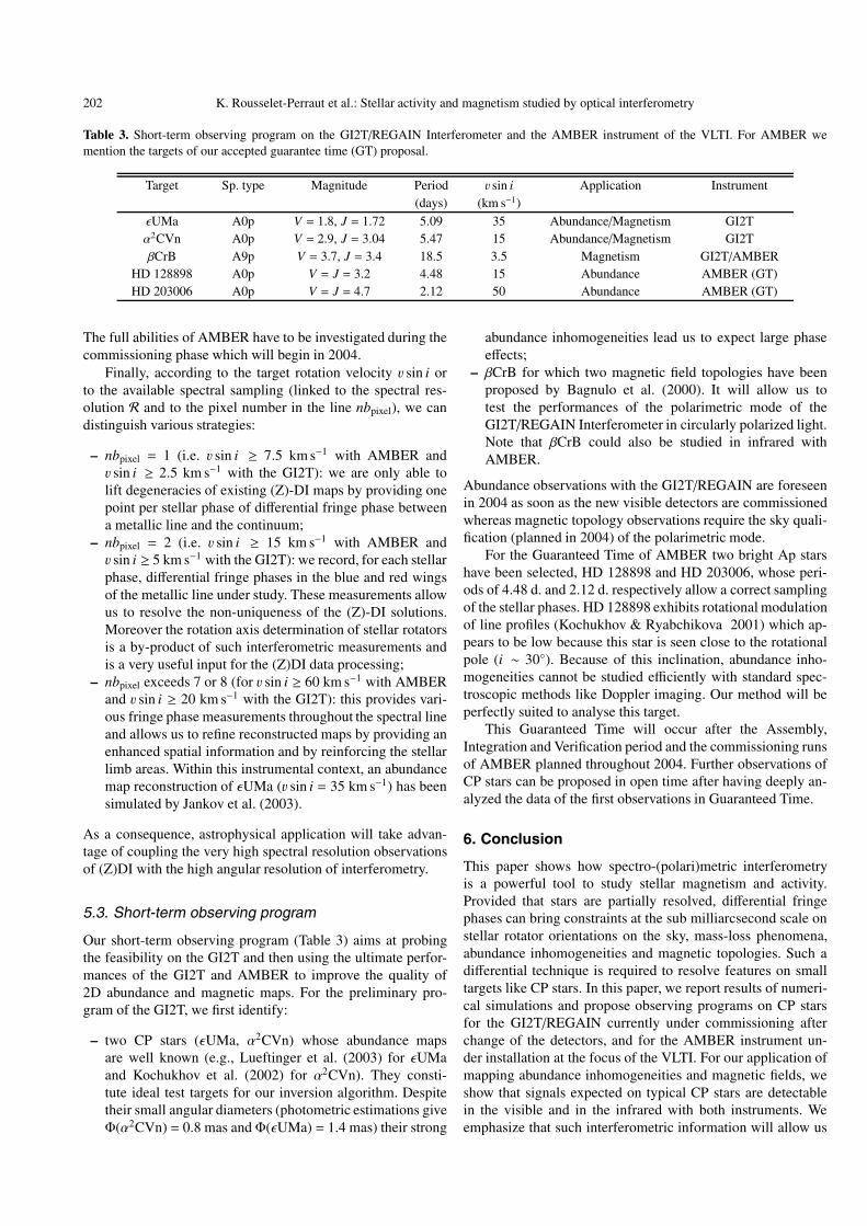
Table 3. Short-term observing program on the GI2T/REGAIN Interferometer and the AMBER instrument of the VLTI. For AMBER wemention the targets of our accepted guarantee time (GT) proposal.

Target Sp. type Magnitude Period v sin i Application Instrument(days) (km s−1)

εUMa A0p V = 1.8, J = 1.72 5.09 35 Abundance/Magnetism GI2Tα2CVn A0p V = 2.9, J = 3.04 5.47 15 Abundance/Magnetism GI2TβCrB A9p V = 3.7, J = 3.4 18.5 3.5 Magnetism GI2T/AMBER

HD 128898 A0p V = J = 3.2 4.48 15 Abundance AMBER (GT)HD 203006 A0p V = J = 4.7 2.12 50 Abundance AMBER (GT)

The full abilities of AMBER have to be investigated during thecommissioning phase which will begin in 2004.

Finally, according to the target rotation velocity v sin i orto the available spectral sampling (linked to the spectral res-olution R and to the pixel number in the line nbpixel), we candistinguish various strategies:

– nbpixel = 1 (i.e. v sin i ≥ 7.5 km s−1 with AMBER andv sin i ≥ 2.5 km s−1 with the GI2T): we are only able tolift degeneracies of existing (Z)-DI maps by providing onepoint per stellar phase of differential fringe phase betweena metallic line and the continuum;

– nbpixel = 2 (i.e. v sin i ≥ 15 km s−1 with AMBER andv sin i ≥ 5 km s−1 with the GI2T): we record, for each stellarphase, differential fringe phases in the blue and red wingsof the metallic line under study. These measurements allowus to resolve the non-uniqueness of the (Z)-DI solutions.Moreover the rotation axis determination of stellar rotatorsis a by-product of such interferometric measurements andis a very useful input for the (Z)DI data processing;

– nbpixel exceeds 7 or 8 (for v sin i ≥ 60 km s−1 with AMBERand v sin i ≥ 20 km s−1 with the GI2T): this provides vari-ous fringe phase measurements throughout the spectral lineand allows us to refine reconstructed maps by providing anenhanced spatial information and by reinforcing the stellarlimb areas. Within this instrumental context, an abundancemap reconstruction of εUMa (v sin i = 35 km s−1) has beensimulated by Jankov et al. (2003).

As a consequence, astrophysical application will take advan-tage of coupling the very high spectral resolution observationsof (Z)DI with the high angular resolution of interferometry.

5.3. Short-term observing program

Our short-term observing program (Table 3) aims at probingthe feasibility on the GI2T and then using the ultimate perfor-mances of the GI2T and AMBER to improve the quality of2D abundance and magnetic maps. For the preliminary pro-gram of the GI2T, we first identify:

– two CP stars (εUMa, α2CVn) whose abundance mapsare well known (e.g., Lueftinger et al. (2003) for εUMaand Kochukhov et al. (2002) for α2CVn). They consti-tute ideal test targets for our inversion algorithm. Despitetheir small angular diameters (photometric estimations giveΦ(α2CVn) = 0.8 mas and Φ(εUMa) = 1.4 mas) their strong

abundance inhomogeneities lead us to expect large phaseeffects;

– βCrB for which two magnetic field topologies have beenproposed by Bagnulo et al. (2000). It will allow us totest the performances of the polarimetric mode of theGI2T/REGAIN Interferometer in circularly polarized light.Note that βCrB could also be studied in infrared withAMBER.

Abundance observations with the GI2T/REGAIN are foreseenin 2004 as soon as the new visible detectors are commissionedwhereas magnetic topology observations require the sky quali-fication (planned in 2004) of the polarimetric mode.

For the Guaranteed Time of AMBER two bright Ap starshave been selected, HD 128898 and HD 203006, whose peri-ods of 4.48 d. and 2.12 d. respectively allow a correct samplingof the stellar phases. HD 128898 exhibits rotational modulationof line profiles (Kochukhov & Ryabchikova 2001) which ap-pears to be low because this star is seen close to the rotationalpole (i ∼ 30◦). Because of this inclination, abundance inho-mogeneities cannot be studied efficiently with standard spec-troscopic methods like Doppler imaging. Our method will beperfectly suited to analyse this target.

This Guaranteed Time will occur after the Assembly,Integration and Verification period and the commissioning runsof AMBER planned throughout 2004. Further observations ofCP stars can be proposed in open time after having deeply an-alyzed the data of the first observations in Guaranteed Time.

6. Conclusion

This paper shows how spectro-(polari)metric interferometryis a powerful tool to study stellar magnetism and activity.Provided that stars are partially resolved, differential fringephases can bring constraints at the sub milliarcsecond scale onstellar rotator orientations on the sky, mass-loss phenomena,abundance inhomogeneities and magnetic topologies. Such adifferential technique is required to resolve features on smalltargets like CP stars. In this paper, we report results of numeri-cal simulations and propose observing programs on CP starsfor the GI2T/REGAIN currently under commissioning afterchange of the detectors, and for the AMBER instrument un-der installation at the focus of the VLTI. For our application ofmapping abundance inhomogeneities and magnetic fields, weshow that signals expected on typical CP stars are detectablein the visible and in the infrared with both instruments. Weemphasize that such interferometric information will allow us

K. Rousselet-Perraut et al.: Stellar activity and magnetism studied by optical interferometry 203

to significantly improve the quality of reconstructed images ofstellar surfaces. We also emphasize that a detailed modellingof the observed objects is essential to correctly and fully in-terpret the future data to be provided by the optical aperturesynthesis array and, even before that, to define the observa-tional strategy and prepare the observations (selection of base-lines, wavelengths, spectral lines, etc). Inversion algorithmsalso must be developed for an optimal use of the planned imag-ing arrays. The additional information recorded in polarizedlight will open new avenues to answer key questions on therole of magnetic fields in stellar physics. That is why the ques-tion of equipping a kilometric array such as OHANA and/ora second generation instrument of the VLTI with a polarimet-ric mode (Vakili et al. 2001) has to be studied as well as thesuitable spectral resolution.

Acknowledgements. The authors want to warmly thank D. Mourard,F. Vakili and G. Mathys for their scientific support and fruitful discus-sions as well as C. Van’t Veer for the spectra of CP stars. They thankthe referees for their constructive comments that improved the qual-ity of the paper. The authors are grateful to French Programs PNPS,PNST and CNRS/ATI for funding the SPIN project, and T. Lanz ac-knowledges the support of the Observatoire de Paris.

References

Babel, J., & Lanz, T. 1992, A&A, 263, 232Bagnulo, S., Landolfi, M., Mathys, G., & Landi Degl’Innocenti, M.

2000, A&A, 358, 929Berio, P., Stee, Ph., Vakili, F., et al. 1999, A&A, 345, 203Brillant, S., Lanz, T., Mathys, G., & Stehle, C. 1998, A&A, 339, 286Cassinelli, J. P., & Hoffman, N. M. 1975, MNRAS, 173, 789Chesneau, O., Rousselet-Perraut, K., Vakili, F., et al. 2000,

in Interferometry in Optical Astronomy, SPIE Conf., ed. A.Quirrenbach, & P. Lena, Proc. SPIE, 4006, 531

Chesneau, O., Vakili. F., Rousselet-Perraut, K., & Stehle, C. 2001,in Magnetic fields across the Hertzsprung-Russell diagram, ed. G.Mathys, S. K. Solanki, & D. T. Wickramasinghe, ASP Conf., 248,633

Chesneau, O., Wolf, S., & Domiciano de Souza, A. 2003, A&A, 410,375

Colavita, M. 1992, in High-Resolution Imaging by Interferometry II,Ground-Based Interferometry at Visible and Infrared Wavelengths,ed. J. M. Beckers, & F. Merkle, ESO Conf., 845

Cowley, C., Hubrig, S., Ryabchikova, T. A., et al. 2001, A&A, 367,939

Donati, J. F. 1996, in Stellar surface structure, IAU Conf., ed. G.Strassmeier, & J. Linsky, 176, 53

Glindemann, A., Algomedo, J., Amestica, R., et al. 2003, inInterferometry for Optical Astronomy II, SPIE Conf., August 2002,Hawaii, 4838, 89

Hanbury Brown, R., Davis, J., & Allen, L. R. 1974, MNRAS, 168, 93Hubeny, I., & Lanz, T. 2000, Am. Astron. Soc. Meet., 197, #78.12Jankov, S., Vakili, F., Domiciano de Souza, A., & Janot-Pacheco, E.

2001, A&A, 377, 721

Jankov, S., Domiciano de Souza, A., Stehle, C., et al. 2003, inInterferometry for Optical Astronomy II, SPIE Conf., August 2002,Hawaii, 4838, 587

Jennison, R. C. 1958, MNRAS, 118, 276Kern, P., Malbet, F., Berger, J. P., et al. 2003, in Interferometry for

Optical Astronomy II, SPIE Conf., August 2002, Hawaii, 4838, 312Kochukhov, O., & Ryabchikova, T. 2001, A&A, 377, L22Kochukhov, O., Piskunov, N., Ilyin, I., et al. 2002, A&A, 389, 420Kurucz, R. L. 1993, VizieR On-line Data Catalog: VI/39Lachaume, R. 2003, A&A, 400, 795Lagarde, S., Sanchez, L., Petrov, R. 1995, in Tridimensional Optical

Spectroscopic Methods in Astrophysics, ed. G. Comte, & M.Marcelin, ASP Conf. Ser., 71, 360

Landstreet, J. 1980, AJ, 85, 611Leblanc, F., Michaud, G., & Babel, J. 1994, ApJ, 431, 388Leroy, J. L., Landolfi, M., & Landi Degl’Innocenti, E. 1993, A&A,

270, 335Lueftinger, T., Kuschnig, R., Piskunov, N., & Weiss, W. 2003, A&A,

406, 1033Mathys, G. 1988, A&A, 189, 179Mathys, G., Stehle, C., Brillant, S., & Lanz, T. 2000, A&A, 358, 1151Michaud, G. 1970, ApJ, 160, 641Moss, D. 2001, in Magnetic fields across the Hertzsprung-Russell dia-

gram, ed. G. Mathys, S. K. Solanki, & D. T. Wickramasinghe, ASPConf., 248, 305

Mourard, D., Bonneau, D., Stee, P., et al. 2002, in Interferometry forOptical Astronomy II, SPIE Conf., August, Hawaii, 4838, in press

Perrin, G., Lai, O., Woillez, J., et al. 2003, in Interferometry forOptical Astronomy II, SPIE Conf., August 2002, Hawaii, 4838,1290

Petrov, R. 1988, in High-Resolution Imaging by Interferometry, ESOConf., March, ed. F. Merkle, Garching, Germany, 235

Petrov, R., Malbet, F., Weigelt, G., et al. 2000, in Interferometry inOptical Astronomy, SPIE Conf., ed. A. Quirrenbach, & P. Lena,Proc. SPIE, 4006, 68

Piskunov, N., & Kochukhov, O. 2002, A&A, 381, 736Rice, J. B., & Wehlau, W. H. 1990, A&A, 233, 503Rousselet-Perraut, K., Vakili, F., & Mourard, D. 1996, Opt. Eng., 35,

2943Rousselet-Perraut, K., Vakili, F., Mourard, D., et al. 1997, A&AS, 123,

173Rousselet-Perraut, K., Chesneau, O., Berio, P., & Vakili, F. 2000,

A&A, 354, 595Ryabchikova, T., Piskunov, N., Kochukhov, O., et al. 2002, A&A, 384,

545Rybicki, G. B., & Hummer, D. G. 1991, A&A, 245, 171Semel, M. 1989, A&A, 225, 456Stehle, C., Brillant, S., & Mathys, G. 2000, Eur. Phys. J. D, 11, 491Vakili, F. 1981, A&A, 101, 352Vakili, F., Mourard, D., Bonneau, D., et al. 1997, A&A, 323, 183Vakili, F., Mourard, D., Stee, Ph., et al. 1998, A&A, 335, 261Vakili, F., Chesneau, O., Delplancke, F., et al. 2001, in Interferometry

for Optical Astronomy II, ESO Workshop Proc., ed. G. Monnet, &J. Bergeron, June, Garching

Wittkowski, M., Scholler, M., Hubrig, S., et al. 2002, Astron. Nachr.,323, 241