Stellar Populations - The LSST Science Book
63
6 Stellar Populations in the Milky Way and Nearby Galaxies Abhijit Saha, Kevin R. Covey, Timothy C. Beers, John J. Bochanski, Pat Boeshaar, Adam J. Burgasser, Phillip A. Cargile, You-Hua Chu, Charles F. Claver, Kem H. Cook, Saurav Dhital, Laurent Eyer, Suzanne L. Hawley, Leslie Hebb, Eric J. Hilton, J. B. Holberg, ˇ Zeljko Ivezi´ c, Mario Juri´ c, Jason Kalirai, S´ ebastien L´ epine, Lucas M. Macri, Peregrine M. McGehee, David Monet, Knut Olsen, Edward W. Olszewski, Joshua Pepper, Andrej Prˇ sa, Ata Sarajedini, Sarah Schmidt, Keivan G. Stassun, Paul Thorman, Andrew A. West, Benjamin F. Williams 6.1 Introduction Stellar populations, consisting of individual stars that share coherent spatial, kinematic, chemical, or age distributions, are powerful probes of a wide range of astrophysical phenomena. The coherent properties of stellar populations allow us to use measurements of an individual member to inform our understanding of the larger system and vice versa. As examples, globular cluster metallicities are often derived from measurements of the brightest few members, while the overall shape of the cluster color magnitude diagram (CMD) enables us to assign ages to an individual star within the system. Leveraging the wealth of information available from such analyses enables us to develop a remarkably detailed and nuanced understanding of these complex stellar systems. By providing deep, homogeneous photometry for billions of stars in our own Galaxy and throughout the Local Group, LSST will produce major advances in our understanding of stellar populations. In the sections that follow, we describe how LSST will improve our understanding of stellar popu- lations in external galaxies (§ 6.2 and § 6.3) and in our own Milky Way (§§ 6.4–6.6), and will allow us to study the properties of rare stellar systems (§§ 6.7–6.11). Many of the science cases in this chapter are based on the rich characterization LSST will provide for stars in the solar neighborhood. This scientific landscape will be irrevocably altered by the Gaia space mission, however, which will provide an exquisitely detailed catalog of millions of solar neighborhood stars shortly after its launch (expected in 2011). To illuminate the scientific areas where LSST provides a strong complement to Gaia’s superb capabilities, § 6.12 develops a quantitative comparison of the astrometric and photometric precision of the two missions; this comparison highlights LSSTs ability to smoothly extend Gaia’s solar neighborhood catalog to redder targets and fainter magnitudes. 137
-
Upload
khangminh22 -
Category
Documents
-
view
4 -
download
0
Transcript of Stellar Populations - The LSST Science Book

6 Stellar Populations in the Milky Way andNearby Galaxies
Abhijit Saha, Kevin R. Covey, Timothy C. Beers, John J. Bochanski, Pat Boeshaar, Adam J.Burgasser, Phillip A. Cargile, You-Hua Chu, Charles F. Claver, Kem H. Cook, Saurav Dhital,Laurent Eyer, Suzanne L. Hawley, Leslie Hebb, Eric J. Hilton, J. B. Holberg, Zeljko Ivezic, MarioJuric, Jason Kalirai, Sebastien Lepine, Lucas M. Macri, Peregrine M. McGehee, David Monet,Knut Olsen, Edward W. Olszewski, Joshua Pepper, Andrej Prsa, Ata Sarajedini, Sarah Schmidt,Keivan G. Stassun, Paul Thorman, Andrew A. West, Benjamin F. Williams
6.1 Introduction
Stellar populations, consisting of individual stars that share coherent spatial, kinematic, chemical,or age distributions, are powerful probes of a wide range of astrophysical phenomena. The coherentproperties of stellar populations allow us to use measurements of an individual member to informour understanding of the larger system and vice versa. As examples, globular cluster metallicitiesare often derived from measurements of the brightest few members, while the overall shape of thecluster color magnitude diagram (CMD) enables us to assign ages to an individual star within thesystem. Leveraging the wealth of information available from such analyses enables us to develop aremarkably detailed and nuanced understanding of these complex stellar systems.
By providing deep, homogeneous photometry for billions of stars in our own Galaxy and throughoutthe Local Group, LSST will produce major advances in our understanding of stellar populations.In the sections that follow, we describe how LSST will improve our understanding of stellar popu-lations in external galaxies (§ 6.2 and § 6.3) and in our own Milky Way (§§ 6.4–6.6), and will allowus to study the properties of rare stellar systems (§§ 6.7–6.11).
Many of the science cases in this chapter are based on the rich characterization LSST will providefor stars in the solar neighborhood. This scientific landscape will be irrevocably altered by theGaia space mission, however, which will provide an exquisitely detailed catalog of millions ofsolar neighborhood stars shortly after its launch (expected in 2011). To illuminate the scientificareas where LSST provides a strong complement to Gaia’s superb capabilities, § 6.12 develops aquantitative comparison of the astrometric and photometric precision of the two missions; thiscomparison highlights LSSTs ability to smoothly extend Gaia’s solar neighborhood catalog toredder targets and fainter magnitudes.
137

Chapter 6: Stellar Populations
6.2 The Magellanic Clouds and their Environs
Abhijit Saha, Edward W. Olszewski, Knut Olsen, Kem H. Cook
The Large and Small Magellanic Clouds (LMC and SMC respectively; collectively referred tohereafter as “the Clouds”) are laboratories for studying a large assortment of topics, ranging fromstellar astrophysics to cosmology. Their proximity allows the study of their individual constituentstars: LSST will permit broad band photometric “static” analysis to MV ∼ +8 mag, probing wellinto the M dwarfs; and variable phenomena to MV ∼ +6, which will track main sequence stars 2magnitudes fainter than the turn-offs for the oldest known systems.
A sense of scale on the sky is given by the estimate of “tidal debris” extending to 14 kpc fromthe LMC center (Weinberg & Nikolaev 2001) based on 2MASS survey data. Newer empirical data(discussed below) confirm such spatial scales. The stellar bridge between the LMC and SMC isalso well established. Studies of the full spatial extent of the clouds thus require a wide areainvestigation of the order of 1000 deg2. We show below that several science applications call forreaching “static” magnitudes to V or g ≈ 27 mag, and time domain data and proper motionsreaching 24 mag or fainter. The relevance of LSST for these investigations is unquestionable.
Nominal LSST exposures will saturate on stars about a magnitude brighter than the horizontalbranch luminosities of these objects, and work on such stars is not considered to be an LSSTforte. Variability surveys like MACHO and SuperMACHO have already covered much ground ontime-domain studies, with SkyMapper to come between now and LSST. We do not consider topicsdealing with stars bright enough to saturate in nominal LSST exposures.
6.2.1 Stellar Astrophysics in the Magellanic Clouds
For stellar astrophysics studies, the Clouds present a sample of stars that are, to first order, ata common distance, but contain the complexity of differing ages and metallicities, and hence anassortment of objects that star clusters within the Galaxy do not have. In addition, the age-metallicity correlation in the Clouds is known to be markedly different from that in the Galaxy.This allows some of the degeneracies in stellar parameters that are present in Galactic stellarsamples to be broken.
LSST’s extended time sampling will reveal, among other things, eclipsing binaries on the mainsequence through the turn-off. We plan to use them to calibrate the masses of stars near the oldmain sequence turnoff. Only a small number of such objects are known in our own Galaxy, butwide area coverage of the Clouds (and their extended structures) promises a sample of ∼ 80, 000such objects with 22 < g < 23 mag, based on projections from MACHO and SuperMACHO.Binaries in this brightness range track evolutionary phases from the main sequence through turn-off. The direct determination of stellar masses (using follow-up spectroscopy of eclipsing binariesidentified by LSST) of a select sub-sample of eclipsing binaries in this range of evolutionary phasewill confront stellar evolution models, and especially examine and refine the stellar age “clock,”which has cosmological implications.
For this question, we need to determine the number of eclipsing binaries (EB) that LSST candetect within 0.5 magnitudes of the old turn-off (r ∼ 22.5). Additionally, because the binary mass
138

6.2 The Magellanic Clouds and their Environs
depends on (sin i)3, we need to restrict the EB sample to those with i = 90◦ ± 10◦ in order todetermine masses to 5%. Such accuracy in mass is required for age sensitivity of ∼ 2 Gyr atages of 10-12 Gyr. We determined the number of LMC EBs meeting these restrictions that couldbe discovered by LSST by projecting from the 4631 eclipsing binaries discovered by the MACHOproject (e.g. Alcock et al. 1995). Selecting only those MACHO EBs with colors placing them onthe LMC main sequence, we calculated the minimum periods which these binaries would need tohave in order for them to have inclinations constrained to be 90◦±10◦, given their masses and radiion the main sequence. Of the MACHO EB sample, 551 systems (12%) had periods longer than theminimum, with the majority of the EBs being short-period binaries with possibly large inclinations.Next, we constructed a deep empirical LMC stellar luminosity function (LF) by combining the V-band luminosity function from the Magellanic Clouds Photometric Survey (Zaritsky et al. 2004,MCPS) with the HST-based LMC LF measured by Dolphin (2002a), using Smecker-Hane et al.(2002) observations of the LMC bar, where we scaled the HST LF to match the MCPS LF overthe magnitude range where the LFs overlapped. We then compared this combined LF to the LFof the MACHO EBs, finding that EBs comprise ∼ 2% of LMC stellar sources. Finally, we usedour deep combined LF to measure the number of LMC stars with 22 < V < 23, multiplied thisnumber by 0.0024 to account for the fraction of sufficiently long-period EBs, and found that LSSTshould be able to detect ∼ 80, 000 EBs near the old main sequence turnoff. Based on the MACHOsample, these EBs will have periods between ∼ 3 and ∼ 90 days, with an average of ∼ 8 days.
LSST is expected to find ∼ 105 RR Lyrae stars over the full face of both Clouds (the specific ratioof RR Lyraes can vary by a factor of 100, and the above estimate, which is based on 1 RR Lyrae per∼ 104L�, represents the geometric mean of that range and holds for HST discoveries of RR Lyraestars in M31 and for SuperMACHO results in the Clouds). The physics behind the range ofsubtler properties of RR Lyrae stars is still being pondered: trends in their period distributions aswell as possible variations in absolute magnitude with period, age, and metallicity. Our empiricalknowledge of these comes from studying their properties in globular clusters, where the distancedeterminations may not be precise enough (at the 20% level). The range of distances within theLMC is smaller than the uncertainty in relative distances between globular clusters in our Galaxy.Ages and metallicities of the oldest stars (the parent population of the RR Lyraes) in any givenlocation in the Clouds may be gleaned from an analysis of the local color-magnitude diagrams, aswe now discuss, and trends in RR Lyrae properties with parent population will be directly mappedfor the first time.
6.2.2 The Magellanic Clouds as “Two-off” Case Studies of Galaxy Evolution
The Clouds are the only systems larger and more complex than dwarf spheroidals outside ourown Galaxy where we can reach the main sequence stars with LSST. Not only are these the mostnumerous, and therefore the most sensitive tracers of structure, but they proportionally representstars of all ages and metallicities. Analyzing the ages, metallicities, and motions of these stars isthe most effective and least biased way of parsing the stellar sub-systems within any galaxy, andthe route to understanding the history of star formation, accretion, and chemical evolution of thegalaxy as a whole. Decades of work toward this end have been carried out to define these elementswithin our Galaxy, but the continuing task is made difficult not only because of the vastness on thesky, but also because determining distances to individual stars is not straightforward. The Clouds
139

Chapter 6: Stellar Populations
are the only sufficiently complex systems (for the purpose of understanding galaxy assembly) wherethe spatial perspective allows us to know where in the galaxy the stars we are examining lie, while atthe same time being close enough for us to examine and parse its component stellar populations inan unbiased way through the main sequence stars. LSST will provide proper motions of individualstars to an accuracy of ∼ 50km s−1 in the LMC, but local ensembles of thousands of stars on spatialscales from 0.1 to several degrees will be able to separate disk rotation from a “stationary” halo.Internal motions have been seen using proper motions measured with only 20 positional pointingswith the HST’s Advanced Camera for Surveys (ACS) with only a few arc-min field of view and a2-3 year time baseline (Piatek et al. 2008).
Color-magnitude and Hess diagrams from a composite stellar census can be decomposed effectivelyusing stellar evolution models (e.g., Tolstoy & Saha 1996; Dolphin 2002b). While the halo of ourGalaxy bears its oldest known stars, models of galaxy formation lead us to expect the oldeststars to live in the central halo and bulge. Age dating the oldest stars toward the center of theGalaxy is thwarted by distance uncertainties, complicated further by reddening and extinction.The Clouds present objects at a known distance, where color-magnitude diagrams are a sensitivetool for evaluating ages. A panoramic unbiased age distribution map from the CMD turn-off isnot possible at distances larger than 100 kpc. The Clouds are a gift in this regard.
6.2.3 The Extended Structure of the Magellanic Clouds
Knowledge of the distribution and population characteristics in outlying regions of the LMC/SMCcomplex is essential for understanding the early history of these objects and their place in theΛCDM hierarchy. In our Galaxy the most metal poor, and (plausibly) the oldest observed starsare distributed in a halo that extends beyond 25 kpc. Their spatial distribution, chemical compo-sition and kinematics provide clues about the Milky Way’s early history, as well as its continuedinteraction with neighboring galaxies. If the Clouds also have similar halos, the history of theirformation and interactions must also be written in their stars. In general how old are the stars inthe extremities of the Clouds? How are they distributed (disk or halo dominated)? How far dosuch stellar distributions extend? What tidal structure is revealed? Is there a continuity in thestellar distribution between the LMC and SMC? Do they share a common halo with the Galaxy?What do the kinematics of stars in outlying regions tell us about the dark matter distribution? Isthere a smooth change from disk to non-disk near the extremities?
Past panoramic studies such as with 2MASS and DENIS have taught us about the LMC diskinterior to 9 kpc (10◦, e.g., van der Marel 2001). Structure beyond that had not been systematicallyprobed in an unbiased way (studies using HII regions, carbon stars, and even RR Lyrae exist, butthey are heavily biased in age and metallicity) until a recent pilot study (NOAO Magellanic OuterLimits Survey) with the MOSAIC imager on the Blanco 4-m telescope at Cerro Tololo Inter-American Observatory, which uses main sequence stars as tracers of structure. Even with theirvery selective spatial sampling of a total of only ∼ 15 deg2 spread out over a region of interestcovering over ∼ 1000 deg2, the LMC disk is seen to continue out to 10 disk scale lengths, beyondwhich there are signs either of a spheroidal halo that finally overtakes the disk (a simple scaledmodel of how our own Galaxy must look when viewed face on), or a tidal pile-up. Main sequencestars clearly associated with the LMC are seen out to 15 degrees along the plane of the disk(Figure 6.1). This exceeds the tidal radius estimate of 11 kpc (12.6◦) by Weinberg (2000), already
140

6.2 The Magellanic Clouds and their Environs
Figure 6.1: The color-magnitude diagrams in C − R vs. R for two fields, 14◦ (left) and 19◦ (right) due north ofthe LMC center. The stub-like locus of stars near C − R ∼ 0.7 and I > 21.0 that can be seen on the left panel forthe 14◦ field corresponds to the locus of old main sequence stars from the LMC, which have a turn-off at I ∼ 21.0.This shows that stars associated with LMC extend past 10 disk scale lengths. The feature is absent in the 19◦ field,which is farther out. Mapping the full extent of the region surrounding the Clouds on these angular scales is onlyfeasible with LSST.
a challenge to existing models of how the LMC has interacted with the Galaxy. (This extendedLMC structure has a surface brightness density of ∼ 35 mag per square arc-sec, which underscoresthe importance of the Clouds and the opportunity they present, because this technique will notwork for objects beyond 100 kpc from us.) In contrast, the structure of the SMC appears to bevery truncated, at least as projected on the sky. Age and metallicity of these tracer stars are alsoderived in straightforward manner.
Not only will LSST map the complete extended stellar distribution (where currently less than 1%of the sky region of interest has been mapped) of the Clouds using main sequence stars as tracersthat are unbiased in age and metallicity, but it will also furnish proper motions. The accuracy ofensemble average values for mapping streaming motions, such as disk rotation and tidal streams,depends eventually on the availability of background quasars and galaxies, which do not move onthe sky. The HST study of proper motions (Kallivayalil et al. 2006b,a; Piatek et al. 2008) was ableto use quasars with a surface density of 0.7 deg−2. We expect that LSST, using the hugely morenumerous background galaxies as the “zero proper motion reference,” and a longer time baselineshould do even better. Individual proper motions of stars at these distances can be measured tono better than ∼ 50 km s−1, but the group motions of stars will be determined to much higheraccuracy, depending ultimately on the positional accuracy attainable with background galaxies.Over scales of 0.1◦, statistical analysis of group motions can be expected to yield systemic motionswith accuracies better than 10 km s−1. This would not only discriminate between disk and halocomponents of the Clouds in their outer regions but also identify any tidally induced structures attheir extremities.
141

Chapter 6: Stellar Populations
6.2.4 The Magellanic Clouds as Interacting Systems
In addition to interacting gravitationally with each other, both Clouds are in the gravitationalproximity of the Galaxy. Until recently, it was held that the Clouds are captive satellites of theGalaxy and have made several passages through the Galaxy disk. The extended stream of HI,called the Magellanic Stream, which emanates from near the SMC and wraps around much of thesky, has been believed to be either a tidal stream or stripped by ram pressure from passages throughthe Galaxy disk. This picture has been challenged recently by new proper motion measurementsin the Clouds from HST data analyzed by two independent sets of investigators (Kallivayalil et al.2006b,a; Piatek et al. 2008). Their results indicate significantly higher proper motions for bothsystems, which in turn imply higher space velocities. Specifically, the LMC and SMC may nothave begun bound to one another, and both may be on their first approach to the Milky Way, notalready bound to it. Attempts to model the motion of the Clouds together with a formation modelfor the Magellanic Stream in light of the new data (e.g., Besla et al. 2009) are very much works inprogress. Even if a higher mass sufficient to bind the Clouds is assumed for the Galaxy, the orbitsof the Clouds are changed radically from prior models: specifically, the last peri-galacticon couldnot have occurred within the last 5 Gyrs with the high eccentricity orbits that are now necessary(Besla et al. 2009), indicating that the Magellanic Stream cannot be tidal. The proper motionanalyses have also determined the rotation speed of the LMC disk (Piatek et al. 2008). The newresult of 120± 15 kms−1 is more reliable than older radial velocity-based estimates for this nearlyface-on galaxy, and as much as twice as large as some of the older estimates. This new scenariochanges the expected tidal structures for the Clouds and argues against a tidal origin for theMagellanic Stream. These expectations are empirically testable with LSST. For instance, a tidalorigin requires a corresponding stream of stars, even though the stellar stream can be spatiallydisplaced with respect to the gas stream: to date, such a star stream, if its exists, has escapeddetection. A definitive conclusion about whether such a stellar stream exists or not, awaits a deepmulti-band wide area search to detect and track main sequence stars, which are the most sensitivetracers of such a stellar stream.
Aside from the specific issue of a stellar stream corresponding to the Magellanic gas stream, thefull area mapping of extremities via the main sequence stars described in § 6.2.3 will reveal anytidally induced asymmetries in the stellar distributions, e.g., in the shape of the LMC disk asresult of the Galactic potential as well as from interaction with the SMC. Proper motions of anytidal debris (see § 6.2.3) will contribute to determining the gravitational field, and eventually to amodeling of the halo mass of the Galaxy. How far out organized structure in the LMC persists,using kinematic measures from proper motions, will yield the mass of the LMC, and thus the sizeof its dark matter halo.
6.2.5 Recent and On-going Star Formation in the LMC
You-Hua Chu
Studies of recent star formation rate and history are complicated by the mass dependence of thecontraction timescale. For example, at t ∼ 105 yr, even O stars are still enshrouded by circumstellardust; at t ∼ 106 yr, massive stars have formed but intermediate-mass stars have not reached the
142

6.2 The Magellanic Clouds and their Environs
Figure 6.2: Hα image of the LMC. CO contours extracted from the NANTEN survey are plotted in blue to showthe molecular clouds. Young stellar objects with 8.0 µm magnitude brighter than 8.0 are plotted in red, and thefainter ones in yellow. Roughly, the brighter objects are of high masses and the fainter ones of intermediate masses.Adapted from Gruendl & Chu (2009).
main sequence; at t ∼ 107 yr, the massive stars have already exploded as supernovae, but thelow-mass stars are still on their way to the main sequence.
The current star formation rate in the LMC has been determined by assuming a Salpeter initialmass function (IMF) and scaling it to provide the ionizing flux required by the observed Hαluminosities of HII regions (Kennicutt & Hodge 1986). Individual massive stars in OB associationsand in the field have been studied photometrically and spectroscopically to determine the IMF,and it has been shown that the massive end of the IMF is flatter in OB associations than in thefield (Massey et al. 1995).
The Spitzer Space Telescope has allowed the identification of high- and intermediate-mass youngstellar objects (YSOs), representing ongoing (within 105 yr) star formation, in the LMC (Cauletet al. 2008; Chen et al. 2009). Using the Spitzer Legacy program SAGE survey of the central 7◦×7◦
area of the LMC with both IRAC and MIPS, YSOs with masses greater than ∼ 4M� have beenidentified independently by Whitney et al. (2008) and Gruendl & Chu (2009). Figure 6.2 shows thedistribution of YSOs, HII regions, and molecular clouds, which represent sites of on-going, recent,and future star formation respectively. It is now possible to fully specify the formation of massivestars in the LMC.
The formation of intermediate- and low-mass stars in the LMC has begun to be studied onlyrecently by identifying pre-main sequence (PMS) stars in (V − I) vs V color-magnitude diagrams(CMDs), as illustrated in Figure 6.3. Using HST WFPC2 observations, low-mass main sequencestars in two OB associations and in the field have been analyzed to construct IMFs, and differentslopes are also seen (Gouliermis et al. 2006a,b, 2007).
Using existing HST image data in LMC molecular clouds to estimate how crowding will limit
143

Chapter 6: Stellar Populations
Figure 6.3: V-I vs. V color-magnitude diagram of stars detected in the OB association LH95 (left), surroundingbackground region (middle), and the difference between the two (right). The zero-age main sequence is plotted as asolid line, and PMS isochrones for ages 0.5, 1.5, and 10 Myr are plotted in dashed lines in the right panel. Adaptedfrom Gouliermis et al. (2007) with permission.
photometry from LSST images, we estimate that PMS stars can be detected down to 0.7-0.8 M�(g ∼ 24 mag: see right hand panel of Figure 6.3). LSST will provide a mapping of intermediate- tolow-mass PMS stars in the entire LMC except the bar, where crowding will prevent reliable photom-etry at these magnitudes. This young lower-mass stellar population, combined with the known in-formation on massive star formation and distribution/conditions of the interstellar medium (ISM),will allow us to fully characterize the star formation process and provide critical tests to differenttheories of star formation.
Conventionally, star formation is thought to start with the collapse of a molecular cloud that isgravitationally unstable. Recent models of turbulent ISM predict that colliding HI clouds can alsobe compressed and cooled to form stars. Thus, both the neutral atomic and molecular componentsof the ISM need to be considered in star formation. The neutral atomic and molecular gas in theLMC have been well surveyed: the ATCA+Parkes map of HI (Kim et al. 2003), the NANTENsurvey of CO (Fukui et al. 2008), and the MAGNA survey of CO (Ott et al. 2008, Hughes et al.,in prep.). Figure 6.2 shows that not all molecular clouds are forming massive stars: How aboutintermediate- and low-mass stars? Do some molecular clouds form only low-mass stars? Do starsform in regions with high HI column density but no molecular clouds? These questions cannot beanswered until LSST has made a complete mapping of intermediate- and low-mass PMS stars inthe LMC.
6.3 Stars in Nearby Galaxies
Benjamin F. Williams, Knut Olsen, Abhijit Saha
144

6.3 Stars in Nearby Galaxies
6.3.1 Star Formation Histories
General Concepts
Bright individual stars can be distinguished in nearby galaxies with ground-based observations.In galaxies with no recent star formation (within ∼1 Gyr), the brightest stars are those on theasymptotic giant branch (AGB) and/or the red giant branch (RGB). The color of the RGB de-pends mostly on metallicity, and only weakly on age, whereas the relative presence and luminositydistribution of the AGB stars is sensitive to the star formation history in the range 2 < t < 8 Gyrs.The brightest RGB stars are at I ∼ −4, and in principle are thus visible to LSST out to distances∼ 10 Mpc. The presence of significant numbers of RR Lyrae stars indicates an ancient populationof stars, 10 Gyrs or older. RR Lyrae, as well the brightest RGB stars, are standard candles thatmeasure the distance of the host galaxy.
In practice, object crowding at such distances is severe for galaxies of any significant size, andresolution of individual RGB stars in galaxies with MV ∼ −10 and higher will be limited todistances of ∼ 4 Mpc, but that includes the Sculptor Group and the Centaurus and M83 groups.Within the Local Group, the “stacked” photometry of individual stars with LSST will reach belowthe Horizontal Branch, and certainly allow the detection of RR Lyraes in addition to the RGB.
Galaxies that have made stars within the last 1 Gyrs or so contain luminous supergiant stars (bothblue and red). The luminosity distributions of these stars reflect the history of star formationwithin the last 1 Gyr. The brightest stars (in the youngest systems) can reach MV ∼ −8, buteven stars at MV ∼ −6 (including Cepheids) will stand out above the crowding in LSST imagesof galaxies at distances of ∼ 7 Mpc.
A great deal of work along these lines is already being done, both from space and the ground.LSST’s role here will be to (1) cover extended structures, and compare, for example, how popula-tions change with location in the galaxies – important clues to how galaxies were formed, and (2)identify the brighter variables, such as RR Lyraes, Cepheids, and the brighter eclipsing binarieswherever they are reachable.
Methods and Techniques
Methods of deriving star formation histories (the distribution of star formation rate as a functionof time and chemical composition) from Hess diagrams given photometry and star counts in twoor more bands (and comparing with synthetic models) are adequately developed, e.g., Dolphin(2002b). For extragalactic systems and in the solar neighborhood, where distances are knownindependently, the six-band LSST data can be used to self-consistently solve for extinction andstar formation history. This is more complicated if distances are not known independently, such aswithin the Galaxy, where other methods must be brought to bear. For nearby galaxies, distancesare known at least from the bright termination of the RGB.
Analysis of a composite population, as observed in a nearby galaxy, is performed through detailedfitting of stellar evolution models to observed CMDs. An example CMD of approximately LSSTdepth is shown in Figure 6.4, along with an example model fit and residuals using the stellar evolu-tion models of Girardi et al. (2002) and Marigo et al. (2008). The age and metallicity distribution
145
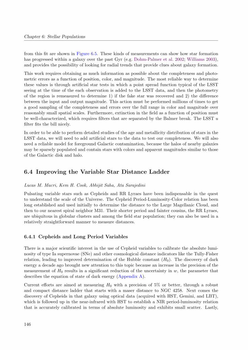
Chapter 6: Stellar Populations
from this fit are shown in Figure 6.5. These kinds of measurements can show how star formationhas progressed within a galaxy over the past Gyr (e.g. Dohm-Palmer et al. 2002; Williams 2003),and provides the possibility of looking for radial trends that provide clues about galaxy formation.
This work requires obtaining as much information as possible about the completeness and photo-metric errors as a function of position, color, and magnitude. The most reliable way to determinethese values is through artificial star tests in which a point spread function typical of the LSSTseeing at the time of the each observation is added to the LSST data, and then the photometryof the region is remeasured to determine 1) if the fake star was recovered and 2) the differencebetween the input and output magnitude. This action must be performed millions of times to geta good sampling of the completeness and errors over the full range in color and magnitude overreasonably small spatial scales. Furthermore, extinction in the field as a function of position mustbe well-characterized, which requires filters that are separated by the Balmer break. The LSST ufilter fits the bill nicely.
In order to be able to perform detailed studies of the age and metallicity distribution of stars in theLSST data, we will need to add artificial stars to the data to test our completeness. We will alsoneed a reliable model for foreground Galactic contamination, because the halos of nearby galaxiesmay be sparsely populated and contain stars with colors and apparent magnitudes similar to thoseof the Galactic disk and halo.
6.4 Improving the Variable Star Distance Ladder
Lucas M. Macri, Kem H. Cook, Abhijit Saha, Ata Sarajedini
Pulsating variable stars such as Cepheids and RR Lyraes have been indispensable in the questto understand the scale of the Universe. The Cepheid Period-Luminosity-Color relation has beenlong established and used initially to determine the distance to the Large Magellanic Cloud, andthen to our nearest spiral neighbor M31. Their shorter period and fainter cousins, the RR Lyraes,are ubiquitous in globular clusters and among the field star population; they can also be used in arelatively straightforward manner to measure distances.
6.4.1 Cepheids and Long Period Variables
There is a major scientific interest in the use of Cepheid variables to calibrate the absolute lumi-nosity of type Ia supernovae (SNe) and other cosmological distance indicators like the Tully-Fisherrelation, leading to improved determination of the Hubble constant (H0). The discovery of darkenergy a decade ago brought new attention to this topic because an increase in the precision of themeasurement of H0 results in a significant reduction of the uncertainty in w, the parameter thatdescribes the equation of state of dark energy (Appendix A).
Current efforts are aimed at measuring H0 with a precision of 5% or better, through a robustand compact distance ladder that starts with a maser distance to NGC 4258. Next comes thediscovery of Cepheids in that galaxy using optical data (acquired with HST, Gemini, and LBT),which is followed up in the near-infrared with HST to establish a NIR period-luminosity relationthat is accurately calibrated in terms of absolute luminosity and exhibits small scatter. Lastly,
146

6.4 Improving the Variable Star Distance Ladder
Figure 6.4: Best fit to a CMD from an archival Hubble Space Telescope Advanced Camera for Surveys field in M33.Upper left: The observed CMD. Upper right: The best-fitting model CMD using stellar evolution models. Lower left:The residual CMD. Redder colors denote an overproduction of model stars. Bluer colors denote an underproductionof model stars. Lower right: The deviations shown in lower left normalized by the Poisson error in each CMD bin,i.e., the statistical significance of the residuals. Only the red clump shows statistically significant residuals.
147

Chapter 6: Stellar Populations
10.00 1.00 0.10 0.01Age (Gyr)
0.000.020.040.060.08
SFR
(Msu
n/yr/d
eg2 ) 5 2 1 0.5 0.2 0.1 0.05 0.02 0.01 0.005 0.002 0.001
Redshift (z)
10.00 1.00 0.10 0.01Age (Gyr)
-2.5-2.0-1.5-1.0-0.50.00.5
[M/H
]
5 2 1 0.5 0.2 0.1 0.05 0.02 0.01 0.005 0.002 0.001Redshift (z)
1.2 1.0 0.8 0.6 0.4 0.2 0.0Age (Gyr)
0.000.02
0.04
0.06
0.08
SFR
(Msu
n/yr/d
eg2 ) 0.1 0.05 0.02 0.01
Redshift (z)
Figure 6.5: The star formation history from the CMD shown in Figure 6.4. Top: The solid histogram marks thestar formation rate (normalized by sky area) as a function of time for the past 14 Gyr. The dashed line marksthe best-fitting constant star formation rate model. Middle: The mean metallicity and metallicity range of thepopulation as a function of time. Heavy error bars mark the measured metallicity range, and lighter error bars markhow that range can slide because of errors in the mean metallicity. Bottom: Same as top, but showing only theresults for the past 1.3 Gyr.
Cepheids are discovered in galaxies that were hosts to modern type Ia SNe to calibrate the absoluteluminosity of these events and determine H0 from observations of SNe in the Hubble flow.
In the next few years before LSST becomes operational, we anticipate using HST and the ladderdescribed above to improve the precision in the measurement of H0 to perhaps 3%. Any furtherprogress will require significant improvement in several areas, and LSST will be able to contributesignificantly to these goals as described below.
• We need to address the intrinsic variation of Cepheid properties from galaxy to galaxy. Thiscan only be addressed by obtaining large, homogeneous samples of variables in many galaxies.LSST will be able to do this for all southern spirals within 8 Mpc.
• We need to calibrate the absolute luminosity of type Ia SNe more robustly, by increasingthe number of host galaxies that have reliable distances. Unfortunately HST cannot dis-cover Cepheids (with an economical use of orbits) much further out than 40 Mpc, and its
148

6.4 Improving the Variable Star Distance Ladder
days are numbered. Here LSST can play a unique role by accurately characterizing long-period variables (LPVs), a primary distance indicator that can be extended to much greaterdistances.
• LPVs are hard to characterize because of the long time scales involved (100-1000 days). Majorbreakthroughs were enabled by the multi-year microlensing surveys of the LMC (MACHO andOGLE) in combination with NIR data from 2MASS, DENIS and the South African/JapaneseIRSF. An extension to Local Group spirals (M31, M33) is possible with existing data. LSSTwould be the first facility that could carry out similar surveys at greater distances and helpanswer the question of intrinsic variation in the absolute luminosities of the different LPVperiod-luminosity relations.
• The LSST observations of these nearby (D < 8 Mpc) spirals would result in accurate Cepheiddistances and the discovery of large LPV populations. This would enable us to accuratelycalibrate the LPV period-luminosity relations for later application to galaxies that hostedtype Ia SNe or even to galaxies in the Hubble flow. This would result in further improvementin the measurement of H0.
6.4.2 RR Lyrae Stars
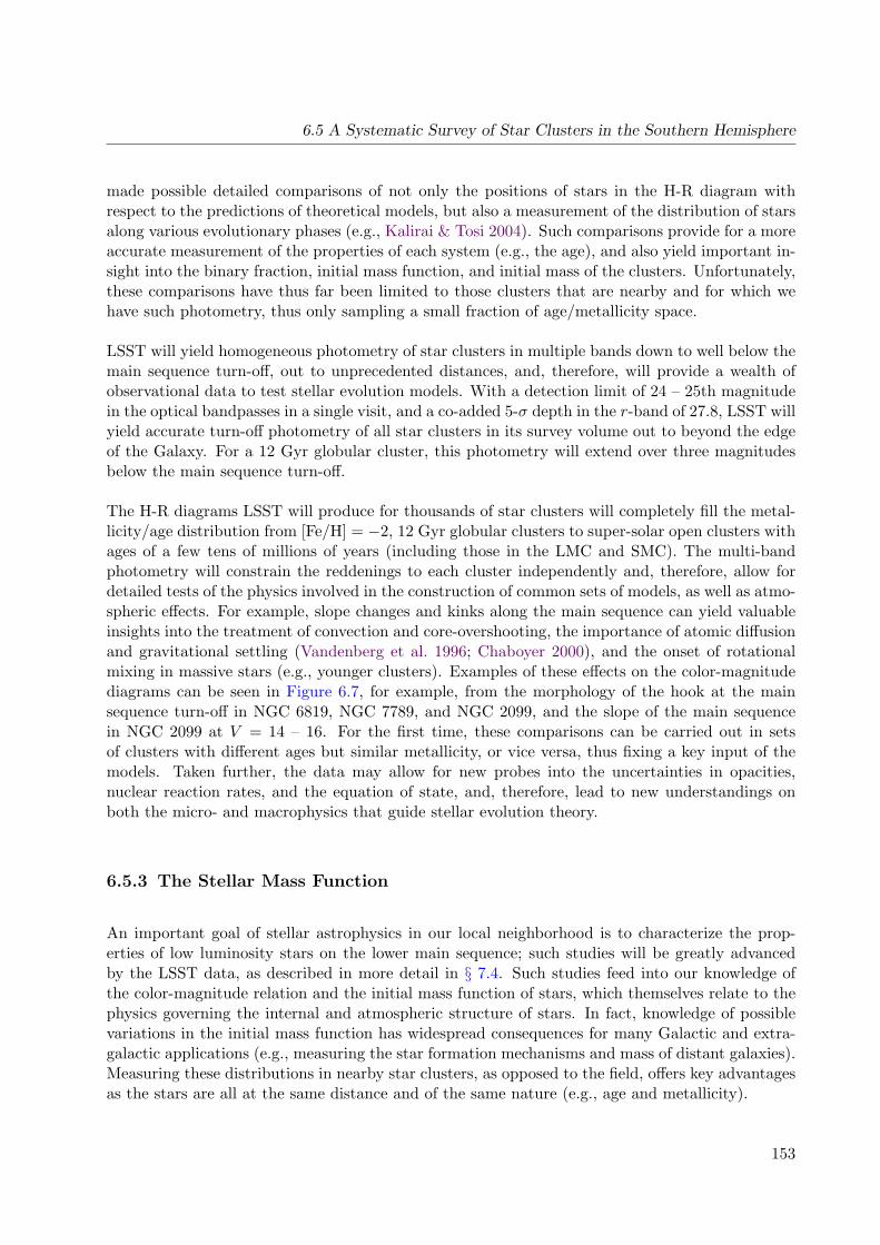
While the empirical properties of RR Lyrae stars have been well studied due to their utility asstandard candles, theoretical models that help us understand the physics responsible for theseproperties are not as advanced. For example, it has been known for a long time that Galacticglobular clusters divide into two groups (Oosterhoff 1939) based on the mean periods of their ab-type RR Lyrae variables - those that pulsate in the fundamental mode. As shown in Figure 6.6,Oosterhoff Type I clusters have ab-type RR Lyraes with mean periods close to ∼0.56 days whiletype II clusters, which are more metal-poor, harbor RR Lyraes with mean periods closer to ∼0.66days (Clement et al. 2001). There have been numerous studies focusing on the Oosterhoff dichotomytrying to understand its origin (e.g. Lee et al. 1990; Sandage 1993). There is evidence to suggestthat globular clusters of different Oosterhoff types have different spatial and kinematic properties,perhaps from distinct accretion events in the Galactic halo (Kinman 1959; van den Bergh 1993).There is also evidence favoring the notion that the Oosterhoff Effect is the result of stellar evolutionon the horizontal branch (HB). In this scenario, RR Lyraes in type I clusters are evolving fromthe red HB blueward through the instability strip while those in type II clusters are evolving fromthe blue HB becoming redward through the instability strip (Lee & Carney 1999). Yet anotherexplanation proposes that the Oosterhoff gap is based on the structure of the envelope in thesepulsating stars. Kanbur & Fernando (2005) have suggested that understanding the physics behindthe Oosterhoff Effect requires a detailed investigation of the interplay between the photosphere andthe hydrogen ionization front in an RR Lyrae variable. Because these features are not co-moving ina pulsating atmosphere, their interaction with each other can affect the period-color relation of RRLyraes, possibly accounting for the behavior of their mean periods as a function of metallicity and,therefore, helping to explain the Oosterhoff Effect. Clearly the Oosterhoff Effect is one example ofa mystery in need of attention from both observers and theoreticians.
One reason there are so many open questions in our theoretical understanding of RR Lyraesand other pulsating variables is that progress requires observations that not only cover the timedomain in exquisite detail but also the parameter space of possible pulsation properties in all of
149

Chapter 6: Stellar Populations
their diversity. This is where the LSST will make a significant contribution. We expect to have asubstantial number of complete light curves for RR Lyraes in Galactic and Large Magellanic Cloudglobular clusters (see the estimate of the RR Lyrae recovery rate in § 8.6.1). In addition, the dataset will contain field RR Lyraes in the Milky Way, the LMC, and the SMC, as well as a number ofdwarf spheroidal galaxies in the vicinity of the Milky Way. Some of these RR Lyraes may turn outto be members of eclipsing binary systems, further adding to their utility, as described in detail in§ 6.10. The depth and breadth of this variability data set will be unprecedented thus facilitatingtheoretical investigations that have been heretofore impossible.
–2.0–1.5–1.0
0.60
0.70
[Fe/H]
< P a
b >
Oosterhoff Gap
Oosterhoff II
Oosterhoff I
Figure 6.6: Plot of the mean fundamental period for RR Lyraes in Galactic globular clusters, as a function of thecluster metal abundance (from data compiled by Catelan et al. 2005). The two types of Oosterhoff clusters dividenaturally on either side of the Oosterhoff gap at 0.6 days.
6.5 A Systematic Survey of Star Clusters in the SouthernHemisphere
Jason Kalirai, Peregrine M. McGehee
6.5.1 Introduction – Open and Globular Star Clusters
Nearby star clusters in the Milky Way are important laboratories for understanding stellar pro-cesses. There are two distinct classes of clusters in the Milky Way, population I open clusters,which are lower mass (tens to thousands of stars) and mostly confined to the Galactic disk, andpopulation II globular clusters (tens of thousands to hundreds of thousands of stars), which are verymassive and make frequent excursions into the Galactic halo. The systems are co-eval, co-spatial,and iso-metallic, and, therefore, represent controlled testbeds with well-established properties. Theknowledge we have gained from studying these clusters grounds basic understanding of how starsevolve, and enables us to interpret light from unresolved galaxies in the Universe.
150

6.5 A Systematic Survey of Star Clusters in the Southern Hemisphere
Despite their importance to stellar astrophysics, most rich star clusters have been relatively poorlysurveyed, a testament to the difficulty of observing targets at large distances or with large angularsizes. The advent of wide-field CCD cameras on 4-meter class telescopes has recently providedus with a wealth of new data on these systems. Both the CFHT Open Star Cluster Survey(Kalirai et al. 2001a, see Figure 6.7) and the WIYN Open Star Cluster Survey (Mathieu 2000)have systematically imaged nearby northern hemisphere clusters in multiple filters, making possiblenew global studies. For example, these surveys have refined our understanding of the fundamentalproperties (e.g., distance, age, metallicity, reddening, binary fraction, and mass) of a large set ofclusters and begun to shed light on the detailed evolution of stars in post main sequence phases(e.g., total integrated stellar mass loss) right down to the white dwarf cooling sequences (Kaliraiet al. 2008).
Even the CFHT and WIYN Open Star Cluster Surveys represent pencil beam studies in com-parison to LSST. The main LSST survey will provide homogeneous photometry of stars in allnearby star clusters in the southern hemisphere (where no survey of star clusters has ever beenundertaken). The LSST footprint contains 419 currently known clusters; of these, 179 are within1 kpc, and several are key benchmark clusters for testing stellar evolution models. Only 15 ofthe clusters in the LSST footprint, however, have more than 100 known members in the WEBDAdatabase, demonstrating the relative paucity of information known about these objects. LSST’sdeep, homogeneous, wide-field photometry will greatly expand this census, discovering new, pre-viously unknown clusters and providing a more complete characterization of the properties andmembership of clusters already known to exist. Analysis of this homogeneous, complete clustersample will enable groundbreaking advances in several fields, which we describe below.
6.5.2 New Insights on Stellar Evolution Theory
A century ago, Ejnar Hertzsprung and Henry Norris Russell found that stars of the same tem-perature and the same parallax and, therefore, at the same distance, could have very differentluminosities (Hertzsprung 1905; Russell 1913, 1914). They coined the terms “giants” and “dwarfs”to describe these stars, and the initial work quickly evolved into the first Hertzsprung-Russell (H-R)Diagram in 1911.
The H-R diagram has since become one of the most widely used plots in astrophysics, and under-standing stellar evolution has been one of the most important pursuits of observational astronomy.Much of our knowledge in this field, and on the ages of stars, is based on our ability to under-stand and model observables in this plane, often for nearby stellar populations. This knowledgerepresents fundamental input into our understanding of many important astrophysical processes.For example, stellar evolution aids in our understanding of the formation of the Milky Way (e.g.,through age dating old stellar populations, Krauss & Chaboyer 2003), the history of star forma-tion in other galaxies (e.g., by interpreting the light from these systems with population synthesismodels), and chemical evolution and feedback processes in galaxies (e.g., by measuring the rateand timing of mass loss in evolved stars).
With the construction of sensitive wide-field imagers on 4-m and 8-m telescopes, as well as thelaunch of the HST, astronomers have recently been able to probe the H-R diagram to unprece-dented depths and accuracy for the nearest systems (e.g., Richer et al. 2008). These studies have
151

Chapter 6: Stellar Populations
0 1 2
25
20
15
10
0 1 2
25
20
15
10
0 1 2
25
20
15
10
0 1 225
20
15
10
0 1 225
20
15
10
0 1 225
20
15
10
Figure 6.7: Color-magnitude diagrams of six rich open star clusters observed as a part of the Canada-France-HawaiiTelescope Open Star Cluster Survey (Kalirai et al. 2001a). The clusters are arranged from oldest in the top-leftcorner (8 Gyr) to the youngest in the bottom-right corner (100 Myr). Each color-magnitude diagram presents a rich,long main sequence stretching from low mass stars with M . 0.5 M� up through the turn-off, including post-mainsequence evolutionary phases. The faint blue parts of each color-magnitude diagram illustrate a rich white dwarfcooling sequence (candidates shown with larger points).
152
6.5 A Systematic Survey of Star Clusters in the Southern Hemisphere
made possible detailed comparisons of not only the positions of stars in the H-R diagram withrespect to the predictions of theoretical models, but also a measurement of the distribution of starsalong various evolutionary phases (e.g., Kalirai & Tosi 2004). Such comparisons provide for a moreaccurate measurement of the properties of each system (e.g., the age), and also yield important in-sight into the binary fraction, initial mass function, and initial mass of the clusters. Unfortunately,these comparisons have thus far been limited to those clusters that are nearby and for which wehave such photometry, thus only sampling a small fraction of age/metallicity space.
LSST will yield homogeneous photometry of star clusters in multiple bands down to well below themain sequence turn-off, out to unprecedented distances, and, therefore, will provide a wealth ofobservational data to test stellar evolution models. With a detection limit of 24 – 25th magnitudein the optical bandpasses in a single visit, and a co-added 5-σ depth in the r-band of 27.8, LSST willyield accurate turn-off photometry of all star clusters in its survey volume out to beyond the edgeof the Galaxy. For a 12 Gyr globular cluster, this photometry will extend over three magnitudesbelow the main sequence turn-off.
The H-R diagrams LSST will produce for thousands of star clusters will completely fill the metal-licity/age distribution from [Fe/H] = −2, 12 Gyr globular clusters to super-solar open clusters withages of a few tens of millions of years (including those in the LMC and SMC). The multi-bandphotometry will constrain the reddenings to each cluster independently and, therefore, allow fordetailed tests of the physics involved in the construction of common sets of models, as well as atmo-spheric effects. For example, slope changes and kinks along the main sequence can yield valuableinsights into the treatment of convection and core-overshooting, the importance of atomic diffusionand gravitational settling (Vandenberg et al. 1996; Chaboyer 2000), and the onset of rotationalmixing in massive stars (e.g., younger clusters). Examples of these effects on the color-magnitudediagrams can be seen in Figure 6.7, for example, from the morphology of the hook at the mainsequence turn-off in NGC 6819, NGC 7789, and NGC 2099, and the slope of the main sequencein NGC 2099 at V = 14 – 16. For the first time, these comparisons can be carried out in setsof clusters with different ages but similar metallicity, or vice versa, thus fixing a key input of themodels. Taken further, the data may allow for new probes into the uncertainties in opacities,nuclear reaction rates, and the equation of state, and, therefore, lead to new understandings onboth the micro- and macrophysics that guide stellar evolution theory.
6.5.3 The Stellar Mass Function
An important goal of stellar astrophysics in our local neighborhood is to characterize the prop-erties of low luminosity stars on the lower main sequence; such studies will be greatly advancedby the LSST data, as described in more detail in § 7.4. Such studies feed into our knowledge ofthe color-magnitude relation and the initial mass function of stars, which themselves relate to thephysics governing the internal and atmospheric structure of stars. In fact, knowledge of possiblevariations in the initial mass function has widespread consequences for many Galactic and extra-galactic applications (e.g., measuring the star formation mechanisms and mass of distant galaxies).Measuring these distributions in nearby star clusters, as opposed to the field, offers key advantagesas the stars are all at the same distance and of the same nature (e.g., age and metallicity).
153

Chapter 6: Stellar Populations
Previous surveys such as the SDSS and 2MASS have yielded accurate photometry of faint M dwarfsout to distances of ∼2 kpc. LSST, with a depth that is two and five magnitudes deeper than Pan-STARRS and Gaia respectively, will enable the first detection of such stars to beyond 10 kpc.At this distance, the color-magnitude relation of hundreds of star clusters will be established andpermit the first systematic investigation of variations in the relation with age and metallicity. Thepresent day mass functions of the youngest clusters will be dynamically unevolved and, therefore,provide for new tests of the variation in the initial mass function as a function of environment.Even for the older clusters, the present day mass function can be related back to the initial massfunction through dynamical simulations (e.g., Hurley et al. 2008), enabling a comparison betweenthese cluster mass functions and that derived from LSST detections of Milky Way field stars.
6.5.4 A Complete Mass Function of Stars: Linking White Dwarfs to MainSequence Stars
The bulk of the mass in old stellar populations is now tied up in the faint remnant stars of moremassive evolved progenitors. In star clusters, these white dwarfs can be uniquely mapped to theirprogenitors to probe the properties of the now evolved stars (see § 6.11 below). The tip of thesequence, formed from the brightest white dwarfs, is located at MV ∼ 11 and will be detectedby LSST in thousands of clusters out to 20 kpc. For a 1 Gyr (10 Gyr) cluster, the faintest whitedwarfs have cooled to MV = 13 (17), and will be detected in clusters out to 8 kpc (1 kpc). Thesewhite dwarf cooling sequences not only provide direct age measurements (e.g., Hansen et al. 2007)for the clusters and, therefore, fix the primary leverage in theoretical isochrone fitting, allowingsecondary effects to be measured, but also can be followed up with current Keck, Gemini, Subaru,and future (e.g., TMT and/or GMT) multi-object spectroscopic instruments to yield the massdistribution along the cooling sequence. These mass measurements represent the critical inputto yield an initial-final mass relation (Kalirai et al. 2008) and, therefore, provide the progenitormass function above the present day turn-off. The relations, as a function of metallicity, willalso yield valuable insight into mass loss mechanisms in post-main sequence evolution and test formass loss-metallicity correlations. The detection of these white dwarfs can, therefore, constraindifficult-to-model phases such as the asymtotic giant branch (AGB) and planetary nebula (PN)stages.
6.5.5 The Utility of Proper Motions
The temporal coverage of LSST will permit the science discussed above to be completed on aproper motion cleaned data set. To date, only a few star clusters have such data down to thelimits that LSST will explore. Those large HST data sets of specific, nearby systems that we docurrently possess (e.g., Richer et al. 2008) demonstrate the power of proper motion cleaning toproduce exquisitely clean H-R diagrams. Tying the relative motions of these cluster members toan extragalactic reference frame provides a means to measure the space velocities of these systemsand, therefore, constrain their orbits in the Galaxy. As open and globular clusters are largelyconfined to two different components of the Milky Way, these observations will enable each ofthese types of clusters to serve as a dynamical tracer of the potential of the Milky Way and help
154

6.6 Decoding the Star Formation History of the Milky Way
us understand the formation processes of the disk and halo (e.g., combining the three-dimensionaldistance, metallicity, age, and star cluster orbit).
6.5.6 Transient Events and Variability in the H-R Diagram
The finer cadence of LSST’s observations will also yield the first homogeneous survey of transientand variable events in a well studied sample of clusters (cataclysmic variables, chromosphericallyactive stars, dwarf novae, etc.). For each of these systems, knowledge of their cluster environmentyields important insight into the progenitors of the transients, information that is typically missingfor field stars. Virtually all of the Galactic transient and variable studies outlined in this chapterand in Chapter 8 will be possible within these star clusters.
6.6 Decoding the Star Formation History of the Milky Way
Kevin R. Covey, Phillip A. Cargile, Saurav Dhital
Star formation histories (SFHs) are powerful tools for understanding galaxy formation. Theoreticalsimulations show that galaxy mergers and interactions produce sub–structures of stars sharing asingle age and coherent spatial, kinematic, and chemical properties (Helmi & White 1999; Loebmanet al. 2008). The nature of these sub–structures places strong constraints on models of structureformation in a ΛCDM universe (Freeman & Bland-Hawthorn 2002).
The Milky Way is a unique laboratory for studying these Galactic sub-structures. Detailed catalogsof stars in the Milky Way provide access to low contrast substructures that cannot be detected inmore distant galaxies. Photometric and spectroscopic surveys have identified numerous spatial–kinematic–chemical substructures: the Sagittarius dwarf, Palomar 5’s tidal tails, the MonocerosRing, etc. (Ibata et al. 1994; Odenkirchen et al. 2001; Yanny et al. 2003; Grillmair 2006; Belokurovet al. 2006). LSST and ESO’s upcoming Gaia mission will produce an order of magnitude increasein our ability to identify such spatial–kinematic substructures (see Sections 7.1, 7.2, and 6.12).
Our ability to probe the Galactic star formation history has severely lagged these rapid advancesin the identification of spatial–kinematic–chemical sub–structures. Age distributions have beenconstructed for halo globular clusters and open clusters in the Galactic disk (de la Fuente Marcos& de la Fuente Marcos 2004), but the vast majority of clusters dissipate soon after their formation(Lada & Lada 2003), so those that persist for more than 1 Gyr are a biased sub–sample of eventhe clustered component of the Galaxy’s star formation history. The star formation histories ofdistributed populations are even more difficult to derive: in a seminal work, Twarog (1980) usedtheoretical isochrones and an age–metallicity relation to estimate ages for Southern F dwarfs andinfer the star formation history of the Galactic disk. The star formation history of the Galacticdisk has since been inferred from measurements of several secondary stellar age indicators: chro-mospheric activity–age relations (Barry 1988; Soderblom et al. 1991; Rocha-Pinto et al. 2000; Giziset al. 2002; Fuchs et al. 2009); isochronal ages (Vergely et al. 2002; Cignoni et al. 2006; Reid et al.2007); and white dwarf luminosity functions (Oswalt et al. 1996; Harris et al. 2006). Despite thesesignificant efforts, no clear consensus has emerged as to the star formaiton history of the thin diskof the Galaxy: most derivations contain episodes of elevated or depressed star formation, but these
155

Chapter 6: Stellar Populations
episodes rarely coincide from one study to the next, and their statistical significance is typicallymarginal (∼ 2σ).
Two questions at the next frontier in stellar and Galactic archeology are: How well can we under-stand and calibrate stellar age indicators? What is the star formation history of the Milky Way,and what does it tell us about galaxy formation and evolution? Answering these questions requiresLSST’s wide-field, high-precision photometry and astrometry to measure proper motions, paral-laxes, and time–variable age indicators (rotation, flares, and so on) inaccessible to Gaia. Aspectsof LSST’s promise in this area are described elsewhere this science book; see, for example, the dis-cussions of LSST’s promise for measuring the age distribution of Southern Galactic Star Clusters(§ 6.5), identifying the lowest metallicity stars (§ 6.7), and deriving stellar ages from white dwarfcooling curves (§ 6.11). Here, we describe three techniques (gyrochronology, age–activity relations,and binary star isochronal ages) that will allow LSST to provide reliable ages for individual fieldstars, unlocking fundamentally new approaches for understanding the SFH of the Milky Way.
6.6.1 Stellar Ages via Gyrochronology
Since the seminal observations by Skumanich (1972), we have known that rotation, age, andmagnetic field strength are tightly coupled for solar–type stars. This relationship reflects a feedbackloop related to the solar–type dynamo’s sensitivity to inner rotational shear: fast rotators generatestrong magnetic fields, launching stellar winds that carry away angular momentum, reducing thestar’s interior rotational shear and weakening the star’s magnetic field. This strongly self–regulatingprocess ultimately drives stars with the same age and mass toward a common rotation period.
Over the past decade, the mass–dependent relationship between stellar rotation and age has beencalibrated for the first time (Barnes 2003; Meibom et al. 2008; Mamajek & Hillenbrand 2008).These calibrations are based on rotation periods measured for members of young clusters (t < 700Myrs) and the Sun, our singular example of an old (t ∼ 4.5 Gyrs), solar–type star with a precise ageestimate. The Kepler satellite is now acquiring exquisite photometry for solar–type stars in NGC6819 and NGC 6791, providing rotation periods for stars with ages of 2.5 and 8 Gyrs, respectively,and placing these gyrochronology relations on a firm footing for ages greater than 1 Gyr (Meibom2008).
We have performed a detailed simulation to identify the domain in age–distance–stellar mass spacewhere LSST will reliably measure stellar rotation periods, and thus apply gyrochronology relationsto derive ages for individual field stars. We begin with a detailed model of a rotating, spotted star,kindly provided by Frasca et al. (private communication). Adopting appropriate synthetic spectrafor the spotted and unspotted photosphere, the disk-averaged spectrum is calculated as a functionof stellar rotational phase; convolving the emergent flux with the LSST bandpasses producessynthetic light curves for rotating spotted stars (see Figure 6.8). Using this model, we produceda grid of synthetic r band light curves for G2, K2, and M2 dwarf stars with ages of 0.25, 0.5, 1.0,2.5, and 5.0 Gyrs. The rotation period and spot size were set for each model to reproduce the age-period-amplitude relations defined by Mamajek & Hillenbrand (2008) and Hartman et al. (2009).An official LSST tool (Interpolator0.9, S. Krughoff, private communication) then sampled thisgrid of synthetic light curves with the cadence and observational uncertainties appropriate for themain LSST survey.
156

6.6 Decoding the Star Formation History of the Milky Way
Figure 6.8: Left: Comparison of our synthetic model of a 5 Gyr solar analog (top panel; image produced by A.Frasca’s star spot light curve modeling code, Macula.pro) with an actual image of the Sun (bottom panel) from LoydOvercash, with permission. Right: Synthetic LSST light curves for the 5 Gyr Solar analog model shown above (solidline), as well as for a 1 Gyr K2 dwarf.
We identify rotation periods from these simulated LSST light curves using a Lomb-Scargle peri-odogram (Scargle 1982; Horne & Baliunas 1986), where we identify the most significant frequencyin the Fourier transform of the simulated light curve. Folding the data at the most significantfrequency then allows visual confirmation of the rotation period. Figure 6.9 shows the unfoldedlight curve, the periodogram, and the folded light curve for a K2 star of age 2.5 Gyr “observed”at r = 19 and 21. As the first panel of each row shows, the noise starts to swamp the signal atfainter magnitudes, making it harder to measure the period. This problem is most important forthe oldest stars: with diminished stellar activity producing small starspots, these stars have lightcurves with small amplitudes. However, with LSST’s accuracy, we will still be able to measureperiods efficiently for G, K, and early-M dwarfs with r ≤ 20 and ages .2 Gyr. All periods in theseregimes were recovered, without prior knowledge of the rotation period. At older ages and faintermagnitudes, the periodogram still finds peaks at the expected values, but the power is low and thefolded light curves are not convincing. Periods could potentially be recovered from lower amplitudeand/or noisier light curves by searching for common periods across LSST’s multiple bandpasses;with coverage in the ugrizy bands, at least four of the bands are expected to exhibit the periodicity.This will allow us to confirm rotation periods using light curves with low amplitudes in a singleband by combining the results at the various bands.
Our simulations indicate LSST will be able to measure rotation periods of 250 Myr solar analogsbetween 1 and 20 kpc; the inner distance limit is imposed by LSST’s r ∼ 16 saturation limit, andthe outer distance limit identifies where LSST’s photometric errors are sufficiently large to preventdetection of photometric variations at the expected level. Older solar analogs will have smallerphotometric variations, reducing the distance to which periods can be measured: LSST will measureperiods for 5 Gyr solar analogs over a distance range from 1 to 8 kpc. Lower mass M dwarfs,which are significantly fainter but also much more numerous, will have reliable rotation periodmeasurements out to 500 pc for stars as old as 5 Gyrs. Measuring photometric rotation periodsfor thousands of field stars in a variety of Galactic environments, LSST will enable gyrochronologyrelations to map out the SFH of the Galactic disk over the past 1-2.5 Gyrs, and as far back as 5Gyrs for brighter stars within the extended solar neighborhood.
157
Chapter 6: Stellar Populations
0 1000 2000 3000JD (50000+)
18.96
19.00
19.04
mag
0 20 40 60 80 100Period (Days)
020406080
100
Powe
r
0.0 0.5 1.0 1.5phase
19.00
19.01
mag
0 1000 2000 3000JD (50000+)
20.96
21.00
21.04
mag
0 20 40 60 80 100Period (Days)
04
8
12Po
wer
0.0 0.5 1.0 1.5phase
20.96
21.00
21.04
mag
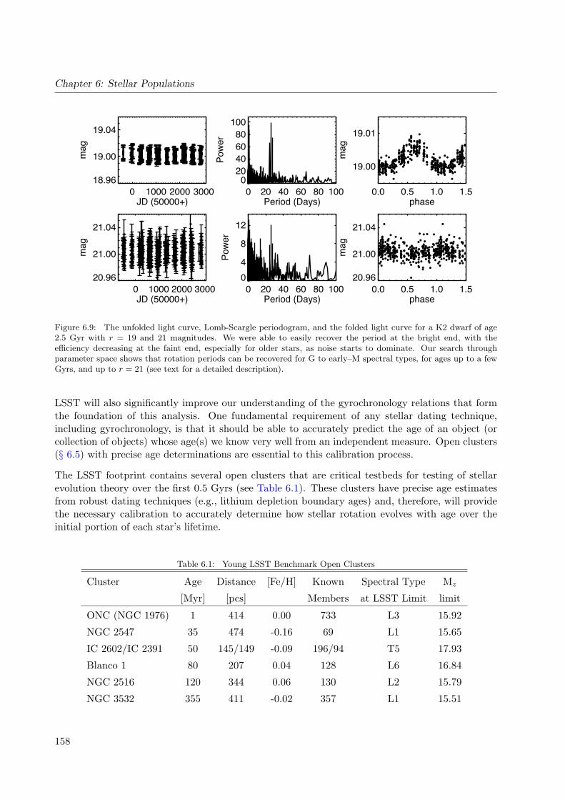
Figure 6.9: The unfolded light curve, Lomb-Scargle periodogram, and the folded light curve for a K2 dwarf of age2.5 Gyr with r = 19 and 21 magnitudes. We were able to easily recover the period at the bright end, with theefficiency decreasing at the faint end, especially for older stars, as noise starts to dominate. Our search throughparameter space shows that rotation periods can be recovered for G to early–M spectral types, for ages up to a fewGyrs, and up to r = 21 (see text for a detailed description).
LSST will also significantly improve our understanding of the gyrochronology relations that formthe foundation of this analysis. One fundamental requirement of any stellar dating technique,including gyrochronology, is that it should be able to accurately predict the age of an object (orcollection of objects) whose age(s) we know very well from an independent measure. Open clusters(§ 6.5) with precise age determinations are essential to this calibration process.
The LSST footprint contains several open clusters that are critical testbeds for testing of stellarevolution theory over the first 0.5 Gyrs (see Table 6.1). These clusters have precise age estimatesfrom robust dating techniques (e.g., lithium depletion boundary ages) and, therefore, will providethe necessary calibration to accurately determine how stellar rotation evolves with age over theinitial portion of each star’s lifetime.
Table 6.1: Young LSST Benchmark Open Clusters
Cluster Age Distance [Fe/H] Known Spectral Type Mz
[Myr] [pcs] Members at LSST Limit limit
ONC (NGC 1976) 1 414 0.00 733 L3 15.92
NGC 2547 35 474 -0.16 69 L1 15.65
IC 2602/IC 2391 50 145/149 -0.09 196/94 T5 17.93
Blanco 1 80 207 0.04 128 L6 16.84
NGC 2516 120 344 0.06 130 L2 15.79
NGC 3532 355 411 -0.02 357 L1 15.51
158

6.6 Decoding the Star Formation History of the Milky Way
Table 6.2: Selection of Old LSST Open Clusters
Cluster Age Distance [Fe/H] Known Spectral Type Mz
[Myr] [pcs] Members at LSST Limit limit
IC 4651 1140 888 0.09 16 L0 14.08
Ruprecht 99 1949 660 ... 7 L1 14.83
NGC 1252 3019 640 ... 22 L2 14.94
NGC 2243 4497 4458 -0.44 8 M5 10.68
Berkeley 39 7943 4780 -0.17 12 M5 10.43
Collinder 261 8912 2190 -0.14 43 M6 11.90
In addition, the WEBDA open cluster database lists over 400 known open clusters in the LSSTfootprint; many of these have poorly constrained cluster memberships (e.g., fewer than 20 knownmembers), especially for the oldest clusters (for example, see Table 6.2). LSST’s deep, homogeneousphotometry and proper motions will significantly improve the census of each of these cluster’smembership, providing new test cases for gyrochronology in age domains not yet investigated withthis dating technique.
6.6.2 Stellar Ages via Age–Activity Relations
Age–activity relations tap the same physics underlying the gyrochronology relations (West et al.2008; Mamajek & Hillenbrand 2008), and provide an opportunity to sample the star formation his-tory of the Galactic disk at ages inaccessible to gyrochronology. Although inherently intermittentand aperiodic, stellar flares, which trace the strength of the star’s magnetic field, are one photo-metric proxy for stellar age that will be accessible to LSST. The same cluster observations thatcalibrate gyrochronology relations will indicate how the frequency and intensity of stellar flaresvary with stellar age and mass (see § 8.9.1), allowing the star formation history of the Galacticdisk to be inferred from flares detected by LSST in field dwarfs. The primary limit on the lookbacktime of a star formation history derived from stellar flare rates relations is the timescale when flaresbecome too rare or weak to serve as a useful proxy for stellar age. We do not yet have a calibrationof what this lifetime is, but early explorations suggest even the latest M dwarfs become inactiveafter ∼5 Gyrs (Hawley et al. 2000; West et al. 2008).
6.6.3 Isochronal Ages for Eclipsing Binaries in the Milky Way Halo
Halo objects are ∼0.5% of the stars in the local solar neighborhood, so the ages of nearby highvelocity stars provide a first glimpse of the halo’s star formation history. The highly substructurednature of the Galactic halo, however, argues strongly for sampling its star formation history in situto understand the early Milky Way’s full accretion history. The stellar age indicators describedin the previous sections are not useful for probing the distant halo, as stellar activity indicators(rotation, flares) will be undetectable for typical halo ages.
159

Chapter 6: Stellar Populations
Eclipsing binary stars (EBs; § 6.10), however, provide a new opportunity for measuring the SFH ofthe distributed halo population. Combined analysis of multi-band light curves and radial velocitymeasurements of detached, double–lined EBs yield direct and accurate measures of the masses,radii, surface gravities, temperatures, and luminosities of the two stars (Wilson & Devinney 1971;Prsa & Zwitter 2005). This wealth of information enables the derivation of distance independentisochronal ages for EBs by comparing to stellar evolution models in different parameter spaces,such as the mass–radius plane. Binary components with M > 1.2M� typically appear co–evalto within 5%, suggesting that the age estimates of the individual components are reliable at thatlevel (Stassun et al. 2009). Lower mass binary components have larger errors, likely due to thesuppression of convection by strong magnetic fields (Lopez-Morales 2007); efforts to include theseeffects in theoretical models are ongoing, and should allow for accurate ages to be derived forlower–mass binaries as well. By identifying a large sample of EBs in the Milky Way halo, LSSTwill enable us to begin mapping out the star formation history of the distributed halo population.
6.7 Discovery and Analysis of the Most Metal Poor Stars in theGalaxy
Timothy C. Beers
Metal-poor stars are of fundamental importance to modern astronomy and astrophysics for avariety of reasons. This long and expanding list includes:
• The Nature of the Big Bang: Standard Big Bang cosmologies predict, with increasingprecision, the amount of the light element lithium that was present in the Universe after thefirst minutes of creation. The measured abundance of Li in very metal-poor stars is thoughtto provide a direct estimate of the single parameter in these models, the baryon-to-photonratio.
• The Nature of the First Stars: Contemporary models and observational constraintssuggest that star formation began no more than a few hundred million years after the BigBang, and was likely to have been responsible for the production of the first elements heavierthan Li. The site of this first element production has been argued to be associated withthe explosions of stars with characteristic masses up to several hundred solar masses. Theseshort-lived objects may have provided the first “seeds” of the heavy elements, thereby stronglyinfluencing the formation of subsequent generations of stars.
• The First Mass Function: The distribution of masses with which stars have formedthroughout the history of the Universe is of fundamental importance to the evolution ofgalaxies. Although the Inital Mass Function (IMF) today appears to be described well bysimple power laws, it is almost certainly different from the First Mass Function (FMF), associ-ated with the earliest star formation in the Universe. Detailed studies of elemental abundancepatterns in low-metallicity stars provide one of the few means by which astronomers mightpeer back and obtain knowledge of the FMF.
• Predictions of Element Production by Supernovae: Modern computers enable in-creasingly sophisticated models for the production of light and heavy elements by supernovae
160

6.7 Discovery and Analysis of the Most Metal Poor Stars in the Galaxy
explosions. Direct insight into the relevant physics of these models can be obtained from in-spection of the abundances of elements in the most metal-deficient stars, which presumablyhave not suffered pollution from numerous previous generations of stars.
• The Nature of the Metallicity Distribution Function (MDF) of the Galactic Halo:Large samples of metal-poor stars are now making it possible to confront detailed Galacticchemical evolution models with the observed distributions of stellar metallicities. Tests forstructure in the MDF at low metallicity, the constancy of the MDF as a function of distancethroughout the Galactic halo, and the important question of whether we are approaching,or have already reached, the limit of low metallicity in the Galaxy can all be addressed withsufficiently large samples of very metal-poor stars.
• The Astrophysical Site(s) of Neutron-Capture Element Production: Elements be-yond the iron peak are formed primarily by captures of neutrons, in a variety of astrophysicalsites. The two principal mechanisms are referred to as the slow (s)-process, in which the timescales for neutron capture by iron-peak seeds are longer than the time required for beta de-cay, and the rapid (r)-process, where the associated neutron capture occurs faster than betadecay. These are best explored at low metallicity, where one is examining the production ofheavy elements from a limited number of sites, perhaps even a single site.
Owing to their rarity, the road to obtaining elemental abundances for metal-poor stars in theGalaxy is long and arduous. The process usually involves three major observational steps: 1)A wide-angle survey must be carried out, and candidate metal-poor stars selected; 2) Moderate-resolution spectroscopic follow-up of candidates is required to validate the genuine metal-poorstars among them; and finally, 3) High-resolution spectroscopy of the most interesting candidatesemerging from step 2) must be obtained.
The accurate ugriz photometry obtained by LSST will provide for the photometric selection ofmetal-poor candidates from the local neighborhood out to over 100 kpc from the Galactic center.Similar techniques have been (and are being) employed during the course of SDSS-II and SDSS-IIIin order to identify candidate very metal-poor ([Fe/H] < −2.0) stars for subsequent follow-up withmedium-resolution (R = 2000) spectroscopic study with the SDSS spectrographs. This approachhas been quite successful, as indicated by the statistics shown in § 6.7, based on work reported byBeers et al. (2009). See Beers & Christlieb (2005) for more discussion of the classes of metal-poorstars.
Table 6.3: Impact of SDSS on Numbers of Metal-Poor Stars
[Fe/H] Pre SDSS-II Post SDSS-II
< −1.0 ∼ 15000 150000+
< −2.0 ∼ 3000 30000+
< −3.0 ∼ 400 1000+
< −4.0 5 5
< −5.0 2 2
< −6.0 0 0
LSST photometric measurements will be more accurate than those SDSS obtains (Ivezic et al.
161

Chapter 6: Stellar Populations
2008a) (Table 1.1). This has three immediate consequences: 1) Candidate metal-poor stars will befar more confidently identified, translating to much more efficient spectroscopic follow-up; 2) Accu-rate photometric metallicity estimates will be practical to obtain down to substantially lower metal-licity (perhaps [Fe/H] < −2.5) than is feasible for SDSS photometric selection ([Fe/H] ' −2.0);and 3) The much deeper LSST photometry means that low-metallicity stars will be identifiableto 100 kpc, covering a thousand times the volume that SDSS surveyed. The photometrically de-termined metallicities from LSST will be of great scientific interest, as they will enable studies ofthe changes in stellar populations as a function of distance based on a sample that includes over99% of main sequence stars in the LSST footprint. This sample will also enable studies of thecorrelations between metallicity and stellar kinematics based on measured proper motions (for anSDSS-based example, see Ivezic et al. 2008a). Detailed metallicity measurements will of courserequire high S/N, high-resolution spectroscopic follow-up of the best candidates.
Proper motions obtained by LSST will also enable spectroscopic targeting of what are likely to besome of the most metal-poor stars known, those belonging to the so-called outer-halo population.Carollo et al. (2007) used a sample of some 10,000 “calibration stars” with available SDSS spec-troscopy, and located within 4 kpc of the Sun, to argue that the halo of the Galaxy comprises (atleast) two distinct populations: a slightly prograde inner halo (which dominates within 10 kpc)with an MDF that peaks around [Fe/H] = −1.6 and an outer halo (which dominates beyond 15-20kpc) in net retrograde rotation with an MDF that peaks around [Fe/H] = −2.2. The expectationis that the tail of the outer-halo MDF will be populated by stars of the lowest metallicities known.Indeed, all three stars recognized at present with [Fe/H] < −4.5, including two stars with [Fe/H]< −5.0, exhibit characteristics of membership in the outer-halo population. Stars can be selectedfrom LSST with proper motions that increase their likelihood of being members of this populationeither based on large motions consistent with the high-energy outer-halo kinematics, or with propermotion components suggesting highly retrograde orbits.
6.8 Cool Subdwarfs and the Local Galactic Halo Population
Sebastien Lepine, Pat Boeshaar, Adam J. Burgasser
Cool subdwarfs are main sequence stars, which have both a low mass and a low abundance of metals.Locally they form the low-mass end of the stellar Population II. Cool subdwarfs have historicallybeen identified from catalogs of stars with large proper motion, where they show up as high velocitystars. Kinematically they are associated with the local thick disk and halo populations. Becausethey are the surviving members of the earliest generations of stars in the Galaxy with evolutionarytimescales well exceeding a Hubble time, cool subdwarfs are true fossils of the early history ofstar formation in the Galaxy, and hold important clues to the formation of the Galactic system.While these stars have already traveled dozens of orbits around the Galaxy and undergone somedynamical mixing, a study of their orbital characteristics and metallicity distribution can still shedlight on the formation and dynamical evolution of our Galaxy. In particular, cool subdwarfs do notundergo any significant enrichment of their atmospheres, but largely retain their original elementalcomposition from the time of their birth. This makes them perfect tracers of the early chemicalcomposition of the gas that formed these first generations of low-mass stars.
162

6.8 Cool Subdwarfs and the Local Galactic Halo Population
Cool stars of spectral type M have atmospheres that are dominated by molecular bands frommetal hydrides and oxides, most notably CaH, FeH, TiO, and VO. Metallicity variations result inmarked differences in the absolute and relative strengths of these bands. As a result, M dwarfsand subdwarfs also display significant variations in their broadband colors depending on theirmetal abundances. The significantly metal-poor subdwarfs from the Galactic halo populate adistinct locus in the g − r/r − i color-color diagram. The strong color-dependence makes the Msubdwarfs easy to identify (Figure 6.10), and also potentially allows one to determine the metallicityfrom broadband photometry alone. The only caveat is that this part of color-color space is alsopopulated by extragalactic sources, which may be distinguishable by their extent and their zeroproper motions.
In Figure 6.11 panels, the blue line shows the mean positions of Pickles (1998) main sequence stars,the dots refer to quasars from z = 0 to 5, and the mean position of the coolest ultra-, extreme-, andM subdwarfs are noted by crosses in grizy color space. Redshifting the locally observed ellipticalgalaxy template (Coleman et al. 1980) over the range z = 0−2 clearly results in colors that occupythe same color space as the subdwarfs of all classes, and even extend into the region of the coolestsubdwarfs. Estimates from the Deep Lens Survey (Boeshaar et al. 2003) indicate that at highGalactic latitudes, up to 30% of the “stellar” objects with M subdwarf colors detected at 23-25mag in ≥ 1′′ seeing will actually be unresolved ellipticals at z = 0.25 − 1. The g − z vs. z − yplot clearly separates the high redshift quasars from the subdwarf region, but quasars should beonly a minor contaminant due to their low spatial density. The net effect of including evolutioninto stellar population models is to shift the elliptical tracks by several tenths of a magnitude ing − r and r − i. Thus unresolved ellipticals may still fall within the overlap envelope. Additionalsynthetic z− y colors for stars, brown dwarfs plus quasars and unevolved galaxies as a function ofredshift with color equations between the UKIRT Wide-Field Camera and SDSS can be found inHewett et al. (2006). A proper motion detection is thus required for formal identification.
Very large uncertainties in the luminosity function and number density of such objects exist (Digbyet al. 2003). It is not known whether the subdwarfs have a mass function similar to that of thedisk stars. Their metallicity distribution is also poorly constrained. The main limitation in usingthe low-mass subdwarfs to study the Galactic halo resides in their relatively low luminosities. Msubdwarfs have absolute magnitudes in the range 10 < Mr < 15. With the SDSS magnitude limitof r = 22 and proper motion data to only r = 20, M subdwarfs can thus only be detected out to afew hundred parsecs. With a local density yielding ∼ 1,000 objects within 100 parsecs of the Sun(all-sky), SDSS can only formally identify a few thousand M subdwarfs.
LSST will open the way for a study of the low-mass halo stars on a much grander scale. Withphotometry to r ' 27 and proper motion data available to r = 24.5, the LSST survey will detectall stellar subdwarfs to 1 kiloparsec. In the Sun’s vicinity, halo stars have large transverse velocities(vT > 100 km s−1), which yield proper motions µ > 20 mas yr−1 up to 1 kpc. With the requiredproper motion accuracy of 0.2 mas yr−1 for LSST, virtually all the subdwarfs will be confirmedthrough proper motion detection. The ability to estimate metallicity classes for the halo subdwarfsbased on the LSST gri magnitudes alone will make it possible to determine the approximatemetallicity distribution of the halo stars from an unprecedented sample of >500,000 objects.
Relatively accurate photometric distances can also be determined for low-mass stars, yieldingdistances generally accurate to better than 50%. These, combined with the proper motion data,
163

Chapter 6: Stellar Populations
Figure 6.10: Distribution of cool subdwarfs in the g−r/r−i color-color diagram. The four metallicity classes (dwarfs,subdwarfs, extreme subdwarfs, and ultrasubdwarfs) are represented in different colors. The segregation according tometallicity class allows one to identify the halo subdwarfs and estimate their metallicities (and temperatures) basedon photometry alone. Photometric data and spectroscopic confirmation of the stars have been obtained from SDSS.
will make it possible to plot large numbers of stars in tangential velocity space and search forpossible substructure in the tangential velocity space distribution.
Besides determining the subdwarf number density and distribution in metallicity, mass, and lu-minosity, the exploration of the time domain by LSST will identify eclipsing doubles, monitorrotational modulation, and search for unexpected flaring activity. The multiplicity fraction ofthe halo population is only weakly constrained due to the paucity of subdwarfs and their greaterdistances relative to their main sequence counterparts. A direct comparison with the number ofeclipsing binaries also expected to be discovered among the disk stars will determine whether closedouble stars are more or less common in the halo population. More critically, no eclipsing systemcomprised of cool subdwarfs has ever been identified, but LSST’s systematic monitoring has ex-cellent prospects for finding at least several sdM+sdM eclipsing systems. Such systems would beimmensely useful in determining the mass and radii of low-mass, metal-poor stars, which is nowpoorly constrained due to a paucity of known binary systems.
Beyond building up very large samples of M-type subdwarfs, LSST will also uncover the first sub-stantial samples of cooler L-type subdwarfs, metal-deficient analogs to the L dwarf population ofvery low mass stars and brown dwarfs (Burgasser et al. 2008). L subdwarfs have masses spanningthe metallicity-dependent, hydrogen-burning limit, making them critical probes of both low-massstar formation processes in the halo and thermal transport in partially degenerate stellar interi-ors. The subsolar metallicities of L subdwarfs are also important for testing chemistry models oflow-temperature stellar and brown dwarf photospheres, in particular condensate grain and cloudformation, a process that largely defines the properties of L dwarfs but may be inhibited or absentin L subdwarfs (Burgasser et al. 2003a; Reiners & Basri 2006). Only a few L subdwarfs have been
164

6.8 Cool Subdwarfs and the Local Galactic Halo Population
Figure 6.11: Upper left: g − r/r − i color-color diagram similar to Figure 6.10 showing the location of the mainsequence stars (purple line), mean position of extreme-, ultra-, and M subdwarfs (crosses), quasars (dots) andunevolved elliptical galaxies (thin colored line) as a function of redshift. Upper right: Same as previous figure withthe Bruzual & Charlot (2003) single stellar population 5 Gyr evolutionary model for the elliptical galaxies. Lowerleft: g-r/z-y color-color diagram for objects in first figure. See also Figure 10.1 in the AGN chapter.
165

Chapter 6: Stellar Populations
identified to date, largely serendipitously with 2MASS and SDSS. But with 15 . Mi . 18, theywill be detected in substantial numbers with LSST, with volume-complete samples out to at least200 pc. LSST should also discover specimens of the even cooler T-type subdwarfs, whose spec-tral properties are as yet unknown but likely to be substantially modified by metallicity effects.Collectively these low-temperature subdwarfs will facilitate the first measurement of the hydrogen-burning gap in the halo luminosity function, a population age indicator that can constrain theformation history of the low-mass halo and its subpopulations (e.g. Burrows et al. 1993).
6.9 Very Low-Mass Stars and Brown Dwarfs in the SolarNeighborhood
Kevin R. Covey, John J. Bochanski, Paul Thorman, Pat Boeshaar, Sarah Schmidt, Eric J. Hilton,Mario Juric, Zeljko Ivezic, Keivan G. Stassun, Phillip A. Cargile, Saurav Dhital, Leslie Hebb,Andrew A. West, Suzanne L. Hawley
6.9.1 The Solar Neighborhood in the Next Decade
The least–massive constituents of the Galactic population are brown dwarfs, objects too small tosustain hydrogen fusion in their cores. These are divided into L dwarfs (Kirkpatrick et al. 1999),which have Teff between 1500K and 2200K, whose spectra show weakening of the TiO absorptionbands, and T dwarfs with Teff between 800K and 1500K, which show the presence of CH4 in theiratmospheres. An additional spectral type, the Y dwarf (after Kirkpatrick et al. 1999), has beenreserved to describe possible dwarfs with even cooler temperatures, which are expected to showNH3 absorption, a weakening in the optical alkali lines, and a reversal of the blueward J−K trendcaused by CH4 absorption in T dwarfs (Kirkpatrick 2005). Although their masses are low, thesebrown dwarfs are relatively common in the solar neighborhood, with 600 L and 150 T dwarfs nowconfirmed. Most of these have been discovered by combining near–infrared imaging (e.g. 2MASS;Skrutskie et al. 2006) with optical surveys (e.g. SDSS; York et al. 2000); the faintness of theseobjects at optical wavelengths (Mz > 13) and the depth of existing NIR imaging are such that thesebrown dwarfs are overwhelmingly located within the immediate solar neighborhood (d < 65 pc).Informing theoretical models of these objects requires measurements of precise physical parameterssuch as radius and mass.
A number of ongoing or near–term surveys will expand the census of brown dwarfs by 2017, whenLSST will begin standard survey operations. The largest single epoch catalog of warm (i.e., Land early T) brown dwarfs will be compiled by the UKIDSS NIR survey (Hewett et al. 2006),which is currently in progress and capable of detecting L0 dwarfs in the J-band within ∼ 250 pc.At the cool end, the upcoming WISE mid-IR space telescope (Mainzer et al. 2005) will provide[3.3]-[4.7] µm colors for early T dwarfs within 200 pc (assuming colors and magnitudes from Pattenet al. 2006) and all T9 dwarfs within 20 pc, and exquisite sensitivity to cooler Y dwarfs. Multi-epoch photometric surveys enable initial measurements of a source’s trigonometric parallax andpotential binarity, such that brown dwarfs detected by such surveys have significantly more valuefor constraining theoretical models. The SkyMapper survey (SSSS Keller et al. 2007), a large-areaimaging survey covering the southern sky to depths similar to SDSS, will begin within the next few
166

6.9 Very Low-Mass Stars and Brown Dwarfs in the Solar Neighborhood
years. SkyMapper’s six-year campaign will produce parallaxes for brown dwarfs within 20 pc. ThePan-STARRS PS1 survey will detect L0 dwarfs in the i band out to 400 pc and measure parallaxesfor those within 100 pc; the volume sampled shrinks for fainter, cooler brown dwarfs.
6.9.2 Simulating LSST’s Yield of Solar Neighborhood MLTY Dwarfs
Unlike previous surveys, LSST will not depend on separate NIR surveys in order to distinguish Land T dwarfs from possible contaminants such as transient detections, high-redshift quasars, andred galaxies (see Figure 10.6). A narrow range of late L dwarfs may overlap with z ' 6.25 quasarsin color; shortly after the start of the survey, even these brown dwarfs will be identifiable by theirproper motions. The addition of the y band allows color identification based on detection in onlythe three reddest LSST bands, allowing LSST to detect (5 σ in full 10-year co-adds) L0 dwarfsout to 2100 pc, and T0 dwarfs to 100 pc. This L dwarf detection limit extends well into the Thickdisk, enabling LSST to probe the physics of old, metal–poor substellar objects (see § 6.7), andpotentially decode the star formation history of the thick and thin disks of the Milky Way fromthe age distribution of field brown dwarfs.
We have constructed a detailed simulation of the very-low mass (VLM) stars and brown dwarfs inthe solar neighborhood; using the baseline specifications for the LSST system, we have identified thesubsets of this population that LSST will characterize with varying degrees of precision. To modelthe stellar population in the stellar neighborhood, we have adopted ugriz absolute magnitudesfor VLM stars as tabulated by Kraus & Hillenbrand (2007), synthetic z − y colors calculatedfrom optical and infrared template spectra provided by Bochanski et al. (2007) and Cushing et al.(2005), and the mass function and space densities of low-mass stars measured by Bochanski et al.(in preparation).
The lack of a hydrogen-burning main sequence in the brown dwarf regime introduces strong degen-eracies into the relationships between the masses, ages, and luminosities of substellar objects. Thesedegeneracies are an important consideration for studies of the properties of field brown dwarfs, asthe properties of brown dwarfs in the solar neighborhood are sensitive to the star formation historyof the Milky Way and the shape of the stellar/substellar mass function. We are currently develop-ing simulations that explore the brown dwarf samples LSST would observe assuming different starformation histories and mass functions; for simplicity, however, the simulations described belowassume a single population of 3 Gyr brown dwarfs. In detail, this substellar population is describedby:
• For 2100 > Teff > 1200 (L dwarfs and the earliest Ts) we adopt empirical SDSS riz mag-nitudes (Schmidt et al. in preparation), supplemented by synthetic ugy magnitudes fromcloudy Burrows et al. (2006) models.
• For 1200 > Teff > 600 (mid-late Ts), we adopt synthetic ugrizy magnitudes calculated fromcloud-free Burrows et al. (2006) models.
• For Teff > 600 (as yet undiscovered Y dwarfs), we adopt synthetic ugrizy magnitudescalculated from the ultra-cool Burrows et al. (2003) models.
• We adopt the Cruz et al. (2007) luminosity function for L dwarfs; for T and Y dwarfs, wedefine a luminosity function with a linear extrapolation anchored by the coolest bin of the
167

Chapter 6: Stellar Populations
Table 6.4: LSST’s MLTY Dwarf Sample
Spectral Class Nrizy Nizy Nzy Nπ
M >347,000 >347,000 >347,000 >347,000
L 18,500 27,500 35,600 6,550
T ∼3-4 50 2,300 ∼260
Y 0 0 ∼18 ∼5
Cruz et al. luminosity and the empirical T dwarf space density measured by Metchev &Hillenbrand (2007).
Using the above parameters as inputs, we simulated the properties of field stars and brown dwarfswithin 200 pc of the Sun. Table 6.4 summarizes the number of stars and brown dwarfs LSST willlikely detect in various filter combinations as a function of spectral type with reliable parallaxes,to the single-visit depth. To make this estimate, we assume the relationship between parallaxuncertainty vs. r band magnitude reported in Table 3.3, but we increase these uncertainties by afactor of 1.25 to reflect that many stars and brown dwarfs will lack u and g band detections.
These results indicate that LSST will greatly expand the sample of ultra–cool objects with reliableparallax measurements. These extremely red objects are ill-suited for parallax measurementswith Gaia’s blue filterset, while LSST’s greater depth and astrometric precision will enable it tomeasure parallaxes for brown dwarfs significantly beyond the parallax limit of Pan-STARRS. Thissample will, therefore, provide a key set of well-characterized brown dwarfs which can confront thepredictions of theoretical models of brown dwarf and planetary atmospheres.
While we focus here primarily on brown dwarfs in the Galactic field, we also note that LSST’s deepphotometric limits and its ability to select cluster members via high-precision proper motions willprovide a high-fidelity census of the very-low-mass populations of many Southern open clusters.LSST will be able to easily identify VLM objects near or below the hydrogen-burning limit inmost of the clusters listed in Tables 6.1 and 6.2, with ages ranging from 1 Myr to ∼10 Gyr andto distances as far as ∼1.5 kpc. LSST will provide colors and magnitudes for a large sample ofL and T dwarfs with ages and metallicities derived from the morphology of each cluster’s uppermain sequence. This sample will define empirical brown dwarf cooling curves over a wide rangeof ages, providing a key calibration for understanding the properties of nearby field brown dwarfswhose ages are almost entirely undetermined.
6.9.3 Science Results
Measuring Fundamental Physical Parameters of VLM stars and Brown Dwarfs
The wide areal coverage, depth, precision, and temporal coverage of LSST photometry make it anideal instrument for the detection and characterization of low–mass (M < 0.8M�) eclipsing binarieswithin the Milky Way. Currently, only ∼ 15 low–mass eclipsing binaries are known (Demory et al.2009), and even fewer VLM binaries, presumably due to their intrinsic faintness (L < 0.05L� fora 0.4M� early M dwarf) and a stellar binary fraction that decreases with mass (Duquennoy &
168

6.9 Very Low-Mass Stars and Brown Dwarfs in the Solar Neighborhood
Mayor 1991; Burgasser et al. 2007). The large volume probed by LSST, with typical low-masspairs being detected at d < 200 pc, will discover a slew of these rare systems.
To quantify the expected yield of VLM star and brown dwarf EBs, we start with the expected yieldof MLTY dwarfs from the Nzy column of Table 6.4. Such objects will already have LSST lightcurves in the z and y bands, which can be complemented by follow-up light curves in the JHKbands. A five-band light curve analysis is sufficient for modeling the EB parameters to ∼ 1% (e.g.Stassun et al. 2004). Assuming that approximately 1/10 of the M dwarfs are M9 brown dwarfs,then the total brown dwarf yield from Table 6.4 is ∼ 70, 000. Recent surveys of binarity amongbrown dwarfs yield fractions of 10–15% for visual binaries with separations of > 1 AU (e.g., Martınet al. 2003; Bouy et al. 2003). Thus a very conservative estimate for the overall binary fraction ofbrown dwarfs is 10%. Next, assuming a distribution of binary separations similar to that for Mdwarfs (Fischer & Marcy 1992) implies that ∼ 10% of these will be tight, spectroscopic binarieswith physical separations < 0.1 AU. Finally, among these, the probability of an eclipse is of order(R1 + R2)/a, where R1 and R2 are the component radii and a is the semi-major axis, so for twobrown dwarfs each with R ∼ 0.1 R� and a ∼ 0.1 AU, we have an eclipse probability of ∼ 1%. Thusthe overall expected brown dwarf EB yield will be 0.1 × 0.1 × 0.01 × 70, 000 ≈ 7. With only onebrown dwarf EB currently known (Stassun et al. 2006, 2007), the LSST yield represents a criticalforward advance for substellar science. The calculation above implies an overall yield of ∼ 40 VLMeclipsing binary systems, a factor of several increase over the number currently known.
These fundamental astrophysical laboratories will redefine the empirical mass–radius relations,for which current data are sparse and derived from heterogeneous sources. For nearby eclipsingsystems, native LSST parallaxes will result in model–free luminosity estimates, and can help con-strain the effective temperature distribution of low–mass stars. This will be especially importantat smaller masses (M < 0.1M�), where only one eclipsing binary is known (Stassun et al. 2006)1.This regime will be well suited to LSST’s survey specifications and complement the Pan-STARRSsurvey as LSST will be probing a different area of the sky (the Southern Hemisphere). At largedistances, the currently elusive halo binaries, identified kinematically through proper motions, mayserve as probes for changes in low–mass stellar structure due to metallicity. Low–mass stars in-habit an interesting regime in stellar structure. At masses ∼ 0.4M�, the interiors of low–massstars transition from a convective core surrounded by a radiative shell to a fully convective in-terior. Observations do not currently constrain how metallicity may affect this transition, andonly the deep photometry that LSST will provide will enable an empirical investigation of thisphenomenon. The eclipsing binaries discovered in LSST will enable new science and redefine theempirical understanding of stellar structure and binary properties. With the “brown dwarf desert”significantly limiting the existence of F/G/K+brown dwarf binaries2, VLM+brown dwarf eclipsingbinaries are the only systems in which masses and radii of brown dwarfs can be measured—alongwith their temperatures.
High-resolution near-infrared spectroscopic follow-up on 10-m class telescopes will be critical fordetermining the radial velocity orbit solutions for the discovered eclipsing binaries. For example,the one known brown dwarf eclipsing binary (Stassun et al. 2006, 2007) is in the Orion Nebula
1This system exhibits interesting behavior: the hotter component (primary) is actually fainter than its companion.2For example, Grether & Lineweaver (2006) find that approximately 16% of solar-type stars have companions with
P < 5 yr, M > 1 MJup. Of these, 4.3 ± 1.0% have companions of planetary mass, 0.1% have brown dwarfcompanions, and 11.2± 1.6% have companions of stellar mass.
169

Chapter 6: Stellar Populations
cluster at a distance of ∼ 500 pc, the outer limit for the systems included in the estimated yieldscalculated above. Its radial velocity curve was obtained with the Phoenix spectrograph on theGemini South 8-m telescope operating in the H band (1.5 µm).
Variability of VLM Stars and Brown Dwarfs
The temporal coverage of LSST opens a window on the time variability of VLM stars, includingflares, spot modulation, and rotation periods. Additionally, by discovering new eclipsing binaries,LSST will provide new laboratories for measuring fundamental stellar parameters like mass andradius.
Stellar magnetic activity has been observed and studied on M dwarfs for several decades (see§ 8.9.1 for a review of this subject), but much less is known about activity on brown dwarfs. Thefraction of stars with Hα in emission, an indicator of magnetic activity, peaks around M7 anddecreases through mid-L (Gizis et al. 2000; West et al. 2004; Schmidt et al. 2007; West et al.2008) although the changing continuum level with spectral type makes this an imperfect tracer ofmagnetic field strength. Burgasser et al. (2003b) report three T dwarfs with Hα activity, one ofwhich has strong, sustained emission (Burgasser et al. 2002). Flares on brown dwarfs appear tobe less frequent than on M dwarfs, but have been seen in both X-ray (Rutledge et al. 2000) andradio (Berger et al. 2001). Optical spectra have shown variable Hα emission in L dwarfs (Hall2002; Liebert et al. 2003; Schmidt et al. 2007; Reiners & Basri 2008) that may be the result offlares. LSST’s new observations of such a large number of brown dwarfs over dozens of epochs willprovide much–needed empirical determinations of flare rates.
LSST’s temporal coverage will permit precise, dense coverage of most main sequence stars withspots. This subject is modeled in detail in § 6.6, and discussed below in the context of low–massstars and brown dwarfs. Starspots, analogous to their solar counterparts, provide a measure ofthe relative magnetic field strength for stars of a given spectral type (and mass), assuming thatthe spot coverage is not so uniform as to prevent rotational modulation of the star’s observed flux.If spot variations can be detected, the ugrizy light curves of these stars can be used to estimatetemperature, from relative depths due to spot modulation, and filling factors, from the absolutedeviations from a pristine stellar photosphere.
Furthermore, the photometric signatures imprinted by these cooler regions provide the opportunityto measure rotation periods that are shorter than the lifetime of a typical starspot (∼weeks tomonths). As demonstrated in § 6.6, LSST will be adept at measuring the rotation periods ofcoherently spotted, magnetically active, low–mass stars. Combining the measured rotation periodswith other proxies of stellar magnetic activity will provide a fundamental test of magnetic dynamogeneration theory. This is particularly interesting within the low–mass regime. At masses∼ 0.4M�,the interior of low–mass stars transition from an convective core surrounded by a radiative shellto a fully convective interior. The transition region between convective core and radiative exterioris thought to drive magnetic activity in earlier type low–mass stars (West et al. 2008).
170

6.10 Eclipsing Variables
Substellar Subdwarfs
The deep LSST survey imaging will photometrically identify statistically significant numbers of Ldwarfs at large distances from the Galactic plane. These dwarfs will allow the spatial distributionof dwarfs in the thin and thick disk populations to be determined, and allow a search for additionalmembers of a halo population of metal–poor subdwarf brown dwarfs to be discovered (e.g., Cushinget al. 2009). The kinematics of the L dwarf and subdwarf populations will also provide an empiricaltest of the metallicity dependence of the hydrogen burning limit, based on the model coolingcurves. The existence of a population of substellar subdwarfs may also indicate star formation dueto infalling primordial gas, or be a relic of the Milky Way’s recent merger history.
6.10 Eclipsing Variables
Andrej Prsa, Keivan G. Stassun, Joshua Pepper
The importance of eclipsing binary stars (EBs) can hardly be overstated. Their analysis provides:
• Calibration-free physical properties of stars (i.e., masses, radii, surface temper-atures, luminosities). Masses are measured dynamically via radial velocities with no sin iambiguity because the eclipses provide an accurate measure of sin i. Radii are measureddirectly from the eclipse durations, the temperature ratio from the eclipse depths. The radiiand temperatures together yield the luminosities.
• Accurate stellar distances. With luminosities measured directly from the componentradii and temperatures, the distance to the EB follows directly from the observed fluxes.
• Precise stellar ages. By comparing the measured mass-radius relationship with stellarevolution models, precise stellar ages can be determined. The accuracy of the age determi-nation is of course model dependent and also mass dependent, with typical accuracy of ∼ 5%for M? > 1.2 M� and ∼ 50% for M? < 0.8 M� (Stassun et al. 2009).
• Stringent tests of stellar evolution models. With accurate, directly determined proper-ties of the two stars in the EB, the basic predictions of stellar evolution models can be tested.For example, the two stars should lie on a single model isochrone under the assumption thatthey formed together as a binary, or the observed parameter relationships (mass-radius,temperature-luminosity, and so on) can be compared against the model predictions.
The products of state-of-the-art EB modeling are seminal to many areas of astrophysics:
• calibrating the cosmic distance scale;
• mapping clusters and other stellar populations (e.g., star-forming regions, streams, tidal tails,etc) in the Milky Way;
• determining initial mass functions and studying stellar population theory;
• understanding stellar energy transfer mechanisms (including activity) as a function of tem-perature, metallicity, and evolutionary stage;
• calibrating stellar color-temperature transformations, mass-radius-luminosity relationships,and other relations basic to a broad array of stellar astrophysics; and
171

Chapter 6: Stellar Populations
Table 6.5: Distance Limits for LSST Detection of Sample EBs.
Sample Binarya Type Binary Absolute Magnitude Distanceb for r = 22.0 [kpc] Distanceb for r = 19.5 [kpc]
M5V + M5V 12.9 0.7 0.2
M2V + M2V 9.0 4.0 1.3
K0V + K0V 5.0 25.1 7.9
G2V + MxV 4.6 30.2 9.5
G5III + GxV 2.9 66.1 20.1
aScientifically interesting EB systems. EBs with M-dwarf components are rare in the literature. Their discoverywill permit detailed testing of stellar models in this important mass regime. G-dwarf/M-dwarf pairs will beparticularly valuable for pinning down the properties of M-dwarfs, since the temperature scale of G-dwarfs isrelatively well established. A particularly exciting prospect are Cepheids (G giants) in EB systems.
bAssuming no extinction.
• studying stellar dynamics, tidal interactions, mass transfer, accretion, chromospheric activity,etc.
LSST will be ideally suited for extensive mapping of EBs. As the simulations described belowdemonstrate, LSST will detect essentially all EBs with orbital periods less than 0.3 days, and 50%of those with periods up to ∼10 days (see Figure 6.13). This completeness estimate is based onanalysis of a single passband; simultaneous analysis of all six LSST bands will in reality improvethis completeness. With a nominal detection limit of r = 24.5, a magnitude of r = 22.0 shouldallow detection of targets with a S/N of 3.5, r = 19.5 will have S/N of 10 per data point. Table 6.5shows the distance out to which certain fiducial EB types can be detected. For example, a pair ofeclipsing M2 dwarfs will be detected out to 1 kpc with S/N of 10.
We can estimate the number of EBs that LSST will be able to fully characterize (our experiencemodeling EB light curves shows that S/N ∼ 3.5 per data point typically suffices for the determi-nation of physical and geometric parameters to a few percent). Gaia will observe ∼1 billion starsdown to r ∼ 20.5 over the whole sky. We can expect that LSST will observe ∼0.5 billion stars tothis same depth in the southern hemisphere. Extrapolating the results from Hipparcos (917 EBsin the sample of 118,218 observed stars; or 0.8%), the LSST sample will contain ∼16 million EBsdown to r ∼ 22.0. The average detection rate for EBs over all periods will be around 40% (∼ 100%for P < 0.3 days, ∼50% for P ∼ 10 days, ∼ 20% for P < 30 days; Figure 6.13), bringing the totalnumber to ∼6.4 million EBs. Roughly 25% of those will have components of similar luminosities(double-lined systems), yielding ∼1.6 million EBs with S/N≥ 10 for ready detailed modeling.
6.10.1 Simulating LSST’s Harvest of Eclipsing Binary Stars
With LSST’s six-band photometry and a cut-off magnitude of r ∼ 24.5, the limiting factor forthe detection of EB stars will be the cadence of observations. To estimate LSST’s EB detectionefficiency, we set up a test-bed by employing PHOEBE (Prsa & Zwitter 2005), a Wilson & Devinney(1971) based eclipsing binary modeling suite. We first partitioned the sky into 1558 fields, coveringall right ascensions and declinations between −90◦ and 10◦. The cadence of observations of thesefields was then determined from the Simulated Survey Technical Analysis Report (SSTAR) for theoperations simulations described in § 3.1.
172

6.10 Eclipsing Variables
Figure 6.12: Schematic view of an EB light curve. Surface brightness ratio B2/B1 directly determines the ratio ofdepths of both eclipses, and can be roughly approximated by the temperature ratio T2/T1. The sum of fractionalradii ρ1 + ρ2 determines the baseline width of the eclipses, while e sin ω determines the ratio between the widths ofeach eclipse, d1 and d2. The phase separation of the eclipses is governed by e cos ω, and the overall amplitude of thelight curve, as well as the shape of eclipses, are determined by sin i.
To estimate LSST detection effectiveness, we synthesized light curves for five EBs that are represen-tative of the given morphology type: well detached, intermediate detached, close detached, close,and contact. These most notably differ in fractional radii and orbital periods, hence in the numberof observed data points in eclipses. Each EB light curve is described by its ephemeris (HJD0 andperiod P0) and five principal parameters: T2/T1, ρ1 + ρ2, e sinω, e cosω and sin i (cf. Figure 6.12;for a thorough discussion about the choice of principal parameters please refer to Prsa et al. 2008).
Let N1 and N2 be the numbers of data points observed in each eclipse. To detect and correctlyclassify light curves, we need as many points in both eclipses as possible. We thus selected theproduct C = N1N2 for the cost function. This way, if all data points are observed during oneeclipse but not the other, this quantity will be zero. Consecutive observations of long period EBspresent another complication: although they contribute equally to the in-eclipse count, they coveressentially the same point in phase space because of the prolonged duration of eclipses. To accountfor that, all adjacent data points in phase space that are separated by less than some thresholdvalue – in our simulation we used 1/1000 of the period – are counted as a single data point.
The cost function C, shaped according to these insights, was computed for all five synthesized EBs(the details of the study are presented in Prsa et al. 2009). The light curves are computed in phasespace, assuming that periodicity can be found correctly by a period search algorithm if the S/N ofa single data point exceeds 3.5 (or, in terms of LSST, r < 22.0). Simulation steps are as follows:
1. given the P0, pick a random phase shift between 0.0 and 1.0 and convert the time array tothe phase array;
2. sort the array and eliminate all data points with adjacent phases closer than the thresholdvalue required to resolve them;
3. given the ρ1 + ρ2, count the number of data points in eclipses (N1, N2);
4. compute the cost function value C = N1N2;
173

Chapter 6: Stellar Populations
0
20
40
60
80
100
-1 -0.5 0 0.5 1 1.5 2 2.5 3
Det
ecti
on r
ate
in %
log(P)
Expected LSST harvest of eclipsing binaries
well detachedintermediate detached
close detachedclose
contact
Figure 6.13: The detection rate of eclipsing binary stars based on their morphology and their orbital period.Assuming that S/N≥ 3.5 per data point suffices for reliable recovery of orbital periods, LSST will detect almostall short period EBs, around 50% of intermediate EBs, and around 10% of long period EBs down to r ∼ 22.0.The simulation is based on a single passband, implying that the values quoted here correspond to the worst casescenario. Since short and intermediate period EBs are most interesting for stellar population studies, it is clear thatthe expected LSST harvest of EB stars will be unprecedented.
5. repeat steps 1-4 for a predefined number of times (say, 100), and find the average value of C;
6. repeat steps 1-5 for all 1588 fields (αi, δi); and
7. repeat steps 1-6 for a range of periods sampled from a uniform distribution in log(P0) ∈[−1, 3].
Figure 6.13 depicts the results of our simulation. Under the assumption that the variability analysisprovides correct periods, the LSST sample of short period eclipsing binary stars will be essentiallycomplete to r ∼ 24.5; these stars have the best characteristics to serve as calibrators – both becauseof their physical properties and because of the feasibility for the follow-up studies.
6.10.2 Effectiveness of EB Parameter Determination from LSST Data
To further qualify LSST’s harvest of EBs, we generated a sample of 10,000 light curves across thesouthern sky, using the cadence coming out of the Operations Simulations (§ 3.1). The values ofprincipal parameters were sampled randomly, according to the following probability distributionfunctions:
• T2/T1 is sampled from a normal distribution G(1.0, 0.18);
• P0 is sampled from a log-uniform distribution [−1, 4];
174

6.11 White Dwarfs
• ρ1+ρ2 is sampled from a uniform distribution [0.05, δmax−0.05], where δmax is the morphologyconstraint parameter that depends exponentially on the value of logP0:
δmax(logP0) = 0.7 exp(−1 + logP0
4
);
• The eccentricity e is sampled from an exponential distribution E(0.0, εmax/2), where εmax isthe attenuation parameter that depends exponentially on the value of ρ1 + ρ2:
εmax = 0.7 exp(−ρ1 + ρ2 − 0.05
1/6
);
• The argument of periastron ω is sampled from a uniform distribution [0, 2π]; the combinationof the e and ω distributions produces a sharp, normal-like distribution in e sinω and e cosω;
• The inclination i is sampled from a uniform distribution [igrazing, 90◦], where igrazing is theinclination of a grazing eclipse.
Once the light curve sample was created, we added random Gaussian errors with σ ranging from0.001 to 0.2 (simulating different distances and, hence, different S/N), and we measured best fitparameters with ebai (Eclipsing Binaries via Artificial Intelligence; Prsa et al. 2008), an efficientartificial intelligence based engine for EB classification via trained neural networks. Backpropa-gation network training, the only computationally intensive part of ebai, needs to be performedonly once for a given passband; this is done on a 24-node Beowulf cluster using OpenMPI. Oncetrained, the network works very fast; 10,000 light curves used in this simulation were processed in0.5 s on a 2.0GHz laptop, where most of this time was spent on I/O operations.
Figure 6.14 depicts the results of ebai: 80% of all stars passed through the engine have less than15% error in all five parameters. A 15% error might seem large at first (typical error estimatesof state-of-the-art EB modeling are close to 2-3%), but bear in mind that ebai serves to providean initial estimate for parameter values that would subsequently be improved by model-basedmethods such as Differential Corrections or Nelder & Mead’s Simplex, as implemented in PHOEBE.
These two simulations indicate LSST will provide a sample of short period EBs (< 1 day) essentiallycomplete to r ∼ 22.0; a sample of EBs with periods of tens of days will be ∼50% complete; a sampleof long-period EBs will be ∼10% complete. Since short period EBs carry the most astrophysicalsignificance, and since parameter determination is most accurate for those stars because of thelarge number of data points in eclipses, LSST’s high detection efficiency and accurate parametermeasurements promise to revolutionize EB science and the many fields that EBs influence.
6.11 White Dwarfs
Jason Kalirai, Charles F. Claver, David Monet, Zeljko Ivezic, J.B. Holberg
175

Chapter 6: Stellar Populations
0
0.5
1
1.5
2
2.5
3
0 0.2 0.4 0.6 0.8 1
Outp
ut
val
ues
of
par
amet
ers
Input values of parameters
T2/T1
ρ1+ρ2
e sin ω
e cos ω
sin i
0
20
40
60
80
100
2.50 5.00 7.50 10.00 12.50 15.00 17.50 20.00
Fra
ctio
n o
f li
ght
curv
es [
%]
O-C differences [%]
LSST efficiency on 10,000 noise-free EB light curves
T2/T1ρ1+ρ2
e sin ωe cos ω
sin i
0
20
40
60
80
100
2.50 5.00 7.50 10.00 12.50 15.00 17.50 20.00
Cumulative distribution
Figure 6.14: Left: comparison between input and ebai-computed values of orbital parameters in a simulation ofLSST-observed eclipsing binaries. For neural network optimization purposes, parameter values were rescaled to theinterval [0.1, 0.9]. Successive parameters are vertically offset by 0.5 and correlation guidelines are provided to facilitatecomparison. Right: histogram of the residuals computed by ebai. Parameter T2/T1 is most weakly determined (26%of all light curves have a corresponding error less than 2.5%) – this is due to the only approximate relationshipbetween T2/T1 and the surface brightness ratio B2/B1. Parameters sin i and e cos ω have the highest success rate(75% and 68% of all light curves have sin i and e cos ω, respectively, determined to better than 2.5%), meaning thatthe cadence suffices for accurate determination of orbital properties. The inset depicts the cumulative distributionof the residuals: over 80% of the sample has errors in all parameters less than 15%.
6.11.1 The Milky Way White Dwarf Population
Over 97% of all stars end their lives passively, shedding their outer layers and forming low masswhite dwarfs. These stellar cinders are the burnt out cores of low and intermediate mass hydrogenburning stars and contain no more nuclear fuel. As time passes, white dwarfs will slowly cooland release stored thermal energy into space becoming dimmer and dimmer. Although they aredifficult to study given their intrinsic faintness, successful observations of white dwarfs can shedlight on a very diverse range of astrophysical problems.
The largest sample of white dwarfs studied to date comes from SDSS, which has increased theknown population of these stars by over an order of magnitude to more than 10,000 stars (Eisen-stein et al. 2006). This has enhanced our knowledge of stellar chemical evolution beyond themain sequence, uncovered new species of degenerate stars such as highly magnetized white dwarfsand accretion disk objects that may harbor planets, and provided a more accurate white dwarfluminosity function for the Galactic disk (Harris et al. 2006).
The luminosity function of white dwarfs rises with increasing photometric depth, such that LSST’ssensitivity and wide areal coverage is expected to yield over 13 million white dwarfs with r < 24.5and over 50 million to the final co-added depth (model luminosity functions are presented later).LSST will completely sample the brightest white dwarfs in our Galaxy (with MV ∼ 11) to 20 kpcand beyond. This broadband study of white dwarfs will yield important leverage on the overallbaryon mass budget of the Milky Way and provide an unprecedented sample of white dwarfs, of allspectral types, to improve our understanding of a variety of astrophysical problems. For example,based on MACHO predictions, LSST will be sensitive to thousands of dark halo white dwarfs andcan therefore verify or rule out whether an appreciable fraction of the Galactic dark matter is tied
176

6.11 White Dwarfs
Figure 6.15: The color-magnitude diagram of NGC 6397 from HST observations with ACS (Richer et al. 2008) basedon all stars (center) and proper motion members over a fraction of the field (right). The proper motion diagram(left) illustrates the motion of the cluster with respect to the field, over a 10 year baseline. The rich white dwarfcooling sequence of the star cluster (faint-blue end) is modeled in Hansen et al. (2007) to yield an independent agefor the cluster of t = 11.5 ± 0.5 Gyr.
up in these stars (Alcock et al. 2000). LSST’s photometry of white dwarfs will also be more thanthree times as precise as SDSS photometry, particularly in the u band, which is often definitive forthese stars. This greatly facilitates the matching of observed colors with predicted colors at the 1%level making it possible to estimate white dwarf temperatures, gravities, and spectral types over amuch wider range of parameter space then is now practical. Below we outline several of the keyscience cases that LSST will address, followed by a specific discussion of the simulated distributionof white dwarfs that LSST will be sensitive to.
6.11.2 White Dwarfs as Chronometers – Dating Stellar Components of theMilky Way
Although SDSS found abundant white dwarfs in the Galactic disk, the survey was too shallow touncover large numbers of halo white dwarfs. These distant objects, which LSST will detect, willallow for the first time the construction of a luminosity function for field halo white dwarfs (see§ 6.11.6 for the expected white dwarf spatial distribution). The structure in this luminosity function(and in particular, the turnover at the faint end) holds important clues about the formation time ofeach specific Galactic component because the white dwarfs cool predictably with time. Therefore,an older population of white dwarfs is expected to show a fainter turnover as the stars have hadmore time to cool. As we show in § 6.11.6, a simulation of the expected LSST white dwarf numbercounts indicates that over 400,000 halo white dwarfs will be measured to r < 24.5.
The faintest white dwarfs in the nearest globular star clusters have now been detected with HST(see Figure 6.15); at MV & 16 (Hansen et al. 2007), they are a full magnitude fainter than theircounterparts in the Galactic disk (Harris et al. 2006). This work provides independent age mea-surements for nearby globular clusters and suggests that these objects formed several Gyr beforethe Galactic disk. By extending these studies to the remnants in the Milky Way field halo, LSSTwill provide us with a direct measurement of the age of the Galactic halo, a vital input into theconstruction of Galactic formation models. These measurements can not only help answer when
177

Chapter 6: Stellar Populations
our Galaxy formed, but also constrain the formation timescales of different populations within thesame component. For example, the age distribution of Milky Way globulars can be contrasted withthe field halo population to shed light on the formation processes of the clusters themselves (e.g.,in situ formation vs. accretion).
LSST will also improve, by several orders of magnitude, the statistics of the field Milky Way diskwhite dwarf luminosity function. Harris et al. (2006) comment on the lack of a precise (σ ∼2 Gyr) age measurement (Leggett et al. 1998; Hansen et al. 2002) given the low numbers of low-luminosity white dwarfs in the SDSS sample. LSST will not only constrain the age of the oldeststars in the Galactic disk to a much higher accuracy than currently possible, but also map out thecomplete star formation history of the disk. Epochs of enhanced star formation in the Galacticdisk’s history will leave imprints on the white dwarf luminosity function in the form of brighterpeaks. The luminosity and width of these peaks can be inverted to shed light on the formationtime and timescale of the star forming events. In § 6.11.6 we simulate the expected LSST whitedwarf disk luminosity function.
A key component of LSST’s study of Milky Way white dwarfs will be a kinematic analysis. WithLSST we will look for dependencies of the white dwarf luminosity function in the disk with thepopulation’s velocity, and therefore verify the age difference between the thin and thick disks. Thevelocity may also be correlated with other Galactic parameters, such as metallicity, to give indirectage-metallicity estimates. Alternatively, dependencies of the luminosity function (and, therefore,age) may exist with scale height above/below the Galactic plane, improving our understandingof Galactic structure. The expected kinematic separation of these populations, based on LSSTstatistics, is also discussed near the end of this chapter.
6.11.3 White Dwarfs in Stellar Populations
The comparison of theoretical isochrones to observational color-magnitude diagrams has histori-cally been used to infer the age of a nearby stellar population, provided that the distance is knownthrough independent methods (e.g., main sequence fitting with the Hyades cluster, for which in-dividual parallax measurements exist). In practice this comparison is often limited by our lackof knowledge of fundamental quantities (e.g., the distance and metallicity) and so the isochronesare used to estimate multiple parameters at once. When combined with the uncertainties in themicrophysics of the models (e.g., the role of gravitational settling or the treatment of convectivecore overshooting), the absolute uncertainty on the age of any stellar population using the mainsequence turn-off method is ∼2 Gyr for old stellar populations (D’Antona 2002). At higher red-shifts, the theoretical isochrones are used to interpret light from distant galaxies in terms of theproperties of the systems (e.g., age and metallicity). These age and metallicity measurements forma major component of our understanding of galaxy formation and evolution.
The study of white dwarfs with LSST will naturally extend to stellar populations such as nearbystar clusters (§ 6.5). LSST will detect the tip of the white dwarf cooling sequence in star clusterslocated over 20 kpc from the Sun. It will also completely map the entire white dwarf coolingsequence in nearby globular and open clusters. For example, the faintest white dwarfs in a clusterwith t = 1 Gyr have MV = 13, and will be seen out to 8 kpc. The white dwarf cooling sequences ofthese clusters provide age and distance measurements (Hansen et al. 2007). This age measurement
178

6.11 White Dwarfs
Figure 6.16: The white dwarf cooling ages of several nearby solar metallicity open star clusters are compared withtheir corresponding main sequence turn-off ages based on a set of theoretical isochrones. The two independent agemeasurements are in good agreement with one another for the assumed models and would not agree if for example,core-overshooting was not allowed. Taken from DeGennaro et al. (2009).
is not affected by our knowledge of rotation, diffusion, overshooting, even metallicity, and is,therefore, independent of the main sequence turn-off approach. By fixing the age and distance ofthe stellar population using white dwarf cooling theory, we will be able to test stellar evolutionmodels in exquisite detail and constrain many of the microphysics. These improved models willdirectly impact our ability to deconvolve the colors of distant galaxies using population synthesismethods.
In Figure 6.16, we compare the main sequence turn-off age with the white dwarf cooling agefor the handful of open star clusters where both measurements exist (DeGennaro et al. 2009, inpreparation). This work has already shown that synthetic color-magnitude diagrams, based onvarious sets of theoretical isochrones, that do not adopt convective core-overshooting yield ages aretoo low to fit the white dwarf cooling measurements (Kalirai et al. 2001b; Kalirai & Tosi 2004).LSST will increase the sample of clusters in which these measurements exist by over an orderof magnitude, and thus allow these comparisons to be made over a substantial range in age andmetallicity to test a broad region of parameter space in the models.
6.11.4 White Dwarfs as Probes of Stellar Evolution
As an intermediate or low mass star evolves off the main sequence and onto the red giant andasymptotic giant branch, it quickly sheds its outer layers into space. The mass loss mechanisms(e.g., helium flash and thermal pulses on the asymptotic giant branch) are poorly understoodtheoretically (Habing 1996) and observational constraints are rare given the very short lifetimes ofstars in these phases (∼105 years) and heavy obscuration by dusty shells. The end products of this
179

Chapter 6: Stellar Populations
stellar evolution are white dwarfs, and studying these stars in detail beyond the initial imagingobservations can directly constrain the total integrated stellar mass loss.
As a follow up study to the initial imaging observations that LSST will undertake, the brightest(i.e., youngest) white dwarfs in nearby stellar populations can be spectroscopically measured withmulti-object technology on 8 – 10-m ground-based telescopes (and possibly with TMT or GMT).The spectra of the DA white dwarfs are remarkably simple, showing pressure broadened Balmerlines caused by the thin hydrogen envelope in the atmosphere of the stars. These Balmer lines canbe easily modeled to yield the temperature and gravity of the stars, and, therefore, the individualstellar masses (Bergeron et al. 1995). These mass measurements can be uniquely connected to theinitial mass of the progenitor star for each white dwarf (e.g., the total cluster age is the sum ofthe white dwarf cooling age and the main sequence lifetime of the progenitor), and, therefore, aninitial-to-final mass relation can be constructed as shown in Figure 6.17 (Kalirai et al. 2008).
LSST will revolutionize our study of the initial-to-final mass relation. The new relation, consistingof hundreds of data points over the full range in initial mass of stars that will form white dwarfs,will directly constrain the amount of mass loss that occurs through stellar evolution. This formsa powerful input to chemical evolution models of galaxies (including enrichment in the interstellarmedium) and, therefore, enhances our understanding of star formation efficiencies in these systems(Somerville & Primack 1999). Moreover, LSST will provide new insights into how stellar evolutionand mass loss rates are affected by metallicity variations. Theoretically it is expected that massloss rates in post main sequence evolution depend on metallicity (e.g., see Kalirai et al. 2007, andreferences therein). These dependencies can be directly tested by constructing relations specificallyfor clusters of different metallicities that LSST will observe.
LSST’s detection of white dwarfs in the youngest stellar systems will also provide new insightsinto the threshold mass that separates white dwarf production from type II SNe formation. Forexample, the most massive singly evolved white dwarf that can be connected to a progenitor massin Figure 6.17 is currently the Pleiades star, which has Minitial = 6.5 M�. However, the remnantstar of this progenitor is 1.0 M�, much smaller than the Chandrasekhar limit, suggesting thatmore massive singly evolving white dwarfs remain to be found in star clusters. Theoretically, thisthreshold mass is difficult to constrain as models do not include rotation and are very sensitive toovershooting and rotationally induced mixing. A shift in the critical mass from 9 M� (as suggestedby an extrapolation of the present initial-final mass relation above) to 6 M� (as suggested by severalmodels for the ignition of carbon in the core of the star, e.g., Girardi et al. 2000) results in a 80%increase in the numbers of type II SNe based on a Salpeter mass function. This changes theamount of kinetic energy imparted into the inter-galactic medium (IGM) and would, in fact, be inbetter agreement with some observations of the IGM (Binney 2001) as well as the mass functionof stars in the solar neighborhood (van den Bergh & Tammann 1991). Such an effect should beseen as a steepening of the initial-final mass relation at higher masses, which LSST will probe bysampling white dwarf populations in successively younger systems. For example, LSST’s detectionof white dwarfs in a cluster of age 50 Myr, where 8 M� stars are still burning hydrogen on the mainsequence, would suggest that the critical mass is above 8 M�. Such young open clusters do existin the southern hemisphere but lack current deep imaging data (e.g., NGC 2451 and NGC 2516).
180
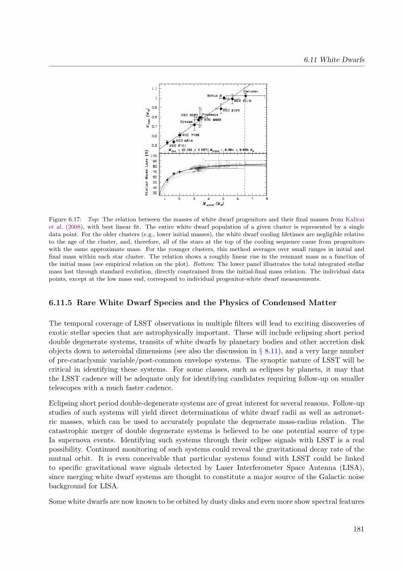
6.11 White Dwarfs
Figure 6.17: Top: The relation between the masses of white dwarf progenitors and their final masses from Kaliraiet al. (2008), with best linear fit. The entire white dwarf population of a given cluster is represented by a singledata point. For the older clusters (e.g., lower initial masses), the white dwarf cooling lifetimes are negligible relativeto the age of the cluster, and, therefore, all of the stars at the top of the cooling sequence came from progenitorswith the same approximate mass. For the younger clusters, this method averages over small ranges in initial andfinal mass within each star cluster. The relation shows a roughly linear rise in the remnant mass as a function ofthe initial mass (see empirical relation on the plot). Bottom: The lower panel illustrates the total integrated stellarmass lost through standard evolution, directly constrained from the initial-final mass relation. The individual datapoints, except at the low mass end, correspond to individual progenitor-white dwarf measurements.
6.11.5 Rare White Dwarf Species and the Physics of Condensed Matter
The temporal coverage of LSST observations in multiple filters will lead to exciting discoveries ofexotic stellar species that are astrophysically important. These will include eclipsing short perioddouble degenerate systems, transits of white dwarfs by planetary bodies and other accretion diskobjects down to asteroidal dimensions (see also the discussion in § 8.11), and a very large numberof pre-cataclysmic variable/post-common envelope systems. The synoptic nature of LSST will becritical in identifying these systems. For some classes, such as eclipses by planets, it may thatthe LSST cadence will be adequate only for identifying candidates requiring follow-up on smallertelescopes with a much faster cadence.
Eclipsing short period double-degenerate systems are of great interest for several reasons. Follow-upstudies of such systems will yield direct determinations of white dwarf radii as well as astromet-ric masses, which can be used to accurately populate the degenerate mass-radius relation. Thecatastrophic merger of double degenerate systems is believed to be one potential source of typeIa supernova events. Identifying such systems through their eclipse signals with LSST is a realpossibility. Continued monitoring of such systems could reveal the gravitational decay rate of themutual orbit. It is even conceivable that particular systems found with LSST could be linkedto specific gravitational wave signals detected by Laser Interferometer Space Antenna (LISA),since merging white dwarf systems are thought to constitute a major source of the Galactic noisebackground for LISA.
Some white dwarfs are now known to be orbited by dusty disks and even more show spectral features
181

Chapter 6: Stellar Populations
of heavy elements (Si, Mg, Ca, Fe, and so on), which quickly settle out of the atmosphere indicatingon-going accretion. In both cases the source of the dust is believed to be collisions of asteroidalbodies in tight orbits around the white dwarf. Because white dwarfs have small diameters, it isquite possible that favorable orbital plane orientations will reveal transits of substantial bodiesfrom the size of massive Jupiters to asteroids having diameters of tens of km. The gravitationalperturbations of such massive bodies are thought to play a role in promoting asteroidal collisionsand in maintaining any dusty ring structures that result.
Finally, it should be possible to identify a large number of pre-cataclysmic variable and post-common envelope systems. In general, eclipses (although helpful) are not even necessary sincereflection effects produced by the hot white dwarf on the low mass secondary are a frequentsignature of these sources. Having a large number of such systems to study will help map out thespectrum of stellar masses and orbital separations that constitute the end states of post-commonenvelope evolution.
With large numbers of detected white dwarfs, LSST can select those that are variable to the limitof LSST’s photometric precision (∼ 1%), and therefore identify new candidate pulsating whitedwarfs. Follow-up time-series photometry of these candidates on other telescopes will lead to asubstantial number of new white dwarf pulsators, and, therefore, provide a more accurate mappingof the boundaries of the known white dwarf instability strips for pulsation (DAV - H, DBV - He,PG1159 - C) in the HR diagram and in log g vs Teff , and also allow exploration to search forpreviously unknown instability strips along the white dwarf cooling sequence. A more detaileddiscussion of LSST’s connection to pulsating white dwarfs is provided in § 8.7.2.
LSST will provide a new test for the internal physics of white dwarf stars. The low luminosityend of the white dwarf luminosity functions (WDLF), log(L/L�) < −3, contains informationabout the equation of state of condensed (degenerate) matter. The shape of the disk WDLFat the turnover (discussed in § 6.11.1) due to the disk’s finite age is affected by the release oflatent heat of crystallization of the carbon-oxygen white dwarf core. The release of latent heatprovides an energy source in an otherwise dead star and slows the white dwarf cooling process.This slowdown manifests itself as an increase in number density of white dwarfs over the luminosityrange corresponding to the crystallization event. Even more intriguing is the possibility of havinga halo WDLF that is sufficiently populated that we can fully resolve the crystallization bump.LSST’s large white dwarf sample will determine if the crystallization bump is indeed present,and if so, at what luminosity (i.e., age), providing new constraints on the equation of state forcarbon-oxygen white dwarfs.
6.11.6 The LSST White Dwarf Model Sample
In the following sections we calculate the expected distributions of white dwarfs that LSST willsee. The main purpose of these simulations is to estimate the accuracy LSST will obtain incalibrating the white dwarf photometric parallax relation, kinematically separating the disk andhalo populations, and measuring their luminosity functions.
In order to generate a simulated sample of disk and halo white dwarfs, five sets of quantities needto be adopted:
182

6.11 White Dwarfs
1. The expected astrometric and photometric measurement errors.
2. The spatial distribution for each Galaxy component.
3. The distributions of three velocity components.
4. The bolometric luminosity functions.
5. The mapping from bolometric luminosity to broad-band luminosity in each LSST bandpass.
The astrometric and photometric measurement errors are computed as described in Chapter 3.We proceed with detailed descriptions of the remaining quantities.
The Spatial Distribution
LSST will detect white dwarfs to distances much larger than the scale heights and lengths of theGalactic disk. Hence the spatial variation of volume density in the Galaxy must be taken intoaccount. We assume that the spatial distribution of white dwarfs traces the distribution of mainsequence stars, both for halo and disk populations (the impact of their different ages is handledthrough adopted luminosity functions). We ignore bulge white dwarfs in the simulations as theyrepresent only a small fraction of the population. The adopted spatial distribution of main sequencestars, based on recent SDSS-based work by Juric et al. (2008) is described in § 3.7.1.
The Kinematic Distributions
We assume that the kinematics (distributions of three velocity components) of white dwarfs are thesame as the corresponding distribution of main sequence stars, both for halo and disk populations.The adopted kinematic distribution of main sequence stars is based on recent SDSS-based workby Ivezic et al. (2008a).
The White Dwarf Luminosity Function
For disk stars, we adopt the measured luminosity function based on SDSS data (Harris et al. 2006).Using their Figure 4, we obtained the following parameters for a power-law approximation to themeasured bolometric Φ (the number of white dwarfs per cubic parsec and magnitude),
log Φ = −2.65 + 0.26 (Mbol − 15.3) for 7 < Mbol < 15.3log Φ = −2.65− 1.70 (Mbol − 15.3) for 15.3 < Mbol < 17.0, (6.1)
which agrees with the data to within 10% at the faint end. The observational knowledge of thehalo white dwarf luminosity function is much poorer. Theoretical predictions (Torres et al. 2005,and references therein) indicate an overall shift of the halo luminosity distribution toward fainterabsolute magnitudes due to its larger age compared to the disk. Motivated by these predictionsand the desire to test the ability to distinguish different luminosity functions when analyzing thesimulated sample, we simply shift the Harris et al. (2006) luminosity function by 0.7 mag towardthe faint end.
183

Chapter 6: Stellar Populations
Figure 6.18: Simulated differential luminosity function for candidate hydrogen white dwarfs in the disk sample(normalized to solar neighborhood). The dots with error bars show the result obtained by binning the cumulativeluminosity function computed using Lynden-Bell’s C− method in 0.1 mag wide Mr bins (based on ∼ 200,000 stars).The red line shows the input luminosity function in the simulation. Note the “feature” in the input luminosityfunction at Mr = 11.8.
We re-express the luminosity function per unit Mr magnitude, Φr by multiplying by dMbol/dMr,determined from the spectral energy distribution, described below. The resulting luminosity func-tions for disk and halo white dwarfs are shown in Figures 6.18 and 6.19, respectively. The integralof the adopted disk luminosity function is 0.0043 stars pc−3 (about 1/10 of the integrated luminos-ity function for main sequence stars). The disk luminosity function reaches its maximum aroundMr = 15.4, and the halo luminosity function at Mr = 16. Both luminosity functions show a ∼ 0.2mag wide and 20-30% strong “feature” at Mr ∼ 11.8 which is due to the behavior of dMbol/dMr.
We assume that 90% of all white dwarfs are hydrogen (DA) white dwarfs and the rest are helium(DB) white dwarfs, but assumed the same luminosity function for both.
The White Dwarf Spectral Energy Distribution
We use models by Bergeron et al. (1995), which produce color tracks that agree with SDSS mea-surements at the ∼0.02 mag level (Eisenstein et al. 2006). Using a sample of ∼ 10,000 white dwarfswith SDSS spectroscopic data, Eisenstein et al. (2006) found a very narrow distribution (0.1 dex)of log g centered on log g = 7.9. Motivated by this result and the desire to simplify analysis of thesimulated sample, we adopt a fixed value of log g = 8.0 (Bergeron’s models are computed with alog g step of 0.5 dex). Hence, for a given type of white dwarf atmosphere (hydrogen vs. helium),the models provide unique relationships between Mr and all relevant colors (including bolometriccorrections). For hydrogen white dwarfs with log g = 8.0, Mr = 15.4 corresponds to an effective
184

6.11 White Dwarfs
Figure 6.19: Similar to Figure 6.18, now showing the luminosity function for the candidate halo sample.
temperature of 4500 K, mass of 0.58 M� and age of 7.6 Gyr. For Mr = 16, the effective tempera-ture is 3900 K, the mass is unchanged and the age is 9.3 Gyr. A 13 Gyr old hydrogen white dwarf,according to Bergeron’s models, would have Mr = 17.4 and an effective temperature of 2250 K.
Preliminary Analysis of the Simulated White Dwarf Sample
The simulated sample includes ∼ 35 million objects with r < 24.5 over the whole sky. Herewe briefly describe the expected counts of white dwarfs in the main (deep-wide-fast, DWF; see§ 2.1) LSST survey, discuss how objects with good trigonometric parallax measurements can beused to derive an empirical photometric parallax relation, and how this relation can be used withproper motion measurements to separate disk and halo candidates. We conclude with preliminaryestimates of the accuracy of disk and halo white dwarf luminosity function measurements.
Counts of Simulated White Dwarfs
The main DWF LSST survey is expected to deliver about 1000 visits (summed over all bands) overa ∼ 20,000 deg2 area, and without including the Galactic plane. Figure 6.20 compares cumulativewhite dwarf counts for several samples. The simulations predict that Gaia’s all-sky survey willdetect about 240,000 white dwarfs with r < 20. Of those, about 1,200 will be halo white dwarfs.These counts are in fair agreement with the results of Torres et al. (2005) who simulated Gaia’sperformance on white dwarfs. We have also compared the simulated counts to photometricallyselected white dwarf candidates from SDSS (see bottom left panel in Fig. 24 of Ivezic et al. 2007).We selected 355 white dwarf candidates over 203 deg2 defined by 330◦ < α < 50◦ and |δ| < 1.267◦;
185
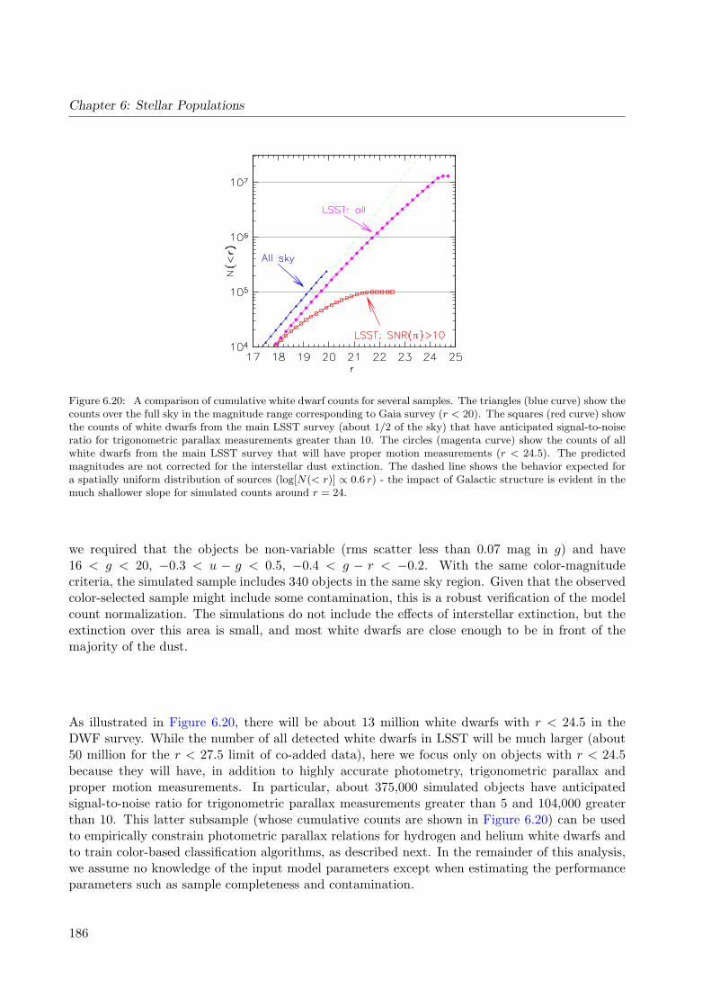
Chapter 6: Stellar Populations
Figure 6.20: A comparison of cumulative white dwarf counts for several samples. The triangles (blue curve) show thecounts over the full sky in the magnitude range corresponding to Gaia survey (r < 20). The squares (red curve) showthe counts of white dwarfs from the main LSST survey (about 1/2 of the sky) that have anticipated signal-to-noiseratio for trigonometric parallax measurements greater than 10. The circles (magenta curve) show the counts of allwhite dwarfs from the main LSST survey that will have proper motion measurements (r < 24.5). The predictedmagnitudes are not corrected for the interstellar dust extinction. The dashed line shows the behavior expected fora spatially uniform distribution of sources (log[N(< r)] ∝ 0.6 r) - the impact of Galactic structure is evident in themuch shallower slope for simulated counts around r = 24.
we required that the objects be non-variable (rms scatter less than 0.07 mag in g) and have16 < g < 20, −0.3 < u − g < 0.5, −0.4 < g − r < −0.2. With the same color-magnitudecriteria, the simulated sample includes 340 objects in the same sky region. Given that the observedcolor-selected sample might include some contamination, this is a robust verification of the modelcount normalization. The simulations do not include the effects of interstellar extinction, but theextinction over this area is small, and most white dwarfs are close enough to be in front of themajority of the dust.
As illustrated in Figure 6.20, there will be about 13 million white dwarfs with r < 24.5 in theDWF survey. While the number of all detected white dwarfs in LSST will be much larger (about50 million for the r < 27.5 limit of co-added data), here we focus only on objects with r < 24.5because they will have, in addition to highly accurate photometry, trigonometric parallax andproper motion measurements. In particular, about 375,000 simulated objects have anticipatedsignal-to-noise ratio for trigonometric parallax measurements greater than 5 and 104,000 greaterthan 10. This latter subsample (whose cumulative counts are shown in Figure 6.20) can be usedto empirically constrain photometric parallax relations for hydrogen and helium white dwarfs andto train color-based classification algorithms, as described next. In the remainder of this analysis,we assume no knowledge of the input model parameters except when estimating the performanceparameters such as sample completeness and contamination.
186

6.11 White Dwarfs
Figure 6.21: The calibration of the photometric parallax relation, Mr(g − r), for white dwarfs. The Mr values arebased on trigonometric parallax and “measured” r band magnitudes. The dots represent ∼ 100,000 simulated objectswith the signal-to-noise ratio for trigonometric parallax measurements greater than 10. The middle dashed line isthe color-magnitude separator described in the text. The other two lines are the median Mr vs. g − r photometricparallax sequences. The true relations used to generate the simulated sample are indistinguishable (rms ∼ 0.01 mag)from these empirically determined median values.
White Dwarf Photometric Parallax Relations
The distribution of the difference between trigonometric and true distance moduli for the 104,000white dwarfs with parallax S/N> 10 is close to Gaussian, with a median value of −0.03 mag andan rms scatter of 0.15 mag. For the subset of 10,000 objects with r < 18, the rms scatter is 0.10mag and the bias is below 0.01 mag.
The absolute magnitude based on “measured” trigonometric parallax as a function of “measured”g − r color is shown in Figure 6.21. The two sequences that correspond to hydrogen and heliumwhite dwarfs are easily discernible. A simple separator of hydrogen and helium color-magnitudesequences is obtained by shifting the median Mr vs. g − r curve for hydrogen white dwarfs by0.4 mag towards the bright end. A slightly better choice would be to account for the shape ofthe helium sequence as well. The application of this separator results in correct classification for99.6% of the objects in the candidate hydrogen sample and for 96.3% of the objects in the candidatehelium sample.
Photometric Separation of Hydrogen and Helium White Dwarfs
The separation of hydrogen and helium white dwarfs based on the Mr vs. g−r diagram is possibleonly for objects with high S/N trigonometric parallax measurements. Since such objects representonly about 1% of the full r < 24.5 LSST white dwarf sample, a color separation method is requiredto classify the latter sample. Although helium white dwarfs represent only 10% of all objects, the
187

Chapter 6: Stellar Populations
Figure 6.22: The distribution of the simulated white dwarfs in the g− r vs. u− g color-color diagram. Black pointsshow objects with r < 24.5 and b > 60◦. Yellow points show a subsample of predominantly brighter sources thathave 10σ or better “measurement” of the trigonometric parallax. The two sequences correspond to He and H whitedwarfs. The distribution of low-redshift (z < 2.2) quasars observed by SDSS is shown by blue contours. The bluepart of the stellar locus (dominated by F and G stars), as observed by SDSS, is shown by the red contours. LSSTphotometry will be sufficiently accurate not only to separate white dwarfs from quasars and main sequence stars,but also to separate hydrogen from helium white dwarfs (the sequences do not overlap in the multi-dimensional colorspace, see text).
differences in Mr vs. g−r relations between helium and hydrogen white dwarfs might significantlybias the luminosity function determination.
We use the two candidate samples with good trigonometric parallax measurements to quantifytheir multi-dimensional color tracks. Figure 6.22 shows the two-dimensional projection of thesetracks. At the hot end, the tracks for hydrogen and helium objects are well separated. Althoughthey appear to cross around g−r = 0.2, they are still separated in the four-dimensional color spacespanned by the u− g, g − r, r − i and i− z colors3.
For each sample, we compute the median u − g, r − i and i − z color for each 0.01 mag wide binof g − r color. Using these tracks, for each star we compute the shortest distance to each locus,denoted here DHe and DH . The difference between these two four-dimensional color distances(4DCD) can be used as a simple color-based classifier. For the training sample, which has smallphotometric errors due to the relatively bright flux limit imposed by requiring high trigonometricparallax signal-to-noise ratio, the separation is essentially perfect (mis-classification rate, or samplecontamination, is less than 1%).
We assess the performance of color separation at the faint end by resorting to true input class,and study the completeness and contamination of candidate samples as a function of δ4DCD =
3Reliable colors are not yet available for the y band so we do not consider it here.
188

6.11 White Dwarfs
Figure 6.23: The completeness and contamination for color-selected subsamples of hydrogen and helium white dwarfs,as a function of the difference between distances to each four-dimensional color sequence (δ4DCD = DHe − DH).The solid lines show completeness and dashed lines show contamination. The blue lines correspond to hydrogensubsample, and red lines to helium subsample. Objects are classified as helium white dwarfs if their δ4DCD is smallerthan the adopted cut-off value. The panel shows a flux-limited sample with r < 23.5.
DHe − DH (see Figure 6.23). The optimal value of δ4DCD for separating two object types isa trade-off and depends on whether a particular science case requires high completeness or lowcontamination. Typically the best δ4DCD value is not zero because hydrogen white dwarfs areten times as numerous as helium white dwarfs. These effects can be elegantly treated using theBayesian formalism developed by Mortlock et al. (2008), hereafter MPI08. Here we follow asimpler approach and, informed by the results shown in Figure 6.23, adopt δ4DCD = −0.05 forthe rest of the analysis presented here. For r < 23.5, the candidate helium sample completenessand contamination are 79% and 0.2%, respectively (see the right panel in Figure 6.23). Wherer < 24.5, the completeness of 99% with a contamination of 3% for the candidate hydrogen sample,and 73% and 14%, respectively, for the candidate helium sample, the degraded but still remarkableperformance being attributed to larger photometric errors.
We note that despite high completeness for the helium subsample, there are ranges of Mr, such asMr ∼ 12.5, where it is sufficiently small to induce large systematic errors in luminosity function.To properly treat the helium subsample, a more sophisticated method, such as that described byMPI08, is required. Nevertheless, the simplistic δ4DCD method used here produces sufficientlyclean samples of candidate hydrogen white dwarfs for further analysis.
189

Chapter 6: Stellar Populations
Figure 6.24: The dependence of tangential velocity on apparent magnitude for white dwarfs with b > 60◦. Themap shows counts of stars in each bin on logarithmic scale, increasing from blue to red. The tangential velocity iscomputed from each star’s measured proper motion and distance estimate from the photometric parallax relationshown in Figure 6.21. At faint magnitudes (r > 22), the sample contains a large fraction of halo white dwarfs. Thehorizontal line at 180 km s−1 separates disk and halo stars with sample completeness and contamination of 99% and3%, respectively, for disk stars, and 78% and 6%, respectively, for halo stars.
Kinematic Separation of Disk and Halo White Dwarfs
The measured proper motion and distance estimate can be used to probabilistically assign diskor halo membership, if suitable kinematic models exist, for an arbitrary direction on the sky. Inthe general case, the observed proper motion depends on a linear combination of all three velocitycomponents, and the probabilistic class assignment can be computed following the approach out-lined in MPI08 (the standard method for separating disk and halo stars based on reduced propermotion diagram will fail at kpc distances probed by LSST, see Appendix B in Sesar et al. 2008).In this preliminary analysis, we limit our sample to the region with b < −60◦, where proper motionprimarily depends on radial, vR, and azimuthal (rotational), vφ, components, while the verticalvelocity component, vZ , is by and large absorbed into the radial (along the line of sight) velocitycomponent.
From ∼ 273,000 simulated objects with r < 24.5 and b < −60◦ (2,680 deg2), we select ∼ 250,000candidate hydrogen white dwarfs using the color-based classification described above. We deter-mine their distances using a photometric parallax relation, and compute the absolute value of theirtangential velocity, vtan. The distribution of vtan as a function of measured apparent r band mag-nitude for this sample is shown in Figure 6.24. The median difference between the “measured” andtrue vtan is 3 km s−1, and ranges from 1 km s−1 at distances smaller than 400 pc, to 30 km s−1 ata distance of 5 kpc.
The vtan distribution is clearly bimodal, with high vtan stars corresponding to the halo sample.Notably a significant fraction of halo white dwarfs is seen only at r > 22. Just as in the case ofcolor separation of the hydrogen and helium sequences, the optimal separation of disk and halo
190

6.11 White Dwarfs
Figure 6.25: The completeness and contamination of candidate disk and halo subsamples selected by tangentialvelocity. The solid lines show completeness and dashed lines show contamination. The blue lines correspond to halosubsample, and red lines to disk subsample. Objects are classified as disk candidates if their tangential velocity issmaller than the adopted cut-off value.
candidates by vtan includes a trade-off between completeness and contamination, as illustrated inFigure 6.25.
Informed by Figure 6.25, we select ∼ 195,000 candidate disk members by requiring vtan < 100km s−1, and ∼ 19,000 candidate halo members by requiring vtan > 200 km s−1. These samplesare optimized for low contamination: the sample contamination for halo candidates is 3.5% and0.5% for disk candidates. The sample completeness is 70% for the halo sample and 87% for thedisk sample. We proceed to determine the luminosity function for these two samples.
Determination of Disk and Halo White Dwarf Luminosity Functions
There are many different methods for estimating a luminosity function from data (e.g., Kellyet al. 2008, and references therein). In the case of uncorrelated variables (the luminosity functionis independent of position once disk and halo candidates are separated. With real data thisassumption can be tested, e.g., Fan et al. 2001). One of the best methods is the C− method(Lynden-Bell 1971), because it requires binning in only one coordinate. We used the C− methodto determine the luminosity functions shown in Figures 6.18 and 6.19.
Although the sample analyzed here (b < −60◦) includes only about 10% of the total DWF area(and ∼2% of the white dwarf counts for the entire LSST sample), the random (statistical) errorsfor both disk and halo luminosity functions are negligible. The dominant systematic errors (withan rms scatter of about 10%) are due to errors in the photometric parallax relation: when the trueMr values are used, the C− method reproduces the input luminosity function essentially perfectly.
191

Chapter 6: Stellar Populations
This nearly perfect agreement also demonstrates that the hydrogen vs. helium separation, anddisk vs. halo separation algorithms have satisfactory performance. Most importantly, the faintend of the luminosity functions for both disk and halo samples is correctly reproduced to within0.1-0.2 mag.
6.12 A Comparison of Gaia and LSST Surveys
Laurent Eyer, Zeljko Ivezic, David Monet
In this section, we compare the design predictions for the astrometric and photometric perfor-mance of the Gaia mission and the LSST system. For Gaia’s performance, we have collected andparametrized predictions from various technical documents, and discussed the adopted model withGaia key technical personnel. For LSST performance, we adopted parameters listed in Chapter 1.While the various adopted errors are probably accurate to much better than a factor of two for bothGaia and LSST, their ultimate values cannot be more precisely known before their data productsare delivered.
6.12.1 Photometric Errors
To determine photometric errors for Gaia and LSST, we follow the discussion in § 3.5. For Gaia, weadopt σsys = 0.001 mag and σsys = 0.0005 mag for single transit and the end-of-mission values inthe G band, respectively. For LSST, we adopt σsys = 0.003 mag. We model random photometricerrors (per transit) for Gaia as
σrand = 0.02× 100.2(G−20) (mag), (6.2)
where G is the Gaia’s broad-band magnitude4. We described the model for LSST’s photometricerrors in Equation 3.2.
The behavior of photometric errors as a function of r band magnitude for Gaia, LSST and SDSSis illustrated in the top panel in Figure 6.26 (for SDSS, we used Equation 3.2 and m5 = 22.1 inthe r band).
6.12.2 Trigonometric Parallax and Proper Motion Errors
Similarly to our treatment of photometric errors, we add systematic and random astrometric errorsin quadrature(see Equation 3.1). For Gaia, we set a systematic trigonometric parallax error of 0.007mas, and model the random errors as
σπrand = 0.30× 100.22(G−20) (mas). (6.3)
4More elaborate models have been produced, for example by C. Jordi; however, for our purpose this simplifiedmodel is a sufficiently accurate approximation.
192

6.12 A Comparison of Gaia and LSST Surveys
We obtain proper motion errors (per coordinate) by multiplying trigonometric parallax errors by0.66 yr−1. We compute LSST trigonometric parallax and proper motion errors using identicalexpressions with performance parameters listed in Table 3.3.
The behavior of trigonometric parallax and proper motion errors as function of r band magnitudefor Gaia and LSST is illustrated in the bottom two panels in Figure 6.26. For comparison, we alsoshow proper motion error behavior for the current state-of-the-art large-area database constructedby Munn et al. (2004) using SDSS and Palomar Observatory Sky Survey data (a baseline of 50years). Following Bond et al. (2009), the SDSS-POSS proper motion errors (per coordinate) aremodeled as
σµSDSS−POSS = 2.7 + 2.0× 100.4(r−20) (mas/yr). (6.4)
(Compare with Table 3.3 to see how much better LSST will do.) All adopted performance param-eters for LSST and Gaia are summarized in Table 6.6.
6.12.3 Implications for Science Projects
Gaia will provide an all-sky map with exquisite trigonometric parallax, proper motion and photo-metric measurements to r ∼ 20 for about billion stars. LSST will extend this map to r ∼ 27 overhalf of the sky, and detect about 10 billion stars. Due to Gaia’s superb astrometric and photometricmeasurements, and LSST’s significantly deeper data, the two surveys are highly complementary:Gaia will map the Milky Way’s disk with unprecedented detail, and LSST will extend this map allthe way to the halo edge.
For example, stars just below the main sequence turn-off with Mr = 4.5 will be detected by Gaiato a distance limit of ∼10 kpc (r < 20), and to ∼100 kpc with LSST’s single-epoch data (r < 24.5).Ivezic et al. (2008b) estimated that LSST will obtain metallicity measurements accurate to 0.2 dexor better, with proper motion measurements accurate to ∼0.2 mas/yr or better, for about 200million F/G dwarf stars within 100 kpc. For intrinsically faint stars, such as late M dwarfs, L/Tdwarfs, and white dwarfs, the deeper limit of LSST will enable detection and characterization ofhalo populations. A star with Mr = 15 will be detectable to a distance limit of 100 pc with Gaiaand ∼800 pc with LSST, and hence LSST samples will be about 100 times larger. For a substantialfraction of red stars with r > 20, LSST will provide trigonometric parallax measurements accurateto better than 10% (see Figure 3.13). In summary, LSST will represent a deep complement toGaia.
193

Chapter 6: Stellar Populations
Figure 6.26: A comparison of photometric, proper motion and parallax errors for SDSS, Gaia and LSST, as a functionof apparent magnitude r, for a G2V star (we assumed r = G, where G is the Gaia’s broad-band magnitude). Inthe top panel, the curve marked “SDSS” corresponds to a single SDSS observation. The red curves correspond toGaia; the long-dashed curve shows a single transit accuracy, and the dot-dashed curve the end of mission accuracy(assuming 70 transits). The blue curves correspond to LSST; the solid curve shows a single visit accuracy, andthe short-dashed curve shows accuracy for co-added data (assuming 230 visits in the r band). The curve marked“SDSS-POSS” in the middle panel shows accuracy delivered by the proper motion catalog of Munn et al. (2004).In the middle and bottom panels, the long-dashed curves correspond to Gaia, and the solid curves to LSST. Notethat LSST will smoothly extend Gaia’s error vs. magnitude curves four magnitudes fainter. The assumptions usedin these computations are described in the text.
194

6.12 A Comparison of Gaia and LSST Surveys
Table 6.6: Adopted Gaia and LSST Performance
Quantity Gaia LSST
Sky Coverage whole sky half sky
Mean number of epochs 70 over 5 yrs 1000 over 10 yrs
Mean number of observations 320a over 5 yrs 1000b over 10 yrs
Wavelength Coverage 320–1050 nm ugrizy
Depth per visit (5σ, r band) 20 24.5; 27.5c
Bright limit (r band) 6 16-17
Point Spread Function (arcsec) 0.14×0.4 0.70 FWHM
Pixel count (Gigapix) 1.0 3.2
Syst. Photometric Err. (mag) 0.001, 0.0005d 0.005, 0.003e
Syst. Parallax Err. (mas) 0.007f 0.40f
Syst. Prop. Mot. Err. (mas/yr) 0.004 0.14a One transit includes the G-band photometry (data collected over 9 CCDs), BP and RP spec-trophotometry, and measurements by the SkyMapper and RVS instruments.b Summed over all six bands (taken at different times).c For co-added data, assuming 230 visits.d Single transit and the end-of-mission values for the G band (from SkyMapper; integrated BPand RP photometry will be more than about 3 times less precise).e For single visit and co-added observations, respectively.f Astrometric errors depend on source color. The listed values correspond to a G2V star.
195

Chapter 6: References
References
Alcock, C. et al., 1995, AJ , 109, 1653—, 2000, ApJ , 542, 281Barnes, S. A., 2003, ApJ , 586, 464Barry, D. C., 1988, ApJ , 334, 436Beers, T. C., & Christlieb, N., 2005, ARAA, 43, 531Beers, T. C., Lee, Y. S., Peruta, C., Sivarani, T., Allende Prieto, C., Aoki, W., Carollo, D., & SDSS, 2009, American
Astronomical Society Meeting Abstracts, Vol. 213, The Lowest Metallicity Stars from SDSS/SEGUE. p. 416Belokurov, V. et al., 2006, ApJL, 642, L137Berger, E. et al., 2001, Nature, 410, 338Bergeron, P., Liebert, J., & Fulbright, M. S., 1995, ApJ , 444, 810Besla, G., Kallivayalil, N., Hernquist, L., van der Marel, R. P., Cox, T. J., Robertson, B., & Alcock, C., 2009, in
IAU Symposium, Vol. 256, The binarity of the Clouds and the formation of the Magellanic Stream, pp. 99–104Binney, J., 2001, in Astronomical Society of the Pacific Conference Series, Vol. 240, Gas and Galaxy Evolution, J. E.
Hibbard, M. Rupen, & J. H. van Gorkom, eds., p. 355Bochanski, J. J., West, A. A., Hawley, S. L., & Covey, K. R., 2007, AJ , 133, 531Boeshaar, P. C., Margoniner, V., & The Deep Lens Survey Team, 2003, in IAU Symposium, Vol. 211, Brown Dwarfs,
E. Martın, ed., p. 203Bond, N. A., Ivezic, Z., Sesar, B., Juric, M., & Munn, J., 2009, ArXiv e-prints, 0909.0013Bouy, H., Brandner, W., Martın, E. L., Delfosse, X., Allard, F., & Basri, G., 2003, AJ , 126, 1526Bruzual, G., & Charlot, S., 2003, MNRAS , 344, 1000Burgasser, A. J. et al., 2003a, ApJ , 592, 1186Burgasser, A. J., Kirkpatrick, J. D., Liebert, J., & Burrows, A., 2003b, ApJ , 594, 510Burgasser, A. J., Lepine, S., Lodieu, N., Scholz, R. D., Delorme, P., Jao, W. C., Swift, B. J., & Cushing, M. C.,
2008, Proc. of the 15th Cambridge Workshop on Cool Stars, Stellar Systems, and the Sun, in prep., arXiv:astro-ph/0810.0569
Burgasser, A. J., Liebert, J., Kirkpatrick, J. D., & Gizis, J. E., 2002, AJ , 123, 2744Burgasser, A. J., Reid, I. N., Siegler, N., Close, L., Allen, P., Lowrance, P., & Gizis, J., 2007, in Protostars and
Planets V, B. Reipurth, D. Jewitt, & K. Keil, eds., pp. 427–441Burrows, A., Hubbard, W. B., Saumon, D., & Lunine, J. I., 1993, ApJ , 406, 158Burrows, A., Sudarsky, D., & Hubeny, I., 2006, ApJ , 640, 1063Burrows, A., Sudarsky, D., & Lunine, J. I., 2003, ApJ , 596, 587Carollo, D. et al., 2007, Nature, 450, 1020Catelan, M., Stephens, A. W., & Contreras, R. P., 2005, American Astronomical Society Meeting Abstracts, 207,
128.11Caulet, A., Gruendl, R. A., & Chu, Y.-H., 2008, ApJ , 678, 200Chaboyer, B., 2000, in Liege International Astrophysical Colloquia, Vol. 35, Liege International Astrophysical Col-
loquia, A. Noels, P. Magain, D. Caro, E. Jehin, G. Parmentier, & A. A. Thoul, eds., p. 451Chen, C.-H. R., Chu, Y.-H., Gruendl, R. A., Gordon, K. D., & Heitsch, F., 2009, ApJ , 695, 511Cignoni, M., Degl’Innocenti, S., Prada Moroni, P. G., & Shore, S. N., 2006, A&A, 459, 783Clement, C. M. et al., 2001, AJ , 122, 2587Coleman, G. D., Wu, C.-C., & Weedman, D. W., 1980, ApJS , 43, 393Cruz, K. L. et al., 2007, AJ , 133, 439Cushing, M. C., Looper, D., Burgasser, A. J., Kirkpatrick, J. D., Faherty, J., Cruz, K. L., Sweet, A., & Sanderson,
R. E., 2009, ApJ , 696, 986Cushing, M. C., Rayner, J. T., & Vacca, W. D., 2005, ApJ , 623, 1115D’Antona, F., 2002, in IAU Symposium, Vol. 207, Extragalactic Star Clusters, D. P. Geisler, E. K. Grebel, &
D. Minniti, eds., p. 599de la Fuente Marcos, R., & de la Fuente Marcos, C., 2004, New Astronomy, 9, 475DeGennaro, S. et al., 2009, in prep.Demory, B. et al., 2009, ArXiv e-prints, 0906.0602Digby, A. P., Hambly, N. C., Cooke, J. A., Reid, I. N., & Cannon, R. D., 2003, MNRAS , 344, 583Dohm-Palmer, R. C., Skillman, E. D., Mateo, M., Saha, A., Dolphin, A., Tolstoy, E., Gallagher, J. S., & Cole, A. A.,
2002, AJ , 123, 813
196

Chapter 6: References
Dolphin, A. E., 2002a, in Astronomical Society of the Pacific Conference Series, Vol. 274, Observed HR Diagramsand Stellar Evolution, T. Lejeune & J. Fernandes, eds., p. 503
—, 2002b, MNRAS , 332, 91Duquennoy, A., & Mayor, M., 1991, A&A, 248, 485Eisenstein, D. J. et al., 2006, ApJS , 167, 40Fan, X. et al., 2001, AJ , 121, 54Fischer, D. A., & Marcy, G. W., 1992, ApJ , 396, 178Freeman, K., & Bland-Hawthorn, J., 2002, ARAA, 40, 487Fuchs, B., Jahreiß, H., & Flynn, C., 2009, AJ , 137, 266Fukui, Y. et al., 2008, ApJS , 178, 56Girardi, L., Bertelli, G., Bressan, A., Chiosi, C., Groenewegen, M. A. T., Marigo, P., Salasnich, B., & Weiss, A.,
2002, A&A, 391, 195Girardi, L., Bressan, A., Bertelli, G., & Chiosi, C., 2000, A&A, 141, 371Gizis, J. E., Monet, D. G., Reid, I. N., Kirkpatrick, J. D., Liebert, J., & Williams, R. J., 2000, AJ , 120, 1085Gizis, J. E., Reid, I. N., & Hawley, S. L., 2002, AJ , 123, 3356Gouliermis, D., Brandner, W., & Henning, T., 2006a, ApJ , 641, 838—, 2006b, ApJL, 636, L133Gouliermis, D. A., Henning, T., Brandner, W., Dolphin, A. E., Rosa, M., & Brandl, B., 2007, ApJL, 665, L27Grether, D., & Lineweaver, C. H., 2006, ApJ , 640, 1051Grillmair, C. J., 2006, ApJL, 645, L37Gruendl, R. A., & Chu, Y.-H., 2009, ArXiv e-prints, 0908.0347Habing, H. J., 1996, A&AS , 7, 97Hall, P. B., 2002, ApJL, 580, L77Hansen, B. M. S. et al., 2007, ApJ , 671, 380—, 2002, ApJL, 574, L155Harris, H. C. et al., 2006, AJ , 131, 571Hartman, J. D. et al., 2009, ApJ , 691, 342Hawley, S. L., Reid, I. N., & Tourtellot, J. G., 2000, in Very Low-mass Stars and Brown Dwarfs, Cambridge University
Press, UK, R. Rebolo & M. R. Zapatero-Osorio, eds., p. 109Helmi, A., & White, S. D. M., 1999, MNRAS , 307, 495Hertzsprung, E., 1905, Zeitschrift fur Wissenschaftliche Photographie, 3, 442Hewett, P. C., Warren, S. J., Leggett, S. K., & Hodgkin, S. T., 2006, MNRAS , 367, 454Horne, J. H., & Baliunas, S. L., 1986, ApJ , 302, 757Hurley, J. R. et al., 2008, AJ , 135, 2129Ibata, R. A., Gilmore, G., & Irwin, M. J., 1994, Nature, 370, 194Ivezic, Z. et al., 2008a, ApJ , 684, 287—, 2007, AJ , 134, 973—, 2008b, ArXiv e-prints, 0805.2366Juric, M. et al., 2008, ApJ , 673, 864Kalirai, J. S., Bergeron, P., Hansen, B. M. S., Kelson, D. D., Reitzel, D. B., Rich, R. M., & Richer, H. B., 2007,
ApJ , 671, 748Kalirai, J. S., Hansen, B. M. S., Kelson, D. D., Reitzel, D. B., Rich, R. M., & Richer, H. B., 2008, ApJ , 676, 594Kalirai, J. S. et al., 2001a, AJ , 122, 257Kalirai, J. S., & Tosi, M., 2004, MNRAS , 351, 649Kalirai, J. S., Ventura, P., Richer, H. B., Fahlman, G. G., Durrell, P. R., D’Antona, F., & Marconi, G., 2001b, AJ ,
122, 3239Kallivayalil, N., van der Marel, R. P., & Alcock, C., 2006a, ApJ , 652, 1213Kallivayalil, N., van der Marel, R. P., Alcock, C., Axelrod, T., Cook, K. H., Drake, A. J., & Geha, M., 2006b, ApJ ,
638, 772Kanbur, S. M., & Fernando, I., 2005, MNRAS , 359, L15Keller, S. C. et al., 2007, Publications of the Astronomical Society of Australia, 24, 1Kelly, B. C., Fan, X., & Vestergaard, M., 2008, ApJ , 682, 874Kennicutt, Jr., R. C., & Hodge, P. W., 1986, ApJ , 306, 130Kim, S., Staveley-Smith, L., Dopita, M. A., Sault, R. J., Freeman, K. C., Lee, Y., & Chu, Y.-H., 2003, ApJS , 148,
473Kinman, T. D., 1959, MNRAS , 119, 559
197

Chapter 6: References
Kirkpatrick, J. D., 2005, ARAA, 43, 195Kirkpatrick, J. D. et al., 1999, ApJ , 519, 802Kraus, A. L., & Hillenbrand, L. A., 2007, AJ , 134, 2340Krauss, L. M., & Chaboyer, B., 2003, Science, 299, 65Lada, C. J., & Lada, E. A., 2003, ARAA, 41, 57Lee, J.-W., & Carney, B. W., 1999, AJ , 118, 1373Lee, Y.-W., Demarque, P., & Zinn, R., 1990, ApJ , 350, 155Leggett, S. K., Ruiz, M. T., & Bergeron, P., 1998, ApJ , 497, 294Liebert, J., Kirkpatrick, J. D., Cruz, K. L., Reid, I. N., Burgasser, A., Tinney, C. G., & Gizis, J. E., 2003, AJ , 125,
343Loebman, S. et al., 2008, in American Institute of Physics Conference Series, Vol. 1082, SDSS Observations of the
Milky Way vs. N-body Models: A Comparison of Stellar Distributions in the Position-Velocity-Metallicity Space,pp. 238–242
Lopez-Morales, M., 2007, ApJ , 660, 732Lynden-Bell, D., 1971, MNRAS , 155, 95Mainzer, A. K., Eisenhardt, P., Wright, E. L., Liu, F.-C., Irace, W., Heinrichsen, I., Cutri, R., & Duval, V., 2005, in
Society of Photo-Optical Instrumentation Engineers (SPIE) Conference Series, Vol. 5899, Preliminary design ofthe Wide-Field Infrared Survey Explorer (WISE), H. A. MacEwen, ed., pp. 262–273
Mamajek, E. E., & Hillenbrand, L. A., 2008, ArXiv e-prints, 0807.1686Marigo, P., Girardi, L., Bressan, A., Groenewegen, M. A. T., Silva, L., & Granato, G. L., 2008, A&A, 482, 883Martın, E. L., Barrado y Navascues, D., Baraffe, I., Bouy, H., & Dahm, S., 2003, ApJ , 594, 525Massey, P., Lang, C. C., Degioia-Eastwood, K., & Garmany, C. D., 1995, ApJ , 438, 188Mathieu, R. D., 2000, in Astronomical Society of the Pacific Conference Series, Vol. 198, Stellar Clusters and
Associations: Convection, Rotation, and Dynamos, R. Pallavicini, G. Micela, & S. Sciortino, eds., p. 517Meibom, S., 2008, ArXiv e-prints, 0812.5078Meibom, S., Mathieu, R. D., & Stassun, K. G., 2008, ArXiv e-prints, 0805.1040Metchev, S. A., & Hillenbrand, L., 2007, in Bulletin of the American Astronomical Society, Vol. 38, The Mass
Function of Brown Dwarf and Stellar Companions, p. 781Mortlock, D. J., Peiris, H. V., & Ivezic, Z., 2008, ArXiv e-prints, 0810.5123Munn, J. A. et al., 2004, AJ , 127, 3034Odenkirchen, M. et al., 2001, ApJL, 548, L165Oosterhoff, P. T., 1939, The Observatory, 62, 104Oswalt, T. D., Smith, J. A., Wood, M. A., & Hintzen, P., 1996, Nature, 382, 692Ott, J. et al., 2008, Publications of the Astronomical Society of Australia, 25, 129Patten, B. M. et al., 2006, ApJ , 651, 502Piatek, S., Pryor, C., & Olszewski, E. W., 2008, AJ , 135, 1024Pickles, A. J., 1998, PASP , 110, 863Prsa, A., Guinan, E. F., Devinney, E. J., DeGeorge, M., Bradstreet, D. H., Giammarco, J. M., Alcock, C. R., &
Engle, S. G., 2008, ApJ , 687, 542Prsa, A., Pepper, J., & Stassun, K., 2009, PASP , in preparationPrsa, A., & Zwitter, T., 2005, ApJ , 628, 426Reid, I. N., Turner, E. L., Turnbull, M. C., Mountain, M., & Valenti, J. A., 2007, ApJ , 665, 767Reiners, A., & Basri, G., 2006, AJ , 131, 1806—, 2008, ApJ , 684, 1390Richer, H. B. et al., 2008, AJ , 135, 2141Rocha-Pinto, H. J., Scalo, J., Maciel, W. J., & Flynn, C., 2000, ApJL, 531, L115Russell, H. N., 1913, The Observatory, 36, 324—, 1914, The Observatory, 37, 165Rutledge, R. E., Basri, G., Martın, E. L., & Bildsten, L., 2000, ApJL, 538, L141Sandage, A., 1993, AJ , 106, 687Scargle, J. D., 1982, ApJ , 263, 835Schmidt, S. J., Cruz, K. L., Bongiorno, B. J., Liebert, J., & Reid, I. N., 2007, AJ , 133, 2258Sesar, B., Ivezic, Z., & Juric, M., 2008, ApJ , 689, 1244Skrutskie, M. F. et al., 2006, AJ , 131, 1163Skumanich, A., 1972, ApJ , 171, 565Smecker-Hane, T. A., Cole, A. A., Gallagher, III, J. S., & Stetson, P. B., 2002, ApJ , 566, 239
198

Chapter 6: References
Soderblom, D. R., Duncan, D. K., & Johnson, D. R. H., 1991, ApJ , 375, 722Somerville, R. S., & Primack, J. R., 1999, MNRAS , 310, 1087Stassun, K. G., Hebb, L., Lopez-Morales, M., & Prsa, A., 2009, IAU Symposium, Vol. 258, Eclipsing binary stars as
tests of stellar evolutionary models and stellar ages, E. E. Mamajek, D. R. Soderblom, & R. F. G. Wyse, eds. pp.161–170
Stassun, K. G., Mathieu, R. D., & Valenti, J. A., 2006, Nature, 440, 311—, 2007, ApJ , 664, 1154Stassun, K. G., Mathieu, R. D., Vaz, L. P. R., Stroud, N., & Vrba, F. J., 2004, ApJS , 151, 357Tolstoy, E., & Saha, A., 1996, ApJ , 462, 672Torres, S., Garcıa-Berro, E., Isern, J., & Figueras, F., 2005, MNRAS , 360, 1381Twarog, B. A., 1980, ApJ , 242, 242van den Bergh, S., 1993, MNRAS , 262, 588van den Bergh, S., & Tammann, G. A., 1991, ARAA, 29, 363van der Marel, R. P., 2001, AJ , 122, 1827Vandenberg, D. A., Stetson, P. B., & Bolte, M., 1996, ARAA, 34, 461Vergely, J.-L., Koppen, J., Egret, D., & Bienayme, O., 2002, A&A, 390, 917Weinberg, M. D., 2000, ApJ , 532, 922Weinberg, M. D., & Nikolaev, S., 2001, ApJ , 548, 712West, A. A., Hawley, S. L., Bochanski, J. J., Covey, K. R., Reid, I. N., Dhital, S., Hilton, E. J., & Masuda, M.,
2008, AJ , 135, 785West, A. A. et al., 2004, AJ , 128, 426Whitney, B. A. et al., 2008, AJ , 136, 18Williams, B. F., 2003, AJ , 126, 1312Wilson, R. E., & Devinney, E. J., 1971, ApJ , 166, 605Yanny, B. et al., 2003, ApJ , 588, 824York, D. G. et al., 2000, AJ , 120, 1579Zaritsky, D., Harris, J., Thompson, I. B., & Grebel, E. K., 2004, AJ , 128, 1606
199