Astronomy&Astrophysics

A&A 652, A104 (2021)https://doi.org/10.1051/0004-6361/202141139© K. Silsbee and R. R. Rafikov 2021

Planet formation in stellar binaries: global simulations ofplanetesimal growth

Kedron Silsbee1 and Roman R. Rafikov2,3,?

1 Max-Planck-Institut für Extraterrestrische Physik, 85748 Garching, Germanye-mail: ksilsbee@mpe.mpg.de

2 Department of Applied Mathematics and Theoretical Physics, University of Cambridge, Cambridge CB3 0WA, UK3 Institute for Advanced Study, Einstein Drive, Princeton, NJ 08540, USA

Received 20 April 2021 / Accepted 21 June 2021

ABSTRACT

Planet formation around one component of a tight, eccentric binary system such as γ Cephei (with semimajor axis around 20 AU)is theoretically challenging because of destructive high-velocity collisions between planetesimals. Despite this fragmentation barrier,planets are known to exist in such (so-called S-type) orbital configurations. Here we present a novel numerical framework forcarrying out multi-annulus coagulation-fragmentation calculations of planetesimal growth, which fully accounts for the specifics ofplanetesimal dynamics in binaries, details of planetesimal collision outcomes, and the radial transport of solids in the disk due to thegas drag-driven inspiral. Our dynamical inputs properly incorporate the gravitational effects of both the eccentric stellar companionand the massive non-axisymmetric protoplanetary disk in which planetesimals reside, as well as gas drag. We identify a set of diskparameters that lead to successful planetesimal growth in systems such as γ Cephei or α Centauri starting from 1 to 10 km sizeobjects. We identify the apsidal alignment of a protoplanetary disk with the binary orbit as one of the critical conditions for successfulplanetesimal growth: It naturally leads to the emergence of a dynamically quiet location in the disk (as long as the disk eccentricityis of order several percent), where favorable conditions for planetesimal growth exist. Accounting for the gravitational effect of aprotoplanetary disk plays a key role in arriving at this conclusion, in agreement with our previous results. These findings lend supportto the streaming instability as the mechanism of planetesimal formation. They provide important insights for theories of planetformation around both binary and single stars, as well as for the hydrodynamic simulations of protoplanetary disks in binaries (forwhich we identify a set of key diagnostics to verify).

Key words. planets and satellites: formation – protoplanetary disks – planet-disk interactions – planet-star interactions –planets and satellites: dynamical evolution and stability – binaries: general

1. Introduction

Planets have been discovered in a wide variety of stellar systems,including stellar binaries and systems of higher multiplicity(Marzari & Thebault 2019). Dynamically active environmentstypical of multiple stellar systems are believed to be hostile forplanetary assembly, positioning such planet-hosting systems asimportant test beds of planet formation theory.

In particular, tight eccentric binary systems that host planetsorbiting one of the stellar companions (so-called S-type systemsin the classification of Dvorak 1982), such as γ Cephei (Hatzeset al. 2003), present important challenges to theories of planetformation via core accretion, which involves a steady agglomer-ation of planetary cores through mutual collisions of numeroussmall planetesimals. Indeed, gravitational perturbations fromthe eccentric companion in such binaries with semimajor axes.20–30 AU are expected to drive planetesimal eccentricities tohigh values. This naturally results in the destruction, rather thanthe growth, of planetesimals in mutual collisions. A simplecalculation (Heppenheimer 1978), including only the dominantsecular effects of the stellar companion on planetesimal orbits,yields planetesimal collision velocities of a few km s−1 at thecurrent location of the planet in the γ Cephei system (around2 AU from the stellar primary). This is enough to destroy evenplanetesimals of hundreds of kilometers in size in catastrophic

? John N. Bahcall Fellow

collisions, presenting an important barrier to planet formation inbinaries.

A number of ideas have been advanced over the years toovercome this “fragmentation barrier.” In particular, Marzari& Scholl (2000) noticed that aerodynamic drag due to thegaseous component of the protoplanetary disk in which plan-etesimals move eventually apsidally aligns their orbits. Whiletheir orbits would still have eccentricities similar to those in theHeppenheimer (1978) model, their relative eccentricities (whichdetermine the magnitude of the mutual collision velocities)would be dramatically reduced by apsidal alignment. However,it was later recognized by Thébault et al. (2006) that, even withapsidal alignment, only planetesimals of similar size would havesmall relative velocities as the strength of the frictional cou-pling to the gas disk is directly determined by the planetesimalsize. As a result, planetesimals with different sizes are not wellaligned with one another and therefore experience high collisionvelocities (Thébault et al. 2008, 2009; Thebault 2011).

On the other hand, Rafikov (2013a,b) noted that the gasdisk should couple to planetesimals not only through gas drag,but also gravitationally. Neglecting the gas drag in the firstinstance, he showed that a massive axisymmetric disk shouldinduce a rapid apsidal precession of planetesimal orbits, severelysuppressing the eccentricity excitation due to the stellar com-panion. However, it is not at all clear that the protoplanetarydisk orbiting one of the components of the binary should beaxisymmetric, given the strong gravitational perturbation due

A104, page 1 of 27Open Access article, published by EDP Sciences, under the terms of the Creative Commons Attribution License (https://creativecommons.org/licenses/by/4.0),

which permits unrestricted use, distribution, and reproduction in any medium, provided the original work is properly cited.Open Access funding provided by Max Planck Society.

A&A 652, A104 (2021)

to the external stellar companion (Paardekooper et al. 2008;Marzari et al. 2009; Regály et al. 2011). For this reason, Silsbee& Rafikov (2015b) generalized the work of Rafikov (2013a) andcalculated the gravitational effect of a massive eccentric disk onthe orbits of planetesimals moving inside such a disk (again,neglecting gas drag), finding that collision outcomes dependheavily on the details of the disk structure.

Subsequently, Rafikov & Silsbee (2015a) extended the modelof Silsbee & Rafikov (2015b) by fully incorporating the effectsof gas drag on planetesimal motion in eccentric protoplane-tary disks and derived collision velocities of planetesimals asa function of their sizes. These results on planetesimal dynam-ics, coupled with simple prescriptions for collisional outcomesbased on Stewart & Leinhardt (2009), were then used in Rafikov& Silsbee (2015b) to determine the conditions under whichplanetesimals could grow to sizes large enough to withstand col-lisional fragmentation and erosion (thus providing a pathway toplanetary core assembly by coagulation).

Despite this work, some uncertainty remains regarding thecollisional environments that would allow planetesimal growth.In particular, Rafikov & Silsbee (2015b) used simple heuristicswhen deciding whether planetesimal growth is possible, such asassuming it to occur if there are no catastrophically disruptivecollisions. However, this condition is neither necessary nor suffi-cient for unimpeded growth, since evolution of the planetesimalmass spectrum is affected both by coagulation at low relativevelocities and by erosion and catastrophic disruption at high rel-ative velocities. The size-dependent alignment of planetesimalorbits (Thébault et al. 2008; Rafikov & Silsbee 2015a) gives riseto a dynamical environment with a mixture of low- and high-velocity collisions, making it challenging, even qualitatively, todetermine the evolution of the size distribution.

The problem is further complicated by the radial inspi-ral of planetesimals due to interaction with the gas. The gasdisk is slightly pressure-supported and orbits ∼30 m s−1 slowerthan the Keplerian speed (Weidenschilling 1977). Large bod-ies with stopping times longer than an orbital time move at theKeplerian speed and therefore experience a headwind, whichcauses them to spiral into the star. The inspiral is more rapidin the case of a body having a nonzero forced eccentricity rela-tive to the gas (Adachi et al. 1976). It was suggested in Rafikov& Silsbee (2015b) that the dependence of the inspiral rate onplanetesimal eccentricity could concentrate solid bodies in theregions of the disk with low relative particle-gas eccentricitywhere radial migration slows down, thus accelerating coagula-tion. Inspiral may also help to alleviate the detrimental effect ofthe erosion of growing planetesimals by small bodies by rapidlyremoving such bodies from the system.

In this paper, we present the first realistic global model ofplanetesimal growth in S-type stellar binaries, which explicitlyincludes the aforementioned physical ingredients missing in pre-vious studies. A specific question we address is whether thefragmentation barrier can somehow be overcome such that plan-etesimals can grow from some small size (that we determine aspart of our analysis) to sizes of several hundred kilometers, atwhich point fragmentation is no longer a threat to their growth.Our modeling framework employs a multi-annulus coagulation-fragmentation code for accurately following the evolution of theplanetesimal size spectrum at every radius in the disk. In additionto that, our model directly follows the exchange of mass in solidobjects between the different radial locations in the disk. Thesecomponents of the model use the collisional velocities and radialinspiral rates calculated in Rafikov & Silsbee (2015a,b), whichfully account for the secular gravitational effects of both the

stellar companion and the massive eccentric disk in which plan-etesimals orbit. Outcomes of planetesimal collisions are deter-mined using the prescriptions derived in Stewart & Leinhardt(2009). With this physical model, we are able to determinewhether the coagulation process as a whole is successful for agiven environment (i.e., a disk model), rather than determiningif it is successful based on the outcomes of individual collisions.Armed with this powerful tool, we then perform an extensiveexploration of the parameter space of the disk models to deter-mine the conditions under which planet formation is possible incompact eccentric binaries such as γ Cephei or α Centauri.

This paper is organized as follows. After describing ourmodel setup in Sect. 2, we provide an overview of the impor-tant aspects of planetesimal dynamics in S-type binaries inSect. 3. We briefly outline the functions of the coagulation codein Sect. 4; a detailed description of the code and its tests canbe found in Appendices A and B, respectively. In Sect. 5, wedescribe simulations for our fiducial disk model, both in single-(Sect. 5.1) and multi-annulus (Sect. 5.2) setups. We then presentthe results of the model parameter space exploration in Sect. 6. InSect. 7, we provide a discussion of our findings with implicationsfor planet formation in binaries (Sect. 7.1), planetesimal forma-tion (Sect. 7.2), and hydrodynamic simulations of protoplanetarydisks in S-type binaries (Sect. 7.3), among other things. Wesummarize our main conclusions in Sect. 8.

2. Model setup

To illustrate our calculations, we consider a model S-type binarywith parameters similar to that of the γ Cephei system (Hatzeset al. 2003; Chauvin et al. 2011). This binary consists of Mp =1.6 M� (primary) and Ms = 0.4 M� (secondary) stars in an orbitwith a semimajor axis ab = 20 AU and eccentricity eb = 0.4.

A planet with mass Mpl = 1.6 MJ orbits the primary star ofthe γ Cephei system with the semimajor axis apl = 2 AU andeccentricity epl = 0.12, which we use to motivate our subse-quent calculations. There are a number of other binaries withab . 20 AU that have similar characteristics (Chauvin et al. 2011;Marzari & Thebault 2019).

We assume the primary component of the binary to host amassive protoplanetary disk, coplanar with the binary orbit, withproperties similar to the disk described in Silsbee & Rafikov(2015b): it is an eccentric disk with a power law radial depen-dence of the surface density Σ(a) and eccentricity e(a) on thesemimajor axis a of the eccentric fluid trajectories. The stateddependence on a strictly applies to the surface density andeccentricity of the gas streamlines at their periastra:

Σ(a) = Σ0

(a0

a

), eg(a) = e0

(a0

a

)−1, a < aout, (1)

where a0 is a reference semimajor axis. We assume the disk tobe sharply truncated by the torque due to the secondary star atthe outer boundary aout = 5 AU (i.e., Σ(a) = 0 for a > aout). Theapsidal angle of the gas streamlines in the disk with respect tothe binary orbit is denoted $d and, for simplicity, is assumedto be independent of a, that is, the disk as a whole is apsidallyaligned. There is no particular reason for choosing eg(a) in theform (1), except that it scales as the forced eccentricity due tothe secondary. Development of a more accurate, better motivatedmodel for the eg(a) behavior is beyond the scope of this study.Throughout this paper, we assume a solid-to-gas ratio of 0.01,and the disk to be slightly flared with the h/r profile given byEq. (14) from Rafikov & Silsbee (2015b) and varying between0.03 and 0.05.

A104, page 2 of 27

K. Silsbee and R. R. Rafikov: Global simulations of planetesimal growth in stellar binaries

As a consequence of the generally nonzero disk eccentricity,the surface density distribution in the disk ends up being non-axisymmetric, as described in Ogilvie (2001), Statler (2001), andSilsbee & Rafikov (2015b). Since in this work we fully accountfor the gravitational effect of the disk on the motion of the plan-etesimals embedded in the disk, the non-axisymmetry of the diskgenerally leads to nonzero torque affecting planetesimal dynam-ics, in addition to the torque exerted by the secondary star. Wecover the roles played by these different dynamical agents next.

3. Physical ingredients of the model

Numerical calculations self-consistently following growth ofplanetesimals in protoplanetary disks from small sizes, and oftenall the way into the planetary regime, have been routinely usedto understand planet formation around single stars. A standardapproach is to follow the evolution of the size (mass) spec-trum of colliding objects by solving the so-called Smoluchowski(Smoluchowski 1916) or coagulation equation (Safronov 1972;Wetherill & Stewart 1989; Kenyon & Luu 1998), often withaccount being given to the possibility of collisional fragmenta-tion (Wetherill & Stewart 1993; Kenyon & Luu 1999). Globalcoagulation simulations, incorporating radial drift of mass inthe disk driven by gas drag (Spaute et al. 1991; Inaba et al.2001; Kenyon & Bromley 2002; Kobayashi et al. 2010), rep-resent more sophisticated versions of such calculations. Somestudies have also included direct N-body integration of a modestnumber (∼103) of planetary embryos formed as a result of plan-etesimal coagulation (Bromley & Kenyon 2011), and accountedfor the most recent results on the outcomes of planetesimalcollisions (Stewart & Leinhardt 2009). However, probably themost important ingredient of such coagulation-fragmentationcalculations is the proper description of planetesimal dynam-ics (Stewart & Wetherill 1988; Stewart & Ida 2000; Rafikov2003a,b,c, 2004), which determines a particular mode of plan-etary growth (Safronov 1972; Ida & Makino 1993; Kokubo &Ida 1998; Rafikov 2003d).

While these developments significantly advanced our ideasabout the origin of planets around single stars, a proper under-standing of planet formation in stellar binaries requires a numberof physical ingredients that are unique to these systems tobe accounted for. These include: (i) excitation of planetesi-mal eccentricities by gravitational perturbations due to both thestellar companion and the massive, non-axisymmetric protoplan-etary disk (Sect. 3.1); (ii) a unique size-dependent dynamicalstate (Sect. 3.2) in which planetesimals are a result of couplingbetween the aforementioned excitation and gas drag, stronglyvarying across the disk and featuring resonant locations; (iii)a nonstandard distribution of planetesimal collisional veloci-ties (Sect. 3.3), different from that in disks around single stars;(iv) an important role played by the destructive collisional out-comes (erosion and catastrophic disruption) in determining theevolution of the planetesimal size distribution (Sect. 3.4); and(v) nonuniform radial drift of planetesimals across the disk(Sect. 3.5) strongly affected by their nontrivial dynamics, whichmay lead to their trapping at certain locations.

In the rest of this section, we expand on how we calculatethese effects in our models.

3.1. Gravitational perturbations in S-type binaries

The motion of planetesimals around the primary in S-type bina-ries is affected by the gravity of both the secondary and the

protoplanetary disk. Since the seminal work of Heppenheimer(1978), the direct effect of the secondary’s gravity has beenaccounted for using the secular approximation, which averagesthe (time-dependent) potential of the secondary over its orbit.However, since the gaseous protoplanetary disks in S-type bina-ries are themselves prone to developing eccentricity under theperturbation due to the secondary (Paardekooper et al. 2008;Regály et al. 2011), one needs to also account for the gravita-tional potential of a non-axisymmetric, eccentric disk. Silsbee& Rafikov (2015b) computed the potential due to an apsidallyaligned disk with the surface density and eccentricity profilesgiven by Eq. (1); their calculation was subsequently general-ized for a disk with arbitrary profiles of Σ(a) and eg(a) byDavydenkova & Rafikov (2018).

Including disk potential, the secular disturbing functioncharacterizing the perturbation of planetesimal motion by theexternal potential becomes (Silsbee & Rafikov 2015b)

R = a2n[12

Ae2 + Bbe cos$ + Bde cos($ −$d)], (2)

where a, n, and $ are the semimajor axis, mean motion, andapsidal angle of planetesimal orbit (both $ and the disk apsidalangle,$d, are measured relative to the apsidal line of the binary),Bb and Bd describe the torques due to the non-axisymmetriccomponents of the potentials of the secondary and the disk, andA = Ab + Ad is the combined free precession rate due to the sec-ondary (Ab) and the disk (Ad). The explicit expressions for Ad,Bd, Ab and Bb can be found in Silsbee & Rafikov (2015b, seetheir Eqs. (5)–(6) and (9)–(10), respectively). We note that whileAd depends only on the Σ(a) profile, Bd is determined by bothΣ(a) and eg(a).

Of particular importance for planet formation in S-type bina-ries is the fact that the secondary companion always drivesprograde apsidal precession of the planetesimal orbit (Ab > 0),while the precession due to disk gravity is usually retrograde(Ad < 0). Since Ab and Ad vary with a in different ways, oneoften finds that A = Ab + Ad → 0 at a particular semimajor axisin the disk, if the disk is sufficiently massive (&10−3 M�, Rafikov& Silsbee 2015b) but not too massive (see below). At this radiallocation a secular resonance emerges, at which the eccentricitiesof planetesimals are driven to very high values (in the absenceof damping effects). Such resonances due to disk gravity werepreviously uncovered in the context of planet formation in bina-ries in Rafikov (2013a), Meschiari (2014), Silsbee & Rafikov(2015b,a), and Rafikov & Silsbee (2015a) and for massive diskswith planets in Heppenheimer (1980), Ward (1981), and Sefilianet al. (2021).

In addition to the secular perturbations we have considered,the companion star also produces short-period perturbationswhich act on the orbital period of the planetesimals (Murray& Dermott 1999). The magnitude of the short-period perturba-tions is quite small for bodies which are close together. If weconsider two bodies with relative eccentricity, er, which will col-lide in the next orbit, then their distance is of order erap. Theirrelative acceleration due to the tidal perturbation of the sec-ondary is GMserap/R3

s . If this acceleration acts over a time ∼n−1p

it results in a relative velocity ervK(ap/Rs)3, which is suppressedby a factor (ap/Rs)3 relative to their typical relative velocity ervKin the absence of such short-period perturbations. Over longertimescales such short-period perturbations average out to zero.

Because the disk we consider is small compared to the binaryorbit, the resonant perturbations are also not important. Indeed,the only resonances present in the disk are of very high order,

A104, page 3 of 27

A&A 652, A104 (2021)

and therefore very narrow and unlikely to significantly affect thedynamics.

The torque due to the secondary is expected to sharply(although not as discontinuously as we assume in Eq. (1))truncate disk density at the semimajor axis aout. We take thistruncation into account when computing disk gravity. The diskgravity-related coefficients Ad and Bd diverge logarithmicallywhen a sharp disk edge is approached (Silsbee & Rafikov 2015b;Davydenkova & Rafikov 2018). For this reason, we leave a bufferof 1 AU between the outer edge of the disk and the region inwhich we model planetesimal growth. The inner boundary of thedisk is ignored in this calculation: As shown in Fig. 10 of Silsbee& Rafikov (2015b), provided that the inner boundary is locatedat no more than half the semimajor axis of interest, it makes nosignificant contribution to the disk disturbing function R.

3.2. Overview of planetesimal dynamics in S-type binaries

The model for planetesimal dynamics employed in this workbuilds upon the understanding of the planetesimal disturbingfunction described in Sect. 3.1, while additionally incorporatingthe dissipative effect of gas drag caused by the relative motion ofplanetesimals with respect to the noncircular streamlines of theeccentric protoplanetary disk. It has been developed in Rafikov& Silsbee (2015a) for the realistic case of the quadratic gas drag(Adachi et al. 1976), and here we briefly summarize its mainfeatures relevant for the present work.

Rafikov & Silsbee (2015a) found that planetesimal dynamicsadmits two distinct regimes, depending on the degree of couplingbetween the planetesimal and the gas. Strongly coupled (small)planetesimals follow orbits nearly aligned with the local eccen-tric gas streamline. Weakly coupled (large) planetesimals haveorbits nearly aligned with the forced eccentricity determinedby the gravitational perturbations due to both the companionand the disk. Separating these two regimes is the characteris-tic planetesimal size dc that is defined as the planetesimal size atwhich the damping timescale1 τd of the planetesimal eccentric-ity (relative to the eccentricity vector of the local gas streamlineeg = eg(cos$d, sin$d)) is of order A−1, where A is the preces-sion rate of free eccentricity in the combined potential of thedisk and perturbing star (see Eq. (2)). More specifically, Rafikov& Silsbee (2015a) show that for a planetesimal of radius dp

|Aτd| =dp

dc

12

+

√14

+

(dc

dp

)2

1/2

(3)

(see their Eq. (32)), so that |Aτd| ≈ 1.27 for dp = dc.Rafikov & Silsbee (2015a) also show that the relative

planetesimal-gas eccentricity er = |e − eg| is given by (see theirEq. (28))

er =vc

vK

Aτd√1 + (Aτd)2

, (4)

where vc = ecvK is the characteristic planetesimal-gas velocityfor planetesimals with dp ≥ dc: ec is the magnitude of the relativeeccentricity between the gas streamlines and the forced eccen-tricity from the gravitational potential. An explicit expression forec in terms of the disk and binary parameters only is provided

1 The damping timescale is defined such that the decay of planetesimaleccentricity vector e due to drag is described by edrag = −(e − eg)/τd; itshould be noted that τd ∝ |e − eg|−1 for the quadratic gas drag law.

1.0

1.0

1.5

1.5

2.0

2.0

2.5

2.5

3.0

3.0

3.5

3.5

4.0

4.0

semi-major axis, AU10 2

10 1

100

101

d c, k

m

(b)

1.0 1.5 2.0 2.5 3.0 3.5 4.0

100

101

102

103

104

v c, m

/s

(a)

e0 = 0.0e0 = 0.005e0 = 0.01

e0 = 0.015e0 = 0.05

0 = 500 g cm 2

d = 90

Fig. 1. Radial profiles of characteristic velocity vc (a) and planetesimalsize dc (b) for different disk models, in which we vary disk eccentricitye0, surface density normalization Σ0, and apsidal angle$d (one parame-ter at a time relative to the fiducial model described in Sect. 5 and shownwith the thick black curve), as indicated in the legend. See the text formore details on various features of these curves.

by Eq. (29) of Rafikov & Silsbee (2015a). Knowing ec one canthen directly compute dc through Eq. (31) of Rafikov & Silsbee(2015a).

Both dc and vc (or ec) are the key metrics of planetesimaldynamics in S-type systems and will frequently appear in thiswork. Using these two parameters, strong coupling correspondsto small bodies, dp � dc, when |Aτd| ≈ (dp/dc)1/2 � 1 ander ≈ ec(dp/dc)1/2 � ec. Weak coupling is realized in the oppo-site limit of dp � dc, when |Aτd| ≈ dp/dc � 1 and er ≈ ec. Thissuggests another intuitive definition of vc (or ec) as the charac-teristic relative velocity (or eccentricity) between the weakly andstrongly coupled (or large and small) objects.

The parameters vc and dc vary significantly throughout thedisk, and with different disk models, which is illustrated inFig. 1, where we vary (one at a time) the values of the diskeccentricity e0, surface density normalization Σ0 and disk orien-tation $d. One can see that the behavior of vc and dc directlyreflects many peculiar features of planetesimal dynamics thatemerge when both secondary and disk gravity are important,as described in Sect. 3.1. In particular, (i) dc and vc diverge at2.5 AU in a model with Σ0 = 500 g cm−2 because of a secular

A104, page 4 of 27

K. Silsbee and R. R. Rafikov: Global simulations of planetesimal growth in stellar binaries

resonance, which is not present in higher-mass models as it getspushed out of the disk (i.e., disk gravity dominates planetesimaldynamics all the way out to aout); (ii) many models, in which thedisk is apsidally aligned with the binary, feature a dynamicallyquiet location where dc, vc → 0 (with the semimajor axis varyingwith Σ0 and e0); (iii) dynamically quiet locations do not appearfor all values of e0 and Σ0 or for apsidally misaligned disks(e.g., for $d = 90◦). These observations will greatly help us ininterpreting the results of our detailed calculations in Sects. 5and 6.

The concept of a dynamically quiet location in the disk willbe very important for understanding the results of this work.Rafikov & Silsbee (2015a) have demonstrated (see their Eq. (50))that in an apsidally aligned disk, in the presence of gas drag,dc, ec → 0 at the semimajor axis adq where

A(adq)eg(adq) + Bd(adq) + Bb(adq) = 0. (5)

At this location, the forced eccentricity is equal to the local gaseccentricity, so weakly and strongly coupled planetesimals aredriven to identical orbits.

It should also be noted that the description of planetesimaldynamics provided in Rafikov & Silsbee (2015a) and used inthis work assumes that planetesimal eccentricities are at theirsteady state values, given by Eqs. (22)–(27) in Rafikov & Silsbee(2015a), to which they converge on a timescale ∼τd due to gasdrag. This is a reasonable assumption since for small objects τd isshort, .103 yr for dp = 1 km objects, while for bigger bodies (forwhich τd ∝ dp is longer) the timescale for collisions with com-parable objects (capable of significantly perturbing eccentricity)is long.

3.3. Collision velocities

An important feature of planetesimal dynamics in S-type bina-ries is that not only the planetesimal eccentricity but also theapsidal angle takes on a unique, size-dependent value at eachsemimajor axis as a result of a competition between gravitationalperturbations and gas drag. This is different from disks aroundsingle stars, in which a balance between gas drag and dynamicalexcitation due to numerous embedded objects – other planetesi-mals and planetary embryos – results in a size-dependent plan-etesimal eccentricity distribution, whereas the apsidal angles ofthe planetesimals are randomly distributed.

This difference becomes important when calculating the dis-tribution of collision velocities of planetesimals, a procedurewhich is described in detail in Sect. A.3. Around single stars,the relative velocities of planetesimals follow a 3D-Gaussian(or Schwarzschild) distribution (Stewart & Ida 2000; Rafikov2003c,a). But in S-type binaries, neglecting dynamical excitationby embedded objects, Rafikov & Silsbee (2015a) found a verydifferent shape for the distribution of relative velocities, given byEq. (A.12), with a velocity scale set by the relative eccentricityof the two colliding objects (see Eq. (62) of that paper).

In this study, we also account for random planetesimalmotions due to dynamical excitation by embedded objects, inaddition to those arising from the secondary and disk eccentric-ity. In particular, we assume that the two components of eachplanetesimal’s inclination vector are drawn independently froma Gaussian distribution with standard deviation σi, which, forsimplicity, is assumed to be independent of the size of the plan-etesimal. We then assume each planetesimal’s eccentricity vectorto consist of the equilibrium component calculated in Rafikov &Silsbee (2015a) as described in Sect. 3.2, plus a random compo-nent. We take this random component of the eccentricity vector

to have standard deviation σe which is twice σi (Stewart & Ida2000), but allow horizontal and vertical motions to be indepen-dent of one another. The degree of random motion can thereforebe fully parameterized by σi.

If random motions result from viscous stirring, one wouldtypically expect them to be on the order of the escape veloc-ity from the planetesimals. However, in the present perturbedsystem, because the relative motions between planetesimals aremuch larger than their random motions, the excitation from two-body encounters is lowered and the damping due to gas drag isenhanced. On the other hand, if present, disk turbulence couldexcite larger random motions. A study of the random planetes-imal motions in a binary system would be subject to manyuncertainties, and we do not attempt it here. We note that ourtypical random motions correspond to the escape velocity fromroughly 10 km planetesimals.

Varying σi has two effects. Let ei j be the relative eccentricitybetween two bodies in the absence of any random motions. Forcollisions between bodies where ei j � σi, varying σi has littleeffect on the collision speed, but the frequency of such collisionsvaries inversely with σi, as σi sets the thickness of the planetes-imal disk and therefore the planetesimal number density. In thelimit that ei j � σi, the collision velocity is proportional to σiand the collision rate becomes independent of σi provided thatσivK � vesc (where v2

esc = 2G(m1 + m2)/(d1 + d2) for collidingobjects with sizes d1, d2 and masses m1,m2), that is, gravitationalfocusing is negligible; the collision rate scales as σ−2

i in theopposite limit σivK � vesc when gravitational focusing enhancesthe collision rate. The effect of random velocities on the collisionvelocities and rates and their implementation in our numericalframework are discussed in detail in Sects. A.3 and A.4.

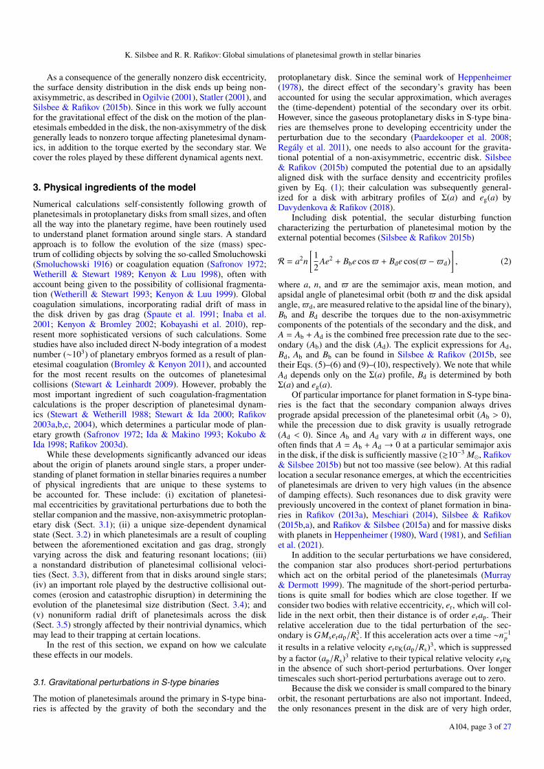
Figure 2 illustrates the collision velocities vcoll betweenplanetesimals as a function of their sizes. These are given byEq. (A.16), with λ and erand assigned their mean values of 0.81and 2

√πσi, respectively. This figure is made for the fiducial sys-

tem described in Sect. 5 with rather small σi = 10−4, so thatrelative velocities are typically dominated by the secondary anddisk forcing (i.e., by ei j). The three panels differ in the assumedlocation ap of the colliding planetesimals in the disk (whichdetermines their vc and dc), as labeled on the figure. As men-tioned in Sect. 3.2, vcoll ∼ vc for pairs of collision partners inwhich one object has size d1 � dc and another has size d2 � dc.If the collision partners have similar size, or both are much larger(or both much smaller) than dc, then the collision velocities aredetermined predominantly by random motions and become inde-pendent of the sizes of the collision partners (since we take σi tobe size independent in this work).

As mentioned above, Fig. 2 would look very different if itwere drawn assuming planetesimal dynamics typical for disksaround single stars (i.e., without apsidal alignment): in that casethe “valley" at d1 ≈ d2 would disappear and vcoll would monoton-ically increase along this line (since smaller planetesimals havelower random velocities as a result of gas drag, Rafikov 2003a,2004). These differences clearly demonstrate the importance ofapsidal alignment naturally emerging in disks around binariesfor setting the pattern of planetesimal collision velocities.

3.4. Collision outcomes

Armed with the understanding of the distribution of relativevelocities of planetesimals (Sect. 3.3), we determine the outcomeof their physical collision using the recipes provided in the workof Stewart & Leinhardt (2009). This study assumes, quite gener-ally, that as a result of a collision one is left with a large remnant

A104, page 5 of 27

A&A 652, A104 (2021)

10 2 10 1 100 101 102

d1, km10 2

10 1

100

101

102

d 2, k

m

ap = 2.5 AUvc = 448 m/sdc = 283 m

(c)10 2

10 1

100

101

102

d 2, k

m

ap = 2.3 AUvc = 265 m/sdc = 177 m

(b)

10 2 10 1 100 101 102

10 2

10 1

100

101

102

d 2, k

m

ap = 2.0 AUvc = 77 m/sdc = 58 m

(a)

10

30

100

300

vij, m/s

Fig. 2. Collision velocities between two planetesimals as a function oftheir sizes d1 and d2 in a disk with the fiducial set of parameters givenin Sect. 5 and σi = 10−4. Each panel corresponds to a different locationin the disk, which leads to the varying values of vc and dc labeled on thepanels. Regions of erosive collisions are outlined in dotted white lines,and regions of catastrophic disruption are enclosed by solid white lines.The horizontal and vertical yellow lines correspond to the initial plan-etesimal size dinit = 4.3 km used in the simulation described in Sect. 5.1.The point (dc, dc) is shown as a red dot.

body and a spectrum of small fragments. The size of the largestremnant is the main ingredient in their description of the colli-sion outcome (see our Eq. (A.4)). We provide the details of ourimplementation of this prescription in Sect. A.2, but will brieflyhighlight the differences with the single-star case here.

Following Rafikov & Silsbee (2015b), we divide the colli-sion outcomes into three classes. We say that a collision leads tocatastrophic disruption if the largest remnant contains less thanhalf the combined mass of the two incoming planetesimals, ero-sion if the largest remnant is smaller than the larger of the twoincoming bodies, and growth if the largest remnant is larger thaneither of the incoming bodies. We can then use the recipe ofStewart & Leinhardt (2009) to delineate in Fig. 2 the domainsin d1 − d2 phase space, corresponding to each to type of theoutcome: regions of catastrophic disruption lie within the solidwhite lines, regions of erosive collisions are outlined in dottedwhite, and regions leading to growth lie outside both white lines.We use the “strong rock” planetesimal composition of Stewart &Leinhardt (2009) in this calculation. One can see that, unless vc isvery high, catastrophic disruption occurs only between collisionpartners with similar (but not equal) sizes. It is mainly relevantfor objects with sizes around dc, as that is where even objects

of comparable size experience high-velocity collisions (althoughthe regions of catastrophic disruption are not exactly centered ondc because the strength of planetesimals is size-dependent, witha minimum around 0.1 km (Stewart & Leinhardt 2009). In con-trast to catastrophic disruption, erosion is possible even when thesizes of the colliding bodies are very unequal.

Due to the complexity of secular dynamics in binaries out-lined in Sect. 3.2, there is a significant variation in the collisionalenvironment across the disk, as different panels of Fig. 2 demon-strate. The regions corresponding to erosion and catastrophicdisruption grow larger as the characteristic velocity vc increases.The weakest planetesimals with sizes around 0.1 km may bedestroyed even in the absence of any secularly excited eccen-tricities, in collisions arising just from random motions, whichis almost what is happening in Fig. 2a. But it is still clear frompanels (b) and (c) of that figure that secular pumping of planetes-imal eccentricities in binaries endows these systems with muchharsher collisional environments than in disks around singlestars.

The heuristic picture of collision outcomes based on therelative velocity maps has been used in Rafikov & Silsbee(2015a) and Silsbee & Rafikov (2015a) to understand the pos-sibility of planetary growth, which was assumed to take placewhen neither catastrophic disruption nor substantial erosionwere taking place at certain locations in the disk. Obviously,such a simplistic approach cannot provide a perfect character-ization of the conditions necessary for sustained planetesimalgrowth. Indeed, persistent planetesimal accretion may be pos-sible even if some collisions are destructive; however, one doesnot know a priori how harsh of a collisional environment canbe tolerated. Thébault et al. (2008, 2009), Thebault (2011), andRafikov & Silsbee (2015b) all had to make certain assump-tions when drawing their conclusions on the likelihood of planetformation in binaries (see Sect. 7.4 for an assessment of theirrealism). For this reason, in this work we follow the evolu-tion of the planetesimal size distribution in full, using detailedcoagulation-fragmentation calculations with realistic physicalinputs as described in Sect. 4 and Appendix A.

3.5. Radial inspiral

In this work, we also explicitly include the radial inspiral of plan-etesimals, which we expect to impact planetesimal growth intwo different ways. First, inspiral drains the disk of solid mate-rial. If this happens more rapidly than coagulation, then largebodies will not form due to lack of solid material needed fortheir growth. Second, since small bodies inspiral more rapidlythan large ones, one might expect that, once small bodies areflushed out, the effect of erosive collisions would be reduced,thus favoring the growth of large planetesimals.

Using the results of Adachi et al. (1976), Rafikov & Silsbee(2015b) found that the inspiral rate ap is given by (their Eq. (11)):

ap = −π ap

erτd

(58

e2r + η2

)1/2 [(α

4+

516

)e2

r + η

], (6)

where er and τd are given by Eqs. (4) and (3), respectively,η∼ (h/ap)2 ∼ 0.003 (h is the disk scale height) is a measure ofthe particle-gas velocity differential due to the pressure supportin the gas disk, and α∼ 1 is a constant that depends on the diskmodel as described in Rafikov & Silsbee (2015b). From Eqs. (3)and (4), one can show (Rafikov & Silsbee 2015b) that erτd ∝ dp.As a result, one finds that ap ∝ d−1

p if either (i) dp � dc, when er

A104, page 6 of 27

K. Silsbee and R. R. Rafikov: Global simulations of planetesimal growth in stellar binaries

10 3 10 2 10 1 100 101 102 103

size dp, km

10 8

10 6

10 4

10 2

drift

rate

, AU/

year

(a)

1.0 AU1.8 AU

3.0 AU4.0 AU

1.0 1.5 2.0 2.5 3.0 3.5 4.0semi-major axis a, AU

10 8

10 6

10 4

drift

rate

, AU/

year

(b)

0.1 km1 km

10 km100 km

Fig. 3. Inspiral speed as a function of planetesimal size at different loca-tions in the disk (a) (see legend), and as a function of location in thedisk for different planetesimal sizes (b) (see legend). The figure wasmade assuming the disk model described in Sect. 5, with e0 = 0.01,Σ0 = 1000 g cm−2, and $d = 0.

becomes constant, or (ii) er � η, so that the last term in bracketsin Eq. (6) dominates.

Figure 3 shows the speed of radial drift for different plan-etesimal sizes and locations in the disk in the γ Cephei system,assuming fiducial disk parameters as in Sect. 5. We see that thecurves in the upper panel match the limiting cases discussed inthe previous paragraph; the regions where ap ∝ d−1

p are joinedby an intermediate region where the inspiral velocity dependsless strongly on dp. In all cases, inspiral speed is a monotonicallydecreasing function of dp, meaning that small bodies are pref-erentially flushed out of the system, thus reducing the erosionsuffered by larger objects.

In the lower panel we see that for moderately large planetes-imals (&0.1 km), there is a noticeable dip in the inspiral rate inthe broad region around 1.8 AU. This is because for this diskmodel vc vanishes at 1.8 AU, so the only contribution to the inspi-ral comes from the sub-Keplerian rotation of the gas and notfrom any relative eccentricity between the planetesimals and gas,significantly reducing ap.

These considerations highlight important differences in theradial drift behavior between the binary and single stars. First,high planetesimal eccentricities driven by the secular effect of

the disk and the secondary result in faster radial drift in disksin binaries compared to single systems (see Eq. (6)). Second,because higher er increases the inspiral rate, planetesimals willbe naturally concentrated in regions where er is low, and thuswhere they can grow more easily. This effect does not exist forplanetesimals around single stars (unless one includes additionalphysics).

4. Numerical ingredients of the model

Our calculations of planetesimal growth in binaries employ amulti-annulus (or multi-zone) coagulation-fragmentation codespecifically designed for this task. Here we briefly summarizeits main features and provide references to relevant sections inAppendices A and B.

4.1. Basics of the code structure

Our code models the evolution of the planetesimal size distribu-tion in Nann discrete spatial annuli placed at different radii fromthe primary. These should really be thought of as bins in thespace of the semimajor axis, rather than radius, but we do notmake that distinction in the following discussion. Within eachannulus, the planetesimal size distribution is represented usingNbins logarithmically spaced mass bins. At any point in time, ina given annulus, all of the information about the size distribu-tion is encoded in a single vector n, such that ni is the number ofplanetesimals in mass bin i. To follow the evolution of ni in eachannulus the code performs two basic functions.

First, in each of the annuli, it calculates the evolution ofthe size distribution due to planetesimal-planetesimal collisions.This is done in a standard fashion, effectively by solving a dis-cretized version of the Smoluchowski equation (Smoluchowski1916) accounting for the possibility of fragmentation (Sects. A.1,A.2, and A.6.1). Inclusion of fragmentation generally makesthis an O(N3

bins) calculation at each time step, which is numer-ically expensive. To overcome this problem, our code employsthe new fragmentation algorithm developed in Rafikov et al.(2020), for which the numerical cost goes only as O(N2

bins), aslong as the size distribution of fragments formed in a collisionof two objects is self-similar (which is a standard and physicallymotivated assumption anyway). The coagulation-fragmentationcomponent of the code has been extensively tested against theknown analytical solutions as described in Sects. B.1 and B.2.

To compute the number of collisions between different massbins we use collision rates calculated using the relative veloc-ities from Rafikov & Silsbee (2015a) and accounting for boththe forced eccentricity and random velocities (see Sects. 3.2and 3.3). Our collision rates include gravitational focusingand smoothly interpolate between the shear- and dispersion-dominated velocity regimes (Sect. A.4). The full distribution ofcollision velocities is also used to model collision outcomes fol-lowing the recipes in Stewart & Leinhardt (2009; see Sects. 3.4and A.2).

Our implementation of many code components has certainelements of stochasticity in it, which is quite important. It hasbeen previously found (Windmark et al. 2012; Garaud et al.2013) that including the distribution of collision velocities canqualitatively change the outcome of the coagulation process. Inparticular, in a study of dust growth, Windmark et al. (2012)found that using a Maxwellian collision velocity distributioninstead of a delta function at the rms velocity of the Maxwelliancan cause a few particles to experience a series of lucky

A104, page 7 of 27

A&A 652, A104 (2021)

low-velocity collisions and grow to larger sizes; the larger bodiesformed via lucky collisions are more resistant to destruction insubsequent collisions and would continue to grow to arbitrarilylarge sizes. In our case, the strong variation in collision veloc-ity with collision partner size provides the dominant source ofsuch randomness. In addition, even for bodies with given sizes,there is a range in their relative collision velocity (see Sect. A.3).To account for such a possibility, we also draw collision veloc-ity between two bodies from a physically motivated distribu-tion (Rafikov & Silsbee 2015a; see Sect. 3.3), as describedin Sect. A.3.

The second operation performed by the code is the radialredistribution of mass between different annuli caused by thesize-dependent inward migration of planetesimals due to gasdrag (Sect. 3.5). The implementation of this procedure and itstests are described in Sects. A.5, A.6.2, and B.3, respectively.

Our model implicitly assumes that other than redistributioncaused by radial drift, planetesimals interact only with otherplanetesimals within their semimajor axis bin. In practice thisis not strictly true: Planetesimals in neighboring bins can alsocollide. However, because the growth we are modeling occurs inregions where the relative eccentricity between planetesimals ofdifferent sizes is very small (typically less than 1%), we expectthe coupling of planetesimals with those in adjacent semimajoraxis bins to be a minor effect.

4.2. Parameters of the numerical model

Multiple modules comprising our code employ a number ofparameters, both numerical and physical. All our simulations usea standard set of these parameters described here and listed inTable C.1.

Our grid in mass space employs Nbins = 100 bins; the small-est size (corresponding to the lowest bin) below which massis supposed to be flushed out from the system due to gas dragis dp = 10 m. The largest mass bin in our simulations corre-sponds to an object with dp = 300 km, since beyond this pointdestructive collisions are no longer able to prevent growth tolarger sizes. This results in a mass ratio between (logarithmicallyuniformly spaced) mass bins of Mi+1/Mi = 1.37. To representour global simulation domain extending from 1 AU to 4 AU weuse Nann = 60 annuli, spaced in semimajor axis as described inSect. A.5. In choosing this radial range we are motivated by theplanetary semimajor axes in several S-type systems: apl = 2 AUin γ Cephei, apl = 2.6 AU in HD 196885, and apl = 1.6 AU inHD 41004 (Chauvin et al. 2011).

Some additional parameters used in our simulations areas follows: the slope of the fragment mass spectrum ξ = −1(Sect. A.2); parameter b = 10−2 used to decide whether thelargest fragment is distinct from the continuous spectrum of frag-ments (Sect. A.2); tolerance parameters ε1 = 0.05 and ε2 = 10−6

used in time step determination (Sect. A.6).We studied the sensitivity of the code to changes of these

parameters and found only slight variations in the outcomes (seeAppendix C).

5. Results: Fiducial model

We start presentation of our results by describing in detail aparticular (fiducial) simulation, which will also illustrate themetric we employ to determine the success of planet forma-tion in a given disk model (Sect. 5.2.1). Our fiducial disk modeluses the orbital parameters of the γ Cephei system and disk

characteristics as described in Sect. 2. For the disk and plan-etesimal parameters it adopts e0 = 0.01, Σ0 = 1000 g cm−2 ata0 = 1 AU, $d = 0◦, σi = 10−4, and a solid to gas ratio of 0.01.The total disk mass is 3.7MJ. We present the results for otherdisk models in Sect. 6.

To assist in interpreting the outcomes of our calculations, wefirst describe the results of several one-zone simulations of plan-etesimal growth at different semimajor axes in Sect. 5.1. We thenmove on to the global, multi-zone calculation of planet formationin the fiducial model in Sect. 5.2. This approach not only allowsus to separate local and global factors affecting planet formationbut also highlights the role played by the gas drag-driven radialinspiral (naturally absent in the former case).

5.1. Coagulation in a single annulus

We ran our single-annulus calculations of planetesimal growthat three semimajor axes – ap = 2 AU, 2.3 AU, and 2.5 AU – inour fiducial disk model. These are the same locations for whichFig. 2 illustrates the distribution of collision velocities, whichhelps us in understanding the role of planetesimal dynamicson their growth. The simulations started with all planetesimalshaving the same size dinit = 4.3 km; for the adopted bulk den-sity ρp = 3 g cm−3 this corresponds to planetesimal mass ofm = 1018 g.

Figure 4 illustrates how the size distribution in our modelsystem changes as a function of time. What is actually shown ismdN/d ln dp, a variable equal to the mass per unit log planetesi-mal size. Different curves correspond to different times since thebeginning of the simulation, as indicated by the color bar. Thesimulation for panel (a) was stopped when the largest body wentbeyond the largest mass bin in the simulation (dp = 300 km). Inpanels (b) and (c), the simulation was stopped after 106 yr.

In all plots, the curves corresponding to times .104 yr dis-play features due to the initial conditions and finite spacing of themass bins. Initially, all of the mass is distributed in just two massbins surrounding the initial (seed) size dinit, which is marked bythe dashed vertical black line. The wiggles just to the right of dinitare related to the finite spacing of the mass bins. The gap just tothe left of dinit exists because debris of that size is not created incollisions of objects with size dinit – they produce only smallerfragments to the left of the gap. The size spectrum of objects tothe left from the gap is universal at early times (∼103–104 yr),as it simply reflects the size distribution of fragments formed incollisions of roughly equal mass planetesimals of size dinit. Thegap region is only later filled in by coagulation of the debris par-ticles produced early on and erosion of the seed bodies by smalldebris.

Over time, memory of the initial conditions is erased, thegaps near dinit get filled, and the size distribution becomessmooth. There are some other notable features that develop inthe size distribution at late times. First, after a few times 104 yrmdN/d ln dp starts featuring a dip around dp ∼ 0.1 km, especiallypronounced in panel (b). Its location corresponds to the plan-etesimal size which is most easily destroyed in collisions (seeRafikov & Silsbee 2015b). In each panel, the vertical dotted linecorresponds to dc for that simulation, which varies by a factor ofseveral across the different environments, but stays pretty closeto dp ∼ 0.1 km. Particles with sizes around dc experience high-velocity collisions with almost all other bodies, and are thereforepreferentially destroyed, which likely affects the depth of the dipin different panels.

Second, one can see (especially in panel (b)) mdN/d ln dpdeveloping power law behavior to the left and right of the

A104, page 8 of 27

K. Silsbee and R. R. Rafikov: Global simulations of planetesimal growth in stellar binaries

10 2 10 1 100 101 102

dp, km

1014

1018

1022

1026

1030

mdN

/dln

(dp)

(c) ap = 2.5 AU, vc = 448 m/s, dc = 283 meters

1014

1018

1022

1026

1030

mdN

/dln

(dp)

ap = 2.3 AU, vc = 265 m/s, dc = 177 meters

(b)

10 2 10 1 100 101 102

1014

1018

1022

1026

1030

mdN

/dln

(dp)

(a) ap = 2.0 AU, vc = 77 m/s, dc = 58 meters

102 103 104 105 106time, years

Fig. 4. Evolution of the size distribution as a function of time in a set ofsingle-annulus simulations, described in Sect. 5.1, which should be con-sulted for details. The three panels correspond to environments with thedifferent values of the critical velocity vc and critical size dc, previouslyshown in Fig. 2, at different locations (as labeled) in the disk aroundthe primary star in the γ Cephei system. The vertical dotted lines corre-spond to the critical size dc, and the vertical dashed lines correspond tothe initial size of the planetesimals dinit.

dp ∼ 0.1 km line, with different slopes. We believe this behav-ior to be real but will refrain from offering an explanation for theslope of these segments. This cannot be done based on standardresults regarding fragmentation (O’Brien & Greenberg 2003;Tanaka et al. 1996) since they assume a power-law dependenceof the collision rate on colliding partner size.

Third, panel c exhibits an accumulation of particles of 10–20 m in size; a similar accumulation is also present in panel bas a small bump in the same size range. This feature is arti-ficial and arises because in our calculations we do not followthe fate of debris smaller than 10 m in size, simply removingit from the system. As a result, 10–20 m objects do not havesmaller bodies to erode them, and their own relative velocitiesare too low to result in catastrophic disruption: because of theircomparable size their collisional velocities are small, thanks tothe peculiarity of planetesimal dynamics in binaries (see Fig.2). Nevertheless, the emergence of this feature near the bottomof our mass grid does not affect the outcome of planetesimalevolution for dp & dinit.

101 102 103 104 105 106

t, years10 2

10 1

100

101

102

max

imum

size

, km

ap = 2.0 AUap = 2.3 AUap = 2.5 AU

Fig. 5. Time evolution of the size of the biggest object in the system,shown for the three simulations depicted in Fig. 4 and labeled accordingto their semimajor axis.

Careful examination of our simulation outputs shows thatthe largest objects grow primarily in collisions with objects ofsimilar size, certainly for dp > dinit. This is because most solidmass is contained in such objects, but also because growth ismost favorable in collisions of such objects.

We observe, not surprisingly, that higher vc suppressesgrowth. In panel (a), with vc = 77 m s−1, growth to hundredsof km occurs within several ×105 yr. This can also be seen inFig. 5 where we show the size of the largest body as a function oftime for the three local simulations discussed here. Were we tosimulate larger bodies, beyond 300 km, growth would continuein panel (a) until the mass reservoir is fully depleted. Becauseof low vc, even when a significant amount of solid mass in thesystem has been converted to debris (at late times), collisions ofthe largest objects with debris particles are not energetic enoughto significantly impede their growth.

In panel b with vc = 265 m s−1, planetesimals can only growto a few times the initial size. After that growth of the largestobjects stalls (see also Fig. 5), while the population of objectswith dp ∼ dinit gets gradually eroded by smaller objects producedin previous collisions (this can be seen in the decay of amplitudeof dN/d ln dp around that size). If we were to run this simula-tion beyond 1 Myr, large objects with dp ∼ dinit would eventuallybe eroded, followed by smaller bodies also grinding themselvesdown.

Finally, in panel c of Fig. 4, collision velocities are so highthat there is barely any growth – the largest objects present inthe system at early time have grown in size beyond dinit only by∼2. But after a population of small debris develops in the system(already by 103 yr), Fig. 5 shows that large bodies get erodedaway by 105 yr, leaving only a small population of debris nearthe lower end of the simulation mass range (which is an artifactof our calculation, as we mentioned earlier).

Figure 5 shows that in all three environments, the largest bod-ies initially evolve in a very similar fashion, steadily growing insize. This universality is caused by the fact that initial growthoccurs by mergers of objects with dp = dinit, which have low rel-ative velocities. The differences emerge only after ∼104 yr whena sufficient amount of small debris capable of efficiently erodingbig bodies in high-vc environments accumulates in the system.

A104, page 9 of 27

A&A 652, A104 (2021)

Here we again consider Fig. 2, which illustrates, in particu-lar, collision outcomes as a function of the sizes of the collisionpartners, for the same environments that the simulations shownin Fig. 4 were run for. Interestingly, we see that to halt planetesi-mal growth it is not necessary to have catastrophic disruption ofobjects at dp ∼ dinit. Indeed, although Fig. 4 shows that growthis halted in panels (B) and (C), Fig. 2 shows no catastrophic dis-ruption of planetesimals at the initial size: the point (dinit, dinit) isoutside the solid white contours for all dynamic environments,as dinit = 4.3 km considerably exceeds dc in all panels.

It may seem strange that in all three panels in Fig. 2 the point(dinit, dinit) also lies outside the dotted contours, bordering theregion of erosive encounters – it would seem natural that oneshould then find growth starting with a population of dp = dinitobjects in all three environments. The resolution of this apparentparadox involves two factors. First, according to our definitionof erosion in Fig. 2 dotted contours correspond to collisions,in which the mass of the largest remnant is equal to the massof the bigger object (target) involved in the collision; the massequal to the mass of the smaller object (projectile) is reduced todebris. Similarly, even though the point (dinit, dinit) sits outsidethe dotted contour, some amount of debris will still be producedin collisions of two objects of initial size dinit; the amount of cre-ated debris is larger the closer this point is to the dotted contour(i.e., in panels b and c relative to (a)). And once some debrisparticles are created, Fig. 2 shows that their collisions with seedbodies (dp = dinit) are very erosive, especially in panel (c), butonly barely so in panel a.

Second, relative velocity maps in Fig. 2 assume a partic-ular (mean) value of encounter velocity, whereas in practicevcoll has a reasonably broad distribution around this mean (seeSect. A.3). As a result, some collisions occur at higher veloci-ties and are more destructive – a fact that is fully accounted forin our coagulation-fragmentation simulations depicted in Fig. 4.This is another clear illustration of the importance of consid-ering the distribution of planetesimal velocities when studyingtheir growth. The combination of the two aforementioned fac-tors leads to erosion eventually becoming the dominant player inthe collisional evolution in panels b and c of Fig. 4.

5.2. Full global calculation with inspiral

We now proceed to describe a fully global, multi-annulus simu-lation of planetesimal growth, fully accounting for the effects ofsize-dependent radial inspiral (see Sect. 3.5) and using the fidu-cial disk parameters. This simulation is also used to motivate ourchoice of a particular metric determining whether planetesimalgrowth in the system successfully overcomes the fragmentationbarrier (see next section).

5.2.1. Outcome diagnostic

In any reasonable environment, planetesimal growth would pro-ceed to very large sizes, eventually leading to planet formation,provided that the initial planetesimal size dinit is large enough.Indeed, objects with sizes dp � dc do not experience catas-trophic disruption and get eroded only by much smaller plan-etesimals, which cannot compete with the addition of mass incollisions with larger bodies. Thus, given large enough dinit,planet formation is guaranteed to be successful (e.g., Thebault2011) even in dynamically harsh environments of the binarystars.

However, in many environments, if the initial planetesimalsare too small, then they will be eroded or destroyed and large

bodies will not form (like in panels b and c of Fig. 4). For thisreason, the appropriate question to ask is not whether planetesi-mal growth can occur, as the answer would depend on the initialcondition – the size of the seed planetesimals dinit. Instead, oneshould be trying to figure out from what initial planetesimal sizedinit can sustained planetesimal growth occur. In a given dynam-ical environment, there will be a minimum size dmin such that ifthe initial bodies are smaller than dmin then planetesimal growthin the system will eventually be halted, as in Fig. 4b,c, whereas ifseed objects have dinit > dmin, then planetesimal coagulation willeventually form large bodies, thus overcoming the fragmentationbarrier.

This question, in principle, can be asked locally, at a givensemimajor axis in the disk. In this case Fig. 4 makes it clear that,for a fiducial disk model, dmin < 4.3 km at ap = 2 AU, whereasdmin > 4.3 km at ap = 2.3 and 2.5 AU. However, the calculationspresented in Sect. 5.1 do not account for radial mass transportdue to gas drag and may thus be inaccurate. For this reason,we will be more interested in a general question of what dminis needed for the fragmentation barrier to be overcome and fora planet to form at some location in the whole disk, given itsparameters. Once dmin is determined, some other information,for example, the location where planetesimal growth is fastest,would be the outcome of our global calculations, giving themcertain predictive power. Of course, dinit may (and probablyshould) vary across the disk. Moreover, at each location, a wholespectrum of initial sizes is likely to be present. However, in thiswork, to reduce the number of degrees of freedom, we assumethat seed planetesimals have the same size dinit across the wholedisk and determine a single value of dmin for a given disk modelbased on this assumption.

To determine dmin defined in this manner, we employed thefollowing iterative algorithm. We chose a value of dmin andused that as our starting size dinit. The simulation was run untilone of three conditions were met: (i) 1 Myr has passed, (ii) a300 km body is formed, or (iii) there is no longer sufficient solidmass remaining in the simulation to produce a 300 km body.If a 300 km body forms, then we know dmin < dinit, whereasif it does not, then dmin > dinit. By trying several values ofdinit and running our global simulations for each of them, wewere able to first bracket dmin within some interval, and thento converge to its value with high accuracy. This procedure isdemonstrated next (allowing us to also illustrate the sensitivityof global planetesimal growth to dinit).

Since the planetesimal composition is uncertain, in addi-tion to our default simulations that use the material propertiesof “strong rock" bodies from Stewart & Leinhardt (2009), wealso ran simulations using the strength parameters for their “rub-ble pile” planetesimals. We denote the minimum size assumingrubble pile planetesimals as drubble

min .

5.2.2. Evolution of the system as a whole

Figure 6 shows the evolution of the planetesimal size distributionin the entire disk for several runs of our fiducial simulation withdifferent initial sizes dinit expressed in terms of dmin = 1.6 km,as determined for this disk model. Curves of different colorcorrespond to different times since the simulation was started.Because collisional processes proceed at different rates acrossthe disk, reflecting the complexity of planetesimal dynamics inbinaries (see Fig. 1), the evolution of the planetesimal mass spec-trum looks somewhat different from that in a single annulus (seeFig. 4; e.g., the initial gaps to the left of dinit are barely there, andthere is no pile-up at small sizes). This is to be expected since the

A104, page 10 of 27

K. Silsbee and R. R. Rafikov: Global simulations of planetesimal growth in stellar binaries

10 2 10 1 100 101 102

dp, km

1019

1022

1025

1028

mdN

/dln

(dp)

, gra

ms

(c)

dinitdmin

= 2

10 2 10 1 100 101 102

1019

1022

1025

1028

mdN

/dln

(dp)

, gra

ms

(a) dinitdmin

= 0.2

10 2 10 1 100 101 102

dp, km

(d)

dinitdmin

= 5

10 2 10 1 100 101 102

(b) dinitdmin

= 0.5

103 3 × 103 104 3 × 104 105 3 × 105 106

time, years

Fig. 6. Evolution of the mass distribution in the entire disk in our fidu-cial multi-zone model (Simulation 1). Different panels are produced fordifferent initial planetesimal sizes dinit in terms of dmin (as labeled onthe plot), which is dmin = 1.6 km for this simulation.

global size spectrum in Fig. 6 is an average of multiple single-zone size distributions (such as the ones shown in Fig. 4) withthe added complication of radial inspiral of solids. Nevertheless,some key features of the size distribution evolution (e.g., a dipin mdN/d ln dp near dp ∼ 0.1 km, mass flow toward small sizes,and so on) are still preserved even in the full disk calculations.

We can see that in panels a and b, essentially no growthoccurs beyond the initial size. The behavior shown in these pan-els differs only in how rapidly the bodies are ground down. Thelack of any appreciable growth in panel b with initial size only afactor of two less than dmin shows that there is a sharp transitionover less than a factor of two in dinit from growth to large sizesto essentially no growth whatsoever.

In panels c and d, coagulation to 300 km does occur. In bothcases, though, less than half of the initial solid mass in thesimulation remains at the end. The time required to produce a300 km body is almost four times less for the simulation withdinit/dmin = 5 than for the one with dinit/dmin = 2 (8× 104 yr vs.3× 105 yr), and in the former case more than twice as much solidmaterial remains (47% of the original 7 M⊕ in panel d vs. 21% inpanel c). In the simulation with dinit/dmin = 2 (5), 79% (88%) ofthe mass is lost to the creation of rubble smaller than the smallestbody tracked in the simulation, with the remaining amount lostto inspiral into the central star.

1.5 2.0 2.5 3.0 3.5 4.0a, AU

1025

1026

1027

1028

1029

dM/d

a, g

ram

s/AU

(c) dinitdmin

= 2

1.5 2.0 2.5 3.0 3.5 4.0

1026

1027

1028

1029

dM/d

a, g

ram

s/AU

(a) dinitdmin

= 0.2

1.5 2.0 2.5 3.0 3.5 4.0a, AU

(d) dinitdmin

= 5

1.5 2.0 2.5 3.0 3.5 4.0

(b) dinitdmin

= 0.5

103 3 × 103 104 3 × 104 105 3 × 105 106

time, years

Fig. 7. Mass in planetesimals of all sizes (tracked in our mass grid) inthe disk per unit semimajor axis dM/da = 2πaΣ(a) as a function of ain our fiducial model at different moments of time (see color bar). Thedifferent panels correspond to the same initial planetesimal sizes dinitas in Fig. 6. The dashed violet horizontal line corresponds to the massdistribution at t = 0.

Figures 7 and 8 provide details on how the coagulation-fragmentation process proceeds as a function of semimajor axisin the disk, for each global simulation shown in Fig. 6. Figure 7shows dM/da – the total solid mass (in planetesimals of all sizes)per unit a, whereas Fig. 8 depicts the size of the largest body (ina given annulus), both as functions of a and time. In Fig. 7, thehorizontal dashed violet line represents the initial mass distribu-tion, which is flat because of our chosen Σ profile (see Eq. (1)).In Fig. 8 that line corresponds to the size of seed objects dinit,which is constant across the disk according to our assumption(see Sect. 5.2.1).

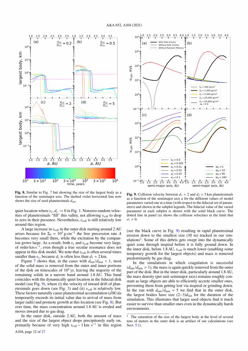
To illustrate how the dynamics of planetesimals affect theirsize evolution, we also show in Fig. 9 the run of the collisionalvelocity vcoll between d1 = 2 and d2 = 5 km planetesimals asa function of semimajor axis (for many of the different sim-ulations carried out in this work, see Sect. 6). It accounts forboth the secular and random velocity contributions and is calcu-lated using Eq. (A.16) with parameters λ and erand taking theirmean values. The black solid line corresponds to the fiducialdisk model, whereas the black dotted line in panel (a) shows vcollcomputed in the absence of random motions. One can easily rec-ognize the “valley” forming around 1.8 AU as the dynamically

A104, page 11 of 27

A&A 652, A104 (2021)

1.0 1.5 2.0 2.5 3.0 3.5a, AU

10 1

100

101

102

larg

est b

ody,

km

dinitdmin

= 2(c)

1.0 1.5 2.0 2.5 3.0 3.5a, AU

dinitdmin

= 5(d)

1.0 1.5 2.0 2.5 3.0 3.5

10 1

100

101

102

larg

est b

ody,

km

dinitdmin

= 0.2(a)1.0 1.5 2.0 2.5 3.0 3.5

dinitdmin

= 0.5(b)

103 3 × 103 104 3 × 104 105 3 × 105 106time, years

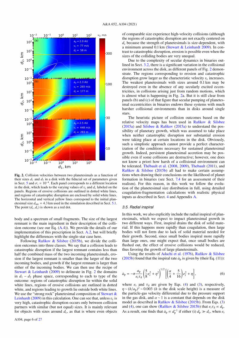
Fig. 8. Similar to Fig. 7 but showing the size of the largest body as afunction of the semimajor axis. The dashed violet horizontal line nowshows the size of seed planetesimals dinit.

quiet location where vc, dc → 0 in Fig. 1. Nonzero random veloc-ities of planetesimals “fill" this valley, not allowing vcoll to dropto zero in their presence. Nevertheless, vcoll is still relatively lowaround this region.

A large increase in vcoll in the outer disk starting around 2 AUarises because for Σ0 = 103 g cm−2 the free precession rate Abecomes very small there, while the excitation by the compan-ion grows large. As a result, both vc and vcoll become very large,of order km s−1, even though a true secular resonance does notappear in this disk model. We note that vcoll is often several timessmaller than vc, because dc is often less than d1 = 2 km.

Figure 7 shows that, in the cases with dinit/dmin < 1, mostof the solid mass is removed from the outer and inner portionsof the disk on timescales of 104 yr, leaving the majority of theremaining solids in a narrow band around 1.8 AU. This bandcoincides with the dynamically quiet location in the fiducial diskmodel (see Fig. 9), where (i) the velocity of inward drift of plan-etesimals goes down (see Fig. 3) and (ii) vcoll is relatively low.These factors naturally cause planetesimal accumulation (dM/datemporarily exceeds its initial value due to arrival of mass fromlarger radii) and promote growth at this location (see Fig. 8). Butover time, the mass concentration around 1.8 AU is eroded andmoves inward due to gas drag.

In the outer disk, outside 2 AU, both the amount of massand the size of the largest object drops precipitously early on,primarily because of very high vcoll ∼ 1 km s−1 in this region

1.0 1.5 2.0 2.5 3.0 3.5 4.0semi-major axis, AU

10 1

100

101

102

103

v col

l, m

/s

(c)

e0 = 0.0e0 = 0.005e0 = 0.01e0 = 0.02e0 = 0.05e0 = 0.1

1.0 1.5 2.0 2.5 3.0 3.5 4.0semi-major axis, AU

(d)

d = 0d = 10d = 90d = 180

1.0 1.5 2.0 2.5 3.0 3.5 4.0

10 1

100

101

102

103

104

v col

l, m

/s

(a) With Disk GravityWithout Disk GravityWithout Random Motions

1.0 1.5 2.0 2.5 3.0 3.5 4.0

(b)

0 = 500 g/cm2

0 = 1,000 g/cm2

0 = 5,000 g/cm2

0 = 20,000 g/cm2

0 = 20,000 g/cm2 e0 = 0.0

Fig. 9. Collision velocity between d1 = 2 and d2 = 5 km planetesimalsas a function of the semimajor axis a for the different values of modelparameters varied one at a time (with respect to the fiducial set of param-eters) and shown in the subplot legends. The fiducial value of the variedparameter in each subplot is shown with the solid black curve. Thedotted line in panel (a) shows the collision velocities in the limit thatσi = 0.

(see the black curve in Fig. 9) resulting in rapid planetesimalerosion down to the smallest size (10 m) tracked in our sim-ulations2. Some of this debris gets swept into the dynamicallyquiet zone through inspiral before it is fully ground down. Inthe inner disk, below 1.8 AU, vcoll is much lower (enabling sometemporary growth for the largest objects) and mass is removedpredominantly by gas drag.

In the simulations in which coagulation is successful(dinit/dmin > 1), the mass is again quickly removed from the outerpart of the disk. But in the inner disk, particularly around 1.8 AU,the mass density (per unit semimajor axis) remains roughly con-stant as large objects are able to efficiently accrete smaller ones,preventing them from getting lost via inspiral or grinding down.In the run with dinit/dmin = 5 we find that in the outer disk,the largest bodies have size (2−3)dinit for the duration of thesimulation. This illustrates that larger seed objects find it mucheasier to survive than smaller ones even in the dynamically harshenvironments.

2 The saturation of the size of the largest body at the level of severaltens of meters in the outer disk is an artifact of our calculations (seeSect. 5.1).

A104, page 12 of 27

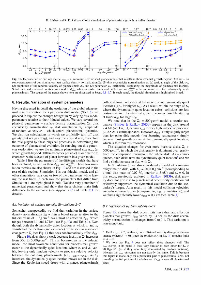
K. Silsbee and R. R. Rafikov: Global simulations of planetesimal growth in stellar binaries

0.5

0.5

1

1

2

2

5

5

10

10

20

20

0, 103g/cm2

0.3

1.0

3.0

10.0

30.0

d min

, km

(a)0

0

0.003

0.003

0.01

0.01

0.03

0.03

0.1

0.1

e0

(b)0

0

60

60

120

120

180

180

d, degrees

(c)10 5

10 5

10 4

10 4

10 3

10 3

i

(d)

With Disk GravityWithout Disk Gravity

0.0

0.0

0.1

0.1

0.3

0.3

1

1

3

3

10

10

ir

(e)

Aligned diskAnti-aligned disk

Fig. 10. Dependence of our key metric dmin – a minimum size of seed planetesimals that results in their eventual growth beyond 300 km – onsome parameters of our simulations: (a) surface density normalization Σ0, (b) disk eccentricity normalization e0, (c) apsidal angle of the disk $d,(d) amplitude of the random velocity of planetesimals σi, and (e) parameter χir (artificially) regulating the magnitude of planetesimal inspiral.Solid lines and diamond points correspond to dmin, whereas dashed lines and circles are for drubble

min – the minimum size for collisionally weakplanetesimals. The causes of the trends shown here are discussed in Sects. 6.1–6.7. In each panel, the fiducial simulation is highlighted in red.

6. Results: Variation of system parameters

Having discussed in detail the evolution of the global planetes-imal size distribution for a particular disk model (Sect. 5), weproceed to explore the changes brought in by varying disk modelparameters relative to their fiducial values. We vary several keyphysical parameters – surface density normalization Σ0, diskeccentricity normalization e0, disk orientation $d, amplitudeof random velocity σi – which control planetesimal dynamics.We also run calculations in which we artificially turn off diskgravity (but not gas drag), and vary the inspiral rate, to explorethe role played by these physical processes in determining theoutcome of planetesimal evolution. In carrying out this param-eter exploration we use the minimum planetesimal size dmin (atwhich growth beyond 300 km becomes possible) as our metric tocharacterize the success of planet formation in a given model.

Table 1 lists the parameters of the different models that havebeen explored, as well as their dmin and drubble

min . These two simu-lation metrics are also shown in Fig. 10 and are discussed in therest of this section. Simulation 1 is our fiducial model, and allother simulations vary one or two of the parameters while leav-ing the rest fixed. In each row, the parameters that differ fromSimulation 1 are highlighted in bold. We also vary a number ofnumerical parameters, and show that these choices make littledifference to the outcome (see Appendix C and Table C.1 fordetails).

6.1. Variation of surface density: Simulations 2–7

Somewhat unexpectedly, we find that variation in the surfacedensity normalization Σ0 within a broad range relative to thefiducial value of 103 g cm−2 has almost no effect on dmin, whichranges between 1.1 and 1.7 km (see Fig. 10a and Table 1). Eventhough both the dynamically quiet location at which vc and dcvanish and the location (and existence) of the secular resonancechange with Σ0 (see Fig. 1), this does not dramatically affect dmin.

Figure 10a does show a weak decrease in dmin as Σ0 increasesfrom 500 to 5000 g cm−2. This is because, as in the fiducialmodel, the most favorable conditions for planetesimal growthoccur at the dynamically quiet location, where vc and dc van-ish, leaving only random velocity to produce relative velocitybetween the colliding planetesimals (i.e., vcoll ∼σivK). As Σ0increases, the dynamically quiet location moves out in the disk.Since the Keplerian speed drops with distance, planetesimals

collide at lower velocities at the more distant dynamically quietlocations (i.e., for higher Σ0). As a result, within the range of Σ0where the dynamically quiet location exists, collisions are lessdestructive and planetesimal growth becomes possible startingat lower dinit for larger Σ0.

We note that in the Σ0 = 500 g cm2 model a secular res-onance (Silsbee & Rafikov 2015b) appears in the disk around2.4 AU (see Fig. 1), driving vcoll to very high values3 at moderate(2–2.5 AU) semimajor axes. However, dmin is only slightly largerthan for other disk models (not featuring resonances), simplybecause most growth occurs at the dynamically quiet location,which is far from this resonance.

The situation changes for even more massive disks, Σ0 >5000 g cm−2, in which the disk gravity is dominant over gravityfrom the companion throughout the whole disk. As a conse-quence, such disks have no dynamically quiet location4 and wefind a slight increase in dmin with Σ0.

In Simulation 7, we also considered a model of a massiveaxisymmetric disk, with Σ0 = 20,000 g cm−2 (corresponding toa total disk mass of 0.07 M� interior to 5 AU) and e0 = 0. Inthis setup, previously explored in Rafikov (2013b), disk grav-ity does not give rise to planetesimal eccentricity excitation buteffectively suppresses the dynamical excitation due to the sec-ondary’s torque. As a result, in this model collision velocitiesare reduced even further (compared to, e.g., Simulation 6), andwe find a significantly lower dmin = 0.7 km (see Table 1).

6.2. Variation of e0: Simulations 8–12

Figure 10b shows that disk eccentricity has a dramatic effect onplanetesimal growth: dmin varies by 1.4 dex as the disk eccen-tricity normalization e0 changes from 0 to 0.1. This variation isnon-monotonic.

3 Unlike vc ∝ A−1, neither er nor collisional velocity diverge at the res-onance (where A → 0), since the product vcA in Eq. (4) remains finiteas A→ 0.4 We note that Fig. 9 does not reflect these changes well: Thevcoll curves in its panel B look very similar to each other for Σ0 ≥2000 g cm−2 (as if they were fully dominated by random motions),whereas the dmin outcomes are not exactly the same. This is becausethis figure is made only for a particular pair of planetesimal sizes, notrevealing the full picture of the behavior of vcoll across all planetesimalsizes.

A104, page 13 of 27

A&A 652, A104 (2021)

Table 1. Parameters of our model runs.

Sim # Σ0(1) (g cm−2) e0

(2) $d(3) σi

(4) Disk gravity (5) χir(6) dmin (km) (7) drubble

min (km) (8)

1 1000 0.01 0◦ 10−4 Yes 1 1.6 3.4

2 500 0.01 0◦ 10−4 Yes 1 1.7 3.93 2000 0.01 0◦ 10−4 Yes 1 1.3 2.84 5000 0.01 0◦ 10−4 Yes 1 1.1 2.55 10 000 0.01 0◦ 10−4 Yes 1 1.3 2.76 20 000 0.01 0◦ 10−4 Yes 1 1.4 2.77 20 000 0.0 0◦ 10−4 Yes 1 0.7 2.1

8 1000 0.0 0◦ 10−4 Yes 1 4.2 6.29 1000 0.005 0◦ 10−4 Yes 1 1.7 3.710 1000 0.02 0◦ 10−4 Yes 1 9.5 13.111 1000 0.05 0◦ 10−4 Yes 1 21.7 29.312 1000 0.1 0◦ 10−4 Yes 1 38.9 52.6

13 1000 0.01 10◦ 10−4 Yes 1 2.5 4.214 1000 0.01 90◦ 10−4 Yes 1 7.8 10.915 1000 0.01 180◦ 10−4 Yes 1 9.7 13.4

16 1000 0.01 0◦ 10−5 Yes 1 0.3 0.517 1000 0.01 0◦ 3 × 10−5 Yes 1 0.7 1.218 1000 0.01 0◦ 3 × 10−4 Yes 1 4.7 12.119 1,000 0.01 0◦ 10−3 Yes 1 27.6 48.5

20 1000 0.01 0◦ 10−5 No 1 6.9 8.621 1000 0.01 0◦ 3 · 10−5 No 1 6.6 9.122 1000 0.01 0◦ 10−4 No 1 6.9 9.323 1000 0.01 0◦ 3 × 10−4 No 1 11.8 18.524 1000 0.01 0◦ 10−3 No 1 20.8 47.5

25 1000 0.01 0◦ 10−4 Yes 0.0 1.0 3.226 1000 0.01 0◦ 10−4 Yes 0.1 1.1 3.127 1000 0.01 0◦ 10−4 Yes 0.3 1.2 3.128 1000 0.01 0◦ 10−4 Yes 3.0 2.3 4.029 1000 0.01 0◦ 10−4 Yes 10.0 4.2 5.630 1000 0.01 0◦ 10−4 Yes 30.0 5.6 7.831 1,000 0.01 0◦ 10−4 Yes 100.0 8.6 9.5

32 1000 0.01 180◦ 10−4 Yes 0.0 9.1 13.433 1000 0.01 180◦ 10−4 Yes 0.1 8.8 12.834 1000 0.01 180◦ 10−4 Yes 0.3 8.9 12.335 1000 0.01 180◦ 10−4 Yes 3.0 10.3 14.536 1000 0.01 180◦ 10−4 Yes 10.0 11.4 15.7

Notes. (1)Disk surface density at a0 = 1 AU. (2)Disk eccentricity at a0 = 1 AU. (3)Angle between the apsidal line of the disk and that of the binary.(4)Dispersion of the distribution for each component of the planetesimal inclination vector. (5)If “yes”, then disk gravity is included when calculatingcollision rates and outcomes, if “no”, then it is ignored. (6)The inspiral rate is artificially multiplied by the inspiral rate multiplier χir. (7)Smallestinitial planetesimals size which results in a 300 km body forming within 1 Myr. (8)Smallest initial planetesimal size which results in a 300 km bodyforming within 1 Myr, assuming rubble-pile planetesimals.

As e0 increases from zero to the fiducial value e0 = 0.01,we find dmin decreasing for reasons similar to the ones men-tioned in Sect. 6.1: Higher e0 means larger |Bd| ∝ e0Σ0 (Silsbee& Rafikov 2015b; Rafikov & Silsbee 2015a), shifting the dynam-ically quiet location further from the primary (here we againassume $d = 0◦; see Fig. 1). As vcoll ∼σivK ∝ a−1/2 at thislocation, higher e0 results in lower vcoll (see Fig. 9c) promotingplanetesimal growth and leading to lower dmin. In an axisym-metric disk (e0 = 0), Bd = 0 and cancellation of the secondary’storque does not occur, leading to a rather high dmin = 4.2 km.The dynamically quiet location exists in our simulation domainfor values of e0 between 0.004 and 0.018.

For e0 > 0.018 the torque due to disk gravity starts todominate planetesimal eccentricity excitation, and vc is nonzerothroughout the whole simulated portion of the disk; the dynami-cally quiet zone disappears. In this regime vc ∝ |Bd| ∝ e0 (Silsbee& Rafikov 2015b), leading to higher vcoll and a less growth-friendly environment as e0 increases (see Fig. 9c); hence therapidly increasing values of dmin. Even a disk with e0 = 0.05requires seed planetesimals with dmin ≈ 22 km to ensure theirgrowth into planetary regime.

We note that while the location of the dynamically quietregion is sensitive to e0, variation of disk eccentricity does notaffect the presence (or location) of the secular resonance in the

A104, page 14 of 27

K. Silsbee and R. R. Rafikov: Global simulations of planetesimal growth in stellar binaries

disk. The latter is determined by the disk mass only, while theformer depends on both Σ0 and e0 (Rafikov 2013b; Silsbee &Rafikov 2015b; Rafikov & Silsbee 2015a).

6.3. Variation of $d: Simulations 13–15

We also find substantial sensitivity of dmin to $d. Figure 10cshows that increasing the deviation of the disk orientation fromapsidal alignment with the binary orbit leads to larger dmin:Keeping everything else fixed, dmin grows from 1.6 km for analigned disk ($d = 0◦) to 9.7 km for an anti-aligned disk ($d =180◦). Even a $d = 10◦ misalignment is sufficient to increasedmin to 2.5 km.

This trend, again, owes its origin to the presence (or absence)of a dynamically quiet location in the disk. Secularly forced vccan vanish only in apsidally aligned disks (see Fig. 1a). A smallmisalignment makes vc nonzero everywhere (Rafikov & Silsbee2015a,b) but only slightly modifies the behavior of vcoll (see, e.g.,the $d = 10◦ curve in Fig. 9d), because (i) vc is still dramaticallyreduced at the location where Eq. (5) is satisfied and (ii) randomvelocity σi is nonzero. However, for a significant misalignment($d ∼ 1), collisional velocities end up being much higher than inthe aligned disk (see$d = 90◦ and$d = 180◦ curves in Fig. 9d),requiring larger seed planetesimals to overcome the fragmenta-tion barrier. Therefore, it is reasonable that dmin increases withthe degree of misalignment, as our results show.

6.4. Variation of σi: Simulations 16–19

Figure 10d demonstrates a strong, monotonic dependence of dminon the magnitude of random motions σi: for collisionally strongplanetesimals dmin rises from 0.3 km at σi = 10−5 to almost30 km at σi = 10−3. This is to be expected for disk models inSimulations 16–19, which all feature a dynamically quiet zonearound 1.8 AU (set by the values of Σ0 and e0). In this narrowzone vc is very low and vcoll is set entirely by random veloc-ity σivK (see the black solid and dotted curves in Fig. 9a). Asa result, even at this favorable location in the disk, dmin is limitedby a combination of radial inspiral and random motions that candestroy small planetesimals if σi gets large, requiring larger seedbodies to ensure steady growth. We anticipate that σi would beless important in models which do not have a dynamically quietregion (see Sect. 6.6).

6.5. Strong versus weak planetesimals

Dashed curves in Fig. 10 show our results for collisionally weak,rubble-pile planetesimals as defined in Stewart & Leinhardt(2009). Rather unsurprisingly, we find that for such planetesi-mals drubble

min is larger than dmin for collisionally stronger objects,typically by a factor of 1.5–3. Thus, more massive seed bod-ies would be necessary to enable sustained growth if they arecollisionally weak.

6.6. The case without disk gravity: Simulations 20–24

In order to better understand the impact of properly accountingfor disk gravity and to isolate its effect on planetesimal growth,we also ran simulations where disk gravity was artificially turnedoff in our secular solutions for planetesimal eccentricity, that is,we set Bd = Ad = 0. In this case, the secular eccentricity of plan-etesimals is set only by the gravity of the companion and gas drag

(Thébault et al. 2008). We carried out this exercise while vary-ing σi, with the results presented by orange curves and pointsin Fig. 10d.

Turning off disk gravity eliminates the region of vanish-ing vc (see Fig. 1a) and collision velocities around 1.8 AU goup substantially (see Fig. 9a). Therefore, as one might expect,planetesimal growth requires significantly higher dmin = 6.9 km,compared to 1.6 km when disk gravity is fully accounted for(assuming the fiducial σi = 10−4). We note that without diskgravity vcoll in the outer disk is lower than with it, but this stilldoes not help to keep dmin low.

In the absence of disk gravity, reducing σi has very littleeffect on dmin because for σi . 10−4, destructive collisions arisemostly due to secularly excited eccentricities and are thereforeunaffected by further reducing σi. But at sufficiently high σi, thecollision velocities are dominated by random motions, and dminis no longer affected by the disk model. We do not consider suchhigh values of σi, but we do find at σi = 10−3 that dmin is lowerin the model with disk gravity than without. This reversal occursbecause for σi = 10−3, the outer part of the disk becomes themost favorable environment for planet formation in the absenceof disk gravity because the random velocities are lower there.With disk gravity the collision velocities in the outer disk arestill dominated by the secular eccentricities, so planet formationmust occur in the inner disk where the random velocities arehigher.

Interestingly, dmin increases very slightly as we go to verylow values of σi, going from 6.6 km at σi = 3× 10−5 to 6.9 kmatσi = 10−5. Possibly that is because decreasingσi decreases thetimescale for collisional evolution (see Eq. (A.25)) while leavingthe timescale for radial inspiral unaffected. As a result, erosionin collisions is more of an issue at low σi because small bodieshave less time to be removed from the system before they collidewith larger ones. But quantitatively, this effect is rather small,and in fact not present for the rubble-pile planetesimals.

6.7. The effect of artificially altering the inspiral rate:Simulations 25–36

The key factor not allowing us to treat the global size evo-lution of planetesimals as a simple superposition of one-zonecoagulation-fragmentation simulations such as the one presentedin Sect. 5.1, is the mass exchange between the different annulicaused by radial inspiral due to gas drag. Thus, to determinethe degree to which the growth process is affected by the massexchange, we also carried out some simulations with the inspi-ral rate artificially increased or decreased compared to the valuegiven by Eq. (6) by a factor χir as indicated in Table 1. Simula-tions 25–31 explore what happens in the fiducial model when theinspiral rate is varied with χir changing from 0 to 100.

One possibility that we wanted to test through this exercise isthat the removal of small planetesimals by inspiral should reducethe detrimental effect of erosion on planetesimal growth, withthe expectation that high χir > 1 (i.e., faster removal of smallfragments) would facilitate growth, while χir < 1 (weakenedinspiral) would suppress it. However, Fig. 10e reveals a pattern ofdmin behavior that runs counter to this expectation. In fact, in theno-inspiral case (χir = 0) we find dmin ≈ 1 km to be lower than inthe case with full inspiral (χir = 1) for which dmin ≈ 1.6 km. Andχir > 1 results in even larger dmin.

We believe that there are two reasons for this behavior. First,in the outer disk, inspiral does not help much with cleaningout small fragments, simply because they get primarily ground

A104, page 15 of 27

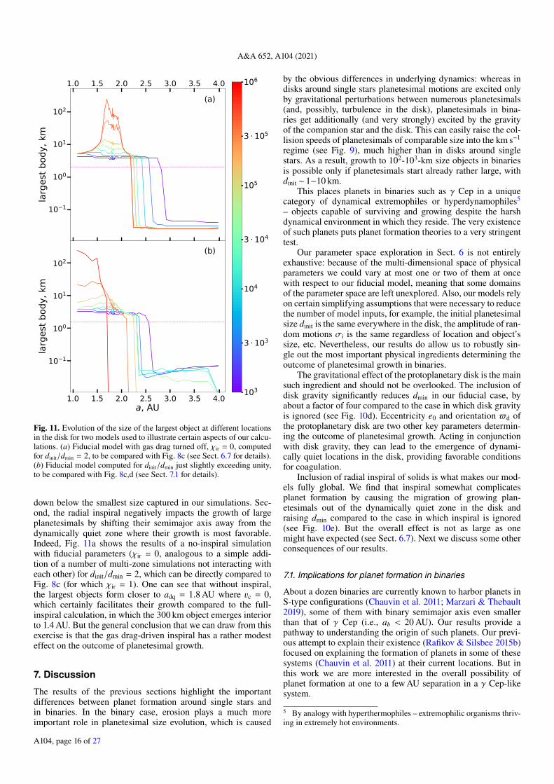
A&A 652, A104 (2021)

1.0 1.5 2.0 2.5 3.0 3.5 4.0a, AU

10 1

100

101

102

larg

est b

ody,

km

(b)

1.0 1.5 2.0 2.5 3.0 3.5 4.0

10 1

100

101

102

larg

est b

ody,

km

(a)

103

3 103

104

3 104

105

3 105

106

Fig. 11. Evolution of the size of the largest object at different locationsin the disk for two models used to illustrate certain aspects of our calcu-lations. (a) Fiducial model with gas drag turned off, χir = 0, computedfor dinit/dmin = 2, to be compared with Fig. 8c (see Sect. 6.7 for details).(b) Fiducial model computed for dinit/dmin just slightly exceeding unity,to be compared with Fig. 8c,d (see Sect. 7.1 for details).

down below the smallest size captured in our simulations. Sec-ond, the radial inspiral negatively impacts the growth of largeplanetesimals by shifting their semimajor axis away from thedynamically quiet zone where their growth is most favorable.Indeed, Fig. 11a shows the results of a no-inspiral simulationwith fiducial parameters (χir = 0, analogous to a simple addi-tion of a number of multi-zone simulations not interacting witheach other) for dinit/dmin = 2, which can be directly compared toFig. 8c (for which χir = 1). One can see that without inspiral,the largest objects form closer to adq = 1.8 AU where vc = 0,which certainly facilitates their growth compared to the full-inspiral calculation, in which the 300 km object emerges interiorto 1.4 AU. But the general conclusion that we can draw from thisexercise is that the gas drag-driven inspiral has a rather modesteffect on the outcome of planetesimal growth.

7. Discussion

The results of the previous sections highlight the importantdifferences between planet formation around single stars andin binaries. In the binary case, erosion plays a much moreimportant role in planetesimal size evolution, which is caused

by the obvious differences in underlying dynamics: whereas indisks around single stars planetesimal motions are excited onlyby gravitational perturbations between numerous planetesimals(and, possibly, turbulence in the disk), planetesimals in bina-ries get additionally (and very strongly) excited by the gravityof the companion star and the disk. This can easily raise the col-lision speeds of planetesimals of comparable size into the km s−1

regime (see Fig. 9), much higher than in disks around singlestars. As a result, growth to 102-103-km size objects in binariesis possible only if planetesimals start already rather large, withdinit ∼ 1−10 km.

This places planets in binaries such as γ Cep in a uniquecategory of dynamical extremophiles or hyperdynamophiles5

– objects capable of surviving and growing despite the harshdynamical environment in which they reside. The very existenceof such planets puts planet formation theories to a very stringenttest.

Our parameter space exploration in Sect. 6 is not entirelyexhaustive: because of the multi-dimensional space of physicalparameters we could vary at most one or two of them at oncewith respect to our fiducial model, meaning that some domainsof the parameter space are left unexplored. Also, our models relyon certain simplifying assumptions that were necessary to reducethe number of model inputs, for example, the initial planetesimalsize dinit is the same everywhere in the disk, the amplitude of ran-dom motions σi is the same regardless of location and object’ssize, etc. Nevertheless, our results do allow us to robustly sin-gle out the most important physical ingredients determining theoutcome of planetesimal growth in binaries.

The gravitational effect of the protoplanetary disk is the mainsuch ingredient and should not be overlooked. The inclusion ofdisk gravity significantly reduces dmin in our fiducial case, byabout a factor of four compared to the case in which disk gravityis ignored (see Fig. 10d). Eccentricity e0 and orientation $d ofthe protoplanetary disk are two other key parameters determin-ing the outcome of planetesimal growth. Acting in conjunctionwith disk gravity, they can lead to the emergence of dynami-cally quiet locations in the disk, providing favorable conditionsfor coagulation.

Inclusion of radial inspiral of solids is what makes our mod-els fully global. We find that inspiral somewhat complicatesplanet formation by causing the migration of growing plan-etesimals out of the dynamically quiet zone in the disk andraising dmin compared to the case in which inspiral is ignored(see Fig. 10e). But the overall effect is not as large as onemight have expected (see Sect. 6.7). Next we discuss some otherconsequences of our results.

7.1. Implications for planet formation in binaries

About a dozen binaries are currently known to harbor planets inS-type configurations (Chauvin et al. 2011; Marzari & Thebault2019), some of them with binary semimajor axis even smallerthan that of γ Cep (i.e., ab < 20 AU). Our results provide apathway to understanding the origin of such planets. Our previ-ous attempt to explain their existence (Rafikov & Silsbee 2015b)focused on explaining the formation of planets in some of thesesystems (Chauvin et al. 2011) at their current locations. But inthis work we are more interested in the overall possibility ofplanet formation at one to a few AU separation in a γ Cep-likesystem.

5 By analogy with hyperthermophiles – extremophilic organisms thriv-ing in extremely hot environments.

A104, page 16 of 27

K. Silsbee and R. R. Rafikov: Global simulations of planetesimal growth in stellar binaries

0.004

0.004

0.008

0.008

0.012

0.012

0.016

0.016

0.02

0.02

e0

1.0

1.5

2.0

2.5

3.0

3.5

4.0

a dq,

AU

0 = 500 g cm 2

0 = 1000 g cm 20 = 2000 g cm 2

0 = 5000 g cm 2

Fig. 12. Location adq of the dynamically quiet zone in an apsidallyaligned disk. We assume the fiducial disk plus binary parameters, exceptfor Σ0 and e0 which are varied as shown on the plot. The fiducialmodel is marked by an orange star along the curve corresponding toΣ0 = 1000 g cm−2.

Our finding that dmin only weakly depends on Σ0 is quiteimportant. As we vary Σ0 from 500 g cm−2 to 20,000 g cm−2

(i.e., between 0.3 and 12 times the minimum mass solar neb-ula density at 1 AU Hayashi 1981), implying the variation of theprotoplanetary disk mass from 1.8 MJ to 70 MJ (for the assumedΣ profile (1) with a0 = 1 AU and aout = 5 AU), dmin changes byless than a factor of two. What this means physically is that, evenwith the variation of Σ0, the dynamically quiet region can stillexist somewhere in the disk, ensuring that planetesimal growthcan be achieved in the disk globally (things may get more com-plicated at very low Σ0 when a secular resonance appears in thedisk; see Fig. 1).

Figure 12 shows adq as a function of e0 for various values ofΣ0 in a system which has, other than the variation of e0 and Σ0,our fiducial parameters. We have marked the fiducial model withan orange star along the Σ0 = 1000 g cm−2 curve. This shows thatover a wide range of disk masses, there is a dynamically quietregion in the disk. For each disk mass however, there is only arelatively narrow (approximately factor of two) range in e0 overwhich the dynamically quiet region exists in the part of the diskoutside 1 AU.

At low disk masses, a secular resonance appears in the disk(see the curve for Σ0 = 500 g cm−2 in Fig. 1). This resonancedramatically increases collision velocities in the outer disk asillustrated in Fig. 9b. Collision velocities between dp > 10 kmplanetesimals are even higher than in that figure, since theirorbits are less affected by gas drag.

In a static disk model such as ours, this resonance is local-ized, and planet formation can still proceed in other regions ofthe disk. In reality though, the disk evaporates over time, whichchanges the resonance location and causes the resonance to“sweep” through the disk. This effect is similar to the sweepingsecular resonances involving planets (Ward 1981).

On the other hand, the dynamically quiet location alsosweeps through the disk, meaning that over the disk lifetime,planetesimal growth may be promoted in many parts of thedisk. Exactly what is the effect of this combined sweeping

dynamically quiet location and sweeping resonance will dependon the details and timing of the disk dispersal.

It is worth noting that Fig. 12 shows that even for a quitelow surface density disk with Σ0 = 500 g cm−2 (correspondingto 6M⊕ of solid material), the dynamically quiet region will notexist if e0 is greater than about 0.02, corresponding to a mass-weighted mean disk eccentricity of 0.05. This is within the rangefound in numerical simulations, but on the low end of that range(see Sect. 7.3 for details).

The low levels of planetesimal random motions required todrive dmin into the kilometer size range may seem problematic:σi = 10−4 featured in our fiducial model corresponds to randomvelocities of about 10 m s−1. However, even this is above the levelof the escape speed from the surface of our initial planetesimalsin most cases, which is the most the two-body relaxation wouldpump up the random motions to. Moreover, given the high rela-tive velocities (up to ∼vc) between the planetesimal populationsof different sizes, both viscous stirring and dynamical frictionare likely to be very inefficient (Stewart & Ida 2000; Rafikov2003a), further reducing the amplitude of planetesimal randommotions.

The precise location and time at which planetesimals reachour assumed threshold size of 300 km are important outcomesof our models. They turn out to be rather strong functions ofdinit/dmin ≥ 1. If the size of seed planetesimals dinit is close todmin, planetesimals grow rather slowly, causing their substantialgas drag-driven inspiral, so that dp reaches 300 km somewhatcloser to the star than adq (see Fig. 11b). As dinit/dmin increases,planetesimals tend to grow to large sizes closer to adq (seeFig. 8c for dinit/dmin = 2). However, further increase in dinit/dmincauses the location of preferential planetesimal growth to shiftinward again (see Fig. 8d), presumably because of faster coag-ulation there. Such non-monotonic variation with dinit/dmin, aswell as the possibility of late-time planet migration (that musthave certainly affected S-type systems harboring hot Jupiters),complicate the effort to constrain the initial planetesimal sizedinit based on the semimajor axes of observed planets withinbinaries.

At the same time, the time to reach 300 km is a monotonicfunction of dinit/dmin, steadily falling from ∼1 Myr to < 105 yras this ratio increases from 1 to 5 in our fiducial model. Theexpectation of short disk lifetimes in S-type binaries (Harris et al.2012; Barenfeld et al. 2019; Zurlo et al. 2020) may then favorlarger dinit, for which the growth time is shorter.

As previously stated, our fiducial disk model contains lessthan four Jupiter masses of material. The planet in the γCephei system was determined to have around ten Jupiter masses(Benedict et al. 2018). Unless the disk is being replenished bymaterial infalling from the circumbinary disk, this would rule outall disk models with less than Σ0 . 5000 g cm−2 in this particularsystem.

7.2. Implications for planetesimal origin

Our finding that some minimum size dmin ∼ 1–10 km of seedplanetesimals is necessary for ensuring the success of planetarygenesis in S-type binary configurations has important conse-quences for theories of planetesimal formation. Two main ideasfor the origin of planetesimals – steady growth by coagulationand rapid formation via streaming instability (Johansen et al.2014) – predict very different formation pathways.

Growth by particle sticking must necessarily cover all sizesin the range from dust grains to multi-kilometer objects (sub-ject to substantial gravitational focusing). This formation mode

A104, page 17 of 27

A&A 652, A104 (2021)

is known to be problematic because of the bouncing barrieraround millimeter to centimeter sizes (Blum & Wurm 2008)and the rapid radial inspiral threatening meter-size objects(Weidenschilling 1977). In S-type binaries this planetesimalformation mechanism encounters another major bottleneck –efficient growth is impossible until seed objects are 1–10 km insize, substantially larger than any of the aforementioned barriers.This additional obstacle significantly reduces chances of slowplanetesimal growth by coagulation in binaries.

On the contrary, the competing mechanism relying on theoperation of streaming instability appears to naturally producelarge planetesimals with sizes in the range from tens to hun-dreds of kilometers (Simon et al. 2016; Schäfer et al. 2017).This mechanism is also rather fast (with a typical timescale oftens of local orbital periods), resulting in a rapid production ofthe population of seed planetesimals with dinit exceeding dmin,which would enable further growth into the planetary regime aswe have demonstrated here.

Thus, results of our work provide indirect support for the ideathat streaming instability is a pathway for forming planetesimalsin binaries (similar reasoning can be found in Thebault 2011).Of course, whether and how this instability would operate inan eccentric disk in presence of strong perturbations from thesecondary, is an open question. But if it works in binaries, thenthere is no reason for it not to be the mechanism for formingplanetesimals also in disks around single stars.

7.3. Implications for simulations of gaseous disks in binaries

Given the strong sensitivity of planetesimal growth to diskeccentricity e0 and orientation $d that we identify in this work,it is imperative to better constrain these variables. Unfortu-nately, observations are not yet at a stage where one can reliablydetermine eccentricity and orientation of protoplanetary disks inbinaries with small separations ab . 30 AU. Instead, one has torely on numerical simulations for guidance in that matter.

A number of studies have explored the amplitude of diskeccentricity excited by the gravity of an eccentric companionin a coplanar S-type configuration using 2D hydrodynamic sim-ulations. The conclusions that can be drawn from these worksvery strongly depend on the assumed physical inputs: equationof state, treatment of disk gravity, inner boundary conditions,and so on.

For example, studies using a locally isothermal equation ofstate (Kley & Nelson 2008; Paardekooper et al. 2008; Marzariet al. 2009; Zsom et al. 2011; Regály et al. 2011; Martin et al.2020) typically find rather high (mass-weighted mean) diskeccentricities, 〈ed〉 ∼ 0.1–0.3, with ed profile typically exhibitinga double-peaked structure as a function of semimajor axis andwith high values of ed close to the disk center. These resultsmay need to be viewed with caution in light of the recentlyidentified issues with using the locally isothermal equation ofstate for numerical modeling of the disk-perturber tidal interac-tion (Miranda & Rafikov 2019). On the contrary, studies thatattempt to represent disk thermodynamics in a more realisticway (Marzari et al. 2012; Gyergyovits et al. 2014) find a dra-matic reduction of disk eccentricity6, down to 〈ed〉 ∼ 0.02–0.05.As our results demonstrate, disk eccentricity at this level wouldallow planetesimal growth to proceed successfully starting from

6 Another work accounting for radiative effects by Picogna & Marzari(2013) is very different from the rest – it is a 3D Smoothed ParticleHydrodynamics (SPH) study – and found high disk eccentricity.

objects of a few to 10 km in size (see Fig. 1b). We note that inour model, 〈ed〉 = 2.5e0.

Similarly, accounting for the effect of disk self-gravity on itsdynamics has also been shown to suppress 〈ed〉 (Marzari et al.2009). Another interesting finding is that S-type disks tend to beless eccentric in more eccentric binaries (Marzari et al. 2009,2012; Regály et al. 2011), presumably because of their morecompact size.

Also important for the possibility of efficient planetesimalgrowth is the orientation of the disk, since the dynamicallyquiet zone, greatly facilitating planetesimal growth, arises onlyin disks which are close to apsidal alignment ($d ≈ 0) with thebinary orbit (see Fig. 1c). Unfortunately, at the moment there islittle clarity regarding this issue. Marzari et al. (2009) find thedisk to be precessing, that is, there is not a well-defined valuefor $d. In some other studies, the disk is aligned with the binaryorbit (Müller & Kley 2012; Martin et al. 2020). Gyergyovits et al.(2014) find the disk to be close to alignment, with |$d| ≈ 0.6 rad.Marzari et al. (2012) find anti-alignment ($d ≈ 180◦), whereasMarzari et al. (2009) find either anti-alignment or precession,depending on whether self-gravity is included. Paardekooperet al. (2008) find either anti-alignment or precession dependingon the flux limiter used in their code.

To summarize, the existing numerical studies of S-type disksin binaries have not yet arrived at a consensus regarding the val-ues of either e0 or $d, and their dependence on various physicalinputs, for example, realistic thermodynamics, disk self-gravity,viscosity, etc. Given the importance of these characteristics forunderstanding planet formation in S-type binaries, we encour-age future numerical efforts to focus on measuring the true valueof $d as well as disk eccentricity e0, using the most realisticphysical inputs, such as disk thermodynamics and self-gravity.

7.4. Comparison of detailed coagulation-fragmentationcalculations with simple heuristics

Full coagulation-fragmentation simulations like the ones fea-tured in this work are the most accurate predictor of the outcomeof planetesimal growth. However, they are numerically expen-sive. For that reason, in our previous work (e.g., Rafikov &Silsbee 2015b), we employed simple local (i.e., neglecting radialinspiral) heuristic criteria to determine conditions under whichgrowth would occur.

The simplest of these is the assumption that growth occursif and only if there are no catastrophically disruptive collisions.However, as shown in Sect. 5.1, it is also possible that erosioncan prevent growth even in the absence of catastrophic disrup-tion. For that reason Rafikov & Silsbee (2015b) considered analternative criterion, in which growth happens provided that noerosive collisions occur between planetesimals of “similar" sizes(i.e., bodies with a mass ratio greater than 10−2).

Now, armed with the full coagulation-simulation code, wecan test the performance of each of these growth criteria in pre-dicting the success of planetesimal evolution. To that effect weused our simulations in a single-annulus mode to calculate dminfor a variety of models featuring different values of dc and vc. Asdiscussed in Rafikov & Silsbee (2015a), the collision rates andvelocities are entirely determined by dc and vc (for the assumedlevel of random motions), regardless of what combination of diskparameters lead to the specific dc and vc (we set vK as appropriateat 2 AU in the disk around γ Cephei). Therefore, by exploringthe range of plausible vc and dc we check the validity of theseheuristics for all values of the disk parameters in our model.

A104, page 18 of 27

K. Silsbee and R. R. Rafikov: Global simulations of planetesimal growth in stellar binaries

100 101

dc, km100

101

102

d min

, km

vc = 8 102 m/s

(c)

100 101

dc, km

vc = 2.7 103 m/s

(d)

100 101

100

101

d min

, km

vc = 80 m/s

(a)100 101

vc = 2.7 102 m/s

(b)

Simulation resultsNo erosion

No catastrophic disruptionGeometric mean

Fig. 13. Minimum planetesimal size dmin resulting in the formation oflarge objects obtained with different methods for different values of vc(indicated in panels) and dc. The solid blue line shows dmin computedusing our multi-annulus simulations. The green line is the analytic esti-mate for dmin assuming that growth can occur starting from the smallestsize that does not suffer erosion by any particle greater than 1% of itsmass, according to the Stewart & Leinhardt (2009) prescription. The redline is the analytic estimate for dmin assuming that growth can occur aslong as catastrophic disruptions are absent. The dashed blue line showsthe geometric mean of the red and green lines.

Figure 13 displays the results of this calculation (each panelcorresponds to a different value of vc), with the solid blue lineshowing dmin as a function of dc, computed by our code using theprocedure described in Sect. 5.2.1. The red line shows the min-imum value of dinit such that no catastrophic disruption occursfor planetesimals of size dinit or larger. The green line shows theminimum value of dinit such that no body larger than dinit suffersan erosive collision with a partner with mass ratio greater than1%. The same criteria were used to determine the gray and blackregions, respectively, in Fig. 4 of Rafikov & Silsbee (2015b).

This figure shows that the criterion of no catastrophic dis-ruption is too optimistic, typically predicting dmin between twoand five times smaller (depending on dc and vc) than the onedetermined by the coagulation-fragmentation simulation. On thecontrary, the criterion of no erosion between bodies with a massratio greater than 1% is too restrictive, with the green curveexceeding the blue curve by a factor two to five.

Interestingly, the blue curve is often roughly equally sep-arated from both red and green ones (in log space), whichmotivated us to also show the dashed blue line computed as thegeometric mean of the predictions from the “no catastrophic dis-ruption” and “no erosion” models. As one can see, it matchesthe simulation-based dmin (blue curve) surprisingly well, withina factor of two or even better (although we do not claim this tohave any deep meaning). Thus, the geometric mean of the pre-dictions for dmin based on the two criteria used in Rafikov &Silsbee (2015b) can be employed as a rough approximation forpredicting the success of planetesimal growth in the absence ofsophisticated coagulation-fragmentation simulations.

7.5. Comparison with previous work

A number of past studies of planet formation in S-type binarieshave arrived at rather pessimistic conclusions regarding plan-etesimal growth starting from a population of 1–10 km objects(Thébault et al. 2006, 2008, 2009; Beaugé et al. 2010). In particu-lar, Thebault (2011) found that even dinit & 102 km planetesimalsdo not ensure planetesimal growth in HD 196885 system at thelocation of the known planet. All these studies included the effectof gas drag on planetesimal dynamics, and Paardekooper et al.(2008) and Beaugé et al. (2010) even considered the possibilityof the disk being eccentric.

However, as noted already in Rafikov (2013b) and Rafikov& Silsbee (2015a,b), all these calculations ignored the effect ofdisk gravity, which dramatically changes planetesimal dynamics.For example, Beaugé et al. (2010) find low planetesimal colli-sional velocities in the outer disk, whereas we find a very hostiledynamical environment there (see Fig. 9). The existence of thedynamically quiet location in apsidally aligned disks substan-tially alleviates the fragmentation bottleneck, allowing in manycases planetesimal growth to proceed even starting at dinit ∼ 1 km(see Fig. 10).

Another factor that distinguishes our study from others interms of realism is our reliance on the global coagulation-fragmentation calculations fully accounting for the gas drag-driven inspiral of planetesimals. Whereas Thébault et al. (2006,2008, 2009) and Rafikov & Silsbee (2015b) drew their conclu-sions based on individual collisional outcomes (see Sect. 7.4),we are able to model the evolution of the planetesimal size dis-tribution in its entirety, fully accounting for the fine details ofplanetesimal dynamics at every step.

Compared to Rafikov & Silsbee (2015b), we find less needfor a massive (&30MJ) protoplanetary disk: the lowest value ofΣ0 allowing growth to proceed starting at dinit ∼ 1 km in Fig. 10acorresponds to a disk mass of just 2 MJ. This difference arisesprimarily from our current full treatment of the planetesimal sizeevolution, but also from focusing on planet formation not at agiven location but globally, in the whole disk.

8. Conclusions

We present the first fully global coagulation-fragmentationframework for exploring planetesimal growth in S-type binarysystems, such as α Cen and γ Cep. Our framework fully accountsfor the specifics of planetesimal dynamics in binaries, includingperturbations not only due to the eccentric stellar companion,but also due to the gravity of the eccentric protoplanetary disk inwhich planetesimals orbit. We include the effects of gas drag onthe eccentricity dynamics of planetesimals, as well as on theirradial inspiral. Thus, this framework brings studies of planetformation in binaries to an entirely new level of realism.

By running a suite of simulations with varied model inputs,we are able to delineate the conditions under which planetesi-mals can grow to large sizes (hundreds of kilometers) despitethe adverse effects of fragmentation. The difficulty of planet for-mation for a given disk model was measured via the parameterdmin – the smallest size of seed planetesimals that allows theirgrowth into the planetary regime – with the smaller dmin imply-ing more favorable conditions for planet formation. Based on theresults of these calculations, we are able to draw the followinggeneral conclusions.

– For most disk parameters considered in this paper, planetformation in binaries such as γ Cephei can successfullyoccur provided that the initial planetesimal size is &10 km;

A104, page 19 of 27

A&A 652, A104 (2021)

however, for favorable disk parameters, this minimum initialsize can go down to .1 km;

– The gravitational effect of the protoplanetary disk plays thekey role in lowering the minimum initial planetesimal sizenecessary for sustained growth by a factor of four. Thisreduction can be achieved in protoplanetary disks apsidallyaligned with the binary, in which a dynamically quiet zoneappears within the disk provided that the mass-weightedmean disk eccentricity .0.05 (corresponding, in the contextof our model, to e0 . 0.02);

– We identify disk eccentricity (e0) and the apsidal misalign-ment angle ($d) as the parameters to which planetesimalgrowth is most sensitive. Whenever the dynamically quietlocation exists in the disk, growth is also strongly dependenton the level of random motion of planetesimals;

– For the models explored in this work, the outcome of plan-etesimal evolution is only weakly dependent on the disksurface density Σ0;

– Radial inspiral of solid material appears to make little differ-ence to the critical planetesimal size from which collisionalagglomeration can occur;

– The planetesimal strength, as parameterized by the two mod-els of Stewart & Leinhardt (2009), makes only about a factorof two difference to the critical planetesimal size;

– Planetesimal growth to large sizes can occur even in theface of some erosion, but in the environments with fre-quent collisions leading to catastrophic disruption, growthwill not occur. We used our coagulation-fragmentation sim-ulations to provide a new heuristic criterion for successfulplanetesimal evolution in Sect. 7.4;

– Our results provide indirect support for models in whichplanetesimals are born large (&10 km), such as those basedon streaming instability.

The general framework for the realistic treatment of planetesimalgrowth in binaries developed in this work can be applied to studya range of other problems: circumbinary planet formation in P-type systems (Silsbee & Rafikov 2015a), collisional evolution ofdebris disks perturbed by planetary (Nesvold & Kuchner 2015;Sefilian et al. 2021) or stellar (Thebault et al. 2021) companions,and so on.

Acknowledgements. The authors acknowledge helpful discussion with Lucas Jor-dan. K.S. acknowledges the support of the Max Planck Society. R.R.R. thanksNASA grant 15-XRP15-2-0139, STFC grant ST/T00049X/1, and John N. BahcallFellowship for financial support.

ReferencesAdachi, I., Hayashi, C., & Nakazawa, K. 1976, Progr. Theor. Phys., 56, 1756Barenfeld, S. A., Carpenter, J. M., Sargent, A. I., et al. 2019, ApJ, 878, 45Beaugé, C., Leiva, A. M., Haghighipour, N., & Otto, J. C. 2010, MNRAS, 408,

503Belyaev, M. A., & Rafikov, R. R. 2011, Icarus, 214, 179Benedict, G. F., Harrison, T. E., Endl, M., & Torres, G. 2018, Res. Notes Am.

Astron. Soc., 2, 7Blum, J., & Wurm, G. 2008, ARA&A, 46, 21Bromley, B. C., & Kenyon, S. J. 2011, ApJ, 731, 101Chauvin, G., Beust, H., Lagrange, A. M., & Eggenberger, A. 2011, A&A, 528,

A8Davydenkova, I., & Rafikov, R. R. 2018, ApJ, 864, 74Dohnanyi, J. S. 1969, J. Geophys. Res., 74, 2531Dvorak, R. 1982, Oesterreich. Akad. Wissensch. Math. Naturwissensch. Klasse

Sitzungsber. Abteilung, 191, 423

Garaud, P., Meru, F., Galvagni, M., & Olczak, C. 2013, ApJ, 764, 146Greenzweig, Y., & Lissauer, J. J. 1992, Icarus, 100, 440Gyergyovits, M., Eggl, S., Pilat-Lohinger, E., & Theis, C. 2014, A&A, 566, A114Harris, R. J., Andrews, S. M., Wilner, D. J., & Kraus, A. L. 2012, ApJ, 751, 115Hatzes, A. P., Cochran, W. D., Endl, M., et al. 2003, ApJ, 599, 1383Hayashi, C. 1981, Progr. Theor. Phys. Suppl., 70, 35Heppenheimer, T. A. 1978, A&A, 65, 421Heppenheimer, T. A. 1980, Icarus, 41, 76Ida, S., & Makino, J. 1993, Icarus, 106, 210Inaba, S., Tanaka, H., Nakazawa, K., Wetherill, G. W., & Kokubo, E. 2001,

Icarus, 149, 235Johansen, A., Blum, J., Tanaka, H., et al. 2014, in Protostars and Planets VI, eds.

H. Beuther, R. S. Klessen, C. P. Dullemond, & T. Henning, 547Kenyon, S. J., & Bromley, B. C. 2002, AJ, 123, 1757Kenyon, S. J., & Luu, J. X. 1998, AJ, 115, 2136Kenyon, S. J., & Luu, J. X. 1999, AJ, 118, 1101Kley, W., & Nelson, R. P. 2008, A&A, 486, 617Kobayashi, H., Tanaka, H., Krivov, A. V., & Inaba, S. 2010, Icarus, 209, 836Kokubo, E., & Ida, S. 1998, Icarus, 131, 171Martin, R. G., Lissauer, J. J., & Quarles, B. 2020, MNRAS, 496, 2436Marzari, F., & Scholl, H. 2000, ApJ, 543, 328Marzari, F., & Thebault, P. 2019, Galaxies, 7, 84Marzari, F., Scholl, H., Thébault, P., & Baruteau, C. 2009, A&A, 508, 1493Marzari, F., Baruteau, C., Scholl, H., & Thebault, P. 2012, A&A, 539, A98Meschiari, S. 2014, ApJ, 790, 41Miranda, R., & Rafikov, R. R. 2019, ApJ, 878, L9Müller, T. W. A., & Kley, W. 2012, A&A, 539, A18Murray, C. D., & Dermott, S. F. 1999, Sol. Syst. Dyn., 253Nesvold, E. R., & Kuchner, M. J. 2015, ApJ, 798, 83O’Brien, D. P., & Greenberg, R. 2003, icarus, 164, 334Ogilvie, G. I. 2001, MNRAS, 325, 231Paardekooper, S.-J., Thébault, P., & Mellema, G. 2008, MNRAS, 386, 973Picogna, G., & Marzari, F. 2013, A&A, 556, A148Rafikov, R. R. 2003a, AJ, 126, 2529Rafikov, R. R. 2003b, AJ, 125, 922Rafikov, R. R. 2003c, AJ, 125, 906Rafikov, R. R. 2003d, AJ, 125, 942Rafikov, R. R. 2004, AJ, 128, 1348Rafikov, R. R. 2013a, ApJ, 764, L16Rafikov, R. R. 2013b, ApJ, 765, L8Rafikov, R. R., & Silsbee, K. 2015a, ApJ, 798, 69Rafikov, R. R., & Silsbee, K. 2015b, ApJ, 798, 70Rafikov, R. R., Silsbee, K., & Booth, R. A. 2020, ApJS, 247, 65Regály, Z., Sándor, Z., Dullemond, C. P., & Kiss, L. L. 2011, A&A, 528, A93Safronov, V. S. 1972, Evolution of the Protoplanetary Cloud and Formation of

the Earth and Planets.Schäfer, U., Yang, C.-C., & Johansen, A. 2017, A&A, 597, A69Sefilian, A. A., Rafikov, R. R., & Wyatt, M. C. 2021, ApJ, 910, 13Silsbee, K., & Rafikov, R. R. 2015a, ApJ, 808, 58Silsbee, K., & Rafikov, R. R. 2015b, ApJ, 798, 71Simon, J. B., Armitage, P. J., Li, R., & Youdin, A. N. 2016, ApJ, 822, 55Smoluchowski, M. V. 1916, Zeitsch. Phys., 17, 557Spaute, D., Weidenschilling, S. J., Davis, D. R., & Marzari, F. 1991, Icarus, 92,

147Statler, T. S. 2001, AJ, 122, 2257Stewart, G. R., & Ida, S. 2000, Icarus, 143, 28Stewart, S. T., & Leinhardt, Z. M. 2009, ApJ, 691, L133Stewart, G. R., & Wetherill, G. W. 1988, Icarus, 74, 542Tanaka, H., Inaba, S., & Nakazawa, K. 1996, icarus, 123, 450Thebault, P. 2011, Celest. Mech. Dyn. Astron., 111, 29Thebault, P., Kral, Q., & Olofsson, J. 2021, A&A, 646, A173Thébault, P., Marzari, F., & Scholl, H. 2006, Icarus, 183, 193Thébault, P., Marzari, F., & Scholl, H. 2008, MNRAS, 388, 1528Thébault, P., Marzari, F., & Scholl, H. 2009, MNRAS, 393, L21Trubnikov, B. A. 1971, Sov. Phys. Dokl., 16, 124Ward, W. R. 1981, Icarus, 47, 234Weidenschilling, S. J. 1977, MNRAS, 180, 57Wetherill, G. W., & Stewart, G. R. 1989, Icarus, 77, 330Wetherill, G. W., & Stewart, G. R. 1993, Icarus, 106, 190Windmark, F., Birnstiel, T., Ormel, C. W., & Dullemond, C. P. 2012, A&A, 544,

A16Zsom, A., Sándor, Z., & Dullemond, C. P. 2011, A&A, 527, A10Zurlo, A., Cieza, L. A., Pérez, S., et al. 2020, MNRAS, 496, 5089

A104, page 20 of 27

K. Silsbee and R. R. Rafikov: Global simulations of planetesimal growth in stellar binaries

Appendix A: Detailed description of the numericalmethods

Here we describe a number of technical details of the implemen-tation of our code, including both numerical details and physicalinputs.

A.1. Mass redistribution due to collisions

In a given annulus, our code solves the standard coagulation-fragmentation problem, which effectively is a version of thecoagulation equation of Smoluchowski (1916) modified toaccount for fragmentation (see Eq. (1) of Rafikov et al. 2020).Our framework employs mass space discretization in the formof logarithmically spaced mass bins with constant Mi+1/Mi. Thegrid extends from the minimum mass corresponding to a 10 mobject to a maximum mass corresponding to a 300 km object.Fragments with sizes below 10 m that form in planetesimal colli-sions are simply removed from the system (i.e., total mass is notconserved for this reason alone). This leads to certain numericalartifacts discussed in Sect. 5.1.

At each time step, the code calculates the mean collisionrate Ri j between planetesimals in bin i and bin j for all i andj in [1,Nbins]. This calculation is described in Appendix A.4.The number of collisions Zi j in a given time step of length ∆tbetween bodies in mass bins i and j is then drawn randomly froma Poisson distribution with the mean Ri j∆t:

Zi j = Poisson(Ri j∆t). (A.1)

We define an operator F such that Fi jk is the number of frag-ments in mass bin i produced by a collision of a particle in bin jwith a particle in bin k (see Sect. A.2).

The mass distribution n is updated as

ni = ni + ΣNbinsj=1 Σ

Nbinsk=1 Ci jk, (A.2)

where

Ci jk = Z jk1 + δ jk

2

[Fi jk − δi j − δik

]. (A.3)

This takes into account both addition of particles to bin i fromcollisional fragments (the Fi jk operator), as well as collisionaldestruction of particles in bin i (the −δi j and −δik terms). Thefactor of (1 + δ jk)/2 is to prevent over-counting when summingover both j and k.

At times, due to a fluctuation, a number of particles in a par-ticular mass bin may become negative. In this case we reset thenumber of particles in such a bin to zero; this effectively leadsto addition of mass to the system. However, we checked severalruns of our fiducial simulation, and found that relative to the totalmass in the simulation, less than 1 part in 105 was added in thisway.

A.2. Collisional outcomes

This section describes the physics which goes into the determi-nation of Fi jk. The outcome of a collision between a body inmass bin i and one in mass bin j is dependent on the collisionvelocity. High-velocity collisions will result in many small frag-ments, and no large remnant bodies. Low-velocity collisions willresult in one body which contains nearly all of the pre-collisionmass and only very small fragments. Calculation of collisionvelocity vcoll is described in Sect. A.3.

Given a value of vcoll, we use the recipe provided in Stewart& Leinhardt (2009) to determine the mass of the largest remnantMlr. We take the mass of the largest remnant to be

Mlr

Mtot= 1 − 0.5

QR

Q∗RD, (A.4)

where Mtot = mi + m j is the total mass of the two incomingbodies, QR is the specific center-of-mass energy of the collisiongiven by

QR = 0.5mim jv

2coll

Mtot, (A.5)

and Q∗RD is the critical value of QR which leads to catastrophicdisruption (which corresponds to Mlr < 0.5Mtot); Q∗RD is a func-tion of the sizes and composition of the planetesimals, and vcoll,which is given by Eq. (2) from Stewart & Leinhardt (2009). Asour default, we used the parameters appropriate for their “strongrock” planetesimals; however we also ran simulations using their“rubble pile” planetesimals.

When Mlr is calculated, it will in general be between Mi andMi+1 for some i. We then add a fraction Pi of the mass to bin iand Pi+1 to bin i + 1 given by

Pi =Mi+1 − Mlr

Mi+1 − Mi, Pi+1 =

Mlr − Mi

Mi+1 − Mi. (A.6)

We assume that the rest of the fragments follow a mass distri-bution with a power law index ξ. The precise value of ξ does notaffect the long-term outcome of fragmentation cascade (O’Brien& Greenberg 2003). The upper cutoff mass for this distributionis given by

Mcutoff =

{0.5(Mtot − Mlr) Mlr/Mtot ≥ 0.5,max(Mtotb, 0.5Mlr) Mlr/Mtot < 0.5.

(A.7)

Here b is an adjustable parameter which determines the cut-off mass for catastrophic collisions: whenever Eq. (A.4) yieldsMlr < 2bMtot, we put all of the mass into fragments (as describedbelow) without leaving a single largest remnant. This situationoften arises in very energetic collisions when Mlr is small.

The fragment mass is assigned to mass bins with 0 < i ≤icutoff , where icutoff is the index of the largest bin with mass lessthan Mcutoff . This is done such that

Fi jk = Υ jk M1+ξi , (A.8)

where Υ jk is a normalization constant. The exponent of Mi is1 + ξ rather than ξ because of the logarithmic spacing of themass bins.

In order to solve for Υ jk, we note that

icutoff∑i=−∞

Υ jk M2+ξi = Mtot − Mlr, (A.9)

where nonpositive values of i correspond to (hypothetical) massbins with Mi less than the minimum size considered in our sim-ulations. Letting R ≡ Mi+1/Mi, we can then solve for Υ jk andwrite

Fi jk =Mtot − Mlr

Mcutoff

× (Mi/Mcutoff)1+ξ ×(1 − R−ξ−2

). (A.10)

A104, page 21 of 27

A&A 652, A104 (2021)

Some mass is lost from the simulation because it is containedin bodies with mass less than M1. This lost mass is equal to

Mlostjk = Υ jk

0∑i=−∞

M2+ξi = (Mtot − Mlr)

[M0

Mcut

]2+ξ

. (A.11)

Because of the self-similar form of the fragment mass spec-trum, we were able to implement this fragmentation algorithmwith numerical cost scaling as O(N2

bins) using explicit time step-ping (see Rafikov et al. 2020 for details). This considerablyreduces the computational burden of our calculations.

A.3. Collision velocity

We calculate the collision velocity vcoll by considering two sep-arate dynamical regimes. In the first, the relative motion ofplanetesimals is dominated by their secularly excited eccentrici-ties. Equation (64) of RS15a then gives the relative eccentricityei j between planetesimals as a function of their masses. Givenei j, there is a distribution of relative encounter velocities vi jbetween vmin = 0.5ei jvK and vmax = ei jvK, where vK is the localKeplerian speed. This distribution is given by Eq. (62) of RS15aas

d fi j

dvi j=

v−1max

E(√

3/2)

v2i j[

(v2max − v2

i j)(v2i j − v2

min)] . (A.12)

At each time step, for each set of collision partners, a randomnumber λ between 0.5 and 1 is drawn based on the distributionin Eq. (A.12), and the collision velocity in this regime is taken tobe

vcoll = λei jvK. (A.13)

In the second dynamical regime, we assume that randommotions dominate over the secularly excited eccentricities. Weassume that planetesimals have eccentricity vectors (k, h) = (ks +krand, hs + hrand) where (ks, hs) and (krand, hrand) are the secular andrandom components, respectively; krand and hrand are assumed tobe drawn from independent Gaussian distributions

ρ(krand) = 1σe√

2πexp

[− (krand)2

2σ2e

],

ρ(hrand) = 1σe√

2πexp

[− (hrand)2

2σ2e

], (A.14)

where we take σe = 2σi. This leads to a distri-bution of the relative random eccentricity erand =√

(krand,1 − krand,2)2 + (hrand,1 − hrand,2)2 given by the Rayleighdistribution

ρ(erand) =erand

2σ2e

exp[− (erand)2

4σ2e

]. (A.15)

In principle, for each set of collision partners, we should thentake the collision velocity to be given by

vcoll = vK

√(λeij

)2+ e2

rand, (A.16)

where erand is drawn from the distribution in Eq. (A.15), and λ isdrawn from the distribution in Eq. (A.12).

In practice, doing this at each time-step would be too time-consuming. Instead, we use the following algorithm. Let F(v)

be the true collision velocity distribution for a given set of col-lision partners in a given annulus. We approximately calculateN1 points in v-space, such that there is a constant fraction ofthe distribution F(v) between consecutive points: this means thatthe ith point vi satisfies the relation

∫ vi

0 F(v)dv = (i + 0.5)/N1, fori ∈ [0,N1 − 1]. We then calculate the collision rates and out-comes for each set of collision partners at the beginning of thesimulation, using the N1 different velocities. During the simula-tion, in each timestep, and for each set of collision partners, werandomly choose one of the N1 collisional outcomes and rates touse for that timestep.

To calculate the N1 values vi, we initially create two vectorszrand and zλ of length N2 with a constant fraction of the distribu-tion for erand between each entry of zrand and a constant fractionof the distribution of λ between each entry of zλ. This means

that∫ zi+1

rand

zirand

ρ(erand) = 1/N2, and a similar relation exists betweenzλ and the distribution for λ implied by Eq. (A.12).

We then draw N3 samples of the collision velocity usingEq. (A.16) and randomly selected entries from zrand and zλ. Wethen select the N1 values of vi so there are an equal number of theN3 sample velocities between consecutive values of vi. We takeN1 = 11, N2 = 100, and N3 = 990.

We ignore shear motion in calculating the collision veloc-ity because if the shear motion is the dominant effect, then theplanetesimals will completely merge in collisions, so there isno reason to consider shear motion except in how it affects thecollision rate.

We note that the differential radial drift described in Sect. 3.5is not included in our calculation of vcoll as it does not typicallycontribute substantially to the collision velocities between bodiesof the sizes that we consider in this paper.

A.4. Collision rate

Next we describe our calculation of the collision rate. In the firstdynamical regime (where the relative motion of planetesimalsis dominated by their secularly excited eccentricities), we useEq. (63) from RS15a (corrected so that emax is replaced withvmax/ap). This gives a flux Fi j of planetesimals from bin j past aplanetesimal in bin i of

Fi j =E(√

3/2)Σ jvmax

π2apm jIi j, (A.17)

where Ii j is the relative inclination between the two groups ofparticles. We assume that all of the planetesimal inclinationis due to random motions. We assume all planetesimals haveinclination vectors (q, p) with q and p drawn from independentGaussian distributions:

ρ(q) =1

σi√

2πexp

− q2

2σ2i

; ρ(p) =1

σi√

2πexp

− p2

2σ2i

.(A.18)

The distribution of Iij =√

(qi − q j)2 + (pi − p j)2 is thereforegiven [analogous to Eq. (A.15)] by

ρ(Ii j) =1

2σ2i

Ii j exp

− I2i j

4σ2i

. (A.19)

Then, averaged over Ii j, the average value of Fi j is given by

〈Fi j〉 =

∫ ∞

Ii j=0ρ(Ii j)Fi jdIi j =

E(√

3/2)Σ jvmax

2π3/2σim jap. (A.20)

A104, page 22 of 27

K. Silsbee and R. R. Rafikov: Global simulations of planetesimal growth in stellar binaries

The collision rate for a given particle in bin i with the populationin bin j is given by Ri j = 〈Fi j〉σi j, where σi j is the collision crosssection including gravitational focusing:

σi j = Ag

1 +

(vesc

λei jvK

)2 , (A.21)

where Ag = π(di + d j)2 is the geometric cross section, and vesc =√2G(mi + m j)/(di + d j). As discussed in Sect. A.3, at each time-

step, we assume a particular value of the collision velocity drawnfrom the distribution F(v). For the purposes of calculating thecollision rate, we assume λ to be in the same quantile of thedistribution for λ as v is for F(v).

In the second dynamical regime of dominant randommotions (

√πσe > ei j) we use the two-body accretion formula

from Eq. (17) of Greenzweig & Lissauer (1992):

Ri j =Σ jAg

2π2m j

F (I∗) +v2

esc

v2K

G (I∗)e2∗

. (A.22)

Here, F and G are functions of I∗ = σi/σe. We assume thatI∗ = 1/2, in which case F (1/2) = 17.3, and G (1/2) = 38.2. e∗is the rms random eccentricity. Greenzweig & Lissauer (1992)considered a planetesimal accreting on a circular orbit, but in ourcase, we should use the rms relative random eccentricity whichcan be shown from Eq. (A.15) to be e∗ = 2σe. Additionally, wemust divide by the orbital period as Eq. (A.22) is in units wherethe orbital period is unity:

Ri j =Σ jAgvK

4π3apm j

F (I∗) +v2

esc

v2K

G (I∗)e2∗

. (A.23)

We approximate the transition to the shear-dominated regimeby replacing e∗ in Eq. (A.23) with e∗+c1eH, and then multiplyingthe entire right hand side by 1 + c2(eH/e∗), where c1 and c2 areinterpolation constants. This gives us a formula

Ri j =Σ jAgvK

4π3apm j

F (I∗) +v2

esc

v2K

G (I∗)(e∗ + c1eH)2

(1 + c2eH

e∗

). (A.24)

We estimate c1 and c2 by comparing the rates given by Eq. (A.24)with those shown in Fig. 5 of Greenzweig & Lissauer (1992).From these data we estimate c1 = 4.75, c2 = 22.6, which we usein our work.

We expect a transition between the two dynamical regimesto occur when eij = 〈er〉 =

√πσ′e, where σ′e = σe + c1eH/2 (the

factor of 2 arising from the fact that e∗ = 2σe). The collisionrates in the two regimes are not exactly equal at the transitionpoint. Let R1 be the collision rate in the low secular velocitylimit given by Eq. (A.24), and let R2 be the collision rate whenthe secular velocity dominates; R2 is given by

R2 =E(√

3/2)Σ jAgvKei j

2π3/2σiapmp

1 +

(vesc

vi j

)2 . (A.25)

Assuming σi/σe = 1/2, then at ei j =√πσe, ignoring shear,

R2/R1 = 2.8 in the limit that vesc/(σevK) � 1, and 1.6/λ2 in thelimit that vesc/(σevK) � 1. To make the collision rate continuous,we approximate it as

Ri j(vi j) = f R1 + (1 − f )R2, (A.26)

with f = 1/(1 + [ei j/(√πσ′e)]2) = 1/(1 + [vi j/(

√πλσ′evK)2]).

vi j = λei jvK is the relative secular velocity between bodies inmass-bins i and j for that time step.

The above prescription needs to be modified in the caseof collisions between two bodies within the same mass bin,where the focusing factor can vary significantly depending onthe location within the mass bin of the two colliding partners.For example, two bodies with masses right at the center of themass bin will have a higher focusing factor than one body at thebottom end of the mass bin and one body at the top end; in thelatter case, the approach velocity will be higher.

Let vmax,i be the relative (secularly excited) velocity betweenthe heaviest body in the ith mass bin and the lightest. Let x1 =(m1 − mbottom)/(mtop − mbottom) be the position of body 1 in themass bin, where mtop and mbottom are the masses of the heav-iest and lightest bodies in the bin. We define x2 analogouslyfor the second body. The relative secularly excited velocity v12between particles 1 and 2 is then equal to vmax|x1 − x2| and hasa distribution (assuming x1 and x2 to be uniformly distributedin [0, 1])

ρ(v12) =2vmax

(1 − v12

vmax

). (A.27)

Therefore, 〈Rii〉, the rate at which a particle in bin i experiencescollisions with other particles in bin i, is given by

〈Rii〉 =

∫ vmax

0ρ(v12)Rii(v12)dv12. (A.28)

A.5. Radial inspiral

Using the results of Rafikov & Silsbee (2015a,b) we obtain theradial drift velocity of particles as a function of their size andsemimajor axis (see Sect. 3.5 for details). Let ∆ri be the radialwidth of annulus i, and let the drift rate of a particle in annulusi and mass bin j be vi, j. We then let the change in the number ofparticles in annulus i and mass bin j in a time interval ∆tinsp begiven by

∆ni, j = −ni, jvi, j∆tinsp

∆ri+

ni+1, jvi+1, j∆tinsp

∆ri+1, (A.29)

We use Nann = 60 annuli. These were spaced so as to mini-mize changes in ec or a within one bin. The exact bin boundariesdepend on the run of ec(a) which varies between our differentdisk models. For the fiducial model, a changed by less than 16%between adjacent bins and ec by less than 41% in the cases whereec > 10−4.

A.6. Time step determination

In this section, we describe how the time steps for the coagula-tion process and the radial inspiral are determined.

A.6.1. Coagulation-fragmentation time step

The time step for the coagulation-fragmentation process must beshort enough that the distribution does not change appreciablyduring the length of a time step. In principle, this means that wewould like

|ni(t) − ni(t + ∆tcoag)|ni(t)

< ε (A.30)

A104, page 23 of 27

A&A 652, A104 (2021)

for all i, where ε is some small number. In practice, this iscomplicated by the fact that mass is added to bins in discretequantities, and that some bins have a small number of particles.In a bin with a small number of particles, even adding one addi-tional particle will make a large fractional change to the amountof mass in that bin. Additionally, collisions are a random pro-cess, so a fluctuation can change the mass in a bin by more thanexpected. To address these concerns, we instead pick the largesttime step ∆tcoag such that for all i∣∣∣∣∣∣⟨

ni(t) − ni(t + ∆tcoag)

ni(t)

⟩∣∣∣∣∣∣ < ε1 or∣∣∣∣∣∣∣⟨

mi(ni(t) − ni(t + ∆tcoag))

ΣNbinsi=1 mini

⟩∣∣∣∣∣∣∣ < ε2, (A.31)

where the angle brackets refer to averaging over the distributionof encounter velocity in Eq. (A.12). To save computational time,we approximate the average over the encounter velocity distri-bution by evaluating the collisional outcomes using the medianencounter velocity. Here, as before, a time step is acceptable iffor each bin, either the fractional decrease in mass is less thanε1, or the decrease in mass is less than ε2 times the total mass inthe system. Time step ∆tcoag is recalculated every time we updatethe mass distribution, separately for each annulus, and the min-imum value among all the annuli is used for each time step. Itis not obvious from first principles which values of ε1 and ε2 areappropriate. But rows 10 and 11 of Table C.1 (which exploressensitivity of our calculations to the numerical parameters used;see Appendix C) show that variation of these values by a factorof two (or more) from our fiducial values of 0.05 and 10−6 havea negligible effect on dmin.

In the simulation used to create Fig. 4, we used a lower valueof ε2 so that the distributions would remain smooth, even inregions of mass-space containing a negligible amount of mass.The success of the coagulation process, and the shape of thedistribution at sizes greater than dinit in those simulations is notaffected by this change.

A.6.2. Radial inspiral time step

The code uses a different time step for the radial drift. Masstransport due to radial drift is recalculated using Eq. (A.29) everyinterval of time ∆tinsp such that

∆tinsp × max(vdrift

∆ri

)= εdrift, (A.32)

which guarantees that the inspiraling particles do not cross thefull radial bin width in time ∆tinsp (vdrift is the inspiral speed).While we see from Eq. (A.29) that εdrift must not be larger than1, it is apparent from the results of Sect. B.3 below that thereis little advantage to picking εdrift less than 1. Therefore, we useεdrift = 1.

Appendix B: Tests of the code

In this section, we describe the tests we did of the code againstknown analytic solutions in certain limiting cases. We inde-pendently verify three code functionalities – coagulation, frag-mentation, and radial inspiral – and find that the code doesa reasonable job of reproducing known solutions to the accu-racy warranted given the imperfect knowledge of the physicalprocesses involved.

100 102 104 106 108 1010

10 2

102

106

1010

coun

t

(a)

Aij = 1

Simulation: = 10Analytic: = 10Simulation: = 100Analytic: = 100Simulation: = 1, 000Analytic: = 1, 000

10 2

102

106

1010

coun

t

(b)Aij = i + j

Simulation: = 1Analytic: = 1Simulation: = 3Analytic: = 3Simulation: = 6Analytic: = 6

100 102 104 106 108 1010

mass

10 6

10 2

102

106

1010co

unt

(c)Aij = ij

Simulation: = 0.3Analytic: = 0.3Simulation: = 0.7Analytic: = 0.7Simulation: = 0.99Analytic: = 0.99Analytic: = 0.997

Fig. B.1. Test of our coagulation module: comparison of simulation andanalytic results for different coagulation kernels starting with N = 1012

particles of unit mass. Here η = Nt is a time coordinate, rescaled by thenumber of particles initially in the system. Each panel is made assuminga different coagulation kernel Ai j, labeled in the panels and discussed inSect. B.1.

B.1. Tests against known solutions of the coagulationequation

In this section we test the coagulation module of our code. Wedescribe the results of simulations of the coagulation alone,without fragmentation, and with simplified collision rates andinitial conditions that have analytic solutions we can comparewith. There are three known analytic solutions to the Smolu-chowski coagulation equation

dnk

dt=

12

∑i+ j=k

Ai jnin j − nk

∞∑i=1

Aikni, (B.1)

obtained for kernels Ai j = 1 (Smoluchowski 1916), Ai j = i + jand Ai j = i j (Trubnikov 1971), with the initial condition of Nparticles of a single mass bin. Our code successfully reproducesthese solutions with small deviations as discussed below.

The top panel of Fig. B.1 shows the number of particles perunit mass as a function of mass for three different times for thekernel Ai j = 1. In this figure we have used a mass bin spacingMi+1/Mi = 1.15. Initially there were N = 1012 particles all ofmass 1. Because the distribution evolves more rapidly if there aremore particles, we express time in terms of η = Nt. In the limitof large N, the shape of the distribution depends only on η, rather

A104, page 24 of 27

K. Silsbee and R. R. Rafikov: Global simulations of planetesimal growth in stellar binaries

than on N or t independently. The large scatter at low masses isdue to the logarithmic spacing of the mass bins and the initialcondition that all the mass is in bodies with unit mass. Since weare assuming perfect sticking in collisions for this exercise, onlymass bins containing integer masses will contain a nonzero num-ber of particles, leading to an uneven distribution at low masses.Other than this discrepancy at low mass, there is nearly perfectagreement between our code and the analytic solution.

The middle panel of Fig. B.1 shows the number of particlesper unit mass as a function of mass for three different valuesof η for the kernel Ai j = i + j. The distribution evolves morerapidly than in the case of the constant kernel because of thehigher collision rates. In this case, in addition to the scatter atlow masses, we see that the numerical solution is slightly behindthe analytic solution at the high-mass end of the distribution.

The bottom panel of Fig. B.1 shows the number of particlesper unit mass as a function of mass for three different values of ηfor the kernel Ai j = i j. Here, the system evolves in a more com-plicated manner than the previous two cases (Trubnikov 1971).For η < 1, orderly growth from smaller to larger particles pro-gresses as in the previous cases. However, for η > 1, one bodybecomes much larger than the others, and eventually consumesall the mass in the system. Our simulation is not well-equippedto handle this runaway growth phase, so we restrict ourselves toreproducing the analytic solutions for η < 1.

The discrepancy between the numerical and analytic solu-tions at η = 0.99 looks somewhat alarming. This is because thedistribution function is evolving quite rapidly at this time. Wealso plotted the analytic solution for η = 0.997, and we see thatit matches the numerical solution well, implying that this differ-ence only corresponds to a time lag of just 0.3% in the numericalsolution, which is not critical for our calculations.

B.2. Tests of the fragmentation module

Next we checked the ability of our code to properly handle frag-mentation. Unlike the coagulation problem, there are no knownanalytical solutions describing time-dependent behavior in frag-menting systems. However, there are some known results for thesteady-state fragmentation cascades to which collisionally evolv-ing systems tend to converge. In this section we use these resultsto verify that the fragmentation module of our code is operatingcorrectly.

O’Brien & Greenberg (2003) present a model of collisionalfragmentation that leads to a steady state size distribution givenby a power-law. Their model has one free parameter s, whichparametrizes the strength of particles of size dp in catastrophicdisruption events as

Q∗RD = Q0dsp. (B.2)

They show that the distribution of debris sizes Df in the steady-state collisional cascade is given by

dnf(Df)dDf

= BD−yf , (B.3)

where nf is the number of objects of size Df (per unit Df), andB is an overall scaling constant. The power-law index of the sizedistribution of the steady-state collisional cascade is given by

y =21 + s6 + s

. (B.4)

O’Brien & Greenberg (2003) have assumed that the colli-sional cross section between two bodies is proportional to the

1011 1016 1021

104

108

1012

coun

t

(a)

1011 1016 1021

Mass, grams

1.4

1.0

0.6

slope

(b)

= 2s = 0z = 5/6

1011 1016 1021

(c)

1011 1016 1021

Mass, grams

(d)

= 0s = 3/2z = 2/3

1011 1016 1021

(e)

1011 1016 1021

Mass, grams

(f)

= 1s = 0z = 2/3

Fig. B.2. Test of our fragmentation module: comparison of our sim-ulation results (blue) with the theoretical predictions of O’Brien &Greenberg (2003, green; they fall on top of the simulation outputs in thetop panels). The upper panel shows the number of particles per massbin as a function of mass. The bottom panel shows the power-law slopeof this mass distribution. The rightmost 40% of the mass bins are heldfixed, so as not to introduce errors due to the finite extent of our simula-tion in mass space and time. The values of α, s, and z are labeled on thepanels. See Sect. B.2 for details.

square of the size of the target body (i.e., the geometric crosssection). If we relax this assumption, as was done in Tanaka et al.(1996), and instead let the collision cross section be proportionalto dαp , one can show that y gets modified to

y =15 + 3α + s

6 + s. (B.5)

Equation (B.5) was derived assuming a steady-state massdistribution with no upper or lower cut-off. Since we are onlyable to simulate a finite range in masses, we must have a wayof supplying mass to the system to achieve a steady state; other-wise, all mass will eventually be contained in particles smallerthan the lower cutoff size for the simulation. We do this byfixing the counts in the top 40% of the mass bins, and lettingthe collisional cascade provide the mass to the mass bins cor-responding to smaller particles. By doing this we continuouslyresupply mass to the large mass bins.

Figure B.2 shows a comparison of the steady-state result ofthe simulation against the expected power law distribution fromEq. (B.5) for three different values of s and α. The simulationswere run with bin spacing Mi+1/Mi = 1.15. In each case, the toppanel shows the number of bodies in each bin as a function of binmass. The blue line shows the particle numbers from the simu-lation, while the green line shows the expected number countsbased on Eq. (B.5). The bottom panels show the logarithmicslope d ln nf/d ln m as a function of mass.

Panels a and b show the case where s = 0 and α = 2(Dohnanyi 1969). In this case Eq. (B.5) predicts y = 7/2. Assum-ing constant bulk density, so that m ∝ d3

p , we can show that

A104, page 25 of 27

A&A 652, A104 (2021)

1 2 3a/a0

0

1

2

3

4

5

/0

(b)

1 2 3a/a0

(d)

1 2 3a/a0

(f)

1 2 3

0

1

2

3

4

5

/0

(a)

5 years

1 2 3(c)

1 2 3(e)

simulation: v0t/a0 = 0simulation: v0t/a0 = 0.1simulation: v0t/a0 = 0.2simulation: v0t/a0 = 0.3

analytic: v0t/a0 = 0analytic: v0t/a0 = 0.1analytic: v0t/a0 = 0.2analytic: v0t/a0 = 0.3

Fig. B.3. Test of the radial inspiral module: a comparison of the evolu-tion of the surface density profile due to radial inspiral in the simulation(dotted lines) vs. the analytic result (solid lines) at different moments oftime for the inspiral rate given by Eq. (B.7). Panels a, c, and e corre-spond to the cases with Nann = 30, 60, and 240 radial annuli between 1and 4 AU, and εdrift = 1.0. The bottom panels, b, d, and f, have the sameNann values, but εdrift = 0.3.

dnf

dm= B′m−

y+23 , (B.6)

where B′ is the appropriate normalization. The number ofparticles contained in the bin with bin mass Mi scales as∆n(Mi)∼M−z

i , with z = (y − 1)/3 = (3 + α)/(6 + s), due to thelogarithmic spacing of the mass bins. For s = 0 and α = 2,z = 5/6.

Panels c and d are the same as a and b except that s = −1.5and α = 0, leading to a slope d ln nf/d ln m = −z = −2/3. Theslope is reproduced faithfully except right near the lower end ofthe mass distribution. This time, there is a regular small oscil-lation of the slope that does not go away with decreasing timestep – a behavior that often emerges in fragmentation simulations(Belyaev & Rafikov 2011).

Finally, in panels e and f we let s = 0 and α = 1. This leadsto the expectation that z = 2/3.

In these three plots, we see that our simulation has nearlyperfect agreement with the expected power-laws, except forunderstandable deviations at specific points. Objects at the small

end of the mass distribution, have nothing smaller than them-selves in the simulation, so they are destroyed less frequentlythan the model would predict, hence the steepening of thepower-law. Then the over-abundance of small masses creates anunder-abundance of objects of slightly larger masses, giving riseto the wave-like pattern that we observe. This effect is reducedin panels c and d because in this example we tuned the Q0 inEq. (B.2) so that objects at the lower end of the simulated massrange would not be destroyed by smaller particles, even if theywere in the simulation. The wiggle at the lowest masses in thisplot is due to the finite spacing of the mass bins.

B.3. Tests of the radial inspiral module

In this section, we describe our test of the code module handlingthe size-dependent radial inspiral. We made this test for a simpleinspiral rate given by

vdrift = v0

(aa0

)2

. (B.7)

Let n(a, t) be the number of particles per unit semimajor axis attime t. Under the influence of inspiral, n solves the equation

∂n(a, t)∂t

− ∂

∂a[vdrift(a)n(a, t)] = 0. (B.8)

We note that the minus sign in Eq. (B.8) arises from the factthat we adopt a sign convention where positive v0 corresponds toinward motion, toward smaller a.

Adopting the initial planetesimal distribution in the disk inthe form

n(a, t = 0) = n0

(4 − a

a0

), (B.9)

for 0 < a < 4a0, this leads to an evolution of the number densitygiven by

n(a, t) =

{n0s−2 (4 − a/(a0s)) a < 4a0/(1 + 4v0t/a0),0 a > 4a0/(1 + 4v0t/a0),

(B.10)

where s = 1 − atv0/a20.

Figure B.3 displays the evolution of the planetesimal radialdistribution obtained by our code, in comparison with the ana-lytical solution (B.10). Panels a, c, and e correspond to the caseswith Nann = 30, 60, and 240 radial annuli between 1 and 4 AU.The annuli are located at the same values of a as in Simu-lations 5, 1, and 7, respectively, and we take εdrift = 1.0. Thecorresponding bottom panels b, d, and f are for εdrift = 0.3.

We see that generally our numerical solutions stay withinseveral percent of the analytic solutions, except the locationswhere the analytic solution tends to zero. The simulation doesnot do a good job of resolving the sharp outer edge of the dis-tribution because particles are effectively redistributed througheach annulus every time-step, leading to substantial numericaldiffusion. The time step (i.e., the choice of εdrift) makes little dif-ference to the results, but the agreement is a strong function ofthe number of radial annuli Nann used in our calculations (seeFig. B.3 and Table C.1).

A104, page 26 of 27

K. Silsbee and R. R. Rafikov: Global simulations of planetesimal growth in stellar binaries

Appendix C: Sensitivity to numerical parameters

Our code employs a number of numerical parameters to setvarious time steps, properly resolve mass and inspiral-drivenevolution, and so on. We varied these numerical code inputs tosee the effect on the calculation outcomes. Table C.1 shows theresults of this exercise, in which we use dmin and drubble

min as oursensitivity metrics.

Table C.1. Variation of numerical parameters.

Sim # Mk+1/Mk(1) Nann min size(2) (m) ε1

(3) ε2(4) ξ (5) b (6) dmin (km) (7) drubble

min(8)

1 1.37 60 10 0.05 10−6 −1.0 10−2 1.6 3.4

1A 1.88 60 10 0.05 10−6 −1.0 10−2 1.4 3.01B 1.17 60 10 0.05 10−6 −1.0 10−2 1.7 3.6

1C 1.37 30 10 0.05 10−6 −1.0 10−2 1.7 3.41D 1.37 120 10 0.05 10−6 −1.0 10−2 1.5 3.3

1E 1.37 60 100 0.05 10−6 −1.0 10−2 1.4 3.41F 1.37 60 1.0 0.05 10−6 −1.0 10−2 1.5 3.3

1G 1.37 60 10 0.01 10−7 −1.0 10−2 1.6 3.41H 1.37 60 10 0.1 10−5 −1.0 10−2 1.6 3.4

1I 1.37 60 10 0.05 10−6 −1.5 10−2 1.6 3.51J 1.37 60 10 0.05 10−6 0.0 10−2 1.6 3.3

1K 1.37 60 10 0.05 10−6 −1.0 10−1 1.6 3.51L 1.37 60 10 0.05 10−6 −1.0 10−4 1.6 3.3

Notes. (1)Ratio of the mass between successive mass bins. (2)Radius of the smallest body considered in the simulation. (3)Parameter which goesinto determining the coagulation time step; see Sect. A.6.1. (4)Parameter which goes into determining the coagulation time step; see Sect. A.6.1.(5)Slope of the fragment mass distribution; see Eq. (A.8). (6)Smallest possible ratio of the mass of the largest rubble particle to the total mass in thecollision; see Eq. (A.7). (7)Smallest initial planetesimal size which results in a 300 km body forming within 1 Myr, assuming solid planetesimals.(8)Smallest initial planetesimal size which results in a 300 km body forming within 1 Myr, assuming rubble-pile planetesimal composition.

Simulation 1 uses the fiducial set of numerical parametersthat we employ in all our production runs. As in Table 1, inall other runs the parameter that is different from Simulation 1is highlighted in bold in each row. We see that dmin does notdepend strongly on the numerical parameters, which justifies ourparticular choice of their values.

A104, page 27 of 27