Thermal conduction and modeling of static stellar coronal loops

THERMAL CONDUCTION AND MODELING OF STATIC STELLAR

CORONAL LOOPS

A. CIARAVELLA 1'2, G. PERES 3, and S. SERIO 1'2'4

(Received 4 May, 1992; in revised form 24 September, 1992)

Abstract. We have modeled stellar coronal loops in static conditions for a wide range of loop length, plasma pressure at the base of the loop and stellar surface gravity, so as to describe physical conditions that can occur in coronae of stars ranging from low mass dwarfs to giants as welt as on a significant fraction of the Main-Sequence stars.

Three alternative formulations of heat conduction have been used in the energy balance equation, de- pending on the ratio 2 o/Lr between electron mean free path and temperature scale height: Spitzer's formulation for 2 o/Lr less than 2 x 10 -3, the Luciani, Mora, and Virmont non-local formulation for 2 o/Lr between 2 x 10 -3 and 6.67 x 10 .3 and the limited free-streaming formulation for )~o/L r larger than 6.67 x 10 -3.

We report the characteristics of all loop models studied, and present examples to illustrate how the temperature and density stratification can be drastically altered by the different conductivity regimes. Sig- nificant differences are evident in the differential emission measure distribution vs temperature, an important observable quantity. We also show how physical conditions of coronal plasma, and in particular thermal conduction, change with stellar surface gravity.

We have found that, for fixed loop length and stellar gravity, a minimum of loop-top plasma temperature occurs, corresponding to the highest value of base plasma pressure for which the limited free-streaming conduction occurs. This value of temperature satisfies the appropriate scaling T~ 10-9L g, in cgs units.

I. Introduction

Given the high temperature of coronal plasma, ranging from a few 106 K to above 107 K on the most active stars, thermal conduction plays a crucial role in its energy balance. Therefore, a correct formulation of heat conduction is important to devise accurate models of stellar coronae. So far, stellar coronal loop models (Schmitt et al., 1985; Giampapa et al., 1985; Landini et al., 1985; Reale, Peres, and Serio, 1988), like most solar loop models, have been built on Spitzer's formulation of thermal flux, which is based on the assumption that the electron mean free path is much shorter than the temperature scale height, L r = Te/]VTe] , and that the electron velocity distribution function is everywhere nearly Maxwellian. This local description of thermal transport, however, becomes invalid already if L r is of the order of 103 electron mean free paths (Gray and Kilkenny, 1980). The non-local formulation of thermal conduction of Lu- ciani, Mora, and Virmont (1983, henceforth LMV), which incorporates Spitzer's conductivity as a special case, can be used even for slightly longer mean free paths.

1 Istituto di Astronomia, Universitfi di Palermo, Italy. 2 IAIF/CNR, Palermo, Italy. 30sservator io Astrofisico di Catania, Italy. 40sservator io Astronomico di Palermo, Italy.

Solar Physics 145: 45-63, 1993. © 1993 Kluwer Academic Publishers. Printed in Belgium.

46 A. CIARAVELLA, G. PERES, AND S. SERIO

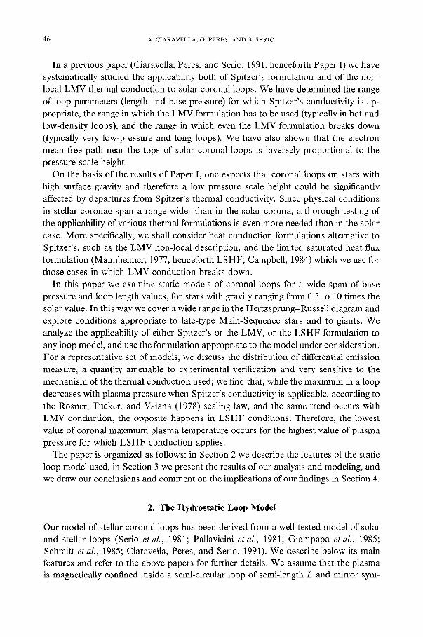
In a previous paper (Ciaravella, Peres, and Serio, 1991, henceforth Paper I) we have systematically studied the applicability both of Spitzer's formulation and of the non- local LMV thermal conduction to solar coronal loops. We have determined the range of loop parameters (length and base pressure) for which Spitzer's conductivity is appropriate, the range in which the LMV formulation has to be used (typically in hot and low-density loops), and the range in which even the LMV formulation breaks down (typically very low-pressure and long loops). We have also shown that the electron mean free path near the tops of solar coronal loops is inversely proportional to the pressure scale height.

On the basis of the results of Paper I, one expects that coronal loops on stars with high surface gravity and therefore a low pressure scale height could be significantly affected by departures from Spitzer's thermal conductivity. Since physical conditions in stellar coronae span a range wider than in the solar corona, a thorough testing of the applicability of various thermal formulations is even more needed than in the solar case. More specifically, we shall consider heat conduction formulations alternative to Spitzer's, such as the LMV non-local description, and the limited saturated heat flux formulation (Mannheimer, 1977, henceforth LSHF; Campbell, 1984) which we use for those cases in which LMV conduction breaks down.

In this paper we examine static models of coronal loops for a wide span of base pressure and loop length values, for stars with gravity ranging from 0.3 to 10 times the solar value. In this way we cover a wide range in the Hertzsprung-Russell diagram and explore conditions appropriate to late-type Main-Sequence stars and to giants. We analyze the applicability of either Spitzer's or the LMV, or the LS H F formulation to any loop model, and use the formulation appropriate to the model under consideration. For a representative set of models, we discuss the distribution of differential emission measure, a quantity amenable to experimental verification and very sensitive to the mechanism of the thermal conduction used; we find that, while the maximum in a loop decreases with plasma pressure when Spitzer's conductivity is applicable, according to the Rosner, Tucker, and Vaiana (1978) scaling law, and the same trend occurs with LMV conduction, the opposite happens in L S H F conditions. Therefore, the lowest value of coronal maximum plasma temperature occurs for the highest value of plasma pressure for which L S H F conduction applies.

The paper is organized as follows: in Section 2 we describe the features of the static loop model used, in Section 3 we present the results of our analysis and modeling, and we draw our conclusions and comment on the implications of our findings in Section 4.

2. The Hydrostatic Loop Model

Our model of stellar coronal loops has been derived from a well-tested model of solar and stellar loops (Serio et al., 1981; Pallavicini et aL, 1981; Giampapa et al., 1985; Schmitt et aL, 1985; Ciaravella, Peres, and Serio, 1991). We describe below its main features and refer to the above papers for further details. We assume that the plasma is magnetically confined inside a semi-circular loop of semi-length L and mirror sym-

THERMAL CONDUCTION AND M O D E L I N G OF STATIC STELLAR CORONAL LOOPS 47

metric with respect to its apex. The loop's cross-section is constant and the plasma is maintained at coronal temperature by uniform heat deposition. The lower boundary of

the model is at T = 2 x 104 K. The plasma is described as a fluid in hydrostatic equilibrium, characterized by en-

ergy balance among heat input (assumed uniform along the loop), optically thin radi- ative losses (Raymond, Cox, and Smith, 1976) and thermal conduction. Proton and electron temperature at any place in the loop are assumed to be the same.

In traditional models of loop plasma, energy balance is described by a differential equation where the conductive flux is the Spitzer value (cf., for instance, Serio et al., 1981). Our model, instead, can consider either Spitzer's, or LMV, or LS H F conduc- tivities. To this end we have developed two codes. The first one is based on the LMV non-local heat flux formulation, and the second one uses the L S H F formulation of thermal conduction. As we shall discuss below in more detail, both include Spitzer's conductivity as a special case.

In the code based on the LMV conductivity the equation of energy is an integro- differential one. The non-local heat flux according to Luciani, Mora, and Virmont (1983) is

q(s) = FNL(S ) = f ds'FsH(s')w(s, s'), (1)

where Fsri(s) is Spitzer-Harm's thermal flux:

d Fsn = -~:TS/Z(s) dss T(s). (2)

The kernel w(s, s') is

w(s,s') - exp - (3) 2~(s') ,~(s')n(s') _l

s'

with

,~(s') = a ( z + 1)1/2 & ( s ' ) , (4)

where a ~ 32. 2 is the effective mean free path of the heat-carrying electrons, much longer than the average electron mean free path 2o, as shown in Equation (4). In this formulation the heat flux at a given place in the loop depends on the physical conditions in a surrounding region whose characteristic length is ~ 22.

The solution with such code is found iteratively: the first distribution of density and temperature is computed using Spitzer's conductivity; the result is used to compute the LMV thermal flux, which is then used to find a new distribution of density and temperature. Such a distribution can he used to compute again the LMV thermal flux. In Paper I we have shown that, by iterating such a procedure, we achieve convergence typically in few steps. For further details on such an algorithm, we refer to Paper I.

It is worth noting that FNL reduces to FsH for small 2, since in such conditions


w(s, s ') behaves like a Dirac delta function. As a matter of fact, our results show that for very short mean free path the results computed with the iterative solution are identical to those computed with Spitzer's conductivity.

The range of applicability of the non-local formulation, as reported by LMV, is

~0 2 x 1 0 - 3 < - - < 6 . 6 7 × 10 -3 . (5) L~

Using Equation (4) with Z = 1 the above formula becomes

9.05 × 1 0 - 2 < - - < 3 . 0 2 × 10 -~ (6) L r

According to LMV, if the ratio 2/Lr is 9.05 × 10 -2 or smaller we can use Spitzer's conductivity, the range between this value and 3.02 × 10 -1 can be described with the LMV formulation. A different treatment is needed if the ratio is larger than 3.02 × 10-1; this last regime is called kinetic by LMV. In Paper I we have pointed out that, for some choice of solar loop parameters, the mean free path at the loop apex is too long to grant the applicability of even LMV conduction. Analogous conditions occur in a rather large number of loop models considered here. For such cases, we have decided to apply the L S H F formulation of the heat flux. In the LSHF formulation the heat flux is

where

and

FLSrlV = min(Fsx-i(s), Q(s)), (7)

Q(s) = f(2/n)1/2 f l e k. B rv e (8)

kBte v~ = , ( 9 )

m e

where T, ne, and Ve are the electron temperature, number density, and velocity, respectively; f is a factor, always less than one, which limits the free-streaming conduction (occurring only for total transport of the electron thermal energy, described with f = 1). We use f - -0 .1 , a value proposed by Mannheimer (1977) as appropriate to astrophysical conditions. Such a formation reduces also to Spitzer's equation when the ratio of heat flux computed as in Equation (2) to the free-streaming heat flux is below 0.1. We shall refer to the conduction regime in which

FLSFH = Q(S) (10)

as the kinetic regime. It is worth noting that the condition of turn-on of limited free streaming is very similar to that determining the upper limit of applicability of LMV conduction. In fact, at the turn on of the kinetic regime, Q(s) = Fsm substituting the definitions of both sides of the equation of state, respectively from Equations (8) and (2), and with some algebra one obtains

T2VT - 1 . 7 4 × 1 0 1 ° . ( 1 1 )

P


On the other hand for

- - = 3.02 x 10 -I , (12) LT

i.e., for the upper limit of applicability of LMV, by substituting the definition of 2 and LT, with some algebra one obtains

T2VT = 3.38 x 10 l° . (13)

P

The two conditions are very similar and one would expect a good complementarity of the two formulations. Indeed in Section 3 we show that, according to our results, the L S H F formulation with the above choice f o r f conveniently complements LMV conduction outside the domain of applicability of the latter, and that whenever LMV conduction is appropriate, the kinetic regime does not apply and vice versa.

More specifically, our approach to derive the results reported in Section 3 with the two codes is the following. First, we have computed the temperature and pressure distribution along the field line coordinates using the model based on LMV conduction, for all cases under consideration. Such cases are identified by the base pressure and loop length and the value of stellar gravity. Then, in order to check the self- consistency of the model, we have computed the ratio between the electron mean free path and the temperature scale height at any point along the loop. If such a ratio was above 6.67 x 10 -3 at some place in the loop, we again computed the loop plasma distribution, but with the model based on the L S H F conduction. The highest values of the ratio typically occur in the corona, and if the conditions of applicability of LMV conduction are violated this occurs first at the top of the loop.

As a further check of the overall self-consistency of our approach, we have also computed a//models with the code based on the L S H F conduction. We have found that in all the cases for which LMV conduction suffices, the LS H F conduction reduces to Spitzer's value.

Figure 1 provides an example of our method. There we report the ratio 2/LT VS plasma temperature for the models described hereafter. The horizontal lines mark the limits of applicability of the three regimes of thermal conduction according to Equa- tion (8), and in particular the lower, medium, and upper zones correspond to local (i.e., Spitzer), non-local (i.e., LMV), and kinetic regimes, respectively, as defined by Luciani, Mora, and Pellat (1985). The loops to which the results pertain are those with base pressure 0.1 dyne crn -2, length ranging from 2 x 109 cm to 5 X 101° cm and stellar sur-

face gravity 10 times the solar value. We first compute the models using Spitzer's conductivity, then we perform the iterative procedure to compute the loop models with LMV conduction. In Figure l(a) we show the ratio 2/L T for the models computed with Spitzer's conductivity and in Figure l(b) the same ratio computed using LMV conductivity. If a curve is completely below the lower line, Spitzer's conduction suffices (and our code based on LMV indeed finds a solution identical to Spitzer's value); if the curve enters the region between the two lines and does not go above the upper one,


C'4

0

4.0

f

4

4.5 5.0 5~5 6~0 7.5

0

0

4.0

S & sls 61o & 71o 7s

O

C

4.0 4.5 5.0 5~5 6a.O 6~5 7~0 7.5 log T(K)

Fig. 1. Ratio of effective mean free path to temperature scale height (2/Lr) vs temperature for five coronal loop models, with gravity g = lOg o, base pressure 0.1 dyne cm -2, and loop half-length ranging from 2 X 10 9 dyne cm -2 to 5 x 10 l° dyne cm -2, The curves in the three panels refer to the same models and are derived with Spitzer's conductivity (a), with LMV conductivity (b), and with LSHF conductivity (c) with f = 0.1 (solid) and f = 0.194 (dashed). The horizontal lines mark the limit of applicability of the three regimes of thermal conduction (see Equation (6)), in particular the lower, medium, and upper zones correspond to

local, non-local, and Mnetic regimes, respectively.

THERMAL CONDUCTION AND MODELING OF STATIC STELLAR CORONAL LOOPS 51

then LMV conduction is necessary; if, finally, the curve goes above the upper horizontal line we use the model with the L S H F conduction.

It is immediately evident from Figure l(b) that one of the models is marginally within the limits of application of LMV conduction, the others, instead, are beyond such a limit and L S H F conduction is required for them. Figure l(c) gives the ratio 2 /Lr for the same loop models, computed with LSHF. The steep change in the curves marks the place where the kinetic regime turns on. Indeed, all models examined in this example go beyond the range of application of LMV conductivity and therefore we have adopted, as our final result, the models as of Figure l(c).

We have already discussed that the 'kinetic' upper limit of the range of application of LMV conduction and the condition for turn-on of L S H F conduction are very similar, but not exactly equivalent. As a matter of fact this is reflected in the turning on of the kinetic regime slightly below the upper horizontal line of Figure 1. A slightly different choice for f, namely 0.194 instead of 0.1, would bring the two conditions (11) and (13) into coincidence. Figure l(c) also shows (dashed lines) the ratio for the same models computed with L S H F but with f = 0.194. Indeed for these models the kinetic regime turns on at the upper line. However, the models do not change significantly with the different choice o f f ; only the one with a lower maximum temperature remains below the kinetic limit, but in general the maximum temperature changes very little and the corresponding differential emission measure distributions, as reported in Figure 2, do not change significantly. In the light of these considerations we have preferred to ad- here to the value of f proposed by Mannheimer (1977).

3. Results

The models computed span a wide range of conditions: we consider loop half-lengths between 2 x 109 cm and 50 x 109 cm, as well as base pressures between 0.03 and 30 dyne cm -2. In Tables I, II, and III, for gravity 10 times, 3 times, and 0.3 times solar, respectively, we report the parameters characterizing each loop: the semi-length and base pressure, the maximum plasma temperature (located at the top of the loop) and the input power per unit volume into the plasma.

In order to show how the regimes of conduction discussed in Section 2 depend on the parameters governing the models, and in order to check the self-consistency of the approach adopted, we have computed the distribution of 2/Lr along the field line coordinate computed from the models themselves as outlined already in Section 2. Figures 3, 4, and 5 show 2/L r vs plasma temperatures for the models with g = 10 go, forg -- 3 go, and forg = 0.3 go, respectively. Each panel of the figures shows the ratio for one value of base pressure and all loop lengths examined. The horizontal lines mark the limits of applicability of the three regimes of thermal conduction according to Equation (8), analogously to Figure 1.

It is worth noting that the figures show our results after having completed the modeling and the consistency check of the model. Therefore, all those models computed with LMV conduction and found to be self-inconsistent, according to what was ex-

52 A. C I A R A V E L L A , G. P E R E S , A N D S. S E R I O

¢.O ¢q

('4

o

(D

* ' 4 . (

CO

4:s s:0 s:s 6:0 6:s 710 7s

t~

~?

hi)

¢'d

~ 4 1

k~

41s s:0 sls 6:0 61s 710 7.5

t'M

(D

t%l

O

T-

.,¢

1 I I I

41s s:o s:s 610 61s 710 7s log r(X)

Fig. 2. Differential emission measure for the same coronal loop models as in Figure 1: models derived with Spitzer's conductivity (a), with LMV conductivity (b), and with LSHF conductivity (c) forf = 0.1 (solid) and

f = 0.194 (dashed).

plained in Section 2, have been substituted by the corresponding models computed with L S H F . Analogously to what was presented in Figure 1, the profile of 2 / L r for all models computed with the L S H F conduct ion goes above the upper line, confirming the self-

consistency of our modeling.


TABLE I

G = 10 G o Maximum loop temperatures Tma x (106 K) and volumetric heating Eu (erg cm -3 s-1)

PO L (10 9 cm) (dyne cm -2)

2 6 10 20 50

0.03 Tmax E~

0.1 Tmax &,

0.3 Tma,~

1 Tmax

3 /'max E~

10 Tma x E,,

30 Tma x

1,19 3.83 5.85 9.38 9 .1 ( -6 ) 2 .9 ( -6 ) 1 .7( -6) 8 .5 ( -7 )

0.77 3.49 5.46 8.93 5.5(-5) 1.7( -5) 1 .0(-5) 5 .1 ( -6)

1.15 2.89 4.68 8.31 2 .3 ( -4 ) 7 .2 ( -5 ) 4 .2 ( -5 ) 2 .1 ( -5 )

1.70 2.53 a 3.58 7.02 9 .7 ( -4 ) 3 .1 ( -4 ) a 1 .8(-4) 9 .1 ( -5 )

2.44 3.44 4.20 a 5.43 a 3 .8 ( -3 ) 1 .2(-3) 7 .2 ( -4 ) a 3 .6 ( -4 ) a

3.70 5.29 6.28 7.80 1 .8(-2) 5 .6 ( -3 ) 3 .3 ( -3 ) 1 .6(-3)

5.43 7.79 9.24 11.4 7 .1 ( -2) 2 . 3 ( -2 ) 1 .4(-2) 6 .8 ( -3 )

15.0 3 .4 ( -7 )

14.4 2 .0 ( -6 )

13.7 8 .4 ( -6)

12.3 3 .6 ( -5 )

9.94 1.4(-4)

i0.4 6 .6 ( -4 )

15.0 2 .7 ( -3 )

a Computed with LMV conduction. The line marks the lower left boundary of the regime where LSHF conduction applies.

Figures 3, 4, and 5 prove the presence of the kinetic regime (i.e., non-applicability of LMV) for a significant fraction of the models computed. It is worth noting that many loops, as characterized by their semi-length and base pressure, can be modeled with LMV conduction for solar gravity (Ciaravella, Peres, and Serio, 1991), but are in the kinetic regime in higher-gravity stars. These figures also confirm that the range of temperatures in which the LSHF treatment is needed depends on the loop length, on the plasma pressure at the base of the loop, and on the star's gravity. The temperature range within a loop where the kinetic regime applies becomes larger for lower pressure and/or longer loops; the lower value of such temperature range decreases with base pressure or with gravity. The temperature range where the LSHF conduction applies becomes wider with gravity, leaving everything else unchanged.

In Tables I, II, and III we have marked, in the same way, those models to which the same conduction formulation applies. LMV conduction applies to those cases marked with a star, LSHF to those case at the right of the tables and separated from the others by a line; Spitzer's conduction applies to all others. Spitzer's conduction is more appropriate for high pressures and/or short loop length; going to lower pressure and/or longer loop length (i.e., moving in the table approximately along the diagonal from the lower left to the upper right) LMV conduction gets more appropriate and going further along this diagonal, at one extremum, LSHF might be needed. Conditions of applicability of each formulation of thermal conduction remain roughly the same going along the other diagonal.


TABLE II

G = 3 G o Maximum loop temperatures Tm~ ~ (106 K) and volumetric heating E n (erg cm 3 s 1)

Po L (109 cm) (dyne cm -2)

2 6 10 20 50

I 0.03 Tma,: 0"531 I 0.77 1.60 3.27 6.41

E q 1 .6( -5) a ] 5 .2 ( -6 ) 3 .1 ( -6 ) 1 .6(-6) 6 .2 ( -7 )

0.1 Tma,, 0.82 1.17 1.42 a ] 2.54 5.66 E~ 7 .7 ( -5) 2 .4 ( -5 ) 1 .5(-5) a ] 7 .2 ( -6 ) 2 .9 ( -6 )

0.3 Tin, x 1.18 1.67 1.97 2.50 a ] 4.38 E~ 2 .9 ( -4 ) 9 .2 ( -5 ) 5 .5( -5) 2 .7 ( -5 ) a [ 1 .1(-5)

1 Tma x 1.74 2.49 2.94 3.66 4.90 a Ez-/ 1 .3(-3) 4 .2 ( -4 ) 2 .5 ( -4 ) 1 .2(-4) 4 .9 ( -5 ) ~

3 Tma x 2.49 3.63 4.31 5.37 7.11 E~ 5 .1( -3) 1 .7(-3) 1 .0(-3) 5 .0 ( -4 ) 1 .9(-4)

10 Tma x 3.77 5.51 6.56 8.19 10.9 E~ 2 .3 ( -2) 7 .7 ( -3 ) 4 .6 ( -3 ) 2 .3 ( -3 ) 9 .4( -4)

30 Tma x 5.50 8.03 9.54 11,9 15.9 E H 8 .4( -2) 2 .9 ( -2 ) 1 .8(-2) 9 .2( -3) 3 .8( -3)

Computed with LMV conduction. The line marks the lower left boundary of the regime where LSHF conduction applies.

None of the lowest gravity cases (g = 0.3 ge), as reported in Table III , require the

L S H F conduction. We have also repeated the calculations of Paper I but with L S H F

conduction and, as expected, the only case where such formulation applies is the one with L = 5 x 10 l° cm andpo = 0.03 dyne cm -2. As discussed in Paper I this was the only model beyond the limits of applicability of LMV. Using L S H F we obtain

Tmax = 2.26 X 106 and Eu = 8.34 x l0 -7. Figure 6 provides an example of the temperature distribution vs field line coordinate

(Figure 6(a)) and differential emission measure vs temperature (Figure 6(b)) for a set of loops, all characterized by the same semi-length, 2 x 10 l° cm, and stellar gravity

10 ge, but with different base pressures (cf. column 2 of Table I). Their parameters are

reported in column 4 of Table I. It is immediately evident that, when only Spitzer's conduction applies, the top temperature decreases as the base pressure decreases. When the base pressure is very low (and the loop density is correspondingly low), first the conditions for applicability of LMV conductivity occur, and then, for even lower pressures, those for L S H F conductivity. We note that, for all high-pressure cases in which Spitzer's conductivity is valid, the distributions of temperature and differential

emission measure obtained with Spitzer and LMV calculations are virtually identical. In the case with p = 3 dyne cm -2 in Figure 6, the coronal plasma is in the non-local regime and requires LMV conductivity. It yields a Tmax higher than with Spitzer's conductivity and the differential emission measure in the upper corona is lower than

for the model with Spitzer's conductivity.

THERMAL CONDUCTION AND MODELING OF STATIC STELLAR CORONAL LOOPS

TABLE III

G = 0.3 G o Maximum loop temperatures irma × (106 K) and volumetric heating E H (erg cm -3 s ~)

55

p0 L (10 9 cm) (dyne cm -2)

2 6 10 20 50

0.03 Tm~ × 0.57 0.82 0.9& 1.19 ~ 1.59 a E~ 2.6(-5) 8.7(-6) 5.3(-6) ~ 2.7(-6) a 1.1 (~-6) ~

0.1 Tin. × 0.84 1.20 t.42 1.77 2.37 ELf 1.0(-4) 3.6(-5) 2.3(-5) 1.2(-5) 4.7(-6)

0.3 Tm~ x 1.19 1.71 2.03 2.55 3.46 E H 3.7(-4) 1.4(-4) 8.7(-5) 4.7(-5) 1.9(-5)

1 Tma x 1.74 2.54 3.03 3.86 5.25 E~/ 1.6(-3) 6.2(-4) 4.0(-4) 2.1(-4) 8.7(-5)

3 Tma x 2.49 3.70 4.43 5.64 7.64 EH 6.1(--3) 2,3(--3) 1.5(-3) 7.8(-4) 3.4(--4)

10 Tma x 3.78 5.59 6,67 8.46 11.4 E g 2.6(-2) 9.6(-3) 6.2(-3) 3.3(-3) 1.4(-3)

30 Tm~ x 5.52 8.09 9.61 12.1 16.3 E/~ 9.2(-2) 3.5(-2) 2.2(-2) 1.2(-2) 5.4(-3)

Computed with LMV conduction.

The L S H F conductivity applies to the remaining models; the temperature and the

differential emission measure are the same as those computed with Spitzer's conduc-

tivity up to the turn-on of the kinetic regime, and then they change significantly. Going

toward the top of the loop, a steep increase of temperature is followed by a region of

very shallow temperature gradient.

Figure 6(b) reports the corresponding distributions of differential emission measure

(DEM) vs plasma temperature. While the general trend of D E M decreasing with base

pressure maintains throughout the whole range, the onset of the kinetic regime leads

to a much flatter D E M profile in the corona, to values of D E M being much higher than

those expected with Spitzer's conductivity, and to the presence of plasma at higher

temperatures. These results provide a good example o f the various conduction regimes

found in the whole set of results.

It is interesting to note that, while Spitzer's conductivity yields loop models in which

the maximum coronal temperature decreases with base pressure according to the Ros-

ner, Tucker, and Vaiana (1978) and SPriG et aL (1981) scaling laws and an analogous

trend occurs with LMV conduct ion (as shown in Paper I), the opposite occurs for

L S H F conduction. Therefore, if we insist on using Spitzer's conductivity for loop

models which, instead, require L S H F conductivity, we obtain a temperature value much

lower than the correct one and, moreover, with the wrong dependence on the base pressure.

It is worth noting that there is a lower bound for coronal temperature in a loop of

56 A. CIARAVELLA, G. PERES, A N D S. SERIO

4 a

o

'!', 4.0 4:5 5:0 5[5 6:0 6:5 7:0 7.5

0

~'4.0 4.5 5.0 5'.5 6[0 6.5 7'.0 7.5

b

4 o v

4.0 4.5 5:0 5:5 6:0 6:5 7:0 7.5

e

¢q

o

4.0 4.5 5.0 5.5 6.0 6.5 7.0 7.5

o

4.0 4.5 510 515 610 615 710 7.5 4.0 4.5 5.0 5'.5 6'.0 6.5 7.0 7.5 log T(K)

Fig. 3. Radio of effective mean free path to temperature scale height (2/Lr) vs temperature for static coronal loop models, for gravity g = 10 go, with base pressure 0.03 dyne cm -2 (a), 0.1 dyne cm -2 (b), 0.3 dyne cm 2 (c), 1 dyne cm 2 (d), 3 dyne cm -2 (e), 10 dyne cm -2 (f). The definition of the horizontal lines is the same as

in Figure 1.

a g iven length and gravity: this is the t e m p e r a t u r e c o r r e s p o n d i n g to the p re s su re at

wh ich the kinet ic cond i t i ons s tar t to occur . O n ei ther side o f this value, the t e m p e r a -

ture inc reases because , in one case L S H F applies, y ie lding an inc rease o f c o r o n a l


. / / -

o

. I

'4,0 4.5 51.0 515 610 615 710 7.5

¢q

0

'¢4.0 4.5 5.0 5.5 6.0 6.5 710 7.5

o

4.0 4.5 5.0 5.5 6.0 6,5 7.0 7.5

0

fl",J

4.0 4.5 5.0 5.5 6.0 6.5 7.0 7.5

t 'd

o q

4.0 4.5 5.0 5.5 6.0 65 7.0 7.5

¢',./

"7, 4.0 45 50 55 60 65 70 7.5.

log T(K)

Fig. 4. The same as Figure 3, but for gravity g = 3 gQ.

temperature with decreasing pressure, in the other case Spitzer 's conduct ion applies

yielding the opposi te behaviour. It should be noted that such a lower bound on coronal temperature depends on the

loop length and the star 's gravity, since it depends on the conditions of turn-on of non-local t ranspor t conditions.


0

'~ l I I i

4.0 4.5 510 515 6.0 615 7.0 7.5

0

"T'4.0 4.5 5.0 5.5 6.0 6.5 710 7.5

b a 0

"T, 4.0 4.5 5.0 5.5 6.0 6.5 7.0 7.5

',@

v

0

f

4.0 4.5 5.0 5.5 6.0 6.5 7.0 7.5

O,,l

~"4.0 4.5 5.0 5.5 6.0 6.5 710 7.5

Fig. 5.

4.0 4.5 5.0 5.5 6.0 6.5 7.0 7.5

10g T(K)

The same as Figures 3 and 4, but for gravity g = 0.3 go.

Fig. 6. (a) Temperature vs field line coordinates for a set of coronal loop models with loop semi-length 2 x 101° cm and gravity g = 10 go. The base plasma presure, in dyne cm -2, is listed on each curve. All dashed curves are computed using Spitzer's conductivity, the solid curve corresponding to base pressure 3 dyne c m 2 is computed with the LMV formulation of conduction. The remaining solid curves refer to models computed with LSHF conductivity. (b) Differential emission vs temperature for the same set of coronal loops as in (a).

THERMAL CONDUCTION AND MODELING OF STATIC STELLAR CORONAL LOOPS 5 9

O

o

f

2- ½ F o

/

I I I I 8.0 8.5 9.0 9.5 10.0

log s (cm)

4.0

I I

t 3O | i i

.1 " \ 1

I / /

/

I I F ~11 I I

4.5 5.0 5.5 6.0 6.5 7.0

log T(K)

Fig. 6.

10,5

7.5


Fig. 7.

g ~._.~- 0 . 3 7 . 5 7 . 5

7- ° 7 . 0

6 . 0 ~ . 0

7.5 c3-~'3 7.5 g = ~ l O

7 . O 7 . 0

6 . 0 6 . 0

Maximum loop plasma temperature (located at the loop apex) as a function of loop semi-length and base pressure, for all coronal loop models and for different gravity in units of solar gravity.

Figure 7(a-d) shows the dependence of the temperature at the loop apex on base pressure and semi-length of the loop for stars with surface gravity, respectively 10, 3, 1 and 0.3 times the solar value. These graphs clearly illustrate the presence of a valley in the T(p, L) surface; such a valley marks the lower bound of loop-top temperature corresponding to the turn-on of kinetic conditions. Only with the turn-on of kinetic conditions does the loop-top temperature start to increase with the decrease of base pressure. In order to characterize such minimum loop temperatures as a function of gravity, loop pressure, and length, we note that it occurs at the turn-on of the LMV conduction regime. Applying the scaling law as in Equation (15) of Paper I*,

2 . . . . = 5.4 x 10-4L exp(O.88L/sp), (14)

and letting L ~ Lr , a reasonable scaling for loop top temperature, we compute readily the ratio 2/Lr which equates to 3.02 x 10 -1 (corresponding to the turn-on of kinetic

* In Paper I the coefficient 0.88 was erroneously reported as 0.988.


conditions). Taking the logarithm of both sides and substituting the expression for the pressure scale height we obtain, in cgs units,

T = 2.69 x 10-9Lg. (15)

We notice, however, that the scaling of Paper I was derived from the application of the Serio et al. (1981) scaling law, valid only in Spitzer's regime. Direct comparison of the temperature values computed with the numerical code with those predicted by Equa- tion (15) for the loop models in the temperature valleys of Figure 7 shows a good correspondence both in value and in trend. More specifically, Equation (15) overesti- mates the top temperature approximately by a factor 2. Empirically, we adopt, in cgs units,

T ~ 10-9L g . (16)

4. Discussion and Conclusions

This paper aims to give a detailed analysis of the coronal plasma confined within magnetic loops on stars different from the Sun; it completes and confirms some of the findings of Paper I. We have modeled coronal loops in the range of stellar gravity 0.3 <g/ge < 10, encompassing stars like giants and late-type dwarfs in a rather broad range of base pressure and looplength. The scope has been to consider a reasonable range of loop parameters that one might expect to find in stellar coronae.

We have ascertained how plasma pressure at the base of the loop, loop length, and stellar gravity, influence thermal conduction. Conduction determines the plasma energy balance and, therefore, the relevant temperature, density, and emission measure distributions. In particular, we have ascertained the conditions of applicability of various formulations of thermal conduction and have found that in some models one can safely apply Spitzer's conductivity in the whole corona; other models instead require the non-local LMV conductivity; in other models even the LMV treatment does not suf- fice and the LS HF treatment is appropriate.

In Paper I we have shown that non-local conduction effects, which require the LMV treatment, are favoured by a small pressure scale height*. Because of the gravity dependence, we expected that non-local conduction effects, and in general departures from the applicability of Spitzer's formulation, would be more significant in the coronae of stars with higher surface gravity, particularly for long loops or with low plasma pressure.

Our results confirm these predictions. In fact, for the modes with g = 10 ge the va- lidity of Spitzer's formulation of heat conduction is limited to the shortest and highest pressure loops; LSHF conduction plays a significant role in a large number of loops considered, whereas the non-local LMV conduction applies only in few loops within an intermediate range in the p - L plane, much smaller than for the solar case. The

* The pressure scale height determines the plasma density distribution, hence the mean free path in coronae and the mode of thermal conduction.


models for g = l0 go are the ones in which we find most extreme departures from Spitzer's conductivity and therefore from standard stellar loop models. Analogous results are found for g = 3 go, although the range of applicability of Spitzer's conductivity is larger. In general we have found that, for gravity higher than for the solar value, varying the loop parameters, the transition from Spitzer's to the kinetic regime (i.e., where LS HF has to be applied) is more rapid than for the solar case. The temperature range within the loop, when LSHF conduction is needed, depends on the loop length, on the plasma pressure at the base of the loop and on the star's gravity; it becomes larger for lower pressure and/or longer loops and/or higher gravity; the lowest temperature at which L S H F applies decreases with base pressure and with gravity. At the other extreme, for g = 0.3 go, and for the range of parameters here considered, Spitzer's conduction can be applied to all models.

We have found that the LSHF formulations, with a reduction parameter f = 0.1 proposed by Mannheimer (1977) for astrophysical plasmas and the LMV formulation, conveniently complement each other, and the ranges of applicability of the two in practice overlap only slightly. A choice of = 0.194 would yield a correct match of the conditions of applicability of the two formulations but would yield no substantial change in our results.

It is worth noting that the onset of L S H F conduction leads to a flat differential emission measure profile in coronae, and to values of coronal temperature and differential emission measure higher than those expected with models using either Spitzer's or LMV conductivity. Therefore, in such cases the use of Spitzer's or LMV conductivity leads to markedly wrong predictions.

For a given gravity and for loops of the same length and different pressure, a minimum of top coronal temperature occurs corresponding to the highest value of pressure for which the kinetic conditions apply, i.e., where we apply the LS H F conduction. The specific value of pressure at which such a minimum occurs depends on loop length and gravity, reflecting the conditions of the turn-on of LS H F conduction. We have also determined an empirical scaling law giving the values for such minimum loop top temperatures: T ~ 10-9L g, in cgs units.

In conclusion, we have found that the expectations concerning the applicability of different regimes of thermal conductivity drawn from Paper I are confirmed and en- larged to a broader range of cases. In high-gravity stars the range of applicability of LMV conductivity is more restricted than in the Sun. A large number of models studied here require L S H F conduction, whereas loops in low-gravity stars can be modeled with Spitzer's conductivity. The models we have described cover a wide range of conditions, thus providing coronal loop models more accurate than those obtained with Spitzer's conductivity only, and in a wide range of the Hertzsprung-Russell diagram. If, for a given loop, the condition for L S H F conduction applies, we have shown that a minimum coronal temperature is achieved, typically at the value of pressure corresponding to the onset of LS HF conditions.

It is worth studying how all these features influence the spectrum of radiation emitted from the loop and to what extent they are observable. We leave for future work the task

THERMAL CONDUCTION AND MODELING" OF STATIC STELLAR CORONAL LOOPS 63

of synthesizing emission in lines and bands typically observed (or to be observed) in

UV and X-rays.

Acknowledgements

This work has been supported by Agenzia Spaziale Italiana and Ministero dell'

Universit/t e della Ricerca Scientifica e Tecnologica.

References

Campbell, P. M.: 1984, Phys. Rev. A30(1), 365. Ciaravella, A., Peres, G., and Serio, S.: 1991, Solar Phys. 132, 279. Giampapa, M. S., Golub, L., Peres, G., Serio, S., and Vaiana, G. S.: 1985, Astrophys. J. 289, 203. Gray, D. R. and Kilkenny, J. D.: 1980, Plasma Phys. 22, 81. Landini, M., Monsignori-Fossi, B. C., Paresce, F., and Stem, R. A.: 1985, Astrophys. J. 289, 709. Luciani, J. F., Mora, P., and Pellat, R.: 1985, Phys. Fluids 28, 1835. Luciani, J. F., Mora, P., and Virmont, L: 1983, Phys. Rev. Letters 51, 1664. Mannheimer, W. M.: 1977, Phys. Fluids 20, 265. Pallavicini, R., Peres, G , Serio, S., Vaiana, G. S., Golub, L;, and Rosner, R.: 1981, Astrophys. J. 247, 692. Raymond, J. C., Cox, Donald P., and Smith, Barbara, W.: 1976, Astrophys. J. 204, 290. Reale, F., Peres, G., and Serio, S.: 1988, Astrophys. J. 328, 256. Rosner, R., Tucker, W., and Vaiana, G. S.: 1978, Astrophys. J. 220, 643. Schmitt, J. H., Harnden, F. R., Jr., Peres, G., Rosner, R., and Serio, S.: 1985, Astrophys. J. 288, 751. Serio, S., Peres, G., Vaiana, G. S., Golub, L., and Rosner, R.: 1981, Astrophys. J. 243, 288.

Thermal conduction and modeling of static stellar coronal loops

Documents

Transcript of Thermal conduction and modeling of static stellar coronal loops