MNRAS 514, 2425–2433 (2022) https://doi.org/10.1093/mnras/stac1388 Advance Access publication 2022 May 19

Cross helicity of interplanetary coronal mass ejections at 1 au

S. W. Good , 1 ‹ L. M. Hatakka, 1 M. Ala-Lahti, 1 , 2 J. E. Soljento, 1 A. Osmane

1 and E. K. J. Kilpua

1

1 Department of Physics, University of Helsinki, PO Box 64, FI-00014 Helsinki, Finland 2 Department of Climate and Space Sciences and Engineering, University of Michigan, 2455 Hayward St, Ann Arbor, MI 48109-2143, USA

Accepted 2022 May 16. Received 2022 May 13; in original form 2022 April 1

A B S T R A C T

Interplanetary coronal mass ejections (ICMEs) contain magnetic field and velocity fluctuations across a wide range of scales. These fluctuations may be interpreted as Alfv enic wave packets propagating parallel or antiparallel to the background magnetic field, with the difference in power between counterpropagating fluxes quantified by the cross helicity. We have determined the cross helicity of inertial range fluctuations at 10

−3 to 10

−2 Hz in 226 ICME flux ropes and 176 ICME sheaths observed by the Wind spacecraft at 1 au during 1995–2015. The flux ropes and sheaths had mean, normalized cross helicities of 0.18 and 0.24, respecti vely, with positi ve v alues here indicating net antisunward fluxes. While still tipped to w ards the antisunw ard direction

on av erage, flux es in ICMEs tend to be more balanced than in the solar wind at 1 au, where the mean cross helicity is larger. Superposed epoch profiles show cross helicity falling sharply in the sheath and reaching a minimum inside the flux rope near the leading edge. More imbalanced, solar wind-like cross helicity was found towards the trailing edge and laterally further from

the rope axis. The dependence of cross helicity on flux rope orientation and the presence of an upstream shock are considered. Potential origins of the low cross helicity in ICMEs at 1 au include balanced driving of the closed-loop flux rope at the Sun and

ICME–solar wind interactions in interplanetary space. We propose that low cross helicity of fluctuations is added to the standard

list of ICME signatures.

Key words: turbulence – Sun: coronal mass ejections (CMEs) – solar wind.

1

Iiafl

s1

ssla

efi

pd

oZ

og

e

fil

�

e

2

p

o

tp

D

ol

e

2

s

1

Tb

b

am

(

P

ct

sS

©PCp

Dow

nloaded from https://academ

ic.oup.com/m

nras/article/514/2/2425/6589412 by guest on 09 July 2022

I N T RO D U C T I O N

nterplanetary coronal mass ejections (ICMEs; e.g. Kilpua, Kosk- nen & Pulkkinen 2017a ) are vast, transient eruptions of plasma nd magnetic field from the Sun with properties that are distinct rom the solar wind. Signatures of ICMEs may variously include ow plasma- β, a smooth rotation of the magnetic field at largecales, and magnetic fluctuations with small amplitudes (e.g. Burlaga 991 ; Cane & Richardson 2003 ). ICMEs with the first two of theseignatures are classified as magnetic clouds. ICMEs displaying the econd signature may be modelled as flux ropes, with twisted field ines in the ICME volume that wind around a common central xis (e.g. Riley et al. 2004 ; Al-Haddad et al. 2013 ). A spacecraftncountering an ICME flux rope will observe a background magnetic eld vector that monotonically rotates by up to 180 ◦ during the ropeassage time. ICMEs are of significant interest as space weather ri vers, gi ven that their flux rope structures are a major sourcef southward magnetic field arriving at Earth (e.g. Wilson 1987 ; hang & Burlaga 1988 ; Kilpua et al. 2017b ). Sheath intervalsf compressed solar wind ahead of ICMEs can also be highly eoef fecti ve (e.g. Tsurutani et al. 1988 ; Lugaz et al. 2016 ; Kilpuat al. 2017a , 2019 ).

Like the solar wind, ICME plasma displays broad-band magnetic eld and velocity fluctuations with power spectra that take power-

aw forms (Leamon, Smith & Ness 1998 ; Liu et al. 2006 ; Hamilton

E-mail: simon.good@helsinki.fi

h

flm

The Author(s) 2022. ublished by Oxford University Press on behalf of Royal Astronomical Society. Thommons Attribution License ( http://cr eativecommons.or g/licenses/by/4.0/), whicrovided the original work is properly cited.

t al. 2008 ; Boro vsk y, Denton & Smith 2019 ; Sorriso-Valvo et al.021 ). In the solar wind, most power is contained in Alfv enicallyolarized fluctuations, with typically a few per cent of total power inther, compressive modes (e.g. Chen 2016 ). It has long been knownhat Alfv enic fluctuations with an antisunward sense of propagation redominate o v er sunward fluctuations in the solar wind (Belcher &avis 1971 ), consistent with the fluctuations having mostly a coronalrigin. This antisunward predominance is present in fluctuations at ow frequencies with an f −1 power spectrum and, to a somewhat lesserxtent, in turbulent fluctuations at higher frequencies (e.g. Chen et al.013 ). The predominance is also typically greater in fast wind than inlow, and declines with distance from the Sun (e.g. Luttrell & Richter987 ; Marsch & Tu 1990 ; Bavassano, Pietropaolo & Bruno 2000 ).he amplitudes of sunward and antisunward fluctuations were found y Boro vsk y ( 2012 ) and Boro vsk y et al. ( 2019 ) to be more equallyalanced in ICME plasma at 1 au than in other solar wind types,part from intervals containing sector reversals in the interplanetary agnetic field. A similar balance was also found by Good et al.

2020 ) in a magnetic cloud observed at 0.25 au by Parker Solarrobe (PSP; Fox et al. 2016 ). Given that the non-linear interaction ofounterpropagating Alfv enic fluctuations is the source of Alfv enic urbulence in the solar wind, the degree of balance or imbalance has aignificant effect on the turbulence properties that are observed (e.g. chekochihin 2020 , and references therein). Imbalance may be quantified in terms of the normalized cross

elicity, σ c , which gives the difference in power between Alfv enicuctuations propagating parallel and antiparallel to a background agnetic field. We here present analysis of σ c for a large number

is is an Open Access article distributed under the terms of the Creative h permits unrestricted reuse, distribution, and reproduction in any medium,

2426 S. W. Good et al.

M

o

t

a

m

s

t

b

c

t

h

o

a

s

H

w

h

fl

c

A

σ

g

fl

o

e

t

r

a

i

o

t

s

h

2

I

W

i

v

5

h

a

m

w

m

h

i

t

nb

a

r

u

w

m

E

1

n

c

σ

a

σ

A

(

d

3

3

F

T

c

r

a

b

o

r

a

t

t

fi

i

l

c

s

P

i

b

e

3

t

s

w

s

i

p

fl

f

s

p

u

A

n

p

p

l

t

g

t

b r

Dow

nloaded from https://academ

ic.oup.com/m

nras/article/514/2/2425/6589412 by guest on 09 July 2022

f ICME flux ropes and their upstream sheath regions observed byhe Wind spacecraft at 1 au o v er a 20-yr period. Fluctuations across decade of frequencies typically falling within the inertial range ofagnetohydrodynamic (MHD) turbulence are investigated, at scales

maller than that of the background flux rope structure. We findhat average values of σ c in the rope and sheath intervals are morealanced (i.e. σ c is closer to zero) than in the solar wind generally,onsistent with previous results. Via superposed epoch analysis, sys-ematic variations in σ c through the sheath–ICME complex along theeliocentric radial direction have been identified. The dependenciesf σ c on the crossing distance of the spacecraft from the flux ropexis, on the presence or absence of an upstream shock bounding theheath, and on the flux rope orientation, are also considered.

Cross helicity may be used to define Alfv enicity (e.g. Stansby,orbury & Matteini 2019 ). This definition equates high Alfv enicityith the presence of unidirectional Alfv en waves, since such wavesave well correlated or anticorrelated magnetic field and velocityuctuations, and cross helicity is ultimately a measure of thisorrelation. In this work, cross helicity is interpreted in terms oflfv enic balance or imbalance, and the normalized residual energy,r , is used to define and measure Alfv enicity . Residual energy , whichives the difference in power between velocity and magnetic fielductuations, is zero for idealized Alfv en waves but is generallybserved to be negative (indicating an excess of magnetic fluctuationnergy) in the solar wind inertial range (e.g. Chen et al. 2013 ). Notehat all mentions of cross helicity and residual energy in this workefer to normalized quantities.

In Section 2 , the spacecraft data set is described and key parametersre defined. The properties of an example ICME flux rope and sheathnterval are described in detail in Section 3.1 , followed by analysisf mean properties across all intervals in Section 3.2 . In Section 3.3 ,he superposed epoch analysis is presented, which considers sub-tructuring within the intervals. Possible origins of the low crosselicity in ICMEs and their sheaths are discussed in Section 4 .

SPAC ECRAFT DATA

CME flux ropes catalogued by Nieves-Chinchilla et al. ( 2018 ) usingind spacecraft data have been analysed. The catalogue 1 lists 272

ntervals with flux rope rotations of the background magnetic fieldector that were observed during 1995–2015; intervals in which per cent or more of magnetic field or plasma data were missingav e been e xcluded, leaving 226 intervals included in the presentnalysis. A total of 176 sheath intervals listed in the catalogue thateet the 5 per cent data gap threshold have also been analysed, ofhich 97 were associated with shocks. Magnetic field data from MFI (Lepping et al. 1995 ) and ionoments from 3DP/PESA-L (Lin et al. 1995 ) on board Wind

ave been used. Data were typically at 3 s resolution, with linearnterpolation applied to close any small data gaps. Measurements ofhe magnetic field, B , proton velocity, v , and proton number density, p , have been used to determine the Elsasser variables, z ± = v ± , where b = B /

√

μ0 ρ and ρ is the ion mass density. It has beenssumed that 4 per cent of solar wind ions are alpha particles and theest protons by number density such that ρ = 7 mn p /6, where m p is thenit proton mass. Fluctuations in z + and z − correspond to Alfv enic ave pack ets propagating antiparallel and parallel to the backgroundagnetic field, respectively. The trace spectral densities of v , b and z ±, denoted by E v , E b , and

±, respectiv ely, hav e been calculated with a Morlet wavelet tech-

NRAS 514, 2425–2433 (2022)

https:// wind.nasa.gov/ ICMEindex.php 2

ique (Torrence & Compo 1998 ) and used to obtain the normalizedross helicity,

c =

E +

− E −E +

+ E −(1)

nd normalized residual energy,

r =

E v − E b

E v + E b

. (2)

similar wavelet method has been applied previously by Chen et al. 2013 ) to calculate σ c and σ r . Values of σ c and σ r are limited byefinition to the range [ − 1, 1].

ANALYSI S

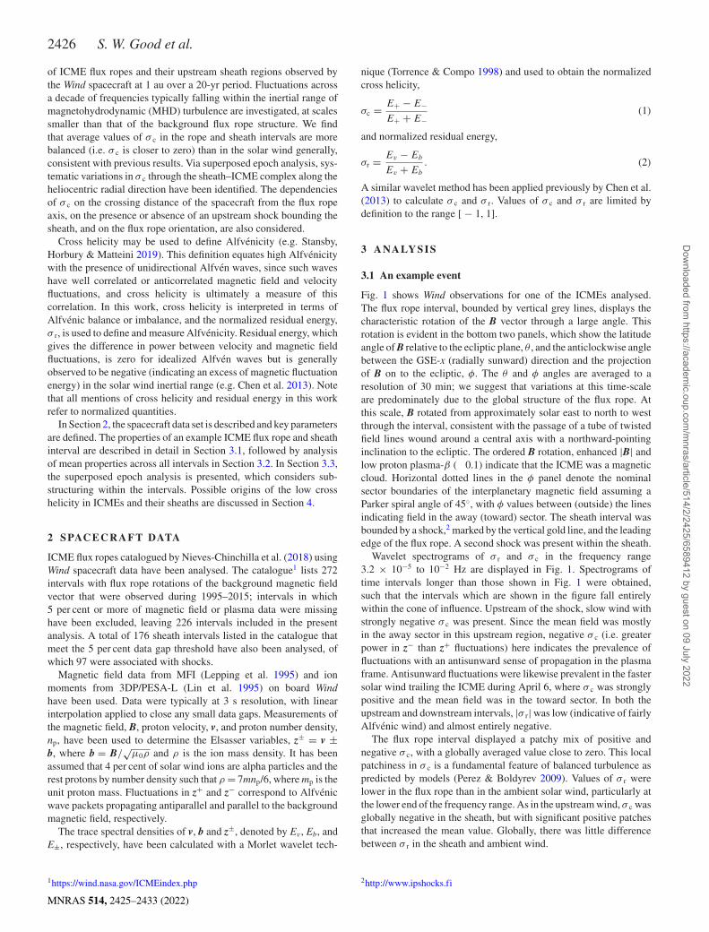
.1 An example event

ig. 1 shows Wind observations for one of the ICMEs analysed.he flux rope interval, bounded by vertical grey lines, displays theharacteristic rotation of the B vector through a large angle. Thisotation is evident in the bottom two panels, which show the latitudengle of B relative to the ecliptic plane, θ , and the anticlockwise angleetween the GSE- x (radially sunward) direction and the projectionf B on to the ecliptic, φ. The θ and φ angles are averaged to aesolution of 30 min; we suggest that variations at this time-scalere predominately due to the global structure of the flux rope. Athis scale, B rotated from approximately solar east to north to westhrough the interval, consistent with the passage of a tube of twistedeld lines wound around a central axis with a northward-pointing

nclination to the ecliptic. The ordered B rotation, enhanced | B | andow proton plasma- β ( � 0.1) indicate that the ICME was a magneticloud. Horizontal dotted lines in the φ panel denote the nominalector boundaries of the interplanetary magnetic field assuming aarker spiral angle of 45 ◦, with φ values between (outside) the lines

ndicating field in the away (toward) sector. The sheath interval wasounded by a shock, 2 marked by the vertical gold line, and the leadingdge of the flux rope. A second shock was present within the sheath.

Wavelet spectrograms of σ r and σ c in the frequency range.2 × 10 −5 to 10 −2 Hz are displayed in Fig. 1 . Spectrograms ofime intervals longer than those shown in Fig. 1 were obtained,uch that the intervals which are shown in the figure fall entirelyithin the cone of influence. Upstream of the shock, slow wind with

trongly ne gativ e σ c w as present. Since the mean field w as mostlyn the away sector in this upstream region, negative σ c (i.e. greaterower in z − than z + fluctuations) here indicates the prevalence ofuctuations with an antisunward sense of propagation in the plasmarame. Antisunward fluctuations were like wise pre v alent in the fasterolar wind trailing the ICME during April 6, where σ c was stronglyositive and the mean field was in the toward sector. In both thepstream and do wnstream interv als, | σ r | was lo w (indicati ve of fairlylfv enic wind) and almost entirely ne gativ e. The flux rope interval displayed a patchy mix of positive and

e gativ e σ c , with a globally averaged value close to zero. This localatchiness in σ c is a fundamental feature of balanced turbulence asredicted by models (Perez & Boldyrev 2009 ). Values of σ r wereower in the flux rope than in the ambient solar wind, particularly athe lower end of the frequency range. As in the upstream wind, σ c waslobally ne gativ e in the sheath, but with significant positiv e patcheshat increased the mean value. Globally, there was little differenceetween σ in the sheath and ambient wind.

http://www.ipshocks.fi

ICME cross helicity 2427

-20

0

20B

(nT)

400

600

v (k

m s

-1)

15

30

n p (cm

-3)

0.250.5

T (M

K)

10-2

100

p

10-2

10-3

10-4

f (H

z)

102

101

s (m

in)

-1

0

1r

10-2

10-3

10-4

f (H

z)

102

101

s (m

in)

-1

0

1c

-45

45

3 4 5 6 7Day of April 2004

90

270

|B|BxByBz

Figure 1. An example ICME. From top to bottom, the panels show the magnetic field in GSE coordinates; bulk proton speed; proton density and temperature; proton plasma- β; normalized residual energy; normalized cross helicity; and 30-min averages of the magnetic field latitude and longitude angles in GSE

coordinates. The ICME boundaries and upstream shock are marked by grey and gold vertical lines, respectively.

1

Tf

m

a

t

mw

h

r

df

3

Ft

Vb

fl

f

a

i

0

i

t

i

fia

o

a

c

a

t

c

m

(

di

Dow

nloaded from https://academ

ic.oup.com/m

nras/article/514/2/2425/6589412 by guest on 09 July 2022

In the following, we restrict our analysis to the frequency range 0 −3 to 10 −2 Hz (equi v alent to wave periods 1.67 −16.7 min).he inertial range of MHD turbulence usually encompasses these

requencies at 1 au (e.g. Kiyani, Osman & Chapman 2015 ). Atuch larger scales (e.g. frequencies � 10 −4 Hz, periods � 2.8 h), significant fraction of fluctuation power in an ICME may be dueo the variation of the flux rope B -field. Rather than this background,ean-field structure, we focus on smaller scale fluctuations present ithin the structure. At 10 −3 to 10 −2 Hz, the ICME shown in Fig. 1ad globally averaged { σ c , σ r } values of { 0.10, −0.47 } in the fluxope and { − 0.38, −0.26 } in the sheath. The sample points used toetermine these averages were equally spaced across the logarithmic requency range.

.2 Mean values

ig. 2 shows the globally averaged values of σ r versus σ c at 10 −3

o 10 −2 Hz for the 226 flux rope and 176 sheath intervals analysed.alues are constrained by definition to fall within the circle described y σ 2

r + σ 2 c = 1. The mean of the globally averaged σ r values for the

ux rope intervals was −0.36, similar to the mean of −0.35 found

or the sheath intervals. None of the flux rope or sheath intervals had globally positive value of σ r .

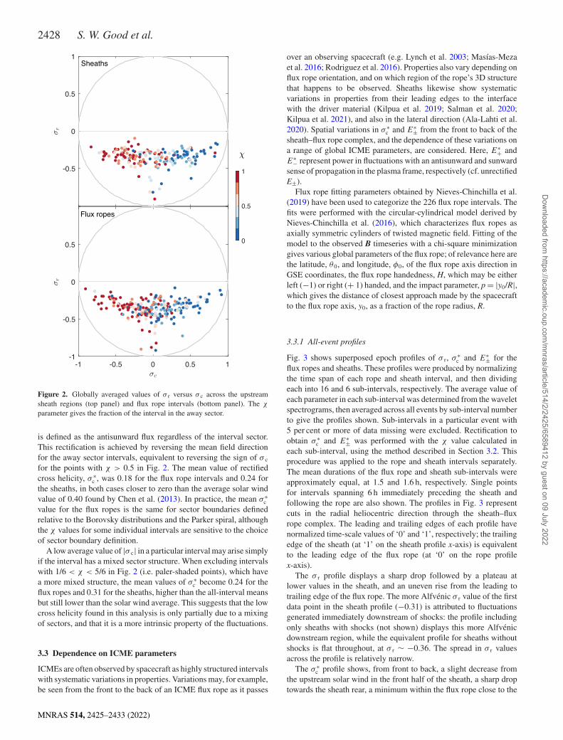
Points in Fig. 2 are colour coded according to the fraction of datan the corresponding interval that was in the away sector, χ . Red ( χ >

.5) and blue ( χ < 0.5) points indicate intervals that were primarilyn the away and toward sectors, respectiv ely. F or the sheath intervals,he sector structure is defined relative to the Parker spiral as describedn Section 3.1 . For the flux ropes, which do not have a Parker spiraleld, we define a sector structure based on the distributions of GSE φ

ngles observed within ICMEs obtained by Boro vsk y ( 2010 ). In fig. 3f Boro vsk y ( 2010 ), broad peaks at around 120 ◦ and less distinctlyt 300 ◦ can be seen in the distributions for three different ICMEatalogues. These two angles are used as the mid-points of the awaynd toward sectors for the flux rope intervals (cf. 135 ◦ and 315 ◦ forhe equi v alent Parker spiral sectors).

The anticorrelation of σ c and χ that can be seen in Fig. 2 isonsistent with the pre v alence of antisunward fluctuations: when theean field is in the aw ay (tow ard) sector, σ c tends to be ne gativ e

positive) and fluctuations in the antisunward z − ( z + ) mode areominant. A meaningful average value of σ c across all intervals s obtained by first rectifying the magnetic field, so that positive σ c

MNRAS 514, 2425–2433 (2022)

2428 S. W. Good et al.

M

Figure 2. Globally averaged values of σ r versus σ c across the upstream

sheath regions (top panel) and flux rope intervals (bottom panel). The χparameter gives the fraction of the interval in the away sector.

i

T

ff

c

t

vv

r

t

o

i

w

a

fl

b

c

o

3

I

w

b

o

e

fl

t

v

w

K

2

s

a

E

s

E

(

fi

N

a

m

g

t

G

l

w

t

3

F

fl

t

e

e

s

t

5

o

e

p

T

a

f

f

c

r

n

e

t

x

l

t

d

g

o

d

s

a

t

t

Dow

nloaded from https://academ

ic.oup.com/m

nras/article/514/2/2425/6589412 by guest on 09 July 2022

s defined as the antisunward flux regardless of the interval sector.his rectification is achieved by reversing the mean field direction

or the away sector interv als, equi v alent to reversing the sign of σ c

or the points with χ > 0.5 in Fig. 2 . The mean value of rectifiedross helicity, σ ∗

c , was 0.18 for the flux rope intervals and 0.24 forhe sheaths, in both cases closer to zero than the average solar windalue of 0.40 found by Chen et al. ( 2013 ). In practice, the mean σ ∗

c alue for the flux ropes is the same for sector boundaries definedelative to the Borovsky distributions and the Parker spiral, althoughhe χ values for some individual intervals are sensitive to the choicef sector boundary definition. A low average value of | σ c | in a particular interval may arise simply

f the interval has a mixed sector structure. When excluding intervalsith 1/6 < χ < 5/6 in Fig. 2 (i.e. paler-shaded points), which have more mixed structure, the mean values of σ ∗

c become 0.24 for theux ropes and 0.31 for the sheaths, higher than the all-interval meansut still lower than the solar wind average. This suggests that the lowross helicity found in this analysis is only partially due to a mixingf sectors, and that it is a more intrinsic property of the fluctuations.

.3 Dependence on ICME parameters

CMEs are often observed by spacecraft as highly structured intervalsith systematic variations in properties. Variations may, for example,e seen from the front to the back of an ICME flux rope as it passes

NRAS 514, 2425–2433 (2022)

v er an observing spacecraft (e.g. Lynch et al. 2003 ; Mas ıas-Mezat al. 2016 ; Rodriguez et al. 2016 ). Properties also vary depending onux rope orientation, and on which region of the rope’s 3D structure

hat happens to be observed. Sheaths likewise show systematicariations in properties from their leading edges to the interfaceith the driver material (Kilpua et al. 2019 ; Salman et al. 2020 ;ilpua et al. 2021 ), and also in the lateral direction (Ala-Lahti et al.020 ). Spatial variations in σ ∗

c and E

∗± from the front to back of the

heath–flux rope complex, and the dependence of these variations on range of global ICME parameters, are considered. Here, E

∗+

and

∗− represent power in fluctuations with an antisunward and sunward

ense of propagation in the plasma frame, respectively (cf. unrectified ±). Flux rope fitting parameters obtained by Nieves-Chinchilla et al.

2019 ) have been used to categorize the 226 flux rope intervals. Thets were performed with the circular-cylindrical model derived byieves-Chinchilla et al. ( 2016 ), which characterizes flux ropes as

xially symmetric cylinders of twisted magnetic field. Fitting of theodel to the observed B timeseries with a chi-square minimization

i ves v arious global parameters of the flux rope; of rele v ance here arehe latitude, θ0 , and longitude, φ0 , of the flux rope axis direction inSE coordinates, the flux rope handedness, H , which may be either

eft ( −1) or right ( + 1) handed, and the impact parameter, p = | y 0 / R | ,hich gives the distance of closest approach made by the spacecraft

o the flux rope axis, y 0 , as a fraction of the rope radius, R .

.3.1 All-event profiles

ig. 3 shows superposed epoch profiles of σ r , σ ∗c and E

∗± for the

ux ropes and sheaths. These profiles were produced by normalizinghe time span of each rope and sheath interval, and then dividingach into 16 and 6 sub-interv als, respecti v ely. The av erage value ofach parameter in each sub-interval was determined from the waveletpectrograms, then averaged across all events by sub-interval numbero give the profiles sho wn. Sub-interv als in a particular event with per cent or more of data missing were excluded. Rectification tobtain σ ∗

c and E

∗± was performed with the χ value calculated in

ach sub-interval, using the method described in Section 3.2 . Thisrocedure was applied to the rope and sheath intervals separately.he mean durations of the flux rope and sheath sub-intervals werepproximately equal, at 1.5 and 1.6 h, respectively. Single pointsor intervals spanning 6 h immediately preceding the sheath andollowing the rope are also shown. The profiles in Fig. 3 representuts in the radial heliocentric direction through the sheath–fluxope complex. The leading and trailing edges of each profile haveormalized time-scale values of ‘0’ and ‘1’, respectively; the trailingdge of the sheath (at ‘1’ on the sheath profile x -axis) is equi v alento the leading edge of the flux rope (at ‘0’ on the rope profile -axis).

The σ r profile displays a sharp drop followed by a plateau ato wer v alues in the sheath, and an une ven rise from the leading torailing edge of the flux rope. The more Alfv enic σ r value of the firstata point in the sheath profile ( −0.31) is attributed to fluctuationsenerated immediately downstream of shocks: the profile includingnly sheaths with shocks (not shown) displays this more Alfv enicownstream region, while the equivalent profile for sheaths withouthocks is flat throughout, at σ r ∼ −0.36. The spread in σ r valuescross the profile is relatively narrow.

The σ ∗c profile shows, from front to back, a slight decrease from

he upstream solar wind in the front half of the sheath, a sharp dropowards the sheath rear, a minimum within the flux rope close to the

ICME cross helicity 2429

Figure 3. Superposed epoch profiles of σ r , σ ∗c , and E

∗± for sheaths (left-hand panels) and flux ropes (right-hand panels), made by binning all events. Dashed lines indicate the start and end of the ICME profile. Single bins spanning 6 h of solar wind before and after the ICMEs are also shown. Shading and error bars indicate the standard error of values in each bin.

Table 1. Mean interval-averaged values of σ r and σ ∗c in

ICME sheaths and flux ropes. Standard deviations (SD) are also listed.

Residual energy Cross helicity σ r SD σ ∗

c SD

Sheaths −0.35 0.12 0.24 0.30 Flux ropes −0.36 0.13 0.18 0.29

str

W

pd

rq

E

w

t

s

e

t

p

r

Figure 4. Superposed epoch profiles of σ ∗c and E

∗± binned according to high and low impact parameter, p , and to the presence or absence of an upstream

shock, in a similar format to Fig. 3 . The number of events contributing to each profile is given in parentheses in the σ ∗

c panels.

3

T

t

0

a

a

p

d

i

s

r

r

p

ap

Dow

nloaded from https://academ

ic.oup.com/m

nras/article/514/2/2425/6589412 by guest on 09 July 2022

heath–flux rope interface, and a gradual rise towards the flux rope railing edge. The average σ r and σ ∗

c values across the sheath and ope profiles are consistent with the values in Table 1 , as expected.

hile remaining at lo w v alues, the average σ ∗c is in all locations

ositive, indicating that the balance is tipped towards the antisunward irection throughout the ICME. It is instructive to consider variations in E

∗+

and E

∗− individually,

ecalling that σ ∗c is the normalized difference between these two

uantities. The E

∗± profiles in Fig. 3 show the typical dominance of

∗+

o v er E

∗− in the solar wind upstream of the sheath. From upstream

ind to sheath, there is a sharp increase in E

∗+

and E

∗−, with both

hen showing a central dip and rise towards the sheath rear. It can beeen that the drop in σ ∗

c at the sheath rear is due to a relatively greaternhancement in E

∗− than E

∗+

. In the front two-thirds of the flux rope,he flat E

∗+

combined with a falling E

∗− causes the rising σ ∗

c notedreviously. Both E

∗+

and E

∗− gradually rise towards the back of the

ope.

.3.2 Impact parameter and shocks

he first and second rows in Fig. 4 show profiles separated accordingo whether the impact parameter through the flux rope was high ( p >.8) or low ( p < 0.2). Lower σ ∗

c can generally be seen across the ropet low p , when the spacecraft trajectory came closer to the centralxis, while higher, more solar wind-like σ ∗

c tends to be found at high , further from the central axis. This σ ∗

c versus p trend is primarilyue to higher E

∗+

at large p within the rope, although the differencesn E

∗± between high and low p encounters is not large. There are weak

ignatures of correlated W-shaped profiles in E

∗+

and E

∗− across the

ope at low p . The bottom two rows of Fig. 4 display profiles for sheaths and

opes sorted according to whether or not an upstream shock wasresent. It can be seen that E

∗± are significantly higher for the shock-

ssociated profiles, to the extent that E

∗− in the shock-associated

rofiles is equal to or greater than E

∗+

in the non-shock profiles

MNRAS 514, 2425–2433 (2022)

2430 S. W. Good et al.

M

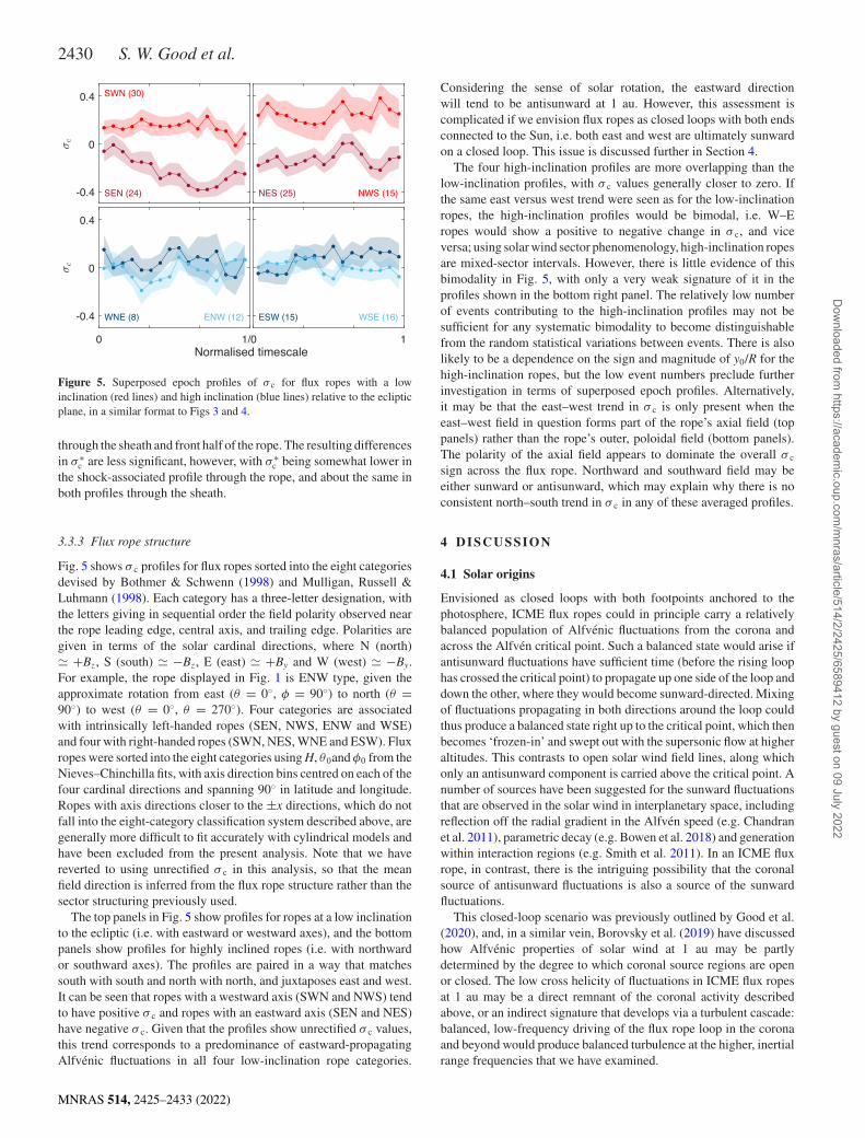
Figure 5. Superposed epoch profiles of σ c for flux ropes with a low

inclination (red lines) and high inclination (blue lines) relative to the ecliptic plane, in a similar format to Figs 3 and 4 .

t

i

t

b

3

F

d

L

t

t

g

�

F

a

9

w

a

r

N

f

R

f

g

h

r

fi

s

t

p

o

s

I

t

h

t

A

C

w

c

c

o

l

t

r

r

v

a

b

p

o

s

f

l

h

i

i

e

p

Ts

e

c

4

4

E

p

b

a

a

h

d

o

t

b

a

o

n

t

r

e

w

r

s

fl

(

h

d

o

a

a

b

a

r

Dow

nloaded from https://academ

ic.oup.com/m

nras/article/514/2/2425/6589412 by guest on 09 July 2022

hrough the sheath and front half of the rope. The resulting differencesn σ ∗

c are less significant, ho we ver, with σ ∗c being some what lo wer in

he shock-associated profile through the rope, and about the same inoth profiles through the sheath.

.3.3 Flux rope structure

ig. 5 shows σ c profiles for flux ropes sorted into the eight categoriesevised by Bothmer & Schwenn ( 1998 ) and Mulligan, Russell &uhmann ( 1998 ). Each category has a three-letter designation, with

he letters giving in sequential order the field polarity observed nearhe rope leading edge, central axis, and trailing edge. Polarities areiven in terms of the solar cardinal directions, where N (north) + B z , S (south) � −B z , E (east) � + B y and W (west) � −B y . or e xample, the rope displayed in Fig. 1 is ENW type, given thepproximate rotation from east ( θ = 0 ◦, φ = 90 ◦) to north ( θ =0 ◦) to west ( θ = 0 ◦, θ = 270 ◦). Four categories are associatedith intrinsically left-handed ropes (SEN, NWS, ENW and WSE)

nd four with right-handed ropes (SWN, NES, WNE and ESW). Fluxopes were sorted into the eight categories using H , θ0 and φ0 from theieves–Chinchilla fits, with axis direction bins centred on each of the

our cardinal directions and spanning 90 ◦ in latitude and longitude.opes with axis directions closer to the ±x directions, which do not

all into the eight-category classification system described above, areenerally more difficult to fit accurately with cylindrical models andave been excluded from the present analysis. Note that we haveeverted to using unrectified σ c in this analysis, so that the meaneld direction is inferred from the flux rope structure rather than theector structuring previously used.

The top panels in Fig. 5 show profiles for ropes at a low inclinationo the ecliptic (i.e. with eastward or westward axes), and the bottomanels show profiles for highly inclined ropes (i.e. with northwardr southward axes). The profiles are paired in a way that matchesouth with south and north with north, and juxtaposes east and west.t can be seen that ropes with a westward axis (SWN and NWS) tendo hav e positiv e σ c and ropes with an eastward axis (SEN and NES)av e ne gativ e σ c . Giv en that the profiles show unrectified σ c values,his trend corresponds to a predominance of eastward-propagatinglfv enic fluctuations in all four low-inclination rope categories.

NRAS 514, 2425–2433 (2022)

onsidering the sense of solar rotation, the eastward directionill tend to be antisunward at 1 au. Ho we ver, this assessment is

omplicated if we envision flux ropes as closed loops with both endsonnected to the Sun, i.e. both east and west are ultimately sunwardn a closed loop. This issue is discussed further in Section 4 . The four high-inclination profiles are more o v erlapping than the

ow-inclination profiles, with σ c values generally closer to zero. Ifhe same east versus west trend were seen as for the low-inclinationopes, the high-inclination profiles would be bimodal, i.e. W–Eopes would show a positive to ne gativ e change in σ c , and viceersa; using solar wind sector phenomenology, high-inclination ropesre mixed-sector interv als. Ho we ver, there is little evidence of thisimodality in Fig. 5 , with only a very weak signature of it in therofiles shown in the bottom right panel. The relati vely lo w numberf events contributing to the high-inclination profiles may not beufficient for any systematic bimodality to become distinguishablerom the random statistical variations between events. There is alsoikely to be a dependence on the sign and magnitude of y 0 / R for theigh-inclination ropes, but the low event numbers preclude furthernvestigation in terms of superposed epoch profiles. Alternatively,t may be that the east–west trend in σ c is only present when theast–west field in question forms part of the rope’s axial field (topanels) rather than the rope’s outer, poloidal field (bottom panels).he polarity of the axial field appears to dominate the o v erall σ c

ign across the flux rope. Northward and southward field may beither sunward or antisunward, which may explain why there is noonsistent north–south trend in σ c in any of these averaged profiles.

DI SCUSSI ON

.1 Solar origins

nvisioned as closed loops with both footpoints anchored to thehotosphere, ICME flux ropes could in principle carry a relativelyalanced population of Alfv enic fluctuations from the corona andcross the Alfv en critical point. Such a balanced state would arise ifntisunward fluctuations have sufficient time (before the rising loopas crossed the critical point) to propagate up one side of the loop andown the other, where they would become sunward-directed. Mixingf fluctuations propagating in both directions around the loop couldhus produce a balanced state right up to the critical point, which thenecomes ‘frozen-in’ and swept out with the supersonic flow at higherltitudes. This contrasts to open solar wind field lines, along whichnly an antisunward component is carried abo v e the critical point. Aumber of sources have been suggested for the sunward fluctuationshat are observed in the solar wind in interplanetary space, includingeflection off the radial gradient in the Alfv en speed (e.g. Chandrant al. 2011 ), parametric decay (e.g. Bowen et al. 2018 ) and generationithin interaction regions (e.g. Smith et al. 2011 ). In an ICME flux

ope, in contrast, there is the intriguing possibility that the coronalource of antisunward fluctuations is also a source of the sunwarductuations. This closed-loop scenario was previously outlined by Good et al.

2020 ), and, in a similar v ein, Boro vsk y et al. ( 2019 ) have discussedow Alfv enic properties of solar wind at 1 au may be partlyetermined by the degree to which coronal source regions are openr closed. The low cross helicity of fluctuations in ICME flux ropest 1 au may be a direct remnant of the coronal activity describedbo v e, or an indirect signature that develops via a turbulent cascade:alanced, lo w-frequency dri ving of the flux rope loop in the coronand beyond would produce balanced turbulence at the higher, inertialange frequencies that we have examined.

ICME cross helicity 2431

Figure 6. Cross helicity in an ICME with a flux rope, sheath and shock sub- structure, propagating through the Parker spiral. Solid lines show the mean field, with the cross helicity of Alfv enic fluctuations at smaller scales indicated by the line colour. Blues and reds show regions where fluctuations are propagating parallel and antiparallel to the local field direction, respectively, with green shades indicating a balance of the two fluxes. Cross helicity values are low within the ICME, but the balance is tipped towards the antisunward direction throughout the ICME volume on average.

ttd

t

a

stl

a

a

T

d

wh

bt

A

e

t

c(

r

tt

a

eh

tl

ti

s

ch

c

a

t

do

mt

h

4

Av

4

mo

lt

s

mt

rl

s

w

i

S

ais

flat

t

fe

h

i

d

ab

ie

p

s

flr

o

e

e

E

i

cs

s

Dow

nloaded from https://academ

ic.oup.com/m

nras/article/514/2/2425/6589412 by guest on 09 July 2022

While the cross helicity magnitude is low, the balance is tipped ow ards the antisunw ard direction – i.e. σ ∗

c is positive – on average hroughout the flux rope volume. Within the closed-loop framework escribed abo v e, this could arise, for example, if balance does notypically extend along the full length of the flux rope loop at 1 aund is limited to some region centred on the loop apex. Thus, randompatial sampling of flux rope loops with balanced fluctuations near he apex and more imbalanced, antisunward fluctuations towards the e gs would giv e a positiv e mean value of σ ∗

c o v erall. Fig. 6 shows schematic picture of an ICME with lower | σ c | around the ropepex and higher | σ c | in the rope legs connecting back to the Sun.he figure also shows higher | σ c | at higher p (i.e. at larger crossingistances from the rope axis), consistent with Fig. 4 . Further analysisould be required to confirm whether ICME legs indeed have the igher | σ c | depicted in Fig. 6 . The extent to which counterpropagating fluctuations reach a

alanced state would be dependent on a number of factors, including he time the flux rope spends in the corona during launch, the locallfv en speed, and field line lengths. Global balance would most

asily be achieved near the Sun, where field lines are shorter andhe Alfv en speed is higher. The same factors are rele v ant whenonsidering the large-scale incoherence of ICME structure: Owens 2020 ) finds that ICMEs are generally too large and expanding tooapidly at 1 au for information propagating at the Alfv en speed toravel from one longitudinal or latitudinal extremity of an ICME to he other.

A further complexity arises if we consider individual flux ropes s tubes that contain twisted field lines with varying lengths. Forxample, the widely used Lundquist flux rope model has longer, ighly twisted field lines in the rope’s outer layers and shorter, lesswisted field lines running through the core. Therefore, if field line ength is a significant factor, longer field lines near the leading and

railing edges might be expected to have less balanced fluctuations n a Lundquist rope. Balance would be further reduced by Alfv enpeeds tending to be lower near the rope edges, at least in magneticlouds (Owens 2020 ). Cross helicity magnitudes are indeed relatively igh towards the trailing edge (Fig. 3 ), but not at the leading edge. Inontrast, Good et al. ( 2020 ) found higher | σ c | near both edges within single magnetic cloud observed at 0.25 au; local interactions withhe solar wind and opening of field lines by reconnection (furtheriscussed below) were suggested in that work as potential causes f the higher cross helicity at the rope edges. Note that other ropeodels (e.g. Gold-Hoyle) have more uniform field line lengths and

wists, and such ropes would be expected to have more uniform crosselicity across their radial profiles.

.2 Interplanetary interactions

nother source of the increasingly more imbalanced, solar wind-like alues of cross helicity towards the flux rope rear seen in Figs 3 and could be the erosion described by Dasso et al. ( 2006 ), wherebyagnetic reconnection progressively peels away the outer field lines

f the flux rope, often at the leading edge. In this scenario, the fieldines remaining at the trailing edge, which were previously connected o the now-eroded leading edge field, form a connection to the openolar wind field and thus (along with the entrained plasma) acquireore solar wind-like properties. This process potentially occurs from

he flux rope launch time onwards. Telloni et al. ( 2020 ) recentlyeported how such erosion could explain significant changes in the arge-scale MHD structure of an ICME flux rope observed by alignedpacecraft at 1 and 5.4 au, with the reconnection in this case occurringith a second, trailing ICME. Cross helicity in ICME sheaths at 1 au is like wise lo wer than

n the solar wind on a verage, b ut not as low as in the flux ropes.ince sheaths at 1 au consist of solar wind that has graduallyccumulated with ICME propagation in interplanetary space, an nterplanetary origin of their reduced cross helicity (e.g. velocity hear) is perhaps more likely. While at low | σ c | , antisunwarductuations still predominate in sheaths: this is consistent with an dmixture of pre-existing antisunward fluctuations swept up from

he solar wind and a balanced, locally generated population that actso reduce the o v erall | σ c | . The same effect has been identified inast–slow solar wind stream interaction regions (SIRs; e.g. Smith t al. 2011 ), which are in many respects analogous to ICME sheaths.

In the preceding discussion, it has been suggested that the low crosselicity in ICME flux ropes is an intrinsic property that originatesn the corona, with the rising σ ∗

c through the flux rope profile beingue to the effects of reconnection or variable field line lengths. Anlternative interpretation is that the entire sheath–ICME complex ehaves like an SIR, with the low cross helicity primarily arisingn interplanetary space via the ICME–solar wind interaction. Some vidence that supports this hypothesis is found in the bottom twoanels of Fig. 4 . Taking the presence of shocks as an indicator oftronger ICME–solar wind interaction, it can be seen that ICMEux ropes driving shocks have enhanced levels of E

∗± and lower σ ∗

c

elative to ropes that do not drive shocks. A possible interpretationf Figs 3 and 4 is that E

∗± are both amplified at the sheath leading

dge and then decay back to ambient solar wind levels (e.g. Pit nat al. 2017 ) with distance behind the leading edge. Since the ambient

∗− is lower than the ambient E

∗+

, this could explain why the dropn E

∗− through the ICME is more pronounced. Ho we ver, it is not

lear what physical mechanism could produce such behaviour. The hock (or sheath leading-edge wave, in the case of sheaths withouthocks) cannot be the direct cause of the low cross helicity within

MNRAS 514, 2425–2433 (2022)

2432 S. W. Good et al.

M

t

p

t

I

b

i

t

a

w

a

D

e

c

p

5

I

h

L

p

fi

a

(

fl

r

w

i

I

h

fi

fi

A

W

s

g

(

t

2

T

F

D

D

h

s

R

AA

B

BBBB

BBB

CC

CC

D

DFG

H

K

K

KK

K

L

LLL

L

L

L

MM

MMM

N

N

N

OP

PPRRS

SS

Dow

nloaded from https://academ

ic.oup.com/m

nras/article/514/2/2425/6589412 by guest on 09 July 2022

he flux rope, since the plasma in the flux rope has not at any stageassed through the shock. Likewise, velocity shears are unlikelyo be a cause, since they occur very infrequently or weakly withinCME plasma (Boro vsk y et al. 2019 ). Ho we v er, v elocity shear maye the cause of the E

∗± enhancement centred at the sheath–flux rope

nterface. Coronal and interplanetary modelling would be required to test

he range of hypotheses discussed in this section. Besides modelling,dditional measurements of ICME cross helicity closer to the Sunould bring some clarity. PSP and Solar Orbiter (M uller et al. 2020 )

re now regularly observing ICMEs in the inner heliosphere (e.g.avies et al. 2021 ; Palmerio et al. 2021 ; Weiss et al. 2021 ; M ostl

t al. 2022 ). As the number of ICMEs observed by these spacecraftontinues to grow, a statistical analysis of ICMEs similar to the oneresented here will be possible for sub-1 au heliocentric distances.

C O N C L U S I O N

n this study, low cross helicity of fluctuations at inertial range scalesas been identified as a typical property of ICME plasma at 1 au.ow cross helicity is indicative of a balance between Alfv enic fluxesropagating parallel and antiparallel to the background magneticeld. The low cross helicity in ICMEs is evident from average valuescross intervals (Section 3.2 ) and from superposed epoch analysesSection 3.3 ), the latter revealing a systematic variation through theux rope and sheath sub-structures: the sheath–flux rope complexepresents a local depression in cross helicity embedded in the solarind flow. We suggest that low cross helicity should be considered

n the same light as more established interplanetary signatures ofCMEs (Zurbuchen & Richardson 2006 ). The relatively low crosselicity in ICME flux ropes may primarily originate from their closedeld structure, in contrast to the higher cross helicities and more openeld structure of the solar wind.

C K N OW L E D G E M E N T S

e thank the Wind instrument teams for the data used in thistudy. SWG was supported by Academy of Finland Fellowshiprants 338486 and 346612 (INERTUM), and Project grant 310445SMASH). EKJK, MA-L, and JES were supported by funding fromhe European Research Council under the European Union’s Horizon020 research and innovation programme, grant 724391 (SolMAG).his work was performed within the framework of Academy ofinland Centre of Excellence grant 312390 (FORESAIL).

ATA AVAILABILITY

ata were obtained from the publicly accessible CDAWeb archive atttps://cda web.sci.gsfc.nasa.go v . The ICME catalogue used in thistudy is found at https:// wind.nasa.gov/ ICMEindex.php .

E FERENCES

l-Haddad N. et al., 2013, Sol. Phys. , 284, 129 la-Lahti M., Ruohotie J., Good S., Kilpua E. K. J., Lugaz N., 2020,

J. Geophys. Res. , 125, e28002 avassano B., Pietropaolo E., Bruno R., 2000, J. Geophys. Res. , 105, 15959elcher J. W., Davis Leverett J., 1971, J. Geophys. Res. , 76, 3534 oro vsk y J. E., 2010, J. Geophys. Res. , 115, A09101 oro vsk y J. E., 2012, J. Geophys. Res. , 117, A05104 oro vsk y J. E., Denton M. H., Smith C. W., 2019, J. Geophys. Res. , 124,

2406

NRAS 514, 2425–2433 (2022)

othmer V., Schwenn R., 1998, Ann. Geophys. , 16, 1 owen T. A., Badman S., Hellinger P., Bale S. D., 2018, ApJ , 854, L33 urlaga L. F. E., 1991, Magnetic Clouds. Springer-Verlag, Berlin, Heidelberg,

New York, p. 152 ane H. V., Richardson I. G., 2003, J. Geophys. Res. , 108, 1156 handran B. D. G., Dennis T. J., Quataert E., Bale S. D., 2011, ApJ , 743,

197 hen C. H. K., 2016, J. Plasma Phys. , 82, 535820602 hen C. H. K., Bale S. D., Salem C. S., Maruca B. A., 2013, ApJ , 770,

125 asso S., Mandrini C. H., D emoulin P., Luoni M. L., 2006, A&A , 455,

349 avies E. E. et al., 2021, A&A , 656, A2 ox N. J. et al., 2016, Space Sci. Rev. , 204, 7 ood S. W., Kilpua E. K. J., Ala-Lahti M., Osmane A., Bale S. D., Zhao L.

L., 2020, ApJ , 900, L32 amilton K., Smith C. W., Vasquez B. J., Leamon R. J., 2008, J. Geo-

phys. Res. , 113, A01106 ilpua E., Koskinen H. E. J., Pulkkinen T. I., 2017a, Living Rev. Sol. Phys. ,

14, 5 ilpua E. K. J., Balogh A., von Steiger R., Liu Y. D., 2017b, Space Sci. Rev. ,

212, 1271 ilpua E. K. J. et al., 2019, Space Weather , 17, 1257 ilpua E. K. J., Good S. W., Ala-Lahti M., Osmane A., Fontaine D.,

Hadid L., Janvier M., Yordanova E., 2021, Front. Astron. Space Sci. , 7,109

iyani K. H., Osman K. T., Chapman S. C., 2015, Phil. Trans. R. Soc. A ,373, 20140155

eamon R. J., Smith C. W., Ness N. F., 1998, Geophys. Res. Lett. , 25,2505

epping R. P. et al., 1995, Space Sci. Rev. , 71, 207 in R. P. et al., 1995, Space Sci. Rev. , 71, 125 iu Y., Richardson J. D., Belcher J. W., Kasper J. C., Elliott H. A., 2006,

J. Geophys. Res. , 111, A01102 ugaz N., Farrugia C. J., Winslow R. M., Al-Haddad N., Kilpua E. K. J.,

Riley P., 2016, J. Geophys. Res. , 121, 10861 uttrell A. H., Richter A. K., 1987, in Pizzo V. J., Holzer T., Sime D. G., eds,

Proceedings of the 6th International Solar Wind Conference, Vol. 2, SolarWind Six. University Corporation for Atmospheric Research, Boulder,Colorado, p. 335

ynch B. J., Zurbuchen T. H., Fisk L. A., Antiochos S. K., 2003, J. Geo-phys. Res. , 108, 1239

arsch E., Tu C. Y., 1990, J. Geophys. Res. , 95, 8211 as ıas-Meza J. J., Dasso S., D emoulin P., Rodriguez L., Janvier M., 2016,

A&A , 592, A118 ostl C. et al., 2022, ApJ , 924, L6 uller D. et al., 2020, A&A , 642, A1 ulligan T., Russell C. T., Luhmann J. G., 1998, Geophys. Res. Lett. , 25,

2959 ieves-Chinchilla T., Linton M. G., Hidalgo M. A., Vourlidas A., Savani N.

P., Szabo A., Farrugia C., Yu W., 2016, ApJ , 823, 27 ieves-Chinchilla T., Vourlidas A., Raymond J. C., Linton M. G., Al-haddad

N., Savani N. P., Szabo A., Hidalgo M. A., 2018, Sol. Phys. , 293,25

ieves-Chinchilla T., Jian L. K., Balmaceda L., Vourlidas A., dos Santos L.F. G., Szabo A., 2019, Sol. Phys. , 294, 89

wens M. J., 2020, Sol. Phys. , 295, 148 almerio E., Kay C., Al-Haddad N., Lynch B. J., Yu W., Stevens M. L., Pal

S., Lee C. O., 2021, ApJ , 920, 65 erez J. C., Boldyrev S., 2009, Phys. Rev. Lett. , 102, 025003 it na A., Safr ankov a J., N eme cek Z., Franci L., 2017, ApJ , 844, 51 iley P. et al., 2004, J. Atmos. Sol.-Terr. Phys. , 66, 1321 odriguez L. et al., 2016, Sol. Phys. , 291, 2145 alman T. M., Lugaz N., Farrugia C. J., Winslow R. M., Jian L. K., Galvin

A. B., 2020, ApJ , 904, 177 chekochihin A. A., 2020, preprint ( arXiv:2010.00699 ) mith C. W., Tessein J. A., Vasquez B. J., Skoug R. M., 2011, J. Geophys. Res. ,

116, A10103

ICME cross helicity 2433

S

STTT

WWZZ

T

orriso-Valvo L., Yordanova E., Dimmock A. P., Telloni D., 2021, ApJ , 919,L30

tansby D., Horbury T. S., Matteini L., 2019, MNRAS , 482, 1706 elloni D. et al., 2020, ApJ , 905, L12 orrence C., Compo G. P., 1998, Bull. Am. Meteorolog. Soc. , 79, 61 surutani B. T., Gonzalez W. D., Tang F., Akasofu S. I., Smith E. J., 1988,

J. Geophys. Res. , 93, 8519

eiss A. J. et al., 2021, A&A , 656, A13 ilson R. M., 1987, Planet. Space Sci. , 35, 329

hang G., Burlaga L. F., 1988, J. Geophys. Res. , 93, 2511 urbuchen T. H., Richardson I. G., 2006, Space Sci. Rev. , 123, 31

his paper has been typeset from a T E

X/L

A T E

X file prepared by the author.

MNRAS 514, 2425–2433 (2022)

Dow

nloaded from https://academ

ic.oup.com/m

nras/article/514/2/2425/6589412 by guest on 09 July 2022